Toeplitz Operators on Symplectic Manifolds › ~gmarines › PREPRINTS › mm_jga_2008.pdfToeplitz...

J Geom Anal (2008) 18: 565–611DOI 10.1007/s12220-008-9022-2

Toeplitz Operators on Symplectic Manifolds

Xiaonan Ma · George Marinescu

Received: 9 October 2007 / Published online: 21 March 2008© Mathematica Josephina, Inc. 2008

Abstract We study the Berezin-Toeplitz quantization on symplectic manifolds mak-ing use of the full off-diagonal asymptotic expansion of the Bergman kernel. Wegive also a characterization of Toeplitz operators in terms of their asymptotic ex-pansion. The semi-classical limit properties of the Berezin-Toeplitz quantization fornon-compact manifolds and orbifolds are also established.

Keywords Toeplitz operator · Berezin-Toeplitz quantization · Bergman kernel ·spinc Dirac operator

Mathematics Subject Classification (2000) Primary 58F06 · 81S10 ·Secondary 32A25 · 47B35

1 Introduction

Quantization is a procedure that leads from a classical dynamical system to an as-sociated algebra whose behavior reduces to that of the given classical system in an

Dedicated to Professor Gennadi Henkin with the occasion of his 65th anniversary.

Second-named author partially supported by the SFB/TR 12.

X. MaUFR de Mathématiques, Université Denis Diderot—Paris 7, Case 7012, Site Chevaleret, 75205 ParisCedex 13, Francee-mail: [email protected]

G. Marinescu (�)Mathematisches Institut, Universität zu Köln, Weyertal 86-90, 50931 Köln, Germanye-mail: [email protected]

G. MarinescuInstitute of Mathematics ‘Simion Stoilow’, Romanian Academy, Bucharest, Romania

566 X. Ma, G. Marinescu

appropriate limit. In the usual case, the limit involves Planck’s constant � approach-ing zero. The aim of the geometric quantization theory [2–5, 21, 25, 35] is to relatethe classical observables (smooth functions) on a phase space (a symplectic mani-fold) to the quantum observables (bounded linear operators) on the quantum space(sections of a line bundle). One particular way to quantize the phase space is theBerezin-Toeplitz quantization, which we briefly describe.

Let us consider a compact Kähler manifold X with Kähler form ω. On X weare given a holomorphic Hermitian line bundle (L,hL) endowed with the Chernconnection ∇L with curvature RL. We assume that the prequantization condition√−1

2πRL = ω is fulfilled. For any p ∈ N let Lp := L⊗p be the pth tensor power of L,

L2(X,Lp) be the space of L2-sections of Lp with norm induced by hL and ω, andPp : L2(X,Lp) → H 0(X,Lp) be the orthogonal projection on the space of holo-morphic sections. To any function f ∈ C∞(X) we associate a sequence of linearoperators

Tf,p : L2(X,Lp) → L2(X,Lp), Tf,p = Ppf Pp, (1.1)

where for simplicity we denote by f the operator of multiplication with f . Then asp → ∞, the following properties hold:

limp→∞‖Tf,p‖ = ‖f ‖∞ := sup

x∈X

|f (x)|,

[Tf,p, Tg,p] =√−1

pT{f,g},p +O(p−2),

(1.2)

where {·, ·} is the Poisson bracket on (X,2πω) (cf. (4.77)) and ‖ · ‖ is the opera-tor norm. Thus, the Poisson algebra (C∞(X), {·, ·}) is approximated by the operatoralgebras of Toeplitz operators in the norm sense as p → ∞; the role of the Planckconstant is played by � = 1/p. This is the so-called semi-classical limit process.

The relations (1.2) were proved first in some special cases: in [24] for Riemanniansurfaces, in [19] for C

n and in [9] for bounded symmetric domains in Cn, by using

explicit calculations. Then, Bordemann et al. [8] treated the case of a compact Käh-ler manifold using the theory of Toeplitz structures (generalized Szegö operators)by Boutet de Monvel and Guillemin [11]. Moreover, Schlichenmaier [34] (cf. also[17, 23]) continued this train of thought and showed that for any f,g ∈ C∞(X), theproduct Tf,pTg,p has an asymptotic expansion

Tf,pTg,p =∞∑

k=0

TCk(f,g)p−k + O(p−∞) (1.3)

in the sense of (4.5), where Ck are bidifferential operators, satisfying C0(f, g) = fg

and C1(f, g) − C1(g, f ) = √−1{f,g}. As a consequence, one constructs geometri-cally an associative star product, defined by setting for any f,g ∈ C∞(X),

f ∗ g :=∞∑

k=0

Ck(f,g)�k ∈ C∞(X)[[�]]. (1.4)

Toeplitz Operators on Symplectic Manifolds 567

For previous work on Berezin-Toeplitz star products in special cases see [13–16, 31].The articles [8, 17, 23, 34] rely on the method and results of Boutet de Monvel,

Guillemin and Sjöstrand [11, 12]. They perform the analysis on the principal bundleassociated to L, i.e., the circle bundle Y of the dual bundle L∗ of L. Actually Y = ∂D,where D := {v ∈ L∗ : |v|hL∗ < 1}, which is a strictly pseudoconvex domain, due tothe positivity of (L,hL) (this fact is a basic observation due to Grauert).

Let us endow Y with the volume form dθ ∧ �∗ωn, where � : Y → X is the bundleprojection. Consider the space L2(Y ) and for each p ∈ Z the subspace L2(Y )p offunctions on Y transforming under the S1-action on Y according to the rule ϕ(eiθ y) =eipθϕ(y). There is a canonical isometry L2(Y )p ∼= L2(X,Lp) which together withthe Fourier decomposition L2(Y ) ∼= ⊕

p∈ZL2(Y )p (the latter is a Hilbert space direct

sum) delivers a canonical isometry L2(Y ) ∼= ⊕p∈Z

L2(X,Lp).

Let ∂b denote the tangential Cauchy-Riemann operator on Y . A functionϕ ∈ L2(Y ) is called Cauchy-Riemann (CR for short) if it satisfies the tangentialCauchy-Riemann equations ∂bϕ = 0 (in the sense of distributions). Let H2(Y ) ⊂L2(Y ) be the space of CR functions (Hardy space). For every p ∈ N let usdenote H2

p(Y ) = L2(Y )p ∩ H2(Y ). Then we have the Hilbert sum decomposi-

tion H2(Y ) = ⊕p∈N

H2p(Y ). Moreover, H2

p(Y ) is identified through the canon-

ical isometry L2(Y )p ∼= L2(X,Lp) to the subspace H 0(X,Lp). Thus, H2(Y ) ∼=⊕p∈N

H 0(X,Lp).Therefore, in order to study the Bergman projections Pp , one can replace the fam-

ily {Pp}p∈N with the orthogonal projection S : L2(Y ) → ⊕p∈N

Hp(Y ), called Szegöprojection. The key result is that S is a Fourier integral operator of order 0 of Hermitetype (Boutet de Monvel-Sjöstrand [12]) and this allows to apply the theory of Fourierintegral operators to obtain the properties of Toeplitz structures.

In the framework of Toeplitz structures, Guillemin [22] (cf. also [10] for relatedresults) constructed a star product on compact symplectic manifolds by replacing theCR functions with functions annihilated by a first order pseudodifferential operatorDb on the circle bundle of L∗ introduced in [11]. The operator Db has the samemicrolocal structure as the tangential Cauchy-Riemann operator ∂b and it is derivedactually by first constructing the Szegö kernel.

In this article, we propose a different approach to the study of Berezin-Toeplitzquantization and Toeplitz operators. This consists in applying the off-diagonal as-ymptotic expansion as p → ∞ of the Bergman kernel Pp(x, x′), which is theSchwartz kernel of the Bergman projection Pp .

We can actually treat the case of symplectic manifolds. Let (X,ω) be a compactsymplectic manifold of real dimension 2n. Let (L,hL) be a Hermitian line bundleon X endowed with a Hermitian connection ∇L. The curvature of this connectionis given by RL = (∇L)2. We will assume throughout the article that (L,hL,∇L)

satisfies the prequantization condition:√−1

2πRL = ω. (1.5)

(L,hL,∇L) is called a prequantum line bundle. Due to the analogy to the complexmanifolds the bundle L will be also called positive. We also consider a twisting Her-mitian vector bundle (E,hE) on X with Hermitian connection ∇E .


Let J be an almost complex structure on T X such that ω is compatible with J andω(·, J ·) > 0. Let gT X be a Riemannian metric on T X compatible with J .

A natural geometric generalization of the operator√

2(∂ + ∂∗) acting on

Ω0,•(X,Lp) is the spinc Dirac operator Dp acting on Ω0,•(X,Lp ⊗ E) (cf. De-finition 3.1) associated to J,gT X , ∇L,∇E .

We refer to the orthogonal projection Pp from Ω0,•(X,Lp ⊗ E) onto Ker(Dp) asthe Bergman projection of Dp . The Schwartz kernel Pp(·, ·) of Pp is called Bergmankernel of Dp (cf. Definition 3.2). For f ∈ C∞(X,End(E)), we define the Berezin-Toeplitz quantization of f as in (1.1) by

Tf,p := Ppf Pp ∈ End(L2(X,Λ(T ∗(0,1)X) ⊗ Lp ⊗ E)). (1.6)

Dai, Liu and Ma [20] proved the asymptotic expansion as p → ∞ of the Bergmankernel Pp(x, x′) of Dp on the symplectic manifold (X,ω) by working directly onthe base manifold. The main idea of their proof is that the positivity of the bundleL implies the existence of a spectral gap of the square of the spinc Dirac operator,which in turn insures that the problem can be localized and transferred to the tangentspace of a point of the manifold.

We are thus lead to study the model operator L on Cn, its Bergman projection

P and Bergman kernel P (Z,Z′). The strategy of our approach is to first study thecalculus of kernels of the type (FP )(Z,Z′) on C

n, where F ∈ C[Z,Z′] is a polyno-mial.

Using this calculus, the asymptotic expansion as p → ∞ of the Bergmankernel of Dp from [20] and the Taylor series expansion of the sections f andg ∈ C∞(X,End(E)), we find the asymptotic expansion of the kernel of Tf,p (cf.Lemma 4.6), and we establish that this kind of asymptotic expansion is also a suffi-cient condition for a family of operators to be a Toeplitz operator (cf. Theorem 4.9).In this way, we conclude from the asymptotic expansion of Tf,pTg,p that Tf,pTg,p isa Toeplitz operator in the sense of Definition 4.1.

The following result is one of our main results in this article.

Theorem 1.1 Let (X,J,ω) be a compact symplectic manifold, (L,hL,∇L),(E,hE,∇E) be Hermitian vector bundles as above, and gT X be an J -compatibleRiemannian metric on T X.

Let f,g ∈ C∞(X,End(E)). Then the product of the Toeplitz operators Tf,p andTg,p is a Toeplitz operator, more precisely, it admits the asymptotic expansion in thesense of (4.5):

Tf,pTg,p =∞∑

r=0

p−rTCr (f,g),p +O(p−∞), (1.7)

where Cr are bidifferential operators and Cr(f,g) ∈ C∞(X,End(E)) andC0(f, g) = fg.

If f,g ∈ C∞(X), we have

C1(f, g) − C1(g, f ) = √−1{f,g} IdE, (1.8)


and therefore

[Tf,p, Tg,p] =√−1

pT{f,g},p +O(p−2). (1.9)

In conclusion, the set of Toeplitz operators forms an algebra. Moreover, theBerezin-Toeplitz quantization has the correct semi-classical behavior (cf. Theo-rem 4.19). In particular, when (X,J,ω) is a compact Kähler manifold and E = C,gT X = ω(·, J ·), these results give a new proof of (1.2)–(1.4) (cf. Remark 5.1). Somerelated results were also announced in [10].

Note that we have established the off-diagonal asymptotic expansion of theBergman kernel for certain non-compact manifolds [28, §3.5] (e.g., quasi-projectivemanifolds) and for orbifolds [20, §5.2]. By combining these results and the methodin this article, we carry the Berezin-Toeplitz quantization over to these cases (cf. The-orems 5.3, 6.13, 6.16).

As explained as above, an interesting corollary of our results is a canonical geo-metric construction of associated star products (1.4) in several cases. We refer toFedosov’s book [21] for a construction of formal star products on symplectic mani-folds and to Pflaum [32] for the generalization to orbifolds. Related results appear in[18, 33].

We refer the readers to our book [30] for a comprehensive study of the Berezin-Toeplitz quantization along the lines of the present article.

For the reader’s convenience, we conclude the introduction with a brief outline ofthe article. We begin in Sect. 2 by explaining the formal calculus on C

n for the modeloperator L. In Sect. 3, we recall the definition of the spinc Dirac operator and theasymptotic expansion of the Bergman kernel obtained in [20]. In Sect. 4, we establishthe characterization of Toeplitz operators in terms of their kernel. As a consequence,we establish that the set of Toeplitz operators forms an algebra. Finally, in Sects. 5and 6, we study the Berezin-Toeplitz quantization for non-compact manifolds andorbifolds.

We will use the following notations throughout. For α = (α1, . . . , αn) ∈ Nn,

B = (B1, . . . ,Bn) ∈ Cn, we set

|α| =n∑

j=1

αj , α! =∏

j

(αj !), Bα =∏

j

Bαj

j .

2 Kernel Calculus on Cn

In this Section we explain the formal calculus on Cn for our model operator L,

and we derive the properties of the calculus of the kernels (FP )(Z,Z′), whereF ∈ C[Z,Z′] and P (Z,Z′) is the kernel of the projection on the null space of themodel operator L. This calculus is the main ingredient of our approach.

Let us consider the canonical coordinates (Z1, . . . ,Z2n) on the real vectorspace R

2n. On the complex vector space Cn we consider the complex coordinates

(z1, . . . , zn). The two sets of coordinates are linked by the relationzj = Z2j−1 + √−1Z2j , j = 1, . . . , n.


We consider the L2-norm ‖·‖L2 = (∫

R2n |·|2dZ)1/2 on R2n, where dZ =

dZ1 · · ·dZ2n is the standard Euclidean volume form.Let 0 < a1 � a2 � · · · � an. We define the differential operators:

bi = −2 ∂∂zi

+ 1

2aizi, b+

i = 2 ∂∂zi

+ 1

2aizi,

b = (b1, . . . , bn).

(2.1)

Then b+i is the adjoint of bi on (L2(R2n),‖·‖L2). Set

L =∑

i

bib+i . (2.2)

Then L acts as a densely defined self-adjoint operator on (L2(R2n),‖·‖L2).

Theorem 2.1 The spectrum of L on L2(R2n) is given by

Spec(L) ={

2n∑

i=1

αiai : α = (α1, . . . , αn) ∈ Nn

}(2.3)

and an orthogonal basis of the eigenspace of 2∑n

i=1 αiai is given by

bα

(zβ exp

(−1

4

n∑

i=1

ai |zi |2))

, with β ∈ Nn. (2.4)

In particular, an orthonormal basis of Ker(L) is

ϕβ(z) =(

aβ

(2π)n2|β|β!n∏

i=1

ai

)1/2

zβ exp

(− 1

4

n∑

j=1

aj |zj |2)

, β ∈ Nn. (2.5)

For a proof we refer to [28, Theorem 1.15] (cf. also [30, Theorem 4.1.20]). LetP (Z,Z′) denote the kernel of the orthogonal projection P : L2(R2n) −→ Ker(L)

with respect to dZ. We call P (·, ·) the Bergman kernel of L.It is easy to see that P (Z,Z′) = ∑

β ϕβ(z)ϕβ(z′). We infer the following formulafor the kernel P (Z,Z′):

P (Z,Z′) =n∏

i=1

ai

2πexp

(− 1

4

n∑

i=1

ai

(|zi |2 + |z′i |2 − 2ziz

′i

))

. (2.6)

In the calculations involving the kernel P (·, ·), we prefer however to use the or-thogonal decomposition of L2(R2n) given in Theorem 2.1 and the fact that P is anorthogonal projection, rather than integrating against the expression (2.6) of P (·, ·).This point of view helps simplify a lot the computations and understand better theoperations. As an example, if ϕ(Z) = bαzβ exp(− 1

4

∑nj=1 aj |zj |2) with α,β ∈ N

n,


then Theorem 2.1 implies immediately that

(Pϕ)(Z) ={

zβ exp(− 14

∑nj=1 aj |zj |2) if |α| = 0,

0 if |α| > 0.(2.7)

In the rest of this section, all operators are defined by their kernels with respect todZ. In this way, if F is a polynomial on Z,Z′, then FP is an operator on L2(R2n)

with kernel F(Z,Z′)P (Z,Z′) with respect to dZ.We will add a subscript z or z′ when we need to specify the operator is acting on

the variables Z or Z′.

Lemma 2.2 For any polynomial F(Z,Z′) ∈ C[Z,Z′], there exist polynomials Fα ∈C[z,Z′] and Fα,0 ∈ C[z, z′], (α ∈ N

n) such that

(FP )(Z,Z′) =∑

α

bαz (FαP )(Z,Z′), (2.8)

((FP ) ◦ P )(Z,Z′) =∑

α

bαz Fα,0(z, z

′)P (Z,Z′). (2.9)

Moreover, |α| + degFα , |α| + degFα,0 have the same parity with the degree of F inZ,Z′. In particular, F0,0(z, z

′) is a polynomial in z, z′ and its degree has the sameparity with degF .

For any polynomials F,G ∈ C[Z,Z′] there exist polynomial K[F,G] ∈ C[Z,Z′]such that

((FP ) ◦ (GP ))(Z,Z′) = K[F,G](Z,Z′)P (Z,Z′). (2.10)

Proof Note that from (2.1) and (2.6), for any polynomial g(z, z) ∈ C[z, z], we get

bj,zP (Z,Z′) = aj (zj − z′j )P (Z,Z′),

[g(z, z), bj,z] = 2∂

∂zj

g(z, z).(2.11)

Let F(Z,Z′) ∈ C[Z,Z′]. Using repeatedly (2.11) we can replace z in the expressionof F(Z,Z′) by a combination of bj,z and z′ and (2.8) follows. We deduce from (2.7)and (2.8) that there exists F0 ∈ C[z,Z′] such that

(P ◦ (FP ))(Z,Z′) = (F0P )(Z,Z′). (2.12)

We apply now (2.12) for F instead of F and take the adjoint of the so obtainedequality. Since P is self-adjoint, this implies the existence of a polynomial F ′ inZ,z′ such that

((FP ) ◦ P )(Z,Z′) = F ′(Z, z′)P (Z,Z′).

The latter formula together with (2.8) imply (2.9). Finally, (2.10) results from (2.8)and (2.9). �


Example 2.3 We illustrate how Lemma 2.2 works. Observe that (2.11) entails

zjP (Z,Z′) = bj,z

aj

P (Z,Z′) + z′jP (Z,Z′). (2.13)

Moreover, specializing (2.11) for g(z, z) = zi we get

zibj,zP (Z,Z′) = bj,z(ziP )(Z,Z′) + 2δijP (Z,Z′). (2.14)

Formulas (2.13) and (2.14) give

zizjP (Z,Z′) = 1

aj

bj,zziP (Z,Z′) + 2

aj

δijP (Z,Z′) + ziz′jP (Z,Z′). (2.15)

Using the preceding formula we calculate further some examples for the expres-sion K[F,G] introduced (2.10). Indeed, equations (2.7), (2.13) and (2.15) imply that

K[1, zj ]P = P ◦ (zjP ) = z′jP , K[1, zj ]P = P ◦ (zjP ) = zjP ,

K[zi, zj ]P = (ziP ) ◦ (zjP ) = ziP ◦ (zjP ) = ziz′jP ,

K[zi, zj ]P = (ziP ) ◦ (zjP ) = ziP ◦ (zjP ) = zizjP ,

K[z′i , zj ]P = (z′

iP ) ◦ (zjP ) = P ◦ (zizjP ) = 2

aj

δijP + ziz′jP ,

K[z′i , zj ]P = (z′

iP ) ◦ (zjP ) = P ◦ (zizjP ) = 2

aj

δijP + z′izjP .

(2.16)

Thus, we get:

K[1, zj ] = z′j , K[1, zj ] = zj ,

K[zi, zj ] = ziz′j , K[zi, zj ] = zizj ,

K[z′i , zj ] = K[z′

j , zi] = 2

aj

δij + z′izj .

(2.17)

Notation 2.4 To simplify our calculations, we introduce the following notation. Forany polynomial F ∈ C[Z,Z′] we denote by (FP )p the operator defined by the kernelpn(FP )(

√pZ,

√pZ′), that is,

((FP )pϕ)(Z) =∫

R2n

pn(FP )(√

pZ,√

pZ′)ϕ(Z′)dZ′,

for any ϕ ∈ L2(R2n). (2.18)

Let F,G ∈ C[Z,Z′]. By a change of variables we obtain

((FP )p ◦ (GP )p)(Z,Z′) = pn((FP ) ◦ (GP ))(√

pZ,√

pZ′). (2.19)


3 Bergman Kernels on Symplectic Manifolds

This section is organized as follows. We recall the definition of the spinc Dirac opera-tor in Sect. 3.1, and in Sect. 3.2, we explain the asymptotic expansion of the Bergmankernel.

3.1 The spinc Dirac Operator

Let X be a compact manifold of real dimension 2n with almost complex structureJ . Let gT X be a Riemannian metric on X compatible with J , i.e., gT X(J ·, J ·) =gT X(·, ·).

The almost complex structure J induces a splitting of the complexification ofthe tangent bundle, T X ⊗R C = T (1,0)X ⊕ T (0,1)X, where T (1,0)X and T (0,1)X

are the eigenbundles of J corresponding to the eigenvalues√−1 and −√−1 re-

spectively. Let P (1,0) = 12 (1 − √−1J ) and P (0,1) be the natural projections from

T X ⊗R C onto T (1,0)X and T (0,1)X. Accordingly, we have a decomposition of thecomplexified cotangent bundle: T ∗X⊗R C = T ∗(1,0)X⊕T ∗(0,1)X. The exterior alge-bra bundle decomposes as Λ(T ∗X) ⊗R C = ⊕p,qΛp,q(T ∗X), where Λp,q(T ∗X) :=Λp(T ∗(1,0)X) ⊗ Λq(T ∗(0,1)X).

Let ∇T X be the Levi–Civita connection of (T X,gT X) with associated curvatureRT X . Let ∇XJ ∈ T ∗X ⊗ End(T X) be the covariant derivative of J induced by ∇T X .Set

∇T (1,0)X = P (1,0)∇T XP (1,0), ∇T (0,1)X = P (0,1)∇T XP (0,1),

0∇T X = ∇T (1,0)X ⊕ ∇T (0,1)X, A2 = ∇T X − 0∇T X.

(3.1)

Then ∇T (1,0)X and ∇T (0,1)X are the canonical Hermitian connections on T (1,0)X andT (0,1)X respectively with curvatures RT (1,0)X and RT (0,1)X . Moreover, 0∇T X

is anEuclidean connection on T X. The tensor A2 ∈ T ∗X ⊗ End(T X) satisfies

A2 = 1

2J (∇XJ ), JA2 = −A2J. (3.2)

For any v ∈ T X with decomposition v = v1,0 + v0,1 ∈ T (1,0)X ⊕ T (0,1)X, letv∗

1,0 ∈ T ∗(0,1)X be the metric dual of v1,0. Then

c(v) = √2(v∗

1,0 ∧ −iv0,1) (3.3)

defines the Clifford action of v on Λ0,• = Λeven(T ∗(0,1)X) ⊕ Λodd(T ∗(0,1)X), where∧ and i denote the exterior and interior product respectively.

The connection ∇T (1,0)X on T (1,0)X induces naturally a Hermitian connection∇Λ0,•

on Λ0,• = Λ•(T ∗(0,1)X) which preserves the natural Z-grading on Λ0,•. Let{wj }nj=1 be a local orthonormal frame of T (1,0)X. Let {wj }nj=1 be the dual frame of{wj }nj=1. Then

e2j−1 = 1√2(wj + wj) and e2j =

√−1√2

(wj − wj), j = 1, . . . , n, (3.4)


form an orthonormal frame of T X. Set

c(A2) = 1

4

∑

i,j

〈A2ei, ej 〉c(ei)c(ej )

= 1

2

∑

l,m

(〈A2wl,wm〉iwliwm + 〈A2wl,wm〉wl ∧ wm∧),

∇Cliff = ∇Λ0,• + c(A2).

(3.5)

The connection ∇Cliff is the Clifford connection on Λ0,• induced canonically by ∇T X

(cf. [27, §2]). (Note that in the definition of the Clifford connection in [27, (2.3)], oneshould add the term “ + 1

2 Tr |T (0,1)X ” in the right-hand side of the first line, and thesecond line should read “ = d + ∑

lm{〈 wl,wm〉wm ∧ iwl+ ”.)

Let (E,hE) be a Hermitian vector bundle on X with Hermitian connection ∇E

and curvature RE . Let (L,hL) be a Hermitian line bundle over X endowed witha Hermitian connection ∇L with curvature RL = (∇L)2. We assume that (L,∇L)

satisfies the prequantization condition, that is

ω(·, J ·) > 0, ω(J ·, J ·) = ω(·, ·), where ω :=√−1

2πRL. (3.6)

This implies in particular that ω is a symplectic form on X.We relate gT X with ω by means of the skew–adjoint linear map J : T X −→ T X

which satisfies the relation

ω(u, v) = gT X(Ju,v) for u,v ∈ T X. (3.7)

Then J commutes with J , and J = J (−J 2)− 12 .

We denote

Ep := Λ0,• ⊗ Lp ⊗ E. (3.8)

Along the fibers of Ep , we consider the pointwise Hermitian product 〈·, ·〉 inducedby gT X , hL and hE . Let dvX be the Riemannian volume form of (T X,gT X). TheL2-Hermitian product on the space Ω0,•(X,Lp ⊗ E) of smooth sections of Ep isgiven by

〈s1, s2〉 =∫

X

〈s1(x), s2(x)〉dvX(x). (3.9)

We denote the corresponding norm with ‖·‖L2 and with L2(X,Ep) the completionof Ω0,•(X,Lp ⊗ E) with respect to this norm.

Let ∇Lp⊗E be the connection on Lp ⊗ E induced by ∇L and ∇E . Let ∇Ep be theconnection on Ep induced by ∇Cliff, ∇Lp⊗E :

∇Ep = ∇Cliff ⊗ Id+ Id⊗∇Lp⊗E. (3.10)


Definition 3.1 The spinc Dirac operator Dp is defined by

Dp =2n∑

j=1

c(ej )∇Epej

: Ω0,•(X,Lp ⊗ E) −→ Ω0,•(X,Lp ⊗ E). (3.11)

Dp is a formally self-adjoint, first order elliptic differential operator on Ω0,•(X,Lp ⊗E), which interchanges Ω0,even(X,Lp ⊗ E) and Ω0,odd(X,Lp ⊗ E) (cf. [30, §1.3]).

Definition 3.2 The orthogonal projection

Pp : L2(X,Ep) −→ Ker(Dp) (3.12)

is called the Bergman projection. Let π1 and π2 be the projections of X × X onthe first and second factor. Since Pp is a smoothing operator, the Schwartz kerneltheorem [36, p. 296], [30, Th. B.2.7] shows that the Schwartz kernel of Pp is smooth,i.e., there exists a section Pp(·, ·) ∈ C∞(X ×X,π∗

1 (Ep)⊗π∗2 (E∗

p)) such that for any

s ∈ L2(X,Ep) we have

(Pps)(x) =∫

X

Pp(x, x′)s(x′)dvX(x′). (3.13)

The smooth kernel Pp(·, ·) is called the Bergman kernel of Dp . Observe thatPp(x, x) is an element of End(Λ(T ∗(0,1)X) ⊗ E)x .

We wish to describe the kernel and spectrum of Dp in the sequel. For any opera-tor A, we denote by Spec(A) the spectrum of A.

Recall that {wi} is an orthonormal frame of (T (1,0)X,gT X). Set

ωd = −∑

l,m

RL(wl,wm)wm ∧ iwl,

τ (x) =∑

j

RL(wj ,wj ) = −π Tr |T X[JJ ],

μ0 = inf{RLx (u,u)/|u|2

gT X : u ∈ T (1,0)x X, x ∈ X} > 0.

(3.14)

The following result was proved in [27, Theorems 1.1, 2.5] as an application of theLichnerowicz formula [6, Theorem 3.52] (cf. also [30, Theorem 1.3.5]) for D2

p .

Theorem 3.3 There exists C > 0 such that for any p ∈ N, s ∈ Ω0,>0(X,Lp ⊗ E) :=⊕k>0 Ω0,k(X,Lp ⊗ E),

‖Dps‖2L2 � (2pμ0 − C)‖s‖2

L2 . (3.15)

Moreover,

Spec(D2p) ⊂ {0} ∪ [2pμ0 − C,+∞[. (3.16)


3.2 Off-Diagonal Asymptotic Expansion of Bergman Kernel

The existence of the spectral gap expressed in Theorem 3.3 allows us to localize thebehavior of the Bergman kernel.

Let aX be the injectivity radius of (X,gT X). We denote by BX(x, ε) andBTxX(0, ε) the open balls in X and TxX with center x and radius ε, respectively. Thenthe exponential map TxX � Z → expX

x (Z) ∈ X is a diffeomorphism from BTxX(0, ε)

onto BX(x, ε) for ε � aX . From now on, we identify BTxX(0, ε) with BX(x, ε) viathe exponential map for ε � aX . Throughout what follows, ε runs in the fixed interval]0, aX/4[.

Let f : R → [0,1] be a smooth even function such that f(v) = 1 for |v| � ε/2, andf(v) = 0 for |v| � ε. Set

F(a) =(∫ +∞

−∞f(v)dv

)−1 ∫ +∞

−∞eivaf(v)dv. (3.17)

Then F(a) is an even function and lies in the Schwartz space S(R) and F(0) = 1.By [20, Proposition 4.1], we have the far off-diagonal behavior of the Bergman ker-nel:

Proposition 3.4 For any l,m ∈ N and ε > 0, there exists Cl,m,ε > 0 such that for anyp � 1, x, x′ ∈ X, the following estimate holds:

|F(Dp)(x, x′) − Pp(x, x′)|Cm(X×X) � Cl,m,εp−l . (3.18)

Especially, for d(x, x′) > ε,

|Pp(x, x′)|Cm(X×X) � Cl,m,εp−l . (3.19)

The Cm norm in (3.18) and (3.19) is induced by ∇L, ∇E , hL, hE and gT X .

We consider the orthogonal projection:

IC⊗E : E := Λ(T ∗(0,1)X) ⊗ E −→ C ⊗ E. (3.20)

Let π : T X ×X T X → X be the natural projection from the fiberwise product of T X

on X. Let ∇End(E) be the connection on End(Λ(T ∗(0,1)X) ⊗ E) induced by ∇Cliff

and ∇E .Let us elaborate on the identifications we use in the sequel, which we state as a

Lemma.

Lemma 3.5 Let x0 ∈ X be fixed and consider the diffeomorphism BTx0X(0,4ε) �Z → expX

x0(Z) ∈ BX(x0,4ε). We denote the pull-back of the vector bundles L, E

and Ep via this diffeomorphism by the same symbols.

(i) There exist trivializations of L, E and Ep over BTx0 X(0,4ε) given by unitframes which are parallel with respect to ∇L, ∇E and ∇Ep along the curvesγZ : [0,1] → BTx0 X(0,4ε) defined for every Z ∈ BTx0X(0,4ε) by γZ(u) =expX

x0(uZ).


(ii) With the previous trivializations, Pp(x, x′) induces a smooth sectionBTx0X(0,4ε) � Z,Z′ �→ Pp,x0(Z,Z′) of π∗(End(Λ(T ∗(0,1)X) ⊗ E)) overT X ×X T X, which depends smoothly on x0.

(iii) ∇End(E) induces naturally a Cm-norm with respect to the parameter x0 ∈ X.(iv) If dvT X is the Riemannian volume form on (Tx0X,gTx0 X), there exists a smooth

positive function κx0 : Tx0X → R, Z �→ κx0(Z) defined by

dvX(Z) = κx0(Z)dvT X(Z), κx0(0) = 1, (3.21)

where the subscript x0 of κx0(Z) indicates the base point x0 ∈ X.(v) By (3.7), J is an element of End(T (1,0)X). Consequently, we can diagonalize

J x0 , i.e., choose an orthonormal basis {wj }nj=1 of T(1,0)x0 X such that

J x0ωj =√−1

2πaj (x0)wj , for all j = 1,2, . . . , n, (3.22)

where 0 < a1(x0) � a2(x0) � · · · � an(x0). Then {ej }2nj=1 defined in (3.4) forms

an orthonormal basis of Tx0X. The diffeomorphism

R2n � (Z1, . . . ,Z2n) �−→

∑

i

Ziei ∈ Tx0X (3.23)

induces coordinates on Tx0X, which we use throughout the article. In these co-ordinates we have ej = ∂/∂Zj .

Let ∇U denote the ordinary differentiation operator on Tx0X in the direction U .We introduce the model operator L on Tx0X � R

2n by setting

∇0,U := ∇U + 1

2RL

x0(Z,U), for U ∈ Tx0X,

L := −∑

j

(∇0,ej)2 − τ(x0).

(3.24)

By (3.14) and (3.22), τ(x0) = ∑j aj (x0). The operator L defined in (3.24) coincides

with the operator L given by (2.1) and (2.2), with aj = aj (x0) for 1 � j � n.We denote by detC for the determinant function on the complex bundle T (1,0)X

and set |J x0 | = (−J 2x0

)1/2. The Bergman kernel Tx0X � Z,Z′ �→ P (Z,Z′) of L hasthe following form in view of (2.6):

P (Z,Z′) = detC(|J x0 |)

× exp

(− π

2

⟨|J x0 |(Z − Z′), (Z − Z′)⟩ − π

√−1⟨J x0Z,Z′⟩

). (3.25)

By [20, Theorem 4.18′] we have the off diagonal expansion of the Bergman kernel:

Theorem 3.6 Let ε ∈]0, aX/4[. For every x0 ∈ X and r ∈ N there exist polynomialsJr,x0(Z,Z′) ∈ End(Λ(T ∗(0,1)X) ⊗ E)x0 , in Z,Z′ with the same parity as r and with


degJr,x0 � 3r , whose coefficients are polynomials in RT X , RT (1,0)X , RE (and RL)and their derivatives of order � r − 1 (resp. � r) and reciprocals of linear combina-tions of eigenvalues of J at x0, such that by setting

P (r)x0

(Z,Z′) = Jr,x0(Z,Z′)P (Z,Z′), J0,x0(Z,Z′) = IC⊗E, (3.26)

the following statement holds: There exists C′′ > 0 such that for every k,m,m′ ∈ N,there exist N ∈ N and C > 0 such that the following estimate holds

∣∣∣∣∣∂ |α|+|α′|

∂Zα∂Z′α′

(1

pnPp(Z,Z′)

−k∑

r=0

P (r)(√

pZ,√

pZ′)κ−1/2(Z)κ−1/2(Z′)p−r/2

)∣∣∣∣∣Cm′

(X)

� Cp−(k+1−m)/2(1 + |√pZ| + |√pZ′|)N

× exp(−√C′′μ0

√p|Z − Z′|) + O(p−∞), (3.27)

for any α,α′ ∈ Nn, with |α| + |α′| � m, any Z,Z′ ∈ Tx0X with |Z|, |Z′| � ε and any

x0 ∈ X, p � 1.

Here Cm′(X) is the Cm′

-norm for the parameter x0 ∈ X. We say that a termGp = O(p−∞) if for any l, l1 ∈ N, there exists Cl,l1 > 0 such that the Cl1 -normof Gp is dominated by Cl,l1p

−l .

Remark 3.7 Set E+ := ⊕jΛ2j (T ∗(0,1)X)⊗E and E− := ⊕jΛ

2j+1(T ∗(0,1)X)⊗E;E−

p := E− ⊗ Lp and E+p := E+ ⊗ Lp . By Theorem 3.3 and because D2

p pre-

serves the Z2-grading of Ω0,•(X, Lp ⊗ E), Pp is the orthogonal projection fromC∞(X,E+

p ) onto Ker(Dp) for p large enough. Thus, Pp(x, x) ∈ End(E+)x andJr(Z,Z′) ∈ End(E+)x0 for p large enough.

Let ∇XJ ∈ T ∗X ⊗ End(T X) be the covariant derivative of J induced by ∇T X .We denote by R = ∑

i Ziei = Z the radial vector field on R2n.

For s ∈ C∞(Tx0X,Ex0), set

‖s‖20,0 =

∫

R2n

|s(Z)|2h

Λ(T ∗(0,1)X)⊗Ex0

dvT X(Z). (3.28)

We adopt the convention that all tensors will be evaluated at the base point x0 ∈ X,and most of the time, we will omit the subscript x0. From (3.14) and (3.24), let us set

L02 :=L − 2ωd =

∑

j

(bj b+j + 2ajw

j ∧ iwj),

O1 := − 2

3∂j (R

L(ek, ei))x0ZjZk∇0,ei− 1

3∂i(R

L(ej , ei))x0Zj

− π√−1

⟨(∇X

RJ )x0el, em

⟩c(el)c(em).

(3.29)


Let P N be the orthogonal projection from (L2(R2n,Ex0),‖ · ‖0,0) onto N =Ker(L0

2), and P N(Z,Z′) its smooth kernel with respect to dvT X(Z′). Let P N⊥ =Id−P N . Since aj > 0 we get from (3.29) that

P N(Z,Z′) = P (Z,Z′)IC⊗E. (3.30)

By [20, Theorem 4.6, (4.107), (4.115) and (4.117)] (or proceeding as in [28,(1.111)], or by [29, Theorem 2.2]), we obtain:

Theorem 3.8 The following identity holds:

P (1)x0

= −P N⊥(L0

2)−1O1P

N − P NO1(L02)

−1P N⊥. (3.31)

Remark 3.9 It is interesting to observe the role of O1 in different geometric situa-tions. Firstly, if (X,J,ω) is Kähler, J = J and L, E are holomorphic vector bundles,we have O1 = 0. Secondly, if (X,J,ω) is symplectic and E is trivial, we do not needthe precise formula of O1 for the proof of Lemma 4.7, but just the information thatO1 acts as the identity on E. Thirdly, to compute the coefficient J2,x0(0,0) in (3.26)as in [29, Theorem 2.1], we need certainly the precise formula of O1 given in (3.29).

Finally, for the proof of Theorem 1.1, the precise formulas for O1 or P (1)x0 are not

needed (cf. Remark 4.8 and formulas (4.86), (4.87)).

4 Berezin-Toeplitz Quantization on Symplectic Manifolds

We give a brief summary of this section. We begin in Sect. 4.1 by establishing theasymptotic expansion for the kernel of Toeplitz operators. In Sect. 4.2, we show thatthe asymptotic expansion is also a sufficient condition for a family of operators tobe Toeplitz. Finally, in Sect. 4.3, we conclude that set of Toeplitz operators forms analgebra.

4.1 Asymptotic Expansion of Toeplitz Operators

In this section, we define the Toeplitz operators and deduce the asymptotic expansionof their Schwartz kernels.

We use the same setting and notations as in Sect. 3. Let (X,J,ω) be a compactsymplectic manifold of real dimension 2n, a Hermitian line bundle (L,hL) over X

endowed with a Hermitian connection ∇L with curvature RL = (∇L)2 satisfyingthe prequantization condition (3.6). Let gT X be an arbitrary Riemannian metric on X

compatible with the almost complex structure J . We consider a Hermitian vector bun-dle (E,hE) on X with Hermitian connection ∇E , and the space (L2(X,Ep), 〈·, ·〉)introduced in (3.9).

A section g ∈ C∞(X,End(E)) defines a vector bundle morphism IdΛ(T ∗(0,1)X)⊗Lp

⊗g of Ep := Λ(T ∗(0,1)X) ⊗ Lp ⊗ E, which we still denote by g.


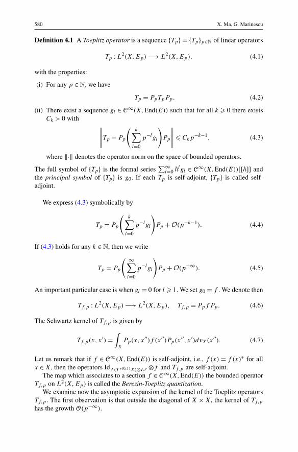
Definition 4.1 A Toeplitz operator is a sequence {Tp} = {Tp}p∈N of linear operators

Tp : L2(X,Ep) −→ L2(X,Ep), (4.1)

with the properties:

(i) For any p ∈ N, we have

Tp = PpTpPp. (4.2)

(ii) There exist a sequence gl ∈ C∞(X,End(E)) such that for all k � 0 there existsCk > 0 with

∥∥∥∥∥Tp − Pp

(k∑

l=0

p−lgl

)Pp

∥∥∥∥∥ � Ckp−k−1, (4.3)

where ‖·‖ denotes the operator norm on the space of bounded operators.

The full symbol of {Tp} is the formal series∑∞

l=0 �lgl ∈ C∞(X,End(E))[[�]] and

the principal symbol of {Tp} is g0. If each Tp is self-adjoint, {Tp} is called self-adjoint.

We express (4.3) symbolically by

Tp = Pp

(k∑

l=0

p−lgl

)Pp +O(p−k−1). (4.4)

If (4.3) holds for any k ∈ N, then we write

Tp = Pp

( ∞∑

l=0

p−lgl

)Pp +O(p−∞). (4.5)

An important particular case is when gl = 0 for l � 1. We set g0 = f . We denote then

Tf,p : L2(X,Ep) −→ L2(X,Ep), Tf,p = Ppf Pp. (4.6)

The Schwartz kernel of Tf,p is given by

Tf,p(x, x′) =∫

X

Pp(x, x′′)f (x′′)Pp(x′′, x′)dvX(x′′). (4.7)

Let us remark that if f ∈ C∞(X,End(E)) is self-adjoint, i.e., f (x) = f (x)∗ for allx ∈ X, then the operators IdΛ(T ∗(0,1)X)⊗Lp ⊗f and Tf,p are self-adjoint.

The map which associates to a section f ∈ C∞(X,End(E)) the bounded operatorTf,p on L2(X,Ep) is called the Berezin-Toeplitz quantization.

We examine now the asymptotic expansion of the kernel of the Toeplitz operatorsTf,p . The first observation is that outside the diagonal of X × X, the kernel of Tf,p

has the growth O(p−∞).


Lemma 4.2 For every ε > 0 and every l,m ∈ N, there exists Cl,m,ε > 0 such that

|Tf,p(x, x′)|Cm(X×X) � Cl,m,εp−l (4.8)

for all p � 1 and all (x, x′) ∈ X×X with d(x, x′) > ε, where the Cm-norm is inducedby ∇L,∇E and hL,hE,gT X .

Proof Due to (3.19), (4.8) holds if we replace Tf,p by Pp . Moreover, from (3.27), forany m ∈ N, there exist Cm > 0,Mm > 0 such that |Pp(x, x′)|Cm(X×X) < CpMm forall (x, x′) ∈ X × X. These two facts and formula (4.7) imply the lemma. �

We concentrate next on a neighborhood of the diagonal in order to obtain theasymptotic expansion of the kernel Tf,p(x, x′).

We adhere to the identifications made in Lemma 3.5. We also identify in the sequelf ∈ C∞(X,End(E)) with a family fx0(Z) ∈ End(Ex0) (with parameter x0 ∈ X) offunctions in Z in normal coordinates near x0. In general, for functions in the normalcoordinates, we will add a subscript x0 to indicate the base point x0 ∈ X.

Let {Ξp}p∈N be a sequence of linear operators Ξp : L2(X,Ep) −→ L2(X,Ep)

with smooth kernel Ξp(x, y) with respect to dvX(y).Recall that π : T X ×X T X → X is the natural projection from the fiberwise

product of T X on X. Under our trivialization, Ξp(x, y) induces a smooth sectionΞp,x0(Z,Z′) of π∗(End(Λ(T ∗(0,1)X) ⊗ E)) over T X ×X T X with Z,Z′ ∈ Tx0X,|Z|, |Z′| < aX . Recall also that Px0 = P was defined in (2.6).

Consider the following condition for {Ξp}p∈N.

Condition 4.3 Let k ∈ N. There exists a family {Qr,x0}0�r�k,x0∈X such that

(a) Qr,x0 ∈ End(Λ(T ∗(0,1)X) ⊗ E)x0[Z,Z′],(b) {Qr,x0}r∈N,x0∈X is smooth with respect to the parameter x0 ∈ X,(c) there exist constants ε′ ∈]0, aX] and C0 > 0 with the following property: for

every l ∈ N, there exist Ck,l > 0, M > 0 such that for every x0 ∈ X, Z,Z′ ∈ Tx0X,|Z|, |Z′| < ε′ and p ∈ N the following estimate holds (in the sense of (3.27)):

∣∣∣∣∣p−nΞp,x0(Z,Z′)κ1/2

x0 (Z)κ1/2x0 (Z′) −

k∑

r=0

(Qr,x0Px0)(√

pZ,√

pZ′)p− r2

∣∣∣∣∣Cl (X)

� Ck,lp− k+1

2 (1 + √p|Z| + √

p|Z′|)M

× exp(−√C0p|Z − Z′|) + O(p−∞). (4.9)

Notation 4.4 Assume that {Ξp}p∈N is subject to the Condition 4.3. Then we write

p−nΞp,x0(Z,Z′) ∼=k∑

r=0

(Qr,x0Px0)(√

pZ,√

pZ′)p− r2 +O(p− k+1

2 ). (4.10)

The family {Jr,x0}r∈N,x0∈X of polynomials Jr,x0(Z,Z′) ∈ End(Λ(T ∗(0,1)X) ⊗E)x0 was defined in Theorem 3.6. Moreover, Jr,x0(Z,Z′) have the same parity as


r , degJr,x0 � 3r , and

J0,x0 = IC⊗E. (4.11)

Lemma 4.5 For any k ∈ N, Z,Z′ ∈ Tx0X, |Z|, |Z′| < 2ε, we have

p−nPp,x0(Z,Z′) ∼=k∑

r=0

(Jr,x0Px0)(√

pZ,√

pZ′)p− r2 +O(p− k+1

2 ), (4.12)

in the sense of Notation 4.4.

Proof Theorem 3.6 shows that for any k,m′ ∈ N, there exist M ∈ N,C > 0 such that∣∣∣∣∣p

−nPp,x0(Z,Z′)κ12x0(Z)κ

12x0(Z

′) −k∑

r=0

(Jr,x0Px0)(√

pZ,√

pZ′)p− r2

∣∣∣∣∣Cm′

(X)

� Cp−(k+1)/2(1 + √p|Z| + √

p|Z′|)M

× exp(−√C′′μ0

√p|Z − Z′|) + O(p−∞), (4.13)

for Z,Z′ ∈ Tx0X, |Z|, |Z′| � 2ε. Hence (4.13) immediately entails (4.12). �

Lemma 4.6 Let f ∈ C∞(X,End(E)). There exists a family {Qr,x0(f )}r∈N,x0∈X suchthat

(a) Qr,x0(f ) ∈ End(Λ(T ∗(0,1)X) ⊗ E)x0 [Z,Z′] are polynomials with the same par-ity as r ,

(b) {Qr,x0(f )}r∈N,x0∈X is smooth with respect to x0 ∈ X,(c) for every k ∈ N, x0 ∈ X, Z,Z′ ∈ Tx0X, |Z|, |Z′| < ε/2 we have

p−nTf,p,x0(Z,Z′) ∼=k∑

r=0

(Qr,x0(f )Px0)(√

pZ,√

pZ′)p− r2 +O(p− k+1

2 ),

(4.14)in the sense of Notation 4.4.

Qr,x0(f ) are expressed by

Qr,x0(f ) =∑

r1+r2+|α|=r

K

[Jr1,x0 ,

∂αfx0

∂Zα(0)

Zα

α! Jr2,x0

]. (4.15)

Especially,

Q0,x0(f ) = f (x0)IC⊗E. (4.16)

We have used here the notations (2.10) and (3.20).

Proof From (4.7) and (4.8), we know that for |Z|, |Z′| < ε/2, Tf,p,x0(Z,Z′) is de-termined up to terms of order O(p−∞) by the behavior of f in BX(x0, ε). Let


ρ : R → [0,1] be a smooth even function such that

ρ(v) = 1 if |v| < 2; ρ(v) = 0 if |v| > 4. (4.17)

For |Z|, |Z′| < ε/2, we get

Tf,p,x0(Z,Z′) =∫

Tx0 X

Pp,x0(Z,Z′′)ρ(2|Z′′|/ε)fx0(Z′′)Pp,x0(Z

′′,Z′)

× κx0(Z′′)dvT X(Z′′) + O(p−∞). (4.18)

We consider the Taylor expansion of fx0 :

fx0(Z) =∑

|α|�k

∂αfx0

∂Zα(0)

Zα

α! + O(|Z|k+1)

=∑

|α|�k

p−|α|/2 ∂αfx0

∂Zα(0)

(√

pZ)α

α! + p− k+12 O(|√pZ|k+1). (4.19)

We multiply now the expansions given in (4.19) and (4.13) and obtain the expan-sion of

κ1/2x0 (Z)Pp,x0(Z,Z′′)(κx0fx0)(Z

′′)Pp,x0(Z′′,Z′)κ1/2

x0 (Z′)

which we substitute in (4.18). We integrate then on Tx0X by using the change of vari-able

√pZ′′ = W and conclude (4.14) and (4.15) by using formulas (2.10) and (2.19).

From (4.11) and (4.15), we get

Q0,x0(f ) = K[1, fx0(0)]IC⊗E = fx0(0)IC⊗E = f (x0)IC⊗E. (4.20)

The proof of Lemma 4.6 is complete. �

As an example, we compute Q1,x0(f ).

Lemma 4.7 Q1,x0(f ) appearing in (4.14) is given by

Q1,x0(f ) = f (x0)J1,x0 + K

[J0,x0 ,

∂fx0

∂Zj

(0)ZjJ0,x0

]. (4.21)

Proof At first, by taking f = 1 in (4.15), we get

J1,x0 = K[J0,x0 , J1,x0 ] + K[J1,x0 , J0,x0 ]. (4.22)

The operator O1 defined in (3.29) (considered as a differential operator with coeffi-cients in End(Λ(T ∗(1,0)X) ⊗ E)x0 ) acts as the identity on the E-component. Thus,from (3.31) and (2.10), we obtain

K[J1,x0 , f (x0)J0,x0 ] = f (x0)K[J1,x0 , J0,x0 ]. (4.23)

From (4.15), (4.22) and (4.23), we get (4.21). �


Remark 4.8 If f ∈ C∞(X) we get (4.23), thus also (4.21), without using the preciseformulas of O1 or J1.

4.2 A Criterion for Toeplitz Operators

We will prove next a useful criterion which ensures that a given family is a Toeplitzoperator.

Theorem 4.9 Let {Tp : L2(X,Ep) −→ L2(X,Ep)} be a family of bounded linearoperators which satisfies the following three conditions:

(i) For any p ∈ N, PpTpPp = Tp .(ii) For any ε0 > 0 and any l ∈ N, there exists Cl,ε0 > 0 such that for all p � 1 and

all (x, x′) ∈ X × X with d(x, x′) > ε0,

|Tp(x, x′)| � Cl,ε0p−l . (4.24)

(iii) There exists a family of polynomials {Qr,x0 ∈ End(Λ(T ∗(0,1)X) ⊗ E)x0 [Z,

Z′]}x0∈X such that:(a) each Qr,x0 has the same parity as r ,(b) the family is smooth in x0 ∈ X and(c) there exists 0 < ε′ < aX/4 such that for every x0 ∈ X, every Z,Z′ ∈ Tx0X

with |Z|, |Z′| < ε′ and every k ∈ N we have

p−nTp,x0(Z,Z′) ∼=k∑

r=0

(Qr,x0Px0)(√

pZ,√

pZ′)p− r2 +O(p− k+1

2 ),

(4.25)in the sense of (4.10) and (4.9).

Then {Tp} is a Toeplitz operator.

Remark 4.10 By Lemmas 4.2 and 4.6, and by (4.2), (4.3) and the Sobolev inequality(cf. [20, (4.14)]), it follows that every Toeplitz operator in the sense of Definition 4.1verifies the conditions (i), (ii), (iii) of Theorem 4.9.

We start the proof of Theorem 4.9. Let T ∗p be the adjoint of Tp . By writing

Tp = 1

2(Tp + T ∗

p ) + √−11

2√−1

(Tp − T ∗p ), (4.26)

we may and will assume from now on that Tp is self-adjoint.We will define inductively the sequence (gl)l�0, gl ∈ C∞(X,End(E)) such that

Tp =m∑

l=0

Ppglp−lPp +O(p−m−1), for every m � 0. (4.27)

Moreover, we can make these gl’s to be self-adjoint.


Let us start with the case m = 0 of (4.27). For an arbitrary but fixed x0 ∈ X, we set

g0(x0) = Q0,x0(0,0)|C⊗E ∈ End(Ex0). (4.28)

We will show that

p−n(Tp − Tg0,p)x0(Z,Z′) ∼= O(p−1), (4.29)

which implies the case m = 0 of (4.27), namely,

Tp = Ppg0Pp +O(p−1). (4.30)

The proof of (4.29)–(4.30) will be done in Propositions 4.11 and 4.17.

Proposition 4.11 In the conditions of Theorem 4.9 we have Q0,x0(Z,Z′) =Q0,x0(0,0) ∈ End(Ex0) ◦ IC⊗E for all x0 ∈ X and all Z,Z′ ∈ Tx0X.

Proof The proof is divided in the series of Lemmas 4.12, 4.13, 4.14, 4.15 and 4.16.Our first observation is as follows.

Lemma 4.12 Q0,x0 ∈ End(Ex0) ◦ IC⊗E[Z,Z′], and Q0,x0 is a polynomial in z, z′.

Proof Indeed, by (4.25)

p−nTp,x0(Z,Z′) ∼= (Q0,x0Px0)(√

pZ,√

pZ′) +O(p−1/2). (4.31)

Moreover, by (4.11) and (4.12), we have

p−n(PpTpPp)x0(Z,Z′)∼= ((PJ0) ◦ (Q0P ) ◦ (PJ0))x0(

√pZ,

√pZ′) +O(p−1/2). (4.32)

Since PpTpPp = Tp , we deduce from (4.31), (4.11) and (4.32) that

Q0,x0Px0 = IC⊗EPx0 ◦ (Q0,x0Px0) ◦ Px0IC⊗E, (4.33)

hence Q0,x0 ∈ End(Ex0) ◦ IC⊗E[z, z′] by (2.8) and (2.12). �

For simplicity we denote in the rest of the proof Fx = Q0,x |C⊗E ∈ End(Ex). LetFx = ∑

i�0 F(i)x be the decomposition of Fx in homogeneous polynomials F

(i)x of

degree i. We will show that F(i)x vanish identically for i > 0, that is,

F (i)x (z, z′) = 0 for all i > 0 and z, z′ ∈ C

n. (4.34)

The first step is to prove

F (i)x (0, z′) = 0 for all i > 0 and all z′ ∈ C

n. (4.35)

Let us remark that since Tp are self-adjoint we have

F (i)x (z, z′) = (F (i)

x (z′, z))∗. (4.36)


Consider ε′ > 0 as in hypothesis (iii) (c) of Theorem 4.9. For Z′ ∈ R2n � TxX with

|Z′| < ε′ and y = expXx (Z′), set

F (i)(x, y) = F (i)x (0, z′) ∈ End(Ex),

F (i)(x, y) = (F (i)(y, x))∗ ∈ End(Ey).(4.37)

F (i) and F (i) define smooth sections on a neighborhood of the diagonal of X × X.Clearly, the F (i)(x, y)’s need not be polynomials in z and z′.

Since we wish to define global operators induced by these kernels, we use a cut-off function in the neighborhood of the diagonal. Pick a smooth function η ∈ C∞(R),such that η(u) = 1 for |u| � ε′/2 and η(u) = 0 for |u| � ε′.

We denote by F (i)Pp and PpF (i) the operators defined by the kernels

η(d(x, y))F (i)(x, y)Pp(x, y) and η(d(x, y))Pp(x, y)F (i)(x, y)

with respect to dvX(y). Set

Tp = Tp −∑

i�degFx

(F (i)Pp)pi/2. (4.38)

The operators Tp extend naturally to bounded operators on L2(X,Ep).From (4.25) and (4.38) we deduce that for all k � 1 and |Z′| � ε′, we have the

following expansion in the normal coordinates around x0 ∈ X (which has to be un-derstood , in the sense of (4.10)):

p−nTp,x0(0,Z′) ∼=k∑

r=1

(Rr,x0Px0)(0,√

pZ′)p−r/2 +O(p−(k+1)/2), (4.39)

for some polynomials Rr,x0 of the same parity as r . For simplicity let us define simi-larly to (4.37) the kernel

Rr,p(x, y) = pn(Rr,xPx)(0,√

pZ′)κ−1/2x (Z′)η(d(x, y)), (4.40)

where y = expXx (Z′), and denote by Rr,p the operator defined by this kernel.

Lemma 4.13 There exists C > 0 such that for every p > p0 and s ∈ L2(X,Ep) wehave

‖Tps‖L2 � Cp−1/2‖s‖L2, (4.41)

‖T ∗p s‖L2 � Cp−1/2‖s‖L2 . (4.42)

Proof In order to use (4.39) we write

‖Tps‖L2 �∥∥∥∥∥(Tp −

k∑

r=1

p−r/2Rr,p)s

∥∥∥∥∥L2

+∥∥∥∥∥

k∑

r=1

p−r/2Rr,ps

∥∥∥∥∥L2

. (4.43)


By the Cauchy-Schwarz inequality we have

∥∥∥∥∥

(Tp −

k∑

r=1

p−r/2Rr,p

)s

∥∥∥∥∥

2

L2

�∫

X

(∫

X

∣∣∣∣∣

(Tp −

k∑

r=1

p−r/2Rr,p

)(x, y)

∣∣∣∣∣dvX(y)

)

×(∫

X

∣∣∣∣∣

(Tp −

k∑

r=1

p−r/2Rr,p

)(x, y)

∣∣∣∣∣|s(y)|2dvX(y)

)dvX(x). (4.44)

We split then the inner integrals into integrals over BX(x, ε′) and X � BX(x, ε′) anduse the fact that the kernel of Tp − ∑k

r=1 p−r/2Rr,p has the growth O(p−∞) outsidethe diagonal. Indeed, this follows by (4.24), the definition of the operators F (i)Pp

in (4.38) (using the cut-off function η), and the definition (4.40) of Rr,p (which in-volves P ). We get for example, uniformly in x ∈ X,

∫

X

∣∣∣∣∣

(Tp −

k∑

r=1

p−r/2Rr,p

)(x, y)

∣∣∣∣∣|s(y)|2dvX(y)

=∫

BX(x,ε′)

∣∣∣∣∣

(Tp −

k∑

r=1

p−r/2Rr,p

)(x, y)

∣∣∣∣∣|s(y)|2dvX(y)

+ O(p−∞)

∫

X�BX(x,ε′)|s(y)|2dvX(y). (4.45)

By (4.9) and (4.39) applied for k sufficiently large, which we fix from now on, weobtain

∫

BX(x,ε′)

∣∣∣∣∣

(Tp −

k∑

r=1

p−r/2Rr,p

)(x, y)

∣∣∣∣∣|s(y)|2dvX(y)

= O(p−1)

∫

BX(x,ε′)|s(y)|2dvX(y). (4.46)

In the same vein we obtain

∫

X

∣∣∣∣∣

(Tp −

k∑

r=1

p−r/2Rr,p

)(x, y)

∣∣∣∣∣dvX(y) = O(p−1) + O(p−∞). (4.47)

Combining (4.44)–(4.47) we infer

∥∥∥∥∥

(Tp −

k∑

r=1

p−r/2Rr,p

)s

∥∥∥∥∥L2

� Cp−1‖s‖L2, s ∈ L2(X,Ep). (4.48)


A similar proof as for (4.48) delivers for s ∈ L2(X,Ep)

∥∥Rr,ps∥∥

L2 � C‖s‖L2 , (4.49)

which implies

∥∥∥∥∥

k∑

r=1

p−r/2Rr,ps

∥∥∥∥∥L2

� Cp−1/2‖s‖L2, for s ∈ L2(X,Ep), (4.50)

for some constant C > 0. Relations (4.48) and (4.50) entail (4.41), which is equivalentto (4.42), by taking the adjoint. �

Let us consider the Taylor development of F (i) in normal coordinates around x

with y = expXx (Z′):

F (i)(x, y) =∑

|α|�k

∂αF (i)

∂Z′α (x,0)(√

pZ′)α

α! p−|α|/2 + O(|Z′|k+1). (4.51)

The next step in the proof of Proposition 4.11 is the following.

Lemma 4.14 For every j > 0 we have

∂αF (i)

∂Z′α (x,0) = 0, for i − |α| � j > 0. (4.52)

Proof The definition (4.38) of Tp shows that

T ∗p = Tp −

∑

i�degFx

pi/2(PpF (i)). (4.53)

Let us develop the sum in the right-hand side. Combining the Taylor development(4.51) with the expansion (4.12) of the Bergman kernel we obtain:

p−n∑

i

(PpF (i))x0(0,Z′)pi/2

∼=∑

i

∑

|α|,r�k

(Jr,x0Px0

)(0,

√pZ′)∂

αF (i)

∂Z′α (x0,0)(√

pZ′)α

α! p(i−|α|−r)/2

+O(p(degF−k−1)/2), (4.54)

where k � degFx + 1. Having in mind (4.42), this is only possible if for every j > 0the coefficients of pj/2 in the right-hand side of (4.54) vanish. Thus, we have forevery j > 0:

degFx∑

l=j

∑

|α|+r=l−j

Jr,x0(0,√

pZ′)∂αF (l)

∂Z′α (x0,0)(√

pZ′)α

α! = 0. (4.55)


From (4.55), we will prove by recurrence that for any j > 0, (4.52) holds. As thefirst step of the recurrence let us take j = degFx in (4.55). Since J0,x0 = IC⊗E (see(4.11)), we get immediately F (degFx)(x0,0) = 0. Hence (4.52) holds for j = degFx .

Assume that (4.52) holds for j > j0 > 0. Then for j = j0, the coefficient withr > 0 in (4.55) is zero. Since J0,x0 = IC⊗E , (4.55) reads

∑

α

∂αF (j0+|α|)

∂Z′α (x0,0)(√

pZ′)α

α! = 0, (4.56)

which entails (4.52) for j = j0. The proof of (4.52) is complete. �

Lemma 4.15 For i > 0, we have

∂αF(i)x

∂z′α (0,0) = 0, |α| � i. (4.57)

Therefore F(i)x (0, z′) = 0 for all i > 0 and z′ ∈ C

n i.e., (4.35) holds true. Moreover,

F (i)x (z,0) = 0 for all i > 0 and all z ∈ C

n. (4.58)

Proof Let us start with some preliminary observations.In view of (4.42), (4.52) and (4.54), a comparison the coefficient of p0 in (4.31)

and (4.53) yields

F (i)(x,Z′) = F (i)x (0, z′) + O(|Z′|i+1). (4.59)

Using the definition (4.37) of F (i)(x,Z′), and taking the adjoint of (4.59) we get

F (i)(Z′, x) = (F (i)x (0, z′))∗ + O(|Z′|i+1), (4.60)

which implies

∂α

∂zαF (i)(·, x)|x =

((∂α

∂z′α F (i)x

)(0, z′)

)∗, for |α| � i, (4.61)

so in order to prove the Lemma it suffices to show that

∂α

∂zαF (i)(·, x)|x = 0, for |α| � i. (4.62)

We prove this by induction over |α|. For |α| = 0, it is obvious that F (i)(0, x) = 0,since F (i)(·, x) is a homogeneous polynomial of degree i > 0. For the induction steplet jX : X → X × X be the diagonal injection. By Lemma 4.12 and the definition(4.37) of F (i)(x, y),

∂

∂z′j

F (i)(x, y) = 0, near jX(X), (4.63)

where y = expXx (Z′). Assume now that α ∈ N

n and (4.62) holds for |α|−1. Considerj with αj > 0 and set α′ = (α1, . . . , αj − 1, . . . , αn).


Taking the derivative of (4.37) and using the induction hypothesis and (4.63), wehave

∂α

∂zαF (i)(·, x)

∣∣∣∣x

= ∂

∂zj

j∗X

(∂α′

∂zα′ F(i)

)∣∣∣∣x

− ∂α′

∂zα′∂

∂z′j

F (i)(·, ·)∣∣∣∣0,0

= 0. (4.64)

Thus, (4.57) is proved. The identity (4.35) follows too, since it is equivalent to(4.57). Furthermore, (4.58) results from (4.35) and (4.36). This finishes the proofof Lemma 4.15. �

Lemma 4.16 We have F(i)x (z, z′) = 0 for all i > 0 and z, z′ ∈ C

n .

Proof Let us consider the operator

1√p

Pp(∇Ep

X,xTp)Pp with X ∈ C∞(X,T X), X(x0) = ∂

∂zj

+ ∂

∂zj

. (4.65)

The leading term of its asymptotic expansion (4.10) is

(∂

∂zj

Fx0

)(√

pz,√

pz′)Px0(√

pZ,√

pZ′). (4.66)

By (4.35) and (4.58), ( ∂∂zj

Fx0)(z, z′) is an odd polynomial in z,z′ whose constant term

vanishes. We reiterate the arguments from (4.38)–(4.61) by replacing the operator Tp

with the operator (4.65); we get for i > 0,

∂

∂zj

F (i)x (0, z′) = 0. (4.67)

By (4.36) and (4.67),

∂

∂z′j

F (i)x (z,0) = 0. (4.68)

By continuing this process, we show that for all i > 0, α ∈ Zn, z, z′ ∈ C

n,

∂α

∂zαF (i)

x (0, z′) = ∂α

∂z′α F (i)x (z,0) = 0. (4.69)

Thus, the Lemma is proved and (4.34) holds true. �

The Lemma 4.16 finishes the proof of Proposition 4.11. �

We come now to the proof of the first induction step leading to (4.27).

Proposition 4.17 We have p−n(Tp − Tg0,p)x0(Z,Z′) ∼= O(p−1) (in the sense of No-tation 4.4). Consequently, Tp = Ppg0Pp + O(p−1) (i.e., relation (4.30)) holds truein the sense of (4.4) .


Proof Let us compare the asymptotic expansion of Tp and Tg0,p = Ppg0Pp . Usingthe Notation 4.4, the expansion (4.14) (for k = 1) reads

p−nTg0,p,x0(Z,Z′)∼= (g0(x0)IC⊗EPx0 + Q1,x0(g0)Px0p

−1/2)(√

pZ,√

pZ′) +O(p−1), (4.70)

since Q0,x0(g0) = g0(x0)IC⊗E by (4.16). The expansion (4.25) (also for k = 1) takesthe form

p−nTp,x0∼= (g0(x0)IC⊗EPx0 +Q1,x0Px0p

−1/2)(√

pZ,√

pZ′) +O(p−1), (4.71)

where we have used Proposition 4.11 and the definition (4.28) of g0. Thus, subtracting(4.70) from (4.71) we obtain

p−n(Tp − Tg0,p)x0(Z,Z′)∼= (

(Q1,x0 − Q1,x0(g0))Px0

)(√

pZ,√

pZ′)p−1/2 +O(p−1). (4.72)

Thus, it suffices to prove the following.

Lemma 4.18

F1,x := Q1,x − Q1,x(g0) ≡ 0. (4.73)

Proof We note first that F1,x is an odd polynomial in z and z′; we verify this state-ment as in Lemma 4.12. Thus, the constant term of F1,x vanishes. To show that therest of the terms vanish, we consider the decomposition F1,x = ∑

i�0 F(i)1,x in homo-

geneous polynomials F(i)1,x of degree i. To prove (4.73) it suffices to show that

F(i)1,x(z, z

′) = 0 for all i > 0 and z, z′ ∈ Cn. (4.74)

The proof of (4.74) is similar to that of (4.34). Namely, we define as in (4.37) the op-erator F

(i)1 , by replacing F

(i)x (0, z′) by F

(i)1,x(0, z′), and we set (analogously to (4.38))

Tp,1 = Tp − Ppg0Pp −∑

i�degF1

(F(i)1 Pp)p(i−1)/2. (4.75)

Due to (4.14) and (4.25), there exist polynomials Rr,x0 ∈ C[Z,Z′] of the same parityas r such that the following expansion in the normal coordinates around x0 ∈ X holdsfor k � 2 and |Z′| � ε′/2:

p−nTp,1,x0(0,Z′) ∼=k∑

r=2

(Rr,x0Px0)(0,√

pZ′)p− r2 +O(p−(k+1)/2), (4.76)

This is the analogue of (4.39). Now we can repeat with obvious modifications theproof of (4.34) and obtain the analogue of (4.34) with Fx replaced by F1,x . Thiscompletes the proof of Lemma 4.18. �


Lemma 4.18 and the expansion (4.72) imply immediately Proposition 4.17. �

Proof of Theorem 4.9 Proposition 4.17 shows that the asymptotic expansion (4.27) ofTp holds for m = 0. Moreover, if Tp is self-adjoint, then from (4.70), (4.71), g0 is alsoself-adjoint. We show inductively that (4.27) holds for every m ∈ N. To prove (4.27)for m = 1 let us consider the operator p(Tp − Ppg0Pp). We have to show now thatp(Tp − Tg0,p) satisfies the hypotheses of Theorem 4.9. The first two conditions areeasily verified. To prove the third, just subtract the asymptotics of Tp,x0(Z,Z′) (givenby (4.25)) and Tg0,p,x0(Z,Z′) (given by (4.14)). Taking into account Proposition 4.11and (4.73) the coefficients of p0 and p−1/2 in the difference vanish, which yields thedesired conclusion.

Propositions 4.11 and 4.17 applied to p(Tp −Ppg0Pp) yield g1 ∈ C∞(X,End(E))

such that (4.27) holds true for m = 1.We continue in this way the induction process to get (4.27) for any m. This com-

pletes the proof of Theorem 4.9. �

4.3 Algebra of Toeplitz Operators

The Poisson bracket {·, ·} on (X,2πω) is defined as follows. For f,g ∈ C∞(X), letξf be the Hamiltonian vector field generated by f , which is defined by 2πiξf

ω = df .Then

{f,g} := ξf (dg). (4.77)

One of our main goals is to show that Theorem 1.1 holds, thus the set of Toeplitzoperators is closed under the composition of operators, so forms an algebra.

Proof of Theorem 1.1 Firstly, it is obvious that PpTf,pTg,pPp = Tf,pTg,p . Lem-mas 4.2 and 4.6 imply Tf,pTg,p verifies (4.24). Like in (4.18), we have for Z,Z′ ∈Tx0X, |Z|, |Z′| < ε/4:

(Tf,pTg,p)x0(Z,Z′) =∫

Tx0 X

Tf,p,x0(Z,Z′′)ρ(4|Z′′|/ε)Tg,p,x0(Z′′,Z′)

× κx0(Z′′)dvT X(Z′′) + O(p−∞). (4.78)

By Lemma 4.6 and (4.78), we deduce as in the proof of Lemma 4.6, that for Z,Z′ ∈Tx0X, |Z|, |Z′| < ε/4, we have

p−n(Tf,pTg,p)x0(Z,Z′) ∼=k∑

r=0

(Qr,x0(f, g)Px0)(√

pZ,√

pZ′)p− r2 +O(p− k+1

2 ),

(4.79)

and with the notation (2.10),

Qr,x0(f, g) =∑

r1+r2=r

K[Qr1,x0(f ),Qr2,x0(g)]. (4.80)


Thus, Tf,pTg,p is a Toeplitz operator by Theorem 4.9. Moreover, it follows from theproofs of Lemma 4.6 and Theorem 4.9 that gl = Cl(f, g), where Cl are bidifferentialoperators.

Recall that we denote by IC⊗E : Λ(T ∗(0,1)X)⊗E → C⊗E the natural projection.From (2.10), (4.16) and (4.80), we get

C0(f, g)(x) = IC⊗EQ0,x(f, g)|C⊗E = IC⊗EK[Q0,x(f ),Q0,x(g)]|C⊗E

= f (x)g(x). (4.81)

By the proof of Theorem 4.9 (cf. Proposition 4.11, Lemma 4.18 and (4.28)), weget

Q1,x(f, g) = Q1,x(C0(f, g)),

C1(f, g) = IC⊗E(Q2,x(f, g) − Q2,x(C0(f, g)))(0,0)|C⊗E.(4.82)

Moreover, by (4.16) and (4.80), we get

Q2,x(f, g) = K[f (x)IC⊗E,Q2,x(g)] + K[Q1,x(f ),Q1,x(g)]+ K[Q2,x(f ), g(x)IC⊗E]. (4.83)

Now Tf,pPp = PpTf,p implies Qr,x(f,1) = Qr,x(1, f ), so we get from (4.83):

K[J0,x ,Q2,x(f )] − K[Q2,x(f ), J0,x]= K[Q1,x(f ), J1,x] − K[J1,x ,Q1,x(f )]

+ K[f (x)J0,x , J2,x] − K[J2,x , f (x)J0,x]. (4.84)

Assume now that f,g ∈ C∞(X). By (4.82), (4.83) and (4.84), we get

C1(f, g)(x) − C1(g, f )(x)

= IC⊗E[K[Q1,x(f ),Q1,x(g)] − K[Q1,x(g),Q1,x(f )]+ f (x)(K[Q1,x(g), J1,x] − K[J1,x ,Q1,x(g)])− g(x)(K[Q1,x(f ), J1,x] − K[J1,x ,Q1,x(f )])]|C⊗E. (4.85)

By Lemma 4.7, Remark 4.8, we have

K[Q1,x(f ),Q1,x(g)]

= K

[K

[1,

∂fx

∂Zj

(0)Zj

],K

[1,

∂gx

∂Zj

(0)Zj

]]

+ K[f (x)J1,Q1,x(g)] + K[Q1,x(f ), g(x)J1] − K[f (x)J1, g(x)J1].(4.86)

From (4.11), (4.85) and (4.86), we get

C1(f, g)(x) − C1(g, f )(x)


= K

[K

[1,

∂fx

∂Zj

(0)Zj

],K

[1,

∂gx

∂Zj

(0)Zj

]]

− K

[K

[1,

∂gx

∂Zj

(0)Zj

],K

[1,

∂fx

∂Zj

(0)Zj

]]. (4.87)

From (2.17) we get

K

[1,

∂fx

∂Zj

(0)Zj

]= ∂fx

∂zi

(0)zi + ∂fx

∂zi

(0)z′i . (4.88)

Plugging (4.88) into (4.87) and using (2.17) we finally obtain:

C1(f, g)(x) − C1(g, f )(x) =n∑

i=1

2

ai

[∂fx

∂zi

(0)∂gx

∂zi

(0) − ∂fx

∂zi

(0)∂gx

∂zi

(0)

]IdE

= √−1{f,g} IdE . (4.89)

This finishes the proof of Theorem 1.1. �

The next result and Theorem 1.1 show that the Berezin-Toeplitz quantization hasthe correct semi-classical behavior.

Theorem 4.19 For f ∈ C∞(X,End(E)), the norm of Tf,p satisfies

limp→∞‖Tf,p‖ = ‖f ‖∞ := sup

0�=u∈Ex,x∈X

|f (x)(u)|hE /|u|hE . (4.90)

Proof Take a point x0 ∈ X and u0 ∈ Ex0 with |u0|hE = 1 such that |f (x0)(u0)| =‖f ‖∞. Recall that in Sect. 4.1, we trivialize the bundles L, E in our normal coor-dinates near x0, and eL is the unit frame of L which trivialize L. Moreover, in thisnormal coordinates, u0 is a trivial section of E. Considering the sequence of sectionsS

px0 = p−n/2Pp(e

⊗pL ⊗ u0), we have by (3.27),

‖Tf,pSpx0 − f (x0)S

px0‖L2 � C√

p‖Sp

x0‖L2 . (4.91)

If f is a real function, then df (x0) = 0, so we can improve the constant C√p

in (4.91)

to Cp

. The proof of (4.90) is complete. �

Remark 4.20 For E = C, Theorem 1.1 shows that we can associate to f,g ∈ C∞(X)

a formal power series∑∞

l=0 �lCl(f, g) ∈ C∞(X)[[�]], where Cl are bidifferential

operators. Therefore, we have constructed in a canonical way an associative star-product f ∗ g = ∑∞

l=0 �lCl(f, g), called the Berezin-Toeplitz star-product.

5 Berezin-Toeplitz Quantizations on Non-Compact Manifolds

In this section, we extend our results to non-compact manifolds. We consider for sim-plicity only complex manifolds, that is, we suppose that (X,J ) is a complex mani-fold with complex structure J and E, L are holomorphic vector bundles on X with


rk(L) = 1. We assume that ∇E , ∇L are the holomorphic Hermitian (i.e., Chern) con-nections on (E,hE), (L,hL). Let gT X be any Riemannian metric on T X compatiblewith J . Since gT X is not necessarily Kähler, the endomorphism J defined in (3.7)does not satisfy J �= J in general. Set

Θ(X,Y ) = gT X(JX,Y ). (5.1)

Then the 2-form Θ need not be closed.Let ∂

Lp⊗E,∗be the formal adjoint of the Dolbeault operator ∂

Lp⊗Eon the Dol-

beault complex Ω0,•(X,Lp ⊗ E) with the Hermitian product induced by gT X , hL,hE as in (3.9). Set

Dp = √2(∂

Lp⊗E + ∂Lp⊗E,∗)

,

�p = ∂Lp⊗E

∂Lp⊗E,∗ + ∂

Lp⊗E,∗∂

Lp⊗E.

(5.2)

Then �p is the Kodaira-Laplacian which preserves the Z-grading of Ω0,•(X,Lp ⊗E) and

D2p = 2�p. (5.3)

Note that Dp is not a spinc Dirac operator on Ω0,•(X,Lp ⊗ E).The space of holomorphic sections of Lp ⊗ E which are L2 with respect to the

norm given by (3.9) is denoted by H 0(2)(X,Lp ⊗E). Let Pp(x, x′), (x, x′ ∈ X) be the

Schwartz kernel of the orthogonal projection Pp , from the space of L2 sections ofLp ⊗E onto H 0

(2)(X,Lp ⊗E), with respect to the Riemannian volume form dvX(x′)associated to (X,gT X). Then Pp(x, x′) is smooth by the ellipticity of the KodairaLaplacian and the Schwartz kernel theorem (cf. also [30, Remark 1.3.3]).

Remark 5.1 If J = J , then (X,J,Θ) is Kähler and Dp in (3.11) and (5.2) coincide.Assume moreover X is compact. Then by the Kodaira vanishing theorem and theDolbeault isomorphism we have

H 0(X,Lp ⊗ E) = Ker(Dp), (5.4)

for p large enough. Thus, if (X,J,Θ) is a compact Kähler manifold and J = J ,E = C, Theorems 1.1, 4.19 recover the main results of Bordemann et al. [8, 17, 23,34].

We denote by Rdet the curvature of the holomorphic Hermitian connection ∇det

on K∗X = det(T (1,0)X).

For a (1,1)-form Ω , we write Ω > 0 (resp. � 0) if Ω(·, J ·) > 0 (resp. � 0).The following result, obtained in [28, Theorem 3.11], extends the asymptotic ex-

pansion of the Bergman kernel to non-compact manifolds.

Theorem 5.2 Suppose that (X,gT X) is a complete Hermitian manifold and thereexist ε > 0,C > 0 such that :

√−1RL > εΘ,√−1(Rdet + RE) > −CΘ IdE, |∂Θ|gT X < C, (5.5)


then the kernel Pp(x, x′) has a full off–diagonal asymptotic expansion analogous tothat of Theorem 3.6 uniformly for any x, x′ ∈ K , a compact set of X. If L = KX :=det(T ∗(1;0)X) is the canonical line bundle on X, the first two conditions in (5.5) areto be replaced by

hL is induced by Θ and√−1Rdet < −εΘ,

√−1RE > −CΘIdE.

The idea of the proof is that (5.5) together with the Bochner-Kodaira-Nakano for-mula imply the existence of the spectral gap for �p acting on L2(X,Lp ⊗ E) asin (3.16).

Let C∞const (X,End(E)) denote the algebra of smooth sections of X which are con-

stant map outside a compact set. For any f ∈ C∞const (X,End(E)), we consider the

Toeplitz operator (Tf,p)p∈N as in (4.6):

Tf,p : L2(X,Lp ⊗ E) −→ L2(X,Lp ⊗ E), Tf,p = Ppf Pp. (5.6)

The following result generalizes Theorems 1.1 and 4.19 to non-compact manifolds.

Theorem 5.3 Assume that (X,gT X) is a complete Hermitian manifold, (L,hL) and(E,hE) are holomorphic vector bundles satisfying the hypotheses of Theorem 5.2with rk(L) = 1. Let f,g ∈ C∞

const (X,End(E)). Then the following assertions hold:

(i) The product of the two corresponding Toeplitz operators admits the asymptoticexpansion (1.7) in the sense of (4.5), where Cr are bidifferential operators, es-pecially, supp(Cr(f, g)) ⊂ supp(f ) ∩ supp(g), and C0(f, g) = fg.

(ii) If f,g ∈ C∞const (X), then (1.9) holds.

(iii) Relation (4.90) also holds for any f ∈ C∞const (X,End(E)).

Proof The most important observation here is that the spectral gap property (3.16)and a similar argument as in Proposition 3.4 deliver

F(Dp)s = Pps, ‖F(Dp) − Pp‖ = O(p−∞), (5.7)

for p large enough and each s ∈ H 0(2)(X,Lp ⊗ E). Moreover, by the proof of Propo-

sition 3.4, for any compact set K , and any l,m ∈ N, ε > 0, there exists Cl,m,ε > 0such that

|F(Dp)(x, x′) − Pp(x, x′)|Cm(K×K) � Cl,m,εp−l , (5.8)

for p � 1, x, x′ ∈ K . By the finite propagation speed for solutions of hyperbolicequations [36, §2.8], [30, Appendix D.2] (cf. also [20, Proposition 4.1]), F(Dp)(x, ·)only depends on the restriction of Dp to BX(x, ε) and is zero outside BX(x, ε).

For g ∈ C∞0 (X,End(E)), let (F (Dp)gF(Dp))(x, x′) be the smooth kernel of

F(Dp)gF(Dp) with respect to dvX(x′). Then for any relative compact open set U

in X such that supp(g) ⊂ U , we have from (5.7) and (5.8),

Tg,p − F(Dp)gF(Dp) = O(p−∞),

Tg,p(x, x′) − (F (Dp)gF(Dp))(x, x′) = O(p−∞) on U × U.(5.9)


Now we fix f,g ∈ C∞0 (X,End(E)). Let U be relative compact open sets in X

such that supp(f ) ∪ supp(g) ⊂ U and d(x, y) > 2ε for any x ∈ supp(f ) ∪ supp(g),y ∈ X � U . From (5.7), we have

Tf,pTg,p = PpF(Dp)f PpgF(Dp)Pp. (5.10)

Let (F (Dp)f PpgF(Dp))(x, x′), be the smooth kernel of F(Dp)f PpgF(Dp)

with respect to dvX(x′). Then the support of (F (Dp)f PpgF(Dp))(·, ·) is con-tained in U × U . If we fix x0 ∈ U , it follows from (5.8) that the kernel ofF(Dp)f PpgF(Dp) has exactly the same asymptotic expansion as in the compactcase. More precisely, as in (4.79), we have

p−n(F (Dp)f PpgF(Dp))x0(Z,Z′)

∼=k∑

r=0

(Qr,x0(f, g)Px0)(√

pZ,√

pZ′)p− r2 +O(p− k+1

2 ), (5.11)

with the same local formula for Qr,x0(f, g) given in (4.80).But since all formal computations are local, Qr,x0(f, g) are the same as in the

compact case, i.e., polynomials with coefficients bidifferential operators acting on f

and g.Thus, we know from (5.9) that there exist (gl)l�0, where gl ∈ C∞

0 (X,End(E)),supp(gl) ⊂ supp(f ) ∩ supp(g) such that for any k � 1, s ∈ L2(X,Ep),

∥∥∥∥∥F(Dp)f PpgF(Dp)s −k∑

l=0

F(Dp)Ppglp−lPpF (Dp)s

∥∥∥∥∥L2

� C

pk+1‖s‖L2 . (5.12)

(5.10) and (5.12) imply that

∥∥∥∥∥Tf,pTg,p −k∑

l=0

Ppglp−lPp

∥∥∥∥∥ � Ckp−k−1. (5.13)

Therefore, (i) is proved. With the asymptotic expansion at hand, we have just to re-peat the proofs given in the compact case in order to verify assertions (ii) and (iii).More precisely, (ii) follows exactly in the same way as in the proof of (1.9) given inTheorem 1.1. Finally, to derive assertion (iii), we apply verbatim the proof of Theo-rem 4.19. This completes the proof of Theorem 5.3. �

Example 5.4 Theorem 5.3 holds for every quasi-projective manifold with L the re-striction of the hyperplane line bundle associated to some arbitrary projective embed-ding and E the trivial bundle. By definition, a quasi-projective manifold X has theform X = Y �Z, where Y and Z are projective varieties, and Z ⊂ Y contains the sin-gular set of Y . Let us consider a holomorphic embedding Y ⊂ CP

m, the hyperplaneline bundle O(1) on CP

m, and set L = O(1)|X .By Hironaka’s theorem of resolution of singularities there exists a projective man-

ifold Y and a holomorphic map π : Y −→ Y (a composition of a finite succession of


blow-ups with smooth centers) such that π : Y � π−1(Z) −→ Y � Z is biholomor-phic and π−1(Z) is a divisor with normal crossings.

In this situation it is shown in [28, §3.6], [30, §6.2] that there exist a completeKähler metric gT X on Y � π−1(Z) � X, called the generalized Poincaré metric, anda metric hL on π∗L � L satisfying the hypotheses of Theorem 5.2 (with E trivial).

Remark 5.5 It is appropriate to remark that the results of Sect. 4.1-4.3 learn that wecan associate to any f,g ∈ C∞(X,End(E)) a formal power series

∑∞l=0 �

lCl(f, g) ∈C∞(X,End(E))[[�]], where Cl are bidifferential operators. This follows from thefact that the construction in Sect. 4.3 is local. However, the problem we addressed inthis section is which Hilbert space the Toeplitz operators act on in the case of a non-compact manifold. Theorem 5.6 shows that the space of holomorphic L2-sectionsH 0

(2)(X,Lp ⊗ E) of Lp ⊗ E, is a suitable Hilbert space which allows the Berezin-Toeplitz quantization of the algebra C∞

const (X,End(E)).

6 Berezin-Toeplitz Quantization on Orbifolds

In this section we establish the theory of Berezin-Toeplitz quantization on symplecticorbifolds, especially we show that set of Toeplitz operators forms an algebra. Forconvenience of exposition, we explain the results in detail in the Kähler orbifoldcase. In [30, §5.4] we find more complete explanations and references for Sects. 6.1and 6.2. For related topics about orbifolds we refer to [1].

This section is organized as follows. In Sect. 6.1 we recall the basic definitionsabout orbifolds. In Sect. 6.2 we explain the asymptotic expansion of Bergman kernelon complex orbifolds [20, §5.2], which we apply in Sect. 6.3 to derive the Berezin-Toeplitz quantization on Kähler orbifolds. Finally, we state in Sect. 6.4 the corre-sponding version for symplectic orbifolds.

6.1 Basic Definitions on Orbifolds

We define at first a category Ms as follows : The objects of Ms are the class ofpairs (G,M) where M is a connected smooth manifold and G is a finite groupacting effectively on M (i.e., if g ∈ G such that gx = x for any x ∈ M , then g isthe unit element of G). If (G,M) and (G′,M ′) are two objects, then a morphismΦ : (G,M) → (G′,M ′) is a family of open embeddings ϕ : M → M ′ satisfying:

(i) For each ϕ ∈ Φ , there is an injective group homomorphism λϕ : G → G′ thatmakes ϕ be λϕ-equivariant.

(ii) For g ∈ G′, ϕ ∈ Φ , we define gϕ : M → M ′ by (gϕ)(x) = gϕ(x) for x ∈ M . If(gϕ)(M) ∩ ϕ(M) �= ∅, then g ∈ λϕ(G).

(iii) For ϕ ∈ Φ , we have Φ = {gϕ,g ∈ G′}.

Definition 6.1 Let X be a paracompact Hausdorff space. An m-dimensional orbifoldchart on X consists of a connected open set U of X, an object (GU, U) of Ms withdim U = m, and a ramified covering τU : U → U which is GU -invariant and induces

a homeomorphism U � U/GU . We denote the chart by (GU, U)τU−→ U .


An m-dimensional orbifold atlas V on X consists of a family of m-dimensional

orbifold charts V(U) = ((GU, U)τU−→ U) satisfying the following conditions:

(i) The open sets U ⊂ X form a covering U with the property:

For any U,U ′ ∈ U and x ∈ U ∩ U ′,

there is U ′′ ∈ U such that x ∈ U ′′ ⊂ U ∩ U ′. (6.1)

(ii) for any U,V ∈ U,U ⊂ V there exists a morphism ϕV U : (GU , U) → (GV , V ),which covers the inclusion U ⊂ V and satisfies ϕWU = ϕWV ◦ ϕV U for anyU,V,W ∈ U , with U ⊂ V ⊂ W .

It is easy to see that there exists a unique maximal orbifold atlas Vmax containing

V ; Vmax consists of all orbifold charts (GU, U)τU−→ U , which are locally isomorphic

to charts from V in the neighborhood of each point of U . A maximal orbifold atlasVmax is called an orbifold structure and the pair (X,Vmax) is called an orbifold. Asusual, once we have an orbifold atlas V on X we denote the orbifold by (X,V), sinceV determines uniquely Vmax .

Note that if U ′ is a refinement of U satisfying (6.1), then there is an orbifold atlasV ′ such that V ∪ V ′ is an orbifold atlas, hence V ∪ V ′ ⊂ Vmax . This shows that wemay choose U arbitrarily fine.

Let (X,V) be an orbifold. For each x ∈ X, we can choose a small neighborhood(Gx, Ux) → Ux such that x ∈ Ux is a fixed point of Gx (it follows from the definitionthat such a Gx is unique up to isomorphisms for each x ∈ X). We denote by |Gx | thecardinal of Gx . If |Gx | = 1, then X has a smooth manifold structure in the neighbor-hood of x, which is called a smooth point of X. If |Gx | > 1, then X is not a smoothmanifold in the neighborhood of x, which is called a singular point of X. We denoteby Xsing = {x ∈ X; |Gx | > 1} the singular set of X, and Xreg = {x ∈ X; |Gx | = 1}the regular set of X.

It is useful to note that on an orbifold (X,V) we can construct partitions of unity.First, let us call a function on X smooth, if its lift to any chart of the orbifold atlas V issmooth in the usual sense. Then the definition and construction of a smooth partitionof unity associated to a locally finite covering carries over easily from the manifoldcase. The point is to construct smooth GU -invariant functions with compact support

on (GU, U).In Definition 6.1 we can replace Ms by a category of manifolds with an addi-

tional structure such as orientation, Riemannian metric, almost-complex structure orcomplex structure. We impose that the morphisms (and the groups) preserve the spec-ified structure. So we can define oriented, Riemannian, almost-complex or complexorbifolds.

Let (X,V) be an arbitrary orbifold. By the above definition, a Riemannian metricon X is a Riemannian metric gT X on Xreg such that the lift of gT X to any chart ofthe orbifold atlas V can be extended to a smooth Riemannian metric. Certainly, forany (GU, U) ∈ V , we can always construct a GU -invariant Riemannian metric on U .By a partition of unity argument, we see that there exist Riemannian metrics on theorbifold (X,V).


Definition 6.2 An orbifold vector bundle E over an orbifold (X,V) is defined as fol-lows: E is an orbifold and for U ∈ U , (GE

U , pU : EU → U ) is a GEU -equivariant vec-

tor bundle and (GEU , EU ) (resp. (GU = GE

U/KEU , U), KE

U = Ker(GEU → Diffeo(U)))

is the orbifold structure of E (resp. X). If GEU acts effectively on U for U ∈ U , i.e.,

KEU = {1}, we call E a proper orbifold vector bundle.

Note that any structure on X or E is locally Gx or GEUx

-equivariant.

Remark 6.3 Let E be an orbifold vector bundle on (X,V). For U ∈ U , let EprU be

the maximal KEU -invariant sub-bundle of EU on U . Then (GU, E

prU ) defines a proper

orbifold vector bundle on (X,V), denoted by Epr.The (proper) orbifold tangent bundle T X on an orbifold X is defined by

(GU,T U → U), for U ∈ U . In the same vein we introduce the cotangent bundleT ∗X. We can form tensor products of bundles by taking the tensor products of theirlocal expressions in the charts of an orbifold atlas. Note that a Riemannian metric onX induces a section of T ∗X ⊗ T ∗X over X which is a positive definite bilinear formon TxX at each point x ∈ X.

Let E → X be an orbifold vector bundle and k ∈ N∪{∞}. A section s : X → E iscalled Ck if for each U ∈ U , s|U is covered by a GE

U -invariant Ck section sU : U →EU . We denote by Ck(X,E) the space of Ck sections of E on X.

If X is oriented, we define the integral∫X

α for a form α over X (i.e., a section ofΛ(T ∗X) over X) as follows. If supp(α) ⊂ U ∈ U set

∫

X

α := 1

|GU |∫

U

αU . (6.2)

It is easy to see that the definition is independent of the chart. For general α we extendthe definition by using a partition of unity.

If X is an oriented Riemannian orbifold, there exists a canonical volume elementdvX on X, which is a section of Λm(T ∗X), m = dimX. Hence, we can also integratefunctions on X.

Assume now that the Riemannian orbifold (X,V) is compact. For x, y ∈ X, put

d(x, y) = Infγ

{∑i

∫ titi−1

| ∂∂t

γi (t)|dt

∣∣∣ γ : [0,1] → X,γ (0) = x, γ (1) = y,

such that there exist t0 = 0 < t1 < · · · < tk = 1, γ ([ti−1, ti]) ⊂ Ui,

Ui ∈ U, and a C∞ map γi : [ti−1, ti] → Ui that covers γ |[ti−1,ti ]}.

Then (X,d) is a metric space. For x ∈ X, set d(x,Xsing) := infy∈Xsingd(x, y).

Let us discuss briefly kernels and operators on orbifolds. For any open set U ⊂ X

and orbifold chart (GU, U)τU−→ U , we will add a superscript ˜ to indicate the corre-

sponding objects on U . Assume that K(x, x′) ∈ C∞(U × U ,π∗1 E ⊗ π∗

2 E∗) verifies

(g,1)K(g−1x, x′) = (1, g−1)K(x, gx′) for any g ∈ GU, (6.3)


where (g1, g2) acts on Ex × E∗x′ by (g1, g2)(ξ1, ξ2) = (g1ξ1, g2ξ2).

We define the operator K : C∞0 (U , E) → C∞(U , E) by

(Ks)(x) =∫

U

K(x, x′)s(x′)dvU (x′) for s ∈ C∞0 (U , E). (6.4)

For s ∈ C∞(U , E) and g ∈ GU , g acts on C∞(U , E) by: (g · s)(x) := g · s(g−1x). Wecan then identify an element s ∈ C∞(U,E) with an element s ∈ C∞(U , E) verifyingg · s = s for any g ∈ GU .

With this identification, we define the operator K : C∞0 (U,E) → C∞(U,E) by

(Ks)(x) = 1

|GU |∫

U

K(x, x′)s(x′)dvU (x′) for s ∈ C∞0 (U,E), (6.5)

where x ∈ τ−1U (x). Then the smooth kernel K(x, x′) of the operator K with respect

to dvX is

K(x, x′) =∑

g∈GU

(g,1)K(g−1x, x′). (6.6)

Indeed, if s ∈ C∞0 (U,E), by (6.3) and (6.5), we have

(Ks)(x) = 1

|GU |∑

g∈GU

∫

U

K(x, x′)g · s(g−1x′)(x′)dvU (x′)

= 1

|GU |∑

g∈GU

∫

U

(g,1)K(g−1x, x′)s(x′)dvU (x′)

=∫

U

∑

g∈GU

(g,1)K(g−1x, x′)s(x′)dvX(x′). (6.7)

Let K1,K2 be two operators as above and assume that the kernel of one of K1, K2has compact support. By (6.2), (6.3) and (6.5), the kernel of K1 ◦K2 is given by

(K1 ◦K2)(x, x′) =∑

g∈GU

(g,1)(K1 ◦ K2)(g−1x, x′). (6.8)

6.2 Bergman Kernel on Kähler Orbifolds

Let X be a compact complex orbifold of complex dimension n with complex structureJ . Let E be a holomorphic orbifold vector bundle on X.

Let OX be the sheaf over X of local GU -invariant holomorphic functions over U ,for U ∈ U . The local GE

U -invariant holomorphic sections of E → U define a sheafOX(E) over X. Let H •(X,OX(E) be the cohomology of the sheaf OX(E) over X.

Notice that by Definition, we have

OX(E) = OX(Epr). (6.9)


Thus, without lost generality, we may and will assume that E is a proper orbifoldvector bundle on X.

Consider a section s ∈ C∞(X,E) and a local section s ∈ C∞(U , EU ) covering s.

Then ∂EU

s covers a section of T ∗(0,1)X ⊗ E over U , denoted ∂Es|U . The family of

sections {∂Es|U : U ∈ U} patch together to define a global section ∂

Es of T ∗(0,1)X ⊗

E over X. In a similar manner we define ∂Eα for a C∞ section α of Λ(T ∗(0,1)X)⊗E

over X. We obtain thus the Dolbeault complex (Ω0,•(X,E), ∂E

):

0 −→ Ω0,0(X,E)∂

E

−→ · · · ∂E

−→ Ω0,n(X,E) −→ 0. (6.10)

From the abstract de Rham theorem there exists a canonical isomorphism

H •(Ω0,•(X,E), ∂E) � H •(X,OX(E)). (6.11)

In the sequel, we also denote H •(X,OX(E)) by H •(X,E).We consider a complex orbifold (X,J ) endowed with the complex structure J . Let

gT X be a Riemannian metric on T X compatible with J . There is then an associated(1,1)-form Θ given by Θ(U,V ) = gT X(JU,V ). The metric gT X is called a Kählermetric and the orbifold (X,J ) is called a Kähler orbifold if Θ is a closed form, thatis, dΘ = 0. In this case Θ is a symplectic form, called Kähler form. We will denotethe Kähler orbifold by (X,J,Θ) or shortly by (X,Θ).

Let (L,hL) be a holomorphic Hermitian proper orbifold line bundle on an orbifoldX, and let (E,hE) be a holomorphic Hermitian proper orbifold vector bundle on X.

We assume that the associated curvature RL of (L,hL) verifies (3.6), i.e., (L,hL)

is a positive proper orbifold line bundle on X. This implies that ω :=√−1

πRL is a

Kähler form on X, (X,ω) is a Kähler orbifold and (L,hL,∇L) is a prequantum linebundle on (X,ω).

Note that the existence of a positive line bundle L on a compact complex orbifoldX implies that the Kodaira map associated to high powers of L gives a holomorphicembedding of X in the projective space. This is the generalization due to Baily of theKodaira embedding theorem (see e.g. [30, Theorem 5.4.20]).

Let gT X = ω(·, J ·) be the Riemannian metric on X induced by ω =√−12π

RL.Using the Hermitian product along the fibers of Lp , E, Λ(T ∗(1,0)X), the Rie-

mannian volume form dvX and the definition (6.2) of the integral on an orbifold, weintroduce an L2-Hermitian product on Ω0,•(X,Lp ⊗E) similar to (3.9). This allows

to define the formal adjoint ∂Lp⊗E,∗

of ∂Lp⊗E

and as in (5.2), the operators Dp and�p . Then D2

p preserves the Z-grading of Ω0,•(X,Lp ⊗ E). We note that Hodgetheory extends to compact orbifolds and delivers a canonical isomorphism

Hq(X,Lp ⊗ E) � Ker(D2p|Ω0,q ). (6.12)

By the same proof as in [27, Theorems 1.1, 2.5], [7, Theorem 1], we get vanishingresults and the spectral gap property.


Theorem 6.4 Let (X,ω) be a compact Kähler orbifold, (L,hL) be a prequantumholomorphic Hermitian proper orbifold line bundle on (X,ω) and (E,hE) be anarbitrary holomorphic Hermitian proper orbifold vector bundle on X.

Then there exists C > 0 such that the Dirac operator Dp satisfies for any p ∈ N

Spec(D2p) ⊂ {0}∪]4πp − C,+∞[, (6.13)

and D2p|Ω0,>0 is invertible for p large enough. Consequently, we have the Kodaira-

Serre vanishing theorem, namely, for p large enough,

Hq(X,Lp ⊗ E) = 0, for every q > 0. (6.14)

In view of Theorem 6.4 and of the isomorphism (6.12), we can define forp > C(2π)−1 the Bergman kernel

Pp(·, ·) ∈ C∞(X × X,π∗1 (Lp ⊗ E) ⊗ π∗

2 ((Lp ⊗ E)∗))

like in Definition 3.2. Namely, the Bergman kernel is the smooth kernel with respectto the Riemannian volume form dvX(x′) of the orthogonal projection (Bergman pro-jection) Pp from C∞(X,Lp ⊗ E) onto H 0(X,Lp ⊗ E).

From now on, we assume p > C(2π)−1. Let dp = dimH 0(X,Lp ⊗ E) and con-

sider an arbitrary orthonormal basis {Spi }dp

i=1 of H 0(X,Lp ⊗ E) with respect to theHermitian product (3.9) and (6.2). In fact, in the local coordinate above, S

pi (z) are

Gx -invariant on Ux , and

Pp(y, y′) =dp∑

i=1

Spi (y) ⊗ (S

pi (y′))∗, (6.15)

where we use y to denote the point in Ux representing y ∈ Ux .The spectral gap property (6.13) shows that we have the analogue of Proposi-

tion 3.4, with the same F as given in (3.17):

|Pp(x, x′) − F(Dp)(x, x′)|Cm(X×X) � Cl,m,εp−l . (6.16)

As pointed out in [26], the property of the finite propagation speed of solutions ofhyperbolic equations still holds on an orbifold (see the proof in [30, Appendix D.2]).Thus, F(Dp)(x, x′) = 0 for every for x, x′ ∈ X satisfying d(x, x′) � ε. Likewise,given x ∈ X, F(Dp)(x, ·) only depends on the restriction of Dp to BX(x, ε). Thusthe problem of the asymptotic expansion of Pp(x, ·) is local.

We recall that for every open set U ⊂ X and orbifold chart (GU, U)τU−→ U , we

add a superscript to indicate the corresponding objects on U . Let ∂U = U \U , U1 ={x ∈ U,d(x, ∂U) < ε}. Then F(Dp)(x, x′) is well defined for x, x′ ∈ U1 = τ−1

U (U1).Since g · F(Dp) = F(Dp)g, we get

(g,1)F (Dp)(g−1x, x′) = (1, g−1)F (Dp)(x, gx′), (6.17)


for every g ∈ GU , x, x′ ∈ U1. Formula (6.6) shows that for every x, x′ ∈ U1 andx, x′ ∈ U1 representing x, x′, we have

F(Dp)(x, x′) =∑

g∈GU

(g,1)F (Dp)(g−1x, x′). (6.18)

For x0 ∈ U2 := {x ∈ U , d(x, ∂U) < 2ε}, and Z, Z′ ∈ Tx0X with |Z|, |Z′| � ε, thekernel F(Dp)(Z, Z′) has an asymptotic expansion as in Theorem 3.6 by the sameargument as in Proposition 3.4. In the present situation J = J , so that aj = 2π andthe kernel P defined in (3.25) takes the form

P (Z, Z′) = exp

(− π

2

∑

i

(|zi |2 + |z′i |2 − 2ziz

′i

)). (6.19)

6.3 Berezin-Toeplitz Quantization on Kähler Orbifolds

We apply now the results of Sect. 6.2 to establish the Berezin-Toeplitz quantizationon Kähler orbifolds. We use the notations and assumptions of that section.

Since we consider the holomorphic case, we denote directly by Pp the orthogonalprojection from C∞(X,Lp ⊗ E) onto H 0(X,Lp ⊗ E) and we replace in (4.1) thespace L2(X,Ep) with L2(X,Lp ⊗ E). Thus, we have the following definition.

Definition 6.5 A Toeplitz operator is a family {Tp} of linear operators

Tp : L2(X,Lp ⊗ E) −→ L2(X,Lp ⊗ E), (6.20)

verifying (4.2) and (4.3).

For any section f ∈ C∞(X,End(E)), the Berezin-Toeplitz quantization of f isdefined by

Tf,p : L2(X,Lp ⊗ E) −→ L2(X,Lp ⊗ E), Tf,p = Ppf Pp. (6.21)

Now, by the same argument as in Lemma 4.2, we get

Lemma 6.6 For any ε > 0 and any l,m ∈ N there exists Cl,m,ε > 0 such that

|Tf,p(x, x′)|Cm(X×X) � Cl,m,εp−l (6.22)

for all p � 1 and all (x, x′) ∈ X×X with d(x, x′) > ε, where the Cm-norm is inducedby ∇L,∇E and hL,hE,gT X .

As in Sect. 4 we obtain next the asymptotic expansion of the kernel Tf,p(x, x′) ina neighborhood of the diagonal.

We need to introduce the appropriate analogue of the Condition 4.3 in the orbifoldcase, in order to take into account the group action associated to an orbifold chart. Let{Ξp}p∈N be a sequence of linear operators Ξp : L2(X,Lp ⊗ E) −→ L2(X,Lp ⊗ E)

with smooth kernel Ξp(x, y) with respect to dvX(y).


Condition 6.7 Let k ∈ N. Assume that for every open set U ∈ U and every orbifold

chart (GU, U)τU−→ U , there exists a sequence of kernels {Ξp,U (x, x′)}p∈N and a

family {Qr,x0}0�r�k,x0∈X such that

(a) Qr,x0 ∈ End(E)x0 [Z, Z′] ,(b) {Qr,x0}r∈N,x0∈X is smooth with respect to the parameter x0 ∈ X,(c) for every fixed ε′′ > 0 and every x, x′ ∈ U the following holds

(g,1)Ξp,U (g−1x, x′) = (1, g−1)Ξp,U (x, gx′)

for any g ∈ GU (cf. (6.17)),

Ξp,U (x, x′) = O(p−∞) for d(x, x′) > ε′′, (6.23)

Ξp(x, x′) =∑

g∈GU

(g,1)Ξp,U (g−1x, x′) + O(p−∞),

and moreover, for every relatively compact open subset V ⊂ U , the relation

p−nΞp,U,x0(Z, Z′) ∼=k∑

r=0

(Qr,x0Px0)(√

pZ,√

pZ′)p− r2 +O(p− k+1

2 )

for x0 ∈ V , (6.24)

holds in the sense of (4.10).

Notation 6.8 If the sequence {Ξp}p∈N satisfies Condition 6.7, we write

p−nΞp,x0(Z,Z′) ∼=k∑

r=0

(Qr,x0Px0)(√

pZ,√

pZ′)p− r2 +O(p− k+1

2 ). (6.25)

Note that although the Notations 6.8 and 4.4 are formally similar, they have dif-ferent meaning.

Lemma 6.9 The smooth family Qr,x0 ∈ End(E)x0 [Z, Z′] in Condition 6.7 is uniquelydetermined by Ξp .

Proof Clearly, for W ⊂ U , the restriction of Ξp,U to W × W verifies (6.23), thus wecan take Ξp,W = Ξp,U |W×W . Since GU acts freely on τ−1

U (Ureg) ⊂ U , we deducefrom (6.23) and (6.24) that

Ξp,x0(Z,Z′) = Ξp,U,x0(Z, Z′) + O(p−∞), (6.26)

for every x0 ∈ Ureg and |Z|, |Z′| small enough. We infer from (6.24) and (6.26) thatQr,x0 ∈ End(E)x0 [Z, Z′] is uniquely determined for x0 ∈ Xreg . Since Qr,x0 dependssmoothly on x0, its lift to U is smooth. Since the set τ−1

U (Ureg) is dense in U , we seethat the smooth family Qr,x0 is uniquely determined by Ξp . �


Lemma 6.10 There exist polynomials Jr,x0 ,Qr,x0(f ) ∈ End(E)x0 [Z, Z′] such thatLemmas 4.2, 4.5, 4.6 and 4.7 still hold under the notation (6.25). Moreover,

J0,x0 = IdE, J1,x0 = 0. (6.27)

Proof The analogues of Proposition 3.4, Theorem 3.6 for the current situation and(6.17), (6.18) show that Lemmas 4.2 and 4.5 still hold under the notation (6.25).Since in our case ω is a Kähler form with respect to the complex structure J andJ = J , we have O1 = 0 (cf. (3.29) and Remark 3.9). Hence (3.31) entails (6.27).Moreover, (6.16) implies

Tf,p(x, x′) =∫

X

F(Dp)(x, x′′)f (x′′)F (Dp)(x′′, x′)dvX(x′′) + O(p−∞). (6.28)

Therefore, we deduce from (6.8), (6.17), (6.18) and (6.28) that Lemmas 4.6 and 4.7still hold under the notation (6.25). �

We will prove next a useful criterion (an analogue of Theorem 4.9) which ensuresthat a given family is a Toeplitz operator.

Theorem 6.11 Let {Tp : L2(X,Lp ⊗E) −→ L2(X,Lp ⊗E)} be a family of boundedlinear operators which satisfies the following three conditions:

(i) For any p ∈ N, PpTpPp = Tp .(ii) For any ε0 > 0 and any l ∈ N, there exists Cl,ε0 > 0 such that for all p � 1 and

all (x, x′) ∈ X × X with d(x, x′) > ε0,

|Tp(x, x′)| � Cl,ε0p−l . (6.29)

(iii) There exists a family of polynomials {Qr,x0 ∈ End(E)x0[Z,Z′]}x0∈X such that:(a) each Qr,x0 has the same parity as r ,(b) the family is smooth in x0 ∈ X and(c) there exists 0 < ε′ < aX/4 such that for every x0 ∈ X, every Z,Z′ ∈ Tx0X

with |Z|, |Z′| < ε′ and every k ∈ N, we have

p−nTp,x0(Z,Z′) ∼=k∑

r=0

(Qr,x0Px0)(√

pZ,√

pZ′)p− r2 +O(p− k+1

2 ) (6.30)

in the sense of (6.25).

Then {Tp} is a Toeplitz operator.

Proof As explained in (4.26), we can assume that Tp is self-adjoint. We will defineinductively the sequence (gl)l�0, gl ∈ C∞(X,End(E)) such that

Tp =m∑

l=0

Ppglp−lPp +O(p−m−1) for every m � 0, (6.31)


using the same procedure as in (4.27). Moreover, we can take these gl’s to be self-adjoint. For x0 ∈ X, we set

g0(x0) = Q0,x0(0,0) ∈ End(Ex0). (6.32)

We will show that

Tp = Ppg0Pp +O(p−1). (6.33)

We need to establish the following analogue of Proposition 4.11.

Proposition 6.12 In the conditions of Theorem 6.11, we have Q0,x0(Z,Z′) =Q0,x0(0,0) ∈ End(Ex0) for all x0 ∈ X and all Z,Z′ ∈ Tx0X.

Proof The key observation is the following. Let {Ξp}p∈N, {Q0,x0}x0∈X and {Ξ ′p}p∈N,

{Q′0,x0

}x0∈X two pairs satisfying Condition 6.7 for k = 0. Then (6.8), (6.23) and(6.24) imply that

p−n(Ξp ◦ Ξ ′p)x0(Z,Z′)

∼= ((Q0,x0Px0) ◦ (Q′0,x0

Px0))(√

pZ,√

pZ′) +O(p− 12 ), (6.34)

in the sense of Notation 6.8 and (2.10).We modify now the proof of Lemma 4.12. Formula (6.30) for k = 0 gives

p−nTp,x0(Z,Z′) ∼= (Q0,x0Px0)(√

pZ,√

pZ′) +O(p−1/2). (6.35)

Moreover, the analogue of Lemma 4.5 shows that

p−nPp,x0(Z,Z′) ∼= (J0,x0Px0)(√

pZ,√

pZ′)p− r2 +O(p−1/2). (6.36)

By (6.35) and (6.36) we can apply the observation at the beginning for Ξp = Tp andΞ ′

p = Pp to obtain

p−n(PpTpPp)x0(Z,Z′)∼= ((PJ0) ◦ (Q0P ) ◦ (PJ0))x0(

√pZ,

√pZ′) +O(p−1/2). (6.37)

Using the same argument as in the proof of Lemma 4.12 (note also that J0,x0 = IdE

by (6.27)) we see that Q0,x0 is a polynomial in z, z′.Now, we need to establish the analogue of (4.34). We define F (i)(x, y), F (i)(x, y)

as in (4.37). Then from (6.17), (6.23), we know that for g ∈ GU , x, y ∈ U1,

g · F (i)(g−1x, y) = F (i)(x, gy). (6.38)

We denote by F (i)F (Dp) and F(Dp)F (i) the operators defined by the kernels

η(d(x, y))F (i)(x, y)F (Dp)(x, y) and η(d(x, y))F (Dp)(x, y)F (i)(x, y)


as in (6.5) and (6.6). Set

Tp = Tp −∑

i�degFx

(F (i)F (Dp))pi/2. (6.39)

Now using (6.39) instead of (4.38), by (6.5) and the proof of Proposition 4.11, weget the analogue of (4.34) and hence Proposition 6.12. �

We go on with the proof of Theorem 6.11. Applying Proposition 6.12 and theproof of Proposition 4.17, we obtain (6.33).

Finally, we deduce (6.31) according to the pattern set down in the proof of Theo-rem 4.9. This completes the proof of Theorem 6.11. �

We can therefore show that the set of Toeplitz operators on a compact orbifold isclosed under the composition of operators, so forms an algebra.

Theorem 6.13 Let (X,ω) be a compact Kähler orbifold and (L,hL) be a holo-morphic Hermitian proper orbifold line bundle satisfying the prequantization condi-tion (1.5). Let (E,hE) be an arbitrary holomorphic Hermitian proper orbifold vectorbundle on X.

Consider f,g ∈ C∞(X,End(E)). Then the product of the Toeplitz operators Tf,p

and Tg,p is a Toeplitz operator, more precisely, it admits an asymptotic expansionin the sense of (1.7), where Cr(f,g) ∈ C∞(X,End(E)) and Cr are bidifferen-tial operators defined locally as in (1.7) on each covering U of an orbifold chart

(GU, U)τU−→ U . In particular C0(f, g) = fg.

If f,g ∈ C∞(X), then (1.9) holds.Relation (4.90) also holds for any f ∈ C∞(X,End(E)).

Proof Notice that by using (6.34) we have

(Tf,pTg,p)(x, x′) =∫

X

(F (Dp)f F(Dp))(x, x′′)(F (Dp)gF(Dp))(x′′, x′)dvX(x′′)

+ O(p−∞). (6.40)

From (6.8), (6.40) and the proof of Theorem 1.1, we get Theorem 6.13. �

Remark 6.14 As in Remark 4.20, Theorem 6.13 shows that on every compact Kählerorbifold X admitting a prequantum line bundle (L,hL), we can define in a canoni-cal way an associative star-product f ∗g = ∑∞

l=0 �lCl(f, g) ∈ C∞(X)[[�]] for every

f,g ∈ C∞(X), called the Berezin-Toeplitz star-product. Moreover, Cl(f, g) are bidif-ferential operators defined locally as in the smooth case.

6.4 Symplectic Orbifolds

In this section we state the result for symplectic orbifolds.We work on a compact symplectic orbifold (X,ω) of real dimension 2n. Assume

that there exists a proper orbifold Hermitian line bundle L over X endowed with a


Hermitian connection ∇L with the prequantization property√−12π

RL = ω. This im-plies in particular that there exist k ∈ N such that Lk is a line bundle in the usualsense. Let (E,hE) be a proper orbifold Hermitian vector bundle on X equipped witha Hermitian connection ∇E .

Let J be an almost complex structure on T X such that (3.6) holds. We endow X

with a Riemannian metric gT X compatible with J .Then the construction in Sect. 3.1 goes through, especially, we can define the

spinc Dirac operator Dp : Ω0,•(X,Lp ⊗ E) −→ Ω0,•(X,Lp ⊗ E). The orthogonalprojection Pp : L2(X,Ep) −→ Ker(Dp) with Ep := Λ0,• ⊗ Lp ⊗ E is called theBergman projection. The smooth kernel Pp(·, ·) of Pp with respect to the Riemannianvolume form dvX , is called the Bergman kernel of Dp .

We define the Toeplitz operator Tp : L2(X,Ep) −→ L2(X,Ep) as in Defini-tion 4.1 by using the orthogonal projection Pp defined above. Especially Tf,p =Ppf Pp for f ∈ C∞(X,End(E)).

By the argument in Sect. 6.2 we see that Theorem 3.3 and Proposition 3.4 stillhold:

Theorem 6.15 Assume that (X,J,ω) is a compact symplectic orbifold endowed witha prequantum proper line bundle (L,hL,∇L). We endow X with a Riemannian metricgT X compatible with J . Let (E,hE) be a proper orbifold Hermitian vector bundleon X with Hermitian connection ∇E . Then

(i) the associated Dirac operator Dp has a spectral gap (3.16), and(ii) Pp(x, x′) = O(p−∞) for d(x, x′) > ε > 0 in the sense of (3.19).

Now by combining the argument in Sects. 3.2 and 6.3, we get the following ex-tension of Theorem 1.1.

Theorem 6.16 Let us make the same assumptions as in Theorem 6.15. Then forevery f,g ∈ C∞(X,End(E)) the product of the Toeplitz operators Tf,p and Tg,p

is a Toeplitz operator, more precisely, it admits an asymptotic expansion in the senseof (1.7), where Cr(f,g) ∈ C∞(X,End(E)) and Cr are bidifferential operators de-

fined locally as in (1.7) on each covering U of an orbifold chart (GU, U)τU−→ U . In

particular, C0(f, g) = fg.If f,g ∈ C∞(X), then (1.9) holds.Relation (4.90) also holds for any f ∈ C∞(X,End(E)).

As before, for the given data X,J,gT X,L,hL,∇L from Theorem 6.15 andE = C, Theorem 6.16 implies a canonical construction of the (associative) Berezin-Toeplitz star-product f ∗ g = ∑∞

l=0 �lCl(f, g) ∈ C∞(X)[[�]] for every f,g ∈

C∞(X).

References

1. Adem, A., Leida, J., Ruan, Y.: Orbifolds and Stringy Topology. Cambridge Tracts in Mathematics,vol. 171. Cambridge University Press, Cambridge (2007)


2. Bayen, F., Flato, M., Fronsdal, C., Lichnerowicz, A., Sternheimer, D.: Deformation theory and quan-tization, part I. Lett. Math. Phys. 1, 521–530 (1977)

3. Bayen, F., Flato, M., Fronsdal, C., Lichnerowicz, A., Sternheimer, D.: Deformation theory and quan-tization, part II. Ann. Phys. 111, 61–110 (1978)

4. Bayen, F., Flato, M., Fronsdal, C., Lichnerowicz, A., Sternheimer, D.: Deformation theory and quan-tization, part III. Ann. Phys. 111, 111–151 (1978)

5. Berezin, F.A.: Quantization. Izv. Akad. Nauk SSSR Ser. Mat. 38, 1116–1175 (1974)6. Berline, N., Getzler, E., Vergne, M.: Heat Kernels and Dirac Operators. Grundl. Math. Wiss. Band,

vol. 298. Springer, Berlin (1992)7. Bismut, J.-M., Vasserot, E.: The asymptotics of the Ray–Singer analytic torsion associated with high

powers of a positive line bundle. Commun. Math. Phys. 125, 355–367 (1989)8. Bordemann, M., Meinrenken, E., Schlichenmaier, M.: Toeplitz quantization of Kähler manifolds and

gl(N), N → ∞ limits. Commun. Math. Phys. 165, 281–296 (1994)9. Borthwick, D., Lesniewski, A., Upmeier, H.: Nonperturbative deformation quantization of Cartan

domains. J. Funct. Anal. 113(1), 153–176 (1993)10. Borthwick, D., Uribe, A.: Almost complex structures and geometric quantization. Math. Res. Lett. 3,

845–861 (1996); Erratum: Math. Res. Lett. 5, 211–212 (1998)11. Boutet de Monvel, L., Guillemin, V.: The Spectral Theory of Toeplitz Operators. Annals of Math.

Studies, vol. 99. Princeton University Press, Princeton (1981)12. Boutet de Monvel, L., Sjöstrand, J.: Sur la singularité des noyaux de Bergman et de Szegö. In:

Journées: Équations aux Dérivées Partielles de Rennes (1975). Astérisque, vol. 34–35, pp. 123–164.Soc. Math. France, Paris (1976)

13. Cahen, M., Gutt, S., Rawnsley, J.: Quantization of Kähler manifolds, part I. J. Geom. Phys. 7(1),45–62 (1990)

14. Cahen, M., Gutt, S., Rawnsley, J.: Quantization of Kähler manifolds, part II. Trans. Am. Math. Soc.337(1), 73–98 (1993)

15. Cahen, M., Gutt, S., Rawnsley, J.: Quantization of Kähler manifolds, part III. Lett. Math. Phys. 30,291–305 (1994)

16. Cahen, M., Gutt, S., Rawnsley, J.: Quantization of Kähler manifolds, part IV. Lett. Math. Phys. 34(2),159–168 (1995)

17. Charles, L.: Berezin-Toeplitz operators, a semi-classical approach. Commun. Math. Phys. 239, 1–28(2003)

18. Charles, L.: Toeplitz operators and Hamiltonian torus actions. J. Funct. Anal. 236(1), 299–350 (2006)19. Coburn, L.A.: Deformation estimates for the Berezin-Toeplitz quantization. Commun. Math. Phys.

149(2), 415–424 (1992)20. Dai, X., Liu, K., Ma, X.: On the asymptotic expansion of Bergman kernel. J. Differ. Geom. 72(1),

1–41 (2006); announced in C.R. Math. Acad. Sci. Paris 339(3), 193–198 (2004)21. Fedosov, B.V.: Deformation Quantization and Index Theory. Mathematical Topics, vol. 9. Akademie,

Berlin (1996)22. Guillemin, V.: Star products on compact pre-quantizable symplectic manifolds. Lett. Math. Phys.

35(1), 85–89 (1995)23. Karabegov, A.V., Schlichenmaier, M.: Identification of Berezin-Toeplitz deformation quantization.

J. Reine Angew. Math. 540, 49–76 (2001)24. Klimek, S., Lesniewski, A.: Quantum Riemann surfaces, I: the unit disc. Commun. Math. Phys.

146(1), 103–122 (1992)25. Kostant, B.: Quantization and unitary representations, I: prequantization. In: Lectures in Modern

Analysis and Applications, III. Lecture Notes in Math., vol. 170, pp. 87–208. Springer, Berlin (1970)26. Ma, X.: Orbifolds and analytic torsions. Trans. Am. Math. Soc. 357(6), 2205–2233 (2005)27. Ma, X., Marinescu, G.: The Spinc Dirac operator on high tensor powers of a line bundle. Math. Z.

240(3), 651–664 (2002)28. Ma, X., Marinescu, G.: Generalized Bergman kernels on symplectic manifolds. Adv. in Math. 217(4),

1756–1815 (2008); announced in: C.R. Acad. Sci. Paris 339(7), 493–498 (2004)29. Ma, X., Marinescu, G.: The first coefficients of the asymptotic expansion of the Bergman kernel of

the spinc Dirac operator. Int. J. Math. 17(6), 737–759 (2006)30. Ma, X., Marinescu, G.: Holomorphic Morse Inequalities and Bergman Kernels. Progress in Math.,

vol. 254. Birkhäuser, Basel (2007)31. Moreno, C., Ortega-Navarro, P.: Deformations of the algebra of functions on Hermitian symmetric

spaces resulting from quantization. Ann. Inst. H. Poincaré Sect. A (N.S.) 38(3), 215–241 (1983)


32. Pflaum, M.J.: On the deformation quantization of symplectic orbispaces. Differ. Geom. Appl. 19(3),343–368 (2003)

33. Pflaum, M.J., Posthuma, H.B., Tang, X.: An algebraic index theorem for orbifolds. Adv. Math. 210(1),83–121 (2007)

34. Schlichenmaier, M.: Deformation quantization of compact Kähler manifolds by Berezin-Toeplitzquantization. In: Conférence Moshé Flato 1999, vol. II. Math. Phys. Stud., vol. 22, pp. 289–306.Kluwer Academic, Dordrecht (2000)

35. Souriau, J.-M.: Structure des Systèmes Dynamiques. Mâtrises de Mathématiques. Dunod, Paris(1970)

36. Taylor, M.E.: Partial Differential Equations, 1: Basic Theory. Applied Mathematical Sciences,vol. 115. Springer, Berlin (1996)

Toeplitz Operators on Symplectic Manifolds › ~gmarines › PREPRINTS › mm_jga_2008.pdfToeplitz...

Documents

Transcript of Toeplitz Operators on Symplectic Manifolds › ~gmarines › PREPRINTS › mm_jga_2008.pdfToeplitz...