To Pre-Announce or Not: New Product Development in a...

1

To Pre-Announce or Not: New Product Development in a Competitive Duopoly Market1

by

Ted Klastorin ([email protected])

Hamed Mamani ([email protected])

Yong-Pin Zhou ([email protected])

ISOM Department Michael G Foster School of Business

Box 353226 University of Washington Seattle, WA 98195-3226

April, 2012; Revised, September, 2013

Abstract

In this paper, we consider the development and introduction of a new product in a durable goods duopoly market with profit maximizing firms. The first firm is an innovator who initially begins developing the product; the second firm is an imitator that begins developing a competing product as soon as it becomes aware of the innovator’s product. We assume that consumers purchase at most one unit of the product when they have maximum positive utility surplus that is determined by the characteristics of the product, the consumer’s marginal utility, and the consumer’s discounted utility for future expected products and prices. The innovator firm can release information about its product when it begins developing the product or can guard information about its product until it introduces the product into the market. Our analysis shows that, contrary to conventional wisdom, conditions may exist when an innovator’s profits increase by releasing information about its product prior to introduction. We discuss these conditions and their implications for new product development efforts.

Keywords: New Product Development; Product Design; New Product Introduction

1 This is a working paper only and should not be reproduced or quoted in any way without the express written consent of the authors. Comments on the paper are welcome. The first author gratefully acknowledges the support of the Burlington Northern/Burlington Resources Foundation, and the third author gratefully acknowledges the support of a McCabe Fellowship. The authors thank Professor Jeff Schulman for his helpful comments on an earlier draft of this paper.

2

To Pre-Announce or Not: New Product Development in a Competitive Duopoly Market

1. Introduction

The introduction of many durable goods follows a common pattern: an innovator firm initially

develops a new product and is then followed by one or more imitator firms who subsequently

produce competing products after learning of the innovator firm’s product design. Many well-

known technology products have followed this pattern; for example, consider the ubiquitous

digital audio player (DAP). In 1997, Saehan Information Systems began development of the first

mass-produced MP3 digital audio player (the MPMan) that it introduced to the US market in the

summer of 1998. At some time after Saehan began developing the MPMan, Diamond Multimedia

began developing a competing product, the Rio PMP300, that was introduced a few months after

the MPMan (in September, 1998). Both players had similar technical characteristics (e.g., they

both used 32MB flash memory) and the market for both products lasted for approximately three

years.

The history of digital audio players (DAPs) illustrates numerous factors that are common in

the development and introduction of many durable goods. Saehan (the innovator firm) introduced

their DAP into the US market first and enjoyed a brief monopoly period before the Rio PMP300

was available. While it is unclear when Diamond Multimedia began to develop their DAP, it is

possible that they started development after learning of the efforts by Saehan but prior to the

introduction of the MPMan. Furthermore, although Saehan had a (brief) monopoly on DAPs

during the summer of 1998, potential consumers during this time were undoubtedly aware of the

impending introduction of the Rio PMP300 later that year—knowledge that may have affected

their purchase decisions. Finally, neither firm significantly changed the design of their respective

player during the life span of these DAPs.

In this paper, we analyze the process of introducing a new durable good in a duopoly market

with an innovator firm and an imitator firm. There is a finite set of potential consumers who

purchase at most one unit. We assume that the product has a fixed life span and represents an

incremental improvement of an existing product so that the information diffusion process can be

considered exogenously and the potential demand is constant at any time during the product life

3

cycle (Klastorin and Tsai 2004, Bayus et al. 1997, Cohen et al. 1996). Assuming that the firms

are homogeneous with respect to development and production functions and want to maximize

their discounted profits over the life of the product, we analyze this market with respect to both

firms’ optimal design and pricing decisions. We specifically consider the issue of whether an

innovator firm has any incentive to release information about its development efforts prior to its

product introduction. We find that conditions do exist when an innovator firm can increase its

profits by pre-announcing its product, even though such an action provides information to the

competitor and appears to contradict conventional wisdom that information about new product

development efforts should always be guarded as long as possible (The Economist 2011).

We assume that consumers are rationally expectant or forward-looking (Coarse 1972, Dhebar

1994); that is, consumers’ purchase decisions are determined by the utility surplus of current

products as well as their (discounted) utility surplus of expected future products and prices. We

assume that consumers initially enter the market when information about the innovator’s product

becomes known (although a product may not be available). For example, Apple’s third quarter

2011 sales of the iPhone were below expectations when many customers postponed their purchase

in anticipation of the rumored introduction of the iPhone 5, even though Apple never intentionally

released such product development information (in fact, Apple introduced the iPhone 4S instead).

The assumption of forward-looking (strategic) consumers is well supported both by empirical and

theoretical research and is an integral part of our models.

We formulate the basic model as a Stackelberg game where the innovator firm initially sets

the quality/design of the product2. At that time, it can either release information about this product

or wait until it introduces the product into the market. When the imitator firm learns about the

innovator firm’s development effort, it immediately begins developing a competing product. This

implies that product development efforts between the two firms proceed concurrently when firm

X pre-announces its product but serially when firm X does not pre-announce.

In our basic model, we assume that all potential consumers enter the market when information

about the new product becomes available. Following Moorthy (1988) and others, we assume that

2 We refer to the design and quality of the product interchangeably but use these terms to refer to the number of features, durability, materials, and other attributes of the product.

4

the firms are homogeneous and the development time and variable cost of each product are

functions of the characteristics of each product that can be measured by a single scalar. We also

assume that marginal production cost (i.e., cost of each unit) is a linear function of the

design/quality level. With these assumptions, we show that a unique equilibrium exists and

analytically derive characteristics of the market when both firms have positive duopoly sales. In

addition to showing that an innovator firm may benefit by pre-announcing its development

efforts, we also show that an innovator firm may choose to forgo a monopoly “opportunity” even

though such action provides its competitor a significant advantage in the market.

To test the sensitivity of our results, we extended the basic model to include the cases when

(1) production costs are a quadratic function of product design and quality, and (2) all potential

consumers do not enter the market when the product is introduced; specifically, the number of

potential consumers who enter at the beginning of the monopoly and duopoly periods are

proportional to the length of the respective period. We show that most of the results derived from

our analysis of the basic model hold in these cases as well, including the result that the innovator

firm may want to pre-announce its development efforts under certain conditions.

1.1 Literature Review

Our work is related to several previous papers in the new product development literature. In

an early paper, Dockner and Jorgensen (1988) generalized dynamic pricing strategies in a

differential game model in dynamic oligopolies. Kouvelis and Mukhopadhyay (1999) studied

pricing and product design quality in a competitive diffusion model setting. Klastorin and Tsai

(2004) extended their work by including pricing and timing decisions in a duopoly market when

the product lifespan is finite. Our work is also related to previous research on time-based

competition. Cohen et al. (1996) analyzed the time-to-market decision for product replacement

over a given entry period when demand was a function of product design level (they did not

consider alternative pricing however). Bayus et al. (1997) studied the trade-off between time-to-

market and product quality in a duopoly market over an infinite time horizon. They analyzed how

one firm’s decision affects the other firm’s design and product entry-timing decisions. Bayus

(1997) analyzed the optimal product quality and entry timing decisions for an imitator firm

following the introduction of a new product under different cost, market and demand conditions.

5

Morgan et al. (2001) extended these previous papers by studying a multi-generation product with

fixed cost of product development.

With respect to product and price competition, our work is related to Hotelling (1929),

Moorthy (1988), and Schmidt and Porteus (2000). Moorthy (1988) studied a duopoly competition

where two firms simultaneously determine their respective product designs and then subsequently

set product prices. In his paper, Moorthy assumed that consumers were myopic and purchased the

product that maximized their utility surplus at the time that they entered the market (a similar

assumption was made by Klastorin and Tsai 2004). Schmidt and Porteus (2000) considered the

case when a firm developed a new product that competes with an existing product in a market

with linear reservation price curves. Finally, our work is related to the seminal paper by Shaked

and Sutton (1982) which considered a market where competing firms sequentially decide to enter,

set quality/design levels, and finally establish prices (after observing competitors’ actions).

Moorthy and Png (1992) studied product positioning in a dynamic context (i.e., when should a

supplier introduce a product sequentially?). Dhebar (1994) analyzed a two-period durable-good

monopolist who introduces a new product in the first period and an upgraded version in the

second period. In Dhebar’s model, the firm determines the product prices in both periods as well

as the upgraded product scope/design to maximize its expected net present profit over both

periods. Consumers in Dhebar’s model are forward-looking in the sense that they consider their

expectation of the upgraded product when making a purchase decision in the first period. Kornish

(2001) extended Dhebar’s model to the case when the upgrade design/scope was exogenously

determined. Ramachandran and Krishnan (2008) studied entry timing decisions in a monopoly

market with a rapidly improving product design. Padmanabhan et al. (1997) analyzed a sequential

product introduction problem and investigated the implications of consumer uncertainty regarding

network externalities. In this work, the authors showed that it might be beneficial to the firm to

provide “private” information to consumers.

A number of researchers have studied related problems in monopoly markets. For example,

Fudenberg and Tirole (1998) studied the monopoly pricing of overlapping generations of a

durable good under different market conditions. Dogan et al. (2006) considered a monopolist’s

software upgrade policies in a two period model when demand is random and impacted by word

of mouth. Bala and Carr (2009) analyzed the upgrade pricing policies by characterizing the

6

relationship between the product upgrade magnitudes and upgrade pricing structures along with

the user upgrade costs. Yin et al. (2010) studied the impact of used goods on the product upgrade

and pricing decisions in a monopoly market.

Other related papers include the work by Bhaskaran and Gilbert (2005) who studied the

selling and leasing strategies of a durable goods manufacturer in the presence of a complementary

product. In the context of the software industry, Mehra et al. (2010) considered the case when

two firms compete by offering possible discounts to existing customers of the first-mover firm for

upgrades.

1.2 Paper Contributions and Overview

To the best of our knowledge, this is the first study to analyze the issue of new product pre-

announcements in a duopoly market with rationally expectant consumers. We model this market

as a Stackelberg game and derive closed form solutions for the firms’ design and price decision

variables when firm X chooses (or not) to pre-announce its product. Using the results from our

models, we show (contrary to conventional wisdom) that, under certain conditions, an innovator

firm’s profits may increase when information about its product is released as the firm begins its

new product development process (even though such action benefits the innovator firm’s

competitor as well). The underlying insight can be used to explain other findings about the timing

and pricing of new products in a duopoly market, including our finding that an innovator firm that

enters the market first may knowingly decide to set a monopoly price that effectively discourages

all monopoly sales. Our analysis shows that one of the most important considerations for an

innovator firm is how the imitator firm reacts in terms of its design and pricing decisions.

Specifically, we show that the imitator firm generally wants to differentiate its product from the

innovator firm’s product as much as possible; this increased differentiation generally increases the

profits of both firms. We present a number of examples that illustrate how these factors interact

to benefit both firms as model parameters vary.

The paper is organized as follows. In the second section, we define our basic model that

assumes linear production costs and all potential consumers enter the market when the product is

introduced. We analyze this model under the conditions that the innovator firm either pre-

announces its development effort or waits until it introduces the product into the market. We

7

show that a unique equilibrium exists in this Stackelberg game (assuming that both firms choose

to compete in the duopoly market) and derive characteristics of both firms’ products and prices.

In the third section, we discuss the implications of the basic model and extend it to the case when

production costs are quadratic and potential consumers enter the market at the beginning of the

monopoly or duopoly periods (the number of consumers who enter each period is proportional to

the length of those respective periods). We show that most of the results derived from the basic

model continue to hold. Finally, we summarize our results and discuss several implications that

our work offers for other fields (e.g., supply chain management).

2. Basic Model Defined

There are two competing firms; we will denote firm X as the innovator firm and firm Y as the

imitator firm (throughout the remainder of this paper, we will use subscripts X and Y to indicate

firm-specific variables). The firms are homogeneous with respect to cost and development time

characteristics. Following Moorthy (1988), Cohen et al. (1996) and others, we assume that each

firm develops a single durable product over a finite lifespan [0, T] that is characterized by a scalar

Sj, j = X, Y. The design level of the product reflects the number of features, the performance level,

and the overall quality of the product. The time it takes to develop the product, g(S), is a linear

function of the product design level S: g(S) = β S where β > 0 is the time to develop an additional

unit of design/quality level. This assumption is based on empirical studies that demonstrated that

the speed of product performance improvement can be represented by a Cobb-Douglas model

(Cohen et al., 1996).

We assume that the marginal production cost (cost per unit sold) is a function of the design

level, c S S h for h 1 where

is the marginal production cost of a unit with design level

S. In the basic model, we assume that h = 1 although we relax this assumption and consider

quadratic costs (h = 2) in the following section. We assume that development costs are zero

although these costs could be included by redefining the function c(S).

We model both firms’ product design and pricing decisions as a Stackelberg game. Firm X

(the innovator firm) begins product development and sets a product design level SX. For analytical

tractability, we assume that SX is an exogenously determined parameter; this is a reasonable

8

assumption if the innovator product is the result of a technological breakthrough such that the

value of SX is largely determined by technological considerations. When firm Y (the imitator firm)

learns of firm X’s product development effort, it begins developing a competing product with

design level SY. We assume that SY is a decision variable so that firm Y can differentiate its

product from SX if it wishes to do so. To avoid trivial cases, we assume that both firms make

decisions that lead to positive sales during the product’s finite life span [0, T].

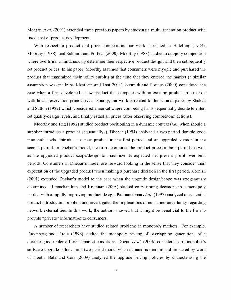
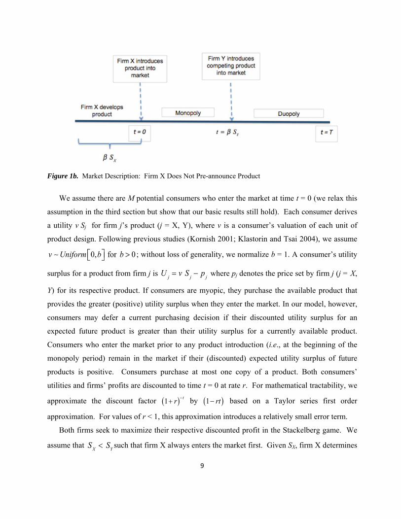
We assume that the product’s life span begins at time t = 0 when firm X introduces the

product into the market. Consumers (and firm Y) become aware of firm X’s product design SX at

time t SX if firm X pre-announces its product, or time t = 0 if firm X does not pre-announce

its product. If firm X does not pre-announce its product, it always enters the market first; if firm

X pre-announces its product, the firm with the lower design level will enter the market first. The

firm that enters the market first sells its product for a monopoly period that persists until the

second firm introduces its product when both firms simultaneously set respective duopoly prices.

In this paper, we focus our analysis on the case when firm X always enters the market first,

regardless of whether or not it pre-announces its product. By focusing on this case, we can make

a more accurate analysis of the trade-offs between pre-announcing and not pre-announcing a

product development effort. The time lines indicating significant events during the product

lifespan when firm X does or does not pre-announce its product are indicated in Figures 1a and

1b.

Figure 1a. Market Description: Firm X Pre-announces New Product

9

Figure 1b. Market Description: Firm X Does Not Pre-announce Product

We assume there are M potential consumers who enter the market at time t = 0 (we relax this

assumption in the third section but show that our basic results still hold). Each consumer derives

a utility v Sj for firm j’s product (j = X, Y), where v is a consumer’s valuation of each unit of

product design. Following previous studies (Kornish 2001; Klastorin and Tsai 2004), we assume

; without loss of generality, we normalize b = 1. A consumer’s utility

surplus for a product from firm j is Uj v S

j p

j where pj denotes the price set by firm j (j = X,

Y) for its respective product. If consumers are myopic, they purchase the available product that

provides the greater (positive) utility surplus when they enter the market. In our model, however,

consumers may defer a current purchasing decision if their discounted utility surplus for an

expected future product is greater than their utility surplus for a currently available product.

Consumers who enter the market prior to any product introduction (i.e., at the beginning of the

monopoly period) remain in the market if their (discounted) expected utility surplus of future

products is positive. Consumers purchase at most one copy of a product. Both consumers’

utilities and firms’ profits are discounted to time t = 0 at rate r. For mathematical tractability, we

approximate the discount factor 1 r t by 1 rt based on a Taylor series first order

approximation. For values of r < 1, this approximation introduces a relatively small error term.

Both firms seek to maximize their respective discounted profit in the Stackelberg game. We

assume that SX S

Ysuch that firm X always enters the market first. Given SX, firm X determines

10

the optimal price of its product in the monopoly period, pXm. As soon as firm Y becomes aware of

firm X’s product, it sets the design/quality level of its product, SY, and begins development. The

introduction of firm Y’s product into the market defines the beginning of the duopoly period

when firms X and Y set their respective duopoly prices, pXd and pYd, in a simultaneous game. The

notation we use in defining our models when firm X does not pre-announce its product is

summarized below:

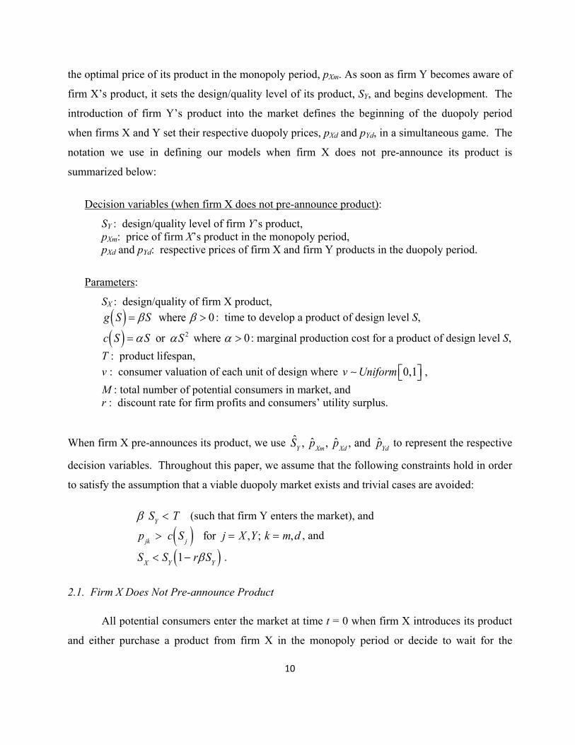
Decision variables (when firm X does not pre-announce product):

SY : design/quality level of firm Y’s product, pXm: price of firm X’s product in the monopoly period, pXd and pYd: respective prices of firm X and firm Y products in the duopoly period.

Parameters:

SX : design/quality of firm X product,

g S S where 0 : time to develop a product of design level S,

c S S or S 2 where 0: marginal production cost for a product of design level S,

T : product lifespan,

v : consumer valuation of each unit of design where ,

M : total number of potential consumers in market, and r : discount rate for firm profits and consumers’ utility surplus.

When firm X pre-announces its product, we use SY, p

Xm, p

Xd, and p

Yd to represent the respective

decision variables. Throughout this paper, we assume that the following constraints hold in order

to satisfy the assumption that a viable duopoly market exists and trivial cases are avoided:

SY T (such that firm Y enters the market), and

pjk

c Sj for j X ,Y; k m,d , and

S

X S

Y1 rS

Y .

2.1. Firm X Does Not Pre-announce Product

All potential consumers enter the market at time t = 0 when firm X introduces its product

and either purchase a product from firm X in the monopoly period or decide to wait for the

11

duopoly period under the expectation that their (discounted) utility surplus in the duopoly period

is greater than their current utility surplus. Some consumers may have negative utility surplus in

both the monopoly and duopoly periods in which case they do not purchase a product at all.

Given the definition of consumers’ utility surplus, a consumer would purchase a firm X

product in the monopoly period if

1 max , ,0 (1)X Xm Y X Xd Y Ydv S p r S v S p v S p

where consumers’ utility surplus in the duopoly period is discounted by the term 1 rSY given

the length of the monopoly period, SY. If a consumer does not purchase a product in the

monopoly period, she will purchase a product from firm k (where k = X, Y) in the duopoly period

if

, max 0 . k kd j X Y j jdv S p v S p (2)

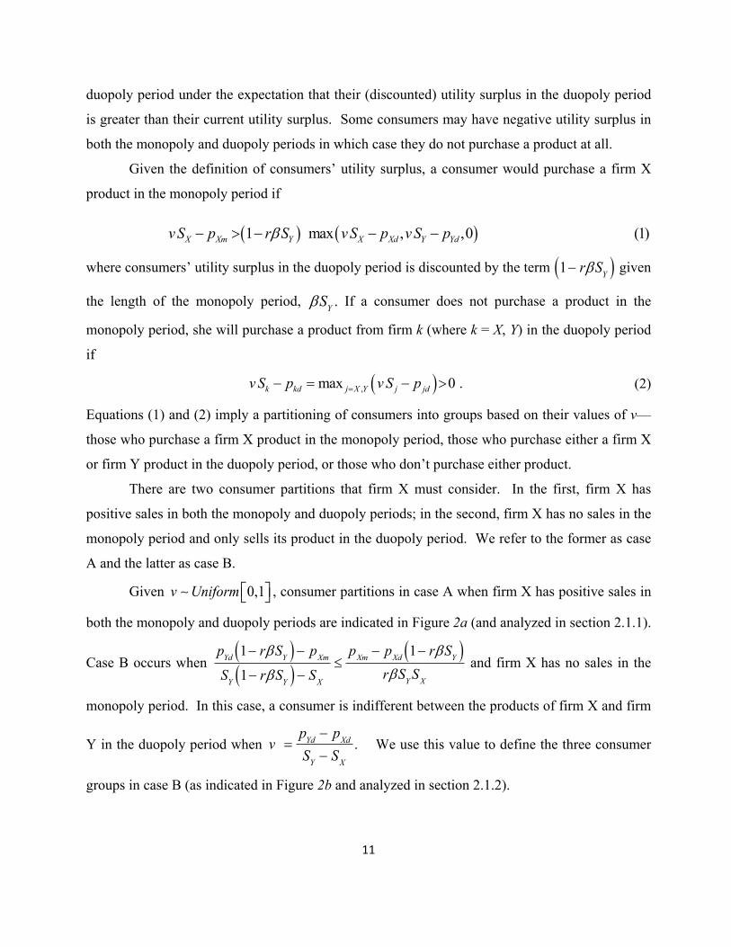
Equations (1) and (2) imply a partitioning of consumers into groups based on their values of v—

those who purchase a firm X product in the monopoly period, those who purchase either a firm X

or firm Y product in the duopoly period, or those who don’t purchase either product.

There are two consumer partitions that firm X must consider. In the first, firm X has

positive sales in both the monopoly and duopoly periods; in the second, firm X has no sales in the

monopoly period and only sells its product in the duopoly period. We refer to the former as case

A and the latter as case B.

Given , consumer partitions in case A when firm X has positive sales in

both the monopoly and duopoly periods are indicated in Figure 2a (and analyzed in section 2.1.1).

Case B occurs when p

Yd1 rS

Y pXm

SY

1 rSY S

X

p

Xm p

Xd1 rS

Y rS

YS

X

and firm X has no sales in the

monopoly period. In this case, a consumer is indifferent between the products of firm X and firm

Y in the duopoly period when v p

Yd p

Xd

SY S

X

. We use this value to define the three consumer

groups in case B (as indicated in Figure 2b and analyzed in section 2.1.2).

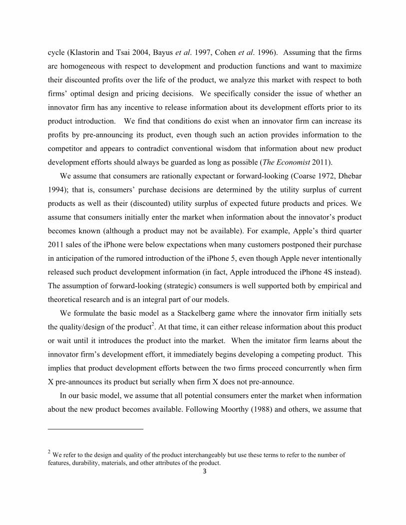
12

Figure 2a. Consumer Partitions When Firm X Does Not Pre-announce Product Development and Has Sales in the Monopoly Period

Figure 2b. Consumer Partitions When Firm X Does Not Pre-announce Product Development and Has No Sales in the Monopoly Period

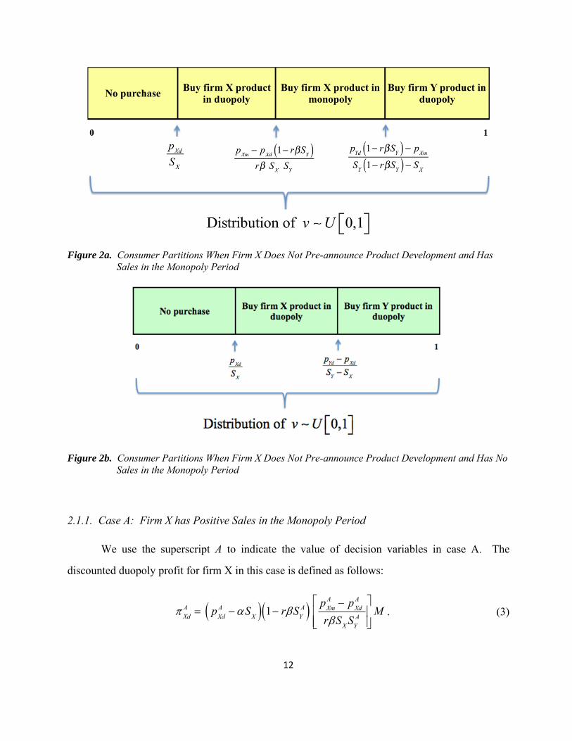
2.1.1. Case A: Firm X has Positive Sales in the Monopoly Period

We use the superscript A to indicate the value of decision variables in case A. The

discounted duopoly profit for firm X in this case is defined as follows:

XdA p

XdA S

X 1 rSYA p

XmA p

XdA

rSXS

YA

M . (3)

13

Given (3), and using the first and second order conditions (FOC and SOC) wrt pXdA , we find the

optimal duopoly price for firm X, pXdA*, to be:

p

XdA* .5 p

XmA S

X . (4)

Since pXmA S

X, the optimal duopoly price defined by (4) indicates that p

XdA* p

XmA* ; i.e., the

competition in the duopoly period forces firm X to reduce its price. Substituting the definition of

pXdA* into (3), firm X’s optimal discounted duopoly profit becomes:

Xd

A p

XmA S

X 4rS

X S

YA

2

1 r SYA M .

Likewise, the discounted duopoly profit for firm Y is defined as follows:

YdA p

YdA S

YA 1 rS

YA 1

pYdA 1 rS

YA p

XmA

SYA 1 rS

YA S

X

M . (5)

Using the FOC and SOC of (5), we find

pYdA* .5 S

YA 1 S

X p

XmA

1 r SYA

, (6)

indicating that firm Y can calculate its optimal duopoly price once the design and monopoly price

of firm X’s product is known. Using the results in (6), firm Y can find the optimal design/quality

of its product, SYA*; the following proposition indicates that there is a unique value of S

YA* that

maximizes (5) subject to the constraints that YdA 0 and the market segments indicated in Figure

2a.

14

Proposition 1A: For given values of pXmA and SX, the unique value of S

YA* that maximizes (5) in

case A subject to the constraints that SYA 1 r S

YA S

X and

0 p

XdA

SX

p

XmA p

XdA 1 rS

YA

r SYA S

X

p

YdA 1 rS

YA p

XmA

SYA 1 rS

YA S

X

1 is given by SYA*

1

2r .

Proof: See Appendix B

Proposition 1A indicates that firm Y sets its product’s design/quality level independent of

firm X’s design level when firm X has sales in the monopoly period. Given the optimal design

value SYA*defined by Proposition 1A, the discount factor 1 rS

Y is equal to 0.5. Substituting

the value of SYA* into (6), the optimal duopoly price set by firm Y can be written as:

pYdA*

14r

SX p

XmA . (7)

Under the conditions in Proposition 1A, there is a unique equilibrium solution for this Stackelberg

game. Given values of SX and pXmA , firm X knows firm Y’s optimal response function. Using the

results of Proposition 1A and the optimal duopoly price for firm Y defined by (7), the total

discounted profit for firm X can be written as a function of SX and the monopoly price, pXmA :

XA p

XmA S

X 1 1 4rS

X 3p

XmA

SX

8r p

XmA

2 1 4r SX

p

XmA S

X 2

4SX

M . (8)

For a given product design SX, the monopoly price, pXmA , that maximizes (8) can be calculated

from the FOC of (8):

pXmA*

SX

1 4rSX 4 1 2rS

X 512r S

X

. (9)

15

SOCs confirm that (9) maximizes firm X’s total profit defined by (9) and satisfies the constraints

that define the Stackelberg game.

Using (4), (6), (9), and the results in Proposition 1, we can characterize the Stackelberg

game completely when firm X conceals its development effort and does not pre-announce its

product—assuming that firm X has positive sales in the monopoly period (i.e., case A). Our

results are summarized in Appendix A. In case B, when firm X sells only in the duopoly period

(but still conceals its development effort), the Stackelberg game is analyzed in the following

section.

2.1.2. Case B: Firm X has No Sales in the Monopoly Period

When p

Xm p

Xd1 rS

Y rS

YS

X

p

YD1 rS

Y pXm

SY

1 rSY S

X

in Figure 2a, firm X has set a design

level and prices such that sales only occur in the duopoly period. In this case, the consumer

partitions indicated in Figure 2b are relevant and the discounted profit for firm X in the duopoly

period is defined as:

XdB p

XdB S

X 1 rSYB p

YdB S

X p

XdB S

YB

SYB S

X SYB

M . (10)

Taking the FOC of (10), the duopoly price for firm X that maximizes (10) is:

pXdB* .5

pYdB S

X

SYB

SX

(11)

such that the discounted duopoly profit for firm X can be rewritten as

XdB

1 rSYB SX

M

4 SYB S

X SYB

pYdB S

YB 2

.

Similarly, the discounted duopoly profit for firm Y is

YdB p

YdB S

YB 1 rS

YB S

YB S

X p

YdB p

XdB

SYB S

X

M

16

such that the optimal duopoly price for firm Y becomes

p

YdB* .5 S

YB S

XS

YB p

XdB . (12)

Using (11) and (12), we obtain the optimal duopoly prices for both firms in terms of SX and SYB :

pYdB*

SYB 2S

YB 1 S

X2

4SYB S

X

; pXdB*

SX

SYB 3S

YB S

X 4S

YB S

X

. (13)

Given the optimal prices defined by (13) and FOC for SY, we can find the optimal design level for

firm Y; this, leads to Proposition 1B.

Proposition 1B: For a given value of SX > 0, the unique value of SYB* that maximizes firm Y’s

discounted duopoly profit subject to the constraints that SYB* 1 r S

YB* S

X and

pXm

B pXd

B 1 rSYB*

rSYB*S

X

p

YD

B 1 rSYB* p

Xm

B

SYB* 1 rS

YB* S

X

and 0 p

XdB

SX

p

YdB p

XdB

SYB S

X

1

is given by

SYB*

2 3rSX 4 4rS

X 3rS

X 2

8r .


In this case, we set pXmB

pXdB S

YB* 1 rS

YB* S

X

p

YdB rS

XS

YB*

SYB* S

X

such that

pXmB p

XdB 1 rS

YB

r SYB S

X

p

YdB 1 rS

YB p

XmB

SYB 1 rS

YB S

X

(the lower bound for which firm X has no monopoly

sales). Any value greater than this lower bound would result in the same profit for both firms.

Since S

YB* 1 rS

YB* S

X , the monopoly price is greater than the duopoly price and greater than

the monopoly price in case A. This, with the optimal prices defined by (13) and Proposition 1B,

completely characterizes the Stackelberg game in case B. In the following section, we compare

the results in cases A and B with no pre-announcement to the cases when firm X chooses to pre-

announce its product and begins product development at time t SX

.

17

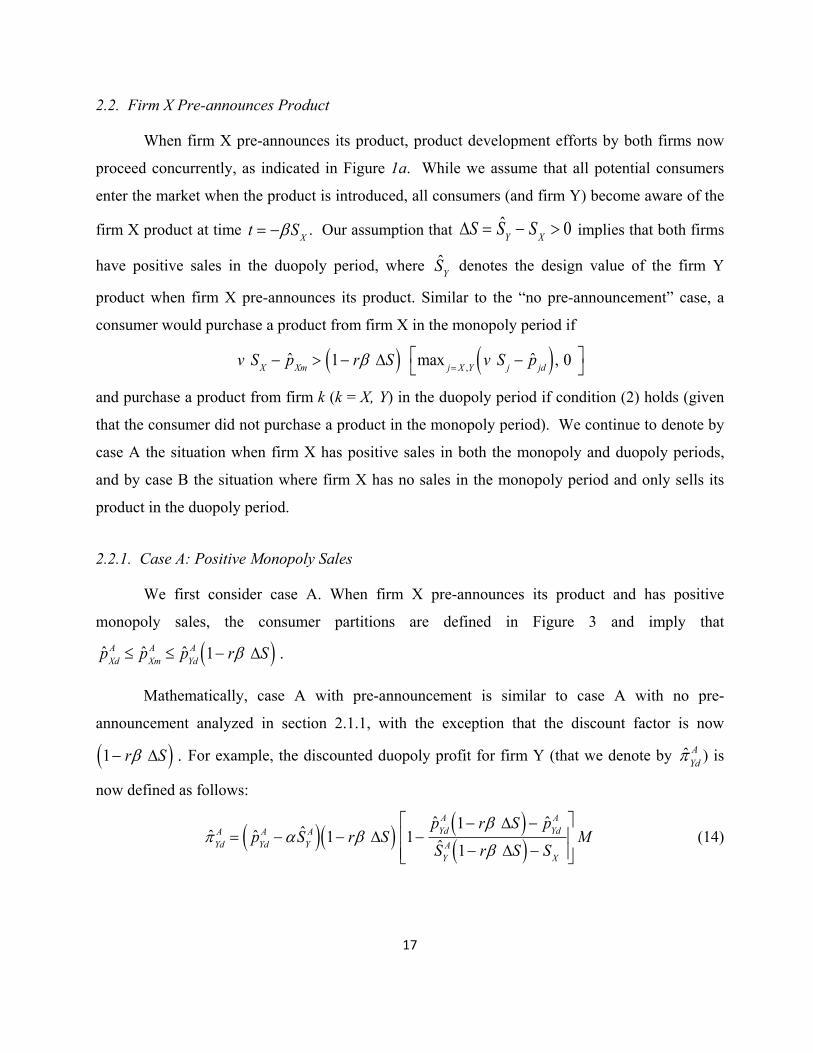
2.2. Firm X Pre-announces Product

When firm X pre-announces its product, product development efforts by both firms now

proceed concurrently, as indicated in Figure 1a. While we assume that all potential consumers

enter the market when the product is introduced, all consumers (and firm Y) become aware of the

firm X product at time t SX

. Our assumption that S SY S

X 0 implies that both firms

have positive sales in the duopoly period, where SY

denotes the design value of the firm Y

product when firm X pre-announces its product. Similar to the “no pre-announcement” case, a

consumer would purchase a product from firm X in the monopoly period if

v SX p

Xm 1 r S max

j X ,Yv S

j p

jd , 0

and purchase a product from firm k (k = X, Y) in the duopoly period if condition (2) holds (given

that the consumer did not purchase a product in the monopoly period). We continue to denote by

case A the situation when firm X has positive sales in both the monopoly and duopoly periods,

and by case B the situation where firm X has no sales in the monopoly period and only sells its

product in the duopoly period.

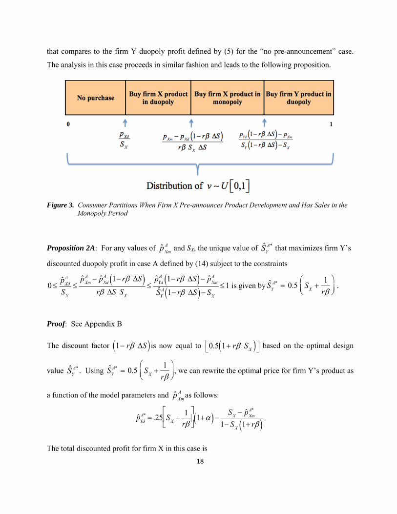
2.2.1. Case A: Positive Monopoly Sales

We first consider case A. When firm X pre-announces its product and has positive

monopoly sales, the consumer partitions are defined in Figure 3 and imply that

pXdA p

XmA p

YdA 1 r S .

Mathematically, case A with pre-announcement is similar to case A with no pre-

announcement analyzed in section 2.1.1, with the exception that the discount factor is now

1 r S . For example, the discounted duopoly profit for firm Y (that we denote by YdA ) is

now defined as follows:

YdA p

YdA S

YA 1 r S 1

pYdA 1 r S p

YdA

SYA 1 r S S

X

M (14)

18

that compares to the firm Y duopoly profit defined by (5) for the “no pre-announcement” case.

The analysis in this case proceeds in similar fashion and leads to the following proposition.

Figure 3. Consumer Partitions When Firm X Pre-announces Product Development and Has Sales in the Monopoly Period

Proposition 2A: For any values of pXmA and SX, the unique value of S

YA* that maximizes firm Y’s

discounted duopoly profit in case A defined by (14) subject to the constraints

0 p

XdA

SX

p

XmA p

XdA 1 r S

r S SX

p

YdA 1 r S p

XmA

SYA 1 r S S

X

1 is given by SYA* 0.5 S

X

1

r

.


The discount factor 1 r S is now equal to 0.5 1 r SX

based on the optimal design

value SYA* . Using S

YA* 0.5 S

X

1

r

, we can rewrite the optimal price for firm Y’s product as

a function of the model parameters and pXmA as follows:

pYdA* .25 S

X 1

r

1 S

X p

XmA*

1 SX

1 r .

The total discounted profit for firm X in this case is

19

XA p

XmA S

X M.5 p

YdA 1 rS

X pXmA

.25 SX (r)1 1 rS

X SX

p

XmA .25 p

XmS

X 1 rSX

.5rSX

1 rSX

pXdA S

X 1 rSX

2SX

M .

(15)

Maximizing (15), we can obtain firm X’s optimal prices for the monopoly and duopoly periods,

respectively:

pXmA*

SX

r 2 1 3 2SX4 2rS

X3 r 1 S

X2 1 3 r 2 2 2S

X

1 4r 2 2SX3 S

X2 8 r 2 2 4S

X

.

and p

XdA* .5 p

XmA S

X . Note that the optimal duopoly price charged by firm X, p

XdA*, is the same in both the pre-

announcement and “no pre-announcement” cases; that is, pXdA* p

XdA* .5 p

Xm S

X as defined

by (4).

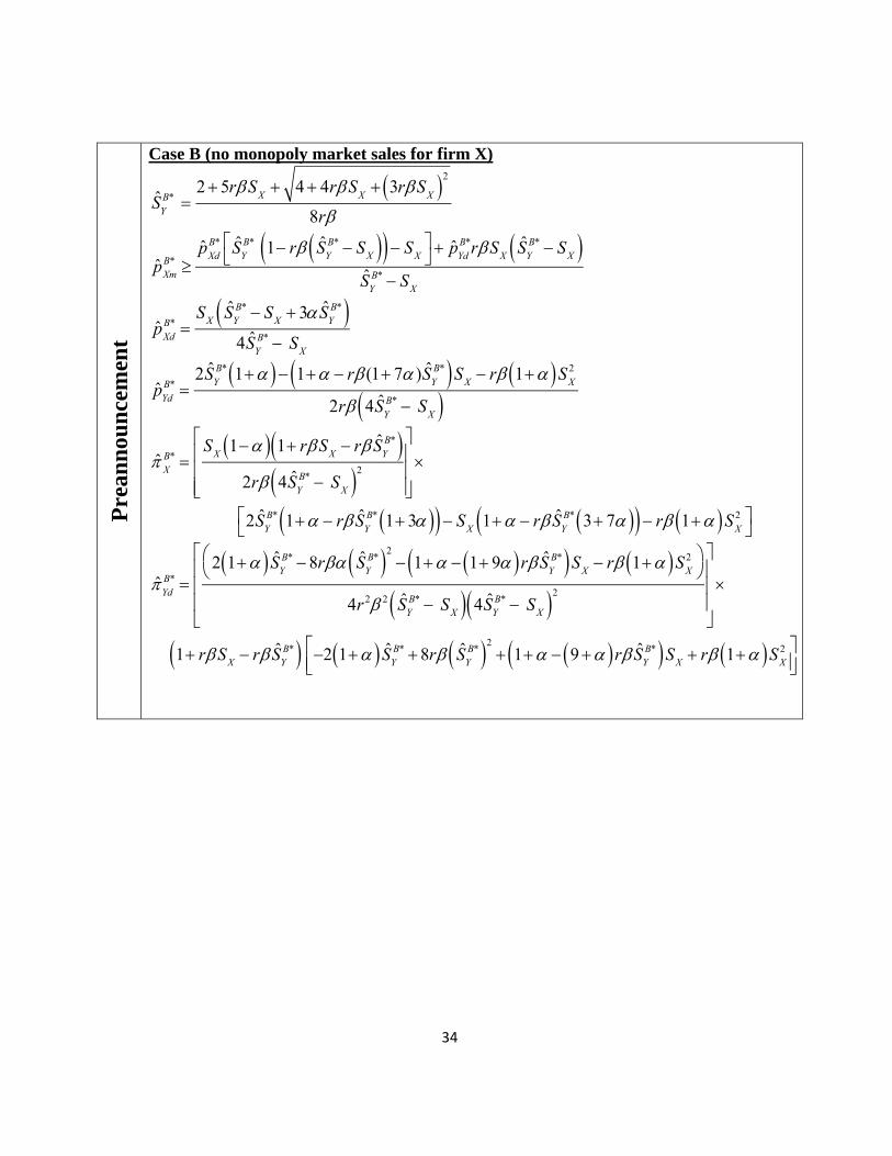
2.2.2. Case B: No Monopoly Sales for Firm X

The case when firm X has no monopoly sales (case B) is analogous to the case in section

2.1.2 with the difference that the discount factor is now equal to 1 r S . This discount

factor results in a changed optimal design SYB* for firm Y; this value and its derivation is given in

Proposition 2B.

Proposition 2B: For a given value of SX, the unique value of SYB* that maximizes firm Y’s

discounted duopoly profit subject to the constraints that SYB* 1 r S

YB* S

X SX

,

20

pYD

B 1 r SYB* SX p

Xm

B

SYB* 1 r S

YB* S

X SX

p

Xm

B pXd

B 1 r SYB* SX

r SYB* S

X SX

, and 0 p

XdB

SX

p

YdB p

XdB

SYB S

X

1 is given

by SYB*

2 5rSX 4 4rS

X 3rS

X 2

8r .


All other aspects of the model described in section 2.1.2 continue to hold; specific results are

summarized in Appendix A.

3. Model and Managerial Implications

In the previous section, we were able to derive close-form expressions for all the key

decisions – firm Y’s design level and both firms’ price decisions – as well as both firms’ profit

functions, in a variety of settings: when firm X pre-announces its product development effort or

does not pre-announce; when firm X has sales in the monopoly period or not. These expressions

are summarized in Appendix A; they not only allow us to understand the Stackelberg game

dynamics and how the two firms strategically react to each other, but, more importantly, also

allow us to evaluate firm X’s profits under pre-announcement and no pre-announcement. We have

used these expressions to carry out a range of numerical tests and will report the results below.

By comparing both firms’ profits in the various settings, we find a number of significant

implications for new product development managers. Two major findings emerge from our

analysis. First, we found that the innovator firm X may, under some conditions, choose to forgo

sales in the monopoly period. This result appears to be counter-intuitive. For example, consider

case B (in section 2.1.2) when firm X does not pre-announce its product development effort and

sells only in the duopoly period. In this case, it would seem that firm X could reduce its

monopoly price pXmB such that

pXmB p

XdB 1 rS

YB

rSYBS

X

p

YdB 1 rS

YB p

XmB

SYB 1 rS

YB S

X

and some consumers

would then purchase firm X’s product in the monopoly period. Since pXmB p

XdB , it would appear

that firm X could do better by setting a monopoly price such that some monopoly sales occur.

21

Our analysis, however, suggests otherwise; namely, once firm X considers firm Y’s

reaction to its pricing and design decisions, we showed that firm X may lower its overall profits

by reducing its monopoly price to stimulate monopoly sales. Specifically, when firm X sets a

monopoly price that is sufficiently high to discourage any monopoly sales (case B), firm Y

produces a product of higher quality/design than when firm X has monopoly sales (case A). This

is supported by the following proposition that is based on previous results derived in section 2.

Proposition 3: For all SX > 0, it holds that SYB* S

YA* and S

YB* S

YA* .


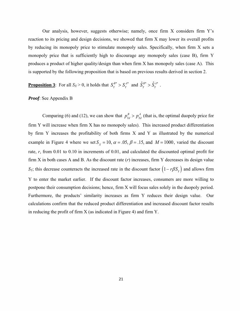
Comparing (6) and (12), we can show that pYdB p

YdA (that is, the optimal duopoly price for

firm Y will increase when firm X has no monopoly sales). This increased product differentiation

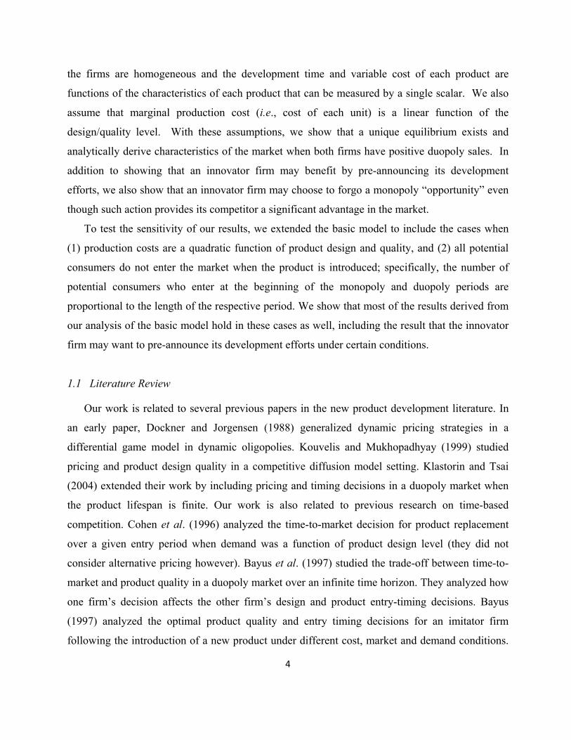
by firm Y increases the profitability of both firms X and Y as illustrated by the numerical

example in Figure 4 where we set SX 10, .05, .15, and M 1000, varied the discount

rate, r, from 0.01 to 0.10 in increments of 0.01, and calculated the discounted optimal profit for

firm X in both cases A and B. As the discount rate (r) increases, firm Y decreases its design value

SY; this decrease counteracts the increased rate in the discount factor 1 rSY and allows firm

Y to enter the market earlier. If the discount factor increases, consumers are more willing to

postpone their consumption decisions; hence, firm X will focus sales solely in the duopoly period.

Furthermore, the products’ similarity increases as firm Y reduces their design value. Our

calculations confirm that the reduced product differentiation and increased discount factor results

in reducing the profit of firm X (as indicated in Figure 4) and firm Y.

22

Figure 4. Profit of Firm X with Monopoly and No Monopoly Sales as Function of Discount Rate, r

The advantages (to both firms) of increased product differentiation is the main factor

behind firm X’s decision to pre-announce or not pre-announce its product development effort. A

comparison of Propositions 1A and 2A indicate that firm Y’s product will have a greater

quality/design when firm X pre-announces its product; that is, SYA* S

YA* (assuming sales in the

monopoly period). Again, the increased product differentiation by firm Y increases the

profitability of both firms, thereby providing an incentive for firm X to pre-announce its product

development effort (depending on the parameter values). The following numerical examples

illustrate these concepts.

Normalizing T to 1, we set .05,Ê .15,ÊM 1000,ÊSX 10, and varied the discount

rate, r, from 0.01 to 0.10 in increments of 0.01. The results in Figure 5 indicate that firm X can

increase its profit by pre-announcing its product development efforts as the discount rate, r,

increases greater than (approximately) 0.075. Since consumers are forward looking, firm Y’s

product does not only compete with firm X’s product in the duopoly period but also in the

monopoly period. While firm Y’s product has a higher design level that firm X’s product, the

increased discount rate diminishes the appeal of firm Y’s product (compared to firm X’s product

in the monopoly period). Alternatively, the increased discount rate reduces the differences

between the two products in the minds of monopoly consumers that, in turn, increases the

competitive pressure on pricing. As a result, the profits of both firms are reduced. However,

$0

$100

$200

$300

$400

$500

0 0.02 0.04 0.06 0.08 0.1

Firm

X Profit

Discount Rate (r)

Firm X Profit (Monopoly Sales) Firm X Profit (No Monopoly Sales)

23

when firm X pre-announces its product development, firm Y begins its product development

effort earlier. This has two effects: (1) firm X has a shorter monopoly period, and (2) firm Y

now has an incentive to increase its product design level (that is, the longer development time is

offset by the earlier development start). The first effect has a negative impact on firm X profits,

but the second effect could increase firm X profits (since the products become more differentiated

and the two firms can better segment the duopoly consumers). When the discount rate is high, the

second effect tends to dominate; hence, firm X prefers to pre-announce its product development.

Figure 5. Firm X Profits when Pre-announcing Product and Not Pre-announcing Product as Function of Discount Rate, r

To investigate the impact of increasing marginal production cost , we normalized T =

1, set r .05, .15, SX 10, M 1000 and varied from 0.01 to 0.10; results are indicated in

Figure 6. For this example, firm Y sets its design level SY = 74.35 for all values of when firm

X pre-announces its product. However, when firm X does not pre-announce its product, firm Y

increases the design level SY monotonically from 66.67 1 / 2r to 69.36 as increases,

reinforcing our finding that SYA* S

YA* . For values of less than 0.05, firm X has no sales in the

monopoly period (case B); as the production cost increases greater then 0.05, firm X can increase

its profits by reducing its monopoly price and beginning sales in the monopoly period. Our

calculations indicate that both firm X and firm Y prices do not change monotonically with ; firm

120.0

170.0

220.0

270.0

320.0

370.0

420.0

470.0

0 0.02 0.04 0.06 0.08 0.1 0.12

Firm

X Profit

Discount Rate, r

Firm X Profit: No Pre‐announcement Firm X Profit: Pre‐announcement

24

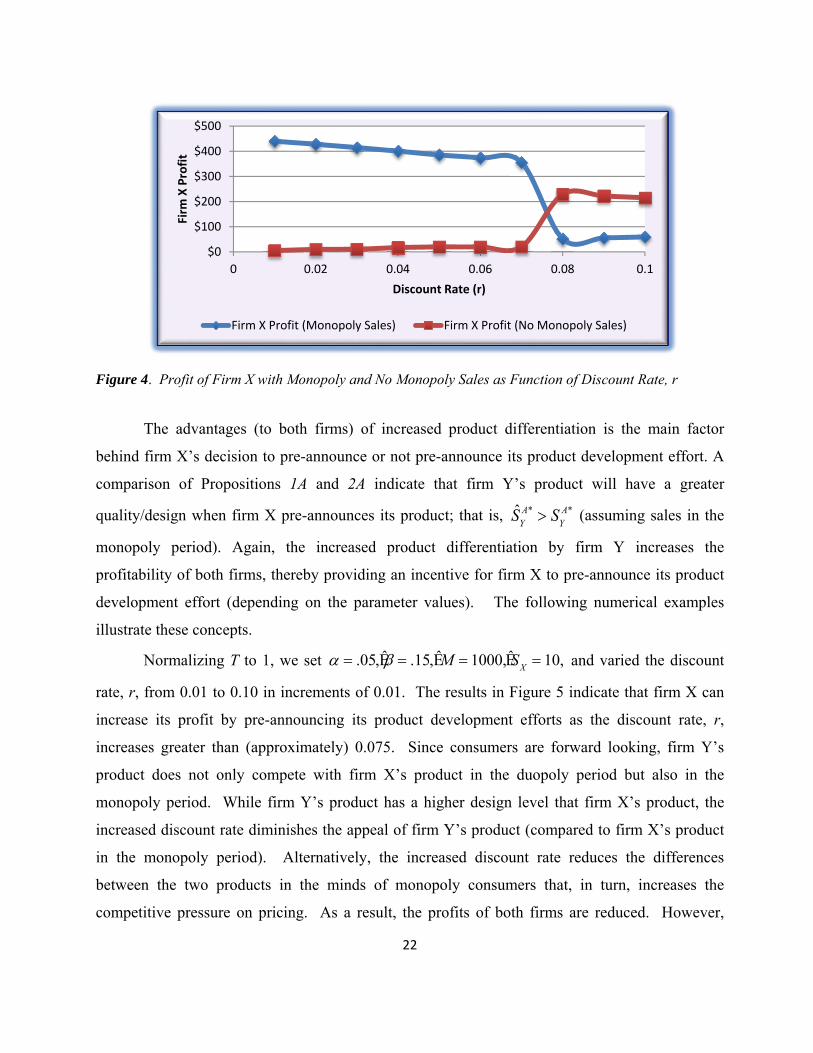
X profits are maximized when = 0.05 when firm X reduces its monopoly price to initiate

monopoly sales. As increases greater than 0.05, firm X increases its monopoly price (to offset

the increase in costs) that reduces overall profits (but still retains monopoly sales). For values of

< 0.05, firm X can increase its profits by approximately 4.5 percent by pre-announcing its product

development effort.

Figure 6. Profit of Firm X when Pre-Announcing Product and Not Pre-announcing Product as Function of Marginal Production Cost,

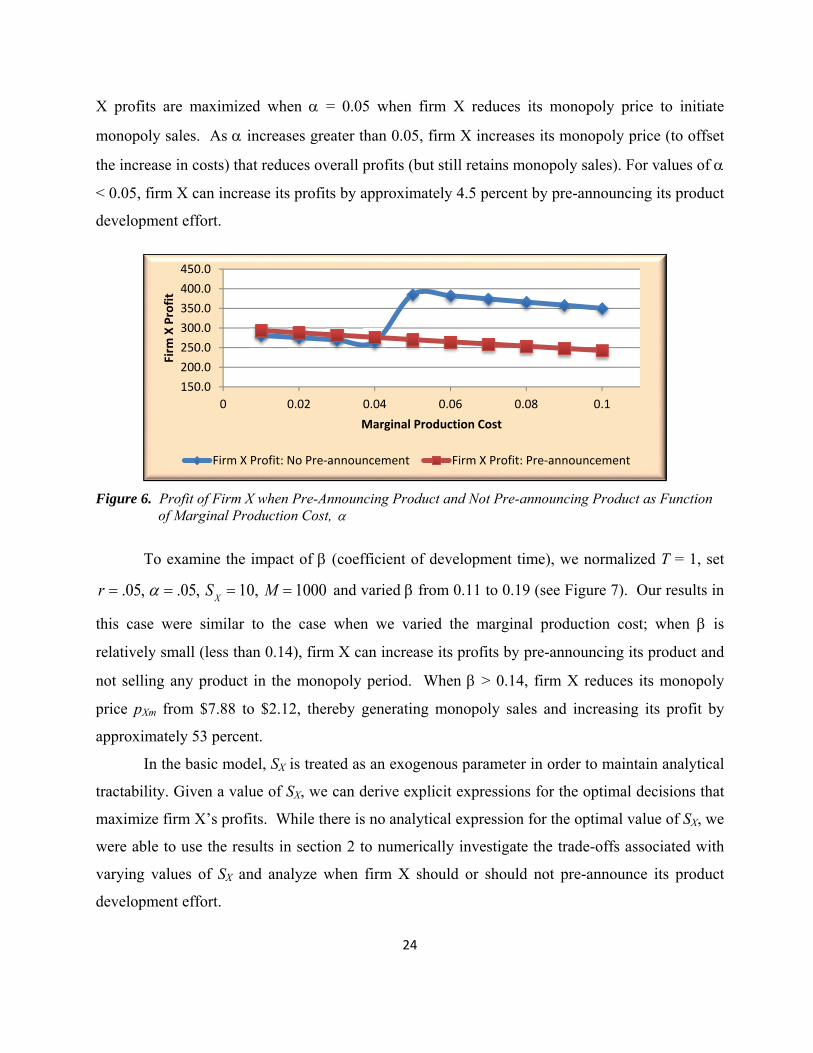
To examine the impact of (coefficient of development time), we normalized T = 1, set

r .05, .05, SX 10, M 1000 and varied from 0.11 to 0.19 (see Figure 7). Our results in

this case were similar to the case when we varied the marginal production cost; when is

relatively small (less than 0.14), firm X can increase its profits by pre-announcing its product and

not selling any product in the monopoly period. When > 0.14, firm X reduces its monopoly

price pXm from $7.88 to $2.12, thereby generating monopoly sales and increasing its profit by

approximately 53 percent.

In the basic model, SX is treated as an exogenous parameter in order to maintain analytical

tractability. Given a value of SX, we can derive explicit expressions for the optimal decisions that

maximize firm X’s profits. While there is no analytical expression for the optimal value of SX, we

were able to use the results in section 2 to numerically investigate the trade-offs associated with

varying values of SX and analyze when firm X should or should not pre-announce its product

development effort.

150.0

200.0

250.0

300.0

350.0

400.0

450.0

0 0.02 0.04 0.06 0.08 0.1

Firm

X Profit

Marginal Production Cost


25

Figure 7. Profit of Firm X when Pre-Announcing Product and Not Pre-announcing Product as Function of the Development Time Coefficient,

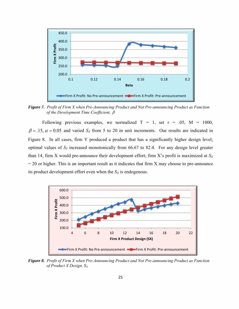
Following previous examples, we normalized T = 1, set r = .05, M = 1000,

.15, 0.05 and varied SX from 5 to 20 in unit increments. Our results are indicated in

Figure 8. In all cases, firm Y produced a product that has a significantly higher design level;

optimal values of SY increased monotonically from 66.67 to 82.4. For any design level greater

than 14, firm X would pre-announce their development effort; firm X’s profit is maximized at SX

= 20 or higher. This is an important result as it indicates that firm X may choose to pre-announce

its product development effort even when the SX is endogenous.

Figure 8. Profit of Firm X when Pre-Announcing Product and Not Pre-announcing Product as Function of Product X Design, SX

200.0

250.0

300.0

350.0

400.0

450.0

0.1 0.12 0.14 0.16 0.18 0.2

Firm

X Profit

Beta


100.0

200.0

300.0

400.0

500.0

600.0

4 6 8 10 12 14 16 18 20 22

Firm

X Profit

Firm X Product Design (SX)


26

To test the sensitivity of our results, we extended the basic model in two ways. First, we

assumed that production costs were quadratic as indicated in some previous studies (Klastorin and

Tsay, 2004); i.e., we let c S S 2 where 0. Second, we relaxed the assumption that all

potential consumers arrive when the product is initially introduced; in this case, we assumed that

potential consumers arrive at the beginning of the monopoly and duopoly periods in numbers that

are proportional to the length of each respective period. Specifically, when firm X does not pre-

announce its product, the number of potential consumers who enter the market at time t = 0 is

SY

T

M ; the number of potential consumers who enter the market at the beginning of the

duopoly period is 1S

Y

T

M . The consumer partitions defined in Figures 2a and 2b continue

to hold; thus, the total discounted profit for firm X (assuming sales in the monopoly period and

quadratic costs) is defined as follows:

X p

XmS

X2 p

Yd1 rS

Y pXm

SY

1 rSY

pXm p

Xd1 rS

Y rS

XS

Y

SY

T

M

pXdS

X2 1 rS

Y Mp

Xm p

Xd

rSXS

Y

SY

T

2

p

YdS

X p

XdS

Y

SX

SY S

X 1S

Y

T

S

Y

T

.

The analysis of this model is similar to the basic model described in section 2. For

example, we can show that the optimal duopoly price for firm Y, pYd* , is equal to

pYd* .5 S

Y1S

Y SX p

Xm

1 rSY

that is independent of firm X’s sales in the monopoly period. However, in this case, Propositions

1 and 2 do not hold (that is, there is no unique equilibrium to the Stackelberg game); thus, to find

SY* , we solved the nonlinear programming problem:

27

Max Yd .25M 1

SY

T

S

YS

Y2 1 rS

Y SX p

Xm

2

SY

1 rSY S

X

subject to

SY T

SY

1 rSY S

X

as an interpreted MATLAB application on a Dell OptiPlex 755 with 4GB of RAM running

Windows 7 OS. Given SY* , we then calculated p

Xd* and p

Xm* using a similar approach described

in section 2 for the basic model.

Overall, we analyzed four models by varying the assumption about production cost (linear

versus quadratic) and consumer arrival patterns (all arrive at time t = 0 or proportionately at the

beginning of the monopoly and duopoly periods). When consumers arrived proportionately, we

found that incentives for firm X to pre-announce its product were generally greater than the

results we observed from the basic model. For example, when production costs are quadratic and

consumers arrive proportionately at the beginning of each period, we varied SX from 5 to 20 in

unit increments and calculated the optimal decisions for firms X and Y (normalizing M = T = 1,

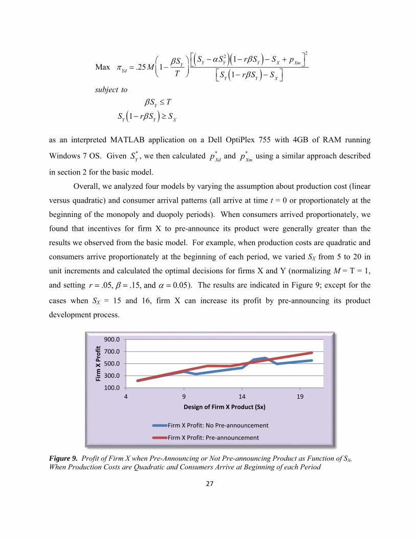
and setting r .05, .15, and 0.05). The results are indicated in Figure 9; except for the

cases when SX = 15 and 16, firm X can increase its profit by pre-announcing its product

development process.

Figure 9. Profit of Firm X when Pre-Announcing or Not Pre-announcing Product as Function of SX, When Production Costs are Quadratic and Consumers Arrive at Beginning of each Period

100.0

300.0

500.0

700.0

900.0

4 9 14 19

Firm

X Profit

Design of Firm X Product (Sx)

Firm X Profit: No Pre‐announcement

Firm X Profit: Pre‐announcement

28

Generally, pre-announcement is a better strategy for firm X when consumers arrive

proportionately over time. For the example in Figure 9 when all potential consumers arrive at

time t = 0, firm X would only pre-announce its product for values of SX ≥ 15. Similarly, linear

production costs tend to increase the benefits of pre-announcement; when we solved the example

in Figure 9 with c S S , firm X could increase profits by pre-announcing its product for all

values of SX. We found similar results as we reduced the values of and .

4. Conclusions and Extensions

In this paper, we studied a durable goods market with two competing homogeneous firms

when one firm is an innovator who initiates development of a new product. The primary research

question we addressed is whether the innovator firm should pre-announce its product

development effort or not. Our work extends previous research in this area in several important

ways. In addition to modeling a durable good market with a finite lifespan as a Stackelberg game,

we modeled rationally expectant consumers who make decisions based on both the value of

current goods and prices as well as their expectation of future products and prices. Using these

models, we were able to show that a unique equilibrium exists for the Stackelberg game in some

cases; in other cases, we were able to find optimal solutions numerically. We derived several

implications for both firms and showed that conditions exist when the innovator firm benefits

from pre-announcing its development project, even though releasing such information increases

the profitability of its competitor and defies conventional wisdom.

This work suggests numerous directions for future research. In this paper, we only

considered whether the innovator firm should pre-announce its new product when it begins

development work (at time t SX

) or wait until the product is introduced into the market (at

time t = 0). Clearly, there may be some cases when the innovator firm should announce its

product at some time between these values (as frequently observed in practice). We are also

investigating measures of “competitive intensity” and its impact on pre-announcement decisions.3

3 The authors gratefully acknowledge this suggestion by an anonymous referee.

29

In this case, we let denote a preference measure for firm Y’s product such that the consumer

utility for firm Y’s product is vSY p

Yd (i.e., consumers are indifferent between the two firms’

products in the duopoly period if vSY p

Yd vS

X p

Xd). A similar measure has been used in

the study of gray markets (Ahmadi and Yang 2000; Xiao et al. 2011).

The models presented in this paper have implications for other areas in marketing and

operations management. For example, a firm’s product design decision impacts the resultant

supply chain; a higher design level product is likely to require a more complex supply chain that

may, in turn, increase both the marginal production cost and the development time (i.e., the

product development time g(S) is no longer an exogenous function). In addition, firms can

frequently compress the development time by increasing the level of resources allocated to

product development (a modification of the time-cost trade-off problem discussed in the project

management literature). This extension would allow a firm to study the impact of its development

costs on resultant market share and profitability.

30

References

Ahmadi, R., B.R. Yang. 2000. “Parallel imports: Challenges from unauthorized distribution channels. Marketing Science. 18(3), 279-294.

Bala, R., S. Carr. 2009. Pricing software upgrades: The role of product improvement and user costs. Production and Operations Management 18(5) 560-580.

Bhaskaran, S. R., S. M. Gilbert. 2005. Selling and leasing strategies for durable goods with complementary products. Management Science 51(8) 1278-1290.

Bayus, B. L. 1997. Speed-to-market and new product performance trade-offs. Journal of Product Innovation Management 14 485-497.

Bayus, B. L., S. Jain, A. G. Rao. 1997. Too little, too early: Introduction timing and new product performance in the personal digital assistant industry. Journal of Marketing Research 34(1) 50-63.

Coase, R.H. 1972. Durability and monopoly. Journal of Law and Economics. 15, 143-149.

Cohen, M., J. Eliashberg, T. H. Ho. 1996. New product development: The performance and time-to-market trade-off. Management Science 42(2) 173-186.

Dogan, K., Y. Ji, V. Mookerjee, S. Radhakrishnan. 2011. “Managing the versions of a software product under variable and endogenous demand” Information Systems Research. 22 (1), 5-21.

Dhebar, A. 1994. Durable-goods monopolists, rational consumers, and improving products. Marketing Science 13(1) 100-120.

Dockner, E., S. Jorgensen. 1988. Optimal pricing strategies for new products in dynamic oligopolies. Marketing Science 7(4) 315-334.

Fudenberg, D., J. Tirole. 1998. Upgrades, trade-ins, and buy-backs. The RAND Journal of Economics 29(2) 235-258.

Hotelling, H. 1929. Stability in competition. The Economic Journal 39 41-57.

Klastorin, T., W. Tsai. 2004. New product introduction: Timing, design, and pricing. Manufacturing & Service Operations Management 6(4) 302-320.

Kornish, L. J. 2001 Pricing for a durable-goods monopolist under rapid sequential innovation. Management Science 47(11) 1552-1561.

Kouvelis, P., S. K. Mukhopadhyay. 1999. Modeling the design quality competition for durable products. IIE Transactions 31(9) 865-880.

31

Mehra, A., R. Bala, R. Rankaranarayanan. “Competitive Behavior-based price discrimination for software upgrades.” Information Systems Research 22(4).

Moorthy, S. K. 1988. Product and price competition in a duopoly. Marketing Science 7(2) 141-168.

Moorthy, K. S., I. P. L. Png. 1992. Market segmentation, cannibalization, and the timing of the product introductions. Management Science 38(3) 345-359.

Morgan,L. O., R. M. Morgan, W. L. Moore. 2001. Quality and time-to-market trade-offs when there are multiple product generations. Manufacturing & Service Operations Management 3(2) 89-104.

Padmanabhan, V., S. Rajiv, K. Sirinivasan. 1997. New products, upgrades, and new releases: A rationale for sequential product introduction. Journal of Marketing Research 34(4) 456-472.

Ramachandran, K., V. Krishnan. 2008. Design architecture and introduction timing for rapidly improving industrial products. Manufacturing & Service Operations Management 10(1) 149-171.

Savin, S., C. Terwiesch. 2005. Optimal product launch times in a duopoly: Balancing life-cycle revenues with product cost. Operations Research 53(1) 26-47.

Schmidt, G. L., E. Porteus. 2000. The impact of an integrated marketing and manufacturing innovation. Manufacturing & Service Operations Management 2(4) 317-336.

Shaked, A. and J. Sutton. 1982. Relaxing Price Competition Through Product Differentiation. The Review of Economic Studies. 49 (1), pp. 3-13.

The Economist. February 26, 2011. The leaky corporation. The Economist Newspaper Limited, London, GB.

Yin, S., S. Ray, H. Gurnani, A. Animesh. 2010. Durable products with multiple used goods markets: Product upgrade and retail pricing implications. Marketing Science 29(3):540–560.

Xiao, Y. U. Palekar, Y. Liu. 2011. Shades of gray – The impact of gray markets on authorized distribution channels. Quantitative Marketing and Economics. 9, 155-178.

32

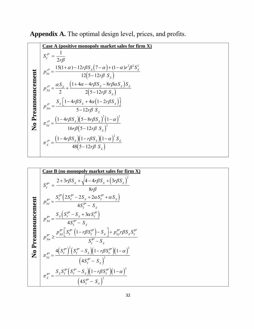
Appendix A. The optimal design level, prices, and profits. N

o P

rean

nou

nce

men

t

Case A (positive monopoly market sales for firm X)

SYA*

1

2r

pYdA*

15(1 )12rSX

7 (1 )r 2 2SX2

12 512r SX

pXdA*

SX

2

1 4 4rSX 8rSX SX

2 512r SX

pXmA*

SX

1 4rSX 4 1 2rS

X 512r S

X

YdA*

1 4rSX 58rS

X 21 2

16r 512r SX 2

XA*

1 4rSX 1 rS

X 1 2S

X

48 512r SX

No

Pre

ann

oun

cem

ent

Case B (no monopoly market sales for firm X)

SYB*

2 3rSX 4 4rS

X 3rS

X 2

8r

pYd

B* SY

B* 2SYB* 2SX 2SY

B* SX 4SY

B* SX

pXd

B* SX SY

B* SX 3SYB*

4SYB* SX

pXmB*

pXdB* S

YB* 1 rS

YB* S

X

p

YdB*rS

XS

YB*

SYB* S

X

YdB*

4 SYB* 2

SYB* S

X 1 rSYB* 1 2

4SYB* S

X 2

XB*

SX SYB* SY

B* SX 1 rSYB* 1 2

4SYB* S

X 2

33

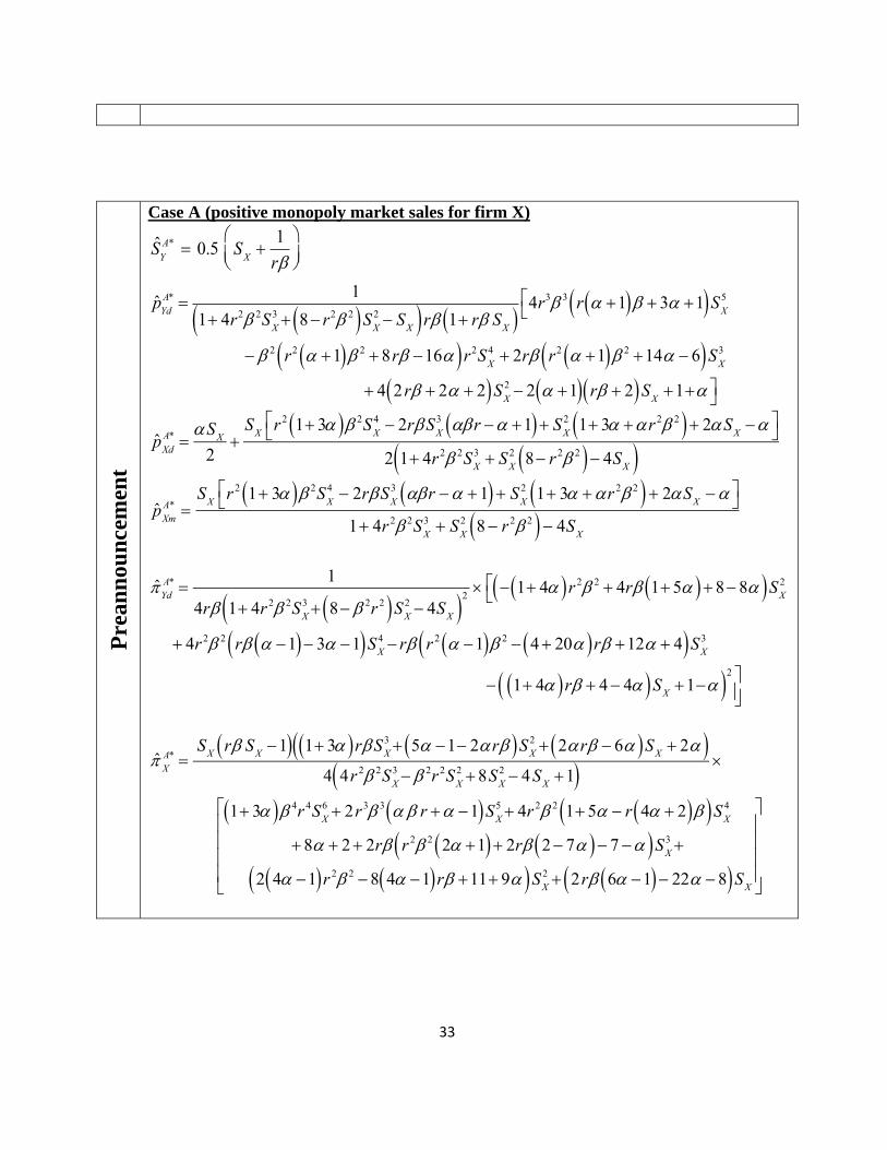
Pre

ann

oun

cem

ent

Case A (positive monopoly market sales for firm X)

SYA* 0.5 S

X

1

r

pYdA*

1

1 4r2 2SX3 8 r2 2 SX

2 SX r 1 r S

X 4r3 3 r 1 3 1 SX

5

2 r2 1 2 8r 16 r2SX4 2r r2 1 2 14 6 SX

3

4 2r 2 2 SX2 2 1 r 2 SX

1

pXdA*

SX

2

SX

r 2 1 3 2SX4 2rS

X3 r 1 S

X2 1 3 r 2 2 2S

X

2 1 4r 2 2SX3 SX

2 8 r 2 2 4SX

pXmA*

SX

r 2 1 3 2SX4 2rS

X3 r 1 S

X2 1 3 r 2 2 2S

X

1 4r 2 2SX3 S

X2 8 r 2 2 4S

X

YdA*

1

4r 1 4r 2 2SX3 8 2r 2 SX

2 4SX 2

1 4 r 2 2 4r 15 8 8 SX2

4r 2 2 r 1 3 1 SX4 r r 2 1 2 4 20 r 12 4 SX

3

1 4 r 4 4 SX1 2

XA*

SX

r SX1 1 3 rS

X3 5 1 2r SX

2 2r 6 SX 2

4 4r 2 2SX3 2r 2SX

2 8SX2 4SX 1

1 3 4r 4SX6 2r3 3 r 1 SX

5 4r 2 2 1 5 r 4 2 SX4

8 2 2r r 2 2 2 1 2r 2 7 7 SX3

2 4 1 r 2 2 8 4 1 r 11 9 SX2 2r 6 1 22 8 SX

34

P

rean

nou

nce

men

t

Case B (no monopoly market sales for firm X)

SYB*

2 5rSX 4 4rS

X 3rS

X 2

8r

p

XmB*

pXdB* S

YB* 1 r S

YB* S

X SX

p

YdB*rS

XS

YB* S

X SY

B* SX

pXdB*

SX SYB* SX 3 SY

B* 4S

YB* S

X

pYdB*

2SYB* 1 1 r(1 7 )S

YB* SX

r 1 SX2

2r 4SYB* S

X

XB*

SX

1 1 rSX r S

YB*

2r 4SYB* S

X 2

2SYB* 1 r S

YB* 1 3 S

X1 r S

YB* 3 7 r 1 SX

2

YdB*

2 1 SYB* 8r S

YB* 2

1 1 9 r SYB* SX

r 1 SX2

4r 2 2 SYB* S

X 4SYB* S

X 2

1 rSX r SYB* 2 1 SY

B* 8r SYB* 2

1 9 r SYB* SX r 1 SX

2

35

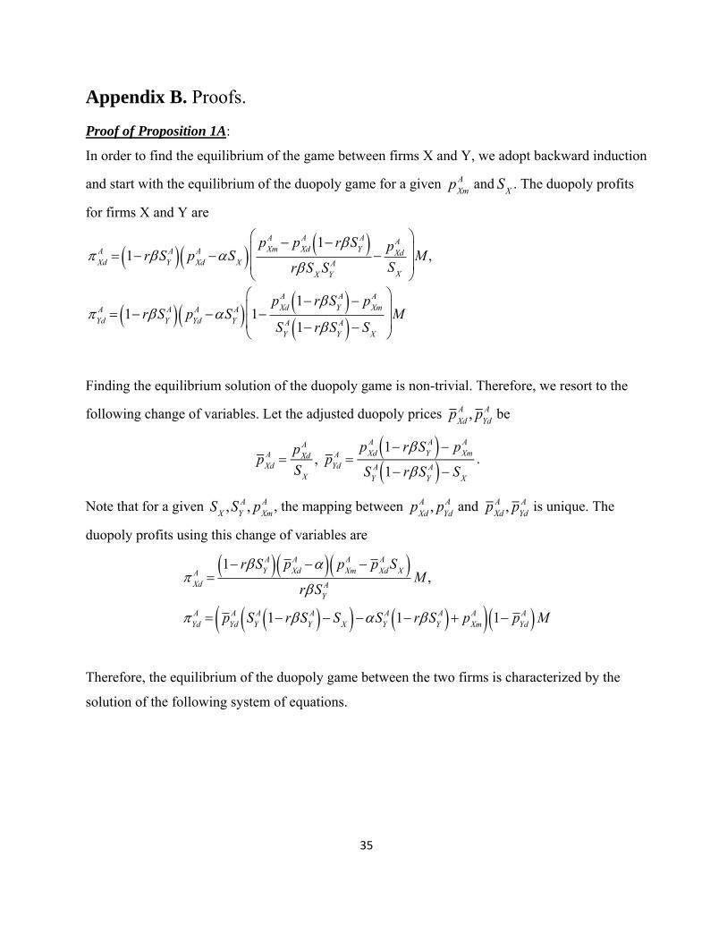
Appendix B. Proofs.

Proof of Proposition 1A:

In order to find the equilibrium of the game between firms X and Y, we adopt backward induction

and start with the equilibrium of the duopoly game for a given pXmA and S

X. The duopoly profits

for firms X and Y are

XdA 1 rS

YA p

XdA S

X p

XmA p

XdA 1 rS

YA

rSX

SYA

p

XdA

SX

M ,

YdA 1 rS

YA p

YdA S

YA 1

pXdA 1 rS

YA p

XmA

SYA 1 rS

YA S

X

M

Finding the equilibrium solution of the duopoly game is non-trivial. Therefore, we resort to the

following change of variables. Let the adjusted duopoly prices pXdA , p

YdA be

pXdA

pXdA

SX

, pYdA

pXdA 1 rSY

A pXmA

SYA 1 rS

YA S

X

.

Note that for a given SX

,SYA , p

XmA , the mapping between p

XdA , p

YdA and p

XdA , p

YdA is unique. The

duopoly profits using this change of variables are

XdA

1 rSYA p

XdA p

XmA p

XdA S

X rS

YA

M ,

YdA p

YdA S

YA 1 rS

YA S

X SYA 1 rS

YA p

XmA 1 p

YdA M

Therefore, the equilibrium of the duopoly game between the two firms is characterized by the

solution of the following system of equations.

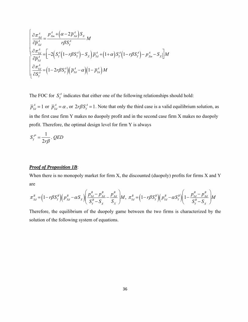
36

XdA

pXdA

pXmA 2 p

XdA S

X

rSYA

M

YdA

pYdA 2 S

YA 1 rS

YA S

X pYdA 1 S

YA 1 rS

YA p

XmA S

X

M

YdA

SYA 1 2rS

YA p

YdA 1 p

YdA M

The FOC for SYA indicates that either one of the following relationships should hold:

pYdA 1 or p

YdA , or 2rS

YA 1. Note that only the third case is a valid equilibrium solution, as

in the first case firm Y makes no duopoly profit and in the second case firm X makes no duopoly

profit. Therefore, the optimal design level for firm Y is always

SYA*

1

2r. QED

Proof of Proposition 1B:

When there is no monopoly market for firm X, the discounted (duopoly) profits for firms X and Y

are

XdB 1 rS

YB p

XdB S

X pYdB p

XdB

SYB S

X

p

XdB

SX

M ,

YdB 1 rS

YB p

YdB S

YB 1

pYdB p

XdB

SYB S

X

M



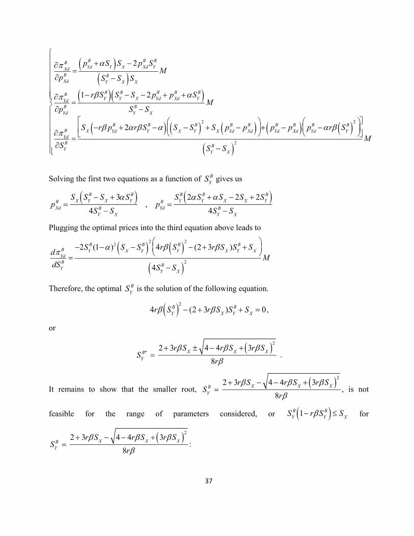
37

XdB

pXdB

p

YdB S

Y SX 2 p

XdB S

YB

SYB S

X SX

M

YdB

pYdB

1 rSYB S

YB S

X 2 p

YdB p

XdB S

YB

SYB S

X

M

YdB

SYB

SXr p

YdB 2rS

YB S

X S

YB 2

SX

pYdB p

XdB

p

YdB p

XdB p

YdB r S

YB 2

SYB S

X 2M

Solving the first two equations as a function of SYB gives us

p

XdB

SX

SYB S

X 3S

YB

4SYB SX

, pYdB

SYB 2S

YB S

X 2S

X 2S

YB

4SYB SX

Plugging the optimal prices into the third equation above leads to

dYdB

dSYB2S

YB (1)2 S

X S

YB 2

4r SYB 2

(23rSX

)SYB S

X

4SYB S

X 2M

Therefore, the optimal SYB is the solution of the following equation.

4r SYB 2

(2 3rSX

)SYB S

X 0,

or

SYB*

2 3rSX 4 4rS

X 3rS

X 2

8r .

It remains to show that the smaller root, SYB

2 3rSX 4 4rS

X 3rS

X 2

8r, is not

feasible for the range of parameters considered, or SYB 1 rS

YB S

X for

SYB

2 3rSX 4 4rS

X 3rS

X 2

8r:

38

SYB 1 rSY

B SX 2 3rSX 4 4rSX 3rSX 2

8r1

2 3rSX 4 4rSX 3rSX 2

8

SX

2 3rSX 4 4rSX 3rSX 2

4 24rSX 3rSX 2

32r

T1 T2

32r

whereT1 2 3rS

X 4 4rSX 3rS

X 2, T

2 4 24rS

X 3rS

X 2. Note that T

1 0 (as

4rSX1 so there exists a feasible S

Y for S

Y1 rS

Y SX ). For rS

X ( 20 4) 3 then

T2 0 and the feasibility condition is violated. Suppose that rS

X ( 20 4) 3 and T

2 0,

then T12 T

22 64rS

X2 6rS

X 9 rS

X 2 , which is positive for all rSX ( 20 4) 3.

Therefore T1 T

2, and the feasibility condition is again violated. Consequently the only solution

for the optimal design level for firm Y is SYB*

2 3rSX 4 4rS

X 3rS

X 2

8r. QED

Proof of Proposition 2A:

Similar to the proof of Proposition 1A, we adopt the following change of variables in order to find

the equilibrium solution of the duopoly game. Let the adjusted duopoly prices pXdA , p

YdA be

p

XdA

pXd

SX

, pYdA

pXd

1 r SY p

Xm

SY

1 r SY S

X

.

Note that for a given SX

,SYA , p

XmA , the mapping between p

XdA , p

YdA and pXd

A , pYdA is unique. The

duopoly profits using this change of variables are

XdA

1 r SY S

X pXd p

Xm p

XdS

X r S

Y

M ,

YdA p

YdA S

Y1 r S

Y S

X SX S

Y1 r S

Y S

X pXm 1 p

Yd M

39



XdA

pXdA

pXmA 2 p

XdA S

X

r SYA S

X M

YdA

pYdA 2 S

YA 1 r S

YA S

X SX pYd

A 1 SYA 1 r S

YA S

X pXmA S

X

M

Yd

SYA 1 2r S

YA rS

X pYdA 1 p

YdA M

The FOC for SYA indicates that either one of the following relationships should hold:

pYdA 1 or pYd

A , or 2rSYA 1 rS

X. Note that only the third case is a valid equilibrium

solution, as in the first case firm Y makes no duopoly profit and in the second case firm X makes

no duopoly profit. Therefore, the optimal design level for firm Y is always

SYA*

1 rSX

2r. QED

Proof of Proposition 2B:

When there is no monopoly market for firm X, the discounted (duopoly) profits for firms X and Y

are

XdB 1 r S

YB p

XdB S

X pYdB p

XdB

SYB S

X

p

XdB

SX

M ,

YdB 1 r S

YB p

YdB S

YB 1

pYdB p

XdB

SYB S

X

M



XdB

pXdB

p

YdB S

Y SX 2 p

XdB S

YB

SYB S

X SX

M

YdB

pYdB

1 r SYB S

YB S

X 2 p

YdB p

XdB S

YB

SYB S

X

M

Solving the two price equations as a function of SYB gives us

40

pXdB

SX

SYB S

X3 S

YB

4SYB S

X

, pYdB

SYB 2 S

YB S

X 2S

X2S

YB

4SYB S

X

Plugging the optimal prices into the third equation above leads to

YdB

SYB2S

YB (1)2 4r S

YB 2

(25rSX

)SYB rS

X2 S

X

4SYB S

X 2M

Therefore, the optimal SYB is the solution of the following equation.

4r SYB 2

(25rSX

)SYB rS

X2 S

X 0 ,

or

SYB*

23rSX 4 4rS

X 3rS

X 2

8r .

It remains to show that the smaller root, SYB

25rSX 44rS

X 3rS

X 2

8r, is not feasible

for the range of parameters considered. Note that,

SYB S

X

25rSX 4 4rS

X 3rS

X 2

8r S

X

23rS

X 4 4rSX 3rS

X 2

8r 0

Consequently the only solution for the optimal design level for firm Y is

SYB*

25rSX 4 4rS

X 3rS

X 2

8r. QED

41

Proof of Proposition 3:

For all SX > 0, it holds that SYB* S

YA* and S

YB* S

YA* .

No Pre-announcement: When firm X has positive monopoly sales, we showed that SYA*

1

2r

and SYB*

2 3rSX 4 4rS

X 3rS

X 2

8r when firm X has no monopoly sales. We know

that 4 4rSX 3rS

X 2 4 12rS

X 3rS

X 2 2 3rS

X for S

X 0.

Thus, it

follows that

SYB*

2 3rSX 4 4rS

X 3rS

X 2

8r

2 3rSX 2 3rS

X 8r

1

2r S

YA* for all

SX > 0.

Pre-announcement: We showed that SYA* 0.5 S

X

1

r

and

SYB*

2 5rSX 4 4rS

X 3rS

X 2

8r when firm X has positive and zero monopoly sales,

respectively. Since SYB*

1

4r

5

8S

X

4 4rSX 3rS

X 2

8r, it holds that S

YB* S

YA* since

4rSX 3rS

X 2

8r 0 for any S

X 0. Q.E.D.

To Pre-Announce or Not: New Product Development in a...

Documents

Transcript of To Pre-Announce or Not: New Product Development in a...