To fluxes & heating rates:Want to do things like:

Calculate IR forcing due to Greenhouse Gases

Changes in IR forcing due to changes in gas constituents

Calculate instantaneous heating rates due to visible & IR

Interactions of clouds & aerosols with all of the above!

In project 2, you will investigate some of these with an off-the-shelf radiation code.

Idea of this section is to know the qualitative ideas behind the calculations, not to write your own code

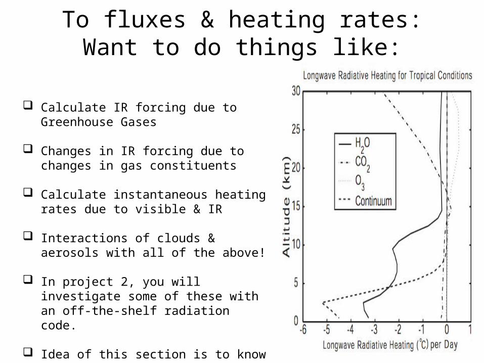
Monochromatic Intensity (nonscattering) at wavenumber

Intensities (up and down) anywhere in atmosphere

Transmittance between layer z1 and z2

Optical depth btn z1 & z2

Contribution from each layer z’ to the intensity at z goes like this.

Must sum over all LINES and continuum contribution to get full absorption coefficient at

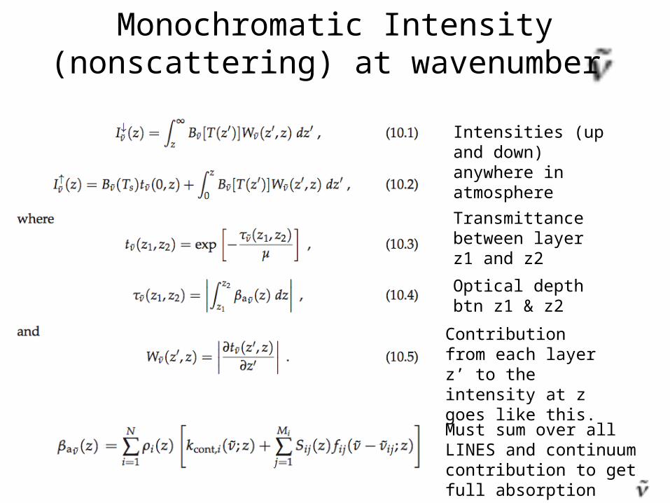
• Must take into account contributions from potentially many gas absorption lines.

• Multiple calculations to get all layers in atmosphere. But is easily do-able.

• To integrate over real instrument response functions, may have to average over several closely-spaced values.

Monochromatic Intensity (nonscattering) at wavenumber

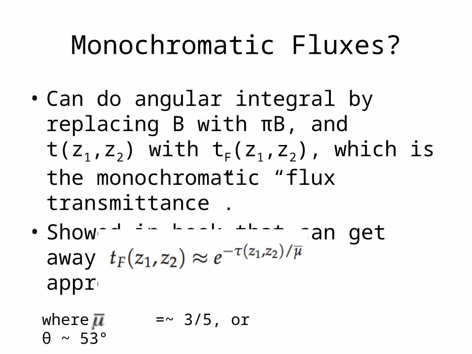
Monochromatic Fluxes?

• Can do angular integral by replacing B with πB, and t(z1,z2) with tF(z1,z2), which is the monochromatic “flux transmittance”.

• Showed in book that can get away with “2-stream approximation”:

where =~ 3/5, or θ ~ 53°

Broadband fluxes?• Needed to calculate forcings (ie cloud forcing,

greenhouse gas forcing)• Needed to calculate heating rates• Thus, needed in all weather and climate models!• Must integrate over all wavelengths!!

350 cm-1670 cm-11250 cm-15000 cm-1

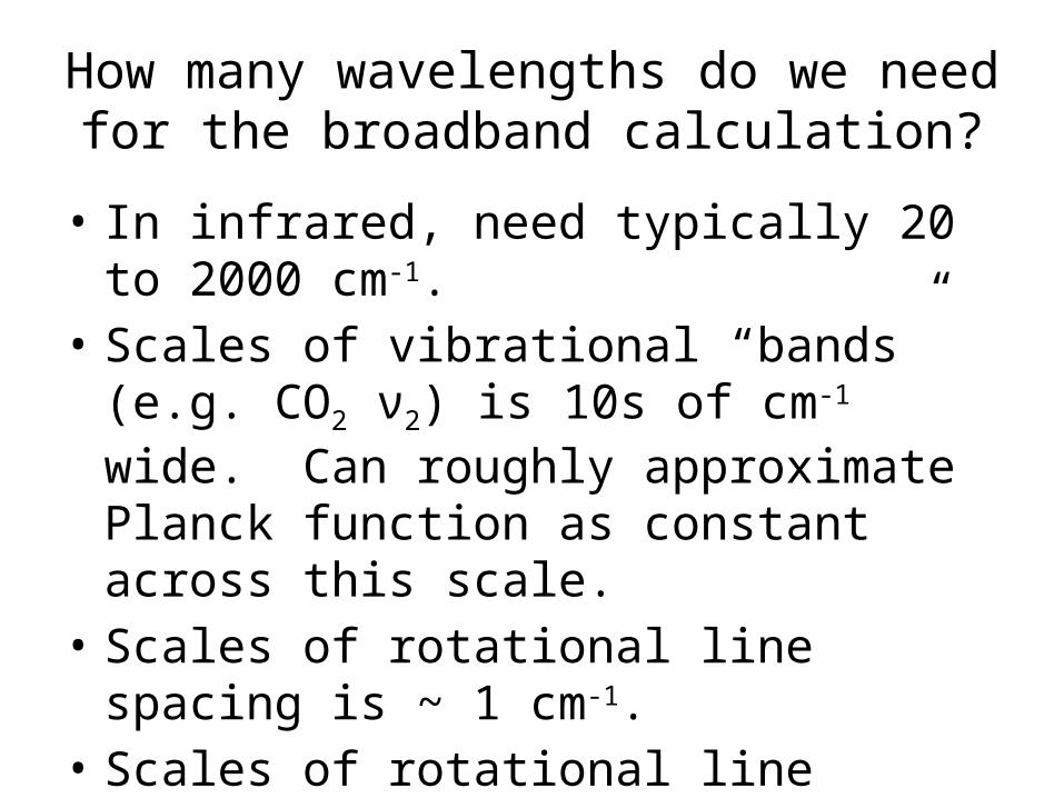
How many wavelengths do we need for the broadband calculation?

• In infrared, need typically 20 to 2000 cm-1. • Scales of vibrational “bands” (e.g. CO2 ν2) is

10s of cm-1 wide. Can roughly approximate Planck function as constant across this scale.

• Scales of rotational line spacing is ~ 1 cm-1.• Scales of rotational line widths (needed to

resolve lines: ~ 10-2 (near surface) to 10-4 cm-1 (in stratosphere).

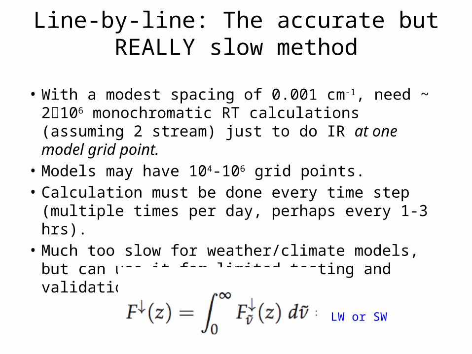
Line-by-line: The accurate but REALLY slow method

• With a modest spacing of 0.001 cm-1, need ~ 2106 monochromatic RT calculations (assuming 2 stream) just to do IR at one model grid point.

• Models may have 104-106 grid points.• Calculation must be done every time step

(multiple times per day, perhaps every 1-3 hrs).• Much too slow for weather/climate models, but

can use it for limited testing and validation (e.g. LBLRTM)

LW or SW

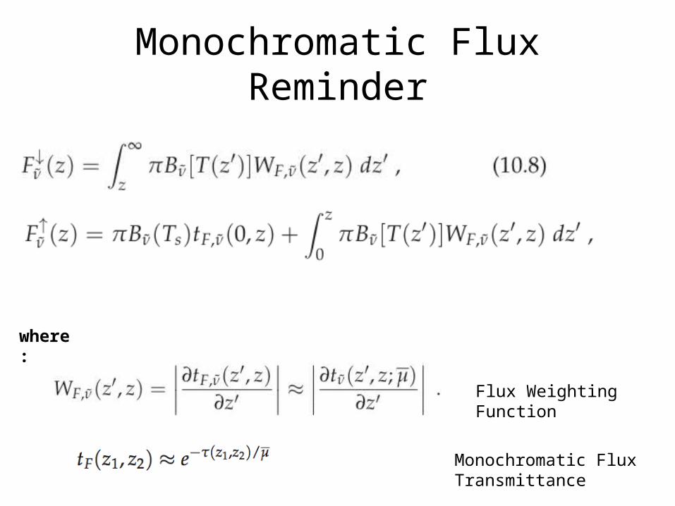
Monochromatic Flux Reminder

where:

Flux Weighting Function

Monochromatic Flux Transmittance

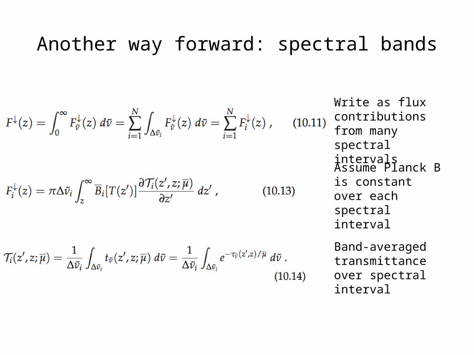
Another way forward: spectral bands

Write as flux contributions from many spectral intervals

Assume Planck B is constant over each spectral interval

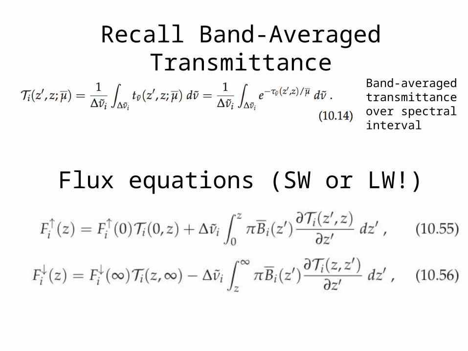
Band-averaged transmittance over spectral interval

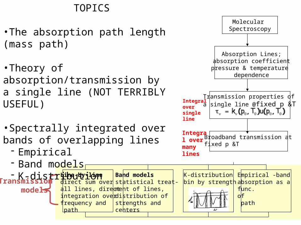
Molecular Spectroscopy

Absorption Lines;absorption coefficient

pressure & temperature dependence

Transmission properties ofa single line @fixed p &T

Broadband transmission at fixed p &T

Empirical -bandabsorption as a func.of path

K-distributionbin by strength

Band modelsstatistical treat-ment of lines, distribution of strengths and centers

Line-by-linedirect sum overall lines, directintegration overfrequency and path

Transmission models

Integral over many lines

Integral over single line

TOPICS

•The absorption path length (mass path)

•Theory of absorption/transmission by a single line (NOT TERRIBLY USEFUL)

•Spectrally integrated over bands of overlapping lines

- Empirical- Band models- K-distribution

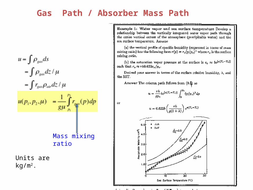
Gas Path / Absorber Mass Path

Mass mixing ratio

Units are kg/m2.

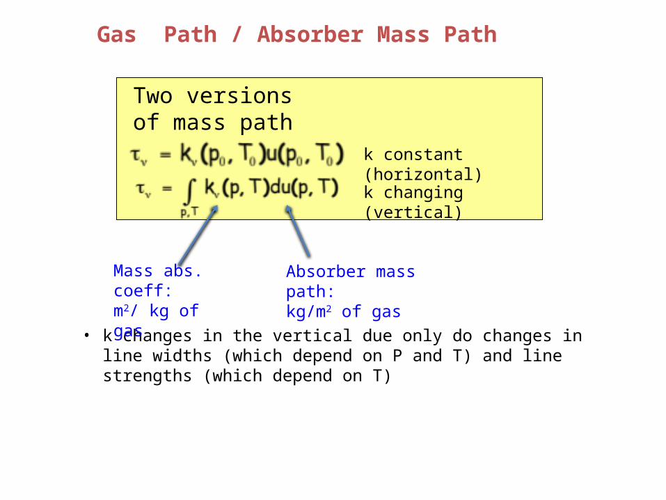
Two versionsof mass path

k constant (horizontal)

k changing (vertical)

• k changes in the vertical due only do changes in line widths (which depend on P and T) and line strengths (which depend on T)

Mass abs. coeff:m2/ kg of gas

Absorber mass path:kg/m2 of gas

Gas Path / Absorber Mass Path

Band Models• Treat spectral interval as containing either

regularly spaced or randomly occurring lines

• Typically assume homogeneous P & T (like on a horizontal path) – no pressure broadening! Later on relax this with additional approaches.

• Not always very accurate (not using real spectroscopy! Essentially fit 2 parameters to spectroscopy)

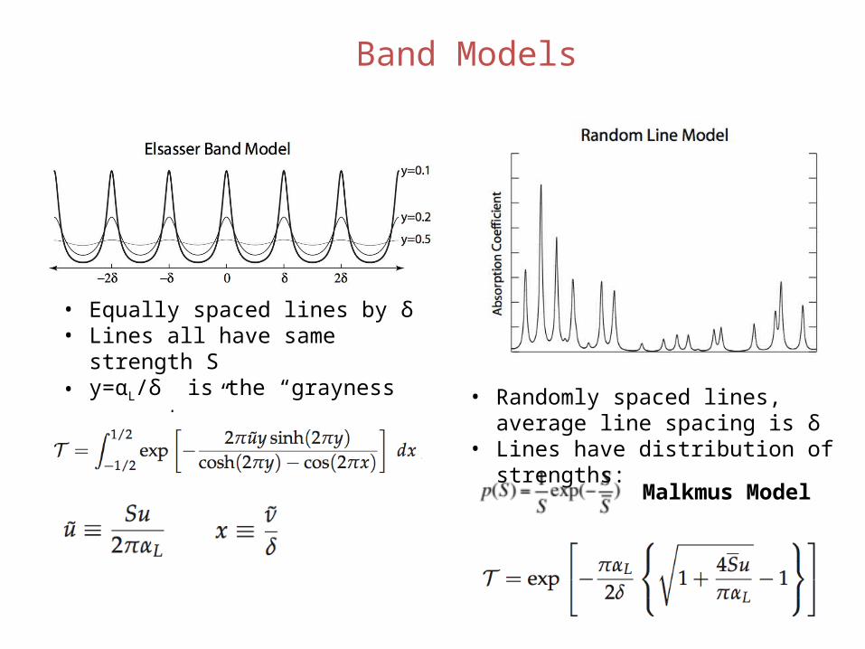
Band Models

• Equally spaced lines by δ• Lines all have same strength S• y=αL/δ is the “grayness parameter”

• Randomly spaced lines, average line spacing is δ

• Lines have distribution of strengths:

Malkmus Model

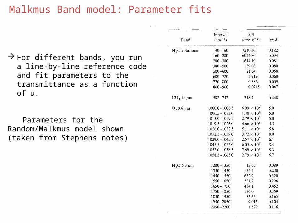
Malkmus Band model: Parameter fits

For different bands, you run a line-by-line reference code and fit parameters to the transmittance as a function of u.

Parameters for the Random/Malkmus model shown (taken from Stephens notes)

kkj-dk/2

kj+dk/2

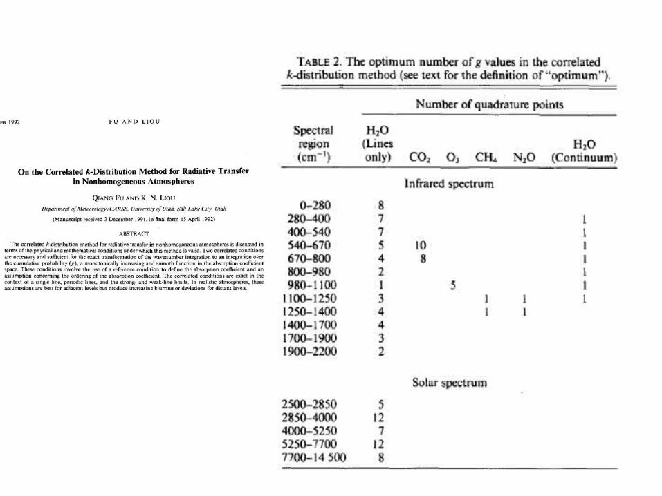
The k-Distribution Method – more modern approach

f(kj) is the fraction of the interval

where kj-dk/2<k< kj+dk/2

Vs. Frequency Sorted lowest-to-highest

Inhomogenous Paths – “Correlated-K method”

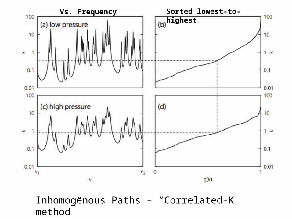
Vs. Frequency Sorted lowest-to-highest

Inhomogenous Paths – “Correlated-K method”

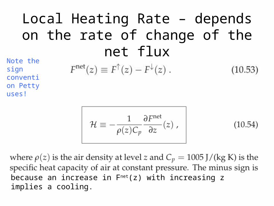
Local Heating Rate – depends on the rate of change of the net flux

because an increase in Fnet(z) with increasing z implies a cooling.

Note the sign convention Petty uses!

Flux equations (SW or LW!)

Band-averaged transmittance over spectral interval

Recall Band-Averaged Transmittance

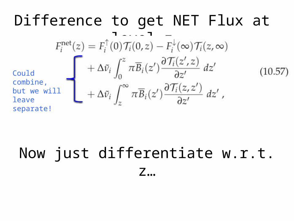
Difference to get NET Flux at level z

Could combine, but we will leave separate!

Now just differentiate w.r.t. z…

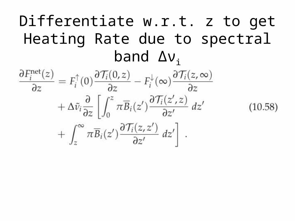
Differentiate w.r.t. z to get Heating Rate due to spectral band Δνi

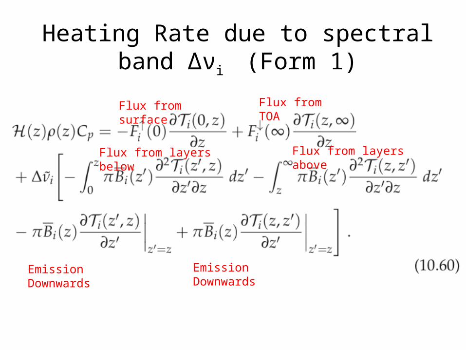
Heating Rate due to spectral band Δνi (Form 1)

Flux from surface Flux from TOA

Flux from layers below Flux from layers above

Emission Downwards Emission Downwards

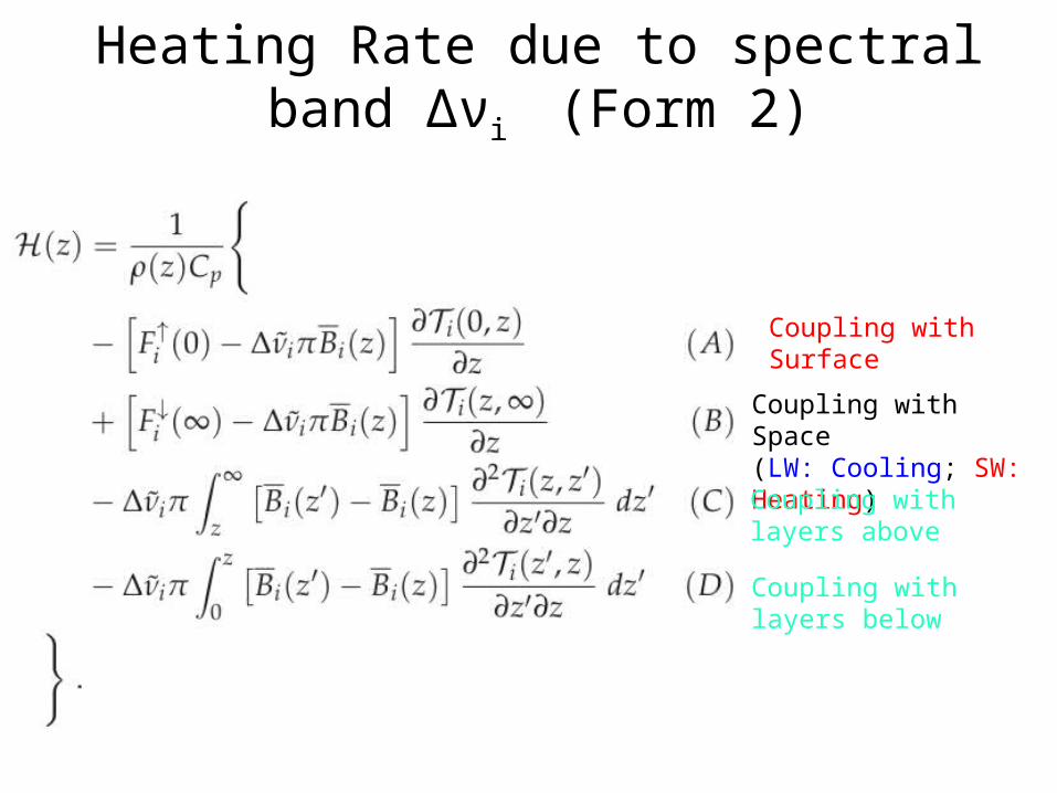
Heating Rate due to spectral band Δνi (Form 2)

Coupling with Surface

Coupling with Space(LW: Cooling; SW: Heating)

Coupling with layers above

Coupling with layers below

Fluxes & heating rates

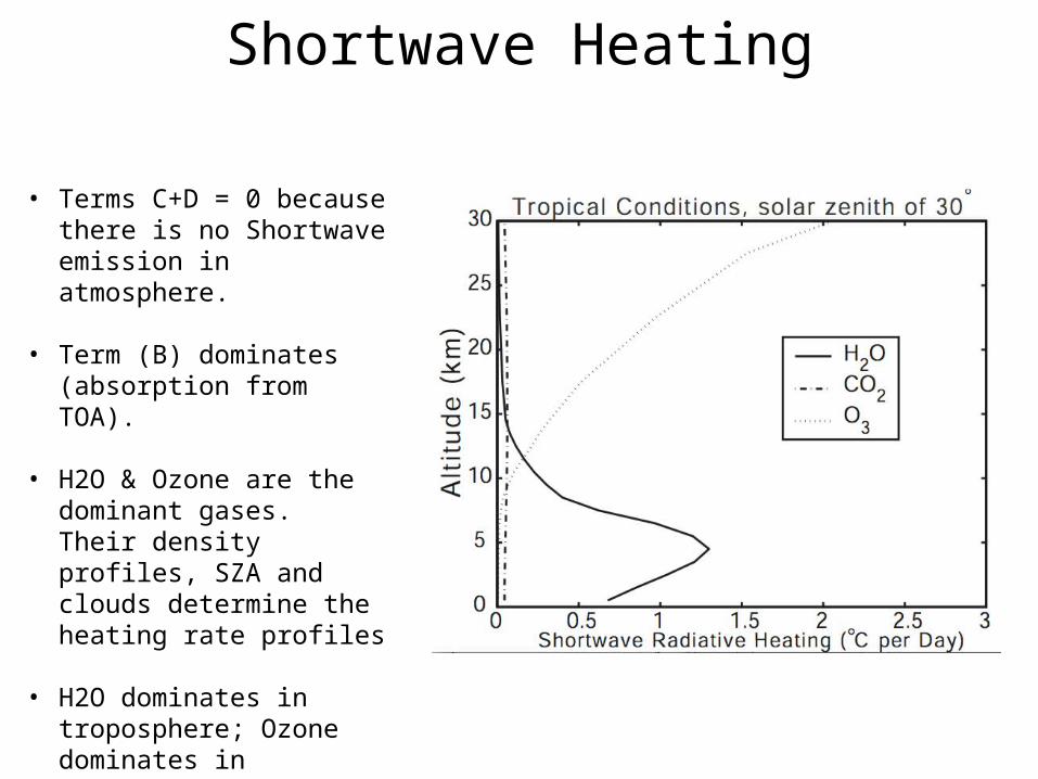
Shortwave Heating

• Terms C+D = 0 because there is no Shortwave emission in atmosphere.

• Term (B) dominates (absorption from TOA).

• H2O & Ozone are the dominant gases. Their density profiles, SZA and clouds determine the heating rate profiles

• H2O dominates in troposphere; Ozone dominates in stratosphere.

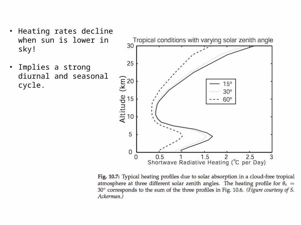
• Heating rates decline when sun is lower in sky!

• Implies a strong diurnal and seasonal cycle.

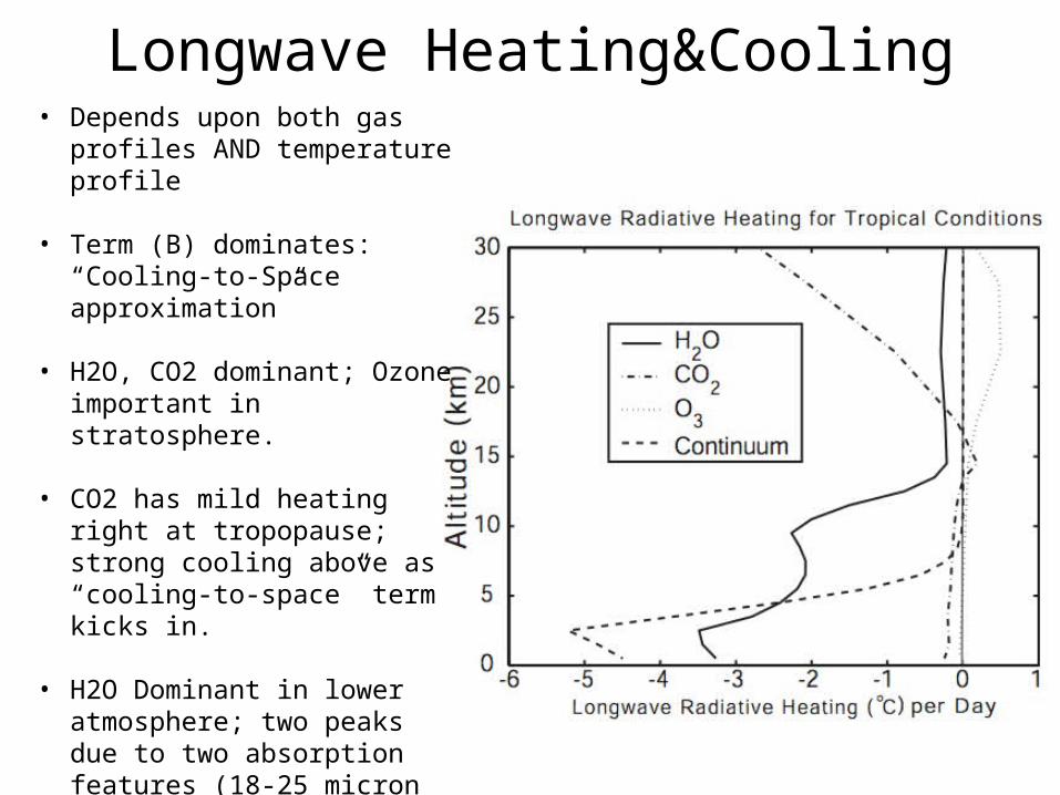
Longwave Heating&Cooling• Depends upon both gas profiles

AND temperature profile

• Term (B) dominates: “Cooling-to-Space approximation”

• H2O, CO2 dominant; Ozone important in stratosphere.

• CO2 has mild heating right at tropopause; strong cooling above as “cooling-to-space” term kicks in.

• H2O Dominant in lower atmosphere; two peaks due to two absorption features (18-25 micron pure rotation feature & 5-8 micron vibration feature)

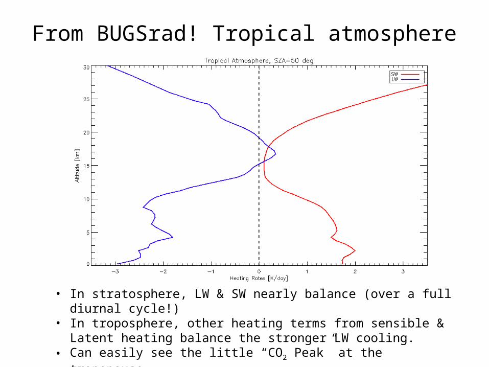
From BUGSrad! Tropical atmosphere

• In stratosphere, LW & SW nearly balance (over a full diurnal cycle!)• In troposphere, other heating terms from sensible & Latent heating balance

the stronger LW cooling.• Can easily see the little “CO2 Peak” at the tropopause

Project 2

• Use Online tool to explore LW & SW heating rates and effects due to adding clouds & gases.

• Write-up to explain what you found.