POLICY BIAS AND AGRICULTURE:PARTIAL AND GENERAL EQUILIBRIUM MEASURES

Romeo M. BautistaSherman Robinson

International Food Policy Research Institute

Finn TarpUniversity of Copenhagen

Peter WobstUniversity of Hohenheim

International Food Policy Research Institute

TMD DISCUSSION PAPER NO. 25

Trade and Macroeconomics Division

International Food Policy Research Institute2033 K Street, N.W.

Washington, D.C. 20006 U.S.A.

June 1998Revised November 1998

Forthcoming in Review of Development Economics.

TMD Discussion Papers contain preliminary material and research results, and are circulatedprior to a full peer review in order to stimulate discussion and critical comment. It is expected that mostDiscussion Papers will eventually be published in some other form, and that their content may also berevised. This paper was written under the IFPRI project “Macroeconomic Reforms and RegionalIntegration in Southern Africa” (MERRISA), which is funded by DANIDA (Denmark) and GTZ(Germany).

TANZANIA

MOZAMBIQUE

MALAWIZAMBIA

ZIMBABWE

SOUTH AFRICA

Policy Bias and Agriculture:

MACRO

ECONOMIC

REFORMS AND

REGIONAL

INTEGRATION IN

SOUTHERN

AFRICA

Trade and Macroeconomics DivisionInternational Food Policy Research InstituteWashington, D.C.

Romeo M. BautistaSherman Robinson

Finn TarpPeter Wobst

May 1998

Partial and General Equilibrium Measures

TMD Discussion Paper No. 25

Table of Contents

1. Introduction . . . . . . . . . . . . . . . . . . . . . . . . . . . . . . . . . . . . . . . . . . . . . . . . . . . . . . . . 1

2. Agricultural bias: partial equilibrium, no product differentiation . . . . . . . . . . . . . . . . . 4

3. Agricultural bias: general equilibrium and product differentiation . . . . . . . . . . . . . . . . 73.1. Structure of the applied CGE approach . . . . . . . . . . . . . . . . . . . . . . . . . . . . 73.2. Measures and policy experiments in the CGE framework . . . . . . . . . . . . . . 12

4. Results . . . . . . . . . . . . . . . . . . . . . . . . . . . . . . . . . . . . . . . . . . . . . . . . . . . . . . . . . . 164.1. Industrial protection and agricultural export taxes . . . . . . . . . . . . . . . . . . . 164.2. Impacts of an overvaluation of the exchange rate . . . . . . . . . . . . . . . . . . . . 20

5. Conclusion . . . . . . . . . . . . . . . . . . . . . . . . . . . . . . . . . . . . . . . . . . . . . . . . . . . . . . . 21

References . . . . . . . . . . . . . . . . . . . . . . . . . . . . . . . . . . . . . . . . . . . . . . . . . . . . . . . . . . 23

Annex I: Export shares . . . . . . . . . . . . . . . . . . . . . . . . . . . . . . . . . . . . . . . . . . . . . . . . 26

Annex II: CGE model equations . . . . . . . . . . . . . . . . . . . . . . . . . . . . . . . . . . . . . . . . . 27

Abstract

The paper examines the impact of industrial protection, agricultural export taxes, andovervaluation of the exchange rate on the balance between the agricultural and non-agricultural sectors. A variety of agricultural terms-of-trade indices are constructed tomeasure the policy bias against agriculture in a general equilibrium framework thatincorporates traded and non-traded goods. These general equilibrium measures are comparedto earlier work in a partial equilibrium framework assuming perfect substitutability betweendomestic and traded goods. Starting from a stylized computable general equilibrium (CGE)model of Tanzania, we simulate a 25 percent tariff on non-agriculture and a 25 percentexport tax on agriculture. We also consider the impact of changes in the equilibriumexchange rate. The results indicate that the partial equilibrium measures miss much of theaction operating through indirect product and factor market linkages, while overstating thestrength of the linkages between changes in the exchange rate and prices of traded goods onthe agricultural terms of trade.

1

1. Introduction

In the early post-World-War-II period, rapid industrialization was widely consideredto be the key to development. Historical and cross-country studies showing the decliningrelative weight of the agricultural sector in the transformation process from poor to richseemed to reinforce this conclusion, and the view was also central to Marxist analysis insocialist countries. During this period, many countries pursued a development strategy ofimport substituting industrialization (ISI), which included a variety of policy measures suchas: (1) high import tariffs on manufacturing to protect “infant” industries and export taxeson agriculture; (2) quantitative import controls, when tariff protection was viewed asproviding inadequate protection; and (3) chronically overvalued exchange rates. Measuresdirectly affecting the agricultural sector were also added, including: (1) agriculturalmarketing boards with monopoly powers, (2) centrally set producer and consumer prices, and(3) input subsidies. The ISI development strategy led to agriculture being both heavily taxedand neglected relative to industry.

The neglect of agriculture was heavily criticized in the 1960s (Schultz 1964), but ISIpolicies were not effectively criticized for another decade. In a different, complementaryvein, it was later pointed out by Lipton (1977), who coined the term “urban bias”, that themost important class conflict in poor countries was neither between labor and capital, norbetween foreign and national interests, but between the rural and urban classes. The “BergReport” (World Bank 1981) identified inappropriate domestic economic policies as thefundamental cause of the deepening agricultural crisis in Sub-Saharan Africa. “Getting pricesright” became an influential catch phrase and it was suggested that this policy approachshould be the key piece of advice to policy-makers in troubled economies. The neoclassicalcounter-revolution (Toye 1993) had arrived, and price reforms became a central componentin the wide ranging economic reforms which African countries initiated from the mid-1980sonwards.

In addition, it gradually became clear to academics and policy makers alike thatwhatever the theoretical merits of the variety of interventionist measures employed bygovernments, they often led to seriously distorted incentives, inefficiencies, and rent seeking.The difference between the nominal and effective rates of protection afforded by tariff rateswas analyzed theoretically and scrutinized empirically — and for good reasons. Empiricalwork indicated that effective protection of industrial products was often much higher thanindicated by nominal protection rates, and the costs of intervention were shown to be veryhigh indeed. Other macro policies and their impact on the performance of the agriculturalsector, including the exchange rate, also came into focus.

2

The findings of a World Bank comparative study during 1987-90 involving 18 countries are1

reported in Krueger (1992) and Schiff and Valdes (1992). Eight country studies done at the InternationalFood Policy Research Institute (IFPRI) from 1981 to 1990 are contained in Bautista and Valdes (1993),together with regional surveys of the literature in Africa, Asia, and Latin America.

Empirical studies on the effects of government price interventions in developingcountries, especially those undertaken since the early 1980s, support the view that there wassubstantial policy bias against agriculture. First, producer prices are often found to have1

been suppressed directly by sector-specific policies, commonly in the form of agriculturalexport taxation or the pricing policy of parastatal marketing organizations. Second,economywide policies, including trade and macroeconomic policies that influence the realexchange rate, are shown to have had significant indirect effects, invariably adverse, onagricultural incentives. In most cases, the indirect impact of economywide policies is foundto be more important than the effect of direct government interventions.

In taking into account the additional effect on agricultural incentives arising fromindirect government interventions, these studies have gone beyond the narrow, sectoralorientation of traditional agricultural policy analysis. However, in general, they have reliedon analytical frameworks that are partial equilibrium. Economists have long recognized thatthe partial measures used in applied work are incomplete and that a general equilibriumframework is needed to capture all the interactions that determine the net relative impact ofa mix of policies on the agricultural and non-agricultural sectors. “Policy bias” is inherentlyan economywide, general equilibrium concept. Nevertheless, to date there has been nosystematic evaluation of the extent of agricultural bias of government interventions using ageneral equilibrium framework.

Another critical problem with partial equilibrium approaches is that they typicallyassume perfect substitutability between domestically produced and imported goods, as wellas between domestic products for export and for internal use. Under these assumptions, weshould never observe two-way trade (“cross hauling”) at the commodity level. If a good istradable, the “law of one price” holds and changes in world prices should be completelytranslated into changes in domestic prices. Furthermore, the responsiveness of sectoraldomestic prices to changes in world prices or in trade policies does not depend on the sharesof trade in sectoral demand or supply. It matters only that the good is “tradable”, not howmuch it is traded.

3

An extended discussion on empirical testing of the law of one price started from an article by2

Peter Isard (1977); see Ceglowski (1994); Blaffes (1991); and Ardeni (1989).

Peterson, Hertel, and Stout (1994) consider the violation of the law of one price in the context of3

a partial equilibrium, multi-commodity, agricultural trade model.

For a description of this CGE model specification see Deverajan et al. (1997) and de Melo and4

Robinson (1989).

For a recent survey on general equilibrium analysis applied to agriculture, see Hertel (1997).5

All these implications of the law of one price are empirically suspect. For example,2

two-way trade is observed in highly disaggregated sectoral data for virtually all countries (deMelo and Robinson 1981; de Melo and Tarr 1992). Within agriculture in developingcountries, there are also significant shares of non-traded goods or goods with very low tradeshares. In any case, the transmission elasticities vary widely across sectors. Evidence formajor traded agricultural commodities indicates that price transmission elasticities are closeto one for developed countries, although significantly lower for developing countries(Mundlak and Larson 1992). Ardeni (1989), on the other hand, finds that changes in worldprices or trade policy measures are generally only partially transmitted through to prices ofdomestic substitutes. In general, elasticities of substitution and transformation are much3

lower for industrial goods in developing countries, especially intermediates and capitalgoods.

By contrast, a widely used specification in multisector, trade-focused, computablegeneral equilibrium (CGE) models is that imports are imperfect substitutes for domesticallyproduced goods with the same sectoral classification. Similarly, in many models, exports arealso differentiated from domestically produced goods sold on the domestic market. Thisformulation removes the extreme dichotomy between tradable and non-tradable goods,allowing differing degrees of tradability corresponding to different values of the substitutionand transformation elasticities (which are either infinite or zero in the partial equilibriumapproach, depending on whether the good is traded or not). This specification gives somerealistic autonomy to the domestic price system in the model and can account for cross-hauling. 4

In this paper, we use a computable general equilibrium (CGE) model thatincorporates the more realistic assumption of imperfect substitutability to provide acomprehensive framework to capture the various repercussions of policy interventions andmeasure their impact on agriculture. Assuming that the economic environment is5

characterized by trade policy distortions such as the ones in focus in Krueger, Schiff, and

4

A related measure of government support to agriculture, the Producer Subsidy Equivalent (PSE),6

was developed during the Uruguay Round GATT negotiations and includes both trade and non-tradepolicies. It is also a partial equilibrium measure which treats trade basically the same way as the Krueger,Schiff, Valdes approach (FAO 1975; Josling and Tangermann 1989; Webb et al. 1990).

Valdes (1988), we will consider the differences between general equilibrium measures of theagricultural sector bias as compared to the results of partial equilibrium analysis. Following6

this introduction, the partial equilibrium measures used in previous work are presented.Section 3 discusses how the bias against agriculture can be measured in a CGE model (fullyspecified in Annex II), and indicates why this frame of reference is preferable to the partialequilibrium approach. The results of a series of policy experiments designed to provideanswers to the questions raised above are reported in Section 4, and Section 5 concludes.

2. Agricultural bias: partial equilibrium, no product differentiation

If a country is small and there is perfect substitutability between domesticallyproduced and imported goods, a change in the import price will — under competitiveconditions — lead to the same change in the domestic producer price of the importable good.Likewise, if domestic products for export and for internal use are perfect substitutes, thedomestic producer price of the exportable good will be equal to its domestic-currency borderprice equivalent. However, in practice, government policies can drive wedges betweenforeign and domestic prices.

Krueger, Schiff, and Valdes (1988) — KSV for short — developed measures of theimpact of these policies on agricultural producer prices. These measures are used to assesswhether the policy-induced incentive structure favors or discriminates against agriculturalproduction, i.e. whether the sector is protected or not relative to non-agriculture. Theydistinguish between policies that have direct and indirect effects on agricultural incentives.

Policies with direct effects include agricultural sector-specific import and exporttaxes, price controls, and production taxes and subsidies, all of which affect the wedgebetween producer and border prices of agricultural products. Policies with indirect effectson agricultural incentives, on the other hand, include the exchange rate, which affects theeconomywide balance between traded and non-traded goods, and import tariffs on non-agricultural products. Contrary to the assumption used by KSV, we recognize below thelatter's influence on the exchange rate.

DABiag 'Piag

P 'iag

& 1 'PXiag

PX 'iag

& 1 .

IABiag 'P 'iag

P (

iag

& 1 'E0 P AGN

X(

E ( P AGNX

& 1 .

PXiag

PX ' iag

P AGNX

Piag 'PXiag

P AGNX

and P 'iag 'PX 'iag

P AGNX

PX (

iag

P AGNX

(

P (

iag 'PX (

iag

P AGNX

(

P AGNX

(' " P AGN

Xt(% (1 & ") P AGN

Xnt

PX ' iag PX (

iag

5

(1)

(2)

Following KSV (but using different notation), let be the domestic producer

price of a specific tradable agricultural product iag, the border-price equivalent at the

official exchange rate E , and the nonagricultural producer price index defined as the0

weighted average of non-agricultural producer prices. The relative producer prices ofagricultural products vis-a-vis the non-agricultural aggregate price are given by

.

The direct agricultural bias against products indexed by iag is defined as theproportionate deviation of relative prices from what they would have been without directinterventions:

This measure is meant to capture the impact on producer incentives of commodity-specificpolicies, and it corresponds to the widely used “nominal protection rate” in the empiricaltrade literature.

Let be the border price evaluated at the equilibrium exchange rate E*, and

define as the nonagricultural price index where the tradable part is evaluated at E*,

defined as a situation with a sustainable trade balance and no trade restrictions. In this case,E* differs from E to the extent that the current account is set at an unsustainable level and0

trade interventions are in place. The relative price is given by where

, and Xt refers to tradable goods (whose price is

evaluated at the equilibrium exchange rate, E*) and Xnt refers to non-traded, non-agriculturalgoods.

The indirect agricultural bias against the sector indexed by iag is the proportionate

deviation of from :

TABiag 'Piag

P (

iag

& 1

TABiag ' DABiag

P 'iag

P (

iag

% IABiag

P AGNX

PXiag

P AGNX

P AGNX

(

E0

E (

PXiag PX (

iag

6

In some of the IFPRI country studies referred to above, trade restrictions (including import7

tariffs and export taxes) are systematically examined as a major source of real exchange rate distortion; see,for example, Cavallo and Mundlak (1982) and Bautista (1987), for an empirical investigation of theArgentine and Philippine cases, respectively.

(3)

(4)

This measure is meant to capture the indirect effects on producer incentives of the exchange

rate disequilibrium (E differing from E*) and of trade policy affecting (e.g., industrial0

protection). Notably, does not appear in the right-hand side of equation (2). Hence,

the indirect agricultural bias is the same for all tradable agricultural goods. The implicit

assumption that and are independent shows that the partial equilibrium

framework does not capture intersectoral price linkages and also assumes no repercussionthrough changes in the exchange rate induced by the price changes.7

The exchange rate affects the terms-of-trade ratio depending on the shares of tradedand non-traded goods within the agricultural and non-agricultural sectors. If all goods in theeconomy are tradable, then the exchange rate is irrelevant since, in that case, all domesticrelative prices are set by world prices. The exchange rate is important precisely because thereare non-traded goods. In the KSV studies, the agricultural products considered were tradable(i.e., some observed exports or imports) and some non-agricultural goods were not tradable.In that environment, exchange rate changes affect tradable agriculture much more thanpartially non-traded non-agriculture. Considering agriculture as a whole, it is important toconsider non-traded agricultural goods in defining aggregate terms-of-trade indices.

The total agricultural bias against sector iag can be represented by the proportionate

deviation of from :

which captures the effects of both direct and indirect government interventions.

The three measures are related as follows:

PMi ' pwmi 1 % tmi EXR and

PEi ' PWEi 1 & tei EXR

PX ' iag PX (

iag

7

(5)

(6)

The first term on the right-hand side of equation (4) is a modified measure of thedirect agricultural bias, which is usually smaller (in absolute value) than the nominal

protection rate since is typically less than in developing countries.

In contrast with the partial equilibrium measures used in the World Bank studies,which are concerned with producer price incentives only, a general equilibrium approach willcapture intersectoral resource shifts, product differentiation in production and demand, andthe effect of induced price changes on the equilibrium exchange rate. The result is a richerspecification of the price system and a more complete concept of agricultural bias.

3. Agricultural bias: general equilibrium and product differentiation

If domestically produced and imported goods (DC and M respectively) are imperfecti i

substitutes, the price of the domestic good, PDC , will no longer be equal to the domestic-i

currency price of the import substitute, PM , as in the partial equilibrium framework.i

Similarly, if there is imperfect substitutability between domestic products for export (e ) andi

for internal use, their prices — PE and PDA respectively — will not be identical. It followsi i

that the domestic prices of exported and imported products are not determined by the law ofone price.

3.1. Structure of the applied CGE approach

Following Armington (1969), we can introduce product differentiation by defininga composite good Q which is a CES (constant elasticity of substitution) function of thei

domestic product DC and the import substitute M . Likewise, a production good X can bei i i

defined as a CET (constant elasticity of transformation) function of the domestic product insector i for internal use DA and for export E . Under the small country assumption, i.e., thei i

country's imports have an infinitely elastic world supply and its exports have an infinitelyelastic world demand, world prices of imports pwm and of exports PWE are exogenouslyi i

determined. The domestic prices of imported and exported products are given by

Mi

DCi

' CES (PMi

PDCi

and

Ei

DAi

' CET (PEi

PDAi

.

PQi 'PDCi @ DCi % PMi @ Mi

Qi

' CES PDCi , PMi and

PXi 'PDAi @ DAi % PEi @ Ei

Xi

' CET PDAi , PEi

8

(7)

(8)

(9)

(10)

respectively, where EXR is the exchange rate (in domestic currency per unit of foreigncurrency), and tm and te are the implicit tariff and export tax rates, respectively, that takei i

account of the legal tariffs and export taxes as well as any quantitative trade restrictions anddirect price controls that affect the disparity between the domestic and border prices of tradedgoods.

From the underlying general equilibrium model used here (see Annex II for acomplete specification), the relationships between relative prices and quantities are:

We use the convention that CES and CET refer to “constant elasticity of substitution” and“constant elasticity of transformation” functions, while CES* and CET* refer to thecorresponding first-order conditions for utility maximization and profit maximization.

Sectoral composite good prices are the weighted averages of the domestic prices oftheir component products:

where the CES and CET functions refer to cost functions relating the composite prices totheir component prices. They reflect the first-order conditions described above.

Equations 5 - 10 are imbedded in the structure of a computable general equilibrium(CGE) model incorporating differentiated products. This model permits the determinationof the direct effects of government interventions (captured in tm and te ) on agriculturali i

9

prices, and also their indirect effects through intersectoral linkages and induced changes inthe exchange rate.

To make the CGE agricultural bias results derived in this study as comparable aspossible to the partial measures described above, we adapt the CGE model to provide a“clean” theoretical starting point for measuring policy bias and also use the framework fordoing controlled experiments that isolate particular effects.

First, in the model, factor markets have been segmented with respect to aggregateagricultural and non-agricultural sectors. Labor and capital can move between sectors withinagriculture and non-agriculture, but cannot move between agriculture and non-agriculture.In this model, the derived agricultural sector bias measures reflect only price changes andintra-sectoral resource shifts. The partial equilibrium measures focus only on prices, and soindicate potential resource pulls if factors were free to move between agriculture and non-agriculture. In the CGE model, by restricting factor mobility between agriculture and non-agriculture, the resulting equilibrium prices, and measures of bias based on them, should becomparable to the partial equilibrium measures. In an “unrestricted” CGE model, allowinginter-aggregate-sector factor mobility, adjustment would include both price and quantityeffects. In general, allowing quantity adjustment will reduce price adjustment, so thesegmentation should lead to price effects which are upper bounds. Indeed, the mostappropriate measure of bias would be to allow full factor mobility and measure changes invalue added across sectors with removal (or addition) of distorting policies.

Second, as the base for our experiments, we create a distortion-free benchmarksolution of the model to provide the theoretically best reference point for the analysis. Asreflected in our preliminary data, the economy has a variety of distorting taxes — sectoraltariffs and domestic indirect taxes. Given these existing distortions, analysis of policyexperiments is made difficult because there are potential “second best” effects fromimposition of new taxes. Given our focus on comparing measures of policy bias, it isconvenient to start from an undistorted base. To achieve this undistorted economicenvironment, all production, sales, and trade taxes in the base data are removed. The lostrevenue is made up by means of a non-distorting, lump-sum income tax on households,yielding the base value of government revenue — the standard approach in public financemodels. This undistorted base solution is the starting point against which we compare all ourexperiments.

Third, the general equilibrium model incorporates the indirect effect of changes intariffs and export subsidies on the economy through their impact on the equilibriumexchange rate — an indirect effect ignored in the partial equilibrium approach. To isolate thiseffect, we run a variant of the tariff and export subsidy experiments in which we fix the

10

In fact, in most of their country studies, overvaluation was the greatest source of policy bias8

against agriculture.

See Devarajan, Lewis, and Robinson (1993) for a discussion of the real exchange rate in this9

class of CGE models.

exchange rate, and so “turn off” this mechanism. In order to fix the exchange rate, we havespecified a different macro “closure” and assumed that the trade balance adjustsendogenously.

Fourth, in the KSV methodology, overvaluation of the exchange rate is a majorsource of policy bias against agriculture. In a general equilibrium context, EXR represents8

the equilibrium exchange rate that is jointly determined by the remaining variables of themodel, including especially the balance of trade. The equilibrium exchange ratecorresponding to a situation with no trade distortion and a “sustainable” (perhaps zero) tradebalance E* can be calculated with the CGE model, which provides a unified frameworkincorporating all relative prices, including the real exchange rate. Unlike KSV, no separatemodel is required to estimate the equilibrium real exchange rate. To measure the effect ofchanges in the exchange rate only (i.e., with no changes in distorting sectoral taxes), wereport on a set of additional experiments where we systematically reduce the trade balanceto zero, and solve for the resulting equilibrium exchange rates, and all other prices andquantities. The results show the sensitivity of the various agricultural terms-of-trademeasures with respect to depreciation of the exchange rate arising from the elimination ofthe trade deficit.

Finally, since the focus of the analysis is on the production rather than theconsumption side, the non-traded producer price index of goods sold on the domestic markethas been chosen as the numeraire of the model. For this choice, the solution value of theexchange rate measures the relative price of traded goods to non-traded goods — the “real”exchange rate of trade theory. In public finance models, it is common to use the consumer9

price index as numeraire, which is convenient for welfare analysis. The choice is only amatter of convenience. The model is a neoclassical general equilibrium model and onlydetermines relative prices.

An overview on the underlying domestic price transmission mechanism is presentedin Figure 1.

AggregateIntermediateInput Price

FactorPricesCET

Function

CESFunction

CESFunction

Sales Tax

FixedProportion

FixedProportion

Figure 1Domestic Price Transmission Mechanism

ExportPrice (PE)

DomesticPrice (PD)

ImportPrice (PM)

ProducerPrice (PX)

CompositeGood Price

(PQ)

Value-addedPrice (PVA)

ConsumerPrice (PC)

11

As discussed in the introduction, a major shortcoming of the partial equilibriumapproach is the assumed complete transmission of world price changes to domestic prices.Figure 1 shows the price links in the CGE model. Domestic prices of exported and importedproducts are determined by world market prices plus any trade taxes (given the small countryassumption). However, domestic sectoral producer prices (PX) are CET cost functions ofexport prices (PE) and domestic prices (PDA, PDC). Similarly, the composite good prices(PQ) are CES cost functions of import prices (PM) and domestic prices. The strength of pricetransmission effects depends both on elasticities (of substitution and transformation) and ontrade shares. There are also links working through intermediate inputs, which includeimported and domestic goods, and finally to factor prices. In this model, the policy biasagainst agriculture will depend on differences in policies, trade shares, and the degree oftradability between agricultural and non-agricultural sectors.

AG TOTX '

jiag

PXiag @ S xiag

jiagn

PXiagn @ S xiagn

S Xiag '

Xiag

jiag

Xiag

and S Xiagn '

Xiagn

jiagn

Xiagn

P AGX ' j

iag

PXiag @ S Xiag and P AGN

X ' jiagn

PXiagn @ S Xiagn

AG TOTM

12

(11)

(12)

(13)

3.2. Measures and policy experiments in the CGE framework

In the general equilibrium approach used here, the measure of agricultural bias iscaptured through various measures of the terms of trade between aggregate agriculture andaggregate non-agriculture. They are defined as the ratio of the relevant price indices. Forexample, the agricultural terms of trade with respect to gross output X in domestic producerprices can be represented as follows:

where

The share parameters are the gross output shares of individual sub-sectors in the agriculturaland non-agricultural sectors. The sum of these shares within each aggregate sector equalsone.

The aggregate sectoral producer price indices are defined as:

The terms-of-trade measures within the CGE framework are constructed using thefollowing prices and corresponding quantity weights:

PM M domestic market price and quantity of importsPE E domestic market price and quantity of exportsPQ Q composite good price and quantityPX X producer price and gross outputPVA X value added price and quantity

Agricultural bias in the CGE framework is measured by various agricultural terms-of-trade indices:

Agricultural TOT regarding PM and M

AG TOTE

AG TOTQ

AG TOTX

AG TOTVA

13

The SAM is based on preliminary and incomplete data for Tanzania. A major work program is10

underway to improve the data base. See Wobst (1998) for a description of an updated 1992 SAM. Notethat the reported economic structure is for the distortion-free base solution of the model.

Agricultural TOT regarding PE and E.

Agricultural TOT regarding PQ and Q

Agricultural TOT regarding PX and X

Agricultural TOT regarding PVA and X

A 28 sector — of which 13 are agricultural sectors — social accounting matrix(SAM) for Tanzania (base year 1990) provides the starting data base for our policysimulations. Given that the data are preliminary and that we start from a distortion-free base10

solution, the model should be seen as reflecting a “stylized” version of a Tanzania-likeeconomy. The SAM was developed as part of a research project which is developingcomparative SAM data for a number of African countries, including: Botswana, Madagascar,Malawi, Mozambique, South Africa, Tanzania, Zambia, and Zimbabwe. The model can beseen as characterizing a highly-agricultural, trade-dependent, developing country.

The structure of the economy is presented in Table 1, which provides sector-specificinformation on production, value-added, and trade shares; export and import ratios withrespect to total production and absorption; and elasticities of substitution and transformation.The characteristics of this economic structure that significantly influence the results of theanalysis can be summarized as follows:

• The share of agriculture in total gross production is 42 percent, and 56 percent invalue-added at market prices. This economy is dominated by agriculture.

• The share of agriculture in total exports is only 26 percent, but the two mostimportant agricultural export sectors (coffee and tea) have export-production ratiosof around 80 percent. Most exports are non-agricultural, but there are some veryexport-dependent agricultural sectors.

• There are virtually no agricultural imports. Most imports are intermediate and capitalgoods for which elasticities of substitution with domestic production is low. Onesector, “fuel”, which includes petrochemicals, has high import and export ratios,indicating the existence of “pass-through” exports.

14

Table 1: Structure of the Model Economy

Composition (%) Ratios (%) Elasticities

X VA EX IM EX/X IM/Q SIGT SIGC

Cotton 0.5 0.3 - - - - - -

Sisal 0.3 0.3 0.8 - 22.6 - 3.0 -

Tea 0.2 0.2 2.6 - 79.7 - 3.0 -

Coffee 0.8 0.8 9.7 - 82.9 - 2.0 -

Sugar 0.4 0.3 1.4 - 27.8 - 3.0 -

Tobacco 0.1 0.0 0.8 - 53.2 - 3.0 -

Cashew 0.1 0.1 0.7 - 46.5 - 3.0 -

Pyrethrum 0.1 0.1 0.5 - 44.1 - 3.0 -

Maize 7.5 10.7 1.5 - 1.5 - 3.0 -

Wheat 0.1 0.2 - 0.0 - 5.4 - 4.0

Paddy 1.9 2.8 - - - - - -

Other Agri. 21.8 29.3 5.4 0.1 1.8 0.1 3.0 1.1

Livestock 8.0 11.3 2.2 0.1 2.0 0.2 3.0 1.1

Mining 1.5 1.8 1.4 6.7 6.7 44.9 1.1 4.0

Food & Bever. 5.4 3.2 4.9 7.1 6.5 21.2 1.1 4.0

Textiles 5.8 4.0 27.3 7.8 33.5 25.2 4.0 1.1

Fuel 0.1 0.1 0.8 4.8 62.4 95.7 1.1 0.8

Other Chemicals 0.9 0.6 0.9 9.5 6.5 64.5 1.1 0.8

Non-Metal 1.0 0.4 1.5 3.5 10.7 40.1 1.1 0.8

Metal 2.2 1.4 2.9 31.9 9.5 73.2 1.1 0.8

T&M Equipment 2.1 2.5 0.1 22.4 0.2 64.1 1.1 0.8

Electr. & Water 1.1 0.2 0.0 0.0 0.3 0.1 4.0 1.1

Construction 5.4 1.5 - 0.0 - 0.1 - 4.0

Commerce 16.6 12.3 21.0 0.3 9.0 0.3 4.0 1.1

Trans. & Comm 5.9 8.3 4.8 0.4 5.8 1.3 4.0 1.1

Financial Inst. 4.7 5.6 - 0.9 - 3.2 - 4.0

Other Services 0.7 0.7 8.6 4.4 83.2 85.6 1.1 4.0

Public Admin. 4.9 0.8 0.1 - 0.2 - 4.0 -

Total/Avg. AG 41.8 56.4 25.7 0.2 3.4 0.1 - -

T./Avg. non-AG 58.2 43.6 74.3 99.8 8.7 23.3 - -

Notes: X = Output, VA = Value-Added, EX = Exports, IM = Imports, Q = Absorption, SIGT = Elasticity of Transformation, and SIGC = Elasticity of Substitution.Source: Distortion-free base solution of the CGE model for Tanzania using a preliminary 1990 SAM (Wobst1998).

15

Other government policies such as sales taxes or fixed producer prices could also be11

investigated within the CGE framework. However, in the present analysis, we focus on trade policy-induced distortions.

Four experiments are carried out to simulate the impact of introducing significantindustrial protection and taxation of agricultural exports, with and without a fixed exchangerate. The first experiment simulates an “import substitution industrialization” (ISI) strategy11

by imposing a 25 percent import tariff (tm(iagn) = 25%) on all non-agricultural imports. Thissort of ISI strategy should hurt agriculture by: (a) raising the relative price of non-agriculturalgoods, which are import substitutes, compared to agriculture; (b) increasing the costs ofproduction in agriculture (since non-agricultural commodities are used as intermediate inputsin agriculture); and (c) inducing an appreciation of the exchange rate which will hurt export-oriented agricultural sectors producing tradable goods.

The induced appreciation of the exchange rate represents an indirect effect which isconsidered to be independent in the partial equilibrium approach to measuring agriculturalbias. To estimate the separate effect of this appreciation, in experiment 2 we also increasethe non-agricultural tariff as in experiment 1, but fix the exchange rate, which serves toisolate the indirect exchange-rate effect. With the exchange rate fixed, the model is solvedby endogenously adjusting the trade balance (as discussed above). This additional experimentallows comparison with the partial equilibrium measures which analyze the effects oftaxation under the assumption of a fixed exchange rate.

The third and fourth experiments simulate the implementation of a 25 percent tax onall agricultural exports, again with a free and fixed exchange rate (te(iag) = 25% and EXRis either free or fixed). The impact of an export tax on agriculture in a partial equilibriumframework with a fixed exchange rate is referred to as the direct bias against agriculture. Inthe general equilibrium framework, the effect of an export tax can be divided into twocomponents: (a) price changes due to trade price transmission effects, given the CES-CETfunctional structure of the model; and (b) price changes due to the induced exchange-rateeffect.

In the partial equilibrium literature, a major source of policy bias is the overvaluationof the exchange rate, even with no sectoral price distortions. To assess this effect, weperform a series of five experiments where we leave all sectoral taxes at zero but reduce thebase value of the trade balance in 20 percent increments, reaching zero in the last experiment.In these experiments, the real exchange is solved endogenously, given the exogenous trade

AG TOTM AG TOT

E

AG TOTQ AG TOT

X

AG TOTVA

16

We could also have fixed (and varied) the exchange rate and “closed” the model by solving for12

the corresponding equilibrium trade balances endogenously. The qualitative results would be the same —we trace out the functional relationship between the real exchange rate and the balance of trade.

balance. A trade balance of zero is often specified as defining the “appropriate” equilibrium12

value of the exchange rate in the partial equilibrium literature. Defining an equilibrium or“sustainable” trade balance is a macro issue, outside the scope of our static generalequilibrium model. In the CGE model, there is a functional relationship between theexchange rate and the trade balance, and hence between the trade balance and measures ofpolicy bias arising from changes in the equilibrium exchange rate. The five experimentsindicate this relationship.

4. Results

4.1. Industrial protection and agricultural export taxes

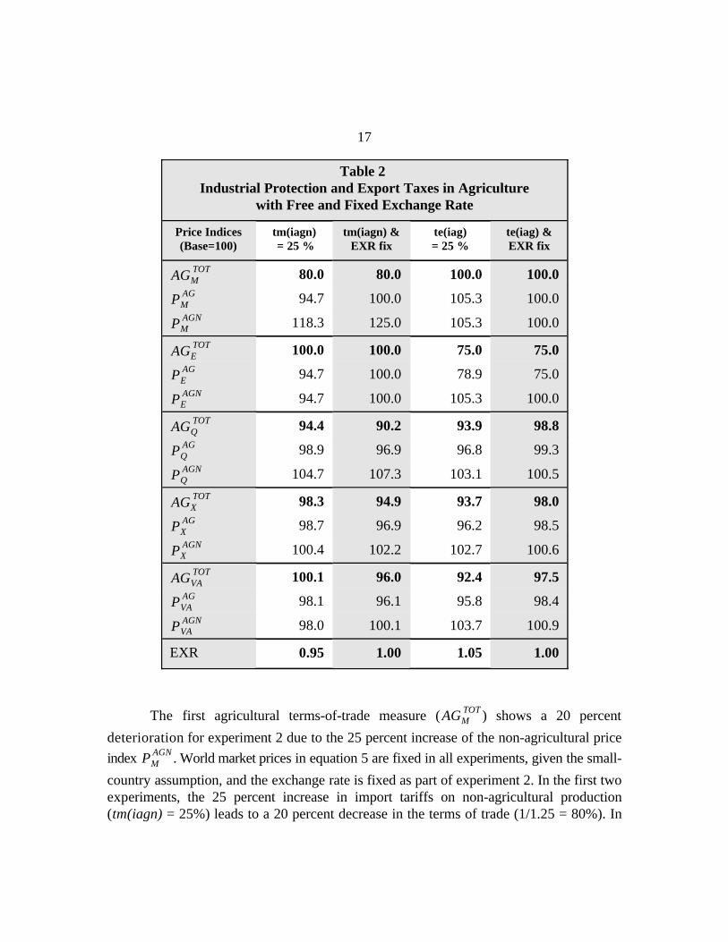
Table 2 presents the impact on the various agricultural terms-of-trade measures of theimposition of the 25 percent non-agriculture import and agriculture export taxes, with andwithout a fixed exchange rate. The agricultural terms-of-trade measures and their underlyingaggregate price indices are shown in the rows. The first two agricultural terms-of-trade

measures with regard to traded goods ( and ) capture price-incentive effects

which are close to the partial equilibrium measure. The last three measures ( , ,

and ) capture the transmission of price changes from traded goods through

commodity, output, and value-added prices, reflecting general equilibrium linkages, theArmington specification of imperfect substitutability, and finally the operation of factormarkets.

The last row shows that the exchange rate, which is fixed in experiments 2 and 4,appreciates by approximately 5 percent in experiment 1 and depreciates by 5 percent inexperiment 3. The signs of the induced changes are predictable from theory — themagnitudes depend on model parameters and the structure of the economy.

AG TOTM

P AGM

P AGNM

AG TOTE

P AGE

P AGNE

AG TOTQ

P AGQ

P AGNQ

AG TOTX

P AGX

P AGNX

AG TOTVA

P AGVA

P AGNVA

AG TOTM

P AGNM

17

Table 2 Industrial Protection and Export Taxes in Agriculture

with Free and Fixed Exchange Rate

Price Indices tm(iagn) tm(iagn) & te(iag) te(iag) &(Base=100) = 25 % EXR fix = 25 % EXR fix

80.0 80.0 100.0 100.0

94.7 100.0 105.3 100.0

118.3 125.0 105.3 100.0

100.0 100.0 75.0 75.0

94.7 100.0 78.9 75.0

94.7 100.0 105.3 100.0

94.4 90.2 93.9 98.8

98.9 96.9 96.8 99.3

104.7 107.3 103.1 100.5

98.3 94.9 93.7 98.0

98.7 96.9 96.2 98.5

100.4 102.2 102.7 100.6

100.1 96.0 92.4 97.5

98.1 96.1 95.8 98.4

98.0 100.1 103.7 100.9

EXR 0.95 1.00 1.05 1.00

The first agricultural terms-of-trade measure ( ) shows a 20 percent

deterioration for experiment 2 due to the 25 percent increase of the non-agricultural price

index . World market prices in equation 5 are fixed in all experiments, given the small-

country assumption, and the exchange rate is fixed as part of experiment 2. In the first twoexperiments, the 25 percent increase in import tariffs on non-agricultural production(tm(iagn) = 25%) leads to a 20 percent decrease in the terms of trade (1/1.25 = 80%). In

P AGNM

AG TOTM

P AGM P AGN

M

AG TOTE

AG TOTM

P AGE

P AGNE AG TOT

E

P AGM P AGN

M

AG TOTE AG TOT

E

P AGE P AGN

E

AG TOTQ AG TOT

X AG TOTVA

AG TOTQ

AG TOTQ

P AGNQ

P AGNM

18

experiment 2, with a fixed exchange rate, the tariff directly increases while agricultural

import prices remain unchanged. In experiment 1, the induced appreciation of the exchangerate changes all import prices, leaving relative prices and hence the agricultural terms oftrade, unchanged. Experiments 3 and 4, in which the domestic prices of agricultural exports

are changed, have no influence on (as can be seen from equation 5). With a fixed

exchange rate, the export tax does not affect domestic import prices. Moreover, with a

flexible exchange rate, as in experiment 1, and change proportionately, leaving

the terms of trade unaffected.

Tracing the effects of the four experiments on is equivalent to tracing the

effects on as shown above. A 25 percent export tax on all agricultural sectors leads

(see equation 6) to a decrease in of 25 percent in experiment 4, where the exchange rate

is fixed. Since remains unchanged, decreases by 25 percent. With a flexible

exchange rate (in experiment 3), the depreciation of the exchange rate following the relative

price decrease of exports affects and equally and therefore has no additional

effect on . Experiments 1 and 2 have no influence on , as can be seen from

equation 6. With a fixed exchange rate, the import tariff does not affect domestic exportprices. With a flexible exchange rate, the induced appreciation in experiment 1 leads to the

same relative changes of and .

We now turn to the impact of the experiments series on , , and .

The third measure of the agricultural terms of trade ( ) is defined with respect to

composite good prices and captures the Armington specification, i.e. the imperfectsubstitutability between imports and domestic products (equation 9). The imposition of a 25

percent non-agricultural import tariff reduces to 90.2 percent when the exchange rate

is fixed. The composite good price index of non-agricultural commodities ( ), which is

effected by domestic import prices (PM) as well as domestic supply prices (PDC), increases

by only 7.3 percent instead of the 25 percent increase of . For a “semi-tradable” good,

both the import share and the substitution elasticity affect how changes in import prices aretransmitted through to the price of domestic substitutes, and hence to the price of thecomposite good.

AG TOTQ

AG TOTQ

AG TOTQ

AG TOTX

P AGX

P AGQ

P AGX

AG TOTX

AG TOTX

19

The agricultural price index drops to 96.9 percent. When the exchange rate is free,

these effects are dampened and drops to only 94.4 percent. The effect of not allowing

the exchange rate feedback on amounts to 4.2 percent points. Allowing exchange rate

flexibility means that agriculture gets hurt less.

The 25 percent export tax on agricultural commodities affects the composite goodprice index of agriculture by only 0.7 percent due to the limited magnitude of agriculturalexports as compared to domestic supply — most of agriculture is not traded. When exchangerate feedback is allowed, EXR depreciates and the agricultural composite good price index

drops while non-agriculture gains. The net result is that the export tax affects

relatively little when the exchange rate is fixed, but substantially more — and negatively —with a flexible exchange rate.

The fourth agricultural terms-of-trade measure ( ) is defined with respect to

producer prices (px), reflecting the imperfect transformation between domestic produce and

exports in the CET function. The 25 percent import tariff in experiments 1 and 2 lowers

in a similar way as . Moreover, allowing for exchange rate flexibility results in an

appreciation of the exchange rate and improves compared to the fixed exchange rate

scenario. This result is a reflection of the very large share of non-traded agricultural productsin total agriculture, which implies that aggregate agriculture is favored when the exchangerate appreciates. In addition, the price index of non-agricultural producer prices is higherunder a fixed exchange rate.

In sum, is 98.3 percent under a flexible exchange rate and 94.9 percent under

a fixed exchange rate. In case of the 25 percent export tax on agricultural products inexperiments 3 and 4, the agricultural terms of trade are affected more under a flexibleexchange rate than under a fixed exchange rate, while the direct impact of the export taxappears relatively limited. The depreciation following the imposition of the export tax in

experiment 3 has a negative influence on the agricultural terms of trade . This result

again is linked to the high share of non-traded agriculture, which is hurt in relative terms bya depreciation. In the partial equilibrium literature, most agricultural commodities are treatedas perfectly substitutable tradable goods for which eliminating an overvaluation of theexchange rate is beneficial.

0

2

4

6

8

10

12

Improvement in Trade Balance ($ million)

Dep

reci

atio

n (%

)

0 127 255 382 510 637

Figure 2

Exchange Rate Depreciation

0

20

40

60

80

100

120

140

Improvement in Trade Balance ($ million)

Per

cent

cha

nge

from

bas

e

0 127 255 382 510 637

imports

exports

Figure 3

Real Trade and Trade Balance

AG TOTVA

AG TOTVA

20

Changes in the terms of trade in value-added prices provide the most

appropriate bias measure because it indicates relative incentives to “pull” productive factorsbetween sectors. A non-agricultural tariff combined with a flexible exchange rate slightlyimproves the terms of trade of agriculture, whereas agriculture is hurt in relative terms undera fixed exchange rate. As noted above, agriculture is relatively non-traded, and thereforebenefits from an appreciation of the exchange rate. Similarly, in the export tax experiment,

exchange rate flexibility implies that drops compared to the situation with fixed

exchange rate.

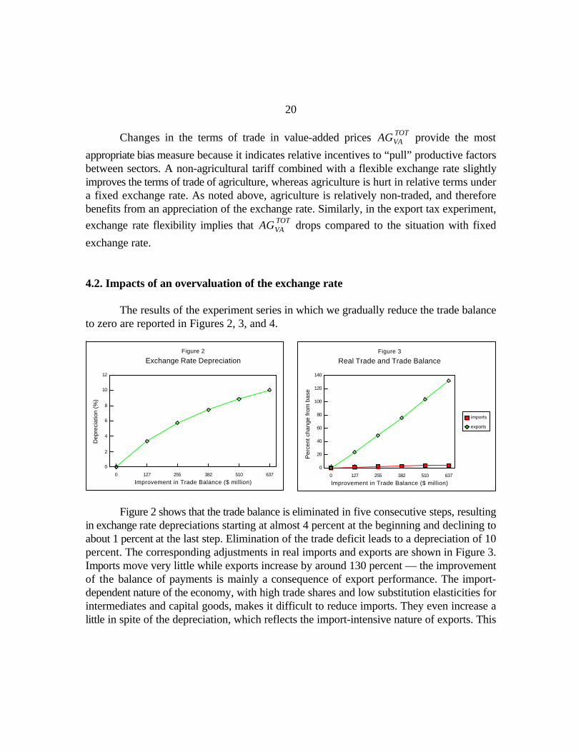
4.2. Impacts of an overvaluation of the exchange rate

The results of the experiment series in which we gradually reduce the trade balanceto zero are reported in Figures 2, 3, and 4.

Figure 2 shows that the trade balance is eliminated in five consecutive steps, resultingin exchange rate depreciations starting at almost 4 percent at the beginning and declining toabout 1 percent at the last step. Elimination of the trade deficit leads to a depreciation of 10percent. The corresponding adjustments in real imports and exports are shown in Figure 3.Imports move very little while exports increase by around 130 percent — the improvementof the balance of payments is mainly a consequence of export performance. The import-dependent nature of the economy, with high trade shares and low substitution elasticities forintermediates and capital goods, makes it difficult to reduce imports. They even increase alittle in spite of the depreciation, which reflects the import-intensive nature of exports. This

0

20

40

60

80

100

120

140

Improvement in Trade Balance ($ million)

Bill

ion

of T

Shs

.

0 127 255 382 510 637

Tea

Coffee

Maize

LFFH 1)

Figure 5

Real Output for Some AG Sectors

1) LFFH = Lifestock, Forestry, Fishing, and Hunting

95

96

97

98

99

100

101

Improvement in Trade Balance ($ million)

Ag

TO

T M

easu

res

0 127 255 382 510 637

TOT(M)

TOT(E)

TOT(Q)

TOT(X)

TOT(VA)

Figure 4

Agricutlure Terms of Trade and Trade Balance

AG TOTM AG TOT

E

AG TOTQ AG TOT

X AG TOTVA

21

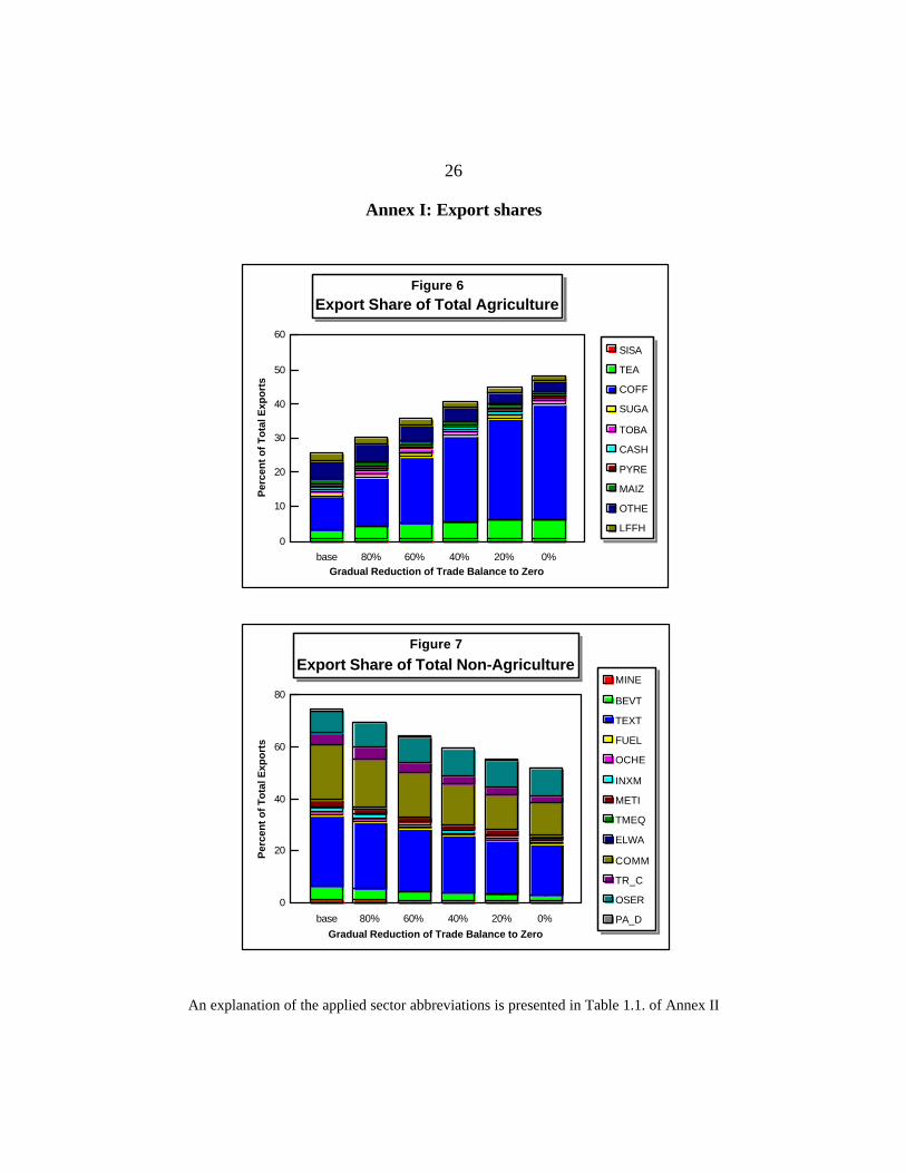
The development of the relative export shares of total agriculture and non-agriculture13

throughout the experiment series is shown in Figure 6 and 7 of Annex I.

result, which is typical of many developing countries, underlines the need to maintainimports at an adequate level if export promotion is to succeed.13

Finally, Figure 4 demonstrates that although the last three agricultural terms of tradeindices fall as the exchange rate depreciates, the changes are small — under 5 percent. The

first two indices, and , do not change since changes in the exchange rate effect

agriculture and non-agriculture symmetrically. The other three agricultural terms-of-trade

measures ( , , and ) decrease in the beginning due to the induced

depreciation of the exchange rate. However, the effect tapers off in the middle of theexperiment series, and the measures improve a little at the end. The turnaround is due to thefact that agricultural exports increase with depreciation and, by the last two experiments inthe series, grow to be a significant share of agricultural output. With depreciation, tradedagriculture becomes more important as can be seen from Figure 5.

5. Conclusion

This paper analyzes the extent of the policy bias against agriculture in a generalequilibrium framework. Various measures of the agricultural terms of trade are constructedto assess the impact of industrial protection, agricultural export taxes, and overvaluation ofthe exchange rate on the balance between agriculture and non-agriculture. The general

22

equilibrium measures are compared with earlier work measuring policy bias in a partialequilibrium framework.

Our results indicate that trade policies — in particular, 25 percent non-agriculturaltariffs and 25 percent agricultural export taxes — have a significant but much lower negativeimpact on relative prices in agriculture than would be indicated by partial equilibriummeasures. The general equilibrium framework captures indirect effects of trade policies thatwork through induced changes in the equilibrium exchange rate — an effect that is notcaptured in partial equilibrium analysis. We use the model to compute the empiricalimportance of this indirect effect, which is potentially significant. The imposition of a non-agricultural tariff with a fixed exchange rate leads to a much stronger deterioration of theterms-of-trade measures as compared to a flexible exchange rate scenario since theappreciation of the exchange rate actually benefits agriculture. The imposition of an exporttax on all agricultural sectors with a fixed exchange rate leads to a much lower deteriorationas compared to a flexible exchange rate scenario since the export tax induced depreciationof the exchange rate hurts the relatively non-traded aggregate agriculture in the case of aflexible exchange rate.

A separate series of experiments is carried out to assess the impact of overvaluationof the exchange rate — characteristic of many developing countries. In earlier work in apartial equilibrium framework, comparative work in a number of countries identifiedexchange rate overvaluation as the largest source of policy bias. In a general equilibriumframework incorporating non-traded goods and imperfect substitutability between domesticand foreign goods, these results are seriously qualified.

In our archetype model of Tanzania, agriculture has a large share of non-traded goodsand traded non-agriculture goods have relatively low substitution elasticities. Thesecharacteristics reflect many developing countries. In this environment, we find a muchsmaller impact on agriculture of depreciating the exchange rate than is indicated by partialequilibrium measures. Actually, our results are contrary to the “conventional wisdom” thata depreciation benefits agriculture. General equilibrium effects are indeed important.

This paper deals only with trade policies and their impact on aggregate agriculture.It is straightforward to expand the analysis to include sector-specific domestic tax andsubsidy policies and their impacts on particular agricultural sectors. The CGE model is anappropriate analytical framework for such analysis.

23

References

Ardeni, P. G. 1989. Does the law of one price really hold for commodity prices? AmericanJournal of Agricultural Economics, 71(3): 661-669.

Armington, P. S. 1969. A theory of demand for products distinguished by place ofproduction. IMF Staff Papers, 16: 159-176.

Baffes, J. 1991. Some further evidence on the law of one price: The law of one price stillholds. American Journal of Agricultural Economics, 73(4):1264-1273.

Ceglowski, J. 1994. The law of one price revisited: New evidence on the behavior ofinternational prices. Economic Inquiry, 32:407-418.

Bautista, R. M. 1987. Production incentives in Philippine agriculture: Effects of trade andexchange rate policies. Research Report 59. Washington, D.C.: International FoodPolicy Research Institute.

Bautista, R. M. and A. Valdes. 1993. The bias against agriculture: Trade andmacroeconomic policies in developing countries. San Francisco: Institute forContemporary Studies Press.

Cavallo, D. and Y. Mundlak. 1982. Agriculture and growth in an open economy: The caseof Argentina. Research Report 36. Washington, D.C.: International Food PolicyResearch Institute.

de Melo, J. and S. Robinson. 1981. Trade policy and resource allocation in the presence ofproduct differentiation. Review of Economics and Statistics, 63: 169-177.

_______. 1989. Product differentiation and the treatment of foreign trade in computablegeneral equilibrium models of small economies. Journal of International Economics,27: 47-67.

de Melo, J. and D.Tarr. 1992. A general equilibrium analysis of US foreign trade policy.Cambridge: Massachusetts Institute of Technology Press.

Devarajan, S., D. S. Go, J. D. Lewis, S. Robinson, and P. Sinko. 1997. Simple generalequilibrium modeling. In: Applied methods for trade policy analysis: A handbook,ed. J. F. Francois and K. A. Reinert. Cambridge: Cambridge University Press.

24

Devarajan, S., J. D. Lewis, and S. Robinson. 1993. External shocks, purchasing powerparity, and equilibrium real exchange rate. The World Bank Economic Review, 7(1):45-63.

Food and Agriculture Organization of the United Nations. 1975. Agricultural protectionand stabilization policies: A framework of measurement in the context of agriculturaladjustment. Rome.

Hertel, T. W. 1997. Applied general equilibrium analysis of agricultural policies. In:Handbook of agricultural economics, ed. B. Gardner and G. Rausser. Amsterdam:North Holland Press, forthcoming.

Isard, P. 1977. How far can we push the law of one price? The American Economic Review,67(5): 942-948.

Josling, T. and S. Tangermann. 1989. Measuring levels of protection in agriculture: Asurvey of approaches and results. In: Agriculture and governments in an independentworld, ed. A. Maunder and A. Valdes. Proceedings of the Twentieth InternationalConference of Agricultural Economists held in Buenos Aires, 24-31 August, 1988.Aldershot, pp. 343-352.

Krueger, A. O. 1992. The political economy of agricultural pricing policy. Volume 5: Asynthesis of the political economy in developing countries. Washington, D.C.: TheWorld Bank.

Krueger, A. O., M. Schiff, and A. Valdes. 1988. Agricultural incentives in developingcountries: Measuring the effect of sectoral and economywide policies. The WorldBank Economic Review, 2(3): 255-271.

Lipton, M. 1977. Why poor people stay poor: Urban bias in world development.Cambridge: Harvard University Press.

Mundlak, Y. and D. F. Larson. 1992. On the transmission of world agricultural prices. TheWorld Bank Economic Review, 6(3): 399-422.

Peterson, E. B., T. W. Hertel, and J. V. Stout. 1994. A critical assessment of supply-demandmodels of agricultural trade. American Journal of Agricultural Economics, 76(4):709-721.

25

Schiff, M. and A. Valdes. 1992. The political economy of agricultural pricing policy.Volume 4: A synthesis of the economics in developing countries. Washington, D.C.:The World Bank.

Schultz, T. W. 1964. Transforming traditional agriculture. New Haven: Yale UniversityPress.

Toye, J. F. J. 1993. Dilemmas of development: Reflections on the counter-revolution indevelopment economics. Oxford: Oxford University Press.

Webb, A. J., M. Lopez, and R. Penn. 1990. Estimates of producer and consumer subsidyequivalents: Government intervention in agriculture, 1982-87. Economic ResearchService. Statistical Bulletin No. 803. Washington, D.C.: U.S. Department ofAgriculture.

Wobst, P. 1998. A social accounting matrix (SAM) for Tanzania. Trade andMacroeconomics Division. TMD Discussion Paper Series. Washington, D.C.:International Food Policy Research Institute, forthcoming

World Bank. 1981. Accelerated development in Sub-Saharan Africa: An agenda for action.Washington, D.C.

0

10

20

30

40

50

60

Gradual Reduction of Trade Balance to Zero

Per

cen

t o

f T

ota

l Exp

ort

s

base 80% 60% 40% 20% 0%

SISA

TEA

COFF

SUGA

TOBA

CASH

PYRE

MAIZ

OTHE

LFFH

Figure 6

Export Share of Total Agriculture

0

20

40

60

80

Gradual Reduction of Trade Balance to Zero

Per

cen

t o

f T

ota

l Exp

ort

s

base 80% 60% 40% 20% 0%

MINE

BEVT

TEXT

FUEL

OCHE

INXM

METI

TMEQ

ELWA

COMM

TR_C

OSER

PA_D

Figure 7

Export Share of Total Non-Agriculture

26

Annex I: Export shares

An explanation of the applied sector abbreviations is presented in Table 1.1. of Annex II

27

Annex II: CGE model equations

Table 1.1. Definition of Model Indices, Parameters, and Variables

Indices

i, j Sectors Cotton (Cott) Processed Food, BeveragesSisal (Sisa) & Tobacco (Bevt)Tea (Tea) Textiles (Text)Coffee (Coff) Petroleum (Fuel)Sugar (Suga) Other Chemicals (Oche)Tobacco (Toba) Non-metal Products (Inxm)Cashew (Cash) Metal products (Meti)Pyrethrum (Pyre) Transport & Mach. Equ. (Tmeq)Maize (Maiz) Electricity & Water (Elwa)Wheat (Whea) Construction (Cnst)Paddy (Padd) Commerce (Comm)Other Agriculture (Othe) Transport & Communication (Tr_c)Livestock, Forestry, Fishing Financial Institutions (Fi_i) & Hunting (Lffh) Other Services (Oser)Mining (Mine) Public Administration (Pa_d)

iag Agricultural Cotton Sisalsectors Tea Coffee

Sugar TobaccoCashew PyrethrumMaize WheatPaddy Other AgricultureLivestock, Forestry, Fishing & Hunting

iagn Non-agricultural sectors (iagn = i - iag)im Import sectorsimn Non-import sectorsie Export sectorsien Non-export sectors

f Factors of Agriculture Rural Paid labor Urban Prof & Tech & Supervisorproduction Urban Unskilled Paid labor Land

Urban Production & Transport & Manual CapitalUrban Clerical & Sales & Services Government Capital

hh, h Households Rural Farmer Rural Non-farmerUrban Farmer Urban Non-farmer

a Ci

a Di

"i, f

a Ti

ai, j

bi, j

clesi,hh

*i

fmaphh, f

(i

glesi

kshri

makei, j

pwmi

pwtsi

DCi

DPi

DTi

sremithh

stranshh

syenthhh

syentf

tci

tei

thhh

tmi

txi

wfdist0 i,f

CDi

CHhh

CONTAXDAi

DCi

DKi

DSTi

ENTSAVENTTAXENTTFESRETR

EXPTAXEXRE i

FBORFDSCi,f

FLABTFFSAVFSf

FSAGf

FXDINVGDTOTGDi

GOVSAVGOVTHGRHHSAVHHTAXIDi

IDSINDTAXINTi

INVESTMPSh

Mi

PCi

PDAi

PDCi

PEi

PINDEXPKi

PMi

PQi

PVi

PWEi

PXi

Qi

REMITREMITENTSAVINGTARIFFWALRASWFDISTi,f

WFAGDISTf

WFf

X i

YENTYFCTRf

YHhh

28

Table 1.1 (cont.)

Parameters (in lower case)

Armington function shift parameter

CES shift parameter

CES factor share parameter

CET function shift parameter

Input-output coefficients

Capital composition matrix

Household consumption shares

Armington function share parameter

Factors to household map

CET function share parameter

gdtot0 Initial real government spendingGovernment consumption shares

ids0 Initial total demand for investmentShares of investment by sector of destination

Make matrix coefficients

World market price of imports (in US$)

Non-traded producer price weights

Armington function exponent

CES production function exponent

CET function exponent

Remittance shares

Government transfer shares

Share of enterprise income to households

Enterprise shares of factor income

Consumption tax (+) or subsidy (-) rates

Tax (+) or subsidy (-) rates on exports

Household tax rate

Tariff rates on imports

Indirect tax rates

Initial factor price sectoral proportionality ratios

Variables (in upper case)

Final demand for private consumption

Household consumption / disposable income

Consumption tax revenueDomestic activity sales

Domestic commodity sales

Volume of investment by sector of destination

Inventory investment by sector

Enterprise savings Enterprise tax revenueEnterprise transfers abroadEnterprise savings rateEnterprise tax rate

Export subsidy payments Exchange rate (TShs. per US$) Exports

Government foreign borrowing Factor demand by sector

Labor transfers abroad Net foreign savings Factor supply

Factor supply in agriculture

Fixed capital investment Total volume of government consumptionFinal demand for government consumption

Government savings Government transfers to HouseholdsGovernment revenue Household savings Household tax revenue Final demand for productive investment

Total final demand for investmentIndirect tax revenue Intermediates uses

Total investment Marginal propensity to save by Household

Imports

Consumption price of composite goods

Domestic activity goods price

Domestic commodity goods price

Domestic price of exports

Non-traded producer price index Price of capital goods by sector of destination

Domestic price of imports

Price of composite good

Value-added price

World price of exports

Average output price

Composite goods supply

Remittances Enterprise remittancesTotal savings Tariff revenueSlack variableFactor price sectoral proportionality ratios

Factor price sectoral proportionality ratios for

agricultural sectorsAverage factor price

Domestic output

Enterprise incomeFactor income

Household income

PMi ' pwmi @ (1% tmi ) @EXR

PEi ' PWEi @ (1& tei ) @EXR

PDCj ' ji

makei, j @PDAi

PQi 'PDCi @CDi % PMi @Mi

Qi

PXi 'PDAi @DAi% PEi @Ei

Xi

PCi ' PQi @ (1%tci)

PVi ' PXi @ (1&txi)&jj

PCj @aj, i

PKi ' jj

bj, i @PCj

PINDEX ' ji

pwtsi @PDAi

PINDEX

Xi ' a Di @ '

f"i, f FDSC

&DPi

i, f

&1

DPi

FDSCi, f ' Xi @"i, f @PVi

(a Di )

DPi @WFf @WFDISTi, f

FPi

WFDISTi , f ' WFAGDIST f @ wfdist0i , f

INTi ' jj

aj, i @Xj

DAi ' jj

makei, j @DCi

Xi ' a Ti (i E

DTi

i % (1 & (i) DADT

i

i

1

DTi

29

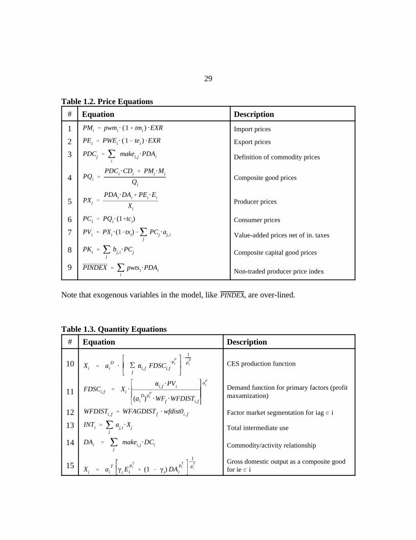
Table 1.2. Price Equations

# Equation Description

1 Import prices

2 Export prices

3 Definition of commodity prices

4 Composite good prices

5 Producer prices

6 Consumer prices

7 Value-added prices net of in. taxes

8 Composite capital good prices

9

Non-traded producer price index

Note that exogenous variables in the model, like , are over-lined.

Table 1.3. Quantity Equations

# Equation Description

10 CES production function

11Demand function for primary factors (profitmaxamization)

12 Factor market segmentation for iag 0 i

13 Total intermediate use

14 Commodity/activity relationship

15 Gross domestic output as a composite goodfor ie 0 i

Xi ' DAi

Ei ' DAi

PEi (1&(i )

PDAi@(i

1

DTi & 1

Qi ' a Ci *i M

&DCi

i % (1&*i) DC&DC

i

i

&1

DCi

Qi ' DCi

Mi ' DCi

PDCi@ *i

PMi (1&*i)

1

1 % DCi

YFCTRf ' ji

WFf @FDSCi, f @WFDISTi, f

YENT ' 'f

syentf @YFCTRf % REMITENT @EXR

YHhh ' 'f

fmaphh, f @ (1& syentf ) @YFCTRf

% sremithh @ (REMIT& FLABTF ) @EXR % stranshh @GOVTH

% syenthhh @ (YENT& ENTTAX& ENTSAV& ENTTF @EXR)

CHhh ' (1& thhh) @ (1& MPShh) @YHhh

TARIFF ' ji

tmi @pwmi @Mi @EXR

CONTAX ' ji

tci @ PQi @ Qi

INDTAX ' ji

txi @ PXi @ Xi

EXPTAX ' ji

tei @PWEi @Ei @EXR

HHTAX ' jh

thh @YHh

ENTTAX ' ETR @YENT

Table 1.3. Quantity Equations (cont.)

30

# Equation Description

16 Gross dom. output for ien 0 i

17 Export supply

18 Total supply of composite good - Armingtonfunction for im 0 i

19 Total supply for imn 0 i

20F.O.C for cost minimization for compositegood for im 0 i

Table 1.4. Income Equations

# Equation Description

21 Factor income

22 Capital income

23 Household income

24 Disposable household income

25 Tariff revenue

26 Consumption taxes

27 Indirect taxes

28 Export tax

29 Household taxes

30 Enterprise taxes

ENTSAV ' ESR @YENT

HHSAV ' jh

MPSh @YHh @ (1& thh )

GR ' TARIFF % CONTAX % INDTAX % HHTAX% FBOR @EXR % ENTTAX % EXPTAX

SAVING ' HHSAV % ENTSAV % GOVSAV % EXR @FSAV

PCi @ CDi ' jhh

clesi,hh @ CHhh

GDi ' glesi @ GDTOT

GR ' 'i

PCi @ GDi % GOVSAV % GOVTH

FXDINV ' INVEST & ji

PCi @ DSTi

PKi @DKi ' kshri @FXDINV

IDi ' jj

bi, j @DKj

IDS ' ji

IDi

Qi ' INTi % CDi % GDi % IDi % DSTi

FSf ' ji

FDSCi, f

FSAGf ' ji

FDSCi, f

Ei

pwmi @Mi ' Ei

PWEi @Ei % FSAV % FBOR % REMIT

% ENTTF & FLABTF % REMITENT

Table 1.4. Income Equations (cont.)

31

# Equation Description

31 Enterprise savings

32 Household savings

33 Government revenue

34 Total savings

Table 1.5. Expenditure Equations

# Equation Description

35 Private consumption

36 Government consumption

37 Government savings

38 Fixed investment

39 Real fixed investment by sector ofdestination

40 Investment final demand by sectorof origin

41 Total final investment demand

Table 1.6. Market clearing

# Equation Description

42 Goods market equilibrium (eq)

43 Factor market eq for iagn 0 i

44 Factor market eq for iag 0 i

45 External balance

SAVING ' INVEST % WALRAS

IDS ' ids0

GDTOT ' gdtot0

Table 1.6. Market Clearing Conditions (cont.)

32

# Equation Description

The model is square and satisfies Walras' law. The set of market clearing equations is14

functionally dependent, and one can be dropped. Instead of dropping an equation, we add a “slack”variable to the savings-investment equation (WALRAS in equation 46). This specification is convenient forchecking model consistency, since WALRAS should always equal zero.

46 14 Saving- investment balance

Table 1.7. Macro economic closures

# Equation Description

47 Fix total real investment

48 Fix real government spending

33

LIST OF TMD DISCUSSION PAPERS

No. 1 - "Land, Water, and Agriculture in Egypt: The Economywide Impact of PolicyReform" by Sherman Robinson and Clemen Gehlhar (January 1995)

No. 2 - "Price Competitiveness and Variability in Egyptian Cotton: Effects of Sectoraland Economywide Policies" by Romeo M. Bautista and Clemen Gehlhar(January 1995)

No. 3 - "International Trade, Regional Integration and Food Security in the Middle East"by Dean A. DeRosa (January 1995)

No. 4 - "The Green Revolution in a Macroeconomic Perspective: The Philippine Case"by Romeo M. Bautista (May 1995)

No. 5 - "Macro and Micro Effects of Subsidy Cuts: A Short-Run CGE Analysis forEgypt" by Hans Löfgren (May 1995)

No. 6 - "On the Production Economics of Cattle" by Yair Mundlak, He Huang andEdgardo Favaro (May 1995)

No. 7 - "The Cost of Managing with Less: Cutting Water Subsidies and Supplies inEgypt's Agriculture" by Hans Löfgren (July 1995, Revised April 1996)

No. 8 - "The Impact of the Mexican Crisis on Trade, Agriculture and Migration" bySherman Robinson, Mary Burfisher and Karen Thierfelder (September 1995)

No. 9 - "The Trade-Wage Debate in a Model with Nontraded Goods: Making Room forLabor Economists in Trade Theory" by Sherman Robinson and KarenThierfelder (Revised March 1996)

No. 10*- "Macroeconomic Adjustment and Agricultural Performance in Southern Africa:A Quantitative Overview" by Romeo M. Bautista (February 1996)

No. 11 - "Tiger or Turtle? Exploring Alternative Futures for Egypt to 2020" by HansLöfgren, Sherman Robinson and David Nygaard (August 1996)

No. 12*- "Water and Land in South Africa: Economywide Impacts of Reform - A CaseStudy for the Olifants River" by Natasha Mukherjee (July 1996)

34

No. 13 - "Agriculture and the New Industrial Revolution in Asia" by Romeo M. Bautistaand Dean A. DeRosa (September 1996)

No. 14 - "Income and Equity Effects of Crop Productivity Growth Under AlternativeForeign Trade Regimes: A CGE Analysis for the Philippines" by Romeo M.Bautista and Sherman Robinson (September 1996)

No. 15*- "Southern Africa: Economic Structure, Trade, and Regional Integration" byNatasha Mukherjee and Sherman Robinson (October 1996)

No. 16 - "The 1990's Global Grain Situation and its Impact on the Food Security ofSelected Developing Countries" by Mark Friedberg and Marcelle Thomas(February 1997)

No. 17 - "Rural Development in Morocco: Alternative Scenarios to the Year 2000" byHans Löfgren, Rachid Doukkali, Hassan Serghini and Sherman Robinson(February 1997)

No. 18 - "Evaluating the Effects of Domestic Policies and External Factors on the PriceCompetitiveness of Indonesian Crops: Cassava, Soybean, Corn, and Sugarcane"by Romeo M. Bautista, Nu Nu San, Dewa Swastika, Sjaiful Bachri, andHermanto (June 1997)

No. 19 - "Rice Price Policies in Indonesia: A Computable General Equilibrium (CGE)Analysis" by Sherman Robinson, Moataz El-Said, Nu Nu San, Achmad Suryana,Hermanto, Dewa Swastika and Sjaiful Bahri (June 1997)

No. 20 - "The Mixed-Complementarity Approach to Specifying Agricultural Supply inComputable General Equilibrium Models" by Hans Löfgren and ShermanRobinson (August 1997)

No. 21*- "Estimating a Social Accounting Matrix Using Entropy Difference Methods" bySherman Robinson and Moataz-El-Said (September 1997)

No. 22 - "Income Effects of Alternative Trade Policy Adjustments on Philippine RuralHouseholds: A General Equilibrium Analysis" by Romeo M. Bautista andMarcelle Thomas (October 1997)

No. 23 - "South American Wheat Markets and MERCOSUR" by Eugenio Díaz-Bonilla(November 1997)

35

No. 24 - "Changes in Latin American Agricultural Markets" by Lucio Reca and EugenioDíaz-Bonilla (November 1997)

No. 25 - "Policy Bias and Agriculture: Partial and General Equilibrium Measures" byRomeo M. Bautista, Sherman Robinson, Finn Tarp and Peter Wobst (May 1998)

No. 26 - "Estimating Income Mobility in Colombia Using Maximum EntropyEconometrics" by Samuel Morley, Sherman Robinson and Rebecca Harris (May1998)

No. 27 - “Rice Policy, Trade, and Exchange Rate Changes in Indonesia: A GeneralEquilibrium Analysis” by Sherman Robinson, Moataz El-Said, and Nu Nu San(June 1998)

No. 28* - “Social Accounting Matrices for Mozambique - 1994 and 1995” by ChanningArndt, Antonio Cruz, Henning Tarp Jensen, Sherman Robinson, and Finn Tarp(July 1998)

No. 29* - “Agriculture and Macroeconomic Reforms in Zimbabwe: A Political-EconomyPerspective” by Kay Muir-Leresche (August 1998)

No. 30* - “A 1992 Social Accounting Matrix (SAM) for Tanzania” by Peter Wobst(August 1998)

No. 31* - “Agricultural Growth Linkages in Zimbabwe: Income and Equity Effects”by Romeo M. Bautista and Marcelle Thomas (September 1998)

No.32* - “Does Trade Liberalization Enhance Income Growth and Equity in Zimbabwe? The Role of Complementary Polices” by Romeo M. Bautista,Hans Lofgren and Marcelle Thomas (September 1998)

No.33 - “Estimating a Social Accounting Matrix Using Cross EntropyMethods” by Sherman Robinson, Andrea Cattaneo, and Moataz El-Said (October 1998)

* TMD Discussion Papers marked with an “*” are MERRISA-related papers.

Copies can be obtained by callingMaria Cohan at 202-862-5627or e-mail m.cohan@cgnet.com