TMA4230 Functional analysis 2006 Assorted notes … · TMA4230 Functional analysis 2006 Assorted...

TMA4230 Functional analysis 2006

Assorted notes on functional analysisHarald Hanche-Olsen

[email protected]

Abstract. These are supplementary notes for a course on functional analysis. The notes werefirst made for the course in 2004. For 2005, those notes were worked into a single documentand some more material has been added.

The basic text for the course is Kreyszig’s Functional analysis. These notes are only in-tended to fill in some material that is not in Kreyszig’s book, or to present a different exposi-tion.

Version 2006–05–11

Assorted notes on functional analysis 2

Chapter 1: Transfinite induction · 3Wellordering · 3

Zorn’s lemma and the Hausdorff maximality principle · 8Further reading · 11

Chapter 2: Some Banach space results · 12Uniform boundedness · 12

Chapter 3: Sequence spaces and Lp spaces · 14Sequence spaces · 14

Lp spaces · 19

Chapter 4: A tiny bit of topology · 32Basic definitions · 32

Neighbourhoods, filters, and convergence · 35Continuity and filters · 38

Compactness and ultrafilters · 39Product spaces and Tychonov’s theorem · 42

Normal spaces and the existence of real continous functions · 43The Weierstrass density theorem · 44

Chapter 5: Topological vector spaces · 49Definitions and basic properties · 49

The Banach–Alaoglu theorem · 52The geometric Hahn–Banach theorem · 54

Uniform convexity and reflexivity · 57The Krein–Milman theorem · 59

Chapter 6: Spectral theory · 61Operators and Banach algebras · 61

The algebraic theory of the spectrum · 61Geometric series in Banach algebras · 63

The resolvent · 64Holomorphic functional calculus · 65

Spectral properties of self-adjoint operators on a Hilbert space · 67Functional calculus · 70

The spectral theorem · 72Spectral families and integrals · 75

Chapter 7: Compact operators · 79Compact operators · 79

Hilbert–Schmidt operators · 81Sturm–Liouville theory · 83

Index · 85

Version 2006–05–11

Chapter 1

Transfinite induction

Chapter abstract.Transfinite induction is like ordinary induction, only more so. The salient feature of trans-

finite induction is that it works by not only moving beyond the natural numbers, but evenworks in uncountable settings.

Wellordering

A strict partial order on a set S is a binary relation, typically written as < or ≺ orsome similar looking symbol (let us pick ≺ for this definition), which is transitivein the sense that, if x ≺ y and y ≺ z, then x ≺ z, and antireflexive in the sensethat x ≺ x never holds. The order is called total if, for every x, y ∈ S, either x ≺ y ,x = y , or y ≺ x. We write x Â y if y ≺ x.

Furthermore, we write x 4 y if x ≺ y or x = y . When ≺ is a partial order then 4is also a transitive relation. Furthermore, 4 is reflexive, i.e., x 4 x always holds,and if x 4 y and y 4 x both hold, then x = y . If a relation 4 satisfies these threeconditions (transitivity, reflexivity, and the final condition) then we can define ≺by saying x ≺ y if and only if x 4 y and x 6= y . This relation is then a partial order(exercise: prove this). We will call a relation of the form 4 a nonstrict partialorder.

There is clearly a one-to-one correspondence between strict and nonstrictpartial orders. Thus we often use the term partial order about one or the other.We rely on context as well as the shape of the symbol used (whether it includessomething vaguely looking like an equality sign) to tell us which kind is meant.

An obvious example of a total order is the usual order on the real numbers,written < (strict) or ≤ (nonstrict).

A much less obvious example is the lexicographic order on the set RN of se-quences x = (x1, x2, . . .) of real numbers: x < y if and only if, for some n, xi = yi

when i < n while xn < yn . Exercise: Show that this defines a total order.An example of a partially ordered set is the set of all real functions on the real

line, ordered by f ≤ g if and only if f (x) ≤ g (x) for all x. This set is not totallyordered. For example, the functions x 7→ x2 and x 7→ 1 are not comparable in thisorder.

3

Another example is the set P (S) of subsets of a given set S, partially orderedby inclusion ⊂. This order is not total if S has at least two elements.

A wellorder on a set S is a total order ≺ so that every nonempty subset A ⊆ Shas a smallest element. That is, there is some m ∈ A so that m 4 a for everya ∈ A.

One example of a wellordered set is the set of natural numbers 1,2, . . . withthe usual order.

Morover, every subset of a wellordered set is wellordered in the inheritedorder.

1 Proposition. (Principle of induction) Let S be a wellordered set, and A ⊆ S.Assume for every x ∈ S that, if y ∈ A for every y ≺ x, then x ∈ A. Then A = S.

Proof: Let B = S \ A. If A 6= S then B 6=∅. Let x be the smallest element of B . Butthen, whenever y ≺ x then y ∈ A. It follows from the assumption that x ∈ A. Thisis a contradiction which completes the proof.

An initial segment of a partially ordered set S is a subset A ⊆ S so that, if a ∈ Aand x ≺ a, then x ∈ A. Two obvious examples are x ∈ S : x ≺ m and x ∈ S : x 4 mwhere m ∈ S. An initial segment is called proper if it is not all of S.

Exercise: Show that every proper initial segment of a wellordered set S is ofthe form x ∈ S : x ≺ m where m ∈ S.

A map f : S → T between partially ordered sets S and T is called order pre-serving if x ≺ y implies f (x) ≺ f (y). It is called an order isomorphism if it has aninverse, and both f and f −1 are order preserving. Two partially ordered sets arecalled order isomorphic if there exists an order isomorphism between them.

Usually, there can be many order isomorphisms between order isomorphicsets. However, this is not so for wellordered sets:

2 Lemma. If S and T are wellordered and f : S → T is an order isomorphism ofS to an initial segment of T , then for each s ∈ S, f (s) is the smallest t ∈ T greaterthan every f (x) where x ≺ s.

Proof: Let S′ be the initial segment of T so that f is an order isomorphism of Sonto S′, and let s ∈ S be arbitrary. Let

z = mint ∈ T : t Â f (x) for all x ≺ s.

Such a z exists, for the set on the righthand side contains f (s), and so isnonempty. In particular, z 4 f (s). If z ≺ f (s) then f (x) 6= z for all x ∈ S: For ifx ≺ s then f (x) ≺ z by the definition of z, and if x < s then f (x) < f (s) Â z. Butthen S′ is not an initial segment of T , since z 6= S′ but z ≺ f (s) ∈ S′. Thus z = f (s)and the proof is complete.

Version 2006–05–11

5 Assorted notes on functional analysis

3 Proposition. There can be only one order isomorphism from one wellorderedset to an initial segment of another.

Proof: Let S and T be wellordered, and f , g two order isomorphisms from S toinitial segments of T . We shall prove by induction that f (x) = g (x) for all x ∈ S.We do this by applying Proposition 1 to the set of all s ∈ S for which f (s) = g (s).

Assume, therefore, that s ∈ S and that f (x) = g (x) for all x ≺ s.By Lemma 2, then

f (s) = mint ∈ T : t Â f (x) for all x ≺ s

= mint ∈ T : t Â g (x) for all x ≺ s = g (s),

and so f = g by induction.

4 Proposition. Given two wellordered sets, one of them is order isomorphic to aninitial segment of the other (which may be all of the other set).

Proof: Let S and T be wellordered sets, and assume that T is not order isomor-phic to any initial segment of S. We shall prove that S is order isomorphic to aninitial segment of T .

Let W be the set of w ∈ S so that y ∈ S : y 4 w is order isomorphic to aninitial segment of T .

Clearly, W is an initial segment of S. In fact, if w1 ∈ S and w2 ∈W with w1 ≺ w2

and we restrict the order isomorphism of y ∈ S : y 4 w2 to the set y ∈ S : y 4w1, we obtain an order isomorphism of the latter set to an initial segment of T .By using Lemma 2, we conclude that the union of all these mappings is an orderisomorphism f of W to an initial segment of T . Since T is not order isomorphicto an initial segment of S, f [W ] 6= T .

Assume that W 6= S. Let m be the smallest element of S \ W . Extend f byletting f (m) be the smallest element of T \ f [W ]. Then the extended map is anorder isomorphism, so that m ∈W . This is a contradiction.

Hence W = S, and the proof is complete.

It should be noted that if S and T are wellordered and each is order isomorphicto an initial segment of the other, then S and T are in fact order isomorphic. Forotherwise, S is order isomorphic to a proper initial segment of itself, and that isimpossible (the isomorphism would have to be the identity mapping).

Thus we have (almost) a total order on all wellordered sets. Given two well-ordered sets S and T , precisely one of the following conditions holds: Either S isorder isomorphic to a proper initial segment of T , or T is order isomorphic to aproper initial segment of S, or S and T are order isomorphic.

Later we shall see how ordinal numbers can be used to keep track of theisomorphism classes of wellordered sets and their order relation.

Version 2006–05–11


5 Theorem. (The wellordering principle) Every set can be wellordered.

Proof: The proof relies heavily on the axiom of choice. Let S be any set, andpick a “complementary” choice function c : P (S) \ S → S.

More precisely, P (S) is the set of all subsets of S, and so c is to be definedon all subsets of S with nonempty complement. We require that c(A) ∈ S \ A foreach A. This is why we call it a complementary choice function: It chooses anelement of each nonempty complement for subsets of S.

We consider subsets G of S. If G is provided with a wellorder, then G (and thewellorder on it) is called good if

c(x ∈G : x ≺ g

)= g

for all g ∈G .The idea is simple, if its execution is less so: In a good wellorder, the smallest

element must be x0 = c(∅). Then the next smallest must be x1 = c(x0), thencomes x2 = c(x0, x1), and so forth. We now turn to the formal proof.

If G1 and G2 are good subsets (with good wellorders ≺1 and ≺2) then oneof these sets is order isomorphic to an initial segment of the other. It is easilyproved by induction that the order isomorphism must be the identity map. Thus,one of the two sets is contained in the other, and in fact one of them is an initialsegment of the other. Let G be the union of all good subsets of S. Then G is itselfa good subset, with an order defined by extending the order on all good subsets.In other words, G is the largest good subset of S.

Assume G 6= S. Then let G ′ = G ∪ c(G), and extend the order on G to G ′ bymaking c(G) greater than all elements of G . This is a wellorder, and makes G ′good. This contradicts the construction of G as the largest good subset of S, andproves therefore that G = S.

Ordinal numbers. We can define the natural numbers (including 0) in terms ofsets, by picking one set of n elements to stand for each natural number n. Thisimplies of course

0 =∅,

so that will be our starting point. But how to define 1? There is one obvious itemto use as the element of 1, so we define

1 = 0.

Now, the continuation becomes obvious:

2 = 0,1, 3 = 0,1,2, . . .

Version 2006–05–11


In general, given a number n, we let its successor be

n+ = n ∪ n.

We define n to be an ordinal number if every element of n is in fact also asubset of n, and the relation ∈ wellorders n.

Obviously, 0 is an ordinal number. Perhaps less obviously, if n is an ordinalnumber then so is n+. Any element of an ordinal number is itself an ordinalnumber, and each element is in fact the set of all smaller elements.

On the other hand, you may verify that, e.g., 0,1,2,4 is not an ordinal num-ber, for though it is wellordered by ∈, 4 is not a subset of the given set.

If m and n are ordinal numbers, then either m = n, m ∈ n, or n ∈ m. For oneof them is order isomorphic to an initial segment of the other, and an inductionproof shows that this order isomorphism must be the identity map.

For the proof of our next result, we are going to need the concept of defini-tion by induction. This means to define a function f on a wellordered set S bydefining f (x) in terms of the values f (z) for z ≺ x. This works by letting A be thesubset of S consisting of those a ∈ S for which there exists a unique function onx ∈ S : x 4 a satisfying the definition for all x 4 a, and then using transfiniteinduction to show that A = S. In the end we have a collection of functions, eachdefined on an initial segment of S, all of which extend each other. The union ofall these functions is the desired function. We skip the details here.

6 Proposition. Every wellordered set is order isomorphic to a unique ordinalnumber.

Proof: The uniqueness part follows from the previous paragraph. We show ex-istence.

Let S be wellordered. Define by induction

f (x) = f (z) : z ≺ x.

In particular, this means that f (m) = ∅ = 0 where m is the smallest element ofS. The second smallest element of S is mapped to f (m) = 0 = 1, the next oneafter that to 0,1 = 2, etc.

Letn = f (s) : s ∈ S.

Then every element of n is a subset of n. Also n is ordered by ∈, and f is an orderisomorphism. Since S is wellordered, then so is n, so n is an ordinal number.

An ordinal number which is not 0, and is not the successor n+ of another ordinalnumber n, is called a limit ordinal.

Version 2006–05–11

We call an ordinal number finite if neither it nor any of its members is a limitordinal. Clearly, 0 is finite, and the successor of any finite ordinal is finite. Letω be the set of all finite ordinals. Then ω is itself an ordinal number. Intuitively,ω= 0,1,2,3, . . .. ω is a limit ordinal, and is in fact the smallest limit ordinal.

There exist uncountable ordinals too; just wellorder any uncountable set, andpick an order isomorphic ordinal number. There is a smallest uncountable ordi-nal, which is called Ω. It is the set of all countable ordinals, and is a rich sourceof counterexamples in topology.

Arithmetic for ordinals can be tricky. If m and n are ordinals, let A and B be wellorderedsets order isomorphic to m and n, with A∩B =∅. Order A∪B by placing all elements ofB after those of A. Then m +n is the ordinal number order isomorphic to A ∪B orderedin this way. You may verify that 0+n = n +0 = n and n+ = n +1. However, addition is notcommutative on infinite ordinals: In fact 1+n = n whenever n is an infinite ordinal. (Thisis most easily verified for n =ω.) You may also define mn by ordering the cross productm×n lexicographically. Or rather, the convention calls for reverse lexicographic order, inwhich (a,b) < (c,d ) means either b < d or b = d and a < c . For example, 0n = n0 = 0 and1n = n1 = n, but ω2 =ω+ω while 2ω=ω:

ω×2 is ordered (0,0), (1,0), (2,0), . . . , (0,1), (1,1), (2,1), . . . ,

2×ω is ordered (0,0), (1,0), (0,1), (1,1), (0,2), (1,2), . . .

Zorn’s lemma and the Hausdorff maximality principle

As powerful as the wellordering principle may be, perhaps the most usefulmethod for doing transfinite induction is by Zorn’s lemma. We need some defi-nitions.

A chain in a partially ordered set is a subset which is totally ordered.

7 Lemma. If C is a collection of chains in a partially ordered set S, and if C isitself a chain with respect to set inclusion, then its union

⋃C is a chain in S.

Proof: Let a,b ∈ ⋃C . There are A,B ∈ C so that a ∈ A and b ∈ B . Since C is a

chain, either A ⊆ B or B ⊆ A. Assume the former. Since now a,b ∈ B and B is achain, a and b are comparable. We have shown that any two elements of

⋃C

are comparable, and so⋃

C is a chain.

An element of a partially ordered set is called maximal if there is no element ofthe set greater than the given element.

8 Theorem. (Hausdorff’s maximality principle)Any partially ordered set contains a maximal chain.

The maximality of the chain is with respect to set inclusion.

Version 2006–05–11

Proof: Denote the given, inductive, order on the given set S by ≺. Let < be awellorder of S.

We shall define a chain (whenever we say chain in this proof, we mean a chainwith respect to ≺) on S by using induction on S. We do this by going through theelements of S one by one, adding each element to the growing chain if it can bedone without destroying its chain-ness.

We shall define f (s) so that it becomes a chain built from a subset of x : x ≤ sfor each s. Define f : S →P (S) by induction as follows. The induction hypothesisshall be that each f (s) ⊂ S is a chain, with f (t ) ⊆ f (s) when t < s.

When s ∈ S and f (t ) has been defined for all t < s so that the induction hy-pothesis holds, let F (s) = ⋃

t<s f (t ). Then F (s) is a chain by the induction hy-pothesis plus the previous lemma.

Let f (s) = F (s)∪ s if this set is a chain, i.e., if s is comparable with everyelement of F (s); otherwise, let f (s) = F (s). In either case, f (s) is a chain, andwhenever t < s then f (t ) ⊆ F (s) ⊆ f (s), so the induction hypothesis remainstrue.

Finally, let C =⋃s∈S f (s). Again by the lemma, C is a chain. To show that C is

maximal, assume not, so that there is some s ∈ S \ C which is comparable withevery element of C . But since F (s) ⊆C , then s is comparable with every elementof F (s). Thus by definition s ∈ f (s), and so s ∈C – a contradiction.

A partially ordered set is called inductively ordered if, for every chain, there is anelement which is greater than or equal to any element of the chain.

9 Theorem. (Zorn’s lemma) Every inductively ordered set contains a maximalelement.

Proof: Let S be inductively ordered, and let C be a maximal chain in S. Let m ∈ Sbe greater than or equal to every element of C . Then m is maximal, for if s Â mthen s is also greater than or equal to every element of C , and so s ∈C becauseC is a maximal chain.

Hausdorff’s maximality principle and Zorn’s lemma can usually be used inter-changably. Some people seem to prefer one, some the other.

The wellordering principle, Zorn’s lemma, and Hausdorff’s maximality lemmaare all equivalent to the axiom of choice. To see this, in light of all we have doneso far, we only need to prove the axiom of choice from Zorn’s lemma.

To this end, let a set S be given, and let a function f be defined on S, so thatf (s) is a nonempty set for each s ∈ S. We define a partial choice function to be afunction c defined on a set Dc ⊆ S, so that c(x) ∈ f (x) for each x ∈ Dc . We createa partial order on the set C of such choice function by saying c 4 c ′ if Dc ⊆ Dc ′

Version 2006–05–11


and c ′ extends c . It is not hard to show that C is inductively ordered. Thus itcontains a maximal element c , by Zorn’s lemma. If c is not defined on all of S,we can extend c by picking some s ∈ S \ Dc , some t ∈ f (s), and letting c ′(s) = t ,c ′(x) = c(x) whenever x ∈ Dc . This contradicts the maximality of c . Hence Dc = S,and we have proved the axiom of choice.

We end this note with an application of Zorn’s lemma. A filter on a set X is a setF of subsets of X so that

∅ ∉F , X ∈F ,A∩B ∈F whenever A ∈F and B ∈F ,B ∈F whenever A ∈F and A ⊆ B ⊆ X .

A filter F1 is called finer than another filter F2 if F1 ⊇F2. An ultrafilter is a filterU so that no other filter is finer than U .

Exercise: Show that a filter F on a set X is an ultrafilter if, and only if, forevery A ⊆ X , either A ∈F or X \ A ∈F . (Hint: If neither A nor X \ A belongs to F ,create a finer filter consisting of all sets A∩F where F ∈F and their supersets.)

10 Proposition. For every filter there exists at least one finer ultrafilter.

Proof: The whole point is to prove that the set of all filters on X is inductivelyordered by inclusion ⊆. Take a chain C of filters, that is a set of filters totallyordered by inclusion. Let F =⋃

C be the union of all these filters. We show thesecond of the filter properties for F , leaving the other two as an exercise.

So assume A ∈ F and B ∈ F . By definition of the union, A ∈ F1 and B ∈ F2

where F1,F2 ∈C . But since C is a chain, we either have F1 ⊆F2 or vice versa.In the former case, both A ∈F2 and B ∈F2. Since F2 is a filter, A∩B ∈F2. ThusA∩B ∈F .

Ultrafilters can be quite strange. There are some obvious ones: For any x ∈ X , A ⊆ X : x ∈A is an ultrafilter. Any ultrafilter that is not of this kind, is called free. It can be provedthat no explicit example of a free ultrafilter can be given, since there are models for settheory without the axiom of choice in which no free ultrafilters exist. Yet, if the axiom ofchoice is taken for granted, there must exist free ultrafilters: On any infinite set X , onecan construct a filter F consisting of precisely the cofinite subsets of X , i.e., the sets witha finite complement. Any ultrafilter finer than this must be free.

Let U be a free ultrafilter on N. Then

U = ∑

k∈A2−k : A ∈U

is a non-measurable subset of [0,1]. The idea of the proof is as follows: First, show thatwhen k ∈N and A ⊆N, then A ∪ k ∈U if and only if A ∈U . Thus the question of mem-bership x ∈ U is essentially independent of any single bit of x: Whether you turn the

Version 2006–05–11


bit on or off, the answer to x ∈U is the same. In particular (using this principle on thefirst bit), the map x 7→ x + 1

2 maps (0, 12 )∩U onto ( 1

2 ,1)∩U . In particular, assuming U ismeasurable, these two sets will have the same measure. But the map x 7→ 1− x invertsall the bits of x, and so maps U onto its complement. It will follow that (0, 1

2 )∩U and

( 12 ,1)∩U must each have measure 1

4 . Apply the same reasoning to intervals of length 14 ,

18 , etc. to arrive at a similar conclusion. In the end one must have |A∩U | = 1

2 |A| for everymeasurable set A, where |A| denotes Lebesgue measure. But no set U with this propertycan exist: Set A =U to get |U | = 0. But we also have |U | = |U ∩ [0,1]| = 1

2 , a contradiction.(One of the details we have skipped in the above proof sketch concerns the dyadically

rational numbers, i.e., numbers of the form n/2k for integers n and k , which have twodifferent binary representations. In fact every dyadically rational number belongs to U(consider the binary representation ending in all ones), and so our statement that x 7→1− x maps U to its complement is only true insofar as we ignore the dyadically rationalnumbers. However, there are only a countable number of these, so they have measurezero, and hence don’t really matter to the argument.)

The existence of maximal ideals of a ring is proved in essentially the same way as theexistence of ultrafilters. In fact, the existence of ultrafilters is a special case of the ex-istence of maximal ideals: The set P (X ) of subsets of X is a ring with addition beingsymmetric difference and multiplication being intersection of subsets. If F is a filter,then X \ A : A ∈ F is an ideal, and similarly the set of complements of sets in an idealform a filter.

Finally we should mention that the axiom of choice has many unexpected conse-quences, the most famous being the Banach–Tarski paradox: One can divide a sphereinto a finite number of pieces, move the pieces around, and assemble them into twosimilar spheres.

Further reading

A bit of axiomatic set theory is really needed to give these results a firm footing.A quite readable account can be found on the Wikepedia:http://en.wikipedia.org/wiki/Axiomatic_set_theory

Version 2006–05–11

Chapter 2

Some Banach space results

Uniform boundedness

The purpose of this section is to present an alternative proof of the uniformboundedness theorem, without the need for the Baire category theorem.

11 Lemma. Let (X ,d ) be a complete, nonempty, metric space, and let F be a setof real, continuous functions on X . Assume that F is pointwise bounded fromabove, in the following sense: For any x ∈ X there is some c ∈ R so that f (x) ≤ cfor all f ∈ F . Then F is uniformly bounded from above on some nonempty opensubset V ⊆ X , in the sense that there is some M ∈ R so that f (x) ≤ M for all f ∈ Fand all x ∈V .

Proof: Assume, on the contrary, that no such open subset exists.That is, for every nonempty open subset V ⊆ X and every M ∈R, there exists

some f ∈ F and x ∈V with f (x) > M .In particular (starting with V = X ), there exists some f1 ∈ F and x1 ∈ X with

f1(x1) > 1. Because f1 is continuous, there exists some ε1 > 0 so that f1(z) ≥ 1 forall z ∈ Bε1 (x1).

We proceed by induction. For k = 2,3, . . ., find some fk ∈ F and xk ∈ Bεk−1 (xk−1)so that fk (xk ) > k . Again, since fk is continuous, we can find some εk > 0 so thatfk (z) ≥ k for all z ∈ Bεk (xk ). In addition, we require that Bεk (xk ) ⊆ Bεk−1 (xk−1),and also εk < k−1.

Now we have a descending sequence of nonempty closed subsets

X ⊇ Bε1 (x1) ⊇ Bε2 (x2) ⊇ Bε3 (x3) ⊇ ·· · ,

and the diameter of Bεk (xk ) converges to zero as k →∞. Since X is complete,the intersection

⋂k Bεk (xk ) is nonempty; in fact, (xk )k is a Cauchy sequence

converging to the single element x of this intersection.But now fk (x) ≥ k for every k , because x ∈ Bεk (xk ). However that contradicts

the upper boundedness of F at x, and this contradiction completes the proof.

12


12 Theorem. (Banach–Steinhaus) Let X be a Banach space and Y a normedspace. Let Φ⊆ B (X ,Y ) be a set of bounded operators from X to Y which is point-wise bounded, in the sense that, for each x ∈ X there is some c ∈R so that ‖T x‖ ≤ cfor all T ∈Φ. Then Φ is uniformly bounded: There is some constant C with ‖T ‖ ≤Cfor all T ∈Φ.

Proof: Apply Lemma 11 to the set of functions x 7→ ‖T x‖ where T ∈ Φ. Thus,there is an open set V ⊆ X and a constant C so that ‖T x‖ ≤ C for all T ∈Φ andall x ∈V .

Pick some z ∈ V and ε > 0 so that Bε(z) ⊆ V . Also fix c ∈ R with ‖T x‖ ≤ cwhenever T ∈Φ. Now, if ‖x‖ ≤ 1 then z +εx ∈V , and so for any T ∈Φ we get

‖T x‖ = ‖ε−1(T (z +εx)−Tz

)‖ ≤ ε−1(‖T (z +εx)‖+‖Tz‖)≤ ε−1(M + c).

Thus ‖T ‖ ≤ ε−1(M + c) for any T ∈Φ.

I found the above proof in Emmanuele DiBenedetto: Real Analysis. DiBenedetto refers toan article by W. F. Osgood: Nonuniform convergence and the integration of series termby term, Amer. J. Math., 19, 155–190 (1897). Indeed, the basic idea of the proof seems tobe present in that paper, although the setting considered there is much less general: It isconcerned with sequences of functions on a real interval.

I rewrote the proof a bit, splitting off the hardest bit as lemma 11.

Version 2006–05–11

Chapter 3

Sequence spaces and Lp spaces

Sequence spaces

A sequence space is a subspace of the set of all sequences x = (x1, x2, . . .) = (xk )∞k=1.For the sake of brevity, we shall simply write x = (xk )k .

We shall be interested in normed sequence spaces. We shall usually considersequences of complex numbers, though almost everything we shall say worksequally well if we restrict our attention to real sequences.

All the sequence spaces we shall be concerned with in this note consist ofbounded sequences, i.e., those for which

‖x‖∞ = supk

|xk | <∞.

We write `∞ for the space of bounded sequences, equipped with the norm ‖·‖∞.

13 Proposition. `∞ is complete.

Proof: Consider a Cauchy sequence (xn )∞n=1 in `∞. Note carefully that each xn

is itself a sequence. Write xn = (xnk )k = (xn1, xn2, . . .). If we fix some k , then thesequence (xnk )∞n=1 is a Cauchy sequence of complex numbers, because |xmk −xnk | ≤ ‖xm − xn‖∞. Since C is complete this sequence has a limit, which weshall call yk . We shall show that the limit sequence y = (yk )k is bounded, and‖y −xn‖∞ → 0 when n →∞.

In fact, given ε> 0, let N be so that ‖xm −xn‖∞ < ε whenever m,n ≥ N .Then, in particular, |xmk − xnk | ≤ ‖xm − xn‖∞ < ε for any k . Let m →∞ to get

|yk −xnk | ≤ ε. As this holds for every k and n ≥ N , we get ‖y −xn‖∞ ≤ ε for everyn ≥ N . Thus y is in fact bounded, and we have proved the desired convergence.

Two interesting subspaces are c0 ⊂ c ⊂ `∞, where c is the set of all convergentsequences and c0 is the set of all sequences in c with limit zero.

14 Proposition. c and c0 are closed subspaces of `∞.

14

Proof: We first show that c is closed. So let xn ∈ c for n = 1,2, . . ., and assumexn → y with y ∈ `∞. We need to show that y ∈ c . For this, it is enough to showthat y is Cauchy. Let ε > 0 and pick some n so that ‖y − xn‖∞ < ε. Since (xn ) isconvergent, it is Cauchy, so there exists some N so that j ,k ≥ N ⇒|xn j −xnk | < ε.Then if j ,k ≥ N :

|y j − yk | ≤ |y j −xn j |+ |xn j −xnk |+ |xnk − yk | < 3ε,

so y is indeed Cauchy.Next, we show that c0 is closed. To this end, define the linear functional f∞

on c by

f∞(x) = limk→∞

xk (x ∈ c).

We note that f∞ is in fact bounded, with norm 1. Hence it is continuous, so itsnull space c0 is closed.

Of course c0 and c , being closed subspaces of a Banach space `∞, are themselvesBanach spaces. We shall want to identify their dual spaces next.

`1 is the space of absolutely summable sequences, i.e., the space of sequencesx for which

‖x‖1 =∞∑

k=1|xk | <∞.

15 Proposition. Whenever x ∈ `1 and y ∈ `∞ then

∞∑k=1

|xk yk | ≤ ‖x‖1 ‖y‖∞.

Thus the sum∑∞

k=1 xk yk is absolutely convergent, and

∣∣∣ ∞∑k=1

xk yk

∣∣∣≤ ‖x‖1 ‖y‖∞.

In particular, any x ∈ `1 defines a bounded linear functional x on `∞, and anyy ∈ `∞ defines a bounded linear functional y on `1 by

x(y) = y(x) =∞∑

k=1xk yk .

We have, in fact,

‖x‖ = ‖x‖1 and ‖y‖ = ‖y‖∞.

Version 2006–05–11


Proof: We find, using |yk | ≤ ‖y‖∞,

∞∑k=1

|xk yk | ≤∞∑

k=1|xk |‖y‖∞ = ‖x‖1 ‖y‖∞,

which proves the first inequality. The second follows immediately from the tri-angle inequality for infinite sums, and the bounds

‖x‖ ≤ ‖x‖1 and ‖y‖ ≤ ‖y‖∞are also immediate.

If x ∈ `1, let yk = sgn xk . 1 Then y ∈ `∞, in fact ‖y‖∞ = 1, and

x(y) =∞∑

k=1xk yk =

∞∑k=1

xk sgn xk =∞∑

k=1|xk | = ‖x‖1,

so that ‖x‖ ≥ ‖x‖1.Similarly, if y ∈ `∞, for any k let ek be the sequence defined by

ek j =

1 if j = k,

0 if j 6= k.

Then ek ∈ `1, ‖ek‖1 = 1, and y(ek ) = yk . Thus ‖y‖ ≥ |yk | for every k , and takingthe supremum over all k we get ‖y‖ ≥ ‖y‖∞.

16 Proposition. Every bounded linear functional on `1 is of the form

y(x) =∞∑

k=1xk yk

for some y ∈ `∞.

Proof: Let f be a bounded linear functional on `1. Define ek ∈ `1 as above, andlet yk = f (ek ). Then |yk | ≤ ‖ f ‖‖ek‖1 = ‖ f ‖, so y ∈ `∞.

Now f and y take the same value on every vector ek . But if x ∈ `1 then

x =∞∑

k=1xk ek , (3.1)

1In this note, we use sgn z for the complex sign of a complex number z: sgn z = z/|z| if z 6= 0,while sgn 0 = 0. In all cases, z = |z| sgn z. We also write sgn z = sgn z for the complex conjugate of thecomplex sign, so that in all cases |z| = z sgn z. (That we use overlines both for complex conjugatesand for closures of sets should cause no confusion.)

Version 2006–05–11

the sum being convergent in `1, and so because f is bounded,

f (x) =∞∑

k=1xk f (ek ) =

∞∑k=1

xk yk = y(x).

It remains to prove (3.1). For any partial sum sk =∑kj=1 x j e j , the vector x−sk has

j -component 0 for j ≤ k , while the other components are those of x itself. So

‖x − sk‖1 =∞∑

j=k+1|x j |→ 0 (k →∞)

because∑∞

j=1|x j | <∞.

In brief, we state the above result by saying that the dual space of `1 is `∞.

17 Proposition. Every bounded linear functional on c0 is of the form

y(x) =∞∑

k=1xk yk

for some y ∈ `1. Moreover, ‖y‖ = ‖y‖1.

Proof: Just like in the preceding proof, define y by yk = f (ek ). Note that (3.1)holds in c0 as well, with convergence in c0 (i.e., in the norm ‖·‖∞) – although fora very different reason, namely that xk → 0 when k →∞ and x ∈ c0. (You shouldwork out the details for yourself.)

Then the same argument shows that f (x) =∑∞k=1 xk yk for every x ∈ c0.

It only remains to show that y ∈ `1 and ‖y‖1 = ‖ f ‖. For each k , let

xk j =

sgn y j , if j ≤ k,

0 otherwise.

Then xk ∈ c0 and ‖xk‖∞ = 1, and f (xk ) = ∑kj=1|y j |. Thus

∑kj=1|y j | ≤ ‖ f ‖. Letting

k →∞, we get y ∈ `1 and ‖y‖1 ≤ ‖ f ‖.On the other hand,

| f (x)| =∣∣∣ ∞∑

k=1xk yk

∣∣∣≤ ∞∑k=1

|xk yk | ≤∞∑

k=1‖x‖∞|yk | = ‖x‖∞ ‖y‖1

proves the opposite inequality ‖ f ‖ ≤ ‖y‖1.

Version 2006–05–11


18 Proposition. Every bounded linear functional on c is of the form

y(x)+α f∞(x) =∞∑

k=1xk yk +α lim

k→∞xk

for some y ∈ `1 and scalar α. Moreover,

‖ f ‖ = ‖y‖1 +|α|.

This means that, if we write z1 = α and put zk+1 = yk for k = 1,2, . . ., then z ∈ `1

and ‖ f ‖ = ‖z‖1. Thus, the dual of c is also `1, so this is an example of distinctspaces having the same dual.

Proof: Let f be a bounded linear functional on c . The restriction of f to c0

equals y for some y ∈ `1 according to our previous result. Let e = (1,1,1, . . .) ∈ c .We find that x − f∞(x)e ∈ c0 whenever x ∈ c , so that

f(x − f∞(x)e

)= y(x − f∞(x)e

)= ∞∑k=1

(xk − f∞(x)

)yk

and hence

f (x) =∞∑

k=1xk yk +α f∞(x), α= f (e)−

∞∑k=1

yk .

The estimate ‖ f ‖ ≤ ‖u‖1+|α| is immediate. To prove the opposite inequality, foreach k define xk ∈ c by setting

xk j =

sgn y j , if j ≤ k,

sgnα, if j > k.

Then ‖xk j ‖ = 1, f∞(xk ) = sgnα, and

f (xk ) =k∑

j=1|y j |+

∞∑j=k+1

sgnα y j +|α|,

so that we get

‖ f ‖ ≥ | f (xk )| ≥k∑

j=1|y j |−

∞∑j=k+1

|y j |+ |α|.

Now let k →∞ to get ‖ f ‖ ≥ ‖y‖1 +|α|.Version 2006–05–11

Lp spaces

In this section µ is a positive, σ-finite measure on a measure space Ω.2 3

Whenever we talk about functions on Ω, we shall only consider measurablecomplex functions. For any function u and real number p > 0, define

‖u‖p =(∫Ω|u|p dµ

)1/p.

We also define

‖u‖∞ = ess.supt∈Ω

|u(t )| = minM : |u(t )| ≤ M for a.e. t ∈Ω.

(The latter equality is the definition of the essential supremum. In this definition,one should first replace the minimum by an infimum, then use a bit of measuretheory to show that the infimum is in fact attained, so that the minimum isdefined.)

We put ‖u‖∞ =∞ if there is no real number M so that |u| ≤ M almost every-where. To sum up:

|u| ≤ ‖u‖∞ a.e., µt ∈Ω : |u(t )| > M > 0 if M < ‖u‖∞.

Exercise: Prove that

limp→∞‖u‖p = ‖u‖∞ if µ(Ω) <∞.

When 0 < p < 1, ‖·‖p is not a norm (the triangle inequality is not satisfied).This case is just too strange in many ways, though it is sometimes encountered.In all cases, the homogeneity ‖αu‖p = |α|‖u‖p is obvious when α ∈ C, but thetriangle inequality is harder to prove. The triangle inequality for ‖·‖p is calledMinkowski’s inequality, and will be proved later. However, as an easy exerciseyou are encouraged to give direct proofs for the cases p = 1 and p =∞.

For 0 < p ≤ ∞, we define Lp to be the set of measurable functions u on Ω

so that ‖u‖p < ∞. You should verify that, as soon as the triangle inequality isproved, it follows that Lp is a vector space. (In fact, this is true even for 0 < p < 1,even though the triangle inequality does not hold in this case.)

We shall say that real numbers p and q are conjugate exponents if any (henceall) of the following equivalent conditions hold:

1

p+ 1

q= 1, p +q = pq, (p −1)(q −1) = 1.

2We do not bother to name the σ-algebra, but simply talk about measurable sets when we doneed them.

3We may be able to get away with less than σ-finiteness: The most important property is thatthere are no atomic sets of infinite measure. An atomic set is a measurable subset A ⊆ Ω so that,whenever B ⊆ A is measurable, then either µ(B ) = 0 or µ(B ) =µ(A).

Version 2006–05–11

In addition to these, we allow as special cases p = 1 and q =∞, or p =∞ andq = 1.

19 Lemma. (Young’s inequality) For a ≥ 0, b ≥ 0, and conjugate exponents p , qwith 1 < p <∞,

ab ≤ ap

p+ bq

q.

Equality holds if and only if ap = bq .For complex numbers a, b, and p , q as above we have

Re(ab) ≤ |a|pp

+ |b|qq

with equality if and only if |a|p sgn a = |b|q sgnb.

Proof: First, assume a > 0 and b > 0. Write a = ex/p and b = e y/q , and also t =1/p and 1− t = 1/q . Then the desired inequality is e t x+(1−t )y ≤ tex + (1− t )e y ,which follows from the strict convexity of the exponential function. Moreover,the inequality is strict unless x = y , which is equivalent to ap = bq .

The case where a ≥ 0, b ≥ 0 and ab = 0 is of course obvious, and so the firstpart is proved.

The second part follows from the first part applied to |a| and |b| instead ofa and b, and the fact that Re ab ≤ |ab| with equality precisely when ab = 0 orsgn a = sgnb.

20 Proposition. (Hölder’s inequality) Let p , q be conjugate exponents with 1 ≤p ≤∞. Then ∫

Ω|uv |dµ≤ ‖u‖p ‖v‖q .

for any two measurable functions u and v . In particular, when the righthand sideis finite then uv is integrable, and∣∣∣∫

Ωuv dµ

∣∣∣≤ ‖u‖p ‖v‖q .

If 0 < ‖u‖p ‖v‖q <∞ and 1 < p <∞, equality holds in the latter inequality if andonly if there is a scalar γ so that |u|p sgnu = γ|v |q sgn v almost everywhere.

Proof: The cases p = 1 and p =∞ are easy and left to the reader. So we assume1 < p <∞. Moreover, we may assume that ‖u‖p <∞ and ‖v‖q <∞, since oth-erwise there is nothing to prove. (The case where one norm is infinite and theother is zero is easy.) Since nothing in the statement of the proposition changes

Version 2006–05–11

when u and v are replaced by scalar multiples of themselves, we may even as-sume that ‖u‖p = ‖v‖q = 1.

Now we apply Young’s inequality and integrate:∫Ω|uv |dµ≤

∫Ω

( |u|pp

+ |v |qq

)dµ= ‖u‖p

p

p+‖v‖q

q

q= 1

p+ 1

q= 1,

which proves the first inequality.The integrability of uv and the second inequality follow immediately from

the first and the definition of integrability together with the triangle inequalityfor the integral.

In order to find the proper condition for equality in the second inequality wemay replace v by a scalar multiple of itself so that

∫Ωuv dµ≥ 0. Then we can use

Young’s inequality again:∫Ω

Re(uv)dµ≤∫Ω

( |u|pp

+ |v |qq

)dµ= ‖u‖p

p

p+‖v‖q

q

q= 1

p+ 1

q= 1,

with equality if and only if |u|p sgnu = |v |q sgn v almost everywhere. The factorγ appears because of the change in v above, and because of our normalizing ofu and v .

21 Corollary. Let p and q be conjugate exponents, 1 ≤ p ≤∞. For any measur-able function u,

‖u‖p = sup‖v‖q=1

∫Ω|uv |dµ.

If 1 ≤ p <∞, and ‖u‖p <∞, there is some v with ‖v‖q = 1 and∫Ω

uv dµ= ‖u‖p .

You may wonder why I call this a corollary when the proof is so long. The reason is thatthe proof, though lengthy, contains no deep or difficult ideas.

Proof: We prove the final part first; this will take care of most cases for the firststatement.

For the case p = 1, if ‖u‖1 <∞ let v = sgnu. Then ‖v‖∞ = 1 and∫Ω

uv dµ=∫Ω|u|dµ= ‖u‖1.

Next, if 1 < p <∞ and ‖u‖p <∞, note that if ‖u‖p = 0 there is nothing to prove;otherwise, let

v = sgnu(|u|/‖u‖p

)p/q .

Version 2006–05–11

Then ‖v‖q = 1, uv > 0 and the conditions for equality in Hölder’s inequality hold,so that ∫

Ωuv dµ=

∫Ω|uv |dµ= ‖u‖p ‖v‖q = ‖u‖p .

The proof of the second part is now done.

To prove the first half, note that the second half (together with Hölder’s inequal-ity) proves the first half whenever 1 ≤ p < ∞ and ‖u‖p < ∞, and in fact thesupremum is attained in these cases. We must show the remaining cases.

Recall that Ω is assumed to be σ-finite. Hence we can find measurable setsE1 ⊂ E2 ⊂ ·· · ⊂Ω, each with finite measure, so that E1 ∪E2 ∪·· · =Ω.

Assume 1 ≤ p < ∞ and ‖u‖p = ∞. Write Dk = t ∈ Ek : |u(t )| < k. ThenD1 ∪ D2 ∪ ·· · = Ω as well. Write uk = uχDk .4 Then uk ∈ Lp . (In fact, ‖uk‖p

p ≤kpµ(Dk ) since |uk | ≤ k .) Now there is some function vk with ‖vk‖q = 1 and∫Ωuk vk dµ = ‖uk‖p . This function must in fact be zero almost everywhere out-

side Dk . Thus∫Ωuvk dµ = ∫

Ωuk vk dµ = ‖uk‖p . But the monotone convergencetheorem implies ∫

Ω|uk |p dµ→

∫Ω|u|p dµ=∞ (k →∞),

since |uk | increases pointwise to |u|. Thus ‖uk‖p → ∞, so we can find v with‖v‖q = 1 and

∫Ω|uv |dµ as large as we may wish.

Only the case p =∞ remains. Whenever M < ‖u‖∞ there is some measurableset E with µ(E ) > 0 and |u| ≥ M on E . Using the σ-finiteness of µ, we can ensurethat µ(E ) <∞ as well. Let v =χE /µ(E ). Then v ∈ L1, ‖v‖1 = 1, and∫

Ω|uv |dµ=

∫E

|u|µ(E )

dµ≥ M .

In other words,

sup‖v‖1=1

∫Ω|uv |dµ≥ M whenever M < ‖u‖∞.

Letting M →‖u‖∞ from below, we conclude that the supremum on the left is atleast ‖u‖∞. But by Hölder’s inequality it can be no bigger, so we have equality.

22 Proposition. (Minkowski’s inequality) Whenever 1 ≤ p ≤∞,

‖u + v‖p ≤ ‖u‖p +‖v‖p .

4χDkis the characteristic function of Dk : It takes the value 1 on Dk and 0 outside Dk . (Statisticians

often use the term indicator function because “characteristic function” has a different meaning instatistics.)

Version 2006–05–11

Proof: Let q be the conjugate exponent. From Corollary 21,

‖u + v‖p = sup‖w‖q=1

∫Ω|(u + v)w |dµ

≤ sup‖w‖q=1

(∫Ω|uw |dµ+

∫Ω|v w |dµ

)≤ ‖u‖p +‖v‖p

where we used the ordinary triangle inequality in the second line and Hölder’sinequality in the final line.

Now that we know that Lp is indeed a normed space when p ≥ 1, it is time totackle completeness. But first a word of caution.

1

tntn −1

ntn +

1

n

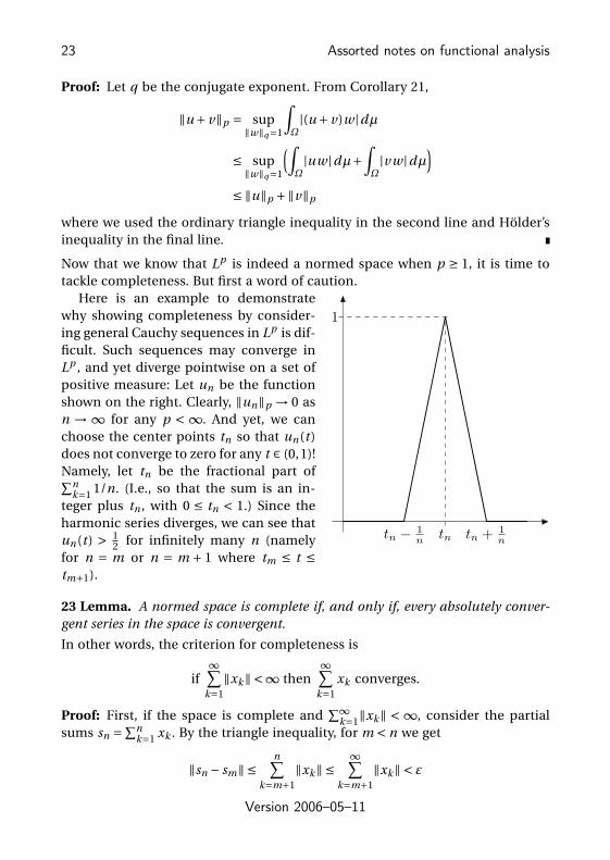
Here is an example to demonstratewhy showing completeness by consider-ing general Cauchy sequences in Lp is dif-ficult. Such sequences may converge inLp , and yet diverge pointwise on a set ofpositive measure: Let un be the functionshown on the right. Clearly, ‖un‖p → 0 asn → ∞ for any p < ∞. And yet, we canchoose the center points tn so that un (t )does not converge to zero for any t ∈ (0,1)!Namely, let tn be the fractional part of∑n

k=1 1/n. (I.e., so that the sum is an in-teger plus tn , with 0 ≤ tn < 1.) Since theharmonic series diverges, we can see thatun (t ) > 1

2 for infinitely many n (namelyfor n = m or n = m + 1 where tm ≤ t ≤tm+1).

23 Lemma. A normed space is complete if, and only if, every absolutely conver-gent series in the space is convergent.

In other words, the criterion for completeness is

if∞∑

k=1‖xk‖ <∞ then

∞∑k=1

xk converges.

Proof: First, if the space is complete and∑∞

k=1‖xk‖ < ∞, consider the partialsums sn =∑n

k=1 xk . By the triangle inequality, for m < n we get

‖sn − sm‖ ≤n∑

k=m+1‖xk‖ ≤

∞∑k=m+1

‖xk‖ < ε

Version 2006–05–11

if m is big enough, which shows that the sequence (sn )n is Cauchy and henceconvergent.

Conversely, assume that every absolutely convergent series is convergent,and consider a Cauchy sequence (un )n . Pick successively k1 < k2 < ·· · so that‖um −un‖ < 2− j whenever m,n ≥ k j . Put x1 = uk1 and x j = uk j+1 −uk j . Then

‖x j ‖ < 2− j for j ≥ 2, so∑∞

j=1 x j is absolutely convergent, and therefore con-vergent. Since uk j+1 = x1 + x2 + ·· · + x j , the sequence (uk j ) j is convergent. Wehave shown that any Cauchy sequence has a convergent subsequence, which isenough to prove completeness.

24 Proposition. Lp is complete (hence a Banach space) for 1 ≤ p ≤∞.

Proof: We first prove this for 1 ≤ p <∞. Let uk ∈ Lp ,∑∞

k=1‖uk‖p = M <∞. By theMinkowski inequality,∫

Ω

( n∑k=1

|uk |)p

dµ=∥∥∥ n∑

k=1|uk |

∥∥∥p

p≤

( n∑k=1

‖uk‖p

)p ≤( ∞∑

k=1‖uk‖p

)p = M p .

By the monotone convergence theorem,∫Ω

( ∞∑k=1

|uk |)p

dµ≤ M p

follows. Thus∑∞

k=1|uk | <∞ almost everywhere, and so∑∞

k=1 uk (t ) converges foralmost every t ∈Ω. Let the sum be s(t ).

Now let ε > 0. Repeating the above computation with the sum starting atk = m +1, we find instead∫

Ω

( ∞∑k=m+1

|uk |)p

dµ≤( ∞∑

k=m+1‖uk‖p

)p < εp

if m is big enough. But∣∣∣s(t )−m∑

k=1uk (t )

∣∣∣= ∣∣∣ ∞∑k=m+1

uk (t )∣∣∣≤ ∞∑

k=m+1|uk (t )|,

so ∥∥∥s −m∑

k=1uk

∥∥∥p≤

∥∥∥ ∞∑k=m+1

|uk |∥∥∥

p< ε

for large enough m. Thus the sum converges in Lp to the limit s.The case p =∞ is similar, but simpler: Now

∞∑k=1

|uk (t )| ≤∞∑

k=1‖uk‖∞ ≤∞

Version 2006–05–11

for almost every t ∈ Ω, so the sum∑∞

k=1 uk (t ) is absolutely convergent, henceconvergent, almost everywhere. Again let s(t ) be the sum. But now∣∣∣s(t )−

m∑k=1

uk (t )∣∣∣= ∣∣∣ ∞∑

k=m+1uk (t )

∣∣∣≤ ∞∑k=m+1

|uk (t )| ≤∞∑

k=m+1‖uk‖∞ < ε

almost everywhere when m is big enough, which implies∥∥∥s(t )−m∑

k=1uk

∥∥∥∞ ≤ ε.

This finishes the proof.

25 Lemma. Assume that µ is a finite measure. Then, if 1 ≤ p < p ′ ≤∞,

µ(Ω)−1/p‖u‖p ≤µ(Ω)−1/p ′‖u‖p ′ .

When p ′ =∞, we write 1/p ′ = 0. Apart from the adjustment by powers of µ(Ω),this roughly states that ‖·‖p is an increasing function of p . In particular, when

p 1. Let s be the exponentconjugate to r . For simplicity, assume u ≥ 0. Then

‖u‖pp =

∫Ω

up dµ=∫Ω

up ·1dµ

≤ ‖up‖r ‖1‖s =(∫Ω

ur p dµ)1/r

µ(Ω)1/s = ‖u‖pp ′µ(Ω)1/s

Raise this to the 1/pth power and note that

1

ps= 1

p

(1− 1

r

)= 1

p− 1

p ′ ,

and a simple rearrangement finishes the proof.

When the measure space Ω is the set of natural numbers 1,2,3, . . . and µ is thecounting measure, the Lp spaces become sequence spaces `p , with norms

‖x‖p =( ∞∑

k=1|xk |p

)1/p.

The Hölder and Minkowski inequalities, and completeness, for these spaces arejust special cases of the same properties for Lp spaces.

The inequalities between norms for different p get reversed however, com-pared to the case for finite measures.

Version 2006–05–11

26 Lemma. Let n ≥ 2 and a1, . . . , an be positive real numbers. Then

(ap1 +ap

2 +·· ·+apn )1/p

is a strictly decreasing function of p , for 0 < p <∞.

Proof: We prove this first for n = 2. We take the natural logarithm of (ap +bp )1/p

and differentiate:

d

d pln

((ap +bp )1/p)= d

d p

1

pln(ap +bp ) =− 1

p2ln(ap +bp )+ ap ln a +bp lnb

pap +pbp .

To show that this is negative is the same as showing that

pap ln a +pbp lnb < ap ln(ap +bp )+bp ln(ap +bp ).

But ap ln(ap +bp ) > ap ln ap = pap ln a, so the first term on the righthand side isbigger than the first term on the lefthand side. The same thing happens to thesecond terms, so we are done with the case n = 2.

The general case can be proved in the same way, or one can proceed byinduction. Consider the case n = 3: We can write

(ap +bp + cp )1/p = ([(ap +bp )1/p ]p + cp)1/p

Increasing p and pretending that the expression in square brackets is un-changed, we get a smaller value from the case n = 2. But then the square bracketalso decreases, again from the case n = 2, and so the total expression decreaseseven more. The general induction step from n to n+1 terms is similar, using the2-term case and the n-term case.

27 Proposition. For a sequence x = (xk )k , ‖x‖p is a decreasing function of p , for0 0there is a δ> 0 so that whenever x and y are vectors with ‖x‖ = ‖y‖ = 1, ‖x+y‖ >2−δ implies ‖x − y‖ < ε.

Perhaps a bit more intuitive is the following equivalent condition, which wemight call thin slices of the unit ball are small: Given ϕ ∈ X ∗ with ‖ϕ‖ = 1, definethe δ-slice Sϕ,δ = x ∈ X : ‖x‖ ≤ 1 and Reϕ(x) > 1−δ. The “thin slices” conditionstates that for each ε> 0 there is some δ> 0 so that, if ϕ ∈ X ∗ with ‖ϕ‖ = 1, then‖x − y‖ < ε for all x, y ∈ Sϕ,δ.

Version 2006–05–11

This condition follows trivially from uniform convexity. The proof of theconverse requires a minor trick: Given x, y ∈ X with ‖x‖ ≤ 1, ‖y‖ ≤ 1 and‖x + y‖ > 2−δ, invoke the Hahn–Banach theorem to pick ϕ ∈ X ∗ with ‖ϕ‖ = 1and Reϕ(x + y) > 2−δ. Then Reϕ(x) = Reϕ(x + y)−Reϕ(y) > 2−δ− 1 = 1−δ,and similarly for y . If δ was chosen according to the “thin slices” condition,‖x − y‖ < ε follows.

Our interest in uniformly convexity stems from the following result. We shallprove it later – see Theorem 68 – as it requires some results we have not coveredyet.

28 Theorem. (Milman–Pettis) A uniformly convex Banach space is reflexive.

The following lemma is a very special case of the “thin slices” condition. In thelemma after it, we shall show that the special case is sufficient for a sufficientlygeneral “thin slices” result to obtain uniform convexity of Lp .

29 Lemma. Given 1 0, there exists δ > 0 so that, for everyprobability space (Ω,ν) and every measurable function z on Ω, ‖z‖p ≤ 1 andRe

∫Ω z dν> 1−δ imply ‖z −1‖p < ε.

Proof: Consider the function

f (u) = |u|p −1+p(1−Reu)

and note that f (u) > 0 everywhere except for the value f (1) = 0. (This is thecase a = u, b = 1 in Young’s inequality.) Further, note that f (u) and |u −1|p areasymptotically equal as |u| →∞. Thus, given ε > 0, we can find some α > 1 sothat

|u −1|p ≤α f (u) whenever |u −1| ≥ ε.

Assume that z satisfies the stated conditions, and let E = ω ∈Ω : |z(ω)−1| < ε.Then

‖z −1‖pp =

∫E|z −1|p dν+

∫Ω\E

|z −1|p dν

≤ εp +α∫Ω

f (z)dν

≤ εp +pα(1−

∫Ω

Re z dν)

< εp +pαδ.

Thus picking δ= εp /(pα) is sufficient to guarantee ‖z −1‖p < 21/pε.

Version 2006–05–11

30 Lemma. Given 1 0, there exists δ > 0 so thatthe following holds: If u, w are measurable functions on a measure space Ω with‖u‖p ≤ 1 and ‖w‖q = 1 and

∫ΩReuw dµ> 1−δ, then ‖u − v‖p < ε, where v is the

function satisfying v w = |v |p = |w |q a.e.

Proof: Let p and ε be given, and choose δ as in Lemma 29.Let u, v and w be as stated above. Since nothing is changed by multiplying

u, v by a complex function of absolute value 1, and dividing w by the samefunction, we may assume without loss of generality that v ≥ 0 and w ≥ 0.

Let z = u/v where v 6= 0 and z = 0 where v = 0. Thus zv = u where v 6= 0 andzv = 0 where v = 0. Since (u − zv)zv = 0 we find ‖u‖p

p = ‖u − zv‖pp +‖zv‖p

p . Also

Re∫Ω zv w dµ= Re

∫Ωuw dµ> 1−δ, so ‖zv‖p > 1−δ, and ‖u−zv‖p

p < 1− (1−δ)p .Let ν be the probability measure

dν= v w dµ= v p dµ= w q dµ.

We find ∫Ω|z|p dν=

∫v 6=0

|u|p dµ≤ 1, Re∫Ω

z dν= Re∫Ω

uw dµ> 1−δ.

By Lemma 29, we now get

εp >∫Ω|z −1|p dν=

∫Ω|z −1|p v p dµ=

∫v 6=0

|u − v |p dµ.

On the other hand,∫v=0

|u − v |p dµ=∫Ω|(u − zv |p dµ< 1− (1−δ)p .

We therefore get ‖u − v‖pp < ε+1− (1−δ)p , and the proof is complete.

31 Theorem. (Clarkson) Lp is uniformly convex when 1 2 − δ. Let v =(x + y)/‖x + y‖p , and choose w ∈ Lq with v w = |v |p = |w |q . In particular ‖v‖p =‖w‖q = 1. Then∫

Ω(x + y)w dµ= ‖x + y‖p

∫Ω

v w dµ= ‖x + y‖p > 2−δ.

Since also Re∫Ω y w dµ ≤ 1, this implies Re

∫Ω xw dµ > 1 − δ. If δ was chosen

according to Lemma 30, we get ‖x − v‖p < ε. Similarly ‖y − v‖p < ε, and so‖x − y‖p < 2ε.

Version 2006–05–11

32 Corollary. Lp is reflexive for 1 < p <∞.

It will often be useful to know that all Lp spaces share a common dense sub-space. First, we prove a result showing that a Lp function cannot have very largevalues on sets of very large measure.

33 Lemma. (Chebyshev’s inequality) If u ∈ Lp where 1 ≤ p <∞ then

µx ∈Ω : |u(x)| ≥ ε ≤ ε−p‖u‖pp (ε> 0).

Proof: The proof is almost trivial, if we start at the righthand side:

‖u‖pp =

∫Ω|u|p dµ≥

∫E|u|p dµ≥ εpµ(E ),

where we used the fact that |u|p ≥ εp on E = x ∈Ω : |u(x)| ≥ ε. (In fact, this isone case where it seems easier to reconstruct the proof than to remember theexact inequality.)

34 Proposition. The space of functions v ∈ L∞ which vanish outside a set of finitemeasure, i.e., for which µt ∈Ω : v(t ) 6= 0 <∞, is dense in Lp whenever 1 ≤ p <∞.

We may further restrict the space to simple functions. This is an exercise inintegration theory which we leave to the reader.

Proof: Let u ∈ Lp . For a given n, define vn by

vn (t ) =

u(t ), 1/n ≤ |u(t )| ≤ n,

0 otherwise.

Then vn belongs to the space in question, thanks to Chebyshev’s inequality.Furthermore, |u − vn |p ≤ |u|p and |u − vn |p → 0 pointwise as n → ∞. It followsfrom the definition of the norm and the dominated convergence theorem that‖u − vn‖p

p → 0.

Whenever Y ⊆ X ∗ is a subset of the dual space of a normed space X , we defineits pre-annihilator as

Y⊥ = x ∈ X : f (x) = 0 for all f ∈ Y .

35 Lemma. Let X be a reflexive Banach space, and let Y ⊆ X ∗ be a closed sub-space with Y⊥ = 0. Then Y = X ∗.

Version 2006–05–11

Proof: Assume Y 6= X ∗. It is a simple consequence of the Hahn–Banach theoremthat there is a nonzero bounded functional ξ on X ∗ which vanishes on Y ; seeKreyszig Lemma 4.6-7 (page 243). (It is important for this that Y is closed.)

But X is reflexive, so there is some x ∈ X so that ξ(g ) = g (x) for all g ∈ X ∗. Butthen g (x) = ξ(g ) = 0 for all g ∈ Y , so x ∈ Y⊥ = 0. But this contradicts ξ 6= 0.

36 Corollary. If Z is a Banach space and Z∗ is reflexive, then Z is reflexive.

Proof: Apply the lemma with X = Z∗ and Y the image of Z under the canonicalmap Z → Z∗∗ = X ∗: This maps z ∈ Z to z ∈ Z∗∗ defined by z( f ) = f (z) wheref ∈ Z∗. This mapping is isometric, so the image is closed. If f ∈ Y⊥ then f (z) =z( f ) = 0 whenever z ∈ Z , so f = 0. Thus the conditions of the lemma are fulfilled.

37 Theorem. Let p and q be conjugate exponents with 1 ≤ p < ∞. Then everybounded linear functional on Lp has the form

v(u) =∫Ω

uv dµ

where v ∈ Lq .Moreover, ‖v‖ = ‖v‖q . Thus, Lq can be identified with the dual space of Lp .

This result is already known for p = 2, since L2 is a Hilbert space, and this is justthe Riesz representation theorem.

Proof: First, we note that as soon as the first part has been proved, the secondpart follows from Corollary 21.

We prove the first part for 1 < p <∞ first. Then Lp is reflexive. The space ofall functionals v on Lp , where v ∈ Lq , satifisies the conditions of Lemma 35. Thiscompletes the proof for this case.

It remains to prove the result for p = 1. We assume first that µ(Ω) < ∞. Letf ∈ (L1)∗. Since then ‖u‖1 ≤ µ(Ω)1/2‖u‖2 (Lemma 25), we find for u ∈ L2 thatu ∈ L1 as well, and | f (u)| ≤ ‖ f ‖‖u‖1 ≤ µ(Ω)1/2‖ f ‖‖u‖2. So f defines a boundedlinear functional on L2 as well, and there is some v ∈ L2 so that

f (u) =∫Ω

uv dµ (u ∈ L2).

We shall prove that v ∈ L∞. Since L2 is dense in L1, the above equality will thenextend to all u ∈ L1 by continuity, and we are done.

Version 2006–05–11

Assume now that ‖v‖∞ > M > ‖ f ‖. Then |v | ≥ M on a measurable set E withµ(E ) > 0. Let u = χE sgn v/µ(E ). Then ‖u‖1 = 1 and u ∈ L2 as well, since it isbounded. Thus

‖ f ‖ ≥ f (u) =∫Ω

uv dµ= 1

µ(E )

∫E|v |dµ≥ M ,

which is a contradiction. This finishes the proof for µ(Ω) <∞.Otherwise, if µ(Ω) = ∞ but µ is σ-finite, write Ω = E1 ∪E2 ∪ ·· · where each

E j has finite measure and all the sets E j are pairwise disjoint. Use what we justproved to find v j ∈ L∞(E j ) with f (u) = ∫

E juv dµ when u ∈ L1E j , and ‖v j ‖∞ ≤

‖ f ‖. Define v on Ω by setting v(t ) = v j (t ) when t ∈ E j . Then, for u ∈ L1,

u =∞∑

j=1uχE j

(convergent in L1), so

f (u) =∞∑

j=1f (uχE j ) =

∞∑j=1

∫E j

uv dµ=∫Ω

uv dµ.

This finishes the proof.

Version 2006–05–11

Chapter 4

A tiny bit of topology

Basic definitions

The reader is supposed to be familiar with metric spaces. To motivate the defi-nitions to come, consider a metric space (X ,d ). Note that many concepts fromthe theory of metric spaces can be formulated without reference to the metricd , so long as we know which sets are open. For example, a function f : X → Y ,where (Y ,ρ) is another metric space, is continuous if and only if1 f −1(V ) is openin X for every open V ⊆ Y , and f is continuous at a point x ∈ X if and only iff −1(V ) is a neighbourhood of x whenever V is a neighbourhood of f (x). (Here,a neighbourhood of a point is a set containing an open set containing the point.)

If you are unfamiliar with the above results, you are adviced to prove them toyour satisfaction before proceeding.

Consider the open subsets of a metric space X . They have these properties:

T1 ∅ and X are open subsets of X ,T2 the intersection of two open sets is open,T3 an arbitrary union of open sets is open.

The basic notion of topology is to take these properties as axioms. Consider anarbitrary set X . A set T of subsets of X satisfying the conditions

T1 ∅ ∈T and X ∈T ,T2 U ∩V ∈T whenever U ∈T and V ∈T ,T3 the union of the members of an arbitrary subset of T belongs to T ,

is called a topology on X . A topological space is a pair (X ,T ) where T is atopology on X . The members of T are called open sets. It is worthwhile to restatethe axioms in this language: We have seen that the open sets given by a metricform a topology. We shall call this the topology induced by the metric. Moreover,we shall call a topology (or a topological space) metrizable if there exists a metricwhich induces the given topology.

1The inverse image of V is f −1(V ) = x ∈ X : f (x) ∈ V . Despite the notation, f need not have aninverse for this definition to make sense.

32

Examples. The discrete topology on a set X is the set of all subsets of X . I.e.,every subset of X is open. This is induced by the discrete metric d , for whichd (x, y) = 1 when x 6= y (and d (x, y) = 0 when x = y of course). It follows from T3

that if x is open for all x ∈ X , then the topology is discrete.A pseudometric on a set X is a function d : X ×X →R so that

PM1 d (x, y) ≥ 0 for all x, y ∈ X ,PM2 d (x, y) = d (y, x) for all x, y ∈ X ,PM3 d (x, z) ≤ d (x, y)+d (y, z) for all x, y, z ∈ X .

In other words, it satisfies all the properties of a metric, except that we allowd (x, y) = 0 for some x 6= y . Now let D be an arbitrary set of pseudometrics onX . These induce a topology on X in a similar way that a single metric would: Asubset A ⊆ X is open in this topology if, whenever a ∈ A, there are a finite num-ber of pseudometrics d1, . . . ,dn ∈D and corresponding numbers ε1 > 0, . . . ,εn > 0so that

d1(x, a) < ε1, . . . ,dn (x, a) < εn ⇒ x ∈ A.

If D is finite, this topology is induced by the single pseudometric d1 + ·· ·+dn ,where D = d1, . . . ,dn. In fact, the same holds when D is countably infinite: IfD = d1,d2, . . ., then

d (x, y) =∞∑

n=12−n ∧dn (x, y)

defines a pseudometric on X , where ∧ selects the minimum of the numberssurrounding it. And this pseudometric induces the same topology as the entirecollection D.

The trivial topology on X consists of only the two sets ∅ and X itself. If X hasat least two distinct points, this is not metrizable. In fact, it does not even satisfythe following separation property:

A topological space X is called Hausdorff if, whenever x, y ∈ X with x 6= y , thereare open sets U and V with x ∈U , y ∈V , and U ∩V =∅.

Any metrizable space is Hausdorff: If d is a metric on X , we can let U and V bethe open ε-balls around x and y , respectively, where ε= 1

2 d (x, y).

A subset of a topological space is called closed if its complement is open. Wemight as well have stated the axioms for the closed sets:

T′1 ∅ and X are closed subsets of X ,

T′2 the union of two closed sets is closed,

T′3 an arbitrary intersection of closed sets is closed.

Version 2006–05–11


The interior of a subset A ⊆ X is the union of all open sets contained in A. It isthe largest open subset of A. The closure of A ⊆ X is the intersection of all closedsets containing A. Written A, it is the smallest closed subset of X containingA. Finally, if we are given two topologies T1 and T2 on the same set X , andT1 ⊇ T2, we say that T1 is stronger than T2, or equivalently, that T2 is weakerthan T2. Thus the trivial topology is the weakest of all topologies on a set, andthe discrete topology is the strongest.

If X is a topological space and Y ⊆ X , then we can give Y a topology con-sisting of all sets of the form Y ∩V where V ⊆ X is open in X . The resultingtopology, sometimes called the relative topology, is said to be inherited fromX . Unless otherwise stated, this is always the topology we use on subsets ofa topological space, when we wish to apply topological concepts to the sub-set itself. Beware though, of an ambiguity: When considering a subset A ⊂ Y , itmay be open in Y , yet not open in X . Consider for example X = R, Y = [0,1],A = ( 1

2 ,1] = ( 12 ,∞)∩Y . Similarly with closed subsets. So openness and closed-

ness, and derived concepts like interior points, isolated points, etc., becomerelative terms in this situation.

We round off this section with some important notions from functional analysis.Let X be a (real or complex) vector space. A seminorm on X is a function

p : X → [0,∞) which is homogeneous and subadditive. I.e., p(αx) = |α|p(x) andp(x + y) ≤ p(x)+p(y) for x, y ∈ X and every scalar α. Thus p is just like a norm,except it could happen that p(x) = 0 for some vectors x 6= 0.

From a seminorm p we can make a pseudometric d (x, y) = p(x − y). Thusfrom a collection P of seminorms on X we get a collection of pseudometrics,which induces a topology on X . This topology is said to be induced by the givenseminorms. The topology is Hausdorff if and only if for each x ∈ X with x 6= 0there is some p ∈P with p(x) 6= 0. (In this case, we say P separates points in X .)

Of particular interest is the case where P is countable; then the inducedtopology is metrizable. Moreover the associated metric, of the form

d (x, y) =∞∑

k=12−k ∧pk (x − y),

is translation invariant in the sense that d (x + z, y + z) = d (x, y).An important class of topological vector spaces is the class Fréchet spaces,

which are locally convex spaces2 whose topology can be induced by a transla-tion invariant metric which, moreover, makes the spaces complete.

For example, let X = C (R) be space of continuous functions defined on the

2For a definition, see the chapter on topological vector spaces.

Version 2006–05–11


real line, and consider the seminorms pM given by

pM (u) = sup|u(t )| : |t | ≤ M (u ∈C (R)).

This induces a topology on C (R) which is called the topology of uniform con-vergence on compact sets, for reasons that may become clear later. This spaceis a Fréchet space.

Let X be a normed vector space, and X ∗ its dual. For every f ∈ X ∗ we can cre-ate a seminorm x 7→ | f (x)| on X . The topology induced by all these seminormsis called the weak topology on X . Because each of the seminorms is continouswith respect to the norm, the weak topology is weaker than the norm topol-ogy on X . (The norm topology is the one induced by the metric given by thenorm.) In fact, the weak topology is the weakest topology for which each f ∈ X ∗is continuous.

Similarly, each x ∈ X defines a seminorm f 7→ | f (x)| on X ∗. These togetherinduce the weak∗ topology on X ∗. X ∗ also has a weak topology, which comesfrom pseudometrics defined by members of X ∗∗. Since these include the former,the weak topology is stronger than the weak∗ topology, and both are weaker thanthe norm topology.

Neighbourhoods, filters, and convergence

Let X be a topological space. A neighbourhood of a point x ∈ X is a subset ofX containing an open subset which in it turn contains x. More precisely, N is aneighbourhood of x if there is an open set V with x ∈V ⊆ N ⊆ X .

If F is the set of all neighbourhoods of x, then

F1 ∅ ∉F and X ∈F ,F2 if A,B ∈F then A∩B ∈F ,F3 if A ∈F and A ⊆ B ⊆ X then B ∈F .

Whenever F is a set of subsets of X satisfying F1–F3, we call F a filter. In par-ticular, the set of all neighbourhoods of a point x ∈ X is a filter, which we callthe neighbourhood filter at x, and write N (x).

If x is an open set, we call the point x isolated. If x is not isolated, then, anyneighbourhood of x contains at least one point different from x. Let us definea punctured neighbourhood of x as a set U so that U ∪ x is a neighbourhoodof x (whether or not x ∈U ). The set of all punctured neighbourhoods of a non-isolated point x forms a filter N ′(x), called the punctured neighbourhood filterof x.

We may read F3 as saying that if we know the small sets in a given filter, weknow the whole filter. In other words, the only interesting aspect of a filter is its

Version 2006–05–11


small members. More precisely, we shall call a subset B ⊆F a base for the filterF if every member of F contains some member of B. In this case, wheneverF ⊆ X ,

F ∈F ⇔ B ⊆ F for some B ∈B. (4.1)

You may also verify these properties:

FB1 ∅ ∉B but B 6=∅,FB2 if A,B ∈B then C ⊆ A∩B for some C ∈B.

Any set of subsets of X satisfying these two requirements is called a filter base.When B is a filter base, (4.1) defines a filter F , which we shall call the filtergenerated by B. Then B is a base for the filter generated by B.

The above would seem like a lot of unnecessary abstraction, if neighbour-hood filters were all we are interested in. However, filters generalize anotherconcept, namely that of a sequence. Recall that the convergence, or not, of asequence in a metric space only depends on what happens at the end of the se-quence: You can throw away any initial segment of the sequence without chang-ing its convergence properties. (But still, if you throw all initial segments away,nothing is left, so there is nothing that might converge.) Let (xk )∞k=1 be a se-

quence in X . We call any set of the form xk : k ≥ n a tail of the sequence.3 Theset of tails of the sequence is a filter base. If X is a metric space then xn → x ifand only if every neighbourhood of x contains some tail of the sequence. Butthat means that every neighbourhood belongs to the filter generated by the tailsof the sequence. This motivates the following definition.

A filter F1 is said to be finer than another filter F2 if F1 ⊇F2. We also say thatF1 is a refinement of F2. This corresponds to the notion of subsequence: Thetails of a subsequence generate a finer filter than those of the original sequence.

A filter F on a topological space X is said to converge to x ∈ X , written F → x,if F is finer than the neighbourhood filter N (x). In other words, every neigh-bourhood of x belongs to F .4 We shall call x a limit of F (there may be several).A filter which converges to some point is called convergent. Otherwise, it is calleddivergent .

If X has the trivial topology, every filter on X converges to every point in X .This is clearly not very interesting. But if X is Hausdorff, no filter can convergeto more than one point. In this case, if the filter F converges to x, we shall callx the limit of F , and write x = limF .

3Beware that in other contexts, one may prefer to use the word tail for the indexed family (xk )∞k=nrather than just the set of values beyond the nth item in the list.

4This would look more familiar if it were phrased “every neighbourhood of x contains a memberof F ”. But thanks to F3, we can express this more simply as in the text.

Version 2006–05–11

We shall say that a sequence (xk ) converges to x if, for every neighbourhoodU of x, there is some n so that xk ∈U whenever k ≥ n. This familiar soundingdefinition is equivalent to the statement that the filter generated by the tails ofthe sequence converges to x.

We shall present an example showing that sequence convergence is insuffi-cient.5 But first a definition and a lemma: A filter F on X is said to be in a subsetA ⊆ X if A ∈F . (Recall that filters only express what is in their smaller elements;thus, this says that all the interesting “action” of F happens within A.)

38 Lemma. Let A be a subset of a topological space X . Then, for x ∈ X , we havex ∈ A if and only if there is a filter in A converging to x.

Proof: Assume x ∈ A. Then any neighbourhood of x meets A,6 for otherwise xhas an open neighbourhood U disjoint from A, and then X \U is a closed setcontaining A, so A ⊆ X \U . But x ∈U , so this contradicts x ∈ A. Now all the setsA∩U where U is a neighbourhood of x form a filter base, and the correspondingfilter converges to x.

Conversely, assume F is a filter in A converging to x. Pick any neighbourhoodU of x. Then U ∈F . Thus U ∩ A 6=∅, since A ∈F as well. This proves that x ∈ A.

We are now ready for the example, which will show that we cannot replace filtersby sequences in the above result. Let Ω be any uncountable set, and let X be theset of all families (xω)ω∈Ω, where each component xω is a real number. In fact,X is a real vector space. For each ω we consider the seminorm x 7→ |xω|. We nowuse the topology on X induced by all these seminorms.7

Let

Z = x ∈ X : |xω| 6= 0 for at most a finite number of ω,

e ∈ X , eω = 1 for all ω ∈Ω.

Then e ∈ Z , but there is no sequence in Z converging to e.In fact, for every neighbourhood U of e there are ω1, . . . ,ωn ∈Ω and ε > 0 so

that|xωk −1| < ε for k = 1, . . . ,n ⇒ x ∈U .

But then we find x ∈ Z ∩U if we put xωk = 1 for k = 1, . . . ,n and xω = 0 for allother ω. Thus e ∈ Z .

5Insufficient for what, you ask? In the theory of metric spaces, sequences and their limits areeverywhere. But they cannot serve the corresponding role in general topology.

6We say that two sets meet if they have a nonempty intersection.7This is called the topology of pointwise convergence.

Version 2006–05–11


Furthermore, if (xn )∞n=1 is a sequence in Z then for each n (writing xnω for theω-component of xn ) we have xnω 6= 0 for only a finite number of ω. Thus xnω 6= 0for only a countable number of pairs (n,ω). Since Ω is not countable, there is atleast one ω ∈Ω with xnω = 0 for all n. Fix such an ω. Now U = z ∈ X : |zω| > 0is a neighbourhood of e, and xn ∉U for all n. Thus the sequence (xn ) does notconverge to e.

A historical note. The theory of filters and the associated notion of convergence wasintroduced by Cartan and publicized by Bourbaki. An alternative notion is to generalizethe sequence concept by replacing the index set 1,2,3, . . . by a partially ordered set Awith the property that whenever a,b ∈ A there is some c ∈ A with c Â a and c Â b. A familyindexed by such a partially ordered set is called a net. The theory of convergence basedon nets is called the Moore–Smith theory of convergence after its inventors. Its advantageis that nets seem very similar to sequences. However, the filter theory is much closer tobeing precisely what is needed for the job, particularly when we get to ultrafilters in ashort while.

Continuity and filters

Assume now that X is a set and Y is a topological space, and let f : X → Y bea function. We say that f (x) → y as x → F if, for each neighbourhood V of y ,there is some F ∈F so that x ∈ F ⇒ f (x) ∈V .

The implication x ∈ F ⇒ f (x) ∈ V is the same as F ⊆ f −1(V ), so we find thatf (x) → y as x →F if and only if f −1(V ) ∈F for every V ∈N (y).

We can formalize this by defining a filter f∗F on Y by the prescription8

B ∈ f∗F ⇔ f −1(B ) ∈F ,

so that f (x) → y as x →F if and only if f∗F → y . We also use the notation

y = limx→F

f (x),

but only when the limit is unique, for example when Y is Hausdorff.Think of the notation x →F as saying that x moves into progressively smaller

members of F . The above definition says that, for every neighbourhood V ofy , we can guarantee that f (x) ∈ V merely by choosing a member F ∈ F andinsisting that x ∈ F .

Examples. Let F be the filter on the set N of natural numbers generated by the filter baseconsisting of the sets n,n +1, . . . where n ∈ N. Let (z1, z2, . . .) be a sequence in Y . Thenzn → y as n →∞ if and only if zn → y as n →F .

8It is customary to write f∗S for some structure S which is transported in the same direction asthe mapping f , as opposed to f ∗S for those that are mapped in the opposite direction. An exampleof the latter kind is the adjoint of a bounded operator.

Version 2006–05–11

Next, consider a function ϕ on an interval [a,b]. Let X consist of all sequences

a = x0 ≤ x∗1 ≤ x1 ≤ x∗

2 ≤ x2 ≤ ·· · ≤ xn−1 ≤ x∗n ≤ xn = b

and consider the filter F on X generated by the filter base consisting of all the sets

x ∈ X : |xk −xk−1| < ε for k = 1, . . . ,n

where ε> 0. Let f : X →R be defined by the Riemann sum

f (x) =n∑

k=1ϕ(x∗

k ) (xk −xk−1).

Then the existence and definition of the Riemann integral of ϕ over [a,b] is stated by theequation ∫ b

aϕ(t )d t = lim

x→Ff (x).

Let us return now to the notion of convergence. If X is a topological space andw ∈ X , we can replace F by the punctured neighbourhood filter N ′(x). Thus wesay f (x) → y as x → w if, for every neighbourhood V of y there is a puncturedneighbourhood U of w so that f (x) ∈ V whenever x ∈ U . This is the same assaying f (x) → y when x →N ′(x).

The function f is said to be continuous at w ∈ X if either w is isolated, or elsef (x) → f (w) as x → w .

In this particular case, though, it is not necessary to avoid the point w in thedefinition of limit, so we might just as well define continuity as meaning: f −1(V )is a neighbourhood of x whenever V is a neighbourhood of f (x).

We can also define continuity over all: f : X → Y is called continuous if f −1(V )is open in X for every open set V ⊆ Y . This is in fact equivalent to f beingcontinuous at every point in X . (Exercise: Prove this!)

Compactness and ultrafilters

A topological space X is called compact if every open cover of X has a finitesubcover.

What do these terms mean? A cover of X is a collection of subsets of X whichcovers X , in the sense that the union of its members is all of X . The cover ifcalled open if it consists of open sets. A finite subcover is then a finite subsetwhich still covers X .

By taking complements, we get this equivalent definition of compactness:X is compact if and only if every set of closed subsets of X , with the finite

intersection property, has nonempty intersection.

Version 2006–05–11


Here, the finite intersection property of a set of subsets of X means that everyfinite subset has nonempty intersection. So what the definition says, in moredetail, is this: Assume C is a set of closed subsets of X . Assume that C1∩. . .∩Cn 6=∅ whenever C1, . . . ,Cn ∈ C . Then

⋂C 6= ∅ (where

⋂C is the intersection of all

the members of C , perhaps more commonly (but reduntantly) written⋂

C∈C C ).The translation between the two definitions goes as follows: Let C be a set of

closed sets and U = X \ C : C ∈ C . Then U covers X if and only if C does nothave nonempty intersection, and U has a finite subcover if and only if C doesnot have the finite intersection property.

One reason why compactness is so useful, is the following result.

39 Theorem. A topological space X is compact if and only if every filter on X hasa convergent refinement.

In order to prove this, we shall detour through the notion of ultrafilters. Manyarguments using compactness in metric spaces require some form of diagonalargument, selecting subsequences of subsequences and finally using the diag-onal to get a sequence which is eventually a subsequence of any of the formersubsequences. The theory of filters neatly sidesteps these arguments by passingto an ultrafilter, which is sort of the ultimate subsequence.

A filter U is called an ultrafilter if, for every A ⊆ X , either A ∈U or X \ A ∈U .The filter U is an ultrafilter if, and only if, there does not exist any strictly

finer filter.Indeed, if F is a filter but not an ultrafilter, and A ⊆ X with A ∉F and X \ A ∉

F , then A ∩B 6= ∅ whenever B ∈ F . For, if A ∩B = ∅ then B ⊆ X \ A, and soX \ A ∈ F . It follows that all the sets A ∩B where B ∈ F form a filter base fora filter that is strictly finer than F . We leave the (easy) converse proof to thereader.

40 Lemma. (Ultrafilter lemma) For every filter there is at least one finer ultra-filter.

Proof: The proof is by appeal to Zorn’s lemma: Given a set of filters totally or-dered by inclusion, the union of all these filters is again a filter. This filter is, ofcourse, finer than any of the original filters. Thus the set of filters finer than onegiven filter is inductively ordered. Then Zorn’s lemma takes care of the rest.

41 Theorem. A topological space X is compact if and only if every ultrafilter onX is convergent.

Version 2006–05–11


Proof: First, assume that every ultrafilter on X is convergent, let C be a setof closed subsets of X , and assume that C has the finite intersection property.Then the set B of all finite intersections of sets in C , i.e.

B = C1 ∩ . . .∩Cn : C1, . . . ,Cn ∈C ,

is a filter base. It generates a filter F , which has an ultrafilter refinement U

according to the ultrafilter lemma. Let x be a limit of U .Now for any C ∈C , if x ∉C then X \C is a neighbourhood of x. Thus X \C ∈U ,

since U converges to x. But C ∈ U as well, and this is a contradiction, since(X \C )∩C =∅. Thus x ∈C for every C ∈C . We have proved that C has nonemptyintersection. Thus X is compact.

Conversely, assume that X is compact, and let U be an ultrafilter on X . LetC = U : U ∈U . By definition, C consists of closed sets, and it obviously inheritsthe finite intersection property from U . Since X is compact, there is a point xin the intersection of C .

To show that U converges to x, let V be an open neighbourhood of x. If V ∉U

then X \ V ∈ U , since U is an ultrafilter. But X \ V is closed, so then X \ V ∈ C ,by construction. But since x ∉ X \V , this contradicts the choice of x. Thus everyopen neighbourhood of x belongs to U , and so U converges to x.

Proof of Theorem 39: First, assume that X is compact, and let F be a filter onX . Let U be an ultrafilter refining F . By Theorem 41, U is convergent. Thus F

has a convergent refinement.Conversely, assume that every filter on X has a convergent refinement. Then

any ultrafilter U on X must be convergent, for it has no proper refinement, sothe convergent refinement of U which exists by assumption must be U itself.Thus every ultrafilter on X is convergent, so X is compact by Theorem 41.

42 Proposition. A continuous image of a compact space is compact.

Proof: Let X and Y be topological spaces, with X compact. Assume f : X → Yis continuous and maps X onto Y . We shall show that then Y is compact.

Let C be an open cover of Y . Then f −1(C ) : C ∈ C is an open cover ofX , since f is continuous. Because X is compact, there is a finite subcover f −1(C1), . . . , f −1(Cn ) of X . And then C1, . . . ,Cn covers Y since f is onto.

A similar proof using families of closed sets with the finite intersection propertyis just as easy to put together.

Version 2006–05–11


Product spaces and Tychonov’s theorem

Let X j be a topological space for every j ∈ J , where J is some index set. Thedirect product

∏j∈J X j consists of all families (x j ) j∈J with x j ∈ X j for each j ∈ J .

From now on, we will often simply write X for the product.It is often useful to consider the projection map π j : X → X j given by π j (x) =

x j , where j ∈ J and x ∈ X .We can define a topology on X as the weakest topology that makes every

projection map π j continuous: First, for each j ∈ J , let

T j = π−1j (U ) : U ⊆ X j is open.

Then T j is a topology on X . Next, let

S = U j1 ∩ . . .∩U jn : jk ∈ J , U jk ∈T jk for k = 1, . . . ,n

(the set of all finite intersections from different T j ). Finally, let T consist of allunions of sets from S . It is clear that any topology on X which makes each π j

continuous must contain T . But T is in fact a topology, so it is, as claimed,the weakest of all topologies on X making each π j continuous. We call this theproduct topology on X .

43 Lemma. Let F be a filter on∏

j∈J X j . Then F converges to x ∈∏j∈J X j if and

only ifz j → x j as z →F for all j ∈ J .

Proof: First, assume that F converges to x. That z j → x j when z →F is merelya consequence of the continuity of π j .

Conversely, assume that z j → x j when z → F for each j . Consider a neigh-bourhood U of x. By the definition of the product topology, there are indexesj1, . . . , jn and neighbourhoods U jk of x jk in X jk so that

z jk ∈U jk for k = 1, . . .n ⇒ z ∈U .

But by assumption, z : z jk ∈U jk ∈F for each k , so

n⋂k=1

z : z jk ∈U jk ∈F .

But the set on the lefthand side is a subset of U , so U ∈ F . This proves that F

converges to x.

44 Theorem. (Tychonov) Any product of compact spaces is compact.

Version 2006–05–11

Proof: Keep the notation used earlier in this section. Let U be an ultrafilter onX . Then (π j )∗(U ) is an ultrafilter on X j for each j . (For if A ⊆ X j , then eitherπ−1

j (A) or its complement π−1j (X j \ A) belongs to U , so either A or X j \ A belongs

to (π j )∗(U ).) But then, since X j is compact, (π j )∗(U ) has a limit9 x j ∈ X j . Inother words, z j → x j as z →F .

Put all these limits x j together into the single element x = (x j ) j∈J of X . By theprevious lemma, U converges to x, so our proof is complete.

Normal spaces and the existence of real continous functions

A topological space X is called normal if any two disjoint closed sets A, B canbe separated by open sets, in the sense that there are open sets U ⊃ A and V ⊃ Bwith U ∩V =∅.

We are interested in normal spaces because one can find a large number ofcontinuous real functions on these spaces.

A neighbourhood of a set A is a set containing an open set which contains A.In other words, a set whose interior contains A.

An equivalent way to state that X is normal, is to say that if A ⊂ X is closed,then any neighbourhood of A, contains a closed neighbourhood of A. (If W isan open neighbourhood of A, let B = X \ W , find disjoint open neighbourhoodsU ⊃ A and V ⊃ B , then U is a closed neighbourhood of A contained in W .)

45 Theorem. (Urysohn’s lemma) Let X be a normal topological space. Let A1 ⊆X be a closed set, and A0 a neighbourhood of A1. Then there exists a continousfunction u : X → [0,1] with u(x) = 1 for x ∈ A1, and u(x) = 0 for x ∉ A0.

Proof: Imagine that we have created sets At for all t in a dense subset T of [0,1],so that A0 and A1 are the sets initially given, and As is a closed neighbourhoodof At whenever s < t . Then define

u(x) =

1, x ∈ A1,

0, x ∉ A0,

supt ∈ T : x ∈ At otherwise.

To prove that u is continuous, pick a point w ∈ X and let v = u(w). If 0 < v < 1,and ε> 0, pick s, t ∈ T with v −ε< s < v < t < v +ε. Now | f (x)−v | < ε whenever x

9If X j is not Hausdorff, it may have several limits, so we need the axiom of choice to pick one ofthem. But this remark is not really important, as the use of ultrafilters relies heavily on the axiom ofchoice anyway.

Version 2006–05–11


is in the neighbourhood As \ At of w . This argument works with trivial changesfor t = 0 and t = 1. Thus continuity follows.

To create the sets At , let T be the set of dyadic rational numbers in [0,1], i.e.,the numbers that can be written 2−k j where j and k are integers. We create setsA2−k j by induction on k .

We make A1/2 first: It shall be a closed neighbourhood of A1 which is con-tained in the interior of A0 (so A0 is itself a neighbourhood of A1/2).

Next, let A1/4 be a closed neighbourhood of A1/2 having A0 as a neighbour-hood. Then let A3/4 be a closed neighbourhood of A1 having A1/2 as a neigh-bourhood.

Next, put A1/8, A3/8, A5/8, A7/8 between A0, A1/4, A1/2, A3/4, A1, in the sameway.

After each A2−k j has been made for a given k , we create the sets A2−k−1 j (forodd j ) in the same manner.

Compact Hausdorff spaces are of special interest, because they occur so often.

46 Proposition. Any compact Hausdorff space is normal.

Proof: Let A and B be two closed subsets of a compact Hausdorff space X .First, we show that we can separate A from any point outside A, in the sense

that whenever y ∉ A, we can find neighbourhoods U of A and V of y with U∩V =∅. Consider the set of all open U with y ∉U . Because X is Hausdorff and y ∉ A,these sets cover A. But A, being a closed subset of a compact space, is compact,so a finite number of these open sets can be found cover A. Say A ⊂U1∪ . . .∪Un

with Uk open and y ∉ Uk . Then U1 ∪ . . .∪Un is a neighbourhood of A whoseclosure U1 ∪ . . .∪Un does not contain y , and from this our first claim follows.

Second, we repeat the above argument with a twist: Consider all of open setsU with U ∩ A = ∅. From what we proved in the previous paragraph, these setscover B . So a finite number of them cover B , and we finish the proof in a waysimilar to the end of the previous paragraph. (Exercise: Fill in the details.)

The Weierstrass density theorem

Bernshteın10 polynomials are ordinary polynomials written on the particularform

b(t ) =n∑

k=0βk

(n

k

)t k (1− t )n−k , (4.2)

10Named after Sergeı Natanovich Bernshteın (1880–1968). The name is often spelled “Bernstein”.

Version 2006–05–11


where β0, . . . ,βn are given coefficients.11 The special case where each βk = 1deserves mention: Then the binomial theorem yields

n∑k=0

(n

k

)t k (1− t )n−k = (

t + (1− t ))n = 1. (4.3)

We can show by induction on n that if b = 0 then all the coefficients βn are zero.The base case n = 0 is obvious. When n > 0, a little bit of binomial coefficientgymnastics shows that the derivative of a Bernshteın polynomial can be writtenas another Bernshteın polynomial:

b′(t ) = nn−1∑k=0

(βk+1 −βk )

(n −1

k

)t k (1− t )n−1−k .

In particular, if b = 0 it follows by the induction hypothesis that all βk are equal,and then they are all zero, by (4.3).

In other words, the polynomials t k (1− t )n−k , where k = 0, . . . ,n, are linearlyindependent, and hence they span the n +1-dimensional space of polynomialsof degree ≤ 1. Thus all polynomials can be written as Bernshteın polynomials, sothere is nothing special about these – only about the way we write them.

To understand why Bernshteın polynomials are so useful, consider the indi-vidual polynomials

bk,n (t ) =(

n

k

)t k (1− t )n−k , k = 0, . . . ,n. (4.4)

If we fix n and t , we see that bk,n (t ) is the probability of k heads in n tosses of abiased coin, where the probability of a head is t . The expected number of headsin such an experiment is nt , and indeed when n is large, the outcome is verylikely to be near that value. In other words, most of the contributions to the sumin (4.2) come from k near nt . Rather than using statistical reasoning, however,we shall proceed by direct calculation – but the probability argument is still auseful guide.

47 Theorem. (Weierstrass) The polynomials are dense in C [0,1].

This will follow immediately from the following lemma.

48 Lemma. Let f ∈C [0,1]. Let bn be the Bernshteın polynomial

bn (t ) =n∑

k=0f( k

n

)(n

k

)t k (1− t )n−k .

11When n = 3, we get a cubic spline. In this case, β0, β1, β2 and β3 are called the control points ofthe spline. In applications, they are usually 2- or 3-dimensional vectors.

Version 2006–05–11

Then ‖ f −bn‖∞ → 0 as n →∞.

Proof: Let t ∈ [0,1]. With the help of (4.3) we can write

f (t )−bn (t ) =n∑

k=0

(f (t )− f

( k

n

))(n

k

)t k (1− t )n−k ,

so that

| f (t )−bn (t )| ≤n∑

k=0

∣∣∣ f (t )− f( k

n

)∣∣∣(n

k

)t k (1− t )n−k , (4.5)

We now use the fact that f is uniformly continuous: Let ε> 0 be given. There isthen a δ> 0 so that | f (t )− f (s)| < ε whenever |t − s| < δ. We now split the abovesum into two parts, first noting that

∑|k−nt |<nδ

∣∣∣ f (t )− f( k

n

)∣∣∣(n

k

)t k (1− t )n−k ≤ ε (4.6)

(where we used | f (t )− f (k/n)| < ε, and then expanded the sum to all indexesfrom 0 to n and used (4.3)). To estimate the remainder, let M = ‖ f ‖∞, so that

∑|k−nt |≥nδ

∣∣∣ f (t )− f( k

n

)∣∣∣(n

k

)t k (1− t )n−k ≤ 2M

∑|k−nt |≥nδ

(n

k

)t k (1− t )n−k . (4.7)

To finish the proof, we need to borrow from the Chebyshev inequality in orderto show that the latter sum can be made small. First we find

n∑k=0

k

(n

k

)t k (1− t )n−k = nt

n−1∑k=0

(n −1

k

)t k (1− t )n−1−k = nt . (4.8)

(Rewrite the binomial coefficient using factorials, perform the obvious cancel-lation using k/k ! = 1/(k − 1)!, put nt outside the sum, change the summationindex, and use (4.3).) Next, using similar methods,

n∑k=0

k(k −1)

(n

k

)t k (1− t )n−k = n(n −1)t 2

n−2∑k=0

(n −2

k

)t k (1− t )n−2−k = n(n −1)t 2.

Adding these two together, we get

n∑k=0

k2

(n

k

)t k (1− t )n−k = nt

((n −1)t +1

). (4.9)

Version 2006–05–11

Finally, using (4.3), (4.8) and (4.9), we find

n∑k=0

(nt −k)2

(n

k

)t k (1− t )n−k = (nt )2 −2(nt )2 +nt

((n −1)t +1

)= nt (1− t ).

The most important feature here is that the n2 terms cancel out. We now have

nt (1− t ) ≥ ∑|k−nt |≥nδ

(nt −k)2

(n

k

)t k (1− t )n−k

≥ (nδ)2∑

|k−nt |≥nδ

(n

k

)t k (1− t )n−k ,

so that ∑|k−nt |≥nδ

(n

k

)t k (1− t )n−k ≤ t (1− t )

nδ2≤ 1

4nδ2. (4.10)

Combining (4.5), (4.6), (4.7) and (4.10), we end up with

| f (t )−bn (t )| < ε+ M

2nδ2, (4.11)

which can be made less than 2ε by choosing n large enough. More importantly,this estimate is independent of t ∈ [0,1].

One final remark: There is of course nothing magical about the interval [0,1].Any closed and bounded interval will do. If f ∈ C [a,b] then t 7→ f

((1− t )a + tb

)belongs to C [0,1], and this operation maps polynomials to polynomials and pre-serves the norm. So the Weierstrass theorem works equally well on C [a,b]. Infact, it works on C (K ) where K is any compact subset of the real line: For anyf ∈C (K ) can be expanded to a continuous function on the smallest interval con-taining K by linearly interpolating the function in each bounded open intervalin the complement of K .

The Stone–Weierstrass theorem is a bit more difficult: It replaces [0,1] by any compactHausdorff space X and the polynomials by any algebra of functions which separatespoints in X and has no common zero in X . (This theorem assumes real functions. If youwork with complex functions, the algebra must also be closed under conjugation. But thecomplex version of the theorem is not much more than an obvious translation of the thereal version into the complex domain.) One proof of the general Stone–Weierstrass theo-rem builds on the Weierstrass theorem. More precisely, the proof needs an approximationof the absolute value |t | by polynomials in t , uniformly for t in a bounded interval.

Version 2006–05–11

An amusing (?) diversion. Any old textbook on elementary statistics shows pictures ofthe binomial distribution, i.e., bk,n (t ) for a given n and t ; see (4.4). But it can be interest-ing to look at this from a different angle, and consider each term as a function of t . Hereis a picture of all these polynomials, for n = 20:

0

0.2

0.4

0.6

0.8

1

0.2 0.4 0.6 0.8 1

t

We may note that bk,n (t ) has its maximum at t = k/n, and∫ 1

0 bk,n (t )d t = 1/(n + 1). Infact, (n + 1)bk,n is the probability density of a beta-distributed random variable withparameters (k +1,n−k +1). Such variables have standard deviation varying between ap-proximately 1/(2

pn) (near the center, i.e., for k ≈ n/2) and 1/n (near the edges). Compare

this with the distance 1/n between the sample points.It is tempting to conclude that polynomials of degree n can only do a good job of

approximating a function which varies on a length scale of 1/p

n.We can see this, for example, if we wish to estimate a Lipschitz continuous function

f , say with | f (t )− f (s)| ≤ L|t − s|. Put ε= Lδ in (4.11) and then determine the δ that givesthe best estimate in (4.11), to arrive at | f (t )−bn (t )| < 3

2 M 1/3(L2/n)2/3. So the n required

for a given accuracy is proportional to L2, in accordance with the analysis in the previoustwo paragraphs.

Reference: S. N. Bernshteın: A demonstration of the Weierstrass theorem based on thetheory of probability. The Mathematical Scientist 29, 127–128 (2004).

By an amazing coincidence, this translation of Bernshteın’s original paper from 1912appeared recently. I discovered it after writing the current note.

Version 2006–05–11

Chapter 5

Topological vector spaces

Definitions and basic propertiesA topological vector space is a (real or complex) vector space equipped with a Hausdorfftopology, so that the vector space operations are continuous. That is, if the space is calledX then vector addition is a continuous map X × X → X , and multiplication by scalars isa continuous map C×X → X (or R×X → X ).

One simple and common way to define a topological vector space, is by starting witha vector space X and a family P of seminorms on X , separating the points of X . (Fordetails see the preceding chapter.) The topology generated by P does in fact make X atopological vector space. (Exercise: Prove this.)

It is useful to note that the topology of a topological vector space is completely spec-ified by the neighbourhoods of 0. For addition by any constant x is continuous with acontinuous inverse (addition by −x), so the neighbourhoods of x are the sets of the formx +U where U is a neighbourhood of 0.

A topological vector space is called locally convex if every neighourhood of 0 containsa convex neighbourhood of 0. If the topology is generated by a family of seminorms, thespace is locally convex, since every neighbourhood of 0 contains a neighbourhood of theform

x ∈ X : p j (x) < ε, j = 1, . . . ,n (p1, . . . , pn ∈P ),

which is clearly convex.Examples include the weak topology on a normed space X , and the weak∗ topology

on its dual.

In fact, the topology of any locally convex space is generated by seminorms. For anyneighbourhood of 0 contains a neighbourhood U that is not only convex but balanced,in the sense that αx ∈U whenever x ∈U and α is a scalar with |α| = 1. For such a neigh-bourhood U we can create a seminorm p by

p(x) = inf t > 0 : x/t ∈U ,

and the set of all such seminorms generate the topology. (p is a seminorm because thesupremum may in fact be infinite, so that p(x) = 0 for some x.) Since we shall not needthis result, we omit the proof. (But proving it could be a useful exercise.)

We already know that bounded linear functionals on a Banach space are continuous.Below is the corresponding result for topological vector spaces.

49

49 Proposition. For a linear functional f on a topological vector space X , the followingare equivalent:

1. f is continous,2. Re f is continous,3. Re f is bounded below or above on some nonempty open set,

Proof: That 1 ⇒ 2 is obvious.2 ⇒ 1: In the case of real scalars, there is nothing to prove. In the case of complex

scalars, use the identity f (x) = Re f (x)− i Re f (i x).2 ⇒ 3: If Re f is continuous then Re f is bounded on the nonempty open set x ∈

X : |Re f (x)| < 1, which implies the third condition.3 =⇒ 2: Finally, if Re f is bounded below on some nonempty open set, say Re f > a

on U , let u ∈ U . Then Re f is bounded below on the neighbourhood U −u of 0, andabove on the neighbourhood u −U of 0. Hence Re f is bounded on a neighbourhoodV = (U −u)∩ (u −U ) of 0.

For simplicity, say |Re f (x)| ≤ M for x ∈ V . Given ε > 0, then |Re f (y)−Re f (x)| < ε onthe neighbourhood x + (ε/M )V of x.

For a linear functional f on X , we define the kernel of f to be

ker f = x ∈ X : f (x) = 0.

50 Proposition. A linear functional on a locally convex topological vector space is con-tinuous if and only if its kernel is closed.

Proof: If f is continuous, then ker f = f −1(0) is closed, since 0 is closed.Next, assume that ker f is closed. If f = 0, then f is continuous. Assume therefore

f 6= 0. Pick w ∈ X with f (w) = 1. Since ker f is closed, f is nonzero on a neighbourhoodW of w . Since X is locally convex, W can be taken to be convex. If X is a real space, wemust have f |W > 0, so f is bounded below on W , and f must be continuous.

If X is a complex space, we note that f (x) : x ∈ W is a convex subset of C whichdoes not contain 0. Then that set lies in some halfplane, meaning that there is some realnumber θ with Re(eiθ f (x)) ≥ 0 for all x ∈W . But then Re(eiθ f ) is bounded below on W ,so eiθ f is continuous. But then so is f .

51 Proposition. Let X be a normed vector space. A linear functional on X∗ is of the formf 7→ f (x) where x ∈ X if and only if it is weakly∗ continuous.

Proof: The functionals f 7→ f (x) are weakly∗ continuous by the construction of theweak∗ topology on X∗.

So we only need to consider a weakly∗ continuous functional ξ on X∗, and must showit can be written f 7→ f (x).

By the construction of the weak∗ topology, there are x1, . . . , xn ∈ X and δ > 0 with|ξ( f )| < 1 whenever | f (xk )| < δ for k = 1, . . . ,n. In particular,

ξ( f ) = 0 whenever(

f (x1), . . . , f (xn ))= (0, . . . ,0)

Version 2006–05–11

(for then |ξ(t f )| < 1 for all t ).It follows that we can define a linear functional ζ on Rn by setting

ζ(

f (x1), . . . , f (xn ))= ξ( f ), f ∈ X∗.

This is well defined, for if(

f (x1), . . . , f (xn )) = (

g (x1), . . . , g (xn ))

then ξ( f − g ) = 0 by theabove. Strictly speaking, this may define ζ only on a subspace of Rn , but the functionalcan be extended to all of Rn . Write ζ(y) = c1 y1 +·· ·+cn yn . Then

ξ( f ) = c1 f (x1)+·· ·+cn f (xn ) = f (x), where x = c1x1 +·· ·+cn xn .

This completes the proof.

The weak topology on a Banach space truly is weaker than the norm topology, at least ifthe space is infinite-dimensional. For any weak neighbourhood of 0 will contain a set ofthe form x : | fk (x)| < ε, k = 1, . . . ,n where fk ∈ X∗. In particular, it contains x : | fk (x)| =0, k = 1, . . . ,n, which is an infinite-dimensional space.

A word on notation: It is common to write* for weak convergence and∗* for weak∗

convergence. In the case of reflexive Banach spaces, such as Hilbert spaces and Lp spacesfor 1 < p <∞, there is of course no essential difference, and the notation * is generallypreferred.

In a weaker topology, convergence is easier to achieve because there are fewer neigh-bourhoods. Here is a simple example. Let 1 < p ≤ ∞ and let ek ∈ `p be the sequencewhich has 1 at position k and 0 at all other positions. Then, because ‖e j − ek‖p = 21/p

when j 6= k , the sequence (ek )∞k=1 is not Cauchy, and therefore not convergent in norm.But still, ek * 0 (weakly) as k →∞, because whenever x ∈ `q with 1 ≤ q <∞ then xk → 0.

In some important cases, however, weak convergence with an added condition doesimply norm convergence. Recall that Lp spaces are uniformly convex for 1 < p <∞. Inthe existence theory of partial differential equations, one commonly proves weak conver-gence of approximate solutions in some Lp space, and one then needs norm convergenceto complete the existence proof. The following result is useful in such situations.

52 Proposition. Let X be a uniformly convex normed space, and let (xk )∞k=1 be a weaklyconvergent sequence in X with weak limit x. Then xk → x (in norm) if and only if ‖xk‖→‖x‖.

Proof: If xk → x in norm then ‖xk‖ → ‖x‖. We need to prove the converse. If x = 0, theconverse is nothing but the definition of norm convergence. So we may assume thatx 6= 0, and (dividing everything by ‖x‖) we may as well assume that ‖x‖ = 1 and ‖xk‖→ 1.We may even replace xk by xk /‖xk‖.

So now our assumptions are ‖xk‖ = ‖x‖ = 1 and xk * x, and we need to prove that‖x −xk‖→ 0.

By (a corollary to) the Hahn–Banach theorem there is a linear functional f ∈ X∗ with‖ f ‖ = f (x) = 1. So f (xk ) → 1. Let ε> 0, and pick δ> 0, thanks to the uniform convexity ofX , so that ‖u−v‖ < ε whenever ‖u‖ = ‖v‖ = 1 and ‖u+v‖ < 2−δ. Pick a number N so that

Version 2006–05–11

Re f (xk ) > 1−δ whenever k ≥ N . For such a k , then, Re f (x +xk ) = f (x)+Re f (xk ) > 2−δ,so ‖x +xk‖ > 2−δ. Thus ‖x −xk‖ < ε for such k .

The Banach–Alaoglu theoremThe following theorem is also known by Alaouglu’s name alone.1

53 Theorem. (Banach–Alaoglu) Let X be a normed space. The closed unit ball in the dualspace X∗ is compact in the weak∗ topology.

Proof: Basically, we can identify the closed unit ball B of X∗ with a closed subset of thespace

Ξ= ∏x∈X

z ∈C : |z| ≤ ‖x‖,

with the product topology. More precisely, if f ∈ X∗ and ‖ f ‖ ≤ 1, we write fx in place off (x), and so f = ( fx )x∈X is the wanted element of Ξ. A general element f ∈Ξ belongs toB if and only if it is linear, i.e.,

f (x + y) = f (x)+ f (y), f (αx) =α f (x), x, y ∈ X ,α ∈C.

(The bound ‖ f ‖ ≤ 1 is already built into Ξ.) But for given x, y ∈ X and α ∈C, the quantitiesf (x + y), f (x), f (y), f (αx) are continuous functions of f with respect to the producttopology (in an earlier notation, they are the projections πx+y ( f ), etc.), which provesthat X∗ is indeed closed in Ξ. Also, the weak∗ topology on X∗ is just the topology whichX∗ inherits as a subspace of Ξ. Thus X∗ is a closed subspace of a compact space, andtherefore itself compact.

This is well and good, but compactness only guarantees the existence of convergentfilters. We wish to have convergent sequences. The following lemma will help.

54 Lemma. Assume that X is a separable normed space. Then the weak∗ topology on theclosed unit ball of X∗ is metrizable.

Proof: Let xk : k = 1,2, . . . be a dense subset of X . We define a metric d on X∗ by

d ( f , g ) =∞∑

k=12−k ∧| f (xk )− g (xk )|.

(Here a∧b is short for the minimum of a and b.) That d satisfies the axioms for a metricis obvious, with the possible exception of the requirement that d ( f , g ) > 0 when f 6= g .

1This theorem was also featured in the Norwegian edition of Donald Duck magazine quite along time ago (seventies?). In the story, Gyro Gearloose (Petter Smart in Norwegian) has created amachine that makes its users very smart. He tries it on Donald’s nephews, and the first thing they saywhen they emerge from the machine is the statement of Alaouglu’s theorem. Well, almost. The exacttext (as far as I remember) was: “Enhetsballen er kompakt i den svarte stjernetypologien.” Closeenough. Apparently, in the American edition, they said something of a rather more trivial nature.

Version 2006–05–11

But if f 6= g then there is some x ∈ X with f (x) 6= g (x). If k is chosen so that ‖xk − x‖ issmall enough, we should get f (xk ) 6= g (xk ), so that one of the terms in the sum definingd ( f , g ) is nonzero. In fact

| f (xk )− g (xk )− (f (x)− g (x)

)| = |( f − g )(xk −x)|≤ ‖ f − g‖‖x −xk‖ < |( f (x)− g (x)

)|if ‖x −xk‖ ≤ |( f (x)− g (x)

)|/‖ f − g‖, and then f (xk )− g (xk ) must be nonzero.We might hope that d generates the weak∗ topology on X∗, but that turns out not to

be so. But it does generate the relative topology inherited to the closed unit ball B of X∗,as we now show.

First consider a d-neighbourhood of g ∈ B . It will contain an ε-ball, that is, f ∈B : d ( f , g ) < ε. Pick n so that

∑∞k=n+1 2−k < 1

2ε. Then the given d-neighbourhood con-tains the weak∗-neighbourhood

f ∈ B : | f (xk )− g (xk )| < ε

2nfor k = 1, . . . ,n

.

On the other hand, consider a weak∗-neighbourhood of g ∈ B . It contains a set of theform

V = f ∈ B : | f (z j )− g (z j )| < ε for j = 1, . . . ,m

,

where z1, . . . , zm ∈ X . Now pick some n so that, for each j = 1, . . . ,n, there is some k ≤ nwith ‖xk − z j ‖ < 1

4ε. Let δ = 2−n ∧ 12ε. We claim that V contains the d-neighbourhood

f ∈ B : d ( f , g ) < δ.To see this, note that if d ( f , g ) < δ then | f (xk )− g (xk | < 1

2ε for k = 1, . . . ,n. For a given

j , pick some k with ‖xk − z j ‖ < 14ε. Then, since ‖ f − g‖ ≤ ‖ f ‖+‖g‖ ≤ 2,

| f (z j )− g (z j )| ≤ |( f − g )(z j −xk )|+ | f (xk )− g (xk )| < 12ε+ 1

2ε= ε,

where have used that ‖ f − g‖ ≤ 2. (This is where we need to restrict our attention to abounded subset of X∗.)

This proves the second half.

55 Proposition. Let X be a separable normed space. Then any bounded sequence in X∗has a weakly∗ convergent subsequence.

Proof: Let ( fk )∞k=1 be a bounded sequence in X∗. We may assume, without loss of gen-erality, that ‖ fk‖ ≤ 1 for all k . The unit ball of X∗ with the weak∗ topology is compactand metrizable, but it is well known that any sequence in a compact metric space has aconvergent subsequence.

We could pretend that we do not know this fact, and proceed directly: This is, if nothingelse, a handy exercise to learn to translate back and forth between filters and sequences.The set of tails fk : k ≥ n of the sequence generates a filter F on B . By compactness,there is a refinement G which converges to some g ∈ B . Then for each ε > 0, the ball f ∈ B : d ( f , g ) < ε belongs to G , and so does every tail of the original sequence. Hence

Version 2006–05–11

the intersection of the ball and the tail belongs to G , and this intersection is thereforenot empty. In plain language, this means that for each ε > 0 and each n there is somek > n with d ( fk , g ) < ε. From this knowledge, building a convergent subsequence is easy:Pick k1 with d ( fk1

, g ) < 1, then pick k2 > k1 with d ( fk2, g ) < 1

2 , then pick k3 > k2 with

d ( fk3, g ) < 1

3 , and so forth.

It is useful to know a sort of converse to the above result: To have any reasonable hope ofgetting a weakly∗ convergent subsequence, we had better start with a bounded sequence.

56 Proposition. Any weakly convergent sequence on a normed space, or weakly∗ conver-gent sequence on the dual of a Banach space, is necessarily bounded.

Proof: Let X be a Banach space, and ( fk )∞k=1 a weakly∗ convergent sequence. For each

x ∈ X , the sequence(

fk (x))∞

k=1 is convergent, and hence bounded. By the Banach–Steinhaus theorem (uniform boundedness principle), the sequence ( fk )∞k=1 is bounded.

The corresponding result for weakly convergent sequences on a normed space isproved the same way, but now using the Banach–Steinhaus theorem for functionals onthe dual space, which as we know is complete, so the theorem is applicable.

It is important in the second part of the previous result that the space be complete. Tosee why, let `1

c ⊂ `1 be the set of sequences all of whose entries except a finite numberare zero. We use the `1 norm on this space. Let fk be the functional fk (x) = kxk . Then

fk∗* 0 on `1

c, but ‖ fk‖ = k →∞.

The geometric Hahn–Banach theoremand its immediate consequences

Let X be a real vector space. Recall that a sublinear functional on X is a function p : X →R

so that p(αx) = αp(x) for α ∈ R+, x ∈ X and p(x + y) ≤ p(x)+p(y) for x, y ∈ X . Let us saythat p dominates a linear functional f if f (x) ≤ p(x) for all x. Finally, recall that the Hahn–Banach theorem states that, if p is a sublinear functional on X and f is a linear functionalon a subspace of X , dominated by p , then f has an extension to all of X which again isdominated by p .

We shall be interested in the geometric implications of the Hahn–Banach theorem.We shall call x an interior point of a set C ⊆ X for every y ∈ X there is some ε> 0 so thatx + t y ∈ C whenever |t | < ε.2 It is easy to show that, if p is a sublinear functional on X ,then x ∈ X : p(x) < 1 and x ∈ X : p(x) ≤ 1 are convex sets with 0 an interior point. Theconverse is also true:

2There is potential for confusion here, as interior is usually a topological concept. If X is a topo-logical vector space then an interior point of C (in the topological sense, i.e., C is a neighbourhoodof x) is also an interior point in the sense defined here. The converse is not true.

Version 2006–05–11

57 Lemma. Let C be a convex subset of a real vector space X , and assume that 0 is aninterior point of C . Then the function p defined by

p(x) = inf

t > 0 : x/t ∈C

is a sublinear functional on X . Moreover, x is an interior point of C if and only if p(x) < 1,and x ∉C if p(x) > 1.

The functional p is sometimes called the gauge of C .

Proof: The homogeneity condition p(αx) =αp(x) when α> 0 is fairly obvious.For subadditivity, if x/s ∈C and y/t ∈C then we can form the convex combination

s

s + t

x

s+ t

s + t

y

t= x + y

s + t

so that (x+y)/(s+t ) ∈C , and p(x+y) ≤ s+t . Taking the infimum over all s and t satisfyingthe conditions, we find p(x + y) ≤ p(x)+p(y).

If p(x) > 1 then x/t ∉ C for some t > 1. Equivalently, sx ∉ C for some s < 1. But thenx ∉C , since sx = sx + (1− s)0 is a convex combination of x and 0 and C is convex.

If p(x) = 1 then x is not an interior point of C . For then x + t x = (1+ t )x ∉ C for anyt > 0.

If p(x) < 1, then x ∈ C first of all, for then there is some t < 1 so that x/t ∈ C . Andso x = t (x/t )+ (1− t )0 ∈ C because C is convex. Next, if y ∈ X and t ∈ R then p(x + t y) ≤p(x)+|t |(p(y)∨p(−y)

)< 1 when |t | is small enough, so x+t y ∈C when |t | is small enough.Thus x is an interior point of C . (Here a ∨b is the maximum of a and b.)

58 Theorem. (Hahn–Banach separation theorem I)Let X be a real vector space, and C a convex subset of X with at least one interior point. Letx ∈ X \C . Then there exists a linear functional f on X so that f (z) ≤ f (x) for every z ∈ C ,and f (z) < f (x) when z is an interior point of C .

Proof: We may, without loss of generality, assume that 0 is an interior point of C . (Oth-erwise, replace C by C −w and x by x −w where w is an interior point of C .)

Let p be the gauge of C . Define f (t x) = t p(x) for t ∈R; then f is a linear functional onthe one-dimensional space spanned by x which is dominated by p . By the Hahn–Banachtheorem, we can extend f to all of X , with the extension still dominated by p . For z ∈Cwe find f (z) ≤ p(z) ≤ 1 ≤ p(x) = f (x), with the middle inequality being strict when z isinterior in C .

59 Theorem. (Hahn–Banach separation theorem II)Let X be a real vector space, and U and V two nonempty disjoint convex subsets of X , atleast one of which contains an interior point. Then there is a nonzero linear functional fon X and a constant c so that f (u) ≤ c ≤ f (v) for all u ∈U , v ∈V . If u is an interior pointof U then f (u) < c . Similarly, if v is an interior point of V then f (v) > c .

Version 2006–05–11

Proof: Let C =U −V = u−v : u ∈U , v ∈V . Then 0 ∉C because U ∩V =∅. Moreover, C isconvex and has an interior point. Thus there is a linear functional f so that f (x) ≤ f (0) = 0for x ∈ C , and f (x) < 0 for any interior point x of C . Thus, if u ∈ U and v ∈ V , we getf (u − v) ≤ 0, and so f (u) ≤ f (v). It follows that supu∈U f (u) ≤ f (v) for all v ∈V , and thenalso supu∈U f (u) ≤ infv∈V f (v). We can pick c between these two numbers to finish theproof. If u is an interior point of U and v ∈ V , let z ∈ X with f (z) > 0. Then u + t z ∈ Uwhen t is small and positive, so f (u) < f (u+t z) ≤ c . The proof of the corresponding strictinequality for an interior point v of V is proved the same way.

We now investigate the consequences of the Hahn–Banach theorem in locally convexspaces.

60 Corollary. Let X be a locally convex topological vector space, C a closed, convex subsetof X , and w ∈ X \C . Then there is a continuous linear functional f on X and a constant cso that Re f (x) ≤ c < Re f (w) for all x ∈C .

Proof: Let V be a convex neighbourhood of w with V ∩C = ∅. Apply the previous the-orem to C and V , noting that w is an interior point of V . If X is a complex space, applythis result to X as a real space, then use the fact that any real linear functional on X isthe real part of a complex linear functional on X . The continuity of the functional followsfrom Proposition 49.

61 Corollary. Let X be a locally convex topological vector space, and A ⊂ X . Then w ∈ co Aif and only if Re f (w) ≤ c for every continuous linear functional f on X and every scalar csatisfying Re f (x) ≤ c for all x ∈ A.

Proof: Let C be the set of points satisfying the stated condition. Clearly, C is closed andconvex, and A ⊆C . Thus co A ⊆C .

If w ∉ co A, then by Corollary 60 (with co A in the place of C ) there is a continuouslinear functional f and a constant c so that Re f (x) ≤ c < Re f (w) for all x ∈ co A. Inparticular this holds for all x ∈ A, and so w ∉C . Thus C ⊆ co A.

62 Corollary. Let X be a locally convex topological vector space, and let w ∈ X be anonzero vector. Then there is a continuous linear functional f on X with f (w) 6= 0.

Proof: Apply the previous corollary with C = 0.

63 Corollary. Let C be a (norm) closed convex subset of a normed space X . Then C isweakly closed.

Proof: Let w ∈ X \ C , and pick a linear functional f as in Corollary 60. Then the weakneighbourhood x : f (x) > c of w is disjoint from C .

Version 2006–05–11

This has interesting consequences for weakly convergent sequences. From a weakly con-vergent sequence one can form a new sequence by taking convex combinations of mem-bers of the original sequence to obtain a norm convergent sequence. The details followthese definitions.

Given a set of points A ⊂ X , a convex combination of points in A is a point which canbe written

n∑k=1

tk ak , ak ∈ A, tk ≥ 0,n∑

k=1tk = 1.

The set of all convex combinations of points in A forms a convex set, called the convexhull of A, and written co A. If X is a topological vector space, the closure of co A is alsoconvex. It is called the closed convex hull of A, and written co A.

64 Corollary. Let X be a normed space, assume xk ∈ X and xk * x (weakly). Then, givenε > 0 and a number N , there exists some convex combination z of xN , xN+1, . . . with‖x − z‖ < ε.

Proof: Let A = xN , xN+1, . . ., and consider co A (with closure in the norm topology). ByCorollary 63, co A is weakly closed as well. Since xk * x and xk ∈ A for k ≥ N , x ∈ co A.The conclusion is immediate.

The Banach–Saks theorem is a special case of the above corollary for Lp spaces. In thiscase, the convex combinations can be chosen to be of the special form

(xn1 +·· ·+xnm

) /m.

Uniform convexity and reflexivityWe are now ready to prove the theorem that will finish our proof on the dual space

of Lp for 1 < p < ∞. The proof of Theorem 68 presented here is essentially due toJ. R. Ringrose (J. London Math. Soc. 34 (1959), 92.)

We need a density result first.

65 Lemma. The closed unit ball in the dual space of a normed space is weakly∗ closed.

Proof: Let X be a normed space, and B the closed unit ball of X∗, Then B is definedby inequalities | f (x)| ≤ 1 where x ∈ X and ‖x‖ ≤ 1, and the maps f 7→ f (x) are weakly∗continuous.

66 Proposition. Let X be a normed space. Identify X with its canonical image in X∗∗.Then the closed unit ball of X∗∗ is the weak∗-closure of the unit ball of X .

Proof: By the above lemma applied to X∗ instead of X , the closed unit ball of X∗∗ isweakly∗ closed.

Let B be the closed unit ball of X , and B its weak∗-closure. If B is not the entireunit ball of X∗∗ there is some ξ ∈ X∗∗ with ‖ξ‖ ≤ 1 and ξ ∉ B . We can find a weakly∗

Version 2006–05–11

continuous linear functional F on X∗∗, and a constant c , so that ReF (x) ≤ c < ReF (ξ)whenever x ∈ B . But according to Proposition 51, this functional must be of the formF (ζ) = ζ( f ) where f ∈ X∗. Bearing in mind that we have identified X with its canonicalimage in X∗∗, we then have Re f (x) ≤ c < Reξ( f ) for every x ∈ B .

The first inequality implies ‖ f ‖ ≤ c . The other implies c < ‖ξ‖ · ‖ f ‖, and combiningthese two inequalities we obtain ‖ξ‖ > 1. But this contradicts the assumption ‖ξ‖ ≤ 1, sowe are done.

The following lemma will perhaps make Ringrose’s extremely short proof clearer. Re-call that the diameter of a subset A of a normed space is defined to be diam A =sup ‖x − y‖ : x, y ∈ A.

67 Lemma. Let A ⊆ X∗ where X is a normed space. Then the diameter of the weak∗-closure of A equals the diameter of A.

Proof: Let d = diam A, and write A for the weak∗-closure of A. Also write X∗1 for the

closed unit ball of X∗.Let x ∈ A. Then A ⊆ x + d X∗

1 . Since x + d X∗1 is weakly∗ closed, A ⊆ x + d X∗

1 . Thus

‖x − y‖ ≤ d for all x ∈ A and y ∈ A.Next, fix y ∈ A. The previous paragraph implies A ⊆ y +d X∗

1 . As before, this implies

A ⊆ y +d X∗1 . Thus ‖x − y‖ ≤ d for all x, y ∈ A, and hence diam A ≤ d .

On the other hand A ⊇ A, so we must have diam A ≥ d as well.

68 Theorem. (Milman–Pettis) A uniformly convex Banach space is reflexive.

Proof: Let X be a uniformly convex Banach space. Let ξ ∈ X∗∗. We must show that ξ ∈ X(where we have again identified X with its canonical image in X∗∗). We may assume that‖ξ‖ = 1.

Let ε > 0, and pick δ > 0 so that ‖x − y‖ < ε whenever x, y ∈ X , ‖x‖ ≤ 1, ‖y‖ ≤ 1 and‖x + y‖ > 2−δ.

Let B be the closed unit ball of X (as a subset of X∗∗), and let B be its weak∗-closure,which as we know is the unit ball in X∗∗. In particular, ξ ∈ B .

From the definition of norm in X∗∗, we can find f ∈ X∗ with ‖ f ‖ = 1 and ξ( f ) > 1− 12δ.

Let V = ζ ∈ X∗∗ : ζ( f ) > 1− 12δ. Then V is weakly∗ open.

Now ξ ∈V ∩B ⊆V ∩B , where the bar denotes weak∗-closure. (See below.)If x, y ∈V ∩B then ‖x + y‖ > 2−δ because f (x + y) = f (x)+ f (y) > 2−δ. Thus ‖x − y‖ <

ε, and so diamV ∩B ≤ ε. By the previous lemma, diamV ∩B ≤ ε as well. In particular,‖ξ−x‖ ≤ ε, where x ∈V ∩B .

We have shown that ξ lies in the norm closure of X . But since X is a Banach space, itis complete and therefore norm closed in X∗∗. Thus ξ ∈ X , and the proof is complete.

Note: The inclusion V ∩B ⊆ V ∩B used above holds in any topological space, whereV is open. For then the complement W of V ∩B is open, and W ∩V ∩B = ∅. And sinceW ∩V is open, this implies W ∩V ∩B = ∅, which is another way to state the desiredinclusion.

Version 2006–05–11

The Krein–Milman theoremAny point in a cube, or an octahedron, or any other convex polygon, can be written

as a convex combination of the corners of the polygon. The Krein–Milman theorem is aninfinite-dimensional generalization of this fact.

Let K be a convex set in some vector space. A face of K is a nonempty convex subsetF ⊆ K so that, whenever u, v ∈ K , 0 < t < 1, and tu+ (1− t )v ∈ F , it follows that u, v ∈ F . Anextreme point of K is a point x so that x is a face of K . In other words, whenever u, v ∈ K ,0 < t < 1, and tu + (1− t )v = x, it follows that u = v = x. The set of extreme points of Kis also called the extreme boundary of K , and written ∂e K . (Make a drawing illustratingthese concepts!)

As an example, assume real scalars (for simplicity) and let f be a linear functional sothat f (x) ≤ c for all x ∈ K . Then x ∈ K : f (x) = c is a face of K , if it is nonempty.

As another example, consider an ordinary closed cube in R3. The faces of this cubeare: The cube itself, its sides (what we think of as its faces in everyday language), itsedges, and its corners (or rather the singleton sets made up of its corners). In particular,the corners are the extreme points of the cube.

69 Theorem. (Krein–Milman) Any compact convex subset of a locally convex vector spaceis the closed convex hull of its extreme boundary.

More briefly, if K is such a set then K = co∂e K .

Proof: We prove this for the case of real scalars. The case for complex scalars follows inthe usual way.

We shall begin by proving a much weaker statement, namely that any compact convexset (in a locally convex space) contains at least one extreme point.

To this end, let K be a compact convex set, and consider the collection Φ of all itsclosed faces. We shall prove that there exists a minimal closed face, and then we shallprove that a minimal closed face contains only one point.

For the first part, we shall use Zorn’s lemma. We need to show that Φ is inductivelyordered by inverse inclusion. If C is a chain in Φ, then

⋂C 6= ∅ because C consists of

closed sets, it has the finite intersection property (for it is totally ordered, so any inter-section of a finite number of members of C is simply the smallest of them), and K iscompact. It is also a face (exercise: show this). Thus Zorn’s lemma proves the existenceof a minimal member of Φ.

Now let F be a minimal closed face of K . Assume that F contains two distinct pointsx and y . Let f be a continous linear functional with f (x) 6= f (y). Then f attains its max-imum on F , because F is compact (it is a closed subset of the compact set K ). Writing cfor this maximum, then z ∈ F : f (z) = c is a face of F , and therefore a face of K as well.Since F was a minimal face, this new face must be all of F , so that f (z) = c for all z ∈ F .But this contradicts f (x) 6= f (y). Thus F cannot contain two distinct points, so it consistsof a single point. Thus K contains at least one extreme point.

Now, assume that K 6= co∂e K . Since obviosly co∂e K ⊆ K , we can now use Corollary 61 tofind a continuous linear functional f and a constant c so that f (x) ≤ c for all x ∈ co∂e K ,

Version 2006–05–11

but f (x) > c for at least some points in K . Let m be the maximum value of f over K . Itexists because K is compact. Then x ∈ X : f (x) = m is a closed face of K . In particular,this set is compact and convex, so it contains at least one extreme point (of itself, andtherefore of K ). But now if this extreme point is called x then f (x) = m, but also f (x) ≤c < m because x ∈ ∂e K ⊆ co∂e K . This contradiction completes the proof.

If we throw away a corner of a polyhedron such as a cube or octahedron in three dimen-sional space, the remaining corners will have a smaller convex hull. On the other hand,we can trow away single points from the extreme boundary of a disk, and the closed con-vex hull of the remaining points will still be the entire disk. The next theorem, known asMilman’s converse to the Krein–Milman theorem, tells us the precise story of what canbe thrown away and what must be kept.

70 Theorem. (Milman) Let K be a compact convex subset of a locally convex topologicalvector space X . Let A ⊆ K so that K = co A. Then ∂e K ⊆ A.

Proof: Assuming the conclusion is wrong, we let w ∈ ∂e K while w ∉ A.There is an open convex neighbourhood U of 0 with (w +U −U )∩ A = ∅. Then (w +

U )∩(A+U ) =∅ as well. Since A is a closed subset of the compact set K , it is compact, sothere are x1, . . . , xn ∈ A so that the n sets xk +U cover A.

Let Kk = co((xk +U )∩ A

). Each Kk is a compact convex subset of K , and K = co(K1 ∪

. . .∪Kn ) because A ⊆ K1 ∪ . . .∪Kn .Even better: Any point x ∈ K can be written as a convex combination

x =n∑

k=1tk zk , tk ≥ 0, zk ∈ Kk , k = 1, . . . ,n,

n∑k=1

tk = 1.

For the set of all sums as given above is a compact set (it is a continous image of thecompact set T ×K1 ×·· ·×Kn , where T = t ∈Rn : tk ≥ 0,

∑nk=1 tk = 1) and also convex, so

that set is the closed convex hull of K1, . . . ,Kn .In particular, w can be written that way. But w ∉ Kk for any k , for Kk ⊆ xk +U which is

disjoint from w +U . Thus, when we write w =∑nk=1 tk zk at least two of the coefficients,

say tk and tk ′ , are nonzero. But then, varying tk and tk ′ while keeping their sum constant,we get a line segment lying in K with w in its interior. This is impossible, since w isassumed to be an extreme point of K .

There is a tiny hole in the above argument, for we could have zk = zk ′ (the sets Kkwill overlap), in which case the line segment degenerates to a point. But this hole is easyto plug: We cannot have all those zk for which tk > 0 being identical, for then we wouldhave w ∈ Kk , and that is not the case.

Version 2006–05–11

Chapter 6

Spectral theory

Chapter abstract. This chapter is intended to be a supplement to Kreyszig’s chapter 7 andthe opening parts of chapter 9. We are trying to exhibit some of the more important pointsand leaving some details aside. Kreyszig is great for details, and I will not try to competewith him on that front. However, I will correct him on one point, namely the proof of histheorem 7.4-2 (Spectral mapping theorem for polynomials), which he has made to be muchmore involved than it needed to be. The rest of the way, this chapter is intended to keep analmost conversational tone.

Operators and Banach algebras

We are of course primarily interested in the spectral theory for bounded operators ona Banach space X . However, much of what we need to do is almost purely algebraic,and so the ideas are actually more clearly exposed if we forget that the operators arein fact operators. There are cases where abstraction goes too far, obscuring rather thanrevealing, and making the theory more difficult than necessary. And there are cases whereabstraction helps by getting rid of irrelevant detail and letting us concentrate on what isessential to the problem at hand. I think the introduction of Banach algebras into spectraltheory is an example of the latter sort.

The space B (X ) = B (X , X ) of bounded linear operators from the Banach space X to it-self is the typical example of a Banach algebra. Composition of operators becomes simplymultiplication in this algebra, and the question of the existence of an inverse becomesdivorced from any concrete questions about the kernel and range of an operator.

The algebraic theory of the spectrum

In this section, A will be a complex algebra with a unit e. (See Kreyszig section 7.6.) Recallthat a ∈ A is called invertible with inverse b if ab = ba = e where b ∈ A. The usual proof ofthe uniqueness of the inverse does in fact show something much more interesting anduseful:

61


71 Lemma. Assume that a ∈ A has a left inverse x and a right inverse y . In other words,assume that xa = e and ay = e. Then x = y , and a is invertible.

Proof: Use the associative law: x = xe = x(ay) = (xa)y = e y = y .

The beginner may be confused by the fact that sometimes ab can be invertible eventhough a and b are not. For example, the right shift operator S on `2 is not invertible,and neither is its adjoint, the left shift operator S∗. However, S∗S is the identity operator,which is clearly invertible. But SS∗ is not invertible: It is the projection on those elementsof `2 whose first component is zero. This situation is typical:

72 Lemma. Assume that ab and ba are both invertible. Then a and b are both invertible.

Proof: ab(ab)−1 = e, so b(ab)−1 is a right inverse for a. And (ba)−1ba = e, so (ba)−1b isa left inverse for a. Thus a is invertible. The invertibility of b can be proved similarly.

Two elements a, b of A are said to commute if ab = ba. An immediate consequence ofthe above lemma is that if ab is invertible and a and b commute, then a and b are bothinvertible. The converse is of course obvious. This is easily extended by induction to morefactors:

73 Lemma. If a1, . . . , an are mutually commuting elements of A then a1 · · ·an is invertibleif and only if a1, . . . , an are all invertible.

The notion of spectrum works just fine for arbitrary complex algebras.

σ(a) = λ ∈C : a −λe is not invertible

.

We can now both generalize Kreyszig’s 7.4-2 and simplify its proof:

74 Proposition. (Spectral mapping theorem) Let A be a complex algebra with unit, leta ∈ A, and let p(λ) be a polynomial in one variable λ. Then

σ(p(a)

)= p(σ(a)

).

Proof: We rely on the fundamental theorem of algebra, which says that every noncon-stant complex polynomial has at least one root, and thus can be factored into a productof first-degree polynomials. So we fix a constant κ, and factor the polynomial p(λ)−κ:

p(λ)−κ=α(λ−µ1) · · · (λ−µn ), (6.1)

where α,µ1, . . . ,µn ∈C. In this identity we can now substitute a for λ, and get

p(a)−κe =α(a −µ1e) · · · (a −µn e).

Notice that the lefthand side is non-invertible if and only if κ ∈σ(p(a)

), while the factor

a−µ j e on the righthand side is non-invertible if and only if µ j ∈σ(a). Since all the factorson the righthand side commute with each other, it follows that

κ ∈σ(p(a)

)if and only if µ j ∈σ(a) for some j .

Version 2006–05–11

But now we go back to equation (6.1). κ ∈ p(σ(a)

)means that the lefthand side is zero for

some λ ∈σ(a). But a look at the righthand side of (6.1) reveals that this means that someµ j equals some λ ∈σ(a), which we have just seen is equivalent to κ ∈σ(

p(a)).

Geometric series in Banach algebras

The whole elementary theory of Banach algebras hinges on the following, almost trivial,observation.

75 Proposition. Given an element x in a Banach algebra A with unit, e − x is invertiblewith inverse

(e −x)−1 =∞∑

k=0xk

provided the series on the righthand side converges – and it will, if ‖x‖ < 1. More generally,the series converges if and only if ‖xk‖ < 1 for some k .

Proof: Clearly, if the series converges then ‖xk‖ → 0 as k → ∞. The conclusion thenfollows immediately by considering the identity (telescoping series)

(e −x)n∑

k=0xk =

( n∑k=0

xk)(e −x) = e −xn+1

and letting n →∞.If ‖x‖ < 1 then of course ‖xk‖ ≤ ‖x‖k , so

∑∞k=0‖xk‖ ≤∑∞

k=0‖x‖k = 1/(1−‖x‖), and thesum is absolutely convergent, and hence convergent, since A is complete. More generally,if ‖xk‖ < 1 for some k , then any sum obtained by including only every kth summand, i.e.∑∞

q=0 xqk+r = xr ∑∞q=0(xk )q , converges. Adding these together for r = 0,1, . . . ,k −1 we get

the original sum, which therefore converges as well.

So any member of A sufficiently close to the identity is invertible. This handy result iseasily extended to a neigbourhood of any invertible element. Assume that w is invertibleand write w−x = w(e−w−1x). This factorization shows that w−x is invertible if ‖w−1x‖ <1. It is useful to have an expression for the inverse as well:

(w −x)−1 = (e −w−1x)−1w−1 =∞∑

k=0(w−1x)k w−1 (‖x‖ < ‖w−1‖−1). (6.2)

If you feel disturbed by the asymmetry of the summand (w−1x)k w−1, don’t. If you ex-pand the expression, the asymmetry disappears. Also, (w−1x)k w−1 = w−1(xw−1)k .

We have proved

76 Proposition. The set of invertible elements of a Banach algebra is open.

Version 2006–05–11


The resolventThe resolvent set of a member x in a Banach algebra A is the complement of the spectrum:ρ(x) = C \σ(x). It is an immediate consequence of Proposition 76 that the resolvent setis open. And it is an immediate consequence of Proposition 75 that λ ∈ ρ(x) whenever|λ| > ‖x‖ (for if λ 6= 0 then λ ∈ ρ(x) if and only if e −x/λ is invertible).

In other words, the spectrum of x is closed and bounded (|λ| ≤ ‖x‖ whenever λ ∈σ(x)):

77 Proposition. The spectrum of any member of a Banach algebra is compact.

The resolvent of x is Rλ(x) = (x−λe)−1, which is defined for λ ∈ ρ(x). When the context isclear, we just write Rλ.

We can use equation (6.2) to find a useful geometric series for the resolvent in theneighbourhood of any given point: Let λ ∈ ρ(x) and let ζ ∈C be small enough. Then (6.2)with the obvious variable substitutions yields

Rλ+ζ = (x −λe −ζe)−1 =∞∑

k=0(Rλζ)k Rλ =

∞∑k=0

Rk+1λ ζk

The important fact to note is that this is a power series in ζ with coefficients in A. Thisproves

78 Proposition. Rλ is a holomorphic function of λ on ρ(x), for any x ∈ A.

There are several possible definitions of holomorphic for a vector valued function. Therepresentation in the neighbourhood of every point as a norm convergent power seriesis the strongest of them, from which all the other forms follow. For example, that f (Rλ)be a holomorphic function of λ for each f ∈ A∗. If A = B (X , X ), some (apparently) evenweaker definitions can be found in Kreyszig’s section 7.5 (p. 388).

79 Proposition. The spectrum of any member of a Banach algebra is nonempty.

Proof: Assume that σ(x) = ∅. Then Rλ is a holomorphic function defined on the wholecomplex plane. Moreover, it is bounded at infinity, since Proposition 75 implies

−Rλ =λ−1(e −x/λ)−1 =∞∑

k=0λ−k−1xk (|λ| > ‖x‖), (6.3)

so

|Rλ| ≤∞∑

k=0‖λ−k−1xk‖ ≤

∞∑k=0

|λ|−k−1‖x‖k = 1

|λ| ·1

1−‖x‖/|λ| → 0 when λ→∞.

Thus Rλ is a bounded holomorphic function on C and by Liouville’s theorem, it is con-stant.

But wait – Liouville’s theorem is about complex functions, not vector valued ones.However, if f ∈ A∗ then Liouville’s theorem does show that f (Rλ) is independent of λ.

Version 2006–05–11


And then the Hahn–Banach theorem shows that Rλ is constant: For if Rλ 6= Rµ then wecan find some f ∈ A∗ with f (Rλ) 6= f (Rµ), and this is what we just saw is impossible.

Having Rλ constant is absurd, however. For then its inverse R−1λ

= x −λe is constant,which it clearly is not. This contradiction finishes the proof.

The occasionally useful resolvent identity appears simpy by multiplying the rather trivialrelationship

(x −λe)− (x −µe) = (µ−λ)e

from the left by Rµ and from the right by Rλ to get

Rµ−Rλ = (µ−λ)RµRλ, λ,µ ∈ ρ(x).

Holomorphic functional calculus1

Multiply equation (6.3) by λn and integrate anticlockwise around a large circle Γ. Recallthat for an integer m ∫

Γλm dλ=

2πi , m =−1,

0 otherwise,

so we get

−∫Γλn Rλdλ= 2πi xn ,

which we write in the much more suggestive form

1

2πi

∫Γ

λn

λe −xdλ= xn , (6.4)

from which we conclude that

1

2πi

∫Γ

p(λ)

λe −xdλ= p(x)

for any polynomial p(λ). (Here, of course, dividing by some element of A means multiply-ing by its inverse. Normally, this operation is not well defined, because we could requiremultiplication on the left or on the right. But in this case, the numerator is a scalar, sothis ambiguity does not happen.)

Note the similarity with Cauchy’s integral formula

f (z) = 1

2πi

∫Γ

f (ζ)

ζ− zdζ

valid for any holomorphic function f , where Γ is a closed path surrounding z once inthe positive direction, and where f has no singularities inside Γ.

Motivated by this, one can define f (x) to be

f (x) =∫Γ

f (λ)

λe −xdλ

1This part is not covered in Kreyszig’s book, but I cannot resist.

Version 2006–05–11

when f is a holomorphic function defined on a neighbourhood of σ(x), and Γ is a pathinside the domain of f , surrounding each point of σ(x) once in the positive direction,but not surrounding any point outside the domain of f .2

One can then prove such results as the spectral mapping theorem σ(

f (x)) = f

(σ(x)

),

and relationships such as ( f +g )(x) = f (x)+g (x) (nearly obvious) and ( f g )(x) = f (x)g (x)(far less obvious).

But this is taking us too far afield. Just one more digression before we leave this sub-ject: The spectral radius of x is the maximum value of λ where λ ∈σ(x) (in other words,the radius of the spectrum relative to the origin).

80 Proposition. (Spectral radius formula) The spectral radius of any element x in acomplex Banach algebra is

r (x) = limn→∞‖xn‖1/n .

The notation lim stands for upper limit or limit superior, defined by

limn→∞an = lim

n→∞supk>n

ak .

Note that the supremum is a decreasing function of n, so the limit is guaranteed to existin [−∞,∞).

Proof: We have proved (6.4) for large circles Γ, where the corresponding geometric seriesconverges. However, the integral can be defined over any circle Γ centered at the originand with radius R > r (x), and the integral is independent of R by standard complexfunction theory generalised to the Banach space setting. Hence the formula remains truefor any such R . From it, we get the estimate

‖xn‖ ≤ MRn+1, M = maxλ∈Γ

‖Rλ‖.

Taking n-th roots and letting n →∞ we obtain

limn→∞‖xn‖1/n ≤ R.

As this holds for any R > r (x), we conclude

limn→∞‖xn‖1/n ≤ r (x).

The opposite inequality follows from Proposition 75 applied to x/λ whenever λ >limn→∞‖xn‖1/n : For then there is some k with λ> ‖xk‖1/k and hence ‖x/λ‖k < 1.

2It is possible that σ(x) has several components, each in its own component of the domain of f .In this case, Γ must consist of several closed paths.

Version 2006–05–11


Spectral properties of self-adjoint operators on a Hilbert spaceFor the remainder of this note, H will be a Hilbert space. We write B (H ) = B (H , H ) for thespace of bounded linear operators H → H , and B (H )sa for the self-adjoint members ofB (H ).

An operator T ∈ B (H ) is called normal if it commutes with its adjoint: T T∗ = T∗T . Itis easily proved that if T is normal then ‖T∗x‖ = ‖T x‖ for every x ∈ H .

81 Lemma. Assume T ∈ B (H ) is normal. Then T is invertible if and only if there is someconstant c > 0 so that ‖T x‖ ≥ c‖x‖ for every x ∈ H .

Proof: If T is invertible, then ‖T−1 y‖ ≤ ‖T−1‖‖y‖. With y = T x this becomes ‖x‖ ≤‖T−1‖‖T x‖. Put c = ‖T−1‖−1 to get ‖T x‖ ≥ c‖x‖.

Conversely, if ‖T x‖ ≥ c‖x‖ for each x ∈ H , then T is an isomorphism from H ontoimT . In particular, since H is complete, then so is imT , and hence imT is closed. It onlyremains to show that imT = H , and for this we only need to show that imT is dense inH . And this is equivalent to (imT )⊥ = 0. But

y ∈ (imT )⊥ ⇔⟨T x, y⟩ = 0 for every x ∈ H

⇔⟨x,T∗y⟩ = 0 for every x ∈ H

⇔ T∗y = 0 ⇔ T y = 0 ⇔ y = 0,

where the next-to-last equivalence is due to T being normal (so ‖T∗y‖ = ‖T y‖), and thefinal one follows directly from the assumptions.

82 Proposition. If T ∈ B (H )sa then σ(T ) ⊆R.

Proof: We first show that T + i I is invertible. It is certainly normal, since it commuteswith its adjoint T − i I . And

‖(T + i I )x‖2 = ⟨T x + i x,T x + i x⟩ = ⟨T x,T x⟩− i ⟨T x, x⟩+ i ⟨x,T x⟩+⟨x, x⟩= ‖T x‖2 +‖x‖2 ≥ ‖x‖2,

so T + i I is invertible by the previous Lemma.In general, if λ=α+ iβ ∉R with α,β ∈R then β 6= 0, so β−1(T +αI )+ i I is invertible by

what we just proved. Multiplying this by β, we conclude that T +λI is invertible.

A sesquilinear form3 on H is a mapping B : H ×H →C which is linear in its first variableand conjugate linear in its second variable. The corresponding quadratic form is given byQ(x) = B (x, x). Note, in particular, that Q(t x) = B (t x, t x) = tB (x, t x) = t tB (x, x) = |t |2Q(x).

83 Lemma. (Polarization identity) If B is a sesquilinear form on H and Q the corre-sponding quadratic form, then

B (x, y) = 1

4

3∑k=0

i kQ(x + i k y).

3The prefix sesqui- is supposed to come from the Latin term for one and a half.

Version 2006–05–11


Proof: Expand Q(x + i k y) = B (x + i k y, x + i k y) = Q(x)+ i k B (y, x)+ i−k B (x, y)+Q(y) anduse the fact that

∑3k=0 i k =∑3

k=0 i 2k = 0.

The sesquilinear form B is called Hermitean if B (y, x) = B (x, y) for all x, y ∈ H . If B is Her-mitean, then clearly Q takes only real values. Conversely, using the polarization identity,it is not hard to show that if Q is real-valued then B is Hermitean. B is called non-negativeif Q(x) ≥ 0 for all x.

84 Lemma. (Cauchy–Schwarz) If B is a non-negative Hermitean form and Q is the asso-ciated quadratic form then

|B (x, y)|2 ≤Q(x)Q(y)

Proof: You have seen this before; the proof is precisely the same as the proof of theCauchy–Schwarz inequality |⟨x, y⟩| ≤ ‖x‖‖y‖ in an inner product space. Here is a quickversion: Whenever t ∈R then

0 ≤Q(x + t y) =Q(y)t 2 +2 ReB (x, y)t +Q(x).

So the discriminant of this second degree polynomial is non-positive, which leads to|ReB (x, y)|2 ≤Q(x)Q(y). Now adjust the phase of B (x, y), making it real by replacing x byeiθx for a suitable real number θ.

The following result is absolutely essential for the whole spectral theory of self-adjointoperators.

85 Proposition. (Kreyszig 9.2-2) If T ∈ B (H )sa then

‖T ‖ = sup‖x‖=1

|⟨T x, x⟩|.

Proof: Let K be the supremum on the righthand side. Clearly, if ‖x‖ = 1 then |⟨T x, x⟩| ≤‖T x‖‖x‖ ≤ ‖T ‖, so K ≤ ‖T ‖.

For the opposite inequality, let B be the sesquilinear form B (x, y) = ⟨T x, y⟩, and let Qbe the corresponding quadratic form.

Note that |Q(x)| = |⟨T x, x⟩| ≤ K ‖x‖2 for all x.If x, y ∈ H then the polarization identity yields

⟨T x, y⟩ = 1

4

3∑k=0

i kQ(x + i k y).

Taking real parts, we throw away the imaginary (k = 1 and k = 3) terms and get

Re⟨T x, y⟩ = 1

4

(Q(x + y)−Q(x − y)

)≤ K

4

(‖x + y‖2 +‖x − y‖2)= K

2

(‖x‖2 +‖y‖2)= K , if ‖x‖ = ‖y‖ = 1.

Version 2006–05–11

In general, given x, y ∈ H we can always adjust phases so that ⟨T (eiθx), y⟩ ≥ 0, and apply-ing the above inequality we end up with |⟨T x, y⟩| ≤ K . Since this is so whenever ‖y‖ = 1we get ‖T x‖ ≤ K , and since that is true whenever ‖x‖ = 1 we get ‖T ‖ ≤ K .

Our next task is to relate the spectrum of T to the extreme values of ⟨T x, x⟩. T ∈ B (H )sais called positive if ⟨T x, x⟩ ≥ 0 for all x ∈ H . We write T ≥ 0 if this is the case.

86 Lemma. If T ≥ 0 then σ(T ) ⊆ [0,∞).

Proof: Whenever λ< 0 then

⟨(T −λI )x, x⟩ = ⟨T x, x⟩−λ⟨x, x⟩ ≥−λ‖x‖2

since T ≥ 0. Thus−λ‖x‖2 ≤ ⟨(T −λI )x, x⟩ ≤ ‖(T −λI )x‖‖x‖

by the Cauchy–Schwarz inequality. Division by ‖x‖ yields −λ‖x‖ ≤ ‖(T −λI )x‖, whichshows that T −λI is invertible by Lemma 81. We have shown that λ< 0 implies λ ∉σ(T ).Since σ(T ) ⊆R, the proof is complete.

87 Lemma. If T ≥ 0 and inf‖x‖=1⟨T x, x⟩ = 0 then T is not invertible.

Proof: We use the Cauchy–Schwarz inequality on the sesquilinear form B (x, y) = ⟨T x, y⟩and its associated quadratic form Q to obtain

|⟨T x, y⟩|2 ≤ ⟨T x, x⟩⟨T y, y⟩ ≤ ⟨T x, x⟩‖T ‖‖y‖2.

Apply this with y = T x to get

‖T x‖4 ≤ ⟨T x, x⟩‖T ‖3‖x‖2.

Since by assumption we can make ⟨T x, x⟩ as small as we wish while ‖x‖ = 1, we can make‖T x‖ as small as we wish with ‖x‖ = 1. Thus T is not invertible.

88 Proposition. If T ∈ B (H )sa, let

m = inf‖x‖=1⟨T x, x⟩, M = sup

‖x‖=1⟨T x, x⟩.

Then σ(T ) ⊆ [m, M ] and m, M ∈σ(T ).

Proof: We find T −mI ≥ 0, so σ(T −mI ) ⊆ [0,∞). This implies σ(T ) ⊆ [m,∞). Similarly,we find M I −T ≥ 0, so σ(M I −T ) ⊆ [0,∞). This implies σ(T ) ⊆ (−∞, M ]. Together, we getσ(T ) ⊆ [m, M ].

Next, it is an immediate result of the previous lemma that T −mI is not invertible, som ∈σ(T ). For the same reason, M I −T is not invertible, so M ∈σ(T ).

The spectral radius of an operator T is the maximum value of |λ| where λ ∈ σ(T ). WhenT is self-adjoint, the spectral radius will be the maximum of |m| and |M |, which is thesupremum of |⟨T x, x⟩| for ‖x‖ = 1, which is the norm of T .

Version 2006–05–11

89 Theorem. The norm of a self-adjoint, bounded linear operator on a Hilbert space isthe same as its spectral radius.

Functional calculusRecall the spectral mapping theorem, Proposition 74. Apply this to a polynomial p withreal coefficients and a self-adjoint operator T . Then p(T ) is also self-adjoint, so its normis its spectral radius, which is the maximum of |µ| where µ ∈σ(p(T )) = p(σ(T )), and so

‖p(T )‖ = max|p(λ)| : λ ∈σ(T )

.

We write this more suggestively as

‖p(T )‖ = ‖p|σ(T )‖∞.

In other words, p 7→ p(T ) is an isometric mapping from those functions on σ(T ) whichare (restrictions of) real polynomials. But the Weierstrass theorem assures us that thereal polynomials are dense in C (σ(T )). Therefore, the mapping considered has a uniquecontinuous extension to a map from C (σ(T )) (where we consider only real continuousfunctions on the spectrum) to B (H )sa.

We use the notation f (T ) for the value of this extended map when applied to a func-tion f .

90 Lemma. If f , g ∈C (σ(T )) then f (T )g (T ) = ( f g )(T ).

Proof: This is true for polynomials, by simple algebra: So p(T )q(T ) = (pq)(T ) for allpolynomials p and q . Now let q → g uniformly. Then pq → pg uniformly, so in thelimit we get p(T )g (T ) = (pg )(T ). Next, let p → f and conclude in the same way thatf (T )g (T ) = ( f g )(T ).

The spectral mapping theorem also extends from polynomials to continuous functions:

91 Proposition. If T ∈ B (H )sa and f ∈C (σ(T )) then σ( f (T )) = f (σ(T )).

Proof: First, if µ ∉ f (σ(T )) then f (λ)−µ 6= 0 for λ ∈σ(T ), so that g (λ) = 1/(

f (λ)−µ)defines

a continuous function g on the spectrum. Since ( f −µ)g = 1 we get ( f (T )−µI )g (T ) = I ,so f (T )−µI is invertible, i.e., µ ∉σ( f (T )). We have proved that σ( f (T )) ⊆ f (σ(T )).

To prove the opposite inclusion, let µ ∈ f (σ(T )). Say µ= f (λ) with λ ∈σ(T ).Let ε > 0. By continuity, there is a δ > 0 so that | f (t )−µ| < ε whenever |t −λ| < δ.

Let g be the restriction to σ(T ) of the continuous function which is 1 at λ, 0 outside[λ− δ,λ+ δ], and is linear in each of the two halves of that interval. Then ‖g‖∞ = 1,while ‖( f −µ)g‖∞ < ε. So ‖g (T )‖ = 1 and ‖( f (T )−µI )g (T )‖ < ε. We can find x ∈ H with‖g (T )x‖ > 1

2 . At the same time, ‖( f (T )−µI )g (T )x‖ < ε. Or put differently, with y = g (T )x,

‖y‖ > 12 while ‖( f (T )−µI )y‖ < ε. This proves that f (T )−µI is not invertible, so µ ∈σ( f (T )).

The above proof also produces this interesting result:

Version 2006–05–11

92 Corollary. An isolated point in the spectrum of a self-adjoint operator is an eigenvalue.

Proof: Let λ ∈ σ(T ) be isolated, i.e., it λ is the only point in some interval (λ−δ,λ+δ)belonging to the spectrum. Let g be the function constructed in the above proof, and pickx with g (T )x 6= 0. By construction, t g (t ) =λg (t ) for all t ∈σ(T ). Thus T g (T ) =λg (T ), andtherefore T g (T )x =λg (T )x. This shows that g (T )x is an eigenvector of T with eigenvalueλ.

93 Lemma. If T ∈ B (H )sa, g ∈C (σ(T )) and f ∈C (g (σ(T ))) then f (g (T )) = ( f g )(T ).

Proof: Lemma 90 and induction on n yields g n (T ) = g (T )n for n = 1,2, . . . . This is alsotrivially true for n = 0. Thus, p(g (T )) = (p g )(T ) for every polynomial p . Let p → f to getthe final conclusion.

All the operators f (T ) commute with T . Even better:

94 Proposition. When f ∈C (σ(T )) then f (T ) commutes with every bounded operator onH which commutes with T .

Proof: Assume S ∈ B (H ) and ST = T S. Then ST 2 = ST T = T ST = T T S = T 2S, and ingeneral it is an easy induction to show that ST n = T n S. Thus Sp(T ) = p(T )S for everypolynomial p . This equality extends by continuity:

S f (T ) = limp→ f

Sp(T ) = limp→ f

p(T )S = f (T )S

where p in the limit is a polynomial, and p → f means ‖p − f ‖∞ → 0.

Square roots, absolute values etc. If T ≥ 0 then σ(T ) ⊆ [0,∞). So the square root is welldefined and continuous on the spectrum. Applying this to T we obtain a positive squareroot of T . We write T 1/2 for this square root. There is only one positive square root of T ,for if S is any positive square root of T we can apply Lemma 93 to get S = (S2)1/2 = T 1/2.

Similarly we can define the absolute value |T |, and the positive and negative parts T+and T− by applying the corresponding functions. (The positive part of a real number ist+ = t if t ≥ 0, t+ = 0 if t < 0. And the negative part is t− = 0 if t > 0, t− =−t if t ≤ 0.) Then|T |, T+ and T− are all positive, |T | = T++T−, T = T+−T−, and T+T− = 0.

We can also use the functional calculus to prove the following converse to Lemma 86:

95 Lemma. If T ∈ B (H )sa and σ(T ) ⊆ [0,∞) then T ≥ 0.

Proof: The given assumption is enough to show the existence of the square root S = T 1/2.Thus T = S2, and so ⟨T x, x⟩ = ⟨S2x, x⟩ = ⟨Sx,Sx⟩ ≥ 0.

Version 2006–05–11


The spectral theoremWe shall now see how the functional calculus can be used to arrive at the spectral theo-rem for bounded, self-adjoint operators. But first, some words about projections.

Projections. First of all, any mapping P of a space into itself is called idempotent if P 2 = P .In other words, for each x in the space, P (P (x)) = P (x). An obvious rephrasing of this isto say that P (y) = y for every y in the range of the map.

Next, if our idempotent P is actually a linear map on a vector space X , a simplecalculation shows that I −P is also idempotent. For every x ∈ X , the identity x = P x +(I −P )x shows that the two subspaces imP = ker(I −P ) and and im(I −P ) = kerP spanX . Moreover, the intersection of the two subspaces is clearly trivial, so X is a direct sumof the two subspaces. Conversely, if X is the direct sum of subspaces U and V , we cancreate an idempotent linear map P by insisting that Pu = u for u ∈ U , and P v = 0 forv ∈V . Thus imP =U and kerP =V .

Assuming next that X is a Banach space, it is clear that if P is a bounded idempotentlinear map, then the two subspaces imP and kerP are closed. As an exercise, use theopen mapping theorem to show the converse: If X = U ⊕V with U and V closed, thenthe corresponding idempotent P is bounded. (Hint: Use the norm ‖(u, v)‖ = ‖u‖+‖v‖ onU ×V . Then (u, v) 7→ u + v is a bounded bijection from U ×V to X . Consider its inverse.)

Finally, consider an idempotent bounded linear map P on a Hilbert space H : We callP a projection if the subspaces imP and kerP = im(I −P ) are orthogonal.4 Clearly, this isequivalent to having ⟨P x, (I−P )y⟩ = 0 for all x, y ∈ H . But from this we get ⟨(P−P∗P )x, y⟩ =0, so that (P −P∗P )x = 0 since this holds for all y , and therefore P −P∗P = 0 since x wasarbitrary. Therefore P = P∗P , and since P∗P is self-adjoint, then so is P . This argumentworks equally well backwards, so we have proved

96 Lemma. A bounded idempotent on a Hilbert space is a projection if and only if it isself-adjoint.

Obviously, there is a one-to-one correspondence between closed subspaces of H andprojections: Given a closed subspace U of H , let P be the idempotent whose image is Uand whose kernel is U⊥. We simply call P the projection on U . Then of course I −P isthe projection on U⊥. It is common to write P⊥ = I −P .

Next, we consider what it means for an operator and a projection to commute: Asubspace U is called invariant for a map A if A maps U into itself.

97 Lemma. Let P be a projection on H and A ∈ B (H ). Then PA = AP if and only if bothimP and kerP are invariant subspaces for A.

Proof: Assume PA = AP . Then for any x ∈ imP , PAx = AP x = Ax, so Ax ∈ imP . ThusimP is invariant. Since A also commutes with I −P , this shows that kerP = im(I −P ) isinvariant as well.

4Sometimes, people call any idempotent a projection, in which case what we call a projectionmust be termed an orthogonal projection. But since we are only interested in the latter kind, we usethe shorter term.

Version 2006–05–11


Conversely, if imP is invariant then for all x we find AP x ∈ imP , so that PAP x = AP x.Thus AP = PAP . Similarly, if im(I −P ) is also invariant then A(I −P ) = (I −P )A(I −P ),which simplifies into PA = PAP . Thus AP = PAP = PA.

A projection splits the Hilbert space into two orthogonal subspaces. We have just seenthat an operator commutes with this projection if and only if the operator also splits intotwo parts, each mapping one of the two orthogonal subspaces into itself.

Let us apply this to another projection Q : If the projections P and Q commute, thencertainly PQ is a projection: For (PQ)2 = PQPQ = PPQQ = PQ , and (PQ)∗ = Q∗P∗ =QP = PQ . Similarly, PQ⊥, P⊥Q and P⊥Q⊥ are all projections, and we find I = (P+P⊥)(Q+Q⊥) = PQ+PQ⊥+P⊥Q+P⊥Q⊥. These four projections are projections onto four mutuallyorthogonal spaces whose sum is the whole space.

We consider the ordering of projections next:

98 Lemma. For any projection P on a Hilbert space, 0 ≤ P ≤ I . Also, σ(P ) = 0,1 exceptfor the two special cases σ(0) = 0 and σ(I ) = 1.

Further, let P and Q be projections. Then P ≤Q if and only if imP ⊆ imQ . In this case,P and Q commute, and PQ = P .

Proof: First, for any projection P , ⟨P x, x⟩ = ⟨P 2x, x⟩ = ⟨P x,P x⟩ = ‖P x‖2, so P ≥ 0. ButP⊥ = I −P is also a projection, so I −P ≥ 0 as well. Thus P ≤ I .

Since P 2 −P = 0 the spectral mapping theorem shows that the function f (t ) = t 2 − tvanishes on σ(P ). Thus σ(P ) ⊆ 0,1. If σ(P ) = 0 then P = 0 (this is true for any self-adjoint operator). If σ(P ) = 1 then σ(I −P ) = 0, so I −P = 0.

If P ≤ Q and Qx = 0 then ‖P x‖2 = ⟨P x, x⟩ ≤ ⟨Qx, x⟩ = 0, so P x = 0. Thus kerQ ⊆ kerP ,and taking orthogonal complements, we find imP ⊆ imQ .

Conversely, if imP ⊆ imQ then QP = P (consider what happens to QP x). Taking ad-joints, we also get PQ = P . Finally, we get P = PQ = QPQ , so that ⟨P x, x⟩ = ⟨PQx,Qx⟩ ≤‖Qx‖2 = ⟨Qx, x⟩, and thus P ≤Q .

The spectral family. Given an operator T ∈ B (H )sa, we are now ready to define the spec-tral family of this operator: Simply let Eλ be the projection onto ker(A −λI )+, for anyλ ∈R.

Before listing the elementary properties of the spectral family, we need a lemma ortwo.

99 Lemma. Assume A,B ∈ B (H )sa and 0 ≤ A ≤ B . Then kerB ⊆ ker A.

Proof: If B x = 0 then ⟨Ax, x⟩ ≤ ⟨B x, x⟩ ≤ 0 since A ≤ B . Since A ≥ 0, we not only conclude⟨Ax, x⟩ = 0, but also from the Cauchy–Schwarz inequality applied to L(x, y) = ⟨Ax, y⟩ weget |⟨Ax, y⟩|2 ≤ ⟨Ax, x⟩⟨Ay, y⟩ = 0 for all y , so that Ax = 0.

100 Lemma. If A ≥ 0, B ≥ 0 and AB = B A then AB ≥ 0.

Version 2006–05–11

Proof: A commutes with B 1/2 as well, so AB = B 1/2 AB 1/2 ≥ 0, since ⟨AB x, x⟩ =⟨B 1/2 AB 1/2x, x⟩ = ⟨AB 1/2x,B 1/2x⟩ ≥ 0.

101 Proposition. (Elementary properties of the spectral family)

(i) If λ<µ then Eλ ≤ Eµ.(ii) If λ lies to the left of σ(T ) then Eλ = 0.

(iii) If λ lies to the right of σ(T ) then Eλ = I .(iv) If λ<µ and [λ,µ]∩σ(T ) =∅ then Eλ = Eµ.(v) Each Eλ commutes with every operator which commutes with T .

(vi) EλT ≤λEλ, and E⊥λ

T ≥λE⊥λ

.

Proof: When λ<µ then (t −λ)+ ≥ (t −µ)+ for all t . Thus (T −λI )+ ≥ (T −µI )+. Lemma 99then completes the proof of (i).

If λ lies to the left of σ(T ) then (t −λ)+ > 0 for all t ∈ σ(T ), so (T −λI )+ is invertible,and (ii) follows.

If λ lies to the right of σ(T ) then (T −λI )+ = 0, and (iii) follows.Next, under the conditions in (iv) we can find a constant c > 0 so that (t −µ)+ ≥

c(t −λ)+ for all t ∈σ(T ), so that (T −µI )+ ≥ c(T −λI )+. By Lemma 99 Eµ ≤ Eλ follows, andso Eµ = Eλ according to (i).

To prove (v), let S ∈ B (H ) commute with T . Then S commutes with (A −λI )+, andtherefore ker(A−λI )+ and im(A−λI )+ are both invariant for S. The orthogonal comple-ment of ker(A−λI )+ is the closure of im(A−λI )+, and therefore also invariant, by Lemma97.

To prove (vi), note that T −λI = (T −λI )+− (T −λI )− and multiply by Eλ. This resultsin Eλ(T −λI ) =−Eλ(T −λI )− ≤ 0 by Lemma 100 and (v). This shows the first inequality.

The second inequality in (vi) is proved the same way: We only need to know thatE⊥λ

(T −λI )− = 0. As noted above, E⊥λ

is the projection onto the closure of im(T −λ)+. But

(T −λ)−(T −λ)+ = 0, so (T −λ)− vanishes on im(T −λ)+, and therefore (T −λ)−E⊥λ

= 0.Since these operators commute by (v), the proof is complete.

We combine Lemma 101 (v) and (vi) with Lemma 100 to obtain the inequalities

λEµE⊥λ ≤ EµE⊥

λ T ≤µEµE⊥λ , λ<µ,

which somehow corresponds to the obvious statement λχ[λ,µ] ≤ tχ[λ,µ] ≤µχ[λ,µ].

We also note that when λ < µ then EµE⊥λ

= Eµ(I −Eλ) = Eµ−EµEλ = Eµ−Eλ, so wecan write the above as

λ(Eµ−Eλ) ≤ (Eµ−Eλ)T ≤µ(Eµ−Eλ), λ<µ.

To make use of this, consider a partition λ0 <λ1 < ·· · <λn with λ0 to the left of σ(T ) andλn to the right of σ(T ), and add:

n∑i=1

λi−1(Eλi−Eλi−1

) ≤n∑

i=1(Eλi

−Eλi−1)T ≤

n∑i=1

λi (Eλi−Eλi−1

)

Version 2006–05–11


We notice that the sum in the middle telescopes, so we are in fact left with

n∑i=1

λi−1(Eλi−Eλi−1

) ≤ T ≤n∑

i=1λi (Eλi

−Eλi−1). (6.5)

Finally, note that the difference between the upper and lower estimates for T is

n∑i=1

λi (Eλi−Eλi−1

)−n∑

i=1λi−1(Eλi

−Eλi−1)

=n∑

i=1(λi −λi−1)(Eλi

−Eλi−1) ≤ max

i(λi −λi−1)I

Thus, as the partition becomes finer and maxi (λi −λi−1) → 0, the two sums in (6.5)converge in norm towards T .

These sums look very much like Riemann sums, and in fact we use them to define thespectral integral: ∫

RλdEλ = lim

n∑i=1

λ∗i (Eλi−Eλi−1

)

where λ∗i can be any value in the interval [λi−1,λi ] and the limit is taken as maxi (λi −λi−1) → 0. We have arrived at

102 Theorem. (Spectral theorem) Any bounded, self-adjoint operator T on a Hilbertspace can be represented as an integral

T =∫RλdEλ

where (Eλ) is the associated spectral family of T .

We can easily recover the functional calculus from the spectral theorem: In fact we find

f (T ) =∫R

f (λ)dEλ.

Our next task is to make this integral meaningful.

Spectral families and integralsWe now study spectral families in general, without any implied connection to a givenoperator. A spectral family is a family (Eλ)λ∈R of projections on a Hilbert space H , sothat Eλ ≤ Eµ whenever λ ≤ µ, and so that ‖Eλx‖ → 0 as λ→ −∞ and ‖Eλx − x‖ → 0 as

λ→∞, for all x ∈ H .5

5One commonly adds a requirement of one-sided strong operator continuity, but we shall dis-pense with this technicality.

Version 2006–05–11

Though we shall not give meaning to the symbol dE (appearing as dEλ in the spectralintegral), we shall still make the following definition: We say that dE vanishes on an openinterval I if Eλ is the same projection for all λ ∈ I . Further, we say that dE is supportedon a closed subset F ⊆ R if it vanishes on every open interval which does not meet6 F .Finally, the support of dE , written suppdE , is the complement of the union of all openintervals on which dE vanishes. Our next lemma shows that the support deserves itsname.

103 Lemma. The support of dE is closed, and suppdE supports dE . It is, in fact, thesmallest closed set that supports dE .

Proof: Any union of open intervals is an open set, so clearly suppdE (which is the com-plement of such a union) is closed.

Now let I be an open interval that does not meet suppdE . We wish to show that dEvanishes on I ; this will prove that suppdE supports dE . Let s < t be two points of I .We can cover [s, t ] by open intervals on which dE vanishes, and by compactness we canfind a finite number of them covering [s, t ]. Thus we can find7 points t0 = s < t1 < t2 <·· · < tn = t so that [ti−1, ti ] is contained in one of these intervals for i = 1,2, . . . ,n. ThusEti−1 = Eti for i = 1,2, . . . ,n, and so Es = Et .

If F ⊆ R supports dE and x ∉ F then there is an open interval I 3 x which does notmeet F . Then by assumption dE vanishes on I , so I does not meet suppdE either, by thedefinition of that set. In particular x ∉ suppdE . It follows that suppdE ⊆ F , so the finalstatement is proved.

Since suppdE is closed, this set is compact if and only if it is bounded. From now on, weshall only investigate spectral families for which this is true.

We shall consider partitions of the form λ0 <λ1 < ·· · <λn with λ0 to the left of suppdEand λn to the right of suppdE .

For any such partition, we pick some λ∗i ∈ [λi−1,λi ] and write up the Riemann sum

n∑i=1

f (λ∗i )(Eλi−Eλi−1

).

We then let the mesh size max|λi −λi−1| go to zero. If the limit exists, no matter how thisis done, that limit is the integral

∫R f (λ)dEλ.

104 Proposition. If dE has bounded support and f : R→ R is continuous, then the spec-tral integral

∫R f (λ)dEλ exists.

Proof sketch: Given ε > 0, use the uniform continuity of f on any bounded interval:There exists δ> 0 so that | f (s)− f (t )| < ε whenever |s− t | < δ and min(suppdE )−δ< s, t <max(suppdE ).

6Two sets meet if they have nonempty intersection7Not hard to believe, but it takes a bit of work to prove it rigorously.

Version 2006–05–11

Pick any partition with mesh finer than δ. Given choices λ∗i ,λ∗∗i ∈ [λi−1,λi ], the dif-ference between the corresponing Riemann sums is

n∑i=1

(f (λ∗i )− f (λ∗∗i )

)(Eλi

−Eλi−1)

where the coefficient of each Eλi−Eλi−1

has absolute value less than ε. Since these aremutually orthogonal projections, it is not hard to see that the whole expression has normless than ε.

Even more interestingly, we are permitted to choose λ∗∗i outside [λi−1,λi ], so long as|λ∗∗i −λ∗i | < δ still holds.

Apply this special case to two partitions, one of which is a refinement of the other. Thismeans that each point in one of the partitions is also a point of the other (the refinementof the first one). If the first partition has mesh size less than δ, so has the refinement,of course. And any Riemann sum associated with the first partition can be rewrittenas an “almost Riemann sum” associated with the refinement, simply by replacing eachdifference Eλi

−Eλi−1from the coarser partition by the sum of projections corresponding

to those subintervals in the refinement whose union is [λi−1,λi ].The estimate obtained above still works, which shows that the two Riemann sums are

closer together that ε.Now if we have any two partitions with mesh size smaller than δ, we can produce a

common refinement of the two, simply by taking the union of their points. Then a quickuse of the triangle inequality will show that any two Riemann sums associated with thesetwo partitions are closer than 2ε.

Thus the family of Riemann sums, indexed by partitions, have a sort of Cauchy prop-erty, which will guarantee the existence of the limit, since the space B (H )sa is complete.(Take any sequence of partitions whose mesh sizes go to zero. This leads to a Cauchy se-quence of operators, which has a limit. Any two such sequence get arbitrary close whenyou go far out in them, so the limits are the same.)

105 Lemma. The map f 7→ ∫R f (λ)dEλ is an algebra homomorphism.

In other words, it is linear and multiplicative.

Proof sketch: Linearity is fairly obvious. For multiplicativity, what we need is the factthat if P1, . . . ,Pn are mutually orthogonal projections then

( n∑i=1

µi Pi

)( n∑i=1

νi Pi

)=

n∑i=1

µiνi Pi ,

so Riemann sums have the multiplicative property, and going to the limit, so does theintegral.

106 Lemma. If f is a continuous function and f (λ) ≥ 0 for all λ ∈ suppdE then∫R f (λ)dEλ ≥ 0.

Version 2006–05–11

Proof: For each index i in a Riemann sum, if Eλi−16= Eλi

then we can pick λ∗i ∈ [λi−1,λi ]so that in fact λ∗i ∈ suppdE . But then f (λ∗i ) ≥ 0. Adding terms, the whole Riemann sumis nonnegative, and hence so is the limit.

As a corollary to this lemma, if f = 0 on suppdE then the spectral integral is zero. Thuswe can in fact define the integral for any real continuous function on suppdE , since allwe have to do is to extend f in a continuous fashion to all of R, and what we have justproved shows that the integral does not depend on how we perform the extension.

We now have a new version of the spectral mapping theorem.

107 Proposition. If f ∈C (suppdE ,R) then

σ(∫R

f (λ)dEλ)= f (suppdE ).

Proof: If µ ∉ f (suppdE ) then f −µ has an inverse 1/( f −µ) which is continuous onsuppdE . Then ∫

Rf (λ)dEλ ·−µI =

∫R

(f (λ)−µ)

dEλ

has the inverse∫R 1/

(f (λ)−µ)

dEλ, so µ ∉σ(∫R f (λ)dEλ

).

Conversely, if µ ∈ f (suppdE ) we mimic the proof of Proposition 91 and find, for givenε > 0, a function g so that ‖∫R(

f (λ)−µ)g (λ)dEλ‖ < ε while ‖∫R g (λ)dEλ‖ = 1. Only the

latter equality pose a problem. The function g needs to be chosen with 0 ≤ g ≤ 1 andso that g (t ) = 1 for t in a neighbourhood of some λ ∈ suppdE . This means there ares < λ < t with g = 1 in [s, t ]. Picking always partitions containing s and t , it is not hardto show that any corresponding Riemann sum is ≥ Et −Es . Thus the same is true of thelimit:

∫R g (λ)dEλ ≥ Et −Es as well. Since the righthand side is a nonzero projection, the

integral must have norm at least 1.

We now return to the case of a given self-adjoint operator T and its spectral family (Eλ).One half of the following result is already contained in Lemma 101 (iv).

108 Corollary. suppdE =σ(T ).

Proof: Apply the above proposition to the identity function f (λ) =λ.

109 Theorem. (Spectral theorem, part 2) For any bounded self-adjoint operator T andits associated spectral family (Eλ) we have

f (T ) =∫R

f (λ)dEλ, f ∈C (σ(T ),R).

Proof: From part 1 of the spectral theorem this is true when f is the identity function.Both sides depend linearly and multiplicatively on f ; hence they are equal for any poly-nomial f . They are also continuous functions of f , and polynomials are dense by theWeierstrass theorem. Thus the general result follows by continuity.

Version 2006–05–11

Chapter 7

Compact operators

Compact operatorsLet X and Y be Banach spaces. Write X1 for the closed unit ball x ∈ X : ‖x‖ ≤ 1 of X .We call a linear operator T : X → Y compact if the image T X1 is precompact in Y (in thenorm topology). A precompact set is one whose closure is compact.

It is useful to know the following equivalent formulation of compactness in metricspaces. First, a metric space is called totally bounded if it contains a finite ε-net for eachε> 0. A subset S ⊆ X is called an ε-net if each x ∈ X is closer than ε to some member ofS.

110 Proposition. A metric space (X ,d ) is compact if, and only if, it is complete and totallybounded.

Proof sketch: First, assume X is compact. To show it is complete, pick any Cauchy se-quence in X . By compactness, some subsequence converges. But since the original se-quence is Cauchy, the original sequence must converge to the limit of the subsequence.To show total boundedness, cover X by a finite number of open balls Bε(x).

Second, assume X is complete and totally bounded, and let F be a set of closedsubsets of X , with the finite intersection property. Pick numbers ε1,ε2, . . . with εk → 0.Let S1 be an ε1-net, so that the balls Bε1 (s), where s ∈ S1, cover X . In particular, theremust be at least one s1 ∈ S1 so that F∩Bε1 (s1) : F ∈F has the finite intersection property.

Next, let S2 be an ε2-net, and pick s2 ∈ S2 so that F ∩Bε1 (s1)∩Bε2 (s2) : F ∈F has thefinite intersection property. Continuing in this way, we end up with a sequence (sk ) sothat F ∩Bε1 (s1)∩·· ·∩Bεn (sn ) : F ∈F ,n = 1,2, . . . has the finite intersection property.

In particular, Bε1 (s1)∩·· ·∩Bεn (sn ) 6=∅, so we can pick xn ∈ Bε1 (s1)∩·· ·∩Bεn (sn ). Byconstruction (xn ) is a Cauchy sequence, so it is convergent. Let x be its limit.

We claim x ∈⋂F . Indeed let F ∈F . But since F∩Bεk (sk ) 6=∅, we have dist(xk ,F ) < 2εk

for all k . But then dist(x,F ) < d (x, xk )+2εk → 0 as k →∞. Since F is closed, x ∈ F .

111 Corollary. A subset of a complete metric space (in particular, a Banach space) is pre-compact if and only if it is totally bounded.

An easy way to remember our next result is this: Precompact sets are almost finite-dimensional.

79

112 Lemma. A subset A of a Banach space X is precompact if and only if it is boundedand, for each ε> 0, there is a finite-dimensional subspace N ⊆ X so that dist(x, N ) < ε forall x ∈ A.

Proof: If A is totally bounded then A is clearly bounded, and a finite ε-net in A spans asubspace N with the given property.

Conversely, assume A is bounded, let ε> 0, and assume N ⊆ X is a subspace with thestated properties. Let B = y ∈ N : dist(y, A) < ε. Since A is bounded, then so is B . Andsince N is finite-dimensional, B is totally bounded. Let y1, . . . , yn be an ε-net in B . Fork = 1, . . . ,n let xk ∈ A with ‖xk − yk‖ < ε.

If x ∈ A then since dist(x,B ) < ε there is some y ∈ B with ‖x − y‖ < ε. Next, there issome k with ‖y − yk‖ < ε. Finally, ‖x − xk‖ < ‖x − y‖+‖y − yk‖+‖yk − xk‖ < 3ε, so thatx1, . . . , xn is a 3ε-net in A. If we can do this for all ε> 0, then this shows that A is totallybounded.

113 Corollary. The set of compact operators on a Banach space X is closed in B (X ).

Proof: Let T belong to the closure of the set of compact operators. If ε> 0, there is somecompact operator S with ‖T −S‖ < ε. And there is a finite-dimensional space N so thatdist(Sx, N ) < ε for all x ∈ X1. Since also ‖T x −Sx‖ < ε, then dist(T x, N ) < 2ε for all x ∈ X1.This proves the compactness of T .

114 Proposition. The set of compact operators on a Hilbert space H is precisely the closureof the set of bounded finite rank operators on H .

Proof: By the previous Corollary, and the obvious fact that all bounded finite rank op-erators are compact, it only remains to prove that the finite rank operators are dense inthe set of compact operators. So let T ∈ B (H ) be compact, and let ε> 0. Let N be a finite-dimensional subspace so that dist(T x, N ) < ε for each x ∈ X1. Let E be the orthogonalprojection onto N . Then ET has finite rank, and if x ∈ X1, ‖T x −ET x‖ = dist(T x, N ) < ε.Thus ‖T −ET ‖ < ε.

To see that the unit ball of an infinite dimensional Banach space does not satisfy thecondition of Lemma 112, we need the following lemma, whose proof is found in Kreyszigp. 78:

115 Lemma. (F. Riesz) Let Y be a closed, proper subspace of a normed space X . Then, foreach ε> 0, there is some vector x ∈ X with ‖x‖ = 1 and dist(x,Y ) > 1−ε.

Recall that we are only dealing with the norm topology presently, so the next result doesnot contradict the Banach–Alaoglu theorem in any way:

116 Proposition. No infinite-dimensional Banach space has a compact unit ball.

Version 2006–05–11

Proof: If N is any finite dimensional subspace of the given space X , apply Lemma 115with Y = N . It follows from Lemma 112 that X1 is not (pre)compact.

117 Corollary. Any eigenspace, for a nonzero eigenvalue, of a compact operator is finite-dimensional.

Proof: Let T be a compact operator with an eigenvalue λ 6= 0. Let Y = ker(T −λI ) be thecorresponding eigenspace. Then T X1 ⊇ T Y1 = λY1. Since T X1 is precompact, then so isλY1, and therefore so is Y1 (just multiply by λ−1). Thus Y is finite-dimensional.

118 Corollary. No compact operator on an infinite-dimensional Banach space can be in-vertible.

Proof: Assume T ∈ B (X ) is compact and invertible. Then T X1 is compact, and hence sois T−1T X1 ⊇ X1. This is impossible.

It is time to apply what we have learned to the spectral theory of compact operators. LetH be a Hilbert space and let T ∈ B (H )sa be compact. Let (Eλ) be the associated spectralfamily.

Recall that T E⊥λ≥λE⊥

λ. When λ> 0, this implies that the restriction of T to the image

of E⊥λ

is an invertible map on that image. Since this restriction, like T itself, is compact,

Corollary 118 implies that E⊥λ

has finite rank. This projection is also a decreasing functionof λ for λ > 0, which means it must have at most a finite number of discontinuities inany interval [ε,∞] where ε> 0. Each discontinuity corresponds to an eigenspace of T .

We can apply the same argument to Eλ for λ< 0, and so we finally arrive at

119 Theorem. Any compact, self-adjoint operator on a Hilbert space H can be written

T =∞∑

k=1λk Ek

where |λk |→ 0, and the Ek are mutually orthogonal projections of finite rank.

Hilbert–Schmidt operatorsIn this section, H will be a separable, infinite-dimensional Hilbert space. In particular, Hcan be equipped with an orthonormal basis (en ). For any bounded operator T ∈ B (H ),we define the Hilbert–Schmidt norm of T to be

‖T ‖HS =( ∞∑

k=1‖Tek‖2

)1/2.

Furthermore, we call T a Hilbert–Schmidt operator if ‖T ‖HS <∞.

Version 2006–05–11


Though these definitions seem to depend on the chosen basis, in fact they do not. Tosee this, first pick any x ∈ H and use x =∑

k ⟨x,ek ⟩ek to compute:

‖T x‖2 = ⟨T x,T x⟩ =∑k⟨x,ek ⟩⟨Tek ,T x⟩ (7.1)

We now let (e′l ) be a different orthonormal basis, put x = e′l , and sum over l to get∑l‖Te′l ‖2 =∑

l

∑k⟨e′l ,ek ⟩⟨Tek ,Te′l ⟩ =

∑k

∑l⟨e′l ,ek ⟩⟨Tek ,Te′l ⟩ =

∑k⟨Tek ,Tek ⟩ =

∑k‖Tek‖2

where we have used ek =∑l ⟨ek ,e′l ⟩e′l on the right.

From (7.1) we also get ‖T x‖2 ≤∑k |⟨x,ek ⟩|‖Tek‖‖T x‖, and therefore

‖T x‖ ≤∑k|⟨x,ek ⟩|‖Tek‖ ≤

(∑k|⟨x,ek ⟩|2

)1/2(∑k‖Tek‖2

)1/2 = ‖x‖‖T ‖HS

(with a little help from the Cauchy–Shwarz inequality for sequences). Thus we get theestimate

‖T ‖ ≤ ‖T ‖HS.

It is now easy to prove the following result:

120 Proposition. Any Hilbert–Schmidt operator is compact.

Proof: Let En be the projection onto line1, . . . ,en : En x = ∑nk=1⟨x,ek ⟩ek . An easy calcu-

lation yields

‖T −T En‖2HS =

∞∑k=n+1

‖Tek‖2 → 0 (n →∞),

In other words T En → T in Hilbert–Schmidt norm, and therefore also in operator norm,as n →∞. By Proposition 114, this finishes the proof.

As an example of a Hilbert–Schmidt operator, consider the Hilbert space L2[a,b] over areal interval, with the Lebesgue measure. Consider an integral kernel k ∈ L2([a,b]×[a,b]),and define K on L2[a,b] by

(K f )(s) =∫ b

ak(s, t ) f (t )d t .

A quick appeal to the Cauchy–Shwarz inequality gives |(K f )(s)|2 ≤ ∫ ba |k(s, t )|2 d t · ‖ f ‖2

2,which we integrate to get ‖K f ‖2 ≤ ‖k‖2 · ‖ f ‖2. Thus K is in fact bounded.

Next, let (en ) be an orthonormal basis for L2[a,b]. Write em ⊗ en (s, t ) = em (s)en (t ).Then the set of all the functions em ⊗ en form an orthonormal basis for L2([a,b]× [a,b]),so we can write

k = ∑m,n

αm,n em ⊗ en , ‖k‖22 = ∑

m,n|αm,n |2.

Then we find K en = ∑m αm,n em , and therefore ‖K en‖2 = ∑

m |αm,n |2, and finally∑n‖K en‖2 = ∑

m,n |αm,n |2 = ‖k‖22. In other words, ‖K ‖HS = ‖k‖2. In particular, K is a

Hilbert–Schmidt operator.

Version 2006–05–11


Sturm–Liouville theorySturm–Liouville theory is the study of the differential operator

L f = (p f ′)′+q f on [a,b]

together with boundary conditions of the form

α f (a)+α′ f ′(a) = 0, β f (b)+β′ f ′(b) = 0.

These problems arise while solving linear partial differential equations by separation ofvariables.

Here p and q are given continuous functions. We shall assume that p > 0 on [a,b].In order to show that the solutions discovered this way span all solutions, it is neces-

sary to show that L possesses a complete system of eigenvectors, i.e., functions solvingL f +λ f = 0, where f is supposed to satisfy the boundary conditions above.

There is a difficulty here: That the operator L is unbounded. However, it turns out tohave an inverse that is not only bounded, but a (self-adjoint) Hilbert–Schmidt operator.Thus the spectral theorem for self-adjoint compact operators will take care of the rest.

Our purpose here is just to briefly outline the procedure.The general theory of ordinary differential equations tells us that the homogeneous

equationL f = (p f ′)′+q f = 0

has a two-dimensional solution space: The solution becomes unique if we specify both fand f ′ at a given point. We shall instead fix two nonzero solutions u and v , each satisfyingone of our two boundary conditions:

αu(a)+α′u′(a) = 0, βv(b)+β′v ′(b) = 0.

We shall assume that these are linearly independent, so that u, v form a basis for thesolution space of the homogeneous equation.1

The Wronskian uv ′−u′v has no zeroes in [a,b]. For if it zero at some point x, then wecould find a nontrival solution (ξ,η) of the equations

ξu(x)+ηv(x) = 0, ξu′(x)+ηv ′(x) = 0,

and then y = ξu +ηv would be a non-trivial solution with y(x) = y ′(x) = 0, and that isimpossible. We can define

w = p · (uv ′−u′v)

and notice by differentiation (exercise!) that w is constant.If we now wish to solve the non-homogeneous equation

L f = (p f ′)′+q f = g ,

1If not, then 0 is an eigenvalue of L, and it turns out that we can avoid the problem by adding asuitable constant to q .

Version 2006–05–11


one common soluton strategy is by variation of parameters: Since the general solutionof the homogeneous equation is given by ϕu +ψv with constants ϕ and ψ, we try tosolve the non-homogeneous problem by using the same formula with functions ϕ and ψ

instead. Since we are thus using two functions to represent one unknown function, wehave a bit of freedom to write an extra equation:

f =ϕu +ψv, f ′ =ϕ′u +ψ′v︸︷︷︸=0

+ϕu′+ψv ′

where we use our new freedom to throw away the terms involving the first order deriva-tives of the unknown functions. Now writing p f ′ =ϕ ·pu′+ψ ·pv ′, we differentiate oncemore and get

(p f ′)′+q f =ϕ · ((pu′)′+qu)︸︷︷︸= 0

+ψ · ((pv ′)′+qv)︸︷︷︸= 0

+ϕ′pu′+ψ′pv ′

where the indicated terms drop out because u, v solve the homogeneous equation. Weare thus led to the system [

u vpu′ pv ′

][ϕ′ψ′

]=

[0g

]which has the solution [

ϕ′ψ′

]= 1

w

[pv ′ −v−pu′ u

][0g

]= 1

w

[−v gug

].

The boundary condition α f (a)+α′ f ′(a) = 0 yields

ϕ(a) · (αu(a)+α′u′(a))︸︷︷︸= 0

+ψ(a) · (αv(a)+α′v ′(a))︸︷︷︸6= 0

,

so that ψ(a) = 0. Similarly we find ϕ(b) = 0. So we can write

ϕ(x) =∫ x

b

−v(τ)g (τ)

wdτ=

∫ b

x

v(τ)g (τ)

wdτ, ψ(x) =

∫ x

a

u(τ)g (τ)

wdτ

leading finally to the solution

f (x) =∫ b

x

v(τ)u(x)

wg (τ)dτ+

∫ x

a

u(τ)v(x)

wg (τ)dτ=

∫ b

ak(x,τ)g (τ)dτ

where

k(x,τ) =

u(x)v(τ)

wa ≤ x ≤ τ≤ b,

v(x)u(τ)

wa ≤ τ≤ x ≤ b.

In other words, the inverse of the operator L – with the given boundary conditions – isthe Hilbert–Schmidt operator K given by the integral kernel k , which is called the Green’sfunction for the problem.

Version 2006–05–11


Index

absolute convergence, 23Alaoglu’s theorem, 52antireflexive, 3axiom of choice, 6, 9balanced neighbourhood, 49Banach–Alaoglu theorem, 52Banach–Saks theorem, 57Banach–Tarski paradox, 11base, 36chain, 8Chebyshev’s inequality, 29closed, 33closed convex hull, 57closure, 34commute, 62compact, 39compact operator, 79conjugate exponents, 19continuous, 39convergence of filter, 36convex combination, 57convex hull, 57cover, 39definition by induction, 7diameter, 58direct product, 42discrete topology, 33divergent filter, 36Donald Duck, 52essential supremum, 19extreme boundary, 59extreme point, 59face, 59filter, 10, 35filter base, 36finer filter, 36finite intersection property, 40finite ordinal, 8finite subcover, 39Fréchet space, 34free ultrafilter, 10gauge, 55

generated filter, 36Green’s function, 84Hölder’s inequality, 20Hahn–Banach separation, 55Hahn–Banach theorem, 54Hausdorff’s maximality principle, 8Hilbert–Schmidt, 81idempotent, 72inductively ordered, 9inherited topology, 34initial segment, 4interior, 34, 54invariant, 72invertible, 61isolated point, 35kernel, 50Krein–Milman theorem, 59lexicographic, 3limit of filter, 36limit ordinal, 7locally convex, 49maximal, 8meet, 37metrizable, 32Milman’s theorem, 60Milman–Pettis, 27Milman–Pettis theorem, 58Minkowski’s inequality, 22Moore–Smith convergence, 38neighbourhood, 35, 43neighbourhood filter, 35net, 38normal space, 43open cover, 39open sets, 32order, 3order isomorphism, 4order preserving, 4ordinal numbers, 6partial order, 3pre-annihilator, 29precompact, 79

Version 2006–05–11


product topology, 42projection, 72projection map, 42pseudometric, 33punctured neighbourhood, 35refinement (of filter), 36reflexive, 3relative topology, 34resolvent, 64resolvent identity, 65resolvent set, 64Riesz representation theorem, 30seminorm, 34sequence space, 14spectral family, 73spectral integral, 75spectral mapping theorem, 62spectral radius, 66spectral radius formula, 66spectrum, 62

stronger topology, 34sublinear functional, 54tail, 36topological space, 32topological vector space, 49topology, 32total order, 3totally bounded, 79trivial topology, 33ultrafilter, 10, 40ultrafilter lemma, 40uniformly convex, 26Urysohn’s lemma, 43weak topology, 35weaker topology, 34weak∗, 35wellorder, 4wellordering principle, 6Young’s inequality, 20Zorn’s lemma, 9

Version 2006–05–11

TMA4230 Functional analysis 2006 Assorted notes … · TMA4230 Functional analysis 2006 Assorted...

Documents

Transcript of TMA4230 Functional analysis 2006 Assorted notes … · TMA4230 Functional analysis 2006 Assorted...