Title stata.com

ladder — Ladder of powers

Description Quick start MenuSyntax Options for ladder Options for gladderOptions for qladder Remarks and examples Stored resultsMethods and formulas Acknowledgment ReferencesAlso see

Description

ladder searches a subset of the ladder of powers (Tukey 1977) for a transform that convertsvarname into a normally distributed variable.

gladder and qladder each display a graph matrix. gladder displays nine histograms of transformsof varname according to the ladder of powers. qladder displays the quantiles of transforms of varnameaccording to the ladder of powers against the quantiles of a normal distribution.

Quick startTable showing Tukey’s ladder of powers transformations for v

ladder v

As above, but with separate tables for each level of the categorical variable catvar

by catvar: ladder v

Display transformations graphically using histogramsgladder v

As above, but using quantile plotsqladder v

Menuladder

Statistics > Summaries, tables, and tests > Distributional plots and tests > Ladder of powers

gladder

Statistics > Summaries, tables, and tests > Distributional plots and tests > Ladder-of-powers histograms

qladder

Statistics > Summaries, tables, and tests > Distributional plots and tests > Ladder-of-powers quantile-normal plots

1

2 ladder — Ladder of powers

Syntax

Ladder of powers

ladder varname[

if] [

in] [

, generate(newvar) noadjust]

Ladder-of-powers histograms

gladder varname[

if] [

in] [

, histogram options combine options]

Ladder-of-powers quantile–normal plots

qladder varname[

if] [

in] [

, qnorm options combine options]

by is allowed with ladder; see [D] by.

Options for ladder

� � �Main �

generate(newvar) saves the transformed values corresponding to the minimum chi-squared valuefrom the table. We do not recommend using generate() because it is literal in interpreting theminimum, thus ignoring nearly equal but perhaps more interpretable transforms.

noadjust is the noadjust option to sktest; see [R] sktest.

Options for gladderhistogram options affect the rendition of the histograms across all relevant transformations; see

[R] histogram. Here the normal option is assumed, so you must supply the nonormal optionto suppress the overlaid normal density. Also, gladder does not allow the width(#) option ofhistogram.

combine options are any of the options documented in [G-2] graph combine. These include options fortitling the graph (see [G-3] title options) and for saving the graph to disk (see [G-3] saving option).

Options for qladderqnorm options affect the rendition of the quantile–normal plots across all relevant transformations.

See [R] diagnostic plots.

combine options are any of the options documented in [G-2] graph combine. These include options fortitling the graph (see [G-3] title options) and for saving the graph to disk (see [G-3] saving option).

ladder — Ladder of powers 3

Remarks and examples stata.com

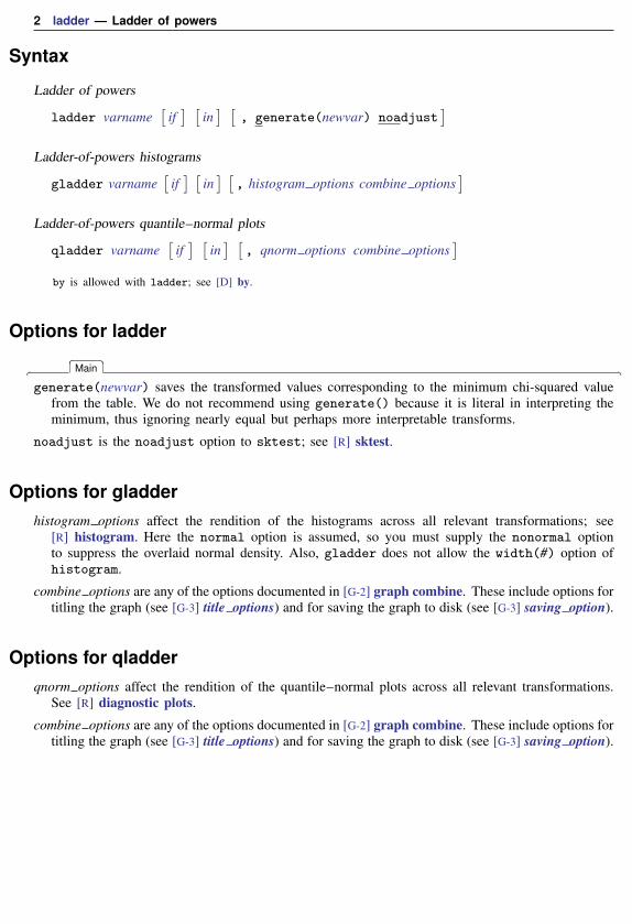
Example 1: ladder

We have data on the mileage rating of 74 automobiles and wish to find a transform that makesthe variable normally distributed:

. use http://www.stata-press.com/data/r15/auto(1978 Automobile Data)

. ladder mpg

Transformation formula chi2(2) P(chi2)

cubic mpg^3 43.59 0.000square mpg^2 27.03 0.000identity mpg 10.95 0.004square root sqrt(mpg) 4.94 0.084log log(mpg) 0.87 0.6471/(square root) 1/sqrt(mpg) 0.20 0.905inverse 1/mpg 2.36 0.3071/square 1/(mpg^2) 11.99 0.0021/cubic 1/(mpg^3) 24.30 0.000

If we had typed ladder mpg, gen(mpgx), the variable mpgx containing 1/√mpg would have been

automatically generated for us. This is the perfect example of why you should not, in general, specifythe generate() option. We also cannot reject the hypothesis that the inverse of mpg is normallydistributed and that 1/mpg—gallons per mile—has a better interpretation. It is a measure of energyconsumption.

4 ladder — Ladder of powers

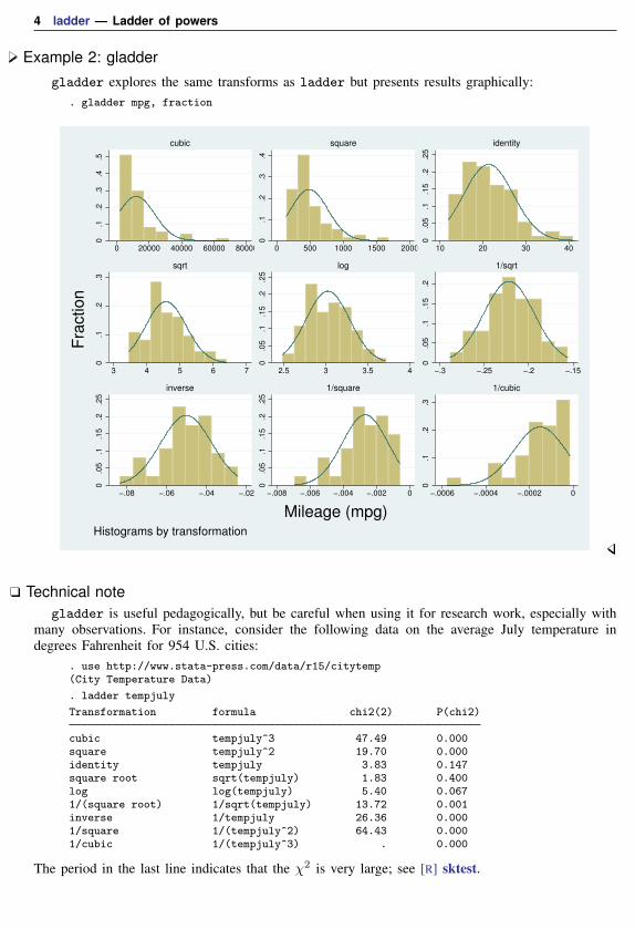
Example 2: gladder

gladder explores the same transforms as ladder but presents results graphically:. gladder mpg, fraction

0.1

.2.3

.4.5

0 20000 40000 60000 80000

cubic

0.1

.2.3

.4

0 500 1000 1500 2000

square

0.0

5.1

.15

.2.2

5

10 20 30 40

identity

0.1

.2.3

3 4 5 6 7

sqrt0

.05

.1.1

5.2

.25

2.5 3 3.5 4

log

0.0

5.1

.15

.2

−.3 −.25 −.2 −.15

1/sqrt

0.0

5.1

.15

.2.2

5

−.08 −.06 −.04 −.02

inverse

0.0

5.1

.15

.2.2

5

−.008 −.006 −.004 −.002 0

1/square

0.1

.2.3

−.0006 −.0004 −.0002 0

1/cubic

Fra

ctio

n

Mileage (mpg)Histograms by transformation

Technical notegladder is useful pedagogically, but be careful when using it for research work, especially with

many observations. For instance, consider the following data on the average July temperature indegrees Fahrenheit for 954 U.S. cities:

. use http://www.stata-press.com/data/r15/citytemp(City Temperature Data)

. ladder tempjuly

Transformation formula chi2(2) P(chi2)

cubic tempjuly^3 47.49 0.000square tempjuly^2 19.70 0.000identity tempjuly 3.83 0.147square root sqrt(tempjuly) 1.83 0.400log log(tempjuly) 5.40 0.0671/(square root) 1/sqrt(tempjuly) 13.72 0.001inverse 1/tempjuly 26.36 0.0001/square 1/(tempjuly^2) 64.43 0.0001/cubic 1/(tempjuly^3) . 0.000

The period in the last line indicates that the χ2 is very large; see [R] sktest.

ladder — Ladder of powers 5

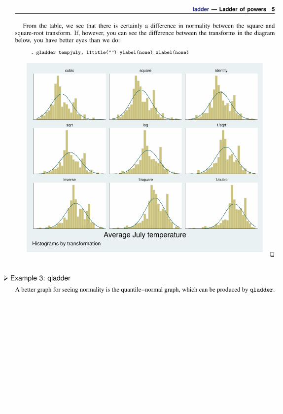
From the table, we see that there is certainly a difference in normality between the square andsquare-root transform. If, however, you can see the difference between the transforms in the diagrambelow, you have better eyes than we do:

. gladder tempjuly, l1title("") ylabel(none) xlabel(none)

cubic square identity

sqrt log 1/sqrt

inverse 1/square 1/cubic

Average July temperatureHistograms by transformation

Example 3: qladder

A better graph for seeing normality is the quantile–normal graph, which can be produced by qladder.

6 ladder — Ladder of powers

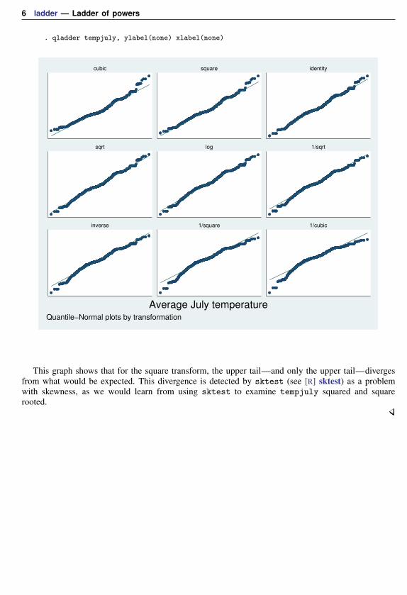
. qladder tempjuly, ylabel(none) xlabel(none)

cubic square identity

sqrt log 1/sqrt

inverse 1/square 1/cubic

Average July temperatureQuantile−Normal plots by transformation

This graph shows that for the square transform, the upper tail—and only the upper tail—divergesfrom what would be expected. This divergence is detected by sktest (see [R] sktest) as a problemwith skewness, as we would learn from using sktest to examine tempjuly squared and squarerooted.

ladder — Ladder of powers 7

Stored resultsladder stores the following in r():

Scalarsr(N) number of observationsr(invcube) χ2 for inverse-cubic transformationr(P invcube) p-value for normality test after inverse-cubic transformationr(invsq) χ2 for inverse-square transformationr(P invsq) p-value for normality test after inverse-square transformationr(inv) χ2 for inverse transformationr(P inv) p-value for normality test after inverse transformationr(invsqrt) χ2 for inverse-root transformationr(P invsqrt) p-value for normality test after inverse-root transformationr(log) χ2 for log transformationr(P log) p-value for normality test after log transformationr(sqrt) χ2 for square-root transformationr(P sqrt) p-value for normality test after square-root transformationr(ident) χ2 for untransformed datar(P ident) p-value for normality test of untransformed datar(square) χ2 for square transformationr(P square) p-value for normality test after square transformationr(cube) χ2 for cubic transformationr(P cube) p-value for normality test after cubic transformation

Methods and formulasFor ladder, results are as reported by sktest; see [R] sktest. If generate() is specified, the

transform with the minimum χ2 value is chosen.

gladder sets the number of bins to min(√n, 10 log10n), rounded to the closest integer, where

n is the number of unique values of varname. See [R] histogram for a discussion of the optimalnumber of bins.

Also see Findley (1990) for a ladder-of-powers variable transformation program that producesone-way graphs with overlaid box plots, in addition to histograms with overlaid normals. Buchner andFindley (1990) discuss ladder-of-powers transformations as one aspect of preliminary data analysis.Also see Hamilton (1992, 18–23) and Hamilton (2013, 129–132).

Acknowledgmentqladder was written by Jeroen Weesie of the Department of Sociology at Utrecht University, The

Netherlands.

ReferencesBuchner, D. M., and T. W. Findley. 1990. Research in physical medicine and rehabilitation: VIII. Preliminary data

analysis. American Journal of Physical Medicine and Rehabilitation 69: 154–169.

Cox, N. J. 2005. Speaking Stata: Density probability plots. Stata Journal 5: 259–273.

Findley, T. W. 1990. sed3: Variable transformation and evaluation. Stata Technical Bulletin 2: 15. Reprinted in StataTechnical Bulletin Reprints, vol. 1, pp. 85–86. College Station, TX: Stata Press.

Hamilton, L. C. 1992. Regression with Graphics: A Second Course in Applied Statistics. Belmont, CA: Duxbury.

. 2013. Statistics with Stata: Updated for Version 12. 8th ed. Boston: Brooks/Cole.

Tukey, J. W. 1977. Exploratory Data Analysis. Reading, MA: Addison–Wesley.

8 ladder — Ladder of powers

Also see[R] boxcox — Box–Cox regression models

[R] diagnostic plots — Distributional diagnostic plots

[R] lnskew0 — Find zero-skewness log or Box–Cox transform

[R] lv — Letter-value displays

[R] sktest — Skewness and kurtosis test for normality