Title of the Paper - Global Strategy improving Agricultural...
24
MULTIPLE-FRAME SAMPLING Ambrosio, Luis Universidad Politécnica de Madrid. Department of Economics, Statistics and Management Ciudad Universitaria Madrid, Spain [email protected] ABSTRACT (all caps, character 14 pt, bold, adjust left) There is consensus in the scientific community about the multidimensional (economic, social, and environmental) nature of sustainable development, and multiple-frame sampling allows for the linkage of the farm as an economic unit, to the household as a social unit, and both to the land as an environmental unit. In this paper we focus on multiple-frame regression estimators as a tool for (i) integrating register data with survey data, (ii) small area estimation, (iii) sampling in time, and (vi) analyzing complex surveys. Keywords: Multiple-frame regression estimator, Integrating survey and register data, Small area estimation, Sampling in time, Analysis of complex surveys 1. Economical, social and environmental surveys for a sustainable development For the analysis of the interrelationships between the economical, social and environmental aspects of sustainable development, we need farm-household-land models (Deaton, 1997). The sample design for gathering the data required for fitting these models should ensure a link between the farm as economics unit, the household as social unit, and the land as environmental unit. The Global Strategy (GS) for improving agricultural and rural official statistics [FAO (2011, 2012, 2015)] focuses on developing master sampling frames that are integrated with the NSS and allow for this linkage. Two keywords in the GS are ‘integration’ and ‘linkage’. ‘Integration’ refers to the use of the same sampling frame and related materials in multiple surveys, as well as the same concepts, survey personnel, and facilities. 'Linkage' is the basis for analyzing the relationships among the economical, the social and the environmental dimensions of sustainable development.
Transcript of Title of the Paper - Global Strategy improving Agricultural...

MULTIPLE-FRAME SAMPLING
Ambrosio, Luis Universidad Politécnica de Madrid. Department of Economics, Statistics and Management
Ciudad Universitaria
Madrid, Spain
ABSTRACT (all caps, character 14 pt, bold, adjust left)
There is consensus in the scientific community about the multidimensional (economic, social,
and environmental) nature of sustainable development, and multiple-frame sampling allows for the
linkage of the farm as an economic unit, to the household as a social unit, and both to the land as an
environmental unit. In this paper we focus on multiple-frame regression estimators as a tool for (i)
integrating register data with survey data, (ii) small area estimation, (iii) sampling in time, and (vi)
analyzing complex surveys.
Keywords: Multiple-frame regression estimator, Integrating survey and register data, Small area
estimation, Sampling in time, Analysis of complex surveys
1. Economical, social and environmental surveys for a sustainable
development
For the analysis of the interrelationships between the economical, social and environmental
aspects of sustainable development, we need farm-household-land models (Deaton, 1997). The
sample design for gathering the data required for fitting these models should ensure a link between
the farm as economics unit, the household as social unit, and the land as environmental unit.
The Global Strategy (GS) for improving agricultural and rural official statistics [FAO (2011,
2012, 2015)] focuses on developing master sampling frames that are integrated with the NSS and
allow for this linkage. Two keywords in the GS are ‘integration’ and ‘linkage’. ‘Integration’ refers
to the use of the same sampling frame and related materials in multiple surveys, as well as the same
concepts, survey personnel, and facilities. 'Linkage' is the basis for analyzing the relationships
among the economical, the social and the environmental dimensions of sustainable development.

This is a standard scheme of the surveys carried out by a National Statistical System (NSS).
The required information
Sustainable development
Economic
Agriculture
Macroeconomy
(Agregated values
Economiccounts and
bilan
Microeconomy)
Farm economic
Remainingsectors
Environmental
Natural resourcesuses and
conservation
Land Water Air
Social
LabourHouseholds Familly
budgetsPoberty
Figure 1: A standard scheme of the surveys carried out by a NSS
Economical aspects
The survey data are used to estimate the macroeconomic aggregates (output, intermediate
consumption, and value added) required for preparing the accounts of the agricultural sector; as
well as to describe and analyze the microeconomics of farms, including factor productivity and the
threshold of profitability.
Social aspects
Surveys concerning social issues include housing and living conditions (surveys on welfare,
poverty and inequality), employment, nutrition, and income, expenses and savings by households
(Deaton, 1997).
Environmental aspects
Environmental surveys collect information on the use of natural resources (soil, water and air)
by the various productive sectors.
2. Multiple-frame surveys: master sampling frames and master samples
Sampling strategies based on multiple overlapping frames have deserved a notable attention
in last years, as a tool to deal with non-sampling errors: under-coverage, non-response, and
measurement errors [Lohr (2011)]. We follow this sampling strategy for integrating agricultural and
household surveys. Focus is on the linkage among farms, households and parcels.

FAO (1996, 1998, 2015), and the United Nations Statistical Division (UNSD, 1986, 2008),
have elaborated guidelines to assist countries in planning and implementing agricultural and
household surveys, respectively. The central topic of these guidelines is the development and
maintenance of master sampling frames.
We focus on the integration of a dual sampling frame for agriculture with a sampling frame
for households to build a multiple sampling frame that allows the required linkage among reporting
units. We apply this strategy in three Latin America countries. We consider multiple-frame
regression estimators, highlighting its usefulness to integrate register and survey data and for small
area estimation.
2.1. Integration of agricultural and household Master Sampling Frames
The sampling frames recommended by FAO and UNSD guidelines are dual frames, with an
area component and a list component. The area frame ensures completeness, accuracy and up-to-
datedness of the master frame: it is well established in the literature [Fecso et al. (1986),
Faulkenberry and Garoui (1991), Vogel (1995), Ambrosio and Iglesias (2014)]. In agricultural
surveys, the list contains the largest farms and contributes to improve the area sample accuracy.
Census enumeration areas are used in household surveys as Primary Sampling Units (PSUs) and a
list is elaborated within selected PSUs and is used to select the household sample.
We integrate the agricultural sampling frame and the household sampling frame in a unique
multiple sampling frame. This multiple-frame provides farms to observe economical variables:
acreage and crop yields, livestock production, aquaculture and forestry. It provides also households
to observe social variables: household composition, living conditions, employment, income, food
and hunger, poverty, or inequality. And it provides parcels to observe environmental variables: soil
degradation, water consumption for irrigation, or the quantity used of chemical fertilizers,
herbicides, pesticides and fungicides.
Country examples
We study the case of three Latin American countries: Guatemala, Costa Rica and Ecuador. In
these countries, there is a dual sampling frame for agricultural surveys. The kind of limits used to
define sampling units differs among countries: limits are geometrics in Guatemala and Ecuador,
while identifiable physical boundaries are used in Costa Rica. The area frame,1A , has 190100
segments in Guatemala [Ambrosio (2013), FAO (2015)], 352254 segments in Ecuador (Ambrosio,
2014) and 120326 segments in Costa Rica (Ambrosio, 2015).
The area frame is stratified into four strata, using the percentage of cultivated surface as
stratification variable. The data source for stratification is a land use map in Guatemala and Ecuador
and a geo-referenced agricultural census in Costa Rica. A target segment size is defined that varies
among strata: in Guatemala it ranges from 6.25 hectares (cultivated surface bigger than 60% and
small fields) to 100 hectares (cultivated surface lower than 20%), in Ecuador the range is from 9 to
576 hectares, and in Costa Rica the range is from 10 to 100 hectares. In Guatemala and Costa Rica 1S has 1500 segments, and in Ecuador 5520 segments. The sample is allocated to strata according
to Neyman’s criterion, and five replicated samples are selected in each stratum.

The list frame,2A , differs among countries according to available resources. In Costa Rica,
there is a recent agricultural census and a list frame for each one of the main crops and animal’
species is available (the bovine list frame has 31171 farms, and the porcine list frame has 14355
farms). In Guatemala and Ecuador, the agricultural censuses are obsoletes and the number of list
frames is reduced to the biggest farms in Ecuador and to the main animals’ species in Guatemala.
An area sampling frame of enumeration areas (EA) with mapped, well-delineated boundaries
is available for household surveys. In Guatemala the frame has 15511 EA with an average of 140
households by EA. The EA are stratified using available population figures, and a two-stage
sampling scheme is used to select the household sample,3S . In the first stage, a sample of EA is
selected with probabilities proportional to size (in Ecuador the sample size is 2586 EA for labor
surveys, 1128 EA for surveys on living standard and 3411 EA for income surveys). In the second-
stage, a list of household is updated within each EA in the first-stage sample and a sample of
households (12 by EA) is selected with equal probabilities.
Figure 2: Master Sampling Frame of Costa Rica
2.2 Sampling a population with multiple overlapping frames
We use P to refer either the farms population, 1,2, ,F f f F the parcels population,
1,2, ,L l l L , or the households population, 1,2, ,H h h H . We assume that each
population unit, jj P , ,j f h lj , is associated with at least one sampling unit in the multiple-
frame 1,2, , ; 1,2, ,qi A q Q I , where qA denotes both, the generic single frame q and
the number of sampling units, and Q is the number of single frames. We define the indicator
variable 1q
ijI if the population unit jj P is associated to the sampling unit qi A , and
0q
ijI otherwise , ,j f h lj .

The sample
We select a set of samples ; 1,2, ,q q QS independently from each single frameqA ,
using a sampling scheme that associates to sampling unit 1,2, , qi A an inclusion probabilityq
i .
From the standard dual frame for agricultural surveys, where 1A is an area frame with 11,2, ,i A
segments and 2A is a list frame with 21,2, ,i A names of farms, we select independently a
sample 1S of segments and a sample
2S of names. From the standard frame for household surveys, 3A , we select a sample
3S of names, independent of 1S and
2S .
As a result, we have: (i) a sample of parcels, 1 1 1S S 1L ill L i I , where 1 1ilI when
the area, ila , of parcel l within the segment 1Si is 0ila , (ii) and a set of three partially
overlapping samples of farms, S ; 1,2,3q
F q , where S S 1q q q
F iff F i I , where 1 1ifI
when the area, ifa , of the farm f within the segment 1Si is 0fia , and
2 1ifI when the
name 2Si is associated with the farm f , and 3 1ifI when the household 3Si is associated with
the farm f , (iii) and a set of three partially overlapping samples of households, S ; 1,2,3q
H q ,
where S 1q q q
H F ifhS h H f I , where 1 1ifhI when the farm f with area 0fia within the
segment 1Si is associated with the household h , and 2 1ifhI when the farm f associated with the
name 2Si is associated with the household h , and 3 1ifhI when the name 3Si is associated with
the household h .
Linkage
A farm f F and a household h H are linked (associated) if at least one person from
h H works for f F . A parcel is linked with the farm to which it belongs and with the
households through the linkage between farms and households. This sampling procedure is related
with both, network sampling and indirect sampling [Falorsi (2014), Singh and Mecatti (2011),
Mecatti and Singh (2014)].

Figure 3: Master Sample of Costa Rica
3. Multiple-frame estimators
Typically, a population unit (e.g. a farm) is covered by two or more single frames (e.g., area
and list frames) and, as a result, the weight estimator, S
1 1
ˆqQ
q
i i
q i
Y w y
P, where
1q
i q
i
w
, is a biased
estimator of the population total, YP . To see this, consider the population partitioned into
2 1QD non-overlapping domains and 1
D
d
d
Y Y
P, where
dY is the domain total, 1,2, ,d D .
For dual frames, 2Q ,
1 22 S S S1 2
1 1 1 1
ˆq
q
i i i i i i
q i i i
Y w y w y w y
P, and 22 1 3D . Domain
1d is the set of units covered only by 1A , domain 2d is covered only by 2A and domain
3d is covered by both, 1A and 2A . The population total is 3
1 2 3
1
d
d
Y Y Y Y Y
P. Now,
1S1
1
i i
i
w y
is a unbiased estimator of 1A total, which is domain 1d total plus 3d total, 1 3Y Y , and
2S2
1
i i
i
w y is a unbiased estimator of 2A total, which is 2d total plus domain 3d total,
2 3Y Y .Thus,
1 2S S1 2
1 2 3
1 1
ˆ 2i i i i
i i
EY E w y E w y Y Y Y
P and the bias of YP is
3ˆ ˆBY EY Y Y P P P
.
A screening approach is followed in FAO (1996, 1998), where the single frames are pre-
screened to remove overlap, so that domains with two o more frames are empty and, as a result, the
weight estimator is unbiased: for dual frames, 3d is empty, 3 0Y , and hence ˆ 0BY P. However,
screening operations are resource-consuming and a number of more cost-efficient alternatives can
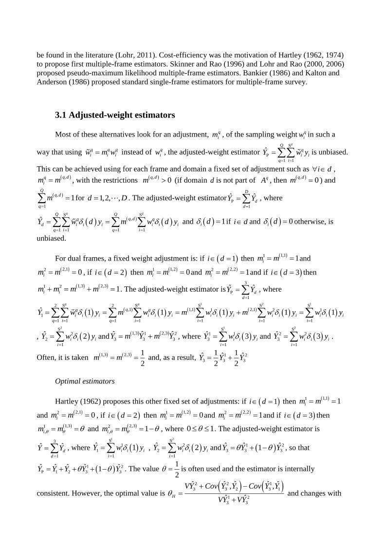
be found in the literature (Lohr, 2011). Cost-efficiency was the motivation of Hartley (1962, 1974)
to propose first multiple-frame estimators. Skinner and Rao (1996) and Lohr and Rao (2000, 2006)
proposed pseudo-maximum likelihood multiple-frame estimators. Bankier (1986) and Kalton and
Anderson (1986) proposed standard single-frame estimators for multiple-frame survey.
3.1 Adjusted-weight estimators
Most of these alternatives look for an adjustment, q
im , of the sampling weight q
iw in such a
way that using q q q
i i iw m w instead of q
iw , the adjusted-weight estimator S
1 1
ˆqQ
q
i i
q i
Y w y
Pis unbiased.
This can be achieved using for each frame and domain a fixed set of adjustment such as i d , ,
q dq
im m , with the restrictions ,
0q d
m (if domain d is not part of qA , then ,
0q d
m ) and
,
1
1
Q
q d
q
m for 1,2, ,d D . The adjusted-weight estimator1
ˆ ˆD
d
d
Y Y
P, where
S S
,
1 1 1 1
ˆ
q qQ Q
q dq q
d i i i i i i
q i q i
Y w d y m w d y and 1i d if i d and 0i d otherwise, is
unbiased.
For dual frames, a fixed weight adjustment is: if 1 i d then 1,11 1 im m and
2,12 0 im m , if 2 i d then 1,21 0 im m and
2,22 1 im m and if 3 i d then
1,3 2,31 2 1 i im m m m . The adjusted-weight estimator is3
1
ˆ ˆd
d
Y Y
P, where
1 2 12 S 2 S S S S
,1 1,1 2,11 2 1
1
1 1 1 1 1 1 1
ˆ 1 1 1 1 1
q q
qq q
i i i i i i i i i i i i i i i
q i q i i i i
Y w y m w y m w y m w y w y
, 2S
2
2
1
ˆ 2
i i i
i
Y w y and 1,3 2,31 2
3 3 3ˆ ˆ ˆ Y m Y m Y , where
1S1 1
3
1
ˆ 3
i i i
i
Y w y and 2S
2 2
3
1
ˆ 3
i i i
i
Y w y .
Often, it is taken 1,3 2,3 1
2m m and, as a result, 1 2
3 3 3
1 1ˆ ˆ ˆ2 2
Y Y Y
Optimal estimators
Hartley (1962) proposes this other fixed set of adjustments: if 1 i d then 1,11 1 im m
and 2,12 0 im m , if 2 i d then
1,21 0 im m and 2,22 1 im m and if 3 i d then
1,31
, im m and 2,32
, 1 im m , where 0 1 . The adjusted-weight estimator is
3
1
ˆ ˆ
d
d
Y Y , where 1S
1
1
1
ˆ 1
i i i
i
Y w y , 2S
2
2
1
ˆ 2
i i i
i
Y w y and 1 2
3 3 3ˆ ˆ ˆ1 Y Y Y , so that
1 2
1 2 3 3ˆ ˆ ˆ ˆ ˆ1Y Y Y Y Y P
. The value 1
2 is often used and the estimator is internally
consistent. However, the optimal value is 2 2 1
3 3 2 3 1
1 2
3 3
ˆ ˆ ˆ ˆ ˆ, ,
ˆ ˆ
H
VY Cov Y Y Cov Y Y
VY VY and changes with

the survey variable, so that it is internally inconsistent. In practice, internal consistency requires that
one set of weights be used to estimate all survey variables: Pseudo-maximum likelihood estimators
are internally consistent (Lohr, 2011).
Single-frame estimator
Kalton and Anderson (1986) propose an adjustment weight, which treats all observations as
though they had been sampled from one frame: if 1 i d , then 1
, 1i Sm , if 2 i d then
2
, 1i Sm and if 3 i d then 2
1
, 1 2
ii s
i i
wm
w w
and
12
, 1 2
ii s
i i
wm
w w
. If
3 i d then 1 2
1 2
1i i
i i
w w
. This estimator is internally consistent.
3.2 Multiplicity-adjusted estimators.
Singh and Mecatti (2011) and Mecatti and Singh (2014) propose to adjust for multiplicity the
survey variable value, instead of the sampling weight. The multiplicity of a population unit, jP
( , ,j f h l and , ,F H LP ), is the number of sampling units, 1
j j
q
m m
, with which it is
associated, where 1
qAq q
j ij
i
m I
is the multiplicity within qA . The population total is 1 1
qQ Aq
i
q i
Y y
P,
where 1
q q
i ij j
j
y y
P
is the multiplicity-adjusted value of the survey variable in the thi sampling unit,
where
q
ijq
ij
j
I
m .
The weight multiplicity-adjusted estimator, 1 1
ˆqQ S
q q
i i
q i
Y w y
P, is unbiased and internally
consistent. Note that the adjustment, 1
jm, applies to the survey variable value,
jy , instead to the
sampling weight, q
iw , and it consists in sharing jy among the number of sampling units with
which jP is associated.
In terms of the population units, the multiplicity-adjusted estimator can be written as an
adjusted-weight estimator, 1 1
ˆ
qSQ
q
j j
q j
Y w y
P
P where S S 1q q q
ijj i I P P is the set of
population units associated with qS and 1
1qS
q q
j i
ij
w wm
. The size of Sq
P is nq
P .

The parameter to be estimated is the population total, , ,L F HP : over land, 1
L
L l
l
Y Y
,
over farms, 1
F
F f
f
Y Y
, and over households, 1
H
H h
h
Y Y
. Given the links ,lf fhI I between
, ,l f h , (i) the multiplicity of the parcel l is 1
l l
q
m m
, where
1
1 1
1
A
l il
i
m I
,
2
2 2 2
1
A
l if lf f lf
i
m I I m I
and 3 3
1
H
l h fh lf
h
m m I I
; (ii) the multiplicity of the farm f is
1
f f
q
m m
, where
1
1 1
1
A
f if
i
m I
,
2
2 2
1
A
f if
i
m I
and 3 3
1
H
f h fh
h
m m I
; and the multiplicity of the household h is 1
h h
q
m m
, where
1 1
1
F
h f fh
f
m m I
, 2 2
1
F
h f fh
f
m m I
and
3
3 3
1
A
h ih
i
m I
.
The total over land is 1
Q
L Lq
q
Y Y
, where 1
qAq
Lq Li
i
Y y
, where
1 1 2 2
1 1 1
,L F L
l lLi il Li if lf
l f ll l
y yy I y I I
m m
and 3 3
1 1 1
F H Ll
Li ih fh lf
f h l l
yy I I I
m
are the multiplicity-adjusted
values of the survey variable associated to the thi sampling unit in each frame. The total over farms
is 1
Q
F Fq
q
Y Y
, where 1
qAq
Fq Fi
i
Y y
, where 1 1 2 2
1 1
,F F
f f
Fi if Fi if
f ff f
y yy I y I
m m
and
3 3
1 1
F Hf
Fi ih fh
f h f
yy I I
m
. The total over households is
1
Q
H Hq
q
Y Y
, where 1
qAq
Hq Hi
i
Y y
and
1 1 2 2
1 1 1 1
,F H F H
h hHi if fh Hi if fh
f h f hh h
y yy I I y I I
m m
, and3 3
1
Hh
Hi ih
h h
yy I
m
.
The multiplicity-adjusted estimator, 1 1
ˆqQ S
q q
i i
q i
Y w y
P P, is unbiased and its variance is
1 1 1
ˆq q q qQ A A
q q q i iii i i q q
q i i i i
y yVY
P PP . The variance estimator is
1 1 1
ˆ ˆq q q q q q qQ S S
ii i i i i
q q qq i i ii i i
y yVY
P P
P .
The multiplicity-adjusted estimator can be written in terms of population units as an adjusted-
weight estimator, 1 1
ˆq
SQq
j j
q j
Y w y
P
P , where 1
1qS
q q
j i
ij
w wm
.
4. Multiple-frame regression estimators
To use auxiliary information, we specify a regression model in terms of population units,
x β+j j jy , where x j is the 1 p vector of auxiliary variables, including the constant 1, β is a

1p vector of regression parameters, 0jE , and 2
jV . The model in terms of sampling
units is, x βq q q
i i iy , where 1
x x
qS
q q
i ij j
j
P
, 1
qS
q q
i ij j
j
P
, 0q
iE , 2
2
1
qS
q q
i ij
j
V
P
.
Lu (2014) proposes four methods to estimateβ . We consider the probability weighted least
square estimator, 2
1 1
ˆ minβ
β x β
qQ Sq q q
w i i i
q i
w y
, where q q q
i i iw w and
2
1
1qP
q
i Sq
ij
j
: it is
1
ˆ T Tβ X D X X D yw w w
, where X is the 1
q
S p
multiplicity-adjusted auxiliary data matrix,
y is the 1
1Q
q
q
S
vector of multiplicity-adjusted survey variable data,
and ; 1,2, , ; 1,2, ,Dq q
w idiag w i S q Q .
βw is a design-consistent estimator of the regression parameter values in the finite population,
1
β X X X yT T
N N N N N
, where 1
q
N A
is the number of sampling units in the multiple-
frame, XN is the N p matrix of multiplicity-adjusted auxiliary variable values, and yN is the
1N vector of the multiplicity-adjusted survey variable values.
The Multiplicity-adjusted General REGression estimator (MGREG) is 1 1
ˆˆ x β
qQ Aq
MGREG i w
q i
Y
:
it is a design-consistent estimator of the population total, Y , and its asymptotic design-variance can
be estimated using1 1
ˆ ˆ ˆ ˆ
qQ Sq q
MGREG i i
q i
VY V w e
g , where ˆˆ -x β
q q q
i i i we y (Fuller, 2009; Kim and Rao,
2012). Ranalli et al (2014) propose calibration estimators. Deville and Särdal (1992) (see also
Fuller, 2009) show how calibration estimators can be approximated by regression estimators.
4.1 Integrating survey and register data
The MGREG estimator is useful to integrate survey and register data. To see this, we assume
that there is a set of values ,xj jy associated with each population unit: jy is the survey variable
value and x j are register values. We assume that the choice of xq
j differs among single frames
(registers) and we use a different working model in each register, x βq q q q
i i iy , where
1
x x
qS
q q q
i ij j
j
P
, 1
qS
q q
i ij j
j
P
, 0q
iE , 2
2,
1
qS
q q q
i ij
j
V
P
. To observe data on ,xq
j jy , we
consider 1Q frames of the target population, P , and we select independently from each one a

sample, 1; 1,2, ,qS q Q . We consider 2Q registers as independent large samples,
2; 1,2, ,qS q Q , selected from P , where we observe only data on xq
j .
To estimate regression parameters, βq , we use data from 1Q and the probability weighted
least square estimator, 2
1
ˆ minβ
β x β
q
q
Sq q q q q
w i i i
i
w y
, which is 1
β X D X X D yq qT q q qT q q
w w w
, where Xq
is the q qS p multiplicity-adjusted auxiliary data matrix, yq is the 1qS vector of
multiplicity-adjusted survey variable data, and ; 1,2, ,Dq q q
w idiag w i S .
We use data from 2Q to estimate
1
x
qAq
i
i
, using1
x
qSq q
i i
i
w
. The MGREG estimator is
2
1 1
ˆ ˆˆ x β
qQ Sq q q
MGREG i i w
q i
Y w
, and its error is
2 1 2 1
1 1 1 1 1 1 1
ˆ ˆ ˆ ˆˆ ˆ x β x β x x β x x β β
q q q
q q q q q
Q Q Q QS S Sq q q q q q q q q q q q q
MGREG MGREG i i i i w N i i wN N A A Aq q i q i q i
Y Y Y y w w
, where1
x x
q
q
Aq q
iAi
,
2
1
x x q
N Aq
, 1
β X X X yq q q q q
q qT q qT q
A A A A A
, X q
q
Nis the q qA p matrix of
multiplicity-adjusted auxiliary variable values, and y qAis the 1qA vector of the multiplicity-
adjusted survey variable values.
ˆMGREGY is design-consistent and its asymptotic design-variance can be estimated
using
1 2
1 1 1 1
ˆ ˆ ˆ ˆˆ ˆ ˆ ˆβ V x β
q qQ QS Sq q qT q q q
MGREG i i w i i w
q i q i
VY V w e w
, where ˆ ˆ-x β
q q q q
i i i we y . The elements of the
covariance matrix, 1
V x
qSq q
i i
i
w
, can be estimated using the HT variance estimator. If 2qA Q is
complete, then 1
x
qAq
i
i
is known and all terms in the covariance matrix related with qA are nulls.
4.2 Small area estimation
A new approach to small area estimation is based on combining data from multiple surveys.
Most works follow a model-assisted approach [Kim and Rao (2012), Merkouris (2010)], using
either regression or calibration estimators. Also, estimators based on measurement error models
have been proposed (Kim et al., 2015).
A working model often used in the model-assisted approach is the regression
model x β+j j jy , where x j is the 1 p vector of auxiliary variables, including the constant 1,

β is a 1p vector of regression parameters, 0jE , 2
jV , and jj P , ,j f h lj is the
population unit.
We consider a partition of the population into 1,2, ,d D non-overlap domains or small
areas. The survey variable total is 1
D
d
d
Y Y
P, where dY is the survey variable total in the small area
1,2, ,d D . We consider two sample, a principal sample, 1S , and a secondary sample, 2S , the
size of the latter being much bigger than the size of the former, 2 1qn n . 2S is selected from
frame 2A , with weights
2q
iw .
The regression estimator of dY is 1
1
1
ˆn
dreg j j j
j
Y w d y
P
, where 1j d if j d and
0j d otherwise, and ˆj jy =x B . This estimator has bias
2
2
1
n
j j j j
j
w d y y
P
and the corrected-
bias estimator is 1 2
1 2
,
1 1
ˆ ˆn n
dreg bc j j j j j j j
j j
Y w d w d y y
x BP P
, that is,
2 1 2
1 1 2
,
1 1 1
ˆ ˆn n n
dreg bc j j j j j j j j j
j j j
Y w d y w d w d
x x B
P P P
.
Under general conditions [if the model holds, or the vector of small area indicators, q
j d , is
in space of the columns of X ; see Kim y Rao (2012)], the bias is null and the estimator reduces to
the projective estimator, 1
1
,
1
ˆ ˆx Bn
dreg bc j j j
j
Y w d
P
.
The estimation error is
2 1 2
, ,
2 1 2
1 1 1
ˆ ˆ
ˆ ˆ
dreg bc d dreg bc d
n n n
j j j j j j j d d j j j
j j j
Y Y Y
w d y w d w d
x β
x β x x B x x B βP P P
d P
P d d P
And the asymptotic design-variance is
2 1
2 1
,
1 1
ˆlim x β β Var x βn n
dreg bc d j j j j j j jd d d
j j
V p Y Y V w d y w d
P P
T
P P d P
These results can be generalized to multiple samples as follow. We consider a number of 2 2Q samples: for instance, administrative registers with data on the auxiliary variables x j . And a
number of 1Q samples with data on ,xj jy , where jy is the survey variable.
Using 1, , 1,2, , , 1,2, ,xq
j j Py j S q Q , we estimate B and we use the projective
estimator 2
1 1
ˆq
SQq
d reg j j j
q j
Y w d y
P
dP =, where ˆx Bj jy , to estimate dY using the 2 2Q samples.
The bias-corrected estimator is

1 2
,
1 1 1
ˆq q
S SQ Qq q
d reg bc j j j j j j j
q j q j
Y w d y w d y y
P P
P , that is,
2 1 2
,
1 1 1 1 1
ˆ ˆq q q
S S SQ Q Qq q q
d reg bc j j j j j j j j j
q j q j q j
Y w d y w d w d
x x BP P P
P .
The estimation error is
2 1 2
, ,
1 1 1 1
ˆ ˆ ˆ ˆx β x β x x B x x B β
q q qS S SQ Q Q
q q
d reg bc d reg bc d j j j j j j d d j j j
q j q j q j
Y Y Y d y w d w d
P P P
P P P P P P P P
And the asymptotic design-variance is
2 1
,
1 1 1 1
ˆlim x β β Var x β
q qS SQ Q
q q
d reg bc j j j j j j jd d d
q j q j
V p Y Y V w d y w d
P P
T
P P P P
4.3 Estimation in time
We want to estimate the survey variable total, ty , in time t using the sample of the period t
and the estimates of the previous periods, ˆ ; 1, 2, ,1ty t t t . We consider a sequence of
multiple-frame samples of the same population selected at regular time intervals. As proposed by
Gurney and Daly (1965), we aggregate the simple data in “elementary estimates” using a same
estimator of the total for every sample of the sequence.
We assume that the sequence of “elementary estimates” ˆ ; 1,2, ,ty t T of
; 1,2, ,ty t T has been generated according to the model ˆt t ty y u , where ˆ
ty is a unbiased
multiple-frame estimator ofty , so that ˆ
t t tE y y y . The estimation error, ˆt t tu y y , has zero
mean, ˆ 0t t t t t t tE u y E y y y y y and design-variance 2ˆt t t t uV u y V y y ,
which is known. The (marginal) variance of ˆ ; 1,2, ,ty t T is
2ˆ ˆ ˆtt t
t t t t t t uyy y
V y V E y y EV y y V y .
We assume that ; .... 2, 1,0,1,2,ty t is a random process. For Tt ,...,2,1 , the model
is y y u , where ˆ , ,y y u are 1T random vectors. ,y u are independent, ,Cov y u =0 , with
mean u 0E , y yE E , and covariance matrices Vy G and Vu R , so that
ˆVy Vy+Vu G+R .
The Best Linear Unbiased Predictor (BLUP) of y is 1ˆ ˆy GV yBLUP
and its variance is
1 11 1ˆVy R G R R R G RBLUP
. Note that 1
1 1 1 1ˆ ˆ ˆ ˆy R G R y y RV yBLUP
,
where 1ˆRV y is the BLUP of u conditionally to y .

If ; .... 2, 1,0,1,2,ty t is AR(1), then
2 1
2
2
1 2 3
1
1
1
Vary G
T
T
y
T T T
If ; .... 2, 1,0,1,2,ty t is a random walk, then 2
1 1 1 1
1 2 2 2
1 2 3
Vary G e
T
With panel data, the sampling errors are correlated and the covariances
ˆ ˆ, ,t t t tCov u u Cov y y in R can be estimated from the multiple samples. Assuming that y is
AR(1), then y is also AR(1) and can be estimate using 1
2
2
1
2
ˆ ˆ
ˆ
ˆ
T
t t
t
T
t
t
y y
y
, and
22
ˆ 2
ˆˆ
ˆ1
ey
, where
22
1
2
1ˆˆ ˆ ˆ
1
T
e t t
t
y yT
.
If ˆ ; 1,2, ,ty t T is a random walk, then ˆ ; 2, ,ty t T is stationary and
ˆ ˆVar y VaryT where 2ˆ ˆ min ,Vary e t t , where
22
1
2
1ˆ ˆ ˆ
1
T
e t t
t
y yT
.
The estimate of the change
The change, 1t t ty y y , is estimated using 1
ˆ ˆ ˆt t BLUP t BLUP
y y y
where
ˆt BLUP
y and
1ˆ
t BLUPy
are in 1ˆ ˆy GV yBLUP
. The change series, 1
ˆ ˆ ˆ ; ....2,t t BLUP t BLUPy y y t T
, is
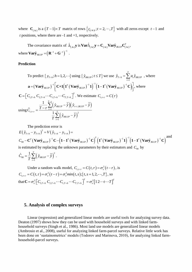
1ˆ ˆ ˆy Cy CGV yBLUP
, where C is a 1T T matrix of rows ; 2, ,tc t T with all zeros
except 1t and t positions, where there are -1 and +1, respectively.
The covariance matrix of ˆ y is, ˆ ˆVar y CVary CT
BLUP , where
1 11 1ˆVary R G R R R G RBLUP
.
The stability of ; .... 2, 1,0,1,2,ty t can be assessed
using 1 ; 1,2, ,t t tV y V y y t T , which are the diagonal elements in
Var y CVaryC CGCT T .
The accumulate change, 1 , 2, ,ty y t T , can be estimated using
1ˆ ˆ ; ....2,
t BLUP BLUPy y t T and can be computed using
1ˆ ˆ ˆy C y C GV yBLUPAc Ac Ac
,
where CAc
is a 1T T matrix of rows ; 2, ,Ac tc t T with all zeros except 1t and
t positions, where there are -1 and +1, respectively.
The covariance matrix of
ˆ yAc
is ˆ ˆVar y C Vary C
T
BLUPAc Ac Ac ,
where 1
1 1ˆVary R GBLUP
.
Prediction
To predict ; 1,2,T hy h using ˆ ;tBLUPy t T we use 1
ˆ ˆT
T h t tBLUP
t
y a y
, where
1
1 1 1ˆ ˆ ˆa Vary C+1 1 Vary 1 1 1 Vary C
T T
BLUP BLUP BLUP
, where
1, 2, , ,CT
T h T h t T h T T hC C C C . We estimate ,t tC C
using
,
1,
2
1
1ˆ ˆ ˆ ˆ
ˆ1
ˆ ˆ
T
tBLUP t BLUP
tt t T
tBLUP
t
y y y yT
C
y yT
The prediction error is
2
11 1 1 1
00
ˆ ˆ
ˆ ˆ ˆ ˆC Vary C 1 1 Vary C 1 Vary 1 1 1 Vary C
T h T h T h T h
TT T T T
BLUP BLUP BLUP BLUP
E y y V y y
C
and
is estimated by replacing the unknown parameters by their estimators and 00C by
2
00
1
1ˆ ˆ ˆT
tBLUP
t
C y yT
.
Under a random walk model, 2
, ,t t eC C t t , is
2 2
, , , ; , 1,2, ,t t e eC C t t min t s t s T , so
that 2 2
1, 2, , , 12CT T
e T h T h t T h T T h eC C C C t T
5. Analysis of complex surveys
Linear (regression) and generalized linear models are useful tools for analyzing survey data.
Deaton (1997) shows how they can be used with household surveys and with linked farm-
household surveys (Singh et al., 1986). Most land use models are generalized linear models
(Ambrosio et al., 2008), useful for analyzing linked farm-parcel surveys. Relative little work has
been done on ‘sustainometrics’ models (Todorov and Marinova, 2010), for analyzing linked farm-
household-parcel surveys.
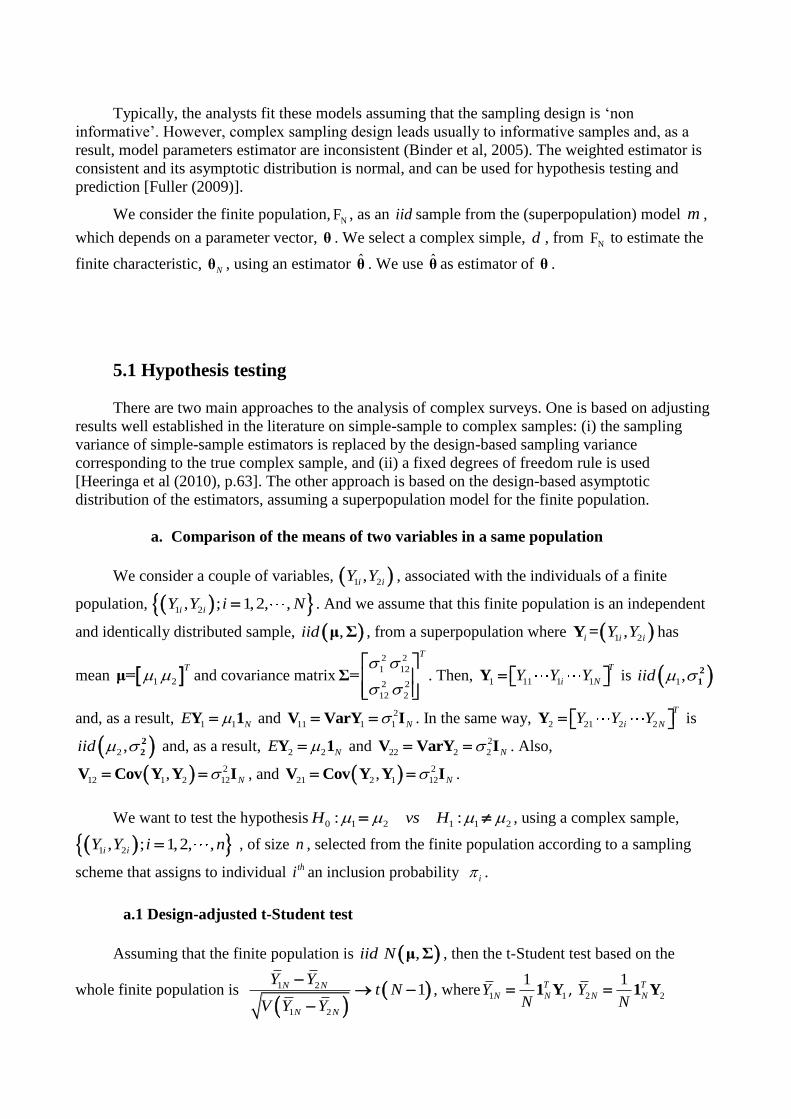
Typically, the analysts fit these models assuming that the sampling design is ‘non
informative’. However, complex sampling design leads usually to informative samples and, as a
result, model parameters estimator are inconsistent (Binder et al, 2005). The weighted estimator is
consistent and its asymptotic distribution is normal, and can be used for hypothesis testing and
prediction [Fuller (2009)].
We consider the finite population,NF , as an iid sample from the (superpopulation) model m ,
which depends on a parameter vector, θ . We select a complex simple, d , from NF to estimate the
finite characteristic, θN, using an estimator θ . We use θ as estimator of θ .
5.1 Hypothesis testing
There are two main approaches to the analysis of complex surveys. One is based on adjusting
results well established in the literature on simple-sample to complex samples: (i) the sampling
variance of simple-sample estimators is replaced by the design-based sampling variance
corresponding to the true complex sample, and (ii) a fixed degrees of freedom rule is used
[Heeringa et al (2010), p.63]. The other approach is based on the design-based asymptotic
distribution of the estimators, assuming a superpopulation model for the finite population.
a. Comparison of the means of two variables in a same population
We consider a couple of variables, 1 2,i iY Y , associated with the individuals of a finite
population, 1 2, ; 1,2, ,i iY Y i N . And we assume that this finite population is an independent
and identically distributed sample, ,iid μ Σ , from a superpopulation where 1 2,i i iY YY = has
mean 1 2
T μ= and covariance matrix
2 2
1 12
2 2
12 2
Σ=
T
. Then, 1 11 1 1
T
i NY Y YY is 1,iid 2
1
and, as a result, 1 1 NE Y 1 and 2
11 1 1 NV VarY I . In the same way, 2 21 2 2
T
i NY Y YY is
2 ,iid 2
2 and, as a result, 2 2 NE Y 1 and 2
22 2 2 NV VarY I . Also,
2
12 1 2 12,V Cov Y Y IN , and 2
21 2 1 12,V Cov Y Y IN .
We want to test the hypothesis 0 1 2 1 1 2: :H vs H , using a complex sample,
1 2, ; 1,2, ,i iY Y i n , of size n , selected from the finite population according to a sampling
scheme that assigns to individual thi an inclusion probability i .
a.1 Design-adjusted t-Student test
Assuming that the finite population is ,iid N μ Σ , then the t-Student test based on the
whole finite population is
1 2
1 2
1N N
N N
Y Yt N
V Y Y
, where 1 1
1 T
N NYN
1 Y , 2 2
1 T
N NYN
1 Y

and 1 11 12
1 2 2
2 21 22
11 11 1 1 1
1
T T T T
N N N N N N
N N T T T TN NN N N N
V Y Y VN N
1 0 1 0 1 0Y V V
Y V V 0 10 1 0 1
so
that
2 2
11 12 1 12 2 2 2
1 2 1 12 22 2 2
21 22 12 2
1 11 1 11 1 1 1 2
1 1
1 V 1 1 V 1
1 V 1 1 V 1
T T
N N N N
N N T T
N N N N
V Y YN N N
.
However, only a complex sample, 1 2, ; 1,2, ,i iY Y i n is available and the t-Student test
based on the complex sample is
1 2
1 2
ˆ ˆ
ˆ ˆˆ
N Ndf
N N
Y Yt
V Y Y
,
where 1 1
1 1
1ˆqQ S
q q
N i i
q i
Y w yN
, 2 2
1 1
1ˆqQ S
q q
N i i
q i
Y w yN
and
1 1 2
1 2
1 2 2
ˆ ˆ ˆˆ ( , ) 1ˆ ˆˆ 1 1ˆ ˆ ˆ 1ˆ( , )
N N N
N N
N N N
VY Cov Y YV Y Y
Cov Y Y VY
, where 1
ˆˆNVY , 2
ˆˆNVY and 1 2
ˆ ˆ( , )N NCov Y Y are
design-based estimators of the variance and covariance estimators.
Determination of the exact degrees of freedom is difficult and “fixed degree of freedom rule”
[Heeringa et al (2010), p.63] is used in practice: 1
1L
h
h
df a
, where ha is the number of
primary sampling units in the thh stratum, so that df is equal to the number of primary sampling
units in the population minus the number of strata.
a.2 Asymptotic test
Now, we consider a classical single-frame design, where the population is stratified into L
strata and each strata 1,2, ,h L is sub-stratified into hM zones. From the hjN individuals of each
zone 1,2, , hj M within each stratum 1,2, ,h L we select a simple random sample of size hr .
We consider a couple of variables, 1 2,h i h iY Y , associated with the individuals of the finite
population in each stratum, 1 2, ; 1,2, , ; 1,2, ,h i h i hY Y i N h L . And we assume that this
finite population is an independent and identically distributed sample, ,μ Σh hiid , from a
superpopulation where 1 2,Y =hi h i h iY Y has mean 1 2μ =T
h h h and covariance
matrix
2 2
1 12
2 2
12 2
Σ =
T
h h
h
h h
.
We consider the total estimator 1
1 1 12
ˆ1ˆˆ
Y= Y
hrL Mh
hj hij
h j ih
YN
r Y . Its asymptotic distribution is
normal [Fuller (2009), p.42]: ˆ ˆ,Y-μ 0 VarYd
n N , where 1 1
μ= μ
hML
hj h
h j
N and

2
1 1
1ˆVarY= Σ
hML
hj h
h j h
Nr
are the mean and the covariance matrix of the Y distribution
; 1,2, , ; 1,2, , ; 1,2, ,Yhij hj hi N j M h L . Note that 1 1
1 1 2 2
μ
hMLh
hj
h j h
N
.
If
2 2
1 12
2 2
12 2
ˆ ˆˆ
ˆ ˆΣ
h h
h
h h
is a design-consistent estimator of Σh ( such as
2 22 2
1 1 1 2 2 2
1 1
1 1ˆ ˆ,
1 1
h hn n
h hi h h hi h
i ih h
Y Y Y Yn n
and 2
12 1 1 2 2
1
1ˆ
1
hn
h hi h hi h
ih
Y Y Y Yn
),
then (asuming a proportional allocation hh h
Nn n W n
N ) 2 2
1 1
1 1ˆ ˆ ˆ ˆVarY= Σ ΣL L
h h h h
h hh
N N Wn n
, is a
design-consistent estimator of ˆVarY and Y-μn converge to a normal
distribution: 2
1
ˆ ˆ,Y-μ 0 ΣLd
h h
h
n N N W
. In the same way,
1
ˆ ˆ,Y-μ 0 ΣLd
h h
h
n N W
, where
1
1 12
ˆ1ˆ
ˆY= Y
hnL
h hi
h ih
YW
n Y
y 1 1
1 2 2
μL
h
h
h h
W
.
We want to test the hypothesis 1 2 : 0 : 0 : 0Rμ= Rμ aH vs H where 1 -1R=
and 1
1 2
2
1 -1Rμ=
. We use the statistics 2
1
ˆ ˆ,R Y-μ 0 RΣ RLd
T
h h
h
n N N W
,
where 2 2
1 12 2 2 2
1 2 122 2
12 2
ˆ ˆ 1ˆ ˆ ˆ ˆ1 -1 2
1ˆ ˆRΣ R
h hT
h h h h
h h
Cov
.
If 0H is true, then 2
1
ˆ ˆ0,RY RΣ RLd
T
h h
h
n N N W
, where 1 2
ˆ ˆ ˆRY= Y Y . We refuse 1 2
(or 1 2 ), with a significance level of when
1 2
122 2 2
1 2 12
1
ˆ ˆ
ˆ ˆ ˆ2L
h h h h
h
Y Yn U
W Cov
,
where 1
2
U
is the 12
quantil of the 0,1N distribution.
b. Comparison of the domain means
We consider the population partioned into 1,2, ,d D domains and we define the variable
dhij i hijY d Y where 1i d if unit i is from domain d and 0i d otherwise. Let
1 1 1
1ˆh hM rL
d hj dhij
h j ih
Y N Yr
be the estimator of the total in domain d . Te vector

1 2ˆ ˆ ˆ ˆ ˆY
T
d DY Y Y Y
converge to a normal distribution [Fuller (2009), p.42]:
ˆ ˆ ˆ- ,Y Y 0 VarYn E N where 1 2Y μT
d DE and ˆVarY is the variances
ˆ ; 1,2, ,dVY d D and covariances ˆ ˆ, ; 1,2, ,d dCov Y Y d d D .
We want to test the hypothesis 0 1 2: d DH
, against the alternative that at
least one of the domain means is different: 0 0: :Rμ 0 Rμ 0H vs H , where R is a D D
matrix with thd rows 1 0 1 0 (1 in the first column and 0 in the remaining except in the
thd column where there is -1).
We use the Wald statistic ˆ ˆ,R Y-μ 0 RVarYRTn AN . If 0H is true,
then ˆ ˆ,RY 0 RVarYRTn AN . The hypothesis is refused if
12
,1ˆ ˆ ˆRY RVarYR RY
TT
D
.
c. Comparison of the domain ratios
Now, we consider a couple of values ,Zhij hij hijY X , with 0hijX , associated with each
population unit. We assume that ; 1,2, , ; 1,2, ,Z hij hj hi N j M are ,μ Σh hiid , where
μ
yh
h
xh
and
2 2
2 2Σ
yh yxh
h
yxh xh
, where i , hij yhEY , hij xhEX ,
2hij yhVY , 2hij xhVX and
2, hij hij yxhCov Y X . The population total of hijZ is 1 1 1 1
Z= Z
L Mh L Mhhij
hij
h j h j hij
Y Y
X X and the ratio
is Y
RX
. Note that this includes the proportions.
We consider the population partioned into 1,2, ,d D domains and we define the variables
dhij i hijY d Y and dhij i hijX d X , where 1i d if unit i is from domain d and 0i d
otherwise. The domain totals are 1 1
zhML
dhij d
d
h j dhij d
Y Y
X X
and the domain ratio is d
d
d
YR
X . The
vector1 2 1
ˆ ˆ ˆ ˆ ˆz z z z zT
T T T T
d D , where
ˆˆ
ˆz
d
d
d
Y
X
, converges to a normal distribution [Fuller
(2009), p.42]: ˆ ˆ ˆ- ,z z 0 Varzn E AN , where zdy
d
dx
E
and ˆVarz is the variances
ˆ ; 1,2, ,Var zd d D and covariances matrix

ˆ ˆ, ; 1,2, ,Cov z zd d d d D where
ˆ ˆ ˆ,ˆ
ˆ ˆ ˆ,Varz
d d d
d
d d d
VY Cov Y X
Cov Y X VX
and
ˆ ˆ ˆ ˆ, ,ˆ ˆ,
ˆ ˆ ˆ ˆ, ,Cov z z
d d d d
d d
d d d d
Cov Y Y Cov Y X
Cov Y X Cov X X
.
We want to test the hypothesis 1 2
0
1 2
:y y dy Dy
x x dx Dx
H
, against the alternative
that at least one of the ratios is different: 0 1: :Rg μ 0 Rg μ 0H vs H , where R is a matrix
D D as before and 1 2
1 2
g μ
T
y y dy Dy
x x dx Dx
.
Given ˆ ˆ ˆ- ,z z 0 Varzn E AN , we have
ˆ ˆ
ˆ ˆˆ ˆ- ,
ˆ ˆz μ z μ
g z g zg z g μ 0 Varz
z z
T
n AN
, where
1 2 1ˆ ˆ ˆ ˆ ˆg z g z g z g z g z
TT T T T
d D
y ˆ
ˆˆ
g zT dd
d
Y
X . Thus
ˆˆ; 1,2, ,
ˆ ˆ
g zg z
z z
T
d
d
diag d D
, where
2
ˆˆ ˆ ˆ 1
ˆ ˆ ˆ ˆˆ
g z g z g z
z
T T T
d d d d
d d d d d
Y
Y X X X
and
ˆ ˆ
ˆˆ; 1,2, ,
ˆ ˆz μ z μ
g zg z
z zd d
T
d
d
diag d D
, where
2
ˆ
ˆ 1
ˆz μ
g z
z
T
d dy
d dx dx
.
We use the Wald statistic
ˆ ˆ
ˆ ˆˆ ˆ,
ˆ ˆz μ z μ
g z g zR g z -g μ 0 R Varz R
z z
T
Tn AN
If
0H is true, then
ˆ ˆ
ˆ ˆˆ ˆ,
ˆ ˆz μ z μ
g z g zRg z 0 R Varz R
z z
T
Tn AN
.
The hypothesis is refused if
1
2
,1
ˆ ˆ
ˆ ˆˆ ˆ ˆ
ˆ ˆz μ z μ
g z g zRg z R Varz R Rg z
z z
T
T T
D
.
5.2 Linear models
We assume that the finite population is a iid sample from a superpopulation generated by the
linear model x β+j j jy , where β is the vector of parameters, 0xj jE e , 2 2xj j eE e and
0;x xj j j jEe e j j . The model in terms of sampling units is, x β
q q q
i i iy and for the whole

set of sampling units it is y X β eN N N , where e X 0N NE and 2
e X IN N e NVar . The finite
population parameter vector is 1
1
1 1
β X X X y x x x yN N
T T T T
N N N N N i i i i
i i
.
Let ; 3, 4,N k k NF be a sequence of finite populations, where 1 2, , ,z z zNNF is
an iid sequence of random 1 1 1k vectors, z xi i iy , with z μi zE and z z MT
i i zzE .
Let ; 3, 4,Nn N k k be a sequence of samples selected from ; 3, 4,N k k NF with
weights ; 1,2, , ; 1,2, ,Dq q
w idiag w i S q Q .
The weighted estimator 1
ˆ T Tβ X D X X D yw w w
is a design-consistent estimator of βN . Its
covariance matrix can be estimated using 1 1ˆˆ ˆ ˆ ˆbb
Vβ M V Mw ww xD x xD xNF where
1M = X D X
w
T
xD x w
Nn and
ˆ ˆbb
V bT
HTV NF is the design-based estimator of the variance of 1 1
1b b
qQ ST q qT
HT i i
q i
wN
where
1 1
b x βqT qT q q
i i i i Nq
BN i
N yn w
and using 1 1 ˆb x β
T qT q q
i i i i wq
i
N yn w
, where qT
i is the thi column
of X DT
w. The asymptotic distribution of βw is
ˆ
,ˆˆ
β -β0 I
Vβ
w N
w
NN
N
F
F
, and can be used for
hypothesis testing and confidence intervals building.
5.3 Generalized linear models
We assume that the finite population is a iid sample from a superpopulation generated by the
generalized linear model ,θjf y . We select a multiple-frame complex sample from the finite
population, with weights ; 1,2, , ; 1,2, ,Dq q
w idiag w i S q Q . The function
1 1
, ,y θ θ
qQ Sq q
w i i
q i
l w l y
can be considered as an estimator of the likelihood function,
1
, ,y θ θN
N i
i
l l y
. Let θw be the value of θ maximizing ˆ, : max ,θ
y θ θ y θw w wl l
and
1 1
ˆ ˆ, ,0
y θ θ
θ θ
q qQ S
w w i wq
i
q i
l l yw
. We follow a Newton-Raphson approach to get the
solution:
12
0 0
0
1 1 1 1
, ,1 1 1ˆθ θ
θ θθ θ θ
q qq qQ QS Si iq q
w i i pTq i q i N
l y l yw w O
N N n

Let θN be the value of θ maximizing
ˆ, : max ,θ
y θ θ y θN N Nl l and
1
, ,0
y θ y θ
θ θ
NN N i N
i
l l
. Using a Newton-Raphson approach
we get the solution:
12
0 0
0
1 1
, , 1θ θθ θ
θ θ θ θ
N Ni i
N pT Ti i
l y l yO
N
.
By subtracting, we have:
12
00 0
1 1 1 1
,, , 1ˆθθ θ
θ θθ θ θ θ
q qQN N Sii i q
w N i pTi i q i N
l yl y l yw O
n
θw can be interpreted as an estimator of θN , which is the maximum likelihood estimator of θ
based on the finite population. The asymptotic distribution of θw is ˆ
,ˆˆ
θ -θ0 I
Vθ
w N
w
NN
N
F
F
, and it
can be used for hypothesis testing and for confidence intervals building. The variance of this
asymptotic distribution can be estimated using, 0 0ˆ ˆˆ ˆ ˆθ θ θ θ θw w N N
d mV V F V , where
1 1ˆˆ ˆ ˆ ˆθ T b TT
w N H HT HdV F V with
1 1
b b
qQ ST q qT
HT i i
q i
w
, using ˆ,ˆ θ
bθ
q
i wq
i
l y
instead of
,θb
θ
q
i Nq
i
l y
and
2
1 1
ˆ,ˆ
θT
θ θ
q qQ S
i wq
H i Tq i
l yw
. And 1 1
0
1 1
ˆ ˆˆ ˆ ˆθ θ T b b T
qQ Sq q qT
N H i i i Hm
q i
V w
.
REFERENCES
Ambrosio L. Iglesias L., Marín C., Pascual V., and Serrano A. (2008). A spatial high-resolution
model of agricultural land use dynamics. Agricultural Economics, 38:233-45.
Ambrosio L. (2013): Marco de muestreo y diseño de la Encuesta Nacional Agropecuaria de
Guatemala. Informe Técnico. FAO. Universidad Politécnica de Madrid.
Ambrosio L. (2014): Diagnóstico del actual sistema de estadísticas agropecuarias y marco
conceptual y metodológico para estadísticas agropecuarias en Ecuador. Informe Técnico. FAO.
Universidad Politécnica de Madrid.
Ambrosio L. and Iglesias L. (2014) Identifying the most appropriate sampling frame for specific
landscape types. Technical Report Series. GO-01-2014. FAO.
Ambrosio L. (2015): Marco de muestreo y muestra maestra para encuestas integradas y vinculadas
en Costa Rica. Informe Técnico. FAO. Universidad Politécnica de Madrid.
Bankier, M.D. 1986. Estimators Based on Several Stratified Samples with Applications to Multiple
Frame Surveys. Journal of the American Statistical Association, 81: 1074-1079.
Binder, D.A., Kovacevic, M.S. and Roberts G. (2005). How important is the informativeness of the
sampling design. Proceedings of the Survey Methods Section, pp 1-11.

Deaton, A. (1997). The analysis of household surveys. A microeconometric approach to
development policy. World Bank. Johns Hopkins University Press
Falorsi P.D. (2014) Integrated survey framework. Technical Report Series GO-02-21014. FAO
Statistics Division. Rome
FAO (1996). Multiple frame agricultural surveys. Vol.1. Current surveys based on area and list
sampling methods. Statistical Development Series. 7. Rome.
FAO (1998). Multiple frame agricultural surveys. Vol.2. Agricultural survey programmes based on
area frame or dual frame (area and list) sample designs. Statistical Development Series. 10.
Rome.
FAO. World Bank and United Nations Statistical Commission (2011). Global Strategy to Improve
Agricultural and Rural Statistics. The World Bank.
FAO. World Bank and United Nations Statistical Commission (2012). Action Plan of the Global
Strategy to Improve Agricultural and Rural Statistics. FAO. Rome.
FAO (2015). Handbook on master sampling frame for agriculture. Technical Report Series. GO-01-
2015.
Faulkenberry, G.D., Garoui, A. (1991): Estimating a population total using an area frame. Journal
of the American Statistical Association, 86 : 445-449.
Fecso R., Tortora R. D. and Vogel F. (1986). Sampling Frames for Agriculture in the United
States. Journal of Official Statistics, 2:279-292.
Fuller, W A. (2009) Sampling Statistics. Wiley
Gurney M. y Dalay JF (1965). A multivariate approach to estimation in periodic sample surveys.
Proc. Survey. Statist. Section. American Statistical Association, 242-257
Hartley, H. O. (1962). Multiple Frame Surveys. Proceedings of the Social Statistics Section.
American Statistical Association.
Hartley, H. O. (1974). Multiple Frame Methodology and Selected Applications. Sankhya, Ser. C,
36: 99-118.
Heeringa, S.G., West, B.T. and Berglund, P.A. (2010). Applied Survey Data Analysis.
Chaoman&Hall/CRC
Kalton G. and Anderson D.W. (1986) Sampling rare populations, Journal of the Royal statistical
Society, Series A, 149: 65-82
Kim J.K., Park S. and Kim S. (2015). Small area estimation combining information from several
sources. Survey Methodology, 41: 21-36.

Kim J.K. and Rao J.N.K. (2012). Combining data from two independent surveys: a model-assisted
approach. Biometrika, 99: 85-100
Lohr, S. and Rao, J. N. K. (2000). Inference from Dual Frame Surveys. Journal of the American
Statistical Association. 95: 271-280.
Lohr, S. and Rao, J. N. K. (2006). Estimation in Multiple-Frame Surveys. Journal of the American
Statistical Association. 101: 1019-1030
Lohr S. (2011). Alternative survey sample designs: Sampling with multiple overlapping frames.
Survey Methodology, 37: 197-213
Lu Y. (2014). Regression coefficient estimation in dual frame surveys. Communication in Statistics-
Simulation and Computation, 43: 1675-84
Mecatti F. and Singh A.C. (2014). Estimation in multiple frame surveys: A simplified and unified
review using multiplicity approach. Journal de la Société Française de Statistique, 155: 51-69
Merkouris, T. (2010). Combining information from multiple surveys by using regression for
efficient small domain estimation. J. R.Statist. Soc. B 72: pp. 27-48
Singh J, Squiere L., and Strauss J (1986) Agricultural household models. World Bank.
Singh A. and Mecatti F. (2011). Generalized multiplicity-adjusted Horvitz-Thompson type
estimation as a unified approach to multiple frame survey. Journal of Official Statistics, 27: 633-
650
Skinner, C.J., and Rao, J.N.K. (1996). Estimation in dual frame surveys with complex designs.
Journal of the American Statistical Association, 91: 349-356.
Todorov V. and Marinova D. (2011). Modelling sustainability. Mathematics and Computers in
Simulation, 81: 1397-1408.
UNSD (1986). National Household Survey Capability Program. Sampling Frames and Sample
Designs for Integrated Household Survey Programs. Department of Technical Co-Operation for
Development and Statistical Office. United Nations. New York.
UNSD (2008). Designing Household Survey Samples: Practical Guides. ST/ESA/STAT/SER.F/98
Department of Economic and Social Affairs. Statistics Division. Studies in Methods. Series F Nº
98. United Nations. New York
Vogel F.A. (1995). The evolution and development of agricultural statistics at the United States
Department of Agriculture. Journal of Official Statistics, 11:161-180.