TimeSeries - Oxford Statisticsreinert/time/notesht08short.pdf · 1 What are TimeSeries?...

Time SeriesHILARY TERM 2008

PROF. GESINE REINERT

��

Overview

� Chapter 1: What are time series? Types of data, examples, objectives. Definitions, sta-tionarity and autocovariances.

� Chapter 2: Models of stationary processes. Linear processes. Autoregressive, movingaverage models, ARMA processes, the Backshift operator. Differencing, ARIMA pro-cesses. Second-order properties. Autocorrelation and partial autocorrelation function.Tests on sample autorcorrelations.

� Chapter 3: Statistical Analyis. Fitting ARIMA models: The Box-Jenkins approach.Model identification, estimation, verification. Analysis in the frequency domain. Spec-trum, periodogram, smoothing, filters.

� Chapter 5: State space models. Linear models. Kalman filters.

� Chapter 6: Nonlinear models. ARCH and stochastic volatility models.

Relevant books

1. Brockwell and Davis (2002). Introduction to Time Series and Forecasting. Springer.

2. Brockwell and Davis (1991). Time Series: Theory and methods. Springer.

3. Diggle (1990). Time Series. Clarendon Press.

4. Harvey (1993). Time Series Models. MIT Press.

5. Shumway and Stoffer (2000). Time Series Analysis and Its Applications. Springer.

6. R.L. SMITH (2001) Time Series. At��

7. Venables and Ripley (2002). Modern Applied Statistics with S. Springer.

Lectures: Mondays and Fridays 11-12. There will be one problem sheet, a Practical classFriday of Week 4, and an Examples class Tuesday 3-4 of Week 5.

While the examples class will cover problems from the problem sheet, there may not beenough time to cover all the problems. You will benefit most from the examples class if you(attempt to) solve the problems on the sheet ahead of the examples class.

Lecture notes are published at�� .The notes may cover more material than the lectures. The notes may be updated throughout

the lecture course.Time series analysis is a very complex topic, far beyond what could be covered in an 8-hour

class. Hence the goal of the class is to give a brief overview of the basics in time series analysis.Further reading is recommended.

1

1 What are Time Series?Many statistical methods relate to data which are independent, or at least uncorrelated. There aremany practical situations where data might be correlated. This is particularly so where repeatedobservations on a given system are made sequentially in time.

Data gathered sequentially in time are called a time series.

Examples

Here are some examples in which time series arise:

� Economics and Finance

� Environmental Modelling

� Meteorology and Hydrology

� Demographics

� Medicine

� Engineering

� Quality Control

The simplest form of data is a long-ish series of continuous measurements at equally spacedtime points.

That is

� observations are made at distinct points in time, these time points being equally spaced

� and, the observations may take values from a continuous distribution.

The above setup could be easily generalised: for example, the times of observation need notbe equally spaced in time, the observations may only take values from a discrete distribution, . . .

If we repeatedly observe a given system at regular time intervals, it is very likely that theobservations we make will be correlated. So we cannot assume that the data constitute a randomsample. The time-order in which the observations are made is vital.

Objectives of time series analysis:

� description - summary statistics, graphs

� analysis and interpretation - find a model to describe the time dependence in the data, canwe interpret the model?

� forecasting or prediction - given a sample from the series, forecast the next value, or thenext few values

� control - adjust various control parameters to make the series fit closer to a target

� adjustment - in a linear model the errors could form a time series of correlated observa-tions, and we might want to adjust estimated variances to allow for this

2 Examples: from Venables and Ripley, data from Diggle (1990)��: a series of 48 observations at 10-minute intervals on luteinizing hormone levels for a

human female

2

Time

lh

0 10 20 30 40

1.5

2.0

2.5

3.0

3.5

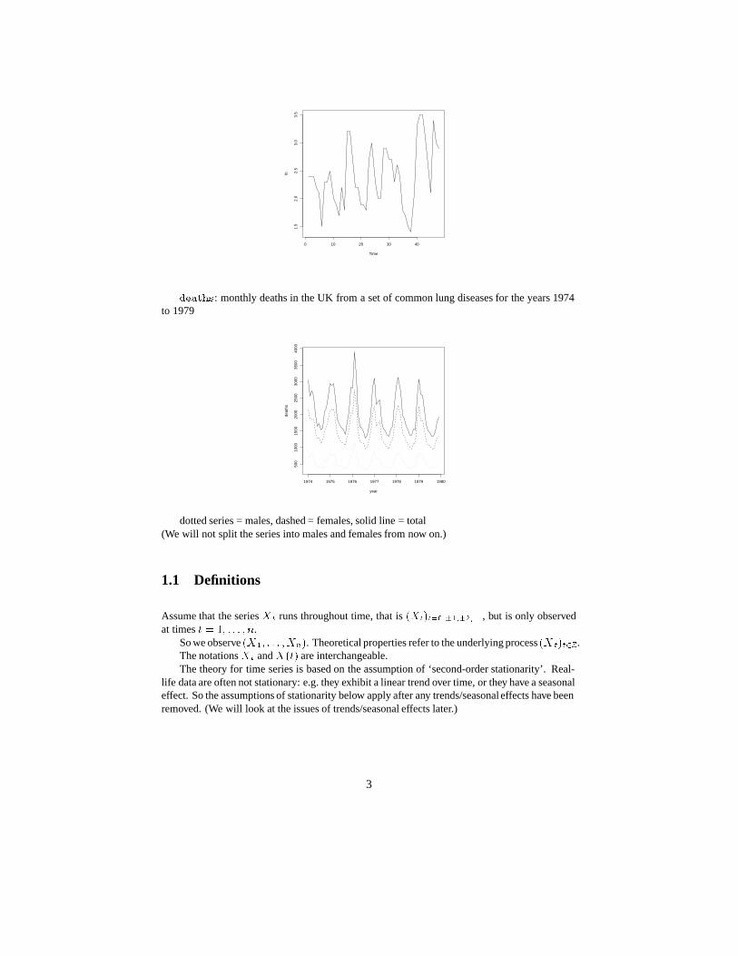
� ��: monthly deaths in the UK from a set of common lung diseases for the years 1974to 1979

year

deat

hs

1974 1975 1976 1977 1978 1979 1980

500

1000

1500

2000

2500

3000

3500

4000

dotted series = males, dashed = females, solid line = total(We will not split the series into males and females from now on.)

1.1 Definitions

Assume that the series �� runs throughout time, that is �� , but is only observedat times � � �� .

So we observe �� . Theoretical properties refer to the underlying process �� .The notations �� and �� are interchangeable.The theory for time series is based on the assumption of ‘second-order stationarity’. Real-

life data are often not stationary: e.g. they exhibit a linear trend over time, or they have a seasonaleffect. So the assumptions of stationarity below apply after any trends/seasonal effects have beenremoved. (We will look at the issues of trends/seasonal effects later.)

3

1.2 Stationarity and autocovariances

The process is called weakly stationary or second-order stationary if for all integers ��

��

��

where � is constant and � does not depend on � .The process is strictly stationary or strongly stationary if

�� and ��

have the same distribution for all sets of time points �� and all integers � .

Notice that a process that is strictly stationary is automatically weakly stationary. The con-verse of this is not true in general.

However, if the process is Gaussian, that is if �� has a multivariate normaldistribution for all �� , then weak stationarity does imply strong stationarity.

Note that �� and, by stationarity, �� .

The sequence � �� is called the autocovariance function.The autocorrelation function (acf) �� is given by

� � ��

�

The acf describes the second-order properties of the time series.

We estimate � by ��, and � by ��, where

��

�

��

�� and ��

� For � �, the covariance �� is estimated from the � � � observed pairs

��

If we take the usual covariance of these pairs, we would be using different estimates ofthe mean and variances for each of the subseries �� and �� ,whereas under the stationarity assumption these have the same mean and variance. So weuse � (twice) in the above formula.

� We use ��

rather than �� , even though there are � � � terms in the sum, to ensure that

�� is the covariance sequence of some second-order stationary series.

4

A plot of �� against � is called the correlogram.A series �� is said to be lagged if its time axis is shifted: shifting by � lags gives the series

�� .So �� is the estimated autocorrelation at lag �; it is also called the sample autocorrelation

function.

��: autocovariance function

0 5 10 15

−0.

050.

000.

050.

100.

150.

200.

250.

30

Lag

AC

F (

cov)

Series lh

��: autocorrelation function

0 5 10 15

−0.

20.

00.

20.

40.

60.

81.

0

Lag

AC

F

Series lh

� ��: autocorrelation function

5

0.0 0.5 1.0 1.5

−0.

50.

00.

51.

0

Lag

AC

F

Series deaths

2 Models of stationary processes

Assume we have a time series without trends or seasonal effects. That is, if necessary, any trendsor seasonal effects have already been removed from the series.

How might we construct a linear model for a time series with autocorrelation?

Linear processes

The process �� is called a linear process if it has a representation of the form

��

��

��

where � is a common mean, �� is a sequence of fixed constants and �� are independentrandom variables with mean 0 and common variance.

We assume�

�� to ensure that the variance of �� is finite.Such a process is strictly stationary. If �� for � � � it is said to be causal, i.e. the

process at time � does not depend on the future, as yet unobserved, values of � �.The AR, MA and ARMA processes that we are now going to define are all special cases of

causal linear processes.

2.1 Autoregressive processesAssume that a current value of the series is linearly dependent upon its previous value, with someerror. Then we could have the linear relationship

��

where �� is a white noise time series. [That is, the �� are a sequence of uncorrelated randomvariables (possibly normally distributed, but not necessarily normal) with mean 0 and variance�� .]

6

This model is called an autoregressive (AR) model, since � is regressed on itself. Here thelag of the autoregression is 1.

More generally we could have an autoregressive model of order �, an AR(�) model, definedby

��

��

��

At first sight, the AR(1) process

��

is not in the linear form ��

�� . However note that

��

� ��

� ��

� �� which is in linear form.

If �� has variance ��, then from independencewe have that

� ��

The sum converges as we assume finite variance.

But the sum converges only if �� . Thus �� is a requirement for the AR(1) processto be stationary.

We shall calculate the acf later.

2.2 Moving average processesAnother possibility is to assume that the current value of the series is a weighted sum of pastwhite noise terms, so for example that

��

Such a model is called a moving average (MA) model, since � is expressed as a weightedaverage of past values of the white noise series.

Here the lag of the moving average is 1. We can think of the white noise series as beinginnovations or shocks: new stochastically uncorrelated information which appears at each timestep, which is combined with other innovations (or shocks) to provide the observable series � .

More generally we could have a moving average model of order �, an MA(�) model, definedby

��

��

��

7

If �� has variance ��, then from independencewe have that

� ��

��

��

We shall calculate the acf later.

2.3 ARMA processesAn autoregressive moving average process ARMA(�� ) is defined by

��

��

��

��

��

where �� .A slightly more general definition of an ARMA process incorporates a non-zero mean value

�, and can be obtained by replacing � � by �� and �� by �� above.

From its definition we see that an MA(�) process is second-order stationary for any � �� .However the AR(�) and ARMA(�� ) models do not necessarily define second-order station-

ary time series.For example, we have already seen that for an AR(1) model we need the condition �� .

This is the stationarity condition for an AR(1) process. All AR processes require a condition ofthis type.

Define, for any complex number �, the autoregressive polynomial

� ��

Then the stationarity condition for an AR(�) process is:

all the zeros of the function � �� lie outside the unit circle in the complex plane�

This is exactly the condition that is needed on �� to ensure that the process is well-defined and stationary (see Brockwell and Davis 1991), pp. 85-87.

2.4 The backshift operatorDefine the backshift operator � by

��

We include the identity operator �� .Using this notation we can write the AR(�) process� � �

�� as�

� ��

��

��

or even more concisely� ��

8

Recall that an MA(�) process is ��

�� .Define, for any complex number �, the moving average polynomial

��

Then, in operator notation, the MA(�) process can be written

��

��

��

��

��

or� � ��

For an MA(�) process we have already noted that there is no need for a stationarity con-dition on the coefficients �� , but there is a different difficulty requiring some restriction on thecoefficients.

Consider the MA(1) process��

As �� has mean zero and variance � � , we can calculate the autocovariances to be

� � � ��

� � ��

� ��

� ��

� ��

� � ��

So the autocorrelations are

� � ��

� ��

Now consider the identical process but with � replaced by ��. From above we can see thatthe autocorrelation function is unchanged by this transformation: the two processes defined by� and �� cannot be distinguished.

It is customary to impose the following identifiability condition:

all the zeros of the function �� lie outside the unit circle in the complex plane�

The ARMA(�� ) process

��

��

��

��

��

where �� , can be written� ��

The conditions required are

9

1. the stationarity condition on �� 2. the identifiability condition on �� 3. an additional identifiability condition: � �� and �� have no common roots.

Condition 3 is to avoid having an ARMA(�� ) model which can, in fact, be expressed as a lowerorder model, say as an ARMA(�� ) model.

2.5 DifferencingThe difference operator� is given by

��

These differences form a new time series �� (of length �� if the original series had length�). Similarly

��

and so on.If our original time series is not stationary, we can look at the first order difference process

�� , or second order differences �� , and so on. If we find that a differenced process is astationary process, we can look for an ARMA model of that differenced process.

In practice if differencing is used, usually � �, or maybe � �, is enough.

2.6 ARIMA processesThe process�� is said to be an autoregressiveintegrated moving averageprocessARIMA(�� )if its th difference�� is an ARMA(�� ) process.

An ARIMA(�� ) model can be written

� ��

or� ��

2.7 Second order properties of MA(�)

For the MA(�) process��

�� , where �� , it is clear that �� for all �.Hence, for � �, the autocovariance function is

� � ��

� �

��

��

��

��

��

�

�

��

��

��

Since the �� sequence is white noise, �� unless ! � " �.

10

Hence the only non-zero terms in the sum are of the form � �� and we have

� �

��

��

� ��

and the acf is obtained via � � ��.In particular notice that the acf if zero for �� . This ‘cut-off’ in the acf after lag � is

a characteristic property of the MA process and can be used in identifying the order of an MAprocess.

��: MA(1) with � � ��

0 5 10 15 20 25 30

0.0

0.2

0.4

0.6

0.8

1.0

Lag

AC

F

Series ma1.sim

��: MA(2) with ��

0 5 10 15 20 25 30

0.0

0.2

0.4

0.6

0.8

1.0

Lag

AC

F

Series ma2.sim

To identify an MA(�) process:We have already seen that for an MA(�) time series, all values of the acf beyond lag � are

zero: i.e. � � � for � �.So plots of the acf should show a sharp drop to near zero after the �th coefficient. This is

therefore a diagnostic for an MA(�) process.

11

2.8 Second order properties of AR(�)

Consider the AR(�) process

��

��

��

For this model �� (why?).Hence multiplying both sides of the above equation by � �� and taking expectations gives

� �

��

��

In terms of the autocorrelations � � ��

� �

��

��

These are the Yule-Walker equations.The population autocorrelations � are thus found by solving the Yule-Walker equations:

these autocorrelations are generally all non-zero.Our present interest in the Yule-Walker equations is that we could use them to calculate the

� if we knew the �. However later we will be interested in using them to infer the values of �

corresponding to an observed set of sample autocorrelation coefficients.

��: AR(1) with � � ��

0 5 10 15 20 25 30

0.0

0.2

0.4

0.6

0.8

1.0

Lag

AC

F

Series ar1.sim

��: AR(2) with ��

12

0 5 10 15 20 25 30

0.0

0.2

0.4

0.6

0.8

1.0

Lag

AC

F

Series ar2.sim

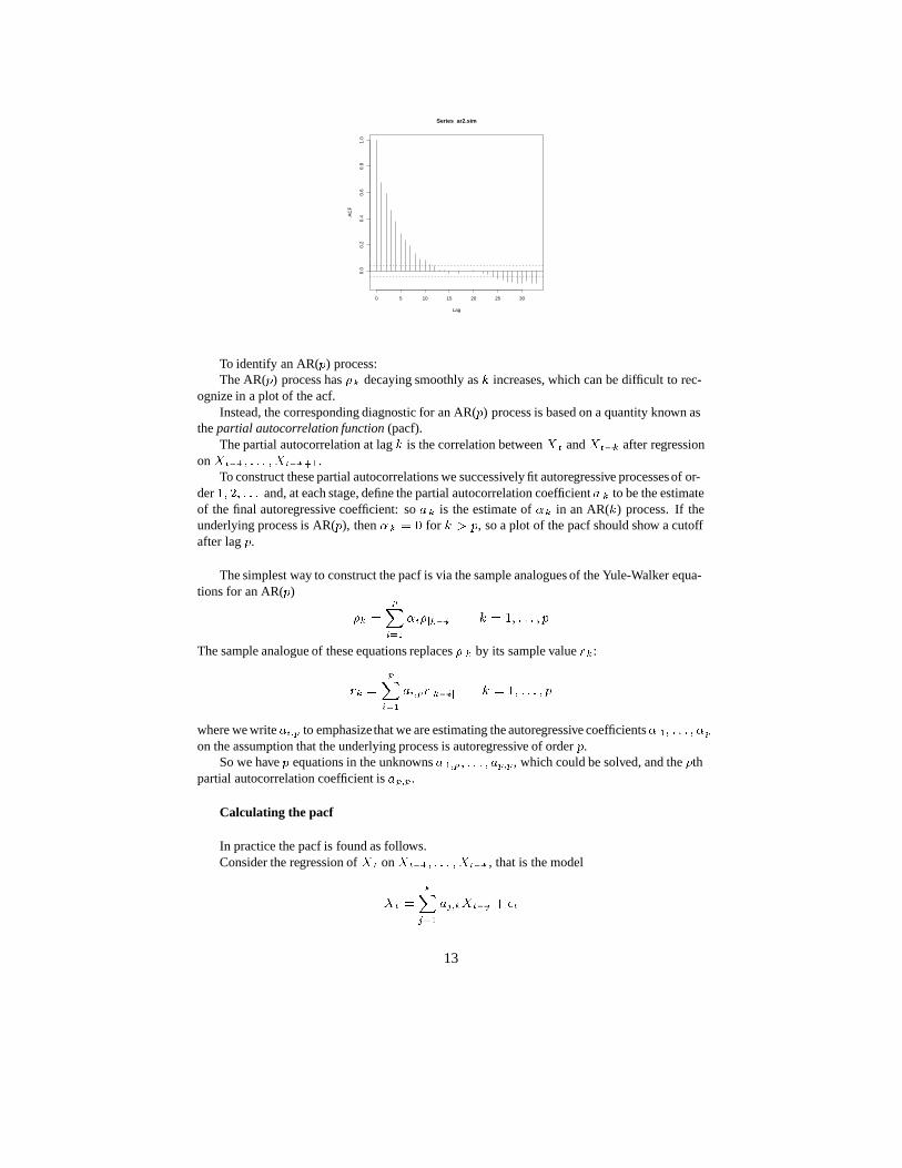
To identify an AR(�) process:The AR(�) process has � decaying smoothly as � increases, which can be difficult to rec-

ognize in a plot of the acf.Instead, the corresponding diagnostic for an AR(�) process is based on a quantity known as

the partial autocorrelation function (pacf).The partial autocorrelation at lag � is the correlation between � � and �� after regression

on �� .To construct these partial autocorrelations we successively fit autoregressive processesof or-

der �� and, at each stage, define the partial autocorrelation coefficient � � to be the estimateof the final autoregressive coefficient: so �� is the estimate of �� in an AR(�) process. If theunderlying process is AR(�), then �� for � �, so a plot of the pacf should show a cutoffafter lag �.

The simplest way to construct the pacf is via the sample analogues of the Yule-Walker equa-tions for an AR(�)

� �

��

��

The sample analogue of these equations replaces � by its sample value ��:

��

��

��

where we write �� to emphasize that we are estimating the autoregressive coefficients� �� on the assumption that the underlying process is autoregressive of order �.

So we have � equations in the unknowns � �� , which could be solved, and the �thpartial autocorrelation coefficient is �� .

Calculating the pacf

In practice the pacf is found as follows.Consider the regression of �� on �� , that is the model

��

��

��

13

with �� independent of �� .Given data �� , least squares estimates of �� are obtained by min-

imising

��

�

��

��

��

��

��

�

These �� coefficients can be found recursively in � for � � �� .For � � �: �� ; �� , and �� .And then, given the �� values, the �� values are given by

��

��

� ��

�� ! � ��

and then

��

This recursive method is the Levinson-Durbin recursion.The �� value is the �th sample partial correlation coefficient.In the case of a Gaussian process, we have the interpretation that

��

If the process�� is genuinely an AR(�) process, then �� for � �.So a plot of the pacf should show a sharp drop to near zero after lag �, and this is a diagnostic

for identifying an AR(�).

��: AR(1) with � � ��

0 5 10 15 20 25 30

0.0

0.1

0.2

0.3

0.4

0.5

Lag

Par

tial A

CF

Series ar1.sim

��: AR(2) with ��

14

0 5 10 15 20 25 30

0.0

0.2

0.4

0.6

Lag

Par

tial A

CF

Series ar2.sim

��: MA(1) with � � ��

0 5 10 15 20 25 30

−0.

2−

0.1

0.0

0.1

0.2

0.3

Lag

Par

tial A

CF

Series ma1.sim

��: MA(2) with ��

0 5 10 15 20 25 30

−0.

20.

00.

20.

4

Lag

Par

tial A

CF

Series ma2.sim

Tests on sample autocorrelations

15

To determine whether the values of the acf, or the pacf, are negligible, we can use the ap-proximation that they each have a standard deviation of around ��

�.

So this would give �� as approximate confidence bounds (2 is an approximation to

1.96). In R these are shown as blue dotted lines.Values outside the range��

� can be regarded as significant at about the 5% level. But if

a large number of �� values, say, are calculated it is likely that some will exceed this thresholdeven if the underlying time series is a white noise sequence.

Interpretation is also complicated by the fact that the �� are not independently distributed.The probability of any one �� lying outside��

� depends on the values of the other � � .

3 Statistical Analysis

3.1 Fitting ARIMA models: The Box-Jenkins approachThe Box-Jenkins approach to fitting ARIMA models can be divided into three parts:

� Identification;

� Estimation;

� Verification.

3.1.1 Identification

This refers to initial preprocessingof the data to make it stationary, and choosingplausible valuesof � and � (which can of course be adjusted as model fitting progresses).

To assess whether the data come from a stationary process we can

� look at the data: e.g. a time plot as we looked at for the �� series;

� consider transforming it (e.g. by taking logs;)

� consider if we need to difference the series to make it stationary.

For stationarity the acf should decay to zero fairly rapidly. If this is not true, then try dif-ferencing the series, and maybe a second time if necessary. (In practice it is rare to go beyond � � stages of differencing.)

The next step is initial identification of � and �. For this we use the acf and the pacf, recallingthat

� for an MA(�) series, the acf is zero beyond lag �;

� for an AR(�) series, the pacf is zero beyond lag �.

We can use plots of the acf/pacf and the approximate�� confidence bounds.

16

3.1.2 Estimation: AR processes

For the AR(�) process

��

��

��

we have the Yule-Walker equations � ��

�� , for � �.We fit the parameters �� by solving

��

��

��

These are � equations for the � unknowns � �� which, as before, can be solved using aLevinson-Durbin recursion.

The Levinson-Durbin recursion gives the residual variance

��

�

��

��

��

��

��

�

This can be used to guide our selection of the appropriate order �. Define an approximate loglikelihood by

�� # � � ��Then this can be used for likelihood ratio tests.

Alternatively, � can be chosen by minimising AIC where

$�� # ��

and � � � is the number of unknown parameters in the model.

If �� is a causal AR(�) process with i.i.d. WN�� , then (see Brockwell and Davis(1991), p.241) then the Yule-Walker estimator �� is optimal with respect to the normal distribu-tion.

Moreover (Brockwell and Davis (1991), p.241) for the pacf of a causal AR(�) process wehave that, for % �,

��

is asymptotically standard normal. However, the elements of the vector �� are in general not asymptotically uncorrelated.

3.1.3 Estimation: ARMA processes

Now we consider an ARMA(�� ) process. If we assume a parametric model for the white noise– this parametric model will be that of Gaussian white noise – we can use maximum likelihood.

We rely on the prediction error decomposition. That is, � �� have joint density

&�� &��

&��

17

Suppose the conditional distribution of �� given �� is normal with mean �� andvariance '��, and suppose that �� (� �� '��. (This is as for the Kalman filter – see later.)

Then for the log likelihood we obtain

�� # ��

��)� �� '��

�� *��'��

�

Here �� and '�� are functions of the parameters �� , and so maximumlikelihood estimators can be found (numerically) by minimising �� # with respect to theseparameters.

The matrix of second derivatives of �� #, evaluated at the mle, is the observed informa-tion matrix, and its inverse is an approximation to the covariance matrix of the estimators. Hencewe can obtain approximate standard errors for the parameters from this matrix.

In practice, for AR(�) for example, the calculation is often simplified if we condition on thefirst % values of the series for some small %. That is, we use a conditional likelihood, and sothe sum in the expression for �� # is taken over � � % � to �.

For an AR(�) we would use some small value of %, % � �.

When comparing models with different numbers of parameters, it is important to use thesame value of %, in particular when minimising AIC � �� # �� . In R this cor-responds to keeping �� in the �� command fixed when comparing the AIC of severalmodels.

3.1.4 Verification

The third step is to check whether the model fits the data.Two main techniques for model verification are

� Overfitting: add extra parameters to the model and use likelihood ratio or � tests to checkthat they are not significant.

� Residual analysis: calculate residuals from the fitted model and plot their acf, pacf, ‘spec-tral density estimates’, etc, to check that they are consistent with white noise.

3.1.5 Portmanteau test of white noise

A useful test for the residuals is the Box-Pierce portmanteau test. This is based on

+ � ��

��

where , � � but much smaller than �, and �� is the acf of the residual series. If the modelis correct then, approximately,

+ � -��

18

so we can base a test on this: we would reject the model at level � if + - �� .

An improved test is the Box-Ljung procedure which replaces + by

�+ � ��

��

�

The distribution of �+ is closer to a -�� than that of +.

3.2 Analysis in the frequency domain

We can consider representing the variability in a time series in terms of harmonic componentsat various frequencies. For example, a very simple model for a time series � � exhibiting cyclicfluctuations with a known period, � say, is

�� .�� .��

where �� is a white noise sequence,. � �)�� is the known frequency of the cyclic fluctuations,and � and � are parameters (which we might want to estimate).

Examining the second-order properties of a time series via autocovariances/autocorrelationsis ‘analysis in the time domain’.

What we are about to look at now, examining the second-order properties by considering thefrequency components of a series is ‘analysis in the frequency domain’.

3.2.1 The spectrum

Suppose we have a stationary time series � � with autocovariances ��.For any sequence of autocovariances � �� generated by a stationary process, there exists a

function / such that

� �

� �

��

0�� / �1�

where / is the unique function on �)� )� such that

1. / ��)� � �

2. / is non-decreasing and right-continuous

3. the increments of / are symmetric about zero, meaning that for � � � � 2 � ),

/ �2�� / �� / �� / ��2��

The function / is called the spectral distribution function or spectrum. / has many of theproperties of a probability distribution function, which helps explain its name, but / �)� � � isnot required.

The interpretation is that, for � � � � 2 � ), / �2��/ �� measures the contribution to thetotal variability of the process within the frequency range � � 1 � 2.

If / is everywhere continuous and differentiable, then

&�1� � / �1�

1

19

is called the spectral density function and we have

� �

� �

��

0��&�1� 1�

It� �� , then it can be shown that & always exists and is given by

&�1� ��

�)

��

�0��

��)

�

)

��

� ��1��

By the symmetry of �, &�1� � &��1�.From the mathematical point of view, the spectrum and acf contain equivalent information

concerning the underlying stationary random sequence �� . However, the spectrum has a moretangible interpretation in terms of the inherent tendency for realizations of �� to exhibit cyclicvariations about the mean.

[Note that some authors put constants of �) in different places. For example, some put afactor of ��)� in the integral expression for � in terms of /�& , and then they don’t need a��)� factor when giving & in terms of � .]

Example: WN(�� )

Here, � � �� , � � � for � �� , and so we have immediately

&�1� ��

�)for all 1

which is independent of 1.The fact that the spectral density is constant means that all frequencies are equally present,

and this is why the sequence is called ‘white noise’. The converse also holds: i.e. a process iswhite noise if and only if its spectral density is constant.

Example: AR(1): �� .

Here � � �� and � � �� for � �� .So

&�1� ��

�)�

��

��0��

��)

�

�)�

��

��0��

�)�

��

��0��

��)

��

�0�

�� 0�

�0��

�� 0��

�

��

�)�� 1 ��

��

�)�� 1 ��

where we used 0�� 0� � �� 1.

��: AR(1) with � � ��

20

0.0 0.1 0.2 0.3 0.4 0.5

0.5

1.0

2.0

frequency

spec

trum

Series: ar1.simAR (1) spectrum

��: AR(1) with � � ��

0.0 0.1 0.2 0.3 0.4 0.5

0.5

1.0

2.0

frequency

spec

trum

Series: ar1b.simAR (2) spectrum

Plotting the spectral density &�1�, we see that in the case� � the spectral density &�1� isa decreasing function of 1: that is, the power is concentrated at low frequencies, correspondingto gradual long-range fluctuations.

For � � � the spectral density &�1� increases as a function of 1: that is, the power isconcentrated at high frequencies, which reflects the fact that such a process tends to oscillate.

ARMA(�� ) process

��

��

��

��

��

The spectral density for an ARMA(�,�) process is related to the AR and MA polynomials � ��and ��.

The spectral density of �� is

&�1� ��

�)

��0�� 0��

21

Example: AR(1) Here � �� and �� , so, for �) � 1 � ),

&�1� ��

�)�� 0��

��

�)�� 1 "� �� 1��

��

�)�� 1�� 1��

��

�)�� 1 ��

as calculated before.

Example: MA(1)Here � �� 3�, and we obtain, for �) � 1 � ),

&�1� ��)�� 30��

��)

�� 3 ��1� 3��

Plotting the spectral density &�1�, we would see that in the case 3 � the spectral densityis large for low frequencies, small for high frequencies. This is not surprising, as we have short-range positive correlation, smoothing the series.

For 3 � � the spectral density is large around high frequencies, and small for low frequen-cies; the series fluctuates rapidly about its mean value. Thus, to a coarse order, the qualitativebehaviour of the spectral density is similar to that of an AR(1) spectral density.

3.2.2 The Periodogram

To estimate the spectral density we use the periodogram.For a frequency . we compute the squared correlation between the time series and the

sine/cosine waves of frequency .. The periodogram ��.� is given by

��.� ��

�)�

��

0��

��

��

�)�

��

�� .��

�

��

�� .��

��

The periodogram is related to the autocovariance function by

��.� ��

�)

��

��0��

��)

�

)

��

�� .��

��

� �

��

0��.� .�

22

So the periodogram and the autocovariance function contain the same information. For thepurposes of interpretation, sometimes one will be easier to interpret, other times the other willbe easier to interpret.

��: AR(1) with � � ��

0.0 0.1 0.2 0.3 0.4 0.5

1e−

031e

−02

1e−

011e

+00

1e+

01

frequency

spec

trum

Series: ar1.simRaw Periodogram

bandwidth = 0.000144

��: AR(1) with � � ��

0.0 0.1 0.2 0.3 0.4 0.5

1e−

031e

−02

1e−

011e

+00

1e+

01

frequency

spec

trum

Series: ar1b.simRaw Periodogram


��: MA(1) with � � ��

0.0 0.1 0.2 0.3 0.4 0.5

1e−

031e

−02

1e−

011e

+00

1e+

01

frequency

spec

trum

Series: ma1.simRaw Periodogram


23

From asymptotic theory, at Fourier frequencies . � . � � �)!��, ! � �� , the peri-odogram ordinates ��.�� .�� are approximately independentwith means�&�. �� &�.�� .That is for these .

��.� � &�.��

where � is an exponential distribution with mean 1.

Note that ��.�� &�.��, which does not tend to zero as � � �. So ��.� is NOT aconsistent estimator.

In addition, the independence of the periodogram ordinates at different Fourier frequenciessuggests that the sample periodogram, as a function of ., will be extremely irregular. For thisreason smoothing is often applied, for instance using a moving average, or more generally asmoothing kernel.

3.2.3 Smoothing

The idea behind smoothing is to take weighted averages over neighbouring frequencies in orderto reduce the variability associated with individual periodogram values.

The main form of a smoothed esimator is given by

�&�.� �

��

4,

�1� .

4

��1� 1�

Here, is some kernel function (� a probability density function), for example a standard normalpdf, and 4 is the bandwidth.

The bandwidth 4 affects the degree to which this process smooths the periodogram. Small4 � a little smoothing, large 4 � a lot of smoothing.

In practice, the smoothed esimate �&�.� will be evaluated by the sum

�&�.� ��

� ��

��

�

4,

�1� .

4

��1� 1

�)

�

��

�

4,�.� � .

4

��.��

As the degree of smoothing 4 increases, the variance decreases but the bias increases.

The cumulative periodogram5�.� is defined by

5�.� ��

��

��.��

��

��.��

This can be used to test residuals in a fitted model, for example. If we hope that our residualseries is white noise, the the cumulative periodogram of the residuals should increase linearly:i.e. we can plot the cumulative periodogram (in R) and look to see if the plot is an approximatestraight line.

Example: Brockwell & Davis (p 339, 340)

24

Data generated by�� )��

where �� is Gaussian white noise with variance 1.Peak in the periodogram at .� � ��).

[Figure from B& D]

Example series: ��

Time

lh

0 10 20 30 40

1.5

2.0

2.5

3.0

3.5

Example series: � ��

year

deat

hs

1974 1975 1976 1977 1978 1979 1980

500

1000

1500

2000

2500

3000

3500

4000

��: unsmoothed periodogram

25

0.1 0.2 0.3 0.4 0.5

−20

−15

−10

−5

0

frequency

spec

trum

(dB

)

lh: Raw Periodogram

bandwidth = 0.00601, 95% C.I. is (−6.26,16.36)dB

� ��: unsmoothed periodogram

0 1 2 3 4 5 6

2530

3540

4550

5560

frequency

spec

trum

(dB

)

deaths: Raw Periodogram

bandwidth = 0.0481, 95% C.I. is (−6.26,16.36)dB

Suppose we have estimated the periodogram values ��. �� .�� , where .� � �)!��,! � �� .

An example of a simple way to smooth is to use a moving average, and so estimate ��. �� by

�

��.��

�

��.�� .�� .��

�

��.��

Observe that the sum of the weights above (i.e. the �� s and the �

� s) is 1.Keeping the sum of weights equal to 1, this process could be modified by using more, or

fewer, ��.�� values to estimate ��.��.Also, this smoothing process could be repeated.

If a series is (approximately) periodic, say with frequency .�, then periodogram will showa peak near this frequency.

It may well also show smaller peaks at frequencies �. �� .�� .The integer multiples of .� are called its harmonics, and the secondary peaks at these high

frequencies arise because the cyclic variation in the original series is non-sinusoidal. (So asituation like this warns against interpreting multiple peaks in the periodogram as indicating thepresence of several distinct cyclic mechanisms in the underlying process.)

26

In R, smoothing is controlled by the option �� to the �� function.The unsmoothed periodogram (above) was obtained via �� The smoothed versions below are

��

��

��

All of the examples, above and below, from Venables & Ripley.V & R advise:

� trial and error needed to choose the spans;

� spans should be odd integers;

� use at least two, which are different, to get a smooth plot.

0.1 0.2 0.3 0.4 0.5

−15

−10

−5

0

frequency

spec

trum

(dB

)

lh: Smoothed Periodogram, spans=3

bandwidth = 0.0159, 95% C.I. is (−4.32, 7.73)dB

0.1 0.2 0.3 0.4 0.5

−14

−12

−10

−8

−6

−4

−2

frequency

spec

trum

(dB

)

lh: Smoothed Periodogram, spans=c(3,3)


27

0.1 0.2 0.3 0.4 0.5

−12

−10

−8

−6

−4

−2

frequency

spec

trum

(dB

)

lh: Smoothed Periodogram, spans=c(3,5)


0 1 2 3 4 5 6

3540

4550

55

frequency

spec

trum

(dB

)

deaths: Smoothed Periodogram, spans=c(3,3)


0 1 2 3 4 5 6

3540

4550

frequency

spec

trum

(dB

)



28

0 1 2 3 4 5 6

3540

4550

frequency

spec

trum

(dB

)



��: cumulative periodogram

0.0 0.1 0.2 0.3 0.4 0.5

0.0

0.2

0.4

0.6

0.8

1.0

frequency

Series: lh

� ��: cumulative periodogram

0 1 2 3 4 5 6

0.0

0.2

0.4

0.6

0.8

1.0

frequency

Series: deaths

29

3.3 Model fitting using time and frequency domain

3.3.1 Fitting ARMA models

The value of ARMA processes lies primarily in their ability to approximate a wide range ofsecond-order behaviour using only a small number of parameters.

Occasionally, we may be able to justify ARMA processes in terms of the basic mechanismsgenerating the data. But more frequently, they are used as a means of summarising a time seriesby a few well-chosen summary statistics: i.e. the parameters of the ARMA process.

Now consider fitting an AR model to the �� series. Look at the pacf:

5 10 15

−0.

20.

00.

20.

40.

6

Lag

Par

tial A

CF

Series lh

Fit an AR(1) model:

�� ! �� "� ��

The fitted model is:��

with �� .One residual plot we could look at is

��#��$� ��

��: cumulative periodogram of residuals from AR(1) model

0.0 0.1 0.2 0.3 0.4 0.5

0.0

0.2

0.4

0.6

0.8

1.0

frequency

AR(1) fit to lh

30

Also try select the order of the model using AIC:

�� ! �� %�

��$��

��$��

This selects the AR(3) model:

��

with �� .The same order is selected when using

�� ! �� &'�

��$��

��: cumulative periodogram of residuals from AR(3) model

0.0 0.1 0.2 0.3 0.4 0.5

0.0

0.2

0.4

0.6

0.8

1.0

frequency

AR(3) fit to lh

By default, � fits by using the Yule-Walker equations.We can also use�� in ��(��)*��

to fit these models using maximum likelihood. (Examples in Venables & Ripley, and in thepractical class)

The function ��# produces diagnostic residuals plots. As mentioned in a previous lec-ture, the �-values from the Ljung-Box statistic are of concern if they go below 0.05 (marked witha dotted line on the plot).

��: diagnostic plots from AR(1) model

31

Standardized Residuals

Time

0 10 20 30 40

−1

01

2

0 5 10 15

−0.

20.

20.

61.

0

Lag

AC

F

ACF of Residuals

2 4 6 8 10

0.0

0.4

0.8

p values for Ljung−Box statistic

lag

p va

lue

��: diagnostic plots from AR(3) model

Standardized Residuals

Time

0 10 20 30 40

−1

01

23

0 5 10 15

−0.

20.

20.

61.

0

Lag

AC

F

ACF of Residuals

2 4 6 8 10

0.0

0.4

0.8

p values for Ljung−Box statistic

lag

p va

lue

3.3.2 Estimation and elimination of trend and seasonal components

The first step in the analysis of any time series is to plot the data.If there are any apparent discontinuities, such as a suddenchangeof level, it may be advisable

to analyse the series by first breaking it into a homogeneous segments.

We can think of a simple model of a time series as comprising

� deterministic components, i.e. trend and seasonal components

� plus a random or stochastic component which shows no informative pattern.

We might write such a decomposition model as the additive model

�� %� 6� 7�

where

%� � trend component (or mean level) at time ��

6� � seasonal component at time ��

7� � random noise component at time ��

32

Here the trend %� is a slowly changing function of �, and if is the number of observations in acomplete cycle then 6� � 6��.

In some applications a multiplicative model may be appropriate

�� %�6�7��

After taking logs, this becomes the previous additive model.

It is often possible to look at a time plot of the series to spot trend and seasonal behaviour.We might look for a linear trend in the first instance, though in many applications non-lineartrend is also of interest and present.

Periodic behaviour is also relatively straightforward to spot. However, if there are two ormore cycles operating at different periods in a time series, then it may be difficult to detect suchcycles by eye. A formal Fourier analysis can help.

The presence of both trend and seasonality together can make it more difficult to detect oneor the other by eye.

Example: Box and Jenkins airline data. Monthly totals (thousands) of international airlinepassengers, 1949 to 1960.

Time

AirP

asse

nger

s

1950 1952 1954 1956 1958 1960

100

200

300

400

500

600

��# ! ��#�*��+�� # ��

��#�

Time

airp

ass.

log

1950 1952 1954 1956 1958 1960

5.0

5.5

6.0

6.5

33

We can aim to estimate and extract the deterministic components % � and 6�, and hope thatthe residual or noise component 7 � turns out to be a stationary process. We can then try to fit anARMA process, for example, to 7�.

An alternative approach (Box-Jenkins) is to apply the difference operator � repeatedly tothe series�� until the differenced series resembles a realization of a stationary process, and thenfit an ARMA model to the suitably differenced series.

3.3.3 Elimination of trend when there is no seasonal component

The model is�� %� 7�

where we can assume��7 �� .

1: Fit a Parametric Relationship

We can take %� to be the linear trend %� � �� , or some similar polynomial trend,and estimate %� by minimising

�� %�� with respect to �� .

Then consider fitting stationary models to * � � �� %�, where �%� � �� .Non-linear trends are also possible of course, say ��% � � ��

� (� � � � �),%� � �� 0

� ��, . . .In practice, fitting a single parametric relationship to an entire time series is unrealistic, so

we may fit such curves as these locally, by allowing the parameters � to vary (slowly) with time.The resulting series *� � �� %� is the detrended time series.

Fit a linear trend:

0 20 40 60 80 100 120 140

5.0

5.5

6.0

6.5

time step

airp

ass.

log

The detrended time series:

34

0 20 40 60 80 100 120 140

−0.

3−

0.2

−0.

10.

00.

10.

20.

3

time step

2: Smoothing

If the aim is to provide an estimate of the local trend in a time series, then we can apply amoving average. That is, take a small sequence of the series values � �� ,and compute a (weighted) average of them to obtain a smoothed series value at time �, say �% �,where �%� �

�

��

��

��

It is useful to think of ��%�� as a process obtained from � �� by application of a linear filter�%� ��

�� , with weights �� , �� ! � �, and �� , �!� �.

This filter is a ‘low pass’ filter since it takes data �� and removes from it the rapidly fluctu-ating component *� � �� %�, to leave the slowly varying estimated trend term �%�.

We should not choose � too large since, if % � is not linear, although the filtered process willbe smooth, it will not be a good estimate of %�.

If we apply two filters in succession, for example to progressively smooth a series, we aresaid to be using a convolution of the filters.

By careful choice of the weights �� , it is possible to design a filter that will not only beeffective in attenuating noise from the data, but which will also allow a larger class of trendfunctions.

Spencer’s 15-point filter has weights

�� !� � �

�� !� �

��

��

and has the property that a cubic polynomial passes through the filter undistorted.

�� ! ��!��!,�!��&��-,�,.�.-�,.�-,�&��!��!,�!��&'

�� ! �� #� ��

��#� �� &��

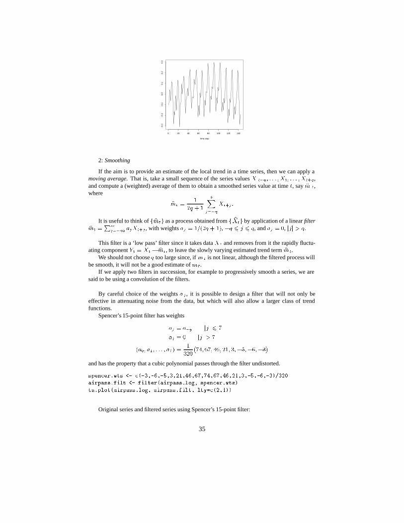
Original series and filtered series using Spencer’s 15-point filter:

35

Time

log(

AirP

asse

nger

s)

1950 1952 1954 1956 1958 1960

5.0

5.5

6.0

6.5

Detrended series via filtering:

Time

airp

ass.

log

− a

irpas

s.fil

t

1950 1952 1954 1956 1958 1960

−0.

15−

0.10

−0.

050.

000.

050.

100.

15

3: Differencing

Recall that the difference operator is�� . Note that differencing is a specialcase of applying a linear filter.

We can think of differencing as a ‘sample derivative’. If we start with a linear function, thendifferentiation yields a constant function, while if we start with a quadratic function we need todifferentiate twice to get to a constant function.

Similarly, if a time series has a linear trend, differencing the series once will remove it, whileif the series has a quadratic trend we would need to difference twice to remove the trend.

Detrended series via differencing:

36

Year

1950 1952 1954 1956 1958 1960

−0.

2−

0.1

0.0

0.1

0.2

3.4 SeasonalityAfter removing trend, we can remove seasonality. (Above, all detrended versions of the airlinedata clearly still have a seasonal component.)

1: Block averagingThe simplest way to remove seasonality is to average the observations at the same point in

each repetition of the cycle (for example, for monthly data average all the January values) andsubtract that average from the values at those respective points in the cycle.

2: Seasonal differencingThe seasonal difference operator is� �� where 6 is the period of the seasonal

cycle. Seasonal differencing will remove seasonality in the same way that ordinary differencingwill remove a polynomial trend.

�� !��#�

��& ! �� #��&�

��&�

Time

airp

ass.

diff2

1950 1952 1954 1956 1958 1960

−0.

15−

0.10

−0.

050.

000.

050.

100.

15

37

After differencing at lag 1 (to remove trend), then at lag 12 (to remove seasonal effects), the��#�*��+�� # �� series appears stationary.

That is, the series�� , or equivalently the series �� , appears stationary.

R has a function �� which you can use to estimate and remove trend and seasonality using‘loess’.

�� is a complex function, you should consult the online documentation before you use it.The time series chapter of Venables & Ripley contains examples of how to use ��. As with allaspects of that chapter, it would be a good idea for you to work through the examples there.

We could now look to fit an ARMA model to �� , or to the residual component ex-tracted by ��.

Seasonal ARIMA models

Recall that � is an ARMA(�� ) process if

��

��

��

��

and � is an ARIMA(�� ) process if �� is ARMA(�� ).In shorthand notation, these processes are

� �� and � ��

Suppose we have monthly observations, so that seasonal patterns repeat every 6 � �� ob-servations. Then we may typically expect � � to depend on such terms as � ��, and maybe��, as well as �� .

A general seasonal ARIMA (SARIMA) model, is

�� * � ��

��

where �� are polynomials of orders ��'� ��+ and where

* � ��

Here:

� 6 is the number of observarions per season, so 6 � �� for monthly data;

� 8 is the order of seasonal differencing, i.e. differencing at lag 6 (we were content with8 � � for the air passenger data);

� is the order of ordinary differencing (we were content with � � for the air passengerdata).

This model is often referred to as an ARIMA(�� '�8�+��) model.

Examples

1. Consider a ARIMA model of order �� .

38

This model can be written

�� *� � ��

where*� � ��

2. The ‘airline model’ (so named because of its relevance to the air passenger data) is aARIMA model of order �� .

This model can be written

*� � ��

where *� � �� is the series we obtained after differencing to reach stationarity, i.e. onestep of ordinary differencing, plus one step of seasonal (lag 12) differencing.

4 State space modelsState-space models assume that the observations �� are incomplete and noisy functions ofsome underlying unobservable process �* ��, called the state process, which is assumed to havea simple Markovian dynamics. The general state space model is described by

1. *�� *�� *�� is a Markov chain

2. Conditionally on �*��, the ��’s are independent, and �� depends on *� only.

When the state variables are discrete, one usually calls this model a hidden Markov model; theterm state space model is mainly used for continuous state variables.

4.1 The linear state space modelA prominent role is played by the linear state space model

*� � 9�*�� (1)

�� :�*� ;�� (2)

where 9� and :� are deterministic matrices, and �� and �;�� are two independent whitenoise sequences with � � and ;� being mean zero and having covariance matrices � �

� and < �� ,

respectively. The general case,

*� � =��*��

�� 4��*�� ;��

is much more flexible. Also, multivariate models are available. The typical question on statespace models is the estimation or the prediction of the states �* �� in terms of the observed datapoints ��.

Example. Suppose the model

*� � �*��

�� *� ;��

39

where �� and �;�� are two independent white noise sequences with � � and ;� being meanzero and having covariance � �

� and < �� , respectively. Then

�� *� � �*�� ;� � �;��

� �� ;� � �;��

The right-hand side shows that all correlations at lags� � are zero. Hence the right-hand side isequivalent to an MA(1) model, and thus �� follows an ARMA(1,1)-model.

In fact any ARMA(�,�)-model with Gaussian WN can be formulated as a state space model.The representation of an ARMA model as a state-space model is however not unique, see Brock-well and Davis (1991), pp.469-470.

Note that the above model is more flexible than an ARMA model. If, for example, theobservation at time � is missing, then we simply put :� � �� .

4.2 Filtering, smoothing, and forecasting

The primary aims of the analysis of state space models are to produce estimators for the un-derlying unobserved signal * � given the data �� up to time 6. When 6 � �the problem is called forecasting, when 6 � � it is called filtering, and when 6 � it is calledsmoothing. For a derivation of the results below see also Smith (2001).

We will throughout assume the white noise to be Gaussian.

For filtering and forecasting, we use the Kalman filter. It is a recursive method to calculatea conditional distribution within a multivariate normal framework. As it is recursive, only theestimated state from the previous time step and the current measurement are needed to computethe estimate for the current state.

The state of the filter is represented by two variables: the estimate of the state at time t;and the error covariance matrix (a measure of the estimated accuracy of the state estimate). TheKalman filter has two distinct phases: Predict and Update. The predict phase uses the state esti-mate from the previous timestep to produce an estimate of the state at the current timestep. In theupdate phase, measurement information at the current timestep is used to refine this predictionto arrive at a new, (hopefully) more accurate state estimate, again for the current timestep.

It is useful to first revise some distributional results for multivariate normal distributions. Sup-pose that �

7�

7�

��

��

�

��

��

� (3)

Then the conditional distribution of 7� given 7� � �� is

��7��7� � ��

��

��

�(4)

and conversely, if 7� �� and if (4) holds, then (3) holds.

Assume the model

*� � 9�*��

�� :�*� ;��

40

with �� independent white noise <(�� , and �;�� ind. <(��<��. Here, *� is avector representing unknown states of the system, and � � are the observed data. . Put �� , the history of � up to time �, and

* �� *��

' �� *�� * �

��*�� * ��

� �� *�� * �

��*�� * ��

� ��When �� , we will write '�

� for convenience.

Suppose * �� and ' �

� � ��, and that the conditional distribution of *�� given the history�� up to time �� ,

��*�� * �� '��

Then ��*�� is again multivariate normal. With

>� � 9�'��9��

we have that

��*�� :�*�

� ��*�� <��

Then the conditional distribution of �� *�� given�� is given by

��

��

*�

��

��

��:�9�*

��

9�*��

�

�<� :�>�:

�� :�>�

>�:�� >�

�

We can compute that the conditional distribution of *� given �� is multivariate normal withmean * �

� and variance '�, where

* �� 9�*

�� >�:

�� <� :�>�:

�� :�9�*

��

'� � >� � >�:�� <� :�>�:

�� :�>��

These equations are known as the Kalman filter updating equations. This solves the filteringproblem.

Have a look at the expression for * �� . It contains the term 9�*

�� , which is simply what we

would predict if it were known that *�� * �� , plus a term which depends on the observed

error in forecasting, i.e. �� :�9�*�� .

Note that we initialized the recursion by � �� and ' �

� � �� . Instead one might haveinitialized the recursion by some prior distribution, of by an uninformative prior � �

� � �� ' ��

�� , where � denotes the identity matrix.

For forecasting, suppose � 6. By induction, assume we know * �� '

��. Then

* �� 9�*

��

' �� 9�'

��9

��

41

Recursion solves the forecasting problem.

We can calculate that the conditional distribution of �� given�� is

�� :��9��*��:��>��:

�� <��

This fact is the basis of the prediction error decomposition, giving us a likelihood for parameterestimation.

For smoothing we use the Kalman smoother. We proceed by backwards induction. Suppose that* �� '

�� are known, where ' �

� is the conditional covariance matrix of �� given �*�� *�� .With a similar derivation as above, for � � �� ,

* �� * ��

�� ?��*�� * ��

� �

'�� ' ��

�� ?��'�� ' ��

� �?��

where

?�� ' ��:

� �' ��

Note that these proceduresdiffer for different initial distributions, and sometimes it may not clearwhich initial distribution is appropriate.

See also Kalman filters made easy by Terence Tong, at �� /�� (�� .

Example: Johnson & Johnson quarterly earnings per share, 1960-1980.Model:

�� @� A� �� observed

@� � �@�� ;�� trend

A� � A�� A�� A�� ;�� seasonal component�

Assume that the seasonal components sum to zero over the four quarters, in expectation.The state vector is

*� � �@�� A�� A�� A��

See Shumway and Stoffer, p.334-336.

5 Non-linear models

Financial time series, e.g. share prices, share price indices, spot interest rates, currency exchangerates, have led to many specialized models and methods.

There are two main types:

� ARCH models

� Stochastic Volatility models

42

ARCH = autoregressive conditionally heteroscedastic

ARCH

ARCH models are models analagous to ARMA models, but with AR and MA componentswhich act on the variances of the process as well as, or instead of, the means.

Stochastic Volatility

In stochastic volatility models there is some unobserved process known as the volatilitywhich directly influences the variance of the observed series. That is, these have some similarcharacteristics to state space models.

A review of ARCH / Stochastic Volatility models is:Shephard (1996), which is Chapter 1 of Time Series Models (editors: Cox, Hinkley, Barndorff-Nielsen), Chapman and Hall

Usually we consider the daily returns B� given by

B� � ��

�C�

C��

where C� is the price on day �.

Common features of series of this type are:

� there is a symmetric distribution about the mean

� there is little autocorrelation among the values of B�

� there is strong autocorrelation among the values of B ��

� the B� have heavy tailed distributions (i.e. heavier tails than a normal distribution)

� the variance of the process changes substantially over time

Most models of financial time series are of the general structure

B� � �� (��

where �� is some set of conditioning random variables (maybe lagged values of B �) and �� and�� are functions of ��.

An example of an ARCH model is:

B� � �� (��

where

�� B�� B��

�� B�� B

��

Clearly here the variance of B� depends on lagged values of B �.

43

An example of a stochastic volatility model is

B� � 4� � (�� 0��

where

4�� 4� D�

D� � (��

with the variables D� being independent as � varies.The state variable 4� is not observed, but could be estimated using the observations. This

situation is similar to that for state space models, but it is the variance (not the mean) of B � thatdepends on 4� here.

ARCH models

The simplest ARCH model, ARCH(1), is

B� � �� B��

with �� (�� , and the sequence of � � variables being independent.

The ARCH model can be thought of as an autoregressive model in B �� . An obvious extension

of this idea is to consider adding moving average terms as well. This generalization of ARCH iscalled GARCH. The simplest GARCH model is GARCH(1,1):

B� � �� B��

��

A further extension (EGARCH, where E is for exponential) is to model the log of � �� as a function

of the magnitude, and of the sign, of ��.

The R command #�� in the �� package uses the Jarque-Bera test for normality,based on sample skewness and kurtosis. For a sample C �� C� the test statistic is given by

�

�

�6�

�E� ��

�

with

6 ��

��C � �C��

��

��C � �C��

� ��

the sample skewness, and

E ��

��C � �C��

��

��C � �C��

��the sample kurtosis. For a normal distribuiton, the expected skewness is 0, and the expectedkurtosis is 3. To test the null hypothesis that the data come from a normal distribution, theJarque-Bera statistic is compared to the chi-square distribution with 2 degrees of freedom.

Stochastic volatility

The basic alternative to ARCH-type models is to allow � �� to dependnot on past observations

but on some unobserved components.The log-normal stochastic volatility model is

B� � !"�4�� 4�� 4� D�

where �� (�� and D� � (�� are independent for all �.

44

TimeSeries - Oxford Statisticsreinert/time/notesht08short.pdf · 1 What are TimeSeries?...

Documents

Transcript of TimeSeries - Oxford Statisticsreinert/time/notesht08short.pdf · 1 What are TimeSeries?...