TimeFlies:

Push-Pull Signal-Function

Functional Reactive Programming

by

Edward Amsden B.S.

THESIS

Presented to the Faculty of

the Golisano College of Computer and Information Sciences

Computer Science Department

Rochester Institute of Technology

in Partial Fulfillment of the Requirements for the Degree of

Master of Science

Rochester Institute of Technology

August 2013

TimeFlies:

Push-Pull Signal-Function

Functional Reactive Programming

APPROVED BY

SUPERVISING COMMITTEE:

Dr. Matthew Fluet, Supervisor

Arthur Nunes-Harwitt, Reader

Dr. Zach Butler, Observer

Acknowledgments

I wish to thank the many people who have supported me as I pursued

this work. In particular, my supervisor Dr. Matthew Fluet was both encour-

aging and challenging as I explored the question posed by this thesis, and

through the long process of revisions and preparing for my defense. Profes-

sor Arthur Nunes-Harwitt’s and Dr. Zack Butler’s feedback and contributions

were invaluable. I would also like to thank Dr. Ryan Newton for his under-

standing and encouragement as I worked concurrently on the beginning of my

PhD studies and this thesis. I thank my family, my mother and father in

particular, for their encouragement and support of my education, and for all

of the teaching they so diligently gave me to enable me to reach this point.

Finally and most importantly, Soli Deo gloria.

iii

Abstract

TimeFlies:

Push-Pull Signal-Function

Functional Reactive Programming

Edward Amsden , M.S.

Rochester Institute of Technology, 2013

Supervisor: Dr. Matthew Fluet

Functional Reactive Programming (FRP) is a promising class of ab-

stractions for interactive programs. FRP systems provide values defined at

all points in time (behaviors or signals) and values defined at countably many

points in time (events) as abstractions.

Signal-function FRP is a subclass of FRP which does not provide direct

access to time-varying values to the programmer, but instead provides signal

functions, which are reactive transformers of signals and events, as first-class

objects in the program.

All signal-function implementations of FRP to date have utilized demand-

driven or “pull-based” evaluation for both events and signals, producing out-

put from the FRP system whenever the consumer of the output is ready.

iv

This greatly simplifies the implementation of signal-function FRP systems,

but leads to inefficient and wasteful evaluation of the FRP system when this

strategy is employed to evaluate events, because the components of the signal

function which process events must be computed whether or not there is an

event occurrence.

In contrast, an input-driven or “push-based” system evaluates the net-

work whenever new input is available. This frees the system from evaluating

the network when nothing has changed, and then only the components neces-

sary to react to the input are re-evaluated. This form of evaluation has been

applied to events in standard FRP systems [7] but not in signal-function FRP

systems.

I describe the design and implementation of a signal-function FRP sys-

tem which applies pull-based evaluation to signals and push-based evaluation

to events (a “push-pull” system). The semantics of the system are discussed,

and its performance and expressiveness for practical examples of interactive

programs are compared to existing signal-function FRP systems through the

implementation of a networking application.

v

Table of Contents

Acknowledgments iii

Abstract iv

List of Figures ix

Chapter 1. Introduction 1

Chapter 2. Background 5

2.1 Classic FRP . . . . . . . . . . . . . . . . . . . . . . . . . . . . 6

2.1.1 History of Classic FRP . . . . . . . . . . . . . . . . . . 7

2.1.2 Current Classic FRP Systems . . . . . . . . . . . . . . . 9

2.2 Signal Function FRP . . . . . . . . . . . . . . . . . . . . . . . 11

2.3 Outstanding Challenges . . . . . . . . . . . . . . . . . . . . . . 13

Chapter 3. System Design and Interface 15

3.1 Goals . . . . . . . . . . . . . . . . . . . . . . . . . . . . . . . . 15

3.1.1 Efficient Evaluation . . . . . . . . . . . . . . . . . . . . 15

3.1.2 Composability . . . . . . . . . . . . . . . . . . . . . . . 15

3.1.3 Simple Integration . . . . . . . . . . . . . . . . . . . . . 16

3.2 Semantics . . . . . . . . . . . . . . . . . . . . . . . . . . . . . 17

3.3 Types . . . . . . . . . . . . . . . . . . . . . . . . . . . . . . . . 19

3.3.1 Signal Vectors . . . . . . . . . . . . . . . . . . . . . . . 19

3.3.2 Signal Functions . . . . . . . . . . . . . . . . . . . . . . 20

3.3.3 Evaluation Monad Transformer . . . . . . . . . . . . . . 21

3.4 Combinators . . . . . . . . . . . . . . . . . . . . . . . . . . . . 22

3.4.1 Basic Signal Functions . . . . . . . . . . . . . . . . . . . 23

3.4.2 Lifting Pure Functions . . . . . . . . . . . . . . . . . . . 23

3.4.3 Routing . . . . . . . . . . . . . . . . . . . . . . . . . . . 23

vi

3.4.4 Reactivity . . . . . . . . . . . . . . . . . . . . . . . . . . 25

3.4.5 Feedback . . . . . . . . . . . . . . . . . . . . . . . . . . 25

3.4.6 Event-Specific Combinators . . . . . . . . . . . . . . . . 28

3.4.7 Joining . . . . . . . . . . . . . . . . . . . . . . . . . . . 30

3.4.8 Time Dependence . . . . . . . . . . . . . . . . . . . . . 32

3.5 Evaluation . . . . . . . . . . . . . . . . . . . . . . . . . . . . . 33

Chapter 4. Implementation 38

4.1 Signal Functions . . . . . . . . . . . . . . . . . . . . . . . . . . 38

4.1.1 Concrete Representations of Signal Vectors . . . . . . . 39

4.1.2 Signal Function Implementation Structure . . . . . . . . 42

4.1.3 Implementation of Signal Function Combinators . . . . 45

4.2 Evaluation Interface . . . . . . . . . . . . . . . . . . . . . . . . 52

4.2.1 Constructs and Interface . . . . . . . . . . . . . . . . . 52

Chapter 5. Example Application 55

5.1 OpenFlow . . . . . . . . . . . . . . . . . . . . . . . . . . . . . 55

5.2 Implementation . . . . . . . . . . . . . . . . . . . . . . . . . . 56

Chapter 6. Evaluation and Comparisons 65

6.1 Methodology and Results . . . . . . . . . . . . . . . . . . . . . 65

Chapter 7. Conclusions and Further Work 68

7.1 Conclusions . . . . . . . . . . . . . . . . . . . . . . . . . . . . 68

7.2 Further Work . . . . . . . . . . . . . . . . . . . . . . . . . . . 69

Appendix 71

Appendix 1. Haskell Concepts 72

1.1 Datatypes and Pattern Matching . . . . . . . . . . . . . . . . 72

1.1.1 Generalized Algebraic Datatypes . . . . . . . . . . . . . 74

1.2 Typeclasses . . . . . . . . . . . . . . . . . . . . . . . . . . . . 77

1.3 Monads and Monad Transformers . . . . . . . . . . . . . . . . 78

1.3.1 Monad Transformers . . . . . . . . . . . . . . . . . . . . 80

vii

Appendix 2. Glossary of Type Terminology 82

Bibliography 85

Vita 88

viii

List of Figures

2.1 Semantic types for Classic FRP. . . . . . . . . . . . . . . . . . 7

2.2 An obvious, yet inefficient and problematic, implementation ofClassic FRP. . . . . . . . . . . . . . . . . . . . . . . . . . . . . 8

2.3 Arrow combinators. . . . . . . . . . . . . . . . . . . . . . . . . 12

3.1 Signal vector types. . . . . . . . . . . . . . . . . . . . . . . . . 20

3.2 Signal function types. . . . . . . . . . . . . . . . . . . . . . . . 21

3.3 Evaluation monad types. . . . . . . . . . . . . . . . . . . . . . 22

3.4 Basic signal function combinators. . . . . . . . . . . . . . . . . 24

3.5 Lifting pure functions. . . . . . . . . . . . . . . . . . . . . . . 24

3.6 Routing combinators. . . . . . . . . . . . . . . . . . . . . . . . 26

3.7 Reactivity combinator. . . . . . . . . . . . . . . . . . . . . . . 27

3.8 Alternate reactivity combinators. . . . . . . . . . . . . . . . . 27

3.9 Feedback combinator. . . . . . . . . . . . . . . . . . . . . . . . 28

3.10 Event-specific combinators. . . . . . . . . . . . . . . . . . . . . 29

3.11 Joining combinators. . . . . . . . . . . . . . . . . . . . . . . . 31

3.12 Time-dependent combinators. . . . . . . . . . . . . . . . . . . 32

3.13 State maintained when evaluating a signal function. . . . . . . 34

3.14 Data type for initial input . . . . . . . . . . . . . . . . . . . . 35

3.15 Data types for ongoing input. . . . . . . . . . . . . . . . . . . 36

3.16 Evaluation combinators . . . . . . . . . . . . . . . . . . . . . . 37

4.1 Datatype for signal samples. . . . . . . . . . . . . . . . . . . . 40

4.2 Datatype for event occurrences. . . . . . . . . . . . . . . . . . 41

4.3 Datatype for signal updates. . . . . . . . . . . . . . . . . . . . 42

4.4 Datatype and empty types for signal functions. . . . . . . . . 44

4.5 Implementation of the identity combinator. . . . . . . . . . . 46

4.6 Implementation of serial composition. . . . . . . . . . . . . . . 48

ix

4.7 Implementation of the swap routing combinator. . . . . . . . . 49

4.8 Implementation of event accumulators. . . . . . . . . . . . . . 51

5.1 Signal function for switch table. . . . . . . . . . . . . . . . . . 57

5.2 Signal function handling incoming packets. . . . . . . . . . . . 59

5.3 Table-cleaning signal function. . . . . . . . . . . . . . . . . . . 60

5.4 The signal function for a learning switch. . . . . . . . . . . . . 61

5.5 Evaluation preliminaries. . . . . . . . . . . . . . . . . . . . . . 63

5.6 Using the evaluation interface for IO. . . . . . . . . . . . . . . 64

6.1 Comparison of timeflies vs. Yampa implementing an OpenFlowlearning switch controller. . . . . . . . . . . . . . . . . . . . . 66

x

Chapter 1

Introduction

Most of the useful programs which programmers are asked to write

must react to inputs which are not available at the time the program starts,

and produce effects at many different times throughout the execution of the

program. Examples of these programs include GUI applications, web browsers,

web applications, video games, multimedia authoring and playback tools, op-

erating system shells and kernels, servers, robotic control programs, and many

others. This attribute of a program is called reactivity.

Functional reactive programming (FRP) is a promising class of ab-

stractions for writing interactive programs in functional languages. The FRP

abstractions are behaviors (also termed signals), which are functions of con-

tinuous time, and events, which are sequences of time-value pairs. These

abstractions translate desirable properties of the underlying functional lan-

guages, such as higher-order functions and referential transparency, to reac-

tive constructs, generally without modifications to the underlying language.

This permits the compositional construction of reactive programs in purely

functional languages.

Functional reactive programming was introduced, though not quite by

1

name, with Fran [8], a compositional system for writingm reactive animations.

From the start, two key challenges emerged: the enforcement of causality1 in

FRP programs, and the efficient evaluation of FRP programs.

The first challenge was addressed by representing FRP programs, not

as compositions of behaviors and events, but as compositions of transformers

of behaviors and events called signal functions. By not permitting direct ac-

cess to behaviors or events, but representing them implicitly, signal functions

prohibit accessing past or future time values, only allowing access to values

in the closure of the signal function and current input values. Signal function

FRP programs are written by composing signal functions, and are evaluated

using a function which provides input to the signal function and acts on the

output values. This evaluation function is generally elided in existing litera-

ture on signal functions, but we provide a documented and improved interface

for evaluating signal functions. A further advantage of signal-function FRP

programs is that they are more readily composed, since additional signal func-

tions may be composed on the input or output side of a signal function, rather

than simply the output side as in classic (non-signal-function) FRP systems.

The second challenge was addressed for classic FRP by the creation

of a hybrid push-pull FRP system [7]. This system relied on the distinction

between reactivity and time dependence to decompose behaviors into phases

1Causality is the property that a value in an FRP program depends only on present andpast values. Obviously, a program which violates this property is impossible to evaluate,but in some FRP systems such programs are unfortunately quite easy to write down.

2

of constant or simply time-dependent values, with new phases initiated by

event occurrences. However, this implementation did not address concerns of

causality or composability. Further, the existence of events as first-class values

in classic FRP forced the use of an impure and resource-leaking technique to

compare events when merging, in order to determine which event had the first

occurrence after the current time. Further, since the classic FRP interface

permits access to only the output of a behavior or event, and is always bound

to its implicit inputs, the best the push-based implementation can do is to

block when no computation needs to be performed. The computation cannot

be suspended entirely as a value representation.

To address both challenges in a FRP implementation, we combine the

approaches and demonstrate a push-pull signal-function FRP system. The

current implementation approach for signal-function FRP is inherently pull-

based [12], but recent work on N-ary FRP [16], a variant of signal-function

FRP which enumerates inputs and distinguishes between events and behav-

iors, provides a representation which suggests a method of push-based evalua-

tion. In previous implementations of signal-function FRP, events were simply

option-valued behaviors. This approach has the advantage of being simple to

implement. However, it does not have an obvious semantics for event merging.

Further, it necessitates pull-based evaluation, since there is no way to separate

the events which may be pushed from the truly continuous values which must

be repeatedly sampled.

This thesis describes the design and implementation of TimeFlies, a

3

push-pull signal-function FRP system. This system is presented as a library

of combinators for constructing and evaluating FRP programs.

4

Chapter 2

Background

The key abstraction of functional programming is the function, which

takes an input and produces an output. Functions may produce functions as

output and/or take functions as input. We say that functions are first-class

values in a functional programming language.

In contrast, the more popular imperative model of programming takes

statements, or actions which modify the state of the world, as the primary

building blocks of programs. Such programs have sequential control flow, and

require reasoning about side-effects. They are thus inherently resistant to

compositional reasoning.

Even in functional languages, reactive programs are generally written in

an imperative style, using low-level and non-composable abstractions including

callbacks or object-based event handlers, called by event loops. This ties the

model of interactivity to low-level implementation details such as timing and

event handling models.

Functional Reactive Programming implies that a model should keep

the characteristics of functional programming (i.e. that the basic constructs

of the language should remain first-class) while incorporating reactivity into

5

the language model. In particular, functions should be lifted to operate on

reactive values, and functions themselves ought to be reactive.

The goal of FRP is to provide compositional and high-level abstractions

for creating reactive programs. The key abstractions of FRP are behaviors 1,

which are time-dependent values defined at every point in continuous time,

and events, which are values defined at countably many points in time. An

FRP system will provide combinators to manipulate events and behaviors and

to react to events by replacing a portion of the running program in response

to an event. Behaviors and events, or some abstraction based on them, will

be first class, in keeping with the spirit of functional programming. Programs

implemented in FRP languages should of course be efficiently executable, but

this has proven to be the main challenge in implementing FRP.

The two general approaches to FRP are “classic” FRP, where behaviors

and events are first-class and reactive objects, and “signal-function” FRP,

where transformers of behaviors and events are first-class and reactive objects.

2.1 Classic FRP

The earliest and still standard formulation of FRP provides two prim-

itive type constructors: Behavior and Event, together with combinators that

produce values of these types. The easiest semantic definition for these types

1Behaviors are generally referred to as signals in signal-function literature. This is un-fortunate, since a signal function may operate on events, behaviors, or some combination ofthe two.

6

type Event a = [(Time, a)]

type Behavior a = Time -> a

Figure 2.1: Semantic types for Classic FRP.

is given in Figure 2.12.

When these two type constructors are exposed directly, the system is

known as a Classic FRP system. If the type aliases are taken as given in

the semantic definition, a simple, yet problematic, implementation is given in

Figure 2.2.

There are several obvious problems with this implementation of course,

but it suffices to show the intuition behind the classic FRP model. Problems

in this implementation which are addressed by real implementations include

the necessity of waiting for event occurrences, the necessity of maintaining the

full history of a behavior in memory, and the lack of an enforced order for

event occurrences.

2.1.1 History of Classic FRP

Classic FRP was originally described as the basis of Fran [8] (Functional

Reactive ANimation), a framework for declaratively specifying interactive an-

imations. Fran represented behaviors as two sampling functions, one from a

time to a value and a new behavior (so that history may be discarded), and

the other from a time interval (a lower and upper time bound) to a value

2The list type constructor [] should be considered to contain infinite as well as finitelists.

7

time :: Behavior Time

time = id

constant :: a -> Behavior a

constant = const

delayB :: a -> Time -> Behavior a -> Behavior a

delayB a td b te = if te <= td

then a

else b (te - td)

instance Functor Behavior where

fmap = (.)

instance Applicative Behavior where

pure = constant

bf <*> ba = (\t -> bf t (ba t))

never :: Event a

never = []

once :: a -> Event a

once a = [(0, a)]

delayE :: Time -> Event a -> Event a

delayE td = map (\(t, a) -> (t + td, a))

instance Functor Event where

fmap f = map (\(t, a) -> (t, f a))

switcher :: Behavior a -> Event (Behavior a) -> Behavior a

switcher b [] t = b t

switcher b ((to, bo):_) t = if t < to

then b t

else bo t

Figure 2.2: An obvious, yet inefficient and problematic, implementation ofClassic FRP.

8

interval and a new behavior. Events are represented as “improving values”,

which, when sampled with a time, produce a lower bound on the time to the

next occurrence, or the next occurrence if it has indeed occurred.

The first implementation of FRP outside the Haskell language was

Frappe [4], implemented in the Java Beans framework. Frappe built on the

notion of events3 and “bound properties” in the Beans framework, providing

abstract interfaces for FRP events and behaviors, and combinators as concrete

classes implementing these interfaces. The evaluation of Frappe used Bean

components as sources and sinks, and the implementation of Bean events and

bound properties to propagate changes to the network.

2.1.2 Current Classic FRP Systems

The FrTime4 citeCooper2006 language extends the Scheme evaluator

with a mutable dependency graph, which is constructed by program evalua-

tion. This graph is then updated by signal changes. FrTime does not provide

a distinct concept of events, and chooses branches of the dependency graph

by conditional evaluation of behaviors, rather than by the substitution of be-

haviors used by FRP systems.

The Reactive [7] system is a push-pull FRP system with first-class

behaviors and events. The primary insight of Reactive is the separation of

3These are semantic objects to which callbacks may be added, and not events in the FRPsense, though they are related.

4FrTime is available in all recent versions of Dr. Racket

9

reactivity (or changes in response to events whose occurrence time could not be

known beforehand) from time-dependence. This gives rise to reactive normal

form, which represents a behavior as a constant or simply time-dependent

value, together with an event stream carrying values which are also behaviors

in reactive normal form. Push-based evaluation is achieved by forking a Haskell

thread to evaluate the head behavior, while waiting on the evaluation of the

event stream. Upon an event occurrence, the current behavior thread is killed

and a new thread spawned to evaluate the new behavior. Unfortunately, the

implementation of Reactive uses a tenuous technique which depends on forking

threads to evaluate two Haskell values concurrently, in order to implement

event merging. This relies on the library author to ensure consistency when

this technique is used, and leads to thread leakage when one of the merged

events is itself the merging of other events.

A recent thesis [6] described Elm, a stand-alone language for reactivity.

Elm provides combinators for manipulating discrete events, and compiles to

JavaScript, making it useful for client-side web programming. However, Elm

does not provide a notion of switching or continuous time behaviors, though

an approximation is given using discrete-time events which are actuated at

repeated intervals specified during the event definition. The thesis asserts

that Arrowized FRP (signal-function FRP, Section 2.2) can be embedded in

Elm, but provides little support for this assertion5

5A form of Arrowized FRP employing applicative functors is presented, and justified bythe assertion that applicative functors are just arrows with the input type parameter fixed.

10

The reactive-banana [1] library is a push-based FRP system designed

for use with Haskell GUI frameworks. In particular, it features a monad for the

creation of behaviors and events which may then be composed and evaluated.

This monad includes constructs for binding GUI library constructs to primi-

tive events. It must be “compiled” to a Haskell IO action for evaluation to take

place. The implementation of reactive-banana is similar to FrTime, using a de-

pendency graph to update the network on event occurences. Reactive-banana

eschews generalized switching in favor of branching functions on behavior val-

ues, similarly to FrTime, but maintains the distinction between behaviors and

events. Rather than a generalized switching combinator which allows the re-

placement of arbitrary behaviors, reactive-banana provides a step combinator

which creates a stepwise behavior from the values of an event stream.

2.2 Signal Function FRP

An alternative approach to FRP was first proposed in work on Fruit [5],

a library for declarative specification of GUIs. This library utilized the concept

of Arrows [9] as an abstraction for signal functions. Arrows are abstract type

constructors with input and output type parameters, together with a set of

routing combinators (see Figure 2.3). The concept of an Arrow in Haskell,

including the axioms the combinators of an arrow must satisfy, are derived

from the concept of arrows from category theory.

While this is true, it ignores the compositional benefits of the general Arrow framework,and it is not clear that it provides the same enforcement of causality.

11

(>>>) :: (Arrow a) => a b c -> a c d -> a b d

arr :: (Arrow a) => (b -> c) -> a b c

first :: (Arrow a) => a b c -> a (b, d) (c, d)

second :: (Arrow a) => a b c -> a (d, b) (d, c)

(***) :: (Arrow a) => a b c -> a b d -> a b (c, d)

loop :: (Arrow a) => a (b, d) (c, d) => a b c

Figure 2.3: Arrow combinators.

Signal functions are time-dependent and reactive transformers of events

and behaviors. Behaviors and events cannot be directly manipulated by the

programmer. This approach has two motivations: it increases modularity

since both the input and output of signal functions may be transformed (as

opposed to behaviors or events which may only be transformed in their output)

and it avoids a large class of time and space leaks which have emerged when

implementing FRP with first-class behaviors and events.

Similarly to FrTime, the netwire [17] library eschews dynamic switch-

ing, in this case in favor of signal inhibition. Netwire is written as an arrow

transformer, and permits the lifting of IO actions as sources and sinks at ar-

bitrary points in a signal function network. Signal inhibition is accomplished

by making the output of signal functions a monoid, and then combining the

outputs of signal functions. An inhibited signal function will produce the

monoid’s zero as an output. Primitives have defined inhibition behavior, and

composed signal functions inhibit if their outputs combine to the monoid’s

zero.

Yampa [11] is an optimization of the Arrowized FRP system first uti-

12

lized with Fruit (see above). The implementation of Yampa makes use of

Generalized Algebraic Datatypes to permit a much larger class of type-safe

datatypes for the signal function representation. This representation, together

with “smart” constructors and combinators, enables the construction of a self-

optimizing arrowized FRP system. Unfortunately, the primary inefficiency,

that of unnecessary evaluation steps due to pull-based evaluation, remains.

Further, the optimization is ad-hoc and each new optimization requires the

addition of new constructors, as well as the updating of every primitive com-

binator to handle every combination of constructors. However, Yampa showed

noticeable performance gains over previous Arrowized FRP implementations.

A recent PhD thesis [16] introduced N-Ary FRP, a technique for typing

Arrowized FRP systems using dependent types. The bulk of the work con-

sisted in using the dependent type system to prove the correctness of the FRP

system discussed. This work introduced signal vectors, a typing construct

which permits the distinction of behavior and event types at the level of the

FRP system, instead of making events merely a special type of behavior.

2.3 Outstanding Challenges

At present, there are two key issues apparent with FRP. First, while

signal-function FRP is inherently safer and more modular than classic FRP, it

has yet to be efficiently implemented. Classic FRP programs are vulnerable to

time leaks and violations of causality due to the ability to directly manipulate

reactive values. Second, the interface between FRP programs and the many

13

different sources of inputs and sinks for outputs available to a modern applica-

tion writer remains ad-hoc and is in most cases limited by the implementation.

One key exception to this is the reactive-banana system, which provides

a monad for constructing primitive events and behaviors from which an FRP

program may then be constructed. However, this approach is still inflexible as

it requires library support for the system which the FRP program will interact

with. Further, being a Classic FRP system, reactive-banana lacks the ability

to transform the inputs of behaviors and events, since all inputs are implicit.

14

Chapter 3

System Design and Interface

3.1 Goals

The goal of FRP is to provide an efficient, declarative abstraction for

creating reactive programs. Towards this overall goal, there are three goals

which this system is intended to meet.

3.1.1 Efficient Evaluation

Efficient evaluation is the motivation for push-based evaluation of events.

Since FRP programs are expected to interact with an outside world in real

time, efficiency cannot simply be measured by the runtime of a program. Thus,

when speaking of efficiency, we are expressing a desire that the system utilize

as few system resources as possible for the task at hand, while responding as

quickly as possible to external inputs and producing output at a consistently

high sample rate.

3.1.2 Composability

A composable abstraction is one in which values in that abstraction

may be combined in such a way that reasoning about their combined actions

involves little more than reasoning about their individual actions. In a signal

15

function system, the only interaction between composed signal functions ought

to be that the output of one is the input of another. Composability permits

a particularly attractive form of software engineering in which successively

larger systems are created from by combining smaller systems, without having

to reason about the implementation of the components of the systems being

combined.

3.1.3 Simple Integration

It is fine for a system to be composable with regards to itself, but an

FRP system must interact with the outside world. Since we cannot anticipate

every possible form of input and output that the system will be asked to

interact with, we must interface with Haskell’s IO system. In particular, most

libraries for user interaction (e.g. GUI and graphics libraries such as GTK+

and GLUT) and most libraries for time-dependent IO (e.g. audio and video

systems) make use of the event-loop abstraction. In this abstraction, event

handlers are registered with the system, and then a command is issued to run

a loop which detects events and runs the handlers, and uses the results of the

handlers to render the appropriate output.

We would like for the FRP system to be easy to integrate with such

IO systems, while being flexible enough to enable its use with other forms of

IO systems, such as simple imperative systems, threaded systems, or network

servers.

16

3.2 Semantics

A rigorous and formal elucidation of the semantics of signal-function

FRP remains unattempted, but there is a sufficient change to the practical

semantics of signal-function FRP between previous signal-function systems

and TimeFlies to warrant some description.

In previous systems such as Yampa, events were understood (and im-

plemented) as option-valued signals.1 This approach is undesirable for several

reasons. The most pressing reason is that it prohibits push-based evaluation

of events, because events are embedded in the samples of a signal and must

be searched for when sampling.

Another concern is that this approach limits the event rate to the sam-

pling rate. The rate of sampling should, at some level, not matter to the FRP

system. Events which occur between sampling intervals are never observed by

the system. Since the signal function is never evaluated except at the sampling

intervals, no events can otherwise be observed.

This concern drives the next concern. Events are not instantaneous in

this formulation. If a signal is option valued, the sampling instant must fall

within the interval where there is an event occurrence present for that event

to be observed. If events are instantaneous, the probability of observing an

event occurrence is zero.

1type Event a = Signal (Maybe a)

17

Therefore, TimeFlies employs the N-Ary FRP type formulation to rep-

resent signals and events as distinct entities in the inputs and outputs of signal

functions. This means we are now free to choose our representation of events,

and to separate it from the representation and evaluation of signals.

This freedom yields the additional ability to make events independent of

the sampling interval altogether. The semantics of event handling in TimeFlies

is that an event occurrence is responded to immediately, and does not wait

for the next sampling instant. This allows events to be instantaneous, and

further, allows multiple events to occur within a single sampling interval.

There are two tradeoffs intrinsic to this approach. The first is that

events are only partially ordered temporally. There is no way to guarantee

the order of observation of event occurrences occurring in the same sampling

interval. Further, the precise time of an event occurrence cannot be observed,

only the time of the last sample prior to the occurrence.

In return for giving up total ordering and precise observation of the tim-

ing of events, we obtain the ability to employ push-based evaluation for event

occurrences, and the ability to non-deterministically merge event occurrences.

When events being input to a non-deterministic merge have simultaneous oc-

currences, we arbitrarily select one to occur first. This does not violate any

guarantee about time values, since they will both have the same time value

in either case, and does not violate any guarantee about ordering, since no

guarantee of their order is given.

18

A formal semantic description of signal function FRP would clarify the

consequences of this decision somewhat, but is outside the scope of this thesis.

3.3 Types

In a strongly and statically typed functional language, types are a key

part of an interface. Types provide a mechanism for describing and ensuring

properties of the interface’s components and about the systems created with

these components.

3.3.1 Signal Vectors

In order to type signal functions, we must be able to describe their

input and output. In most signal function systems, a signal function takes

exactly one input and produces exactly one output. Multiple inputs or outputs

are handled by making the input or output a tuple, and combinators which

combine or split the inputs or outputs of a signal assume this. Events are

represented at the type level as a particular type of signal, and at the value

level as an option, either an event occurrence or not.

This method of typing excludes push-based evaluation at the outset.

It is not possible to construct a “partial tuple” nor in general is it possible

to construct only part of any type of value. Push-based evaluation depends

on evaluating only that part of the system which is updated, which means

evaluating only that part of the input which is updated.

In order to permit the construction of partial inputs and outputs, we

19

data SVEmpty -- An empty signal vector component,

-- neither event nor signal

data SVSignal a -- A signal, carrying values of type a

data SVEvent a -- An event, whose occurrences carry values of type a

data SVAppend svLeft svRight -- The combination of the signal vectors

-- svLeft and svRight

Figure 3.1: Signal vector types.

make use of signal vectors. Signal vectors are uninhabited types which describe

the input and output of a signal function. Singleton vectors are parameterized

over the type carried by the signal or by event occurrences. The definition of

the signal vector type is shown in Figure 3.1.

Having an uninhabited signal vector type allows us to construct repre-

sentations of inputs and outputs which are hidden from the user of the system,

and are designed for partial representations.

3.3.2 Signal Functions

The type constructor for signal functions is shown in Figure 3.2. For

the init parameter, only one possible instantiation is shown. The usefulness

of this type parameter, along with another instantation which is hidden from

users of the library, is discussed in the section on implementation of signal

functions (Section 4.1).

Signal functions with signal vectors as input and output types form a

Haskell GArrow [10]. Specifically, the signal function type constructor (with

the initialization parameter fixed) forms the arrow type, the SVAppend type

20

-- Signal functions

-- init: The initialization type for

-- the signal function, always NonInitialized

-- for exported signal functions

-- svIn: The input signal vector

-- svOut: The output signal vector

data SF init svIn svOut

data NonInitialized

type svIn :~> svOut = SF NonInitialized svIn svOut

type svLeft :^: svRight = SVAppend svLeft svRight

Figure 3.2: Signal function types.

constructor forms the product type, and the SVEmpty type constructor forms

the unit type.

The representation of signal functions is discussed in Section 4.1. The

type synonyms :~> and :^: are included for readability and are not crucial

to the FRP system.

3.3.3 Evaluation Monad Transformer

TimeFlies provides a monad transformer for evaluating signal functions.

This monad transformer may be used in conjunction with the IO monad (or any

other monad) to describe how input is to be obtained for the signal function

being evaluated, and how outputs are to be handled.

The evaluation monad, in addition to the standard monad operators,

provides a means of initializing a signal function, and a means of translating

the monadic value describing evaluation to a value in the underlying monad.

21

-- A signal function’s evaluation state

data SFEvalState svIn svOut m

-- The evaluation monad

data SFEvalT svIn svOut m a

instance Monad m => Monad (SFEvalT svIn svOut m)

Figure 3.3: Evaluation monad types.

This means, for instance, that we can obtain an action in the IO monad to

evaluate a signal function.

The type of the evaluation monad must track the input and output

type of the signal function. The monad is a state monad, and its state is

a record (the SFEvalState type) with fields for a mapping from outputs to

handling actions, the current state of the signal function, the last time the sig-

nal function was sampled, and the currently-unsampled input. There are thus

four type parameters to the monad’s type constructor: the input signal vector

(to type the signal function and unsampled input), the output signal vector

(to type the signal function and output handlers), the type of the underlying

monad, and the monadic type parameter. The type is shown in Figure 3.3.

3.4 Combinators

Signal functions are constructed from combinators, which are primitive

signal functions and operations to combine these primitives. These combina-

tors are grouped as basic signal functions, lifting operations for pure functions,

routing, reactivity, feedback, event processing, joining, and time dependence.

22

3.4.1 Basic Signal Functions

The basic signal functions (Figure 3.4) provide very simple operations.

The identity signal function, as expected, simply copies its input to its out-

put. The constant signal function produces the provided value as a signal

at all times. The never signal function has an event output which never pro-

duces occurrences. The asap function produces an event occurrence with the

given value at the first time step after it is switched into the network. The

after function waits for the specified amount of time before producing an

event occurrence.

With the exception of identity, all of the basic signal functions have

empty inputs. This allows these signal functions to be used to insert values

into the network which are known when the signal function is created, without

having to route those values from an external input.

3.4.2 Lifting Pure Functions

Two combinators are provided to lift pure functions to signal func-

tions (Figure 3.5). The pureSignalTransformer combinator applies the pure

function to a signal at every sample point. The pureEventTransformer com-

binator applies the function to each occurrence of an input event.

3.4.3 Routing

The routing combinators are used to combine signal functions, and to

re-arrange signal vectors in order to connect signal functions. The routing

23

-- Pass the input unmodified to the output

identity :: sv :~> sv

-- Produce a signal which is at all times the supplied value

constant :: a -> SVEmpty :~> SVSignal a

-- An event with no occurrences

never :: SVEmpty :~> SVEvent a

-- An event with one occurrence, as soon as possible after

-- the signal function is initialized

asap :: a -> SVEmpty :~> SVEvent a

-- An event with one occurrence

-- after the specified amount of time has elapsed.

after :: Double -> a -> SVEmpty :~> SVEvent a

Figure 3.4: Basic signal function combinators.

-- Apply the given function to a signal at all points in time

pureSignalTransformer :: (a -> b) -> SVSignal a :~> SVSignal b

-- Apply the given function to each event occurrence

pureEventTransformer :: (a -> b) -> SVEvent a :~> SVEvent b

Figure 3.5: Lifting pure functions.

24

combinators are shown in Figure 3.6.

Only those combinators which modify or combine signal functions ((>>>),

first, second) are reactive (may replace themselves in response to events),

and then only if they inherit their reactivity from the signal function(s) which

are inputs to combinator. The rest do not react to or modify the input in any

way, except to re-arrange it, copy it, or discard it altogether.

3.4.4 Reactivity

Reactivity is introduced by means of the switch combinator (Fig-

ure 3.7). The design of this combinator allows modular packaging of reac-

tivity. A signal function can determine autonomously when to replace itself,

based only on its input and state, by emitting an event occurrence carrying

its replacement. The combinator consumes and hides the event carrying the

replacement signal function, so the reactivity is not exposed by the resulting

reactive signal function.

There are other formulations of a reactive combinator found in FRP

literature and libraries, which may be implemented using the one supplied.

Some of these are shown in Figure 3.8 and may be provided in a future version

of the TimeFlies library.

3.4.5 Feedback

It is often useful for a signal function to receive a portion of its own

output as input. This is especially useful when we have two signal functions

25

-- Use the output of one signal function as the input for another

(>>>) :: (svIn :~> svBetween) -> (svBetween :~> svOut) -> svIn :~> svOut

-- Pass through the right side of the input unchanged

first :: (svIn :~> svOut) -> (svIn :^: sv) :~> (svOut :^: sv)

-- Pass through the left side of the input unchanged

second :: (svIn :~> svOut) -> (sv :^: svIn) :~> (sv :^: svOut)

-- Swap the left and right sides

swap :: (svLeft :^: svRight) :~> (svRight :^: svLeft)

-- Duplicate the input

copy :: sv :~> (sv :^: sv)

-- Ignore the input

ignore :: sv :~> svEmpty

-- Remove an empty vector on the left

cancelLeft :: (SVEmpty :^: sv) :~> sv

-- Add an empty vector on the left

uncancelLeft :: sv :~> (SVEmpty :^: sv)

-- Remove an empty vector on the right

cancelRight :: (sv :^: SVEmpty) :~> sv

-- Add an empty vector on the right

uncancelRight :: sv :~> (sv :^: SVEmpty)

-- Make right-associative

associateRight :: ((sv1 :^: sv2) :^: sv3) :~> (sv1 :^: (sv2 :^: sv3))

-- Make left-associative

associateLeft :: (sv1 :^: (sv2 :^: sv3)) :~> ((sv1 :^: sv2) :^: sv3)

Figure 3.6: Routing combinators.

26

switch :: (svIn :~> (svOut :^: SVEvent (svIn :~> svOut)))

-> svIn :~> svOut

Figure 3.7: Reactivity combinator.

-- Alternate version of switch,

-- implemented in terms of supplied version

switch_gen :: (svIn :~> (svOut :^: SVEvent a))

-> (a -> svIn :~> svOut)

-> svIn :~> svOut

switch_gen sf f =

switch (sf >>> second (pureEventTransformer f))

-- Repeated switch, which takes replacement signal functions

-- externally.

rswitch :: (svIn :~> svOut)

-> (svIn :^: SVEvent (svIn :~> svOut)) :~> svOut

rswitch sf =

switch (first sf >>> second (pureEventTransformer rswitch))

Figure 3.8: Alternate reactivity combinators.

27

loop :: ((svIn :^: svLoop) :~> (svOut :^: svLoop))

-> svIn :~> svOut

Figure 3.9: Feedback combinator.

which we would like to mutually interact. We cannot just serially compose

them, we must also bring the output of the second back around to the first.

Many signal-processing algorithms also depend on feedback. The combinator

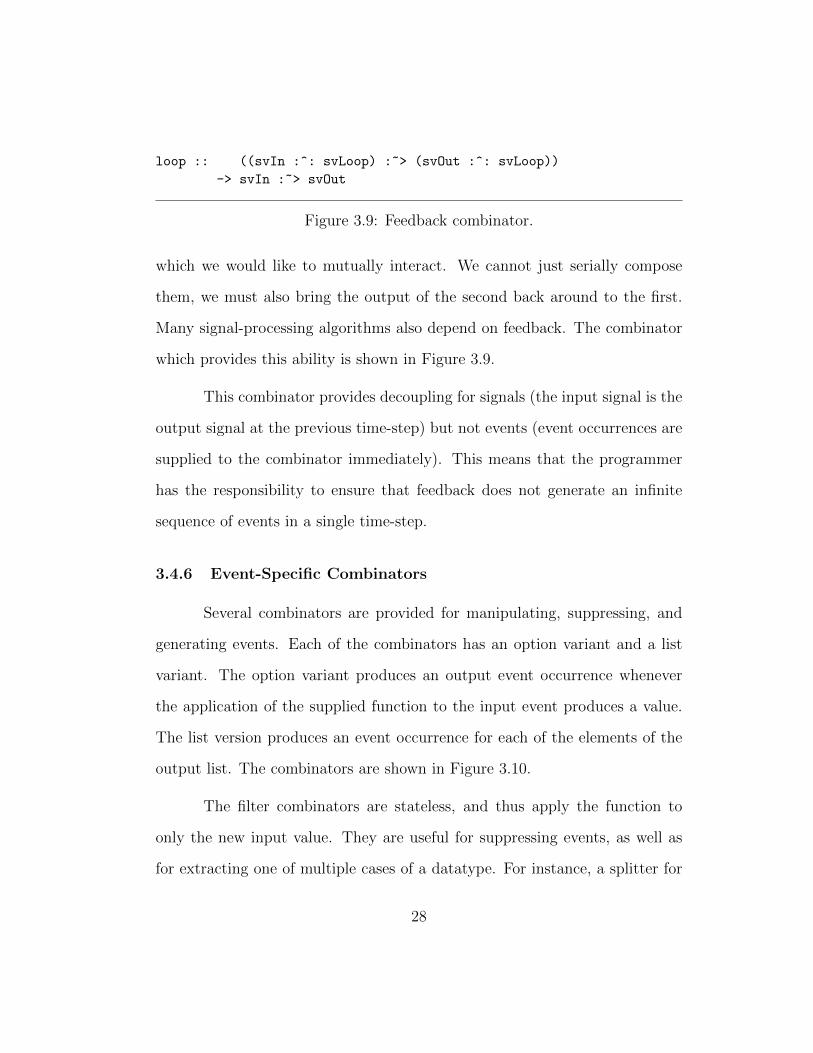
which provides this ability is shown in Figure 3.9.

This combinator provides decoupling for signals (the input signal is the

output signal at the previous time-step) but not events (event occurrences are

supplied to the combinator immediately). This means that the programmer

has the responsibility to ensure that feedback does not generate an infinite

sequence of events in a single time-step.

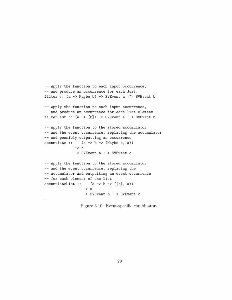
3.4.6 Event-Specific Combinators

Several combinators are provided for manipulating, suppressing, and

generating events. Each of the combinators has an option variant and a list

variant. The option variant produces an output event occurrence whenever

the application of the supplied function to the input event produces a value.

The list version produces an event occurrence for each of the elements of the

output list. The combinators are shown in Figure 3.10.

The filter combinators are stateless, and thus apply the function to

only the new input value. They are useful for suppressing events, as well as

for extracting one of multiple cases of a datatype. For instance, a splitter for

28

-- Apply the function to each input occurrence,

-- and produce an occurrence for each Just.

filter :: (a -> Maybe b) -> SVEvent a :~> SVEvent b

-- Apply the function to each input occurrence,

-- and produce an occurrence for each list element

filterList :: (a -> [b]) -> SVEvent a :~> SVEvent b

-- Apply the function to the stored accumulator

-- and the event occurrence, replacing the accumulator

-- and possibly outputting an occurrence

accumulate :: (a -> b -> (Maybe c, a))

-> a

-> SVEvent b :~> SVEvent c

-- Apply the function to the stored accumulator

-- and the event occurrence, replacing the

-- accumulator and outputting an event occurrence

-- for each element of the list

accumulateList :: (a -> b -> ([c], a))

-> a

-> SVEvent b :~> SVEvent c

Figure 3.10: Event-specific combinators.

29

events carrying Either-valued occurrences could be written as:

getLeft :: Either a b -> Maybe a

getLeft (Left x) = Just x

getLeft _ = Nothing

getRight :: Either a b -> Maybe b

getRight (Right x) = Just x

getRight _ = Nothing

split :: SVEvent (Either a b) :~> (SVEvent a :^: SVEvent b)

split = copy >>> first (filter getLeft) >>> second (filter getRight)

The accumulate combinators are stateful, applying the supplied func-

tion to both the input value and an accumulator. This function has two results:

the option or list of output event occurrence values, and the new value for the

accumulator.

The accumulator is useful when responses to multiple event occurrences

(from one or more sources) must be coordinated. For instance, in the bench-

mark application (see Chapter 6), a table is maintained that allows knowledge

from previous event occurrences (packets from a network switch) to be used

in deciding where the present packet ought to go.

3.4.7 Joining

The joining combinators provide the ability to combine two event streams,

two signals, or a signal and an event stream. These combinators are shown in

Figure 3.11

The union combinator is a non-deterministic merge of event streams.

30

union :: (SVEvent a :^: SVEvent a) :~> SVEvent a

combineSignals :: (a -> b -> c) -> (SVSignal a :^: SVSignal b) :~> SVSignal c

capture :: (SVSignal a :^: SVEvent b) :~> SVEvent (b, a)

Figure 3.11: Joining combinators.

Any event which occurs on either input will occur on the output. For simul-

taneous event occurrences, the order of occurrence is not guaranteed, but the

occurrence itself is. This construct is also guaranteed to respect the relation-

ship of event occurrences to sampling intervals.

The combineSignals combinator applies a binary function pointwise

to two signals, and produces the result of this application as a third signal.

The combining function is necessary because we will have two input samples

at each time step, and must produce exactly one output sample. Even if we

restrict the types to be the same, parametricity forbids assuming that we can

combine two values of an arbitrary type.2

The capture combinator adds the last-sampled value of a signal at the

time of an event occurrence to that event occurrence.

These three combinators together provide the ability to combine el-

ements of signal vectors. By combining these combinators, along with the

cancelLeft and cancelRight routing combinators, arbitrary signal vectors

can be reduced.

2The union combinator does not encounter this difficulty since event occurrences, beingtemporally discrete, can be temporally interleaved without combining their individual values

31

time :: SVEmpty :~> SVSignal Double

delay :: Double -> (SVEvent a :^: SVEvent Double) :~> SVEvent a

integrate :: TimeIntegrate i => SVSignal i :~> SVSignal i

Figure 3.12: Time-dependent combinators.

3.4.8 Time Dependence

A set of combinators are provided for making use of time-dependence

in a signal function. These combinators allow the modification of signals and

events with respect to time, and the observation of the current time value.

The combinators are shown in Figure 3.12

The simplest time-dependent combinator is time, which simply outputs

the time since it began to be evaluated. This does not necessarily correspond

to the time since the global signal function began to be evaluated, since the

signal function in which the time combinator is used may have been introduced

through switch.

The delay signal function allows events to be delayed. An initial delay

time is given, and event occurrences on the right input can carry a new delay

time. Event occurrences on the left input are stored and output when their

delay time has passed. Changing the delay time does not affect occurrences

already waiting.

The integrate combinator outputs the rectangle-rule approximation

of the integral of its input signal with respect to time.

32

3.5 Evaluation

The goal of the evaluation interface is to provide a means to evalu-

ate declaratively specified signal functions in the context of a monadic in-

put/output system, such as Haskell’s IO monad. The means providing a sim-

ple monadic interface for taking actions on a signal function in response to

inputs, and for actuating the outputs of a signal function.

The evaluation interface provides a modified state monad which holds a

signal function, together with some additional information, as its state (shown

in Figure 3.13). Rather than monadic instructions to put and get the state,

the monad provides instructions to trigger an input event, update an input

signal, and trigger sampling of signals in the signal function. Additional state

includes the current set of modifications to the input signals (since the last

sample) and a set of handlers which actuate effects based on output events or

changes to the output signal.

Sets which correspond to signal vectors are built with “smart” construc-

tors. For instance, to construct a set of handlers, individual handling func-

tions are lifted to handler sets with the signalHandler and eventHandler

functions, and then combined with each other and emptyHandler leaves using

the combineHandlers function.

Building the initial input sample is similar, but sampleEvt leaves do

not carry a value.

In order to initialize the state, the user must supply a set of handlers,

33

-- A vector of handlers for outputs

data SVHandler out sv

-- A dummy handler for an empty output

emptyHandler :: SVHandler out SVEmpty

-- A handler for an updated signal sample

signalHandler :: (a -> out) -> SVHandler out (SVSignal a)

-- A handler for an event occurrence

eventHandler :: (a -> out) -> SVHandler out (SVEvent a)

-- Combine handlers for a vector

combineHandlers :: SVHandler out svLeft

-> SVHandler out svRight

-> SVHandler out (svLeft :^: svRight)

-- The state maintained when evaluating a signal function

data SFEvalState m svIn svOut

-- Create the initial state for evaluating a signal function

initSFEval :: SVHandler (m ()) svOut -- Output handlers

-> SVSample svIn -- Initial input samples

-> Double -- Initial external time,

-- corresponding to time 0 for

-- the signal function

-> (svIn :~> svOut) -- Signal function to evaluate

-> SFEvalState m svIn svOut

Figure 3.13: State maintained when evaluating a signal function.

34

-- A sample for all leaves of a signal vector

data SVSample sv

-- Create a sample for a signal leaf

sample :: a -> SVSample (SVSignal a)

-- A dummy sample for an event leaf

sampleEvt :: SVSample (SVEvent a)

-- A dummy sample for an empty leaf

sampleNothing :: SVSample SVEmpty

-- Combine two samples

combineSamples :: SVSample svLeft

-> SVSample svRight

-> SVSample (svLeft :^: svRight)

Figure 3.14: Data type for initial input

the signal function to evaluate, and initial values for all of the signal inputs

(Figure 3.14).

This state can then be passed to a monadic action which will supply

input to the signal function. Inputs are constructed using a simple interface

with functions to construct sample updates and event occurrences, and to

specify their place in the vector (Figure 3.15).

The SFEvalT monad is actually a monad transformer, that is, it is pa-

rameterized over an underlying monad whose actions may be lifted to SFEvalT.

In the usual case, this will be the IO monad.

SFEvalT actions are constructed using combinators to push events, up-

date inputs, and step time, as well as actions lifted from the underlying monad

35

-- Class to overload left and right functions

class SVRoutable r where

svLeft :: r svLeft -> r (svLeft :^: svRight)

svRight :: r svRight -> r (svLeft :^: svRight)

-- An input event occurrence

data SVEventInput sv

instance SVRoutable SVEventInput sv

-- An updated sample for a signal

data SVSignalUpdate sv

instance SVRoutable SVSignalUpdate sv

-- Create an event occurrence

svOcc :: a -> SVEventInput (SVEvent a)

-- Create an updated sample

svSig :: a -> SVSignalUpdate (SVSignal a)

Figure 3.15: Data types for ongoing input.

36

-- The evaluation monad

data SFEvalT svIn svOut m a

instance MonadTrans (SFEvalT svIn svOut)

instance (Monad m) => Monad (SFEvalT svIn svOut m)

instance (Functor m) => Functor (SFEvalT svIn svOut m)

instance (Monad m, Functor m) => Applicative (SFEvalT svIn svOut m)

instance (MonadIO m) => MonadIO (SVEvalT svIn svOut m)

-- Obtain an action in the underlying monad

-- from an SFEvalT and a new state.

runSFEvalT :: SFEvalT svIn svOut m a

-> SFEvalState m svIn svOut

-> m (a, SFEvalState m svIn svOut)

-- Push an event occurrence.

push :: (Monad m) => SVEventInput svIn -> SFEvalT svIn svOut m ()

-- Update the value of an input signal sample

-- (not immediately observed)

update :: (Monad m) => SVSignalUpdate svIn -> SFEvalT svIn svOut m ()

-- Step forward in time, observing the updated signal values

step :: (Monad m) => Double -> SFEvalT svIn svOut m ()

Figure 3.16: Evaluation combinators

(used to obtain these inputs). An action in the underlying monad which pro-

duces the result and a new state is obtained with the runSFEvalT function.

These combinators are shown in Figure 3.16.

37

Chapter 4

Implementation

Having established the design and semantics of the reactive system,

I present a purely functional implementation. For this implementation, I

will make significant use of Generalized Algebraic Datatypes (GADTs) [3, 18].

GADTs provide a mechanism for expressing abstractions which are not easily

expressible in a standard Hindley-Milner type system, while maintaining the

type soundness of Haskell. In particular, GADTs provide the power we require

to take advantage of the signal vector representation of signal function inputs

and outputs.

4.1 Signal Functions

The design of signal functions specifies a family of types for the inputs

and outputs of signal functions. Signal functions are not functions in the purest

sense, however. They are not mappings from a single instance of their input

type to a single instance of their output type. They must be implemented

with respect to the temporal semantics of their inputs and outputs.

We therefore start by creating a set of concrete datatypes for the inputs

and outputs of signal functions. These datatypes will be parameterized by the

38

input and output types of the signal function, and will not be exposed to the

user of the library. Rather, they will specify how data is represented during

the temporal evaluation of signal functions.

We then describe how signal functions are implemented using these

concrete types, along with higher-order functions and continuations.

4.1.1 Concrete Representations of Signal Vectors

In Chapter 3 we presented signal vectors as a set of types. In order

to be completely principled, we should isolate these types into their own kind

(a sort of type of types); however, the Haskell extension for this was far from

stable at the time this system was created.

The types are therefore expressed in the system exactly as they were

described in Chapter 3. (To refresh, see Figure 3.1.) The striking observation

about these types is that they have no data constructors. There are no values

which have these types.

Instead, we will create concrete representations which are parameter-

ized over these types. These concrete representations will be expressed as

GADTs, allowing each data constructor of the representation to fill in a spe-

cific signal vector type for the parameter of the representation.

The first thing to represent is samples, which are sets of values for the

signal components of a signal vector. Therefore, we create a representation

which carries a value for every SVSignal leaf of a signal vector. In order to

do this, we restrict each of our constructors to a single signal vector type.

39

data SVSample sv where

-- Store a value at an SVSignal leaf

SVSample :: a

-> SVSample (SVSignal a)

-- Empty constructor for event leaves

SVSampleEvent :: SVSample (SVEvent a)

-- Empty constructor for empty leaves

SVSampleEmpty :: SVSample SVEmpty

-- Construct a sample from two samples, typed

-- with the SVAppend of their signal vectors

SVSampleBoth :: SVSample svLeft

-> SVSample svRight

-> SVSample (SVAppend svLeft svRight)

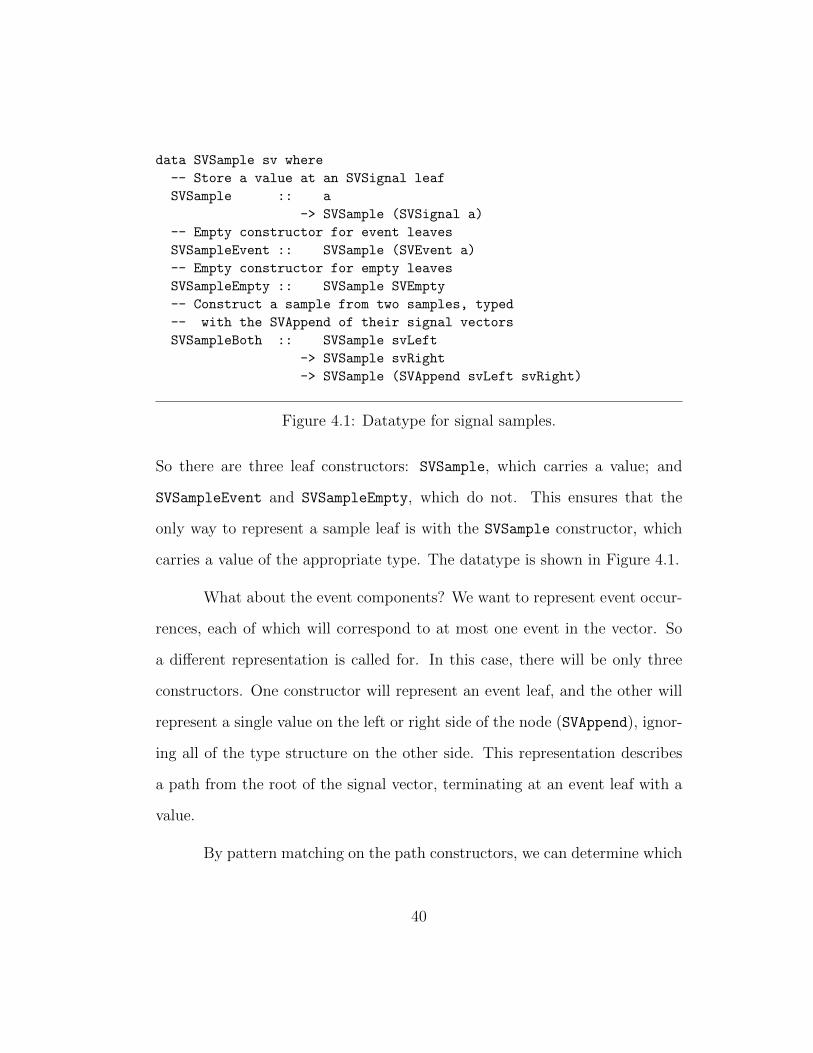
Figure 4.1: Datatype for signal samples.

So there are three leaf constructors: SVSample, which carries a value; and

SVSampleEvent and SVSampleEmpty, which do not. This ensures that the

only way to represent a sample leaf is with the SVSample constructor, which

carries a value of the appropriate type. The datatype is shown in Figure 4.1.

What about the event components? We want to represent event occur-

rences, each of which will correspond to at most one event in the vector. So

a different representation is called for. In this case, there will be only three

constructors. One constructor will represent an event leaf, and the other will

represent a single value on the left or right side of the node (SVAppend), ignor-

ing all of the type structure on the other side. This representation describes

a path from the root of the signal vector, terminating at an event leaf with a

value.

By pattern matching on the path constructors, we can determine which

40

data SVOccurrence sv where

-- Leaf, carrying a value for the occurrence

SVOccurrence :: a

-> SVOccurrence (SVEvent a)

-- Lift an occurrence to be on the left side of a signal vector

SVOccLeft :: SVOccurrence svLeft

-> SVOccurrence (SVAppend svLeft svRight)

-- Lift an occurrence to be on the right side of a signal vector

SVOccRight :: SVOccurrence svRight

-> SVOccurrence (SVAppend svLeft svRight)

Figure 4.2: Datatype for event occurrences.

subvector of a signal vector an event occurrence belongs to, repeatedly refining

it until we determine which event in the vector the occurrence corresponds to.

The datatype for occurrences is shown in Figure 4.2.

We add one more representation for signals, in order to avoid unec-

cessary representations of the values of all signals when not all signals have

changed their values. This representation allows us to represent the values of

zero or more of the signals in a signal vector. To accomplish this, we replace

the individual constructors for the SVEmpty and SVEvent leaves with a sin-

gle, unconstrained constructor. This constructor can represent an arbitrary

signal vector. We can use the constructor for signal vector nodes and the con-

structor for sample leaves to represent the updated values, while filling in the

unchanged portions of the signal vector with this general constructor. This

datatype is shown in Figure 4.3.

41

data SVDelta sv where

-- A replacement value for a sample of a single signal

SVDeltaSignal :: a

-> SVDelta (SVSignal a)

-- No replacement value for a sample of an arbitrary

-- signal vector

SVDeltaNothing :: SVDelta sv

-- Combine replacements for component signal vectors into

-- replacements for the SVAppend of the vectors.

SVDeltaBoth :: SVDelta svLeft

-> SVDelta svRight

-> SVDelta (SVAppend svLeft svRight)

Figure 4.3: Datatype for signal updates.

4.1.2 Signal Function Implementation Structure

We now have concrete datatypes for an implementation to operate on.

Our next task is to represent transformers of temporal data, which themselves

may change with time. The common approach to this task is sampling, in

which a program repeatedly checks for updated information, evaluates it, up-

dates some state, and produces an output. This is the essence of pull-based

evaluation.

Another approach is notification, in which the program exposes an in-

terface which the source of updated information may invoke. This is a re-

peated entry point to the program, which causes the program to perform the

same tasks listed above, namely, evaluate the updated information, update

state, and produce output. The strategy of notification as opposed to repeated

checking is the essence of push-based evaluation.

42

Signal functions are declarative objects, and not running processes.

They have no way to invoke sampling themselves. They can, however, expose

separate interfaces for when sampling is invoked, and when they are notified of

an event occurrence. This creates two control paths through a signal function.

One of these control paths is intended to be invoked regularly and frequently

with updates to the time and sample values, and the other is intended to be

invoked only when an event occurs. The benefit of separating these control

paths is that events are no longer defined in terms of sampling intervals, and

need not even be considered in sampling, except when they are generated by

a condition on a sample. On the other hand, events can be responded to even

if the time has not yet come for another sample, and multiple events can be

responded to in a single sampling interval.

We represent signal functions as a GADT with three type parameters

and two constructors. The first type parameter represents the initialization

state, and is specialized to Initialized or NonInitialized depending on

the constructor. The other two type parameters are the input and output

signal vectors, respectively. The signal functions that a user will compose are

non-initialized signal functions. They must be provided with an initial set of

input signals (corresponding to time zero). When provided with this input,

they produce their time-zero output, and an initialized signal function. The

datatype is shown in Figure 4.4.

Initialized signal functions carry two continuations. The first continu-

ation takes a time differential and a set of signal updates, and returns a set of

43

-- Type tag for signal functions which don’t require

-- an initial input

data Initialized

-- Type tag for signal functions which require

-- an initial input

data NonInitialized

-- Type of signal functions

data SF init svIn svOut where

-- Non-initialized signal functions consist of a function

-- from an input sample to a pair of an output sample

-- and an initialized continuation of the signal function

SF :: (SVSample svIn

-> (SVSample svOut,

SF Initialized svIn svOut))

-> SF NonInitialized svIn svOut

-- Initialized signal functions consist of two functions.

-- The first function’s inputs are the time delta, and updates

-- to the input signals. Its outputs are updates to the output

-- signals, a set of output events, and a continuation of the

-- signal function.

SFInit :: (Double

-> SVDelta svIn

-> (SVDelta svOut,

[SVOccurrence svOut],

SF Initialized svIn svOut))

-- The second function’s input is an event occurrence for an

-- event in its input signal vector. Its outputs are a set

-- of output occurrences for events in its output signal

-- vector, and a continuation of the signal function.

-> (SVOccurrence svIn

-> ([SVOccurrence svOut],

SF Initialized svIn svOut))

-> SF Initialized svIn svOut

Figure 4.4: Datatype and empty types for signal functions.

44

signal updates, a collection of event occurrences, and a new initialized signal

function of the same type. This is the continuation called when sampling.

The second continuation takes an event occurrence, and returns a col-

lection of event occurrences and a new signal function of the same type. This

continuation is only called when there is an event occurrence to be input to

the signal function.

Note that each of these continuations uses one or more of the concrete

representations of signal vectors, and applies the type constructor for the rep-

resentation to the input or output signal vector for the signal function.

4.1.3 Implementation of Signal Function Combinators

Having specified a datatype for signal functions, we must now provide

combinators which produce signal functions of this type. Each combinator’s

implementation must specify how it is initialized, how it samples its input,

and how it responds to event occurrences.

We will not detail every combinator here, but we will discuss each of

the implementation challenges encountered.

As an example of the implementation of combinators, we show the

implementation of the identity signal function in Figure 4.5. This signal

function simply passes all of its inputs along as outputs. The initialization

function simply passes along the received sample and outputs the initialized

version of the signal function. The initialized version of the input is similar,

but is self-referential. It outputs itself as its replacement. This is standard

45

identity :: sv :~> sv

identity =

SF (\initSample -> (initSample, identityInit))

identityInit :: SF Initialized sv sv

identityInit =

SFInit (\dt sigDelta -> (sigDelta, [], identityInit))

(\evtOcc -> ([evtOcc], identityInit))

Figure 4.5: Implementation of the identity combinator.

for simple and routing combinators which are not reactive, and simply move

samples and event occurrences around.

In order for our primitive signal functions to be useful, we need a means

of composing them. Serial composition creates one signal function from two,

by using the output of one as the input of the other. The serial composition

combinator is styled (>>>). The implementation of this operator is one place

where the advantage of responding to events independently from signal samples

becomes clear.

This is the only primitive combinator which takes two signal functions,

and thus, it is the only way to combine signal functions. Parallel, branching,

and joining composition can be achieved by modifying signal functions with

the first and second combinators and composing them with the routing and

joining combinators.

Combinators which take one or more signal functions as input must

recursively apply themselves, as is shown in the implementation of serial com-

position (Figure 4.6). They must also handle initialization, retaining the ini-

46

tialized signal functions and passing them to the initialized version of the

combinator.

The switch combinator is the means of introducing reactivity into a

signal function. This combinator allows a signal function to replace itself by

producing an event occurrence. The combinator wraps a signal function, and

observes an event on the right side of the output signal vector. At the first

occurrence of the event, the signal function carried by the occurrence replaces

the signal function.

The switch combinator stores the input sample provided during ini-

tialization, and updates it with the input signal updates. When the wrapped

signal function produces an occurrence carrying a new signal function, that

signal function is initialized with the stored input sample. It is then “wrapped”

by another function which closes over its output sample, and outputs the sam-

ple as a signal update as the next time step. After this, it acts as the new

signal function. This wrapping has some performance implications, which are

discussed in Chapter 6.

This combinator checks the outputs of the wrapped signal function for

an event occurrence from which an uninitialized signal function is extracted.

The switch combinator stores the full sample for its input vector (which is

identical to the input vector of the supplied signal function) to initialize the

new signal function. This also demands that it add a wrapper to the new

signal function which waits for the next sampling interval and actuates the

sample output at initialization as an output set of changes to the signal. This

47

(>>>) :: (svIn :~> svBetween)

-> (svBetween :~> svOut)

-> (svIn :~> svOut)

(SF sigSampleF1) >>> (SF sigSampleF2) =

SF (\sigSample -> let (sigSample’, sfInit1) = sigSampleF1 sigSample

(sigSample’’, sfInit2) = sigSampleF2 sigSample’

in (sigSample’’, composeInit sfInit1 sfInit2))

composeInit :: SF Initialized svIn svBetween

-> SF Initialized svBetween svOut

-> SF Initialized svIn svOut

composeInit (SFInit dtCont1 inputCont1) sf2@(SFInit dtCont2 inputCont2) =

SFInit

(\dt sigDelta ->

let (sf1MemOutput, sf1EvtOutputs, sf1New) = dtCont1 dt sigDelta

(sf2MemOutput, sf2EvtOutputs, sf2New) = dtCont2 dt sf1MemOutput

(sf2EvtEvtOutputs, sf2Newest) = applySF sf2New sf1EvtOutputs

in (sf2MemOutput,

sf2EvtOutputs ++ sf2EvtEvtOutputs,

composeInit sf1New sf2Newest)

)

(\evtOcc ->

let (sf1Outputs, sf1New) = inputCont1 evtOcc

(sf2FoldOutputs, sf2New) = applySF sf2 sf1Outputs

in (sf2FoldOutputs, composeInit sf1New sf2New)

)

-- The programmer should not rely on any

applySF :: SF Initialized svIn svOut

-> [SVOccurrence svIn]

-> ([SVOccurrence svOut],

SF Initialized svIn svOut)

applySF sf indices =

foldr (\evtOcc (changes, SFInit _ changeCont) ->

let (newChanges, sfNew) = changeCont evtOcc

in (newChanges ++ changes, sfNew))

([], sf)

indices

Figure 4.6: Implementation of serial composition.

48

-- T.swap is imported from Data.Tuple

-- chooseOccurrence, splitSample, splitDelta,

-- combineSamples, combineDeltas, occRight, and

-- occLeft are convenience functions for manipulating

-- signal sample

swap :: (sv1 :^: sv2) :~> (sv2 :^: sv1)

swap =

SF (\sigSample ->

(uncurry combineSamples $ T.swap $ splitSample sigSample,

swapInit)

swapInit :: SF Initialized (SVAppend sv1 sv2) (SVAppend sv2 sv1)

swapInit =

SFInit (\_ sigDelta ->

(uncurry combineDeltas $ T.swap $ splitDelta sigDelta,

swapInit)

(\evtOcc ->

(case chooseOccurrence evtOcc of

Left lOcc -> [occRight lOcc]

Right rOcc -> [occLeft rOcc], swapInit))

Figure 4.7: Implementation of the swap routing combinator.

has some performance implications, which are discussed in Chapter 6.

Most of the routing combinators are simple to implement. The only

task is to add remove, or replace routing constructors on signal updates and

event occurrences. Since these signal functions are stateless and primitive, they

can simply return themselves as their replacements. The swap combinator is

shown as an example in Figure 4.7

The first and second combinators are similar to serial composition,

but they transform only one signal function. For signal changes, they must

split the set of input changes into those which will be passed to the signal

49

function and those which will be simply passed along to the output, and then

recombine them on the other side. For event occurrences, the occurrence must

be pattern-matched to determine whether to call the event continuation from

the provided signal function or passed through, and output event occurrences

must have the suitable routing constructor re-applied. In any case, when a

continuation has been applied, the combinator must be recursively applied to

the new signal function.

The looping feedback combinator is particularly tricky. As it is cur-

rently implemented, the initial sample for the right side of the input signal

vector to the supplied function is the right side of the output sample. This

is acceptable, given Haskell’s non-strict evaluation strategy, but it is neces-

sary that the right side of the signal function’s output not be immediately

dependent on its input. The feedback combinator makes use of Haskell’s lazy

evaluation to feed events back into the combinator, and stores signal updates

until the next sample. Signal samples are thus automatically decoupled after

initialization. The implementation makes use of the recursive nature of the let

construct in Haskell, and the non-strict evaluation of Haskell, to implement

feedback.

The filter combinators are simple to implement. Their sampling

continuation is superfluous, and the event continuation merely applies the

supplied function, and constructs an output list based on the result.

The accumulate combinators are implemented in terms of the filter

and switch combinators, as shown in Figure 4.8.

50

-- | Accumulate over event occurrences

accumulate :: (a -> b -> (Maybe c, a)) -> a -> SVEvent b :~> SVEvent c

accumulate f a = acc a

where acc a = switch (pureEventTransformer (f a) >>>

copy >>>

first (pureEventTransformer fst >>> filter id) >>>

second (pureEventTransformer (acc . snd)))

-- | Accumulate over event occurrences, with lists of event outputs

accumulateList :: (a -> b -> ([c], a)) -> a -> SVEvent b :~> SVEvent c

accumulateList f a = acc a

where acc a = switch (pureEventTransformer (f a) >>>

copy >>>

first (pureEventTransformer fst >>> filterList id) >>>

second (pureEventTransformer (acc . snd)))

Figure 4.8: Implementation of event accumulators.

The union combinator’s implementation passes along every event oc-

currence it receives on either input, stripping off the left and right combinator.

This is acceptable since we do not insist on a total ordering of events, or an

event time resolution greater than the sampling rate. The combineSignals

combinator maintains the values of both signals, and applies the combination

function whenever one is updated, producing an update to the output signal’s

value. The capture combinator similarly maintains the input signal value,

and adds it to each event occurrence.

Time dependence is introduced by the time, delay, and integrate

combinators. The time combinator simply sums the time updates and provides

the sum as a signal output. The delay combinator keeps a table of events

which have come in, along with their schedule occurrence time, and produces

51

them as output when time advances far enough. The integrate combinator

performs rectangle-rule integration on signal samples with respect to time.

The implementation strategy leaves room for optimizations. In par-

ticular, an additional constructor for time-independent signal functions would

allow portions of a signal function to forgo evaluation during time steps un-

less they had signal updates. Optimizations in the style of Yampa, where

an AST for the current signal function is maintained alongside the contina-

tions and checked for opportunities to eliminate redundant components of the

signal function, might further improve performance. In particular, collapsing

nested or serially-composed switches which have occurred since the last time

step would remove at least some of the observed dependence of performance

on sampling rate. Nevertheless, this implementation performs quite well as it

currently exists, as we demonstrate in Chapter 6.

4.2 Evaluation Interface

The evaluation interface provides the means of evaluating a signal func-

tion with inputs and producing effects in response to the signal function’s out-

puts. We would like to produce a set of constructs that interacts well with

Haskell’s system for external IO.

4.2.1 Constructs and Interface

The evaluation interface is exported as shown in Section 3.5.

The SFEvalState type constructor parameterizes over input types for

52

signal functions, and underlying monads for a monad transformer, but is not

itself a monad transformer. It describes the state of signal function evaluation.

It consists of a record with four members: the current signal function, the set

of handlers for outputs, the current input signal delta, and the last sample

time.

The SFEvalT monad transformer is a newtype wrapper around the

StateT monad available in the Haskell transformers package. The StateT

monad wraps any other monad, providing a state which may be read using

the get action and replaced with the put action. An action in the underlying

monad is obtained by supplying a StateT value and an initial state value to

the runStateT function.

The SFEvalT monad transformer does not make the get and put actions

available, but uses them in its implementation of the push, update, and sample

actions.

The push action pushes an event onto the input of the signal function,

resulting in immediate evaluation of the relevant components signal function

and possible actuation of handlers specified for output events. It is imple-

mented by fetching the SFEvalState, applying the event continuation of the

signal function contained by the SFEvalState to the pushed event, thus ob-

taining a new signal function and a list of events, applying the handlers con-

tained in the SFEvalState to the output events, replacing the signal function

in the SFEvalState, and replacing the SFEvalState.

53

The update action updates the current input signal delta, which will

be sampled at the next step action. It has no immediately observable effect.

It simply updates the value of one signal in the input signal vector, a delta of

which is stored in the SFEvalState record.

The step action takes a time delta, and calls the signal continuation of

the stored signal function. It actuates the outputs using the stored handlers,

replaces the stored delta with an empty delta, and stores the resulting new

signal function in the state.

54

Chapter 5

Example Application

TimeFlies is a library for Functional Reactive Programming, which is

a paradigm for creating interactive and time-dependent applications. This

chapter presents the design of one such application, and its implementation

using TimeFlies. The application is an OpenFlow controller which implements

a learning switch. In short, it is a re-implementation of the standard kind

of switch used in local area networks, using “software-defined networking.”

This is the application which is benchmarked for performance comparisons in

Chapter 6.

5.1 OpenFlow

The OpenFlow protocol [13] is a protocol for software-defined network-

ing applications. In particular, it defines the communication between switches

(devices which quickly route packets from input ports to output ports based

on learned rules) and controllers, which are generally devices with large com-

putational resources, such as servers. OpenFlow allows switches to report

packets for which no rule exists to a controller, and provides a means for the

controller to install new rules on a switch either preemptively, or in response

55

to a reported packet.

One of the simplests tasks which may be implemented as a OpenFlow

controller is a “learning switch”. Such a switch uses the source and destination

hardware addresses in network packets to make routing decisions. A table is

kept which records the ports where source addresses are observed on incoming

packets. This table thus contains knowledge of which hardware address(es)

can be reached on which port. Using this table, rules are constructed to route

packets with particular source-destination pairs to the correct port. When a

packet is seen for which no rule exists, it is reported to the controller, which

updates the table and rules based on the new knowledge, and broadcasts the

packet so that it can reach its intended destination and receive a response.

Our example application is a controller for a “learning switch.” We

describe its implementation as a TimeFlies signal function, and two approaches

to running this signal function using the TimeFlies evaluation interface.

5.2 Implementation

The first component for our learning switch is the table which maps ad-

dresses to ports. This is a stateful data structure which will be updated by in-

put events and possibly produce output events. We employ the accumulateList

combinator to produce the signal function shown in Figure 5.1.

Note that the input events are closures which expect the table as input

and produce an updated table as output. This enables us to write several

56

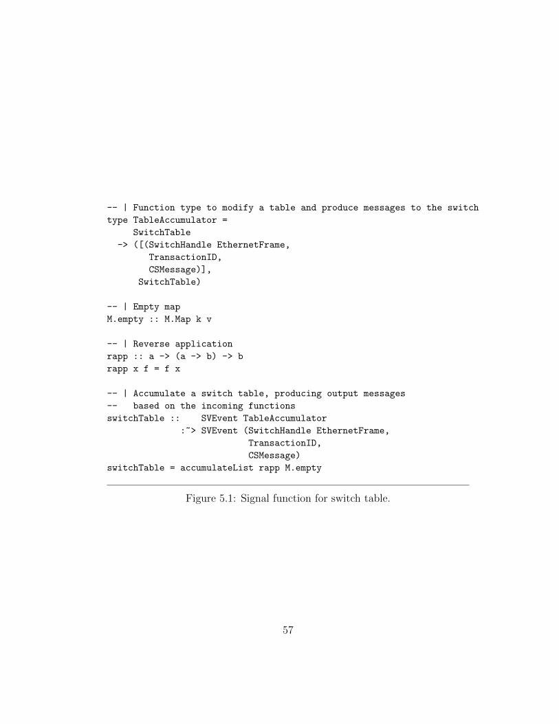
-- | Function type to modify a table and produce messages to the switch

type TableAccumulator =

SwitchTable

-> ([(SwitchHandle EthernetFrame,

TransactionID,

CSMessage)],

SwitchTable)

-- | Empty map

M.empty :: M.Map k v

-- | Reverse application

rapp :: a -> (a -> b) -> b

rapp x f = f x

-- | Accumulate a switch table, producing output messages

-- based on the incoming functions

switchTable :: SVEvent TableAccumulator

:~> SVEvent (SwitchHandle EthernetFrame,

TransactionID,

CSMessage)

switchTable = accumulateList rapp M.empty

Figure 5.1: Signal function for switch table.

57

different event sources whose final events require state (the table) and produce

messages to the switch.

The first source of such events is packets forwarded to the controller

by switches. The closures carried by these events implement the response to

packet inputs. The signal function from input switch message events to events

from the accumulator is shown in Figure 5.2, but the details of the switch

routing algorithm are elided.

The captureTime signal function attaches the time to incoming pack-

ets. The getPacketIn signal function extracts packet-in messages from the

variety of message events that a switch may send to the controller. These

two signal functions feed into the packetIn signal function, which builds the

closures for the accumulator using the handlePacketIn pure function.

The other task is to periodically eliminate all rules which are older than

a specified threshold. For this purpose, we construct another signal function

which produces TableAccumulator events. This signal function runs a timer

(the every combinator, which is implemented using switch and after and

produces an event repeatedly on a given interval) and produces events carrying

closures which scan the table for old rules, delete them, and produces messages

to inform the switches of their deletion. This signal function is shown in

Figure 5.3, again eliding the implementation of the closures.

We now have all of the pieces for a signal function implementing a

learning switch, as shown in Figure 5.4.

58

getPacketIn :: SVEvent (SwitchHandle EthernetFrame,

TransactionID,

SCMessage EthernetFrame)

:~> SVEvent (SwitchHandle EthernetFrame,

TransactionID,

PacketInfo EthernetFrame)

-- | Handle a packet in event

handlePacketIn :: ((SwitchHandle EthernetFrame,

TransactionID,

PacketInfo EthernetFrame), Double)

-> TableAccumulator

packetIn :: SVEvent ((SwitchHandle EthernetFrame,

TransactionID,

PacketInfo EthernetFrame),

Double)

:~> SVEvent TableAccumulator

packetIn = pureEventTransformer handlePacketIn

-- | Capture the occurrence time of an event.

captureTime :: SVEvent a :~> SVEvent (a, Double)

captureTime = uncancelLeft >>>

first time >>>

capture

-- | Build TableAccumulator events from input packets.

handleSCMessage :: SVEvent (SwitchHandle EthernetFrame,

TransactionID,

SCMessage EthernetFrame)

:~> SVEvent TableAccumulator

handleSCMessage = getPacketIn >>> captureTime >>> packetIn

Figure 5.2: Signal function handling incoming packets.

59

-- | Take a function-value pair and return the application.

pairApp :: (a -> b, a) -> b

pairApp (f, x) = f x

-- | Alter a table and generate messages to remove expired entries and rules

cleanTable :: Double -> Double -> TableAccumulator

-- | Produce an event with the rule-cleaning accumulator.

cleanRules :: Double -> SVEmpty :~> SVEvent TableAccumulator

cleanRules t = copy >>>

second (every t cleanRulesAcc) >>>

first time >>>

capture >>>

pureEventTransformer pairApp

where

cleanRulesAcc :: Double -> TableAccumulator

cleanRulesAcc nowT table = cleanTable t nowT table

Figure 5.3: Table-cleaning signal function.

60

-- | A constant, for how long rules may survive

tableTime :: Double

-- | Make IO actions to send each packet.

sendCSMessage :: SVEvent (SwitchHandle EthernetFrame,

TransactionID,

CSMessage)

:~> SVEvent (IO ())

-- | The learning switch

learn :: SVEvent (SwitchHandle EthernetFrame,

TransactionID,

SCMessage EthernetFrame)

:~> SVEvent (IO ())

learn = uncancelLeft >>>

first (cleanRules tableTime) >>>

second handleSCMessage >>>

union >>>

switchTable >>>

sendCSMessage

Figure 5.4: The signal function for a learning switch.

61

The learning switch composes the cleanRules and handleSCMessage

signal functions in parallel, but routes input only to handleSCMessage, by

using the uncancelLeft routing combinator. The event streams are merged

and fed to the switchTable signal function, and the resulting packets are fed

to the sendCSMessage signal function which constructs IO () events.

Note that this approach enables a modular design where each task

is implemented in its own signal function. Additional behaviors could be

coded as additional signal functions, whose events were also routed to the

table accumulator.

Finally, we show how the signal function is interfaced with IO code

using the evaluation interface. First, we need a few extra definitions. For

starters, a controller must also handle switches when they first connect. We

create a separate signal function for this purpose, and compose it in parallel

with our learning switch signal function. We also need a definition of which

port to listen on, and an IO action for reading the time. These are shown in

Figure 5.5.

Now we can create the main procedure for our learning switch. Note

that the code for placing an event on the input of a signal function is a simple

monadic sequence, sandwich between IORef reads and writes of an opaque

value (Figure 5.6).

62

-- | The port for the server to listen on.

port :: Word16

-- | Get the current time from the monotonic timer

getMonoTimeAsDouble :: IO Double

-- | Handle the connection of a new switch

switchConnect :: SVEvent (SwitchHandle EthernetFrame)

:~> SVEvent (IO ())

switchConnect = pureEventTransformer (void . handshake)

-- | Run switch connection and learning concurrently

learningSwitch :: (SVEvent (SwitchHandle EthernetFrame) :^:

SVEvent (SwitchHandle EthernetFrame,

TransactionID,

SCMessage EthernetFrame))

:~> SVEvent (IO ())

learningSwitch = first switchConnect >>> second learn >>> union

Figure 5.5: Evaluation preliminaries.

63

-- | Entry point

main :: IO ()

main = do (argS:_) <- getArgs

let sampleTime = read argS

time <- getMonoTimeAsDouble

reactiveRef <- newIORef $ initSFEval

(eventHandler id)

(combineSamples sampleEvt sampleEvt)

time

learningSwitch

ofEventManager <-

openFlowEventManager

Nothing

port

-- Switch addition inputs

(\handle -> do rState <- readIORef reactiveRef

((), rState’) <- runSFEvalT

(push $ svLeft $ svOcc handle)

rState

writeIORef reactiveRef rState’)

-- Switch message inputs:

(\((tid, msg), handle) ->

do rState <- readIORef reactiveRef

((), rState’) <- runSFEvalT

(push $ svRight $

svOcc (handle, tid, msg))

rState

writeIORef reactiveRef rState’)

let evtMgr = getEventManager ofEventManager

-- Sampling:

sample = void $ registerTimeout evtMgr sampleTime $

do rState <- readIORef reactiveRef

time <- getMonoTimeAsDouble

((), rState’) <- runSFEvalT (step time) rState

writeIORef reactiveRef rState’

sample

sample

loop evtMgr

Figure 5.6: Using the evaluation interface for IO.

64

Chapter 6

Evaluation and Comparisons

We have described the implementation of a push-pull signal-function

FRP system. Push-based event evaluation should have advantages in event

latency and overall performance over pull-based event evaluation. We would

also like to compare the evaluation interface in the current widely-used system

with the one proposed here, again in order to verify that the theoretical benefits

do appear in practice.

One way to evaluate this is to write an application in two systems, and

benchmark these systems for comparison. In order to compare TimeFlies with

Yampa, the most recently released pull-based signal-function FRP system, we

decided to implement a suitable application in both.

6.1 Methodology and Results

The example application from Chapter 5, an OpenFlow controller, was

also implemented in Yampa. A slightly-modified TimeFlies implementation,

which used a polling loop rather than the GHC event system to obtain events,

but still “pushed” events to TimeFlies once they were acquired, was also im-

plemented.

65

10

100

1000

10000

100000

0 10000 20000 30000 40000 50000

Perf

orm

ance

(Fl

ow

Mod

s/s)

(re

port

ed

by c

bench

)

Pause times (s) (inverse sampling rate)

Event performance comparison of signal-function FRP systems

YampaTimeFlies spinning input

Timeflies event input

Figure 6.1: Comparison of timeflies vs. Yampa implementing an OpenFlowlearning switch controller.

These three controllers were benchmarked using the cbench program [2].

The amount to time to pause between time and signal updates (the inverse of

the sampling rate for signals) was passed as a parameter to each program. The

cbench benchmark operates by sending a simulated packet-in event, waiting

for a rule response, and then repeating. The output of the benchmark is the

number of times this occurs in a second. This is thus a test of event latency

in a reactive system.

Figure 6.1 shows the performance comparison. Toward the left of the

graph is lower pause times (more frequent sampling). The y-axis is a higher

rate of responses (higher numbers are preferred).

There is some correlation between the sampling rate and the response

66

rate for TimeFlies, which is due to the continued wrapping of a replacement

signal function by switch until the next time step (see Section 4.1.3). Nev-

ertheless, TimeFlies outperforms Yampa in event response by several orders

of magnitude, even at a very high sampling rate. This is due to two factors.

First, TimeFlies can react to individual events without evaluating the whole

signal function. Second, in the implementation described in Chapter 5, the

interface of TimeFlies permits us to connect its evaluation directly to GHC’s

event manager, while the design of Yampa requires us to use threads and syn-

chronized communication1. Even the TimeFlies implementation using polling

IO outperforms the Yampa version, due to the ability to evaluate multiple

events per time step.

1Yampa does include a step-wise evaluation function, but it still couples event evaluationfirmly to time steps, and is not well documented.

67

Chapter 7

Conclusions and Further Work

I have presented TimeFlies, a push-based signal-function FRP system.

I have demonstrated that TimeFlies does realize the theoretical benefits of a

push-based signal-function system.

7.1 Conclusions

The TimeFlies system is a fully-implemented and fully-documented

FRP library which may be extended with utility functions and further opti-

mized. Its performance in responding to events is demonstrated to be superior

to that of the predominant pull-based signal-function FRP library.

Further, the model of events used by TimeFlies subverts problematic

semantic questions about the evaluation of events in an FRP system. By using

the N-Ary FRP type model and separating the evaluation of events from the

time steps used for signals, TimeFlies fully supports non-deterministic merging

of events, and provides a semantic guarantee that events are not “lost” during

evaluation.

TimeFlies includes a fully-documented evaluation interface which clar-

ifies and simplifies the task of integrating the TimeFlies system with the many

68

IO systems available to Haskell programmers.

7.2 Further Work

The TimeFlies system would benefit from attentive microbenchmarking

and performance tuning, as well as optimizations to avoid evaluating irrelevant

parts of the network during the the evaluation of time steps. A formal seman-

tic justification for the formulation of event evaluation (which would require a

full formal semantics of FRP) would enable a far more robust correctness ar-

gument, as well as providing a basis for semantic extensions to signal-function

FRP.

FRP is not yet mature, and has not been the subject of focused ap-

plication development. Thus, there is a dearth of design patterns for FRP

applications. Such design patterns would yield necessary feedback as to which

generalizations and restrictions of FRP would be appropriate and useful, and

clarify the necessity of various utility combinators to be included in the stan-

dard libraries of FRP systems.

In order to improve the performance of FRP yet further, it may be

productive to attempt to introduce parallel evaluation into FRP, taking ad-

vantage of the functional purity in the implementation of the signal function

combinators. This may involve, for instance, evaluating several time-steps at

once in a data-parallel manner, task parallelism between different branches of

a signal function, or speculative evaluation of switch combinators.

69

Many classes of reactive application would benefit from a “dynamic

collections” combinator similar to pSwitch in Yampa. Such a combinator

allows a collection of signal functions to be evaluated as one signal function,

with addition or removal of signal functions instead of the total replacement

given by the switch combinator. This is useful, for instance, when simulating

objects for games or computer models, as the behavior of each object can be

modeled as a signal function, and these signal functions can be added to and

removed from the collection. An attempt was made to add such a function to

TimeFlies, but it is not clear what the type of such a combinator would be in a

system employing signal vectors, or how the “routing” of inputs to individual

signal functions in the collection would be specified.

The TimeFlies system provides a principled and performant system for

future experimentation on FRP, as well as implementation of FRP applica-

tions.

70

Appendix

71

Appendix 1

Haskell Concepts

One of the primary attractions of the Haskell language, and the reason

for its use throughout this work, is its advanced yet practical and usable type

system. This type system enables the use of compositional software design

that would be rendered infeasible without a type system to both inform and

verify composition and implementation. This appendix gives an overview of

Haskell concepts, design patterns, and idioms which are used in this thesis.

1.1 Datatypes and Pattern Matching

In Haskell, new type constructors are introduced by defining Algebraic

Datatypes. An ADT declaration can take one of two forms. The first is a data

declaration, e.g.:

data Bool = True | False

data Maybe a = Just a | Nothing

In this form the identifier(s) preceding the = character are a type con-

structor followed by zero or more type variables. Following the = character,

and separated by | characters, are data constructors. Each data constructor

72

is an identifier followed by zero or more types, which are the types of its argu-

ments. Data constructors can be used in expressions to construct a value of

this newly-declared type constructor, and in pattern matching to “take apart”

the value and observe its components (the arguments to the data constructor.

The second form is the newtype declaration. This form is more re-

stricted. It is limited to one data constructor with exactly one argument. It

introduces a new type without introducing a new runtime restriction, though

the Haskell code must still use the data constructor in pattern matches and

expressions to explicitly coerce between the new type and the type of its data

constructor’s parameter. This behavior is most often used to hide implementa-

tion types without introducing the runtime overhead of value construction and

pattern-matching, as these are erased for constructors declared using newtype

once type-checking is complete.

Once a type constructor has been introduced, it can be used in a type,

with its arguments replaced by any valid Haskell type. For instance:

not :: Bool -> Bool

cbool :: Bool -> Int

maybeInt :: Int -> Maybe Int -> Int

isJust :: Maybe a -> Bool

mapMaybe :: (a -> b) -> Maybe a -> Maybe b

Its data constructors can be used in the patterns of functions, and in

their expressions. For instance:

not :: Bool -> Bool

not True = False

73

not False = True

isJust :: Maybe a -> Bool

isJust (Just _) = True

isJust Nothing = False

mapMaybe :: (a -> b) -> Maybe a -> Maybe b

mapMaybe f (Just x) = Just (f x)

mapMaybe _ Nothing = Nothing

1.1.1 Generalized Algebraic Datatypes

GADTs [3, 18] permit us to specify what types fill in the type parame-

ters for specific constructors. For instance, if we wish to build a tiny expression

language, we can use a standard ADT:

data Exp a = Const a

| Plus (Exp a) (Exp a)

| LessThan (Exp a) (Exp a)

| If (Exp a) (Exp a) (Exp a)

Let us assume for the moment that Haskell exports functions1:

(+) :: Int -> Int -> Int

(<) :: Int -> Int -> Bool

An attempt to write an evaluation function for our expression type is:

eval :: Exp a -> a

eval (Const x) = x

eval (Plus x y) = eval x + eval y

1The types for addition and comparison actually involve a typeclass constraint, but thepoint is that the functions’ types are not parametric.

74

eval (LessThan x y) = eval x < eval y

eval (If p c a) = if (eval p)

then eval c

else eval a

But this function will not typecheck. In the Plus case, we cannot

assume that the argument to the type constructor Exp typing x or y is Int,

and similarly for the LessThan case. Again in the If case, we cannot assume

that the predicate is of type Exp Bool, and if we could, that would force our

results to be of type Exp Bool as well.

Let’s try a slightly modified ADT:

data Exp a = Const a

| Plus (Exp Int) (Exp Int)

| LessThan (Exp Int) (Exp Int)

| IfThenElse (Exp Bool) (Exp a) (Exp a)

Here the motivation for a type parameter to our type constructor be-

comes clear. We can introduce both Bool and Int constants (as well as others,

but we cannot do anything with them unless we extend the language). Further,

we can constrain the types of the input expressions to each of our constructors

to be of the appropriate type.

The code for our our evaluator is the same. But now note that the

in the Plus and LessThan cases, even though the input types are compatible

with the functions used, the output type expected from our function is not.

Plus x y has type Exp a in the pattern match, so our output is expected to

be of type a for any a argument to type of an input Exp.

75

Here is our expression type as a GADT:

data Exp a where

Const :: a -> Exp a

Plus :: Exp Int -> Exp Int -> Exp Int

LessThan :: Exp Int -> Exp Int -> Exp Bool

If :: Exp Bool -> Exp a -> Exp a -> Exp a

Now our evaluation function can typecheck. Each constructor is able

to constrain the type parameter for output, not just its arguments. So when

pattern matching on the Plus case, we know that each of our inputs will be

of type Exp Int, and that the type of the expression we are pattern matching

has type Exp Int, so the output from our function can be constrained to type

Int, similarly for LessThan. The type argument to Exp in the type of the If

is constrainted to be the same as that as the argument to the types of the

consequent and alternate to the conditional. This permits our If statement

to be parametric while still allowing our evaluation to typecheck.

This capacity to constrain the output types of data constructors, and

thus, to constrain the types of expressions in the scope of pattern matches

of these data constructors, is called type refinement. We will make use of

this ability to parameterize concrete datatypes over abstract type structures,

rather than to permit typechecking in specific cases, but the principle is the

same.

76

1.2 Typeclasses

Typeclasses in Haskell provide a means to implement functions that

are openly polymorphic while not being parametric. A typeclass is declared

as follows:

class Show t where

show :: t -> String

A typeclass has an identifier and a single type parameter. This type

parameter is used in the type of one or more functions which are members of

the class.

The class can then be instantiated:

instance Show Bool where

show True = "True"

show False = "False"

instance (Show a) => Show (Maybe a) where

show (Just x) = "Just " ++ show x

show Nothing = Nothing

Functions can now be written polymorphically over the types instanti-

ating the typeclass, by including the typeclass as a constraint:

repL :: (Show t) => t -> Int

repL x = length (show x)

Typeclasses are used in Haskell to provide common interfaces or func-

tionality across types. The Show class used as an example is exported, along

with instances for most of the basic Haskell types, from Haskell’s Prelude (the

standard module imported into every Haskell module).

77

1.3 Monads and Monad Transformers

One of the primary concepts employed in Haskell programs is that of

the monad [14, 15]. The concept of the monad is borrowed from category

theory, but it is quite simple when understood within Haskell. A monad is

a type constructor with a single parameter, and two associated functions. In

Haskell’s Monad typeclass, these functions are denoted return and tt (¿¿=).

class Monad m where

return :: a -> m a

(>>=) :: m a -> (a -> m b) -> m b

A monad must obey the following axioms:

• Left identity: return x >>= f = f x

• Right identity: m >>= return = m

• Associativity: (a >>= b) >>= c) = (a >>= (

x -> b x >>= c))

Several standard Haskell type constructor are monads in interesting

ways, but the most well-known is Haskell’s IO type constructor. This is the

basis of Haskell’s input/output system. The entry point to a Haskell program is

the main function, of type IO (). This function can be constructed by using

the monadic functions to sequence an arbitrary number of other functions

whose output type is IO a. Since the sequencing operator takes an arbitrary

function, this allows the full power of Haskell functions, including first-class

78

and higher-order functions, to be employed in defining a program’s input and

output. A convenience function is commonly used when the result is not

necessary as part of the sequencing:

(>>) :: Monad m => m a -> m b -> m b

(>>) m1 m2 = m1 >>= (const m2)

\subsection{Do-notation}

\label{subsection:Haskell_Concepts-Monads_and_Monad_Transformers-Do_notation}

Because monads are such a pervasive concept in Haskell, the language includes

special syntax for writing monadic expressions. Do-notation is expression syntax

which begins with the keyword {\tt do} and is followed by lines of two forms:

\begin{code}

do

x <- m1

m2

The first form is a binding expression: it binds the variable x to the

output of the monadic value m2. The second form simply sequences the monad

value m2 into the monadic value being built. Do-notation has a syntax-driven

translation to desugared Haskell expression:

desugar {

do x <- m1

...} =

m1 >>= \x -> desugar {do ...}

desugar {

do m1

...} =

m1 >> desugar {do ...}

79

1.3.1 Monad Transformers

A monad transformer is a type constructor with two parameters. The

first parameter parameterizes over a one-parameter type constructor, rather

than a type. The second is the monadic type parameter. A type constructor T

is a monad transformer if it has the following instance of the Monad typeclass:

instance Monad m => Monad T m

and is also an instance of the class

class MonadTrans t where

lift :: (Monad m) => m a -> t m a

The axioms for the lift function are:

• lift . return = return

• lift (m >>= f) = lift m >>= (lift . f)

Restated, lift does not modify return and distributes over monadic

sequencing.

As an example of a monad transformer, we can consider the StateT

type, which is employed in the implementation of this thesis.

The type is declared:

newtype StateT s m a = S { runStateT :: s -> m (s, a) }

Its monad instance, for any s, is

80

instance Monad m => Monad (StateT s m) where

return x = S (\s -> return (x, s))

(>>=) (S f) mf = S (\s -> f s >>= (\ (x, s’) -> let (S f’) = mf x in f’ s ))

The return and sequencing functions carry the state through the un-

derlying monad.

The MonadTrans instance is:

instance MonadTrans (StateT s) where

lift m = S (\s -> m >>= (\x -> return (x, s))

Finally, there are two functions provided to access and set the state:

put :: s -> StateT s m ()

put = S (\_ -> return ((), s’))

get :: StateT s m s

get = S (\s -> return (s, s))

If we use StateT as a wrapper around the IO monad, we might employ

it as a way to generate a unique line number for each ”putStrLn” we call.

putStrLnN :: String -> StateT Int IO ()

putStrLnN s = do i <- get

put (i + 1)

lift (putStrLn (show i ++ " " ++ s))

main = runStateT mainSt 1

where mainSt = do g <- lift getLine

putStrLnN g

mainSt

81

Appendix 2

Glossary of Type Terminology

ADT See Algebraic Datatype.

Algebraic Datatype An Algebraic Datatype or ADT is a type whose terms

are data constructors. An ADT is defined by naming a type constructor

and its parameters (zero or more) (as type variables), together with one

or more data constructors and the types of their members. Each data

constructor takes a fixed number (zero or more) data members, whose

types are given following the constructor name. These types are defined

in terms of the type variables named as parameters of the type construc-

tor and any type constructors (including the type constructor associated

with the ADT) in scope in the module.

Data Constructor A Data Constructor is a component of an Algebraic Datatype

which, when applied to values of the appropriate type, creates a value

typed with the ADT. Data constructors are the primary element which

may be pattern matched in languages such as Haskell.

GADT See Generalized Algebraic Datatype.

Generalized Algebraic Datatype Similar to an Algebraic Datatype, but

82

type variables in the type constructor declaration serve merely to denote

the number of type parameters (and thus may be replaced by a kind

signature) and types are given for each data constructor. These types

must have the type constructor as their top-level term, but may fill in the

parameters of the type constructor with arbitrary types. Variables which

appear in the data member types but on in the data constructor type

are existentially quantified, and types appearing in the data constructor

type but not the data member types may be instantiated arbitrarily.

Kind A “type of types.” Kinds are used to verify that types are consistent

during typechecking. The kind of types which contain values is *, and

the kind of single-parameter type constructors which take a type is *

-> *. Other kinds may also be introduced. For instance, signal vectors

should be their own separate kind, but the Haskell type mechanism was

not mature enough to support this at the time of this writing..

Kind Signature A means of specifying the number and kind of types which

may instantiate type variables. Type variables in Haskell are not re-

stricted to types, but may be instantiated by type constructors as well.

The kind of a variable restricts what it may be instantiated with. A kind

signature gives kinds to a type constructor, and thus to its parameters.

Specifying the kind of a type constructor perfectly constrains the number

of parameters.

Type Constructor A type constructor is a type level term which, when ap-

83

plied to the proper number of types, produces a type. Type constructors,

together with type variables, form the basis of polymorphism in Haskell

and similar languages.

Type Variable A type variable is a type-level term which may be instanti-

ated (by the typechecker via inference, or by the user via annotation)

with any type at the point where the value so typed is used. Together

with type constructors, type variables form the basis of polymorphism in

Haskell and similar languages.

84

Bibliography

[1] Heinrich Apfelmus. reactive-banana library. http://hackage.haskell.

org/package/reactive-banana.

[2] cbench benchmark. git://gitosis.stanford.edu/oflops.git.

[3] James Cheney and Ralf Hinze. First-class phantom types. Technical

report, Cornell University, 2003.

[4] Antony Courtney. Frappe: Functional reactive programming in Java. In

Proceedings of the Third International Symposium on Practical Aspects of

Declarative Languages, PADL ’01, pages 29–44, London, UK, UK, 2001.

Springer-Verlag.

[5] Antony Courtney and Conal Elliott. Genuinely functional user interfaces.

In Proceedings of the 2001 Haskell Workshop, pages 41–69, 2001.

[6] Evan Czaplicki. Elm: Concurrent FRP for functional GUIs. http://

www.testblogpleaseignore.com/wp-content/uploads/2012/03/thesis.

pdf, 2012.

[7] Conal Elliott. Push-pull functional reactive programming. In Haskell

Symposium, 2009.

85

[8] Conal Elliott and Paul Hudak. Functional reactive animation. In Pro-

ceedings of the second ACM SIGPLAN international conference on Func-

tional programming, ICFP ’97, pages 263–273, New York, NY, USA, 1997.

ACM.

[9] John Hughes. Generalising monads to arrows. Science of Computer

Programming, 37(13):67 – 111, 2000.

[10] Adam Megacz. Multi-level languages are generalized arrows. CoRR,

abs/1007.2885, 2010.

[11] Henrik Nilsson. Dynamic optimization for functional reactive program-

ming using generalized algebraic data types. In Proceedings of the tenth

ACM SIGPLAN international conference on Functional programming,

ICFP ’05, pages 54–65, New York, NY, USA, 2005. ACM.

[12] Henrik Nilsson, Antony Courtney, and John Peterson. Functional reac-

tive programming, continued. In Proceedings of the 2002 ACM SIGPLAN

workshop on Haskell, Haskell ’02, pages 51–64, New York, NY, USA, 2002.

ACM.

[13] OpenFlow specification v.1.0.0. http://www.openflow.org/documents/

openflow-spec-v1.0.0.pdf, December 2009.

[14] Simon Peyton Jones. Tackling the awkward squad: Monadic input/output,

concurrency, exceptions, and foreign-language calls in Haskell. In Tony

86

Hoare, Manfred Broy, and Ralf Steinbruggen, editors, Engineering Theo-

ries of Software Construction, volume 180 of NATO Science Series: Com-

puter & Systems Sciences, pages 47–96. IOS Press, Amsterdam, The

Netherlands, 2001.

[15] Simon L. Peyton Jones and Philip Wadler. Imperative functional pro-

gramming. In Proceedings of the 20th ACM SIGPLAN-SIGACT sympo-

sium on Principles of programming languages, POPL ’93, pages 71–84,

New York, NY, USA, 1993. ACM.

[16] Neil Schulthorpe. Towards Safe and Efficient Functional Reactive Pro-

gramming. PhD thesis, University of Nottingham, UK, 2011.

[17] Ertugrul Soylemez. netwire library. http://hackage.haskell.org/

package/netwire-3.1.0.

[18] Hongwei Xi, Chiyan Chen, and Gang Chen. Guarded recursive datatype

constructors. SIGPLAN Not., 38(1):224–235, January 2003.

87

Vita

Edward Amsden was born in Dayton, Ohio in the year 1990, to Andrew

and Vivian Amsden. He is pursuing concurrent B.S. and M.S. degrees at the

Rochester Institute of Technology. Once his M.S. is completed, he plans to

begin his Ph. D. at Indiana University. His research interests include functional

programming languages, concurrency and parallelism, computer graphics, and

computer audio.

Permanent address: 13567 McCartyville RoadAnna, Ohio 45302

This thesis was typeset with LATEX† by the author.

†LATEX is a document preparation system developed by Leslie Lamport as a specialversion of Donald Knuth’s TEX Program.

88