Time Value of Money - IFTift.world/wp-content/uploads/2016/11/R06-Time-Value-of-Money-IFT... ·...

R06 Time Value of Money 2017 Level I Notes

Copyright © IFT. All rights reserved www.ift.world

1. Introduction ............................................................................................................................... 3

2. Interest Rates: Interpretation ..................................................................................................... 3

3. The Future Value of a Single Cash Flow .................................................................................. 4

3.1. The Frequency of Compounding........................................................................................ 5

3.2. Continuous Compounding ................................................................................................. 7

3.3. Stated and Effective Rates.................................................................................................. 7

4. The Future Value of a Series of Cash Flows ............................................................................ 8

4.1. Equal Cash Flows – Ordinary Annuity .............................................................................. 8

4.2. Unequal Cash Flows......................................................................................................... 10

5. The Present Value of a Single Cash Flow .............................................................................. 10

5.1. Finding the Present Value of a Single Cash Flow ............................................................ 10

5.2. The Frequency of Compounding...................................................................................... 11

6. The Present Value of a Series of Cash Flows ......................................................................... 12

6.1. The Present Value of a Series of Equal Cash Flows ........................................................ 12

6.2. The Present Value of an Infinite Series of Equal Cash Flows – Perpetuity ..................... 15

6.3. Present Values Indexed at Times Other Than t = 0.......................................................... 16

6.4. The Present Value of a Series of Unequal Cash Flows .................................................... 16

7. Solving for Rates, Number of Periods, or Size of Annuity Payments .................................... 17

7.1. Solving for Interest Rates and Growth Rates ................................................................... 17

7.2. Solving for the Number of Periods .................................................................................. 18

7.3. Solving for the Size of Annuity Payments ....................................................................... 19

7.4. Review of Present and Future Value Equivalence ........................................................... 21

7.5. The Cash Flow Additivity Principle................................................................................. 21



This document should be read in conjunction with the corresponding reading in the 2017 Level I

CFA® Program curriculum. Some of the graphs, charts, tables, examples, and figures are

copyright 2016, CFA Institute. Reproduced and republished with permission from CFA Institute.

All rights reserved.

Required disclaimer: CFA Institute does not endorse, promote, or warrant the accuracy or quality

of the products or services offered by IFT. CFA Institute, CFA®, and Chartered Financial

Analyst® are trademarks owned by CFA Institute.



1. Introduction

Individuals often save money for future use or borrow money for current consumption. In order

to determine the amount needed to invest (in case of saving) or the cost of borrowing, we need to

understand the time value of money. Money has a time value, in that individuals place a higher

value on a given amount, the earlier it is received.

2. Interest Rates: Interpretation

Interest rates can be interpreted in three ways: 1) required rates of return, 2) discount rates and 3)

opportunity costs. Let’s consider a simple example. If $9,500 today and $10,000 in one year are

equivalent in value, then $10,000 - $9,500 = $500 is the required compensation for receiving

$10,000 in one year rather than $9500 now. The required rate of return is $500/$9,500 =

0.0526 or 5.26%. This rate can be used to discount the future payment of $10,000 to determine

the present value of $9,500. Hence, 5.26% can be thought of as a discount rate. Opportunity

cost is the value that investors forgo by choosing a particular course of action. If the party who

supplied $9,500 had instead decided to spend it today, he would have forgone earning 5.26%.

Let’s now look at the components that make up an interest rate from an investor’s perspective.

Interest rate = Real risk-free interest rate + Inflation premium + Default risk premium +

Liquidity premium + Maturity premium.

Real risk-free interest rate is the interest rate for a security with high liquidity and no

default risk. It assumes zero inflation.

Inflation premium reflects the expected inflation rate. Together, the real risk-free interest

rate and the inflation premium are known as the nominal risk-free interest rate.

Default risk premium compensates investors for the possibility that the borrower will fail to

make a promised payment at the pre-determined date. If there is no risk of default, as is often

the case with government bonds, the default risk premium is 0.

Liquidity premium compensates investors for the risk of loss relative to an investment’s fair

value, if the investment needs to be converted to cash quickly. For very liquid investments

the liquidity premium is 0. As investments become less liquid the liquidity premium



increases.

Maturity premium compensates investors for the increased sensitivity of the market value

of debt to a change in market interest rates as maturity is extended (holding all else equal).

Example: Bond A is a 5-year highly liquid government bond with no default risk. This bond has

an interest rate of 10%. Bond B is 5-year highly liquid corporate bond with an interest rate of

12%. What is Bond B’s default risk premium?

Solution: Both bonds have a liquidity premium of 0 because they are highly liquid. The maturity

premium for both bonds is the same because they have the same maturity (5 years). The real risk

free rate and the inflation premium is also the same for both bonds. Since Bond B is a corporate

bond with a risk of default, investors demand a higher return (12% versus 10%) for holding

Bond B. The difference in interest rates of 2% must be because of Bond B’s default risk

premium.

3. The Future Value of a Single Cash Flow

Say you invest $100.00 at the rate of 5% per year.

The future value at the end of one year is $100.00 *(1.05)1 = $105.00

The future value at the end of two years is $100.00 *(1.05)2 = $110.25

The future value is determined by compounding the initial investment at the given interest rate.

Equation 2: Future value

FVN = PV (1 + r)N

where:

FVN = future value of the investment

N = number of periods

PV = present value of the investment

r = rate of interest

Financial Calculator

You must learn how to use a financial calculator to solve problems related to the time value of



money. CFA Institute allows only two calculator models during the exam:

Texas Instruments BA II Plus (including BA II Plus Professional)

Hewlett Packard 12C (including the HP 12C Platinum, 12C Platinum 25th anniversary

edition, 12C 30th anniversary edition, and HP 12C Prestige)

Unless you are already comfortable with the HP financial calculator, we recommend using the

Texas Instruments financial calculator. Explanations and keystrokes in our notes are based on the

Texas Instruments BA II Plus calculator. Before you start using the calculator to solve problems,

we recommend you set the number of decimal places to ‘floating decimal’. This can be

accomplished through the following keystrokes:

Keystrokes Explanation Display

[2nd] [FORMAT] [ ENTER ] Get into format mode DEC = 9

[2nd] [QUIT] Return to standard calc mode 0

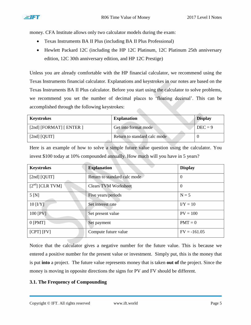
Here is an example of how to solve a simple future value question using the calculator. You

invest $100 today at 10% compounded annually. How much will you have in 5 years?



[2nd

] [CLR TVM] Clears TVM Worksheet 0

5 [N] Five years/periods N = 5

10 [I/Y] Set interest rate I/Y = 10

100 [PV] Set present value PV = 100

0 [PMT] Set payment PMT = 0

[CPT] [FV] Compute future value FV = -161.05

Notice that the calculator gives a negative number for the future value. This is because we

entered a positive number for the present value or investment. Simply put, this is the money that

is put into a project. The future value represents money that is taken out of the project. Since the

money is moving in opposite directions the signs for PV and FV should be different.

3.1. The Frequency of Compounding



Remember compounding is a term associated only with future value. Many investments pay

interest more than once a year, so interest is not calculated just at the end of a year. For example,

a bank might offer a monthly interest rate that compounds 12 times a year. Financial institutions

often quote an annual interest rate that we refer to as the stated annual interest rate or quoted

interest rate. With more than one compounding period per year, the future value formula can be

expressed as:

Equation 2: Future value for multiple compounding periods

FVN = (

)

where

rs = the stated annual interest rate in decimal format

m = the number of compounding periods per year

N = the number of years

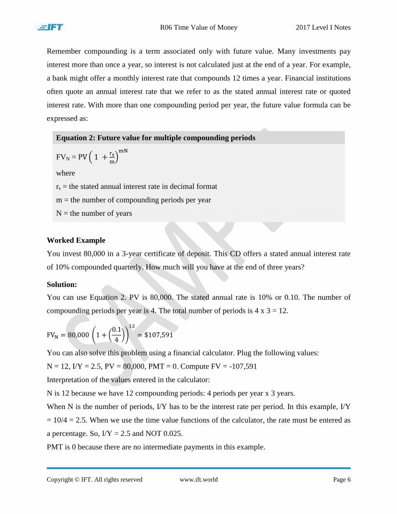
Worked Example

You invest 80,000 in a 3-year certificate of deposit. This CD offers a stated annual interest rate

of 10% compounded quarterly. How much will you have at the end of three years?

Solution:

You can use Equation 2. PV is 80,000. The stated annual rate is 10% or 0.10. The number of

compounding periods per year is 4. The total number of periods is 4 x 3 = 12.

( (

))

You can also solve this problem using a financial calculator. Plug the following values:

N = 12, I/Y = 2.5, PV = 80,000, PMT = 0. Compute FV = -107,591

Interpretation of the values entered in the calculator:

N is 12 because we have 12 compounding periods: 4 periods per year x 3 years.

When N is the number of periods, I/Y has to be the interest rate per period. In this example, I/Y

= 10/4 = 2.5. When we use the time value functions of the calculator, the rate must be entered as

a percentage. So, I/Y = 2.5 and NOT 0.025.

PMT is 0 because there are no intermediate payments in this example.



Signs of PV and FV: Notice that the calculator gives a negative number for future value (FV).

When using the TVM functions on the calculator, the sign of the future value will always be the

opposite of the sign of the present value (PV). The calculator assumes that if the PV is a cash

inflow then the FV must be an outflow and vice versa.

3.2. Continuous Compounding

In the previous section, we saw how discrete compounding works: interest rate is credited after a

discrete amount of time has elapsed. If the number of compounding periods per year becomes

infinite, then interest is said to compound continuously.

Equation 3: Future value for continuous compounding

FVN = PVerN

where r = continuously compounded rate and N = the number of years

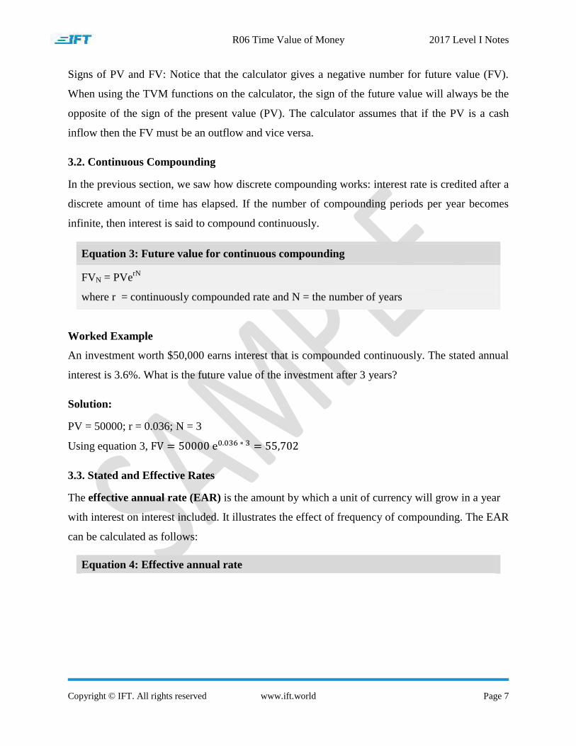
Worked Example

An investment worth $50,000 earns interest that is compounded continuously. The stated annual

interest is 3.6%. What is the future value of the investment after 3 years?

Solution:

PV = 50000; r = 0.036; N = 3

Using equation 3,

3.3. Stated and Effective Rates

The effective annual rate (EAR) is the amount by which a unit of currency will grow in a year

with interest on interest included. It illustrates the effect of frequency of compounding. The EAR

can be calculated as follows:

Equation 4: Effective annual rate



Effective annual rate for discrete compounding:

EAR = (1 + periodic interest rate)m

– 1

where m = number of compounding periods in one year

Effective annual rate for continuous compounding:

where rs = stated annual interest rate

Worked Example

Assume the stated annual interest rate is 8%; compounding is semiannual. What is the effective

annual rate?

In this case, periodic interest rate = 4%. Using Equation 4, EAR = (1.04)2 – 1 = 8.16%. This

means that for every $1 invested, we can expect to receive $1.0816 after one year if there is

semiannual compounding.

4. The Future Value of a Series of Cash Flows

The different types of cash flows based on the time periods over which they occur include:

Annuity: A finite set of constant cash flows that occur at regular intervals.

Ordinary annuity: The first cash flow occurs one period from now (indexed at t = 1).

Annuity due: The first cash flow occurs immediately (indexed at t = 0).

Perpetuity: A set of constant never-ending cash flows at regular intervals, with the first

cash flow occurring one period from now. The period is finite in case of an annuity

whereas in perpetuity it is infinite.

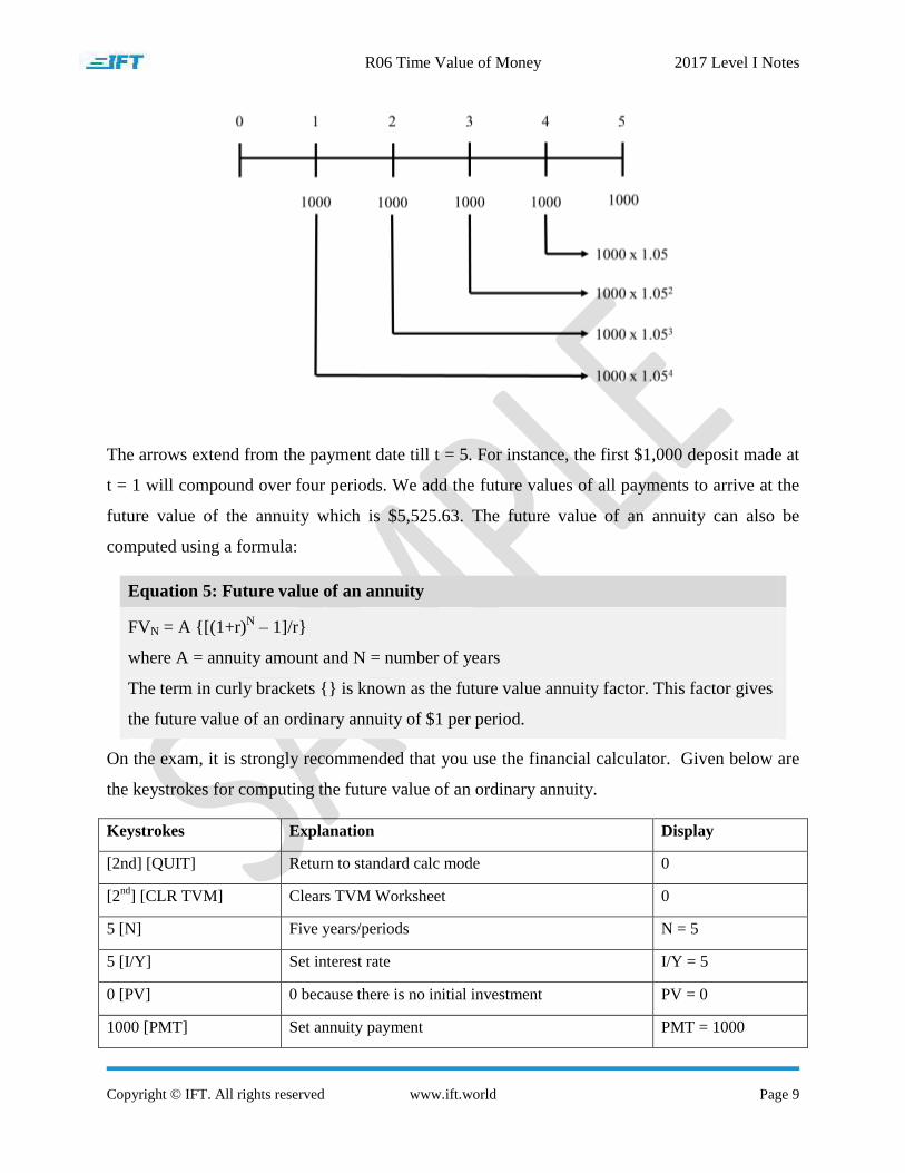
4.1. Equal Cash Flows – Ordinary Annuity

Consider an ordinary annuity paying 5% annually. Suppose we have five separate deposits of

$1,000 occurring at equally spaced intervals of one year, with the first payment occurring at t =

1. Our goal is to find the future value of this ordinary annuity after the last deposit at t = 5. The

calculation of future value for each $1,000 deposit is shown in the figure below.



The arrows extend from the payment date till t = 5. For instance, the first $1,000 deposit made at

t = 1 will compound over four periods. We add the future values of all payments to arrive at the

future value of the annuity which is $5,525.63. The future value of an annuity can also be

computed using a formula:

Equation 5: Future value of an annuity

FVN = A {[(1+r)N – 1]/r}

where A = annuity amount and N = number of years

The term in curly brackets {} is known as the future value annuity factor. This factor gives

the future value of an ordinary annuity of $1 per period.

On the exam, it is strongly recommended that you use the financial calculator. Given below are

the keystrokes for computing the future value of an ordinary annuity.



[2nd



5 [I/Y] Set interest rate I/Y = 5

0 [PV] 0 because there is no initial investment PV = 0

1000 [PMT] Set annuity payment PMT = 1000



[CPT] [FV] Compute future value FV = -5525.63

Hence, the future value is $5,525.63. As explained earlier the calculator shows the future value

as a negative number because the payment has been entered as a positive number.

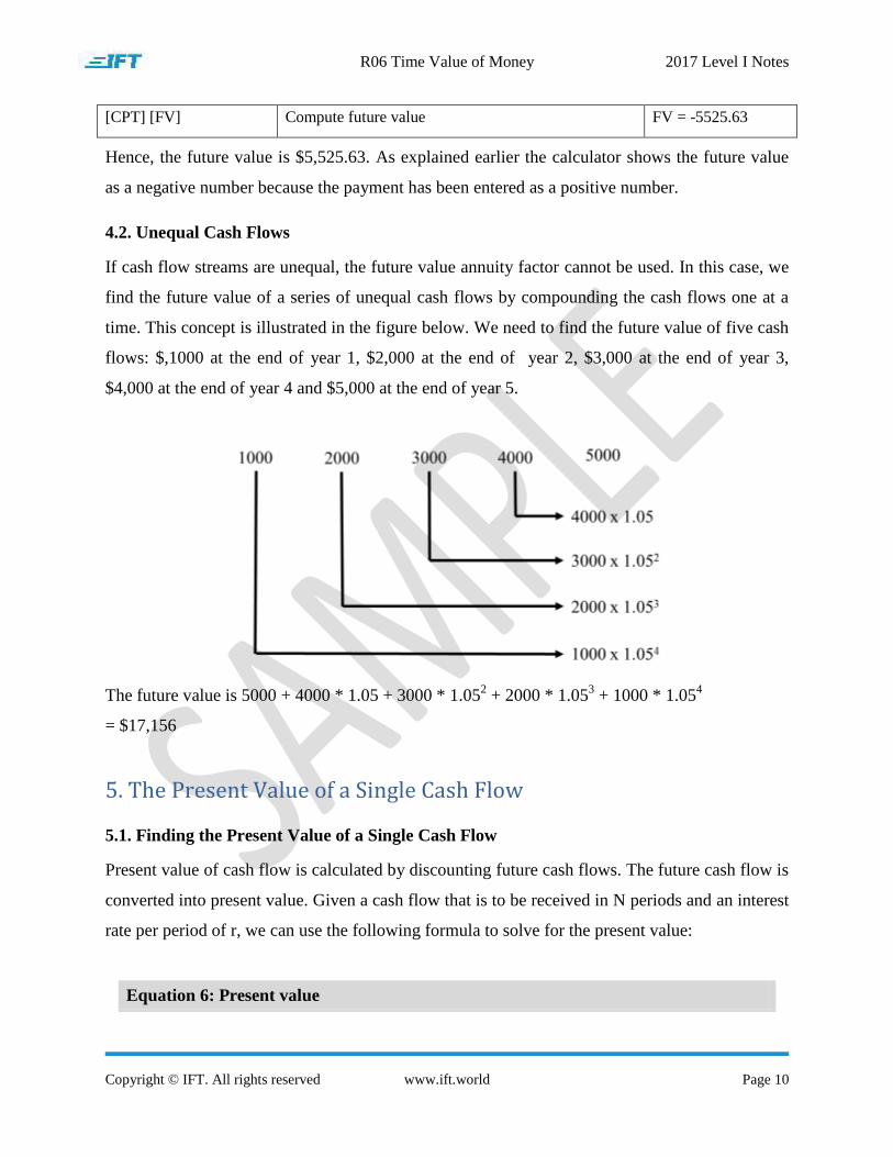
4.2. Unequal Cash Flows

If cash flow streams are unequal, the future value annuity factor cannot be used. In this case, we

find the future value of a series of unequal cash flows by compounding the cash flows one at a

time. This concept is illustrated in the figure below. We need to find the future value of five cash

flows: $,1000 at the end of year 1, $2,000 at the end of year 2, $3,000 at the end of year 3,

$4,000 at the end of year 4 and $5,000 at the end of year 5.

The future value is 5000 + 4000 * 1.05 + 3000 * 1.052 + 2000 * 1.05

3 + 1000 * 1.05

4

= $17,156

5. The Present Value of a Single Cash Flow

5.1. Finding the Present Value of a Single Cash Flow

Present value of cash flow is calculated by discounting future cash flows. The future cash flow is

converted into present value. Given a cash flow that is to be received in N periods and an interest

rate per period of r, we can use the following formula to solve for the present value:

Equation 6: Present value



( )

where N = number of periods, r = rate of interest, FV = future value of investment

Some obvious deductions on present value and future value based on the above formula:

r > 0 which implies that 1/(1 + r) < 1

Present value of a cash flow is always less than the future value

Present value decreases as discount rate or number of periods increases.

Worked Example

Liam purchases a contract from an insurance company. The contract promises to pay $600,000

after 8 years with a 5% return rate. What amount of money should Liam most likely invest

today?

Solution:

FV = 600,000; N = 8; r = 5%

Using Equation 6 for calculating the present value,

( )

You can solve the same using a calculator by entering the following values:

N = 8, I = 5, PMT = 0, FV = $600,000. Compute PV = - 406,104.

5.2. The Frequency of Compounding

For interest rates that can be paid semiannually, quarterly, monthly or even daily, we can modify

the present value formula as follows:

Equation 7: Present value for multiple compounding periods

(

)

where

m = number of compounding periods per year

rs = quoted annual interest rate or discount rate

N = number of years



When using the calculator, we set N as the number of periods. The interest rate should be set as

the per-period rate. For example, if you will receive $100 after one year and the stated annual

rate is 12%, compounded monthly, and then input the following values:

N = 12, I = 1, PMT = 0, FV = 100. Compute PV = -88.74

6. The Present Value of a Series of Cash Flows

6.1. The Present Value of a Series of Equal Cash Flows

An ordinary annuity is a series of equal annuity payments at equal intervals for a finite period of

time. Examples of ordinary annuity: mortgage payments, pension income. The present value can

be computed in three ways:

1. Sum the present values of each individual annuity payment

2. Use the present value of an annuity formula

3. Use the TVM functions of the financial calculator

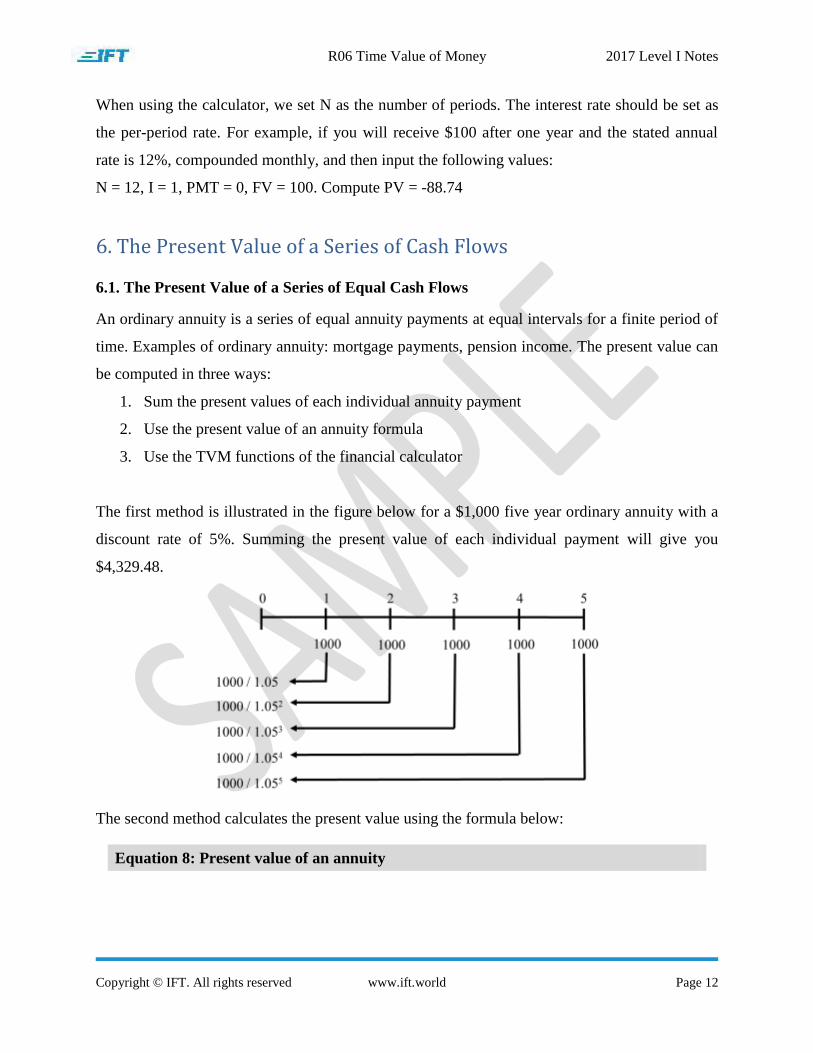
The first method is illustrated in the figure below for a $1,000 five year ordinary annuity with a

discount rate of 5%. Summing the present value of each individual payment will give you

$4,329.48.

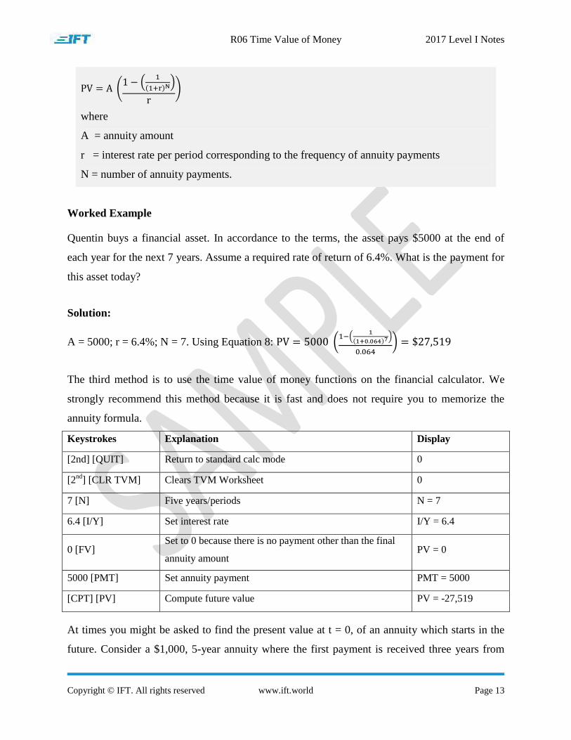
The second method calculates the present value using the formula below:

Equation 8: Present value of an annuity



( (

( ) )

)

where

A = annuity amount

r = interest rate per period corresponding to the frequency of annuity payments

N = number of annuity payments.

Worked Example

Quentin buys a financial asset. In accordance to the terms, the asset pays $5000 at the end of

each year for the next 7 years. Assume a required rate of return of 6.4%. What is the payment for

this asset today?

Solution:

A = 5000; r = 6.4%; N = 7. Using Equation 8: ( (

( ) )

)

The third method is to use the time value of money functions on the financial calculator. We

strongly recommend this method because it is fast and does not require you to memorize the

annuity formula.



[2nd



6.4 [I/Y] Set interest rate I/Y = 6.4

0 [FV] Set to 0 because there is no payment other than the final

annuity amount PV = 0

5000 [PMT] Set annuity payment PMT = 5000

[CPT] [PV] Compute future value PV = -27,519

At times you might be asked to find the present value at t = 0, of an annuity which starts in the

future. Consider a $1,000, 5-year annuity where the first payment is received three years from



today. The discount rate is 5%. To solve this problem first compute the present value of the

annuity at t = 2, and then discount to t = 0. The present value of the five year annuity at t = 2 is

4,329. Note that this value was calculated earlier as the present value at t = 0 for an annuity

where the first cash flow is at t = 1. In this example, the first cash flow is at t = 3 so the present

value is at t = 2. Having 4,329 at t = 2 is equivalent to five cash flows of 1,000 starting at t = 3.

Now we simply need to discount 4,329 back two periods to get the present value at t = 0. This

value is 4,329 / 1.052 = 3,927.

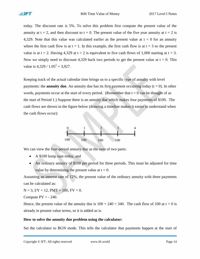
Keeping track of the actual calendar time brings us to a specific type of annuity with level

payments: the annuity due. An annuity due has its first payment occurring today (t = 0). In other

words, payments occur at the start of every period. (Remember that t = 0 can be thought of as

the start of Period 1.) Suppose there is an annuity due which makes four payments of $100. The

cash flows are shown in the figure below (drawing a timeline makes it easier to understand when

the cash flows occur):

We can view the four-period annuity due as the sum of two parts:

A $100 lump sum today, and

An ordinary annuity of $100 per period for three periods. This must be adjusted for time

value by determining the present value at t = 0.

Assuming an interest rate of 12%, the present value of the ordinary annuity with three payments

can be calculated as:

N = 3, I/Y = 12, PMT = 100, FV = 0.

Compute PV = - 240.

Hence, the present value of the annuity due is 100 + 240 = 340. The cash flow of 100 at t = 0 is

already in present value terms, so it is added as is.

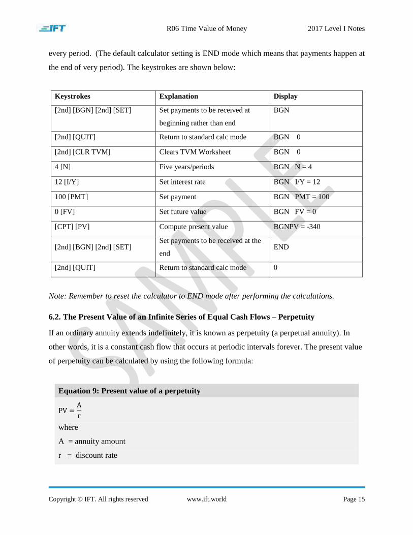
How to solve the annuity due problem using the calculator:

Set the calculator to BGN mode. This tells the calculator that payments happen at the start of



every period. (The default calculator setting is END mode which means that payments happen at

the end of very period). The keystrokes are shown below:


[2nd] [BGN] [2nd] [SET] Set payments to be received at

beginning rather than end

BGN

[2nd] [QUIT] Return to standard calc mode

BGN 0

[2nd] [CLR TVM] Clears TVM Worksheet BGN 0

4 [N] Five years/periods BGN N = 4

12 [I/Y] Set interest rate BGN I/Y = 12

100 [PMT] Set payment BGN PMT = 100

0 [FV] Set future value BGN FV = 0

[CPT] [PV] Compute present value BGNPV = -340

[2nd] [BGN] [2nd] [SET] Set payments to be received at the

end END


Note: Remember to reset the calculator to END mode after performing the calculations.

6.2. The Present Value of an Infinite Series of Equal Cash Flows – Perpetuity

If an ordinary annuity extends indefinitely, it is known as perpetuity (a perpetual annuity). In

other words, it is a constant cash flow that occurs at periodic intervals forever. The present value

of perpetuity can be calculated by using the following formula:

Equation 9: Present value of a perpetuity

where

A = annuity amount

r = discount rate



This equation is only valid for a perpetuity with level payments.

Example of a perpetuity: certain government bonds and preferred stocks.

Consider a preferred share, which pays a dividend of 5.00 every year forever. The appropriate

discount rate is 10%. The present value of the dividend payments is 5 / 0.1 = 50.

6.3. Present Values Indexed at Times Other Than t = 0

An annuity or perpetuity beginning sometime in the future can be expressed in present value

terms one period prior to the first payment. That present value can then be discounted back to

today’s present value. The following example illustrates this concept.

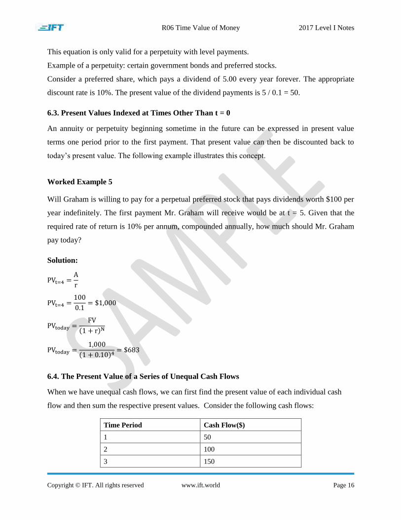
Worked Example 5

Will Graham is willing to pay for a perpetual preferred stock that pays dividends worth $100 per

year indefinitely. The first payment Mr. Graham will receive would be at t = 5. Given that the

required rate of return is 10% per annum, compounded annually, how much should Mr. Graham

pay today?

Solution:

( )

( )

6.4. The Present Value of a Series of Unequal Cash Flows

When we have unequal cash flows, we can first find the present value of each individual cash

flow and then sum the respective present values. Consider the following cash flows:

Time Period Cash Flow($)

1 50

2 100

3 150



4 200

5 250

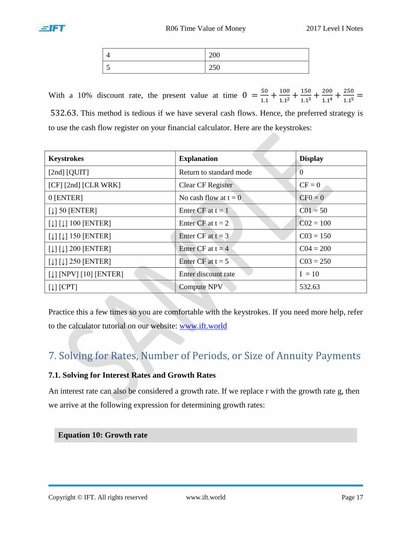
With a 10% discount rate, the present value at time

This method is tedious if we have several cash flows. Hence, the preferred strategy is

to use the cash flow register on your financial calculator. Here are the keystrokes:


[2nd] [QUIT] Return to standard mode 0

[CF] [2nd] [CLR WRK] Clear CF Register CF = 0

0 [ENTER] No cash flow at t = 0 CF0 = 0

[↓] 50 [ENTER] Enter CF at t = 1 C01 = 50

[↓] [↓] 100 [ENTER] Enter CF at t = 2 C02 = 100




[↓] [NPV] [10] [ENTER] Enter discount rate I = 10

[↓] [CPT] Compute NPV 532.63

Practice this a few times so you are comfortable with the keystrokes. If you need more help, refer

to the calculator tutorial on our website: www.ift.world

7. Solving for Rates, Number of Periods, or Size of Annuity Payments

7.1. Solving for Interest Rates and Growth Rates

An interest rate can also be considered a growth rate. If we replace r with the growth rate g, then

we arrive at the following expression for determining growth rates:

Equation 10: Growth rate

http://www.ift.world/



g = (FVN /PV)1/N

– 1

where

FV = future vale

PV = present value

N = number of years

Consider the following scenario: The population of a small town is 100,000 on 1 Jan., 2000. On

31 Dec., 2001 the population is 121,000. What is the growth rate?

Since the growth is happening over two years, N = 2.

Using equation 10, (

)

–

We can also use the calculator: N = 2, PV = 100,000, PMT = 0, FV = -121,000 (remember that

PV and FV should have different signs). Compute I/Y = 10. I/Y represents the growth rate and is

given as a percentage.

7.2. Solving for the Number of Periods

Say you invest 2,500 today and want to know how many years it will take for your money to

grow by three times if the annual interest rate is 6%. This can be solved using the formula or

with a calculator.

Method 1:

FV = PV (1 + r) N

7,500 = 2,500 (1 + 0.06) N

1.06N = 3

N x ln 1.06 = ln 3

N = (

) = 18.85

Method 2:

Using the calculator: I/Y = 6, PV = 2,500, PMT = 0, FV = -7,500. Compute N = 18.85.



7.3. Solving for the Size of Annuity Payments

Given the number of periods, interest rate per period, present value and future value, it is easy to

solve for the annuity payment amount. This concept can be applied to mortgages and retirement

planning. Consider the following examples:

Worked Example 6

Wally Hammond is planning to buy a house worth $300,000. He will make a 20% down

payment and borrow the remainder with a 30-year fixed rate mortgage with monthly payments.

The first payment is due at t = 1. The current mortgage interest rate is quoted at 12% with

monthly compounding. Calculate the monthly mortgage payments.

Solution:

Amount borrowed = 80% of 300,000 = 240,000. This represents the present value. We need to

determine the 360 (30 years * 12 periods/year) equal payments which have a present value of

240,000 given a periodic interest rate of 1% (12% per year means 12/12 = 1% per period).

While this can be solved using the annuity formula, it is much easier to use the calculator:

N = 360, I/Y = 1, PV = 240000, FV = 0. CPT PMT = -246.87.

This means that 360 level payments of 246.87 is equivalent to a present value of 240,000, given

an interest rate of 1% per period.

Worked Example 7

Your client is 25 years old (at t = 0) and plans to retire at age 60 (at t = 35). He wants to save

$3,000 per year for the next 10 years (from t = 1 to t = 10). He would like a retirement income of

100,000 per year for 21 years, with the first retirement payment starting at t = 35. How much will

you advise him to save each year from t = 11 to t = 34? Assume a return of 10% per year on

average.

Solution:

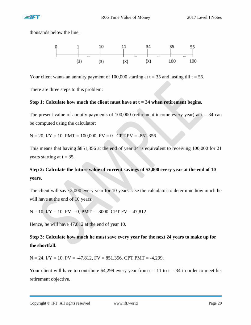
First set up a timeline. The time periods are shown above the line. Each number represents the

end of that period. So 1 means the end of period 1 and so on. The cash amounts are shown in



thousands below the line.

Your client wants an annuity payment of 100,000 starting at t = 35 and lasting till t = 55.

There are three steps to this problem:

Step 1: Calculate how much the client must have at t = 34 when retirement begins.

The present value of annuity payments of 100,000 (retirement income every year) at t = 34 can

be computed using the calculator:

N = 20, I/Y = 10, PMT = 100,000, FV = 0. CPT PV = -851,356.

This means that having $851,356 at the end of year 34 is equivalent to receiving 100,000 for 21

years starting at t = 35.

Step 2: Calculate the future value of current savings of $3,000 every year at the end of 10

years.

The client will save 3,000 every year for 10 years. Use the calculator to determine how much he

will have at the end of 10 years:

N = 10, I/Y = 10, PV = 0, PMT = -3000. CPT FV = 47,812.

Hence, he will have 47,812 at the end of year 10.

Step 3: Calculate how much he must save every year for the next 24 years to make up for

the shortfall.

N = 24, I/Y = 10, PV = -47,812, FV = 851,356. CPT PMT = -4,299.

Your client will have to contribute $4,299 every year from t = 11 to t = 34 in order to meet his

retirement objective.



7.4. Review of Present and Future Value Equivalence

As discussed in the earlier sections, finding the present and the future values involves moving

amounts of money to different points in time. These operations are possible because present

value and future value are equivalent measures separated in time. This equivalence illustrates an

important point: a lump sum amount can generate an annuity. If we place a lump sum in an

account that earns the stated interest rate for all periods, we can generate an annuity that is

equivalent to the lump sum.

Here is a simple example to illustrate how a lump sum can generate an annuity. Suppose that we

place $4,329.48 in the bank today at 5% interest. We can calculate the size of the annuity

payments:

N = 5, I/Y = 5, PV = 4329.48, FV = 0. CPT PMT = 1000. Hence, an amount of $4,329.48

deposited in the bank today can generate five $1,000 withdrawals over the next five years.

Now consider another scenario. Invest 4,329.48 today at 5%. How much will we have at the end

of 5 years? Using the calculator: N = 5, I/Y = 5, PV = 4,329.48, PMT = 0. CPT FV = -5,526. In

other words, we will have $5,526 at the end of 5 years.

Here is the final scenario. We invest 1,000 per year for 5 years. How much will we have at the

end of 5 years? Using the calculator: N = 5, I/Y = 5, PV = 0, PMT = 1000. Compute FV = -

5,526. Here again we will have $5,526 at the end of 5 years.

To summarize: A lump sum can be seen as equivalent to an annuity, and an annuity can be seen

as equivalent to its future value. Thus, present values, future values, and a series of cash flows

can all be considered equivalent as long as they are indexed at the same point in time.

7.5. The Cash Flow Additivity Principle

This principle states that the amounts of money indexed at the same point in time are additive.

The principle is useful to determine the future value/present value when there is a series of

uneven cash flows.



First, let’s take a simple example. There are two cash flows: $50 occurring today, and $100 at the

end of period 1. What is the value of this cash flow?

Is this correct? 50 (today) + 100 (after one year) = 150

No. Because these cash flows are at two different points in time, so they are not additive. There

are two options to make them additive:

Present value: 50 + PV (100)

Future value: FV(50) + 100

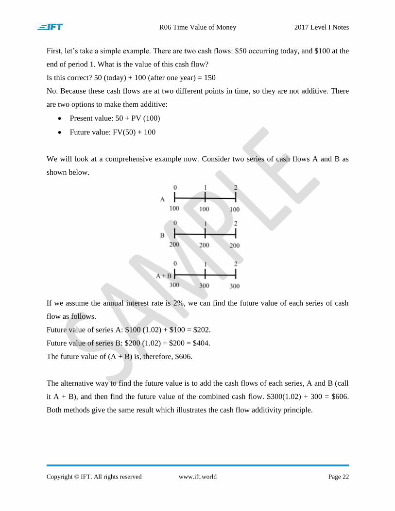
We will look at a comprehensive example now. Consider two series of cash flows A and B as

shown below.

If we assume the annual interest rate is 2%, we can find the future value of each series of cash

flow as follows.

Future value of series A: $100 (1.02) + $100 = $202.

Future value of series B: $200 (1.02) + $200 = $404.

The future value of (A + B) is, therefore, $606.

The alternative way to find the future value is to add the cash flows of each series, A and B (call

it A + B), and then find the future value of the combined cash flow. $300(1.02) + 300 = $606.

Both methods give the same result which illustrates the cash flow additivity principle.

Time Value of Money - IFTift.world/wp-content/uploads/2016/11/R06-Time-Value-of-Money-IFT... ·...

Documents

Transcript of Time Value of Money - IFTift.world/wp-content/uploads/2016/11/R06-Time-Value-of-Money-IFT... ·...