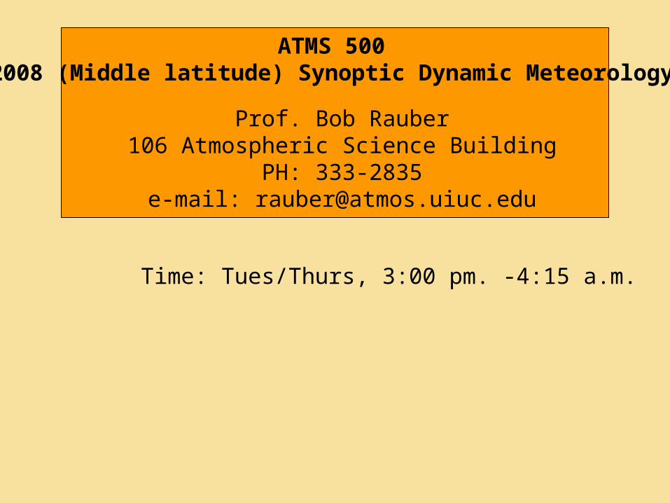
Time: Tues/Thurs, 3:00 pm. -4:15 a.m.

ATMS 5002008 (Middle latitude) Synoptic Dynamic Meteorology

Prof. Bob Rauber106 Atmospheric Science Building

PH: 333-2835e-mail: rauber@atmos.uiuc.edu

Synoptic dynamics of extratropical cyclones

-Kinematic properties of the horizontal wind field-Fundamental and apparent forces-Mass, Momentum and Energy -Governing equations (Conservation of momentum, mass, energy, eqn of state)-Equations of motion and their application -Balanced flow-Isentropic flow-Circulation, vorticity, Potential vorticity-Quasi-Geostrophic theory-Ageostrophic flow-QG diagnostic tools ( equation, Q vectors)-Frontogenesis-Vertical circulation about fronts-Semi-geostrophic theory-Potential vorticity diagnostics

Our goal: Examine the fundamental dynamical constructs required to examine the behavior of extratropical cyclones:

Martin, J. “Mid-latitude atmospheric dynamics” Wiley

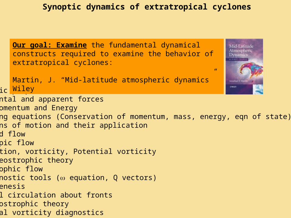
Synoptic dynamics of extratropical cyclones

Potential additional topics

-Wave dynamics-Jetstream and Jetstreak dynamics-Subtropical and Polar front jets

-Cyclogenesis and explosive cyclogenesis-Cyclone lifecycle-Pacific/Continental/East Coast cyclone structure and dynamics

-Fronts and frontal dynamics-Occlusions

Extratropical Cyclones

COURSE WEBSITE

http://www.atmos.uiuc.edu/courses/atmos500-fa08/

Posted on this website are:

1) All PowerPoint files I use in class2) Any Papers I will review3) Syllabus

GRADES

A. Mid-term exam (25% of grade)B. Final exam (25% of grade)C. Derivation Notebooks (26% of grade)D. Homework (24% of grade)

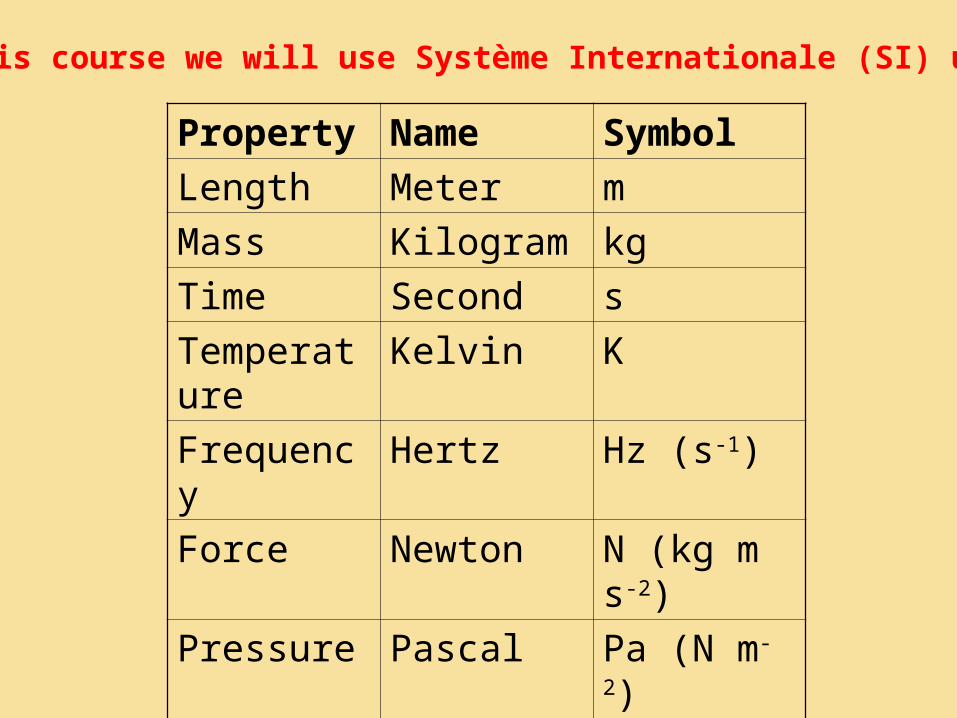
In this course we will use Système Internationale (SI) units

Property Name Symbol

Length Meter m

Mass Kilogram kg

Time Second s

Temperature Kelvin K

Frequency Hertz Hz (s-1)

Force Newton N (kg m s-2)

Pressure Pascal Pa (N m-2)

Energy Joule J (N m)

Power Watt W (J s-1)

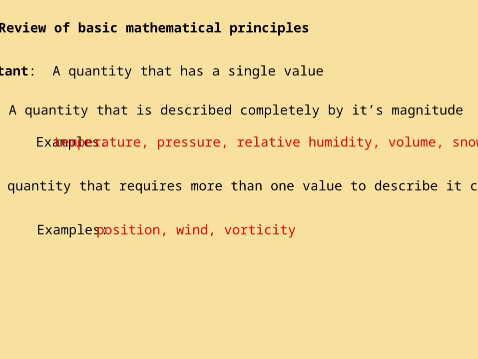
Review of basic mathematical principles

Scalar: A quantity that is described completely by it’s magnitude

Vector: A quantity that requires more than one value to describe it completely

Examples: temperature, pressure, relative humidity, volume, snowfall

Constant: A quantity that has a single value

Examples: position, wind, vorticity

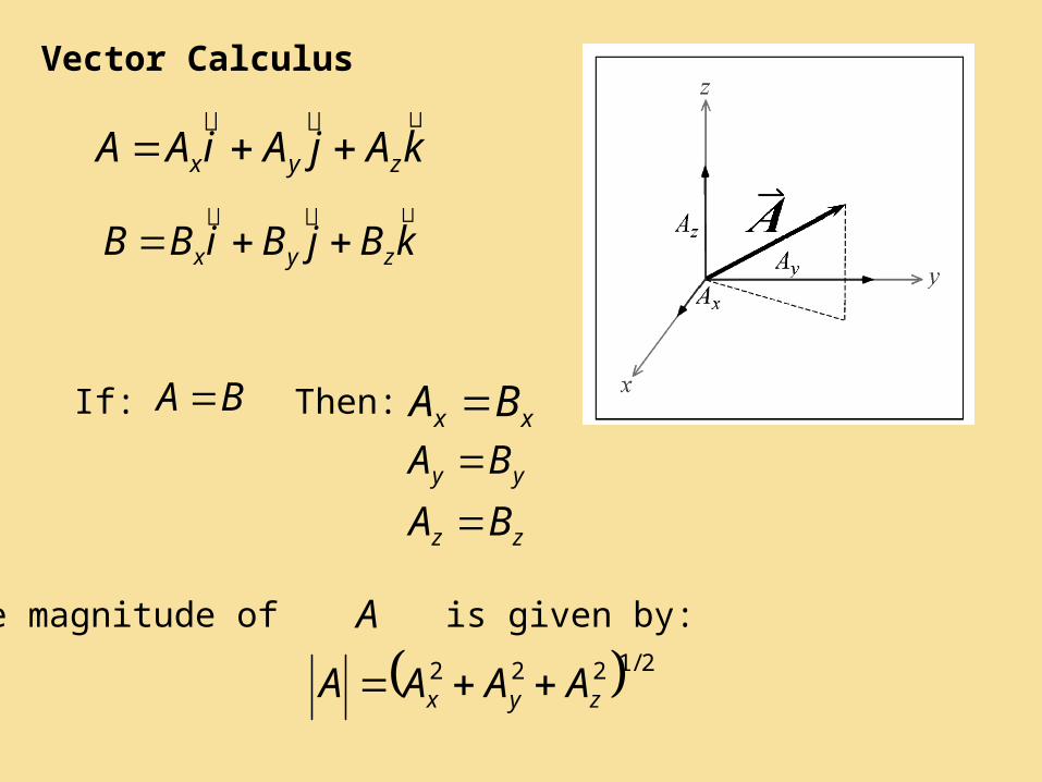
Vector Calculus

kAjAiAA zyx

kBjBiBB zyx

xx BA

yy BA

zz BA

BA

2/1222zyx AAAA

If: Then:

The magnitude of is given by: A

kBAjBAiBABA zzyyxx

ABBA

CBACBA

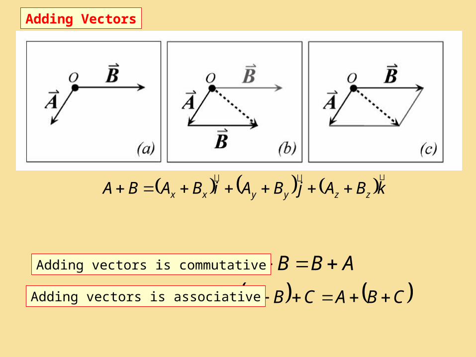
Adding Vectors

Adding vectors is commutative

Adding vectors is associative

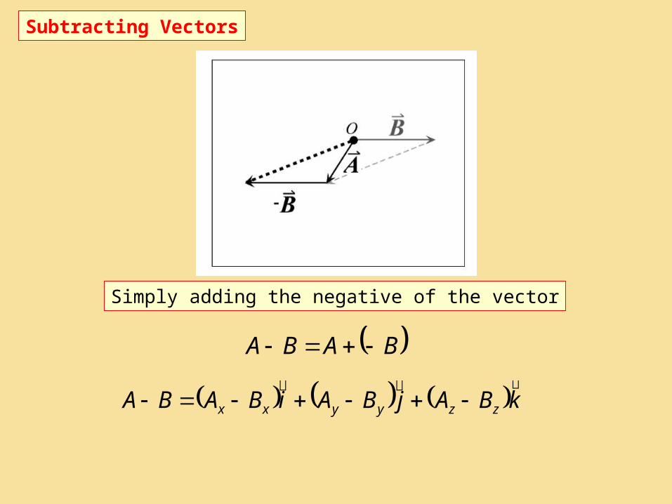
BABA

kBAjBAiBABA zzyyxx

Subtracting Vectors

Simply adding the negative of the vector

kFAjFAiFAAF zyx

kBjBiBkAjAiABA zyxzyx

kkBAjkBAikBA

kjBAjjBAijBA

kiBAjiBAiiBABA

zzyzxz

zyyyxy

zxyxxx

zzyyxx BABABABA

ABBA

CABACBA

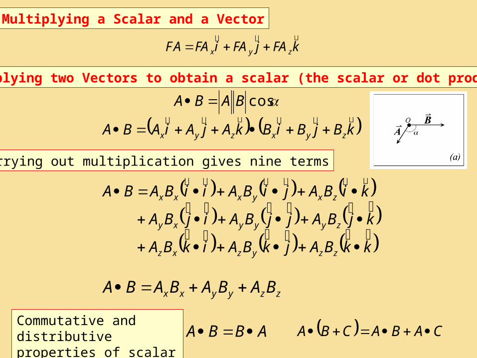
Multiplying a Scalar and a Vector

Multiplying two Vectors to obtain a scalar (the scalar or dot product)

Carrying out multiplication gives nine terms

cosBABA

Commutative and distributive properties of scalar product

sinBABA

ABBA

ABBA

CBACBA

CABACBA

z

z

yx

yx

B

A

k

BB

AA

ji

BA

kBABAjBABAiBABABA xyyxxzzxyzzy

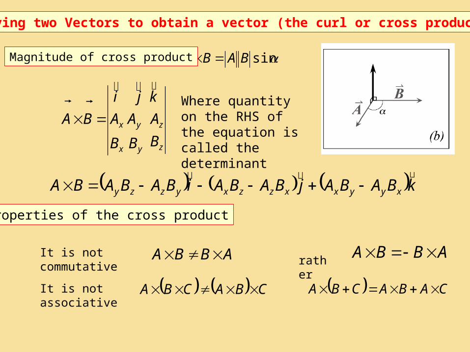
Multiplying two Vectors to obtain a vector (the curl or cross product)

Magnitude of cross product

Where quantity on the RHS of the equation is called the determinant

Properties of the cross product

It is not commutative rather

It is not associative

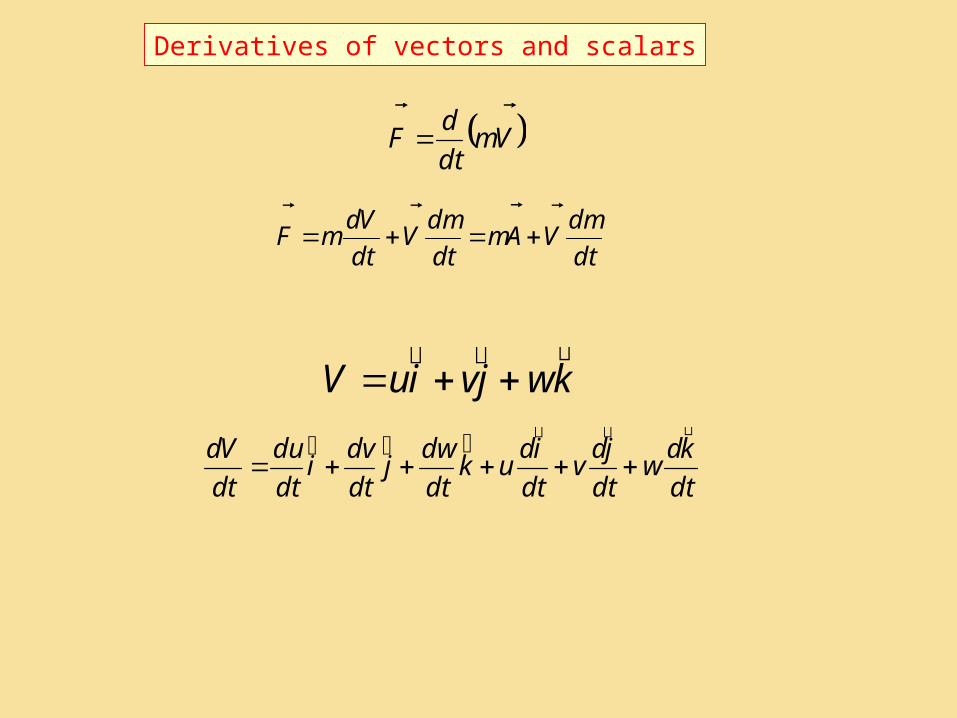
Derivatives of vectors and scalars

Vmdt

dF

dt

dmVAm

dt

dmV

dt

VdmF

kwjviuV

dt

kdw

dt

jdv

dt

iduk

dt

dwj

dt

dvi

dt

du

dt

Vd

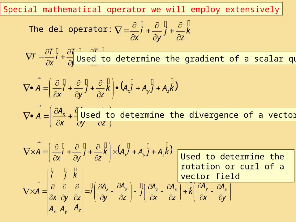
Special mathematical operator we will employ extensively

The del operator: kz

jy

ix

kz

Tj

y

Tix

TT

Used to determine the gradient of a scalar quantity

kAjAiAkz

jy

ix

A zyx

z

A

y

A

x

AA zyx

Used to determine the divergence of a vector field

kAjAiAkz

jy

ix

A zyx

y

A

x

Ak

z

A

x

Aj

z

A

y

Ai

Az

k

AA

yx

ji

A xyxzyz

zyx

Used to determine the rotation or curl of a vector field

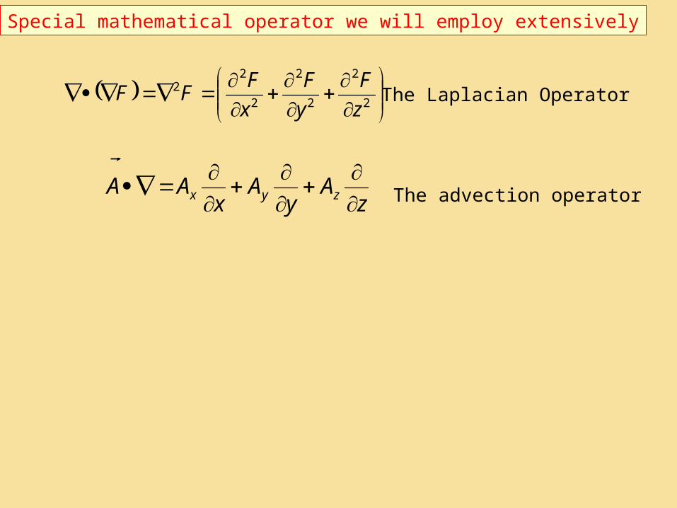
Special mathematical operator we will employ extensively

2

2

2

2

2

22

z

F

y

F

x

FFF

zA

yA

xAA zyx

The Laplacian Operator

The advection operator

nn

n

nn xaxaxaaxaxf

...)( 2210

0

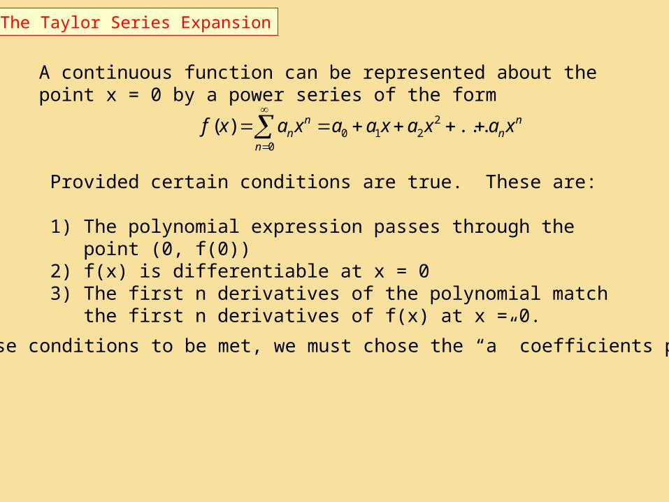
The Taylor Series Expansion

A continuous function can be represented about the point x = 0 by a power series of the form

Provided certain conditions are true. These are:

1) The polynomial expression passes through the point (0, f(0))2) f(x) is differentiable at x = 03) The first n derivatives of the polynomial match the first n derivatives of

f(x) at x = 0.

For these conditions to be met, we must chose the “a” coefficients properly

!

)0(

n

fa

n

n

nn

xn

fx

fx

fxffxf

!

)0(...

!3

)0(

!2

)0()0()0()( 32

nn

n

nn xaxaxaaxaxf

...)( 2210

0

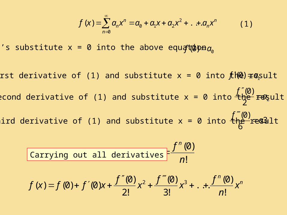
Let’s substitute x = 0 into the above equation0)0( af

(1)

Take first derivative of (1) and substitute x = 0 into the result 1)0( af

Take second derivative of (1) and substitute x = 0 into the result 22

)0(a

f

Take third derivative of (1) and substitute x = 0 into the result 36

)0(a

f

Carrying out all derivatives

nn

xxn

xfxx

xfxxxfxfxf 0

020

0000 !

)(...

!2

)()()()(

000 )()()( xxxfxfxf

nn

xn

fx

fx

fxffxf

!

)0(...

!3

)0(

!2

)0()0()0()( 32

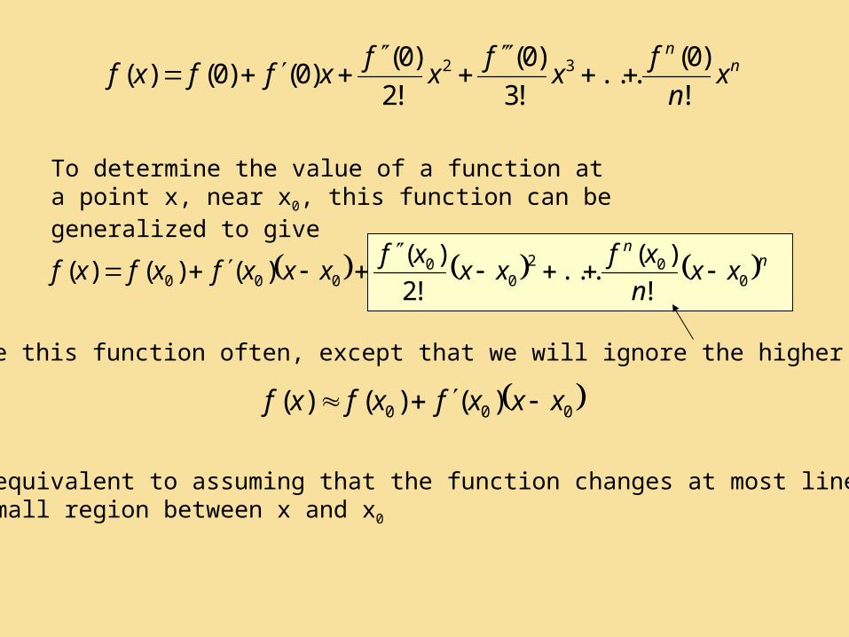
To determine the value of a function at a point x, near x0, this function can be generalized to give

We will use this function often, except that we will ignore the higher order terms

This is equivalent to assuming that the function changes at most linearlyIn the small region between x and x0

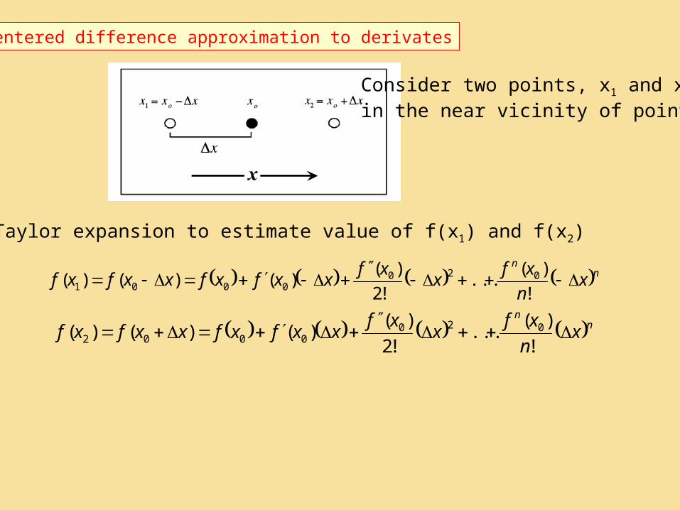
Centered difference approximation to derivates

nn

xn

xfx

xfxxfxfxxfxf

!

)(...

!2

)()()()( 020

0001

nn

xn

xfx

xfxxfxfxxfxf

!

)(...

!2

)()()()( 020

0002

Consider two points, x1 and x2

in the near vicinity of point x0

Use Taylor expansion to estimate value of f(x1) and f(x2)

nn

xn

xfx

xfxxfxfxxfxf

!

)(...

!2

)()()()( 020

0001

nn

xn

xfx

xfxxfxfxxfxf

!

)(...

!2

)()()()( 020

0002

...!3

)(2)(2)()( 30

000

xxf

xxfxxfxxf

....

6)(

2)(

2

000

0

xxf

x

xxfxxfxf

x

xxfxxfxf

2

)( 000

2

0000

2)(

x

xxfxfxxfxf

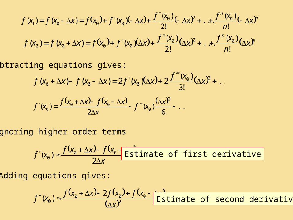
Subtracting equations gives:

Ignoring higher order terms

Estimate of first derivative

Adding equations gives:

Estimate of second derivative

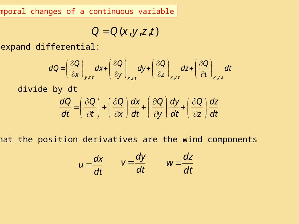
Temporal changes of a continuous variable

),,,( tzyxQQ

dtt

Qdz

z

Qdy

y

Qdx

x

QdQ

zyxtyxtzxtzy ,,,,,,,,

dt

dz

z

Q

dt

dy

y

Q

dt

dx

x

Q

t

Q

dt

dQ

dt

dxu

dt

dyv

dt

dzw

expand differential:

divide by dt

Note that the position derivatives are the wind components

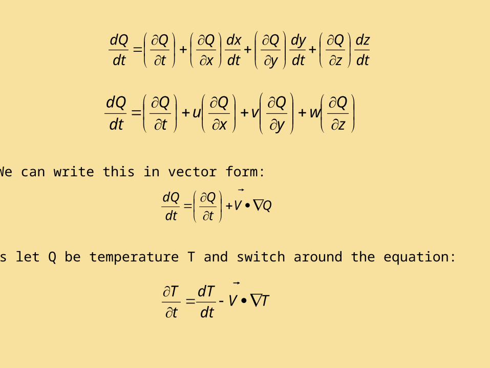
z

Qw

y

Qv

x

Qu

t

Q

dt

dQ

QVt

Q

dt

dQ

TVdt

dT

t

T

dt

dz

z

Q

dt

dy

y

Q

dt

dx

x

Q

t

Q

dt

dQ

We can write this in vector form:

Let’s let Q be temperature T and switch around the equation:

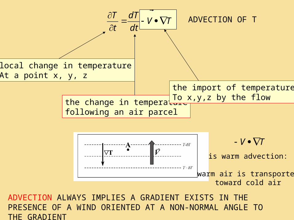
TVdt

dT

t

T

local change in temperatureAt a point x, y, z

the change in temperaturefollowing an air parcel

ADVECTION OF T

the import of temperatureTo x,y,z by the flow

TV

is warm advection:

warm air is transportedtoward cold air

ADVECTION ALWAYS IMPLIES A GRADIENT EXISTS IN THE PRESENCE OF A WIND ORIENTED AT A NON-NORMAL ANGLE TO THE GRADIENT