Time Series Study on Bitcoin and Crude Oil Prices

A T I M E S E R I E SS T U D Y O NB I T C O I N &C R U D E O I L

A U N I V A R I A T E A N D M U L T I V A R I A T EA N A L Y S I S

V I V E K A D I T H Y A M O H A N K U M A R

R A M A B H A D R A R A J UT I R U M A L A R A J U

E C O N 5 3 3 8 A P P L I E D T I M E S E R I E S

ABSTRACT Bitcoin is the world's first completely decentralized digital payment system, the emergence of

bitcoin represents a revolutionary phenomenon in financial markets. This paper mainly studies

the relationship between bitcoin and crude oil prices. A multivariate analysis between bitcoin

and crude oil was carried out to establish the relationship between bitcoin and crude oil.

Cointegration analysis, VAR and ARDL models were considered for the research. Also,

univariate analysis was carried out to establish the effect of past values on bitcoin and future

prices are forecasted.

INTRODUCTION Our research was based on analyzing the economic relationship between Bitcoin and Crude Oil

prices. Bitcoin is a form of digital asset, that is created and held electronically. The system is

peer-to-peer, and the transactions happen directly among users without an intermediary. No one

has control over it or prints it unlike USD or INR. Bitcoin has exhibited large volatility in a short

period. The price of bitcoin has gone through cycles of bubbles and busts.

Bitcoin was quite cheap at its birth, only about 5 cents per Bitcoin. But with the promotion of its

influence around the world, its price boomed. In 2013, with the personal virtual currency

regulation, which admitted the legal status of Bitcoin, and the Bitcoin price raised to more than

$1000. With the global bitcoin, hot the demand of bitcoin in China increased, further increasing

the Bitcoin prices to a historic $1151 [1].

This paper mainly studies the price fluctuations of Bitcoin and discusses its variation with the

crude oil prices.

VARIABLE SELECTION It is since 2011 that Bitcoin price began to fluctuate significantly and attract increasing attention.

So, the sample period we choose is from August 2011 to October 2016, too much noise exists in

the data before 2011 due to the small trading volume. Since dollar is a major foreign exchange

currency of Bitcoin, we use the exchange rate of Bitcoin and dollar to represent the price of

Bitcoin. When measuring the Crude oil price, we chose the WTI crude oil price, which is a

benchmark in crude oil prices. As there is a huge fluctuation in the data, logarithmic treatment to

the Bitcoin price, oil price is conducted. Data stream is used to download the weekly data for

Bitcoin and WTI crude oil prices from august 2011 to October 2016. Eviews is used for

statistical analysis.

EMPIRICAL RESEARCH

STATIONARITY TEST OF VARIABLES

LINE GRAPH AT LEVEL

At level, Bitcoin seems to be violating the conditions for stationarity, with a visible upward trend

and exhibits structural breaks in the mid 2013 to 2014.

At level, Crude Oil seems to be violating the conditions for stationarity. The mean seems to be

varying over time. And, exhibits structural breaks in the early 2014 to mid-2014.

LINE GRAPH AFTER LOG TRANSFORMATION

Even after the log transformation, the bitcoin series doesn’t seem stationary.

20

40

60

80

100

120

III IV I II III IV I II III IV I II III IV I II III IV I II III IV

2011 2012 2013 2014 2015 2016

Oil at Level

0

1

2

3

4

5

6

7


2012 2013 2014 2015 2016

BC Log

0

200

400

600

800

1,000

1,200


2012 2013 2014 2015 2016

Bit Coin at Level

Even after the log transformation, the crude oil series too doesn’t seem stationary.

LINE GRAPH AFTER FIRST DIFFERENCE

On taking first difference of the original series, the bitcoin series seems to satisfy the stationarity

restrictions.

Likewise, on taking first difference on the original crude oil series seems to look stationary.

3.2

3.4

3.6

3.8

4.0

4.2

4.4

4.6

4.8


2011 2012 2013 2014 2015 2016

Oil on Log Transformation

-300

-200

-100

0

100

200

300

400


2012 2013 2014 2015 2016

Bit Coin at First Difference

-8

-4

0

4

8

12


2012 2013 2014 2015 2016

Oil at First Difference

UNIT ROOT TEST To estimate the stationarity of the variables under study, we performed Break point unit root test

for data with structural breaks on both Bitcoin and Crude Oil.

Bitcoin – Break Point

Null Hypothesis: BC_LEVEL has a unit root

Trend Specification: Intercept only

Break Specification: Intercept only

Break Type: Innovational outlier

Break Date: 10/14/2013

Break Selection: Minimize Dickey-Fuller t-statistic

Lag Length: 5 (Automatic - based on Schwarz information criterion,

maxlag=15)

t-Statistic Prob.*

Augmented Dickey-Fuller test statistic -3.288637 0.5096

Test critical values: 1% level -4.949133

5% level -4.443649

10% level -4.193627

*Vogelsang (1993) asymptotic one-sided p-values.

Augmented Dickey-Fuller Test Equation

Dependent Variable: BC_LEVEL

Method: Least Squares

Date: 12/08/16 Time: 23:29

Sample (adjusted): 10/24/2011 11/28/2016

Included observations: 267 after adjustments

Variable Coefficient Std. Error t-Statistic Prob.

BC_LEVEL(-1) 0.936587 0.019282 48.57227 0.0000

D(BC_LEVEL(-1)) 0.234270 0.060800 3.853125 0.0001

D(BC_LEVEL(-2)) 0.145811 0.062514 2.332474 0.0204

D(BC_LEVEL(-3)) -0.244241 0.060246 -4.054075 0.0001

D(BC_LEVEL(-4)) 0.013573 0.061926 0.219181 0.8267

D(BC_LEVEL(-5)) 0.199967 0.061031 3.276472 0.0012

C 3.117503 4.256371 0.732432 0.4646

INCPTBREAK 27.90130 9.528453 2.928209 0.0037

BREAKDUM -10.45596 43.21340 -0.241961 0.8090

R-squared 0.971725 Mean dependent var 292.8742

Adjusted R-squared 0.970848 S.D. dependent var 249.7502

S.E. of regression 42.64243 Akaike info criterion 10.37670

Sum squared resid 469141.2 Schwarz criterion 10.49762

Log likelihood -1376.290 Hannan-Quinn criter. 10.42528

F-statistic 1108.314 Durbin-Watson stat 2.000894

Prob(F-statistic) 0.000000

The test captures the structural breaks in August 2013. And the P value of 0.5096 assures that the

series is non-stationary indeed.

UNIT ROOT TEST AT FIRST DIFFERENCE

Unit root test indicates a clear stationarity at first difference.

Oil – Break Point

Null Hypothesis: OIL_W has a unit rootTrend Specification: Trend and interceptBreak Specification: Trend and interceptBreak Type: Innovational outlier

Break Date: 9/29/2014Break Selection: Minimize Dickey-Fuller t-statisticLag Length: 0 (Automatic - based on Schwarz information criterion, maxlag=15)

t-Statistic Prob.*

Augmented Dickey-Fuller test statistic -4.231900 0.3750Test critical values: 1% level -5.719131

5% level -5.17571010% level -4.893950

*Vogelsang (1993) asymptotic one-sided p-values.

Augmented Dickey-Fuller Test EquationDependent Variable: OIL_WMethod: Least SquaresDate: 12/13/16 Time: 13:35Sample (adjusted): 9/12/2011 11/28/2016Included observations: 273 after adjustments

Variable Coefficient Std. Error t-Statistic Prob.

OIL_W(-1) 0.914133 0.020290 45.05233 0.0000C 8.227171 1.916508 4.292794 0.0000

TREND 0.001184 0.004765 0.248484 0.8040INCPTBREAK -4.626444 1.023853 -4.518662 0.0000TRENDBREAK -0.001266 0.010746 -0.117851 0.9063

BREAKDUM 7.134492 2.789607 2.557526 0.0111

R-squared 0.989036 Mean dependent var 76.74392Adjusted R-squared 0.988831 S.D. dependent var 25.34818S.E. of regression 2.678913 Akaike info criterion 4.830432Sum squared resid 1916.145 Schwarz criterion 4.909761Log likelihood -653.3540 Hannan-Quinn criter. 4.862276F-statistic 4817.122 Durbin-Watson stat 1.923453Prob(F-statistic) 0.000000

The test captures the structural breaks in October 2014. And a highly significant test statistic of

-4.23 assures that the series is non-stationary indeed.

UNIT ROOT TEST AT FIRST DIFFERENCE

Oil at first difference is clearly stationary.

MULTIVARIATE ANALYSIS OF BITCOIN AND CRUDE OIL

COINTEGERATION The two variables are stationary series after the first order difference, so the Johansen method

can be used for cointegration test. Cointegration relationship among variables can be determined

through trace statistic and the maximum eigenvalue likelihood ratio statistic.

Both Trace and eigen values indicates no co-integration at the 0.05 level.

VAR MODEL ESTIMATION

LAG LENGTH SELECTION

Before doing VAR analysis it is essential to estimate the lag length of the model, Based on the

estimation, a VAR (3) analysis is suitable for estimation.

DUMMY VARIABLES

There's a clear structural break in the data, hence a dummy variable, BREAK, is added that takes

the value 1 for these observations, and 0 everywhere else. The structural break variable is

included while running the tests for better model selection.

VAR ESTIMATION

Running a VAR (3) model, we can see that Bitcoin is highly significant onto itself. We can also

see that oil is significant onto Bitcoin (-3).

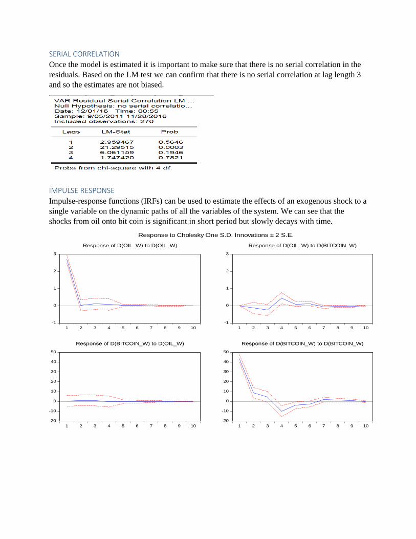
SERIAL CORRELATION

Once the model is estimated it is important to make sure that there is no serial correlation in the

residuals. Based on the LM test we can confirm that there is no serial correlation at lag length 3

and so the estimates are not biased.

IMPULSE RESPONSE Impulse-response functions (IRFs) can be used to estimate the effects of an exogenous shock to a

single variable on the dynamic paths of all the variables of the system. We can see that the

shocks from oil onto bit coin is significant in short period but slowly decays with time.

-1

0

1

2

3

1 2 3 4 5 6 7 8 9 10

Response of D(OIL_W) to D(OIL_W)

-1

0

1

2

3

1 2 3 4 5 6 7 8 9 10

Response of D(OIL_W) to D(BITCOIN_W)

-20

-10

0

10

20

30

40

50

1 2 3 4 5 6 7 8 9 10

Response of D(BITCOIN_W) to D(OIL_W)

-20

-10

0

10

20

30

40

50

1 2 3 4 5 6 7 8 9 10

Response of D(BITCOIN_W) to D(BITCOIN_W)

Response to Cholesky One S.D. Innovations ± 2 S.E.

ARDL MODEL ESTIMATION

GRANGER CAUSALITY

Granger causality test indicates that bitcoin Granger causes oil. Based on this a ARDL model can

be estimated for the model.

LAG LENGTH SELECTION Based on the Akaike information criteria an ARDL(1,3) has the least AIC value.

ARDL(1,3)

The estimated model suggest that oil is significant onto bitcoin(-3).

SERIAL CORRELATION

It's important that the errors of this model are serially independent - if not, the parameter

estimates won't be consistent. To that end, we can use the Q-STATISTICS to check for the serial

correlation, and this gives us the following results.

The p-values strongly suggest that there is no evidence of autocorrelation in the model's

residuals.

TEST FOR LONG RUN RELATIONSHIP

One of the main purposes of estimating an ARDL model is to use it as the basis for applying the

"Bounds Test". The null hypothesis is that there is no long-run relationship between the variables

- in this case, crude oil and bitcoin.

A high F-static value indicates that a long run relationship exists between crude oil and bitcoin.

COINTEGERATION AND LONG RUN FORM

Testing for co-integration and long run form we can see that the cointegration equation is quite

significant and the error-correction coefficient is negative (-0.959). The long-run coefficients

from the cointegrating equation are reported, with their standard errors, t-statistics, and p-values.

UNIVARIATE ANALYSIS OF BITCOIN

HISTOGRAM On plotting the histogram, the data exhibits a kurtosis of 17.09 which clearly says the

distribution is not normal, but it is leptokurtic.

TESTING VOLATILITY CLUSTERING To examine the presence of volatility clustering, we ran a regression of the first difference bit

coin price and constant, and then ran a test for heteroskedasticity. The residual plot shows large

fluctuations at certain parts of the data.

MODEL SELECTION We ran the following ARCH/GARCH models and selected the one that the least AIC and SIC

scores.

MODEL AIC SIC

ARCH 1 9.49 9.54

ARCH 2 8.57 8.63

ARCH 3 7.83 7.91

ARCH 4 7.52 7.61

ARCH 5 7.49 7.60

GARCH (1,1)* 7.50* 7.56* * Best Model

MODEL ESTIMATION The GARCH (1,1) model was estimated for Bitcoin sampling just the time period 9/12/2011 to

11/23/2015, and the following statistical inferences were obtained.

Estimation Equation: ========================= BC_DIFF = C(1) GARCH = C(2) + C(3)*RESID(-1)^2 + C(4)*GARCH(-1) Substituted Coefficients: ========================= BC_DIFF = 0.0490868635154 GARCH = 0.0128152265882 + 0.892205093166*RESID(-1)^2 + 0.569459038953*GARCH(-1)

Dependent Variable: BC_DIFF

Method: ML ARCH - Normal distribution (BFGS / Marquardt steps)

Date: 12/15/16 Time: 03:27

Sample: 9/12/2011 11/23/2015

Included observations: 220

Convergence achieved after 50 iterations

Coefficient covariance computed using outer product of gradients

Presample variance: backcast (parameter = 0.7)

GARCH = C(2) + C(3)*RESID(-1)^2 + C(4)*GARCH(-1)

Variable Coefficient Std. Error z-Statistic Prob.

C 0.049087 0.048704 1.007862 0.3135

Variance Equation

C 0.012815 0.011640 1.100979 0.2709

RESID(-1)^2 0.892205 0.098228 9.083023 0.0000

GARCH(-1) 0.569459 0.022672 25.11693 0.0000

R-squared -0.000828 Mean dependent var 1.430000

Adjusted R-squared -0.000828 S.D. dependent var 48.09213

S.E. of regression 48.11204 Akaike info criterion 7.501205

Sum squared resid 506934.3 Schwarz criterion 7.562907

Log likelihood -821.1326 Hannan-Quinn criter. 7.526122

Durbin-Watson stat 1.577601

MODEL FORECAST Using the estimates, we then forecasted the data between 11/23/2015 and 11/21/2016 and found

the forecasts to approximately follow the pattern in the original data for that period.

CONCLUSION Multivariate VAR models were developed based on the results of ADF break point unit root test,

cointegration analysis, impulse response functions. Granger causality test was used to establish

the Univariate ARDL model. The univariate model was developed to study the effect of past

bitcoin prices on its future prices. The research revealed the stable long-term relationship

between the daily trading volume of oil and bitcoin price with bitcoin price, and that in short-

term the bitcoin established a dynamic mechanism that adjusts itself to the long-term equilibrium

level. Changes in bitcoin prices revealed to have a lesser impact on oil prices, which may be due

to the reason that bitcoin being used as a currency has the power to affect prices of commodities.

The high volatility in the bitcoin price was the basis for estimating GARCH model.

In general, bitcoin’s daily trading volume can reflect the degree of investor’s attention to bitcoin.

The more active the market is, the price shoots up high. However, the high volatility of its price

is also a matter of concern for investors, and they don’t consider this to be a good investment

option. Many governments haven’t reacted positive to the digital currencies, thus making the

development of bitcoin in the future uncertain. [2,3]

References: [1] Briere M,Oosterlinck Szafarz A. Virtual currency, tangible return: portfolio diversification

with bitcoins. Tangible Return: Portfolio Diversification with Bitcoins (September

12,2013),2013

[2] Guo,Di. Research on the development prospect of bitcoin. Securities & Futures of China,

Vol. 07 2013.

[3] Cai,Zhihong. The development, possible influence and supervision progress of digital

money. Financial Development Review, 2015(3):133-138.

Time Series Study on Bitcoin and Crude Oil Prices

Data & Analytics

Transcript of Time Series Study on Bitcoin and Crude Oil Prices