Time Series Models for Discrete Data:solutions to a problem with quantitative studies of

international conflict

Simon Jackman1

July 21, 1998

1Department of Political Science, 455 Serra Mall, Building 160, Stanford University, Stanford,CA 94305-2044, USA. e-mail: jackman@stanford.edu I thank Neal Beck, Brad Carlin, KateCowles, Claudia Czado, Richard Juster, Jonathan Katz, and Douglas Rivers for useful commentsand discussion, and Adelchi Azzalini, Neal Beck, Jonathan Katz, Richard Tucker, and JoanneGowa for sharing their data. Errors and omissions remain my responsibility.

Abstract

Discrete dependent variables with a time series structure occupy something of a statisti-cal limbo for even well-trained political scientists, prompting awkward methodologicalcompromises and dubious substantive conclusions. An important example is the use ofbinary response models in the analysis of longitudinal data on international conflict: re-searchers understand that the data are not independent, but lack any way to model serialdependence in the data. Here I survey methods for modeling categorical data with a se-rial structure. I consider a number of simple models that enjoy frequent use outside ofpolitical science (originating in biostatistics), as well as a logit model with an autoregres-sive error structure (the latter model is fit via Bayesian simulation using Markov chainMonte Carlo methods). I illustrate these models in the context of international conflictdata. Like other re-analyses of these data addressing the issue of serial dependence, (e.g.,Beck, Katz and Tucker 1998), I find economic interdependence does not lessen the chancesof international conflict. Other findings include a number of interesting asymmetries inthe effects of covariates on transitions from peace to war (and vice versa). Any reasonablemodel of international conflict should take into account the high levels of persistence inthe data; the models I present here suggest a number of methods for doing so.

1

Underlying virtually all the previous discussion lies a quite strong assumption of inde-pendence. When, as is quite often the case, this assumption is abandoned, appreciable

complications are to expected....

Cox and Snell, The Analysis of Binary Data (2nd edition, p96).

1 Discrete Data, Time Series, and Political Methodology

For most political scientists, training in quantitative methods follows a similar path.In expanding our statistical toolkit beyond linear regression, political scientists tradi-tionally proceed in two directions: (a) models for qualitative dependent variables in a

cross-sectional setting (e.g., probit/logit for discrete data, Poisson models for counts), and(b) models for continuous dependent variables in a time series setting (e.g., Box-JenkinsARIMA models, error-correction and co-integration, vector auto-regressions).1

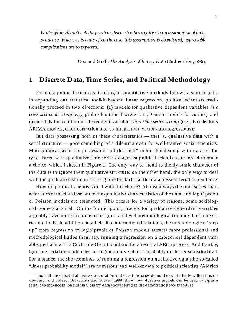
But data possessing both of these characteristics — that is, qualitative data with aserial structure — pose something of a dilemma even for well-trained social scientists.Most political scientists possess no “off-the-shelf” model for dealing with data of thistype. Faced with qualitative time-series data, most political scientists are forced to makea choice, which I sketch in Figure 1. The only way to atend to the dynamic character ofthe data is to ignore their qualitative structure; on the other hand, the only way to dealwith the qualitative structure is to ignore the fact that the data possess serial dependence.

How do political scientists deal with this choice? Almost always the time series char-acteristics of the data lose out to the qualitative characteristics of the data, and logit/probitor Poisson models are estimated. This occurs for a variety of reasons, some sociolog-ical, some statistical. On the former point, models for qualitative dependent variablesarguably have more prominence in graduate-level methodological training than time se-ries methods. In addition, in a field like international relations, the methodological “stepup” from regression to logit/probit or Poisson models attracts more professional andmethodological kudos than, say, running a regression on a categorical dependent vari-able, perhaps with a Cochrane-Orcutt band-aid for a residual AR(1) process. And frankly,ignoring serial dependencies in the (qualitative) data is probably the lesser statistical evil.For instance, the shortcomings of running a regression on qualitative data (the so-called“linear probability model”) are numerous and well-known to political scientists (Aldrich

1I note at the outset that models of duration and event histories do not lie comfortably within this di-chotomy; and indeed, Beck, Katz and Tucker (1998) show how duration models can be used to captureserial dependence in longitudinal binary data encountered in the democratic peace literature.

2

regression

(continuous y)

��

���

��

���

@@@@@@@@@@

time series

(continuous y, serially dependent)

qualitative dependent variables

(discrete y, serially independent)

Figure 1: A stylized, graphical rendering of quantitative political science. Beyond re-gression models for continuous, serially independent, dependent variables, political sci-entists typically proceed in one of the two directions indicated in the graph. When con-fronted with categorical time series data, political scientists must decide which feature ofthe data to deal with — qualitative characteristics, or serial structure — since there are nooff-the-shelf techniques available for dealing with both.

3

and Nelson 1984). On the other hand, it is also well known that estimators of the effectsof covariates can remain unbiased and consistent even in the presence of autocorrela-tion. Indeed, Poirier and Ruud (1988) show that an “ordinary probit” estimated in thepresence of autocorrelated disturbances still yields consistent estimates, if less efficientthan a “generalized” estimator that dealt with the serial dependence. Nonetheless, theinefficient estimates produced by ignoring any serial dependence raise the possibility ofinferential errors, and are a serious problem.

Numerous examples of political scientists encountering this dilemma appear in quan-titative studies of international relations. For instance, Oneal and Russett (1997) employlogit models of a binary dependent variable (dispute/no dispute), with data at the levelof the dyad-year. They acknowledge that “the greatest danger arises from autocorrela-tion, but that there are not yet generally accepted means of testing for or correcting thisproblem in logistic regressions.” Working with similar data, Farber and Gowa (1997, 397)note that serial dependence threatens the validity of their analysis of dyad-year data, but“proceed ignoring this lack of independence” since “a better solution is not obvious”.

Likewise, consider Gowa’s (1998) study of the United States’ involvement in “milita-rized interstate disputes” (MIDs) between 1870 and 1992. The dependent variable is acount of the MIDs the United States is involved in per year, data that are simultaneouslyqualitative and serial.2 Faced with the choice between treating these data as either a timeseries or as qualitative count data, Gowa chose the later, estimating a Poisson model bymaximum likelihood. Gowa notes that “[s]ince the values of the dependent variables arediscrete and truncated at zero, an OLS regression does not generate efficient parameterestimates” (p18). By the same token, ignoring serial correlation in one’s data creates infer-ential dangers too. But in moving to the discrete (Poisson) data framework, the dangersof serial correlation are ignored, since social scientists typically lack the tools for testingand/or correcting for serial correlation in discrete data.

2 Classes of Models for Discrete Serial Data

In this paper I attempt to fill this methodological void between time series and qual-itative dependent variables. A useful starting point is the large literature in biostatistics

2These counts come from the Correlated of War (COW) data set (Singer and Small 1994); the operationaldefinition of a MID is as an international event that involves “government-sanctioned” “threats to usemilitary force, displays of military force, ... actual uses of force,” and war (Gochman and Maoz 1984), asquoted in (Gowa 1998). Predictor variables include a GNP growth, a series of political indicator variables,and a series of period-specific indicator variables; the hypothesis of interest is the extent to which domesticpolitical or economic conditions increase the involvement of the United States in MIDs.

4

on models for discrete (and continuous) “time series” data. Biostatisticians encounter anabundance of time series data, both in the form of reasonably short panel studies, and inlonger longitudinal designs. Typical examples are monitoring a set of patients or subjectsover time, sometimes in an experimental setting (as in pharmaceutical trials), generating“repeated measures” of subjects. Furthermore, bio-statistical outcomes are often discretein nature. Different types of categorical times series can be distinguished, depending onthe nature of the response, and the design of the study. For instance,

� daily rainfall data (1 if measurable precipitation, 0 otherwise) on June days in Madi-son, Wisconsin for various years (Klotz 1973) are pooled binary time series

� a study in which children are monitored for respiratory disease (Sommer, Katzand Tarwotjo 1984; Ware et al. 1984), or experimental subjects report arthritic pain(Bombardier and Russell 1986) over a sequence of observations generates repeatedmeasures on a binary response;

� the number of asthma presentations recorded per day by an emergency room (Davis,Dunsmuir and Wang 1998), or the number of deaths in the British coalmining indus-try (Carlin, Gelfand and Smith 1992) is a time series of counts,

� the number of deaths by horse kicks in 14 corps of the Prussian army (Andrews andHerzberg 1985, 18), or the number of patents received by 642 firms between 1975-79(Hausman, Hall and Grilliches 1984; Chib, Greenberg and Winkelmann 1998) arerepeated measures of counts.

Reviews of the biostatistical literature (e.g., Diggle, Liang and Zeger 1994; Ashbyet al. 1992) distinguish three classes of models for discrete data with a serial structure.Marginal models deliberately divorce the issue of serial dependence from modeling theeffects of covariates. Serial dependence is considered a nuisance in this model and cap-tured via association parameters. The model for y is a marginal model in the sense thatthere is no explicit conditioning on the history of the discrete responses. This model is em-ployed when multiple time series are being modeled (i.e., panels or pooled time-series)and effectively average away any variation reflected in the unit-specific response histo-ries.

Models with random effects address the issue of heterogeneity across units by allow-ing the marginal model to include unit-specific terms, that are drawn from a populationdistribution. A frequently encountered example in the biostatistical literature is to aug-ment a panel study with unit-specific linear or quadratic time trends, or even simply aunit-specific intercept capturing unobserved heterogeneity across units. However, when

5

the panels are short and there is very little data per unit, estimates of these unit-specificcoefficients will tend to be imprecise. The random coefficients approach substitutes theimprecise-but-unbiased unit-specific estimates with estimates drawn from a population,“borrowing strength” across units. Random effects models are far from unknown in po-litical science:3 applications include King’s (1997) method for estimating unit-specific pa-rameters from aggregate data and Western’s (1998) analysis of variation in the determi-nants of economic growth among OECD countries. Alvarez and Glasgow (1997) use asimple random effects model to capture individual-level heterogeneity in a panel studyof voters over the 1976 and 1980 presidential campaigns (with a continuous dependentvariable), while Plutzer (1997) estimated a random effects growth curve tapping changein voter turnout over the three-wave Jennings and Niemi (1981) Student-Parent Social-ization Study (with a dichotomous dependent variable). Given the relative familiarity ofthese models, I will not elaborate further.

Transitional models explicitly incorporate the history of the responses in the modelfor yt. In this way each unit-specific history can be used to generate forecasts for that unit,as opposed to the marginal model which makes forecasts solely on the basis of the valuesof exogenous variables. In addition, Cox (1981) distinguishes two types of transitionalmodels; observation-driven models (where the “transitions” are with respect to observeddata) and parameter-driven models (where the “transitions” are with respect to a latentprocess, and tapped by a transitional parameter). As we shall see, Markov chains are animportant component of observation-driven transitional models for discrete data. I alsoconsider a parameter-driven transitional model, where I posit an AR(1) error process onthe regression function for the latent variable underlying the discrete responses.

This typology is neither exhaustive nor mutually exclusive. The lengthy review inMacDonald and Zucchini (1997, ch1) reveals no shortage of proposals for characterizingand modeling discrete time series, though only a modest proportion of these proposalshave been accompanied by applications. Furthermore, there are also models that arehybrids and there are even differences within categories of these models.

As the research designs shift from short panels to longer time series studies, the mod-els tend to shift in emphasis from attempting to capture “correlation”, “dependence” or“association” in the marginal probabilities, to dealing with the data as time series perse. As the length of the series becomes longer, the serial component of the data is lessa “nuisance” and perhaps more a “feature” of the data, and so in these circumstances atransitional model might be preferred to a marginal model. In other instances, the data

3Jones and Steenbergen (1997) provides a fairly general summary of the technique for political scientists,from the perspective of multilevel models, also known as hierarchical models.

6

are explicitly transitional and the past history of an individual subject is important.4 Thenagain, despite having a long time series, the nature of the study may be such that interestfocuses on a marginal model, in which serial dependence is considered a nuisance. Inshort, depending on the goal of a particular study and the research design, one modelingstrategy may be preferred over others.

3 The Binary Response Model

So as to fix ideas and to introduce some notation, I present a model for independentbinary data, yt 2 f0;1g; t= 1; : : : ;T. Let �t � Pr[yt = 1], which in turn depends on covari-ates via a latent regression function

h(�t) � y�t = xt�+ ut;

where

� xt is a row vector of observations on k independent variables at time t,

� � is a column vector of parameters to be estimated,

� y�t 2 R is a latent dependent variable, observed only in terms of its sign:

yt =

(0; if y�t � 01; if y�t > 0

� ut is a zero mean stochastic disturbance, identically and independently distributedfor all t. For probit, we will assume f (ut) = N(0;1) � �();8 t, while for logit weassume a logistic distribution, also normalized to have unit variance.5

The function h() : [0; 1]! R is a link function (McCullagh and Nelder 1989) known to theanalyst, while the inverse link function h�1() maps the linear predictors into probabilities:

4Consider a learning model, in which experimental subjects receive a reward or punishment over aseries of trials (e.g., Lindsey 1995, 165ff). In this case the history of a specific individual is of interest, andnot just their characteristics as measured with a set of covariates.

5The regression parameters � are identified only up to the scale factor �, and so setting � = 1 is aconvenient normalization with no substantive implications.

7

i.e.,

Pr[yt = 1] = Pr[y� > 0] = Pr[xt�+ ut > 0] = Pr[ut > �xt�] =

Z 1

�xt�

f (ut)dut

= 1�Z �xt�

1f (ut)dut:

For probit and logit f (ut) is symmetric about 0, so

Pr[yt = 1] =Z xt�

�1f (ut)dut and Pr[yt = 0] =

Z �xt�

�1f (ut)dut

Substituting the respective functional forms of f (u) yields

�t = Pr[yt = 1] = h�1(xt�) =

8>>><>>>:

Φ(xt�) =Z xt�

�1

1p2�

exp��z2

2

�dz (probit)

Λ(xt�) =exp xt�

1+ exp(xt�)(logit):

Serial independence means that

Pr(y1 = 1; y2 = 1; : : : ; yT = 1) = Pr(y1 = 1)Pr(y1 = 2) : : :Pr(yT = 1);

or, in words, the joint probability equals the product of the marginal probabilities, and sothe log-likelihood of the data equals the sum of the individual log-likelihoods. That is,

ln L =T

∑t=1

�yt ln �t+ (1� yt) ln(1� �t)

�: (1)

The log-likelihood function in (1) is easily maximized to yield consistent estimates of� whose asymptotic distribution is multivariate normal. Moreover, the matrix of secondderivatives of the log-likelihood function (1) with respect to � are easily calculated andyield an estimate for the asymptotic covariance matrix of the estimated �.

4 Observation-Driven Transitional Model

Diggle, Liang and Zeger (1994, 135) define a transitional model as one in which cor-relation among the discrete responses arises because past responses explicitly influencethe present outcome. Past realizations of the discrete response help determine the currentresponse, and so enter the model as additional predictor variables. A two-state Markov

8

chain is a straightforward way to model a binary time series, and forms the basis of thetransitional model. A first-order Markov chain for binary data has a transition matrix

p00 p01

p10 p11

!

where pi j = Pr(yt = jjyt�1 = i). With binary data there are just two unique elements of the2-by-2 transition matrix. A simple way to relate covariates to the transitional probabilitiesis via a link function and a regression structure for each of the two transition probabilities.With a logit link we have

logit�Pr(yt = 1jyt�1 = 0)

�= xt�0

and

logit�Pr(yt = 1jyt�1 = 1)

�= xt�1

where the possibility that �0 6= �1 taps the possibility that the effects of explanatory vari-ables will differ depending on the previous response. Diggle, Liang and Zeger (1994, 195)show that the two equations above can be combined to form the model

logit�Pr(yt = 1jyt�1)

�= xt�0+ yt�1xt� (2)

where �1 = �0+�, since when yt�1 = 0 the xt� part of the model is zeroed out. This is anextremely simple format with which to test hypotheses about the effects of the covariateson the transition probabilities. Tests of the null hypothesis�= 0 tap whether the effects ofx are constant irrespective of the previous state of the binary process. Furthermore, if thefirst-order Markov specification is correct, then ordinary binary response models can beused to estimate �0 and � and their standard errors. The model is estimated conditionalon the first observation in the time series, and care needs to taken interpreting predictedprobabilities and model summaries, since the model is now predicting conditional prob-abilities.

This model enjoys widespread use in the bio-statistics literature, with Cox (1970, 72ff)drawing attention to the link between the transition probabilities for a Markov chain anda logistic regression. Korn and Whittemore (1979) applied the model to panel data onthe effects of air pollution; Stern and Cole (1984) used the model to estimate a modelof rainfall data. The model extends readily to the case of an ordered or multinomialoutcome, and Zeger and Qaqish (1988) extend the model for count data.

9

5 A Parameter-Driven Transitional Model

I now consider a transitional model but in which the transitions are with respect to thelatent dependent variable y�. In some ways this is a fairly natural way to approach theserial dependence in the binary responses, since it combines familiar time series methodsfor continuous y variables with the standard binary response model given in section 3.Unfortunately, as we shall see, the offspring of the union of these two familiar models issomething of a monster, or at the very least, a problem child.

I introduce serial dependence in the latent variable y� by positing a stationary, zeromean, autoregressive process on the disturbances futg. For simplicity, consider the AR(1)process

ut = �ut�1+ �t; (3)

where �t is zero-mean Gaussian white noise. The model for y� is now a regression withAR(1) errors, a model with properties well known to political scientists. I briefly re-statea number of these properties, which will help us understand why this seemingly simplemodel is so complicated to estimate in the context of a discrete response.

We retain the assumption made for the binary response model in section 3 that var(ut)��2

u = 1, losing the t subscript via the stationarity assumption. Since the �t are orthogonalwith the ut, the variance of ut can be decomposed as

var(ut) = �2 var(ut�1)+ var(�t):

Exploiting the stationarity assumption,

var(ut) = �2 var(ut)+ var(�t)

or

�2u = �2 �2

u+ �2� ;

and since �u = 1, �2� = 1� �2; note that stationarity also requires j�j< 1 and so 0< �2

� < 1.Note also that cov(ut;us) = �js�tj=(1� �2). Thus, the variance-covariance matrix for u =

10

(u1;u2; : : : ;uT)0 is

Σu(�) =1

1� �2

266664

1 � �2 : : : �T�1

� 1 � : : : �T�2

......

... : : :...

�T�1 �T�2 �T�3 : : : 1

377775 6= IT;8 � 6= 0:

The likelihood function for the binary response model with an autoregressive errorstructure is considerably more complex than the likelihood for the serially independentmodel. The joint probability Pr(Y1 = y1;Y2 = y2; : : : ;YT = yT) can’t be factored into theproduct of the observation-specific marginal probabilities. Instead,

L = Pr[y1; y2; : : : ; yT]

=

Z b1

a1

Z b2

a2

: : :Z bT

aT

fT(y�jX�;Σu) dy�T : : :dy�2 dy�1; (4)

where

(at; bt) =

((�1;0) if yt = 0(0;1) if y1 = 1

(5)

and fT(y�jX�;Σu) is the T-dimensional probability density for the latent variable y� (Poirierand Ruud 1988, equation 2.8). In the case of probit, this density is the multivariate normalprobability density function

(2�)�T2 jΣuj� 1

2 exp��u0�1

u u2

�;

with u = y��X�.The logit model is of limited use given the AR(1) structure of the dependency across

observations; the logistic distribution generalizes to a multivariate setting in a fairly cum-bersome way. In the time series context, this problem gets more pressing as the lengthof the series increases, leading to a proliferation of parameters tapping the dependenciesacross time points which I detail below.6 Nonetheless, the logit model can still be used forthe marginal probabilities, even though a multivariate normal distribution is used to cap-

6The situation here is directly analogous with the independence of irrelevant alternatives assumptionunderlying the use of the logit model in a multinomial choice setting. Nesting or grouping alternativesis the way the logit model accommodates interdependence among discrete outcomes; Chamberlain (1980)proposes an analogous logit model for panel data, although the model seems plausible only for short panelsand not at all feasible for a single time series.

11

ture the dependencies among observations (e.g., le Cessie and van Houwelingen 1994).The likelihood function in (4) poses a ferocious maximization problem, bearing a close

resemblance to the intractabilities presented by the multinomial probit (MNP) model forqualitative choice. In MNP, the likelihood function becomes increasingly complex as thenumber of choices increases; each choice adds another dimension to the integral in thelikelihood. Here we have a “multi-period” probit model with the likelihood involving in-tegration of a T-dimensional Normal density. In most time series settings T will be largerthan the number of choices in a MNP model, although there are considerably fewer pa-rameters to estimate than in say, a MNP model with four or more outcomes; for instance,in the AR(1) case, Σu(�) is a function of a single parameter, while the corresponding matrixin a MNP setting will usually contain more free parameters than this.

The question of the number of parameters aside, the real difficulty with the binaryprobit model with AR(1) errors is the T-dimensional integral in the likelihood function.Geweke, Keane and Runkle (1997) report that simulation methods for dealing with thehigh-dimensional integrals required in multi-period probit models perform poorly as se-rial dependency increases; the Geweke-Hajivassiliou-Keane (GHK) simulator needs to berun for increasingly longer simulation runs as the magnitude of � increases. Indeed, aMarkov Chain Monte Carlo (MCMC) approach generally outperforms the GHK simula-tor for the experimental conditions considered by Geweke, Keane and Runkle.

5.1 Estimation by Bayesian Simulation

The MCMC approach to the time series probit problem has been used by Czado (N.d.).The MCMC approach is attractive in this context because it exploits the fact that the highdimensional integral in the likelihood function in (4) can be well approximated by suc-cessively sampling from the series of conditional densities f (y�t jy�r<t). This sampling algo-rithm is an example of Gibbs sampling, the workhorse of MCMC. A review of Gibbssampling need not detain us here; the key idea is that “conditional [densities] deter-mine marginals” (a fact well known to Bayesians), even if the particular details of therelationship in a high dimensional setting can be “obscure” or complicated (Casella andGeorge 1992, 170-1).

In this case we seek the posterior distribution for the unknown parameters and latentdata �(�; �;y�jX;y), recalling that X and y are the observed data. The MCMC approachbreaks this distribution into the conditional distributions �(�j�;y�;X;y), �(�j�;y�;X;y)and �(y�j�; �;X;y). The MCMC algorithm here consists of sampling from each of thesedistribution, replacing �, � and y� when they appear as conditioning arguments with the

12

most recently sampled value for each. At the end a pass m over each of the conditionaldistributions, the vector of a sampled vectors (�(m); �(m);y�(m))0 consists the state vector ofa Markov chain that has the joint posterior as its invariant distribution. When the Markovchain Monte Carlo algorithm has been run for a sufficiently lengthy period, each realiza-tion of the state vector is a draw from the joint posterior. These draws from the posteriordistribution are saved and summarized for the purposes of statistical inference. Otherrelevant quantities (e.g., the value of the log-likelihood, percent cases correctly predicted)can also be calculated at each stage of the chain.

In addition, the vector of unknown quantities can be augmented to include miss-ing data; in the application I present below, missing values on the discrete response aretreated in this way. This potential for dealing with missing data “on the fly” is an excep-tionally useful feature of the MCMC approach.

I turn now to each of the conditional distributions. If the prior distribution for � isassumed to N(�p;Σp), then the conditional distribution for the regression coefficients � ismultivariate normal with mean

(Σ�1p +X0Σ�1

u X)�1(Σ�1�p+X0Σ�1u y�)

and variance-covariance matrix

(Σ�1p +X0Σ�1

u X)�1:

The conditional distribution of y� is a truncated multivariate normal distribution withmean vector X� and variance-covariance matrix Σu, truncated to (a1; b1)� (a2; b2)� : : :�(aT; bT), defined in (5). Czado (N.d.) notes that sampling from this truncated multivariatedistribution can be accomplished by sequentially sampling from the conditional distri-butions for each element of y�t , where the conditioning is not just on the observed dataand the parameters � and �, but also on the sampled values for y�r<t. Each conditionaldistribution is a truncated univariate normal distribution. Given the marginal model forthe latent dependent variable

y�t = xt� + ut

with the stationary AR(1) error process

ut = �ut�1+ �t;

13

where j�j < 1 and �t � N(0; �2� )8 t, substitution and re-arranging yields

y�t jy�t�1 � N�xt�+ �(y�t�1 � xt�1�); �2

�

�I(at; bt) (6)

for t = 2; : : : ;T, where �2� = 1� �2 and the function I(�; �) is a binary (0,1) indicator func-

tion for the truncation bounds.7 Note that this sampling algorithm is all conditional onthe first observation of the series, which is sampled as

y�1 � N(x1�; �2u)I(a1; b1)

or use of the Prais-Winsten (1954) transformation might also be used, as is common inGLS fixes for residual autocorrelation in the linear regression setting.

The conditional distribution for � is less straightforward. Given the current iteration’sestimates of y�, X and �, we obtain u = y� � X�. Given our assumption that u followsan AR(1) process, with �2

u = 1 and �t � N(0;1� �2);8 t, we can obtain a likelihood for �,l(�ju), equivalent to f (uj�). If all that is known is that � is stationary, then the prior for �is uniform on the interval [-1, 1], i.e.,

�(�) =

(12 �1� � � 1;0 otherwise.

Recall that a posterior distribution is proportional to the likelihood times the prior, or inthis case

�(�ju)/ f (uj�) � �(�); (7)

and so the posterior will also have zero probability mass outside the stationarity bounds[-1, 1]. Given the normal-based likelihood, this implies that the posterior distribution isproportional to a normal distribution (net of the complications imposed by stationarity),with mean

r =∑T

t=2 ut�1ut

∑t=2 ut�1

and variance R = ∑Tt=2 ut�1ut, but truncated to the [-1,1] interval. In my implementation,

7Hajivassiliou (1995, n13) notes it is necessary to restrict the truncation region to a compact region, suchthat �1 < at < bt < +1. This is a technical restriction entailing no loss of generality; in place of �1or +1 we merely substitute an arbitrarily large number (signed appropriately), subject to computationallimitations.

14

a Metropolis method8 is used to sample from the posterior for �. Briefly, the Metropolismethod supplies transition probabilities for the Markov chain that “help” it traverse theparameter space and reach its invariant distribution more efficiently. But importantly,the mathematics of the Metropolis method are such that the normalizing constants forthe conditional (posterior) distributions are not required, and for this reason Metropolismethods are very attractive in Bayesian analysis, whenever posterior distributions areonly defined up to normalizing constants.

In the context considered here, we have a posterior for � that is proportional to anormal-based likelihood times a uniform prior. A Metropolis step starts with �(q), thecurrent realization of f�g in the Markov chain. Then,

1. Given u(q+1), sample �� from N(r(q+1); R(q+1))I(�1;1).

2. With probability

min�

f (u(q+1)j��)f (u(q+1)j�(q))

;1�

accept �� as �(q+1), otherwise set �(q+1)= �(q).

This problem — the absence of a normalizing constant in a posterior distribution — arisesfrequently in Bayesian analyses of time series, where flat priors over the stationary regionfor autoregressive parameters give rise to posteriors known only up to a constant factorof proportionality (e.g., Chib and Greenberg 1994; Marriot et al. 1996; West and Harrison1997). The extension to the discrete time series case introduces no new complicationssince all the calculations take place with respect to the estimates of the continuous latentquantities (conditional on the observed discrete responses). Previous implementationsinclude work by and has been addressed in the specific context of time series models fordiscrete data by Geweke, Keane and Runkle (1997) (a multi-period, multinomial probitmodel) and Czado (N.d.).

6 Marginal Models

Marginal models treat the issue of serial dependence separately from the effect of ex-planatory variables on the response variable. For instance, consider a binary (0,1) timeseries y = (y1; : : : ; yT). Let �t = E(yt) � Pr[yt = 1], which in turn depends on covariates

8Chib and Greenberg (1995) and Tanner (1996, 176ff) are useful introductions to Metropolis method.

15

as follows:

h(�t) = xt�;

where h() is a link function known to the analyst and xt is the vector of observations on kcovariates at time t. Note that although we are modeling serial data, there are no dynam-ics or conditioning on history in the model for yt; in this sense the model can be thoughtof a marginal model, or a model for the marginal expectation of yt. The marginal varianceof yt is not a critical issue here, and so is assumed to depend on the marginal expectationvia a known variance function v(�t)�, where � is a scale parameter: for instance, when h()is the logit link function, Var(Yt) = �t(1� �t) and � is set to 1.

Turning to the time series characteristics of the data, consider the correlation betweentwo adjacent observations, y1 and y2. By definition,

Corr(y1; y2) =E(y1; y2)� E(y1)E(y2)

(Var(y1)Var(y2))1=2;

which in the logit case becomes

Corr(y1; y2) =Pr(y1 = 1; y2 = 1)� �1�2

(�1(1� �1)�2(1� �2))1=2:

However, the marginal quantities �1 and �2 impose constraints on the correlation acrossadjacent observations, as the following table helps demonstrate:

y2

y1 0 10 p00 p01

1 p10 p11 �1

�2

Our interest is in Pr(y1 = 1; y2 = 1), denoted by p11 in the table. Note that this joint prob-ability is bounded by the marginal probabilities �1 and �2:

max(0; �1+ �2 � 1) < p11 < min(�1; �2) (8)

and so the correlation between y1 and y2 exhibits an awkward (and potentially implausi-ble) dependency on the marginal probabilities �1 and �2 (Prentice 1988, 1037). It is moreconvenient to model the odds ratio of successive observations in the binary time series,effectively collapsing away the marginal terms in equation (8). For the (y1; y2) pair con-

16

sidered here, we have

12 =Pr[“no change”]

Pr[“change”]

=Pr(y1 = 1; y2 = 1)Pr(y1 = 0; y2 = 0)Pr(y1 = 0; y2 = 1)Pr(y1 = 1; y2 = 0)

=p11p00

p01p10

The odds ratio takes on values in (0;1); if 12 = 1 then “change” is as likely as “nochange”. Values of 12 less than 1 indicate that switching or change is more likely thannon-switching or stability, while values of 12 greater than 1 indicate that “no change” ismore likely than “change” (Diggle, Liang and Zeger 1994, 150). In this way the odds ratio 12 taps dependencies between observations 1 and 2 of the time series.

The model parameters are now � and , with the log-odds approach ensuring near-orthogonality between the two parameters (Fitzmaurice and Laird 1993). The model iseasily extended to handle higher order forms of dependency. For instance, the odds-ratiocan be defined in terms of two observations at any arbitrary distance apart in the timeseries:

rs =Pr(yr = 1; ys = 1)Pr(yr = 0; ys = 0)Pr(yr = 0; ys = 1)Pr(yr = 1; ys = 0)

(9)

The full distribution of y can be modeled in terms of the covariates (via � and the cho-sen link function) and the entire

�T2

�set of odds ratios between adjacent observations. Of

course, this “saturated” model gives rise to a large number of parameters that can greatlycomplicate the analysis of lengthy time series. In general, the number of association pa-rameters to estimate increases exponentially with the length of the time series, and netof some simplifying assumptions, the fully unconstrained model is not feasible. Furthercomplications arise should one be dealing with panel or pooled cross-sectional time seriesdata that is unbalanced (the number of observations varies across subjects or units).

Diggle, Liang and Zeger (1994, 151) suggest a number of simplifications for dealingwith the proliferation of associational parameters. In a repeated measures or panel set-ting, one approach might be to set irs = i (i.e., the degree of longitudinal association isconstant for all pairs of observations for unit i). Another approach might be to parame-terize rs as a function of temporal distance: e.g.,

ln rs = �0+ �1jr� sj�1

17

such that the degree of longitudinal association is inversely proportional to the time be-tween observations. Finally, Carey, Zeger and Diggle (1993) show how to include covari-ates in an auxiliary model for the rs terms; they estimate this model using “alternatinglogistic regressions”, where the term “alternating” reflects the fact that the estimation it-erates between estimates of � in the marginal model for y and the � coefficients in theauxiliary model for the (log) odds ratios.

Generally, these models are estimates by quasi-likelihood methods, called general-ized estimating equations, or GEE (Fitzmaurice, Laird and Rotnitzky 1993). These are“quasi-likelihood” models in the sense that in the discussion thus far, there has been nomention of the distribution of error terms that would typically give rise to a likelihoodfunction for the data. The marginal model is for the the first moment of the yt, the choiceof link function usually implies a simple function for the second moment, and the odds-ratios (with or without regressors) imply some structure on the covariances of the yt. ForNormal-based likelihoods, or for the logit-link binary case, these moments are sufficientto characterize the entire likelihood, and the GEE approach coincides with conventionallikelihood based methods. However, the likelihoods for these marginal models are some-what complicated to directly maximize, and the iterative approach of GEE (successivelyapproximating solutions to the moment equations) has computational advantages, in ad-dition to being free of distributional assumptions.

6.1 A Marginal-Transitional Hybrid

Azzalini (1994) provides an interesting simplification of the marginal model, using aMarkov chain to characterize the dynamics in the time series. In this sense Azzalini’smodel is a hybrid of the marginal and transitional models encountered above. Changesin the binary series y can be modeled as a Markov chain over the two states (0 and 1),with a transition matrix

1� p0 p0

1� p1 p1

!;

where p0 = Pr(yt = 1jyt�1 = 0) and p1 = Pr(yt = 1jyt�1 = 1). These transition probabilitiesneed not be constant over time (and in general will not be constant), and could themselvesbe modeled with covariates as in the marginal model suggested above. As in the marginalmodel, it is more convenient to model the odds ratio of the probability of a transition, .

18

The Markov structure implies

Pr(yt = 1) = Pr(yt�1 = 1)Pr(yt = 1jyt�1 = 1)+ Pr(yt�1 = 0)Pr(yt = 1jyt�1 = 0)

�t = �t�1p1+ (1� �t�1)p0:

Thus the transitional parameters p0 and p1 appear in the model relating the covariates tothe responses (recall that h(�)= xt�). Combined with the odds ratio representation of thetransitional dynamics

=p1=(1� p1)p0=(1� p0)

(10)

we now have a complete characterization of the process for y, subject to the assumptionof a first order Markov process. Because the transitional parameters p0 and p1 appearin the expression for �t, they will vary over time themselves: MacDonald and Zucchini(1997, 11) use the notation t p j to reflect this time variation, where j = 0;1.

The odds ratio representation and the Markov representation in equation (10) can becombined and re-arranged to yield the following expression

t p j =

(�t if = 1;��1+( �1)(�t��t�1)

2( �1)(1��t�1) + j 1��+( �1)(�t+�t�1�2�t�t�1)2( �1)�t�1(1��t�1) if 6= 1;

)(11)

for t = 2; : : : ;T, and where

�2= 1+ ( � 1)

�(�t � �t�1)2 � (�t+ �t�1)2

+ 2(�t+ �t�1)�:

We can condition on the first observation, setting Pr(y1 = 1) = �1 to complete the specifi-cation of the model. Since 2 (0;1), it is more convenient to work with � = ln( ), andso the log-likelihood function for this process is

ln L(�; �)=T

∑t=1

�yt logit( tpyt�1 )+ ln(1� tpyt�1 )

�; (12)

This log-likelihood is relatively straightforward to maximize; first and second derivativesof the log-likelihood with respect to to the parameters are provided in Azzalini, or onecan also use software specifically designed for this model using Splus (Azzalini andChiogna 1995).

19

7 An example: dyadic conflict data

To see how these models work in practice, I turn to a large data set gathered for study-ing the determinants of international conflict. The data consist of 20,990 observations atthe level of the dyad-year, where a dyad refers to a pairing of countries, with the binaryindicator yit coded 1 if dyad i engaged in a militarized interstate dispute (a MID) in yeart, and 0 otherwise.

These data were gathered and analyzed by scholars working on substantive problemsinternational relations (e.g., Russett 1990; Russett 1993; Oneal and Russett 1997). Keyissues in this large literature concern the effects of the following covariates:9

� democracy (the “liberal peace” hypothesis), with the democracy score for each dyadset to the lesser democracy score of the dyad partners, with the scores scaled to runfrom -1 to 1, using indicators in the Polity III data base (Gurr and Jaggers 1996).

� intra-dyad trade, measured as the ratio (percent) of intra-dyad trade to GDP, foreach partner, but with the dyad’s score set to the smaller of these ratios. This vari-able is lagged one year, so as not to proxy a current dispute (Oneal and Russett 1997;Beck, Katz and Tucker 1998).

� dyad partners who are allies are presumed to be less likely to engage in MIDs. Thisvariable takes the value 1 if the dyad partners were allied, or if both were allied withthe United States.

� military capabilities are measured as the ratio of the stronger partners’ score to theweaker partner’s score, on an index based on indicators in the Correlates of Wardata collection (Singer and Small 1994).

� geographic contiguity within a dyad (1 if the partners are geographically contigu-ous, 0 otherwise), since ceteris paribus it is more difficult to engage in a MID with adyad partner who is distant, or if another country’s borders have to be crossed inorder to instigate a MID.

� economic growth measures the lesser of the rates of economic growth of the part-ners.

These data have been reanalyzed by a number of scholars attracted to the method-ological problems presented by these data. For instance, Beck and Jackman (1998) focus

9My source for these data is Beck, Katz and Tucker (1998), who obtained the data from Oneal and Russett(1997). Further details on these data and definitions appear in those articles.

20

on possible non-linearities and interactions in the latent regression function, ignoring anyserial component to the data; Beck, King and Zeng’s (1998) reanalysis is in a similar vein,but using neural networks. Beck, Katz and Tucker’s (1998) reanalysis of these data fo-cuses the serial properties of these data, and draws attention to some of the shortcomingsof previous analyses that omit to control for serial dependence in the data (I mentionedsome of the these in section 1). Beck, Katz and Tucker account for serial dependencein these data by augmenting a marginal logit model with non-parametric term (a cubicsmoothing spline) for time since last conflict.

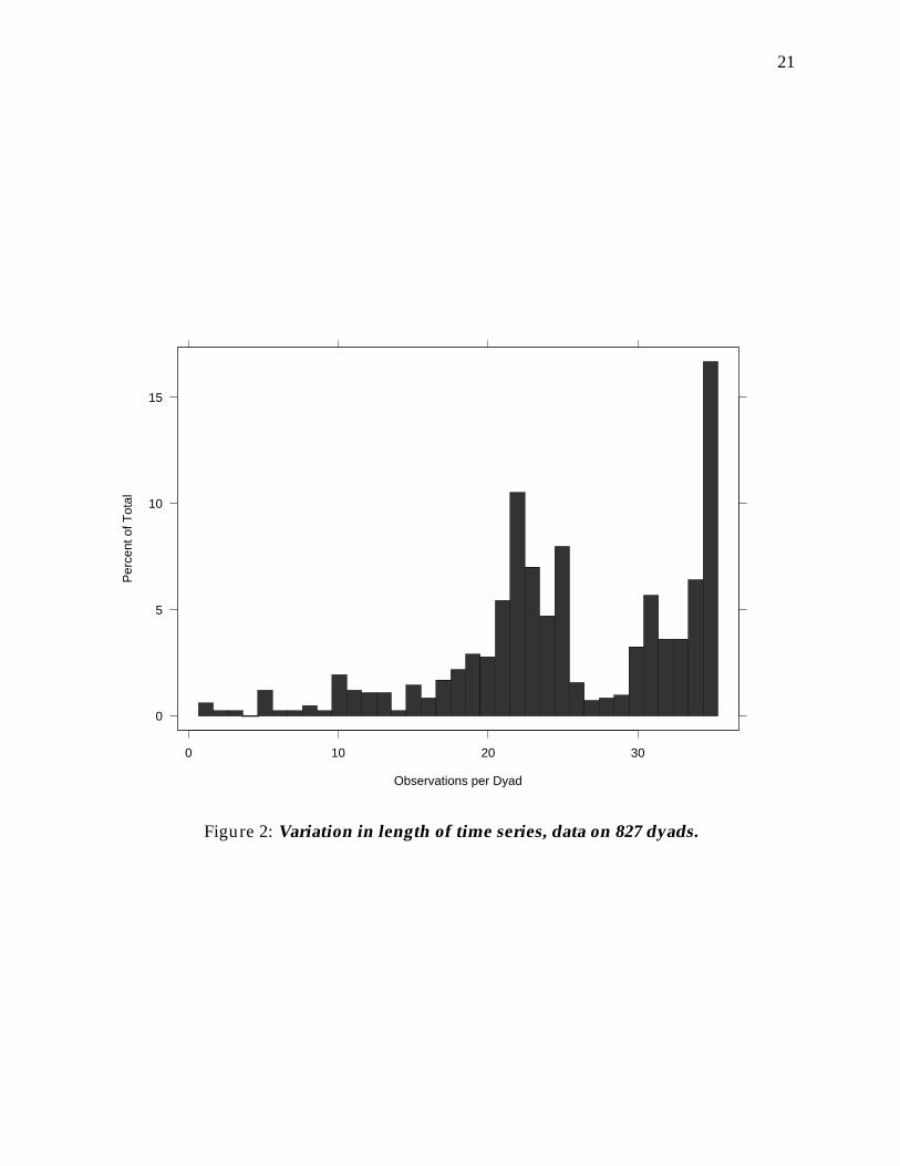
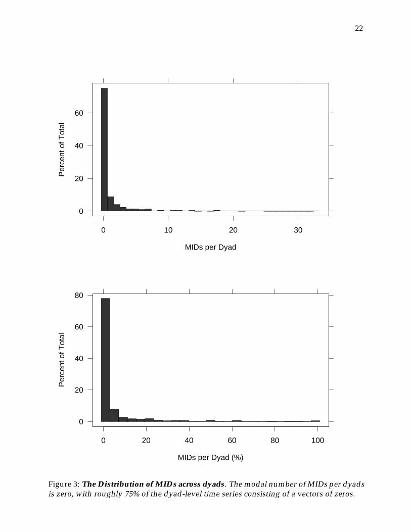
Several features of the data should be pointed out. First, MIDs are extremely rare inthese data. Of the 20,990 dyad-years in the data I analyze, just 947 or 4.5% are coded 1 forthe presence of a MID. The data are also highly unbalanced in their design, in the sensethat there is much variation in the length of time each dyad is present in the data (seeFigure 2). The maximum length of any dyad-series is 35 yearly observations (1951-1985),but with only 138 (16.7%) of the 827 dyads contributing this much data. This feature ofthe data creates a formidable barrier for marginal models employing log-odds parameter-izations for temporal association; many software implementations of this model requirethe data to be balanced, and so I do not fit marginal models of this type to these dyadicdata.

Coupled with the rarity of MIDs, Figure 3 shows that the overwhelming majority ofdyads record no MIDs whatsoever; approximately 75% of the dyad-specific time series onthe dependent variable consist of a vector of zeros and only 20 dyads (2.4%) report moreyears with MIDs than without MIDs. Even this cursory examination of the data suggeststremendous “stability” in the data, and ignoring this serial dependence is likely to lead tofaulty inferences.

Finally, 293 (35.4%) of dyads contain temporal breaks. This poses problems for severalof the models considered earlier, especially the transitional models, and to a lesser extentthe marginal models (by heightening the unbalanced design problem). One solution is totreat temporally-contiguous sequence of observations as a “unit”, with possibly multiple“units” per dyad entering the analysis; I adopt this approach when fitting the hybridmarginal-transitional model of Azzalini (1994) I described in section 6.1.

A more attractive solution is to treat the temporal breaks within each dyad as missingdata, and make imputations for the data, treating them as missing at random (conditionalon the covariates). This is relatively easy to accomplish with the MCMC implementationof the parameter-driven transitional model considered in section 5. I linearly interpolatethe missing data on the covariates for the missing observations,10 but leave the dependent

10Most of these temporal gaps are short (1 or 2 yearly observations) and the covariates exhibit modest

21

0

5

10

15

0 10 20 30

Observations per Dyad

Per

cent

of T

otal

Figure 2: Variation in length of time series, data on 827 dyads.

22

0

20

40

60

0 10 20 30

MIDs per Dyad

Per

cent

of T

otal

0

20

40

60

80

0 20 40 60 80 100

MIDs per Dyad (%)

Per

cent

of T

otal

Figure 3: The Distribution of MIDs across dyads. The modal number of MIDs per dyadsis zero, with roughly 75% of the dyad-level time series consisting of a vectors of zeros.

23

variable as missing data. The MCMC procedure is augmented to imputations for thesemissing, discrete yit. When the data are “padded out” so as to remove any temporaldiscontinuities within dyads, the total number of observations increases from 20,990 to21,844. This means that there are 854 values of yit to impute, or some 3.9% of the data.

In these senses, these data are a “hard case” with which to assess the utility of themodels presented above; these are not at all like the relatively small and well-mannered“canonical” data sets encountered in statistical literature developing these models.

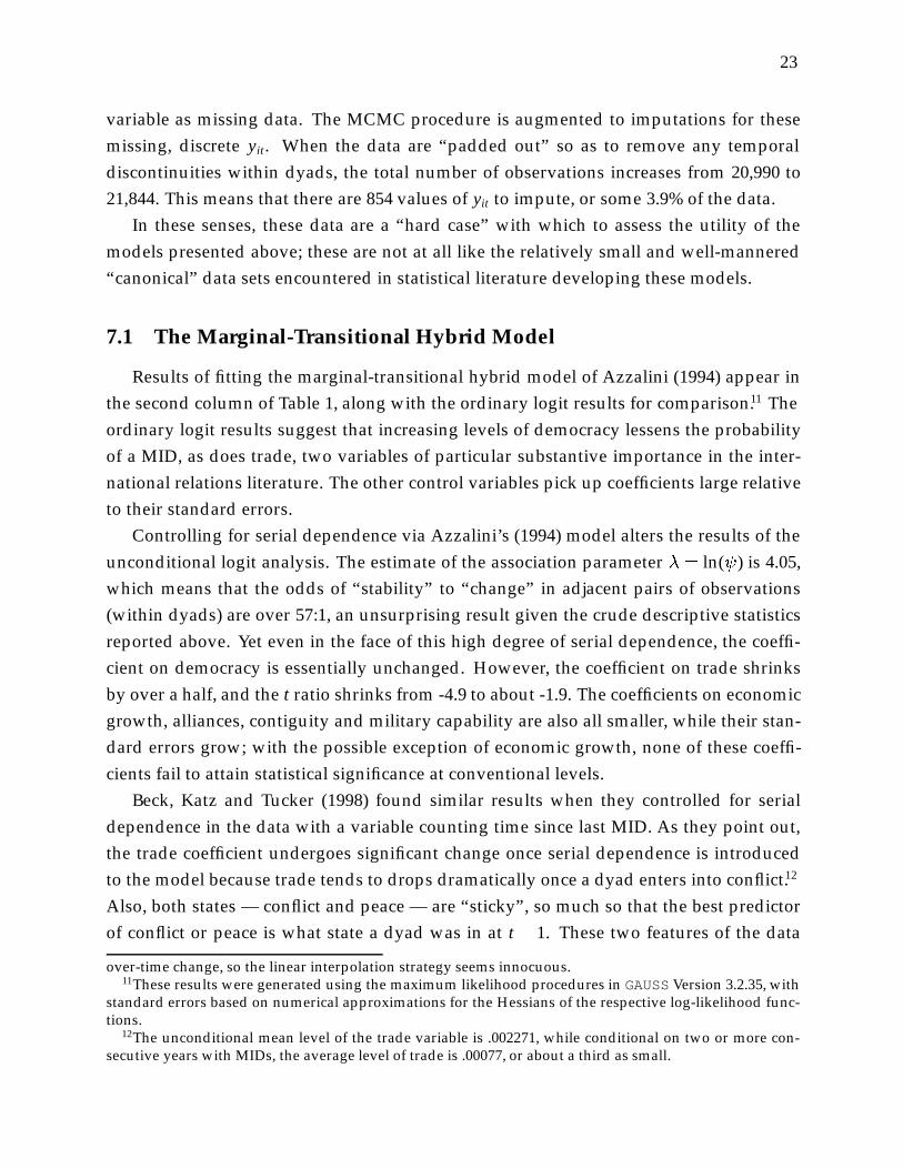
7.1 The Marginal-Transitional Hybrid Model

Results of fitting the marginal-transitional hybrid model of Azzalini (1994) appear inthe second column of Table 1, along with the ordinary logit results for comparison.11 Theordinary logit results suggest that increasing levels of democracy lessens the probabilityof a MID, as does trade, two variables of particular substantive importance in the inter-national relations literature. The other control variables pick up coefficients large relativeto their standard errors.

Controlling for serial dependence via Azzalini’s (1994) model alters the results of theunconditional logit analysis. The estimate of the association parameter � = ln( ) is 4.05,which means that the odds of “stability” to “change” in adjacent pairs of observations(within dyads) are over 57:1, an unsurprising result given the crude descriptive statisticsreported above. Yet even in the face of this high degree of serial dependence, the coeffi-cient on democracy is essentially unchanged. However, the coefficient on trade shrinksby over a half, and the t ratio shrinks from -4.9 to about -1.9. The coefficients on economicgrowth, alliances, contiguity and military capability are also all smaller, while their stan-dard errors grow; with the possible exception of economic growth, none of these coeffi-cients fail to attain statistical significance at conventional levels.

Beck, Katz and Tucker (1998) found similar results when they controlled for serialdependence in the data with a variable counting time since last MID. As they point out,the trade coefficient undergoes significant change once serial dependence is introducedto the model because trade tends to drops dramatically once a dyad enters into conflict.12

Also, both states — conflict and peace — are “sticky”, so much so that the best predictorof conflict or peace is what state a dyad was in at t� 1. These two features of the data

over-time change, so the linear interpolation strategy seems innocuous.11These results were generated using the maximum likelihood procedures in GAUSSVersion 3.2.35, with

standard errors based on numerical approximations for the Hessians of the respective log-likelihood func-tions.

12The unconditional mean level of the trade variable is .002271, while conditional on two or more con-secutive years with MIDs, the average level of trade is .00077, or about a third as small.

24

Ordinary Marginal-Logit Transitional

Intercept �3:3 �3:40(:079) (:12)

Democracy �:49 �:51(:074) (:11)

Economic Growth �2:23 �1:91(:85) (1:01)

Alliance �:82 �:69(:080) (:13)

Contiguity 1:31 1:24(:080) (:13)

Military Capability �:31 �:22(:041) (:045)

Trade �66:1 �28:2(13:4) (14:7)

� 4:05(:092)

Table 1: Estimates of Ordinary Logit Model, and Marginal-Transitional Hybrid Model.Standard errors appears in parentheses. The parameter � = ln( ), where is the odds-ratio defined in equation (10). n = 20,990, over 827 dyads of unequal lengths.

25

— underlying inertia, and drops in trade once a dyad enters into conflict — serve toundermine the effects of trade once some attempt is made to condition on the history ofthe dyad, a finding will we see repeated below.

7.2 The Observation-Driven Transitional Model

The Markov-based transitional model reviewed in section 4 permits the explorationof conjectures like those above. In particular, if the effects of covariates are thought tobe state-dependent, then the Markov model is a useful way to proceed. Given my as-sumption of a first-order Markov chain, the effects of the covariates are presumed to beconditional on whether a dyad experienced a MID in the preceding year or not, and theeffects of earlier states only effect the present via their indirect effects through t� 1. Asremarked earlier, this model can be estimated simply with software for ordinary binaryresponse models. Estimates of the first-order Markov model appear in Table 2, again,along with the ordinary logit estimates for comparison.

Ordinary Observation-DrivenLogit Transitional Model� �0 � �1

Intercept �3:3 �4:5 5:0 :55(:079) (:12) (:21) (:17)

Democracy �:49 �:33 :075 �:25(:074) (:11) (:20) (:17)

Economic Growth �2:2 �3:5 :13 �3:4(:85) (1:40) (2:29) (1:8)

Alliance �:82 �:39 �:30 �:70(:080) (:12) (:21) (:17)

Contiguity 1:31 1:48 �1:41 :070(:080) (:13) (:21) (:17)

Military Capability �:31 �:15 :12 �:028(:041) (:045) (:08) (:071)

Trade �66:1 �31:2 �46:0 �77:2(13:4) (13:5) (35:45) (32:8)

n 20,990 19,776

Table 2: Estimates of an Observation-Driven Transitional Model. The estimates for �contrast the effects of the covariates across states; i.e, Pr[yt = 1jyt�1 = j] = x� j, where�1 = �0 +�. Standard errors appear in parentheses, and the ordinary (unconditional)logit estimates are presented for comparison. The different numbers of observations arisebecause the transitional-model loses the first observation of each dyad.

26

These results are provocative, illustrating that even this modest conditioning on eachdyad’s history leads to some different interpretations to those we might take away froman ordinary, unconditional analysis. First, note the changes between the ordinary (un-conditional) logit analysis and the estimates for �0 (governing Pr[yt = 1jyt�1 = 0]). Theeffects of democracy in stopping a transition to a dispute are smaller than the uncondi-tional analysis would suggest, with the coefficient in the transitional analysis about two-thirds of the magnitude of the coefficient obtained from the unconditional analysis (-.33versus -.49). Other coefficients that appear to change substantially are those for the al-liance indicator, military capabilities, and trade; an ordinary logit analysis would appearto overstate the contribution of these variables in preventing MIDs. Note also that the in-tercept in �0 for the conditional model is also somewhat larger (more negative) than thatfor the unconditional analysis, reflecting that “peace” is highly persistent in these data.

The other difference with an ordinary logit analysis arises via the conditioning on thedyad’s past, reflected in the estimates of �, and the implied estimates of �1. The inter-cept and the contiguity coefficient are distinguishable from zero at conventional levels ofstatistical significance. The positive intercept in � means that the intercept in �1 is actu-ally close to zero (about .55), highlighting persistence in MIDs: i.e., putting the predictorsto one side, a good predictor of a dyad recording a MID in a given year is whether itrecorded a MID in the previous period.

Note also the effects of alliances in the two states. Conditional on a dispute existingbetween the two countries, alliances help return the dyad to peace, and this contributionof alliances would seem greater than the role of alliances in preventing MIDs arising inthe first instance. The coefficient tapping the difference across states is the relevant entryin �, and has a t-statistic of -1.44 (p � :075), suggesting that this difference is signifi-cant. The magnitude of the difference is also impressive, with the coefficient for alliancesconditional on a MID in the previous period being about 170% of the magnitude of the co-efficient conditional on peace (-.70 versus -.39). The conventional analysis reports a largeeffect (-.82), but the transitional model shows that the effect of alliances varies dependingon the history of a particular dyad.

A similar story emerges for military capabilities, where a significant negative coeffi-cient conditional on peace (-.15) switches to a zero effect conditional on a dispute (-.028,with a standard error of .071). That is, the balance of military power within a dyad is adeterminant of whether the dyad records a MID, but conditional on a dispute existing be-tween the partners, relative military capabilities are not useful predictors of whether theMID continues. Likewise for the effects of contiguity. The significant negative coefficientfor the contiguity indicator in � effectively nullifies the significant positive coefficient for

27

contiguity in �0. This implies that the effects of contiguity are asymmetric, and essentiallylimited to the decision to instigate a MID: contiguity increases the probability that a dyadwill record a MID, but once the dyad is engaged in a militarized dispute, contiguity hasno bearing on whether the MID continues.

The trade coefficient is also worth consideration. An ordinary logit analysis assumingthe data to be serially independent would appear to overestimate the effects of trade inpreventing MIDs by over a factor of 2. But this is only part of the story. The transitionalmodel points to differences in the effect of trade conditional on the state of the dyad, withtrade having a much larger role in preventing MIDs from continuing than in preventinga MID from arising in the first instance. Despite the large differences in the magnitudesof the coefficients on trade in the two states (-31.2 and -77.2), the difference between thecoefficients struggles to attain statistically significance at conventional levels (t = -1.29,p � :10, one-tailed). Nonetheless, the difference between the two estimates is impressive,and potentially y more informative than the estimate obtained from a conventional anal-ysis. Note also that this finding mirrors the changes I found in switching from ordinarylogit to the marginal-transitional hybrid model in the previous section, and the changesnoted by Beck, Katz and Tucker (1998). Here we gain some further insight into this phe-nomenon, by explicitly conditioning on the history of the process under study. Beck,Katz and Tucker (1998) speculated as to the effects of trade in diminishing the duration ofconflicts, while the transitional model I employ allows the conditional or “transitional”effects of trade to be estimated directly.

Finally, consider the effects of democracy and economic growth, two important vari-ables in the liberal peace conjecture. I have already noted that an unconditional modelwould appear to overestimate the effects of democracy and underestimate the effects ofeconomic growth in maintaining peace. The other conclusion to be drawn from the tran-sitional model is that increasing levels of democracy and economic growth help preventmilitarized disputes from starting, and have roughly similar effects in stopping MIDsfrom continuing.

7.3 Parameter-Driven Transitional Model

I estimated the parameter-driven transitional model discussed in section 5 with MCMCmethods. The analysis was run on a subset of the data; only those dyads with data startingin 1951 (the earliest possible start date) and ending in 1985 (the latest possible end date)entered the analysis. Nonetheless, a significant proportion of these dyads have tempo-ral breaks within the 1951-1985 intervals. I “padded out” these temporal discontinuities

28

within dyads (and linearly interpolating on the covariates,as discussed in section 5) suchthat the full set of 8,540 “observations” analyzed here contain 261 (3%) observations withmissing data on the dependent variable. These 8,540 data points thus constitute a bal-anced design (with missing data) on 244 dyads, over 35 years, versus the full set of 827dyads and 21,844 observations in the full data set (20,990, plus an extra 854 missing datapoints). MIDs are slightly more common in these subset of the data than in the full dataset: 419 dyad-years (4.9%) of the observations considered here experience a MID, whilethis percentage is 4.3% in the full data set.13

Diffuse normal priors were used for the seven regression parameters, and a uniformprior on [-1,1] for the autoregressive parameter on the latent error process. Multiple runsof the the MCMC algorithm were started with perturbations of the ordinary logit param-eter estimates, and with � set to a variety of different values over the stationary interval.In each instance the algorithm converges back to the same region of the parameter space,although sometimes quite slowly. The slow performance of the MCMC algorithm is un-surprising, given that the vector y� (of length 8,540) is sampled element-by-element, andthe high value of � (suggesting a high degree of dependence across adjacent y�t withindyads). Convergence diagnostics suggested that lengthy runs of the MCMC algorithmare required. The results reported here are based on runs of 5,000 iterations, after a burn-in period of 5,000 iterations, and a trace plot of a typical run is presented in Figure 4.A binning interval of 25 samples is used for calculating the standard deviations of themarginal posterior distributions of the parameters.

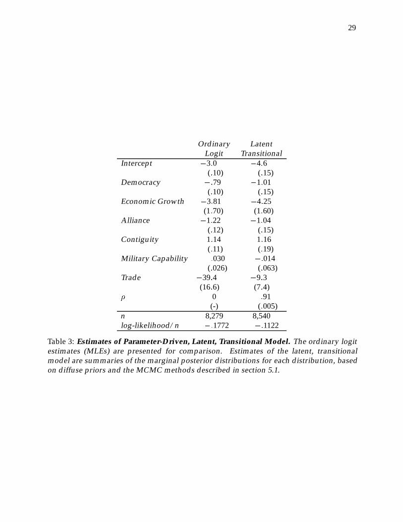
There are few differences between the ordinary logit results and those for the transi-tional model. The intercept for the logit with latent AR(1) errors is substantially greaterin magnitude than that for the corresponding ordinary logit model, and the coefficientfor democracy is also larger (by about 20%), although this difference is small relative tostandard errors of each estimated coefficient. The biggest differences across the modelsare to do with the trade variable. Augmenting the logit model with an AR(1) process onthe disturbances causes the effects of trade to be washed out (t = 1:26); recall that trade isone of the few covariates to exhibit a reasonable amount of time variation (and in a wayrelated to the dependent variable), and so might be reasonably expected to be affectedby the introduction of a correction for serial dependence in the disturbances.14 The latentAR(1) model captures the fact that each yearly observations can not be treated de novo.But since most of the covariates capture little of the serial structure in the data, the AR1(1)

13My excuse for working with this smaller data set is part sloth and part computational. Each MCMCrun with even these n=8,540 subset took well over 24 hours.

14Greene (1997, 587ff) details the relationship between �, serial persistence in the covariates and the inef-ficiency of OLS in the linear regression setting.

29

Ordinary LatentLogit Transitional

Intercept �3:0 �4:6(:10) (:15)

Democracy �:79 �1:01(:10) (:15)

Economic Growth �3:81 �4:25(1:70) (1:60)

Alliance �1:22 �1:04(:12) (:15)

Contiguity 1:14 1:16(:11) (:19)

Military Capability :030 �:014(:026) (:063)

Trade �39:4 �9:3(16:6) (7:4)

� 0 :91(-) (:005)

n 8,279 8,540log-likelihood/n �:1772 �:1122

Table 3: Estimates of Parameter-Driven, Latent, Transitional Model. The ordinary logitestimates (MLEs) are presented for comparison. Estimates of the latent, transitionalmodel are summaries of the marginal posterior distributions for each distribution, basedon diffuse priors and the MCMC methods described in section 5.1.

30

error process does, and fits the data much better: the estimate of � is around .91, andthe (normalized) log-likelihood15 is much higher than that obtained for the ordinary logitanalysis.

8 Conclusion

I have surveyed a number of ways of dealing with discrete, serial data. The marginal-transitional hybrid model of Azzalini (1994) and the observation-driven transitional modelare easily implemented. The dyadic conflict example shows these models to produce in-teresting and plausible departures from the ordinary logit results. The latent, parameter-driven, transitional model also produces a number of interesting findings, although isconsiderably harder to implement, requiring the evaluation of a T-dimensional integral(which I deal with via MCMC methods). In many ways the latent AR() model is more“natural” model for political scientists to work with, combining a familiar discrete choicemodel with an auto-regressive error process, a well-known and widely understood modelfor dealing with serial dependence.

On the other hand, the former two models make us confront the fact that these arediscrete data, and model the dynamics using Markov chains over the discrete binary re-sponses. In so doing, we probably learn more about the determinants of internationalconflict from the observation-driven transitional model, and it certainly dominates theother models considered here in terms of substantive mileage per CPU hour, requiringnothing more than some interaction terms to be added to an ordinary binary responsemodel.

In a recent paper analyzing these data, Beck, King and Zeng (1998, 2) claim that amajor problem with previous analyses is that “[m]ost scholars use statistical proceduresthat assume the effects of the causes of war are nearly the same for all dyads”. Thisposition is a reasonable characterization, amounting to a criticism of simple marginalmodels (Beck, King and Zeng go on to advocate and use neural nets; i.e., complicatedmarginal models). But one extremely easy way to escape this shortcoming is to not treateach dyad-year de novo, by conditioning estimates of the causes of war on the history ofthe dyad.16 Even the most cursory look at the data reveals that the current state of the

15For the latent transitional model — estimated by MCMC methods — I take the median of the sam-pled log-likelihoods produced over the 5,000 iterations of the MCMC algorithm I use for summarizing theparameters.

16Beck, King and Zeng go some way towards accomplishing conditioning on the history of the dyadby having time since last dispute enter as a predictor in a neural-net; constrast Beck, Katz and Tucker(1998),who introduce time since last dispute as a predictor in marginal model.

31

dyad is an important predictor of the future trajectory of a dyad; this is information thatwould be readily used in an applied setting, and ought to belong in any reasonable model.Moreover, conditioning on the past is an important guiding principle in the analysis oftime series data for continuous variables; the models presented here point to ways we cando this in the case of discrete time series data.

32

0 2000 4000 6000 8000 10000

-5.0

-4.5

-4.0

-3.5

0 2000 4000 6000 8000 10000

-1.4

-1.0

-0.6

0 2000 4000 6000 8000 10000

-10

-8-6

-4-2

0

0 2000 4000 6000 8000 10000

-1.6

-1.2

-0.8

0 2000 4000 6000 8000 10000

0.6

1.0

1.4

1.8

0 2000 4000 6000 8000 10000

-0.3

-0.2

-0.1

0.0

0.1

0 2000 4000 6000 8000 10000

-60

-40

-20

0

0 2000 4000 6000 8000 10000

0.75

0.80

0.85

0.90

Inte

rcep

t

Dem

ocra

cy

Eco

nom

icG

row

th

Alli

ance

Con

tigu

ity

Mili

tary

Cap

abili

ty

Trad

e

�

IterationIteration

IterationIteration

IterationIteration

IterationIteration

Figure 4: Trace Plot of MCMC Algorithm, Parameter-Driven Transitional Model. Thelast 5,000 simulations are retained for analysis in the results reported in Table 3.

33

References

Aldrich, John H. and Forrest D. Nelson. 1984. Linear Probability, Logit, and Probit Models.Number 07-045 in Sage University Paper Series on Quantitative Applications in theSocial Sciences. Beverly Hills: Sage.

Alvarez, R. Michael and Garrett Glasgow. 1997. “Do Voters Learn from Presidential Elec-tion Campaigns?” http://wizard.ucr.edu/polmeth/working_papers97/

alvar97e.html .

Andrews, D. F. and A. M. Herzberg. 1985. Data. A Collection of Problems from Many Fieldsfor the Student and Research Worker. Berlin: Springer-Verlag.

Ashby, M., J. M. Neuhaus, W. M. Hauck, P. Bacchetti, D. C. Heilborn, N. P. Jewell, M. R.Segal and R. E. Fusaro. 1992. “An Annotated Bibliography of Methods for AnalysingCorrelated Categorical Data.” Statistics in Medicine 11:67–99.

Azzalini, A. 1994. “Logistic regression for autocorrelated data with application to re-peated measures.” Biometrika 81:767–75.

Azzalini, A. and M. Chiogna. 1995. rm.tools : some S-plus tools for the exploratoryand parametric analysis of repeated measures data. Technical Report. Dipartimentodi Scienze Statistiche, Universita di Padova, Italy. http://lib.stat.cmu.edu/

S/rm.tools2 .

Beck, Nathaniel, Gary King and Langche Zeng. 1998. “The Problem with Quanti-tative Studies of International Conflict.” http://wizard.ucr.edu/polmeth/

working_papers98/beck98.html .

Beck, Nathaniel, Jonathan N. Katz and Richard Tucker. 1998. “Taking Time Seriously inBinary Time-Series Cross-Section Models.” American Journal of Political Science. forth-coming.

Beck, Nathaniel and Simon Jackman. 1998. “Beyond Linearity by Default: GeneralizedAdditive Models.” American Journal of Political Science 42:596–627.

Bombardier, C., J. H. Ware and I. J. Russell. 1986. “Auranofin therapy and quality ofin-patients with rheumatoid arthritis.” American Journal of Medicine 81:565–578.

Carey, Vince C., Scott L. Zeger and Peter J. Diggle. 1993. “Modelling multivariate binarydata with alternating logistic regressions.” Biometrika 80:517–26.

34

Carlin, B. P., A. E. Gelfand and A. F. M. Smith. 1992. “Hierarchical Bayesian analysis ofchange point problems.” Applied Statistics 41:389–405.

Casella, George and Edward I. George. 1992. “Explaining the Gibbs Sampler.” The Amer-ican Statistician 46:167–74.

Chamberlain, G. 1980. “Analysis of Covariance with Qualitative Data.” Review of Economic

Studies 47:225–238.

Chib, Siddhartha and Edward Greenberg. 1994. “Bayes inference in regression modelswith ARMA (p; q) errors.” Journal of Econometrics 64:188–206.

Chib, Siddhartha and Edward Greenberg. 1995. “Explaining the Metropolis-Hastingsalgorithm.” The American Statistician 49:327–335.

Chib, Siddhartha, Edward Greenberg and Rainer Winkelmann. 1998. “Posterior simula-tion and Bayes factors in panel count data models.” Journal of Econometrics 86:33–54.

Cox, D. 1970. The Analysis of Binary Data. London: Chapman and Hall.

Cox, D. R. and E.J. Snell. 1989. Analysis of Binary Data. Second ed. London: Chapman andHall.

Cox, David R. 1981. “Statistical issues in the analysis of time series: some recent develop-ments.” Scandinavian Journal of Statistics 8:93–115.

Czado, Claudia. N.d. “Multivariate Probit Analysis of Binary Time Series Data withMissing Responses.” Department of Mathematics and Statistics, York University.http://math.yorku.ca/Who/Faculty/Czado/bin.ps .

Davis, Richard A., W. T. M. Dunsmuir and Y. Wang. 1998. “Modelling time series ofcount data.” In Asymptotics, Nonparametrics and Time Series, ed. Subir Ghosh. MarcelDekker.

Diggle, Peter, Kung-Yee Liang and Scott L. Zeger. 1994. Analysis of Longitudinal Data.Oxford: Oxford University Press.

Farber, Henry S. and Joanne Gowa. 1997. “Common Interests or Common Polities: Rein-terpreting the Democratic Peace.” Journal of Politics 59(2):393–417.

Fitzmaurice, Garrett M. and Nan M. Laird. 1993. “A likelihood-based method foranalysing longitudinal binary responses.” Biometrika 80:141–51.

35

Fitzmaurice, Garrett M., Nan M. Laird and Andrea G. Rotnitzky. 1993. “Regression Mod-els for Discrete Longitudinal Responses.” Statistical Sciences 8:284–309.

Geweke, John F., Michael P. Keane and David E. Runkle. 1997. “Statistical inference in themultinomial multiperiod probit model.” Journal of Econometrics 80:125–165.

Gochman, Charles S. and Zeev Maoz. 1984. “Militarized Interstate Disputes 1816–1976.”Journal of Conflict Resolution 28:585–615.

Gowa, Joanne. 1998. “Politics at the Water’s Edge: Parties, Voters, and the Use of ForceAbroad.” International Organization 52. forthcoming (page numbers refer to type-script version).

Greene, William H. 1997. Econometric Analysis. Third ed. New York: Prentice-Hall.

Gurr, Ted Robert and Keith Jaggers. 1996. “Polity III: Regime Change and Political Au-thority, 1800-1994.” Computer file, Inter-university Consortium for Political and So-cial Research, Ann Arbor, MI.

Hajivassiliou, V. A. 1995. “A Simulation Estimation Analysis of the External Debt Coun-tries of Developing Countries.” In Econometric Inference Using Simulation Techniques,ed. Herman K. Van Dijk, Alain Monfort and Bryan W. Brown. New York: Wileypp. 191–213.

Hausman, J. A., B. H. Hall and Z. Grilliches. 1984. “Econometric models for count datawith an application to the patents-R&D relationship.” Econometrica 52:909–938.

Jennings, M. Kent and Richard Niemi. 1981. Generations and Politics. Princeton, NJ: Prince-ton University Press.

Jones, Bradford S. and Marco R. Steenbergen. 1997. Modeling Multilevel Data Structures.Technical Report. Political Methodology Working Papers. http://wizard.ucr.

edu/polmeth/working_papers97/jones97.html .

King, Gary. 1997. A Solution to the Ecological Inference Problem. Princeton: Princeton Uni-versity Press.

Klotz, J. 1973. “Statistical inference in Bernoulli trials with dependence.” Annals of Statis-

tics 1:373–379.

Korn, E. L. and A. S. Whittemore. 1979. “Methods for analyzing panel studies of acutehealth effects of air pollution.” Biometrics 35:795–802.

36

le Cessie, S. and J. C. van Houwelingen. 1994. “Logistic Regression for Correlated BinaryData.” Applied Statistics 43:95–108.

Lindsey, J. K. 1995. Modelling Frequency and Count Data. Oxford: Oxford University Press.

MacDonald, Iain L. and Walter Zucchini. 1997. Hidden Markov Models and Othr Models forDiscrete-valued Time Series. Vol. 70 of Monographs on Statistics and Applied Probability

London: Chapman and Hall.

Marriot, John, Nalini Ravishanker, Alan Gelfand and Jeffrey Pai. 1996. “Bayesian Analysisof ARMA Processes: Complete Sampling-Based Inference under Exact Likelihoods.”In Bayesian Analysis in Statistics and Econometrics: Essays in Honor of Arnold Zellner,ed. Donald A. Berry, Kathryn M. Chaloner and John K. Geweke. New York: Wileypp. 243–256.

McCullagh, P. and J.A. Nelder. 1989. Generalized Linear Models. Second ed. London: Chap-man and Hall.

Oneal, John R. and Bruce Russett. 1997. “The Classical Liberals Were Right: Democracy,Interdependence, and Conflict, 1950–1985.” International Studies Quarterly 41(2):267–94.

Plutzer, Eric. 1997. Voter Turnout and the Life Cycle: A Latent Growth Curve Analysis.Technical Report. Political Methodology Working Papers. http://wizard.ucr.

edu/polmeth/working_papers97/plutz97.html .

Poirier, Dale J. and Paul A. Ruud. 1988. “Probit with Dependent Observations.” Review of

Economic Studies 55:593–614.

Prais, S.J. and C.B. Winsten. 1954. Trend estimators and serial correlation. Number 373Chicago: Cowles Commission Discussion Paper.

Prentice, Ross L. 1988. “Correlated Binary Regression with Covariates Specific to EachBinary Observation.” Biometrics 44:1033–48.

Russett, Bruce. 1990. “Economic Decline, Electoral Pressure, and the Initiation of In-ternational Conflict.” In The Prisoners of War, ed. Charles Gochman and Ned AllanSabrosky. Lexington, MA: Lexington Books pp. 123–140.

Russett, Bruce. 1993. Grasping the Democratic Peace. Princeton, New Jersey: PrincetonUniversity Press.

37

Singer, J. David and Melvin Small. 1994. Correlates of War Project: International and CivilWar Data, 1816-1992. Ann Arbor, Michigan: Inter-university Consortium for Politicaland Social Research. ICPSR Study Number 9905.

Sommer, A., J. Katz and I. Tarwotjo. 1984. “Increased risk of respiratory infection anddiarrhea in children with pre-existing mild vitamin A deficiency.” American Journal

of Clinical Nutrition 40:1090–95.

Stern, R. D. and R. Cole. 1984. “A model fitting analysis of daily rainfall data (with dis-cussion).” Journal of the Royal Statistical Society, Series A 147:1–34.

Tanner, Martin A. 1996. Tools for Statistical Inference: Methods for the Exploration of PostriorDistributions and Likelihood Functions. Third ed. New York: Springer-Verlag.

Ware, J. H., D. W. Dockery, A. Spiro III, F. E. Speizer and B. G. Ferris Jr. 1984. “Passivesmoking, gas cooking, and respiratory health of children living in six cities.” Ameri-

can Review of Respiratory Disease 129:366–374.

West, Mike and Jeff Harrison. 1997. Bayesian Forecasting and Dynamic Models. New York:Springer-Verlag.

Western, Bruce. 1998. “Causal Heterogeneity in Comparative Research: A Bayesian Hier-archical Modelling Approach.” American Journal of Political Science 42. in press.

Zeger, S. L. and B. Qaqish. 1988. “Markov regression models for time sries.” Biometrics44:1019–31.