Time Series Based Forecasting of Renewable Power Infeed ...

Time Series Based Forecasting ofRenewable Power Infeed for Operation

of Microgrids

Master thesis

from

Elin Klages

born on

08. June 1989 in Hamburg, Germany

04. October 2016

Supervisor: Christian A. Hans

Examiner: Prof. Dr.-Ing. Jörg RaischControl Systems GroupDepartment of Energy and Automation TechnologyFaculty IV - Electrical Engineering and Computer ScienceTechnische Universität Berlin

Second Examiner: Prof.-Dr.-Ing. Clemens GühmannChair of Electronic Measurement and Diagnostic TechnologyDepartment of Energy and Automation TechnologyFaculty IV - Electrical Engineering and Computer ScienceTechnische Universität Berlin

i

Eidesstattliche Erklärung

Hiermit erkläre ich, dass ich die vorliegende Arbeit selbstständig und eigenhändig sowieohne unerlaubte fremde Hilfe und ausschließlich unter Verwendung der aufgeflührtenQuellen und Hilfsmittel angefertigt habe.

Berlin, den 01. August 2016

ii

Abstract

The proportion of renewable energy, in relation to conventional energy, is increasing.Especially the fluctuation of energy from renewable sources causes difficulties for theoperation of electrical grids. In the present thesis, methods for time series based fore-casts of renewable power infeed are investigated. Therefore, Autoregressive IntegratedMoving Average (ARIMA) Models, Kernel, k Nearest Neighbour (kNN), and Support Vec-tor (SV) Regression are applied to predict future values of wind speed and solar irra-diance. Forecasts up to 2 h in advance with a resolution of 10 min are considered asrelevant for the operation of a microgrid. The performance of the trained models isevaluated based on a comparison to a naive forecast. Results show that prediction offuture values of solar irradiance is most accurate if the the observed values of solar ir-radiance measured at ground level are normalized using the estimated extraterrestrialsolar irradiance. Support Vector Regression yields the most accurate forecasts for solarirradiance of the above mentioned techniques. For forecasting windspeed, the results donot indicate a clear tendency which regression technique to use. While Support VectorRegression works best for forecast from 10 min up to 2 h, ARIMA provides better resultsfor the first predictions steps and Kernel Regression for the last prediction steps. Forboth techniques, improvement over the naive forecast is highest for prediction horizonsclose to 2 h (up to 20.9% for solar irradiance), while prediction of the next 10 min cannotbe improved significantly compared with a naive forecast (<3%).

iii

Kurzfassung

Der Anteil von regenerativen Energien, im Vergleich zu konventionellen Energien, nimmtstetig zu. Insbesondere die Fluktuation von Energien aus erneuerbaren Quellen, wirktsich negativ auf die Regelung von elektrischen Netzen aus. In der vorliegenden Arbeitwerden Methoden zur Vorhersage der Einspeisung von erneuerbaren Energien unter-sucht. Es werden "Autoregressive Integrated Moving Average (ARIMA)" Modelle, Kernel,k Nächste Nachbarn (kNN), und Stützvektor (SV) Regression verwendet um zukünftigeWerte für Sonneneinstrahlung und Windgeschwindigkeit vorherzusagen. Vorhersagenbis zu 2 h in die Zukunft bei einer Auflösung von 10 min werden als relevant für dieRegelung eines Microgrids angenommen. Die Bewertung der tranierten Modelle erfolgtim Vergleich zu einer naiven Vorhersage. Ergebnisse für die Vorhersage von Sonnenein-strahlung zeigen, dass die beste Vorhersagengenauigkeit erreicht wird, wenn die Datenzunächst mit der extraterrestrialen Sonneneinstrahlung normiert werden. StützvektorRegression erreicht, von den oben genannten Techniken, die höchste Vorhersagege-nauigkeit für die Vorhersage von Sonneneinstrahlung. Die Ergebnisse für dieWindgeschwindigkeitvorhersagen sind weniger deutlich. Stützvektor Regression erre-icht die höchste Genauigkeit für Vorhersagen von 10 min bis 2 h, während ARIMA bessereErgebnisse für Vorhersagen bis zu 30 min erzielt und Kernel Regression für die Vorher-sagen nah an 2 h am genausten ist. In beiden Fällen zeigt sich, dass die Vorhersagege-nauigkeit im Vergleich zu einer naiven Vorhersage am meisten für Vorhersagen von 2 hin die Zukunft zunimmt (bis zu 20,9% für Sonneneinstrahlung), während bei Vorher-sagen für 10 min in die Zukunft die Vorhersagegenauigkeit nur geringfügig verbessertwerden kann (<3%).

Contents

List of Figures v

List of Tables vi

1 Introduction 1

2 Background 32.1 Statistics . . . . . . . . . . . . . . . . . . . . . . . . . . . . . . . . . . . . . . . 32.2 Solar Radiation . . . . . . . . . . . . . . . . . . . . . . . . . . . . . . . . . . . 72.3 Summary . . . . . . . . . . . . . . . . . . . . . . . . . . . . . . . . . . . . . . 9

3 Time Series Based Forecast 113.1 Parametric Regression . . . . . . . . . . . . . . . . . . . . . . . . . . . . . . 123.2 Nonparametric Regression. . . . . . . . . . . . . . . . . . . . . . . . . . . . 163.3 Multiple step forecasts. . . . . . . . . . . . . . . . . . . . . . . . . . . . . . . 203.4 Estimating the Probability of a Forecast . . . . . . . . . . . . . . . . . . . . 203.5 Summary . . . . . . . . . . . . . . . . . . . . . . . . . . . . . . . . . . . . . . 21

4 Implementation 234.1 Implementation of Regression Techniques . . . . . . . . . . . . . . . . . . 234.2 Data Used for Training and Testing. . . . . . . . . . . . . . . . . . . . . . . . 244.3 Search for Models with Highest Forecast Accuracy . . . . . . . . . . . . . . 254.4 Performance Evaluation . . . . . . . . . . . . . . . . . . . . . . . . . . . . . 284.5 Summary . . . . . . . . . . . . . . . . . . . . . . . . . . . . . . . . . . . . . . 32

5 Results and Analysis 335.1 Results for Forecasting Solar Irradiance . . . . . . . . . . . . . . . . . . . . 335.2 Results for Forecasting Wind Speed . . . . . . . . . . . . . . . . . . . . . . . 365.3 Summary . . . . . . . . . . . . . . . . . . . . . . . . . . . . . . . . . . . . . . 39

6 Case Study 43

7 Conclusion 47

Bibliography 49

iv

List of Figures

2.1 Example: Discrete Probability Distribution . . . . . . . . . . . . . . . . . . . . 42.2 Zenith angle z and solar altitude γ. . . . . . . . . . . . . . . . . . . . . . . . . . 72.3 Absorption of extraterriestral solar radiation. . . . . . . . . . . . . . . . . . . . 8

3.1 Stages in the iterative approach to model building. . . . . . . . . . . . . . . . . 143.2 Example for local regression. . . . . . . . . . . . . . . . . . . . . . . . . . . . . 173.3 Linear one dimensional example for Support Vector regression. . . . . . . . . 18

4.1 Flow chart of grid search for ARIMA models. . . . . . . . . . . . . . . . . . . . 274.2 Flow chart of grid search for k Nearest Neighbors and Kernel Regression. . . 284.3 Flow chart of grid search for Support Vector Regression. . . . . . . . . . . . . 294.4 Forecasts of solar irradiance beginning at different time steps. . . . . . . . . . 31

5.1 Performance of naive forecast predicting solar irradiance. . . . . . . . . . . . 335.2 Performance solar irradiance forecasting using solar irradiance directly. . . . 345.3 Performance wind speed forecasting - 12 prediction steps. . . . . . . . . . . . 375.4 Performance wind speed forecasting - 3 prediction steps. . . . . . . . . . . . . 385.5 Performance wind speed forecasting - 12 prediction steps. . . . . . . . . . . . 415.6 Performance wind speed forecasting - 3 prediction steps. . . . . . . . . . . . . 42

6.1 Exemplary microgrid. . . . . . . . . . . . . . . . . . . . . . . . . . . . . . . . . . 436.2 Block diagram for a stochastic model predictive control approach. . . . . . . 446.3 Scenario fan for a forecast of solar irradiance. . . . . . . . . . . . . . . . . . . . 446.4 Case Study: Thermal, storage, renewable and stored energy and load. . . . . 45

v

List of Tables

4.1 Parameter space to search for ARIMA models. . . . . . . . . . . . . . . . . . . 254.2 Parameter space to search for seasonal ARIMA models with highest forecast

accuracy. . . . . . . . . . . . . . . . . . . . . . . . . . . . . . . . . . . . . . . . . 254.3 Parameter space for k Nearest Neighbors Regression. . . . . . . . . . . . . . . 264.4 Parameter space for Kernel Regression. . . . . . . . . . . . . . . . . . . . . . . . 264.5 Parameter space for the grid search for SVR. . . . . . . . . . . . . . . . . . . . . 28

5.1 Models that predict most accurate the solar irradiance. . . . . . . . . . . . . . 355.2 Models that predict most accurate the wind speed test data. . . . . . . . . . . 40

6.1 Results case study. . . . . . . . . . . . . . . . . . . . . . . . . . . . . . . . . . . . 46

vi

Glossary

B Backwards shift operator. vii, viii, 12, 13

Φ(B s ) Seasonal autoregressive operator of a seasonal ARIMA model. 13

Θ(B s ) Seasonal moving average operator of a seasonal ARIMA model. 13

α Significance level of the hypothesis test. 6, 15, 16

γ Solar altitude. v, 6, 7

y Predicted time series. 11, 12, 16

µ Mean value, also called expected value. 3, 4, 5, 6, 20

φ(B ) Autoregressive operator of an ARIMA model. 12, 13

ρ Correlation. 5

σ2 Variance. 4, 5

σ Standard Deviation. 3, 4, 5

τ Transmissivity. Relation between solar irradiance that reaches the earth surface andthat enters the earths atmospehere. 9

Cov Covariance. 4, 5

DN Observed data. N pairs of measured independent variable xi and dependent vari-

able yi , DN ={(

x1, y1)

,(x2, y2

). . .

(xn , yn

)}. 11, 12, 16, 17, 19

G0 Extraterriestral solar irradiance. 6, 7, 9

Gdh Diffuse horizontal irradiance. 8, 9

Gdn Direct normal irradiance. 9

Gsc Solar constant. 7

G Global horizontal irradiance. 8, 9

vii

viii GLOSSARY

H0 Null hypothesis. 5, 6

Nmin Number of historical data points needed to predict future values.. 29, 30, 32

Np Number of parameters of a model. 15, 16

N Number of samples. 11, 15, 16, 28, 29

T Test statistic of hypothesis test. 5, 6

c Critical value of hypothesis test. 5, 6

θ(B ) Moving average operator of an ARIMA model. 12, 13

θ Parameter vector of a parametric model. 12

a Julian day.. 7

d Degree of differencing of an ARIMA model. 12

e Residuals. Prediction minus measured values. 12, 26, 28, 29, 30, 31, 32

f Regression function or index to indicate forecast. Clear from context.. 12

j Index to indicate prediction horizon. 5, 30, 31, 32

k Index to indicate time instant or number of neighbors used for k Nearest NeighbourRegression. Clear from context.. 5, 11, 12, 13, 15, 16, 20, 28, 32

p(i ) Probability associated with the i th value of the set of possible values of the randomvariable. 3, 4

p Prediction Horizon. 29, 32

r Autocorrelation. 5, 15

s Length of one season of an SARIMA model. 13

xi i th value of the set of possible values of the random variable X . 3, 4, 16

x Time series respectively independent variable.. 11, 12, 16, 20

y Time series respectively response/dependent variable.. 5, 6, 11, 12, 13, 16, 20, 32

z Zenith angle. v, 6, 9

X Random Variable. viii, 3, 4, 5

RMSE Root mean square error. 28, 30, 31, 32, 33, 35, 36, 40, 41

sr Index to indicate sunrise. 30, 31

ss Index to indicate sunset. 30, 31

Chapter 1

Introduction

Time series based forecasting, i.e., predicting future values based on previously observedvalues, has been used in various areas. In the context of the operation of a microgrid, it isof interest to estimate beforehand future power infeed and load. In contrast to infeed ofconventional energy, infeed of renwable energy1 cannot be set by the operators. Whileload is relatively predictable2, the fluctuation of renewable power infeed make it difficultto manage in the context of the operation of electrical grids. Here, accurate forecasts ofrenewable power infeed could improve the operation of the grid and yield to decreaseduse of energy from conventional sources. Solutions, based merely on already providedinformation due to the operation of a microgrid (like current time, previously measuredpower infeed and basic knowledge about the location of the grid) keep additional costsand effort small. Therefore, the present work aims to present how short term predic-tion (here up to 2 h) of renewable power infeed (solar and wind power) can be realizedaccurately and efficiently.

Various studies on forecasting wind speed and solar irradiance have been published.However, most focus on either physical models or long term predictions or both. Espe-cially for forecasting of solar irradiance, hardly any work can be found for forecastingintervals less than 1 hour. Still, previous research indicates that time series based fore-casts perform better for short term predictions, while physical models work best for longterm predictions, e.g., two days ahead, [Qiao and Zeng, 2012, Section 1.], [Heinemannet al., 2006, Section 1.], [Bacher et al., 2009, Section 7.]. This supports the approach ofthe present work, to explore the information provided by historical data instead of usingcomplex numerical simulations to obtain estimates of future values of renewable powerinfeed.

In both fields, forecasting solar irradiance and wind speed, as for time series forecasts

1In 2015, already 32.6% of electric current in Germany came from renewable sources, [Statistik, 2016].Until 2025, a percentage of 40-45% is planned, [Werdermann, 2016].

2For example, lights are switched on when it gets dark.

1

2 CHAPTER 1. INTRODUCTION

in general, classically used are Autoregressive Integrated Moving Average (ARIMA) mod-els. Recently, research has been done on using other techniques, as e.g., Artificial Neu-ral Networks (ANN), [Sfetos, 2001], [Cadenas and Rivera, 2006], [Qiao and Zeng, 2012],[Mellit and Pavan, 2010], Fuzzy Logic Models (especially for wind speed), [Monfaredet al., 2009] and Support Vector Regression (SVR), [Qiao and Zeng, 2012], [Zhou et al.,2011]. There are various studies that compare two or more techniques, although com-parison is done mainly for ARIMA models and one Artificial Intelligence related tech-nique. However, no clear conclusion can be drawn from these. Firstly, results differ.For example, a study on forecasting wind speed, concludes that ANN achieves signifi-cantly better results than ARIMA models, [Sfetos, 2001]. Another study that comparesANN and ARIMA for forecasting wind speed, comes to the opposite conclusion, say-ing that Seasonal ARIMA models perform better than ANN, [Cadenas and Rivera, 2006].Secondly, the use of different data sets measured at different locations, and the use ofdifferent error measurements, make it hard to compare results and to use the informa-tion provided by previous research. Sfetos suggests, that the improvement over the naiveforecast could be used to compare the performance forecast techniques, evaluated ondifferent data, [Sfetos, 2001, Section 1.]. However, the results of a naive forecast are oftennot provided in the articles.

The present work focuses on forecasting wind speed and solar radiation using exclu-sively data that is already provided by the operation of a microgrid. Different techniquesfor time series based forecasts with predictions steps of 10 min with prediction hori-zons up to 2 h are explored, to find the most adequate technique for the operation ofa microgrid, based on high solution data. The chosen techniques are ARIMA models,k Nearest Neighbour Regression (kNN), Kernel Regression and Support Vector Regres-sion. ARIMA models are selected to be able to compare the performance of other tech-niques to ARIMA models, since they are considered as the classical way to approximatetime series. Kernel and kNN Regression are simple, intuitive techniques that can be im-plemented with little effort. Also, no training of a model is needed. For these reasons,these techniques were chosen to examine if with simple regression methods good fore-cast quality can be achieved. As a more complex regression technique, Support VectorRegression was chosen. Studies using SVR indicate that it could provide better resultsthan ANN, e.g., [Qiao and Zeng, 2012]. As mentioned above, the trained models areevaluated based on the improvement relative to a naive forecast.

The reminder of this paper is organized as follows. Basic information on statistics andsolar radiation are given in chapter 2. In chapter 3, the applied regression techniquesare explained in detail. How the techniques were implemented is clarified in chapter4. In chapter 5, achieved forecast accuracy is presented and discussed. As an example,results of a performed simulation of the operation of a microgrid, using Support VectorRegression to predict solar irradiance, is presented in chapter 6.

Chapter 2

Background

Before introducing the applied regression techniques to forecast future values of windand solar power, information on statistics and solar radiation is provided by this chapter.This chapter aims to provide the needed background information for Chapter 3 and 4.

2.1 Statistics

In the following, some basics and some content of more advanced topics of statistic aregiven. This section primarly intends providing sufficient information to understand thiswork. It is also thought to simplifify understanding the cited literature.

Probability and Random Variables

A random variable X represents a set of possible different values xi , where the occur-rence of each value, for example as output of an experiment, is associated with a prob-ability p(i ). A probability distribution describes the random variable completely, i.e.,its values and their associated probabilities (see , e.g., figure 2.1, example is explainedbelow), [Wasserman, 2005, Sec. 1.1.-1.4, 2.1]. Random variables can be continuous ordiscrete. However, in this work only discrete variables (time series) are considered.

One example of a random variable is the occurence of rain fall during one day in Berlin1.The two possible outcomes, the so called sample space, are day with rainfall or daywithout rainfall, represented by 1 and 0. Their probability distribution is2

p(i ) =0.73, if i = 0

0.27, if i = 1.(2.1)

1Another example of a random variable is the side of a coin, that occurs when a coin is flipped, wherethe sample space includes the two sides and the probability of each side is 0.5. An example with a samplespace that includes more than two possible outcomes would be , e.g., the number of children in family.

2This is meant to serve as an example, for this reason the probabilities should not be taken too seriously.

3

4 CHAPTER 2. BACKGROUND

0 1 2

0.53

0.39

7 ·10−2

µ

2σ

xi

p(i )

Figure 2.1: The discrete probability distribution, with mean value µ = 0.54 and standarddeviation σ = 0.68, of the example in (2.2). The colored part indicates the part of theprobability distribution included by the standard deviation. Nonnegative values are notcolored, since it is impossible to get a negative number of days with rainfall.

If two days instead of one are considered, the example changes. The probability distri-bution would be

p(i ) =

0.73 ·0.73 = 0.53, if i = 0, it does not rain on both days,

0.73 ·0.27+0.27 ·0.73 = 0.39, if i = 1, it rains on one day,

0.27 ·0.27 = 0.07, if i = 2, it rains on both days.

(2.2)

The probability is visualized in figure 2.1.

In the following it is assumed that the underlying random process is stationary, i.e. theprobability distribution is time independent.

The mean value µ of a random variable X , also called expected value, is defined as

µ(X ) =n∑

i=1p(i ) xi . (2.3)

As a measure of the spread of a random value, its variance σ2 ,

σ2 (X ) =µ((

X −µX)2

), (2.4)

respectively its standard deviationσ can be used. The variable µX refers to µ(X ). A highdispersion around the mean value is indicated by a high variance / standard deviation,while a small variance / standard deviation indicates that the results tend to lie close tothe mean, [Wasserman, 2005, Def. 3.14], (see figure 2.1 for an example).

If, instead of one variable X , two random variables X , X∗ are considered (e.g. if it rainsin Berlin and if it rains in Potsdam), the variance (see (2.4)), turns into the covariance,

Cov(X ,X∗) =µ ((X −µX ) (X∗−µX∗)

), (2.5)

2.1. STATISTICS 5

where µX is the mean value of X and µX∗ is the mean value of X∗. The correlation be-tween these two variables is defined by

ρ (X ,X∗) = Cov(X ,X∗)

σ X σ X∗, (2.6)

whereσ X is the standard deviation of X andσ X∗ is the standard deviation of X∗. The co-variance and the correlation are both measurements of the linear relationship betweenthe two variables X and X∗, [Wasserman, 2005, Def. 3.18].

If the correlation (see (2.5)) is applied for the same random variable (e.g. if it rains duringthe day) but at different points of time, X k , X k− j (e.g. if rains on Monday and if it rains onTuesday) the autocorrelation is obtained, [Hyndman and Athanasopoulos, 2014, p.35],

r (X k ,X k− j ) =µ

((X k −µX ) (X k− j −µX )

)σ2 . (2.7)

As an alternative to autocorrelation as a measure between correlation of elements of atime series, the partial autocorrelation can be used. The partial autocorrelation of X k ,X k− j is the correlation after removing all correlation with X k−1, . . . ,X k+1− j , [Hyndmanand Athanasopoulos, 2014].

Statistical Inference

Statistical inference deals with infering information about the data generating processfrom the observed data, [Wasserman, 2005, preface]. This section does not serve as ageneral overview about statistical inference; the aim is merely to present some tech-niques, later on used in the context of time series forecasting using ARIMA models (seeSection 3.1). For a general overview the reader is referred to the cited books in this sec-tion.

Hypothesis Testing

Hypothesis testing refers to a procedure used to measure how much evidence providesthe observed data against a theory, typically named null hypothesis H0, about the pop-ulation the data is coming from, [Wasserman, 2005, p.94].

The hypothesis test itself is a rule that specifies when to reject or retain the null hypoth-esis. Usually a test statistic T(y), a function of a sample of the population y , in combi-nation with a critical value c that functions as threshold for the test statistic, is used astest rule, [Casella and Berger, 2001, Chapter 8, p.374-375].

An example for a null hypothesis could be the theory that the mean height s of all habi-tants of a certain region is 170 cm, written as

H0 :µ(s) = 170cm. (2.8)


To test H0, a group of 30 habitants is taken and the height s of each one is measured.As test statistic might be used the distance of mean height of these 30 habitants to thetheoretical mean height,

T(s) =∣∣170cm −µ(si )∣∣ , i = 1, . . . ,30. (2.9)

If the mean hight results to be , e.g., 172.34 cm (T(s) = 2.34cm), the observed data (the 30habitants) would not provide much evidence to reject the null hypothesis, but neitherproves it. But if 30 other people were chosen and the mean hight was , e.g., 145,12 cm(T(s) = 24.88cm), the null hypothesis would seem to be more likely false. But, as before,the test statistic doesn’t prove that the null hypothesis is wrong or right.

To decide to reject or retain the null hypothesis, the test statistic is compared to a prede-fined critical value,

H0 is

rejected, if T (y) ≥ c,

retained, if T (y) < c,(2.10)

[Kalbfleisch, 1979, p.136].

The choice of the critical value is linked to the so called significance level α of the test.The significance level is defined by the probability that the test statistic T (y) is smalleror equal to the critical value c, if the null hypothesis H0 is true,

α= p{c ≥ T(y)|H0

}. (2.11)

Hence, the significance level α does not refer to the probability that the null hypothesisis true, [Kalbfleisch, 1979, p.136-137].

A statement as

The hypothesis test xy was passed at the 5% significance level.

means that the critical value c was chosen to obtain an α (see (2.11)) of 0.05 and thatthe test statistic T(y) for the given data is as least as large as c. This means the test isalso passed for all significance level less than 5%. This statement does not provide theinformation if the test would be also passed at the 10% or even 90% level. Therefore itmight be more informative to pass on the lowest significance level the data passes. Thislowest passed significance level is often referred to as p-value3.

2.2. SOLAR RADIATION 7

ZenithSun

Earth’s surface

zγ

Figure 2.2: Zenith angle z and solar altitude γ.

2.2 Solar Radiation

This section intends to provide all information needed, to understand how the solar ra-diation data is used in this work and in work cited work by others. The solar energythat arrives at the limit of the earth’s atmosphere is called extraterriestral solar radiation,[IS/ISO-9488, 1999]. It can be predicted by the amount of energy emitted by the sunand the position of the sun relatively to the earth. The extraterrestrial solar irradiance,irradiation per area, G0 is given by

G0 = εGsc sin(γ) (2.12)

where Gsc = 1360.8W/m2 is the solar constant4, γ is the solar altitude in degrees (seefigure 2.2) , ε a correction factor for the distance of the sun to the earth5

ε= 1+0.0334 cos( j’−2.80◦), (2.13)

j’ the day angle,

j’ = a

365.25360◦, (2.14)

3For example in this section cited book All about Statistics, [Wasserman, 2005], or by MATLAB. In theother here cited book Probability and Statistical Inference, [Kalbfleisch, 1979], p-value and significance levelare used synonymously.

4Different references define slightly different values for the solar constant. Although in the The Euro-pean Solar Radiation Atlas, where equation (2.12) is taken from, the solar constant is defined as 1367W/m2,[Scharmer and Greif, 2000, Chapter 3, p.28], the value used in this work, 1360.8W/m2, is chosen after Koppand Lean, Kopp and Lean [2011].

5The distance between sun and earth varies over the year, because the earth’s orbit isn’t a circle.


Figure 2.3: Nominal range of clear sky absorption and scattering of incident solar energy,[Stine and Harrigan, 1986, Figure 2.9]. Note: Insolation is a deprecated term for solarradiation, [IS/ISO-9488, 1999, 3.13].

and a is the Julian Day 6 the number of the day in the year (1-366) [Scharmer and Greif,2000, Chapter 3, p.28].

Ground level solar radiation is more difficult to predict than the radiation that reachesthe outer edge of the atmosphere, as only a part of solar radiation is transmitted directlywhile other parts are absorbed, reflected, and scattered by the atmosphere and clouds(see figure 2.3), [Stine and Harrigan, 1986, Section 2.2].

The solar radiation received on a horizontal plane on earth is called global solar radia-tion, [IS/ISO-9488, 1999, 3.2], or global horizontal radiation7. The global horizontal irra-

6A note to avoid confusion. In other references, the term Julian Day might be used for numbering thedays when counting them continuously since some historical date (see https://en.wikipedia.org/w/

index.php?title=Julian_day&oldid=715401672), while in the context of counting them from January1st, the term day number might be used, as for example in the book Solar Energy Systems Design, [Stine andHarrigan, 1986, Section 2.1.3, equation 2.1].

7e.g. National Renewable Energy Laboratory (NREL)

https://en.wikipedia.org/w/index.php?title=Julian_day&oldid=715401672

https://en.wikipedia.org/w/index.php?title=Julian_day&oldid=715401672

2.3. SUMMARY 9

diance G includes the direct irradiance Gdh (often called beam irradiance, [Quaschning,2004, Section 2.1]), which comes directly from the sun, and the diffuse irradiance Gdh,which includes scattered and ground reflected8 irradiance, [IS/ISO-9488, 1999, 3.20,3.21, 3.25]. Direct irradiance is usually measured at normal incidence (see figure 2.2),[IS/ISO-9488, 1999, 3.17], and therefore in the context of this work called direct normalirradiance to avoid confusion. Hence, the relation between global horizontal irradianceand it’s both components is,

G = Gdn +Gdh cos(z ). (2.15)

Direct normal irradiance Gdn can be measured by a pyrheliometer, that is always aimedat the sun, [IS/ISO-9488, 1999, 4.7] with help of a solar tracking algorithm. A pyranome-ter, which measures solar irradiance on a plan surface, [IS/ISO-9488, 1999, 4.4] can beused to measure the global horizontal irradiance G or the diffuse horizontal irradianceGdh. The latter can be obtained either by taking the difference between the global hori-zontal irradiance or by measuring the solar irradiance while covering the current normalto the sun.

Another possible representation of the solar radiation reaching the earth, instead of us-ing it’s absolute amount, is using the transmissivity for the comparison between solarradiation entering the earth’s atmosphere and the radiation reaching earth’s surface,

τ= G

G0(2.16)

as for example used in [Qiao and Zeng, 2012]. By using also the extraterriestral irradi-ance, which can be easily predicted, as explained above (see equation (2.12)), this rep-resentation already includes meteorological information.

2.3 Summary

Hypotheis tests, as used for the evaluation of ARIMA models, are described. For this rea-son and also as background information for forecasting in general, the basics of proba-bilites are discussed shortly. To give an explanation of the particularity of solar radiationdata in relation to wind speed data, solar radiation is discussed. In the same context, thetransmissivity is introduced. An explanation of the used regression techniques, as forexample ARIMA models, follows in the next chapter.

8The part reflected by the ground is usually an insignificant amount http://rredc.nrel.gov/

solar/glossary/gloss_g.html, see Global Horizontal Radiation

http://rredc.nrel.gov/solar/glossary/gloss_g.html

http://rredc.nrel.gov/solar/glossary/gloss_g.html

Chapter 3

Time Series Based Forecast

This chapter aims to give an overview about the regression techniques used in this work.Regression in general refers to infer information about the data generating process fromhistorical data. In other words, regression is about finding a regression function f (x)that approximates y ,

y = f (x), (3.1)

based on the observed data

DN ={(

x1, y1)

,(x2, y2

). . .

(xN, yN

)}, (3.2)

where x is the independent variable and y is the dependent variable, [Gyoerfi et al., 2002,p.1-3].

Autoregression is regression using only historical data of the response variable y . There-fore, the independent variable x represents one or more historical values of y ,

xk = [yk−1, yk−2, . . . , yk−n], (3.3)

where n is the number of elements in x. In this chapter as in this work in general, thefocus lies on autoregression. In contrast, regression in general can rely on any historicaldata. However, all in the following presented techniques can be also used, or at leastextended, to regression in general.

In the following, it is differentiated between parametric and nonparametric regression.In parametric regression, the model, used to approximate the data, depends on the pa-rameters derived from the data, while in non parametric regression, the model dependsdirectly on the data.

On purpose, it is not focused on separating between Statistical Inference and MachineLearning. The main reason is that there is no clear difference between these two fields.

11

12 CHAPTER 3. TIME SERIES BASED FORECAST

In contrast, they are often described as the same, e.g., by Larry Wasserman in All aboutstatistics1 or nearly the same, e.g., by Jerome H. Friedmann in The Role of Statistics inthe Data Revolution? 2. The main difference may lie in the way their techniques are pre-sented.

Apart from the techniques used for the forecasts, this chapter also explains how multi-ple step forecasts are done and how a probability distribution for the forecasts is hereestimated.

3.1 Parametric Regression

In parametric regression, the regression function f depends on the independent vari-able x and the parameters θ,

y = f (x,θ). (3.4)

The parameters θ are estimated based on the observed data DN. In the following theonly parametric models used in this work, ARIMA models, are presented.

The ARIMA Model

Often used linear models for time series forecasting are autoregressive integrated mov-ing average (ARIMA) models. Making use of the backwards shift operator B and thebackward difference operator ∇, which are defined by

B m yk = yk−m , (3.5)

∇d yk = (yk − yk−1

)d , (3.6)

[Box et al., 1994, p.8], an ARIMA model can be defined as follows,

φ(B )∇d yk = θ0 +θ(B )ek , (3.7)

where yk is a sample of the time series at time instant k, ek the error of the forecastcompared to the measured value, φ(B ) the autoregressive operator, ∇d the integrativepart, and θ(B ) the moving average operator. The autoregressive and the moving averageoperator are polynomials with degree p and q respectively,

φ(B ) = 1 − φ1 B −1 − φ2 B −2 −·· ·− φp B −p , (3.8)

θ(B ) = 1 − θ1 B −1 − θ2 B −2 −·· ·− θq B −q , (3.9)

1The basic problem of statistical inference is about the inverse of probability, infer the data generatingprocess from the observed data. Prediction, classification, clustering and estimation are all cases of statisticalinference. Data analysis, data mining and machine learning are just different names given to the practise ofstatistical inference, [Wasserman, 2005, Preface, page ix].

2Had we incorporated computing methodology from its inception as a fundamental statistical tool (. . . )many of the other data related fields [e.g., machine learning] would not have needed to exist. They wouldhave been part of our field [statistics], [Friedmann, 2001]

3.1. PARAMETRIC REGRESSION 13

[Box et al., 1994, p.96].

Due to its different parts, this class of models also includes autoregressive (AR) models,moving average models (MA), and the mixed autoregressive, moving average (ARMA)models. Due to differencing (the integrative part of the ARIMA model), ARIMA modelscan be also fitted to nonstationary data, if stationary data can be obtained by differenc-ing of the original data, [Box et al., 1994, p.89].

To fit a model to data that exhibits seasonality, ARIMA models can be extended by sea-sonality of a certain period s. These models can be described by,

φ(B )Φ(B s )∇d ∇Ds yk = θ0 +θ(B )Θ(B s )ek , (3.10)

where Φ(B s ) and Θ(B s ) are the seasonal autoregressive and seasonal moving averageoperator, [Box et al., 1994, Chapter 9, p.332], defined as

Φ(B s ) = 1 − Φ1 B −s − Φ2 B −2 s −·· ·− Φp B −P s , (3.11)

Θ(B s ) = 1 − Θ1 B −s − Θ2 B −2 s −·· ·− Θq B −Q s , (3.12)

and ∇Ds represents seasonal differencing

∇Ds yk = (

yk − yk−s)D . (3.13)

Model Identification and Estimation

To fit a model to a given time series, at first, the order of the autoregressive and the mov-ing average operator of the model and the degree of differencing needs to be defined.This step is called Identification. The second step, Estimation refers to the process ofobtaining the values of the parameters. Identification and estimation usually overlap,since identification refers to obtaining a rough idea of the kind of model needed, [Boxet al., 1994, Chapter 6, p.183-184]. See also figure 3.1.

The first step of identification is to difference the data as many times as needed to getstationary data. As second step follows to identify the resulting ARMA model. Here,the autocorrelation and the partial autocorrelation can be used. For an AR model, thelast significant lag of the partial autocorrelation of the sample represents roughly theorder of the autoregressive operator, [Box et al., 1994, Chapter 6, p.184-185]. Likewisethe autocorrelation can be used to identify the order of a moving average operator in aMA model. For mixed models such approaches are usually not very effective in pratice,[Liu and Hudak, 1992, Chapter 5, p.5.7-5.9].

For identified models, estimation of the parameters can be done for example by maxi-mum likelihood estimation3.

3As used for example by MATLAB, see documentation of function estimate.


Figure 3.1: Stages in the iterative approach to model building as proposed by Box, Jenk-ins and Reinsel, [Box et al., 1994, Fig. 1.7]

Diagnostic Checks on the Model

The residuals from a well fitted model are expected to be independent and normallydistributed. If this assumptions cannot be proved, the model needs modification, [Liuand Hudak, 1992, Chapter 5, p.5.15]. The independence of the residuals can be checkedby the Ljung-Box Test, which tests whether the residuals exhibit autocorrelation or not.To access information about the distribution of the residuals, the Kolmogrov-SmirnovTest, which compares the distribution of two samples, can be used.

It is also of interest to check against overfitting, that means if some estimated parametersare not statistically different4 from zero, [Liu and Hudak, 1992, Chapter 5, p.5.16]. Tofind an adequate number of parameters for the model, the Akaike information criterion,described in 3.1, can be also helpful.

The above mentioned hypothesis tests5 are described in the following sections.

4The term statistically different refers to an assumption made based on a statistic. This does not provethat the parameter actually is different from zero, nor that the data generating process can be approximatedby the chosen model.

5For general information about hypothesis tests see section 2.1

3.1. PARAMETRIC REGRESSION 15

Ljung-Box Test

To test the null hypothesis that the residuals that result from the estimation of an ARIMAmodel, exhibit no autocorrelation, the Ljung-Box Test can be applied.

It is therefore used the test statistic

Q(m) = N(N+2)m∑

k=1

r 2k

T −k(3.14)

where r k is the autocorrelation of the residuals and N the number of observed samples.Under the null hypothesis, Q(m) follows a chi squared distribution χ2

h , where the de-gree of freedom h equals the difference of the maximum lag of autocorrelation m andthe number of parameters of the ARIMA model, [Enders, 1994, p.87]. A chi squared dis-tribution is the distribution of a sum of the squares of h independent standard normalrandom variables [Woolridge, 2015, Section B-5d].

The test rule is to reject the null hypothesis if

Q(m) >χ21−α,m−Np

,

[Enders, 1994, p.88], where α is the significance level, Np the number of parameters of amodel and χ2

1−α,h refers to the 1−α quantile of the chi square distribution.

Kolmogrov-Smirnov Test

Generally, the Kolmogorov-Smirnov Test compares the distribution of two samples. How-ever, in this case it is applied to compare the empirical cumulative distribution of theresiduals that result from the estimation of an ARIMA model to a normal distribution.

The test statistic

d(N) = max∣∣F0(x)−SN(x)

∣∣ , (3.15)

is the maximum distance between the empirical cumulative distribution SN (x) and ahypothetical cumulative distribution (null distribution) F0(x). Depending on the chosenconfidence interval, the test statistic d(N) is then compared to the corresponding criticalvalue d(N)α (see e.g. table 1 in [Massey, 1951]). If the test statistic d(N) exceeds thecritical value, the null hypothesis is rejected, [Massey, 1951, Section 2].

Statistical Significance of Model Parameters

To access information about the significance of an estimated parameter, the null hy-pothesis, that the parameter equals zero, is considered. The used test statistic is definedas6

tθ =θ

se(θ)(3.16)

6See documentation of MATLAB function estimate.


where θ is the estimated parameter and se the estimated standard error of the param-eter estimation. Under the null hypothesis the distribution of tθ follows the Student’s tdistribution [7].

The null hypothesis is rejected for

p(tθ) ≤α, (3.17)

where α is the chosen significance level.

Selection of Model (Akaike Information Criterion)

Adding additional lags to a model reduces the training error, but, on the other hand,leads to more complicated models and doesn’t necessarily improve the forecast quality.There exist various criteria that trade off a reduction of the trainings error for a simplermodel. One of the most used is the Akaike Information Criteria, [Enders, 1994, Chapter7, p.88]. The criterion is given by

AIC = −2ln(maximum likelihood)

N+ 2Np

N, (3.18)

where the maximum likelihood of the model comes from the estimation by maximumlikelihood methods. Following the criteria, the best model is the one with the smallestAIC. Therefore the second term in equation (3.18) can be seen as a penalty factor for theinclusion of additional parameters, [Box et al., 1994, Chapter 6, p. 201].

3.2 Nonparametric Regression.

In nonparametric regression, the regression function f depends on the independentvariable x and the observed data8 DN,

y = f (x,DN). (3.19)

In the following, the nonparametric regression techniques, used in this work, are pre-sented.

Kernel and K Nearest Neighbor Regression

K nearest neighbor and kernel regression are two similar algorithms. Both provide aregression function f by using the nearest neighbors of x in the training sample. Theregression function can be written as,

y(x) = f (x,DN) = 1

k

∑x i∈K (x)

y(xi ), (3.20)

7https://en.wikipedia.org/w/index.php?title=T-statistic&oldid=7371161788Recall that in parametric regression the regression function depends on x and the parameter(s) θ.

https://en.wikipedia.org/w/index.php?title=T-statistic&oldid=737116178

3.2. NONPARAMETRIC REGRESSION. 17

where K (xi ) is the neighborhood of x in the trainings sample in (3.2) and k refers to thenumber of neighbors, [Altman, 1992, Equation 1]. For the k nearest neighbors algorithm,the number of neighbors k is fixed. While, the neighborhood for kernel regression isdetermined by a fixed maximum distance to x, [Altman, 1992, Section 2.].

An example is shown in figure 3.2. Let’s assume one is interested in estimating the wageper hour based on the years of education and of experience of the considered worker. Adata set, including various examples, is given. Based on this data set, an estimation ofthe wage per hour for two other employees, Andrew and Lilly, is requested.

years of education

years of experience

9.5Maira

14.0Peter

6.5

Emmanuel

12.34Laura

5.5

William

11.8Jorge

12.0

Christina

13.84

Pablo

9.2Martina

13.5Oscar

?

Lilly

?

Andrew

Figure 3.2: Example for local regression.

In figure 3.2 is shown which neighbors are selected, depending on the chosen regressiontechnique. For k nearest neighbors, the same number of given examples are used toestimate the wage of Andrew and Lilly. k is here set to three. For kernel regression, theneighborhood K (x) is described by the circle around x. For Andrew, four examples areincluded, for Lilly just one.

As an alternative to (3.20), a weighted average can be used, [Altman, 1992, Section 4.],

f (x,D) =∑

xi∈K (x) wi y(xi )∑xi∈K (x) wi

(3.21)

In this work, the distance to the neighbor is used as weight.

Support Vector Regression

The Support Vector algorithm has its initials in Russia in the sixties. The today knownform for classification was mainly developed in the nineties, focusing on optical charac-ter recognition. In the late nineties, good results were also obtained for regression andtime series prediction, [Smola and Schölkopf, 2004, Section 1.1].


The Basic Idea.

The basic idea of Support Vector regression is to fit all given data DN into a tube withwidth 2ε around an estimated regression function f (x) (see figure 3.3). For the linearcase, the model can be written as

y = f (x) = wT x +b. (3.22)

The non linear case is considered in the next section.

y

x

y

x

Figure 3.3: Linear one dimensional example for Support Vector regression.

The aim is to find a tube as flat as possible. This can be formulated as

minimize1

2‖w‖2, (3.23)

subject to

yi −wT x −b < ε,

−yi +wT x +b < ε,(3.24)

where (3.23) is the objective function and (3.24) represents the corresponding constraints.Minimizing (3.23) is one option to search for a flat regression function. The square andthe factor 1

2 are not necessary but usually used, because this causes a simple deviationwith respect to w .

For the optimization problem in equation (3.23)-(3.24), it is assumed that at least onefeasible solution exists. Since this may not be the case using real data, an extension, theso called soft margin, is presented in the following. Let’s consider the example in figure3.3. Some data points are relatively far from the others. This data points can be includedwithout choosing a large ε, by introducing slack variables ξ and ξ∗i ,

minimize1

2‖w‖2 +C

N∑i=1

(ξi +ξ∗i ), (3.25)

subject to

yi −wT xi −b < ε+ξi ,

−yi +wT xi +b < ε+ξ∗i ,

ξi ,ξ∗i > 0.

(3.26)

3.2. NONPARAMETRIC REGRESSION. 19

The added slack variables ξi ,ξ∗i on the right hand side in (3.26) make it possible to havesome data points with a larger distance than ε to the regression function f (x). The ad-ditional term in the objective function penalizes the use of slack variables. This meansthat errors smaller than ε are not penalized, but that errors larger than ε are penalizedproportional to its distance to ε, [Smola and Schölkopf, 2004, Section 1.2],

|ξ|ε =0, if |yi − f (xi )| < ε,

C(ξi −ε

), if |yi − f (xi )| > ε.

(3.27)

The Non Linear Case.

In (3.22), a linear SVR is stated. To represent non linear behaviour, the data DN can betransferred to another spaceΦ

(DN

), where it is possible to approximate it well by a linear

function, [Smola and Schölkopf, 2004, Section 2.1].

Practically this isn’t done by preprocessing the data, but by using so called Kernel9 func-tions as part of the regression function in (3.22). First, it is necessary to have a look onhow to resolve the optimization problem, before Kernel functions can be explained.

Including the constraints in the objective function using the Lagrange multipliersαi andα∗

i yields

L =1

2‖w‖2 +C

N∑i=1

(ξi −ξ∗i

)−

N∑i=1

ηiξi +η∗i ξ∗i

−N∑

i=1αi

(yi −wT xi −b +ε+ξi

)−

N∑i=1

α∗i

(−yi +wT xi +b +ε+ξ∗i

). (3.28)

In an extrema of the objective function L(w,η,η∗,α,α∗,ξ,ξ∗,b), the deviation with re-spect to all variables should be zero. From the derivative with respect to w

Lw = w −l∑

i=1(α∗

i −αi ) xi = 0, (3.29)

one can conclude that the vector w can be represented by the Lagrange multipliers andthe vectors of the trainings sample xi ,

w =l∑

i=1(α∗

i −αi ) xi . (3.30)

Therefore (3.22) can be rewritten as

y = f (x) =l∑

i=1(α∗

i −αi )Φ(xi )Φ(x j )+b. (3.31)

9Kernel functions should not be confused with Kernel Regression. Although names are really similar,they are not related.


for the general non linear case. The same can be done for the objective function (3.23),[Smola and Schölkopf, 2004, Section 1.3],

minimize1

2

l∑i=1

(α∗i −αi ) (α∗

j −α j )Φ(xi )Φ(x j ). (3.32)

This shows that neither the vector w nor the explicit transformation of the vectors xi arenecessary. Needed is only the scalar product of two transformed vectors xi . These areKernel functions, [Smola and Schölkopf, 2004, Section 2.2],

k(xi , x j ) =Φ(xi )Φ(x j ). (3.33)

3.3 Multiple step forecasts.

To create multiple step forecasts, recursive strategy is applied. The trained regressionmodel f (x) is used for one step forecasts,

yk+1 = f (xk ) = f (yk , yk−1, . . . , yk−Nmin ),

yk+2 = f (xk+1) = f (yk+1, yk , . . . , yk−Nmin+1),

yk+3 = f (xk+2) = f (yk+2, yk+1, yk , . . . , yk−Nmin+2),

(3.34)

where the elements of x are adapted in each step, [Bontempi et al., 2013, Section 4.].

3.4 Estimating the Probability of a Forecast

Forecasts are often expressed as single values, so called point estimations, which includeno information about their uncertainty. However, it is more informative to pass addi-tionally a probability of the estimation value or a range of most probable future values,called prediction interval, or even a probability distribution. Since the real future valueis unknown, probabilities can only be estimated, [Chatfield, 2001]. Different approachesare presented, e.g., by [Chatfield, 2001] and [Kumar and Srivastava, 2012].

However, here the simple approach is used to assume normally distributed errors of theprediction, independent of the observed behaviour of the residuals resulting from fore-casting the training and test data. The mean value µ of the residuals is assumed to bezero; the variance of the distribution is estimated based on the data used for the trainingof the model used for prediction. Based on this assumption a discrete probability distri-bution of the forecasts is estimated. Randomly created fictive errors ei are added to theestimated values,

yk,i = yk +ei , i = 1, ...,Ns, (3.35)

3.5. SUMMARY 21

where Ns defines the number of estimated values for the probability distribution. In caseof multiple step forecasts, the predictions with added noise are used for the predictionof the next time step.

3.5 Summary

This chapter presents the regression techniques that are used in this work for time seriesbased forecasts of solar irradiance and wind speed. It is also presented how multiple stepforecasts can be done. How these techniques are implemented is explained in the nextchapter.

Additionally it was shortly discussed how to forecast the probability of a prediction. Theestimated probability is used for the case study, as explained in Chapter 6.

Chapter 4

Implementation

Building on the previous chapter, the present chapter explains how forecasting usingthe different regression techniques is implemented. Additionally it is presented how theperformance of the forecasts is evaluated.

4.1 Implementation of Regression Techniques

External libraries are used for the implementation of all regression techniques. In thefollowing, for each technique is explained where the original functions come from andhow they are used.

ARIMA Models

The Econometrics Toolbox provided by MATLAB is used to fit ARIMA Models to giventraining data and for forecasts using ARIMA Models.

Kernel and k Nearest Neighbors Regression

The public Statistical Learning Toolbox for MATLAB, provided by Dahua Lin includes afunction to find the nearest neighbors, for k Nearest Neighbors Regressiond and KernelRegression.

Using Kernel Regression, caused the problem that, depending on the chosen thresholdfor the distance to neighbors, no neighbor could be found. For this reason, Kernel Re-gression was implemented using k Nearest Neighbor as backup, in case no neighborswithin the chosen distance could be found. The parameter k is therefore also used as aninput of the, for the present work, implemented version of Kernel Regression.

23

24 CHAPTER 4. IMPLEMENTATION


For Support Vector Regression, the libary LibSVM is used, [Chang and Lin, 2011]. Lib-SVM provides a MATLAB interface, but does not depend on MATLAB. Functions for Sup-port Vector Classification and Regression are provided.

4.2 Data Used for Training and Testing.

To train and test the models, a data set from the Azores Island including wind speed andsolar irradiance data, provided by the ARM Climate Research Facility, is used. The dataprovides data points of every minute from the 01. June 2009 until the 31. December2010. In the present work, mean values for every ten minutes for

• downwelling shortwave hemispheric irradiance,• artihmetic average wind speed

are used.

Due to quality issues, like values out of range or missing data, only part of the data withlittle quality issues is used. Three months are used for training and one month for test-ing,

• Data Training 01. April - 30. June 2010,• Data Testing 01. July - 31. July 2010.

Using the Solar Position Algorithm (SPA) from the National Renewable Energy Labo-ratory, [Reda and Andreas, 2008], and a corresponding MATLAB Interface mspa1, pro-vided by Anders Lennartsson, the zenith angel is estimated. From the zenith angle, theextraterrestrial irradiance (see Section 2.2) and therefore the transmissivity can be ob-tained. Data made available by the National Renewable Energy Laboratory2, recordedat a station in Hefei, China, that includes the zenith angle were used to verify the results.

To the end, data of the three variables

• solar irradiance,• transmissivity,• wind speed

is available. Additionally, copies of the data for solar irradiance and the transmissivity,where night data is removed, are created.

1http://www.mathworks.com/matlabcentral/fileexchange/32507-mspa2http://www.nrel.gov/

http://www.mathworks.com/matlabcentral/fileexchange/32507-mspa

4.3. SEARCH FOR MODELS WITH HIGHEST FORECAST ACCURACY 25

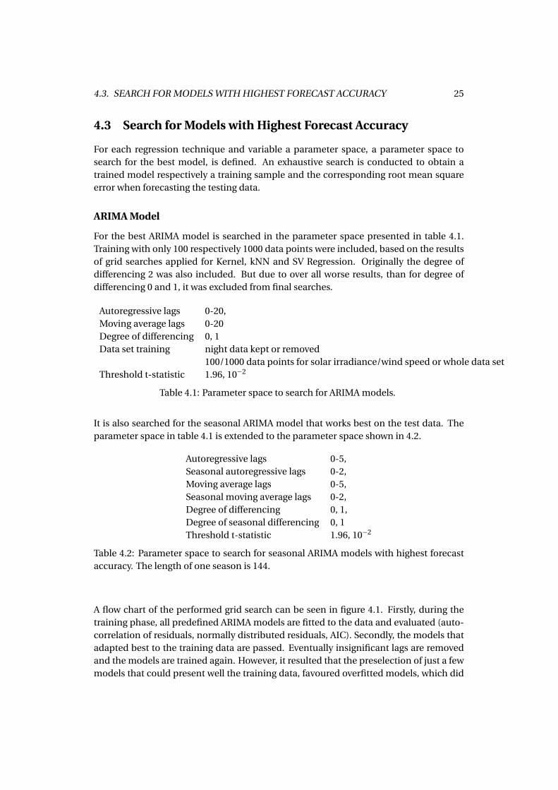
4.3 Search for Models with Highest Forecast Accuracy

For each regression technique and variable a parameter space, a parameter space tosearch for the best model, is defined. An exhaustive search is conducted to obtain atrained model respectively a training sample and the corresponding root mean squareerror when forecasting the testing data.

ARIMA Model

For the best ARIMA model is searched in the parameter space presented in table 4.1.Training with only 100 respectively 1000 data points were included, based on the resultsof grid searches applied for Kernel, kNN and SV Regression. Originally the degree ofdifferencing 2 was also included. But due to over all worse results, than for degree ofdifferencing 0 and 1, it was excluded from final searches.

Autoregressive lags 0-20,Moving average lags 0-20Degree of differencing 0, 1Data set training night data kept or removed

100/1000 data points for solar irradiance/wind speed or whole data setThreshold t-statistic 1.96, 10−2

Table 4.1: Parameter space to search for ARIMA models.

It is also searched for the seasonal ARIMA model that works best on the test data. Theparameter space in table 4.1 is extended to the parameter space shown in 4.2.

Autoregressive lags 0-5,Seasonal autoregressive lags 0-2,Moving average lags 0-5,Seasonal moving average lags 0-2,Degree of differencing 0, 1,Degree of seasonal differencing 0, 1Threshold t-statistic 1.96, 10−2

Table 4.2: Parameter space to search for seasonal ARIMA models with highest forecastaccuracy. The length of one season is 144.

A flow chart of the performed grid search can be seen in figure 4.1. Firstly, during thetraining phase, all predefined ARIMA models are fitted to the data and evaluated (auto-correlation of residuals, normally distributed residuals, AIC). Secondly, the models thatadapted best to the training data are passed. Eventually insignificant lags are removedand the models are trained again. However, it resulted that the preselection of just a fewmodels that could present well the training data, favoured overfitted models, which did


not perform well for forecasting the test data. For this reason, preselection were skipped.During the following testing phase, forecasts of the test data are performed, and the re-sults are saved to use them for model selection.

Kernel and k Nearest Neighbors Regression

For the best combination of parameters for Kernel and k Nearest Neighbors Regressionis searched in the parameter space shown in table 4.3 respectively 4.4. In figure 4.2 a

k 1-20,Autoregressive lags 1-20,Number of feature vectors 50, 100, 500, 1000, 2000, whole data set,Weights uniform, distance.

Table 4.3: Parameter space for k Nearest Neighbors Regression.

ε 0.01, 0.05, 0.1, 0.5k 1-3,Autoregressive lags 1-20,Number of feature vectors 50, 100, 500, 1000, 2000, whole data set,Weights uniform, distance.

Table 4.4: Parameter space for Kernel Regression. The threshold for the distance ε ismultiplicated with 13.4 (maximal value in training data) for wind speed.

flowchart of the performed grid searches is shown. The training phase can be omitted,since no model needs to be trained.


The parameter space used for the search for the Support Vector Regression model thatachieves the best forecast, can be seen in table 4.5. The chosen values for ε depend onthe chosen variable, since ε functions on a threshold when to accept errors of the model(see section 3.2) and should, therefore, depend on the range of values of the consideredtime series. For the grid search for the best combination of SVR, some combinations areomitted to decrease running time.

The flowchart in figure 4.3 visualizes the performed grid search. In the training phase,all models are trained. In the test phase, the models are used to predict the test data.

4.3. SEARCH FOR MODELS WITH HIGHEST FORECAST ACCURACY 27

subclass ofARIMA models,

variable of models

Get all models ofsubclass fittedto given data.

Preselection of modelswith smallest rmse.

Parameters

significant?

Leave out insignif-icant parameters.

Fit models to data.

Forecast at eachstep of test data

Average rootmean square error

Bestmodel

DataTraining

Data Test

results

no

yes

Training

Test

Figure 4.1: Flow chart of grid search for ARIMA models.


parameterspace, variable

Extract featurematrix X and re-sponse variable y

from data training.



Bestmodel.

DataTraining

Extract feature matrixX and response vari-able y from data test.

Data Test

resultsTraining

Test

Figure 4.2: Flow chart of grid search for k Nearest Neighbors and Kernel Regression.

Autoregressive lags 1, 3, 5, 7, 9, 11, 13, 15, 17, 19Number of feature vectors 100, 1000, whole data set,ε 0.001, 0.01, 0.1, 0.3C 1, 5, 10Kernel function linear, radial basis, sigmoid.

Table 4.5: Parameter space for grid search for SVR using the transmittivity (maximum= 1). For solar irradiance, the values for ε are multiplicated with 1300 (approximatesthe solar constant). For wind speed, the values for ε are multiplicated with 13.4 (themaximum wind speed in the training data).

4.4 Performance Evaluation

Root Mean Square Error for Multiple Steps Forecasts

To evaluate the performance of a chosen model, the residuals of a forecast performed bythe model are used. The residuals e are defined as the difference between the predictedvalues y and the measured values y ,

ek = yk − yk , (4.1)

4.4. PERFORMANCE EVALUATION 29

parameterspace, variable

Extract featurematrix X and re-sponse variable y

from data training.

Train model.



Bestmodel

DataTraining

Extract feature matrixX and response vari-able y from data test.

Data Test

resultsTraining

Test

Figure 4.3: Flow chart of grid search for Support Vector Regression.

where k refers to the time instant. An often used measure for the distance between themeasured and predicted time series is the root mean square error,

RMSE =√√√√ 1

N

N∑k=1

(yk − yk

). (4.2)

The symbol N refers in general to the number of samples of a time series. Here, N refersto the number of residuals.

Typically a time series with N À Nmin, where Nmin is the number of historical data pointsneeded to predict future values, is used to evaluate performance. This means, that morethan one multiple step forecast is done (see, e.g., figure 4.4) and each data point yk ispredicted more than once. Therefore, various residuals ek|k−1, . . . ,ek|k−p are obtained,where the first index indicates the time instant of the predictions, the second index isused to define the last known historic value and p refers to the prediction horizon. As a


consequence, it isn’t straight forward to apply the root mean square error (see equation(4.2)) to the result of multiple step forecasts. Three different adapted formulas are shownin the following.

Let n f be the number of forecast that can be done for the given time series, f the indexof the forecast, and j the steps ahead the last known value. The first approach is tocalculate the RMSE of each forecast separately and to take the mean of them,

RMSE1 = 1

N f

N f∑f =1

√√√√ 1

p

p∑j=1

e2j+Nmin+ f |Nmin+ f︸︷︷︸

RMSE of forecast f .

. (4.3)

With the second formula, the mean of the RMSE for all predictions at the same predic-tion horizon is calculated,

RMSE2 = 1

p

p∑j=1

√√√√ 1

N f

N f∑f =1

e2j+Nmin+ f |Nmin+ f︸︷︷︸

RMSE at prediction horizon j

. (4.4)

To avoid taking the mean before calculating the square root, the RMSE over all the pre-dictions can be used,

RMSE3 = 1

p · N f

√√√√ p∑j=1

N f∑f =1

e2j+Nmin+ f |Nmin+ f . (4.5)

Root Mean Square Error for Predictions of Solar Irradiance

In case of predicting the solar irradiance, the matter gets slightly more complicated. Incontrast to wind speed, it is already known that the solar irradiance during night is zero.Therefore, it is of interest to predict only part of the time series. Hence, it would notmake sense to evaluate the model based partly on predictions the model is not used for.

For one step predictions, the procedure to omit data is straight forward. For multiplestep forecasts, on the other hand, it is to decide how to deal with forecasts includingdaylight and night data. One option is to exclude each multiple step forecast that is notpurely about daylight data. See, e.g., figure 4.4, forecast (b)-(d) would be included inthe evaluation of the model. Another option is to include each multiple step forecastthat includes at least one prediction during daylight (compare forecast (a) and (d) infigure 4.4). In this work the second option is used to avoid putting more emphasis onmidday, than on the morning and evening of the day, for the model selection. Therefore

4.4. PERFORMANCE EVALUATION 31

0 20 40 60 80 100 120 140 160 180 200 220 2400

200

400

600

800

time instant k

sola

rir

rad

ian

ce

measured values(a) predicted values(b) predicted values(c) predicted values(d) predicted values(e) predicted values

Figure 4.4: Five forecasts (a)-(e), with prediction horizon 20, of solar irradiance, withsample time = 10 min, beginning at different time steps. It is used an ARIMA(20,0,1)model, fitted to solar irradiance data without night data. Forecast (a) includes the calcu-lated Sunrise (considered daylight), likewise forecast (e) includes the calculated Sunset(considered daylight). Forecast (b),(c) and (d) include only predictions of daylight data.

all predictions for solar irradiance during night are automatically set to zero,

yk

output of model if ss ≤ k ≤ sr,

0 if k ≤ sr, k ≥ ss.(4.6)

The Sunset is indicated by the time instant ss, likewise the Sunrise by sr. It is alwaysreferred to the Sunset and Sunrise at the same day as the time instant k.

Applying the first proposed RMSE to the forecasts of solar irradiance, as explained abovein 4.3, results in

RMSE1 =√

1

p

(ess|ss−p +

√e2

ss+1|ss−p+1 +e2ss|ss−p+1 +·· ·+

√√√√ p∑j=1

e2ss−1+ j |ss−1

+ 1

n f ,d ay

n f ,d ay∑f =1

√√√√ p∑j=1

e2ss+ f + j |ss+ f +

√√√√p−1∑j=1

e2sr− j |sr−p+1 + . . .

+√

e2sr−1|sr−2 +e2

sr|sr−2 +esr|sr−1

).


As one can see, the residuals have different influences on the error measurement, as of,e.g., the first predicted daylight data point yss|ss−p . The other two presented variantsof the RMSE (see equation (4.7), (4.5)) for multiple step forecasts are not effected byomitting night data. Since it is also of interest to get information about the forecastaccuracy depending on the prediction step, RMSE2 is used respectively the particularerrors for each prediction step,

RMSE( j ) =√√√√ 1

N f

N f∑f =1

e2j+Nmin+ f |Nmin+ f , j = 1, .., p (4.7)

Comparison of Performance of Different Models

The quality of the forecast obtained by different models is evaluated by comparing theRMSE2 to a naive forecast. Using a naive model means to assume, that the next valueequals the current one,

yk+1 = yk . (4.8)

For comparison the distance between the naive forecast and the forecast performed bythe chosen model,

d =p∑

j=1RMSE( j )naive −RMSE( j ), (4.9)

is used. In the following chapter, the model with the highest distance d is considered thebest model.

4.5 Summary

All regression techniques are implemented using external libraries. Due to practical is-sues with Kernel Regression, the implemented technique is slightly modified, using kNearest Neighbour Regression as back up.

The data used here, provides wind speed and solar irradiance data. The transmissiv-ity is calculated from the given data of solar irradiance and the estimated data for theextraterrestrial irradiance, using a solar position algorithm.

A grid search for each technique is performed to chose the model that achieves the mostaccurate forecasts. Performance of the forecasts provided by each of the models is eval-uated comparing the resulting root mean square error to a naive forecast.

In the next chapter, the chosen models are presented. The performance of the chosenmodels is evaluated and analysed.

Chapter 5

Results and Analysis

In this chapter, results of the grid search (see Section 4.3) are presented. Multiple stepforecasts are performed with chosen models and evaluated as explained in Section 4.4.

5.1 Results for Forecasting Solar Irradiance

For each technique and variable, the model that predicts most accurate the test data, incomparison to a naive forecast of transmittivity, is selected (see (4.9)). The naive forecastof transmittivity outperforms the naive forecast using the irradiance directly (see figure5.1), therefore the naive forecast of transmittivity is chosen as reference.

Forecasting Solar Irradiance Using Solar Irradiance as Input

For all the in this work considered techniques, forecasting the solar irradiance, usingthe solar irradiance directly as input, yields worse results than a naive forecast using thetransmittivity. Results are shown in figure 5.2. Therefore, in the following only the resultsfor forecasting solar irradiance using the transmittivity are discussed in detail.

1 2 3 4 5 6 7 8 9 10 11 120

100

200

300

prediction horizon

RM

SEW

/m2 transmittivity

solar irradiance

Figure 5.1: Performance of naive forecast predicting solar irradiance using the solar ir-radiance directly and using the transmittivity.

33

34 CHAPTER 5. RESULTS AND ANALYSIS

1 2 3 4 5 6 7 8 9 1011120

10

20SARIMA

%

1 2 3 4 5 6 7 8 9 1011120

50100150200

naive forecast transmittivity

RM

SE

1 2 3 4 5 6 7 8 9 1011120

10

20ARIMA

1 2 3 4 5 6 7 8 9 1011120

10

20kNN

1 2 3 4 5 6 7 8 9 1011120

10

20SVR

prediction horizon

1 2 3 4 5 6 7 8 9 1011120

10

20Kernel

prediction horizon

%

Figure 5.2: Performance of models forecasting the solar irradiance. For each techniquethe model with lowest RMSE (in comparison to a naive forecast using the transmittivityfor predictions up to 2 h/12 prediction steps) is chosen. The red filled bars indicate thatthe forecast for the corresponding model and prediction step is worse than the naiveforecast. Here, only an ARIMA model achieves just for the first prediction step a slightlyhigher accuracy (0.6%) than the naive forecast.

Forecasting Solar Irradiance Using Transmittivity as Input

In the following, it is distinguished between accuracy achieved for the following predic-tion steps

• 10 - 120 min, 12 prediction steps,• 10 - 30 min, 3 prediction steps,• 100 - 120 min, 3 prediction steps.

For each prediction range, the model is selected that predicts most accurate the consid-ered prediction steps. The selected models are described in table 5.1. The performanceof the particular models is visualized in figure 5.3, 5.4(a) and 5.4(b). Most importantly,the results show that Support Vector Regression, independently of the considered pre-diction range, achieves better results when forecasting the test data than the other con-sidered techniques. For prediction step 12 (120 min ahead), the improvement is 20,90%in comparison to a naive forecast. However, for predictions 10 min ahead, the improve-ment is only 2,35%.

tech

niq

ue

dat

atr

ain

ing

mo

del

spec

ifica

tio

ns

dis

tan

ceto

nai

vefo

reca

st

pre

dic

tio

nst

eps

1-

12R

MSE

1st

epR

MSE

12st

eps

Nai

ve85

.56

198.

72A

RIM

AW

ND

,th

ree

mo

nth

sA

R=

0,M

A=

10,d

=1

84.0

916

4.16

211.

75SA

RIM

Ath

ree

mo

nth

sA

R=

3,SA

R=

2,M

A=

0,SM

A=

0,d

=0,

D=

083

.55

193.

8459

.41

kNN

WN

D,1

00A

R=

2,k

=11

,wei

ght=

dis

tan

ce93

.97

163.

4719

2.98

Ker

nel

WN

D,1

00A

R=

2,ε

=0.

1,w

eigh

t=d

ista

nce

94.3

616

5.28

185.

32SV

R10

0A

R=

7,ε

=0.

1,ra

dia

lbas

iske

rnel

,C=

1083

.93

157.

1824

9.12

pre

dic

tio

nst

eps

1-

3R

MSE

1st

epR

MSE

3st

eps

Nai

ve85

.56

127.

31A

RIM

AW

ND

,th

ree

mo

nth

sA

R=

4,M

A=

4,d

=0,

t-st

atis

tic≥

1.96

82.8

811

9.78

15.7

3SA

RIM

Ath

ree

mo

nth

sA

R=

3,SA

R=

2,M

A=

0,SM

A=

0,d

=0,

D=

083

.55

122.

2811

.13

kNN

2000

AR

=3,

k=

20,w

eigh

t=u

ni

84.2

911

9.05

14.7

4K

ern

elth

ree

mo

nth

sA

R=

3,ε

=0.

1,w

eigh

t=u

ni

84.3

211

9.94

13.9

8SV

R10

0A

R=

7,ε

=0.

1,ra

dia

lbas

iske

rnel

,C=

583

.55

118.

5316

.89

pre

dic

tio

nst

eps

10-

12R

MSE

10st

eps

RM

SE12

step

sN

aive

187.

2819

8.72

AR

IMA

WN

D,1

00A

R=

17,M

A=

0,d

=1

157.

0916

2.11

97.9

8SA

RIM

Ath

ree

mo

nth

sA

R=

2,SA

R=

2,M

A=

4,SM

A=

2,d

=1,

D=

018

1.14

193.

0317

.30

kNN

WN

D,1

00A

R=

2,k

=11

,wei

ght=

dis

tan

ce15

7.86

163.

4796

.88

Ker

nel

WN

D,1

00A

R=

2,ε

=0.

1,w

eigh

t=d

ista

nce

159.

9316

5.28

91.5

3SV

R10

0A

R=

7,ε

=0.

1,ra

dia

lbas

iske

rnel

,C=

1015

2.75

157.

1811

3.4

Tab

le5.

1:M

od

els

that

pre

dic

tm

ost

accu

rate

the

sola

rir

rad

ian

cete

std

ata

usi

ng

the

tran

smit

tivi

ty.

Mo

del

sar

ech

ose

nb

ased

on

the

dis

tan

ceb

etw

een

the

mo

del

’ser

ror

and

the

nai

vem

od

el’s

erro

rfo

reca

stin

gth

ete

std

ata.

Th

eab

bre

viat

ion

WN

Dst

and

sfo

rtr

ain

ing

wit

ho

utn

igh

tdat

a.


Independently of the technique, one can see, that there is only small improvement forpredictions up to 30 min ahead in comparison to a naive forecast. Significantly betterresults are achieved for higher prediction horizons.

Another interesting results is, that often the models that predict most accurate the data,were trained with only 100 data points (see table 5.1). 100 data points include less than17 h of data. Other models were trained with data covering three months. Since the100 data points used for training, are the most recent data points, this result indicatesthat using less, but recent data, may yield to better results than using a large data set fortraining.

While the Kolmogorv-Smirnov test for all selected ARIMA models is not passed (noteven at a 1% significance level), the ARIMA model chosen for forecasts from 10-120 minachieves a p-value for the Ljung-Box Test of 19.05%. However, the chosen ARIMA mod-els for the first and last prediction steps do not achieve p-Values for the Ljung-Box Test ofless than 5%.

5.2 Results for Forecasting Wind Speed

In contrast to solar irradiance forecasting, the improvement of wind speed forecastingusing ARIMA Models, k Nearest Neighbour, Kernel or Support Vector Regression, in com-parison to a naive forecast, is small. Results are visualized in figure 5.5, 5.6(a) and 5.6(b).Selected models are shown in table 5.2. As can be recognized considering all results,the different used regression techniques yield to similar forecasting accuracy. No tech-nique obviously achieves best results for forecasting the wind speed test data. While asimple ARIMA model achieves best results for predictions up to 30 min, best results forpredictions from 100 min to 120 min are obtained by Kernel Regression using the 5 lasttime steps. For predictions from 10 min up to 120 min, linear Support Vector Regressionforecasts the data most accurate.

Improvement of accuracy relative to a naive forecast might be low in contrast to fore-casting solar irradiance, because no additional information than historical data of windspeed itself is provided. Relatively good results for forecasting solar irradiance are pro-vided if the transmittivity is used1. However, results for predictions 2 h ahead can beimproved by 7.3%.

In contrast to the results of forecasting solar irradiance, here in each case, models trainedusing a t-statistic threshold of 1.96 perform best. Anyway, neither the p-value for theLjung-Box Testnor for the Kolomogrov-Smirnov Test is significantly different from zero.

1The transmittivity already includes location and time specific information about the solar irradiance.

5.2. RESULTS FOR FORECASTING WIND SPEED 37

1 2 3 4 5 6 7 8 9 10 11 1205

101520

ARIMA

imp

rove

men

t%

1 2 3 4 5 6 7 8 9 10 11 120

50100150200

naive forecast

RM

SE

1 2 3 4 5 6 7 8 9 10 11 1205

101520

SARIMA

imp

rove

men

t%

105

101520

Kernel

imp

rove

men

t%

105

101520

KNN

imp

rove

men

t%

1 2 3 4 5 6 7 8 9 10 11 1205

101520

SVR

prediction horizon

imp

rove

men

t%

Figure 5.3: Performance of models forecasting the solar irradiance test data. For eachtechnique the model with lowest RMSE (in comparison to a naive forecast using trans-mittivity for predictions up to 2 h/12 prediction steps) is chosen. The red filled bars in-dicate that the forecast for the corresponding model and prediction step is worse thanthe naive forecast. Here, SVR performs best, followed by ARIMA and Kernel.


1 2 30

2

4

6 ARIMA

%

1 2 30

50100150200

naive forecast

RM

SE

1 2 30

2

4

6 SARIMA

%

1 2 30

2

4

6 kNN

%

1 2 30

2

4

6 Kernel

%

1 2 30

2

4

6 SVR

prediction horizon

%

(a) Prediction step 1-3.

10 11 1205

1015

ARIMA

10 11 120

50100150200

naive forecast

10 11 1205

1015

SARIMA

10 11 1205

1015

kNN

10 11 1205

1015

Kernel

10 11 1205

1015

SVR

prediction horizon

(b) Prediction step 10-12.

Figure 5.4: Performance of models forecasting the solar irradiance test data using thetransmittivity. For each technique the model with lowest RMSE (in comparison to anaive forecast) when forecasting the first free prediction steps / first 30 min (a) respec-tively the last three prediction steps / 100 - 120 min (b) is chosen. The red filled barsindicate that the forecast for the corresponding model and prediction step is worse thanthe naive forecast. Here, ARIMA performs best for predictions of the first three steps,followed by SVR. For forecasts of prediction step 10, 11, 12, Kernel Regression performsbest, followed by SVR.

5.3. SUMMARY 39

5.3 Summary

The regression techniques, yielding relatively accurate forecasts, are ARIMA models,Kernel Regression and Support Vector Regression. Overall, Support Vector Regressionoutperforms the other techniques. In case of forecasting wind speed, the improvementover the naive forecast is between 0-8%. For forecasts of solar irradiance, improvementis roughly in the range from 0 to 20%.

tech

niq

ue

nu

mb

ero

fdat

ap

oin

tstr

ain

ing

mo

del

spec

ifica

tio

ns

dis

tan

ceto

nai

vefo

reca

stp

red

icti

on

step

s1

-12

RM

SE1

step

RM

SE12

step

sN

aive

0.46

1.10

AR

IMA

1000

AR

=6,

MA

=6,

d=

0,t-

stat

isti

c≥

1.96

0.45

1.04

0.49

SAR

IMA

thre

em

on

ths

AR

=1,

SAR

=0,

MA

=1,

SMA

=0,

d=

1,D

=0

0.46

1.08

0.19

KN

Nth

ree

mo

nth

sA

R=

7,k

=18

,wei

ght=

un

i0.

481.

050.

39K

ern

el10

0A

R=

2,ε

=1.

34,w

eigh

t=d

ista

nce

0.50

1.02

0.50

SVR

1000

AR

=7,ε

=0.

134,

lin

ear

kern

el,C

=1

0.46

1.03

0.53

pre

dic

tio

nst

eps

1-

3R

MSE

1st

epR

MSE

3st

eps

Nai

ve0.

460.

72A

RIM

A10

00A

R=

6,M

A=

6,d

=0,

t-st

atis

tic≥

1.96

0.45

0.69

0.07

0SA

RIM

Ath

ree

mo

nth

sA

R=

1,SA

R=

0,M

A=

1,SM

A=

0,d

=1,

D=

00.

460.

710.

025

KN

Nth

ree

mo

nth

sA

R=

6,k

=20

,wei

ght=

un

i0.

480.

690.

027

Ker

nel

thre

em

on

ths

AR

=6,ε

=0.

67,w

eigh

t=u

ni

0.47

0.70

0.02

4SV

R10

00A

R=

7,ε

=0.

134,

lin

ear

kern

el,C

=1

0.45

0.69

0.06

8

pre

dic

tio

nst

eps

10-

12R

MSE

10st

eps

RM

SE12

step

sN

aive

1.03

1.10

AR

IMA

1000

AR

=6,

MA

=6,

d=

0,t-

stat

isti

c≥

1.96

0.98

1.04

0.16

SAR

IMA

thre

em

on

ths

AR

=1,

SAR

=0,

MA

=1,

SMA

=0,

d=

1,D

=0

1.01

1.08

0.05

KN

Nth

ree

mo

nth

sA

R=

7,k

=17

,wei

ght=

un

i0.

981.

050.

14K

ern

elth

ree

mo

nth

sA

R=

6,ε

=1.

34,w

eigh

t=u

ni

0.96

1.02

0.21

SVR

thre

em

on

ths

AR

=3,ε

=0.

134,

rad

ialb

asis

kern

el,C

=10

0.96

1.03

0.20

Tab

le5.

2:M

od

els

that

pre

dic

tmo

stac

cura

teth

ew

ind

spee

dte

std

ata.

Mo

del

sar

ech

ose

nb

ased

on

the

dis

tan

ceb

etw

een

the

mo

del

’ser

ror

and

the

nai

vem

od

el’s

erro

rfo

reca

stin

gth

ete

std

ata.

5.3. SUMMARY 41

1 2 3 4 5 6 7 8 9 10 11 120

2

4

6 ARIMA

imp

rove

men

t%

1 2 3 4 5 6 7 8 9 10 11 120

0.5

1 naive forecast

RM

SE

1 2 3 4 5 6 7 8 9 10 11 120

2

4

6 SARIMA

imp

rove

men

t%

10

2

4

6 kNN

imp

rove

men

t%

10

2

4

6 Kernel

imp

rove

men

t%

1 2 3 4 5 6 7 8 9 10 11 120

2

4

6 SVR

prediction horizon

imp

rove

men

t%

Figure 5.5: Performance of models forecasting the wind speed test data. For each tech-nique the model with lowest RMSE (in comparison to a naive forecast for predictions upto 2 h/12 prediction steps) is chosen. The red filled bars indicate that the forecast for thecorresponding model and prediction step is worse than the naive forecast. Here, SVRperforms best, followed by Kernel and ARIMA.


1 2 30

2

4 ARIMA

%

1 2 30

0.5

1

naive forecast

RM

SE

1 2 30

2

4SARIMA

%

10

2

4 kNN

%

10

2

4 Kernel

%

1 2 30

2

4SVR

prediction horizon

%

(a) Prediction step 1-3.

10 11 120

2

4

6 ARIMA

10 11 120

0.5

1

naive forecast

10 11 120

2

4

6 SARIMA

10 11 120

2

4

6 kNN

10 11 120

2

4

6 Kernel

10 11 120

2

4

6 SVR

prediction horizon

(b) Prediction step 10-12.

Figure 5.6: Performance of models forecasting the wind speed test data. For each tech-nique the model with lowest RMSE (in comparison to a naive forecast) when forecastingthe first free prediction steps / first 30 min (a) respectively the last three prediction steps/ 100 - 120 min (b) is chosen. The red filled bars indicate that the forecast for the cor-responding model and prediction step is worse than the naive forecast. Here, ARIMAperforms best for predictions of the first three steps, followed by SVR. For forecasts ofprediction step 10, 11, 12, Kernel Regression performs best, followed by SVR.

Chapter 6

Case Study

Building on a previous performed case study for the operation of a microgrid, using windpower as renewable infeed and ARIMA models to perform the forecasts, [Hans et al.,2015], for the present work, an additional case study, using solar power as renewableinfeed and Support Vector Regression to perform the forecasts for solar irradiance, isaccomplished. Seven days in July are chosen, conform to the data used in the formersections to evaluate the performance of the regression techniques. For Support VectorRegression, the parameters that yield the most accurate forecasts on test data for 10 minto 2 h are used (see table 5.1). For the load forecast, an ARIMA model, provided by [Hanset al., 2015], is applied. The sampling time is set, as before, to 10 min.

The modelled microgrid includes a conventional generator, solar panels to provide re-newable power infeed and a storage device. Its basic structure is shown in figure 6.1.

Conventionalgenerator

Solarpanels

Storage

Load

wR (k) x(k)

wL(k)

uT (k),δT (k) uS (k),δS (k)uR (k),δR (k)

p1(k) p2(k) p3(k)

Figure 6.1: Exemplary microgrid, [based on a version by C. Hans.]. The set points areindicated by the symbol u, δ includes the information if the corresponding element ofthe grid is connected or not (0 or 1), p stands for the power, w for disturbances (load andsolar power are considered disturbances) and x is the stored energy.

The general structure of the operation of the microgrid is shown in figure 6.2. StochasticModel Predictive Control is applied, [Hans et al., 2015]. Therefore, a scenario fan, i.e.,several different forecasts for the same time steps, based on the forecasts provided bySupport Vector Regression, is created (see section 3.4). An example of a scenario fan,

43

44 CHAPTER 6. CASE STUDY

created with Support Vector Regression, is shown in figure 6.3. It is aimed to provide thedemanded power, while minimizing the generator costs (thermal energy and thermalswitching), [Hans et al., 2015].

SMPC operationoptimizer

Microgrid

Disturbancewk

Scenarioreduction

Forecast

Past datawl , l ≤ k

Input

uk , δk

Measurement

xk ,δk−1

Forecastscenarios

wk+ j |k

Scenariotree

wk+ j |k , pk+ j |k

Figure 6.2: Block diagram for a stochastic model predictive control approach, [Hanset al., 2015].

To evaluate the performance, the results are compared with a case study performed un-der the ideal, not realistic conditions that a perfect forecast is performed. The results ofthe case study are presented in table 6.1. The simulated values are plotted in figure 6.4.The results show that the gap to the reference with perfect forecasts is small. Even lessthermal switching is done. However, in case of perfect knowledge about future values ofsolar irradiance and load, the energy infeed of renewable energy is increased, while thethermal energy decreases.

0 10 20 30 40 50 60 700

200

400

600

800

time step k, 10 min

sola

rir

rad

ian

ceW

/m2

Figure 6.3: Scenario fan (—) for a forecast of solar irradiance on 01 July 2010. SupportVector Regression is used to perform the forecast (—). The 95% prediction interval (—)is estimated based on the scenario fan.

45

0 100 200 300 400 500 600 700 800 9000

0.5

1

Time k

Th

erm

alP

ower

[pu

h]

0 100 200 300 400 500 600 700 800 9000

2

4

6

Time k

Sto

red

En

ergy

[pu

h]

0 100 200 300 400 500 600 700 800 900−1

−0.5

0

0.5

1

Time k

Sto

rage

Pow

er[p

uh

]

0 100 200 300 400 500 600 700 800 9000

0.5

1

1.5

2

Time k

Ren

ewab

lePo

wer

[pu

h]

0 100 200 300 400 500 600 700 800 900−0.8

−0.6

−0.4

−0.2

0

Time k

Load

Pow

er[p

uh

]

Figure 6.4: Thermal, storage, renewable and stored energy and load from the case study(—) in comparison to an ideal case study (—) with perfect forecasts.

46 CHAPTER 6. CASE STUDY

SMPC Perfect ForecastSolar energy infeed in puh 56.61 57.81Thermal energy infeed in puh 39.09 37.81Thermal switching 26 28

Table 6.1: Results of the simulation of the operation of a microgrid using Support Vec-tor Regression in comparison to the results of a case study where the future values areknown.

Chapter 7

Conclusion

Based on the results presented in chapter 5, Support Vector Regression yields, of all con-sidered regression techniques, to most accurate forecasts. For solar irradiance forecast-ing, SVR outporformes for all considered prediction ranges (10-120 min, 10-30 min, 100-120 min) the other here considered techniques. Although, this is not the case for thewind speed forecasting, SVR here also achieves most accurate results considering pre-dictions from 10 min up to 2 h.

Another interesting conclusion that can be drawn from the results, is that using recentdata yields better forecast quality than using a large data set including the same recentdata, but additionally less recent data. This indicates, that it might be a mistaken ap-proach to train one model for forecasts of solar irradiance respectively wind speed ingeneral. Preferably, during the operation of the microgrid, recently observed data canbe used to search for and train a new model frequently.

For very short term prediction (up to 10 min), a naive forecast already performs well.Little improvement is achieved by applying other techniques. For this reason, for ap-plications using only very short term predictions, it might be sufficient to use a naiveforecast, instead of training a more complex model. For predictions with larger hori-zons, however, applying more complex techniques leads to significant improvement.

The poor performance of SARIMA models, in comparison to all other considered tech-niques including ARIMA models, leads to the conclusion that using seasonality cannotimprove forecasts for solar irradiance nor wind speed. Anyway, here it might be helpfulto consider first a larger parameter space to search for most accurate SARIMA models,to come to a definite conclusion. In the present work the last fifty minutes of the currentday and the two days before are included.

However, since the result may largely depend on the chosen data and season, resultsshould be validated first using different data sets, measured at different locations and

47

48 CHAPTER 7. CONCLUSION

tested on data throughout the whole year.

To extend the considered regression techniques, it might be interesting to include Arti-ficial Neural Networks. It could be also of interest to consider hybrid models. A studyperformed on wind speed forecasting achieves better results for a Hybrid model of anARIMA model and an Artificial Neural Network, than for both of these techniques usedalone, [Cadenas and Rivera, 2010].

In the case of forecasting solar irradiance using the transmissivity, instead of the solar ir-radiance directly, significantly improves the accuracy. This raises the question if the useof other additional variables than solar irradiance respectively wind speed forecastingcould improve the forecast accuracy in a similar way. For the forecast of solar irradiance,it could be considered including cloud cover, since other studies are able to improveresults by using it, e.g., [Qiao and Zeng, 2012].

Additionally, estimation of a probability distribution of the forecast could be probablyimproved. Here, it is to analyse how the quality of the probability estimation affects thecontrol of the microgrid.

Bibliography

Altman. An intoduction to kernel and nearest-neighbor nonparametric regression. TheAmerican Statistican, 1992.

Peder Bacher, Henrik Madsen, and Henrik Aalborg Nielsen. Online short-term solarpower forecasting. Elsevier, 2009.

Gianluca Bontempi, Souhaib Ben Taieb, and Yann-Ael Le Borgne. Lecture Notes inBusiness Information Processing, chapter Machine Learning Strategies for Time SeriesForecasting. Springer, 2013.

George E. P. Box, Gwilym M. Jenkins, and Gregory C. Reinsel. Time Series Analysis - Fore-casting and Control. Prentice- Hall, Inc., 1994.

Erasmo Cadenas and Wilfrido Rivera. Wind speed forecasting in the south coast of oax-aca, mexico. Renewable Energy, Elsevier, 2006.

Erasmo Cadenas and Wilfrido Rivera. Wind speed forecasting in three different regionsof mexico, using a hybrid arima-ann model. Renewable Energy, Elsevier, 2010.

George Casella and Roger L. Berger. Statistical Inference. Duxbury, 2001.

Chih-Chung Chang and Chih-Jen Lin. LIBSVM: A library for support vector machines.ACM Transactions on Intelligent Systems and Technology, 2:27:1–27:27, 2011. Softwareavailable at http://www.csie.ntu.edu.tw/~cjlin/libsvm.

Chris Chatfield. Principles of Forecasting, chapter Prediction Intervals for Time-SeriesForecasting, pages 475–499. Springer, 2001.

Walter Enders. Applied Econometric Time Series. John Wiley & Sons, 1994.

J. H. Friedmann. The role of statistics in the data revolution? International StatisticalReview/Revue Internationale de Statistique, 5-10, 2001.

Lazlo Gyoerfi, Michael Kohler, Adam Krzyzak, and Harro Walk. A Distribution Free The-ory of Nonparametric Regression. Springer, 2002.

49

http://www.csie.ntu.edu.tw/~cjlin/libsvm

50 BIBLIOGRAPHY

C. A. Hans, P. Sopasakis, A. Bemporad, J. Raisch, and C. Reincke-Collon. Scenario-basedmodel predictive operation control of islanded microgrid. 2015 54th IEEE Conferenceon Decision and Control (CDC), 2015.

Detlev Heinemann, Elke Lorenz, and Marco Grirodo. Solar irradiance forecasting for themanagement of solar energy systems. University Oldenburg, 2006.

Rob J Hyndman and George Athanasopoulos. Forecasting: principles and practice.OTexts, 2014.

IS/ISO-9488. Solar energy - vocabulary. Technical report, Bureau of Indian Standads -Non-conventional Energy Sources Sectional Committee, 1999.

J.G. Kalbfleisch. Probability and Statistical Inference. Springer Verlag, 1979.

Greg Kopp and Judith L. Lean. A new, lower value of total solar irradiance: Evidence andclimate significance. Geophysical Research Letters, 2011.

Sricharan Kumar and Ashok Srivastava. Bootstrap prediction intervals in non-parametric regression with applications to anomaly detection. NASA, 2012.

Lon-Mu Liu and Gregory B. Hudak. Forecasting and Time Forecast Analysis using the SCAStatistic. Scientific Computing Associates, 1992.

Frank J. Massey. The kolmogrov-smirnov test for goodness of fit. American StatisticalAssociation Journal, 1951.

Adel Mellit and Alessandro Massi Pavan. A 24-h forecast of solar irradiance using arti-ficial neural network: Application for performance prediction of a grid-connected pvplant at trieste, italy. Solar Energy, 84(5):807–821, 2010.

Mohammad Monfared, Hasan Rastegar a, and Hossein Madadi Kojabadi. A new strat-egy for wind speed forecasting using artificial intelligent methods. Renewable Energy,Elsevier, 2009.

Wei Qiao and Jianwu Zeng. Short-term solar power prediction using a support vectormachine. EElsevier- Renewable Energy, 2012.

Volker Quaschning. Technical and economical system comparison of photovoltaic andconcentrating solar thermal power systems depending on annual global irradiation.Elsevier, 2004.

Ibrahim Reda and Afshin Andreas. Solar position algorithm for solar radiation applica-tions. Technical report, National Renewable Energy Laboratory, 2008.

K. Scharmer and J. Greif. The European Solar Radiation Atlas. Le Presses de l’Ecole deMines, 2000.

BIBLIOGRAPHY 51

A. Sfetos. A novel approach for the forecasting of mean hourly wind speed time series.Renewable Energy, Elsevier, 2001.

Alex J. Smola and Bernhard Schölkopf. A tutorial on support vector regression. Statisticsand Computing, 2004.

Arbeitsgruppe Erneuerbare Energien Statistik. Zeitreihen zur Entwicklung der erneuer-baren Energien in Deutschland. Bundesministerium für Wirtschaft und Energie, 2016.

W. B. Stine and R. W. Harrigan. Solar Energy Systems Design. John Wiley and Sons, Inc.,1986.

Larry Wasserman. All of Statistics - A Concise Course in Statistical Inference. Springer,2005.

Felix Werdermann. Wind aus den segeln genommen. Der Freitag, May 2016.

Jeffrey M. Woolridge. Introductory Econometric, chapter The Normal and Related Distri-butions, page 665ff. Cengage Learning, 2015.

Junyi Zhou, Jing Shi, and Gong Li. Fine tuning support vector machines for short-termwind speed forecasting. Energy Conversion and Managemen, Elsevier, 2011.

Time Series Based Forecasting of Renewable Power Infeed ...

Documents

Transcript of Time Series Based Forecasting of Renewable Power Infeed ...