TIME SERIES ANALYSIS OF MOROCCAN STOCKS: Attijariwafa Bank, BMCE Bank ... · Attjariwafa Bank, BMCE...
48
SCHOOL OF SCIENCE & ENGINEERING – AL AKHAWAYN UNIVERSITY SCHOOL OF SCIENCE AND ENGINEERING TIME SERIES ANALYSIS OF MOROCCAN STOCKS: Attijariwafa Bank, BMCE Bank, and La Banque Populaire Capstone design May 2018 Youssef Ourkia Supervised by : Dr. Lahcen Laayouni
Transcript of TIME SERIES ANALYSIS OF MOROCCAN STOCKS: Attijariwafa Bank, BMCE Bank ... · Attjariwafa Bank, BMCE...
SCHOOL OF SCIENCE & ENGINEERING – AL AKHAWAYN UNIVERSITY
SCHOOL OF SCIENCE AND ENGINEERING
TIME SERIES ANALYSIS OF MOROCCAN STOCKS:
Attijariwafa Bank, BMCE Bank, and La Banque Populaire
Capstone design
May 2018
Youssef Ourkia
Supervised by : Dr. Lahcen Laayouni

TIME SERIES ANALYSIS OF MOROCCAN STOCKS
2

TIME SERIES ANALYSIS OF MOROCCAN STOCKS
3
Table of Contents
Abstract ......................................................................................................................................................... 4
Abstract (French) .......................................................................................................................................... 5
Introduction: .................................................................................................................................................. 6
Definitions: ................................................................................................................................................... 7
Methodology: ................................................................................................................................................ 9
Procedure undertaken in the study: ............................................................................................................. 10
Attijariwafa Bank: ................................................................................................................................... 10
Gathering the data: .............................................................................................................................. 10
Importing the data to RStudio: ............................................................................................................ 11
Plotting the time series: ....................................................................................................................... 12
Data smoothing: .................................................................................................................................. 14
Data forecasting: ................................................................................................................................. 17
Data Testing: ....................................................................................................................................... 19
Forecasting using a different ARIMA model: .................................................................................... 20
BMCE: .................................................................................................................................................... 24
Plotting the time series: ....................................................................................................................... 24
Data smoothing: .................................................................................................................................. 26
The seasonal part of the ARIMA model: ............................................................................................ 29
La Banque Populaire: .............................................................................................................................. 34
Plotting the time series: ....................................................................................................................... 34
Smoothing the data: ............................................................................................................................ 36
Building the ARIMA model: non-seasonal parameters ...................................................................... 38
STEEPLE Analysis: .................................................................................................................................... 43
Social Aspect: ......................................................................................................................................... 43
Technological Aspect: ............................................................................................................................ 43
Economic Aspect: ................................................................................................................................... 43
Environmental Aspect: ............................................................................................................................ 44
Political and Legal Aspect: ..................................................................................................................... 44
Ethical Aspect: ........................................................................................................................................ 44
Conclusion: ................................................................................................................................................. 45
References: .................................................................................................................................................. 46

TIME SERIES ANALYSIS OF MOROCCAN STOCKS
4
Abstract
The financial sector in Morocco is still undergoing major development as stock trading
doesn‟t play a significant role in the Moroccan culture compared to other countries, mostly the
United States of America, England, and Japan. However, Morocco is directing a significant
amount of its efforts towards enriching the financial domain as we can see from the recent
projects undertaken mainly the Casablanca Finance City. The CFC project aims to create a
financial hub in Casablanca inspired by Wall Street in New York to encourage people to invest
in stocks and become more accustomed with finance. For the time being, the financial activity in
Morocco comes down to the selling and buying of stocks in the Casablanca Stock Exchange.
This shows that the financial field in Morocco is still growing and has a lot of room of
improvement. The financial decisions in Morocco are based on different news and available
information rather than models and mathematical forecasts. In this project, we will extract the
data for the three biggest banks traded in Casablanca Stock Exchange: Attijariwafa Bank,
Banque Populaire, and BMCE Bank from the website. Based on the information of the year
2017, we will create a time series analysis in the R language to forecast the upcoming values of
the stock prices for the different companies for the month of January 2018. This mathematical
and statistical approach could not be trusted fully in making a decisive financial decision, but it
can greatly help direct our focus to a specific stock. We will therefore, gather different news that
might be related to the companies we are interested in and to the market itself in order to explain
fluctuation in the price of stocks for the year of 2017. The month of January will be used in order
to verify the accuracy of our forecasts.

TIME SERIES ANALYSIS OF MOROCCAN STOCKS
5
Abstract (French)
Le secteur financier marocain est en pleine évolution car la bourse ne joue pas encore un
rôle très significatif dans la culture du Maroc comparé aux autres pays, principalement les Etats-
Unis, l'Angleterre et le Japon. Cependant, le Maroc consacre une grande partie de ses efforts à
l'enrichissement et le développement du domaine financier, comme en témoignent les récents
projets menés principalement le project du Casablanca Finance City. Le projet CFC vise à créer
un centre financier à Casablanca inspiré par Wall Street à New York pour encourager les gens à
investir et à s'habituer à la finance. Pour le moment, l'activité financière au Maroc se résume à la
vente et à l'achat d‟actions à la Bourse de Casablanca. Cela montre que le secteur financier au
Maroc continue de croître et peut encore progresser. Les décisions financières au Maroc sont
plus basées sur différentes informations plutôt que sur des modèles et des prévisions
mathématiques. Dans ce projet, nous allons extraire les données des trois plus grandes banques
cotées à la Bourse de Casablanca: Attijariwafa Bank, Banque Populaire et BMCE Bank. En
utilisant les informations de l'année 2017, nous allons créer une analyse de séries chronologiques
en langage R pour prévoir les prochaines valeurs des cours des actions des différentes sociétés
pour le mois de janvier 2018. Cette approche mathématique ne peut pas être pleinement prise en
compte pour prendre une décision financière décisive, mais elle peut grandement aider à orienter
notre attention vers un stock spécifique. Nous allons donc rassembler différentes nouvelles qui
pourraient être liées aux sociétés qui nous intéressent et au marché lui-même afin d'expliquer la
fluctuation du prix des actions pour l'année 2017. Le mois de janvier sera utilisé afin de vérifier
l'exactitude de nos prévisions.

TIME SERIES ANALYSIS OF MOROCCAN STOCKS
6
Introduction:
In this Study we will use the R language to perform a time series analysis for three
different Moroccan companies listed in the Casablanca stock exchange with the aim of finding a
viable model that could be used to forecast their future values. The choice of the companies was
based on their sector of activity: banking and their capitalization. The three chosen banks are:
Attjariwafa Bank, BMCE Bank, and La Banque Populaire which are the most traded Banks in
the stock exchange the thing that gives us enough data to conduct our study. The modeling
technique that will be used in the study is called ARIMA that stands for Auto-Regressive
Integrated Moving Average and which will be defined further in the paper.

TIME SERIES ANALYSIS OF MOROCCAN STOCKS
7
Definitions:
Finance is a field of study dealing with the management of valuable assets, notably
money. In this field, applied mathematics are used in order to get ahold of the way the market is
behaving and get a slight idea on what will be its movement in the coming years. Two main
technics are used in order to forecast future prices of different financial products. The first one is
the use of stochastic differential equations, notably Thiele‟s differential equation and Black-
Scholes differential equation in determining future prices of different financial product in the
financial market. The second method and the one that we will be using in this project, is the
application of statistics in predicting future prices of different stocks. This technique is based
mainly on the use of time series in the forecasting of the future prices.
Time series are a multitude of data points taken in different points in time spaced by the
same interval. In our case, the data points will be the closing stock prices that are taken daily
during the working days of the Casablanca Stock Exchange, meaning from Monday to Friday.
The plotted time series will give a visual insight on the behavior of the data prices and will
enable us to run different averaging methods, with which we will get the trend of the prices.
Different autoregressive models are already developed to fit different data plots using a
multitude of variables. In this study we will choose the ones that will suit us best.
An autoregressive model is a model that uses previous data collected of a phenomenon –
in our case stock prices of listed Moroccan companies in the Casablanca stock exchange market-
to predict its future behavior. These models have a mathematic correlation between the future
data and the previous recordings.

TIME SERIES ANALYSIS OF MOROCCAN STOCKS
8
The most used model for forecasting based on time series is the ARIMA model which
stands for Auto-Regressive Integrated Moving Average. The ARIMA (p, d, q) model has three
variables: p, d, and q that are to be changed in order to find the best fit of the data at hand. As its
name implies, the variables p, d, and q are respectively the auto regressive variable, the
integration variable, and the moving average variable. Different combinations of variables lead
to different smoothing models, mainly the first-order auto-regressive model which only takes
into consideration one preceding value to get the present value of the data. The more preceding
values the model takes into account, the higher its order and the more accurate it becomes. The
second smoothing model is the random walk that is used mainly for non-stationary series, when
the change from one period to another is arbitrary. The last model within the ARIMA is the
exponential smoothing, which exponentially weights the average of the previous recordings to
forecast future values.
In the second part of the project, we will be using the ARIMA model with seasonality
which adds a seasonal part to the configuration. In addition to the three first parameters which
are p, d, and q, we will have P, D, Q, and m which is called the span of seasonality. The
determination of these parameters can be done using ACF and PACF which stand for
Autocorrelation and Partial Autocorrelation respectively. These two plots can be used to guide us
determine what parameters should be used based on the behavior of the lags. Using this method
will not be deterministic on what parameters should be chosen for the seasonal ARIMA model. It
can only guide our choices of parameters. For this project, we will choose a multitude of models
with different parameters and compare between them using two information criterions.
The two information criterions used are the AIC and BIC which stand for the Akaike and
Bayesian information criterions. They are both used to evaluate the effectiveness of models by

TIME SERIES ANALYSIS OF MOROCCAN STOCKS
9
assigning values to the models and the lower the value the better the model fits the data. We
could have used the Akaike information criterion alone but it is better to use the Bayesian in case
the data set is large because it takes into account the number of points in the data set.
Methodology:
The goal of this capstone project is to find the model that will have the best fit to the
stock prices of different companies using time series. The steps undertaken in this study with the
methodologies used is as follows:
We started by gathering the data of the different Moroccan banks chosen to be a part of
the study, starting by Attijariwafa Bank then BMCE, and at last La Banque Populaire. In order to
fulfill this step, we went to the Casablanca Stock Exchange website where we got the stock
prices for the year 2017 on which we will base our study.
The methodology used to forecast the stock prices for January 2017 is based on a
standardized set of models called ARIMA. ARIMA stands for Auto Regressive Integrated
Moving average which represents a combination of two methods of modeling which are: Auto
Regression and Differencing. In this study we will use the full ARIMA model which has two
parts: the seasonal and the non-seasonal. This technique turned out to be very effective in
different sectors and mainly in forecasting stock prices according to a study that has been done
constructed around Indian stocks [4]. The study was based on the two-years data collected for
fifty-six companies listed in the stock exchange market with the biggest volume in India: The
National Stock Exchange. The study concluded that the ARIMA models are very effective when
it comes to predicting stock prices as for all the companies used, the accuracy turned out to be at

TIME SERIES ANALYSIS OF MOROCCAN STOCKS
10
least 85%, which is very accurate in financial predictions, knowing the number of parameters
that intervene in the fluctuation of the stock prices [4].
Procedure undertaken in the study:
The first steps of the procedure consisting of gathering the data and importing it to
RStudio are the same for Attijariwafa Bank, BMCE Bank and La Banque Populaire. The steps
that follow will give different results for different companies due to the variance in primary data.
For convenience, the first two steps of the procedure will only be mentioned in Attijariwafa
Bank‟s process but it is implied that they have already been carried out as preparation for the
data of the other two companies, being BMCE Bank and La Banque Populaire, in order to start
the study.
Attijariwafa Bank:
Gathering the data:
The first step of this project was to gather the desired data upon which we will base our
study. The first and most fundamental data set is the historical stock prices of the listed
companies chosen for the study that are namely: Attijariwafa Bank, Banque Populaire, and
BMCE Bank. These companies were chosen based on their field of activity and their market
capitalization which directly correlates to their number of shares outstanding. The daily stock
prices of 2017 of each company have been extracted from the official website of the Casablanca
Stock Exchange, in addition to the stock prices of January 2018 that will be used to test the
results of our predictions.
TIME SERIES ANALYSIS OF MOROCCAN STOCKS
11
The second valuable data are the news related to the different chosen companies that will
be used afterwards to explain fluctuations in the plots of the stock prices. Other world or local
news could be valuable to our research as well. The news was retrieved from the Morocco World
News website which has a special rubric for economy that highlights all the major changes
occurring in the economy sector in Morocco. Other websites are used as well but the main events
are extracted from MWN website.
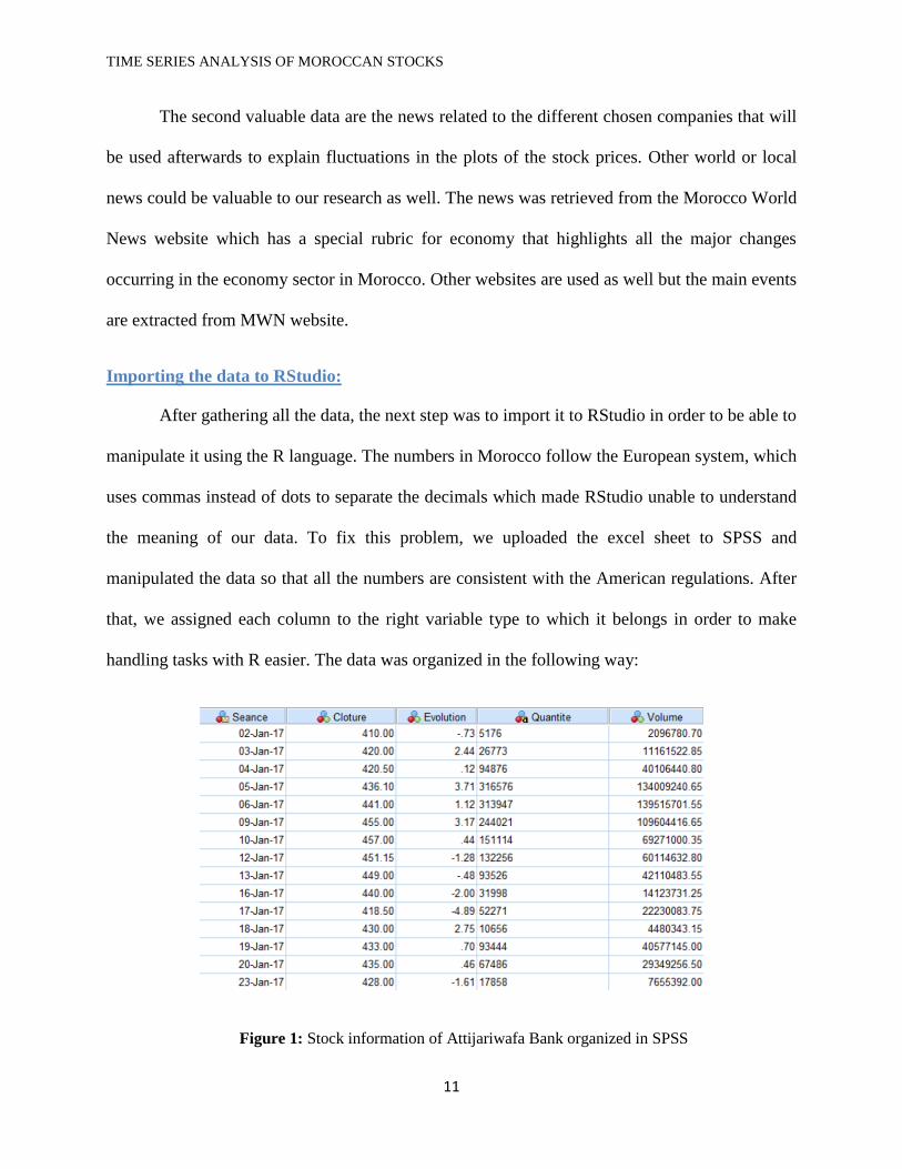
Importing the data to RStudio:
After gathering all the data, the next step was to import it to RStudio in order to be able to
manipulate it using the R language. The numbers in Morocco follow the European system, which
uses commas instead of dots to separate the decimals which made RStudio unable to understand
the meaning of our data. To fix this problem, we uploaded the excel sheet to SPSS and
manipulated the data so that all the numbers are consistent with the American regulations. After
that, we assigned each column to the right variable type to which it belongs in order to make
handling tasks with R easier. The data was organized in the following way:
Figure 1: Stock information of Attijariwafa Bank organized in SPSS

TIME SERIES ANALYSIS OF MOROCCAN STOCKS
12
Even if the initial data contained different components, we only took into consideration
two of them in our study: The „Date‟ (Séance) and „The closing price‟ (Cloture) which we
assume reflects the average price of the stock for the same day. We only imported the two pieces
of information of interest to our study into RStudio to have the following figure:
Figure 2: Stock prices of Attijariwafa Bank as imported in RStudio
For the data to be fully maneuverable using the R language, we had to use the haven
library. This library enables us to retrieve and manipulate data using the R language, which is the
first and most crucial step in our project. The following piece of code in R gets the data and
displays it in the viewer of RStudio:
Figure 3: Reading and displaying the stock information in RStudio
The data at this point is available and fully manageable in the R language so the next step
would be to plot the prices with respect to time and find the trend with which it varies and use
our method to find the most appropriate model.
Plotting the time series:
In this step, we will plot the data of the stock prices with respect to time using the tools
available in the R language. We will create a time series object in R studio that will contain the

TIME SERIES ANALYSIS OF MOROCCAN STOCKS
13
data imported previously. To do so, we will need to use two famous libraries: “zoo” and “xts”
that are made specifically to make handling time series in R very intuitive. These libraries are
equipped with different built-in functions to create and manipulate time series objects. The
function plot is then used to get a chart of stock closing prices versus their respective dates. The
following piece of code was used to create a time series object and generate the plot:
Figure 4: R code to create a time series object and plot the data
The following plot of stock prices in different points in time was generated in RStudio
and it shows that the stock prices have a tendency to increase with time:
Figure 5: Data plot of stock prices of Attijariwafa Bank for the year 2017
From the plot, we can see that the data is increasing in the long term but we still cannot
say that the prices will keep following this trend. At this stage of the analysis, we still can‟t draw
any conclusions concerning the evolution of the stock prices of the company Attijariwafa Bank.

TIME SERIES ANALYSIS OF MOROCCAN STOCKS
14
This plot is only a mere visual representation of the data we have gathered from the Casablanca
Stock Exchange.
From the graph, we can see that the stock prices started peaking with a fast pace in
January 2017 and after that, it dropped until May when it started growing with a slow pace and a
small amount of noise. The change that occurred in January can actually be explained by an
event that occurred at the end of December 2016, where Attijariwafa Bank got awarded three
different prizes in London. The year 2016 was a great year for Attijariwafa Bank, as it got
awarded „Best Moroccan bank of the year‟ in addition to other trophies by a subsidiary magazine
of the Financial Times. All of these awards drew the attention of Moroccan investors towards
Attijariwafa Bank, which impacted greatly its stock price.
The slow paced increase that the stock price of Attijariwafa Bank knew starting May and
that lasted for the remaining of the year, excluding the perturbations that it went through during
that period, is thanks to its new acquisition. In May 5th
2016, Attijariwafa Bank acquired 100%
of an Egyptian Bank called „Barclays‟, which extends its domain of practice to a new country.
This event helped attract a lot of investors in the long term seen the profitability of the new
acquisition. The next step of this study is the smoothing of the time series data of Attijariwafa
Bank by different averaging and smoothing methods in order to run the auto.arima() function
and get the non-seasonal parameters of ARIMA.
Data smoothing:
Data smoothing is a technique used to remove the noise from plots to better see and
recognize the patterns with which the data is changing. There are different techniques that could
be used to make the data at hand smoother mainly: Seasonal Adjustment and Moving Averages.

TIME SERIES ANALYSIS OF MOROCCAN STOCKS
15
In this study we will start by averaging the data plotted weekly and monthly to see which of the
two better removes noise and fits the data. The function used to compute the moving averages is
the built-in function: ma() which stands for moving average. This function takes two arguments:
the first one is the data to be averaged and the second one is the order of smoothing, which
means the width of the period. For the weekly moving average, we took the order to be 5 instead
of 7 because a week in the Casablanca Stock Exchange starts Monday and ends Friday as the
market is closed for the week ends. For the „Monthly moving average‟, the order is 20, which
represents the number of working days in a month. For both averages, the data given to the
function is the stock prices of Attijariwafa Bank. After plotting the original data and the two
averages in one reference, we get the following plot:
Figure 6: The moving averages compared to the original data of Attijariwafa Bank
For the remaining of the project, we will be using the weekly moving average instead of
the monthly moving average because of different factors. The first is that even if the monthly
average cancels out a lot of noise from the graph, we might lose valuable information in the

TIME SERIES ANALYSIS OF MOROCCAN STOCKS
16
process. The weekly average in the other hand is the closest to the original plot of data prices
with a considerable smoothing and cancelation of noise, which will enable us to preserve the
major information presented by the graph. All of the advantages cited above make the weekly
moving average very reliable and can be used in our study.
The next step in smoothing the data is the elimination of the seasonal effect from the
previous plot of stock prices. The seasonality represents any change in the evolution of the
prices that occurs every definite period of time. To do so, we will first use the function stl() from
the forecast library that will enable us to clearly see the seasonality of the data at hand. After
applying the function, we will plot the resulting data and examine the seasonality of Attijariwafa
Bank‟s stock prices in the year 2017. The following graph represents the different seasonality
and the trend of the data at hand:
Figure 7: The representation of the seasonality of the Attijariwafa Bank Stock prices

TIME SERIES ANALYSIS OF MOROCCAN STOCKS
17
From the resulting graph, we can see that our data has a seasonal component that should
be taken out of the equation before proceeding into the application of the ARIMA model. Taking
out the seasonality from the plot will make our forecasting more accurate and closer to the real
values that will be used later for testing our model. The forecast package enables us to take the
seasonality out of the equation with a simple function called seasadj() that modifies the original
plot by subtracting the seasonality.
Data forecasting:
The next step will be to try a model on our data to see how the prices will behave in the
future. The model that we will be using at first is the ARIMA which stands for Auto Regressive
Integrated Moving Average which is the most widely used to study future changes in data. It is
known for its flexibility because it could be controlled by changing one or more of its
parameters. The function used to find the best parameters that would generate the most accurate
fit of the data is called auto.arima() and it belongs to the forecast library. The function runs the
autocorrelation function and evaluates where the lags spikes up which gives the values of the
ARIMA parameters. After using the auto.arima() function on the data that doesn‟t have the
seasonal component, we get a (3,1,3) ARIMA that give an approximated behavior for the next 20
days using the forecast() function. The following code in R was used in order to forecast the
values:
Figure 8: Displaying the forecast of the prices using ARIMA model in RStudio
The following graph results from running the previous code in RStudio and represents the
forecast of the data for the next twenty days given by the model ARIMA(3,1,3). The model may

TIME SERIES ANALYSIS OF MOROCCAN STOCKS
18
not be the best fit for our data but we decided to start from it and refine the model to get the best
fit. We may end up using other models throughout the study if they better fit the graphs of the
stock prices.
Figure 9: The forecast of the Stock prices for the January 2018 for Attijariwafa Bank using
auto.arima
The blue portion of the graph represents the values generated by the forecast() function
using the ARIMA(3,1,3) model. In our study, other models should be used in order to find the
most appropriate fit to the data at hand. The most accurate model will be determined by
comparing the values predicted by the model and the real stock values of the year 2017. The
same analysis should be conducted on the other stocks and news will be taken into account when
coming up with a theory about the fluctuation of the stock prices.

TIME SERIES ANALYSIS OF MOROCCAN STOCKS
19
Data Testing:
The next step that comes after forecasting the data is to test its accuracy by comparing it
with the daily prices of the stock for the month of January 2018. To do so, we will have to import
the data of January 2018 to RStudio and suppress the seasonality using the function seasadj().
The resulted deseasonalized function will be then plotted in the same graph as the forecast that
resulted from applying the auto.arima() function in order to see how close our predictions are to
the real values. The following figure shows the gap between the forecasted values and the real
deseasonalized values:
Figure 10: Comparison between the real deseasonalized values and the forecasted values
We can see from the graph that the difference between the two is very significant. This
forecasting ARIMA model doesn‟t give us a real insight on how the stock prices of Attijariwafa

TIME SERIES ANALYSIS OF MOROCCAN STOCKS
20
Bank will behave in January 2018. We conclude that we need a different ARIMA model in order
to be able to predict more accurately the future fluctuations of our data.
Forecasting using a different ARIMA model:
In order to achieve our goal and get the maximum accuracy, we will use a more complex
ARIMA model by adding the seasonality component which adds three parameters to the
equation. Concerning the non-seasonal part of the ARIMA model, we will use the parameters
that resulted from running the auto.arima() function on the time series after removing the
seasonality. The parameters used will then be 3, 1, and 3 respectively. When it comes to the
seasonal part, we will compare different models using different parameters and get the closest to
the real values by using two evaluation criterions: AKAIKE and BAYESIAN information
criterions. These two parameters show how accurate our model is and the smaller they are, the
better the model suits our data.
Seasonal part of the model:
To get the best results, we will compare different ARIMA models with 3, 1, and 3 as non-
seasonal parameters and different seasonal parameters. Based on the two criterions discussed
before, we will choose the closest model to our data and compare its forecasting of January 2018
to the real values of the same month. The next table shows the AIC and BIC of different ARIMA
models that can be fitted to Attijariwafa Bank‟s stock price:

TIME SERIES ANALYSIS OF MOROCCAN STOCKS
21
Figure 11: Comparison of different ARIMA models for Attijariwafa Bank
When we compare the AICs of the different models chosen, we get that the one with the
lowest value is (3,1,3)(3,1,0) but the one with the lowest BIC value is (3,1,3)(2,2,0). To choose
between the two previous models with the best AIC and BIC, we will compare their Variance.
For the (3,1,3)(2,2,0), the variance is equal to 47.14 and it is equal to 28.82 for the (3,1,3)(3,1,0)
model. The difference is very significant so the one we will be choosing is the (3,1,3)(3,1,0)
model.
Testing the model:
After plugging different parameters and selecting one combination based on the two
information criterions, we found that the ARIMA(3,1,3) is the best fit for our data and
gives the closest forecast to the real values. The first three parameters that represent the non-
seasonal part of our model were retrieved from running the auto.arima() function on the
deseasonalized stock prices of Attijariwafa Bank. The parameters of the seasonal part of the
model, however, were chosen after the trial of different model with different parameters. The
following plot represents the results of the forecasting using the new model in comparison with
the real data retrieved from the Casablanca Stock Exchange website of January 2018:
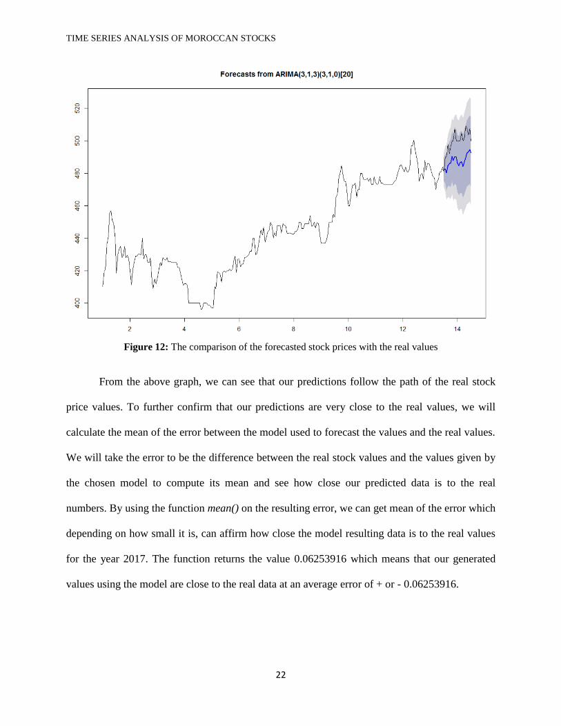
TIME SERIES ANALYSIS OF MOROCCAN STOCKS
22
Figure 12: The comparison of the forecasted stock prices with the real values
From the above graph, we can see that our predictions follow the path of the real stock
price values. To further confirm that our predictions are very close to the real values, we will
calculate the mean of the error between the model used to forecast the values and the real values.
We will take the error to be the difference between the real stock values and the values given by
the chosen model to compute its mean and see how close our predicted data is to the real
numbers. By using the function mean() on the resulting error, we can get mean of the error which
depending on how small it is, can affirm how close the model resulting data is to the real values
for the year 2017. The function returns the value 0.06253916 which means that our generated
values using the model are close to the real data at an average error of + or - 0.06253916.

TIME SERIES ANALYSIS OF MOROCCAN STOCKS
23
Predicted Values:
In order to further demonstrate the accuracy of the chosen model, we will extract the
numerical values given by the model for the month of January of the year 2018 to compare them
with the real values recorded that same month. The following table shows the comparison
between the two values and the percent accuracy for each day:
Figure 13: Comparison between the real and forecasted values of Attijariwafa Bank
We can see from the table that the lowest accuracy percentage is equal to 96.13%, which
is a good indicator of the performance of the model at hand. After calculating the average of the
percentages, which turned out to be 97.59%, we had a better idea on the precision of the
forecasting. This value shows that the model chosen is highly accurate. This finding is
unexpected because it models a Moroccan company in the Casablanca stock exchange where the
trades are not usually based on mathematical models and algorithms which make the stock prices
hardly predictable.

TIME SERIES ANALYSIS OF MOROCCAN STOCKS
24
Concerning the two other banks used in our study being La Banque Populaire and
BMCE, we will directly use the seasonal ARIMA model in order to have the best fits possible to
the data and therefore get the most accurate forecasting. The ARIMA models‟ parameters will
differ between the three data samples at hand but the processes of determining the best fit of the
data will be similar to Attijariwafa Bank.
BMCE:
For the forecasting of the future stock prices of BMCE, the process is similar to
Attijariwafa bank. The first step would be to get the parameters of the ARIMA model which will
be composed of two parts: the non-seasonal parameters and the seasonal parameters and the
second step will consist of testing the results of the forecast with the real values of January 2018
in order to assess the accuracy of our prediction.
Plotting the time series:
The first step after gathering the data and importing to RStudio following the same steps
of Attijariwafa Bank is plotting the time series generated from this data. This step is crucial
because it gives a first insight on how the data behaved during the year 2017. To perform this
action, we will used a prebuilt function in the R language called plot() with the function lines():

TIME SERIES ANALYSIS OF MOROCCAN STOCKS
25
We call the function plot() by giving it the name of the graph using the parameter main
and the x and y axis names using respectively xlab and ylab. The type = “n” is used in order to
avoid plotting each point of the time series so only the plot() function would give us a blank
graph. The function lines is then added in order to plot the BMCE times series by linking the
points in time without plotting the dots. The result of the combination of these two functions is
given in the following graph where we can see the evolution of the stock prices of BMCE
throughout the year 2017:
Figure 14: Data plot of stock prices of BMCE for the year 2017
We can see from the graph that the stock prices of BMCE didn‟t vary much throughout
the year 2017 except the drop that happened between January and March and the clear peak in
July 2017. These two occurrences can be explained by going back to the major events that
BMCE went through in the year 2017. The news concerning the company in question was

TIME SERIES ANALYSIS OF MOROCCAN STOCKS
26
retrieved from the business section in the Website Morocco World News after making a careful
search of the history of BMCE Bank. The massive drop in January can be linked to the fact that
BMCE was ordered to pay a huge amount of taxes for the years ranging from 2012 to 2015, that
constituted half of its revenues according to MWN. This news constituted a massive hit to the
companies‟ revenues and created a tremendous fear for investors that started withdrawing their
money from its stocks.
The peak that the stock prices knew in July 2017 is due to the speculations that investors
and financial analysts had about the new project of BMCE that was announced a little later
during the same month. The speculations were about the tower that was to be constructed in
Rabat by BMCE. The project required a huge investment in order to create the biggest tower in
Africa that will be mainly the bank‟s headquarter. The tower was announced in July 20 after the
official signing of the contract and the project launch.
The previous explanations were intended to know the irregularities in the graph of the
stock prices knowing that the Casablanca Stock Exchange is not as active as other stock
exchanges throughout the world. The next steps will deal with the statistical approach to forecast
he future stock prices of BMCE starting by the choice of a moving average to base our study on
and ending by the testing and comparison of the results. The best fitting ARIMA model will be
chosen and its results will be compared to the real values of the stock prices of the month
January 2018 extracted previously from the Casablanca Stock Exchange website.
Data smoothing:
The next step will be smoothing the data in order to get the non-seasonal parameters of
the ARIMA model. The goal from this step is to check if there is any seasonality in the data and
remove it in order to have a smooth data to which we can apply the auto.arima() function in

TIME SERIES ANALYSIS OF MOROCCAN STOCKS
27
order to get the non-seasonal part of the ARIMA model. To get a deseasonalized set of data, we
will have first to make the data smoother by applying the moving average method.
Concerning the moving average, we will test two different periods: weekly moving
average and monthly moving average. For the weekly moving average, we will apply the
function ma() with a period of 5 which is the number of working days in a week in the
Casablanca Stock exchange. The monthly moving average will have a period of 20 representing
the number of working days in a month. The following graph will contain the original set of data
in comparison with the weekly and the monthly moving averages:
Figure 15: The moving averages compared to the original data of BMCE

TIME SERIES ANALYSIS OF MOROCCAN STOCKS
28
We can see that the monthly moving average smoothens the original data by removing
the variations, but it loses a considerable amount of information during the process. The weekly
moving average, however, makes the data smoother without losing its significance. For this
matter, we will be using the weekly moving average over the monthly as the basis to check for
the seasonality and remove if it is present.
The function that will be used in the auto.arima() function is the deseasonalized weekly
moving averages of the stock prices. To remove the seasonality from our data, we will have to
run first the function stl() that takes the time series and divides it into three main component
which are the seasonality, the trend, and the noise. The result of this function can be plotted so
that the seasonality is clearly visible.
The following figure shows the seasonality, trend and noise of the BMCE stock:
Figure 16: The representation of the seasonality of the BMCE Stock prices

TIME SERIES ANALYSIS OF MOROCCAN STOCKS
29
The seasonality component is clearly represented in the above graph. To remove
this element from our data we will need to call the function seasadj() that only keeps the other
two components. After deseasonalizing the BMCE stock prices, we will call the auto.arima()
function with a “ seasonal = FALSE “ parameter in order to know that the data doesn‟t contain
seasonality. The parameters returned by the function: 2, 1, and 3 will be given to the ARIMA
model as the non-seasonal components.
The seasonal part of the ARIMA model:
For the seasonal components, we tried different parameters in our ARIMA model in order
to get the best fit possible for the data at hand. The First Step is to try the different models with
different seasonal part and choose the best fit based on the AKAIKE information criteria and the
Bayesian information criteria. The second step is to plot the model with the real values of the
month of January 2018 in order to check the accuracy of the model. The last step will be to
compare the resulted values for the forecast with the real values retrieved for the testing month
and get the percent accuracy for each date.
Models comparison:
The first step is to compare different models with different seasonal parameters in order
to find the one with the best AIC and BIC. In addition to those two criterions, we calculated the
variance for the cases where we will have similar or close AIC and BIC values. The following
table shows different models with different seasonal parameters with their AIC, BIC and
Variance:

TIME SERIES ANALYSIS OF MOROCCAN STOCKS
30
Figure 17: Comparison of different ARIMA models for BMCE
In the case of BMCE, the choice is straight forward because we can see that the model
with (2,1,3)(0,2,2) has the lowest AIC and BIC which makes it the best choice. To know how
accurate our prediction is, we will plot the forecasts with the real values of January 2018.
Testing the Model:
In this step, we will test the chosen model by plotting its forecast with the real values of the
month January of the year 2018 retrieved from the Casablanca stock exchange. This step gives a
visual insight on how the predicted values compare to the real values. The next graph will
contain both plots in order to be able to get ahold of the accuracy of our predictions:

TIME SERIES ANALYSIS OF MOROCCAN STOCKS
31
Figure 18: The comparison of the forecasted stock prices with the real values for BMCE
From the above graph we can see that the predicted values are fairly close to the real
value extracted from the Casablanca stock exchange. In order to affirm the closeness of the
forecasted data to the real values, we will calculate the error between the model and the weekly
moving averages of the data. We calculated the error for each point in time and executed the
mean() function in order to get the average of the errors which was -0.09674665. The value
returned is in the order of which shows how accurate our predictions are.
Predicted values:
The last step can give a visual insight on how close the predicted data is to the real values
but it only shows that our predictions follow the trend of evolution of the market. In this step we
will extract the values predicted and the real values retrieved from the market and calculate the
percentage of accuracy of our forecasting for the values of each day of the month of January
TIME SERIES ANALYSIS OF MOROCCAN STOCKS
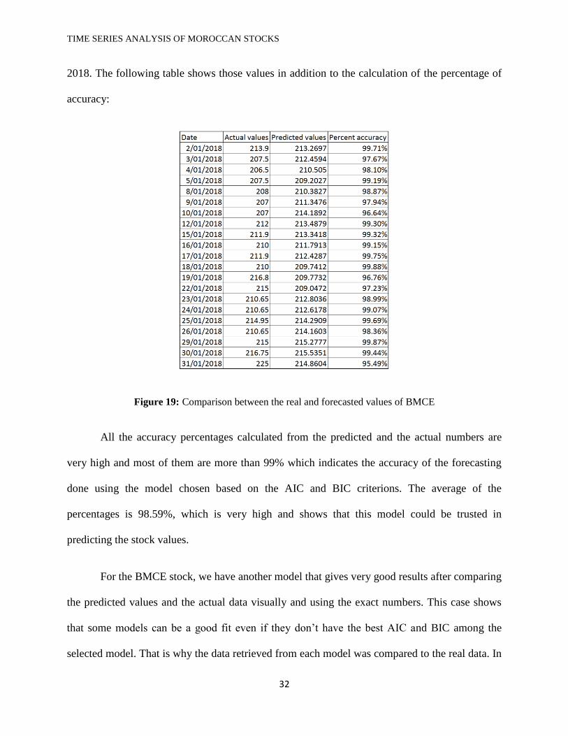
32
2018. The following table shows those values in addition to the calculation of the percentage of
accuracy:
Figure 19: Comparison between the real and forecasted values of BMCE
All the accuracy percentages calculated from the predicted and the actual numbers are
very high and most of them are more than 99% which indicates the accuracy of the forecasting
done using the model chosen based on the AIC and BIC criterions. The average of the
percentages is 98.59%, which is very high and shows that this model could be trusted in
predicting the stock values.
For the BMCE stock, we have another model that gives very good results after comparing
the predicted values and the actual data visually and using the exact numbers. This case shows
that some models can be a good fit even if they don‟t have the best AIC and BIC among the
selected model. That is why the data retrieved from each model was compared to the real data. In

TIME SERIES ANALYSIS OF MOROCCAN STOCKS
33
the case of Attijariwafa Bank, no other model gave better or similar results to the one chosen
using the two criterions. The other model that gives very decent results has the following
parameters (2,1,3)(2,2,0). This model captured my interest when visually comparing the results
of the forecast with the real values because they seem very similar. The following graph can
show the strong similarity between the two plots:
Figure 20: The comparison of the forecasted stock prices with the real values for BMCE using a
different model
After seeing this eye-catching resemblance, I further investigated this model by
comparing the values it predicted with the real values of January 2018 and calculating the
percentage of accuracy for each day. The following table shows the results obtained:

TIME SERIES ANALYSIS OF MOROCCAN STOCKS
34
Figure 21: Comparison between the real and forecasted values of BMCE using a different model
From the table we can see that the values predicted are very close to the real recordings
of the stock prices of BMCE. The lowest percentage of accuracy is 95.08% and the average of all
the percentages is 98.61% which is also very high and very close to the previous model. In
addition to this, the mean of the error between the stock prices of the year 2017 and the values of
the model is very small with a value of -0.06449976. This shows that the criterions can give an
insight on which model is better to model the data but other models should also be considered in
the study and we should look for other indicators and further investigate any interesting model.
La Banque Populaire:
Plotting the time series:
In order to start this analysis and be able to forecast the price accurately we should first
plot the time series at hand and explain the sudden fluctuations of the data at hand. The following
graph will represent the raw data of the stock prices of La Banque Populaire plotted in a graph:

TIME SERIES ANALYSIS OF MOROCCAN STOCKS
35
Figure 22: Data plot of stock prices of La Banque Populaire for the year 2017
From the graph we can see that there is a significant rise in the stock prices of La Banque
Populaire starting the month of January until February where it relapses. This rapid fluctuation
could be explained by the speculations of the market about an award that a subsidiary of La
Banque Populaire could get in the near future. The stocks of La Banque Populaire have known a
significant rush where their price has risen until the news became public where it relapsed
quickly. A subsidiary of La Banque Populaire has been awarded two awards from S&P Global
for their high level of security and managerial quality in the third of February of the year 2017.
This shows that there is a movement in the Casablanca stock exchange and people are getting
interested in buying and selling stocks, but the number of investors is small, which can be seen in
the fast and vertically linear drop or rise that stock prices know. This vertical and sudden drop

TIME SERIES ANALYSIS OF MOROCCAN STOCKS
36
can be explained by the fact that one or very small number of investors withdraw or deposit large
amounts of money in one transaction.
Smoothing the data:
The next phase in analyzing the data of La Banque Populaire is to remove the seasonality
component from our data in order to run the auto.arima() and get the non-seasonal parameters of
the ARIMA model. We will start first by making the data a little smoother by applying the
moving average technique with different orders as we have done for the two previous companies.
The graph that we will plot will have a representation of the real values in green, the weekly
moving average in blue and the monthly moving average in red. The next graph displays the
three plots:
Figure 23: The moving averages compared to the original data of La Banque Populaire

TIME SERIES ANALYSIS OF MOROCCAN STOCKS
37
As we saw for the two previous companies: Attijariwafa Bank and BMCE Bank, the
monthly moving average smoothens the data but loses very important information which can be
valuable to our study. So we will take the weekly moving averages as they make the data
smoother and at the same time keep the maximum information about the original data set.
After choosing the order with which we will compute our moving average and keep the
most of the information that we could about the data, we should check for the seasonality in the
stock prices time series and remove it if present. We will plot the result of the function stl()
which separates the different components of our time series and the results will be shown in the
following figure:
Figure 24: The representation of the seasonality of La Banque Populaire Stock prices

TIME SERIES ANALYSIS OF MOROCCAN STOCKS
38
From the graph above, we can see that our data set has a clear and non-negligible
seasonal component that should be removed in order to apply the non-seasonal auto.arima()
function to get the non-seasonal part of the ARIMA model.
To remove the seasonality, we will apply the function seasadj() on the result of the
function stl() which we named decomp in our program:
After removing the seasonality, we will run the auto.arima() function without the
seasonality component by adding “seasonal = FALSE” to our function. The returned numbers
being 2, 1, and 2 are then used as the non-seasonal parameters of the ARIMA model.
Building the ARIMA model: non-seasonal parameters
When it comes to the seasonal parameters of the ARIMA model, they will be chosen after
a trial of different sequences of numbers and finding the best fit for our data based on different
criterions. The AIC and BIC will be the main factors in determining the model that best fits the
data at hand as it was done for the two previous companies.
Models comparison:
The first step towards finding the best seasonal parameters for the ARIMA model is to
use different combination of numbers and choose the one with the lowest AIC and BIC. The
following table contains different models from which we will choose one based on the criterions
cited above:

TIME SERIES ANALYSIS OF MOROCCAN STOCKS
39
Figure 25: Comparison of different ARIMA models for La Banque Populaire
From the table above, we can see that the one with the model with the lowest AIC and
BIC have the following parameters (2,1,2)(2,1,2). Even though this model is clearly the best pick
when it comes to the evaluation of the two criterions, we run simulations to see the forecasts of
the other models. This step enables us to see if one of the other models is interesting enough to
be investigated but fortunately for this company, the other models were far from the real values
and the difference is clearly visible.
Testing the model:
The chosen model will be tested in this phase by plotting the forecasted values in the
same graph with the values of the BMCE stock for the month of January 2018 retrieved from the
Casablanca stock Exchange website. The following graph shows the forecasts made by this
model in comparison to the real values of the stock prices:

TIME SERIES ANALYSIS OF MOROCCAN STOCKS
40
Figure 26: The comparison of the forecasted stock prices with the real values for La Banque Populaire
In contrary to the two other companies, the predicted values do not seem very close to the
real values from the graph. In order to see how close the values generated by the ARIMA model
and the real stock prices we will calculate the error between the two values. The error will be
calculated at any point in time by taking the difference between the two values: the model and
the real.
By visualizing this computed error at any point in time using the function as.numeric() we get an
array of number shown in the next figure:

TIME SERIES ANALYSIS OF MOROCCAN STOCKS
41
Figure 27: The values of the error between the ARIMA model generated values and the real values
This array already shows that the values are in the order of , which is showing the
closeness of the values generated by the ARIMA model that has those specific parameters to the
real values retrieved from the Casablanca stock Exchange website. In order to get a better
representation of the accuracy of the model, we will calculate the average of those values using
the function mean(). The returned value by this function is 0.01280953 which affirms that our
prediction is accurate.
Predicted values:
This step consists of comparing the everyday recorded values of the stock and the
predicted values using the model we chose. After visualizing the closeness of the prediction by
plotting the forecasting with the real values, we will compare the numbers given by the model
with the real figures and compute the percentage of accuracy for each day.

TIME SERIES ANALYSIS OF MOROCCAN STOCKS
42
The following table shows the two figures with the percentage of accuracy:
Figure 28: Comparison between the real and forecasted values of La Banque Populaire
This table shows the closeness of the predicted data to the real stock prices using
numbers and percentages. The percentage of accuracy for our predictions using the model with
the parameters (2,1,2)(2,1,2) for La Banque Populaire is very high because it never goes below
95.65%. The average of the accuracy percentages is 97.9% which shows the extent to which our
predictions are accurate.

TIME SERIES ANALYSIS OF MOROCCAN STOCKS
43
STEEPLE Analysis:
Social Aspect:
One of the aims of this study is to encourage people to invest in stocks by showing them
how they can be studied and informed decisions could be made. By encouraging Moroccans to
invest in companies listed in the stock exchange, we will boost entrepreneurs to establish new
businesses that will help in the development of Morocco. Investing in stocks can represent a
combination of personal gain and social responsibility because we can help developing our
country by joining small individual investments with the efforts of managers of big corporations.
Technological Aspect:
The technological aspect in this capstone project resides in the use of computer science to
find mathematical models that could be fitted to the data at hand and forecast future stock prices.
Computer science is a huge added value to the domain of finance as new data could be added in
real time and predictions calculated and refined. The program could be connected directly to the
source website of data and the model could be refined in real time.
Economic Aspect:
By encouraging people to invest in stocks, the Moroccan economy will flourish. This
study can help people see that buying and selling stocks is far from gambling. Moroccans should
know that finance can help them not only grow their riches but it can also help in the
development in their country.

TIME SERIES ANALYSIS OF MOROCCAN STOCKS
44
Environmental Aspect:
This study has no environmental implications as it only deals with the financial sector in
Morocco. We could have used stock prices of environmental businesses in our study in order to
work in the intersection of the two fields.
Political and Legal Aspect:
Concerning the stock exchange in Morocco, the rules governing it are made to suit
Moroccan people‟s needs and encourage them to invest. The rules are made to limit the risk of
losing money but the drawback is that one can‟t get a huge profit out of it. When it comes to
insider trading, the law is still not enforced and we can see it from the fluctuation that market
knows before publicly announcing major events.
Ethical Aspect:
This project was conducted following the ethical rules as we used only data that is
publicly available. All the resources used did not require permission and the RStudio offers a
free version hat suited our needs.

TIME SERIES ANALYSIS OF MOROCCAN STOCKS
45
Conclusion:
In this capstone project, we studied different companies listed in Casablanca stock
exchange in order to find mathematical models that could be used to predict future stock price
values. The companies chosen were the three highest traded bank stocks in the market in order to
have enough data to conduct our research. The method used to model the stock prices is called
ARIMA which is short for Auto Regressive Integrated Moving Average. A different model with
different parameters was chosen for each data set and it was tested using the data of the first
month of the year 2018. All the predictions were fairly precise and the percent accuracy is very
high. But even though the numbers are very convincing, predictions could not be made only
based on the model. News and events should be taken into consideration as well as the model. In
Morocco, Financial decisions of withdrawal or deposit of money are not made based on
mathematical and statistical methods but rather based on news. Due to the lack of supervision,
insider trading is still a wide spread practice in Morocco and can be seen in the graphs where the
plots peak before the publication of a major announcement and suddenly fall afterwards. The
financial sector in Morocco needs more attention and regulations should be enforced in order to
make the Casablanca stock exchange more appealing to small investors.

TIME SERIES ANALYSIS OF MOROCCAN STOCKS
46
References:
[1] Time Series Analysis of Stock Prices Using the Box-Jenkins ... (n.d.). Retrieved March 1,
2018, from:
https://digitalcommons.georgiasouthern.edu/cgi/viewcontent.cgi?article=1668&context=etd
[2] Kabacoff, R. (n.d.). R Tutorial. Retrieved April 15, 2018, from
https://www.statmethods.net/r-tutorial/index.html
[3] Ariyo, A. A., Adewumi, A. O., & Ayo, C. K. (2014). Stock Price Prediction Using
the ARIMA Model. 2014 UKSim-AMSS 16th International Conference on Computer
Modelling and Simulation. doi:10.1109/uksim.2014.67
[4] Mondal, P., Shit, L., & Goswami, S. (2014). Study of Effectiveness of Time Series Modeling
(Arima) in Forecasting Stock Prices. International Journal of Computer Science, Engineering and
Applications, 4(2), 13-29. doi:10.5121/ijcsea.2014.4202
[5] Xts Cheat Sheet: Time Series in R. (n.d.). Retrieved April 15, 2018, from
https://www.datacamp.com/community/blog/r-xts-cheat-sheet
[6] Prabhakaran, S. (n.d.). Time Series Analysis. Retrieved April 15, 2018, from
http://r-statistics.co/Time-Series-Analysis-With-R.html
[7] An Introduction to Stock Market Data Analysis with R (Part 1). (2017, March 28). Retrieved
March 01, 2018, from https://ntguardian.wordpress.com/2017/03/27/introduction-stock-market-
data-r-1/

TIME SERIES ANALYSIS OF MOROCCAN STOCKS
47
[8] Useful Tools for Practical Business Forecasting. (n.d.). Practical Business Forecasting, 29-
63. doi:10.1002/9780470755624.ch2
[9] ARIMA: How to Avoid the Herd When Analyzing Time Series Data. (n.d.). Retrieved April
15, 2018, from https://www.minitab.com/en-us/Published-Articles/ARIMA--How-to-Avoid-the-
Herd-When-Analyzing-Time-Series-Data/
[10] 6.5 STL decomposition. (n.d.). Retrieved April 15, 2018, from
https://www.otexts.org/fpp/6/5
[11] ARIMA model for forecasting– Example in R. (n.d.). Retrieved April 15, 2018, from
https://rpubs.com/riazakhan94/arima_with_example
[12] R. (n.d.). Step-by-Step Graphic Guide to Forecasting through ARIMA. Retrieved April 15,
2018, from http://ucanalytics.com/blogs/step-by-step-graphic-guide-to-forecasting-through-
arima-modeling-in-r-manufacturing-case-study-example/
[13] Deshpande, B. (n.d.). Time series analysis using R for cost forecasting models in 8 steps.
Retrieved April 15, 2018, from http://www.simafore.com/blog/bid/105815/Time-series-analysis-
using-R-for-cost-forecasting-models-in-8-steps
[14] Dalinina, R. (n.d.). Introduction to Forecasting with ARIMA in R. Retrieved April 15, 2018,
from https://www.datascience.com/blog/introduction-to-forecasting-with-arima-in-r-learn-data-
science-tutorials
[15] 8.7 ARIMA modelling in R. (n.d.). Retrieved April 15, 2018, from
https://www.otexts.org/fpp/8/7

TIME SERIES ANALYSIS OF MOROCCAN STOCKS
48
[16] Moving Averages. (n.d.). Retrieved April 15, 2018, from http://uc-
r.github.io/ts_moving_averages
[17] Time Series Regression. (n.d.). Retrieved April 15, 2018, from
https://www.mathworks.com/discovery/time-series-regression.html