Time-Independent Perturbation Theory
20
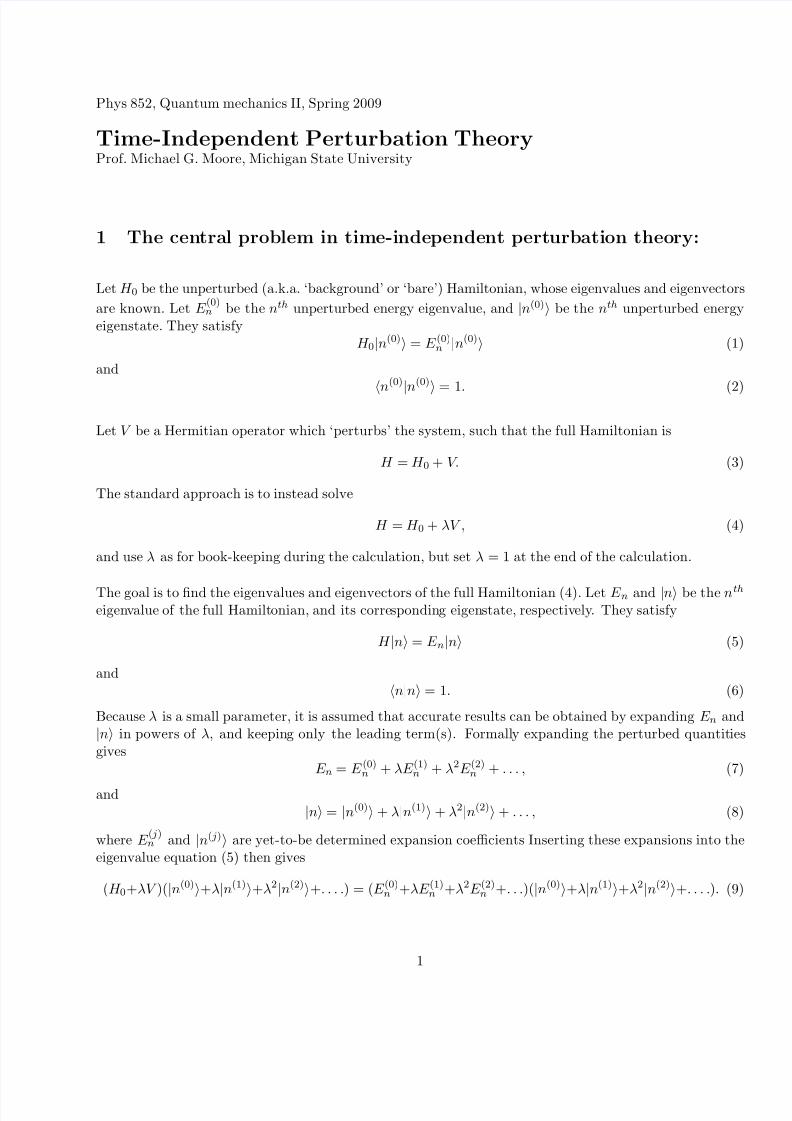
Phys 852, Quantum mechanics II, Spring 2009 Time-Independent Perturbation Theory Prof. Michael G. Moore, Michigan State University 1 The central problem in time-i ndependent perturbation theory: Let H 0 be the unperturbed (a.k.a. ‘background’ or ‘bare’) Hamiltonian, whose eigenvalues and eigenvectors are known. Let E (0) n be the n th unperturbed energy eigenvalue, and |n (0) be the n th unperturbed energy eigenstate. They satisfy H 0 |n (0) = E (0) n |n (0) (1) and n (0) |n (0) = 1. (2) Let V be a Hermitian operator which ‘perturbs’ the system, such that the full Hamiltonian is H = H 0 + V. (3) The standard approach is to instead solve H = H 0 + λV , (4) and use λ as for book-keeping during the calculation, but set λ = 1 at the end of the calculation. The goal is to find the eigenvalues and eigenvectors of the full Hamiltonian (4). Let E n and | n be the n th eigen value of the full Hamilt onian, and its corre sponding eigenstate, respectively. They satisfy H |n = E n |n (5) and n|n = 1. (6) Because λ is a small parameter, it is assumed that accurate results can be obtained by expanding E n and |n in powers of λ, and keepin g only the leading term(s). F ormall y expanding the perturbed quantities gives E n = E (0) n + λE (1) n + λ 2 E (2) n + ..., (7) and |n = |n (0) + λ|n (1) + λ 2 |n (2) + ..., (8) where E ( j ) n and |n ( j) are yet-to-be determined expansion coefficients Inserting these expansions into the eigenvalue equation (5) then gives (H 0 +λV )(|n (0) +λ|n (1) +λ 2 |n (2) +....) = (E (0) n +λE (1) n +λ 2 E (2) n +...)(|n (0) +λ|n (1) +λ 2 |n (2) +....). (9) 1
-
Upload
abinaspradhan -
Category
Documents
-
view
229 -
download
0
Transcript of Time-Independent Perturbation Theory
8/11/2019 Time-Independent Perturbation Theory
http://slidepdf.com/reader/full/time-independent-perturbation-theory 1/20
Phys 852, Quantum mechanics II, Spring 2009
Time-Independent Perturbation TheoryProf. Michael G. Moore, Michigan State University
1 The central problem in time-independent perturbation theory:
Let H 0 be the unperturbed (a.k.a. ‘background’ or ‘bare’) Hamiltonian, whose eigenvalues and eigenvectors
are known. Let E (0)n be the nth unperturbed energy eigenvalue, and |n(0) be the nth unperturbed energy
eigenstate. They satisfyH 0|n(0) = E (0)n |n(0) (1)
and
n
(0)
|n(0)
= 1. (2)
Let V be a Hermitian operator which ‘perturbs’ the system, such that the full Hamiltonian is
H = H 0 + V. (3)
The standard approach is to instead solve
H = H 0 + λV , (4)
and use λ as for book-keeping during the calculation, but set λ = 1 at the end of the calculation.
The goal is to find the eigenvalues and eigenvectors of the full Hamiltonian (4). Let E n and |n be the nth
eigenvalue of the full Hamiltonian, and its corresponding eigenstate, respectively. They satisfy
H |n = E n|n (5)
andn|n = 1. (6)
Because λ is a small parameter, it is assumed that accurate results can be obtained by expanding E n and|n in powers of λ, and keeping only the leading term(s). Formally expanding the perturbed quantitiesgives
E n = E (0)n + λE (1)n + λ2E (2)n + . . . , (7)
and|n = |n(0) + λ|n(1) + λ2|n(2) + . . . , (8)
where E ( j)n and |n( j) are yet-to-be determined expansion coefficients Inserting these expansions into the
eigenvalue equation (5) then gives
(H 0+λV )(|n(0)+λ|n(1)+λ2|n(2)+. . . .) = (E (0)n +λE (1)n +λ2E (2)n +. . .)(|n(0)+λ|n(1)+λ2|n(2)+. . . .). (9)
1

8/11/2019 Time-Independent Perturbation Theory
http://slidepdf.com/reader/full/time-independent-perturbation-theory 2/20
Because of the linear independence of terms in a power series, this equation can only be satisfied forarbitrary λ if all terms with the same power of λ cancel independently. Equating powers of λ thus gives
λ0 : H 0|n(0) = E (0)n |n(0), (10)
λ1 : (H 0 − E (0)n )|n(1) = − V |n(0) + E (1)n |n(0) (11)
λ2
: (H 0 − E (0)n )|n
(2)
= −V |n(1)
+ E (2)n |n
(0)
+ E (1)n |n
(1)
(12)etc . . . (13)
This generalizes to
λ j : (H 0 − E (0)n )|n( j) = −V |n( j−1) +
jk=1
E (k)n |n( j−k). (14)
Similiarly, we can expand the normalization equation in powers of λ, giving
1 = n(0)|n(0) + λ(n(1)|n(0) + n(0)|n(1)) + λ2(n(2)|n(0) + n(1)|n(1) + n(0)|n(2)) + . . . . (15)
Again, we require that all terms of the same power in λ cancel independently, resulting in the set o
equations:
λ0 : n(0)|n(0) = 1, (16)
λ1 : n(1)|n(0) + n(0)|n(1) = 0, (17)
λ2 : n(2)|n(0) + n(1)|n(1) + n(0)|n(2), (18)
which readily generalizes to
λ j :
jk=0
n( j−k)|n(k) = 0. (19)
Solving these equations can be simplified by choosing a convenient global phase-factor. In this case, we
can choose the phase of the full eigenstates to be such that n(0)
|n is real-valued. To enforce our choiceof global phase, we can expand n(0)|n in power series, giving
n(0)|n = 1 + λn(0)|n(1) + λ2n(0)|n(2) + . . . . (20)
Requiring that the r.h.s. be real-values for any real-valued λ requires that each term be independentlyreal-valued, so that
n(0)|n( j) = n( j)|n(0). (21)
2

8/11/2019 Time-Independent Perturbation Theory
http://slidepdf.com/reader/full/time-independent-perturbation-theory 3/20
2 The non-degenerate case
We will now describe how to solve these equations in the case where none of the unperturbed energy levelsare degenerate.
Step #1: To obtain the jth correction to the nth energy eigenvalue, simply hit the λ j equation from the
left with the bra n(0)| and solve for E ( j)n , giving
E ( j)n = n(0)|V |n( j−1) − j−1k=1
E (k)n n(0)|n( j−k), (22)
where we have used n(0)|(H 0 − E (0)n ) = 0 and n(0)|n(0) = 1. Note that all quantities on the r.h.s are o
order < j, and are thus presumed to be known.
Step #2: To obtain the j th correction to the nth eigenstate, we hit both sides of the λ j equation with the
bra m(0)
| where m = n. This gives
m(0)|n( j) = −m(0)|V |n( j−1)E
(0)m − E
(0)n
+
j−1k=1
E (k)n m(0)|n( j−k)
E (0)m − E
(0)n
, (23)
which is the expansion coefficient of the jth correction onto the mth bare eigenvector.
Step #3: To obtain the remaining unknown quantity, n(0)|n( j), we simply solve the normalizationequation, giving
n(0)|n( j) = −1
2
j−1
k=1
n( j−k)|n(k). (24)
Steps 1, 2, and 3 must be solved iteratively, starting with j = 1, and repeating for each order until thedesired accuracy is achieved.
Final Step: Once these quantities are computed, we can reconstruct the nth eigenvalue and eigenvectorvia
E n =∞ j=0
λ jE ( j)n
= E (0)n + λE (1)n + λ2E (2)n + . . . , (25)
and
|n = |n(0)∞ j=0
n(0)|n( j) +m=n
|m(0)∞ j=0
m(0)|n( j)
= |n(0)
1 + λn(0)|n(1) + λ2n(0)|n(2) + . . .
+m=n
|m(0)
λm(0)|n(1) + λ2m(0)|n(2) + . . .
.
(26)
3
8/11/2019 Time-Independent Perturbation Theory
http://slidepdf.com/reader/full/time-independent-perturbation-theory 4/20
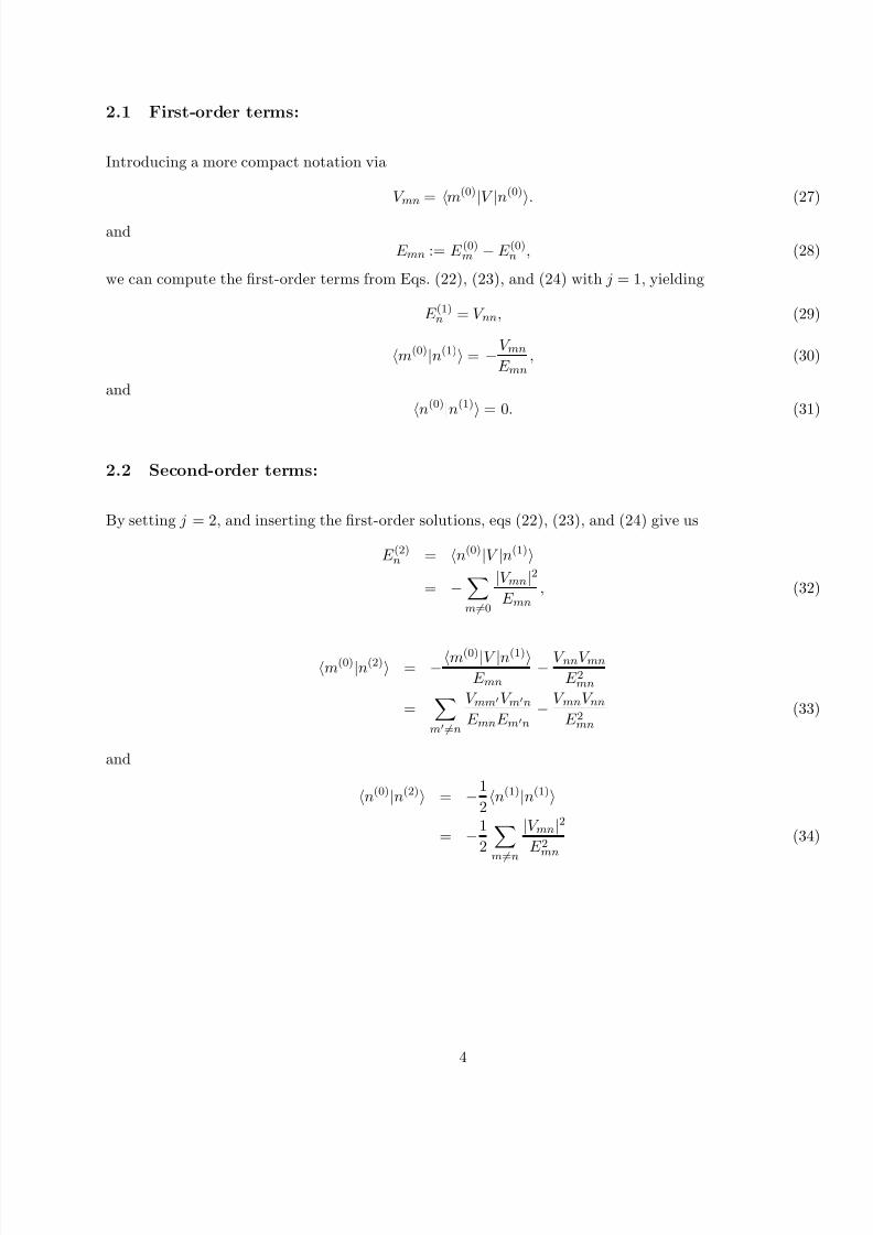
2.1 First-order terms:
Introducing a more compact notation via
V mn =
m(0)
|V
|n(0)
. (27)
andE mn := E (0)m − E (0)n , (28)
we can compute the first-order terms from Eqs. (22), (23), and (24) with j = 1, yielding
E (1)n = V nn, (29)
m(0)|n(1) = −V mn
E mn
, (30)
andn(0)|n(1) = 0. (31)
2.2 Second-order terms:
By setting j = 2, and inserting the first-order solutions, eqs (22), (23), and (24) give us
E (2)n = n(0)|V |n(1)= −
m=0
|V mn|2E mn
, (32)
m(0)|n(2) = −m(0)|V |n(1)E mn
− V nnV mn
E 2mn
=m=n
V mmV mn
E mnE mn
− V mnV nnE 2mn
(33)
and
n(0)|n(2) = −1
2n(1)|n(1)
= −1
2 m=n|V mn|2
E 2mn
(34)
4

8/11/2019 Time-Independent Perturbation Theory
http://slidepdf.com/reader/full/time-independent-perturbation-theory 5/20
2.3 Eigenvectors and eigenvalues to second-order:
Putting the first- and second-order terms together then gives the results
E n = E (0)n + λV nn −
λ2 m=n
|V mn|2
E mn
+ O(λ3), (35)
and
|n = |n(0)1 − λ2
2
m=n
|V mn|2E 2mn
+ O(λ3)
+m=n
|m(0)−λ
V mn
E mn
+ λ2
m=n
V mmV mn
E mnE mn
− V mnV nnE 2mn
+ O(λ3)
. (36)
Truncating the series, and setting λ = 1 then gives the approximations
E n ≈ E (0)n + V nn −m=n
|V mn|2E mn
, (37)
and
|n ≈ |n(0)1 − 1
2
m=n
|V mn|2E 2mn
+
m=n
|m(0)− V mn
E mn+
m=n
V mmV mn
E mnE mn
− V mnV nnE 2mn
. (38)
5
8/11/2019 Time-Independent Perturbation Theory
http://slidepdf.com/reader/full/time-independent-perturbation-theory 6/20
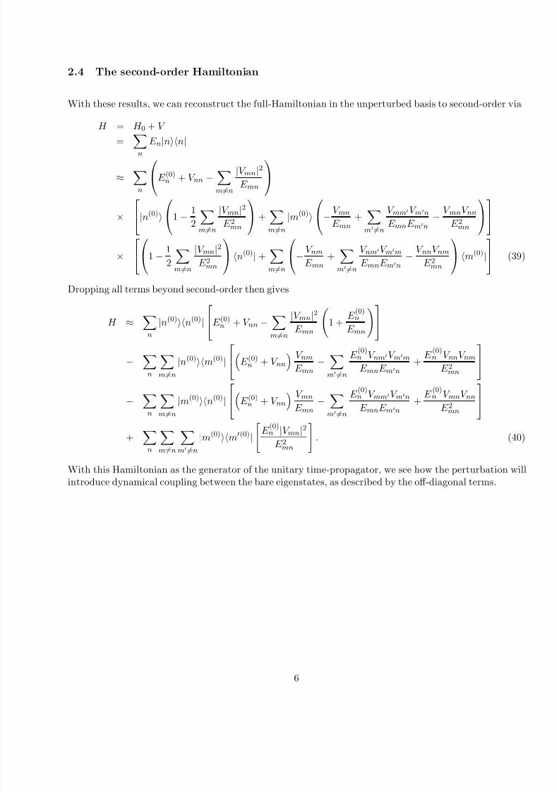
2.4 The second-order Hamiltonian
With these results, we can reconstruct the full-Hamiltonian in the unperturbed basis to second-order via
H = H 0 + V
=n
E n|nn|
≈n
E (0)n + V nn −
m=n
|V mn|2E mn
×|n(0)
1 − 1
2
m=n
|V mn|2E 2mn
+
m=n
|m(0)− V mn
E mn
+m=n
V mmV mn
E mnE mn
− V mnV nnE 2mn
×
1 − 1
2 m=n|V mn|2
E 2mn
n(0)| +
m=n
− V nm
E mn
+
m
=n
V nmV mm
E mnE mn
− V nnV nmE 2mn
m(0)|
(39)
Dropping all terms beyond second-order then gives
H ≈n
|n(0)n(0)|E (0)n + V nn −
m=n
|V mn|2E mn
1 +
E (0)n
E mn
−n
m=n
|n(0)m(0)|E (0)n + V nn
V nmE mn
−m=n
E (0)n V nmV mm
E mnE mn
+ E
(0)n V nnV nm
E 2mn
− n
m=n
|m(0)n(0)|E (0)n + V nn
V mn
E mn
− m
=n
E (0)n V mmV mn
E mnE mn
+ E
(0)n V mnV nn
E 2mn
+n
m=n
m=n
|m(0)m(0)|
E (0)n |V mn|2
E 2mn
. (40)
With this Hamiltonian as the generator of the unitary time-propagator, we see how the perturbation willintroduce dynamical coupling between the bare eigenstates, as described by the off-diagonal terms.
6
8/11/2019 Time-Independent Perturbation Theory
http://slidepdf.com/reader/full/time-independent-perturbation-theory 7/20
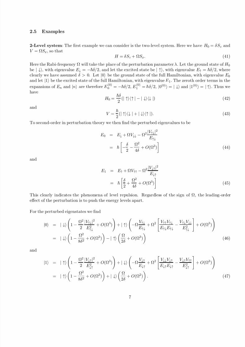
2.5 Examples
2-Level system: The first example we can consider is the two-level system. Here we have H 0 = δS z andV = ΩS x, so that
H = δS z + ΩS x. (41)
Here the Rabi-frequency Ω will take the place of the perturbation parameter λ. Let the ground state of H 0be | ↓, with eigenvalue E ↓ = − δ/2, and let the excited state be | ↑, with eigenvalue E ↑ = δ/2, whereclearly we have assumed δ > 0. Let |0 be the ground state of the full Hamiltonian, with eigenvalue E 0and let |1 be the excited state of the full Hamiltonian, with eigenvalue E 1. The zeroth order terms in the
expansions of E n and |n are therefore E (0)0 = − δ/2, E
(0)1 = δ/2, |0(0) = | ↓ and |1(0) = | ↑. Thus we
have
H 0 = δ
2 (| ↑↑ | − | ↓↓ |) (42)
and
V =
2(| ↑↓ | + | ↓↑ |). (43)
To second-order in perturbation theory we then find the perturbed eigenvalues to be
E 0 = E ↓ + ΩV ↓↓ − Ω2 |V ↑↓|2E ↑↓
=
−δ
2 − Ω2
4δ + O(Ω3)
(44)
and
E 1 = E ↑ + ΩV ↑↑ − Ω2 |V ↓↑|2E ↓↑
=
δ 2 + Ω
2
4δ + O(Ω3)
(45)
This clearly indicates the phenomena of level repulsion. Regardless of the sign of Ω, the leading-ordereffect of the perturbation is to push the energy levels apart.
For the perturbed eigenstates we find
|0 = | ↓
1 − Ω2
2
|V ↑↓|2E 2↑↓
+ O(Ω3)
+ | ↑
−Ω
V ↑↓E ↑↓
+ Ω2
V ↑↑V ↑↓E ↑↓E ↑↓
− V ↑↓V ↓↓E 2↑↓
+ O(Ω3)
=
| ↓1
−
Ω2
8δ 2
+ O(Ω3) − | ↑Ω
2δ
+ O(Ω3) (46)
and
|1 = | ↑
1 − Ω2
2
|V ↓↑|2E 2↓↑
+ O(Ω3)
+ | ↓
−Ω
V ↓↑E ↓↑
+ Ω2
V ↓↓V ↓↑E ↓↑E ↓↑
− V ↓↑V ↑↑E 2↓↑
+ O(Ω3)
= | ↑
1 − Ω2
8δ 2 + O(Ω3)
+ | ↓
Ω
2δ + O(Ω2)
. (47)
7
8/11/2019 Time-Independent Perturbation Theory
http://slidepdf.com/reader/full/time-independent-perturbation-theory 8/20
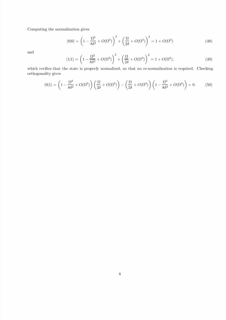
Computing the normalization gives
0|0 =
1 − Ω2
8δ 2 + O(Ω3)
2
+
Ω
2δ + O(Ω3)
2
= 1 + O(Ω3) (48)
and
1|1 =
1 − Ω2
8δ 2 + O(Ω3)
2
+
Ω2δ
+ O(Ω3)2
= 1 + O(Ω3), (49)
which verifies that the state is properly normalized, so that no re-normalization is required. Checkingorthogonality gives
0|1 =
1 − Ω2
8δ 2 + O(Ω3)
Ω
2δ + O(Ω3)
−
Ω
2δ + O(Ω3)
1 − Ω3
8δ 2 + O(Ω3)
= 0. (50)
8

8/11/2019 Time-Independent Perturbation Theory
http://slidepdf.com/reader/full/time-independent-perturbation-theory 9/20
Square well with delta-function For the second example we consider an infinite square-well potentialas the unperturbed problem, and we perturb it by placing a delta-function potential at the center. Ourgoal will be to compute the energy shifts to second order and the perturbed eigenstates to first order. Wewill attempt to explicitly evaluate all sums for the ground state only. The unperturbed Hamiltonian is
H 0 =
P 2
2M + U (X ), (51)
where
U (x) =
0 : 0 < x < L∞ : else
(52)
The form of the perturbation is
V (X ) =
2
MLδ (X − L
2), (53)
so that the full Hamiltonian is
H = H 0 + λV = P 2
2M + U (X ) + λ
2
M Lδ (X − L
2). (54)
The unperturbed energy levels are given by
E (0)n =
2π2
2M L2n2; n = 1, 2, 3, . . . , (55)
with corresponding unperturbed wavefunctions
φn(x) ≡ x|n(0) =
2
L sin
πn
L x
. (56)
The first order energy shift is given by E (1)n = V nn, where V nn ≡ n(0)|V |n(0). Inserting the projector onto
position eigenstates gives
V nn =
dx φ∗n(x)V (x)φn(x) =
2 2
M L2
dx sin2
nπ
L x
δ (x − L
2) =
2 2
ML2; n odd
0; n even . (57)
The matrix element vanishes for even n because these wavefunctions have a node at x = L/2., the odd nwavefunctions have an anti-node at x = L/2, so that the sin-function takes on its maximum value of unity
The first order correction to the wavefunction is given by the usual expression |n(1) = −m=n |m(0) V mn
E mnThus we must evaluate the off-diagonal matrix elements, giving
V mn = 2
2
M L2 dx sin mπ
L
x δ (x
− L
2
)sinnπ
L
x = −(−1)m+n
2 2 2
ML2 : m and n odd
0; m and/or n even
. (58)
The energy denominator is E mn = E (0)m − E
(0)n = 2π2
2ML2(m2 − n2). The perturbed wavefunction to first
order is defined as ψn(x) ≡ x|n(0) + λx|n(1), giving
ψn(x) =
2
L sin
nπ
L x
+ 4λ
π2
2
L
∞m,n=1m=n
sin
(2m − 1)π
L x
(−1)m+n−1
(2m−1)2 − (2n−1)2. (59)
9

8/11/2019 Time-Independent Perturbation Theory
http://slidepdf.com/reader/full/time-independent-perturbation-theory 10/20
In fact, this sum can be performed analytically, although the result is not very illuminating. Computingthe first-order perturbed ground-state (n = 1) wavefunction, for example, gives
ψ1(x) ≈
2
L
1 − λ
π2
sin(πx/L) +
2λ
πL (x − Lu(x − L/2))
2
L cos(πx/L), (60)
where u(x) is the unit step function. The discontinuous derivative at x = L/2 is characteristic of eigenstateswith delta-potentials.
The second order correction to the energy-shift is computed from E (2)n = −
m=n|V mn|2E mn
, which yields
E (2)n = − 8 2
π2M L2
∞m,n=1m=n
1
(2m−1)2 − (2n−1)2. (61)
Here the sum can be computed exactly, giving
E (2)n = − 2 2
π2M L2 1n2 . (62)
The resulting energy eigenvalue accurate to second order is
E n ≈ 2π2
2M L2n2 + λ
2
M L2 − λ2 2
2
π2M L2
1
n2; n odd, (63)
and
E n =
2π2
2M L2n2; n even. (64)
10

8/11/2019 Time-Independent Perturbation Theory
http://slidepdf.com/reader/full/time-independent-perturbation-theory 11/20
3 The degenerate case
We now consider the case where some, but not all, of the unperturbed eigenvalues are the same. In thissituation, the non-degenerate formulas (22), (23), and (24) cannot be used because the E mn terms in thedenominator go to zero when levels m and n are degenerate. Our goal is still to find the eigenvalues andeigenstates of the full Hamiltonian
H = H 0 + V, (65)
where the bare eigenstates of H 0 are now given two quantum numbers, one which labels the energy leveland the other which takes into account the degeneracy. Our bare basis is thus |nm(0), where m labelsthe degenerate sub-levels. They satisfy
H 0|nm(0) = E (0)n |nm(0). (66)
In the case of degeneracy, the choice of basis which satisfied (59) is not unique. Provided that the pertur-bation lifts the degeneracy, then a unique unperturbed basis is defined by
|nm(0) = limλ→0 |nm. (67)
To see why this defines a unique basis, let’s look at a very simple example. Consider a two-level Rabsystem, governed by the bare Hamiltonian H 0 = δS z and the perturbation V = S x. For the case δ = 0, theeigenstates of H 0 become degenerate, so that for every complex number z , we can define a unique possiblebasis choice via
|1(0) = z| ↑z + | ↓z
1 + |z|2 , (68)
|2(0) = | ↑z − z∗| ↓z
1 +|z|2
. (69)
On the other hand, for any non-zero λ, the eigenstates of H = H 0 + λV are the S x eigenstates, given by
|1 = | ↑z − | ↓z√
2, (70)
|2 = | ↑z + | ↓z√
2. (71)
Thus if we use |1(0) = limλ→0 |1 = |1, and |2(0) = limλ→0 |2 = |2, we have specified a unique barebasis.
In fact, the ‘good’ eigenstates will always be the eigenstates of V in the degenerate subspace. To prove thiswe start by introducing the projector into the degenerate subspace, I n, which clearly satisfies I n|nm(0) =
|nm(0), I nH 0 = H 0I n = I nH 0I n = E (0)n I n, and I 2n = I n, while for n = n, we have I n|nm = nm|I n = 0
The energy eigenvalue equation is(H 0 + λV − E nm)|nm = 0. (72)
Since limλ→0 |nm = |nm(0), we can therefore write
limλ→0
(H 0 + λV − E nm)|nm(0) = 0. (73)
11
8/11/2019 Time-Independent Perturbation Theory
http://slidepdf.com/reader/full/time-independent-perturbation-theory 12/20
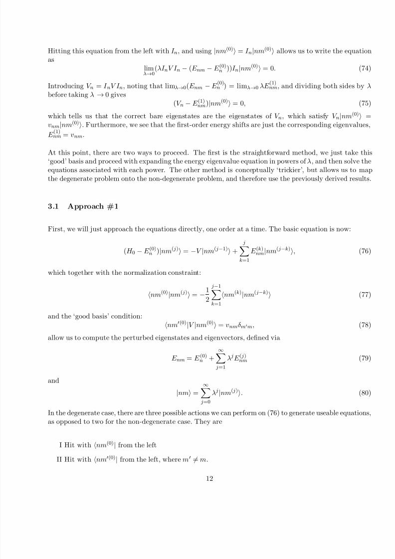
Hitting this equation from the left with I n, and using |nm(0) = I n|nm(0) allows us to write the equationas
limλ→0
(λI nV I n − (E nm − E (0)n ))I n|nm(0) = 0. (74)
Introducing V n = I nV I n, noting that limλ→0(E nm − E (0)n ) = limλ→0 λE
(1)nm, and dividing both sides by λ
before taking λ → 0 gives (V n − E (1)nm)|nm(0) = 0, (75)
which tells us that the correct bare eigenstates are the eigenstates of V n, which satisfy V n|nm(0) =vnm|nm(0). Furthermore, we see that the first-order energy shifts are just the corresponding eigenvalues,
E (1)nm = vnm.
At this point, there are two ways to proceed. The first is the straightforward method, we just take this‘good’ basis and proceed with expanding the energy eigenvalue equation in powers of λ, and then solve theequations associated with each power. The other method is conceptually ‘trickier’, but allows us to mapthe degenerate problem onto the non-degenerate problem, and therefore use the previously derived results
3.1 Approach #1
First, we will just approach the equations directly, one order at a time. The basic equation is now:
(H 0 − E (0)n )|nm( j) = −V |nm( j−1) +
jk=1
E (k)nm|nm( j−k), (76)
which together with the normalization constraint:
nm(0)|nm( j) = −1
2
j−1k=1
nm(k)|nm( j−k) (77)
and the ‘good basis’ condition:nm(0)|V |nm(0) = vnmδ mm, (78)
allow us to compute the perturbed eigenstates and eigenvectors, defined via
E nm = E (0)n +∞ j=1
λ jE ( j)nm (79)
and
|nm =
∞ j=0
λ j |nm( j). (80)
In the degenerate case, there are three possible actions we can perform on (76) to generate useable equations,as opposed to two for the non-degenerate case. They are
I Hit with nm(0)| from the left
II Hit with nm(0)| from the left, where m = m.
12

8/11/2019 Time-Independent Perturbation Theory
http://slidepdf.com/reader/full/time-independent-perturbation-theory 13/20
III Hit with nm(0)| from the left, where n = n.
The main thing we hope to prove is that the ‘good basis’ condition is sufficient to remove any singularitiesdue to vanishing energy denominators when degenerate levels are mixed.
3.1.1 First-order terms
With j = 1 we can start by computing nm(0)|nm(1), giving
nm(0)|nm(1) = −1
2
0k=1
nm(k)|nm( j−k) = 0. (81)
The energy equation is then
(H 0 − E
(0)
n )|nm
(1)
= −V |nm
(0)
+ E
(1)
nm|nm
(0)
. (82)
From action I, we get0 = −nm(0)|V |nm(0) + E (1)nm, (83)
which givesE (1)nm = vnm. (84)
as expected.From II, we get
0 = −nm(0)|V |nm(0) (85)
which is just a re-statement of the ‘good basis’ constraint (78).
From III, we find (E (0)n − E (0)n )nm(0)|nm(1) = −nm(0)|V |nm(0). (86)
Solving for nm(0)|nm(1) gives
nm(0)|nm(1) = −V nmnm
∆nn
, (87)
where we have introduced the new notation ∆nn = E (0)n
− E (0)n to avoid confusing the energy denominator
with the full energy level E nm.
At this point, we note that we have exhausted all of our equations, but have not found the componentsnm(0)|nm(1). We will, however, proceed to the case ( j = 2), and hope for the best.
3.1.2 Second-order terms
With j = 2, we find
nm(0)|nm(2) = −1
2nm(1)|nm(1)
13
8/11/2019 Time-Independent Perturbation Theory
http://slidepdf.com/reader/full/time-independent-perturbation-theory 14/20
= −1
2
nm
nm(0)|nm(1)2
= −1
2
m=m
nm(0)|nm(1)2 − 1
2
n=nm
nm(0)|nm(1)2
= −12
m=m
nm(0)|nm(1)2 − 1
2
n=nm
|V nmnm|2∆2nn
, (88)
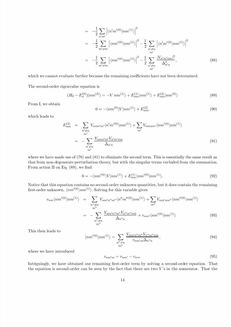
which we cannot evaluate further because the remaining coefficients have not been determined.
The second-order eigenvalue equation is
(H 0 − E (0)n )|nm(2) = −V |nm(1) + E (1)nm|nm(1) + E (2)nm|nm(0) (89)
From I, we obtain0 = −nm(0)|V |nm(1) + E (2)nm, (90)
which leads to
E (2)nm =n=nm
V nmnmnm(0)|nm(1) +m
V nmnmnm(0)|nm(1)
= −n=nm
V nmnmV nmnm
∆nn
(91)
where we have made use of (78) and (81) to eliminate the second term. This is essentially the same result asthat from non-degenerate perturbation theory, but with the singular terms excluded from the summationFrom action II on Eq. (89), we find
0 = −nm(0)|V |nm(1) + E (1)nmnm(0)|nm(1). (92)
Notice that this equation contains no second-order unknown quantities, but it does contain the remainingfirst-order unknown, nm(0)|nm(1). Solving for this variable gives
vnmnm(0)|nm(1) =n=nm
V nmnmnm(0)|nm(1) +m
V nmnmnm(0)|nm(1)
= −n=nm
V nmnmV nmnm
∆nn
+ vnmnm(0)|nm(1) (93)
This then leads to
nm(0)|nm(1) =n=nm
V nmnmV nmnm
vnmm∆nn
, (94)
where we have introducedvnmm = vnm − vnm. (95)
Intriguingly, we have obtained our remaining first-order term by solving a second-order equation. Thatthe equation is second-order can be seen by the fact that there are two V ’s in the numerator. That the
14

8/11/2019 Time-Independent Perturbation Theory
http://slidepdf.com/reader/full/time-independent-perturbation-theory 15/20
resulting term is first-order can be seen by the fact that there is a v in the denominator, so that the termscales as λ
2
λ = λ.
This allows us to complete our expression for nm(0)|nm(2), yielding
nm(0)|nm(2) = −1
2 m
=m
n
=nmn
=nm
V nmnmV nmnmV nmnmV nmnm
∆nnv2nmm∆nn
− 1
2 n
=nm
V nmnmV nmnm
∆2nn
(96)Lastly, from III, we obtain
∆nnnm(0)|nm(2) = −nm(0)|V |nm(1) + E (1)nmnm(0)|nm(1), (97)
which gives us
nm(0)|nm(2) =n=nm
V nmnmV nmnm
∆nn∆nn
−
m=m
n=nm
V nmnmV nmnmV nmnm
∆nnvnmm∆nn
− V nmnmvnm∆2nn
(98)At this point we see that we have run out of second-order equations, yet have not obtained an expression
for the components nm(0)|nm(2). It is logical at this point to assume that we can obtain these coefficientsby solving a third-order equation, which is left as an exercise.
3.1.3 Results to second-order (almost)
Thus we have found
E nm = E (0)n + λvnm −n=nm
V nmnmV nmnm
∆nn
+ O(λ3) (99)
as well as
|nm = |nm(0)
1 − λ2
2
n=nm
V nmnm
∆nn
m=m
n=nm
V nmnmV nmnmV nmnm
v2nmm∆nn
+ V nmnm
∆nn
+ O(λ3
+m=m
|nm(0)
λ
n=nm
V nmnmV nmnm
vnmm∆nn
+ O(λ2)
+n=nm
|nm(0)
− λ
V nmnm
∆nn
1 + λ
vnm
∆nn
+ λ2 n=nm
V nmnm −
m=m
V nmnmV nmnm
vnmm
V nmnm
∆nn∆nn
+ O(λ3)
(1
Note, in going from Eq. (98) to (100) it was necessary to make the change of dummy variables n → n
m → m, and m → m.
15
8/11/2019 Time-Independent Perturbation Theory
http://slidepdf.com/reader/full/time-independent-perturbation-theory 16/20
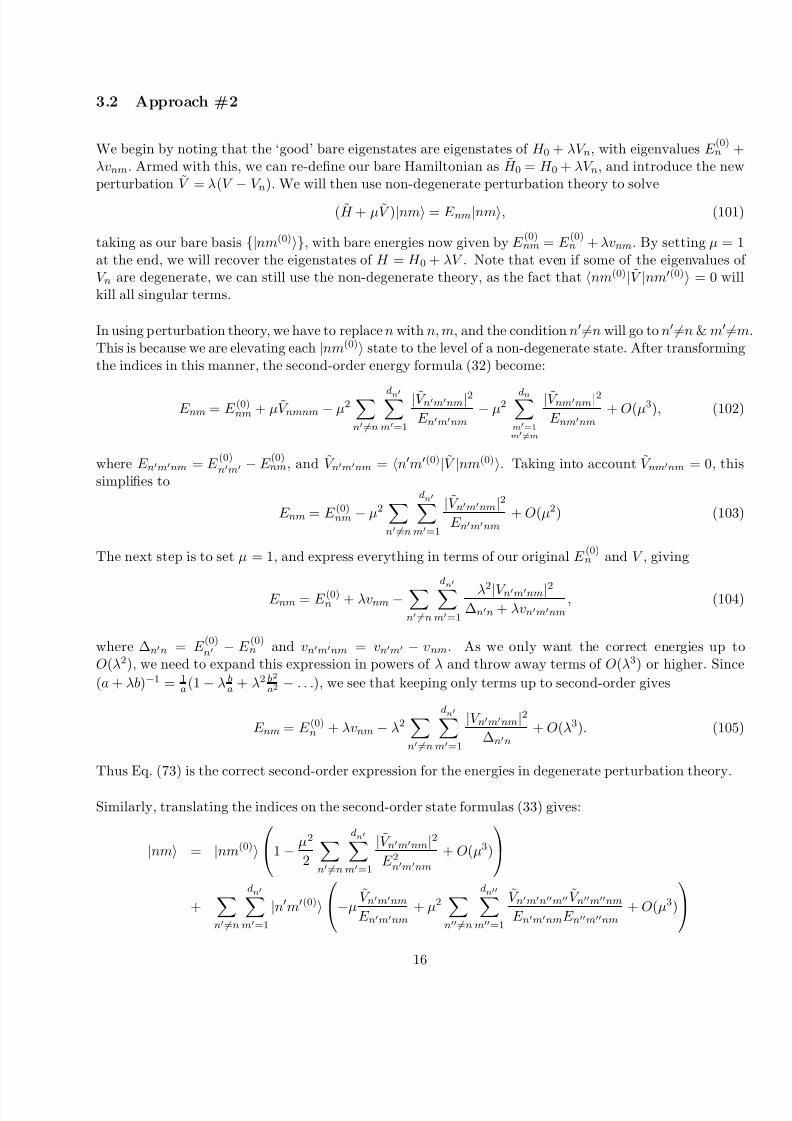
3.2 Approach #2
We begin by noting that the ‘good’ bare eigenstates are eigenstates of H 0 + λV n, with eigenvalues E (0)n +
λvnm. Armed with this, we can re-define our bare Hamiltonian as H 0 = H 0 + λV n, and introduce the newperturbation V = λ(V
−V n). We will then use non-degenerate perturbation theory to solve
( H + µV )|nm = E nm|nm, (101)
taking as our bare basis |nm(0), with bare energies now given by E (0)nm = E
(0)n + λvnm. By setting µ = 1
at the end, we will recover the eigenstates of H = H 0 + λV . Note that even if some of the eigenvalues oV n are degenerate, we can still use the non-degenerate theory, as the fact that nm(0)|V |nm(0) = 0 wilkill all singular terms.
In using perturbation theory, we have to replace n with n, m, and the condition n=n will go to n=n & m=mThis is because we are elevating each |nm(0) state to the level of a non-degenerate state. After transformingthe indices in this manner, the second-order energy formula (32) become:
E nm = E (0)nm + µV nmnm − µ2 n=n
dnm=1
|V nmnm|2E nmnm
− µ2dnm=1
m=m
|V nmnm|2E nmnm
+ O(µ3), (102)
where E nmnm = E (0)nm − E
(0)nm, and V nmnm = nm(0)|V |nm(0). Taking into account V nmnm = 0, this
simplifies to
E nm = E (0)nm − µ2 n=n
dn
m=1
|V nmnm|2E nmnm
+ O(µ2) (103)
The next step is to set µ = 1, and express everything in terms of our original E (0)n and V , giving
E nm = E (0)n + λvnm −n=n
dn
m=1
λ2|V nmnm|2∆nn + λvnmnm
, (104)
where ∆nn = E (0)n
− E (0)n and vnmnm = vnm − vnm. As we only want the correct energies up to
O(λ2), we need to expand this expression in powers of λ and throw away terms of O(λ3) or higher. Since
(a + λb)−1 = 1a
(1 − λ ba
+ λ2 b2
a2 − . . .), we see that keeping only terms up to second-order gives
E nm = E (0)n + λvnm − λ2 n=n
dn
m=1
|V nmnm|2∆nn
+ O(λ3). (105)
Thus Eq. (73) is the correct second-order expression for the energies in degenerate perturbation theory.
Similarly, translating the indices on the second-order state formulas (33) gives:
|nm = |nm(0)1 − µ2
2
n=n
dn
m=1
|V nmnm|2E 2nmnm
+ O(µ3)
+n=n
dn
m=1
|nm(0)−µ
V nmnm
E nmnm
+ µ2 n=n
dn
m=1
V nmnm V nmnm
E nmnmE nmnm
+ O(µ3)
16

8/11/2019 Time-Independent Perturbation Theory
http://slidepdf.com/reader/full/time-independent-perturbation-theory 17/20
+
dnm=1
m=m
|nm(0)µ2
n=n
dn
m=1
V nmnmV nmnm
E nmnmE nmnm
+ O(µ3)
(106)
where we have again relied on V nmnm = 0 for simplifications. Setting µ = 1 and expressing everything in
terms of V and E
(0)
n gives
|nm = |nm(0)1 − 1
2
n=n
dn
m=1
λ2|V nmnm|2∆E nn + λ(vnm − vnm)
+n=n
dn
m=1
|nm(0)− λV nmnm
∆nn+λvnmnm
+n=n
dn
m=1
λ2V nmnmV nmnm
(∆nn+λvnmnm)(∆nn+λvnmnm)
+dnm=1
m=m
|nm(0)n=n
dn
m=1
λ2V nmnmV nmnm
λvnmnm(∆nn + λvnmnm). (107)
The next step is to expand in powers of λ and keep only terms up to O(λ2), which gives
|nm = |nm(0)1 − 1
2
n=n
dn
m=1
λ2|V nmnm|2∆nn
+n=n
dn
m=1
|nm(0)−λV nmnm
∆nn
+ λ2V nmnmvnmnm
∆2nn
+n=n
dn
m=1
λ2V nmnmV nmnm
∆nn∆nn
+dn
m=1
m=m
|nm(0)λ
n=ndn
m=1
V nmnmV nmnm
vnmm∆nn
. (108)
Notice that something very strange has occurred with the final term. This term, which was originallysecond order in µ, has become first-order in λ. This means that a second-order calculation was necessaryto obtain the correct state to first-order. Thus we can predict that a third-order calculation will similarlyyield second-order terms. This means that we can actually only trust our states (76) up to first-orderDropping all terms greater than first-order gives
|nm = |nm(0) 1 + O(λ2)
+
n=ndn
m=1
|nm(0)
−λV nmnm
∆nn
+ O(λ2)
+dnm=1
m=m
|nm(0)λ
n=n
dn
m=1
V nmnmV nmnm
vnmm∆nn
+ O(λ2)
. (109)
Equations (73) and (77) are the main results of this section, giving the energies to second-order and thestates to first-order.
17

8/11/2019 Time-Independent Perturbation Theory
http://slidepdf.com/reader/full/time-independent-perturbation-theory 18/20
3.3 Examples
A three level system: The simplest quantum system which can require degenerate perturbation theoryis the three-state system. If a two-state system is degenerate, it must first be diagonalized in the degeneratesubspace, after which the problem is solved exactly. Let us consider, therefore, a three-level system with
H 0 → E 0
0 0 0
0 1 00 0 1
, (110)
and
V → V 0
0
√ 2 2
√ 2√
2 0 2
2√
2 2 0
, (111)
both defined in the ’physical’ basis |1, |2, |3. The bare Hamiltonian has two energy eigenvalues E (0)1 = 0
and E (0)2 = E 0. The first eigenvalue is non-degenerate, with eigenvector
|1, 1(0)
=
|1
, while the second is
doubly degenerate, with a degenerate subspace spanned by |2 and |3. The projection operator for thedegenerate subspace is
I 2 = |22| + |33| → 0 0 0
0 1 00 0 1
. (112)
This leads to the projection
V 2 = I 2V I 2 = V 0
0 0 0
0 0 20 2 0
. (113)
This operator has eigenvalues 0, −2V 0, and 2V 0, with corresponding eigenvectors |1, 1√ 2
(|2 − |3), and1√ 2(|2 + 3). To determine which two eigenvectors live in the degenerate subspace (pretending for themoment that it is not completely obvious), we can apply I 2 to each, and discard any states which givezero. Applying this test, we find that the two ‘good’ basis states for the degenerate subspace are |2, 1(0) =1√ 2
(|2 − |3) and |2, 2(0) = 1√ 2
(|2 + |3).
In the new basis |1, 1(0), |2, 1(0), |2, 2(0), the bare Hamiltonian matrix is unchanged, and the perturba-tion is diagonalized in the degenerate subspace giving
V →
V 1111 V 1121 V 1122V ∗1121 −2V 0 0V ∗1122 0 2V 0
. (114)
Computing the necessary matrix elements, we find
V 1111 = 1, 1(0)|V |1, 1(0) = 1|V |1 = 0, (115)
V 1121 = 1, 1(0)|V |2, 1(0) = 1√
2(1|V |2 − 1|V |3) = −V 0, (116)
and
V 1122 = 1, 1(0)|V |2, 2(0) = 1√
2(1|V |2 + 1|V |3) = 3V 0, (117)
18
8/11/2019 Time-Independent Perturbation Theory
http://slidepdf.com/reader/full/time-independent-perturbation-theory 19/20
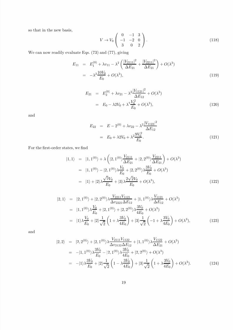
so that in the new basis,
V → V 0
0 −1 3
−1 −2 03 0 2
. (118)
We can now readily evaluate Eqs. (73) and (77), giving
E 11 = E (0)1 + λv11 − λ2
|V 2111|2∆E 21
+ |V 2211|2
∆E 21
+ O(λ3)
= −λ210V 0E 0
+ O(λ3), (119)
E 21 = E (0)2 + λv21 − λ2 |V 1121|2
∆E 12+ O(λ3)
= E 0 − λ2V 0 + λ2 V 20E 0
+ O(λ3), (120)
and
E 22 = E − 2(0) + λv22 − λ2 |V 1122|2∆E 12
= E 0 + λ2V 0 + λ29V 20E 0
. (121)
For the first-order states, we find
|1, 1 = |1, 1(0) + λ
|2, 1(0) V 2111
∆E 21+ |2, 2(0) V 2211
∆E 21
+ O(λ3)
=
|1, 1(0)
− |2, 1(0)
λ
V 0
E 0+
|2, 2(0)
λ
3V 0
E 0+ O(λ3)
= |1 + |2λ
√ 2V 0
E 0+ |3λ
2√
2V 0E 0
+ O(λ3), (122)
|2, 1 = |2, 1(0) + |2, 2(0)λ V 2211V 1121∆v2221∆E 12
+ |1, 1(0)λV 1121∆E 12
+ O(λ3)
= |1, 1(0)λV 0E 0
+ |2, 1(0) + |2, 2(0)λ3V 04E 0
+ O(λ3)
= |1λV 0E 0
+ |2 1√ 2
1 + λ
3V 04E 0
+ |3 1√
2
−1 + λ
3V 04E 0
+ O(λ3), (123)
and
|2, 2 = |2, 2(0) + |2, 1(0)λ V 2111V 1122∆v2122∆E 12
+ |1, 1(0)λV 1122∆E 21
+ O(λ3)
= −|1, 1(0)λ3V 0E 0
− |2, 1(0)λ3V 04E 0
+ |2, 2(0) + O(λ3)
= −|1λ3V 0E 0
+ |2 1√ 2
1 − λ
3V 04E 0
+ |3 1√
2
1 + λ
3V 04E 0
+ O(λ3). (124)
19
8/11/2019 Time-Independent Perturbation Theory
http://slidepdf.com/reader/full/time-independent-perturbation-theory 20/20
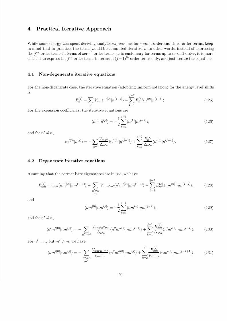
4 Practical Iterative Approach
While some energy was spent deriving analytic expressions for second-order and third-order terms, keepin mind that in practice, the terms would be computed iteratively. In other words, instead of expressingthe j th-order terms in terms of zeroth order terms, as is customary for terms up to second-order, it is moreefficient to express the j th-order terms in terms of ( j −1)th order terms only, and just iterate the equations
4.1 Non-degenerate iterative equations
For the non-degenerate case, the iterative equation (adopting uniform notation) for the energy level shiftsis
E ( j)n =n
V nnn(0)|n( j−1) − j−2k=1
E (k)n n(0)|n( j−k). (125)
For the expansion coefficients, the iterative equations are
n(0)|n( j) = −1
2
j−1k=1
n(k)|n( j−k), (126)
and for n = n,
n(0)|n( j) = −n
V nn
∆nn
n(0)|n( j−1) +
j−2k=1
E (k)n
∆nn
n(0)|n( j−k). (127)
4.2 Degenerate iterative equations
Assuming that the correct bare eigenstates are in use, we have
E ( j)nm = vnmnm(0)|nm( j−1) +n=nm
V nmnmnm(0)|nm( j−1) − j−2k=1
E (k)nmnm(0)|nm( j−k), (128)
and
nm(0)|nm( j) = −1
2
j−1k=1
nm(k)|nm( j−k), (129)
and for n = n,
nm(0)|nm( j) = −n,m
V nmnm
∆nn
nm(0)|nm( j−1) + j−1k=1
E (k)nm
∆nn
nm(0)|nm( j−k). (130)
For n = n, but m = m, we have
nm(0)|nm( j) = −n=nm
V nmnm
vnmm
nm(0)|nm( j) +
jk=2
E (k)nm
vnmm
nm(0)|nm( j−k+1) (131)
20