LUND UNIVERSITY

PO Box 117221 00 Lund+46 46-222 00 00

Time domain Green functions for the homogeneous Timoshenko beam

Folkow, Peter D.; Kristensson, Gerhard; Olsson, Peter

1996

Link to publication

Citation for published version (APA):Folkow, P. D., Kristensson, G., & Olsson, P. (1996). Time domain Green functions for the homogeneousTimoshenko beam. (Technical Report LUTEDX/(TEAT-7047)/1-19/(1996); Vol. TEAT-7047). [Publisherinformation missing].

Total number of authors:3

General rightsUnless other specific re-use rights are stated the following general rights apply:Copyright and moral rights for the publications made accessible in the public portal are retained by the authorsand/or other copyright owners and it is a condition of accessing publications that users recognise and abide by thelegal requirements associated with these rights. • Users may download and print one copy of any publication from the public portal for the purpose of private studyor research. • You may not further distribute the material or use it for any profit-making activity or commercial gain • You may freely distribute the URL identifying the publication in the public portal

Read more about Creative commons licenses: https://creativecommons.org/licenses/Take down policyIf you believe that this document breaches copyright please contact us providing details, and we will removeaccess to the work immediately and investigate your claim.

CODEN:LUTEDX/(TEAT-7047)/1-19/(1996)

Time domain Green functions for thehomogeneous Timoshenko beam

Peter D. Folkow, Gerhard Kristensson, Peter Olsson

Department of ElectroscienceElectromagnetic TheoryLund Institute of TechnologySweden

Peter D. Folkow

Division of MechanicsChalmers University of TechnologySE-412 96 GoteborgSweden

Gerhard Kristensson

Department of Electromagnetic TheoryLund Institute of TechnologyP.O. Box 118SE-221 00 LundSweden

Peter Olsson

Division of MechanicsChalmers University of TechnologySE-412 96 GoteborgSweden

Editor: Gerhard Kristenssonc© Peter D. Folkow, Gerhard Kristensson, Peter Olsson, Lund, September 24, 1996

1

Abstract

In this paper, wave splitting technique is applied to a homogeneous Timo-shenko beam. The purpose is to obtain a diagonal equation in terms of thesplit fields. These fields are calculated in the time domain from an appropri-ate set of boundary conditions. The fields along the beam are represented asa time convolution of Green functions with the excitation. The Green func-tions do not depend on the wave fields but only on the parameters of thebeam. Green functions for a Timoshenko beam are derived, and the expo-nential behaviour of these functions as well as the split modes are discussed.A transformation that extracts the exponential part is performed. Some nu-merical examples for various loads are presented and compared with resultsappearing in the literature.

1 Introduction

The usefulness of time domain techniques to solve direct and inverse scatteringproblems has been corroborated during the last decade. The mathematical toolsto solve these problems are the wave splitting, in conjunction with the invariantimbedding or the Green function technique. The wave splitting concept in thetime domain was introduced by Corones, Davison and Krueger [6, 7] in order tosolve the inverse scattering problem in acoustics. The major developments in thesolution of the inverse scattering problem using time domain techniques are foundin electromagnetics, e.g. Refs. [19, 23]. Other fields of expansive research are theelastic applications [12, 29], the viscoelastic case [3] and the fluid-saturated porousmedia [9]. Recently, the three- dimensional inverse scattering problem has beenfocused [31]. The interested reader is referred to Ref. [8] for additional referencesand for a general overview of research field.

The Green function approach to solve the inverse scattering problem was firstintroduced by Krueger and Ochs [23] for a non-dispersive second order wave equa-tion, and by Kristensson [18] in the dispersive case. A number of problems has beeninvestigated ever since, such as scattering problems for a dispersive cylinder [17],non-dispersive anisotropic media [28], dissipative stratified media [14, 15] and thethree-dimensional case [32]. During the last years, the Green function techniquehas been adopted to solve scattering problems for complex media, e.g. anisotropic,gyrotropic, bi-isotropic and non- stationary media [1, 13, 16, 20–22].

The application of the theory alluded to above to fourth order hyperbolic sys-tems, e.g. the Timoshenko beam equation [30], calls for the development of newand more extended methods. In a first paper [26], the wave splitting of this fourthorder system was developed. This paper also contains a discussion and a comparisonbetween the different equations that are frequently used in the literature to modelwave propagation in a beam, i.e. the Euler-Bernoulli, the Rayleigh, and the Timo-shenko equations. As a result, it was found that only the Timoshenko equation isa hyperbolic system, and therefore suitable as a model for propagation of transientwaves in a beam.

2

The aim of this paper is to further develop the Green function formulation asit applies to a fourth order hyperbolic system. In order to illustrate the method,some numerical results are shown. These are compared with results calculated in theLaplace domain, Refs. [4] and [25]. The advantages of performing the calculationsin the time domain are discussed.

In Section 2 the basic equations used in this paper as well as conservation ofenergy are presented. The wave splitting is introduced in Section 3, and the asymp-totic behavior of the kernels in the splitting is analyzed in Section 4. The dynamicsand the splitting are modified due to the long time behavior of the wave splitting.This analysis is presented in Section 5. The Green function equations are introducedin Section 6, and some numerical results are presented in Section 7. The paper endswith two appendices.

2 Basic equations

In [26] a time domain wave splitting of the Timoshenko equation was derived. Thestarting point in that case was a formulation of the equation in terms of the de-pendent variables {u, ψ, ∂zu, ∂zψ}. Here u(z, t) and ψ(z, t) are the mean verticaldisplacement and the mean angle of rotation of the cross section, respectively. How-ever, there is reason to modify the starting point of the splitting so as to simplifythe application of boundary conditions. Hence, instead of using the variables above,we express the Timoshenko equation in terms of {u, ψ, γ, ∂zψ}, where γ(z, t) is themean shear angle, defined as γ(z, t) = ∂zu(z, t)−ψ(z, t). Written as a spatially firstorder system, the Timoshenko equation reads

∂

∂z

uψγ

∂zψ

= D

uψγ

∂zψ

(2.1)

where

D =

0 1 1 00 0 0 1

c−21 ∂2

t 0 −∂ ln f1

∂z0

0 c−22 ∂2

t −f1/f2 −∂ ln f2

∂z

In the present paper, where a homogeneous beam with constant shape of the crosssection is studied, the operator D simplifies to

D =

0 1 1 00 0 0 1

c−21 ∂2

t 0 0 00 c−2

2 ∂2t −f1/f2 0

(2.2)

The two velocities c1 (effective shear velocity) and c2 (rod velocity) are defined by

c1 =

√k′G

ρc2 =

√E

ρ

3

while the shear stiffness f1 and the bending stiffness f2 are given by

f1 = k′GA f2 = EI (2.3)

In these equations E is Young’s modulus, G the shear modulus and ρ is the densityof the beam. I and A are the moment of inertia and the area of the cross section,respectively. We assume that

ν =E − 2G

2G0 ≤ ν <

1

2(2.4)

which amounts to saying that the material is compressible with a non-negativePoisson’s ratio. The shear coefficient k′ depends on the shape of the cross section.A relatively simple expression for this quantity is

k′ =bI

SA(2.5)

where b is the width of the beam at y = 0 and S is the static area moment of theupper half of the cross section, that is

S =

∫y≥0

y dA

However, a more accurate determination of k′ is given by Cowper [11]. These ex-pressions, based on a 3D analysis, reveal that k′ is not purely a geometrical factorbut does in fact also depend on the Poisson ratio. We refer to [11] for a comparisonbetween various theories. For future needs, we define the radius of gyration r0 anda characteristic time τ as

r0 =

√I

A=

c1

c2

√f2

f1

τ =1

2c1

(1 − c2

1

c22

) √f2

f1

We will as well have reason to refer to the non-dimensional ratio

q =c22 + c2

1

c22 − c2

1

which under the assumption in equation (2.4) satisfies

3 + k′

3 − k′ < q ≤ 2 + k′

2 − k′

2.1 Conservation of energy

The energy in a Timoshenko beam satisfies an equation of continuity. Consider ahomogeneous beam. The kinetic and potential energy density are defined as [24]

εkin =1

2

(f1

c21

(∂u

∂t

)2

+f2

c22

(∂ψ

∂t

)2)

4

εpot =1

2

(f1γ

2 + f2

(∂ψ

∂z

)2)So, we have the equation of continuity

∂

∂t(εkin + εpot) +

∂j

∂z= 0

where the power flow is given by

j = −(

f1 γ∂u

∂t+ f2

∂ψ

∂z

∂ψ

∂t

)The Timoshenko equation, while being inherently dispersive, is thus a non-dissi-pative equation which conserves the energy of the total field.

3 Wave splitting

We wish to perform a transformation that diagonalizes the Timoshenko equation fora homogeneous beam. The present formulation essentially follows [26], apart fromthe choice of dependent variables. Introduce the transformation of the dependentvariables

u+1

u+2

u−1

u−2

= P

uψγ

∂zψ

(3.1)

with formal inverse uψγ

∂zψ

= P−1

u+

1

u+2

u−1

u−2

(3.2)

The matrix P has an operator representation

P = Q

−

(λ2

2 − c−21 ∂2

t

)−λ1 Sλ2 − λ1 1

λ21 − c−2

1 ∂2t λ2 − (Sλ1 − λ2) −1

−(λ2

2 − c−21 ∂2

t

)λ1 − (Sλ2 − λ1) 1

λ21 − c−2

1 ∂2t −λ2 Sλ1 − λ2 −1

while the operator P−1 is defined as

P−1 =

1 1 1 1

−λ1 (1 − Uλ22) −λ2 (1 − Uλ2

1) λ1 (1 − Uλ22) λ2 (1 − Uλ2

1)−λ1Uλ2

2 −λ2Uλ21 λ1Uλ2

2 λ2Uλ21

λ21 − c−2

1 ∂2t λ2

2 − c−21 ∂2

t λ21 − c−2

1 ∂2t λ2

2 − c−21 ∂2

t

The various operators appearing in P and P−1 can be found in Appendix A. Theperformed change of basis turns the Timoshenko equation (2.1) into

∂

∂z

u+

1

u+2

u−1

u−2

= ∗

u+

1

u+2

u−1

u−2

(3.3)

5

where

∗ =

−λ1 0 0 00 −λ2 0 00 0 λ1 00 0 0 λ2

The operators λi are the eigenvalues of (2.2) and may be represented by

λif(t) = c−1i

∂f(t)

∂t+

(Fi (·) ∗ f (·)

)(t) i = 1, 2 (3.4)

whereupon the dynamics is written

∂u±i (z, t)

∂z= ∓

(c−1i

∂u±i (z, t)

∂t+

(Fi (·) ∗ u±

i (z, ·))(t)

)(3.5)

The u+i are thus the fields which propagate towards increasing z, i.e. right-going

fields, and u−i are the left-going fields. The star (∗) denotes time convolution, which

throughout this paper is defined by

(f(·) ∗ g(·)

)(t) =

∫ t

0

f(t′)g(t − t′) dt′

All fields are assumed quiescent at time t < 0. The kernel functions Fi(t) havecertain properties that are worth emphasizing. They can be expressed in seriesrepresentations according to [26]

F1(t) =H(t)

c2τ 2

∞∑k=1

Γ(3/2)

k!Γ(3/2 − k)(−1)k(q + 1)−kWk(t/τ)

F2(t) =H(t)

c2τ 2

∞∑k=1

Γ(3/2)

k!Γ(3/2 − k)(q − 1)−kWk(t/τ)

(3.6)

where H(t) is the Heaviside step function and Wk(ξ) are integrals of modified Besselfunctions

Wk(ξ) = ∂−k+1ξ

kIk(ξ)

ξ∂−1

ξ f(ξ) =

∫ ξ

0

f(ξ′) dξ′

For small arguments, the kernel functions may readily be expanded in a power series

Fi(t) = H(t)∞∑

k=0

ai,kt2k

However, for large arguments it is advantageous to represent (3.6) asymptotically,since Wk(ξ) are of exponential order 1/τ . We obtain

Fi(t) ≈ et/τ

∞∑k=1

bi,kt−(2k+1)/2

Schemes for computing the coefficients ai,k and bi,k are indicated in [26].

6

4 Long time behaviour

The exponential behaviour of the kernels Fi(t) is made apparent by the use of Laplace

transform techniques. Denote the transformation as LFi = Fi(s), whereupon equa-tion (3.4) turns into

Fi(s) = λi(s) − ci−1s (4.1)

The transformed eigenvalue operators are [25]

λ1,2(s) = A√

s(s±q−1

√s2 − τ−2

)1/2

A =√

q/c22(q − 1)

When studying the singularities of equation (4.1), we see that there are branchpoints according to

F1 : s = 0 s = ±1/τ

F2 : s = 0 s = ±1/τ s = ±ic1/r0

Since the inversion integral is performed along a line in the half- plane of convergence,this line must be to the right of 1/τ . Thus, the structure of (4.1) indicates thatthe kernels Fi actually are of exponential order 1/τ , see Ref. [27]. We may nowmake comments on the long time behaviour of the split modes u±

i . By analysingthe transformations, defined by (3.1) and (3.2), it turns out that the split modesincrease exponentially for all feasible combinations of the physical fields. Hence,unless an unbounded amount of energy is injected into the beam, the differentmodes must coexist in order to cancel each other for large times. It is primarily thelow frequency intervals that are affected, since these parts of the wave propagate atthe lowest speed.

5 The modified splitting and dynamics

From a numerical point of view the properties of the modes discussed above are ofcourse troublesome. It is somewhat unpleasant to deal with modes which eventuallydiverge exponentially at every point along the beam. Fortunately, a remedy isimmediately suggested by the analysis of the previous section. Since the split fieldsare of exponential order 1/τ , we extract a corresponding factor. Define

v±i (z, t) = exp(±z/ciτ − t/τ)u±

i (z, t)

These new fields are of exponential order 0. The dynamics of the v±i fields are

∂v±i (z, t)

∂z= ∓

(c−1i

∂v±i (z, t)

∂t+

(Ai (·) ∗ v±

i (z, ·))(t)

)(5.1)

where the new kernel functions Ai(t) are given as

Ai(t) = e−t/τFi(t) (5.2)

7

Gi

z z0

u (+i )z,t)(+i z0 ,tu

Figure 1: The Green function approach.

Thus, the dynamics according to (3.5) and (5.1) have the same basic structure,except that the functions in the latter are much more well behaved. Note that fromthe expressions of the Fi(t) we can infer that Ai∈L1∩L2. In conformity with (3.1),a transformation of {u, ψ, γ, ∂zψ} to the modified field v±

i is obtained by means ofa simple modification of the operator P . Define the diagonal operator matrix by E

E = e−t/τ

ez/c1τ 0 0 0

0 ez/c2τ 0 00 0 e−z/c1τ 00 0 0 e−z/c2τ

The new operator that corresponds to P is then given by R = EP with formalinverse R−1 = P−1E−1.

6 The Green functions

This section contains an analysis of the relationship between the fields in a fixed crosssection and the fields in an arbitrary position along the beam, see Figure 1. We solelystudy a homogeneous beam of infinite extension, implying that multiple reflectionsat ends are not taken into account. Therefore, it is sufficient to exclusively examinethe right-going waves, since the left-going fields can be treated in an analogousmanner.

The operator that maps the fields at a certain position to those at another crosssection has an integral representation. By placing the origin z = 0 at the fixed crosssection, we obtain (Appendix B)

u+i (z, t + z/ci) = u+

i (0, t) +(Gi(z, ·) ∗ u+

i (0, ·))(t) (6.1)

The kernels Gi(z, t) are the Green functions. Equations for the Green functions areobtained from the representation above and the dynamics (3.5). The total derivativewith respect to z of both expressions yields

dzu+i (z, t + z/ci) =

( ∂

∂zGi(z, ·) ∗ u+

i (0, ·))(t) (6.2)

dzu+i (z, t + z/ci) = −

(Fi(·) ∗ u+

i (z, z/ci + ·))(t) (6.3)

where dz = d/dz. In the right-hand side of equation (6.3), we can apply the rep-resentation according to equation (6.1). Using this relation together with (6.2), weobtain

∂

∂zGi(z, t) = −Fi(t) −

(Fi(·) ∗ Gi(z, ·)

)(t) (6.4)

8

with boundary and initial conditions

Gi(0, t) = 0 t > 0 Gi(z, t) = 0 t < 0 Gi(z, 0+) = −zFi(0+)

This integro-differential equation may be rewritten by applying Laplace transformtechniques. The transformed equation turns into an ordinary differential equation

∂

∂zGi(z, s) = −Fi(s) − Fi(s)Gi(z, s)

with formal solutionGi(z, s) = exp

(−zFi(s)

)− 1 (6.5)

Consequently, the Green functions can be expressed in a series containing repeatedconvolutions of Fi(t). However, it is convenient to proceed in another way. Bydifferentiating (6.5) with respect to s, it yields

∂

∂sGi(z, s) = −z

∂

∂sFi(s)

(Gi(z, s) + 1

)A transformation of this expression to the time domain reads

Gi(z, t) = −z

t

∫ t

0

t′Fi(t′)Gi(z, t − t′)dt′ − zFi(t) (6.6)

These Green functions equations are Volterra equations of the second kind.The analysis above is easily modified when the fields introduced in Section 5 are

concerned. Equation (6.1) turns into

v+i (z, t + z/ci) = v+

i (0, t) +(Bi(z, ·) ∗ v+

i (0, ·))(t)

The modified Green functions Bi(z, t) are defined as

Bi(z, t) = e−t/τGi(z, t)

Thus, the integro-differential equation (6.4) is written

∂

∂zBi(z, t) = −Ai(t) −

(Ai(·) ∗ Bi(z, ·)

)(t)

with Ai(t) given by (5.2).

7 Numerical verification

We intend to determine the physical fields along the beam from given boundaryconditions. This is accomplished by applying the transformations of variables inconjunction with the Green function technique. Hence, a given set of boundaryconditions are transformed to the split fields according to equation (3.1). Thesefields are mapped to a position along the beam by means of (6.1), whereupon theinverse transformation, (3.2), is performed.

9

Due to the complexity of the system, the problem is solved numerically. TheGreen functions are easily calculated from the Volterra equations (6.6). Using thetrapezoidal rule to approximate the integrals, we obtain

Gi(z, jh) = − z

2jjhFi(jh)Gi(z, 0+)

− z

j

j−1∑k=1

khFi(kh)Gi

(z, (j − k)h

)− zFi(jh) j ≥ 1

where the parameter h is the time step. It is then straightforward to tackle equation(6.1). Concerning the convolutions appearing in the operators P and P−1, we couldhave used the trapezoidal rule as well. However, a more efficient method is justifiedby the following arguments. Suppose our interest is focused on the propagating fieldsin the vicinity of the wave fronts. Since the local time coordinates originates fromthese wave fronts, the relevant results are obtained from a relatively small intervalof time. We may thus expand the functions defined in Appendix A in a power series,see Ref. [2]. When expressed in these series, the convolutions are readily performed.Given functions as

f(t) =∞∑

k=0

aktk g(t) =

∞∑k=0

bktk

the convolution reads

(f(·) ∗ g(·)

)(t) = t

∞∑k=0

cktk ck =

1

(k + 1)!

k∑j=0

ajbk−jj!(k − j)!

Repeated application of this result allows us to compute multiple convolutions in anefficient manner.

As noted in Section 6, it suffices to examine only the right-going waves. Con-sequently, we may consider a semi-infinite beam with a proper set of boundaryconditions at the left end. In order to elucidate the choice of boundary conditions,equation (3.1) is written{

u+i = Pi1u + Pi2ψ + Pi3γ + Pi4∂zψ

u−i = Pi1u − Pi2ψ − Pi3γ + Pi4∂zψ = 0

Combining the fields as u+i ± u−

i = u+i , we obtain

u+i = 2Pi1u + 2Pi4∂zψ (7.1)

u+i = 2Pi2ψ + 2Pi3γ (7.2)

In the numerical examples below, the set of boundary conditions are prescribed interms of the fields appearing in the right-hand sides of (7.1) or (7.2). The inter-pretation of these fields can be made more tangible, since the fields γ and ∂zψ arerelated to the shear force Q and the bending moment M as [24]

γ = Q/f1 ∂zψ = M/f2

10

t

v

t0 1

0

v1

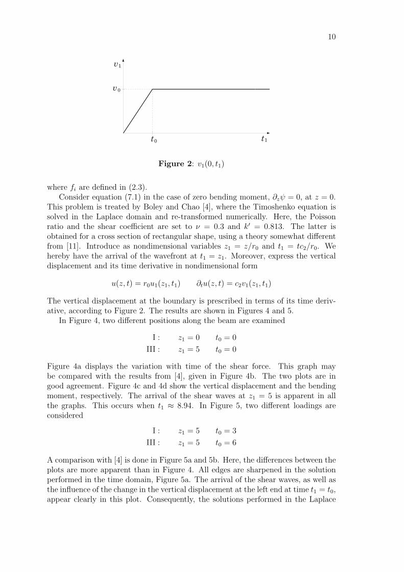
Figure 2: v1(0, t1)

where fi are defined in (2.3).Consider equation (7.1) in the case of zero bending moment, ∂zψ = 0, at z = 0.

This problem is treated by Boley and Chao [4], where the Timoshenko equation issolved in the Laplace domain and re-transformed numerically. Here, the Poissonratio and the shear coefficient are set to ν = 0.3 and k′ = 0.813. The latter isobtained for a cross section of rectangular shape, using a theory somewhat differentfrom [11]. Introduce as nondimensional variables z1 = z/r0 and t1 = tc2/r0. Wehereby have the arrival of the wavefront at t1 = z1. Moreover, express the verticaldisplacement and its time derivative in nondimensional form

u(z, t) = r0u1(z1, t1) ∂tu(z, t) = c2v1(z1, t1)

The vertical displacement at the boundary is prescribed in terms of its time deriv-ative, according to Figure 2. The results are shown in Figures 4 and 5.

In Figure 4, two different positions along the beam are examined

I : z1 = 0 t0 = 0

III : z1 = 5 t0 = 0

Figure 4a displays the variation with time of the shear force. This graph maybe compared with the results from [4], given in Figure 4b. The two plots are ingood agreement. Figure 4c and 4d show the vertical displacement and the bendingmoment, respectively. The arrival of the shear waves at z1 = 5 is apparent in allthe graphs. This occurs when t1 ≈ 8.94. In Figure 5, two different loadings areconsidered

I : z1 = 5 t0 = 3

III : z1 = 5 t0 = 6

A comparison with [4] is done in Figure 5a and 5b. Here, the differences between theplots are more apparent than in Figure 4. All edges are sharpened in the solutionperformed in the time domain, Figure 5a. The arrival of the shear waves, as well asthe influence of the change in the vertical displacement at the left end at time t1 = t0,appear clearly in this plot. Consequently, the solutions performed in the Laplace

11

t

2I

II

Q /

11.5

0

Q_

Figure 3: Q(0, t1)

domain using numerical integration show a restriction in reproducing such distinctvariations. Neither the vertical displacement nor the bending moment contain anysort of visible edges, Figure 5cd.

In the work of Miklowitz [25], boundary conditions according to equation (7.2)are considered. Here, an infinite beam is excited at its center by a suddenly appliedshear force, Q0. Therefore, the boundary conditions are ψ = 0 and Q = −Q0/2. Along-time solution using the method of stationary phase is used in [25]. The Poissonratio and the shear coefficient are set to ν = 0.3 and k′ = 2/3. The latter is obtainedfor a cross section of rectangular shape, using elementary theory (2.5). We introducea new set of nondimensional variables z1 = z/r0 and t1 = 4tc2/r0−4z1, by which thevertical displacement may be expressed u1(z1, t1) = r0u(z, t). This transformationcauses the wavefront to arrive at t1 = 0. Both a step and a rectangular pulse in theshear force is prescribed at the boundary, according to Figure 3. Figure 6 shows thefields at z1 = 1.

In Figure 6a, a modified time variable has been introduced in order to simplifycomparisons with the results from [25], Figure 6b. This is due to the fact that theshear waves are assumed to have arrived at the time marked by τ01 in Figure 6b.Since the shear waves arrive at t1 ≈ 3.9, the modified variable is set to t′1 = t1−3.65.The two plots do not resemble each other in many aspects. The main reason is theuse of a long-time solution in Figure 6b. As can be seen from the definition of thevariables, neither the time nor the space variables are very big. Figure 6c shows thatthe vertical displacement is mainly affected by the shear waves, while the bendingmoment is being influenced by the faster longitudinal waves as well, Figure 6d.

The numerical examples presented above emphasize some of the advantages whenperforming calculations in the time domain. At points where the fields changeabruptly, the resolutions using time domain solutions are generally superior to theones where calculations in the Laplace domain have been used. The inversion of theLaplace transform is a delicate task, since it is equivalent to the solution of an integralequation of the first kind [33]. Concerning the numerical implementation, the timedomain method yields very fast algorithms. Once the transformation matrices Pand P−1 defined in Section 3 and the Green functions Gi from Section 6 have beencalculated, the fields are readily determined along the beam for various boundary

12

conditions.

8 Conclusions

Wave splitting technique in conjunction with the Green function approach have beenutilised to solve the wave propagation problem in a homogeneous Timoshenko beam.The analysis is performed in the time domain, and the pertinent integro-differentialequations for the Green functions have been derived. The long time behavior of theGreen functions leads to a modification of these equations. This new set of equationsis appropriate for numerical implementations. The theory is illustrated in a seriesof numerical computations. These confirm several pleasant properties that can beexpected when working in the time domain. Transient wave propagation is treatedin a natural way using time domain techniques and the effects of rapid changes inthe propagating fields is readily visible. Since the Green functions are independentof the wave fields, the numerical implementation is performed in an efficient way forvarious boundary conditions.

Apart from being an efficient tool to solve direct problems, the major intereststowards the Green function technique concerns applications to the inverse formu-lation. Hence, the Green function approach may be extended to cover direct andinverse problems for more complicated structures, such as an inhomogeneous beamresting on a viscoelastic layer. Direct and inverse analysis of corresponding problemsare natural extensions of this paper.

Acknowledgement

The present work is supported by the Swedish Research Council for EngineeringSciences (TFR) and this is gratefully acknowledged.

Appendix A Operators appearing in P and P−1

The operators Q, U and S act as convolution operatorsQf(t) =

(Q(·) ∗ f(·)

)(t)

Uf(t) =(U(·) ∗ f(·)

)(t)

Sf(t) =c1

c2

(f(t) +

(S(·) ∗ f(·)

)(t)

)where

Q(t) =r0c2

4H(t)

∫ t/τ

0

I0(ξ) dξ

U(t) =r0c

22

c1

H(t) sin

(c1t

r0

)S(t) =

c1

r0

H(t)

∫ c1t/r0

0

J1(ξ)

ξdξ

13

0 2 4 6 8 10 12 14 16 18 20

-0.6

-0.4

-0.2

0.0

0.2

0.4

0.6

t1III

I

Q/EAv0

(a) The shear force Q. (b) The shear force Q according to [4].

0 2 4 6 8 10 12 14 16 18 20-2

2

6

10

14

18

22

t1

u1/v0

I

III

(c) The vertical displacement u1.

0 2 4 6 8 10 12 14 16 18 200.0

0.1

0.2

0.3

0.4

0.5

0.6Mr0/EIv0

t1

III

Mr0/EIv0

t1

III

(d) The bending moment M .

Figure 4: M(0, t1) = 0 and u1(0, t1) given. I : z1 = 0 and t0 = 0 III : z1 = 5 andt0 = 0.

14

0 2 4 6 8 10 12 14 16 18 20

-0.3

-0.2

-0.1

0.0

0.1

0.2

0.3

t1

III

I

-Q/EAv0

(a) The shear force Q. (b) The shear force Q according to [4].

0 2 4 6 8 10 12 14 16 18 20

-1.0

-0.5

0.0

0.5

1.0

1.5

2.0

2.5

t1

I

u1/v0

III

(c) The vertical displacement u1.

0 2 4 6 8 10 12 14 16 18 200.0

0.1

0.2

0.3

0.4

0.5

Mr0/EIv0

t1

I

III

(d) The bending moment M .

Figure 5: M(0, t1) = 0 and u1(0, t1) given. I : z1 = 5 and t0 = 3 III : z1 = 5 andt0 = 6.

15

0 1 2 3 4 5

-0.5

-0.4

-0.3

-0.2

-0.1

0.0

0.1

0.2

Q/Q0 I

II

t' 1

(a) The shear force Q. (b) The shear force Q according to [25].

0 1 2 3 4 5 6 7 80.0

0.2

0.4

0.6

0.8

1.0

I

II

t1

u1EA/Q0

(c) The vertical displacement u1.

0 1 2 3 4 5 6 7 8

-0.08

-0.04

0.00

0.04

0.08

0.12

0.16

0.20M/r0Q0

I

II

M/r0Q0

I

II

t1

(d) The bending moment M .

Figure 6: ψ(0, t1) = 0 and Q(0, t1) given. I : z1 = 1 and step shear force II :z1 = 1 and rectangular shear force of width ∆t1 = 1.5.

16

The operator Q satisfies

2Q(λ2

1 − λ22

)= 2

(λ2

1 − λ22

)Q = 1

Here, λ21 and λ2

2 can be represented asλ2

1 =1

c21

∂2

∂t2− 1

2r0c2τ− V (·)∗

λ22 =

1

c22

∂2

∂t2+

1

2r0c2τ+ V (·)∗

where the function V (t) is defined by

V (t) =1

r0c2τtH(t)I2(t/τ)

An error in the expressions for λ2i in Ref. [26] has been corrected above.

Appendix B The canonical representation

Since the differential operator in the Timoshenko equation is linear and invariantto time-translations, we may define operators Ti(z) that map the fields u+

i (0, t)to the internal fields u+

i (z, t). Introduce the canonical impulse responses U+i (z, t),

according to

δi(t)Ti(z)−→ U+

i (z, t)

where δi(t) are the Dirac delta functions. The fields u+i (0, t) are thus transformed

as

u+i (0, t)

Ti(z)−→∫ ∞

−∞u+

i (0, t′)U+i (z, t − t′)dt′ = u+

i (z, t)

according to Borel’s theorem [5]. If causality is considered, we obtain

u+i (z, t) =

∫ t+−z/ci

0−u+

i (0, t′)U+i (z, t − t′)dt′

By extracting the distribution and performing a transformation of the time coordi-nate, the former equation can be written as

u+i (z, t + z/ci) = u+

i (0, t)V +i (z, z+/ci) +

∫ t−

0+

u+i (0, t′)U+

i (z, t + z/ci − t′)dt′ (B.1)

Here, V +i (z, t) are the step function responses. The magnitudes of the steps can

easily be determined, as V +i (z, t) must satisfy the dynamics (3.5). Hence

dzV+i (z, z+/ci) = 0 =⇒ V +

i (z, z+/ci) = 1

17

since V +i (0, 0+) = 1. Defining the Green functions by Gi(z, t) = U+

i (z, t + z/ci),equation (B.1) reads

u+i (z, t + z/ci) = u+

i (0, t) +

∫ t

0

u+i (0, t′)Gi(z, t − t′)dt′

where we have prescribed the integrands to contain no distributions. So, the Greenfunctions are causal with boundary conditions according to

Gi(0, t) = 0 t > 0

This representation is of course analogous to the results when applying Duhamel’sintegral [10].

References

[1] I. Aberg, G. Kristensson, and D.J.N. Wall. Propagation of transient electro-magnetic waves in time-varying media—direct and inverse scattering problems.Inverse Problems, 11(1), 29–49, 1995.

[2] M. Abramowitz and I.A. Stegun, editors. Handbook of Mathematical Functions.Applied Mathematics Series No. 55. National Bureau of Standards, WashingtonD.C., 1970.

[3] E. Ammicht, J.P. Corones, and R.J. Krueger. Direct and inverse scattering forviscoelastic media. J. Acoust. Soc. Am., 81, 827–834, 1987.

[4] B.A. Boley and C.C. Chao. Some solutions of the Timoshenko beam equations.J. Appl. Mech., pages 579–586, December 1955.

[5] Y. Chen. Vibrations: Theoretical Methods. Addison-Wesley, Reading, 1966.

[6] J.P. Corones, M.E. Davison, and R.J. Krueger. Direct and inverse scatteringin the time domain via invariant imbedding equations. J. Acoust. Soc. Am.,74(5), 1535–1541, 1983.

[7] J.P. Corones, M.E. Davison, and R.J. Krueger. Wave splittings, invariantimbedding and inverse scattering. In A.J. Devaney, editor, Inverse Optics,pages 102–106, Bellingham, WA, 1983. Proc. SPIE 413, SPIE.

[8] J.P. Corones, G. Kristensson, P. Nelson, and D.L. Seth, editors. InvariantImbedding and Inverse Problems. SIAM, Philadelphia, 1992.

[9] J.P. Corones and Z. Sun. Transient Reflection and Transmission Problems forFluid-Saturated Porous Media. In J.P. Corones, G. Kristensson, P. Nelson, andD.L. Seth, editors, Invariant Imbedding and Inverse Problems. SIAM, 1992.

[10] R. Courant and D. Hilbert. Methods of Mathematical Physics, volume 2. In-terscience, New York, 1962.

18

[11] G.R. Cowper. The Shear Coefficient in Timoshenko’s Beam Theory. J. Appl.Mech., pages 335–340, June 1966.

[12] R.P. Dougherty. Direct and inverse scattering of classical waves at obliqueincidence to stratified media via invariant imbedding equations. PhD thesis,Iowa State University, Ames, Iowa, 1986.

[13] J. Friden, G. Kristensson, and R.D. Stewart. Transient electromagnetic wavepropagation in anisotropic dispersive media. J. Opt. Soc. Am. A, 10(12), 2618–2627, 1993.

[14] S. He. Factorization of a dissipative wave equation and the Green functionstechnique for axially symmetric fields in a stratified slab. J. Math. Phys., 33(3),953–966, 1992.

[15] S. He and A. Karlsson. Time domain Green function technique for a pointsource over a dissipative stratified half-space. Radio Science, 28(4), 513–526,1993.

[16] A. Karlsson, G. Kristensson, and H. Otterheim. Transient wave propagation ingyrotropic media. In J.P. Corones, G. Kristensson, P. Nelson, and D.L. Seth,editors, Invariant Imbedding and Inverse Problems. SIAM, 1992.

[17] K.L. Kreider. Time dependent direct and inverse electromagnetic scattering forthe dispersive cylinder. Wave Motion, 11, 427–440, 1989.

[18] G. Kristensson. Direct and inverse scattering problems in dispersive media—Green’s functions and invariant imbedding techniques. In R. Kleinman,R. Kress, and E. Martensen, editors, Direct and Inverse Boundary Value Prob-lems, Methoden und Verfahren der Mathematischen Physik, Band 37, pages105–119, Frankfurt am Main, 1991. Peter Lang.

[19] G. Kristensson and R.J. Krueger. Direct and inverse scattering in the timedomain for a dissipative wave equation. Part 2: Simultaneous reconstructionof dissipation and phase velocity profiles. J. Math. Phys., 27(6), 1683–1693,1986.

[20] G. Kristensson and S. Rikte. Scattering of transient electromagnetic wavesin reciprocal bi-isotropic media. J. Electro. Waves Applic., 6(11), 1517–1535,1992.

[21] G. Kristensson and S. Rikte. The inverse scattering problem for a homoge-neous bi-isotropic slab using transient data. In L. Paivarinta and E. Somersalo,editors, Inverse Problems in Mathematical Physics, pages 112–125. Springer,Berlin, 1993.

[22] G. Kristensson and S. Rikte. Transient wave propagation in reciprocal bi-isotropic media at oblique incidence. J. Math. Phys., 34(4), 1339–1359, 1993.

19

[23] R.J. Krueger and R.L. Ochs, Jr. A Green’s function approach to the determi-nation of internal fields. Wave Motion, 11, 525–543, 1989.

[24] L. Meirovitch. Analytical Methods in Vibrations. MacMillan, New York, 1967.

[25] J. Miklowitz. The theory of elastic waves and waveguides. North-Holland Pub-lishing Company, Amsterdam, 1978.

[26] P. Olsson and G. Kristensson. Wave splitting of the Timoshenko beam equationin the time domain. Zeitschrift fur andgewandte Mathematik und Physik, 45,866–881, 1994.

[27] A.C. Pipkin. A Course on Integral Equations. Springer-Verlag, New York,1991.

[28] R.D. Stewart. Transient electromagnetic scattering on anisotropic media. PhDthesis, Iowa State University, Ames, Iowa, 1989.

[29] Z. Sun and G. Wickham. The inversion of transient reflection data to determinesolid grain structure. Wave Motion, 18, 143–162, 1993.

[30] S.P. Timoshenko. On the correction for shear of the differential equationfor transverse vibrations of prismatic bars. Phil. Mag., XLI, 744–746, 1921.Reprinted in The Collected Papers of Stephen P. Timoshenko, McGraw-Hill,London 1953.

[31] V.H. Weston. Invariant imbedding for the wave equation in three dimensionsand the applications to the direct and inverse problems. Inverse Problems, 6,1075–1105, 1990.

[32] V.H. Weston. Invariant imbedding and wave splitting in R3: II. The Green

function approach to inverse scattering. Inverse Problems, 8, 919–947, 1992.

[33] G.M. Wing. A Primer on Integral Equations of the First Kind. SIAM, Philadel-phia, 1991.