Topic Introduction

Time-Domain Fluorescence Lifetime Imaging Microscopy:A Quantitative Method to Follow Transient Protein–ProteinInteractions in Living Cells

Sergi Padilla-Parra, Nicolas Audugé, Marc Tramier, and Maïté Coppey-Moisan

Quantitative analysis in Förster resonance energy transfer (FRET) imaging studies of protein–proteininteractions within live cells is still a challenging issue. Many cellular biology applications aim at thedetermination of the space and time variations of the relative amount of interacting fluorescentlytagged proteins occurring in cells. This relevant quantitative parameter can be, at least partially,obtained at a pixel-level resolution by using fluorescence lifetime imaging microscopy (FLIM).Indeed, fluorescence decay analysis of a two-component system (FRET and no FRET donorspecies), leads to the intrinsic FRET efficiency value (E) and the fraction of the donor-taggedprotein that undergoes FRET (fD). To simultaneously obtain fD and E values from a two-exponentialfit, data must be acquired with a high number of photons, so that the statistics are robust enough toreduce fitting ambiguities. This is a time-consuming procedure. However, when fast-FLIM acquisi-tions are used tomonitor dynamic changes in protein–protein interactions at high spatial and temporalresolutions in living cells, photon statistics and time resolution are limited. In this case, fitting proce-dures are unreliable, even for single lifetime donors. We introduce the concept of a minimal fraction ofdonor molecules involved in FRET (mfD), obtained from the mathematical minimization of fD. Here,we discuss different FLIM techniques and the compromises that must be made between precision andtime invested in acquiring FLIM measurements. We show that mfD constitutes an interesting quan-titative parameter for fast FLIM because it gives quantitative information about transient interactionsin live cells.

INTRODUCTION

During the last 40 years, Förster resonance energy transfer (FRET) has been used to understand a greatvariety of molecular interactions, both in vitro and in vivo. Advances in different photonic imagingtechniques and the development of fluorescent probes, and particularly fluorescent proteins (FPs)(Tsien 1998; Shaner et al. 2005), have made FRET microscopy an extremely useful methodology.Protein–protein interactions in living cells can be directly monitored using FRET. This aspect is criticalto improve our understanding of different processes occurring in vivo (biochemical protein cascades)and, if it is performed quantitatively, to build or to improve biological mathematical models (Tus-zynski et al. 2006). A quantitative parameter of FRET is the quantum yield of the energy transferprocess (E). Donor fluorescence lifetime decreases because of energy transfer in the excited state, andthe percentage of the decrease is equal to E. The determination of FRET efficiency by fluorescencelifetime measurements is advantageous in living cell studies because the fluorescence lifetime isindependent of the fluorophore concentration and the excitation light path—parameters that are

Adapted from Imaging: A Laboratory Manual (ed. Yuste). CSHL Press, Cold Spring Harbor, NY, USA, 2011.

© 2015 Cold Spring Harbor Laboratory PressCite this introduction as Cold Spring Harb Protoc; doi:10.1101/pdb.top086249

508

Cold Spring Harbor Laboratory Press on August 5, 2020 - Published by http://cshprotocols.cshlp.org/Downloaded from

unknown in cells under the microscope. Other quantitative FRET techniques based on steady-stateintensity allow determination of the apparent FRET efficiency, Eapp (Gordon et al. 1998; Hoppe et al.2002; Berney and Danuser 2003; Elangovan et al. 2003; Stockholm et al. 2004; van Rheenen et al. 2004;Zal and Gascoigne 2004; Wlodarczyk et al. 2008). Eapp depends directly on the product of twoparameters: the intrinsic FRET efficiency value (E) and the fraction of the donor that undergoesFRET (fD) (Hoppe et al. 2002). Steady-state intensity-based approaches are not able to obtain fD out ofEapp (Neher and Neher 2004). To determine fD, the intrinsic FRET efficiency (E) must be calculatedindependently. Fluorescence lifetime imaging microscopy (FLIM) is a well-established technique todetermine the fluorescence kinetics of the donor emission for FRET measurements (Verveer et al.2000; Emiliani et al. 2003; Peter et al. 2005). In FLIM, using the mean lifetime does not require a highnumber of measured photons. However, to simultaneously obtain fD and E values from the fit,fluorescence decay analysis must be performed with two or more components, and data have to beacquired with the highest number of photon counts so that statistics are robust enough to reducefitting ambiguities. Using time-correlated single-photon counting (TCSPC), a high temporal resolu-tion of the fluorescence kinetics (few tens of picoseconds) can be achieved. Several minutes of dataacquisition are necessary, however, to obtain sufficient photon statistics per pixel. Such long acqui-sition times are incompatible with high spatiotemporal resolution of quantitative FRET images. Afast-gated charge-coupled device (CCD) camera combined with a pulsed, wide-field, or pseudowide-field excitation (TriM-FLIM system) can be used to acquire fluorescence decays faster than with theTCSPC method but at the expense of a smaller temporal resolution. To acquire images as fast aspossible, a small number of time-gated images together with a low value of photon counts arerequired. Note, however, that under these conditions, the quality of a double-exponential fit is farfrom optimal. However, if we consider a two-component system with a narrow distribution of E, theconcept of a minimal percentage of donor molecule involved in FRET (mfD) can be calculated withoutfitting directly from the mean fluorescence lifetime of the donor (in the absence and in the presence ofthe acceptor). mfD is an interesting approach because it provides information about a known thresh-old of interacting donor protein and is related to the relative concentration of the interacting protein.

PRINCIPLES OF FRET QUANTIFICATION BY TIME-DOMAIN FLIM

Theory of FRET

FRET (or, more correctly, Förster-type resonance energy transfer; Förster 1948) is a nonradiativeprocess that occurs between the excited state of a donor and the ground state of an acceptor.

The Transfer Rate

The rate of energy transfer (kt[r]) from the donor to the acceptor is defined by the following equations(Valeur 2002; Lakowicz 2006):

kt(r) = 1/tD(R60/r

6), (1)

where R0 is the Förster radius, r is the distance between donor and acceptor, and tD is fluorescencelifetime of the donor in the absence of the acceptor. Because the Förster radius is defined as thedistance at which FRET is 50% efficient, if R0 = r, the rate transfer will be the same as the decay rateof the donor. R0 can be defined as

R0 = 0.211· [k2n−4QDJ]1/6(Å), (2)

with

J = �1A(l)· fD(l)·l4· dl/ � fD(l)· dl, (3)

Cite this introduction as Cold Spring Harb Protoc; doi:10.1101/pdb.top086249 509

Time-Domain FLIM

Cold Spring Harbor Laboratory Press on August 5, 2020 - Published by http://cshprotocols.cshlp.org/Downloaded from

and κ2 is derived from

k2 = (cos u− 3 cos uD cos uA)2, (4)

where n is the refractive index, QD is the fluorescence quantum yield of the donor, κ is the parameterrelated to the orientation of donor and acceptor (Dale et al. 1979; Cheung 1991), εA(λ) is the acceptorabsorption spectrum, and fD(λ) is the donor emission spectrum. Note that θ is the angle betweenthe emission transition dipole of the donor and the absorption transition dipole of the acceptor, andθD and θA are the angles between the two dipoles and the vector that goes from the donor to theacceptor (Lakowicz 2006). Förster distances are reported in literature for a value of κ2 = 2/3.

The Efficiency of Energy Transfer

We can define the efficiency by calculating the proportion of photons absorbed in the donor versus theexcitation transferred to the acceptor:

E = kT/ kT + kD( ), (5)

where kD is the sum of all of the relaxation pathways (Fig. 1) of the excited donor other than FRET.Experimentally, the transfer efficiency is calculated by using the lifetime of the donor alone or in

the presence of the acceptor, applying a lifetime methodology:

E = 1− tFtD

, (6)

in which tF and tD are the lifetimes of the donor in the presence of the acceptor and the donor alone,respectively. Observe that tF and tD are defined on the basis of the following rate constants:

tF = 1

kr + knr + kT, (7)

tD = 1

kr + knr. (8)

Fluorescence Decay of the Donor

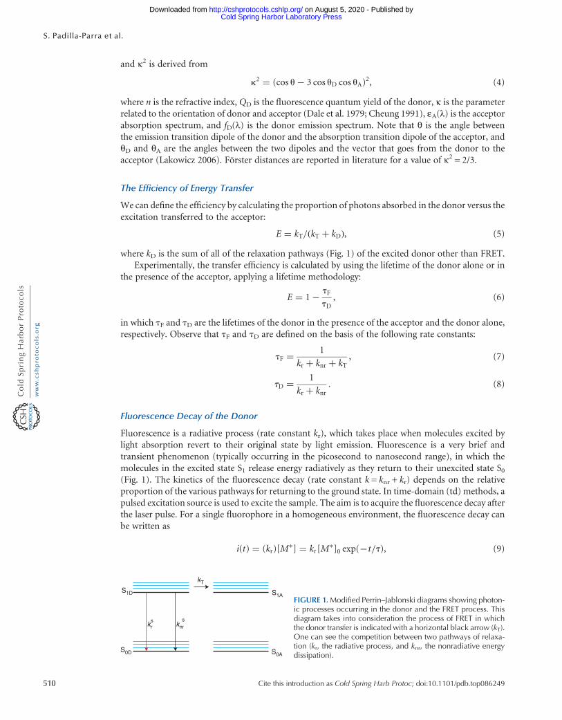
Fluorescence is a radiative process (rate constant kr), which takes place when molecules excited bylight absorption revert to their original state by light emission. Fluorescence is a very brief andtransient phenomenon (typically occurring in the picosecond to nanosecond range), in which themolecules in the excited state S1 release energy radiatively as they return to their unexcited state S0(Fig. 1). The kinetics of the fluorescence decay (rate constant k = knr + kr) depends on the relativeproportion of the various pathways for returning to the ground state. In time-domain (td) methods, apulsed excitation source is used to excite the sample. The aim is to acquire the fluorescence decay afterthe laser pulse. For a single fluorophore in a homogeneous environment, the fluorescence decay canbe written as

i(t) = (kr)[M∗] = kr [M

∗]0 exp(−t/t), (9)

S1D S1A

S0A

kT

S0D

krs

knrs

FIGURE 1.Modified Perrin–Jablonski diagrams showing photon-ic processes occurring in the donor and the FRET process. Thisdiagram takes into consideration the process of FRET in whichthe donor transfer is indicated with a horizontal black arrow (kT).One can see the competition between two pathways of relaxa-tion (kr, the radiative process, and knr, the nonradiative energydissipation).

510 Cite this introduction as Cold Spring Harb Protoc; doi:10.1101/pdb.top086249

S. Padilla-Parra et al.

Cold Spring Harbor Laboratory Press on August 5, 2020 - Published by http://cshprotocols.cshlp.org/Downloaded from

where [M*] is the concentration of molecules in the excited state and t is the lifetime of theexcited state. Equation 9 defines the fluorescence decay profile of the donor in the absence of theacceptor.

Now, if we consider a donor–acceptor interaction in which not all of the donor is engaged in theprocess of FRET, then

i(t) = (kr)[M∗] = kr([D]0 exp(−t/tD)+ [DA]0 exp(−t/tF)) (10)

applies. In the above expression, the process of energy transfer is taken into account, and a discretedouble exponential describes the fluorescence decay of the donor in the presence of the acceptor.Equation 10 assumes that there is only one orientation that enables the energy transfer to occur. If wenormalize the amplitudes of both preexponential factors to 1, we can introduce the concept of thefraction of the interacting donor (fD), and the last equation simplifies to

i(t) = (1−fD) exp(−t/tD)+ fD( )

exp(−t/tF), (11)

where fD is a parameter that is particularly interesting in the study of the interactions of a relatedprotein in cellular biology. td-FLIM allows for the simultaneous calculation of the fluorescencelifetime of the donor and the other important parameters that describe the fluorescence decay(preexponential factors and, hence, fD) pixel by pixel. This makes this technique extremely usefulbecause it retrieves information about the location and the extent of the interaction under study.

Time-Domain Picosecond FLIM: TCSPC-FLIM

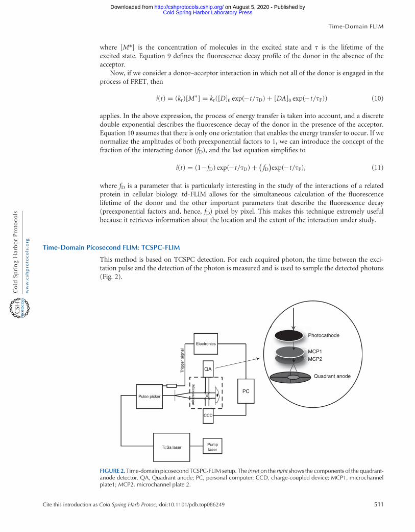
This method is based on TCSPC detection. For each acquired photon, the time between the exci-tation pulse and the detection of the photon is measured and is used to sample the detected photons(Fig. 2).

MCP1

MCP2

PC

CCD

Pulse picker

Ti:Sa laserPumplaser

Electronics

Trig

ger

sign

al

Microscope

Quadrant anode

Photocathode

QA

FIGURE 2. Time-domain picosecond TCSPC-FLIM setup. The inset on the right shows the components of the quadrant-anode detector. QA, Quadrant anode; PC, personal computer; CCD, charge-coupled device; MCP1, microchannelplate1; MCP2, microchannel plate 2.

Cite this introduction as Cold Spring Harb Protoc; doi:10.1101/pdb.top086249 511

Time-Domain FLIM

Cold Spring Harbor Laboratory Press on August 5, 2020 - Published by http://cshprotocols.cshlp.org/Downloaded from

Excitation:Mode-locked titanium:sapphire lasers can deliver picosecond (1 psec) or femtosecond(100 fsec) pulses and can be tuned between 760 and 980 nm. They can be used for two-photonexcitation or for one-photon excitation after frequency doubling. Pulsed laser diodes (1 psec) arenow also available for one-photon excitation at 440, 470, and 635 nm and longer wavelengths.Another option for pulsed excitation is supercontinuum sources.

Microscope and detection: Conventional confocal microscopes have an external port to couplean infrared or visible-light pulsed laser. The laser beam is scanned through the sample, and thesingle photons are detected by a photomultiplier tube with a time resolution corresponding to 10psec. Avalanche photodiodes are also used because they are more sensitive in the red part of thespectrum; however, they provide a lower time resolution for the corresponding fluorescence decay.A computer card (e.g., Becker & Hickl GmbH or Picoquant GmbH) integrates delay time measure-ments (between emitted photons and excitation pulses) and scan position. Wide-field microscopycan also be used (an approach usually used in our laboratory). In this case, the laser beam of atitanium:sapphire laser (after passing through a frequency doubler and a pulse picker, which providea reduced repetition rate of 4 MHz) is coupled to an inverted microscope. A quadrant-anode detector(Europhoton GmbH) provides information relative to the temporal and spatial correlation timesof each single photon counted. Fluorescence decays are acquired by counting and sampling singleemitted photons according to both the time delay between their arrival and the laser pulse and theirx–y coordinates.

Note that TCSPC is a statistical method that requires high photon counts to analyze the fluores-cence decay: The faster the count rate, the lower the acquisition time. The detector count rate is thelimiting step for the acquisition time. Indeed, in the case of two photons emitted in a very short time(high intensity of the laser), only the first one will be processed, which will induce artificially fasterfluorescence kinetics (shorter lifetime). The benefit of using a very low excitation intensity level(currently 20 nW at the sample) is to avoid photobleaching and/or photoconversion of the FPs(Tramier et al. 2006). Moreover, because of the high sensitivity, very dim cells can be analyzed,avoiding undesirable overexpression effects. Using a high-numerical-aperture (high-NA) 60× objec-tive, a typical acquisition of an enhanced green FP (eGFP)-labeled cell takes �2–3 min.

Multiphoton Multifocal FLIM: TriM-FLIM

The objective of multifocal multiphoton FLIM (TriM-FLIM) is to combine pseudowide-fieldpulsed excitation (here in two-photon excitation) and a fast-gated CCD camera (Fig. 3; for an ex-ample of an application of two-photon FLIM see also Imaging Intracellular Signaling UsingTwo-Photon Fluorescent Lifetime Imaging Microscopy [Yasuda 2012]). The principle is to openthe intensifier in front of the camera for short times (during the fluorescence decay) after the laserpulse.

Excitation: The excitation source for the TriM-FLIM is a femtosecond-pulsed mode-locked Ti:sapphire laser (Spectra-Physics, France) that is tunable from 700 to 950 nm. The laser is directed intothe TriMScope (LaVision Biotec GmbH) box, which contains a 50/50 beam splitter and mirrors todivide the incoming laser into from 2 to 64 beams. The set of beams passes through a 2000 Hz scannerbefore illuminating the back aperture of a 60×NA 1.2 infrared water-immersion objective (Olympus).A line of foci is then created at the focal plane, which can be scanned across the sample, producingpseudowide-field illumination.

Detection: A filter wheel of different spectral filters is used to select the fluorescence imaged onto afast-gated light intensifier connected to a CCD camera (PicoStar, LaVision Biotec GmbH). The gate ofthe intensifier (adjusted to 1 or 2 nsec, depending on the experiment) is triggered by an electronicsignal coming from the laser and a programmable delay box, which together are used to acquire a stackof time-correlated images. The number of gates and their time width determine the time resolution ofthe fluorescence kinetics. The acquisition time for each gate determines the signal-to-noise ratio. Thetime-correlated gated images are acquired sequentially. Thus, use caution to avoid photobleachingduring acquisition, which can artificially shorten the fluorescence decay.

512 Cite this introduction as Cold Spring Harb Protoc; doi:10.1101/pdb.top086249

S. Padilla-Parra et al.

Cold Spring Harbor Laboratory Press on August 5, 2020 - Published by http://cshprotocols.cshlp.org/Downloaded from

ANALYSIS OF THE FLUORESCENCE DECAYS OF THE DONOR

The biological information that can be obtained from the fluorescence decay depends on the analysisthat is performed. Mainly, the fluorescence decay can be fitted with different models (one or twodiscrete exponentials or more complex models) or the mean fluorescence lifetime t can be obtainedwithout fitting procedures to obtain raw FLIM data. If, in either case, FRET is detected, the biologicalinformation will be different in terms of quantification and spatial and temporal resolutions. Toobtain quantitative measurements about the fraction of donor molecules interacting with the accep-tor, it is necessary to perform a fit of the donor fluorescence decay obtained with a high signal-to-noiseratio, and hence a high photon count, using a two-exponential model. This fitting process requires anacquisition method, which is time consuming (TCSPC method) and impedes the measurement oftransient interactions at high spatial resolution. A compromise can be found by using a fast-gatedCCD, exploiting the mean fluorescence lifetime of the donor by calculating the minimal fraction ofinteracting donor mfD pixel by pixel. Interestingly, the mfD spatiotemporal variations within a singlecell are similar to those of fD obtained from the fit of the fluorescence decay using a double-expo-nential model (Padilla-Parra et al. 2008).

PC

CL2

CCD

CL1

Gated opticalintensifier

Delay generator

Pic

osta

rFFW

TL2

DM

z piezo

x–y stage

OL

Ti:sapphirefs laser

PD

Trigger signal

Beam splitterand mirrors

Mic

rosc

ope

TriM

Sco

pe

TL1 Shutter

Scanningmirrors

FIGURE 3. Time-domain TriM-FLIM setup for fast acquisitions. PD, photodiode; OL, objective lens; DM, dichroicmirror; TL1, transfer lens 1; TL2, transfer lens 2; FFW, fast filter wheel; CL1, camera lens 1; CL2, camera lens 2; CCD,charge-coupled device; PC, personal computer.

Cite this introduction as Cold Spring Harb Protoc; doi:10.1101/pdb.top086249 513

Time-Domain FLIM

Cold Spring Harbor Laboratory Press on August 5, 2020 - Published by http://cshprotocols.cshlp.org/Downloaded from

Fitting Data from a TCSPC-FLIM System

The fluorescence decay obtained by using the TCSPCmethod shows a high photon count (binning thepixels over large area) with picosecond time resolution. The least-squaresmethod is a valid way to findmechanistic parameters of the system, such as the fluorescence lifetimes and amplitudes, by usingGlobals (University of California at Irvine) with a Levenberg–Marquardt algorithm (LMA). NonlinearLMA for parameter estimation should take into consideration the following hypotheses: (i) Datauncertainties should be related to the fluorescence intensity (photon counts); (ii) fluorescence inten-sity uncertainties should be Gaussian distributed; (iii) there should not be systematic uncertaintiesrelated to all data; (iv) the model used (single exponential [in the case of eGFP alone expressed in livecells]; double exponential, stretched exponential, or Gaussian exponential in all cases) should be agood description of the experimental data; and (v) enough photon counts should be acquired toobtain a good fit.

Among the different models that can be applied to describe the fluorescence intensity decayprofile of a related fluorophore, we use a two-species model in which two populations are takeninto consideration (an interacting fraction corresponding to a population that relaxes throughFRET (fD) and a noninteracting fraction in which the donor lifetime remains undisturbed[1 – fD]). The donor lifetime obtained out of the single-exponential fit from cells expressing thedonor alone is assigned and is fixed into the noninteracting fraction of the double-exponentialmodel in the corresponding cotransfected cell in which a given protein interaction is under study(Emiliani et al. 2003),

i(t) = (1− fD)e−t/tD + fDe

−t/tF , (12)

where fD stands for the fraction of the interacting donor, tD is the fixed donor lifetime, and tF is thediscrete FRET lifetime. In this type of analysis, the total intensity (I0) is normalized to 1; and, therefore,both preexponential factors, and particularly fD, vary from 0 to 1. As an example, Figure 4 depicts thefluorescence decay of eGFP fused to the double bromodomain ([BD]-eGFP) of the transcriptionfactor TAFIID 250, together with the corresponding fits (black line) expressed in a live HeLa cell(green line) in the absence (Fig. 4A) and the presence (Fig. 4B) of mCherry fused to histone H4(mCherry-H4).

10

0

–10

Residues

10

0

–10

Residues

1

102

Pho

ton

num

ber

104

1

102

Pho

ton

num

ber

104

A B

0 4 8

Time (nsec)

120 4 8Time (nsec)

12

FIGURE 4. eGFP–BD interaction with acetylated mCherry-H4 in the nucleus of HEK293 live cells using the TCSPCmethod. (A) Steady-state intensity image of eGFP-BD expressed alone in HEK293 cells (green). The correspondingeGFP-BD fluorescence decay (green curve) extracted from the whole nucleus is fitted by a single exponential(black line, tD = 2.59 nsec), and the residues are presented (blue curve). (B) Steady-state intensity images of eGFP-BD (green) and mCherry-H4 (red) coexpressed in HEK293 cells. The corresponding eGFP-BD fluorescence decay(green curve) extracted from the whole nucleus is fitted by a single model (t = 2.46 nsec) and by a biexponentialmodel (tD = 2.59 nsec fixed and tF = 0.65 nsec) and residues are presented (blue curve and red curve, respec-tively). Note that the fluorescence decay is better fitted with a biexponential model as shown by residues. Scalebar, 2 µm.

514 Cite this introduction as Cold Spring Harb Protoc; doi:10.1101/pdb.top086249

S. Padilla-Parra et al.

Cold Spring Harbor Laboratory Press on August 5, 2020 - Published by http://cshprotocols.cshlp.org/Downloaded from

Data Treatment Coming from the TriM-FLIM System

With the TriM-FLIM system, themean fluorescence lifetime is determined for each pixel of the image.Considering a fluorescence decay i(t), the mean fluorescence (t) is defined as

,t. = �t· i t( )· dt/ � i t( )· dt, (13)

in which t is the time. To analyze data coming from a discrete sampling, the mean lifetime is directlycalculated by applying Equation 13. For a time-gated stack of images, we have

,t. = SDti· Ii/SIi, (14)

where Δti corresponds to the time delay after the laser pulse of the ith image acquired and Ii corre-sponds to the pixel intensity map in the ith image (Fig. 5). The map of the mean fluorescence lifetimecan be calculated and displayed.

If enough time-gated images are acquired (up to 11), the fluorescence decay can be fitted with anLMA, applying, for example, a discrete two-exponential model as in the case of the TCSPC method,and tD and tF will be determined together with fD.

The fraction of donor that is involved in FRET can be calculated directly from the mean lifetime ofthe donor tD and tF:

t = [(1− fD)· (t2D + fD· t2F]/[(1− fD)· tD + fD· tF]. (15)

Isolating fD and normalizing the last expression by dividing by tD, we find an expression that accountsfor the fraction of interacting donor:

fD = [1−(,t./tD)]/[1−(t/tD)−(tF/tD)2 + (t/tD)·(tF/tD)]. (16)

Maps of t and of fD (assuming the same tF value for each pixel) are obtained as shown in Figure 6,in which the interaction between BD-eGFP andmCherry-H4 is visualized in the nucleus of living cellsby the decrease of the fluorescence lifetime of eGFP-BD compared with that of eGFP-BD in theabsence of mCherry-H4 (monotransfected cells, the mean lifetime averaged throughout the nucleusdecreased from 2.41 nsec for the control to 2.34 nsec for the cotransfection). The fraction of eGFP-BDinteracting with mCherry-H4 can be determined and mapped within the nucleus.

The Minimal Fraction of Interacting Donor

The minimal fraction of interacting donor,mfD (Padilla-Parra et al. 2008), is calculated directly fromthe values of the mean fluorescence lifetime of the donor in the absence and in the presence ofthe acceptor.

Mathematically, fD depends on two variables (tF and t) and can be minimized following tF:

m fD = [1− (t/tD)]/[(t/2· tD)−1]2. (17)

I0

Δt

t

FIGURE 5. Cartoon representing a sequential acquisitionof images from the time-domain TriM-FLIM setup.

Cite this introduction as Cold Spring Harb Protoc; doi:10.1101/pdb.top086249 515

Time-Domain FLIM

Cold Spring Harbor Laboratory Press on August 5, 2020 - Published by http://cshprotocols.cshlp.org/Downloaded from

mfD provides instantaneous knowledge about the minimal extent of the interaction under study. Thisis particularly relevant in biology because, without knowing the intrinsic transfer efficiency (becausemfD does not require previous knowledge of tF), quantitative data related to the relative concentrationare immediately at hand.

The impact of fast acquisitions of fD and mfD with the same biological example (eGFP-BD andmCherry-H4) was investigated by using the TriM-FLIM system (Fig. 7). On the same cells, twowindowing schemes were chosen, one using only five time-gated images (2 nsec gate width) forvery fast acquisition times (�3 sec) and the other using 11 time-gated images (1 nsec gate width)for longer acquisition times (�30 sec).

fD was calculated from the value of tF determined from the biexponential fit of the fluorescencedecay of the donor in the presence of the acceptor from the stack of 11 time-gated images (tF = 0.65 ±0.59 nsec, n = 33). The donor lifetime was fixed to tD = 2.40 nsec, coming from the monoexponentialfit of the donor alone. A 3D representation of both fD andmfD images using a threshold limit given bythe control is included to reveal the differences between control and FRET images (Fig. 7). Both fD andmfD images are very similar and present the same pattern when FRET occurs with a very close meanvalue of fD (0.13) andmfD (0.11). The two histograms are also superimposed in Figure 7 (right panel).The underestimation of the amount of donor that undergoes FRET when taking mfD relative to fD isonly 15% in this example.

Number of Interacting Particles and Relative Concentration

When we are interested in following the spatiotemporal changes of a highly localized protein, it isconvenient to use a different approach related to the relative concentration: the number of interactingparticles (NP). Assuming a two-species model and single-exponential behavior of the donor, fluo-rescence intensity as a function of time can be defined as

i(t) = I0 fD· e−t/tF + I0(1− fD)· e−t/tD , (18)

where I0 is the fluorescence intensity at time 0. All of the other parameters have already been defined.Note that here, i(t) is not normalized to 1, and its amplitude corresponds to the relative concentrationof fluorophores:

i t( ) = kr([DA]· e−t/tF + [D]· e−t/tD), (19)

IntensityA B

Cot

rans

fect

ed

Num

ber

of p

ixel

s

Con

trol

Lifetime

1.9 2.9

80

40

02.0 2.4

Lifetime (nsec)

2.2 2.6 2.8

FIGURE 6. Intensity and FLIM images of eGFP-BD expressed alone as the control or with mCherry-H4 as the cotrans-fection in HEK293 live cells using a TriM-FLIM system and 11 time-gated images. (A) Intensity images were obtainedby summing the time-gated stack. FLIM images were obtained by using Equation 14 in a pixel-by-pixel manner. Whitearrows show two chromatin domains in which eGFP-BD mean lifetime decreases significantly. (B) Histograms of themean fluorescence lifetime for the control (black line) and the cotransfected cell (red line). Themean lifetime averagedthroughout the nucleus decreased from 2.41 nsec for the control to 2.34 nsec for the cotransfection. Scale bar, 2 µm.

516 Cite this introduction as Cold Spring Harb Protoc; doi:10.1101/pdb.top086249

S. Padilla-Parra et al.

Cold Spring Harbor Laboratory Press on August 5, 2020 - Published by http://cshprotocols.cshlp.org/Downloaded from

where kr is the rate constant of the radiative process, [DA] is the concentration of the interactingcomplex, and [D] is the concentration of the noninteracting donor population. In Equation 19, [DA]is proportional to (I0 × fD). Note that we can approximate fD by using the mfD image and I0 by usingthe corresponding first gated image. We present a biological example corresponding to the activationof Rac followed by FRET occurring between eGFP-Rac and PBD-mCherry (which is the bindingdomain of an effector of Rac fused to mCherry) and applying the number of particles in Figure 8 (seeonlineMovie 1 at cshprotocols.cshlp.org, which shows a time lapse of the spatiotemporal activation ofRac [relative NP =mfD × I0], and online Movie 2 at cshprotocols.cshlp.org, which shows a time lapseof the corresponding eGFP-Rac fluorescence intensity).

PRACTICAL CONSIDERATIONS

Limitations and Use of mfD

The use of mfD described here is applicable if we consider a two-component system, the unbounddonor and donor involved in FRETwith the acceptor with a narrow distribution of E. Although one ofthe constraints mentioned above deals with the single-exponential behavior of the donor (e.g., eGFP),the mfD concept can be extended to multiexponential donors, such as cyan FP (CFP) (Padilla-Parraet al. 2008).

Choice of the Best FRET Couple

The most important characteristics of good FRET–FLIM donors are that (i) their fluorescence decayprofile must be fit best with a single-exponential model, (ii) their fluorescence intensity as a function

0 0.5 0 0.5

0.5

0.2

0.5

0.2

30

20

10N

umbe

r of

pix

els

00

fD & mfD

mfDfD

fDfD

0.5

0.2

0.5

0.2

mfD

mfD

0.1 0.2 0.3 0.4

FIGURE 7. (Top) fD and mfD images obtained by using Equation 16 (with tD = 2.41 nsec and tF = 0.65 nsec) andEquation 17 (with tD = 2.41 nsec), respectively. Three-dimensional representation of the corresponding fD and mfDimages using a threshold limit given by the control (0.2) are also presented. (Bottom) The comparison between thehistogram coming from fD andmfD clearly show that, for this example, both values behave similarly for all pixels of theimage. Note that this is the same cell showed in Figure 6 and the dimensions of the micrograph are 12 × 12 µm.

Cite this introduction as Cold Spring Harb Protoc; doi:10.1101/pdb.top086249 517

Time-Domain FLIM

Cold Spring Harbor Laboratory Press on August 5, 2020 - Published by http://cshprotocols.cshlp.org/Downloaded from

of time should remain constant under different illumination conditions (i.e., they have good photo-stability), and (iii) they should not be susceptible to undergoing photoconversion.

mTFP1 is a monomeric cyan protein whose fluorescence decay is best described with a single-exponential model (Ai et al. 2006; Padilla-Parra et al. 2009) as is eGFP (Tramier et al. 2006). DifferentFRET pairs were tested by linking two different FPs with a polypeptide chain (tandem). By usingTCSPC-FLIM, we compared different tandems (Table 1). The relatively low fD percentages couldcome from a possible spectroscopic heterogeneity of the acceptor population, which is partially causedby different maturation rates for the donor and the acceptor (Padilla-Parra et al. 2009).

The usefulness of mTFP1-enhanced yellow FP (eYFP) as a FRET couple is supported by thetwofold increase of the minimal fraction of interacting histone H4 with the double BD of TAFII250, when using mTFP1-H4/eYFP-BD instead of eGFP-H4/mCherry-BD using the TriM-FLIM(Fig. 9). Note that mTFP1 is fairly resistant to photobleaching. However, attention should be paidto the effect of photobleaching when performing time-lapse TriM-FLIM acquisition with fusionproteins using mTFP1 in biological systems in which the proteins are highly immobile, as is thecase for histone H4 incorporated into chromatin.

Effect of Photobleaching on FRET Determination: False FRET Signals

The existence of photobleaching and/or photoconversion before or during the acquisition can inducefalse-positive FRET determination. In steady-state measurements, especially with the CFP/YFP

300

300

t = 180 sec

Inte

nsity

(I 0)

t = 195 sec t = 210 sec t = 225 sec

300

90300

90

np 90

Threshold given by the negative control

90

FIGURE 8. Time lapse of Rac activation followed by fast FLIM. A cotransfected cell with eGFP-Rac and Pbd-mCherryshows a transient activation localized preferentially in subcellular domains at the periphery of the cell. (Top) The firsttime-gated intensity image of a sequential acquisition of five time-gated images (2 nsec each) is presented (see onlineMovie 2 at cshprotocols.cshlp.org). (Bottom) The corresponding NP images are shown with a threshold given by thenegative control (eGFP-Rac expressed alone coming from a cell with the same signal-to-noise ratio) (see onlineMovie 1 at cshprotocols.cshlp.org). The NP is determined by the product of the first gated image and the mfDvalue, as described in the text. The Rac activation (bottom) is independent of the eGFP-Rac fluorescence intensity(top). The dimensions of the micrograph are 16 × 15 µm.

TABLE 1. Intrinsic FRET efficiency (E) and the fraction of interacting donor (fD) for a set of different tandemconstructsusing a two-species model with a double-exponential model fixing the donor to a previously calculated value N = 5

Tandem fD E

mRFP1-eGFP 0.26 ± 0.08 0.56 ± 0.02mStrawberry-eGFP 0.37 ± 0.07 0.58 ± 0.02mCherry-eGFP 0.45 ± 0.02 0.58 ± 0.03mTFP1-mOrange 0.37 ± 0.01 0.68 ± 0.02mTFP1-eYFP 0.71 ± 0.01 0.61 ± 0.08

RFP, red fluorescent protein; eGFP, enhanced green fluorescent protein; eYFP, enhanced yellow fluorescent protein.

518 Cite this introduction as Cold Spring Harb Protoc; doi:10.1101/pdb.top086249

S. Padilla-Parra et al.

Cold Spring Harbor Laboratory Press on August 5, 2020 - Published by http://cshprotocols.cshlp.org/Downloaded from

(yellow fluorescent protein) couple, donor photobleaching (CFP is more sensitive to excitation lightthan YFP) or photoconversion of YFP into a CFP-like species (with the acceptor photobleachingmethod) results in a ratio of CFP and YFP intensity similar to what can be obtained in a FRETsituation (Valentin et al. 2006). The excitation light intensity is much lower with the TCSPCmethod; and thus this method is less prone to photobleaching. However, photobleaching canoccur before the acquisition when observing and choosing the cells. Importantly, when using fastacquisitions (e.g., TriM-FLIM or any other sequential method for the fluorescence lifetime measure-ment; Grant et al. 2007), the occurrence of photobleaching on single-exponential fluorophores duringthe acquisition of FLIM has a drastic effect on the mean fluorescence lifetime, which is not the casewith TCSPC (Tramier et al. 2006; Padilla-Parra et al. 2009). When acquiring images very quickly (e.g.,by taking five time-gated images), if photobleaching occurs, the intensity of the fifth image can be tooweak to have a significant value. This phenomenon shortens the mean lifetime determination as in theFRET situation, causing a bias in the interpretation of results.

Reasons for the Absence of a FRET Signal

The occurrence of FRET with a particular FP couple relies on the close proximity of the donor and theacceptor (R < 80 Å) and on the correct orientation of their dipoles (they cannot be perpendicular toeach other). In addition to these basic requirements, FRET cannot be detected in certain situationseven if the corresponding endogenous proteins interact to some extent. The classic reason for theabsence of FRET is the localization of the fluorescent tag to a position of the protein sequence thatimpedes the interaction with its partners. More often encountered is the situation in which theamount of interacting donor per pixel is very weak in front of the noninteracting donor; therefore,it is difficult to get a significant FRET signal. We observe this situation, for example, in polymericprotein structures, such as actin filaments or microtubules. Hetero-FRET detection arises from theclose proximity of a donor-tagged and an acceptor-tagged monomer within the polymer. The occur-rence of this situation is statistically weak, and no FRET is detected. A related situation, in which it isdifficult to unveil FRET, occurs when the interactions between the proteins of interest are transient

0.1

1

0.1

1

80

A B

mTFP1-H4+BD-YFP mfD

GFP-H4+BD-mCherry

70

60

50

4030

20

10

00–0.2–0.3 –0.1 0.1 0.2 0.3 0.4 0.5

Num

ber

of p

ixel

s

mfD

mfD

mfD

FIGURE 9. mfD comparison between the FRET couples mTFP1/eYFP and eGFP/mCherry from fast-FLIM acquisitions.(A) Three-dimensional maps of mfD for mTFP1-H4 coexpressed with eYFP-BD (upper panel) and eGFP-H4 coex-pressedwith mCherry-BD (lower panel). (B) The overlappingmfD distribution for both examples is shown as well as thehigher average mfD for the mTFP-H4+ eYFP-BD couple. The dimensions of both micrographs are 14 × 14 µm.

Cite this introduction as Cold Spring Harb Protoc; doi:10.1101/pdb.top086249 519

Time-Domain FLIM

Cold Spring Harbor Laboratory Press on August 5, 2020 - Published by http://cshprotocols.cshlp.org/Downloaded from

and subject to spatiotemporal fluctuations, as we saw in the examples above. In this situation, fasttime-lapse FLIM has to be performed to avoid the average of the FRET signals in space and time. Theexistence of a big proportion of immature red acceptor (up to 60%) artificially decreases the amountof bound donor. All these considerations show the difficulties (and likely the impossibility) of ob-taining true quantitative measurements for the amount of donor protein that is interacting when wecarry out live cell studies. This state of affairs reinforces the use of the concept of the minimal fractionof interacting donor protein mfD. When using bioprobes based on intramolecular FRET (such asRaichu or other tandem probes used to monitor changes in biochemical activity), the steady-stateintensity ratio measurements can be competitive in front of the fast FRET–FLIM method. However,for protein–protein interaction measurements (intermolecular FRET with no control on the amountof each partner within live cells), determining mfD by using fast FRET–FLIM (time or frequencydomain) is the best method because it is independent of the local concentration of protein.

CONCLUSIONS

The classical analysis FLIM technique in which the fluorescent decay is fitted to each pixel of a relatedimage remains challenging when it is used to monitor protein–protein interactions in live cells.Compromises must be made between the precision and the time invested in the measurement. Wehave shown a simple way to analyze data derived from setups based on TCSPC detection, and we havealso provided an alternative way to quantify transient protein interactions with faster systems based onsequential acquisitions. In that sense, the mfD approach is an original method to quantify proteininteractions for very fast acquisitions in which low photon counts and time points are required. Thismethod is capable of providing information related to transient interactions in live cells.

ACKNOWLEDGMENTS

We thank Jean ClaudeMevel, Dr. Marie JoMasse, Dr. AllisonMarty, and Dr. Guy Van Tran Nhieu fortechnical assistance with plasmid constructs. Work described in this introduction was performed atthe Imaging Center (ImagoSeine) of the Institut Jacques Monod and was supported by the Fondationpour la Recherche Medicale, the Region Ile de France (Soutien aux Equipes Scientifiques pourl’Acquisition de Moyens Expérimentaux), the Centre National de la Recherche Scientifique (ActionConcertee Incitative Biologie Cellulaire, Moleculaire et Structurale), the Association pour la Recher-che sur le Cancer, and the Association Nationale pour le Recherche. S.P.-P. is a recipient of a EuropeanUnion predoctoral fellowship (Marie-Curie Grant No. MRTN-CT 2005-019481).

REFERENCES

Ai HW, Henderson JN, Remington SJ, Campbell RE. 2006. Directed evolu-tion of a monomeric, bright and photostable version of Clavularia cyanfluorescent protein: Structural characterization and applications influorescence imaging. Biochem J 400: 531–540.

Berney C, Danuser G. 2003. FRET or no FRET: A quantitative comparison.Biophys J 84: 3992–4010.

Cheung HC. 1991. Resonance energy transfer. In Topics of fluorescencemicroscopy, Volume 2, Principles (ed. Lakowicz JL), Chapter 3, pp.123–176. Plenum, New York.

Dale RE, Eisinger J, Blumberg WE. 1979. The orientational freedom ofmolecular probes: The orientation factor in intramolecular energytransfer. Biophys J 26: 161–194. Errata: 30: 365.

Elangovan M, Wallrabe H, Che Y, Day RN, Barroso M, Periasamy A. 2003.Characterization of one- and two-photon excitation fluorescence res-onance energy transfer microscopy. Methods 29: 58–73.

Emiliani V, Sanvitto D, Tramier M, Piolot T, Petrasek Z, Kemnitz K,Durieux C, Coppey-Moisan M. 2003. Low intensity two-dimensional

imaging of fluorescence lifetimes in living cells. Appl Phys Lett 83:2471–2473.

Förster T. 1948. Intermolecular energy migration and fluorescence. AnnPhys 6: 55–75.

Gordon GW, Berry G, Liang XH, Levine B, Herman B. 1998. Quantitativefluorescence resonance energy transfer measurements using fluores-cence microscopy. Biophys J 74: 2702–2713.

Grant DM, McGinty J, McGhee EJ, Bunney TD, Owen DM, Talbot CB,Zhang W, Kumar S, Munro I, Lanigan PMP, et al. 2007. High speedoptically sectioned fluorescence lifetime imaging permits study of livecell signaling events. Opt Express 15: 15656–15673.

Hoppe A, Christensen K, Swanson JA. 2002. Fluorescence resonance energytransfer-based stoichiometry in living cells. Biophys J 83: 3652–3664.

Lakowicz JR. 2006. Principles of fluorescence spectroscopy, 3rd ed. Springer,New York.

Neher RA, Neher E. 2004. Applying spectral fingerprinting to the analysis ofFRET images. Microsc Res Tech 64: 185–195.

520 Cite this introduction as Cold Spring Harb Protoc; doi:10.1101/pdb.top086249

S. Padilla-Parra et al.

Cold Spring Harbor Laboratory Press on August 5, 2020 - Published by http://cshprotocols.cshlp.org/Downloaded from

Padilla-Parra S, Audugé N, Coppey-Moisan M, Tramier M. 2008. Quanti-tative FRET analysis by fast acquisition time domain FLIM at highspatial resolution in living cells. Biophys J 95: 2976–2988.

Padilla-Parra S, Audugé N, Coppey-Moisan M, Tramier M. 2009. Quanti-tative comparison of different fluorescent protein couples for fastFRET-FLIM acquisition. Biophys J 97: 2368–2376.

Peter M, Ameer-Beg SM, Hughes MKY, Keppler MD, Prag S, Marsh M,Vojnovic B, Ng T. 2005. Multiphoton-FLIM quantification of theeGFP-mRFP1 FRET pair for localization of membrane receptor-kinase interactions. Biophys J 88: 1224–1237.

Shaner NC, Steinbach PA, Tsien RY. 2005. A guide to choosing fluorescentproteins. Nat Methods 2: 905–909.

Stockholm D, Bartoli M, Sillon G, Bourg N, Davoust J, Richard I. 2004.Imaging calpain protease activity by multiphoton FRET in living mice.J Mol Biol 346: 215–222.

Tramier M, Zahid M, Mevel JC, Masse MJ, Coppey-Moisan M. 2006. Sen-sitivity of CFP/YFP and GFP/mCherry pairs to donor photobleachingon FRET determination by fluorescence lifetime imagingmicroscopy inliving cells. Microsc Res Tech 11: 933–942.

Tsien RY. 1998. The green fluorescence protein. Annu Rev Biochem 67:509–524.

Tuszynski J, Portet S, Dixon J. 2006. Nonlinear assembly kinetics and me-chanical properties of biopolymers. Nonlinear Anal 63: 915–925.

Valentin G, Verheggen C, Piolot T, Neel H, Coppey-Moisan M, Bertrand E.2006. Photoconversion of YFP into a CFP-like species during acceptorphotobleaching FRET experiments. Nat Methods 3: 491–492.

Valeur B. 2002. Molecular fluorescence: Principles and applications Wiley-VCH, Weinheim, Germany.

van Rheenen J, Langeslag M, Jalink K. 2004. Correcting confocal acquisitionto optimize imaging of fluorescence resonance energy transfer by sen-sitized emission. Biophys J 86: 2517–2529.

Verveer PJ, Wouters FS, Reynolds AR, Bastiaens PIH. 2000. Quantitativeimaging of lateral ErbB1 receptor signal propagation in the plasmamembrane. Science 290: 1567–1570.

Wlodarczyk J, Woehler A, Kobe F, Ponimaskin E, Zeug A, Neher E. 2008.Analysis of FRET signals in the presence of free donors and acceptors.Biophys J 94: 986–1000.

Yasuda R. 2012. Imaging intracellular signaling using two-photon fluores-cent lifetime imagingmicroscopy.Cold Spring Harb Protoc doi: 10.1101/pdb.top072090.

Zal T, Gascoigne NRJ. 2004. Photobleaching-corrected FRET efficiencyimaging of live cells. Biophys J 86: 3923–3939.

Cite this introduction as Cold Spring Harb Protoc; doi:10.1101/pdb.top086249 521

Time-Domain FLIM

Cold Spring Harbor Laboratory Press on August 5, 2020 - Published by http://cshprotocols.cshlp.org/Downloaded from

doi: 10.1101/pdb.top086249Cold Spring Harb Protoc;  Sergi Padilla-Parra, Nicolas Audugé, Marc Tramier and Maïté Coppey-Moisan 

Protein Interactions in Living Cells−Method to Follow Transient Protein Time-Domain Fluorescence Lifetime Imaging Microscopy: A Quantitative

ServiceEmail Alerting click here.Receive free email alerts when new articles cite this article -

CategoriesSubject Cold Spring Harbor Protocols.Browse articles on similar topics from

(106 articles)Visualization of Proteins (516 articles)Visualization

(85 articles)Protein Expression and Interactions (273 articles)Live Cell Imaging

(320 articles)In Vivo Imaging (575 articles)Imaging/Microscopy, general

(337 articles)Fluorescence, general (511 articles)Fluorescence

(521 articles)Cell Imaging (1347 articles)Cell Biology, general

http://cshprotocols.cshlp.org/subscriptions go to: Cold Spring Harbor Protocols To subscribe to

© 2015 Cold Spring Harbor Laboratory Press

Cold Spring Harbor Laboratory Press on August 5, 2020 - Published by http://cshprotocols.cshlp.org/Downloaded from