Tilted Edgeworth Expansions forAsymptotically Normal Vectors

C. S. Withers & S. Nadarajah

First version: 6 December 2007

Research Report No. 16, 2007, Probability and Statistics Group

School of Mathematics, The University of Manchester

Tilted Edgeworth Expansions for

Asymptotically Normal Vectors

by

Christopher S. WithersApplied Mathematics GroupIndustrial Research Limited

Lower Hutt, NEW ZEALAND

Saralees NadarajahSchool of Mathematics

University of ManchesterManchester M60 1QD, UK

Abstract We obtain the Edgeworth expansion for P (n1/2(θ− θ) < x) and its derivatives, and thetilted Edgeworth (or saddlepoint or small sample) expansion for P (θ < x) and its derivatives whereθ is any vector estimate having the standard cumulant expansions in powers of n−1.

AMS 2000 Subject Classification: Primary 60F10; Secondary 62F05.

Keywords and Phrases: Cornish and Fisher; Cumulants; Distribution; Edgeworth; Expansions;Lagrange inversion; Tilted Edgeworth.

1 Introduction and Summary

We obtain the Edgeworth expansion in powers of n−1/2 for P (n1/2(θ − θ) < x) and its derivatives,and the tilted Edgeworth expansion (also known as the saddlepoint or small sample expansion)for P (θ < x) and its derivatives, where θ is any vector estimate having the standard cumulantexpansions in powers of n−1. The general term in these expansions is given explicitly in terms ofBell polynomials.

The univariate Edgeworth expansion is given in Theorem 2.1. The univariate expansions forP (θ < x) and its derivatives are given in Section 3 – in particular (29)-(31), with proofs in Section4. Multivariate extensions are given in Section 5 – in particular (55). Section 6 gives expansions forθ a function of a sample mean. We believe that all of the results presented in the paper includingthe examples are new.

Nearly all of the literature on saddlepoint methods in statistics has been for the sample meanor functions of it. Concerning densities, Daniels (1954, 1980) gave the first two terms of theexpansions for the density of a sample mean (or sum) from a univariate sample for both continuousand discrete rvs (random variables) extended to multivariate continuous rvs by Barndorff-Nielsenand Cox (1979). Blackwell and Hodges (1959) and Good (1957) gave results for the density of themean of discrete univariate rvs, extended to multivariate discrete rvs by Good (1961). Easton andRonchetti (1986) gave an example of the effect of setting cumulants of order great than 4 to 0: theresults are surprisingly good considering that the results are not even asymptotically correct. Fraser(1988) considered the density of MLEs and 1 to 1 functions of them. (The MLE can be regarded as

1

a function of a sample mean.) Jensen (1988) gives a very clear account of both the density and tailprobability of a univariate sample mean, as well as an extension to sums of the form SN where N isan independent Poisson rv, and also to a normal autoregressive estimate. Shuteev (1990) essentiallystudies the density of a smooth function of a univariate sample mean. Field and Ronchetti (1990)suggest that for general estimates one can approximate the cumulants, or for estimates that aresmooth functions of an empirical distribution, one can approximate it using the first functionalderivative. (But however well these may perform empirically, their asymptotic behaviour will beincorrect if not done properly. Compare Remark 4 of Easton and Ronchetti (1986), Wang (1990a)who uses the second functional derivative, and Ohman-Strickland and Casella (2002).) They alsotouch on confidence intervals. Barndoff-Nielsen (1990) approximates the density and tail probabilityof an MLE.

Concerning tail probabilities, Lugannani and Rice (1980) and Robinson (1982) gave approxi-mations for a univariate sample mean, compared in Daniels (1983, 1987). Daniels (1983) also givestail and density results for a univariate maximum likelihood estimate. Barndoff-Nielsen (1990)views the tilted estimate as involving the MLE of a 1 parameter exponential family, and extendsthis to more general exponential families. Diciccio and Field (1990) consider bivariate tail prob-abilities. Fraser (1990) gives a variation of Lugannani and Rice (1980). Wang (1990b) gives tailprobabilities for bivariate means for both continuous and discrete rvs. Robinson et al. (1990)give tail probabilities and mixed density/tail probabilities for a vector mean with some elementscontinuous and others lattice. Unlike the previous results, they give full expansions in powers ofn−1/2 or n−1, as do we. They give full regularity conditions for the remainder after s terms tohave a given order of magnitude. Kolassa (1991) proposes approximating a cumulant generatingfunction (cgf) by a close one for which the saddlepoint is analytic. Routledge and Tsao (1997)showed that one can differentiate the result of Lugannani and Rice (1980) to obtain that of Daniels(1954). Conditional densities and tail probabilities have been studied by Skovgaard (1987) andJing and Robinson (1994). Applications are many. They include Daniels and Young (1991) toa studentized mean, Pazman (1991) and Spady (1991) to regression, Butler et al. (1992) to thegeneralized variance and Wilk’s statistic, Jenson (1992) to the signed likelihood statistic, Wang(1992) to autoregression, Maeson and Penev(1998) to improve on the Cornish-Fisher expansion fora quantile, Kuonen (1999) to quadratic forms in normal rvs, Giles (2001) to the Anderson-Darlingstatistic, Kathman and Terrell (2002) on Poisson approximations, and many others. For other re-lated work, see Riordan (1949), Fisher and Cornish (1960), Bhattacharya and Ghosh (1978), Honda(1978), Pedersen (1979), Lazakovich (1982), Skovgaard (1989), Jensen (1992), Jing et al. (1994),Maesono and Penev (1998), Kolassa (2000), Anderson and Robinson (2001), Jing et al. (2002),Yang and Kolassa (2002), Anderson and Robinson (2003), Jermiin et al. (2003), Kolassa (2003a,2003b), Helmers et al. (2004), Jing et al. (2004), Robinson and Wang (2005), and Kolassa andRobinson (2007). A review article is Skovgaard (2001).

This paper is the first time that general term of the Edgeworth expansions has been given foreither the density or the distribution. It is also the first time general tilted expansions have beenobtained. Tilted expansions have been obtained in the past for the sample mean or functions ofit. For example, Monti (1993) obtains a titled expansion for the sample mean up to the secondorder by expanding the saddlepoint approximation. Kakizawa and Taniguchi (1994) obtain tiltedexpansions for P (θ < x) under the assumption that θ has a cumulant expansion in powers of n−1,similar to the assumption made in this paper. However, the results of Kakizawa and Taniguchi(1994) are limited to the univariate case and the expansions are given only up to the order n−3/2.Furthermore, Kakizawa and Taniguchi (1994) make no considerations of the derivatives of P (θ < x)and the only example discussed is limited to the Gaussian AR process. Attempts by other authors

2

have generally assumed that the cgf for θ is known, and have used its saddlepoint (rather thanthe asymptotic saddlepoint) or used an approximation for the cgf and saddlepoint. For example,Gatto and Ronchetti (1996) claim to approximate P (m(X) < x) to 1 + O(n−1) for m(·) a smoothfunction. But since they ignore cumulants beyond the fifth their saddlepoint and index of largedeviation are not correct asymptotically and their results will not be even 1 + o(1). That theirexample (based on simulations for their logit model with n = 20) does so well seems to imply thatfor this case the missing contributions from the higher cumulants are not critical.

Our general term is expressed using the Bell polynomials (the coefficients of a power seriesraised to a power). Appendix A gives their uses needed here and a number of other applicationsincluding to Cornish-Fisher expansions. The truncated expansion for P (n1/2(θ − θ) < x) requiresthe truncated triangular array of cumulant coefficients: a finite number of coefficients. By contrastthe truncated expansion for P (θ < x) requires the leading diagonals of this array: an infinite numberof coefficients. Appendices B and C give series expansions for the main index of large deviation forthe univariate and multivariate cases. It is this index that is needed to complete the asymptoticfixed α, fixed β (or Bahadur) and Bayes (or Chernoff) efficiencies.

Using Withers (1996), the results given here may be extended to repeated integrals of P (θ < x)or – if θ is a vector – to its mixed integrals and differentials, such as

∫ x1 dx1(∂/∂x2)P (θ < x). Weuse the notation fn ≈∑∞

i=0 fni to mean that RHS is an asymptotic expansion for LHS which mayor may not converge.

2 Univariate Edgeworth Expansions

Let θ be a real estimate and that its cgf exists for some non-zero arguments. Suppose that forr ≥ 1, its rth cumulant has the standard expansion

κr(θ) ≈∞∑

j=r−1

arjn−j (1)

for r ≥ 1 with a10 = θ, or the more general expansion

κr(θ) ≈∞∑

k=2r−2

brkn−k/2 (2)

for r ≥ 1 with b10 = θ with the coefficients {arj} or {brk} not depending on n, or at least boundedas n → ∞ with a21 and b22 bounded away from 0. (This form arises for expansions of 1-sidedconfidence limits: see Withers (1983a, 1983b, 1988).) In the next section we shall also assume thatthe cgf of θ exists in a neighbourhood of the origin.

Example 2.1 If θ = X is the mean of an i.i.d. (identically and independently distributed) sampleof size n from a distribution on R with rth cumulant κr then

κr(θ) = κrn1−r (3)

with θ = κ1, so (1) holds with ar,r−1 = κr and ari = 0 for i ≥ r.

Example 2.2 Suppose that θ is the mean of independent rvs X1, . . . ,Xn with finite cumulants.Then (3) holds with κr = n−1

∑ni=1 κr(Xi). For example, if Y, Y1, . . . , Yn are i.i.d. and θ is the

3

weighted mean

θ = n−1n∑

i=1

winYi (4)

then (3) holds with κr = Wrnκr(Y ) and Wrn = n−1∑n

i=1 wrin. If say win = iα, where α > 0, then

Wrn and ar,r−1 are unbounded so that this section does not apply. However, if say win = w(i/n)for some bounded function w(t) : [0, 1] → R then Wrn is bounded so this section applies unlessw(t) ≡ 0. (If it has bounded derivatives then by the Euler-McLaurin expansion Wrn can be expandedas a power series in 1/n.)

Example 2.3 If θ = t(X) is a real function of X, the mean of an i.i.d. sample of size n from adistribution on Rs with mean µ and finite cumulants, and if t(·) has finite derivatives at µ then (1)holds with leading coefficients given by Withers (1982). The same is true with t replaced by tn iftn(·) has an expansion in powers of n−1. If θ = tn(X) and if tn(·) has an expansion in powers ofn−1/2 then (2) holds with leading coefficients given by Withers (1982, 1988), and (5.3) of Withers(1983b) - (in which n−j/2 should be n−k/2).

Example 2.4 If θ = Tn(Fn) is a regular functional of Fn, the empirical distribution of an i.i.d.sample of size n on Rs, and Tn has a power series in n−1 (or n−1/2) then (1) (or (2)) holds withleading coefficients given as in Example 2.3.

In the above three examples the {arj} and {brk} do not depend on n. This is not the case fortheir multi-sample extensions.

Example 2.5 If θ = tn(X1, . . . , Xk) or Tn(Fn11,. . . , Fnkk) is a smooth function or functional ofthe means or empirical distributions of k independent random samples of sizes n1, . . . , nk and Tn

is expandable in powers of n−1 (or n−1/2) then (1) (or (2)) holds with n = minki=1ni. The simplest

case is

θ =

k∑

i=1

ciXi; (5)

in this case (3) holds with

κr =

k∑

i=1

cri (n/ni)

1−rκr(Xi). (6)

We may take

n =k

mini=1

ni

or n =

k∑

i=1

ni. (7)

4

The expansion (1) is more familiar, but that of (2) is useful in constructing 1-sided confidenceintervals: see Withers (1983b). We assume that a21 or b22 is bounded away from 0 as n → ∞. Theaim of this section is to give an expansion in powers of n−1/2 for the distribution of

Yn = (n/b22)1/2(θ − θ − b11n

−1/2)

= (n/a21)1/2(θ − θ) if (1) holds

= (n/κ2)1/2(X − EX) if (3) holds.

Note that for r ≥ 1

κr(Yn) ≈ nr/2∞∑

k=2r−2

Brk(Yn)n−k/2 (8)

with B10(Yn) = B11(Yn) = 0 and

Brk(Yn) = brkb−r/222 (9)

otherwise. Let Y be any rv with cumulants of the form (8) with B10(Y ) = B11(Y ) = 0 andB22(Y ) = 1. Set

Brk = Brk(Yn) − Brk(Y ), (10)

ej(t) =

j+2∑

r=1

Br,r+jtr/r! (11)

and B = {Brk} for j ≥ 1.

Note 2.1 The usual choice is Y ∼ N (0, 1), the unit normal, so that for (r, k) 6= (2,2), Brk(Y ) = 0

and Brk = brkb−r/222 . However, one could also choose Y depending on n and asymptotically N(0, 1).

For x = (x1, x2, . . .) a sequence from R, let Br(x) denote the coefficient of yr in exp(∑∞

j=1 xjyj).

See Appendix A for these. Then for e(t) of (11), Br(e(t)) has the form

Br(e(t)) =

3r∑

j=0

Prjtj (12)

for r ≥ 0, where Prj = Prj(B) are given as polynomials in B for r ≤ 4 in Appendix A. That is, Prj

is the coefficient of yrtj in the expansion for exp{∑∞j=1 ej(t)y

j}. An explicit expression for Prj for

X is given by (67).

Theorem 2.1 Suppose that Yn and Y have densities pn(y) and p(y) with respect to Lebesgue mea-sure. Set

Pn(y) = P (Yn < y),

P (y) = P (Y < y),

Hk(y) = p(y)−1(−∂/∂y)kp(y) for k ≥ 0,

H−1(y) = −p(y)−1P (y),

hkr(y) = hkr(y,B)

=

3r∑

j=0

PrjHk+j−1(y) (13)

= p(y)−1(−∂/∂y)kBr(e(−∂/∂y))P (y)

5

for Prj of (12). Then

Pn(y) ≈ P (y) − p(y)∞∑

r=1

n−r/2h0r(y)

= −p(y)

∞∑

r=0

n−r/2h0r(y)

= Pn(y,B) say. (14)

Its kth derivative is

P (k)n (y) ≈ (−1)k−1p(y)

∞∑

r=0

n−r/2hkr(y) (15)

for k ≥ 0.

Proof Note κr(Yn) − κr(Y ) ≈ nr/2∑∞

k=2r−2 Brkn−k/2, so the difference in the cgfs of Yn and Y is

△n(t) ≈ KYn(t)−KY (t) =∑∞

j=1 n−j/2ej(t). So, exp(△n(t)) ≈∑∞r=0 n−r/2Br(e(t)). By the Charlier

differential series – see Cornish and Fisher (1937) – Pn(y) = exp(△n(−∂/∂y))P (y), which with (13)proves (14). Differentiating gives (15). �

Note 2.2 Let φ(y) and Φ(y) be the density and distribution of N (0, 1). If Y ∼ N (0, 1) thenp(y) = φ(y), P (y) = Φ(y) and Hk(y) is the kth Hermite polynomial.

Note 2.3 The expansions (15) usually diverge but truncation at r = p−1 gives remainder O(n−p/2)as n → ∞: see, for example, Bhattacharya and Rao (1976) for θ = X, Y ∼ N (0, 1), and Bickeland Robinson (1982).

Note 2.4 If Y is symmetric about 0 and (2) holds then p(−y) = p(y) and h0r(−y) = (−1)rh0r(y)so that

P (|Yn| < y) ≈ 2P (y) − 1 − 2p(y)

∞∑

r=1

n−rh0,2r(y),

with kth derivative

2(−1)k−1p(y)∞∑

r=0

n−rhk,2r(y)

for k ≥ 1.

Note 2.5 The expansion (14) of Pn(y) about P (y) implies expansions of the form

P−1(Pn(y)) ≈ y −∞∑

r=1

n−r/2fr(y)

and

P−1n (P (y)) ≈ y +

∞∑

r=1

n−r/2gr(y).

For example, taking r terms in the last expression gives the fixed-level quantiles of θ to a factor1 + O(n−r/2). See Cornish and Fisher (1937) and Withers (1984) for the case Y ∼ N (0, 1) andHill and Davis (1968) for the general case.

6

Note 2.6 Let us write (2) as

Eθ = b10 + b11n−1/2 + b12n

−1 + b13n−3/2 + · · · ,

µ2(θ) = b22n−1 + b23n

−3/2 + b24n−2 + · · · ,

µ3(θ) = b34n−2 + b35n

−5/2 + · · · ,

κ4(θ) = b46n−3 + · · · .

Then the CLT (Central Limit Theorem) approximation needs the coefficients

b10 b11

b22, or

a10

a21

if (1) holds. The distribution of Yn to O(n−1) needs

b10 b11 b12

b22 b23

b34

ora10 a11

a21

a32 .

The distribution to O(n−r/2) needs the upper left triangle of coefficients

b10 b11 · · · b1r

b22 · · · b2,r+1

· · ·· · ·

br+1,2r

or

a10 a11 · · ·a21 · · ·

a32 · · ·· · ·

ar+1,r .

By contrast, we shall see in Section 3 that given x < θ,

P (θ < x) ≈ exp{−nJ0 − n1/2J1}n−1/2∞∑

i=0

n−i/2Ji+2,

where J0 requires all coefficients (b10, b22, b34, b46, . . .) of the first diagonal, J1 requires all thesecond diagonal (b11, b23, b35, . . .), and Jr requires all the (r + 1)st diagonal (b1r, b2,r+2, b3,r+4,. . .). So, in the usual case (1), Jr = 0 for r odd, J0 needs (a10, a21, a32, . . .), J2 needs (a11,a22, a33, . . .), and J2r needs (a1r, a2,r+1, a3,r+2, . . .). The coefficients needed for the multivariate

expansions are analogous: replace brj by the set bi1···ijr as defined by (46).

3 Univariate Tilted Expansions and Cumulant Functions

Here, we obtain expansions for P (θ < x) and its derivatives. Again we assume that the cumulantsof θ can be expanded in the form (2). We give our results in terms of the functions

kj = kj(t) =

∞∑

r=1

br,j+2r−2tr/r! (16)

for j ≥ 0, where brk are the coefficients of (2). We call kj the jth cumulant function or the cumulant

function of order j. The cgf of nθ is given in terms of {kj} by

n−1Knθ(t) ≈∞∑

j=0

n−j/2kj(t) (17)

7

since (2) is equivalent to (17) and (16). If (1) holds then kj = 0 for j odd and

k2j =∞∑

r=1

ar,r+j−1tr/r!.

The most important cumulant function is that of order 0 given by k0(t) = limn→∞ Knθ(t). For θ asample mean (Example 2.1), k0 is the cgf of X and the other cumulant functions are 0.

Example 3.1 If (3) holds then kj = 0 for j > 0 and k0 =∑∞

r=1 κrtr/r!. For example, for the

weighted estimate (4), k0(t) =∑∞

r=1 Wrnκr(X1)tr/r!. Similarly, if (5) holds then as noted (3)

holds with κr given by (6), and (17) holds with

kj(t) = δj0

k∑

i=1

(ni/n)KXi(λit) (18)

for λi = cin/ni, and δj0 = 1 or 0 for j = 0 or otherwise.

We assume that k(2)0 (t) > 0. (If (3) holds this is equivalent to κ2 > 0.) Let t in R be an interior

point in

T = {t : k0(t) < ∞}. (19)

In Section 4, we show that (16) implies that k(2)0 (t) > 0, so there is a unique function t = t(x) :

R → R maximising xt − k0(t) and satisfying

x = k(1)0 (t) (20)

at t = t(x). Set

I(x) = supt∈T

(xt − k0(t))

= xt − k0(t) (21)

at t = t(x) so that t(x) = I(1)(x). We assume that x < x(k0) = supt∈T k(1)0 (t). When (1) holds,

Appendix B gives expansions for these of the form I(x) = J(zx) and t(x) = a−1/221 J (1)(zx), where

zx = (x − θ)/a1/221 , J(z) =

∑∞i=2 Ci−1z

i/i!, J (1)(z) =∑∞

i=1 Cizi/i!, and the coefficients Ci are

polynomials in the leading standardised cumulant coefficients.

Since k(1)0 (0) = θ, x > θ ⇐⇒ t(x) > 0. Also y = θt is the tangent to y = k0(t) at t = 0. Define

Hk(y) in terms of p(y), the density of Y , as in (13). We now give our basic result. In Section 4, wesee that it follows from the fact that if θt is a rv with density proportional to exp(ntx) times thedensity of θ then its cumulants can be expanded in the basic form (1) or (2) with arj of (1) or brk

of (2) replaced by

arj(t) = k(r)2k−2r+2(t),

brk(t) = k(r)k−2r+2(t). (22)

Just as (10), (9) and (12) defined B = {Brk} and Prj in terms of {brk}, we define B(t) = {Brk(t)}and Prj(t) in terms of {brk(t)}. However, for notational simplicity we drop the dependency on tin this section. That is, in this section B = {Brk} and Prj will now refer to B(t) = {Brk(t)} andPrj(t).

8

Theorem 3.1 Fix x in R and set αn(x, t) = exp{−n(xt − k0(t)) + n1/2k1(t) + k2(t)}. Chooset = t(x) of (20) and let I(x) be defined by (21). Set

L = tk(2)0 (t)1/2. (23)

Also, set y = −k(1)1 (t)k

(2)0 (t)−1/2 and αn = αn(x, t) = exp{−nI(x) + n1/2k1(t) + k2(t)}. Then for

x < θ,

P (θ < x) ≈ αnn−1/2p(y)|L|−1{1 +∞∑

i=1

n−i/2C0i}, (24)

where C0i = C0i(y, t) =∑i

p=0 C0pBi−p(d), Br(d) is given by (65) of Appendix A in terms of {dr}for dr = kr+2(t),

C0p = C0p(y, t) =

p∑

j=0

(−L)−jDp−j,j

and

Drp = Drp(y, t) =3r∑

j=0

PrjHj+p(y) = hp+1,r(y,B(t))

of (13). Also, for x > θ,

P (θ > x) = RHS (24), (25)

and for k ≥ 1, Qn(x) = P (θ < x) has kth derivative

Q(k)n (x) ≈ αnnk−1/2p(y)|t|k−1k

(2)0 (t)−1/2

∞∑

i=0

n−i/2Cki, (26)

where

Cki = Cki(y, t)

= Cki ⊗ Bi(d)

=

i∑

p=0

CkpBi−p(d),

and

Ckp = Ckp(y, t)

=

p∑

j=0

(

k − 1

j

)

L−jDp−j,j. (27)

Note 2.1 applies to B = B(t). The first four coefficients in the expansions (24) and (26) areCk0 = 1, Ck1 = k3 + Ck1, Ck2 = k4 + k2

3/2 + k3Ck1 + Ck2, and

Ck3 = k5 + k4k3 + k33/6 + (k4 + k2

3/2)Ck1 + k3Ck2 + Ck3.

Truncating the sum in the expansions (24) or (26) to O(n−r/2) requires knowing k0, . . . , kr.

9

Corollary 3.1 Fix x in R. Suppose that (1) holds and Y of Theorem 2.1 is symmetric about 0.So, k2j+1 = 0 and

k2j =

∞∑

r=1

ar,r+j−1tr/r!. (28)

Define t = t(x) by (20), I(x) by (21), L by (23), αn = exp{−nI(x) + k2(t)}, and Prj = Prj(t) by(66) of Appendix A in terms of {Arj = Arj(t) = Br,2j} of Theorem 3.1. Then, for x < θ,

P (θ < x) ≈ αnn−1/2p(0)|L|−1{1 +∞∑

i=1

n−iC0,2i}, (29)

and, for x > θ,

P (θ > x) = RHS (29). (30)

Set Qn(x) = P (θ < x). Then, for k ≥ 1 and x 6= θ,

Q(k)n (x) ≈ αnnk−1/2p(0)|L|−1|t|k{1 +

∞∑

i=1

n−iCk,2i}, (31)

where Ck2 = k4 + Ck2, Ck4 = k6 + 3k24/2 + k4Ck2 + Ck4, and Ck2 and Ck4 are given by (27) in

terms of

D0p = Hp(0),

D1p =∑

{P1jHj+p(0) : j = 1, 3},

D2p =∑

{P2jHj+p(0) : j = 2, 4, 6},D3p = {P3jHj+p(0) : j = 1, 3, 5, 7, 9},D40 =

∑

{P4jHj(0) : j = 2, 4, . . . , 12}.

Note 3.1 Suppose that Y ∼ N (0, 1). Then, for (r, i) 6= (2, 1), Ari(t) = ari(t)/a21(t)r/2, where

ari(t) = k(r)2i−2r+2(t) and H2j(0) = (−1)j1.3.5 · · · (2j − 1) = (−1/2)j(2j)!/j! = E(−Y 2)j . Note Ck2

needs

D02 = −1,

D11 = −P11 + 3P13 = −A11 + A32/2,

D20 = −P22 + 3P24 − 3.5P26

= −A22/2 − A211/2 + A43/8 + A11A32/2 − 5A2

32/24,

which are given by (66) in terms of a21 = k(2)0 , a11 = k

(1)2 , a32 = k

(3)0 , a22 = k

(2)2 and a43 = k

(4)0 .

Similarly, ar,r−1 = k(r)0 (t), arr = k

(r)2 (t), ar,r+1 = k

(r)4 (t), · · · . Note Ck4 needs

D04 = 3,

D13 = 3P11 − 3 · 5P13 = 3A11 − 5A32/2,

D22 = 3P22 − 3 · 5P24 + 3 · 5 · 7P26

= 3(A22 + A211)/2 − 5(A43 + 4A11A32)/8 + 35A2

32/24,

D31 = −P31 + 3P33 − 3 · 5P35 + 3 · 5 · 7P37 − 3 · 5 · 7 · 9P39,

D40 = −P42 + 3P44 − 3 · 5P46 + 3 · 5 · 7P48 − 3 · 5 · 7 · 9P4,10 + 3 · 5 · 7 · 9 · 11P4,12,

10

which are given by (66) in terms of the above Ari, ari,

a12 = k(1)4 ,

a33 = k(3)2 ,

a54 = k(5)0 ,

a23 = k(2)4 ,

a44 = k(4)2 ,

a65 = k(6)0 .

The coefficients needed for the density are particularly simple: C1,2i = D2i,0.

Note 3.2 One can avoid the possibility of a negative probability by replacing the last factor in (29)by exp{∑∞

i=1 n−iC∗2i}, where C∗

2 = C02, C∗4 = C04 − C2

02/2, · · · .

Our first example extends Daniels’ expansion for the density of the sample mean.

Example 3.2 Suppose that θ = X in R with cumulants {κr}, and Y ∼ N (0, 1). Then k0 = KX(t)and the other ki are zero. (For expansions for t(x) and I(x) in terms of the cumulants of X seeExample B.1.) So, Ck,2i = Ck,2i is given for i = 1, 2 in terms of {Prj} of (68) with

κr = κr(t) = K(r)X (t)

and

λr = λr(t) = κr/κr/22 .

So, the coefficient needed for the density to a factor 1+O(n−2) is C12 = D20 = λ4/8−5λ23/24. This

gives Daniels’ formula for the density of X: (2.5) of Daniels (1980) or (2.6) of Daniels (1954).We now improve on his density formula. For the density to a factor 1 + O(n−3) the coefficientneeded is

C14 = D40 = −λ6/48 + 35(λ3λ5/15 + λ24/24 − λ2

3λ4/4 + 11λ43/72)/16.

Daniels did not give a formula for the distribution or other derivatives. For these, to a second orderapproximation one needs Ck2 given by (27) in terms of D20 above, D02 = −1 and D11 = λ3/2, whilefor a third order approximation one needs Ck4 given by (27) in terms of D40 above,

D04 = 3,

D13 = −5λ3/2,

D22 = 5(−λ4 + 7λ23/3)/8,

D31 = −λ5/8 + 35(λ3λ4 − λ33)/48.

Example 3.3 Suppose that θ = θχ2n/n, where θ > 0 and Y ∼ N (0, 1). We can take θ = 1. (For

if θ 6= 1, replace x by x/θ in the expansions below.) Since θ > 0 with probability 1 we can assume

11

x > 0. The distribution of θ and its derivatives are given by (29)-(31) in terms of

I(x) = (x − 1 − log x)/2,

k2(t) = 0,

p(0) = (2π)−1/2,

L = (x − 1)2−1/2,

t = 7(1 − x−1)/2,

Ckj = Ckj =

k−1∑

i=0

(k − 1)i(x − 1)−icji,

where

(k − 1)i = (k − 1)(k − 2) · · · (k − i) = Γ(k)/Γ(k − i),

cji = 2i/2Dj−i,i/i!

c20 = −1/6,

c21 = 2,

c22 = −1,

c40 = 1/72,

c41 = −1/3,

c42 = 25/6,

c43 = −10/3,

c44 = 1/2.

For θ = 1,

k0 = −2−1 log(1 − 2t),

ki = 0 otherwise,

k(r)0 = (r − 1)!(2x)r/2 for r ≥ 1,

λr = Ar,r−1 = (r − 1)!2r/2−1,

Ari = 0 for i > r − 1,

D11 = 21/2,

D20 = −1/6,

D13 = −521/2,

D22 = 25/6,

D31 = −21/2/6,

D40 = 1/72.

Now suppose that v/v ∼ χ2n/n and we test H0 : v = v0 versus H1 : v > v0, rejecting H0 if

v/v0 > χ2n,1−α/n = xn

say. So, this test has level 1 − α. So,

xn = 1 + (2/n)1/2zα + O(n−1),

12

where zα = Φ−1(1 − α). Set x = xnv0/v. Then this test has type 2 error

P (θ < x) = (nπ)−1/2(xe1−x)n/2|x − 1|−1{1 + n−1C02 + n−2C04 + · · · }, (32)

where

C02 = −1/6 − 2(x − 1)−1 − 2(x − 1)−2

and

C04 = 1/72 + (x − 1)−1/3 + (25/3)(x − 1)−2 + 20(x − 1)−3 + 12(x − 1)−4.

Similarly, a test of level 1 − 2α of H0 : v = v0 versus H2 : v 6= v0 is to reject H0 if

v/v0 > χ2n,1−α/n = xn

or

v/v0 < χ2n,α/n = yn

say. Set y = ynv/v0. This test has type 2 error P (y < θ < x). To within a factor 1 + O(e−nJ),where J > 0, this is equal to P (θ < x) given above if θ > x, and to P (y < θ) if θ < y. The secondprobability is given by RHS (32) with x replaced by y.

Let Γ(γ) be a gamma rv with mean γ. So, Γ(γ)/γ = χ2n/n with n = 2γ. So, for x > 1,

P (Γ(γ)/γ > x) = e−γI1(x)(2πγ)−1/2|L1|−1{1 + O(γ)−1} (33)

for I1(x) = 2I(x) = x − 1 − ln x and L1 = 21/2L = x − 1. Figure 1 illustrates the accuracy of theapproximation in (33) for γ = 10. In general, the approximation performs well for large values ofx and γ.

[Figure 1 about here.]

Example 3.4 Suppose that (5) holds with Xi ∼ χ2ni

/ni. Taking n as in (7), the only non-zero kj is

2k0(t) = −∑ki=1(ni/n) ln(1−λit) for λi = 2(n/ni)ci. So, t(x) is the smallest root of the polynomial

in t of degree k, x =∑k

i=1 ci(1 − λit)−1, and the only real root less that 1/λi for all i.

For a further extension see Example 3.12. We now extend Example 3.3 to θ = θχ2nν(λ)/n, where

θ > 0. Again we take θ = 1. (If not, replace x in the expansions below by x/θ.)

Example 3.5 Take X = χ2ν(λ) and Y ∼ N (0, 1). Again we take θ = 1. (If not, replace x in the

expansions below by x/θ.) By equation (12), Chapter 28 of Johnson and Kotz (1970),

2K(t) = −ν log s + λ(1/s − 1)

for s = 1 − 2t increases with t. Take λ > 0. Then x = K gives xs2 − νs − λ = 0, so thats = (ν ± d1/2)/(2x) for d = ν2 + 4xλ. The negative root gives s < 0 so we must take the positiveroot. One obtains 2I(x) = x + λ − d1/2 + ν log(ν + d1/2) − ν log(2x), and L = (s−1 − 1)2−1/2d1/4

at s−1 = (d1/2 − ν)/(2λ).

13

Example 3.6 Suppose that θ = log Fn1,n2and Y ∼ N (0, 1). Set λi = ni/n, where n = n1 + n2.

Since χ2n/n = gammaN/N, where N = n/2, E(χ2

n/n)t = N−tΓ(N + t)/Γ(N). Set νi = λi/2 andAM (t) = {(ν1 + t)−M − ν−M

1 + (ν2 − t)−M − ν−M2 }BM+1/M(M + 1), where B2m are the Bernouilli

numbers. By the expansion for log(Γ(z)) of equation (6.1.40) of Abramowitz and Stegun (1964), itfollows that

k0(t) = (ν1 + t) log(1 + t/ν1) + (ν2 − t) log(1 − t/ν2)

and

k2M (t) = AM (t) − I(M = 1){log(1 + t/ν1) − log(1 − t/ν2)}/2

for M = 1, 3, 5, · · · , the other {ki} being 0. (Here, I(M = 1) = 1 if M = 1 and 0 otherwise.) So,taking x = log z, P (Fn1,n2

< z) = P (θ < x) and its derivatives are given by (29)-(31) in terms ofp(0) = (2π)−1/2 and t satisfying

x = log(1 + t/ν1) − log(1 − t/ν2), (34)

that is

t = (z − 1)/(1/ν1 + z/ν2) = (z − 1)/d

say,

2I(x) = log(λ2 + λ1z) − λ1x,

and

k(2)0 (t) = (ν1 + t)−1 + (ν2 − t)−1 = λ1λ2d

2/(2z).

One can now evaluate the type 2 error for one- and two-sided tests based on the F -statistic as in theprevious example. Note that RHS (34) is one to one from (−ν1, ν2) to R, so there is no restrictionon x. An equivalent but simpler method is given in Example 3.13.2.

Example 3.7 Suppose that X ∼ Ns(µ, vIs), θ = |X|2/2, t < v−1 and x > 0. Since

θ = (2n)−1vχ2s(2nθ/v),

Example 3.3 does not apply. However, θ = |µ|2/2 and Knθ(t) = nk0(t) + k2(t), where

k0(t) = θt(1 − vt)−1

and

k2(t) = −2−1s log(1 − vt).

So, Corollary 3.1 applies with the other {ki} zero, giving

t(x) = {1 − (θ/x)1/2}/v,

I(x) = v−1(x1/2 − θ1/2)2,

L = (2/v)1/2(x/θ)1/4(x1/2 − θ1/2),

Ck,2i = Ck,2i.

14

The distribution of θ and its derivatives are given by (31). Choosing Y ∼ N (0, 1), {Prj = Prj(t)}are given by (66) in terms of Ar,r−1 = 2−1r!(xθv−2/4)−(r−1)/4 and Arr = 2−1s(r − 1)!(4xθ)−r/4,the odd {Arj} being zero. (This follows since

ar,r−1 = k(r)0 (t) = r!θvr−1(1 − vt)−r−1

and

arr = k(r)2 (t) = 2−1s(r − 1)!vr(1 − vt)−r

for r ≥ 1, the other {arj} being zero.) The equation x = k(1)0 (t) has 2 roots but only the root t(x)

above is less than 1/v.

Example 3.8 Suppose that X ∼ Ns(µ, V ), θ = |X|2/2, and t < 1/λ1, where λ1 is the largesteigenvalue of V . Then θ is a weighted sum of non-central χ2

1 rvs given by

θ = |µ|2/2,θ = (2n)−1vχ2

s(2nθ/v),

k0 = tµ′(I − tV )−1µ/2,

k2 = −2−1 log det(I − tV ),

and the other {ki} are zero. The distribution of θ and its derivatives are given by (29)-(31). WriteV = H ′ΛH with H ′H = Is and Λ = diag(λ1, . . . , λs). Set m = Hµ. Then

k0 = ts∑

i=1

m2i (1 − λit)

−1/2 < ∞

for t < λ−11 . So, t(x) is the unique t < λ−1

1 such that 2x =∑s

i=1 m2i (1 − λit)

−2. Also

I(x) = t2s∑

i=1

λim2i (1 − λit)

−2

at t = t(x). The non-zero {arj} are for r ≥ 1 with

ar,r−1 = k(r)0

= r!µ′(I − tV )−r−1V r−1µ/2

= r!

s∑

i=1

m2i λ

r−1i (1 − λit)

−r−1/2,

and

arr = k(r)2

= 2−1(r − 1)! trace{V r(I − tV )−r}

= 2−1(r − 1)!s∑

i=1

λri (1 − λit)

−r.

15

Example 3.9 We write X ∼ IG(µ, λ) (inverse Gaussian) if it has density

(λ/(2πx3))1/2 exp{−λ(x − µ)2/(2µ2x)}

for x > 0, where λ and µ are positive. So, X has the same distribution as µXω for Xω ∼ IG(1, ω)with ω = λ/µ. So, without loss of generality, consider X = Xω. Its cgf is K(t) = ω−ω(1+2t/ω)1/2.So, it is infinitely divisible. For θ the mean of a sample from Xω, I(x) = ω(x1/2 − x1/2)2/2. Nowsuppose that (5) holds with Xi ∼ IG(1, ωi). By (18),

k0(t) =

p∑

i=1

(ni/n)ωi[1 − (1 − 2γit)1/2]

for γi = ci(n/ni)/ωi. So, I(x) = xtx − k0(tx), tx the solution of x =∑k

i=1 ci(1 − 2γit)−1/2.

Example 3.10 Suppose that θ = |X|2/2 with X in Rp with i.i.d. components each with densityfγ(x) = xγ−1 exp(−x)/Γ(γ) on (0,∞). So, nX1 has density fnγ(x). Then one can show that

k2i = pγ1−ihi(γt/2),

where

h0(x) = x + 2x2 + 20x3/3 + 28x4 + 672x5/5 + 704x6 + 27456x7/7 + · · · ,

h1(x) = x + 5x2 + 88x3/3 + 186x4 + 6176x5/5 + 25376x6/3 + · · · ,

h2(x) = 3x2 + 128x3/3 + 468x4 + 4640x5 + 43616x6 + 396800x7 + · · · ,

h3(x) = 20x3 + 520x4 + 8800x5 + 122400x6 + 1518720x7 + · · · ,

h4(x) = 210x4 + 41424x5/5 + 584000x6/3 + 3548672x7 + · · · ,

h5(x) = 3024x5 + 163568x6 + 4996352x7 + · · · ,

h6(x) = 55440x6 + 27022848/7x7 + · · · ,

h7(x) = 1235520x7 + · · ·

and so on.

Example 3.11 Suppose that θ = n−1/2tn = N/χn, where tn is Student’s t with n degrees offreedom, and N ∼ N (0, 1) independently of χn. Suppose also that Y ∼ N (0, 1). Set y = t2/2. Wenow show that

k0 = y + y2 + 10y3/3 + 46y4/3 + · · · ,

k2 = 2y + 11y2 + 220y3 + · · · ,

k4 = 6y + 254y2/3 + · · · ,

k6 = 52y/3 + · · · ,

and the odd ki being zero. Set m = n/2, skj =∑j

i=1 ik, and

cmj = −j∑

i=1

log(1 − i/m) =∞∑

k=1

m−kskj.

16

So, exp(cmj) =∑∞

k=0 m−kfkj, where fkj = Bk(s1j , sk2j, · · · ) =∑k

l=0 Bkl(s1j , sk2j, · · · )/l! of (65),

and Eχ−2jn = 2jΓ(m − j)/Γ(m) = (2/m)j(1 − 1/m)−1 · · · (1 − j/m)−1. So,

E exp(t tn) = E exp(ny/χ2n) =

∞∑

j=0

Eχ−2jn (ny)j/j! =

∞∑

k=0

m−kbk,

where bk =∑∞

j=0 fkjyj/j! = Gk exp(y) say. So,

G0 = 1,

G1 = y2/2 + y,

G2 = (3y4 + 38y3 + 96y2 + 36y)/24.

So, Ktn(t) =∑∞

k=0 m−kCk, where C0 = y and for k ≥ 1, Ck =∑k

l=1 Bkl(B)(−1)l−1/l for Bkl of(65). So,

C1 = y2/2 + y,

C2 = 5y3/6 + 11y2/4 + 3y/2,

C3 = 23y4/22 + 55y3/6 + 127y2/12 + 13y/6, · · · .

So, (17) holds with ki given above. In Section 6, we show how to obtain a closed form for I(x).

Example 3.12 Suppose that θ = X + Z1/n + Z2/n2 with X, Z1 and Z2 independent. Then

κr(θ) = n1−rκr(X) + n−rκr(Z1) + n−2rκr(Z2),

k0 = KX(t),

k2 = KZ1(t),

k2r+2 = Kr(Z2)tr/r!

for r ≥ 1.

We now give an example which will give us as special cases expansions for the distributions ofFkn and the sample multiple correlation coefficient from a normal. It is an extension of Example3.6.

Example 3.13 Suppose that θ = (∑M

i=1 αiχ2λin+νi

+∑N

j=1 βjχ2γj

)/n. Then

θ =M∑

i=1

αiλi

and

κr(θ) =

r∑

i=r−1

arin−i,

17

where

ar,r−1 = 2r−1(r − 1)!

M∑

i=1

λiαri ,

arr = 2r−1(r − 1)!(

M∑

i=1

νiαri +

N∑

j=1

γjβrj ),

k0 = −2−1M∑

i=1

λi log(1 − 2αit),

k2 = −2−1M∑

i=1

νi log(1 − 2αit) − 2−1N∑

j=1

γj log(1 − 2βjt).

The other kj are zero. Let t(x) be the unique root of x = k(1)0 (t) =

∑Mi=1 λiαi/(1−2αit) in (t−, t+),

where t− = 2−1 max(α−1i : αi < 0) = −∞ if all αi > 0 and t+ = 2−1 min(α−1

i : αi > 0) = ∞ if allαi < 0. For {αi} distinct, there are M roots if x 6= 0 and M − 1 roots if x = 0. So, if M=1, oneneeds x 6= 0 since |t| → ∞ as x → 0. We assume that x satisfies 1 > maxM

j=1 βjt.

Example 3.13.1 Take y > 0. Note P (χ2γ/χ2

n > y) = P (θ < 0) for θ = (χ2n − y−1χ2

γ)/n. By thesecond to last sentence this case is not dealt with. However, k0, t, L and I(x) are given by Example3.3, and

k2 = −2−1γ log(1 + 2t/y) = −2−1γ log(1 + y−1 − x−1y−1),

k(1)2 (t) = γ/(y + 2t),

k(2)2 (t) = −2γ/(y + 2t)2.

So, for (1 + y)−1 < x < 1 and k ≥ 0,

P (k)(θ < x) ≈ exp(−nI(x))(1 + y−1 − x−1y−1)−γ/2(πn)−1/2(1 − x)−1(n/2)k

×(x−1 − 1)k(1 +∞∑

i=1

Ck,2in−i), (35)

where Ck,2 and Ck,4 are given by Note 3.1 in terms of

A12 = A23 = 0,

A11 = 2−1/2γ/d,

A22 = −γ/d2,

A33 = 23/2γ/d3,

A44 = −12γ/d4

and Ar,r−1 for d = xy + x− 1. Figure 2 illustrates the accuracy of the approximation given by (35)up to the order 1/n for y = 9, γ = 1, n = 100 and k = 0. The approximation performs well forsmall enough values of x. Further investigation suggests that the best performance is achieved wheny is large, γ is small and n is large.

Example 3.13.2 Here, we give a simpler method for achieving the expansion given in Example 3.6for the distribution of Fisher’s F statistic. Suppose that z > 0. Set n = n1 + n2, λi = ni/n and

18

y = λ1λ−12 z. Then P (Fn1,n2

< z) = P (χ2n1

/χ2n2

< y) = P (θ < 0), where θ = (χ2n1

− yχ2n2

)/n. So,−2k0 = λ1 log(1 − 2t) + λ2 log(1 + 2yt), k2 = 0, 2t(0) = λ2 − λ1/y = λ2(1 − z−1) = 2t say,

P (Fn1,n2< z) =

{

Qn if z < 1,1 − Qn if z > 1

and

Qn ≈ exp(−nJ/2)(2πn)−1/2|L|−1(1 +∞∑

i=1

C0,2in−i), (36)

where

J = 2I(0)

= −2k0

=

2∑

i=1

λi(log λi + log(1 + yi))

= log(λ2 + λ1z) − λ1 log(z),

y1 = y−1,

y2 = y,

L = tk(2)0 (t)1/2,

k(2)0 (t) = 2λ1/(1 − 2t)2 + 2λ2y/(1 + 2yt)2

= 2(1 + y)−2(λ−11 + λ−1

2 y−1),

C02 = −L−2 − L−1A32/2 + A43/8 − 5A232/24,

C04 = 3L−4 + 5L−3A32/2 + L−2D22 − L−1D31 + D40,

D22 = −5A43/8 + 35A232/24,

D31 = −15(P35 − 7P37 + 63P39),

D40 = −15(P46 − 7P48 + 63P4,10 − 693P4,12),

given by (67) with λr replaced by Ar,r−1. Note

A32 = 23/2λ−1/21 y3(1 + y−1λ1λ

−12 )−3/2(1 − y−1λ2

1λ−22 )

and

A43 = 12λ−11 y4(1 + y−1λ1λ

−12 )−2(1 + y−1λ3

1λ−32 )

since

k(3)0 (t) = 8λ1/(1 − 2t)3 − 8y2λ2/(1 + 2yt)3

= 8(1 + y−1)−3(λ−21 − λ−2

2 y−1)

and

k(4)0 (t) = 48λ1/(1 − 2t)4 + 48y3λ2/(1 + 2yt)4

= 48(1 + y−1)−4(λ−31 + λ−3

2 y−1).

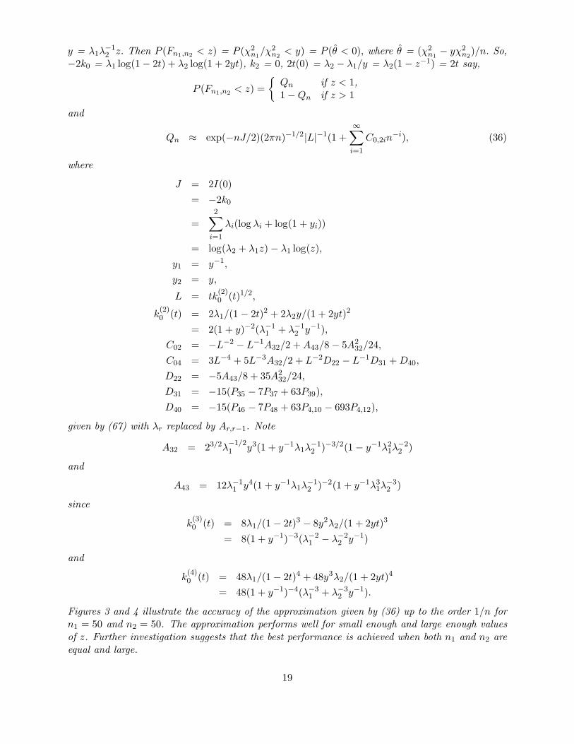
Figures 3 and 4 illustrate the accuracy of the approximation given by (36) up to the order 1/n forn1 = 50 and n2 = 50. The approximation performs well for small enough and large enough valuesof z. Further investigation suggests that the best performance is achieved when both n1 and n2 areequal and large.

19

[Figures 2, 3 and 4 about here.]

4 Proofs for Section 3

Here, we prove and extend Theorem 3.1 and Corollary 3.1. Let us write∫ x

for∫ x−∞ and

∫

x for∫∞x .

By (2) the cgf of nθ satisfies

n−1Knθ(t) ≈∞∑

j=0

n−j/2kj = K(t)

say. Set Kjr = k(r)j (t) and Kr = K(r)(t). For t satisfying (19) let θt be a rv with distribution

P (θt < x) = exp(−nK0)∫ x

exp(ntx)dP (θ < x). So,

P (θ < x) = exp(nK0)

∫ x

exp(−ntx)dP (θt < x). (37)

Since

Knθt(τ) = Knθ(t + τ) − Knθ(t), (38)

κr(nθt) = nKr, so by (37), θt satisfies (2) with brk replaced by brk(t) of (22). Since θ is not aconstant, K2 > 0 and K02 > 0. Since K02 > 0, there is a unique function t = t(x) satisfying (20).Set

ynt(x) = (n/b22(t))1/2(x − b10(t) − b11(t)n

−1/2)

= (n/K02)1/2(x − K01 − K11n

−1/2), (39)

xnt(y) = K01 + K11n−1/2 + K

1/202 n−1/2y, its inverse,

Ynt = ynt(θt),

Qnt(x) = P (θt < x).

Theorem 3.1 follows by choosing t = t(x) in the following more general result. (See Theorem 3.1for the notation.)

Theorem 4.1 For t < 0,

Qn(x) = P (θn < x)

≈ n−1/2αn(x, t)p(y)|L|−1∞∑

i=0

n−i/2Ci(y, t), (40)

where y = ynt(x) of (39). For t > 0, 1 − Qn(x) = P (θn > x) = RHS (40). For t 6= 0 andk = 1, 2, 3, . . .,

Q(k)n (x) ≈ nk−1/2αn(x, t)p(y)|t|k−1k

(2)0 (t)−1/2

∞∑

i=0

n−i/2Ck−1,i(y, t). (41)

Note 4.1 These asymptotic expansions may diverge if y and z are O(n1/2). This restricts the usefulrange of Theorem 4.1 to t = t(x) + O(n−1/2).

20

Proof of Theorem 4.1 Set y = ynt(x), Brk(t) = brk(t)b22(t)−r/2, and B(t) = {Brk(t)}. Then

Qnt(x) = P (Ynt < y) = Pn(y,B(t)) of (14). By (37),

Qn(x) = exp(nK0)

∫ x

exp(−ntx′)dQnt(x′)

= exp(nK0)

∫ y

exp{−ntxnt(y′)}dP (Ynt < y′)

=

∫ y

exp{Ant(y′)}dPn(y′, B(t)),

where

Ant(y′) = nK0 − ntxnt(y

′)

= −nI0 − n1/2I1 + K20 + △n − n1/2Ly′,

Ii = tKi1 − Ki0,

△n ≈∞∑

r=1

n−r/2dr,

dr = kr+2(t).

So, for Br of (65), exp(△n) =∑∞

r=0 n−r/2Br(d) = βn say. So,

Qn(x) = αnβnJt(y, n1/2L), (42)

where

αn = exp(−nI0 − n1/2I1 + K20),

Jt(y, z) =

∫ y

exp(−yz)dPn(y,B(t))

≈∞∑

r=0

n−r/2Jrt(y, z),

Jrt(y, z) =

∫ y

exp(−y′z)p(y′)h1r(y′, B(t))dy′

=3r∑

j=0

Prjgj(y, z) at Prj = Prj(B(t)),

gj(y, z) =

∫ y

exp(−yz)Hj(y)p(y)dy

= −cj−1 − zgj−1(y, z)

= −z−1{cj + gj+1(y, z)},ck = exp(−yz)Hk(y)p(y).

So,

gj(y, z) =I∑

i=1

(−z)−icj+i−1 + (−z)Igj+I for I ≥ 1,

=∞∑

i=1

(−z)−icj+i−1

=

∞∑

k=0

(−z)−k−1cj+k for z < 0. (43)

21

So, for t < 0, L < 0 and z = n1/2L,

Qn(x) ≈ αnβnn−1/2|L|−1∞∑

r=0

n−r/2∞∑

k=0

(−n1/2L)−k3r∑

j=0

cj+kPrj

= αnβn exp(−yn1/2L)p(y)n−1/2|L|−1∞∑

p=0

n−p/2C0p(y, y)

= RHS (40)

since αn(x, t) = αn exp(−yn1/2L) and I0 + t(x − K01) = tx − k0. Similarly,

P (θ > x) = αnβnJ∗t (y, n1/2L)

at y = ynt(x), where

J∗t (y, z) =

∫

yexp(−yz)dPn(y,B(t))

≈∞∑

r=0

n−r/2J∗rt(y, z),

J∗rt(y, z) =

3r∑

j=0

Prjg∗j (y, z) at Prj = Prj(B(t)),

g∗j (y, z) =

∫

yexp(−yz)Hj(y)p(y)dy

= z−1cj − z−1g∗j+1(y, z)

=

∞∑

i=1

(−z)−icj+i−1

= z−1∞∑

k=0

(−z)−kcj+k (44)

for z > 0. So, for t > 0, P (θ > x) = RHS (40). Differentiating (42),

Q(1)n (x) ≈ αnβn(n/K02)

1/2∞∑

r=0

n−r/2∂Jrt(y, n1/2L)/∂y

at y = ynt(x). Also, ∂Jrt(y, z)/∂y = exp(−yz)p(y)∑3r

j=0 PrjHj(y). Similarly,

Q(k)n (x) ≈ αnβn(n/K02)

k/2∞∑

r=0

n−r/2(∂/∂y)kJrt(y, n1/2L)

and

(∂/∂y)kJrt(y, z) = (−1)k−13r∑

j=0

PrjMk−1,j(y, z),

22

where, by Leibniz rule,

Mk−1,j(y, z) = (−∂/∂y)k−1{exp(−yz)(−∂/∂y)jp(y)}

=

k−1∑

i=0

(

k − 1

i

)

Ak−1−i(y, z)Bi+j(y)

for Ar(y, z) = (−∂/∂y)r exp(−yz) = zr exp(−yz) and Br(y) = (−∂/∂y)rp(y) = Hr(y)p(y). So, fork ≥ 1 at y = ynt(x),

Q(k)n (x) ≈ (−1)k−1αn(x, t)βn(n/K02)

k/2(n1/2L)k−1p(y)

∞∑

p=0

n−p/2Ckp(t, y)

= RHS (41). �

Note 4.2 An alternative proof say for t < 0 is to differentiate (43). This gives for k ≥ 1,

(∂/∂y)kgj(y, z) = (−z)k−1e−yzk−1∑

a=0

(−z)−aTak(−∂/∂y)j+ap(y),

where Tak =∑a

b=0(−1)b(

kb

)

. Now use Tak = (−1)a(

k−1a

)

I(0 ≤ a ≤ k) + δ0,kI(a ≥ k). (Its proof isby induction on a.)

Proof of Corollary 3.1 This follows from Theorem 3.1 since y = 0 and Prj = 0 for r + j odd,Hj(0) = kj = Bj(d) = Cj = Cj = 0 for j odd and Ckj = Ckj = 0 for k + j even. �

Note 4.3 We can combine the asymptotic expansions (43) and (44) as

∫ y

y0

exp(−yz)(−∂/∂y)jp(y)dy = exp(−yz)∞∑

k=0

(−z)−1−k(−∂/∂y)j+kp(y)

for z 6= 0, where y0 = ∞sign(z) = ∞ if z > 0 and y0 = ∞sign(z) = −∞ if z < 0.

5 Multivariate Expansions

Here, we give the multivariate versions of the results of Sections 2-4. Suppose that θ is a rv in Rp

with the standard cumulant expansion

κ(θi1 , . . . , θir) =

∞∑

j=r−1

ai1···irj n−j (45)

for r ≥ 1 or the extended expansion

κ(θi1 , . . . , θir) ≈∞∑

k=2r−2

bi1···irk n−k/2 (46)

for r ≥ 1. Equivalently, suppose that the cgf of nθ can be expanded as (17), that is,

n−1Knθ(t) ≈∞∑

j=0

n−j/2kj(t).

23

In the case of (45), kj(t) = 0 for j odd. The examples of Section 2 all extend to p ≥ 1. Set

Yn = (Yni) = n1/2(θ − θ − b1n−1/2)

in Rp, where θi = bi0 and (b1)i = bi

1. So, for r ≥ 1,

κ(Yni1 , . . . , Ynir) ≈ nr/2∞∑

k=2r−2

bi1···irk (Yn)n−k/2, (47)

where bi0(Yn) = bi

1(Yn) = 0 and otherwise bi1···irk (Yn) = bi1···ir

k . Let Y be another rv in Rp withcumulants expandable as (47) with Yn replaced by Y and the same asymptotic covariance, say V= (bij

2 (Y )) = (bij2 (Yn)). Then

κ(Yni1 , . . . , Ynir) − κ(Yi1 , . . . , Yir) ≈ nr/2∞∑

k=2r−2

Bi1···irk n−k/2,

where Bi0 = Bi

1 = Bij2 = 0 and otherwise Bi1···ir

k = bi1···irk − bi1···ir

k (Yn) = bi1···irk if Y ∼ Np(0, V ). For

t in Cp, the difference in their cgfs is

▽n(t) = KYn(t) − KY (t) ≈∞∑

j=1

n−j/2ej(t),

where ej(t) =∑j+2

r=1 Bi1···irr+j ti1 · · · tir/r! and here and below the repeated pairs of subscripts i1, . . . , ir

are implicitly summed over their range 1, . . . , p. Set B = {Bi1···irk } and

P(n)(t, B) = exp(▽n(t)) ≈∞∑

r=0

n−r/2Pr(t, B)

for Pr(t, B) = Br(e(t)) of (65): P1(t, B) = e1(t), P2(t, B) = e2(t) + e1(t)2/2, · · · . They have the

dual forms

Pr(t, B) =

3r∑

j=0

Pi1···ijr ti1 · · · tij

=

3r∑

|ν|=0

Prνtν ,

where ν = (ν1, . . . , νp) lies in Np, N = {0, 1, 2, . . .}, |ν| =∑p

i=1 νi, and ts = ts1

1 · · · tspp for t, s

in Cp. By an extension of Appendix A, the coefficients Prν(B) = Prν may be written as explicitpolynomials in B: P i1···ir

1 (B) = Bi1···irr+1 , · · · . Suppose that Yn and Y have densities with respect to

Lebesgue measure on Rp. Then Pn(y) = P (Yn < y) satisfies

P (Yn < y) = P(n)(−∂/∂y,B)ΦV (y)

= Pn(y,B) (48)

say, with density p(n)(y) = P(n)(−∂/∂y,B)φV (y) ≈ ∑∞r=0 n−r/2pr(y,B), where ΦV and φV are the

distribution and density of Y given by pr(y,B) = Pr(−∂/∂y,B)φV (y) = φV (y)∑3r

|ν|=0 PrνHν(y, V )

and Hν(y, V ) = Hν(y) = φV (y)−1(−∂/∂y)νφV (y).

24

Note 5.1 Consider the usual choice, Y ∼ Ns(0, V ). Then by Withers (2000),

Hν(y, V ) = E

s∏

k=1

(zk + iZk)νk ,

where i =√−1, z = V −1y and Z ∼ Ns(0, V

−1). Setting {V ab} = V −1, Hν(0, V ) is zero for |ν| oddwhile for |ν| = 2r even Hν(0, V ) = (−1)rEZν = (−1)r

∑

V abV cd · · · summed over all 1.3 · · · (2r−1)choices of a, b, c, d, · · · from ν1 · · · νr giving distinct terms.

The expansion (48) is a linear combination of the functions (−∂/∂y)νΦV (y). Consider the casewhere some elements of ν are zero, say the first q. Partition ν as

( 0ν2

)

, y as(y1

y2

)

and V as (Vij),2 × 2, where 0 and y1 have dimension p1 = q, ν2, y2 and V22 have dimension p2 = s − q, and Vij

is pi × pj. Set V1.2 = V12V−122 V21 and l2 = ν2 − 1s−q, where 1q is a q-vector of 1’s. Then

ΦV (y) = E P (Y1 < y1|Y2)I(Y2 < y2)

=

∫ y2

ΦV1.2(y1 − V12V

−122 x2)φV22

(x2)dx2

and

(−∂/∂y)νΦV (y)

= (−∂/∂y2)ν2ΦV (y)

= (−∂/∂y2)ν2−1q(−1)s−q

∫ y1

φV (y)dy1

= (−1)s−q(−∂/∂y2)l2ΦV1.2

(y1 − V12V−122 y2)φV22

(y2)

= (−1)s−q∑

0q≤m2≤l2

(

l2m2

)

(V12V−122 )m2Φm2

V1.2(y1 − V12V

−122 y2)Hm2

(y2, V22)φV22(y2).

Let k = (k1, . . . , ks) ∈ N s. Then

p(k)(n)(y) ≈ (−1)|k|

∞∑

r=0

n−r/2pkr(y)

for

pkr(y) = (−∂/∂y)kPr(−∂/∂y,B) = φv(y)3r∑

|ν|=0

PrνHν+k(y).

Note 5.2 If Y is symmetric about 0 and (45) holds and A ⊂ Rs satisfies −A = A then

Pn(A) =

∫

AdPn(y) ≈

∞∑

r=0

n−r

∫

Ap2r(y,B)dy

since (45) =⇒ Prν = 0 for r + |ν| odd.

The cgf of nθ satisfies n−1Knθ(t) ≈ ∑∞j=0 n−j/2kj(t) = K(t) say, where

kj(t) =

∞∑

r=1

Bi1···irj+2r−2ti1 · · · tir/r!

=

∞∑

r=1

∑

|ν|=r

Bν,j+2r−2tν/ν!

25

say. For example,

k0(t) = Bi0ti + Bi1i2

1 ti1ti2/2! + · · · .

Let t be an interior point in T = {t = k0(t) < ∞}. Define the partial derivatives Ki1···irj = k

(i1···ir)j (t)

and Ki1···ir = K(i1···ir)(t). Let θt be a rv in Rs with distribution

P (θt < x) = exp(−nK(t))

∫ x

exp(nt′x)dP (θ < x).

So, P (θ < x) = exp(nK(t))∫ x

exp(−nt′x)dP (θt < x). The cgf of nθt is again given by (38) so

κi1···ir(nθt) = nKi1···ir . So, θt satisfies (46) with B = {bi1···irk } replaced by

B(t) = {bi1···irk (t) = Ki1···ir

k−2r+2 = k(i1···ir)k−2r+2(t)}.

Assume θ is not a constant so (Kij) and (Kij0 ) are positive-definite. Set

ynt(x) = n1/2(x − (Ki0) − (Ki

1)n−1/2)

= n1/2(x − k0(t) − n1/2k1(t)), (49)

xnt(y) = (Ki0) + (Ki

1)n−1/2 + n−1/2y,

Ynt = ynt(θt),

Qnt(x) = P (θt < x)

= P (Ynt < ynt(x)).

Then Qnt(x) = Pn(ynt(x), B(t)) for Pn(y,B) of (48) and

P (θ < x) = exp(nK(t))

∫ ynt(x)

exp(Ant(y))dPn(y,B(t)),

where Ant(y) = nK(t) − nt′xnt(y) = −nI − n1/2I1 + k2(t) + △n − n1/2t′y, Ii =∑s

j=1 tjKji − ki,

△n =∑∞

r=1 n−r/2dr and dr = kr+2. Set αn = exp(−nI − n1/2I1 + k2(t)) and βn = exp(△n). So,

P (θ < x) = αnβnJt(y, n1/2t) at y = ynt(x), where

Jt(y, z) =

∫ y

exp(−y′z)dPn(y,B(t))

=

∞∑

r=0

n−r/2Jrt(y, z),

Jrt(y, z) =

∫ y

exp(−y′z)pr(y,B(t))dy

=

3r∑

|ν|=0

Prνgν(y, z, Vt),

Prν = Prν(B(t)),

Vt = ∂2k0(t)/∂t∂t′,

gν(y, z, V ) =

∫ y

exp(−y′z)Hν(y, V )φV (y)dy.

26

By (2.18) of Withers (1996), for z1 . . . zp 6= 0 and (y0)j = ∞signzj, we have the asymptoticexpansion

∫ y

y0

exp(−y′z)Hν(y, V )φV (y)dy = exp(−y′z)

∞∑

λ=0

(−z)−1p−λHν+λ(y, V )φV (y). (50)

(This identity was given in Note 4.3 for the case p = 1).

For z < 0, LHS (51) = gν(y, z, V ). This proves the following result for the case t < 0 in Rs.

Theorem 5.1 Define Br(d) by (65). Set

Jrt(y, z) = exp(−y′z)φVt(y)

3r∑

|ν|=0

Prν(B(t))

∞∑

λ=0

(−z)−1s−λHν+λ(y, Vt).

For t1 · · · ts 6= 0 and y = ynt(x) of (49),

P ((sign tj)(θj − xj) > 0 for 1 ≤ j ≤ s)

≈ αnβn

∞∑

r=0

n−r/2Jrt(y, n1/2t)

= αn(x, t)n−s/2|t1 · · · ts|−1φVt(y)

∞∑

i=0

n−i/2C0i(y, t), (51)

where αn(x, t) = exp{−n(x′t−k0)+n1/2k1+k2}, C0i(y, t) =∑i

j=0 C0j(y, t)Bi−j(d) at dr = kr+2(t),

C0j(y, t) =∑j

r=0(−1)j−rGr,j−r, Grk =∑

|λ|=k t−λDrλ, and Drλ =∑3r

|ν|=0 Prν(B(t))Hν+λ(y, Vt).

Note 5.3 Note gj(y, z) = (−z)jg0(y, z)− exp(−yz)∑∞

k=0(−z)kHj−1−k(y)p(y). This is useful nearz = 0, but not here.

Proof of Theorem 5.1 In Section 3 we gave the proof for s = 1 and t > 0. Here, we have giventhe proof for the case t < 0 in Rs. The proof for t in the other 2s − 1 quadrants is the same byvirtue of (50). �

Note 5.4 Set Aj = (sign tj)(θj − xj). Then Theorem 5.1 gives an expansion for

P (A1 > 0, . . . , As > 0).

Other quadrants are given using the usual rules, such as

P (A1 < 0, A2 < 0) = 1 − P (A1 > 0) − P (A2 > 0) + P (A1 > 0, A2 > 0).

Corollary 5.1 Given x in Rs, choose t = t(x) to maximise

x′t − k0(t). (52)

So, x = ∂k0(t)/∂t at t = t(x). Suppose that xj 6= θj for 1 ≤ j ≤ s, where θj = Bj0. Set

y(x) = −∂k1(t)/∂t at t = t(x). Then at y = y(x)

P ((θ − x)j . sign (θ − x)j < 0 for 1 ≤ j ≤ s) = RHS (51). (53)

27

Also at t = t(x), αn(x, t) = exp{−nI(x) + n1/2k1 + k2}, where

I(x) = supt∈T (x′t − k0(t))

= x′t(x) − k0(t(x)) (54)

for T = {t : k0(t) < ∞}.

Proof y = (x − θ)′t is parallel to the tangent plane to k0(t) − θ′t at t = t(x). Consider a plotof k0(t) − θ′t = Bij

1 titj/2! + · · · . Its tangent plane at t = 0 has gradient 0. Its tangent plane att = t(x) has gradient x − θ, and I(x) is the distance of the point (k0(t) − θ′t, t) below the planey = (x − θ)′t at t = t(x). So, sign (x − θ)j = sign tj at t = t(x). �

Corollary 5.2 If (45) holds and Y is symmetric about 0, that is Y and −Y have the same distri-bution, then provided xi 6= θi for i = 1, . . . , s,

LHS(53) = P ((sign tj)(θj − xj) > 0 for 1 ≤ j ≤ s)

≈ exp{−nI(x) + k2(t)}n−s/2|t1 · · · ts|−1φVt(0)

∞∑

i=0

n−iC0,2i(0, t) (55)

for I(x) of (54).

Proof Note Hλ(0, Vt) = 0 for |λ| odd, Prν = 0 for r + |ν| odd, kj = Bj(d) = Cj = Cj = 0 for jodd, and Drλ = 0 for r + |λ| odd. �

Note 5.5 Putting Prν = Prν(B(t)), the leading terms are given by

C00(0, t) = C00(0, t) = D00 = P00 = 1

and

C02(0, t) = C02(0, t) + k4,

where

C02(0, t) = G02 − G11 + G20,

G02 =∑

|λ|=2

t−λD0λ,

G11 =∑

|λ|=1

t−λD1λ,

G20 = D20

=∑

|ν|=2,4,6

P2νHν(0, Vt),

D0λ = Hλ(0, Vt),

D1λ =∑

|ν|=1,3

P1νHν+λ(θ, Vt).

The next term is

C04(0, t) = k6 + 3k24/2 + k4C02(0, t) + C04(0, t),

28

where

C04(0, t) =

4∑

r=0

(−1)rGr,4−r,

G04 =∑

|λ|=4

t−λHλ(0, Vt),

G13 =∑

|λ|=3

t−λD1λ,

G22 =∑

|λ|=2

t−λD2λ,

D2λ =∑

|ν|=2,4,6

P2ν(B(t))Hν+λ(0, Vt),

G31 =∑

|λ|=1

t−λD3λ,

D3λ =∑

|ν|=1,3,...,7,9

P3ν(B(t))Hν+λ(0, Vt),

G40 = D40

=∑

|ν|=2,4,...,10,12

P4ν(B(t))Hν(0, Vt).

Example 5.1 Suppose that θ = X is the mean of independent random vectors in Rs with finitecgfs in a neighbourhood of the origin. Suppose that x > θ = Eθ. Then P (θ > x) is given by (55)with k0(t) the mean cgf, and the other ki equal to 0. In (3.7)-(3.13) of Robinson et al. (1990)an equivalent expansion for the usual choice Y ∼ Ns(0, V ) is given in terms of the cumulants ofthe standardised mean V −1/2θ with Prj replaced by Prj(t) . The important difference is that thecoefficients of our expansion are given explicitly by Notes 5.2 and 5.3.

Theorem 5.2 Take y = ynt(x) of (49) and αn(x, t) of Theorem 5.1. For k ≥ 0 in N s andt1 . . . ts 6= 0, the partial derivatives of Qn(x) = LHS(51) can be expanded as

Q(k)n (x) =

s∏

j=1

(∂/∂xj)kjQ(x)

≈ αn(x, t)n|k|−s/2|tk−1s |φVt(y)∞∑

i=0

n−i/2Ck,i,

29

where

Cki = Cki(y, t) =i∑

j=0

CkjBi−j(d), (56)

Ckj = Ckj(y, t) =

j∑

r=0

Gkr,j−r,

Gkrs =∑

|λ|=s

Tλk(−t)−λDrλ,

Tλk =

s∏

j=1

{(−1)λj

(

kj − 1

λj

)

I(λj < kj) + δ0,kjI(λj ≥ kj)}, (57)

and αn(x, t) and Drλ as defined in Theorem 5.1. So, if k ≥ 1p then Gkrs =∑

|λ|=s

(k−1p

λ

)

t−λDrλ.

Proof Consider the case t < 0 in Rs. Set z = n1/2t and γnk =∏p

i=1(∂yi/∂xi)ki = n|k|/2. Differen-

tiating (51) gives

Q(k)n (x) ≈ αnβnγnk

∞∑

r=0

n−r/23r∑

|ν|=0

Prν

∞∑

λ=0

(−z)−1s−λAk,ν+λ,

where

Ak,ν+λ = (∂/∂y)k{exp(−y′z)(−∂/∂y)ν+λφV (y)}

= exp(−y′z)k∑

a=0

(

k

a

)

(−z)k−a(−1s)a(−∂/∂y)ν+λ+aφV (y)

by Leibniz’ rule. So

Q(k)n (x) = αnβnγnk(−z)k−1s exp(−y′z)φVt(y)Snk,

where

Snk ≈∞∑

r=0

n−r/2∞∑

λ,a=0

(−z)−λ−a

(

k

a

)

(−1s)aDr,λ+a

=∞∑

j=0

n−j/2Ck−1s,j,

Ck−1s,j =∑

r+|c|=j

(−t)−cDrcTck,

and Tck =∑c

a=0(−1s)a(ka

)

= RHS (57) at λ = c by Note 4.3. �

Corollary 5.3 Suppose that (45) holds and Y is symmetric about 0. Set

t = t(x)

30

of (52),

I(x) = x′t − k0(t)

and

Hλ = Hλ(0, Vt).

Define Tλk by (57). Then for k in Np, and xi 6= θi for i = 1, . . . , p

Q(k)n (x) = exp{−nI(x) + k2(t)}n|k|−s/2|tk−1s |φVt(0)

∞∑

i=0

n−iCk,2i

for I(x) of (54) and Ck,i = Ck,i(0, t) of (56). The leading terms are Ck,0 = 0, Ck,2 = k4 +Ck,2 andCk,4 = k6 + 3k2

4/2 + k4Ck,2 + Ck,4, where

Ck,2 =∑

|λ|=2

Tλkt−λHλ −

∑

|λ|=1

Tλkt−λD1λ + D20

and

Ck4 =∑

|λ|=4

Tλkt−λHλ −

∑

|λ|=3

Tλkt−λD1λ

+∑

|λ|=2

Tλkt−λD2λ −

∑

|λ|=1

Tλkt−λD3λ + D40

for D1λ, D2λ, D3λ and D40 given by Note 5.5.

Proof This is as for that of Corollary 5.2. �

6 Functions of a Sample Mean

A weakness of the method so far is the difficulty of obtaining the functions {ki(t)}. For θ = X thesehave been given in terms of the cgf of X. But usually only the leading coefficients {ari} are available.Here, we show how to obtain {ki(t)} - or rather P (θ > x) - directly in terms of the cgf of X whenθ is any smooth function of X. We restrict ourselves to the multivariate version of Example 2.3.Let X be the mean of an i.i.d. sample of size n from a distribution on Rk with mean µ, covarianceVX and cgf KX(s) =

∑

k κλsλ/λ! for s in Ck, where∑

k sums over λ in Nk − {0}. Let θ = H(X)for H : Rk → Rp a function with finite derivatives at µ. The condition det V > 0 implies p ≤ k.So, (45) holds with the leading cumulant coefficients ai1···ir

j needed for the Edgeworth expansions(14) and (15) given by the appendix to Withers (1982) or alternatively, by the multivariate versionof the formula for arj given in Corollary 3.1 of Withers (1983b).

Take θ < x in Rp and Y ∼ Np(0, V ). Since

P (θ > x) =

∫

H(z)>xdP (X < z), (58)

we have two methods of evaluating (58). By (55),

P (θ > x) = exp{−nI(x) + k2(t)}n−p/2|t1 · · · tp|−1φVt(0)

∞∑

i=0

n−iC0,2i(0, t)

31

at t = t(x), where I(x) = x′t − k0(t). Also

φVt(0) = (2π)−p/2det(k(2)0 (t))−1/2,

where k(2)(t) = ∂2k(t)/∂t∂t′. Set Cm,i(y, t : θ) = Cm,i(y, t) of (56). By Corollary 5.3 with k = 1p

and p replaced by k,

P (θ > x) =

∫

H(z)>xdP (X < z)

= (n/2π)k/2det(K(2)X (s))−1/2

∫

H(z)>xdz exp{−nJ(z)}

∞∑

i=0

n−iC1p,2i(z, s : X),

where J(z) = z′s − KX(s) at s = s(z) such that z = K(1)X (s).

We now sketch a way of obtaining our expression for LHS (58) from that for RHS (58). Sinceour functions are analytic we may write

s(z) =∑

k

(z − µ)νSν/ν!

and

J0(z) = J0(z, s(z)) =∑

k

(z − µ)νJν/ν!

with Sν = (Sνi) in Rk and Jν in R. Appendix C shows how to obtain these coefficients from thecumulants of X and that J0(z) =

∑

|ν|≥2(z − µ)νJν/ν! that is, J0(z) is quadratic at z = µ. Theleading term in RHS (58) is

φVX(0)nk/2

∫

{exp(−nJ0(z))dz : H(z) > x}. (59)

Suppose there is a unique z = Z = Zx in Rk maximising J0(z) over {z : H(z) > x} and that itlies in {z : H(z) = x}. Then (Z,w) in Rk+p is the solution of the K +p equations J0(z) = H(Z)wand H(Z) = x, where J0(Z) = ∂J0(Z)/∂Z is k × 1, H(Z) = ∂H(Z)′/∂Z is k × p, and w is a p× 1Lagrange multiplier.

Let us transform to u = n(z − Z). So, |∂u/∂z′| = nk and

nJ0(z) = n∑

k

(z − Z)νJ(ν)0 (Z)/ν! = nJ0(Z) +

∞∑

i=0

n−iai(u),

where a0(u) = u′J0(Z). Similarly, H(z) ≈ H(Z) + n−1∑∞

i=0 n−ibi(u)′, where b0(u)′ = u′H(Z) is1 × p. So, RHS (59) is φVX

(0) exp{−nJ0(Z)}{L(Z) + O(n−1)}, where

L(Z) =

∫

[exp{−a0(u)} : b0(u) ≥ 0]

=

∫

Bu>0exp(−a′u)du, (60)

a = J0(Z),

B = H(Z)′.

32

Note N is p × k. Set v = Bu. If p = k, det B 6= 0, and c = (B′)−1a then

L(Z) =

∫

v>0exp(−c′v)dv|det (∂v/∂u′)|

= det B ·k∏

i=1

ci|−1 (61)

assuming c > 0 in Rk. So, if p = k this gives

[x′t − k0(t)]t=t(x) = I(x) = J0(Z), (62)[

exp{k2(t)}|t1 · · · tp|−1φV (0)]

t=t(x)= φVX

(0)L(ZX ). (63)

Since Appendix B gives t(x) in terms of the coefficients of k0(t), (62) does not provide an alternativemethod for obtaining k0(t). However, (63) could in theory be used to obtain k2(t) by puttingx = t−1(t), this inverse being obtained in Appendix C. If p < k, (60) gives L(Z) = ∞, so thismethod breaks down.

Example 6.1 Suppose that p = 1, and θ = H(X) = |X |2/2 =∑k

i=1 X2i /2. Set

µi1···ir = E(X − µ)i1 · · · (X − µ)ir ,

the joint central moment of X. By Corollary 3.1 of Withers (1983b), (1) holds with the coefficientsneeded in the expansions (14) and (15) for the distribution (and continuous derivatives) of

Yn = (|X |2/2 − a10)a−1/221

to O(n−2) are

a10 = |µ|2/2,a21 = µaµ

abµb

= µ′covar(X)µ,

a11 = µaa/2,

a32 = µaµbµcµabc + 3µaµbµ

acµbc,

a22 = µaµabb + µacµac/2,

a43 = µa · · ·µdµa···d − 3a2

21 + 12µaµbµcµadµbcd + 12µaµbµ

acµbeµce,

a12 = 0,

a33 = (3/2)µaµbµabcc − (3/2)a21µ

aa − 3µaµbµacµbc

+3µaµabµbdd + 3µaµ

abdµbd + µafµacµcf ,

a54 = µa · · ·µeµa···e − 10a21µaµbµcµ

abc − 60a21µaµbµacµbc

+20µaµbµcµdµaeµbcde + 15µaµbµcµdµ

abeµcde

+60µaµbµcµadµbdfµcf + 60µaµbµcµ

adµbcdµdf + 60µaµbµaeµbgµceµcg.

So, for θ = |µ|2/2 < x and θ = |X |2/2, P (θ > x) is given by (25) in terms of the functions

k0 =∞∑

r=1

ar,r−1tr/r!, k2 =

∞∑

r=1

arrtr/r!, · · ·

33

of (28). If k = 1 we can use the alternative expression

P (θ > x) = exp{−nJ0(Z)}φVX(0)L(Z){1 + O(n−1)},

where L(Z) is given by (61). This assumes that a21 6= 0. However, if µ = 0 then these coefficientsare all zero except for

a11 = µaa/2 = trV/2,

a22 = µacµac/2 = trV 2/2,

a33 = µafµacµcf = trV 3.

If µ = 0, or if θ = H(X) = |X−µ|2/2 then the distribution of θ can be derived from the Edgeworthexpansion for the distribution of X using polar coordinates. For example, if k = 2 then by (3.30)of Withers (1996) Tn = nθ = n|X − µ|2/2 satisfies

P (Tn < t) ≈∞∑

j=0

n−jQ2j(t, 2π), (64)

where

Q0(t, 2π) = P (T < t),

N ∼ Nk(0, I),

Q2j(t, 2π) = c0

3j∑

i=0

∫ t

0tidt

∫ 2π

0exp(−tJθ/2)rji(θ)dθ,

c0 = φVX(0),

2Jθ = (λ−11 − λ−1

2 )cos 2θ + λ−11 + λ−1

2

for T = N ′VXN . Here, λ1 and λ2 are the eigenvalues of VX and rji(θ) is as given by (3.10) inWithers (1996). Now suppose that t → ∞. One may show that Q2j(t, 2π) has magnitude φVX

(t)t3j .So, if t → ∞ as n → ∞ then the expression (64) remains useful provided that n−jt3j → 0, thatis t = o(n1/3). If this condition fails then the Edgeworth expansion (64) breaks down.

Appendix A

For x = (x1, x2, . . .) a sequence in R or C, and y in R or C define Brj(x) by

(

∞∑

i=1

xiyi)j =

∞∑

r=j

Brj(x)yr

for j = 0, 1, 2, . . . and Br(x) by

exp(∞∑

i=1

xiyi) =

∞∑

r=0

Br(x)yr.

So,

Br(x) =r∑

j=0

Brj(x)/j!. (65)

34

Comtet (1974) calls Br(x) and Brj(x) the complete and partial ordinary Bell polynomials and

tables the latter on page 309. (We use ∼ rather than his ˆ to avoid confusion with θ as an estimatefor θ.) So,

B0(x) = 1,

B1(x) = x1,

B2(x) = x2 + x21/2,

B3(x) = x3 + x2x1 + x31/6,

B4(x) = x4 + x3x1 + x22/2 + x2x

21/2 + x4

1/24,

35

and so on. Substituting xj = ej(t) of (11), that is ej(t) =∑j+2

r=1 Br,r+jtr/r! for j ≥ 1, gives

P00 = 1,

Pr0 = 0 for r ≥ 1,

Pr1 = B1,r+1 for r ≥ 1

P13 = B34/6,

P22 = (B24 + B212)/2,

P23 = B35/6 + B12B23/2,

P24 = B46/24 + B12B34/6 + B223/8,

P25 = B23B34/12,

P26 = B234/72,

P32 = B25/2 + B12B13,

P33 = B36/6 + B12B24/2 + B13B23/2 + B312/6,

P34 = B47/24 + B12B35/6 + B13B34/6 + B23B24/4 + B212B23/4,

P35 = B58/120 + B12B46/24 + B23B35/12 + (B24 + B212)B34/12

+B12B223/8,

P36 = (B23B46/4 + B34B35/3 + B12B23B34 + B323/4)/12,

P37 = (B34B46/6 + B12B234/3 + B2

23B34/2)/24,

P38 = B23B234/144,

P39 = B334/1296,

P42 = B26/2 + B213/2 + B12B14,

P43 = B37/6 + B12B25/2 + B13B24/2 + B23B14/2 + B212B13/2,

P44 = B48/24 + B12B36/6 + B13B35/6 + +B14B34/6 + B23B25/4

+B224/8 + B12B23B13/2 + B2

12B24/4 + B412/24,

P45 = B59/120 + (B23B36 + B13B46/2 + B25B34 + B12B47/2

+B24B35)/12 + B223B13/8 + B12B13B34/6 + B13B23B24/4

+B212B35/12 + B3

12B23/12,

P46 = (B6,10/60 + B34B36/3 + B12B58/10 + B235/6 + B23B47/4

+B24B46/4 + B212B46/4 + 3B2

23B24/4 + B13B23B34 + B12B23B35

+B12B24B34 + 3B212B

223/4 + B3

12B34/3)/12,

P47 = (B35B46/12 + B23B58/20 + B34B47/12 + B23B24B34/2

+B223B35/4 + B12B34B35/3 + B12B23B46/4 + B13B

234/6

+B212B23B34/2 + B12B

323/4)/12,

P48 = (B34B58/15 + B246/24 + B12B34B46/3 + B24B

234/3

+3B23B34B35/2 + B223B46/4 + B4

23/8 + B12B223B34 + B2

12B234/3)/48,

P49 = (B234B35/3 + B12B23B

234 + B3

23B34/2 + B323B34B46/2)/144,

P4,10 = (B234B46/12 + B12B

334/9 + B2

23B234/4)/144,

P4,11 = B23B334/2592,

P4,12 = B434/31104.

36

Higher order coefficients are easily found using say MAPLE. When (1) holds, (8) simplifies to

κr(Yn) ≈ nr/2∑∞

k=r−1 Ari(Yn)n−i with A10(Yn) = 0 and Ari(Yn) = aria−r/221 otherwise. If also the

cumulants of Y have this form with A10(Y ) = 0 and A21(Y ) = 1 then (9) simplifies to

κr(Yn) − κr(Y ) ≈ nr/2∞∑

i=r−1

Arin−i,

where Ari = Ari(Yn)−Ari(Y ), so A10 = A21 = 0 and (11) simplifies to e2j(t) =∑j+1

r=1 A2r,r+jt2r/(2r)!

and e2j−1(t) =∑j

r=0 A2r+1,r+jt2r−1/(2r + 1)!. Also Prj = 0 for r + j odd and the non-zero Prj for

r ≤ 4 are (c.f. Section 4 of Withers (1984))

P11 = A11,

P13 = A32/6,

P22 = (A22 + A211)/2,

P24 = (A43 + 4A11A32)/4!,

P26 = A232/72,

P31 = A12,

P33 = (A33 + 3A11A22 + A311)/3!,

P35 = (A54/10 + A11A43/2 + A22A32 + A211A32)/12,

P37 = (A32A43/2 + A11A232)/72,

P39 = A332/1296,

P42 = A11A12 + A23/2,

P44 = (A411 + 6A2

11 A22 + 4A11A33 + 4A12A32 + 3A222 + A44)/4!,

P46 = (20A311A32 + 60A11A22A32 + 15A2

11A43 + 6A11A54 + 15A22A43

+20A32A33 + A65)/6!,

P48 = (A211A

232 + A11A32A43 + A22A

232 + A32A54/5 + A2

43/8)/144,

P4,10 = (A11A332/3 + A2

32A43/4)/432,

P4,12 = A432/31104. (66)

If (3) holds and λr = κrκ−r/22 then the r non-zero {Prk} are given by

Prk = Brj(α)/j! (67)

for r < k ≤ 3r, k − r = 2j even and αj = λj+2/(j + 2)!. For r ≤ 4 these are

P13 = λ3/3!,

P24 = λ4/4!,

P26 = λ23/72,

P35 = λ5/5!,

P37 = λ3λ4/144,

P39 = λ33/1296,

P46 = λ6/6!,

P48 = λ3λ5/720 + λ24/1152,

P4,10 = λ23λ4/12

3,

P4,12 = λ43/31104. (68)

37

Appendix B

Here, we assume that (1) holds. So, the saddlepoint t(x) and the index of large deviation I0(x) of(20) and (21) are determined by the leading cumulant coefficients {ar,r−1}. In many situations aclosed form for the saddlepoint and the index may not exist. In this appendix we give expansionsfor them amenable to computer calculation directly in terms of the leading coefficients.

Set (z)k = z!/(z − k)! = z(z − 1) . . . (z − k + 1). For x = (x1, x2, . . .), a sequence in C, and y inC, Comtet (1954) defines the partial exponential Bell polynomial Brj(x) by

(

∞∑

i=1

xiyi/i!

)j

/j! =

∞∑

r=j

Brj(x)yr/r! (69)

for j = 0, 1, 2, . . .. Comtet (1954) tables them on pages 307 and 308 and gives simple recurrenceformulas for them.

Theorem B.1 Set lr = ar,r−1, νr = lr/lr/22 , βr = νr+2/(r + 1), C1 = 1, Ci =

∑i−1k=1 (−i)kBi−1,k(β)

for i ≥ 2, zx = (x− l1)/l1/22 = (x−θ)/a

1/221 , and J(z) =

∑∞i=2 Ci−1z

i/i!. So, J(z) has first derivativeJ(z) =

∑∞i=1 Ciz

i/i!. Then

t(x) = l−1/22 J(zx) (70)

and

I(x) = J(zx). (71)

So, the leading coefficients are

C1 = 1,

C2 = −ν3,

C3 = −ν4 + 3ν23 ,

C4 = −ν5 + 10ν3ν4 − 15ν33 ,

C5 = −ν6 + 5(3ν3ν5 + 2ν24 ) − 3 · 5 · 7(ν2

3ν4 − ν43),

C6 = −ν7 + 7(3ν3ν6 + 5ν4ν5) − 70(3ν23ν5 + 4ν3ν

24) − 5 · 7 · 9(4ν3

3ν4 − 3ν53 ),

C7 = −ν8 + 7(4ν3ν7 + 8ν4ν6 + 5ν25 ) − 14(27ν2

3ν6 + 90ν3ν4ν5 + 20ν34 )

+5 · 7 · 9 · 10(ν33ν5 + 2ν2

3ν24) − 5 · 7 · 9 · 11(5ν4

3ν4 − 3ν63),

C8 = −ν9 + 6(6ν3ν8 + 14ν4ν7 + 21ν5ν6) − 3 · 5 · 7(6ν23ν7 + 24ν3ν4ν6 + 15ν3ν

25

+20ν24ν5) + 7 · 10 · 11(9ν3

3ν6 + 45ν23ν4ν5 + 20ν3ν

25 )

−15 · 5 · 7 · 9 · 11(3ν43ν5 + 8ν3

3ν24) + 3 · 5 · 7 · 9 · 11 · 13(2ν5

3ν4 − ν73).

Proof Set bi = li+1/l2 and yx = (x− l1)/l2. Write x = k(1)0 (t) as zx =

∑∞i=1 bit

i/i!. By page 151 of

Comtet (1954), t(x) = l−1/22

∑∞i=1 ciy

ix/i!, where c1 = 1 and ci =

∑i−1k=1 (−i)kBi−1,k(b2/2, b3/3, . . .)

for i ≥ 2. Now substitute into I(x) = xt − k0(t) at t = t(x) to obtain I(x) =∑∞

i=2 diyix/i!,

where di = ici−1k2 −∑ir=2 krBir(c). Putting Ci = cil

(1−i)/22 and Di = dil

−i/22 , we obtain (70)

and I(x) =∑∞

i=2 Dizix/i!. That di = l2ci−1 and Di = Ci−1 hold, that is, (71) holds, follows since

differentiating (71) gives (70). �

38

Examples B.1 Suppose that θ = X as in Example 2.1, or more generally that (3) holds. (This

includes the case of linear combinations of independent sample means.) As usual set λr = κr/κr/22 .

Then Theorem B.1 holds with ar,r−1 = κr and νr = λr.

Examples B.2 Consider the Studentised statistic θ = (X−κ1)/κ21/2 with κ2 = n−1

∑ni=1(Xi−X)2.

Then the leading ari are given in Example 1.2 of Withers (1989) in terms of λr = κr/κr/22 as a21 = 1

and ν3 = a32 = −2λ3, ν4 = a43 = 12 − 2λ4 + 12λ23, ν5 = a54 = −180λ3 + 6λ5 + 20λ3λ4 − 105λ3

3,· · · . So, Theorem B.1 holds with C2 = 2λ3, C3 = 2λ4 − 12, C4 = −60λ3 − 6λ5 + 20λ3λ4 − 15λ3

3,· · · .

Appendix C

Here, we show how to obtain series expressions for J0(z) and s(z) of Section 6 and its inverse z(s).(Replacing k, s, z, KX(s), κr by p, t, x, k0(t), ar,r−1 this gives series expressions for I(x) and t(x)of Section 5.) Because KX(s) is analytic, these functions J0(z), s(z) and z(s) have the form

J0(z) =∑

k

(z − µ)νJν/ν!,

s(z) =∑

k

(z − µ)νSν/ν!, (72)

z(s) = µ +∑

k

sνTν/ν!, (73)

where∑

k sums over ν in Nk − 0. Let ei be the ith unit vector in Rk. Set V = covar(X) soVij = κei+ej

. Set (V ij) = V −1. For ν, λ in Nk define the multivariate partial exponential Bellpolynomial for the sequence S = {Sν} in Rk by

s(z)λ/λ! =∑

k

{(z − µ)νBνλ(S)/ν! : |ν| ≥ |λ|}.

For ν in Nk, set

Cν = Cν(S, κ) =∑

k

{κλBνλ(S) : |λ| ≤ |ν|}.

Set dλi = κλ+eiand dλ = (dλ1, . . . , dλk)′. Note s(z) is the solution of

z − µ = ∂KX(s)/∂s − µ.

Since

RHS =∑

k

dνsν/ν! =

∑

k

(z − µ)νCν(S, d),

S of (72) is given by the recurrence relations Cνi = (Cν)i = I(ν = ei), where I(A) = 0 or 1 for Afalse or true. For example, since

Bνea(S) = (Sν)a = Sνa,

Seαa = V αa. Since

Bν,ea+eb(S) = ν!{(ea + eb)!}−1

∑

ν1+ν2=ν

Sν1aSν2b/(ν1!ν2!),

39

Seα+eβ ,c = −(eα + eβ)!∑

1≤a≤b≤k

2∑

ab

V aαV bβ/(ea + eb)!

and∑k

d=1 V cdκea+eb+ed, where

∑2ab fab = fab + fba.

Substituting s(z) into (73),

RHS =∑

k

(z − µ)νCν(S, T ).

So, T of (73) is given in terms of S by the recurrence relations Cνi(S, T ) = I(ν = ei). For example,ν = ea gives Teαi = Vαi and ν = eα + eβ gives

0 =∑

|λ|≤2

Beα+eβ ,λ(S)

=

k∑

a=1

VaiSeα+eβ ,a +∑

1≤a≤b≤k

Bαβ:abTea+eb,i, (74)

where

Bαβ:ab = Beα+eβ ,ea+eb(S)(eα + eβ)!{(ea + eb)!}−1

2∑

ab

V aαV bβ.

For each i = 1, . . . , k, (74) gives(

k2

)

linear equations in the(

k2

)

unknowns {Tea+eb,i}. Set

B′αβ = vec(Bαβ:ab)

and

Ti = vec(Tea+eb,i),

both(k2

)

× 1. Then (74) can be written as

B′αβTi = −

k∑

a=1

VaiSeα+eβ ,a,

or in matrix form BTi = −∑ka=1 VaiSa, where B is

(k2

)

×(k2

)

and Sa = vec(Seα+eβ ,a). So,

Ti = −k∑

a=1

VaiB−1Sa

gives {Tea+eb,i}. Now, for s = s(z),

KX − µ′s =∑

κλ{(z − µ)νBνλ(S)/ν! : |ν| ≥ |λ| ≥ 2} =∑

{(z − µ)νC∗ν (S, κ)/ν! : |ν| ≥ 2},

where

C∗ν (S, κ) =

∑

{κλBνλ(S) : 2 ≤ |λ| ≤ |ν|}.

So, J0(z) =∑

k{(z − µ)νJν/ν! : |ν| ≥ 2} with Jν =∑k

i=1 νiSν−ei,i − C∗ν (S, κ), showing that the

leading term in J0(z) is actually quadratic in z − µ. The leading term in J0(z) is∑

|ν|=2

(z − µ)νJν/ν! = (z − µ)′V −1(z − µ)/2.

40

Appendix D

Here we give a formal method for obtaining the moment generating function of a function of a rvX from that of X.

Let i =√

( − 1). Let∫

C denote a contour integral about 0 in the complex plane. Thenfor r a positive integer, EXr/r! = (2πi)−1

∫

C t−rE exp(tX)dt/t. So, we obtain the formal resultE exp(sXk) = (2πi)−1

∫

C fk(s, t)E exp(tX)dt/t, where fk(s, t) =∑∞

j=0(kj)!(s/tk)j/j!, a divergentseries.

Example D.1 Suppose that X ∼ N (0, 1), so E exp(tX) = exp(t2/2). Take the contour

C = {t = exp(iθ), 0 < θ < 2π.}.

So, E exp(sX2) = (2πi)−1∫

C f2(s, t) exp(t2/2)dt/t =∑∞

j=0(2j)!sjaj/j!, where

aj = (2π)−1

∫ 2π

0exp[−2jiθ + exp(2iθ)/2]dθ =

∞∑

k=0

2−kajk/k!,

ajk = (2π)−1

∫ 2π

0exp[2(k − j)iθ]dθ = I(j = k),

and I(A) is 1 or 0 for A true or false. So, aj = 2−j/j!, giving

E exp(sX2) =

∞∑

j=0

(

2j

j

)

(s/2)j = (1 − 2s)−1/2

for Re(s) < 1/2. Note that E exp(sXk) = ∞ for k > 2.

We now extend this result to any analytic function of X, say g(X) =∑∞

r=1 grXr/r!. Using the

Bell polynomials of (69), we have the formal expansion E exp(sg(X)) =∑

r=0 xrBr(gs)/r!, whereBr(gs) =

∑rk=0 skBrk(g) is called by Comtet (1954) the complete exponential Bell polynomial. So,

we obtain formally

E exp(sg(X)) = (2πi)−1

∫

Cf(s, t)E exp(tX)dt/t,

where f(s, t) =∑∞

r=0 Br(gs)t−r.

References

[1] Abramowitz, M and Stegun, I. A. (1964). Handbook of Mathematical Functions. U.S. Depart-ment of Commerce, National Bureau of Standards, Applied Mathematics Series 55.

[2] Anderson, M. J. and Robinson, J. (2001). Permutation tests for linear models. Australian andNew Zealand Journal of Statistics, 43, 75-88.

[3] Anderson, M. J. and Robinson, J. (2003). Generalized discriminant analysis based on dis-tances. Australian and New Zealand Journal of Statistics, 45, 301-318.

41

[4] Barndoff-Nielsen, O. E. (1990). Approximate interval probabilities. Journal of the Royal Sta-tistical Society, Series B, 52, 485–496.

[5] Barndorff-Nielsen, O. E. and Cox, D. R. (1979). Edgeworth and saddlepoint approximationswith satistical applications (with discussion). Journal of the Royal Statistical Society, SeriesB, 41, 279–312.

[6] Bhattacharya, R. N. and Ghosh, J. K. (1978). On the validity of the formal Edgeworthexpansion. Annals of Statistics, 6, 434–451.

[7] Bhattacharya, R. N. and Rao, R. R. (1976). Normal approximations and Asymptotic Expan-sions. Wiley, New York.

[8] Bickel, P. J. and Robinson, J. (1982). Edgeworth expansions and smoothness. Annals ofProbability, 10, 500–503.

[9] Blackwell, D. and Hodges, J. L. (1959). The probability in the extreme tail of a convolution.Annals of Mathematical Statistics, 31, 1113–1120.

[10] Butler, R. W., Huzurbazar, S. and Booth, J. G. (1992). Saddlepoint approximations for thegeneralized variance and Wilk’s statistic. Biometrika, 79, 157–169.

[11] Comtet, L. (1954). Advanced Combinatorics. Reidel, Dordrecht.

[12] Cornish, E. A. and Fisher, R. A. (1937). Moments and cumulants in the specification ofdistributions. Rev. de l’Inst. Int. de Statist., 5, 307–322. Reproduced in the collected papersof R.A. Fisher, 4.

[13] Daniels, H. E. (1954). Saddlepoint approximations in statistics. Annals of MathematicalStatistics, 25, 631–650.

[14] Daniels, H. E. (1980). Exact saddlepoint approximations. Biometrika, 67, 59–63.

[15] Daniels, H. E. (1983). Saddlepoint approximations for estimating equations. Biometrika, 70,89–96.

[16] Daniels, H. E. (1987). Tail probability expansions. International Statistical Review, 55, 37–48.

[17] Daniels, H. E. and Young, G. A. (1991). Saddlepoint approximations for the studentizedmean, with an application to the bootstrap. Biometrika, 78, 169–179.

[18] Diciccio, T. J. and Field, C. A. (1990). Approximations of marginal tail probabilities andinference for scale parameters. Biometrika, 77, 77–95.

[19] Easton, G. S. and Ronchetti, E. (1986). General saddlepoint approximations with applicationsto L statistics. Journal of the American Statistical Association, 81, 420–430.

[20] Field, C. and Ronchetti, E. (1990). Small Sample Asymptotics. Institute of MathematicalStatistics, Lecture Notes - Monograph Series, Hayward.

[21] Fisher, R. A. and Cornish, E. A. (1960). The percentile points of distributions having knowncumulants. Technometrics, 2, 209–225.

[22] Fraser, D. A. S. (1988). Normed likelihood as saddlepoint approximation. Journal of Multi-variate Analysis, 27, 181–193.

42

[23] Fraser, D. A. S. (1990). Tail probabilities from observed likelihoods. Biometrika, 77, 65–76.

[24] Gatto, R. and Ronchetti, E. (1996). General saddlepoint approximations of marginal densitiesand tail probabilities. Journal of the American Statistical Association, 91, 666–673.

[25] Giles, D. E. A. (2001). A saddlepoint approximation to the distribution function of theAnderson-Darling test statistic. Communications in Statistics, B, 30, 899–905.

[26] Good, I. J. (1957). Saddle-point methods for the multinomial distribution. Annals of Mathe-matical Statistics, 28, 861–881.

[27] Good, I. J. (1961). The multivariate saddle-point method and chi-sqaured for the multinomialdistribution. Annals of Mathematical Statistics, 32, 535–548.

[28] Helmers, R., Jing, B., Qin, G. and Zhou, W. (2004). Saddlepoint approximations to thetrimmed mean. Bernoulli, 10, 465–501.

[29] Hill, G. W. and Davis, A. W. (1968). Generalised asymptotic expansions of Cornish-Fishertype. Annals of Mathematical Statistics, 39, 1264–1273.

[30] Honda, I. (1978). On the rate of the central limit theorem for additive processes. Keio Math.Sem. Rep. No.3, 11–21.

[31] Jensen, J. L. (1988). Uniform saddlepoint approximations. Advances in Applied Probability,20, 622–634.

[32] Jensen, J. L. (1992). The modified signed likelihood statistic and saddlepoint approximations.Biometrika, 79, 693–703.

[33] Jermiin, L. S., Ho, S. Y. W., Abebneh, F., Robinson, J. and Larkum, A. W. D. (2003). Hetero:a program to simulate the evolution of DNA on a four-taxon tree. Applied Bioinformatics, 2,159-163.

[34] Jing, B., Feuerverger, A. and Robinson, J. (1994). On the bootstrap saddlepoint approxima-tions. Biometrika, 81, 211–215.

[35] Jing, B., Kolassa, J. E. and Robinson, J. (2002). Partial saddlepoint approximations fortransformed means. Scandinavian Journal of Statistics, 29, 721–731.

[36] Jing, B. and Robinson, J. (1994). Saddlepoint approximations for marginal and conditionalprobabilities of transformed variables. Annals of Statistics, 22, 1115–1132.

[37] Jing, B., Shao, Q. and Zhou, W. (2004). Saddlepoint approximation for Student’s t-statisticwith no moment conditions. Annals of Statistics, 32, 2679–2711.

[38] Johnson, N. L. and Kotz, S. (1970). Continuous Univariate Distributions, volume 2. HoughtonMiflin, New York.

[39] Kakizawa, Y. and Taniguchi, M. (1994). Higher order asymptotic relation between Edgeworthapproximation and saddlepoint approximation. Journal of the Japan Statistical Society, 24,109–119.

[40] Kathman, S. J. and Terrell G. R. (2002). Improving Poisson approximations through tiltingand expansion. 104, 315–327.

43

[41] Kolassa, J. E. (1991). Saddlepoint approximations in the case of intractable cumulant gener-ating functions. Sheffield Symposium on Applied Probability, 236–255

[42] Kolassa, J. E. (2000). Saddlepoint approximation at the edges of a conditional sample space.Statistics and Probability Letters, 50, 343–349.

[43] Kolassa, J. E. (2003a). Saddlepoint distribution function approximations in biostatisticalinference. Statistical Methods in Medical Research, 12, 59–71.

[44] Kolassa, J. E. (2003b). Multivariate saddlepoint tail probability approximations. Annals ofStatistics, 31, 274–286.

[45] Kolassa, J. E. and Robinson, J. (2007). Conditional saddlepoint approximations for non-continuous and non-lattice distributions. Journal of Statistical Planning and Inference, 137,133–147.

[46] Kuonen, D. (1999). Saddlepoint approximations for distributions of quadratic forms in normalvariables. Biometrika, 86, 929–935.

[47] Lazakovich, N. (1982). Asymptotic expansions for distributions of sums of independent latticerandom vectors. Litovsk. Mat. Sb., 22, 86–100.

[48] Lugannani, R. and Rice, S. (1980). Saddlepoint approximation for the distribution of the sumof independent random variables. Advances in Applied Probability, 12, 475–490 .

[49] Maesono, Y. and Penev, S. I. (1998). Higher order relations between Cornish-Fisher expan-sions and inversions of saddlepoint approximations. Journal of the Japan Statistical Society,28, 21–38.

[50] Monti, A. C. (1993). A new look at the relationship between Edgeworth expansion andsaddlepoint approximation. Statistics and Probability Letters, 17, 49–52.

[51] Ohman-Strickland, P. and Casella, G. (2002). Approximate and estimated saddlepoint ap-proximations. Canadian Journal of Statistics, 30, 97–108.

[52] Pazman, A. (1991). Pivotal variables and confidence regions in flat nonlinear regression modelswith unknown σ. Statistics, 22, 177–189.

[53] Pedersen, B. V. (1979). Approximating conditional distributions by the mixed Edgeworth-saddlepoint expansion. Biometrika, 66, 597–604.

[54] Riordan, J. (1949). Inversion formulas in normal variable mapping. Annals of MathematicalStatistics, 20, 417–425.

[55] Robinson, J. (1982). Saddlepoint approximations for permutation tests and confidence inter-vals. Journal of the Royal Statistical Society, Series B, 44, 91–101.

[56] Robinson, J. and Wang Q. (2005). On the self-normalized Cramer–type large deviation. Jour-nal of Theoretical Probability, 18, 891-909.

[57] Robinson, J., Hoglund, T., Holst, L. and Quine, M. P. (1990). On approximating probabilitiesfor small and large deviations in Rd. Annals of Probability, 18, 727–753.

44

[58] Routledge, R. and Tsao, M. (1997). On the relationship between two asymptotic expansionsfor the distribution of sample mean and its application. Annals of Statistics, 25, 2200–2209.

[59] Shuteev, G. E. (1990). Saddlepoint approximation of a distribution of a statistic. Theory ofProbability and Its Applications, 35, 607–612.

[60] Skovgaard, I. M. (1987). Saddlepoint expansions for conditional distributions. Journal ofApplied Probability, 24, 875–887.

[61] Skovgaard, I. M. (1989). Saddlepoint expansions for directional test probabilities. Journal ofthe Royal Statistical Society, Series B, 50, 269–280.

[62] Skovgaard, I. M. (2001). Likelihood asymptotics. Scandinavian Journal of Statistics, 28, 3–32.

[63] Spady, R. H. (1991). Saddlepoint approximations for regression models. Biometrika, 78, 879–889.

[64] Wang, S. (1990a). Saddlepoint approximations for nonlinear statistics. Canadian Journal ofStatistics, 18, 255–264.

[65] Wang, S. (1990b). Saddlepoint approximations for bivariate distributions. Journal of AppliedProbability, 27, 586–597.

[66] Wang, S. (1992). Tail probability approximations in the first-order noncircular autoregression.Biometrika, 79, 431–434.

[67] Withers, C. S. (1982). The distribution and quantiles of a function of parameter estimates.Annals of the Institute of Statistical Mathematics, Series A, 34, 55–68.

[68] Withers, C. S. (1983a). Accurate confidence intervals for distributions with one parameter.Annals of the Institute of Statistical Mathematics, Series A, 35, 49–61.

[69] Withers C. S. (1983b). Expansions for the distribution and quantiles of a regular functionalof the empirical distribution with applications to nonparametric confidence intervals. Annalsof Statistics, 11, 577–587.

[70] Withers, C. S. (1984). Asymptotic expansions for distributions and quantiles with powerseries cumulants. Journal of the Royal Statistical Society, Series B, 46, 389–396.

[71] Withers, C. S. (1988). Nonparametric confidence intervals for functions of several distribu-tions. Annals of the Institute of Statistical Mathematics, 40, 727–746.

[72] Withers, C. S. (1989). The distribution and cumulants of a Studentised statistic. Communi-cations in Statistics—Theory and Methods, 18, 295–318.

[73] Withers, C. S. (1996). Expansions for repeated integrals of products, with applications to themultivariate normal. Technical Report.

[74] Withers, C. S. (2000). A simple expression for the multivariate Hermite polynomials. Statisticsand Probability Letters, 47, 165–169.

[75] Yang, B. and Kolassa, J. E. (2002). Saddlepoint approximation for the distribution functionnear the mean. Annals of the Institute of Statistical Mathematics, 54, 743–747.

45

2.0 2.5 3.0 3.5 4.0 4.5 5.0

0.000

0.001

0.002

0.003

0.004

0.005

0.006

x

P(GAM

MA(γ)

γ>x)

2.0 2.5 3.0 3.5 4.0 4.5 5.0

0.000

0.001

0.002

0.003

0.004

0.005

0.006

x

Figure 1. Comparison of P (Γ(γ)/γ > x) (the solid curve) versus the RHS of (33) (the brokencurve) for γ = 10.

0.2 0.4 0.6 0.8 1.0

0.00

0.02

0.04

0.06

0.08

0.10

x

P(θ<x

)

0.2 0.4 0.6 0.8 1.0

0.00

0.02

0.04

0.06

0.08

0.10

x

Figure 2. Comparison of P (θ < x) (the solid curve) versus the RHS of (35) (the broken curve)for y = 9, γ = 1, n = 100 and k = 0, where θ = (χ2

n − y−1χ2γ)/n.

46

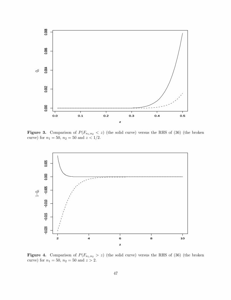
0.0 0.1 0.2 0.3 0.4 0.5

0.000

0.002

0.004

0.006

0.008

z

Q n

0.0 0.1 0.2 0.3 0.4 0.5

0.000

0.002

0.004

0.006

0.008

z

Figure 3. Comparison of P (Fn1,n2< z) (the solid curve) versus the RHS of (36) (the broken

curve) for n1 = 50, n2 = 50 and z < 1/2.

2 4 6 8 10

−0.02

0−0

.015

−0.01

0−0

.005

0.000

0.005

z

1−Q n

2 4 6 8 10

−0.02

0−0

.015

−0.01

0−0

.005

0.000

0.005

z

Figure 4. Comparison of P (Fn1,n2> z) (the solid curve) versus the RHS of (36) (the broken

curve) for n1 = 50, n2 = 50 and z > 2.

47