‘Til Dowry Do Us Part:

Bargaining and Violence in Indian Families

Rossella Calvi∗ Ajinkya Keskar†

September 2021

Abstract

We develop a non-cooperative bargaining model with incomplete informationlinking dowry payments, domestic violence, resource allocation between ahusband and a wife, and separation. Our model generates several predictions,which we test empirically using amendments to the Indian anti-dowry law as anatural experiment. We document a decline in women’s decision-making powerand separations, and a surge in domestic violence following the amendments.These unintended effects are attenuated when social stigma against separation islow and, in some circumstances, when gains from marriage are high. Wheneverpossible, parents increase investment in their daughters’ human capital tocompensate for lower dowries in the marriage market.

Keywords: Domestic violence, dowry, non-cooperative bargaining, India, maritalsurplus, women’s empowerment, human capital, gender norms, mental health.

∗Corresponding author: Rice University, Department of Economics, Houston, TX. E-mail:rossella.calvi@rice.edu.

†Rice University, Department of Economics, Houston, TX. E-mail: ajinkya.keskar@rice.edu.This paper has benefited from helpful comments from Abi Adams, Samson Alva, Dan Anderberg, Siwan

Anderson, Manuela Angelucci, S Anukriti, Abhijit Banerjee, Prashant Bharadwaj, Dan Bennett, ChrisBidner, Girija Borker, Nathan Canen, Pierre-André Chiappori, Flavio Cunha, Gaurav Chiplunkar, EstherDuflo, Bilge Erten, Willa Friedman, Yinghua He, Seema Jayachandran, Gaurav Khanna, Yunmi Kong,Jeanne Lafortune, Sylvie Lambert, Arthur Lewbel, Bolun Li, Karen Macours, Karthik Muralidharan, JacobPenglase, Isabelle Perrigne, Vijayendra Rao, Manisha Shah, Frank Schilbach, Tavneet Suri, Lauren Hoehn-Velasco, Tom Vogl, Fan Wang, and Jeff Weaver. All errors are our own.

1

1 Introduction

Transfers of wealth between families at the time of marriage existed historically in many

parts of the world, from the Babylonian civilization to Renaissance Europe, from the

Roman and Byzantine empires to the Song Period in China. In current times, marriage

payments remain pervasive in many areas of the developing world. While the practice

of bride-price (a transfer from the groom’s side to the bride’s) is widespread in parts of

East Asia and some African countries, dowries (wealth transfers from the bride’s family

to the groom or his family) are most common in South Asia. In India, Pakistan, and

Bangladesh, dowry payments are nearly universal and quite sizable, often amounting to

several times more than a household’s annual income (Goody, 1973; Anderson, 2007).

The custom of dowry in India has been linked to extreme forms of gender inequal-

ity, such as sex-selective abortion related to parental preferences for sons (Alfano, 2017;

Bhalotra et al., 2020), and the occurrence of bride-burning, dowry-deaths, and other

forms of domestic violence (Bloch and Rao, 2002; Srinivasan and Bedi, 2007). It has

also been shown that higher dowries can increase women’s status and decision power in

their marital families (Zhang and Chan, 1999). Since more than one-third of women in

India report being physically abused by their husbands and about half are excluded from

consequential household decisions,1 understanding the connections between marriage

transfers and women’s status in their marital family is of primary importance.

In this paper, we develop a non-cooperative bargaining model that links marriage

payments, women’s human capital, domestic violence, intra-couple resource allocation,

and separation. Popular models of intra-household bargaining (e.g., Chiappori (1988,

1992)) assume complete information and generally predict that the household alloca-

tion is efficient. However, this assumption conflicts with the occurrence of domestic

violence, a prominent form of inefficient household behavior. Instead, we consider a

bargaining model with incomplete information, where domestic violence is used by the

husband to signal his private type and extract resources from his wife. We extend the

non-cooperative framework of Bloch and Rao (2002) in multiple directions: by con-

sidering within-couple bargaining, by accounting for gains from marriage and their

division, by endogenizing parental investments in the human capital of girls, and by

1These figures are based on women’s responses to the National Family Health Survey (see Section 2for more details).

2

examining the role of social norms against separation. To this point, we follow the

insights of sociological and psychological studies on the consequences of marital disso-

lution in traditional societies and account for the social cost and psychological distress

associated with separation (Sharma, 2011; Ragavan et al., 2015; Pachauri, 2018).

Our model generates several predictions, which we test empirically using amend-

ments to the Indian anti-dowry law as a natural experiment. We estimate a fall in

dowries following the amendments, along with a decline in women’s empowerment, a

surge in domestic violence, and a decrease in separations. These unintended effects are

attenuated (and can even be reversed) when social stigma against separation is low.

Our model helps make sense of this heterogeneity.

We start by modeling the relationship between dowries and women’s status in their

marital family. In our model, at the time of marriage, a dowry is paid and the husband

learns his private type, which we interpret as his level of satisfaction with the match.

This timeline of events is consistent with the widespread custom of arranged marriage,

whereby the spouses are selected for each other by their parents, and the bride and

the groom often meet on or shortly before their wedding day. After the marriage, the

husband and the wife bargain over the allocation of gains from marriage, which may

arise from joint consumption and joint production (Becker, 1973, 1991). The post-

marital bargaining game consists of three stages. In the first stage, the husband chooses

whether to exercise violence. If violence occurs, then both the husband and the wife

incur a utility cost: the cost for women is fixed, while the cost faced by husbands varies

with their private type. At this time, the husband may demand a higher fraction of

marital gains. In the second stage, the wife chooses whether to accept the husband’s

demand. In the last stage of the game, the husband decides whether to separate from

his wife. Under certain assumptions outlined in Section 3, there exists a unique perfect

bayesian equilibrium of the game that satisfies the intuitive criterion: it is a separating

equilibrium, whereby only dissatisfied husbands facing a low cost of violence engage

in domestic violence, only dissatisfied husbands with a high cost of violence separate

from their wives, and wives accept their husband’s demand for a reallocation of marital

gains only if violence occurs.

Our model yields five testable predictions linking changes in dowries to changes

in women’s post-marital outcomes. First, the share of marital gains commanded by the

3

husband and the likelihood of domestic violence increase following a decrease in dowry.

Second, the probability of separation decreases following a decrease in dowry. Third,

these effects are reduced and can even be of opposite signs when social stigma against

separation is low. Through the lens of our model, we interpret this heterogeneity as

resulting from the psychological distress faced by women after separation.2 Fourth,

the impact of a reduction in dowry on the husband’s share of marital gains weakens as

marital gains increase. Fifth, the impact of a reduction in dowry on the probability of

wife-abuse strengthens when marital gains are high.

We also consider the pre-marital bargaining game between the bride’s family and

the groom or his family. In this game, parents make decisions about how much to

invest in the human capital of their daughter and how much to save for the dowry

(Anukriti et al., 2019). Such decisions culminate in a marriage offer by the bride’s

parents that the groom can accept or reject. Under the assumptions that parents prefer

their daughters to be married relative to them remaining unmarried and that grooms

value brides’ education (Adams and Andrew, 2019), the pre-marital model yields an

additional prediction: parents invest more in their daughters’ human capital in response

to a decrease in expected dowry payments.

Our empirical analysis exploits the introduction of amendments to the Dowry Pro-

hibition Act between 1985 and 1986 as a natural experiment, and consists of two main

parts. Using data from the Rural Economic and Demographic Survey, we first confirm

that the amendments, which tightened the existing anti-dowry legislation, were suc-

cessful at reducing dowry payments (Alfano, 2017). Next, using data from the National

Family Health Survey, we test the predictions of our model. Since the Dowry Prohibi-

tion Act (initially introduced in 1961) and its amendments did not apply to Muslims,3

we exploit variation in religion and year of marriage to identify the effect of the amend-

ments in a difference-in-differences framework. The validity of this approach requires

that, in the absence of the 1985-1986 amendments, the evolution of dowry payments

and the model’s outcomes should have been the same for Muslims and non-Muslims.

We provide empirical evidence supporting this fact. As recent work in econometrics has

2We model such distress as affecting women’s preferences over consumption. This is consistent withanhedonia, a common symptom of depression and other mental health disorders (Angelucci and Bennett,2021).

3The Shariat governs marriage and family matters for Muslims.

4

shown that difference-in-differences estimates may be biased due to treatment effects

heterogeneity over time and across groups (Goodman-Bacon, 2018; De Chaisemartin

and d’Haultfoeuille, 2020; Callaway and Sant’Anna, 2020), we also assess the issue of

heterogeneous effects in our setting, finding it not to be a critical source of concern.

We estimate that the Dowry Prohibition Act amendments significantly reduced

dowry payments. Women exposed to the amendments paid 0.2 standard deviations

lower dowries, on average. This corresponds to a 11,951 Rupees decline in dowry pay-

ments (in 1999 Rupees). We carefully rule out that these findings are driven by changes

in reporting, which would be relevant if survey respondents were less keen to answer

dowry-related questions after the reforms. We also assess the potential endogeneity of

the time of marriage, which could matter if parents anticipated the introduction of the

amendments and scheduled the wedding date of their sons and daughters accordingly.

Next, we analyze the interaction between the Dowry Prohibition Act amendments and

other reforms that may have had differential impacts by religion, and do not find it

critical for our findings. Finally, we show that our findings are confirmed by a triple-

difference specification that exploits inter-caste variation in dowry prevalence.

Turning to the model predictions, we estimate a decline in women’s involvement

in household decision-making (which we use to measure her share of marital gains;

Browning et al. (2013)), and an increase in domestic violence following the introduc-

tion of the amendments. For instance, we find that women exposed to the reforms (and

the subsequent decline in dowry payments) are 3 percent less likely to be involved in

household decisions, on average. The decline in women’s decision-making power is

particularly pronounced for infrequent, possibly more consequential decisions, such as

large household purchases and women’s health care decisions. We also show that the

amendments resulted in a 16 percent increase in the probability of domestic violence

against women. Conditional on ever experiencing violence by their husbands, treated

women suffer a wider array of injuries, such as cuts, bruises, burns, sprains, disloca-

tions, broken bones or teeth. Consistent with our model, we document a decrease in

separations after the reforms. Finally, we show that women exposed to the amendments

have better human capital outcomes (e.g., education and height), suggesting that par-

ents increased investment in the human capital of their daughters to compensate for

lower expected dowries. These findings are robust to various specifications and appro-

5

priate restrictions of the estimation sample, and are not driven by changes in marital

sorting.

We uncover substantial heterogeneity in the impact of the anti-dowry reforms on

women’s status in their marital families. We provide evidence of differential effects

by a couple’s gains from marriage, which we proxy with fertility outcomes (Becker,

1973, 1991). In line with our predictions, we show that the impact of the reforms on

women’s decision making power is alleviated when gains from marriage are high. By

contrast, the impact on domestic violence and separation is exacerbated when marital

gains are large. Importantly, the effects of the reforms on women’s post-marital out-

comes are mitigated when social stigma against separation is low (such as in North-East

and South India, urban areas, and villages with relatively higher rates of separation)

and exacerbated when social norms concerning marital dissolution are strict. This find-

ing suggests that the local cultural context (and the possible social pressure associated

with it) may matter a great deal when designing policies aimed at changing traditional

customs (e.g., Rao and Walton (2004) and Ashraf et al. (2020)). It also emphasizes the

need of “development approaches based on a fuller consideration of psychological and

social influences" (World Bank, 2015, p.582).

The rest of the paper is organized as follows. In Section 2, we provide an overview

of the custom of dowry, discuss the issues of domestic violence and women’s limited

power in India, and illustrate the legal framework governing marital transfers. In Sec-

tion 3, we set out our theoretical model and derive six testable predictions. In Section

4, we discuss the identification strategy and data sources. In Section 5, we present our

main empirical results. Section 6 concludes. A detailed literature review, proofs and

additional material are in an online Appendix.

2 Dowries, Violence, and Women’s Power in Indian Fam-

ilies

In contemporary India, dowry payments are nearly universal, and a woman is typi-

cally unable to marry without such transfers. The prospect of paying a dowry is often

listed as a critical factor in parents’ desire to have sons rather than daughters and has

been linked to female infanticide, sex-selective abortion, and the missing-women phe-

6

nomenon (Sen, 1990; Anderson and Ray, 2010, 2012; Jayachandran, 2015; Borker

et al., 2017). Dowries have also been associated with the dreadful occurrence of bride-

burning and dowry-deaths (Bloch and Rao, 2002; Srinivasan and Bedi, 2007; Sekhri and

Storeygard, 2014). These are extreme forms of domestic violence, which is pervasive in

India as well as in other developing countries. The following figures may help gauge the

gravity of the phenomenon. According to the latest National Family and Health Survey

(hereafter NFHS), 36 percent of ever-married Indian women have experienced physi-

cal or sexual violence by their husbands. The most common type of domestic violence

is less severe physical violence (28 percent), followed by severe physical violence (8

percent), and sexual violence (7 percent). One out of three female respondents in the

India Human Development Survey (IHDS) answers affirmatively when asked whether

in their community it is usual for a husband to beat his wife when her natal family does

not provide enough money or gifts. According to data from the National Crime Records

Bureau (NCRB), out of the almost 330,000 crimes against women committed in 2015,4

19 percent consisted of acts of "cruelty by husband or his relatives," and 1 percent were

dowry deaths.

Domestic violence is a dramatic form of gender inequality, but the limited decision-

making power of women inside their families is another widespread example. Due

to growing attention regarding the status of women in developing countries, in many

household surveys, a common type of question to ask is, "Who usually makes decisions

about [X] in your household?" The NFHS asks this question to ever-married women

aged 15 to 49, with [X] referring to decisions regarding, e.g., own health care, con-

traceptive use, household purchases and finances, visits to relatives, or even what to

cook. According to the most recent wave of the survey, less than two-thirds of currently

married women participate in decision making about their health, major household

purchases, or visits to their own family or relatives. One in six women reports being

involved in no decision at all.

Divorce is rare in India and often riddled with stigma.5 According to the 20114The NCRB classifies as crimes against women: rape, attempt to commit rape, kidnapping and abduc-

tion of women, dowry deaths, assault on women with intent to outrage her modesty, insult to the mod-esty of women, cruelty by husband or his relatives, importation of girls from foreign country, abetmentof suicides of women, and violations of the Dowry Prohibition Act (1961), the Indecent Representationof Women (Prohibition) Act (1986), the Commission of Sati Prevention Act (1987), the Protection ofWomen from Domestic Violence Act (2005), and the Immoral Traffic (Prevention) Act (1956).

5Pothen (1989), for example, writes: "Many people waited for a number of years in order to approach

7

Census of India, 1.36 million individuals in India are divorced, amounting to 0.24 per-

cent of the married population and 0.11 percent of the total population (Jacob and

Chattopadhyay, 2016). The dissolution of a marriage is often seen as damaging to a

woman’s reputation and is a source of substantial distress (Ragavan et al., 2015).6 So-

cial spaces may become unpleasant for separated women since their marital status is

either the starting point or the focus of most conversations. They may be cast out by

friends and relatives as broken, atypical, or having some astrological affliction. They

may also be excluded from many religious practices supposedly meant to be performed

only by married people.7

Several sociological and psychological studies document the adverse consequences

of marital dissolution for Indian women, which may lead to depression and anhedo-

nia (inability to derive pleasure from various activities).8 We also provide empirical

evidence in this direction. Using data from the 2004-2005 Survey on Morbidity and

Health Care, we compare women’s probability of suffering from psychiatric disorders

across marital statuses. While concerns related to underreporting, underdiagnosis, and

reverse causality are valid, we document a significantly higher probability of suffering

from mental distress for women who are divorced or separated (even conditional on

a battery of individual controls; see Figure A2 in the Appendix). As we discuss later

on, the extent of women’s psychological and emotional distress after separation may be

critical to predict how a change in dowry may impact women’s post-marital outcomes.

the court even after the marriage had broken down. Fear of social stigma, uncertainty about future, lackof legal knowledge, emotional upheavals, etc. were the main reasons for this delay."

6The likelihood of remarriage is low in India, but somewhat higher for men. According to the IndiaHuman Development Survey, less than 1 percent of ever-married Indian women remarry, while about 3.5percent of them report their husband being married more than once. This figures exclude polygamousfamilies and include remarriage after the death of the spouse.

7As discussed in Ragavan et al. (2015), "[If a woman gets a divorce] they [her family, the community]will think badly of her. They will think she had an affair or did something wrong, and for those reasonsshe asked for a divorce. Even if her husband made a mistake, and she did nothing wrong, the wholecommunity will still think that the woman is wrong."

8Based on a qualitative study in Jaipur, Rajasthan, Sharma (2011) finds that divorced women facesignificantly higher risk of suffering from anxiety, depression, stress, and fatigue. Interviewing divorcedwomen in Meerut, Uttar Pradesh, Pachauri (2018) shows that they face various challenges related tosocial, familial, financial, emotional, and psychological problems. Kotwal and Prabhakar (2009) studythe issues faced by single mothers (which includes divorced, separated, and widowed women) and showthat majority report feeling of loneliness, helplessness, hopelessness, lack of identity, and lack of con-fidence. Amudhan et al. (2020) study the prevalence and sociodemographic differentials of suicidalityusing data from the 2015-2016 National Mental Health Survey, finding widowed, separated, or divorcedindividuals to have a higher risk of overall suicidality.

8

The Dowry Prohibition Act and Its Amendments. In 1961, the government

of India enacted the Dowry Prohibition Act, prohibiting both the giving or receiving

of a dowry. The law defined a dowry as "any property or valuable security given or

agreed to be given either directly or indirectly (a) by one party to a marriage to the

other party to the marriage; or (b) by the parents of either party to a marriage or by

any other person, to either party to the marriage or any other person [...]." The act

explicitly excluded from the definition of dowry (and hence from the law itself) any

marital transfers "in the case or persons to whom the Muslim Personal Law (Shariat)

applied." It also stipulated that dowries could be punished either by imprisonment up

to six months or with a fine up to 5,000 Rupees.

The provisions of the act were not strong enough and its attempt to reduce dowries

proved mostly unsuccessful (Chiplunkar and Weaver, 2019). Between 1985 and 1986,

the Indian government took a series of steps towards tightening the existing anti-dowry

legislation. The Dowry Prohibition Rules (introduced in October 1985) established a

set of rules according to which a list of wedding gifts must be maintained. The list must

include a brief description of each gift, the approximate value of the gift, the name of

the person who has given the gift, and, when the person giving the present is related to

the bride or groom, a description of such a relationship. Another amendment followed

closely in 1986, increasing the minimum punishment for taking or abetting dowry to

five years of imprisonment and to a fine of not less than 15,000 Rupees (or the amount

of the value of the dowry, whichever is higher).9 Finally, the amendment gave power

to any state government to appoint "as many Dowry Prohibition Officers as it thinks

fit," to prevent the taking or demanding of dowry and to collect the necessary evidence

for the prosecution of violators of the Dowry Prohibition Act. By showing an increase

in the number of convicted offenders and of dowry cases heard by the Supreme Court

after 1986, Alfano (2017) provides evidence of both the enforcement and the public

awareness of the amendments.

Figure A3 in the Appendix plots the results of local polynomial regressions of real

dowry payments on year of marriage. We obtain information about dowry payments

9Between 1975 and 1976, the states of Bihar, Punjab, Haryana, Himachal Pradesh, West Bengal, andOrissa implemented state-level amendments to the 1961 act. The changes introduced by these earlyamendments, however, were moderate. In the states of Bihar and Punjab, for instance, the taking ofdowry was made punishable by a prison sentence of six months and a fine of 5,000 Rupees. In HimachalPradesh, the punishment was changed to 1-year imprisonment and a 5,000 Rupees fine (Alfano, 2017).

9

Figure 1: Dowries: Differences Between Non-Muslims and Muslims

(A) Gross Dowries (B) Net DowriesNOTES: This figure plots the the differences between non-Muslims and Muslims in gross dowries (Panel A) and net dowries (Panel B) around the amendments and 90 percentconfidence intervals. The coefficients are estimated in 2-year intervals from the year of treatment conditional on state, religion, and year of marriage and birth fixed effects.Zero denotes the reform year 1985. Gross dowries represent the value of transfers made to the groom’s family at the time of marriage. Net dowries are defined as grossdowries minus the value of transfers made from the groom’s family to the bride’s family. All dowry amounts are converted to 1999 Rupees.

from the 1999 Rural Economic and Demographic Survey (we provide details about this

survey in Section 4.1) and convert all dowries to 1999 Rupees. Gross dowries represent

the value of transfers made to the groom’s family at the time of marriage, while net

dowries are defined as gross dowries minus the value of transfers made from the groom’s

family to the bride’s family. Before 1985, the average gross dowry ranged between

42,000 and 56,000 Rupees, and net dowries varied between approximately 24,000 and

33,000 Rupees. Between 1985 and 1990, both gross and net dowries declined by more

than 20 percent. Dowry transfers kept declining in subsequent years, but at a slower

pace.

Consistent with the scope of the law, dowry payments for non-Muslim declined

after 1985, while marital transfers for Muslims were virtually unaffected. In Figure

1, we present event-study graphs displaying the differences between non-Muslims and

Muslims in gross and net dowries before and after 1985 (for clarity, we consider two-

year periods and normalize the difference in 1985 to zero). It is reassuring to see that

these gaps are not statistically different from zero before the amendments. Moreover,

the gaps in both gross and net dowries between non-Muslims and Muslims are negative

and increasingly significant in the years following the reforms.10

Given the connections between dowry payments, violence, and women’s empow-

erment, one natural question is whether (and how) the 1985-1986 tightening of the

10In Appendix D, we investigate the possible misreporting of dowry data, finding that it is unaffectedby the amendments.

10

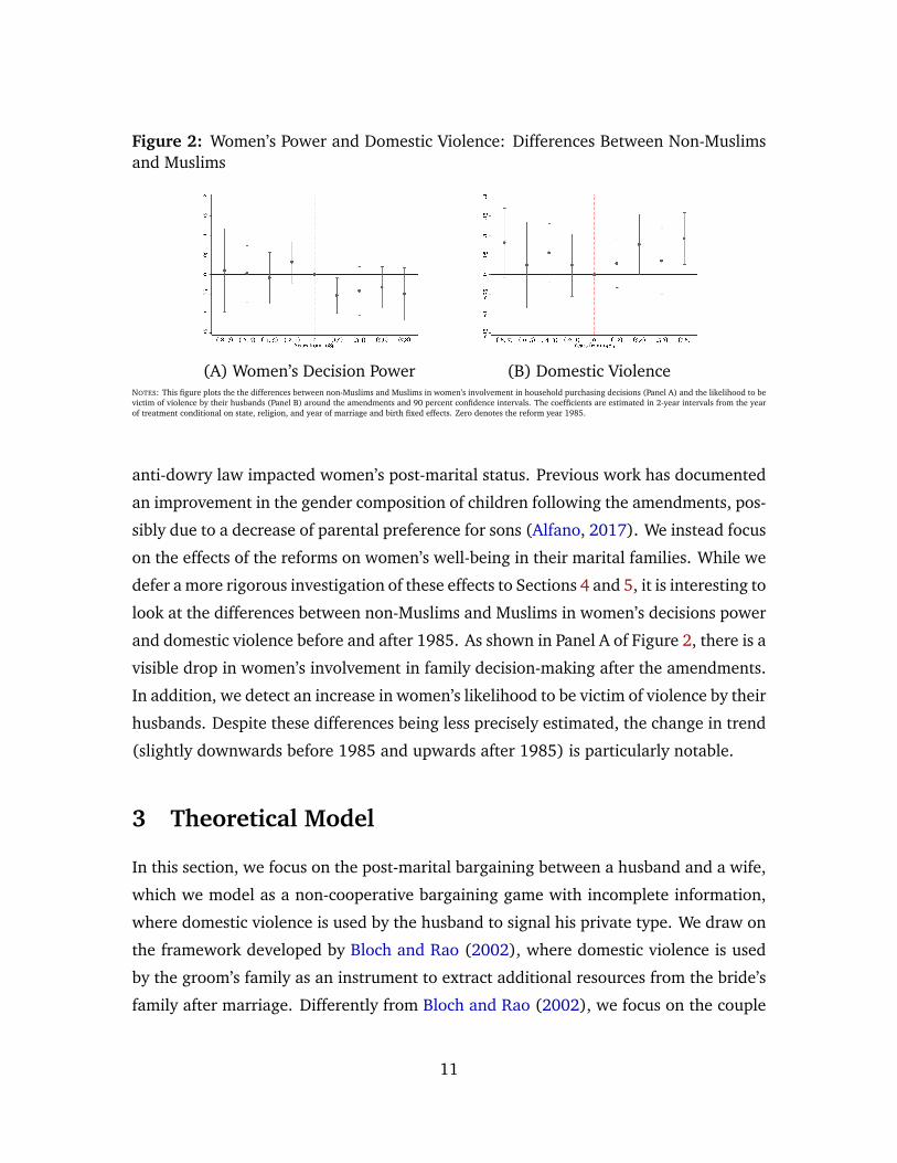
Figure 2: Women’s Power and Domestic Violence: Differences Between Non-Muslimsand Muslims

(A) Women’s Decision Power (B) Domestic ViolenceNOTES: This figure plots the the differences between non-Muslims and Muslims in women’s involvement in household purchasing decisions (Panel A) and the likelihood to bevictim of violence by their husbands (Panel B) around the amendments and 90 percent confidence intervals. The coefficients are estimated in 2-year intervals from the yearof treatment conditional on state, religion, and year of marriage and birth fixed effects. Zero denotes the reform year 1985.

anti-dowry law impacted women’s post-marital status. Previous work has documented

an improvement in the gender composition of children following the amendments, pos-

sibly due to a decrease of parental preference for sons (Alfano, 2017). We instead focus

on the effects of the reforms on women’s well-being in their marital families. While we

defer a more rigorous investigation of these effects to Sections 4 and 5, it is interesting to

look at the differences between non-Muslims and Muslims in women’s decisions power

and domestic violence before and after 1985. As shown in Panel A of Figure 2, there is a

visible drop in women’s involvement in family decision-making after the amendments.

In addition, we detect an increase in women’s likelihood to be victim of violence by their

husbands. Despite these differences being less precisely estimated, the change in trend

(slightly downwards before 1985 and upwards after 1985) is particularly notable.

3 Theoretical Model

In this section, we focus on the post-marital bargaining between a husband and a wife,

which we model as a non-cooperative bargaining game with incomplete information,

where domestic violence is used by the husband to signal his private type. We draw on

the framework developed by Bloch and Rao (2002), where domestic violence is used

by the groom’s family as an instrument to extract additional resources from the bride’s

family after marriage. Differently from Bloch and Rao (2002), we focus on the couple

11

instead of their families, account for potential gains from marriage and their division,

and examine the role of social norms against separation. We first develop a model where

the dowry amount and the human capital of future brides are taken as given. We then

extend the model to endogenize dowry payments as well as parental investment in their

daughters’ human capital. For simplicity, we do not model the process through which

the agents pair up and instead take the marital match as given.

3.1 Setup

Agents and Preferences. There are two agents in our model, a husband and a wife,

which we index by j = h, w. The two agents can be married to each other or sepa-

rated. Each agent derives utility from their consumption and characteristics (such as

their health and education) and, when married, from their spouse’s characteristics. We

denote by Uh and Uw the husband’s and the wife’s present discounted utility at the time

of marriage. Let Uh = uh(Ch,xw,xh,θ ) and Uw = uw(Cw,xw,xh), where C j indicates

j’s consumption, x j is a vector of human capital characteristics (which are ordered so

that higher values of x j correspond to more desirable traits), and θ is the husband’s

private type. In the spirit of Bloch and Rao (2002), we interpret θ as the husband’s

level of satisfaction with the match.11 We assume that the functions uh(·) and uw(·) are

increasing in all their arguments.

When married, the agents partake in marital gains, which may arise from joint

consumption and production. For instance, both spouses can enjoy their children and

live in the same home. They could also partially share some goods, such as fuel for

transportation, and save on food waste and spoilage. The couple can also benefit from

specialization in production, comparative advantage, and increasing returns to scale

(Becker, 1973, 1991). We denote by M the material gains from marriage and define

them as follows:

M = Yhw− Yh− Yw ≥ 0,

where the Yh is how much the husband can produce if unmarried, Yw is how much

the wife can produce if unmarried, and Yhw is the sum of husband’s and wife’s produc-

11Alternative interpretations are of course possible: θ , for instance, could be interpreted as a genericshock to the husband, whose consequence are unknown to the wife.

12

tion when married.12 Yh and Yw may include, but are not limited to, the husband’s

and the wife’s family wealth. In our model, we focus on the allocation of M between

the husband and the wife, and denote by γ the share of marital gains commanded by

the husband. Importantly, the insights and implications of our model are invariant to

interpreting γ as the share of Yhw (and not only M) allocated to the husband.

Let Vh = vh(Ch,xh, m) and Vw = vw(Cw,xw, m) be the husband’s and the wife’s dis-

counted utility flows when separated, where m denotes the marriage market conditions

at the time of separation. Note that we can interpret separation as a situation where

the husband and the wife stop living together while staying married. Alternatively,

separation can represent an unproductive marriage, where the marital surplus is null

(Lundberg and Pollak, 1993) and the spouses stop deriving utility from each others’

traits. As above, we require the functions vh(·) and vw(·) to be increasing in all their

arguments.

At the time of marriage, the bride’s family pays a dowry D to the husband’s family,

which we take as given for now. The consumption levels of the husband and the wife

can be summarized as follows: if the marriage is intact, then Ch = Yh + D+ γM and

Cw = Yw− D+(1−γ)M ; if separation occurs, then Ch = Yh+ D and Cw = Yw− D.

There are some features in our baseline model that deserve mention. First, dowries

enter each spouse’s utility through consumption and the husband’s private type is not af-

fected by them. Second, the impact of dowry on the woman’s post-marital consumption

is twofold: on one hand, it may change the share of marital surplus she commands; on

the other hand, it may decrease her consumption directly, which is consistent with her

post-marital consumption being partially driven by her natal family wealth.13 Third,

we take gains from marriage as given and do not treat them as a strategic lever of the

spouses. Fourth, we assume that dowries do not serve as early bequests for daughters

and that dowries are not returned to the bride’s family in case of separation. In Section

C in the Appendix, we consider several extensions to our baseline model that relax or

modify some of these features.14

12There may be emotional gains from marriage, such as love and companionship, but we abstract fromthem for simplicity.

13While we do not explicitly model post-marital transfers from the woman’s natal family, it is reasonableto assume that such transfers could be lower the higher is the amount of dowry paid upon marriage, whichwould be reflected in our specification.

14First, we extend our model to a framework where the husband (or his family) receives a transfer

13

The Bargaining Game. We model the interaction between the husband and

the wife as a non-cooperative bargaining game with incomplete information. When the

marriage takes place, the newlyweds learn about observable marriage characteristics.

We denote such characteristics by z. These include (but are not limited to) the initial

division of the gains from marriage, γ0, which we assume to be fully determined by the

marriage market conditions for brides and grooms at the time of the match. Right after

marriage, the husband learns his private type θ , that is, his level of satisfaction with

the match.15 This new information may trigger a post-marital renegotiation over the

division of the marital surplus. For simplicity, we define θ to be binary, with satisfied

husbands having θ equal to 1 and dissatisfied husbands having θ equal to 0. We denote

by p(z) the prior probability that the husband is not satisfied with the marriage.

The post-marital bargaining game consists of three stages. In the first stage, the

husband decides whether to exercise violence. If violence occurs, then the husband

and the wife incur a utility cost, which we denote by Kh and Kw, respectively. For

tractability, we assume that satisfied husbands face an infinite cost of violence (i.e.,

Kh(1) =∞). For dissatisfied husbands, the cost of violence is a random variable with

cumulative distribution function Fκ on [0,∞). At this time, the husband may request

a reallocation of marital gains and make a take-it-or-leave-it demand for a higher share

γ > γ0.16 In the second stage, the wife decides whether to accept the husband’s request.

In the third stage, the husband chooses whether to separate. To avoid issues related to

limited commitment, we assume that any intra-household reallocation of marital gains

occurs after the husband makes the separation decision.

equal to αD, while the wife retains control over (1−α)D (Appendix C.1). Such a model, which leadsto qualitatively similar predictions, accommodates situations in which dowries serve as early bequestsfor daughters. Second, we consider a model where the occurrence of domestic violence decreases gainsfrom marriage (Appendix C.2). Third, we develop a model where dowries can impact the likelihood thatthe husband is satisfied with the marriage (Appendix C.3). Under some assumptions, the predictions ofour baseline model remain. Fourth, we consider a framework where women have varying access to theirnatal family’s wealth when married vs. separated (Appendix C.4). This version allows for an additionalchannel through which social stigma against separation may play a role: not only through women’spreferences for consumption, but also through their ability to access their natal family’s resources afterseparation.

15This timing of events is reasonable in the Indian context, where the majority of marriages is arrangedby the bride’s and the groom’s family (Anukriti and Dasgupta, 2017; Vogl, 2013) and the spouses onlymeet on the day of the wedding (or shortly before then).

16In this regard, in our model, domestic violence has an extractive (or instrumental) motive (Angelucciand Heath, 2020) and does not provide intrinsic utility to husbands.

14

Context-driven Assumptions. As discussed in Section 2, divorce and separa-

tion are riddled with stigma in India, especially for women. So, while separation is

undesirable for all, women disproportionately bear the cost of marital dissolution. This

is an essential feature of the Indian context that we embed in our model as follows.

Under the initial allocation of marital gains, women prefer to be in a marriage than to

separate, even when the husband exercises domestic violence:17

uw(Yw− D+(1−γ0)M ,xh,xw)− Kw > vw(Yw− D,xw, m).

Moreover, satisfied husbands always prefer to stay married:

uh(Yh+ D+γM ,xh,xw, 1)> vh(Yh+ D,xh, m),

while, under the initial allocation of marital gains, dissatisfied husbands prefer to sep-

arate:

uh(Yh+ D+γ0M ,xh,xw, 0)< vh(Yh+ D,xh, m).

3.2 Solving for Equilibrium

We solve the game by backward induction. In the last stage of the game, only dissat-

isfied husbands whose demand for a higher share of marital gains is not met decide to

end their marriage. In particular, dissatisfied husbands choose not to separate if the

following inequality holds:

uh(Yh+ D+γM ,xh,xw, 0)≥ vh(Yh+ D,xh, m). (1)

Denote by γ the minimal transfer that keeps the marriage intact. Then, for γ = γ

equation (1) holds with equality.

In the second stage, the wife decides whether to accept or reject the husband’s

request for a reallocation of resources. The wife rejects any request for γ < γ, since it

would not dissuade the husband from separating. Denote by σ the wife’s belief that

the husband is dissatisfied after observing the occurrence of violence and the request17According to the Survey of Status of Women and Fertility, 90 percent of women would not consider

leaving their husbands even if he abuses her or if he is a drunk or drug addict; only one out of five womenbelieves that she could leave her husband if he were unable to provide for the family financially.

15

for resource reallocation. Then, if γ ≥ γ, the wife accepts any request that satisfies the

following condition:

uw(Yw−D+(1−γ)M ,xh,xw)≥ σvw(Yw−D,xw, m)+(1−σ)uw(Yw−D+(1−γ0)M ,xh,xw).

(2)

When the wife is indifferent between accepting or rejecting her husband’s request,

then equation (2) holds with equality and γ = γ̄(σ). So, γ̄(σ) is the maximal share of

marital gains that the husband can extract. Note that this maximal share is an increasing

function of the wife’s beliefs. In other words, the wife is willing to forgo a higher share

of the marital gains when she is more likely to believe that her husband is dissatisfied.

The wife’s optimal decision is to accept any request for γ̄(σ) ≥ γ ≥ γ and to reject it

otherwise. In the first stage, the husband decides whether to exercise violence and may

demand a higher γ.

To calculate the perfect bayesian equilibria (PBE) of the game, we consider both

pooling equilibria and separating equilibria. In what follows, we assume that the wife

rejects any request for reallocation if she does not update her beliefs about the husband’s

degree of satisfaction. We also assume that she is willing to increase her husband’s share

of gains from marriage and keep the marriage intact when she believes that her husband

is dissatisfied. More formally, we assume that γ̄(1)> γ > γ(p(z)).

Any pooling equilibria would be such that both satisfied and dissatisfied husbands

send the same signal with probability one. Given that the cost of violence for satis-

fied husbands is infinite, there are no equilibria where both satisfied and dissatisfied

husbands behave violently. Consider instead a situation where both satisfied and dis-

satisfied husbands do not exercise violence. Then, the husband’s signal would be un-

informative, the wife’s prior and posterior beliefs would coincide, and the wife would

reject any request for reallocation. For such equilibrium to exist, off-the-equilibrium

beliefs must be specified so that no one has an incentive to deviate. For this to occur,

however, the wife must assign a positive probability to the event that a satisfied husband

would exercise violence, which violates the intuitive criterion.

Any separating equilibria would be such that different types of husbands send dif-

ferent signals. There are no equilibria where satisfied husbands exercise violence and

dissatisfied husbands do not. Moreover, there exists no separating equilibrium satisfy-

ing the intuitive criterion, where neither types exercise violence but demand different

16

shares. Consider instead a scenario where the husband chooses violence when θ = 0,

he chooses non-violence when θ = 1, and γ ≤ γ(1) ≤ γ̄(1). Then, after observing

violence, the wife accepts any request for an intra-couple reallocation of the surplus.

Consequently, the husband’s optimal strategy is to request a share of marital surplus

equal to γ̄(1).

Denote by κ∗ the cost of violence that makes dissatisfied husbands indifferent

between exercising domestic violence or not. Husbands with high costs of violence

(Kh = κ, with κ > κ∗) will not exercise violence, even when dissatisfied. The wife’s

posterior belief that the husband is dissatisfied after not observing violence is therefore

given by:

σ(0) =p(z)[1− Fκ(κ∗)]

p(z)[1− Fκ(κ∗)]+1− p(z). (3)

Since σ(0)< p(z) and γ̄(σ) is an increasing function, the wife rejects any request

from a non-violent husband.

In summary, there is a unique PBE of the game that satisfies the intuitive criterion.

It is a separating equilibrium, where satisfied husbands and dissatisfied husbands with

a high cost of violence do not behave violently, and dissatisfied husbands with a low

cost of violence behave violently. After observing violence, the wife accepts the request

for reallocation of the marital surplus and γ= γ̄(1). If violence does not occur, then the

wife rejects any request. Satisfied husbands and dissatisfied husbands with low cost of

violence remain married. By contrast, dissatisfied husbands with high cost of violence

separate.

3.3 Comparative Statics

In order to derive empirical predictions, we assume that the utility functions of both

spouses are additively separable in consumption. So, we assume that the husband’s and

the wife’s discounted utilities when married are uh(Ch,xh,xw,θ ) = fh(Ch)+φh(xh,xw,θ )

and uw(Cw,xh,xw) = fw(Cw) +φw(xh,xw), respectively. Analogously, we assume that

the discounted utilities when separated are vh(Ch,xh, m) = fh(Ch) +ψh(xh, m) and

vw(Cw,xw, m) = gw(Cw)+ψw(xw, m) and that f j(·) and g j(·) are increasing and concave

functions.

As discussed in Section 2, marital dissolution is highly stigmatized in India, espe-

17

cially for women, which may have important consequences for their psychological well-

being and mental health (Sharma (2011), Ragavan et al. (2015), Pachauri (2018)).

Consistent with anhedonia (a common symptom of depression and psychological dis-

tress), we posit that women may have different preferences for consumption when mar-

ried vs. separated. Specifically, as illustrated in Figure A4 in the Appendix, we posit

that their marginal utility of consumption when married may be higher than when sep-

arated in spite of the concavity of gw(·) and fw(·) and the higher level of consumption

achieved when married.18,19

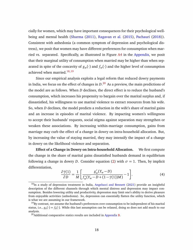
Since our empirical analysis exploits a legal reform that reduced dowry payments

in India, we focus on the effect of changes in D.20 As a preview, the main predictions of

the model are as follows. When D declines, the direct effect is to reduce the husband’s

consumption, which increases his propensity to bargain over the marital surplus and, if

dissastisfied, his willingness to use marital violence to extract resources from his wife.

So, when D declines, the model predicts a reduction in the wife’s share of marital gains

and an increase in episodes of marital violence. By impacting women’s willingness

to accept their husbands’ requests, social stigma against separation may strengthen or

weaken these associations. By increasing within-marriage consumption, gains from

marriage may curb the effect of a change in dowry on intra-household allocation. But,

by increasing the value of staying married, they may intensify the impact of a change

in dowry on the likelihood violence and separation.

Effect of a Change in Dowry on Intra-household Allocation. We first compute

the change in the share of marital gains dissatisfied husbands demand in equilibrium

following a change in dowry D. Consider equation (2) with σ = 1. Then, by implicit

differentiation,∂ γ̄(1)∂ D

=1M

�

g ′w(Yw− D)

f ′w(Yw− D+(1− γ̄(1))M)−1

�

. (4)

18In a study of depression treatment in India, Angelucci and Bennett (2021) provide an insightfuldescription of the different channels through which mental distress and depression may impact con-sumption. Besides lowering utility and productivity, depression may limit one’s ability to derive pleasurefrom enjoyable activities (anhedonia). So, depression can essentially flatten the utility function, whichis what we are assuming in our framework.

19By contrast, we assume the husband’s preferences over consumption to be independent of his maritalstatus, i.e., gh(·) = fh(·). While this last assumption can be relaxed, doing so does not add much to ouranalysis.

20Additional comparative statics results are included in Appendix B.

18

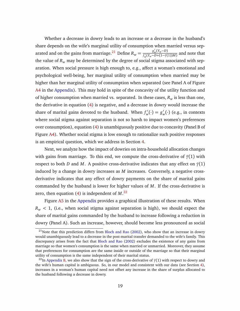
Whether a decrease in dowry leads to an increase or a decrease in the husband’s

share depends on the wife’s marginal utility of consumption when married versus sep-

arated and on the gains from marriage.21 Define Rw =g′w(Yw−D)

f ′w(Yw−D+(1−γ̄(1))M) and note that

the value of Rw may be determined by the degree of social stigma associated with sep-

aration. When social pressure is high enough to, e.g., affect a woman’s emotional and

psychological well-being, her marginal utility of consumption when married may be

higher than her marginal utility of consumption when separated (see Panel A of Figure

A4 in the Appendix). This may hold in spite of the concavity of the utility function and

of higher consumption when married vs. separated. In these cases, Rw is less than one,

the derivative in equation (4) is negative, and a decrease in dowry would increase the

share of marital gains devoted to the husband. When f ′w(·) = g ′w(·) (e.g., in contexts

where social stigma against separation is not so harsh to impact women’s preferences

over consumption), equation (4) is unambiguously positive due to concavity (Panel B of

Figure A4). Whether social stigma is low enough to rationalize such positive responses

is an empirical question, which we address in Section 4.

Next, we analyze how the impact of dowries on intra-household allocation changes

with gains from marriage. To this end, we compute the cross-derivative of γ̄(1) with

respect to both D and M . A positive cross-derivative indicates that any effect on γ̄(1)

induced by a change in dowry increases as M increases. Conversely, a negative cross-

derivative indicates that any effect of dowry payments on the share of marital gains

commanded by the husband is lower for higher values of M . If the cross-derivative is

zero, then equation (4) is independent of M .22

Figure A5 in the Appendix provides a graphical illustration of these results. When

Rw < 1, (i.e., when social stigma against separation is high), we should expect the

share of marital gains commanded by the husband to increase following a reduction in

dowry (Panel A). Such an increase, however, should become less pronounced as social

21Note that this prediction differs from Bloch and Rao (2002), who show that an increase in dowrywould unambiguously lead to a decrease in the post-marital transfer demanded to the wife’s family. Thisdiscrepancy arises from the fact that Bloch and Rao (2002) excludes the existence of any gains frommarriage so that women’s consumption is the same when married or unmarried. Moreover, they assumethat preferences for consumption are the same inside or outside of the marriage so that their marginalutility of consumption is the same independent of their marital status.

22In Appendix B, we also show that the sign of the cross-derivative of γ̄(1) with respect to dowry andthe wife’s human capital is ambiguous. So, in our model and consistent with our data (see Section 4),increases in a woman’s human capital need not offset any increase in the share of surplus allocated tothe husband following a decrease in dowry.

19

stigma against separation falls. When social stigma against separation is low enough,

it is possible that the share of marital gains commanded by the husband decreases

following a reduction in dowry (Panel A). Any impact of a decline in dowry on intra-

couple allocation should also be less severe for couples with substantial gains from

marriage (Panel B).

Effect of a Change in Dowry on Domestic Violence. To understand how

a change in dowry impacts domestic violence, we analyze how such change would

impact κ∗ (i.e., the maximal cost of violence that dissatisfied husbands are willing to

face in order to command a reallocation of resources and avoid separation). When

κ∗ increases, the probability that the husband exercises domestic violence increases;

vice versa, if κ∗ decreases, then a higher fraction of dissatisfied husbands refrains from

exercising violence. In equilibrium, such threshold is defined by

κ∗ = fh(Yh+ D+ γ̄(1)M)+φh(xh,xw, 0)− fh(Yh+ D)−ψh(xh, m). (5)

So,∂ κ∗

∂ D= Rw f ′h(Yh+ D+ γ̄(1)M)− f ′h(Yh+ D). (6)

Recall that, given equation (4) and given that fw(·) and gw(·) are increasing func-

tions, Rw is always positive. If Rw ≤ 1, the derivative in equation (6) is unambiguously

negative due to concavity and any decrease in dowry would increase the probability of

domestic violence. The sign of ∂ κ∗

∂ D , however, is ambiguous overall. The derivative in

equation (6) is negative as long as Rw < Rh, with Rh =f ′h(Yh+D)

f ′h((Yh+D)+γ̄(1)M) . So, whether

a decrease in dowry increases domestic violence depends not only on the wife’s rela-

tive marginal utility of consumption when married vs. separated (our proxy for social

stigma) but also on her husband’s and on the extent of marital gains. As before, ∂ κ∗

∂ D is

increasing in Rw and hence decreasing in social stigma against separation. In a context

like India with high social stigma against separation which is particularly strong, we

expect the probability of domestic violence to increase following a decrease in dowry

payments (see Panel A of Figure A6 in the Appendix). Since gender norms and stigma-

tization of marital dissolution vary substantially across India, however, we expect the

effect of a change in dowry on the probability of domestic violence to be highly hetero-

geneous.

20

Our analysis of the cross-derivative of κ∗ with respect to D and M yields some

additional insights. As we show in Appendix B, ∂ 2κ∗

∂ D∂M is always negative. So, any

increase in violence following a decrease in dowry would be particularly strong when

gains from marriage are high (see Panel B of Figure A6).

Effect of a Change in Dowry on Separations. Recall that, in the last stage

of the game, the husband decides whether to separate from his wife and that, in equi-

librium, only dissatisfied husbands with a high cost of violence (i.e., with κ above the

equilibriums threshold κ∗) separate. Thus, any change in dowry payments would have

an impact on separations that is the reverse of its impact on domestic violence: when so-

cial stigma against separation is high, a decrease in dowry should decrease separations.

In other words, the model predicts a negative correlation between changes in domestic

violence and separation following a change in dowry. Figure A7 in the Appendix helps

illustrate this prediction. The figure shows a hypothetical unimodal distribution of the

cost of violence κ and the cost of violence threshold κ∗. When Rw < Rh (i.e., when

social stigma against separation is high), the threshold κ∗ shifts upwards when D de-

clines, hence increasing the probability of domestic violence and decreasing the prob-

ability of separation; by contrast, when Rw > Rh, the threshold κ∗ shifts downwards

when D declines, hence decreasing the probability of domestic violence and increasing

the probability of separation.

Once again, it is important to note that, in our baseline model, dowry payments do

not affect the husband’s level of satisfaction with the marriage (see Appendix C.3 for

an extension). Instead, a dowry increases the husband’s consumption level both within

and outside of the marriage (in line with marriage practices, dowries are not returned

to the bride or her family in case of separation). This feature of the model is critical to

make sense of the predicted relationship between dowries and separations.

3.4 Endogenous Dowry and Human Capital

So far, we have taken dowry payments and the bride’s characteristics as given. In Sec-

tion C.5 in Appendix, we provide an extension to our model that includes a pre-marital

bargaining game between the bride’s family and the groom (or his family). We inter-

pret this first stage, which we briefly summarize below, as one in which parents make

decisions about how much to invest in the human capital of their daughter and about

21

how much to save for a future dowry (Anukriti et al., 2019). For simplicity, we abstract

from the specific process through which potential grooms match with brides.

In line with the social norms in the Indian context, we assume a very high social

cost of a daughter remaining unmarried (as in Borker et al. (2017)). So, parents strictly

prefer their daughters to be married relative to them remaining unmarried. Before the

marriage takes place, the bride’s parents make a take-it-or-leave-it offer to the groom.

This offer consists of the dowry payment and a set of bridal characteristics, including her

human capital. At this stage, the marriage characteristics, the cost of domestic violence,

and the future marriage market conditions are unknown to the potential groom and the

bride’s parents (although their distributions are known). The groom decides to accept

or reject the offer based on how his expected utility from marriage fares relative to

his reservation utility. His expected utility from marriage takes into account the three

possible post-marital scenarios discussed before (that he is satisfied, dissatisfied but

non-violent, or dissatisfied and violent), while his reservation utility depends on his

income, human capital, and the current marriage market conditions.

In equilibrium, the bride’s parents’ offer makes the potential groom indifferent be-

tween accepting and rejecting the marriage proposal. Since the groom values consump-

tion as well as his future wife’s human capital, and parents strictly prefer to have their

daughter married over remaining unmarried, a decrease in dowry would lead to an in-

crease in the human capital of future brides. However, the impact of a change in human

capital on domestic violence, intra-household resource allocation, and marital dissolu-

tion is ambiguous (see Section B in the Appendix). So, an increase in women’s human

capital may not help offset the negative consequences of lower dowries on women’s

well-being after marriage. In Section 5, we explore this issue empirically.

3.5 Summary of the Model Predictions

Our theoretical framework illustrates the relationship between dowry payments, the

allocation of marital gains between a husband and a wife, and the occurrence of do-

mestic violence and separation. It also describes the link between dowry payments

and parental investment in the human capital of future brides. Our model incorpo-

rates many features of the Indian cultural and social norms associated with marriage,

including the widespread social stigma associated with separation.

22

Prediction 1. If social stigma against separation is high, the share of marital gains

commanded by the husband increases following a decrease in dowry.

Prediction 2. If social stigma against separation is high, the probability of domestic

violence increases following a decrease in dowry.

Prediction 3. The effect of a decrease in dowry on the share of marital gains com-

manded by the husband and on the probability of domestic violence weakens as social

stigma against separation decreases. If social stigma against separation is low enough,

the husband’s share of marital gains and the probability of domestic violence decrease

following a decrease in dowry.

Prediction 4. The effect of a decrease in dowry on the share of marital gains com-

manded by the husband weakens as marital gains increase. The effect of a decrease in

dowry on the probability of domestic violence strengthens as marital gains increase.

Prediction 5. If social stigma against separation is high, the probability of separation

decreases following a decrease in dowry.

Prediction 6. Parental investment in the human capital of future brides increases fol-

lowing a decrease in (expected) dowry payments.

4 Empirical Strategy

4.1 Data and Measurement

To our knowledge, no nationally-representative dataset exists recording dowry pay-

ments, women’s decision power and living arrangements, and information about do-

mestic violence against women. So, for our empirical application, we rely on two sep-

arate data sources: data on dowry payments are from the 1999 Rural Economic and

Demographic Survey; data on intra-household bargaining power, domestic violence,

and separations are from the 2005-2006 National Family Health Survey.

Dowries. The Rural Economic and Demographic Survey (hereafter REDS) is a

detailed panel survey of rural households conducted by the National Council of Applied

Economic Research. The survey covers sixteen of the most populous states in India and

contains detailed retrospective information on year of marriage and marital transfers

for the household head, their parents, their sisters and brothers, and their daughters

23

and sons. It also includes socio-economic and demographic traits.23 From the 1999

REDS round, we select a sample of 17,897 marriages that took place between 1975

and 1999. The average gross dowry is about 38,000 Rupees ($4,104 PPP), the average

net dowry is about 25,000 Rupees ($2,699 PPP), and respondents reported that dowries

were paid in 90 percent of marriages (see Table A9 in the Appendix). The average year

of marriage in the sample is 1986, while the median is 1985. All respondents live in

rural areas, and they are primarily Hindu (though Muslims account for 6.8 percent of

the sample). More than half of the sample belongs to Scheduled Castes, Scheduled

Tribes or other backward castes. Educational attainment is low, with average years of

schooling being four and five for women and their spouses, respectively.

Intra-household Allocation, Domestic Violence, and Separation. One well-

known issue in empirical applications of household economics is that the allocation

of gains from marriage (or of household resources in general) is not directly observ-

able. We overcome this data limitation by using self-reported measures of women’s

decision-making power to construct proxies for the share of gains from marriages com-

manded by the wife (i.e., 1−γ).24 The National Family Health Survey (NFHS) contains

information about both a woman’s involvement in household decisions and domestic

violence. The survey also provides information on year of marriage and religion as well

as women’s current marital status, educational attainment, anthropometric indicators,

and other demographic and socioeconomic traits. To ensure an adequate number of

marriages before and after the 1985-1986 anti-dowry law amendments, we use data

from the 2005-2006 round. To ensure comparability with our analysis of dowry pay-

ments, we select a sample of more than 65,000 married women whose marriage took

place between 1975 and 1999.

As we report in Table A10 in the Appendix, slightly more than half of the women in

our sample reside in rural areas, 74 percent are Hindu, 13 percent are Muslim, and two-

thirds married after 1985. For women, the average age is 34, and the average schooling

is five years. For their husbands, the average age is 40, and the average schooling is

23In Section D in the Appendix, we investigate the quality of the REDS data, with a particular focus onthe possible misreporting of dowry amounts.

24While these measures have been widely used in the literature, we acknowledge some importantlimitations. First, having a say in decisions may not always be empowering to women. Moreover, someareas of decision-making may be more desirable than others and therefore reflect higher decision-makingpower (Heath and Tan, 2019).

24

seven years. More than 10 percent of women report having experienced injuries caused

by the husband or severe physical violence, and one-third of women report ever expe-

riencing less severe physical violence. Questions about injuries caused by the husband

are quite detailed: 33 percent of women report cuts, bruises, or aches, 8 percent report

eye injuries, sprains, dislocations, or burns, and 6 percent report deep wounds, broken

bones, broken teeth, or any other serious injury. Based on these reports, as well as on

general questions about experiences of different types of domestic violence, we con-

struct an ordinal measure of violence, which ranges between 1 and 6. Conditional on

ever experiencing any injuries or violence, a woman experiences two types of injuries,

on average.25

For a number of household decisions, the survey asks respondents about their de-

gree of involvement in the decision-making process. We construct several indicator

variables for whether the respondent reports participating in household decisions. One

in three women in our sample has no say in decisions about household purchases; in

one out of six families, the husband is in charge of all decisions regarding contraception

and his wife’s health care. To capture the scope of women’s decision-making power, we

also consider the number of decisions she reports being involved in (conditional on be-

ing involved in at least one). This variable ranges between 1 and 6 and is based on

women’s answers to questions regarding decisions over large and small household pur-

chases, how to spend their husband’s money, health and contraception decisions, and

decisions about what to cook.

4.2 Identification Strategy

As discussed in Section 2, the Dowry Prohibition Act and its amendments explicitly ex-

clude marital transfers governed by the Muslim Personal Law. So, for our identification

strategy, we exploit variation by religion as well as the timing of the marriages. Our

25One concern about using self-reported occurrences of domestic violence is misreporting (Aldermanet al., 2013). Looking at a sample of women in Peru, Agüero and Frisancho (2017) employ indirect ques-tioning techniques to measure the misreporting of intimate partner violence when using direct questions(such as those included in the NFHS). They find that, on average, there are no significant differencesin direct versus indirect questions. However, they find significant underreporting of violence for highlyeducated women. Since education levels are quite low in our context, concerns about misreporting maybe less critical.

25

baseline specification is as follows:

yi = β1Posti ×Non-Muslimi +β2Posti +β3Non-Muslimi + X ′iγ+αc +αs + εi, (7)

where yi is the outcome of interest for woman i and Posti is an indicator variable equal

to one if woman i got married in or after 1986; X i is a vector of exogenous covariates

(indicator variables for religion, for living in rural areas, and for being part of disad-

vantaged social groups such as Scheduled Castes, Scheduled Tribes or other backward

castes); αc are women’s birth-cohort fixed effects and αs are state fixed effects. In al-

ternative specifications, we include year of marriage fixed effects, district-level fixed

effects, state by year of birth fixed effects, or religion-specific time trends. β1 is the

parameter of interest and captures the average treatment effect on the treated of being

exposed to the 1985-1986 tightening of anti-dowry laws in India. As a robustness check,

we also include covariates that may be impacted directly by the amendments, such as

women’s education, household size and wealth, as well as husband’s characteristics.

Unless otherwise noted, we estimate equation (7) with OLS, using a sample of married

women, who got married between 1975 and 1999. Standard errors are clustered at

the state level. Whenever appropriate, we account for multiple hypothesis testing and

apply the Romano-Wolf step-down procedure to compute adjusted p-values.

Parallel Trends. As typical in a difference-in-difference framework, the validity

of our results relies on the parallel trend assumption. This assumption requires that,

in the absence of the 1985-1986 amendments, the evolution of dowry payments, do-

mestic violence, women’s decision power and human capital, and separations should

have been the same for Muslims and non-Muslims. To confirm that this is the case in

our framework, we restrict the sample to the pre-reform period (that is, to women who

married between 1975 and 1985), and regress the outcomes of interest on indicators

for the year of marriage and for being non-Muslim, and their interactions. As shown in

Figure A8, we do not detect any significant divergence in dowry payments, occurrence

of violence and separations, women’s decision power, and human capital outcomes be-

26

tween the two religious groups before the reforms.26,27

Treatment Effect Heterogeneity. There is a recent literature indicating that es-

timates of equation (7) may be biased if treatment effects are heterogeneous across

groups or periods.28 To assess the robustness of our estimates to this issue, we fol-

low De Chaisemartin and d’Haultfoeuille (2020) and estimate the minimal value of the

standard deviation of the average treatment effects under which β1 and the average

treatment effect on the treated could be of opposite signs. When this measures is large,

it means that the estimated β1 is not an appropriate estimate of the average treatment

effect on the treated only if there is an implausible amount of treatment effect hetero-

geneity. In this case, treatment effect heterogeneity is not too much of a concern. By

contrast, if this measure is too close to zero, then the average treatment effect on the

treated and the estimate of β1 can be of opposite signs even under small and plausi-

ble amount of treatment effect heterogeneity.29 As discussed later on, we do not find

treatment effect heterogeneity to be a critical issue in our setting.

Alternative Policies. One might also worry that, during our period of analysis,

other policies were implemented that may have had an impact on dowry payments

and women’s outcomes. We are primarily concerned about two sets of reforms. The

first set consists of early amendments to the Dowry Prohibition Act. Between 1975

26In our model, any change in dowry impacts women’s power, domestic violence, and separationsthrough consumption. So, it is also critical to rule out that, in the absence of the 1985-1986 amendments,the evolution of consumption should have been the same for Muslims and non-Muslims. To this aim,we again restrict the sample to the pre-reform period and regress the household income (from REDS),household wealth (from NFHS), and an indicator for owning a below-poverty-line card (from NFHS)on indicators for the year of marriage and for being non-Muslim, and their interactions. The estimatedcoefficients for the interaction terms are not statistically different from zero (results are available onrequest).

27We also perform a falsification test and estimate our baseline model with Posti being replaced bya variable equal to one if the marriage took place between 1980 and 1985 and to zero if it took placebetween 1975 and 1979. If there were differences in trends between Muslims and non-Muslims, wewould find statistically significant coefficients on the newly defined interaction term. This is not the casefor any of our outcomes of interest (results are available on request).

28See, e.g., Goodman-Bacon (2018), Callaway and Sant’Anna (2020), Sun and Abraham (2020).29Under the assumption that the treatment effects of the treated groups and time periods are drawn

from a uniform distribution, De Chaisemartin and d’Haultfoeuille (2020) suggest the following rule ofthumb. Assume that the treatment effect of every group and time period cannot be larger in absolutevalue than B > 0. If |cβ1|≥ σ̂

p3, then σ̂ may not be an implausibly high amount of treatment effect

heterogeneity, and the average treatment effect on the treated may be equal to 0. By contrast, if |cβ1|<σ̂p

3, then σ̂may or may not be an implausibly high amount of treatment effect heterogeneity, dependingon whether the maximum reasonable B < σ̂

p3 or B ≥ σ̂

p3. Since we do not know the true value of B,

we consider our estimates robust to treatment effect heterogeneity if |cβ1|< σ̂p

3.

27

and 1976, the states of Bihar, Punjab, Himachal Pradesh, Haryana, West Bengal, and

Orissa introduced local amendments, increasing penalties for requesting, receiving, or

giving a dowry. Though the prescriptions of the local amendments were more moderate

than those introduced in 1986 nationwide, we check that the impact of the reforms

is not limited to these early amended states. The second set of reforms pertains to

amendments to the Hindu Succession Act that equalized women’s inheritance rights

to men in several Indian states between 1976 and 2005. These reforms only applied

to Hindu, Buddhist, Sikh or Jain women, who were not yet married at the time of

the amendment in their state. We check that the Dowry Protection Act amendments

affected dowry payments and women’s outcomes independently of their exposure to

the inheritance rights reforms.30

We start by establishing that the amendments were successful at reducing dowries.

To this aim, we estimate equation (7) with measures of dowry amounts and prevalence

as outcomes. Next, we test the model predictions we outlined in Section 3.3. We test

Predictions 1 and 2 by estimating the regression model in equation (7) using NFHS

responses to questions on domestic violence and intra-household decision-making as

outcomes of interest. To test whether the impact of an exogenous decrease in dowry on

the women’s decision power varies with societal norms about divorce and separation

(Prediction 3), we check whether β1 is lower in villages with higher rates of divorced or

separated women or in urban, possibly more progressive, areas. We also check whether

the Dowry Protection Act amendments had weaker effects in North-East and South

India, where marriage dissolution rates are higher (Dyson and Moore, 1983).

A central assumption of household economics is that children provide union-specific

utility to parents. This is particularly true in the Indian context, where out-of-wedlock

fertility is rare. According to the World Values Survey (1990-1994), four out of five

women in India consider children a critical component of a successful marriage. So, in

the spirit of Becker (1973, 1991) and, more recently, of Angelucci and Bennett (2019),

we use fertility outcomes and fertility preferences to construct measures of gains from

marriage. We then test Prediction 4 by allowing β1 to vary with these measures. If

30Kerala in 1976, Andhra Pradesh in 1986, Tamil Nadu in 1989, and Maharashtra and Karnataka in1994 passed reforms making daughters coparceners. National ratification of the amendments occurredin 2005. Importantly for our analysis, Roy (2015) shows that women who were close to marriageableage at the time of the reform in their state subsequently made higher dowry payments to their husbands.

28

the data support this prediction, we expect β1 to be decreasing in gains from marriage

when we use women’s decision-making power as the dependent variable. By contrast,

we expect the effect of the anti-dowry reforms on domestic violence to be increasing in

gains from marriage.

To test Prediction 5, we estimate the impact of the 1985-1986 amendments on the

probability of being divorced or separated. Since divorce is extremely rare and may be

suffering from underreporting due to social stigma, we define women to be separated

if they report not living together with their husbands.31 Finally, we test Prediction 6

by comparing the human capital outcomes of women who were exposed to the amend-

ments to those of women who were not. Since we expect younger girls to be more

responsive to changes in human capital investment (especially for outcomes such as

height and primary school completion), we estimate different effects based on the age

of women at the time of the reform.

5 Results

We now present our empirical results. We begin by documenting a decline in dowries

following the introduction of the Dowry Prohibition Act amendments. We then pro-

ceed by discussing the empirical results for women’s decision-making power, domestic

violence, separations, and human capital, which we present in the order in which our

predictions were introduced in Section 3.5.

5.1 Dowries

Table 1 contains the baseline estimates of the impact of the 1985-1986 reforms on

dowry payments.32 The first four columns focus on dowry amounts over the full sample

(Columns (1) and (2)) and a sample restricted to marriages with non-zero transfers

(Columns (3) and (4)). In Columns (5), we study the probability of a marriage involving

no dowry. In Columns (6), we estimate the effect of the reforms on the likelihood of

31One possible drawback of this approach is that we do not observe why the couple does not livetogether, and so it may include cases of temporary or permanent migration.

32We wish to stress that Alfano (2017) has previously investigated the impact of these reforms on dowrypayments. While our analysis is qualitatively in line with this previous work, we estimate a differentempirical specification and unpack effects at the intensive and extensive margins.

29

Table 1: Dowries

GrossDowry

NetDowry

GrossDowry(if>0)

NetDowry(if 6= 0)

ZeroDowry

MissingDowry

(1) (2) (3) (4) (5) (6)

Post × Non-Muslim -11.951∗∗ -6.700∗∗ -9.681∗ -3.750 0.060∗ -0.034(4.081) (2.342) (4.762) (2.843) (0.029) (0.024)

Obs. 15,008 9,069 13,689 7,979 13,779 15,918R sq. 0.244 0.150 0.251 0.179 0.136 0.250Mean Dep. Var. 37.960 25.234 41.618 28.681 0.096 0.147FWER Adj. P-values 0.002 0.004 0.016 0.069 0.016 0.070TEH Robust σ̂ 72.445 32.273 56.599 17.275 0.464 0.181

NOTES: OLS estimates. Sample of women aged 15 to 49 in 2005, who married between 1975 and 1999. All dowry amounts are converted to 1999 Rupees (×1000). Allspecifications include state fixed effects, year of birth fixed effects and individual controls. Individual controls include indicator variables for being Muslim, Christian orHindu, for year of marriage after 1985, for type of residence (rural or urban), and for belonging to schedule caste, schedule tribe or other backward caste. Standard errors(in parentheses) are clustered at the state level. ***, **, * mean statistical significance at 1, 5 and 10 percent levels. The Romano-Wolf FWER adjusted p-values are basedon 500 bootstrap replications. TEH (Treatment Effect Heterogeneity) Robust σ̂ corresponds to the minimal value of the standard deviation of the treatment effect acrossthe treated groups and time periods under which β̂1 and the average treatment effect on the treated could be of opposite signs. When this measures is large, it means thatthe estimated β1 is not an appropriate estimate of the average treatment effect on the treated only if there is an implausible amount of treatment effect heterogeneity (seefootnote 29).

missing dowry information, possibly related to respondents refusing to answer dowry-

related questions.

We estimate that the 1985-1986 reforms to the Dowry Prohibition Act were success-

ful at reducing dowries. Specifically, the amendments decreased gross and net dowries

by approximately 12,000 and 6,700 Rupees over the full sample. To gauge magnitudes,

these correspond to reductions in dowry payments by roughly 0.2 standard deviations.

Such reductions result from changes occurring both at the extensive and intensive mar-

gins: on the one hand, we document a 6 percentage points increase in the probability

that the marriage involved no transfer at all; on the other hand, we detect sizable and

negative declines in dowry payments when we restrict our attention to non-zero trans-

fers (though caution needs to be applied here, since we are restricting our sample based

on outcomes).33 Importantly, the reforms did not have any impact on the probability

of the information about dowry being missing or not reported, which curbs concerns

related to changes in reporting following the introduction of the amendments (for a

more detailed analysis of changes in misreporting of dowry amounts after the reforms,

see Appendix D). These results are robust to accounting for multiple hypothesis test-

33The estimation of tobit models for censored outcomes yields qualitatively similar results. Our resultsare also quantitatively confirmed when we estimate probit regressions for binary outcomes. Finally, ourresults are robust to excluding or downweighting outliers. We estimated equation (7) after trimmingor topcoding the top 1 and 5 percent of dowry amounts and after transforming dowry amounts usinglogarithmic or inverse hyperbolic sine transformations of the dowry amounts. The full set of estimates isavailable upon request.

30

ing and treatment effect heterogeneity, as indicated by the low Romano-Wolf adjusted

p-values and the high De Chaisemartin-d’Haultfoeuille summary measures reported in

Table 1. They are also robust to changes in the estimation sample and more restrictive

specifications, as we describe in details in Section E in the Appendix.34

5.2 Predictions 1 to 4: Women’s Decision Power and Domestic Vi-

olence

Predictions 1 and 2. If social stigma against marital dissolution is high, Predictions

1 and 2 state that women exposed to the reforms should have lower decision-making

power in their marital families and should face a higher likelihood of domestic violence,

on average. If social stigma is low, we may see an increase in women’s decision-making

power and a decrease in domestic violence following the amendments.

Table 2 reports the estimated impact of the Dowry Prohibition Act amendments on

women’s participation in family decisions. The table reports estimates of linear proba-

bility models. The estimation of probit models for binary outcomes delivers estimated

effects that are quantitatively similar and significantly smaller standard errors (results

are available upon request). In Columns (1) and (2), the dependent variables are an

indicator variable equal to one if the woman reports being involved in at least one finan-

cial or health-related decision (see Section 4.1 for details) and the number of decisions

she has a say in (conditional on being involved in at least one decisions). In line with

the prediction of our model and the widespread societal attitude against separation in

India, we find that women’s decision-making power declines following the introduction

of the 1985-1986 reforms: women exposed to the reforms are 2.6 percentage points less

likely to being involved in household decisions, on average (approximately 3 percent);

if they are at all involved, the scope of their involvement declined by approximately

2.9 percent (once again these results need to be interpreted with caution, as we are

restricting the estimation sample based on an outcome).

34While we do not report these results for space constraints, we take several steps to address concernsabout the possible endogeneity of treatment. First, we show that excluding marriages that occurredbetween 1984 and 1987 does not substantially impact our estimates. Next, we develop an intent-to-treat analysis, where the treatment variable is defined as the interaction between an indicator variablefor being non-Muslim and an indicator variable equal to 1 if the woman was 14 or younger in 1986(hence, likely not married) and to zero if she was older than 23 (hence, likely married). Our findings areconfirmed.

31

To better understand these results, we estimate equation (7) using indicators for

specific decisions as dependent variables (Columns (3) to (6)). The estimated coeffi-

cients are negative and statistically significant for infrequent and possible more con-

sequential decisions, such as large household purchases and a woman’s health care

(including decisions about contraception). We also document a reduction in women’s

decision-making power regarding how to spend their husband’s earnings.

We present the estimation results for the domestic violence outcomes in Table 3.

Following a structure similar to Table 2, the first two columns feature, as outcomes,

an indicator for a woman ever suffering injuries due to her husband’s actions and the

number of different types of injuries she has suffered, respectively. As we described in

Section 4.1, the array of injuries we consider include eye injuries, sprains, dislocations,

burns, deep wounds, broken bones or teeth, or any other serious injury. In line with

Prediction 2, women’s exposure to the Dowry Prohibition Act amendments increases

their likelihood of being victims of domestic violence, both at the extensive and (in a

slight misuse of terminology) at the intensive margin. The estimated effects are sizable

and indicate that the reforms increased the likelihood of wife-abuse by 1.9 percentage

points (15.8 percent). Conditional on ever experiencing violence by their husbands,

treated women suffer a wider array of injuries.

In Columns (3) to (6), we exploit additional survey questions about women’s ex-

perience of physical, sexual, and emotional violence by the husband. While all the

point estimates support the existence of a positive association between women’s ex-

posure to the amendments and their likelihood to be abused by their husbands, the

estimated coefficients for women’s exposure to sexual and emotional violence are not

statistically significant at conventional levels. By contrast, we find that the amendments

substantially increased the likelihood of severe and less severe physical violence (by 3.4

percentage points and 2.9 percentage points, respectively).

To gauge the magnitudes of the estimated effects presented in Tables 2 and Tables

3, we compare them to alternative policies. For example, Heath and Tan (2019) esti-

mate that amendments to Hindu Succession Act (that equalized inheritance rights for

women and men in several Indian states between 1976 and 2005) increased women’s

participation in decisions about large purchases by 10 percentage points, about their

own health by 5 percentage points, and about how to spend their husbands’ money by

32

Table 2: Prediction 1: Women’s Decision Power

Type of Decision

AnyDecision

Number ofDecisions

(if>0)HouseholdPurchases

Health &Contracept.

Husband’sMoney

DailyDecisions

(1) (2) (3) (4) (5) (6)

Post × Non-Muslim -0.026∗ -0.125∗∗ -0.056∗∗∗ -0.029∗ -0.025∗ -0.017(0.014) (0.052) (0.017) (0.016) (0.014) (0.016)

Obs. 65,105 61,309 65,054 62,496 59,977 65,105Mean Dep. Var. 0.917 4.219 0.619 0.876 0.737 0.816R sq. 0.088 0.066 0.063 0.068 0.047 0.063FWER Adj. P-values 0.078 0.030 0.008 0.078 0.078 0.132TEH Robust σ̂ 0.091 0.644 0.057 0.034 0.141 0.002

NOTES: OLS estimates. Sample of women aged 15 to 49 in 2005, who married between 1975 and 1999. All specifications include state fixed effects, year of birth fixed effects and individualcontrols. Individual controls include indicator variables for being Muslim, Christian or Hindu, for year of marriage after 1985, for type of residence (rural or urban), and for belonging to schedulecaste, schedule tribe or other backward caste. Standard errors (in parentheses) are clustered at the state level. ***, **, * mean statistical significance at 1, 5 and 10 percent levels. The Romano-WolfFWER adjusted p-values are based on 500 bootstrap replications. See Table 1 for details on TEH Robust σ̂.

3 percentage points (though this coefficient is not statistically different from zero). Sun-

der (2020) shows that women’s exposure to the District Primary Education Programme

(a flagship policy of the Indian government in the 1990s, which led to the construc-

tion of over 160,000 new schools and boosted female primary school completion rates

by 12 percentage points) increased women’s participation in household spending de-

cisions by 8 percentage points. In the Kenyan context, Haushofer et al. (2019) find

that a large cash transfer targeting men (approximately equal to $700 PPP, on average)

decreased the likelihood of women being slapped by their husband by 10 percentage

points (32 percent) and kicked, dragged, or beaten by 9 percentage points (59 percent).

In our context, the Dowry Prohibition Act amendments (which reduced gross dowries

by roughly $1,200 PPP and net dowries by $600 PPP) increased the likelihood of se-

vere and less severe physical violence by 33 and 9 percent, and the likelihood of ever

suffering any injury by the husband by 16 percent.

As indicated by the Romano-Wolf p-values and the De Chaisemartin-d’Haultfoeuille

summary measures reported in Table 1, our estimates are generally robust to account-

ing for multiple hypothesis testing and treatment effect heterogeneity. For women’s

involvement in large household purchases and decisions about health and contracep-

tion, however, the De Chaisemartin-d’Haultfoeuille measures are quite low relative to

the estimated effects, suggesting that treatment effect heterogeneity may be a source of

concern (see footnote 29). To test the sensitivity of our findings, we perform a battery

of additional robustness checks, which we present in Section E in the Appendix.

Prediction 3. Next, we study the presence of differential effects of the anti-

33

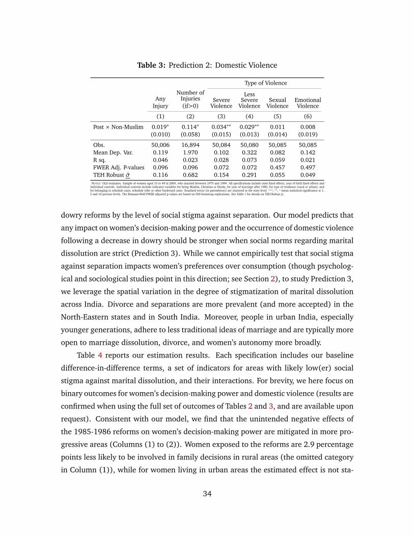
Table 3: Prediction 2: Domestic Violence

Type of Violence

AnyInjury

Number ofInjuries(if>0)

SevereViolence

LessSevere

ViolenceSexual

ViolenceEmotionalViolence

(1) (2) (3) (4) (5) (6)

Post × Non-Muslim 0.019∗ 0.114∗ 0.034∗∗ 0.029∗∗ 0.011 0.008(0.010) (0.058) (0.015) (0.013) (0.014) (0.019)

Obs. 50,006 16,894 50,084 50,080 50,085 50,085Mean Dep. Var. 0.119 1.970 0.102 0.322 0.082 0.142R sq. 0.046 0.023 0.028 0.073 0.059 0.021FWER Adj. P-values 0.096 0.096 0.072 0.072 0.457 0.497TEH Robust σ̂ 0.116 0.682 0.154 0.291 0.055 0.049

NOTES: OLS estimates. Sample of women aged 15 to 49 in 2005, who married between 1975 and 1999. All specifications include state fixed effects, year of birth fixed effects andindividual controls. Individual controls include indicator variables for being Muslim, Christian or Hindu, for year of marriage after 1985, for type of residence (rural or urban), andfor belonging to schedule caste, schedule tribe or other backward caste. Standard errors (in parentheses) are clustered at the state level. ***, **, * mean statistical significance at 1,5 and 10 percent levels. The Romano-Wolf FWER adjusted p-values are based on 500 bootstrap replications. See Table 1 for details on TEH Robust σ̂.

dowry reforms by the level of social stigma against separation. Our model predicts that

any impact on women’s decision-making power and the occurrence of domestic violence

following a decrease in dowry should be stronger when social norms regarding marital

dissolution are strict (Prediction 3). While we cannot empirically test that social stigma

against separation impacts women’s preferences over consumption (though psycholog-

ical and sociological studies point in this direction; see Section 2), to study Prediction 3,

we leverage the spatial variation in the degree of stigmatization of marital dissolution

across India. Divorce and separations are more prevalent (and more accepted) in the

North-Eastern states and in South India. Moreover, people in urban India, especially

younger generations, adhere to less traditional ideas of marriage and are typically more

open to marriage dissolution, divorce, and women’s autonomy more broadly.

Table 4 reports our estimation results. Each specification includes our baseline

difference-in-difference terms, a set of indicators for areas with likely low(er) social

stigma against marital dissolution, and their interactions. For brevity, we here focus on

binary outcomes for women’s decision-making power and domestic violence (results are

confirmed when using the full set of outcomes of Tables 2 and 3, and are available upon

request). Consistent with our model, we find that the unintended negative effects of

the 1985-1986 reforms on women’s decision-making power are mitigated in more pro-

gressive areas (Columns (1) to (2)). Women exposed to the reforms are 2.9 percentage

points less likely to be involved in family decisions in rural areas (the omitted category

in Column (1)), while for women living in urban areas the estimated effect is not sta-

34

Table 4: Prediction 3: Differential Effects by Social Stigma

Any Decision Any Injury

(1) (2) (3) (4) (5) (6)

Post × Non-Muslim -0.029∗∗ -0.037∗∗ -0.029∗ 0.020∗ 0.015 0.023∗

(0.014) (0.016) (0.015) (0.011) (0.013) (0.014)Post × Non-Muslim × Urban 0.010∗ -0.001

(0.005) (0.011)Post × Non-Muslim × East India 0.009 0.010

(0.021) (0.014)Post × Non-Muslim × West India 0.012 0.002

(0.011) (0.011)Post × Non-Muslim × South India 0.028∗∗∗ 0.010

(0.007) (0.011)Post × Non-Muslim × North-East India 0.047∗∗∗ -0.021∗∗

(0.010) (0.010)Post × Non-Muslim × High Divorce Rate 0.007 -0.011

(0.008) (0.013)

Obs. 65,105 65,105 65,105 50,006 50,006 50,006R sq. 0.088 0.088 0.088 0.046 0.046 0.046Mean Dep. Var. 0.917 0.917 0.917 0.119 0.119 0.119

NOTES: OLS estimates. Sample of women aged 15 to 49 in 2005, who married between 1975 and 1999. Rural is the omitted category in Columns (1) and (4), North India is the omitted category in Columns(2) and (5), areas with low prevalence of divorce (below median) is the omitted category in Columns (3) and (6). All specifications include state fixed effects, year of birth fixed effects and individual controls.Individual controls include indicator variables for being Muslim, Christian or Hindu, for year of marriage after 1985, for type of residence (rural or urban), and for belonging to schedule caste, schedule tribe orother backward caste. Standard errors (in parentheses) are clustered at the state level. ***, **, * mean statistical significance at 1, 5 and 10 percent levels.

tistically different from zero. The most striking differences in the impact of the reforms

on women’s decision power, however, are found across regions, with the nation-wide

effects presented in Table 2 being driven mostly by North Indian states (which are often

viewed as the most conservative and traditional states for gender norms). In this region

(the omitted category in Column (2)), women exposed to the reforms are 3.7 percent-

age points less likely to be involved in household decisions relative to non-exposed

women. Note that these spatial differences are present, though less pronounced, for

the domestic violence outcomes (Columns (4) to (5)).

To measure the prevalence of divorce and separations at the village level, we com-

pute the share of respondents within a primary sampling unit (which in the NFHS is a

village in rural areas or a block in urban areas) who report being divorced, separated,

or living apart from their spouse. In high-prevalence areas (i.e., in the top half of the

distribution, where marital dissolution may be less stigmatized), the introduction of the

Dowry Prohibition Act amendments had a weaker impact on women’s involvement in

household decisions (the point estimate is -0.021, but not statistically different from

zero). This pattern is qualitatively confirmed for the domestic violence outcome, with

women experiencing a 1.1 percentage point (9.5 percent) increase in violence in high-

prevalence areas and a 2.3 percentage points (19 percent) increase in low-prevalence

areas.

35

Prediction 4. We now turn to Prediction 4, which states that the effect of a

change in dowry payments should vary with gains from marriage. Specifically, any

impact on women’s decision-making power following a decrease in dowry should be

weaker when gains from marriage are high; by contrast, the impact on domestic vio-

lence should be more pronounced when gains from marriage are large. As discussed in

Section 4.2, we construct proxies for gains from marriage based on a couple’s fertility

outcomes and preferences.35

Table A11 in the Appendix reports estimates of the differential effects by gains from

marriage of the anti-dowry reforms on women’s decision-making power and domestic

violence. In Columns (1) and (4), we measure a couple’s marital gains with the number

of children they have. The estimated coefficients are consistent with the model predic-

tions. Women who were exposed to the anti-dowry reforms are 7.9 percentage points

(8.6 percent) less likely to be involved in financial and health-related decisions if they

have no children. These effects, however, are significantly weaker for women with chil-

dren. In line with our model, the impact on wife-abuse is stronger when children are

present, as indicated by the positive coefficients on the interaction terms in Column (4).

In essence, exposure to the anti-dowry reforms increased domestic violence for women

with and without children. However, the effect is more prominent (and statistically

significant only) when children are present.

One might worry that more children do not necessarily yield higher gains. This is

especially true if there is a mismatch between realized and desired fertility. One may

expect gains from marriage to be the highest when the couple meets their fertility pref-

erences, and the fertility is complete. In Columns (2) and (5), we estimate different

effects by a couple’s achievement of their desired fertility, which we measure with an

indicator variable equal to one if the number of children equals a woman’s ideal num-

ber of children and her spouse does not want any more (or any less) children. While

the estimated coefficient is only significant for the violence outcome, both signs are as

expected.

35We also test Prediction 4 using alternative measures of marital surplus. Similarly-educated orsimilarly-aged spouses may experience higher gains from marriage; so, we test whether the impact ofthe amendments are heterogeneous by the absolute value of the spousal gaps in age or schooling. Wefind the effects of the reforms on women’s decision-making power to be statistically significant only forthose couples with low gains from marriage (with large spousal gaps in age or education). Results areavailable on request.

36

Finally, we use the gender of the first born child as an alternative measure of mar-

ital gains. While parental preferences for sons are widespread in India, the sex of the

firstborn child is quasi-random (Anukriti et al., 2016). We find that the impact of the

policy on women’s decision power is mitigated when gains from marriage are high (i.e.,

when the first born child is male). We do not find any statistically significant difference

for domestic violence.

Discussion. Taken together, the results presented so far are mostly consistent

with Predictions 1 to 4 of our model. They also imply that the tightening of anti-dowry

laws introduced by the Indian government between 1985 and 1986 had some unin-

tended negative consequences for women’s welfare. The overall decline in women’s

involvement in household decisions and the increase in domestic violence following

the amendments (and the consequent decreases in dowry payments documented in

Section 5.1) indicate that social stigma against separation in India is high, on average

(that is, Rw < 1). We document substantial variation in the stigmatization and social

cost of marital dissolution across regions, which results in markedly differential im-

pacts of the anti-dowry reforms on women’s outcomes (Prediction 3). The unintended

consequences of the reforms appear to be mitigated in more progressive areas and exac-

erbated in more conservative regions, suggesting that one-size-fits-all policies may not

be optimal, and that the social and cultural context may matter a great deal when de-

signing policies aimed at changing traditional customs (an important point also raised

by Rao and Walton (2004), World Bank (2015), and Ashraf et al. (2020)).

Our heterogeneity analysis by gains from marriage hinges on the assumption that

any changes in dowry payments did not affect the number of children a couple decides

to have. In our theoretical model, this assumption is reflected in gains from marriage

being taken as given and not chosen strategically by the agents. While this is a chal-

lenging task, we attempt to empirically investigate the validity of this assumption by

estimating the impact of the anti-dowry reforms on fertility. In Section F, we compare

the fertility preferences and outcomes of treated and untreated women and do not find

noteworthy differences. Although these results provide suggestive evidence of the va-

lidity of our assumption, given the challenge of accurately measuring marital gains, we

wish to interpret our test of Prediction 4 with caution.

As discussed in Section 3.4, the model predictions about how the effects of a change

37

in dowry should vary with women’s human capital are ambiguous. Stating it differently,

the impact of the amendments could be exacerbated or weakened or unchanged for

women with higher human capital relative to women with lower levels of human capi-

tal. We estimate alternative specifications that allow for differential effects of the anti-

dowry reforms on women’s decision-making power and domestic violence by women’s

completed years of education. We do not detect any significant heterogeneity by human

capital, suggesting that increases in women’s education may not help curb the negative

consequences of reducing dowries for women’s post-marital welfare. The full set of

results is available on request.

5.3 Prediction 5: Separations

We have documented a surge in domestic violence following the amendments to the

Dowry Prohibition Act. The fifth prediction to emerge from our model states that the

effect on the probability of separation should be the reverse. This prediction follows

from the fact that, in equilibrium, only dissatisfied husbands with a high cost of violence

choose to separate. So, we expect the decrease in dowries induced by the amendments

to decrease the probability of separation.

The estimated effects reported in Table A12 in the Appendix are consistent with this

prediction. Odd numbered columns report estimates of equation (7) featuring a binary

indicator for a woman being divorced, separated, or living apart from her husband as

the dependent variable. The estimation sample varies across columns. In Column (1),

we consider the full sample of ever-married women aged 15 to 49, who got married

between 1975 and 1999, and find a 2.9 percentage points decrease in the probability

of separation following the anti-dowry amendments. In Column (3), we restrict the

estimation sample to rural areas outside of the North-East and South India regions

(hence more traditional and less open to divorce and separation), while in Columns

(5), we only consider women who live in urban areas, North-East India or South India

(typically more progressive and more acceptive of marital dissolution). A comparison

of the estimated coefficients across columns indicates that the decrease in separation

induced by the reforms is primarily driven by more conservative areas, where social

stigma against marital dissolution is high. In even numbered columns, we report the

estimated differential effects by gains from marriage. Consistent with our model, we

38

find evidence of a more pronounced decline in the probability of separation following

the 1985-1986 amendments for couples with high marital gains.

5.4 Prediction 6: Women’s Human Capital

We now turn to our last prediction, which states that parental investment in the human

capital of future brides should increase following a tightening of anti-dowry laws. The

NFHS does not include information on past expenditure or saving patterns of a woman’s

natal family. So, we rely on women’s outcomes in adulthood to inform us of any changes

in parental investment induced by the reforms.

We focus on two sets of human capital outcomes: outcomes related to education,

such as years of schooling and the probability of having completed primary school; and

long-run health outcomes, such as height and the probability of being in the bottom

half of the stature distribution in our sample. Naturally, parents’ ability to shape their

daughters’ human capital in response to the 1985-1986 amendments would be limited

if their daughters were too old at the time of the reforms. Height, for instance, is mostly

determined by early childhood inputs. So, any response from parents whose daughters

were, e.g., five or older in 1985, may not be reflected in their daughter’s outcomes

in adulthood. Similarly, the effect of the amendments on primary school completion

may be strongest for those women who were not too old to attend primary school in

1985. We test these hypotheses by estimating equation (7) using measures of women’s

education and height as dependent variables over four subsamples based on women’s

age in 1985.36

We summarize the results of our analysis in Figure A9 in the Appendix (the corre-

sponding coefficients and standard errors are reported Tables A13 and A14). Panel A

shows the estimated effects of the reforms on education outcomes (years of schooling

on the left-hand side axis and a binary indicator for primary school completing on the

right-hand side); Panel B plots the estimated effects on long-run health (height in cen-

timeters on the left axis and a binary indicator for below-median height on the right

axis). The horizontal axis denotes each cohort’s age as of 1985. The estimated coeffi-

36Note that any change in women’s human capital outcomes may also reflect a change in parentalbeliefs about their marriage market return and in parental preference for girls’ human capital. Given thedata at hand, however, it is not possible to distinguish one channel from the other.

39

cients are consistent with our expectations. If possible (that is, for girls who were not

too old at the time of the amendments), parents successfully improved their daughters’

human capital outcomes: the younger the girls at the time of the reforms, the more pro-

nounced the effects. For the education outcomes, the gradient is positive (with younger

cohort experiencing the largest increases), and the estimated effects are statistically dif-

ferent from zero for women who were children or teenagers at the time of the reforms.

For height, the gradient is also positive. As expected, however, we do not detect any

statistically significant differences for those cohorts who were six or older at the time

of the reform.

5.5 Alternative Channels

In the previous sections, we established that the 1985-1986 amendments to the Dowry

Prohibition Act were successful at reducing dowry payments. We also tested the six

predictions that emerge from our theoretical model and find that they are consistent

with the data. Nonetheless, there may be alternative explanations of our findings that

are outside of our model but may be critical to fully understand the connections between

dowries, domestic violence, women’s decision-making power, and the occurrence of

separation. Fort instance, marital sorting and matching, may change in response to

a drop in dowries. Fertility outcomes and preferences may also be impacted by the

reforms. Finally, the validity of our domestic violence findings may be jeopardized if

the reforms changed women’s propensity to report domestic abuse. In Section F in the

Appendix, we assess the scope of these alternative mechanisms, but find them not to be

critical for out results.

6 Conclusion

We provide a framework to understand the complex connections between dowry pay-

ments, parental investment in girls, women’s decision-making power in their marital

families, the occurrence of domestic violence, and the likelihood of separation. We

derive predictions on how changes in dowries can impact women’s well-being in their

marital families. To test these predictions empirically, we exploit legal reforms to the

Indian anti-dowry law that successfully reduced dowry payments. Consistent with our

40

model, we find that women’s decision-making power decreases and domestic violence

increases following a reduction in dowries. The likelihood of separation also decreases,

indicating that women are unable or unwilling to exit abusive marriages. To compen-

sate for lower dowries in the marriage market, parents increase their investment in the

human capital of their daughters.

For women, the reputation cost of separating from their husbands is prohibitive,

which leaves them little to no escape from unsatisfying or abusive marriages. We in-

corporate this fact in our model and argue that the extent of women’s psychological

distress after separation may be critical to predict how a change in dowry may impact

women’s post-marital outcomes. In line with this model insight, we unveil substan-

tial heterogeneity by social stigma against separation in the impact of the anti-dowry

reforms on women’s status in their marital families, suggesting that one-size-fits-all

policies may not be optimal and that the local social and cultural context may matter

a great deal when designing policies aimed at changing traditional customs. We hope

future work will further investigate the interactions between such policies and local

gender norms, and directly study their psychological and emotional effects. Doing so

will require collecting detailed data on psychological and emotional well-being, a task

that is especially challenging in developing countries where mental illness is frequently

stigmatized (Ridley et al., 2020; Baranov et al., 2020; Angelucci and Bennett, 2021).

While previous work has stressed the positive impact of anti-dowry policies on son-

preference and sex-ratios, our analysis unveils some unintended consequence of such

policies. Understanding the interlinkages between dowry payments and a woman’s

well-being at different stages of her life is critical to devise policies to successfully im-

prove the status of Indian women. As one-sixth of the world female population live in

India, doing so would represent a significant step toward eliminating gender inequality

globally — a United Nations Sustainable Development Goal to be achieved by 2030.

References

ADAMS, A. AND A. ANDREW (2019): “Preferences and beliefs in the marriage market for

young brides,” Tech. rep., IFS Working Papers. [4]

AGÜERO, J. AND V. FRISANCHO (2017): “Misreporting in Sensitive Health Behaviors and

41

Its Impact on Treatment Effects: An Application to Intimate Partner Violence,” IDB

Working Paper No. IDB-WP-853. [25]

ALDERMAN, H., J. DAS, AND V. RAO (2013): Conducting Ethical Economic Research Com-

plications from the Field: Complications from the Field, The World Bank. [25]

ALFANO, M. (2017): “Daughters, dowries, deliveries: The effect of marital payments on

fertility choices in India,” Journal of Development Economics, 125, 89–104. [2], [4],[9], [11], [29]

AMUDHAN, S., G. GURURAJ, M. VARGHESE, V. BENEGAL, G. N. RAO, D. V. SHEEHAN, A. M.

KOKANE, B. S. CHAVAN, P. K. DALAL, D. RAM, ET AL. (2020): “A population-based

analysis of suicidality and its correlates: findings from the National Mental Health

Survey of India, 2015–16,” The Lancet Psychiatry, 7, 41–51. [8]

ANDERSON, S. (2007): “The economics of dowry and brideprice,” Journal of Economic

Perspectives, 21, 151–174. [2]

ANDERSON, S. AND D. RAY (2010): “Missing women: age and disease,” The Review of

Economic Studies, 77, 1262–1300. [7]

——— (2012): “The age distribution of missing women in India,” Economic and Political

Weekly, 87–95. [7]

ANGELUCCI, M. AND D. BENNETT (2019): “The Marriage Market for Lemons: HIV Test-

ing and Marriage in Rural Malawi,” Unpublished Manuscript. [28]

——— (2021): “The Economic Impact of Depression Treatment in India,” Unpublished

Manuscript. [4], [18], [41]

ANGELUCCI, M. AND R. HEATH (2020): “Women Empowerment Programs and Intimate

Partner Violence,” in AEA Papers and Proceedings, vol. 110, 610–14. [14]

ANUKRITI, S., S. R. BHALOTRA, AND E. H. F. TAM (2016): “On the quantity and quality

of girls: New evidence on abortion, fertility, and parental investments,” . [37]

ANUKRITI, S. AND S. DASGUPTA (2017): “Marriage markets in developing countries,” in

The Oxford Handbook of Women and the Economy. [14]

42

ANUKRITI, S., S. KWON, AND N. PRAKASH (2019): “Saving for Dowry: Evidence from

Rural India,” Unpublished Manuscript. [4], [22]

ASHRAF, N., N. BAU, N. NUNN, AND A. VOENA (2020): “Bride price and female educa-

tion,” Journal of Political Economy, 128, 591–641. [6], [37]

BARANOV, V., S. BHALOTRA, P. BIROLI, AND J. MASELKO (2020): “Maternal depression,

women’s empowerment, and parental investment: evidence from a randomized con-

trolled trial,” American economic review, 110, 824–59. [41]

BECKER, G. S. (1973): “A theory of marriage: Part I,” Journal of Political economy, 81,

813–846. [3], [6], [12], [28]

——— (1991): “Fertility and the Economy,” Journal of Population Economics, 5, 185–

201. [3], [6], [12], [28]

BHALOTRA, S., A. CHAKRAVARTY, AND S. GULESCI (2020): “The price of gold: Dowry

and death in India,” Journal of Development Economics, 143, 102413. [2]

BLOCH, F. AND V. RAO (2002): “Terror as a Bargaining Instrument: A Case Study of

Dowry Violence in Rural India,” American Economic Review, 92, 1029–1043. [2],[7], [11], [12], [19]

BORKER, G., J. EECKHOUT, N. LUKE, S. MINZ, K. MUNSHI, AND S. SWAMINATHAN (2017):

“Wealth, marriage, and sex selection,” Tech. rep., Technical report, Working Paper,

Cambridge University. [7], [22]

BROWNING, M., P.-A. CHIAPPORI, AND A. LEWBEL (2013): “Estimating Consumption

Economies of Scale, Adult Equivalence Scales, and Household Bargaining Power,”

The Review of Economic Studies, 80, 1267–1303. [5]

CALLAWAY, B. AND P. H. SANT’ANNA (2020): “Difference-in-differences with multiple

time periods,” Journal of Econometrics. [5], [27]

CHIAPPORI, P.-A. (1988): “Rational Household Labor Supply,” Econometrica, 63–90. [2]

——— (1992): “Collective Labor Supply and Welfare,” Journal of Political Economy,

437–467. [2]

43

CHIPLUNKAR, G. AND J. WEAVER (2019): “Marriage markets and the rise of dowry in

India,” Unpublished Manuscript. [9]

DE CHAISEMARTIN, C. AND X. D’HAULTFOEUILLE (2020): “Two-way fixed effects estima-

tors with heterogeneous treatment effects,” American Economic Review, 110, 2964–

96. [5], [27]

DYSON, T. AND M. MOORE (1983): “On kinship structure, female autonomy, and demo-

graphic behavior in India,” Population and development review, 35–60. [28]

GOODMAN-BACON, A. (2018): “Difference-in-differences with variation in treatment

timing,” Tech. rep., National Bureau of Economic Research. [5], [27]

GOODY, J. (1973): “Bridewealth and Dowry in Africa and Eurasia,” . [2]

HAUSHOFER, J., C. RINGDAL, J. P. SHAPIRO, AND X. Y. WANG (2019): “Income changes

and intimate partner violence: Evidence from unconditional cash transfers in kenya,”

Tech. rep., National Bureau of Economic Research. [33]

HEATH, R. AND X. TAN (2019): “Intrahousehold bargaining, female autonomy, and labor

supply: Theory and evidence from India,” Journal of the European Economic Associa-

tion. [24], [32]

JACOB, S. AND S. CHATTOPADHYAY (2016): “Marriage dissolution in India,” Economic &

Political Weekly, 51, 25. [8]

JAYACHANDRAN, S. (2015): “The roots of gender inequality in developing countries,”

economics, 7, 63–88. [7]

KOTWAL, N. AND B. PRABHAKAR (2009): “Problems faced by single mothers,” Journal of

Social Sciences, 21, 197–204. [8]

LUNDBERG, S. AND R. A. POLLAK (1993): “Separate spheres bargaining and the marriage

market,” Journal of political Economy, 101, 988–1010. [13]

PACHAURI, P. (2018): “Problems faced by divorced women in their pre and post-divorce

period: A sociological study with reference to District Meerut,” Journal of Pharma-

cognosy and Phytochemistry, 7, 207–212. [3], [8], [18]

44

POTHEN, S. (1989): “Divorce in Hindu society,” Journal of Comparative Family Studies,

20, 377–392. [7]

RAGAVAN, M., K. IYENGAR, AND R. WURTZ (2015): “Perceptions of options available

for victims of physical intimate partner violence in northern India,” Violence against

women, 21, 652–675. [3], [8], [18]

RAO, V. AND M. WALTON (2004): Culture and public action, The World Bank. [6], [37]

RIDLEY, M., G. RAO, F. SCHILBACH, AND V. PATEL (2020): “Poverty, depression, and anx-

iety: Causal evidence and mechanisms,” Science, 370. [41]

ROY, S. (2015): “Empowering women? Inheritance rights, female education and dowry

payments in India,” Journal of Development Economics, 114, 233–251. [28]

SEKHRI, S. AND A. STOREYGARD (2014): “Dowry deaths: Response to weather variability

in India,” Journal of development economics, 111, 212–223. [7]

SEN, A. (1990): “More than 100 million women are missing,” The New York Review of

Books, 37, 61–66. [7]

SHARMA, B. (2011): “Mental and Emotional Impact of Divorce on Women,” Journal of

the Indian Academy of Applied Psychology, 37, 125–31. [3], [8], [18]

SRINIVASAN, S. AND A. S. BEDI (2007): “Domestic violence and dowry: Evidence from

a South Indian village,” World Development, 35, 857–880. [2], [7]

SUN, L. AND S. ABRAHAM (2020): “Estimating dynamic treatment effects in event studies

with heterogeneous treatment effects,” Journal of Econometrics. [27]

SUNDER, N. (2020): “Parents’ Schooling and Intergenerational Human Capital: Evi-

dence from India,” Unpublished Manuscript. [33]

VOGL, T. S. (2013): “Marriage institutions and sibling competition: Evidence from

South Asia,” The Quarterly journal of economics, 128, 1017–1072. [14]

WORLD BANK (2015): “World development report 2015: Mind, society, and behavior,”

Tech. rep. [6], [37]

ZHANG, J. AND W. CHAN (1999): “Dowry and Wife’s Welfare: A Theotrical and Empirical

Analysis,” Journal of Political Economy, 107, 786–808. [2]

45