Approaches to convective scale data assimilation

Tijana Janjić1, Y. Zeng2, Y.Ruckstuhl2, Heiner Lange2

1Hans-Ertel-Centre for Weather Research, Deutscher Wetterdienst (DWD)2Hans-Ertel-Centre for Weather Research, LMU

Outline

I Convective scale data assimilation characteristics

I Our approach of addressing non-Gaussianity: Ensemble dataassimilation scheme with constraints

I Illustrate approach on simple examplesI Explore which constraints should be included

Outline

I Convective scale data assimilation characteristicsI Our approach of addressing non-Gaussianity:

Ensemble dataassimilation scheme with constraints

I Illustrate approach on simple examplesI Explore which constraints should be included

Outline

I Convective scale data assimilation characteristicsI Our approach of addressing non-Gaussianity: Ensemble data

assimilation scheme with constraints

I Illustrate approach on simple examplesI Explore which constraints should be included

Outline

I Convective scale data assimilation characteristicsI Our approach of addressing non-Gaussianity: Ensemble data

assimilation scheme with constraintsI Illustrate approach on simple examplesI Explore which constraints should be included

— Convective scale data assimilation —

Convective scale data assimilation

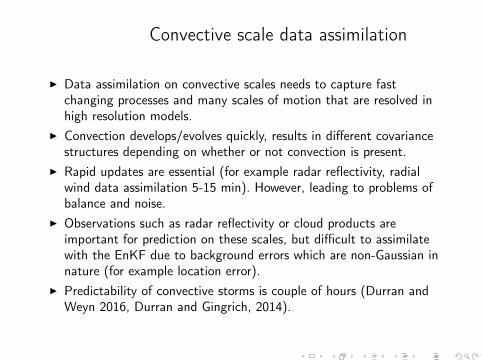
I Data assimilation on convective scales needs to capture fastchanging processes and many scales of motion that are resolved inhigh resolution models.

I Convection develops/evolves quickly, results in different covariancestructures depending on whether or not convection is present.

I Rapid updates are essential (for example radar reflectivity, radialwind data assimilation 5-15 min). However, leading to problems ofbalance and noise.

I Observations such as radar reflectivity or cloud products areimportant for prediction on these scales, but difficult to assimilatewith the EnKF due to background errors which are non-Gaussian innature (for example location error).

I Predictability of convective storms is couple of hours (Durran andWeyn 2016, Durran and Gingrich, 2014).

Convective scale DA at DWD

I Kilometre-scale Ensemble Data Assimilation (KENDA) based onLETKF (Schraff et al. 2016)

1 40-member ensemble2 adaptive localization in horisontal, in vertical 0.075–0.5 in ln p3 adaptive inflation4 RTPP scheme with 0.75 (Zhang et al 2004)

I COSMO model (Baldauf et al. 2011) in the domain over Germany,2.8km horizontal resolution, 50 hybrid levels. Deep convectionexplicit, shallow convection parametrized.

I 1h updatesI Each member consists of the prognostic variables of velocity,

temperature, pressure perturbation, specific humidity, cloud waterand ice.

I The prognostic variables of turbulent kinetic energy, rain, snow, andgraupel are excluded from the analysis update.

I For radar data, LHN in all ensemble members

Convective scale DA at DWD

I Kilometre-scale Ensemble Data Assimilation (KENDA) based onLETKF (Schraff et al. 2016)

1 40-member ensemble2 adaptive localization in horisontal, in vertical 0.075–0.5 in ln p3 adaptive inflation4 RTPP scheme with 0.75 (Zhang et al 2004)

I COSMO model (Baldauf et al. 2011) in the domain over Germany,2.8km horizontal resolution, 50 hybrid levels. Deep convectionexplicit, shallow convection parametrized.

I 1h updatesI Each member consists of the prognostic variables of velocity,

temperature, pressure perturbation, specific humidity, cloud waterand ice.

I The prognostic variables of turbulent kinetic energy, rain, snow, andgraupel are excluded from the analysis update.

I For radar data, LHN in all ensemble members

Convective scale DA at DWD

I Kilometre-scale Ensemble Data Assimilation (KENDA) based onLETKF (Schraff et al. 2016)

1 40-member ensemble2 adaptive localization in horisontal, in vertical 0.075–0.5 in ln p3 adaptive inflation4 RTPP scheme with 0.75 (Zhang et al 2004)

I COSMO model (Baldauf et al. 2011) in the domain over Germany,2.8km horizontal resolution, 50 hybrid levels. Deep convectionexplicit, shallow convection parametrized.

I 1h updatesI Each member consists of the prognostic variables of velocity,

temperature, pressure perturbation, specific humidity, cloud waterand ice.

I The prognostic variables of turbulent kinetic energy, rain, snow, andgraupel are excluded from the analysis update.

I For radar data, LHN in all ensemble members

Convective scale DA at DWD

I Kilometre-scale Ensemble Data Assimilation (KENDA) based onLETKF (Schraff et al. 2016)

1 40-member ensemble2 adaptive localization in horisontal, in vertical 0.075–0.5 in ln p3 adaptive inflation4 RTPP scheme with 0.75 (Zhang et al 2004)

I COSMO model (Baldauf et al. 2011) in the domain over Germany,2.8km horizontal resolution, 50 hybrid levels. Deep convectionexplicit, shallow convection parametrized.

I 1h updatesI Each member consists of the prognostic variables of velocity,

temperature, pressure perturbation, specific humidity, cloud waterand ice.

I The prognostic variables of turbulent kinetic energy, rain, snow, andgraupel are excluded from the analysis update.

I For radar data, LHN in all ensemble members

Idealized radar data assimilation

I Challenges of radar data assimilation will be illustrated usingidealized example

I Lange and Craig 2014 setup is used with 32 ensemble membersI The non-hydrostatic COSMO model is employed with a 2 km

horizontal resolution and 50 vertical levelsI Six moisture variables: specific humidity, specific cloud liquid water,

specific cloud ice, prognostic rain, prognostic snow and prognosticgraupel.

I Simulated observations of radar data are taken from a true runand assimilated every 5 minutes.

Experiments

After analysis is done physical consistency checks are made that includesetting the negative values of rain, graupel and snow to 0 in eachensemble member.

The following experiments assimilate every 5 minutes:

Cntrl Velocity with the STD observation error of 1 m/s andreflectivity STD of 5 dBZ;

PosR5 In addition to previous setup no-reflectivity data isassimilated with 5 dBZ STD following Aksoy et al. 2009;

PosR20 The previous experiment is repeated with assigned STD tono-reflectivity data of 20 dBZ;

Motivation

0 50 100 150 200 250 300 350Distance [km]

0

50

100

150

200

250

300

350

Distance [km

]

Nature Run Reflectivity, 14.15 UTC

5

15

25

35

45

55

dBZ

0 50 100 150 200 250 300 350Distance [km]

0

50

100

150

200

250

300

350

Distance

[km

]

Anamean (U 1 m/s, Refl 5 dBZ) Reflectivity, 14.15 UTC

5

15

25

35

45

55

dBZ

0 50 100 150 200 250 300 350Distance [km]

0

50

100

150

200

250

300

350

Distance [km]

Anamean (U 1 m/s, Refl 5 dBZ, No-Refl 5dBZ) Reflectivity, 14.15 UTC

5

15

25

35

45

55

dBZ

0 50 100 150 200 250 300 350Distance [km]

0

50

100

150

200

250

300

350

Distance [km]

Anamean (U 1 m/s, Refl 5 dBZ, No-Refl 20 dBZ) Reflectivity, 14.15 UTC

5

15

25

35

45

55

dBZ

Nature run (top left). The analysis means for experiments Cntrl (topright), PosR5 (bottom left) and PosR20 (bottom right).

MotivationRelative mass bias is calculated

|S(wak)i − S(wt

k)i |S(wt

k)i

[S(wak)]i =

∫ρ(x , y , z)qi (x , y , z)dxdydz , i = 1, . . . 6,

discretized domain integrated values for every hydrometeor qi where ρ isdensity.

Analysis Times

1 2 3 40

0.5

1Relative mass bias for rain

Analysis Times

1 2 3 40

0.5

1Relative mass bias for graupel

Cntrl

PosR5

PosR20

Relative mass bias for rain and graupel of analyses mean.

Characteristics of the problem

I Non-Gaussian background errorI Nonlinear observation operator, non-Gaussian observation errorI prognostic variables that are nonnegativeI Sources or sinksI Numerical discretization of the dynamics is physically plausible, in

case of no sources and sinks evolution through time should conservemass and the mass should be nonnegative.

I frequent updates

Characteristics of the problem

In this talk we first discuss:I Non-Gaussian background error, non-Gaussian observation errorI prognostic variables that are nonnegativeI linear dynamics

and present the solution from Janjic et al. 2014.

Second we consider:I nonlinear dynamics

— EnKF with constraints —

Preserving physical properties

0 10 20 30 400

0.2

0.4

0.6

0.8

1Forecast replicates, true, mean

location0 10 20 30 40

−0.5

0

0.5

1

1.5EnKF analysis replicates, obs, true, mean

location

QPEns algorithm

Inverse of ensemble derived analysis error covariance can be used tominimize the cost function to obtain the analysis

wa,ik = wb,i

k + arg minδw i

12[δwi T (Pb)−1δwi + f i

TR−1f i ]

subject to

δwi ≥ −wb,ik .

where

δwi = wa,ik −wb,i

k , f i = wo,ik −Hkwb,i

k −Hkδwi − rok .

QPEns algorithm in ensemble space

ρ = Rank(Pb), which is no larger than N − 1

δwi = Lηi

Pb = LQLT

QPEns Algorithm in ensemble space

ηi = arg minηi

12[ηi

Tηi + f i

TR−1f i ]

subject to the following non-negativity constraint:

−Lηi ≤ wf ,ik .

The algorithm reduces to EnKF if there are no constraints present.

QPEns algorithm in ensemble space

ρ = Rank(Pb), which is no larger than N − 1

δwi = Lηi

Pb = LQLT

QPEns Algorithm in ensemble space

ηi = arg minηi

12[ηi

Tηi + f i

TR−1f i ]

subject to the following non-negativity constraint:

−Lηi ≤ wf ,ik .

The algorithm reduces to EnKF if there are no constraints present.

Preserving physical properties

0 10 20 30 400

0.2

0.4

0.6

0.8

1Forecast replicates, true, mean

location0 10 20 30 40

−0.2

0

0.2

0.4

0.6

0.8

1

QP analysis replicates, obs, true, mean

location

QPEns analysis in ensemble space with positivity constraint. Both massconservation and positivity constraint improve analysis.

EnKF vs. QPEns

EnKF vs. QPEns analysis with positivity and mass constraint for modifiedshallow water model (Wuersch and Craig 2014).

RMSEs

— Other constraints ? —

RMSE

h

u

Obs u,v and h Obs u and v Obs h

Energy and Enstrophy

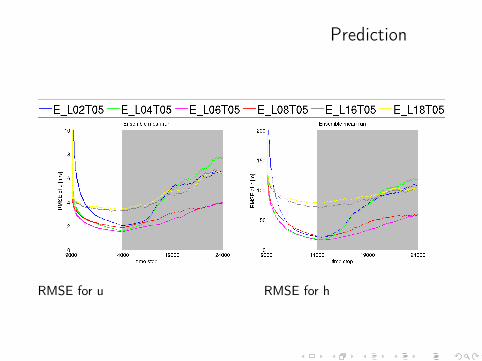
Prediction

RMSE for u RMSE for h

abs(w)

0:00:00 0:33:20 1:06:40 1:40:00 2:13:20 2:46:40Hourly Forecast Time (minutes)

12

13

14

15

16

17

cm/s

Mean Absolute Vertical Velocity 850 hpa (MUC domain average)

MUC Ens ReflWindMUC Ens ReflMUC Ens WindMUC Ens ConvMUC NudgLHNMUC NudgNoLHN

Conclusion

I QPEns a method for addressing non-GaussianityI Improves accuracy and bias in simple problemsI Although total energy of the analysis ensemble mean converges

towards the nature run value with time, enstrophy does not.I Assimilation of velocity observations bounds enstrophy.I Next steps: use QPEns to constrain energy and enstrophy

References

Durran, D.R. and J.A. Weyn, 2016: Thunderstorms don’t get butterflies. Bull. Amer.Meteor. Soc., 97, 237-243.

Durran, D.R. and M.A. Gingrich, 2014: Atmospheric Predictability: Why ButterfliesAre Not of Practical Importance. J. Atmos. Sci., 71, 2476-2488.

Janjic, T., D. McLaughlin, S. E. Cohn, M. Verlaan, 2014: Conservation of mass andpreservation of positivity with ensemble-type Kalman filter algorithms, Mon. Wea.Rev., 142, No. 2, 755-773.

Lange, H. and G. C. Craig, 2014: The impact of data assimilation length scales onanalysis and prediction of convective storms. Mon. Wea. Rev, 142, 3781-3808.

Schraff, C., H. Reich, A. Rhodin, A. Schomburg, K. Stephan, A. Perianez, and R.Potthast,2016: Kilometer Scale Ensemble Data Assimilation for the COSMO Model(KENDA). Q.J.R. Meteorol. Soc., 142, 1453–1472.

Zeng Y., T. Janjić, 2016: Study of Conservation Laws with the Local EnsembleTransform Kalman Filter, Q. J. R. Meteorol. Soc., 142:699, 2359–2372, doi:10.1002/qj.2829.

Würsch, M. and GC Craig, 2014, A simple dynamical model of cumulus convection fordata assimilation research., Meteorol. Z., 23, 483-490.

Extra references

Lange, H., G. C. Craig, T. Janjić, 2016: Characterizing Noise and Spurious Convectionin Convective Data Assimilation submitted to Q. J. R. Meteorol. Soc.

Lange, H., T. Janjić, 2016: Assimilation of Mode-S Aircraft Observations inCOSMO-KENDA, Mon. Wea. Rev., 144:5, 1697–1711.Haslehner, M., T. Janjic, G. C. Craig, 2014: Testing particle fllters on convective scalemodels. Part l: A stochastic cloud model, Q. J. R. Meteorol. Soc., 142:696,1439-1452, doi:10.1002/qj.2745.

Haslehner, M., T. Janjic, G. C. Craig, 2014: Testing particle filters on convective scalemodels. Part lI: A modified shallow water model, Q. J. R. Meteorol. Soc.,142:697,1628-1646, doi: 10.1002/qj.2757.

Simmer, C., G. Adrian, S. Jones, V. Wirth, M. Goeber, C. Hohenegger, T. Janjic, J.Keller, C. Ohlwein, A. Seifert, S. Tromel, T. Ulbrich, K. Wapler, M. Weissmann, J.Keller, M. Masbou, S. Meilinger, N. Riβ, A. Schomburg, C. Stein, A. Vormann: HErZThe German Hans-Ertel Centre for Weather Research, Bull. Amer. Meteor. Soc., 97,1057-1068, doi: 10.1175/BAMS-D-13-00227.1.

Weissmann,M., M. Goeber, C. Hohenegger, T. Janjic, J. Keller, C. Ohlwein, A.Seifert, S. Troemel, T. Ulbrich, K. Wapler, C. Bollmeyer, H. Deneke, 2014: TheHans-Ertel Centre for Weather Research Research objectives and highlights from itsfirst three years, Meteoroligische Zeitschrift, Vol. 23, No. 3, 193–208.