TightRope: Towards Optimal Load-balancing of Paths inAnonymous Networks

Hussein Darir, Hussein Sibai, Nikita Borisov, Geir Dullerud, Sayan MitraCoordinated Science Laboratory

University of Illinois at Urbana-Champaignhdarir2,sibai2,nikita,dullerud,mitras@illinois.edu

ABSTRACTWe study the problem of load-balancing in path selection in anony-mous networks such as Tor. We first find that the current Tor pathselection strategy can create significant imbalances. We then de-velop a (locally) optimal algorithm for selecting paths and show,using flow-level simulation, that it results in much better balancingof load across the network. Our initial algorithm uses the completestate of the network, which is impractical in a distributed settingand can compromise users’ privacy. We therefore develop a revisedalgorithm that relies on a periodic, differentially private summaryof the network state to approximate the optimal assignment. Oursimulations show that the revised algorithm significantly outper-forms the current strategy while maintaining provable privacyguarantees.ACM Reference Format:Hussein Darir, Hussein Sibai, Nikita Borisov, Geir Dullerud, Sayan Mitra.2018. TightRope: Towards Optimal Load-balancing of Paths in AnonymousNetworks. In WPES ’18: 2018 Workshop on Privacy in the Electronic Society,Oct. 15, 2018, Toronto, ON, Canada. ACM, New York, NY, USA, 10 pages.https://doi.org/10.1145/3267323.3268953

1 INTRODUCTIONUsers are increasingly turning to anonymous communication net-works to protect themselves from surveillance, online tracking,or government censorship. The Tor network has several milliondaily active users [20] and has recently been integrated into theprivacy-focused Brave browser [4].

To achieve anonymity in Tor, users’ traffic is routed across a se-ries of servers, called relays. There are several thousand relays, runby volunteers; each user’s path through the network, called a circuit,typically transits three of them. This creates a load-balancing prob-lem of assigning circuits to relays while ensuring no relay gets over-loaded and all circuits receive good performance. Complicating thisproblem are the highly heterogeneous relay capacities—spanningsome five orders of magnitude—and the privacy requirements of cir-cuit construction. In particular, no one except the user must knowthe entirety of the circuit, precluding any centralized load-balancingsolution.

Permission to make digital or hard copies of all or part of this work for personal orclassroom use is granted without fee provided that copies are not made or distributedfor profit or commercial advantage and that copies bear this notice and the full citationon the first page. Copyrights for components of this work owned by others than theauthor(s) must be honored. Abstracting with credit is permitted. To copy otherwise, orrepublish, to post on servers or to redistribute to lists, requires prior specific permissionand/or a fee. Request permissions from permissions@acm.org.WPES ’18, October 15, 2018, Toronto, ON, Canada© 2018 Copyright held by the owner/author(s). Publication rights licensed to ACM.ACM ISBN 978-1-4503-5989-4/18/10. . . $15.00https://doi.org/10.1145/3267323.3268953

Currently, the Tor network uses a randomized assignment offlows circuits to relays, where each user chooses the relays for theircircuits randomly weighted by their measured capacity (with someother constraints, see section 2.1). This ensures that each relay hasthe same average load; however, as we demonstrate in Section 3,this can create significant imbalances at any given point in time. Wetherefore consider the question of whether it is possible to providebetter load balancing while satisfying the privacy requirements.

We first study a non-private load-balancing algorithm. We adaptan algorithm that calculates the max-min-fair allocation of band-width to circuits to select an optimal set of relays for a new path.We show that this results in significantly better load-balancing.Running this algorithm for each new flow would be impractical,therefore we create a batch version of the algorithm, which spec-ulatively generates new circuits using the optimal algorithm anduses these circuits to induce a distribution over the relays, whichis then sampled from to generate new circuits. Note that, unlikethe Tor algorithm, the distribution reflects the current state of thenetwork and is periodically refreshed; we show that this resultsin significantly better load-balancing performance than the Toralgorithm.

We then design a private version of this algorithm. Rather thanworking with a list of circuits, we break each hop into two 2-hopsegments. We can then summarize the state of the network by creat-ing a histogram of segments with one entry for each pair of relays.Our design is motivated by the fact that each entry in this histogramcan be filled in by a single relay; moreover, each relay can locallyadd noise to the entry resulting in a differentially private histogram.We show that using a private histogram, we can implement a modi-fied batch algorithm that approximates the optimal load-balancing.Our experiments show that the algorithm results in significantlybetter balanced circuits than the Tor randomized approach, whilepreserving privacy.

2 BACKGROUNDIn this section we review the key properties of anonymous com-munication networks relevant to load balancing. We then presentthe max-min fair bandwidth allocation algorithm that we will useto model the load-balancing performance, and introduce the dif-ferential privacy framework that will be used to maintain users’anonymity.

2.1 Anonymous Networks and TorAnonymity networks provide users a way to communicate withoutrevealing their identity, and without revealing their relationships

0 1000 2000 3000 4000 5000 6000Relay number

100

101

102

103

104

105

Con

sens

usw

eigh

t

2018-02-05 19:002018-07-26 00:00

Figure 1: Measured relay bandwidths from two Tor consen-sus documents: February 5, 2018 at 19:00 (UTC) and July 26,2018 at 00:00 (UTC). Note the logarithmic scale of the y-axis.

to third parties. Starting with Chaum’s seminal mix network de-sign [6], anonymity has been most frequently achieved by forward-ing traffic through a series of servers in order to disguise its origin.In onion routing networks [24], each packet is multiply encrypted,with a layer of encryption being removed by each server in thepath. This makes it impossible for any server to learn the entirepath; rather, it knows only the preceding and following hops.

Tor [9] is the most popular anonymity network. In Tor, paths(called circuits) typically take three hops to transit the network.These hops are chosen from a collection of volunteer-run servers,called relays. These relays have vastly varying bandwidth capac-ity; in order to balance the load among them, their bandwidth ismeasured using TorFlow [17]. Relays are then allocated to circuitsrandomly, weighted by their measured bandwidth (also known asthe consensus weight). The full Tor path selection algorithm [8] issomewhat complex because it must account for some relays notbeing usable in certain positions of the circuit as well as other con-straints. For the purposes of this paper, we will approximate thealgorithm as picking three random relays, without replacement,from the distribution induced by the measured bandwidth, leavingsimulations of the full Tor algorithm for future work.

An important feature of the Tor network is that the relays, dueto being supplied by volunteers, vary wildly in their bandwidthcapacity. Figure 1 shows the relays and their measured capacityfrom two consensus documents take about five months apart. Thedistribution is highly skewed, with measured capacities spanningover five orders of magnitude. Note that the distribution in the twoconsensus documents follows a similar pattern; we therefore usethe February 5, 2018 19:00 (UTC) consensus as representative forour experiments in the remainder of the paper.

2.2 Max-min FairnessIn this section we introduce our model of Tor performance usingmax-min fair bandwidth allocation. Our model of the Tor networkincludes two simplifying assumptions: (a) each user holds a singlepath through relays and (b) path capacities are constrained only by

the relays, and not by the links between relays. The former can beeasily adjusted by creating virtual users; the latter assumption isstandard in analyzing Tor, and indeed central to the Tor bandwidthmeasurement and allocation architecture. We use the max-min fairallocation as a model because Tor schedules circuits in a round-robinfashion, which has been shown to achieve max-min fairness [12].One further assumption is that each path is in simultaneous activeuse. We discuss some relaxations of this assumption in section 5.4,and defer more complex modeling and simulation of circuit usageto future work.

Notation. We introduce some notation for the rest of the paper.For any positive integer k , [k] denotes the set 1, . . . ,k. We denotethe number of relays byn and the number of users (and therefore thenumber of paths) bym. We assign integer identifiers to the relaysand users, and thus, the sets of relays and users are [n] and [m],respectively. The capacity of relay r ∈ [n] is the positive constantC[r ]. The path assigned to user p ∈ [m] is a sequence of three relaysand is denoted by P[p]. We identify this sequence with the the pth

path. Given an allocation of paths to all users, for any relay r ∈ [n]we define R[r ] = p ∈ [m] | r ∈ P[p] to be the set of identifiers ofthe paths to which the relay r belongs.

Each relay r allocates some bandwidth to each of the paths inR[r ].The bandwidth allocated to the pth path is the minimum bandwidthallocated for it by its three relays and is denoted by band[p]. Forany relay r , the total allocated bandwidth to all paths in R[r ], mustbe less than the capacity of r :

∀ r ∈ [n],∑

p∈R[r ]

band[p] ≤ C[r ]. (1)

Allocations satisfying eq. (1) are said to be feasible.A feasible allocation band is max-min fair if and only if an in-

crease of bandwidth allocation to any path ( within the set of feasibleallocations), must be at the cost of a decrease in allocation of an-other path with an already lower bandwidth in band (See Section6.5.2 in [3]). That is, for any other feasible allocation band ′ and anypath p1 ∈ [m], if band ′[p1] > band[p1], then there exists p2 ∈ [m]such that band ′[p2] < band[p2] and band[p2] ≤ band[p1].

It is well-known that the allocation algorithm shown below(algorithm 1) achieves max-min fairness. It takes as input a networkof relays and paths, and allocates a bandwidth to each path in aniterative fashion. Specifically, the inputs are the array or map C ofall the relay capacities, the array of user paths P , and the array R.The algorithm keeps track of the residual capacity, Cres, of eachrelay after subtracting the bandwidths of the paths passing throughit. It also keeps track of the residual paths, Rres, that is, the setof paths passing through each relay after removing those pathswhose bandwidths are already allocated. At each iteration, one relayr∗ ∈ [n] is chosen and each path in Rres[r∗] is allocated a bandwidth.The chosen relay r∗ is the one that has the smallest ratio Rat[r ] :=Cres[r ]/|Rres[r ]| at the corresponding iteration (line 7). After it ischosen, each of the paths in Rres[r∗] is assigned a bandwidth ofRat[r∗] (line 9). Relay r∗ is called the bottleneck relay of these paths.Then, these paths are removed from their corresponding relays(line 12) and the capacities of these relays get subtracted by Rat[r∗](line 11). This is repeated until all paths are allocated bandwidth.

Algorithm 1 Max-min Bandwidth Allocation Algorithm1: input: C,R, P2: Cres[r ] ← C[r ], ∀ r ∈ [n]3: Rres[r ] ← R[r ], ∀ r ∈ [n]4: band[p] ← 0, ∀p ∈ [m]5: while ∃ p | band[p] = 0 do

6: Rat[r ] ←

Cres[r ]|Rres[r ] | ∀ r ∈ [n] | |Rres[r ]| , 0∞ otherwise

7: r∗ ← argminr ∈[n]

Rat[r ]

8: for p ∈ Rres[r∗] do9: band[p] ← Rat[r∗]

10: for r ∈ P[p] do11: Cres[r ] ← Cres[r ] − Rat(r∗)12: Rres[r ] ← Rres[r ] \ p13: return band

Remark 1. Suppose the relay r∗ chosen at line 7 of algorithm 1belongs to a path p. Then, path p is allocated bandwidth of Rat[r∗],that is band[p] = Rat[r∗]. Further, this allocation is not changed insubsequent iterations.

2.3 Differential PrivacyTo perform load-balancing, we would like to incorporate feedbackabout the state of the network into the path selection process. How-ever, as discussed above, the state of the network is explicitly re-quired to be private, as this is key to preserving users’ anonymity.We will use differential privacy to ensure our feedback mechanismdoes not result in privacy loss.

Differential privacy was first proposed by Dwork [10]. It formal-izes the notion that a mechanism operating over a private data setmust produce an output that depends only minimally on each itemin the data set. We will use the formulation given by Vadhan [25]:

Definition 1 ((Approximate) differential privacy). [25, Definition1.4] For ϵ ≥ 0,δ ∈ [0, 1] we say that a randomized mechanismM : χn × Ω→ Y is (ϵ,δ )-differentially private if for every pair ofneighboring datasets x ∼ x ′ ∈ χn (i.e. x and x ′ differ in one row),and every query q ∈ Ω, we have:

∀T ⊆ Y, Pr[M(x, q) ∈ T ] ≤ eϵ · Pr[M(x ′, q) ∈ T ] + δ ,where Ω is the set of possible queries. Moreover, δ should typicallysatisfy δ ≤ n−ω(1) for this definition to be meaningful.

In our case, the dataset in question will be the complete list ofcircuits in the Tor network, with each circuit representing a row.As a result, differential privacy will guarantee the privacy of eachindividual circuit while providing aggregate traffic statistics. Wenote that differential private mechanisms have previously beenused to study traffic properties of Tor [15].

3 ANALYZING THE RANDOMIZEDALLOCATION ALGORITHM

In this section, we will present the current method used to createpaths in the Tor network. Incoming users sample without replace-ment three relays using the distribution over relays where eachrelay is weighed by its capacity.

Algorithm 2 Random Path Allocation Algorithm1: input: C2: Sample three relays r1, r2, r3 without replacement from the

set of relay where each relay is weighed by its capacity.3: return: r1, r2, r3

0 200000 400000 600000 800000 1000000Circuit number

100

101

102

Ban

dwid

thFigure 2: Bandwidth allocation of 1 million paths using therandom algorithm 2.

0 2000 4000 6000 8000 10000Circuit number

101

102

103

104

Ban

dwid

th

Figure 3: Bandwidth allocation of 10 000 paths using the ran-dom algorithm 2.

We evaluate the performance of this algorithm with respect to theparameters of the Tor network. Jansen and Johnson [15] estimatedthat there were approximately 1.2 million active circuits (95% CI+/- 500,000) in the network. We therefore created 1 million pathsusing the random algorithm 2 and then computed their bandwidthallocation using max-min fair algorithm 1. The results are in fig. 2.We can see that the majority of circuits receive an allocation closeto the average of 10.9, but there are significant tails at both ends ofthe distribution: the minimum circuit has allocation of 1.0 and themaximum of 190. (The standard deviation is 1.28.)

Jansen and Johnson define an active circuit as one that has everbeen used to forward data; however, at any given moment, most

circuits are idle. This can be seen by comparing the data about theaggregate Tor network traffic of approximately 100 Gbps [19] tothe performance of a sustained download, which is roughly 10 sfor 5 MiB [18]. Given that each circuit gets carried by 3 relays, thissuggests that 100 Gbps/3/(5 MiB/10 s) ≈ 10 000 circuits are activeat any given time. Figure 3 shows the bandwidth allocation of 10 000circuits generated by algorithm 2. Observe that the imbalances inthis case are much more significant: the minimum allocation is 14and the maximum is 6419, with a standard deviation of 475.8. 932out of 10 000 flows receive less than half of the average bandwidthof 980, and 37 receive less than 10%.

4 LOCALLY OPTIMAL INCREMENTAL PATHALLOCATION

In this section, we modify the max-min fair allocation algorithm 1 todesign an algorithm that, given the state of the Tor network, returnsthree relays that would result in an optimal allocated bandwidth fora new path. The result is algorithm 3. This algorithm assumes thatthe bandwidths of the existing paths in the network are allocatedusing max-min fairness (algorithm 1).

4.1 Algorithm DescriptionThe algorithm iteratively creates a listB of (bandwidth, relay)-pairs.This list determines how much bandwidth would be allocated to anewly added path to the network. That is, of the relays appearingin a new path, the one that appears earliest in B determines thebandwidth of the path.

The idea of algorithm 3 is to simulate the behaviour of the max-min fairness algoirthm algorithm 1 on the network when an arbi-trary new path is added. This simulation allows us to know howmuch bandwidth it would get allocated. A trivial but key observa-tion is that when a new path is added, the number of paths passingthrough each of its three relays will be incremented by one. For allother relays, the number of paths will remain unchanged. More-over, as per remark 1, the relay that is chosen first from a pathdetermines the path’s bandwidth allocation. Since we are searchingfor the relays that would maximize the bandwidth allocation fora newly added path, algorithm 3 computes the different possibleallocations based on the different possible bottlenecks.

In addition to the ratio Cres[r ]/|Rres[r ]| tracked in algorithm 1(line 7), algorithm 3 also tracks Cres[r ]/(|Rres[r ]| + 1), for each relayr (line 8). In other words, Rat is now a 2 × n matrix: row 1 storesCres[r ]/|Rres[r ]| and row 2 stores Cres[r ]/(|Rres[r ]| + 1).

At each iteration, a minimum of all the 2n ratios is chosen. Wedenote the minimizing row by t∗ ∈ 1, 2 and the correspondingrelay by r∗ ∈ [n]. If the minimizing row t∗ = 1, the algorithmproceeds as max-min fair allocation algorithm 1 by allocating band-width of Rat[1, r∗] to each of the paths in Rres[r∗]. Then, it removesthem from the other relays in which they pass (lines 17 and 18).Both ratios in the same column of Rat, i.e., ratios correspondingto the same relay, are updated in the same way unless the ratioin the second row is already added to B (line 8). That is becauseboth ratios use the same arrays Cres and Rres for their numeratorand denominator. Otherwise, if t∗ = 2, the pair (Rat[2, r∗], r∗) isadded to the end of B. It is added at the end since the r∗ will be thebottleneck of the added path only when its other relays are not in

already in B at this iteration. If one of its relays is already in B atthis iteration, that would be its bottleneck instead of r∗. This will beproved in the next section. The algorithm iterates until all n relayshave entries in B.

Algorithm 3 Locally Optimal Path Allocation Algorithm1: input: C,R, P2: B ← ∅3: Cres[r ] ← C[r ], ∀ r ∈ [n]4: Rres[r ] ← R[r ], ∀ r ∈ [n]5: band[p] ← 0, ∀p ∈ [m]6: while ∃ i < B do

7: Rat[1, r ] ←

Cres[r ]|Rres[r ] | if |Rres[r ]| , 0∞ otherwise

8: Rat[2, r ] ←

Cres[r ]|Rres[r ] |+1 if r < B∞ otherwise

9: (t∗, r∗) ← argmint ∈

1,2,r ∈[n]

Rat[t , r ]

10: if t∗ == 2 then11: B.push([Rat[t∗, r∗], r∗])12: Rat[t∗, r∗] ← ∞13: else14: for p ∈ Rres[r∗] do15: band[p] ← Rat[t∗, r∗]16: for r ∈ P[p] do17: Cres[r ] ← Cres[r ] − Rat[t∗, r∗]18: Rres[r ] ← Rres[r ] \ p19: Let ((b1, r1), (b2, r2), (b3, r3)) be the last three elements of B20: return: r1, r2, r3

4.2 Algorithm CorrectnessIn this section, we will prove that the output of algorithm 3 is apath with maximum bandwidth allocation possible, for a new paththat is to be added to the given network. In this analysis, we willcompare the state of algorithm 3 with the state of max-min fairallocation algorithm 1, in the same iteration. We will add bars ontop of the variable names of algorithm 3 to distinguish them fromthe variables with the same names in algorithm 1. A subscript ofzero refers to the initial values of the variables. A subscript l > 0denotes the value of the variable at the end of the l th while-loopiteration, for the corresponding program1. For example, Cres2 isthe value of Cres of algorithm 3 at the end of the second iterationof its while loop. We will use ⊕ to represent sum of sets.

The following key lemma is used to prove an equivalence be-tween the behaviors of algorithm 1 and algorithm 3: given anynew path p, the bandwidth allocated to p by algorithm 1 equals thebandwidth associated with the relay in p that appears earliest in B(computed by algorithm 3).

Lemma 1. Let the new path beH = h1,h2,h3 ∈ [n]3. Assume (a)C = C , (b) R[r ] = R[r ] for all r ∈ [n] \H and R[r ] = R[r ] ∪ m + 1for r ∈ H , and (c) P[p] = P[p] for all p ∈ [m], and P[m + 1] = H .1For algorithm 1, it is the value of the variable after the execution of line 12 and foralgorithm 3 it is the value after the execution of line 18

Assume w.l.o.g thath1 is the first relay to be added by algorithm 3 to B.Let l1, l2, . . . lk be the iterations in algorithm 3 at which t∗ = 1 beforeh1 is added to B. Then, for all s ≤ k , Cress = Cresls and Rress [r ] =Rresls [r ] for all r ∈ [n] \ H and Rress [r ] = Rresls [r ] ∪ m + 1 forr ∈ H .

Proof. First, Cres0 = C1 = C2 = Cres0. Second, note thatRat1[r ] = Rat1[1, r ] for all r ∈ [n] \ H and Rat1[r ] = Rat1[2, r ]for all r ∈ H . Hence, if the minimum ratio at the first iterationof algorithm 3 exists in Rat1, that same ratio will be chosen byalgorithm 1 at its first iteration. Thus, if t∗1 = 2 and r∗1 = h1 (r∗1cannot be h2,h3 as we assumed that h1 is chosen first), then thelemma would hold with k = 0 and r∗1 = h1.

If t∗1 = 2 and r∗1 , h1, then the minimum ratio of algorithm 3does not belong to Rat1 and neither Cres nor Rres would be changedin this iteration, i.e. Cres1 = Cres0 and Rres1 = Rres0. In that case,Rat2 would still be a subset of Rat2.

The case where t∗1 = 1 and r∗1 ∈ H cannot happen since Rat1[2, r ] ≤Rat1[1, r ] for all r ∈ [n].

Finally, if t∗1 = 1 and r∗1 < H , then l1 = 1 and both algorithmswill have the same minimum ratio, the else branch would be takenin algorithm 3 and Cres and Rres would be updated in the samemanner as those Cres and Rres. Thus, the property in the lemmawould be preserved.

Hence, the above analogy can be repeated to shown that the l thiteration of algorithm 3 at which t∗ = 1 will run the same updates asthat of the l th iteration of algorithm 1 till h1 is added to B. Iterationsof the while loop in algorithm 3 at which t

∗= 2 does not affect Cres,

Rres, and the ratios common with algorithm 1 until h1 is chosen.Once h1 is added to B, that corresponds to the k + 1th iteration ofalgorithm 1 where h1 will be chosen as the minimizing relay tooand the bandwidth of the new path would be determined.

Corollary 1. For any new pathH = h1,h2,h3. The bandwidthassociated with h1 in B (algorithm 3) equals the bandwidth allocatedfor H by algorithm 1.

Since in the following lemma we will be only analyzing algo-rithm 3, there will be no confusion with the variables of algorithm 1so we drop the bars.

Lemma 2. The ratios in B appear in increasing order.

Proof. Consider the l th iteration of algorithm 3 at which a ratio-relay pair (b, r∗l ) is added to B, i.e. t∗l = 2. If in the preceding it-eration l − 1, t∗l−1 = 2, another ratio-relay (b1, r∗l−1) would havebeen added to B before it. Moreover, both Cres and Rres would nothave changed and since b1 was chosen first means it is smallerthan b2 and thus in this case the B would be increasing. Otherwise,if t∗l−1 = 1, the “else” branch would be taken. Denote the num-ber of paths r∗l−1 and r∗l share at the (l − 1)th iteration be s . Then,

Ratl [2, r∗l ] =Cresl−1[r ∗l ]−Ratl−1[1,r ∗l−1]

|Rresl−1[r ∗l ] |+1−s . We will show that it is larger

than Ratl−1[1, r∗l−1] =Cresl−1[r ∗l−1]

|Rresl−1[r ∗l−1] |.

0 200000 400000 600000 800000 1000000Circuit number

100

101

102

Ban

dwid

th

Algorithm 3Algorithm 2

Figure 4: Graph comparing the bandwidth allocation ofone million paths generated using the locally optimal algo-rithm 2 and the random algorithm 3. Note the logarithmicscale of the y-axis.

We know that Ratl−1[2, r∗l ] := Cresl−1[r ∗l ]|Rresl−1[r ∗l ] |+1 >

Cresl−1[r ∗l−1]

|Rresl−1[r ∗l−1] |.

Hence,Cresl−1[r

∗l ]|Rresl−1[r

∗l−1]| > Cresl−1[r

∗l−1](|Rresl−1[r

∗l ]| + 1)

=⇒ Cresl−1[r∗l ]|Rresl−1[r

∗l−1]| − s(Cresl−1[r

∗l−1])

> Cresl−1[r∗l−1](|Rresl−1[r

∗l ]| + 1 − s)

=⇒ |Rresl−1[r∗l−1]|(Cresl−1[r

∗l ] − s

Cresl−1[r∗l−1]

|Rresl−1[r∗l−1]|)

> Cresl−1[r∗l−1](|Rresl−1[r

∗l ]| + 1 − s)

=⇒

Cresl−1[r∗l ] − s

Cresl−1[r ∗l−1]

|Rresl−1[r ∗l−1] |

|Rresl−1[r∗l ]| + 1 − s >

Cresl−1[r∗l−1]

|Rresl−1[r∗l−1]|

.

Therefore, the ratios are non decreasing in the iterations at whicht∗ = 1 and constant (other than the one added to B) when t∗ = 2which means that every time a ratio is added to B, it will be equalor larger than all previously added ones.

Corollary 2. Choosing the last three relays of the resulting B forthe new path would result in maximum bandwidth allocated for itby algorithm 1. That bandwidth is the one associated with the thirdrelay from the end of B.

4.3 Results in Tor NetworkStarting with an empty set, one million paths were created byrepetitively running our locally optimal algorithm 3 while addingthe output path to the network. The bandwidth allocation of the onemillion paths generated is found using the max-min fair algorithm 1.Those results were then compared to the bandwidth allocations ofone million paths generated using the random algorithm 2. Theresults are shown in fig. 4.

The locally optimal algorithm 3 produces a much more well-balanced set of paths: the minimum allocation if 10.96 is nearly thesame as the average of 10.97, and the maximum is 21. In contrast,the paths created using the random algorithm 2, while having a

similar average bandwidth allocation of 10.94, span a much broaderrange, with a minimum allocation of 1 and a maxium of 210.14.

5 DIFFERENTIALLY PRIVATE ALGORITHM:The locally optimal algorithm 3 requires the knowledge of the stateof the network as input. Thus, if it is going to be used, every userwill need to know the state of the network, i.e., the paths of everyother user, in order to be able to construct a path for herself. Thiswill defeat the purpose of onion routing as it will then be possibleto deanonymize users. In this section, we will be discussing how toimplement a differentially private version of algorithm 3.

In the private version of the algorithm, we first decompose eachcircuit (r1, r2, r3) into two circuit segments, (r2, r1) and (r2, r3). Wethen adapt the locally optimal algorithm 3 to use these segments,rather than complete circuits, in creating an optimal new path. Toadd privacy, we summarize the list of segments as a histogram,indexed by pairs of relays, of the number of circuit segments (ri , r j )that are present. We then create a differentially private versionof this histogram by using a threshold-based differentially privatecount, to account for the sparse nature of the histogram.

One feature of the private count algorithm is that each histogramentry can be processed individually. Therefore, a relay ri can applyit to the count of each histogram entry (ri , r j ), since it knows the(actual, non-private) number of such flow segments. The privatecounts can then be aggregated and distributed using a modificationof the existing Tor directory mechanism or another peer-to-peerbroadcast scheme.

Since the private histogram can only be updated periodically, weuse this histogram to generate the next N near-optimal circuits. Wecannot assign these circuits directly to each new user; instead, wecount the number of times each relay appears in theseN circuits anduse it to induce a distribution over relays that the users sample fromfor their circuit. This approach is similar to the random algorithm 2,except that the weights reflect relays that are underloaded in thecurrent state of the network, rather than the static relay capacities.

5.1 Pair-baserd Algorithm DescriptionAs in the locally optimal algorithm 3, we denote the capacity of ther th relay by C[r ]. As discussed before, the paths are now orderedpairs of relays. Being ordered is essential for the correctness ofthe pair-based algorithm 4 as will be discussed later. We denoteby P the map from these paths to the ordered pairs of relays towhich they belong. For example, those corresponding to the pth

path are P[p] = (rp,1, rp,2). Also, as before, we define R[r ] to bethe set p | r ∈ P[p] of paths to which relay r belongs. However,we decompose R into two maps: Rc mapping relays to the paths inwhich they appear in the first component of the ordered pair, i.e.the central relay, and Re mapping relays to the paths in which theyappear in the second component of the ordered pair, i.e. the endrelay.

We finally define Nres[r ] as the number of actual paths (pathswith three relays) containing relay r . We can compute it as: Nres[r ] =|Rresc [r ]|/2+ |Rrese [r ]|, since for an actual path in the Tor networkwhere r is the central relay, it will appear as two pairs in Rresc [r ]while it should be counted once. It will only appear once in Rrese [r ]if r is one of its end relays.

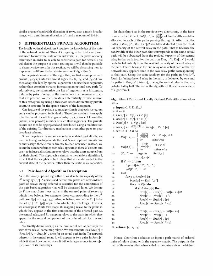
In algorithm 4, as in the previous two algorithms, in the itera-tions at which t∗ = 1, Rat[1, r∗] = Cres[r ]

Nres[r ] of bandwidth would beallocated to each of the paths passing through it. After that, thepaths in Rrese [r∗], Rat[1, r∗]/2 would be deducted from the resid-ual capacity of the central relay in the path. That is because thebandwidth of the other path that corresponds to the same actualpath will be subtracted from the residual capacity of the centralrelay in that path too. For the paths in Rresc [r∗], Rat[1, r∗] wouldbe deducted entirely from the residual capacity of the end relay ofthe path. That is because the end relay of an actual path of the Tornetwork only appears once in the two-relay paths correspondingto that path. Using the same analogy, for the paths in Rresc [r∗],Nres[r ], r being the end relay in the path, is deducted by one andfor paths in Rrese [r∗], Nres[r ], r being the central relay in the path,is deducted by half. The rest of the algorithm follows the same stepsof algorithm 3.

Algorithm 4 Pair-based Locally Optimal Path Allocation Algo-rithm

1: input: C,R, Rc, Re, P2: B ← ∅3: Cres[r ] ← C[r ], ∀ r ∈ [n]4: Rres[r ] ← R[r ], ∀ r ∈ [n]5: band[p] ← 0, ∀p ∈ [m]6: Nres[r ] ← |Rresc [r ] |

2 + |Rrese [r ]|, ∀ r ∈ [n]7: while ∃ i < B do

8: Rat[1, r ] ←

Cres[r ]Nres[r ] ∀ r | Nres[r ] , 0∞ otherwise

9: Rat[2, r ] ←

Cres[r ]Nres[r ]+1 if r < B∞ otherwise

10: (t∗, r∗) ← argmint ∈

1,2,r ∈[n]

Rat[t , r ]

11: if t∗ == 2 then12: B.push([Rat[t∗, r∗], r∗])13: Rat[t∗, r∗] ← ∞14: else15: for p ∈ Rres[r∗] do16: band[p] ← Rat[t∗, r∗]17: for r ∈ P[p] do18: if p ∈ Rresc [r ] then19: Cres[r ] ← Cres[r ] − Rat[t∗, r∗]/220: Nres[r ] ← Nres[r ] − 1/221: Rres[r ] ← Rres[r ] \ p22: Rresc[r ] ← Rresc[r ] \ p23: else24: Cres[r ] ← Cres[r ] − Rat[t∗, r∗]25: Nres[r ] ← Nres[r ] − 126: Rres[r ] ← Rres[r ] \ p27: Rrese[r ] ← Rrese[r ] \ p

28: return: r1, r2, r3

Hence, algorithm 4 takes as an input a path matrix of orderedpairs of relays along with the capacity matrix. The output is thepath of three relays that when added to the system gives the highest

0 2000 4000 6000 8000 10000Circuit number

103

2 × 103

Ban

dwid

th

Algorithm 3Algorithm 4

Figure 5: Graph comparing the bandwidth allocation of10 000 paths generated using the pair-based algorithm 4 andthe locally optimal algorithm 3.

bandwidth allocation compared to any other path that can be addedto the system.

5.2 Experimental ResultsStarting from an empty set, the pair-based algorithm 4 was usedrepetitively to generate a set of 10 000 paths of three relays. At eachrun, a path matrix representing the decomposition of the paths inthe network into segments of two relays is constructed, and theninput to algorithm 4 along with the capacity matrix. The output, thepath of three relays, is then added to the network. The bandwidthallocations for these paths are then computed using the max-minfairness algorithm 1.

The results were then compared to the bandwidth allocations of10 000 paths generated by repetitive application of locally optimalalgorithm 3 starting from an empty set to know how much accuracywe lost by the decomposition of paths into pairs. The results areshown in fig. 5. The two curves coincide which shows there is zeroloss of accuracy.

The same experiment is repeated but instead 1 million pathswere created using both algorithms. The results are shown in fig. 6.The maximum difference between the two allocations was 0.918.

5.3 Batch Path Allocation Algorithm ResultsAs we discussed earlier, the server would periodically collect datafrom the relays and create a histogram mapping each ordered pairof relays to the number of paths passing through them. It wouldthen create a differentially private version of this histogram. Afterthat, given the current state of the network, it runs the pair-basedalgorithm 4 repetitively to generate K additional paths. These pathsare not added to the actual network but to a virtual copy of thenetwork. The number of times each relay appeared in these K pathsis counted to generate a probability distribution over the relays. Thedistribution is then released to the public. Incoming users wouldsample that distribution (without replacement) to get three differentrelays which would constitute their paths.

0 200000 400000 600000 800000 1000000Circuit number

2 × 101

Ban

dwid

th

Algorithm 3Algorithm 4

Figure 6: Graph comparing the bandwidth allocation of onemillion paths generated using pair-based algorithm 4 andlocally optimal algorithm 3 (in blue). Note the logarithmicscale of the y-axis.

The batch algorithm 5 creates a batch of L random paths using theprocedure we just described. L represents the expected number ofpaths that would be created in a single period before the distributiongets updated.

Algorithm 5 Batch Path Allocation Algorithm1: input: C,R, Rc, Re, P,K ,L2: Repeat K times:3: Input C, Rres, Rc, Re, P to algorithm 4.4: Add the returned path to the network.5: Update Rres, Rc, Re, P accordingly.6: Compute the distribution of the relays in the added K paths.7: Sample L paths with three relays from that distribution8: return: Generated L paths

To evaluate the behaviour of the batch algorithm 5, K is set to10 000 and L to 200. Then, starting from a network with no paths,we ran it repetitively to create a network with 600 000 paths, 200 at atime. At each run, a path matrix is constructed by decomposing thepaths in the network to paths of two ordered relays as previouslydiscussed and taken as input for the next run.

After that, the bandwidth allocations of the created paths werecomputed using the max-min fair algorithm 1 and compared tothe bandwidth allocations of 600 000 paths generated using the therandom algorithm 2. The results are shown in fig. 7.

The minimum bandwidth of a path generated using the batchalgorithm 5 was 6.33, the maximum was 37.23 and the average was17.29. On the other hand, for the set of paths generated randomly,the minimum bandwidth of a path was 1, the maximum was 287.99and the average was 17.23.

The simulation demonstrates the fairness property of algorithm 5The range of the bandwidth allocations of the paths is [6.33, 37.23]compared to a range of [1, 287.99] for the random paths, whilethe average is being conserved. The algorithm hence avoids the

0 100000 200000 300000 400000 500000 600000Circuit number

100

101

102

Ban

dwid

th

Algorithm 5Algorithm 2

Figure 7: Graph comparing the bandwidth allocation of600 000 paths generated using the random algorithm 2 andthe batch algorithm 5. Note the logarithmic scale of the y-axis.

use of paths with very low bandwidth and guarantees a more fairdistribution of the bandwidth between users.

5.4 Adding Differential PrivacyIn this section, we show how the server ensures differential privacyof the statistics it releases about the network. As discussed earlier, atthe end of each period, it generates a differentially private version ofa histogram (matrix) of sizen2. In this paper, we use the notion (ϵ,δ )-differential privacy defined in section 2.3. We did not use the usual ϵ-differential privacy since the histogram that we are making privateis very large (n2 ≈ 36 000 000) and is very sparse. Using (ϵ,δ )-differential privacy allows us to operate on the sparse histogram,as described below, rather than producing a noisy version of each0 value in the histogram, which would overwhelm the algorithm.We replace n with n2 in the original definition since in our case thedataset is of size n2.

The following theorem shows that there is a mechanism thatensures the differential privacy of the histogram against queriesconsisting of point functions while guaranteeing an acceptable levelof accuracy of query responses. Before stating the theorem, let usdefine formally the set of queries for which the mechanism ensuresprivacy.

Definition 2 (page 6 in [25]). Point Functions (Histograms): LetXbe an arbitrary set and for eachy ∈ X, we consider the predicateqy :X → 0, 1 that evaluates to 1 only on input y. The family Qpt =

Qpt (X) consists of the counting queries corresponding to all pointfunctions on data universe X. (Approximately) answering all of thecounting queries in Qpt amounts to (approximately) computing thehistogram of the dataset.

As before we substitute n by n2 from the original theorem.

Theorem 3. (stability-based histograms [5]). For every finite datauniverse χ ,n ∈ N, ϵ ∈ (0, 2 lnn), and δ ∈ (0, 1/n2) there is an (ϵ,δ )-differentially private mechanism M : χn

2→ Rχ that on every

dataset x ∈ χn2, with high probability M(x) answers all of the

counting queries in Qpt (χ ) to within error

O(

log(1/δ )ϵn2

)In the proof of the theorem, the authors provided such mecha-

nism which takes a dataset (histogram) x ∈ χn2 as input and returns

a privatized version of it. The mechanism is shown in algorithm 6.It iterates over the elements of the histogram, those that are zeroare kept zero. A positive entry would be added to an independentLaplace variable with λ = 2/(ϵn2). If the result is below the thresh-old ((2 ln(2/δ ))/(ϵ))+ (1), the entry would be set to zero, otherwiseit is set to the result. Note that we multiplied the threshold thatis in the mechanism by n2 since we do not need the result of thequery to be normalized, i.e. between 0 and 1, so we do not need then2 factor.

Algorithm 6 (ϵ,δ )-differentially Private Histogram Mechanism1: input: x , χ2: For every y ∈ χ :3: If qy (x) = 0 then:4: Set ay = 05: If qy (x) > 0 then:6: Set ay ←− qy (x) + Lap(2/(ϵn2)).7: If ay < 2 ln(2/δ )/ϵn2 + 1/n2 then:8: Set ay = 09: return: (ay )y∈χ

As discussed earlier, the server releases a distribution over therelays at the beginning of every period based on the generatedprivate histogram. Thus, information about the paths that remainover multiple periods in the network will be released several times.This will deteriorate the level of privacy they are guaranteed. Tobound this deterioration we consult the following compositiontheorem of differential privacy.

Theorem 4. (Composition of (ϵ,δ )-differentially-private algo-rithms, Theorem 16 in [11]). LetT1 : D −→ T1(D) be (ϵ,δ )-differentially-private, and for all J ≥ 2,Tj : (D, s1, ..., s J−1) −→ TJ (D, s1, ..., s J−1) ∈

ζ J be (ϵ,δ )-differentially-private, for all given (s1, ..., s J−1) ∈ ⊗J−1j=1 ζj ,

where "⊗" denotes direct product of spaces. Then for all neighboringD, D ′ and all S ⊆ ⊗ J−1

j=1 ζj :

P((T1, ...,TJ ) ∈ S) ≤ e J ϵP ′((T1, ...,TJ ) ∈ S) + Jδ

We can conclude that the parameters of privacy ϵ and δ that wecan guarantee for a certain path increase linearly in the number ofperiods it stays in the network.

We chose the parameters ϵ and δ to be 0.3 and 0.001, respectively.To evaluate the behaviour of algorithm 5 after we privatize thehistogram before using it to generate the distribution over relays,we conducted the following experiment: starting from an emptynetwork, we generated N = 1 000 000 paths using repetitive appli-cation of batch algorithm 5 with K = 10 000 and L = 200 whileusing a private version of the histogram before each run, usingalgorithm 7, and generating the distribution from the result.

The bandwidth allocations of those paths are then computedusing max-min fair allocation algorithm 1 and compared to the

Algorithm 7 (ϵ,δ )-differentially Private Optimal Path AllocationAlgorithm

1: input: C,R, Rc, Re, P,N ,K ,L2: for i ∈ [⌈NL ⌉] do3: A histogram mapping the pairs of relays in the network to

the number of paths between each pair is constructed.4: A private version of the histogram is generated using the

mechanism described in algorithm 6.5: The private histogram is input to the batch algorithm 5

with parameters K and L.6: The generated L paths are added to the network.7: Update R, Rc, Re, P .

0 200000 400000 600000 800000 1000000Circuit number

100

101

102

103

104

Ban

dwid

th

Algorithm 7Algorithm 2

Figure 8: Graph comparing the bandwidth allocation of onemillion paths generated using the differentially private al-gorithm 7 and using the random algorithm 2. Note the loga-rithmic scale of the y-axis.

bandwidth allocations of one million paths generated using therandom algorithm 2. The sorted (in bandwidth) results are shownin fig. 8.

The minimum bandwidth allocation of a path of differentially pri-vate algorithm 7 was 8.2, the maximum was 9603.5 and the averagewas 10.54. While for those generated randomly using algorithm 2,the minimum was 1, the maximum was 210.14 and the average was10.94. Although the average was lower for our algorithm, it has nopaths with low bandwidth as the random one. The tail on the leftis much shorter while the tail on the right is much longer than therandom one. The difference in most paths is negligible.

Finally we evaluate the scenario where only a subset of thegenerated paths are active, as discussed in section 3. We take themillion circuits generated using the privacy-preserving algorithm 7,as above, and choose a random sample of 10 000 circuits as beingactive. We then compare the bandwidth allocated to those circuitswith 10 000 circuits chosen by the random algorithm 2 in fig. 9. Notethat the randomized algorithm has a significantly longer tail onthe left side of the graph, representing circuits with a pathologicalbandwidth allocation. The minimum bandwidth in algorithm 2 is7, whereas the minimum for the sampled algorithm 7 is 171. Therandomized algorithm produces 953 flows with a bandwidth less

0 2000 4000 6000 8000 10000Circuit number

101

102

103

104

Ban

dwid

th

Algorithm 7, sampledAlgorithm 2

Figure 9: Comparing random allocation in algorithm 2 to asample of 10 000 circuits out of 1million thatwere generatedby the differentially private algorithm 7.

than half of the average, 980. The sampled circuits from the privatealgorithm have a slightly lower average of 960, but only 326 flowshave a bandwidth of less than 980/2. The lower average performanceis due to some relays being underutilized, as evidenced by the longertail on the right-hand side of the graph; in our ongoing work weare investigating adjustments to the algorithm to make better useof these relays.

6 RELATEDWORKWe next review some closely related work; for more comprehensiveof work covering all aspects of Tor performance we direct interestedreaders to the survey by AlSabah and Goldberg [2].

Snader and Borisov studied the problem of path selection inTor and suggested biasing selection towards higher bandwidth re-lays, showing that it improved performance in both simulationand real-world Tor measurements [21, 23]. They also developed aflow simulator based on max-min fair flow allocation, using an algo-rithm similar to Algorithm 1. Herbert et al. modeled Tor traffic as anM/D/1 queuing network and proposed a relay selection algorithmfor optimizing the queuing latency [13]. Both these papers arguedthat the bandwidth-weighted relay selection results in suboptimalpath selection, but their solutions did not incorporate any feedbackmechanisms.

Wang et al. proposed a congestion-aware path selection algo-rithm [26]. It suggests that user perform latency measurements oncircuits in the network to detect congested relays and avoid themduring path selection. Although each user will have a partial view ofthe network, their experiments show that significant improvementscan be realized. Likewise, Conflux [1] mitigates congested pathsby multiplexing traffic across two paths through the Tor network;this significantly improves performance although it cannot miti-gate congestion at the last node in the circuits, where traffic mustconverge. Both these schemes use a partial view of the network todetect and avoid localized congestion, rather than balancing loadacross the entire Tor network, as in our scheme.

Load balancing in Tor requires an accurate measure of relay ca-pacity, which is currently performed by TorFlow [17]. TorFlow usesbandwidth authorities to proactively measure relay performance,and incorporates a long-term feedback mechanism: relays that areassigned too high a bandwidth value and become overloaded willperform worse in subsequent measurements and thus have theirconsensus weight reduced, and vice versa. This feedback, however,occurs over a period of days and does not deal with more tran-sient congestion and load imbalances. EigenSpeed [22] proposedan alternate measurement approach that relied on opportunisticmeasurements of relays by other relays; Johnson et al. identifiedseveral attacks on both TorFlow and EigenSpeed and proposed animproved peer measurement scheme called PeerFlow [16].

7 CONCLUSIONS AND FUTUREWORKWe have presented an algorithm that approximates locally optimalload-balancing of circuits in the Tor network while preservinguser privacy. We demonstrated that the algorithm significantlyimproves on the randomized relay assignment in Tor using flow-level simulations of max-min fair bandwidth allocation.

Our promising results encourage the further exploration of us-ing privacy-preserving feedback for load balancing in anonymitynetworks. Several important challenges remain. First, load imbal-ance occurs over short time scales, thus the private summary ofthe network state must be quickly distributed to all users. We notethat this is a similar problem to that of distributing blocks in cryp-tocurrencies; in the Bitcoin network, which is similarly sized to Tor,measurements have shown that blocks reach the median node in6.5s and the 90th percentile node in 26s [7]. Improving this latencywhile maintaining resilience to attack is an area of active research.

A second problem is that malicious nodes may misreport theircontributions to the histogram to direct circuits away from honestnodes and towards malicious ones. We note that this problem issomewhat similar to the peer bandwidth measurement problem inEigenSpeed [22] and PeerFlow [16] and thus some of the defensesused in those systems may be adaptable to this setting.

Finally, flow-level simulation is a coarse-grained approximationof Tor traffic; web browsing is a dominant use of Tor and webtraffic is known to be quite bursty. Further evaluation of the load-balancing mechanism using queuing-based traffic models or fullnetwork simulation [14] is needed.

ACKNOWLEDGMENTSWe would like to thank the anonymous referees for their helpfulsuggestions. This material is based upon work supported by theNational Science Foundation under Grant No. 1739966.

REFERENCES[1] Mashael AlSabah, Kevin Bauer, Tariq Elahi, and Ian Goldberg. 2013. The path

less travelled: Overcoming Tor’s bottlenecks with traffic splitting. In Proceedingsof the Privacy Enhancing Technologies Symposium (PETS). Springer, 143–163.

[2] Mashael AlSabah and Ian Goldberg. 2016. Performance and security improve-ments for Tor: A survey. ACM Computing Surveys (CSUR) 49, 2 (2016), 32.

[3] Dimitri Bertsekas and Robert Gallager. 1992. Data Networks (2nd ed.). Prentice-Hall, Inc., Upper Saddle River, NJ, USA.

[4] Brave. 2018. Brave Introduces Beta of Private Tabs with Tor for Enhanced Privacywhile Browsing. https://brave.com/tor-tabs-beta.

[5] Mark Bun, Kobbi Nissim, and Uri Stemmer. 2015. Simultaneous Private Learningof Multiple Concepts. CoRR abs/1511.08552 (2015). arXiv:1511.08552 http:

//arxiv.org/abs/1511.08552[6] David Chaum. 1981. Untraceable electronic mail, return addresses, and digital

pseudonyms. Commun. ACM 24, 2 (February 1981), 84–90.[7] Christian Decker and Roger Wattenhofer. 2013. Information propagation in the

Bitcoin network. In 13th International Conference on Peer-to-Peer Computing (P2P).IEEE, 1–10.

[8] Roger Dingledine and Nick Mathewson. 2017. Tor Path Specification. https://gitweb.torproject.org/torspec.git/plain/path-spec.txt.

[9] Roger Dingledine, Nick Mathewson, and Paul F. Syverson. 2004. Tor: The Second-Generation Onion Router. In USENIX Security Symposium. USENIX, 303–320.

[10] Cynthia Dwork. 2006. Differential Privacy. In Automata, Languages and Pro-gramming, Michele Bugliesi, Bart Preneel, Vladimiro Sassone, and Ingo Wegener(Eds.). Springer, Berlin, Heidelberg, 1–12.

[11] Cynthia Dwork and Jing Lei. 2009. Differential Privacy and Robust Statistics. InProceedings of the Forty-first Annual ACM Symposium on Theory of Computing(STOC ’09). ACM, New York, NY, USA, 371–380. https://doi.org/10.1145/1536414.1536466

[12] Ellen L. Hahne. 1991. Round-robin scheduling for max-min fairness in datanetworks. IEEE Journal on Selected Areas in Communications 9, 7 (1991), 1024–1039.

[13] S.J. Herbert, Steven J. Murdoch, and Elena Punskaya. 2014. Optimising nodeselection probabilities in multi-hop M/D/1 queuing networks to reduce latencyof Tor. Electronics Letters 50, 17 (2014), 1205–1207.

[14] Rob Jansen, Kevin Bauer, Nicholas Hopper, and Roger Dingledine. 2012. Me-thodically Modeling the Tor Network. In Proceedings of the USENIX Workshop onCyber Security Experimentation and Test (CSET 2012).

[15] Rob Jansen and Aaron Johnson. 2016. Safely Measuring Tor. In Proceedings of the2016 ACM SIGSACConference on Computer and Communications Security (CCS ’16).ACM, New York, NY, USA, 1553–1567. https://doi.org/10.1145/2976749.2978310

[16] Aaron Johnson, Rob Jansen, Nicholas Hopper, Aaron Segal, and Paul Syverson.2017. PeerFlow: Secure load balancing in Tor. Proceedings on Privacy EnhancingTechnologies 2017, 2 (2017), 74–94.

[17] Mike Perry. 2009. TorFlow: Tor network analysis. In Proceedings of the 2ndWorkshop on Hot Topics in Privacy Enhancing Technologies (HotPETs). 1–14.

[18] The Tor Project. 2018. Tor Metrics: Performance. https://metrics.torproject.org/torperf.html.

[19] The Tor Project. 2018. Tor Metrics: Traffic. https://metrics.torproject.org/bandwidth.html.

[20] The Tor Project. 2018. Tor Metrics: Users. https://metrics.torproject.org/userstats-relay-country.html.

[21] Robin Snader and Nikita Borisov. 2008. A Tune-up for Tor: Improving Securityand Performance in the Tor Network. In 15th Network and Distributed SystemSecurity Symposium (NDSS), Crispin Cowan and Giovanni Vigna (Eds.). InternetSociety, Reston, VA, USA.

[22] Robin Snader and Nikita Borisov. 2009. EigenSpeed: Secure Peer-To-Peer Band-width Evaluation. In 8th International Workshop on Peer-To-Peer Systems, RodrigoRodrigues and Keith Ross (Eds.). USENIX Association, Berkeley, CA, USA.

[23] Robin Snader and Nikita Borisov. 2011. Improving Security and Performance inthe Tor Network through Tunable Path Selection. IEEE Transactions on Dependableand Secure Computing 8, 5 (2011), 728–741. https://doi.org/10.1109/TDSC.2010.40

[24] Paul F. Syverson, Gene Tsudik, Michael G. Reed, and Carl E. Landwehr. 2000.Towards an Analysis of Onion Routing Security. In Workshop on Design Issuesin Anonymity and Unobservability (Lecture Notes in Computer Science), HannesFederrath (Ed.), Vol. 2009. Springer, 96–114.

[25] Salil Vadhan. 2017. The Complexity of Differential Privacy. https://privacytools.seas.harvard.edu/publications/complexity-differential-privacy.

[26] Tao Wang, Kevin Bauer, Clara Forero, and Ian Goldberg. 2012. Congestion-awarepath selection for Tor. In International Conference on Financial Cryptography andData Security. Springer, 98–113.