The MIT Joint Program on the Science and Policy of Global Change combines cutting-edge scientific research with independent policy analysis to provide a solid foundation for the public and private decisions needed to mitigate and adapt to unavoidable global environmental changes. Being data-driven, the Joint Program uses extensive Earth system and economic data and models to produce quantitative analysis and predictions of the risks of climate change and the challenges of limiting human influence on the environment—essential knowledge for the international dialogue toward a global response to climate change.

To this end, the Joint Program brings together an interdisciplinary group from two established MIT research centers: the Center for Global Change Science (CGCS) and the Center for Energy and Environmental Policy Research (CEEPR). These two centers—along with collaborators from the Marine Biology Laboratory (MBL) at

Woods Hole and short- and long-term visitors—provide the united vision needed to solve global challenges.

At the heart of much of the program’s work lies MIT’s Integrated Global System Model. Through this integrated model, the program seeks to discover new interactions among natural and human climate system components; objectively assess uncertainty in economic and climate projections; critically and quantitatively analyze environmental management and policy proposals; understand complex connections among the many forces that will shape our future; and improve methods to model, monitor and verify greenhouse gas emissions and climatic impacts.

This reprint is intended to communicate research results and improve public understanding of global environment and energy challenges, thereby contributing to informed debate about climate change and the economic and social implications of policy alternatives.

—Ronald G. Prinn and John M. Reilly, Joint Program Co-Directors

MIT Joint Program on the Science and Policy of Global Change

Massachusetts Institute of Technology 77 Massachusetts Ave., E19-411 Cambridge MA 02139-4307 (USA)

T (617) 253-7492 F (617) 253-9845 globalchange@mit.edu http://globalchange.mit.edu

Reprint 2018-4

Reprinted with permission from Energy Economics, 70: 70–83. © 2018 the authors

Tight Oil Market Dynamics: Benchmarks, Breakeven Points, and InelasticitiesR.L. Kleinberg, S. Paltsev, C.K.E. Ebinger, D.A. Hobbs and T. Boersma

Energy Economics 70 (2018) 70–83

Contents lists available at ScienceDirect

Energy Economics

j ourna l homepage: www.e lsev ie r .com/ locate /eneeco

Tight oil market dynamics: Benchmarks, breakeven points,and inelasticities

R.L. Kleinberg a,⁎, S. Paltsev b, C.K.E. Ebinger c, D.A. Hobbs d, T. Boersma e

a Schlumberger-Doll Research, One Hampshire Street, Cambridge, MA 02139, United Statesb Joint Program on Science and Policy of Global Change, Massachusetts Institute of Technology, Cambridge, MA 02139, United Statesc Atlantic Council, 1030 15th Street NW, Washington, DC 20005, United Statesd King Abdullah Petroleum Studies and Research Center, Airport Road, Riyadh 11672, Saudi Arabiae Center on Global Energy Policy, School of International and Public Affairs, Columbia University, 420 West 118th Street, New York, NY 10027, United States

⁎ Corresponding author.E-mail addresses: kleinberg@slb.com (R.L. Kleinberg),

cebinger@atlanticcouncil.org (C.K.E. Ebinger), david.hobbtb2720@columbia.edu (T. Boersma).

https://doi.org/10.1016/j.eneco.2017.11.0180140-9883/© 2017 The Authors. Published by Elsevier B.V

a b s t r a c t

a r t i c l e i n f o

Article history:Received 20 December 2016Received in revised form 17 July 2017Accepted 25 November 2017Available online 28 November 2017

JEL classification:Q35Hydrocarbon resources

When comparing oil and gas projects - their relative attractiveness, robustness, and contribution to markets -various dollar per barrel benchmarks are quoted in the literature and in public debates. Among these bench-marks are a variety of breakeven points (also called breakeven costs or breakeven prices), widely used to predictproducer responses tomarket conditions. These analyses have not proved reliable because (1) there has been nobroadly accepted agreement on the definitions of breakeven points, (2) there are various breakeven points (andother benchmarks) each of which is applicable only at a certain stage of the development of a resource, and(3) each breakeven point is considerably more dynamic than many observers anticipated, changing over timein response to internal and external drivers. In this paperwe propose standardized definitions of each breakevenpoint, showingwhich elements of field andwell development are included in each.We clarify the purpose of eachbreakeven point and specify atwhich stage of the development cycle the use of each becomes appropriate.We dis-cuss in general terms the geological, geographical, product quality, and exchange rate factors that affect breakevenpoints.We describe other factors that contribute to tight oil market dynamics, including factors that accelerate thegrowth and retard the decline of production; technological and legal influences on the behavior of market partic-ipants; and infrastructure, labor, andfinancial inelasticities. The role of tight oil in short-term andmedium-termoilmarket stability is discussed. Finally, we explore the implications of a broader, more rigorous, andmore consistentapplication of the breakeven point concept, taking into account the inelasticities that accompany it.

© 2017 The Authors. Published by Elsevier B.V. This is an open access article under the CC BY license (http://creativecommons.org/licenses/by/4.0/).

Keywords:Tight oilShaleMarket dynamicsBreakeven

1. Introduction

From2011 tomid-2014, Brent crude oil generally traded above $100per barrel (1 bbl= 0.159m3). During that period, U.S. crude oil produc-tion increased from about 5.5 million barrels per day (bbl/d) to about8.9million bbl/d. Most of the increase was due to the growth in produc-tion of tight oil, which is often erroneously termed “shale oil” (asexplained in Kleinberg, forthcoming) but is correctly defined by theU.S. Energy Information Administration as oil that is produced fromrock formations that have low permeability to fluid flow (EIA, 2016i).

Tensions among oil producers, which originated in the oil price col-lapse of the mid-1980s, have weakened the ability and willingness ofthe Organization of Petroleum Exporting Countries (OPEC) to act as an

paltsev@mit.edu (S. Paltsev),s@kapsarc.org (D.A. Hobbs),

. This is an open access article under

oil market stabilizer (McNally, 2015). By the third quarter of 2014 ithad become apparent that the rate of increase of supply of U.S. tightoil had significantly outstripped the rate of increase of worldwidedemand, leading to persistent increases in the amount of oil sent to stor-age, see Fig. 1. Thiswas an unsustainable situation. In light of the tight oilboom, numerous publications declared America to be the world's mar-ginal producer (e.g., The Economist, 2014), and when oil productionhad to decrease, it seemed that burdenwould fall on theU.S. tight oil in-dustry, whose per barrel costs were far above those of Middle East, andmost other, producers.

Many analysts suggested that the oil price needed to maintain theeconomic viability of the preponderance of U.S. tight oil projects - thebreakeven point - was in the range of $60/bbl to $90/bbl (e.g., EY,2014;WoodMackenzie, 2014c; Bloomberg, 2014). It was furtherwidelybelieved that once the oil price fell below $60/bbl, many investments intight oil projects would end and “since shale-oil [sic] wells are short-lived (output can fall by 60–70% in the first year), any slowdown ininvestment will quickly translate into falling production” (TheEconomist, 2014). Thus the $60–$90 range for the U.S. tight oil

the CC BY license (http://creativecommons.org/licenses/by/4.0/).

Fig. 1. The growth of United States tight oil production (upper curve) (EIA, 2016i) upsetthe global balance between supply and demand, leading to persistent additions of storedoil after early 2014 (lower curve) (EIA, 2016g).

Fig. 2. a. A sharp decline in Williston Basin oil-directed rig count, which is dominated byBakken field activity (dotted curve) (Baker Hughes, 2016), followed a drop in WTI crudeoil price (lower solid curve) (EIA, 2016m) with a lag of less than three months. Bakkenoil production (upper solid curve) (EIA, 2016k) started falling in mid-2015. b. As in theWilliston Basin, the Permian Basin oil-directed rig count (dotted curve) (Baker Hughes,2016) swiftly followed the decline of WTI crude oil price (lower solid curve) (EIA,2016m). However, oil production (upper solid curve) continued to increase slowly (EIA,2016k), defying expectations.

71R.L. Kleinberg et al. / Energy Economics 70 (2018) 70–83

breakeven point was thought to act as a shock absorber, with tight oilprojects quickly coming onto production as prices increased, anddropping out of production as prices decreased through this range.With tight oil accounting for roughly 4% of global production, and seem-ingly able to respond to price signals considerably faster than conven-tional projects, analysts predicted that this new resource could bringwelcome stability and price support to oil markets (see e.g. IHS,2013a; Krane and Agerton, 2015; Ezrati, 2015; The Economist, 2015).There is no documented evidence that the Organization of PetroleumExporting Countries acted on these assessments, but we can speculatethat these considerations might have influenced their decision late in2014 to preserve their share of the international oil market by increas-ing oil production. If the conventional wisdom were to hold true, mod-erate increases of OPEC oil production, accompanied by a moderate oilprice decline, would result in prompt declines of tight oil production,thereby preserving both OPEC market share and profits.

In reality, markets did not respond to a modest increase of supply assmoothly as had been predicted. The West Texas Intermediate bench-mark oil price fell from $108/bbl in mid-2014 to $32/bbl in early 2016,well below tight oil minimum breakeven points calculated by energyeconomists. Moreover, tight oil production did not start to declineuntil mid-2015, when it started falling at a moderate rate in the Bakkenregion, see Fig. 2a, and more rapidly in the Eagle Ford region (EIA,2016k). Remarkably, oil production from the Permian Basin continuedto increase through 2016, see Fig. 2b. As OPEC reported in October2016, “… the resilience of supply in the lower oil price environmentcaught the industry by surprise, particularly tight oil in NorthAmerica.” (OPEC, 2016).

The industry was “caught by surprise” in part because the dynamicsof breakeven points were not broadly understood. The effects of othermarket drivers were also incompletely understood, including factorsthat accelerated the growth and retarded the decline of tight oil pro-duction. Technological, legal, infrastructure, labor and financial influ-ences must also be considered. The goal of this paper is to provide aconsistent methodological approach to understanding the costs of oilproduction, and to show, in a systematic way, how those costs changewith time and circumstances. We analyze the various breakeven pointsand other benchmarks, show how they are calculated, and point outhow they can sometimes provide misleading signals to analysts andmarkets. We also explore the difference between the decline rates ofa single well and a field, and remark on other inelasticities inherentin the production of crude oil in general and tight oil in particular. Fi-nally we remark on how tight oil influences short-term and mediumterm market stability.

2. Methods

When evaluating the economic viability of a resource or project, oneof the most commonly used economic concepts is benchmarking. Wediscuss how various benchmarks are appropriately used. Whencomparing projects, companies may wish to prioritize short term cashflow per dollar of investment, reserve additions per dollar, or the ro-bustness of project economics to price declines. In the latter case, themost commonly used measure is the “breakeven point”, also calledbreakeven cost or breakeven price.

The breakeven point is the combination of project costs and marketprices for which the net present value of a project is zero (Brealey et al.,2009). In this paper the breakeven concept is analyzed as follows. Westart with the definitions of breakeven points; in many publicationsthey are presented without adequate disclosure of what exactly ismeant by breakeven. While we realize we cannot promulgate rigorousdefinitions by fiat, in this paper we offer definitions we believe to bein the mainstream of analyst and corporate practice; the proposedscheme can and should be modified according to individual circum-stances. We discuss how breakeven points are partitioned, and whenthe various breakeven points are appropriately used. We show howbreakeven points changewith time, due to internal and external drivers.

We discuss other inelasticities that accompany expansions and con-tractions of output. To address amisconception of fast decline of tight oil

0

200

400

600

800

1000

1200

0 24 48 72 96 120

Pro

du

ctio

n (

b/d

)

Month

Conventional

Bakken

150511-02

single well

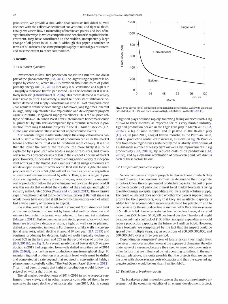
Fig. 3. Type curves for oil production from individual conventional wells with an annualrate of decline of−6%, and from individual tight oil (Bakken) wells (IHS, 2013b).

72 R.L. Kleinberg et al. / Energy Economics 70 (2018) 70–83

production, we provide a simulation that contrasts individual oil welldeclines with the collective declines of conventional and tight oil fields.Finally, we assess how amisreading of breakeven points, and lack of in-sight into theways inwhich companies use benchmarks to prioritize in-vestment, may have contributed to the sudden, unexpectedly largechange of oil prices in 2014–2016. Although this paper is couched interms of oil markets, the same principles apply to natural gas resources,and to some extent to other commodities.

3. Results

3.1. Oil market dynamics

Investments in fossil fuel production constitute a multitrillion dollarpart of the global economy (IEA, 2014). The largest single segment is oc-cupied by crude oil, which in 2015 provided about one-third of globalprimary energy use (BP, 2016). Not only is oil consumed at a high rate- roughly a thousand barrels per second - but the demand for it is rela-tively inelastic (Labandeira et al., 2016). This means demand is relativelyinsensitive to price. Conversely, a small but persistent imbalance be-tween demand and supply - sometimes as little as 1% of total production- can result in dramatic price changes. Moreover, long lag times inherentin large, risky, capital-intensive exploration and development projectscause substantial, long-lived supply overshoots. Thus the oil price col-lapse of 2014–2016, when West Texas Intermediate benchmark crudeoil prices fell by 70%, was accompanied by substantial increases in pro-duction from long lead-time projects in the U.S. Gulf of Mexico (EIA,2016b) and elsewhere. These were not unprecedented events.

Also contributing tomarket instability is the complication that a bar-rel of oil with a relatively high cost of production can enter the marketbefore another barrel that can be produced more cheaply. It is truethat the lower the cost of the resource, the more likely it is to beexploited by a producer who holds a range of resources, and lower-cost resources present less risk of loss in the event of a decline ofmarketprice. However, dispersal of resources among awide variety of indepen-dent actors, as in theUnited States, implies that oil and gas resources arenot developed in seriatim order of cost. If oil sells for $100/bbl, the smallproducer with costs of $90/bbl will sell as much as possible, regardlessof lower-cost resources owned by others. Thus, given a range of pro-ducers acting independently of each other, any resourcewith amarginalcost of production below the prevailingmarket price can be produced. Itwas this reality that enabled the creation of the shale gas and tight oilindustry in theUnited States (Wang and Krupnick, 2013). The extensiveexperimentation that led to the commercialization of Barnett shale gaswould never have occurred if left to commercial entities each of whichhad a wide variety of resources to exploit.

It is in this context that the advent of abundant North American tightoil resources, brought to market by horizontal well construction andmassive hydraulic fracturing, was believed to be a market stabilizer(Maugeri, 2013). Unlike deepwater and Arctic projects, for which leadtimes are typically a decade or more, a tight oil well can be planned,drilled, and completed in months. Furthermore, unlike wells in conven-tional reservoirs, which decline at around 6% per year (IEA, 2013) andcontinue producing for decades, tight oil wells typically decline byabout 60% in the first year and 25% in the second year of production(IHS, 2013b), see Fig. 3. As a result, nearly half of Lower 48 U.S. oil pro-duction in 2015 had originated fromwells drilled since the start of 2014(EIA, 2016d);much of this new production came from tight oil plays. Tomaintain tight oil production at a constant level, wells must be drilledand completed at a rate beyond that required in conventional fields, aphenomenon colorfully called “The Red Queen Race” (Likvern, 2012).Thus it had been thought that tight oil production would follow theprice of oil with a short time lag.

The oil market developments of 2014–2016 in some respects con-firmed these views, and in other respects contradicted them. In re-sponse to the rapid decline of oil prices after June 2014, U.S. rig counts

in tight oil plays declined rapidly, following falling oil prices with a lagof two to three months, as expected for this very nimble industry.Tight oil production peaked in the Eagle Ford play in March 2015 (EIA,2016k), a lag of nine months, and it peaked in the Bakken play(Fig. 2a) in June 2015, a lag of twelve months. In the Permian Basin,tight oil production continued to increase, as shown in Fig. 2b. Produc-tion from these regions was sustained by the relatively slow decline ofa substantial number of legacy tight oil wells, by improvements in rigproductivity (EIA, 2016k), by reduced costs of oil production (EIA,2016c), and by a dynamic redefinition of breakeven point. We discusseach of these factors below.

3.2. Cost per unit productive capacity

When companies compare projects to choose those in which theyintend to invest, the benchmarks they use depend on their corporatepriorities. One is the cost per unit of productive capacity. The cost of pro-ductive capacity is of particular interest to oil market forecasters tryingto relate changes in capital expenditures to likely levels of future supply.The crude oil market does not care whether the barrels supplied madeprofits for their producers, only that they are available. Capacity isadded both to accommodate increasing demand for petroleum and tocompensate for the natural decline ofmature fields. Recently an averageof 5 million bbl/d of new capacity has been added each year, at a cost ofmore than $500 billion: $100,000 per barrel per day. Therefore it mightbe expected that a cut back of $100 billion in capital expenditureswouldreduce production capacity in the future by 1 million bbl/d. However,these forecasts are complicated by the fact that the impact could bespread over multiple years, e.g. as reductions of 200,000, 300,000, and500,000 bbl/d over a three year period.

Depending on companies' view of future prices, they might favorone investment over another, even at the expense of damaging the ulti-mate value of a resource, because they need to meet debt covenants orother factors that are influenced by net operating cash flow. In themar-ket example above, it is quite possible that the projects that are cut arethe ones with above average costs of capacity and thus the expected ag-gregate cutback would be less than 1 million bbl/d.

3.3. Definitions of breakeven points

The breakeven point is seen by some as themost comprehensive as-sessment of the economic viability of an energy development project.

73R.L. Kleinberg et al. / Energy Economics 70 (2018) 70–83

Breakeven points are also called breakeven costs or breakeven prices.The difference is in the point of view, not in any aspect of the underlyingeconomics. In brief, a hypothetical breakeven project has a net presentvalue of zero. In other words, negative cash flows (capital and operatingexpenses, taxes, overheads, and so on) are exactly balanced by thediscounted positive cash flows (income from sales) expected over thelifetime of the project (Brealey et al., 2009).

Given an expected production schedule, variability of futurediscounted cash flow due to predicted changes in the price of oil canbe built into the breakeven estimates. For tight oil wells, which can beconstructed relatively rapidly, and whose production is front loaded,as in Fig. 3, such estimates can be made with some confidence. For pro-jects with long construction schedules and extended production life-times, such as those in deepwater offshore, or in the Arctic, risks arecommensurately greater. These projects are not sanctioned unlesstheir breakeven points arewell below conservative estimates for the fu-ture price of oil.

Different assumptions about the discount rate (or required internalrate of return) can have very substantial effects on the breakevenpoint. Among oil analysts a discount rate of 10% has beenwidely accept-ed as a standard, though sometimes 15% is used. Discrepancies alsooccur because various analysts have used differing slates of costs to in-clude in their breakeven estimates. Because these slates of costs arenot standardized nor usually explicitly and fully disclosed, breakevenpoints published by various analysts, agencies, and oil producers aregenerally not comparable, and therefore easily misunderstood.

In reality, there are various breakeven points for any given project.Each of these breakeven points is valid, but only for a specific purpose,which is sometimes not stated explicitly. Here we present a schemewhich does not necessarily follow any one methodology found in ana-lyst, agency or corporate reports. While recognizing that users willwant to define breakeven points in ways most useful to them, we pro-pose a model breakeven point scheme that incorporates elements of

Table 1Components of various breakeven points.

Breakeven Costs

Full Cycle

Capital Expense

Explora�onLeasingReservoir Delinea�onFinancing of Field DevEngineeringRegional PipelinesRoads & Infrastructure

Half Cycle

Financing of Well DevWell Pad Construc�onLocal PipelinesWell Construc�on● Drill, Case, Cement● Complete

Reservoir Mgmt CAPEX● Secondary Recovery● Ter�ary Recovery

WorkoversRefractureDecommissioning● Plug & Abandon● Site Restora�on

Lifting Cost

Operating Expense

Lease Opera�ng Expense● Repair & Maintain● Fuels & Power● Labor

Reservoir Mgmt OPEX● Secondary Recovery● Ter�ary Recovery

Royal�es & TaxesTransport to MarketWater & Waste DisposalGeneral & Administra�ve

Dev

elop

men

tPr

oduc

tion

diverse breakeven analyses used by analysts and industry participants.We avoid de novo terminology by utilizing terms commonly found inreports of breakeven points - “full cycle”, “half cycle”, and “lifting cost”- and provide explicit definitions of these terms. Table 1 summarizesthe definitions, and compares them to related terms: capital expendi-tures, operating expenditures, finding costs, and development costs.

3.3.1. Lifting costLifting cost is the incremental cost of producing one additional barrel

of oil from an existing well in an existing field. This includes leaseoperating expense, which comprises well site costs such as the cost ofoperating and maintaining equipment, fuels, labor costs, and the like.

At present, tight oil resources are produced almost entirely by pri-mary recovery: oil is pushed out of the rock formation and into thewell by the natural pressure of the overburden, plus the pressure gener-ated by gas expansion during production, a process called solution gasdrive. Nearly all conventional reservoirs are produced by secondary re-covery, during which either reservoir pressure is maintained by injec-tions of water or gas, or water is pumped into injector wells to pushoil into nearby producer wells (Cosse, 1993). Tertiary recovery (alsocalled enhanced oil recovery) methods include the employment ofsteam, chemicals, or carbon dioxide tomobilize oil. Lifting costs includeexpenses associated with these methods.

Lifting cost also includes taxes and royalties charged to production atthe wellhead, and the expense of disposal of oilfield wastes. When themarginal cost of transporting product to market is included, the break-even point is conventionally referenced to a pricing hub, e.g. Brent innorthwest Europe, or West Texas Intermediate in Cushing, Oklahoma.The wellhead breakeven price is the hub price minus the cost oftransporting the oil fromwell to hub. Lifting costs are similar to variablecosts of production, but also include general and administrative ex-penses, which are corporate overheads. Lifting cost is the appropriatebreakeven point to usewhen the producer acknowledges afield is in de-cline and is functioning as a “cash cow”, for which little or no further in-vestment is anticipated in the present phase of the business cycle.

3.3.2. Half cycle breakevenThe half cycle breakeven point is the cost of oil production, including

lifting cost, the expense of existingwell workovers, and of drilling, com-pleting, and stimulating additional wells in a developed field, with thegoal of maintaining level production. The cost of financing these activi-ties is included in the half cycle breakeven point.

Half-cycle breakeven costs are often the largest expenses incurred inthe development of an oil field. Drilling expenses include the rental of adrilling rig, and ancillary equipment and supplies such as drill bits anddrilling fluids. Directional drilling services enable the construction of in-creasingly popular horizontal wells. Completion expenses include thesteel casing used to stabilize the wellbore, and the cement placed be-tween casing andwellbore to assure that hydrocarbons cannot contam-inate potable water resources by moving upwards between casing andsubsurface rock. Such operations are more efficient and economicwhen multiple wells are serviced from a single site, a development re-ferred to as “pad drilling”. A review of half-cycle costs can be found inEIA (2016c).

Stimulation was historically a small part of the total cost of wellconstruction. With the advent of massive hydraulic fracturing, it isnow roughly half the expense of drilling and completing a shale gas ortight oil well. In modern practice, well stimulation is a choreographedindustrial operation involvingmultiple service providers using a consid-erable quantity of heavy equipment, along with roughly 30,000 cubicmeters of water, 3000 tons of sand, and 300 tons of specialty chemicalsper well.

For the purposes of taxation in the United States, the expenses ofdrilling and completing a well are divided into tangible and intangibledrilling costs (IRS, 2016). The exact division between the two is declaredby the owner. Generally, the former are permanent fixtures of wells and

74 R.L. Kleinberg et al. / Energy Economics 70 (2018) 70–83

pads, including well heads, casings, pumps, gathering lines, and storagetanks. Intangible drilling costs include items with no salvage value, in-cluding wages, fuel, repairs, hauling, and supplies. In North America in2014, 23% of the average well cost was classified as tangible drilling ex-pense, with the balance classified as intangible drilling expense (WoodMackenzie, 2015b).

Stopping (“shutting in”) production from a producing oil well isproblematic, both technically and economically. However, there is asafer strategy to delay production. After wells are drilled they must becased and cemented in order to protect potable water resources andto prevent the wellbore from collapsing. Drilling, casing, and cementingusually account for roughly half the expense of a modern horizontal,massively fractured well. Remaining operations required to start theflow of oil, including perforating, stimulating, and installing productiontubing and downhole pumps, can be delayed indefinitely at very littlecost and with little or no geological risk. Such wells are called “drilledbut uncompleted” wells (“DUCs”). This strategy is useful when anoilfield operator is under contractual obligation to continue drilling (tohold a lease or to satisfy a drilling rig rental contract, for example), butwishes to conserve capital and delay production untilmarket conditionsare more favorable (EIA, 2016l).

Half cycle breakeven costs include the capital expense ofimplementing secondary and tertiary recovery methods, where used.These expenses can be significant, particularly for tertiary recoverymethods. For example, heavy oil production requires large scaleinfrastructure to generate steam.

A workover is a procedure in which the subsurface plumbing of awell is repaired or replaced after it has been in service for some time.Refracture is a procedure in which current fractures of a well areenlarged, or new fractures are created. Refracture is most commonlyperformed several years after the well has been completed and initiallystimulated, and is described further in Section 4.3.

The ultimate cost of decommissioning should also be included in thehalf cycle breakeven point. Decommissioning includes the secureplugging and abandonment (P&A) of the wells, and any necessary ordesirable site restoration. P&A expenses are largest in offshore develop-ments; in 2016 the U.S. Bureau of Ocean Energy Management promul-gated new rules governing liability (Gladstone et al., 2016). The TexasRailroad Commission requires oil and gas producers to post suretybonds (Texas, 2005), but in many cases liability must be determinedthrough litigation, particularly when an operator has abandoned thewell or declared bankruptcy (Oran and Reiner, 2016).

3.3.3. Full cycle breakevenThe full cycle breakeven point encompasses the cost of oil produc-

tion including all expenses of developing a new field. It is thus themost comprehensive measure of the cost of oil, and is appropriatelyused when planning a major extension of operations. It includes allthe expenses of finding and delineating a resource, including geophysi-cal prospecting, exploratory drilling, and measurements of the size andrichness of the resource (“reservoir characterization”). It also includesobtaining rights to resource exploitation, which can be a complicatedprocesswheremineral rights are broadly distributed. Above-ground in-frastructure such as roads are also included in full-cycle costs. If a com-mon carrier is not available, as with liquefied natural gas projects, itincludes takeaway capacity, including the capital expense of providingtransportation to a market or to a specified pricing hub. The cost of fi-nancing all the above activities is included in the full cycle breakevenpoint. It might also include property tax on reserves, where levied(see e.g. Texas, 2016). Half cycle expenses, including all costs of main-taining level production, and lifting cost expenses, to actually produceoil and pay taxes and royalties as described above, are subsets of fullcycle expenses.

The costs of financingfield andwell development are included in fullcycle and half cycle categories respectively. Remarkably, free cash flow(cash flow less capital expenditures) has been negative for U.S. onshore

producers from the inception of the shale gas and tight oil boomthrough at least 2016 (Wall Street Journal, 2014; Sandrea, 2014;Domanski et al., 2015; EIA, 2016h). Producers have remained solventby taking on debt, and by selling assets and equity; it appears someinvestors view tight oil plays primarily as real estate deals. Negativefree cash flow is a characteristic of an industry in the process of buildingup its stock of productive assets. Indeed, since drilling slowed in Q12015, the gap between capital expenditures and operating cash flowhas narrowed (EIA, 2016h).

3.3.4. Relationship between fixed and variable costsFixed costs do not depend on the level of production, whereas vari-

able costs scale with output. The division between fixed and variablecosts in Table 1 depends on the maturity of the asset. Finding costscome closest to being purely fixed costs, because normally geophysicalsurveys and leasing are completed prior to the drilling of producingwells. Delineation wells, which are generally not significant contribu-tors to production, are part of the fixed costs.

Whether development costs are considered fixed or variable de-pends on the maturity of the asset. Early in the life of a field, its valueis directly proportional to the number of wells drilled; thus these canbe considered variable costs. Once drilling ceases, the cost of the wellsis sunk, and the only variable cost is the lifting cost, except for generaland administrative costs.

3.3.5. Fiscal breakevenFull cycle breakeven costs, and all its components, are essentially

technical and economic in nature, and as such are controlled bycorporate decision-making, geological and geographic factors, mar-ket forces, and rates of taxation. Fiscal breakeven is of a completelydifferent nature. It is the price of oil required to finance nationalexpenditures, for those nations which depend heavily on oil receiptsto fund government operations (Clayton and Levi, 2015; IMF, 2016).It includes full-cycle, half-cycle, or lifting cost expenses, dependingon the state of the indigenous industry. Moreover, it dependsdirectly on certain components of the technical breakeven costs,such as leases, royalties, and taxes. Where government is a majorshareowner in oil companies, as is often the case in countries heavilydependent on resources, fiscal breakeven also depends on corporatedividends and similar payouts.

Although not generally expressed in this manner, individual corpo-rations also have fiscal breakevens, which relate to the expectations oftheir investors. For those corporations financed predominantly byequity, fiscal breakeven includes revenues required to meet expectedcorporate dividends. Corporations like to show steady or risingdividends over time, which are put under pressure when income fallsas a result of unexpected costs, or falling commodity prices. Recently,corporations have increased their debt load in order to pay dividends(Bloomberg, 2016).

3.3.6. Externalities breakevenIn some cases, breakeven costs might be considered to include addi-

tional aspects of production activities, such as social cost of carbon (EPA,2016), direct and indirect costs of accidents, environmental impacts,and societal impacts (Greenstone and Looney, 2012; Jackson et al.,2014; HEI, 2015).

3.4. Geological, geographical, quality, taxation and exchange rate influenceson breakeven points

3.4.1. Geological factorsEvery oil field has a range of distinct breakeven points. A primary

cause of breakeven point variation is geological. Conventional oil playsare defined by traps: the subsurface structural or stratigraphic geome-tries of oil or gas reservoirs in which the placement of fluids is drivenby their buoyancy (USGS, 2016). Small traps are clearly harder to find,

75R.L. Kleinberg et al. / Energy Economics 70 (2018) 70–83

and are less productive when found. Large traps can be delineated andproduced at exceptionally low cost - as low as a few dollars per barrelof oil produced.

Unlike conventional reservoirs found in traps, “shales” (more prop-erly referred to as organic-rich mudstones (Kleinberg, forthcoming))are continuous: “large volumes of rock pervasively charged with oiland gas” (USGS, 2016). Although these plays may be hundreds of kilo-meters in extent, the richest rock bodies, and those most susceptibleto hydraulic fracturing, can be quite localized (Gulen et al., 2015;Ikonnikova et al., 2015). Thus there are considerable variations in break-even points between and within sub-plays (North Dakota Departmentof Mineral Resources, 2015; Wood Mackenzie, 2015a).

3.4.2. Geographical factorsEqually important are geographical factors. The local availability of

oil field infrastructure has a major influence on breakeven points.Much of the field and well development inherent in resource exploita-tion is performed by a network of contractors who provide materialsand perform services essential to every aspect of this process. Localavailability of - and the presence of competitivemarkets for - explorationexpertise and instrumentation; drilling rigs, equipment and services;and completion and stimulation services, have a major influence on oilfield development costs. Operators engaged in onshore exploratory dril-ling in advanced industrialized nations in Europe are dismayed to learnthey are in “frontier areas” with respect to oil field services, wherecosts can be double or triple those prevailing in Texas or Oklahoma.This is true even when those nations, such as the United Kingdom,have well established offshore exploration and production industrieswith globally competitive economic structures.

All else being equal, well construction costs in ultra-deepwater(greater than 1500 m water depth) are an order of magnitude greaterthan on land. Therefore only very productive reservoirs can beexploited, and there must be a strong expectation that future oil priceswill be high enough to warrant investment. Arctic regions can also beeconomically challenging, even though in various parts of the Arcticvery significant amounts of oil have been produced.

Nonetheless, the petroleum industry is remarkably adaptable, andoperates efficiently in many improbably remote locations. Economy ofscale is key, and once sufficient activity develops in a geographical lo-cale, nomatter how remote or uninhabitable, cost reductionwill follow.Thus the lowest-cost places in the world to work are many areas in theUnited States and Canada, the nations surrounding the Arabian Gulf,and infrastructure-rich parts of Russia, all of which have long historiesof intensive oil and gas development. For example, in mid-2014, at a re-cent peak of oil prices, there were 1850 land rigs in the United Statesand only 100 in all of Europe. This is one of the reasonswhy exploitationof shale gas resources developed so much more rapidly in the UnitedStates than anywhere else.

One of the greatest hurdles to working in remote areas is the cost oftransporting product to markets (“takeaway”). This is particularly truefor natural gas, for which practical transport is limited to large-diameter high-pressure pipelines, or liquefied natural gas ships and as-sociated export and import facilities. Both approaches are costly (ShawandKleinberg, forthcoming). Thus, for example, plans for exploitation ofnatural gas on theNorth Slope of Alaska have been repeatedly frustratedby the cost of moving gas to markets. Oil transportation is generallycheaper and easier because of itsmuchhigher energy density under am-bient conditions of temperature and pressure.

Finally, country risk can be a decisive factor in the decision whetheror not to develop a resource. There are a wide variety of risk factors, in-cluding the extent and stability of environmental regulations; laboravailability, regulations, and militancy; disputed land claims; politicaland legal instability; and insecurity arising from crime, conflict, or ter-rorism (Jackson et al., 2016). Arguably, tight oil fields are less subjectto political risk such as expropriation because the payback time of an in-dividual well is short, and field production can only be maintained by

continuous drilling of wells requiring technically sophisticated horizon-tal well construction and high volume multistage fracturing.

3.4.3. Quality factors and price hub locationsThe market price of a barrel of crude oil depends on its value to re-

finers. Generally speaking, “light” (low mass density) oils comprisinglow molecular weight hydrocarbons are more valuable than “heavy”(high mass density) oils with high contents of nitrogen-, sulfur-, andoxygen-bearing compounds.

The location of the hub at which oil is priced can also be an impor-tant factor. As mentioned above, oil is normally relatively inexpensiveto ship long distances via pipeline or tanker (Shaw and Kleinberg,forthcoming). However, when the rate of oil production temporarily ex-ceeds available transport capacity, significant price differentials be-tween hubs can develop. Historically, prices of Brent Crude, traded innorthwestern Europe, and West Texas Intermediate (WTI), traded inCushing, Oklahoma, have beenwithin a fewpercent of each other. How-ever, between 2011 and 2014, when U.S. tight oil production increasedso rapidly that pipeline capacity was exceeded and railroads werebrought into service to move crude oil (EIA, 2016o), the Brent priceexceeded WTI by as much as 20% (EIA, 2013).

When quality and hub location factors combine, price differencescan be especially large. For example, in December 2013, WTI sold for$98/bbl in Cushing, while Western Canadian Select, which is bothheavy and transportation constrained, sold for $59/bbl in Hardisty,Alberta (Alberta, 2016).

In many plays, substantial quantities of associated gas are producedwith oil. In such circumstances, the heating value of the combined pro-duction can be referenced to barrels of oil equivalent (boe), which is de-fined in terms of the higher heating value (HHV) of the oil and gasproducts upon combustion: 1 boe = 5.8 million Btu = 6.1 GJ (IRS,2005). However, the barrel of oil equivalent is not a valid means of esti-mating the economic value of production, as the relative prices of gas andoil often do not scale with their heating values. Associated gas rich inmethane and natural gas liquids - ethane, propane, normal butane, iso-butane, and natural gasoline - can be more accurately assessed in termsof the individual product streams, which have species-specific values tothe refining and petrochemical industries (Braziel, 2016; EIA, 2016e).

3.4.4. TaxationThe kinds and amounts of taxes imposed on the petroleum indus-

try by governments are driven by two conflicting desires: first tomaximize tax receipts, and second to encourage economic develop-ment associated directly and indirectly with hydrocarbon produc-tion. Generally speaking, the easier it is to find oil, and the cheaperit is to extract, the larger the tax (Brackett, 2014). Practices varywidely among countries (EY, 2015) and from state to state withinthe United States (EIA, 2015c). In the U.S., oil and gas production isencouraged by special tax preferences, the three most important ofwhich were worth about $5 billion in net tax reductions to the indus-try in 2017 (Metcalf, 2018).

3.4.5. Exchange rate factorsBreakeven points are conventionally stated in U.S. dollars per barrel

of oil. While oil is traded internationally in dollar-denominated con-tracts, in some cases breakeven points are more appropriately statedin terms of national currencies. For example, the Russian oilfield servicesector is large and well-developed, and prices its services in Russian ru-bles. Frommid-2014 to early 2016, when the ruble fell in value relativeto the dollar in synchrony with the decline in the international price ofoil, Russian oil companies came under less financial pressure than didWestern oil companies (Financial Times, 2016; IHS, 2016). In essence,technical breakeven points in ruble terms remained mostly unchanged.However, Russia's dollar-denominated balance of trade with othercountries suffered as a result of the dollar-denominated oil pricedecline.

0

100

200

300

400

500

600

2011 2012 2013 2014 2015 2016

New

Well O

il P

roduction p

er R

ig

(bbl/day)

Year161114-02b

Fig. 4. Productivity of drilling rigs directed to Bakken tight oil. Internally-driven changesoccur throughout the period shown. Externally-driven changes are driven by rapiddeclines in the price of oil, e.g. mid-2014 through 2016. The vertical axis represents theamount of new production an average rig, operating for one month, contributes to theoil supply (EIA, 2016k).

76 R.L. Kleinberg et al. / Energy Economics 70 (2018) 70–83

3.5. How breakeven points change with time

Despite the lack of transparency of many breakeven point estimates,themid-2014 consensus range of $60/bbl to $90/bbl for full cycle break-even in tight oil plays, appears to have been broadly accurate. Once oilprices fell through this range, in the second half of 2014, rig counts inthe major tight oil basins collapsed, as illustrated by Fig. 2a and b.More than 100 North American exploration and production companies,and a similar number of oilfield service companies, filed for bankruptcybetween January 2015 and mid-2016 (Haynes and Boone, 2016a;Haynes and Boone, 2016b). Even the strongest of the U.S. independenttight oil producers reported negative operating and net incomesthroughout this period.

However, one of the pitfalls of inadequate understanding of break-even points is a failure to realize that they change with time. For exam-ple, in Andrews, Martin, Howard, andMidland counties, in the PermianBasin of Texas, breakeven points declined from $76/bbl in June 2014(Wood Mackenzie, 2014b) to $37/bbl in August 2016 (WoodMackenzie, 2016c), behavior that was typical of U.S. tight oil plays(IHS, 2017).We identify two kinds of changes. Internally-driven changesreflect steady microeconomic improvements in infrastructure and effi-ciency. Externally-driven changes occur in response to changing macro-economic conditions. In the dynamic U.S. oil and gas industry, andparticularly in the tight oil sector in which production technology isevolving rapidly, internally and externally driven changes can signifi-cantly alter production economics on a time scale of 1–2 years.

3.5.1. Internally-driven changesTable 2 outlines some of the internal drivers of breakeven point

change. Changes can be early or late in the development cycle, andcan increase or decrease costs. Often, breakeven points are high or in-creasing early in development, as oil producers compete for resourcessuch as leases, personnel, and infrastructure. Later in the developmentcycle, debottlenecking and increased competition among service pro-viders causes costs to fall. Thus well drilling and completion costs infive U.S. shale gas and tight oil plays rose from 2010 to 2012 and fellfrom 2012 to 2015 (EIA, 2016c), during a period in which oil priceswere stable.

Decreasing costs can be accompanied by increasing production.From late 2012 to the third quarter of 2014, internally-driven improve-ments led to a doubling of new well oil productivity per rig in theBakken tight oil play, see Fig. 4. Thiswas partly due towells being drilledand completed more quickly, and partly due to increases in the initialproduction per well (EIA, 2016a). Throughout this period, West TexasIntermediate crude traded in a narrow range around $100/bbl (EIA,2016m).

Taxes and other aspects of “government take” can be importantexceptions to the pattern of costs falling over time. Governments seek

Table 2Internally-driven factors which change breakeven points, early and late in the develop-ment cycle. Factors which increase costs are shown in bold font, and factors which de-crease costs are shown in italic font.

Stage in Development CycleetaLylraE

Exploration & delineation De-risked geologyWell construction surprises Efficient well constructionCompetition for leases Consolidation of leasesSupply chain bottlenecks Supply chain optimizationInfrastructure bottlenecks Infrastructure buildoutService cost increases

Equipment shortagesPersonnel shortages

Service cost discountsIncreased competition

Tax Decreases Tax Increases

to maximize their share of oil industry revenues, and while somecountries have fixed rates of taxation, others change their tax rates atwill, increasing taxes to just short of the point atwhich local oil explora-tion and production is discouraged and moves elsewhere. At the incep-tion of activity, when risks are high and sunk costs are low, or when oilprices are low, governments encourage activity with low tax rates. Afterreserves have been booked and expensive infrastructure built, or whenoil prices increase, tax rates can increase.

3.5.2. Externally-driven changesBreakeven points change as a result of changes in the price of oil.

While the price of oil depends on the cost of its production, the oppositeis also true: the cost of oil production depends on capital, labor, andma-terial inputs, the prices of which are affected by the state of the oil mar-ket.When the price of oil is high relative to long term trends, as it was in2011–2014, the goals of producers are rapid growth of reserves and pro-duction: they are incentivized to find, delineate, and develop new fields,with all the attendant inefficiencies. Service providers offer new, moreexpensive technology directed to those objectives. Cost control is a sec-ondary consideration. Service company profitability increases.

These trends are also dependent on the rate of change of the oilprice. Rapid expansion of the industry creates bottlenecks in equipment,supplies, labor, and infrastructure. The oil industry faced such stressesfrom the early 1970s to the early 1980s, when the price of oil quadru-pled in inflation-adjusted dollars. Discovery of rich new plays sets off asimilar gold-rush mentality, as illustrated by the advent of tight oil pro-duction in 2009–2014.

When oil prices decline, all these trends are reversed. Exploration,the growth engine of the industry, slows to a crawl. Determination ofthe areal and vertical extent of the reservoir, and measurements of thespatial variation of its richness (asset delineation or “de-risking”) is nolonger prioritized. The industry tends to focus on familiar resourcesand geographical areas known to contain substantial recoverable re-serves (with a few notable exceptions, such as the Alpine High field(Apache, 2016)), and within those areas, the best drilling locations(“sweet spots”), a process known as asset high grading. This leads to agreater responsiveness to price changes (Smith and Lee, 2017). More-over, a large reduction in the number of drilling rigs results in survivalof themostmodern and efficient rigs, manned by themost experiencedand successful drilling crews. This might be termed operational highgrading. Thus over the period 2004 to 2015, the IHS Upstream Capital

77R.L. Kleinberg et al. / Energy Economics 70 (2018) 70–83

Cost Index (IHS, 2015a) tended to increase after increases in the price ofBrent crude, and tended to decrease after decreases in the crude price.

As illustrated in Fig. 4, rig productivity can increase rapidly due toexternally-driven factors. After having doubled during times of relativelyconstant oil prices, Bakken rig productivity increased by another factor ofthree while oil prices declined precipitously from the third quarter of2014 through 2016. During this period, normal process improvementswere amplified by asset high grading and operational high grading.

In addition to internally-driven cost reductions due to normal im-provements in efficiency, and externally-driven market-related cost re-ductions due to asset high grading, steep declines in activity enableoperators to drive down costs while the supply of services exceeds thedemand for them. Service providers respond by laying off personneland by warehousing (“stacking”) or destroying or cannibalizing(“writing off”) equipment, but these cost-control measures, which arecostly in themselves, usually do not keep pace with the rapid declinesin business activity, such as occurred in 2014–2016.

The Permian Basin provides another dramatic example of how rap-idly price structures can change. Following the national trend, the Perm-ian Basin oil-directed rig count fell by more than 75%, from a peak ofabout 560 rigs in November 2014 to a trough of about 130 rigs inApril of 2016 (Baker Hughes, 2016), see Fig. 2b. Much of this declinewas due to retirement of almost all of the 200 vertical and directionalrigs, which were primarily exploiting the conventional subplays of thebasin, but even the horizontal rig fleet declined by almost two-thirds.Nonetheless, tight oil production continued to increase through 2016(EIA, 2016k). While oil prices were relatively stable between 2012 andlate 2014, internally-driven improvements doubled rig productivity.Falling oil prices after late 2014 triggered externally-driven improve-ments, which increased rig productivity by a further factor of 2.7 (EIA,2016k), while well costs declined by 35% and production costs declinedby 25% (Pioneer Natural Resources, 2016).

Governments can change tax structures and rates in response tomarket conditions.When oil prices are rising, governments can increasetax rates without driving producers out of business or to other coun-tries. When oil prices fall, governments are forced to make tax conces-sions to maintain the viability of their petroleum industry (WoodMackenzie, 2017).

3.5.3. Change in type of breakeven pointJust as importantly, the relevant type of breakeven point changes

with time. Once finding costs are sunk, the full cycle breakeven oilprice is no longer relevant in assessing project economics going forward.Similarly, once drilling concludes, the cost of well construction becomesirrelevant. Thus there is a natural progression of a project from full cycleeconomics through half cycle economics to lifting cost economics.

The relevance of the various breakeven points also changes due toexternal drivers:

• During periods of rising oil prices, when producers move into newplays, full cycle breakeven is relevant to planners and investors.

• In stable markets, when activity is focused on in-fill drilling andmod-est step outs in de-risked plays where infrastructure is in place, halfcycle breakeven economics is most relevant.

• Whenmarkets are in free fall and oil companies are focused on surviv-al, the viability of existing assets is measured against lifting costs.

• When prices rebound, some operators will have accumulated sub-stantial acreages of derisked prospects, with plenty of undrilled sitesin their inventories. They will be able to continue with favorablehalf-cycle economics for some time. However, as their sweet spotsare depleted, as is already occurring in the Barnett shale, and theyhave to move to fresh prospects, they will be forced to return to fullcycle economics.

The tiered nature of breakeven points is important because the tiersare relatively far apart. In mid-2014, full cycle breakeven points for U.S.

tight oil produced bymassive hydraulic fracturingwere generally in therange of $60–$90/bbl. Given that the excess of oil supply over demandwas in the range of 1–2%, and that “rapidly responding” tight oil consti-tuted about 4% of the world oil market, one might have expected thatthe price of oil was unlikely to fall below about $60/bbl. However, halfcycle breakeven points were in the range of $50–$70/bbl, and liftingcosts were below $20/bbl. When oil prices declined, not only did thesebrackets move to lower cost ranges due to internal and external drivers(compare e.g. Wood Mackenzie, 2014a, 2015a, 2016b; Goldman Sachs,2017), but there was a large-scale transition from greenfield full cycleeconomics, to the half cycle economics of drilling to maintain level pro-duction, and eventually, after the second half of 2015, to productionfrom existing wells. Anticipated profits vanished, and the capitalexpenses accounted for in full-cycle economics became sunk costsreflected in falling share prices, debt restructuring, asset sales, orbankruptcy.

4. Other factors affecting tight oil market dynamics

The conventional definition of price elasticity of supply is the ratio ofthe percentage change of quantity supplied to the percentage change inprice.When this ratio is less than unity, themarket is said to be inelastic(Mankiw, 2011). The supply of oil is inelastic in the short term. Thisinelasticity arises from many sources, each of which has its owncharacteristics.

4.1. Rate of growth of tight oil production

Part of the conventional wisdom surrounding tight oil production isthat it is very responsive to changes in markets. This certainly seemedtrue from 2009 to 2014, when tight oil production grew from700,000 bbl/d to 4,200,000 bbl/d (EIA, 2015b). During the latter partof this period (following recovery from the recession of 2008), rates ofgrowth of U.S. oil production were the largest in more than 100 years,mostly attributable to tight oil (EIA, 2015a).

However, these dramatic growth rates do not imply tight oil ischeaper or easier to produce than conventional oil. In fact, tight oilwells aremore expensive andmore complex to construct thanmost con-ventional oil wells, requiring specialized equipment, such as bottomholeassemblies capable of horizontal drilling and fleets of truck-mountedhigh-pressure high-volume pumps. However, exactly the same drillingrigs and hydraulic fracturing equipment are used to exploit shale gasand tight oil, and large quantities of this equipment had been broughtinto service during the shale gas boom that started in 2004. That boomterminated abruptly at the end of 2008, when gas prices fell from$6–$14 per million British thermal units (1 MMBtu = 1.055 GJ) to$2–$4/MMBtu, causing the number of U.S. gas-directed drilling rigs tofall from1600 to 700. Thus tight oil drilling programs could ramp up rap-idly when theWest Texas Intermediate benchmark oil price doubled in2009, as shown in Fig. 5. The rapid increase of tight oil production, ratherthan being a property intrinsic to tight oil, was the product of the acci-dental, rapid crossing of oil and gas prices, and the fact that shale gasand tight oil drilling and stimulation equipment is interchangeable.

Note however that despite the redirection of drilling rigs from shalegas to tight oil, U.S. natural gas production did not decrease. One reasonwas continued improvement in well recovery rates in theMarcellus drygas play. Another was the rapidly increasing production of natural gasassociated with tight oil, mostly from the Bakken, Eagle Ford, and un-conventional Permian plays, which grew from essentially zero in 2009to 13% of total U.S. gas production by mid-2015 (IHS, 2015b).

Once drilling and stimulation infrastructure are generally available,onshore production of oil can respond rapidly to price signals. The aver-age lag between investment and production for tight oil wells is aboutone year, coincident with the shortest lags associated with all oil wellsdrilled in 14,000 oilfields between 1970 and 2015 (Bornstein et al.,2017). The entire Bornstein data set is broadly distributed, the longest

Fig. 5. Horizontal drilling rigs (bottom) (Baker Hughes, 2016) and hydraulic fracturing equipment moved from gas plays (dotted curve) to oil plays (solid curve) after oil and gas pricesdiverged (top) (EIA, 2016m, 2016n).

78 R.L. Kleinberg et al. / Energy Economics 70 (2018) 70–83

lags presumably associated with wells drilled in deepwater or frontierregions.

4.2. Rate of decline of tight oil production

When oil prices fell, the decrease of tight oil production provedslower than some expected. In the two years following the completionof a well, tight oil production from that well declines quickly, in contrastto conventional oil wells under secondary recovery. Thereafter, thedecline of tight oil wells roughly parallels that of conventional wells,see Fig. 3. However, there are important differences between theproduction rate of individual wells and that of a field of such wells.The rate of decline of production for a field comprising numerouswells drilled at various times is not necessarily the same as the rate ofdecline of an individual well in that field, even if all wells have exactlythe same production parameters.

To illustrate this principle, we compare a simplified model of a con-ventional oil fieldwith a comparablemodel tight oil field.Wemodel theconventional oil field development as a series of 48 wells, completed atthe rate of one per month. Each well has an initial (maximum) produc-tion of 1000 bbl/d, performancewhich is above average but not unknownin U.S. onshore fields. Following standard oilfield practice (Cosse, 1993),the field is assumed to be put on secondary recovery immediately afterproduction starts, thereby maintaining reservoir pressure.

We model tight oil field development using assumptions similar tothose used for the model conventional field: 48 wells, completed atthe rate of one per month, with initial production of 1000 bbl/d, againabove average but not exceptional (Sandrea, 2012; EIA, 2016a). Becausetight oil fields cannot normally be put on secondary recovery(Kleinberg, 2014), individual wells decline rapidly in the first severalyears, typical of primary recovery.

For an ensemble of wells completed at times tk, with k ranging from1 to N, where N is the total number of wells completed, the rate of oilproduction from the field at any time t is given by

Q tð Þ ¼XN

k¼1

qk t−tkð Þ ð1Þ

where qk(t-tk) is rate of production from a single well k at the time tsubsequent to the completion of that well at time tk. Since wells do notproduce prior to being completed, qk = 0 for all t b tk. Eq. (1) allowseach well to have a unique decline curve qk. In our models we assumeall conventional wells have a common decline curve, qc, and all tight oilwells have a different common decline curve, qt.

In a conventional oil field under secondary recovery, rates of declineare roughly uniform over much of the life of each well:

1qc

dqcdt

¼ −αy ð2Þ

where αy is the annual rate of decline, which we shall assume to beαy = 0.06/yr. This corresponds to an annual rate of decline of 6%, avalue that is justified below. The monthly rate of decline is αm = αy/12.This simple differential equation is integrated to find the conventionaloil well decline curve when the field is on secondary recovery; IP is theinitial production rate of an individual well:

qc ¼ IP � exp −αyt� �

t½ � ¼ years ð3aÞ

qc ¼ IP � exp −αmtð Þ t½ � ¼ months ð3bÞ

For themodel of a tight oil field, we assume that all wells have a com-mon decline curve qt, given by a Bakken average type curve (IHS, 2013b)normalized to an initial production rate of 1000 bbl/d, see Fig. 3.

After the cessation of completions in month 48, the conventional oilfield declines at an annual rate of 6%; a sum of exponentials decays atthe same rate as the individual exponential functions of the argumentof the summation. With this knowledge, we selected the individualwell decline rate,αy=0.06/yr, based on a global average of conventionaloil field decline rates (IEA, 2013).

The results of the two models are shown in Fig. 6. During months 1to 48, while wells are being completed, the production from both fieldsincreases with time. Because the conventional wells decline ratherslowly, the ramp up of production during the development phase isnearly linear. The much more rapid initial decline of production of the

0

10000

20000

30000

40000

50000

0 24 48 72 96 120

Prod

uction

(b/d

)

Month

Conventional

6% Decline Per Year

10 year cumulative = 111 mmbbl

Bakken

10 year cumulative = 37 mmbbl

one well per month for 48 months

initial production = 1000 b/d per well

150517-02

Fig. 6.Modeled field-level production in conventional and tight oil (Bakken) fields, duringand after 48 month drilling and completion campaigns, using the individual well declinecurves shown in Fig. 3.

79R.L. Kleinberg et al. / Energy Economics 70 (2018) 70–83

tight oil wells leads to a distinctly sublinear ramp up of production. Thisis the origin of the “Red Queen Race” (Likvern, 2012).

After the cessation of completions in month 48, the conventional oilfield declines at an annual rate of 6%, the global average of conventionaloil field decline rates. Unlike the conventional oil field, the tight oil fielddoes not decline at a time-invariant rate following the cessation ofdrilling, as shown in Fig. 6. Table 3 provides a summary of annual pro-duction decline rates of the model conventional and tight oil wells andfields. Although tight oil fields experience a substantial decline in pro-duction in the first two years after cessation of drilling, as the mostrecently-drilled wells decline, a larger number of slowly-declining lega-cy wells supports substantial continued production. Thus tight oil fieldswith large legacy inventories of wells will produce substantial quanti-ties of oil for many years after completions have ceased. Note thatTable 3 is only illustrative: tight oil field decline rates depend on detailsof the development schedule. If completion activity has increased im-mediately prior to cessation, a large proportion of wells in the field arerelatively new, leading to faster initial decline of field-level productiononce drilling and completion comes to an end. On the other hand, ifcompletion activity has slowed in the year or two before terminating,production after termination will decline more slowly than suggestedby Fig. 6 and Table 3.

Table 3Percentage annual decline of conventional oil well and field under secondary recovery,and tight oil well and field under primary recovery. The field level declines follow thetermination of the drilling and completion program. The tight oil results are model-dependent, as explained in the text.

Conventional oil(secondary recovery)

Tight oil(primary recovery)

Year Well Field Well Field

1 6% 6% 60% 28%2 6 6 27 163 6 6 18 124 6 6 13 115 6 6 11 11

4.3. Refracturing

It is generally agreed among oilfield service companies that hydrau-lic fracturing is an imperfectmethod for connecting gas or oil in lowper-meability formations to the wellbore; according to production logs, 30–40% of fractures do not produce fluids (Jacobs, 2015; Hunter et al.,2015). Either of two types of refracturing are used to overcome thisproblem. In the “reconnect” procedure, fractures that are poor conduitsfor fluid flow can be reopened, whereas in the “restimulate” procedure,new fractures are created (Hunter et al., 2015). Refractures costbetween about 20% and 40% of the cost of a new well (Lindsay et al.,2016), so it would seem the economic case for these techniqueswould be compelling. Nonetheless, experience has shown that arigorous screening process maximizes the chance of success (Hunteret al., 2015), and only a few percent of shale gas and tight oil wellsdrilled in the last ten years have been refractured using chemical diver-sion, the most cost-effective technique (Lindsay et al., 2016). Lack ofpredictability is the main barrier to widespread implementation(Wood Mackenzie, 2016a).

4.4. Infrastructure, labor and financial inelasticities

Following an industry collapse, as occurred in 2014–2016, the rate atwhich tight oil production can ramp up once drilling resumes dependson how equipmentwas taken out of service during the period of low ac-tivity. If equipment is written off, it is destroyed or cannibalized. How-ever, when equipment is stacked, as is the practice of some largeservice providers (Schlumberger, 2015; Seeking Alpha, 2016), it isassumed to retain value as a productive asset and is warehousedaccordingly.

A second factor is labor availability. Labor required in the tight oilsector, along with associated equipment, made a smooth transitionfrom gas drilling to oil drilling in 2009. Following massive layoffs fromthe petroleum industry in 2015 and 2016, skilled labor may not be asabundant in the future as it has been in recent years. The duration oftraining varies with the degree of skill and specialization required, andcan exceed a year to gain proficiency in some job categories.

Financialmarkets also introduce inelasticity. The ready availability ofcapital played an important role in the initial growth of the US tight oilindustry, with many producers, year after year, operating at negativefree cash flow (cash flow after capital investments) (Sandrea, 2014;EIA, 2014, 2015d; Domanski et al., 2015). It remains to be seen whetherdebt and equity financing is as available in the future.

5. Oil market stability

5.1. Short term market stability

5.1.1. Spare capacityAlthough it has been stated that US tight oil can challenge Saudi

Arabia as the world's marginal producer (e.g. The Economist, 2014),this assertion is open to question. Spare capacity is the most importantcharacteristic of a swing producer. Spare capacity is defined as produc-tion that can be brought on linewithin 30 days and sustained for at least90 days (EIA, 2016f; Munro, 2014). While there is no doubt SaudiAramco can increase production this rapidly, the US tight oil industrycannot. In addition, unlike OPEC members, who can in theory increaseor reduce their oil production in concert, the hundreds of U.S. producerscannot and will not coordinate their activities.

5.1.2. InventoriesInventories of crude oil and petroleum products are also drivers of

short termmarket stability. As of the first quarter of 2017, US commer-cial crude oil and product inventories amounted to 1.34 billion barrels,with an additional 0.69 billion barrels of crude oil in the U.S. StrategicPetroleum Reserve (SPR) (EIA, 2017a). Altogether this amounts to

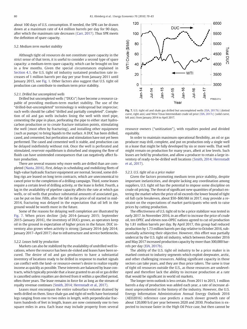
Fig. 7. U.S. tight oil and shale gas drilled but uncompleted wells (EIA, 2017b) (dottedcurve, right axis) and West Texas Intermediate crude oil price (EIA, 2017c) (solid curve,left axis) from January 2014 to April 2017.

80 R.L. Kleinberg et al. / Energy Economics 70 (2018) 70–83

about 100 days of U.S. consumption. If needed, the SPR can be drawndown at a maximum rate of 4.4 million barrels per day for 90 days,after which the maximum rate decreases (Carr, 2017). Thus SPR meetsthe definition of spare capacity.

5.2. Medium term market stability

Although tight oil resources do not constitute spare capacity in thestrict sense of that term, it is useful to consider a second type of sparecapacity: a medium-term spare capacity, which can be brought on linein a few months. Given the special circumstances explained inSection 4.1, the U.S. tight oil industry sustained production rate in-creases of 1 million barrels per day per year from January 2011 untilJanuary 2015, see Fig. 1. Other factors also suggest that U.S. tight oilproduction can contribute to medium term price stability.

5.2.1. Drilled but uncompleted wellsDrilled but uncompletedwells (“DUCs”) have become a resource ca-

pable of providing medium-term market stability. The use of the“drilled-but-uncompleted” terminology is widespread but imprecise;such wells should be called “drilled and partially completed”. Comple-tion of oil and gas wells includes lining the well with steel pipe,cementing the pipe in place, perforating the pipe to either start hydro-carbon production or to create fracture initiation points, stimulatingthe well (most often by fracturing), and installing other equipment(such as pumps) to bring liquids to the surface. A DUC has been drilled,cased, and cemented, but perforation and stimulation have not yet beenperformed. The cased and cemented well is stable, and production canbe delayed indefinitely without risk. Once the well is perforated andstimulated, reservoir equilibrium is disturbed and stopping the flow offluids can have unintended consequences that can negatively affect fu-ture production.

There are several reasons why more wells are drilled than are com-pleted (Nasta, 2016). First, delays in scheduling and mobilizing fleets ofhigh-value hydraulic fracture equipment are normal. Second, somedril-ling rigs are leased on long term contracts, which are uneconomical tocancel prior to the completion of a drilling campaign. Third, some leasesrequire a certain level of drilling activity, or the lease is forfeit. Fourth, alag in the availability of pipeline capacity affects the rate at which gaswells, or oil wells that produce substantial amounts of associated gas,can be put on line. Fifth, after the fall in the price of oil started in mid-2014, fracturing was delayed in the expectation that oil left in theground would be worth more in the future.

Some of the reasons for delaying well completion are illustrated byFig. 7. When prices decline (July 2014–January 2015; September2015–January 2016), the inventory of DUCs grows, as operators keepoil in the ground in expectation of higher prices in the future. DUC in-ventory also grows when activity is strong (January 2014–July 2014;January 2017–April 2017) due to infrastructure and service bottlenecks.

5.2.2. Leases held by productionMarkets can also be stabilized by the availability of undrilledwell lo-

cations, where the resource has been de-risked and leases have been se-cured. The desire of oil and gas producers to have a substantialinventory of locations ready to be drilled in response to market signalscan conflict with the land- or resource-owner's desire to realize royaltyincome as quickly as possible. These interests are balanced by lease con-tracts, which typically provide that a lease granted to an oil or gas drilleris cancelled unless royalties are derived from it within a specified period,often three years. The lease remains in force for as long as the stream ofroyalty revenue continues (Smith, 2014; Herrnstadt et al., 2017).

Leases must encompass the entire subsurface volume drained bywells drilled on them. Since shale gas and tight oil wells have horizontallegs ranging from one to two miles in length, with perpendicular frac-tures hundreds of feet in length, leases are now commonly one to twosquare miles in area. Each lease may include property from several

resource owners (“unitization”), with royalties pooled and dividedequitably.

In order to maintain maximum operational flexibility, an oil or gasproducer may drill, complete, and put on production only a single wellin a lease that might be fully developed by six or more wells. That wellmight remain on production for many years, albeit at low levels. Suchleases are held by production, and allow a producer to retain a large in-ventory of ready-to-be-drilled well locations (Smith, 2014; Herrnstadtet al., 2017).

5.2.3. U.S. tight oil as a price makerGiven the factors promoting medium term price stability, despite

important inelasticities, and despite lacking any coordination amongsuppliers, U.S. tight oil has the potential to impose some discipline oncrude oil pricing. The threat of significant new quantities of product en-tering themarketwhen the price of oil exceeds the lower bound of tightoil full cycle breakeven, about $50–$60/bbl in 2017, may provide a re-straint on the expectations of market participants who seek to raiseprices by cutting production.

The effectiveness of U.S. tight oil to be a price stabilizer was tested inearly 2017. In November 2016, in an effort to increase the price of crudeoil, ten OPEC and eleven non-OPEC nations agreed to cut oil productionby 1.81 million barrels per day. By April 2017, this group had reducedproduction by 1.73million barrels per day relative toOctober 2016, sub-stantially achieving their objective. However, this effort was partiallyundercut by the U.S. tight oil industry, which between December 2016andMay 2017 increased production capacity bymore than 300,000 bar-rels per day (EIA, 2017b).

The ability of the U.S. tight oil industry to be a price maker is inmarked contrast to industry segments which exploit deepwater, arctic,and other challenging resources. Adding significant capacity in thosesectors can take years, and they are thus price takers. The same is trueof tight oil resources outside the U.S., as those resources are undevel-oped and therefore lack the ability to increase production at a ratethat would be significant in world oil markets.

The longer term outlook is less certain. From 2011 to 2015, 1 millionbarrels a day of production was added each year, a rate of increase al-most unprecedented in the history of the industry. However, the U.S.Energy Information Administration Annual Energy Outlook 2016(AEO2016) reference case predicts a much slower growth rate ofabout 120,000 b/d per year between 2020 and 2030. Production is ex-pected to increase faster in the High Oil Price case, but then cannot be

81R.L. Kleinberg et al. / Energy Economics 70 (2018) 70–83

sustained after 2025. Only in the High Oil and Gas Resource andTechnology case do the rate increases of 2011–2015 continue past2020 (EIA, 2016j).

6. Discussion

Given knowledge of a range of breakeven points for a relativelyhigh-cost resource, a lower-cost competitor with ample spare ca-pacity might be tempted to increase production to the extent thatthe price of the resource falls below the breakeven point range ofits higher-cost rival. To be successful, this strategy requires an un-derstanding of the tiered nature of breakeven points. Frequently,breakeven point data are presented by analysts, or in corporate pre-sentations to investors, without adequate disclosure of what exactlyis meant by breakeven. In this paper we have shown that bench-mark and breakeven points are only useful to the extent their calcu-lation is transparent.

In projections of the reaction of oil production to changes in the priceof oil, many analysts underestimated the dynamic nature of tight oileconomics. In mid-2014, full cycle breakeven points for U.S. tight oilproduced by horizontal well construction and massive hydraulic frac-turing were generally in the range of $60–$90/bbl, giving rise to expec-tations that the price of oil was unlikely to fall below about $60/bbl. Halfcycle breakeven points were in the range of $50–$70/bbl, and liftingcosts were below $15/bbl. When oil prices declined, not only did thesebrackets move to lower cost ranges due to internal and external driversdiscussed in this paper, but there was a large-scale transition of break-even points. Oil production promptly shifted from full cycle projects tothe half cycle economics of drilling to maintain level production. Afterthe second half of 2015, drilling was no longer adequate to maintainlevel production, but oil production continued from pre-existing wells,the rate of production from which falls rather slowly after the firsttwo years or so.

In this paper we propose a consistent treatment of breakevenpoints - full cycle, half cycle, and lifting cost - and explain internally-driven and externally-driven changes in breakeven point economics.In a rapidly evolving industry such as tight oil production this analysisis itself subject to change. Nonetheless, it is important for a variety ofreasons:

• The various levies imposed by governments, including leases and roy-alties, are calculated to maximize payments while allowing oil pro-ducers to retain sufficient profit to make resource developmentattractive. A better understanding of breakeven points by govern-ments would facilitate this process.

• Asset valuation depends critically on estimates of future costs. Be-cause stable tight oil production requires the continuous drilling andcompletion of wells, the economics of a long-lived play requires un-derstanding how half cycle breakeven points change over time. Simi-larly, the economics of growing oil volumes requires analysis of fullcycle breakeven points. In both cases, secular changes due to internaland external drivers should be taken into account.

• Energy analysts, in both private and government sectors, can improveforecasts by incorporating into their economic models realistic rangesof breakeven points, and models of how these change under variousconditions.

Inelasticity in the response of oil production to market signals isa further complication, the understanding of which requires closeexamination of individual well decline curves and their implica-tions at play level. The interaction between productive capacityand technical features of oilfield practice, such as drilled but un-completed wells and refractured wells, must also be considered,as does oilfield and takeaway infrastructure, capital markets, andlabor factors.

7. Conclusions

Breakeven points are among the most useful measures of the eco-nomic viability of a hydrocarbon development project. They are partic-ularly useful in assessing the robustness of the project with respect to adecline in the price of the produced commodity: if future market pricesare projected to be comfortably above the breakeven cost of a project,the investment is likely to be a profitable one.

This work explores the following characteristics of breakeven pointanalysis:

• The breakeven point is most useful when its calculation is transpar-ent. We argue that the purveyors of breakeven point data have a re-sponsibility to carefully define the elements that go into theircalculations.

• While recognizing that various users will want to define breakevenpoints in ways most useful to them, we propose a model breakevenpoint scheme that incorporates many elements of these calculations,and which approximates consensus schemes used by analysts and in-dustry participants.

• We define and explain each major category of expense in our slate ofbreakeven costs.

• Wedivide our slate of costs into threemajor categories: full cycle, halfcycle, and lifting cost. These terms are common in the breakeven anal-yses found in the work of analysts, agencies, and oil producers; weprovide precise definitions of them.

• We show how breakeven costs change due to internally-driven fac-tors. These are microeconomic factors which represent normal im-provements in operational efficiency. Efficiency improves over timein every new play exploited by the petroleum industry, as geologicalknowledge and infrastructure maturity progress. Because tightoil production technology has developed rapidly in this decade,internally-driven improvements have been very pronounced.

• Externally-driven factors, driven by the macroeconomic environment- principally the price of oil - also have a strong effect on breakevenpoint dynamics because, counterintuitively, changes in the marketprice of oil lead the cost of producing oil.

• Not only do individual costs change due to macroeconomic factors,but the breakeven point structure itself changes. As prices fall, fullcycle economics gives way to half cycle economics, and eventuallyto lifting cost economics. In rising markets, the reverse is true.

We have discussed other factors affecting oil market stability:

• The surprising speed with which U.S. tight oil production increasedafter 2010 is explained, in part, by the timely availability of specializedoilfield equipment built between 2004 and 2009 to exploit shale gas.

• The unexpectedly slow decline of U.S. tight oil supplies during the oilprice declines of 2014–2015 is shown to be due to the relatively slowdecline of production from legacy tight oil wells, when considered ona field-average basis.

• Infrastructure, labor, and financial inelasticities also affect oil marketdynamics.

• U.S. tight oil production does not ramp up or down quickly enough tosignificantly affect short term oil market stability. However, it doeshave the potential to stabilize oilmarkets in themedium term. Thus un-like deepwater, heavy, or arctic oil resources,which are price takers, U.S.tight oil is likely to function as a price maker in the medium term.

Acknowledgments

The authors wish to thank Vello Kuuskraa, Kenneth Austin, RustyBraziel, Imelda Foley, Joel Enderlin, Jan Mares, and the anonymous ref-erees for their helpful comments and suggestions. This research didnot receive any specific grant from funding agencies in the public, com-mercial, or not-for-profit sectors.

82 R.L. Kleinberg et al. / Energy Economics 70 (2018) 70–83

References

Alberta, 2016. Oil prices. http://economicdashboard.alberta.ca/OilPrice, Accessed date: 16December 2016.

Apache, 2016. Apache Corporation Discovers Significant New Resource Play in SouthernDelaware Basin, 7 September 2016.

Baker Hughes, 2016. North America Rotary Rig Count, September 2016.Bloomberg, 2014. Break-Even Points for US Shale Oil, 17 October 2014.Bloomberg, 2016. BigOilGobblesUpRecordDebt as BorrowingCostsDecline,May 13, 2016.Bornstein, G., Krusell, P., Rebelo, S., 2017. Lags, costs, and shocks: An equilibriummodel of

the oil industry. National Bureau of Economic Research Working Paper 23423.BP, 2016. BP Statistical Review of World Energy, June 2016.Brackett, B., 2014. My perspective on global geopolitical risk, EIA conference, 15 July 2014.

https://www.eia.gov/outlooks/documentation/workshops/pdf/4_Brackett%202014-07-15%20final%20EIA%20Geopolitics.pdf, Accessed date: 25 June 2017.

Braziel, E.R., 2016. The Domino Effect. NTA Press.Brealey, R., Myers, S., Marcus, A., Maynes, E., Mitra, D., 2009. Fundamentals of Corporate

Finance. McGraw-Hill Ryerson.Carr, H., 2017. Need You Now - The Strategic Petroleum Reserve's Muted Effect in the

Shale Era. RBN Energy (29 January 2017).Clayton, B., Levi, M., 2015. Fiscal Breakeven Oil Prices: Uses, Abuses, and Opportunities for

Improvement. Council on Foreign Relations (November 2015).Cosse, R., 1993. Chap. 8. Basics of Reservoir Engineering. Editions Technip, Paris.Domanski, D., Kearns, J., Lombardi, M., Shin, H.S., 2015. Oil and debt. BIS Q. Rev, pp. 55–65

(March 2015).EIA, 2013. Price difference between Brent and WTI crude oil narrowing. Today in Energy.

US Energy Information Administration (28 June 2013).EIA, 2014. As cash flow flattens, major energy companies increase debt, sell assets. Today

in Energy. US Energy Information Administration (29 July 2014).EIA, 2015a. U.S. oil production growth in 2014 was largest in more than 100 years. Today

in Energy. US Energy Information Administration (30 March 2015).EIA, 2015b. Annual Energy Outlook 2015, DOE/EIA-0383 (2015). US Energy Information

Administration (April 2015).EIA, 2015c. Major fossil fuel-producing states relay heavily on severance taxes. Today in

Energy. US Energy Information Administration (21 August 2015).EIA, 2015d. US onshore producers face challenging times. This Week in Petroleum. US

Energy Information Administration (10 September 2015).EIA, 2016a. Initial production rates in tight oil formations continue to rise. Today in

Energy. US Energy Information Administration (11 February 2016).EIA, 2016b. Oil production in federal Gulf of Mexico projected to reach record high in

2017. Today in Energy. US Energy Information Administration (18 February 2016).EIA, 2016c. Trends in U.S. Oil and Natural Gas Upstream Costs. US Energy Information

Administration (March 2016).EIA, 2016d. Wells drilled since start of 2014 provided nearly half of lower 48 oil produc-

tion in 2015. Today in Energy. US Energy Information Administration (22 March2016).

EIA, 2016e. Hydrocarbon gas liquids production and related industrial development.Annual Energy Outlook 2016. US Energy Information Administration (20 June 2016).

EIA, 2016f. What Drives Crude Oil Prices? US Energy Information Administration (12 July2016)

EIA, 2016g. Short Term Energy Outlook. US Energy Information Administration (12 July2016.

EIA, 2016h. U.S. oil companies closer to balancing capital investment with operating cashflow. Today in Energy. US Energy Information Administration (18 July 2016).

EIA, 2016i. Shale in theUnited States, Energy in Brief. US Energy InformationAdministration(updated 20 July 2016).

EIA, 2016j. Future U.S. tight oil and shale gas production depends on resources, technology,markets. Today in Energy. US Energy Information Administration (22 August 2016).

EIA, 2016k. Drilling Productivity Report. US Energy Information Administration (12September 2016).

EIA, 2016l. EIA nowprovides estimates of drilled but uncompletedwells inmajor productionregions. Today in Energy. US Energy Information Administration (September 14, 2016).

EIA, 2016m. Weekly Cushing OKWTI Spot Price FOB. US Energy Information Administra-tion (21 September 2016).

EIA, 2016n. Henry Hub Natural Gas Spot Price. US Energy Information Administration (13October 2016).

EIA, 2016o. US crude oil by rail. http://www.eia.gov/dnav/pet/hist/LeafHandler.ashx?n =PET&s= ESM_EPC0_RAIL_NUS-NUS_MBBL&f =M, Accessed date: 16 December 2016.

EIA, 2017a. Short-Term Energy Outlook, Tables 3a, 4a. US Energy Information Administra-tion (9 May 2017).

EIA, 2017b. How much shale (tight) oil is produced in the United States? https://www.eia.gov/tools/faqs/faq.php?id = 847&t = 6, Accessed date: 27 June 2017

EIA, 2017c. Weekly Cushing OK WTI Spot Price FOB. US Energy Information Administra-tion (17 May 2017).

EPA, 2016. The Social Cost of Carbon. US Environmental Protection Agency updated 23February 2016. https://www3.epa.gov/climatechange/EPAactivities/economics/scc.html.

EY, 2014. US upstream: costs, prices and the unconventional treadmill. http://www.ey.com/Publication/vwLUAssets/EY-US-upstream-costs-prices-and-the-unconventional-treadmill/$FILE/EY-US-upstream-costs-prices-and-the-unconventional-treadmill.pdf.

EY, 2015. Global Oil and Gas Tax Guide.Ezrati, M., 2015. America: oil's new swing producer, National Interest. 11 August 2015.

http://nationalinterest.org/print/feature/america-oils-new-swing-producer-13556.Financial Times, 2016. Amid the Oil Price Crash, Rosneft is Running to Stand Still. Financial

Times (23 March 2016).

Gladstone, A., Halftermeyer, M., Plough, A., 2016. Dangers in the Deep: A $40 billion Time-bomb Threatening the Gulf. Debtwire 12 September 2016. http://www.debtwire.com/info/2016/09/12/dangers-deep-40-billion-time-bomb-threatening-gulf/.

Goldman Sachs, 2017. Top Projects 2017 (25 May 2017).Greenstone, M., Looney, A., 2012. Paying too much for energy? The true costs of our

energy choices. Daedalus 141 (2), 10–30.Gulen, G., Ikkonikova, S., Browning, J., Smye, K., Tinker, S., 2015. Production Scenarios for the

Haynesville Shale Play, SPE-176022. SPE Economics & Management (October 2015).Haynes & Boone, 2016a. Oil Patch Bankruptcy Monitor, October 19, 2016.Haynes & Boone, 2016b. Oilfield Services Bankruptcy Monitor, October 25, 2016.HEI, 2015. Strategic Research Agenda on the Potential Impacts of 21st Century Oil and

Natural Gas Development in the Appalachian Region and Beyond. Health Effects Insti-tute October 2015. http://www.healtheffects.org/UOGD/UOGD.htm.

Herrnstadt, E., Kellogg, R., Lewis, E., 2017. Information Asymmetry, Drilling Distortions,and Oil and Gas Leases (preprint).

Hunter,W., Turner, M., Villalobos, J., Baihly, J., Pena, A., 2015. Systematic candidate selectionimproves Haynesville refracturing economics. World Oil 236 (12), 67–72 (December2015).

IEA, 2013. Decline rate analysis. World Energy Outlook 2013. International EnergyAgency.

IEA, 2014. World Energy Investment Outlook, Annex A - Investment Tables. InternationalEnergy Agency.

IHS, 2013a. Tight Oil Brings the Swing Era Back to the United States, August 2013.IHS, 2013b. Bakken Shale Workbook, August 2013.IHS, 2015a. What's Cost Got to Dowith it? How Oil Prices and Upstream Costs Help Shape

Each Other, July 2015.IHS, 2015b. US Gas Forecast: Associated Gas Setting Up for Recovery? November 2015.IHS, 2016. Low Operating Costs Make Russian Oil Production Economic Even at Very Low

International Oil Prices, April 2016.IHS, 2017. Making Ends Meet: How the Oil Industry Is Cutting Costs to Make up for Lower

Prices, May 2017.Ikonnikova, S., Browning, J., Gulen, G., Smye, K., Tinker, S., 2015. Factors influencing shale

gas production forecasting: empirical studies of Barnett, Fayetteville, Haynesville, andMarcellus Shale plays. Econ. Energy Environ. Policy 4, 19–35.

IMF, 2016. Regional economic outlook, Middle East and Central Asia, International Mon-etary Fund, October 2016; see Statistical Appendix. https://www.imf.org/external/pubs/ft./reo/2016/mcd/eng/pdf/mreo0416st.pdf.

IRS, 2005. Internal Revenue Cumulative Bulletin 2005-1, January–June, Part III - Adminis-trative, Procedural, and Miscellaneous; Nonconventional Source Fuel Credit, §29Inflation Adjustment Factor and §29 Reference Price; Notice 2005-33. US InternalRevenue Service.

IRS, 2016. Costs You can Deduct or Capitalize, Internal Revenue Service Publication. 535(Chap. 7).

Jackson, T., Green, K.P., Sholes, K., 2016. Global Petroleum Survey. Fraser Institute.Jackson, R.B., Vengosh, A., Carey, J.W., Davies, R.J., Darrah, T.H., O'Sullivan, F., Petron, G.,

2014. The environmental costs and benefits of fracking. Annu. Rev. Environ. Resour.39, 327–362.

Jacobs, T., 2015. Halliburton reveals refracturing strategy. J. Pet. Technol. 67 (11), 40–41(November 2015).

Kleinberg, R.L., 2014. Technology on the horizon & over the horizon. EIA Energy Conference,15 July 2014 https://www.eia.gov/conference/2014/.

Kleinberg, R.L., 2017. Unconventional fossil fuels. In: Aziz, M.J., Johnson, A.C. (Eds.), Intro-duction to Energy Technology: Depletable and Renewable.Wiley-VCH (forthcoming).

Krane, J., Agerton, M., 2015. OPEC imposes ‘swing producer’ role upon U.S. shale:evidence and implications, IAEE Energy Forum, third quarter 2015. https://iaee.org/en/publications/fullnewsletter.aspx?id=36.

Labandeira, X., Labeaga, J., Lopez-Otero, X., 2016. Ameta-analysis on the price-elasticity ofenergy demand. Robert Schuman Centre for Advanced Studies. European UniversityInstitute, Working paper RSCAS 2016/25 http://fsr.eui.eu/meta-analysis-price-elasticity-energy-demand/.

Likvern, R., 2012. Is shale oil production from Bakken headed for a run with “The RedQueen”? The Oil Drum 25 September 2012. http://www.theoildrum.com/node/9506

Lindsay, G.J., White, D.J., Miller, G.A., Baihly, J.D., Sinosic, B., 2016. Understanding the Ap-plicability and Economic Viability of Refracturing HorizontalWells in UnconventionalPlays, Society of Petroleum Engineers Paper SPE 179113.

Mankiw, N.G., 2011. Principles of Economics. Fifth edition. South-Western CengageLearning.

Maugeri, L., 2013. The Shale Oil Boom: A U.S. Phenomenon, Discussion Paper 2013-05.Belfer Center for Science and International Affairs, Harvard Kennedy School (June2013).

McNally, R., 2015. Commentary: Welcome Back to Boom-Bust Oil Prices. ColumbiaUniversity Center on Global Energy Policy (17 December 2015).

Metcalf, G.E., 2018. The impact of removing tax preferences for U.S. oil and natural gasproduction. J. Assoc. Environ. Resour. Econ. 5 (1), 1–37 (January 2018).

Munro, D., 2014. “Effective” OPEC Spare Capacity: Reality-based Data, IEA Energy, Issue 7,4th Quarter 2014.

Nasta, S., 2016. DUC, DUC, Produce - The New EIA DUC Estimates and U.S. Oil & GasProduction, RBN Energy, 28 September 2016.

North Dakota Department of Mineral Resources, 2015. Testimony before North DakotaHouse Appropriations Committee. 8 January 2015. https://www.dmr.nd.gov/oilgas/presentations/FullHouseAppropriations010815.pdf.

OPEC, 2016. World Oil Outlook 2016. Organization of the Petroleum Exporting Countries(October 2016).

Oran Jr., R., Reiner, D., 2016. Who Is Responsible for Decommissioning Costs for Oil andGas Assets Abandoned or Sold in Bankruptcy? American Bar Association http://apps.americanbar.org/litigation/committees/energy/articles/winter2016-0216-who-is-

83R.L. Kleinberg et al. / Energy Economics 70 (2018) 70–83

responsible-decommissioning-costs-oil-gas-assets-abandoned-sold-bankruptcy.html,Accessed date: 25 June 2017 (26 February 2016)

Pioneer Natural Resources, 2016. Investor Presentation (September 2016).Sandrea, R., 2012. Evaluating production potential of mature US oil, gas shale plays. Oil

Gas J. 110 (12) (3 December 2012).Sandrea, I., 2014. US Shale Gas and Tight Oil Industry Performance: Challenges and

Opportunities. Oxford Institute for Energy Studies (March 2014).Schlumberger, 2015. Third Quarter 2015 Results, 15 October 2015.SeekingAlpha, 2016. Schlumberger's (SLB) CEOPaal Kibsgaard onQ32016Results - Earnings

Call Transcript, 21 October 2016.Shaw, J.H., Kleinberg, R.L., 2017. Oil and natural gas. In: Aziz, M.J., Johnson, A.C. (Eds.), Intro-

duction to Energy Technology: Depletable and Renewable. Wiley-VCH (forthcoming).Smith, J.L., 2014. The Option to Hold a Petroleum Lease by Production: A User's Guide to

the Shale Gas Drilling Boom. SSRN https://doi.org/10.2139/ssrn.2531997.Smith, J.L., Lee, T.K., 2017. The Price Elasticity of U.S. Shale Oil Reserves. Energy Econ. 67,

121–135.Texas, 2005. Individual & Blanket Performance Bonds - Letters of Credit or Cash Deposits -

ForWells and Other Oil and Gas Operations, Railroad Commission of Texas. December2005. http://www.rrc.state.tx.us/media/8216/bondi.pdf, Accesseddate: 25 June 2017.

Texas, 2016. Property Tax Code 23.17, Mineral Interest Not Being Produced, Rendered on10 February 2016.

The Economist, 2014. Sheikhs v Shale, 6 December 2014.

The Economist, 2015. After OPEC, 16 May 2015.USGS, 2016. National oil and gas assessment methodology, US geological survey. http://

energy.usgs.gov/OilGas/AssessmentsData/NationalOilGasAssessment/Methodology.aspx, Accessed date: 12 January 2016.

Wall Street Journal, 2014. The NewWinners and Losers in America's Shale Boom, 21 April2014.

Wang, Z., Krupnick, A., 2013. A Retrospective Review of Shale Gas Development in theUnited States, Resources for the Future, RFF DP 13-12.

Wood Mackenzie, 2014a. Bakken/Three Forks Key Play Report, March 2014.Wood Mackenzie, 2014b. Wolfcamp Key Play Report, June 2014.Wood Mackenzie, 2014c. Oil Prices: North American Oil Plays - Breakeven Analysis,

October 2014.Wood Mackenzie, 2015a. Bakken/Three Forks Key Play Report, June 2015.Wood Mackenzie, 2015b. North America Supply Chain Analysis Tool, June 2015.Wood Mackenzie, 2016a. Revisiting Re-fracturing: Still As Attractive as It Was in 2015?

May 2016.Wood Mackenzie, 2016b. Bakken/Three Forks Key Play Report, August 2016.Wood Mackenzie, 2016c. Midland Wolfcamp Key Play Report, August 2016.Wood Mackenzie, 2017. Petroleum Fiscal Systems: 2016 in Review, January 2017.

Joint Program Reprint Series - Recent ArticlesFor limited quantities, Joint Program publications are available free of charge. Contact the Joint Program office to order.

Complete list: http://globalchange.mit.edu/publications

MIT Joint Program on the Science and Policy of Global Change

Massachusetts Institute of Technology 77 Massachusetts Ave., E19-411 Cambridge MA 02139-4307 (USA)

T (617) 253-7492 F (617) 253-9845 globalchange@mit.edu http://globalchange.mit.edu

2018-4 Tight Oil Market Dynamics: Benchmarks, Breakeven Points, and Inelasticities. Kleinberg, R.L., S. Paltsev, C.K.E. Ebinger, D.A. Hobbs and T. Boersma, Energy Economics 70: 70–83 (2018)

2018-3 The Impact of Water Scarcity on Food, Bioenergy and Deforestation. Winchester, N., K. Ledvina, K. Strzepek and J.M. Reilly, Australian Journal of Agricultural and Resource Economics, online first (doi:10.1111/1467-8489.12257) (2018)

2018-2 Modelling Ocean Colour Derived Chlorophyll-a. Dutkiewicz, S., A.E. Hickman and O. Jahn, Biogeosciences 15: 613–630 (2018)

2018-1 Hedging Strategies: Electricity Investment Decisions under Policy Uncertainty. Morris, J., V. Srikrishnan, M. Webster and J. Reilly, Energy Journal, 39(1) (2018)

2017-24 Towards a Political Economy Framework for Wind Power: Does China Break the Mould?. Karplus, V.J., M. Davidson and F. Kahrl, Chapter 13 in: The Political Economy of Clean Energy Transitions, D. Arent, C. Arent, M. Miller, F. Tarp, O. Zinaman (eds.), UNU-WIDER/Oxford University Press, Helsinki, Finland (2017)

2017-23 Carbon Pricing under Political Constraints: Insights for Accelerating Clean Energy Transitions. Karplus, V.J. and J. Jenkins, Chapter 3 in: The Political Economy of Clean Energy Transitions, D. Arent, C. Arent, M. Miller, F. Tarp, O. Zinaman (eds.), UNU-WIDER/Oxford University Press, Helsinki, Finland (2017)

2017-22 “Climate response functions” for the Arctic Ocean: a proposed coordinated modelling experiment. Marshall, J., J. Scott and A. Proshutinsky, Geoscientific Model Development 10: 2833–2848 (2017)

2017-21 Aggregation of gridded emulated rainfed crop yield projections at the national or regional level. Blanc, É., Journal of Global Economic Analysis 2(2): 112–127 (2017)

2017-20 Historical greenhouse gas concentrations for climate modelling (CMIP6). Meinshausen, M., E. Vogel, A. Nauels, K. Lorbacher, N. Meinshausen, D. Etheridge, P. Fraser, S.A. Montzka, P. Rayner, C. Trudinger, P. Krummel, U. Beyerle, J.G. Cannadell, J.S. Daniel, I. Enting, R.M. Law, S. O’Doherty, R.G. Prinn, S. Reimann, M. Rubino, G.J.M. Velders, M.K. Vollmer, and R. Weiss, Geoscientific Model Development 10: 2057–2116 (2017)

2017-19 The Future of Coal in China. Zhang, X., N. Winchester and X. Zhang, Energy Policy, 110: 644–652 (2017)

2017-18 Developing a Consistent Database for Regional Geologic CO2 Storage Capacity Worldwide. Kearns, J., G. Teletzke, J. Palmer, H. Thomann, H. Kheshgi, H. Chen, S. Paltsev and H. Herzog, Energy Procedia, 114: 4697–4709 (2017)

2017-17 An aerosol activation metamodel of v1.2.0 of the pyrcel cloud parcel model: development and offline assessment for use in an aerosol–climate model. Rothenberg, D. and C. Wang, Geoscientific Model Development, 10: 1817–1833 (2017)

2017-16 Role of atmospheric oxidation in recent methane growth. Rigby, M., S.A. Montzka, R.G. Prinn, J.W.C. White, D. Young, S. O’Doherty, M. Lunt, A.L. Ganesan, A. Manning, P. Simmonds, P.K. Salameh, C.M. Harth, J. Mühle, R.F. Weiss, P.J. Fraser, L.P. Steele, P.B. Krummel, A. McCulloch and S. Park, Proceedings of the National Academy of Sciences, 114(21): 5373–5377 (2017)

2017-15 A revival of Indian summer monsoon rainfall since 2002. Jin, Q. and C. Wang, Nature Climate Change, 7: 587–594 (2017)

2017-14 A Review of and Perspectives on Global Change Modeling for Northern Eurasia. Monier, E., D. Kicklighter, A. Sokolov, Q. Zhuang, I. Sokolik, R. Lawford, M. Kappas, S. Paltsev and P. Groisman, Environmental Research Letters, 12(8): 083001 (2017)

2017-13 Is Current Irrigation Sustainable in the United States? An Integrated Assessment of Climate Change Impact on Water Resources and Irrigated Crop Yields. Blanc, É., J. Caron, C. Fant and E. Monier, Earth’s Future, 5(8): 877–892 (2017)

2017-12 Assessing climate change impacts, benefits of mitigation, and uncertainties on major global forest regions under multiple socioeconomic and emissions scenarios. Kim, J.B., E. Monier, B. Sohngen, G.S. Pitts, R. Drapek, J. McFarland, S. Ohrel and J. Cole, Environmental Research Letters, 12(4): 045001 (2017)

2017-11 Climate model uncertainty in impact assessments for agriculture: A multi-ensemble case study on maize in sub-Saharan Africa. Dale, A., C. Fant, K. Strzepek, M. Lickley and S. Solomon, Earth’s Future 5(3): 337–353 (2017)

2017-10 The Calibration and Performance of a Non-homothetic CDE Demand System for CGE Models. Chen, Y.-H.H., Journal of Global Economic Analysis 2(1): 166–214 (2017)

2017-9 Impact of Canopy Representations on Regional Modeling of Evapotranspiration using the WRF-ACASA Coupled Model. Xu, L., R.D. Pyles, K.T. Paw U, R.L. Snyder, E. Monier, M. Falk and S.H. Chen, Agricultural and Forest Meteorology, 247: 79–92 (2017)

2017-8 The economic viability of Gas-to-Liquids technology and the crude oil-natural gas price relationship. Ramberg, D.J., Y.-H.H. Chen, S. Paltsev and J.E. Parsons, Energy Economics, 63: 13–21 (2017)

2017-7 The Impact of Oil Prices on Bioenergy, Emissions and Land Use. Winchester, N. and K. Ledvina, Energy Economics, 65(2017): 219–227 (2017)