TI-83 GUIDEBOOK · TI-83 Graphing Calculator Guidebook English WWW 13 Mar 1997, Rev A 12...
446
TI-83 GRAPHING CALCULATOR GUIDEBOOK TI-GRAPH LINK, Calculator-Based Laboratory, CBL, CBL 2, Calculator-Based Ranger, CBR, Constant Memory, Automatic Power Down, APD, and EOS are trademarks of Texas Instruments Incorporated. IBM is a registered trademark of International Business Machines Corporation. Macintosh is a registered trademark of Apple Computer, Inc. Windows is a registered trademark of Microsoft Corporation. © 1996, 2000, 2001 Texas Instruments Incorporated.
Transcript of TI-83 GUIDEBOOK · TI-83 Graphing Calculator Guidebook English WWW 13 Mar 1997, Rev A 12...
8300INTR.DOC TI-83 Intl English, Title Page Bob Fedorisko Revised: 02/19/01 2:32 PM Printed: 02/21/01 9:05AM Page iii of 8
TI-83GRAPHING CALCULATOR
GUIDEBOOK
TI-GRAPH LINK, Calculator-Based Laboratory, CBL, CBL 2, Calculator-Based Ranger, CBR,Constant Memory, Automatic Power Down, APD, and EOS are trademarks of TexasInstruments Incorporated.
IBM is a registered trademark of International Business Machines Corporation.Macintosh is a registered trademark of Apple Computer, Inc.Windows is a registered trademark of Microsoft Corporation.
© 1996, 2000, 2001 Texas Instruments Incorporated.
Revision_Information
TI-83 Graphing Calculator Guidebook English WWW 13 Mar 1997, Rev A 12 Mar 2001, Rev B
8300INTR.DOC TI-83 Intl English, Title Page Bob Fedorisko Revised: 02/19/01 11:26 AM Printed: 02/19/01 1:46PM Page iv of 8
Texas Instruments makes no warranty, either expressed orimplied, including but not limited to any implied warranties ofmerchantability and fitness for a particular purpose, regarding anyprograms or book materials and makes such materials availablesolely on an “as-is” basis.
In no event shall Texas Instruments be liable to anyone for special,collateral, incidental, or consequential damages in connection withor arising out of the purchase or use of these materials, and thesole and exclusive liability of Texas Instruments, regardless of theform of action, shall not exceed the purchase price of thisequipment. Moreover, Texas Instruments shall not be liable for anyclaim of any kind whatsoever against the use of these materials byany other party.
This equipment has been tested and found to comply with thelimits for a Class B digital device, pursuant to Part 15 of the FCCrules. These limits are designed to provide reasonable protectionagainst harmful interference in a residential installation. Thisequipment generates, uses, and can radiate radio frequency energyand, if not installed and used in accordance with the instructions,may cause harmful interference with radio communications.However, there is no guarantee that interference will not occur ina particular installation.
If this equipment does cause harmful interference to radio ortelevision reception, which can be determined by turning theequipment off and on, you can try to correct the interference byone or more of the following measures:
• Reorient or relocate the receiving antenna.
• Increase the separation between the equipment and receiver.
• Connect the equipment into an outlet on a circuit differentfrom that to which the receiver is connected.
• Consult the dealer or an experienced radio/televisiontechnician for help.
Caution: Any changes or modifications to this equipment notexpressly approved by Texas Instruments may void your authorityto operate the equipment.
Important
US FCCInformationConcerningRadio FrequencyInterference
Introduction iii
8300INTR.DOC TI-83 Intl English, Title Page Bob Fedorisko Revised: 02/19/01 11:26 AM Printed: 02/19/01 1:46PM Page iii of 8
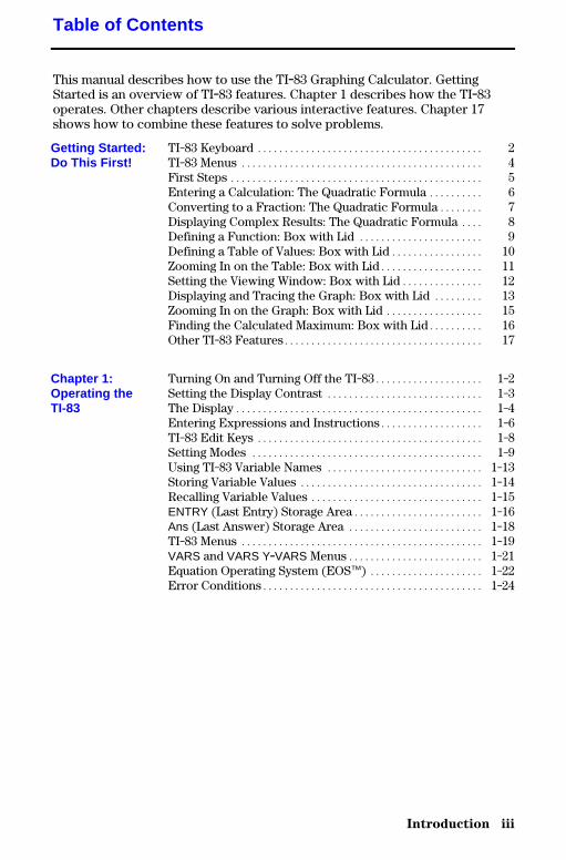
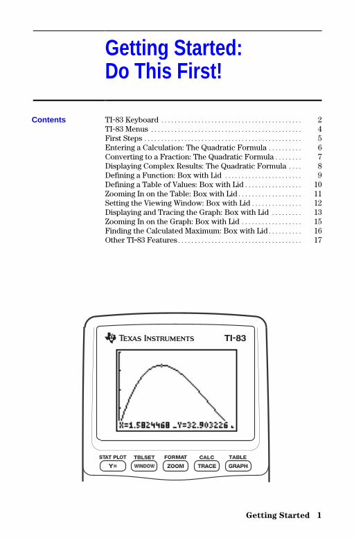
This manual describes how to use the TI.83 Graphing Calculator. GettingStarted is an overview of TI.83 features. Chapter 1 describes how the TI.83operates. Other chapters describe various interactive features. Chapter 17shows how to combine these features to solve problems.
TI-83 Keyboard .......................................... 2TI-83 Menus ............................................. 4First Steps ............................................... 5Entering a Calculation: The Quadratic Formula .......... 6Converting to a Fraction: The Quadratic Formula........ 7Displaying Complex Results: The Quadratic Formula .... 8Defining a Function: Box with Lid ....................... 9Defining a Table of Values: Box with Lid................. 10Zooming In on the Table: Box with Lid................... 11Setting the Viewing Window: Box with Lid............... 12Displaying and Tracing the Graph: Box with Lid ......... 13Zooming In on the Graph: Box with Lid .................. 15Finding the Calculated Maximum: Box with Lid.......... 16Other TI-83 Features..................................... 17
Turning On and Turning Off the TI-83.................... 1-2Setting the Display Contrast ............................. 1-3The Display .............................................. 1-4Entering Expressions and Instructions................... 1-6TI-83 Edit Keys .......................................... 1-8Setting Modes ........................................... 1-9Using TI-83 Variable Names ............................. 1-13Storing Variable Values .................................. 1-14Recalling Variable Values ................................ 1-15ENTRY (Last Entry) Storage Area........................ 1-16Ans (Last Answer) Storage Area ......................... 1-18TI-83 Menus ............................................. 1-19VARS and VARS Y.VARS Menus......................... 1-21Equation Operating System (EOSé) ..................... 1-22Error Conditions......................................... 1-24
Table of Contents
Getting Started:Do This First!
Chapter 1:Operating theTI-83
iv Introduction
8300INTR.DOC TI-83 Intl English, Title Page Bob Fedorisko Revised: 02/19/01 11:26 AM Printed: 02/19/01 1:46PM Page iv of 8
Getting Started: Coin Flip ................................ 2-2Keyboard Math Operations .............................. 2-3MATH Operations ........................................ 2-5Using the Equation Solver ............................... 2-8MATH NUM (Number) Operations........................ 2-13Entering and Using Complex Numbers................... 2-16MATH CPX (Complex) Operations ....................... 2-18MATH PRB (Probability) Operations ..................... 2-20ANGLE Operations....................................... 2-23TEST (Relational) Operations............................ 2-25TEST LOGIC (Boolean) Operations ...................... 2-26
Getting Started: Graphing a Circle ....................... 3-2Defining Graphs ......................................... 3-3Setting the Graph Modes................................. 3-4Defining Functions ...................................... 3-5Selecting and Deselecting Functions ..................... 3-7Setting Graph Styles for Functions....................... 3-9Setting the Viewing Window Variables ................... 3-11Setting the Graph Format ................................ 3-13Displaying Graphs ....................................... 3-15Exploring Graphs with the Free-Moving Cursor.......... 3-17Exploring Graphs with TRACE........................... 3-18Exploring Graphs with the ZOOM Instructions........... 3-20Using ZOOM MEMORY .................................. 3-23Using the CALC (Calculate) Operations .................. 3-25
Getting Started: Path of a Ball ........................... 4-2Defining and Displaying Parametric Graphs.............. 4-4Exploring Parametric Graphs ............................ 4-7
Getting Started: Polar Rose .............................. 5-2Defining and Displaying Polar Graphs ................... 5-3Exploring Polar Graphs.................................. 5-6
Chapter 2:Math, Angle, andTest Operations
Chapter 3:FunctionGraphing
Chapter 4:ParametricGraphing
Chapter 5:Polar Graphing
Introduction v
8300INTR.DOC TI-83 Intl English, Title Page Bob Fedorisko Revised: 02/19/01 11:26 AM Printed: 02/19/01 1:46PM Page v of 8
Getting Started: Forest and Trees ........................ 6-2Defining and Displaying Sequence Graphs ............... 6-3Selecting Axes Combinations ............................ 6-8Exploring Sequence Graphs.............................. 6-9Graphing Web Plots...................................... 6-11Using Web Plots to Illustrate Convergence............... 6-12Graphing Phase Plots .................................... 6-13Comparing TI-83 and TI.82 Sequence Variables .......... 6-15Keystroke Differences Between TI-83 and TI-82 ......... 6-16
Getting Started: Roots of a Function ..................... 7-2Setting Up the Table ..................................... 7-3Defining the Dependent Variables........................ 7-4Displaying the Table ..................................... 7-5
Getting Started: Drawing a Tangent Line ................. 8-2Using the DRAW Menu................................... 8-3Clearing Drawings ....................................... 8-4Drawing Line Segments.................................. 8-5Drawing Horizontal and Vertical Lines ................... 8-6Drawing Tangent Lines .................................. 8-8Drawing Functions and Inverses ......................... 8-9Shading Areas on a Graph ............................... 8-10Drawing Circles.......................................... 8-11Placing Text on a Graph ................................. 8-12Using Pen to Draw on a Graph ........................... 8-13Drawing Points on a Graph .............................. 8-14Drawing Pixels .......................................... 8-16Storing Graph Pictures (Pic) ............................. 8-17Recalling Graph Pictures (Pic) ........................... 8-18Storing Graph Databases (GDB) ......................... 8-19Recalling Graph Databases (GDB) ....................... 8-20
Getting Started: Exploring the Unit Circle................ 9-2Using Split Screen ....................................... 9-3Horiz (Horizontal) Split Screen........................... 9-4G-T (Graph-Table) Split Screen .......................... 9-5TI.83 Pixels in Horiz and G-T Modes ..................... 9-6
Chapter 6:SequenceGraphing
Chapter 7:Tables
Chapter 8:DRAWOperations
Chapter 9:Split Screen

vi Introduction
8300INTR.DOC TI-83 Intl English, Title Page Bob Fedorisko Revised: 02/19/01 11:26 AM Printed: 02/19/01 1:46PM Page vi of 8
Getting Started: Systems of Linear Equations ............ 10-2Defining a Matrix ........................................ 10-3Viewing and Editing Matrix Elements .................... 10-4Using Matrices with Expressions ........................ 10-7Displaying and Copying Matrices ........................ 10-8Using Math Functions with Matrices ..................... 10-9Using the MATRX MATH Operations ..................... 10-12
Getting Started: Generating a Sequence .................. 11-2Naming Lists............................................. 11-3Storing and Displaying Lists ............................. 11-4Entering List Names ..................................... 11-6Attaching Formulas to List Names ....................... 11-7Using Lists in Expressions ............................... 11-9LIST OPS Menu.......................................... 11-10LIST MATH Menu ........................................ 11-17
Getting Started: Pendulum Lengths and Periods ......... 12-2Setting up Statistical Analyses ........................... 12-10Using the Stat List Editor ................................ 12-11Attaching Formulas to List Names ....................... 12-14Detaching Formulas from List Names.................... 12-16Switching Stat List Editor Contexts ...................... 12-17Stat List Editor Contexts................................. 12-18STAT EDIT Menu ........................................ 12-20Regression Model Features .............................. 12-22STAT CALC Menu........................................ 12-24Statistical Variables...................................... 12-29Statistical Analysis in a Program ......................... 12-30Statistical Plotting ....................................... 12-31Statistical Plotting in a Program ......................... 12-37
Getting Started: Mean Height of a Population ............ 13-2Inferential Stat Editors................................... 13-6STAT TESTS Menu ...................................... 13-9Inferential Statistics Input Descriptions.................. 13-26Test and Interval Output Variables ....................... 13-28Distribution Functions................................... 13-29Distribution Shading ..................................... 13-35
Chapter 10:Matrices
Chapter 11:Lists
Chapter 12:Statistics
Chapter 13:InferentialStatistics andDistributions
Introduction vii
8300INTR.DOC TI-83 Intl English, Title Page Bob Fedorisko Revised: 02/19/01 11:26 AM Printed: 02/19/01 1:46PM Page vii of 8
Getting Started: Financing a Car ......................... 14-2Getting Started: Computing Compound Interest.......... 14-3Using the TVM Solver .................................... 14-4Using the Financial Functions ........................... 14-5Calculating Time Value of Money (TVM) ................. 14-6Calculating Cash Flows .................................. 14-8Calculating Amortization ................................ 14-9Calculating Interest Conversion.......................... 14-12Finding Days between Dates/Defining Payment Method ..... 14-13Using the TVM Variables ................................. 14-14
Browsing the TI-83 CATALOG ........................... 15-2Entering and Using Strings............................... 15-3Storing Strings to String Variables ....................... 15-4String Functions and Instructions in the CATALOG ...... 15-6Hyperbolic Functions in the CATALOG .................. 15-10
Getting Started: Volume of a Cylinder.................... 16-2Creating and Deleting Programs ......................... 16-4Entering Command Lines and Executing Programs ...... 16-5Editing Programs ........................................ 16-6Copying and Renaming Programs ........................ 16-7PRGM CTL (Control) Instructions ....................... 16-8PRGM I/O (Input/Output) Instructions ................... 16-16Calling Other Programs as Subroutines .................. 16-22
Comparing Test Results Using Box Plots ................ 17-2Graphing Piecewise Functions........................... 17-4Graphing Inequalities .................................... 17-5Solving a System of Nonlinear Equations ................ 17-6Using a Program to Create the Sierpinski Triangle ....... 17-7Graphing Cobweb Attractors ............................ 17-8Using a Program to Guess the Coefficients............... 17-9Graphing the Unit Circle and Trigonometric Curves...... 17-10Finding the Area between Curves ........................ 17-11Using Parametric Equations: Ferris Wheel Problem...... 17-12Demonstrating the Fundamental Theorem of Calculus ... 17-14Computing Areas of Regular N-Sided Polygons .......... 17-16Computing and Graphing Mortgage Payments ........... 17-18
Chapter 14:FinancialFunctions
Chapter 15:CATALOG,Strings,HyperbolicFunctions
Chapter 16:Programming
Chapter 17:Applications
viii Introduction
8300INTR.DOC TI-83 Intl English, Title Page Bob Fedorisko Revised: 02/19/01 11:26 AM Printed: 02/19/01 1:46PM Page viii of 8
Checking Available Memory ............................. 18-2Deleting Items from Memory ............................ 18-3Clearing Entries and List Elements ...................... 18-4Resetting the TI.83 ...................................... 18-5
Getting Started: Sending Variables ....................... 19-2TI-83 LINK ............................................... 19-3Selecting Items to Send .................................. 19-4Receiving Items.......................................... 19-5Transmitting Items....................................... 19-6Transmitting Lists to a TI-82 ............................. 19-8Transmitting from a TI-82 to a TI-83 ..................... 19-9Backing Up Memory ..................................... 19-10
Table of Functions and Instructions ..................... A-2Menu Map ............................................... A-39Variables ................................................ A-49Statistical Formulas ..................................... A-50Financial Formulas ...................................... A-54
Battery Information...................................... B-2In Case of Difficulty ..................................... B-4Error Conditions......................................... B-5Accuracy Information.................................... B-10Support and Service Information......................... B-12Warranty Information.................................... B-13
Chapter 18:MemoryManagement
Chapter 19:CommunicationLink
Appendix A:Tables andReferenceInformation
Appendix B:GeneralInformation
Index
Getting Started 1
8300GETM.DOC TI-83 international English Bob Fedorisko Revised: 02/19/01 11:06 AM Printed: 02/19/01 11:06AM Page 1 of 18
Gettin g Started:Do This First!
TI-83 Keyboard .......................................... 2TI-83 Menus ............................................. 4First Steps ............................................... 5Entering a Calculation: The Quadratic Formula .......... 6Converting to a Fraction: The Quadratic Formula........ 7Displaying Complex Results: The Quadratic Formula .... 8Defining a Function: Box with Lid ....................... 9Defining a Table of Values: Box with Lid................. 10Zooming In on the Table: Box with Lid................... 11Setting the Viewing Window: Box with Lid............... 12Displaying and Tracing the Graph: Box with Lid ......... 13Zooming In on the Graph: Box with Lid .................. 15Finding the Calculated Maximum: Box with Lid.......... 16Other TI.83 Features..................................... 17
Contents

2 Getting Started
8300GETM.DOC TI-83 international English Bob Fedorisko Revised: 02/19/01 11:11 AM Printed: 02/19/01 11:14AM Page 2 of 18
Generally, the keyboard is divided into these zones: graphing keys, editingkeys, advanced function keys, and scientific calculator keys.
Graphing keys access the interactive graphing features.
Editing keys allow you to edit expressions and values.
Advanced function keys display menus that access theadvanced functions.
Scientific calculator keys access the capabilities of astandard scientific calculator.
TI-83 Keyboard
Keyboard Zones
Editing Keys
AdvancedFunction Keys
ScientificCalculator Keys
Graphing Keys
Getting Started 3
8300GETM.DOC TI-83 international English Bob Fedorisko Revised: 02/19/01 11:06 AM Printed: 02/19/01 11:06AM Page 3 of 18
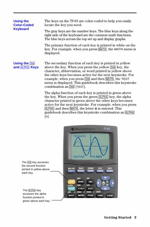
The keys on the TI.83 are color-coded to help you easilylocate the key you need.
The gray keys are the number keys. The blue keys along theright side of the keyboard are the common math functions.The blue keys across the top set up and display graphs.
The primary function of each key is printed in white on thekey. For example, when you press �, the MATH menu isdisplayed.
The secondary function of each key is printed in yellowabove the key. When you press the yellow y key, thecharacter, abbreviation, or word printed in yellow abovethe other keys becomes active for the next keystroke. Forexample, when you press y and then �, the TESTmenu is displayed. This guidebook describes this keystrokecombination as y [TEST].
The alpha function of each key is printed in green abovethe key. When you press the green ƒ key, the alphacharacter printed in green above the other keys becomesactive for the next keystroke. For example, when you pressƒ and then �, the letter A is entered. Thisguidebook describes this keystroke combination as ƒ[A].
Using theColor-CodedKeyboard
Using the yand ƒ Keys
The y key accessesthe second functionprinted in yellow aboveeach key.
The ƒ keyaccesses the alphafunction printed ingreen above each key.

4 Getting Started
8300GETM.DOC TI-83 international English Bob Fedorisko Revised: 02/19/01 11:11 AM Printed: 02/19/01 11:15AM Page 4 of 18
Displaying a Menu
While using your TI.83, you often will needto access items from its menus.
When you press a key that displays a menu,that menu temporarily replaces the screenwhere you are working. For example, whenyou press �, the MATH menu is displayedas a full screen.
After you select an item from a menu, thescreen where you are working usually isdisplayed again.
Moving from One Menu to Another
Some keys access more than one menu. Whenyou press such a key, the names of allaccessible menus are displayed on the topline. When you highlight a menu name, theitems in that menu are displayed. Press ~ and| to highlight each menu name.
Selecting an Item from a Menu
The number or letter next to the current menuitem is highlighted. If the menu continuesbeyond the screen, a down arrow ( $ )replaces the colon ( : ) in the last displayeditem. If you scroll beyond the last displayeditem, an up arrow ( # ) replaces the colon inthe first item displayed.You can select an itemin either of two ways.¦ Press † or } to move the cursor to the
number or letter of the item; press Í.¦ Press the key or key combination for the
number or letter next to the item.
Leaving a Menu without Making a Selection
You can leave a menu without making aselection in any of three ways.¦ Press ‘ to return to the screen
where you were.¦ Press y [QUIT] to return to the home
screen.¦ Press a key for another menu or screen.
TI-83 Menus
Getting Started 5
8300GETM.DOC TI-83 international English Bob Fedorisko Revised: 02/19/01 11:06 AM Printed: 02/19/01 11:06AM Page 5 of 18
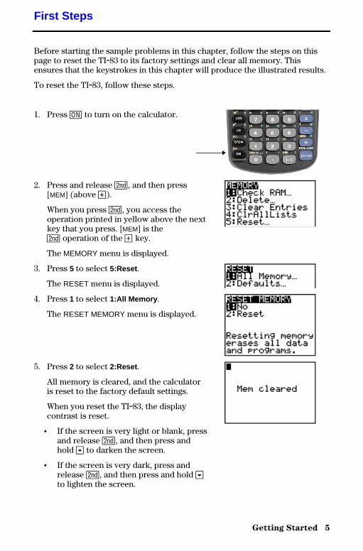
Before starting the sample problems in this chapter, follow the steps on thispage to reset the TI.83 to its factory settings and clear all memory. Thisensures that the keystrokes in this chapter will produce the illustrated results.
To reset the TI.83, follow these steps.
1. Press É to turn on the calculator.
2. Press and release y, and then press[MEM] (above Ã).
When you press y, you access theoperation printed in yellow above the nextkey that you press. [MEM] is they operation of the à key.
The MEMORY menu is displayed.
3. Press 5 to select 5:Reset .
The RESET menu is displayed.
4. Press 1 to select 1:All Memory .
The RESET MEMORY menu is displayed.
5. Press 2 to select 2:Reset .
All memory is cleared, and the calculatoris reset to the factory default settings.
When you reset the TI.83, the displaycontrast is reset.
¦ If the screen is very light or blank, pressand release y, and then press andhold } to darken the screen.
¦ If the screen is very dark, press andrelease y, and then press and hold †to lighten the screen.
First Steps
6 Getting Started
8300GETM.DOC TI-83 international English Bob Fedorisko Revised: 02/19/01 11:06 AM Printed: 02/19/01 11:06AM Page 6 of 18
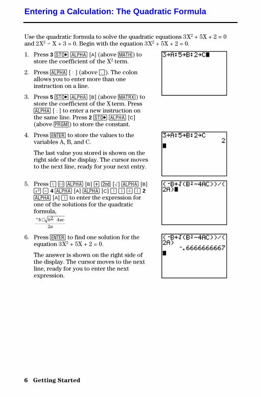
Use the quadratic formula to solve the quadratic equations 3X2 + 5X + 2 = 0and 2X2 N X + 3 = 0. Begin with the equation 3X2 + 5X + 2 = 0.
1. Press 3 ¿ ƒ [A] (above �) tostore the coefficient of the X2 term.
2. Press ƒ [ : ] (above Ë). The colonallows you to enter more than oneinstruction on a line.
3. Press 5 ¿ ƒ [B] (above �) tostore the coefficient of the X term. Pressƒ [ : ] to enter a new instruction onthe same line. Press 2 ¿ ƒ [C](above �) to store the constant.
4. Press Í to store the values to thevariables A, B, and C.
The last value you stored is shown on theright side of the display. The cursor movesto the next line, ready for your next entry.
5. Press £ Ì ƒ [B] Ã y [‡] ƒ [B]¡ ¹ 4 ƒ [A] ƒ [C] ¤ ¤ ¥ £ 2ƒ [A] ¤ to enter the expression forone of the solutions for the quadraticformula,− + −b b ac
a
2 4
2
6. Press Í to find one solution for theequation 3X2 + 5X + 2 = 0.
The answer is shown on the right side ofthe display. The cursor moves to the nextline, ready for you to enter the nextexpression.
Entering a Calculation: The Quadratic Formula

Getting Started 7
8300GETM.DOC TI-83 international English Bob Fedorisko Revised: 02/19/01 11:06 AM Printed: 02/19/01 11:06AM Page 7 of 18
You can show the solution as a fraction.
1. Press � to display the MATH menu.
2. Press 1 to select 1:4Frac from the MATHmenu.
When you press 1, Ans 4Frac is displayed onthe home screen. Ans is a variable thatcontains the last calculated answer.
3. Press Í to convert the result to afraction.
To save keystrokes, you can recall the last expression you entered, and thenedit it for a new calculation.
4. Press y [ENTRY] (above Í) to recallthe fraction conversion entry, and thenpress y [ENTRY] again to recall thequadratic-formula expression,− + −b b ac
a
2 4
2
5. Press } to move the cursor onto the + signin the formula. Press ¹ to edit thequadratic-formula expression to become:− − −b b ac
a
2 4
2
6. Press Í to find the other solution forthe quadratic equation 3X2 + 5X + 2 = 0.
Converting to a Fraction: The Quadratic Formula
8 Getting Started
8300GETM.DOC TI-83 international English Bob Fedorisko Revised: 02/19/01 11:06 AM Printed: 02/19/01 11:06AM Page 8 of 18
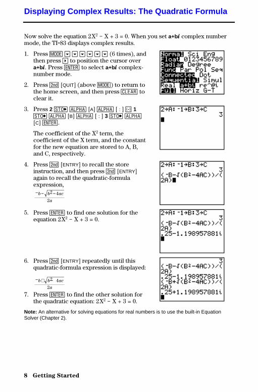
Now solve the equation 2X2 N X + 3 = 0. When you set a+bi complex numbermode, the TI.83 displays complex results.
1. Press z † † † † † † (6 times), andthen press ~ to position the cursor overa+bi. Press Í to select a+bi complex-number mode.
2. Press y [QUIT] (above z) to return tothe home screen, and then press ‘ toclear it.
3. Press 2 ¿ ƒ [A] ƒ [ : ] Ì 1¿ ƒ [B] ƒ [ : ] 3 ¿ ƒ[C] Í.
The coefficient of the X2 term, thecoefficient of the X term, and the constantfor the new equation are stored to A, B,and C, respectively.
4. Press y [ENTRY] to recall the storeinstruction, and then press y [ENTRY]again to recall the quadratic-formulaexpression,− − −b b ac
a
2 4
2
5. Press Í to find one solution for theequation 2X2 N X + 3 = 0.
6. Press y [ENTRY] repeatedly until thisquadratic-formula expression is displayed:
− + −b b ac
a
2 4
2
7. Press Í to find the other solution forthe quadratic equation: 2X2 N X + 3 = 0.
Note: An alternative for solving equations for real numbers is to use the built-in EquationSolver (Chapter 2).
Displaying Complex Results: The Quadratic Formula
Getting Started 9
8300GETM.DOC TI-83 international English Bob Fedorisko Revised: 02/19/01 11:06 AM Printed: 02/19/01 11:06AM Page 9 of 18
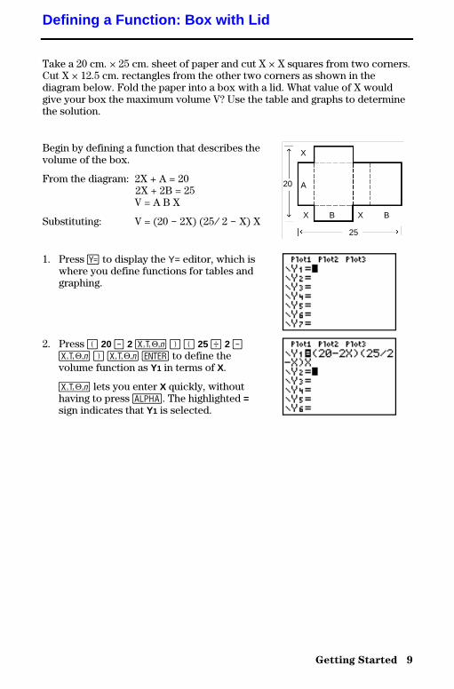
Take a 20 cm. × 25 cm. sheet of paper and cut X × X squares from two corners.Cut X × 12.5 cm. rectangles from the other two corners as shown in thediagram below. Fold the paper into a box with a lid. What value of X wouldgive your box the maximum volume V? Use the table and graphs to determinethe solution.
Begin by defining a function that describes thevolume of the box.
From the diagram: 2X + A = 20 2X + 2B = 25V = A B X
Substituting: V = (20 N 2X) (25à 2 N X) X
1. Press o to display the Y= editor, which iswhere you define functions for tables andgraphing.
2. Press £ 20 ¹ 2 „ ¤ £ 25 ¥ 2 ¹„ ¤ „ Í to define thevolume function as Y1 in terms of X.
„ lets you enter X quickly, withouthaving to press ƒ. The highlighted =sign indicates that Y1 is selected.
Defining a Function: Box with Lid
20 A
X
X B X B
25
10 Getting Started
8300GETM.DOC TI-83 international English Bob Fedorisko Revised: 02/19/01 11:06 AM Printed: 02/19/01 11:06AM Page 10 of 18
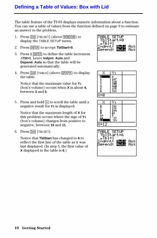
The table feature of the TI.83 displays numeric information about a function.You can use a table of values from the function defined on page 9 to estimatean answer to the problem.
1. Press y [TBLSET] (above p) todisplay the TABLE SETUP menu.
2. Press Í to accept TblStart=0 .
3. Press 1 Í to define the table increment@Tbl=1 . Leave Indpnt: Auto andDepend: Auto so that the table will begenerated automatically.
4. Press y [TABLE] (above s) to displaythe table.
Notice that the maximum value for Y1
(box’s volume) occurs when X is about 4,between 3 and 5.
5. Press and hold † to scroll the table until anegative result for Y1 is displayed.
Notice that the maximum length of X forthis problem occurs where the sign of Y1
(box’s volume) changes from positive tonegative, between 10 and 11.
6. Press y [TBLSET].
Notice that TblStart has changed to 6 toreflect the first line of the table as it waslast displayed. (In step 5, the first value ofX displayed in the table is 6.)
Defining a Table of Values: Box with Lid
Getting Started 11
8300GETM.DOC TI-83 international English Bob Fedorisko Revised: 02/19/01 11:06 AM Printed: 02/19/01 11:06AM Page 11 of 18
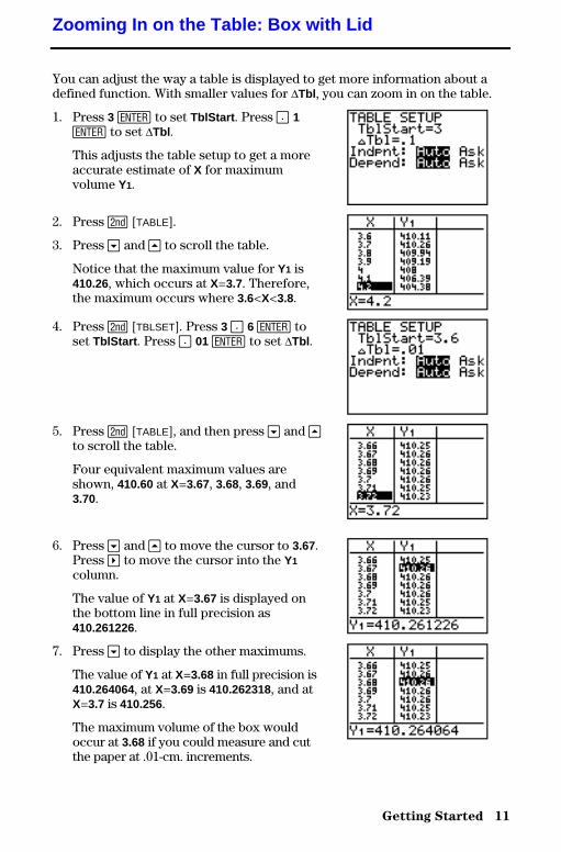
You can adjust the way a table is displayed to get more information about adefined function. With smaller values for @Tbl , you can zoom in on the table.
1. Press 3 Í to set TblStart . Press Ë 1Í to set @Tbl .
This adjusts the table setup to get a moreaccurate estimate of X for maximumvolume Y1.
2. Press y [TABLE].
3. Press † and } to scroll the table.
Notice that the maximum value for Y1 is410.26, which occurs at X=3.7. Therefore,the maximum occurs where 3.6<X<3.8.
4. Press y [TBLSET]. Press 3 Ë 6 Í toset TblStart . Press Ë 01 Í to set @Tbl .
5. Press y [TABLE], and then press † and }to scroll the table.
Four equivalent maximum values areshown, 410.60 at X=3.67, 3.68, 3.69, and3.70.
6. Press † and } to move the cursor to 3.67.Press ~ to move the cursor into the Y1
column.
The value of Y1 at X=3.67 is displayed onthe bottom line in full precision as410.261226.
7. Press † to display the other maximums.
The value of Y1 at X=3.68 in full precision is410.264064, at X=3.69 is 410.262318, and atX=3.7 is 410.256.
The maximum volume of the box wouldoccur at 3.68 if you could measure and cutthe paper at .01-cm. increments.
Zooming In on the Table: Box with Lid
12 Getting Started
8300GETM.DOC TI-83 international English Bob Fedorisko Revised: 02/19/01 11:06 AM Printed: 02/19/01 11:06AM Page 12 of 18
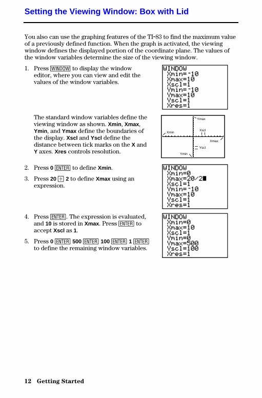
You also can use the graphing features of the TI.83 to find the maximum valueof a previously defined function. When the graph is activated, the viewingwindow defines the displayed portion of the coordinate plane. The values ofthe window variables determine the size of the viewing window.
1. Press p to display the windoweditor, where you can view and edit thevalues of the window variables.
The standard window variables define theviewing window as shown. Xmin , Xmax ,Ymin , and Ymax define the boundaries ofthe display. Xscl and Yscl define thedistance between tick marks on the X andY axes. Xres controls resolution.
Xmax
Ymin
Ymax
Xscl
Yscl
Xmin
2. Press 0 Í to define Xmin .
3. Press 20 ¥ 2 to define Xmax using anexpression.
4. Press Í. The expression is evaluated,and 10 is stored in Xmax . Press Í toaccept Xscl as 1.
5. Press 0 Í 500 Í 100 Í 1 Íto define the remaining window variables.
Setting the Viewing Window: Box with Lid
Getting Started 13
8300GETM.DOC TI-83 international English Bob Fedorisko Revised: 02/19/01 11:06 AM Printed: 02/19/01 11:06AM Page 13 of 18
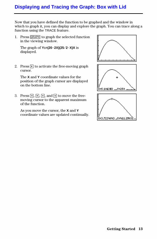
Now that you have defined the function to be graphed and the window inwhich to graph it, you can display and explore the graph. You can trace along afunction using the TRACE feature.
1. Press s to graph the selected functionin the viewing window.
The graph of Y1=(20N2X)(25à2NX)X isdisplayed.
2. Press ~ to activate the free-moving graphcursor.
The X and Y coordinate values for theposition of the graph cursor are displayedon the bottom line.
3. Press |, ~, }, and † to move the free-moving cursor to the apparent maximumof the function.
As you move the cursor, the X and Ycoordinate values are updated continually.
Displaying and Tracing the Graph: Box with Lid

14 Getting Started
8300GETM.DOC TI-83 international English Bob Fedorisko Revised: 02/19/01 11:06 AM Printed: 02/19/01 11:06AM Page 14 of 18
4. Press r. The trace cursor is displayedon the Y1 function.
The function that you are tracing isdisplayed in the top-left corner.
5. Press | and ~ to trace along Y1, one X dotat a time, evaluating Y1 at each X.
You also can enter your estimate for themaximum value of X.
6. Press 3 Ë 8. When you press a number keywhile in TRACE, the X= prompt is displayedin the bottom-left corner.
7. Press Í.
The trace cursor jumps to the point on theY1 function evaluated at X=3.8.
8. Press | and ~ until you are on themaximum Y value.
This is the maximum of Y1(X) for the Xpixel values. The actual, precise maximummay lie between pixel values.
Getting Started 15
8300GETM.DOC TI-83 international English Bob Fedorisko Revised: 02/19/01 11:06 AM Printed: 02/19/01 11:06AM Page 15 of 18
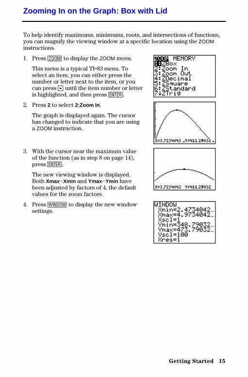
To help identify maximums, minimums, roots, and intersections of functions,you can magnify the viewing window at a specific location using the ZOOMinstructions.
1. Press q to display the ZOOM menu.
This menu is a typical TI.83 menu. Toselect an item, you can either press thenumber or letter next to the item, or youcan press † until the item number or letteris highlighted, and then press Í.
2. Press 2 to select 2:Zoom In .
The graph is displayed again. The cursorhas changed to indicate that you are usinga ZOOM instruction.
3. With the cursor near the maximum valueof the function (as in step 8 on page 14),press Í.
The new viewing window is displayed.Both XmaxNXmin and YmaxNYmin havebeen adjusted by factors of 4, the defaultvalues for the zoom factors.
4. Press p to display the new windowsettings.
Zooming In on the Graph: Box with Lid
16 Getting Started
8300GETM.DOC TI-83 international English Bob Fedorisko Revised: 02/19/01 11:06 AM Printed: 02/19/01 11:06AM Page 16 of 18
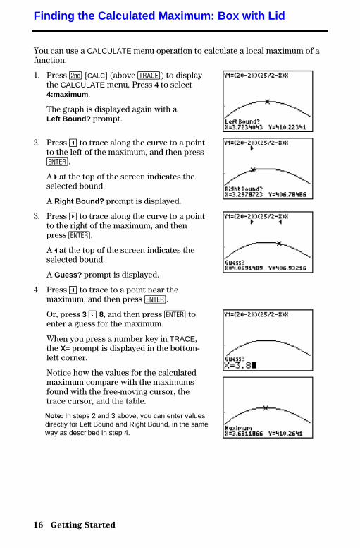
You can use a CALCULATE menu operation to calculate a local maximum of afunction.
1. Press y [CALC] (above r) to displaythe CALCULATE menu. Press 4 to select4:maximum .
The graph is displayed again with aLeft Bound? prompt.
2. Press | to trace along the curve to a pointto the left of the maximum, and then pressÍ.
A 4 at the top of the screen indicates theselected bound.
A Right Bound? prompt is displayed.
3. Press ~ to trace along the curve to a pointto the right of the maximum, and thenpress Í.
A 3 at the top of the screen indicates theselected bound.
A Guess? prompt is displayed.
4. Press | to trace to a point near themaximum, and then press Í.
Or, press 3 Ë 8, and then press Í toenter a guess for the maximum.
When you press a number key in TRACE,the X= prompt is displayed in the bottom-left corner.
Notice how the values for the calculatedmaximum compare with the maximumsfound with the free-moving cursor, thetrace cursor, and the table.
Note: In steps 2 and 3 above, you can enter valuesdirectly for Left Bound and Right Bound, in the sameway as described in step 4.
Finding the Calculated Maximum: Box with Lid
Getting Started 17
8300GETM.DOC TI-83 international English Bob Fedorisko Revised: 02/19/01 11:06 AM Printed: 02/19/01 11:06AM Page 17 of 18
Getting Started has introduced you to basic TI.83 operation. This guidebookdescribes in detail the features you used in Getting Started. It also covers theother features and capabilities of the TI.83.
You can store, graph, and analyze up to 10 functions(Chapter 3), up to six parametric functions (Chapter 4), upto six polar functions (Chapter 5), and up to threesequences (Chapter 6). You can use DRAW operations toannotate graphs (Chapter 8).
You can generate sequences and graph them over time. Or,you can graph them as web plots or as phase plots(Chapter 6).
You can create function evaluation tables to analyze manyfunctions simultaneously (Chapter 7).
You can split the screen horizontally to display both agraph and a related editor (such as the Y= editor), thetable, the stat list editor, or the home screen. Also, you cansplit the screen vertically to display a graph and its tablesimultaneously (Chapter 9).
You can enter and save up to 10 matrices and performstandard matrix operations on them (Chapter 10).
You can enter and save as many lists as memory allows foruse in statistical analyses. You can attach formulas to listsfor automatic computation. You can use lists to evaluateexpressions at multiple values simultaneously and to grapha family of curves (Chapter 11).
You can perform one- and two-variable, list-basedstatistical analyses, including logistic and sine regressionanalysis. You can plot the data as a histogram, xyLine,scatter plot, modified or regular box-and-whisker plot, ornormal probability plot. You can define and store up tothree stat plot definitions (Chapter 12).
Other TI-83 Features
Graphing
Sequences
Tables
Split Screen
Matrices
Lists
Statistics
18 Getting Started
8300GETM.DOC TI-83 international English Bob Fedorisko Revised: 02/19/01 11:06 AM Printed: 02/19/01 11:06AM Page 18 of 18
You can perform 16 hypothesis tests and confidenceintervals and 15 distribution functions. You can displayhypothesis test results graphically or numerically(Chapter 13).
You can use time-value-of-money (TVM) functions toanalyze financial instruments such as annuities, loans,mortgages, leases, and savings. You can analyze the valueof money over equal time periods using cash flowfunctions. You can amortize loans with the amortizationfunctions (Chapter 14).
The CATALOG is a convenient, alphabetical list of allfunctions and instructions on the TI.83. You can paste anyfunction or instruction from the CATALOG to the currentcursor location (Chapter 15).
You can enter and store programs that include extensivecontrol and input/output instructions (Chapter 16).
The TI.83 has a port to connect and communicate withanother TI.83, a TI.82, the Calculator-Based Laboratoryé(CBL 2é, CBLé) System, a Calculator-Based Rangeré(CBRé), or a personal computer. The unit-to-unit linkcable is included with the TI.83 (Chapter 19).
InferentialStatistics
FinancialFunctions
CATALOG
Programming
CommunicationLink

Operating the TI-83 1-1
8301OPER.DOC TI-83 international English Bob Fedorisko Revised: 02/19/01 12:09 PM Printed: 02/19/01 1:34PM Page 1 of 24
1 Operatin gthe TI-83
Turning On and Turning Off the TI.83.................... 1-2Setting the Display Contrast ............................. 1-3The Display .............................................. 1-4Entering Expressions and Instructions................... 1-6TI.83 Edit Keys .......................................... 1-8Setting Modes ........................................... 1-9Using TI.83 Variable Names ............................. 1-13Storing Variable Values .................................. 1-14Recalling Variable Values ................................ 1-15ENTRY (Last Entry) Storage Area........................ 1-16Ans (Last Answer) Storage Area ......................... 1-18TI.83 Menus ............................................. 1-19VARS and VARS Y.VARS Menus......................... 1-21Equation Operating System (EOSé) ..................... 1-22Error Conditions......................................... 1-24
Contents
1-2 Operating the TI-83
8301OPER.DOC TI-83 international English Bob Fedorisko Revised: 02/19/01 12:09 PM Printed: 02/19/01 1:34PM Page 2 of 24
To turn on the TI.83, press É.
• If you previously had turned off the calculator bypressing y [OFF], the TI.83 displays the home screenas it was when you last used it and clears any error.
• If Automatic Power Down™ (APDé) had previouslyturned off the calculator, the TI.83 will return exactly asyou left it, including the display, cursor, and any error.
To prolong the life of the batteries, APD turns off the TI.83automatically after about five minutes without any activity.
To turn off the TI.83 manually, press y [OFF].
• All settings and memory contents are retained byConstant Memoryé.
• Any error condition is cleared.
The TI.83 uses four AAA alkaline batteries and has a user-replaceable backup lithium battery (CR1616 or CR1620).To replace batteries without losing any information storedin memory, follow the steps in Appendix B.
Turning On and Turning Off the TI-83
Turning On theCalculator
Turning Off theCalculator
Batteries
Operating the TI-83 1-3
8301OPER.DOC TI-83 international English Bob Fedorisko Revised: 02/19/01 12:09 PM Printed: 02/19/01 1:34PM Page 3 of 24
You can adjust the display contrast to suit your viewingangle and lighting conditions. As you change the contrastsetting, a number from 0 (lightest) to 9 (darkest) in thetop-right corner indicates the current level. You may not beable to see the number if contrast is too light or too dark.
Note: The TI.83 has 40 contrast settings, so each number 0 through 9represents four settings.
The TI.83 retains the contrast setting in memory when it isturned off.
To adjust the contrast, follow these steps.
1. Press and release the y key.
2. Press and hold † or }, which are below and above thecontrast symbol (yellow, half-shaded circle).
• † lightens the screen.• } darkens the screen.
Note: If you adjust the contrast setting to 0, the display may becomecompletely blank. To restore the screen, press and release y, andthen press and hold } until the display reappears.
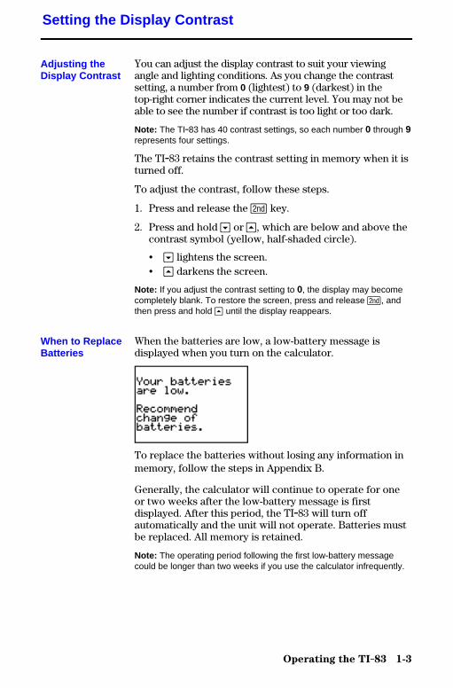
When the batteries are low, a low-battery message isdisplayed when you turn on the calculator.
To replace the batteries without losing any information inmemory, follow the steps in Appendix B.
Generally, the calculator will continue to operate for oneor two weeks after the low-battery message is firstdisplayed. After this period, the TI.83 will turn offautomatically and the unit will not operate. Batteries mustbe replaced. All memory is retained.
Note: The operating period following the first low-battery messagecould be longer than two weeks if you use the calculator infrequently.
Setting the Display Contrast
Adjusting theDisplay Contrast
When to ReplaceBatteries

1-4 Operating the TI-83
8301OPER.DOC TI-83 international English Bob Fedorisko Revised: 02/19/01 12:09 PM Printed: 02/19/01 1:34PM Page 4 of 24
The TI.83 displays both text and graphs. Chapter 3describes graphs. Chapter 9 describes how the TI.83 candisplay a horizontally or vertically split screen to showgraphs and text simultaneously.
The home screen is the primary screen of the TI.83. Onthis screen, enter instructions to execute and expressionsto evaluate. The answers are displayed on the same screen.
When text is displayed, the TI.83 screen can display amaximum of eight lines with a maximum of 16 charactersper line. If all lines of the display are full, text scrolls offthe top of the display. If an expression on the home screen,the Y= editor (Chapter 3), or the program editor(Chapter 16) is longer than one line, it wraps to thebeginning of the next line. In numeric editors such as thewindow screen (Chapter 3), a long expression scrolls tothe right and left.
When an entry is executed on the home screen, the answeris displayed on the right side of the next line.
Entry Answer
The mode settings control the way the TI.83 interpretsexpressions and displays answers (page 1.9).
If an answer, such as a list or matrix, is too long to displayentirely on one line, an ellipsis (...) is displayed to the rightor left. Press ~ and | to scroll the answer.
Entry Answer
To return to the home screen from any other screen, pressy [QUIT].
When the TI.83 is calculating or graphing, a verticalmoving line is displayed as a busy indicator in the top-rightcorner of the screen. When you pause a graph or aprogram, the busy indicator becomes a vertical movingdotted line.
The Display
Types ofDisplays
Home Screen
DisplayingEntries andAnswers
Returning to theHome Screen
Busy Indicator
Operating the TI-83 1-5
8301OPER.DOC TI-83 international English Bob Fedorisko Revised: 02/19/01 12:09 PM Printed: 02/19/01 1:34PM Page 5 of 24
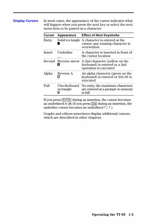
In most cases, the appearance of the cursor indicates whatwill happen when you press the next key or select the nextmenu item to be pasted as a character.
Cursor Appearance Effect of Next Keystroke
Entry Solid rectangle$
A character is entered at thecursor; any existing character isoverwritten
Insert Underline__
A character is inserted in front ofthe cursor location
Second Reverse arrowÞ
A 2nd character (yellow on thekeyboard) is entered or a 2ndoperation is executed
Alpha Reverse AØ
An alpha character (green on thekeyboard) is entered or SOLVE isexecuted
Full Checkerboardrectangle#
No entry; the maximum charactersare entered at a prompt or memoryis full
If you press ƒ during an insertion, the cursor becomesan underlined A (A) If you press y during an insertion, theunderline cursor becomes an underlined # ( # ).
Graphs and editors sometimes display additional cursors,which are described in other chapters.
Display Cursors
1-6 Operating the TI-83
8301OPER.DOC TI-83 international English Bob Fedorisko Revised: 02/19/01 12:09 PM Printed: 02/19/01 1:34PM Page 6 of 24
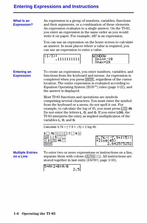
An expression is a group of numbers, variables, functionsand their arguments, or a combination of these elements.An expression evaluates to a single answer. On the TI.83,you enter an expression in the same order as you wouldwrite it on paper. For example, pR2 is an expression.
You can use an expression on the home screen to calculatean answer. In most places where a value is required, youcan use an expression to enter a value.
To create an expression, you enter numbers, variables, andfunctions from the keyboard and menus. An expression iscompleted when you press Í, regardless of the cursorlocation. The entire expression is evaluated according toEquation Operating System (EOSé) rules (page 1.22), andthe answer is displayed.
Most TI.83 functions and operations are symbolscomprising several characters. You must enter the symbolfrom the keyboard or a menu; do not spell it out. Forexample, to calculate the log of 45, you must press « 45.Do not enter the letters L, O, and G. If you enter LOG, theTI.83 interprets the entry as implied multiplication of thevariables L, O, and G.
Calculate 3.76 ÷ (L7.9 + ‡5) + 2 log 45.
3 Ë 76 ¥ £ Ì 7 Ë 9 Ãy [‡] 5 ¤ ¤Ã 2 « 45 ¤Í
To enter two or more expressions or instructions on a line,separate them with colons (ƒ [:]). All instructions arestored together in last entry (ENTRY; page 1.16).
Entering Expressions and Instructions
What Is anExpression?
Entering anExpression
Multiple Entrieson a Line
Operating the TI-83 1-7
8301OPER.DOC TI-83 international English Bob Fedorisko Revised: 02/19/01 12:09 PM Printed: 02/19/01 1:34PM Page 7 of 24
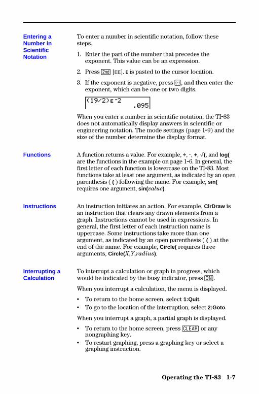
To enter a number in scientific notation, follow thesesteps.
1. Enter the part of the number that precedes theexponent. This value can be an expression.
2. Press y [EE]. å is pasted to the cursor location.
3. If the exponent is negative, press Ì, and then enter theexponent, which can be one or two digits.
When you enter a number in scientific notation, the TI.83does not automatically display answers in scientific orengineering notation. The mode settings (page 1.9) and thesize of the number determine the display format.
A function returns a value. For example, ÷, L, +, ‡(, and log(are the functions in the example on page 1.6. In general, thefirst letter of each function is lowercase on the TI.83. Mostfunctions take at least one argument, as indicated by an openparenthesis ( ( ) following the name. For example, sin(requires one argument, sin( value).
An instruction initiates an action. For example, ClrDraw isan instruction that clears any drawn elements from agraph. Instructions cannot be used in expressions. Ingeneral, the first letter of each instruction name isuppercase. Some instructions take more than oneargument, as indicated by an open parenthesis ( ( ) at theend of the name. For example, Circle( requires threearguments, Circle( X,Y,radius).
To interrupt a calculation or graph in progress, whichwould be indicated by the busy indicator, press É.
When you interrupt a calculation, the menu is displayed.
• To return to the home screen, select 1:Quit .• To go to the location of the interruption, select 2:Goto .
When you interrupt a graph, a partial graph is displayed.
• To return to the home screen, press ‘ or anynongraphing key.
• To restart graphing, press a graphing key or select agraphing instruction.
Entering aNumber inScientificNotation
Functions
Instructions
Interrupting aCalculation
1-8 Operating the TI-83
8301OPER.DOC TI-83 international English Bob Fedorisko Revised: 02/19/01 12:09 PM Printed: 02/19/01 1:34PM Page 8 of 24
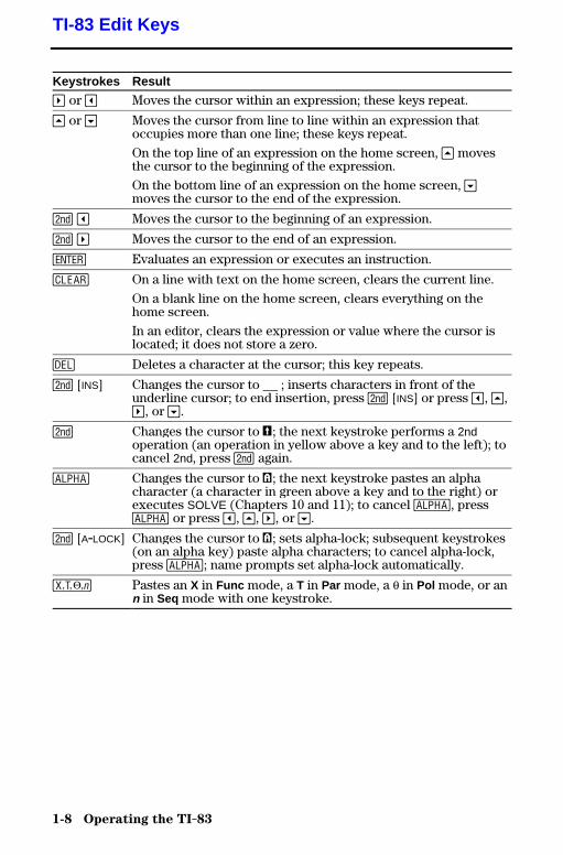
Keystrokes Result
~ or | Moves the cursor within an expression; these keys repeat.
} or † Moves the cursor from line to line within an expression thatoccupies more than one line; these keys repeat.
On the top line of an expression on the home screen, } movesthe cursor to the beginning of the expression.
On the bottom line of an expression on the home screen, †moves the cursor to the end of the expression.
y | Moves the cursor to the beginning of an expression.
y ~ Moves the cursor to the end of an expression.
Í Evaluates an expression or executes an instruction.
‘ On a line with text on the home screen, clears the current line.
On a blank line on the home screen, clears everything on thehome screen.
In an editor, clears the expression or value where the cursor islocated; it does not store a zero.
{ Deletes a character at the cursor; this key repeats.
y [INS] Changes the cursor to __ ; inserts characters in front of theunderline cursor; to end insertion, press y [INS] or press |, },~, or †.
y Changes the cursor to Þ; the next keystroke performs a 2ndoperation (an operation in yellow above a key and to the left); tocancel 2nd, press y again.
ƒ Changes the cursor to Ø; the next keystroke pastes an alphacharacter (a character in green above a key and to the right) orexecutes SOLVE (Chapters 10 and 11); to cancel ƒ, pressƒ or press |, }, ~, or †.
y [A.LOCK] Changes the cursor to Ø; sets alpha-lock; subsequent keystrokes(on an alpha key) paste alpha characters; to cancel alpha-lock,press ƒ; name prompts set alpha-lock automatically.
„ Pastes an X in Func mode, a T in Par mode, a q in Pol mode, or ann in Seq mode with one keystroke.
TI-83 Edit Keys
Operating the TI-83 1-9
8301OPER.DOC TI-83 international English Bob Fedorisko Revised: 02/19/01 12:09 PM Printed: 02/19/01 1:34PM Page 9 of 24
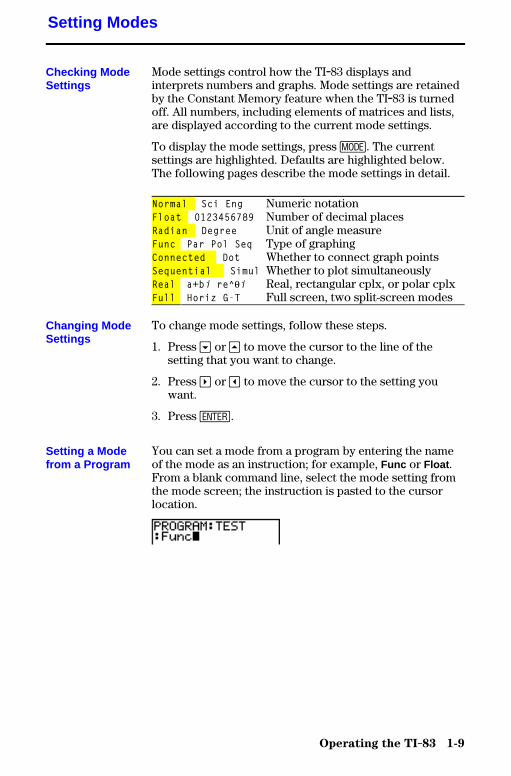
Mode settings control how the TI.83 displays andinterprets numbers and graphs. Mode settings are retainedby the Constant Memory feature when the TI.83 is turnedoff. All numbers, including elements of matrices and lists,are displayed according to the current mode settings.
To display the mode settings, press z. The currentsettings are highlighted. Defaults are highlighted below.The following pages describe the mode settings in detail.
Normal Sci Eng Numeric notationFloat 0123456789 Number of decimal placesRadian Degree Unit of angle measureFunc Par Pol Seq Type of graphingConnected Dot Whether to connect graph pointsSequential Simul Whether to plot simultaneouslyReal a+bi re^qi Real, rectangular cplx, or polar cplxFull Horiz G-T Full screen, two split-screen modes
To change mode settings, follow these steps.
1. Press † or } to move the cursor to the line of thesetting that you want to change.
2. Press ~ or | to move the cursor to the setting youwant.
3. Press Í.
You can set a mode from a program by entering the nameof the mode as an instruction; for example, Func or Float .From a blank command line, select the mode setting fromthe mode screen; the instruction is pasted to the cursorlocation.
Setting Modes
Checking ModeSettings
Changing ModeSettings
Setting a Modefrom a Program
1-10 Operating the TI-83
8301OPER.DOC TI-83 international English Bob Fedorisko Revised: 02/19/01 12:09 PM Printed: 02/19/01 1:34PM Page 10 of 24
Notation modes only affect the way an answer is displayedon the home screen. Numeric answers can be displayedwith up to 10 digits and a two-digit exponent. You canenter a number in any format.
Normal notation mode is the usual way we expressnumbers, with digits to the left and right of the decimal, asin 12345.67.
Sci (scientific) notation mode expresses numbers in twoparts. The significant digits display with one digit to the leftof the decimal. The appropriate power of 10 displays to theright of E, as in 1.234567E4.
Eng (engineering) notation mode is similar to scientificnotation. However, the number can have one, two, or threedigits before the decimal; and the power-of-10 exponent isa multiple of three, as in 12.34567E3.
Note : If you select Normal notation, but the answer cannot display in10 digits (or the absolute value is less than .001), the TI.83 expressesthe answer in scientific notation.
Float (floating) decimal mode displays up to 10 digits, plusthe sign and decimal.
0123456789 (fixed) decimal mode specifies the number ofdigits (0 through 9) to display to the right of the decimal.Place the cursor on the desired number of decimal digits,and then press Í.
The decimal setting applies to Normal , Sci , and Engnotation modes.
The decimal setting applies to these numbers:
• An answer displayed on the home screen• Coordinates on a graph (Chapters 3, 4, 5, and 6)• The Tangent( DRAW instruction equation of the line, x,
and dy/dx values (Chapter 8)• Results of CALCULATE operations (Chapters 3, 4, 5,
and 6)• The regression equation stored after the execution of a
regression model (Chapter 12)
Normal, Sci, Eng
Float,0123456789

Operating the TI-83 1-11
8301OPER.DOC TI-83 international English Bob Fedorisko Revised: 02/19/01 12:09 PM Printed: 02/19/01 1:34PM Page 11 of 24
Angle modes control how the TI.83 interprets angle valuesin trigonometric functions and polar/rectangularconversions.
Radian mode interprets angle values as radians. Answersdisplay in radians.
Degree mode interprets angle values as degrees. Answersdisplay in degrees.
Graphing modes define the graphing parameters. Chapters3, 4, 5, and 6 describe these modes in detail.
Func (function) graphing mode plots functions, where Y isa function of X (Chapter 3).
Par (parametric) graphing mode plots relations, where Xand Y are functions of T (Chapter 4).
Pol (polar) graphing mode plots functions, where r is afunction of q (Chapter 5).
Seq (sequence) graphing mode plots sequences (Chapter 6).
Connected plotting mode draws a line connecting eachpoint calculated for the selected functions.
Dot plotting mode plots only the calculated points of theselected functions.
Radian, Degree
Func, Par, Pol,Seq
Connected, Dot
1-12 Operating the TI-83
8301OPER.DOC TI-83 international English Bob Fedorisko Revised: 02/19/01 12:09 PM Printed: 02/19/01 1:34PM Page 12 of 24
Sequential graphing-order mode evaluates and plots onefunction completely before the next function is evaluatedand plotted.
Simul (simultaneous) graphing-order mode evaluates andplots all selected functions for a single value of X and thenevaluates and plots them for the next value of X.
Note: Regardless of which graphing mode is selected, the TI.83 willsequentially graph all stat plots before it graphs any functions.
Real mode does not display complex results unlesscomplex numbers are entered as input.
Two complex modes display complex results.
• a+bi (rectangular complex mode) displays complexnumbers in the form a+bi.
• re^ qi (polar complex mode) displays complex numbersin the form re^qi.
Full screen mode uses the entire screen to display a graphor edit screen.
Each split-screen mode displays two screenssimultaneously.
• Horiz (horizontal) mode displays the current graph onthe top half of the screen; it displays the home screen oran editor on the bottom half (Chapter 9).
• G.T (graph-table) mode displays the current graph onthe left half of the screen; it displays the table screen onthe right half (Chapter 9).
Sequential, Simul
Real, a+b i, re^ qi
Full, Horiz, G .T
Operating the TI-83 1-13
8301OPER.DOC TI-83 international English Bob Fedorisko Revised: 02/19/01 12:09 PM Printed: 02/19/01 1:34PM Page 13 of 24
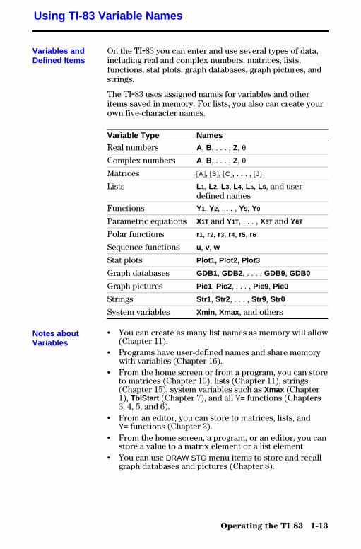
On the TI.83 you can enter and use several types of data,including real and complex numbers, matrices, lists,functions, stat plots, graph databases, graph pictures, andstrings.
The TI.83 uses assigned names for variables and otheritems saved in memory. For lists, you also can create yourown five-character names.
Variable Type Names
Real numbers A, B, . . . , Z, q
Complex numbers A, B, . . . , Z, q
Matrices ãAä, ãBä, ãCä, . . . , ãJä
Lists L1, L2, L3, L4, L5, L6, and user-defined names
Functions Y1, Y2, . . . , Y9, Y0
Parametric equations X1T and Y1T, . . . , X6T and Y6T
Polar functions r1, r2, r3, r4, r5, r6
Sequence functions u, v, w
Stat plots Plot1, Plot2, Plot3
Graph databases GDB1, GDB2, . . . , GDB9, GDB0
Graph pictures Pic1 , Pic2 , . . . , Pic9 , Pic0
Strings Str1 , Str2 , . . . , Str9 , Str0
System variables Xmin , Xmax , and others
• You can create as many list names as memory will allow(Chapter 11).
• Programs have user-defined names and share memorywith variables (Chapter 16).
• From the home screen or from a program, you can storeto matrices (Chapter 10), lists (Chapter 11), strings(Chapter 15), system variables such as Xmax (Chapter1), TblStart (Chapter 7), and all Y= functions (Chapters3, 4, 5, and 6).
• From an editor, you can store to matrices, lists, andY= functions (Chapter 3).
• From the home screen, a program, or an editor, you canstore a value to a matrix element or a list element.
• You can use DRAW STO menu items to store and recallgraph databases and pictures (Chapter 8).
Using TI-83 Variable Names
Variables andDefined Items
Notes aboutVariables
1-14 Operating the TI-83
8301OPER.DOC TI-83 international English Bob Fedorisko Revised: 02/19/01 12:09 PM Printed: 02/19/01 1:34PM Page 14 of 24
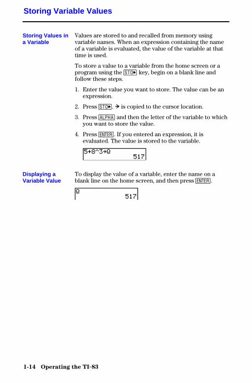
Values are stored to and recalled from memory usingvariable names. When an expression containing the nameof a variable is evaluated, the value of the variable at thattime is used.
To store a value to a variable from the home screen or aprogram using the ¿ key, begin on a blank line andfollow these steps.
1. Enter the value you want to store. The value can be anexpression.
2. Press ¿. ! is copied to the cursor location.
3. Press ƒ and then the letter of the variable to whichyou want to store the value.
4. Press Í. If you entered an expression, it isevaluated. The value is stored to the variable.
To display the value of a variable, enter the name on ablank line on the home screen, and then press Í.
Storing Variable Values
Storing Values ina Variable
Displaying aVariable Value
Operating the TI-83 1-15
8301OPER.DOC TI-83 international English Bob Fedorisko Revised: 02/19/01 12:09 PM Printed: 02/19/01 1:34PM Page 15 of 24
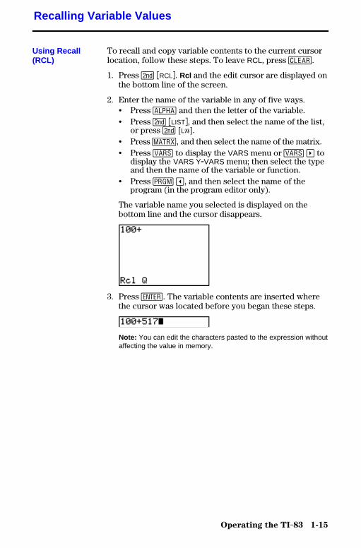
To recall and copy variable contents to the current cursorlocation, follow these steps. To leave RCL, press ‘.
1. Press y ãRCLä. Rcl and the edit cursor are displayed onthe bottom line of the screen.
2. Enter the name of the variable in any of five ways.• Press ƒ and then the letter of the variable.• Press y ãLISTä, and then select the name of the list,
or press y [Ln].• Press �, and then select the name of the matrix.• Press � to display the VARS menu or � ~ to
display the VARS Y.VARS menu; then select the typeand then the name of the variable or function.
• Press � |, and then select the name of theprogram (in the program editor only).
The variable name you selected is displayed on thebottom line and the cursor disappears.
3. Press Í. The variable contents are inserted wherethe cursor was located before you began these steps.
Note: You can edit the characters pasted to the expression withoutaffecting the value in memory.
Recalling Variable Values
Using Recall(RCL)
1-16 Operating the TI-83
8301OPER.DOC TI-83 international English Bob Fedorisko Revised: 02/19/01 12:09 PM Printed: 02/19/01 1:34PM Page 16 of 24
When you press Í on the home screen to evaluate anexpression or execute an instruction, the expression orinstruction is placed in a storage area called ENTRY (lastentry). When you turn off the TI.83, ENTRY is retained inmemory.
To recall ENTRY, press y [ENTRY]. The last entry ispasted to the current cursor location, where you can editand execute it. On the home screen or in an editor, thecurrent line is cleared and the last entry is pasted to theline.
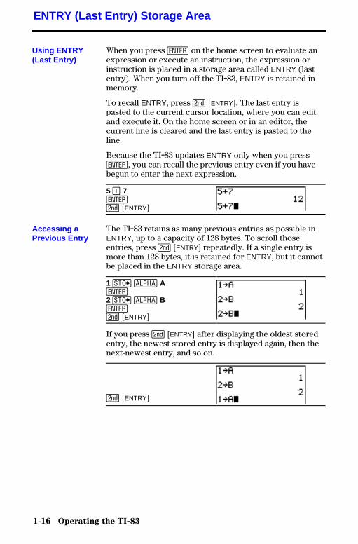
Because the TI.83 updates ENTRY only when you pressÍ, you can recall the previous entry even if you havebegun to enter the next expression.
5 Ã 7Íy [ENTRY]
The TI.83 retains as many previous entries as possible inENTRY, up to a capacity of 128 bytes. To scroll thoseentries, press y [ENTRY] repeatedly. If a single entry ismore than 128 bytes, it is retained for ENTRY, but it cannotbe placed in the ENTRY storage area.
1 ¿ ƒ AÍ2 ¿ ƒ BÍy [ENTRY]
If you press y [ENTRY] after displaying the oldest storedentry, the newest stored entry is displayed again, then thenext-newest entry, and so on.
y [ENTRY]
ENTRY (Last Entry) Storage Area
Using ENTRY(Last Entry)
Accessing aPrevious Entry

Operating the TI-83 1-17
8301OPER.DOC TI-83 international English Bob Fedorisko Revised: 02/19/01 12:09 PM Printed: 02/19/01 1:34PM Page 17 of 24
After you have pasted the last entry to the home screenand edited it (if you chose to edit it), you can execute theentry. To execute the last entry, press Í.
To reexecute the displayed entry, press Í again. Eachreexecution displays an answer on the right side of thenext line; the entry itself is not redisplayed.
0 ¿ ƒ N̓ N à 1 ¿ ƒ Nƒ ã:ä ƒ N ¡ ÍÍÍ
To store to ENTRY two or more expressions orinstructions, separate each expression or instruction witha colon, then press Í. All expressions and instructionsseparated by colons are stored in ENTRY.
When you press y [ENTRY], all the expressions andinstructions separated by colons are pasted to the currentcursor location. You can edit any of the entries, and thenexecute all of them when you press Í.
For the equation A=pr2, use trial and error to find the radius of acircle that covers 200 square centimeters. Use 8 as your firstguess.
8 ¿ ƒ R ƒ[:] y [p] ƒ R ¡ Íy [ENTRY]
y | 7 y [INS] Ë 95Í
Continue until the answer is as accurate as you want.
Clear Entries (Chapter 18) clears all data that the TI.83 isholding in the ENTRY storage area.
Reexecuting thePrevious Entry
Multiple EntryValues on a Line
Clearing ENTRY
1-18 Operating the TI-83
8301OPER.DOC TI-83 international English Bob Fedorisko Revised: 02/19/01 12:09 PM Printed: 02/19/01 1:34PM Page 18 of 24
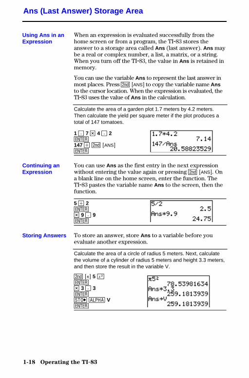
When an expression is evaluated successfully from thehome screen or from a program, the TI.83 stores theanswer to a storage area called Ans (last answer). Ans maybe a real or complex number, a list, a matrix, or a string.When you turn off the TI.83, the value in Ans is retained inmemory.
You can use the variable Ans to represent the last answer inmost places. Press y [ANS] to copy the variable name Ansto the cursor location. When the expression is evaluated, theTI.83 uses the value of Ans in the calculation.
Calculate the area of a garden plot 1.7 meters by 4.2 meters.Then calculate the yield per square meter if the plot produces atotal of 147 tomatoes.
1 Ë 7 ¯ 4 Ë 2Í147 ¥ y [ANS]Í
You can use Ans as the first entry in the next expressionwithout entering the value again or pressing y [ANS]. Ona blank line on the home screen, enter the function. TheTI.83 pastes the variable name Ans to the screen, then thefunction.
5 ¥ 2ͯ 9 Ë 9Í
To store an answer, store Ans to a variable before youevaluate another expression.
Calculate the area of a circle of radius 5 meters. Next, calculatethe volume of a cylinder of radius 5 meters and height 3.3 meters,and then store the result in the variable V.
y [p] 5 ¡Í¯ 3 Ë 3Í¿ ƒ VÍ
Ans (Last Answer) Storage Area
Using Ans in anExpression
Continuing anExpression
Storing Answers
Operating the TI-83 1-19
8301OPER.DOC TI-83 international English Bob Fedorisko Revised: 02/19/01 12:09 PM Printed: 02/19/01 1:34PM Page 19 of 24
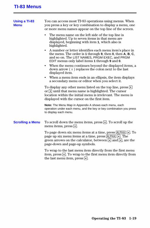
You can access most TI.83 operations using menus. Whenyou press a key or key combination to display a menu, oneor more menu names appear on the top line of the screen.
• The menu name on the left side of the top line ishighlighted. Up to seven items in that menu aredisplayed, beginning with item 1, which also ishighlighted.
• A number or letter identifies each menu item’s place inthe menu. The order is 1 through 9, then 0, then A, B, C,and so on. The LIST NAMES, PRGM EXEC, and PRGMEDIT menus only label items 1 through 9 and 0.
• When the menu continues beyond the displayed items, adown arrow ( $ ) replaces the colon next to the lastdisplayed item.
• When a menu item ends in an ellipsis, the item displaysa secondary menu or editor when you select it.
To display any other menu listed on the top line, press ~or | until that menu name is highlighted. The cursorlocation within the initial menu is irrelevant. The menu isdisplayed with the cursor on the first item.
Note: The Menu Map in Appendix A shows each menu, eachoperation under each menu, and the key or key combination you pressto display each menu.
To scroll down the menu items, press †. To scroll up themenu items, press }.
To page down six menu items at a time, press ƒ †. Topage up six menu items at a time, press ƒ }. Thegreen arrows on the calculator, between † and }, are thepage-down and page-up symbols.
To wrap to the last menu item directly from the first menuitem, press }. To wrap to the first menu item directly fromthe last menu item, press †.
TI-83 Menus
Using a TI-83Menu
Scrolling a Menu
1-20 Operating the TI-83
8301OPER.DOC TI-83 international English Bob Fedorisko Revised: 02/19/01 12:09 PM Printed: 02/19/01 1:34PM Page 20 of 24
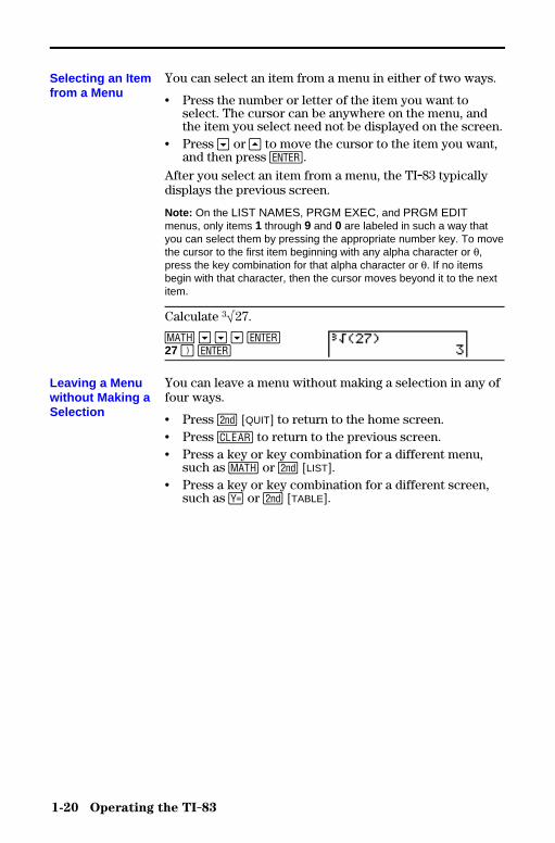
You can select an item from a menu in either of two ways.
• Press the number or letter of the item you want toselect. The cursor can be anywhere on the menu, andthe item you select need not be displayed on the screen.
• Press † or } to move the cursor to the item you want,and then press Í.
After you select an item from a menu, the TI.83 typicallydisplays the previous screen.
Note: On the LIST NAMES, PRGM EXEC, and PRGM EDITmenus, only items 1 through 9 and 0 are labeled in such a way thatyou can select them by pressing the appropriate number key. To movethe cursor to the first item beginning with any alpha character or q,press the key combination for that alpha character or q. If no itemsbegin with that character, then the cursor moves beyond it to the nextitem.
Calculate 3‡27.
� † † † Í27 ¤ Í
You can leave a menu without making a selection in any offour ways.
• Press y [QUIT] to return to the home screen.• Press ‘ to return to the previous screen.• Press a key or key combination for a different menu,
such as � or y [LIST].• Press a key or key combination for a different screen,
such as o or y [TABLE].
Selecting an Itemfrom a Menu
Leaving a Menuwithout Making aSelection
Operating the TI-83 1-21
8301OPER.DOC TI-83 international English Bob Fedorisko Revised: 02/19/01 12:09 PM Printed: 02/19/01 1:34PM Page 21 of 24
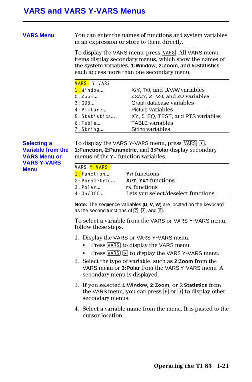
You can enter the names of functions and system variablesin an expression or store to them directly.
To display the VARS menu, press �. All VARS menuitems display secondary menus, which show the names ofthe system variables. 1:Window , 2:Zoom , and 5:Statisticseach access more than one secondary menu.
VARS Y-VARS1:Window... X/Y, T/q, and U/V/W variables2:Zoom... ZX/ZY, ZT/Zq, and ZU variables3:GDB... Graph database variables4:Picture... Picture variables5:Statistics... XY, G, EQ, TEST, and PTS variables6:Table... TABLE variables7:String... String variables
To display the VARS Y.VARS menu, press � ~.1:Function , 2:Parametric , and 3:Polar display secondarymenus of the Y= function variables.
VARS Y-VARS1:Function... Yn functions2:Parametric... XnT, YnT functions3:Polar... rn functions4:On/Off... Lets you select/deselect functions
Note: The sequence variables (u, v, w) are located on the keyboardas the second functions of ¬, −, and ®.
To select a variable from the VARS or VARS Y.VARS menu,follow these steps.
1. Display the VARS or VARS Y.VARS menu.• Press � to display the VARS menu.• Press � ~ to display the VARS Y.VARS menu.
2. Select the type of variable, such as 2:Zoom from theVARS menu or 3:Polar from the VARS Y.VARS menu. Asecondary menu is displayed.
3. If you selected 1:Window , 2:Zoom , or 5:Statistics fromthe VARS menu, you can press ~ or | to display othersecondary menus.
4. Select a variable name from the menu. It is pasted to thecursor location.
VARS and VARS Y-VARS Menus
VARS Menu
Selecting aVariable from theVARS Menu orVARS Y-VARSMenu
1-22 Operating the TI-83
8301OPER.DOC TI-83 international English Bob Fedorisko Revised: 02/19/01 12:09 PM Printed: 02/19/01 1:34PM Page 22 of 24
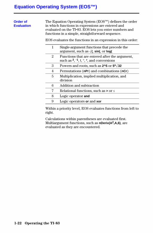
The Equation Operating System (EOSé) defines the orderin which functions in expressions are entered andevaluated on the TI.83. EOS lets you enter numbers andfunctions in a simple, straightforward sequence.
EOS evaluates the functions in an expression in this order:
1 Single-argument functions that precede theargument, such as ‡(, sin( , or log(
2 Functions that are entered after the argument,such as 2, M1, !, ¡, r, and conversions
3 Powers and roots, such as 2^5 or 5x‡32
4 Permutations (nPr) and combinations (nCr)
5 Multiplication, implied multiplication, anddivision
6 Addition and subtraction
7 Relational functions, such as > or �
8 Logic operator and
9 Logic operators or and xor
Within a priority level, EOS evaluates functions from left toright.
Calculations within parentheses are evaluated first.Multiargument functions, such as nDeriv(A 2,A,6), areevaluated as they are encountered.
Equation Operating System (EOS™)
Order ofEvaluation
Operating the TI-83 1-23
8301OPER.DOC TI-83 international English Bob Fedorisko Revised: 02/19/01 12:09 PM Printed: 02/19/01 1:34PM Page 23 of 24
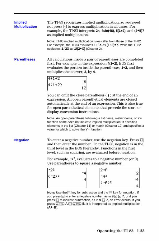
The TI.83 recognizes implied multiplication, so you neednot press ¯ to express multiplication in all cases. Forexample, the TI.83 interprets 2p, 4sin(46) , 5(1+2), and (2ä5)7as implied multiplication.
Note: TI.83 implied multiplication rules differ from those of the TI.82.For example, the TI.83 evaluates 1à2X as (1à2)äX, while the TI.82evaluates 1à2X as 1/(2äX) (Chapter 2).
All calculations inside a pair of parentheses are completedfirst. For example, in the expression 4(1+2), EOS firstevaluates the portion inside the parentheses, 1+2, and thenmultiplies the answer, 3, by 4.
You can omit the close parenthesis ( ) ) at the end of anexpression. All open parenthetical elements are closedautomatically at the end of an expression. This is also truefor open parenthetical elements that precede the store ordisplay-conversion instructions.
Note: An open parenthesis following a list name, matrix name, or Y=function name does not indicate implied multiplication. It specifieselements in the list (Chapter 11) or matrix (Chapter 10) and specifies avalue for which to solve the Y= function.
To enter a negative number, use the negation key. Press Ìand then enter the number. On the TI.83, negation is in thethird level in the EOS hierarchy. Functions in the firstlevel, such as squaring, are evaluated before negation.
For example, MX2, evaluates to a negative number (or 0).Use parentheses to square a negative number.
Note: Use the ¹ key for subtraction and the Ì key for negation. Ifyou press ¹ to enter a negative number, as in 9 ¯ ¹ 7, or if youpress Ì to indicate subtraction, as in 9 Ì 7, an error occurs. If youpress ƒ A Ì ƒ B, it is interpreted as implied multiplication(AäMB).
ImpliedMultiplication
Parentheses
Negation
1-24 Operating the TI-83
8301OPER.DOC TI-83 international English Bob Fedorisko Revised: 02/19/01 12:09 PM Printed: 02/19/01 1:34PM Page 24 of 24
The TI.83 detects errors while performing these tasks.
• Evaluating an expression• Executing an instruction• Plotting a graph• Storing a value
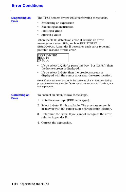
When the TI.83 detects an error, it returns an errormessage as a menu title, such as ERR:SYNTAX orERR:DOMAIN. Appendix B describes each error type andpossible reasons for the error.
• If you select 1:Quit (or press y [QUIT] or ‘), thenthe home screen is displayed.
• If you select 2:Goto , then the previous screen isdisplayed with the cursor at or near the error location.
Note : If a syntax error occurs in the contents of a Y= function duringprogram execution, then the Goto option returns to the Y= editor, notto the program.
To correct an error, follow these steps.
1. Note the error type (ERR:error type).
2. Select 2:Goto , if it is available. The previous screen isdisplayed with the cursor at or near the error location.
3. Determine the error. If you cannot recognize the error,refer to Appendix B.
4. Correct the expression.
Error Conditions
Diagnosing anError
Correcting anError
Math, Angle, and Test Operations 2-1
2 Math, An gle, and TestOperations
Getting Started: Coin Flip ................................ 2-2Keyboard Math Operations .............................. 2-3MATH Operations ........................................ 2-5Using the Equation Solver ............................... 2-8MATH NUM (Number) Operations........................ 2-13Entering and Using Complex Numbers................... 2-16MATH CPX (Complex) Operations ....................... 2-18MATH PRB (Probability) Operations ..................... 2-20ANGLE Operations....................................... 2-23TEST (Relational) Operations............................ 2-24TEST LOGIC (Boolean) Operations ...................... 2-26
Contents
2-2 Math, Angle, and Test Operations
8302MATH.DOC TI-83 international English Bob Fedorisko Revised: 02/19/01 12:12 PM Printed: 02/19/01 2:27PM Page 2 of 26
Getting Started is a fast-paced introduction. Read the chapter for details.
Suppose you want to model flipping a fair coin 10 times. You want to trackhow many of those 10 coin flips result in heads. You want to perform thissimulation 40 times. With a fair coin, the probability of a coin flip resulting inheads is 0.5 and the probability of a coin flip resulting in tails is 0.5.
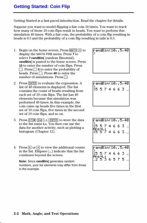
1. Begin on the home screen. Press � | todisplay the MATH PRB menu. Press 7 toselect 7:randBin( (random Binomial).randBin( is pasted to the home screen. Press10 to enter the number of coin flips. Press¢. Press Ë 5 to enter the probability ofheads. Press ¢. Press 40 to enter thenumber of simulations. Press ¤.
2. Press Í to evaluate the expression. Alist of 40 elements is displayed. The listcontains the count of heads resulting fromeach set of 10 coin flips. The list has 40elements because this simulation wasperformed 40 times. In this example, thecoin came up heads five times in the firstset of 10 coin flips, five times in the secondset of 10 coin flips, and so on.
3. Press ¿ y ãL1ä Í to store the datato the list name L1. You then can use thedata for another activity, such as plotting ahistogram (Chapter 12).
4. Press ~ or | to view the additional countsin the list. Ellipses (...) indicate that the listcontinues beyond the screen.
Note: Since randBin( generates randomnumbers, your list elements may differ from thosein the example.
Getting Started: Coin Flip
Math, Angle, and Test Operations 2-3
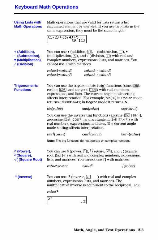
Math operations that are valid for lists return a listcalculated element by element. If you use two lists in thesame expression, they must be the same length.
You can use + (addition, Ã), N (subtraction, ¹), ä(multiplication, ¯), and à (division, ¥) with real andcomplex numbers, expressions, lists, and matrices. Youcannot use à with matrices.
valueA+valueB valueA N valueB
valueAävalueB valueA à valueB
You can use the trigonometric (trig) functions (sine, ˜;cosine, ™; and tangent, š) with real numbers,expressions, and lists. The current angle mode settingaffects interpretation. For example, sin(30) in Radian modereturns L.9880316241; in Degree mode it returns .5.
sin( value) cos( value) tan(value)
You can use the inverse trig functions (arcsine, y [SINL1];arccosine, y [COSL1]; and arctangent, y [TANL1]) withreal numbers, expressions, and lists. The current anglemode setting affects interpretation.
sin L1(value) cos L1(value) tan L1(value)
Note: The trig functions do not operate on complex numbers.
You can use ^ (power, ›), 2 (square, ¡), and ‡( (squareroot, y [‡]) with real and complex numbers, expressions,lists, and matrices. You cannot use ‡( with matrices.
value^power value2 ‡(value)
You can use L1 (inverse, — ) with real and complexnumbers, expressions, lists, and matrices. Themultiplicative inverse is equivalent to the reciprocal, 1àx.
valueL1
Keyboard Math Operations
Using Lists withMath Operations
+ (Addition),N (Subtraction),ä (Multiplication),à (Division)
TrigonometricFunctions
^ (Power),2 (Square),‡( (Square Root)
L1 (Inverse)
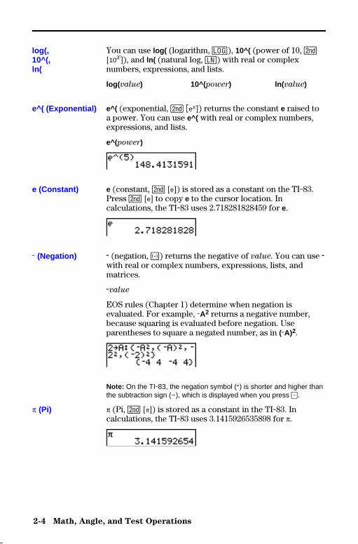
2-4 Math, Angle, and Test Operations
8302MATH.DOC TI-83 international English Bob Fedorisko Revised: 02/19/01 12:12 PM Printed: 02/19/01 2:27PM Page 4 of 26
You can use log( (logarithm, «), 10^( (power of 10, y[10x]), and ln( (natural log, µ) with real or complexnumbers, expressions, and lists.
log( value) 10^(power) ln(value)
e^( (exponential, y ãex]) returns the constant e raised toa power. You can use e^( with real or complex numbers,expressions, and lists.
e^(power)
e (constant, y [e]) is stored as a constant on the TI-83.Press y [e] to copy e to the cursor location. Incalculations, the TI-83 uses 2.718281828459 for e.
M (negation, Ì) returns the negative of value. You can use Mwith real or complex numbers, expressions, lists, andmatrices.
Mvalue
EOS rules (Chapter 1) determine when negation isevaluated. For example, LA2 returns a negative number,because squaring is evaluated before negation. Useparentheses to square a negated number, as in (LA)2.
Note: On the TI-83, the negation symbol (M) is shorter and higher thanthe subtraction sign (N), which is displayed when you press ¹.
p (Pi, y [p]) is stored as a constant in the TI-83. Incalculations, the TI-83 uses 3.1415926535898 for p.
log(,10^(,ln(
e^( (Exponential)
e (Constant)
L (Negation)
p (Pi)
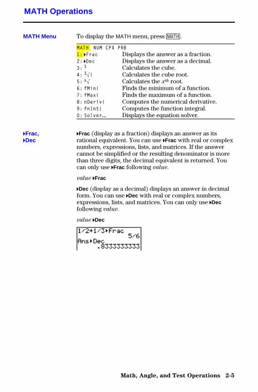
Math, Angle, and Test Operations 2-5
To display the MATH menu, press �.
MATH NUM CPX PRB1: 4Frac Displays the answer as a fraction.2: 4Dec Displays the answer as a decimal.3: 3 Calculates the cube.4: 3‡( Calculates the cube root.5: x‡ Calculates the xth root.6: fMin( Finds the minimum of a function.7: fMax( Finds the maximum of a function.8: nDeriv( Computes the numerical derivative.9: fnInt( Computes the function integral.0: Solver... Displays the equation solver.
4Frac (display as a fraction) displays an answer as itsrational equivalent. You can use 4Frac with real or complexnumbers, expressions, lists, and matrices. If the answercannot be simplified or the resulting denominator is morethan three digits, the decimal equivalent is returned. Youcan only use 4Frac following value.
value 4Frac
4Dec (display as a decimal) displays an answer in decimalform. You can use 4Dec with real or complex numbers,expressions, lists, and matrices. You can only use 4Decfollowing value.
value 4Dec
MATH Operations
MATH Menu
4Frac,4Dec
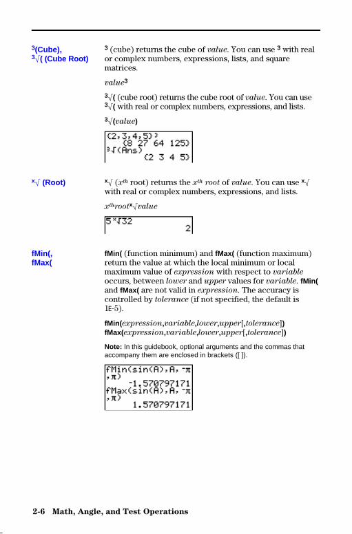
2-6 Math, Angle, and Test Operations
8302MATH.DOC TI-83 international English Bob Fedorisko Revised: 02/19/01 12:12 PM Printed: 02/19/01 2:27PM Page 6 of 26
3 (cube) returns the cube of value. You can use 3 with realor complex numbers, expressions, lists, and squarematrices.
value3
3‡( (cube root) returns the cube root of value. You can use3‡( with real or complex numbers, expressions, and lists.
3‡(value)
x‡ (xth root) returns the xth root of value. You can use x‡with real or complex numbers, expressions, and lists.
xthrootx‡value
fMin( (function minimum) and fMax( (function maximum)return the value at which the local minimum or localmaximum value of expression with respect to variable
occurs, between lower and upper values for variable. fMin(and fMax( are not valid in expression. The accuracy iscontrolled by tolerance (if not specified, the default is1âL5).
fMin( expression,variable,lower,upper[,tolerance])fMax(expression,variable,lower,upper[,tolerance])
Note: In this guidebook, optional arguments and the commas thataccompany them are enclosed in brackets ([ ]).
3(Cube),3‡( (Cube Root)
x‡ (Root)
fMin(,fMax(

Math, Angle, and Test Operations 2-7
nDeriv( (numerical derivative) returns an approximatederivative of expression with respect to variable, given thevalue at which to calculate the derivative and H (if notspecified, the default is 1âL3). nDeriv( is valid only for realnumbers.
nDeriv( expression,variable,value[,H])
nDeriv( uses the symmetric difference quotient method,which approximates the numerical derivative value as theslope of the secant line through these points.
f(x+H)Nf(xNH)f¢(x) =
2HAs H becomes smaller, the approximation usually becomesmore accurate.
You can use nDeriv( once in expression. Because of themethod used to calculate nDeriv( , the TI-83 can return afalse derivative value at a nondifferentiable point.
fnInt( (function integral) returns the numerical integral(Gauss-Kronrod method) of expression with respect tovariable, given lower limit, upper limit, and a tolerance (ifnot specified, the default is 1âL5). fnInt( is valid only for realnumbers.
fnInt( expression,variable,lower,upper[,tolerance])
Tip: To speed the drawing of integration graphs (when fnInt( is usedin a Y= equation), increase the value of the Xres window variablebefore you press s.
nDeriv(
fnInt(
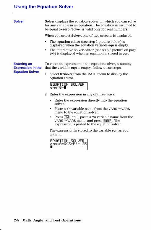
2-8 Math, Angle, and Test Operations
8302MATH.DOC TI-83 international English Bob Fedorisko Revised: 02/19/01 12:12 PM Printed: 02/19/01 2:27PM Page 8 of 26
Solver displays the equation solver, in which you can solvefor any variable in an equation. The equation is assumed tobe equal to zero. Solver is valid only for real numbers.
When you select Solver , one of two screens is displayed.
• The equation editor (see step 1 picture below) isdisplayed when the equation variable eqn is empty.
• The interactive solver editor (see step 3 picture on page2.9) is displayed when an equation is stored in eqn .
To enter an expression in the equation solver, assumingthat the variable eqn is empty, follow these steps.
1. Select 0:Solver from the MATH menu to display theequation editor.
2. Enter the expression in any of three ways.
• Enter the expression directly into the equationsolver.
• Paste a Y= variable name from the VARS Y.VARSmenu to the equation solver.
• Press y [RCL], paste a Y= variable name from theVARS Y.VARS menu, and press Í. Theexpression is pasted to the equation solver.
The expression is stored to the variable eqn as youenter it.
Using the Equation Solver
Solver
Entering anExpression in theEquation Solver
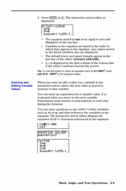
Math, Angle, and Test Operations 2-9
3. Press Í or †. The interactive solver editor isdisplayed.
• The equation stored in eqn is set equal to zero anddisplayed on the top line.
• Variables in the equation are listed in the order inwhich they appear in the equation. Any values storedto the listed variables also are displayed.
• The default lower and upper bounds appear in thelast line of the editor (bound={ L1å99,1å99}).
• A $ is displayed in the first column of the bottom lineif the editor continues beyond the screen.
Tip: To use the solver to solve an equation such as K=.5MV2, entereqn:0=K N.5MV2 in the equation editor.
When you enter or edit a value for a variable in theinteractive solver editor, the new value is stored inmemory to that variable.
You can enter an expression for a variable value. It isevaluated when you move to the next variable.Expressions must resolve to real numbers at each stepduring the iteration.
You can store equations to any VARS Y.VARS variables,such as Y1 or r6, and then reference the variables in theequation. The interactive solver editor displays allvariables of all Y= functions referenced in the equation.
Entering andEditing VariableValues
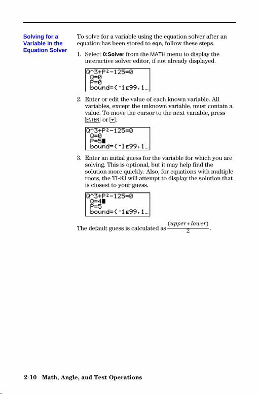
2-10 Math, Angle, and Test Operations
8302MATH.DOC TI-83 international English Bob Fedorisko Revised: 02/19/01 12:12 PM Printed: 02/19/01 2:27PM Page 10 of 26
To solve for a variable using the equation solver after anequation has been stored to eqn , follow these steps.
1. Select 0:Solver from the MATH menu to display theinteractive solver editor, if not already displayed.
2. Enter or edit the value of each known variable. Allvariables, except the unknown variable, must contain avalue. To move the cursor to the next variable, pressÍ or †.
3. Enter an initial guess for the variable for which you aresolving. This is optional, but it may help find thesolution more quickly. Also, for equations with multipleroots, the TI-83 will attempt to display the solution thatis closest to your guess.
The default guess is calculated as (upper+lower)
2 .
Solving for aVariable in theEquation Solver
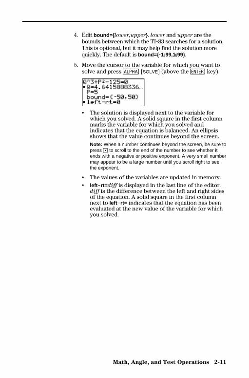
Math, Angle, and Test Operations 2-11
4. Edit bound={ lower,upper}. lower and upper are thebounds between which the TI-83 searches for a solution.This is optional, but it may help find the solution morequickly. The default is bound={ L1å99,1å99}.
5. Move the cursor to the variable for which you want tosolve and press ƒ [SOLVE] (above the Í key).
• The solution is displayed next to the variable forwhich you solved. A solid square in the first columnmarks the variable for which you solved andindicates that the equation is balanced. An ellipsisshows that the value continues beyond the screen.Note: When a number continues beyond the screen, be sure topress ~ to scroll to the end of the number to see whether itends with a negative or positive exponent. A very small numbermay appear to be a large number until you scroll right to seethe exponent.
• The values of the variables are updated in memory.• left Nrt=diff is displayed in the last line of the editor.
diff is the difference between the left and right sidesof the equation. A solid square in the first columnnext to left Nrt= indicates that the equation has beenevaluated at the new value of the variable for whichyou solved.
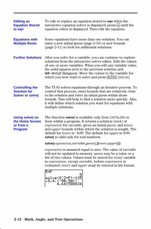
2-12 Math, Angle, and Test Operations
8302MATH.DOC TI-83 international English Bob Fedorisko Revised: 02/19/01 12:12 PM Printed: 02/19/01 2:27PM Page 12 of 26
To edit or replace an equation stored to eqn when theinteractive equation solver is displayed, press } until theequation editor is displayed. Then edit the equation.
Some equations have more than one solution. You canenter a new initial guess (page 2.10) or new bounds(page 2.11) to look for additional solutions.
After you solve for a variable, you can continue to exploresolutions from the interactive solver editor. Edit the valuesof one or more variables. When you edit any variable value,the solid squares next to the previous solution andleft Nrt=diff disappear. Move the cursor to the variable forwhich you now want to solve and press ƒ [SOLVE].
The TI-83 solves equations through an iterative process. Tocontrol that process, enter bounds that are relatively closeto the solution and enter an initial guess within thosebounds. This will help to find a solution more quickly. Also,it will define which solution you want for equations withmultiple solutions.
The function solve( is available only from CATALOG orfrom within a program. It returns a solution (root) ofexpression for variable, given an initial guess, and lower
and upper bounds within which the solution is sought. Thedefault for lower is L1â99. The default for upper is 1â99.solve( is valid only for real numbers.
solve( expression,variable,guess[,{lower,upper}])
expression is assumed equal to zero. The value of variable
will not be updated in memory. guess may be a value or alist of two values. Values must be stored for every variablein expression, except variable, before expression isevaluated. lower and upper must be entered in list format.
Editing anEquation Storedto eqn
Equations withMultiple Roots
Further Solutions
Controlling theSolution forSolver or solve(
Using solve( onthe Home Screenor from aProgram

Math, Angle, and Test Operations 2-13
To display the MATH NUM menu, press � ~.
MATH NUM CPX PRB1: abs( Absolute value2: round( Round3: iPart( Integer part4: fPart( Fractional part5: int( Greatest integer6: min( Minimum value7: max( Maximum value8: lcm( Least common multiple9: gcd( Greatest common divisor
abs( (absolute value) returns the absolute value of real orcomplex (modulus) numbers, expressions, lists, andmatrices.
abs(value)
Note: abs( is also available on the MATH CPX menu.
round( returns a number, expression, list, or matrixrounded to #decimals (�9). If #decimals is omitted, value
is rounded to the digits that are displayed, up to 10 digits.
round( value[,#decimals])
MATH NUM (Number) Operations
MATH NUM Menu
abs(
round(
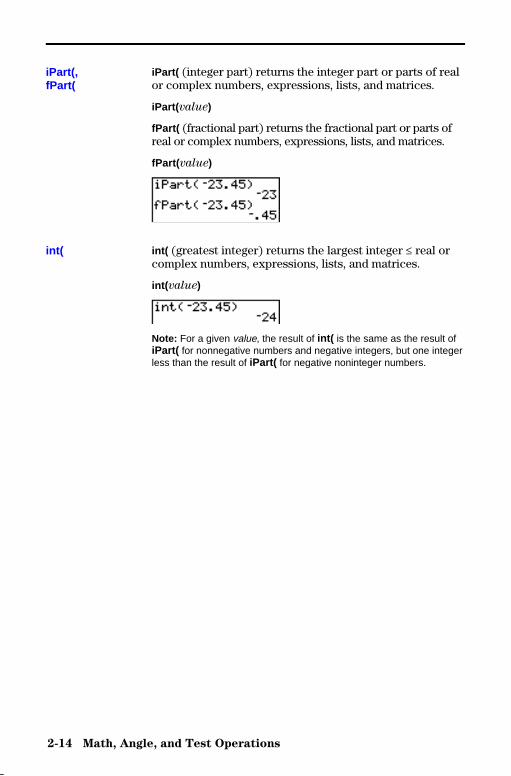
2-14 Math, Angle, and Test Operations
8302MATH.DOC TI-83 international English Bob Fedorisko Revised: 02/19/01 12:12 PM Printed: 02/19/01 2:27PM Page 14 of 26
iPart( (integer part) returns the integer part or parts of realor complex numbers, expressions, lists, and matrices.
iPart( value)
fPart( (fractional part) returns the fractional part or parts ofreal or complex numbers, expressions, lists, and matrices.
fPart( value)
int( (greatest integer) returns the largest integer � real orcomplex numbers, expressions, lists, and matrices.
int( value)
Note: For a given value, the result of int( is the same as the result ofiPart( for nonnegative numbers and negative integers, but one integerless than the result of iPart( for negative noninteger numbers.
iPart(,fPart(
int(

Math, Angle, and Test Operations 2-15
min( (minimum value) returns the smaller of valueA andvalueB or the smallest element in list. If listA and listB arecompared, min( returns a list of the smaller of each pair ofelements. If list and value are compared, min( compareseach element in list with value.
max( (maximum value) returns the larger of valueA andvalueB or the largest element in list. If listA and listB arecompared, max( returns a list of the larger of each pair ofelements. If list and value are compared, max( compareseach element in list with value.
min( valueA,valueB) max(valueA,valueB)min( list) max( list)min( listA,listB) max( listA,listB)min( list,value) max( list,value)
Note: min( and max( also are available on the LIST MATH menu.
lcm( returns the least common multiple of valueA andvalueB, both of which must be nonnegative integers. WhenlistA and listB are specified, lcm( returns a list of the lcmof each pair of elements. If list and value are specified,lcm( finds the lcm of each element in list and value.
gcd( returns the greatest common divisor of valueA andvalueB, both of which must be nonnegative integers. WhenlistA and listB are specified, gcd( returns a list of the gcdof each pair of elements. If list and value are specified,gcd( finds the gcd of each element in list and value.
lcm( valueA,valueB) gcd( valueA,valueB)lcm( listA,listB) gcd( listA,listB)lcm( list,value) gcd( list,value)
min(,max(
lcm(,gcd(
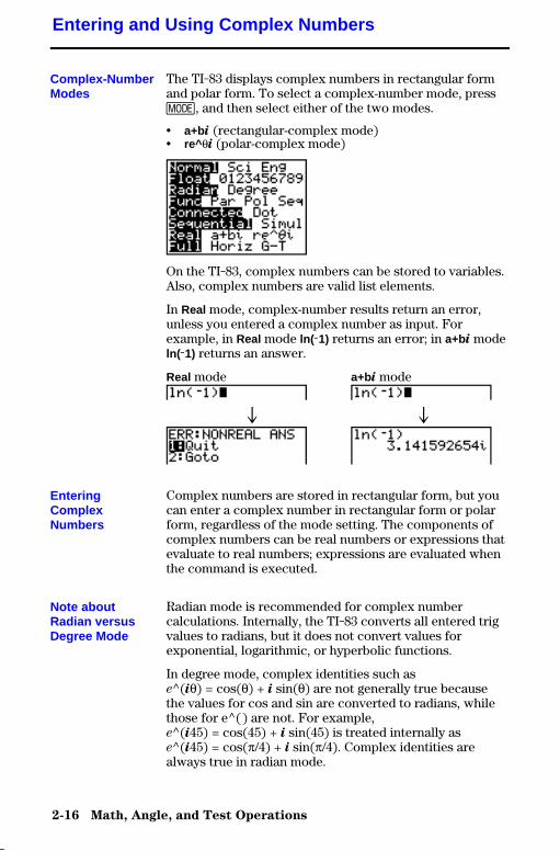
2-16 Math, Angle, and Test Operations
8302MATH.DOC TI-83 international English Bob Fedorisko Revised: 02/19/01 12:12 PM Printed: 02/19/01 2:27PM Page 16 of 26
The TI-83 displays complex numbers in rectangular formand polar form. To select a complex-number mode, pressz, and then select either of the two modes.
• a+bi (rectangular-complex mode)• re^ qi (polar-complex mode)
On the TI-83, complex numbers can be stored to variables.Also, complex numbers are valid list elements.
In Real mode, complex-number results return an error,unless you entered a complex number as input. Forexample, in Real mode ln(L1) returns an error; in a+bi modeln(L1) returns an answer.
Real mode a+bi mode
$ $
Complex numbers are stored in rectangular form, but youcan enter a complex number in rectangular form or polarform, regardless of the mode setting. The components ofcomplex numbers can be real numbers or expressions thatevaluate to real numbers; expressions are evaluated whenthe command is executed.
Radian mode is recommended for complex numbercalculations. Internally, the TI-83 converts all entered trigvalues to radians, but it does not convert values forexponential, logarithmic, or hyperbolic functions.
In degree mode, complex identities such ase^(iq) = cos(q) + i sin(q) are not generally true becausethe values for cos and sin are converted to radians, whilethose for e^() are not. For example,e^(i45) = cos(45) + i sin(45) is treated internally ase^(i45) = cos(p/4) + i sin(p/4). Complex identities arealways true in radian mode.
Entering and Using Complex Numbers
Complex-NumberModes
EnteringComplexNumbers
Note aboutRadian versusDegree Mode
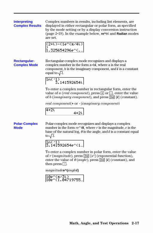
Math, Angle, and Test Operations 2-17
Complex numbers in results, including list elements, aredisplayed in either rectangular or polar form, as specifiedby the mode setting or by a display conversion instruction(page 2.19). In the example below, re^ qi and Radian modesare set.
Rectangular-complex mode recognizes and displays acomplex number in the form a+bi, where a is the realcomponent, b is the imaginary component, and i is a constantequal to -1.
To enter a complex number in rectangular form, enter thevalue of a (real component), press à or ¹, enter the valueof b (imaginary component), and press y [i] (constant).
real component(+ or N)imaginary componenti
Polar-complex mode recognizes and displays a complexnumber in the form re^qi, where r is the magnitude, e is thebase of the natural log, q is the angle, and i is a constant equalto -1.
To enter a complex number in polar form, enter the valueof r (magnitude), press y [ex] (exponential function),enter the value of q (angle), press y [i] (constant), andthen press ¤.
magnitudee^(anglei)
InterpretingComplex Results
Rectangular-Complex Mode
Polar-ComplexMode
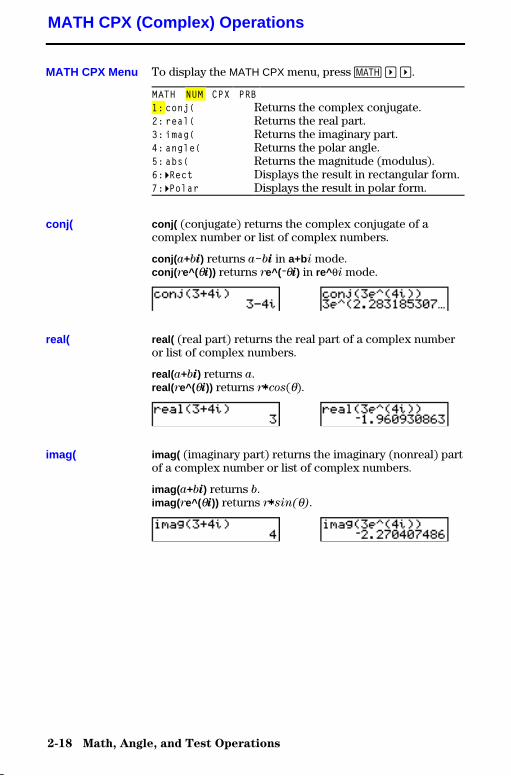
2-18 Math, Angle, and Test Operations
8302MATH.DOC TI-83 international English Bob Fedorisko Revised: 02/19/01 12:12 PM Printed: 02/19/01 2:27PM Page 18 of 26
To display the MATH CPX menu, press � ~ ~.
MATH NUM CPX PRB1:conj( Returns the complex conjugate.2:real( Returns the real part.3:imag( Returns the imaginary part.4:angle( Returns the polar angle.5:abs( Returns the magnitude (modulus).6: 4Rect Displays the result in rectangular form.7: 4Polar Displays the result in polar form.
conj( (conjugate) returns the complex conjugate of acomplex number or list of complex numbers.
conj( a+bi) returns aNbi in a+bi mode.conj( re^(qi)) returns re^(Lqi) in re^ qi mode.
real( (real part) returns the real part of a complex numberor list of complex numbers.
real(a+bi) returns a.real(re^(qi)) returns räcos(q).
imag( (imaginary part) returns the imaginary (nonreal) partof a complex number or list of complex numbers.
imag( a+bi) returns b.imag( re^(qi)) returns räsin(q).
MATH CPX (Complex) Operations
MATH CPX Menu
conj(
real(
imag(
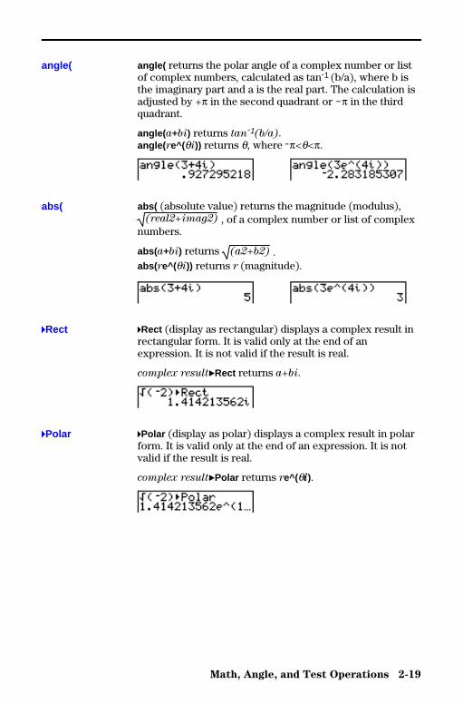
Math, Angle, and Test Operations 2-19
angle( returns the polar angle of a complex number or listof complex numbers, calculated as tanL1 (b/a), where b isthe imaginary part and a is the real part. The calculation isadjusted by +p in the second quadrant or Np in the thirdquadrant.
angle( a+bi) returns tanL1(b/a).angle( re^(qi)) returns q, where Lp<q<p.
abs( (absolute value) returns the magnitude (modulus),(real2+imag2) , of a complex number or list of complex
numbers.
abs(a+bi) returns (a2+b2) .abs(re^(qi)) returns r (magnitude).
4Rect (display as rectangular) displays a complex result inrectangular form. It is valid only at the end of anexpression. It is not valid if the result is real.
complex result8Rect returns a+bi.
4Polar (display as polar) displays a complex result in polarform. It is valid only at the end of an expression. It is notvalid if the result is real.
complex result8Polar returns re^(qi).
angle(
abs(
4Rect
4Polar

2-20 Math, Angle, and Test Operations
8302MATH.DOC TI-83 international English Bob Fedorisko Revised: 02/19/01 12:12 PM Printed: 02/19/01 2:27PM Page 20 of 26
To display the MATH PRB menu, press � |.
MATH NUM CPX PRB1: rand Random-number generator2: nPr Number of permutations3: nCr Number of combinations4: ! Factorial5: randInt( Random-integer generator6: randNorm( Random # from Normal distribution7: randBin( Random # from Binomial distribution
rand (random number) generates and returns one or morerandom numbers > 0 and < 1. To generate a list of random-numbers, specify an integer > 1 for numtrials (number oftrials). The default for numtrials is 1.
rand [(numtrials)]
Tip: To generate random numbers beyond the range of 0 to 1, youcan include rand in an expression. For example, rand ä5 generates arandom number > 0 and < 5.
With each rand execution, the TI-83 generates the samerandom-number sequence for a given seed value. The TI-83factory-set seed value for rand is 0. To generate a differentrandom-number sequence, store any nonzero seed value torand . To restore the factory-set seed value, store 0 to randor reset the defaults (Chapter 18).
Note: The seed value also affects randInt( , randNorm( , andrandBin( instructions (page 2.22).
MATH PRB (Probability) Operations
MATH PRB Menu
rand
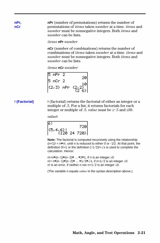
Math, Angle, and Test Operations 2-21
nPr (number of permutations) returns the number ofpermutations of items taken number at a time. items andnumber must be nonnegative integers. Both items andnumber can be lists.
items nPr number
nCr (number of combinations) returns the number ofcombinations of items taken number at a time. items andnumber must be nonnegative integers. Both items andnumber can be lists.
items nCr number
! (factorial) returns the factorial of either an integer or amultiple of .5. For a list, it returns factorials for eachinteger or multiple of .5. value must be ‚L.5 and �69.
value!
Note: The factorial is computed recursively using the relationship(n+1)! = nän!, until n is reduced to either 0 or L1/2. At that point, thedefinition 0!=1 or the definition (L1à2)!=‡p is used to complete thecalculation. Hence:
n!=nä(nN1)ä(nN2)ä ... ä2ä1, if n is an integer ‚0n!= nä(nN1)ä(nN2)ä ... ä1à2ä‡p, if n+1à2 is an integer ‚0n! is an error, if neither n nor n+1à2 is an integer ‚0.
(The variable n equals value in the syntax description above.)
nPr,nCr
! (Factorial)
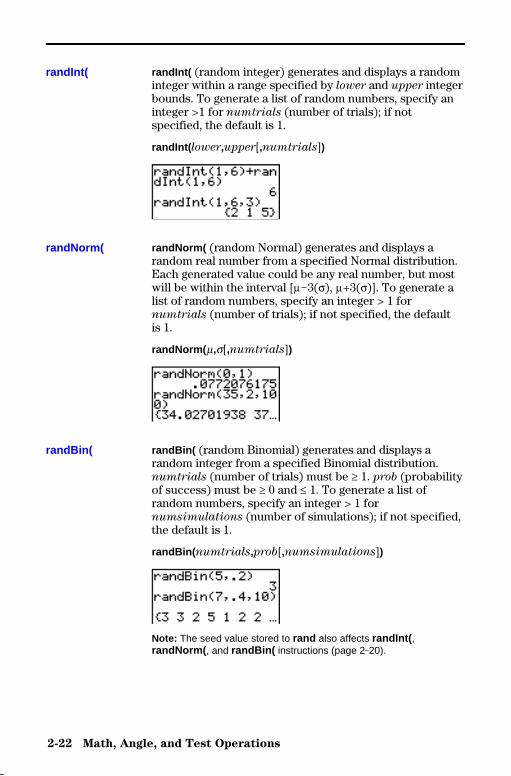
2-22 Math, Angle, and Test Operations
8302MATH.DOC TI-83 international English Bob Fedorisko Revised: 02/19/01 12:12 PM Printed: 02/19/01 2:27PM Page 22 of 26
randInt( (random integer) generates and displays a randominteger within a range specified by lower and upper integerbounds. To generate a list of random numbers, specify aninteger >1 for numtrials (number of trials); if notspecified, the default is 1.
randInt( lower,upper[,numtrials])
randNorm( (random Normal) generates and displays arandom real number from a specified Normal distribution.Each generated value could be any real number, but mostwill be within the interval [mN3(s), m+3(s)]. To generate alist of random numbers, specify an integer > 1 fornumtrials (number of trials); if not specified, the defaultis 1.
randNorm( m,s[,numtrials])
randBin( (random Binomial) generates and displays arandom integer from a specified Binomial distribution.numtrials (number of trials) must be ‚ 1. prob (probabilityof success) must be ‚ 0 and � 1. To generate a list ofrandom numbers, specify an integer > 1 fornumsimulations (number of simulations); if not specified,the default is 1.
randBin( numtrials,prob[,numsimulations])
Note: The seed value stored to rand also affects randInt( ,randNorm( , and randBin( instructions (page 2-20).
randInt(
randNorm(
randBin(
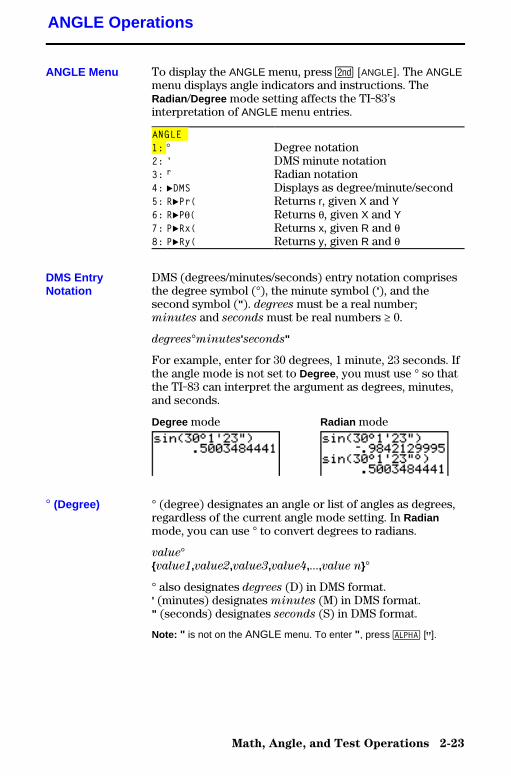
Math, Angle, and Test Operations 2-23
To display the ANGLE menu, press y [ANGLE]. The ANGLEmenu displays angle indicators and instructions. TheRadian /Degree mode setting affects the TI-83’sinterpretation of ANGLE menu entries.
ANGLE1: ¡ Degree notation2: ' DMS minute notation3: r Radian notation4: 8DMS Displays as degree/minute/second5: R8Pr( Returns r, given X and Y6: R8Pq( Returns q, given X and Y7: P8Rx( Returns x, given R and q8: P8Ry( Returns y, given R and q
DMS (degrees/minutes/seconds) entry notation comprisesthe degree symbol (¡), the minute symbol ('), and thesecond symbol ("). degrees must be a real number;minutes and seconds must be real numbers ‚ 0.
degrees¡minutes'seconds"
For example, enter for 30 degrees, 1 minute, 23 seconds. Ifthe angle mode is not set to Degree , you must use ¡ so thatthe TI-83 can interpret the argument as degrees, minutes,and seconds.
Degree mode Radian mode
¡ (degree) designates an angle or list of angles as degrees,regardless of the current angle mode setting. In Radianmode, you can use ¡ to convert degrees to radians.
value¡{value1,value2,value3,value4,...,value n}¡
¡ also designates degrees (D) in DMS format.' (minutes) designates minutes (M) in DMS format." (seconds) designates seconds (S) in DMS format.
Note: " is not on the ANGLE menu. To enter " , press ƒ [ã].
ANGLE Operations
ANGLE Menu
DMS EntryNotation
¡ (Degree)
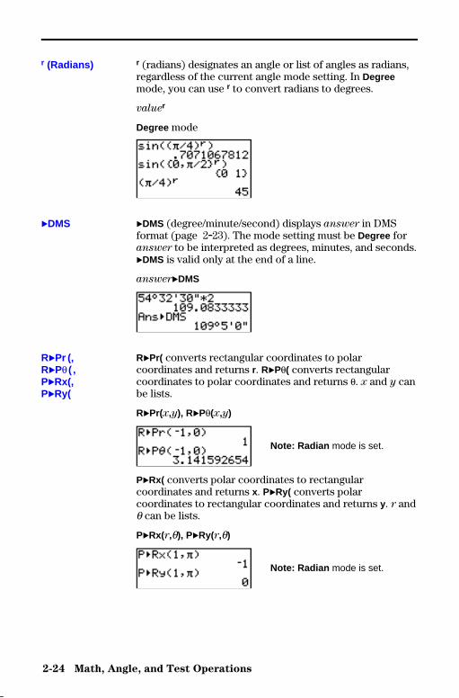
2-24 Math, Angle, and Test Operations
8302MATH.DOC TI-83 international English Bob Fedorisko Revised: 02/19/01 12:12 PM Printed: 02/19/01 2:27PM Page 24 of 26
r (radians) designates an angle or list of angles as radians,regardless of the current angle mode setting. In Degreemode, you can use r to convert radians to degrees.
valuer
Degree mode
8DMS (degree/minute/second) displays answer in DMSformat (page 2.23). The mode setting must be Degree foranswer to be interpreted as degrees, minutes, and seconds.8DMS is valid only at the end of a line.
answer8DMS
R8Pr( converts rectangular coordinates to polarcoordinates and returns r. R8Pq( converts rectangularcoordinates to polar coordinates and returns q. x and y canbe lists.
R8Pr(x,y), R8Pq(x,y)
Note: Radian mode is set.
P8Rx( converts polar coordinates to rectangularcoordinates and returns x. P8Ry( converts polarcoordinates to rectangular coordinates and returns y. r andq can be lists.
P8Rx(r,q), P8Ry(r,q)
Note: Radian mode is set.
r (Radians)
8DMS
R8Pr (,R8Pq ( ,P8Rx(,P8Ry(

Math, Angle, and Test Operations 2-25
To display the TEST menu, press y [TEST].
This operator... Returns 1 (true) if...TEST LOGIC1: = Equal2: ƒ Not equal to3: > Greater than4: ‚ Greater than or equal to5: < Less than6: � Less than or equal to
Relational operators compare valueA and valueB andreturn 1 if the test is true or 0 if the test is false. valueA andvalueB can be real numbers, expressions, or lists. For =and ƒ only, valueA and valueB also can be matrices orcomplex numbers. If valueA and valueB are matrices, bothmust have the same dimensions.
Relational operators are often used in programs to controlprogram flow and in graphing to control the graph of afunction over specific values.
valueA=valueB valueAƒvalueB
valueA>valueB valueA‚valueB
valueA<valueB valueA�valueB
Relational operators are evaluated after mathematicalfunctions according to EOS rules (Chapter 1).
• The expression 2+2=2+3 returns 0. The TI-83 performsthe addition first because of EOS rules, and then itcompares 4 to 5.
• The expression 2+(2=2)+3 returns 6. The TI-83 performsthe relational test first because it is in parentheses, andthen it adds 2, 1, and 3.
TEST (Relational) Operations
TEST Menu
=, ƒ,>, ‚,<, �
Using Tests
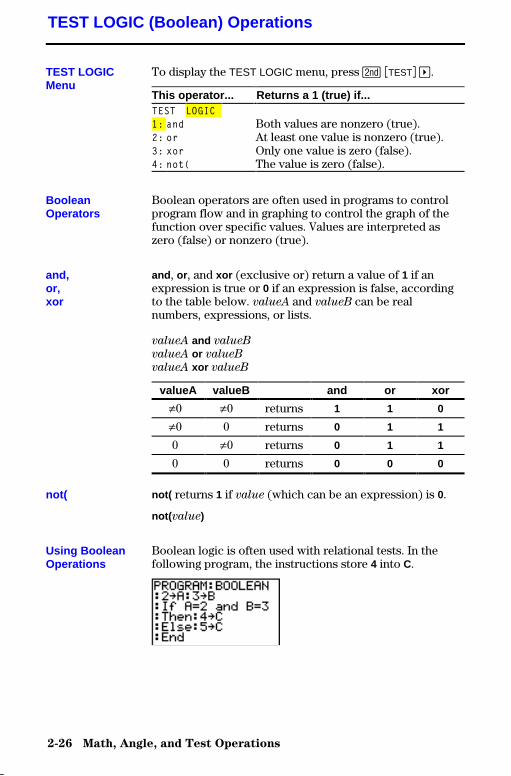
2-26 Math, Angle, and Test Operations
8302MATH.DOC TI-83 international English Bob Fedorisko Revised: 02/19/01 12:12 PM Printed: 02/19/01 2:27PM Page 26 of 26
To display the TEST LOGIC menu, press y ãTESTä ~.
This operator... Returns a 1 (true) if...TEST LOGIC1: and Both values are nonzero (true).2: or At least one value is nonzero (true).3: xor Only one value is zero (false).4: not( The value is zero (false).
Boolean operators are often used in programs to controlprogram flow and in graphing to control the graph of thefunction over specific values. Values are interpreted aszero (false) or nonzero (true).
and , or , and xor (exclusive or) return a value of 1 if anexpression is true or 0 if an expression is false, accordingto the table below. valueA and valueB can be realnumbers, expressions, or lists.
valueA and valueB
valueA or valueB
valueA xor valueB
valueA valueB and or xor
ƒ0 ƒ0 returns 1 1 0
ƒ0 0 returns 0 1 1
0 ƒ0 returns 0 1 1
0 0 returns 0 0 0
not( returns 1 if value (which can be an expression) is 0.
not( value)
Boolean logic is often used with relational tests. In thefollowing program, the instructions store 4 into C.
TEST LOGIC (Boolean) Operations
TEST LOGICMenu
BooleanOperators
and,or,xor
not(
Using BooleanOperations
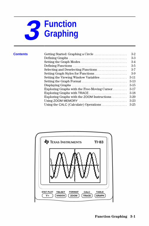
Function Graphing 3-1
8303FUNC.DOC TI-83 international English Bob Fedorisko Revised: 02/19/01 12:16 PM Printed: 02/19/01 1:50PM Page 1 of 28
3 FunctionGraphin g
Getting Started: Graphing a Circle ....................... 3-2Defining Graphs ......................................... 3-3Setting the Graph Modes................................. 3-4Defining Functions ...................................... 3-5Selecting and Deselecting Functions ..................... 3-7Setting Graph Styles for Functions....................... 3-9Setting the Viewing Window Variables ................... 3-11Setting the Graph Format ................................ 3-13Displaying Graphs ....................................... 3-15Exploring Graphs with the Free-Moving Cursor.......... 3-17Exploring Graphs with TRACE........................... 3-18Exploring Graphs with the ZOOM Instructions........... 3-20Using ZOOM MEMORY .................................. 3-23Using the CALC (Calculate) Operations .................. 3-25
Contents
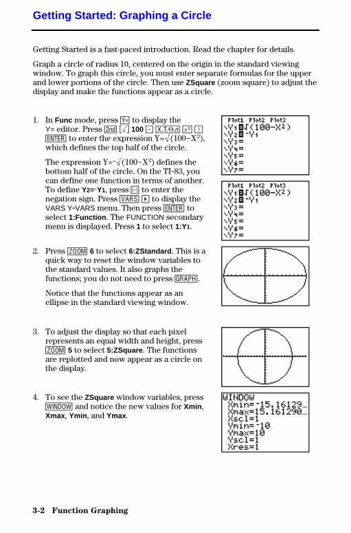
3-2 Function Graphing
8303FUNC.DOC TI-83 international English Bob Fedorisko Revised: 02/19/01 12:16 PM Printed: 02/19/01 1:35PM Page 2 of 288303FUNC.DOC TI-83 international English Bob Fedorisko Revised: 02/19/01 12:16 PM Printed: 02/19/01 1:35PM Page 2 of 28
Getting Started is a fast-paced introduction. Read the chapter for details.
Graph a circle of radius 10, centered on the origin in the standard viewingwindow. To graph this circle, you must enter separate formulas for the upperand lower portions of the circle. Then use ZSquare (zoom square) to adjust thedisplay and make the functions appear as a circle.
1. In Func mode, press o to display theY= editor. Press y ã‡ä 100 ¹ „ ¡ ¤Í to enter the expression Y=‡(100NX2),which defines the top half of the circle.
The expression Y=L‡(100NX2) defines thebottom half of the circle. On the TI-83, youcan define one function in terms of another.To define Y2=LY1, press Ì to enter thenegation sign. Press � ~ to display theVARS Y.VARS menu. Then press Í toselect 1:Function . The FUNCTION secondarymenu is displayed. Press 1 to select 1:Y1.
2. Press q 6 to select 6:ZStandard . This is aquick way to reset the window variables tothe standard values. It also graphs thefunctions; you do not need to press s.
Notice that the functions appear as anellipse in the standard viewing window.
3. To adjust the display so that each pixelrepresents an equal width and height, pressq 5 to select 5:ZSquare . The functionsare replotted and now appear as a circle onthe display.
4. To see the ZSquare window variables, pressp and notice the new values for Xmin ,Xmax , Ymin , and Ymax .
Getting Started: Graphing a Circle
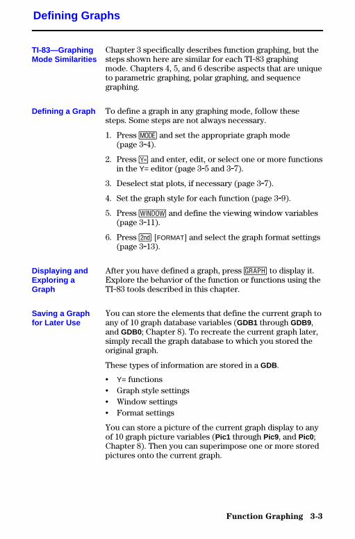
Function Graphing 3-3
8303FUNC.DOC TI-83 international English Bob Fedorisko Revised: 02/19/01 12:16 PM Printed: 02/19/01 1:35PM Page 3 of 28
Chapter 3 specifically describes function graphing, but thesteps shown here are similar for each TI-83 graphingmode. Chapters 4, 5, and 6 describe aspects that are uniqueto parametric graphing, polar graphing, and sequencegraphing.
To define a graph in any graphing mode, follow thesesteps. Some steps are not always necessary.
1. Press z and set the appropriate graph mode(page 3.4).
2. Press o and enter, edit, or select one or more functionsin the Y= editor (page 3.5 and 3.7).
3. Deselect stat plots, if necessary (page 3.7).
4. Set the graph style for each function (page 3.9).
5. Press p and define the viewing window variables(page 3.11).
6. Press y [FORMAT] and select the graph format settings(page 3.13).
After you have defined a graph, press s to display it.Explore the behavior of the function or functions using theTI-83 tools described in this chapter.
You can store the elements that define the current graph toany of 10 graph database variables (GDB1 through GDB9,and GDB0; Chapter 8). To recreate the current graph later,simply recall the graph database to which you stored theoriginal graph.
These types of information are stored in a GDB.
• Y= functions• Graph style settings• Window settings• Format settings
You can store a picture of the current graph display to anyof 10 graph picture variables (Pic1 through Pic9 , and Pic0 ;Chapter 8). Then you can superimpose one or more storedpictures onto the current graph.
Defining Graphs
TI-83—GraphingMode Similarities
Defining a Graph
Displaying andExploring aGraph
Saving a Graphfor Later Use
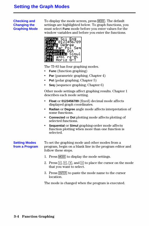
3-4 Function Graphing
8303FUNC.DOC TI-83 international English Bob Fedorisko Revised: 02/19/01 12:16 PM Printed: 02/19/01 1:35PM Page 4 of 288303FUNC.DOC TI-83 international English Bob Fedorisko Revised: 02/19/01 12:16 PM Printed: 02/19/01 1:35PM Page 4 of 28
To display the mode screen, press z. The defaultsettings are highlighted below. To graph functions, youmust select Func mode before you enter values for thewindow variables and before you enter the functions.
The TI-83 has four graphing modes.• Func (function graphing)• Par (parametric graphing; Chapter 4)• Pol (polar graphing; Chapter 5)• Seq (sequence graphing; Chapter 6)
Other mode settings affect graphing results. Chapter 1describes each mode setting.
• Float or 0123456789 (fixed) decimal mode affectsdisplayed graph coordinates.
• Radian or Degree angle mode affects interpretation ofsome functions.
• Connected or Dot plotting mode affects plotting ofselected functions.
• Sequential or Simul graphing-order mode affectsfunction plotting when more than one function isselected.
To set the graphing mode and other modes from aprogram, begin on a blank line in the program editor andfollow these steps.
1. Press z to display the mode settings.
2. Press †, ~, |, and } to place the cursor on the modethat you want to select.
3. Press Í to paste the mode name to the cursorlocation.
The mode is changed when the program is executed.
Setting the Graph Modes
Checking andChanging theGraphing Mode
Setting Modesfrom a Program
Function Graphing 3-5
8303FUNC.DOC TI-83 international English Bob Fedorisko Revised: 02/19/01 12:16 PM Printed: 02/19/01 1:35PM Page 5 of 28
To display the Y= editor, press o. You can store up to 10functions to the function variables Y1 through Y9, and Y0.You can graph one or more defined functions at once. Inthis example, functions Y1 and Y2 are defined and selected.
To define or edit a function, follow these steps.
1. Press o to display the Y= editor.
2. Press † to move the cursor to the function you want todefine or edit. To erase a function, press ‘.
3. Enter or edit the expression to define the function.
• You may use functions and variables (includingmatrices and lists) in the expression. When theexpression evaluates to a nonreal number, the valueis not plotted; no error is returned.
• The independent variable in the function is X. Funcmode defines „ as X. To enter X, press „or press ƒ [X].
• When you enter the first character, the = ishighlighted, indicating that the function is selected.
As you enter the expression, it is stored to the variableYn as a user-defined function in the Y= editor.
4. Press Í or † to move the cursor to the nextfunction.
Defining Functions
DisplayingFunctions in theY= Editor
Defining orEditing aFunction
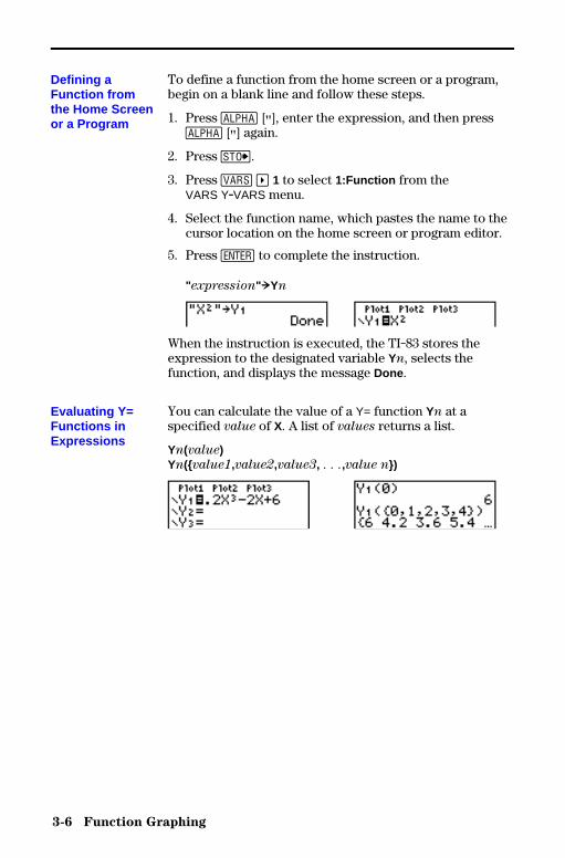
3-6 Function Graphing
8303FUNC.DOC TI-83 international English Bob Fedorisko Revised: 02/19/01 12:16 PM Printed: 02/19/01 1:35PM Page 6 of 288303FUNC.DOC TI-83 international English Bob Fedorisko Revised: 02/19/01 12:16 PM Printed: 02/19/01 1:35PM Page 6 of 28
To define a function from the home screen or a program,begin on a blank line and follow these steps.
1. Press ƒ [ã], enter the expression, and then pressƒ [ã] again.
2. Press ¿.
3. Press � ~ 1 to select 1:Function from theVARS Y.VARS menu.
4. Select the function name, which pastes the name to thecursor location on the home screen or program editor.
5. Press Í to complete the instruction.
"expression" !Yn
When the instruction is executed, the TI-83 stores theexpression to the designated variable Yn, selects thefunction, and displays the message Done .
You can calculate the value of a Y= function Yn at aspecified value of X. A list of values returns a list.
Yn(value)Yn({value1,value2,value3, . . .,value n})
Defining aFunction fromthe Home Screenor a Program
Evaluating Y=Functions inExpressions
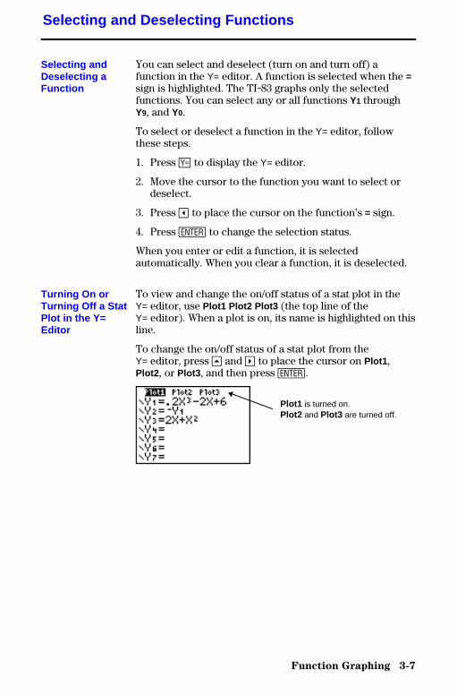
Function Graphing 3-7
8303FUNC.DOC TI-83 international English Bob Fedorisko Revised: 02/19/01 12:16 PM Printed: 02/19/01 1:35PM Page 7 of 28
You can select and deselect (turn on and turn off) afunction in the Y= editor. A function is selected when the =sign is highlighted. The TI-83 graphs only the selectedfunctions. You can select any or all functions Y1 throughY9, and Y0.
To select or deselect a function in the Y= editor, followthese steps.
1. Press o to display the Y= editor.
2. Move the cursor to the function you want to select ordeselect.
3. Press | to place the cursor on the function’s = sign.
4. Press Í to change the selection status.
When you enter or edit a function, it is selectedautomatically. When you clear a function, it is deselected.
To view and change the on/off status of a stat plot in theY= editor, use Plot1 Plot2 Plot3 (the top line of theY= editor). When a plot is on, its name is highlighted on thisline.
To change the on/off status of a stat plot from theY= editor, press } and ~ to place the cursor on Plot1 ,Plot2 , or Plot3 , and then press Í.
Selecting and Deselecting Functions
Selecting andDeselecting aFunction
Turning On orTurning Off a StatPlot in the Y=Editor
Plot1 is turned on.Plot2 and Plot3 are turned off.
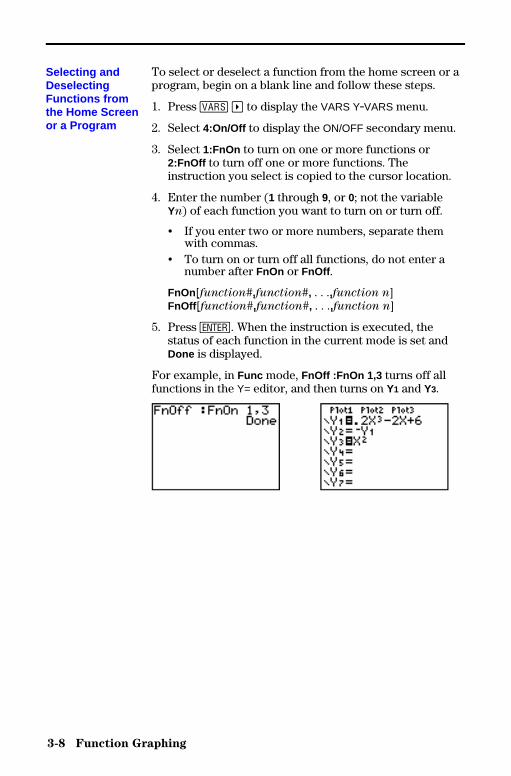
3-8 Function Graphing
8303FUNC.DOC TI-83 international English Bob Fedorisko Revised: 02/19/01 12:16 PM Printed: 02/19/01 1:35PM Page 8 of 288303FUNC.DOC TI-83 international English Bob Fedorisko Revised: 02/19/01 12:16 PM Printed: 02/19/01 1:35PM Page 8 of 28
To select or deselect a function from the home screen or aprogram, begin on a blank line and follow these steps.
1. Press � ~ to display the VARS Y.VARS menu.
2. Select 4:On/Off to display the ON/OFF secondary menu.
3. Select 1:FnOn to turn on one or more functions or2:FnOff to turn off one or more functions. Theinstruction you select is copied to the cursor location.
4. Enter the number (1 through 9, or 0; not the variableYn) of each function you want to turn on or turn off.
• If you enter two or more numbers, separate themwith commas.
• To turn on or turn off all functions, do not enter anumber after FnOn or FnOff .
FnOn[function#,function#, . . .,function n]FnOff [function#,function#, . . .,function n]
5. Press Í. When the instruction is executed, thestatus of each function in the current mode is set andDone is displayed.
For example, in Func mode, FnOff :FnOn 1,3 turns off allfunctions in the Y= editor, and then turns on Y1 and Y3.
Selecting andDeselectingFunctions fromthe Home Screenor a Program
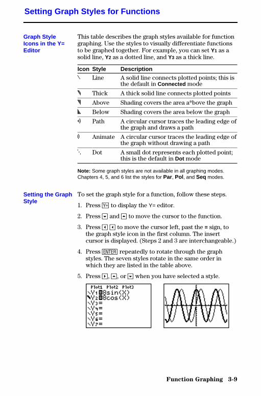
Function Graphing 3-9
8303FUNC.DOC TI-83 international English Bob Fedorisko Revised: 02/19/01 12:16 PM Printed: 02/19/01 1:35PM Page 9 of 28
This table describes the graph styles available for functiongraphing. Use the styles to visually differentiate functionsto be graphed together. For example, you can set Y1 as asolid line, Y2 as a dotted line, and Y3 as a thick line.
Icon Style Description
ç Line A solid line connects plotted points; this isthe default in Connected mode
è Thick A thick solid line connects plotted points
é Above Shading covers the area a*bove the graph
ê Below Shading covers the area below the graph
ë Path A circular cursor traces the leading edge ofthe graph and draws a path
ì Animate A circular cursor traces the leading edge ofthe graph without drawing a path
í Dot A small dot represents each plotted point;this is the default in Dot mode
Note: Some graph styles are not available in all graphing modes.Chapters 4, 5, and 6 list the styles for Par, Pol , and Seq modes.
To set the graph style for a function, follow these steps.
1. Press o to display the Y= editor.
2. Press † and } to move the cursor to the function.
3. Press | | to move the cursor left, past the = sign, tothe graph style icon in the first column. The insertcursor is displayed. (Steps 2 and 3 are interchangeable.)
4. Press Í repeatedly to rotate through the graphstyles. The seven styles rotate in the same order inwhich they are listed in the table above.
5. Press ~, }, or † when you have selected a style.
Setting Graph Styles for Functions
Graph StyleIcons in the Y=Editor
Setting the GraphStyle
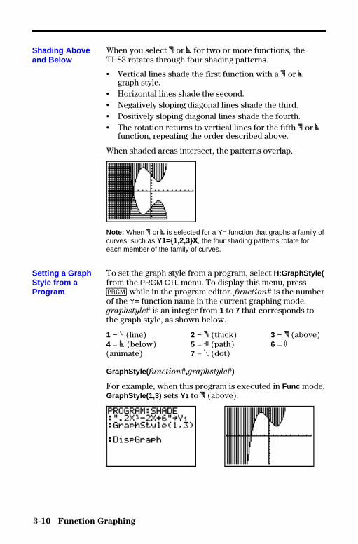
3-10 Function Graphing
8303FUNC.DOC TI-83 international English Bob Fedorisko Revised: 02/19/01 12:16 PM Printed: 02/19/01 1:35PM Page 10 of 288303FUNC.DOC TI-83 international English Bob Fedorisko Revised: 02/19/01 12:16 PM Printed: 02/19/01 1:35PM Page 10 of 28
When you select é or ê for two or more functions, theTI-83 rotates through four shading patterns.
• Vertical lines shade the first function with a é or êgraph style.
• Horizontal lines shade the second.• Negatively sloping diagonal lines shade the third.• Positively sloping diagonal lines shade the fourth.• The rotation returns to vertical lines for the fifth é or ê
function, repeating the order described above.
When shaded areas intersect, the patterns overlap.
Note: When é or ê is selected for a Y= function that graphs a family ofcurves, such as Y1={1,2,3}X , the four shading patterns rotate foreach member of the family of curves.
To set the graph style from a program, select H:GraphStyle(from the PRGM CTL menu. To display this menu, press� while in the program editor. function# is the numberof the Y= function name in the current graphing mode.graphstyle# is an integer from 1 to 7 that corresponds tothe graph style, as shown below.
1 = ç (line) 2 = è (thick) 3 = é (above)4 = ê (below) 5 = ë (path) 6 = ì(animate) 7 = í (dot)
GraphStyle( function#,graphstyle#)
For example, when this program is executed in Func mode,GraphStyle(1,3) sets Y1 to é (above).
Shading Aboveand Below
Setting a GraphStyle from aProgram

Function Graphing 3-11
8303FUNC.DOC TI-83 international English Bob Fedorisko Revised: 02/19/01 12:16 PM Printed: 02/19/01 1:35PM Page 11 of 28
The viewing window is the portion of the coordinate planedefined by Xmin , Xmax , Ymin , and Ymax . Xscl (X scale)defines the distance between tick marks on the x-axis. Yscl(Y scale) defines the distance between tick marks on they-axis. To turn off tick marks, set Xscl=0 and Yscl=0 .
Xmax
Ymin
Ymax
Xscl
Yscl
Xmin
To display the current window variable values, pressp. The window editor above and to the right showsthe default values in Func graphing mode and Radian anglemode. The window variables differ from one graphingmode to another.
Xres sets pixel resolution (1 through 8) for function graphsonly. The default is 1.
• At Xres=1 , functions are evaluated and graphed at eachpixel on the x-axis.
• At Xres=8 , functions are evaluated and graphed at everyeighth pixel along the x-axis.
Tip: Small Xres values improve graph resolution but may cause theTI-83 to draw graphs more slowly.
To change a window variable value from the windoweditor, follow these steps.
1. Press † or } to move the cursor to the windowvariable you want to change.
2. Edit the value, which can be an expression.
• Enter a new value, which clears the original value.• Move the cursor to a specific digit, and then edit it.
3. Press Í, †, or }. If you entered an expression, theTI-83 evaluates it. The new value is stored.
Note: Xmin <Xmax and Ymin <Ymax must be true in order to graph.
Setting the Viewing Window Variables
The TI-83 ViewingWindow
Displaying theWindowVariables
Changing aWindow VariableValue
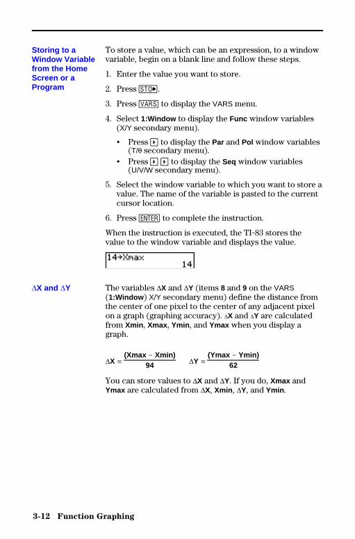
3-12 Function Graphing
8303FUNC.DOC TI-83 international English Bob Fedorisko Revised: 02/19/01 12:16 PM Printed: 02/19/01 1:35PM Page 12 of 288303FUNC.DOC TI-83 international English Bob Fedorisko Revised: 02/19/01 12:16 PM Printed: 02/19/01 1:35PM Page 12 of 28
To store a value, which can be an expression, to a windowvariable, begin on a blank line and follow these steps.
1. Enter the value you want to store.
2. Press ¿.
3. Press � to display the VARS menu.
4. Select 1:Window to display the Func window variables(X/Y secondary menu).
• Press ~ to display the Par and Pol window variables(T/q secondary menu).
• Press ~ ~ to display the Seq window variables(U/V/W secondary menu).
5. Select the window variable to which you want to store avalue. The name of the variable is pasted to the currentcursor location.
6. Press Í to complete the instruction.
When the instruction is executed, the TI-83 stores thevalue to the window variable and displays the value.
The variables @X and @Y (items 8 and 9 on the VARS(1:Window ) X/Y secondary menu) define the distance fromthe center of one pixel to the center of any adjacent pixelon a graph (graphing accuracy). @X and @Y are calculatedfrom Xmin , Xmax , Ymin , and Ymax when you display agraph.
@X = (Xmax N Xmin)
94 @Y = (Ymax N Ymin)
62
You can store values to @X and @Y. If you do, Xmax andYmax are calculated from @X, Xmin , @Y, and Ymin .
Storing to aWindow Variablefrom the HomeScreen or aProgram
@X and @Y
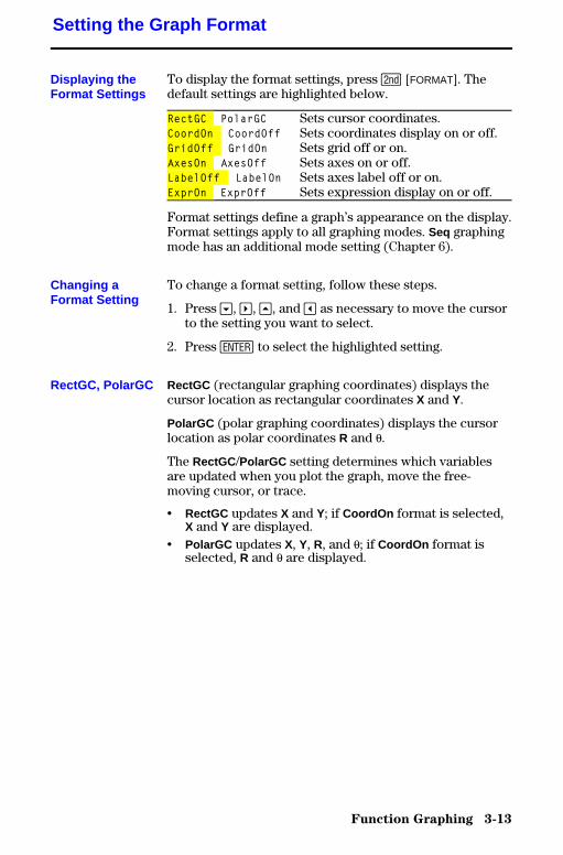
Function Graphing 3-13
8303FUNC.DOC TI-83 international English Bob Fedorisko Revised: 02/19/01 12:16 PM Printed: 02/19/01 1:35PM Page 13 of 28
To display the format settings, press y [FORMAT]. Thedefault settings are highlighted below.
RectGC PolarGC Sets cursor coordinates.CoordOn CoordOff Sets coordinates display on or off.GridOff GridOn Sets grid off or on.AxesOn AxesOff Sets axes on or off.LabelOff LabelOn Sets axes label off or on.ExprOn ExprOff Sets expression display on or off.
Format settings define a graph’s appearance on the display.Format settings apply to all graphing modes. Seq graphingmode has an additional mode setting (Chapter 6).
To change a format setting, follow these steps.
1. Press †, ~, }, and | as necessary to move the cursorto the setting you want to select.
2. Press Í to select the highlighted setting.
RectGC (rectangular graphing coordinates) displays thecursor location as rectangular coordinates X and Y.
PolarGC (polar graphing coordinates) displays the cursorlocation as polar coordinates R and q.
The RectGC /PolarGC setting determines which variablesare updated when you plot the graph, move the free-moving cursor, or trace.
• RectGC updates X and Y; if CoordOn format is selected,X and Y are displayed.
• PolarGC updates X, Y, R, and q; if CoordOn format isselected, R and q are displayed.
Setting the Graph Format
Displaying theFormat Settings
Changing aFormat Setting
RectGC, PolarGC
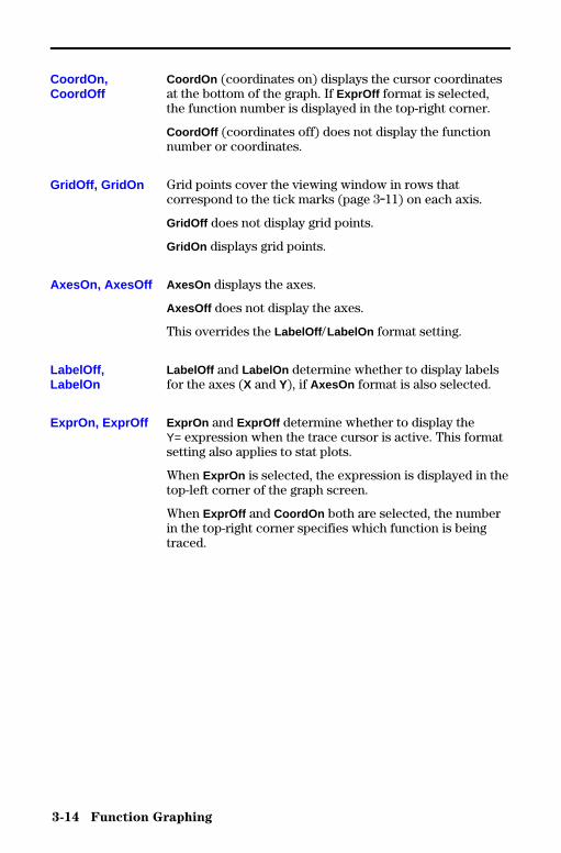
3-14 Function Graphing
8303FUNC.DOC TI-83 international English Bob Fedorisko Revised: 02/19/01 12:16 PM Printed: 02/19/01 1:35PM Page 14 of 288303FUNC.DOC TI-83 international English Bob Fedorisko Revised: 02/19/01 12:16 PM Printed: 02/19/01 1:35PM Page 14 of 28
CoordOn (coordinates on) displays the cursor coordinatesat the bottom of the graph. If ExprOff format is selected,the function number is displayed in the top-right corner.
CoordOff (coordinates off) does not display the functionnumber or coordinates.
Grid points cover the viewing window in rows thatcorrespond to the tick marks (page 3.11) on each axis.
GridOff does not display grid points.
GridOn displays grid points.
AxesOn displays the axes.
AxesOff does not display the axes.
This overrides the LabelOff /LabelOn format setting.
LabelOff and LabelOn determine whether to display labelsfor the axes (X and Y), if AxesOn format is also selected.
ExprOn and ExprOff determine whether to display theY= expression when the trace cursor is active. This formatsetting also applies to stat plots.
When ExprOn is selected, the expression is displayed in thetop-left corner of the graph screen.
When ExprOff and CoordOn both are selected, the numberin the top-right corner specifies which function is beingtraced.
CoordOn,CoordOff
GridOff, GridOn
AxesOn, AxesOff
LabelOff,LabelOn
ExprOn, ExprOff
Function Graphing 3-15
8303FUNC.DOC TI-83 international English Bob Fedorisko Revised: 02/19/01 12:16 PM Printed: 02/19/01 1:35PM Page 15 of 28
To display the graph of the selected function or functions,press s. TRACE, ZOOM instructions, and CALCoperations display the graph automatically. As the TI-83plots the graph, the busy indicator is on. As the graph isplotted, X and Y are updated.
While plotting a graph, you can pause or stop graphing.
• Press Í to pause; then press Í to resume.• Press É to stop; then press s to redraw.
Smart Graph is a TI-83 feature that redisplays the lastgraph immediately when you press s, but only if allgraphing factors that would cause replotting haveremained the same since the graph was last displayed.
If you performed any of these actions since the graph waslast displayed, the TI-83 will replot the graph based on newvalues when you press s.
• Changed a mode setting that affects graphs• Changed a function in the current picture• Selected or deselected a function or stat plot• Changed the value of a variable in a selected function• Changed a window variable or graph format setting• Cleared drawings by selecting ClrDraw
• Changed a stat plot definition
Displaying Graphs
Displaying a NewGraph
Pausing orStopping a Graph
Smart Graph

3-16 Function Graphing
8303FUNC.DOC TI-83 international English Bob Fedorisko Revised: 02/19/01 12:16 PM Printed: 02/19/01 1:35PM Page 16 of 288303FUNC.DOC TI-83 international English Bob Fedorisko Revised: 02/19/01 12:16 PM Printed: 02/19/01 1:35PM Page 16 of 28
On the TI-83, you can graph one or more new functionswithout replotting existing functions. For example, storesin(X) to Y1 in the Y= editor and press s. Then storecos(X) to Y2 and press s again. The function Y2 isgraphed on top of Y1, the original function.
If you enter a list (Chapter 11) as an element in anexpression, the TI-83 plots the function for each value inthe list, thereby graphing a family of curves. In Simulgraphing-order mode, it graphs all functions sequentiallyfor the first element in each list, and then for the second,and so on.
{2,4,6}sin(X) graphs three functions: 2 sin(X) , 4 sin(X) , and6 sin(X) .
{2,4,6}sin({1,2,3}X) graphs 2 sin(X) , 4 sin(2X) , and 6 sin(3X) .
Note: When using more than one list, the lists must have the samedimensions.
OverlayingFunctions on aGraph
Graphing aFamily of Curves
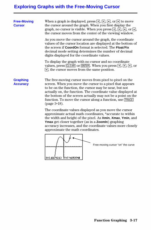
Function Graphing 3-17
8303FUNC.DOC TI-83 international English Bob Fedorisko Revised: 02/19/01 12:16 PM Printed: 02/19/01 1:35PM Page 17 of 28
When a graph is displayed, press |, ~, }, or † to movethe cursor around the graph. When you first display thegraph, no cursor is visible. When you press |, ~, }, or †,the cursor moves from the center of the viewing window.
As you move the cursor around the graph, the coordinatevalues of the cursor location are displayed at the bottom ofthe screen if CoordOn format is selected. The Float /Fixdecimal mode setting determines the number of decimaldigits displayed for the coordinate values.
To display the graph with no cursor and no coordinatevalues, press ‘ or Í. When you press |, ~, }, or†, the cursor moves from the same position.
The free-moving cursor moves from pixel to pixel on thescreen. When you move the cursor to a pixel that appearsto be on the function, the cursor may be near, but notactually on, the function. The coordinate value displayed atthe bottom of the screen actually may not be a point on thefunction. To move the cursor along a function, use r(page 3.18).
The coordinate values displayed as you move the cursorapproximate actual math coordinates, *accurate to withinthe width and height of the pixel. As Xmin , Xmax , Ymin , andYmax get closer together (as in a ZoomIn ) graphingaccuracy increases, and the coordinate values more closelyapproximate the math coordinates.
Exploring Graphs with the Free-Moving Cursor
Free-MovingCursor
GraphingAccuracy
Free-moving cursor “on” the curve
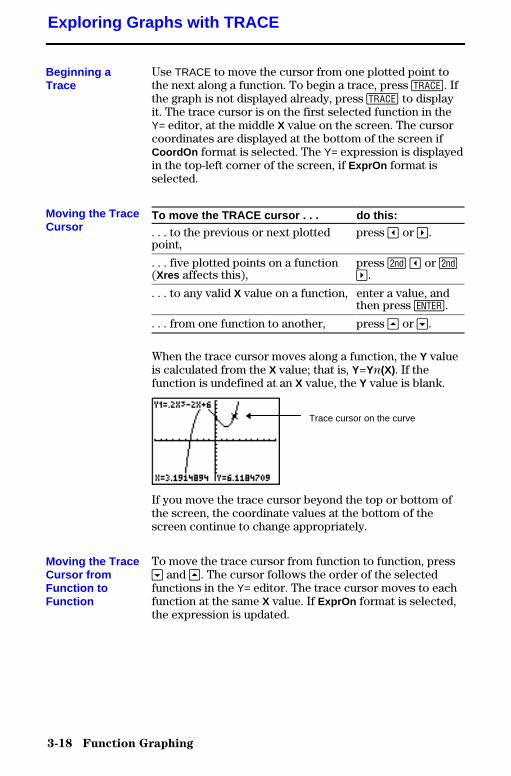
3-18 Function Graphing
8303FUNC.DOC TI-83 international English Bob Fedorisko Revised: 02/19/01 12:16 PM Printed: 02/19/01 1:35PM Page 18 of 288303FUNC.DOC TI-83 international English Bob Fedorisko Revised: 02/19/01 12:16 PM Printed: 02/19/01 1:35PM Page 18 of 28
Use TRACE to move the cursor from one plotted point tothe next along a function. To begin a trace, press r. Ifthe graph is not displayed already, press r to displayit. The trace cursor is on the first selected function in theY= editor, at the middle X value on the screen. The cursorcoordinates are displayed at the bottom of the screen ifCoordOn format is selected. The Y= expression is displayedin the top-left corner of the screen, if ExprOn format isselected.
To move the TRACE cursor . . . do this:
. . . to the previous or next plottedpoint,
press | or ~.
. . . five plotted points on a function(Xres affects this),
press y | or y~.
. . . to any valid X value on a function, enter a value, andthen press Í.
. . . from one function to another, press } or †.
When the trace cursor moves along a function, the Y valueis calculated from the X value; that is, Y=Yn(X). If thefunction is undefined at an X value, the Y value is blank.
If you move the trace cursor beyond the top or bottom ofthe screen, the coordinate values at the bottom of thescreen continue to change appropriately.
To move the trace cursor from function to function, press† and }. The cursor follows the order of the selectedfunctions in the Y= editor. The trace cursor moves to eachfunction at the same X value. If ExprOn format is selected,the expression is updated.
Exploring Graphs with TRACE
Beginning aTrace
Moving the TraceCursor
Moving the TraceCursor fromFunction toFunction
Trace cursor on the curve
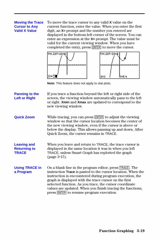
Function Graphing 3-19
8303FUNC.DOC TI-83 international English Bob Fedorisko Revised: 02/19/01 12:16 PM Printed: 02/19/01 1:35PM Page 19 of 28
To move the trace cursor to any valid X value on thecurrent function, enter the value. When you enter the firstdigit, an X= prompt and the number you entered aredisplayed in the bottom-left corner of the screen. You canenter an expression at the X= prompt. The value must bevalid for the current viewing window. When you havecompleted the entry, press Í to move the cursor.
Note: This feature does not apply to stat plots.
If you trace a function beyond the left or right side of thescreen, the viewing window automatically pans to the leftor right. Xmin and Xmax are updated to correspond to thenew viewing window.
While tracing, you can press Í to adjust the viewingwindow so that the cursor location becomes the center ofthe new viewing window, even if the cursor is above orbelow the display. This allows panning up and down. AfterQuick Zoom, the cursor remains in TRACE.
When you leave and return to TRACE, the trace cursor isdisplayed in the same location it was in when you leftTRACE, unless Smart Graph has replotted the graph(page 3.15).
On a blank line in the program editor, press r. Theinstruction Trace is pasted to the cursor location. When theinstruction is encountered during program execution, thegraph is displayed with the trace cursor on the firstselected function. As you trace, the cursor coordinatevalues are updated. When you finish tracing the functions,press Í to resume program execution.
Moving the TraceCursor to AnyValid X Value
Panning to theLeft or Right
Quick Zoom
Leaving andReturning toTRACE
Using TRACE ina Program
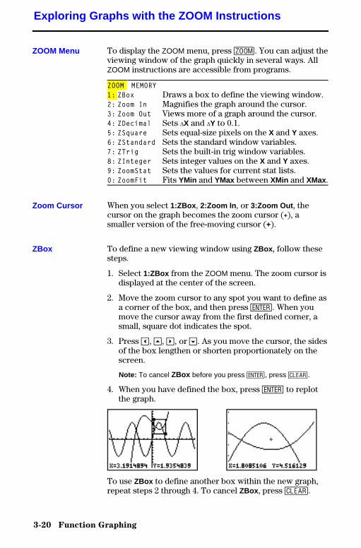
3-20 Function Graphing
8303FUNC.DOC TI-83 international English Bob Fedorisko Revised: 02/19/01 12:16 PM Printed: 02/19/01 1:35PM Page 20 of 288303FUNC.DOC TI-83 international English Bob Fedorisko Revised: 02/19/01 12:16 PM Printed: 02/19/01 1:35PM Page 20 of 28
To display the ZOOM menu, press q. You can adjust theviewing window of the graph quickly in several ways. AllZOOM instructions are accessible from programs.
ZOOM MEMORY1: ZBox Draws a box to define the viewing window.2: Zoom In Magnifies the graph around the cursor.3: Zoom Out Views more of a graph around the cursor.4: ZDecimal Sets @X and @Y to 0.1.5: ZSquare Sets equal-size pixels on the X and Y axes.6: ZStandard Sets the standard window variables.7: ZTrig Sets the built-in trig window variables.8: ZInteger Sets integer values on the X and Y axes.9: ZoomStat Sets the values for current stat lists.0: ZoomFit Fits YMin and YMax between XMin and XMax.
When you select 1:ZBox , 2:Zoom In , or 3:Zoom Out , thecursor on the graph becomes the zoom cursor (+), asmaller version of the free-moving cursor (+).
To define a new viewing window using ZBox , follow thesesteps.
1. Select 1:ZBox from the ZOOM menu. The zoom cursor isdisplayed at the center of the screen.
2. Move the zoom cursor to any spot you want to define asa corner of the box, and then press Í. When youmove the cursor away from the first defined corner, asmall, square dot indicates the spot.
3. Press |, }, ~, or †. As you move the cursor, the sidesof the box lengthen or shorten proportionately on thescreen.
Note: To cancel ZBox before you press Í, press ‘.
4. When you have defined the box, press Í to replotthe graph.
To use ZBox to define another box within the new graph,repeat steps 2 through 4. To cancel ZBox , press ‘.
Exploring Graphs with the ZOOM Instructions
ZOOM Menu
Zoom Cursor
ZBox
Function Graphing 3-21
8303FUNC.DOC TI-83 international English Bob Fedorisko Revised: 02/19/01 12:16 PM Printed: 02/19/01 1:35PM Page 21 of 28
Zoom In magnifies the part of the graph that surrounds thecursor location. Zoom Out displays a greater portion of thegraph, centered on the cursor location. The XFact andYFact settings determine the extent of the zoom.
To zoom in on a graph, follow these steps.
1. Check XFact and YFact (page 3.24); change as needed.
2. Select 2:Zoom In from the ZOOM menu. The zoomcursor is displayed.
3. Move the zoom cursor to the point that is to be thecenter of the new viewing window.
4. Press Í. The TI-83 adjusts the viewing window byXFact and YFact ; updates the window variables; andreplots the selected functions, centered on the cursorlocation.
5. Zoom in on the graph again in either of two ways.• To zoom in at the same point, press Í.• To zoom in at a new point, move the cursor to the
point that you want as the center of the new viewingwindow, and then press Í.
To zoom out on a graph, select 3:Zoom Out and repeatsteps 3 through 5.
To cancel Zoom In or Zoom Out , press ‘.
ZDecimal replots the functions immediately. It updates thewindow variables to preset values, as shown below. Thesevalues set @X and @Y equal to 0.1 and set the X and Y valueof each pixel to one decimal place.
Xmin= L4.7 Ymin= L3.1Xmax=4.7 Ymax=3.1Xscl=1 Yscl=1
ZSquare replots the functions immediately. It redefines theviewing window based on the current values of thewindow variables. It adjusts in only one direction so that@X=@Y, which makes the graph of a circle look like a circle.Xscl and Yscl remain unchanged. The midpoint of thecurrent graph (not the intersection of the axes) becomesthe midpoint of the new graph.
Zoom In,Zoom Out
ZDecimal
ZSquare
3-22 Function Graphing
8303FUNC.DOC TI-83 international English Bob Fedorisko Revised: 02/19/01 12:16 PM Printed: 02/19/01 1:35PM Page 22 of 288303FUNC.DOC TI-83 international English Bob Fedorisko Revised: 02/19/01 12:16 PM Printed: 02/19/01 1:35PM Page 22 of 28
ZStandard replots the functions immediately. It updates thewindow variables to the standard values shown below.
Xmin= L10 Ymin= L10 Xres=1Xmax=10 Ymax=10Xscl=1 Yscl=1
ZTrig replots the functions immediately. It updates thewindow variables to preset values that are appropriate forplotting trig functions. Those preset values in Radian modeare shown below.
Xmin= L(47à24)p Ymin= L4Xmax=(47à24)p Ymax=4Xscl= p/2 Yscl=1
ZInteger redefines the viewing window to the dimensionsshown below. To use ZInteger , move the cursor to the pointthat you want to be the center of the new window, andthen press Í; ZInteger replots the functions.
@X=1 Xscl=10@Y=1 Yscl=10
ZoomStat redefines the viewing window so that allstatistical data points are displayed. For regular andmodified box plots, only Xmin and Xmax are adjusted.
ZoomFit replots the functions immediately. ZoomFitrecalculates YMin and YMax to include the minimum andmaximum Y values of the selected functions between thecurrent XMin and XMax. XMin and XMax are not changed.
ZStandard
ZTrig
ZInteger
ZoomStat
ZoomFit
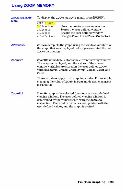
Function Graphing 3-23
8303FUNC.DOC TI-83 international English Bob Fedorisko Revised: 02/19/01 12:16 PM Printed: 02/19/01 1:35PM Page 23 of 28
To display the ZOOM MEMORY menu, press q ~.
ZOOM MEMORY1:ZPrevious Uses the previous viewing window.2:ZoomSto Stores the user-defined window.3:ZoomRcl Recalls the user-defined window.4:SetFactors... Changes Zoom In and Zoom Out factors.
ZPrevious replots the graph using the window variables ofthe graph that was displayed before you executed the lastZOOM instruction.
ZoomSto immediately stores the current viewing window.The graph is displayed, and the values of the currentwindow variables are stored in the user-defined ZOOMvariables ZXmin , ZXmax , ZXscl , ZYmin , ZYmax , ZYscl , andZXres .
These variables apply to all graphing modes. For example,changing the value of ZXmin in Func mode also changes itin Par mode.
ZoomRcl graphs the selected functions in a user-definedviewing window. The user-defined viewing window isdetermined by the values stored with the ZoomStoinstruction. The window variables are updated with theuser-defined values, and the graph is plotted.
Using ZOOM MEMORY
ZOOM MEMORYMenu
ZPrevious
ZoomSto
ZoomRcl
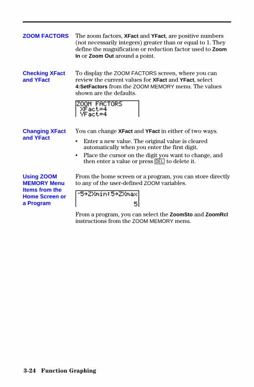
3-24 Function Graphing
8303FUNC.DOC TI-83 international English Bob Fedorisko Revised: 02/19/01 12:16 PM Printed: 02/19/01 1:35PM Page 24 of 288303FUNC.DOC TI-83 international English Bob Fedorisko Revised: 02/19/01 12:16 PM Printed: 02/19/01 1:35PM Page 24 of 28
The zoom factors, XFact and YFact , are positive numbers(not necessarily integers) greater than or equal to 1. Theydefine the magnification or reduction factor used to ZoomIn or Zoom Out around a point.
To display the ZOOM FACTORS screen, where you canreview the current values for XFact and YFact , select4:SetFactors from the ZOOM MEMORY menu. The valuesshown are the defaults.
You can change XFact and YFact in either of two ways.
• Enter a new value. The original value is clearedautomatically when you enter the first digit.
• Place the cursor on the digit you want to change, andthen enter a value or press { to delete it.
From the home screen or a program, you can store directlyto any of the user-defined ZOOM variables.
From a program, you can select the ZoomSto and ZoomRclinstructions from the ZOOM MEMORY menu.
ZOOM FACTORS
Checking XFactand YFact
Changing XFactand YFact
Using ZOOMMEMORY MenuItems from theHome Screen ora Program
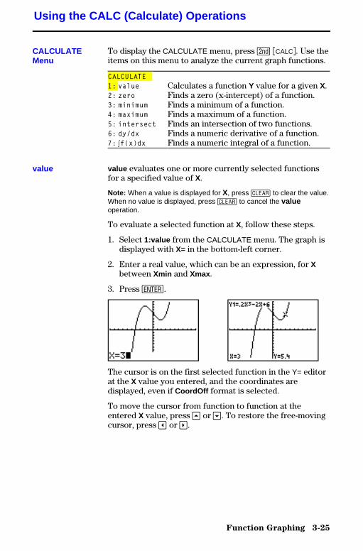
Function Graphing 3-25
8303FUNC.DOC TI-83 international English Bob Fedorisko Revised: 02/19/01 12:16 PM Printed: 02/19/01 1:35PM Page 25 of 28
To display the CALCULATE menu, press y ãCALCä. Use theitems on this menu to analyze the current graph functions.
CALCULATE1: value Calculates a function Y value for a given X.2: zero Finds a zero (x-intercept) of a function.3: minimum Finds a minimum of a function.4: maximum Finds a maximum of a function.5: intersect Finds an intersection of two functions.6: dy/dx Finds a numeric derivative of a function.7: ‰f(x)dx Finds a numeric integral of a function.
value evaluates one or more currently selected functionsfor a specified value of X.
Note: When a value is displayed for X, press ‘ to clear the value.When no value is displayed, press ‘ to cancel the valueoperation.
To evaluate a selected function at X, follow these steps.
1. Select 1:value from the CALCULATE menu. The graph isdisplayed with X= in the bottom-left corner.
2. Enter a real value, which can be an expression, for Xbetween Xmin and Xmax .
3. Press Í.
The cursor is on the first selected function in the Y= editorat the X value you entered, and the coordinates aredisplayed, even if CoordOff format is selected.
To move the cursor from function to function at theentered X value, press } or †. To restore the free-movingcursor, press | or ~.
Using the CALC (Calculate) Operations
CALCULATEMenu
value

3-26 Function Graphing
8303FUNC.DOC TI-83 international English Bob Fedorisko Revised: 02/19/01 12:16 PM Printed: 02/19/01 1:35PM Page 26 of 288303FUNC.DOC TI-83 international English Bob Fedorisko Revised: 02/19/01 12:16 PM Printed: 02/19/01 1:35PM Page 26 of 28
zero finds a zero (x-intercept or root) of a function usingsolve( . Functions can have more than one x-interceptvalue; zero finds the zero closest to your guess.
The time zero spends to find the correct zero valuedepends on the accuracy of the values you specify for theleft and right bounds and the accuracy of your guess.
To find a zero of a function, follow these steps.
1. Select 2:zero from the CALCULATE menu. The currentgraph is displayed with Left Bound? in the bottom-leftcorner.
2. Press } or † to move the cursor onto the function forwhich you want to find a zero.
3. Press | or ~ (or enter a value) to select the x-value forthe left bound of the interval, and then press Í. A 4indicator on the graph screen shows the left bound.Right Bound? is displayed in the bottom-left corner.Press | or ~ (or enter a value) to select the x-value forthe right bound, and then press Í. A 3 indicator onthe graph screen shows the right bound. Guess? is thendisplayed in the bottom-left corner.
4. Press | or ~ (or enter a value) to select a point nearthe zero of the function, between the bounds, and thenpress Í.
The cursor is on the solution and the coordinates aredisplayed, even if CoordOff format is selected. To move tothe same x-value for other selected functions, press } or†. To restore the free-moving cursor, press | or ~.
zero
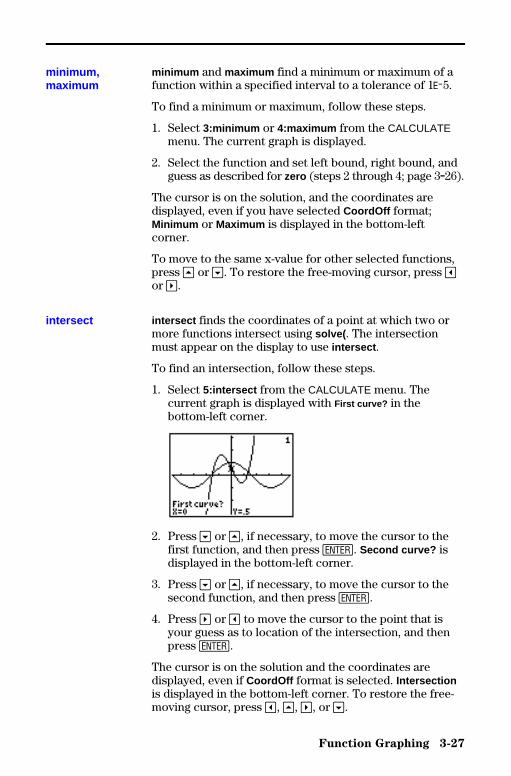
Function Graphing 3-27
8303FUNC.DOC TI-83 international English Bob Fedorisko Revised: 02/19/01 12:16 PM Printed: 02/19/01 1:35PM Page 27 of 28
minimum and maximum find a minimum or maximum of afunction within a specified interval to a tolerance of 1âL5.
To find a minimum or maximum, follow these steps.
1. Select 3:minimum or 4:maximum from the CALCULATEmenu. The current graph is displayed.
2. Select the function and set left bound, right bound, andguess as described for zero (steps 2 through 4; page 3.26).
The cursor is on the solution, and the coordinates aredisplayed, even if you have selected CoordOff format;Minimum or Maximum is displayed in the bottom-leftcorner.
To move to the same x-value for other selected functions,press } or †. To restore the free-moving cursor, press |or ~.
intersect finds the coordinates of a point at which two ormore functions intersect using solve( . The intersectionmust appear on the display to use intersect .
To find an intersection, follow these steps.
1. Select 5:intersect from the CALCULATE menu. Thecurrent graph is displayed with First curve? in thebottom-left corner.
2. Press † or }, if necessary, to move the cursor to thefirst function, and then press Í. Second curve? isdisplayed in the bottom-left corner.
3. Press † or }, if necessary, to move the cursor to thesecond function, and then press Í.
4. Press ~ or | to move the cursor to the point that isyour guess as to location of the intersection, and thenpress Í.
The cursor is on the solution and the coordinates aredisplayed, even if CoordOff format is selected. Intersectionis displayed in the bottom-left corner. To restore the free-moving cursor, press |, }, ~, or †.
minimum,maximum
intersect
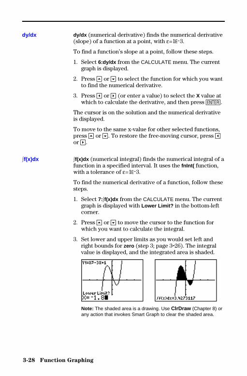
3-28 Function Graphing
8303FUNC.DOC TI-83 international English Bob Fedorisko Revised: 02/19/01 12:16 PM Printed: 02/19/01 1:35PM Page 28 of 288303FUNC.DOC TI-83 international English Bob Fedorisko Revised: 02/19/01 12:16 PM Printed: 02/19/01 1:35PM Page 28 of 28
dy/dx (numerical derivative) finds the numerical derivative(slope) of a function at a point, with H=1âL3.
To find a function’s slope at a point, follow these steps.
1. Select 6:dy/dx from the CALCULATE menu. The currentgraph is displayed.
2. Press } or † to select the function for which you wantto find the numerical derivative.
3. Press | or ~ (or enter a value) to select the X value atwhich to calculate the derivative, and then press Í.
The cursor is on the solution and the numerical derivativeis displayed.
To move to the same x-value for other selected functions,press } or †. To restore the free-moving cursor, press |or ~.
‰f(x)dx (numerical integral) finds the numerical integral of afunction in a specified interval. It uses the fnInt( function,with a tolerance of H=1âL3.
To find the numerical derivative of a function, follow thesesteps.
1. Select 7:‰f(x)dx from the CALCULATE menu. The currentgraph is displayed with Lower Limit? in the bottom-leftcorner.
2. Press } or † to move the cursor to the function forwhich you want to calculate the integral.
3. Set lower and upper limits as you would set left andright bounds for zero (step 3; page 3.26). The integralvalue is displayed, and the integrated area is shaded.
Note: The shaded area is a drawing. Use ClrDraw (Chapter 8) orany action that invokes Smart Graph to clear the shaded area.
dy/dx
‰f(x)dx
Parametric Graphing 4-1
8304PARA.DOC TI-83 international English Bob Fedorisko Revised: 02/19/01 12:17 PM Printed: 02/19/01 1:36PM Page 1 of 8
4 ParametricGraphin g
Getting Started: Path of a Ball ........................... 4-2Defining and Displaying Parametric Graphs.............. 4-4Exploring Parametric Graphs ............................ 4-7
Contents
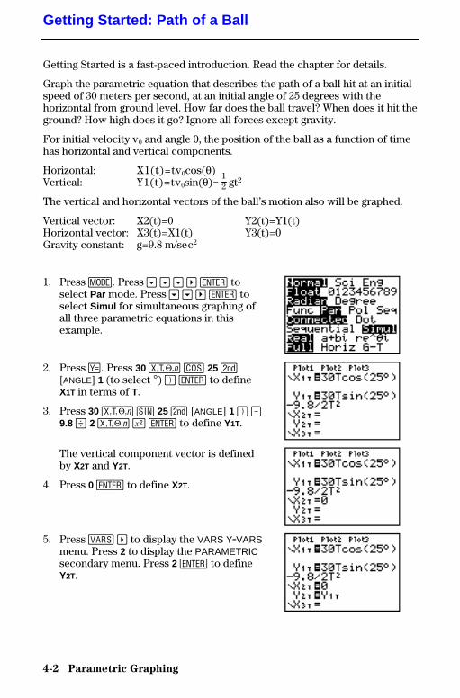
4-2 Parametric Graphing
8304PARA.DOC TI-83 international English Bob Fedorisko Revised: 02/19/01 12:17 PM Printed: 02/19/01 1:36PM Page 2 of 8
Getting Started is a fast-paced introduction. Read the chapter for details.
Graph the parametric equation that describes the path of a ball hit at an initialspeed of 30 meters per second, at an initial angle of 25 degrees with thehorizontal from ground level. How far does the ball travel? When does it hit theground? How high does it go? Ignore all forces except gravity.
For initial velocity v0 and angle q, the position of the ball as a function of timehas horizontal and vertical components.
Horizontal: X1(t)=tv0cos(q)Vertical: Y1(t)=tv0sin(q)N
12 gt2
The vertical and horizontal vectors of the ball’s motion also will be graphed.
Vertical vector: X2(t)=0 Y2(t)=Y1(t)Horizontal vector: X3(t)=X1(t) Y3(t)=0Gravity constant: g=9.8 m/sec2
1. Press z. Press † † † ~ Í toselect Par mode. Press † † ~ Í toselect Simul for simultaneous graphing ofall three parametric equations in thisexample.
2. Press o. Press 30 „ ™ 25 y[ANGLE] 1 (to select ¡) ¤ Í to defineX1T in terms of T.
3. Press 30 „ ˜ 25 y [ANGLE] 1 ¤ ¹9.8 ¥ 2 „ ¡ Í to define Y1T.
The vertical component vector is definedby X2T and Y2T.
4. Press 0 Í to define X2T.
5. Press � ~ to display the VARS Y.VARSmenu. Press 2 to display the PARAMETRICsecondary menu. Press 2 Í to defineY2T.
Getting Started: Path of a Ball
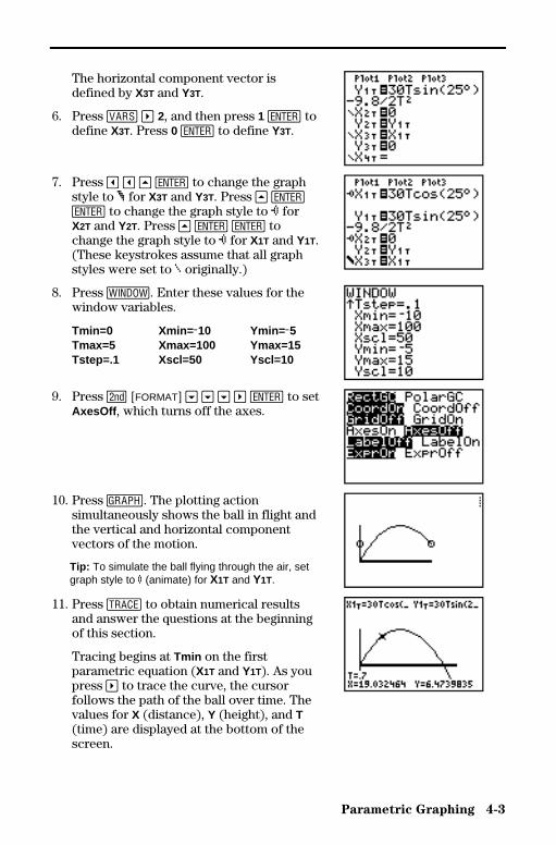
Parametric Graphing 4-3
8304PARA.DOC TI-83 international English Bob Fedorisko Revised: 02/19/01 12:17 PM Printed: 02/19/01 1:36PM Page 3 of 8
The horizontal component vector isdefined by X3T and Y3T.
6. Press � ~ 2, and then press 1 Í todefine X3T. Press 0 Í to define Y3T.
7. Press | | } Í to change the graphstyle to è for X3T and Y3T. Press } ÍÍ to change the graph style to ë forX2T and Y2T. Press } Í Í tochange the graph style to ë for X1T and Y1T.(These keystrokes assume that all graphstyles were set to ç originally.)
8. Press p. Enter these values for thewindow variables.
Tmin=0 Xmin= L10 Ymin= L5Tmax=5 Xmax=100 Ymax=15Tstep=.1 Xscl=50 Yscl=10
9. Press y [FORMAT] † † † ~ Í to setAxesOff , which turns off the axes.
10. Press s. The plotting actionsimultaneously shows the ball in flight andthe vertical and horizontal componentvectors of the motion.
Tip: To simulate the ball flying through the air, setgraph style to ì (animate) for X1T and Y1T.
11. Press r to obtain numerical resultsand answer the questions at the beginningof this section.
Tracing begins at Tmin on the firstparametric equation (X1T and Y1T). As youpress ~ to trace the curve, the cursorfollows the path of the ball over time. Thevalues for X (distance), Y (height), and T(time) are displayed at the bottom of thescreen.
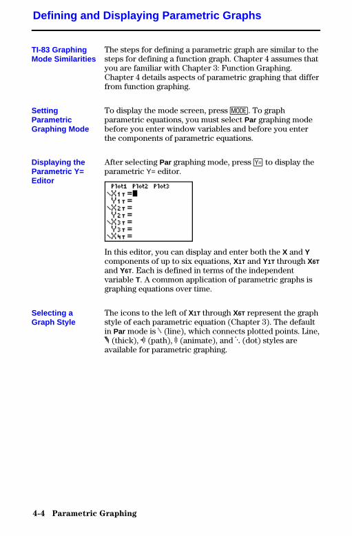
4-4 Parametric Graphing
8304PARA.DOC TI-83 international English Bob Fedorisko Revised: 02/19/01 12:17 PM Printed: 02/19/01 1:36PM Page 4 of 8
The steps for defining a parametric graph are similar to thesteps for defining a function graph. Chapter 4 assumes thatyou are familiar with Chapter 3: Function Graphing.Chapter 4 details aspects of parametric graphing that differfrom function graphing.
To display the mode screen, press z. To graphparametric equations, you must select Par graphing modebefore you enter window variables and before you enterthe components of parametric equations.
After selecting Par graphing mode, press o to display theparametric Y= editor.
In this editor, you can display and enter both the X and Ycomponents of up to six equations, X1T and Y1T through X6T
and Y6T. Each is defined in terms of the independentvariable T. A common application of parametric graphs isgraphing equations over time.
The icons to the left of X1T through X6T represent the graphstyle of each parametric equation (Chapter 3). The defaultin Par mode is ç (line), which connects plotted points. Line,è (thick), ë (path), ì (animate), and í (dot) styles areavailable for parametric graphing.
Defining and Displaying Parametric Graphs
TI-83 GraphingMode Similarities
SettingParametricGraphing Mode
Displaying theParametric Y=Editor
Selecting aGraph Style

Parametric Graphing 4-5
8304PARA.DOC TI-83 international English Bob Fedorisko Revised: 02/19/01 12:17 PM Printed: 02/19/01 1:36PM Page 5 of 8
To define or edit a parametric equation, follow the steps inChapter 3 for defining a function or editing a function. Theindependent variable in a parametric equation is T. In Pargraphing mode, you can enter the parametric variable T ineither of two ways.
• Press „.• Press ƒ ãTä.
Two components, X and Y, define a single parametricequation. You must define both of them.
The TI-83 graphs only the selected parametric equations.In the Y= editor, a parametric equation is selected when the= signs of both the X and Y components are highlighted.You may select any or all of the equations X1T and Y1T
through X6T and Y6T.
To change the selection status, move the cursor onto the =sign of either the X or Y component and press Í. Thestatus of both the X and Y components is changed.
To display the window variable values, press p.These variables define the viewing window. The valuesbelow are defaults for Par graphing in Radian angle mode.
Tmin=0 Smallest T value to evaluateTmax=6.2831853... Largest T value to evaluate (2p)Tstep=.1308996... T value increment (pà24)Xmin=L10 Smallest X value to be displayedXmax=10 Largest X value to be displayedXscl=1 Spacing between the X tick marksYmin=L10 Smallest Y value to be displayedYmax=10 Largest Y value to be displayedYscl=1 Spacing between the Y tick marks
Note: To ensure that sufficient points are plotted, you may want tochange the T window variables.
Defining andEditingParametricEquations
Selecting andDeselectingParametricEquations
Setting WindowVariables
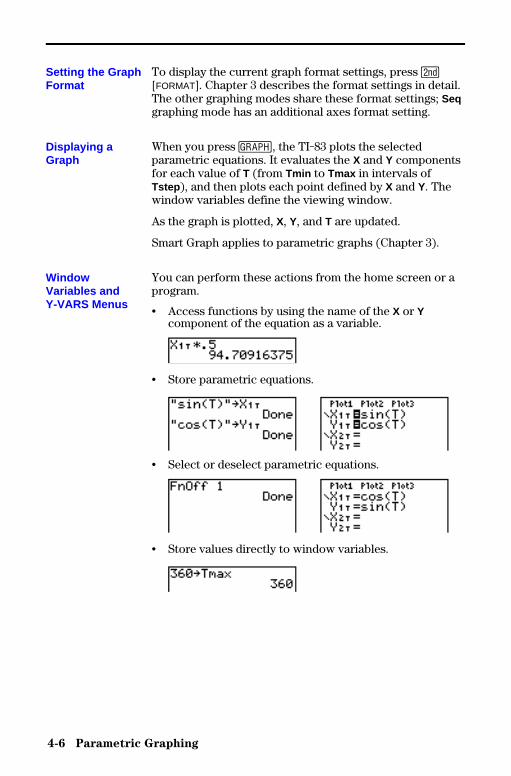
4-6 Parametric Graphing
8304PARA.DOC TI-83 international English Bob Fedorisko Revised: 02/19/01 12:17 PM Printed: 02/19/01 1:36PM Page 6 of 8
To display the current graph format settings, press y[FORMAT]. Chapter 3 describes the format settings in detail.The other graphing modes share these format settings; Seqgraphing mode has an additional axes format setting.
When you press s, the TI-83 plots the selectedparametric equations. It evaluates the X and Y componentsfor each value of T (from Tmin to Tmax in intervals ofTstep ), and then plots each point defined by X and Y. Thewindow variables define the viewing window.
As the graph is plotted, X, Y, and T are updated.
Smart Graph applies to parametric graphs (Chapter 3).
You can perform these actions from the home screen or aprogram.
• Access functions by using the name of the X or Ycomponent of the equation as a variable.
• Store parametric equations.
• Select or deselect parametric equations.
• Store values directly to window variables.
Setting the GraphFormat
Displaying aGraph
WindowVariables andY-VARS Menus
Parametric Graphing 4-7
8304PARA.DOC TI-83 international English Bob Fedorisko Revised: 02/19/01 12:17 PM Printed: 02/19/01 1:36PM Page 7 of 8
The free-moving cursor in Par graphing works the same asin Func graphing.
In RectGC format, moving the cursor updates the values ofX and Y; if CoordOn format is selected, X and Y aredisplayed.
In PolarGC format, X, Y, R, and q are updated; if CoordOnformat is selected, R and q are displayed.
To activate TRACE, press r. When TRACE is active,you can move the trace cursor along the graph of theequation one Tstep at a time. When you begin a trace, thetrace cursor is on the first selected function at Tmin . IfExprOn is selected, then the function is displayed.
In RectGC format, TRACE updates and displays the valuesof X, Y, and T if CoordOn format is on.
In PolarGC format, X, Y, R, q and T are updated; if CoordOnformat is selected, R, q, and T are displayed. The X and Y(or R and q) values are calculated from T.
To move five plotted points at a time on a function, pressy | or y ~. If you move the cursor beyond the top orbottom of the screen, the coordinate values at the bottomof the screen continue to change appropriately.
Quick Zoom is available in Par graphing; panning is not(Chapter 3).
Exploring Parametric Graphs
Free-MovingCursor
TRACE
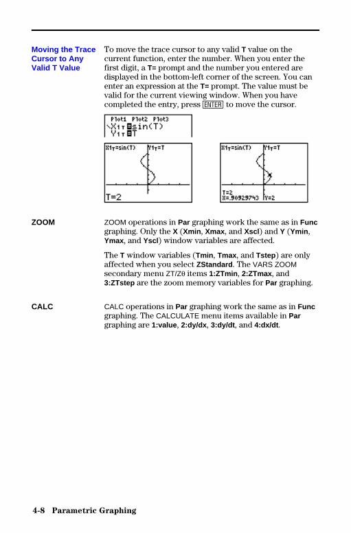
4-8 Parametric Graphing
8304PARA.DOC TI-83 international English Bob Fedorisko Revised: 02/19/01 12:17 PM Printed: 02/19/01 1:36PM Page 8 of 8
To move the trace cursor to any valid T value on thecurrent function, enter the number. When you enter thefirst digit, a T= prompt and the number you entered aredisplayed in the bottom-left corner of the screen. You canenter an expression at the T= prompt. The value must bevalid for the current viewing window. When you havecompleted the entry, press Í to move the cursor.
ZOOM operations in Par graphing work the same as in Funcgraphing. Only the X (Xmin , Xmax , and Xscl ) and Y (Ymin ,Ymax , and Yscl ) window variables are affected.
The T window variables (Tmin , Tmax , and Tstep ) are onlyaffected when you select ZStandard . The VARS ZOOMsecondary menu ZT/Zq items 1:ZTmin , 2:ZTmax , and3:ZTstep are the zoom memory variables for Par graphing.
CALC operations in Par graphing work the same as in Funcgraphing. The CALCULATE menu items available in Pargraphing are 1:value , 2:dy/dx , 3:dy/dt , and 4:dx/dt .
Moving the TraceCursor to AnyValid T Value
ZOOM
CALC
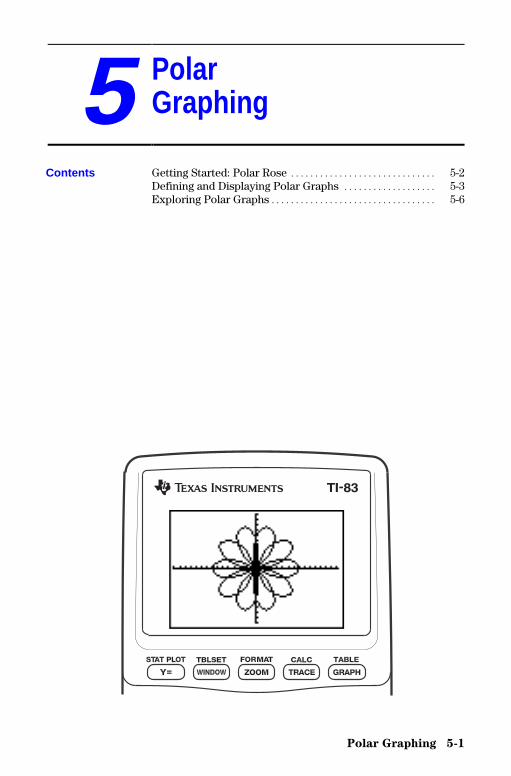
Polar Graphing 5-1
8305POLR.DOC TI-83 international English Bob Fedorisko Revised: 02/19/01 12:19 PM Printed: 02/19/01 1:36PM Page 1 of 6
5 PolarGraphin g
Getting Started: Polar Rose .............................. 5-2Defining and Displaying Polar Graphs ................... 5-3Exploring Polar Graphs.................................. 5-6
Contents
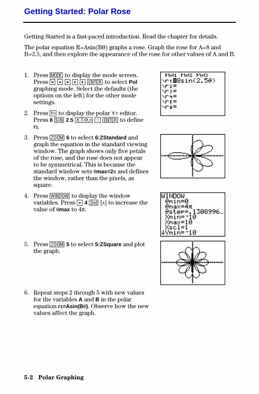
5-2 Polar Graphing
8305POLR.DOC TI-83 international English Bob Fedorisko Revised: 02/19/01 12:19 PM Printed: 02/19/01 1:36PM Page 2 of 6
Getting Started is a fast-paced introduction. Read the chapter for details.
The polar equation R=Asin(Bq) graphs a rose. Graph the rose for A=8 andB=2.5, and then explore the appearance of the rose for other values of A and B.
1. Press z to display the mode screen.Press † † † ~ ~ Í to select Polgraphing mode. Select the defaults (theoptions on the left) for the other modesettings.
2. Press o to display the polar Y= editor.Press 8 ˜ 2.5 „ ¤ Í to definer1.
3. Press q 6 to select 6:ZStandard andgraph the equation in the standard viewingwindow. The graph shows only five petalsof the rose, and the rose does not appearto be symmetrical. This is because thestandard window sets qmax=2p and definesthe window, rather than the pixels, assquare.
4. Press p to display the windowvariables. Press † 4 y [p] to increase thevalue of qmax to 4p.
5. Press q 5 to select 5:ZSquare and plotthe graph.
6. Repeat steps 2 through 5 with new valuesfor the variables A and B in the polarequation r1=Asin(B q). Observe how the newvalues affect the graph.
Getting Started: Polar Rose
Polar Graphing 5-3
8305POLR.DOC TI-83 international English Bob Fedorisko Revised: 02/19/01 12:19 PM Printed: 02/19/01 1:36PM Page 3 of 6
The steps for defining a polar graph are similar to the stepsfor defining a function graph. Chapter 5 assumes that youare familiar with Chapter 3: Function Graphing. Chapter 5details aspects of polar graphing that differ from functiongraphing.
To display the mode screen, press z. To graph polarequations, you must select Pol graphing mode before youenter values for the window variables and before you enterpolar equations.
After selecting Pol graphing mode, press o to display thepolar Y= editor.
In this editor, you can enter and display up to six polarequations, r1 through r6. Each is defined in terms of theindependent variable q (page 5.4).
The icons to the left of r1 through r6 represent the graphstyle of each polar equation (Chapter 3). The default in Polgraphing mode is ç (line), which connects plotted points.Line, è (thick), ë (path), ì (animate), and í (dot) styles areavailable for polar graphing.
Defining and Displaying Polar Graphs
TI-83 GraphingMode Similarities
Setting PolarGraphing Mode
Displaying thePolar Y= Editor
Selecting GraphStyles
5-4 Polar Graphing
8305POLR.DOC TI-83 international English Bob Fedorisko Revised: 02/19/01 12:19 PM Printed: 02/19/01 1:36PM Page 4 of 6
To define or edit a polar equation, follow the steps inChapter 3 for defining a function or editing a function. Theindependent variable in a polar equation is q. In Polgraphing mode, you can enter the polar variable q in eitherof two ways.
• Press „.• Press ƒ ãqä.
The TI-83 graphs only the selected polar equations. In theY= editor, a polar equation is selected when the = sign ishighlighted. You may select any or all of the equations.
To change the selection status, move the cursor onto the= sign, and then press Í.
To display the window variable values, press p.These variables define the viewing window. The valuesbelow are defaults for Pol graphing in Radian angle mode.
qmin=0 Smallest q value to evaluateqmax=6.2831853... Largest q value to evaluate (2p)qstep=.1308996... Increment between q values (pà24)Xmin=L10 Smallest X value to be displayedXmax=10 Largest X value to be displayedXscl=1 Spacing between the X tick marksYmin=L10 Smallest Y value to be displayedYmax=10 Largest Y value to be displayedYscl=1 Spacing between the Y tick marks
Note: To ensure that sufficient points are plotted, you may want tochange the q window variables.
Defining andEditing PolarEquations
Selecting andDeselecting PolarEquations
Setting WindowVariables
Polar Graphing 5-5
8305POLR.DOC TI-83 international English Bob Fedorisko Revised: 02/19/01 12:19 PM Printed: 02/19/01 1:36PM Page 5 of 6
To display the current graph format settings, press y[FORMAT]. Chapter 3 describes the format settings in detail.The other graphing modes share these format settings.
When you press s, the TI-83 plots the selected polarequations. It evaluates R for each value of q (from qmin toqmax in intervals of qstep ) and then plots each point. Thewindow variables define the viewing window.
As the graph is plotted, X, Y, R, and q are updated.
Smart Graph applies to polar graphs (Chapter 3).
You can perform these actions from the home screen or aprogram.
• Access functions by using the name of the equation as avariable.
• Store polar equations.
• Select or deselect polar equations.
• Store values directly to window variables.
Setting the GraphFormat
Displaying aGraph
WindowVariables andY.VARS Menus
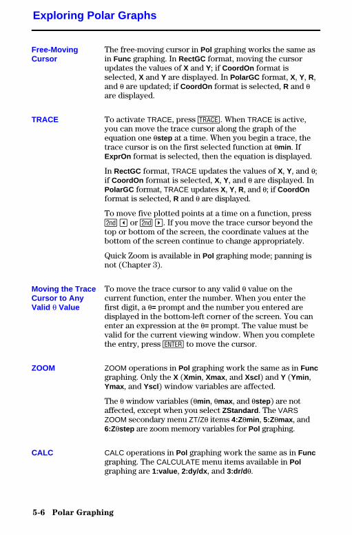
5-6 Polar Graphing
8305POLR.DOC TI-83 international English Bob Fedorisko Revised: 02/19/01 12:19 PM Printed: 02/19/01 1:36PM Page 6 of 6
The free-moving cursor in Pol graphing works the same asin Func graphing. In RectGC format, moving the cursorupdates the values of X and Y; if CoordOn format isselected, X and Y are displayed. In PolarGC format, X, Y, R,and q are updated; if CoordOn format is selected, R and qare displayed.
To activate TRACE, press r. When TRACE is active,you can move the trace cursor along the graph of theequation one qstep at a time. When you begin a trace, thetrace cursor is on the first selected function at qmin . IfExprOn format is selected, then the equation is displayed.
In RectGC format, TRACE updates the values of X, Y, and q;if CoordOn format is selected, X, Y, and q are displayed. InPolarGC format, TRACE updates X, Y, R, and q; if CoordOnformat is selected, R and q are displayed.
To move five plotted points at a time on a function, pressy | or y ~. If you move the trace cursor beyond thetop or bottom of the screen, the coordinate values at thebottom of the screen continue to change appropriately.
Quick Zoom is available in Pol graphing mode; panning isnot (Chapter 3).
To move the trace cursor to any valid q value on thecurrent function, enter the number. When you enter thefirst digit, a q= prompt and the number you entered aredisplayed in the bottom-left corner of the screen. You canenter an expression at the q= prompt. The value must bevalid for the current viewing window. When you completethe entry, press Í to move the cursor.
ZOOM operations in Pol graphing work the same as in Funcgraphing. Only the X (Xmin , Xmax , and Xscl ) and Y (Ymin ,Ymax , and Yscl ) window variables are affected.
The q window variables (qmin , qmax , and qstep ) are notaffected, except when you select ZStandard . The VARSZOOM secondary menu ZT/Zq items 4:Zqmin , 5:Zqmax , and6:Zqstep are zoom memory variables for Pol graphing.
CALC operations in Pol graphing work the same as in Funcgraphing. The CALCULATE menu items available in Polgraphing are 1:value , 2:dy/dx , and 3:dr/d q.
Exploring Polar Graphs
Free-MovingCursor
TRACE
Moving the TraceCursor to AnyValid q Value
ZOOM
CALC
Sequence Graphing 6-1
8306SEQN.DOC TI-83 international English Bob Fedorisko Revised: 02/19/01 12:22 PM Printed: 02/19/01 1:36PM Page 1 of 16
6 SequenceGraphin g
Getting Started: Forest and Trees ........................ 6-2Defining and Displaying Sequence Graphs ............... 6-3Selecting Axes Combinations ............................ 6-8Exploring Sequence Graphs.............................. 6-9Graphing Web Plots...................................... 6-11Using Web Plots to Illustrate Convergence............... 6-12Graphing Phase Plots .................................... 6-13Comparing TI-83 and TI.82 Sequence Variables .......... 6-15Keystroke Differences Between TI-83 and TI-82 ......... 6-16
Contents
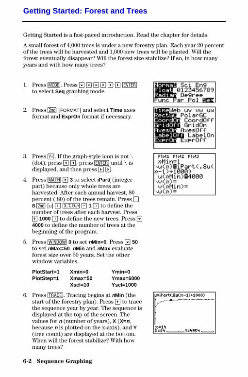
6-2 Sequence Graphing
8306SEQN.DOC TI-83 international English Bob Fedorisko Revised: 02/19/01 12:22 PM Printed: 02/19/01 1:36PM Page 2 of 16
Getting Started is a fast-paced introduction. Read the chapter for details.
A small forest of 4,000 trees is under a new forestry plan. Each year 20 percentof the trees will be harvested and 1,000 new trees will be planted. Will theforest eventually disappear? Will the forest size stabilize? If so, in how manyyears and with how many trees?
1. Press z. Press † † † ~ ~ ~ Íto select Seq graphing mode.
2. Press y [FORMAT] and select Time axesformat and ExprOn format if necessary.
3. Press o. If the graph-style icon is not í(dot), press | |, press Í until í isdisplayed, and then press ~ ~.
4. Press � ~ 3 to select iPart( (integerpart) because only whole trees areharvested. After each annual harvest, 80percent (.80) of the trees remain. Press Ë8 y [u] £ „ ¹ 1 ¤ to define thenumber of trees after each harvest. Pressà 1000 ¤ to define the new trees. Press †4000 to define the number of trees at thebeginning of the program.
5. Press p 0 to set nMin=0 . Press † 50to set nMax=50. nMin and nMax evaluateforest size over 50 years. Set the otherwindow variables.
PlotStart=1 Xmin=0 Ymin=0PlotStep=1 Xmax=50 Ymax=6000
Xscl=10 Yscl=1000
6. Press r. Tracing begins at nMin (thestart of the forestry plan). Press ~ to tracethe sequence year by year. The sequence isdisplayed at the top of the screen. Thevalues for n (number of years), X (X=n,because n is plotted on the x-axis), and Y(tree count) are displayed at the bottom.When will the forest stabilize? With howmany trees?
Getting Started: Forest and Trees
Sequence Graphing 6-3
8306SEQN.DOC TI-83 international English Bob Fedorisko Revised: 02/19/01 12:22 PM Printed: 02/19/01 1:36PM Page 3 of 16
The steps for defining a sequence graph are similar to thesteps for defining a function graph. Chapter 6 assumes thatyou are familiar with Chapter 3: Function Graphing.Chapter 6 details aspects of sequence graphing that differfrom function graphing.
To display the mode screen, press z. To graphsequence functions, you must select Seq graphing modebefore you enter window variables and before you entersequence functions.
Sequence graphs automatically plot in Simul mode,regardless of the current plotting-order mode setting.
The TI-83 has three sequence functions that you can enterfrom the keyboard: u, v, and w. They are above the ¬, −,and ® keys.
You can define sequence functions in terms of:
• The independent variable n• The previous term in the sequence function, such as
u(nN1)
• The term that precedes the previous term in thesequence function, such as u(nN2)
• The previous term or the term that precedes theprevious term in another sequence function, such asu(nN1) or u(nN2) referenced in the sequence v(n).
Note: Statements in this chapter about u(n) are also true for v(n) andw(n); statements about u(nN1) are also true for v(nN1) and w(nN1);statements about u(nN2) are also true for v(nN2) and w(nN2).
Defining and Displaying Sequence Graphs
TI-83 GraphingMode Similarities
Setting SequenceGraphing Mode
TI-83 SequenceFunctions u, v,and w
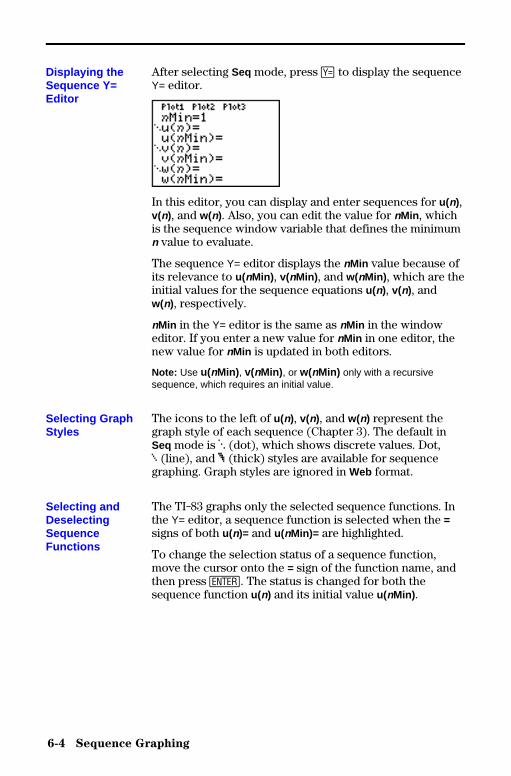
6-4 Sequence Graphing
8306SEQN.DOC TI-83 international English Bob Fedorisko Revised: 02/19/01 12:22 PM Printed: 02/19/01 1:36PM Page 4 of 16
After selecting Seq mode, press o to display the sequenceY= editor.
In this editor, you can display and enter sequences for u(n),v(n), and w(n). Also, you can edit the value for nMin , whichis the sequence window variable that defines the minimumn value to evaluate.
The sequence Y= editor displays the nMin value because ofits relevance to u(nMin) , v(nMin) , and w(nMin) , which are theinitial values for the sequence equations u(n), v(n), andw(n), respectively.
nMin in the Y= editor is the same as nMin in the windoweditor. If you enter a new value for nMin in one editor, thenew value for nMin is updated in both editors.
Note: Use u(nMin) , v(nMin) , or w(nMin) only with a recursivesequence, which requires an initial value.
The icons to the left of u(n), v(n), and w(n) represent thegraph style of each sequence (Chapter 3). The default inSeq mode is í (dot), which shows discrete values. Dot,ç (line), and è (thick) styles are available for sequencegraphing. Graph styles are ignored in Web format.
The TI-83 graphs only the selected sequence functions. Inthe Y= editor, a sequence function is selected when the =signs of both u(n)= and u(nMin)= are highlighted.
To change the selection status of a sequence function,move the cursor onto the = sign of the function name, andthen press Í. The status is changed for both thesequence function u(n) and its initial value u(nMin) .
Displaying theSequence Y=Editor
Selecting GraphStyles
Selecting andDeselectingSequenceFunctions
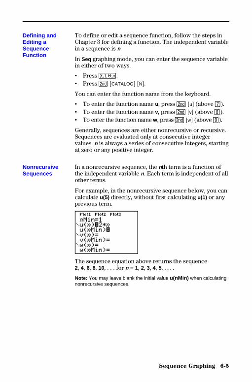
Sequence Graphing 6-5
8306SEQN.DOC TI-83 international English Bob Fedorisko Revised: 02/19/01 12:22 PM Printed: 02/19/01 1:36PM Page 5 of 16
To define or edit a sequence function, follow the steps inChapter 3 for defining a function. The independent variablein a sequence is n.
In Seq graphing mode, you can enter the sequence variablein either of two ways.
• Press „.• Press y [CATALOG] [N].
You can enter the function name from the keyboard.
• To enter the function name u, press y [u] (above ¬).• To enter the function name v, press y [v] (above −).• To enter the function name w, press y [w] (above ®).
Generally, sequences are either nonrecursive or recursive.Sequences are evaluated only at consecutive integervalues. n is always a series of consecutive integers, startingat zero or any positive integer.
In a nonrecursive sequence, the nth term is a function ofthe independent variable n. Each term is independent of allother terms.
For example, in the nonrecursive sequence below, you cancalculate u(5) directly, without first calculating u(1) or anyprevious term.
The sequence equation above returns the sequence2, 4, 6, 8, 10, . . . for n = 1, 2, 3, 4, 5, . . . .
Note: You may leave blank the initial value u(nMin) when calculatingnonrecursive sequences.
Defining andEditing aSequenceFunction
NonrecursiveSequences
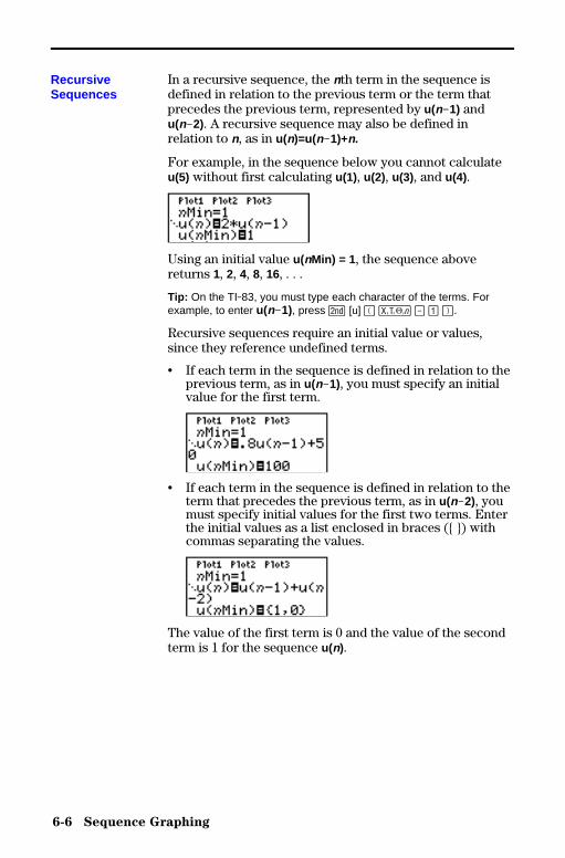
6-6 Sequence Graphing
8306SEQN.DOC TI-83 international English Bob Fedorisko Revised: 02/19/01 12:22 PM Printed: 02/19/01 1:36PM Page 6 of 16
In a recursive sequence, the nth term in the sequence isdefined in relation to the previous term or the term thatprecedes the previous term, represented by u(nN1) andu(nN2). A recursive sequence may also be defined inrelation to n, as in u(n)=u(nN1)+n.
For example, in the sequence below you cannot calculateu(5) without first calculating u(1), u(2), u(3), and u(4).
Using an initial value u(nMin) = 1 , the sequence abovereturns 1, 2, 4, 8, 16, . . .
Tip: On the TI-83, you must type each character of the terms. Forexample, to enter u(nN1), press y [u] £ „ ¹ À ¤.
Recursive sequences require an initial value or values,since they reference undefined terms.
• If each term in the sequence is defined in relation to theprevious term, as in u(nN1), you must specify an initialvalue for the first term.
• If each term in the sequence is defined in relation to theterm that precedes the previous term, as in u(nN2), youmust specify initial values for the first two terms. Enterthe initial values as a list enclosed in braces ({ }) withcommas separating the values.
The value of the first term is 0 and the value of the secondterm is 1 for the sequence u(n).
RecursiveSequences
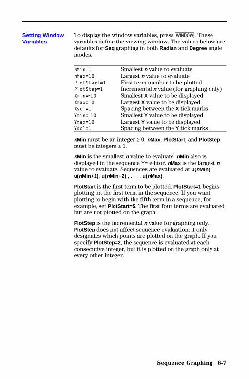
Sequence Graphing 6-7
8306SEQN.DOC TI-83 international English Bob Fedorisko Revised: 02/19/01 12:22 PM Printed: 02/19/01 1:36PM Page 7 of 16
To display the window variables, press p. Thesevariables define the viewing window. The values below aredefaults for Seq graphing in both Radian and Degree anglemodes.
nMin=1 Smallest n value to evaluatenMax=10 Largest n value to evaluatePlotStart=1 First term number to be plottedPlotStep=1 Incremental n value (for graphing only)Xmin=L10 Smallest X value to be displayedXmax=10 Largest X value to be displayedXscl=1 Spacing between the X tick marksYmin=L10 Smallest Y value to be displayedYmax=10 Largest Y value to be displayedYscl=1 Spacing between the Y tick marks
nMin must be an integer ‚ 0. nMax, PlotStart , and PlotStepmust be integers ‚ 1.
nMin is the smallest n value to evaluate. nMin also isdisplayed in the sequence Y= editor. nMax is the largest nvalue to evaluate. Sequences are evaluated at u(nMin) ,u(nMin+1) , u(nMin+2) , . . . , u(nMax).
PlotStart is the first term to be plotted. PlotStart=1 beginsplotting on the first term in the sequence. If you wantplotting to begin with the fifth term in a sequence, forexample, set PlotStart=5 . The first four terms are evaluatedbut are not plotted on the graph.
PlotStep is the incremental n value for graphing only.PlotStep does not affect sequence evaluation; it onlydesignates which points are plotted on the graph. If youspecify PlotStep=2 , the sequence is evaluated at eachconsecutive integer, but it is plotted on the graph only atevery other integer.
Setting WindowVariables
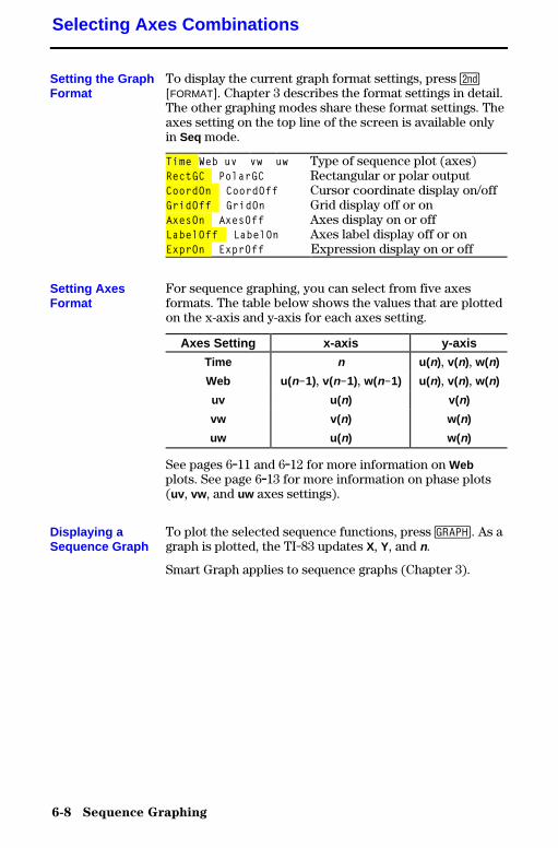
6-8 Sequence Graphing
8306SEQN.DOC TI-83 international English Bob Fedorisko Revised: 02/19/01 12:22 PM Printed: 02/19/01 1:36PM Page 8 of 16
To display the current graph format settings, press y[FORMAT]. Chapter 3 describes the format settings in detail.The other graphing modes share these format settings. Theaxes setting on the top line of the screen is available onlyin Seq mode.
Time Web uv vw uw Type of sequence plot (axes)RectGC PolarGC Rectangular or polar outputCoordOn CoordOff Cursor coordinate display on/offGridOff GridOn Grid display off or onAxesOn AxesOff Axes display on or offLabelOff LabelOn Axes label display off or onExprOn ExprOff Expression display on or off
For sequence graphing, you can select from five axesformats. The table below shows the values that are plottedon the x-axis and y-axis for each axes setting.
Axes Setting x-axis y-axis
Time n u(n), v(n), w(n)
Web u(nN1), v(nN1), w(nN1) u(n), v(n), w(n)
uv u( n) v(n)
vw v( n) w(n)
uw u( n) w(n)
See pages 6.11 and 6.12 for more information on Webplots. See page 6.13 for more information on phase plots(uv , vw , and uw axes settings).
To plot the selected sequence functions, press s. As agraph is plotted, the TI-83 updates X, Y, and n.
Smart Graph applies to sequence graphs (Chapter 3).
Selecting Axes Combinations
Setting the GraphFormat
Setting AxesFormat
Displaying aSequence Graph
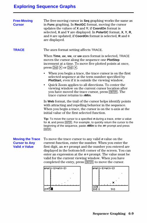
Sequence Graphing 6-9
8306SEQN.DOC TI-83 international English Bob Fedorisko Revised: 02/19/01 12:22 PM Printed: 02/19/01 1:36PM Page 9 of 16
The free-moving cursor in Seq graphing works the same asin Func graphing. In RectGC format, moving the cursorupdates the values of X and Y; if CoordOn format isselected, X and Y are displayed. In PolarGC format, X, Y, R,and q are updated; if CoordOn format is selected, R and qare displayed.
The axes format setting affects TRACE.
When Time , uv , vw , or uw axes format is selected, TRACEmoves the cursor along the sequence one PlotStepincrement at a time. To move five plotted points at once,press y ~ or y |.
• When you begin a trace, the trace cursor is on the firstselected sequence at the term number specified byPlotStart , even if it is outside the viewing window.
• Quick Zoom applies to all directions. To center theviewing window on the current cursor location afteryou have moved the trace cursor, press Í. Thetrace cursor returns to nMin .
In Web format, the trail of the cursor helps identify pointswith attracting and repelling behavior in the sequence.When you begin a trace, the cursor is on the x-axis at theinitial value of the first selected function.
Tip: To move the cursor to a specified n during a trace, enter a valuefor n, and press Í. For example, to quickly return the cursor to thebeginning of the sequence, paste nMin to the n= prompt and pressÍ.
To move the trace cursor to any valid n value on thecurrent function, enter the number. When you enter thefirst digit, an n = prompt and the number you entered aredisplayed in the bottom-left corner of the screen. You canenter an expression at the n = prompt. The value must bevalid for the current viewing window. When you havecompleted the entry, press Í to move the cursor.
Exploring Sequence Graphs
Free-MovingCursor
TRACE
Moving the TraceCursor to AnyValid n Value
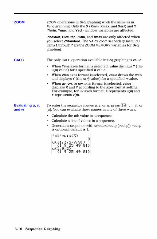
6-10 Sequence Graphing
8306SEQN.DOC TI-83 international English Bob Fedorisko Revised: 02/19/01 12:22 PM Printed: 02/19/01 1:36PM Page 10 of 16
ZOOM operations in Seq graphing work the same as inFunc graphing. Only the X (Xmin , Xmax , and Xscl ) and Y(Ymin , Ymax , and Yscl ) window variables are affected.
PlotStart , PlotStep , nMin , and nMax are only affected whenyou select ZStandard . The VARS Zoom secondary menu ZUitems 1 through 7 are the ZOOM MEMORY variables for Seqgraphing.
The only CALC operation available in Seq graphing is value .
• When Time axes format is selected, value displays Y (theu(n) value) for a specified n value.
• When Web axes format is selected, value draws the weband displays Y (the u(n) value) for a specified n value.
• When uv , vw , or uw axes format is selected, valuedisplays X and Y according to the axes format setting.For example, for uv axes format, X represents u(n) andY represents v(n).
To enter the sequence names u, v, or w, press y [u], [v], or[w]. You can evaluate these names in any of three ways.
• Calculate the nth value in a sequence.• Calculate a list of values in a sequence.• Generate a sequence with u(nstart,nstop[,nstep]). nstep
is optional; default is 1.
ZOOM
CALC
Evaluating u, v,and w

Sequence Graphing 6-11
8306SEQN.DOC TI-83 international English Bob Fedorisko Revised: 02/19/01 12:22 PM Printed: 02/19/01 1:36PM Page 11 of 16
To select Web axes format, press y [FORMAT] ~ Í. Aweb plot graphs u(n) versus u(nN1), which you can use tostudy long-term behavior (convergence, divergence, oroscillation) of a recursive sequence. You can see how thesequence may change behavior as its initial value changes.
When Web axes format is selected, a sequence will notgraph properly or will generate an error.
• It must be recursive with only one recursion level(u(nN1) but not u(nN2)).
• It cannot reference n directly.• It cannot reference any defined sequence except itself.
In Web format, press s to display the graph screen.The TI-83:
• Draws a y=x reference line in AxesOn format.• Plots the selected sequences with u(nN1) as the
independent variable.
Note: A potential convergence point occurs whenever a sequenceintersects the y=x reference line. However, the sequence may or maynot actually converge at that point, depending on the sequence’s initialvalue.
To activate the trace cursor, press r. The screendisplays the sequence and the current n, X, and Y values (Xrepresents u(nN1) and Y represents u(n)). Press ~repeatedly to draw the web step by step, starting at nMin .In Web format, the trace cursor follows this course.
1. It starts on the x-axis at the initial value u(nMin) (whenPlotStart=1 ).
2. It moves vertically (up or down) to the sequence.
3. It moves horizontally to the y=x reference line.
4. It repeats this vertical and horizontal movement as youcontinue to press ~.
Graphing Web Plots
Graphing a WebPlot
Valid Functionsfor Web Plots
Displaying theGraph Screen
Drawing the Web
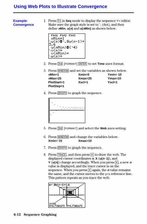
6-12 Sequence Graphing
8306SEQN.DOC TI-83 international English Bob Fedorisko Revised: 02/19/01 12:22 PM Printed: 02/19/01 1:36PM Page 12 of 16
1. Press o in Seq mode to display the sequence Y= editor.Make sure the graph style is set to í (dot), and thendefine nMin , u(n) and u(nMin) as shown below.
2. Press y [FORMAT] Í to set Time axes format.
3. Press p and set the variables as shown below.nMin=1 Xmin=0 Ymin= L10nMax=25 Xmax=25 Ymax=10PlotStart=1 Xscl=1 Yscl=1PlotStep=1
4. Press s to graph the sequence.
5. Press y [FORMAT] and select the Web axes setting.
6. Press p and change the variables below.Xmin= L10 Xmax=10
7. Press s to graph the sequence.
8. Press r, and then press ~ to draw the web. Thedisplayed cursor coordinates n, X (u(nN1)), andY (u(n)) change accordingly. When you press ~, a new nvalue is displayed, and the trace cursor is on thesequence. When you press ~ again, the n value remainsthe same, and the cursor moves to the y=x reference line.This pattern repeats as you trace the web.
Using Web Plots to Illustrate Convergence
Example:Convergence
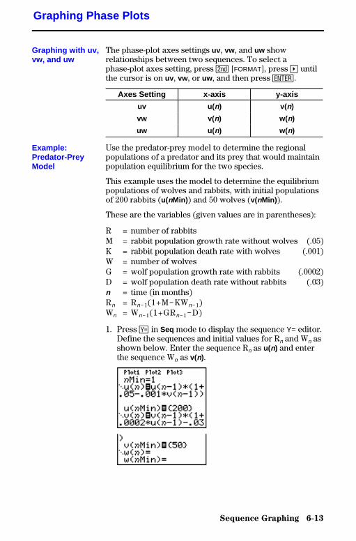
Sequence Graphing 6-13
8306SEQN.DOC TI-83 international English Bob Fedorisko Revised: 02/19/01 12:22 PM Printed: 02/19/01 1:36PM Page 13 of 16
The phase-plot axes settings uv , vw , and uw showrelationships between two sequences. To select aphase-plot axes setting, press y [FORMAT], press ~ untilthe cursor is on uv , vw , or uw , and then press Í.
Axes Setting x-axis y-axis
uv u( n) v(n)
vw v( n) w(n)
uw u( n) w(n)
Use the predator-prey model to determine the regionalpopulations of a predator and its prey that would maintainpopulation equilibrium for the two species.
This example uses the model to determine the equilibriumpopulations of wolves and rabbits, with initial populationsof 200 rabbits (u(nMin)) and 50 wolves (v(nMin)).
These are the variables (given values are in parentheses):
R = number of rabbitsM = rabbit population growth rate without wolves (.05)K = rabbit population death rate with wolves (.001)W = number of wolvesG = wolf population growth rate with rabbits (.0002)D = wolf population death rate without rabbits (.03)n = time (in months)Rn = RnN1(1+MNKWnN1)Wn = WnN1(1+GRnN1ND)
1. Press o in Seq mode to display the sequence Y= editor.Define the sequences and initial values for Rn and Wn asshown below. Enter the sequence Rn as u(n) and enterthe sequence Wn as v(n).
Graphing Phase Plots
Graphing with uv,vw, and uw
Example:Predator-PreyModel
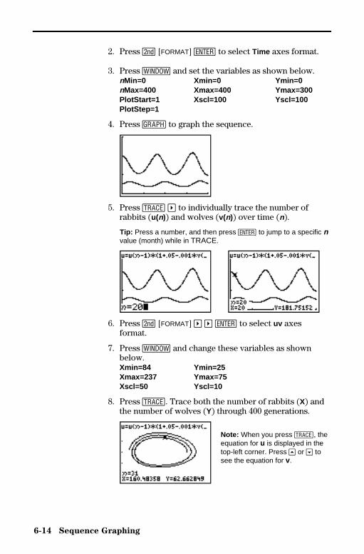
6-14 Sequence Graphing
8306SEQN.DOC TI-83 international English Bob Fedorisko Revised: 02/19/01 12:22 PM Printed: 02/19/01 1:36PM Page 14 of 16
2. Press y [FORMAT] Í to select Time axes format.
3. Press p and set the variables as shown below.nMin=0 Xmin=0 Ymin=0nMax=400 Xmax=400 Ymax=300PlotStart=1 Xscl=100 Yscl=100PlotStep=1
4. Press s to graph the sequence.
5. Press r ~ to individually trace the number ofrabbits (u(n)) and wolves (v(n)) over time (n).
Tip: Press a number, and then press Í to jump to a specific nvalue (month) while in TRACE.
6. Press y [FORMAT] ~ ~ Í to select uv axesformat.
7. Press p and change these variables as shownbelow.Xmin=84 Ymin=25Xmax=237 Ymax=75Xscl=50 Yscl=10
8. Press r. Trace both the number of rabbits (X) andthe number of wolves (Y) through 400 generations.
Note: When you press r, theequation for u is displayed in thetop-left corner. Press } or † tosee the equation for v.
Sequence Graphing 6-15
8306SEQN.DOC TI-83 international English Bob Fedorisko Revised: 02/19/01 12:22 PM Printed: 02/19/01 1:36PM Page 15 of 16
Refer to the table if you are familiar with the TI-82. Itshows TI-83 sequences and sequence window variables, aswell as their TI-82 counterparts.
TI.83 TI.82
In the Y= editor:
u(n) Un
u(nMin) UnStart (window variable)
v(n) Vn
v(nMin) VnStart (window variable)
w(n) not available
w(nMin) not available
In the window editor:
nMin nStart
nMax nMax
PlotStart nMin
PlotStep not available
Comparing TI-83 and TI-82 Sequence Variables
Sequences andWindowVariables

6-16 Sequence Graphing
8306SEQN.DOC TI-83 international English Bob Fedorisko Revised: 02/19/01 12:22 PM Printed: 02/19/01 1:36PM Page 16 of 16
Refer to the table if you are familiar with the TI-82. Itcompares TI-83 sequence-name syntax and variable syntaxwith TI.82 sequence-name syntax and variable syntax.
TI.83 / TI.82 On TI.83, press: On TI .82, press:
n / n „ y [n]
u(n) / Un y [u]£ „ ¤
y [Y.VARS] ¶ À
v(n) / Vn y [v]£ „ ¤
y [Y.VARS] ¶ Á
w(n) y [w]£ „ ¤
not available
u(nN1) / UnN1 y [u]£ „ ¹ À ¤
y [UnN1]
v(nN1) / VnN1 y [v]£ „ ¹ À ¤
y [VnN1]
w(nN1) y [w]£ „ ¹ À ¤
not available
Keystroke Differences Between TI-83 and TI-82
SequenceKeystrokeChanges
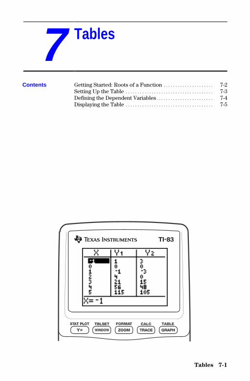
Tables 7-1
8307TABL.DOC TI-83 international English Bob Fedorisko Revised: 02/19/01 12:26 PM Printed: 02/19/01 1:36PM Page 1 of 6
7 Tables
Getting Started: Roots of a Function ..................... 7-2Setting Up the Table ..................................... 7-3Defining the Dependent Variables........................ 7-4Displaying the Table ..................................... 7-5
Contents

7-2 Tables
8307TABL.DOC TI-83 international English Bob Fedorisko Revised: 02/19/01 12:26 PM Printed: 02/19/01 1:36PM Page 2 of 6
Getting Started is a fast-paced introduction. Read the chapter for details.
Evaluate the function Y = X3 N 2X at each integer between L10 and 10. Howmany sign changes occur, and at what X values?
1. Press z † † † Í to set Funcgraphing mode.
2. Press o. Press „ � 3 to select 3.Then press ¹ 2 „ to enter thefunction Y1=X3N2X.
3. Press y [TBLSET] to display the TABLESETUP screen. Press Ì 10 Í to setTblStart= L10. Press 1 Í to set @Tbl=1 .
Press Í to select Indpnt: Auto(automatically generated independentvalues). Press † Í to selectDepend: Auto (automatically generateddependent values).
4. Press y [TABLE] to display the tablescreen.
5. Press † until you see the sign changes inthe value of Y1. How many sign changesoccur, and at what X values?
Getting Started: Roots of a Function
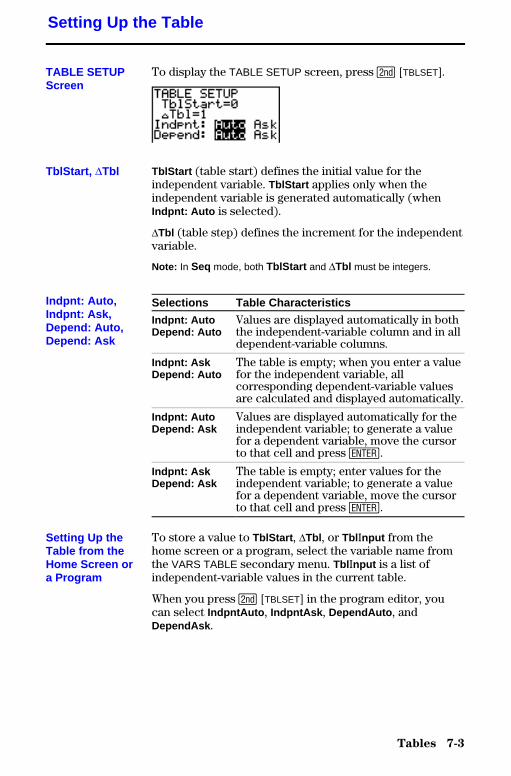
Tables 7-3
8307TABL.DOC TI-83 international English Bob Fedorisko Revised: 02/19/01 12:26 PM Printed: 02/19/01 1:36PM Page 3 of 6
To display the TABLE SETUP screen, press y [TBLSET].
TblStart (table start) defines the initial value for theindependent variable. TblStart applies only when theindependent variable is generated automatically (whenIndpnt: Auto is selected).
@Tbl (table step) defines the increment for the independentvariable.
Note: In Seq mode, both TblStart and @Tbl must be integers.
Selections Table Characteristics
Indpnt: AutoDepend: Auto
Values are displayed automatically in boththe independent-variable column and in alldependent-variable columns.
Indpnt: AskDepend: Auto
The table is empty; when you enter a valuefor the independent variable, allcorresponding dependent-variable valuesare calculated and displayed automatically.
Indpnt: AutoDepend: Ask
Values are displayed automatically for theindependent variable; to generate a valuefor a dependent variable, move the cursorto that cell and press Í.
Indpnt: AskDepend: Ask
The table is empty; enter values for theindependent variable; to generate a valuefor a dependent variable, move the cursorto that cell and press Í.
To store a value to TblStart , @Tbl , or Tbl Znput from thehome screen or a program, select the variable name fromthe VARS TABLE secondary menu. Tbl Znput is a list ofindependent-variable values in the current table.
When you press y [TBLSET] in the program editor, youcan select IndpntAuto , IndpntAsk , DependAuto , andDependAsk .
Setting Up the Table
TABLE SETUPScreen
TblStart, @Tbl
Indpnt: Auto,Indpnt: Ask,Depend: Auto,Depend: Ask
Setting Up theTable from theHome Screen ora Program
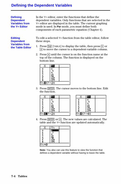
7-4 Tables
8307TABL.DOC TI-83 international English Bob Fedorisko Revised: 02/19/01 12:26 PM Printed: 02/19/01 1:36PM Page 4 of 6
In the Y= editor, enter the functions that define thedependent variables. Only functions that are selected in theY= editor are displayed in the table. The current graphingmode is used. In Par mode, you must define bothcomponents of each parametric equation (Chapter 4).
To edit a selected Y= function from the table editor, followthese steps.
1. Press y [TABLE] to display the table, then press ~ or| to move the cursor to a dependent-variable column.
2. Press } until the cursor is on the function name at thetop of the column. The function is displayed on thebottom line.
3. Press Í. The cursor moves to the bottom line. Editthe function.
4. Press Í or †. The new values are calculated. Thetable and the Y= function are updated automatically.
Note: You also can use this feature to view the function thatdefines a dependent variable without having to leave the table.
Defining the Dependent Variables
DefiningDependentVariables fromthe Y= Editor
EditingDependentVariables fromthe Table Editor
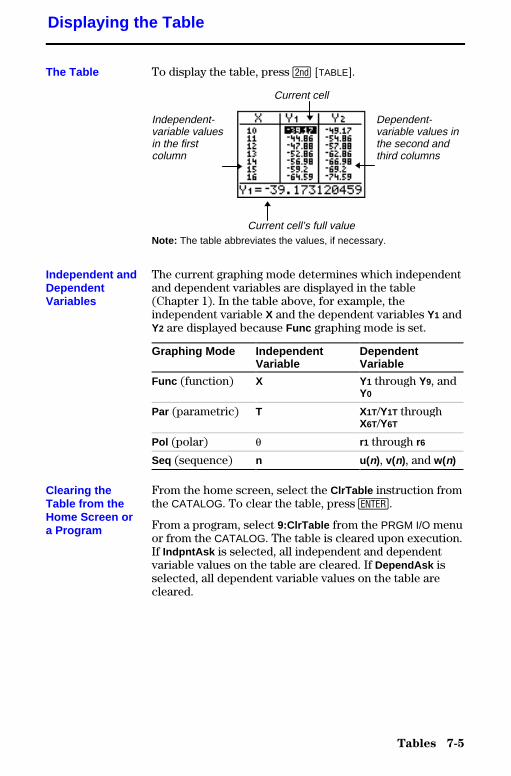
Tables 7-5
8307TABL.DOC TI-83 international English Bob Fedorisko Revised: 02/19/01 12:26 PM Printed: 02/19/01 1:36PM Page 5 of 6
To display the table, press y [TABLE].
Current cell
Independent-variable valuesin the firstcolumn
Dependent-variable values inthe second andthird columns
Current cell’s full valueNote: The table abbreviates the values, if necessary.
The current graphing mode determines which independentand dependent variables are displayed in the table(Chapter 1). In the table above, for example, theindependent variable X and the dependent variables Y1 andY2 are displayed because Func graphing mode is set.
Graphing Mode IndependentVariable
DependentVariable
Func (function) X Y1 through Y9, andY0
Par (parametric) T X1T/Y1T throughX6T/Y6T
Pol (polar) q r1 through r6
Seq (sequence) n u(n), v(n), and w(n)
From the home screen, select the ClrTable instruction fromthe CATALOG. To clear the table, press Í.
From a program, select 9:ClrTable from the PRGM I/O menuor from the CATALOG. The table is cleared upon execution.If IndpntAsk is selected, all independent and dependentvariable values on the table are cleared. If DependAsk isselected, all dependent variable values on the table arecleared.
Displaying the Table
The Table
Independent andDependentVariables
Clearing theTable from theHome Screen ora Program
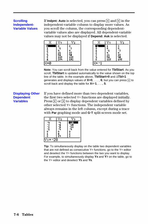
7-6 Tables
8307TABL.DOC TI-83 international English Bob Fedorisko Revised: 02/19/01 12:26 PM Printed: 02/19/01 1:36PM Page 6 of 6
If Indpnt: Auto is selected, you can press } and † in theindependent-variable column to display more values. Asyou scroll the column, the corresponding dependent-variable values also are displayed. All dependent-variablevalues may not be displayed if Depend: Ask is selected.
Note: You can scroll back from the value entered for TblStart . As youscroll, TblStart is updated automatically to the value shown on the topline of the table. In the example above, TblStart=0 and @Tbl=1generates and displays values of X=0, . . . , 6; but you can press } toscroll back and display the table for X=M1, . . ., 5.
If you have defined more than two dependent variables,the first two selected Y= functions are displayed initially.Press ~ or | to display dependent variables defined byother selected Y= functions. The independent variablealways remains in the left column, except during a tracewith Par graphing mode and G.T split-screen mode set.
Tip: To simultaneously display on the table two dependent variablesthat are not defined as consecutive Y= functions, go to the Y= editorand deselect the Y= functions between the two you want to display.For example, to simultaneously display Y4 and Y7 on the table, go tothe Y= editor and deselect Y5 and Y6.
ScrollingIndependent-Variable Values
Displaying OtherDependentVariables
DRAW Instructions 8-1
8308DRAW.DOC TI-83 international English Bob Fedorisko Revised: 02/19/01 12:29 PM Printed: 02/19/01 1:49PM Page 1 of 20
8 DrawInstructions
Getting Started: Drawing a Tangent Line ................. 8-2Using the DRAW Menu................................... 8-3Clearing Drawings ....................................... 8-4Drawing Line Segments.................................. 8-5Drawing Horizontal and Vertical Lines ................... 8-6Drawing Tangent Lines .................................. 8-8Drawing Functions and Inverses ......................... 8-9Shading Areas on a Graph ............................... 8-10Drawing Circles.......................................... 8-11Placing Text on a Graph ................................. 8-12Using Pen to Draw on a Graph ........................... 8-13Drawing Points on a Graph .............................. 8-14Drawing Pixels .......................................... 8-16Storing Graph Pictures (Pics) ............................ 8-17Recalling Graph Pictures (Pics) .......................... 8-18Storing Graph Databases (GDBs) ........................ 8-19Recalling Graph Databases (GDBs) ...................... 8-20
Contents

8-2 DRAW Instructions
8308DRAW.DOC TI-83 international English Bob Fedorisko Revised: 02/19/01 12:29 PM Printed: 02/19/01 1:49PM Page 2 of 20
Getting Started is a fast-paced introduction. Read the chapter for details.
Suppose you want to find the equation of the tangent line at X = ‡2/2 for thefunction Y = sinX.
Before you begin, select Radian and Funcmode from the mode screen, if necessary.
1. Press o to display the Y= editor. Press˜ „ ¤ to store sin(X) in Y1.
2. Press q 7 to select 7:ZTrig , whichgraphs the equation in the Zoom Trigwindow.
3. Press y [DRAW] 5 to select 5:Tangent( .The tangent instruction is initiated.
4. Press y [‡] 2 ¤ ¥ 2.
5. Press Í. The tangent line is drawn; theX value and the tangent-line equation aredisplayed on the graph.
Getting Started: Drawing a Tangent Line
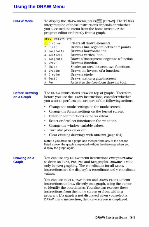
DRAW Instructions 8-3
8308DRAW.DOC TI-83 international English Bob Fedorisko Revised: 02/19/01 12:29 PM Printed: 02/19/01 1:49PM Page 3 of 20
To display the DRAW menu, press y [DRAW]. The TI-83’sinterpretation of these instructions depends on whetheryou accessed the menu from the home screen or theprogram editor or directly from a graph.
DRAW POINTS STO1: ClrDraw Clears all drawn elements.2: Line( Draws a line segment between 2 points.3: Horizontal Draws a horizontal line.4: Vertical Draws a vertical line.5: Tangent( Draws a line segment tangent to a function.6: DrawF Draws a function.7: Shade( Shades an area between two functions.8: DrawInv Draws the inverse of a function.9: Circle( Draws a circle.0: Text( Draws text on a graph screen.A: Pen Activates the free-form drawing tool.
The DRAW instructions draw on top of graphs. Therefore,before you use the DRAW instructions, consider whetheryou want to perform one or more of the following actions.
• Change the mode settings on the mode screen.• Change the format settings on the format screen.• Enter or edit functions in the Y= editor.• Select or deselect functions in the Y= editor.• Change the window variable values.• Turn stat plots on or off.• Clear existing drawings with ClrDraw (page 8.4).
Note: If you draw on a graph and then perform any of the actionslisted above, the graph is replotted without the drawings when youdisplay the graph again.
You can use any DRAW menu instructions except DrawInvto draw on Func , Par, Pol , and Seq graphs. DrawInv is validonly in Func graphing. The coordinates for all DRAWinstructions are the display’s x-coordinate and y-coordinatevalues.
You can use most DRAW menu and DRAW POINTS menuinstructions to draw directly on a graph, using the cursorto identify the coordinates. You also can execute theseinstructions from the home screen or from within aprogram. If a graph is not displayed when you select aDRAW menu instruction, the home screen is displayed.
Using the DRAW Menu
DRAW Menu
Before Drawingon a Graph
Drawing on aGraph
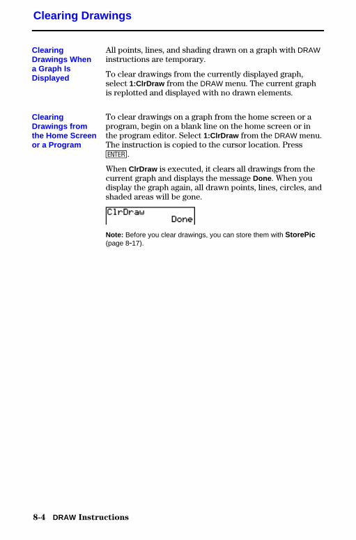
8-4 DRAW Instructions
8308DRAW.DOC TI-83 international English Bob Fedorisko Revised: 02/19/01 12:29 PM Printed: 02/19/01 1:49PM Page 4 of 20
All points, lines, and shading drawn on a graph with DRAWinstructions are temporary.
To clear drawings from the currently displayed graph,select 1:ClrDraw from the DRAW menu. The current graphis replotted and displayed with no drawn elements.
To clear drawings on a graph from the home screen or aprogram, begin on a blank line on the home screen or inthe program editor. Select 1:ClrDraw from the DRAW menu.The instruction is copied to the cursor location. PressÍ.
When ClrDraw is executed, it clears all drawings from thecurrent graph and displays the message Done . When youdisplay the graph again, all drawn points, lines, circles, andshaded areas will be gone.
Note: Before you clear drawings, you can store them with StorePic(page 8.17).
Clearing Drawings
ClearingDrawings Whena Graph IsDisplayed
ClearingDrawings fromthe Home Screenor a Program
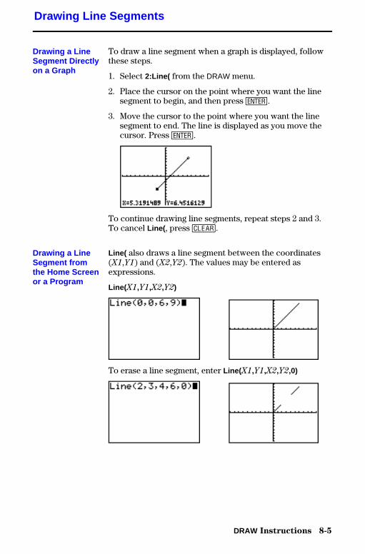
DRAW Instructions 8-5
8308DRAW.DOC TI-83 international English Bob Fedorisko Revised: 02/19/01 12:29 PM Printed: 02/19/01 1:49PM Page 5 of 20
To draw a line segment when a graph is displayed, followthese steps.
1. Select 2:Line( from the DRAW menu.
2. Place the cursor on the point where you want the linesegment to begin, and then press Í.
3. Move the cursor to the point where you want the linesegment to end. The line is displayed as you move thecursor. Press Í.
To continue drawing line segments, repeat steps 2 and 3.To cancel Line( , press ‘.
Line( also draws a line segment between the coordinates(X1,Y1) and (X2,Y2). The values may be entered asexpressions.
Line( X1,Y1,X2,Y2)
To erase a line segment, enter Line( X1,Y1,X2,Y2,0)
Drawing Line Segments
Drawing a LineSegment Directlyon a Graph
Drawing a LineSegment fromthe Home Screenor a Program
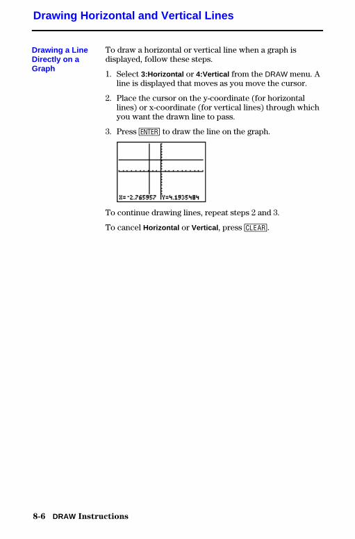
8-6 DRAW Instructions
8308DRAW.DOC TI-83 international English Bob Fedorisko Revised: 02/19/01 12:29 PM Printed: 02/19/01 1:49PM Page 6 of 20
To draw a horizontal or vertical line when a graph isdisplayed, follow these steps.
1. Select 3:Horizontal or 4:Vertical from the DRAW menu. Aline is displayed that moves as you move the cursor.
2. Place the cursor on the y-coordinate (for horizontallines) or x-coordinate (for vertical lines) through whichyou want the drawn line to pass.
3. Press Í to draw the line on the graph.
To continue drawing lines, repeat steps 2 and 3.
To cancel Horizontal or Vertical , press ‘.
Drawing Horizontal and Vertical Lines
Drawing a LineDirectly on aGraph
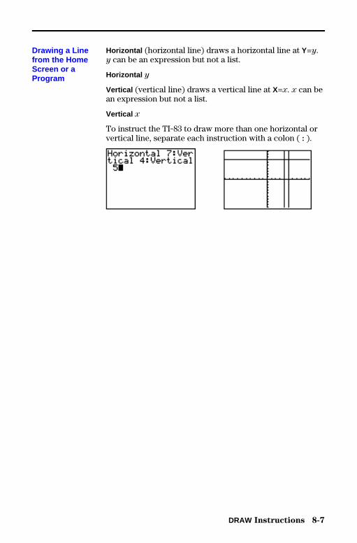
DRAW Instructions 8-7
8308DRAW.DOC TI-83 international English Bob Fedorisko Revised: 02/19/01 12:29 PM Printed: 02/19/01 1:49PM Page 7 of 20
Horizontal (horizontal line) draws a horizontal line at Y=y.y can be an expression but not a list.
Horizontal y
Vertical (vertical line) draws a vertical line at X=x. x can bean expression but not a list.
Vertical x
To instruct the TI-83 to draw more than one horizontal orvertical line, separate each instruction with a colon ( : ).
Drawing a Linefrom the HomeScreen or aProgram
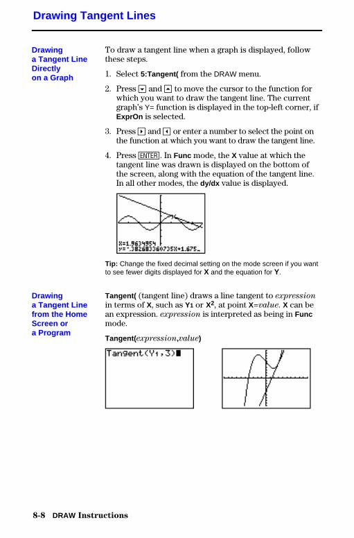
8-8 DRAW Instructions
8308DRAW.DOC TI-83 international English Bob Fedorisko Revised: 02/19/01 12:29 PM Printed: 02/19/01 1:49PM Page 8 of 20
To draw a tangent line when a graph is displayed, followthese steps.
1. Select 5:Tangent( from the DRAW menu.
2. Press † and } to move the cursor to the function forwhich you want to draw the tangent line. The currentgraph’s Y= function is displayed in the top-left corner, ifExprOn is selected.
3. Press ~ and | or enter a number to select the point onthe function at which you want to draw the tangent line.
4. Press Í. In Func mode, the X value at which thetangent line was drawn is displayed on the bottom ofthe screen, along with the equation of the tangent line.In all other modes, the dy/dx value is displayed.
Tip: Change the fixed decimal setting on the mode screen if you wantto see fewer digits displayed for X and the equation for Y.
Tangent( (tangent line) draws a line tangent to expression
in terms of X, such as Y1 or X2, at point X=value. X can bean expression. expression is interpreted as being in Funcmode.
Tangent( expression,value)
Drawing Tangent Lines
Drawinga Tangent LineDirectlyon a Graph
Drawinga Tangent Linefrom the HomeScreen ora Program
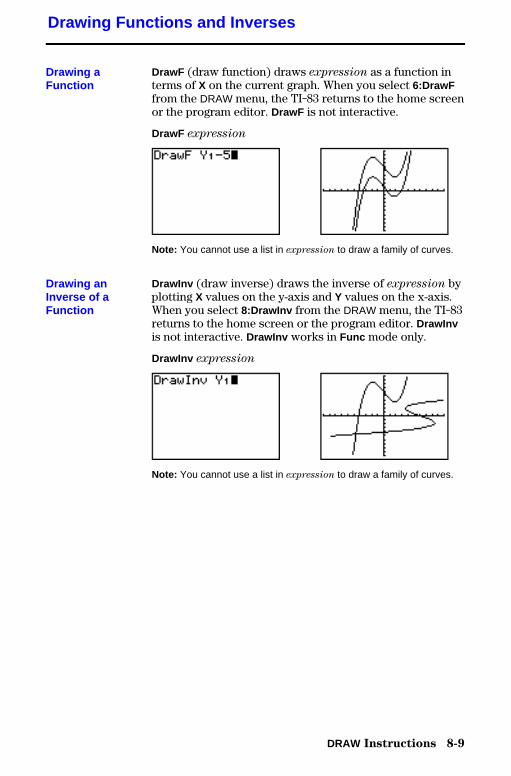
DRAW Instructions 8-9
8308DRAW.DOC TI-83 international English Bob Fedorisko Revised: 02/19/01 12:29 PM Printed: 02/19/01 1:49PM Page 9 of 20
DrawF (draw function) draws expression as a function interms of X on the current graph. When you select 6:DrawFfrom the DRAW menu, the TI-83 returns to the home screenor the program editor. DrawF is not interactive.
DrawF expression
Note: You cannot use a list in expression to draw a family of curves.
DrawInv (draw inverse) draws the inverse of expression byplotting X values on the y-axis and Y values on the x-axis.When you select 8:DrawInv from the DRAW menu, the TI-83returns to the home screen or the program editor. DrawInvis not interactive. DrawInv works in Func mode only.
DrawInv expression
Note: You cannot use a list in expression to draw a family of curves.
Drawing Functions and Inverses
Drawing aFunction
Drawing anInverse of aFunction
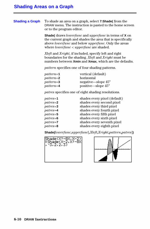
8-10 DRAW Instructions
8308DRAW.DOC TI-83 international English Bob Fedorisko Revised: 02/19/01 12:29 PM Printed: 02/19/01 1:49PM Page 10 of 20
To shade an area on a graph, select 7:Shade( from theDRAW menu. The instruction is pasted to the home screenor to the program editor.
Shade( draws lowerfunc and upperfunc in terms of X onthe current graph and shades the area that is specificallyabove lowerfunc and below upperfunc. Only the areaswhere lowerfunc < upperfunc are shaded.
Xleft and Xright, if included, specify left and rightboundaries for the shading. Xleft and Xright must benumbers between Xmin and Xmax , which are the defaults.
pattern specifies one of four shading patterns.
pattern=1 vertical (default)pattern=2 horizontalpattern=3 negative—slope 45¡pattern=4 positive—slope 45¡
patres specifies one of eight shading resolutions.
patres=1 shades every pixel (default)patres=2 shades every second pixelpatres=3 shades every third pixelpatres=4 shades every fourth pixelpatres=5 shades every fifth pixelpatres=6 shades every sixth pixelpatres=7 shades every seventh pixelpatres=8 shades every eighth pixel
Shade( lowerfunc,upperfunc[,Xleft,Xright,pattern,patres])
Shading Areas on a Graph
Shading a Graph
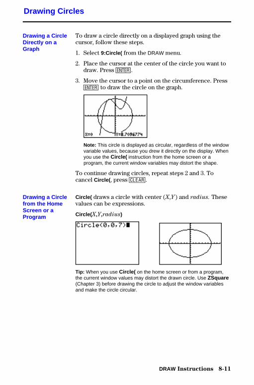
DRAW Instructions 8-11
8308DRAW.DOC TI-83 international English Bob Fedorisko Revised: 02/19/01 12:29 PM Printed: 02/19/01 1:49PM Page 11 of 20
To draw a circle directly on a displayed graph using thecursor, follow these steps.
1. Select 9:Circle( from the DRAW menu.
2. Place the cursor at the center of the circle you want todraw. Press Í.
3. Move the cursor to a point on the circumference. PressÍ to draw the circle on the graph.
Note: This circle is displayed as circular, regardless of the windowvariable values, because you drew it directly on the display. Whenyou use the Circle( instruction from the home screen or aprogram, the current window variables may distort the shape.
To continue drawing circles, repeat steps 2 and 3. Tocancel Circle( , press ‘.
Circle( draws a circle with center (X,Y) and radius. Thesevalues can be expressions.
Circle( X,Y,radius)
Tip: When you use Circle( on the home screen or from a program,the current window values may distort the drawn circle. Use ZSquare(Chapter 3) before drawing the circle to adjust the window variablesand make the circle circular.
Drawing Circles
Drawing a CircleDirectly on aGraph
Drawing a Circlefrom the HomeScreen or aProgram
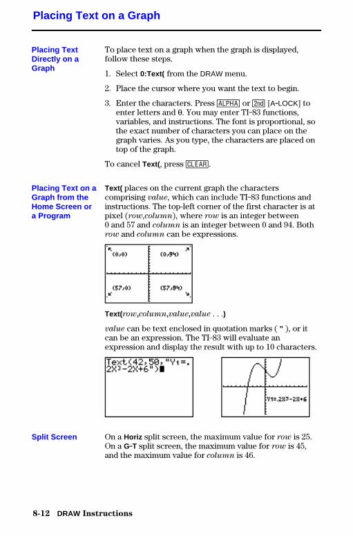
8-12 DRAW Instructions
8308DRAW.DOC TI-83 international English Bob Fedorisko Revised: 02/19/01 12:29 PM Printed: 02/19/01 1:49PM Page 12 of 20
To place text on a graph when the graph is displayed,follow these steps.
1. Select 0:Text( from the DRAW menu.
2. Place the cursor where you want the text to begin.
3. Enter the characters. Press ƒ or y [A.LOCK] toenter letters and q. You may enter TI-83 functions,variables, and instructions. The font is proportional, sothe exact number of characters you can place on thegraph varies. As you type, the characters are placed ontop of the graph.
To cancel Text( , press ‘.
Text( places on the current graph the characterscomprising value, which can include TI-83 functions andinstructions. The top-left corner of the first character is atpixel (row,column), where row is an integer between0 and 57 and column is an integer between 0 and 94. Bothrow and column can be expressions.
Text(row,column,value,value . . .)
value can be text enclosed in quotation marks ( " ), or itcan be an expression. The TI-83 will evaluate anexpression and display the result with up to 10 characters.
On a Horiz split screen, the maximum value for row is 25.On a G.T split screen, the maximum value for row is 45,and the maximum value for column is 46.
Placing Text on a Graph
Placing TextDirectly on aGraph
Placing Text on aGraph from theHome Screen ora Program
Split Screen
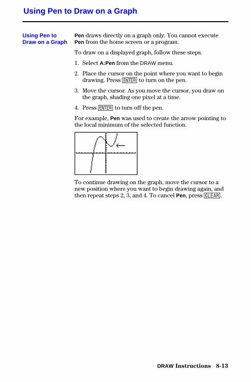
DRAW Instructions 8-13
8308DRAW.DOC TI-83 international English Bob Fedorisko Revised: 02/19/01 12:29 PM Printed: 02/19/01 1:49PM Page 13 of 20
Pen draws directly on a graph only. You cannot executePen from the home screen or a program.
To draw on a displayed graph, follow these steps.
1. Select A:Pen from the DRAW menu.
2. Place the cursor on the point where you want to begindrawing. Press Í to turn on the pen.
3. Move the cursor. As you move the cursor, you draw onthe graph, shading one pixel at a time.
4. Press Í to turn off the pen.
For example, Pen was used to create the arrow pointing tothe local minimum of the selected function.
To continue drawing on the graph, move the cursor to anew position where you want to begin drawing again, andthen repeat steps 2, 3, and 4. To cancel Pen, press ‘.
Using Pen to Draw on a Graph
Using Pen toDraw on a Graph
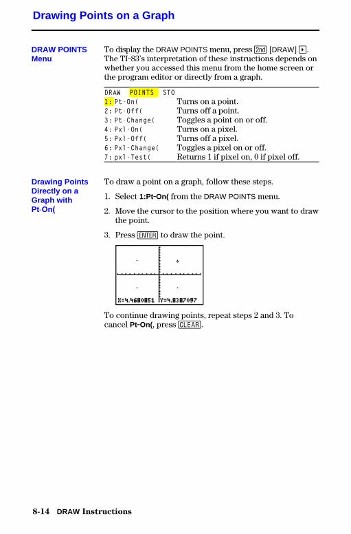
8-14 DRAW Instructions
8308DRAW.DOC TI-83 international English Bob Fedorisko Revised: 02/19/01 12:29 PM Printed: 02/19/01 1:49PM Page 14 of 20
To display the DRAW POINTS menu, press y [DRAW] ~.The TI-83’s interpretation of these instructions depends onwhether you accessed this menu from the home screen orthe program editor or directly from a graph.
DRAW POINTS STO1: Pt-On( Turns on a point.2: Pt-Off( Turns off a point.3: Pt-Change( Toggles a point on or off.4: Pxl-On( Turns on a pixel.5: Pxl-Off( Turns off a pixel.6: Pxl-Change( Toggles a pixel on or off.7: pxl-Test( Returns 1 if pixel on, 0 if pixel off.
To draw a point on a graph, follow these steps.
1. Select 1:Pt.On( from the DRAW POINTS menu.
2. Move the cursor to the position where you want to drawthe point.
3. Press Í to draw the point.
To continue drawing points, repeat steps 2 and 3. Tocancel Pt.On(, press ‘.
Drawing Points on a Graph
DRAW POINTSMenu
Drawing PointsDirectly on aGraph withPt-On(
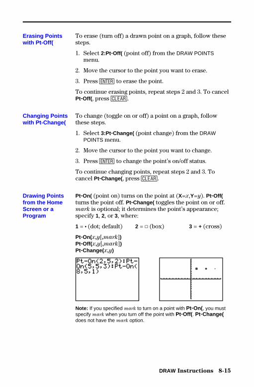
DRAW Instructions 8-15
8308DRAW.DOC TI-83 international English Bob Fedorisko Revised: 02/19/01 12:29 PM Printed: 02/19/01 1:49PM Page 15 of 20
To erase (turn off) a drawn point on a graph, follow thesesteps.
1. Select 2:Pt.Off( (point off) from the DRAW POINTSmenu.
2. Move the cursor to the point you want to erase.
3. Press Í to erase the point.
To continue erasing points, repeat steps 2 and 3. To cancelPt.Off( , press ‘.
To change (toggle on or off) a point on a graph, followthese steps.
1. Select 3:Pt.Change( (point change) from the DRAWPOINTS menu.
2. Move the cursor to the point you want to change.
3. Press Í to change the point’s on/off status.
To continue changing points, repeat steps 2 and 3. Tocancel Pt.Change( , press ‘.
Pt.On( (point on) turns on the point at (X=x,Y=y). Pt.Off(turns the point off. Pt.Change( toggles the point on or off.mark is optional; it determines the point’s appearance;specify 1, 2, or 3, where:
1 = ¦ (dot; default) 2 = › (box) 3 = + (cross)
Pt.On(x,y[,mark])Pt.Off(x,y[,mark])Pt.Change( x,y)
Note: If you specified mark to turn on a point with Pt.On(, you mustspecify mark when you turn off the point with Pt.Off( . Pt.Change(does not have the mark option.
Erasing Pointswith Pt-Off(
Changing Pointswith Pt-Change(
Drawing Pointsfrom the HomeScreen or aProgram
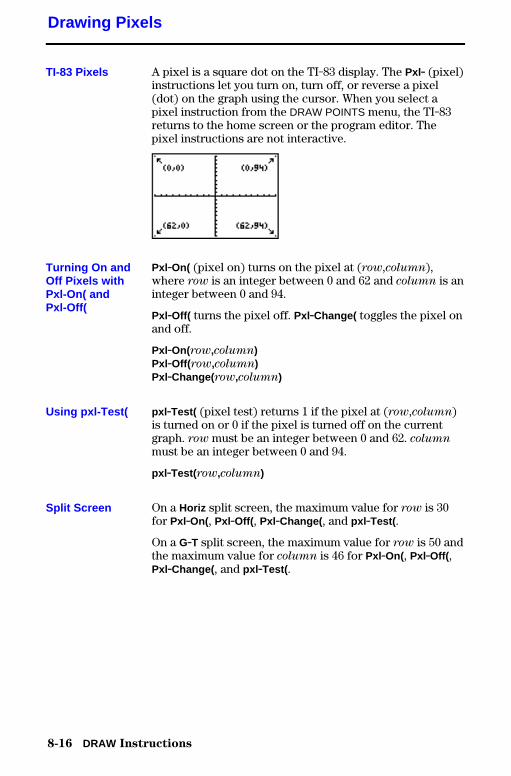
8-16 DRAW Instructions
8308DRAW.DOC TI-83 international English Bob Fedorisko Revised: 02/19/01 12:29 PM Printed: 02/19/01 1:49PM Page 16 of 20
A pixel is a square dot on the TI-83 display. The Pxl. (pixel)instructions let you turn on, turn off, or reverse a pixel(dot) on the graph using the cursor. When you select apixel instruction from the DRAW POINTS menu, the TI-83returns to the home screen or the program editor. Thepixel instructions are not interactive.
Pxl.On( (pixel on) turns on the pixel at (row,column),where row is an integer between 0 and 62 and column is aninteger between 0 and 94.
Pxl.Off( turns the pixel off. Pxl.Change( toggles the pixel onand off.
Pxl.On(row,column)Pxl.Off(row,column)Pxl.Change( row,column)
pxl .Test( (pixel test) returns 1 if the pixel at (row,column)is turned on or 0 if the pixel is turned off on the currentgraph. row must be an integer between 0 and 62. column
must be an integer between 0 and 94.
pxl .Test(row,column)
On a Horiz split screen, the maximum value for row is 30for Pxl.On(, Pxl.Off( , Pxl.Change( , and pxl .Test( .
On a G.T split screen, the maximum value for row is 50 andthe maximum value for column is 46 for Pxl.On(, Pxl.Off( ,Pxl.Change( , and pxl .Test( .
Drawing Pixels
TI-83 Pixels
Turning On andOff Pixels withPxl-On( andPxl-Off(
Using pxl-Test(
Split Screen
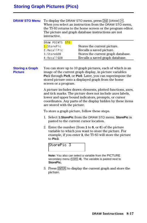
DRAW Instructions 8-17
8308DRAW.DOC TI-83 international English Bob Fedorisko Revised: 02/19/01 12:29 PM Printed: 02/19/01 1:49PM Page 17 of 20
To display the DRAW STO menu, press y [DRAW] |.When you select an instruction from the DRAW STO menu,the TI-83 returns to the home screen or the program editor.The picture and graph database instructions are notinteractive.
DRAW POINTS STO1:StorePic Stores the current picture.2:RecallPic Recalls a saved picture.3:StoreGDB Stores the current graph database.4:RecallGDB Recalls a saved graph database.
You can store up to 10 graph pictures, each of which is animage of the current graph display, in picture variablesPic1 through Pic9 , or Pic0 . Later, you can superimpose thestored picture onto a displayed graph from the homescreen or a program.
A picture includes drawn elements, plotted functions, axes,and tick marks. The picture does not include axes labels,lower and upper bound indicators, prompts, or cursorcoordinates. Any parts of the display hidden by these itemsare stored with the picture.
To store a graph picture, follow these steps.
1. Select 1:StorePic from the DRAW STO menu. StorePic ispasted to the current cursor location.
2. Enter the number (from 1 to 9, or 0) of the picturevariable to which you want to store the picture. Forexample, if you enter 3, the TI-83 will store the pictureto Pic3 .
Note: You also can select a variable from the PICTUREsecondary menu (� 4). The variable is pasted next toStorePic .
3. Press Í to display the current graph and store thepicture.
Storing Graph Pictures (Pics)
DRAW STO Menu
Storing a GraphPicture
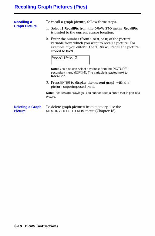
8-18 DRAW Instructions
8308DRAW.DOC TI-83 international English Bob Fedorisko Revised: 02/19/01 12:29 PM Printed: 02/19/01 1:49PM Page 18 of 20
To recall a graph picture, follow these steps.
1. Select 2:RecallPic from the DRAW STO menu. RecallPicis pasted to the current cursor location.
2. Enter the number (from 1 to 9, or 0) of the picturevariable from which you want to recall a picture. Forexample, if you enter 3, the TI-83 will recall the picturestored to Pic3 .
Note: You also can select a variable from the PICTUREsecondary menu (� 4). The variable is pasted next toRecallPic .
3. Press Í to display the current graph with thepicture superimposed on it.
Note: Pictures are drawings. You cannot trace a curve that is part of apicture.
To delete graph pictures from memory, use theMEMORY DELETE FROM menu (Chapter 18).
Recalling Graph Pictures (Pics)
Recalling aGraph Picture
Deleting a GraphPicture
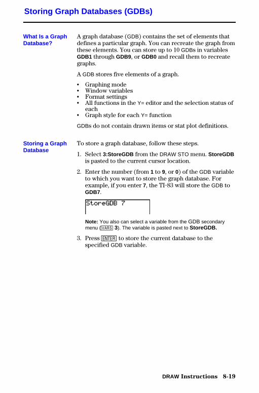
DRAW Instructions 8-19
8308DRAW.DOC TI-83 international English Bob Fedorisko Revised: 02/19/01 12:29 PM Printed: 02/19/01 1:49PM Page 19 of 20
A graph database (GDB) contains the set of elements thatdefines a particular graph. You can recreate the graph fromthese elements. You can store up to 10 GDBs in variablesGDB1 through GDB9, or GDB0 and recall them to recreategraphs.
A GDB stores five elements of a graph.
• Graphing mode• Window variables• Format settings• All functions in the Y= editor and the selection status of
each• Graph style for each Y= function
GDBs do not contain drawn items or stat plot definitions.
To store a graph database, follow these steps.
1. Select 3:StoreGDB from the DRAW STO menu. StoreGDBis pasted to the current cursor location.
2. Enter the number (from 1 to 9, or 0) of the GDB variableto which you want to store the graph database. Forexample, if you enter 7, the TI-83 will store the GDB toGDB7.
Note: You also can select a variable from the GDB secondarymenu (� 3). The variable is pasted next to StoreGDB .
3. Press Í to store the current database to thespecified GDB variable.
Storing Graph Databases (GDBs)
What Is a GraphDatabase?
Storing a GraphDatabase
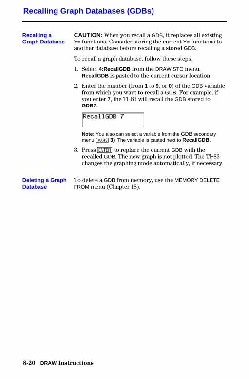
8-20 DRAW Instructions
8308DRAW.DOC TI-83 international English Bob Fedorisko Revised: 02/19/01 12:29 PM Printed: 02/19/01 1:49PM Page 20 of 20
CAUTION: When you recall a GDB, it replaces all existingY= functions. Consider storing the current Y= functions toanother database before recalling a stored GDB.
To recall a graph database, follow these steps.
1. Select 4:RecallGDB from the DRAW STO menu.RecallGDB is pasted to the current cursor location.
2. Enter the number (from 1 to 9, or 0) of the GDB variablefrom which you want to recall a GDB. For example, ifyou enter 7, the TI-83 will recall the GDB stored toGDB7.
Note: You also can select a variable from the GDB secondarymenu (� 3). The variable is pasted next to RecallGDB .
3. Press Í to replace the current GDB with therecalled GDB. The new graph is not plotted. The TI-83changes the graphing mode automatically, if necessary.
To delete a GDB from memory, use the MEMORY DELETEFROM menu (Chapter 18).
Recalling Graph Databases (GDBs)
Recalling aGraph Database
Deleting a GraphDatabase
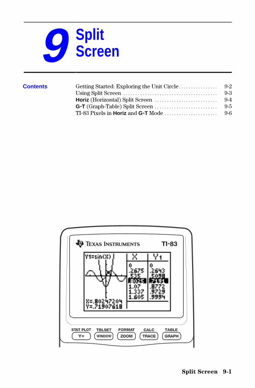
Split Screen 9-1
8309SPLT.DOC TI-83 international English Bob Fedorisko Revised: 02/19/01 12:31 PM Printed: 02/19/01 1:36PM Page 1 of 6
9 SplitScreen
Getting Started: Exploring the Unit Circle................ 9-2Using Split Screen ....................................... 9-3Horiz (Horizontal) Split Screen .......................... 9-4G.T (Graph-Table) Split Screen .......................... 9-5TI-83 Pixels in Horiz and G.T Mode ...................... 9-6
Contents
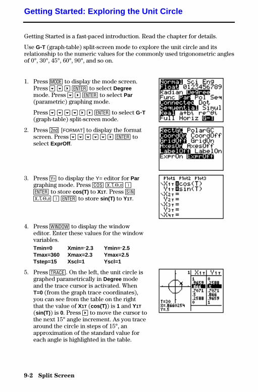
9-2 Split Screen
8309SPLT.DOC TI-83 international English Bob Fedorisko Revised: 02/19/01 12:31 PM Printed: 02/19/01 1:36PM Page 2 of 6
Getting Started is a fast-paced introduction. Read the chapter for details.
Use G.T (graph-table) split-screen mode to explore the unit circle and itsrelationship to the numeric values for the commonly used trigonometric anglesof 0°, 30°, 45°, 60°, 90°, and so on.
1. Press z to display the mode screen.Press † † ~ Í to select Degreemode. Press † ~ Í to select Par(parametric) graphing mode.
Press † † † † ~ ~ Í to select G.T(graph-table) split-screen mode.
2. Press y [FORMAT] to display the formatscreen. Press † † † † † ~ Í toselect ExprOff .
3. Press o to display the Y= editor for Pargraphing mode. Press ™ „ ¤Í to store cos(T) to X1T. Press ˜„ ¤ Í to store sin(T) to Y1T.
4. Press p to display the windoweditor. Enter these values for the windowvariables.Tmin=0 Xmin= L2.3 Ymin= L2.5Tmax=360 Xmax=2.3 Ymax=2.5Tstep=15 Xscl=1 Yscl=1
5. Press r. On the left, the unit circle isgraphed parametrically in Degree modeand the trace cursor is activated. WhenT=0 (from the graph trace coordinates),you can see from the table on the rightthat the value of X1T (cos(T) ) is 1 and Y1T
(sin(T) ) is 0. Press ~ to move the cursor tothe next 15° angle increment. As you tracearound the circle in steps of 15°, anapproximation of the standard value foreach angle is highlighted in the table.
Getting Started: Exploring the Unit Circle
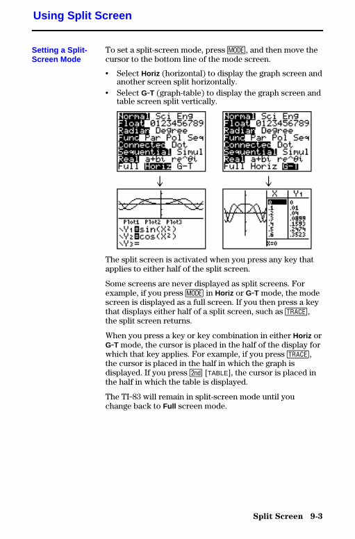
Split Screen 9-3
8309SPLT.DOC TI-83 international English Bob Fedorisko Revised: 02/19/01 12:31 PM Printed: 02/19/01 1:36PM Page 3 of 6
To set a split-screen mode, press z, and then move thecursor to the bottom line of the mode screen.
• Select Horiz (horizontal) to display the graph screen andanother screen split horizontally.
• Select G.T (graph-table) to display the graph screen andtable screen split vertically.
$ $
The split screen is activated when you press any key thatapplies to either half of the split screen.
Some screens are never displayed as split screens. Forexample, if you press z in Horiz or G.T mode, the modescreen is displayed as a full screen. If you then press a keythat displays either half of a split screen, such as r,the split screen returns.
When you press a key or key combination in either Horiz orG.T mode, the cursor is placed in the half of the display forwhich that key applies. For example, if you press r,the cursor is placed in the half in which the graph isdisplayed. If you press y [TABLE], the cursor is placed inthe half in which the table is displayed.
The TI-83 will remain in split-screen mode until youchange back to Full screen mode.
Using Split Screen
Setting a Split-Screen Mode
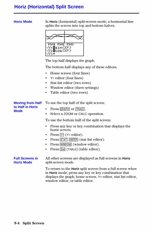
9-4 Split Screen
8309SPLT.DOC TI-83 international English Bob Fedorisko Revised: 02/19/01 12:31 PM Printed: 02/19/01 1:36PM Page 4 of 6
In Horiz (horizontal) split-screen mode, a horizontal linesplits the screen into top and bottom halves.
The top half displays the graph.
The bottom half displays any of these editors.
• Home screen (four lines)• Y= editor (four lines)• Stat list editor (two rows)• Window editor (three settings)• Table editor (two rows)
To use the top half of the split screen:
• Press s or r.• Select a ZOOM or CALC operation.
To use the bottom half of the split screen:
• Press any key or key combination that displays thehome screen.
• Press o (Y= editor).• Press … Í (stat list editor).• Press p (window editor).• Press y [TABLE] (table editor).
All other screens are displayed as full screens in Horizsplit-screen mode.
To return to the Horiz split screen from a full screen whenin Horiz mode, press any key or key combination thatdisplays the graph, home screen, Y= editor, stat list editor,window editor, or table editor.
Horiz (Horizontal) Split Screen
Horiz Mode
Moving from Halfto Half in HorizMode
Full Screens inHoriz Mode
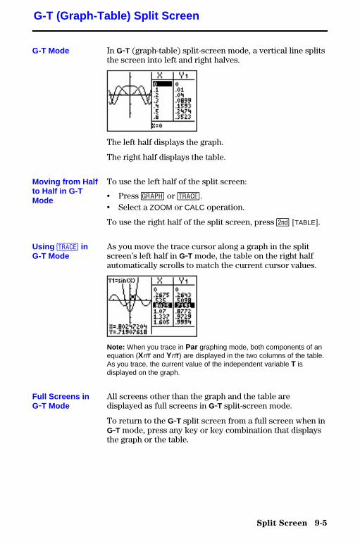
Split Screen 9-5
8309SPLT.DOC TI-83 international English Bob Fedorisko Revised: 02/19/01 12:31 PM Printed: 02/19/01 1:36PM Page 5 of 6
In G.T (graph-table) split-screen mode, a vertical line splitsthe screen into left and right halves.
The left half displays the graph.
The right half displays the table.
To use the left half of the split screen:
• Press s or r.• Select a ZOOM or CALC operation.
To use the right half of the split screen, press y [TABLE].
As you move the trace cursor along a graph in the splitscreen’s left half in G.T mode, the table on the right halfautomatically scrolls to match the current cursor values.
Note: When you trace in Par graphing mode, both components of anequation (XnT and YnT) are displayed in the two columns of the table.As you trace, the current value of the independent variable T isdisplayed on the graph.
All screens other than the graph and the table aredisplayed as full screens in G.T split-screen mode.
To return to the G.T split screen from a full screen when inG.T mode, press any key or key combination that displaysthe graph or the table.
G-T (Graph-Table) Split Screen
G-T Mode
Moving from Halfto Half in G-TMode
Using r inG-T Mode
Full Screens inG.T Mode
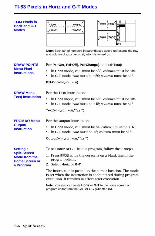
9-6 Split Screen
8309SPLT.DOC TI-83 international English Bob Fedorisko Revised: 02/19/01 12:31 PM Printed: 02/19/01 1:36PM Page 6 of 6
Note: Each set of numbers in parentheses above represents the rowand column of a corner pixel, which is turned on.
For Pxl.On(, Pxl.Off( , Pxl.Change( , and pxl .Test( :
• In Horiz mode, row must be {30; column must be {94.• In G.T mode, row must be {50; column must be {46.
Pxl.On(row,column)
For the Text( instruction:
• In Horiz mode, row must be {25; column must be {94.• In G.T mode, row must be {45; column must be {46.
Text(row,column," text")
For the Output( instruction:
• In Horiz mode, row must be {4; column must be {16.• In G.T mode, row must be {8; column must be {16.
Output( row,column," text")
To set Horiz or G.T from a program, follow these steps.
1. Press z while the cursor is on a blank line in theprogram editor.
2. Select Horiz or G.T.
The instruction is pasted to the cursor location. The modeis set when the instruction is encountered during programexecution. It remains in effect after execution.
Note: You also can paste Horiz or G.T to the home screen orprogram editor from the CATALOG (Chapter 15).
TI-83 Pixels in Horiz and G-T Modes
TI-83 Pixels inHoriz and G-TModes
DRAW POINTSMenu PixelInstructions
DRAW MenuText( Instruction
PRGM I/O MenuOutput(Instruction
Setting aSplit-ScreenMode from theHome Screen ora Program
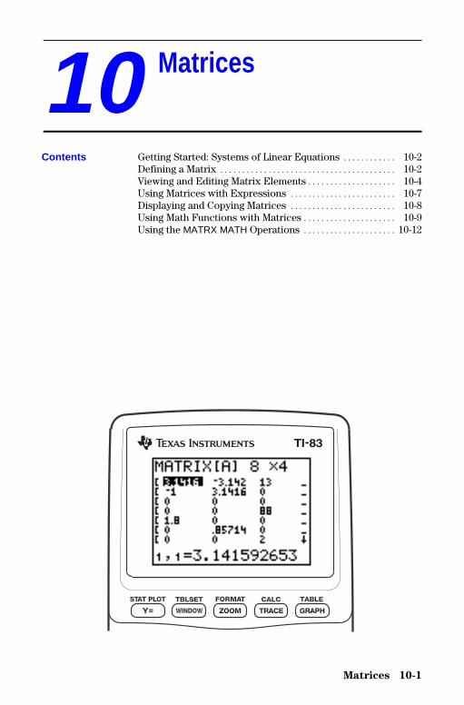
Matrices 10-1
8310MTRX.DOC TI-83 international English Bob Fedorisko Revised: 02/19/01 12:35 PM Printed: 02/19/01 1:36PM Page 1 of 16
10 Matrices
Getting Started: Systems of Linear Equations ............ 10-2Defining a Matrix ........................................ 10-2Viewing and Editing Matrix Elements .................... 10-4Using Matrices with Expressions ........................ 10-7Displaying and Copying Matrices ........................ 10-8Using Math Functions with Matrices ..................... 10-9Using the MATRX MATH Operations ..................... 10-12
Contents

10-2 Matrices
8310MTRX.DOC TI-83 international English Bob Fedorisko Revised: 02/19/01 12:35 PM Printed: 02/19/01 1:36PM Page 2 of 16
Getting Started is a fast-paced introduction. Read the chapter for details.
Find the solution of X + 2Y + 3Z = 3 and 2X + 3Y + 4Z = 3. On the TI-83, youcan solve a system of linear equations by entering the coefficients as elementsin a matrix, and then using rref( to obtain the reduced row-echelon form.
1. Press �. Press ~ ~ to display theMATRX EDIT menu. Press 1 to select 1: [A] ¸
2. Press 2 Í 4 Í to define a 2×4matrix. The rectangular cursor indicatesthe current element. Ellipses (...) indicateadditional columns beyond the screen.
3. Press 1 Í to enter the first element.The rectangular cursor moves to thesecond column of the first row.
4. Press 2 Í 3 Í 3 Í to completethe first row for X + 2Y + 3Z = 3.
5. Press 2 Í 3 Í 4 Í 3 Í toenter the second row for 2X + 3Y + 4Z = 3.
6. Press y [QUIT] to return to the homescreen. If necessary, press ‘ to clearthe home screen. Press � ~ todisplay the MATRX MATH menu. Press } towrap to the end of the menu. Select B:rref(to copy rref( to the home screen.
7. Press � 1 to select 1: [A] from theMATRX NAMES menu. Press ¤ Í. Thereduced row-echelon form of the matrix isdisplayed and stored in Ans .
1X N 1Z = L3 so X = L3 + Z1Y + 2Z = 3 so Y = 3 N 2Z
Getting Started: Systems of Linear Equations
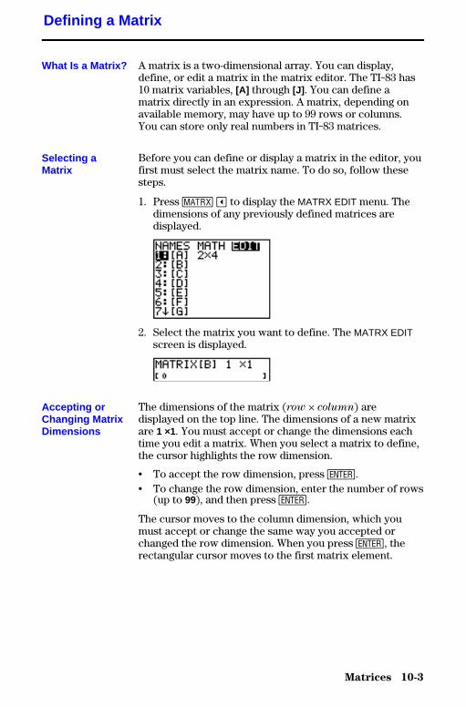
Matrices 10-3
8310MTRX.DOC TI-83 international English Bob Fedorisko Revised: 02/19/01 12:35 PM Printed: 02/19/01 1:36PM Page 3 of 16
A matrix is a two-dimensional array. You can display,define, or edit a matrix in the matrix editor. The TI-83 has10 matrix variables, [A] through [J] . You can define amatrix directly in an expression. A matrix, depending onavailable memory, may have up to 99 rows or columns.You can store only real numbers in TI-83 matrices.
Before you can define or display a matrix in the editor, youfirst must select the matrix name. To do so, follow thesesteps.
1. Press � | to display the MATRX EDIT menu. Thedimensions of any previously defined matrices aredisplayed.
2. Select the matrix you want to define. The MATRX EDITscreen is displayed.
The dimensions of the matrix (row × column) aredisplayed on the top line. The dimensions of a new matrixare 1 ×1. You must accept or change the dimensions eachtime you edit a matrix. When you select a matrix to define,the cursor highlights the row dimension.
• To accept the row dimension, press Í.• To change the row dimension, enter the number of rows
(up to 99), and then press Í.
The cursor moves to the column dimension, which youmust accept or change the same way you accepted orchanged the row dimension. When you press Í, therectangular cursor moves to the first matrix element.
Defining a Matrix
What Is a Matrix?
Selecting aMatrix
Accepting orChanging MatrixDimensions
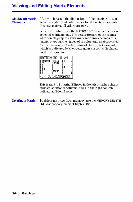
10-4 Matrices
8310MTRX.DOC TI-83 international English Bob Fedorisko Revised: 02/19/01 12:35 PM Printed: 02/19/01 1:36PM Page 4 of 16
After you have set the dimensions of the matrix, you canview the matrix and enter values for the matrix elements.In a new matrix, all values are zero.
Select the matrix from the MATRX EDIT menu and enter oraccept the dimensions. The center portion of the matrixeditor displays up to seven rows and three columns of amatrix, showing the values of the elements in abbreviatedform if necessary. The full value of the current element,which is indicated by the rectangular cursor, is displayedon the bottom line.
This is an 8 × 4 matrix. Ellipses in the left or right columnindicate additional columns. # or $ in the right columnindicate additional rows.
To delete matrices from memory, use the MEMORY DELETEFROM secondary menu (Chapter 18).
Viewing and Editing Matrix Elements
Displaying MatrixElements
Deleting a Matrix
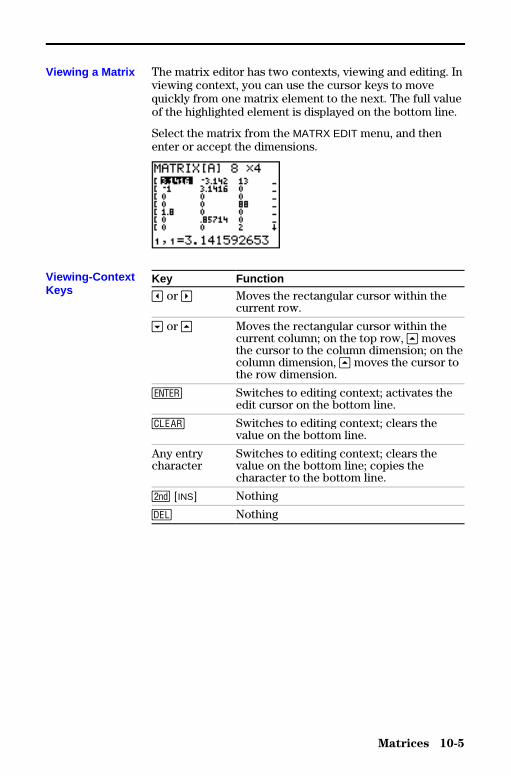
Matrices 10-5
8310MTRX.DOC TI-83 international English Bob Fedorisko Revised: 02/19/01 12:35 PM Printed: 02/19/01 1:36PM Page 5 of 16
The matrix editor has two contexts, viewing and editing. Inviewing context, you can use the cursor keys to movequickly from one matrix element to the next. The full valueof the highlighted element is displayed on the bottom line.
Select the matrix from the MATRX EDIT menu, and thenenter or accept the dimensions.
Key Function
| or ~ Moves the rectangular cursor within thecurrent row.
† or } Moves the rectangular cursor within thecurrent column; on the top row, } movesthe cursor to the column dimension; on thecolumn dimension, } moves the cursor tothe row dimension.
Í Switches to editing context; activates theedit cursor on the bottom line.
‘ Switches to editing context; clears thevalue on the bottom line.
Any entrycharacter
Switches to editing context; clears thevalue on the bottom line; copies thecharacter to the bottom line.
y [INS] Nothing
{ Nothing
Viewing a Matrix
Viewing-ContextKeys
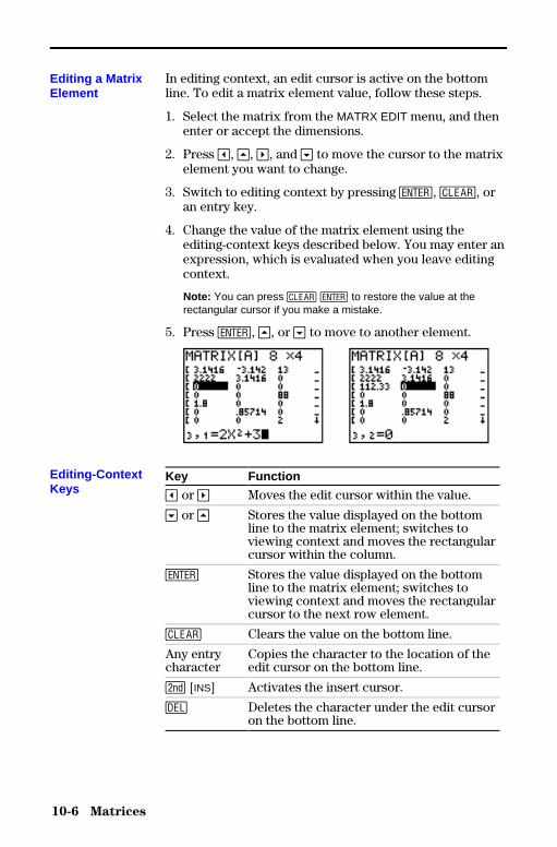
10-6 Matrices
8310MTRX.DOC TI-83 international English Bob Fedorisko Revised: 02/19/01 12:35 PM Printed: 02/19/01 1:36PM Page 6 of 16
In editing context, an edit cursor is active on the bottomline. To edit a matrix element value, follow these steps.
1. Select the matrix from the MATRX EDIT menu, and thenenter or accept the dimensions.
2. Press |, }, ~, and † to move the cursor to the matrixelement you want to change.
3. Switch to editing context by pressing Í, ‘, oran entry key.
4. Change the value of the matrix element using theediting-context keys described below. You may enter anexpression, which is evaluated when you leave editingcontext.
Note: You can press ‘ Í to restore the value at therectangular cursor if you make a mistake.
5. Press Í, }, or † to move to another element.
Key Function
| or ~ Moves the edit cursor within the value.
† or } Stores the value displayed on the bottomline to the matrix element; switches toviewing context and moves the rectangularcursor within the column.
Í Stores the value displayed on the bottomline to the matrix element; switches toviewing context and moves the rectangularcursor to the next row element.
‘ Clears the value on the bottom line.
Any entrycharacter
Copies the character to the location of theedit cursor on the bottom line.
y [INS] Activates the insert cursor.
{ Deletes the character under the edit cursoron the bottom line.
Editing a MatrixElement
Editing-ContextKeys
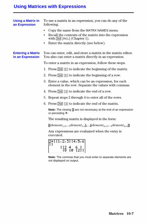
Matrices 10-7
8310MTRX.DOC TI-83 international English Bob Fedorisko Revised: 02/19/01 12:35 PM Printed: 02/19/01 1:36PM Page 7 of 16
To use a matrix in an expression, you can do any of thefollowing.
• Copy the name from the MATRX NAMES menu.• Recall the contents of the matrix into the expression
with y [RCL] (Chapter 1).• Enter the matrix directly (see below).
You can enter, edit, and store a matrix in the matrix editor.You also can enter a matrix directly in an expression.
To enter a matrix in an expression, follow these steps.
1. Press y [ [ ] to indicate the beginning of the matrix.
2. Press y [ [ ] to indicate the beginning of a row.
3. Enter a value, which can be an expression, for eachelement in the row. Separate the values with commas.
4. Press y [ ] ] to indicate the end of a row.
5. Repeat steps 2 through 4 to enter all of the rows.
6. Press y [ ] ] to indicate the end of the matrix.
Note: The closing ]] are not necessary at the end of an expressionor preceding !.
The resulting matrix is displayed in the form:
[[element1,1,...,element1,n],...,[elementm,1,...,elementm,n]]
Any expressions are evaluated when the entry isexecuted.
Note: The commas that you must enter to separate elements arenot displayed on output.
Using Matrices with Expressions
Using a Matrix inan Expression
Entering a Matrixin an Expression
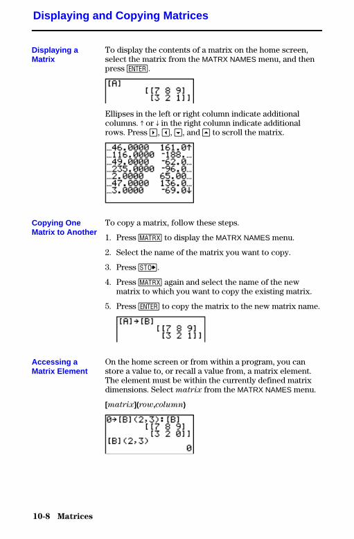
10-8 Matrices
8310MTRX.DOC TI-83 international English Bob Fedorisko Revised: 02/19/01 12:35 PM Printed: 02/19/01 1:36PM Page 8 of 16
To display the contents of a matrix on the home screen,select the matrix from the MATRX NAMES menu, and thenpress Í.
Ellipses in the left or right column indicate additionalcolumns. # or $ in the right column indicate additionalrows. Press ~, |, †, and } to scroll the matrix.
To copy a matrix, follow these steps.
1. Press � to display the MATRX NAMES menu.
2. Select the name of the matrix you want to copy.
3. Press ¿.
4. Press � again and select the name of the newmatrix to which you want to copy the existing matrix.
5. Press Í to copy the matrix to the new matrix name.
On the home screen or from within a program, you canstore a value to, or recall a value from, a matrix element.The element must be within the currently defined matrixdimensions. Select matrix from the MATRX NAMES menu.
[matrix](row,column)
Displaying and Copying Matrices
Displaying aMatrix
Copying OneMatrix to Another
Accessing aMatrix Element
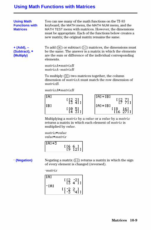
Matrices 10-9
8310MTRX.DOC TI-83 international English Bob Fedorisko Revised: 02/19/01 12:35 PM Printed: 02/19/01 1:36PM Page 9 of 16
You can use many of the math functions on the TI-83keyboard, the MATH menu, the MATH NUM menu, and theMATH TEST menu with matrices. However, the dimensionsmust be appropriate. Each of the functions below creates anew matrix; the original matrix remains the same.
To add (Ã) or subtract (¹) matrices, the dimensions mustbe the same. The answer is a matrix in which the elementsare the sum or difference of the individual correspondingelements.
matrixA+matrixB
matrixANmatrixB
To multiply (¯) two matrices together, the columndimension of matrixA must match the row dimension ofmatrixB.
matrixAämatrixB
Multiplying a matrix by a value or a value by a matrix
returns a matrix in which each element of matrix ismultiplied by value.
matrixävalue
valueämatrix
Negating a matrix (Ì) returns a matrix in which the signof every element is changed (reversed).
Lmatrix
Using Math Functions with Matrices
Using MathFunctions withMatrices
+ (Add), –(Subtract), ä(Multiply)
L (Negation)
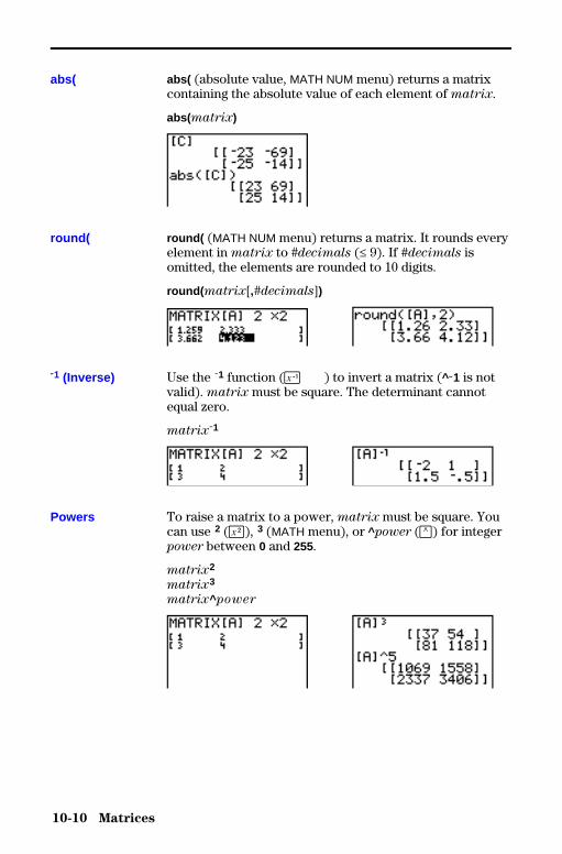
10-10 Matrices
8310MTRX.DOC TI-83 international English Bob Fedorisko Revised: 02/19/01 12:35 PM Printed: 02/19/01 1:36PM Page 10 of 16
abs( (absolute value, MATH NUM menu) returns a matrixcontaining the absolute value of each element of matrix.
abs(matrix)
round( (MATH NUM menu) returns a matrix. It rounds everyelement in matrix to #decimals (� 9). If #decimals isomitted, the elements are rounded to 10 digits.
round( matrix[,#decimals])
Use the L1 function (— ) to invert a matrix (^L1 is notvalid). matrix must be square. The determinant cannotequal zero.
matrixL1
To raise a matrix to a power, matrix must be square. Youcan use 2 (¡), 3 (MATH menu), or ^power (›) for integerpower between 0 and 255.
matrix2
matrix3
matrix^power
abs(
round(
M1 (Inverse)
Powers
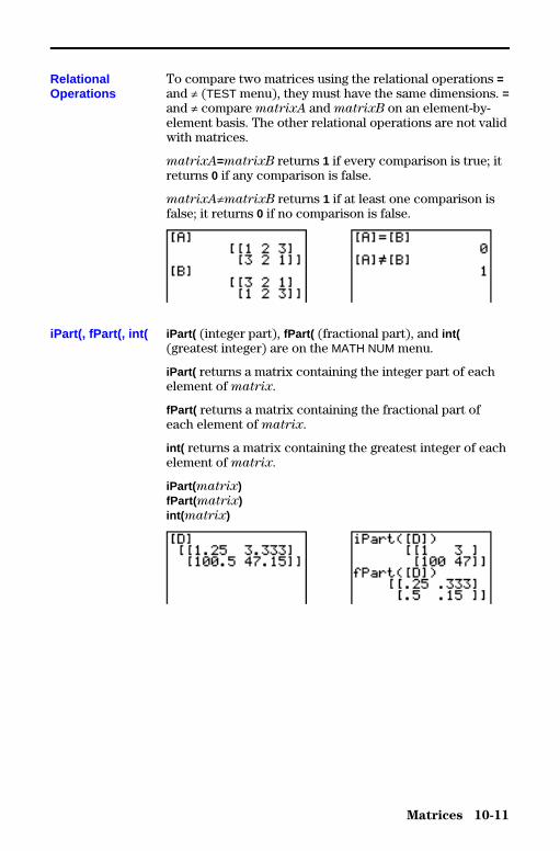
Matrices 10-11
8310MTRX.DOC TI-83 international English Bob Fedorisko Revised: 02/19/01 12:35 PM Printed: 02/19/01 1:36PM Page 11 of 16
To compare two matrices using the relational operations =and ƒ (TEST menu), they must have the same dimensions. =and ƒ compare matrixA and matrixB on an element-by-element basis. The other relational operations are not validwith matrices.
matrixA=matrixB returns 1 if every comparison is true; itreturns 0 if any comparison is false.
matrixAƒmatrixB returns 1 if at least one comparison isfalse; it returns 0 if no comparison is false.
iPart( (integer part), fPart( (fractional part), and int((greatest integer) are on the MATH NUM menu.
iPart( returns a matrix containing the integer part of eachelement of matrix.
fPart( returns a matrix containing the fractional part ofeach element of matrix.
int( returns a matrix containing the greatest integer of eachelement of matrix.
iPart( matrix)fPart( matrix)int( matrix)
RelationalOperations
iPart(, fPart(, int(
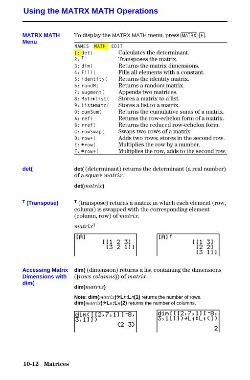
10-12 Matrices
8310MTRX.DOC TI-83 international English Bob Fedorisko Revised: 02/19/01 12:35 PM Printed: 02/19/01 1:36PM Page 12 of 16
To display the MATRX MATH menu, press � ~.
NAMES MATH EDIT1: det( Calculates the determinant.2: T Transposes the matrix.3: dim( Returns the matrix dimensions.4: Fill( Fills all elements with a constant.5: identity( Returns the identity matrix.6: randM( Returns a random matrix.7: augment( Appends two matrices.8: Matr4list( Stores a matrix to a list.9: List4matr( Stores a list to a matrix.0: cumSum( Returns the cumulative sums of a matrix.A: ref( Returns the row-echelon form of a matrix.B: rref( Returns the reduced row-echelon form.C: rowSwap( Swaps two rows of a matrix.D: row+( Adds two rows; stores in the second row.E: ärow( Multiplies the row by a number.F: ärow+( Multiplies the row, adds to the second row.
det( (determinant) returns the determinant (a real number)of a square matrix.
det(matrix)
T (transpose) returns a matrix in which each element (row,column) is swapped with the corresponding element(column, row) of matrix.
matrixT
dim( (dimension) returns a list containing the dimensions({rows columns}) of matrix.
dim( matrix)
Note: dim( matrix)!Ln:Ln(1) returns the number of rows.dim( matrix)!Ln:Ln(2) returns the number of columns.
Using the MATRX MATH Operations
MATRX MATHMenu
det(
T (Transpose)
Accessing MatrixDimensions withdim(

Matrices 10-13
8310MTRX.DOC TI-83 international English Bob Fedorisko Revised: 02/19/01 12:35 PM Printed: 02/19/01 1:36PM Page 13 of 16
Use dim( with ¿ to create a new matrixname ofdimensions rows × columns with 0 as each element.
{rows,columns}!dim( matrixname)
Use dim( with ¿ to redimension an existingmatrixname to dimensions rows × columns. The elementsin the old matrixname that are within the new dimensionsare not changed. Additional created elements are zeros.Matrix elements that are outside the new dimensions aredeleted.
{rows,columns}!dim( matrixname)
Fill( stores value to every element in matrixname.
Fill( value,matrixname)
identity( returns the identity matrix of dimension rows ×dimension columns.
identity( dimension)
randM( (create random matrix) returns a rows × columns
random matrix of integers ‚ L9 and � 9. The seed valuestored to the rand function controls the values (Chapter 2).
randM( rows,columns)
Creating a Matrixwith dim(
Redimensioning aMatrix with dim(
Fill(
identity(
randM(
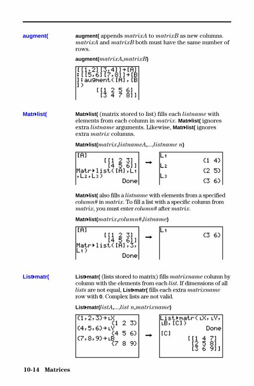
10-14 Matrices
8310MTRX.DOC TI-83 international English Bob Fedorisko Revised: 02/19/01 12:35 PM Printed: 02/19/01 1:36PM Page 14 of 16
augment( appends matrixA to matrixB as new columns.matrixA and matrixB both must have the same number ofrows.
augment( matrixA,matrixB)
Matr4list( (matrix stored to list) fills each listname withelements from each column in matrix. Matr4list( ignoresextra listname arguments. Likewise, Matr4list( ignoresextra matrix columns.
Matr4list( matrix,listnameA,...,listname n)
&
Matr4list( also fills a listname with elements from a specifiedcolumn# in matrix. To fill a list with a specific column frommatrix, you must enter column# after matrix.
Matr4list( matrix,column#,listname)
&
List 4matr( (lists stored to matrix) fills matrixname column bycolumn with the elements from each list. If dimensions of alllists are not equal, List 4matr( fills each extra matrixname
row with 0. Complex lists are not valid.
List 4matr( listA,...,list n,matrixname)
&
augment(
Matr4list(
List 4matr(
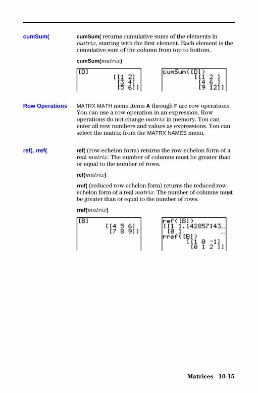
Matrices 10-15
8310MTRX.DOC TI-83 international English Bob Fedorisko Revised: 02/19/01 12:35 PM Printed: 02/19/01 1:36PM Page 15 of 16
cumSum( returns cumulative sums of the elements inmatrix, starting with the first element. Each element is thecumulative sum of the column from top to bottom.
cumSum( matrix)
MATRX MATH menu items A through F are row operations.You can use a row operation in an expression. Rowoperations do not change matrix in memory. You canenter all row numbers and values as expressions. You canselect the matrix from the MATRX NAMES menu.
ref( (row-echelon form) returns the row-echelon form of areal matrix. The number of columns must be greater thanor equal to the number of rows.
ref(matrix)
rref( (reduced row-echelon form) returns the reduced row-echelon form of a real matrix. The number of columns mustbe greater than or equal to the number of rows.
rref( matrix)
cumSum(
Row Operations
ref(, rref(
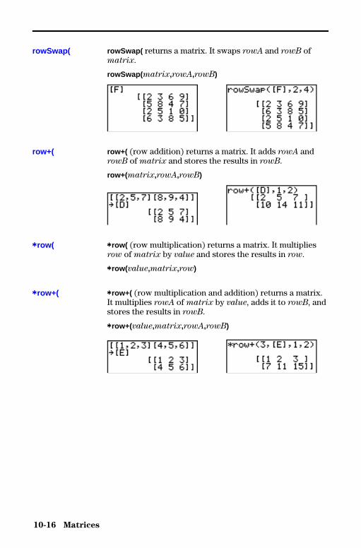
10-16 Matrices
8310MTRX.DOC TI-83 international English Bob Fedorisko Revised: 02/19/01 12:35 PM Printed: 02/19/01 1:36PM Page 16 of 16
rowSwap( returns a matrix. It swaps rowA and rowB ofmatrix.
rowSwap( matrix,rowA,rowB)
row+( (row addition) returns a matrix. It adds rowA androwB of matrix and stores the results in rowB.
row+( matrix,rowA,rowB)
ärow( (row multiplication) returns a matrix. It multipliesrow of matrix by value and stores the results in row.
ärow( value,matrix,row)
ärow+( (row multiplication and addition) returns a matrix.It multiplies rowA of matrix by value, adds it to rowB, andstores the results in rowB.
ärow+( value,matrix,rowA,rowB)
rowSwap(
row+(
ärow(
ärow+(
Lists 11-1
8311LIST.DOC TI-83 international English Bob Fedorisko Revised: 02/19/01 1:21 PM Printed: 02/19/01 1:37 PMPage 1 of 18
11 Lists
Getting Started: Generating a Sequence .................. 11-2Naming Lists............................................. 11-3Storing and Displaying Lists ............................. 11-4Entering List Names ..................................... 11-6Attaching Formulas to List Names ....................... 11-7Using Lists in Expressions ............................... 11-9LIST OPS Menu.......................................... 11-10LIST MATH Menu ........................................ 11-17
Contents

11-2 Lists
8311LIST.DOC TI-83 international English Bob Fedorisko Revised: 02/19/01 1:21 PM Printed: 02/19/01 1:37 PMPage 2 of 18
Getting Started is a fast-paced introduction. Read the chapter for details.
Calculate the first eight terms of the sequence 1/A2. Store the results to a user-created list. Then display the results in fraction form. Begin this example on ablank line on the home screen.
1. Press y [LIST] ~ to display the LIST OPSmenu.
2. Press 5 to select 5:seq( , which pastes seq( tothe current cursor location.
3. Press 1 ¥ ƒ [A] ¡ ¢ ƒ [A] ¢ 1¢ 8 ¢ 1 ¤ to enter the sequence.
4. Press ¿, and then press y ƒ toturn on alpha-lock. Press [S] [E] [Q], andthen press ƒ to turn off alpha-lock.Press 1 to complete the list name.
5. Press Í to generate the list and store itin SEQ1. The list is displayed on the homescreen. An ellipsis (...) indicates that the listcontinues beyond the viewing window.Press ~ repeatedly (or press and hold ~)to scroll the list and view all the listelements.
6. Press y [LIST] to display the LIST NAMESmenu. Press Í to paste ÙSEQ1 to thecurrent cursor location. (If SEQ1 is not item1 on your LIST NAMES menu, move thecursor to SEQ1 before you press Í.)
7. Press � to display the MATH menu.Press 1 to select 1:4Frac , which pastes 4Fracto the current cursor location.
8. Press Í to show the sequence infraction form. Press ~ repeatedly (or pressand hold ~) to scroll the list and view allthe list elements.
Getting Started: Generating a Sequence
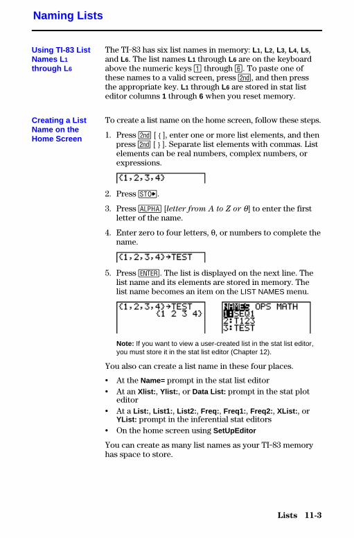
Lists 11-3
8311LIST.DOC TI-83 international English Bob Fedorisko Revised: 02/19/01 1:21 PM Printed: 02/19/01 1:37 PMPage 3 of 18
The TI-83 has six list names in memory: L1, L2, L3, L4, L5,and L6. The list names L1 through L6 are on the keyboardabove the numeric keys À through ¸. To paste one ofthese names to a valid screen, press y, and then pressthe appropriate key. L1 through L6 are stored in stat listeditor columns 1 through 6 when you reset memory.
To create a list name on the home screen, follow these steps.
1. Press y [ { ], enter one or more list elements, and thenpress y [ } ]. Separate list elements with commas. Listelements can be real numbers, complex numbers, orexpressions.
2. Press ¿.
3. Press ƒ [letter from A to Z or q] to enter the firstletter of the name.
4. Enter zero to four letters, q, or numbers to complete thename.
5. Press Í. The list is displayed on the next line. Thelist name and its elements are stored in memory. Thelist name becomes an item on the LIST NAMES menu.
Note: If you want to view a user-created list in the stat list editor,you must store it in the stat list editor (Chapter 12).
You also can create a list name in these four places.
• At the Name= prompt in the stat list editor• At an Xlist: , Ylist: , or Data List: prompt in the stat plot
editor• At a List: , List1: , List2: , Freq: , Freq1: , Freq2: , XList: , or
YList: prompt in the inferential stat editors• On the home screen using SetUpEditor
You can create as many list names as your TI-83 memoryhas space to store.
Naming Lists
Using TI-83 ListNames L 1
through L 6
Creating a ListName on theHome Screen
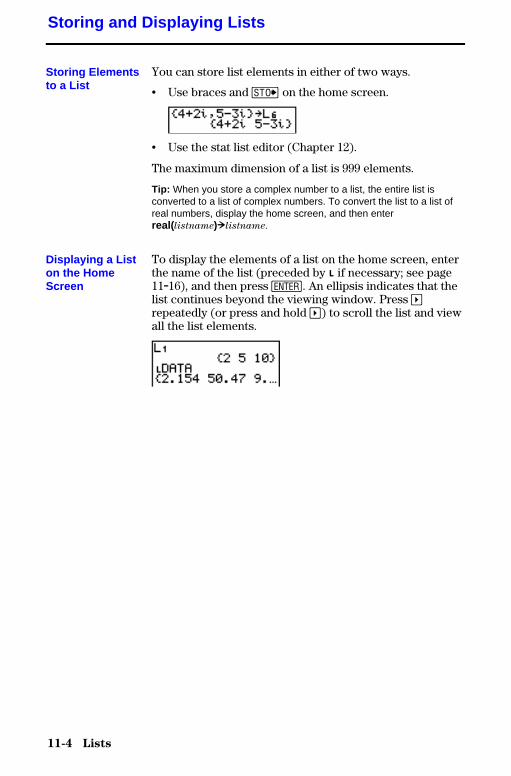
11-4 Lists
8311LIST.DOC TI-83 international English Bob Fedorisko Revised: 02/19/01 1:21 PM Printed: 02/19/01 1:37 PMPage 4 of 18
You can store list elements in either of two ways.
• Use braces and ¿ on the home screen.
• Use the stat list editor (Chapter 12).
The maximum dimension of a list is 999 elements.
Tip: When you store a complex number to a list, the entire list isconverted to a list of complex numbers. To convert the list to a list ofreal numbers, display the home screen, and then enterreal( listname)!listname.
To display the elements of a list on the home screen, enterthe name of the list (preceded by Ù if necessary; see page11.16), and then press Í. An ellipsis indicates that thelist continues beyond the viewing window. Press ~repeatedly (or press and hold ~) to scroll the list and viewall the list elements.
Storing and Displaying Lists
Storing Elementsto a List
Displaying a Liston the HomeScreen
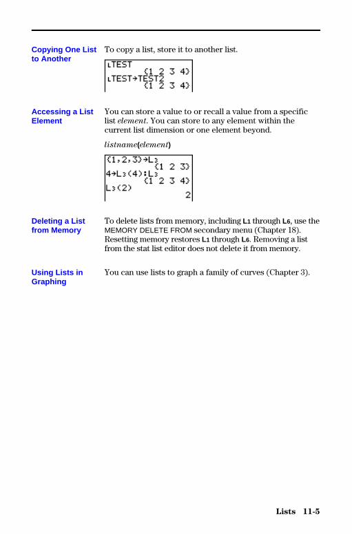
Lists 11-5
8311LIST.DOC TI-83 international English Bob Fedorisko Revised: 02/19/01 1:21 PM Printed: 02/19/01 1:37 PMPage 5 of 18
To copy a list, store it to another list.
You can store a value to or recall a value from a specificlist element. You can store to any element within thecurrent list dimension or one element beyond.
listname(element)
To delete lists from memory, including L1 through L6, use theMEMORY DELETE FROM secondary menu (Chapter 18).Resetting memory restores L1 through L6. Removing a listfrom the stat list editor does not delete it from memory.
You can use lists to graph a family of curves (Chapter 3).
Copying One Listto Another
Accessing a ListElement
Deleting a Listfrom Memory
Using Lists inGraphing
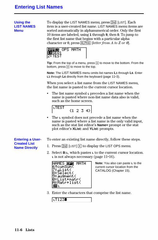
11-6 Lists
8311LIST.DOC TI-83 international English Bob Fedorisko Revised: 02/19/01 1:21 PM Printed: 02/19/01 1:37 PMPage 6 of 18
To display the LIST NAMES menu, press y [LIST]. Eachitem is a user-created list name. LIST NAMES menu items aresorted automatically in alphanumerical order. Only the first10 items are labeled, using 1 through 9, then 0. To jump tothe first list name that begins with a particular alphacharacter or q, press ƒ [letter from A to Z or q].
Tip: From the top of a menu, press } to move to the bottom. From thebottom, press † to move to the top.
Note: The LIST NAMES menu omits list names L1 through L6. EnterL1 through L6 directly from the keyboard (page 11.3).
When you select a list name from the LIST NAMES menu,the list name is pasted to the current cursor location.
• The list name symbol Ù precedes a list name when thename is pasted where non-list name data also is valid,such as the home screen.
• The Ù symbol does not precede a list name when thename is pasted where a list name is the only valid input,such as the stat list editor’s Name= prompt or the statplot editor’s XList: and YList: prompts.
To enter an existing list name directly, follow these steps.
1. Press y [LIST] ~ to display the LIST OPS menu.
2. Select B:Ù, which pastes Ù to the current cursor location.Ù is not always necessary (page 11.16).
Note: You also can paste Ù to thecurrent cursor location from theCATALOG (Chapter 15).
3. Enter the characters that comprise the list name.
Entering List Names
Using theLIST NAMESMenu
Entering a User-Created ListName Directly
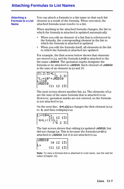
Lists 11-7
8311LIST.DOC TI-83 international English Bob Fedorisko Revised: 02/19/01 1:21 PM Printed: 02/19/01 1:37 PMPage 7 of 18
You can attach a formula to a list name so that each listelement is a result of the formula. When executed, theattached formula must resolve to a list.
When anything in the attached formula changes, the list towhich the formula is attached is updated automatically.
• When you edit an element of a list that is referenced inthe formula, the corresponding element in the list towhich the formula is attached is updated.
• When you edit the formula itself, all elements in the listto which the formula is attached are updated.
For example, the first screen below shows that elementsare stored to L3, and the formula L3+10 is attached to thelist name ÙADD10. The quotation marks designate theformula to be attached to ÙADD10. Each element of ÙADD10is the sum of an element in L3 and 10.
The next screen shows another list, L4. The elements of L4
are the sum of the same formula that is attached to L3.However, quotation marks are not entered, so the formulais not attached to L4.
On the next line, L6!L3(1):L3 changes the first element in L3
to L6, and then redisplays L3.
The last screen shows that editing L3 updated ÙADD10, butdid not change L4. This is because the formula L3+10 isattached to ÙADD10, but it is not attached to L4.
Note: To view a formula that is attached to a list name, use the stat listeditor (Chapter 12).
Attaching Formulas to List Names
Attaching aFormula to a ListName
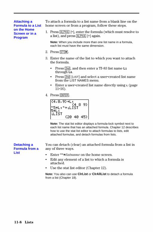
11-8 Lists
8311LIST.DOC TI-83 international English Bob Fedorisko Revised: 02/19/01 1:21 PM Printed: 02/19/01 1:37 PMPage 8 of 18
To attach a formula to a list name from a blank line on thehome screen or from a program, follow these steps.
1. Press ƒ [ã], enter the formula (which must resolve toa list), and press ƒ [ã] again.
Note: When you include more than one list name in a formula,each list must have the same dimension.
2. Press ¿.
3. Enter the name of the list to which you want to attachthe formula.
• Press y, and then enter a TI-83 list name L1through L6.
• Press y [LIST] and select a user.created list namefrom the LIST NAMES menu.
• Enter a user.created list name directly using Ù (page11.16).
4. Press Í.
Note: The stat list editor displays a formula-lock symbol next toeach list name that has an attached formula. Chapter 12 describeshow to use the stat list editor to attach formulas to lists, editattached formulas, and detach formulas from lists.
You can detach (clear) an attached formula from a list inany of three ways.
• Enter "" !listname on the home screen.• Edit any element of a list to which a formula is
attached.• Use the stat list editor (Chapter 12).
Note: You also can use ClrList or ClrAllList to detach a formulafrom a list (Chapter 18).
Attaching aFormula to a Liston the HomeScreen or in aProgram
Detaching aFormula from aList
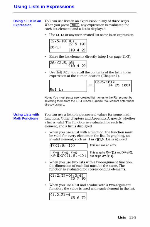
Lists 11-9
8311LIST.DOC TI-83 international English Bob Fedorisko Revised: 02/19/01 1:21 PM Printed: 02/19/01 1:37 PMPage 9 of 18
You can use lists in an expression in any of three ways.When you press Í, any expression is evaluated foreach list element, and a list is displayed.
• Use L1–L6 or any user-created list name in an expression.
• Enter the list elements directly (step 1 on page 11.3).
• Use y [RCL] to recall the contents of the list into anexpression at the cursor location (Chapter 1).
&
Note: You must paste user-created list names to the Rcl prompt byselecting them from the LIST NAMES menu. You cannot enter themdirectly using Ù.
You can use a list to input several values for some mathfunctions. Other chapters and Appendix A specify whethera list is valid. The function is evaluated for each listelement, and a list is displayed.
• When you use a list with a function, the function mustbe valid for every element in the list. In graphing, aninvalid element, such as L1 in ‡({1,0,L1}), is ignored.
This returns an error.
This graphs Xä‡(1) and Xä‡(0),but skips Xä‡(L1).
• When you use two lists with a two-argument function,the dimension of each list must be the same. Thefunction is evaluated for corresponding elements.
• When you use a list and a value with a two-argumentfunction, the value is used with each element in the list.
Using Lists in Expressions
Using a List in anExpression
Using Lists withMath Functions

11-10 Lists
8311LIST.DOC TI-83 international English Bob Fedorisko Revised: 02/19/01 1:21 PM Printed: 02/19/01 1:37 PMPage 10 of 18
To display the LIST OPS menu, press y [LIST] ~.
NAMES OPS MATH1:SortA( Sorts lists in ascending order.2:SortD( Sorts lists in descending order.3:dim( Sets the list dimension.4:Fill( Fills all elements with a constant.5:seq( Creates a sequence.6:cumSum( Returns a list of cumulative sums.7:@List( Returns difference of successive elements.8:Select( Selects specific data points.9:augment( Concatenates two lists.0:List4matr( Stores a list to a matrix.A:Matr4list( Stores a matrix to a list.B:Ù Designates the list-name data type.
SortA( (sort ascending) sorts list elements from low to highvalues. SortD( (sort descending) sorts list elements fromhigh to low values. Complex lists are sorted based onmagnitude (modulus).
With one list, SortA( and SortD( sort the elements oflistname and update the list in memory.
SortA( listname) SortD( listname)
With two or more lists, SortA( and SortD( sort keylistname,and then sort each dependlist by placing its elements in thesame order as the corresponding elements in keylistname.All lists must have the same dimension.
SortA( keylistname,dependlist1[,dependlist2,...,dependlist n])SortD( keylistname,dependlist1[,dependlist2,...,dependlist n])
Note: In the example, 5 is the first element in L4, and 1 is the firstelement in L5. After SortA(L 4,L5), 5 becomes the second element ofL4, and likewise, 1 becomes the second element of L5.
Note: SortA( and SortD( are the same as SortA( and SortD( on theSTAT EDIT menu (Chapter 12).
LIST OPS Menu
LIST OPS Menu
SortA(, SortD(
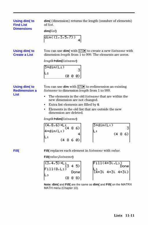
Lists 11-11
8311LIST.DOC TI-83 international English Bob Fedorisko Revised: 02/19/01 1:21 PM Printed: 02/19/01 1:37 PMPage 11 of 18
dim( (dimension) returns the length (number of elements)of list.
dim( list)
You can use dim( with ¿ to create a new listname withdimension length from 1 to 999. The elements are zeros.
length!dim( listname)
You can use dim with ¿ to redimension an existinglistname to dimension length from 1 to 999.
• The elements in the old listname that are within thenew dimension are not changed.
• Extra list elements are filled by 0.• Elements in the old list that are outside the new
dimension are deleted.
length!dim( listname)
Fill( replaces each element in listname with value.
Fill( value,listname)
Note: dim( and Fill( are the same as dim( and Fill( on the MATRXMATH menu (Chapter 10).
Using dim( toFind ListDimensions
Using dim( toCreate a List
Using dim( toRedimension aList
Fill(
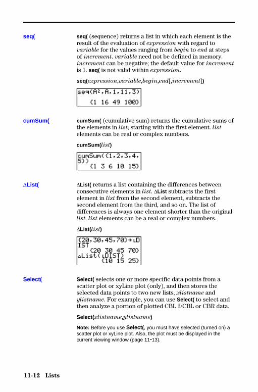
11-12 Lists
8311LIST.DOC TI-83 international English Bob Fedorisko Revised: 02/19/01 1:21 PM Printed: 02/19/01 1:37 PMPage 12 of 18
seq( (sequence) returns a list in which each element is theresult of the evaluation of expression with regard tovariable for the values ranging from begin to end at stepsof increment. variable need not be defined in memory.increment can be negative; the default value for increment
is 1. seq( is not valid within expression.
seq(expression,variable,begin,end[,increment])
cumSum( (cumulative sum) returns the cumulative sums ofthe elements in list, starting with the first element. list
elements can be real or complex numbers.
cumSum( list)
@List( returns a list containing the differences betweenconsecutive elements in list. @List subtracts the firstelement in list from the second element, subtracts thesecond element from the third, and so on. The list ofdifferences is always one element shorter than the originallist. list elements can be a real or complex numbers.
@List( list)
Select( selects one or more specific data points from ascatter plot or xyLine plot (only), and then stores theselected data points to two new lists, xlistname andylistname. For example, you can use Select( to select andthen analyze a portion of plotted CBL 2/CBL or CBR data.
Select( xlistname,ylistname)
Note: Before you use Select( , you must have selected (turned on) ascatter plot or xyLine plot. Also, the plot must be displayed in thecurrent viewing window (page 11.13).
seq(
cumSum(
@List(
Select(
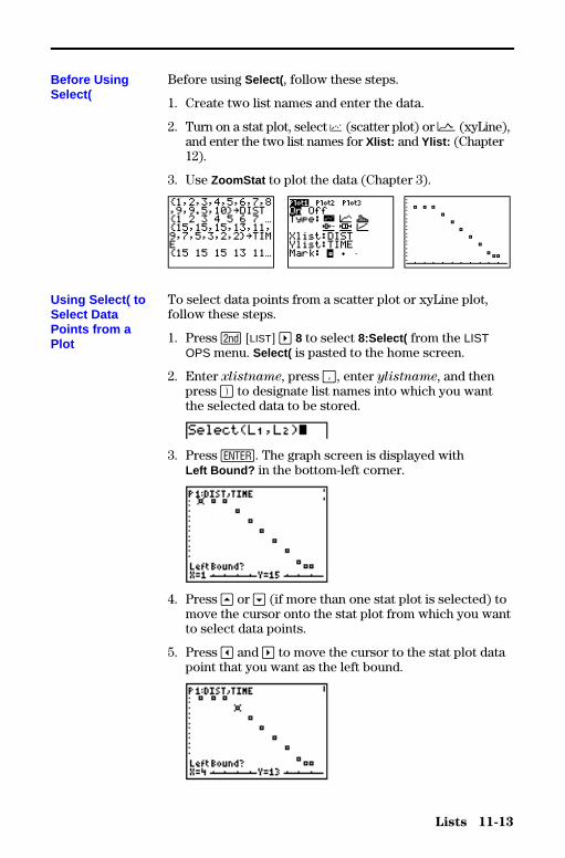
Lists 11-13
8311LIST.DOC TI-83 international English Bob Fedorisko Revised: 02/19/01 1:21 PM Printed: 02/19/01 1:37 PMPage 13 of 18
Before using Select( , follow these steps.
1. Create two list names and enter the data.
2. Turn on a stat plot, select " (scatter plot) or Ó (xyLine),and enter the two list names for Xlist: and Ylist: (Chapter12).
3. Use ZoomStat to plot the data (Chapter 3).
To select data points from a scatter plot or xyLine plot,follow these steps.
1. Press y [LIST] ~ 8 to select 8:Select( from the LISTOPS menu. Select( is pasted to the home screen.
2. Enter xlistname, press ¢, enter ylistname, and thenpress ¤ to designate list names into which you wantthe selected data to be stored.
3. Press Í. The graph screen is displayed withLeft Bound? in the bottom-left corner.
4. Press } or † (if more than one stat plot is selected) tomove the cursor onto the stat plot from which you wantto select data points.
5. Press | and ~ to move the cursor to the stat plot datapoint that you want as the left bound.
Before UsingSelect(
Using Select( toSelect DataPoints from aPlot

11-14 Lists
8311LIST.DOC TI-83 international English Bob Fedorisko Revised: 02/19/01 1:21 PM Printed: 02/19/01 1:37 PMPage 14 of 18
6. Press Í. A 4 indicator on the graph screen showsthe left bound. Right Bound? is displayed in the bottom-left corner.
7. Press | or ~ to move the cursor to the stat plot pointthat you want for the right bound, and then press Í.
The x-values and y-values of the selected points arestored in xlistname and ylistname. A new stat plot ofxlistname and ylistname replaces the stat plot fromwhich you selected data points. The list names areupdated in the stat plot editor.
Note: The two new lists (xlistname and ylistname) will include thepoints you select as left bound and right bound. Also, left-bound
x-value � right-bound x-value must be true.
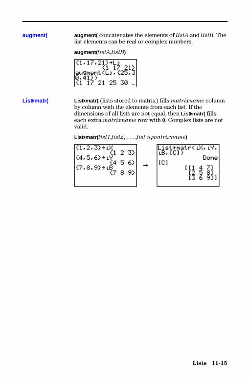
Lists 11-15
8311LIST.DOC TI-83 international English Bob Fedorisko Revised: 02/19/01 1:21 PM Printed: 02/19/01 1:37 PMPage 15 of 18
augment( concatenates the elements of listA and listB. Thelist elements can be real or complex numbers.
augment( listA,listB)
List 4matr( (lists stored to matrix) fills matrixname columnby column with the elements from each list. If thedimensions of all lists are not equal, then List 4matr( fillseach extra matrixname row with 0. Complex lists are notvalid.
List 4matr( list1,list2, . . . ,list n,matrixname)
&
augment(
List 4matr(
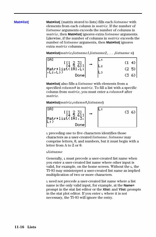
11-16 Lists
8311LIST.DOC TI-83 international English Bob Fedorisko Revised: 02/19/01 1:21 PM Printed: 02/19/01 1:37 PMPage 16 of 18
Matr4list( (matrix stored to lists) fills each listname withelements from each column in matrix. If the number oflistname arguments exceeds the number of columns inmatrix, then Matr4list( ignores extra listname arguments.Likewise, if the number of columns in matrix exceeds thenumber of listname arguments, then Matr4list( ignoresextra matrix columns.
Matr4list( matrix,listname1,listname2, . . . ,listname n)
&
Matr4list( also fills a listname with elements from aspecified column# in matrix. To fill a list with a specificcolumn from matrix, you must enter a column# aftermatrix.
Matr4list( matrix,column#,listname)
&
Ù preceding one to five characters identifies thosecharacters as a user-created listname. listname maycomprise letters, q, and numbers, but it must begin with aletter from A to Z or q.
Ùlistname
Generally, Ù must precede a user-created list name whenyou enter a user-created list name where other input isvalid, for example, on the home screen. Without the Ù, theTI-83 may misinterpret a user-created list name as impliedmultiplication of two or more characters.
Ù need not precede a user-created list name where a listname is the only valid input, for example, at the Name=prompt in the stat list editor or the Xlist: and Ylist: promptsin the stat plot editor. If you enter Ù where it is notnecessary, the TI-83 will ignore the entry.
Matr4list(
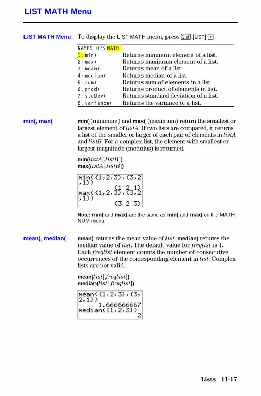
Lists 11-17
8311LIST.DOC TI-83 international English Bob Fedorisko Revised: 02/19/01 1:21 PM Printed: 02/19/01 1:37 PMPage 17 of 18
To display the LIST MATH menu, press y [LIST] |.
NAMES OPS MATH1: min( Returns minimum element of a list.2: max( Returns maximum element of a list.3: mean( Returns mean of a list.4: median( Returns median of a list.5: sum( Returns sum of elements in a list.6: prod( Returns product of elements in list.7: stdDev( Returns standard deviation of a list.8: variance( Returns the variance of a list.
min( (minimum) and max( (maximum) return the smallest orlargest element of listA. If two lists are compared, it returnsa list of the smaller or larger of each pair of elements in listA
and listB. For a complex list, the element with smallest orlargest magnitude (modulus) is returned.
min( listA[,listB])max( listA[,listB])
Note: min( and max( are the same as min( and max( on the MATHNUM menu.
mean( returns the mean value of list. median( returns themedian value of list. The default value for freqlist is 1.Each freqlist element counts the number of consecutiveoccurrences of the corresponding element in list. Complexlists are not valid.
mean( list[,freqlist])median( list[,freqlist])
LIST MATH Menu
LIST MATH Menu
min(, max(
mean(, median(

11-18 Lists
8311LIST.DOC TI-83 international English Bob Fedorisko Revised: 02/19/01 1:21 PM Printed: 02/19/01 1:37 PMPage 18 of 18
sum( (summation) returns the sum of the elements in list.start and end are optional; they specify a range ofelements. list elements can be real or complex numbers.
prod( returns the product of all elements of list. start andend elements are optional; they specify a range of listelements. list elements can be real or complex numbers.
sum( list[,start,end]) prod( list[,start,end])
You can combine sum( or prod( with seq( to obtain:
upper upper
Gexpression(x) ∏expression(x)
x=lower x=lower
To evaluate G 2(N–1) from N=1 to 4:
stdDev( returns the standard deviation of the elements in list.The default value for freqlist is 1. Each freqlist elementcounts the number of consecutive occurrences of thecorresponding element in list. Complex lists are not valid.
variance( returns the variance of the elements in list. Thedefault value for freqlist is 1. Each freqlist element countsthe number of consecutive occurrences of the correspondingelement in list. Complex lists are not valid.
stdDev( list[,freqlist]) variance( list[,freqlist])
sum(, prod(
Sums andProducts ofNumericSequences
stdDev(,variance(
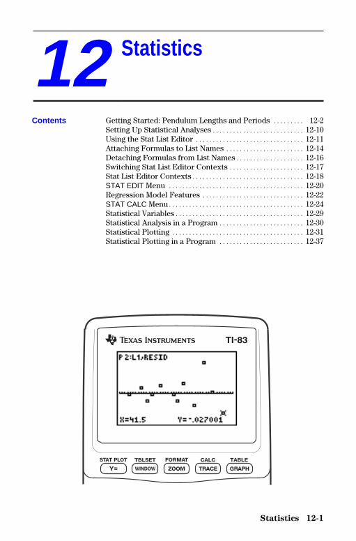
Statistics 12-1
8312STAT.DOC TI-83 international English Bob Fedorisko Revised: 02/19/01 12:42 PM Printed: 02/19/01 1:37PM Page 1 of 38
12 Statistics
Getting Started: Pendulum Lengths and Periods ......... 12-2Setting Up Statistical Analyses........................... 12-10Using the Stat List Editor ................................ 12-11Attaching Formulas to List Names ....................... 12-14Detaching Formulas from List Names.................... 12-16Switching Stat List Editor Contexts ...................... 12-17Stat List Editor Contexts................................. 12-18STAT EDIT Menu ........................................ 12-20Regression Model Features .............................. 12-22STAT CALC Menu........................................ 12-24Statistical Variables...................................... 12-29Statistical Analysis in a Program ......................... 12-30Statistical Plotting ....................................... 12-31Statistical Plotting in a Program ......................... 12-37
Contents

12-2 Statistics
8312STAT.DOC TI-83 international English Bob Fedorisko Revised: 02/19/01 12:42 PM Printed: 02/19/01 1:37PM Page 2 of 38
Getting Started is a fast-paced introduction. Read the chapter for details.
A group of students is attempting to determine the mathematical relationshipbetween the length of a pendulum and its period (one complete swing of apendulum). The group makes a simple pendulum from string and washers andthen suspends it from the ceiling. They record the pendulum’s period for eachof 12 string lengths.*
Length (cm) Time (sec) 6.5 0.5111.0 0.6813.2 0.7315.0 0.7918.0 0.8823.1 0.9924.4 1.0126.6 1.0830.5 1.1334.3 1.2637.6 1.2841.5 1.32
1. Press z † † † Í to set Funcgraphing mode.
2. Press … 5 to select 5:SetUpEditor .SetUpEditor is pasted to the homescreen.
Press Í. This removes lists from statlist editor columns 1 through 20, andthen stores lists L1 through L6 incolumns 1 through 6.
Note: Removing lists from the stat list editor does notdelete them from memory.
3. Press … 1 to select 1:Edit from theSTAT EDIT menu. The stat list editor isdisplayed. If elements are stored in L1
and L2, press } to move the cursor ontoL1, and then press ‘ Í ~ }‘ Í to clear both lists. Press |to move the rectangular cursor back tothe first row in L1.
*This example is quoted and adapted from Contemporary Precalculus Through Applications,by the North Carolina School of Science and Mathematics, by permission of JansonPublications, Inc., Dedham, MA. 1-800-322-MATH. © 1992. All rights reserved.
Getting Started: Pendulum Lengths and Periods
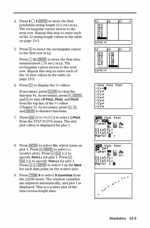
Statistics 12-3
8312STAT.DOC TI-83 international English Bob Fedorisko Revised: 02/19/01 12:42 PM Printed: 02/19/01 1:37PM Page 3 of 38
4. Press 6 Ë 5 Í to store the firstpendulum string length (6.5 cm) in L1.The rectangular cursor moves to thenext row. Repeat this step to enter eachof the 12 string length values in the tableon page 12.2.
5. Press ~ to move the rectangular cursorto the first row in L2.
Press Ë 51 Í to store the first timemeasurement (.51 sec) in L2. Therectangular cursor moves to the nextrow. Repeat this step to enter each ofthe 12 time values in the table onpage 12.2.
6. Press o to display the Y= editor.
If necessary, press ‘ to clear thefunction Y1. As necessary, press }, Í,and ~ to turn off Plot1 , Plot2 , and Plot3from the top line of the Y= editor(Chapter 3). As necessary, press †, |,and Í to deselect functions.
7. Press y [STAT PLOT] 1 to select 1:Plot1from the STAT PLOTS menu. The statplot editor is displayed for plot 1.
8. Press Í to select On, which turns onplot 1. Press † Í to select "(scatter plot). Press † y [L1] tospecify Xlist:L 1 for plot 1. Press †y [L2] to specify Ylist:L 2 for plot 1.Press † ~ Í to select + as the Markfor each data point on the scatter plot.
9. Press q 9 to select 9:ZoomStat fromthe ZOOM menu. The window variablesare adjusted automatically, and plot 1 isdisplayed. This is a scatter plot of thetime-versus-length data.
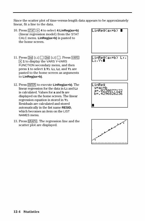
12-4 Statistics
8312STAT.DOC TI-83 international English Bob Fedorisko Revised: 02/19/01 12:42 PM Printed: 02/19/01 1:37PM Page 4 of 38
Since the scatter plot of time-versus-length data appears to be approximatelylinear, fit a line to the data.
10. Press … ~ 4 to select 4:LinReg(ax+b)(linear regression model) from the STATCALC menu. LinReg(ax+b) is pasted tothe home screen.
11. Press y [L1] ¢ y [L2] ¢. Press �~ 1 to display the VARS Y.VARSFUNCTION secondary menu, and thenpress 1 to select 1:Y1. L1, L2, and Y1 arepasted to the home screen as argumentsto LinReg(ax+b) .
12. Press Í to execute LinReg(ax+b) . Thelinear regression for the data in L1 and L2
is calculated. Values for a and b aredisplayed on the home screen. The linearregression equation is stored in Y1.Residuals are calculated and storedautomatically in the list name RESID,which becomes an item on the LISTNAMES menu.
13. Press s. The regression line and thescatter plot are displayed.
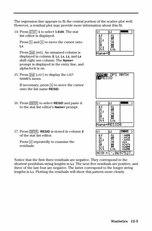
Statistics 12-5
8312STAT.DOC TI-83 international English Bob Fedorisko Revised: 02/19/01 12:42 PM Printed: 02/19/01 1:37PM Page 5 of 38
The regression line appears to fit the central portion of the scatter plot well.However, a residual plot may provide more information about this fit.
14. Press … 1 to select 1:Edit . The statlist editor is displayed.
Press ~ and } to move the cursor ontoL3.
Press y [INS]. An unnamed column isdisplayed in column 3; L3, L4, L5, and L6
shift right one column. The Name=prompt is displayed in the entry line, andalpha-lock is on.
15. Press y [LIST] to display the LISTNAMES menu.
If necessary, press † to move the cursoronto the list name RESID.
16. Press Í to select RESID and paste itto the stat list editor’s Name= prompt.
17. Press Í. RESID is stored in column 3of the stat list editor.
Press † repeatedly to examine theresiduals.
Notice that the first three residuals are negative. They correspond to theshortest pendulum string lengths in L1. The next five residuals are positive, andthree of the last four are negative. The latter correspond to the longer stringlengths in L1. Plotting the residuals will show this pattern more clearly.

12-6 Statistics
8312STAT.DOC TI-83 international English Bob Fedorisko Revised: 02/19/01 12:42 PM Printed: 02/19/01 1:37PM Page 6 of 38
18. Press y [STAT PLOT] 2 to select 2:Plot2from the STAT PLOTS menu. The statplot editor is displayed for plot 2.
19. Press Í to select On, which turns onplot 2.
Press † Í to select " (scatter plot).Press † y [L1] to specify Xlist:L 1 forplot 2. Press † [R] [E] [S] [I] [D](alpha-lock is on) to specify Ylist:RESIDfor plot 2. Press † Í to select › asthe mark for each data point on thescatter plot.
20. Press o to display the Y= editor.
Press | to move the cursor onto the= sign, and then press Í to deselectY1. Press } Í to turn off plot 1.
21. Press q 9 to select 9:ZoomStat fromthe ZOOM menu. The window variablesare adjusted automatically, and plot 2 isdisplayed. This is a scatter plot of theresiduals.
Notice the pattern of the residuals: a group of negative residuals, then a groupof positive residuals, and then another group of negative residuals.
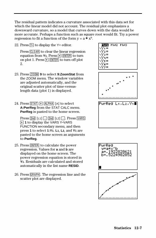
Statistics 12-7
8312STAT.DOC TI-83 international English Bob Fedorisko Revised: 02/19/01 12:42 PM Printed: 02/19/01 1:37PM Page 7 of 38
The residual pattern indicates a curvature associated with this data set forwhich the linear model did not account. The residual plot emphasizes adownward curvature, so a model that curves down with the data would bemore accurate. Perhaps a function such as square root would fit. Try a powerregression to fit a function of the form y = a ä xb.
22. Press o to display the Y= editor.
Press ‘ to clear the linear regressionequation from Y1. Press } Í to turnon plot 1. Press ~ Í to turn off plot2.
23. Press q 9 to select 9:ZoomStat fromthe ZOOM menu. The window variablesare adjusted automatically, and theoriginal scatter plot of time-versus-length data (plot 1) is displayed.
24. Press … ~ ƒ [A] to selectA:PwrReg from the STAT CALC menu.PwrReg is pasted to the home screen.
Press y [L1] ¢ y [L2] ¢. Press �~ 1 to display the VARS Y.VARSFUNCTION secondary menu, and thenpress 1 to select 1:Y1. L1, L2, and Y1 arepasted to the home screen as argumentsto PwrReg .
25. Press Í to calculate the powerregression. Values for a and b aredisplayed on the home screen. Thepower regression equation is stored inY1. Residuals are calculated and storedautomatically in the list name RESID.
26. Press s. The regression line and thescatter plot are displayed.
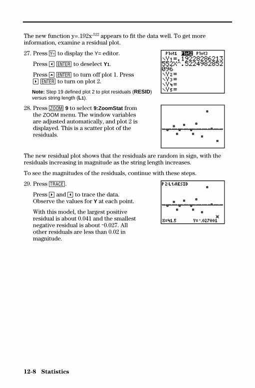
12-8 Statistics
8312STAT.DOC TI-83 international English Bob Fedorisko Revised: 02/19/01 12:42 PM Printed: 02/19/01 1:37PM Page 8 of 38
The new function y=.192x.522 appears to fit the data well. To get moreinformation, examine a residual plot.
27. Press o to display the Y= editor.
Press | Í to deselect Y1.
Press } Í to turn off plot 1. Press~ Í to turn on plot 2.
Note: Step 19 defined plot 2 to plot residuals (RESID)versus string length (L1).
28. Press q 9 to select 9:ZoomStat fromthe ZOOM menu. The window variablesare adjusted automatically, and plot 2 isdisplayed. This is a scatter plot of theresiduals.
The new residual plot shows that the residuals are random in sign, with theresiduals increasing in magnitude as the string length increases.
To see the magnitudes of the residuals, continue with these steps.
29. Press r.
Press ~ and | to trace the data.Observe the values for Y at each point.
With this model, the largest positiveresidual is about 0.041 and the smallestnegative residual is about L0.027. Allother residuals are less than 0.02 inmagnitude.
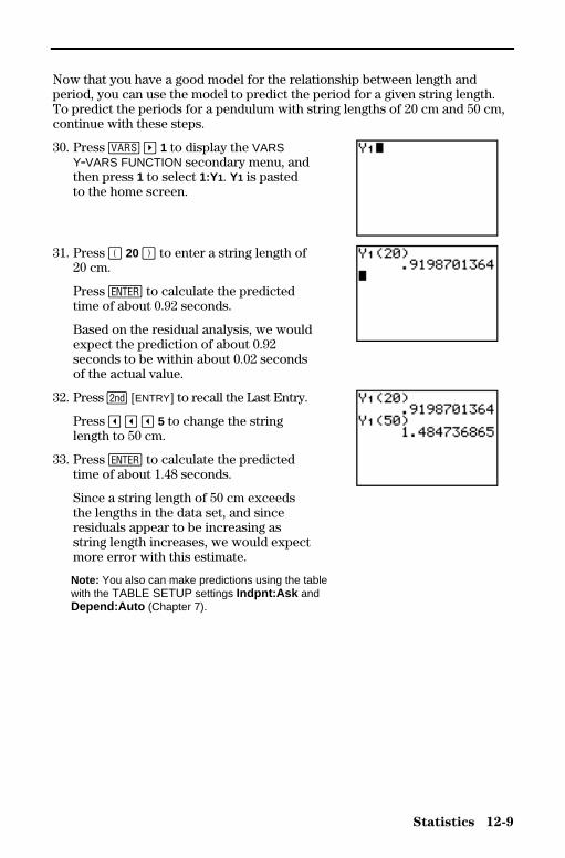
Statistics 12-9
8312STAT.DOC TI-83 international English Bob Fedorisko Revised: 02/19/01 12:42 PM Printed: 02/19/01 1:37PM Page 9 of 38
Now that you have a good model for the relationship between length andperiod, you can use the model to predict the period for a given string length.To predict the periods for a pendulum with string lengths of 20 cm and 50 cm,continue with these steps.
30. Press � ~ 1 to display the VARSY.VARS FUNCTION secondary menu, andthen press 1 to select 1:Y1. Y1 is pastedto the home screen.
31. Press £ 20 ¤ to enter a string length of20 cm.
Press Í to calculate the predictedtime of about 0.92 seconds.
Based on the residual analysis, we wouldexpect the prediction of about 0.92seconds to be within about 0.02 secondsof the actual value.
32. Press y [ENTRY] to recall the Last Entry.
Press | | | 5 to change the stringlength to 50 cm.
33. Press Í to calculate the predictedtime of about 1.48 seconds.
Since a string length of 50 cm exceedsthe lengths in the data set, and sinceresiduals appear to be increasing asstring length increases, we would expectmore error with this estimate.
Note: You also can make predictions using the tablewith the TABLE SETUP settings Indpnt:Ask andDepend:Auto (Chapter 7).
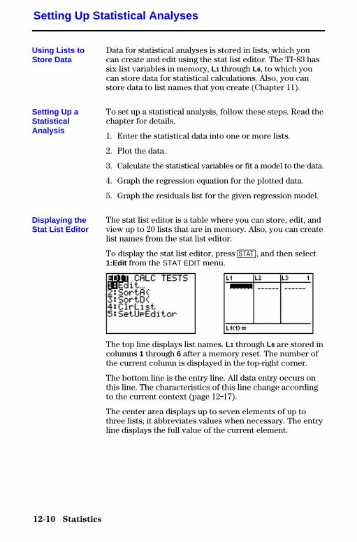
12-10 Statistics
8312STAT.DOC TI-83 international English Bob Fedorisko Revised: 02/19/01 12:42 PM Printed: 02/19/01 1:37PM Page 10 of 38
Data for statistical analyses is stored in lists, which youcan create and edit using the stat list editor. The TI-83 hassix list variables in memory, L1 through L6, to which youcan store data for statistical calculations. Also, you canstore data to list names that you create (Chapter 11).
To set up a statistical analysis, follow these steps. Read thechapter for details.
1. Enter the statistical data into one or more lists.
2. Plot the data.
3. Calculate the statistical variables or fit a model to the data.
4. Graph the regression equation for the plotted data.
5. Graph the residuals list for the given regression model.
The stat list editor is a table where you can store, edit, andview up to 20 lists that are in memory. Also, you can createlist names from the stat list editor.
To display the stat list editor, press …, and then select1:Edit from the STAT EDIT menu.
The top line displays list names. L1 through L6 are stored incolumns 1 through 6 after a memory reset. The number ofthe current column is displayed in the top-right corner.
The bottom line is the entry line. All data entry occurs onthis line. The characteristics of this line change accordingto the current context (page 12.17).
The center area displays up to seven elements of up tothree lists; it abbreviates values when necessary. The entryline displays the full value of the current element.
Setting Up Statistical Analyses
Using Lists toStore Data
Setting Up aStatisticalAnalysis
Displaying theStat List Editor
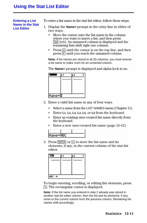
Statistics 12-11
8312STAT.DOC TI-83 international English Bob Fedorisko Revised: 02/19/01 12:42 PM Printed: 02/19/01 1:37PM Page 11 of 38
To enter a list name in the stat list editor, follow these steps.
1. Display the Name= prompt in the entry line in either oftwo ways.• Move the cursor onto the list name in the column
where you want to insert a list, and then pressy [INS]. An unnamed column is displayed and theremaining lists shift right one column.
• Press } until the cursor is on the top line, and thenpress ~ until you reach the unnamed column.
Note: If list names are stored to all 20 columns, you must removea list name to make room for an unnamed column.
The Name= prompt is displayed and alpha-lock is on.
2. Enter a valid list name in any of four ways.
• Select a name from the LIST NAMES menu (Chapter 11).• Enter L1, L2, L3, L4, L5, or L6 from the keyboard.• Enter an existing user-created list name directly from
the keyboard.• Enter a new user-created list name (page 12.12).
3. Press Í or † to store the list name and itselements, if any, in the current column of the stat listeditor.
To begin entering, scrolling, or editing list elements, press†. The rectangular cursor is displayed.
Note: If the list name you entered in step 2 already was stored inanother stat list editor column, then the list and its elements, if any,move to the current column from the previous column. Remaining listnames shift accordingly.
Using the Stat List Editor
Entering a ListName in the StatList Editor

12-12 Statistics
8312STAT.DOC TI-83 international English Bob Fedorisko Revised: 02/19/01 12:42 PM Printed: 02/19/01 1:37PM Page 12 of 38
To create a name in the stat list editor, follow these steps.
1. Follow step 1 on page 12.11 to display the Name=prompt.
2. Press [letter from A to Z or q] to enter the first letter ofthe name. The first character cannot be a number.
3. Enter zero to four letters, q, or numbers to complete thenew user-created list name. List names can be one tofive characters long.
4. Press Í or † to store the list name in the currentcolumn of the stat list editor. The list name becomes anitem on the LIST NAMES menu (Chapter 11).
To remove a list from the stat list editor, move the cursoronto the list name and then press {. The list is not deletedfrom memory; it is only removed from the stat list editor.
Note: To delete a list name from memory, use the MEMORYDELETE:List selection screen (Chapter 18).
You can remove all user-created lists from the stat listeditor and restore list names L1 through L6 to columns 1through 6 in either of two ways.
• Use SetUpEditor with no arguments (page 12.21).• Reset all memory (Chapter 18).
You can clear all elements from a list in any of five ways.
• Use ClrList to clear specified lists (page 12.20).• In the stat list editor, press } to move the cursor onto a
list name, and then press ‘ Í.• In the stat list editor, move the cursor onto each
element, and then press { one by one.• On the home screen or in the program editor, enter
0!dim( listname) to set the dimension of listname to 0(Chapter 11).
• Use ClrAllLists to clear all lists in memory (Chapter 18).
Creating a Namein the Stat ListEditor
Removing a Listfrom the Stat ListEditor
Removing AllLists andRestoring L 1
through L 6
Clearing AllElements from aList
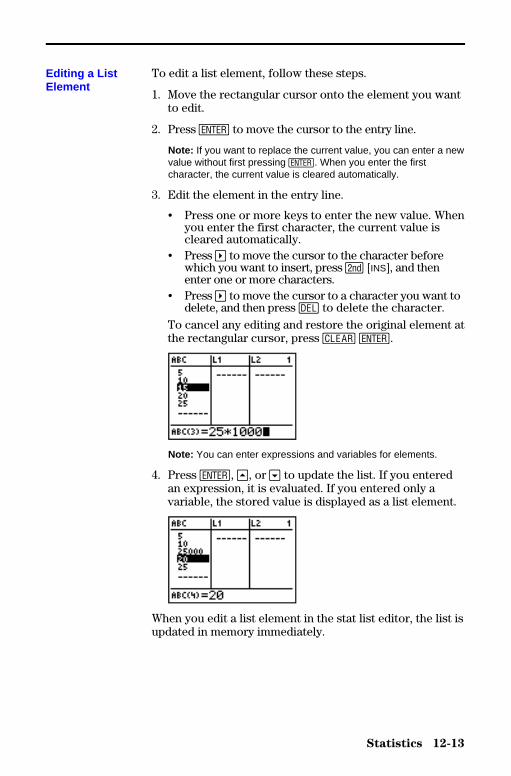
Statistics 12-13
8312STAT.DOC TI-83 international English Bob Fedorisko Revised: 02/19/01 12:42 PM Printed: 02/19/01 1:37PM Page 13 of 38
To edit a list element, follow these steps.
1. Move the rectangular cursor onto the element you wantto edit.
2. Press Í to move the cursor to the entry line.
Note: If you want to replace the current value, you can enter a newvalue without first pressing Í. When you enter the firstcharacter, the current value is cleared automatically.
3. Edit the element in the entry line.
• Press one or more keys to enter the new value. Whenyou enter the first character, the current value iscleared automatically.
• Press ~ to move the cursor to the character beforewhich you want to insert, press y [INS], and thenenter one or more characters.
• Press ~ to move the cursor to a character you want todelete, and then press { to delete the character.
To cancel any editing and restore the original element atthe rectangular cursor, press ‘ Í.
Note: You can enter expressions and variables for elements.
4. Press Í, }, or † to update the list. If you enteredan expression, it is evaluated. If you entered only avariable, the stored value is displayed as a list element.
When you edit a list element in the stat list editor, the list isupdated in memory immediately.
Editing a ListElement
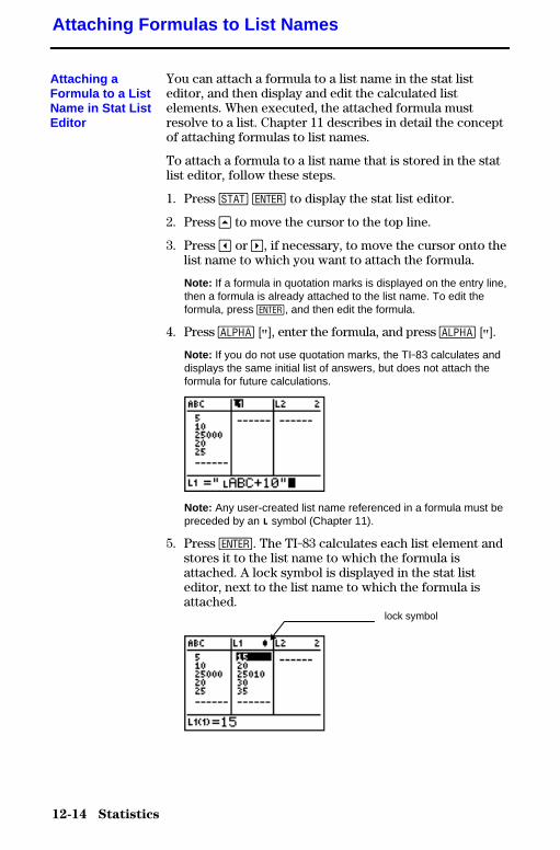
12-14 Statistics
8312STAT.DOC TI-83 international English Bob Fedorisko Revised: 02/19/01 12:42 PM Printed: 02/19/01 1:37PM Page 14 of 38
You can attach a formula to a list name in the stat listeditor, and then display and edit the calculated listelements. When executed, the attached formula mustresolve to a list. Chapter 11 describes in detail the conceptof attaching formulas to list names.
To attach a formula to a list name that is stored in the statlist editor, follow these steps.
1. Press … Í to display the stat list editor.
2. Press } to move the cursor to the top line.
3. Press | or ~, if necessary, to move the cursor onto thelist name to which you want to attach the formula.
Note: If a formula in quotation marks is displayed on the entry line,then a formula is already attached to the list name. To edit theformula, press Í, and then edit the formula.
4. Press ƒ [ã], enter the formula, and press ƒ [ã].
Note: If you do not use quotation marks, the TI-83 calculates anddisplays the same initial list of answers, but does not attach theformula for future calculations.
Note: Any user-created list name referenced in a formula must bepreceded by an Ù symbol (Chapter 11).
5. Press Í. The TI-83 calculates each list element andstores it to the list name to which the formula isattached. A lock symbol is displayed in the stat listeditor, next to the list name to which the formula isattached.
Attaching Formulas to List Names
Attaching aFormula to a ListName in Stat ListEditor
lock symbol
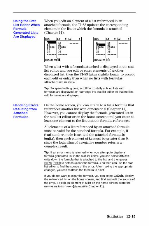
Statistics 12-15
8312STAT.DOC TI-83 international English Bob Fedorisko Revised: 02/19/01 12:42 PM Printed: 02/19/01 1:37PM Page 15 of 38
When you edit an element of a list referenced in anattached formula, the TI-83 updates the correspondingelement in the list to which the formula is attached(Chapter 11).
When a list with a formula attached is displayed in the statlist editor and you edit or enter elements of anotherdisplayed list, then the TI-83 takes slightly longer to accepteach edit or entry than when no lists with formulasattached are in view.
Tip: To speed editing time, scroll horizontally until no lists withformulas are displayed, or rearrange the stat list editor so that no listswith formulas are displayed.
On the home screen, you can attach to a list a formula thatreferences another list with dimension 0 (Chapter 11).However, you cannot display the formula-generated list inthe stat list editor or on the home screen until you enter atleast one element to the list that the formula references.
All elements of a list referenced by an attached formulamust be valid for the attached formula. For example, ifReal number mode is set and the attached formula islog(L 1), then each element of L1 must be greater than 0,since the logarithm of a negative number returns acomplex result.
Tip: If an error menu is returned when you attempt to display aformula-generated list in the stat list editor, you can select 2:Goto ,write down the formula that is attached to the list, and then press‘ Í to detach (clear) the formula. You then can use the statlist editor to find the source of the error. After making the appropriatechanges, you can reattach the formula to a list.
If you do not want to clear the formula, you can select 1:Quit , displaythe referenced list on the home screen, and find and edit the source ofthe error. To edit an element of a list on the home screen, store thenew value to listname(element#) (Chapter 11).
Using the StatList Editor WhenFormula-Generated ListsAre Displayed
Handling ErrorsResulting fromAttachedFormulas
12-16 Statistics
8312STAT.DOC TI-83 international English Bob Fedorisko Revised: 02/19/01 12:42 PM Printed: 02/19/01 1:37PM Page 16 of 38
You can detach (clear) a formula from a list name in any offour ways.
• In the stat list editor, move the cursor onto the name ofthe list to which a formula is attached. Press Í‘ Í. All list elements remain, but the formulais detached and the lock symbol disappears.
• In the stat list editor, move the cursor onto an elementof the list to which a formula is attached. Press Í,edit the element, and then press Í. The elementchanges, the formula is detached, and the lock symboldisappears. All other list elements remain.
• Use ClrList (page 12.20). All elements of one or morespecified lists are cleared, each formula is detached, andeach lock symbol disappears. All list names remain.
• Use ClrAllLists (Chapter 18). All elements of all lists inmemory are cleared, all formulas are detached from alllist names, and all lock symbols disappear. All listnames remain.
As described above, one way to detach a formula from alist name is to edit an element of the list to which theformula is attached. The TI-83 protects againstinadvertently detaching the formula from the list name byediting an element of the formula-generated list.
Because of the protection feature, you must press Íbefore you can edit an element of a formula-generated list.
The protection feature does not allow you to delete anelement of a list to which a formula is attached. To deletean element of a list to which a formula is attached, youmust first detach the formula in any of the ways describedabove.
Detaching Formulas from List Names
Detaching aFormula from aList Name
Editing anElement of aFormula-Generated List

Statistics 12-17
8312STAT.DOC TI-83 international English Bob Fedorisko Revised: 02/19/01 12:42 PM Printed: 02/19/01 1:37PM Page 17 of 38
The stat list editor has four contexts.
• View-elements context • Edit-elements context• View-names context • Enter-name context
The stat list editor is first displayed in view-elementscontext. To switch through the four contexts, select 1:Editfrom the STAT EDIT menu and follow these steps.
1. Press } to move the cursor onto a list name. You arenow in view-names context. Press ~ and | to view listnames stored in other stat list editor columns.
2. Press Í. You are now in edit-elements context. Youmay edit any element in a list. All elements of thecurrent list are displayed in braces ( { } )in the entryline. Press ~ and | to view more list elements.
3. Press Í again. You are now in view-elementscontext. Press ~, |, †, and } to view other listelements. The current element’s full value is displayedin the entry line.
4. Press Í again. You are now in edit-elementscontext. You may edit the current element in the entryline.
5. Press } until the cursor is on a list name, then pressy [INS]. You are now in enter-name context.
6. Press ‘. You are now in view-names context.
7. Press †. You are now back in view-elements context.
Switching Stat List Editor Contexts
Stat List EditorContexts
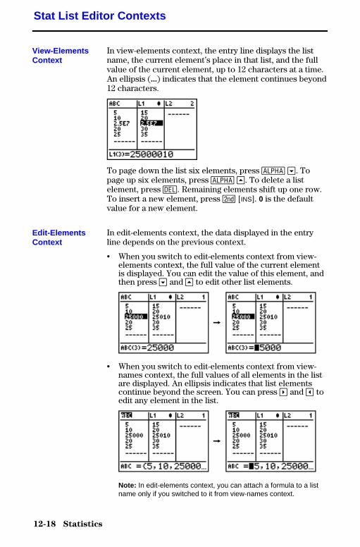
12-18 Statistics
8312STAT.DOC TI-83 international English Bob Fedorisko Revised: 02/19/01 12:42 PM Printed: 02/19/01 1:37PM Page 18 of 38
In view-elements context, the entry line displays the listname, the current element’s place in that list, and the fullvalue of the current element, up to 12 characters at a time.An ellipsis (...) indicates that the element continues beyond12 characters.
To page down the list six elements, press ƒ †. Topage up six elements, press ƒ }. To delete a listelement, press {. Remaining elements shift up one row.To insert a new element, press y [INS]. 0 is the defaultvalue for a new element.
In edit-elements context, the data displayed in the entryline depends on the previous context.
• When you switch to edit-elements context from view-elements context, the full value of the current elementis displayed. You can edit the value of this element, andthen press † and } to edit other list elements.
&
• When you switch to edit-elements context from view-names context, the full values of all elements in the listare displayed. An ellipsis indicates that list elementscontinue beyond the screen. You can press ~ and | toedit any element in the list.
&
Note: In edit-elements context, you can attach a formula to a listname only if you switched to it from view-names context.
Stat List Editor Contexts
View-ElementsContext
Edit-ElementsContext
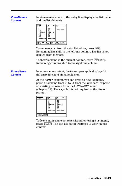
Statistics 12-19
8312STAT.DOC TI-83 international English Bob Fedorisko Revised: 02/19/01 12:42 PM Printed: 02/19/01 1:37PM Page 19 of 38
In view-names context, the entry line displays the list nameand the list elements.
To remove a list from the stat list editor, press {.Remaining lists shift to the left one column. The list is notdeleted from memory.
To insert a name in the current column, press y [INS].Remaining columns shift to the right one column.
In enter-name context, the Name= prompt is displayed inthe entry line, and alpha-lock is on.
At the Name= prompt, you can create a new list name,paste a list name from L1 to L6 from the keyboard, or pastean existing list name from the LIST NAMES menu(Chapter 11). The Ù symbol is not required at the Name=prompt.
To leave enter-name context without entering a list name,press ‘. The stat list editor switches to view-namescontext.
View-NamesContext
Enter-NameContext
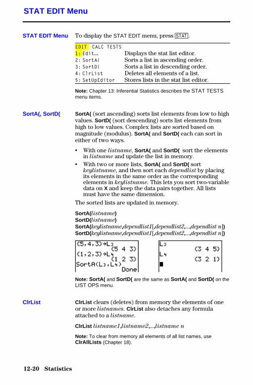
12-20 Statistics
8312STAT.DOC TI-83 international English Bob Fedorisko Revised: 02/19/01 12:42 PM Printed: 02/19/01 1:37PM Page 20 of 38
To display the STAT EDIT menu, press ….
EDIT CALC TESTS1: Edit... Displays the stat list editor.2: SortA( Sorts a list in ascending order.3: SortD( Sorts a list in descending order.4: ClrList Deletes all elements of a list.5: SetUpEditor Stores lists in the stat list editor.
Note: Chapter 13: Inferential Statistics describes the STAT TESTSmenu items.
SortA( (sort ascending) sorts list elements from low to highvalues. SortD( (sort descending) sorts list elements fromhigh to low values. Complex lists are sorted based onmagnitude (modulus). SortA( and SortD( each can sort ineither of two ways.
• With one listname, SortA( and SortD( sort the elementsin listname and update the list in memory.
• With two or more lists, SortA( and SortD( sortkeylistname, and then sort each dependlist by placingits elements in the same order as the correspondingelements in keylistname. This lets you sort two-variabledata on X and keep the data pairs together. All listsmust have the same dimension.
The sorted lists are updated in memory.
SortA( listname)SortD( listname)SortA( keylistname,dependlist1[,dependlist2,...,dependlist n])SortD( keylistname,dependlist1[,dependlist2,...,dependlist n])
Note: SortA( and SortD( are the same as SortA( and SortD( on theLIST OPS menu.
ClrList clears (deletes) from memory the elements of oneor more listnames. ClrList also detaches any formulaattached to a listname.
ClrList listname1,listname2,...,listname n
Note: To clear from memory all elements of all list names, useClrAllLists (Chapter 18).
STAT EDIT Menu
STAT EDIT Menu
SortA(, SortD(
ClrList

Statistics 12-21
8312STAT.DOC TI-83 international English Bob Fedorisko Revised: 02/19/01 12:42 PM Printed: 02/19/01 1:37PM Page 21 of 38
With SetUpEditor you can set up the stat list editor todisplay one or more listnames in the order that youspecify. You can specify zero to 20 listnames.
SetUpEditor [listname1,listname2,...,listname n]
SetUpEditor with one to 20 listnames removes all listnames from the stat list editor and then stores listnames inthe stat list editor columns in the specified order,beginning in column 1.
If you enter a listname that is not stored in memoryalready, then listname is created and stored in memory; itbecomes an item on the LIST NAMES menu.
SetUpEditor with no listnames removes all list names fromthe stat list editor and restores list names L1 through L6 inthe stat list editor columns 1 through 6.
SetUpEditor
Restoring L 1
through L 6 to theStat List Editor
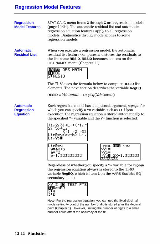
12-22 Statistics
8312STAT.DOC TI-83 international English Bob Fedorisko Revised: 02/19/01 12:42 PM Printed: 02/19/01 1:37PM Page 22 of 38
STAT CALC menu items 3 through C are regression models(page 12.24). The automatic residual list and automaticregression equation features apply to all regressionmodels. Diagnostics display mode applies to someregression models.
When you execute a regression model, the automaticresidual list feature computes and stores the residuals tothe list name RESID. RESID becomes an item on theLIST NAMES menu (Chapter 11).
The TI-83 uses the formula below to compute RESID listelements. The next section describes the variable RegEQ.
RESID = Ylistname N RegEQ(Xlistname)
Each regression model has an optional argument, regequ, forwhich you can specify a Y= variable such as Y1. Uponexecution, the regression equation is stored automatically tothe specified Y= variable and the Y= function is selected.
Regardless of whether you specify a Y= variable for regequ,the regression equation always is stored to the TI-83variable RegEQ, which is item 1 on the VARS Statistics EQsecondary menu.
Note: For the regression equation, you can use the fixed-decimalmode setting to control the number of digits stored after the decimalpoint (Chapter 1). However, limiting the number of digits to a smallnumber could affect the accuracy of the fit.
Regression Model Features
RegressionModel Features
AutomaticResidual List
AutomaticRegressionEquation
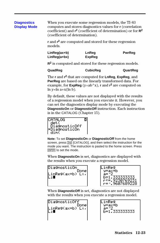
Statistics 12-23
8312STAT.DOC TI-83 international English Bob Fedorisko Revised: 02/19/01 12:42 PM Printed: 02/19/01 1:37PM Page 23 of 38
When you execute some regression models, the TI-83computes and stores diagnostics values for r (correlationcoefficient) and r2 (coefficient of determination) or for R2
(coefficient of determination).
r and r2 are computed and stored for these regressionmodels.
LinReg(ax+b) LnReg PwrRegLinReg(a+bx) ExpReg
R2 is computed and stored for these regression models.
QuadReg CubicReg QuartReg
The r and r2 that are computed for LnReg , ExpReg , andPwrReg are based on the linearly transformed data. Forexample, for ExpReg (y=ab^x), r and r2 are computed onln y=ln a+x(ln b).
By default, these values are not displayed with the resultsof a regression model when you execute it. However, youcan set the diagnostics display mode by executing theDiagnosticOn or DiagnosticOff instruction. Each instructionis in the CATALOG (Chapter 15).
Note: To set DiagnosticOn or DiagnosticOff from the homescreen, press y [CATALOG], and then select the instruction for themode you want. The instruction is pasted to the home screen. PressÍ to set the mode.
When DiagnosticOn is set, diagnostics are displayed withthe results when you execute a regression model.
When DiagnosticOff is set, diagnostics are not displayedwith the results when you execute a regression model.
DiagnosticsDisplay Mode

12-24 Statistics
8312STAT.DOC TI-83 international English Bob Fedorisko Revised: 02/19/01 12:42 PM Printed: 02/19/01 1:37PM Page 24 of 38
To display the STAT CALC menu, press … ~.
EDIT CALC TESTS1: 1-Var Stats Calculates 1-variable statistics.2: 2-Var Stats Calculates 2-variable statistics.3: Med-Med Calculates a median-median line.4: LinReg(ax+b) Fits a linear model to data.5: QuadReg Fits a quadratic model to data.6: CubicReg Fits a cubic model to data.7: QuartReg Fits a quartic model to data.8: LinReg(a+bx) Fits a linear model to data.9: LnReg Fits a logarithmic model to data.0: ExpReg Fits an exponential model to data.A: PwrReg Fits a power model to data.B: Logistic Fits a logistic model to data.C: SinReg Fits a sinusoidal model to data.
For each STAT CALC menu item, if neither Xlistname norYlistname is specified, then the default list names are L1
and L2. If you do not specify freqlist, then the default is 1occurrence of each list element.
For most STAT CALC menu items, you can specify a list ofdata occurrences, or frequencies (freqlist).
Each element in freqlist indicates how many times thecorresponding data point or data pair occurs in the data setyou are analyzing.
For example, if L1={15,12,9,14} and ÙFREQ={1,4,1,3} , thenthe TI-83 interprets the instruction 1.Var Stats L1, ÙFREQ tomean that 15 occurs once, 12 occurs four times, 9 occursonce, and 14 occurs three times.
Each element in freqlist must be ‚ 0, and at least oneelement must be > 0.
Noninteger freqlist elements are valid. This is useful whenentering frequencies expressed as percentages or partsthat add up to 1. However, if freqlist contains nonintegerfrequencies, Sx and Sy are undefined; values are notdisplayed for Sx and Sy in the statistical results.
STAT CALC Menu
STAT CALCMenu
Frequency ofOccurrence forData Points
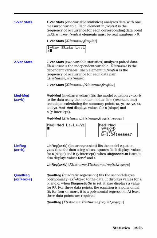
Statistics 12-25
8312STAT.DOC TI-83 international English Bob Fedorisko Revised: 02/19/01 12:42 PM Printed: 02/19/01 1:37PM Page 25 of 38
1.Var Stats (one-variable statistics) analyzes data with onemeasured variable. Each element in freqlist is thefrequency of occurrence for each corresponding data pointin Xlistname. freqlist elements must be real numbers > 0.
1.Var Stats [Xlistname,freqlist]
2.Var Stats (two-variable statistics) analyzes paired data.Xlistname is the independent variable. Ylistname is thedependent variable. Each element in freqlist is thefrequency of occurrence for each data pair(Xlistname,Ylistname).
2.Var Stats [Xlistname,Ylistname,freqlist]
Med.Med (median-median) fits the model equation y=ax+bto the data using the median-median line (resistant line)technique, calculating the summary points x1, y1, x2, y2, x3,and y3. Med.Med displays values for a (slope) andb (y-intercept).
Med.Med [Xlistname,Ylistname,freqlist,regequ]
LinReg(ax+b) (linear regression) fits the model equationy=ax+b to the data using a least-squares fit. It displays valuesfor a (slope) and b (y-intercept); when DiagnosticOn is set, italso displays values for r2 and r.
LinReg(ax+b) [Xlistname,Ylistname,freqlist,regequ]
QuadReg (quadratic regression) fits the second-degreepolynomial y=ax2+bx+c to the data. It displays values for a,b, and c; when DiagnosticOn is set, it also displays a valuefor R2. For three data points, the equation is a polynomialfit; for four or more, it is a polynomial regression. At leastthree data points are required.
QuadReg [Xlistname,Ylistname,freqlist,regequ]
1-Var Stats
2-Var Stats
Med-Med(ax+b)
LinReg(ax+b)
QuadReg(ax2+bx+c)
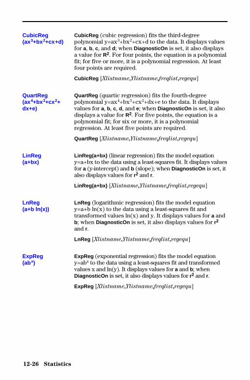
12-26 Statistics
8312STAT.DOC TI-83 international English Bob Fedorisko Revised: 02/19/01 12:42 PM Printed: 02/19/01 1:37PM Page 26 of 38
CubicReg (cubic regression) fits the third-degreepolynomial y=ax3+bx2+cx+d to the data. It displays valuesfor a, b, c, and d; when DiagnosticOn is set, it also displaysa value for R2. For four points, the equation is a polynomialfit; for five or more, it is a polynomial regression. At leastfour points are required.
CubicReg [Xlistname,Ylistname,freqlist,regequ]
QuartReg (quartic regression) fits the fourth-degreepolynomial y=ax4+bx3+cx2+dx+e to the data. It displaysvalues for a, b, c, d, and e; when DiagnosticOn is set, it alsodisplays a value for R2. For five points, the equation is apolynomial fit; for six or more, it is a polynomialregression. At least five points are required.
QuartReg [Xlistname,Ylistname,freqlist,regequ]
LinReg(a+bx) (linear regression) fits the model equationy=a+bx to the data using a least-squares fit. It displays valuesfor a (y-intercept) and b (slope); when DiagnosticOn is set, italso displays values for r2 and r.
LinReg(a+bx) [Xlistname,Ylistname,freqlist,regequ]
LnReg (logarithmic regression) fits the model equationy=a+b ln(x) to the data using a least-squares fit andtransformed values ln(x) and y. It displays values for a andb; when DiagnosticOn is set, it also displays values for r2
and r.
LnReg [Xlistname,Ylistname,freqlist,regequ]
ExpReg (exponential regression) fits the model equationy=abx to the data using a least-squares fit and transformedvalues x and ln(y). It displays values for a and b; whenDiagnosticOn is set, it also displays values for r2 and r.
ExpReg [Xlistname,Ylistname,freqlist,regequ]
CubicReg(ax3+bx 2+cx+d)
QuartReg(ax4+bx 3+cx 2+dx+e)
LinReg(a+bx)
LnReg(a+b ln(x))
ExpReg(abx)
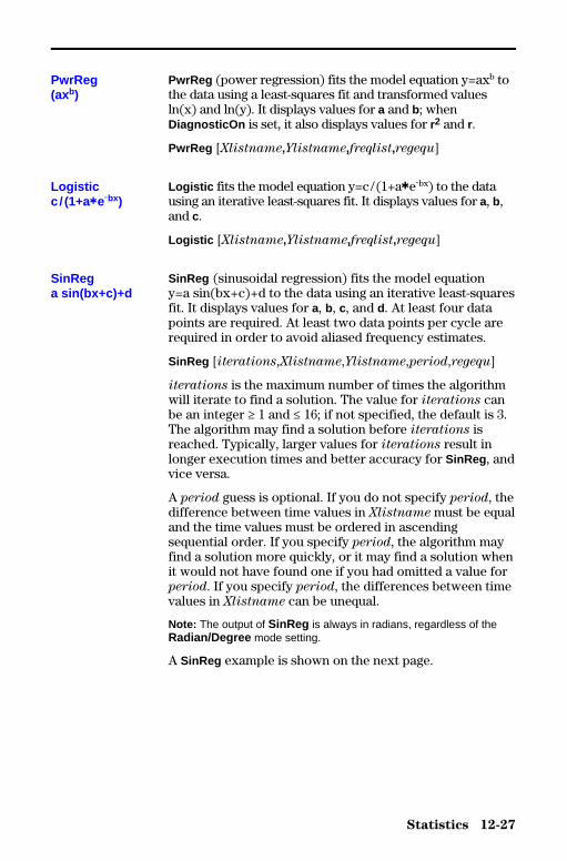
Statistics 12-27
8312STAT.DOC TI-83 international English Bob Fedorisko Revised: 02/19/01 12:42 PM Printed: 02/19/01 1:37PM Page 27 of 38
PwrReg (power regression) fits the model equation y=axb tothe data using a least-squares fit and transformed valuesln(x) and ln(y). It displays values for a and b; whenDiagnosticOn is set, it also displays values for r2 and r.
PwrReg [Xlistname,Ylistname,freqlist,regequ]
Logistic fits the model equation y=c/(1+aäeLbx) to the datausing an iterative least-squares fit. It displays values for a, b,and c.
Logistic [Xlistname,Ylistname,freqlist,regequ]
SinReg (sinusoidal regression) fits the model equationy=a sin(bx+c)+d to the data using an iterative least-squaresfit. It displays values for a, b, c, and d. At least four datapoints are required. At least two data points per cycle arerequired in order to avoid aliased frequency estimates.
SinReg [iterations,Xlistname,Ylistname,period,regequ]
iterations is the maximum number of times the algorithmwill iterate to find a solution. The value for iterations canbe an integer ‚ 1 and � 16; if not specified, the default is 3.The algorithm may find a solution before iterations isreached. Typically, larger values for iterations result inlonger execution times and better accuracy for SinReg , andvice versa.
A period guess is optional. If you do not specify period, thedifference between time values in Xlistname must be equaland the time values must be ordered in ascendingsequential order. If you specify period, the algorithm mayfind a solution more quickly, or it may find a solution whenit would not have found one if you had omitted a value forperiod. If you specify period, the differences between timevalues in Xlistname can be unequal.
Note: The output of SinReg is always in radians, regardless of theRadian/Degree mode setting.
A SinReg example is shown on the next page.
PwrReg(axb)
Logisticc / (1+aäeLbx)
SinRega sin(bx+c)+d

12-28 Statistics
8312STAT.DOC TI-83 international English Bob Fedorisko Revised: 02/19/01 12:42 PM Printed: 02/19/01 1:37PM Page 28 of 38
Compute the regression model for the number of hours ofdaylight in Alaska during one year.
&
&
With noisy data, you will achieve better convergenceresults when you specify an accurate estimate for period.You can obtain a period guess in either of two ways.
• Plot the data and trace to determine the x-distancebetween the beginning and end of one complete period,or cycle. The illustration above and to the rightgraphically depicts a complete period, or cycle.
• Plot the data and trace to determine the x-distancebetween the beginning and end of N complete periods,or cycles. Then divide the total distance by N.
After your first attempt to use SinReg and the default valuefor iterations to fit the data, you may find the fit to beapproximately correct, but not optimal. For an optimal fit,execute SinReg 16, Xlistname,Ylistname,2p / b where b isthe value obtained from the previous SinReg execution.
SinReg Example:Daylight Hours inAlaska for OneYear
1 period
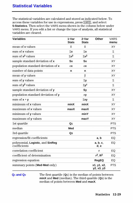
Statistics 12-29
8312STAT.DOC TI-83 international English Bob Fedorisko Revised: 02/19/01 12:42 PM Printed: 02/19/01 1:37PM Page 29 of 38
The statistical variables are calculated and stored as indicated below. Toaccess these variables for use in expressions, press �, and select5:Statistics . Then select the VARS menu shown in the column below underVARS menu. If you edit a list or change the type of analysis, all statisticalvariables are cleared.
Variables 1.VarStats
2.VarStats
Other VARSmenu
mean of x values v v XY
sum of x values Gx Gx G
sum of x2 values Gx2 Gx2 G
sample standard deviation of x Sx Sx XY
population standard deviation of x sx sx XY
number of data points n n XY
mean of y values w XY
sum of y values Gy G
sum of y2 values Gy2 G
sample standard deviation of y Sy XY
population standard deviation of y sy XY
sum of x … y Gxy G
minimum of x values minX minX XY
maximum of x values maxX maxX XY
minimum of y values minY XY
maximum of y values maxY XY
1st quartile Q1 PTS
median Med PTS
3rd quartile Q3 PTS
regression/fit coefficients a, b EQ
polynomial, Logistic , and SinRegcoefficients
a, b, c,d, e
EQ
correlation coefficient r EQ
coefficient of determination r2, R2 EQ
regression equation RegEQ EQ
summary points (Med.Med only) x1, y1, x2,y2, x3, y3
PTS
The first quartile (Q1) is the median of points betweenminX and Med (median). The third quartile (Q3) is themedian of points between Med and maxX .
Statistical Variables
Q1 and Q3
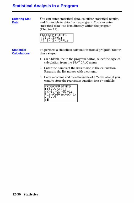
12-30 Statistics
8312STAT.DOC TI-83 international English Bob Fedorisko Revised: 02/19/01 12:42 PM Printed: 02/19/01 1:37PM Page 30 of 38
You can enter statistical data, calculate statistical results,and fit models to data from a program. You can enterstatistical data into lists directly within the program(Chapter 11).
To perform a statistical calculation from a program, followthese steps.
1. On a blank line in the program editor, select the type ofcalculation from the STAT CALC menu.
2. Enter the names of the lists to use in the calculation.Separate the list names with a comma.
3. Enter a comma and then the name of a Y= variable, if youwant to store the regression equation to a Y= variable.
Statistical Analysis in a Program
Entering StatData
StatisticalCalculations

Statistics 12-31
8312STAT.DOC TI-83 international English Bob Fedorisko Revised: 02/19/01 12:42 PM Printed: 02/19/01 1:37PM Page 31 of 38
You can plot statistical data that is stored in lists. The sixtypes of plots available are scatter plot, xyLine, histogram,modified box plot, regular box plot, and normal probabilityplot. You can define up to three plots.
To plot statistical data in lists, follow these steps.
1. Store the stat data in one or more lists.
2. Select or deselect Y= functions as appropriate.
3. Define the stat plot.
4. Turn on the plots you want to display.
5. Define the viewing window.
6. Display and explore the graph.
Scatter plots plot the data points from Xlist and Ylist ascoordinate pairs, showing each point as a box ( › ), cross( + ), or dot ( ¦ ). Xlist and Ylist must be the same length.You can use the same list for Xlist and Ylist .
xyLine is a scatter plot in which the data points are plottedand connected in order of appearance in Xlist and Ylist .You may want to use SortA( or SortD( to sort the listsbefore you plot them (page 12.20).
Statistical Plotting
Steps for PlottingStatistical Data inLists
"(Scatter)
Ó(xyLine)
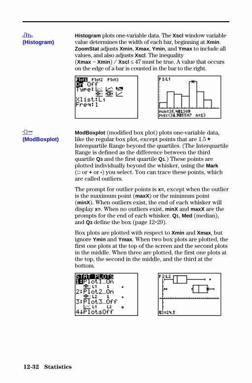
12-32 Statistics
8312STAT.DOC TI-83 international English Bob Fedorisko Revised: 02/19/01 12:42 PM Printed: 02/19/01 1:37PM Page 32 of 38
Histogram plots one-variable data. The Xscl window variablevalue determines the width of each bar, beginning at Xmin .ZoomStat adjusts Xmin , Xmax , Ymin , and Ymax to include allvalues, and also adjusts Xscl . The inequality(Xmax N Xmin ) à Xscl � 47 must be true. A value that occurson the edge of a bar is counted in the bar to the right.
ModBoxplot (modified box plot) plots one-variable data,like the regular box plot, except points that are 1.5 äInterquartile Range beyond the quartiles. (The InterquartileRange is defined as the difference between the thirdquartile Q3 and the first quartile Q1.) These points areplotted individually beyond the whisker, using the Mark(› or + or ¦) you select. You can trace these points, whichare called outliers.
The prompt for outlier points is x=, except when the outlieris the maximum point (maxX) or the minimum point(minX ). When outliers exist, the end of each whisker willdisplay x=. When no outliers exist, minX and maxX are theprompts for the end of each whisker. Q1, Med (median),and Q3 define the box (page 12.29).
Box plots are plotted with respect to Xmin and Xmax , butignore Ymin and Ymax . When two box plots are plotted, thefirst one plots at the top of the screen and the second plotsin the middle. When three are plotted, the first one plots atthe top, the second in the middle, and the third at thebottom.
Ò(Histogram)
Õ(ModBoxplot)

Statistics 12-33
8312STAT.DOC TI-83 international English Bob Fedorisko Revised: 02/19/01 12:42 PM Printed: 02/19/01 1:37PM Page 33 of 38
Boxplot (regular box plot) plots one-variable data. Thewhiskers on the plot extend from the minimum data pointin the set (minX ) to the first quartile (Q1) and from the thirdquartile (Q3) to the maximum point (maxX). The box isdefined by Q1, Med (median), and Q3 (page 12.29).
Box plots are plotted with respect to Xmin and Xmax , butignore Ymin and Ymax . When two box plots are plotted, thefirst one plots at the top of the screen and the second plotsin the middle. When three are plotted, the first one plots atthe top, the second in the middle, and the third at thebottom.
NormProbPlot (normal probability plot) plots eachobservation X in Data List versus the correspondingquantile z of the standard normal distribution. If the plottedpoints lie close to a straight line, then the plot indicatesthat the data are normal.
Enter a valid list name in the Data List field. Select X or Yfor the Data Axis setting.
• If you select X, the TI-83 plots the data on the x-axis andthe z-values on the y-axis.
• If you select Y, the TI-83 plots the data on the y-axis andthe z-values on the x-axis.
Ö(Boxplot)
Ô(NormProbPlot)
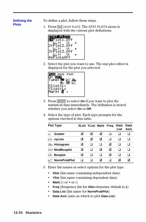
12-34 Statistics
8312STAT.DOC TI-83 international English Bob Fedorisko Revised: 02/19/01 12:42 PM Printed: 02/19/01 1:37PM Page 34 of 38
To define a plot, follow these steps.
1. Press y [STAT PLOT]. The STAT PLOTS menu isdisplayed with the current plot definitions.
2. Select the plot you want to use. The stat plot editor isdisplayed for the plot you selected.
3. Press Í to select On if you want to plot thestatistical data immediately. The definition is storedwhether you select On or Off .
4. Select the type of plot. Each type prompts for theoptions checked in this table.
Plot Type XList YList Mark Freq DataList
DataAxis
" Scatter � � � œ œ œ
Ó xyLine � � � œ œ œ
Ò Histogram � œ œ � œ œ
Õ ModBoxplot � œ � � œ œ
Ö Boxplot � œ œ � œ œ
Ô NormProbPlot œ œ � œ � �
5. Enter list names or select options for the plot type.
• Xlist (list name containing independent data)• Ylist (list name containing dependent data)• Mark (› or + or ¦)• Freq (frequency list for Xlist elements; default is 1)• Data List (list name for NormProbPlot )• Data Axis (axis on which to plot Data List )
Defining thePlots
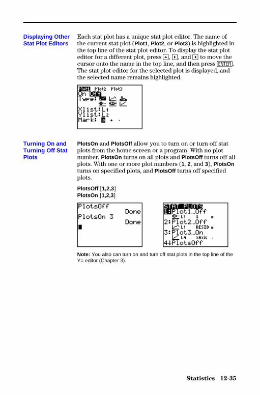
Statistics 12-35
8312STAT.DOC TI-83 international English Bob Fedorisko Revised: 02/19/01 12:42 PM Printed: 02/19/01 1:37PM Page 35 of 38
Each stat plot has a unique stat plot editor. The name ofthe current stat plot (Plot1 , Plot2 , or Plot3 ) is highlighted inthe top line of the stat plot editor. To display the stat ploteditor for a different plot, press }, ~, and | to move thecursor onto the name in the top line, and then press Í.The stat plot editor for the selected plot is displayed, andthe selected name remains highlighted.
PlotsOn and PlotsOff allow you to turn on or turn off statplots from the home screen or a program. With no plotnumber, PlotsOn turns on all plots and PlotsOff turns off allplots. With one or more plot numbers (1, 2, and 3), PlotsOnturns on specified plots, and PlotsOff turns off specifiedplots.
PlotsOff [1,2,3]PlotsOn [1,2,3]
Note: You also can turn on and turn off stat plots in the top line of theY= editor (Chapter 3).
Displaying OtherStat Plot Editors
Turning On andTurning Off StatPlots

12-36 Statistics
8312STAT.DOC TI-83 international English Bob Fedorisko Revised: 02/19/01 12:42 PM Printed: 02/19/01 1:37PM Page 36 of 38
Stat plots are displayed on the current graph. To define theviewing window, press p and enter values for thewindow variables. ZoomStat redefines the viewing windowto display all statistical data points.
When you trace a scatter plot or xyLine, tracing begins atthe first element in the lists.
When you trace a histogram, the cursor moves from thetop center of one column to the top center of the next,starting at the first column.
When you trace a box plot, tracing begins at Med (themedian). Press | to trace to Q1 and minX . Press ~ to traceto Q3 and maxX .
When you press } or † to move to another plot or toanother Y= function, tracing moves to the current orbeginning point on that plot (not the nearest pixel).
The ExprOn /ExprOff format setting applies to stat plots(Chapter 3).When ExprOn is selected, the plot number andplotted data lists are displayed in the top-left corner.
Defining theViewing Window
Tracing a StatPlot

Statistics 12-37
8312STAT.DOC TI-83 international English Bob Fedorisko Revised: 02/19/01 12:42 PM Printed: 02/19/01 1:37PM Page 37 of 38
To display a stat plot from a program, define the plot, andthen display the graph.
To define a stat plot from a program, begin on a blank linein the program editor and enter data into one or more lists;then, follow these steps.
1. Press y [STAT PLOT] to display the STAT PLOTS menu.
2. Select the plot to define, which pastes Plot1( , Plot2( , orPlot3( to the cursor location.
3. Press y [STAT PLOT] ~ to display the STAT TYPEmenu.
4. Select the type of plot, which pastes the name of theplot type to the cursor location.
Statistical Plotting in a Program
Defining a StatPlot in a Program

12-38 Statistics
8312STAT.DOC TI-83 international English Bob Fedorisko Revised: 02/19/01 12:42 PM Printed: 02/19/01 1:37PM Page 38 of 38
5. Press ¢. Enter the list names, separated by commas.
6. Press ¢ y [STAT PLOT] | to display theSTAT PLOT MARK menu. (This step is not necessary ifyou selected 3:Histogram or 5:Boxplot in step 4.)
Select the type of mark (› or + or ¦) for each data point.The selected mark symbol is pasted to the cursorlocation.
7. Press ¤ Í to complete the command line.
To display a plot from a program, use the DispGraphinstruction (Chapter 16) or any of the ZOOM instructions(Chapter 3).
Displaying a StatPlot from aProgram
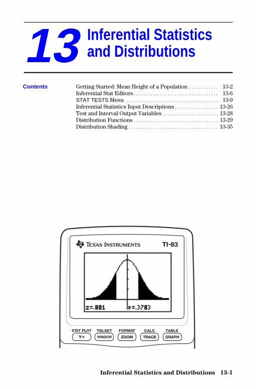
Inferential Statistics and Distributions 13-1
8313INFE.DOC TI-83 international English Bob Fedorisko Revised: 02/19/01 12:47 PM Printed: 02/19/01 1:38 PMPage 1 of 36
13 Inferential Statisticsand Distributions
Getting Started: Mean Height of a Population ............ 13-2Inferential Stat Editors................................... 13-6STAT TESTS Menu ...................................... 13-9Inferential Statistics Input Descriptions.................. 13-26Test and Interval Output Variables ....................... 13-28Distribution Functions................................... 13-29Distribution Shading ..................................... 13-35
Contents
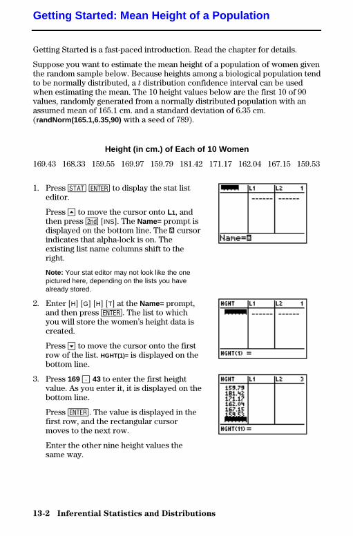
13-2 Inferential Statistics and Distributions
8313INFE.DOC TI-83 international English Bob Fedorisko Revised: 02/19/01 12:47 PM Printed: 02/19/01 1:38 PMPage 2 of 36
Getting Started is a fast-paced introduction. Read the chapter for details.
Suppose you want to estimate the mean height of a population of women giventhe random sample below. Because heights among a biological population tendto be normally distributed, a t distribution confidence interval can be usedwhen estimating the mean. The 10 height values below are the first 10 of 90values, randomly generated from a normally distributed population with anassumed mean of 165.1 cm. and a standard deviation of 6.35 cm.(randNorm(165.1,6.35,90) with a seed of 789).
Height (in cm.) of Each of 10 Women
169.43 168.33 159.55 169.97 159.79 181.42 171.17 162.04 167.15 159.53
1. Press … Í to display the stat listeditor.
Press } to move the cursor onto L1, andthen press y [INS]. The Name= prompt isdisplayed on the bottom line. The Ø cursorindicates that alpha-lock is on. Theexisting list name columns shift to theright.
Note: Your stat editor may not look like the onepictured here, depending on the lists you havealready stored.
2. Enter [H] [G] [H] [T] at the Name= prompt,and then press Í. The list to whichyou will store the women’s height data iscreated.
Press † to move the cursor onto the firstrow of the list. HGHT(1)= is displayed on thebottom line.
3. Press 169 Ë 43 to enter the first heightvalue. As you enter it, it is displayed on thebottom line.
Press Í. The value is displayed in thefirst row, and the rectangular cursormoves to the next row.
Enter the other nine height values thesame way.
Getting Started: Mean Height of a Population
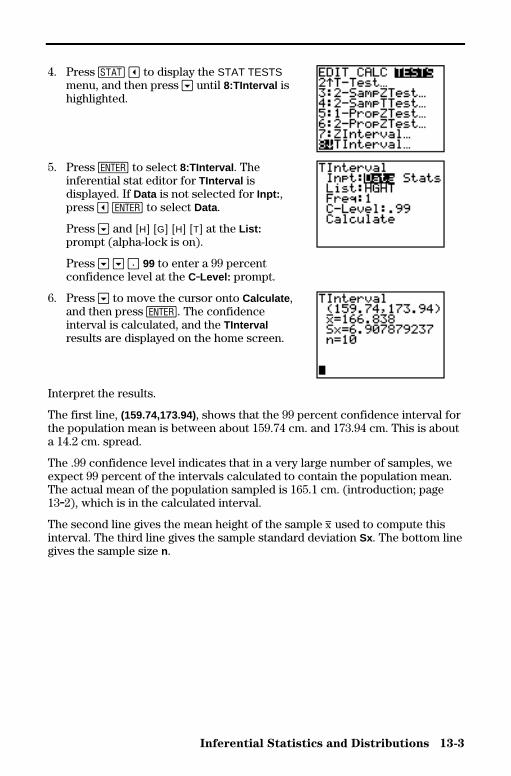
Inferential Statistics and Distributions 13-3
8313INFE.DOC TI-83 international English Bob Fedorisko Revised: 02/19/01 12:47 PM Printed: 02/19/01 1:38 PMPage 3 of 36
4. Press … | to display the STAT TESTSmenu, and then press † until 8:TInterval ishighlighted.
5. Press Í to select 8:TInterval . Theinferential stat editor for TInterval isdisplayed. If Data is not selected for Inpt: ,press | Í to select Data.
Press † and [H] [G] [H] [T] at the List:prompt (alpha-lock is on).
Press † † Ë 99 to enter a 99 percentconfidence level at the C.Level: prompt.
6. Press † to move the cursor onto Calculate ,and then press Í. The confidenceinterval is calculated, and the TIntervalresults are displayed on the home screen.
Interpret the results.
The first line, (159.74,173.94), shows that the 99 percent confidence interval forthe population mean is between about 159.74 cm. and 173.94 cm. This is abouta 14.2 cm. spread.
The .99 confidence level indicates that in a very large number of samples, weexpect 99 percent of the intervals calculated to contain the population mean.The actual mean of the population sampled is 165.1 cm. (introduction; page13.2), which is in the calculated interval.
The second line gives the mean height of the sample þ used to compute thisinterval. The third line gives the sample standard deviation Sx. The bottom linegives the sample size n.
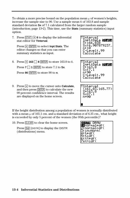
13-4 Inferential Statistics and Distributions
8313INFE.DOC TI-83 international English Bob Fedorisko Revised: 02/19/01 12:47 PM Printed: 02/19/01 1:38 PMPage 4 of 36
To obtain a more precise bound on the population mean m of women’s heights,increase the sample size to 90. Use a sample mean þ of 163.8 and samplestandard deviation Sx of 7.1 calculated from the larger random sample(introduction; page 13.2). This time, use the Stats (summary statistics) inputoption.
7. Press … | 8 to display the inferentialstat editor for TInterval .
Press ~ Í to select Inpt:Stats . Theeditor changes so that you can entersummary statistics as input.
8. Press † 163 Ë 8 Í to store 163.8 to þ.
Press 7 Ë 1 Í to store 7.1 to Sx.
Press 90 Í to store 90 to n.
9. Press † to move the cursor onto Calculate ,and then press Í to calculate the new99 percent confidence interval. The resultsare displayed on the home screen.
If the height distribution among a population of women is normally distributedwith a mean m of 165.1 cm. and a standard deviation σ of 6.35 cm., what heightis exceeded by only 5 percent of the women (the 95th percentile)?
10. Press ‘ to clear the home screen.
Press y [DISTR] to display the DISTR(distributions) menu.
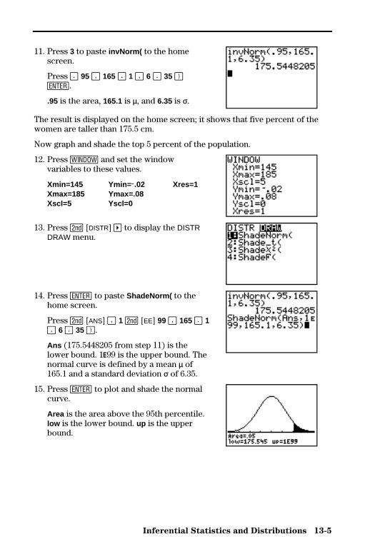
Inferential Statistics and Distributions 13-5
8313INFE.DOC TI-83 international English Bob Fedorisko Revised: 02/19/01 12:47 PM Printed: 02/19/01 1:38 PMPage 5 of 36
11. Press 3 to paste invNorm( to the homescreen.
Press Ë 95 ¢ 165 Ë 1 ¢ 6 Ë 35 ¤Í.
.95 is the area, 165.1 is µ, and 6.35 is σ.
The result is displayed on the home screen; it shows that five percent of thewomen are taller than 175.5 cm.
Now graph and shade the top 5 percent of the population.
12. Press p and set the windowvariables to these values.
Xmin=145 Ymin= L.02 Xres=1Xmax=185 Ymax=.08Xscl=5 Yscl=0
13. Press y [DISTR] ~ to display the DISTRDRAW menu.
14. Press Í to paste ShadeNorm( to thehome screen.
Press y [ANS] ¢ 1 y [EE] 99 ¢ 165 Ë 1¢ 6 Ë 35 ¤.
Ans (175.5448205 from step 11) is thelower bound. 1å99 is the upper bound. Thenormal curve is defined by a mean µ of165.1 and a standard deviation σ of 6.35.
15. Press Í to plot and shade the normalcurve.
Area is the area above the 95th percentile.low is the lower bound. up is the upperbound.

13-6 Inferential Statistics and Distributions
8313INFE.DOC TI-83 international English Bob Fedorisko Revised: 02/19/01 12:47 PM Printed: 02/19/01 1:38 PMPage 6 of 36
When you select a hypothesis test or confidence intervalinstruction from the home screen, the appropriateinferential statistics editor is displayed. The editors varyaccording to each test or interval’s input requirements.Below is the inferential stat editor for T.Test .
Note: When you select the ANOVA( instruction, it is pasted to thehome screen. ANOVA( does not have an editor screen.
To use an inferential stat editor, follow these steps.
1. Select a hypothesis test or confidence interval from theSTAT TESTS menu. The appropriate editor is displayed.
2. Select Data or Stats input, if the selection is available.The appropriate editor is displayed.
3. Enter real numbers, list names, or expressions for eachargument in the editor.
4. Select the alternative hypothesis (ƒ, <, or >) againstwhich to test, if the selection is available.
5. Select No or Yes for the Pooled option, if the selection isavailable.
6. Select Calculate or Draw (when Draw is available) toexecute the instruction.• When you select Calculate , the results are displayed
on the home screen.• When you select Draw , the results are displayed in a
graph.
This chapter describes the selections in the above steps foreach hypothesis test and confidence interval instruction.
Inferential Stat Editors
Displaying theInferential StatEditors
Using anInferential StatEditor
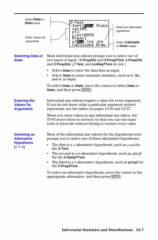
Inferential Statistics and Distributions 13-7
8313INFE.DOC TI-83 international English Bob Fedorisko Revised: 02/19/01 12:47 PM Printed: 02/19/01 1:38 PMPage 7 of 36
Most inferential stat editors prompt you to select one oftwo types of input. (1.PropZInt and 2.PropZTest , 1.PropZIntand 2.PropZInt , c2.Test , and LinRegTTest do not.)
• Select Data to enter the data lists as input.• Select Stats to enter summary statistics, such as þ, Sx,
and n, as input.
To select Data or Stats , move the cursor to either Data orStats , and then press Í.
Inferential stat editors require a value for every argument.If you do not know what a particular argument symbolrepresents, see the tables on pages 13.26 and 13.27.
When you enter values in any inferential stat editor, theTI.83 stores them in memory so that you can run manytests or intervals without having to reenter every value.
Most of the inferential stat editors for the hypothesis testsprompt you to select one of three alternative hypotheses.
• The first is a ƒ alternative hypothesis, such as mƒm0 forthe Z.Test .
• The second is a < alternative hypothesis, such as m1<m2for the 2.SampTTest .
• The third is a > alternative hypothesis, such as p1>p2 forthe 2.PropZTest .
To select an alternative hypothesis, move the cursor to theappropriate alternative, and then press Í.
Selecting Data orStats
Entering theValues forArguments
Selecting anAlternativeHypothesis(ƒ < >)
Enter values forarguments
Select an alternativehypothesis
Select Calculateor Draw output
Select Data orStats input
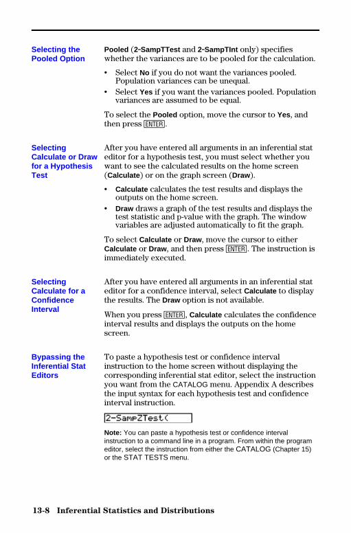
13-8 Inferential Statistics and Distributions
8313INFE.DOC TI-83 international English Bob Fedorisko Revised: 02/19/01 12:47 PM Printed: 02/19/01 1:38 PMPage 8 of 36
Pooled (2.SampTTest and 2.SampTInt only) specifieswhether the variances are to be pooled for the calculation.
• Select No if you do not want the variances pooled.Population variances can be unequal.
• Select Yes if you want the variances pooled. Populationvariances are assumed to be equal.
To select the Pooled option, move the cursor to Yes, andthen press Í.
After you have entered all arguments in an inferential stateditor for a hypothesis test, you must select whether youwant to see the calculated results on the home screen(Calculate ) or on the graph screen (Draw).
• Calculate calculates the test results and displays theoutputs on the home screen.
• Draw draws a graph of the test results and displays thetest statistic and p-value with the graph. The windowvariables are adjusted automatically to fit the graph.
To select Calculate or Draw , move the cursor to eitherCalculate or Draw , and then press Í. The instruction isimmediately executed.
After you have entered all arguments in an inferential stateditor for a confidence interval, select Calculate to displaythe results. The Draw option is not available.
When you press Í, Calculate calculates the confidenceinterval results and displays the outputs on the homescreen.
To paste a hypothesis test or confidence intervalinstruction to the home screen without displaying thecorresponding inferential stat editor, select the instructionyou want from the CATALOG menu. Appendix A describesthe input syntax for each hypothesis test and confidenceinterval instruction.
Note: You can paste a hypothesis test or confidence intervalinstruction to a command line in a program. From within the programeditor, select the instruction from either the CATALOG (Chapter 15)or the STAT TESTS menu.
Selecting thePooled Option
SelectingCalculate or Drawfor a HypothesisTest
SelectingCalculate for aConfidenceInterval
Bypassing theInferential StatEditors
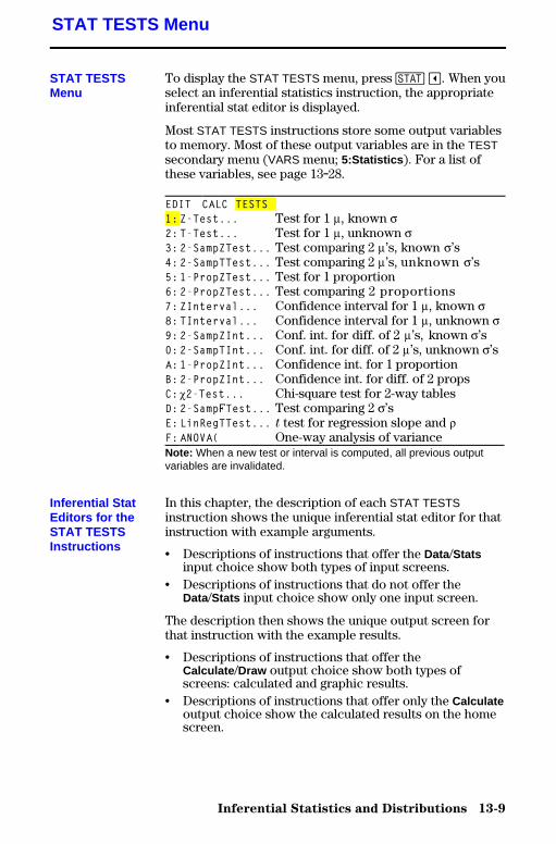
Inferential Statistics and Distributions 13-9
8313INFE.DOC TI-83 international English Bob Fedorisko Revised: 02/19/01 12:47 PM Printed: 02/19/01 1:38 PMPage 9 of 36
To display the STAT TESTS menu, press … |. When youselect an inferential statistics instruction, the appropriateinferential stat editor is displayed.
Most STAT TESTS instructions store some output variablesto memory. Most of these output variables are in the TESTsecondary menu (VARS menu; 5:Statistics ). For a list ofthese variables, see page 13.28.
EDIT CALC TESTS1:Z-Test... Test for 1 m, known s2:T-Test... Test for 1 m, unknown s3:2-SampZTest... Test comparing 2 m’s, known s’s4:2-SampTTest... Test comparing 2 m’s, unknown s’s5:1-PropZTest... Test for 1 proportion6:2-PropZTest... Test comparing 2 proportions7:ZInterval... Confidence interval for 1 m, known s8:TInterval... Confidence interval for 1 m, unknown s9:2-SampZInt... Conf. int. for diff. of 2 m’s, known s’s0:2-SampTInt... Conf. int. for diff. of 2 m’s, unknown s’sA:1-PropZInt... Confidence int. for 1 proportionB:2-PropZInt... Confidence int. for diff. of 2 propsC:c2-Test... Chi-square test for 2-way tablesD:2-SampÛTest... Test comparing 2 s’sE:LinRegTTest... t test for regression slope and rF:ANOVA( One-way analysis of varianceNote: When a new test or interval is computed, all previous outputvariables are invalidated.
In this chapter, the description of each STAT TESTSinstruction shows the unique inferential stat editor for thatinstruction with example arguments.
• Descriptions of instructions that offer the Data/Statsinput choice show both types of input screens.
• Descriptions of instructions that do not offer theData/Stats input choice show only one input screen.
The description then shows the unique output screen forthat instruction with the example results.
• Descriptions of instructions that offer theCalculate /Draw output choice show both types ofscreens: calculated and graphic results.
• Descriptions of instructions that offer only the Calculateoutput choice show the calculated results on the homescreen.
STAT TESTS Menu
STAT TESTSMenu
Inferential StatEditors for theSTAT TESTSInstructions
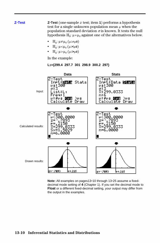
13-10 Inferential Statistics and Distributions
8313INFE.DOC TI-83 international English Bob Fedorisko Revised: 02/19/01 12:47 PM Printed: 02/19/01 1:38 PMPage 10 of 36
Z.Test (one-sample z test; item 1) performs a hypothesistest for a single unknown population mean m when thepopulation standard deviation s is known. It tests the nullhypothesis H0: m=m0 against one of the alternatives below.
• Ha: mƒm0 (m:ƒm0)• Ha: m<m0 (m:<m0)• Ha: m>m0 (m:>m0)
In the example:
L1={299.4 297.7 301 298.9 300.2 297}
Data Stats
Input:
, ,
Calculated results:
, ,
Drawn results:
Note: All examples on pages13.10 through 13.25 assume a fixed-decimal mode setting of 4 (Chapter 1). If you set the decimal mode toFloat or a different fixed-decimal setting, your output may differ fromthe output in the examples.
Z.Test

Inferential Statistics and Distributions 13-11
8313INFE.DOC TI-83 international English Bob Fedorisko Revised: 02/19/01 12:47 PM Printed: 02/19/01 1:38 PMPage 11 of 36
T.Test (one-sample t test; item 2) performs a hypothesistest for a single unknown population mean m when thepopulation standard deviation s is unknown. It tests thenull hypothesis H0: m=m0 against one of the alternativesbelow.
• Ha: mƒm0 (m:ƒm0)• Ha: m<m0 (m:<m0)• Ha: m>m0 (m:>m0)
In the example:
TEST={91.9 97.8 111.4 122.3 105.4 95}
Data Stats
Input:
, ,
Calculated results:
, ,
Drawn results:
T.Test
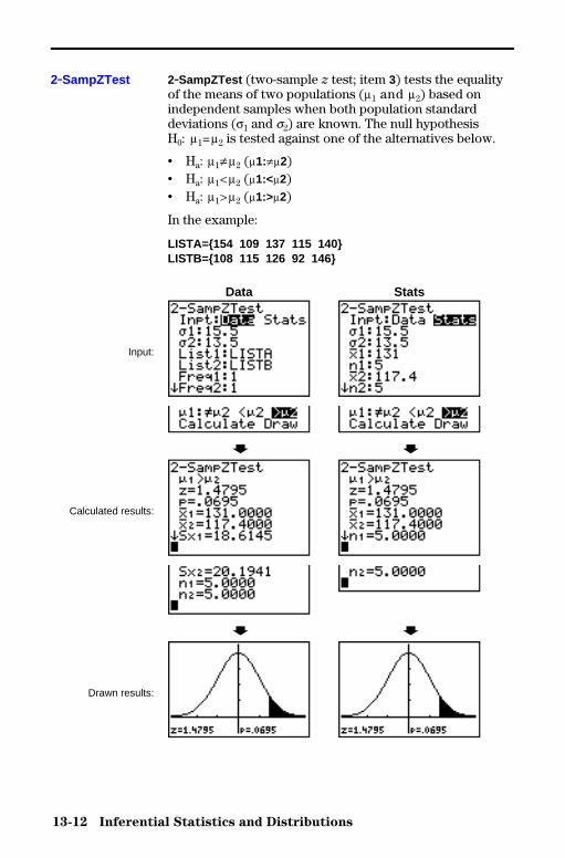
13-12 Inferential Statistics and Distributions
8313INFE.DOC TI-83 international English Bob Fedorisko Revised: 02/19/01 12:47 PM Printed: 02/19/01 1:38 PMPage 12 of 36
2.SampZTest (two-sample z test; item 3) tests the equalityof the means of two populations (m1 and m2) based onindependent samples when both population standarddeviations (s1 and s2) are known. The null hypothesisH0: m1=m2 is tested against one of the alternatives below.
• Ha: m1ƒm2 (m1:ƒm2)• Ha: m1<m2 (m1:<m2)• Ha: m1>m2 (m1:>m2)
In the example:
LISTA={154 109 137 115 140}LISTB={108 115 126 92 146}
Data Stats
Input:
, ,
Calculated results:
, ,
Drawn results:
2.SampZTest
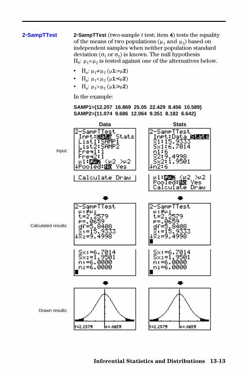
Inferential Statistics and Distributions 13-13
8313INFE.DOC TI-83 international English Bob Fedorisko Revised: 02/19/01 12:47 PM Printed: 02/19/01 1:38 PMPage 13 of 36
2.SampTTest (two-sample t test; item 4) tests the equalityof the means of two populations (m1 and m2) based onindependent samples when neither population standarddeviation (s1 or s2) is known. The null hypothesisH0: m1=m2 is tested against one of the alternatives below.
• Ha: m1ƒm2 (m1:ƒm2)• Ha: m1<m2 (m1:<m2)• Ha: m1>m2 (m1:>m2)
In the example:
SAMP1={12.207 16.869 25.05 22.429 8.456 10.589}SAMP2={11.074 9.686 12.064 9.351 8.182 6.642}
Data Stats
Input:
, ,
Calculated results:
, ,
Drawn results:
2.SampTTest
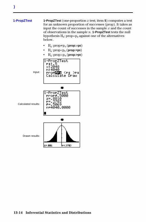
13-14 Inferential Statistics and Distributions
8313INFE.DOC TI-83 international English Bob Fedorisko Revised: 02/19/01 12:47 PM Printed: 02/19/01 1:38 PMPage 14 of 36
1.PropZTest (one-proportion z test; item 5) computes a testfor an unknown proportion of successes (prop). It takes asinput the count of successes in the sample x and the countof observations in the sample n. 1.PropZTest tests the nullhypothesis H0: prop=p0 against one of the alternativesbelow.
• Ha: propƒp0 (prop: ƒp0)• Ha: prop<p0 (prop:<p 0)• Ha: prop>p0 (prop:>p 0)
Input:
,
Calculated results:
,
Drawn results:
)
1-PropZTest

Inferential Statistics and Distributions 13-15
8313INFE.DOC TI-83 international English Bob Fedorisko Revised: 02/19/01 12:47 PM Printed: 02/19/01 1:38 PMPage 15 of 36
2.PropZTest (two-proportion z test; item 6) computes a testto compare the proportion of successes (p1 and p2) fromtwo populations. It takes as input the count of successes ineach sample (x1 and x2) and the count of observations ineach sample (n1 and n2). 2.PropZTest tests the nullhypothesis H0: p1=p2 (using the pooled sample proportionÇ) against one of the alternatives below.
• Ha: p1ƒp2 (p1:ƒp2)• Ha: p1<p2 (p1:<p2 )• Ha: p1>p2 (p1:>p2 )
Input:
,
Calculated results:
,
Drawn results:
2-PropZTest
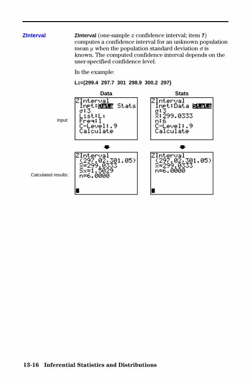
13-16 Inferential Statistics and Distributions
8313INFE.DOC TI-83 international English Bob Fedorisko Revised: 02/19/01 12:47 PM Printed: 02/19/01 1:38 PMPage 16 of 36
ZInterval (one-sample z confidence interval; item 7)computes a confidence interval for an unknown populationmean m when the population standard deviation s isknown. The computed confidence interval depends on theuser-specified confidence level.
In the example:
L1={299.4 297.7 301 298.9 300.2 297}
Data Stats
Input:
, ,
Calculated results:
ZInterval
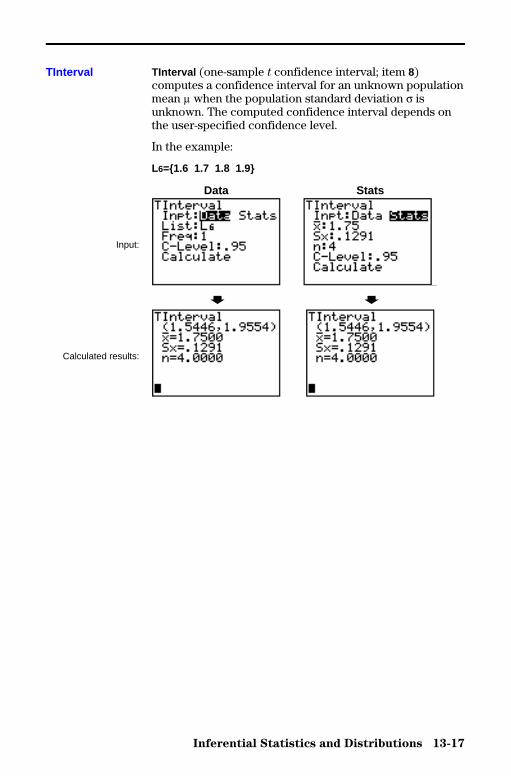
Inferential Statistics and Distributions 13-17
8313INFE.DOC TI-83 international English Bob Fedorisko Revised: 02/19/01 12:47 PM Printed: 02/19/01 1:38 PMPage 17 of 36
TInterval (one-sample t confidence interval; item 8)computes a confidence interval for an unknown populationmean m when the population standard deviation s isunknown. The computed confidence interval depends onthe user-specified confidence level.
In the example:
L6={1.6 1.7 1.8 1.9}
Data Stats
Input:
, ,
Calculated results:
TInterval
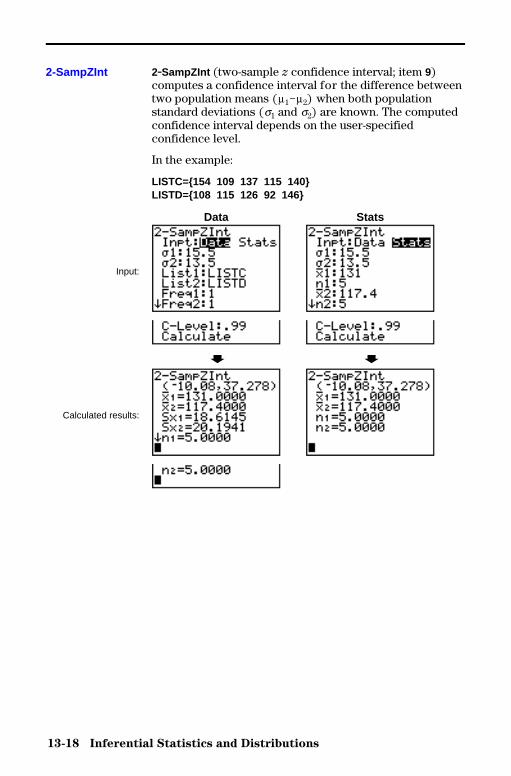
13-18 Inferential Statistics and Distributions
8313INFE.DOC TI-83 international English Bob Fedorisko Revised: 02/19/01 12:47 PM Printed: 02/19/01 1:38 PMPage 18 of 36
2.SampZInt (two-sample z confidence interval; item 9)computes a confidence interval for the difference betweentwo population means (m1Nm2) when both populationstandard deviations (s1 and s2) are known. The computedconfidence interval depends on the user-specifiedconfidence level.
In the example:
LISTC={154 109 137 115 140}LISTD={108 115 126 92 146}
Data Stats
Input:
, ,
Calculated results:
2-SampZInt
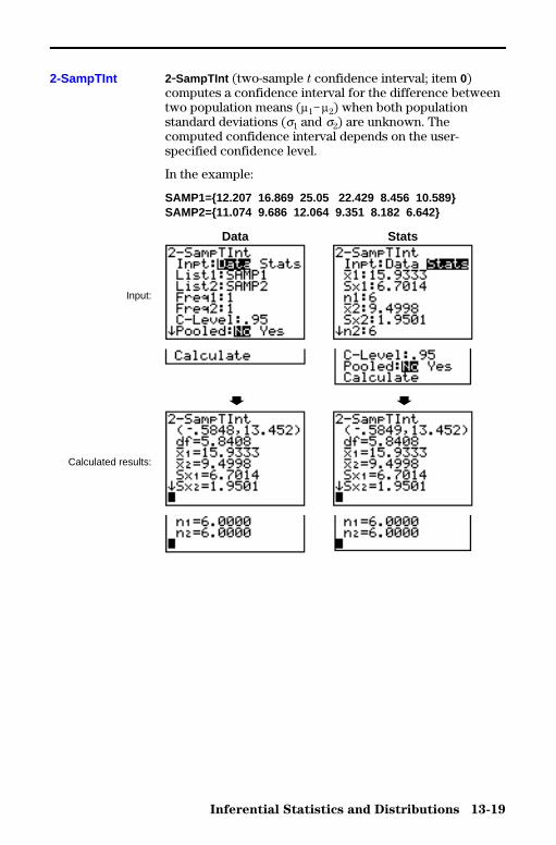
Inferential Statistics and Distributions 13-19
8313INFE.DOC TI-83 international English Bob Fedorisko Revised: 02/19/01 12:47 PM Printed: 02/19/01 1:38 PMPage 19 of 36
2.SampTInt (two-sample t confidence interval; item 0)computes a confidence interval for the difference betweentwo population means (m1Nm2) when both populationstandard deviations (s1 and s2) are unknown. Thecomputed confidence interval depends on the user-specified confidence level.
In the example:
SAMP1={12.207 16.869 25.05 22.429 8.456 10.589}SAMP2={11.074 9.686 12.064 9.351 8.182 6.642}
Data Stats
Input:
, ,
Calculated results:
2-SampTInt
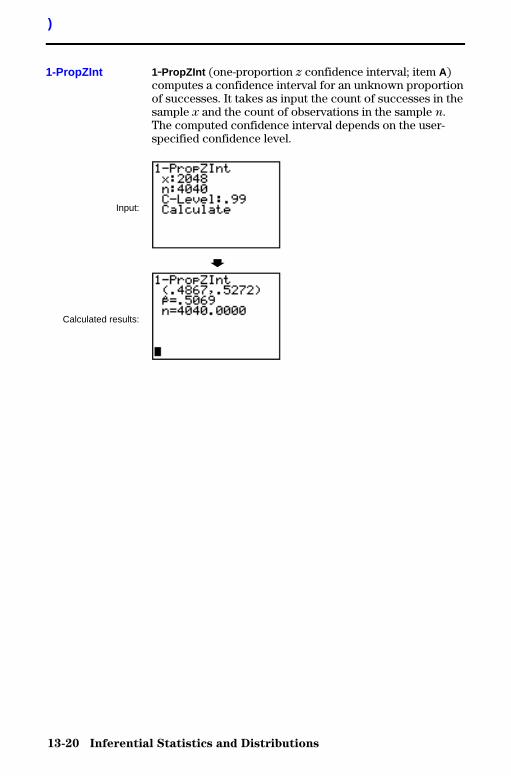
13-20 Inferential Statistics and Distributions
8313INFE.DOC TI-83 international English Bob Fedorisko Revised: 02/19/01 12:47 PM Printed: 02/19/01 1:38 PMPage 20 of 36
1.PropZInt (one-proportion z confidence interval; item A)computes a confidence interval for an unknown proportionof successes. It takes as input the count of successes in thesample x and the count of observations in the sample n.The computed confidence interval depends on the user-specified confidence level.
Input:
,
Calculated results:
)
1-PropZInt
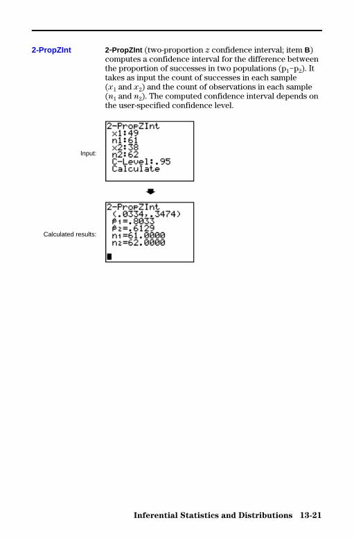
Inferential Statistics and Distributions 13-21
8313INFE.DOC TI-83 international English Bob Fedorisko Revised: 02/19/01 12:47 PM Printed: 02/19/01 1:38 PMPage 21 of 36
2.PropZInt (two-proportion z confidence interval; item B)computes a confidence interval for the difference betweenthe proportion of successes in two populations (p1Np2). Ittakes as input the count of successes in each sample(x1 and x2) and the count of observations in each sample(n1 and n2). The computed confidence interval depends onthe user-specified confidence level.
Input:
,
Calculated results:
2-PropZInt
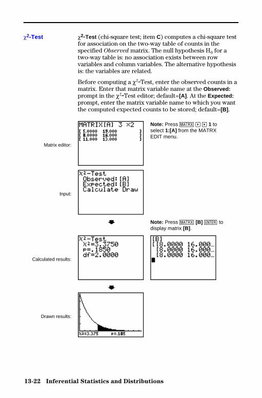
13-22 Inferential Statistics and Distributions
8313INFE.DOC TI-83 international English Bob Fedorisko Revised: 02/19/01 12:47 PM Printed: 02/19/01 1:38 PMPage 22 of 36
c2.Test (chi-square test; item C) computes a chi-square testfor association on the two-way table of counts in thespecified Observed matrix. The null hypothesis H0 for atwo-way table is: no association exists between rowvariables and column variables. The alternative hypothesisis: the variables are related.
Before computing a c2.Test, enter the observed counts in amatrix. Enter that matrix variable name at the Observed:prompt in the c2.Test editor; default=[A] . At the Expected:prompt, enter the matrix variable name to which you wantthe computed expected counts to be stored; default=[B] .
Matrix editor:
Note: Press � ~ ~ 1 toselect 1:[A] from the MATRXEDIT menu.
Input:
, Note: Press � [B] Í todisplay matrix [B] .
Calculated results:
,
Drawn results:
c2-Test
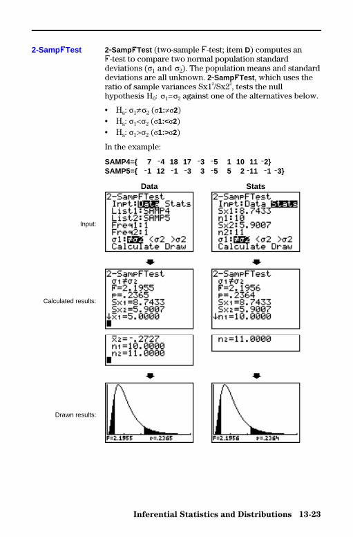
Inferential Statistics and Distributions 13-23
8313INFE.DOC TI-83 international English Bob Fedorisko Revised: 02/19/01 12:47 PM Printed: 02/19/01 1:38 PMPage 23 of 36
2.SampÜTest (two-sample Û-test; item D) computes anÛ-test to compare two normal population standarddeviations (s1 and s2). The population means and standarddeviations are all unknown. 2.SampÜTest , which uses theratio of sample variances Sx12/Sx22, tests the nullhypothesis H0: s1=s2 against one of the alternatives below.
• Ha: s1ƒs2 (s1:ƒs2)• Ha: s1<s2 (s1:<s2)• Ha: s1>s2 (s1:>s2)
In the example:
SAMP4={ 7 L4 18 17 L3 L5 1 10 11 L2}SAMP5={ L1 12 L1 L3 3 L5 5 2 L11 L1 L3}
Data Stats
Input:
, ,
Calculated results:
, ,
Drawn results:
2-SampÜTest
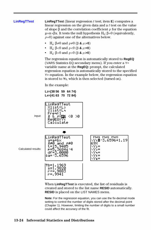
13-24 Inferential Statistics and Distributions
8313INFE.DOC TI-83 international English Bob Fedorisko Revised: 02/19/01 12:47 PM Printed: 02/19/01 1:38 PMPage 24 of 36
LinRegTTest (linear regression t test; item E) computes alinear regression on the given data and a t test on the valueof slope b and the correlation coefficient r for the equationy=a+bx. It tests the null hypothesis H0: b=0 (equivalently,r=0) against one of the alternatives below.
• Ha: bƒ0 and rƒ0 (b & r:ƒ0)• Ha: b<0 and r<0 (b & r:<0)• Ha: b>0 and r>0 (b & r:>0)
The regression equation is automatically stored to RegEQ(VARS Statistics EQ secondary menu). If you enter a Y=variable name at the RegEQ: prompt, the calculatedregression equation is automatically stored to the specifiedY= equation. In the example below, the regression equationis stored to Y1, which is then selected (turned on).
In the example:
L3={38 56 59 64 74}L4={41 63 70 72 84}
Input:
,
Calculated results:
When LinRegTTest is executed, the list of residuals iscreated and stored to the list name RESID automatically.RESID is placed on the LIST NAMES menu.
Note: For the regression equation, you can use the fix-decimal modesetting to control the number of digits stored after the decimal point(Chapter 1). However, limiting the number of digits to a small numbercould affect the accuracy of the fit.
LinRegTTest
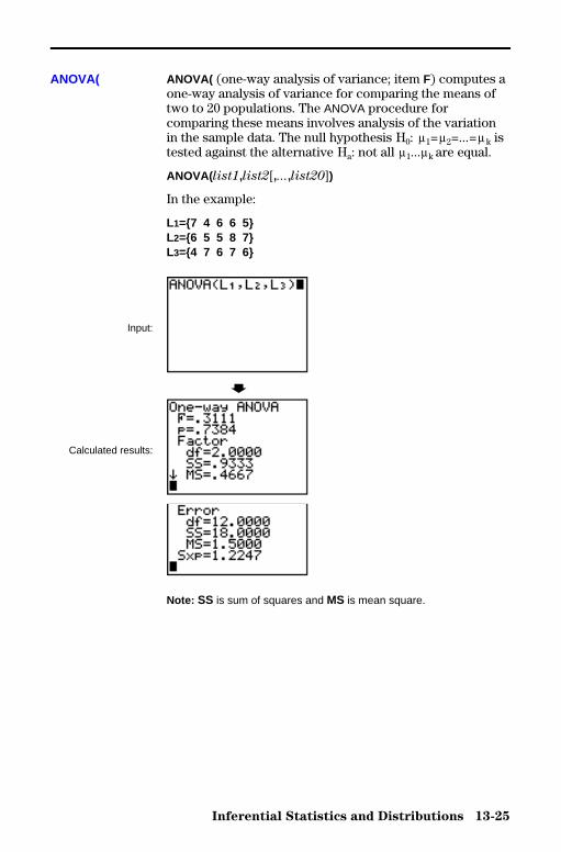
Inferential Statistics and Distributions 13-25
8313INFE.DOC TI-83 international English Bob Fedorisko Revised: 02/19/01 12:47 PM Printed: 02/19/01 1:38 PMPage 25 of 36
ANOVA( (one-way analysis of variance; item F) computes aone-way analysis of variance for comparing the means oftwo to 20 populations. The ANOVA procedure forcomparing these means involves analysis of the variationin the sample data. The null hypothesis H0: m1=m2=...=mk istested against the alternative Ha: not all m1...mk are equal.
ANOVA( list1,list2[,...,list20])
In the example:
L1={7 4 6 6 5}L2={6 5 5 8 7}L3={4 7 6 7 6}
Input:
,
Calculated results:
Note: SS is sum of squares and MS is mean square.
ANOVA(
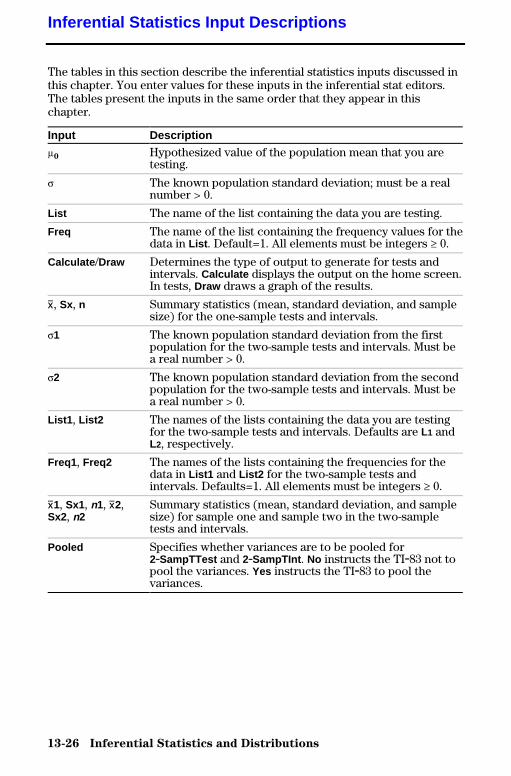
13-26 Inferential Statistics and Distributions
8313INFE.DOC TI-83 international English Bob Fedorisko Revised: 02/19/01 12:47 PM Printed: 02/19/01 1:38 PMPage 26 of 36
The tables in this section describe the inferential statistics inputs discussed inthis chapter. You enter values for these inputs in the inferential stat editors.The tables present the inputs in the same order that they appear in thischapter.
Input Description
m0 Hypothesized value of the population mean that you aretesting.
s The known population standard deviation; must be a realnumber > 0.
List The name of the list containing the data you are testing.
Freq The name of the list containing the frequency values for thedata in List . Default=1. All elements must be integers | 0.
Calculate /Draw Determines the type of output to generate for tests andintervals. Calculate displays the output on the home screen.In tests, Draw draws a graph of the results.
v, Sx, n Summary statistics (mean, standard deviation, and samplesize) for the one-sample tests and intervals.
s1 The known population standard deviation from the firstpopulation for the two-sample tests and intervals. Must bea real number > 0.
s2 The known population standard deviation from the secondpopulation for the two-sample tests and intervals. Must bea real number > 0.
List1 , List2 The names of the lists containing the data you are testingfor the two-sample tests and intervals. Defaults are L1 andL2, respectively.
Freq1 , Freq2 The names of the lists containing the frequencies for thedata in List1 and List2 for the two-sample tests andintervals. Defaults=1. All elements must be integers | 0.
v1, Sx1, n1, v2,Sx2, n2
Summary statistics (mean, standard deviation, and samplesize) for sample one and sample two in the two-sampletests and intervals.
Pooled Specifies whether variances are to be pooled for2.SampTTest and 2.SampTInt . No instructs the TI.83 not topool the variances. Yes instructs the TI.83 to pool thevariances.
Inferential Statistics Input Descriptions
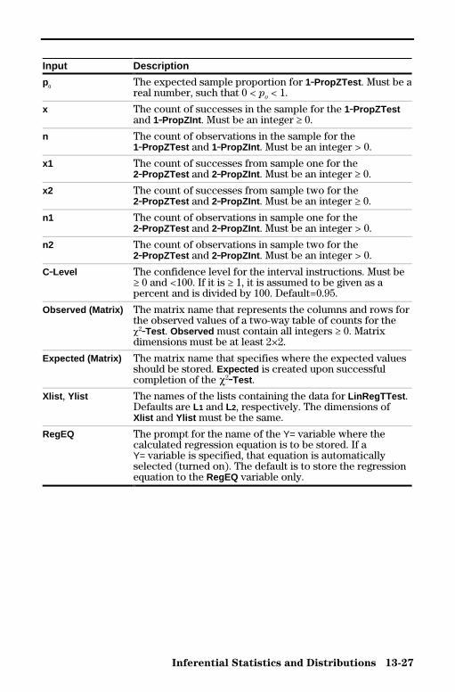
Inferential Statistics and Distributions 13-27
8313INFE.DOC TI-83 international English Bob Fedorisko Revised: 02/19/01 12:47 PM Printed: 02/19/01 1:38 PMPage 27 of 36
Input Description
p0 The expected sample proportion for 1.PropZTest . Must be areal number, such that 0 < p
0 < 1.
x The count of successes in the sample for the 1.PropZTestand 1.PropZInt . Must be an integer ‚ 0.
n The count of observations in the sample for the1.PropZTest and 1.PropZInt . Must be an integer > 0.
x1 The count of successes from sample one for the2.PropZTest and 2.PropZInt . Must be an integer ‚ 0.
x2 The count of successes from sample two for the2.PropZTest and 2.PropZInt . Must be an integer ‚ 0.
n1 The count of observations in sample one for the2.PropZTest and 2.PropZInt . Must be an integer > 0.
n2 The count of observations in sample two for the2.PropZTest and 2.PropZInt . Must be an integer > 0.
C.Level The confidence level for the interval instructions. Must be‚ 0 and <100. If it is ‚ 1, it is assumed to be given as apercent and is divided by 100. Default=0.95.
Observed (Matrix) The matrix name that represents the columns and rows forthe observed values of a two-way table of counts for thec2.Test . Observed must contain all integers ‚ 0. Matrixdimensions must be at least 2×2.
Expected (Matrix) The matrix name that specifies where the expected valuesshould be stored. Expected is created upon successfulcompletion of the c2.Test .
Xlist , Ylist The names of the lists containing the data for LinRegTTest .Defaults are L1 and L2, respectively. The dimensions ofXlist and Ylist must be the same.
RegEQ The prompt for the name of the Y= variable where thecalculated regression equation is to be stored. If aY= variable is specified, that equation is automaticallyselected (turned on). The default is to store the regressionequation to the RegEQ variable only.
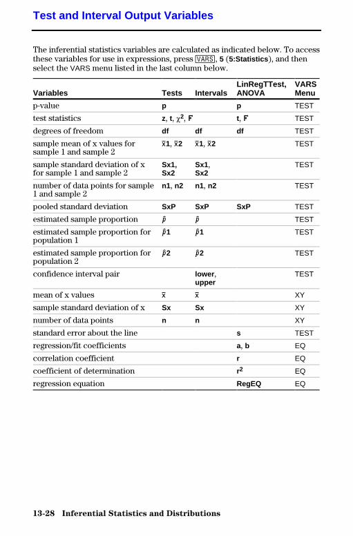
13-28 Inferential Statistics and Distributions
8313INFE.DOC TI-83 international English Bob Fedorisko Revised: 02/19/01 12:47 PM Printed: 02/19/01 1:38 PMPage 28 of 36
The inferential statistics variables are calculated as indicated below. To accessthese variables for use in expressions, press �, 5 (5:Statistics ), and thenselect the VARS menu listed in the last column below.
Variables Tests IntervalsLinRegTTest,ANOVA
VARSMenu
p-value p p TEST
test statistics z, t, c2, Ü t, Ü TEST
degrees of freedom df df df TEST
sample mean of x values forsample 1 and sample 2
v1, v2 v1, v2 TEST
sample standard deviation of xfor sample 1 and sample 2
Sx1,Sx2
Sx1,Sx2
TEST
number of data points for sample1 and sample 2
n1, n2 n1 , n2 TEST
pooled standard deviation SxP SxP SxP TEST
estimated sample proportion Ç Ç TEST
estimated sample proportion forpopulation 1
Ç1 Ç1 TEST
estimated sample proportion forpopulation 2
Ç2 Ç2 TEST
confidence interval pair lower ,upper
TEST
mean of x values v v XY
sample standard deviation of x Sx Sx XY
number of data points n n XY
standard error about the line s TEST
regression/fit coefficients a, b EQ
correlation coefficient r EQ
coefficient of determination r2 EQ
regression equation RegEQ EQ
Test and Interval Output Variables
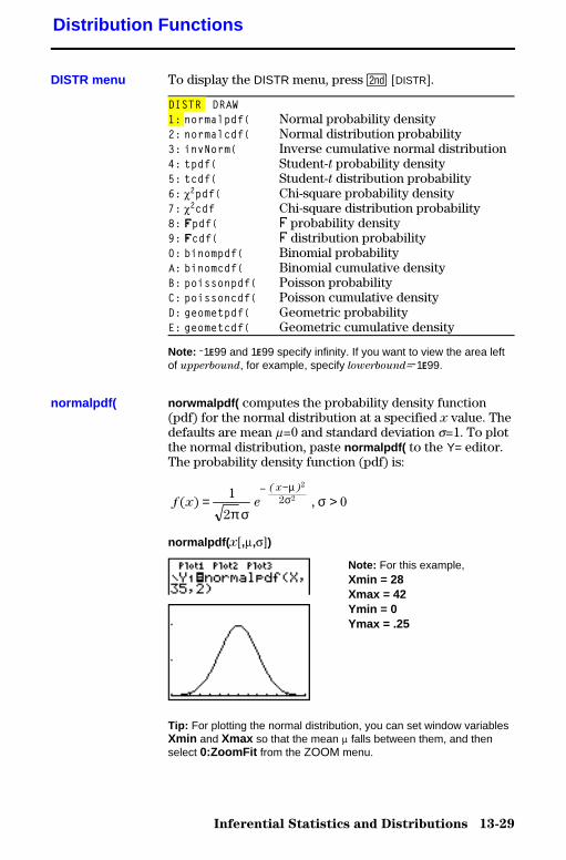
Inferential Statistics and Distributions 13-29
8313INFE.DOC TI-83 international English Bob Fedorisko Revised: 02/19/01 12:47 PM Printed: 02/19/01 1:38 PMPage 29 of 36
To display the DISTR menu, press y [DISTR].
DISTR DRAW1: normalpdf( Normal probability density2: normalcdf( Normal distribution probability3: invNorm( Inverse cumulative normal distribution4: tpdf( Student-t probability density5: tcdf( Student-t distribution probability6: c2pdf( Chi-square probability density7: c2cdf Chi-square distribution probability8: Üpdf( Û probability density9: Ücdf( Û distribution probability0: binompdf( Binomial probabilityA: binomcdf( Binomial cumulative densityB: poissonpdf( Poisson probabilityC: poissoncdf( Poisson cumulative densityD: geometpdf( Geometric probabilityE: geometcdf( Geometric cumulative density
Note: L1å99 and 1å99 specify infinity. If you want to view the area leftof upperbound, for example, specify lowerbound=L1å99.
norwmalpdf( computes the probability density function(pdf) for the normal distribution at a specified x value. Thedefaults are mean m=0 and standard deviation s=1. To plotthe normal distribution, paste normalpdf( to the Y= editor.The probability density function (pdf) is:
f x e
x
( ) = >− −1
20
2
22
π σσ
µσ
( )
,
normalpdf( x[,m,s])
Note: For this example,Xmin = 28Xmax = 42Ymin = 0Ymax = .25
Tip: For plotting the normal distribution, you can set window variablesXmin and Xmax so that the mean m falls between them, and thenselect 0:ZoomFit from the ZOOM menu.
Distribution Functions
DISTR menu
normalpdf(
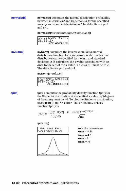
13-30 Inferential Statistics and Distributions
8313INFE.DOC TI-83 international English Bob Fedorisko Revised: 02/19/01 12:47 PM Printed: 02/19/01 1:38 PMPage 30 of 36
normalcdf( computes the normal distribution probabilitybetween lowerbound and upperbound for the specifiedmean m and standard deviation s. The defaults are m=0and s=1.
normalcdf( lowerbound,upperbound[,m,s])
invNorm( computes the inverse cumulative normaldistribution function for a given area under the normaldistribution curve specified by mean m and standarddeviation s. It calculates the x value associated with anarea to the left of the x value. 0 � area � 1 must be true.The defaults are m=0 and s=1.
invNorm( area[,m,s])
tpdf( computes the probability density function (pdf) forthe Student-t distribution at a specified x value. df (degreesof freedom) must be >0. To plot the Student-t distribution,paste tpdf( to the Y= editor. The probability densityfunction (pdf) is:
f xdf
df
x df
df
df
( )[( ) ]
( )( ) ( )
= + + − +ΓΓ
1 22
1 2 1 2/
/
/ /
π
tpdf( x,df)
Note: For this example,Xmin = L4.5Xmax = 4.5Ymin = 0Ymax = .4
normalcdf(
invNorm(
tpdf(
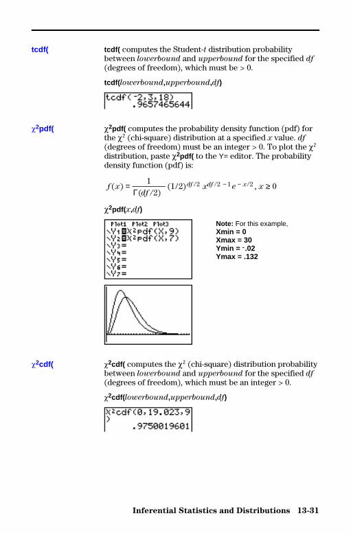
Inferential Statistics and Distributions 13-31
8313INFE.DOC TI-83 international English Bob Fedorisko Revised: 02/19/01 12:47 PM Printed: 02/19/01 1:38 PMPage 31 of 36
tcdf( computes the Student-t distribution probabilitybetween lowerbound and upperbound for the specified df
(degrees of freedom), which must be > 0.
tcdf( lowerbound,upperbound,df)
c2pdf( computes the probability density function (pdf) forthe c2 (chi-square) distribution at a specified x value. df
(degrees of freedom) must be an integer > 0. To plot the c2
distribution, paste c2pdf( to the Y= editor. The probabilitydensity function (pdf) is:
f xdf
x e xdf df x( )( )
(1/2)= ≥− −12
02 2 1 2Γ /
,/ / /
c2pdf( x,df)
Note: For this example,Xmin = 0Xmax = 30Ymin = L.02Ymax = .132
c2cdf( computes the c2 (chi-square) distribution probabilitybetween lowerbound and upperbound for the specified df
(degrees of freedom), which must be an integer > 0.
c2cdf( lowerbound,upperbound,df)
tcdf(
c2pdf(
c2cdf(
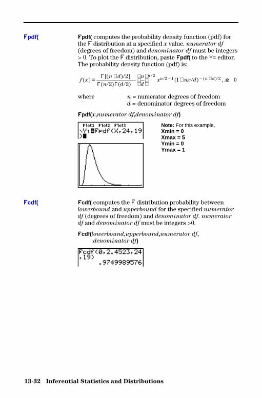
13-32 Inferential Statistics and Distributions
8313INFE.DOC TI-83 international English Bob Fedorisko Revised: 02/19/01 12:47 PM Printed: 02/19/01 1:38 PMPage 32 of 36
Üpdf( computes the probability density function (pdf) forthe Û distribution at a specified x value. numerator df
(degrees of freedom) and denominator df must be integers> 0. To plot the Û distribution, paste Üpdf( to the Y= editor.The probability density function (pdf) is:
f xn d
n d
n
dx nx d x
nn n d( )
[( ) ]( ) ( )
( ) ( )= +
+ ≥− − +ΓΓ Γ
/
/ // ,
// /2
2 21 0
22 1 2
where n = numerator degrees of freedomd = denominator degrees of freedom
Üpdf( x,numerator df,denominator df)
Note: For this example,Xmin = 0Xmax = 5Ymin = 0Ymax = 1
Ücdf( computes the Û distribution probability betweenlowerbound and upperbound for the specified numerator
df (degrees of freedom) and denominator df. numerator
df and denominator df must be integers >0.
Ücdf( lowerbound,upperbound,numerator df,denominator df)
Üpdf(
Ücdf(
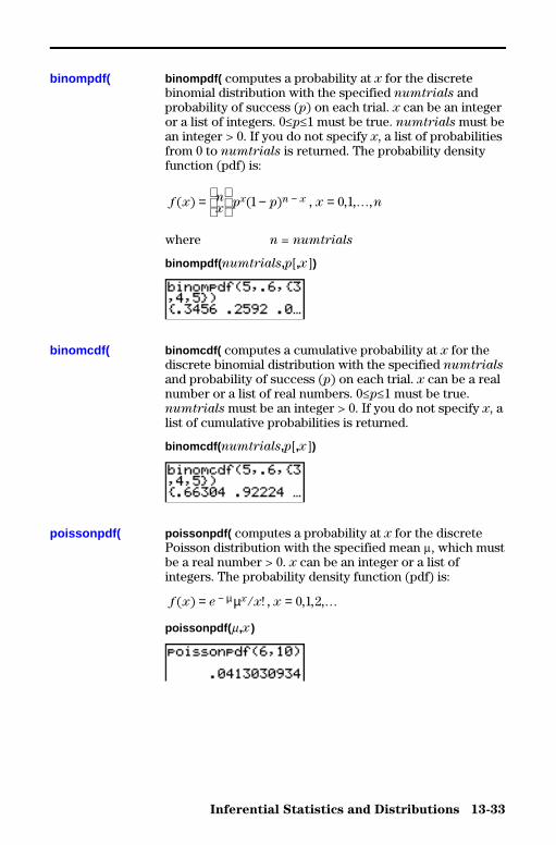
Inferential Statistics and Distributions 13-33
8313INFE.DOC TI-83 international English Bob Fedorisko Revised: 02/19/01 12:47 PM Printed: 02/19/01 1:38 PMPage 33 of 36
binompdf( computes a probability at x for the discretebinomial distribution with the specified numtrials andprobability of success (p) on each trial. x can be an integeror a list of integers. 0�p�1 must be true. numtrials must bean integer > 0. If you do not specify x, a list of probabilitiesfrom 0 to numtrials is returned. The probability densityfunction (pdf) is:
f x nx
p p x nx n x( ) ( )=
− =−1 0 1, , , ,�
where n = numtrials
binompdf( numtrials,p[,x ])
binomcdf( computes a cumulative probability at x for thediscrete binomial distribution with the specified numtrials
and probability of success (p) on each trial. x can be a realnumber or a list of real numbers. 0�p�1 must be true.numtrials must be an integer > 0. If you do not specify x, alist of cumulative probabilities is returned.
binomcdf( numtrials,p[,x ])
poissonpdf( computes a probability at x for the discretePoisson distribution with the specified mean m, which mustbe a real number > 0. x can be an integer or a list ofintegers. The probability density function (pdf) is:
f x e x xx( ) != =− µµ / , , , ,0 1 2 �
poissonpdf( m,x )
binompdf(
binomcdf(
poissonpdf(
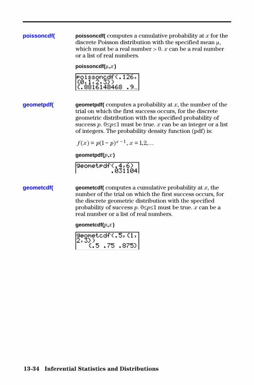
13-34 Inferential Statistics and Distributions
8313INFE.DOC TI-83 international English Bob Fedorisko Revised: 02/19/01 12:47 PM Printed: 02/19/01 1:38 PMPage 34 of 36
poissoncdf( computes a cumulative probability at x for thediscrete Poisson distribution with the specified mean m,which must be a real number > 0. x can be a real numberor a list of real numbers.
poissoncdf( m,x )
geometpdf( computes a probability at x, the number of thetrial on which the first success occurs, for the discretegeometric distribution with the specified probability ofsuccess p. 0�p�1 must be true. x can be an integer or a listof integers. The probability density function (pdf) is:
f x p p xx( ) ( )= − =−1 1 21 , , ,�
geometpdf( p,x )
geometcdf( computes a cumulative probability at x, thenumber of the trial on which the first success occurs, forthe discrete geometric distribution with the specifiedprobability of success p. 0�p�1 must be true. x can be areal number or a list of real numbers.
geometcdf( p,x )
poissoncdf(
geometpdf(
geometcdf(
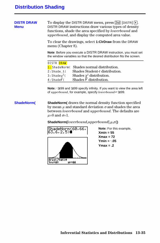
Inferential Statistics and Distributions 13-35
8313INFE.DOC TI-83 international English Bob Fedorisko Revised: 02/19/01 12:47 PM Printed: 02/19/01 1:38 PMPage 35 of 36
To display the DISTR DRAW menu, press y [DISTR] ~.DISTR DRAW instructions draw various types of densityfunctions, shade the area specified by lowerbound andupperbound, and display the computed area value.
To clear the drawings, select 1:ClrDraw from the DRAWmenu (Chapter 8).
Note : Before you execute a DISTR DRAW instruction, you must setthe window variables so that the desired distribution fits the screen.
DISTR DRAW1: ShadeNorm( Shades normal distribution.2:Shade_t( Shades Student-t distribution.3:Shadec2( Shades c2 distribution.4:ShadeÛ( Shades Û distribution.
Note: L1å99 and 1å99 specify infinity. If you want to view the area leftof upperbound, for example, specify lowerbound=L1å99.
ShadeNorm( draws the normal density function specifiedby mean m and standard deviation s and shades the areabetween lowerbound and upperbound. The defaults arem=0 and s=1.
ShadeNorm( lowerbound,upperbound[,m,s])
Note: For this example,Xmin = 55Xmax = 72Ymin = L.05Ymax = .2
Distribution Shading
DISTR DRAWMenu
ShadeNorm(
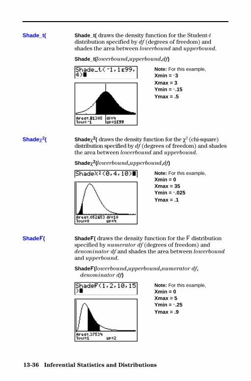
13-36 Inferential Statistics and Distributions
8313INFE.DOC TI-83 international English Bob Fedorisko Revised: 02/19/01 12:47 PM Printed: 02/19/01 1:38 PMPage 36 of 36
Shade_t( draws the density function for the Student-tdistribution specified by df (degrees of freedom) andshades the area between lowerbound and upperbound.
Shade_t( lowerbound,upperbound,df)
Note: For this example,Xmin = L3Xmax = 3Ymin = L.15Ymax = .5
Shadec2( draws the density function for the c2 (chi-square)distribution specified by df (degrees of freedom) and shadesthe area between lowerbound and upperbound.
Shadec2(lowerbound,upperbound,df)
Note: For this example,Xmin = 0Xmax = 35Ymin = L.025Ymax = .1
ShadeÜ( draws the density function for the Û distributionspecified by numerator df (degrees of freedom) anddenominator df and shades the area between lowerbound
and upperbound.
ShadeÜ(lowerbound,upperbound,numerator df, denominator df)
Note: For this example,Xmin = 0Xmax = 5Ymin = L.25Ymax = .9
Shade_t(
Shadec2(
ShadeÜ(
Financial Functions 14-1
8314FINA.DOC TI-83 international English Bob Fedorisko Revised: 02/19/01 12:50 PM Printed: 02/19/01 1:38 PMPage 1 of 14
14 FinancialFunctions
Getting Started: Financing a Car ......................... 14-2Getting Started: Computing Compound Interest.......... 14-3Using the TVM Solver .................................... 14-4Using the Financial Functions ........................... 14-5Calculating Time Value of Money (TVM) ................. 14-6Calculating Cash Flows .................................. 14-8Calculating Amortization ................................ 14-9Calculating Interest Conversion.......................... 14-12Finding Days between Dates/Defining Payment Method ..... 14-13Using the TVM Variables ................................. 14-14
Contents
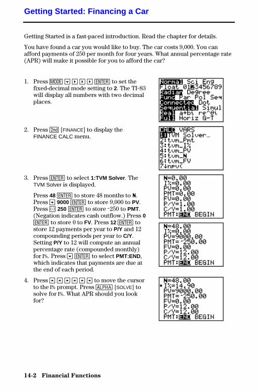
14-2 Financial Functions
8314FINA.DOC TI-83 international English Bob Fedorisko Revised: 02/19/01 12:50 PM Printed: 02/19/01 1:38 PMPage 2 of 14
Getting Started is a fast-paced introduction. Read the chapter for details.
You have found a car you would like to buy. The car costs 9,000. You canafford payments of 250 per month for four years. What annual percentage rate(APR) will make it possible for you to afford the car?
1. Press z † ~ ~ ~ Í to set thefixed-decimal mode setting to 2. The TI-83will display all numbers with two decimalplaces.
2. Press y [FINANCE] to display theFINANCE CALC menu.
3. Press Í to select 1:TVM Solver . TheTVM Solver is displayed.
Press 48 Í to store 48 months to Ú.Press † 9000 Í to store 9,000 to PV.Press Ì 250 Í to store L250 to PMT.(Negation indicates cash outflow.) Press 0Í to store 0 to FV. Press 12 Í tostore 12 payments per year to P/Y and 12compounding periods per year to C/Y.Setting P/Y to 12 will compute an annualpercentage rate (compounded monthly)for æ. Press † Í to select PMT:END,which indicates that payments are due atthe end of each period.
4. Press } } } } } } to move the cursorto the æ prompt. Press ƒ [SOLVE] tosolve for æ. What APR should you lookfor?
Getting Started: Financing a Car
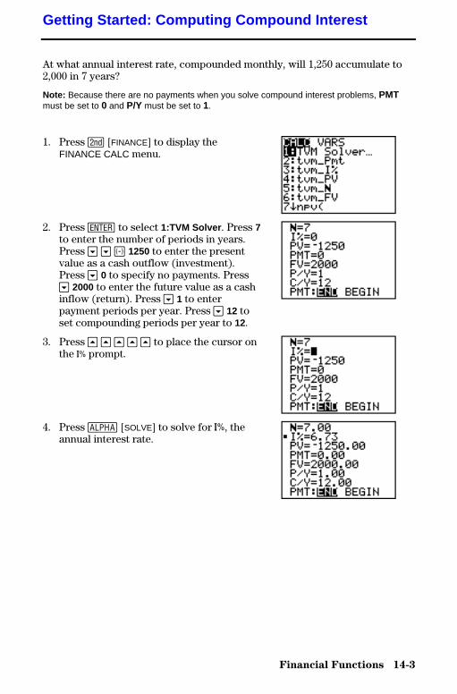
Financial Functions 14-3
8314FINA.DOC TI-83 international English Bob Fedorisko Revised: 02/19/01 12:50 PM Printed: 02/19/01 1:38 PMPage 3 of 14
At what annual interest rate, compounded monthly, will 1,250 accumulate to2,000 in 7 years?
Note: Because there are no payments when you solve compound interest problems, PMTmust be set to 0 and P/Y must be set to 1.
1. Press y [FINANCE] to display theFINANCE CALC menu.
2. Press Í to select 1:TVM Solver . Press 7to enter the number of periods in years.Press † † Ì 1250 to enter the presentvalue as a cash outflow (investment).Press † 0 to specify no payments. Press† 2000 to enter the future value as a cashinflow (return). Press † 1 to enterpayment periods per year. Press † 12 toset compounding periods per year to 12.
3. Press } } } } } to place the cursor onthe æ prompt.
4. Press ƒ [SOLVE] to solve for æ, theannual interest rate.
Getting Started: Computing Compound Interest
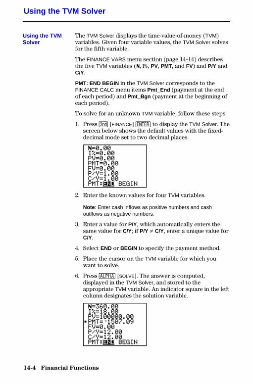
14-4 Financial Functions
8314FINA.DOC TI-83 international English Bob Fedorisko Revised: 02/19/01 12:50 PM Printed: 02/19/01 1:38 PMPage 4 of 14
The TVM Solver displays the time-value-of-money (TVM)variables. Given four variable values, the TVM Solver solvesfor the fifth variable.
The FINANCE VARS menu section (page 14.14) describesthe five TVM variables (Ú, æ, PV, PMT, and FV) and P/Y andC/Y.
PMT: END BEGIN in the TVM Solver corresponds to theFINANCE CALC menu items Pmt_End (payment at the endof each period) and Pmt_Bgn (payment at the beginning ofeach period).
To solve for an unknown TVM variable, follow these steps.
1. Press y [FINANCE] Í to display the TVM Solver. Thescreen below shows the default values with the fixed-decimal mode set to two decimal places.
2. Enter the known values for four TVM variables.
Note : Enter cash inflows as positive numbers and cashoutflows as negative numbers.
3. Enter a value for P/Y, which automatically enters thesame value for C/Y; if P/Y ƒ C/Y, enter a unique value forC/Y.
4. Select END or BEGIN to specify the payment method.
5. Place the cursor on the TVM variable for which youwant to solve.
6. Press ƒ [SOLVE]. The answer is computed,displayed in the TVM Solver, and stored to theappropriate TVM variable. An indicator square in the leftcolumn designates the solution variable.
Using the TVM Solver
Using the TVMSolver
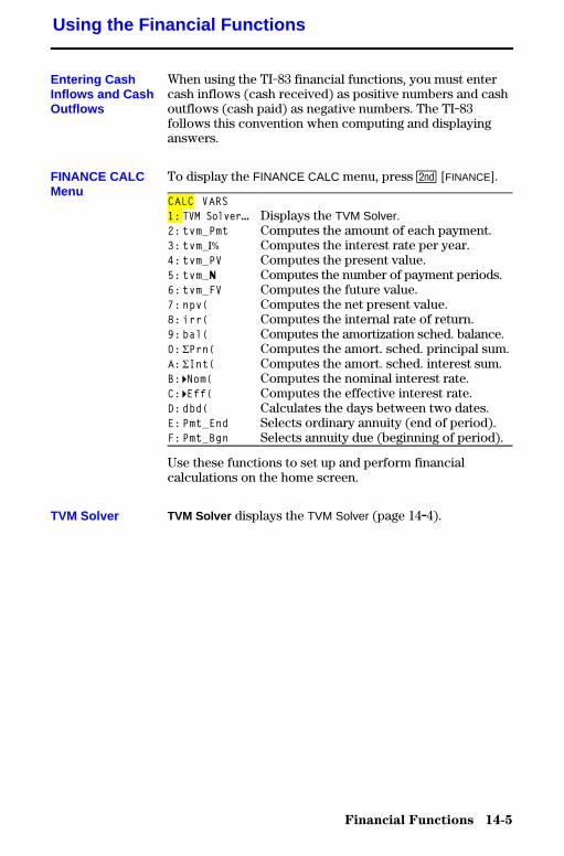
Financial Functions 14-5
8314FINA.DOC TI-83 international English Bob Fedorisko Revised: 02/19/01 12:50 PM Printed: 02/19/01 1:38 PMPage 5 of 14
When using the TI-83 financial functions, you must entercash inflows (cash received) as positive numbers and cashoutflows (cash paid) as negative numbers. The TI-83follows this convention when computing and displayinganswers.
To display the FINANCE CALC menu, press y [FINANCE].
CALC VARS1:TVM Solver... Displays the TVM Solver.2:tvm_Pmt Computes the amount of each payment.3:tvm_æ Computes the interest rate per year.4:tvm_PV Computes the present value.5:tvm_Ú Computes the number of payment periods.6:tvm_FV Computes the future value.7:npv( Computes the net present value.8:irr( Computes the internal rate of return.9:bal( Computes the amortization sched. balance.0:GPrn( Computes the amort. sched. principal sum.A:GInt( Computes the amort. sched. interest sum.B: 4Nom( Computes the nominal interest rate.C: 4Eff( Computes the effective interest rate.D:dbd( Calculates the days between two dates.E:Pmt_End Selects ordinary annuity (end of period).F:Pmt_Bgn Selects annuity due (beginning of period).
Use these functions to set up and perform financialcalculations on the home screen.
TVM Solver displays the TVM Solver (page 14.4).
Using the Financial Functions
Entering CashInflows and CashOutflows
FINANCE CALCMenu
TVM Solver

14-6 Financial Functions
8314FINA.DOC TI-83 international English Bob Fedorisko Revised: 02/19/01 12:50 PM Printed: 02/19/01 1:38 PMPage 6 of 14
Use time-value-of-money (TVM) functions (menu items 2through 6) to analyze financial instruments such asannuities, loans, mortgages, leases, and savings.
Each TVM function takes zero to six arguments, whichmust be real numbers. The values that you specify asarguments for these functions are not stored to the TVMvariables (page 14.14).
Note: To store a value to a TVM variable, use the TVM Solver (page14.4) or use ¿ and any TVM variable on the FINANCE VARSmenu (page 14.14).
If you enter less than six arguments, the TI-83 substitutes apreviously stored TVM variable value for each unspecifiedargument.
If you enter any arguments with a TVM function, you mustplace the argument or arguments in parentheses.
tvm_Pmt computes the amount of each payment.
tvm_Pmt [(Ú,æ,PV,FV,P/Y,C/Y)]
Note: In the example above, the values are stored to the TVMvariables in the TVM Solver. Then the payment (tvm_Pmt ) iscomputed on the home screen using the values in the TVM Solver.Next, the interest rate is changed to 9.5 to illustrate the effect on thepayment amount.
Calculating Time Value of Money (TVM)
Calculating TimeValue of Money
tvm_Pmt
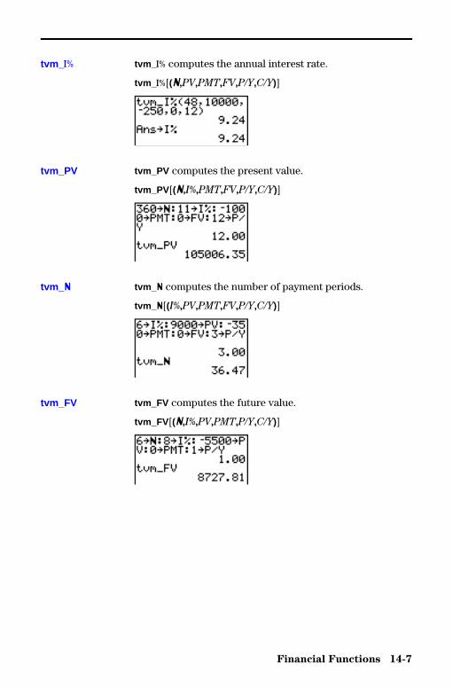
Financial Functions 14-7
8314FINA.DOC TI-83 international English Bob Fedorisko Revised: 02/19/01 12:50 PM Printed: 02/19/01 1:38 PMPage 7 of 14
tvm_ æ computes the annual interest rate.
tvm_ æ[(Ú,PV,PMT,FV,P/Y,C/Y)]
tvm_PV computes the present value.
tvm_PV [(Ú,æ,PMT,FV,P/Y,C/Y)]
tvm_ Ú computes the number of payment periods.
tvm_ Ú[(æ,PV,PMT,FV,P/Y,C/Y)]
tvm_FV computes the future value.
tvm_FV [(Ú,æ,PV,PMT,P/Y,C/Y)]
tvm_ æ
tvm_PV
tvm_ Ú
tvm_FV
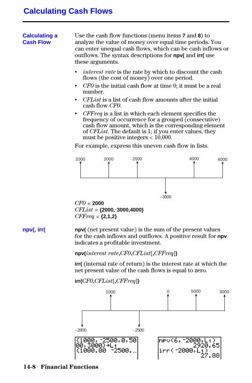
14-8 Financial Functions
8314FINA.DOC TI-83 international English Bob Fedorisko Revised: 02/19/01 12:50 PM Printed: 02/19/01 1:38 PMPage 8 of 14
Use the cash flow functions (menu items 7 and 8) toanalyze the value of money over equal time periods. Youcan enter unequal cash flows, which can be cash inflows oroutflows. The syntax descriptions for npv( and irr( usethese arguments.
• interest rate is the rate by which to discount the cashflows (the cost of money) over one period.
• CF0 is the initial cash flow at time 0; it must be a realnumber.
• CFList is a list of cash flow amounts after the initialcash flow CF0.
• CFFreq is a list in which each element specifies thefrequency of occurrence for a grouped (consecutive)cash flow amount, which is the corresponding elementof CFList. The default is 1; if you enter values, theymust be positive integers < 10,000.
For example, express this uneven cash flow in lists.
2000 40002000 2000
- 3000
4000
CF0 = 2000CFList = {2000,L3000,4000}CFFreq = {2,1,2}
npv( (net present value) is the sum of the present valuesfor the cash inflows and outflows. A positive result for npvindicates a profitable investment.
npv( interest rate,CF0,CFList[,CFFreq])
irr( (internal rate of return) is the interest rate at which thenet present value of the cash flows is equal to zero.
irr( CF0,CFList[,CFFreq])
300050001000
- 2000 - 2500
0
Calculating Cash Flows
Calculating aCash Flow
npv(, irr(
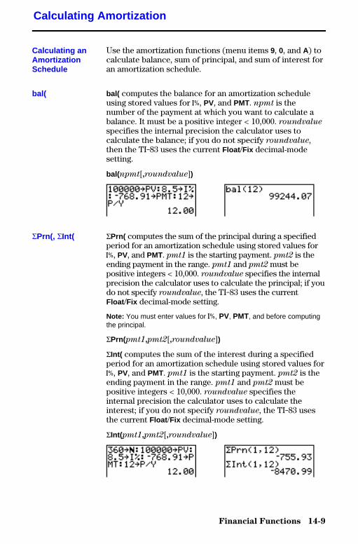
Financial Functions 14-9
8314FINA.DOC TI-83 international English Bob Fedorisko Revised: 02/19/01 12:50 PM Printed: 02/19/01 1:38 PMPage 9 of 14
Use the amortization functions (menu items 9, 0, and A) tocalculate balance, sum of principal, and sum of interest foran amortization schedule.
bal( computes the balance for an amortization scheduleusing stored values for æ, PV, and PMT. npmt is thenumber of the payment at which you want to calculate abalance. It must be a positive integer < 10,000. roundvalue
specifies the internal precision the calculator uses tocalculate the balance; if you do not specify roundvalue,then the TI-83 uses the current Float /Fix decimal-modesetting.
bal(npmt[,roundvalue])
GPrn( computes the sum of the principal during a specifiedperiod for an amortization schedule using stored values foræ, PV, and PMT. pmt1 is the starting payment. pmt2 is theending payment in the range. pmt1 and pmt2 must bepositive integers < 10,000. roundvalue specifies the internalprecision the calculator uses to calculate the principal; if youdo not specify roundvalue, the TI-83 uses the currentFloat /Fix decimal-mode setting.
Note: You must enter values for æ, PV, PMT, and before computingthe principal.
GPrn(pmt1,pmt2[,roundvalue])
GInt( computes the sum of the interest during a specifiedperiod for an amortization schedule using stored values foræ, PV, and PMT. pmt1 is the starting payment. pmt2 is theending payment in the range. pmt1 and pmt2 must bepositive integers < 10,000. roundvalue specifies theinternal precision the calculator uses to calculate theinterest; if you do not specify roundvalue, the TI-83 usesthe current Float /Fix decimal-mode setting.
GInt(pmt1,pmt2[,roundvalue])
Calculating Amortization
Calculating anAmortizationSchedule
bal(
GPrn(, GInt(
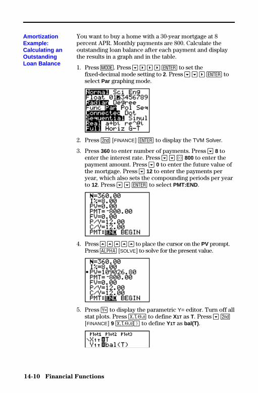
14-10 Financial Functions
8314FINA.DOC TI-83 international English Bob Fedorisko Revised: 02/19/01 12:50 PM Printed: 02/19/01 1:38 PMPage 10 of 14
You want to buy a home with a 30-year mortgage at 8percent APR. Monthly payments are 800. Calculate theoutstanding loan balance after each payment and displaythe results in a graph and in the table.
1. Press z. Press † ~ ~ ~ Í to set thefixed-decimal mode setting to 2. Press † † ~ Í toselect Par graphing mode.
2. Press y [FINANCE] Í to display the TVM Solver.
3. Press 360 to enter number of payments. Press † 8 toenter the interest rate. Press † † Ì 800 to enter thepayment amount. Press † 0 to enter the future value ofthe mortgage. Press † 12 to enter the payments peryear, which also sets the compounding periods per yearto 12. Press † † Í to select PMT:END.
4. Press } } } } } to place the cursor on the PV prompt.Press ƒ [SOLVE] to solve for the present value.
5. Press o to display the parametric Y= editor. Turn off allstat plots. Press „ to define X1T as T. Press † y[FINANCE] 9 „¤ to define Y1T as bal(T) .
AmortizationExample:Calculating anOutstandingLoan Balance
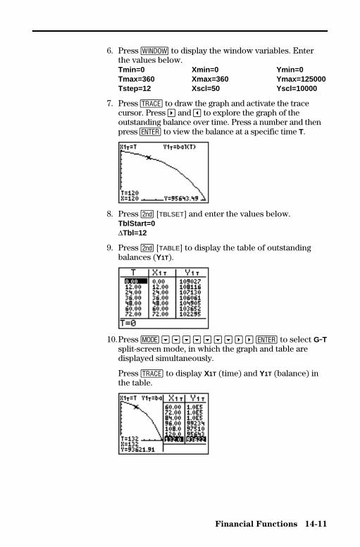
Financial Functions 14-11
8314FINA.DOC TI-83 international English Bob Fedorisko Revised: 02/19/01 12:50 PM Printed: 02/19/01 1:38 PMPage 11 of 14
6. Press p to display the window variables. Enterthe values below.Tmin=0 Xmin=0 Ymin=0Tmax=360 Xmax=360 Ymax=125000Tstep=12 Xscl=50 Yscl=10000
7. Press r to draw the graph and activate the tracecursor. Press ~ and | to explore the graph of theoutstanding balance over time. Press a number and thenpress Í to view the balance at a specific time T.
8. Press y [TBLSET] and enter the values below.TblStart=0@Tbl=12
9. Press y [TABLE] to display the table of outstandingbalances (Y1T).
10.Press z † † † † † † † ~ ~ Í to select G.Tsplit-screen mode, in which the graph and table aredisplayed simultaneously.
Press r to display X1T (time) and Y1T (balance) inthe table.

14-12 Financial Functions
8314FINA.DOC TI-83 international English Bob Fedorisko Revised: 02/19/01 12:50 PM Printed: 02/19/01 1:38 PMPage 12 of 14
Use the interest conversion functions (menu items B andC) to convert interest rates from an annual effective rate toa nominal rate (4Nom( ) or from a nominal rate to an annualeffective rate (4Eff( ).
4Nom( computes the nominal interest rate. effective rate
and compounding periods must be real numbers.compounding periods must be >0.
4Nom(effective rate,compounding periods)
4Eff( computes the effective interest rate. nominal rate andcompounding periods must be real numbers.compounding periods must be >0.
4Eff(nominal rate,compounding periods)
Calculating Interest Conversion
Calculating anInterestConversion
4Nom(
4Eff(
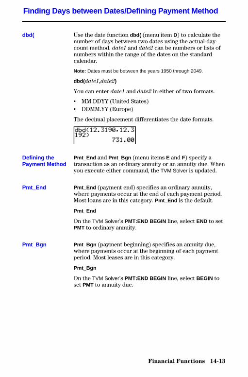
Financial Functions 14-13
8314FINA.DOC TI-83 international English Bob Fedorisko Revised: 02/19/01 12:50 PM Printed: 02/19/01 1:38 PMPage 13 of 14
Use the date function dbd( (menu item D) to calculate thenumber of days between two dates using the actual-day-count method. date1 and date2 can be numbers or lists ofnumbers within the range of the dates on the standardcalendar.
Note: Dates must be between the years 1950 through 2049.
dbd( date1,date2)
You can enter date1 and date2 in either of two formats.
• MM.DDYY (United States)• DDMM.YY (Europe)
The decimal placement differentiates the date formats.
Pmt_End and Pmt_Bgn (menu items E and F) specify atransaction as an ordinary annuity or an annuity due. Whenyou execute either command, the TVM Solver is updated.
Pmt_End (payment end) specifies an ordinary annuity,where payments occur at the end of each payment period.Most loans are in this category. Pmt_End is the default.
Pmt_End
On the TVM Solver’s PMT:END BEGIN line, select END to setPMT to ordinary annuity.
Pmt_Bgn (payment beginning) specifies an annuity due,where payments occur at the beginning of each paymentperiod. Most leases are in this category.
Pmt_Bgn
On the TVM Solver’s PMT:END BEGIN line, select BEGIN toset PMT to annuity due.
Finding Days between Dates/Defining Payment Method
dbd(
Defining thePayment Method
Pmt_End
Pmt_Bgn
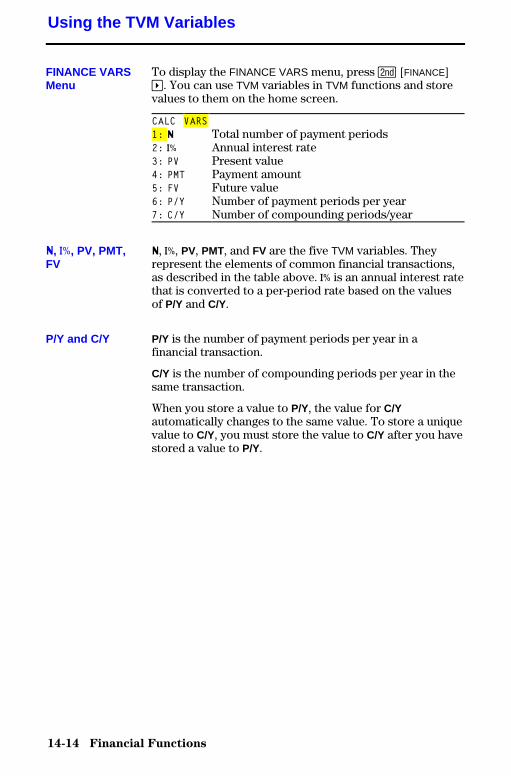
14-14 Financial Functions
8314FINA.DOC TI-83 international English Bob Fedorisko Revised: 02/19/01 12:50 PM Printed: 02/19/01 1:38 PMPage 14 of 14
To display the FINANCE VARS menu, press y [FINANCE]~. You can use TVM variables in TVM functions and storevalues to them on the home screen.
CALC VARS1: Ú Total number of payment periods2: æ Annual interest rate3: PV Present value4: PMT Payment amount5: FV Future value6: P/Y Number of payment periods per year7: C/Y Number of compounding periods/year
Ú, æ, PV, PMT, and FV are the five TVM variables. Theyrepresent the elements of common financial transactions,as described in the table above. æ is an annual interest ratethat is converted to a per-period rate based on the valuesof P/Y and C/Y.
P/Y is the number of payment periods per year in afinancial transaction.
C/Y is the number of compounding periods per year in thesame transaction.
When you store a value to P/Y, the value for C/Yautomatically changes to the same value. To store a uniquevalue to C/Y, you must store the value to C/Y after you havestored a value to P/Y.
Using the TVM Variables
FINANCE VARSMenu
Ú, æ, PV, PMT,FV
P/Y and C/Y
CATALOG , Strings, Hyperbolic Functions 15-1
8315CATS.DOC TI-83 international English Bob Fedorisko Revised: 02/19/01 12:54 PM Printed: 02/19/01 1:39PM Page 1 of 10
15 CATALOG, Strin gs,Hyperbolic Functions
Browsing the TI-83 CATALOG ........................... 15-2Entering and Using Strings............................... 15-3Storing Strings to String Variables ....................... 15-4String Functions and Instructions in the CATALOG ...... 15-6Hyperbolic Functions in the CATALOG .................. 15-10
Contents

15-2 CATALOG , Strings, Hyperbolic Functions
8315CATS.DOC TI-83 international English Bob Fedorisko Revised: 02/19/01 12:54 PM Printed: 02/19/01 1:39PM Page 2 of 10
The CATALOG is an alphabetical list of all functions andinstructions on the TI-83. You also can access eachCATALOG item from a menu or the keyboard, except:
• The six string functions (page 15.6)• The six hyperbolic functions (page 15.10)• The solve( instruction without the equation solver editor
(Chapter 2)• The inferential stat functions without the inferential stat
editors (Chapter 13)
Note: The only CATALOG programming commands you can executefrom the home screen are GetCalc( , Get(, and Send( .
To select a CATALOG item, follow these steps.
1. Press y ãCATALOGä to display the CATALOG.
The 4 in the first column is the selection cursor.
2. Press † or } to scroll the CATALOG until the selectioncursor points to the item you want.
• To jump to the first item beginning with a particularletter, press that letter; alpha-lock is on.
• Items that begin with a number are in alphabeticalorder according to the first letter after the number.For example, 2.PropZTest( is among the items thatbegin with the letter P.
• Functions that appear as symbols, such as +, L1, <,and ‡(, follow the last item that begins with Z. Tojump to the first symbol, !, press [q].
3. Press Í to paste the item to the current screen.
Tip: From the top of the CATALOG menu, press } to move to thebottom. From the bottom, press † to move to the top.
Browsing the TI-83 CATALOG
What Is theCATALOG?
Selecting an Itemfrom theCATALOG
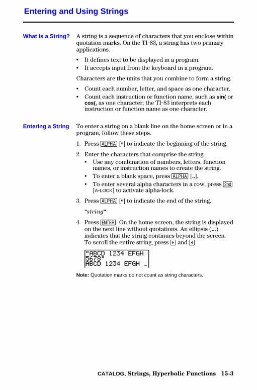
CATALOG , Strings, Hyperbolic Functions 15-3
8315CATS.DOC TI-83 international English Bob Fedorisko Revised: 02/19/01 12:54 PM Printed: 02/19/01 1:39PM Page 3 of 10
A string is a sequence of characters that you enclose withinquotation marks. On the TI-83, a string has two primaryapplications.
• It defines text to be displayed in a program.• It accepts input from the keyboard in a program.
Characters are the units that you combine to form a string.
• Count each number, letter, and space as one character.• Count each instruction or function name, such as sin( or
cos( , as one character; the TI-83 interprets eachinstruction or function name as one character.
To enter a string on a blank line on the home screen or in aprogram, follow these steps.
1. Press ƒ [ã] to indicate the beginning of the string.
2. Enter the characters that comprise the string.• Use any combination of numbers, letters, function
names, or instruction names to create the string.• To enter a blank space, press ƒ ['].• To enter several alpha characters in a row, press y
[A.LOCK] to activate alpha-lock.
3. Press ƒ [ã] to indicate the end of the string.
"string"
4. Press Í. On the home screen, the string is displayedon the next line without quotations. An ellipsis (...)indicates that the string continues beyond the screen.To scroll the entire string, press ~ and |.
Note: Quotation marks do not count as string characters.
Entering and Using Strings
What Is a String?
Entering a String

15-4 CATALOG , Strings, Hyperbolic Functions
8315CATS.DOC TI-83 international English Bob Fedorisko Revised: 02/19/01 12:54 PM Printed: 02/19/01 1:39PM Page 4 of 10
The TI-83 has 10 variables to which you can store strings.You can use string variables with string functions andinstructions.
To display the VARS STRING menu, follow these steps.
1. Press � to display the VARS menu. Move the cursorto 7:String .
2. Press Í to display the STRING secondary menu.
Storing Strings to String Variables
String Variables
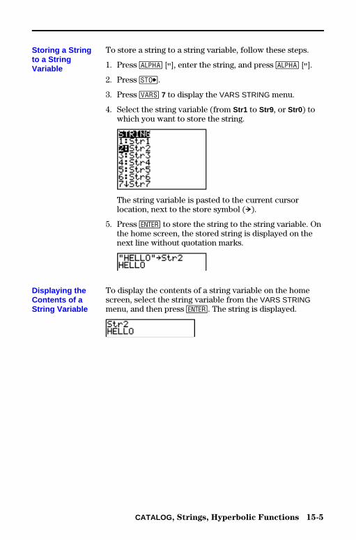
CATALOG , Strings, Hyperbolic Functions 15-5
8315CATS.DOC TI-83 international English Bob Fedorisko Revised: 02/19/01 12:54 PM Printed: 02/19/01 1:39PM Page 5 of 10
To store a string to a string variable, follow these steps.
1. Press ƒ [ã], enter the string, and press ƒ [ã].
2. Press ¿.
3. Press � 7 to display the VARS STRING menu.
4. Select the string variable (from Str1 to Str9 , or Str0) towhich you want to store the string.
The string variable is pasted to the current cursorlocation, next to the store symbol (!).
5. Press Í to store the string to the string variable. Onthe home screen, the stored string is displayed on thenext line without quotation marks.
To display the contents of a string variable on the homescreen, select the string variable from the VARS STRINGmenu, and then press Í. The string is displayed.
Storing a Stringto a StringVariable
Displaying theContents of aString Variable
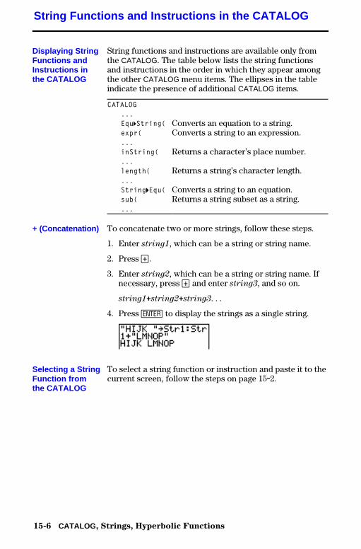
15-6 CATALOG , Strings, Hyperbolic Functions
8315CATS.DOC TI-83 international English Bob Fedorisko Revised: 02/19/01 12:54 PM Printed: 02/19/01 1:39PM Page 6 of 10
String functions and instructions are available only fromthe CATALOG. The table below lists the string functionsand instructions in the order in which they appear amongthe other CATALOG menu items. The ellipses in the tableindicate the presence of additional CATALOG items.
CATALOG...Equ4String( Converts an equation to a string.expr( Converts a string to an expression....inString( Returns a character’s place number....length( Returns a string’s character length....String4Equ( Converts a string to an equation.sub( Returns a string subset as a string....
To concatenate two or more strings, follow these steps.
1. Enter string1, which can be a string or string name.
2. Press Ã.
3. Enter string2, which can be a string or string name. Ifnecessary, press à and enter string3, and so on.
string1+string2+string3. . .
4. Press Í to display the strings as a single string.
To select a string function or instruction and paste it to thecurrent screen, follow the steps on page 15.2.
String Functions and Instructions in the CATALOG
Displaying StringFunctions andInstructions inthe CATALOG
+ (Concatenation)
Selecting a StringFunction fromthe CATALOG
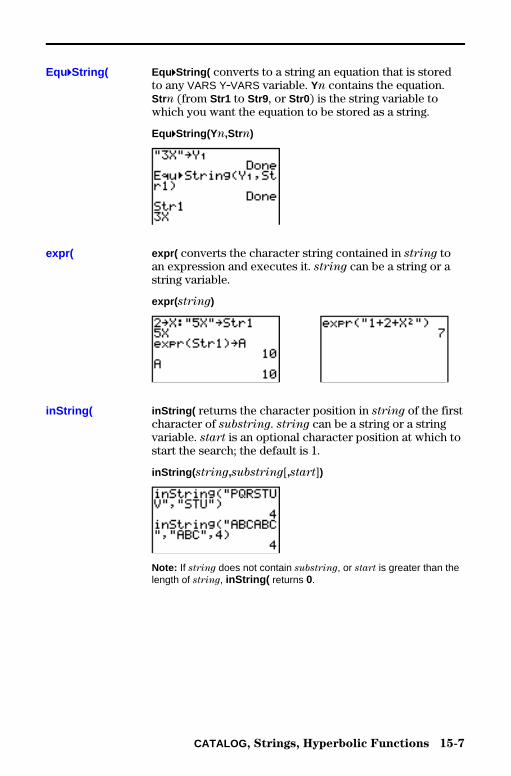
CATALOG , Strings, Hyperbolic Functions 15-7
8315CATS.DOC TI-83 international English Bob Fedorisko Revised: 02/19/01 12:54 PM Printed: 02/19/01 1:39PM Page 7 of 10
Equ4String( converts to a string an equation that is storedto any VARS Y.VARS variable. Yn contains the equation.Strn (from Str1 to Str9 , or Str0) is the string variable towhich you want the equation to be stored as a string.
Equ4String(Y n,Strn)
expr( converts the character string contained in string toan expression and executes it. string can be a string or astring variable.
expr( string)
inString( returns the character position in string of the firstcharacter of substring. string can be a string or a stringvariable. start is an optional character position at which tostart the search; the default is 1.
inString( string,substring[,start])
Note: If string does not contain substring, or start is greater than thelength of string, inString( returns 0.
Equ4String(
expr(
inString(

15-8 CATALOG , Strings, Hyperbolic Functions
8315CATS.DOC TI-83 international English Bob Fedorisko Revised: 02/19/01 12:54 PM Printed: 02/19/01 1:39PM Page 8 of 10
length( returns the number of characters in string. string
can be a string or string variable.
Note: An instruction or function name, such as sin( or cos( , counts asone character.
length( string)
String 4Equ( converts string into an equation and stores theequation to Yn. string can be a string or string variable.String 4Equ( is the inverse of Equ4String( .
String 4Equ(string,Yn)
length(
String 4Equ(
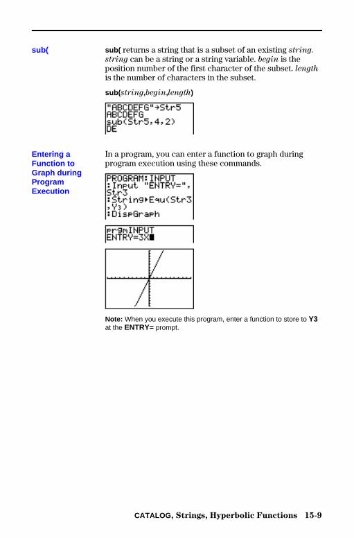
CATALOG , Strings, Hyperbolic Functions 15-9
8315CATS.DOC TI-83 international English Bob Fedorisko Revised: 02/19/01 12:54 PM Printed: 02/19/01 1:39PM Page 9 of 10
sub( returns a string that is a subset of an existing string.string can be a string or a string variable. begin is theposition number of the first character of the subset. length
is the number of characters in the subset.
sub( string,begin,length)
In a program, you can enter a function to graph duringprogram execution using these commands.
Note: When you execute this program, enter a function to store to Y3at the ENTRY= prompt.
sub(
Entering aFunction toGraph duringProgramExecution
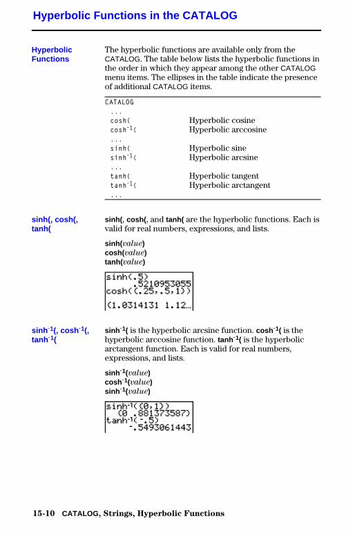
15-10 CATALOG , Strings, Hyperbolic Functions
8315CATS.DOC TI-83 international English Bob Fedorisko Revised: 02/19/01 12:54 PM Printed: 02/19/01 1:39PM Page 10 of 10
The hyperbolic functions are available only from theCATALOG. The table below lists the hyperbolic functions inthe order in which they appear among the other CATALOGmenu items. The ellipses in the table indicate the presenceof additional CATALOG items.
CATALOG...cosh( Hyperbolic cosinecoshL1( Hyperbolic arccosine...sinh( Hyperbolic sinesinhL1( Hyperbolic arcsine...tanh( Hyperbolic tangenttanhL1( Hyperbolic arctangent...
sinh( , cosh( , and tanh( are the hyperbolic functions. Each isvalid for real numbers, expressions, and lists.
sinh( value)cosh( value)tanh( value)
sinh L1( is the hyperbolic arcsine function. cosh L1( is thehyperbolic arccosine function. tanh L1( is the hyperbolicarctangent function. Each is valid for real numbers,expressions, and lists.
sinh L1(value)cosh L1(value)sinh L1(value)
Hyperbolic Functions in the CATALOG
HyperbolicFunctions
sinh(, cosh(,tanh(
sinh L1(, cosh L1(,tanh L1(
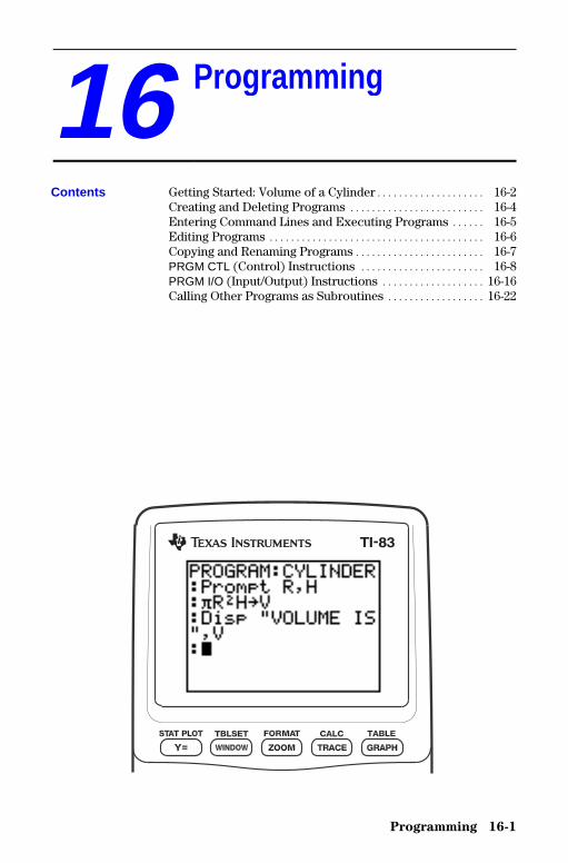
Programming 16-1
8316PROG.DOC TI-83 international English Bob Fedorisko Revised: 02/19/01 1:23 PM Printed: 02/19/01 1:39PM Page 1 of 22
16 Programmin g
Getting Started: Volume of a Cylinder.................... 16-2Creating and Deleting Programs ......................... 16-4Entering Command Lines and Executing Programs ...... 16-5Editing Programs ........................................ 16-6Copying and Renaming Programs ........................ 16-7PRGM CTL (Control) Instructions ....................... 16-8PRGM I/O (Input/Output) Instructions ................... 16-16Calling Other Programs as Subroutines .................. 16-22
Contents
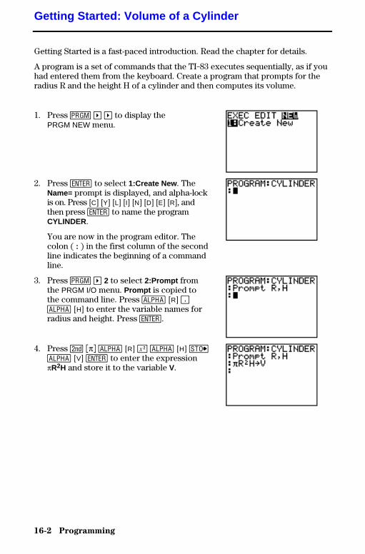
16-2 Programming
8316PROG.DOC TI-83 international English Bob Fedorisko Revised: 02/19/01 1:23 PM Printed: 02/19/01 1:39PM Page 2 of 22
Getting Started is a fast-paced introduction. Read the chapter for details.
A program is a set of commands that the TI-83 executes sequentially, as if youhad entered them from the keyboard. Create a program that prompts for theradius R and the height H of a cylinder and then computes its volume.
1. Press � ~ ~ to display thePRGM NEW menu.
2. Press Í to select 1:Create New . TheName= prompt is displayed, and alpha-lockis on. Press [C] [Y] [L] [I] [N] [D] [E] [R], andthen press Í to name the programCYLINDER.
You are now in the program editor. Thecolon ( : ) in the first column of the secondline indicates the beginning of a commandline.
3. Press � ~ 2 to select 2:Prompt fromthe PRGM I/O menu. Prompt is copied tothe command line. Press ƒ [R] ¢ƒ [H] to enter the variable names forradius and height. Press Í.
4. Press y ãpä ƒ [R] ¡ ƒ [H] ¿ƒ [V] Í to enter the expressionpR2H and store it to the variable V.
Getting Started: Volume of a Cylinder
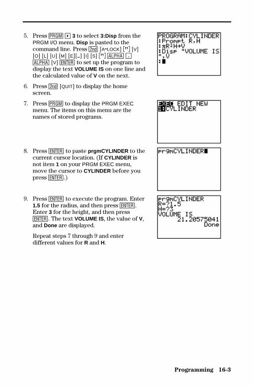
Programming 16-3
8316PROG.DOC TI-83 international English Bob Fedorisko Revised: 02/19/01 1:23 PM Printed: 02/19/01 1:39PM Page 3 of 22
5. Press � ~ 3 to select 3:Disp from thePRGM I/O menu. Disp is pasted to thecommand line. Press y [A.LOCK] ããä [V][O] [L] [U] [M] [E]['] [I] [S] ããä ƒ ¢ƒ [V] Í to set up the program todisplay the text VOLUME IS on one line andthe calculated value of V on the next.
6. Press y [QUIT] to display the homescreen.
7. Press � to display the PRGM EXECmenu. The items on this menu are thenames of stored programs.
8. Press Í to paste prgmCYLINDER to thecurrent cursor location. (If CYLINDER isnot item 1 on your PRGM EXEC menu,move the cursor to CYLINDER before youpress Í.)
9. Press Í to execute the program. Enter1.5 for the radius, and then press Í.Enter 3 for the height, and then pressÍ. The text VOLUME IS, the value of V,and Done are displayed.
Repeat steps 7 through 9 and enterdifferent values for R and H.

16-4 Programming
8316PROG.DOC TI-83 international English Bob Fedorisko Revised: 02/19/01 1:23 PM Printed: 02/19/01 1:39PM Page 4 of 22
A program is a set of one or more command lines. Eachline contains one or more instructions. When you execute aprogram, the TI-83 performs each instruction on eachcommand line in the same order in which you enteredthem. The number and size of programs that the TI-83 canstore is limited only by available memory.
To create a new program, follow these steps.
1. Press � | to display the PRGM NEW menu.
2. Press Í to select 1:Create New . The Name= promptis displayed, and alpha-lock is on.
3. Press a letter from A to Z or q to enter the firstcharacter of the new program name.
Note: A program name can be one to eight characters long. Thefirst character must be a letter from A to Z or q. The secondthrough eighth characters can be letters, numbers, or q.
4. Enter zero to seven letters, numbers, or q to completethe new program name.
5. Press Í. The program editor is displayed.
6. Enter one or more program commands (page 16.5).
7. Press y [QUIT] to leave the program editor and returnto the home screen.
To check whether adequate memory is available for aprogram you want to enter, press y [MEM], and thenselect 1:Check RAM from the MEMORY menu (Chapter 18).
To increase available memory, press y [MEM], and thenselect 2:Delete from the MEMORY menu (Chapter 18).
To delete a specific program, press y [MEM], select2:Delete from the MEMORY menu, and then select 7:Prgmfrom the DELETE FROM secondary menu (Chapter 18).
Creating and Deleting Programs
What Is aProgram?
Creating a NewProgram
ManagingMemory andDeleting aProgram
Programming 16-5
8316PROG.DOC TI-83 international English Bob Fedorisko Revised: 02/19/01 1:23 PM Printed: 02/19/01 1:39PM Page 5 of 22
You can enter on a command line any instruction orexpression that you could execute from the home screen. Inthe program editor, each new command line begins with acolon. To enter more than one instruction or expression on asingle command line, separate each with a colon.
Note: A command line can be longer than the screen is wide; longcommand lines wrap to the next screen line.
While in the program editor, you can display and selectfrom menus. You can return to the program editor from amenu in either of two ways.
• Select a menu item, which pastes the item to thecurrent command line.
• Press ‘.
When you complete a command line, press Í. Thecursor moves to the next command line.
Programs can access variables, lists, matrices, and stringssaved in memory. If a program stores a new value to avariable, list, matrix, or string, the program changes thevalue in memory during execution.
You can call another program as a subroutine (page 16.15and page 16.22).
To execute a program, begin on a blank line on the homescreen and follow these steps.
1. Press � to display the PRGM EXEC menu.
2. Select a program name from the PRGM EXEC menu(page 16.7). prgm name is pasted to the home screen(for example, prgmCYLINDER ).
3. Press Í to execute the program. While the programis executing, the busy indicator is on.
Last Answer (Ans ) is updated during program execution.Last Entry is not updated as each command is executed(Chapter 1).
The TI-83 checks for errors during program execution. Itdoes not check for errors as you enter a program.
To stop program execution, press É. The ERR:BREAKmenu is displayed.
• To return to the home screen, select 1:Quit .• To go where the interruption occurred, select 2:Goto .
Entering Command Lines and Executing Programs
Entering aProgramCommand Line
Executing aProgram
Breaking aProgram
16-6 Programming
8316PROG.DOC TI-83 international English Bob Fedorisko Revised: 02/19/01 1:23 PM Printed: 02/19/01 1:39PM Page 6 of 22
To edit a stored program, follow these steps.
1. Press � ~ to display the PRGM EDIT menu.
2. Select a program name from the PRGM EDIT menu (page16.7). Up to the first seven lines of the program aredisplayed.
Note: The program editor does not display a $ to indicate thata program continues beyond the screen.
3. Edit the program command lines.
• Move the cursor to the appropriate location, andthen delete, overwrite, or insert.
• Press ‘ to clear all program commands on thecommand line (the leading colon remains), and thenenter a new program command.
Tip: To move the cursor to the beginning of a command line, pressy |; to move to the end, press y ~. To scroll the cursor downseven command lines, press ƒ †. To scroll the cursor up sevencommand lines, press ƒ }.
To insert a new command line anywhere in the program,place the cursor where you want the new line, press y[INS], and then press Í. A colon indicates a new line.
To delete a command line, place the cursor on the line,press ‘ to clear all instructions and expressions onthe line, and then press { to delete the command line,including the colon.
Editing Programs
Editing aProgram
Inserting andDeletingCommand Lines
Programming 16-7
8316PROG.DOC TI-83 international English Bob Fedorisko Revised: 02/19/01 1:23 PM Printed: 02/19/01 1:39PM Page 7 of 22
To copy all command lines from one program into a newprogram, follow steps 1 through 5 for Creating a NewProgram (page 16.4), and then follow these steps.
1. Press y [RCL]. Rcl is displayed on the bottom line ofthe program editor in the new program (Chapter 1).
2. Press � | to display the PRGM EXEC menu.
3. Select a name from the menu. prgm name is pasted tothe bottom line of the program editor.
4. Press Í. All command lines from the selectedprogram are copied into the new program.
Copying programs has at least two convenientapplications.
• You can create a template for groups of instructionsthat you use frequently.
• You can rename a program by copying its contents intoa new program.
Note: You also can copy all the command lines from one existingprogram to another existing program using RCL.
The TI-83 sorts PRGM EXEC and PRGM EDIT menu itemsautomatically into alphanumerical order. Each menu onlylabels the first 10 items using 1 through 9, then 0.
To jump to the first program name that begins with aparticular alpha character or q, press ƒ [letter from A
to Z or q].
Tip: From the top of either the PRGM EXEC or PRGM EDIT menu,press } to move to the bottom. From the bottom, press † to move tothe top. To scroll the cursor down the menu seven items, press ƒ†. To scroll the cursor up the menu seven items, press ƒ }.
Copying and Renaming Programs
Copying andRenaming aProgram
Scrolling thePRGM EXEC andPRGM EDITMenus
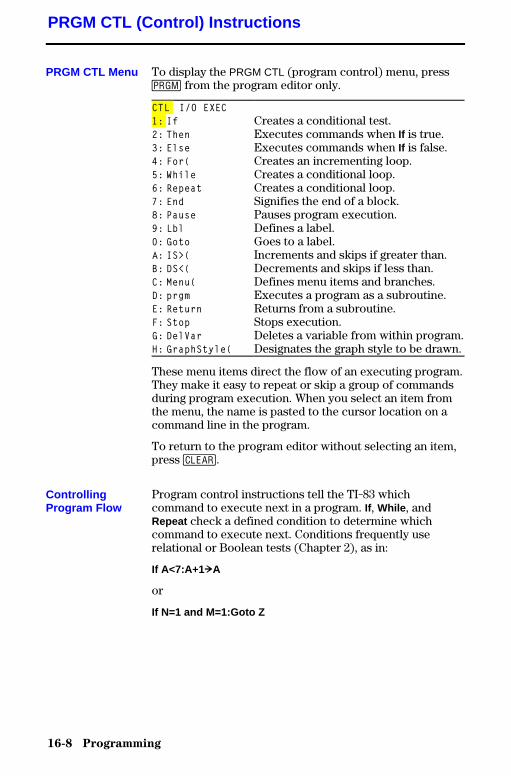
16-8 Programming
8316PROG.DOC TI-83 international English Bob Fedorisko Revised: 02/19/01 1:23 PM Printed: 02/19/01 1:39PM Page 8 of 22
To display the PRGM CTL (program control) menu, press� from the program editor only.
CTL I/O EXEC1: If Creates a conditional test.2: Then Executes commands when If is true.3: Else Executes commands when If is false.4: For( Creates an incrementing loop.5: While Creates a conditional loop.6: Repeat Creates a conditional loop.7: End Signifies the end of a block.8: Pause Pauses program execution.9: Lbl Defines a label.0: Goto Goes to a label.A: IS>( Increments and skips if greater than.B: DS<( Decrements and skips if less than.C: Menu( Defines menu items and branches.D: prgm Executes a program as a subroutine.E: Return Returns from a subroutine.F: Stop Stops execution.G: DelVar Deletes a variable from within program.H: GraphStyle( Designates the graph style to be drawn.
These menu items direct the flow of an executing program.They make it easy to repeat or skip a group of commandsduring program execution. When you select an item fromthe menu, the name is pasted to the cursor location on acommand line in the program.
To return to the program editor without selecting an item,press ‘.
Program control instructions tell the TI-83 whichcommand to execute next in a program. If, While , andRepeat check a defined condition to determine whichcommand to execute next. Conditions frequently userelational or Boolean tests (Chapter 2), as in:
If A<7:A+1 !A
or
If N=1 and M=1:Goto Z
PRGM CTL (Control) Instructions
PRGM CTL Menu
ControllingProgram Flow
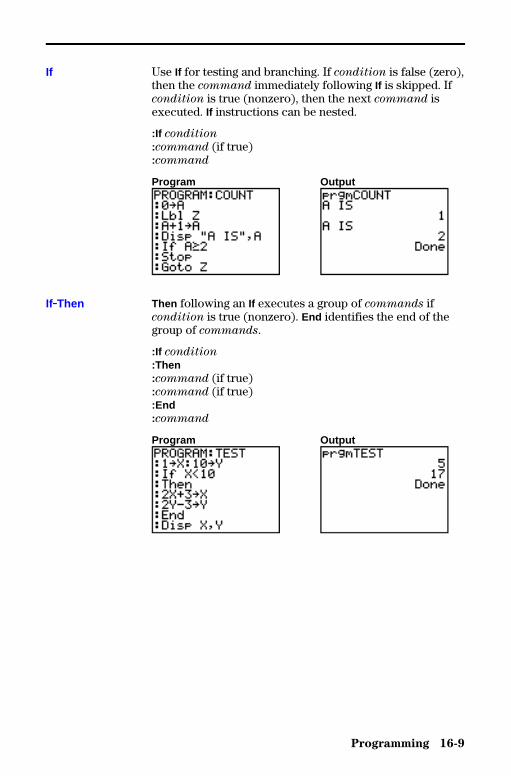
Programming 16-9
8316PROG.DOC TI-83 international English Bob Fedorisko Revised: 02/19/01 1:23 PM Printed: 02/19/01 1:39PM Page 9 of 22
Use If for testing and branching. If condition is false (zero),then the command immediately following If is skipped. Ifcondition is true (nonzero), then the next command isexecuted. If instructions can be nested.
:If condition
:command (if true):command
Program Output
Then following an If executes a group of commands ifcondition is true (nonzero). End identifies the end of thegroup of commands.
:If condition
:Then:command (if true):command (if true):End:command
Program Output
If
If.Then
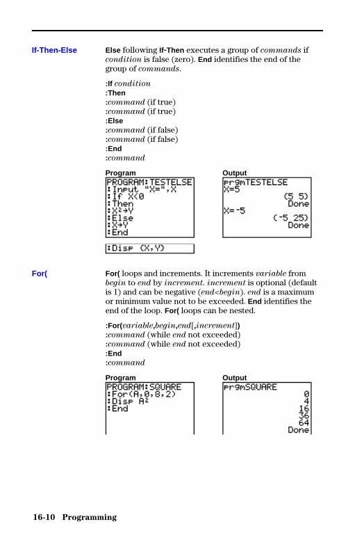
16-10 Programming
8316PROG.DOC TI-83 international English Bob Fedorisko Revised: 02/19/01 1:23 PM Printed: 02/19/01 1:39PM Page 10 of 22
Else following If.Then executes a group of commands ifcondition is false (zero). End identifies the end of thegroup of commands.
:If condition
:Then:command (if true):command (if true):Else:command (if false):command (if false):End:command
Program Output
For( loops and increments. It increments variable frombegin to end by increment. increment is optional (defaultis 1) and can be negative (end<begin). end is a maximumor minimum value not to be exceeded. End identifies theend of the loop. For( loops can be nested.
:For( variable,begin,end[,increment]):command (while end not exceeded):command (while end not exceeded):End:command
Program Output
If-Then-Else
For(
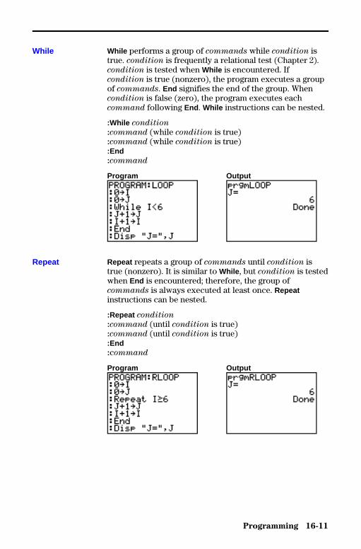
Programming 16-11
8316PROG.DOC TI-83 international English Bob Fedorisko Revised: 02/19/01 1:23 PM Printed: 02/19/01 1:39PM Page 11 of 22
While performs a group of commands while condition istrue. condition is frequently a relational test (Chapter 2).condition is tested when While is encountered. Ifcondition is true (nonzero), the program executes a groupof commands. End signifies the end of the group. Whencondition is false (zero), the program executes eachcommand following End . While instructions can be nested.
:While condition
:command (while condition is true):command (while condition is true):End:command
Program Output
Repeat repeats a group of commands until condition istrue (nonzero). It is similar to While , but condition is testedwhen End is encountered; therefore, the group ofcommands is always executed at least once. Repeatinstructions can be nested.
:Repeat condition
:command (until condition is true):command (until condition is true):End:command
Program Output
While
Repeat
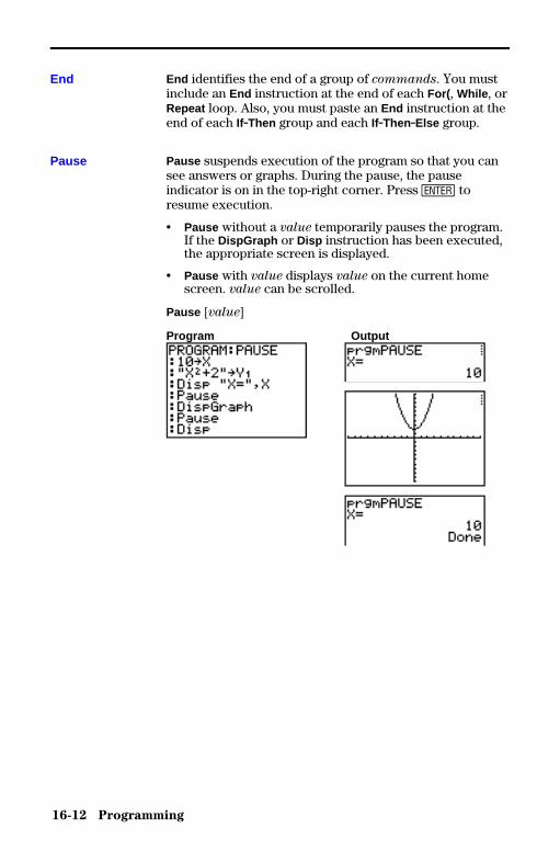
16-12 Programming
8316PROG.DOC TI-83 international English Bob Fedorisko Revised: 02/19/01 1:23 PM Printed: 02/19/01 1:39PM Page 12 of 22
End identifies the end of a group of commands. You mustinclude an End instruction at the end of each For( , While , orRepeat loop. Also, you must paste an End instruction at theend of each If.Then group and each If.Then.Else group.
Pause suspends execution of the program so that you cansee answers or graphs. During the pause, the pauseindicator is on in the top-right corner. Press Í toresume execution.
• Pause without a value temporarily pauses the program.If the DispGraph or Disp instruction has been executed,the appropriate screen is displayed.
• Pause with value displays value on the current homescreen. value can be scrolled.
Pause [value]
Program Output
End
Pause
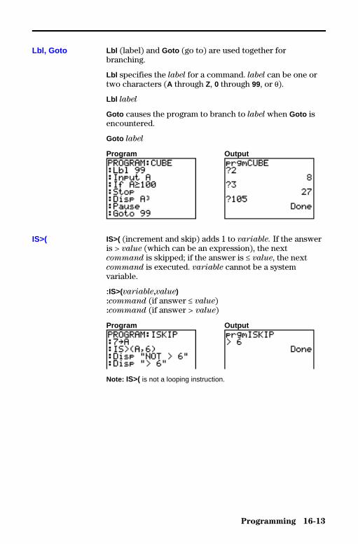
Programming 16-13
8316PROG.DOC TI-83 international English Bob Fedorisko Revised: 02/19/01 1:23 PM Printed: 02/19/01 1:39PM Page 13 of 22
Lbl (label) and Goto (go to) are used together forbranching.
Lbl specifies the label for a command. label can be one ortwo characters (A through Z, 0 through 99, or q).
Lbl label
Goto causes the program to branch to label when Goto isencountered.
Goto label
Program Output
IS>( (increment and skip) adds 1 to variable. If the answeris > value (which can be an expression), the nextcommand is skipped; if the answer is { value, the nextcommand is executed. variable cannot be a systemvariable.
:IS>(variable,value):command (if answer � value):command (if answer > value)
Program Output
Note: IS>( is not a looping instruction.
Lbl, Goto
IS>(
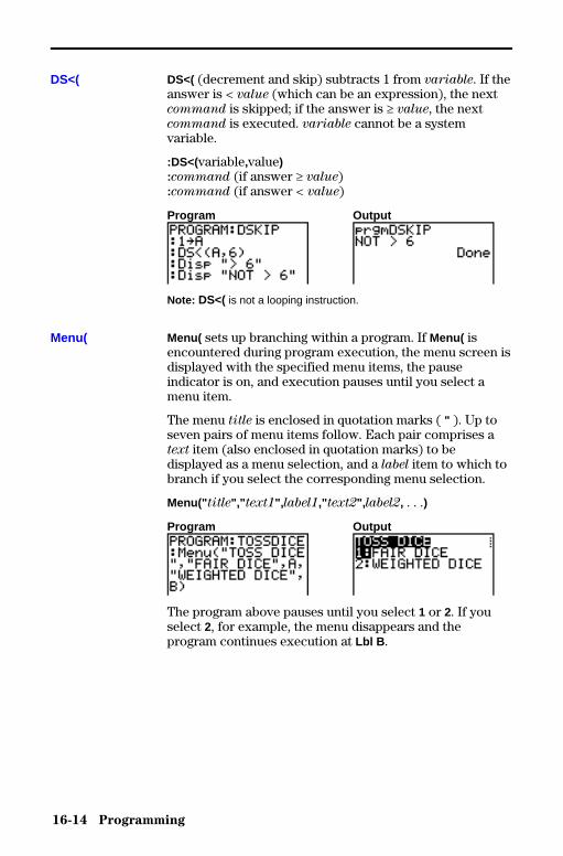
16-14 Programming
8316PROG.DOC TI-83 international English Bob Fedorisko Revised: 02/19/01 1:23 PM Printed: 02/19/01 1:39PM Page 14 of 22
DS<( (decrement and skip) subtracts 1 from variable. If theanswer is < value (which can be an expression), the nextcommand is skipped; if the answer is | value, the nextcommand is executed. variable cannot be a systemvariable.
:DS<(variable,value):command (if answer ‚ value):command (if answer < value)
Program Output
Note: DS<( is not a looping instruction.
Menu( sets up branching within a program. If Menu( isencountered during program execution, the menu screen isdisplayed with the specified menu items, the pauseindicator is on, and execution pauses until you select amenu item.
The menu title is enclosed in quotation marks ( " ). Up toseven pairs of menu items follow. Each pair comprises atext item (also enclosed in quotation marks) to bedisplayed as a menu selection, and a label item to which tobranch if you select the corresponding menu selection.
Menu(" title"," text1", label1," text2", label2, . . .)
Program Output
The program above pauses until you select 1 or 2. If youselect 2, for example, the menu disappears and theprogram continues execution at Lbl B .
DS<(
Menu(
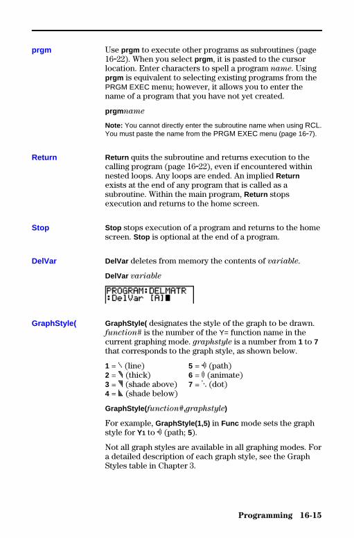
Programming 16-15
8316PROG.DOC TI-83 international English Bob Fedorisko Revised: 02/19/01 1:23 PM Printed: 02/19/01 1:39PM Page 15 of 22
Use prgm to execute other programs as subroutines (page16.22). When you select prgm , it is pasted to the cursorlocation. Enter characters to spell a program name. Usingprgm is equivalent to selecting existing programs from thePRGM EXEC menu; however, it allows you to enter thename of a program that you have not yet created.
prgm name
Note: You cannot directly enter the subroutine name when using RCL.You must paste the name from the PRGM EXEC menu (page 16.7).
Return quits the subroutine and returns execution to thecalling program (page 16.22), even if encountered withinnested loops. Any loops are ended. An implied Returnexists at the end of any program that is called as asubroutine. Within the main program, Return stopsexecution and returns to the home screen.
Stop stops execution of a program and returns to the homescreen. Stop is optional at the end of a program.
DelVar deletes from memory the contents of variable.
DelVar variable
GraphStyle( designates the style of the graph to be drawn.function# is the number of the Y= function name in thecurrent graphing mode. graphstyle is a number from 1 to 7that corresponds to the graph style, as shown below.
1 = ç (line) 5 = ë (path)2 = è (thick) 6 = ì (animate)3 = é (shade above) 7 = í (dot)4 = ê (shade below)
GraphStyle( function#,graphstyle)
For example, GraphStyle(1,5) in Func mode sets the graphstyle for Y1 to ë (path; 5).
Not all graph styles are available in all graphing modes. Fora detailed description of each graph style, see the GraphStyles table in Chapter 3.
prgm
Return
Stop
DelVar
GraphStyle(
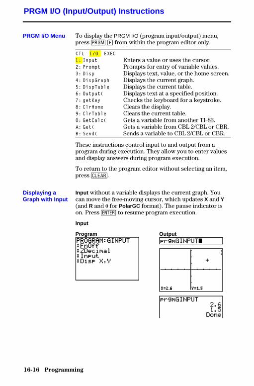
16-16 Programming
8316PROG.DOC TI-83 international English Bob Fedorisko Revised: 02/19/01 1:23 PM Printed: 02/19/01 1:39PM Page 16 of 22
To display the PRGM I/O (program input/output) menu,press � ~ from within the program editor only.
CTL I/O EXEC1: Input Enters a value or uses the cursor.2: Prompt Prompts for entry of variable values.3: Disp Displays text, value, or the home screen.4: DispGraph Displays the current graph.5: DispTable Displays the current table.6: Output( Displays text at a specified position.7: getKey Checks the keyboard for a keystroke.8: ClrHome Clears the display.9: ClrTable Clears the current table.0: GetCalc( Gets a variable from another TI-83.A: Get( Gets a variable from CBL 2/CBL or CBR.B: Send( Sends a variable to CBL 2/CBL or CBR.
These instructions control input to and output from aprogram during execution. They allow you to enter valuesand display answers during program execution.
To return to the program editor without selecting an item,press ‘.
Input without a variable displays the current graph. Youcan move the free-moving cursor, which updates X and Y(and R and q for PolarGC format). The pause indicator ison. Press Í to resume program execution.
Input
Program Output
PRGM I/O (Input/Output) Instructions
PRGM I/O Menu
Displaying aGraph with Input
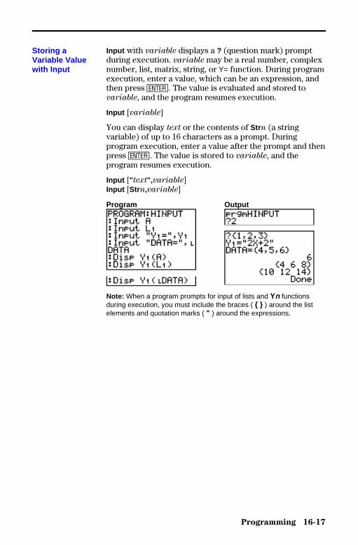
Programming 16-17
8316PROG.DOC TI-83 international English Bob Fedorisko Revised: 02/19/01 1:23 PM Printed: 02/19/01 1:39PM Page 17 of 22
Input with variable displays a ? (question mark) promptduring execution. variable may be a real number, complexnumber, list, matrix, string, or Y= function. During programexecution, enter a value, which can be an expression, andthen press Í. The value is evaluated and stored tovariable, and the program resumes execution.
Input [variable]
You can display text or the contents of Strn (a stringvariable) of up to 16 characters as a prompt. Duringprogram execution, enter a value after the prompt and thenpress Í. The value is stored to variable, and theprogram resumes execution.
Input [" text",variable]Input [Strn,variable]
Program Output
Note: When a program prompts for input of lists and Yn functionsduring execution, you must include the braces ( { } ) around the listelements and quotation marks ( " ) around the expressions.
Storing aVariable Valuewith Input
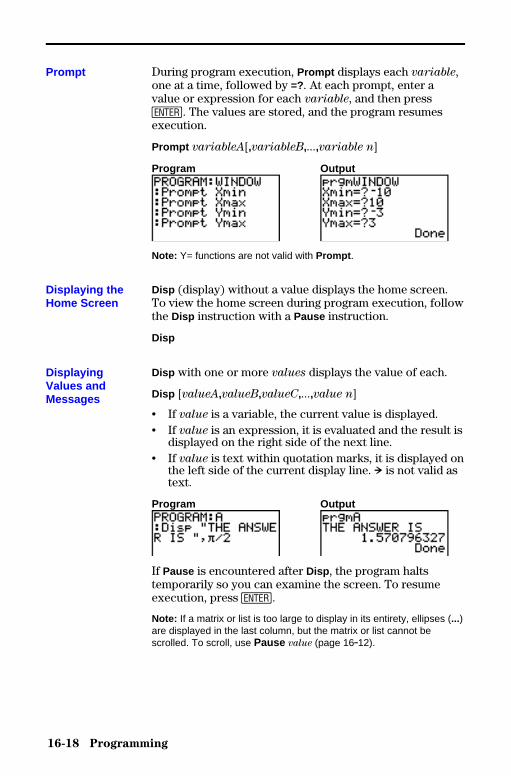
16-18 Programming
8316PROG.DOC TI-83 international English Bob Fedorisko Revised: 02/19/01 1:23 PM Printed: 02/19/01 1:39PM Page 18 of 22
During program execution, Prompt displays each variable,one at a time, followed by =?. At each prompt, enter avalue or expression for each variable, and then pressÍ. The values are stored, and the program resumesexecution.
Prompt variableA[,variableB,...,variable n]
Program Output
Note: Y= functions are not valid with Prompt .
Disp (display) without a value displays the home screen.To view the home screen during program execution, followthe Disp instruction with a Pause instruction.
Disp
Disp with one or more values displays the value of each.
Disp [valueA,valueB,valueC,...,value n]
• If value is a variable, the current value is displayed.• If value is an expression, it is evaluated and the result is
displayed on the right side of the next line.• If value is text within quotation marks, it is displayed on
the left side of the current display line. ! is not valid astext.
Program Output
If Pause is encountered after Disp , the program haltstemporarily so you can examine the screen. To resumeexecution, press Í.
Note: If a matrix or list is too large to display in its entirety, ellipses (...)are displayed in the last column, but the matrix or list cannot bescrolled. To scroll, use Pause value (page 16.12).
Prompt
Displaying theHome Screen
DisplayingValues andMessages
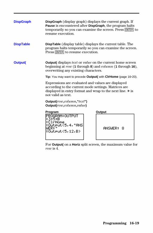
Programming 16-19
8316PROG.DOC TI-83 international English Bob Fedorisko Revised: 02/19/01 1:23 PM Printed: 02/19/01 1:39PM Page 19 of 22
DispGraph (display graph) displays the current graph. IfPause is encountered after DispGraph , the program haltstemporarily so you can examine the screen. Press Í toresume execution.
DispTable (display table) displays the current table. Theprogram halts temporarily so you can examine the screen.Press Í to resume execution.
Output( displays text or value on the current home screenbeginning at row (1 through 8) and column (1 through 16),overwriting any existing characters.
Tip: You may want to precede Output( with ClrHome (page 16.20).
Expressions are evaluated and values are displayedaccording to the current mode settings. Matrices aredisplayed in entry format and wrap to the next line. ! isnot valid as text.
Output( row,column," text")Output( row,column,value)
Program Output
For Output( on a Horiz split screen, the maximum value forrow is 4.
DispGraph
DispTable
Output(
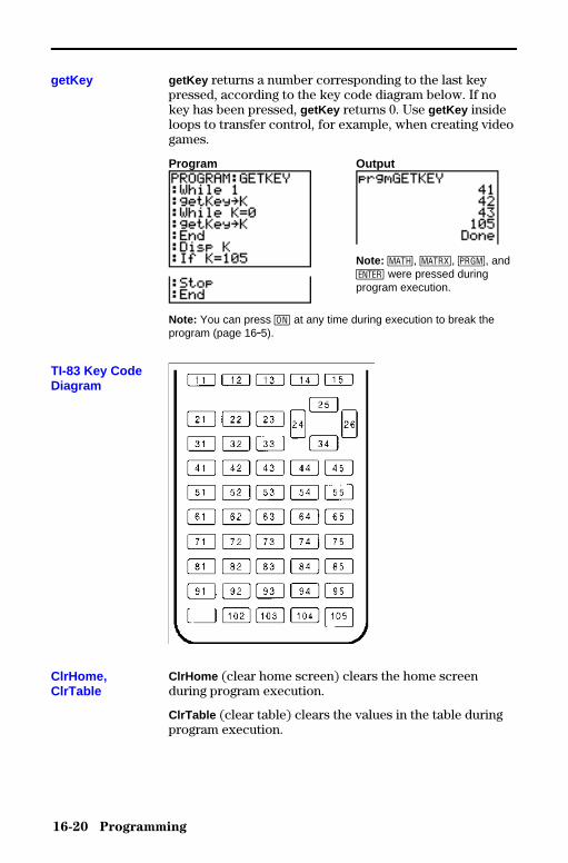
16-20 Programming
8316PROG.DOC TI-83 international English Bob Fedorisko Revised: 02/19/01 1:23 PM Printed: 02/19/01 1:39PM Page 20 of 22
getKey returns a number corresponding to the last keypressed, according to the key code diagram below. If nokey has been pressed, getKey returns 0. Use getKey insideloops to transfer control, for example, when creating videogames.
Program Output
Note: �, �, �, andÍ were pressed duringprogram execution.
Note: You can press É at any time during execution to break theprogram (page 16.5).
ClrHome (clear home screen) clears the home screenduring program execution.
ClrTable (clear table) clears the values in the table duringprogram execution.
getKey
TI-83 Key CodeDiagram
ClrHome,ClrTable
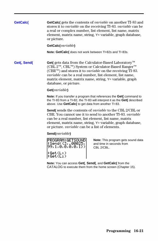
Programming 16-21
8316PROG.DOC TI-83 international English Bob Fedorisko Revised: 02/19/01 1:23 PM Printed: 02/19/01 1:39PM Page 21 of 22
GetCalc( gets the contents of variable on another TI-83 andstores it to variable on the receiving TI-83. variable can bea real or complex number, list element, list name, matrixelement, matrix name, string, Y= variable, graph database,or picture.
GetCalc( variable)
Note: GetCalc( does not work between TI.82s and TI-83s.
Get( gets data from the Calculator-Based Laboratoryé(CBL 2é, CBLé) System or Calculator-Based Rangeré(CBRé) and stores it to variable on the receiving TI-83.variable can be a real number, list element, list name,matrix element, matrix name, string, Y= variable, graphdatabase, or picture.
Get(variable)
Note: If you transfer a program that references the Get( command tothe TI-83 from a TI.82, the TI-83 will interpret it as the Get( describedabove. Use GetCalc( to get data from another TI-83.
Send( sends the contents of variable to the CBL 2/CBL orCBR. You cannot use it to send to another TI-83. variable
can be a real number, list element, list name, matrixelement, matrix name, string, Y= variable, graph database,or picture. variable can be a list of elements.
Send(variable)
Note: This program gets sound dataand time in seconds fromCBL 2/CBL.
Note: You can access Get(, Send( , and GetCalc( from theCATALOG to execute them from the home screen (Chapter 15).
GetCalc(
Get(, Send(
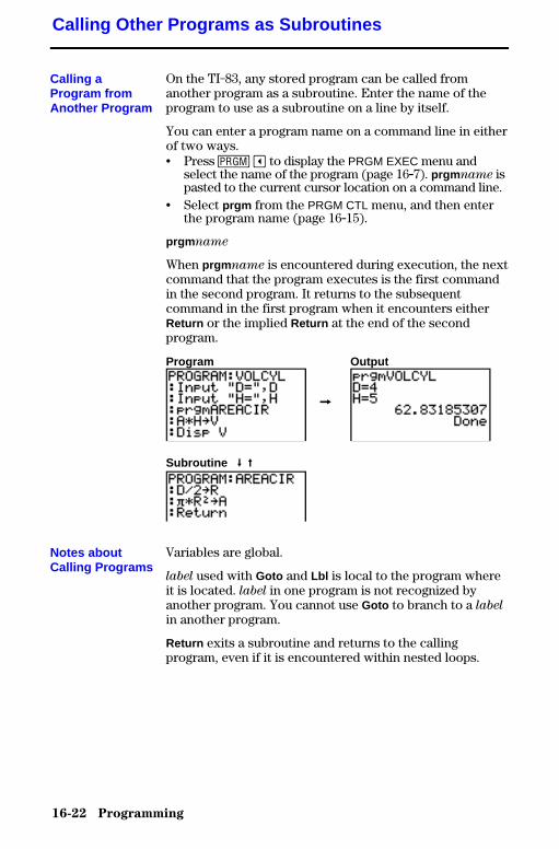
16-22 Programming
8316PROG.DOC TI-83 international English Bob Fedorisko Revised: 02/19/01 1:23 PM Printed: 02/19/01 1:39PM Page 22 of 22
On the TI-83, any stored program can be called fromanother program as a subroutine. Enter the name of theprogram to use as a subroutine on a line by itself.
You can enter a program name on a command line in eitherof two ways.• Press � | to display the PRGM EXEC menu and
select the name of the program (page 16.7). prgm name ispasted to the current cursor location on a command line.
• Select prgm from the PRGM CTL menu, and then enterthe program name (page 16.15).
prgm name
When prgm name is encountered during execution, the nextcommand that the program executes is the first commandin the second program. It returns to the subsequentcommand in the first program when it encounters eitherReturn or the implied Return at the end of the secondprogram.
Program Output
&
Subroutine ( '
Variables are global.
label used with Goto and Lbl is local to the program whereit is located. label in one program is not recognized byanother program. You cannot use Goto to branch to a label
in another program.
Return exits a subroutine and returns to the callingprogram, even if it is encountered within nested loops.
Calling Other Programs as Subroutines
Calling aProgram fromAnother Program
Notes aboutCalling Programs
Applications 17-1
8317APPS.DOC TI-83 international English Bob Fedorisko Revised: 02/19/01 1:00 PM Printed: 02/19/01 1:39 PMPage 1 of 20
17 Applications
Comparing Test Results Using Box Plots ................ 17-2Graphing Piecewise Functions........................... 17-4Graphing Inequalities .................................... 17-5Solving a System of Nonlinear Equations ................ 17-6Using a Program to Create the Sierpinski Triangle ....... 17-7Graphing Cobweb Attractors ............................ 17-8Using a Program to Guess the Coefficients............... 17-9Graphing the Unit Circle and Trigonometric Curves...... 17-10Finding the Area between Curves ........................ 17-11Using Parametric Equations: Ferris Wheel Problem...... 17-12Demonstrating the Fundamental Theorem of Calculus ... 17-14Computing Areas of Regular N-Sided Polygons .......... 17-16Computing and Graphing Mortgage Payments ........... 17-18
Contents
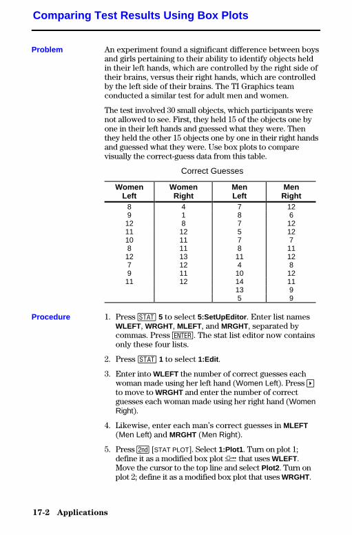
17-2 Applications
8317APPS.DOC TI-83 international English Bob Fedorisko Revised: 02/19/01 1:00 PM Printed: 02/19/01 1:39 PMPage 2 of 20
An experiment found a significant difference between boysand girls pertaining to their ability to identify objects heldin their left hands, which are controlled by the right side oftheir brains, versus their right hands, which are controlledby the left side of their brains. The TI Graphics teamconducted a similar test for adult men and women.
The test involved 30 small objects, which participants werenot allowed to see. First, they held 15 of the objects one byone in their left hands and guessed what they were. Thenthey held the other 15 objects one by one in their right handsand guessed what they were. Use box plots to comparevisually the correct-guess data from this table.
Correct Guesses
WomenLeft
WomenRight
MenLeft
MenRight
8 4 7 129 1 8 612 8 7 1211 12 5 1210 11 7 78 11 8 1112 13 11 127 12 4 89 11 10 1211 12 14 11
13 95 9
1. Press … 5 to select 5:SetUpEditor . Enter list namesWLEFT, WRGHT, MLEFT, and MRGHT, separated bycommas. Press Í. The stat list editor now containsonly these four lists.
2. Press … 1 to select 1:Edit .
3. Enter into WLEFT the number of correct guesses eachwoman made using her left hand (Women Left). Press ~to move to WRGHT and enter the number of correctguesses each woman made using her right hand (WomenRight).
4. Likewise, enter each man’s correct guesses in MLEFT(Men Left) and MRGHT (Men Right).
5. Press y [STAT PLOT]. Select 1:Plot1 . Turn on plot 1;define it as a modified box plot Õ that uses WLEFT.Move the cursor to the top line and select Plot2 . Turn onplot 2; define it as a modified box plot that uses WRGHT.
Comparing Test Results Using Box Plots
Problem
Procedure

Applications 17-3
8317APPS.DOC TI-83 international English Bob Fedorisko Revised: 02/19/01 1:00 PM Printed: 02/19/01 1:39 PMPage 3 of 20
6. Press o. Turn off all functions.
7. Press p. Set Xscl=1 and Yscl=0 . Press q 9 toselect 9:ZoomStat . This adjusts the viewing window anddisplays the box plots for the women’s results.
8. Press r.
% Women’s left-hand data
% Women’s right-hand data
Use | and ~ to examine minX , Q1, Med, Q3, and maxXfor each plot. Notice the outlier to the women’s right-hand data. What is the median for the left hand? For theright hand? With which hand were the women moreaccurate guessers, according to the box plots?
9. Examine the men’s results. Redefine plot 1 to useMLEFT, redefine plot 2 to use MRGHT. Press r.
% Men’s left-hand data
% Men’s right-hand data
Press | and ~ to examine minX , Q1, Med, Q3, and maxXfor each plot. What difference do you see between theplots?
10.Compare the left-hand results. Redefine plot 1 to useWLEFT, redefine plot 2 to use MLEFT, and then pressr to examine minX , Q1, Med, Q3, and maxX for eachplot. Who were the better left-hand guessers, men orwomen?
11.Compare the right-hand results. Define plot 1 to useWRGHT, define plot 2 to use MRGHT, and then pressr to examine minX , Q1, Med, Q3, and maxX for eachplot. Who were the better right-hand guessers?
In the original experiment boys did not guess as wellwith right hands, while girls guessed equally well witheither hand. This is not what our box plots show foradults. Do you think that this is because adults havelearned to adapt or because our sample was not largeenough?
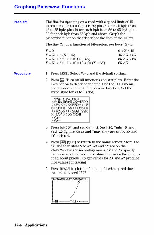
17-4 Applications
8317APPS.DOC TI-83 international English Bob Fedorisko Revised: 02/19/01 1:00 PM Printed: 02/19/01 1:39 PMPage 4 of 20
The fine for speeding on a road with a speed limit of 45kilometers per hour (kph) is 50; plus 5 for each kph from46 to 55 kph; plus 10 for each kph from 56 to 65 kph; plus20 for each kph from 66 kph and above. Graph thepiecewise function that describes the cost of the ticket.
The fine (Y) as a function of kilometers per hour (X) is:
Y = 0 0 < X � 45Y = 50 + 5 (X N 45) 45 < X � 55Y = 50 + 5 … 10 + 10 (X N 55) 55 < X � 65Y = 50 + 5 … 10 + 10 … 10 + 20 (X N 65) 65 < X
1. Press z. Select Func and the default settings.
2. Press o. Turn off all functions and stat plots. Enter theY= function to describe the fine. Use the TEST menuoperations to define the piecewise function. Set thegraph style for Y1 to í (dot).
3. Press p and set Xmin= L2, Xscl=10 , Ymin= L5, andYscl=10 . Ignore Xmax and Ymax ; they are set by @X and@Y in step 4.
4. Press y [QUIT] to return to the home screen. Store 1 to@X, and then store 5 to @Y. @X and @Y are on theVARS Window X/Y secondary menu. @X and @Y specifythe horizontal and vertical distance between the centersof adjacent pixels. Integer values for @X and @Y producenice values for tracing.
5. Press r to plot the function. At what speed doesthe ticket exceed 250?
Graphing Piecewise Functions
Problem
Procedure
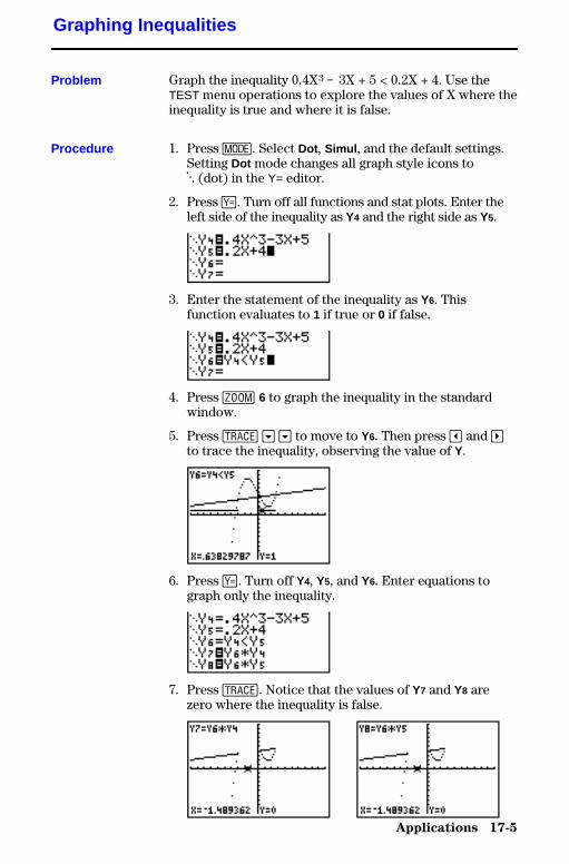
Applications 17-5
8317APPS.DOC TI-83 international English Bob Fedorisko Revised: 02/19/01 1:00 PM Printed: 02/19/01 1:39 PMPage 5 of 20
Graph the inequality 0.4X3 N 3X + 5 < 0.2X + 4. Use theTEST menu operations to explore the values of X where theinequality is true and where it is false.
1. Press z. Select Dot , Simul , and the default settings.Setting Dot mode changes all graph style icons toí (dot) in the Y= editor.
2. Press o. Turn off all functions and stat plots. Enter theleft side of the inequality as Y4 and the right side as Y5.
3. Enter the statement of the inequality as Y6. Thisfunction evaluates to 1 if true or 0 if false.
4. Press q 6 to graph the inequality in the standardwindow.
5. Press r † † to move to Y6. Then press | and ~to trace the inequality, observing the value of Y.
6. Press o. Turn off Y4, Y5, and Y6. Enter equations tograph only the inequality.
7. Press r. Notice that the values of Y7 and Y8 arezero where the inequality is false.
Graphing Inequalities
Problem
Procedure
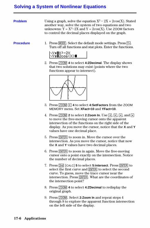
17-6 Applications
8317APPS.DOC TI-83 international English Bob Fedorisko Revised: 02/19/01 1:00 PM Printed: 02/19/01 1:39 PMPage 6 of 20
Using a graph, solve the equation X3 N 2X = 2cos(X). Statedanother way, solve the system of two equations and twounknowns: Y = X3N2X and Y = 2cos(X). Use ZOOM factorsto control the decimal places displayed on the graph.
1. Press z. Select the default mode settings. Press o.Turn off all functions and stat plots. Enter the functions.
2. Press q 4 to select 4:ZDecimal . The display showsthat two solutions may exist (points where the twofunctions appear to intersect).
3. Press q ~ 4 to select 4:SetFactors from the ZOOMMEMORY menu. Set XFact=10 and YFact=10 .
4. Press q 2 to select 2:Zoom In . Use |, ~, }, and †to move the free-moving cursor onto the apparentintersection of the functions on the right side of thedisplay. As you move the cursor, notice that the X and Yvalues have one decimal place.
5. Press Í to zoom in. Move the cursor over theintersection. As you move the cursor, notice that nowthe X and Y values have two decimal places.
6. Press Í to zoom in again. Move the free-movingcursor onto a point exactly on the intersection. Noticethe number of decimal places.
7. Press y [CALC] 5 to select 5:intersect . Press Í toselect the first curve and Í to select the secondcurve. To guess, move the trace cursor near theintersection. Press Í. What are the coordinates ofthe intersection point?
8. Press q 4 to select 4:ZDecimal to redisplay theoriginal graph.
9. Press q. Select 2:Zoom In and repeat steps 4through 8 to explore the apparent function intersectionon the left side of the display.
Solving a System of Nonlinear Equations
Problem
Procedure
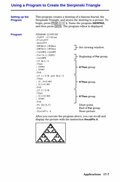
Applications 17-7
8317APPS.DOC TI-83 international English Bob Fedorisko Revised: 02/19/01 1:00 PM Printed: 02/19/01 1:39 PMPage 7 of 20
This program creates a drawing of a famous fractal, theSierpinski Triangle, and stores the drawing to a picture. Tobegin, press � ~ ~ 1. Name the program SIERPINS,and then press Í. The program editor is displayed.
PROGRAM:SIERPINS:FnOff :ClrDraw:PlotsOff:AxesOff:0!Xmin:1!Xmax:0!Ymin:1!Ymax Set viewing window.
:rand!X:rand!Y:For(K,1,3000):rand!N Beginning of For group.
:If N�1à3:Then:.5X!X:.5Y!Y:End
If/Then group
:If 1à3<N and N�2à3:Then:.5(.5+X)!X:.5(1+Y)!Y:End
If/Then group.
:If 2à3<N:Then:.5(1+X)!X:.5Y!Y:End
If/Then group.
:Pt-On(X,Y) Draw point.:End End of For group.:StorePic 6 Store picture.
After you execute the program above, you can recall anddisplay the picture with the instruction RecallPic 6 .
Using a Program to Create the Sierpinski Triangle
Setting up theProgram
Program
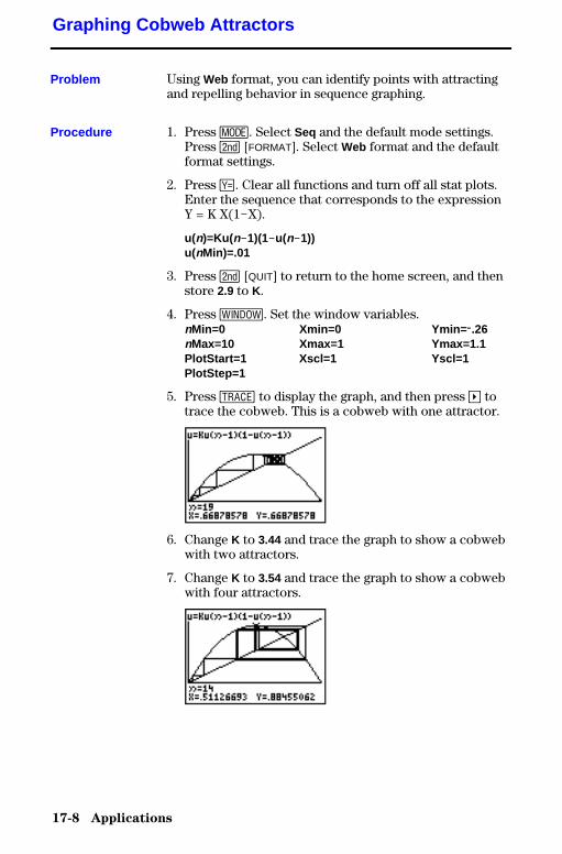
17-8 Applications
8317APPS.DOC TI-83 international English Bob Fedorisko Revised: 02/19/01 1:00 PM Printed: 02/19/01 1:39 PMPage 8 of 20
Using Web format, you can identify points with attractingand repelling behavior in sequence graphing.
1. Press z. Select Seq and the default mode settings.Press y [FORMAT]. Select Web format and the defaultformat settings.
2. Press o. Clear all functions and turn off all stat plots.Enter the sequence that corresponds to the expressionY = K X(1NX).
u(n)=Ku(nN1)(1Nu(nN1))u(nMin)=.01
3. Press y [QUIT] to return to the home screen, and thenstore 2.9 to K.
4. Press p. Set the window variables.nMin=0 Xmin=0 Ymin= M.26nMax=10 Xmax=1 Ymax=1.1PlotStart=1 Xscl=1 Yscl=1PlotStep=1
5. Press r to display the graph, and then press ~ totrace the cobweb. This is a cobweb with one attractor.
6. Change K to 3.44 and trace the graph to show a cobwebwith two attractors.
7. Change K to 3.54 and trace the graph to show a cobwebwith four attractors.
Graphing Cobweb Attractors
Problem
Procedure
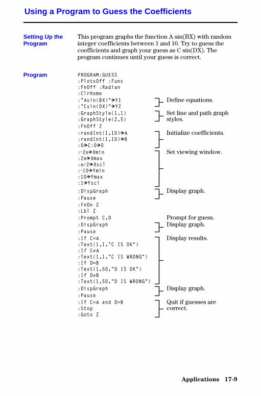
Applications 17-9
8317APPS.DOC TI-83 international English Bob Fedorisko Revised: 02/19/01 1:00 PM Printed: 02/19/01 1:39 PMPage 9 of 20
This program graphs the function A sin(BX) with randominteger coefficients between 1 and 10. Try to guess thecoefficients and graph your guess as C sin(DX). Theprogram continues until your guess is correct.
PROGRAM:GUESS:PlotsOff :Func:FnOff :Radian:ClrHome:"Asin(BX)"!Y1:"Csin(DX)"!Y2
Define equations.
:GraphStyle(1,1):GraphStyle(2,5)
Set line and path graphstyles.
:FnOff 2:randInt(1,10)!A:randInt(1,10)!B:0!C:0!D
Initialize coefficients.
:L2p!Xmin:2p!Xmax:pà2!Xscl:L10!Ymin:10!Ymax:1!Yscl
Set viewing window.
:DispGraph:Pause
Display graph.
:FnOn 2:Lbl Z:Prompt C,D Prompt for guess.:DispGraph:Pause
Display graph.
:If C=A:Text(1,1,"C IS OK"):If CƒA:Text(1,1,"C IS WRONG"):If D=B:Text(1,50,"D IS OK"):If DƒB:Text(1,50,"D IS WRONG")
Display results.
:DispGraph:Pause
Display graph.
:If C=A and D=B:Stop:Goto Z
Quit if guesses arecorrect.
Using a Program to Guess the Coefficients
Setting Up theProgram
Program
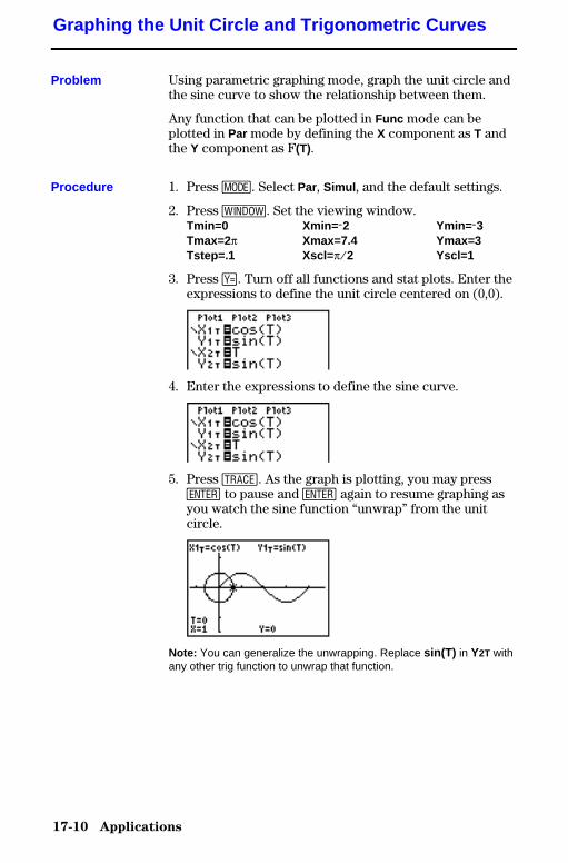
17-10 Applications
8317APPS.DOC TI-83 international English Bob Fedorisko Revised: 02/19/01 1:00 PM Printed: 02/19/01 1:39 PMPage 10 of 20
Using parametric graphing mode, graph the unit circle andthe sine curve to show the relationship between them.
Any function that can be plotted in Func mode can beplotted in Par mode by defining the X component as T andthe Y component as F(T).
1. Press z. Select Par, Simul , and the default settings.
2. Press p. Set the viewing window.Tmin=0 Xmin= L2 Ymin= L3Tmax=2p Xmax=7.4 Ymax=3Tstep=.1 Xscl= pà2 Yscl=1
3. Press o. Turn off all functions and stat plots. Enter theexpressions to define the unit circle centered on (0,0).
4. Enter the expressions to define the sine curve.
5. Press r. As the graph is plotting, you may pressÍ to pause and Í again to resume graphing asyou watch the sine function “unwrap” from the unitcircle.
Note: You can generalize the unwrapping. Replace sin(T) in Y2T withany other trig function to unwrap that function.
Graphing the Unit Circle and Trigonometric Curves
Problem
Procedure
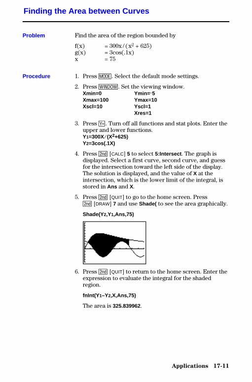
Applications 17-11
8317APPS.DOC TI-83 international English Bob Fedorisko Revised: 02/19/01 1:00 PM Printed: 02/19/01 1:39 PMPage 11 of 20
Find the area of the region bounded by
f(x) = 300x / (x2 + 625)g(x) = 3cos(.1x)x = 75
1. Press z. Select the default mode settings.
2. Press p. Set the viewing window.Xmin=0 Ymin= L5Xmax=100 Ymax=10Xscl=10 Yscl=1
Xres=1
3. Press o. Turn off all functions and stat plots. Enter theupper and lower functions.Y1=300Xà(X2+625)Y2=3cos(.1X)
4. Press y [CALC] 5 to select 5:Intersect . The graph isdisplayed. Select a first curve, second curve, and guessfor the intersection toward the left side of the display.The solution is displayed, and the value of X at theintersection, which is the lower limit of the integral, isstored in Ans and X.
5. Press y [QUIT] to go to the home screen. Pressy [DRAW] 7 and use Shade( to see the area graphically.
Shade(Y2,Y1,Ans,75)
6. Press y [QUIT] to return to the home screen. Enter theexpression to evaluate the integral for the shadedregion.
fnInt(Y 1–Y2,X,Ans,75)
The area is 325.839962.
Finding the Area between Curves
Problem
Procedure
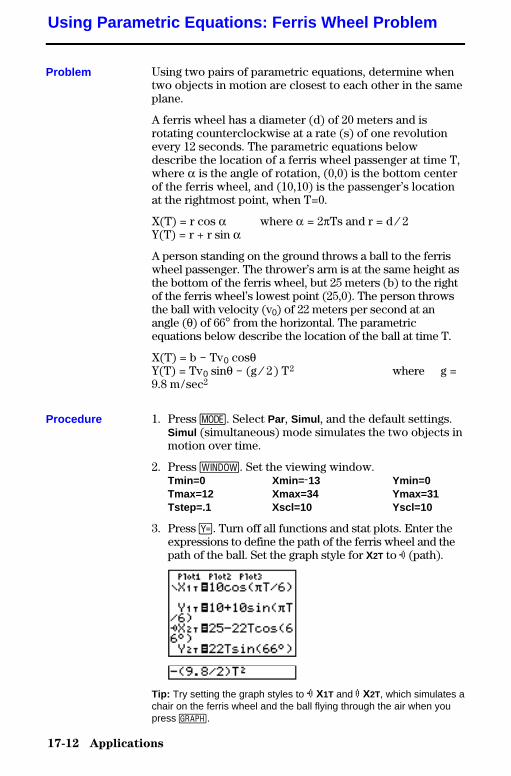
17-12 Applications
8317APPS.DOC TI-83 international English Bob Fedorisko Revised: 02/19/01 1:00 PM Printed: 02/19/01 1:39 PMPage 12 of 20
Using two pairs of parametric equations, determine whentwo objects in motion are closest to each other in the sameplane.
A ferris wheel has a diameter (d) of 20 meters and isrotating counterclockwise at a rate (s) of one revolutionevery 12 seconds. The parametric equations belowdescribe the location of a ferris wheel passenger at time T,where a is the angle of rotation, (0,0) is the bottom centerof the ferris wheel, and (10,10) is the passenger’s locationat the rightmost point, when T=0.
X(T) = r cos a where a = 2pTs and r = dà 2Y(T) = r + r sin a
A person standing on the ground throws a ball to the ferriswheel passenger. The thrower’s arm is at the same height asthe bottom of the ferris wheel, but 25 meters (b) to the rightof the ferris wheel’s lowest point (25,0). The person throwsthe ball with velocity (v0) of 22 meters per second at anangle (q) of 66¡ from the horizontal. The parametricequations below describe the location of the ball at time T.
X(T) = b N Tv0 cosqY(T) = Tv0 sinq N (g à 2) T2 where g =9.8 m/sec2
1. Press z. Select Par, Simul , and the default settings.Simul (simultaneous) mode simulates the two objects inmotion over time.
2. Press p. Set the viewing window.Tmin=0 Xmin= L13 Ymin=0Tmax=12 Xmax=34 Ymax=31Tstep=.1 Xscl=10 Yscl=10
3. Press o. Turn off all functions and stat plots. Enter theexpressions to define the path of the ferris wheel and thepath of the ball. Set the graph style for X2T to ë (path).
Tip: Try setting the graph styles to ë X1T and ì X2T, which simulates achair on the ferris wheel and the ball flying through the air when youpress s.
Using Parametric Equations: Ferris Wheel Problem
Problem
Procedure
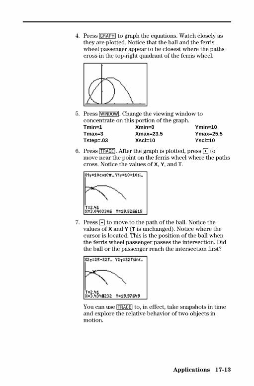
Applications 17-13
8317APPS.DOC TI-83 international English Bob Fedorisko Revised: 02/19/01 1:00 PM Printed: 02/19/01 1:39 PMPage 13 of 20
4. Press s to graph the equations. Watch closely asthey are plotted. Notice that the ball and the ferriswheel passenger appear to be closest where the pathscross in the top-right quadrant of the ferris wheel.
5. Press p. Change the viewing window toconcentrate on this portion of the graph.Tmin=1 Xmin=0 Ymin=10Tmax=3 Xmax=23.5 Ymax=25.5Tstep=.03 Xscl=10 Yscl=10
6. Press r. After the graph is plotted, press ~ tomove near the point on the ferris wheel where the pathscross. Notice the values of X, Y, and T.
7. Press † to move to the path of the ball. Notice thevalues of X and Y (T is unchanged). Notice where thecursor is located. This is the position of the ball whenthe ferris wheel passenger passes the intersection. Didthe ball or the passenger reach the intersection first?
You can use r to, in effect, take snapshots in timeand explore the relative behavior of two objects inmotion.
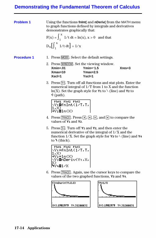
17-14 Applications
8317APPS.DOC TI-83 international English Bob Fedorisko Revised: 02/19/01 1:00 PM Printed: 02/19/01 1:39 PMPage 14 of 20
Using the functions fnInt( and nDeriv( from the MATH menuto graph functions defined by integrals and derivativesdemonstrates graphically that:
F(x) = ‰1
x 1àt dt = ln(x), x > 0 and that
Dx[‰1
x 1àt dt] = 1àx
1. Press z. Select the default settings.
2. Press p. Set the viewing window.Xmin=.01 Ymin= M1.5 Xres=3Xmax=10 Ymax=2.5Xscl=1 Yscl=1
3. Press o. Turn off all functions and stat plots. Enter thenumerical integral of 1àT from 1 to X and the functionln(X). Set the graph style for Y1 to ç (line) and Y2 toë (path).
4. Press r. Press |, }, ~, and † to compare thevalues of Y1 and Y2.
5. Press o. Turn off Y1 and Y2, and then enter thenumerical derivative of the integral of 1àX and thefunction 1àX. Set the graph style for Y3 to ç (line) and Y4
to è (thick).
6. Press r. Again, use the cursor keys to compare thevalues of the two graphed functions, Y3 and Y4.
Demonstrating the Fundamental Theorem of Calculus
Problem 1
Procedure 1
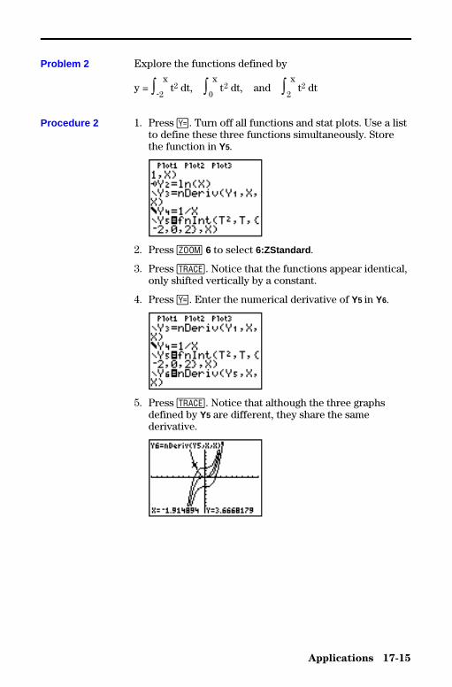
Applications 17-15
8317APPS.DOC TI-83 international English Bob Fedorisko Revised: 02/19/01 1:00 PM Printed: 02/19/01 1:39 PMPage 15 of 20
Explore the functions defined by
y = ‰M2
x t2 dt, ‰
0
x t2 dt, and ‰
2
x t2 dt
1. Press o. Turn off all functions and stat plots. Use a listto define these three functions simultaneously. Storethe function in Y5.
2. Press q 6 to select 6:ZStandard .
3. Press r. Notice that the functions appear identical,only shifted vertically by a constant.
4. Press o. Enter the numerical derivative of Y5 in Y6.
5. Press r. Notice that although the three graphsdefined by Y5 are different, they share the samederivative.
Problem 2
Procedure 2
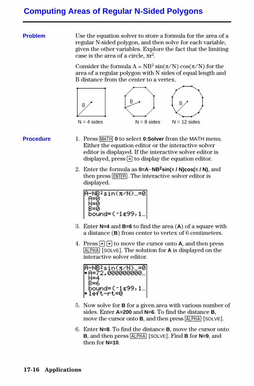
17-16 Applications
8317APPS.DOC TI-83 international English Bob Fedorisko Revised: 02/19/01 1:00 PM Printed: 02/19/01 1:39 PMPage 16 of 20
Use the equation solver to store a formula for the area of aregular N-sided polygon, and then solve for each variable,given the other variables. Explore the fact that the limitingcase is the area of a circle, pr2.
Consider the formula A = NB2 sin(pàN) cos(pàN) for thearea of a regular polygon with N sides of equal length andB distance from the center to a vertex.
N = 4 sides N = 8 sides N = 12 sides
1. Press � 0 to select 0:Solver from the MATH menu.Either the equation editor or the interactive solvereditor is displayed. If the interactive solver editor isdisplayed, press } to display the equation editor.
2. Enter the formula as 0=ANNB2sin( p / N)cos( p / N), andthen press Í. The interactive solver editor isdisplayed.
3. Enter N=4 and B=6 to find the area (A) of a square witha distance (B) from center to vertex of 6 centimeters.
4. Press } } to move the cursor onto A, and then pressƒ [SOLVE]. The solution for A is displayed on theinteractive solver editor.
5. Now solve for B for a given area with various number ofsides. Enter A=200 and N=6. To find the distance B,move the cursor onto B, and then press ƒ [SOLVE].
6. Enter N=8. To find the distance B, move the cursor ontoB, and then press ƒ [SOLVE]. Find B for N=9, andthen for N=10.
Computing Areas of Regular N-Sided Polygons
Problem
Procedure

Applications 17-17
8317APPS.DOC TI-83 international English Bob Fedorisko Revised: 02/19/01 1:00 PM Printed: 02/19/01 1:39 PMPage 17 of 20
Find the area given B=6, and N=10, 100, 150, 1000, and10000. Compare your results with p62 (the area of a circlewith radius 6), which is approximately 113.097.
7. Enter B=6. To find the area A, move the cursor onto A,and then press ƒ [SOLVE]. Find A for N=10, thenN=100, then N=150, then N=1000, and finally N=10000.Notice that as N gets large, the area A approaches pB2.
Now graph the equation to see visually how the areachanges as the number of sides gets large.
8. Press z. Select the default mode settings.
9. Press p. Set the viewing window.Xmin=0 Ymin=0 Xres=1Xmax=200 Ymax=150Xscl=10 Yscl=10
10.Press o. Turn off all functions and stat plots. Enter theequation for the area. Use X in place of N. Set the graphstyles as shown.
11.Press r. After the graph is plotted, press 100 Íto trace to X=100. Press 150 Í. Press 188 Í.Notice that as X increases, the value of Y converges top62, which is approximately 113.097. Y2=pB2 (the area ofthe circle) is a horizontal asymptote to Y1. The area ofan N-sided regular polygon, with r as the distance fromthe center to a vertex, approaches the area of a circlewith radius r (pr2) as N gets large.
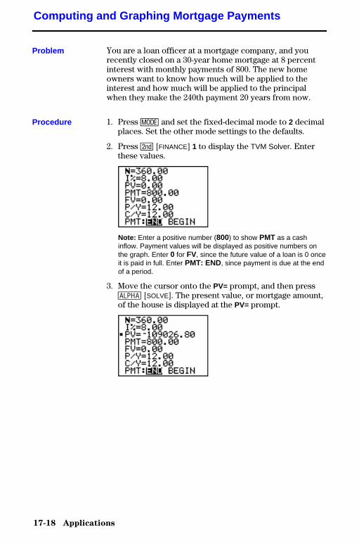
17-18 Applications
8317APPS.DOC TI-83 international English Bob Fedorisko Revised: 02/19/01 1:00 PM Printed: 02/19/01 1:39 PMPage 18 of 20
You are a loan officer at a mortgage company, and yourecently closed on a 30-year home mortgage at 8 percentinterest with monthly payments of 800. The new homeowners want to know how much will be applied to theinterest and how much will be applied to the principalwhen they make the 240th payment 20 years from now.
1. Press z and set the fixed-decimal mode to 2 decimalplaces. Set the other mode settings to the defaults.
2. Press y [FINANCE] 1 to display the TVM Solver. Enterthese values.
Note: Enter a positive number (800) to show PMT as a cashinflow. Payment values will be displayed as positive numbers onthe graph. Enter 0 for FV, since the future value of a loan is 0 onceit is paid in full. Enter PMT: END, since payment is due at the endof a period.
3. Move the cursor onto the PV= prompt, and then pressƒ [SOLVE]. The present value, or mortgage amount,of the house is displayed at the PV= prompt.
Computing and Graphing Mortgage Payments
Problem
Procedure
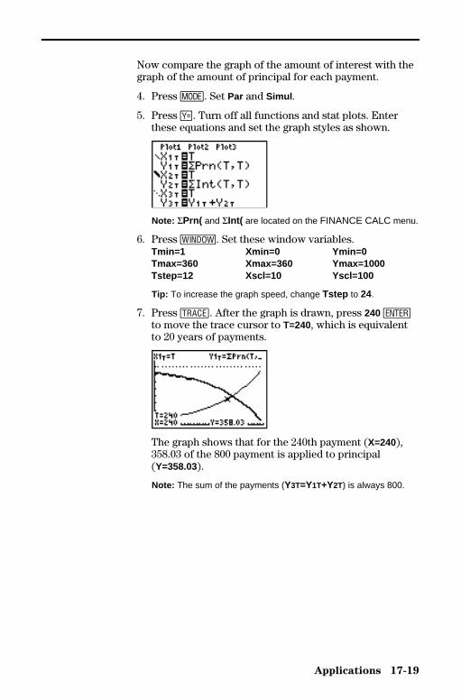
Applications 17-19
8317APPS.DOC TI-83 international English Bob Fedorisko Revised: 02/19/01 1:00 PM Printed: 02/19/01 1:39 PMPage 19 of 20
Now compare the graph of the amount of interest with thegraph of the amount of principal for each payment.
4. Press z. Set Par and Simul .
5. Press o. Turn off all functions and stat plots. Enterthese equations and set the graph styles as shown.
Note: GPrn( and GInt( are located on the FINANCE CALC menu.
6. Press p. Set these window variables.Tmin=1 Xmin=0 Ymin=0Tmax=360 Xmax=360 Ymax=1000Tstep=12 Xscl=10 Yscl=100
Tip: To increase the graph speed, change Tstep to 24.
7. Press r. After the graph is drawn, press 240 Íto move the trace cursor to T=240, which is equivalentto 20 years of payments.
The graph shows that for the 240th payment (X=240),358.03 of the 800 payment is applied to principal(Y=358.03).
Note: The sum of the payments (Y3T=Y1T+Y2T) is always 800.
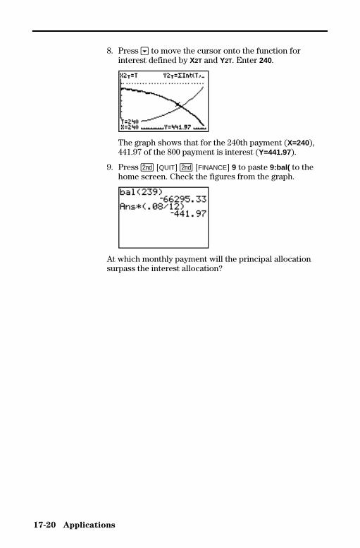
17-20 Applications
8317APPS.DOC TI-83 international English Bob Fedorisko Revised: 02/19/01 1:00 PM Printed: 02/19/01 1:39 PMPage 20 of 20
8. Press † to move the cursor onto the function forinterest defined by X2T and Y2T. Enter 240.
The graph shows that for the 240th payment (X=240),441.97 of the 800 payment is interest (Y=441.97).
9. Press y [QUIT] y [FINANCE] 9 to paste 9:bal( to thehome screen. Check the figures from the graph.
At which monthly payment will the principal allocationsurpass the interest allocation?
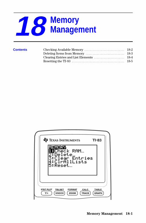
Memory Management 18-1
8318MEMR.DOC TI-83 international English Bob Fedorisko Revised: 02/19/01 1:01 PM Printed: 02/19/01 1:40PM Page 1 of 6
18 Memor yManagement
Checking Available Memory ............................. 18-2Deleting Items from Memory ............................ 18-3Clearing Entries and List Elements ...................... 18-4Resetting the TI-83 ...................................... 18-5
Contents
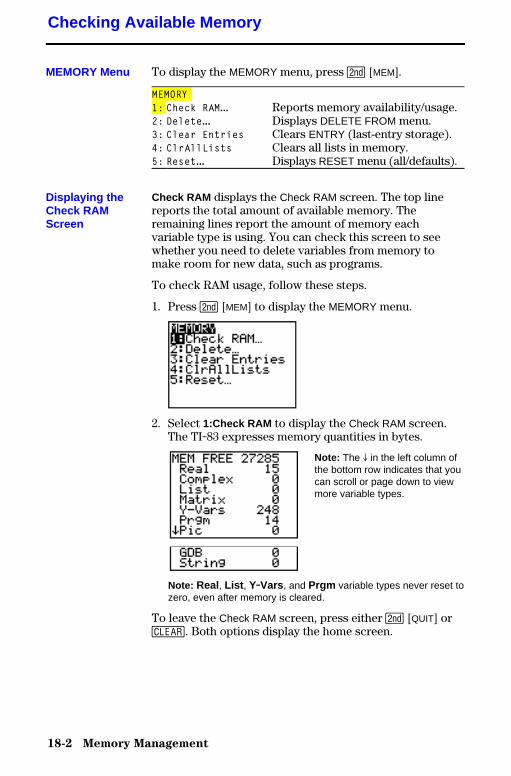
18-2 Memory Management
8318MEMR.DOC TI-83 international English Bob Fedorisko Revised: 02/19/01 1:01 PM Printed: 02/19/01 1:40PM Page 2 of 6
To display the MEMORY menu, press y [MEM].
MEMORY1: Check RAM... Reports memory availability/usage.2: Delete... Displays DELETE FROM menu.3: Clear Entries Clears ENTRY (last-entry storage).4: ClrAllLists Clears all lists in memory.5: Reset... Displays RESET menu (all/defaults).
Check RAM displays the Check RAM screen. The top linereports the total amount of available memory. Theremaining lines report the amount of memory eachvariable type is using. You can check this screen to seewhether you need to delete variables from memory tomake room for new data, such as programs.
To check RAM usage, follow these steps.
1. Press y [MEM] to display the MEMORY menu.
2. Select 1:Check RAM to display the Check RAM screen.The TI-83 expresses memory quantities in bytes.
Note: The $ in the left column ofthe bottom row indicates that youcan scroll or page down to viewmore variable types.
Note: Real, List , Y.Vars , and Prgm variable types never reset tozero, even after memory is cleared.
To leave the Check RAM screen, press either y [QUIT] or‘. Both options display the home screen.
Checking Available Memory
MEMORY Menu
Displaying theCheck RAMScreen
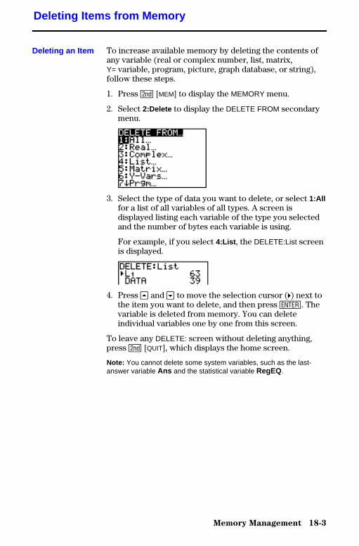
Memory Management 18-3
8318MEMR.DOC TI-83 international English Bob Fedorisko Revised: 02/19/01 1:01 PM Printed: 02/19/01 1:40PM Page 3 of 6
To increase available memory by deleting the contents ofany variable (real or complex number, list, matrix,Y= variable, program, picture, graph database, or string),follow these steps.
1. Press y [MEM] to display the MEMORY menu.
2. Select 2:Delete to display the DELETE FROM secondarymenu.
3. Select the type of data you want to delete, or select 1:Allfor a list of all variables of all types. A screen isdisplayed listing each variable of the type you selectedand the number of bytes each variable is using.
For example, if you select 4:List , the DELETE:List screenis displayed.
4. Press } and † to move the selection cursor (4) next tothe item you want to delete, and then press Í. Thevariable is deleted from memory. You can deleteindividual variables one by one from this screen.
To leave any DELETE: screen without deleting anything,press y [QUIT], which displays the home screen.
Note: You cannot delete some system variables, such as the last-answer variable Ans and the statistical variable RegEQ.
Deleting Items from Memory
Deleting an Item
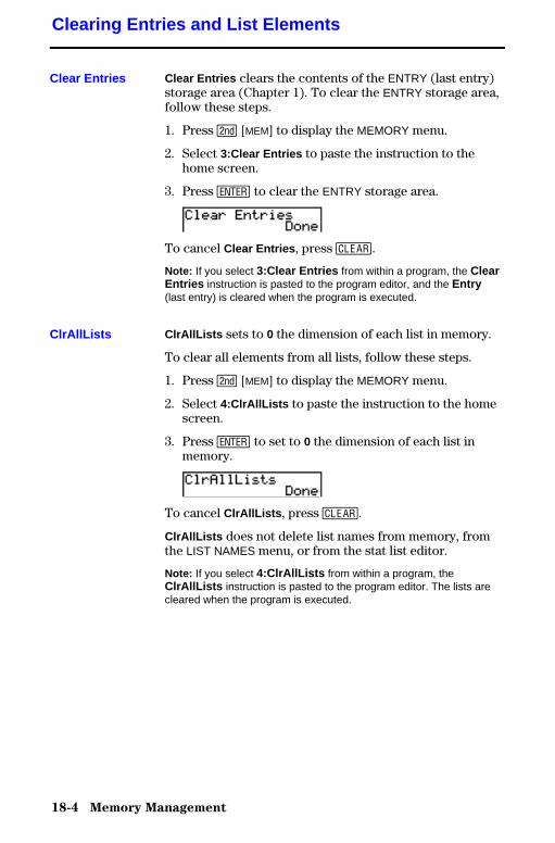
18-4 Memory Management
8318MEMR.DOC TI-83 international English Bob Fedorisko Revised: 02/19/01 1:01 PM Printed: 02/19/01 1:40PM Page 4 of 6
Clear Entries clears the contents of the ENTRY (last entry)storage area (Chapter 1). To clear the ENTRY storage area,follow these steps.
1. Press y [MEM] to display the MEMORY menu.
2. Select 3:Clear Entries to paste the instruction to thehome screen.
3. Press Í to clear the ENTRY storage area.
To cancel Clear Entries , press ‘.
Note: If you select 3:Clear Entries from within a program, the ClearEntries instruction is pasted to the program editor, and the Entry(last entry) is cleared when the program is executed.
ClrAllLists sets to 0 the dimension of each list in memory.
To clear all elements from all lists, follow these steps.
1. Press y [MEM] to display the MEMORY menu.
2. Select 4:ClrAllLists to paste the instruction to the homescreen.
3. Press Í to set to 0 the dimension of each list inmemory.
To cancel ClrAllLists , press ‘.
ClrAllLists does not delete list names from memory, fromthe LIST NAMES menu, or from the stat list editor.
Note: If you select 4:ClrAllLists from within a program, theClrAllLists instruction is pasted to the program editor. The lists arecleared when the program is executed.
Clearing Entries and List Elements
Clear Entries
ClrAllLists

Memory Management 18-5
8318MEMR.DOC TI-83 international English Bob Fedorisko Revised: 02/19/01 1:01 PM Printed: 02/19/01 1:40PM Page 5 of 6
The RESET secondary menu gives you the option ofresetting all memory (including default settings) orresetting the default settings while preserving other datastored in memory, such as programs and Y= functions.
Resetting all memory on the TI-83 restores memory to thefactory settings. It deletes all nonsystem variables and allprograms. It resets all system variables to the defaultsettings.
Tip: Before you reset all memory, consider restoring sufficientavailable memory by deleting only selected data (page 18.3).
To reset all memory on the TI-83, follow these steps.
1. Press y [MEM] to display the MEMORY menu.
2. Select 5:Reset to display the RESET secondary menu.
3. Select 1:All Memory to display the RESET MEMORYtertiary menu.
4. Read the message below the RESET MEMORY menu.
• To cancel memory reset and return to the homescreen, select 1:No .
• To erase from memory all data and programs, select2:Reset . All factory defaults are restored.Mem cleared is displayed on the home screen.
Note: When you clear memory, the contrast sometimes changes. Ifthe screen is faded or blank, adjust the contrast (Chapter 1).
Resetting the TI-83
RESETSecondary Menu
Resetting AllMemory
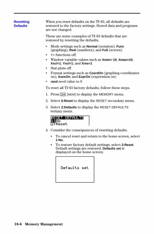
18-6 Memory Management
8318MEMR.DOC TI-83 international English Bob Fedorisko Revised: 02/19/01 1:01 PM Printed: 02/19/01 1:40PM Page 6 of 6
When you reset defaults on the TI-83, all defaults arerestored to the factory settings. Stored data and programsare not changed.
These are some examples of TI-83 defaults that arerestored by resetting the defaults.
• Mode settings such as Normal (notation); Func(graphing); Real (numbers); and Full (screen)
• Y= functions off• Window variable values such as Xmin= L10; Xmax=10 ;
Xscl=1 ; Yscl=1 ; and Xres=1
• Stat plots off• Format settings such as CoordOn (graphing coordinates
on); AxesOn ; and ExprOn (expression on)• rand seed value to 0
To reset all TI-83 factory defaults, follow these steps.
1. Press y [MEM] to display the MEMORY menu.
2. Select 5:Reset to display the RESET secondary menu.
3. Select 2:Defaults to display the RESET DEFAULTStertiary menu.
4. Consider the consequences of resetting defaults.
• To cancel reset and return to the home screen, select1:No .
• To restore factory default settings, select 2:Reset .Default settings are restored. Defaults set isdisplayed on the home screen.
ResettingDefaults
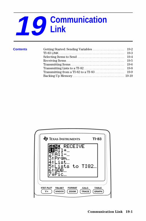
Communication Link 19-1
8319LINK.DOC TI-83 Intl English, Chap 19 Bob Fedorisko Revised: 02/19/01 1:24 PM Printed: 02/19/01 1:40 PMPage 1 of 10
19 CommunicationLink
Getting Started: Sending Variables ....................... 19-2TI-83 LINK ............................................... 19-3Selecting Items to Send .................................. 19-4Receiving Items.......................................... 19-5Transmitting Items....................................... 19-6Transmitting Lists to a TI-82 ............................. 19-8Transmitting from a TI-82 to a TI-83 ..................... 19-9Backing Up Memory ..................................... 19-10
Contents
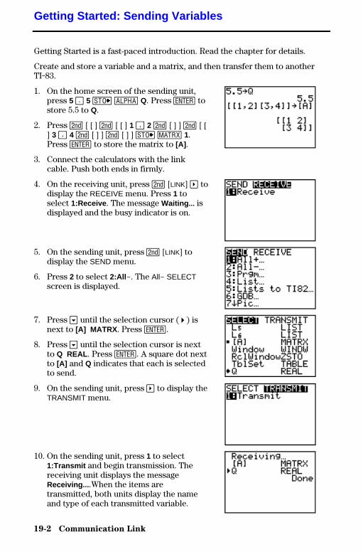
19-2 Communication Link
8319LINK.DOC TI-83 Intl English, Chap 19 Bob Fedorisko Revised: 02/19/01 1:24 PM Printed: 02/19/01 1:40 PMPage 2 of 10
Getting Started is a fast-paced introduction. Read the chapter for details.
Create and store a variable and a matrix, and then transfer them to anotherTI-83.
1. On the home screen of the sending unit,press 5 Ë 5 ¿ ƒ Q. Press Í tostore 5.5 to Q.
2. Press y [ [ ] y [ [ ] 1 ¢ 2 y [ ] ] y [ [] 3 ¢ 4 y [ ] ] y [ ] ] ¿ � 1.Press Í to store the matrix to [A] .
3. Connect the calculators with the linkcable. Push both ends in firmly.
4. On the receiving unit, press y [LINK] ~ todisplay the RECEIVE menu. Press 1 toselect 1:Receive . The message Waiting ... isdisplayed and the busy indicator is on.
5. On the sending unit, press y [LINK] todisplay the SEND menu.
6. Press 2 to select 2:All N. The AllN SELECTscreen is displayed.
7. Press † until the selection cursor ( 4 ) isnext to [A] MATRX . Press Í.
8. Press † until the selection cursor is nextto Q REAL . Press Í. A square dot nextto [A] and Q indicates that each is selectedto send.
9. On the sending unit, press ~ to display theTRANSMIT menu.
10. On the sending unit, press 1 to select1:Transmit and begin transmission. Thereceiving unit displays the messageReceiving... .When the items aretransmitted, both units display the nameand type of each transmitted variable.
Getting Started: Sending Variables
Communication Link 19-3
8319LINK.DOC TI-83 Intl English, Chap 19 Bob Fedorisko Revised: 02/19/01 1:24 PM Printed: 02/19/01 1:40 PMPage 3 of 10
The TI-83 has a port to connect and communicate withanother TI-83, a TI-82, the Calculator-Based Laboratoryé(CBL 2é, CBLé) System, the Calculator-Based Rangeré(CBRé), or a personal computer. The unit-to-unit linkcable is included with the TI-83. This chapter describeshow to communicate with another calculator.
You can transfer all variables and programs to anotherTI-83 or backup the entire memory of a TI-83. Thesoftware that enables this communication is built into theTI-83. To transmit from one TI-83 to another, follow thesteps on pages 19.6 and 19.7.
You can transfer from a TI-82 to a TI-83 all variables andprograms. Also, you can transfer from a TI-83 to a TI-82 listsL1 through L6.
The software that enables this communication is built into theTI-83. To transmit data from a TI-82 to a TI-83, follow thesteps on pages 19.6 and 19.7.
• You cannot perform a memory backup from a TI-82 to aTI-83.
• The only data type you can transmit from a TI-83 to aTI-82 is list data stored in L1 through L6. Use the LINKSEND menu item 5:Lists to TI82 (page 19.8).
1. Insert either end of the cable into the port very firmly.
2. Insert the other end of the cable into the othercalculator’s port.
CBR and the CBL 2/CBL System are optional accessoriesthat connect to a TI-83 with the unit-to-unit link cable.With a CBR or a CBL 2/CBL and a TI-83, you can collectand analyze real-world data.
TI.GRAPH LINKé is an optional accessory that links a TI-83to enable communication with a personal computer.
TI-83 LINK
TI-83 LinkCapabilities
Linking TwoTI-83s
Linking a TI-82and a TI-83
Connecting TwoCalculators withthe Cable
Linking to a CBRor the CBL 2/CBLSystem
Linking to a PCor Macintosh
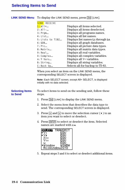
19-4 Communication Link
8319LINK.DOC TI-83 Intl English, Chap 19 Bob Fedorisko Revised: 02/19/01 1:24 PM Printed: 02/19/01 1:40 PMPage 4 of 10
To display the LINK SEND menu, press y [LINK].
SEND RECEIVE1: All+... Displays all items selected.2: AllN... Displays all items deselected.3: Prgm... Displays all programs names.4: List... Displays all list names.5: Lists to TI82... Displays list names L1 through L6.6: GDB... Displays all graph databases.7: Pic... Displays all picture data types.8: Matrix... Displays all matrix data types.9: Real... Displays all real variables.0: Complex... Displays all complex variables.A: Y-Vars... Displays all Y= variables.B: String... Displays all string variables.C: Back Up... Selects all for backup to TI-83.
When you select an item on the LINK SEND menu, thecorresponding SELECT screen is displayed.
Note: Each SELECT screen, except All+ SELECT, is displayedinitially with no data selected.
To select items to send on the sending unit, follow thesesteps.
1. Press y [LINK] to display the LINK SEND menu.
2. Select the menu item that describes the data type tosend. The corresponding SELECT screen is displayed.
3. Press } and † to move the selection cursor ( 4 ) to anitem you want to select or deselect.
4. Press Í to select or deselect the item. Selectednames are marked with a 0.
5. Repeat steps 3 and 4 to select or deselect additional items.
Selecting Items to Send
LINK SEND Menu
Selecting Itemsto Send
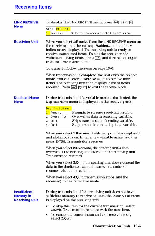
Communication Link 19-5
8319LINK.DOC TI-83 Intl English, Chap 19 Bob Fedorisko Revised: 02/19/01 1:24 PM Printed: 02/19/01 1:40 PMPage 5 of 10
To display the LINK RECEIVE menu, press y [LINK] ~.
SEND RECEIVE1: Receive Sets unit to receive data transmission.
When you select 1:Receive from the LINK RECEIVE menu onthe receiving unit, the message Waiting... and the busyindicator are displayed. The receiving unit is ready toreceive transmitted items. To exit the receive modewithout receiving items, press É, and then select 1:Quitfrom the Error in Xmit menu.
To transmit, follow the steps on page 19.6.
When transmission is complete, the unit exits the receivemode. You can select 1:Receive again to receive moreitems. The receiving unit then displays a list of itemsreceived. Press y [QUIT] to exit the receive mode.
During transmission, if a variable name is duplicated, theDuplicateName menu is displayed on the receiving unit.
DuplicateName1: Rename Prompts to rename receiving variable.2: Overwrite Overwrites data in receiving variable.3: Omit Skips transmission of sending variable.4: Quit Stops transmission at duplicate variable.
When you select 1:Rename , the Name= prompt is displayed,and alpha-lock is on. Enter a new variable name, and thenpress Í. Transmission resumes.
When you select 2:Overwrite , the sending unit’s dataoverwrites the existing data stored on the receiving unit.Transmission resumes.
When you select 3:Omit , the sending unit does not send thedata in the duplicated variable name. Transmissionresumes with the next item.
When you select 4:Quit , transmission stops, and thereceiving unit exits receive mode.
During transmission, if the receiving unit does not havesufficient memory to receive an item, the Memory Full menuis displayed on the receiving unit.
• To skip this item for the current transmission, select1:Omit . Transmission resumes with the next item.
• To cancel the transmission and exit receive mode,select 2:Quit .
Receiving Items
LINK RECEIVEMenu
Receiving Unit
DuplicateNameMenu
InsufficientMemory inReceiving Unit

19-6 Communication Link
8319LINK.DOC TI-83 Intl English, Chap 19 Bob Fedorisko Revised: 02/19/01 1:24 PM Printed: 02/19/01 1:40 PMPage 6 of 10
To transmit selected items after you have selected items tosend on the sending unit (page 19.4) and set the receivingunit to receive (page 19.5), follow these steps.
1. Press ~ on the sending unit to display the TRANSMITmenu.
2. Confirm that Waiting... is displayed on the receivingunit, which indicates it is set to receive (page 19.5).
3. Press Í to select 1:Transmit . The name and type ofeach item are displayed line by line on the sending unitas the item is queued for transmission, and then on thereceiving unit as each item is accepted.
After all selected items have been transmitted, the messageDone is displayed on both calculators. Press } and † toscroll through the names.
To stop a link transmission, press É. The Error in Xmitmenu is displayed on both units. To leave the error menu,select 1:Quit .
A transmission error occurs after one or two seconds if:
• A cable is not attached to the sending unit.• A cable is not attached to the receiving unit.
Note: If the cable is attached, push it in firmly and try again.
• The receiving unit is not set to receive transmission.• You attempt a backup between a TI-82 and a TI-83.• You attempt a data transfer from a TI-83 to a TI-82 with
data other than lists L1 through L6 or without usingmenu item 5:Lists to TI82 .
Although a transmission error does not occur, these twoconditions may prevent successful transmission.
• You try to use Get( with a calculator instead of aCBL 2/CBL or CBR.
• You try to use GetCalc( with a TI-82 instead of a TI-83.
Transmitting Items
TransmittingItems
Stopping aTransmission
Error Conditions
Communication Link 19-7
8319LINK.DOC TI-83 Intl English, Chap 19 Bob Fedorisko Revised: 02/19/01 1:24 PM Printed: 02/19/01 1:40 PMPage 7 of 10
After sending or receiving data, you can repeat the sametransmission to additional TI-83 units—from either thesending unit or the receiving unit—without having toreselect data to send. The current items remain selected.
Note: You cannot repeat transmission if you selected All+ or All..
To transmit to an additional TI-83, follow these steps.
1. Set the TI-83 to receive (page 19.5).
2. Do not select or deselect any new items to send. If youselect or deselect an item, all selections or deselectionsfrom the previous transmission are cleared.
3. Disconnect the link cable from one TI-83 and connect itto the additional TI-83.
4. Set the additional TI-83 to receive (page 19.5).
5. Press y [LINK] on the sending TI-83 to display theLINK SEND menu.
6. Select the menu item that you used for the lasttransmission. The data from your last transmission isstill selected.
7. Press ~ to display the LINK TRANSMIT menu.
8. Confirm that the receiving unit is set to receive(page 19.5).
9. Press Í to select 1:Transmit and begin transmitting.
TransmittingItems to anAdditional TI-83
19-8 Communication Link
8319LINK.DOC TI-83 Intl English, Chap 19 Bob Fedorisko Revised: 02/19/01 1:24 PM Printed: 02/19/01 1:40 PMPage 8 of 10
The only data type you can transmit from a TI-83 to a TI-82is list data stored in L1 through L6.
To transmit to a TI-82 the list data that is stored to TI-83lists L1, L2, L3, L4, L5, or L6, follow these steps.
1. Set the TI-82 to receive (page 19.5).
2. Press y [LINK] 5 on the sending TI-83 to select5:Lists to TI82 . The SELECT screen is displayed.
3. Select each list to transmit.
4. Press ~ to display the LINK TRANSMIT menu.
5. Confirm that the receiving unit is set to receive(page 19.5).
6. Press Í to select 1:Transmit and begin transmitting.
Note: If dimension > 99 for a TI-83 list that is selected to send, thereceiving TI-82 will truncate the list at the ninety-ninth element duringtransmission.
Transmitting Lists to a TI-82
TransmittingLists to a TI-82
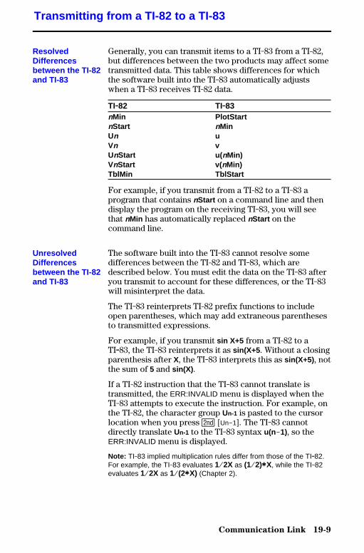
Communication Link 19-9
8319LINK.DOC TI-83 Intl English, Chap 19 Bob Fedorisko Revised: 02/19/01 1:24 PM Printed: 02/19/01 1:40 PMPage 9 of 10
Generally, you can transmit items to a TI-83 from a TI-82,but differences between the two products may affect sometransmitted data. This table shows differences for whichthe software built into the TI-83 automatically adjustswhen a TI-83 receives TI-82 data.
TI.82 TI.83nMin PlotStartnStart nMinUn uVn vUnStart u( nMin)VnStart v( nMin)TblMin TblStart
For example, if you transmit from a TI-82 to a TI-83 aprogram that contains nStart on a command line and thendisplay the program on the receiving TI-83, you will seethat nMin has automatically replaced nStart on thecommand line.
The software built into the TI-83 cannot resolve somedifferences between the TI-82 and TI-83, which aredescribed below. You must edit the data on the TI-83 afteryou transmit to account for these differences, or the TI-83will misinterpret the data.
The TI-83 reinterprets TI-82 prefix functions to includeopen parentheses, which may add extraneous parenthesesto transmitted expressions.
For example, if you transmit sin X+5 from a TI-82 to aTI.83, the TI-83 reinterprets it as sin(X+5 . Without a closingparenthesis after X, the TI-83 interprets this as sin(X+5) , notthe sum of 5 and sin(X) .
If a TI-82 instruction that the TI-83 cannot translate istransmitted, the ERR:INVALID menu is displayed when theTI-83 attempts to execute the instruction. For example, onthe TI-82, the character group Un-1 is pasted to the cursorlocation when you press y [UnN1]. The TI-83 cannotdirectly translate Un-1 to the TI-83 syntax u(nN1), so theERR:INVALID menu is displayed.
Note: TI-83 implied multiplication rules differ from those of the TI.82.For example, the TI-83 evaluates 1à2X as (1à2)äX, while the TI-82evaluates 1à2X as 1à(2äX) (Chapter 2).
Transmitting from a TI-82 to a TI-83
ResolvedDifferencesbetween the TI-82and TI-83
UnresolvedDifferencesbetween the TI-82and TI-83

19-10 Communication Link
8319LINK.DOC TI-83 Intl English, Chap 19 Bob Fedorisko Revised: 02/19/01 1:24 PM Printed: 02/19/01 1:40 PMPage 10 of 10
To copy the exact contents of memory in the sending TI-83to the memory of the receiving TI-83, put the other unit inreceive mode. Then, on the receiving unit, select C:Back Upfrom the LINK SEND menu.
• Warning: C:Back Up overwrites the memory in thereceiving unit; all information in the memory of thereceiving unit is lost.Note: If you do not want to do a backup, select 2:Quit to return tothe LINK SEND menu.
• Select 1:Transmit to begin transmission.
As a safety check to prevent accidental loss of memory,the message WARNING . Backup is displayed when thereceiving unit receives notice of a backup.
• To continue with the backup process, select 1:Continue .The backup transmission begins.
• To prevent the backup, select 2:Quit .
Note: If a transmission error is returned during a backup, the receivingunit is reset.
When the backup is complete, both the sending calculatorand receiving calculator display a confirmation screen.
Backing Up Memory
Memory Backup
Receiving Unit
Memory BackupComplete
Tables and Reference Information A-1
8399APXA.DOC TI-83 international English Bob Fedorisko Revised: 02/19/01 1:25 PM Printed: 02/19/01 1:40 PMPage 1 of 58
A Tables and ReferenceInformation
Table of Functions and Instructions ..................... A-2TI.83 Menu Map ......................................... A-39Variables ................................................ A-49Statistics Formulas ...................................... A-50Financial Formulas ...................................... A-54
Contents

A-2 Tables and Reference Information
8399APXA.DOC TI-83 international English Bob Fedorisko Revised: 02/19/01 1:25 PM Printed: 02/19/01 1:40 PMPage 2 of 58
Functions return a value, list, or matrix. You can use functions in an expression.Instructions initiate an action. Some functions and instructions have arguments.Optional arguments and accompanying commas are enclosed in brackets ( [ ] ).For details about an item, including argument descriptions and restrictions, turnto the page listed on the right side of the table.
From the CATALOG, you can paste any function or instruction to the homescreen or to a command line in the program editor. However, some functionsand instructions are not valid on the home screen. The items in this tableappear in the same order as they appear in the CATALOG.
† indicates keystrokes that are valid in the program editor only. Some keystrokesdisplay menus that are available only in the program editor. Others paste mode,format, or table-set instructions only when you are in the program editor.
Function or Instruction/Arguments Result
Key or Keys/Menu or Screen/Item
abs(value) Returns the absolute value of areal number, expression, list,or matrix.
�NUM1:abs( 2-13
10-10abs(complex value) Returns the magnitude of a
complex number or list.�CPX5:abs( 2-19
valueA and valueB Returns 1 if both valueA andvalueB are ƒ 0. valueA andvalueB can be real numbers,expressions, or lists.
y [TEST]LOGIC1:and
2-26angle( value) Returns the polar angle of a
complex number or list ofcomplex numbers.
�CPX4:angle( 2-19
ANOVA( list1,list2 [,list3,...,list20])
Performs a one-way analysis ofvariance for comparing themeans of two to 20populations.
…TESTSF:ANOVA(
13-25Ans Returns the last answer. y [ANS] 1-18
Table of Functions and Instructions
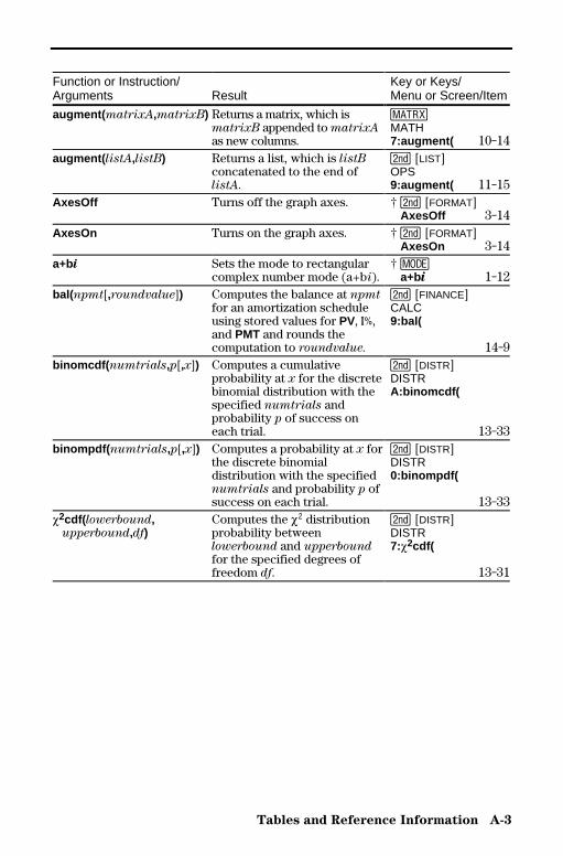
Tables and Reference Information A-3
8399APXA.DOC TI-83 international English Bob Fedorisko Revised: 02/19/01 1:25 PM Printed: 02/19/01 1:40 PMPage 3 of 58
Function or Instruction/Arguments Result
Key or Keys/Menu or Screen/Item
augment( matrixA,matrixB) Returns a matrix, which ismatrixB appended to matrixAas new columns.
�MATH7:augment( 10-14
augment( listA,listB) Returns a list, which is listBconcatenated to the end oflistA.
y [LIST]OPS9:augment( 11-15
AxesOff Turns off the graph axes. † y [FORMAT] AxesOff 3-14
AxesOn Turns on the graph axes. † y [FORMAT] AxesOn 3-14
a+bi Sets the mode to rectangularcomplex number mode (a+bi).
† z a+bi 1-12
bal(npmt[,roundvalue]) Computes the balance at npmtfor an amortization scheduleusing stored values for PV, æ,and PMT and rounds thecomputation to roundvalue.
y [FINANCE]CALC9:bal(
14-9binomcdf( numtrials,p[,x]) Computes a cumulative
probability at x for the discretebinomial distribution with thespecified numtrials andprobability p of success oneach trial.
y [DISTR]DISTRA:binomcdf(
13-33binompdf( numtrials,p[,x]) Computes a probability at x for
the discrete binomialdistribution with the specifiednumtrials and probability p ofsuccess on each trial.
y [DISTR]DISTR0:binompdf(
13-33c2cdf( lowerbound, upperbound,df)
Computes the c2 distributionprobability betweenlowerbound and upperboundfor the specified degrees offreedom df.
y [DISTR]DISTR7:c2cdf(
13-31
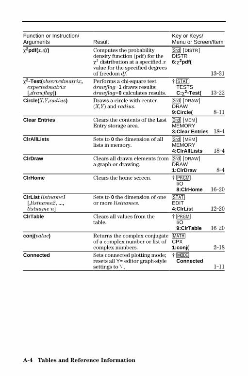
A-4 Tables and Reference Information
8399APXA.DOC TI-83 international English Bob Fedorisko Revised: 02/19/01 1:25 PM Printed: 02/19/01 1:40 PMPage 4 of 58
Function or Instruction/Arguments Result
Key or Keys/Menu or Screen/Item
c2pdf( x,df) Computes the probabilitydensity function (pdf) for thec2 distribution at a specified xvalue for the specified degreesof freedom df.
y [DISTR]DISTR6:c2pdf(
13-31c2.Test(observedmatrix, expectedmatrix [,drawflag])
Performs a chi-square test.drawflag=1 draws results;drawflag=0 calculates results.
† … TESTS C:c2.Test( 13-22
Circle( X,Y,radius) Draws a circle with center(X,Y) and radius.
y [DRAW]DRAW9:Circle( 8-11
Clear Entries Clears the contents of the LastEntry storage area.
y [MEM]MEMORY3:Clear Entries 18-4
ClrAllLists Sets to 0 the dimension of alllists in memory.
y [MEM]MEMORY4:ClrAllLists 18-4
ClrDraw Clears all drawn elements froma graph or drawing.
y [DRAW]DRAW1:ClrDraw 8-4
ClrHome Clears the home screen. † � I/O 8:ClrHome 16-20
ClrList listname1 [,listname2, ..., listname n]
Sets to 0 the dimension of oneor more listnames.
…EDIT4:ClrList 12-20
ClrTable Clears all values from thetable.
† � I/O 9:ClrTable 16-20
conj( value) Returns the complex conjugateof a complex number or list ofcomplex numbers.
�CPX1:conj( 2-18
Connected Sets connected plotting mode;resets all Y= editor graph-stylesettings to ç .
† z Connected
1-11
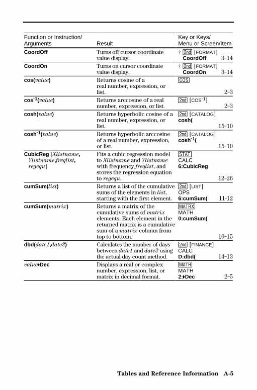
Tables and Reference Information A-5
8399APXA.DOC TI-83 international English Bob Fedorisko Revised: 02/19/01 1:25 PM Printed: 02/19/01 1:40 PMPage 5 of 58
Function or Instruction/Arguments Result
Key or Keys/Menu or Screen/Item
CoordOff Turns off cursor coordinatevalue display.
† y [FORMAT] CoordOff 3-14
CoordOn Turns on cursor coordinatevalue display.
† y [FORMAT] CoordOn 3-14
cos( value) Returns cosine of areal number, expression, orlist.
™
2-3cos L1(value) Returns arccosine of a real
number, expression, or list.y [COSL1]
2-3cosh( value) Returns hyperbolic cosine of a
real number, expression, orlist.
y [CATALOG]cosh(
15-10cosh L1(value) Returns hyperbolic arccosine
of a real number, expression,or list.
y [CATALOG]cosh L1(
15-10CubicReg [Xlistname, Ylistname,freqlist, regequ]
Fits a cubic regression modelto Xlistname and Ylistnamewith frequency freqlist, andstores the regression equationto regequ.
…CALC6:CubicReg
12-26cumSum( list) Returns a list of the cumulative
sums of the elements in list,starting with the first element.
y [LIST]OPS6:cumSum( 11-12
cumSum( matrix) Returns a matrix of thecumulative sums of matrixelements. Each element in thereturned matrix is a cumulativesum of a matrix column fromtop to bottom.
�MATH0:cumSum(
10-15dbd( date1,date2) Calculates the number of days
between date1 and date2 usingthe actual-day-count method.
y [FINANCE]CALCD:dbd( 14-13
value4Dec Displays a real or complexnumber, expression, list, ormatrix in decimal format.
�MATH2:4Dec 2-5

A-6 Tables and Reference Information
8399APXA.DOC TI-83 international English Bob Fedorisko Revised: 02/19/01 1:25 PM Printed: 02/19/01 1:40 PMPage 6 of 58
Function or Instruction/Arguments Result
Key or Keys/Menu or Screen/Item
Degree Sets degree angle mode. † z Degree 1-11
DelVar variable Deletes from memory thecontents of variable.
† � CTL G:DelVar 16-15
DependAsk Sets table to ask fordependent-variable values.
† y [TBLSET] Depend: Ask 7-3
DependAuto Sets table to generatedependent-variable valuesautomatically.
† y [TBLSET] Depend: Auto
7-3det(matrix) Returns determinant of
matrix.�MATH1:det( 10-12
DiagnosticOff Sets diagnostics-off mode; r, r2,and R2 are not displayed asregression model results.
y [CATALOG]DiagnosticOff
12-23DiagnosticOn Sets diagnostics-on mode; r, r2,
and R2 are displayed asregression model results.
y [CATALOG]DiagnosticOn
12-23dim( listname) Returns the dimension of
listname.y [LIST]OPS3:dim( 11-11
dim( matrixname) Returns the dimension ofmatrixname as a list.
�MATH3:dim( 10-12
length!dim( listname) Assigns a new dimension(length) to a new or existinglistname.
y [LIST]OPS3:dim( 11-11
{rows,columns}! dim( matrixname)
Assigns new dimensions to anew or existing matrixname.
�MATH3:dim( 10-13
Disp Displays the home screen. † � I/O 3:Disp 16-18
Disp [valueA,valueB, valueC,...,value n]
Displays each value. † � I/O 3:Disp 16-18
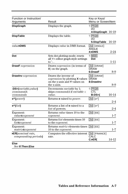
Tables and Reference Information A-7
8399APXA.DOC TI-83 international English Bob Fedorisko Revised: 02/19/01 1:25 PM Printed: 02/19/01 1:40 PMPage 7 of 58
Function or Instruction/Arguments Result
Key or Keys/Menu or Screen/Item
DispGraph Displays the graph. † � I/O 4:DispGraph 16-19
DispTable Displays the table. † � I/O 5:DispTable 16-19
value4DMS Displays value in DMS format. y [ANGLE]ANGLE4:4DMS 2-24
Dot Sets dot plotting mode; resetsall Y= editor graph-style settingsto í .
† z Dot
1-11DrawF expression Draws expression (in terms of
X) on the graph.y [DRAW]DRAW6:DrawF 8-9
DrawInv expression Draws the inverse ofexpression by plotting X valueson the y-axis and Y values onthe x-axis.
y [DRAW]DRAW8:DrawInv
8-9:DS<(variable,value):commandA:commands
Decrements variable by 1;skips commandA if variable <value.
† � CTL B:DS<( 16-14
e^(power) Returns e raised to power. y [ex]2-4
e^( list) Returns a list of e raised to alist of powers.
y [ex]2-4
Exponent: valueEexponent
Returns value times 10 to theexponent.
y [EE]1-7
Exponent: listEexponent
Returns list elements times 10to the exponent.
y [EE]1-7
Exponent: matrixEexponent
Returns matrix elements times10 to the exponent.
y [EE]1-7
4Eff(nominal rate, compounding periods)
Computes the effective interestrate.
y [FINANCE]CALCC:4Eff( 14-12
Else See If:Then:Else
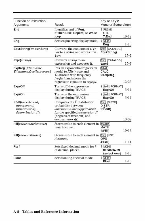
A-8 Tables and Reference Information
8399APXA.DOC TI-83 international English Bob Fedorisko Revised: 02/19/01 1:25 PM Printed: 02/19/01 1:40 PMPage 8 of 58
Function or Instruction/Arguments Result
Key or Keys/Menu or Screen/Item
End Identifies end of For( ,If-Then -Else , Repeat , or Whileloop.
† � CTL 7:End 16-12
Eng Sets engineering display mode. † z Eng 1-10
Equ4String( Y= var,Strn) Converts the contents of a Y=var to a string and stores it inStrn.
y [CATALOG]Equ4String(
15-7expr( string) Converts string to an
expression and executes it.y [CATALOG]expr( 15-7
ExpReg [Xlistname,Ylistname,freqlist,regequ]
Fits an exponential regressionmodel to Xlistname andYlistname with frequencyfreqlist, and stores theregression equation to regequ.
…CALC0:ExpReg
12-26ExprOff Turns off the expression
display during TRACE.† y [FORMAT] ExprOff 3-14
ExprOn Turns on the expressiondisplay during TRACE.
† y [FORMAT] ExprOn 3-14
Ücdf( lowerbound, upperbound, numerator df, denominator df)
Computes the Û distributionprobability betweenlowerbound and upperboundfor the specified numerator df(degrees of freedom) anddenominator df.
y [DISTR]DISTR9:Ûcdf(
13-32Fill( value,matrixname) Stores value to each element in
matrixname.�MATH4:Fill( 10-13
Fill( value,listname) Stores value to each element inlistname.
y [LIST]OPS4:Fill( 11-11
Fix # Sets fixed-decimal mode for #of decimal places.
† z 0123456789 (select one) 1-10
Float Sets floating decimal mode. † z Float 1-10
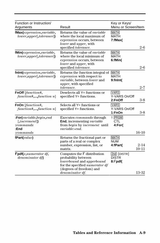
Tables and Reference Information A-9
8399APXA.DOC TI-83 international English Bob Fedorisko Revised: 02/19/01 1:25 PM Printed: 02/19/01 1:40 PMPage 9 of 58
Function or Instruction/Arguments Result
Key or Keys/Menu or Screen/Item
fMax(expression,variable, lower,upper[,tolerance])
Returns the value of variablewhere the local maximum ofexpression occurs, betweenlower and upper, withspecified tolerance.
�MATH7:fMax(
2-6fMin( expression,variable, lower,upper[,tolerance])
Returns the value of variablewhere the local minimum ofexpression occurs, betweenlower and upper, withspecified tolerance.
�MATH6:fMin(
2-6fnInt( expression,variable, lower,upper[,tolerance])
Returns the function integral ofexpression with respect tovariable, between lower andupper, with specifiedtolerance.
�MATH9:fnInt(
2-7FnOff [function#, function#,...,function n]
Deselects all Y= functions orspecified Y= functions.
�Y-VARS On/Off2:FnOff 3-8
FnOn [function#, function#,...,function n]
Selects all Y= functions orspecified Y= functions.
�Y-VARS On/Off1:FnOn 3-8
:For( variable,begin,end [,increment]):commands:End:commands
Executes commands throughEnd , incrementing variablefrom begin by increment untilvariable>end.
† � CTL 4:For(
16-10fPart( value) Returns the fractional part or
parts of a real or complexnumber, expression, list, ormatrix.
�NUM4:fPart( 2-14
10-11Üpdf( x,numerator df, denominator df)
Computes the Û distributionprobability betweenlowerbound and upperboundfor the specified numerator df(degrees of freedom) anddenominator df.
y [DISTR]DISTR8:Ûpdf(
13-32
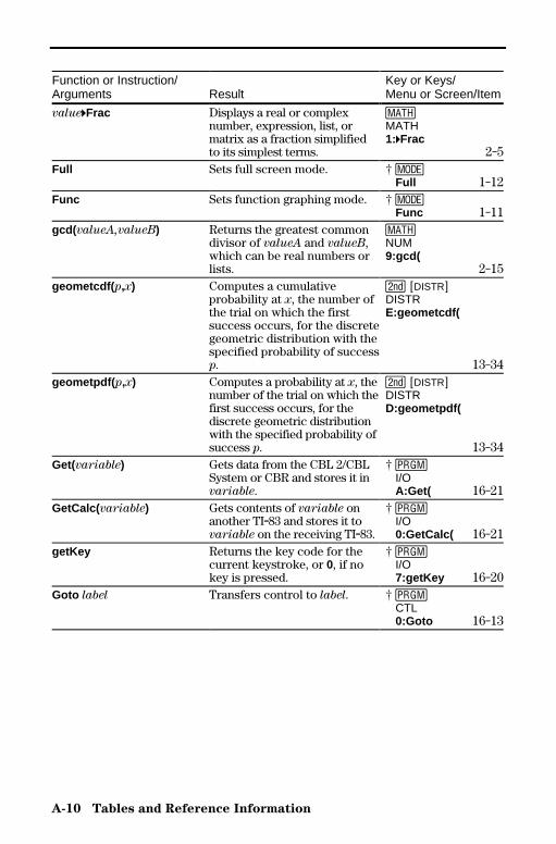
A-10 Tables and Reference Information
8399APXA.DOC TI-83 international English Bob Fedorisko Revised: 02/19/01 1:25 PM Printed: 02/19/01 1:40 PMPage 10 of 58
Function or Instruction/Arguments Result
Key or Keys/Menu or Screen/Item
value4Frac Displays a real or complexnumber, expression, list, ormatrix as a fraction simplifiedto its simplest terms.
�MATH1:4Frac
2-5Full Sets full screen mode. † z
Full 1-12Func Sets function graphing mode. † z
Func 1-11gcd( valueA,valueB) Returns the greatest common
divisor of valueA and valueB,which can be real numbers orlists.
�NUM9:gcd(
2-15geometcdf( p,x) Computes a cumulative
probability at x, the number ofthe trial on which the firstsuccess occurs, for the discretegeometric distribution with thespecified probability of successp.
y [DISTR]DISTRE:geometcdf(
13-34geometpdf( p,x) Computes a probability at x, the
number of the trial on which thefirst success occurs, for thediscrete geometric distributionwith the specified probability ofsuccess p.
y [DISTR]DISTRD:geometpdf(
13-34Get(variable) Gets data from the CBL 2/CBL
System or CBR and stores it invariable.
† � I/O A:Get( 16-21
GetCalc( variable) Gets contents of variable onanother TI.83 and stores it tovariable on the receiving TI.83.
† � I/O 0:GetCalc( 16-21
getKey Returns the key code for thecurrent keystroke, or 0, if nokey is pressed.
† � I/O 7:getKey 16-20
Goto label Transfers control to label. † � CTL 0:Goto 16-13
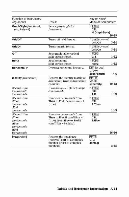
Tables and Reference Information A-11
8399APXA.DOC TI-83 international English Bob Fedorisko Revised: 02/19/01 1:25 PM Printed: 02/19/01 1:40 PMPage 11 of 58
Function or Instruction/Arguments Result
Key or Keys/Menu or Screen/Item
GraphStyle( function#, graphstyle#)
Sets a graphstyle forfunction#.
† � CTL H:GraphStyle(
16-15GridOff Turns off grid format. † y [FORMAT]
GridOff 3-14GridOn Turns on grid format. † y [FORMAT]
GridOn 3-14G-T Sets graph-table vertical
split-screen mode.† z G-T 1-12
Horiz Sets horizontalsplit-screen mode.
† z Horiz 1-12
Horizontal y Draws a horizontal line at y. y [DRAW]DRAW3:Horizontal 8-6
identity( dimension) Returns the identity matrix ofdimension rows × dimensioncolumns.
�MATH5:identity( 10-13
:If condition:commandA:commands
If condition = 0 (false), skipscommandA.
† � CTL 1:If 16-9
:If condition:Then:commands:End:commands
Executes commands fromThen to End if condition = 1(true).
† � CTL 2:Then
16-9:If condition:Then:commands:Else:commands:End:commands
Executes commands fromThen to Else if condition = 1(true); from Else to End ifcondition = 0 (false).
† � CTL 3:Else
16-10imag( value) Returns the imaginary
(nonreal) part of a complexnumber or list of complexnumbers.
�CPX3:imag(
2-18
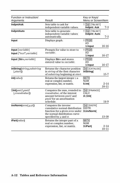
A-12 Tables and Reference Information
8399APXA.DOC TI-83 international English Bob Fedorisko Revised: 02/19/01 1:25 PM Printed: 02/19/01 1:40 PMPage 12 of 58
Function or Instruction/Arguments Result
Key or Keys/Menu or Screen/Item
IndpntAsk Sets table to ask forindependent-variable values.
† y [TBLSET] Indpnt: Ask 7-3
IndpntAuto Sets table to generateindependent-variable valuesautomatically.
† y [TBLSET] Indpnt: Auto
7-3Input Displays graph. † �
I/O 1:Input 16-16
Input [variable]Input [" text",variable]
Prompts for value to store tovariable.
† � I/O 1:Input 16-17
Input [Strn,variable] Displays Strn and storesentered value to variable.
† � I/O 1:Input 16-17
inString( string,substring [,start])
Returns the character positionin string of the first characterof substring beginning at start.
y [CATALOG]inString(
15-7int( value) Returns the largest integer � a
real or complex number,expression, list, or matrix.
�NUM5:int( 2-14
10-11GInt(pmt1,pmt2 [,roundvalue])
Computes the sum, rounded toroundvalue, of the interestamount between pmt1 andpmt2 for an amortizationschedule.
y [FINANCE]CALCA:GInt(
14-9invNorm( area[,m,s]) Computes the inverse
cumulative normal distributionfunction for a given area underthe normal distribution curvespecified by m and s.
y [DISTR]DISTR3:invNorm(
13-30iPart( value) Returns the integer part of a
real or complex number,expression, list, or matrix.
�NUM3:iPart( 2-14
10-11
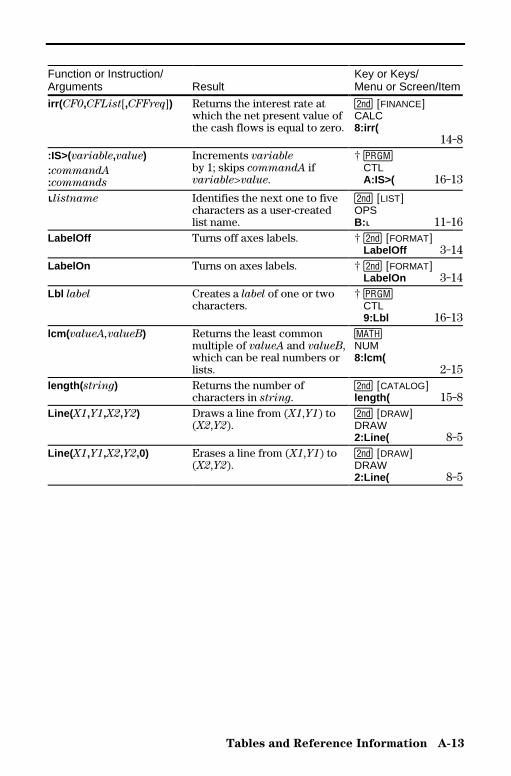
Tables and Reference Information A-13
8399APXA.DOC TI-83 international English Bob Fedorisko Revised: 02/19/01 1:25 PM Printed: 02/19/01 1:40 PMPage 13 of 58
Function or Instruction/Arguments Result
Key or Keys/Menu or Screen/Item
irr( CF0,CFList[,CFFreq]) Returns the interest rate atwhich the net present value ofthe cash flows is equal to zero.
y [FINANCE]CALC8:irr(
14-8:IS>(variable,value):commandA:commands
Increments variableby 1; skips commandA ifvariable>value.
† � CTL A:IS>( 16-13
Ùlistname Identifies the next one to fivecharacters as a user-createdlist name.
y [LIST]OPSB: Ù 11-16
LabelOff Turns off axes labels. † y [FORMAT] LabelOff 3-14
LabelOn Turns on axes labels. † y [FORMAT] LabelOn 3-14
Lbl label Creates a label of one or twocharacters.
† � CTL 9:Lbl 16-13
lcm( valueA,valueB) Returns the least commonmultiple of valueA and valueB,which can be real numbers orlists.
�NUM8:lcm(
2-15length( string) Returns the number of
characters in string.y [CATALOG]length( 15-8
Line( X1,Y1,X2,Y2) Draws a line from (X1,Y1) to(X2,Y2).
y [DRAW]DRAW2:Line( 8-5
Line( X1,Y1,X2,Y2,0) Erases a line from (X1,Y1) to(X2,Y2).
y [DRAW]DRAW2:Line( 8-5
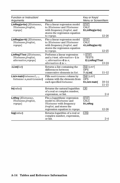
A-14 Tables and Reference Information
8399APXA.DOC TI-83 international English Bob Fedorisko Revised: 02/19/01 1:25 PM Printed: 02/19/01 1:40 PMPage 14 of 58
Function or Instruction/Arguments Result
Key or Keys/Menu or Screen/Item
LinReg(a+bx) [Xlistname, Ylistname,freqlist, regequ]
Fits a linear regression modelto Xlistname and Ylistnamewith frequency freqlist, andstores the regression equationto regequ.
…CALC8:LinReg(a+bx)
12-26LinReg(ax+b) [Xlistname, Ylistname,freqlist, regequ]
Fits a linear regression modelto Xlistname and Ylistnamewith frequency freqlist, andstores the regression equationto regequ.
…CALC4:LinReg(ax+b)
12-25LinRegTTest [Xlistname, Ylistname,freqlist, alternative,regequ]
Performs a linear regressionand a t-test. alternative=L1 is<; alternative=0 is ƒ;alternative=1 is >.
† … TESTS E:LinRegTTest
13-24@List( list) Returns a list containing the
differences betweenconsecutive elements in list.
y [LIST]OPS7:@List( 11-12
List 4 matr( listname1,..., listname n,matrixname)
Fills matrixname column bycolumn with the elements fromeach specified listname.
y [LIST]OPS0:List 4 matr( 10-14
11-15ln(value) Returns the natural logarithm
of a real or complex number,expression, or list.
µ
2-4LnReg [Xlistname, Ylistname,freqlist, regequ]
Fits a logarithmic regressionmodel to Xlistname andYlistname with frequencyfreqlist, and stores theregression equation to regequ.
…CALC9:LnReg
12-26log( value) Returns logarithm of a real or
complex number, expression,or list.
«
2-4
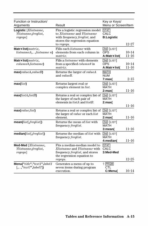
Tables and Reference Information A-15
8399APXA.DOC TI-83 international English Bob Fedorisko Revised: 02/19/01 1:25 PM Printed: 02/19/01 1:40 PMPage 15 of 58
Function or Instruction/Arguments Result
Key or Keys/Menu or Screen/Item
Logistic [Xlistname, Ylistname,freqlist, regequ]
Fits a logistic regression modelto Xlistname and Ylistnamewith frequency freqlist, andstores the regression equationto regequ.
…CALCB:Logistic
12-27Matr 4 list( matrix, listnameA,...,listname n)
Fills each listname withelements from each column inmatrix.
y [LIST]OPS 10-14A:Matr 4 list( 11-16
Matr 4 list( matrix, column#,listname)
Fills a listname with elementsfrom a specified column# inmatrix.
y [LIST]OPS 10-14A:Matr 4 list( 11-16
max(valueA,valueB) Returns the larger of valueAand valueB.
�NUM7:max( 2-15
max( list) Returns largest real orcomplex element in list.
y [LIST]MATH2:max( 11-16
max( listA,listB) Returns a real or complex list ofthe larger of each pair ofelements in listA and listB.
y [LIST]MATH2:max(
11-16max(value,list) Returns a real or complex list of
the larger of value or each listelement.
y [LISTäMATH2:max( 11-16
mean( list[,freqlist]) Returns the mean of list withfrequency freqlist.
y [LIST]MATH3:mean( 11-16
median( list[,freqlist]) Returns the median of list withfrequency freqlist.
y [LIST]MATH4:median( 11-16
Med-Med [Xlistname, Ylistname,freqlist, regequ]
Fits a median-median model toXlistname and Ylistname withfrequency freqlist, and storesthe regression equation toregequ.
…CALC3:Med-Med
12-25Menu(" title"," text1", label1 [,...," text7", label7])
Generates a menu of up toseven items during programexecution.
† � CTL C:Menu( 16-14
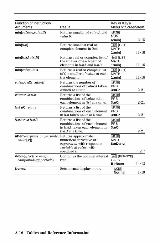
A-16 Tables and Reference Information
8399APXA.DOC TI-83 international English Bob Fedorisko Revised: 02/19/01 1:25 PM Printed: 02/19/01 1:40 PMPage 16 of 58
Function or Instruction/Arguments Result
Key or Keys/Menu or Screen/Item
min( valueA,valueB) Returns smaller of valueA andvalueB.
�NUM6:min( 2-15
min( list) Returns smallest real orcomplex element in list.
y [LIST]MATH1:min( 11-16
min( listA,listB) Returns real or complex list ofthe smaller of each pair ofelements in listA and listB.
y [LIST]MATH1:min( 11-16
min( value,list) Returns a real or complex listof the smaller of value or eachlist element.
y [LIST]MATH1:min( 11-16
valueA nCr valueB Returns the number ofcombinations of valueA takenvalueB at a time.
�PRB3:nCr 2-21
value nCr list Returns a list of thecombinations of value takeneach element in list at a time.
�PRB3:nCr 2-21
list nCr value Returns a list of thecombinations of each elementin list taken value at a time.
�PRB3:nCr 2-21
listA nCr listB Returns a list of thecombinations of each elementin listA taken each element inlistB at a time.
�PRB3:nCr
2-21nDeriv( expression,variable, value[,H])
Returns approximatenumerical derivative ofexpression with respect tovariable at value, withspecified H.
�MATH8:nDeriv(
2-74Nom(effective rate, compounding periods)
Computes the nominal interestrate.
y [FINANCE]CALCB:4Nom( 14-12
Normal Sets normal display mode. † z Normal 1-10
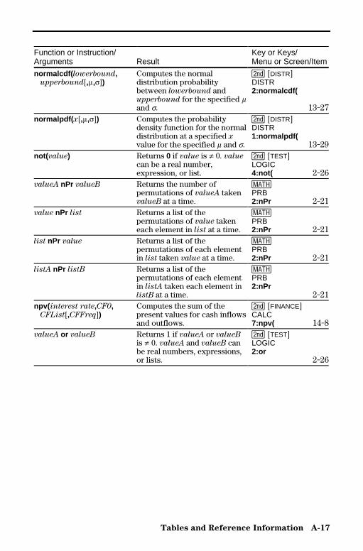
Tables and Reference Information A-17
8399APXA.DOC TI-83 international English Bob Fedorisko Revised: 02/19/01 1:25 PM Printed: 02/19/01 1:40 PMPage 17 of 58
Function or Instruction/Arguments Result
Key or Keys/Menu or Screen/Item
normalcdf( lowerbound, upperbound[,m,s])
Computes the normaldistribution probabilitybetween lowerbound andupperbound for the specified mand s.
y [DISTR]DISTR2:normalcdf(
13-27normalpdf( x[,m,s]) Computes the probability
density function for the normaldistribution at a specified xvalue for the specified m and s.
y [DISTR]DISTR1:normalpdf(
13-29not( value) Returns 0 if value is ƒ 0. value
can be a real number,expression, or list.
y [TEST]LOGIC4:not( 2-26
valueA nPr valueB Returns the number ofpermutations of valueA takenvalueB at a time.
�PRB2:nPr 2-21
value nPr list Returns a list of thepermutations of value takeneach element in list at a time.
�PRB2:nPr 2-21
list nPr value Returns a list of thepermutations of each elementin list taken value at a time.
�PRB2:nPr 2-21
listA nPr listB Returns a list of thepermutations of each elementin listA taken each element inlistB at a time.
�PRB2:nPr
2-21npv( interest rate,CF0, CFList[,CFFreq])
Computes the sum of thepresent values for cash inflowsand outflows.
y [FINANCE]CALC7:npv( 14-8
valueA or valueB Returns 1 if valueA or valueBis ƒ 0. valueA and valueB canbe real numbers, expressions,or lists.
y [TEST]LOGIC2:or
2-26

A-18 Tables and Reference Information
8399APXA.DOC TI-83 international English Bob Fedorisko Revised: 02/19/01 1:25 PM Printed: 02/19/01 1:40 PMPage 18 of 58
Function or Instruction/Arguments Result
Key or Keys/Menu or Screen/Item
Output( row,column," text") Displays text beginning atspecified row and column.
† � I/O 6:Output( 16-19
Output( row,column,value) Displays value beginning atspecified row and column.
† � I/O 6:Output( 16-19
Param Sets parametric graphingmode.
† z Par 1-11
Pause Suspends program executionuntil you press Í.
† � CTL 8:Pause 16-12
Pause [value] Displays value; suspendsprogram execution until youpress Í.
† � CTL 8:Pause 16-12
Plot #(type,Xlistname, Ylistname,mark)
Defines Plot # (1, 2, or 3) oftype Scatter or xyLine forXlistname and Ylistnameusing mark.
† y [STAT PLOT] PLOTS 1:Plot1( 2:Plot2( 3:Plot3( 12-37
Plot #(type,Xlistname, freqlist)
Defines Plot # (1, 2, or 3) oftype Histogram or Boxplot forXlistname with frequencyfreqlist.
† y [STAT PLOT] PLOTS 1:Plot1( 2:Plot2( 3:Plot3( 12-37
Plot #(type,Xlistname, freqlist,mark)
Defines Plot # (1, 2, or 3) oftype ModBoxplot forXlistname with frequencyfreqlist using mark.
† y [STAT PLOT] PLOTS 1:Plot1( 2:Plot2( 3:Plot3( 12-37
Plot #(type,datalistname, data axis,mark)
Defines Plot # (1, 2, or 3) oftype NormProbPlot fordatalistname on data axisusing mark. data axis can be Xor Y.
† y [STAT PLOT] PLOTS 1:Plot1( 2:Plot2( 3:Plot3( 12-37
PlotsOff [1,2,3] Deselects all stat plots or oneor more specified stat plots (1,2, or 3).
y [STAT PLOT]STAT PLOTS4:PlotsOff 12-35
PlotsOn [1,2,3] Selects all stat plots or one ormore specified stat plots (1, 2,or 3).
y [STAT PLOT]STAT PLOTS5:PlotsOn 12-35
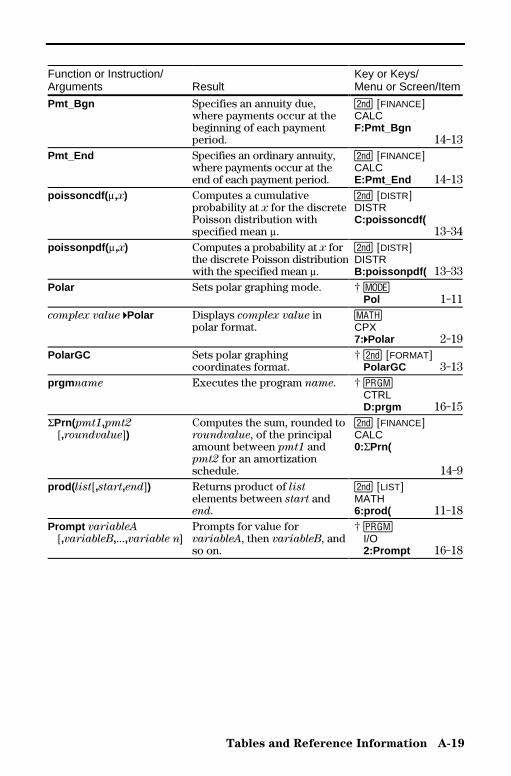
Tables and Reference Information A-19
8399APXA.DOC TI-83 international English Bob Fedorisko Revised: 02/19/01 1:25 PM Printed: 02/19/01 1:40 PMPage 19 of 58
Function or Instruction/Arguments Result
Key or Keys/Menu or Screen/Item
Pmt_Bgn Specifies an annuity due,where payments occur at thebeginning of each paymentperiod.
y [FINANCE]CALCF:Pmt_Bgn
14-13Pmt_End Specifies an ordinary annuity,
where payments occur at theend of each payment period.
y [FINANCE]CALCE:Pmt_End 14-13
poissoncdf( m,x) Computes a cumulativeprobability at x for the discretePoisson distribution withspecified mean m.
y [DISTR]DISTRC:poissoncdf(
13-34poissonpdf( m,x) Computes a probability at x for
the discrete Poisson distributionwith the specified mean m.
y [DISTR]DISTRB:poissonpdf( 13-33
Polar Sets polar graphing mode. † z Pol 1-11
complex value 4Polar Displays complex value inpolar format.
�CPX7:4Polar 2-19
PolarGC Sets polar graphingcoordinates format.
† y [FORMAT] PolarGC 3-13
prgm name Executes the program name. † � CTRL D:prgm 16-15
GPrn(pmt1,pmt2 [,roundvalue])
Computes the sum, rounded toroundvalue, of the principalamount between pmt1 andpmt2 for an amortizationschedule.
y [FINANCE]CALC0:GPrn(
14-9prod( list[,start,end]) Returns product of list
elements between start andend.
y [LIST]MATH6:prod( 11-18
Prompt variableA [,variableB,...,variable n]
Prompts for value forvariableA, then variableB, andso on.
† � I/O 2:Prompt 16-18
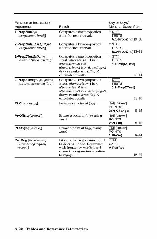
A-20 Tables and Reference Information
8399APXA.DOC TI-83 international English Bob Fedorisko Revised: 02/19/01 1:25 PM Printed: 02/19/01 1:40 PMPage 20 of 58
Function or Instruction/Arguments Result
Key or Keys/Menu or Screen/Item
1.PropZInt( x,n [,confidence level])
Computes a one-proportionz confidence interval.
† … TESTS A:1.PropZInt( 13-20
2.PropZInt( x1,n1,x2,n2 [,confidence level])
Computes a two-proportionz confidence interval.
† … TESTS B:2.PropZInt( 13-21
1.PropZTest( p0,x,n [,alternative,drawflag])
Computes a one-proportionz test. alternative=L1 is <;alternative=0 is ƒ;alternative=1 is >. drawflag=1draws results; drawflag=0calculates results.
† … TESTS 5:1.PropZTest(
13-142.PropZTest( x1,n1,x2,n2 [,alternative,drawflag])
Computes a two-proportionz test. alternative=L1 is <;alternative=0 is ƒ;alternative=1 is >. drawflag=1draws results; drawflag=0calculates results.
† … TESTS 6:2.PropZTest(
13-15Pt.Change( x,y) Reverses a point at (x,y). y [DRAW]
POINTS3:Pt.Change( 8-15
Pt.Off(x,y[,mark]) Erases a point at (x,y) usingmark.
y [DRAW]POINTS2:Pt.Off( 8-15
Pt.On(x,y[,mark]) Draws a point at (x,y) usingmark.
y [DRAW]POINTS1:Pt.On( 8-14
PwrReg [Xlistname, Ylistname,freqlist, regequ]
Fits a power regression modelto Xlistname and Ylistnamewith frequency freqlist, andstores the regression equationto regequ.
…CALCA:PwrReg
12-27
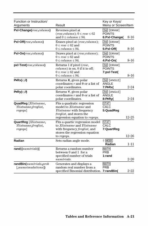
Tables and Reference Information A-21
8399APXA.DOC TI-83 international English Bob Fedorisko Revised: 02/19/01 1:25 PM Printed: 02/19/01 1:40 PMPage 21 of 58
Function or Instruction/Arguments Result
Key or Keys/Menu or Screen/Item
Pxl.Change( row,column) Reverses pixel at(row,column); 0 � row � 62and 0 � column � 94.
y [DRAWäPOINTS6:Pxl .Change( 8-16
Pxl.Off(row,column) Erases pixel at (row,column);0 � row � 62 and0 � column � 94.
y [DRAW]POINTS5:Pxl .Off( 8-16
Pxl.On(row,column) Draws pixel at (row,column);0 � row � 62 and0 � column � 94.
y [DRAW]POINTS4:Pxl .On( 8-16
pxl .Test(row,column) Returns 1 if pixel (row,column) is on, 0 if it is off;0 � row � 62 and0 � column � 94.
y [DRAW]POINTS7:pxl .Test(
8-16P4Rx(r,q) Returns X, given polar
coordinates r and q or a list ofpolar coordinates.
y [ANGLE]ANGLE7:P4Rx( 2-24
P4Ry(r,q) Returns Y, given polarcoordinates r and q or a list ofpolar coordinates.
y [ANGLE]ANGLE8:P4Ry( 2-24
QuadReg [Xlistname, Ylistname,freqlist, regequ]
Fits a quadratic regressionmodel to Xlistname andYlistname with frequencyfreqlist, and stores theregression equation to regequ.
…CALC5:QuadReg
12-25QuartReg [Xlistname, Ylistname,freqlist, regequ]
Fits a quartic regression modelto Xlistname and Ylistnamewith frequency freqlist, andstores the regression equationto regequ.
…CALC7:QuartReg
12-26Radian Sets radian angle mode. † z
Radian 1-11rand [(numtrials)] Returns a random number
between 0 and 1 for aspecified number of trialsnumtrials.
�PRB1:rand
2-20randBin( numtrials,prob [,numsimulations])
Generates and displays arandom real number from aspecified Binomial distribution.
�PRB7:randBin( 2-22
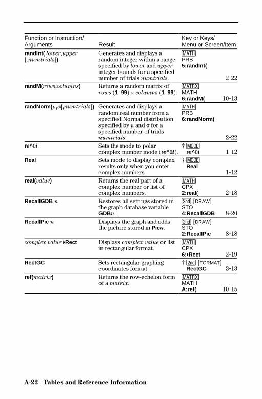
A-22 Tables and Reference Information
8399APXA.DOC TI-83 international English Bob Fedorisko Revised: 02/19/01 1:25 PM Printed: 02/19/01 1:40 PMPage 22 of 58
Function or Instruction/Arguments Result
Key or Keys/Menu or Screen/Item
randInt( lower,upper[,numtrials])
Generates and displays arandom integer within a rangespecified by lower and upperinteger bounds for a specifiednumber of trials numtrials.
�PRB5:randInt(
2-22randM( rows,columns) Returns a random matrix of
rows (1–99) × columns (1–99).�MATH6:randM( 10-13
randNorm( m,s[,numtrials]) Generates and displays arandom real number from aspecified Normal distributionspecified by m and s for aspecified number of trialsnumtrials.
�PRB6:randNorm(
2-22re^qi Sets the mode to polar
complex number mode (re^qi).† z re^qi 1-12
Real Sets mode to display complexresults only when you entercomplex numbers.
† z Real
1-12real(value) Returns the real part of a
complex number or list ofcomplex numbers.
�CPX2:real( 2-18
RecallGDB n Restores all settings stored inthe graph database variableGDBn.
y [DRAW]STO4:RecallGDB 8-20
RecallPic n Displays the graph and addsthe picture stored in Picn.
y [DRAW]STO2:RecallPic 8-18
complex value 4Rect Displays complex value or listin rectangular format.
�CPX6:4Rect 2-19
RectGC Sets rectangular graphingcoordinates format.
† y [FORMAT] RectGC 3-13
ref(matrix) Returns the row-echelon formof a matrix.
�MATHA:ref( 10-15
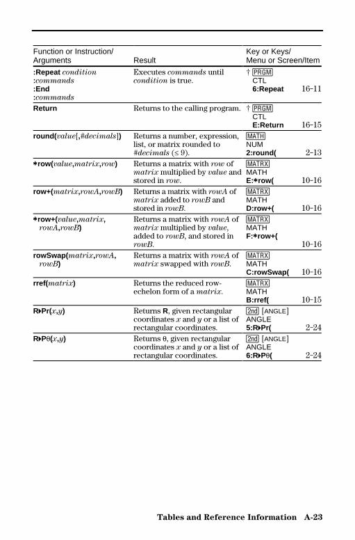
Tables and Reference Information A-23
8399APXA.DOC TI-83 international English Bob Fedorisko Revised: 02/19/01 1:25 PM Printed: 02/19/01 1:40 PMPage 23 of 58
Function or Instruction/Arguments Result
Key or Keys/Menu or Screen/Item
:Repeat condition:commands:End:commands
Executes commands untilcondition is true.
† � CTL 6:Repeat 16-11
Return Returns to the calling program. † � CTL E:Return 16-15
round( value[,#decimals]) Returns a number, expression,list, or matrix rounded to#decimals (� 9).
�NUM2:round( 2-13
ärow( value,matrix,row) Returns a matrix with row ofmatrix multiplied by value andstored in row.
�MATHE:ärow( 10-16
row+( matrix,rowA,rowB) Returns a matrix with rowA ofmatrix added to rowB andstored in rowB.
�MATHD:row+( 10-16
ärow+( value,matrix, rowA,rowB)
Returns a matrix with rowA ofmatrix multiplied by value,added to rowB, and stored inrowB.
�MATHF:ärow+(
10-16rowSwap( matrix,rowA, rowB)
Returns a matrix with rowA ofmatrix swapped with rowB.
�MATHC:rowSwap( 10-16
rref( matrix) Returns the reduced row-echelon form of a matrix.
�MATHB:rref( 10-15
R4Pr(x,y) Returns R, given rectangularcoordinates x and y or a list ofrectangular coordinates.
y [ANGLE]ANGLE5:R4Pr( 2-24
R4Pq(x,y) Returns q, given rectangularcoordinates x and y or a list ofrectangular coordinates.
y [ANGLE]ANGLE6:R4Pq( 2-24
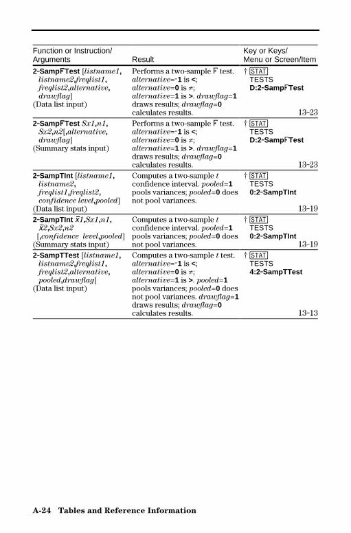
A-24 Tables and Reference Information
8399APXA.DOC TI-83 international English Bob Fedorisko Revised: 02/19/01 1:25 PM Printed: 02/19/01 1:40 PMPage 24 of 58
Function or Instruction/Arguments Result
Key or Keys/Menu or Screen/Item
2.SampÜTest [listname1, listname2,freqlist1, freqlist2,alternative, drawflag](Data list input)
Performs a two-sample Û test.alternative=L1 is <;alternative=0 is ƒ;alternative=1 is >. drawflag=1draws results; drawflag=0calculates results.
† … TESTS D:2.SampÛTest
13-232.SampÜTest Sx1,n1, Sx2,n2[,alternative, drawflag](Summary stats input)
Performs a two-sample Û test.alternative=L1 is <;alternative=0 is ƒ;alternative=1 is >. drawflag=1draws results; drawflag=0calculates results.
† … TESTS D:2.SampÛTest
13-232.SampTInt [listname1, listname2, freqlist1,freqlist2, confidence level,pooled](Data list input)
Computes a two-sample tconfidence interval. pooled=1pools variances; pooled=0 doesnot pool variances.
† … TESTS 0:2.SampTInt
13-192.SampTInt v1,Sx1,n1, v2,Sx2,n2 [,confidence level,pooled](Summary stats input)
Computes a two-sample tconfidence interval. pooled=1pools variances; pooled=0 doesnot pool variances.
† … TESTS 0:2.SampTInt
13-192.SampTTest [listname1, listname2,freqlist1, freqlist2,alternative, pooled,drawflag](Data list input)
Computes a two-sample t test.alternative=L1 is <;alternative=0 is ƒ;alternative=1 is >. pooled=1pools variances; pooled=0 doesnot pool variances. drawflag=1draws results; drawflag=0calculates results.
† … TESTS 4:2.SampTTest
13-13
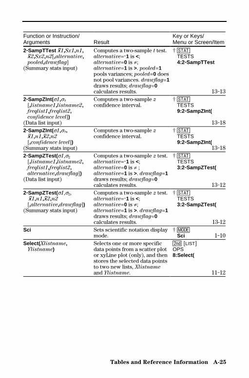
Tables and Reference Information A-25
8399APXA.DOC TI-83 international English Bob Fedorisko Revised: 02/19/01 1:25 PM Printed: 02/19/01 1:40 PMPage 25 of 58
Function or Instruction/Arguments Result
Key or Keys/Menu or Screen/Item
2.SampTTest v1,Sx1,n1, v2,Sx2,n2[,alternative, pooled,drawflag](Summary stats input)
Computes a two-sample t test.alternative=L1 is <;alternative=0 is ƒ;alternative=1 is >. pooled=1pools variances; pooled=0 doesnot pool variances. drawflag=1draws results; drawflag=0calculates results.
† … TESTS 4:2.SampTTest
13-132.SampZInt( s1,s2 [,listname1,listname2, freqlist1,freqlist2, confidence level])(Data list input)
Computes a two-sample zconfidence interval.
† … TESTS 9:2.SampZInt(
13-182.SampZInt( s1,s2, v1,n1,v2,n2 [,confidence level])(Summary stats input)
Computes a two-sample zconfidence interval.
† … TESTS 9:2.SampZInt(
13-182.SampZTest( s1,s2 [,listname1,listname2, freqlist1,freqlist2, alternative,drawflag])(Data list input)
Computes a two-sample z test.alternative=L1 is <;alternative=0 is ƒ ;alternative=1 is >. drawflag=1draws results; drawflag=0calculates results.
† … TESTS 3:2.SampZTest(
13-122.SampZTest( s1,s2, v1,n1,v2,n2 [,alternative,drawflag])(Summary stats input)
Computes a two-sample z test.alternative=L1 is <;alternative=0 is ƒ;alternative=1 is >. drawflag=1draws results; drawflag=0calculates results.
† … TESTS 3:2.SampZTest(
13-12Sci Sets scientific notation display
mode.† z Sci 1-10
Select( Xlistname, Ylistname)
Selects one or more specificdata points from a scatter plotor xyLine plot (only), and thenstores the selected data pointsto two new lists, Xlistnameand Ylistname.
y [LIST]OPS8:Select(
11-12

A-26 Tables and Reference Information
8399APXA.DOC TI-83 international English Bob Fedorisko Revised: 02/19/01 1:25 PM Printed: 02/19/01 1:40 PMPage 26 of 58
Function or Instruction/Arguments Result
Key or Keys/Menu or Screen/Item
Send(variable) Sends contents of variable tothe CBL 2/CBL System or CBR.
† � I/O B:Send( 16-21
seq(expression,variable, begin,end[,increment])
Returns list created byevaluating expression withregard to variable, from beginto end by increment.
y [LIST]OPS5:seq(
11-11Seq Sets sequence graphing mode. † z
Seq 1-11Sequential Sets mode to graph functions
sequentially.† z Sequential 1-12
SetUpEditor Removes all list names fromthe stat list editor, and thenrestores list names L1 throughL6 to columns 1 through 6.
…EDIT5:SetUpEditor
12-21SetUpEditor listname1 [,listname2,..., listname20]
Removes all list names fromthe stat list editor, then sets itup to display one or morelistnames in the specifiedorder, starting with column 1.
…EDIT5:SetUpEditor
12-21Shade( lowerfunc, upperfunc[,Xleft,Xright, pattern,patres])
Draws lowerfunc andupperfunc in terms of X on thecurrent graph and usespattern and patres to shade thearea bounded by lowerfunc,upperfunc, Xleft, and Xright.
y [DRAW]DRAW7:Shade(
8-10Shadec2(lowerbound, upperbound,df)
Draws the density function forthe c2 distribution specified bydegrees of freedom df andshades the area betweenlowerbound and upperbound.
y [DISTR]DRAW3:Shade c2(
13-36
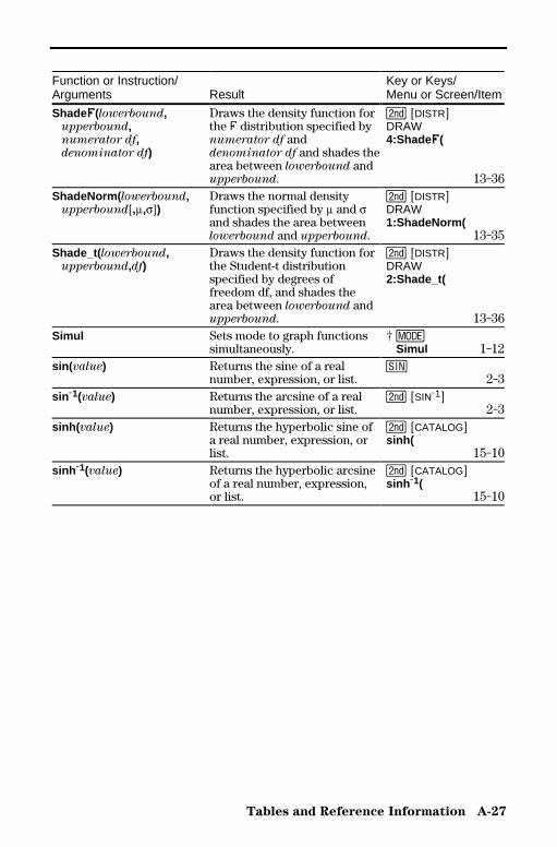
Tables and Reference Information A-27
8399APXA.DOC TI-83 international English Bob Fedorisko Revised: 02/19/01 1:25 PM Printed: 02/19/01 1:40 PMPage 27 of 58
Function or Instruction/Arguments Result
Key or Keys/Menu or Screen/Item
ShadeÜ(lowerbound, upperbound, numerator df, denominator df)
Draws the density function forthe Û distribution specified bynumerator df anddenominator df and shades thearea between lowerbound andupperbound.
y [DISTR]DRAW4:Shade Ü(
13-36ShadeNorm( lowerbound, upperbound[,m,s])
Draws the normal densityfunction specified by m and sand shades the area betweenlowerbound and upperbound.
y [DISTR]DRAW1:ShadeNorm(
13-35Shade_t( lowerbound, upperbound,df)
Draws the density function forthe Student-t distributionspecified by degrees offreedom df, and shades thearea between lowerbound andupperbound.
y [DISTR]DRAW2:Shade_t(
13-36Simul Sets mode to graph functions
simultaneously.† z Simul 1-12
sin( value) Returns the sine of a realnumber, expression, or list.
˜2-3
sin L1(value) Returns the arcsine of a realnumber, expression, or list.
y [SINL1]2-3
sinh( value) Returns the hyperbolic sine ofa real number, expression, orlist.
y [CATALOG]sinh(
15-10sinh L1(value) Returns the hyperbolic arcsine
of a real number, expression,or list.
y [CATALOG]sinh L1(
15-10
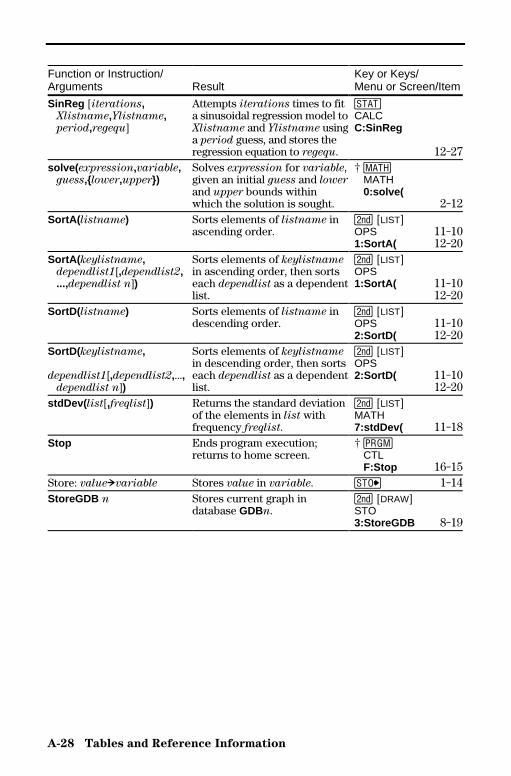
A-28 Tables and Reference Information
8399APXA.DOC TI-83 international English Bob Fedorisko Revised: 02/19/01 1:25 PM Printed: 02/19/01 1:40 PMPage 28 of 58
Function or Instruction/Arguments Result
Key or Keys/Menu or Screen/Item
SinReg [iterations, Xlistname,Ylistname, period,regequ]
Attempts iterations times to fita sinusoidal regression model toXlistname and Ylistname usinga period guess, and stores theregression equation to regequ.
…CALCC:SinReg
12-27solve( expression,variable, guess,{lower,upper})
Solves expression for variable,given an initial guess and lowerand upper bounds withinwhich the solution is sought.
† � MATH 0:solve(
2-12SortA( listname) Sorts elements of listname in
ascending order.y [LIST]OPS 11-101:SortA( 12-20
SortA( keylistname, dependlist1[,dependlist2, ...,dependlist n])
Sorts elements of keylistnamein ascending order, then sortseach dependlist as a dependentlist.
y [LIST]OPS1:SortA( 11-10
12-20SortD( listname) Sorts elements of listname in
descending order.y [LIST]OPS 11-102:SortD( 12-20
SortD( keylistname,
dependlist1[,dependlist2,..., dependlist n])
Sorts elements of keylistnamein descending order, then sortseach dependlist as a dependentlist.
y [LIST]OPS2:SortD( 11-10
12-20stdDev( list[,freqlist]) Returns the standard deviation
of the elements in list withfrequency freqlist.
y [LIST]MATH7:stdDev( 11-18
Stop Ends program execution;returns to home screen.
† � CTL F:Stop 16-15
Store: value!variable Stores value in variable. ¿ 1-14StoreGDB n Stores current graph in
database GDBn.y [DRAW]STO3:StoreGDB 8-19

Tables and Reference Information A-29
8399APXA.DOC TI-83 international English Bob Fedorisko Revised: 02/19/01 1:25 PM Printed: 02/19/01 1:40 PMPage 29 of 58
Function or Instruction/Arguments Result
Key or Keys/Menu or Screen/Item
StorePic n Stores current picture inpicture Picn.
y [DRAW]STO1:StorePic 8-17
String 4Equ(string,Y= var) Converts string into anequation and stores it in Y=var.
y [CATALOG]String 4Equ(
15-8sub( string,begin,length) Returns a string that is a subset
of another string, from beginto length.
y [CATALOG]sub(
15-9sum( list[,start,end]) Returns the sum of elements of
list from start to end.y [LIST]MATH5:sum( 11-18
tan(value) Returns the tangent of a realnumber, expression,or list.
š
2-3tan L1(value) Returns the arctangent of a
real number, expression, orlist.
y [TANL1]
2-3Tangent( expression,value) Draws a line tangent to
expression at X=value.y [DRAWäDRAW5:Tangent( 8-8
tanh( value) Returns hyperbolic tangent of areal number, expression, or list.
y [CATALOG]tanh( 15-10
tanh L1(value) Returns the hyperbolicarctangent of a real number,expression,or list.
y [CATALOG]tanh L1(
15-10tcdf( lowerbound, upperbound,df)
Computes the Student-tdistribution probabilitybetween lowerbound andupperbound for the specifieddegrees of freedom df.
y [DISTR]DISTR5:tcdf(
13-31Text(row,column,text1, text2,...,text n)
Writes text on graph beginningat pixel (row,column), where0 � row � 57 and0 � column � 94.
y [DRAW]DRAW0:Text(
8-12Then See If:Then
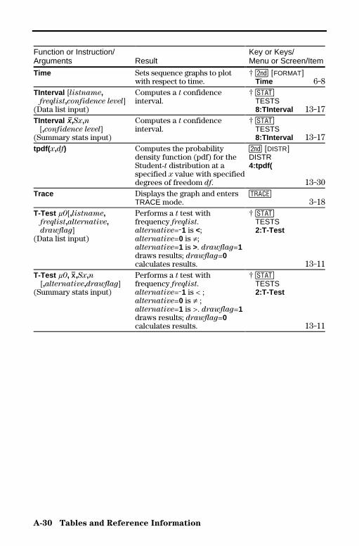
A-30 Tables and Reference Information
8399APXA.DOC TI-83 international English Bob Fedorisko Revised: 02/19/01 1:25 PM Printed: 02/19/01 1:40 PMPage 30 of 58
Function or Instruction/Arguments Result
Key or Keys/Menu or Screen/Item
Time Sets sequence graphs to plotwith respect to time.
† y [FORMAT] Time 6-8
TInterval [listname, freqlist,confidence level](Data list input)
Computes a t confidenceinterval.
† … TESTS 8:TInterval 13-17
TInterval v,Sx,n [,confidence level](Summary stats input)
Computes a t confidenceinterval.
† … TESTS 8:TInterval 13-17
tpdf( x,df) Computes the probabilitydensity function (pdf) for theStudent-t distribution at aspecified x value with specifieddegrees of freedom df.
y [DISTR]DISTR4:tpdf(
13-30Trace Displays the graph and enters
TRACE mode.r
3-18T-Test m0[,listname, freqlist,alternative, drawflag](Data list input)
Performs a t test withfrequency freqlist.alternative=L1 is <;alternative=0 is ƒ;alternative=1 is >. drawflag=1draws results; drawflag=0calculates results.
† … TESTS 2:T-Test
13-11T-Test m0, v,Sx,n [,alternative,drawflag](Summary stats input)
Performs a t test withfrequency freqlist.alternative=L1 is < ;alternative=0 is ƒ ;alternative=1 is >. drawflag=1draws results; drawflag=0calculates results.
† … TESTS 2:T-Test
13-11

Tables and Reference Information A-31
8399APXA.DOC TI-83 international English Bob Fedorisko Revised: 02/19/01 1:25 PM Printed: 02/19/01 1:40 PMPage 31 of 58
Function or Instruction/Arguments Result
Key or Keys/Menu or Screen/Item
tvm_FV [(Ú,æ,PV,PMT, P/Y,C/Y)]
Computes the future value. y [FINANCE]CALC6:tvm_FV 14-7
tvm_ æ[(Ú,PV,PMT,FV, P/Y,C/Y)]
Computes the annual interestrate.
y [FINANCE]CALC3:tvm_ æ 14-7
tvm_ Ú[(æ,PV,PMT,FV, P/Y,C/Y)]
Computes the number ofpayment periods.
y [FINANCE]CALC5:tvm_ Ú 14-7
tvm_Pmt [(Ú,æ,PV,FV, P/Y,C/Y)]
Computes the amount of eachpayment.
y [FINANCE]CALC2:tvm_Pmt 14-6
tvm_PV [(Ú,æ,PMT,FV, P/Y,C/Y)]
Computes the present value. y [FINANCE]CALC4:tvm_PV 14-7
uvAxes Sets sequence graphs to plotu(n) on the x-axis and v(n) onthe y-axis.
† y [FORMAT] uv
6-8uwAxes Sets sequence graphs to plot
u(n) on the x-axis and w(n) onthe y-axis.
† y [FORMAT] uw
6-81-Var Stats [Xlistname, freqlist]
Performs one-variable analysison the data in Xlistname withfrequency freqlist.
…CALC1:1-Var Stats 12-25
2-Var Stats [Xlistname, Ylistname,freqlist]
Performs two-variable analysison the data in Xlistname andYlistname with frequencyfreqlist.
…CALC2:2-Var Stats
12-25variance( list[,freqlist]) Returns the variance of the
elements in list with frequencyfreqlist.
y [LIST]MATH8:variance( 11-18
Vertical x Draws a vertical lineat x.
y [DRAW]DRAW4:Vertical 8-6
vwAxes Sets sequence graphs to plotv(n) on the x-axis and w(n) onthe y-axis.
† y [FORMAT] vw
6-8Web Sets sequence graphs to trace
as webs.† y [FORMAT] Web 6-8
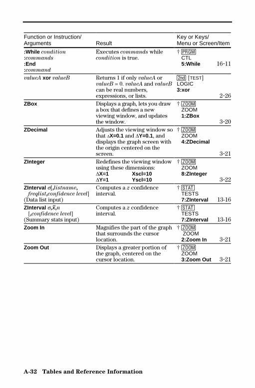
A-32 Tables and Reference Information
8399APXA.DOC TI-83 international English Bob Fedorisko Revised: 02/19/01 1:25 PM Printed: 02/19/01 1:40 PMPage 32 of 58
Function or Instruction/Arguments Result
Key or Keys/Menu or Screen/Item
:While condition:commands:End:command
Executes commands whilecondition is true.
† � CTL 5:While 16-11
valueA xor valueB Returns 1 if only valueA orvalueB = 0. valueA and valueBcan be real numbers,expressions, or lists.
y [TEST]LOGIC3:xor
2-26ZBox Displays a graph, lets you draw
a box that defines a newviewing window, and updatesthe window.
† q ZOOM 1:ZBox
3-20ZDecimal Adjusts the viewing window so
that @X=0.1 and @Y=0.1, anddisplays the graph screen withthe origin centered on thescreen.
† q ZOOM 4:ZDecimal
3-21ZInteger Redefines the viewing window
using these dimensions:@X=1 Xscl=10@Y=1 Yscl=10
† q ZOOM 8:ZInteger
3-22ZInterval s[,listname, freqlist,confidence level](Data list input)
Computes a z confidenceinterval.
† … TESTS 7:ZInterval 13-16
ZInterval s,v,n [,confidence level](Summary stats input)
Computes a z confidenceinterval.
† … TESTS 7:ZInterval 13-16
Zoom In Magnifies the part of the graphthat surrounds the cursorlocation.
† q ZOOM 2:Zoom In 3-21
Zoom Out Displays a greater portion ofthe graph, centered on thecursor location.
† q ZOOM 3:Zoom Out 3-21
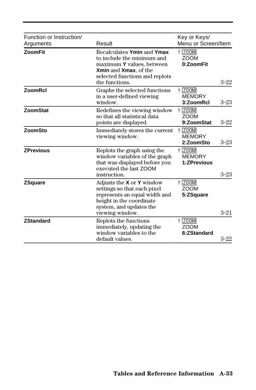
Tables and Reference Information A-33
8399APXA.DOC TI-83 international English Bob Fedorisko Revised: 02/19/01 1:25 PM Printed: 02/19/01 1:40 PMPage 33 of 58
Function or Instruction/Arguments Result
Key or Keys/Menu or Screen/Item
ZoomFit Recalculates Ymin and Ymaxto include the minimum andmaximum Y values, betweenXmin and Xmax , of theselected functions and replotsthe functions.
† q ZOOM 0:ZoomFit
3-22ZoomRcl Graphs the selected functions
in a user-defined viewingwindow.
† q MEMORY 3:ZoomRcl 3-23
ZoomStat Redefines the viewing windowso that all statistical datapoints are displayed.
† q ZOOM 9:ZoomStat 3-22
ZoomSto Immediately stores the currentviewing window.
† q MEMORY 2:ZoomSto 3-23
ZPrevious Replots the graph using thewindow variables of the graphthat was displayed before youexecuted the last ZOOMinstruction.
† q MEMORY 1:ZPrevious
3-23ZSquare Adjusts the X or Y window
settings so that each pixelrepresents an equal width andheight in the coordinatesystem, and updates theviewing window.
† q ZOOM 5:ZSquare
3-21ZStandard Replots the functions
immediately, updating thewindow variables to thedefault values.
† q ZOOM 6:ZStandard
3-22
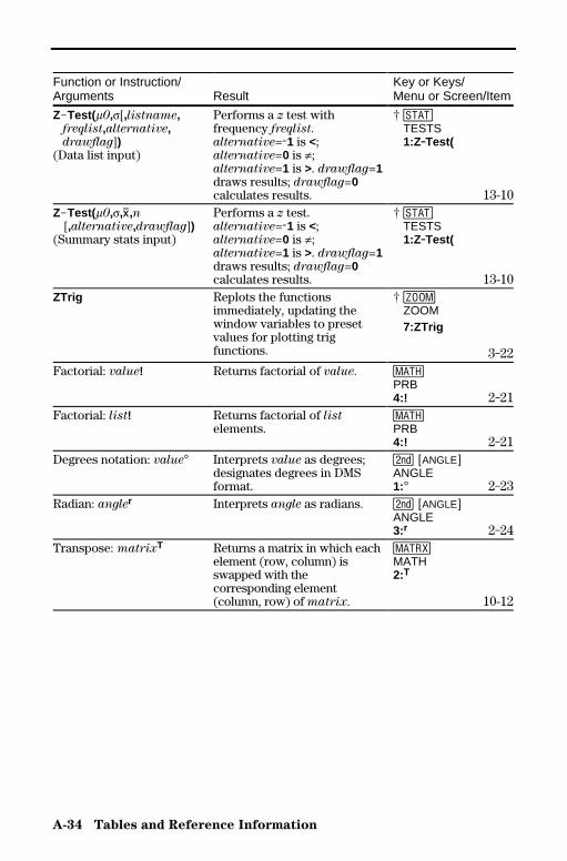
A-34 Tables and Reference Information
8399APXA.DOC TI-83 international English Bob Fedorisko Revised: 02/19/01 1:25 PM Printed: 02/19/01 1:40 PMPage 34 of 58
Function or Instruction/Arguments Result
Key or Keys/Menu or Screen/Item
ZNTest(m0,s[,listname, freqlist,alternative, drawflag])(Data list input)
Performs a z test withfrequency freqlist.alternative=L1 is <;alternative=0 is ƒ;alternative=1 is >. drawflag=1draws results; drawflag=0calculates results.
† … TESTS 1:Z.Test(
13-10ZNTest(m0,s,v,n [,alternative,drawflag])(Summary stats input)
Performs a z test.alternative=L1 is <;alternative=0 is ƒ;alternative=1 is >. drawflag=1draws results; drawflag=0calculates results.
† … TESTS 1:Z.Test(
13-10ZTrig Replots the functions
immediately, updating thewindow variables to presetvalues for plotting trigfunctions.
† q ZOOM 7:ZTrig
3-22Factorial: value! Returns factorial of value. �
PRB4:! 2-21
Factorial: list! Returns factorial of listelements.
�PRB4:! 2-21
Degrees notation: value¡ Interprets value as degrees;designates degrees in DMSformat.
y [ANGLE]ANGLE1:¡ 2-23
Radian: angler Interprets angle as radians. y [ANGLE]ANGLE3:r 2-24
Transpose: matrixT Returns a matrix in which eachelement (row, column) isswapped with thecorresponding element(column, row) of matrix.
�MATH2:T
10-12
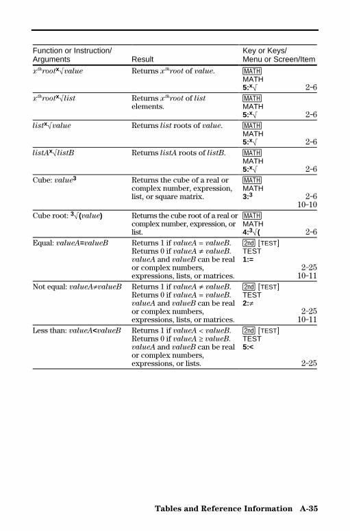
Tables and Reference Information A-35
8399APXA.DOC TI-83 international English Bob Fedorisko Revised: 02/19/01 1:25 PM Printed: 02/19/01 1:40 PMPage 35 of 58
Function or Instruction/Arguments Result
Key or Keys/Menu or Screen/Item
xthrootx‡value Returns xthroot of value. �MATH5:x‡ 2-6
xthrootx‡list Returns xthroot of listelements.
�MATH5:x‡ 2-6
listx‡value Returns list roots of value. �MATH5:x‡ 2-6
listAx‡listB Returns listA roots of listB. �MATH5:x‡ 2-6
Cube: value3 Returns the cube of a real orcomplex number, expression,list, or square matrix.
�MATH3:3 2-6
10-10Cube root: 3‡(value) Returns the cube root of a real or
complex number, expression, orlist.
�MATH4:3‡( 2-6
Equal: valueA=valueB Returns 1 if valueA = valueB.Returns 0 if valueA ƒ valueB.valueA and valueB can be realor complex numbers,expressions, lists, or matrices.
y [TEST]TEST1:=
2-2510-11
Not equal: valueAƒvalueB Returns 1 if valueA ƒ valueB.Returns 0 if valueA = valueB.valueA and valueB can be realor complex numbers,expressions, lists, or matrices.
y [TEST]TEST2:ƒ
2-2510-11
Less than: valueA<valueB Returns 1 if valueA < valueB.Returns 0 if valueA ‚ valueB.valueA and valueB can be realor complex numbers,expressions, or lists.
y [TEST]TEST5:<
2-25
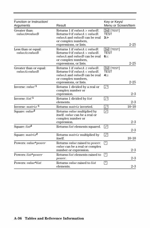
A-36 Tables and Reference Information
8399APXA.DOC TI-83 international English Bob Fedorisko Revised: 02/19/01 1:25 PM Printed: 02/19/01 1:40 PMPage 36 of 58
Function or Instruction/Arguments Result
Key or Keys/Menu or Screen/Item
Greater than: valueA>valueB
Returns 1 if valueA > valueB.Returns 0 if valueA � valueB.valueA and valueB can be realor complex numbers,expressions, or lists.
y [TEST]TEST3:>
2-25Less than or equal: valueA�valueB
Returns 1 if valueA � valueB.Returns 0 if valueA > valueB.valueA and valueB can be realor complex numbers,expressions, or lists.
y [TEST]TEST6:�
2-25Greater than or equal: valueA‚valueB
Returns 1 if valueA ‚ valueB.Returns 0 if valueA < valueB.valueA and valueB can be realor complex numbers,expressions, or lists.
y [TEST]TEST4:‚
2-25Inverse: valueL1 Returns 1 divided by a real or
complex number orexpression.
—
2-3Inverse: listL1 Returns 1 divided by list
elements.—
2-3Inverse: matrixL1 Returns matrix inverted. — 10-10Square: value2 Returns value multiplied by
itself. value can be a real orcomplex number orexpression.
¡
2-3Square: list2 Returns list elements squared. ¡
2-3Square: matrix2 Returns matrix multiplied by
itself.¡
10-10Powers: value^power Returns value raised to power.
value can be a real or complexnumber or expression.
›
2-3Powers: list^power Returns list elements raised to
power.›
2-3Powers: value^ list Returns value raised to list
elements.›
2-3
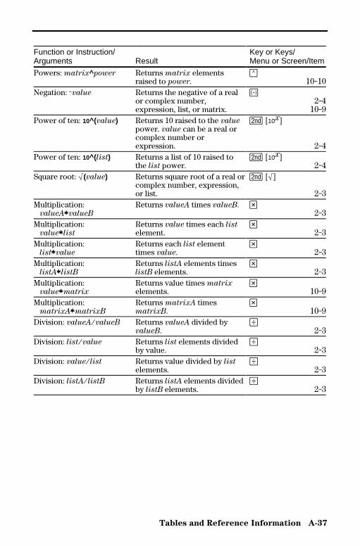
Tables and Reference Information A-37
8399APXA.DOC TI-83 international English Bob Fedorisko Revised: 02/19/01 1:25 PM Printed: 02/19/01 1:40 PMPage 37 of 58
Function or Instruction/Arguments Result
Key or Keys/Menu or Screen/Item
Powers: matrix^power Returns matrix elementsraised to power.
›10-10
Negation: Lvalue Returns the negative of a realor complex number,expression, list, or matrix.
Ì2-4
10-9Power of ten: 10^(value) Returns 10 raised to the value
power. value can be a real orcomplex number orexpression.
y [10x]
2-4Power of ten: 10^( list) Returns a list of 10 raised to
the list power.y [10x]
2-4Square root: ‡(value) Returns square root of a real or
complex number, expression,or list.
y [‡]
2-3Multiplication: valueAävalueB
Returns valueA times valueB. ¯2-3
Multiplication: valueälist
Returns value times each listelement.
¯2-3
Multiplication: listävalue
Returns each list elementtimes value.
¯2-3
Multiplication: listAälistB
Returns listA elements timeslistB elements.
¯2-3
Multiplication: valueämatrix
Returns value times matrixelements.
¯10-9
Multiplication: matrixAämatrixB
Returns matrixA timesmatrixB.
¯10-9
Division: valueAàvalueB Returns valueA divided byvalueB.
¥2-3
Division: listàvalue Returns list elements dividedby value.
¥2-3
Division: valueàlist Returns value divided by listelements.
¥2-3
Division: listAàlistB Returns listA elements dividedby listB elements.
¥2-3
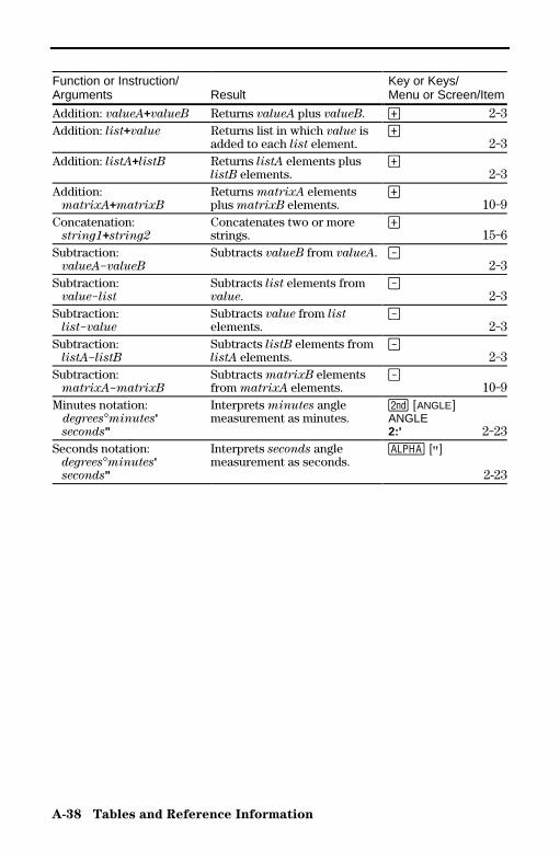
A-38 Tables and Reference Information
8399APXA.DOC TI-83 international English Bob Fedorisko Revised: 02/19/01 1:25 PM Printed: 02/19/01 1:40 PMPage 38 of 58
Function or Instruction/Arguments Result
Key or Keys/Menu or Screen/Item
Addition: valueA+valueB Returns valueA plus valueB. Ã 2-3Addition: list+value Returns list in which value is
added to each list element.Ã
2-3Addition: listA+listB Returns listA elements plus
listB elements.Ã
2-3Addition: matrixA+matrixB
Returns matrixA elementsplus matrixB elements.
Ã10-9
Concatenation: string1+string2
Concatenates two or morestrings.
Ã15-6
Subtraction: valueANvalueB
Subtracts valueB from valueA. ¹2-3
Subtraction: valueNlist
Subtracts list elements fromvalue.
¹2-3
Subtraction: listNvalue
Subtracts value from listelements.
¹2-3
Subtraction: listANlistB
Subtracts listB elements fromlistA elements.
¹2-3
Subtraction: matrixANmatrixB
Subtracts matrixB elementsfrom matrixA elements.
¹10-9
Minutes notation: degrees¡minutes' seconds"
Interprets minutes anglemeasurement as minutes.
y [ANGLE]ANGLE2:' 2-23
Seconds notation: degrees¡minutes' seconds"
Interprets seconds anglemeasurement as seconds.
ƒ [ã]
2-23

Tables and Reference Information A-39
8399APXA.DOC TI-83 international English Bob Fedorisko Revised: 02/19/01 1:25 PM Printed: 02/19/01 1:40 PMPage 39 of 58
The TI.83 Menu Map begins at the top-left corner of the keyboard and followsthe keyboard layout from left to right. Default values and settings are shown.
o ÚÁÄÄÄÄÄÄÄÄÄÄÄÄÂÄÄÄÄÄÄÄÄÄÄÄÄÄÂÄÄÄÄÄÄÄÄÄÄÄÄÄ¿(Func mode)Plot1 Plot2Plot3çY1=çY2=çY3=çY4=...çY9=çY0=
(Par mode)Plot1 Plot2Plot3çX1T= Y1T=çX2T= Y2T=...çX6T= Y6T=
(Pol mode)Plot1 Plot2Plot3çr1=çr2=çr3=çr4=çr5=çr6=
(Seq mode)Plot1 Plot2Plot3 nMin=1íu(n)= u(nMin)=ív(n)= v(nMin)=íw(n)= w(nMin)=
y [STAT PLOT] ÚÄÄÄÄÄÙ
y [STAT PLOT] ÚÄÄÄÄÄÁÄÄÄÄÄÄÂÄÄÄÄÄÄÄÄÄÄÄÄÄÄ¿
STAT PLOTS1:Plot1…Off " L1 L2 ›
2:Plot2…Off " L1 L2 ›
3:Plot3…Off " L1 L2 ›
4:PlotsOff5:PlotsOn
(PRGM editor)PLOTS1:Plot1(2:Plot2(3:Plot3(4:PlotsOff5:PlotsOn
(PRGM editor)TYPE1:Scatter2:xyLine3:Histogram4:ModBoxplot5:Boxplot6:NormProbPlot
(PRGM editor)MARK1:›
2:+3:¦
p ÚÁÄÄÄÄÄÄÄÄÄÄÄÄÂÄÄÄÄÄÄÄÄÄÄÄÄÄÂÄÄÄÄÄÄÄÄÄÄÄÄÄ¿(Func mode)WINDOW Xmin=-10 Xmax=10 Xscl=1 Ymin=-10 Ymax=10 Yscl=1 Xres=1
(Par mode)WINDOW Tmin=0 Tmax=pä2 Tstep=pà24 Xmin=-10 Xmax=10 Xscl=1 Ymin=-10 Ymax=10 Yscl=1
(Pol mode)WINDOW qmin=0 qmax=pä2 qstep=pà24 Xmin=-10 Xmax=10 Xscl=1 Ymin=-10 Ymax=10 Yscl=1
(Seq mode)WINDOW nMin=1 nMax=10 PlotStart=1 PlotStep=1 Xmin=-10 Xmax=10 Xscl=1 Ymin=-10 Ymax=10 Yscl=1
y [TBLSET] ÚÄÄÄÙ
y [TBLSET] ÚÄÄÄÄÙ
TABLE SETUP TblStart=0 @Tbl=1 Indpnt:Auto Ask Depend:Auto Ask
(PRGM editor)TABLE SETUP Indpnt:Auto Ask Depend:Auto Ask
TI-83 Menu Map
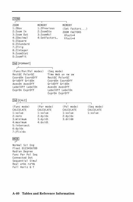
A-40 Tables and Reference Information
8399APXA.DOC TI-83 international English Bob Fedorisko Revised: 02/19/01 1:25 PM Printed: 02/19/01 1:40 PMPage 40 of 58
q ÚÁÄÄÄÄÄÄÄÄÄÄÄÄÄÂÄÄÄÄÄÄÄÄÄÄÄÄÄ¿ZOOM1:ZBox2:Zoom In3:Zoom Out4:ZDecimal5:ZSquare6:ZStandard7:ZTrig8:ZInteger9:ZoomStat0:ZoomFit
MEMORY1:ZPrevious2:ZoomSto3:ZoomRcl4:SetFactors…
MEMORY(Set Factors...)ZOOM FACTORS XFact=4 YFact=4
y [FORMAT] ÚÁÄÄÄÄÄÄÄÄÄÄÄÄÄÄÄÄÄÄ¿(Func/Par/Pol modes)RectGC PolarGCCoordOn CoordOffGridOff GridOnAxesOn AxesOffLabelOff LabelOnExprOn ExprOff
(Seq mode)Time Web uv vw uwRectGC PolarGCCoordOn CoordOffGridOff GridOnAxesOn AxesOffLabelOff LabelOnExprOn ExprOff
y [CALC] ÚÄÁÄÄÄÄÄÄÄÄÄÄÄÂÄÄÄÄÄÄÄÄÄÄÄÄÄÂÄÄÄÄÄÄÄÄÄÄÄÄÄ¿(Func mode)CALCULATE1:value2:zero3:minimum4:maximum5:intersect6:dy/dx7:‰f(x)dx
(Par mode)CALCULATE1:value2:dy/dx3:dy/dt4:dx/dt
(Pol mode)CALCULATE1:value2:dy/dx3:dr/dq
(Seq mode)CALCULATE1:value
z ÚÙNormal Sci EngFloat 0123456789Radian DegreeFunc Par Pol SeqConnected DotSequential SimulReal a+b× re^q×Full Horiz G-T

Tables and Reference Information A-41
8399APXA.DOC TI-83 international English Bob Fedorisko Revised: 02/19/01 1:25 PM Printed: 02/19/01 1:40 PMPage 41 of 58
y [LINK] ÚÄÁÄÄÄÄÄÄÄÄÄÄÄÄÄÄÄÄÄ¿SEND1:All+…2:AllN…3:Prgm…4:List…5:Lists to TI82…6:GDB…7:Pic…8:Matrix…9:Real…0:Complex…A:Y-Vars…B:String…C:Back Up…
RECEIVE1:Receive
… ÚÁÄÄÄÄÄÄÄÄÄÄÄÄÄÄÂÄÄÄÄÄÄÄÄÄÄÄÄÄÄÄÄÄÄÄ¿EDIT1:Edit…2:SortA(3:SortD(4:ClrList5:SetUpEditor
CALC1:1-Var Stats2:2-Var Stats3:Med-Med4:LinReg(ax+b)5:QuadReg6:CubicReg7:QuartReg8:LinReg(a+bx)9:LnReg0:ExpRegA:PwrRegB:LogisticC:SinReg
TESTS1:Z-Test…2:T-Test…3:2-SampZTest…4:2-SampTTest…5:1-PropZTest…6:2-PropZTest…7:ZInterval…8:TInterval…9:2-SampZInt…0:2-SampTInt…A:1-PropZInt…B:2-PropZInt…C:c2-Test…D:2-SampÛTest…E:LinRegTTest…F:ANOVA(

A-42 Tables and Reference Information
8399APXA.DOC TI-83 international English Bob Fedorisko Revised: 02/19/01 1:25 PM Printed: 02/19/01 1:40 PMPage 42 of 58
y [LIST] ÚÄÄÁÄÄÄÄÄÄÄÄÂÄÄÄÄÄÄÄÄÄÄÄÄ¿NAMES1:listname2:listname3:listname...
OPS1:SortA(2:SortD(3:dim(4:Fill(5:seq(6:cumSum(7:@List(8:Select(9:augment(0:List4matr(A:Matr4list(B:Ù
MATH1:min(2:max(3:mean(4:median(5:sum(6:prod(7:stdDev(8:variance(
� ÚÁÄÄÄÄÄÄÄÄÄÄÄÂÄÄÄÄÄÄÄÄÄÄÄÄÂÄÄÄÄÄÄÄÄÄÄÄ¿MATH1:4Frac2:4Dec3:3
4:3‡(5:x‡
6:fMin(7:fMax(8:nDeriv(9:fnInt(0:Solver…
NUM1:abs(2:round(3:iPart(4:fPart(5:int(6:min(7:max(8:lcm(9:gcd(
CPX1:conj(2:real(3:imag(4:angle(5:abs(6:4Rect7:4Polar
PRB1:rand2:nPr3:nCr4:!5:randInt(6:randNorm(7:randBin(
y [TEST] ÚÄÄÁÄÄÄÄÄÄÄÄÄ¿TEST1:=2:ƒ3:>4:‚5:<6:�
LOGIC1:and2:or3:xor4:not(
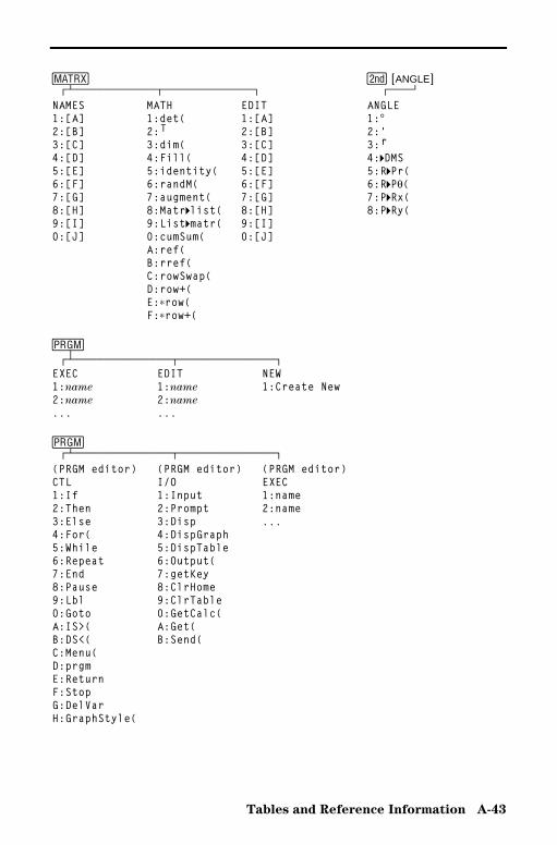
Tables and Reference Information A-43
8399APXA.DOC TI-83 international English Bob Fedorisko Revised: 02/19/01 1:25 PM Printed: 02/19/01 1:40 PMPage 43 of 58
� ÚÁÄÄÄÄÄÄÄÄÄÄÄÂÄÄÄÄÄÄÄÄÄÄÄÄ¿
y [ANGLE] ÚÄÄÄÙ
NAMES1:[A]2:[B]3:[C]4:[D]5:[E]6:[F]7:[G]8:[H]9:[I]0:[J]
MATH1:det(2:T
3:dim(4:Fill(5:identity(6:randM(7:augment(8:Matr4list(9:List4matr(0:cumSum(A:ref(B:rref(C:rowSwap(D:row+(E:…row(F:…row+(
EDIT1:[A]2:[B]3:[C]4:[D]5:[E]6:[F]7:[G]8:[H]9:[I]0:[J]
ANGLE1:¡2:'3:r
4:4DMS5:R4Pr(6:R4Pq(7:P4Rx(8:P4Ry(
� ÚÁÄÄÄÄÄÄÄÄÄÄÄÄÄÂÄÄÄÄÄÄÄÄÄÄÄÄÄ¿EXEC1:name
2:name
...
EDIT1:name
2:name
...
NEW1:Create New
� ÚÁÄÄÄÄÄÄÄÄÄÄÄÄÄÂÄÄÄÄÄÄÄÄÄÄÄÄÄ¿(PRGM editor)CTL1:If2:Then3:Else4:For(5:While6:Repeat7:End8:Pause9:Lbl0:GotoA:IS>(B:DS<(C:Menu(D:prgmE:ReturnF:StopG:DelVarH:GraphStyle(
(PRGM editor)I/O1:Input2:Prompt3:Disp4:DispGraph5:DispTable6:Output(7:getKey8:ClrHome9:ClrTable0:GetCalc(A:Get(B:Send(
(PRGM editor)EXEC1:name2:name...
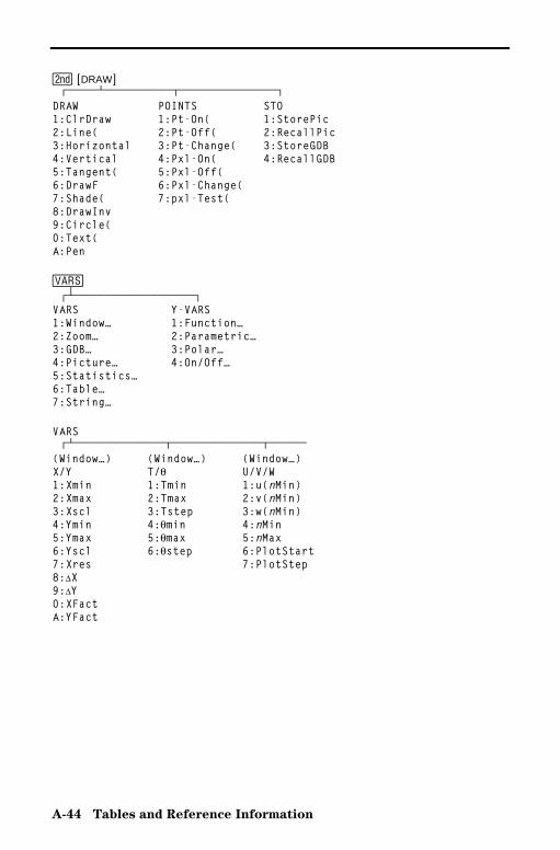
A-44 Tables and Reference Information
8399APXA.DOC TI-83 international English Bob Fedorisko Revised: 02/19/01 1:25 PM Printed: 02/19/01 1:40 PMPage 44 of 58
y [DRAW] ÚÄÄÄÄÁÄÄÄÄÄÄÄÄÄÂÄÄÄÄÄÄÄÄÄÄÄÄÄ¿DRAW1:ClrDraw2:Line(3:Horizontal4:Vertical5:Tangent(6:DrawF7:Shade(8:DrawInv9:Circle(0:Text(A:Pen
POINTS1:Pt-On(2:Pt-Off(3:Pt-Change(4:Pxl-On(5:Pxl-Off(6:Pxl-Change(7:pxl-Test(
STO1:StorePic2:RecallPic3:StoreGDB4:RecallGDB
� ÚÁÄÄÄÄÄÄÄÄÄÄÄÄÄÄÄÄ¿VARS1:Window…2:Zoom…3:GDB…4:Picture…5:Statistics…6:Table…7:String…
Y-VARS1:Function…2:Parametric…3:Polar…4:On/Off…
VARS ÚÁÄÄÄÄÄÄÄÄÄÄÄÄÂÄÄÄÄÄÄÄÄÄÄÄÄÂÄÄÄÄÄ(Window…)X/Y1:Xmin2:Xmax3:Xscl4:Ymin5:Ymax6:Yscl7:Xres8:@X9:@Y0:XFactA:YFact
(Window…)T/q1:Tmin2:Tmax3:Tstep4:qmin5:qmax6:qstep
(Window…)U/V/W1:u(nMin)2:v(nMin)3:w(nMin)4:nMin5:nMax6:PlotStart7:PlotStep
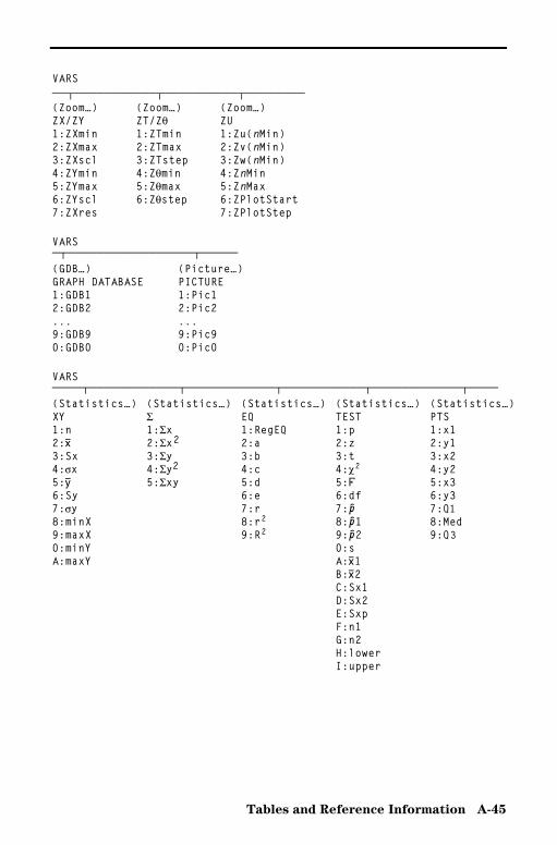
Tables and Reference Information A-45
8399APXA.DOC TI-83 international English Bob Fedorisko Revised: 02/19/01 1:25 PM Printed: 02/19/01 1:40 PMPage 45 of 58
VARSÄÄÂÄÄÄÄÄÄÄÄÄÄÄÂÄÄÄÄÄÄÄÄÄÄÂÄÄÄÄÄÄÄÄ(Zoom…)ZX/ZY1:ZXmin2:ZXmax3:ZXscl4:ZYmin5:ZYmax6:ZYscl7:ZXres
(Zoom…)ZT/Zq1:ZTmin2:ZTmax3:ZTstep4:Zqmin5:Zqmax6:Zqstep
(Zoom…)ZU1:Zu(nMin)2:Zv(nMin)3:Zw(nMin)4:ZnMin5:ZnMax6:ZPlotStart7:ZPlotStep
VARSÄÂÄÄÄÄÄÄÄÄÄÄÄÄÄÄÄÄÄÂÄÄÄÄÄ(GDB…)GRAPH DATABASE1:GDB12:GDB2...9:GDB90:GDB0
(Picture…)PICTURE1:Pic12:Pic2...9:Pic90:Pic0
VARSÄÄÄÄÂÄÄÄÄÄÄÄÄÄÄÄÄÂÄÄÄÄÄÄÄÄÄÄÄÄÂÄÄÄÄÄÄÄÄÄÄÄÂÄÄÄÄÄÄÄÄÄÄÄÄÂÄÄÄÄ(Statistics…)XY1:n2:v3:Sx4:sx5:w6:Sy7:sy8:minX9:maxX0:minYA:maxY
(Statistics…)G1:Gx2:Gx2
3:Gy4:Gy2
5:Gxy
(Statistics…)EQ1:RegEQ2:a3:b4:c5:d6:e7:r8:r2
9:R2
(Statistics…)TEST1:p2:z3:t4:c2
5:Û6:df7:Ç8:Ç19:Ç20:sA:ü1B:ü2C:Sx1D:Sx2E:SxpF:n1G:n2H:lowerI:upper
(Statistics…)PTS1:x12:y13:x24:y25:x36:y37:Q18:Med9:Q3

A-46 Tables and Reference Information
8399APXA.DOC TI-83 international English Bob Fedorisko Revised: 02/19/01 1:25 PM Printed: 02/19/01 1:40 PMPage 46 of 58
VARSÄÂÄÄÄÄÄÄÄÄÄÄÄÄÄÄÄÄ¿(Table…)TABLE1:TblStart2:@Tbl3:TblInput
(String…)STRING1:Str12:Str23:Str34:Str4...9:Str90:Str0
Y-VARS ÚÄÁÄÄÄÄÄÄÄÄÄÄÄÂÄÄÄÄÄÄÄÄÄÄÄÄÄÂÄÄÄÄÄÄÄÄÄ¿(Function…)FUNCTION1:Y12:Y23:Y34:Y4...9:Y90:Y0
(Parametric…)PARAMETRIC1:X1T2:Y1T3:X2T4:Y2T...A:X6TB:Y6T
(Polar…)POLAR1:r12:r23:r34:r45:r56:r6
(On/Off…)ON/OFF1:FnOn2:FnOff
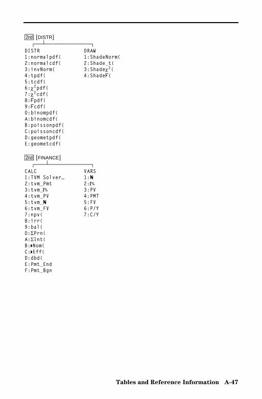
Tables and Reference Information A-47
8399APXA.DOC TI-83 international English Bob Fedorisko Revised: 02/19/01 1:25 PM Printed: 02/19/01 1:40 PMPage 47 of 58
y [DISTR] ÚÄÄÁÄÄÄÄÄÄÄÄÄÄÄÄÄ¿DISTR1:normalpdf(2:normalcdf(3:invNorm(4:tpdf(5:tcdf(6:c2pdf(7:c2cdf(8:Ûpdf(9:Ûcdf(0:binompdf(A:binomcdf(B:poissonpdf(C:poissoncdf(D:geometpdf(E:geometcdf(
DRAW1:ShadeNorm(2:Shade_t(3:Shadec2(4:ShadeÛ(
y [FINANCE] ÚÄÄÄÁÄÄÄÄÄÄÄÄÄÄÄÄ¿CALC1:TVM Solver…2:tvm_Pmt3:tvm_æ4:tvm_PV5:tvm_Ú6:tvm_FV7:npv(8:irr(9:bal(0:GPrn(A:GInt(B:4Nom(C:4Eff(D:dbd(E:Pmt_EndF:Pmt_Bgn
VARS1:Ú2:æ3:PV4:PMT5:FV6:P/Y7:C/Y
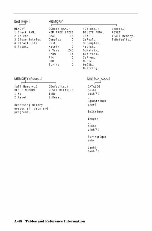
A-48 Tables and Reference Information
8399APXA.DOC TI-83 international English Bob Fedorisko Revised: 02/19/01 1:25 PM Printed: 02/19/01 1:40 PMPage 48 of 58
y [MEM] ÚÄÄÙ
MEMORY ÚÄÄÁÄÄÄÄÄÄÄÄÄÄÄÄÄÄÄÂÄÄÄÄÄÄÄÄÄÄÄÄ¿
MEMORY1:Check RAM…2:Delete…3:Clear Entries4:ClrAllLists5:Reset…
(Check RAM…)MEM FREE 27225Real 15Complex 0List 0Matrix 0Y-Vars 240Prgm 14Pic 0GDB 0String 0
(Delete…)DELETE FROM…1:All…2:Real…3:Complex…4:List…5:Matrix…6:Y-Vars…7:Prgm…8:Pic…9:GDB…0:String…
(Reset…)RESET1:All Memory…2:Defaults…
MEMORY (Reset...) ÚÄÁÄÄÄÄÄÄÄÄÄÄÄÄÄÄ¿
y [CATALOG] ÚÄÄÙ
(All Memory…)RESET MEMORY1:No2:Reset
Resetting memoryerases all data andprograms.
(Defaults…)RESET DEFAULTS1:No2:Reset
CATALOGcosh(coshL1(...Equ4String(expr(...inString(...length(...sinh(sinhL1(...String4Equ(sub(...tanh(tanhL1(
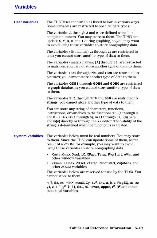
Tables and Reference Information A-49
8399APXA.DOC TI-83 international English Bob Fedorisko Revised: 02/19/01 1:25 PM Printed: 02/19/01 1:40 PMPage 49 of 58
The TI.83 uses the variables listed below in various ways.Some variables are restricted to specific data types.
The variables A through Z and q are defined as real orcomplex numbers. You may store to them. The TI.83 canupdate X, Y, R, q, and T during graphing, so you may wantto avoid using these variables to store nongraphing data.
The variables (list names) L1 through L6 are restricted tolists; you cannot store another type of data to them.
The variables (matrix names) [A] through [J] are restrictedto matrices; you cannot store another type of data to them.
The variables Pic1 through Pic9 and Pic0 are restricted topictures; you cannot store another type of data to them.
The variables GDB1 through GDB9 and GDB0 are restrictedto graph databases; you cannot store another type of datato them.
The variables Str1 through Str9 and Str0 are restricted tostrings; you cannot store another type of data to them.
You can store any string of characters, functions,instructions, or variables to the functions Yn, (1 through 9,and 0), XnT/YnT (1 through 6), rn (1 through 6), u(n), v(n),and w(n) directly or through the Y= editor. The validity of thestring is determined when the function is evaluated.
The variables below must be real numbers. You may storeto them. Since the TI.83 can update some of them, as theresult of a ZOOM, for example, you may want to avoidusing these variables to store nongraphing data.
• Xmin , Xmax , Xscl , @X, XFact , Tstep , PlotStart , nMin , andother window variables.
• ZXmin , ZXmax , ZXscl , ZTstep , ZPlotStart , Zu(nMin) , andother ZOOM variables.
The variables below are reserved for use by the TI.83. Youcannot store to them.
n, v, Sx, sx, minX , maxX , Gy, Gy2, Gxy , a, b, c, RegEQ, x1, x2,
y1, z, t, F, c2, Ç, v1, Sx1, n1, lower , upper , r2, R2 and otherstatistical variables.
Variables
User Variables
System Variables
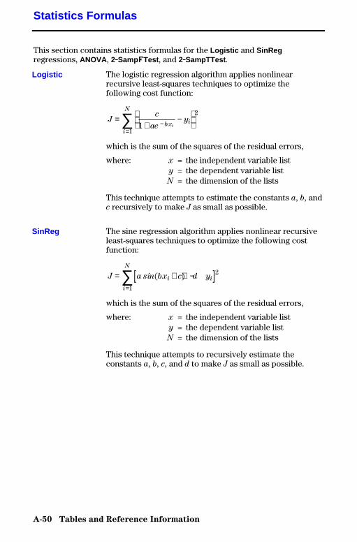
A-50 Tables and Reference Information
8399APXA.DOC TI-83 international English Bob Fedorisko Revised: 02/19/01 1:25 PM Printed: 02/19/01 1:40 PMPage 50 of 58
This section contains statistics formulas for the Logistic and SinRegregressions, ANOVA , 2.SampÜTest , and 2.SampTTest .
The logistic regression algorithm applies nonlinearrecursive least-squares techniques to optimize thefollowing cost function:
Jc
aey
bx i
i
N
i
=+
−
−
=∑ 1
2
1
which is the sum of the squares of the residual errors,
where: x = the independent variable listy = the dependent variable listN = the dimension of the lists
This technique attempts to estimate the constants a, b, andc recursively to make J as small as possible.
The sine regression algorithm applies nonlinear recursiveleast-squares techniques to optimize the following costfunction:
[ ]J a bx c d yi i
i
N
= + + −=
∑ sin( ) 2
1
which is the sum of the squares of the residual errors,
where: x = the independent variable listy = the dependent variable listN = the dimension of the lists
This technique attempts to recursively estimate theconstants a, b, c, and d to make J as small as possible.
Statistics Formulas
Logistic
SinReg

Tables and Reference Information A-51
8399APXA.DOC TI-83 international English Bob Fedorisko Revised: 02/19/01 1:25 PM Printed: 02/19/01 1:40 PMPage 51 of 58
The ANOVA Û statistic is:
Û = Factor MS
Error MS
The mean squares (MS) that make up Û are:
Factor MSFactor SS
Factor df =
Error MSError SS
Error df =
The sum of squares (SS) that make up the mean squaresare:
Factor SS n x xi i
i
I
( )= −=
∑ 2
1
Error SS n Sxi i
i
I
( )= −=∑ 1 2
1
The degrees of freedom df that make up the mean squaresare:
Factor df I df= − =1 numerator for Û
Error df n dfi
i
I
( ) denominator for= − ==
∑ 11
Û
where: I = number of populations
xi = the mean of each listSxi = the standard deviation of each listni = the length of each list
x = the mean of all lists
ANOVA(
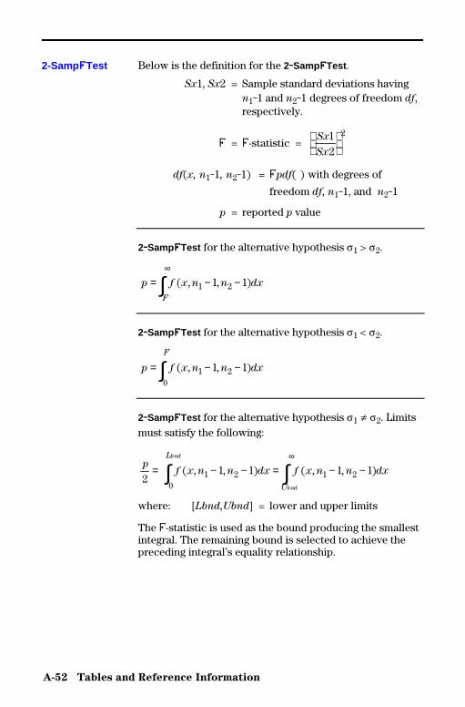
A-52 Tables and Reference Information
8399APXA.DOC TI-83 international English Bob Fedorisko Revised: 02/19/01 1:25 PM Printed: 02/19/01 1:40 PMPage 52 of 58
Below is the definition for the 2.SampÜTest .
Sx1, Sx2 = Sample standard deviations havingn1-1 and n2-1 degrees of freedom df,respectively.
Û = Û-statistic = Sx
Sx
12
2
df(x, n1-1, n2-1) = Ûpdf( ) with degrees of
freedom df, n1-1, and n2-1
p = reported p value
2.SampÜTest for the alternative hypothesis s1 > s2.
p f x n n dx
F
= − −∞
∫ ( ), ,1 21 1
2.SampÜTest for the alternative hypothesis s1 < s2.
p f x n n dx
F
= − −∫ ( ), ,1 20
1 1
2.SampÜTest for the alternative hypothesis s1 ƒ s2. Limitsmust satisfy the following:
pf x n n dx f x n n dx
L
U
bnd
bnd
21 1 1 11 2
01 2= − − = − −∫ ∫
∞
( ) ( ), , , ,
where: [Lbnd,Ubnd] = lower and upper limits
The Û-statistic is used as the bound producing the smallestintegral. The remaining bound is selected to achieve thepreceding integral’s equality relationship.
2-SampÜTest
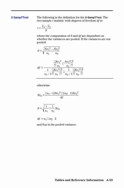
Tables and Reference Information A-53
8399APXA.DOC TI-83 international English Bob Fedorisko Revised: 02/19/01 1:25 PM Printed: 02/19/01 1:40 PMPage 53 of 58
The following is the definition for the 2.SampTTest . Thetwo-sample t statistic with degrees of freedom df is:
tx x
S= −1 2
where the computation of S and df are dependent onwhether the variances are pooled. If the variances are notpooled:
SSx
n
Sx
n= +1
2
1
22
2
df
Sx
n
Sx
n
n
Sx
n n
Sx
n
=+
−
+−
12
1
22
2
2
1
12
1
2
2
22
2
211
11
otherwise:
Sxn Sx n Sx
dfp = − + −( ) ( )1 1
22 2
21 1
Sn n
Sxp= +1 1
1 2
df n n= + −1 2 2
and Sxp is the pooled variance.
2-SampTTest
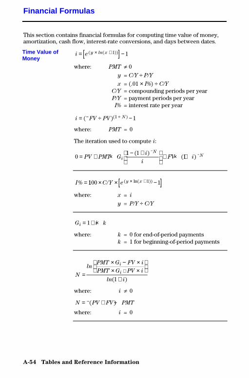
A-54 Tables and Reference Information
8399APXA.DOC TI-83 international English Bob Fedorisko Revised: 02/19/01 1:25 PM Printed: 02/19/01 1:40 PMPage 54 of 58
This section contains financial formulas for computing time value of money,amortization, cash flow, interest-rate conversions, and days between dates.
[ ]i e y x= −× +( ( ))ln 1 1
where: PMT ƒ 0
y = C/Y ÷ P/Y
x = (.01 × I%) ÷ C/Y
C/Y = compounding periods per yearP/Y = payment periods per yearI% = interest rate per year
i FV PV N= ÷ −− ÷( )( )1 1
where: PMT = 0
The iteration used to compute i:
01 1
1= + × − +
+ × +−
−PV PMT G
i
iFV ii
NN( )
( )
[ ]I C Y e y x% /= × × −× +1100 ( ln( ))1 1
where: x = i
y = P/Y ÷ C/Y
G i ki = + ×1
where: k = 0 for end-of-period paymentsk = 1 for beginning-of-period payments
N
PMT G FV i
PMT G PV i
i
i
i=
× − ×× ×
++
ln
ln( )1
where: i ƒ 0
N PV FV PMT= + ÷−( )
where: i = 0
Financial Formulas
Time Value ofMoney

Tables and Reference Information A-55
8399APXA.DOC TI-83 international English Bob Fedorisko Revised: 02/19/01 1:25 PM Printed: 02/19/01 1:40 PMPage 55 of 58
PMTi
GPV
PV FV
iiN
= × + ++ −
−
( )1 1
where: i ƒ 0
PMT PV FV N= + ÷−( )
where: i = 0
PVPMT G
iFV
i
PMT G
i
i
N
i= × −
×+
− ×11( )
where: i ƒ 0
PV FV PMT N= + ×−( )
where: i = 0
FVPMT G
ii PV
PMT G
i
i N i= × − + × + ×
( )1
where: i ƒ 0
FV PV PMT N= + ×−( )
where: i = 0
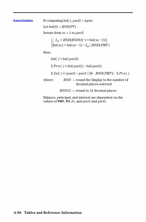
A-56 Tables and Reference Information
8399APXA.DOC TI-83 international English Bob Fedorisko Revised: 02/19/01 1:25 PM Printed: 02/19/01 1:40 PMPage 56 of 58
If computing bal(), pmt2 = npmt
Let bal(0) = RND(PV)
Iterate from m = 1 to pmt2
I
I
m
m
= × −= − − +
−RND RND i bal m
bal m bal m RND PMT
[ ( ( ))]
( ) ( ) ( )
12 1
1
then:
bal bal pmt( ) ( )= 2
Σ Prn bal pmt bal pmt( ) ( ) ( )= −2 1
Σ ΣInt pmt pmt RND PMT n( ) ( ) ( ) ( )= − + × −2 1 1 Pr
where: RND = round the display to the number ofdecimal places selected
RND12 = round to 12 decimal places
Balance, principal, and interest are dependent on thevalues of PMT, PV, æ, and pmt1 and pmt2.
Amortization

Tables and Reference Information A-57
8399APXA.DOC TI-83 international English Bob Fedorisko Revised: 02/19/01 1:25 PM Printed: 02/19/01 1:40 PMPage 57 of 58
npv CF CF ii
ij
Sn
j
N
jj
() ( )( ( ) )= + + − +− −
−
=∑0
1
11 11
where: Sn j
j
ji
i
j
= ≥
=
=∑
1
1
0 0
Net present value is dependent on the values of the initialcash flow (CF0), subsequent cash flows (CFj), frequency ofeach cash flow (nj), and the specified interest rate (i).
irr() = 100 × i, where i satisfies npv() = 0
Internal rate of return is dependent on the values of theinitial cash flow (CF0) and subsequent cash flows (CFj).
i = I% ÷ 100
4Eff ( ) ( )( )= × −× +100 11e CP xln
where: x = .01 × NOM ÷ CP
[ ]4Nom( ) ( )= × × −÷ × +100 11 1CP e CP xln
where: x = .01 × EFF
EFF = effective rate
CP = compounding periods
NOM = nominal rate
Cash Flow
Interest RateConversions
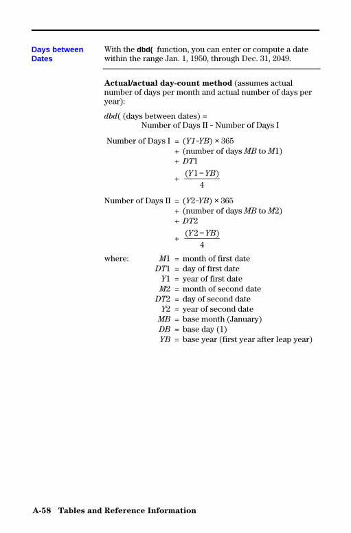
A-58 Tables and Reference Information
8399APXA.DOC TI-83 international English Bob Fedorisko Revised: 02/19/01 1:25 PM Printed: 02/19/01 1:40 PMPage 58 of 58
With the dbd( function, you can enter or compute a datewithin the range Jan. 1, 1950, through Dec. 31, 2049.
Actual/actual day-count method (assumes actualnumber of days per month and actual number of days peryear):
dbd( (days between dates) =Number of Days II - Number of Days I
Number of Days I = (Y1-YB) × 365+ (number of days MB to M1)+ DT1
+( )Y YB1
4
−
Number of Days II = (Y2-YB) × 365+ (number of days MB to M2)+ DT2
+( )Y YB2
4
−
where: M1 = month of first dateDT1 = day of first date
Y1 = year of first dateM2 = month of second date
DT2 = day of second dateY2 = year of second date
MB = base month (January)DB = base day (1)YB = base year (first year after leap year)
Days betweenDates
General Information B-1
8399APXB.DOC TI-83 Intl English, Appendix B Bob Fedorisko Revised: 02/19/01 1:12 PM Printed: 02/19/01 1:41PM Page 1 of 14
B General Information
Battery Information...................................... B-2In Case of Difficulty ..................................... B-4Error Conditions......................................... B-5Accuracy Information.................................... B-10Support and Service Information......................... B-12Warranty Information.................................... B-13
Contents
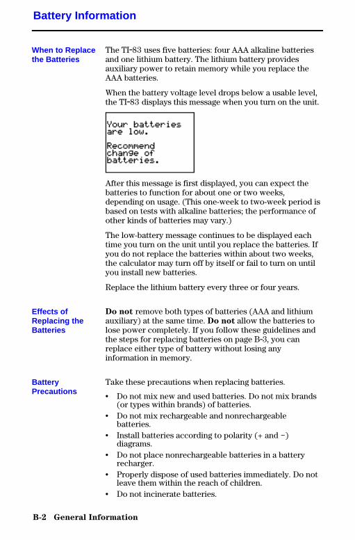
B-2 General Information
8399APXB.DOC TI-83 Intl English, Appendix B Bob Fedorisko Revised: 02/19/01 1:12 PM Printed: 02/19/01 1:41PM Page 2 of 14
The TI.83 uses five batteries: four AAA alkaline batteriesand one lithium battery. The lithium battery providesauxiliary power to retain memory while you replace theAAA batteries.
When the battery voltage level drops below a usable level,the TI.83 displays this message when you turn on the unit.
After this message is first displayed, you can expect thebatteries to function for about one or two weeks,depending on usage. (This one-week to two-week period isbased on tests with alkaline batteries; the performance ofother kinds of batteries may vary.)
The low-battery message continues to be displayed eachtime you turn on the unit until you replace the batteries. Ifyou do not replace the batteries within about two weeks,the calculator may turn off by itself or fail to turn on untilyou install new batteries.
Replace the lithium battery every three or four years.
Do not remove both types of batteries (AAA and lithiumauxiliary) at the same time. Do not allow the batteries tolose power completely. If you follow these guidelines andthe steps for replacing batteries on page B.3, you canreplace either type of battery without losing anyinformation in memory.
Take these precautions when replacing batteries.
• Do not mix new and used batteries. Do not mix brands(or types within brands) of batteries.
• Do not mix rechargeable and nonrechargeablebatteries.
• Install batteries according to polarity (+ and N)diagrams.
• Do not place nonrechargeable batteries in a batteryrecharger.
• Properly dispose of used batteries immediately. Do notleave them within the reach of children.
• Do not incinerate batteries.
Battery Information
When to Replacethe Batteries
Effects ofReplacing theBatteries
BatteryPrecautions
General Information B-3
8399APXB.DOC TI-83 Intl English, Appendix B Bob Fedorisko Revised: 02/19/01 1:12 PM Printed: 02/19/01 1:41PM Page 3 of 14
To replace the batteries, follow these steps.
1. Turn off the calculator. Replace the slide cover over thekeyboard to avoid inadvertently turning on thecalculator. Turn the back of the calculator toward you.
2. Hold the calculator upright. Place your thumb on theoval indentation on the battery cover. Push down andtoward you to slide the cover about ¼ inch (6 mm). Liftoff the cover to expose the battery compartment.
Note: To avoid loss of information stored in
memory, you must turn off the calculator. Do not
remove the AAA batteries and the lithium battery
simultaneously.
3. Replace all four AAA alkaline batteries at the sametime. Or, replace the lithium battery.
• To replace the AAA alkaline batteries, remove allfour discharged AAA batteries and install new onesaccording to the polarity (+ and N) diagrams in thebattery compartment.
• To remove the lithium battery, place your indexfinger on the battery. Insert the tip of a ball-point pen(or similar instrument) under the battery at the smallopening provided in the battery compartment.Carefully pry the battery upward, holding it withyour thumb and finger. (There is a spring that pushesagainst the underside of the battery.)
• Install the new battery, + side up, by inserting thebattery and gently snapping it in with your finger.Use a CR1616 or CR1620 (or equivalent) lithiumbattery.
4. Replace the battery compartment cover. Turn thecalculator on and adjust the display contrast, ifnecessary (step 1; page B.4).
Replacing theBatteries
B-4 General Information
8399APXB.DOC TI-83 Intl English, Appendix B Bob Fedorisko Revised: 02/19/01 1:12 PM Printed: 02/19/01 1:41PM Page 4 of 14
To handle a difficulty, follow these steps.
1. If you cannot see anything on the screen, the contrastmay need to be adjusted.
To darken the screen, press and release y, and thenpress and hold } until the display is sufficiently dark.
To lighten the screen, press and release y, and thenpress and hold † until the display is sufficiently light.
2. If an error menu is displayed, follow the steps inChapter 1. Refer to pages B.5 through B.9 for detailsabout specific errors, if necessary.
3. If a checkerboard cursor ( # ) is displayed, then eitheryou have entered the maximum number of characters ina prompt, or memory is full. If memory is full, press y[MEM] 2 to select 2:Delete , and then delete some itemsfrom memory (Chapter 18).
4. If the busy indicator (dotted line) is displayed, a graphor program has been paused; the TI.83 is waiting forinput. Press Í to continue or press É to break.
5. If the calculator does not seem to work at all, be surethe batteries are fresh and that they are installedproperly. Refer to battery information on pages B.2 andB.3.
In Case of Difficulty
Handling aDifficulty
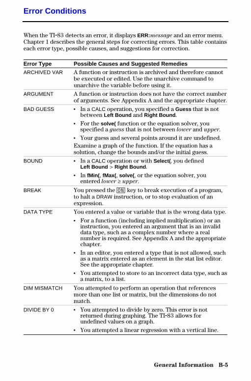
General Information B-5
8399APXB.DOC TI-83 Intl English, Appendix B Bob Fedorisko Revised: 02/19/01 1:12 PM Printed: 02/19/01 1:41PM Page 5 of 14
When the TI.83 detects an error, it displays ERR:message and an error menu.Chapter 1 describes the general steps for correcting errors. This table containseach error type, possible causes, and suggestions for correction.
Error Type Possible Causes and Suggested Remedies
ARCHIVED VAR A function or instruction is archived and therefore cannotbe executed or edited. Use the unarchive command tounarchive the variable before using it.
ARGUMENT A function or instruction does not have the correct numberof arguments. See Appendix A and the appropriate chapter.
BAD GUESS ¦ In a CALC operation, you specified a Guess that is notbetween Left Bound and Right Bound .
¦ For the solve( function or the equation solver, youspecified a guess that is not between lower and upper.
¦ Your guess and several points around it are undefined.Examine a graph of the function. If the equation has asolution, change the bounds and/or the initial guess.
BOUND ¦ In a CALC operation or with Select( , you definedLeft Bound > Right Bound .
¦ In fMin( , fMax( , solve( , or the equation solver, youentered lower ‚ upper.
BREAK You pressed the É key to break execution of a program,to halt a DRAW instruction, or to stop evaluation of anexpression.
DATA TYPE You entered a value or variable that is the wrong data type.
¦ For a function (including implied multiplication) or aninstruction, you entered an argument that is an invaliddata type, such as a complex number where a realnumber is required. See Appendix A and the appropriatechapter.
¦ In an editor, you entered a type that is not allowed, suchas a matrix entered as an element in the stat list editor.See the appropriate chapter.
¦ You attempted to store to an incorrect data type, such asa matrix, to a list.
DIM MISMATCH You attempted to perform an operation that referencesmore than one list or matrix, but the dimensions do notmatch.
DIVIDE BY 0 ¦ You attempted to divide by zero. This error is notreturned during graphing. The TI.83 allows forundefined values on a graph.
¦ You attempted a linear regression with a vertical line.
Error Conditions
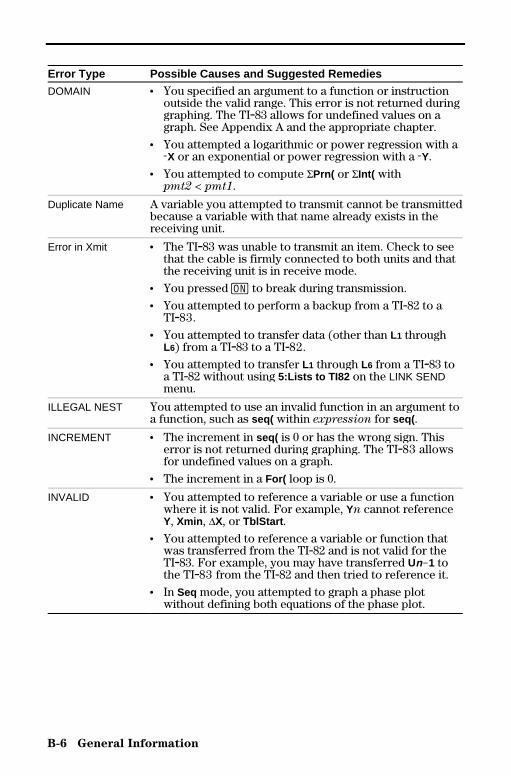
B-6 General Information
8399APXB.DOC TI-83 Intl English, Appendix B Bob Fedorisko Revised: 02/19/01 1:12 PM Printed: 02/19/01 1:41PM Page 6 of 14
Error Type Possible Causes and Suggested Remedies
DOMAIN ¦ You specified an argument to a function or instructionoutside the valid range. This error is not returned duringgraphing. The TI.83 allows for undefined values on agraph. See Appendix A and the appropriate chapter.
¦ You attempted a logarithmic or power regression with aLX or an exponential or power regression with a LY.
¦ You attempted to compute GPrn( or GInt( withpmt2 < pmt1.
Duplicate Name A variable you attempted to transmit cannot be transmittedbecause a variable with that name already exists in thereceiving unit.
Error in Xmit ¦ The TI.83 was unable to transmit an item. Check to seethat the cable is firmly connected to both units and thatthe receiving unit is in receive mode.
¦ You pressed É to break during transmission.
¦ You attempted to perform a backup from a TI.82 to aTI.83.
¦ You attempted to transfer data (other than L1 throughL6) from a TI.83 to a TI.82.
¦ You attempted to transfer L1 through L6 from a TI.83 toa TI.82 without using 5:Lists to TI82 on the LINK SENDmenu.
ILLEGAL NEST You attempted to use an invalid function in an argument toa function, such as seq( within expression for seq( .
INCREMENT ¦ The increment in seq( is 0 or has the wrong sign. Thiserror is not returned during graphing. The TI.83 allowsfor undefined values on a graph.
¦ The increment in a For( loop is 0.
INVALID ¦ You attempted to reference a variable or use a functionwhere it is not valid. For example, Yn cannot referenceY, Xmin , @X, or TblStart .
¦ You attempted to reference a variable or function thatwas transferred from the TI.82 and is not valid for theTI.83. For example, you may have transferred UnN1 tothe TI.83 from the TI.82 and then tried to reference it.
¦ In Seq mode, you attempted to graph a phase plotwithout defining both equations of the phase plot.
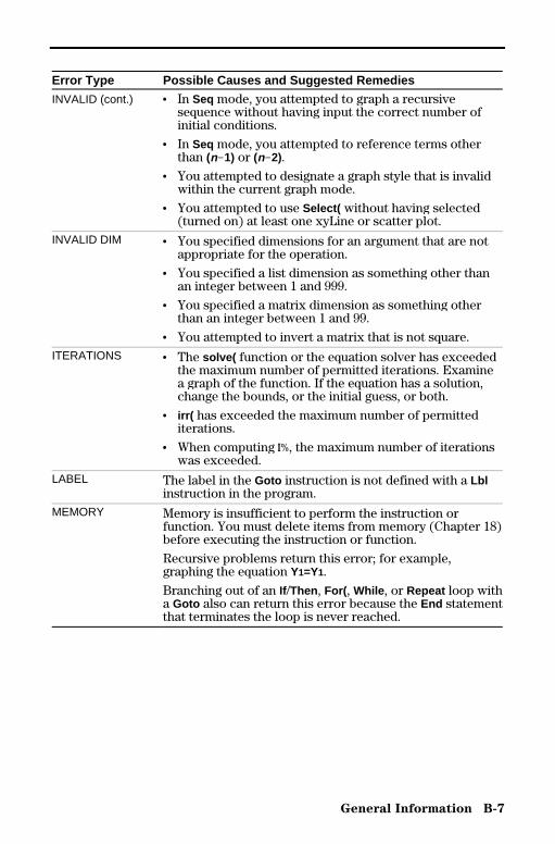
General Information B-7
8399APXB.DOC TI-83 Intl English, Appendix B Bob Fedorisko Revised: 02/19/01 1:12 PM Printed: 02/19/01 1:41PM Page 7 of 14
Error Type Possible Causes and Suggested Remedies
INVALID (cont.) ¦ In Seq mode, you attempted to graph a recursivesequence without having input the correct number ofinitial conditions.
¦ In Seq mode, you attempted to reference terms otherthan (nN1) or (nN2).
¦ You attempted to designate a graph style that is invalidwithin the current graph mode.
¦ You attempted to use Select( without having selected(turned on) at least one xyLine or scatter plot.
INVALID DIM ¦ You specified dimensions for an argument that are notappropriate for the operation.
¦ You specified a list dimension as something other thanan integer between 1 and 999.
¦ You specified a matrix dimension as something otherthan an integer between 1 and 99.
¦ You attempted to invert a matrix that is not square.ITERATIONS ¦ The solve( function or the equation solver has exceeded
the maximum number of permitted iterations. Examinea graph of the function. If the equation has a solution,change the bounds, or the initial guess, or both.
¦ irr( has exceeded the maximum number of permittediterations.
¦ When computing æ, the maximum number of iterationswas exceeded.
LABEL The label in the Goto instruction is not defined with a Lblinstruction in the program.
MEMORY Memory is insufficient to perform the instruction orfunction. You must delete items from memory (Chapter 18)before executing the instruction or function.
Recursive problems return this error; for example,graphing the equation Y1=Y1.
Branching out of an If/Then , For( , While , or Repeat loop witha Goto also can return this error because the End statementthat terminates the loop is never reached.
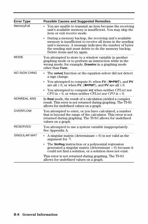
B-8 General Information
8399APXB.DOC TI-83 Intl English, Appendix B Bob Fedorisko Revised: 02/19/01 1:12 PM Printed: 02/19/01 1:41PM Page 8 of 14
Error Type Possible Causes and Suggested RemediesMemoryFull ¦ You are unable to transmit an item because the receiving
unit’s available memory is insufficient. You may skip theitem or exit receive mode.
¦ During a memory backup, the receiving unit’s availablememory is insufficient to receive all items in the sendingunit’s memory. A message indicates the number of bytesthe sending unit must delete to do the memory backup.Delete items and try again.
MODE You attempted to store to a window variable in anothergraphing mode or to perform an instruction while in thewrong mode; for example, DrawInv in a graphing modeother than Func .
NO SIGN CHNG ¦ The solve( function or the equation solver did not detecta sign change.
¦ You attempted to compute æ when FV, (ÚäPMT), and PVare all ‚ 0, or when FV, (ÚäPMT), and PV are all � 0.
¦ You attempted to compute irr( when neither CFList norCFO is > 0, or when neither CFList nor CFO is < 0.
NONREAL ANS In Real mode, the result of a calculation yielded a complexresult. This error is not returned during graphing. The TI.83allows for undefined values on a graph.
OVERFLOW You attempted to enter, or you have calculated, a numberthat is beyond the range of the calculator. This error is notreturned during graphing. The TI.83 allows for undefinedvalues on a graph.
RESERVED You attempted to use a system variable inappropriately.See Appendix A.
SINGULAR MAT ¦ A singular matrix (determinant = 0) is not valid as theargument for L1.
¦ The SinReg instruction or a polynomial regressiongenerated a singular matrix (determinant = 0) because itcould not find a solution, or a solution does not exist.
This error is not returned during graphing. The TI.83allows for undefined values on a graph.
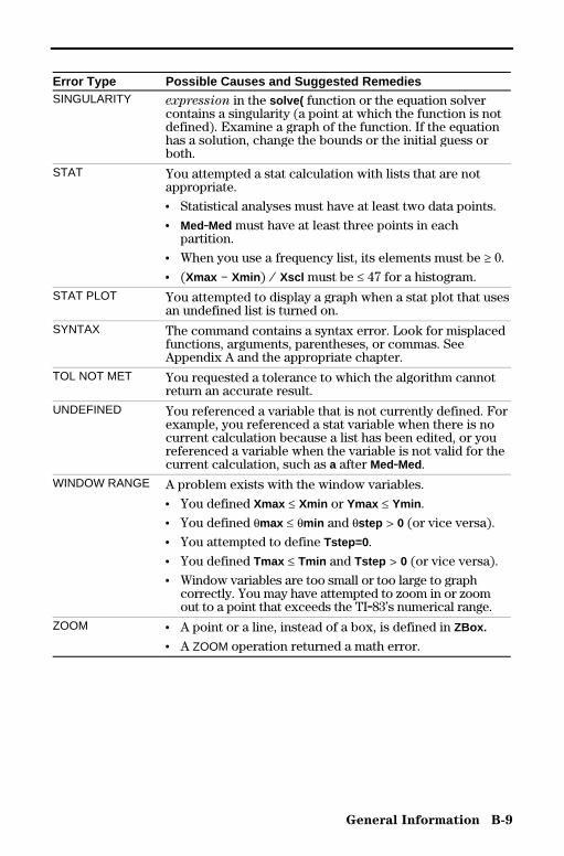
General Information B-9
8399APXB.DOC TI-83 Intl English, Appendix B Bob Fedorisko Revised: 02/19/01 1:12 PM Printed: 02/19/01 1:41PM Page 9 of 14
Error Type Possible Causes and Suggested RemediesSINGULARITY expression in the solve( function or the equation solver
contains a singularity (a point at which the function is notdefined). Examine a graph of the function. If the equationhas a solution, change the bounds or the initial guess orboth.
STAT You attempted a stat calculation with lists that are notappropriate.
¦ Statistical analyses must have at least two data points.
¦ Med.Med must have at least three points in eachpartition.
¦ When you use a frequency list, its elements must be ‚ 0.
¦ (Xmax N Xmin ) à Xscl must be � 47 for a histogram.STAT PLOT You attempted to display a graph when a stat plot that uses
an undefined list is turned on.SYNTAX The command contains a syntax error. Look for misplaced
functions, arguments, parentheses, or commas. SeeAppendix A and the appropriate chapter.
TOL NOT MET You requested a tolerance to which the algorithm cannotreturn an accurate result.
UNDEFINED You referenced a variable that is not currently defined. Forexample, you referenced a stat variable when there is nocurrent calculation because a list has been edited, or youreferenced a variable when the variable is not valid for thecurrent calculation, such as a after Med.Med.
WINDOW RANGE A problem exists with the window variables.
¦ You defined Xmax � Xmin or Ymax � Ymin .
¦ You defined qmax � qmin and qstep > 0 (or vice versa).
¦ You attempted to define Tstep=0 .
¦ You defined Tmax � Tmin and Tstep > 0 (or vice versa).
¦ Window variables are too small or too large to graphcorrectly. You may have attempted to zoom in or zoomout to a point that exceeds the TI.83’s numerical range.
ZOOM ¦ A point or a line, instead of a box, is defined in ZBox.
¦ A ZOOM operation returned a math error.

B-10 General Information
8399APXB.DOC TI-83 Intl English, Appendix B Bob Fedorisko Revised: 02/19/01 1:12 PM Printed: 02/19/01 1:41PM Page 10 of 14
To maximize accuracy, the TI.83 carries more digitsinternally than it displays. Values are stored in memoryusing up to 14 digits with a two-digit exponent.
• You can store a value in the window variables using upto 10 digits (12 for Xscl , Yscl , Tstep , and qstep ).
• Displayed values are rounded as specified by the modesetting with a maximum of 10 digits and a two-digitexponent.
• RegEQ displays up to 14 digits in Float mode. Using afixed-decimal setting other than Float causes RegEQresults to be rounded and stored with the specifiednumber of decimal places.
Xmin is the center of the leftmost pixel, Xmax is the centerof the next-to-the-rightmost pixel. (The rightmost pixel isreserved for the busy indicator.) @X is the distancebetween the centers of two adjacent pixels.
• In Full screen mode, @X is calculated as(Xmax N Xmin ) à 94. In G.T split-screen mode, @X iscalculated as (Xmax N Xmin ) à 46.
• If you enter a value for @X from the home screen or aprogram in Full screen mode, Xmax is calculated asXmin + @X … 94. In G.T split-screen mode, Xmax iscalculated as Xmin + @X … 46.
Ymin is the center of the next-to-the-bottom pixel; Ymax isthe center of the top pixel. @Y is the distance between thecenters of two adjacent pixels.
• In Full screen mode, @Y is calculated as(Ymax N Ymin ) à 62. In Horiz split-screen mode, @Y iscalculated as (Ymax N Ymin ) à 30. In G.T split-screenmode, @Y is calculated as (Ymax N Ymin ) à 50.
• If you enter a value for @Y from the home screen or aprogram in Full screen mode, Ymax is calculated asYmin + @Y … 62. In Horiz split-screen mode, Ymax iscalculated as Ymin + @Y … 30. In G.T split-screen mode,Ymax is calculated as Ymin + @Y … 50.
Accuracy Information
ComputationalAccuracy
GraphingAccuracy
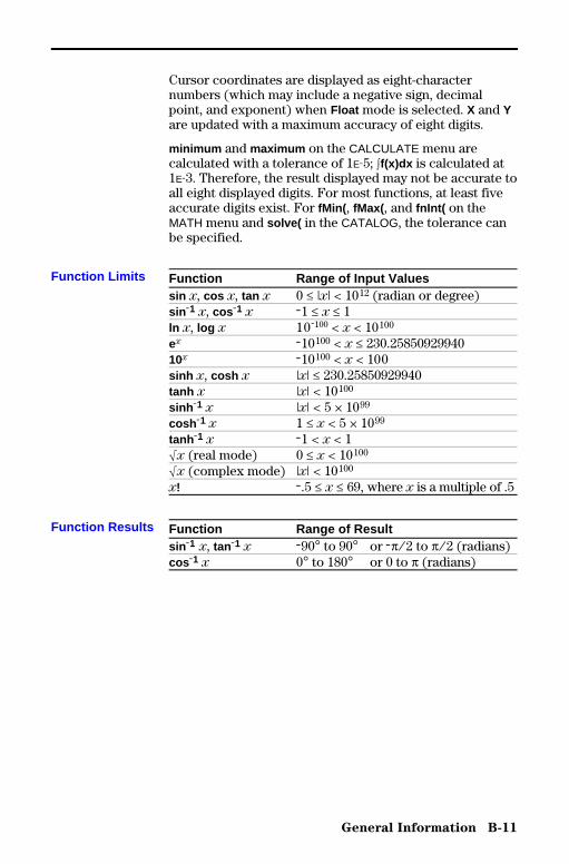
General Information B-11
8399APXB.DOC TI-83 Intl English, Appendix B Bob Fedorisko Revised: 02/19/01 1:12 PM Printed: 02/19/01 1:41PM Page 11 of 14
Cursor coordinates are displayed as eight-characternumbers (which may include a negative sign, decimalpoint, and exponent) when Float mode is selected. X and Yare updated with a maximum accuracy of eight digits.
minimum and maximum on the CALCULATE menu arecalculated with a tolerance of 1EL5; ‰f(x)dx is calculated at1EL3. Therefore, the result displayed may not be accurate toall eight displayed digits. For most functions, at least fiveaccurate digits exist. For fMin( , fMax( , and fnInt( on theMATH menu and solve( in the CATALOG, the tolerance canbe specified.
Function Range of Input Valuessin x, cos x, tan x 0 � |x| < 1012 (radian or degree)sin L1 x, cos L1 x L1 � x � 1ln x, log x 10L100 < x < 10100
ex L10100 < x � 230.2585092994010x L10100 < x < 100sinh x, cosh x |x| � 230.25850929940tanh x |x| < 10100
sinh L1 x |x| < 5 × 1099
cosh L1 x 1 � x < 5 × 1099
tanh L1 x L1 < x < 1‡x (real mode) 0 � x < 10100
‡x (complex mode) |x| < 10100
x! L.5 � x � 69, where x is a multiple of .5
Function Range of Resultsin L1 x, tan L1 x L90¡ to 90¡ or Lpà2 to pà2 (radians)cos L1 x 0¡ to 180¡ or 0 to p (radians)
Function Limits
Function Results
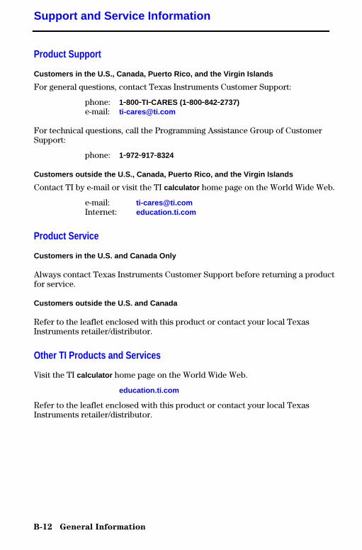
B-12 General Information
8399APXB.DOC TI-83 Intl English, Appendix B Bob Fedorisko Revised: 02/19/01 1:12 PM Printed: 02/19/01 1:41PM Page 12 of 14
Product Support
Customers in the U.S., Canada, Puerto Rico, and the Virgin Islands
For general questions, contact Texas Instruments Customer Support:
phone: 1.800.TI.CARES (1.800.842.2737)e-mail: [email protected]
For technical questions, call the Programming Assistance Group of CustomerSupport:
phone: 1.972.917.8324
Customers outside the U.S., Canada, Puerto Rico, and the Virgin Islands
Contact TI by e-mail or visit the TI calculator home page on the World Wide Web.
e-mail: [email protected]: education.ti.com
Product Service
Customers in the U.S. and Canada Only
Always contact Texas Instruments Customer Support before returning a productfor service.
Customers outside the U.S. and Canada
Refer to the leaflet enclosed with this product or contact your local TexasInstruments retailer/distributor.
Other TI Products and Services
Visit the TI calculator home page on the World Wide Web.
education.ti.com
Refer to the leaflet enclosed with this product or contact your local TexasInstruments retailer/distributor.
Support and Service Information
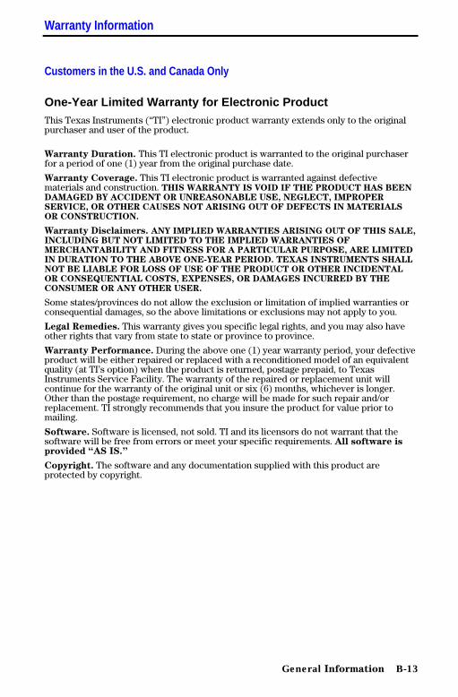
General Information B-13
8299APPB.DOC TI-82, Appendix B, English Bob Fedorisko Revised: 02/27/01 12:20 PM Printed:02/27/01 12:25 PM Page 12 of 13
Warranty Information
Customers in the U.S. and Canada Only
One-Year Limited Warranty for Electronic ProductThis Texas Instruments (“TI”) electronic product warranty extends only to the originalpurchaser and user of the product.
Warranty Duration. This TI electronic product is warranted to the original purchaserfor a period of one (1) year from the original purchase date.
Warranty Coverage. This TI electronic product is warranted against defectivematerials and construction. THIS WARRANTY IS VOID IF THE PRODUCT HAS BEENDAMAGED BY ACCIDENT OR UNREASONABLE USE, NEGLECT, IMPROPERSERVICE, OR OTHER CAUSES NOT ARISING OUT OF DEFECTS IN MATERIALSOR CONSTRUCTION.
Warranty Disclaimers. ANY IMPLIED WARRANTIES ARISING OUT OF THIS SALE,INCLUDING BUT NOT LIMITED TO THE IMPLIED WARRANTIES OFMERCHANTABILITY AND FITNESS FOR A PARTICULAR PURPOSE, ARE LIMITEDIN DURATION TO THE ABOVE ONE-YEAR PERIOD. TEXAS INSTRUMENTS SHALLNOT BE LIABLE FOR LOSS OF USE OF THE PRODUCT OR OTHER INCIDENTALOR CONSEQUENTIAL COSTS, EXPENSES, OR DAMAGES INCURRED BY THECONSUMER OR ANY OTHER USER.
Some states/provinces do not allow the exclusion or limitation of implied warranties orconsequential damages, so the above limitations or exclusions may not apply to you.
Legal Remedies. This warranty gives you specific legal rights, and you may also haveother rights that vary from state to state or province to province.
Warranty Performance. During the above one (1) year warranty period, your defectiveproduct will be either repaired or replaced with a reconditioned model of an equivalentquality (at TI’s option) when the product is returned, postage prepaid, to TexasInstruments Service Facility. The warranty of the repaired or replacement unit willcontinue for the warranty of the original unit or six (6) months, whichever is longer.Other than the postage requirement, no charge will be made for such repair and/orreplacement. TI strongly recommends that you insure the product for value prior tomailing.
Software. Software is licensed, not sold. TI and its licensors do not warrant that thesoftware will be free from errors or meet your specific requirements. All software isprovided “AS IS.”
Copyright. The software and any documentation supplied with this product areprotected by copyright.
B-14 General Information
8299APPB.DOC TI-82, Appendix B, English Bob Fedorisko Revised: 02/27/01 12:20 PM Printed:02/27/01 12:25 PM Page 13 of 13
Australia & New Zealand Customers only
One-Year Limited Warranty for Commercial Electronic Product
This Texas Instruments electronic product warranty extends only to theoriginal purchaser and user of the product.Warranty Duration. This Texas Instruments electronic product is warrantedto the original purchaser for a period of one (1) year from the originalpurchase date.Warranty Coverage. This Texas Instruments electronic product is warrantedagainst defective materials and construction. This warranty is void if theproduct has been damaged by accident or unreasonable use, neglect, improperservice, or other causes not arising out of defects in materials or construction.Warranty Disclaimers. Any implied warranties arising out of this sale,including but not limited to the implied warranties of merchantabilityand fitness for a particular purpose, are limited in duration to theabove one-year period. Texas Instruments shall not be liable for lossof use of the product or other incidental or consequential costs,expenses, or damages incurred by the consumer or any other user.
Some jurisdictions do not allow the exclusion or limitation of impliedwarranties or consequential damages, so the above limitations or exclusionsmay not apply to you.Legal Remedies. This warranty gives you specific legal rights, and you mayalso have other rights that vary from jurisdiction to jurisdiction.Warranty Performance. During the above one (1) year warranty period,your defective product will be either repaired or replaced with a new orreconditioned model of an equivalent quality (at TI’s option) when the productis returned to the original point of purchase. The repaired or replacement unitwill continue for the warranty of the original unit or six (6) months, whicheveris longer. Other than your cost to return the product, no charge will be madefor such repair and/or replacement. TI strongly recommends that you insurethe product for value if you mail it.Software. Software is licensed, not sold. TI and its licensors do not warrantthat the software will be free from errors or meet your specific requirements.All software is provided “AS IS.”Copyright. The software and any documentation supplied with this productare protected by copyright.
All Customers Outside the U.S. and CanadaFor information about the length and terms of the warranty, refer to your packageand/or to the warranty statement enclosed with this product, or contact your local TexasInstruments retailer/distributor.
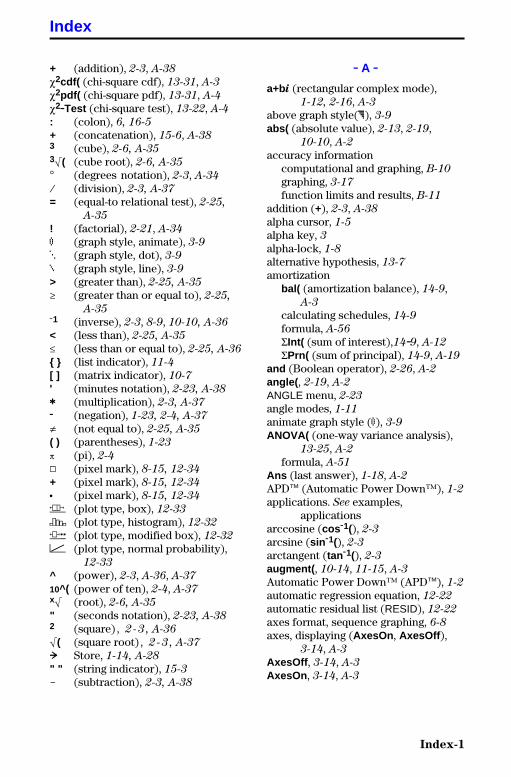
Index-1
Index
8399INDX.DOC TI-83 international English Bob Fedorisko Revised: 02/20/01 10:54 AM Printed: 02/21/01 8:40AM Page 1 of 16
+ (addition), 2-3, A-38
c2cdf( (chi-square cdf), 13-31, A-3
c2pdf( (chi-square pdf), 13-31, A-4
c2.Test (chi-square test), 13-22, A-4
: (colon), 6, 16-5
+ (concatenation), 15-6, A-383 (cube), 2-6, A-353‡( (cube root), 2-6, A-35
¡ (degrees notation), 2-3, A-34
à (division), 2-3, A-37
= (equal-to relational test), 2-25,
A-35
! (factorial), 2-21, A-34
ì (graph style, animate), 3-9
í (graph style, dot), 3-9
ç (graph style, line), 3-9
> (greater than), 2-25, A-35
‚ (greater than or equal to), 2-25,
A-35L1 (inverse), 2-3, 8-9, 10-10, A-36
< (less than), 2-25, A-35
� (less than or equal to), 2-25, A-36
{ } (list indicator), 11-4
[ ] (matrix indicator), 10-7
' (minutes notation), 2-23, A-38
ä (multiplication), 2-3, A-37
M (negation), 1-23, 2-4, A-37
ƒ (not equal to), 2-25, A-35
( ) (parentheses), 1-23
p (pi), 2-4
› (pixel mark), 8-15, 12-34
+ (pixel mark), 8-15, 12-34
¦ (pixel mark), 8-15, 12-34
Ö (plot type, box), 12-33
Ò (plot type, histogram), 12-32
Õ (plot type, modified box), 12-32
Ô (plot type, normal probability),12-33
^ (power), 2-3, A-36, A-37
10^( (power of ten), 2-4, A-37x‡ (root), 2-6, A-35
" (seconds notation), 2-23, A-382 (square) , 2-3 , A-36
‡( (square root) , 2-3 , A-37
! Store, 1-14, A-28
" " (string indicator), 15-3
N (subtraction), 2-3, A-38
. A .
a+bi (rectangular complex mode),1-12, 2-16, A-3
above graph style(é), 3-9
abs( (absolute value), 2-13, 2-19,10-10, A-2
accuracy informationcomputational and graphing, B-10
graphing, 3-17
function limits and results, B-11
addition (+), 2-3, A-38
alpha cursor, 1-5
alpha key, 3alpha-lock, 1-8
alternative hypothesis, 13-7
amortizationbal( (amortization balance), 14-9,
A-3
calculating schedules, 14-9
formula, A-56
GInt( (sum of interest),14.9, A-12
GPrn( (sum of principal), 14-9, A-19
and (Boolean operator), 2-26, A-2
angle( , 2-19, A-2
ANGLE menu, 2-23
angle modes, 1-11
animate graph style (ì), 3-9
ANOVA( (one-way variance analysis),13-25, A-2
formula, A-51
Ans (last answer), 1-18, A-2
APDé (Automatic Power Down™), 1-2
applications. See examples,applications
arccosine (cos M1(), 2-3
arcsine (sin M1(), 2-3
arctangent (tan M1(), 2-3
augment( , 10-14, 11-15, A-3
Automatic Power Down™ (APDé), 1-2
automatic regression equation, 12-22
automatic residual list (RESID), 12-22
axes format, sequence graphing, 6-8
axes, displaying (AxesOn , AxesOff ),3-14, A-3
AxesOff , 3-14, A-3
AxesOn , 3-14, A-3
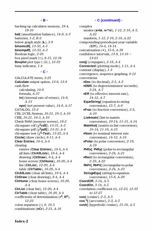
Index-2
8399INDX.DOC TI-83 international English Bob Fedorisko Revised: 02/20/01 10:54 AM Printed: 02/21/01 8:40AM Page 2 of 16
. B .
backing up calculator memory, 19-4,
19-10
bal( (amortization balance), 14-9, A-3
batteries, 1-2, B-2
below graph style (ê), 3-9
binomcdf( , 13-33, A-3
binompdf( , 13-33, A-3
Boolean logic, 2-26
box pixel mark (›), 8-15, 12-34
Boxplot plot type ( Ö), 12-33
busy indicator, 1-4
. C .
CALCULATE menu, 3-25
Calculate output option, 13-6, 13-8
cash flowcalculating, 14-8
formula, A-57
irr( (internal rate of return), 14-8,A-13
npv( (net present value), 14-8, A-17
CATALOG, 15-2
CBL 2/CBL System, 16-21, 19-3, A-10
CBR, 16-21, 19-3, A-10
Check RAM (memory screen), 18-2
chi-square cdf (c2cdf( ), 13-31, A-3
chi-square pdf (c2pdf( ), 13-31, A-4
chi-square test (c2.Test), 13-22, A-4
Circle( (draw circle), 8-11, A-4
Clear Entries , 18-4, A-4
clearingentries (Clear Entries ), 18-4, A-4
all lists (ClrAllLists ), 18-4, A-4
drawing (ClrDraw ), 8-4, A-4
home screen (ClrHome ), 16-20, A-4
list (ClrList ), 12-20, A-4
table (ClrTable ), 16-20, A-4
ClrAllLists (clear all lists), 18-4, A-4
ClrDraw (clear drawing), 8-4, A-4
ClrHome (clear home screen), 16-20,A-4
ClrList (clear list), 12-20, A-4
ClrTable (clear table), 16-20, A-4
coefficients of determination (r2, R2),12-23
colon separator (:), 6, 16-5
combinations (nCr), 2-21, A-16
. C (continued) .
complexmodes (a+bi, re^qi), 1-12, 2-16, A-3,
A-22
numbers, 1-12, 2-16, 2-18, A-22
compounding-periods-per-year variable(C/Y), 14-4, 14-14
concatenation (+), 15-6, A-38
confidence intervals, 13-8, 13-16 N13.21
conj( (conjugate), 2-18, A-4
Connected (plotting mode), 1-11, A-4
contrast (display), 1-3
convergence, sequence graphing, 6-12
conversions4Dec (to decimal), 2-5, A-5
4DMS (to degrees/minutes/ seconds),2-24, A-7
4Eff (to effective interest rate),14-12, A-7
Equ4String( (equation-to-stringconversion), 15-7, A-8
4Frac (to fraction conversion), 2-5,
A-10
List 4matr( (list-to-matrixconversion), 10-14, 11-15, A-14
Matr4list( (matrix-to-list conversion),10-14, 11-16, A-15
4Nom (to nominal interest rateconversion), 14-12, A-16
4Polar (to polar conversion), 2-19,
A-19
P4Rx(, P4Ry( (polar-to-rectangularconversion), 2-24, A-21
4Rect (to rectangular conversion),2-19, A-22
R4Pr(, R4Pq( (rectangular-to-polarconversion), 2-24, A-23
String 4Equ( (string-to-equationconversion), 15-8, A-29
CoordOff , 3-14, A-5
CoordOn , 3-14, A-5
correlation coefficient (r), 12-23, 12-25
to 12-27
cos( (cosine), 2-3, A-5
cos M1( (arccosine), 2-3, A-5
cosh( (hyperbolic cosine), 15-10, A-5

Index-3
8399INDX.DOC TI-83 international English Bob Fedorisko Revised: 02/20/01 10:54 AM Printed: 02/21/01 8:40AM Page 3 of 16
. D (continued) .
cosh M1( (hyperbolic arccosine), 15-10,
A-5
cosine (cos( ), 2-3, A-5
cross pixel mark (+), 8-15, 12-34
cube ( 3) , 2-6, A-35
cube root (3‡(), 2-6, A-35
CubicReg (cubic regression), 12-26,
A-5
cubic regression (CubicReg ), 12-26,
A-5
cumulative sum (cumSum( ), 10-15,11-12, A-5
cumSum( (cumulative sum), 10-15,11-12, A-5
cursors, 1-5, 1-8
C/Y (compounding-periods-per-yearvariable), 14-4, 14-14
. D .
Data input option, 13-6, 13-7
days between dates (dbd( ), 14-13, A-5,
A-58
dbd( (days between dates), 14-13, A-5,
A-58
4Dec (to decimal conversion), 2-5, A-5
decimal mode (float or fixed), 1-10
decrement and skip (DS<(), 16-14, A-7
definite integral, 2-7, 3-28, 4-8, 5-6
Degree angle mode, 1-11, 2-23, A-6
degrees notation ( ¡) , 2-3, A-34
DELETE FROM menu, 18-3
delete variable contents (DelVar),16-15, A-6
DelVar (delete variable contents),16-15, A-6
DependAsk , 7-3, 7-5, A-6
DependAuto , 7-3, 7-5, A-6
derivative. See numerical derivativedet( (determinant), 10-12, A-6
determinant (det(), 10-12, A-6
DiagnosticOff , 12-23, A-6
DiagnosticOn , 12-23, A-6
diagnostics display mode(r, r2, R2),12-23
differentiation, 2-8, 3-28, 4-8, 5-6
. D (continued) .
dimensioning a list or matrix, 10-12,10-13, 11-11, A-6
dim( (dimension), 10-12, 11-11, A-6
!dim( (assign dimension), 10-13,11-11, A-6
Disp (display), 16-18, A-6
DispGraph (display graph), 16-19, A-7
display contrast, 1-3
display cursors, 1-5
DispTable (display table), 16-19, A-7
DISTR (distributions menu), 13-29
DISTR DRAW (distributions drawingmenu), 13-35
distribution functionsbinomcdf( , 13-33, A-3
binompdf( , 13-33, A-3
c2cdf( , 13-31, A-3
c2pdf( , 13-31, A-4
Ûcdf( , 13-32, A-8
Ûpdf( , 13-32, A-9
geometcdf( , 13-34, A-10
geometpdf( , 13-34, A-11
invNorm( , 13-30, A-12
normalcdf( , 13-30, A-17
normalpdf( , 13-29, A-17
poissoncdf( , 13-34, A-99
poissonpdf( , 13-33, A-19
tcdf( , 13-31, A-29
tpdf( , 13-30, A-29
distribution shading instructionsShadec2(, 13-36, A-26
ShadeÛ(, 13-36, A-27
ShadeNorm( , 13-35, A-27
Shade_t( , 13-36, A-27
division (à) , 2-3, A-37
DMS (degrees/minutes/seconds entrynotation), 2-23, A-38
4DMS (to degrees/minutes/seconds),2-24, A-7
dot graph style (í), 3-9
dot pixel mark (¦), 8-15, 12-34
Dot (plotting mode), 1-11, A-7
DrawF (draw a function), 8-9, A-7
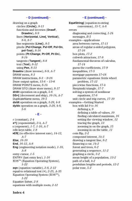
Index-4
8399INDX.DOC TI-83 international English Bob Fedorisko Revised: 02/20/01 10:54 AM Printed: 02/21/01 8:40AM Page 4 of 16
. D (continued) .
drawing on a graphcircles (Circle( ), 8-11
functions and inverses (DrawF ,DrawInv ), 8-9
lines (Horizontal , Line( , Vertical ),8-6, 8-7
line segments (Line( ), 8-5
pixels (Pxl.Change , Pxl.Off , Pxl.On,pxl .Test), 8-16
points (Pt.Change , Pt.Off , Pt.On),8-14
tangents (Tangent ), 8-8
text (Text), 8-12
using Pen, 8-13
DrawInv (draw inverse), 8-9, A-7
DRAW menu, 8-3
DRAW instructions, 8-3 N 8.16
Draw output option, 13-6 N 13.8DRAW POINTS menu, 8-14
DRAW STO (draw store menu), 8-17
dr/d q operation on a graph, 5-6
DS<( (decrement and skip), 16-14, A-7
DuplicateName menu, 19-5
dx/dt operation on a graph, 3-28, 4-8
dy/dx operation on a graph, 3-28, 4-8,
5-6
. E .
e (constant), 2-4
e^( (exponential), 2-4, A-7
å (exponent), 1-7, 1-10, A-7
edit keys table, 1-8
4Eff( (to effective interest rate), 14-12,
A-7
Else , 16-10
End , 16-12, A-8
Eng (engineering notation mode), 1-10,
A-8
entry cursor, 1-5
ENTRY (last entry key), 1-16
EOSé (Equation Operating System),1-22
eqn (equation variable), 2-8, 2-12
equal-to relational test (=), 2-25, A-35
Equation Operating System (EOSé),1-22
Equation Solver, 2-8
equations with multiple roots, 2-12
. E (continued) .
Equ4String( (equation-to-stringconversion), 15-7, A-8
errorsdiagnosing and correcting, 1-24
messages, B-5
examples—applicationsarea between curves, 17-11
areas of regular n-sided polygons,17-16
box plots, 17-2
cobweb attractors, 17-8
fundamental theorem of calculus,17-14
guess the coefficients, 17-9
inequalities, 17-5
mortgage payments 17.18
parametric equations: ferris wheelproblem, 17-12
piecewise functions, 17-4
Sierpinski triangle, 17-7
solving a system of nonlinearequations, 17-6
unit circle and trig curves, 17-10
examples—Getting Startedbox with lid 9 to 16
defining a, 9defining a table of values, 10
finding calculated maximum, 16
setting the viewing window, 12
tracing the graph, 13
zooming in on the graph, 15
zooming in on the table, 11
coin flip, 2-2
compound interest, 14-3
drawing a tangent line, 8-2
financing a car, 14-2
forest and trees, 6-2
generating a sequence, 11-2
graphing a circle, 3-2
mean height of a population, 13-2
path of a ball, 4-2
pendulum lengths and periods, 12-2
polar rose, 5-2
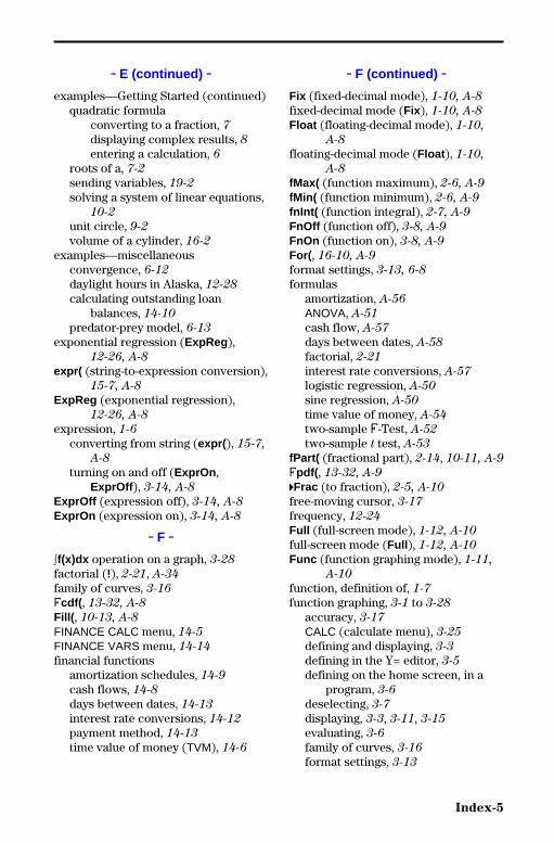
Index-5
8399INDX.DOC TI-83 international English Bob Fedorisko Revised: 02/20/01 10:54 AM Printed: 02/21/01 8:40AM Page 5 of 16
. E (continued) .
examples—Getting Started (continued)quadratic formula
converting to a fraction, 7displaying complex results, 8entering a calculation, 6
roots of a, 7-2
sending variables, 19-2
solving a system of linear equations,10-2
unit circle, 9-2
volume of a cylinder, 16-2
examples—miscellaneousconvergence, 6-12
daylight hours in Alaska, 12-28
calculating outstanding loanbalances, 14-10
predator-prey model, 6-13
exponential regression (ExpReg ),12-26, A-8
expr( (string-to-expression conversion),15-7, A-8
ExpReg (exponential regression),12-26, A-8
expression, 1-6
converting from string (expr( ), 15-7,
A-8
turning on and off (ExprOn ,ExprOff ), 3-14, A-8
ExprOff (expression off), 3-14, A-8
ExprOn (expression on), 3-14, A-8
. F .
‰f(x)dx operation on a graph, 3-28
factorial (!), 2-21, A-34
family of curves, 3-16
Ûcdf( , 13-32, A-8
Fill( , 10-13, A-8
FINANCE CALC menu, 14-5
FINANCE VARS menu, 14-14
financial functionsamortization schedules, 14-9
cash flows, 14-8
days between dates, 14-13
interest rate conversions, 14-12
payment method, 14-13
time value of money (TVM), 14-6
. F (continued) .
Fix (fixed-decimal mode), 1-10, A-8
fixed-decimal mode (Fix), 1-10, A-8
Float (floating-decimal mode), 1-10,
A-8
floating-decimal mode (Float ), 1-10,
A-8
fMax( (function maximum), 2-6, A-9
fMin( (function minimum), 2-6, A-9
fnInt( (function integral), 2-7, A-9
FnOff (function off), 3-8, A-9
FnOn (function on), 3-8, A-9
For( , 16-10, A-9
format settings, 3-13, 6-8
formulasamortization, A-56
ANOVA, A-51
cash flow, A-57
days between dates, A-58
factorial, 2-21
interest rate conversions, A-57
logistic regression, A-50
sine regression, A-50
time value of money, A-54
two-sample Û-Test, A-52
two-sample t test, A-53
fPart( (fractional part), 2-14, 10-11, A-9
Ûpdf( , 13-32, A-9
4Frac (to fraction), 2-5, A-10
free-moving cursor, 3-17
frequency, 12-24
Full (full-screen mode), 1-12, A-10
full-screen mode (Full ), 1-12, A-10
Func (function graphing mode), 1-11,
A-10
function, definition of, 1-7
function graphing, 3-1 to 3-28
accuracy, 3-17
CALC (calculate menu), 3-25
defining and displaying, 3-3
defining in the Y= editor, 3-5
defining on the home screen, in aprogram, 3-6
deselecting, 3-7
displaying, 3-3, 3-11, 3-15
evaluating, 3-6
family of curves, 3-16
format settings, 3-13
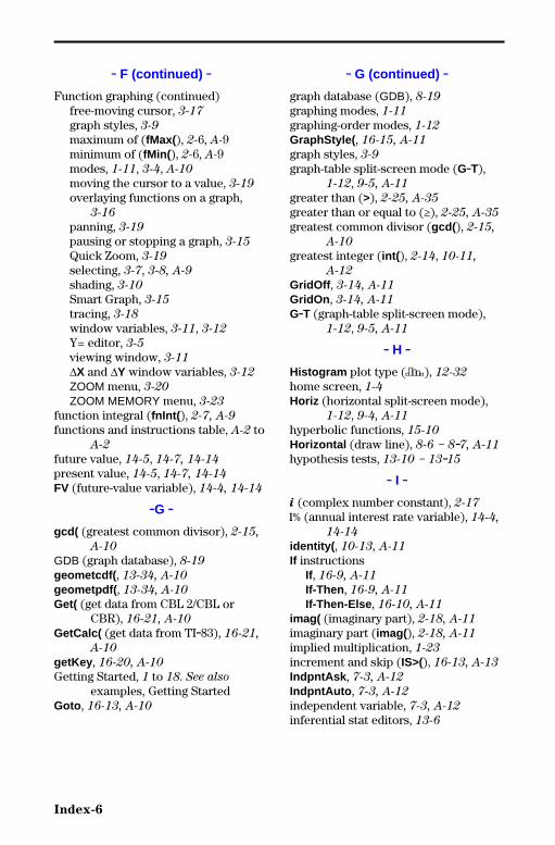
Index-6
8399INDX.DOC TI-83 international English Bob Fedorisko Revised: 02/20/01 10:54 AM Printed: 02/21/01 8:40AM Page 6 of 16
. F (continued) .
Function graphing (continued)free-moving cursor, 3-17
graph styles, 3-9
maximum of (fMax(), 2-6, A-9minimum of (fMin( ), 2-6, A-9modes, 1-11, 3-4, A-10
moving the cursor to a value, 3-19
overlaying functions on a graph,3-16
panning, 3-19
pausing or stopping a graph, 3-15
Quick Zoom, 3-19
selecting, 3-7, 3-8, A-9
shading, 3-10
Smart Graph, 3-15
tracing, 3-18
window variables, 3-11, 3-12
Y= editor, 3-5
viewing window, 3-11
@X and @Y window variables, 3-12
ZOOM menu, 3-20
ZOOM MEMORY menu, 3-23
function integral (fnInt( ), 2-7, A-9
functions and instructions table, A-2 toA-2
future value, 14-5, 14-7, 14-14
present value, 14-5, 14-7, 14-14
FV (future-value variable), 14-4, 14-14
.G .
gcd( (greatest common divisor), 2-15,
A-10
GDB (graph database), 8-19
geometcdf( , 13-34, A-10
geometpdf( , 13-34, A-10
Get( (get data from CBL 2/CBL orCBR), 16-21, A-10
GetCalc( (get data from TI.83), 16-21,
A-10
getKey , 16-20, A-10
Getting Started, 1 to 18. See also
examples, Getting StartedGoto , 16-13, A-10
. G (continued) .
graph database (GDB), 8-19
graphing modes, 1-11
graphing-order modes, 1-12
GraphStyle( , 16-15, A-11
graph styles, 3-9
graph-table split-screen mode (G.T),1-12, 9-5, A-11
greater than (>), 2-25, A-35
greater than or equal to (‚), 2-25, A-35
greatest common divisor (gcd( ), 2-15,
A-10
greatest integer (int( ), 2-14, 10-11,
A-12
GridOff , 3-14, A-11
GridOn , 3-14, A-11
G.T (graph-table split-screen mode),1-12, 9-5, A-11
. H .
Histogram plot type (Ò), 12-32
home screen, 1-4
Horiz (horizontal split-screen mode),1-12, 9-4, A-11
hyperbolic functions, 15-10
Horizontal (draw line), 8-6 N 8.7, A-11
hypothesis tests, 13-10 N 13.15
. I .
i (complex number constant), 2-17
æ (annual interest rate variable), 14-4,
14-14
identity( , 10-13, A-11
If instructionsIf, 16-9, A-11
If-Then , 16-9, A-11
If-Then-Else , 16-10, A-11
imag( (imaginary part), 2-18, A-11
imaginary part (imag( ), 2-18, A-11
implied multiplication, 1-23
increment and skip (IS>(), 16-13, A-13
IndpntAsk , 7-3, A-12
IndpntAuto , 7-3, A-12
independent variable, 7-3, A-12
inferential stat editors, 13-6
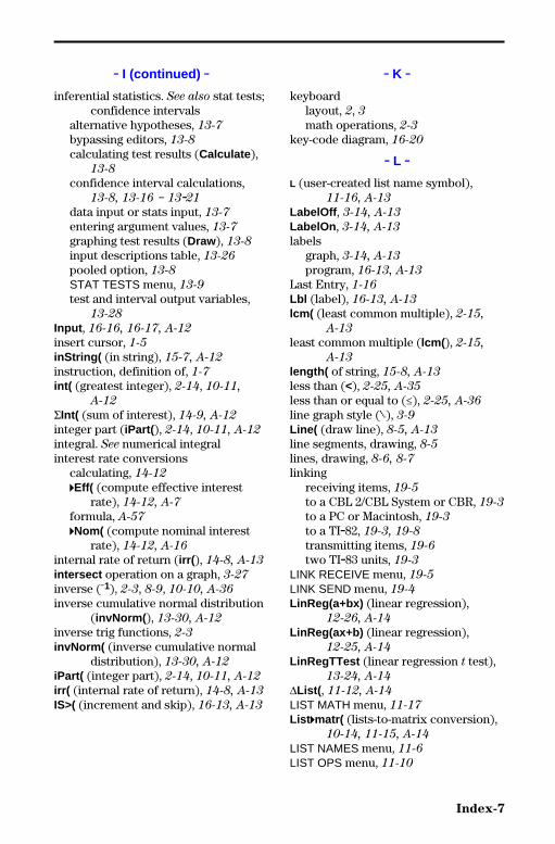
Index-7
8399INDX.DOC TI-83 international English Bob Fedorisko Revised: 02/20/01 10:54 AM Printed: 02/21/01 8:40AM Page 7 of 16
. I (continued) .
inferential statistics. See also stat tests;confidence intervals
alternative hypotheses, 13-7
bypassing editors, 13-8
calculating test results (Calculate ),13-8
confidence interval calculations,13-8, 13-16 N 13.21
data input or stats input, 13-7
entering argument values, 13-7
graphing test results (Draw), 13-8
input descriptions table, 13-26
pooled option, 13-8
STAT TESTS menu, 13-9
test and interval output variables,13-28
Input , 16-16, 16-17, A-12
insert cursor, 1-5
inString( (in string), 15-7, A-12
instruction, definition of, 1-7
int( (greatest integer), 2-14, 10-11,
A-12
GInt( (sum of interest), 14-9, A-12
integer part (iPart( ), 2-14, 10-11, A-12
integral. See numerical integralinterest rate conversions
calculating, 14-12
4Eff( (compute effective interestrate), 14-12, A-7
formula, A-57
4Nom( (compute nominal interestrate), 14-12, A-16
internal rate of return (irr( ), 14-8, A-13
intersect operation on a graph, 3-27
inverse (L1), 2-3, 8-9, 10-10, A-36
inverse cumulative normal distribution(invNorm( ), 13-30, A-12
inverse trig functions, 2-3
invNorm( (inverse cumulative normaldistribution), 13-30, A-12
iPart( (integer part), 2-14, 10-11, A-12
irr( (internal rate of return), 14-8, A-13
IS>( (increment and skip), 16-13, A-13
. K .
keyboardlayout, 2, 3math operations, 2-3
key-code diagram, 16-20
. L .
L (user-created list name symbol),11-16, A-13
LabelOff , 3-14, A-13
LabelOn , 3-14, A-13
labelsgraph, 3-14, A-13
program, 16-13, A-13
Last Entry, 1-16
Lbl (label), 16-13, A-13
lcm( (least common multiple), 2-15,
A-13
least common multiple (lcm( ), 2-15,
A-13
length( of string, 15-8, A-13
less than (<), 2-25, A-35
less than or equal to (�), 2-25, A-36
line graph style (ç), 3-9
Line( (draw line), 8-5, A-13
line segments, drawing, 8-5
lines, drawing, 8-6, 8-7
linkingreceiving items, 19-5
to a CBL 2/CBL System or CBR, 19-3
to a PC or Macintosh, 19-3
to a TI.82, 19-3, 19-8
transmitting items, 19-6
two TI.83 units, 19-3
LINK RECEIVE menu, 19-5
LINK SEND menu, 19-4
LinReg(a+bx) (linear regression),12-26, A-14
LinReg(ax+b) (linear regression),12-25, A-14
LinRegTTest (linear regression t test),13-24, A-14
@List( , 11-12, A-14
LIST MATH menu, 11-17
List 4matr( (lists-to-matrix conversion),10-14, 11-15, A-14
LIST NAMES menu, 11-6
LIST OPS menu, 11-10
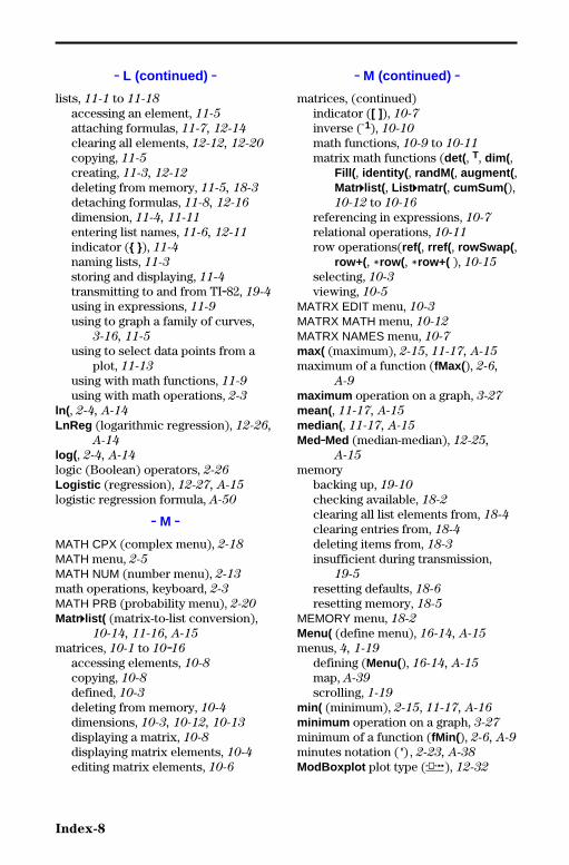
Index-8
8399INDX.DOC TI-83 international English Bob Fedorisko Revised: 02/20/01 10:54 AM Printed: 02/21/01 8:40AM Page 8 of 16
. L (continued) .
lists, 11-1 to 11-18
accessing an element, 11-5
attaching formulas, 11-7, 12-14
clearing all elements, 12-12, 12-20
copying, 11-5
creating, 11-3, 12-12
deleting from memory, 11-5, 18-3
detaching formulas, 11-8, 12-16
dimension, 11-4, 11-11
entering list names, 11-6, 12-11
indicator ({ }), 11-4
naming lists, 11-3
storing and displaying, 11-4
transmitting to and from TI.82, 19-4
using in expressions, 11-9
using to graph a family of curves,3-16, 11-5
using to select data points from aplot, 11-13
using with math functions, 11-9
using with math operations, 2-3
ln( , 2-4, A-14
LnReg (logarithmic regression), 12-26,
A-14
log( , 2-4, A-14
logic (Boolean) operators, 2-26
Logistic (regression), 12-27, A-15
logistic regression formula, A-50
. M .
MATH CPX (complex menu), 2-18
MATH menu, 2-5
MATH NUM (number menu), 2-13
math operations, keyboard, 2-3
MATH PRB (probability menu), 2-20
Matr4list( (matrix-to-list conversion),10-14, 11-16, A-15
matrices, 10-1 to 10.16
accessing elements, 10-8
copying, 10-8
defined, 10-3
deleting from memory, 10-4
dimensions, 10-3, 10-12, 10-13
displaying a matrix, 10-8
displaying matrix elements, 10-4
editing matrix elements, 10-6
. M (continued) .
matrices, (continued)indicator ([ ]), 10-7
inverse (L1), 10-10
math functions, 10-9 to 10-11
matrix math functions (det( , T, dim( ,Fill( , identity( , randM( , augment( ,Matr4list( , List 4matr( , cumSum( ),10-12 to 10-16
referencing in expressions, 10-7
relational operations, 10-11
row operations(ref( , rref( , rowSwap( ,row+( , †row( , †row+( ), 10-15
selecting, 10-3
viewing, 10-5
MATRX EDIT menu, 10-3
MATRX MATH menu, 10-12
MATRX NAMES menu, 10-7
max( (maximum), 2-15, 11-17, A-15
maximum of a function (fMax(), 2-6,
A-9
maximum operation on a graph, 3-27
mean( , 11-17, A-15
median( , 11-17, A-15
Med.Med (median-median), 12-25,
A-15
memorybacking up, 19-10
checking available, 18-2
clearing all list elements from, 18-4
clearing entries from, 18-4
deleting items from, 18-3
insufficient during transmission,19-5
resetting defaults, 18-6
resetting memory, 18-5
MEMORY menu, 18-2
Menu( (define menu), 16-14, A-15
menus, 4, 1-19
defining (Menu(), 16-14, A-15
map, A-39
scrolling, 1-19
min( (minimum), 2-15, 11-17, A-16
minimum operation on a graph, 3-27
minimum of a function (fMin( ), 2-6, A-9
minutes notation ( ') , 2-23, A-38
ModBoxplot plot type (Õ), 12-32
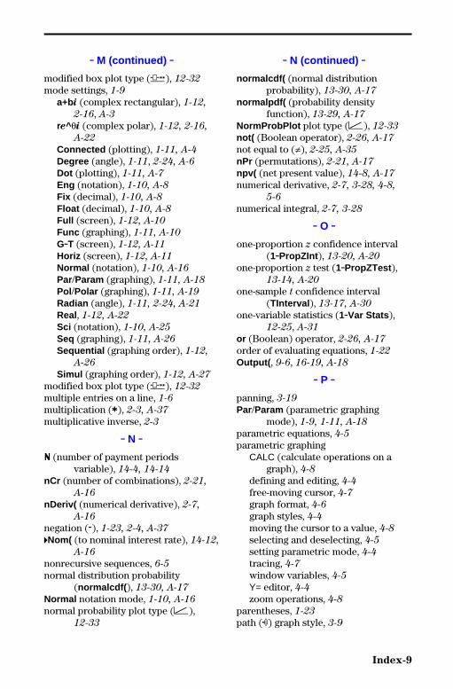
Index-9
8399INDX.DOC TI-83 international English Bob Fedorisko Revised: 02/20/01 10:54 AM Printed: 02/21/01 8:40AM Page 9 of 16
. M (continued) .
modified box plot type (Õ), 12-32
mode settings, 1-9
a+bi (complex rectangular), 1-12,
2-16, A-3
re^qi (complex polar), 1-12, 2-16,
A-22
Connected (plotting), 1-11, A-4
Degree (angle), 1-11, 2-24, A-6
Dot (plotting), 1-11, A-7
Eng (notation), 1-10, A-8
Fix (decimal), 1-10, A-8
Float (decimal), 1-10, A-8
Full (screen), 1-12, A-10
Func (graphing), 1-11, A-10
G.T (screen), 1-12, A-11
Horiz (screen), 1-12, A-11
Normal (notation), 1-10, A-16
Par/Param (graphing), 1-11, A-18
Pol /Polar (graphing), 1-11, A-19
Radian (angle), 1-11, 2-24, A-21
Real, 1-12, A-22
Sci (notation), 1-10, A-25
Seq (graphing), 1-11, A-26
Sequential (graphing order), 1-12,
A-26
Simul (graphing order), 1-12, A-27
modified box plot type (Õ), 12-32
multiple entries on a line, 1-6
multiplication (ä), 2-3, A-37
multiplicative inverse, 2-3
. N .
Ú (number of payment periodsvariable), 14-4, 14-14
nCr (number of combinations), 2-21,
A-16
nDeriv( (numerical derivative), 2-7,
A-16
negation (M), 1-23, 2-4, A-37
4Nom( (to nominal interest rate), 14-12,
A-16
nonrecursive sequences, 6-5
normal distribution probability(normalcdf( ), 13-30, A-17
Normal notation mode, 1-10, A-16
normal probability plot type (Ô),12-33
. N (continued) .
normalcdf( (normal distributionprobability), 13-30, A-17
normalpdf( (probability densityfunction), 13-29, A-17
NormProbPlot plot type (Ô), 12-33
not( (Boolean operator), 2-26, A-17
not equal to (ƒ), 2-25, A-35
nPr (permutations), 2-21, A-17
npv( (net present value), 14-8, A-17
numerical derivative, 2-7, 3-28, 4-8,
5-6
numerical integral, 2-7, 3-28
. O .
one-proportion z confidence interval(1.PropZInt ), 13-20, A-20
one-proportion z test (1.PropZTest ),13-14, A-20
one-sample t confidence interval(TInterval ), 13-17, A-30
one-variable statistics (1.Var Stats ),12-25, A-31
or (Boolean) operator, 2-26, A-17
order of evaluating equations, 1-22
Output( , 9-6, 16-19, A-18
. P .
panning, 3-19
Par/Param (parametric graphingmode), 1-9, 1-11, A-18
parametric equations, 4-5
parametric graphingCALC (calculate operations on a
graph), 4-8
defining and editing, 4-4
free-moving cursor, 4-7
graph format, 4-6
graph styles, 4-4
moving the cursor to a value, 4-8
selecting and deselecting, 4-5
setting parametric mode, 4-4
tracing, 4-7
window variables, 4-5
Y= editor, 4-4
zoom operations, 4-8
parentheses, 1-23
path (ë) graph style, 3-9
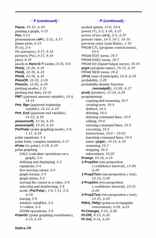
Index-10
8399INDX.DOC TI-83 international English Bob Fedorisko Revised: 02/20/01 10:54 AM Printed: 02/21/01 8:40AM Page 10 of 16
. P (continued) .
Pause , 16-12, A-18
pausing a graph, 3-15
Pen, 8-13
permutations (nPr), 2-21, A-17
phase plots, 6-13
Pi (p), 2-4
Pic (pictures), 8-17, 8-18
pictures (Pic), 8-17, 8-18
pixel, 8-16
pixels in Horiz /G.T modes, 8-16, 9-6
Plot1( , 12-34, A-18
Plot2( , 12-34, A-18
Plot3( , 12-34, A-18
PlotsOff , 12-35, A-18
PlotsOn , 12-35, A-18
plotting modes, 1-11
plotting stat data, 12-31
PMT (payment amount variable), 14-4,
14-14
Pmt_Bgn (payment beginningvariable), 14-13, A-19
Pmt_End (payment end variable),14-13, A-19
poissoncdf( , 13-34, A-19
poissonpdf( , 13-33, A-19
Pol /Polar (polar graphing mode), 1-9,1-11, A-19
polar equations, 5-4
polar form, complex numbers, 2-17
4Polar (to polar), 2-19, A-19
polar graphingCALC (calculate operations on a
graph), 5-6
defining and displaying, 5-3
equations, 5-4
free-moving cursor, 5-6
graph format, 5-5
graph styles, 5-3
moving the cursor to a value, 5-6
selecting and deselecting, 5-4
mode (Pol /Polar ), 1-9, 1-11, 5-3,A-19
tracing, 5-6
window variables, 5-4
Y= editor, 5-3
ZOOM operations, 5-6
PolarGC (polar graphing coordinates),3-13, A-19
. P (continued) .
pooled option, 13-6, 13-8
power (^), 2-3, A-36, A-37
power of ten (10^(), 2-4, A-37
present value, 14-5, 14-7, 14-14
previous entry (Last Entry), 1-16
PRGM CTL (program control menu),16-8
PRGM EDIT menu, 16-7
PRGM EXEC menu, 16-7
PRGM I/O (Input/Output menu), 16-16
prgm (program name), 16-15, A-19
PRGM NEW menu, 16-4
GPrn( (sum of principal), 14-9, A-19
probability, 2-20
probability density function(normalpdf( ), 13-29, A-17
prod( (product), 11-18, A-19
programmingcopying and renaming, 16-7
creating new, 16-4
defined, 16-4
deleting, 16-4
deleting command lines, 16-6
editing, 16-6
entering command lines, 16-5
executing, 16-5
instructions, 16-9 N 16.21
inserting command lines, 16-6
name (prgm ), 16-15, A-19
renaming, 16-7
stopping, 16-5
subroutines, 16-22
Prompt , 16-18, A-19
1.PropZInt (one-proportionz confidence interval), 13-20,
A-20
1.PropZTest (one-proportion z test),13-14, A-20
2.PropZInt (two-proportionz confidence interval), 13-21,
A-20
2.PropZTest (two-proportion z test),13-15, A-20
P4Rx(, P4Ry( (polar-to-rectangularconversions), 2-24, A-21
Pt.Change( , 8-15, A-20
Pt.Off( , 8-15, A-20
Pt.On(, 8-14, A-20

Index-11
8399INDX.DOC TI-83 international English Bob Fedorisko Revised: 02/20/01 10:54 AM Printed: 02/21/01 8:40AM Page 11 of 16
. P (continued) .
PV (present value variable), 14-4,
14-14
p-value, 13-28
PwrReg (power regression), 12-27,
A-20
Pxl.Change( , 8-16, A-21
Pxl.Off( , 8-16, A-21
Pxl.On(, 8-16, A-21
pxl .Test( , 8-16, A-21
P/Y (number-of-payment-periods-per-year variable), 14-4, 14-14
. Q .
QuadReg (quadratic regression),12-25, A-21
QuartReg (quartic regression), 12-26
Quick Zoom, 3-19, A-21
. R .r (radian notation), 2-24, A-34
r (correlation coefficient), 12-23
r2, R2 (coefficients of determination),12-23
Radian angle mode, 1-11, 2-24, A-21
radian notation (r), 2-24, A-34
rand (random number), 2-20, A-21
randBin( (random binomial), 2-22,
A-21
randInt( (random integer), 2-22, A-22
randM( (random matrix), 10-13, A-22
randNorm( (random Normal), 2-22,
A-22
random seed, 2-20, 2-22
RCL (recall), 1-15, 11-9
re^qi (polar complex mode), 1-12,
2-16, A-22
Real mode, 1-12, A-22
real( (real part), 2-18, A-22
RecallGDB , 8-20, A-22
RecallPic , 8-18, A-22
4Rect (to rectangular), 2-19, A-22
rectangular form, complex numbers,2-17
RectGC (rectangular graphingcoordinates), 3-13, A-22
recursive sequences, 6-6
ref( (row-echelon form), 10-15, A-22
. R (continued) .
RegEQ (regression equation variable),12-22, 12-29
regression modelautomatic regression equation,
12-22
automatic residual list feature,12-22
diagnostics display mode, 12-23
models, 12-25
relational operations, 2-25, 10-11
Repeat , 16-11, A-23
RESET menu, 18-5
resettingdefaults, 18-6
memory, 5, 18-5
residual list (RESID), 12-22
Return , 16-15, A-23
root (x‡), 2-6, A-35
root of a function, 3-26
round( , 2-13, 10-10, A-23
row+( , 10-16, A-23
…row( , 10-16, A-23
…row+( , 10-16, A-23
rowSwap( , 10-16, A-23
R4Pr(, R4Pq( (rectangular-to-polarconversions), 2-24, A-23
rref( (reduced-row-echelon form),10-15, A-23
. S .
2.SampÛTest (two-sample Û-Test),13-23, A-24
2.SampTInt (two-sample t confidenceinterval), 13-19, A-24
2.SampTTest (two-sample t test),13-13, A-24, A-25
2.SampZInt (two-sample z confidenceinterval), 13-18, A-25
2.SampZTest (two-sample z test),13-12, A-25
Scatter plot type ("), 12-31
Sci (scientific notation mode), 1-10,
A-25
scientific notation, 1-7,1.10
screen modes, 1-12
second cursor (2nd), 1-5
second key (2nd), 3
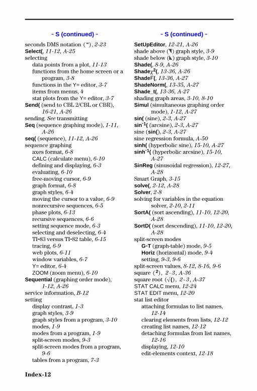
Index-12
8399INDX.DOC TI-83 international English Bob Fedorisko Revised: 02/20/01 10:54 AM Printed: 02/21/01 8:40AM Page 12 of 16
. S (continued) .
seconds DMS notation ( ") , 2-23
Select( , 11-12, A-25
selectingdata points from a plot, 11-13
functions from the home screen or aprogram, 3-8
functions in the Y= editor, 3-7
items from menus, 4stat plots from the Y= editor, 3-7
Send( (send to CBL 2/CBL or CBR),16-21, A-26
sending. See transmittingSeq (sequence graphing mode), 1-11,
A-26
seq( (sequence), 11-12, A-26
sequence graphingaxes format, 6-8
CALC (calculate menu), 6-10
defining and displaying, 6-3
evaluating, 6-10
free-moving cursor, 6-9
graph format, 6-8
graph styles, 6-4
moving the cursor to a value, 6-9
nonrecursive sequences, 6-5
phase plots, 6-13
recursive sequences, 6-6
setting sequence mode, 6-3
selecting and deselecting, 6-4
TI.83 versus TI.82 table, 6-15
tracing, 6-9
web plots, 6-11
window variables, 6-7
Y= editor, 6-4
ZOOM (zoom menu), 6-10
Sequential (graphing order mode),1-12, A-26
service information, B-12
settingdisplay contrast, 1-3
graph styles, 3-9
graph styles from a program, 3-10
modes, 1-9
modes from a program, 1-9
split-screen modes, 9-3
split-screen modes from a program,9-6
tables from a program, 7-3
. S (continued) .
SetUpEditor , 12-21, A-26
shade above (é) graph style, 3-9
shade below (ê) graph style, 3-10
Shade( , 8-9, A-26
Shadec2(, 13-36, A-26
ShadeÛ(, 13-36, A-27
ShadeNorm( , 13-35, A-27
Shade_t( , 13-36, A-27
shading graph areas, 3-10, 8-10
Simul (simultaneous graphing ordermode), 1-12, A-27
sin( (sine), 2-3, A-27
sin M1( (arcsine), 2-3, A-27
sine (sin( ), 2-3, A-27
sine regression formula, A-50
sinh( (hyperbolic sine), 15-10, A-27
sinh M1( (hyperbolic arcsine), 15-10,
A-27
SinReg (sinusoidal regression), 12-27,
A-28
Smart Graph, 3-15
solve( , 2-12, A-28
Solver , 2-8
solving for variables in the equationsolver, 2-10, 2-11
SortA( (sort ascending), 11-10, 12-20,
A-28
SortD( (sort descending), 11-10, 12-20,
A-28
split-screen modesG.T (graph-table) mode, 9-5
Horiz (horizontal) mode, 9-4
setting, 9-3, 9-6
split-screen values, 8-12, 8-16, 9-6
square ( 2) , 2-3 , A-36
square root (‡() , 2-3 , A-37
STAT CALC menu, 12-24
STAT EDIT menu, 12-20
stat list editorattaching formulas to list names,
12-14
clearing elements from lists, 12-12
creating list names, 12-12
detaching formulas from list names,12-16
displaying, 12-10
edit-elements context, 12-18

Index-13
8399INDX.DOC TI-83 international English Bob Fedorisko Revised: 02/20/01 10:54 AM Printed: 02/21/01 8:40AM Page 13 of 16
. S (continued) .
stat list editor (continued)editing elements of formula-
generated lists, 12-16
editing list elements, 12-13
enter-names context, 12-19
entering list names, 12-11
formula-generated list names, 12-15
removing lists, 12-12
restoring list names L1–L6, 12-12,
12-21
switching contexts, 12-17
view-elements context, 12-18
view-names context, 12-19
STAT PLOTS menu, 12-34
stat tests and confidence intervalsANOVA( (one-way analysis of
variance), 13-25
c².Test (chi-square test), 13-22
LinRegTTest (linear regressiont test), 13-24
1.PropZInt (one-proportionz confidence interval), 13-20
1.PropZTest (one-proportion z test),13-14
2.PropZInt (two-proportionz confidence interval), 13-21
2.PropZTest (two-proportion z test),13-15
2.SampÛTest (two-sample Û.Test),13-23
2.SampTInt (two-samplet confidence interval), 13-19
2.SampTTest (two-sample t test),13-13
2.SampZInt (two-samplez confidence interval), 13-18
2.SampZTest (two-sample z test),13-12
TInterval (one-sample t confidenceinterval), 13-17
T.Test (one-sample t test), 13-11
ZInterval (one-sample z confidenceinterval), 13-16
Z.Test (one-sample z test), 13-10
Stats input option, 13-6, 13-7
STAT TESTS menu, 13-9
statistical distribution functions. See
distribution functions
. S (continued) .
statistical plotting, 12-31
Boxplot (regular box plot), 12-33
defining, 12-34
from a program, 12-37
Histogram , 12-32
ModBoxplot (modified box plot),12-32
NormProbPlot (normal probabilityplot), 12-33
Scatter , 12-31
tracing, 12-36
turning on/off stat plots, 3-7, 12-35
viewing window, 12-36
xyLine , 12-31
statistical variables table, 12-29
stdDev( (standard deviation), 11-18,
A-28
Stop , 16-15, A-28
Store (!), 1-14, A-28
StoreGDB , 8-19, A-28
StorePic , 8-17, A-29
storinggraph databases (GDBs), 8-19
graph pictures, 8-17
variable values, 1-14
String 4Equ( (string-to-equationconversions), 15-8, A-29
strings, 15-3 to 15-9
concatenation (+), 15-6, A-38
converting, 15-7, 15-8
defined, 15-3
displaying contents, 15-5
entering, 15-3
functions in CATALOG, 15-6
indicator ("), 15-3
length (length( ), 15-8, A-13
storing, 15-5
variables, 15-4
student-t distributionprobability (tcdf( ), 13-31, A-29
probability density function (tpdf( ),13-30, A-30
sub( (substring), 15-9, A-29
subroutines, 16-15, 16-22
subtraction (N), 2-3, A-38
sum( (summation), 11-18, A-29
system variables, A-49
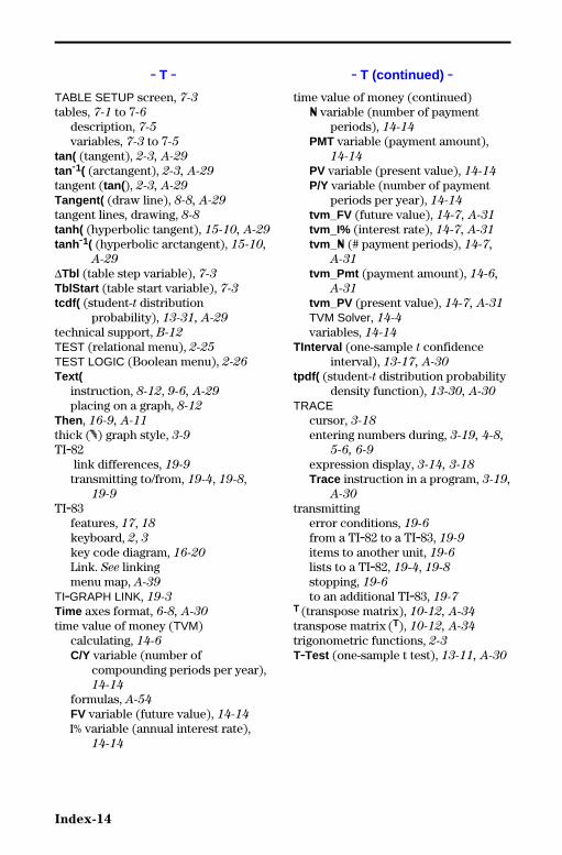
Index-14
8399INDX.DOC TI-83 international English Bob Fedorisko Revised: 02/20/01 10:54 AM Printed: 02/21/01 8:40AM Page 14 of 16
. T .
TABLE SETUP screen, 7-3
tables, 7-1 to 7-6
description, 7-5
variables, 7-3 to 7-5
tan( (tangent), 2-3, A-29
tan M1( (arctangent), 2-3, A-29
tangent (tan(), 2-3, A-29
Tangent( (draw line), 8-8, A-29
tangent lines, drawing, 8-8
tanh( (hyperbolic tangent), 15-10, A-29
tanh M1( (hyperbolic arctangent), 15-10,
A-29
@Tbl (table step variable), 7-3
TblStart (table start variable), 7-3
tcdf( (student-t distributionprobability), 13-31, A-29
technical support, B-12
TEST (relational menu), 2-25
TEST LOGIC (Boolean menu), 2-26
Text(instruction, 8-12, 9-6, A-29
placing on a graph, 8-12
Then , 16-9, A-11
thick (è) graph style, 3-9
TI.82 link differences, 19-9
transmitting to/from, 19-4, 19-8,19-9
TI.83features, 17, 18
keyboard, 2, 3key code diagram, 16-20
Link. See linkingmenu map, A-39
TI.GRAPH LINK, 19-3
Time axes format, 6-8, A-30
time value of money (TVM)calculating, 14-6
C/Y variable (number ofcompounding periods per year),14-14
formulas, A-54
FV variable (future value), 14-14
æ variable (annual interest rate),14-14
. T (continued) .
time value of money (continued)Ú variable (number of payment
periods), 14-14
PMT variable (payment amount),14-14
PV variable (present value), 14-14
P/Y variable (number of paymentperiods per year), 14-14
tvm_FV (future value), 14-7, A-31
tvm_I% (interest rate), 14-7, A-31
tvm_ Ú (# payment periods), 14-7,
A-31
tvm_Pmt (payment amount), 14-6,
A-31
tvm_PV (present value), 14-7, A-31
TVM Solver, 14-4
variables, 14-14
TInterval (one-sample t confidenceinterval), 13-17, A-30
tpdf( (student-t distribution probabilitydensity function), 13-30, A-30
TRACEcursor, 3-18
entering numbers during, 3-19, 4-8,
5-6, 6-9
expression display, 3-14, 3-18
Trace instruction in a program, 3-19,
A-30
transmittingerror conditions, 19-6
from a TI.82 to a TI.83, 19-9
items to another unit, 19-6
lists to a TI.82, 19-4, 19-8
stopping, 19-6
to an additional TI.83, 19-7T (transpose matrix), 10-12, A-34
transpose matrix (T), 10-12, A-34
trigonometric functions, 2-3
T.Test (one-sample t test), 13-11, A-30
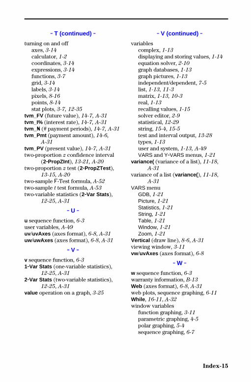
Index-15
8399INDX.DOC TI-83 international English Bob Fedorisko Revised: 02/20/01 10:54 AM Printed: 02/21/01 8:40AM Page 15 of 16
. T (continued) .
turning on and offaxes, 3-14
calculator, 1-2
coordinates, 3-14
expressions, 3-14
functions, 3-7
grid, 3-14
labels, 3-14
pixels, 8-16
points, 8-14
stat plots, 3-7, 12-35
tvm_FV (future value), 14-7, A-31
tvm_I% (interest rate), 14-7, A-31
tvm_ Ú (# payment periods), 14-7, A-31
tvm_Pmt (payment amount), 14-6,
A-31
tvm_PV (present value), 14-7, A-31
two-proportion z confidence interval(2.PropZInt ), 13-21, A-20
two-proportion z test (2.PropZTest ),13-15, A-20
two-sample Û-Test formula, A-52
two-sample t test formula, A-53
two-variable statistics (2.Var Stats ),12-25, A-31
. U .
u sequence function, 6-3
user variables, A-49
uv /uvAxes (axes format), 6-8, A-31
uw /uwAxes (axes format), 6-8, A-31
. V .
v sequence function, 6-3
1.Var Stats (one-variable statistics),12-25, A-31
2.Var Stats (two-variable statistics),12-25, A-31
value operation on a graph, 3-25
. V (continued) .
variablescomplex, 1-13
displaying and storing values, 1-14
equation solver, 2-10
graph databases, 1-13
graph pictures, 1-13
independent/dependent, 7-5
list, 1-13, 11-3
matrix, 1-13, 10-3
real, 1-13
recalling values, 1-15
solver editor, 2-9
statistical, 12-29
string, 15-4, 15-5
test and interval output, 13-28
types, 1-13
user and system, 1-13, A-49
VARS and Y.VARS menus, 1-21
variance( (variance of a list), 11-18,A-31
variance of a list (variance( ), 11-18,A-31
VARS menuGDB, 1-21
Picture, 1-21
Statistics, 1-21
String, 1-21
Table, 1-21
Window, 1-21
Zoom, 1-21
Vertical (draw line), 8-6, A-31
viewing window, 3-11
vw /uvAxes (axes format), 6-8
. W .
w sequence function, 6-3
warranty information, B-13Web (axes format), 6-8, A-31
web plots, sequence graphing, 6-11
While , 16-11, A-32
window variablesfunction graphing, 3-11
parametric graphing, 4-5
polar graphing, 5-4
sequence graphing, 6-7
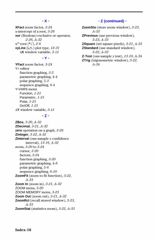
Index-16
8399INDX.DOC TI-83 international English Bob Fedorisko Revised: 02/20/01 10:54 AM Printed: 02/21/01 8:40AM Page 16 of 16
. X .
XFact zoom factor, 3-24
x-intercept of a root, 3-26
xor (Boolean) exclusive or operator,2-26, A-32
xth root (x‡), 2-6
xyLine (Ó) plot type, 12-31
@X window variable, 3-12
. Y .
YFact zoom factor, 3-24
Y= editorfunction graphing, 3-5
parametric graphing, 4-4
polar graphing, 5-3
sequence graphing, 6-4
Y.VARS menuFunction, 1-21
Parametric, 1-21
Polar, 1-21
On/Off, 1-21
@Y window variable, 3-12
. Z .
ZBox , 3-20, A-32
ZDecimal , 3-21, A-32
zero operation on a graph, 3-26
ZInteger , 3-22, A-32
ZInterval (one-sample z confidenceinterval), 13-16, A-32
zoom, 3-20 to 3-24
cursor, 3-20
factors, 3-24
function graphing, 3-20
parametric graphing, 4-8
polar graphing, 5-6
sequence graphing, 6-10
ZoomFit (zoom to fit function), 3-22,A-33
Zoom In (zoom in), 3-21, A-32
ZOOM menu, 3-20
ZOOM MEMORY menu, 3-23
Zoom Out (zoom out), 3-21, A-32
ZoomRcl (recall stored window), 3-23,A-33
ZoomStat (statistics zoom), 3-22, A-33
. Z (continued) .
ZoomSto (store zoom window), 3-23,A-33
ZPrevious (use previous window),3-23, A-33
ZSquare (set square pixels), 3-21, A-33
ZStandard (use standard window),3-22, A-33
Z.Test (one-sample z test), 13-10, A-34
ZTrig (trigonometric window), 3-22,A-34
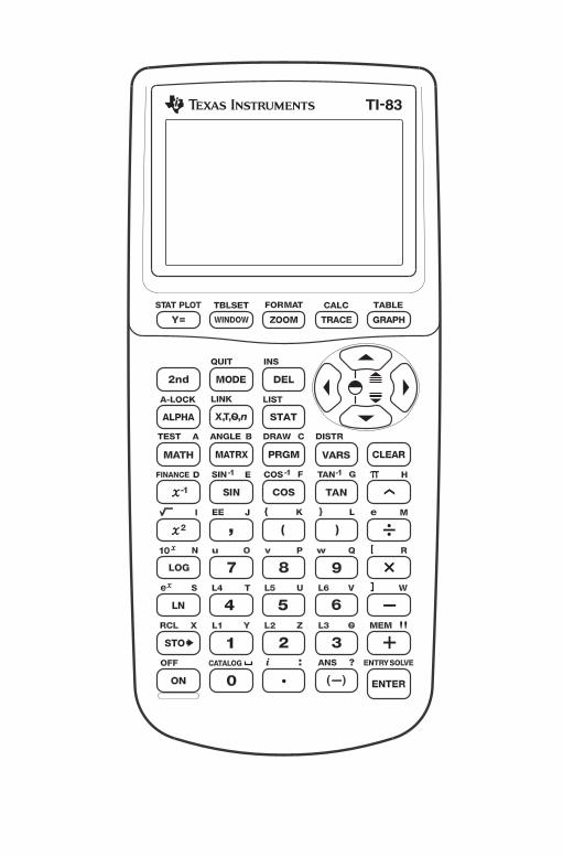
TI83CALC.DOC TI 83 Inside Cover Bob Fedorisko Revised: 12/03/99 8:31 AM Printed: 03/12/01 1:49PM Page 1 of 2
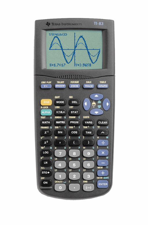
TI83CALC.DOC TI 83 Inside Cover Bob Fedorisko Revised: 12/03/99 8:31 AM Printed: 03/12/01 1:49PM Page 2 of 2