THÈSE - unistra.fr · my supervisors, I am particularly grateful for the assistance given by...
221
UNIVERSITÉ DE STRASBOURG ÉCOLE DOCTORALE DES SCIENCES CHIMIQUES [ UMR 7140 ] THÈSE présentée par : [ Glavatskikh Marta ] soutenue le : 09 juillet 2018 pour obtenir le grade de : Docteur de l’université de Strasbourg Discipline/ Spécialité : Chimie/Chémoinformatique Modeling and visualization of complex chemical data using local descriptors THÈSE dirigée par : M. VARNEK Alexandre Professeur, Université de Strasbourg M. MADZHIDOV Timur Docteur, Université Fédérale de Kazan RAPPORTEURS : M. AIRES DE SOUSA João Professeur, Université de Lisbonne M. BONNET Pascal Professeur, Université d’Orléans AUTRES MEMBRES DU JURY : M. ANTIPIN Igor Professeur, Université Fédérale de Kazan
Transcript of THÈSE - unistra.fr · my supervisors, I am particularly grateful for the assistance given by...

UNIVERSITÉ DE STRASBOURG
ÉCOLE DOCTORALE DES SCIENCES CHIMIQUES
[ UMR 7140 ]
THÈSE présentée par :
[ Glavatskikh Marta ]
soutenue le : 09 juillet 2018
pour obtenir le grade de : Docteur de l’université de Strasbourg
Discipline/ Spécialité : Chimie/Chémoinformatique
Modeling and visualization of complex chemical data using local descriptors
THÈSE dirigée par :
M. VARNEK Alexandre Professeur, Université de Strasbourg M. MADZHIDOV Timur Docteur, Université Fédérale de Kazan
RAPPORTEURS : M. AIRES DE SOUSA João Professeur, Université de Lisbonne M. BONNET Pascal Professeur, Université d’Orléans
AUTRES MEMBRES DU JURY : M. ANTIPIN Igor Professeur, Université Fédérale de Kazan

2
Marta GLAVATSKIKH
Modeling and visualization of complex
chemical data using local descriptors
Résumé
Cette étude considère des systèmes où non seulement la structure moléculaire, mais les conditions expérimentales sont impliquées. Les structures chimiques ont été codées par des descripteurs locaux ISIDA MA ou ISIDA CGR, ciblant spécifiquement les centres actifs et leur environnement le plus proche. Les descripteurs locaux ont été combinés avec les paramètres spécifiques des conditions expérimentales, codant ainsi un objet chimique particulier. La méthodologie a été appliquée avec succès pour la modélisation QSPR des paramètres thermodynamiques et cinétiques des interactions intermoléculaires (liaisons halogène et hydrogène), des équilibres tautomères et des réactions chimiques (cycloaddition et SN1). La méthode GTM a été appliquée pour la première fois pour la modélisation et la visualisation de données chimiques mixtes.La méthode sépare avec succès les groupes de données à la fois en raison des structures et des conditions.
Résumé en anglais
This work describes original approaches for predictive chemoinformatics modeling of molecular interactions and reactions as a function of the structures of interacting partners and of the chemical environment (experimental conditions). Chemical structures have been encoded by local ISIDA MA-based or CGR-based descriptors, specifically targeting the active centers and their closest environment. The local descriptors have been combined with the specific parameters of experimental conditions, thereby encoding a particular chemical object. The methodology has been successfully applied for QSPR modeling of thermodynamic and kinetic parameters of intermolecular interactions (halogen and hydrogen bonds), tautomeric equilibria and chemical reactions (cycloaddition and SN1). GTM method has been applied for the first time for QSPR modeling and visualization of mixed chemical data. This method successfully separates data clusters on account of both chemical structures and experimental conditions.

3
Acknowledgements
I would like to express my great appreciation to my supervisors, Prof. Alexandre Varnek and
Dr. Timur Madzhidov for their thorough guidance, continuous solicitude and care. Besides of
my supervisors, I am particularly grateful for the assistance given by Dragos Horvath, who
directed me in the practicalities of the field, carefully taught and instruct me all over my PhD
studentship. I also wish to acknowledge the help and advises provided by Gilles Marcou. I
greatly appreciate the assistance and tutelage of these people.
I would like to express my deep gratitude to the members of my jury, Pascal Bonnet and Joao
Aires de Sousa for having time to revise and evaluate my work.
I wish to acknowledge the help of our collaborators: Vitaly Solov’ev, Jerome Graton and Jean-
Yves Le Questel for data collection and participation. Also, the help of all members of the
Laboratory of Chemoinformatics and Molecular Modeling (Kazan) and Laboratory of
Chemoinformatics (Strasbourg) was highly appreciated.
My special thanks are extended to my colleagues, Timur Gimadiev, Fanny Bonachera, Arkadij
Lin, Ramil Nugmanov and Iuri Casciuc for their support and spirit.

4
Contents
Contents .................................................................................................... 4
Résumé en français ........................................................................................ 8
PART I. REVIEW, METHODOLOGY AND TOOLS .................................... 22
1. Introduction ............................................................................................ 22
2.Molecular descriptors for interacting chemical entities ......................................... 27
2.1 Local descriptors for chemical structure representation ................................ 28
2.1.1 Substituent constants .................................................................. 28
2.1.1.1 Hammet constants ..................................................................... 28
2.1.1.2 Inductive constants .................................................................... 29
2.1.1.3 Resonance (mesomeric) constants .................................................. 31
2.1.1.4 Steric constants ........................................................................ 32
2.1.2 Quantum-chemical descriptors ..................................................... 33
2.1.2.1 Atomic charges ......................................................................... 33
2.1.2.2 Electrophilic and nucleophilic frontier electron densities ...................... 34
2.1.2.3 Electrophilic, nucleophilic and radical superdelocalizabilities ................. 35
2.1.2.4 Atomic polarizability .................................................................. 36
2.1.2.5 TAE descriptors based on Bader’s quantum theory of atoms in molecules .. 38
2.1.2.6 Conceptual Density Functional Theory Indices .................................. 39
2.1.3 Electrotopological indices ............................................................ 42
2.1.4 ISIDA fragment descriptors .......................................................... 44
2.2 Descriptors of the reaction conditions ..................................................... 50

5
3. QSPR methodology ................................................................................... 54
3.1 Quantitative Structure-Property Relationships (QSPR) ................................ 54
3.2 Machine Learning algorithms ................................................................ 56
3.2.1 Support Vector Machine (SVM) .................................................... 56
3.2.2 Multiple Linear Regression (MLR) ................................................. 57
3.2.3 Generative Topographic Mapping (GTM) ........................................ 58
3.3 Model quality estimation ..................................................................... 61
3.3.1 Cross-validation and external validation ........................................... 61
3.3.2 Regression- and classification model’s performance criteria ................... 62
3.4 Applicability Domain ......................................................................... 63
PART II. RESULTS AND DISCUSSIONS ................................................... 65
4. QSPR modeling of halogen bond basicity of binding sites of polyfunctional molecules .. 65
4.1 Modeled object and property ................................................................ 67
4.2 Data preparation ............................................................................... 68
4.3 Computational details ......................................................................... 69
4.4 Results and discussions ....................................................................... 70
4.4.1 Cross-validation. ....................................................................... 70
4.4.2 External validation. ................................................................... 70
4.4.3 Comparison of the strength of halogen and hydrogen bonding ................ 71
4.5 Conclusion ...................................................................................... 72
5. QSPR modeling of the Free Energy of hydrogen-bonded complexes with single and
cooperative hydrogen bonds. ........................................................................... 84
5.1 Modeled object and property ................................................................ 86
5.2 Modeling workflow ........................................................................... 86
5.3 Data preparation ............................................................................... 86
5.4 Computational details ......................................................................... 88
5.5 Results and discussions ....................................................................... 89

6
5.4.1 Cross-validation ........................................................................ 89
5.4.2 External validation .................................................................... 90
5.6 Conclusion ...................................................................................... 92
6. QSPR modeling and visualization of tautomeric equilibria. ................................. 104
6.1 Modeled object and property .............................................................. 105
6.2 Modeling workflow ......................................................................... 107
6.3 Data preparation ............................................................................. 107
6.4 Computational details ....................................................................... 109
6.5 Results and discussions ..................................................................... 110
6.5.1 Data visualization and analysis with GTM ....................................... 111
6.5.2 Cross-validation of the SVR and GTM models ................................. 113
6.5.3 GTM solvent separation analysis .................................................. 114
6.5.4 External validation of the SVR and GTM models .............................. 115
6.6 Conclusion .................................................................................... 116
7. QSPR modeling and visualization of kinetics properties of cycloaddition reactions. .... 130
7.1 Computational procedure .................................................................. 132
7.1.1 Data preparation ..................................................................... 132
7.1.2 Descriptors ........................................................................... 134
7.1.3 Building and validation of the models ............................................ 135
7.1.4 Different scenarios of logk assessment for the test set reactions ............. 135
7.2 Results and discussions ..................................................................... 137
7.2.1 GTM visualization of the training set............................................. 137
7.2.2 Cross validation of the SVR and GTM models ................................. 139
7.2.3 External validation of the SVR and GTM models .............................. 139
7.3 Conclusion .................................................................................... 142
8. QSPR modeling of the rate constant of SN1 reactions. ....................................... 144
8.1 Computational procedure .................................................................. 145
7
8.1.1 Data preparation ..................................................................... 146
8.1.2 Descriptors ........................................................................... 148
8.1.3 Building and validation of the models ............................................ 149
8.2 Results and discussions ..................................................................... 149
8.2.1 GTM visualization of the training set............................................. 149
8.2.2 Cross validation of the SVR models .............................................. 150
8.2.3 External validation of the SVR models ........................................... 150
8.3 Conclusion .................................................................................... 151
9. Models implementation. ........................................................................... 153
Conclusion ............................................................................................... 157
References ............................................................................................... 159
Appendix. Part I ................................................................................. 179
Appendix. Part II ................................................................................ 189
Appendix. Part III ............................................................................... 212

8
Résumé en français
La complexité des données chimiques reste un défi pour la modélisation structure-
propriété. En particulier, ceci concerne le développement de modèles prédictifs
pour les propriétés liées à des centres sélectionnés (atomes ou groupes chimiques),
par exemple les différents types d'interactions intermoléculaires ou de réactions
chimiques. Un autre niveau de complexité vient du fait que ces propriétés
dépendent souvent non seulement de la structure chimique des molécules en
interaction, mais aussi des conditions expérimentales (solvant et température).
Afin de décrire correctement cette complexité, les modèles de propriété-
structure associés doivent impliquer des descripteurs caractérisant à la fois les
aspects structurels et conditionnels. De plus, les structures chimiques doivent de
préférence être codées par un descripteur local spécial1-2 ciblant spécifiquement
les centres sélectionnés sur les espèces d'interaction et leur environnement le plus
proche.
Cette étude considère des systèmes de niveau de complexité différents dans la
plupart desquels non seulement la structure moléculaire, mais aussi les conditions
9
expérimentales jouent un rôle significatif (Tableau 1). Le premier exemple est le
plus simple : il concerne la modélisation de la stabilité de la liaison halogène
mesurée par la constante d’équilibre de complexes de molécules organiques avec
le même accepteur (I2) dans un solvant (hexane) à 298K. Dans ce cas, les
conditions expérimentales sont contrôlées et fixes ; seule l’espèce chimique varie.
La complexité augmente avec la modélisation de l'énergie libre de liaisons
hydrogène. Dans ce second exemple, les modèles sont construits sur des données
obtenues en environnement contrôlé : un solvant de référence (CCl4) et une
température (298K). Mais cette propriété fait maintenant intervenir deux espèces
chimiques : l’accepteur et le donneur de liaison hydrogène. Ceux-ci doivent être
simultanément pris en compte dans les modèles et dans l’évaluation des
performances de ces modèles.
Le troisième exemple illustre un niveau de complexité encore supérieur : la
modélisation des équilibres tautomères. Une molécule peut exister sous plusieurs
formes qui ne se distinguent que par la position dans la structure chimique, d’un
ou plusieurs atomes d’hydrogènes. Ces différents états sont les tautomères et leur
prévalence relative est contrôlée par une constante d’équilibre tautomères. Cette
constante dépend, en fait, de conditions expérimentales : solvant et température.
Afin d’en tenir compte explicitement, il est nécessaire d’introduire des variables
supplémentaires et pertinentes pour les décrire.
Le dernier exemple traite des réactions de cycloaddition et de SN1, où différents
réactifs et différentes conditions réactionnelles sont impliqués (Tableau 1). Ce
projet met en œuvre tous les développements présentés auparavant.

10
Tableau 1. Informations sur les modèles prédictifs développés dans ce travail.
Système étudié Propriété
modélisée
Objets encodés Descripte
urs
locaux
Taille de
l'ensemb
le
d'entraîn
ement
Méthode
d'appren
issage
automati
que
1 Complexes de
molécules
organiques avec I2
dans l'hexanei
Logarithme de
constante de
liaison
Structure
moléculaire de la
molécule
individuelle
Basés sur
MAa
598 SVM
MLR
2 Complexes 1: 1
entre un donneur de
liaison H et un
accepteur de liaison
H dans CCl4ii
Energies libres de
complexes
Structures
moléculaires des H-
donneur et H-
accepteur
Basés sur
MA
3373
SVM
MLR
3 Équilibre
tautomères dans
différents solvants
Logarithme des
constantes
d'équilibre
Structure
moléculaire d'un
tautomère
sélectionné, solvant
et température
Basés sur
MA
695 SVM
GTM
4 Les réactions de
cycloaddition (4 +
2), (3 + 2) et (2 + 2)
Logarithme de la
constante de
vitesse, énergie
d'activation,
facteur pré-
exponentiel
Tous les réactifs et
produits, solvant et
température
Basés sur
CGR b
1849 SVM
GTM
5 SN1 réactions Logarithme de la
constante de
vitesse
Tous les réactifs et
produits, solvant et
température
Basés sur
CGR b
8056 SVM
GTM
a descripteurs basés sur des atomes marqués (MA) b descripteurs basés sur graphes condensés de réaction
(CGR)
i. Glavatskikh, M., Madzhidov, T., Solov'ev, V., Marcou, G., Horvath, D., Graton, J., ... & Varnek, A. (2016).
Predictive Models for Halogen‐bond Basicity of Binding Sites of Polyfunctional Molecules. Molecular informatics, 35(2), 70-80.
ii. Glavatskikh, M., Madzhidov, T., Solov'ev, V., Marcou, G., Horvath, D., & Varnek, A. (2016). Predictive models for the free energy of hydrogen bonded complexes with single and cooperative hydrogen bonds. Molecular informatics, 35(11-12), 629-638.

11
Les modèles ont été construits à l'aide des méthodes SVM (Support Vector
Machine), MLR (Multiple Linear Regression) et GTM (Generative Topographic
Mapping). La SVM et la MLR sont des procédés d'apprentissage automatique
conventionnels largement utilisés en chémoinformatique, tandis que le second,
initialement développé comme outil de visualisation de données3, a été étendu en
laboratoire à des tâches de modélisation structure-propriété4-5. Différents types de
descripteurs locaux (à base de MA et à base de CGR, voir section 2) ont été utilisés
dans la modélisation de la stabilité des liaisons halogènes, des liaisons hydrogènes
et des équilibres de réactions chimiques. Pour ces derniers, les descripteurs
structuraux ont été complétés par des descripteurs spécifiques de solvant et de
température.
La thèse comprend sept chapitres. Le premier chapitre d'introduction décrit
divers descripteurs locaux utilisés dans la modélisation. Le deuxième chapitre
fournit des informations sur les outils chémoinformatiques utilisés dans cette
étude. Les chapitres 3 et 4 décrivent des modèles prédictifs pour évaluer les
stabilités des liaisons halogènes et hydrogènes, respectivement. Les chapitres 5, 6
et 7 sont consacrés à la modélisation prédictive de certaines propriétés
thermodynamiques et cinétiques des réactions chimiques : la constante d'équilibre
tautomère et les constantes de vitesse de la cycloaddition et des réactions SN1.
1.1 Descripteurs locaux ISIDA pour la modélisation, l'analyse et la
visualisation de données chimiques
Les descripteurs locaux utilisés dans ce travail sont des sous-ensembles des
descripteurs ISIDA1 représentant des fragments de différentes longueurs et
topologies d'un graphe moléculaire donné. Ces fragments contiennent au moins

12
un atome ou une liaison étiqueté. Deux types de fragments ont été considérés:
basés sur les atomes marqués et sur le graphe condensé de réaction (voir la Figure
1).
Les atomes marqués (MA) sont des atomes d’une structure chimique, annotés pour
leur pertinence vis-à-vis d’un problème donné. Dans ce travail, ce sont les atomes
impliqués dans les interactions intermoléculaires. En d’autres termes, ce sont des
atomes donneurs d'électrons dans des accepteurs de liaison halogène, donneurs et
accepteurs de proton dans les espèces formant des liaisons hydrogènes, les atomes
qui perdent / reçoivent des protons dans des équilibres tautomères.
Quatre scénarios de descripteurs à base de MA ont été considérés2:
• Séquences d'atomes à partir de l'atome marqué, avec des fragments centrés
sur l'atome avec l'atome marqué central (MA1).
• Fragments contenant des atomes marqués (MA2).
• Fragments avec et sans atomes marqués (MA3).
• N’utilisant pas les atomes marqués (MA0), également utilisés à des fins de
comparaison.
La longueur du vecteur des descripteurs varie en fonction de la stratégie
sélectionnée. Ainsi, MA0 et MA2 sont des sous-ensembles de MA3, alors que M1
est un sous-ensemble de MA2.
Dans le graphe condensé de réaction (CGR)6, les structures de tous les réactifs et
produits sont fusionnées en un seul graphe (Figure 1, en bas) qui décrit à la fois les
liaisons chimiques conventionnelles (simples, doubles, aromatiques, ...) et
dynamiques des liaisons caractérisant des transformations chimiques (par

13
exemple, simple à double, simple brisée, simple créée, etc.). Les fragments
contenant des liaisons dynamiques ont été utilisés comme descripteurs locaux.
Les conditions expérimentales ont été codées par 13 paramètres de solvant7 reflétant
la polarité, la polarisabilité, l'acidité et la basicité, et l’inverse de la température
(1/T).
Le vecteur des descripteurs entier pour un processus donné résulte de la
concaténation de descripteurs de conditions structurelles et expérimentales.
2. Modélisation quantitative de la relation structure / propriété /
réactivité (QSPR) de différents objets chimiques.
Le workflow général de modélisation incluait les étapes suivantes: (1) collecte et
conservation de données, (2) génération de différents ensembles de descripteurs
ISIDA, (3) sélection du meilleur ensemble de descripteurs en fonction des
performances des modèles en validation croisée, (4) construction de modèles
Figure 1. Exemple de structures pour lesquelles des descripteurs locaux basés sur MA (en haut) ou
basés sur CGR (en bas) ont été générés. En haut: dans le complexe lié à l'hydrogène, les croix
désignent les Atomes Marqués. En bas: dans le Graphique Condensé codant pour la réaction de
cycloaddition (4 + 2), les points et les tirets représentent respectivement des liaisons chimiques
formées et rompues. Quelques exemples de descripteurs générés sont donnés sur la droite.

14
individuels et consensus (pour SVM seulement) impliquant des descripteurs
sélectionnés, (5) validation externe des modèles.
2.1 Modélisation QSPR de la constante de liaison des complexes liés à
l'halogène.
L'ensemble de données comprenait 598 composés organiques pour lesquels le
logarithme de la constante de stabilité du complexe 1:1 avec I2 (logKBI2) a été
mesuré dans l'hexane à 298K. Différents types de modèles de consensus
correspondant à 4 scénarios possibles de génération de descripteurs à base de MA
ont été comparés. Les meilleurs descripteurs, de type MA3, conduisent à des
performances prédictives raisonnables à la fois dans la validation croisée et sur
l'ensemble externe de 11 composés polyfonctionnels portant 2 ou 3 sites de liaison
putatifs (Tableau 2 et Figure 2).
Tableau 2. Performance prédictive des modèles en validation croisée 5 fois et sur
l'ensemble externe.
SVM MLR
RMSE R2 RMSE R2
5-fois CV 0.39 0.93 0.43 0.92
Ensemble externe 0.44 0.81 0.56 0.70
Figure 2. Valeurs de logKBI2
prédites vs expérimentales pour
l'ensemble de test externe (à gauche)
et des exemples d'évaluation de
logKBI2 pour deux molécules
polyfonctionnelles (à droite).

15
2.2. Modélisation QSPR de l'énergie libre de liaison hydrogène.
L'ensemble de données comprenait 3373 paires de complexes 1:1 formant une
seule liaison hydrogène, pour lesquelles les mesures expérimentales de ΔG (kJ /
mol) ont été reportées en conditions standard (dans du CCl4 et à 298K). Les
modèles consensus SVR et MLR, basés sur les descripteurs MA3 les plus
performants, ont été utilisés pour la prédiction de l'ensemble de test externe de
629 complexes (R2 = 0.65-0.74, RMSE = 3.2-3.8 (Figure 3)), mesurés dans
différents solvants puis ramenés au CCl4, et l’ensemble d'essai de 12 complexes
polyfonctionnels (Figure 4).
Figure 4. Les énergies libres
prédites vs expérimentales (kJ /
mol) pour les complexes 1:1 avec
deux liaisons hydrogènes
coopératives (à gauche) et les
deux exemples de ces complexes
(à droite).
Gpred
Gexp
Figure 3. Les énergies libres
prédites vs expérimentales (kJ /
mol) pour l'ensemble de test
externe de stabilité de la liaison
hydrogène mesurés dans
différents solvants.

16
2.3 Modélisation QSPR et visualisation de la constante d'équilibre (logKT)
de différentes classes de transformations tautomères.
L'ensemble de données consistait en 695 équilibres tautomères attribués à 10
classes de transformation distinctes. Les deux modèles de classification prédisant
le type de tautomérisation et les modèles de régression prédisant le logKT ont été
obtenus avec les méthodes SVM et GTM. Les modèles impliquant des descripteurs
locaux MA2 fonctionnent bien sur deux ensembles de tests externes: l'un
contenant des transformations tautomères connues étudiées dans de nouvelles
conditions (test set 1, Figure 5) et l'autre contenant de nouvelles transformations,
au sens de leurs structures chimiques (test set 2, Figure 5).
Cet ensemble de données a été visualisé sur une carte bidimensionnelle construite
en utilisant l'approche GTM (Figure 6). Cette carte sépare avec succès différentes
classes de transformations tautomères et les équilibres différant soit par structure,
soit par solvant.
Figure 5. Valeurs de constante d'équilibres tautomères pour l'ensemble de transformations étudié
dans de nouvelles conditions (à gauche) et l’ensemble de test contenant de nouvelles
transformations (à droite).

17
2.4 Modélisation QSPR des propriétés cinétiques des réactions de
cycloaddition.
Le jeu de données incluait 1849 réactions de types (4+2), (3+2) et (2+2),
associées à leurs valeurs expérimentales de la constante de vitesse (logk), à 1356
valeurs des énergies d'activation (Ea) et à 1237 valeurs du coefficient pré-
exponentiel (logA). Les descripteurs basés sur les graphes condensés de réactions
ont été utilisés pour construire des modèles SVM et GTM individuels, suivis de
leur validation (les valeurs du log k ont été prédites) sur le jeu de test de 200
réactions sélectionnées aléatoirement dans la base de données. Les énergies
d'activation et le facteur pré-exponentiel ont été modélisés. Ceux-ci sont utilisés
pour estimer la constante de vitesse, logk, en suivant une loi d'Arrhenius.
La Figure 7 représente les paysages d'activité généré par la GTM, pour le logk,
l’Ea et le logA. Les résultats sont en accord avec des concepts chimiques généraux,
les réactions à faible logk, projetées dans les zones de faibles logA bas et Ea sont
caractérisées par d’importantes contraintes stériques (Figure 7, a). Pendant ce
Figure 6. Paysage de classe GTM (à gauche) et paysage d'activité (au milieu). Les réactions 1 (a,
b) et 2 (a, b) sont données à droite. Les nombres entre parenthèses correspondent aux valeurs logKT.

18
temps, la distribution des énergies des orbitales frontières des réactions à faible
logk, projetées dans les zones de fortes valeurs de logA et Ea, sont affectées par
des substituant électroniquement défavorable (Figure 7, b).
Sur l’ensembles de tests externes, le modèle de régression basé sur la GTM est
moins performant que le modèle SVM associé (R2=0.74, RMSE=0.90 (GTM) et
R2=0.92, RMSE=0.50 (SVM)). Ceci s’explique par le fait que le modèle GTM a
été optimisé pour prédire les trois propriétés (logk, Ea, logA) simultanément. Au
contraire de l’approche SVM qui utilise des modèles spécifiques pour chacune des
propriétés. Néanmoins, les différentes classes de réaction sont bien séparées sur
la carte GTM, voir Figure 8.
a
log k = -3.55 (403K, benzene)
b
log k = -4.2 (313K, dichoroethane)
Figure 7. Paysages de propriétés GTM pour la constante de vitesse (log k), l'énergie d'activation (Ea)
et le coefficient pré-exponentiel (log A) pour les réactions de cycloaddition (en haut). Les exemples
ci-dessous correspondent aux réactions qui caractérisées par des contraintes stériques (a) ou par une
distribution défavorable des énergies des orbitales frontières (b).

19
2.5 Modélisation QSPR de la constante de vitesse des réactions SN1.
Un ensemble de 8056 données de réactions SN1 a été utilisé pour construire des
modèles de régression SVM de leur vitesse de réaction. Les réactions étaient
codées par des descripteurs intégrant des atomes marqués de type MA3 ou calculés
sur de structures CGR. Les modèles ont été validés sur deux jeux de données
supplémentaires: l’un contenant des réactions connues étudiées dans de nouvelles
conditions (test 1) et l’autre de nouvelles réactions (test 2). Le modèle fonctionne
de manière similaire sur les deux ensembles de test: R2 test1= 0.64-0.67, R2
test2=
0.55-0.58, RMSE test1 = 0.68-0.70, RMSE test2 = 0.87-0.90.
Figure 8. Modélisation des logarithmes de constantes de vitesse : valeurs prédites vs valeurs
expérimentales pour le jeu de test (à gauche). Séparation de trois classes de réactions (4+2, 3+2,
2+2) en utilisant la méthode GTM (à droite).
Figure 5. Modélisation des logarithmes de constantes de vitesse : valeurs prédites vs valeurs
expérimentales pour le test externe étudiées dans de nouvelles conditions (à gauche) et de test externe
contenant de nouvelles transformations (à droite).

20
Les questions méthodologiques suivantes ont été considérées dans notre travail:
(1) une stratégie axée sur le processus de génération de descripteurs locaux; (2)
la sélection et l’élaboration d'une combinaison optimale de descripteurs
caractérisant la structure chimique, d'une part, et les conditions expérimentales,
d'autre part; (3) la capacité de la GTM à visualiser et à modéliser des processus
chimiques entiers (structures et conditions); (4) la capacité des modèles formés
sur les complexes avec une seule liaison halogène ou hydrogène à prédire la
stabilité des complexes avec de multiples liaisons de ces types.
3. Conclusions
▪ Une combinaison de descripteurs de fragments locaux décrivant des
structures moléculaires et de descripteurs spéciaux caractérisant les
conditions expérimentales (solvant et température) a été utilisée avec
succès pour développer des modèles prédictifs de certains paramètres
cinétiques et thermodynamiques des liaisons halogènes et hydrogènes, des
équilibres tautomères et de deux types de réactions chimiques. Les
descripteurs les plus appropriés pour les réactions chimiques combinant
plusieurs réactifs et produits sont ceux générés à partir des Graphes
Condensés de Réaction. Sinon, diverses stratégies utilisant les Atomes
Marqués ont été recommandées.
▪ Les modèles construit sur des mesures réalisées sur des complexes
impliquant une seule liaison halogène ou une seule liaison hydrogène ont pu

21
être utiliser avec succès pour estimer les stabilités des complexes contenant
plusieurs liaisons de ces types. Cela ouvre des perspectives pour utiliser ces
modèles dans la conception assistée par ordinateur de nouveaux systèmes
supramoléculaires.
▪ Pour la première fois, la méthode GTM a permis de visualiser des processus
chimiques décrits par l’ensemble de leurs réactifs et de leurs produits et
leurs conditions réactionnelles plutôt que par des espèces chimiques
individuelles. Ainsi, sur l'exemple des équilibres tautomères, il a été montré
que les espèces mesurées dans différents solvants sont bien séparées sur la
carte. Dans l'exemple de la cycloaddition, les trois types de réaction sont
bien séparés aussi.
▪ Les modèles QSPR développés prédisant les constantes d'équilibre des
transformations tautomères, la stabilité des liaisons halogène avec I2 et la
constante de vitesse, le facteur pré-exponentiel et les énergies d'activation
des réactions de cycloadditions sont disponibles pour les utilisateurs via nos
plateformes internet https://cimm.kpfu.ru/ et http://infochim.u-
strasbg.fr/webserv/VSEngine.html.

22
PART I. REVIEW, METHODOLOGY AND TOOLS
Chapter 1
Introduction
The requirements of modern knowledge-intensive fields of chemistry, such as drug
development and chemical engineering, are constantly expanding, requiring more elaborated
techniques and methods. Started by focusing on management of structural information of
single molecular entities, present-day Chemoinformatics is developing the methods that
follow the practical interest in predicting properties of compounds in condensed phase and in
interaction with various partners, and not those of single molecules in vacuum. Consequently,
tools and approaches maintaining single molecule study is not satisfying for multi-depended
properties, i.e. the ones that depend on several parameters, or assemblage of molecules,
bounded by a variety of intermolecular interactions. Exemplary objects are the host-guest
complexation and molecular recognition, driven by weak interactions and, certainly, chemical
reactions and chemical equilibria, thermodynamics and kinetics of which depends
simultaneously on chemical structure and on reaction conditions. The mentioned processes
represent the interactions incorporating several molecules, the structure of each of which has
to be taken into thorough consideration. That, however, is not sufficient: for the case of

23
intermolecular interactions (for instance), the interaction of two molecules, possessing
several putative active sites, could result in different intermolecular complexes, that are not
possible to differentiate if only the generic structures of the reagents are taken into account.
The dynamics of the chemical process is thus characterized by the structural localities, directly
involved into a chemical interaction and forming the active sites. Explicitly accentuated, the
active sites define the dynamics of a particular chemical interaction. A generic task of
prediction of the possibility of an interaction hence grow up into a new challenge of prediction
of interactions with multiple putative active sites, for which one needs to predict which
centers will interact and their interaction strength. This level requires a rigorous description
of structural aspects of all the reagents, altogether with the accounting and explicit designation
of the local regions signifying the active sites.
Another degree of freedom comes from the necessity of the reaction condition
consideration. Indeed, small changes in solvent nature could drastically influence the property,
in some cases being a determinative factor in the feasibility of the process. A simple solvent
effect consideration may include a categorical assignment of a solvent to a certain group, such
as polar/nonpolar or protic/aprotic. However, with regard to chemical reactions or
intermolecular interactions, this simple approach could not already be sufficient. Indeed, the
equilibrium or the rate constants remarkably depend on various factors included into the
reaction conditions, such as solvent’s polarity, solvent’s H-acidity/basicity, temperature,
pressure, etc. Thus, the new challenge addressed in this work is the necessity of the
consideration and the description of the experimental conditions, including variety of solvent
effects the property could depends on.
Chemical reaction data requires to be analyzed in terms of structural/conditional
contents, its relationship with each other and with the property and data distribution in a
chemical space. As an example, for the case of chemical reactions, the arrangement of the
structural and reaction condition parts according with its influence on the property value,
helps to understand the nature and the mechanism of the process. The need of such kind of
analysis of complex data is increasing with the growth of the number of data constituents. A
tool aimed at data analysis and visualization and used in this study is the Generative
Topographic Mapping3-4, 8 (GTM). The method provides a visual, 2D-map projected data
clustering and property distribution which is of great support for large data analysis. In this
study, for the first time, it is used for complex chemical data modeling and analysis. Apart
from common structural patterns identification, GTM helped to demonstrate the reaction

24
condition influence, to estimate the quality of the data and the preferable way of its
description. Moreover, the understanding of the underlying clustering principles contributes
to revealing of the interrelation of data constituents and are helpful in determination of more
suitable modeling approach and way of description.
One of the most demanded practical task, related to chemical processes, is the prediction of
thermodynamic, kinetic or other parameters of a certain transformation. That could be
achieved by the Quantitative Structure-Property Relationship (QSPR) modeling, one of the
main tools of chemoinformatics, the goal of which is to provide an equation that relates an
object (e.g. chemical reaction) with the value of the property of interest (e.g. rate constant).
Various algorithms, so-called machine learning methods, have been developed for the QSPR
modeling, each of which derive the equation in its own way. The mentioned GTM, first
designed as the tool for data visualization, has been further extended for QSPR modeling,
allowed a single GTM model to be used for the prediction of different, not necessarily related
properties. The supervised methods such as Support Vector Machine (SVR) or Multiple
Linear Regression (MLR), notwithstanding their inability in chemical data visualization,
though could provide more accurate results of the prediction, since they are built specifically
for a given property.
Thus, the challenge of this work is to expand QSPR methodology for problems, where the
working hypothesis of a "constant" environment does no longer apply: interactions of both
covalent and non-covalent nature, with different partners in multiple solvents, at various
temperatures. These processes are characterized by local interactions, that imply the
representation of both, structural and conditional aspects, along with the explicit designation
of the dynamics of the process. The complexity of the tasks is raising form intermolecular
interactions to chemical reactions.
The work is divided into two parts, where the first one describes the general methodology
and the second is devoted to its practical application for different chemical objects. The first
chapter gives an overview of the existing local descriptors, providing the structural
characterization of a process, and the descriptors encompassing the solvent effects. The

25
purpose of that section is to select an appropriate way of chemical data representation. As it
will be discussed in the next section, one of the most convenient types of description for
complex chemical processes is the ISIDA Marked Atom-based (MA) and the ISIDA Condensed
Graph of Reaction-based (CGR) fragment descriptors, representing substructures of a
molecular structure. The second chapter describes the general practices of QSPR modeling
and the details and particularities of the machine learning methods, used during the study:
SVM, MLR and GTM. The second part of the thesis, devoted to the practical application,
consists of five projects. The part of intermolecular interaction modeling starts with halogen
bonding, where the data represent a set of single molecules measured in unified conditions.
The topic continues with hydrogen bonding interaction, for which the model predicting the
strength of intermolecularly-bonded complexes of different donors and acceptors was built.
The work continues with even more challenging modeling of chemical reactions. The section
starts with the project of tautomeric equilibria modeling and visualization, accounting for the
impact of reaction condition changes. The section continues with an exhaustive modeling and
visualization of kinetic parameters of reactions of cycloaddition. The final chapter is dedicated
to the modeling of a large set of SN1 reactions, where both approaches of structure
representation (CGR-based and MA-based) are employed. Table 1 illustrates the overview of
the application part providing the class of chemical processes, property and the descriptors
and tools that have been employed during the study.

26
Table 1. Information about the predictive models developed in this work
Studied system Modeled
property
Encoded
information
Local
descriptors
Training
set size
Machine-
learning
method
1 Complexes of
organic molecules
with I2 in hexanei
Logarithm
of binding
constant
Molecular
structure of
individual
molecule
MA-based a 598 SVR,
MLR
2 1:1 complexes
between H-bond
donor and H-bond
acceptor in CCl4ii
Free
energies of
complexes
Molecular
structures of
both, H-donor
and H-
acceptor
MA-based 3373
SVR,
MLR
3 Tautomeric
equilibria in
different solvents
Logarithm
of the
equilibrium
constants
Molecular
structure of
one selected
tautomer,
solvent and
temperature
MA-based 697 SVR,
GTM
4 The (4+2), (3+2)
and (2+2)
cycloaddition
reactions
Logarithm
of the rate
constant,
activation
energy, pre-
exponential
factor
All reactants
and products,
solvent and
temperature
CGR-based b 1849 SVR,
GTM
5 SN1 reactions Logarithm
of the rate
constant
All reactants
and products,
solvent and
temperature
CGR-based 8256 SVR,
GTM
a Marked Atoms (MA) based and b Condensed Graph of Reaction (CGR) based local descriptors
i. Glavatskikh, M., Madzhidov, T., Solov'ev, V., Marcou, G., Horvath, D., Graton, J., ... & Varnek, A.
(2016). Predictive Models for Halogen‐bond Basicity of Binding Sites of Polyfunctional Molecules. Molecular informatics, 35(2), 70-80.
ii. Glavatskikh, M., Madzhidov, T., Solov'ev, V., Marcou, G., Horvath, D., & Varnek, A. (2016). Predictive models for the free energy of hydrogen bonded complexes with single and cooperative hydrogen bonds. Molecular informatics, 35(11-12), 629-638.

27
Chapter 2
Molecular descriptors for interacting chemical
entities
The Quantitative Structure-Property Relationship (QSPR) presupposes a molecular structure
to be encoded in a way that is, first, adapted for the machine learning algorithm and, second,
convenient for the evaluation of the corresponding structure-property relationship. The
attributes used for the description of a molecule, called descriptors, should be chosen in
accordance with the task, taking into account the nature of the process, its driving force and
the factors that could affect the process. Regarding to the modeled processes, a simplified
categorization could include global processes, referred to the whole structure, for which,
among the scope of possible local interactions, the property-defined ones could not be
specified (solubility). These properties are thus could be considered as depending on the
structure as a whole. Local processes are defined primarily by local interactions of the active
centers (intermolecular binding). Thus, for local processes the interaction centers could be
pointed out.
28
This chapter gives an outlook of the variety of descriptors applicable for the QSPR modeling
of local processes (local descriptors). The description of a chemical process includes the
structural and the experimental condition parts. Correspondingly, local descriptors are
referred to chemical structure, and discussed in section 2.1, whereas the parameters, by which
the reaction conditions could be taken into account, are reviewed in section 2.2. A
comprehensive overview of this field is not a goal of the present chapter and the attention will
be paid to the most common, widely-used descriptors conforming the definition of ‘local
descriptors’ i.e. bearing an information about certain atoms or group of atoms. That includes:
substituent constants, quantum-chemical descriptors, electrotopological indices and ISIDA
fragment descriptors. A full comprehensive review of major types of global and local
descriptors, used in chemoinformatics, are given in works and books of R.Todeschini and
V.Consonni9-10.
2.1 Local descriptors for chemical structure representation
2.1.1 Substituent constants
Substituent constants could be proclaimed as the first attempt in classification of local effects
of certain structural groups. A pioneer work belongs to Hammet11, treating the electronic
effect of substituents on the rate and equilibrium constants of organic reactions, and Taft12,
applying similar approach for derivation of series of constants, differentiated by nature of the
contributed electronic effect.
2.1.1.1 Hammet constants
An American physical chemist Louis Hammett noted that a particular substituent on the
aromatic ring of benzoic acid would affect its acidity in a similar manner as it would affect
other aromatic structures. For instance, a para-nitro group would affect the value of the
dissociation of benzoic acid in a manner similar to that of salicylic acid. That was the beginning
of the concept of substituent constants. The well-known Hammet constants are derived from
the dissociation constants ratio of benzoic acid (K0) and a corresponding substituted benzoic
acid:
σ = log KK0
⁄ (1)

29
Because of the drastic dependence of the dissociation constants upon temperature and the
nature of solvent, the σ-constants are specifically given for water solution and at the
temperature of 25° C.
The magnitude of the electronic effect caused by the substituent is influenced by its position
to the carboxylic group. In this way, the σ-constant for para-position will mainly describe the
electronic influence by means of resonance effect, while the σ-constant for ortho-position
will describe both fluctuations via σ and π –bonds. Since the strength of the effects varies
depending on the position of the substituent in the ring, the meta, ortho and para constants,
σm, σo and σp, are distinguished.. If the ratio K K0⁄ is more than one, i.e., the substituent
leads to an increased acidity of the benzoic acid, σ is positive and the substituent is considered
to be an electron-withdrawing group, if the ratio is less than one, the substituent is electron-
donating and σ will be negative. Hammett substituent constants are referred to hydrogen and
σH is thus equal to zero.
Despite of the empirical derivation from the benzoic acids equilibrium, substituent constants
can be successfully applied for the prediction of the variety of families of reactions in solution,
such as electrophilicity of substituted benzoic esters, the nucleophilicity of anilines, and the
solvolysis of benzyl halides13. Hammet constants are important constituents in the field of
QSPR modeling and were applied for the modeling of protein-ligand interactions14,
interactions with enzymes15, antitumor and antimalarial activity16-17 as well as toxicology and
mutagenicity18.
2.1.1.2 Inductive constants
The electronic constants devised by Hammett reflects three types of electronic influences:
• resonance (mesomeric) effect
• inductive effect: electrostatic influence of a group which is transmitted primarily by
polarization through a chain of neighboring atoms
• field effect: electrical influence of a substituent transmitted through space
The last two are hard to distinguish and usually they are considered to be a unified composite
inductive effect and are treated together. Thus, because of the complexity and unified nature
of the overall electronic constants, the establishing of the way by which the substituent

30
influences on the reaction rate and equilibrium is very important, because some chemical
reactions are driven either by the resonance or by the inductive effect. The approaches of
quantitative evaluation of a pure inductive effect were first devised by Taft and Ingold19 and
then proceeded in works of Roberts and Moreland20, Holtz–Stock21, Siegel–Kormany22 and
others.
Taft inductive constant
In 1930 Ingold proposed the idea of measurement of an inductive effect through a ratio of
dissociation constants rates of acid and base hydrolysis of acetic acid esters. Developing the
Ingold’s idea, Taft19 derived series of inductive substituent constants (σ* constants) estimating
quantitatively an inductive effect and defined as :
𝜎∗ = 12.48⁄ × [log(
𝑘𝑥
𝑘𝑀𝑒)𝑏 − log(
𝑘𝑥
𝑘𝑀𝑒)𝑎] (2)
where the indexes A and B refer to acid and base hydrolysis. The factor 2.48 is introduced to
make the 𝜎∗ values comparable in magnitude to the widely used Hammett constants. A
positive 𝜎∗ value indicates that the group is electron-withdrawing relative to methyl, while a
negative value indicates electron contribution. In acid and base series of the reactions, the
steric and resonance effects can be considered to be the same: the transition state of both
mechanisms passes through tetrahedral intermediate (Figure 1). The acidic intermediate will
differ from the one of base-catalyzed by one proton, which can not affect the steric factor
significantly. In case of the resonance influence possibility, it will also be involved in both
intermediates and the effect should be nearly the same for both mechanism.
Roberts–Moreland inductive constant
The Robert-Moreland constants20 derived from the measurement of the dissociation constants
for a series of 4-substituted bicyclo-[2.2.2]-octane-l-carboxylic acids (Fig. 2). This molecule
Figure 1. Transition state for the acid
(a) and base (b) hydrolysis of esters.

31
has no unsaturation, hence, the transmission of electrical effects of substituents through the
ring by resonance is not possible and the substituent can induce the inductive effect only.
Moreover, the chosen reference compound is free from conformational effects and no steric
effect is observed, as the substituent and the active site are not in close proximity to each
other. The dissociation constant is measured in 50% ethanol at 25°C.
The Roberts–Moreland inductive constant measured in 50% ethanol at 25°C, and defined as:
𝜎 = 1
1.464 ( 𝑙𝑜𝑔𝐾 − 𝑙𝑜𝑔𝐾0 ) (3)
Where 𝐾0 is the dissociation constant of unsubstituted bicyclo-[2.2.2]- octane-l-carboxylic
acid. The coefficient of 1.464 is given to refer the scale to the Hammett equation.
2.1.1.3 Resonance (mesomeric) constants
Taft resonance constant
The application of the well-known Hammett sigma constants referred to meta- and para-
substitutions sometimes can be limited by the fact that some reactions are mostly driven by
resonance effect, which is implicitly included into the para- substitution constant and not for
the meta- one. Thus, the resonance contribution for the series of para-substituted benzene
derivatives can be simply expressed through the subtraction of the pure inductive contribution
from the Hammett sigma constant. That was done by Taft12 who proposed the first scale of a
resonance effect of the given series of compounds:
𝜎𝑟 = 𝜎 – 𝜎𝑖 (4)
Where 𝜎𝑖 is the Taft inductive constant (see 2.1.1.2). The resonance constants express the
influence of the π-bonded electrons of the substituent to the benzene ring due to resonance
fluctuation. As a measure of withdrawing of the electronic charge, the values of the 𝜎𝑟 are
Figure 2. The structure of bicyclo-
[2.2.2]-octane-l-carboxylic acids.
32
negative for ortho- and para- groups and positive for the meta- groups. Later on, Taft23 also
proposed the estimation of 𝜎𝑟 by means of 19F-NMR spectroscopy, where the 19F-chemical
shift indicates the resonance interaction between the para-substituent and fluorobenzene
system.
It should be noticed, that the 𝜎𝑟 resonance scale is only suitable for benzene derivatives as the
resonance effect in general has a great variability upon the reaction type. Although, the scale
can provide a general qualitative estimation of resonance ability of a certain substituent.
Swain-Lupton approach
The other approach of separate estimation of the inductive and resonance effects was proposed
by Swain and Lupton. The idea of the authors is that the Hammett constant, which included
inductive along with the resonance effect, can be represented as a linear combination of both
contributions with the corresponding parameters:
𝜎 = 𝑓𝐹 + 𝑟𝑅 (5)
where the polar component (𝐹) is calculated from the 𝜎𝑚 and 𝜎𝑝 Hammett constants: 𝐹 =
𝑏0 + 𝑏1𝜎𝑚 + 𝑏2𝜎𝑝 (the coefficients are evaluated by least square regression using pKa values
of bicyclo-[2.2.2]- octane-l-carboxylic acid), and the resonance component 𝑅 is estimated as
𝜎𝑝 − 0.921𝐹.
The main assumption hence that the substituent in para-position induce the main resonance
perturbation. The corresponding 𝐹 and 𝑅 parameters were initially calculated for 43
substituents and then further expanded to a few hundreds.
2.1.1.4 Steric constants
Taft steric constant
The first steric constant 𝐸𝑠 was defined empirically by Taft as the extension of Hammett
equation11. 𝐸𝑠 is a measurement of the steric effect caused by the group X and influenced the
acid-catalyzed hydrolytic rate of esters of substituted acetic acids:
𝐸𝑠 = log (𝑘𝑋)𝐴 − log (𝑘𝐻)𝐴 (6)

33
where 𝑘𝑋 and 𝑘𝐻 are the rates of substituted and unsubstituted acetic acids esters hydrolysis.
This scale is based on the assumption that the corresponding rates are influenced mainly by
steric effects and no polar interruption is introduced. The bulkier the substituent, the more
negative the 𝐸𝑠 constant value is.
The 𝐸𝑠 scale succeeded in reproducing of steric effect, giving, at least, qualitative
approximation for the measured substituent effect. Later on, more unified and revised scales
have been proposed: Hancock24 corrected the 𝐸𝑠 parameter with the inclusion of the
hyperconjugation influence of α-hydrogens, Palm25 enlarged the latter with the C-C and C-
H hyperconjugation effect corrections, Dubois26 proposed a modified scale defined on the
basis of more unified reactions and over wider range of substituents.
Charton steric constant
Charton found that Taft’s steric constant is linearly dependent on the van der Waals radius of
substituent, which led to the developments of Charton’s steric parameter. The constant is
defined as the difference of the corresponding van der Waals radius of substituent X and
hydrogen atom radius:
𝑣𝑥 = 𝑅𝑣𝑑𝑤(𝑋) − 𝑅𝑣𝑑𝑤(𝐻) (7)
υ is defined as the difference between the van der Waals radii of H and substituent X.
Charton’s steric parameter related to the van der Waals radius of any symmetrical substituent
(H, Cl, CN) or to the minimum width of asymmetrical ones (CH3, CMe3). Charton also
defined the minimum and maximum van der Waals radius in order to take into account the
possibility of conformation of a group thus seeking for the repulsive effect minimization, the
average of which well correlated to Taft steric constant.
2.1.2 Quantum-chemical descriptors
2.1.2.1 Atomic charges
According to the classical chemical theory, the driving force of all chemical reactions is either
of the electrostatic or of the orbital-control driven nature. Thus, charges are responsible for

34
the whole variety of electrostatic-driven processes. It has been shown that local electron
densities or charges are essential parameters in description and interpretation of the
mechanism of chemical reactions and physico-chemical properties27. That is the reason of wide
usage of charge-based descriptors in QSPR modeling of different physico-chemical properties,
chemical reactions and weak intra- or intermolecular interactions.
Most common schemes for atomic charges derivation are based on the population analysis of
the wave function obtained by quantum-chemical calculation. Several schemes for the analysis
of the wave function have been proposed. The most common and utilized are Mulliken28 and
Löwdin29 atomic charges, those based on natural bond orbital theory30 (NBO), the Bader AIM
theory31 and the ones fitting the point charges such as to produce an intrinsic electrostatic
potential calculated from the wave function32. The diversity of the calculation methods is a
consequence of the fact that none of the values obtained by any of the methods corresponds
to a directly experimentally measurable quantity. That should be mentioned, however, that
partial charges could be obtained by empirical methods, such as Gasteiger-Marsilli33.
Atomic charges have been used as static chemical reactivity indices. One of the most
commonly used nondirectional indices are net atomic charges, which can be obtained by
subtracting the number of valence electron belonging to the atom from the total electron
density on the atom. As a global version of charge-based descriptors, the most positive and
the most negative net atomic charges and the average absolute atomic charge are often used34-
35.
Atomic charges have been successfully used as local descriptors for QSPR modeling of
different physico-chemical properties such as partition octanol-air coefficient36, adsorption
coefficient37, dopamine and benzodiazepine agonists38, acid dissociation constant (pKa)39-40
and hydrogen-bong strength prediction41.
2.1.2.2 Electrophilic and nucleophilic frontier electron densities
One of the most powerful tool for chemical reactivity interpretation is the frontier molecular
orbitals theory (FMO), developed by Kenichi Fukui in 1950’s. The theory is based on the
consideration of the frontier molecular orbitals, correspondingly, the highest occupied and
the lowest unoccupied molecular orbitals (HOMO and LUMO), as the ones mainly
responsible for molecule’s reactivity. Thus, the frontier orbital theory predicts the site of the

35
lowest unoccupied orbital localization to be an electrophilic region, similarly, the site where
the highest occupied orbital is localized is a nucleophilic region.
The theory gave rise to many different global and local descriptors which are widely usable
due to its high information content, wide applicability and easiness of calculation. The most
common local FMO descriptors are based on the atomic contribution to HOMO or LUMO.
Thus, an electrophilic frontier electron density 𝐹𝑎𝐸 indicates how easy the atom a interacts
with an electrophile. Opposite, a nucleophilic frontier electron density 𝐹𝑎𝑁 is a measure of
the atom a to be exposed for the nucleophilic attack. These descriptors are defined as:
𝐹𝑎𝐸 =
∑(𝐶 ℎ𝑜𝑚𝑜,𝑗)2
|𝐸 ℎ𝑜𝑚𝑜| and 𝐹𝑎
𝑁 =∑(𝐶 𝑙𝑢𝑚𝑜,𝑗)2
|𝐸 𝑙𝑢𝑚𝑜| (8)
where 𝐶ℎ𝑜𝑚𝑜 , 𝑗 and 𝐶 𝑙𝑢𝑚𝑜 , 𝑗 are the coefficients of contributions of the j-atomic orbital of
the atom a to HOMO and LUMO, and 𝐸 ℎ𝑜𝑚𝑜 𝐸 𝑙𝑢𝑚𝑜 are the energies of the corresponding
orbitals. The FMO descriptors perform better when HOMO and LUMO are well separated
in energy and the reaction is fully controlled by the frontier orbitals (which, for example, is
not the case of aromatic ring system). The examples of the application of the electrophilic and
nucleophilic frontier electron densities are: modeling of mutagenicity42, antioxidant activity43,
adsorption of organic compounds on soils44 and porphines and chlorins reactivities45.
2.1.2.3 Electrophilic, nucleophilic and radical superdelocalizabilities
Along with the electrophilic and nucleophilic frontier electron densities, another type of
descriptors derived from the Fukui’s theory are superdelocalizability indices, which can be
defined as the contribution of the atom a to the stabilization energy in the formation of a
charge-transfer complex or the ability to form bonds through charge transfer. Thus, the
electrophilic superdelocalizability (𝑆𝑎𝐸) describes the interaction with the electrophilic center
and the nucleophilic superdelocalizability (𝑆𝑎𝑁) describes the interaction with the nucleophilic
center:
𝑆𝑎𝐸 = 2 × ∑
∑ 𝑐 𝑖,𝑗2
|𝐸𝑖|
𝑁𝑜𝑐𝑐
𝑖
𝑎𝑛𝑑 𝑆𝑎𝑁 = 2 × ∑
∑ 𝑐 𝑖,𝑗2
|𝐸𝑖|
𝑁𝑚𝑜
𝑁𝑜𝑐𝑐+1
(9)

36
where 𝑐𝑖,𝑗 are the coefficients of the contribution of the j’s atomic orbital to the i’s molecular
orbital summed over all occupied/unoccupied molecular orbitals, 𝐸𝑖 is the energy of the i’s
molecular orbital.
These are useful parameters to characterize molecular interactions and to compare
corresponding atoms in different molecules. Electrophilic and nucleophilic
superdelocalizabilities themselves are local descriptors that describe atom in a molecule, in
parallel, there are important global descriptors, based on the atomic superdelocalizabilities
such as maximum, total and average superdelocalizabilities. Superdelocalizabilities are so-
called dynamic reactivity indices, referring to the transition states of the reactions46, while the
static indices (e.g. charges) describe isolated molecules in their ground state.
Superdelocalizability indices have been used as descriptors in different works devoted to the
modeling of physico-chemical parameters or reactivities. Some of the examples are modeling
of the acute toxicity of the substituted benzenes47, modeling of series of benzodioxanes as
alpha-1-adrenergic antagonists48, of carbonic anhydrase inhibitors49 and of the permeability
coefficient of aminobenzoates50.
Radical superdelocalizability is defined as the sum of the electrophilic and nucleophilic
superdelocalizabilities:
𝑆𝑎𝑅 = 2 × ∑
∑ 𝑐 𝑖,𝑗2
|𝐸𝑖|
𝑁𝑜𝑐𝑐
𝑖
+ 2 × ∑∑ 𝑐 𝑖,𝑗
2
|𝐸𝑖|
𝑁𝑚𝑜
𝑁𝑜𝑐𝑐+1
(10)
Radical superdelocalizability refers to radical attack and have been used as an important
descriptor in the modeling of toxicity of halogenated aliphatic compounds51 , reactions of
hydroxyl radicals with nucleic acids52, reactions of hydroxylations of aromatic compounds53
and carcinogenicity of polycyclic hydrocarbons54.
2.1.2.4 Atomic polarizability
Among common local quantum-chemical descriptors, the polarizability indices occupy an
important place. In general, atomic polarizability is the polarization effect at atomic level,
where dipole moment µ 𝑖𝑛𝑑,𝑖 is induced on the ith atom:
µ 𝑖𝑛𝑑,𝑖 = 𝑎𝑖 × 𝐸𝑖 (11)

37
where 𝐸𝑖 is the electric field at the ith atom and 𝑎𝑖 is the corresponding atomic polarizability
tensor.
Several methods have been proposed for the atomic polarizability calculation. One of the first
was developed by Kang55 in which the atomic polarizabilities were obtained from the
experimental polarizabilities of homologous molecules. The method of Miller56 allows to
calculate so-called atomic hybrid polarizabilities which take into account the hybridization of
the atom. These atomic hybrid polarizabilities can be combined to generate bond
polarizabilities and the average molecular polarizability. The method developed by No57
proposes to calculate the effective atomic polarizabilities as functions of net atomic charges.
In addition to the simple atomic polarizabilities, the common descriptors of this family are
atom-atom polarizability and self-atomic polarizabilities. Atom-atom polarizability is an index
of chemical reactivity, denoted as 𝜋𝑎𝑏 and calculated from the perturbation theory as:
𝜋𝑎𝑏 = 4 ∑ ∑ ∑ ∑𝑐𝑖µ,𝑎𝑐𝑗µ,𝑎𝑐𝑖𝑣,𝑏𝑐𝑗𝑣,𝑏
𝐸𝑖 − 𝐸𝑗 (12)
𝑣µ
𝑁𝑜𝑐𝑐
𝑗
𝑁𝑜𝑐𝑐
𝑖
where i and j run over the molecular orbitals and µ and v run over the atomic orbitals, 𝑐𝑖µ,𝑎
denotes the i-th molecular orbital coefficient for atomic orbital μ located on atom a.
The self-atom polarizability is analogously defined as
𝜋𝑎𝑏 = 4 ∑ ∑ ∑ ∑𝑐2
𝑖µ,𝑎 𝑐2𝑗𝑣,𝑏
𝐸𝑖 − 𝐸𝑗𝑣µ
𝑁𝑜𝑐𝑐
𝑗
𝑁𝑜𝑐𝑐
𝑖
(13)
Polarizability indices have been successfully applied for the calculation of the conjugation
energies58, nuclear spin-spin coupling constants59, treatment of induction effects in molecular
mechanics simulations60 and carcinogenicity of nitroso-compounds61.
38
2.1.2.5 TAE descriptors based on Bader’s quantum theory of atoms
in molecules
The theory of Atoms in Molecules (AIM) was developed by Bader62 and remains to be
commonly used and applicable methods for the calculation of atomic and different molecular
properties and study of molecular interactions. The theory is based on the properties of the
observable charge distribution of a molecular system and provides a unique mapping between
the topological elements of a molecular charge distribution and the structural elements, atoms
and bonds, underlying the notion of molecular structure63. Central to this theory is the
identification of an atom with a particular region of real space as determined by a fundamental
topological property of a charge distribution. By appealing to quantum mechanics one finds
that the atoms so defined possess a unique set of properties and behave as closed physical
system. In particular, the theory shows that the average value of every mechanical property
(a property whose associated operator can be expressed in terms of the coordinate and/or
momentum operators) of some system can be expressed as a sum of corresponding atomic
contributions. The total energy of a crystal, for example, is equal to the sum of the energies
of the atoms in the crystal where each atom is a well-defined object in real space. An important
point of the theory that properties attributed to atoms and functional groups are transferable
from one molecule to another64. The most applicable and practically used characteristics
coming from AIM theory are bond critical point properties and atomic properties.
Bond critical points (BCP) are saddle points in electron density distribution in the region
between bonded atoms having two negative and one positive eigenvalue of hessian. Several
BCP properties have been shown to be correlated with experimental molecular properties65.
For example, the electron density at the BCP correlates with the bond energies, and hence
provides a measure of bond order66, the potential energy density at the BCP has been shown
to be highly correlated with hydrogen bond energies67 and theoretically computed proton
shielding68.
Atomic properties have been used to recover and directly predict several additive atomic and
group contributions to molecular properties, including, for example, heats of formation69
magnetic susceptibility70, molecular volumes71, dipole moment72, polarizability73-74 and many
others. Atomic properties have also been used build QSPR models predicting several
experimental properties including, for example, the pKa of carboxylic acids, anilines and
phenols75 a wide array of biological and physicochemical properties of the amino acids, and

39
the effects of mutation on protein stability76, NMR spin–spin coupling constants of aromatic
compounds from the electron delocalization indices77.
However, the properties of atoms and bonds derived from the QTAIM and based on quantum-
mechanical calculation require significant computational costs. In order to overcome the
problem, Breneman78 introduced the concept of ‘transferable atom equivalents’ (TAE) –
atom-based electron density fragments obtained using the AIM approach. The underlying
concepts for the TAE method is the additivity of atomic properties in Bader’s theory and the
transferability of topological atoms. A TAE is a mononuclear atomic region of space filled
with electron density delimited by zero-flux surfaces in the gradient vector field of the
electron density extracted from a parent molecule at its zero-flux surface. Extracted atoms
representing a large number of differing combinations of elements, atom types, and
immediate electronic environments, are stored in a computerized database. A program called
RECON is then used to assemble the electron densities (and other properties) of a target large
molecule by matching the appropriate zero-flux surfaces of different TAEs recalled from the
database79. Once the target molecule is reconstructed by the automated merging of TAEs, the
molecular descriptors are then calculated by arithmetic or vector sums of the properties of
the composing TAEs. The reconstructed descriptors include, for example, the total molecular
energy, the total molecular volume, the electrostatic potential, the molecular dipole moment,
and the Fukui functions. The TAE approach, being a useful tool in QSAR/QSPR modeling,
has been proved to be relevant for modeling of protein-ligand binding affinity80, Mu-opioid
receptor affinity81, for high-throughput screening82 and molecular surface autocorrelation
analysis83.
2.1.2.6 Conceptual Density Functional Theory Indices
Among others commonly used local descriptors, Fukui Functions are one of the most popular
in describing molecule’s site selectivity and chemical reactivity. Fukui Functions find their
origin within Conceptual Density Functional Theory (Conceptual DFT) and are defined as:
𝑓(𝑟) =𝑑𝒑(𝑟)
𝑑𝑵(𝑟)=
𝑑µ
𝑑𝝂(𝑟) (14)
where 𝒑(𝑟) is the electron density at a point r, 𝑵(𝑟) is a total number of electrons of the
system at a given external potential 𝝂(𝑟). Besides, the Fukui function corresponds to the first
derivative of the electronic chemical potential µ with respect to the external potential 𝝂(𝑟)

40
for a given number of electrons. Depending on the nature of the electron transfer, the Fukui
function for removal of an electron from the molecule, called the Fukui function for
electrophilic attack, is labeled as 𝑓−, and the Fukui function for addition of an electron to the
molecule, called the Fukui function for nucleophilic attack, is labeled as 𝑓+ are distinguished:
𝑓 −(𝑟) = 𝒑(𝑟)𝑁 − 𝒑(𝑟)𝑁−1 (15)
𝑓+ (𝑟) = 𝒑(𝑟)𝑁+1 − 𝒑(𝑟)𝑁) (16)
where 𝒑(𝑟)𝑁 is the electron density at a point r for the molecule possessing N electrons (N
corresponds to neutral molecule). Thus, 𝑓− is large in the regions of space where a given
molecule readily donates electrons and 𝑓+ is large in the regions where a molecule accepts
electrons. A reaction thus is likely to occur between regions (or atoms) where 𝑓− is large in
one molecule and 𝑓+ is large in another reacting molecule.
The evaluation of the Fukui function values is not straightforward and number of methods and
algorithms have been developed in order to ease the calculation. Thus, Yang and Mortier84
proposed three different condensed forms of f (r), based on atomic charges of N, N + 1, and
N – 1 electron systems, Nalewajski85 has studied the f (r) indices in respect of Bader’s ‘atom
in molecules’ (AIM) theory, Komorowski et al86 proposed the atomic and group resolution of
f (r) indices based on semiempirical method. The most popular method, proposed by Yang
and Mortier84, based on the condensation of the Fukui functions to atomic resolution:
𝑓 −(𝑟) = 𝒒𝒂(𝑁) − 𝒒𝒂(𝑁 − 1) (17)
𝑓+ (𝑟) = 𝒒𝒂(𝑁 + 1) − 𝒒𝒂(𝑁) (18)
where 𝒒𝒂 is the charge on an atom a for a molecule having N electrons. The method has a
simple procedure to calculate the atomic condensed Fukui function indices using a charge
partitioning schemes, e.g. Natural, Mulliken or Hirschfeld Population Analysis. However,
despite of the possibility of using any type of atomic charges, it was shown that Hirschfeld
charges are likely the most accurate87 for Fukui indices calculation. Thus, ranking of atoms
within a molecule in terms of condensed Fukui functions enable the identification of
preferential sites of reactions. Nevertheless, one should remember that the Fukui functions
have a poor performance in handling the hard-hard interactions, but they are the good
descriptors for the soft-soft interactions known to be frontier controlled.

41
Characteristic examples of QSRP modeling with Fukui functions included modeling of keto-
enol tautomerism87, local reactivities during electrophilic, nucleophilic and radical attacks88
and reactivity for protonation reactions89.
The topic of hard-soft interactions and the derived local chemical reactivity implies a logical
continuation into local softness/hardness introduction. The concepts of a local softness and
hardness, as goes from the name, is the exertion of the principles of softness and hardness in
local sense so as to explain the response of a chemical system to different kinds of reagents.
Thus, while the global properties may explain the reactivity, for understanding selectivity the
local quantities come into the picture. By direct computation of the local parameters one can
probe the sensitivities of different sites in a molecule. The idea is labeled the local hard–soft
acid– base (HSAB) principle in analyzing the site selectivity in a molecule.
The local softness describes the response of any particular site of a chemical species (in terms
of a change in electron density p(r) to any global change in its chemical potential) and is defined
as:
𝑠(𝑟) = 𝑑𝒑
𝑑µ (20)
The local softness condensed to an atom site say k, can be written as:
𝑠(𝑟) = 𝑓(𝑟)𝑆 (21)
Where 𝑓(𝑟) is the Fukui function and 𝑆 is a global softness, which is the integral of 𝑠(𝑟)𝑑𝑟.
Thus, as a result of the relation of 𝑠(𝑟) to the Fukui function 𝑓(𝑟), the local softness is a
density-functional concept for characterizing a site and carries the information on site
selectivity within a molecule contained in the Fukui function and also the information on
relative reactivity from molecule to molecule contained in the global softness. The Fukui
function may be thought of as the normalized local softness.
An original direct definition of the local hardness starts from the second functional derivative
of the Hohenberg Kohn functional 𝐹[𝑝]. This is the sum of the kinetic energy functional T[p]
and the electron repulsion functional 𝑉∞[𝑝] and is defined for all ground-state densities 𝑝.
The second derivative is the hardness kernel, the two-variable
𝜂(𝑟, 𝑟′) = 𝑑2𝐹[𝑝]
𝑑𝑝(𝑟)𝑑𝑝(𝑟′) (22)

42
The local hardness may then be specified as: 𝜂(𝑟) = 1/𝑁 ∫ 𝑝(𝑟) 𝜂(𝑟, 𝑟′) 𝑑𝑟′ .
However, several definitions of local hardness have been proposed and compared90-91. This
local index is then not a local quantity in the sense the local softness is, since it does not
integrate to the hardness; consequently, its integral over a given region in a molecule won’t
necessarily give a regional global hardness.
Local softness and hardness combined with the Fukui functions is thus a basic package to
evaluate local reactivity and site selectivity. Consequently, the corresponding QSRP modeling
include: regioselectivity of chemical reactions91-92, reactivity sequences (intramolecular and
intermolecular) of carbonyl compounds toward nucleophilic attack93 and reactivity of
inorganic compounds94-95.
2.1.3 Electrotopological indices
In contrast to the computationally expensive quantum-chemical descriptors, Kier and Hall96-
98 provided an easier approach to analyse the molecular structure at the atomic level. The
descriptors, called electrotopological state indices and encode the electronic as well as the
topological description of the individual constituent atoms of the molecule99, are defined as :
𝑆 = 𝐼𝑖 + ∆𝐼𝑖 = 𝐼𝑖 + ∑𝐼𝑗 − 𝐼𝑖
(𝑑𝑖𝑗 + 1)2
𝐴
𝑗=1
(23)
where A is the number of atoms, 𝑑𝑖𝑗 is the topological distance between the ith and the jth
atoms, 𝐼𝑖 is the intrinsic state of atom, and ∆𝐼𝑖 is a perturbation factor determined by the
influence of the electronic field of a molecule on a particular atom in the molecule. The
intrinsic state of the atom is defined as:
𝐼𝑖 =
(2𝐿𝑖)⁄
2
𝛿𝑖 𝑣 + 1
𝛿𝑖 (24)
where 𝐿𝑖 is the principal quantum number for atom i, 𝛿𝑖 𝑣 is the number of valence electrons
and 𝛿𝑖 is the number of sigma electrons. In terms of E-state determination, each atom has its
pure intrinsic state perturbed by the electronic environment of every other atom in the
molecule. Thus, the intrinsic state encodes the electronic feature of the atom throughout the
embodying of the valence electrons which are the most reactive and involved in chemical

43
reactions and bond formations. Further, the presence of the principal quantum number in the
expression reflects the differences in the electronegativity of the atoms while the adjacency
count of the atom is used to determine its topological features. The ratio of p- and lone-pair
electrons over the count of the valence electrons reflects the electronic accessibility and
richness of the atom and hence indicated a capability to be involved in intermolecular
interactions.
In addition to the individual topological information of an atom, the E-state index can also be
utilized to determine the overall contribution of a particular atomic fragment. These indices,
called E-state parameters, include the valence state of the atoms of the group along with its
hybridization characteristics. Due to the full electronic and topological representation of the
group, the E-state parameters are valuable in distinguishing the influence of a certain
structural group to the activity profile of the molecule.
Due to its universality and simplicity, the original E-state gave raise to voluminous series of
modifications adapted for specific tasks. Thus, the necessity of separated treatment of heavy
atoms and their bonded hydrogens for molecules with highly polar functional groups
determined the development of hydrogen electrotopological state indices (HE-state indices)
complimenting the original E-state indices with electronic and tolopogical information about
the chosen hydrogens. Further, this combination has been used for calculation of molecular
interaction fields with the assumption that the E-state is defined by superimposing 3D fixed
grid over the molecule and hence calculated at each of kth grid point100. Generalizing the E-
state indices, an additional parameter encoding topological and electronic information related
to particular atom types has been proposed as the corresponding sum of E-state values of all
atoms of the same atom type in the molecule101. Finally, a parameter for bond specification
based on the akin bond intrinsic state summed with its perturbation term, has been tentatively
proposed for aimed local bond description102.
The E-state indices are valuable tools for QSAR studies of biological activities. Thus, it has
been successfully applied for the modeling of antithyroid agents with fewer side effects103,
mutagenicity of aromatic and heteroaromatic amines104, anti-inflammatory activity of
corticosteroids105 and receptor binding affinity of progestagens106 as well as for modeling of
fundamental properties such as aqueous solubility107 and logP coefficient108.
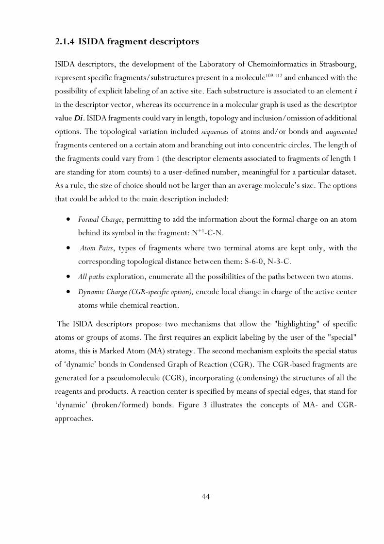
44
2.1.4 ISIDA fragment descriptors
ISIDA descriptors, the development of the Laboratory of Chemoinformatics in Strasbourg,
represent specific fragments/substructures present in a molecule109-112 and enhanced with the
possibility of explicit labeling of an active site. Each substructure is associated to an element i
in the descriptor vector, whereas its occurrence in a molecular graph is used as the descriptor
value Di. ISIDA fragments could vary in length, topology and inclusion/omission of additional
options. The topological variation included sequences of atoms and/or bonds and augmented
fragments centered on a certain atom and branching out into concentric circles. The length of
the fragments could vary from 1 (the descriptor elements associated to fragments of length 1
are standing for atom counts) to a user-defined number, meaningful for a particular dataset.
As a rule, the size of choice should not be larger than an average molecule’s size. The options
that could be added to the main description included:
• Formal Charge, permitting to add the information about the formal charge on an atom
behind its symbol in the fragment: N+1-C-N.
• Atom Pairs, types of fragments where two terminal atoms are kept only, with the
corresponding topological distance between them: S-6-0, N-3-C.
• All paths exploration, enumerate all the possibilities of the paths between two atoms.
• Dynamic Charge (CGR-specific option), encode local change in charge of the active center
atoms while chemical reaction.
The ISIDA descriptors propose two mechanisms that allow the "highlighting" of specific
atoms or groups of atoms. The first requires an explicit labeling by the user of the "special"
atoms, this is Marked Atom (MA) strategy. The second mechanism exploits the special status
of ‘dynamic’ bonds in Condensed Graph of Reaction (CGR). The CGR-based fragments are
generated for a pseudomolecule (CGR), incorporating (condensing) the structures of all the
reagents and products. A reaction center is specified by means of special edges, that stand for
‘dynamic’ (broken/formed) bonds. Figure 3 illustrates the concepts of MA- and CGR-
approaches.

45
The atoms for MA fragments should be labeled with a special flag in a special field of the input
file (SDF). Depending on the task, that could be performed by hand, mapping atoms directly
in a chemical editor and saving the SDF, or by editing the unlabeled SDF, or with the help of
CGR. For the CGR-based fragment, the corresponding input file contains the denotation of
the dynamic bonds, constituting the reaction center. The generation of the CGRs could be
done by hand or by a special soft, identifying the dynamic bonds by atom mapping.
The preferences of the two types of description should rely on the specificity of the modeling
task, i.e. whether the intrinsic nature of the active atoms should be preserved and taken into
account, and on the complexity of a chemical transformation. Thus, the task of intermolecular
interactions (Figure 3, top) implied an explicit consideration of donor/acceptor (D/A)
function of the active atoms, which determines the choice of MA-based descriptors. The
descriptors for donors and acceptors in this case could be generated separately and at the end
concatenated altogether, always in the same strict order, e.g donor’s descriptors-acceptor’s
descriptors, forming a descriptor vector representing a particular D:A complex. In such
manner, the D/A attribution is preserved and will be taken into account by the machine
learning algorithm. With regards to chemical reactions, an indisputable advantage of the
CGRs is the allowance to encode the structures of all the reactants (reagents and products)
altogether with the description of the structural changes. The order of representation of the
reactants does not matter in this case. A demonstrative example of the CGRs application is
the reactions of cycloaddition (Figure 3, bottom) which involved multiple bond
Figure 3. Example of structures for which MA- based (top) or CGR-based (bottom) local fragment descriptors
were generated. Top: in the hydrogen-bonded complex, the stars denote Marked Atoms. Bottom: in the Condensed
Graph encoding the (4+2) cycloaddition reaction, dots and dashes represent, respectively, formed and broken
chemical bonds. Some examples of generated descriptors are given on the right.
46
transformations. It should be noted, however, that structural representation of these reactions
could be done with the MA-based descriptors as well, by simultaneous labeling of all the atoms
of the active center, but the length of the descriptor vector in this case would be too big. In
addition, the attribution of the atoms to diene/dienophile (Diels-Alder case) could be lost, if
the order of the reactants in the database in not strict. The CGR-based representation thus
allows to encode the structures altogether with the active center transformation in a
condensed compact form.
For MA-based fragment descriptors an important parameter that could be varied is the degree
of ‘locality’ of the description. An internal mechanism of regularization of the portion of pure
local fraction included into the MA-based descriptors is implemented by four marked atom
strategies:
▪ -MA0 strategy generates fragments without introduction of the marked atom labels
and thus gives a general representation of a structure
▪ -MA1 exclusively generates fragments that starts or ends with the marked atom and
hence contains only local fragments
▪ -MA2 exclusively generates fragments that contain the marked atom and is a pure local
strategy as well
▪ -MA3 generates all kind of fragments but the marked atom has an explicit label
Figure 4 represent the difference between the strategies.
Correspondingly, MA1 is the subset of MA2 descriptor space, which, in turn, the subset of
MA3 descriptors altogether with the MA0 nonlocal descriptors.
CGR-based descriptors possess similar, but more restricted option of locality degree
regulation:
Figure 4. Examples of ISIDA MA descriptors (sequences of the length 4) generated for different marked atom
strategies.

47
• CGR0 strategy generates all possible fragments
• CGR1 strategy generates only the fragments that contain at least one dynamic bond.
Unlike the CGR-based descriptors, where the fragments are generated for a pseudomolecule,
the generation of MA-based descriptors, is performed for each participant of a chemical
reaction separately, i.e. for a single molecule. For the case of a molecule possessing more than
one marked atom, the two strategies of description are possible:
1. When a local fragment contains more than one labeled atom
2. When local fragments contain one labeled atom and further concatenated with the
fragments containing another labeled atom
The preference depends on the specificity of the task. For the case of a bifunctional molecule
bearing functional groups (atoms) G1 and G2, the molecule could be represented by local
descriptors including both labels (first strategy) or formally represented by two distinct
descriptor species - one with focus/label on G1, the other with focus/label on G2. The second
approach implicates emphasis on different nature and functions of the groups G1 and G2. For
the case of SN1 dissociation (Figure 5, bottom), the ‘active site’ is the two atoms connected
to the breaking bond, in this case there is no special meaning for these atoms but designating
the place of splitting. The fragments will include two labels simultaneously. No difference in
labels attribution is encoded. The second instance is hydrogen-bond forming molecule (Figure
5, top) with two binding centers, the first of which is the donor of hydrogen (the
corresponding atom is denoted with a green star) and the second is the acceptor of hydrogen
atom (denoted with red star). Both atoms are oxygens, thus their nature and their functions
during the chemical process should be explicitly designated. These atoms are labeled
separately, one by one, and the fragments, generated for each of the atoms then concatenated
with each other, so that the atom’s nature are encoded by the descriptors number, e.g the
descriptors from 1 to 100 reflects the fragments including acceptor atom, the remain
descriptors 101 -200 are the fragments with the donor part. In this manner, the atom’s
functions are preserved and segregated from each other.

48
ISIDA property-labeled descriptors. Apart from the explicit labeling of active
atoms/groups, the ISIDA package supports other, more specific, property labeling2, 113. It
bears a peculiar information about a particular atom/site that could be maintain alone or
coupled with the other fragment generation schemes. These includes:
• partial charge increment
• logP increment
• topological electrostatic potential coloration
On the considered example, the histogram of the corresponding property is constructed to
estimate the boundaries of the property spectrum to which the atoms are further assigned in
accordance to the value of its property, calculated by ChemAxon114. Figure 6 (created by
MarvinView115), gives an example of logP increment, where the corresponding boundaries
and atoms they cover are differentiated by color.
Partial charge labels in ISIDA descriptors calculated according to Gasteiger’s method based
on the electronegativity of the σ- and π- bonds. For the logP coloration, the Ghose-
Figure 6. An example of ISIDA
atomic logP increments. The atoms
are divided into groups, which are
denoted by the color code, in
accordance to their calculated logP
increments.
Figure 5. Example of the processes
where the difference in the active atom
functions are taken or not into
account: the reaction of dissociation
(bottom) has same labels on the active
atoms so as to pinpoint the location of
the bond cleavage, whereas the
hydrogen bond complex (top) has
different labels to denote
donor/acceptor nature of the atom.

49
Grippen116 approach is used, according to which the atoms are classified into 120 categories
according to their element, oxidation state and the surrounding atoms. The topological
electrostatic potential Vi on each atom i are calculated from the partial charges according to
the formula: 𝑉𝑖 =𝑞𝑖
𝑑0⁄ + ∑
𝑞𝑗
𝑑𝑖𝑗⁄𝑗≠𝑖 , where 𝑞𝑖,𝑗 are partial charges on atoms i and j, 𝑑𝑖𝑗
is the topological distance, and 𝑑0 is empirically determined virtual distance to take into
account the concerned atom charges.
ISIDA fragment descriptors thus propose an efficient way of structural representation.
However, it should be noted that relatively long descriptor vector, coming from an exhaustive
molecular description, could somehow restricts its applicability.
Thus, all the considered types of local descriptors could be used for structural representation
of chemical processes, however, some of them have distinct shortcomings. Thus, the
substituent constants, coming from the experiment and measured only for some of the
groups, could not be served as a universal description and suitable only for homogeneous data
sets of few varying substituents. The quantum-chemical descriptors, correspondingly, require
high computational costs, which is a strong limitation in case of modeling of big data sets. The
electrotopological indices are not expensive computationally, however, they do not reflect
the structural aspects explicitly, and are composed for each atom as the sum of the
corresponding electrotolopogical aspects, thus becoming not interpretable in terms of
chemical structure. Moreover, neither of these descriptor types supports an explicit emphasis
on the active centers. Therefore, ISIDA descriptors offer the best solutions to the above-
mentioned constraints due to fast computation, direct structural representation and various
possibilities of designation of the active sites.

50
2.2 Descriptors of the reaction conditions
For most of chemical processes, the influence of the experimental conditions is as important
as the structural impact of the reagents. Thus, the description of the process should explicitly
include the parameters of the solvent medium, temperature, pressure, etc. If for the latter
two the description implies just the corresponding magnitude, the solvent description is more
complex and needs to take into account the specific and nonspecific solvent effects, able to
affect the stability of the formed complex or the transition state, and thus influencing the
property.
Accounting for solvent effects is a conventional task in the field of quantum-chemical
modeling (QM) and molecular mechanics (MM), where the thermodynamic calculations of
chemical, biological or environmental processes referred to the solvated condensed phases.
The solvent models are classified into implicit, explicit and hybrid ones. The earliest attempts
of a solvent effect modeling give rise to the implicit models, where the solvent molecules are
accounted as isotropic polarizable media. Among widely used, the GB/SA117, PCM118 and
COSMO119-120 approaches should be mentioned. These models are computationally cheap and
often provide an acceptable estimation of solvent influence on the process, however, they can
not correctly describe specific interactions (e.g. H-bonds), that is of major importance for
particular solvents (e.g. water), and thus could fail to describe the influence of media in some
systems. More elaborated description is provided by explicit models121-123, which take the
solvent molecules into consideration explicitly, so that, their coordinates and some degrees
of freedom are included. These models (AMOEBA, SIBFA, COS) are mostly used in
molecular mechanics or molecular dynamics simulation. The parametrization and fitting
parameters of these models are therefore derived for a certain solvent group, which, as a
consequence, could lead to inability to reproduce some experimental results. The main
shortcoming of the explicit methods though is its computational demand. The hybrid
QM/MM methods124-125, as follows, incorporate the implicit and explicit approaches, so as to
provide a reasonable accuracy at fair computational costs. In the frame of the hybrid methods,
the energy of the system is composed from the QM-derived energies of the closest to the
solute molecular environment, the MM-derived energies of the distant zones and the
correction term, refer to the interaction QM/MM energy. The latter is the weakest part of
the approach, determining the emergence of various of methods and specific parametrizations
51
for the interaction energy calculation, that complicates the application of the approach. The
hybrid methods thus could be tested and used thoroughly, so as to give a reliable result.
In QSPR, it is important to provide the machine learner with enough information about the
solvent properties. Machine learning will then figure out which of the provided solvent
properties appear to correlate with the modeled property of the studied solute(s), and
propose the optimal (non)linear functional form to express the dependence of the latter with
respect to the former. So far, however, there were too few works related to the modeling of
chemical processes with the account for the solvent environment. The one that explicitly
include the solvent parameters is related to the modeling of SN2 reaction126. The solvent media
has been rendered there with the six parameters, standing for polarity and polarizability,
derived on the basis of the works of Born127 and Kirkwood128. These works emphasize the
importance of nonspecific solvation, which is determined by polarity and polarizability. The
former term could be expressed by the three functions of dielectric constant ɛ129, whereas the
polarizability could be represented by the three functions of refractive index nD20 129.
The consideration of the solvent effects, however, should be completed with the inclusion of
the specific solvation term. These parameters should meet the following requirement: derived
from the experiment, be measured for a large set of different solvents and not to be biased by
the probe, used during the experiment, but referred to a ‘general’ solute behavior toward a
particular solvent. These preconditions are met for the solvents effect scales, among which
Kamlet-Taft solvent effect scale is one of the most widely known. The first one, α scale130 is
referred to hydrogen bonding ability of solvents. This scale is based on solvatochromic
parameters, averaged for several probes, so that it has a built-in 'fuzziness' and measure the
ability to donate hydrogen bonds of the solvent molecules to a 'general solute', rather than
specifically for the probe employed in the experiment. The second one, scale131, is based
on the ultraviolet-visible spectral band of suitable probes. This is again an averaged quantity,
for which the wavenumber shifts of several protic indicators, relative to structurally similar,
but aprotic probes, are used. The third value is the π* value132, based on the average of values
of the π →π* transition energies for several nitro-substituted aromatic indicators. The
quantity is normalized to give pi* = 0 to cyclohexane and pi* = 1 to dimethylsulfoxide, and,
as for the previous two scales, multiple probes are used to eliminate specific interactions and
spectral anomalies. This value measures a certain ‘blend’ of polarity and polarizability.
Another set of specific interaction-referred scale is the Catalan parameters. Similar to Kamlet-

52
Taft scales, the Catalan parameters included the solvent polarity/ polarizability (SPP)133,
solvent basicity (SB)133 and solvent acidity (SA)134 measures.
In the frame of this thesis, the solvent effects have been described with the following set of
the experimental parameters:
• four functions of dielectric constant ε, standing for nonspecific interactions : Born
1−=Bf
, Kirkwood 12
1
+
−=
Kf
, 1
11
+
−=
f
and 2
12
+
−=
f
.
• three functions of the refractive index nD20(n), as well reflecting the nonspecific effects:
2
12
2
1+
−=
n
ng ,
12
12
2
2+
−=
n
ng ,
)12)(12(
)1)(1(2
2
++
−−=
n
nh .
• Kamlet–Taft’s α, β and π* parameters
• Catalan’s SPP, SA and SB constants
An additional reaction condition term of temperature has been included as the reversed value:
1/T in Kelvin degrees, as it corresponds to the Arrhenius equation (ln 𝑘 = ln 𝐴 − 𝐸𝑎𝑅𝑇⁄ ). In
case of water-organic mixtures, a molar fraction of the organic solvent has been added as a
descriptor. The hierarchical clustering dendrogram of the solvents used in different projects
of this study and based on the 13 chosen solvent parameters is given on Figure 7.

53
Fig
ure 7
. Hiera
rchica
l clu
sterin
g d
end
rog
ram
ba
sed o
n th
e 13
solven
t pa
ram
eters used
for th
e solven
t effect a
cco
un
t in th
e ap
plica
tion
pa
rt of th
e thesis.

54
Chapter 3
QSPR methodology
3.1 Quantitative Structure-Property Relationships (QSPR)
QSPR modeling is the determination of a mathematical relationship between the chemical
structure (or more complex information included in the description) and a modeled
property/activity:
𝑷𝒓𝒐𝒑𝒆𝒓𝒕𝒚 (𝑎𝑐𝑡𝑖𝑣𝑖𝑡𝑦) = 𝒇(𝑐ℎ𝑒𝑚𝑖𝑐𝑎𝑙 𝑠𝑡𝑟𝑢𝑐𝑡𝑢𝑟𝑒, 𝑠𝑜𝑙𝑣𝑒𝑛𝑡, 𝑇, 𝑝𝑟𝑒𝑠𝑠𝑢𝑟𝑒, 𝑒𝑡𝑠)
The corresponding structure-related information in the function argument should be encoded
numerically, composing the descriptor vector, defining the position of an object in chemical
space. The object’s numerical description then used to build a QSPR model, embodied the
mentioned mathematical relationship, the goal of which is to be able to predict a certain
property/activity over a wide range of new (in a sense they were not used for a model’s
building) chemical objects.

55
A general used for model building procedure of QSPR model building included the following
steps:
i. Data curation and standardizations. This includes rejection of entries associated to
missing or chemically invalid structures, missing or unreliable experimental endpoints,
removal of counterions not needed for modeling, conversion of structures into a
common, standardized representation style (aromatic bonds, split-charge nitro
groups, etc) and removal of duplicates (complete removal if a same structure is
associated to conflictingly different experimental values).
ii. Descriptors calculation. In this work, we used ISIDA fragment (Marked Atom or
CGR-based) descriptors for structural representation of a chemical object (described in
section 2.1.4). Accordingly, the descriptor vector is constructed from structural
fragments of different length with the corresponding occurrences being the
descriptor’s value. The descriptors’ values are then normalized form 0 to 1.
iii. Model building. The algorithms used for building of the predictive models called the
machine learning methods. Whereas there is a diversity of different algorithms, the ones
chosen for modeling in this work are the state-of-the-art techniques proved its
efficiency and usability: the Support Vector Machines and Multiple Linear Regression.
The tool combining both possibilities, regression and visualization, is the Generative
Topographic Mapping. The description of these methods is given in section 3.2. A data
set used for building of the model is called training set
iv. Model validation. This includes cross-validation, performed at the stage of model
building (cross-validation is described in section 3.3.1) and evaluating the model
performance on the training set and external validation. For the latter, some part of data
could be excluded from the initial data set at the beginning or new data could be used.
These data were not involved in model’s building at all. This test set is required to
assess predictive power of the model and its utility.
The constructed model is used for the prediction of the corresponding property/activity of
unknown or untested structures thus providing, of course depending on the overall accuracy
of the model, a numeric value or a classification belonging of the structures given.

56
3.2 Machine Learning algorithms
3.2.1 Support Vector Machine (SVM)
Firstly introduced by V.Vapnik135-136, Support Vector Machine at its origin is a binary classifier
that finds a separating hyperplane so as to best segregate the two classes (Figure 8). The
hyperplane is constructed in such a way to have the biggest gap between the hyperplane and
the data instances of either side, so that to minimize the chance of misclassification.
Accordingly, the SVM model then categorizes new examples according to which side of the
hyperplane they fall.
The method however is suitable not only for linearly separated objects, but for nonlinear task
as well. To perform the separation in this case, a new coordinate is introduced in such a way
that in the resulting higher-dimensional space the classes are easily separated (Figure 9). The
possibility to perform nonlinear separation in case of usage of linear classifier utilizes so called
kernel trick and is widely used in kernel-based methods.
Figure 8. An illustration of the SVR algorithm: a
separating hyperplane (denoted with red line) is
drawn so that to separate the objects belong to
different classes with the maximal distance between
the nearest points and the hyperplane.
Figure 9. The kernel trick of the SVR: a non-
linear transformation from feature space to
higher-dimensional space where the objects
are easily separated.

57
The Support Vector Machines for the regression task implies optimization of the regression
function f(x), which is searched under the following constraint:
|𝑦 − 𝑓(𝑥)| < 휀 (25)
here 휀 is the error threshold. The function is optimizing till no errors largen than 휀 are
produced. However, to be able to model data with persisting errors, a proportional cost is
introduced:
𝜉 = |𝑦 − 𝑓(𝑥) − 휀| (26)
The model is fitted so that to minimize its complexity and the proportional cost.
In this work the Support Vector Regression (SVR) is the main or benchmarking method of
modeling, the developed models of which are the resulting web-implemented output of the
projects.
3.2.2 Multiple Linear Regression (MLR)
Multiple Linear Regression aimed at finding the equation between the property/activity and
the descriptors, encoded the chemical object, with a crucial assumption that the relationship
is linear. That could be represented as follows:
𝑷𝒓𝒐𝒑𝒆𝒓𝒕𝒚 = 𝛼 + 𝛽1 ∗ 𝑑𝑒𝑠𝑐𝑟𝑖𝑝𝑡𝑜𝑟1 + 𝛽2 ∗ 𝑑𝑒𝑠𝑐𝑟𝑖𝑝𝑡𝑜𝑟2 … + 𝛽𝑁 ∗ 𝑑𝑒𝑠𝑐𝑟𝑖𝑝𝑡𝑜𝑟𝑁
The goal thus is to find the intercept 𝛼 and the corresponding regression coefficient 𝛽𝑥, which
could be considered as a contribution of a certain descriptor into the property i.e. measures
the unit change in the dependent variable with the change of the descriptor, so as to fit the
property variation.
The software for MLR in this study is ISIDA QSPR1, which combines backward and forward
stepwise variable selection (prior selection of those variables influencing most on the model’s
predictive ability, needed to provide more robust and cost-effective prediction) generating a
large number of linear models forward by the selection of the most robust ones for the
consensus prediction, that is an average of the estimated property values obtained with the
selected individual models.

58
3.2.3 Generative Topographic Mapping (GTM)
Generative Topographic Mapping is a method combining the modeling capability along with
data visualization and data analysis tools. Firstly introduced by Bishop3 in 1990th, the method
performs a non-linear dimensionality reduction of the D-dimensional data space (where D is
the number of descriptors) onto a 2-dimesional latent space (GTM map) by embedding a
flexible 2D manifold into the D-dimensional data (Figure 10).
The ‘unfolded’ manifold is a square grid of K nodes. The assignment (mapping) of the nodes
to the manifold points is defined by a mapping function 𝑦𝑑(𝑥; 𝑊) set up with the help of M
radial basis functions (RBFs).
𝑦𝑑(𝑥; 𝑊) = ∑ 𝑊𝑚𝑑exp (‖𝑥 − 𝑥𝑚‖2
2𝜎)
𝑀
𝑚=1
(27)
where d goes from 1 to D, W is the 𝑀 × 𝐷 weight matrix connecting RBF and data space
points, 𝑥𝑚 is the center of the m-th RBF. The overall number of the RBFs and the width σ
are the optimizable parameters of the method.
As a probabilistic extension of the Kohonen Self-Organizing Maps, GTM operates with
probabilities of a data object to be mapped into a certain node. Moreover, the object has non-
zero probability over all the nodes. Consequently, it could be characterized by its
probabilities, which are called responsibilities. Responsibilities constitute a responsibility vector,
the main descriptive characteristic of an object, used for class belonging assignation in case of
classification, or property value calculation for the case of regression modeling.
The responsibility of the k-th node for n-th data point 𝑡𝑛 is calculated using Bayes’ theorem:
Figure 10. An illustration of how the data
points are fitted by the GTM manifold (left)
and further projected on the GTM map
(right).

59
𝑅𝑛𝑘 =exp (−
𝛽2
‖𝑡𝑛 − 𝑦𝑑(𝑥𝑘; 𝑊)‖2)
∑ exp (−𝛽2
‖𝑡𝑛 − 𝑦𝑑(𝑥𝑘; 𝑊)‖2)𝐾𝑘=1
(28)
Responsibilities are normalized over the grid of nodes and their sum for a given item is equal
to 1.
GTM-based regression and classification models
The general procedure of the model building is similar for regression and classification tasks,
as in both cases an object (for simple case – a single molecule) is characterized by the assigned
responsibility vector. The following steps are included:
i. Obtaining a GTM grid, each node of which will be attributed with the corresponding
responsibilities of every molecule of the training set.
ii. Defining the property/class value of each node based on the contribution of each
molecule to a certain node (which is molecule’s responsibility) and its corresponding
property/class value. This procedure is called coloration, since the property
distribution will be expressed as the color profile of the map. The same GTM map
hence could be colored differently depending on the training set property/class values.
iii. Projecting the test set compounds and calculating its responsibility vectors further used
for the property/class prediction.
The node property value �̂�𝑘 of GTM regression model (step ii) is calculated as follow:
�̂�𝑘 =∑ 𝐴𝑛𝑅𝑘𝑛
𝑁𝑛=1
∑ 𝑅𝑘𝑛𝑁𝑛=1
(29)
where N is the number of molecules, 𝐴𝑛 is the experimental property of the n-th molecule,
𝑅𝑘𝑛 is its responsibility in the k-th node (see eq. 28). The calculated node property values are
used for the GTM activity landscape representation (eq. 29.2) – the final result of the map
coloration (detailed below).
𝐴𝑞 = ∑ �̂�𝑘𝑅𝑘𝑞 (29.2)

60
Similarly, GTM classification model attributes a class accessory to each node by averaging
the responsibilities over all training set compounds, then, for any q-th test set compound, the
probability to belong to the i-th class 𝑃(𝐶𝑖|𝑞) is calculated according to the formulae:
𝑃(𝐶𝑖|𝑞) = ∑ 𝑃(𝐶𝑖|𝑘) × 𝑅𝑞𝑘
𝑘
(30)
where P(Ci|k) is the conditional probability of the class Ci for the given node k, calculated
according to the Bayes’ theorem:
𝑃(𝐶𝑖|𝑘) =𝑃(𝑘|𝐶𝑖) × 𝑃(𝐶𝑖)
∑ 𝑃(𝑘|𝐶𝑗) × 𝑃(𝐶𝑗)𝐶𝑗
(31)
where 𝑃(𝐶𝑖) and 𝑃(𝑘|𝐶𝑖) are, respectively, a fraction of compounds of the class Ci and a
normalized cumulated responsibility of the class Ci in the training set.
GTM visualization
The ability to visualize the data distribution is the main advantage of GTM over the classical
machine learning methods. The method proposes different schemes of representation of data
distribution thus allowing to analyze various aspects of data. The main visualization techniques
used herein are GTM property landscape and GTM class landscape, correspondingly, representing
data form regression or classification side. The landscapes are created according to the
mentioned equations (eq. 29-31) and reflect the node’s property- or class attribution. In
addition, the landscapes are weighted by data density: the more molecules (or more complex
chemical objects) are located near a certain node, the more opaque the color of the node,
correspondingly, if no molecules are projected into a node with any reasonable responsibility,
the node remains to be transparent (blank). Figure 11 shows examples of property- and class
landscapes providing the equilibrium constant distribution and the tautomeric type separation
of 695 tautomeric equilibria (the project is described in section chapter 6).

61
3.3 Model quality estimation
3.3.1 Cross-validation and external validation
A QSPR model needs to be validated in order to estimate whether it has a key competence -
the ability to predict the property of new objects. The model performance should not be
evaluated on the data that was used to build the model: indeed, the model would just repeat
the property value/class of the samples that it has just seen and shows a perfect score (if the
samples were not ‘outliers’ constantly mispredicted by the model), but would fail to predict
yet-unseen data. This situation is called overfitting. To avoid overfitting, the model’s
performance is estimated during cross-validation, the procedure that envisages retention of
a part of data and its further usage for model’s evaluation. The initial data is thus divided into
two parts, training set and test set. However, to get unbiased independent predictions for
each object of the data, all of them should be estimated during test set prediction. To do so,
the portioning of data is performed several times, usually 5, times, correspondingly called 5-
fold cross-validation. Each time the different 5th part of data is retained as a test set, and the
Figure 11. Possibilities of GTM visualization: the class landscape (left), representing the separation of 10
different tautomeric classes, and the property landscape (right) characterizing the distribution of the
equilibrium constant values over the map.

62
other 4/5 are used as the training set (Figure 12). That insures the unbiased prediction will
be obtained for each object of the data.
As a rule, the built model should be also estimated on a data set not at all related to the initial
data (used for building) and comes from different source, or, if not possible, randomly chosen
from the initial data before any modeling, and retained. This set, called external test set, is a key
tool for model’s performance analysis and shortcomings revealing.
3.3.2 Regression- and classification model’s performance criteria
The predictive performance of a regression model (estimating continuous property) is
obtained with the following parameters:
▪ Determination coefficient:
𝑄2 (𝑜𝑟 𝑅2) = 1 − ∑(𝑌𝑒𝑥𝑝,𝑖 − 𝑌𝑝𝑟𝑒𝑑,𝑖)2/ ∑(𝑌𝑒𝑥𝑝,𝑖 − < 𝑌 >𝑒𝑥𝑝)2
𝑛
𝑖=1
𝑛
𝑖=1
(32)
▪ Root Mean Squared Error:
𝑅𝑀𝑆𝐸 = [1/𝑛 ∑(𝑌𝑒𝑥𝑝,𝑖 − 𝑌𝑝𝑟𝑒𝑑,𝑖)2
𝑛
𝑖=1
]1/2 (33)
Figure 12. Schematic representation of 5-fold cross-validation procedure. Initial dataset is divided into 5
parts, on each fold a model is trained on 4 parts and is applied to predict the last one. At final, all predicted
values are gathered for statistical evaluation.
63
where Yexp and Ypred are, respectively experimental and predicted values of property and
<Y>exp is the mean of experimental values.
Classification models (predicting the label of an object, i.e. active/inactive) estimated here by
the following:
▪ True Positive Rate:
𝑇𝑃𝑅 = 𝑇𝑃/𝑃 (34)
where TP is the number of True Positive (being positive and predicted as positive)
species while P is the overall number of experimentally positive class species in the
data set.
▪ True Negative Rate:
𝑇𝑁𝑅 = 𝑇𝑁/𝑁 (35)
where, similarly, TN is the number of True Negative (being negative and predicted as
negative as well) species and N is the number of experimentally negative class species.
▪ Balanced Accuracy:
𝐵𝐴 =𝑇𝑃𝑅 + 𝑇𝑁𝑅
2 (36)
3.4 Applicability Domain
Applicability Domain (AD) defines the area of chemical space where the model is presumably
accurate. The concept of Applicability Domain assumes that the objects similar to those used
for model building, will be predicted accurately rather than very different, in terms of
descriptor vector similarity, targets. Figure 13 gives an illustration on the example of 2D
chemical space.

64
The definition of the AD is a crucial aspect since the prediction of an object which is being outside
the AD is unreliable and could lead to wrong conclusions and undesired consequences.
A lot of different schemes proposed for the AD determination, that could rely purely on the
descriptors constituents or could be derived from the machine learning method. The
designation of the most appropriate AD is still a matter of discussion.
The AD of all the projects of this study is based on Bounding Box, for each descriptor vector
reckoning the minimum and maximum values encountered in the training set. An object is
considered to be out of AD if at least one of its descriptor values violates the defined min-max
range. The Bounding Box techniques by definition encompasses so-called Fragment Control:
if the data set encoded in structural fragment descriptors, then any molecule of the test set
possessing a new structural fragment considered to be out of AD.
Figure 13. Representation of the concept
of applicability domain for the chemical
space based on two descriptors. The
prediction of the test compound inside the
domain is reliable whereas of the
compound outside the domain the
prediction is not trustworthy.

65
PART II. RESULTS AND DISCUSSIONS
Chapter 4
QSPR modeling of halogen bond basicity of
binding sites of polyfunctional molecules
Halogen bonding started to attract specific attention across the chemical, biochemical, and
material sciences very recently – this peculiar interaction received its official IUPAC definition
only in 2013137. Indeed, a predisposition of halogen atoms to behave as nucleophiles due to
their high electronegativity is a well-established understanding, thereupon halogen atoms are
mostly considered as the regions of high electron density. However, their ability to behave as
Lewis acids notwithstanding their intrinsic nature was revealed in the beginning of the 1900th
by the formation of complexes such as Hal2…NH3 and Hal2…OH2138-139. Nonetheless, the
revelation of the electron density in halogen atoms being anisotropically distributed whenever
the atom is covalently bound to one or more atoms, has emerged only recently140-141.
A covalently-bonded halogen atom surrounded by the area of rich electron density forming a
belt, orthogonal to the covalent bond, where the electrostatic potential is negative, but at the
same time the electronic distribution anisotropy shapes a region of lower electron density (the
so-called σ-hole) where the potential is frequently positive. This region can form attractive
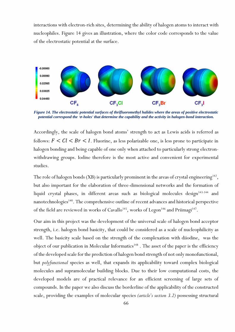
66
interactions with electron-rich sites, determining the ability of halogen atoms to interact with
nucleophiles. Figure 14 gives an illustration, where the color code corresponds to the value
of the electrostatic potential at the surface.
Figure 14. The electrostatic potential surfaces of thrifluoromethyl halides where the areas of positive electrostatic
potential correspond the ‘σ-holes’ that determine the capability and the activity in halogen-bond interaction.
Accordingly, the scale of halogen bond atoms’ strength to act as Lewis acids is referred as
follows: 𝐹 < 𝐶𝑙 < 𝐵𝑟 < 𝐼. Fluorine, as less polarizable one, is less prone to participate in
halogen bonding and being capable of one only when attached to particularly strong electron-
withdrawing groups. Iodine therefore is the most active and convenient for experimental
studies.
The role of halogen bonds (XB) is particularly prominent in the areas of crystal engineering142,
but also important for the elaboration of three-dimensional networks and the formation of
liquid crystal phases, in different areas such as biological molecules design143-144 and
nanotechnologies140. The comprehensive outline of recent advances and historical perspective
of the field are reviewed in works of Cavallo145, works of Legon146 and Priimagi147.
Our aim in this project was the development of the universal scale of halogen bond acceptor
strength, i.e. halogen bond basicity, that could be considered as a scale of nucleophilicity as
well. The basicity scale based on the strength of the complexation with diiodine, was the
object of our publication in Molecular Informatics148 . The asset of the paper is the efficiency
of the developed scale for the prediction of halogen bond strength of not only monofunctional,
but polyfunctional species as well, that expands its applicability toward complex biological
molecules and supramolecular building blocks. Due to their low computational costs, the
developed models are of practical relevance for an efficient screening of large sets of
compounds. In the paper we also discuss the borderline of the applicability of the constructed
scale, providing the examples of molecular species (article’s section 3.2) possessing structural

67
features responsible for certain steric effects, affecting the complexation constant, that should
be thus treated cautiously. Apart from the contribution toward halogen-bond driven
processes, one could find the section of comparison of the strength of halogen and hydrogen
bonding to be of particular interest (article’s section 3.4).
The project was done in collaboration with Jerome Graton and Jean-Yves Le Questel
(University of Nantes) providing thorough experimental data, and Vitaly Solov’ev (Institute
of Physical Chemistry, Moscow) conducting the MLR-related part of calculation as well as the
effective constant evaluation by means of ChemEqui149 software.
The corresponding article is given in the end of the section, with the authorization of all
authors.
4.1 Modeled object and property
Herein, the halogen bond (XB) donor molecule is the same for all the complexes, hence, its
structure could be excluded from consideration. The modeled object is thus the structure of
a designated XB acceptor, the active center of which, binding the halogen atom, is attributed.
The modeled property is the complexation constant (log KBI2) of an organic molecule,
considered as a Lewis base, with diiodine (I2). The experimental values are referred to 1:1
complexation in hexane at 298K. The structure of a XB acceptor is represented by the Marked
Atom (MA)-based descriptors, where the corresponding marked atom is attributed to the
active site of a molecule, binding with I2. All four marked atom strategies of MA-based
descriptors have been tried and compared. In case if molecules possessing two putative
binding centers, the main one has been indicated in the initial source.

68
4.2 Modeling workflow
4.3 Data preparation
Initial data has been reported in the work of Laurence et al.150. The log KBI2 values represented
primary the experimentally measured values in heptane, hexane, cyclohexane and
methylcyclohexane at 298K. Their differences as a result of solvent effects are generally within
the experimental uncertainties151. Some of the log KBI2 have been experimentally measured
in CCl4, CH2Cl2 or CHCl3. In this case, the corresponding values have been recalculated
and referred to hexane by known linear Gibbs energy relationship151. If a compound had
several reported equilibrium constants values in different solvents, only the primary value in
alkane was selected. Cis/trans-isomers with diverging XB acceptor propensities have been
removed. The structures have been standardized according to the procedure used on our
virtual screening web server (http://infochim.u-strasbg.fr/webserv) and based on
ChemAxon’s Standardizer152 (neutralization, isotopes removal, conversion to ‘basic’ aromatic
form etc.) The labeling of the concerned XB active sites, explicitly assigned in the initial
database, has been performed manually. Thus, the training set consisted of 598 organic
molecules of 14 different types of XB acceptor atoms, the weakest of which is the π-electronic
carbon and the strongest is the sulfur of thiophosphoryl group (App., part I, Table I.1).
Figure 15. Workflow of the modeling of the strength of halogen bonding between organic accceptors and
diiodine (logKBI2).

69
The external set consisted of 11 polyfunctional species, collected from the same source, for
which the effective constants (log KBeff), attributed to the binding that involved all of the active
centers, have been experimentally measured. The measurements performed in solvents,
different from hexane, have been recalculated to the appropriate solvent by known151 linear
free energy relationships.
4.4 Computational details
The fragmentation schemes included various atom coloration by elements symbol, by CVFF
force field label or by pharmacophoric types (described in section 2.1.4). The considered
fragment topologies were sequences and atom-centered fragments of the minimal length from
2 to 4 and the maximal length from 3 to 8. Overall, 480 descriptor sets (120 for each marked
atom strategy) have been tested. The modeling has been performed by SVR and MLR
methods. The performance of the models has been estimated by the R2 and RMSE values in
5-fold cross-validation. The applicability domain control method was Bounding Box. The
most robust SVR and MLR models constituted the consensus SVR (MLR) models (CM),
rendering the property value as the corresponding average of the values, predicted by the
individual models. The prepared consensus SVR and MLR models have been further used for
the prediction of the external test set.
The assessment of log KBeff values for polyfunctional molecules of the external set was derived
from the predicted log KBI2 of each individual active center of a molecule. The corresponding
estimation was done with the help of ChemEqui153 program simulating a network of chemical
equilibria in solution and designed to handle the cases of simultaneous coexistence of several
mono- and polybinded species.
The details of the computational procedure including the specification of the scanned
descriptor spaces for SVR and MLR, list of the models included into the final web-deployed
consensus SVR model, as well as the detailed workflow of data curation and treatment are
described in the article.

70
4.5 Results and discussions
4.4.1 Cross-validation.
The average statistical values in 5-fold cross validation returned by the consensus SVR/MLR
prediction for each marked atom strategy are summarized in Table 2. The best result is
achieved by the MA3 strategy, which explicitly distinguish fragments belonging to the reaction
center and its environment. The MA3 strategy could be seen as the sum of MA2 and MA0
descriptors, where the MA2 describes the immediate surrounding of the active center and
MA0 does not pinpoint the active center but generally characterizes the molecule.
Marked Atom
strategy
SVR MLR
R2 RMSE R2 RMSE
MA0 0.88 0.48 0.83 0.59
MA1 0.89 0.47 0.87 0.51
MA2 0.91 0.43 0.88 0.49
MA3 0.93 0.39 0.92 0.43
Table 2. The modeling performance of log KBI2 prediction obtained in 5-fold cross validation on the training set
of 598 molecules.
The MA3 strategy thus has been chosen for the construction of the consensus SVR and MLR
models (the constituting individual models are listed in Appendix, part I, Table I.2) which
were used for the prediction of the external set of 11 polyfunctional molecules.
4.4.2 External validation.
The predicted values obtained by the model for individual binding centers were combined
into the effective constants (log KBeff), the comparison of which with the experimental values
is given on the Figure 16. The predicted effective constant reproduces the experimental
logKBeff with the RMSE values close to the ones of the cross-validation stage.

71
4.4.3 Comparison of the strength of halogen and hydrogen bonding
A set of 166 molecules with available H-bonding acceptor strength data against 4-F-phenol in
CCl4154
has been used for the evaluation of the relationship between halogen and hydrogen
bonding strength. As expected, the general overall tendency, concerning the predominance
of one or another binding type, could not be observed, however, strong correlations have
been found within specific chemical families (Table 3; App., part I, Table I.5).
Chemical class α β n Rcorr2 s
Oxygen bases (the C=O, -O-, P=O, S=O sites) -1.07 0.97 85 0.942 0.20
Nitriles -0.89 0.94 11 0.978 0.05
Sulfur bases 1.74 1.39 21 0.904 27
Primary, secondary and tertiary amines 0.61 1.50 13 0.833 0.45
Complexes with aromatic nitrogen -0.5 1.42 36 0.876 0.25
Table 3. Comparison of hydrogen and halogen bond strength. a, b are parameters of linear correlation
logKI2=a+b logBHX, s - standard deviation.
This can be explained by the fact that the physico-chemical nature of the acceptor site –
chemical element, hybridization, etc – defines the generic order of the magnitude of the
interactions. Within a given family, the generic acceptor propensity of the center is modulated
Figure 16. Predicted vs experimental log KBeff for the external test set of 11 polyfunctional molecules.

72
by its chemical context – and it turns out that this modulating effect is comparable for both
H-bonding and XB strength: a same substituent will impact both properties similarly. As it
was determined, for oxygen bases (the C=O, -O-, P=O, S=O sites), the log KBI2 is lower
than the log KBHX of the H-bond complexes. An opposite trend is observed for sulfur bases
(the -S-, C=S, P=S sites), for which halogen-bonding is considerably stronger than H-
bonding. Similar regularity is observed for the stability of diiodine complexes with primary,
secondary and tertiary amines, as well as in the case of aromatic nitrogen bases, for which the
stability of diiodine complexation is compatible or higher than the stability of H-bond
complexation.
4.6 Conclusion
This project is a starting point of this thesis, representing the simplest case of the modeling
for the system, where one of the participants and the experimental conditions stay constant.
The modeled property is the binding strength of complexes of organic molecules with diiodine
(I2). The quantitative value of the binding strength serves as the halogen bond basicity scale,
or, more general, as a scale of nucleophilicity of organic molecules. Here we report a
successful QSPR modeling of the halogen bond basicity of 598 organic molecules for which
the binding constants have been measured at unified conditions (hexane, 298K). The structure
of an organic molecule has been characterized by Marked Atom-based descriptors, the
different labeling strategies of which, representing particular levels of
generalization/specification of structural description have been applied and compared. The
MA3 strategy turned out to be the best performer as it combines an explicit characterization
of the active sites with the description of the overall structural arrangement of a molecule.
The cross-validation results of the SVR and MLR individual models built on the MA3-based
descriptors spaces are close to the experimental errors: RMSE=0.39-0.43 (R2 =0.92-0.93).
That should be noted, that regardless of the use of the best fragment descriptors, these can
not cover the entire range of different structural and electronic effects playing a role in the
complexation strength, notably the bidentate halogen/hydrogen bond interaction scenarios
occurring in certain conformations. However, during model building, the fitting errors
caused by any types of similar effects are minimized so that their average affect over the
property is below the intrinsic imprecision of the model. Extensively cross-validated
consensus SVR and MLR models have been challenged to predict the effective complexation

73
constants of polyfunctional molecules of the external test set. The models showed robust
cross-validation statistics (R2 =0.70-0.81, RMSE=0.44-0.56) and were able to successfully
extrapolate the interaction of polyfunctional compounds with I2, for which the experimental
effective binding constant could be inferred from the individual propensities of all the groups
putatively participating in XB. The comparison of the H-bond and XB complexation constants
does not show any global relationship between these related, but mechanistically quite
different chemical interactions. However, strong piecewise correlations within chemical
families based on the same type of H-bond/XB donor were found, which means that while
the intrinsic HB or XB strength of these centers are uncorrelated, the modulating impact of
the substituents on both HB and XB are comparable.
A predictor of the halogen-bond basicity of acceptor sites of organic molecules was created
on the entire training set and comprises the best performing SVR models (App., part I, Table
I.2). The consensus model is publicly available on the web server: http://infochim.u-
strasbg.fr/webserv/VSEngine.html, altogether with the automatic binding centers labeling
and molecule’s applicability domain estimation.
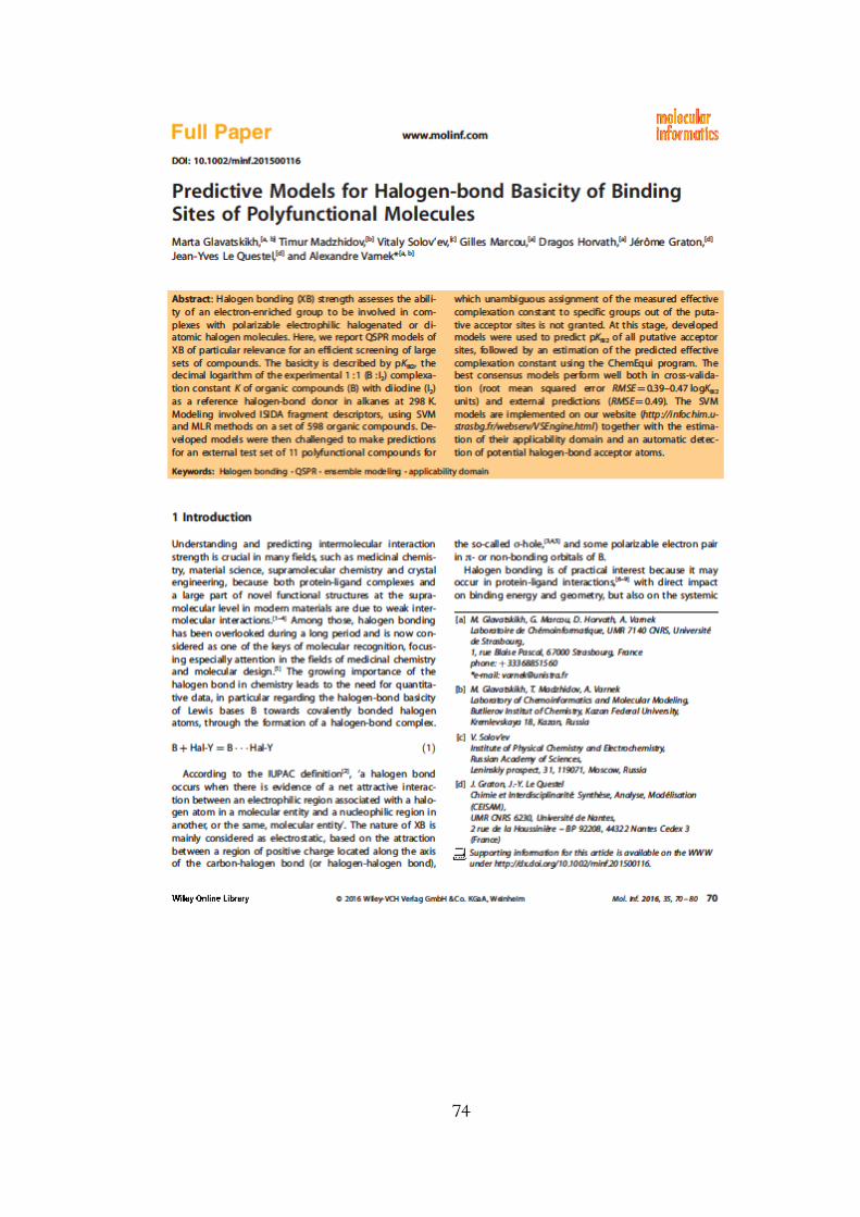
74

75

76

77

78

79

80

81

82

83
84
Chapter 5
QSPR modeling of the Free Energy of hydrogen-
bonded complexes with single and cooperative
hydrogen bonds.
Discovered first around 100 years ago155, hydrogen bond is still object of numerous research
and debates. The reason of this long-lasting interest is determined by the importance of
hydrogen-bond based interactions to a broad spectrum of fields varying from biology to
material science. The topic of hydrogen bond interactions drew particular attention in 1990th
with the boom in developing of supramolecular and crystal engineering researches. Since that
time, the depth and the complexity of the phenomena have expanded drastically. A new
concept of hydrogen bonds has been emerged156 and new aspects of weak hydrogen bonding
occurring in biological systems have been discovered157. Hydrogen bond in the present time
is interpreted as a region alternating from covalent bonds to van der Waals interactions, ionic
interaction and even π-cation interchange.

85
The following definition is proposed for the complexity of hydrogen-based interactions: An
X-H…A interaction is called a “hydrogen bond” (HB), if (1) it constitutes a local bond, and (2)
X-H acts as proton donor to A. The energy range of hydrogen bond dissociation varies from
4 to 160 kJ/mol, and the distance up to 3.2Å is considered potentially capable of bonding.
Within this range, the nature of the interaction is not constant, but includes electrostatic,
covalent, and dispersion contributions in varying weights. More about the nature and the
variety of HB interactions could be found in numerous related books156, 158-159, works of
Desiraju160-161, Leiserowitz162-163 and Steiner164, while the biological aspects could be found in
a book of Jeffrey and Saenger165.
Following the line of mono- and polyfunctional intermolecular interactions, this project deals
with the modeling of the strength of hydrogen-bonded complexes. Our paper on this topic
has been published in Molecular Informatics166. The task is aimed at the modeling of the
strength of both, mono- and polyfunctional hydrogen bonds, which, this time is formed by
different acceptors and different donors. The data set used for modeling is so-far the biggest
used for QSPR study of hydrogen bond strength. Initial data included the measurements of
the same complexes in different solvents, that allows to build linear correlations, so as to go
from the reference solvent to the required one, allowing the comparison of HB strength
relative to different media. The obtained linear correlations have been estimated during the
external validation. The performance of the developed models has been evaluated on two
external sets. The first one was formed by the complexes with single HB, among which there
where donors/acceptors encountered in the training set as well as structurally unknown
molecules. This fact suggests a different from the traditional, ubiquitously applicable for single
molecules, manner of the model’s predictive performance estimation. Here, the external set
complexes have been attributed to four different classes that correspond to a certain degree
of ‘novelty’ of the complex with respect to the training set. Consequently, the model’s
performance has been evaluated for each of the classes.
The work was done in collaboration with Vitaly Solov’ev (Institute of Physical Chemistry,
Moscow) carried out the MLR calculation.
The article is given in the end of this section, with the authorization of all authors.

86
5.1 Modeled object and property
The data set, referred to ‘standard’ conditions, was composed of varying donors and acceptors
coupled by single hydrogen bonds. The active site of each participating molecule was
attributed and explicitly marked: correspondingly, this is the donor atom, providing
hydrogen, and the acceptor atom with free electron pair. The Marked Atom (MA)-based
descriptors have been used. The structures of the donor and the acceptor molecules have been
treated separately: for each of the participants the fragment descriptors, including the local
ones, i.e. with the corresponding donor/acceptor (D/A) labels on the active sites, have been
prepared and in the end concatenated altogether, forming an integrated descriptor vector,
representing a particular donor-acceptor complex. The MA3 strategy was the best one in the
previous project with similar task of modeling of the strength of intermolecular complexation,
which could be explained by the fact that the strategy encompasses and describes the whole
molecule but at the same time explicitly distinguish fragments belonging to the reaction
center. Thus, the MA3 strategy is involved herein.
5.2 Modeling workflow
5.3 Data preparation
An initial data set consisted of 4002 HB complexes measured in different solvents at several
temperatures has been compiled from the literature151, 154, 167-170. The complexes have been
Figure 17. Workflow of the modeling of the Gibbs Energy (ΔG, kJ/mol) of hydrogen bonded complexes of
different donors and acceptors.

87
attributed with the experimentally estimated ΔG values for 1:1 complexation. The
measurements were carried out in 17 different organic solvents at the temperatures varying
from 293K to 303K. From this data, a homogeneous set of 3373 complexes, where the
measurements have been carried out in CCl4 under the standard temperature of 298K, has
been extracted and constituted the training set. The set underwent cleaning and filtering
excluding all inorganic, metalorganic, deuterium containing compounds and salts. The donors
and the acceptors structures underwent a prescribed standardization procedure used on our
virtual screening web server (http://infochim.u-strasbg.fr/webserv) and based on
ChemAxon’s Standardizer152 (neutralization, isotopes removal, conversion to ‘basic’ aromatic
form etc.). The labeling of the active sites of donor molecules have been performed by
SMARTS-based substructure search (by means on an in-house tool using the ChemAxon
substructure search API), whereas the acceptors’ active sites have been detected and marked
by means of the previously developed HB acceptor strength model113 (http://infochim.u-
strasbg.fr/webserv/VSEngine.html). If multiple centers were found, the one with the
strongest acceptor propensity was the kept working hypothesis.
Both external test sets have been collected from the same literature. Monofunctional test
set (test set 1) consisted of 629 complexes with single HBs. Unlike for the training set, where
the strength of the complexes was referred as the Free Energy (ΔG, kJ/mol) for 1:1
complexation at unified conditions, for monofunctional test set the experimental ΔG values
were given for different solvents, meaning that the predicted values of ΔG underwent the
solvent-specific corrections. The corrections have been obtained with the help of linear
solvents correlations, retrieved from the initial data, where some of the complexes, apart
from the values in CCl4, had additional measurements in other solvents. The second
external set (test set 2) contains 12 dimers with cooperative HBs (Figure 18) measured at
‘standard’ (meaning the same as for the training set) conditions.
Figure 18. An example of complex with two
cooperative hydrogen bonds.

88
5.4 Computational details
Out of four available marked atom strategies, the MA3 strategy was chosen for the modeling,
based on a preliminary MLR study (App., part II, Table II.5) and on previous experience,
showing it to be the best suited in similar contexts113. The fragmentation schemes for the SVR
calculation included various atom coloration by elements symbol, by CVFF force field label
or by pharmacophoric types, so that the descriptors are enhanced with an additional
chemically relevant information (see section 2.1.4). The considered fragments topologies were
sequences and atom-centered fragments of the minimal length from 2 to 4 and the maximal
length from 3 to 14. Overall, 64 descriptor sets have been tested, where 40 of which,
producing the individual SVR models of maximal robustness constituted the consensus SVR
model. For MLR, only one atom coloring scheme (by elements) and one fragments topology
(sequences) were used. This resulted in 40 descriptors sets used to build 480 MLR individual
models, the best of which were kept for the consensus prediction.
The prepared consensus SVR and MLR models have been validated on two external test sets.
For the first, monofunctional one, six linear correlations, that relate the ΔG value in a certain
solvent and in CCl4 have been prepared: correspondingly, for C2Cl4, C6H6, C6H5Cl,
CCl3CH3, C2H4Cl2, C6H12 (App., part II, Table II.1-2). The Pearson correlation coefficient for
the correlations varies from 0.78 to 0.98. Test sets featuring novel combinations of training-
set donor with a training-set acceptor are typically easier to predict than test sets in which a
training-set donor is challenged to interact with a never-encountered acceptor or vice versa.
Eventually, sets featuring new donors in interactions with new acceptors are still a bigger
challenge. Thus, the monofunctional external set could be considered as containing four classes
of complexes attributed to four distinct degrees of ‘novelty’:
• PAIROUT- both donor and acceptor were featured in some of the training set
complexes, but never together;
• ACCOUT- the acceptor of this pair was not included the training set, but the donor
was present in some HB complexes;
• DONOUT- the donor of this pair was not in the training set, but the acceptor was seen
in some HB complexes;
• BOTHOUT- neither donor nor acceptor were in the training set.

89
The model’s predictive performance thus is referred to these four specific classes represent
an increasing degree of difficulty of extrapolation. The ΔG assessment for the second external
test set with cooperative HBs was calculated with the assumption that the observed
experimental affinity linearly correlates with the sum of individually assessed ΔG values.
The performance of the models has been estimated by R2 and RMSE values. The applicability
domain was defined by Bounding Box. Winning SVR and MLR models constituted the
consensus SVR/MLR models, that predict the property as an average of the values, predicted
by individual SVR (MLR) models.
The details of the computational procedure concerning the specification of the winning
descriptor spaces, the list of the descriptor spaces and the corresponding SVR parameters of
the individual models included into the final consensus SVR model (CM), as well as the
detailed protocol of data curation and treatment are described in the corresponding sections
of the article.
5.5 Results and discussions
5.4.1 Cross-validation
The performance of the individual models has been estimated in three-fold cross-validation
(3CV). Since various descriptors represent various, complementary points of view of the
molecular structure, the individual models using them capture the chemical information of
different nature. Therefore, the combination of the 40 individual SVR models into the SVR
CM model leads to a significant synergetic effect, boosting RMSE to 1.50 and R2 to 0.94. The
performance achieved with consensus MLR calculations (RMSE = 2.22 and R2 = 0.87), see
Figure 19, is less impressive. There may be several reasons for this:
a. The ISIDA MLR tool automatically scans through possible fragmentation schemes, but
has no access to the “colored” ISIDA descriptors (described in section 2.1.4) that were
manually added to the pool of candidate SVR descriptor spaces, and were found to
win the competition.
b. Non-linearity seems to play an important role in HB affinity modeling: albeit the linear
kernel was available amongst SVR options, only two models out of the 40 constituting
the CM incorporated this option, and both of their ranks are at the bottom of fitness-

90
ranked list. Accounting for model applicability domain slightly improves predictive
performance because of discarding some 10% compounds: RMSEMLR (within AD) =
2.11 kJ/mol.
5.4.2 External validation
External test set 1 (complexes with single hydrogen bond)
Results given in Table 4 show that the predictive performance of both SVR and MLR
consensus models is not as good as the one observed in cross-validation (Figure 19). This can
be explained by the noise caused by the inclusion of solvent corrections as well as the fact that
one third of the compounds are outside of the models’ applicability domain. Discarding these
species resulted in significant decrease of RMSE till 2.5-3.01 kJ/mol. The comparison of four
validation scenarios corresponding to different degrees of novelty revealed that the accuracy
of the prediction decreases in order: DONOUT > ACCOUT > BOTHOUT > PAIROUT.
Class Number of
compounds
Number of outliers RMSE, kJ/mol R2
SVR MLR SVR MLR SVR M LR
PAIROUT 262 6 4 2.17 2.51 0.87 0.83
BOTHOUT 23 1 2 2.18 3.22 0.72 0.41
ACCOUT 257 48 40 3.83 4.36 0.72 0.64
Figure 19. Predictive performance of the consensus SVR and MLR models achieved in 3-fold cross-validation
on the training set of 3373 hydrogen bonded complexes.
SVR MLR
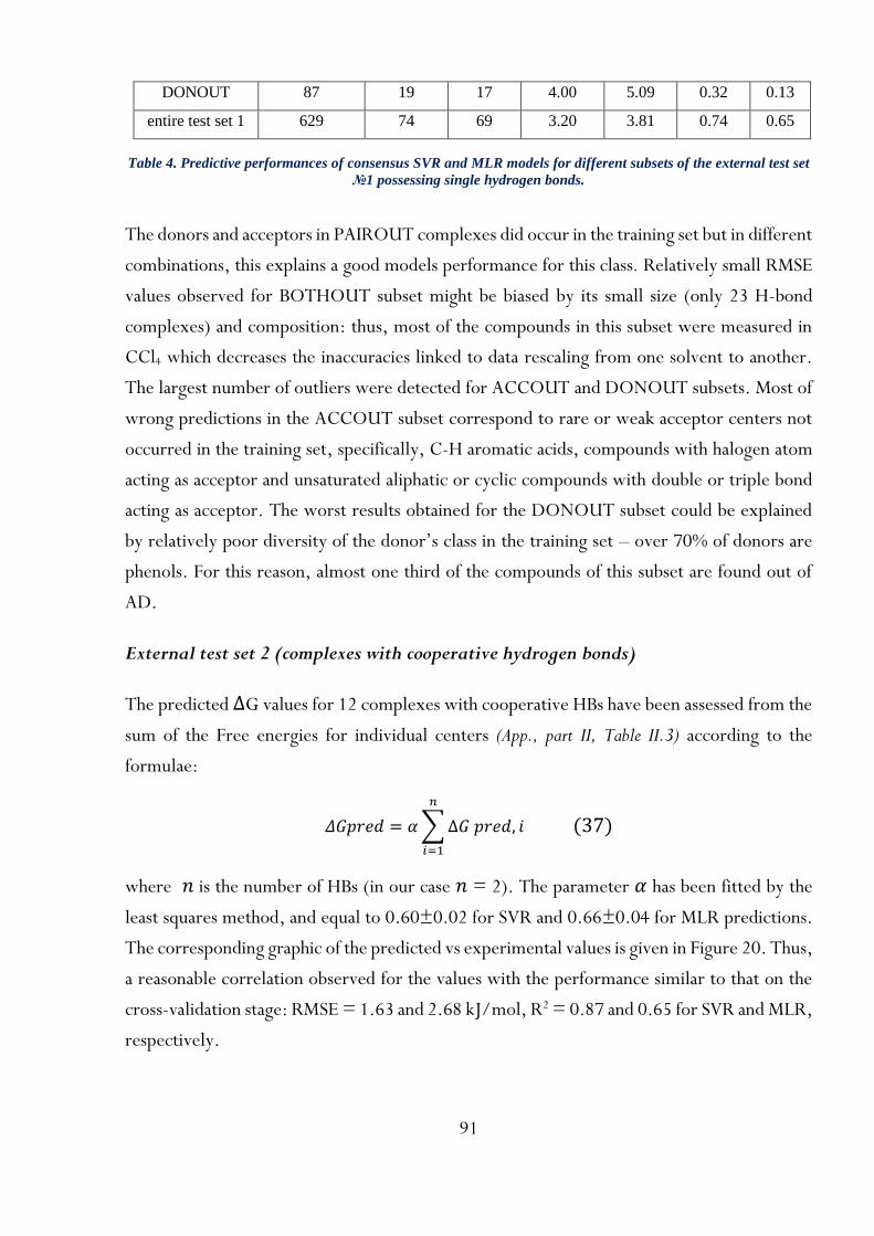
91
DONOUT 87 19 17 4.00 5.09 0.32 0.13
entire test set 1 629 74 69 3.20 3.81 0.74 0.65
Table 4. Predictive performances of consensus SVR and MLR models for different subsets of the external test set
№1 possessing single hydrogen bonds.
The donors and acceptors in PAIROUT complexes did occur in the training set but in different
combinations, this explains a good models performance for this class. Relatively small RMSE
values observed for BOTHOUT subset might be biased by its small size (only 23 H-bond
complexes) and composition: thus, most of the compounds in this subset were measured in
CCl4 which decreases the inaccuracies linked to data rescaling from one solvent to another.
The largest number of outliers were detected for ACCOUT and DONOUT subsets. Most of
wrong predictions in the ACCOUT subset correspond to rare or weak acceptor centers not
occurred in the training set, specifically, C-H aromatic acids, compounds with halogen atom
acting as acceptor and unsaturated aliphatic or cyclic compounds with double or triple bond
acting as acceptor. The worst results obtained for the DONOUT subset could be explained
by relatively poor diversity of the donor’s class in the training set – over 70% of donors are
phenols. For this reason, almost one third of the compounds of this subset are found out of
AD.
External test set 2 (complexes with cooperative hydrogen bonds)
The predicted ΔG values for 12 complexes with cooperative HBs have been assessed from the
sum of the Free energies for individual centers (App., part II, Table II.3) according to the
formulae:
𝛥𝐺𝑝𝑟𝑒𝑑 = 𝛼 ∑ ∆𝐺 𝑝𝑟𝑒𝑑, 𝑖
𝑛
𝑖=1
(37)
where 𝑛 is the number of HBs (in our case 𝑛 = 2). The parameter 𝛼 has been fitted by the
least squares method, and equal to 0.60±0.02 for SVR and 0.66±0.04 for MLR predictions.
The corresponding graphic of the predicted vs experimental values is given in Figure 20. Thus,
a reasonable correlation observed for the values with the performance similar to that on the
cross-validation stage: RMSE = 1.63 and 2.68 kJ/mol, R2 = 0.87 and 0.65 for SVR and MLR,
respectively.

92
5.6 Conclusion
By contrast to the previous project where one of the interacting entities remained constant,
this project is devoted to the modeling of the strength of intermolecular complexes formed
by varying donors and acceptors. The structures of the complexes have been represented by
the Marked Atom (MA)-based descriptors, where the corresponding atoms that have been
labeled are the donor and the acceptor of hydrogen. The strength of hydrogen bond
complexation was characterized by the experimental Free Energies (ΔG, kJ/mol) measured
at ‘standard’ conditions: CCl4, 298K. To our knowledge, the data set utilized (3373
complexes) is so far the largest used for hydrogen-bond complexation propensity prediction.
The cross-validation performances of the models are similar (R2 =0.87-0.94, RMSE=1.50-
2.22), however still, the MLR method noticeably concede in accuracy. That could be
explained, at first, by the lack of information-rich ‘colored’ descriptor spaces i.e. the ISIDA
descriptors enhanced with an additional chemical information (formal charge, force field
types, etc.) and, at second, by the important role of non-linearity in HB affinity modeling:
thus, out of 40 winning individual SVR models only two of them are based on linear kernel,
nevertheless bearing the lowest rank of the statistical score. Successfully cross-validated SVR
and MLR consensus models have been challenged for the prediction of two external test sets,
the first one of which consisted of complexes with single HBs, measured in either standard
Figure 20. Predicted (ΔGpred) vs
experimental (ΔGexp) free energies for
the 1:1 complexes with two cooperative
hydrogen bonds. Predicted values were
estimated by eq. 37..

93
CCl4, or in other solvent, whereas the second test set was constituted by 12 complexes with
cooperative HBs. Apart from the standard model’s performance evaluation encompassing all
the objects of the test set, a fractional model validation has been performed. The latter
considers the test set to be composed of four distinct classes differing by the proportion of
‘novelty’ of the included compounds. It has been shown that the external sets featuring known
partners in novel combinations are indeed easier to predict than sets containing either donors
or acceptors that were never seen at the training stage. Logically, the situation should be even
more tense for the challenge of predicting a set in which neither acceptors nor donors were
met at training stage - however, since that collection was rather small and biased, it was
predicted well. The solvent corrections performed with the obtained linear relationships and
involved in the assessment of ΔG values of the test set 1 are shown to be a useful tool for the
evaluation of ΔG for different solvents, not occurred in the training set. The overall
performance referred to the entire test set of single HBs is reasonable: R2 =0.65-0.74,
RMSE=3.20-3.81kJ/mol. At last, on the example of the test set of polyfunctional molecules
with multiple intermolecular interactions, it has been shown that the sum of HB affinities for
each individual interaction robustly correlates with the observed experimental value (R2
=0.65-0.87, RMSE=1.63-2.68 kJ/mol), which opens a perspective for the model to be
applicable for supramolecular crystal engineering and drug design.

94

95

96

97

98

99

100

101

102

103

104
Chapter 6
QSPR modeling and visualization of tautomeric
equilibria.
The complex phenomenon of tautomerism is still a challenge for chemoinformatics and
computational chemistry in terms of quantitative estimation, mode of transformation and
representation. Tautomerism is ubiquitous and plays a key role in practically important
processes including biochemical ones, such as the relation of tautomeric transformations to
spontaneous mutations as a consequence of mispairing by rare tautomeric forms of purines
and pyrimidines171-174 and its relation to enzyme-substrate interactions175-176. As for organic
chemistry, the prevailing conformation of a certain tautomeric form may affect the product
in a chemical reaction. The field of drug design likewise needs the determination of the
predominant ligand structure for virtual screening and modeling177-178. The number of works
devoted to the elucidation of the qualitative and quantitative aspects of tautomerism is still
being extended178-181. However, most of them are related to quantum chemistry. In spite of
the importance of this phenomenon, only two software tools dedicated to the assessment of
the tautomeric population are currently available: the Marvin Tautomerization Plugin182 and
TauThor/MOKA183. Both of those tools estimate the equilibrium constants in water at room
temperature using predicted pKa values for all individual tautomeric forms. In many
important cases, their predictive performance appears, however, to be too low, because of

105
accumulation of errors on the individually predicted pKa terms. Furthermore, the approach
does not consider varying reaction conditions. Here we propose to treat the problem of
tautomeric equilibria evaluation directly, based on the experimental KT values and Marked
Atom-based descriptors characterizing the structure of the molecules and the character of the
transformation. The data set included 10 different types of tautomeric transformations
measured in different solvents and temperatures. Presence of reaction conditions allows a full-
blown modeling of the combined structural and reaction condition impact on the equilibrium
constant as well as to seek for the specific patterns characterizing various types of
tautomerism.
This is the first time the Generative Topographic Mapping (described in section 3.2.3) is
challenged in modeling and visualization of combined structure/conditions chemical data. An
impact of the reaction conditions on the property could be examined by means of GTM maps
exploring different subsets of the initial data: involving or not involving the conditional part.
The initial data set comprised a few tautomeric transformations measured at different solvents
with significant difference in the equilibrium constant values. These species could be an
additional criterion for GTM models quality estimation: thus, their successful separation is an
evidence of the model being able to differentiate these objects in spite of the fact that their
structures are the same. As a measure of the quality of tautomeric classes separation we
applied a special characteristic, Г-score184, which can be computed from the GTM class maps
and hence does not need the property values be measured in the experiment. The SVR method
is used here for the benchmarking purposes.
The article related to this project is given in in the end of this section, with the authorization
of all authors.
6.1 Modeled object and property
The modeled item is a prototropic tautomeric transformation, for which the equilibrium
constant (log KT) referred to a certain solvent/mixture of solvents and temperature is given.
The transformations are assigned to 10 distinct tautomeric classes (Table 5) the active atoms
of which, i.e. accepting/donating the hydrogen atom, are attributed and marked. The Marked
Atom (MA)-based descriptors are used to compare their performance with the CGR-based
approach, that had been tried previously in our group185. The structural characterization of
the tautomeric transformation was undertaken by describing the "reference" tautomer of each

106
pair. This "reference" tautomer is chosen as the left side of equilibria listed in Table 5, and
then coherently applied throughout the work: the "keto" form will be reference for all keto-
enol processes. An example of active atoms labeling is given of Figure 21. That is done, at
first, in order to avoid repeating description of the same atoms of the second form so that to
reduce the overall number of descriptors and, at second, to reduce the number of classes for
the depiction and analysis for the case of GTM classification modeling. Thus, the labeling of
both active atoms and the preorganized assignation defined by Table 5 allows to fully describe
a given equilibrium. The descriptor vector has been composed of the fragments with the
labeled donor atom, the fragments with the labeled acceptor atom and the reactions condition
descriptors, that were concatenated into a unified descriptor vector representing a single
tautomeric transformation of a particular type, measured under a certain reaction condition.
Two types of modeling had been performed: the ‘structural’ and the ‘general’ ones. The
structural models were referred to the GTM classification task solely and were built on a
subset of structurally unique transformations, which were 350 out of 695 initial equilibria.
The experimental conditions were not included into the descriptor vector for the ‘structural’
modeling. The ‘general’ modeling has been performed on the initial data of 695. The
descriptor vector in this case included the structures and the conditions. The performance of
the GTM for the regression task has been compared with SVR.
Figure 21. Example of atom labeling to encode
a tautomeric process. The right-hand side
tautomer results from the motion of proton
from donor atom (red star) to acceptor atom
(green star) in the left-hand side tautomer.

107
6.2 Modeling workflow
6.3 Data preparation
The training set, composed of 695 tautomeric transformations, with the values of the
logarithm of the equilibrium constant (logKT) measured in different solvents and at different
temperatures, has been critically selected form the database prepared by Gimadiev et al185.
The selected dataset contains equilibria for which only two stable tautomeric forms may
potentially exist. All transformations are assigned to 10 types of tautomerism (Table 5). The
equilibrium constants for them were measures in 12 pure solvents (water, methanol, ethanol,
propanol, butanol, cyclohexane, benzene, chlorophorm, DMSO, acetone, DMFA, ethyl
ether) and 7 different types of water-organic solvent mixtures (water/ethanol,
water/propanol, water/butanol, water/acetone, water/DMFA, water/DMSO, water/ethyl
ether) with different proportions of components. The temperatures varied from 233K to
373K.
Type of tautomerism The number of transformations in the
DB
Keto-Enol (I) 271
Amino-Imino (II) 178
Figure 22. Workflow of the modeling of tautomeric equilibria constant (log KT).

108
Hydrazine-Hydrazone (III) 12
Pyridol-Pyridon (IV) 5
Phenol-Imine - Keto-Amine (V) 33
Thione-Enol – Keto-Thiol (VI) 10
Amine-Thione–Imine-Thiol (VII) 18
Nitro-Aci (VII) 8
Classical Form - Zwitterion (IX) 28
Chain-Ring (X) 132
Table 5. Composition of the DB. The types of tautomerism and the number of transformations in the DB for each
tautomeric type.
For some transformations not one, but several different KT values measured at the same
conditions were reported in the literature. In this case, logKT for a given equilibrium was
calculated as an average of the related experimental values. The structures were standardized
by the ChemAxon’s Standardizer utility152 (‘basic aromatization’ was used).
The subject of unbiased model validation has already been raised in the previous project,
where four different scenarios of ‘novelty’ of the complex with respect to the training set have
been introduced (see chapter 5). Regarding to tautomeric transformations, the
uncertain/biased statistics could arise for a data set comprising structurally identical equilibria
measured in different reaction conditions. In this case, external prediction of the equilibrium
constant distinguishes four scenarios: (1) tautomers present in the training set, to be predicted
under reaction conditions also seen at training stage (but not in conjunction with those specific
tautomers), (2) tautomers not in training set to be predicted under conditions already met
among training examples, (3) tautomers in training set to be predicted under novel conditions
and eventually, (4) novel tautomers under not yet encountered conditions. Only scenarios
(2) and (3) were envisaged here, since not enough external data to support the other two was
available. Thus, two test sets, collected from the same literature170, 185, have been used for
external validation. The first test set (test set 1) consists of 20 tautomeric transformations
(App., part III, Table III.1). which have been occurred in the training set, but under different
reaction conditions. Test set 2 consists of 26 unique transformations (App., part III, Table
III.2). without structural duplicates in the training set.

109
The same equilibria of the initial data set were frequently measured under different reaction
conditions, so the number of the unique transformations (i.e. without considering the same
structural changes in different solvents as different transformations) in the data base is 350.
These transformations have been extracted without the reaction condition part and gathered
into the subset of unique transformations, employed in GTM data analysis for the
evaluation of the reaction condition influence on data distribution of GTM maps, as well as
for the estimation of pure structural clustering as the criteria of appropriateness of a certain
descriptor type.
6.4 Computational details
The preliminary scanning of 64 different descriptor spaces has been performed by SVR, the
MA3 strategy has been used exclusively. The generated structural descriptors have been
concatenated with the 14 reaction condition parameters for solvent and temperature (described
in section 2.2) and molar fraction of organic component (for water/organic mixtures).
The descriptor set producing the SVR models with the highest R2 score has been chosen for
further evaluation of the remaining labeling strategies. The best descriptor set was based on
atom-centered fragments of the length 1-3 and has been used for GTM modeling and
visualization and for the external validation of the obtained individual SVR and GTM
regression models. The applicability domain method was Fragment Control.
Γ-score. The clustering performance of the GTM can be estimated by the Γ-score186 which is
normalized from 0 to 1 and can be calculated for any data set where the information about
classes is available. The Γ-function takes into account k nearest neighbors of each projection.
The more neighbors of each point belong to the same class the higher is the Γ-score. Thus,
this score characterizes the quality of class separation on the map. First, for each compound
𝒗𝒊, 𝑮(𝒍, 𝒌) should be computed:
𝐺(𝑙, 𝑘) = 1/𝑘 ∑ 𝑔(𝑣𝑖, 𝑗)
𝑘
𝑗=1
(38)
where k is the number of nearest neighbors, 𝑔(𝑣𝑖 , 𝑗) =1 if the jth nearest neighbor of 𝑣𝑖 belong
to the same class, otherwise 𝑔(𝑣𝑖 , 𝑗) = 0. Then, for each class i, 𝑦𝑖(𝑘) is defined as

110
𝑦𝑖(𝑘) = 1/𝑛𝑖 ∑ 𝐺(𝑙, 𝑘)
𝑛𝑖
𝑙=1
(39)
where 𝑛𝑖 is the number of compounds of the class i. And, finally the Γ-score is
Г(𝑘) = 1/𝑁 ∑ 𝑦𝑖(𝑘)
𝑁
𝑖=1
(40)
where N is the number of classes. The k number is set to 7.
The details of the computational procedure concerning the specification of the scanned
descriptor spaces, the corresponding SVR and GTM parameters of the individual models, as
well as the details of data curation and treatment are described in the corresponding sections
of the article.
6.5 Results and discussions
6.5.1 Data visualization and analysis with GTM
Unique structure subset
The unique data set helps to estimate the influence of the reaction conditions and
demonstrates the ability of the GTM method to classify different tautomeric types with and
without specification of reaction conditions. The task of predicting the type of tautomeric
transformation itself does not have any intrinsic value, because the type of tautomeric
transformation can be easily extracted from the transformation equation with a well-known
atom-atom mapping without the need to build any models using machine learning methods.
Nevertheless, the ability of a given descriptor set to discriminate effectively different types of
chemical objects indicates its quality and the ability to be used in building and analysis of
different models. The performance of different marked atom strategies has been analyzed with
respect to the same descriptor set (the one used herein and after is based on atom-centered
fragments, see 6.4).
Figure 23 depicts the GTM classification landscapes for four marked atom strategies for the
unique structures subset. Different colors in each landscape correspond to 10 types of
tautomerism (Table 5). The corresponding Balanced Accuracy is close to 1 for all tautomeric

111
classes, which correspond to their good separation on the map (App., part III, Table III.3).
However, a visual comparison of the landscapes reveals that the labeling strategies MA1 and
MA2 separate different classes equally well and better than MA0 and MA3. Thus, the keto-
enol and amino-imino classes of tautomeric transformations are well separated from each
other and from the other tautomeric types for strategies MA1 and MA2, but not for MA0 and
MA3 (Table 6). The corresponding Г-scores for MA1 and MA2 are also higher (Table 6)
resulting in maps with more distinct separation of classes compared to MA0 and MA3 maps,
where there are more areas of adjoining occupation for different classes.
Marked atom strategy Number of descriptors Г-score
MA0 431 0.55
MA1 204 0.74
MA2 232 0.73
MA3 662 0.52
Table 6. The separation quality of the classification GTM landscapes of the unique structures subset expressed by
Г-score.
The entire data set
The entire data set, in which different conditions for the same unique transformation are
included in the description, has been visualized and analyzed in the same way as for the unique
structure subset above. The corresponding GTM property landscapes, characterizing the
Figure 23. GTM classification landscapes for four marked atom strategies for the unique structures subset of 350
equilibria.

112
distribution of log KT, and the GTM maps colored by classes (class landscapes) for four marked
atom strategies are represented in Figure 24.
In comparison with the maps for the subsets of unique structures presented in Figure 23, the
maps obtained for the entire data set contain substantially more points, since the individual
points on them correspond to different combinations of structural changes with reaction
conditions, i.e. different solvents and temperature. The Balanced Accuracy for all tautomeric
classes are close to 1 (App., part III, Table III.4), in correspondence with its good separation
on the maps, especially for the MA1 and MA2 strategies, the Г-scores of which are higher as
well. These results can be explained by the fact that the MA1 and MA2 fragments are more
specific for a given type of transformations and therefore different types of equilibria form
better separated clusters. The comparison with the unique subset maps shows that the
Figure 24. GTM property (top) landscapes, representing the distribution of the logKT values, and the GTM
classification (bottom) landscapes, representing the separation of 10 different tautomeric classes, built for the
entire data set of 697 equilibria. The descriptors spaces for four marked atom strategies are based on atom-
centered fragments of the length 1-3.
logKT

113
inclusion of the reaction conditions leads to better delimitation of the tautomeric classes: thus,
the entire set maps possess less areas occupying by several classes where they are closely
located. This could be derived from different solvent affinity and solubility for different
chemical transformation, varying structurally within the same tautomeric group, but much
more on going from one tautomeric class to another. The GTM method thus clusters data on
account of both structures of transformations and the reaction conditions.
6.5.2 Cross-validation of the SVR and GTM models
The performances of the regression SVR and GTM models built on the entire data set for four
marked atom strategies are shown in Table 7. According to the results, the MA2 and MA1
strategies lead to the higher predictive performance of GTM models, so as in the case of the
SVR models. It could be suggested, that the MA0 strategy is worse because of lack of local
descriptors, explicitly accentuating the active atoms and hence bearing the information about
the tautomeric type. The weaker performance of MA3 compare to MA1 and MA2 could be
due to large number of global descriptors, occulting the influence of both important local
descriptors and descriptors of reaction conditions. Notice also that for the GTM models the
difference in performances between different strategies is considerably more pronounced than
for the SVR models. That could also be due to the fact that the SVR method is known to
perform implicit weighting of descriptors, so unimportant global descriptors get low weights,
and their adverse effect is minimized. One can also pay attention to the fact that the MA2
strategy very slightly but consistently outperforms MA1 in both GTM and SVR modeling. A
putative explanation for this is that the MA2 strategy provides a more detailed description of
the environment of the active center due to additional descriptors that are important for
modeling of tautomeric transformations.
Table 7. The comparison of the performance of SVR and GTM methods for four marked atom strategies. The
individual model based on ISIDA atom-centered fragments (length 1-3).
Marked
atom
strategy
Number of
descriptors
GTM SVR
Г-score R2 RMSE R2 RMSE
MA0 445 0.68 0.72 0.82 0.77 0.76
MA1 218 0.76 0.83 0.64 0.81 0.68
MA2 246 0.75 0.84 0.63 0.82 0.67
MA3 676 0.69 0.78 0.73 0.80 0.71

114
Comparison of R2 and RMSE values, which characterize the predictive performance of the
models, and the Г-scores, which characterize the quality of class (tautomeric type) separation
on GTM maps, reveals a consistent correspondence between them: labeling strategies with
higher Г-score lead to regression models with higher predictive power. A putative explanation
for this is that the map with higher Г-score is characterized by more uniform distribution of
data points, which leads to smoother property landscapes with higher predictive power. This
opens up interesting prospects for using GTM maps for improving the regression models,
because the construction of GTM maps and the maximization of the Г-score for them does
not require the knowledge of property values measured in experiment and therefore can be
performed for virtual datasets of any size.
6.5.3 GTM solvent separation analysis
The way in which reaction conditions are shaping the logKT property landscapes can be
observed by looking at tautomeric equilibria that were studied in different solvents. One can
expect that if combinations of the same tautomeric transformation with different solvents are
mapped to nearly the same location in the latent space (2D GTM map), while the difference
between the values of equilibrium constants for them is significant, then this produces an
“activity cliff” which hampers the predictive performance of a models. Otherwise, if they are
mapped onto a broad region in the latent space, then the property landscape is smoother,
which is favorable for the high predictive performance of the models. To examine this issue,
of species on the map, a subset of tautomeric transformations that have a considerable
difference (more than 1 in log scale) between the log KT values measured in different solvents
have been retrieved. The results are presented in Figure 25 and Table 8. The color of the node
corresponds to the property value (log KT) based on the responsibility contribution of each
molecule into the node. According to the obtained picture, the data points are well
distinguished on all four GTM maps. The GTM model thus correctly recognizes the
dependency of the property from both chemical structure and the solvent nature.

115
Table 8. Example of tautomeric transformations with considerable log KT difference for different solvents.
6.5.4 External validation of the SVR and GTM models
To estimate the predictive performance of GTM and SVR models on external test sets, we
have chosen the models based on MA2 descriptor set as the one providing the best results.
The results of the prediction for the first external set (test set 1), assessing the models
performance as a function of experimental conditions, and the second test set (test set №2)
assessing the predictive performance for new chemical entities, are given in Figure 26. For
both sets the predictive quality of the GTM is better than the one obtained with the SVR
model. For the set 2 comprising new structures, thirteen out of 26 transformations were
Solvent logK Tautomeric transformation
1a DMSO (307K) 0.62
1b Chloroform (307 K) -0.49
2a Dioxane (293 K) -1.52
2b Ethanol (293 K) 0.10
logKT
Figure 25. The solvent separation of structurally same pairs of tautomeric equilibria (Table 8) with considerable
difference in logKT values due to measurements in different solvents.

116
found to be out of the model’s applicability domain. Statistical parameters calculated for the
remaining equilibria within AD show an equivalent performance of both methods (R2 = 0.83
and 0.82; RMSE= 1.0 and 1.2 log units for GTM and SVR, respectively).
6.6 Conclusion
This project is devoted to the modeling of tautomeric equilibria accounting for different
experimental conditions. At this level, the constituents that need to be considered are the
structures of chemical participants, the active centers responsible for chemical transformation
and the conditions, under which the latter is conducted. The structures have been encoded
with Marked Atom (MA)-based fragment descriptors, where the labels were assigned to
atoms donating or accepting hydrogen while the conversion.
Four marked atom strategies have been tried and compared in the frame of the same descriptor
type. It was revealed, that the use of labeled (local) fragment descriptors (strategies MA1 and
MA2) leads to models with better predictive performance for both, SVR and GTM machine
learning methods, rather than the use of unlabeled (global) fragment descriptors (strategy
MA0). Moreover, mixing unlabeled and labeled fragment descriptors (strategy MA3) results
in a deterioration of the predictive performance in comparison with the use of only the labeled
ones (MA1 and MA2). This can be explained by the important role of local structural factors
and inessential role of global ones for predicting the constant of tautomeric equilibrium.
Figure 26. Predictive performance of the models on the external sets of new conditions (test set 1) and new
structural transformations (test set 2).
117
The GTM method for the first time has been applied for modeling and visualization of data,
which is more complex than the subsets of single molecules ordinarily used for GTM before.
The visual GTM analysis, performed using class and property landscapes, has shown that the
ability of a descriptor set to provide good separation between different classes of tautomeric
transformations correlates with the overall model’s predictive performance. For both
methods, the best performance has been obtained with MA1 and MA2 strategies, that provides
an optimal structural description at the same time not producing a redundant amount of
descriptors, that could occult the influence of important local or condition descriptors. The
difference in performances for different strategies is less pronounced for SVR models due to
the internal mechanism of assigning lower weights to unimportant descriptors in the SVR
algorithm.
To quantify the quality of class separation, we applied a special characteristic, Г-score, which
can be computed from GTM class landscapes. It was shown, that the descriptor sets providing
higher Г-score values in GTM classification landscapes lead to regression models with higher
predictive power. This opens up interesting prospects for using GTM maps for improving the
predictive models for chemical reactions, since building GTMs having the maximization of Г-
score as objective function is a simulation which only requires the knowledge of the reaction
types and not of their explicit kinetic or thermodynamic parameters.
The predictive performance of the GTM and SVR models have been compared using two
external test sets, providing an unbiased assessment of model’s ability in predicting different
structures or different reaction condition. The GTM models have shown better predictions
(R2 = 0.62-0.65, RMSE = 0.6-1.96) in comparison with the SVR models (R2 = 0.39-0.53,
RMSE = 0.76-2.2). The GTM approach therefore can be recommended for building other
QSPR models, as it combines good predictive performance with the ability to conduct in-
depth visual analysis of data constituent and of the influence of various factors on quantitative
characteristics of chemical processes.
The SVR individual model that includes the assessment of the applicability domain and an
automatic labeling of the active atoms, is freely available on our web-server
(http://cimm.kpfu.ru/models).

118

119

120

121

122

123

124

125

126

127

128

129

130
Chapter 7
QSPR modeling and visualization of kinetics
properties of cycloaddition reactions.
Cycloaddition (CA) is a classic reaction in organic chemistry being of a fundamental
importance for organic synthesis as the main tool for the production of the compounds of
cyclic architecture. A large variety of cycloaddition reactions arises from the diversity of
reagents, allows to design cyclic adducts of different size, nature and functions. A high regio-
and stereo-selectivity of cycloaddition explains its wide application at different stages of
complex organic synthesis.
In early works, frontier molecular orbitals (FMO) 187-191 calculated by quantum mechanics
methods for small congeneric series were widely used for interpretation of thermodynamic
and kinetic properties of cycloaddition. Most of modeling studies of the kinetics were
conducted using a time-consuming quantum-chemical calculation. An effort has been made
to build a linear correlation with experimentally measured physicochemical parameters of the
reagents192-193. This, however, significantly limits application of the latter to already studied
molecules.

131
Earlier QSPR modeling of chemical reactions were performed on homogeneous series either
keeping the solvent, or the structure of the reactants constant194-197. In these studies
topological indexes198, quantum-chemical194-195, 199 200 or mixed201-203 descriptors for reagents
were used. These works however were restricted to water or gas media exclusively. Such
models show high correlation coefficients, but cannot be thought of as universal. For a non-
exhaustive overview of the studies carried out in the field of chemical reactivity one can refer
to work of A.Warr204, I.Baskin et al.,205 or earlier works196-197, 206.
In spite of significant progress in the field, few attempts have yet been made towards more
extensive consideration of chemical reaction: the first one refer to the classification problem
in terms of categorical prediction of the conditions (solvent type, catalyst) of the Michael
addition207. The multicomponent approach of quantitative estimation of the kinetics of
chemical reactions explicitly considering both reactants and solvents have been applied to the
modeling of the rate constant of SN2126, 208 and E2209-210 reactions leading to a fairly good
correlations with the experimental values (R2=0.67-0.79).
This chapter is devoted to the modeling of kinetic properties of the reactions of cycloadditions
comprising (4+2), (3+2) and (2+2) types. The considered properties included the rate
constant (logk), the activation energy (Ea) and the pre-exponential factor (logA). Two
machine learning methods, SVR and GTM have been involved, where for the latter a unified
model, eligible for the prediction, visualization and analysis of all three properties, has been
constructed.
Chemical structures of reactants and products were encoded by a single Condensed Graph of
Reaction (CGR) representing a given reaction as a single pseudomolecule (described in detail in
section 2.1.4). The CGR-based descriptors explicitly characterize the reaction center together
with its immediate structural neighborhood. The CGR-based descriptors and the reaction
conditions descriptors have been concatenated resulting in descriptors vector describing the
entire transformation.
The prepared models have been exhaustively validated on the external test set comprising
reactions both structurally different from those in the training set and the same
transformations measured under different reaction conditions. Different scenarios of logk
assessment were exploited: direct modeling, application of the Arrhenuis equation and
temperature-scaled GTM landscapes.

132
7.1 Computational procedure
The modeling workflow is shown in Figure 27. The database of 1849 reactions of
cycloadditions, for which the logk, Ea and logA values have been measured in different
solvents and at different temperatures, has been collected from the literature (see 7.1.1). The
data set has been divided into the training and test set, where the latter has been composed
out of 200 reactions picked up randomly from the data set. The remaining 1649 reactions
constituting the training set has been used to build three individual models, correspondingly,
for logk, Ea and logA prediction. The obtained best SVR and GTM models have been further
challenged for an exhaustive external prediction of logk on the prepared test set of 200
reactions.
7.1.1 Data preparation
An initial data set of 2551 reactions of cycloaddition for which all of the reactions contained
the experimental measurements of the rate constant (logk), 1356 reactions had activation
energies (Ea, in kJ/mol) and 1237 had pre-exponential factor (logA) values was collected
manually from the manuscripts of PhD thesis works of Prof. Konovalov’s group from Kazan
Federal University published in 1970-1990. The data set contained about 85% of Diels-Alder
Figure 27. Workflow for the modeling of the rate constant (log k), activation energy (Ea)
and pre-exponential coefficient (log A) of the reactions of cycloaddition.
133
(4+2) cycloaddition, about 8% (3+2) dipolar cyclisation, and 7% (2+2) cycloadditions. The
measurements were carried out in C6H5CH3, CH3COOC2H5, C6H5OCH3, C6H5NO2,
CH3CN, C2H5OH, C6H5Cl, THF, CH2Cl2, DMSO, CHCl3, C2H4OC2H4O, C5H11OH,
C6H5Br, C6H6, CH3COCH3, C6H12 and CH2ClCH2Cl solvents at temperatures varying from
273 to 423 K. The most frequently occurred dienes for the Diels-Alder series are: condensed
aromatic cycles, cyclopentadienones, cyclopentadienes and benzofuranes. Among
dienophiles, the prevailing structures are: maleic acid derivatives, cyanoethylenes, Ph-
substituted ethylenes and benzoquinones. The data set (reagents and products) underwent an
accustomed standardization protocol using ChemAxon’s Standardizer Utility: basic
aromatization, isotopes removal, NO2-, NO-, N3-, RRSO2-, CN- group transformation152
While cyclization due to the reaction mechanism different stereoisomers can be formed. An
analysis of the rate constants of reactions forming two different stereoisomers have shown that
logk difference was from 0.01 to 1.0 log values. Based on our previous work209 we considered
that the difference is too small to be taken into account and comparable with the
interlaboratory errors. Thus, for the reactions able to form different stereoisomers during
cyclisation, the logk constants were calculated as a mean of given experimental values. No
other duplicates were found in the dataset. The 1849 reactions remaining after cleaning have
been characterized by 1849 values of logk, 1356 values of Ea (kJ/mol) and 1237 values of
logA, where among the latter there were no reactions without Ea. The prepared data has been
divided into the training and test sets.
External test set. The test set consisted of 200 reactions randomly picked from the initial
data set. For the reactions possessing logA and Ea values and comprised into the test set, the
corresponding values were not taken into consideration. In such a way, the test set is
considered to be attributed with 200 experimentally measured logk values solely. Out of 200
reactions in the test set, there were 57 structurally new transformations, that did not occur
in the training set. Individual statistics for them is discussed (see 7.2.3). For the most, the
transformations in the test set were measured once, at one temperature. However, there have
been 26 reactions with experimental measurements at two different temperatures.

134
The training set hence encompasses the remain 1649 reactions. The histograms of the
distribution for the three properties for the training set is given on Figure 28.
7.1.2 Descriptors
The ISIDA fragment descriptors have been calculated by the in-house ISIDA Fragmentor
software1, for which the corresponding CGRs were created from the reaction RDF files using
the in-house CGR Designer tool and were stored in modified SDF format. The length of
fragments varied for 2 to 14 for sequences and from 2 to 6 for atom-centered fragments. The
following options were also used at choice: charges on atoms (Formal Charge), accounting
for the terminal atoms of a fragment exclusively (Atom Pairs), and exploring all possible paths
instead of shortest paths (DoAllWays). An important option regulating the amount of the
overall generated CGR fragments is the ‘dynamic bond’. Toggled on, the option produces the
fragments, that contains the bonds forming/breaking while chemical reaction and omits the
‘generic’ fragments, not assigned to the reaction center (see section 2.1.4). That could be used
to generate fragments that describe local environment of the reaction center exclusively. For
this project, the CGR fragmentation implied the generation of all possible, local and nonlocal,
fragments. Overall, 728 descriptor sets have been generated for the preliminary SVR
scanning. Structural descriptors have been concatenated with the 14 descriptors of the
reaction conditions characterizing solvent and temperature (described in section 2.2).
Figure 28. Distribution of rate constant, activation energy and pre-exponential factor values in the training set of
1649 cycloaddition reactions.

135
7.1.3 Building and validation of the models
SVR modeling
SVR models were built and validated using the SVR algorithm implemented in the libSVR
package211. The modeling was performed using the evolutionary SVR optimizer,212 which can
be used to perform both descriptor space selection and optimization of the operational
parameters (epsilon, kernel type, cost, gamma) of the SVR method. The procedure, run for
the training set with logk as a modeled property, generated a total of 6000 models. The
descriptor set producing SVR individual model of maximal robustness (estimated by the R2
value) was based on atom-centered fragments of the length 2-3. This descriptor space
encompassing 688 descriptors (674 of fragments, 14 of the reaction conditions) was used
further for SVR and GTM models building and their external validation.
GTM modeling
The GTM models were built using the evolutionary optimizer212 which supports the choice of
the operational GTM parameters (the number of RBF kernels, the number of grid points, the
width factor of radial basis functions, and the regularization coefficient). The descriptor space,
based on atom-centered fragments of the length 2-3, chosen by the preliminary SVR scanning
was considered. The genetic optimization procedure included 3000 generations. The
operational parameters of the GTM method were optimized to predict all three properties,
logk, Ea and logA with the highest average R2 value. The prepared GTM manifold has been
used for the visualization of property distribution (property landscapes) and for analysis of
separation of three different cycloaddition types on the map (class landscape). The description
and the technique of ‘coloring’ of a GTM manifold with regard to class/property is given in
section 3.2.3.
Validation of the models
The performance of the models has been compared by R2 and RMSE values in 5-fold cross-
validation procedure repeated 10 times after data reshuffling.
7.1.4 Different scenarios of logk assessment for the test set reactions
The logk values for the external set of 200 reactions were obtained using three different
approaches: direct assessment, Arrhenius-based assessment and temperature-scaled GTM

136
landscapes. The direct assessment envisages the application of SVR or GTM logk predictive
models to the test set reactions.
In the Arrhenius-based assessment the logk values are calculated using the Arrhenius equation (eq.
41). The latter implies the usage of predicted Ea and logA values obtained with the help of the
related SVR or GTM models.
ln 𝑘 = ln 𝐴 − 𝐸𝑎𝑅𝑇⁄ (41)
Rate constant is more sensitive to temperature compared to any other individual structural or
solvent descriptors. This effect could hardly be accounted for by GTM-based model where
each descriptor has exactly the same weight. Therefore, the temperature-scaled approach has
been proposed for this purpose. It implies the construction of series of logk GTM landscapes
each corresponding to a specific temperature range.
Scaling of logk measured at temperature T1 to temperature T2 can be performed according
to Van’t Hoff equation: 𝑙𝑜𝑔𝑘2
𝑘1=
𝑇2−𝑇1
10log 𝑦. The temperature coefficient log 𝑦 was
computed as an average of log 𝑦𝑖 (i = 1 – n) values calculated for n series of reactions, each
studied at several temperatures. Overall, the reaction rates of 358 reactions in the training set
ware measured at 2 - 6 different temperatures. The smallest temperature difference in a series
was 10K and the largest was 110K. The temperature coefficient log 𝑦 varied from 0.08 to
0.59; its average value was 0.26.
The entire temperature range (273K-423K) has been divided into 15 subranges of 10K each,
e.g. from 273K to 283K. For each subrange, the corresponding logk landscape was
constructed, i.e., each logk was recalculated to median temperature of a subrange (e.g., 278K
for the range 273K-283K) using Van’t Hoff equation. It should be noted, that the error related
to temperature deviation of 5K (0.15-0.3 logk unit) is far less than the related RMSE values
(Table 10). Each of 15 temperature-scaled logk landscapes were calculated from experimental
logk values of the training set using the Van’t Hoff relationship, log 𝑦 = 0.26 and related
median subrange temperature. At the validation stage, the program selects particular logk
landscape that will be used for prediction, corresponding to the external reaction
temperature.

137
7.2 Results and discussions
7.2.1 GTM visualization of the training set
Generative Topographic Map shown on Figure 29 shows well separated zones populated by
the (4+2), (3+2) and (2+2) cycloaddition reactions. The ratio of sizes of these zones
correspond to classes occurrences in the training set: thus, the major class (4+2) occupies the
largest area, the following after is the (3+2) zone, which in turn is slightly bigger than the
zone populated by (2+2) reactions. A distinct separation of cycloaddition classes on the map
infers a competency of the chosen descriptors space, able to correctly discriminate reactions
belonging to different types.
Another technique of GTM visualization is the property landscapes, characterizing the training
set distribution of a certain property. Figure 30 shows GTM property landscapes for logk, Ea
and logA, where the gradient from blue to red corresponds to the property value variating
from low to high (in the range its own for each property). Simultaneous analysis of all three
landscapes helps to understand decomposition of logk on Arrhenius equation parameters logA
and Ea (eq. 41). According to collision theory, A is the frequency of collisions in the “correct
orientation”. Thus, logA values might be related to steric interaction of reactants in a pre-
reaction complex. Activation barrier Ea accounts for electronic and steric effects in the
transition state.
Figure 29. GTM class landscape
displaying separation of three different
types of cycloaddition in the training set
of 1649 reactions.

138
Table 9. Examples of reactions projected into the zones corresponding to Figure 29.
Typically, high reaction rates correspond to large logA and small Ea (zone A on the maps)
whereas low logk values result from a combination of small logA and large Ea (zone B).
However, in some cases low activation barriers doesn’t compensate too low logA (zone C),
or, on the contrary, large logA is associated with high activation barriers (zone D).
Zones Example of reaction logk
A 2.1 (toluene,
320 K)
B -4.7 (benzene,
403 K
C -4.2
(dichloroethane,
313 K)
D -3.55 (benzene,
403 K)
Figure 30. GTM property landscapes for the rate constant (logk), activation energy (Ea) and the pre-exponential
coefficient (log A) for the training set of 1649 reactions of cycloaddition. The encircled areas correspond to
different combinations of logA and Ea contributions into logk.

139
7.2.2 Cross validation of the SVR and GTM models
The cross-validation result (5CV) for all three properties, logk, Ea (kJ/mol) and logA, for
SVR and GTM models are shown in Table 10. The SVR modeling involved the construction
of three different models for each property, whereas for the GTM model predictions were
assessed with three property landscapes built on one same manifold (see section 7.1.3). The
performances of SVR models exceed those of GTM model. However, the overall statistics for
GTM looks reasonable for all three properties.
Property SVR GTM
R2 RMSE R2 RMSE
log k 0.94 0.45 0.78 0.86
Ea 0.92 3.65 0.80 5.92
log A 0.89 0.36 0.62 0.67
Table 10. Predictive performance of the SVR models, built separately for each of the property, and a single GTM
model, universal for all three properties, in 5-fold cross validation for the training set of 1649 reactions of
cycloaddition. The descriptor space is based on atom-centered fragments of the length 2-3.
7.2.3 External validation of the SVR and GTM models
The external test set has been predicted in three different ways (see 7.1.3), two common for
both, SVR and GTM are (i) the direct logk prediction and (ii) the prediction of the logk using
the Arrhenius equation (eq. 41) and the predicted values of Ea and logA. The results for both
strategies are given in Table 11 and Figure 31. The weaker results for the Arrhenius-derived
logk prediction could be explained, first, by the accumulation of errors and, second, by the
narrower Applicability Domain (AD). The accumulation error comes from the prediction of
a property by means of the accessory predicted values. The many are the latter, that bigger is
the chance of misprediction, affecting the overall accuracy. The second reason is related to
the fact, that the amount of experimental data for Ea and logA is smaller by one third than for
logk, meaning less accurate training and a narrower AD. The corresponding statistics
accounting for AD (Fragment Control) for the Arrhenius-based prediction is much better,
where the number of the compounds is however shrinked from 200 to 164.
Method of logk
assessment
SVR GTM
R2 RMSE R2 RMSE
Direct 0.92 0.50 0.74 0.90
Direct (AD) 0.96 0.35 0.84 0.74

140
Arrhenius-based 0.72 0.93 0.51 1.23
Arrhenius-based
(AD)
0.93 0.51 0.83 0.79
Temperature-
scaled GTM
- - 0.76 0.88
Table 11. Validation of four different methods of logk assessment on the test set of 200 cycloaddition reactions.
Notice that only 164 reactions are retained by the Fragment Control applicability domain.
Temperature-scaled logk GTM landscape. Reaction rate assessment with temperature-scaled logk
landscapes shows a minor predominance over the direct GTM logk prediction (Table 11).
This trend was confirmed in logk predictions for a set of 13 reactions, each measured at two
different temperatures (Figure 32). The temperature-scaled approach is less prone to return
the same rate constant values at different temperatures, showing an overall better
reproduction of temperature dependence.
Figure 31. Predicted vs experimental log k values obtained with the direct log k prediction (left) or with the
Arrhenius-based recalculation (right) for the external test set of 200 reactions of cycloaddition. The statistics
is given in Table 11.
Arrhenius-based
logk assessment
Direct logk
assessment
Figure 32. The comparison of the predictive accuracy for the direct GTM log k calculation and the
temperature-scaled GTM landscape, for the subset of 26 reactions of cycloaddition measured at different
temperatures.
GTM-based temperature-scaled approach
GTM-based direct logk prediction
R2=0.90 RMSE=0.48
R2=0.94 RMSE=0.39

141
Subset of unique structural transformations.
Since the external test set has been randomly chosen from the initial data set, it includes
reactions already occurred in the training set but proceeding under different reaction
conditions. That may lead to an overestimation of model’s predictive performance, due to
occurrence of same reactions in both training and test sets. Thus, individual statistics for the
structures, never encountered in the training set provides an unbiased assessment of the
model’s predictive ability with regard to new structures. Among 200 external set’s reactions,
only 57 transformations didn’t occur in the training set. Table 11 shows that only direct logk
assessment with SVM model leads to reasonable correlation between predicted and
experimental values: R2 = 0.72 which is close to the determination coefficient on the
validation stage for the entire test set. On the other hand, application of the Arrhenius-based
SVR assessment as well as GTM-based models result in relatively poor predictions R2 < 0.5.
Log k predictive
method
SVR GTM
R2 RMSE R2 RMSE
Direct 0.72 0.80 0.38 1.21
Arrhenius-based 0.33 1.26 -0.48 1.87
Temperature-
corrected GTM
- - 0.40 1.15
Table 12. The comparison of the direct , Arrhenius-based and temperature-scaled logk assessment for the subset
of 57 unique structural transformations.
Figure 33. Performances of SVR and GTM models
for the subset of unique structural transformations
(57 reactions) obtained with the direct log k
prediction method. The statistics is given in Table 12.
Direct log k assessment

142
7.3 Conclusion
This project is devoted to the modeling of reactions of cycloaddition, with structurally varying
reagents, measured at different reaction conditions. Involvement of multiple atoms and bonds
during the chemical transformation needs an efficient way of structural description. Here the
structures have been encoded with the Condensed Graph of Reaction (CGR), that explicitly
designates the bonds forming/breaking while the reaction transformation. The data set of
1849 reactions, comprised of (4+2), (3+2) and (2+2) types of cycloaddition, has been
attributed with three experimentally measured properties: rate constants (logk), activation
energies (Ea, kJ/mol) pre-exponential coefficients (logA).
Demonstrated a strong ability in the managing of structural/condition chemical data in the
previous project of tautomeric equilibria modeling, the GTM method is challenged here in
prediction of several kinetic properties with one single GTM model. The SVR models have
been built individually for each property. The cross-validation R2 range for the GTM model
is 0.62-0.80 and for the SVR models is 0.89-0.94.
The external validation has been performed on a set of 200 molecules, randomly picked from
the initial dataset. Two common ways of logk estimation have been fulfilled: the direct
prediction with the corresponding logk models, and the Arrhenius-based recalculation
through the predicted Ea and logA values. For both methods, the direct prediction is more
accurate than the Arrhenius-based assessment (RMSEdirect = 0.5 (SVR) and 0.9 (GTM);
RMSEArrhenius = 0.93 (SVR) and 1.23 (GTM)), which is mostly related to the fact that the
amount of data for logA and Ea is much less, than for the logk training set, meaning narrower
AD. Thus, Fragment Control AD significantly improved the performance of both SVR and
GTM models.
The overall results of SVR method, having the mechanism of implicit ranging of descriptors
according to their impact, are better, than for a single unified GTM model, where all the
descriptors are taken into relatively equal account. To enhance the predictive ability of GTM
with respect to temperature, the temperature-scaled landscapes have been constructed. The
performance of the approach was the same as for the direct logk GTM assessment, with a
slight improvement in temperature dependency reproduction with regard to 13 reactions
measured at two different temperatures (RMSEdirect = 0.48, RMSEtemperature-scaled = 0.39).

143
Using a single GTM map provides another advantage: thus, since the distribution of the
reactions are the same for each property, it is possible to analyze the dependencies of the
properties and the structural features they could be determined by. Thus, simultaneous
analysis of property landscapes for logk, logA and Ea helped to identify different types of
reactions with respect to the interplay between the Arrhenius parameters logA and Ea. With
respect to class separation, the three classes, (4+2), (3+2) and (2+2) are well-separated on
the map, occupying the areas proportional to their share in the training set.
The SVR individual models for the rate constant, activation energy and pre-exponential
coefficient, supporting the choice of solvent and temperature, are freely available on our web-
server: http://cimm.kpfu.ru/models.

144
Chapter 8
QSPR modeling of the rate constant of SN1
reactions.
In this chapter we report predictive models for the rate constant of SN1 reactions involving
both Marked Atom-based and the Condensed Graph of Reaction-based approaches.
Unimolecular nucleophilic substitution (SN1) is a reaction with a two-stage mechanism, in
which the heterolytic bond cleavage of a neutral molecule precedes the reaction with the
nucleophile (Figure 37). Since the rate-determining step of a bond cleavage involves only a
substrate, SN1 is the first-order reaction.
The factors affecting the rate constant of SN1 reactions were investigated in numerous
quantum mechanical calculations of different levels (HF, MP2, G2)211-215. These works are
useful in investigation of various factors, such as electronic effects of substituent or size of the
molecule, influencing the rate constant. The molecular dynamics allows to go further and
investigate the reaction process altogether with solvent effects: these works216-217 help to
evaluate the effects of the solvation energy (water only) to the feasibility of the reaction
process. Some of the experimental studies were devoted to the substituent effects192 or certain
steric influence218 (ortho-effect). However, all these studies were performed on small series
of reactions and did not account for solvent effects, or only water medium was considered.

145
In order to generalize the substituent effects on the rate constant, several scales have been
proposed. Thus, the α constants introduced by Uggerud219 has been designed to rationalize
the substituent effects of the alkyl groups. A comprehensive nucleofugality scale has been
proposed by Mayr220-221 and Denegri213, 222. Later on, the applicability of this scale was
expanded for the prognosis of the preferable, SN1 or Sn2, mechanism223. It should be noted,
however, that the borderline between SN1 and SN2 mechanisms is the subject of considerable
controversy. Thus, opposed to Ingold224, considering the two mechanism to be distinct,
discrete processes it has been ascertained that the clear-cut distinction for many cases could
not be established due to gradual transformation of one mechanism into the other. The
borderline cases of the concurrent SN1 - SN2 reactions have been pointed out for benzylation
of pyridines214, benzophenones and benzhydrols223, arylbromoethanes225, tosylates226-227 and
4-methoxybenzyl derivatives228. To interpret these interjacent cases, Winstein’s and Sneen
developed a concept of different types of ion pairs intermediates229-232. Schleyer and Bentley
criticized this concept and suggested that there is a gradation of transition states between the
SN1 and SN2 extremes233-234. The differentiation of the mechanism, however, to a fair degree
of accuracy could be delineated by the lifetimes of the potential intermediates235-236. The
abovementioned scales could be a useful tool for reactivity analysis only within a congeneric
series of substrates reacting under similar conditions. The first attempt to develop a more
generalized model was performed by Kravtsov et al.237 on a set of 1661 reactions studied in
different solvents. The model involving fragmental descriptors and Fukui indices for
structures and solvent descriptors performed well in cross-validation (R2 = 0.75 and RMSE
= 0.61 logk units).
The goal of this work is to build a model for the rate constant of SN1 reactions applicable for
a wide variety of structures and accounting for reaction conditions. A large data set of 8056
reactions, representing the first dissociation step of SN1 reactions (Figure 37), was used in
SVR model building. The molecules have been classified according to the atoms attached to
the cleaved bond (C-Hal, C-C, etc). The GTM method was employed for the purposes of
data visualization. The most robust SVR model was applied to two external test sets,
evaluating the model performance to predict new structures and new reaction conditions.
8.1 Computational procedure
The workflow of the rate constant modeling is given in Figure 34. The training set of 8056
reactions of dissociation, has been encoded by CGR-based and MA-based fragment

146
descriptors. The best descriptor space for MA and CGR approaches, producing the most
robust SVR models has been chosen for the prediction of two external test sets.
8.1.1 Data preparation
The data set of 11748 transformation measured in 28 different solvents under the temperature
range from 202K to 528K, has been collected form the literature25, 170. For each of the
reaction, the experimental rate constant value (logk) has been attributed. The transformations
have been represented as the first step of SN1 reaction, the heterolytic bond dissociation
(Figure 37). The measurements have been carried out in: CH2OHCHOHCH2OH,
CH2ClCH2Cl, C2H4OC2H4O, CF3CH2OH, CH2ClCH2OH, (CH₃)₃COH, CH3COOH,
CH3CN, C2H5COHCH3, C4H9OH, CH2OHCH2OH, C2H5OH, C2H5OC2H5, NH2COH,
D2O, C6H11OH, DMSO, CH3OH, C6H5NO2, DMF, C8H17OH, THF, C3H7OH,
CH3CHOHCH3, CH3COCH3, H20, C4H8SO2 and C6H5CH3. An accustomed standardization
protocol of ChemAxon’s Standardizer Utility has been applied: basic aromatization, NO2-,
NO-, N3-, RRSO2-, CN- group transformation152. The data set underwent an exhaustive
cleaning protocol of removing duplicates, inorganic and wrong-drawn compounds. For more
nearly 2000 compounds, the reaction rate has been assigned to the catalytic reaction and for
some of the cases the catalyst (carbonic acids’ salts) significantly influenced the reaction rate.
As the structure of the catalyst is not included into consideration, these reactions have been
removed. The data set contained a lot of duplicates, when the reactions are the same in terms
of both, structure and condition, but the experimental rate constant for them were different.
Figure 34. Workflow of the modeling of the rate constant of the dissociation step of
Sn1 reactions.

147
The amount of these species with respect to the corresponding difference in log k values is
shown in Figure 35. The molecules of the first series (the logk difference is within 0.1-1) that
had same structures and same reaction conditions have been merged and an average logk value
has been assigned. For the cases with logk difference more than 1, all the duplicates have been
removed.
The prepared data set of 8456 heterolytic dissociations could be classified in five classes, upon
the basis of the type of breaking bond,correspondingly:
• class 1: C-Hal (Hal=F,Cl,Br,I), ~50% of the data
• class 2: C-O, ~45% of the data
• class 3: C-C, ~3% of the data
• class 4: C-S, ~1,5% of the data
• class 5: S-O and S-N, ~0.5% of the data
This classification will be further used for the GTM visualization.
The data set has been divided into the training and test set data. Two external sets, each
containing 200 dissociations have been prepared. The first one consists of the transformations
that have been already occurred in the training set, but under different reaction conditions.
This set is aimed at assessing the model’s ability to predict the rate constant in new reaction
conditions. The second test set comprised the structures which are different from the ones in
the training set and thus assessing the model’s ability to manage with structurally new
transformations. The training set included the remaining 8056 reactions. The histograms of
logk distribution of the training set is given in Figure 36.
Figure 35. Occurrence frequency distribution
histogram indication the amount of duplicates
with a certain (log unit) difference in log k
values.

148
8.1.2 Descriptors
Both types of ISIDA descriptors, MA-based and the CGR-based, have been used (described in
section 2.1.4). For the MA-based descriptors, the atom neighboring to the leaving group was
marked only (Figure 37).
The CGR-based fragments have been counted by the in-house ISIDA Fragmentor software1,
for which the corresponding CGRs were created from the reaction RDF files using the in-
house CGR Designer tool and were stored in modified SDF format. The labeling of the
structure for MA descriptors was performed through the CGR, the ‘dynamic charge’ option
of which allows unambiguously locate the atom acquiring positive or negative charge during
the reaction. The degrees of ‘locality’ and the thoroughness of structural description are
represented in various marked atom strategies for the MA-based descriptors and in toggling
the ‘dynamic bonds only’ option for CGR-based fragments (see section 2.1.4). The most
detailed structural description was involved herein: correspondingly, the MA3 strategy and
local and nonlocal CGR-based fragments. The length of a chosen topology varied from 1 (the
fragment standing for atom’s count) to 8 for sequences and from 1 to 4 for atom-centered
Figure 36. The distribution of the rate
constant (log k) for the training set of
8056 Sn1 reactions.
Figure 37. Performed
structural encoding of
Sn1 reactions by MA-
based and CGR-based
ISIDA fragment
descriptors with the
examples of generated
fragments of different
length (right).

149
fragments. The Formal Charge, Atom Pairs and DoAllWays options were also used. The
structural descriptors have been concatenated with 14 reaction condition parameters
reflecting solvent and temperature (described in section 2.2). Overall, 270 CGR- and MA-based
descriptor spaces have been generated and examined.
8.1.3 Building and validation of the models
SVR modeling
SVR models were built and validated using the SVR algorithm implemented in the libSVR
package211. The modeling was performed using the evolutionary SVR optimizer212. The
procedure run for the training set and generated a total of 3000 models. The best descriptor
spaces for each descriptor type (MA or CGR), producing the SVR individual models of
maximal robustness (selected descriptor space, prescribed kernel type, epsilon, gamma and
cost parameters), have been chosen for the cross-validation comparison performance and the
external test sets prediction. The winning CGR descriptor set is based on sequences of atom
and bonds of the length from 1 to 5, accounting for the charge of the atom (‘Formal Charge
option) and encompasses 1186 descriptors overall. The winning MA descriptor set is based
on atom-centered fragments of atoms and bonds of the length 1-4, accounts for atom’s charges
and encompasses 996 descriptors.
Validation of the models
The performances of the two SVR models have been compared by R2 and RMSE values in 5-
fold cross-validation procedure repeated 10 times after data reshuffling and on external
validation on two external test sets.
8.2 Results and discussions
8.2.1 GTM visualization of the training set
The GTM method has been employed for data visualization. The training set reactions were
classified according to the type of cleaved heterolytic bond: C-Hal, C-O, C-C, C-S or S-O
(S-N). Since experimental conditions had no impact on this analysis, a subset of 1820
reactions differed only by their structures were considered. The GTM manifold has been built

150
on the CGR-based descriptors with default parameters. Figure 38 shows that all 5 classes of
reactions are well separated on the map.
8.2.2 Cross validation of the SVR models
The performance of the two winning SVR models are represented in Table 13.The CGR-
based descriptors explicitly describe the reaction center, corresponding to the breaking bond.
The MA-based descriptors took into account an atom neighboring to the leaving group. It
means that for the MA-based descriptors, the structure of the leaving group was encoded, but
it’s association with the active center was not specified. Similar performance of both models
suggests that both strategies of reaction center encoding provide with similar description of a
reaction.
Descriptors Descriptor space № of
descriptors R2 RMSE
CGR Sequences of atoms and bonds, length 1-5
accounting for formal charge 1186 0.84 0.52
MA Atom-centered fragment of the length 1-4,
accounting for formal charge 996 0.85 0.51
Table 13. Predictive performance of the best individual SVR models in 5-fold cross-validation for the training set
of 8056 SN1 reactions.
8.2.3 External validation of the SVR models
The results of the external validation are shown in Table 14 and Figure 39. The predictions
for reactions already occurred in the training set (test set 1) are slightly better than for
Figure 38. GTM class separation for the
training set of 8056 Sn1 reactions. The
classes are formed in accordance with the
bond that breaks while the dissociation.

151
structurally new reactions (test set 2). The performances of both descriptor types are similar,
as it was observed on the cross-validation stage.
That should also be noted, that for some of the reactions a concurrent SN1-SN2 mechanism
could emerge (examples are given in ‘Introduction’ of this section), thereby the experimental rate
constant would be affected by the competitive mechanism, that would lead to experimental
uncertainties. Furthermore, the SN1 mechanism is often accompanied with the rival E1
reaction, that could complicate the retrieving of ‘pure’ SN1 rate constants. The mentioned
facts should be taken into account when reckoning the expected predictive accuracy of any
SN1 model.
Table 14. Predictive performance of the SVR models on the external test sets of new conditions (test set №1) and
new structural transformations (test set №2). The predicted property is the Sn1 rate constant.
8.3 Conclusion
A large dataset of 8056 SN1 reactions proceeding in various solvents and at different
temperature has been collected from the literature. The data was visualized with the help of
CGR MA
R2 RMSE R2 RMSE
Test set 1 0.64 0.70 0.67 0.68
Test set 2 0.58 0.87 0.55 0.90
Figure 39. Predicted vs experimental values of the Sn1 rate constant for the external sets of new
reaction conditions (test set №1) and new structural transformations (test set №2).
Test set 1 Test set 2

152
Generative Topographic Mapping. Reactions with different types of reaction centers were
well separated on the map.
Predictive SVR models for the rate constants of SN1 reactions were built using two types of
descriptors: Condensed Graph of Reaction-based and Marked Atoms-based. Both types of
models performed well in cross-validation (RMSE = 0.51-0.52) and on the external test sets.
The model predicts logk better for the reactions with new conditions (RMSE = 0.68-0.70)
than for the reactions with new structures (RMSE = 0.87-0.90).
153
Chapter 9
Models implementation.
Halogen bond basicity of organic molecules.
The model predicting the strength of halogen bonding between an organic molecule and
diiodine (log KI2) is available on the web-server http://infochim.u-
strasbg.fr/webserv/VSEngine.html. The SVR consensus model consist of 9 best individual
models with fitness score (R2) from 0.903 to 0.920. The detailed information about the
employed descriptors spaces is given in Appendix (part I, Table I.2).
The model allows:
• An automated detection of the main halogen bond acceptor
• Prediction with/without accounting for Applicability Domain (Figure 40, encircled in
blue)
• Estimation of the level of trust of the prediction, ranged from ‘poor’ to ‘good’ (Figure
40, encircled in green)

154
The model is suitable for the prediction of both mono- and polyfunctional species. For the
latter, the model should be provided with an input file (.sdf) with labeled active centers, one
label per one molecule. Thus, a molecule with two binding centers should be written in the
input file twice, with the first labeled active atom and with the second.
Tautomeric equilibria of different tautomeric classes.
The model predicts tautomeric equilibrium constant (log KT) and is available on the web-
server https://cimm.kpfu.ru/. The SVR consensus model consists of ten best individual models
with R2 ranging from 0.75 to 0.82. The employed descriptors spaces are listed in Appendix
(part III, Table III.5). Ten tautomeric classes are supported (see Table 5). The prediction is
rendered for the left-to-right type of equilibria, as listed in Table 5, and not vice versa. That
means that the user is expected to write ketone transforming to enol to obtain a keto-enol
equilibrium constant, the enol-ketone query would not pass. The models are based on Marked
Atom descriptors. The labeling of the corresponding atoms is done automatically. The model
supports:
• Various reaction conditions: solvent, mixture of solvents, temperature (Figure 41, a)
Figure 40. Web-implementation of the predictive model for halogen bond strength.

155
• Estimation of the level of trust of the prediction (Figure 41, b)
Kinetic properties of cycloaddition reactions
Three SVR individual models devoted to the kinetic properties of reactions of (4+2), (3+2)
and (2+2) cycloadditions are available on the web server https://cimm.kpfu.ru/. The models
are built on atom-centered CGR-based fragments of the length 2-3. Three properties are
considered: the rate constant (logk), the activation energy (Ea) and the pre-exponential factor
(logA). The performances of the models are given in Table 10. For each of the model,
variability of the reaction conditions (solvent, temperature) (Figure 42, a) as well as the
estimation of the level of trust of the prediction are supported (Figure 42, b).
Figure 41. Web-implementation of the predictive model for tautomeric equilibrium constant.
a
b

156
Figure 42. Web-implementation of the predictive models for kinetic properties of cycloaddition reactions.
a
b

157
Conclusion
This thesis has been devoted to the modeling and visualization of chemical interactions with
the aid of local descriptors, identifying and explicitly distinguishing the dynamic nature of
molecular sites, directly involved into a chemical process. The consideration has been carried
out with respect to the sophistication of the modeled chemical object, correspondingly from
intermolecular interactions to chemical reactions, varying reagents and different reaction
conditions of which have been explicitly taken into account.
The developed methodology represents a chemical interaction by local fragment descriptors,
encoding structural features of the interacting molecules, coupled with special
physicochemical parameters of the experimental conditions (solvent, solvent mixtures,
temperature). The Marked Atom (MA)-based and the Condensed Graph of Reaction (CGR)-
based ISIDA fragment descriptors have been employed. The MA-based local descriptors have
been chosen for the description of chemical processes, the active site of which involved no
more than two atoms, since otherwise, the length of the descriptor vector could be too large.
These were the cases of intermolecular interactions and tautomeric equilibria. For the case of
chemical reactions, involving different reactants and undergoing multiple bond cleavage-
formation, the CGR-based fragments, enable to efficiently encode chemical transformation in
a condensed, concise form, have been used. The local approach has been successfully used to
predict different thermodynamic and kinetic properties of halogen and hydrogen bonding,
tautomeric equilibria, cycloaddition and SN1 reactions. The accuracy of the developed QSPR
models are close to experimental errors.

158
It has been demonstrated, that the models, trained on the complexes with single halogen or
hydrogen bonds were able to predict stabilities of the complexes with multiple bonds of these
types. This opens a perspective to use the models in computer-aided drug- and supramolecular
systems design.
For the first time, the GTM method has been employed to model and visualize entire chemical
processes instead of individual species. Thus, on the example of tautomeric equilibria it was
shown that the species, measured in different solvents are well separated on the map, meaning
that the GTM-based model could successfully perceive the dependence of the modeled
property as a function of two equally important components, the structural and the reaction
conditions one. The capability of GTM in building one single model able to predict different
kinetic properties of chemical reactions has been demonstrated on the example of
cycloaddition. For the classification task, employed in the projects devoted to tautomeric
equilibria, cycloaddition and SN1 reactions, a good class-determination performance, resulting
in a perfect visual separation of the classes on the GTM map, has been accomplished.
The developed QSPR models for the prediction of the stability of halogen-bonded
complexes with I2, of the equilibrium constant of tautomeric transformations and of the rate
constant, activation energy and the pre-exponential factor of cycloaddition reactions are
publicly available via our internet-platforms https://cimm.kpfu.ru/ and http://infochim.u-
strasbg.fr/webserv/VSEngine.html. The implementation incorporates an automatic detection
and labeling of the active atoms, or CGR generation, as well as the applicability domain
estimation.

159
References
1. Varnek, A.; Fourches, D.; Horvath, D.; Klimchuk, O.; Gaudin, C.; Vayer, P.; Solov'ev, V.; Hoonakker, F.; Tetko, I. V.; Marcou, G., ISIDA - Platform for virtual screening based on fragment and pharmacophoric descriptors. Curr. Comput.-Aided Drug Des. 2008, 4 (3), 191-198. 2. Ruggiu, F.; Marcou, G.; Varnek, A.; Horvath, D., ISIDA Property-Labelled Fragment Descriptors. Mol. Inform. 2010, 29 (12), 855-868. 3. Bishop, C. M.; Svensen, M.; Williams, C. K. I., GTM: The generative topographic mapping. Neural Comput. 1998, 10 (1), 215-234. 4. Gaspar, H. A.; Baskin, II; Marcou, G.; Horvath, D.; Varnek, A., GTM-Based QSAR Models and Their Applicability Domains. Mol Inform 2015, 34 (6-7), 348-56. 5. Gaspar, H. A.; Baskin, II; Marcou, G.; Horvath, D.; Varnek, A., Chemical data visualization and analysis with incremental generative topographic mapping: big data challenge. J Chem Inf Model 2015, 55 (1), 84-94. 6. Hoonakker, F.; Lachiche, N.; Varnek, A.; Wagner, A., Condensed Graph of Reaction: considering a chemical reaction as one single pseudo molecule. Int. J. Artif. Intell. Tools 2011, 20 (2), 253-270. 7. Madzhidov, T. I.; Polishchuk, P. G.; Nugmanov, R. I.; Bodrov, A. V.; Lin, A. I.; Baskin, I. I.; Varnek, A. A.; Antipin, I. S., Structure-reactivity relationships in terms of the condensed graphs of reactions. Russ. J. Org. Chem. 2014, 50 (4), 459-463. 8. Gaspar, H. A.; Marcou, G.; Horvath, D.; Arault, A.; Lozano, S.; Vayer, P.; Varnek, A., Generative Topographic Mapping-Based Classification Models and Their Applicability Domain: Application to the Biopharmaceutics Drug Disposition Classification System (BDDCS). J. Chem Inf. Model. 2013, 53 (12), 3318-3325. 9. Todeschini, R.; Consonni, V., Molecular descriptors for chemoinformatics: volume I: alphabetical listing/volume II: appendices, references. John Wiley & Sons: 2009; Vol. 41. 10. Todeschini, R.; Consonni, V., Handbook of molecular descriptors. John Wiley & Sons: 2008; Vol. 11. 11. Hammett, L. P., The effect of structure upon the reactions of organic compounds. Benzene derivatives. J. Am. Chem. Soc. 1937, 59 (1), 96-103.

160
12. Taft Jr, R. W., The evaluation of inductive and resonance effects in reactivity. II. Thermodynamic properties of hydrogenation of non-conjugated olefins, aldehydes and ketones. J. Am. Chem. Soc. 1957, 79 (15), 4011-4015. 13. P, S., A guidebook to mechanism in organic chemistry. 6th Edition ed.; England: Pearson Education Limited: 1986. 14. Sung, K. M.; Holm, R. H., Functional analogue reaction systems of the DMSO reductase isoenzyme family: Probable mechanism of S-oxide reduction in oxo transfer reactions mediated by bis(dithiolene)-tungsten(IV,VI) complexes. J. Am. Chem. Soc. 2002, 124 (16), 4312-4320. 15. Hansch, C.; Klein, T. E., Molecular graphics and QSAR in the study of enzyme-ligand interactions. On the definition of bioreceptors. Accounts of Chemical Research 1986, 19 (12), 392-400. 16. Selassie, C. D.; Strong, C. D.; Hansch, C.; Delcamp, T. J.; Freisheim, J. H.; Khwaja, T. A., Comparison of triazines as inhibitors of L1210 dihydrofolate reductase and of L1210 cells sensitive and resistant to methotrexate. Cancer Res 1986, 46 (2), 744-56. 17. Wipf, P.; Mo, T.; Geib, S. J.; Caridha, D.; Dow, G. S.; Gerena, L.; Roncal, N.; Milner, E. E., Synthesis and biological evaluation of the first pentafluorosulfanyl analogs of mefloquine. Org. Biomol. Chem. 2009, 7 (20), 4163-4165. 18. Hansch, C.; Leo, A.; Taft, R. W., A survey of Hammett substituent constants and resonance and field parameters. Chemical Reviews 1991, 91 (2), 165-195. 19. Taft Jr, R. W.; Lewis, I. C., The general applicability of a fixed scale of inductive effects. II. Inductive effects of dipolar substituents in the reactivities of m- and p-substituted derivatives of benzene 1,2. J. Am. Chem. Soc. 1958, 80 (10), 2436-2443.
20. Roberts, J. D.; Moreland Jr, W. T., σ-constants of the carbethoxyl and hydroxyl groups. J. Am. Chem. Soc. 1953, 75 (9), 2267-2268. 21. Holtz, H. D.; Stock, L. M., Dissociation constants for 4-substituted bicyclo[2.2.2]octane-1-carboxylic acids. Empirical and theoretical analysis. J. Am. Chem. Soc. 1964, 86 (23), 5188-5194. 22. Siegel, S.; Komarmy, J. M., Quantitative relationships in the reactions of trans-4-X-cyclohexanecarboxylic acids and their methyl esters. J. Am. Chem. Soc. 1960, 82 (10), 2547-2553. 23. Taft Jr, R. W., A precise correlation of nuclear magnetic shielding in m- and p-substituted fluorobenzenes by inductive and resonance parameters from reactivity. J. Am. Chem. Soc. 1957, 79 (5), 1045-1049.

161
24. Fujita, T.; Takayama, C.; Nakajima, M., Nature and composition of Taft-Hancock steric constants. The Journal of Organic Chemistry 1973, 38 (9), 1623-1630. 25. Palm, V. A., Fundamentals of Quantitative Theory of Organic Reactions. Khimiya: Leningrad, 1964. 26. Hirota, M.; Sakakibara, K.; Komatsuzaki, T.; Akai, I., A new steric
substituent constant Ωs based on molecular mechanics calculations. Computers & Chemistry 1991, 15 (3), 241-248. 27. Karelson, M.; Lobanov, V. S.; Katritzky, A. R., Quantum-chemical descriptors in QSAR/QSPR studies. Chemical Reviews 1996, 96 (3), 1027-1043. 28. Mulliken, R. S., Electronic Population Analysis on LCAO–MO Molecular Wave Functions. I. The Journal of Chemical Physics 1955, 23 (10), 1833-1840. 29. Löwdin, P.-O., On the Nonorthogonality Problem*. In Advances in Quantum Chemistry, Per-Olov, L., Ed. Academic Press: 1970; Vol. Volume 5, pp 185-199. 30. Foster, J. P.; Weinhold, F., Natural hybrid orbitals. J. Am. Chem. Soc. 1980, 102 (24), 7211-7218. 31. Bader, R. F. W., A quantum theory of molecular structure and its applications. Chemical Reviews 1991, 91 (5), 893-928. 32. Breneman, C. M.; Wiberg, K. B., Determining atom-centered monopoles from molecular electrostatic potentials. The need for high sampling density in formamide conformational analysis. J. Comput. Chem. 1990, 11 (3), 361-373. 33. Gasteiger, J.; Marsili, M., A new model for calculating atomic charges in molecules. Tetrahedron Letters 1978, 19 (34), 3181-3184. 34. Collantes, E. R.; Dunn III, W. J., Amino acid side chain descriptors for quantitative structure-activity relationship studies of peptide analogs. Journal of medicinal chemistry 1995, 38 (14), 2705-2713. 35. Mamy, L.; Patureau, D.; Barriuso, E.; Bedos, C.; Bessac, F.; Louchart, X.; Martin-laurent, F.; Miege, C.; Benoit, P., Prediction of the Fate of Organic Compounds in the Environment From Their Molecular Properties: A Review. Critical Reviews in Environmental Science and Technology 2015, 45 (12), 1277-1377. 36. Chen, J. W.; Quan, X.; Zhao, Y. Z.; Yang, F. L.; Schramm, Y. W.; Kettrup, A., Quantitative structure-property relationships for octanol-air partition coefficients of PCDD/Fs. Bulletin of Environmental Contamination and Toxicology 2001, 66 (6), 755-761. 37. Baker, J. R.; Mihelcic, J. R.; Luehrs, D. C.; Hickey, J. P., Evaluation of estimation methods for organic carbon normalized sorption coefficients. Water Environment Research 1997, 69 (2), 136-145.

162
38. Bauknecht, H.; Zell, A.; Bayer, H.; Levi, P.; Wagener, M.; Sadowski, J.; Gasteiger, J., Locating biologically active compounds in medium-sized heterogeneous datasets by topological autocorrelation vectors: Dopamine and benzodiazepine agonists. J. Chem. Inf. Comput. Sci. 1996, 36 (6), 1205-1213. 39. Dixon, S. L.; Jurs, P. C., Estimation of pKa for organic oxyacids using calculated atomic charges. J. Comput. Chem. 1993, 14 (12), 1460-1467. 40. Svobodova Varekova, R.; Geidl, S.; Ionescu, C.-M.; Skrehota, O.; Kudera, M.; Sehnal, D.; Bouchal, T.; Abagyan, R.; Huber, H. J.; Koca, J., Predicting pK(a) values of substituted phenols from atomic charges: comparison of different quantum mechanical methods and charge distribution schemes. J. Chem Inf. Model. 2011, 51 (8), 1795-806. 41. Gancia, E.; Montana, J. G.; Manallack, D. T., Theoretical hydrogen bonding parameters for drug design. Journal of Molecular Graphics and Modelling 2001, 19 (3–4), 349-362. 42. Tuppurainen, K.; Lotjonen, S.; Laatikainen, R.; Vartiainen, T.; Maran, U.; Strandberg, M.; Tamm, T., About the mutagenicity of chlorine-substituted furanones and halopropenals - a QSAR study using molecular-orbital indexes. Mutation Research 1991, 247 (1), 97-102. 43. Sarkar, A.; Middya, T. R.; Jana, A. D., A QSAR study of radical scavenging antioxidant activity of a series of flavonoids using DFT based quantum chemical descriptors - the importance of group frontier electron density. Journal of Molecular Modeling 2012, 18 (6), 2621-2631. 44. Liu, G. S.; Yu, J. G., QSAR analysis of soil sorption coefficients for polar organic chemicals: Substituted anilines and phenols. Water Research 2005, 39 (10), 2048-2055. 45. Knop, J. V.; Fuhrhop, J. H., The reactivities of porphin, chlorin, bacteriochlorin, and phlorin. Electron densities, free valences and frontier orbital densities. Zeitschrift fur Naturforschung. Teil B: Chemie, Biochemie, Biophysik, Biologie 1970, 25 (7), 729-34. 46. Karelson, M.; Lobanov, V. S.; Katritzky, A. R., Quantum-Chemical Descriptors in QSAR/QSPR Studies. Chemical Reviews 1996, 96 (3), 1027-1044. 47. Karabunarliev, S.; Mekenyan, O. G.; Karcher, W.; Russom, C. L.; Bradbury, S. P., Quantum-chemical descriptors for estimating the acute toxicity of substituted benzenes to the guppy (Poecilia reticulata) and fathead minnow (Pimephales promelas). Quantitative Structure-Activity Relationships 1996, 15 (4), 311-320. 48. Venturelli, P.; Menziani, M. C.; Cocchi, M.; Fanelli, F.; Debenedetti, P. G., Molecular modeling and quantitative structure activity relationship analysis

163
using theoretical descriptors of 1,4-benzodioxan (wb-4101) related-compounds alpha-1-adrenergic antagonists. Theochem-Journal of Molecular Structure 1992, 95, 327-340. 49. Supuran, C. T.; Clare, B. W., A quantitative structure-activity relationship study of positively charged sulfonamide inhibitors. European Journal of Medicinal Chemistry 1995, 30 (9), 687-696. 50. Fu, X. C.; Liang, W. Q., Study on percutaneous rate of P-aminobenzoates using molecular orbital method. Yao xue xue bao = Acta pharmaceutica Sinica 1994, 29 (1), 74-7. 51. Chroust, K.; Pavlova, M.; Prokop, Z.; Mendel, J.; Bozkova, K.; Kubat, Z.; Zajickova, V.; Damborsky, J., Quantitative structure-activity relationships for toxicity and genotoxicity of halogenated aliphatic compounds: Wing spot test of Drosophila melanogaster. Chemosphere 2007, 67 (1), 152-159. 52. Masuda, T.; Shinoara, H.; Kondo, M., Reactions of hydroxyl radicals with nucleic acid bases and the related compounds in gamma-irradiated aqueous solution. Journal of radiation research 1975, 16 (3), 153-61. 53. Omori, T.; Yamada, K., Relation between electronic structure and hydroxylation of aromatic compounds by microorganisms. Agricultural and Biological Chemistry 1973, 37 (8), 1809-1811. 54. Pullman, B., Electronic aspects of the interactions between the carcinogens and possible cellular sites of their activity. Journal of cellular physiology 1964, 64, SUPPL 1:91-109. 55. Kang, Y. K.; Jhon, M. S., Additivity of atomic static polarizabilities and dispersion coefficients. Theoretica Chimica Acta 1982, 61 (1), 41-48. 56. Miller, K. J., Additivity methods in molecular polarizability. J. Am. Chem. Soc. 1990, 112 (23), 8533-8542. 57. No, K. T.; Cho, K. H.; Jhon, M. S.; Scheraga, H. A., An empirical-method to calculate average molecular polarizabilities from the dependence of effective atomic polarizabilities on net atomic charge. J. Am. Chem. Soc. 1993, 115 (5), 2005-2014. 58. Brown, R. D., Conjugation energy. Australian Journal of Chemistry 1952, 5 (2), 339-345. 59. Joela, H., Theoretical nuclear spin–spin coupling constants using atom–
atom polarizabilities. 13C-H and H-H′ coupling constants of some [2.2.1] bicyclic compounds using the INDO approximation. Organic Magnetic Resonance 1977, 9 (6), 338-340. 60. Soteras, I.; Curutchet, C.; Bidon-Chanal, A.; Dehez, F.; Angyan, J. G.; Orozco, M.; Chipot, C.; Luque, F. J., Derivation of distributed models of atomic

164
polarizability for molecular Simulations. Journal of Chemical Theory and Computation 2007, 3 (6), 1901-1913. 61. Helguera, A. M.; Cordeiro, M. N. D. S.; Pérez, M. Á. C.; Combes, R. D.; González, M. P., Quantitative structure carcinogenicity relationship for detecting structural alerts in nitroso-compounds. Species: Rat; Sex: Male; Route of administration: Water. Toxicology and Applied Pharmacology 2008, 231 (2), 197-207. 62. Bader, R. F. W.; Nguyendang, T. T.; Tal, Y., A topological theory of molecular-structure. Reports on Progress in Physics 1981, 44 (8), 893-948. 63. F. Matta, C.; Boyd, R., An Introduction to the Quantum Theory of Atoms in Molecules. 2018. 64. Bader, R. F. W.; Becker, P., Transferability of atomic properties and the theorem of Hohenberg and Kohn. Chemical Physics Letters 1988, 148 (5), 452-458. 65. Becke, A., The quantum theory of atoms in molecules: from solid state to DNA and drug design. John Wiley & Sons: 2007. 66. Carroll, M. T.; Cheeseman, J. R.; Osman, R.; Weinstein, H., Nucleophilic-addition to activated double-bonds - predictions of reactivity from the laplacian of the charge-density. Journal of Physical Chemistry 1989, 93 (13), 5120-5123. 67. Espinosa, E.; Molins, E.; Lecomte, C., Hydrogen bond strengths revealed by topological analyses of experimentally observed electron densities. Chemical Physics Letters 1998, 285 (3-4), 170-173. 68. Buttingsrud, B.; Alsberg, B. K.; Åstrand, P.-O., An investigation of descriptors based on the critical points in the electron density by building quantitative structure–property relationships for proton chemical shifts. Journal of Molecular Structure: THEOCHEM 2007, 810 (1–3), 15-24. 69. Wiberg, K. B.; Bader, R. F. W.; Lau, C. D. H., Theoretical-analysis of hydrocarbon properties. Additivity of group properties and the origin of strain-energy. J. Am. Chem. Soc. 1987, 109 (4), 1001-1012. 70. Keith, T. A.; Bader, R. F. W., Calculation of magnetic response properties using atoms in molecules. Chemical Physics Letters 1992, 194 (1-2), 1-8. 71. Bader, R. F. W.; Carroll, M. T.; Cheeseman, J. R.; Chang, C., Properties of atoms in molecules - atomic volumes. J. Am. Chem. Soc. 1987, 109 (26), 7968-7979. 72. Bader, R. F. W.; Larouche, A.; Gatti, C.; Carroll, M. T.; MacDougall, P. J.; Wiberg, K. B., Properties of atoms in molecules: Dipole moments and transferability of properties. The Journal of Chemical Physics 1987, 87 (2), 1142-1152.

165
73. Gough, K. M.; Yacowar, M. M.; Cleve, R. H.; Dwyer, Jr., Analysis of molecular polarizabilities and polarizability derivatives in H-2, N-2, F-2, CO, and HF, with the theory of atoms in molecules. Canadian Journal of Chemistry-Revue Canadienne De Chimie 1996, 74 (6), 1139-1144. 74. Bader, R. F. W.; Keith, T. A.; Gough, K. M.; Laidig, K. E., Properties of atoms in molecules - additivity and transferability of group polarizabilities. Molecular Physics 1992, 75 (5), 1167-1189. 75. Chaudry, U. A.; Popelier, P. L. A., Estimation of pK(a) using quantum topological molecular similarity descriptors: Application to carboxylic acids, anilines and phenols. J. Org. Chem. 2004, 69 (2), 233-241. 76. Matta, C. F.; Bader, R. F. W., Atoms-in-molecules study of the genetically encoded amino acids. III. Bond and atomic properties and their correlations with experiment including mutation-induced changes in protein stability and genetic coding. Proteins-Structure Function and Bioinformatics 2003, 52 (3), 360-399. 77. Castillo, N.; Matta, C. F.; Boyd, R. J., Fluorine-fluorine spin-spin coupling constants in aromatic compounds: Correlations with the delocalization index and with the internuclear separation. J. Chem Inf. Model. 2005, 45 (2), 354-359. 78. Breneman, C. M.; Thompson, T. R.; Rhem, M.; Dung, M., Electron-density modeling of large systems using the transferable atom equivalent method. Computers & Chemistry 1995, 19 (3), 161-&. 79. Matta, C. F.; Arabi, A. A., Electron-density descriptors as predictors in quantitative structure–activity/property relationships and drug design. Future Medicinal Chemistry 2011, 3 (8), 969-994. 80. Ryan, M. D.; Deng, W.; Embrechts, M. J.; Breneman, C. M., Application of novel refined distance-dependent descriptors, Transferable Atom Equivalent (TAE) techniques and machine-learning methods in predicting protein-ligand binding affinity. Abstr. Pap. Am. Chem. Soc. 2006, 232, 90-90. 81. Shen, L. L.; Breneman, C. M.; Sukumar, N.; Wentland, M. P.; Embrechts, M. J., Modeling the Mu-opiod receptor affinity of synthetic 8-aminocyclazocine analogues using TAE, PEST and PAD descriptors and machine-learning methods. Abstr. Pap. Am. Chem. Soc. 2003, 226, U430-U431. 82. Sukumar, N.; Breneman, C. M.; Katt, W. P., Virtual high-throughput screening of large datasets using TAE/RECON descriptors. Abstr. Pap. Am. Chem. Soc. 2001, 221, U400-U400. 83. Breneman, C. M.; Sundling, C. M.; Sukumar, N.; Shen, L. L.; Katt, W. P.; Embrechts, M. J., New developments in PEST shape/property hybrid descriptors. J. Comput.-Aided Mol. Des. 2003, 17 (2), 231-240.

166
84. Yang, W.; Mortier, W. J., The use of global and local molecular-parameters for the analysis of the gas-phase basicity of amines. J. Am. Chem. Soc. 1986, 108 (19), 5708-5711. 85. Nalewajski, R. F., Qualitative charge stability and fukui function-analysis of a model system with implications for chemical-reactivity. Journal of Molecular Catalysis 1993, 82 (2-3), 371-381. 86. Komorowski, L.; Lipinski, J.; Pyka, M. J., Electronegativity and hardness of chemical groups. Journal of Physical Chemistry 1993, 97 (13), 3166-3170. 87. Hocquet, A.; Toro-Labbe, A.; Chermette, H., Intramolecular interactions along the reaction path of keto-enol tautomerism: Fukui functions as local softnesses and charges as local hardnesses. Journal of Molecular Structure-Theochem 2004, 686 (1-3), 213-218. 88. Kolandaivel, P.; Praveena, G.; Selvarengan, P., Study of atomic and condensed atomic indices for reactive sites of molecules. Journal of Chemical Sciences 2005, 117 (5), 591-598. 89. Melin, J.; Aparicio, F.; Subramanian, V.; Galván, M.; Chattaraj, P. K., Is the Fukui Function a Right Descriptor of Hard−Hard Interactions? The Journal of Physical Chemistry A 2004, 108 (13), 2487-2491. 90. Chattaraj, P. K.; Roy, D. R.; Geerlings, P.; Torrent-Sucarrat, M., Local hardness: a critical account. Theoretical Chemistry Accounts 2007, 118 (5-6), 923-930. 91. Ayers, P. W.; Parr, R. G., Local hardness equalization: Exploiting the ambiguity. J. Chem. Phys. 2008, 128 (18), 8. 92. Saha, S.; Roy, R. K., N-Dependence problem of local hardness parameter. Physical Chemistry Chemical Physics 2008, 10 (36), 5591-5598. 93. Roy, R. K.; Krishnamurti, S.; Geerlings, P.; Pal, S., Local softness and hardness based reactivity descriptors for predicting intra- and intermolecular reactivity sequences: Carbonyl compounds. J. Phys. Chem. A 1998, 102 (21), 3746-3755. 94. Chatterjee, A.; Iwasaki, T.; Ebina, T., Reactivity index scale for interaction of heteroatomic molecules with zeolite framework. J. Phys. Chem. A 1999, 103 (15), 2489-2494. 95. Ghosh, D. C.; Jana, J., Frontier orbital and density functional study of the variation of the hard-soft behavior of monoborane (BH3) and boron trifluoride (BF3) as a function of angles of reorganization from planar (D-3h) to pyramidal (C-3v) shape. International Journal of Quantum Chemistry 2003, 92 (6), 484-505.

167
96. Hall, L. H.; Kier, L. B., Electrotopological State Indices for Atom Types: A Novel Combination of Electronic, Topological, and Valence State Information. J. Chem. Inf. Comput. Sci. 1995, 35 (6), 1039-1045. 97. Kier, L. B.; Hall, L. H., An electrotopological-state index for atoms in molecules. Pharm. Res. 1990, 7 (8), 801-807. 98. Kier, L. B.; Hall, L. H., Molecular Structure Description: The Electrotopological State. Academic Press: 1999. 99. Hall, L. H.; Kier, L. B., Electrotopological state indexes for atom types - a novel combination of electronic, topological, and valence state information. J. Chem. Inf. Comput. Sci. 1995, 35 (6), 1039-1045. 100. Kellogg, G. E.; Kier, L. B.; Gaillard, P.; Hall, L. H., E-state fields: Applications to 3D QSAR. J. Comput.-Aided Mol. Des. 1996, 10 (6), 513-520. 101. Hall, L. H.; Kier, L. B.; Brown, B. B., Molecular similarity based on novel atom-type electrotopological state indices. J. Chem. Inf. Comput. Sci. 1995, 35 (6), 1074-1080. 102. Kier, L. B.; Hall, L. H., Molecular structure description. Academic: 1999. 103. AbouShaaban, R. R. A.; AlKhamees, H. A.; AbouAuda, H. S.; Simonelli, A. P., Atom level electrotopological state indexes in QSAR: Designing and testing antithyroid agents. Pharm. Res. 1996, 13 (1), 129-136. 104. Cash, G. G.; Anderson, B.; Mayo, K.; Bogaczyk, S.; Tunkel, J., Predicting genotoxicity of aromatic and heteroaromatic amines using electrotopological state indices. Mutation Research/Genetic Toxicology and Environmental Mutagenesis 2005, 585 (1–2), 170-183. 105. De, K. K.; Roy, K.; Saha, A.; Sengupta, C., QSAR with electrotopological state atom index. Part-V. Anti-inflammatory activity of 7 alpha-halogenocorticosteroids and their derivatives. Journal of the Indian Chemical Society 2002, 79 (6), 513-519. 106. Saha, A.; Roy, K.; De, K.; Sengupta, C., QSAR with electrotopological state atom index: Part IV - Receptor binding affinity of progestagens. Indian J. Chem. Sect B-Org. Chem. Incl. Med. Chem. 2002, 41 (6), 1268-1275. 107. Tetko, I. V.; Tanchuk, V. Y.; Kasheva, T. N.; Villa, A. E. P., Estimation of aqueous solubility of chemical compounds using E-state indices. J. Chem. Inf. Comput. Sci. 2001, 41 (6), 1488-1493. 108. Tetko, I. V.; Tanchuk, V. Y.; Villa, A. E. P., Prediction of n-octanol/water partition coefficients from PHYSPROP database using artificial neural networks and E-state indices. J. Chem. Inf. Comput. Sci. 2001, 41 (5), 1407-1421.

168
109. Varnek, A.; Fourches, D.; Hoonakker, F.; Solov'ev, V. P., Substructural fragments: an universal language to encode reactions, molecular and supramolecular structures. J. Comput.-Aided Mol. Des. 2005, 19 (9-10), 693-703. 110. Baskin, I. I.; Skvortsova, M. I.; Stankevich, I. V.; Zefirov, N. S., On the Basis of Invariants of Labeled Molecular Graphs. J. Chem. Inf. Comput. Sci. 1995, 35 (3), 527-31. 111. Baskin, I.; Varnek, A., Fragment Descriptors in SAR/QSAR/QSPR Studies, Molecular Similarity Analysis and in Virtual Screening. In Chemoinformatics Approaches to Virtual Screening Varnek, A.; Tropsha, A., Eds. RSC Publisher: Cambridge, 2008; pp 1-43. 112. Baskin, I.; Varnek, A., Building a chemical space based on fragment descriptors. Comb. Chem. High T. Scr. 2008, 11 (8), 661-668. 113. Ruggiu, F.; Solov'ev, V.; Marcou, G.; Horvath, D.; Graton, J.; Le Questel, J. Y.; Varnek, A., Individual Hydrogen-Bond Strength QSPR Modelling with ISIDA Local Descriptors: a Step Towards Polyfunctional Molecules. Mol. Inform. 2014, 33 (6-7), 477-487. 114. CalculatorPlugins, ChemAxon (http://www.chemaxon.com): 2013. 115. MarvinView, 16.9.26.0. ChemAxon (http://www.chemaxon.com): 2013. 116. Ghose, A. K.; Crippen, G. M., Atomic physicochemical parameters for
three‐dimensional structure‐directed quantitative structure‐activity relationships I. Partition coefficients as a measure of hydrophobicity. J. Comput. Chem. 1986, 7 (4), 565-577. 117. Qiu, D.; Shenkin, P. S.; Hollinger, F. P.; Still, W. C., The GB/SA Continuum Model for Solvation. A Fast Analytical Method for the Calculation of Approximate Born Radii. The Journal of Physical Chemistry A 1997, 101 (16), 3005-3014. 118. Mennucci, B.; Tomasi, J.; Cammi, R.; Cheeseman, J.; Frisch, M.; Devlin, F.; Gabriel, S.; Stephens, P., Polarizable continuum model (PCM) calculations of solvent effects on optical rotations of chiral molecules. The Journal of Physical Chemistry A 2002, 106 (25), 6102-6113. 119. Klamt, A.; Schüürmann, G., COSMO: a new approach to dielectric screening in solvents with explicit expressions for the screening energy and its gradient. Journal of the Chemical Society, Perkin Transactions 2 1993, (5), 799-805. 120. Klamt, A.; Moya, C.; Palomar, J., A comprehensive comparison of the IEFPCM and SS (V) PE continuum solvation methods with the COSMO approach. Journal of chemical theory and computation 2015, 11 (9), 4220-4225.

169
121. Ponder, J. W.; Wu, C.; Ren, P.; Pande, V. S.; Chodera, J. D.; Schnieders, M. J.; Haque, I.; Mobley, D. L.; Lambrecht, D. S.; DiStasio Jr, R. A., Current status of the AMOEBA polarizable force field. The journal of physical chemistry B 2010, 114 (8), 2549-2564. 122. Goldwaser, E.; de Courcy, B.; Demange, L.; Garbay, C.; Raynaud, F.; Hadj-Slimane, R.; Piquemal, J.-P.; Gresh, N., Conformational analysis of a polyconjugated protein-binding ligand by joint quantum chemistry and polarizable molecular mechanics. Addressing the issues of anisotropy, conjugation, polarization, and multipole transferability. Journal of molecular modeling 2014, 20 (11), 2472. 123. Yu, H.; van Gunsteren, W. F., Charge-on-spring polarizable water models revisited: from water clusters to liquid water to ice. The Journal of chemical physics 2004, 121 (19), 9549-9564. 124. Skyner, R.; McDonagh, J.; Groom, C.; Van Mourik, T.; Mitchell, J., A review of methods for the calculation of solution free energies and the modelling of systems in solution. Physical Chemistry Chemical Physics 2015, 17 (9), 6174-6191. 125. Tomasi, J.; Mennucci, B.; Cammi, R., Quantum mechanical continuum solvation models. Chemical reviews 2005, 105 (8), 2999-3094. 126. Kravtsov, A.; Karpov, P.; Baskin, I.; Palyulin, V.; Zefirov, N. In Prediction of rate constants of S N 2 reactions by the multicomponent QSPR method, Doklady Chemistry, Springer: 2011; pp 299-301. 127. Born, M., Volumes and heats of hydration of ions. Z. Phys 1920, 1 (1), 45-48. 128. Kirkwood, J. G., The dielectric polarization of polar liquids. The Journal of Chemical Physics 1939, 7 (10), 911-919.
129. Palʹm, V. A., Osnovy kolichestvennoĭ teorii organicheskikh reakt ͡s iĭ. Khimii͡a Leningradskoe otd-nie: 1977. 130. Taft, R.; Kamlet, M. J., The solvatochromic comparison method. 2. The. alpha.-scale of solvent hydrogen-bond donor (HBD) acidities. J. Am. Chem. Soc. 1976, 98 (10), 2886-2894. 131. Kamlet, M. J.; Taft, R., The solvatochromic comparison method. I. The. beta.-scale of solvent hydrogen-bond acceptor (HBA) basicities. J. Am. Chem. Soc. 1976, 98 (2), 377-383. 132. Kamlet, M. J.; Abboud, J. L.; Taft, R., The solvatochromic comparison method. 6. The. pi.* scale of solvent polarities. J. Am. Chem. Soc. 1977, 99 (18), 6027-6038.
133. Catalán, J.; López, V.; Pérez, P.; Martin‐Villamil, R.; Rodríguez, J. G.,
Progress towards a generalized solvent polarity scale: The solvatochromism of 2‐

170
(dimethylamino)‐7‐nitrofluorene and its homomorph 2‐fluoro‐7‐nitrofluorene. European Journal of Organic Chemistry 1995, 1995 (2), 241-252. 134. Catalán, J.; Díaz, C.; López, V.; Pérez, P.; De Paz, J. L. G.; Rodríguez, J.
G., A Generalized Solvent Basicity Scale: The Solvatochromism of 5‐
Nitroindoline and Its Homomorph 1‐Methyl‐5‐nitroindoline. European Journal of Organic Chemistry 1996, 1996 (11), 1785-1794. 135. Cortes, C.; Vapnik, V., Support-vector networks. Machine learning 1995, 20 (3), 273-297. 136. Drucker, H.; Burges, C. J.; Kaufman, L.; Smola, A. J.; Vapnik, V. In Support vector regression machines, Advances in neural information processing systems, 1997; pp 155-161. 137. Desiraju Gautam, R.; Ho, P. S.; Kloo, L.; Legon Anthony, C.; Marquardt, R.; Metrangolo, P.; Politzer, P.; Resnati, G.; Rissanen, K., Definition of the halogen bond (IUPAC Recommendations 2013). In Pure and Applied Chemistry, 2013; Vol. 85, p 1711. 138. Rhoussopoulos, O., Einwirkung von Chinolin Auf Chloroform Und Jodoform. European Journal of Inorganic Chemistry 1883, 16 (1), 202-203. 139. Remsen, I.; Norris, J., Action of the halogens on the methylamines. Am Chem J 1896, 18, 90-95. 140. Arman, H. D., Halogen bonding: fundamentals and applications. Springer Science & Business Media: 2008.
141. Murray, J. S.; Lane, P.; Politzer, P., Expansion of the σ-hole concept. Journal of molecular modeling 2009, 15 (6), 723-729. 142. Fourmigué, M., Halogen bonding: Recent advances. Current Opinion in Solid State and Materials Science 2009, 13 (3), 36-45. 143. Auffinger, P.; Hays, F. A.; Westhof, E.; Ho, P. S., Halogen bonds in biological molecules. Proceedings of the National Academy of Sciences of the United States of America 2004, 101 (48), 16789-16794. 144. Carter, M.; Rappe, A. K.; Ho, P. S., Scalable Anisotroplic Shape and Electrostatic Models for Biological Bromine Halogen Bonds. Journal of Chemical Theory and Computation 2012, 8 (7), 2461-2473. 145. Cavallo, G.; Metrangolo, P.; Milani, R.; Pilati, T.; Priimagi, A.; Resnati, G.; Terraneo, G., The Halogen Bond. Chemical Reviews 2016, 116 (4), 2478-2601. 146. Legon, A. C., The halogen bond: an interim perspective. Physical Chemistry Chemical Physics 2010, 12 (28), 7736-7747.

171
147. Priimagi, A.; Cavallo, G.; Metrangolo, P.; Resnati, G., The halogen bond in the design of functional supramolecular materials: recent advances. Accounts of chemical research 2013, 46 (11), 2686-2695. 148. Glavatskikh, M.; Madzhidov, T.; Solov'ev, V.; Marcou, G.; Horvath, D.; Graton, J.; Le Questel, J.-Y.; Varnek, A., Predictive Models for Halogen-bond Basicity of Binding Sites of Polyfunctional Molecules. Mol. Inform. 2016, 35 (2), 70-80. 149. Solov’ev, V.; Tsivadze, A. Y., Supramolecular complexes: Determination of stability constants on the basis of various experimental methods. Protection of Metals and Physical Chemistry of Surfaces 2015, 51 (1), 1-35. 150. Laurence, C.; Graton, J.; Berthelot, M.; El Ghomari, M. J., The Diiodine Basicity Scale: Toward a General Halogen-Bond Basicity Scale. Chemistry-a European Journal 2011, 17 (37), 10431-10444. 151. Laurence, C.; Gal, J.-F., Lewis Basicity and Affinity Scales. Data and Measurement. John Wiley & Sons Ltd: Chichester, 2010; p 490. 152. Standardizer, 6.1.5. ChemAxon (http://www.chemaxon.com): 2013. 153. Solov’ev, V. P.; Baulin, V. E.; Strakhova, N. N.; Kazachenko, V. P.; Belsky, V. K.; Varnek, A. A.; Volkova, T. A.; Wipff, G., Complexation of phosphoryl-containing mono-, bi-and tri-podands with alkali cations in acetonitrile. Structure of the complexes and binding selectivity. Journal of the Chemical Society, Perkin Transactions 2 1998, (6), 1489-1498. 154. Laurence, C.; Brameld, K. A.; Graton, J.; Le Questel, J.-Y.; Renault, E., The pKBHX Database: Toward a Better Understanding of Hydrogen-Bond Basicity for Medicinal Chemists. J. Med. Chem. 2009, 52 (14), 4073-4086. 155. McClellan, A.; Pimentel, G., The Hydrogen Bond. WH Freeman and Co., San Francisco 1960. 156. Jeffrey, G. A.; Jeffrey, G. A., An introduction to hydrogen bonding. Oxford university press New York: 1997; Vol. 32. 157. Hamilton, W. C.; Ibers, J. A., Hydrogen bonding in solids; methods of molecular structure determination. 1968. 158. Scheiner, S., Hydrogen bonding: a theoretical perspective. Oxford University Press on Demand: 1997. 159. Desiraju, G. R.; Steiner, T., The weak hydrogen bond: in structural chemistry and biology. International Union of Crystal: 2001; Vol. 9. 160. Desiraju, G. R., Supramolecular synthons in crystal engineering—a new organic synthesis. Angewandte Chemie International Edition 1995, 34 (21), 2311-2327.

172
161. Desiraju, G. R., Designer crystals: intermolecular interactions, network structuresand supramolecular synthons. Chemical Communications 1997, (16), 1475-1482. 162. Leiserowitz, L., Molecular packing modes. Carboxylic acids. Acta Crystallographica Section B: Structural Crystallography and Crystal Chemistry 1976, 32 (3), 775-802. 163. Berkovitch-Yellin, Z.; Leiserowitz, L., Atom-atom potential analysis of the packing characteristics of carboxylic acids. A study based on experimental electron-density distributions. J. Am. Chem. Soc. 1982, 104 (15), 4052-4064. 164. Steiner, T., The hydrogen bond in the solid state. Angewandte Chemie International Edition 2002, 41 (1), 48-76. 165. Saenger, W.; Jeffrey, G., Hydrogen bonding in biological structures. Springer-Verlag, Berlin: 1991. 166. Glavatskikh, M.; Madzhidov, T.; Solov'ev, V.; Marcou, G.; Horvath, D.; Varnek, A., Predictive Models for the Free Energy of Hydrogen Bonded Complexes with Single and Cooperative Hydrogen Bonds. Mol. Inform. 2016, 35 (11-12), 629-638. 167. Joesten, M. D.; Schaad, L. J., Hydrogen bonding M. Dekker: New York, 1974. 168. Raevskii, O. A.; Solov'ev, V. P.; Grigor'ev, V. Y., Thermodynamic Characteristics of Hydrogen Bond of Phenols with Organic Bases. VINITI: Moscow, 1988; p 83. 169. Terent'ev, V. A., Thermodynamics of Hydrogen Bond. University of Saratov Kuibyshev, 1973; p 260. 170. Palm, V. A., Tables of Rate and Equilibrium Constants of Heterolytic Organic Reactions. VINITI: Moscow, 1978. 171. Danilov, V.; Kventsel, G., Electronic representations in the point mutation theory. Naukova Dumka: Kiev 1971. 172. Danilov, V. I.; Anisimov, V. M.; Kurita, N.; Hovorun, D., MP2 and DFT studies of the DNA rare base pairs: the molecular mechanism of the spontaneous substitution mutations conditioned by tautomerism of bases. Chemical Physics Letters 2005, 412 (4-6), 285-293. 173. Podolyan, Y.; Gorb, L.; Leszczynski, J., Ab initio study of the prototropic tautomerism of cytosine and guanine and their contribution to spontaneous point mutations. Molecular Diversity Preservation International: 2003. 174. Shugar, D.; Kierdaszuk, B., New light on tautomerism of purines and pyrimidines and its biological and genetic implications. Journal of Biosciences 1985, 8 (3-4), 657-668.

173
175. Mozzarelli, A.; Peracchi, A.; Rossi, G.; Ahmed, S.; Miles, E., Microspectrophotometric studies on single crystals of the tryptophan synthase alpha 2 beta 2 complex demonstrate formation of enzyme-substrate intermediates. Journal of Biological Chemistry 1989, 264 (27), 15774-15780. 176. Zafaralla, G.; Mobashery, S., Pyrroline tautomerization of carbapenem antibiotics by the highly conserved arginine. J. Am. Chem. Soc. 1992, 114 (4), 1505-1506. 177. Pospisil, P.; Ballmer, P.; Scapozza, L.; Folkers, G., Tautomerism in
Computer‐Aided Drug Design. J. Recept. Signal Transduct. 2003, 23 (4), 361-371. 178. Greenwood, J. R.; Calkins, D.; Sullivan, A. P.; Shelley, J. C., Towards the comprehensive, rapid, and accurate prediction of the favorable tautomeric states of drug-like molecules in aqueous solution. J. Comput.-Aided Mol. Des. 2010, 24 (6-7), 591-604. 179. Martin, Y. C., Let’s not forget tautomers. J. Comput.-Aided Mol. Des. 2009, 23 (10), 693. 180. Katritzky, A. R.; Hall, C. D.; El-Gendy, B. E.-D. M.; Draghici, B., Tautomerism in drug discovery. J. Comput.-Aided Mol. Des. 2010, 24 (6-7), 475-484. 181. Kwiatkowski, J. S.; Zielinski, T. J.; Rein, R., Quantum-mechanical prediction of tautomeric equilibria. In Advances in quantum chemistry, Elsevier: 1986; Vol. 18, pp 85-130. 182. ChemAxon,TautomerizationPlugin, http://www.chemaxon.com/marvin/help/calculations/tautomers.html. 183. Milletti, F.; Storchi, L.; Sforna, G.; Cross, S.; Cruciani, G., Tautomer enumeration and stability prediction for virtual screening on large chemical databases. J Chem Inf Model 2009, 49 (1), 68-75. 184. Kireeva, N.; Kuznetsov, S. L.; Tsivadze, A. Y., Toward Navigating Chemical Space of Ionic Liquids: Prediction of Melting Points Using Generative Topographic Maps. Ind. Eng. Chem. Res. 2012, 51 (44), 14337-14343. 185. Gimadiev, T. R.; Madzhidov, T. I.; Nugmanov, R. I.; Baskin, I. I.; Antipin, I. S.; Varnek, A., Assessment of tautomer distribution using the condensed reaction graph approach. J. Comput.-Aided Mol. Des. 2018. 186. Ovchinnikova, S. I.; Bykov, A. A.; Tsivadze, A. Y.; Dyachkov, E. P.; Kireeva, N. V., Supervised extensions of chemography approaches: case studies of chemical liabilities assessment. Journal of Cheminformatics 2014, 6. 187. Kahn, S. D.; Pau, C. F.; Overman, L. E.; Hehre, W. J., Modeling chemical reactivity 1. Regioselectivity of Diels-Alder cycloaddition of electron-rich dienes aith electron-deficient dienophiles. J. Am. Chem. Soc. 1986, 108 (23), 7381-7396.

174
188. Kahn, S.; Pau, C.; Overman, L.; Hehre, W. J., Modeling chemical reactivity. 1. Regioselectivity of Diels-Alder cycloadditions of electron-rich dienes with electron-deficient dienophiles. J. Am. Chem. Soc. 1986, 108 (23), 7381-7396. 189. Chandrasekhar, J.; Shariffskul, S.; Jorgensen, W. L., QM/MM simulations for Diels− Alder reactions in water: Contribution of enhanced hydrogen bonding at the transition state to the solvent effect. The Journal of Physical Chemistry B 2002, 106 (33), 8078-8085. 190. Acevedo, O.; Jorgensen, W. L., Understanding Rate Accelerations for Diels−Alder Reactions in Solution Using Enhanced QM/MM Methodology. Journal of Chemical Theory and Computation 2007, 3 (4), 1412-1419. 191. Acevedo, O.; Jorgensen, W. L.; Evanseck, J. D., Elucidation of rate variations for a Diels− Alder reaction in ionic liquids from QM/MM simulations. Journal of chemical theory and computation 2007, 3 (1), 132-138. 192. Kiselev, V. D.; Ustiugov, A. N.; Breus, I. P.; Konovalov, A. I., Kinetic and thermodynamic study of Diels-Alder reactions. Doklady Akademii Nauk Sssr 1977, 234 (5), 1089-1092. 193. Kiselev, V. D.; Konovalov, A. I., Internal and external factors influencing the Diels–Alder reaction. J. Phys. Org. Chem. 2009, 22 (5), 466-483. 194. Szabo, G.; Nyulaszi, L., Substituent effect on the hydrolysis of chlorosilanes: quantum chemical and QSPR study. Struct. Chem. 2017, 28 (2), 333-343. 195. Long, X.; Niu, J., Estimation of gas-phase reaction rate constants of alkylnaphthalenes with chlorine, hydroxyl and nitrate radicals. Chemosphere 2007, 67 (10), 2028-2034.
196. Ho, T. C., Kinetic Modeling of Large‐Scale Reaction Systems. Catalysis reviews 2008, 50 (3), 287-378. 197. Fernández-Ramos, A.; Miller, J. A.; Klippenstein, S. J.; Truhlar, D. G., Modeling the kinetics of bimolecular reactions. Chemical reviews 2006, 106 (11), 4518-4584. 198. Toropov, A. A.; Kudyshkin, V. O.; Voropaeva, N. L.; Ruban, I. N.; Rashidova, S. S., QSPR Modeling of the Reactivity Parameters of Monomers in Radical Copolymerizations. J. Struct. Chem 2004, 45 (6), 945-950. 199. Yu, X.; Yi, B.; Wang, X., Quantitative structure–property relationships for the reactivity parameters of acrylate monomers. European Polymer Journal 2008, 44 (12), 3997-4001. 200. Gasteiger, J.; Hondelmann, U.; Röse, P.; Witzenbichler, W., Computer-assisted prediction of the degradation of chemicals: hydrolysis of amides and

175
benzoylphenylureas. Journal of the Chemical Society, Perkin Transactions 2 1995, (2), 193-204. 201. Jin, X. H.; Peldszus, S.; Huck, P. M., Predicting the reaction rate constants of micropollutants with hydroxyl radicals in water using QSPR modeling. Chemosphere 2015, 138, 1-9. 202. Latino, D. A.; Aires-de-Sousa, J., Assignment of EC numbers to enzymatic reactions with MOLMAP reaction descriptors and random forests. J. Chem Inf. Model. 2009, 49 (7), 1839-1846. 203. Morrill, J. A.; Biggs, J. H.; Bowman, C. N.; Stansbury, J. W., Development of quantitative structure–activity relationships for explanatory modeling of fast reacting (meth) acrylate monomers bearing novel functionality. Journal of Molecular Graphics and Modelling 2011, 29 (5), 763-772. 204. Warr, W. A., A Short Review of Chemical Reaction Database Systems, Computer-Aided Synthesis Design, Reaction Prediction and Synthetic Feasibility. Mol. Inform. 2014, 33 (6-7), 469-476. 205. Baskin, I. I.; Madzhidov, T. I.; Antipin, I. S.; Varnek, A. A., Artificial intelligence in synthetic chemistry: achievements and prospects. Russian Chemical Reviews 2017, 86 (11), 1127. 206. Zevatskii, Y. E.; Samoilov, D. V., Some modern methods for estimation of reactivity of organic compounds. Russ. J. Org. Chem. 2007, 43 (4), 483-500. 207. Marcou, G.; Aires de Sousa, J.; Latino, D. A.; de Luca, A.; Horvath, D.; Rietsch, V.; Varnek, A., Expert system for predicting reaction conditions: the Michael reaction case. J. Chem Inf. Model. 2015, 55 (2), 239-250. 208. Madzhidov, T.; Polishchuk, P.; Nugmanov, R.; Bodrov, A.; Lin, A.; Baskin, I.; Varnek, A.; Antipin, I., Structure-reactivity relationships in terms of the condensed graphs of reactions. Russ. J. Org. Chem. 2014, 50 (4), 459-463. 209. Madzhidov, T. I.; Bodrov, A. V.; Gimadiev, T. R.; Nugmanov, R. I.; Antipin, I. S.; Varnek, A. A., Structure-reactivity relationship in bimolecular elimination reactions based on the condensed graph of a reaction. J. Struct. Chem 2015, 56 (7), 1227-1234. 210. Polishchuk, P.; Madzhidov, T.; Gimadiev, T.; Bodrov, A.; Nugmanov, R.; Varnek, A., Structure-reactivity modeling using mixture-based representation of chemical reactions. J. Comput.-Aided Mol. Des. 2017, 31 (9), 829-839. 211. Chang, C.-C.; Lin, C.-J., LIBSVM: A library for support vector machines. ACM Trans. Intell. Syst. Technol. 2011, 2 (3), 1-27. 212. Horvath, D.; Brown, J.; Marcou, G.; Varnek, A., An Evolutionary Optimizer of libsvm Models. Challenges 2014, 5 (2), 450.

176
213. Bouchoux, G.; Choret, N.; Berruyer-Penaud, F.; Flammang, R., Unimolecular reactivity of protonated alpha,omega-alkanediamines in the gas phase. J. Phys. Chem. A 2001, 105 (40), 9166-9177. 214. Bache-Andreassen, L.; Uggerud, E., Trends in alkyl substituent effects on nucleophilic reactions of carbonyl compounds: Gas phase reactions between ammonia and (RRCOCH3+)-R-1-C-2 oxonium ions. Org. Biomol. Chem. 2003, 1 (4), 705-713. 215. Matic, M.; Juric, S.; Denegri, B.; Kronja, O., Effect of the Leaving Group and Solvent Combination on the LFER Reaction Constants. Int. J. Mol. Sci. 2012, 13 (2), 2012-2024. 216. Yoh, S. D.; Cheong, D. Y.; Lee, C. H.; Kim, S. H.; Park, J. H.; Fujio, M.; Tsuno, Y., Concurrent S(N)1 and S(N)2 reactions in the benzylation of pyridines. J. Phys. Org. Chem. 2001, 14 (3), 123-130. 217. Yamabe, S.; Zeng, G. X.; Guan, W.; Sakaki, S., SN1-SN2 and SN2-SN3 Mechanistic Changes Revealed by Transition States of the Hydrolyses of Benzyl Chlorides and Benzenesulfonyl Chlorides. J. Comput. Chem. 2014, 35 (15), 1140-1148. 218. Keirstead, W. P.; Wilson, K. R.; Hynes, J. T., Molecular-dynamics of a model sn1 reaction in water. J. Chem. Phys. 1991, 95 (7), 5256-5267. 219. Datta, M.; Kundu, K. K., Transfer free-energies of trimethylammonium hydrochloride-a precursor to a potential model transition-state for sn1-type hydrolysis of tert-butyl chloride in some aquo-organic solvents. Indian J. Chem. Sect A-Inorg. Phys. Theor. Anal. Chem. 1993, 32 (6), 478-484. 220. Park, K. H.; Kevill, D. N., The importance of the ortho effect in the solvolyses of 2,6-difluorobenzoyl chloride. J. Phys. Org. Chem. 2012, 25 (3), 267-270. 221. Uggerud, E., Correlation between alkyl cation affinities and proton affinities—a means to rationalise alkyl group substituent effects. European Journal of Mass Spectrometry 2000, 6 (2), 131-134. 222. Mayr, H.; Bug, T.; Gotta, M. F.; Hering, N.; Irrgang, B.; Janker, B.; Kempf, B.; Loos, R.; Ofial, A. R.; Remennikov, G., Reference scales for the characterization of cationic electrophiles and neutral nucleophiles. J. Am. Chem. Soc. 2001, 123 (39), 9500-9512. 223. Mayr, H.; Ofial, A. R., Do general nucleophilicity scales exist? J. Phys. Org.
Chem. 2008, 21 (7‐8), 584-595.
224. Denegri, B.; Streiter, A.; Jurić, S.; Ofial, A. R.; Kronja, O.; Mayr, H., Kinetics of the solvolyses of benzhydryl derivatives: Basis for the construction of

177
a comprehensive nucleofugality scale. Chemistry-A European Journal 2006, 12 (6), 1648-1656. 225. Phan, T. B.; Nolte, C.; Kobayashi, S.; Ofial, A. R.; Mayr, H., Can One Predict Changes from S(N)1 to S(N)2 Mechanisms? J. Am. Chem. Soc. 2009, 131 (32), 11392-11401. 226. Ingold, C. K., Structure and mechanism in organic chemistry. Cornell University Press; Ithaca; New York: 1953. 227. Kozuka, S.; Nakamura, H., The Reaction Of (Arylthio)Trimethylstannanes with 1-aryl-1-bromoethanes - Effect of substituent on the process shifting from unimolecular to bimolecular substitution. Bull. Chem. Soc. Jpn. 1991, 64 (8), 2407-2410. 228. Lim, C.; Kim, S.-H.; Yoh, S.-D.; Fujio, M.; Tsuno, Y., The Menschutkin reaction of 1-arylethyl bromides with pyridine: Evidence for the duality of clean SN1 and SN2 mechanisms. Tetrahedron letters 1997, 38 (18), 3243-3246. 229. Tsuno, Y.; Fujio, M., The yukawa-tsuno relationship in carbocationic systems. In Advances in Physical Organic Chemistry, Elsevier: 1999; Vol. 32, pp 267-385. 230. Amyes, T. L.; Richard, J. P., Concurrent stepwise and concerted substitution reactions of 4-methoxybenzyl derivatives and the lifetime of the 4-methoxybenzyl carbocation. J. Am. Chem. Soc. 1990, 112 (26), 9507-9512. 231. Winstein, S.; Clippinger, E.; Fainberg, A.; Heck, R.; Robinson, G., Salt Effects and Ion Pairs in Solvolysis and Related Reactions. III. 1 Common Ion Rate Depression and Exchange of Anions during Acetolysis2, 3. J. Am. Chem. Soc. 1956, 78 (2), 328-335. 232. Bartlett, P. D., Scientific work of Saul Winstein. J. Am. Chem. Soc. 1972, 94 (7), 2161-2170. 233. Sneen, R. A., Substitution at a saturated carbon atom. XVII. Organic ion pairs as intermediates in nucleophilic substitution and elimination reactions. Accounts of Chemical Research 1973, 6 (2), 46-53. 234. Sneen, R. A.; Larsen, J. W., Substitution at a saturated carbon atom. XII. Generality of the ion-pair mechanism of nucleophilic substitution. J. Am. Chem. Soc. 1969, 91 (22), 6031-6035. 235. Dietze, P. E.; Jencks, W. P., Swain-Scott correlations for reactions of nucleophilic reagents and solvents with secondary substrates. J. Am. Chem. Soc. 1986, 108 (15), 4549-4555. 236. Bentley, T. W.; Bowen, C. T.; Morten, D. H.; Schleyer, P. v. R., The SN2-SN1 spectrum. 3. Solvolyses of secondary and tertiary alkyl sulfonates in

178
fluorinated alcohols. Further evidence for the SN2 (intermediate) mechanism. J. Am. Chem. Soc. 1981, 103 (18), 5466-5475. 237. Richard, J. P.; Jencks, W. P., Concerted bimolecular substitution reactions of 1-phenylethyl derivatives. J. Am. Chem. Soc. 1984, 106 (5), 1383-1396. 238. Richard, J. P.; Jencks, W. P., Reactions of substituted 1-phenylethyl carbocations with alcohols and other nucleophilic reagents. J. Am. Chem. Soc. 1984, 106 (5), 1373-1383. 239. Kravtsov, A.; Karpov, P.; Baskin, I.; Palyulin, V.; Zefirov, N. In Prediction of the preferable mechanism of nucleophilic substitution at saturated carbon atom and prognosis of S N 1 rate constants by means of QSPR, Doklady Chemistry, Springer: 2011; pp 314-317.

179
Appendix. Part I
QSPR modeling of halogen bond basicity of
binding sites of polyfunctional molecules.
Supporting Materials.
Table I.1. Chemical families of 598 compounds of the training set.
- the π-electronic carbons (alkyl benzenes, alkenes and cycloalkenes)
- the ether oxygen (cyclic and acyclic ethers)
- the carbonyl oxygen (aldehydes, carbonates, esters, ketones, amides, carbamates,
lactams, ureas)
- the oxygen of phosphoryl group (phosphoramides, phosphine oxides,
phosphonates,
phosphates)
- the oxygen of sulfinyl group (sulfates, sulfoxides, sulfites)
- the amine nitrogen (primary, secondary and tertiary amines)
- the aromatic nitrogen (pyridins, quinolins, pyrazines, phenanthrolines, thiazoles,
imidazols)
- the nitrile nitrogen (nitriles)
- the sulfur ((di)sulfides, thiols, thiophenols)

180
- the sulfur of thiocarbonyl group (thioamides, thioureas, thiocarbonates,
dithioxamides,
thioketones)
- the sulfur of thiophosphoryl group (thiophosphines, thiophosphates,
thiophosphonates)
- the selenium of selenides
- the bromine of bromoalkanes
- the iodine of iodoalkanes
Table I.2. SVM model building parameters emerging from the evolutionary libSVM
parametrization strategy.
Descriptor Space LibSVM setup 5CV
RMSE
5CV
Q2
IAB2-5_P-MA3 -s 3 -t 2 -c 29.96 -e 0.287 -g 0.103 -r
0.8 0.41 0.918
IAB2-5_P-FC-
MA3
-s 3 -t 2 -c 298.87 -e 0.287-g 0.010
-r 6.7 0.40 0.920
IAB2-6_P-FC-
MA3
-s 3 -t 2 -c 298.87 -e 0.430 -g 0.007
-r 5.0 0.42 0.914
IAB2-5_FC-MA3 -s 3 -t 2 -c 221.41 -e 0.717 -g 0.003
-r -7.6 0.41 0.918
IAB2-6_FC-MA3 -s 3 -t 2 -c 492.75 -e 0.717 -g 0.007
-r 5.0 0.43 0.911
IAB2-5-MA3 -s 3 -t 2 -c 364.10 -e 0.574 -g 0.008
-r 5.0 0.42 0.913
IAB2-6_P-MA3 -s 3 -t 2 -c 7.39 -e 0.287 -g 0.200 -r
7.9 0.44 0.903
IAB2-7_FC-MA3 -s 3 -t 2 -c 2.46 -e 0.574 -g 0.126 -r
-10.0 0.44 0.904
IAB2-6_AP-FC-
MA3
-s 3 -t 2 -c 812.41 -e 0.287 -g 0.003
-r -10.0 0.44 0.906

181
Table I.3. Predictive performances of the MLR consensus models in 5-fold cross-validation
involving the different marked atom strategies using bounding box and fragment control AD
approaches.
Mark atom
strategy
MLR CM with AD
5CV RMSE Q2
MA0 0.46 0.902
MA1 0.39 0.930
MA2 0.36 0.944
MA3 0.36 0.942
Table I.4. The list of outliers. The third column contains name, solvent and log KI2 value
correspondingly.
Structure Molecule Title
1
Tetramethylguanidine, Hept, 4,37
2
N,N-Diisobutylmethylamine, Hept, 1,45
3
2-Dimethylaminopyridine, cHex, 0,95

182
4
2-Amino-4,6-dichloropyrimidine, CCl4,
2,03
5
Thionyl chloride, CCl4, -0,76
6
Dichlorophenylphosphane_sulfide, CCl4, -
0,56
7
Trimethylphosphane_sulfide, CCl4, 3,60
8
N,N-Diisobutyl-n-propylamine, Hept, 1,11
9
1,3-Diethyl-1,3-imidazolidine-2-thione,
CH2Cl2, 3,40

183
10
Betta-propiolactone, CCl4, -1,02
Structure Molecule Title
11
Carbimazole, CH2Cl2, 2,95
12
1,1,3,3-Tetramethyl-2-thiourea, Hept,
4,00
13
N-Butylpyrrolidine, Hept, 4,20
14
N,N-Di-n-propylsec-butylamine, Hept,
2,00

184
15
Sulfolane, CCl4, -0,12
16
N-Isopropylpyrrolidine, Hept, 4,23
17
2-Fluoropyridine, Hept, 0,43
18
1,3,5,5-Tetramethyl-2-thiohydantoin,
CH2Cl2, 1,20
19
Dibenzoselenophene, CCl4, 0,28
20
2-Methyl-2-thiazoline, CCl4, 3,18

185
Structure Molecule Title
21
Triethoxyphosphane_sulfide, cHex, 1,26
22
N,N-Dimethylthiocarbamoyl_chloride, Hept,
1,16
23
Triethylphosphane_sulfide, CCl4, 3,68
24
1,3-Dithianecyclohexane-2-thione, CHCl3, 1,36
25
4-Dimethylaminopyridine, Hept, 3,78
26
Dimethylamine, Hept, 3,71

186
27
N,N-Di-n-propylisobutylamine, Hept, 2,06
28
Piperidine, Hept, 3,85
29
N,N-Dimethylcyclohexylamine, Hept, 3,99
30
Tetrahydropyran, Hept, 0,40
Structure Molecule Title
31
Diisopropylamine, Hept, 2,85
32
Pyrrolidine-2-thione, CH2Cl2, 4,01

187
Table I.5. Halogen bond versus Hydrogen bond
Here, logKBI2 is logarithm of stability constant of the
1:1 complexation of organic Lewis bases with I2 in
heptane, cyclohexane, hexane or methylcyclohexane
at 298K,
logKBHX is logarithm of stability constant of the 1:1
hydrogen bonding of the same organic bases with 4-
F-phenol in CCl4 at 298K.
0.0 0.5 1.0 1.5 2.0 2.5 3.0 3.5
-1.0
-0.5
0.0
0.5
1.0
1.5
2.0
2.5
0.5 1.0 1.5 2.0
0.5
1.0
1.5
2.0
2.5
3.0
3.5
4.0
0.0 0.5 1.0 1.5
1.0
1.5
2.0
2.5
3.0
3.5
4.0
oxygen bases: C=O, -O-, P=O,
S=O
logKBI2
logKBHX
n = 85
s = 0.20, Rcorr2 = 0.942
logKBI2 = - 1.07 + 0.97logKBHX
primary, secondary and tertiary
amines
n = 13
s = 0.45, Rcorr2 = 0.833
logKBI2 = 0.61 + 1.50logKBHX
logKBHX
logKBI2 logKBI2
logKBHX
n = 21
s = 0.27, Rcorr2 = 0.904
logKBI2 = 1.74 + 1.39logKBHX
sulfur bases: -S-, C=S,
P=S

188
1.0 1.5 2.0 2.5
1.0
1.5
2.0
2.5
3.0
3.5
0.5 1.0 1.5
-0.5
0.0
0.5
logKBI2
logKBHX
n = 11
s = 0.05, Rcorr2 = 0.978
logKBI2 = -0.89 + 0.94logKBHX
nitrogen bases: nitriles
logKBI2
logKBHX
logKBI2 = - 0.50 + 1.42logKBHX
n = 36
s = 0.25, Rcorr2 = 0.876
aromatic nitrogen bases: Nsp2

189
Appendix. Part II
QSPR modeling of the Free Energy of hydrogen-
bonded complexes with single and cooperative
hydrogen bonds. Supporting Materials.
Table II.1. Linear correlations for the Gibbs energies of Hydrogen bonding measured in
different solvents in temperature range 293 - 298 K. Verical axis corresponds to the
complexation in CCl4. r is Pearson correlation coefficient.
y = 0.9746x + 0.4249r = 0.98
-20
-15
-10
-5
0
5
-20 -15 -10 -5 0 5
CCl4 - C2Cl4
y = 1.0236x - 1.4371r = 0.96
-30
-20
-10
0
10
-30 -20 -10 0 10
CCl4 - C6H6

190
Table II.2. Linear Gibbs energy relationships for the Gibbs energy of H-bonding: the parameters
of the linear equation G (in CCl4) = a G (in solvent) + b, where R is Pearson correlation
coefficient, the temperature range is 293 - 298 K
no. solvent a ± a b ± b R2 s n
1 C2Cl4 0.975 ±0.027 0.42 ±0.29 0.982 0.70 25
2 C6H6 1.024 ±0.034 1.44 ±0.30 0.916 1.62 87
3 C6H5Cl 1.089 ±0.062 0.02 ±0.66 0.951 1.13 18
4 CCl3CH3 0.962 ±0.066 2.14 ±0.89 0.922 1.36 20
5 1,2-C2H4Cl2 1.109 ±0.063 3.07 ±0.51 0.783 1.95 86
6 C6H12 0.891 ±0.020 0.64 ±0.19 0.929 1.71 145
Table II.3. Experimental and predicted by SVM model complexation free energies ∆G of the
external test set with two cooperative H-bonds (dimers set).
y = 1.0893x + 0.0156r = 0.97
-25
-20
-15
-10
-5
0
-20 -15 -10 -5 0
CCl4 - C6H5Cl
y = 0.9615x - 2.1432r=0.96
-25
-20
-15
-10
-5
0
-30 -20 -10 0
ССl4-CH3CCl3
y = 1.1092x - 3.0692r = 0.88
-25
-20
-15
-10
-5
0
-20 -15 -10 -5 0 5
CCl4 - 1,2-C2H4Cl2
y = 0.8913x + 0.637r = 0.96
-25
-20
-15
-10
-5
0
5
10
-30 -20 -10 0 10
CCl4 - C6H12

191
Structures Experimental G Predicted ∆G per
individual bond
Predicted G a
-2.89 -4.45 -5.34
-6.2 -7.06 -8.47
-14.58 -11.76 -14.11
-11.23 -9.28 -11.14
-14.53 -11.69 -14.03

192
-19.87 -15.30 -18.35
-13.89 -11.12 -13.35
-14.04 -10.21 -12.25
-8.58 -8.81 -10.57

193
-6.45 -7.38 -8.85
-14.83 -11.09 -13.30
-11.58 -10.89 -13.07
Gpred = 0.6* Σ Gpred,i
Table II.4. SVM model building parameters emerging from the evolutionary libSVM
parameterization strategy.
Descriptor space LibSVM setup 3CV RMSE 3CV Q2
IIRB-MA3--FC-1-4 -s 3 -t 1 -c 0.01005184 -e 1.208808
-g 1.041811 -r 6.9
1.60 0.93
IIRA-MA3-FF-P-FC-1-4 -s 3 -t 1 -c 1 -e 0.604404 -g
0.2255989 -r 6.7
1.61 0.93
IIRAB-MA3--1-3 -s 3 -t 1 -c 0.4065697 -e 1.208808 -
g 0.1595604 -r 3.2
1.66 0.92
IIAB-MA3--1-3 -s 3 -t 1 -c 0.003345965 -e
1.813212 -g 1.60849 -r 7.7
1.65 0.93

194
IAB-MA3-FF-FC-2-6 -s 3 -t 2 -c 403.4288 -e 1.208808 -g
0.02113487 -r -4.2
1.68 0.92
IIRAB-MA3-FF-FC-1-3 -s 3 -t 2 -c 134.2898 -e 1.208808 -g
0.03769055 -r -8.6
1.71 0.92
IA-MA3-FF-FC-2-6 -s 3 -t 1 -c 0.1826835 -e 3.02202 -g
0.4574021 -r 8.2
1.69 0.92
IIRA-MA3-FF-1-3 -s 3 -t 1 -c 0.004991594 -e
1.813212 -g 0.8649552 -r 8.3
1.70 0.92
IAB-MA3-FF-P-FC-AP-
2-14
-s 3 -t 2 -c 6002.912 -e 1.208808 -g
0.01445564 -r -8.7
1.65 0.93
IIAB-MA3--FC-1-3 -s 3 -t 1 -c 0.4965853 -e 1.208808 -
g 1.141204 -r 9
1.66 0.93
IAB-MA3--P-FC-AP-FC-
2-14
-s 3 -t 1 -c 0.1826835 -e 3.626424 -
g 0.458963 -r 3.6
1.72 0.92
IIRA-MA3-FF-FC-1-3 -s 3 -t 1 -c 0.01005184 -e 1.208808
-g 1.546994 -r 5.6
1.75 0.92
IIRA-MA3-FF-P-1-4 -s 3 -t 1 -c 0.1652989 -e 3.626424 -
g 0.8285236 -r 9.1
1.77 0.91
IIA-MA3-FF-1-3 -s 3 -t 2 -c 2980.958 -e 1.813212 -g
0.05798813 -r -1.3
1.79 0.91
IIAB-MA3-FF-FC-1-3 -s 3 -t 2 -c 4447.067 -e 1.813212 -g
0.04713464 -r -1.7
1.77 0.91
IA-MA3-FF-2-6 -s 3 -t 1 -c 0.0450492 -e 4.835232 -
g 0.3077967 -r 3.2
1.82 0.91
IIRB-MA3--1-4 -s 3 -t 2 -c 19930.37 -e 2.417616 -g
0.08263579 -r -8.9
1.81 0.91
IA-MA3-FF-P-FC-2-15 -s 3 -t 1 -c 0.67032 -e 2.417616 -g
2.75392 -r 9
1.74 0.92
IA-MA3-FF-FC-AP-2-5 -s 3 -t 1 -c 4.481689 -e 4.230828 -g
0.5732196 -r 9.5
1.73 0.92
IAB-MA3--P-FC-AP-2-14 -s 3 -t 2 -c 18.17415 -e 1.208808 -g
0.07017611 -r 0.9
1.88 0.90
IAB-MA3-FF-P-FC-2-14 -s 3 -t 1 -c 0.5488116 -e 3.02202 -g
0.8004951 -r 8.3
1.72 0.92
IIA-MA3-FF-FC-1-3 -s 3 -t 2 -c 14.87973 -e 1.208808 -g
0.08614339 -r 10.1
1.90 0.90
IAB-MA3-FF-FC-AP-2-5 -s 3 -t 1 -c 1 -e 5.439636 -g
0.4101905 -r 6.7
1.77 0.91

195
IAB-MA3--FC-AP-FC-2-
9
-s 3 -t 2 -c 221.4064 -e 2.417616 -g
0.05948169 -r 3
1.91
0.90
IIAB-MA3-FF-1-3 -s 3 -t 2 -c 1808.042 -e 2.417616 -g
0.00000005180399 -r 4.1
1.93 0.90
IIRA-MA3--P-1-5 -s 3 -t 2 -c 8.16617 -e 2.417616 -g
0.03170207 -r 1.3
2.08 0.88
III-MA3-FF-FC-3-5 -s 3 -t 1 -c 0.02237077 -e 6.648444
-g 0.8064668 -r 9.9
1.94 0.90
IIRA-MA3--FC-1-4 -s 3 -t 1 -c 0.05502322 -e 1.208808
-g 0.006016901 -r 8
2.14 0.87
IIRAB-MA3-FF-1-3 -s 3 -t 1 -c 12.18249 -e 1.208808 -g
1.50794 -r 3.4
1.84 0.91
IAB-MA3--FC-AP-2-9 -s 3 -t 2 -c 8103.084 -e 3.02202 -g
0.0005244257 -r 9.1
1.92 0.90
IA-MA3-FF-P-2-15 -s 3 -t 0 -c 1.105171 -e 1.813212 -g
0.02405992 -r -10
2.20 0.87
IIRA-MA3--1-4 -s 3 -t 2 -c 1211.967 -e 4.230828 -g
0.07828205 -r -10
2.14 0.87
IAB-MA3-FF-2-6 -s 3 -t 1 -c 0.009095277 -e
4.835232 -g 1.692345 -r -2.1
2.11 0.88
IAB-MA3--FC-2-10 -s 3 -t 0 -c 0.8187308 -e 4.835232 -
g 0.01504444 -r -10
2.22 0.87
IIRAB-MA3--FC-1-3 -s 3 -t 1 -c 1.221403 -e 3.626424 -g
1.00341 -r 2.4
1.93 0.90
IIB-MA3--1-4 -s 3 -t 1 -c 0.1652989 -e 5.439636 -
g 2.193162 -r 0.7
2.23 0.86
IIA-MA3-FF-P-FC-1-4 -s 3 -t 2 -c 445.8578 -e 6.04404 -g
0.07517971 -r -10
2.32 0.85
IIA-MA3--1-4 -s 3 -t 2 -c 44.70118 -e 1.208808 -g
0.01610162 -r 1.8
2.43 0.84
IA-MA3-FF-FC-AP-FC-
2-5
-s 3 -t 2 -c 5.473947 -e 4.835232 -g
0.06745895 -r -9.9
2.53 0.82
IA-MA3--FC-AP-FC-2-11 -s 3 -t 2 -c 54.59815 -e 2.417616 -g
0.001289735 -r -1.7
2.49 0.83

196
Table II.5. Predictive performances of the MLR consensus models in 3-fold cross-validation
involving the different marked atom strategies without accounting for the models applicability
domain.
Descriptor
strategy
MLR CM
3CV RMSE 3CV R2det
MA0 2.73 0.796
MA2 2.48 0.832
MA3 2.30 0.855
Here R2det is the squared determination coefficient of 3CV predictions
Table II.6. Predictive performances of the MLR consensus models in 3-fold cross-validation
using bounding box and fragment control AD approaches. The MA3 type of descriptors were
used.
MLR CM with AD
3CV RMSE 3CV R2det npred
a
2.11 0.880 3084
a the number of species within D. R2det is the squared determination coefficient of 3CV predictions
Table II.7. Predictive performances of the MLR Consensus Model for different classes of the
external test set accounting for the model’s applicability domain.
Class name
Number of
compounds
Number of
predicted
compounds
RMSE R2det
PAIROUT 262 262 2.51 0.830
BOTHOUT 23 11 3.63 -
ACCOUT 257 105 3.34 0.735
DONOUT 99 44 4.35 0.164
Solvent CCl4 287 179 3.63 0.637
Solvent Other 354 243 2.45 0.843
entire test set 629 422 3.01 0.759

197
Table S9. Outliers detected for the external test-set with single H-bonds.
Structure Experimental
∆G a
Predicted
∆G b Solvent Subset c
1
2.40 -3.25 C6H12 DONOUT
2
-0.75 -5.95 C6H12 DONOUT
3
0.24 -7.17 1,2-
Cl2C2H4 ACCOUT
4
-6.90 -12.51 CCl4 ACCOUT

198
5
5.52 -0.52 C6H12 DONOUT
6
-13.47 -18.69 1,2-
Cl2C2H4 ACCOUT
7
6.84 -2.30 C6H12 DONOUT
8
6.36 -2.62 C6H12 DONOUT
9
2.30 -3.66 CCl4 ACCOUT

199
10
4.40 -5.06 CCl4 ACCOUT
11
0.75 -4.40 CCl4 DONOUT
12
0.64 -6.98 CCl4 DONOUT
13
5.87 -7.62 CCl4 DONOUT
14
1.56 -10.24 CCl4 DONOUT

200
15
1.77 -6.84 CCl4 DONOUT
16
6.28 0.54 CCl4 ACCOUT
17
3.64 -3.66 CCl4 ACCOUT
18
0.63 -5.82 CCl4 ACCOUT
19
1.26 -5.31 CCl4 ACCOUT

201
20
0.30 -4.85 CCl4 ACCOUT
21
2.07 -4.85 CCl4 ACCOUT
22
2.21 -4.85 CCl4 ACCOUT
23
2.32 -4.85 CCl4 ACCOUT
24
2.05 -4.47 CCl4 ACCOUT

202
25
2.66 -4.47 CCl4 ACCOUT
26
2.45 -4.57 CCl4 ACCOUT
27
2.44 -4.57 CCl4 ACCOUT
28
2.83 -4.57 CCl4 ACCOUT
29
2.18 -4.57 CCl4 ACCOUT

203
30
1.84 -4.41 CCl4 ACCOUT
31
2.01 -4.41 CCl4 ACCOUT
32
1.56 -4.52 CCl4 ACCOUT
33
2.82 -4.52 CCl4 ACCOUT
34
2.62 -4.52 CCl4 ACCOUT

204
35
2.89 -4.52 CCl4 ACCOUT
36
1.77 -3.46 CCl4 ACCOUT
37
4.60 -3.72 CCl4 ACCOUT
38
2.51 -4.06 CCl4 ACCOUT
39
2.01 -3.50 CCl4 ACCOUT

205
40
3.72 -3.82 CCl4 ACCOUT
41
3.18 -3.84 CCl4 ACCOUT
42
3.05 -3.94 CCl4 ACCOUT
43
3.01 -4.11 CCl4 ACCOUT
44
2.64 -4.32 CCl4 ACCOUT

206
45
2.30 -3.65 CCl4 ACCOUT
46
3.64 -1.71 CCl4 BOTHOUT
47
6.28 0.67 CCl4 ACCOUT
48
3.65 -3.16 CCl4 ACCOUT
49
3.08 -4.53 CCl4 ACCOUT
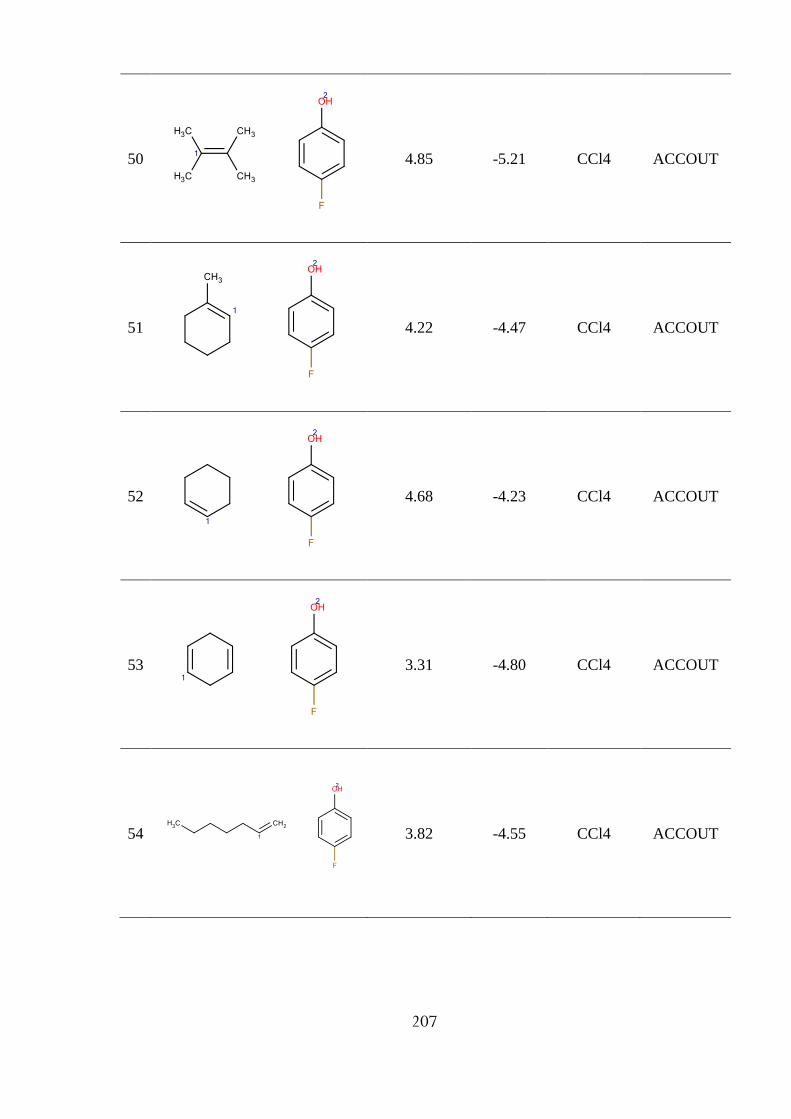
207
50
4.85 -5.21 CCl4 ACCOUT
51
4.22 -4.47 CCl4 ACCOUT
52
4.68 -4.23 CCl4 ACCOUT
53
3.31 -4.80 CCl4 ACCOUT
54
3.82 -4.55 CCl4 ACCOUT

208
55
1.26 -4.22 CCl4 ACCOUT
56
-4.49 2.15 C6H12 DONOUT
57
-3.67 2.41 C6H12 PAIROUT
58
-4.09 2.39 C6H12 DONOUT
59
-6.35 2.64 C6H12 DONOUT

209
60
-3.20 2.40 C6H12 DONOUT
61
-19.83 -11.98 CCl4 PAIROUT
62
-25.67 -18.21 1,2-
Cl2C2H4 ACCOUT
63
-34.22 -14.84 CCl4 PAIROUT
64
-20.38 -11.34 C6H6 ACCOUT

210
65
-14.09 -7.96 CCl3CH3 DONOUT
66
-21.37 -15.83 1,2-
Cl2C2H4 PAIROUT
67
-22.90 -16.33 1,2-
Cl2C2H4 PAIROUT
68
-15.31 -10.16 1,1,1-
Cl3CCH3 DONOUT
69
-31.31 -13.73 CCl4 ACCOUT

211
70
-25.86 -14.07 CCl4 ACCOUT
71
-4.18 1.25 CCl4 DONOUT
72
-6.26 2.49 C6H12 DONOUT
73
-13.81 -7.75 CCl4 PAIROUT
74
-13.30 -3.57 CCl4 DONOUT
a experimental G values were recalculated to CCl4 using linear correlations (see Table S1)
b SVM method has been used.
c see annotations in section 2.1.2.

212
Appendix. Part III
QSPR modeling and visualization of tautomeric
equilibria. Supporting Materials.
Table III.1. External test set 1.
№ External test set №1 T, °C Solvent Log
KT
exp
Log KT
pred
SVM/GTM
1
20 Methanol 0.63 0.39/-0.26
2
50 Methanol -
1.21
-0.68/-0.71
3 25 Acetonitrile 0.15 0.07/0.34

213
4
20 1,4-Dioxan -1.4 -1.27/-1.26
5
55 DMSO 0.36 0.22/0.20
6
55 DMSO -
0.31
0.31/0.54
7
20 Water 2.96 3.01/3.66
8
60 Water 0.03 -0.17/-0.21
9
30 Chloroform -
0.44
-0.27/-0.48

214
10
20 Water
(97%)
0.13 -0.12/-0.01
11
20 Ethanol
(61%)
-
0.92
-0.39/-0.34
12
30 Methanol -0.6 -0.9/-0.77
13
30 1-Propanol -1 -1.01/-1.27
14
10 Toluene -
0.32
-0.09/-0.22
15
40 Toluene 0.96 -0.12/-0.01

215
16
50 Acetone 0.01 -0.27/-0.32
17
20 Water 1.53 -1.34/-0.21
18
49.8 DMSO -
0.31
-0.01/-0.31
29
25.1 Tetracloro
methane
-
0.13
-0.17/-0.07
20
37 Tetracloro
methane
-
0.69
-0.01/-0.19
Table III.2. External test set 2.
№ External test set №2 T,
°C
Solvent Log
KT
exp
Log KT
pred
SVM/GT
M
AD
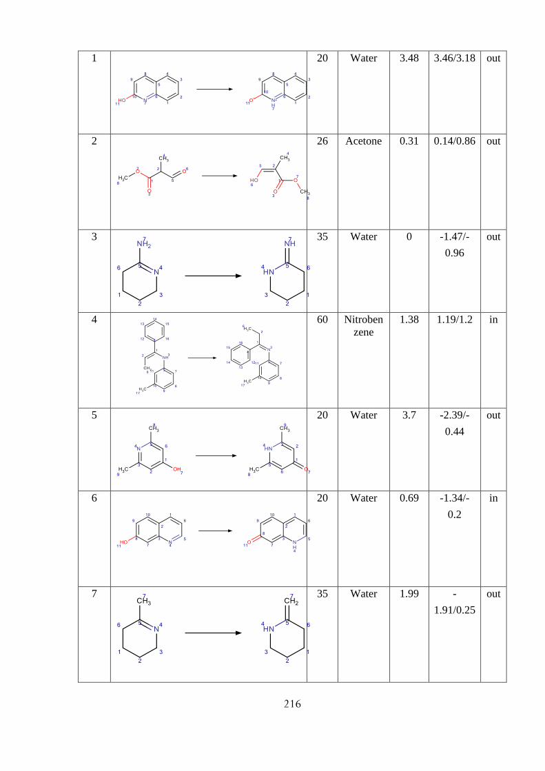
216
1
20 Water 3.48 3.46/3.18
out
2
26 Acetone 0.31 0.14/0.86 out
3
35 Water 0 -1.47/-
0.96
out
4
60 Nitroben
zene
1.38 1.19/1.2 in
5
20 Water 3.7 -2.39/-
0.44
out
6
20 Water 0.69 -1.34/-
0.2
in
7
35 Water 1.99 -
1.91/0.25
out

217
8
25 Water 8.6 7.55/8.3 in
9
25 Water -4.9 -5.61/-
5.8
out
10
25 Water 0.7 -3.61/-
3.56
out
11
0 Water -1.4 -2.01/-
3.56
out
12
20 Water 5.83 4.12/3.79 in
13
20 Ethanol 0.29 -0.32/-
0.33
out
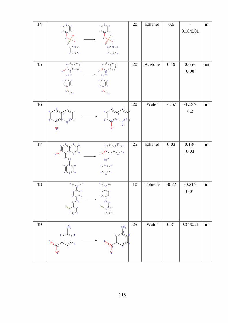
218
14
20 Ethanol 0.6 -
0.10/0.01
in
15
20 Acetone 0.19 0.65/-
0.08
out
16
20 Water -1.67 -1.39/-
0.2
in
17
25 Ethanol 0.03 0.13/-
0.03
in
18
10 Toluene -0.22 -0.21/-
0.01
in
19
25 Water 0.31 0.34/0.21 in

219
20
60 BromoB
enzene
0.27 0.18/0.06 in
21
35 Acetonitr
ile
-0.17 -0.01/-
0.56
in
22
35 1,4-
Dioxan
1.42 0.39/0.33 in
23
70 DMSO -1.28 0.51/0.47 in
24 100 Water -6.96 -2.19/-
2.55
out
25 100 Water -6.95 -2.19/-
2.55
out
26
100 Water -0.69 -0.88/-
0.27
out

220
Table III.3. Balanced accuracy for GTM class maps for the unique data set (the classes with the
number of objects more than 10 are considered only).
Balanced Accuracy
(BA) ISIDA M0 ISIDA M1 ISIDA M2 ISIDA M3
Keto-enol 0.975 1 1 1
Amine-imine 0.984 0.997 0.946 0.993
Hydrazine-Hydrazone 1 1 1 1
Ph-imine-keto-amine 0.998 1 1 0.998
Thion-ol-keto-thiol 1 1 1 1
Am-thion-im-thiol 1 1 1 1
Nutro-aci 1 1 1 1
Classic-zwitterion 0.904 0.989 0.992 0.990
Chain-ring 0.948 1 1 1
Table III.4. Balanced accuracy for GTM class maps for the entire data set (the classes with the
number of objects more than 10 are considered only).
Balanced Accuracy
(BA) ISIDA M0 ISIDA M1 ISIDA M2 ISIDA M3
Keto-enol 0.999 0.982 0.999 0.998
Amine-imine 0.997 0.999 0.999 0.998
Hydrazine-Hydrazone 1 1 1 1
Ph-imine-keto-amine 1 1 1 0.999
Thion-ol-keto-thiol 1 1 1 1
Am-thion-im-thiol 1 1 1 1
Nutro-aci 1 1 1 1
Classic-zwitterion 0.993 0.992 0.994 0.995
Chain-ring 1 0.991 0.998 0.998

221
Table III.5. SVR individual models constituting the web-deployed consensus model. Model
building parameters emerged from the evolutionary libSVM parametrization strategy.
Descriptor set LibSVM setup 5CV R2 5CV
RMSE
IAB-MA2--P-2-14 -s 3 -t 2 -c 2.446919e+02 -p 1.576160e-01 -g
6.167045e-02 -r -5.9 0.83 0.65
IIAB-MA2—FC-1-
3
-s 3 -t 2 -c 2.704264e+02 -p 3.152320e-01 -g
2.622281e-03 -r -0.5 0.83 0.66
IAB-MA2---P-AP-
2-14
-s 3 -t 2 -c 3.311545e+01 -p 3.152320e-01 -g
7.793662e-02 -r 5.5 0.81 0.68
IIAB-MA2—FC-1-
3
-s 3 -t 0 -c 3.320117e+00 -p 4.728480e-01 -g
6.962674e-03 -r -10.0 0.76 0.75
IAB-MA2—FC-2-
10
-s 3 -t 2 -c 3.311545e+01 -p 3.152320e-01 -g
3.356975e-02 -r 9.7 0.80 0.70
IA-MA2—1-4 -s 3 -t 2 -c 1.808042e+03 -p 3.152320e-01 -g
4.553438e-04 -r 4.3 0.82 0.67
IAB-MA2—FC-2-
14
-s 3 -t 1 -c 3.011942e-01 -p 1.576160e-01 -g
4.419572e-01 -r 2.8 0.78 0.71
IAB-MA2—2-10 -s 3 -t 2 -c 2.214064e+02 -p 3.152320e-01 -g
3.745244e-02 -r -6.3 0.82 0.68
IAB-MA2—P-AP-
2-14
-s 3 -t 1 -c 3.311545e+01 -p 3.152320e-01 -g
2.799525e-01 -r 3.1 0.80 0.69
IAB-MA2—P-2-10 -s 3 -t 0 -c 2.013753e+00 -p 1.576160e-01 -g
7.174630e-03 -r -10.0 0.75 0.79