
Three Paths to Particle Dark Matter -...
165
Three Paths to Particle Dark Matter Thesis by Samuel K. Lee In Partial Fulfillment of the Requirements for the Degree of Doctor of Philosophy California Institute of Technology Pasadena, California 2012 (Defended April 16, 2012)
Transcript of Three Paths to Particle Dark Matter -...

Three Paths to Particle Dark Matter
Thesis by
Samuel K. Lee
In Partial Fulfillment of the Requirements
for the Degree of
Doctor of Philosophy
California Institute of Technology
Pasadena, California
2012
(Defended April 16, 2012)

ii
c© 2012
Samuel K. Lee
All Rights Reserved
iii
Some realize the Supreme by meditating, by its aid, on the Self within, others by pure reason,
others by right action.
Others again, having no direct knowledge but only hearing from others, nevertheless worship, and
they, too, if true to the teachings, cross the sea of death.
— The Bhagavad Gita (13.25–26)
Forgotten rimes, and college themes,
Worm-eaten plans, and embryo schemes;–
A mass of heterogeneous matter,
A chaos dark, nor land nor water...
— An Inventory of the Furniture in Dr. Priestley’s Study (37–40),
Anna Lætitia Barbauld (1825)

iv
Acknowledgments
Astronomy now demands bodily abstraction of its devotee. . . To see into the beyond requires
purity. . . and the securing it makes him perforce a hermit from his kind. . . .
— Mars and Its Canals,
Percival Lowell (1906)
I first encountered the above words on my recent cross-country emigration from Caltech to Johns
Hopkins; they were engraved as an epitaph on Lowell’s mausoleum, which is located on the grounds
of the observatory bearing the learn’d astronomer’s name. Upon reading them, I felt grateful that I
could count myself luckier than Lowell in two respects: first, that we can be reasonably sure that dark
matter will not follow the canals of Mars into the forgotten annals of science, and, more importantly,
that my experience as a scientist thus far was neither as lonely nor as forsaken as Lowell’s profound
yet depressing words suggest it should have been. I have no quarrel with Lowell — and perhaps I
have not achieved sufficient purity to see into the beyond just yet — but if ever my life’s deeds are
enough to warrant a mausoleum of my own, I will be sure that my epitaph not imply that those
deeds were a solitary effort. In contrast, my pursuits and ambitions have always been supported by
a large number of people; I hope they will accept the humble and sincere thanks I offer here.
First and foremost, I am indebted to my adviser, Marc Kamionkowski. The possibility of working
with Marc was perhaps the primary reason I decided to attend Caltech for graduate school. Since he
has afforded me the opportunity of working on a number of fascinating and intellectually stimulating
research topics, it a decision I am very glad to have made. As an adviser, Marc has always been
extremely generous with his encouragement and support, as well as with dispensing thoughtful advice
that has proved invaluable in matters academic and otherwise. As a scientist, Marc has never failed
to impress; many are the times I have been sitting in a colloquium or seminar, usually on a subject
far afield from my own interests and expertise, admitting to myself that I have become hopelessly
lost and perplexed by the presentation — it is usually at this point that Marc raises his hand and
asks some piercing question, physically insightful yet completely clear even to one as confused as
me. Although humbling, it is a great source of inspiration to realize that despite the years invested
in this thesis, I still have a long way to go before I can hope to match his versatility as a physicist.
v
Next, I would like to thank those that I collaborated with to produce the work presented in this
thesis. To Shin’ichiro Ando, Jonathan Feng, and Annika Peter — I learned many things from the
science we did together, for which I am grateful; I am also immensely appreciative of the support you
provided during the postdoctoral application process. I would also like to thank Kirill Melnikov and
Andrzej Czarnecki for teaching me a thing or ten about thermal field theory. Furthermore, although
not presented in this thesis, the work I have completed (or started...) with Savvas Koushiappas,
Stefano Profumo, Lorenzo Ubaldi, Michael Dine, and Chris Hirata and the interactions we have had
have also been important to my development as a physicist.
I would also like to express gratitude to the students, postdocs, professors, and staff that make
Caltech such A Nice Place To Live (And Do A Ph.D.). I am glad to number myself among the
Caltech Astronomy graduate students, and am proud of the community we have built during my
time in the department. However, were it not for the friendship of my fellow classmates — Mike
Anderson, Krzysztof Findeisen, Vera Gluscevic, Tucker Jones, Elisabeth Krause, Tim Morton, Drew
Newman, and Gwen Rudie — the first year of graduate school would certainly not have been as
enjoyable as it was, much less those years subsequent. I am also obliged to Gina Armas and Gita
Patel for their diligence and assistance.
Thanks goes to the numerous denizens of TAPIR: my most recent set of office mates Yacine
Ali-Haımoud, Nate Bode, and Anthony Pullen, who deserve credit for not giving me too hard a time
about my odd hours; the members of the Tuesday group meetings — especially my elder academic
siblings Adrienne Erickcek, Dan Grin, and Tristan Smith, as well as Fabian Schmidt, who have
all been welcoming whenever our paths were fortunate enough to cross again, and Donghui Jeong,
my fellow Caltech expatriate here at Johns Hopkins; the staff members that kept things running
smoothly — JoAnn Boyd, Shirley Hampton, and Chris Mach; and the graduate students that politely
put up with my ramblings on particle physics at our Thursday lunch lectures — Esfandiar Alizadeh,
Laura Book, Michael Cohen, Jeff Kaplan, Keith Matthews, David Nichols, Evan O’Connor, Chris
Wegg, Fan Zhang, Aaron Zimmerman, and others. In particular, I would like to commend Chris
Wegg for his excellent taste in music, and thank him for filling the time between the support and
the headliner with entertaining conversation. I would also like to generally thank the graduate and
undergraduate students of the physics department for many positive experiences, both academic and
social.
Some recognition is due to roommates I had through the years spent living in the Caltech Catalina
Apartments; thanks to Steven Frankel, Zakary Singer, and Scott Steger for many memories in 201.
Many enjoyable trips to the great outdoors — snowboarding, hiking, camping, and so forth — were
had with Matt Schenker, who was always rather understanding of my general inexperience with
much of the great outdoors. I had many stimulating talks with Thinh Bui during our frequent
runs for Vietnamese food, and spent many equally stimulating hours in front of our CRT television
vi
digesting the great epics of our time with him. Finally, Ryan Trainor has been one of the most
dependable, capable, and good-spirited friends I have had the pleasure to know — and his family
has always been very good to me, as well.
In the spring of my fourth year, I found myself volunteering to design and build handcrank-
powered generators for a public-outreach installation promoting energy conservation and sustain-
ability at the Coachella Valley Music and Arts Festival. I would like to thank Jelena Culic-Viskota,
Toni Lee, Jeff Lehew, Mike Shearn, and Ryan Trainor for entrusting a theoretical astrophysicist
with the responsibility of engineering something remotely resembling a functional device (and for
letting him use power tools in close proximity to you); the experience was a welcome diversion from
my usual pencil-and-paper-and-programming routine.
In my fifth year, I found myself moving across the country to Baltimore. The physicists of
Johns Hopkins have been most welcoming, for which I am grateful. However, the chemists also
let me occasionally infiltrate their ranks; thanks to Chris Bianco, Tyler Chavez, Mark Hutchinson,
and Chris Malbon for times around our kitchen island and elsewhere. In particular, my current
housemates Jacob Kravetz and David Wallace deserve special praise for always being scholars (albeit
of chemistry) and gentlemen (usually in that order).
As a physicist, I have been fortunate enough to attend a number of schools and conferences; I
would like to thank the friends I have made during my travels for opening my eyes to the dedication
required to do science in some parts of the world, and for showing me that physics is nevertheless a
universal language.
However, I would not be able to speak that language were it not for my experiences during my
MIT years. Without my former classmate Duncan Ma, I never would have gotten past 8.012, and
it was Scott Hughes’s excellent 8.022 lectures that cemented my desire to follow my current career
path. Paul Schechter and Harvey Moseley were also great mentors during this formative period.
Outside of my physics studies, some of my most challenging and gratifying experiences were had
with the MIT Pistol Team, coached by Will Hart.
Even before MIT, several of my friends and teachers played important roles in shaping my growth.
Although I have lost touch with some, time has not diminished their contribution; thanks to Anne
Barrera (nee Nugent), Dwo Chu, Johanna Chu (nee Yu), Deborah Crawford, Robert Dennison, Jane
Fain, Philip Ho, Jennifer Lee (nee Yu), Matt Lee, Kanwar Singh, Chris Vollmer, and innumerable
others. Charles Wei has proven to be an invaluable friend through the years.
On a larger scale, I express thanks to those that make my somewhat impractical profession
possible. The epigraph that opens this thesis, although a tongue-in-cheek comparison between the
three paths leading to particle dark matter and those leading to enlightenment and salvation, may
perhaps be more obliquely read as expressing my sentiments on the role of a scientist in a society that
values knowledge and the pursuit of deeper truths. Similar sentiments, with which I wholeheartedly
vii
agree, may also be found in the dedication of Misner, Thorne, and Wheeler’s well known tome on
Gravitation.
At this point, I am running out of synonymous words with which to relate my thanks and
gratitude. Fortunately, no words are necessary to express those feelings to my family, who have
always loved and supported me unconditionally. To my father and mother — any virtues I may
claim to have are merely echoes of yours, and any faults are mine alone. To Elaine and Peter —
siblings are among the few people to ever truly know each other from childhood to maturity, and I
hope that I have grown into someone you are proud to call your brother.
Finally, I am ever thankful to, and for, Zhitong Zhang. Her love has been a constant through
many years of time, and, more often than not, across many miles of space. Despite my years
devoted to studying the cosmos — with all its breadth and endless variety — I have yet to come
across anything in it more lovely and delightful than she. With her companionship, the Universe
seems far less cold, dark, and infinite.

viii
Abstract
In this thesis, we explore examples of each of the three primary strategies for the detection of particle
dark matter: indirect detection, direct detection, and collider production.
We first examine the indirect detection of weakly interacting massive particle (WIMP) dark mat-
ter via the gamma-ray photons produced by astrophysical WIMP annihilation. Such photons may
be observed by the Fermi Gamma-ray Space Telescope. We propose the gamma-ray-flux probabil-
ity distribution function (PDF) as a probe of the Galactic halo substructure predicted to exist by
N-body simulations. The PDF is calculated for a phenomenological model of halo substructure; it
is shown that the PDF may allow a statistical detection of substructure.
Next, we consider the direct detection of WIMPs. We explore the ability of directional nuclear-
recoil detectors to constrain the local velocity distribution of WIMP dark matter by performing
Bayesian parameter estimation on simulated recoil-event data sets. We discuss in detail how direc-
tional information, when combined with measurements of the recoil-energy spectrum, helps break
degeneracies in the velocity-distribution parameters. Considering the possibility that velocity struc-
tures such as cold tidal streams or a dark disk may also be present in addition to the Galactic halo,
we discuss the potential of upcoming experiments to probe such structures.
We then study the collider production of light gravitino dark matter. Light gravitino production
results in spectacular signals, including di-photons, delayed photons, kinked charged tracks, and
heavy metastable charged particles. We find that observable numbers of light-gravitino events may
be found in future collider data sets. Remarkably, this data is also well suited to distinguish between
scenarios with light gravitino dark matter, with striking implications for early-Universe cosmology.
Finally, we investigate the related matter of radiative corrections to the decay rate of charged
fermions caused by the presence of a thermal bath of photons. The cancellation of finite-temperature
infrared divergences in the decay rate is described in detail. Temperature-dependent radiative cor-
rections to the two-body decay of a hypothetical charged fermion and to electroweak decays of a
muon are given. We touch upon possible implications of these results for charged particles in the
early Universe.

ix
Contents
Acknowledgments iv
Abstract viii
List of Figures xii
List of Tables xv
1 Introduction 1
2 Indirect detection: The gamma-ray-flux probability distribution function from
Galactic halo substructure 11
2.1 Motivation: Supersymmetric neutralinos as WIMP dark matter . . . . . . . . . . . . 11
2.1.1 The WIMP miracle . . . . . . . . . . . . . . . . . . . . . . . . . . . . . . . . . 11
2.1.2 Supersymmetry and neutralino dark matter . . . . . . . . . . . . . . . . . . . 14
2.2 Introduction . . . . . . . . . . . . . . . . . . . . . . . . . . . . . . . . . . . . . . . . . 21
2.3 Substructure/annihilation models and EGRET constraints . . . . . . . . . . . . . . . 23
2.3.1 Halo model and microhalo mass function . . . . . . . . . . . . . . . . . . . . 23
2.3.2 Microhalo annihilation models . . . . . . . . . . . . . . . . . . . . . . . . . . 24
2.3.3 EGRET constraints . . . . . . . . . . . . . . . . . . . . . . . . . . . . . . . . 25
2.4 Calculation of the PDF . . . . . . . . . . . . . . . . . . . . . . . . . . . . . . . . . . 28
2.4.1 Derivation of P1(F ) . . . . . . . . . . . . . . . . . . . . . . . . . . . . . . . . 29
2.4.2 Calculation of the counts distribution . . . . . . . . . . . . . . . . . . . . . . 29
2.5 Numerical results . . . . . . . . . . . . . . . . . . . . . . . . . . . . . . . . . . . . . . 32
2.6 Detectability . . . . . . . . . . . . . . . . . . . . . . . . . . . . . . . . . . . . . . . . 33
2.7 Conclusions . . . . . . . . . . . . . . . . . . . . . . . . . . . . . . . . . . . . . . . . . 35
3 Direct detection: Probing the local velocity distribution of WIMP dark matter
with directional detectors 38
3.1 Motivation: The directional recoil spectrum from WIMP-nucleus collisions . . . . . . 38

x
3.1.1 Simple estimates for direct detection . . . . . . . . . . . . . . . . . . . . . . . 38
3.1.2 The directional recoil spectrum . . . . . . . . . . . . . . . . . . . . . . . . . . 40
3.2 Introduction . . . . . . . . . . . . . . . . . . . . . . . . . . . . . . . . . . . . . . . . . 43
3.3 The binned likelihood function . . . . . . . . . . . . . . . . . . . . . . . . . . . . . . 44
3.4 Likelihood analyses of simulated data . . . . . . . . . . . . . . . . . . . . . . . . . . 47
3.4.1 Halo-only model . . . . . . . . . . . . . . . . . . . . . . . . . . . . . . . . . . 48
3.4.1.1 vlab-σH analyses . . . . . . . . . . . . . . . . . . . . . . . . . . . . . 49
3.4.1.2 6-parameter analyses . . . . . . . . . . . . . . . . . . . . . . . . . . 51
3.4.2 Halo+stream model . . . . . . . . . . . . . . . . . . . . . . . . . . . . . . . . 52
3.4.3 Halo+disk model . . . . . . . . . . . . . . . . . . . . . . . . . . . . . . . . . . 54
3.5 Conclusions . . . . . . . . . . . . . . . . . . . . . . . . . . . . . . . . . . . . . . . . . 55
4 Collider production: Light gravitinos at colliders and implications for cosmology 70
4.1 Motivation: Supergravity and the gravitino . . . . . . . . . . . . . . . . . . . . . . . 70
4.1.1 A local U(1) symmetry . . . . . . . . . . . . . . . . . . . . . . . . . . . . . . 70
4.1.2 From local supersymmetry to gravity . . . . . . . . . . . . . . . . . . . . . . . 72
4.1.3 The super-Higgs mechanism . . . . . . . . . . . . . . . . . . . . . . . . . . . . 77
4.1.4 Gravitino interactions . . . . . . . . . . . . . . . . . . . . . . . . . . . . . . . 79
4.2 Introduction . . . . . . . . . . . . . . . . . . . . . . . . . . . . . . . . . . . . . . . . . 82
4.3 Light-gravitino cosmology . . . . . . . . . . . . . . . . . . . . . . . . . . . . . . . . . 84
4.3.1 Canonical scenario . . . . . . . . . . . . . . . . . . . . . . . . . . . . . . . . . 84
4.3.1.1 Relic abundance . . . . . . . . . . . . . . . . . . . . . . . . . . . . . 84
4.3.1.2 Cosmological constraints . . . . . . . . . . . . . . . . . . . . . . . . 86
4.3.2 Nonstandard early-Universe scenarios . . . . . . . . . . . . . . . . . . . . . . 87
4.4 Light gravitinos at colliders . . . . . . . . . . . . . . . . . . . . . . . . . . . . . . . . 88
4.4.1 Mass and interactions . . . . . . . . . . . . . . . . . . . . . . . . . . . . . . . 88
4.4.2 GMSB models . . . . . . . . . . . . . . . . . . . . . . . . . . . . . . . . . . . 89
4.4.3 Current collider constraints . . . . . . . . . . . . . . . . . . . . . . . . . . . . 91
4.5 Tevatron and LHC prospects . . . . . . . . . . . . . . . . . . . . . . . . . . . . . . . 92
4.5.1 Gravitino signals . . . . . . . . . . . . . . . . . . . . . . . . . . . . . . . . . . 92
4.5.2 GMSB scan and collider simulations . . . . . . . . . . . . . . . . . . . . . . . 94
4.5.3 Cosmological implications . . . . . . . . . . . . . . . . . . . . . . . . . . . . . 95
4.6 Conclusions . . . . . . . . . . . . . . . . . . . . . . . . . . . . . . . . . . . . . . . . . 96
5 A detour: Charged-particle decay at finite temperature 103
5.1 Introduction . . . . . . . . . . . . . . . . . . . . . . . . . . . . . . . . . . . . . . . . . 103
5.2 Toy model . . . . . . . . . . . . . . . . . . . . . . . . . . . . . . . . . . . . . . . . . . 105

xi
5.2.1 Photon absorption . . . . . . . . . . . . . . . . . . . . . . . . . . . . . . . . . 106
5.2.2 Photon emission . . . . . . . . . . . . . . . . . . . . . . . . . . . . . . . . . . 107
5.2.3 Real-radiation corrections . . . . . . . . . . . . . . . . . . . . . . . . . . . . . 108
5.3 Virtual corrections . . . . . . . . . . . . . . . . . . . . . . . . . . . . . . . . . . . . . 109
5.3.1 Vertex correction . . . . . . . . . . . . . . . . . . . . . . . . . . . . . . . . . . 109
5.3.2 Self-energy corrections . . . . . . . . . . . . . . . . . . . . . . . . . . . . . . . 110
5.4 Total decay rate in the toy model . . . . . . . . . . . . . . . . . . . . . . . . . . . . . 114
5.5 Muon decay µ→ eνµνe . . . . . . . . . . . . . . . . . . . . . . . . . . . . . . . . . . 115
5.6 Conclusions . . . . . . . . . . . . . . . . . . . . . . . . . . . . . . . . . . . . . . . . . 116
A Kinetic decoupling 118
A.1 Elastic-scattering cross sections . . . . . . . . . . . . . . . . . . . . . . . . . . . . . . 120
B Derivation of P (F ) 125
C Generation of directional-detection events 127
D Mass singularities and thermal fermionic corrections 129
Bibliography 133
xii
List of Figures
1.1 Three paths to particle dark matter . . . . . . . . . . . . . . . . . . . . . . . . . . . . 5
2.1 Contributions to the Higgs self-energy from fermion and complex scalar couplings . . 18
2.2 The intensity Ih(ψ) above 10 GeV from microhalos . . . . . . . . . . . . . . . . . . . . 27
2.3 The flux-density distribution P1(F,ψ = 90) for the flux from an individual microhalo 30
2.4 The angular-averaged discrete probability distribution function P (C) for the neutralino
model . . . . . . . . . . . . . . . . . . . . . . . . . . . . . . . . . . . . . . . . . . . . . 31
2.5 The angular-averaged discrete probability distribution function P (C), with an arbitrary
diffuse background added . . . . . . . . . . . . . . . . . . . . . . . . . . . . . . . . . . 31
2.6 The angular-averaged discrete probability distribution function P (C) for the line model,
with an arbitrary diffuse background added . . . . . . . . . . . . . . . . . . . . . . . . 32
2.7 The KE-Mmin parameter space for the line models . . . . . . . . . . . . . . . . . . . . 34
3.1 The elastic scattering of a WIMP off of a nucleus initially at rest . . . . . . . . . . . . 40
3.2 Allowed incoming-WIMP velocities v for an observed nuclear-recoil momentum q . . 41
3.3 Left: Simulated recoil spectrum for the halo-only 2-parameter and 3-parameter anal-
yses, with binned signal events. Right: Simulated recoil map for these analyses, in
Mollweide projection . . . . . . . . . . . . . . . . . . . . . . . . . . . . . . . . . . . . . 58
3.4 Top row: Contour plots for the 2D posterior probability distribution in vlab-σH space,
for the halo-only 2-parameter analyses with fixed mχ. Bottom row: The same for the
3-parameter analyses assuming a flat mass prior . . . . . . . . . . . . . . . . . . . . . 59
3.5 Recoil spectra showing the energy distribution (normalized to unity) of events in the
energy range of 5–50 keV for a halo-only model . . . . . . . . . . . . . . . . . . . . . . 60
3.6 Recoil maps showing the angular distribution (normalized to unity) of events in the
energy range of 5–50 keV for a halo-only model . . . . . . . . . . . . . . . . . . . . . . 61
3.7 Simulated recoil spectrum for the halo-only 6-parameter analysis . . . . . . . . . . . . 62
3.8 Simulated recoil maps for the halo-only 6-parameter analysis . . . . . . . . . . . . . . 62
3.9 Triangle plot showing 1D and 2D posterior probability distributions for the halo-only
6-parameter analysis using only energy information . . . . . . . . . . . . . . . . . . . 63

xiii
3.10 Triangle plot showing 1D and 2D posterior probability distributions over the full prior
ranges, for the halo-only 6-parameter analysis using direction+energy information . . 64
3.11 Simulated recoil spectrum for the halo+stream analysis . . . . . . . . . . . . . . . . . 65
3.12 Simulated recoil maps for the halo+stream analysis . . . . . . . . . . . . . . . . . . . 65
3.13 Triangle plot for the halo+stream analysis . . . . . . . . . . . . . . . . . . . . . . . . . 66
3.14 Simulated recoil spectrum for the halo+disk analyses . . . . . . . . . . . . . . . . . . 67
3.15 Simulated recoil maps for the halo+disk analyses . . . . . . . . . . . . . . . . . . . . . 67
3.16 Triangle plot for the 0–50-keV halo+disk analysis . . . . . . . . . . . . . . . . . . . . 68
3.17 Triangle plot for the 5–50-keV halo+disk analysis . . . . . . . . . . . . . . . . . . . . 69
4.1 Supersymmetrization of the gauge vertex . . . . . . . . . . . . . . . . . . . . . . . . . 80
4.2 Supersymmetrization of the graviton couplings . . . . . . . . . . . . . . . . . . . . . . 81
4.3 Plots showing the mapping between the mG-mNLSP and the Mmess-Λ GMSB parameter
spaces . . . . . . . . . . . . . . . . . . . . . . . . . . . . . . . . . . . . . . . . . . . . . 95
4.4 Contour plots over the mG-mNLSP parameter space showing the expected number of
prompt di-photon events in a model with a neutralino NLSP . . . . . . . . . . . . . . 98
4.5 Contour plots over the mG-mNLSP parameter space showing the expected number of
nonprompt photon events in a model with a neutralino NLSP . . . . . . . . . . . . . . 99
4.6 Contour plots showing the expected number of nonprompt lepton events in a model
with a stau NLSP . . . . . . . . . . . . . . . . . . . . . . . . . . . . . . . . . . . . . . 100
4.7 Contour plots showing the expected number of metastable slepton events in a model
with a stau NLSP . . . . . . . . . . . . . . . . . . . . . . . . . . . . . . . . . . . . . . 101
4.8 Simulated probability distribution functions for the speed β (top panels) and Lorentz
factor γ (bottom panels) of mother particles decaying to gravitinos . . . . . . . . . . . 102
5.1 The diagram for the decay ψ → χφ . . . . . . . . . . . . . . . . . . . . . . . . . . . . . 104
5.2 The two diagrams via which absorption of a photon can lead to induced ψ decay (or χ
and φ production) . . . . . . . . . . . . . . . . . . . . . . . . . . . . . . . . . . . . . . 105
5.3 The diagrams for radiative ψ-decays . . . . . . . . . . . . . . . . . . . . . . . . . . . . 107
5.4 The T -dependent part of the photon propagator . . . . . . . . . . . . . . . . . . . . . 109
5.5 The diagram contributing to the T -dependent part of the O(α) correction to the vertex 110
5.6 The diagram contributing to the T -dependent part of the fermion self-energy . . . . . 111
A.1 Feynman diagrams for scattering of a fermion f by a neutralino χ . . . . . . . . . . . 120
D.1 The T -dependent part of the fermion propagator . . . . . . . . . . . . . . . . . . . . . 130

xiv
D.2 The additional diagrams (appearing at temperatures mχ T mψ) that contribute
to the T -dependent part of the real corrections, including the thermal corrections to
the bare fermion propagator . . . . . . . . . . . . . . . . . . . . . . . . . . . . . . . . 130
D.3 The additional diagrams (appearing at temperatures mχ T mψ) that contribute
to the T -dependent part of the virtual corrections, including the thermal corrections
to the bare fermion propagator . . . . . . . . . . . . . . . . . . . . . . . . . . . . . . . 131

xv
List of Tables
2.1 Particle content of the minimal supersymmetric standard model . . . . . . . . . . . . 16
3.1 Experimental parameters used to simulate data for likelihood analyses . . . . . . . . . 48
3.2 Fiducial parameter values and flat prior ranges used to simulate data and perform
likelihood analyses . . . . . . . . . . . . . . . . . . . . . . . . . . . . . . . . . . . . . . 57
4.1 Analogy between the Higgs and super-Higgs mechanisms . . . . . . . . . . . . . . . . 78
1
Chapter 1
Introduction
The problem of dark matter is surely one of the most exciting open questions in physics. The
discovery of dark matter followed in the vein of a historical tradition in astronomy — namely, the
revelation of hitherto unknown phenomena via their gravitational effects on visible matter.1 As
early as the 1920s, measurements of the vertical motions of stars near the Galactic plane implied
the gravitational influence of an unseen dark component [1]. In 1933, Fritz Zwicky deduced the
existence of a non-luminous constituent of the Coma cluster by observing the dynamics of the
galaxies contained therein, famously conferring upon it the name of “dark matter” [2].2
Evidence for dark matter from astrophysical and cosmological observations now abounds. The
astrophysical evidence includes the flattening of galactic rotation curves at radii beyond the visi-
ble edges of galaxies, studies of gravitational lensing — both strong and weak — in galaxies and
clusters, and so on. Meanwhile, cosmological observations of the cosmic-microwave-background
(CMB) anisotropies constrain the dark-matter density (in units of the critical density) of the Uni-
verse to be Ωdm = 0.222 ± 0.026 [4]. The constraint can be improved when taken in conjunction
with measurements of the local Hubble expansion rate calibrated using Cepheid variables [5], the
luminosity-distance–redshift relation determined from the light curves of Type Ia supernovae [6], and
baryon acoustic oscillations measured from large-scale galaxy surveys [7]. At the same time, these
measurements, as well as those of the chemical abundances of the light elements produced during
big-bang nucleosynthesis, also determine the density of baryonic matter to be Ωb = 0.0449± 0.0028.
Thus, that non-baryonic dark matter composes the majority — roughly 80–85% — of the matter
in the Universe, and approximately a quarter of the total matter-energy content, is overwhelmingly
suggested by both astrophysical and cosmological evidence (for a more comprehensive overview, see,
e.g., Ref. [8]).3
1The respective discoveries of Neptune and general relativity from the observed deviations of the orbits of Uranusand Mercury from the predictions of Newtonian theory followed this pattern.
2The dynamics revealed “die Notwendigkeit einer enorm grossen Dichte dunkler Materie”, the need for an enor-mously large density of dark matter. Interestingly enough, Zwicky also uses the phrase “dunkle (kalte) Materie” inthe paper, although the use of “cold” here presumably equates to “non-luminous” (and not the modern interpretationof “nonrelativistic”). A brief overview of the historical development of dark matter is given in Ref. [3].
3The other possible explanation — a modification of the laws of gravity — is strongly disfavored, most convincingly

2
However, despite this abundance of evidence for the existence of dark matter, the nature of
dark matter remains to be understood precisely. Perhaps one reason for this is that the pieces of
evidence accumulated so far are derived from the observation of gravitational effects, and do not
strongly preclude the possibility that dark matter interacts solely via the comparatively feeble force
of gravity. Conversely, the exciting possibility that dark matter has “stronger-than-gravitational”
interactions with everyday particles of the standard model, potentially allowing for detectable signals,
remains viable. Interestingly enough, this latter scenario is realized in numerous theories of particle
physics that resolve outstanding issues in the standard model. Many such extensions of the standard
model hypothesize the existence of new particles that may naturally be interesting dark-matter
candidates. That is, these particles are predicted to have properties that not only allow for them
to fulfill the astrophysical and cosmological roles that dark matter play gravitationally, but may
also allow them to be accessible experimentally. There is no shortage of well-motivated particle
candidates; sterile neutrinos, supersymmetric neutralinos and gravitinos, axions, and Kaluza-Klein
excitations in theories with extra dimensions number among the more commonly studied (reviews
are given in, e.g., Refs. [10–13]).
There are a number of basic criteria related to the fundamental, microphysical particle properties
of a dark-matter candidate that must first be satisfied if the particle is to successfully act out its
various gravitational roles in a straightforward and non-contrived manner [14]:
• Relic abundance: The aforementioned new theories of physics should become relevant at
energies greater than those previously explored by particle accelerators. Such energies may
have been accessed in the early moments of the Universe, during the hot big bang. It is
possible that dark-matter particles were produced then, by either standard thermal production
via scattering interactions in the thermal bath or nonthermal mechanisms, in quantities that
should be predictable given the new theory and its fundamental parameters. The parameters
of the theory — which in turn determine the dark-matter particle properties — and the early-
Universe conditions and production mechanisms must then conspire to produce the correct,
observed abundance of dark matter.
• Electromagnetic neutrality: The dark matter must be truly dark. That is, the electro-
magnetic interactions of dark-matter particles with photons must be much weaker than those
of conventionally charged particles. Limits on the strength of the electromagnetic interaction
can be expressed in terms of the fractional charge (with respect to the elementary charge) of
the dark-matter particle, and can be derived from the non-observation of the variety of astro-
physical effects charged dark-matter particles would engender. The strongest constraint comes
from the requirement that the dark matter not couple too strongly to photons during the
by observations of the Bullet galaxy cluster [9]. In this sense, the discovery of dark matter shares more in commonwith that of Neptune than that of general relativity.

3
recombination epoch (avoiding disruption of the CMB acoustic peaks), yielding an upper limit
on the fractional charge of ∼10−6 for GeV-mass particles, rising to ∼10−4 for 10-TeV–mass
particles [15]. Similarly, astrophysical constraints may be placed on the electric or magnetic
dipole moments of the dark-matter particle (see, e.g., [16, 17]).
• Interaction strength: Not only should the dark-matter particle not interact with photons
and electrically charged particles, it must also not couple too strongly to electrically neutral
standard-model particles. Again, one reason for this is the requirement that the dark matter
not couple too strongly to baryons during the recombination epoch, as this would also change
the CMB acoustic peaks. Significant coupling would also allow the baryon–dark-matter fluid
to radiatively cool via the baryons, affecting structure formation. Thus, the link between dark
matter and baryons must be relatively “weak” in strength, as a result of either a smallness of the
fundamental interaction coupling or by some other mechanism which suppresses the observable
consequences of “strong” interactions phenomenologically. Although this interaction between
dark matter and baryons need not necessarily be the weak interaction of the standard model,
many extensions of the standard model do generically predict the existence of new weakly
interacting massive particles (WIMPs) that couple to the weak gauge bosons. As it can
be shown that these WIMPs, if produced thermally in the early Universe, naturally have
the correct dark-matter relic abundance (a coincidence referred to as the “WIMP miracle”),
WIMPs are hence the most well-studied class of dark-matter candidates.
• Non-baryonic nature: In the same vein, the dark matter cannot be a non-exotic baryon
(here, we actually mean hadron, although the use of the word “baryon” thus far, and conven-
tionally in the literature, is as a misnomer that includes hadronic and leptonic matter). As
previously mentioned, this is required in order for the predictions of big-bang nucleosynthesis,
which are sensitive to the baryon-to-photon ratio, to be realized. Related to this criterion
is the fact that massive compact halo objects (MACHOs), which are dark baryonic objects
(including faint neutron stars, brown dwarfs, white dwarfs, planets, etc.) that were once a
possible solution to the dark-matter problem, are ruled out [18]. Strong constraints on a pos-
sible MACHO population can be deduced from the disagreement of the observed chemical
abundances with those expected to be produced by the evolution of stellar MACHOs [19], as
well as from searches for microlensing by MACHOs [20, 21]. These constraints indicate that
the dark matter may indeed be composed of elementary particles.
• Self-interaction strength: Furthermore, the self-interaction of the dark-matter particle
must be consistent with observations. Interestingly enough, dark matter with some degree of
strong scattering self-interactions (but negligible annihilation or dissipation interactions) may
alleviate some tensions between observations and collisionless-dark-matter simulations, such
4
as those arising from the “missing satellite” problem and the issue of the central cuspiness of
dark-matter halos [22]. Several astrophysical constraints may be placed on self-interacting dark
matter. For example, observations of the aforementioned Bullet cluster place an upper limit on
the ratio of the self-scattering cross section to the dark-matter-particle mass σ/m . 1 cm2 g−1,
which must be satisfied if the dark-matter components of the two colliding clusters are to pass
through each other as implied by gravitational-lensing maps of the mass distribution.
• Temperature: As dark matter must be able to gravitationally collapse to form small-scale
structure after it has decoupled from the thermal bath and the Universe becomes matter
dominated, the dark-matter particles must have a small or nonrelativistic velocity at that time
if they are not to free stream out of density perturbations. The “temperature” of the dark
matter must then be fairly cold. At most, the dark matter may be “tepid” or “lukewarm”, with
free-streaming lengths on the order of galactic scales, if the correct matter power spectrum is
to be realized [23]. Neutrinos, the only standard-model particles that have heretofore satisfied
all of the above constraints, are then ruled out, as they decouple when they are relativistic and
thus compose hot matter. Mixed dark matter, composed of several distinct particle species with
different temperatures, may also be a possibility that can be constrained by such considerations.
These considerations then translate into constraints on both the mass of the dark-matter
particle and the details of its kinetic decoupling, the latter of which depends on the scattering
interactions of the dark-matter particle with particles in the thermal bath.
• Stability: The dark matter must be stable on cosmological timescales [24] if it is to produced
in the early Universe, affect the CMB anisotropies formed during recombination, and persist
to collapse to form structures present today. The avoidance of significant energy injection from
standard-model decay products after the epochs of big-bang nucleosynthesis and recombination
is also desirable. Scenarios in which a number of multiple dark-matter species exist and may
decay to the lightest among them at late times are also strongly constrained by the requirement
that the kicks given to the dark decay products not disrupt dark-matter-halo structure and
formation [25, 26]. At the microphysical level, stability is commonly effected by introducing
discrete symmetries, such that the dark-matter particle is the lightest of those particles that
carry a conserved quantum number not possessed by the particles of the standard model.
• Equivalence principle: There is no a priori reason that the dark matter should obey the
equivalence principle, even though ordinary matter does. For example, a violation of the equiv-
alence principle might arise if light particles mediate an additional long-range force between
dark-matter particles. However, observations of the dynamics of tidal tails in the Milky Way
strongly constrain such theories [27,28].
Certainly it is conceivable that some of these basic criteria might be relaxed in the context of a
5
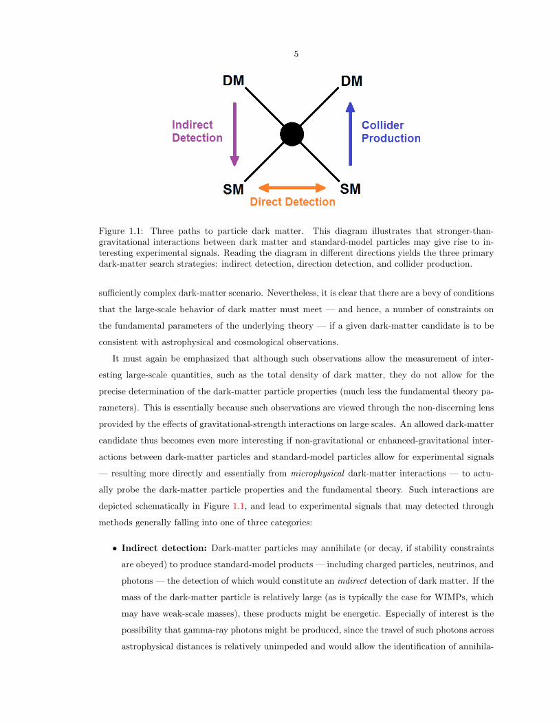
Figure 1.1: Three paths to particle dark matter. This diagram illustrates that stronger-than-gravitational interactions between dark matter and standard-model particles may give rise to in-teresting experimental signals. Reading the diagram in different directions yields the three primarydark-matter search strategies: indirect detection, direction detection, and collider production.
sufficiently complex dark-matter scenario. Nevertheless, it is clear that there are a bevy of conditions
that the large-scale behavior of dark matter must meet — and hence, a number of constraints on
the fundamental parameters of the underlying theory — if a given dark-matter candidate is to be
consistent with astrophysical and cosmological observations.
It must again be emphasized that although such observations allow the measurement of inter-
esting large-scale quantities, such as the total density of dark matter, they do not allow for the
precise determination of the dark-matter particle properties (much less the fundamental theory pa-
rameters). This is essentially because such observations are viewed through the non-discerning lens
provided by the effects of gravitational-strength interactions on large scales. An allowed dark-matter
candidate thus becomes even more interesting if non-gravitational or enhanced-gravitational inter-
actions between dark-matter particles and standard-model particles allow for experimental signals
— resulting more directly and essentially from microphysical dark-matter interactions — to actu-
ally probe the dark-matter particle properties and the fundamental theory. Such interactions are
depicted schematically in Figure 1.1, and lead to experimental signals that may detected through
methods generally falling into one of three categories:
• Indirect detection: Dark-matter particles may annihilate (or decay, if stability constraints
are obeyed) to produce standard-model products — including charged particles, neutrinos, and
photons — the detection of which would constitute an indirect detection of dark matter. If the
mass of the dark-matter particle is relatively large (as is typically the case for WIMPs, which
may have weak-scale masses), these products might be energetic. Especially of interest is the
possibility that gamma-ray photons might be produced, since the travel of such photons across
astrophysical distances is relatively unimpeded and would allow the identification of annihila-

6
tion sources. Such sources are provided by astrophysical concentrations of dark-matter, such
as may be found in the Galactic center, Galactic substructure, dwarf galaxies, extragalactic
dark-matter halos, and in clumps of dark matter that may have been captured in the center
of baryonic astrophysical objects. A wide array of cosmic-ray and gamma-ray observatories —
both in space and on the ground — are currently searching for indirect signals. A complete
understanding of the implications of such signals for the microphysical dark-matter properties
may inevitably require a parallel understanding of the distribution of dark matter on astro-
physical scales. Nevertheless, indirect-detection signals may ultimately yield measurements
of the dark-matter mass and the annihilation cross section and spectrum (or the equivalent
quantities for decay), providing some insight on the parameters of the underlying theory.
• Direct detection: It may also be possible to directly detect the local dark-matter particles
from our Galactic halo scattering off of ordinary nuclei. A variety of detectors designed to
be sensitive to the nuclear recoils induced by collisions with WIMPs are currently collecting
data, and have placed bounds on the WIMP-nucleon–cross section—WIMP–mass parameter
space. These studies also depend on astrophysical input (in particular, the local phase-space
distribution of dark-matter particles), a link that may lead to further insight on the role of
dark matter in structure formation.
• Collider production: Finally, particle accelerators collide together ordinary, standard-model
particles at tremendous energies, in the hopes that heretofore undiscovered particles will emerge
from the collisions. Such collisions may then produce dark-matter particles, in processes that
are the inverse of those that result in annihilation. With detailed studies of the production
rates and signals of any other predicted new particles, collider experiments may ultimately
result in the most complete picture of the underlying theory, if the relevant energies are acces-
sible. However, there is an epistemological subtlety: we cannot be sure that any given particle
observed at colliders is the astrophysical dark-matter particle, even if its properties are consis-
tent with the criteria listed above. Thus, the particle properties inferred from collider signals
must be cross-checked with those derived from signals arising from astrophysical sources in
order to resolve this issue.
Each chapter in this thesis focuses on a study that falls into one of these detection-method cat-
egories. The bulk of the presentation of these studies has been adapted from material, previously
published or forthcoming, of which I was the first author. However, portions of the pedagogical dis-
cussions that preface and motivate each study are original to this thesis, although they are largely
adapted from the sources referenced.
We begin Chapter 2 by discussing the indirect detection of WIMP annihilation, examining in
7
some detail perhaps the best studied WIMP dark-matter candidate: the lightest neutralino of su-
persymmetry. We then focus on a study concerning gamma-ray photons resulting from WIMP
annihilation in a particular class of astrophysical sources — the dense dark-matter microhalos that
are thought to compose Galactic substructure, as predicted by N-body simulations. In particular, we
present a calculation of the gamma-ray-flux probability distribution function (PDF) for microhalos,
as might be observed by the Fermi Gamma-ray Space Telescope [29].
Material in this chapter was adapted from “The gamma-ray-flux PDF from Galactic halo sub-
structure”, by Samuel K. Lee, Shin’ichiro Ando, and Marc Kamionkowski [30]. The basic result of
this work can be easily summarized: If dark matter was uniformly distributed in our Galactic halo,
then the variation in the number of diffuse-background gamma-ray photons from one Fermi sky
pixel to another would arise only from Poisson fluctuations, giving rise to a Poissonian flux PDF.
However, if dark matter is indeed clumped into substructure, there will be additional flux variations
arising from the discrete nature of the halos, giving a PDF with a power-law tail at high fluxes.
This one-point statistic may allow the gamma-ray signal arising from annihilation in microhalos
— or other unresolved point-source populations — to be distinguished from the diffuse gamma-ray
background.
The idea of exploring the statistical signatures of WIMP annihilation in Galactic substructure
to which Fermi might be sensitive, focusing first on the one-point flux PDF for a simple halo-
substructure model and the case of monoenergetic annihilation to gamma-ray lines, was proposed
by Kamionkowski. After investigating similar and analogous calculations in the literature, I sug-
gested the application of the P (D) formalism as a means to this end, and worked out the calculation
of the PDF, guided by discussions with my coauthors. My coauthors also made some edits to the
manuscript. Following the remarks of an anonymous referee, I significantly expanded the work to
consider a more complex substructure model, as well as the specific case of neutralino annihilation
(which leads to a continuum, rather than monoenergetic, annihilation spectrum).
Also of note is the work “Can proper motions of dark-matter subhalos be detected?”, by Shin’ichiro
Ando, Marc Kamionkowski, Samuel K. Lee, and Savvas M. Koushiappas [31], which is not presented
in this thesis but was nevertheless completed concurrently with the study of the flux-PDF. In this
paper (authored by Ando), we reexamine the idea, originally proposed by Koushiappas in Ref. [32],
that microhalos might present as gamma-ray sources exhibiting proper motion. We point out that
existing limits on the integrated gamma-ray intensity from the Galactic center severely constrain
this possibility. The main argument is that only very nearby and luminous microhalos would be
observed as point sources with proper motions, given the point-source sensitivity and angular resolu-
tion of Fermi, thus requiring that either the microhalo number density or the microhalo luminosity
must be large. Hence, the integrated intensity of such a population of sources would exceed the
8
aforementioned limits from the Galactic center.
Chapter 3 turns to direct detection, focusing on that of WIMP dark matter. A short primer
on the physics of direct detection is given. We then focus on a study of directional detection, as
may be carried out by experiments sensitive to not only the energy of nuclear recoils induced by
collisions with WIMPs incoming from the Galactic halo, but also their direction. Since the motion
of our Sun-Earth system through the galaxy causes a peak in the incoming dark-matter flux in the
direction of motion, this directional information may be crucial in distinguishing dark-matter recoil
events from background events of terrestrial origin (which should be isotropic).
The directional-detection study presented in Chapter 3 was adapted from “Probing the local
velocity distribution of WIMP dark matter with directional detectors”, by Samuel K. Lee and Annika
H. G. Peter [33]. In this paper, we use Bayesian likelihood analyses of simulated data to explore
the statistical power of directional-detection experiments. Besides allowing for simple background
discrimination, these experiments may additionally reveal interesting structures in the local dark-
matter velocity distribution, such as those arising from the dark-matter disks, tidal streams, and
debris flows predicted by N-body simulations. As such, these directional detectors — essentially,
dark-matter telescopes — may allow for the carrying out of “WIMP astronomy”, and may reveal
insights about structure formation on galactic scales via observations of the local dark-matter sky.
The result of the paper shows that dark-matter velocity structures present at the level indicated
by simulations may indeed be detectable with exposures of 30 kg-yr, given the specifications of
upcoming directional-detection experiments.
The idea of using Bayesian methods to study the local dark-matter velocity distribution was
suggested to me by Peter. Using previous results from the literature, I constructed the necessary
theoretical formalism and wrote computer codes to perform the likelihood analyses on simulated re-
coil events, which were generated for various velocity-distribution models. Peter provided guidance
and suggestions, and also assisted in the editing of the manuscript.
Chapter 4 examines the collider production of dark matter. Although collider searches for WIMPs
are underway, this thesis shall focus on the production of gravitinos, another dark-matter candidate.
Light gravitinos arise naturally in theories of supergravity with gauge-mediated supersymmetry
breaking (GMSB). Although gravitinos communicate with standard-model particles via interactions
that are fundamentally of gravitational strength (i.e., interactions suppressed by the Planck mass),
light gravitinos have interactions that are enhanced by a factor inversely proportional to the gravitino
mass. These “stronger-than-gravitational” interactions thus allow for the intriguing possibility of
observable light-gravitino phenomenology. These aspects of light gravitinos will be demonstrated in
a heuristic and pedagogical discussion.
9
We then present a study of light-gravitino collider signals and their ramifications for early-
Universe cosmology. This study was originally published as “Light gravitinos at colliders and im-
plications for cosmology”, by Jonathan L. Feng, Marc Kamionkowski, and Samuel K. Lee [34]. In
this paper, we simulate the rate of various light-gravitino collider signals at the Tevatron and the
Large Hadron Collider (LHC), including relatively spectacular signals such as prompt di-photons,
delayed photons, kinked charged tracks, and metastable charged tracks. By examining the rates of
these various signals as a function of the gravitino mass, we demonstrate an intriguing coincidence
with current astrophysical constraints on the gravitino mass and the possible gravitino-dark-matter
scenarios allowed by these constraints. In particular, the observation of a large number of prompt
signals would indicate the gravitino is extremely light, implying that it could compose a warm frac-
tion of the dark matter and still be consistent with both small-scale structure constraints (from the
CMB anisotropies and observations of the Lyman-α forest) and the canonical cosmological thermal
history. However, nonprompt or metastable signals would indicate that the gravitino has an inter-
mediate or a relatively heavy mass, which would require a noncanonical thermal history in order
to be consistent with astrophysical observations. Thus, we argue that the observation of gravitino
collider signals might have profound implications for the physics of the early Universe.
The idea of exploring the collider phenomenology of gravitino dark matter was suggested jointly
by Feng and Kamionkowski. Although I oversaw development of the manuscript, Kamionkowski
first developed the argument for the thermalization of light gravitinos in Section 4.3 and Feng con-
tributed material in Section 4.4; both also assisted in the editing of the manuscript. I was responsible
for coding the collider simulations, with liberal suggestions and guidance from Feng. I also devel-
oped the central arguments pointing out the connection between collider and cosmological scenarios.
Finally, having explored examples from each of the three paths of particle-dark-matter detection
methods, we close with a slight detour. Chapter 5 explores a technical curiosity that arose during the
writing of the light-gravitino paper. Our paper relied on a previous calculation of the rate at which
gravitinos were produced via scattering interactions in the thermal bath of particles that existed after
the big bang. Upon examining these calculations, we discovered that some of the scattering rates
seemed to possess infrared divergences, curiously implying unphysical infinite gravitino production
rates!
As it turns out, these infrared divergences are not specific to gravitino production, and are in fact
rather generic in processes involving charged particles at finite temperature. Chapter 5 thus presents
a study of these processes, originally published as “Charged-particle decay at finite temperature”,
by Andrzej Czarnecki, Marc Kamionkowski, Samuel K. Lee, and Kirill Melnikov [35]. In this paper,
we demonstrate how the infrared divergences cancel, and discuss the possible implications of mass
singularities that may also appear in the finite-temperature rates. Consideration of these divergences

10
may be important for understanding the production of charged particles in the early Universe, as
well as the impact such particles may have on cosmology. For example, these finite-temperature
effects may have implications for some proposed models in which charged particles decay or scatter
to produce dark matter.
I originally pointed out the problem of finite-temperature infrared divergences in gravitino pro-
duction to Feng and Kamionkowski during the writing of the light-gravitino paper. However, the
problem remained unsolved until Czarnecki and Melnikov brought to our attention their solution to
analogous infrared divergences in the process of 3-body muon decay. I then worked out the solution
for a more simple process — the 2-body decay of a charged fermion — with some assistance from
Melnikov. Although the original muon-decay results are briefly given, the paper mainly focuses on
a pedagogical discussion of the simpler 2-body decay.
We close this introduction by noting that a relatively recent collection of reviews on a wide
array of topics in particle dark matter may be found in Ref. [36], for example; we do not attempt a
comprehensive survey of particle dark matter and the current status of experimental searches in this
thesis. That such a survey would necessarily be quite long, and yet would quickly become outdated
— due to the rapid and exciting pace of new experimental and theoretical results in recent years
— attests to the breadth and profound importance of the problem of dark matter. With a large
number of space-based and ground-based observatories conducting indirect dark-matter-annihilation
searches, a plethora of direct-detection experiments searching for the elusive signatures of dark-
matter-induced nuclear recoils, and the LHC running smoothly and at ever-increasing energies in
the hope that production of dark-matter particles will be observed, that an imminent discovery of
particle dark matter might be just over the horizon cannot be ignored. Nevertheless, these three
paths will certainly require further exploration; whether they will converge at an understanding of
the underlying particle physics and cosmology that give rise to the dark matter — or if they will lead
us to theoretical landscapes richer and more complex than those previously envisioned — remains
to be seen.

11
Chapter 2
Indirect detection: Thegamma-ray-flux probabilitydistribution function from Galactichalo substructure
2.1 Motivation: Supersymmetric neutralinos as WIMP dark
matter
2.1.1 The WIMP miracle
Weakly interacting massive particles (WIMPs) are the most favored dark-matter candidate, as they
satisfy the astrophysical and cosmological criteria laid out in Section 1 yet still offer the possibil-
ity of detectable experimental signals. In particular, the annihilation of WIMPs with weak-scale
masses (∼100 GeV) should yield energetic standard-model particles, the observation of which would
constitute an indirect detection of dark matter.
Perhaps the most intriguing piece of cosmological evidence in favor of WIMP dark matter is that
thermally produced WIMPs naturally have a relic abundance close to that observed for dark matter.
We shall now show demonstrate this using simple arguments to calculate the WIMP relic abundance.
Consider a WIMP χ with mass mχ. In the early Universe, such a particle is in equilibrium at
temperatures T mχ; equilibrium is maintained by χχ annihilation processes to standard-model
particles and antiparticles — the same processes shown schematically in Figure 1.1 that allow for
the possibility of indirect detection — and their inverses.
If it is assumed that the standard-model annihilation products are also in equilibrium, the evo-
Material in Sections 2.2–2.7 was first published in “The gamma-ray-flux PDF from Galactic halo substructure,”Samuel K. Lee, Shin’ichiro Ando, and Marc Kamionkowski, JCAP 0907, 007 (2009) [30]. Reproduced here withpermission, c©2009 by IOP Publishing Limited.

12
lution of the WIMP number density nχ is given by the Boltzmann equation
dnχdt
+ 3Hnχ = −〈σv〉[n2χ − (nEQ
χ )2], (2.1)
where H is the Hubble expansion rate, 〈σv〉 is the thermally averaged total annihilation cross sec-
tion, and nEQχ is the equilibrium WIMP number density. At temperatures at which Γ = nχ〈σv〉 & H
is satisfied, the WIMP annihilation rate Γ is sufficiently high enough to keep the WIMPs in equilib-
rium; WIMP annihilation is then balanced by the rate of WIMP-creating inverse processes, driving
nχ to nEQχ . However, as the Universe expands and its temperature falls, the number density of
WIMPs decreases, reducing the WIMP annihilation rate until it is smaller than the Hubble expan-
sion rate. The number-changing processes of WIMP annihilation and creation can then no longer
maintain chemical equilibrium; the WIMPs chemically decouple from the thermal bath, and the
WIMP number density is said to “freeze out”.
The temperature at which freeze-out occurs, Tf , is then roughly given by
Γ(Tf ) = nχ(Tf )〈σv〉(Tf ) ∼ H(Tf ) . (2.2)
We see that Tf depends on the annihilation cross section; we shall assume that the cross section is
sufficiently large, so that Tf < mχ. That is, WIMPs freeze out when they are nonrelativistic, at a
temperature where their equilibrium number density is Boltzmann suppressed and their velocity is
small,
nEQχ ∼ (mχTf )3/2 exp−mχ/Tf (2.3)
v ∼ (Tf/mχ)1/2 , (2.4)
where we have assumed that the chemical potential of the WIMPs vanishes.
Before continuing the calculation of the relic abundance, let us first show that a simple argument
confirms that nonrelativistic freeze-out is indeed realized for WIMPs. Consider a nonrelativistic
WIMP-annihilation process that occurs via a weak interaction, resulting in products of energy
E ∼ mχ. The amplitude for such a process is then M ∼ αmχE/M2W ∼ α, where α is the fine-
structure constant and MW ∼ 100 GeV is the energy scale of the weak interaction. We further
assume that the WIMP has a weak-scale mass mχ ∼ MW. This amplitude then gives a weak-scale
annihilation cross section on the order of a picobarn,
σ ∼ |M|2/m2χ ∼ α2/m2
χ (2.5)
≈ 2 pb
(100 GeV
mχ
)2
. (2.6)
13
Assuming that freeze-out occurs during the radiation-dominated era, during which
H ≈ 1.66g1/2∗ T 2/Mpl (2.7)
depends on the number of relativistic degrees of freedom g∗ and the Planck mass Mpl, the condition
Γ(Tf ) ∼ H(Tf ) then yields
mχ
Tf∼ ln
[〈σv〉(mχTf )3/2Mpl
T 2f
](2.8)
∼ ln
(α2Mpl
mχ
)∼ 30 , (2.9)
so the assumption Tf < mχ is indeed self-consistent for WIMPs. Note that at such temperatures, the
rate of inverse WIMP-creating processes is also suppressed kinematically, since colliding standard-
model particles no longer have sufficient energy to create WIMPs. Thus, it is clear that processes
that change the number of WIMPs indeed freeze out at Tf ∼ mχ/30.
With the assumption of Tf < mχ and nonrelativistic freeze-out, the present-day WIMP num-
ber density nχ0 can then be derived. This is accomplished by numerically solving Eq. (2.1), using
the nonrelativistic equilibrium number density nEQχ as an initial condition at T ∼ mχ and evolv-
ing until the asymptotic value nχ∞ has been found [37]. Assuming s-wave annihilation (so that
〈σv〉 = σ0(T/mχ)n is temperature independent, with n = 0), this asymptotic value can be approxi-
mated bynχ∞sf≈ Hm
〈σv〉msm
(mχ
Tf
), (2.10)
where
sx =2π2
45g∗S,xT
3x (2.11)
is the entropy density at temperature Tx, the values of variables evaluated at T = mχ are denoted
by a subscript m, and
g∗S,x =∑
i=bosons
gi
(TiTx
)3
+7
8
∑
i=fermions
gi
(TiTx
)3
. (2.12)
After the WIMP number density freezes out to this asymptotic value at Tf , its further evolution is
simply dictated by the expansion of the Universe. Hence, it scales as a−3 ∝ s ∝ g∗ST3, where a is

14
the scale factor. The end result is
nχ0 = nχ∞
(s0
sf
)(2.13)
≈ 104 cm−3
(g
1/2∗,m
g∗S,m
)(mχ
Tf
)(1
Mplmχσ0
). (2.14)
Here, the factors of g∗,m and g∗S,m account for the annihilation of particles with mass less than mχ
after WIMP freeze-out, which slows the decrease of T ∝ g−1/3∗S a−1 to be slower than a−1.1 Since the
majority of the standard-model particles are still relativistic when WIMPs freeze out, typical values
are g∗,m ∼ g∗S,m ∼ 100.
The WIMP relic abundance is then given by the present-day WIMP density in terms of the
critical density ρcr = 3H2/8πG ≈ 10−5h2 GeV/cm3,
Ωχh2 =
mχnχ0
ρcr≈ 0.1
(g
1/2∗,m/g∗S,m
0.1
)(mχ/Tf
30
)(pb
σ0
), (2.15)
where h = H/(100 km/ sec /Mpc) ≈ 0.7. This expression, despite being derived using rough argu-
ments and approximations, is nevertheless mostly correct; a calculation done with greater care gives
the more common form
Ωχh2 ≈ 0.1
(3× 10⁻²⁶ cm3/sec
〈σv〉
), (2.16)
although this expression likewise assumes values for g∗,m and g∗S,m and also ignores logarithmic
corrections arising from the weak dependence of Tf on mχ.
We see that the final WIMP relic abundance is inversely proportional to the annihilation cross
section. This result is intuitively clear; the larger the annihilation cross section, the longer WIMPs
remain chemically coupled to the thermal bath and track the equilibrium number density, which
is falling as the Universe expands and cools. Most interestingly, a weak-scale annihilation cross
section naturally gives a thermally produced WIMP relic abundance that matches the observed
dark-matter relic abundance! This striking coincidence is known as the “WIMP miracle”, and is
the reason that WIMPs are attractive from a cosmological standpoint and are the best studied
dark-matter candidates.
2.1.2 Supersymmetry and neutralino dark matter
In turn, the lightest supersymmetric neutralino is the best studied WIMP, primarily because super-
symmetry not only yields the neutralino as a viable dark-matter candidate but is also independently
attractive from a particle-physics standpoint. Since being proposed in the 1970s, supersymmet-
1This is analogous to the effect of electron-positron annihilation on the ratio of the CMB-photon and neutrinotemperatures; the latter have a lower temperature, since they decouple before this annihilation occurs.

15
ric theories have been thoroughly explored in the literature; we shall review only those aspects of
supersymmetry necessary to introduce the neutralino as a well-motivated dark-matter candidate. 2
Supersymmetry first arose as a result of investigations of the symmetries of the scattering matrix
of quantum field theory. It was shown that the group of the usual symmetries of a nontrivial
scattering matrix — which can be expressed as a direct product of the Poincare group (which gives
the symmetries of Minkowski spacetime) and a group of internal symmetries — can be extended by
the introduction of anticommuting spinor generators QA, A = 1, . . . , N .3 These generators obey the
supersymmetry algebra
QA, Q†B = −2σµPµδAB (2.17)
QA, QB = Q†A, Q†B = 0 (2.18)
[QA, Pµ] = [Q†A, Pµ] = 0 , (2.19)
where σµ are the Pauli matrices (with σ0 = I), Pµ is the 4-momentum, and the spinor indices on Q
and Q† have been suppressed. Just as the generators of the Poincare and internal groups transform
states in spacetime (by Lorentz boosts, translations, or rotations) or internal spaces, respectively,
these spinor generators Q effect the aforementioned transformations between bosonic states |B〉 and
fermionic states |F 〉. Hence, in the same sense that the generators of the internal isospin symmetry
“rotate” neutrons and protons into each other, the generators of supersymmetry convert between
bosons and fermions; schematically,
Q|B〉 = |F 〉 (2.20)
Q|F 〉 = |B〉 . (2.21)
The simplest N = 1 supersymmetry is of primary interest, since it admits the existence of
chiral fermions. In such a theory, bosonic and fermionic are paired in supermultiplets, which are
irreducible representations of the supersymmetry algebra. We can further discern between chiral
supermultiplets, which consist of a spin-1/2 Weyl fermion and a spin-0 complex scalar sfermion,
and gauge or vector supermultiplets, which consist of a real spin-1 gauge field and a spin-1/2 Weyl-
fermion gaugino.4
Hence, supersymmetry is a symmetry that relates elementary particles that differ by a half unit of
2Additional details on supersymmetry may be found in Refs. [38–40], from which some of the material presentedhere was adapted. The standard review of supersymmetric dark matter is given in Ref. [41]; more recent reviews aregiven by, e.g., Refs. [42, 43].
3This is the Haag-Lopuszanski-Sohnius extension of the Coleman-Mandula no-go theorem.4Specifically, this is true in the two-component spinor representation. Note that an “s-” prefix is added to the name
of a fermion to denote the fermion’s scalar superpartner (e.g., squark, slepton, stop, sbottom, selectron, sneutrino, etc.),while an “-ino” suffix replaces the “-on” suffix in the name of a boson to denote the boson’s fermionic superpartner,with some straightforward exceptions (e.g., photino, gravitino, zino, wino, higgsino, etc.).

16
Name SM SUSY
Chiral supermultiplets spin 1/2 spin 0
quarks & squarks (uL dL) (uL dL)
(3 generations) uR, dR uR, dR
leptons & sleptons (eL νL) (eL νL)
(3 generations) eR eR
Higgs & higgsinos (H+u H0
u) (H+u H0
u)
(H0d H−d ) (H0
d H−d )
Gauge supermultiplets spin 1 spin 1/2
gluons & gluinos g g
W bosons & winos W±, W 0 W±, W 0
B boson & bino B0 B0
Table 2.1: Particle content of the minimal supersymmetric standard model (MSSM). Standard-model (SM) particles and their superpartners predicted by supersymmetry (SUSY) are listed. Theneutral higgsinos, wino, and bino mix to give the neutralinos χ0
i , i = 1, . . . , 4, while the chargedhiggsinos and winos mix to give the charginos χ±i , i = 1, 2.
spin, which are termed superpartners. If supersymmetry is unbroken in a theory, this means that the
theory is invariant under transformations that convert between superpartner bosons and fermions;
these paired bosons and fermions must additionally have identical quantum numbers. Since the
known particles of the standard model cannot be paired as such, the existence of new particles
is required if supersymmetry is to be realized. In the minimal supersymmetric standard model
(MSSM), the addition of new particles is accomplished by pairing new bosons with the standard-
model matter fields in chiral supermultiplets and new fermions with the standard-model gauge fields
in gauge supermultiplets; a pair of chiral Higgs supermultiplets is also required if triangle gauge
anomalies are to avoided. The field content of the MSSM is shown in Table 2.1.
Unbroken supersymmetry further requires that the masses of these bosonic and fermionic super-
partners are identical. Since particles with such masses are not observed, supersymmetry must be a
broken symmetry at the known energy scales — that is, the masses of these new particles must be at
scales yet unexplored by colliders. Interestingly enough, if supersymmetric particles have weak-scale
(∼TeV) masses, several outstanding problems of the standard model may be resolved.
The first problem solved by weak-scale supersymmetry is the so-called “hierarchy problem”
involving stabilization of the Higgs potential and the energy scale of electroweak symmetry breaking,
which we now describe. The standard model may not be applicable at energies above the ∼TeV
scales explored thus far; it will certainly require modifications near the ∼1019-GeV Planck scale
of quantum gravity, but new physics may require extensions of the standard model even at some
intermediate energy scale Λ. It is then reasonable to impose Λ as an ultraviolet cutoff in momentum
17
integrals, interpreting it as the scale at which the standard model ceases to be valid.
This cutoff then regularizes divergent loop integrals, such as those that enter in radiative cor-
rections to particle masses. Insensitivity to this cutoff is then a desirable feature in the theory.
Interestingly enough, in a theory without elementary scalars, the masses of fermions are protected
against large corrections — linear or quadratic in Λ — by chiral symmetry. Only at most loga-
rithmic corrections appear; for example, quantum corrections to fermion masses m are of the form
δm ∝ m ln(Λ/m), so no fine-tuning between the bare fermion masses appearing in the Lagrangian
and the physical fermion masses is needed — even if the cutoff scale Λ is large. Similarly, the
vanishing mass of the photon is exactly protected by gauge invariance.
However, the mass of the Higgs boson is not afforded any such protection, a feature that is
essentially due to the scalar nature of the Higgs. In the standard model, the classical potential of
the complex scalar Higgs SU(2)L doublet φ = (φ+ φ0) is given by
V = −µ2|φ|2 + λ|φ|4 , (2.22)
where vacuum stability requires λ > 0. By further requiring µ2 > 0, the minimum of the potential
and the corresponding vacuum state are shifted away from φ = 0. Electroweak symmetry breaking
is thus achieved via the Higgs mechanism, and the Higgs field is given a vacuum expectation value
(VEV) 〈φ〉 = (0 v/√
2), where v =√µ2/λ. Essentially, the SU(2)L symmetry between the two
components of the doublet, which dictates that SU(2) “rotations” in the φ+-φ0 “space” leave the
theory invariant, is now broken by the VEV, which picks out a unique direction in this space. Thus,
SU(2)L × U(1)Y is broken to U(1)EM.
The tree-level mass of the physical Higgs boson (defined as the real scalar field H, such that
φ0 = (v +H)/√
2, with mass term −m2HH
2/2 appearing in the potential V ) is then
m2H = 2v2λ = 2µ2 , (2.23)
and is not fixed by the theory or observations. In contrast, the physical masses of the electroweak
gauge bosons that couple to the Higgs are fixed by the theory and observations. For example,
the tree-level masses of the W and Z bosons are given by mW = vg2/2 ≈ 80.4 GeV and mZ =
v√g2
1 + g22/2 ≈ 91.2 GeV, where g1 and g2 are the U(1)Y and SU(2)L gauge couplings. From
the measurement of particle masses it is therefore experimentally known that v ≈ (√
2GF )−1/2 ≈246 GeV, where GF is the Fermi constant. A weak-scale Higgs mass is then expected at tree level
if λ ∼ 1.
The discussion thus far has been at tree level. Let us now consider quantum corrections, starting
with those arising from the coupling of the Higgs to fermions. A fermion f coupling to the Higgs

18
f
f
φ φ
f
φ φ
Figure 2.1: Feynman diagrams showing the contributions to the Higgs self-energy from fermion(left) and scalar (right) couplings. Separately, these diagrams yield quantum corrections to theHiggs–mass-squared parameter µ2 that depend on the cutoff scale as Λ2. However, the quadraticdivergences cancel in the sum of the diagrams if the fermion and scalar have related couplings andidentical masses, yielding only a logarithmic correction ln Λ. This suggests that paired fermions andscalars may stabilize the weak scale, solving the hierarchy problem.
via the Yukawa-interaction term −λfφff has a tree-level mass
mf = vλf/√
2 , (2.24)
since fermion mass terms are of the form −mf ff .5 However, this interaction also gives rise to
a leading-order quantum 1-loop correction to the µ2 parameter via the first diagram shown in
Figure 2.1,
δµ2 = −|λf |2
16π2Λ2 , (2.25)
which is quadratically sensitive to the cutoff scale Λ. Since the top quark is the heaviest fermion,
with a mass mt ≈ 173 GeV ≈ v/√
2, its Yukawa coupling λt ≈ 1 then provides the largest correction.
Now, if the cutoff scale is indeed close to the Planck scale, such that Λ ∼ 1019 GeV, then this implies
that the quantum corrections δµ2 to the Higgs-mass–squared parameter µ2 are radically larger than
the classical weak-scale value. Put another way, if there is no new physics between the weak scale and
the Planck scale, maintaining the weak scales of the physical µ2 parameter and VEV v implied by
the weak–gauge-boson masses would require a cancellation between the bare µ2 parameter and these
quantum fermion-loop corrections δµ2 of approximately 1 in 1034! Similar quadratic corrections also
arise from the coupling of the Higgs to gauge bosons and self-coupling of the Higgs. Since the masses
of the other particles in the standard model also depend on the VEV v, they are likewise sensitive
to these corrections.
Clearly it is desirable to avoid such drastic fine-tuning. As such, several constructs have been
proposed to solve the hierarchy problem — supersymmetry among them. To see how supersymmetry
resolves the issue of sensitivity to quadratic corrections, consider now the 1-loop correction to the
5We schematically write the interaction as −λfφff , although more rigorously one should perhaps write −λfφLfR+h.c., where L is an SU(2)L doublet containing fL and fR is a singlet; here, f is a Dirac fermion and fL and fR are Weylfermions. In the interest of conciseness, the general level of rigor in our arguments here will be only that necessaryto motivate the basic ideas of supersymmetry. We shall also not take too much care with factors of order unity, forexample.
19
µ2 parameter arising from the −λf |φ|2|f |2 coupling of the Higgs to a complex scalar particle f , as
shown by the second diagram in Figure 2.1. Such a complex scalar would have a mass term −m2f|f |2,
and hence a corresponding mass
mf = v√λf/2 . (2.26)
The sum of the leading-order corrections from both the fermion and scalar couplings is then
δµ2 =1
16π2
(λf − |λf |2
)Λ2 . (2.27)
The relative minus sign between the fermion and scalar contributions arises because of the anticom-
mutation of the fermions in the fermion loop. We then see that the quadratic correction arising from
the coupling of the Higgs to a fermion f can be canceled by the contribution from a scalar f if the
couplings obey
λf = |λf |2 . (2.28)
Furthermore, this condition also implies that the masses of the fermion and the scalar should be
identical,
mf = mf . (2.29)
Our result is then that the introduction of new complex scalars with related couplings and masses
identical to those of the standard-model fermions can stabilize the weak scale associated with the
Higgs mechanism against quadratic divergences. It can likewise be shown that quadratic corrections
arising from the coupling of the Higgs with gauge bosons can be canceled by the introduction of
new fermions with related couplings and identical masses. The introduction of superpartners with
identical masses in unbroken supersymmetry then realizes this scenario, removing the need for fine-
tuning.
Unfortunately, unbroken supersymmetry is not realized in nature. However, recall that it was
advertised that weak-scale broken supersymmetry — in which the masses of the superpartners are
not identical to those of the standard-model particles, but are instead at the weak scale — can still
solve the problems of the standard model. In particular, if supersymmetry is broken softly by adding
supersymmetry-violating mass terms and couplings with positive mass dimension to the Lagrangian,
then dimensional arguments show that the additional leading-order quantum corrections to µ2 will
be of the form
δµ2 ≈ m2soft
[g
16π2ln
(Λ
msoft
)], (2.30)
where g is representative of dimensionless couplings of order unity. Hence, fine-tuning can still be
avoided if the mass scale msoft of these terms is not too large. In particular, weak-scale values of
msoft ∼ TeV still avoid fine-tuning even if Λ ∼ Mpl. Furthermore, although the relation Eq. (2.28)

20
between the couplings must still be satisfied to avoid quadratic divergences, soft supersymmetry
breaking yields mf 6= mf ; the splitting between the standard-model and superpartner masses in-
duced by the soft breaking terms is then roughly msoft.
Thus, the key result of our arguments here is that weak-scale broken supersymmetry, which
predicts the existence of new particles with weak-scale masses, admits a solution to the hierarchy
problem. That weak-scale supersymmetry solves this issue in the standard model is perhaps its
greatest strength. However, another attractive feature of supersymmetry is that the inclusion of
superpartners in the renormalization-group equations for the evolution of gauge couplings yields
unification at high energies, which is not realized if only standard-model particles are accounted for.
Furthermore, supersymmetry favors a relatively light Higgs boson (in simple models, the lightest
supersymmetric Higgs should be less massive then ∼140 GeV), which is also preferred by electroweak
precision data. Moreover, another fascinating quality of supersymmetry is that theories that are
locally supersymmetric necessarily incorporate general relativity; gravity arises classically in theories
with local supersymmetry (albeit in a non-renormalizable, effective manner).6 Such supergravity
theories hint at the unification of general relativity and quantum field theories, and are generically
components of string theories.7
All of these features already indicate that weak-scale supersymmetry is extremely well motivated.
However, as previously indicated, the most attractive feature of weak-scale supersymmetry from the
viewpoint of cosmology is that it predicts the existence of WIMPs, which we have already shown to be
natural dark-matter candidates. Be that as it may, there are a few remaining issues to consider before
we can have confidence in the ability of supersymmetric WIMPs to play the role of dark matter.
The foremost of these is that supersymmetric theories do not generically yield WIMPs that are
stable. 8 Requiring invariance under supersymmetry restricts the form of terms in the Lagrangian,
but nevertheless generally allows for renormalizable interactions that violate baryon and lepton
number. Baryon-number and lepton-number processes that are strongly constrained by experiment,
e.g., proton decay, would then proceed via these interactions, mediated by superpartners. Such a
situation is undesirable, and is typically avoided by further imposing a discrete symmetry called
R-parity. This symmetry demands the conservation of the quantum number Rp ≡ (−1)3B+L+2s,
6This results because the generators Q of the supersymmetry transformations are intimately connected to thegenerators Pµ of spacetime translations, as can be seen from the supersymmetry algebra given in Eq. (2.17).
7We shall further discuss supergravity in Chapter 4, in which we shall be concerned with the viability of thegravitino — the existence of which is predicted by supergravity theories — as an interesting dark-matter candidate.
8Another issue is that the correct dark-matter relic abundance must also be obtained. Although we shall notelaborate this point in detail, we mention that supersymmetric WIMPs are generally overproduced — indeed, detailedcalculations show that the predicted supersymmetric-WIMP relic abundances may differ from the observed dark-matter abundance by several orders of magnitude, making the WIMP miracle somewhat less miraculous. Mechanismsthat effectively increase the rate of WIMP annihilation, such as coannihilation or resonances, are then necessary.This requirement constrains the regions of supersymmetry parameter space that yield viable WIMP dark matter.However, the dimensionality of this parameter space is quite large — even in the case of the MSSM, where thereare 120 free parameters (the majority of which specify the details of soft supersymmetry breaking). In practice, thisdimensionality is typically dramatically reduced by making further simplifying assumptions about the parameters.Nevertheless, enough freedom exists to allow regions of parameter space where the correct relic abundance is produced.

21
where B is baryon number, L is lepton number, and s is spin. All standard-model particles therefore
have Rp = 1, while their superpartners have Rp = −1 (since their spins s differ by 1/2). R-parity
conservation then implies that the lightest supersymmetric particle (LSP) is stable against decay to
solely standard-model particles (although annihilation of two LSPs to standard-model particles is
still allowed).
Depending on the supersymmetric-particle mass spectrum, the LSP may be an electrically neu-
tral WIMP, and hence may be a good dark-matter candidate. WIMPs predicted by supersymmetry
include the sneutrinos ν (the superpartners of the neutrinos) and the neutralinos χ0 (linear combi-
nations of the neutral gauginos H0u , H0
d , W 0, and B0, which mix to give a total of 4 neutralinos).
As sneutrinos should have relatively large scattering cross sections and are thus strongly disfavored
by direct-detection experiments, we have finally reached the conclusion advertised at the outset: the
lightest neutralino is the most promising supersymmetric WIMP dark-matter candidate, and is well
motivated in the context of weak-scale supersymmetry.
As noted previously, the annihilation of WIMPs yields energetic standard-model products, giving
rise to the possibility of indirect detection. For example, neutralinos may self-annihilate 9 via weak
interactions to produce quarks, leptons, and gauge bosons, which may themselves then further decay.
In general, the end result of WIMP annihilation is then the production of cosmic rays and gamma-
rays. Gamma-rays are especially of interest — since they are not deflected by magnetic fields, unlike
charged cosmic rays, and point back to the astrophysical sources of WIMP annihilation — and may
be observed by the Fermi Gamma-ray Space Telescope.
We now turn to the study of a particular topic in indirect detection: the one-point statistics of the
gamma-ray flux from WIMP annihilation in Galactic substructure, which may be observed by Fermi.
We note that although the aim of the pedagogical introduction here has been to motivate neutralinos
as WIMP dark-matter candidates that may yield indirect detection signals — and indeed, one of the
models in the study focuses on a scenario with neutralino dark matter — the basic results presented
below are applicable to WIMPs in general.
2.2 Introduction
It has long been a goal of astrophysics and cosmology to determine the distribution and nature
of the dark matter that populates our Galactic halo. Only more recently have we begun to focus
on the possibility to detect substructures in the Galactic halo [44–55]. In hierarchical structure
formation, small gravitationally bound dark-matter systems form first and then merge to form
progressively more massive systems. In each stage, some of the earlier generations of structure may
9Since the neutralino is a Majorana fermion, it is its own antiparticle.
22
remain intact after merging, and so the Milky Way halo may contain substructures over a wide
array of masses. Scaling arguments suggest that substructures may continue all the way down to
the smallest mass scales at which there is primordial power [56–62], although the precise details may
be uncertain [63–66]. If WIMPs [10, 41, 67] make up the dark matter, the cutoff mass should be in
the range 10−4–103M⊕ [68–70], and if axions [71–74] make up the dark matter, it may be as small
as 10−12M⊕ [75]. These mass ranges are determined by the temperature at which the dark-matter
particle kinetically decouples from the thermal bath; see Appendix A for more details.
If WIMPs make up the dark matter, there may be several avenues toward detecting them. With
the launch of the Fermi Gamma-ray Space Telescope (formerly GLAST) [29], however, there is now
particular attention being paid to detection of energetic gamma-rays from dark-matter annihilation
in the Galactic halo (see, e.g., Ref. [76] and references therein). While the diffuse flux from such
annihilation has long been considered [77–95], the possibility to detect substructure, through angular
variations in the background, is more recent [96–101]. It is possible that individual substructures
may be resolved [102]. Proper motions of the smallest microhalos have also been considered [31,103].
In this work, we propose the one-point gamma-ray-flux probability distribution function (PDF)
as a probe of halo substructure. If dark matter is smoothly distributed, then the variation in the
number of diffuse-background photons from one pixel to another should arise only from Poisson
fluctuations. If, however, there is substructure, there will be additional flux variations from pixel
to pixel. This may provide another route — an alternative to the angular two-point correlation
function [96, 97, 100, 101] — to detect substructure statistically, especially for the very smallest
microhalo mass scales.10 It may also allow measurement of the substructure mass function, under
certain model assumptions outlined below.
We illustrate with a phenomenological model for Galactic substructure in which a fraction f of the
halo is made of dark-matter microhalos with a power-law mass function (with a lower mass cutoff
Mmin) and a constant mass–to–gamma-ray-luminosity ratio Υ = Mmin/Lmin. The next section
introduces this model and discusses the constraints from the Energetic Gamma-Ray Experiment
Telescope (EGRET) [105] to the parameter space. In Section 2.4, we calculate the flux PDF for this
model and discuss the translation to a discrete distribution of counts in each Fermi pixel. We provide
in Section 2.5 numerical results for the PDF for an illustrative model. Section 2.6 determines the
regions of the parameter space in which the PDF of substructure can be distinguished from that of
a smoothly distributed background. In Section 2.7 we summarize and comment on additional steps
that must be taken to implement this probe.
10It has been similarly suggested [104] that background fluctuations may be used to learn about the traditionalastrophysical sources contributing to the diffuse background.

23
2.3 Substructure/annihilation models and EGRET constraints
2.3.1 Halo model and microhalo mass function
We assume that a fraction f of the dark matter in the Galactic halo is composed of objects with a
power-law mass function dnh/dMh ∝ M−αh , independent of Galactocentric radius r. We shall take
α = 2 in this work when evaluating numerical results, but our approach will hold in general. The
mass function obeys the relation
fρ(r) =
∫ Mmax
Mmin
dMhMhdnhdMh
(r,Mh) ≡ 〈Mh〉nh(r), (2.31)
where ρ(r) is the density profile of the Milky Way halo, Mmin and Mmax are the masses of the
smallest and largest subhalos, and in the last equality we define the mean mass 〈Mh〉 as well as
spatial number density nh(r) of subhalos. From Eq. (2.31) and the assumed shape of the mass
function, we obtain
dnhdMh
(r,Mh) =fρ(r)
ln(Mmax/Mmin)M−2h , (2.32)
nh(r) =fρ(r)
Mmin ln(Mmax/Mmin), (2.33)
〈Mh〉 = Mmin ln(Mmax/Mmin), (2.34)
where in Eq. (2.33), we assumed Mmin Mmax. We use the NFW [106] profile,
ρ(r) =ρs
(r/rs)(1 + r/rs)2, (2.35)
where ρs = 5.4× 10⁻³ M pc−3 is the characteristic density, and rs = 21.7 kpc is the scale radius.
The density is set to zero beyond a cutoff radius rc = 10 rs, which is approximately the virial radius
(i.e., the concentration parameter is c ≡ rvir/rs ≈ 10). This normalizes the virial mass of the Milky
Way halo to be 1012M, and gives ρ0 = 7× 10⁻³ M pc−3 as the local density at the solar radius
(r0 = 8.5 kpc).
Following other studies [107], we normalize the mass function by using the results of simulations
[108] to fix the fraction of mass contained in high-mass microhalos. Specifically, we choose f such
that 10% of the total mass of the halo is contained in microhalos of mass 107–1010M. We then
extrapolate the power-law mass function found by the simulations down to a cutoff mass Mmin below
the simulation resolution; taking Mmax = 1010M, f then becomes a function of Mmin:
f(Mmin) = 0.10 log(Mmax/Mmin)/ log(Mmax/107M). (2.36)
24
We shall suppress the argument Mmin when referring to f below.
For a halo model with Mmin = M⊕, we find that approximately 52% of the total halo mass
is contained in roughly 4.8 × 10¹⁶ microhalos in the specified mass range. The number density of
microhalos in the solar neighborhood is about 34 pc−3. In this work, we will examine a class of halo
models in which Mmin is a free parameter, and falls in the range 10−4–103M⊕ predicted by WIMP
kinetic decoupling studies.
2.3.2 Microhalo annihilation models
Let us assume that the microhalos have NFW density profiles. The integrated number luminosity
Lh from WIMP annihilation in an microhalo with NFW profile parameters rs, c, and ρs is given by
Lh =Nγ〈σv〉m2χ
∫
h
dV ρ2 ≡ a(c)KρsMh. (2.37)
Here, Nγ is the integrated number of photons per annihilating particle, 〈σv〉 is the thermally averaged
annihilation cross section multiplied by the relative velocity, and mχ is the mass of the WIMP. In
the second equality,
a(c) ≡ 1− 1/(1 + c)3
3[ln(1 + c)− c/(1 + c)](2.38)
is a numerical factor resulting from the volume integral (with a dependence on c), and we have
defined
K ≡ Nγ〈σv〉m2χ
=〈σv〉m2χ
∫dE
dNγdE
. (2.39)
Here, dNγ/dE is the photon spectrum per annihilating particle. For the Galactic halo, using the
NFW profile parameters defined in the previous section, we find that
LMW = 1.2× 10⁹KM2 pc−3 = 5.1× 1067K GeV2 cm−3. (2.40)
We now also assume that the integrated gamma-ray number luminosity Lh of each microhalo is
proportional to its mass Mh, with constant mass-to-light ratio Υ ≡ Mh/Lh. Then, the luminosity
function is dnh/dLh = Υ(dnh/dMh). Note that throughout this study, the luminosity is the number
(not energy) of photons emitted per unit time; similarly, we deal with number fluxes (fluences) and
intensities.
These assumptions are consistent with the results of simulations, which indeed roughly find that
Lh ∝Mh. In particular, Ref. [108] finds that
LhLMW
=
∫hρ2dVh∫
MWρ2dVMW
≈ 3× 10⁻¹²
(Mh
M
)(2.41)
25
in the range of their simulation, which resolves subhalos down to Mh ≈ 4×10⁶M. We shall assume
this relation holds down to the microhalo masses under discussion in this study. Note that Eq. (2.41)
essentially relates the microhalo NFW profile parameters rs, c, and ρs (which may be complicated
functions of mass) to those of the Galactic halo, which were stated previously.
Combining Eqs. (2.37)–(2.41), we can now parameterize the magnitude of the annihilation signal
by the parameter K (or equivalently, Υ−1 = 3.6 × 10⁻³ K M pc−3 = 0.14 K GeV cm−3 or
Lmin = Υ−1Mmin, which are both proportional to K). Given that our halo model and microhalo
mass function were parameterized by Mmin, we see that our overall model has two parameters. We
now discuss a constraint on this model, arising from an intensity limit observed by EGRET.
2.3.3 EGRET constraints
The gamma-ray intensity Ih(ψ) (units of photons cm−2 sec−1 sr−1) from microhalos along a line of
sight at an angular separation ψ from the Galactic center can be estimated as
Ih(ψ) =1
4π
∫dl
∫ Lmax
Lmin
dLh LhdnhdLh
(r(l, ψ), Lh)
=f
4πΥ
∫dl ρ (r(l, ψ)) , (2.42)
where l is the distance along the line of sight; i.e., r2 = r20 + l2−2r0l cosψ. Compare Eq. (2.42) with
the intensity IG(ψ) from annihilation in the smooth component of the Galactic halo, which contains
a fraction 1− f of the total halo mass:
IG(ψ) =K(1− f)2
4π
∫dl ρ2 (r(l, ψ)) . (2.43)
Note that Ih and IG depend differently on ρ (r(l, ψ)), causing them to vary differently with ψ.
Current upper bounds to the diffuse gamma-ray background from EGRET place an upper limit
on Ih + IG. However, because of the lower energy range of EGRET, these upper limits apply to
energies in the range 0.1 GeV ≤ E ≤ 10 GeV. Fermi will be more sensitive to photons with energies
above 10 GeV (due to larger volume and better angular resolution at higher energies). For any
given annihilation model, we are thus interested in the signal of gamma-rays above 10 GeV, but
must also check to see that the constraint in the lower energy range is obeyed. We see that we must
examine the energy dependence of Ih + IG, and hence the annihilation photon spectrum dNγ/dE,
in order to properly apply these constraints. We shall consider the annihilation photon spectrum in
two different scenarios.
In the first scenario, we assume that the WIMP is a neutralino, resulting in a photon spectrum
26
per annihilating particle fit by an analytic approximation given by Ref. [109]:
dNγdE
=1
mχ
0.42e−8x
x1.5 + 0.00014, (2.44)
where x ≡ E/mχ. For the neutralino particle properties, we choose typical values used in the
literature. We set 〈σv〉 = 3× 10⁻²⁶ cm3 sec−1, which reproduces the observed dark matter density
if the WIMP is a thermal relic. We also choose mχ = 85 GeV; this choice maximizes K for photon
energies above 10 GeV, and hence maximizes the annihilation signal.
Along these lines, when discussing annihilation signals in this scenario, we shall redefine the
parameter K in all of the relevant preceding equations by using Eq. (2.44) in Eq. (2.39), and
integrating only over the energy range of interest to Fermi (E ≥ 10 GeV). Definitions for Υ, Lh,
Ih, etc. in this energy range follow. With these values, we find the annihilation parameter for the
neutralino model
KN = 4.2× 1028 pc3 sec−1M−2 = 9.9× 10⁻³¹ cm3 sec−1 GeV−2. (2.45)
By choosing these properties, we fix the annihilation parameter K; our model then depends only
on the single parameter Mmin. Hereafter, we shall refer to our overall model in this scenario as the
“neutralino model”.
To constrain this model, we rule out values of Mmin that result in intensities exceeding up-
per limits on the diffuse gamma-ray background found by EGRET (see Ref. [110]). That is,
for a given Mmin, we require dIh/dE + dIG/dE ≤ dIobs/dE over the EGRET energy range.
Ref. [110] found that the gamma-ray background as observed by EGRET is roughly isotropic (af-
ter masking out the Galactic plane and center), and is suitably parameterized by dIobs/dE ≈2.7 × 10⁻⁸ (E/6.5 GeV)−2.1 cm−2 sec−1 sr−1 GeV−1. For our choice of neutralino properties,
the relative shapes of the background and annihilation spectra are such that if the constraint
dIh/dE + dIG/dE ≤ dIobs/dE holds at 6.5 GeV, then it is also satisfied over the entire energy
range; thus, it suffices to check the constraint at this energy. We find that the constraint is satisfied
for all Mmin in the range 10−4–103M⊕ predicted by kinetic decoupling studies.
We plot in Figure 2.2 the angular dependence of the microhalo intensity Ih above 10 GeV for
a model in this scenario with fiducial cutoff mass Mmin = M⊕.11 We also plot IG, the angular
dependence of the intensity above 10 GeV from dark-matter annihilation from a smooth component
containing 1 − f of the total Galactic halo mass, in order to show that it varies more rapidly with
ψ than the angular dependence of the gamma-ray intensity from substructure. We also show the
intensity dIobs/dE of the gamma-ray background as measured by EGRET, integrated above 10 GeV.
11Note that if ρ(r) ∝ r−1 as r → 0, the intensity is formally infinite at ψ = 0. However, the flux from any finite-sizewindow about the Galactic center involves an integral over the intensity, and the divergence of I(ψ) at ψ = 0 is such
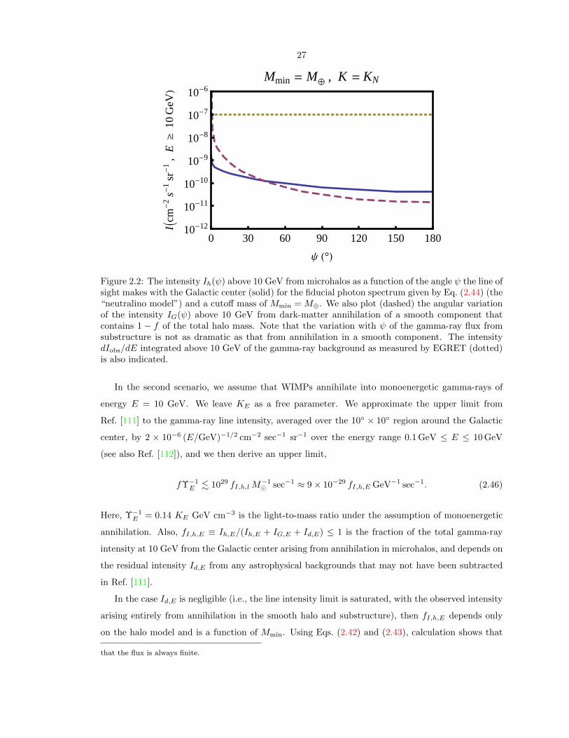
27
0 30 60 90 120 150 18010-12
10-11
10-10
10-9
10-8
10-7
10-6
Ψ H°L
IIcm-
2s-
1sr-
1,
E³
10G
eVL
Mmin = MÅ , K = KN
Figure 2.2: The intensity Ih(ψ) above 10 GeV from microhalos as a function of the angle ψ the line ofsight makes with the Galactic center (solid) for the fiducial photon spectrum given by Eq. (2.44) (the“neutralino model”) and a cutoff mass of Mmin = M⊕. We also plot (dashed) the angular variationof the intensity IG(ψ) above 10 GeV from dark-matter annihilation of a smooth component thatcontains 1 − f of the total halo mass. Note that the variation with ψ of the gamma-ray flux fromsubstructure is not as dramatic as that from annihilation in a smooth component. The intensitydIobs/dE integrated above 10 GeV of the gamma-ray background as measured by EGRET (dotted)is also indicated.
In the second scenario, we assume that WIMPs annihilate into monoenergetic gamma-rays of
energy E = 10 GeV. We leave KE as a free parameter. We approximate the upper limit from
Ref. [111] to the gamma-ray line intensity, averaged over the 10 × 10 region around the Galactic
center, by 2 × 10⁻⁶ (E/GeV)−1/2 cm−2 sec−1 sr−1 over the energy range 0.1 GeV ≤ E ≤ 10 GeV
(see also Ref. [112]), and we then derive an upper limit,
fΥ−1E . 1029 fI,h,lM
−1 sec−1 ≈ 9× 10⁻²⁹ fI,h,E GeV−1 sec−1. (2.46)
Here, Υ−1E = 0.14 KE GeV cm−3 is the light-to-mass ratio under the assumption of monoenergetic
annihilation. Also, fI,h,E ≡ Ih,E/(Ih,E + IG,E + Id,E) ≤ 1 is the fraction of the total gamma-ray
intensity at 10 GeV from the Galactic center arising from annihilation in microhalos, and depends on
the residual intensity Id,E from any astrophysical backgrounds that may not have been subtracted
in Ref. [111].
In the case Id,E is negligible (i.e., the line intensity limit is saturated, with the observed intensity
arising entirely from annihilation in the smooth halo and substructure), then fI,h,E depends only
on the halo model and is a function of Mmin. Using Eqs. (2.42) and (2.43), calculation shows that
that the flux is always finite.
28
a good estimate is given by fI,h,E ≈ 0.086 (Mmin/M⊕)−0.081
. For a given Mmin, the intensity limit
then provides an upper bound on KE ; using Eq. (2.46) gives
KE . 2× 10⁻²⁹ (Mmin/M⊕)−0.81
f(Mmin)cm3 sec−1 GeV−2. (2.47)
Thus, in this scenario we shall consider models parameterized by Mmin and KE , constrained by this
limit. We shall refer to models in this scenario as “line models”. Comparing Eq. (2.47) to Eq. (2.45),
we note that these line models may have much larger fluxes than the neutralino model.
In Sections 2.4-2.5, we shall discuss the neutralino model, using the assumed form of the photon
spectrum to predict the PDF for this fiducial model. In Section 2.6, we shall examine how observation
of the PDF may place constraints on the KE-Mmin parameter space for line models.
2.4 Calculation of the PDF
The Fermi angular resolution at energies above 10 GeV is roughly 0.1; throughout this work we
shall assume square pixels of solid angle (0.1)2. This implies that the background flux will be
measured in ∼4 × 10⁶ beams on the sky. One can then make a histogram of the number of counts
in each beam. Our goal here is to make predictions for the shape P (F ) for the distribution of these
fluxes, under the assumption that these photons come from dark-matter annihilation in a clumpy
Galactic halo.
Although P (F ) will in general be a function of the line-of-sight direction ψ, we shall suppress this
dependence in much of the presentation, reinserting it later when required for numerical results. We
also refer to all probability distribution functions as P (x); the particular function under discussion
should be clear from the argument x.
If the population of sources has a flux-density distribution P1(F ), then the probability P (F ) to
see a total flux F (integrated over all sources in the beam) in a given beam is [113]
P (F ) = F−1eµ(FP1(F )−1)
. (2.48)
Here Fx is the Fourier transform of x and F−1 its inverse, and the flux-density distribution P1(F )
is normalized to∫dF P1(F ) = 1. The quantity
µ(ψ) =Ωbeamf
〈Mh〉
∫ lc(ψ)
0
dl′ l′2ρ(r(l′, ψ)), (2.49)
is the mean number of sources in each beam of solid angle Ωbeam (in sr). We reproduce in the
Appendix the derivation of Eq. (2.48) originally provided by Ref. [113] (see also [114–117]).

29
2.4.1 Derivation of P1(F )
The first step is thus to find the flux-density distribution P1(F ) for individual sources in the beam.
This depends on the luminosity function and on the spatial distribution of microhalos. The lumi-
nosity function is P (Lh) ∝ L−αh , where again we take α = 2. The probability for an individual
microhalo to be at a distance l along a line of sight ψ is P (l, ψ) ∝ l2ρ(r(l, ψ)). We take a maximum
cutoff at lc(ψ), corresponding to a cutoff radius rc = r(lc(ψ), ψ).
We then find P1(F ) is given by
P1(F,ψ) =
∫dl dLh P (l, ψ)P (Lh)δ
(F − Lh
4πl2
)
∝∫ lc(ψ)
0
dl l4ρ(r(l, ψ)) (l2F )−αθ(4πl2F − Lmin
)θ(Lmax − 4πl2F
)
∝ F−α∫ min[lc(ψ),l(Lmax,F )]
l(Lmin,F )
dl l4−2αρ(r(l, ψ)), (2.50)
where the step functions enforce the cutoffs in P (Lh), and l(Li, F ) ≡ (Li/4πF )1/2. Note also the
implicit cutoff in P1(F ) for F < Lmin/4πl2c . Eq. (2.50) can be evaluated numerically for a given
value of the parameter Lmin = Υ−1Mmin. The result is presented in Figure 2.3 for the neutralino
model, with the fiducial cutoff mass Mmin = M⊕.
Note that Eq. (2.50) yields the familiar P1(F ) ∝ F−5/2 (conventionally written as N (> S) ∝S−3/2) for a homogeneous spatial distribution of sources with a general luminosity function, if the
condition lc(ψ) ≥ l(Lmax, F ) is satisfied over the range of F of interest. Under this condition, P1(F )
will also asymptote to F−5/2 at large F for a non-pathological spatial distribution. However, if
lc(ψ) < l(Lmax, F ) for values of F within the range of interest, then there will be a break in P1(F );
P1(F ) will tend to F−α at F for which the second condition holds, and will then tend to F−5/2 at
higher F .
For the problem under discussion, values of Lmax in the interesting regions of parameter space
are such that P1(F ) is negligible in the F−5/2 regime. Thus, the essential “large-F” dependence of
P1(F ) will be F−α.
2.4.2 Calculation of the counts distribution
The function P (F ) gives the probability to observe a flux F from annihilation in substructure.
Unlike the function P (FBG) giving the probability to observe a flux FBG from smoothly distributed
background sources (such as annihilation in the smooth component of the Galactic halo or other
diffuse backgrounds), P (F ) will not be a Poisson distribution.
We will observe these fluxes in terms of photons beam−1 year−1, or similar units. However, the
limits from EGRET require that the mean photon count per beam per year be less than one; thus,
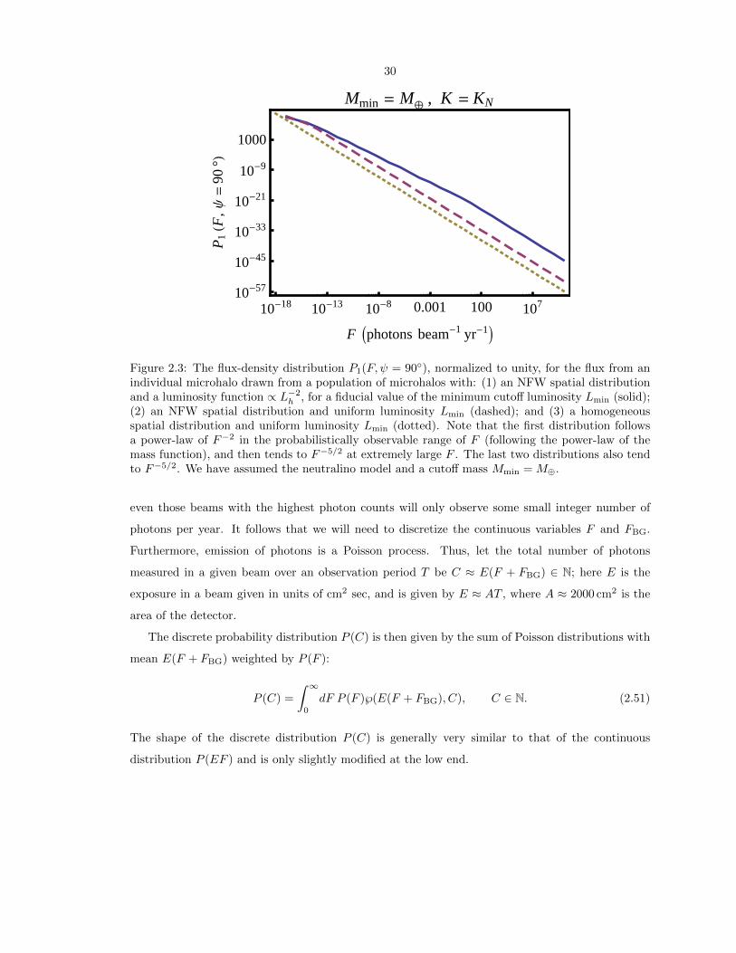
30
10-18 10-13 10-8 0.001 100 10710-57
10-45
10-33
10-21
10-9
1000
F Iphotons beam-1 yr-1M
P1HF
,Ψ=
90°L
Mmin = MÅ , K = KN
Figure 2.3: The flux-density distribution P1(F,ψ = 90), normalized to unity, for the flux from anindividual microhalo drawn from a population of microhalos with: (1) an NFW spatial distributionand a luminosity function ∝ L−2
h , for a fiducial value of the minimum cutoff luminosity Lmin (solid);(2) an NFW spatial distribution and uniform luminosity Lmin (dashed); and (3) a homogeneousspatial distribution and uniform luminosity Lmin (dotted). Note that the first distribution followsa power-law of F−2 in the probabilistically observable range of F (following the power-law of themass function), and then tends to F−5/2 at extremely large F . The last two distributions also tendto F−5/2. We have assumed the neutralino model and a cutoff mass Mmin = M⊕.
even those beams with the highest photon counts will only observe some small integer number of
photons per year. It follows that we will need to discretize the continuous variables F and FBG.
Furthermore, emission of photons is a Poisson process. Thus, let the total number of photons
measured in a given beam over an observation period T be C ≈ E(F + FBG) ∈ N; here E is the
exposure in a beam given in units of cm2 sec, and is given by E ≈ AT , where A ≈ 2000 cm2 is the
area of the detector.
The discrete probability distribution P (C) is then given by the sum of Poisson distributions with
mean E(F + FBG) weighted by P (F ):
P (C) =
∫ ∞
0
dF P (F )℘(E(F + FBG), C), C ∈ N. (2.51)
The shape of the discrete distribution P (C) is generally very similar to that of the continuous
distribution P (EF ) and is only slightly modified at the low end.
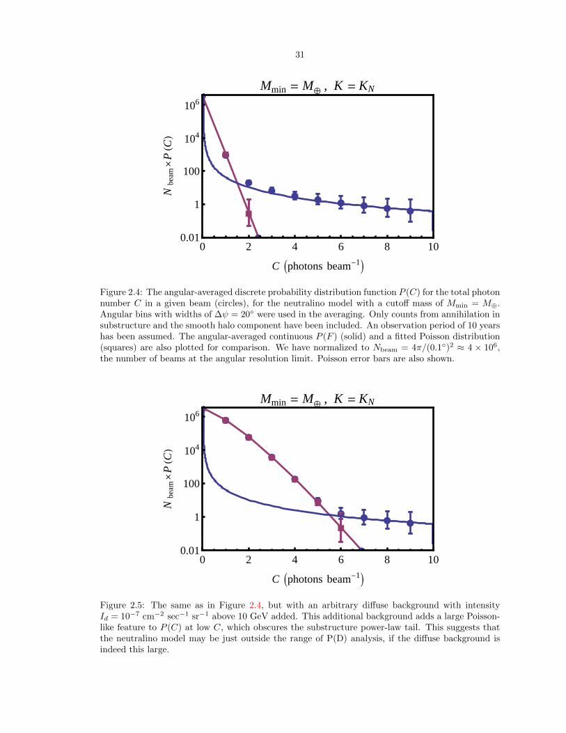
31
æ
æ
ææ
ææ
æ
æ æ æ æ
à
à
à
0 2 4 6 8 100.01
1
100
104
106
C Iphotons beam-1M
Nbe
am
PHCL
Mmin = MÅ
, K = KN
Figure 2.4: The angular-averaged discrete probability distribution function P (C) for the total photonnumber C in a given beam (circles), for the neutralino model with a cutoff mass of Mmin = M⊕.Angular bins with widths of ∆ψ = 20 were used in the averaging. Only counts from annihilation insubstructure and the smooth halo component have been included. An observation period of 10 yearshas been assumed. The angular-averaged continuous P (F ) (solid) and a fitted Poisson distribution(squares) are also plotted for comparison. We have normalized to Nbeam = 4π/(0.1)2 ≈ 4 × 10⁶,the number of beams at the angular resolution limit. Poisson error bars are also shown.
æ
æ
æ
æ
æ
æ
æ
ææ æ æ
à
à
à
à
à
à
à
0 2 4 6 8 100.01
1
100
104
106
C Iphotons beam-1M
Nbe
am
PHCL
Mmin = MÅ
, K = KN
Figure 2.5: The same as in Figure 2.4, but with an arbitrary diffuse background with intensityId = 10−7 cm−2 sec−1 sr−1 above 10 GeV added. This additional background adds a large Poisson-like feature to P (C) at low C, which obscures the substructure power-law tail. This suggests thatthe neutralino model may be just outside the range of P(D) analysis, if the diffuse background isindeed this large.
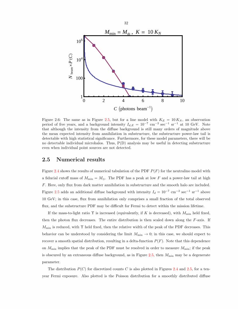
32
æ
æ
æ
æ
æ
æ
ææ
æ æ æ
à
à
à
à
à
0 2 4 6 8 101
100
104
106
C Iphotons beam-1M
Nbe
am
PHCL
Mmin = MÅ
, K = 10 KN
Figure 2.6: The same as in Figure 2.5, but for a line model with KE = 10KN , an observationperiod of five years, and a background intensity Id,E = 10−7 cm−2 sec−1 sr−1 at 10 GeV. Notethat although the intensity from the diffuse background is still many orders of magnitude abovethe mean expected intensity from annihilation in substructure, the substructure power-law tail isdetectable with high statistical significance. Furthermore, for these model parameters, there will beno detectable individual microhalos. Thus, P(D) analysis may be useful in detecting substructureeven when individual point sources are not detected.
2.5 Numerical results
Figure 2.4 shows the results of numerical tabulation of the PDF P (F ) for the neutralino model with
a fiducial cutoff mass of Mmin = M⊕. The PDF has a peak at low F and a power-law tail at high
F . Here, only flux from dark matter annihilation in substructure and the smooth halo are included.
Figure 2.5 adds an additional diffuse background with intensity Id = 10−7 cm−2 sec−1 sr−1 above
10 GeV; in this case, flux from annihilation only comprises a small fraction of the total observed
flux, and the substructure PDF may be difficult for Fermi to detect within the mission lifetime.
If the mass-to-light ratio Υ is increased (equivalently, if K is decreased), with Mmin held fixed,
then the photon flux decreases. The entire distribution is then scaled down along the F -axis. If
Mmin is reduced, with Υ held fixed, then the relative width of the peak of the PDF decreases. This
behavior can be understood by considering the limit Mmin → 0; in this case, we should expect to
recover a smooth spatial distribution, resulting in a delta-function P (F ). Note that this dependence
on Mmin implies that the peak of the PDF must be resolved in order to measure Mmin; if the peak
is obscured by an extraneous diffuse background, as in Figure 2.5, then Mmin may be a degenerate
parameter.
The distribution P (C) for discretized counts C is also plotted in Figures 2.4 and 2.5, for a ten-
year Fermi exposure. Also plotted is the Poisson distribution for a smoothly distributed diffuse

33
background of the same mean flux. As the figures indicate, the large-F power-law tail of the PDF is
qualitatively different from the exponential falloff of the Poisson distribution with F . Thus, detection
of substructure amounts to detection of such a power-law tail.
Furthermore, the power-law tail of P (F ) follows the power-law tail of P1(F ). This is simply
because single bright sources dominate beams with high F . However, as discussed in Section 2.4.1,
the power-law tail of P1(F ) in turn follows the power-law of the mass function. For example, the
power-law tail in Figure 2.4 indeed follows an F−2 dependence. Thus, P (F ) not only provides a
method of substructure detection; it can also reveal the substructure mass function.
2.6 Detectability
Figures 2.4 and 2.5 are plotted for the neutralino model in which a fiducial value of K is chosen.
This model predicts a mean flux far below the EGRET continuum limit; even Fermi may have to
observe for a period of at least ten years in order to detect significant numbers of photons in beams
in the substructure power-law tail. However, the constraint on line models given by Eq. (2.46) allows
for choices of the parameters KE and Mmin that result in mean fluxes much closer to the EGRET
line intensity limit. Line models that saturate the limit will produce signals that could be easily
detected by Fermi within a year. Figure 2.6 plots the PDF for a fiducial line model.
Of course, Fermi will also be sensitive to a range of line models predicting fluxes below the
EGRET bound. However, for line models with mean fluxes below a certain level, the amplitude
of the substructure power-law tail will so reduced that it will be impossible to detect, as it was
for the neutralino model in Figure 2.5. In this section, we determine the regions of the line model
parameter space in which the PDF can be distinguished from the Poisson distribution expected for
a completely smooth or diffuse background of the same mean flux, over an observation period of five
years. Combined with the EGRET limit, this analysis will show the region of allowed parameter
space that can be probed by study of the PDF.
We determine the signal-to-noise with which the PDF P (C) can be distinguished from the Poisson
distribution ℘ (〈C〉, C) with the same mean count rate 〈C〉. The null hypothesis of no substructure
can be eliminated at the 3σ level if S/N > 3, where
S
N=
√√√√∑
ψi
Nbeam,bin(ψi)
(S
N
)2
ψi
, (2.52)
and (S
N
)2
ψi
=
Cmax(ψi)∑
C=0
[P (C,ψi)− ℘ (〈C〉ψi , C)]2
℘ (〈C〉ψi , C). (2.53)
Here, we label the angular bins by the central value of the bin ψi. The quantity Nbeam,bin(ψi) is

34
10-4 0.01 1 1001
10
100
1000
Mmin MÅ
KE
KN
Above EGRET Limit
t100
t10
t1
SN d 3 HPoissonianL
Figure 2.7: The KE-Mmin parameter space for the line models. On the vertical axis, KE is scaledby KN , the annihilation parameter for the neutralino model given by Eq. (2.45). We indicate theregion that is already ruled out by the EGRET upper limit to the diffuse background; where therewill be & 1, & 10, and & 100 detectable point sources with flux greater than the five-year point-source sensitivity of Fermi; and where measurements of the flux PDF cannot be distinguished from aPoisson distribution, for an observation period of five years. Angular bins with widths of ∆ψ = 20
were used in the calculation of S/N, and regions near the Galactic center (ψ ≤ 30) were masked.
the number of beams contained in each bin, Cmax(ψi) is the highest count observed in each bin,
and 〈C〉ψi is the mean of the best-fit Poisson distribution in each bin. Eq. (2.52) then quantifies
the difference between the discrete probability distributions P (C,ψ) and ℘ (〈C〉ψ, C), comparing the
substructure PDF with the Poissonian distribution expected from a diffuse background (which may
have angular dependence). In Figure 2.7, we plot the regions of the KE-Mmin parameter space in
which the value of S/N indicates that substructure can be detected. Also plotted are the regions of
the parameter space ruled out already by the current EGRET upper limit to the diffuse background.
Note that in Figure 2.7, models fall in the Poissonian regime when the substructure power-law tail
at high C is obscured by the Poisson-like feature at low C; in this regime, P(D) analysis cannot be
used. Since the Poisson-like feature arises from the flux from extraneous diffuse backgrounds (from
sources other than dark matter annihilation in substructure and the smooth halo), the demarcation
of the Poissonian regime is ultimately determined by the level of these backgrounds. In determining
the Poissonian regime, we have conservatively assumed an arbitrary diffuse background of Id,E =

35
10−7 cm−2 sec−1 sr−1; in this case, the EGRET intensity limit is severely unsaturated, and only a
small fraction of the observed diffuse background arises from dark matter annihilation in substructure
and the smooth halo. In practice, the actual level of these diffuse backgrounds will determine the
Poissonian regime, which may then cover a smaller region of parameter space than the conservative
estimate presented in Figure 2.7.
Of course, detection of a nontrivial PDF is also intimately related to the criteria for detection of
point sources. The number of sources observed with flux greater than F is given by
N(≥ F ) = 2π
∫dψ sinψ
∫dLh
∫ l(Lh,F )
0
dl l2dnhdLh
(r(l, ψ), Lh). (2.54)
Examining this equation shows that N(≥ F ) is only weakly dependent on the cutoff mass Mmin.
Furthermore, since the observed microhalos essentially comprise a volume-limited sample, for KE
in the range of interest N(≥ F ) ∝ KE (at lower KE , N(≥ F ) ∝ K3/2E as expected for a flux-
limited sample). Numerical calculation of dN(≥ F )/dM shows that the observed microhalos will
predominantly be those of higher mass & 103 M; although lower-mass microhalos are far more
numerous, Fermi will not be sensitive enough to detect them individually [31].
In certain regions of the parameter space for which Figure 2.7 indicates a nontrivial PDF, sub-
structure will be detectable via detection of individual microhalos, even without a detailed analysis
of the PDF. We plot these regions, taking the Fermi five-year 5σ point-source sensitivity at 10 GeV
of F ≈ 2× 10⁻¹⁰ cm−2 sec−1 [29] (note that this sensitivity assumes the same background level as
in our determination of the Poissonian regime). The advantage of the full PDF, however, is that
substructure can be detected even in regions of parameter space where individual microhalos elude
detection. Measurement of the detailed shape of the PDF can also provide more information on the
microhalo mass function and/or spatial distribution in the halo than would be obtained simply by
point-source counts; e.g., the slope of the power-law tail in the PDF depends upon the slope of the
mass function.
Note that we could have done a similar analysis for a more general WIMP and substructure
model in which some of the parameters (e.g., annihilation cross section and spectrum, or subhalo
concentration/boost parameters) were allowed to vary. The EGRET continuum constraint allows
for a large range of such models. However, for simplicity we have only considered the parameter
space of line models and the specific substructure model assumed in Section 2.3.
2.7 Conclusions
We have proposed that the distribution of fluxes measured in individual Fermi pixels can be used to
probe the existence of substructure in the Galactic halo to very small mass scales. By characterizing

36
fluctuations in the diffuse gamma-ray background in this way, the existence of Galactic substructure
may be inferred statistically even if individual halos cannot be detected. This statistical approach
should be viewed as complementary to the use of an angular correlation function [96, 97, 100, 101].
Since the PDF is a convolution of the microhalo mass function and spatial distribution, constraints
to the parameters of these distributions may be obtained by measuring the PDF.
The full PDF we have calculated may be useful even in situations where individual microhalos
can be detected. For example, the flux in a pixel with a 3σ excess which is interpreted as detection
of a single point source may actually be due to several point sources; the probability that this is so
may be inferred from the PDF.
We have illustrated the PDF that results in a phenomenological model for substructure param-
eterized a microhalo mass cutoff Mmin, and a mass-to-light ratio Υ. This is almost certainly an
oversimplification. In more realistic models, the mass function may differ from the particular power
law we have assumed. The mass-to-light ratio may depend on the microhalo mass, and there may
even be a spread of luminosities for each mass. The spatial distribution of microhalos may not
trace the Galactic halo. Similarly, contributions to the PDF from astrophysical backgrounds (e.g.,
from cosmic-ray spallation or extragalactic sources) may need to be considered before a complete
comparison of our model predictions with data can be made [118].
In our P(D) analysis, we did not consider the dependence of the angular resolution on the
photon energy. Furthermore, we have also assumed here that each microhalo will fall within a
single resolution element of Fermi. Taking into account the finite angular size of each microhalo
will reduce the length of the power-law tails in the PDF, and will decrease the region of parameter
space in which the PDF can probe substructure. However, note that individual extended sources
will also be more difficult to detect than point sources. A generalization of Eq. (2.54) will give a
smaller number of detectable extended sources; the corresponding lines in Figure 2.7 will also shift
upwards. Thus, there will still be an appreciable region of parameter space in which the PDF can be
used to detect substructure even if individual sources cannot be detected. Moreover, a conservative
rough estimate of the size of these microhalos can be found by approximating the microhalo mass
density ρh, assuming a formation redshift of z ≈ 100 and a concentration parameter of c ≈ 1 [52].
A simple calculation then gives the angular size of the closest and most extended microhalos as
θ ≈ (fρ0/ρh)1/3 ≈ 4f1/3. Thus, if the beam size is increased such that the majority of extended
microhalos fall within a single beam, then the point source P(D) formalism presented here is roughly
valid. A more careful generalization may be required for comparison to data.
We leave the inclusion of these additional levels of complication to future work. In addition to
these future directions, one may also consider going further by combining the angular-correlation
and PDF approaches. For example, the full two-point flux probability distribution function can
be calculated and may provide additional observables with which to constrain the models or to

37
distinguish a dark-matter background from other astrophysical backgrounds. Again, this is left for
future investigation.
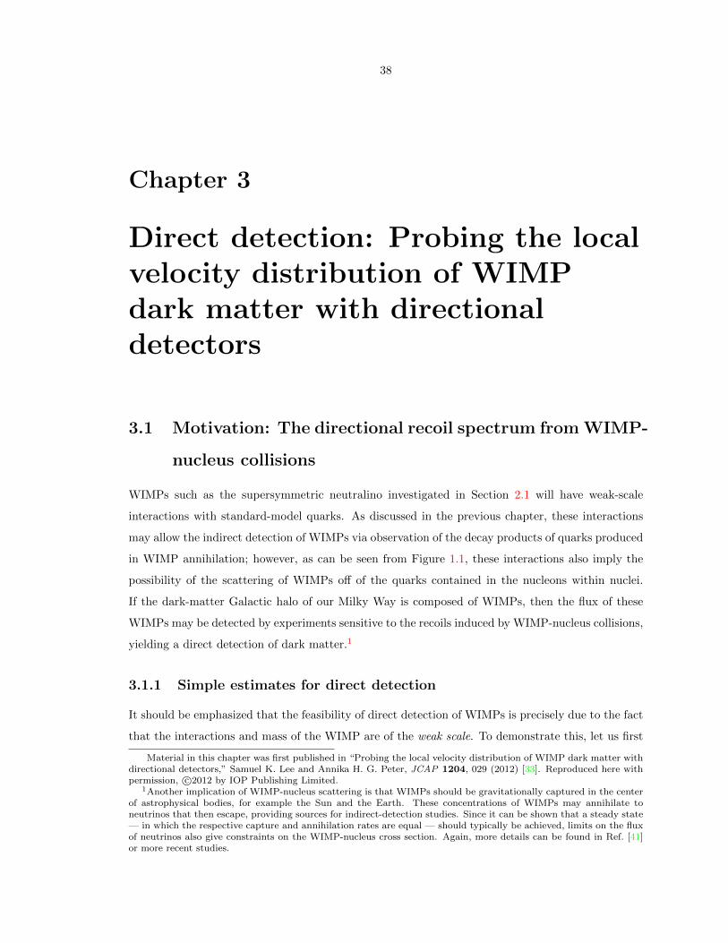
38
Chapter 3
Direct detection: Probing the localvelocity distribution of WIMPdark matter with directionaldetectors
3.1 Motivation: The directional recoil spectrum from WIMP-
nucleus collisions
WIMPs such as the supersymmetric neutralino investigated in Section 2.1 will have weak-scale
interactions with standard-model quarks. As discussed in the previous chapter, these interactions
may allow the indirect detection of WIMPs via observation of the decay products of quarks produced
in WIMP annihilation; however, as can be seen from Figure 1.1, these interactions also imply the
possibility of the scattering of WIMPs off of the quarks contained in the nucleons within nuclei.
If the dark-matter Galactic halo of our Milky Way is composed of WIMPs, then the flux of these
WIMPs may be detected by experiments sensitive to the recoils induced by WIMP-nucleus collisions,
yielding a direct detection of dark matter.1
3.1.1 Simple estimates for direct detection
It should be emphasized that the feasibility of direct detection of WIMPs is precisely due to the fact
that the interactions and mass of the WIMP are of the weak scale. To demonstrate this, let us first
Material in this chapter was first published in “Probing the local velocity distribution of WIMP dark matter withdirectional detectors,” Samuel K. Lee and Annika H. G. Peter, JCAP 1204, 029 (2012) [33]. Reproduced here withpermission, c©2012 by IOP Publishing Limited.
1Another implication of WIMP-nucleus scattering is that WIMPs should be gravitationally captured in the centerof astrophysical bodies, for example the Sun and the Earth. These concentrations of WIMPs may annihilate toneutrinos that then escape, providing sources for indirect-detection studies. Since it can be shown that a steady state— in which the respective capture and annihilation rates are equal — should typically be achieved, limits on the fluxof neutrinos also give constraints on the WIMP-nucleus cross section. Again, more details can be found in Ref. [41]or more recent studies.

39
estimate the energy deposited in a detector by a WIMP-induced nuclear recoil. Since the detector
moves (roughly) with our local standard of rest (LSR), which has a velocity vLSR ∼ 220 km/s
through the Galactic halo, the momentum of an incoming WIMP is roughly p ∼ mχvLSR. The
energy imparted to a nucleus with atomic mass A and mass mN ≈ Amp is then approximately
E ∼ p2/2mN ∼ 25 keV, if A ∼ 100, mχ ∼ 100 GeV ∼ mN, and the scattering is elastic.2 Energies
of this magnitude are accessible to detectors, via the signals that result as the recoiling nucleus
distributes its energy to the rest of the detector; such signals include ionization, scintillation, and
phonon signatures. Thus, WIMPs with weak-scale masses indeed offer the possibility of direct
detection via nuclear recoils.
However, that the energies of such recoils are detectable is moot if the recoils do not occur at an
appreciable rate; accordingly, let us now estimate the event rate of WIMP-induced nuclear recoils.
Consider the event rate observed in a detector of total mass M , composed of a total number N of
nuclei with mass mN. The WIMP number flux at the Earth is approximately ρ0vLSR/mχ, where
ρ0 ≈ 0.3 GeV/cm3 is the typical value for the local dark-matter density. Defining R as the total
event rate per detector mass M = NmN and σN as the WIMP-nucleus scattering cross section, we
then have
RM ∼ ρ0σNvLSRN
mχ(3.1)
→ R ∼ ρ0σNvLSR
mχmN(3.2)
∼ 10 kg−1yr−1
(ρ0
0.3 GeV/cm3
)(σN
pb
)(100 GeV
mχ
)(100
A
). (3.3)
Thus, we see that the event rate is non-negligible for detectors of reasonable mass if both the
WIMP mass and WIMP-nucleon scattering cross section are indeed of the weak scale. 3
2Inelastic dark matter has also been investigated [119], primarily as a possible explanation for the annual-modulation signal (which should occur as a result of the variation in the WIMP flux caused by the orbit of theEarth around the Sun) seen at high significance in the DAMA/LIBRA experiment [120]. However, models withinelastic dark matter seem to be in tension with other experiments [121], although there is still some uncertainty.
3However, we note that it is actually the fundamental WIMP-quark interactions, which give rise to these crosssections, that should be of weak-scale strength. The relations between the WIMP-nucleon cross sections σp,n, theWIMP-nucleus cross sections σN, and the fundamental WIMP-quark cross sections depend on whether the WIMP-quark interaction is spin-dependent or spin-independent. More importantly, these relations also require some consid-eration of nuclear physics — essentially, since the WIMP is nonrelativistic, its de Broglie wavelength may be largeenough to probe the entire nucleus, leading to coherent-scattering effects. For example, WIMP-nucleus cross sec-tions σN scale with A2 for a spin-independent interaction, and so heavier target nuclei are generally used to increasesensitivity; however, this effect is balanced by the loss of coherence as the nucleus increases in size, which results inform-factor suppression. Since such nuclear effects vary for different target nuclei, results in the literature are typicallystated in terms of the WIMP-nucleon cross sections σp,n to ease comparisons. For example, typical WIMP-nucleonspin-independent and spin-dependent cross sections for MSSM neutralinos may be as large as ∼10−5 pb and ∼10−3 pb,respectively, although the predictions span several orders of magnitude. Current limits from direct-detection experi-ments constrain the former to be less than ∼10−8 pb, although corresponding constraints on the latter are relativelyweak; however, as will become clear, these constraints rely on astrophysical inputs. Cross section constraints fromWIMP capture in the Sun and colliders are comparatively stringent, but are also accompanied by assumptions.
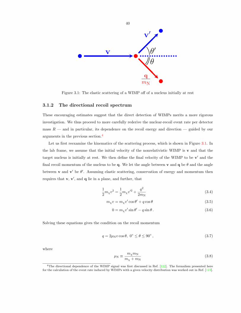
40
v
v′
qmN
θ′
θ
Figure 3.1: The elastic scattering of a WIMP off of a nucleus initially at rest
3.1.2 The directional recoil spectrum
These encouraging estimates suggest that the direct detection of WIMPs merits a more rigorous
investigation. We thus proceed to more carefully rederive the nuclear-recoil event rate per detector
mass R — and in particular, its dependence on the recoil energy and direction — guided by our
arguments in the previous section.4
Let us first reexamine the kinematics of the scattering process, which is shown in Figure 3.1. In
the lab frame, we assume that the initial velocity of the nonrelativistic WIMP is v and that the
target nucleus is initially at rest. We then define the final velocity of the WIMP to be v′ and the
final recoil momentum of the nucleus to be q. We let the angle between v and q be θ and the angle
between v and v′ be θ′. Assuming elastic scattering, conservation of energy and momentum then
requires that v, v′, and q lie in a plane, and further, that
1
2mχv
2 =1
2mχv
′2 +q2
2mN(3.4)
mχv = mχv′ cos θ′ + q cos θ (3.5)
0 = mχv′ sin θ′ − q sin θ . (3.6)
Solving these equations gives the condition on the recoil momentum
q = 2µNv cos θ, 0 ≤ θ ≤ 90 , (3.7)
where
µN ≡mχmN
mχ +mN(3.8)
4The directional dependence of the WIMP signal was first discussed in Ref. [122]. The formalism presented herefor the calculation of the event rate induced by WIMPs with a given velocity distribution was worked out in Ref. [123].
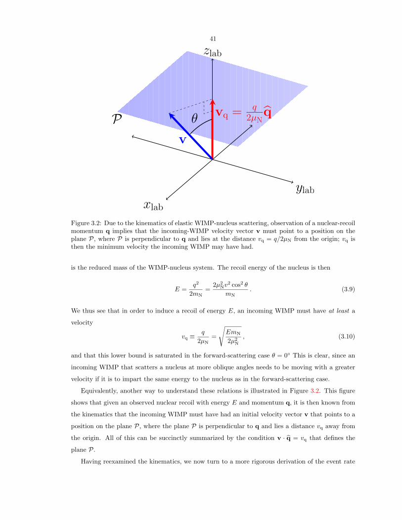
41
P
xlab
ylab
zlab
vq =q
2µNq
v
θ
Figure 3.2: Due to the kinematics of elastic WIMP-nucleus scattering, observation of a nuclear-recoilmomentum q implies that the incoming-WIMP velocity vector v must point to a position on theplane P, where P is perpendicular to q and lies at the distance vq = q/2µN from the origin; vq isthen the minimum velocity the incoming WIMP may have had.
is the reduced mass of the WIMP-nucleus system. The recoil energy of the nucleus is then
E =q2
2mN=
2µ2Nv
2 cos2 θ
mN. (3.9)
We thus see that in order to induce a recoil of energy E, an incoming WIMP must have at least a
velocity
vq ≡q
2µN=
√EmN
2µ2N
, (3.10)
and that this lower bound is saturated in the forward-scattering case θ = 0 This is clear, since an
incoming WIMP that scatters a nucleus at more oblique angles needs to be moving with a greater
velocity if it is to impart the same energy to the nucleus as in the forward-scattering case.
Equivalently, another way to understand these relations is illustrated in Figure 3.2. This figure
shows that given an observed nuclear recoil with energy E and momentum q, it is then known from
the kinematics that the incoming WIMP must have had an initial velocity vector v that points to a
position on the plane P, where the plane P is perpendicular to q and lies a distance vq away from
the origin. All of this can be succinctly summarized by the condition v · q = vq that defines the
plane P.
Having reexamined the kinematics, we now turn to a more rigorous derivation of the event rate
42
as a function of recoil energy and direction. It is clear that the energy and direction dependence will
be dictated partially by the kinematics; however, the dependence of the WIMP flux on energy and
direction will also be important. In our previous estimate of the WIMP flux, we simply assumed
that all of the incoming WIMPs had speeds roughly that of the LSR; we now relax this assumption.
Let the distribution of WIMP velocities vg in the Galactic rest frame be given by fg(vg). If we
neglect the gravitational influence of solar-system bodies, the distribution of WIMP velocities v in
the lab frame moving with velocity vlab with respect to the Galactic frame is then
f(v) = fg(v + vlab) , (3.11)
since the various velocities are related by v = vg − vlab.
We may then rewrite the simple expression in Eq. (3.2) as
dR =ρ0
mχmN
(dσ
dEdΩq(v)dEdΩq
)(vf(v)d3v
), (3.12)
making explicit the energy and direction dependence. We can further write
dσ
dEdΩq(v) =
dσ
dE
1
2πδ
(cos θ − q
2µNv
)(3.13)
=dσ
dE
v
2πδ (v · q− vq) , (3.14)
where the delta function fixes the angle θ such that it respects the kinematics, and the factor of
1/2π is simply from the symmetry in the azimuthal angle. It can then be shown that the directional
recoil rate is given bydR
dEdΩq=ρ0σNS(q)
4πmχµ2N
f(vq, q) . (3.15)
Again, R is the number of events per exposure (detector mass multiplied by time), ρ0 is the local
WIMP density, µN = mχmN/(mχ +mN) is the reduced mass of the WIMP-nucleus system, q = qq
is the lab-frame nuclear-recoil momentum, E = q2/2mN is the lab-frame nuclear-recoil energy, and
vq = q/2µN is the minimum lab-frame WIMP speed required to yield a recoil energy E. Furthermore,
we have written the WIMP-nucleus elastic cross section as dσ/dq2 = σNS(q)/4µ2Nv
2 (where S(q) is
the nuclear form factor), and
f(vq, q) =
∫δ(v · q− vq)f(v) d3v (3.16)
is the Radon transform of the lab-frame WIMP velocity distribution. In practice, it is often easier

43
to take the Radon transform of the Galactic-frame velocity distribution, and then use the relation
f(vq, q) = fg(vq + vlab · q, q) (3.17)
in Eq. (3.15) to find the directional recoil spectrum. In this work, we shall assume that the velocity of
the lab frame is given by that of the LSR; i.e., we take vlab = (vLSR, lLSR, bLSR) = (220 km/s, 90, 0)
in Galactic coordinates [124]. We shall ignore both the motion of the Earth around the Sun and the
rotation of the Earth.
Having derived the directional recoil rate, we shall now turn to a investigation of the statistical
power of experiments that may be able to measure it.
3.2 Introduction
Solid-state and liquid WIMP-dark-matter detectors designed to measure the energy of nuclear recoils
from WIMP collisions are entering maturity on both theoretical and experimental fronts. Indeed,
a large number of theoretical studies have investigated the statistical power of these experiments
to characterize WIMP dark matter [125–132]. Furthermore, a variety of experiments [133–143]
are currently running, with a few tantalizing signals already observed [144–146]. In contrast, gas
detectors with sensitivity to the nuclear-recoil direction via the measurement of ionization tracks are
still relatively nascent. Nevertheless, some theoretical studies on directional dark-matter detection
have likewise been conducted [147–162], and a small number of directional detectors are currently
under development [163–168].
A primary advantage of these directional detectors is that they allow the possibility of easily
distinguishing between terrestial background events (which should be isotropic) and WIMP-induced
recoil events (which should be non-isotropic, due to our motion through the Galactic halo, and
should additionally have diurnal and annual modulations, due to the rotation of the Earth and the
orbit of the Earth around the Sun, respectively). Perhaps even more intriguing is the possibility that
directional detectors may allow the details of the local WIMP velocity distribution to be inferred.
Theoretical expectations and N-body simulations of the Galactic halo both give us reason to believe
that even if the local spatial distribution of dark matter might be expected to be relatively smooth,
the velocity distribution may possess interesting structure. Possibilities include cold tidal streams
passing through the local solar neighborhood, a dark-matter disk aligned with the stellar disk, and
warm debris flows [169–184]. Directional-detection experiments may confirm this picture, perhaps
shedding light on not only the local velocity distribution but also the process of structure formation
on galactic scales. Furthermore, a better understanding of the dark-matter velocity distribution will

44
yield improved constraints on the particle properties of the dark matter — in particular, the WIMP
mass and the WIMP-nucleon cross section.
In this study, we explore the statistical ability of directional detectors to constrain the local WIMP
velocity distribution. The organization of the study is as follows. In Section 3.3, we discuss how a
binned likelihood analysis of the directional recoil-event data may be used to estimate the parameters
of the velocity distribution. In Section 3.4, we perform parameter estimation on simulated data sets
to demonstrate the power of these methods. We consider three specific distributions as examples: (1)
the standard halo model, (2) a halo model with an additional cold dark-matter stream component,
and (3) a halo model with an additional dark-matter disk component. We discuss implications for
future directional dark-matter-detection studies and give our conclusions in Section 3.5.
Due to their large sizes, several of the remaining tables and figures in this chapter have been
placed at the end of the chapter.
3.3 The binned likelihood function
Our ultimate goal will be to investigate the degree to which a binned likelihood analysis of observed
recoil events might recover the parameters of the dark-matter velocity distribution. Given a number
of observed events, we may construct a sky map of the data by binning both signal and background
events into Npix pixels (we shall use the pixels of equal angular area given by HEALPix [185] in
this work), as well as binning events in each pixel into Nbins energy bins (we shall also assume the
energy bins are of equal width). That is, the sky map specifies the number of observed signal and
background events Mij in the i-th pixel of solid angle dΩi and the j-th energy bin of width ∆Ej
for all Npix pixels. We use pixels and bins as a proxy for finite angular and energy resolution in the
detectors.
We would then like to construct a likelihood function that may be used to compare the observed
sky map to the predicted sky map. The predicted sky map can be specified by the total number
of events Ntot, which are observed over the energy-sensitivity range [Emin, Emax], as well as the
normalized distribution P (q, E) in angle and energy of these events. These quantities are simply
related to the direction recoil spectrum via
λNtotP (q, E) = E dR
dEdΩq, E ∈ [Emin, Emax] . (3.18)
Here, λ is related to the background-rejection power of the experiment, defined so that the number
of signal events is Nsig = λNtot and the number of background events is Nbg = (1 − λ)Ntot. The
effective exposure E gives the fraction of the total exposure Etot arising from the total mass of target
nuclei; we have implicitly assumed the detector acceptance is not energy dependent.
45
Note that the predicted angular distribution of signal events is then given by a normalized integral
over the energy-sensitivity range
P (q) =
∫ Emax
EmindE dR
dEdΩq∫dΩq
∫ Emax
EmindE dR
dEdΩq
=
∫ vq,max
vq,mindvqvqS(2µNvq)f(vq, q)
∫dΩq
∫ vq,max
vq,mindvqvqS(2µNvq)f(vq, q)
, (3.19)
where Emin = 2v2q,minµ
2N/mN and Emax = 2v2
q,maxµ2N/mN. The energy distribution P (E) of signal
events is similarly given by a normalized integral over all angles.
For a given velocity distribution, we see that the predicted mean number of signal and isotropic
background events in the i-th pixel (centered at the direction qi) and j-th energy bin is then given
by
Mij = Ntot
∫
dΩi
dΩ
∫
∆Ej
dE [λP (q, E) + (1− λ)PB(E)
4π]
≈ NtotdΩi
∫
∆Ej
dE [λP (qi, E) + (1− λ)PB(E)
4π] , (3.20)
where PB(E) is the energy distribution of the isotropic background events, normalized to unity over
the recoil-energy sensitivity range. The approximation in the second line (which approximates the
angular integral over each pixel with the value of the integrand at the center of each pixel multiplied
by the pixel size) holds in the limit that Npix is large. In each energy-binned pixel, the number
of events is Poisson distributed, so a suitable likelihood function is given by the product of the
distributions in each energy-binned pixel
L =
Npix∏
i=1
Nbins∏
j=1
℘(Mij |Mij) , (3.21)
where ℘(Mij |Mij) is the Poisson distribution function for the random variable Mij (the observed
number of events) with mean Mij (the predicted number of events, which depends on the velocity
distribution fg and the experimental conditions).
Let us now assume that the Galactic-frame velocity distribution fg depends on the model pa-
rameters θk, the measurement of which is of interest. Then the Radon transform f(vq, q) of the
lab-frame velocity distribution also depends on θk. From Eq. (3.17), we see it further depends on
vlab, which may be treated as three additional model parameters vlab, llab, blab (in Galactic coor-
dinates). Thus, it is clear that P (q, E) depends on θk and vlab. Furthermore, examining the form of
P (q, E) in Eq. (3.18), we see from Eq. (3.15) that P (q, E) additionally depends on µN (explicitly, as
well as implicitly through the dependence on vq). Therefore, it depends on the known target-nucleus
46
mass mN and the unknown WIMP mass mχ, the latter of which may be treated as yet another model
parameter we would like to measure. However, the direct dependence of P (q, E) on mχ weakens
at high values of mχ, since the dependence of µN on mχ is also weak at such values. Finally, the
background-rejection power of the detector may not be well known, so we may also treat λ as a
model parameter.
The likelihood function L can therefore be written in terms of the functions and parameters speci-
fying both the velocity distribution and the experimental conditions as L[mχ,λ,vlab,llab,blab,θk,S(q);
mN,Emin,Emax,Npix,Nbins,Ntot,PB(E)]. By assuming the forms of S(q) and PB(E), a likelihood
analysis of observed data can then be done to estimate the parameters that are unknown. In this
work, we shall take S(q) = 1 and assume that PB(E) = 1/(Emax − Emin) is a flat spectrum for
simplicity.
Note that in this treatment, we have folded all the dependence of the amplitude of the signal
Nsig = λNtot into λ. However, from Eqs. (3.15) and (3.18), it is clear that Nsig will itself depend
not only on the exposure Etot, but also on the additional, totally degenerate parameters ρ0 and
σN. If one is more interested in the particle properties of the WIMP, the usual procedure is to fix
ρ0 ≈ 0.3 GeV/cm3 (the standard estimate of the local dark-matter density, although various means
of measurement yield slightly different values [186–191]) and to treat σN as the parameter of interest.
In fact, more often the focus is placed on the WIMP-nucleon cross section σp,n; for a spin-dependent
interaction, this is related to the WIMP-nucleus cross section via
σN
σp,n=
4
3
µ2N
µ2p,n
J + 1
J
(ap〈Sp〉+ an〈Sn〉)2
a2p,n
, (3.22)
where µp,n is the WIMP-nucleon reduced mass, J is the nuclear spin, ap,n are the effective nucleon
coupling strengths, and 〈Sp,n〉 are the expectation values of the spin content of the nucleon group
[41,192].
However, it can be argued that the typical value of ρ0 ≈ 0.3 GeV/cm3 usually assumed may not
even be relevant for direction-detection experiments; it is simply a large-scale average of the dark-
matter density at the Galactic radius of the Sun r0 ≈ 8.5 kpc, and does not account for the possible
existence of substructure in the immediate neighborhood of the Earth [61, 174]. The assumption
of this typical value then strongly colors any conclusions drawn about the estimated value of σp,n.
Thus, perhaps a more assumption-independent approach would be to ask: if we have observed a
given number of events Ntot, how well can the parameters of an assumed velocity distribution be
estimated using only the distribution P (q, E) of these events? In this way, we will sidestep the issues
introduced by the degeneracy of ρ0 and σN, which are now subsumed into the single parameter λ.
47
3.4 Likelihood analyses of simulated data
We shall now explicitly demonstrate the feasibility of estimating the parameters of the velocity
distribution by performing likelihood analyses on simulated data sets. We shall consider three
parameterized velocity distributions: 1) the standard halo model, 2) a halo model with an additional
cold stream component, and 3) a halo model with a disk component. The method of analysis is as
follows. Assigning fiducial values for the velocity-distribution and experimental parameters, we first
randomly generate a number of recoil events using the procedure described in appendix C. We then
bin the simulated events in angle (using HEALPix) and in energy to create a simulated sky map.
We then use this to calculate the likelihood function, employing MultiNest [193,194] to sample the
likelihood function within the model parameter space, assuming flat priors. The getdist routine
from the CosmoMC package [195] is then used to calculate the 1D and 2D marginalized posterior
probability distributions. We also calculate the minimum credible intervals (MCIs) (as defined
in [196]) of the posterior probability distributions, and examine how well the fiducial parameters
have been recovered.
The fiducial values chosen for the velocity-distribution parameters will be discussed below for
each of the three cases. However, let us first motivate the choice of the values for the experimental
parameters. We shall perform the analyses assuming that the simulated data were collected by a
CF4 MIMAC-like experiment [163, 197–199]. That is, we assume the target nucleus is 19F , and
that the relevant WIMP-nucleus interaction is spin-dependent and can be modeled using J = 1/2,
and assuming a pure proton coupling with ap = 1, an = 0, and 〈Sp〉 = 0.5. Furthermore, we
take the energy-sensitivity range to be 5–50 keV. This range corresponds to that quoted by the
MIMAC collaboration; the 5-keV threshold arises from the ionization threshold (taking into account
quenching), while the upper bound is chosen to limit contamination from background events that
dominate the signal at higher energies. We shall take a fiducial value of mχ = 50 GeV, so we
see that the 5-keV recoil-energy threshold corresponds to a sensitivity to WIMP velocities down to
∼150 km/s.
The experimental parameters also include the angular and energy resolution. In all of the anal-
yses below in which we use directional information, we shall take the number of pixels to be the
same, setting Npix = 768 (i.e., HEALPix order 8). This roughly corresponds to the ∼10 angular
resolution expected to be attained by a MIMAC-like experiment. 5 On the other hand, we shall
investigate the effect of varying the energy resolution by considering different numbers of energy
bins Nbins for each analysis, which will be given in detail below. For now, we note that the bin
widths we shall assume are relatively large and conservative, considering that the energy resolution
5This is the expectation in the long term, and will be sufficient to begin to characterize the dark matter. However,such angular resolution is not required for the near-term exclusion or discovery of dark matter. In that case, angularresolutions of ∼20–80 might be sufficient, even if only axial directional data (without ionization-track head-tail sensediscrimination) is available [200].

48
model Npix NbinsEmin Emax Nsig Nbg Ntot
Etot Rbg(keV) (keV) (kg-yr) ([kg-yr]−1)
halo-only 768 105 50 100 0 100 4.4 0(mχ fixed) (or 1) (or 1)
halo-only 768 105 50 100 0 100 4.4 0(mχ flat prior) (or 1) (or 1)
halo-only 76810 5 50 100 100 200 4.4 23(6 parameters) (or 1)
halo+stream 768 20 5 50 650 300 950 28.9 10.4halo+disk 768 36 5 50 541 272 813 20 15halo+disk
768 40 0 50 900 300 1200 20 15(zero threshold)
Table 3.1: Experimental parameters used to simulate data for each analysis. The quoted values ofEtot and Rbg assume a CF4 detector and the typical values ρ0 ≈ 0.3 GeV/cm3 and σp,n ≈ 10−3 pb.
of the micromegas detectors used in the MIMAC experiment is expected to be ∼15%. In any case,
the exact values assumed for the angular and energy resolutions do not have a large effect on the
quality of the parameter estimation, and it can be shown that unbinned likelihood analyses yield
similar results.
Finally, there remains the question of the number of signal and background events we should
examine for each analysis. We will assume various values of Nsig and Nbg for each case, as will be
discussed and motivated below.
Values for the experimental parameters used for each analysis are summarized in Table 3.1.
Fiducial values for the velocity-distribution parameters and the flat prior ranges are summarized
in Table 3.2; we shall proceed to discuss the choice of these fiducial parameters for each velocity
distribution in detail.
3.4.1 Halo-only model
For simplicity, we shall first consider a Galactic dark-matter halo with a velocity distribution that
may be locally approximated as an isotropic Maxwellian with velocity dispersion σH, truncated at
the Galactic escape speed vesc. This truncated-Maxwellian distribution is generally referred to as
the standard halo model, and is of the form
fTMg (vg;σH, vesc) =
1
Nesc(2πσ2H)3/2
exp
(− v2
g
2σ2H
)θ(vesc − vg) , (3.23)
where
Nesc(σH, vesc) = erf
(vesc√2σH
)−√
2
π
vesc
σHexp
(− v
2esc
2σ2H
). (3.24)

49
The Radon transform of this distribution is given by
fTMg (w, w;σH, vesc) =
∫δ(vg · w − w)fTM
g (vg;σH,vesc) d3vg (3.25)
=1
Nesc(2πσ2H)1/2
[exp
(− w2
2σ2H
)− exp
(− v
2esc
2σ2H
)]θ(vesc − w) . (3.26)
The lab frame moves with respect to this velocity distribution with a velocity vlab, so as in Eq. (3.17)
we may find the Radon transform of the velocity distribution in the lab frame
fH(vq, q) = fTMg (vq + vlab · q, q;σH, vesc) , (3.27)
which yields the directional recoil spectrum via Eq. (3.15).
Note that integration of fH(vq, q) over angles gives the recoil spectrum in the usual way; this
integral takes the simple analytic form [201]
dR
dE∝√π
2√
2
σH
vlab
erf
[vq(E) + vlab√
2σH
]− erf
[vq(E)− vlab√
2σH
]− exp
(− v
2esc
2σ2H
), (3.28)
which approaches a falling exponential in the limit that vlab → 0 and vesc →∞.
For the standard halo model, we see that the set of parameters determining the Galactic-frame
velocity distribution is simply θk = σH, vesc. Here and afterwards, we shall assume vesc = 550 km/s
is known independently (and in practice, the energy-sensitivity range is such that the analysis is not
sensitive to the exact value of vesc). In total, there are then six parameters mχ, λ, vlab, llab, blab, σHthat will determine the energy and angular distribution of events. In the following analyses, we shall
consider a standard halo model with fiducial parameter values mχ = 50 GeV, vlab = 220 km/s,
llab = 90, blab = 0, σH = vlab/√
2 = 155 km/s. Note that the choice of σH = vlab/√
2 yields a ve-
locity distribution corresponding to a singular isothermal sphere, with halo profile ρ(r) ≈ ρ0(r0/r)2.
3.4.1.1 vlab-σH analyses
To first gain a qualitative and intuitive understanding of the additional power that directional
information provides, let us perform a simple illustrative exercise. Using the fiducial parameter values
defining the standard halo model above, we generate Nsig = 100 signal and Nbg = 0 background
events (i.e., we take Ntot = 100 and λ = 1). The spectrum and recoil map for these events is shown
in Figure 3.3.
We then further assume that the values of the parameters mχ, λ, llab, blab are known exactly, so
that only vlab, σH are unknown and remain to be estimated. Sampling the likelihood function over
the 2D vlab, σH parameter space using MultiNest (assuming flat priors over the ranges given
in Table 3.2), we then perform three separate likelihood analyses of these 100 events. For the first
50
analysis, we use only the energy information of the recoil events, accomplished by setting Npix = 1
and Nbins = 10. For the second analysis, we use only the directional information, setting Npix = 768
and Nbins = 1. Finally, we analyze the data using both direction and energy information, setting
Npix = 768 and Nbins = 10. Doing these three separate analyses allows us to study exactly how the
direction and energy information translate into information about vlab and σH.
The results of the three analyses are presented in the top row of Figure 3.4. We see that the
energy-only analysis yields contours for the 2D marginalized posterior probability distribution in
vlab-σH space that indicate that vlab and σH are anti-correlated. This can be understood simply by
noting from Eq. (3.28) that the dependencies of the shape of the energy spectrum on vlab and σH are
similar. Increasing the value of either vlab or σH results in a larger fraction of recoil events at higher
energies, with both actions flattening out the exponentially falling recoil spectrum; this behavior is
illustrated in Figure 3.5. Thus, the free parameters vlab and σH can only vary in a roughly inverse
manner with each other if the observed shape of the spectrum is to be maintained.
On the other hand, the direction-only analysis yields contours that indicate vlab and σH are
correlated. Again, this can be easily understood by considering the dependence of the directional
recoil map on vlab and σH, illustrated in Figure 3.6. Note that in the limit that vlab vanishes, the
recoil map becomes isotropic; conversely, it is clear that increasing the value of vlab makes the map
more anisotropic and asymmetric by increasing the enhancement in one hemisphere due to forward
scattering by incoming particles from the “WIMP wind”. In contrast, the recoil map becomes more
isotropic as σH increases and becomes much larger than vlab, since the number of incoming WIMPs
arriving in the opposite direction from the WIMP wind is then increased. We see that vlab and σH
must vary in a roughly proportional manner with each other if the observed large-scale anisotropy
of the recoil map is to be maintained.
Thus, the energy-only and direction-only analyses provide orthogonal sets of information on the
velocity and dispersion parameters. It is then easy to see how combining both sets of information
in the direction+energy analysis yields contours that demonstrate that vlab and σH are relatively
uncorrelated.
We can repeat this exercise using the same recoil-event data set, this time relaxing the assumption
that the WIMP mass mχ is known independently. We now allow mχ to be an additional free
parameter to be estimated, assuming a flat prior as shown in Table 3.2 and sampling over the 3D
mχ, vlab, σH parameter space. The results of the energy-only, direction-only, and direction+energy
analyses are shown in the bottom row of Figure 3.4. Interestingly, we see that the quality of the
contours in the energy-only analysis is severely degraded compared to the case where the mass
is known exactly, with a long, flat tail in the σH direction appearing in the posterior probability
distribution. This can be explained in a similar manner as before; allowing for decreased values
of mχ is only possible if increased values of either vlab and σH compensate to fix the observed

51
fraction of events at high energies. However, the slope of the spectrum is slightly more sensitive to
changes in σH than to changes in vlab, as can be shown by examining Eq. (3.28) (in particular, by
considering the absolute magnitude of the derivatives of dR/dE with respect to vlab and σH in the
relevant regions of parameter space). Thus, small values of mχ are more easily compensated for by
increasing σH, so a long tail appears in the σH direction.
It is notable that the analyses incorporating directional information are relatively insensitive to
the lack of prior knowledge of the WIMP mass. This again demonstrates the power and robustness
of combining directional and energy information to fix parameters of the velocity distribution.
3.4.1.2 6-parameter analyses
We now proceed to perform likelihood analyses over the full 6D standard-halo-model parameter space
of mχ, λ, vlab, llab, blab, σH. Using the same fiducial values for the velocity-distribution parameters
as before, we simulate a total of Ntot = 200 events and take λ = 0.5, corresponding to Nsig = 100
and Nbg = 100. For a MIMAC-like experiment with 10 kg of target mass, assuming a WIMP mass
mχ = 50 GeV, a typical local density ρ0 ≈ 0.3 GeV/cm3, and a spin-dependent WIMP-nucleon cross
section of σp,n ≈ 10−3 pb (consistent with current observational limits from both direct-detection
and neutrino experiments [202–204]), this number of signal events roughly corresponds to a 5-month
observation period. The number of background events then corresponds to the assumption of a
relatively high background event rate of ∼23/kg/yr (in comparison, it may be reasonable to expect
background event rates as low as 10/kg/yr [160]). We again take Npix = 768, and bin events into
Nbins = 10 energy bins. The recoil spectrum and binned recoil sky maps for the simulated data are
shown in Figures 3.7 and 3.8, respectively.
We shall perform both an energy-only (Npix = 1) analysis and a direction+energy analysis. The
results of the parameter estimation are shown in the triangle plots of the 1D and 2D marginalized
posterior probability distributions in Figures 3.9 and 3.10. Note that the 68% MCIs for each pa-
rameter are plotted there, and are also given in Table 3.2 along with the 1D marginal posterior
modes.
From the triangle plots, it is clear that the analysis incorporating the directional information is
able to recover the parameters with greater fidelity than the energy-only analysis. Not only does this
information allow for the direction (llab, blab) of the lab frame to be recovered quite accurately, it also
allows a rough measurement of the background-rejection power λ from the data itself. That is to
say, the directional information indeed allows the isotropic background component to be separated
from the anisotropic signal component. In contrast, the energy-only analysis is unable to recover
λ correctly. As we saw above, flattening of the exponentially falling spectrum may be caused
by variations in the other parameters, and cannot be easily separated from the introduction of a
truly flat background spectral component using only the energy information (at least, not without

52
improved statistics from a larger number of events).
Note also that the estimate of mχ is quite poor for both analyses, with a long tail extending to
large values of mχ. This partially stems from the fact that we are only using information from the
distribution of the events, which only has weak dependence on mχ as mχ increases, as discussed
previously. Since there is some additional dependence of the amplitude of the signal on mχ, as can be
seen from Eq. (3.15), making the aforementioned assumptions about the additional amplitude-fixing
parameters ρ0 and σN can greatly improve these estimates of mχ.
Finally, from examination of the plots for vlab and σH in Figures 3.9 and 3.10, we see that the
intuitive results about the ability to constrain these parameters from the simple 2-parameter and
3-parameter analyses are basically borne out even in the full 6-parameter analysis. However, we note
that the presence of a flat isotropic background at this level does degrade the ability to pin down
σH, even with directional information, as is evident from the long tail in the marginalized posterior
probability distribution for σH. This tail may likewise be reduced by improved statistics or better
background rejection.
To summarize, for the standard halo model, the measurement of 100 signal events (which might
be observed in a 5-month period, if the cross section is sufficiently large) recovers the direction of
the LSR and allows rough constraints to be placed on the velocity and dispersion of the Galactic
halo, the presence of a non-negligible background notwithstanding. Of course, the results may be
improved simply by lengthening the observation period; a 3-year observation period resulting in a
30-kg-yr exposure might be expected. In such a period, for the fiducial parameter values we have
assumed for the standard halo model and WIMP properties, one would expect ∼650 signal events
within the energy-sensitivity range 5–50 keV (and ∼900 total events down to zero threshold). It
is then interesting to ask whether or not any interesting structure in the local dark-matter velocity
distribution, such as cold streams or disk components, may be detected with a comparable number
of events. We shall proceed to investigate this question in the subsections to follow.
3.4.2 Halo+stream model
Motivated by the results of the simulations mentioned in Section 3.2, we next consider a model with
a local dark-matter stream in addition to the dark-matter halo. We shall assume that the velocity
distribution in the Galactic frame of a stream component is given by
fSg (vg) = fTM
g (vg − vS;σS, vesc) , (3.29)
where the velocity vector of the stream in the Galactic frame is vS (and may be indicated by its
magnitude vS and its direction (lS, bS) in Galactic coordinates) and the velocity dispersion σS is small
for a cold tidal stream. We further assume that the dark-matter particles in the stream consist of a

53
fraction AS of the total particles in both the halo and the stream locally. Using the linearity of the
Radon transform and Eq. (3.17), we find
fH+S(vq, q) = (1−AS)fTMg (vq +vlab · q, q;σH, vesc)+ASfTM
g (vq +(vlab − vS) · q, q;σS, vesc) , (3.30)
which yields the directional recoil spectrum via Eq. (3.15).
We shall assume the fiducial values of the parameters mχ, vlab, llab, blab, σH determining the
halo component of the distribution are identical to those used in the halo-only model above. For
simplicity, we shall further assume that the parameter vlab = vLSR = 220 km/s is known exactly,
so that the halo component is specified by 4 free parameters. This is done simply to differentiate
between the two Maxwellian components of the velocity distribution within the likelihood analysis,
which would otherwise be arbitrarily assigned. By fixing vlab, we can identify the “halo” as the
Maxwellian component that moves with mean velocity vlab with respect to the lab frame, while the
“stream” is identified as the secondary component. For the 5 stream parameters, we shall take the
fiducial values AS = 0.1, lS = 65, bS = 25, vS = 510 km/s, σS = 10 km/s. Including λ, the
halo+stream model is specified by 10 parameters in total.
For this halo+stream model, we shall perform only a direction+energy analysis, assuming we
have observed an number of events comparable to that expected in the baseline halo-only scenario
with a 30 kg-yr total exposure. For the experimental parameters, we adopt Npix = 768, Nbins = 20,
Ntot = 950, λ = 650/950 ≈ 0.684. This yields Nsig = 650 and Nbg = 300, roughly corresponding
to an exposure of 28.9 kg-yr and background rate of 10.4/kg/yr. These values are close to those in
the baseline model, since the 10% stream component is merely a small perturbation of the standard
halo-only model.
The recoil spectrum and sky maps for the simulated data are shown in Figures 3.11 and 3.12,
respectively. The triangle plot of the posterior probability distributions resulting from the direc-
tion+energy analysis is shown in Figure 3.13, and the posterior modes and MCIs are given in
Table 3.2. The quality of parameter estimation is quite good; with the exception of mχ, all the
parameters are recovered accurately without bias and with a low degree of correlation.
This seems to suggest that streams may be detectable with a MIMAC-like experiment. However,
let us note that we have adopted a somewhat unrealistically high stream fraction AS here (solely
for illustrative purposes, e.g., to make visible in the recoil maps in Figure 3.12 the feature arising
from the stream). More realistically, simulations suggest that typical stream fractions are more
likely at the ∼1% level, and furthermore, that the probability that a tidal stream dominates the
local neighborhood of the Sun (averaged on kpc scales) is less than 1% [174, 180]. Nevertheless,
our analysis here serves as a proof of principle for the possibility of detecting structure in the
velocity distribution beyond the standard halo model and using directional information to constrain

54
parameters. Furthermore, for a more realistic stream fraction of AS ∼ 1%, one might expect
only a ∼√
10 reduction in statistical power when constraining the stream parameters. Finally, this
result suggests that one would expect comparable — or even improved — statistical power when
constraining warm debris flows, which may have similarly large mean velocities but are thought to
compose a more significant fraction (tens of percent, becoming dominant at large velocities) of the
local dark-matter density.
3.4.3 Halo+disk model
Finally, we consider a Galactic model with a dark-matter-disk component in addition to the dark-
matter halo [173, 205]. We assume that disk rotates such that local particles in the disk move with
some average velocity vD with respect to the halo/Galactic frame; this velocity may be specified by
its magnitude vD and its direction (lD, bD) in Galactic coordinates. We shall take vD to be parallel
to vLSR, so that these particles lag the LSR by vlag = vD − vLSR; typical values from simulations
are vD ≈ 170 km/s and vlag ≈ −50 km/s, such that the dark disk rotates more slowly than the
stellar disk. We again assume that the local velocity distribution of the disk component is also a
truncated Maxwellian with dispersion σD and that particles in the disk compose a fraction AD of
the local particles, so that the disk velocity distribution is identical to that of halo+stream model
for AS, vS, σS → AD, vD, σD.We again use the fiducial values of the halo component parameters, assuming vlab = vLSR =
220 km/s is known as before. For the disk parameters, we shall take the fiducial values AD = 0.5,
lD = 90, bD = 0, vD = 170 km/s, σD = 100 km/s.6
It is clear that detecting nuclear recoils from collisions with low-velocity WIMPs in the disk
component may be challenging, since the average lab-frame speed vD = 170 km/s for such WIMPs
is close to the ∼150 km/s velocity threshold (corresponding to the 5-keV energy threshold, with our
fiducial values for mN and mχ). Therefore, to investigate the effect of the energy threshold on the
parameter estimation, we shall perform two direction+energy analyses: the first with a zero-energy
threshold, and the second with a 5-keV threshold as before.
Again, we would like to evaluate the statistical power of our halo+disk analysis, assuming we
have observed an number of events comparable to that expected in the baseline halo-only scenario
with a 30-kg-yr exposure. As mentioned previously, this baseline scenario would yield ∼900 signal
events in the 0–50-keV range, along with 300 background events (assuming the expected rate of
10/kg/yr). We therefore adopt we adopt Npix = 768, Nbins = 40, Ntot = 1200, λ = 0.75 for the
first zero-threshold analysis. For the second analysis, we then make a cut of all events below the
6Disk fractions as high as AD = 0.5 have indeed been suggested by galactic-scale simulations [173, 205], althoughrecent results find that the disk fraction in the Milky Way should be smaller (AD . 0.2) [206,207]. We take the valueAD = 0.5 here in order to investigate the difficulty of detecting a signal even in this optimistic case; as with the streamfraction, a reduction of the disk fraction would likely result in a
√N reduction in statistical power in recovering the
disk parameters.
55
5-keV threshold, resulting in Nbins = 36, Ntot = 813, λ = 541/813 ≈ 0.665. Worth mentioning
here is the fact that simulations show that the presence of a disk component enhances the local
dark-matter density over that from the halo alone, so that ρ0 → ρ0/(1−AD). This correspondingly
decreases the amount of exposure needed to reach the baseline of 900 signal events, and also allows
for a larger background rate.
The recoil spectrum and sky maps are shown in Figures 3.14 and 3.15, the triangle plots for the
zero-threshold and 5-keV-threshold analyses are shown in Figures 3.16 and 3.17, and the posterior
modes and MCIs are again given in Table 3.2. From the triangle plots, it is immediately clear that
the finite energy threshold severely restricts the ability to constrain the disk-component parameters,
even leading to multimodal posterior probabilities for some of the parameters. Even in the idealized
case of zero threshold the parameter estimation is imperfect, as is evidenced by the amount of bias
in the estimation of the disk fraction AD. Although these results may be improved with better
statistics or reduced background, it is clear that measurement of the parameters of a dark-matter
disk will be challenging with current energy thresholds, if predictions of the disk parameters from
N-body simulations are indeed valid.
3.5 Conclusions
Using binned likelihood analyses of simulated WIMP-nucleus recoil events, we have demonstrated
how detectors with directional sensitivity may place constraints on the parameters of the local
dark-matter velocity distribution. Directional sensitivity allows isotropic background events to be
distinguished from signal events, but more interestingly, it also helps to break degeneracies in the
velocity-distribution parameters that cannot be broken with spectral information alone. As an illus-
trative example, we examined the case of a Maxwellian standard-halo-model velocity distribution.
By comparing the statistical power of energy-only, direction-only, and direction+energy analyses,
we demonstrated how the degeneracy in the standard halo model between the velocity vlab of the
Earth through the halo and the halo velocity dispersion σH is broken with directional information.
If the local dark-matter density is indeed ρ0 ≈ 0.3 GeV/cm3, for a 50-GeV WIMP and a WIMP-
nucleon spin-dependent cross section of 10−3 pb, a MIMAC-like, 10-kg CF4 directional dark-matter
detector might observe several hundred WIMP-nucleus recoil events in an observation period of
3 years. With 650 signal events, the presence of a cold stream composing a fraction of the local
dark-matter density may be detected, and its properties measured with relatively good accuracy.
However, the detection of a dark-disk component requires sensitivity to WIMPs moving at relatively
low velocities, and may only be feasible if energy thresholds are improved.
We have focused on an approach that seeks to maximize the amount of information about the
velocity distribution, while minimizing the number of assumptions about the particle properties of

56
the WIMP or the local density of dark matter. The only assumptions of our approach are: 1) the
form of the velocity distribution is known and can be parameterized, 2) the background is flat and
isotropic. Future work might consider the relaxation of these assumptions. Furthermore, the analyses
presented in this work simply provide a proof of principle, showing that the parameter estimation
might be feasible in cases of interest. However, a more in-depth study of how the statistics of the
parameter estimation improve as the experimental conditions are varied might be warranted, with
the goal of finding the best balance between directional sensitivity and the overall event rate. In the
event that directional detectors do indeed detect WIMP-induced recoil events, such studies will be
crucial in forming a complete picture of the dark-matter particle and the structure of the Galactic
halo.

57
mod
elmχ
λl l
ab
b lab
v lab
σH
v esc
AC
l Cb C
v Cσ
C(G
eV)
()
()
(km
/s)
(km
/s)
(km
/s)
()
()
(km
/s)
(km
/s)
hal
o-on
ly50
190
0220
155
550
––
––
–(m
χfi
xed
)[5
0][1
][9
0]
[0]
[0,
880]
[0,
620]
[550]
––
––
–h
alo-
only
501
900
220
155
550
––
––
–(m
χfl
atp
rior
)[0
,50
0][1
][9
0]
[0]
[0,
880]
[0,
620]
[550]
––
––
–
hal
o-on
ly50
0.5
900
220
155
550
––
––
–[0
,50
0][0
,1]
[0,
180]
[-90,
90]
[0,
880]
[0,
620]
[550]
––
––
–(6
par
amet
ers,
62.5
1.00
-81.8
-33.7
168
207
––
––
––
ener
gy-o
nly
)[0
,30
0][0
.68,
1.0]
[-130,
110]
[-67,
25]
[35,
270]
[110,
400]
––
––
––
hal
o-on
ly50
0.5
900
220
155
550
––
––
–[0
,50
0][0
,1]
[0,
180]
[-90,
90]
[0,
880]
[0,
620]
[550]
––
––
–(6
par
amet
ers,
24.4
0.53
710
111.0
215
136
––
––
––
dir
ecti
on+
ener
gy)
[0,
290]
[0.4
5,0.
62]
[85,
110]
[2.5
,20]
[160,
280]
[98,
180]
––
––
––
hal
o+st
ream
500.
684
900
220
155
550
0.1
65
25
510
10
[0,
500]
[0,
1][0
,180]
[-90,
90]
[220]
[0,
620]
[550]
[0,
1]
[0,
180]
[-90,
90]
[0,
1020]
[0,
40]
(dir
ecti
on+
ener
gy)
78.4
0.64
788
.2-1
.76
–134
–0.1
18
67.1
22.9
460
13.3
[45,
200]
[0.6
1,0.
69]
[82,
97]
[-4.7
,4.2
]–
[110,
150]
–[0
.10,
0.1
5]
[59,
74]
[20,
27]
[430,
490]
[11,
15]
hal
o+d
isk
500.
665
900
220
155
550
0.5
90
0170
100
[0,
500]
[0,
1][0
,180]
[-90,
90]
[220]
[0,
620]
[550]
[0,
1]
[0,
180]
[-90,
90]
[0,
680]
[0,
400]
(dir
ecti
on+
ener
gy,
29.4
0.74
595
.35.2
9–
134
–0.6
67
95.3
-0.1
76
173
94.1
zero
thre
shol
d)
[3.9
,19
0][0
.71,
0.78
][8
5,
100]
[-2.3
,11]
–[1
10,
180]
–[0
.46,
0.7
5]
[85,
110]
[-13,
12]
[140,
200]
[92,
110]
hal
o+d
isk
500.
7590
0220
155
550
0.5
90
0170
100
[0,
500]
[0,
1][0
,180]
[-90,
90]
[220]
[0,
620]
[550]
[0,
1]
[0,
180]
[-90,
90]
[0,
680]
[0,
400]
(dir
ecti
on+
ener
gy)
23.8
0.65
992
.26.5
9–
177
–0.1
43
111
-4.2
997.1
114
[0,
59]
[0.6
0,0.
70]
[76,
100]
[-3.8
,14]
–[1
10,
240]
–[0
,0.3
8]
[-80,
-10]
[-45,
28]
[9.4
,170]
[65,
250]
[0.5
2,
0.7
7]
[62,
160]
Tab
le3.
2:F
idu
cial
par
amet
erva
lues
and
flat
pri
or
ran
ges
use
dto
sim
ula
ted
ata
an
dp
erfo
rmli
kelih
ood
an
aly
ses,
resp
ecti
vely
.M
arg
inali
zed
post
erio
rp
rob
abil
ity
mod
esan
d68
%m
inim
um
cred
ible
inte
rvals
are
als
ogiv
enin
ase
con
dse
tof
row
sfo
rth
eh
alo
-on
ly6-p
ara
met
er,
halo
+st
ream
,an
dh
alo+
dis
kan
alyse
s.P
aram
eter
sfo
rth
est
ream
an
dd
isk
com
pon
ents
(den
ote
dby
asu
bsc
rip
tC
)are
both
giv
enin
the
5le
ftm
ost
colu
mn
s.

58
0 10 20 30 40 5005
101520253035
Energy HkeVL
Eve
nts
4.50
keV
Figure 3.3: Left: Simulated recoil spectrum for the halo-only 2-parameter and 3-parameter analysesin Section 3.4.1.1, with binned signal events. The halo-only spectrum calculated from the fiducialvalues is also plotted, and is shown in solid black inside the energy sensitivity range. Right: Simulatedrecoil map for these analyses, in Mollweide projection. The black dot indicates the direction of theLSR, given in Galactic coordinates by (lLSR, bLSR) = (90, 0).
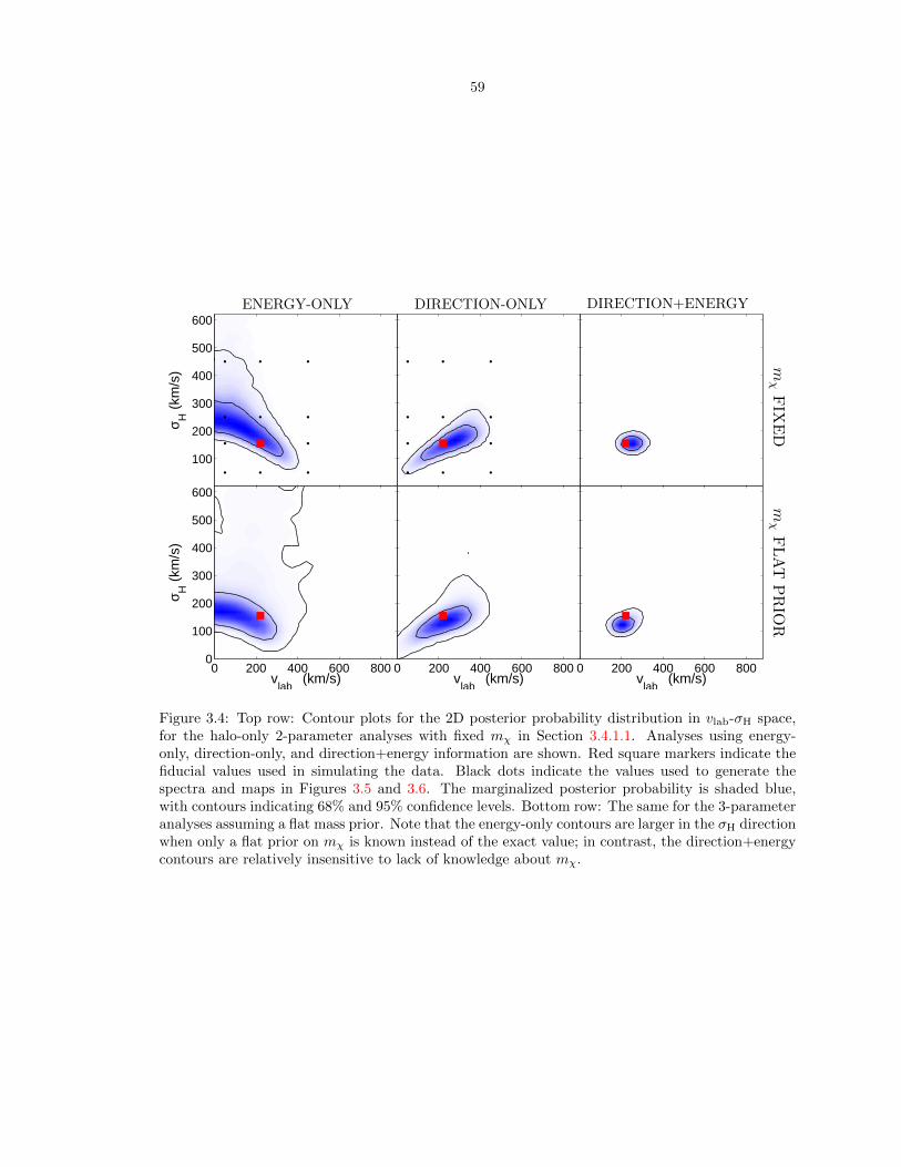
59
ENERGY-ONLY DIRECTION-ONLY DIRECTION+ENERGY
σ H (
km/s
)
100
200
300
400
500
600
mχFIX
ED
vlab
(km/s)
σ H (
km/s
)
0 200 400 600 8000
100
200
300
400
500
600
vlab
(km/s)0 200 400 600 800
vlab
(km/s)0 200 400 600 800
mχFLAT
PRIO
R
Figure 3.4: Top row: Contour plots for the 2D posterior probability distribution in vlab-σH space,for the halo-only 2-parameter analyses with fixed mχ in Section 3.4.1.1. Analyses using energy-only, direction-only, and direction+energy information are shown. Red square markers indicate thefiducial values used in simulating the data. Black dots indicate the values used to generate thespectra and maps in Figures 3.5 and 3.6. The marginalized posterior probability is shaded blue,with contours indicating 68% and 95% confidence levels. Bottom row: The same for the 3-parameteranalyses assuming a flat mass prior. Note that the energy-only contours are larger in the σH directionwhen only a flat prior on mχ is known instead of the exact value; in contrast, the direction+energycontours are relatively insensitive to lack of knowledge about mχ.
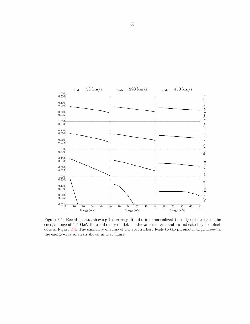
60
vlab = 50 km/s vlab = 220 km/s vlab = 450 km/s
0.0050.010
0.0500.100
0.5001.000 σ
H=
450km/s
0.0050.010
0.0500.100
0.5001.000 σ
H=
250km/s
0.0050.010
0.0500.100
0.5001.000 σ
H=
155km/s
0 10 20 30 40 500.001
0.0050.010
0.0500.100
0.5001.000
Energy HkeVL
10 20 30 40 50Energy HkeVL
10 20 30 40 50Energy HkeVL
σH=
50km/s
Figure 3.5: Recoil spectra showing the energy distribution (normalized to unity) of events in theenergy range of 5–50 keV for a halo-only model, for the values of vlab and σH indicated by the blackdots in Figure 3.4. The similarity of some of the spectra here leads to the parameter degeneracy inthe energy-only analysis shown in that figure.

61
vlab = 50 km/s vlab = 220 km/s vlab = 450 km/s
σH=
450km/s
σH=
250km/s
σH=
155km/s
σH=
50km/s
Figure 3.6: Recoil maps showing the angular distribution (normalized to unity) of events in theenergy range of 5–50 keV for a halo-only model, for the values of vlab and σH indicated in Figure 3.4.Note the correspondence between the similarity of some of the maps and the parameter degeneracyin the direction-only analysis. Note also that as vlab increases, a deficit of events at the usual peakof the distribution appears, since the most energetic foward-scattering events have energies greaterthan 50 keV at large vlab. See also the discussion in Ref. [208].

62
0 10 20 30 40 500
10
20
30
40
Energy HkeVL
Eve
nts
4.50
keV
Figure 3.7: Simulated recoil spectrum for the halo-only 6-parameter analysis in Section 3.4.1.2, withbinned signal and background events. The fiducial halo-only spectrum with a flat background isalso plotted.
Figure 3.8: Simulated recoil maps for the halo-only 6-parameter analysis in Section 3.4.1.2. Mapsof the signal events due to WIMP-induced recoils in 5 different energy bins are shown, along witha map including both signal and background events. Note that the clustering of events tightens astheir energy increases because of the kinematics of the scattering process.
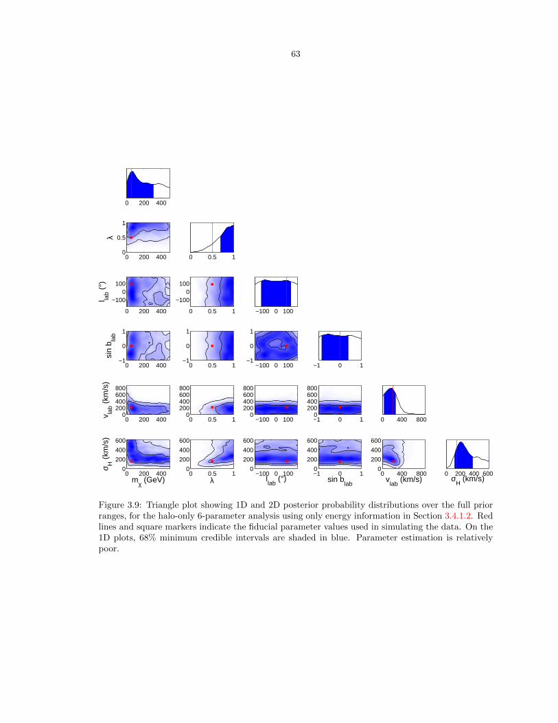
63
0 200 400
0 0.5 1
−100 0 100
−1 0 1
0 400 800
0 200 400 600σ
H (km/s)
λ
0 200 4000
0.5
1
l lab (
°)
0 200 400
−1000
100
sin
b lab
0 200 400−1
0
1
v lab (
km/s
)
0 200 4000
200400600800
mχ (GeV)
σ H (
km/s
)
0 200 4000
200
400
600
0 0.5 1
−1000
100
0 0.5 1−1
0
1
0 0.5 10
200400600800
λ0 0.5 1
0
200
400
600
−100 0 100−1
0
1
−100 0 1000
200400600800
llab
(°)−100 0 100
0
200
400
600
−1 0 10
200400600800
sin blab
−1 0 10
200
400
600
vlab
(km/s)0 400 800
0
200
400
600
Figure 3.9: Triangle plot showing 1D and 2D posterior probability distributions over the full priorranges, for the halo-only 6-parameter analysis using only energy information in Section 3.4.1.2. Redlines and square markers indicate the fiducial parameter values used in simulating the data. On the1D plots, 68% minimum credible intervals are shaded in blue. Parameter estimation is relativelypoor.

64
200 400
0 0.5 1
−100 0 100
−50 0 50
0 400 800
0 200 400 600σ
H (km/s)
λ
0 200 4000
0.5
1
l lab (
°)
0 200 400
−1000
100
b lab (
°)
0 200 400
−500
50
v lab (
km/s
)
0 200 4000
200400600800
mχ (GeV)
σ H (
km/s
)
0 200 4000
200
400
600
0 0.5 1
−1000
100
0 0.5 1
−500
50
0 0.5 10
200400600800
λ0 0.5 1
0
200
400
600
−100 0 100
−500
50
−100 0 1000
200400600800
llab
(°)−100 0 100
0
200
400
600
−50 0 500
200400600800
blab
(°)−50 0 50
0
200
400
600
vlab
(km/s)0 400 800
0
200
400
600
Figure 3.10: The same as Figure 3.9, but for the halo-only 6-parameter analysis using direc-tion+energy information in Section 3.4.1.2. Parameter estimation is much improved over the energy-only analysis.
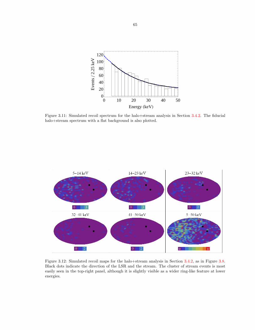
65
0 10 20 30 40 500
20
40
60
80
100
120
Energy HkeVL
Eve
nts
2.25
keV
Figure 3.11: Simulated recoil spectrum for the halo+stream analysis in Section 3.4.2. The fiducialhalo+stream spectrum with a flat background is also plotted.
Figure 3.12: Simulated recoil maps for the halo+stream analysis in Section 3.4.2, as in Figure 3.8.Black dots indicate the direction of the LSR and the stream. The cluster of stream events is mosteasily seen in the top-right panel, although it is slightly visible as a wider ring-like feature at lowerenergies.

66
020
040
0
00.
51
−10
00
100
−50
050
020
040
060
0
00.
51
−10
00
100
−50
050
050
010
00
020
40σ S
(km
/s)
λ
020
040
00
0.51
llab (°)
020
040
0
−10
0010
0
blab (°)
020
040
0
−50050
σH (km/s)
020
040
00
200
400
600
AS
020
040
00
0.51
lS (°)
020
040
0
−10
0010
0
bS (°)
020
040
0
−50050
vS (km/s)
020
040
00
500
1000
mχ (
GeV
)
σS (km/s)
020
040
002040
00.
51
−10
0010
0 00.
51
−50050
00.
51
0
200
400
600 0
0.5
10
0.51 0
0.5
1
−10
0010
0 00.
51
−50050
00.
51
0
500
1000
λ0
0.5
102040
−10
00
100
−50050
−10
00
100
0
200
400
600
−10
00
100
0
0.51
−10
00
100
−10
0010
0
−10
00
100
−50050
−10
00
100
0
500
1000
l lab (
°)−
100
010
002040
−50
050
0
200
400
600
−50
050
0
0.51
−50
050
−10
0010
0
−50
050
−50050
−50
050
0
500
1000
b lab (
°)−
500
5002040
020
040
060
00
0.51 0
200
400
600
−10
0010
0 020
040
060
0
−50050
020
040
060
00
500
1000
σ H (
km/s
)0
200
400
600
02040
00.
51
−10
0010
0 00.
51
−50050
00.
51
0
500
1000
AS
00.
51
02040
−10
00
100
−50050
−10
00
100
0
500
1000
l S (
°)−
100
010
002040
−50
050
0
500
1000
b S (
°)−
500
5002040
v S (
km/s
)0
500
1000
02040
Fig
ure
3.13
:T
rian
gle
plo
tfo
rth
eh
alo+
stre
aman
aly
sis
inS
ecti
on
3.4
.2,
usi
ng
dir
ecti
on
+en
ergy
info
rmati
on
.P
ara
met
eres
tim
ati
on
isre
lati
vely
good
.

67
0 10 20 30 40 500
20
40
60
80
100
120
140
Energy HkeVL
Eve
nts
1.25
keV
Figure 3.14: Simulated recoil spectrum for the halo+disk analyses in Section 3.4.3. The fiducialhalo+disk spectrum with a flat background is also plotted. The shaded light-blue bars indicate thebinned events below the 5-keV energy threshold included in the second 0–50-keV analysis.
Figure 3.15: Simulated recoil maps for the halo+disk analyses in Section 3.4.3, as in Figure 3.8.Black dots indicate the common direction of the LSR and the disk. Events over the full 0–50-keVenergy range are shown.

68
020
040
0
00.
51
−10
00
100
−50
050
020
040
060
0
00.
51
−10
00
100
−50
050
020
040
060
0
020
040
0σ D
(km
/s)
λ
020
040
00
0.51
llab (°)
020
040
0
−10
0010
0
blab (°)
020
040
0
−50050
σH (km/s)
020
040
00
200
400
600
AD
020
040
00
0.51
lD (°)
020
040
0
−10
0010
0
bD (°)
020
040
0
−50050
vD (km/s)
020
040
00
200
400
600
mχ (
GeV
)
σD (km/s)
020
040
00
200
400
00.
51
−10
0010
0 00.
51
−50050
00.
51
0
200
400
600 0
0.5
10
0.51 0
0.5
1
−10
0010
0 00.
51
−50050
00.
51
020
040
060
0
λ0
0.5
10
200
400
−10
00
100
−50050
−10
00
100
0
200
400
600
−10
00
100
0
0.51
−10
00
100
−10
0010
0
−10
00
100
−50050
−10
00
100
020
040
060
0
l lab (
°)−
100
010
00
200
400
−50
050
0
200
400
600
−50
050
0
0.51
−50
050
−10
0010
0
−50
050
−50050
−50
050
020
040
060
0
b lab (
°)−
500
500
200
400
020
040
060
00
0.51 0
200
400
600
−10
0010
0 020
040
060
0
−50050
020
040
060
00
200
400
600
σ H (
km/s
)0
200
400
600
0
200
400
00.
51
−10
0010
0 00.
51
−50050
00.
51
020
040
060
0
AD
00.
51
0
200
400
−10
00
100
−50050
−10
00
100
020
040
060
0
l D (
°)−
100
010
00
200
400
−50
050
020
040
060
0
b D (
°)−
500
500
200
400
v D (
km/s
)0
200
400
600
0
200
400
Fig
ure
3.16
:T
rian
gle
plo
tfo
rth
e0–
50-k
eVh
alo+
dis
kan
aly
sis
inSec
tion
3.4
.3.
Para
met
eres
tim
ati
on
isfa
ir,
bu
tso
me
of
the
dis
kp
ara
met
ers
are
reco
vere
dw
ith
less
accu
racy
.
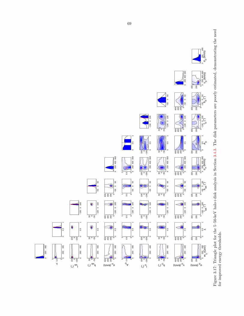
69
020
040
0
00.
51
−10
00
100
−50
050
020
040
060
0
00.
51
−10
00
100
−50
050
020
040
060
0
020
040
0σ D
(km
/s)
λ
020
040
00
0.51
llab (°)
020
040
0
−10
0010
0
blab (°)
020
040
0
−50050
σH (km/s)
020
040
00
200
400
600
AD
020
040
00
0.51
lD (°)
020
040
0
−10
0010
0
bD (°)
020
040
0
−50050
vD (km/s)
020
040
00
200
400
600
mχ (
GeV
)
σD (km/s)
020
040
00
200
400
00.
51
−10
0010
0 00.
51
−50050
00.
51
0
200
400
600 0
0.5
10
0.51 0
0.5
1
−10
0010
0 00.
51
−50050
00.
51
020
040
060
0
λ0
0.5
10
200
400
−10
00
100
−50050
−10
00
100
0
200
400
600
−10
00
100
0
0.51
−10
00
100
−10
0010
0
−10
00
100
−50050
−10
00
100
020
040
060
0
l lab (
°)−
100
010
00
200
400
−50
050
0
200
400
600
−50
050
0
0.51
−50
050
−10
0010
0
−50
050
−50050
−50
050
020
040
060
0
b lab (
°)−
500
500
200
400
020
040
060
00
0.51 0
200
400
600
−10
0010
0 020
040
060
0
−50050
020
040
060
00
200
400
600
σ H (
km/s
)0
200
400
600
0
200
400
00.
51
−10
0010
0 00.
51
−50050
00.
51
020
040
060
0
AD
00.
51
0
200
400
−10
00
100
−50050
−10
00
100
020
040
060
0
l D (
°)−
100
010
00
200
400
−50
050
020
040
060
0
b D (
°)−
500
500
200
400
v D (
km/s
)0
200
400
600
0
200
400
Fig
ure
3.17
:T
rian
gle
plo
tfo
rth
e5–
50-k
eVh
alo+
dis
kan
aly
sis
inS
ecti
on
3.4
.3.
Th
ed
isk
para
met
ers
are
poorl
yes
tim
ate
d,
dem
on
stra
tin
gth
en
eed
for
imp
roved
ener
gyth
resh
old
s.
70
Chapter 4
Collider production: Lightgravitinos at colliders andimplications for cosmology
4.1 Motivation: Supergravity and the gravitino
Stabilization of the weak scale and solving the hierarchy problem were given as the primary motiva-
tions for supersymmetry in Section 2.1. However, it was mentioned that another promising aspect
of supersymmetry is that gravity naturally arises in the theory when supersymmetry is promoted
to a local (or gauge) symmetry. We shall now heuristically examine the super-Higgs mechanism by
which this occurs.1 Interestingly enough, we shall see that a new dark-matter candidate also arises
in some theories of supergravity as the LSP — the gravitino.
4.1.1 A local U(1) symmetry
We first start with a discussion of the promotion of global symmetries to local symmetries. Before
examining how this occurs in the case of supersymmetry, let us begin by studying the more simple
case of the U(1)EM symmetry in electromagnetism. Consider the theory of a free, massless Weyl
fermion χ, which has the Lagrangian
LM = ıχ†σµ∂µχ . (4.1)
Material in Sections 4.2–4.6 was first published in “Light gravitinos at colliders and implications for cosmology,”Jonathan L. Feng, Marc Kamionkowski, and Samuel K. Lee, Phys.Rev. D82, 015012 (2010) [34]. Reproduced herewith permission, c©2010 by the American Physical Society.
1Our presentation will be largely pedagogical, relatively elementary, and rather non-rigorous, and is based in parton Refs. [39] and [209] (and references therein).

71
This Lagrangian is invariant under a global U(1) transformation of χ; that is, a transformation that
multiplies χ by a complex phase, with the form
χ→ e−ıε χ (4.2)
δχ = −ıε χ , (4.3)
leaves the Lagrangian unchanged, with the vanishing variation
δLM = 0 . (4.4)
Here, the infinitesimal parameter ε parameterizes the symmetry transformation and is a dimension-
less constant.
Let us attempt to promote this U(1) global symmetry to a U(1) local symmetry, by allowing this
parameter to depend on the spacetime position x; that is, we promote ε→ εx in Eqs. (4.2) and (4.3).
However, the Lagrangian is not invariant under this local transformation (since the derivative acting
upon χ in Eq. (4.1) also acts upon εx), and we now have an additional term in the variation,
δLM = 0 + ∂µεx Jµ , (4.5)
where the current Jµ multiplying the derivative of the transformation parameter is given by
Jµ ≡ χ†σµχ . (4.6)
Note that this current is invariant under the transformation of Eqs. (4.2) and (4.3), since the complex
phases acting on χ and its Hermitian conjugate cancel, so that
δJµ = 0 . (4.7)
Furthermore, by considering the Euler-Lagrange equations of motion it can also be shown that this
current is also conserved, so that ∂µJµ = 0.
Since now δLM 6= 0, promoting the global symmetry to a local symmetry has broken the in-
variance. However, we may restore the invariance by adding to the Lagrangian a real, vector gauge
field Aµ that couples to the current with an interaction strength determined by the dimensionless
coupling constant g,
LM = ıχ†σµ∂µχ− gAµJµ . (4.8)
Using the product rule, we see that the interaction term −gAµJµ then gives rise to two additional
72
terms in the variation,
δLM = 0 + ∂µεx Jµ
− g δAµ Jµ − g Aµ δJµ︸︷︷︸0
, (4.9)
where the last term vanishes as in Eq. (4.7). We also note here that the second-to-last term may be
viewed as arising from the variation of the Lagrangian with respect to the field Aµ,
∂LM
∂AµδAµ = −g δAµ Jµ . (4.10)
It is now clear that invariance can be restored in Eq. (4.9), provided the gauge field Aµ also
transforms as
Aµ → Aµ +1
g∂µεx (4.11)
δAµ =1
g∂µεx . (4.12)
Indeed, this is just the familiar gauge transformation of the scalar and vector potentials allowed in
electromagnetism; the gauge field Aµ is simply the photon, and the addition of its usual kinetic term
− 14FµνF
µν , which is invariant under the gauge transformation, to the Lagrangian yields Maxwell’s
equations. However, note that the mass term proportional to m2AAµA
µ for the photon is not
invariant; hence, such a mass term is not allowed in the Lagrangian, requiring that mA = 0 and that
the photon is massless. Further note that the presence of the derivative acting on the parameter
εx in the above transformation implies that the spin of the gauge field is a unit larger than that of
the parameter itself; here, the gauge field is a spin-1 vector, since the parameter is a spin-0 scalar.
From this example, we thus glean the basic principle of the “Noether method”: in order to maintain
invariance under local symmetry transformations, one may add massless gauge fields which couple
to currents in the theory so that the variation of the Lagrangian vanishes.
4.1.2 From local supersymmetry to gravity
The promotion of global supersymmetry to local supersymmetry follows analogously; we will see that
the gauge fields that must be added are the gravitino and the graviton. Let us examine the simplest
supersymmetric Lagrangian, the non-interacting Wess-Zumino model of a free, massless complex
scalar φ (with mass dimension [M ]1) and a free, massless Weyl fermion χ (with mass dimension
[M ]3/2):
LM = −∂µφ† ∂µφ+ ıχ†σµ∂µχ . (4.13)
73
We also note that the mass dimensions of LM and the derivative operator are [M ]4 and [M ]1,
respectively.
This Lagrangian is globally symmetric under a supersymmetric transformation that rotates the
bosonic φ and fermionic χ into each other, which takes the infinitesimal form
δ
φχ
=
0 ε
−ıσµε†∂µ 0
φχ
, (4.14)
where the infinitesimal parameter ε is a fermionic (anticommuting) Grassmann constant spinor with
mass dimension [M ]−1/2 and spin-1/2. The variation of the Lagrangian under this transformation
is a total derivative, so the theory is indeed globally supersymmetric. Thus, φ and χ are members
of a chiral supermultiplet.
Let us now promote the supersymmetry to a local symmetry, by again allowing the parameter ε to
be a function of space time and letting ε→ εx in Eq. (4.14). As before, as a result of the derivatives
in the Lagrangian acting on this spacetime dependence, the variation of the Lagrangian then picks
up a nonvanishing term that is proportional to the derivative of the transformation parameter,
δLM = tot. der. + (∂µεx Sµ + h.c.) , (4.15)
where the supercurrent Sµ is given by
Sµ ≡ σν σµχ∂νφ† . (4.16)
Note that the supercurrent has mass dimension [M ]7/2; furthermore, it is not invariant under the
supersymmetry transformation, as some algebra shows that
δSµ 6= 0 . (4.17)
We will shortly see that both of these facts have important consequences for the interpretation of
the locally supersymmetric theory as a theory of gravity.
Again, we try to restore invariance by adding a gravitino gauge field ψµ that couples to the
supercurrent.2 As we saw in the U(1) example, the spin of the gauge field must be a unit larger
than that of the transformation parameter εx. As a result, since εx is a spin-1/2 spinor, ψµ is
then a fermionic, spin-3/2 vectorial spinor; furthermore, since we expect ψµ to be a propagating
fermionic field, it should have mass dimension [M ]3/2. Accordingly, we couple the gravitino to the
2We shall also refer to the gravitino as G below.

74
supercurrent by adding a term to the Lagrangian
LM = −∂µφ† ∂µφ+ ıχ†σµ∂µχ−(κ ψµS
µ + h.c.), (4.18)
where the coupling κ is required to be dimensionful, with mass dimension [M ]−1, due to the mass
dimensions of ψµ and Sµ. We will see shortly that κ is related to the reduced Planck mass
M∗ = Mpl/√
8π = (8πG)−1/2, showing the connection of this theory to gravity. Indeed, gravity
is known to be non-renormalizable, as are theories with couplings of negative mass dimension such
as we have found here.
However, the similarities to gravity do not end here. We can see this by noting that the variation
of the Lagrangian does not completely vanish, even with the addition of the gravitino gauge field.
This is precisely because the supercurrent is not invariant under the supersymmetry transformation,
as claimed in Eq. (4.17), so the variation of the Lagrangian is
δLM = tot. der. + ∂µεx Sµ
− κ δψµ Sµ − κ ψµ δSµ︸︷︷︸6=0
+h.c , (4.19)
which may be contrasted with the analogous expression for the U(1) example given by Eq. (4.9).
Thus, even when we set the transformation of the gravitino gauge field to cancel the original non-
vanishing term in the variation [as we did for the photon field in Eq. (4.12)],
δψµ =1
κ∂µεx , (4.20)
the nonvanishing of the supercurrent variation δSµ prevents the restoration of local invariance.
A hint to the resolution of this problem can be found by explicitly working out the form of δSµ,
starting from Eqs. (4.14) and (4.16). To do so requires some nontrivial algebraic manipulations, but
schematically, the basic result is
−κ ψµ δSµ ∼ κ ψµσνε†xTµν + . . . , (4.21)
where we have omitted some terms for brevity. Here, Tµν is a spin-2 field with mass dimension [M ]4;
further manipulations show that Tµν can in fact be related to the canonical energy-momentum tensor
Tµν for the fields φ and χ arising due to invariance under translations in flat spacetime,
Tµν ∼ Tµν ≡ ∂LM
∂(∂µφ)∂νφ+
∂LM
∂(∂µχ)∂νχ− ηµνLM , (4.22)
up to numerical factors and divergenceless terms that may be added to ensure Tµν is symmetric and
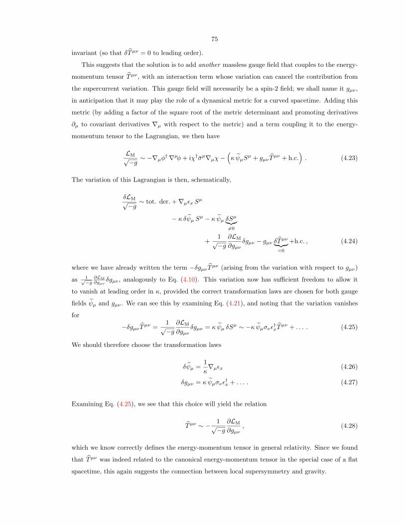
75
invariant (so that δTµν = 0 to leading order).
This suggests that the solution is to add another massless gauge field that couples to the energy-
momentum tensor Tµν , with an interaction term whose variation can cancel the contribution from
the supercurrent variation. This gauge field will necessarily be a spin-2 field; we shall name it gµν ,
in anticipation that it may play the role of a dynamical metric for a curved spacetime. Adding this
metric (by adding a factor of the square root of the metric determinant and promoting derivatives
∂µ to covariant derivatives ∇µ with respect to the metric) and a term coupling it to the energy-
momentum tensor to the Lagrangian, we then have
LM√−g ∼ −∇µφ†∇µφ+ ıχ†σµ∇µχ−
(κ ψµS
µ + gµν Tµν + h.c.
). (4.23)
The variation of this Lagrangian is then, schematically,
δLM√−g ∼ tot. der. +∇µεx Sµ
− κ δψµ Sµ − κ ψµ δSµ︸︷︷︸6=0
+1√−g
∂LM
∂gµνδgµν − gµν δTµν︸ ︷︷ ︸
=0
+h.c. , (4.24)
where we have already written the term −δgµν Tµν (arising from the variation with respect to gµν)
as 1√−g
∂LM
∂gµνδgµν , analogously to Eq. (4.10). This variation now has sufficient freedom to allow it
to vanish at leading order in κ, provided the correct transformation laws are chosen for both gauge
fields ψµ and gµν . We can see this by examining Eq. (4.21), and noting that the variation vanishes
for
−δgµν Tµν =1√−g
∂LM
∂gµνδgµν = κ ψµ δS
µ ∼ −κ ψµσνε†xTµν + . . . . (4.25)
We should therefore choose the transformation laws
δψµ =1
κ∇µεx (4.26)
δgµν = κ ψµσνε†x + . . . . (4.27)
Examining Eq. (4.25), we see that this choice will yield the relation
Tµν ∼ − 1√−g∂LM
∂gµν, (4.28)
which we know correctly defines the energy-momentum tensor in general relativity. Since we found
that Tµν was indeed related to the canonical energy-momentum tensor in the special case of a flat
spacetime, this again suggests the connection between local supersymmetry and gravity.

76
Furthermore, note that we can view Eqs. (4.26) and (4.27) as a supersymmetry transformation
relating ψµ and gµν , parameterized by εx as before; compare to Eq. (4.14). In particular, we may
introduce a propagating spin-2 graviton field hµν (i.e., one of mass dimension [M ], as appropriate
for propagating bosonic fields), defined perturbatively such that
gµν = ηµν + κhµν . (4.29)
In a sense, this graviton field, which should mediate the force of gravity, is then the superpartner of
the gravitino field ψµ; both fields can be placed in a supergravity multiplet.3
Let us summarize the progress so far. We have shown that the addition of both a spin-3/2
gravitino and a spin-2 graviton gauge field can maintain invariance under local supersymmetry. We
just showed that if the graviton is viewed as a dynamical metric, then the relation between the
Lagrangian and the energy-momentum tensor that arises is that expected from general relativity.
Earlier, we also showed that the gravitino couples to the supercurrent with an interaction strength
determined by the dimensionful coupling κ, noting that this interaction is non-renormalizable —
as we know gravitational interactions to be — due to the negative mass dimension [M ]−1 of κ.
However, we have not yet demonstrated that κ is related to the Planck mass that determines the
strength of the gravitational interaction.
This final piece of the puzzle falls into place as follows. We recall that we were allowed to add a
kinetic term for the photon gauge field to the Lagrangian in the U(1) example, since such a term was
gauge invariant. We may now add similar kinetic terms for the gravitino and the metric. For the
metric, the appropriate kinetic term is given by the usual Einstein-Hilbert action of gravity; for the
gravitino, which is a spin-3/2 fermion, the appropriate kinetic term is given by the Rarita-Schwinger
action [210]. This yields the gravitational part of the Lagrangian
LG = LEH + LRS =1
16πG
√−gR+ εµνρσψ†µσν∇ρψσ , (4.30)
where R is the Ricci scalar for the metric gµν and the covariant derivative acting on ψ includes
a spin-connection term. It is precisely the requirement that the variation of this Lagrangian also
vanish under the transformations for the gravitino and graviton given in Eqs. (4.26) and (4.27) that
sets the coupling constant
κ =1
M∗=√
8πG . (4.31)
The total Lagrangian including both the gravitational and matter components
L = LG + LM (4.32)
3More precisely, it is the vierbein eµa, related to the metric by gµν = ηabeµaeνb, that appear in the supergravity
multiplet, along with auxiliary fields.

77
then gives rise to the celebrated Einstein field equation
Gµν = Rµν −1
2gµνR = 8πGTµν (4.33)
through the usual procedure, firmly establishing the connection between local supersymmetry and
gravity.4
4.1.3 The super-Higgs mechanism
We have shown how local supersymmetry gives rise to gravity, via the introduction of massless gauge
fields — including the spin-3/2 gravitino. However, we have not yet explained how the gravitino
acquires its mass, thereby allowing it to be a dark-matter candidate. We may roughly explain the
super-Higgs mechanism by which this occurs using an analogy to the familiar Higgs mechanism that
is responsible for imparting mass to the weak gauge fields (as well as the other particles in the
standard model).
The matter Lagrangian of the electroweak theory (containing massless fermions) has a global
SU(2)L × U(1)Y symmetry that can be made local by the introduction of massless weak gauge
fields, which couple to the matter fields with interaction strengths g1,2. As we saw in Section 2.1,
we may also introduce the Higgs-field doublet and the Higgs potential. Due to the shape of the
potential, one component of the Higgs doublet then gets a weak-scale VEV v that spontaneously
breaks the local SU(2)L×U(1)Y electroweak symmetry down to U(1)EM. This produces three spin-0
Goldstone bosons, the degrees of freedom of which three of the massless spin-1 weak gauge fields
“eat” to acquire masses. This results in the massive Z and W± bosons, which thereby gain masses
that are proportional to both the interaction strengths and the VEV,
MZ,W ∼ g1,2v . (4.34)
This is the standard Higgs mechanism, by which local electroweak symmetry is spontaneously broken
and the electroweak bosons and the other particles of the standard-model acquire mass, despite the
fact that gauge-field mass terms are not allowed by the requirement of local invariance.
Analogously, as we saw in the previous section, the matter Lagrangian of a globally supersymmet-
ric theory (containing massless scalars and fermions in chiral supermultiplets) can be made locally
invariant by the introduction of a massless gravitino gauge field, which couples to the matter fields
with interaction strength suppressed by the reduced Planck mass as 1/M∗. Let us now introduce
a chiral supermultiplet of fields, one of which obtains a VEV F in superspace due to the shape of
4Again, our presentation here has been largely heuristic. To rigorously demonstrate the invariance of the totalLagrangian (including gauge supermultiplets) under local supersymmetry transformations by deriving the correcttransformation laws for the fields using the Noether method iteratively — while also maintaining covariance undergeneral coordinate transformations — is a formidable task, well beyond the pedagogical scope of this section.

78
Electroweak SU(2)L × U(1)Y Supergravity
Local symmetryδ
(νe
e−
)
L
= ı(g1ε1x + g2ε
k2xσk
)(νe
e
)
L
δ
(φ
χ
)=
(0 εx
−ıσµε†x∂µ 0
)(φ
χ
)
transformation
MasslessBµ and W k
µ (spin-1) ψµ (spin-3/2) and gµν (spin-2)gauge fields
Local Higgs: vev v super-Higgs: vev F
SSB 3 spin-0 Goldstone bosons eaten spin-1/2 goldstino fermion eaten
MassiveZµ and W±µ with MZ,W ∼ g1,2v ψµ with mG ∼ 1
M∗F
gauge fields
Table 4.1: We may understand the super-Higgs mechanism by an analogy to the familiar Higgsmechanism, since both mechanisms exhibit general characteristics of spontaneous symmetry breaking(SSB).
the potential of these fields; schematically, the VEV picks out a direction in the “boson-fermion”
space upon which supersymmetry transformations act.5 This spontaneous supersymmetry breaking
produces a spin-1/2 goldstino (a Goldstone fermion) with two degrees of freedom, which the massless
spin-3/2 gravitino gauge field eats to acquire mass. In analogy to Eq. (4.34), we may guess that the
mass of the gravitino is likewise proportional to the interaction strength and the VEV,
mG ∼F
M∗. (4.35)
This indeed happens to be the case when worked out in detail. This is therefore known as the
super-Higgs mechanism, by which local supersymmetry is broken and the gravitino acquires mass.
The analogy is summarized in Table 4.1.
Just as the VEV v sets the energy scale for electroweak symmetry breaking and the mass scale
of the particles in the weak sector, the VEV F (which has dimensions of [M ]2) sets the energy scale√F for supersymmetry breaking and the mass scale of the superpartners, msoft. However, the exact
relation between F and msoft depends on how the supersymmetry-breaking field communicates with
the superpartners. For various reasons, in the MSSM, this field cannot be one of the MSSM fields;
most likely, it should instead be a gauge singlet that does not directly (or strongly) communicate
with the fields of the standard model. Many models of supersymmetry breaking thus place the
supersymmetry-breaking field in a “hidden” sector; supersymmetry is first broken in this sector, and
5This is a rough description of simple “F -term” breaking. In F -term breaking, the VEV is actually given to anauxiliary field in the supermultiplet, not the complex scalar or the Weyl fermion. Such auxiliary fields are introducedto close the supersymmetry algebra off-shell (where the Weyl fermion gains two extra degrees of freedom), such thatthe numbers of bosonic and fermionic degrees of freedom remain equal. Auxiliary fields also appear in the superfieldand superspace formulations of supersymmetric theories. Also note that “D-term” breaking, where a VEV is givento a auxiliary component of a gauge supermultiplet, is also possible, as well as some combination of both F -term andD-term breaking.

79
then this is communicated to the MSSM via interactions common to both the hidden and MSSM
sectors.
These interactions must avoid increasing the amount of flavor violation in standard-model pro-
cesses, since flavor violation is strongly constrained by experiments. The two obvious possibilities
are gravitational interactions and the standard-model gauge interactions, since these are both indeed
flavor blind. The first possibility is thus called gravity-mediated supersymmetry breaking. Since we
require msoft to vanish in the limits F → 0 (where supersymmetry is restored) and M∗ →∞ (where
gravity is negligible), by dimensional analysis, the superpartner masses in such models must be
msoft ∼F
M∗∼ mG , (4.36)
which can be compared to the gravitino mass found in Eq. (4.35). Since the superpartner masses
should be at the weak scale, the energy scale of supersymmetry breaking is relatively high in these
models,√F ∼ 1010–1011 GeV. Furthermore, the mass of the gravitino would also be at the weak
scale and would be comparable to the masses of the superpartners; it is thus possible that the
gravitino is not the LSP in such scenarios, possibly ruling it out as a dark-matter candidate.
However, in the second possibility, supersymmetry breaking is communicated by the ordinary
standard-model gauge interactions, which also avoids flavor violation [211–216]. In such models,
mediating fields that couple the supersymmetry-breaking field in the hidden sector and also have
standard-model gauge interactions communicate the supersymmetry breaking radiatively via loop
diagrams. These “messenger” fields may have masses Mmess M∗, leading to superpartner masses
msoft ∼αi4π
F
Mmess, (4.37)
where αi/4π is a loop factor arising from the loop diagrams involving gauge interactions. Again
requiring weak-scale superpartner masses, we see that the energy scale of supersymmetry breaking√F may be low if Mmess is small; in fact, it may be as low as
√F ∼ 104 GeV, if
√F and Mmess
are comparable. Comparing with the gravitino mass given by Eq. (4.35), we see that gravitino
masses as small as an eV are possible! Thus, mG msoft may be realized in such gauge-mediated
supersymmetry breaking (GMSB) scenarios, and the gravitino may indeed be the LSP — and hence,
a dark-matter candidate.
4.1.4 Gravitino interactions
Let us now discuss the interactions between gravitinos and other particles in the MSSM. One intuitive
way to understand the interactions can be gleaned from a discussion of how supersymmetry relates
standard-model interaction vertices to their “supersymmetrized” analogues. An example of this
80
f
f
γ
QED Vertex
−→ f
f
χ0
SUSY VertexFigure 4.1: Supersymmetrization of the gauge vertex for quantum electrodynamics (on the left)implies a coupling between a neutralino, a charged fermion, and a charged sfermion (on the right).This is achieved by exchanging the photon and one of the fermions in the gauge vertex with theirsuperpartners.
supersymmetrization is shown in Figure 4.1. The basic gauge vertex, which couples the gauge field
to the matter current via a gauge-field–fermion–fermion interaction, is shown on the left; specifically,
we show the basic vertex of quantum electrodynamics (QED), which couples charged fermions to
photons. In general, supersymmetry implies that there are supersymmetrized versions of such gauge
vertices, with similar coupling strengths, which may be found by exchanging in the gauge vertex
two of the legs with their superpartners. On the right of Figure 4.1, both the gauge boson and one
of the fermions have been exchanged, yielding a supersymmetrized vertex that implies a gaugino-
fermion-sfermion coupling; in particular, the supersymmetrized QED vertex shown here implies that
a coupling between a neutralino, a charged fermion, and a charged sfermion exists.6
Thus, to find the gravitino interactions, we may similarly use this supersymmetrization procedure
on interactions involving gravitons, such as those shown on the left in Figure 4.2. Although the
complete quantum field theory involving gravitons is not known, if they are to serve as the gauge
fields that mediate the force of gravity between other particles, the effective vertices coupling the
graviton to both matter fermions and gauge bosons shown in this figure should exist, with couplings
suppressed by the Planck mass. The supersymmetrized versions of these vertices then yield the
gravitino interactions; as can be seen, the interactions are of the form gravitino-partner-superpartner,
and should also be of gravitational strength.
More rigorously, these properties of the gravitino interactions can be straightforwardly read off
from the interaction terms we derived previously. Recall that an interaction term coupling the
gravitino to the supercurrent was added to the Lagrangian to partially restore local supersymmetry
invariance. Examination of the form of the supercurrent Sµ, given in Eq. (4.16), shows that it
contains both χ and φ — i.e., both partner and superpartner; similarly, if gauge supermultiplets are
also properly accounted for, the supercurrent will also include terms containing both the gauge-boson
6Taking the rule strictly, one might take that the coupling here is to the superpartner of the photon (i.e., thephotino), but there are in fact such couplings for neutralinos in general.

81
f
f
G
Gravity Vertex
−→ f
f
G
Supergravity Vertex
γ
γ
G
Gravity Vertex
−→ χ0
γ
G
Supergravity VertexFigure 4.2: Examples of graviton (represented here by G) and gravitino (G) couplings. Top row:Supersymmetrization of the graviton-fermion coupling implies a gravitino-fermion-sfermion interac-tion. In GMSB models, this leads to τ → τG decays. Bottom row: Supersymmetrization of thegraviton-photon coupling implies a gravitino-photon-neutralino interaction. In GMSB models, thisleads to χ0 → γG decays.
partners and gaugino superpartners. It is then clear that interactions of the form gravitino-partner-
superpartner should indeed arise from the gravitino-supercurrent coupling. Furthermore, since the
coupling occurs with strength κ = 1/M∗, we should expect these gravitino interactions to be Planck-
suppressed along with the analogous graviton interactions.
One might expect that the suppression of these gravitino interactions by their Planck-mass-
scale couplings dims the prospects for interesting gravitino phenomenology. However, a subtlety
prevents the complete Planck suppression of the gravitino interactions, giving rise to the possibility
of “stronger-than-gravitational” interactions. This subtlety stems from the details of the super-
Higgs mechanism. Recall that the gravitino acquires its mass by eating the spin-1/2 goldstino
fermion G that arises when supersymmetry is broken by a field that gains a VEV F [217–220].
Another consequence of this mechanism is that an effective goldstino interaction term appears in
the Lagrangian,
LG = − 1
FG∂µSµ + h.c. (4.38)
=1
F∂µGSµ + h.c. + tot. der. , (4.39)
which exhibits a derivative coupling between the goldstino and the supercurrent; this implies in-
teractions of the form goldstino-partner-superpartner — similar to that of the gravitino interac-

82
tions — should exist. Furthermore, we see that although the strength of the coupling given by
1/F ∼ 1/M∗mG is Planck-suppressed, it is also enhanced by a factor inversely proportional to the
gravitino mass. Thus, when the gravitino eats the two degrees of freedom of the goldstino in order
to acquire mass, it inherits the stronger-than-gravitational interactions of the goldstino components.
Light gravitinos — such as those that arise in GMSB models — may then have phenomenology that
is experimentally accessible.
Let us summarize our motivations from particle physics for considering the light gravitino as
a dark-matter candidate: Weak-scale supersymmetry is one of the most promising ideas for new
physics beyond the standard model. Supersymmetric theories that incorporate local supersymmetry
(or supergravity) predict the existence of the gravitino, the spin-3/2 superpartner of the graviton.
When supersymmetry is broken, the gravitino acquires a mass through the super-Higgs mechanism,
eating the spin-1/2 goldstino, the Goldstone fermion associated with spontaneously broken local
supersymmetry. In contrast to other superpartners, the gravitino can have a mass mG that is
not at the weak scale, and viable models exist for gravitino masses as low as the eV scale and as
high as 100 TeV. In this work, we specifically consider light gravitinos, with mass in the eV to
MeV range. Such gravitinos are highly motivated in particle physics, as they emerge in models
with gauge-mediated supersymmetry breaking, in which constraints on flavor violation are naturally
satisfied. Furthermore, the interactions of such light gravitinos with other particles in the MSSM are
enhanced such that they are stronger-than-gravitational, giving rise to the possibility of interesting
phenomenology.
We now turn to a study of the collider phenomenology of light gravitinos and the cosmological
implications that observation of gravitino signals might have for the early Universe.
4.2 Introduction
Although highly motivated from a particle-physics standpoint alone, light gravitinos with mass
in the eV to MeV range also have cosmological motivations. In particular, they are the original
supersymmetric dark-matter candidate [221]. Assuming a high reheating temperature, gravitinos
are initially in thermal equilibrium and then freeze out while still relativistic. As we discuss in detail
below, their resulting relic density is
ΩGh2 ≈
[ mG
1 keV
] [106.75
g∗S,f
], (4.40)
where g∗S,f is the number of relativistic degrees of freedom at freeze-out, and has been normalized
to the total number of degrees of freedom in the standard model. When originally proposed in
83
the 1980s, uncertainties in h and the total matter relic density allowed mG ∼ keV. This led to a
simple and attractive gravitino-dark-matter scenario, consistent with standard big bang cosmology,
in which the Universe cooled from some high temperature, and keV gravitinos froze out and now
form all of the dark matter.
In the intervening years, however, a variety of astrophysical constraints have greatly complicated
this picture. First, the dark-matter relic density is now known to be ΩDMh2 ≈ 0.11. Second,
constraints on structure formation, as probed by galaxy surveys and Lyman-α forest observations,
require that the bulk of dark matter be cold or warm [222]. As we will discuss more fully below,
this leads to three scenarios of interest:
1. mG . 15–30 eV: Gravitinos are produced by the standard cosmology leading to Eq. (4.40);
they are hot dark matter, but their contribution is small enough to be consistent with the
observed small-scale structure. Some other dark-matter particle is required.
2. 15–30 eV . mG . few keV: Nonstandard cosmology and a nonstandard gravitino production
mechanism are required, both to avoid overclosure and to cool the gravitinos to satisfy small-
scale-structure constraints. Some other dark-matter particle may be required.
3. mG & few keV: Nonstandard cosmology is required to dilute the thermal relic density of
Eq. (4.40). Gravitinos produced by thermal freeze-out are cold enough to be all of the dark
matter.
Note that the original “keV gravitino” scenario, previously favored, is now the most disfavored, in
the sense that it is excluded by both overclosure and small-scale-structure constraints. All of the
possibilities are rather complicated, however, as in each case, some additional physics is required,
either to provide the rest of the dark matter or to modify the history of the early Universe to allow
gravitinos to be all of the dark matter.
In this study, we discuss how collider data may help clarify this picture. Light gravitinos are
primarily produced at colliders in the decays of the next-to-lightest supersymmetric particle (NLSP).
It is a remarkable coincidence that modern particle detectors, with components placed between 1 cm
to 10 m from the beamline, are beautifully suited to distinguish between the NLSP decay lengths
predicted in scenarios 1, 2, and 3. For example, the decay length of a bino NLSP decaying to a
gravitino is [223]
cτ ≈ 23 cm[ mG
100 eV
]2 [100 GeV
mB
]5
. (4.41)
This implies that scenarios 1, 2, and 3 make distinct predictions for collider phenomenology, and the
identification of the gravitino collider signatures realized in nature may have far-reaching implications
for the early Universe.
Of course, this requires that gravitinos can be produced in sufficient numbers and distinguished
from standard-model backgrounds. In this work, we determine event rates for a variety of signatures,
84
including prompt di-photons and delayed and nonpointing photons (relevant for neutralino-NLSP
scenarios), as well as kinked charged tracks and heavy metastable charged particles (relevant for
stau-NLSP scenarios). We present results for an assumed final Tevatron dataset (20 fb−1 of 2 TeV
pp collisions), an early LHC dataset (1 fb−1 of 7 TeV pp collisions), and a future LHC dataset
(10 fb−1 of 14 TeV pp collisions). We find that the final Tevatron and early LHC data have roughly
equivalent sensitivity to these events, with both capable of seeing hundreds of distinctive light-
gravitino events. The full LHC data greatly extends the reach in parameter space, and may also
allow precision measurements of NLSP lifetimes and gravitino masses.
We begin in Section 4.3 by reviewing the cosmological bounds on light gravitinos and discussing
how these bounds are relaxed in early-Universe scenarios that differ from the canonical one. In Sec-
tion 4.4 we then discuss NLSP decays to gravitinos, GMSB models, and current collider constraints.
In Section 4.5 we present our results for the number of light-gravitino events at colliders, based on
collider simulations, and discuss the cosmological implications. We summarize our conclusions in
Section 4.6.
Due to their large sizes, several of the remaining figures in this chapter have been placed at the
end of the chapter.
4.3 Light-gravitino cosmology
4.3.1 Canonical scenario
4.3.1.1 Relic abundance
In the currently canonical scenario, after inflation, the Universe is reheated to a temperature TR that
is assumed to be far higher (e.g., 1012 or 1015 GeV) than the weak scale. During this phase, inelastic
scattering processes and decays can convert standard-model particles in the thermal bath into grav-
itinos [224–228]. The rate CG per unit volume for production of light gravitinos (strictly speaking,
only the spin-1/2 goldstino components) can be calculated by considering all such processes, which
primarily involve strong [229] and electroweak gauge bosons [230, 231], as well as top quarks [232].
The total result, valid in the limit T mSUSY, where mSUSY is the scale of the superpartner masses,
is [232]
CG ≈ 15m2g
m2G
T 6
M2pl
, (4.42)
where Mpl ≈ 1.2× 10¹⁹ GeV is the Planck mass. Here we have assumed that the gaugino masses
mg,1, mg,2, and mg,3 and the trilinear scalar coupling At are at a common mass scale. For simplicity,
we have set them equal to a universal gaugino mass mg.
The evolution of the gravitino number density nG via these production processes, and their

85
inverses, is governed by the Boltzmann equation
dnGdt
+ 3HnG = CG − ΓnG , (4.43)
where H is the Hubble expansion rate and Γ is the rate of processes that annihilate gravitinos. The
3HnG term accounts for dilution of the number density due to cosmological expansion. If Γ H,
gravitinos are in thermal equilibrium, ΓnG = CG, and their number density (the solution to the
Boltzmann equation) is
neq
G= g
3ζ(3)
4π2T 3 ≈ 0.18T 3 . (4.44)
Here we used g = 2, since it is primarily the spin-1/2 goldstino components that are produced
thermally. 7
The rate Γ at which a given gravitino is destroyed in the plasma is then
Γ =CGneq
G
≈ 80m2gT
3
m2GM2
pl
. (4.45)
Since Γ ∝ T 3 and H ∝ T 2, the ratio Γ/H ∝ T is largest at the highest temperatures. Thus, if
Γ(TR) & H(TR) at reheating, then gravitinos come into thermal equilibrium shortly after reheating.
During this era, the expansion rate is given by H ≈ 1.66 g1/2∗ T 2/Mpl; assuming reheating tempera-
tures TR TeV, at which all particles in the minimal supersymmetric standard model (MSSM) are
relativistic, we set the number g∗ of relativistic degrees of freedom to g∗(TR) ≈ 228.75. Comparing
Γ(TR) and H(TR), we then see that if the reheating temperature satisfies
TR & Tf ≡ 4 GeV[mG
keV
]2 [TeV
mg
]2
, (4.46)
then gravitinos come into thermal equilibrium after reheating. Recalling that the production rate,
Eq. (4.42), used here is valid only for T mNLSP (i.e., T & 10 TeV), we conclude that for weak-scale
gluino masses, light gravitinos with mG . MeV will come into thermal equilibrium if the reheating
temperature is TR & 4× 10⁶ GeV.
The creation/annihilation rates for gravitinos at temperatures T . 10 TeV have not yet been
calculated, and so the precise temperature at which gravitinos freeze out (which occurs when Γ ≈ H)
cannot yet be determined. Still, gravitinos are produced and destroyed individually, requiring (from
R-parity conservation) that each creation/destruction is accompanied by creation/destruction of
some other supersymmetric particle. Therefore, the freeze-out temperature Tf cannot be much
lower than the mass mNLSP of the NLSP, as the equilibrium abundance of SUSY particles then
7This expression has been corrected from the published version, where the number density n = gζ(3)T 3/π2 ≈0.24T 3 for relativistic Bose-Einstein particles was mistakenly used (and a typo added an extra factor of 2 in the firstequality). This also results in minor corrections to the numerical prefactors that follow.
86
decreases exponentially. We thus conclude that the freeze-out temperature for light gravitinos falls
roughly in the range 10 GeV . Tf . 10 TeV.
With this range of freeze-out temperatures, Tf mG, so gravitinos are relativistic when they
freeze out. The relic gravitino density is then [221]
ΩGh2 ≈ 0.1
[ mG
100 eV
] [106.75
g∗S,f
], (4.47)
the standard result for hot relics with g = 2, where g∗S,f is the number of relativistic degrees of
freedom when the gravitinos freeze out. If gravitinos freeze out when all of the MSSM degrees of
freedom are relativistic, Tf mSUSY, and g∗S,f = 228.75. However, it is more likely that freeze-out
occurs at T ∼ mNLSP ∼ 100 GeV, when g∗S,f ∼ 100 [233].
4.3.1.2 Cosmological constraints
Given that current cosmic-microwave-background and structure-formation measurements constrain
the density of dark matter to be ΩDMh2 ≈ 0.11, Eq. (4.47) implies an upper bound mG . 200 eV.
The upper limit mG ≈ 200 eV is saturated if the gravitino makes up all of the dark matter and freeze-
out occurs when g∗S,f = 228.75 is the maximum value allowed in the MSSM. However, a gravitino
of this mass would be hot dark matter. It would smooth density perturbations on scales probed
by galaxy surveys and the Lyman-α forest to a degree that is highly inconsistent with data. As
mG is reduced from this upper limit, the smoothing scale is increased (the gravitinos get “hotter”),
but the gravitino abundance is reduced, thus making the magnitude of the smoothing smaller. A
combination of data from the cosmic microwave background, galaxy surveys, and the Lyman-α
forest constrain the contribution of a hot component of dark matter to be . 15% [222], implying
for g∗S,f ≈ 100 that mG . 15 eV. This suggests that the most conservative upper bound is given
by mG . 30 eV, in the case that g∗S,f ≈ 200 approaches the maximal value allowed in the MSSM.
Therefore, in this canonical scenario, thermal gravitinos with mass less than 30 eV make up only a
fraction of the dark matter, thus requiring some other particle to be the cold dark matter. This is
the first cosmological scenario listed in Sec. 4.2.
We conclude by noting that future astrophysical data are likely to improve. And while the
current sensitivity is to gravitino masses as small as 15–30 eV, it is forecast that next-generation
experiments may be sensitive to gravitino masses as small as 1 eV [234]. A collider detection of a
gravitino in the mass range mG = 1–30 eV would thus lead to testable consequences in forthcoming
cosmological data.

87
4.3.2 Nonstandard early-Universe scenarios
There are several ways in which the early-Universe production of relic gravitinos could differ from
the canonical scenario outlined above. Thus, there are scenarios in which a gravitino of mass
mG & 30 eV, ruled out in the canonical model, could be cosmologically consistent or, better yet,
completely compose the dark matter.
Let us first consider scenarios in which the gravitinos reach thermal equilibrium in the early
Universe, since most observational constraints are strictly valid only under this assumption. As
mentioned above, if we only consider particles in the MSSM, then g∗S,f ≤ 228.75, and Eq. (4.47)
suggests an upper limit of mG . 200 eV from the relic abundance constraint. One way to evade this
limit is to simply consider higher values of g∗S,f ; i.e., gravitinos decouple and freeze out earlier than
in the canonical scenario. This may be possible in models with more degrees of freedom than the
MSSM. More massive gravitinos that decouple earlier may then be viable, if they have an abundance
that obeys the constraint ΩDMh2 . 0.11.
It is possible that this constraint is saturated and that these heavier gravitinos entirely com-
pose the dark matter. Of course, we must still require that these heavier gravitinos are not so
hot as to erase structure to a degree that contradicts observations. The same combination of
cosmic-microwave-background, galaxy-survey, and Lyman-α–forest data that was used to constrain
mG . 30 eV in the canonical scenario can also be used to constrain the gravitino mass in this early-
decoupling scenario, assuming that thermal gravitinos make up all of the dark matter. With this
assumption, Ref. [222] finds mG & 550 eV, using a selection of Lyman-α data. The same authors
later find a stronger constraint, mG & 2 keV, with SDSS Lyman-α data [235, 236], a result slightly
weaker than a bound on warm dark-matter models obtained by Ref. [237]. A number of other
small-scale observations also seem to support that mG & few keV under these assumptions [23].
We thus conclude that if 30 eV . mG . few keV, then thermal gravitinos are too warm to be the
only component of the dark matter, regardless of whether or not they have the correct abundance.
Gravitinos in this mass range would only be viable if some other nonstandard early-Universe process
cools them, or if there is an additional cold component. This is the second scenario mentioned in
Sec. 4.2. However, if mG & few keV, then gravitinos may be sufficiently cold, and may in early-
decoupling scenarios have the right abundance, to be the dark matter. This is the third scenario
outlined in Sec. 4.2.
Of course, aside from early decoupling, there are other nonstandard mechanisms that can reduce
the gravitino abundance. For example, recall that we have no empirical constraints to the early
Universe prior to the epoch of big-bang nucleosynthesis (BBN), at which T & few MeV [238]. Thus,
some entropy-producing process prior to BBN could also dilute the gravitino abundance. It is
possible that there may be some exotic early-Universe physics that conspires to produce the same
effect. One relatively simple possibility is that the reheating temperature is low. If the reheating

88
temperature is smaller than the freeze-out temperature, then gravitinos will never come into thermal
equilibrium, and their relic abundance will thus be accordingly smaller [239–245]. The only catch
is that for the light gravitinos we consider here, the reheating temperature must be unusually low
for this to occur. For example, if mG = keV and mg = 300 GeV, then Eq. (4.46) suggests that
the reheating temperature must be TR . 40 GeV. However, recall that this estimate may not be
strictly valid at T . 10 TeV, as we have already noted. Thus, a more careful calculation of the
production rate of light gravitinos at low reheating temperatures may be necessary. Nevertheless,
such low reheating temperatures have been considered [246], and Ref. [247] has examined an explicit
low-reheat scenario in which a gravitino of mass mG = 1–15 keV can have the right abundance to
be the dark matter.
Finally, we also note that there may be additional mechanisms affecting the generation of graviti-
nos. For example, in our discussion we have neglected the nonthermal contribution to the gravitino
abundance from out-of-equilibrium decays of other supersymmetric particles. There may also be
other significant modes of gravitino production or dilution, including processes involving the messen-
ger particles responsible for GMSB [248–253], nonthermal production via oscillations of the inflaton
field [254], Q-ball decays [255], and various other mechanisms [256]. There may thus be other reasons
why the gravitino abundance or temperature differs from those in the canonical thermal-production
scenario; this may be true even if mG . 30 eV.
To summarize, in the canonical model, gravitinos are required to have mass mG . 30 eV and
form only a fraction of the dark matter. Gravitinos with mass range mG & 30 eV would require non-
standard physics or cosmology to reduce their abundance or temperature to agree with observations.
Below we discuss collider signatures of light gravitinos. We close here by noting that such collider
data may, if gravitinos are discovered, thus help discriminate between the diversity of early-Universe
scenarios for gravitino production.
4.4 Light gravitinos at colliders
4.4.1 Mass and interactions
As discussed in Section 4.1, the gravitino mass is determined by the super-Higgs mechanism. In
simple models, it is given in terms of the supersymmetry-breaking scale F , which has mass dimension
2, as
mG =F√3M∗
≈ 240 eV
[ √F
103 TeV
]2
, (4.48)
where M∗ ≡Mpl/√
8π ≈ 2.4× 10¹⁸ GeV is the reduced Planck mass.
The interactions of weak-scale gravitinos are of gravitational strength, as expected since they
are the superpartners of gravitons. However, as discussed previously, the couplings of the goldstino
89
are proportional to 1/F [257, 258]. The interactions of light gravitinos are therefore dominated by
their goldstino components, and may be much stronger than gravitational. Decays to gravitinos are
faster for light gravitinos.
For reasons to be discussed below, we will focus on cases where the NLSP is either the neutralino
or the stau. The interactions of these NLSPs with the gravitino were previously shown in Figure 4.2.
For a neutralino NLSP that is dominantly a bino, the decay widths to gravitinos are [223,259]
Γ(B → γG) =cos2 θWm
5B
16πF 2(4.49)
Γ(B → ZG) =sin2 θWm
5B
16πF 2
[1− m2
Z
m2B
]4
, (4.50)
where θW is the weak mixing angle. For mB . mZ , decays to Z bosons are negligible or kinematically
forbidden, and the corresponding decay length is
cτ ≈ 23 cm[ mG
100 eV
]2 [100 GeV
mB
]5
. (4.51)
For heavier neutralinos, the Z mode may be significant; for very heavy binos, the branching ratio
for this mode is B(Z) ≈ sin2 θW ≈ 0.23. Decays to l+l−G, where l = (e, µ, or τ) is a charged lepton,
and hG may also be possible; however, these modes have branching ratios of ∼0.01 and ∼10−6,
respectively.
For stau NLSPs, the decay width is [260]
Γ(τ → τG) =m5τ
16πF 2, (4.52)
corresponding to a decay length
cτ ≈ 18 cm[ mG
100 eV
]2 [100 GeV
mτ
]5
. (4.53)
As anticipated, in both the neutralino-NLSP and stau-NLSP scenarios, the decay lengths for
gravitinos in the cosmologically interesting range correspond to distances that bracket the size of
collider detectors.
4.4.2 GMSB models
Light gravitinos are expected to be dominantly produced at colliders in the cascade decays of strongly
interacting superpartners, such as squarks and gluinos. Collider constraints therefore depend on the
full superpartner spectrum, and so are model dependent. Following most of the literature, we will
work in the framework of minimal GMSB, and so we briefly review its features here.

90
Typical GMSB models are characterized by a hidden sector, a messenger sector, and a visible
sector, the MSSM. Supersymmetry breaking is triggered by a hidden-sector gauge-singlet superfield
S acquiring the vacuum expectation value S = M + θ2FS . This then generates masses for the
messenger-sector fields Mmess = λM , where λ is a coupling in the superpotential. These in turn
generate masses for the visible-sector superpartners that are roughly a loop factor times Λ ≡ FS/M ,
and so Λ ∼ 100 TeV. Note that Mmess > Λ is generally assumed.
In the minimal GMSB framework, the entire superpartner spectrum is specified by the parameters
Λ, Mmess, N5, tanβ, sgn(µ), cgrav . (4.54)
Here, Λ and Mmess are as described above; masses and couplings are generated at Mmess and then
evolved to the weak scale via the renormalization group. The number of messenger superfields is
given by N5, the effective number of 5 + 5 representations of SU(5). The Higgs sector is specified
by the usual parameters tanβ and sgn(µ). The last parameter is
cgrav ≡F
λFS, (4.55)
where F = (F 2S +
∑i F
2i )1/2 is the total supersymmetry-breaking vacuum expectation value, which
appears in Eq. (4.48). These relations imply
mG = cgravMmessΛ√
3M∗. (4.56)
We expect cgrav & 1, since F ≥ FS and λ . 1, and in the minimal case that there is only one nonzero
F -term, we expect cgrav ∼ 1.
The superpartner masses are determined by the parameters of Eq. (4.54); for details, see Ref. [40].
Here we note only two things. First, the superpartner masses are determined by gauge couplings.
Thus, although, for example, chargino [261] and sneutrino [262] NLSPs have been considered, the
canonical NLSP candidates are those with only hypercharge interactions, namely, the bino and
right-handed sleptons. Among the right-handed sleptons, the stau is typically the lightest, as
renormalization-group evolution and left-right–mixing effects both decrease the stau mass relative to
the selectron and smuon, and so we will focus on the bino-NLSP and stau-NLSP scenarios.8 Second,
the bino and stau masses are proportional to N5 and√N5, respectively. For N5 = 1, the NLSP
is the bino in minimal GMSB, but for N5 > 1, the stau may also be the NLSP; see, for example,
Figure 1 of Ref. [260].
Thus, to study the bino-like neutralino-NLSP scenario, we will choose N5 = 1; likewise, we choose
8Note that in the “slepton co-NLSP” scenario, where the three charged sleptons are degenerate to within the massof the tau, the number of e→ eG and µ→ µG decays may be comparable to that of the τ → τG decay that usuallydominates gravitino production.
91
N5 = 4 to study the stau-NLSP scenario. For both scenarios, we fix tanβ = 20, µ > 0, and cgrav = 1.
We let Λ and Mmess be free parameters. Note that the overall mass scale of the supersymmetric
partners is roughly proportional to Λ, while the gravitino mass depends on both Λ and Mmess as in
Eq. (4.56). Thus, scanning over the free GMSB parameters will allow us to explore collider signals
for a range of masses. We shall now examine the existing collider constraints on the parameter
spaces of these two scenarios.
4.4.3 Current collider constraints
The high-energy collider signals of GMSB and gravitinos are well studied [259, 260, 263–277]; for a
review of current bounds, see Ref. [278]. Here we summarize the most relevant results for the models
and signals we consider below.
We shall discuss GMSB signals in more detail below, but we summarize them briefly here. In the
neutralino-NLSP scenario, there are several possible signals. For short-lived neutralinos, nearly all
supersymmetry events include two prompt high-energy photons. For longer-lived neutralinos that
travel a macroscopic distance before decaying to photons in the detector, delayed or nonprompt
photons are possible. The stau-NLSP scenario may also lead to a variety of signatures, depending on
the stau lifetime, including acoplanar leptons, tracks with large impact parameters, kinked charged
tracks, and heavy metastable charged particles.
Several studies have attempted to place constraints on GMSB models by searching for these
signals. Given that we will scan over a large range of the GMSB parameter space, we are primarily
interested in constraints that are generally valid over this entire range. We shall thus focus on
limits from LEP studies, based on an integrated luminosity of 628 pb−1 at center-of-mass energies
of 189–209 GeV, which combined searches for both GMSB and neutral-Higgs signals [279,280]. The
relevant results for our models are the lower limits of Λ & 70 TeV for our neutralino-NLSP model,
and Λ & 20 TeV for our stau-NLSP model; see Figure 6 of Ref. [279]. These constraints on Λ are
valid for all values of Mmess we include in our scan. Therefore, the allowed region of Mmess-Λ
parameter space is constrained by these LEP bounds.
However, there are also a number of studies that focused on constraining specific benchmark
models [281], which occupy certain points or lines in the GMSB parameter space. Although these
constraints cannot be directly applied to our models, we discuss them to get an idea of the robustness
of the LEP bounds on our parameter space.
Of these benchmark-model constraints, the best collider bounds on di-photon events are from
the Tevatron, including a D0 search based on an integrated luminosity of 1.1 fb−1 [282] and a
CDF search based on 2.6 fb−1 [283]. The D0 and CDF bounds, when interpreted assuming the
benchmark GMSB model SPS 8 from Ref. [281], lead to lower bounds on the bino mass of 125 GeV
and 150 GeV, respectively. For longer-lived neutralinos that travel a macroscopic distance before

92
decaying to photons in the detector, a CDF search for delayed photons, based on 570 pb−1 of data,
established lower bounds on mB from 70 to 100 GeV for neutralino decay lengths between 20 cm
and 6 m, again when interpreted in the context of SPS 8 [284].
Searches for heavy metastable charged particles have also been performed at D0 [285], assuming
the benchmark GMSB model SPS 7 from Ref. [281]. A similar search was performed at CDF [286],
but did not interpret results in the context of GMSB models. Based on ∼ 1 fb−1 of data, and
assuming only Drell-Yan slepton production, the constraints resulting from these two searches are
not competitive with the LEP bounds stated previously.
Thus, we shall take the more general LEP bounds as constraints on the two models we consider
in this work, and shall further take only conservative values of the lower limits. For the neutralino-
NLSP model, we shall only scan the parameter space with Λ ≥ 80 TeV, which should be comfortably
allowed by the LEP bounds. However, we acknowledge that it is possible that the Tevatron data
may exclude a small range of NLSP masses within this parameter space comparable to that ruled
out in the benchmark model (i.e., . 150 GeV), should this data be reanalyzed in the context of our
models. For the stau-NLSP model, we shall scan over Λ ≥ 30 TeV. Given that the current Tevatron
constraints are not competitive with the LEP bounds, all of this parameter space should be allowed.
As we will see, hadron colliders have bright prospects for probing the parameter spaces of these
models.
4.5 Tevatron and LHC prospects
4.5.1 Gravitino signals
The collider signal of a supersymmetric particle decaying to a gravitino can be classified by (1) the
distance from the interaction point at which the decay occurs, and (2) the nature of the accompanying
standard-model decay products. The former is determined by the gravitino mass and the masses
of the decaying supersymmetric particles, as well as the speed with which the decaying particles
are produced. The latter is determined primarily by the nature of the NLSP. We shall define and
investigate the following categories of events:
1. Prompt di-photons (in neutralino-NLSP models): Events in which two photons are produced
(via a pair of neutralino decays to gravitinos) within dpr of the interaction point. We take
dpr = 1 cm as a conservative estimate of the distance to which the origin of any photon can
be resolved in detectors at the Tevatron and the LHC. Note that here and below, we cut on
the total distance traveled by the NLSP before it decays, not its (transverse) distance from
the beamline when it decays.
2. Nonprompt photons (neutralino NLSP): Events in which at least one photon is produced at
93
a mid-detector distance ddecay away from the interaction point, where dpr ≤ ddecay ≤ dnp, and
dnp is the maximum distance from the interaction point at which a photon can be observed.
We conservatively take dnp = 3 m, roughly the outer radius of the hadronic calorimeters at
both the Tevatron and the LHC. (Note that although the calorimeters in the ATLAS detector
at the LHC actually extend to ∼4 m, those in the CMS detector only extend to ∼3 m; we
have thus taken the more conservative 3 m as our cut.) Photons may also convert and be seen
in the muon chambers, extending the sensitivity to decays ∼10 m from the interaction point,
but we neglect this possibility here. Here we also take dpr = 1 cm.
Note that this category of events encompasses both nonpointing photons and delayed
photons. A nonpointing photon is simply a photon that does not spatially point back to
the interaction point. A delayed photon has the further distinction of being produced only
after a significant temporal delay following the time of the initial collision. This may occur
when the particle that decays to the photon is produced with a low speed, so that it takes a
non-negligible amount of time to travel away from the interaction point before it decays. If
this amount of time is comparable to the time between collision events, it may be difficult to
properly identify the delayed photon with its originating event.
3. Nonprompt leptons (stau NLSP): Events in which at least one charged lepton is produced (via
charged-slepton decays to gravitinos) at a mid-detector distance ddecay, where dpr ≤ ddecay ≤ dnp
as before. We take dnp = 5 m and dnp = 7 m as the outer radii of the muon chambers in the
detectors at the Tevatron and the LHC, respectively. (As above, although the muon chambers
in the ATLAS detector at the LHC extend to ∼10 m, those in the CMS detector only extend
to ∼7 m; we take the more conservative 7 m as our cut.) We again take dpr = 1 cm. Each of
these events produces a distinctive charged track with a kink due to the momentum carried
away by the gravitino.
As above, both nonpointing and delayed events are included in this category. Furthermore,
we include all generations (e, µ, and τ). As mentioned previously, the stau is generally the
lightest slepton, and hence we expect the majority of the decays in the stau-NLSP scenario to
be of the form τ → τG. Although the heavier sleptons l = (e or µ) may also decay to lG, the
branching ratio of this decay is generally suppressed compared to the decay to a lepton and a
neutralino, i.e., lχ0. If the latter is kinematically forbidden, then the 3-body decays to lτ−τ+
or lτ+τ− dominate instead. However, as the mass splitting between the stau NLSP and the
heavier sleptons decreases, these 3-body decays become less dominant (becoming kinematically
forbidden if the mass splitting becomes less than the tau mass). The decays to lG may then
occur if the heavier sleptons l are produced at the end of a decay chain.
4. Metastable sleptons (stau NLSP): Events in which at least one charged slepton passes through
the entire detector before decaying to a charged lepton and a gravitino. That is, the gravitino
94
is produced at ddecay ≥ dms, where dms is the distance to the outer edge of the detector. We
take dms = 5 m and dms = 10 m as conservative estimates of the sizes of the detectors at the
Tevatron and the LHC, respectively. All generations (e, µ, and τ) are included. These events
will produce charged tracks with a relatively large radius of curvature.
For this category, we impose a further cut, requiring that the speeds β of the sleptons
satisfy the criteria βlower ≤ β ≤ βupper. The lower cut removes slower sleptons, which may be
identified with the incorrect collision event. The higher cut removes faster sleptons, which
may be misidentified as muons. We take typical values βlower = 0.6 and βupper = 0.8. Note,
however, that Ref. [277] suggests a new search strategy that may be sensitive to even higher
values of β.
All of these events will also be distinguished by missing energy and momentum carried away
by the gravitinos. Note that these categories are chosen to be illustrative of the variety of signals
that may be observed, and that they are not comprehensive — we do not investigate prompt di-
lepton events or neutralino decays to Z bosons, for example. Furthermore, the categories are not
mutually exclusive; for example, one may easily have a single event in which both a nonprompt
lepton and a metastable slepton are produced. It is also clear that the relevant detector systematics
and backgrounds will also be different for each category. Finally, note that axino-LSP scenarios may
have signals that are qualitatively similar to the very long-lived signatures discussed here; however,
the gravitino-LSP and axino-LSP scenarios may be distinguished quantitatively by detailed studies
of 3-body decay rates [287].
This categorization of events is somewhat oversimplified, as it is based primarily on cuts on the
decay length. Certainly, additional cuts will be required in a realistic analysis, possibly reducing the
number of detected signals. However, we shall soon see that these simple categories align with the
three cosmological scenarios outlined previously.
4.5.2 GMSB scan and collider simulations
We now calculate the event rates for these gravitino signals in a parameterized GMSB model. A
large number of programs have been written for the numerical computation of the mass spectra
and collider predictions for parameterized supersymmetric models [288, 289]. In this work, we use
ISAJET 7.80/ISASUSY [290] to generate mass spectra and decay branching ratio tables. ISASUSY
properly includes a number of 3-body decay processes relevant for gravitino phenomenology that are
missing in other branching ratio programs.
ISAJET/ISASUSY takes values of the GMSB parameters listed in Eq. (4.54) as input. As
discussed previously, here we focus on parameterizations that fix a subset of the GMSB parameters,
resulting in either a neutralino or a stau NLSP. We then scan over Mmess and Λ (requiring that

95
100
150
200
250
300
350
400
450
500
550600650
10-3
10-2
10-1
100
101
102
103
mN
LS
P (
Ge
V)
mG~ (keV)
Neutralino NLSP
400 TeV
300 TeV
200 TeV
100 TeV
100
150
200
250
300
350
400
450
500
550600650
10-3
10-2
10-1
100
101
102
103
mN
LS
P (
Ge
V)
mG~ (keV)
Neutralino NLSP
400 TeV
300 TeV
200 TeV
100 TeV
10
5
10
4
10
3
10
2
10
100
150
200
250
300
350
400
450
500
550600650
10-3
10-2
10-1
100
101
102
103
mN
LS
P (
Ge
V)
mG~ (keV)
Neutralino NLSP
Λ < 80 TeV
400 TeV
300 TeV
200 TeV
100 TeV
10
5
10
4
10
3
10
2
10
Λ >
Mm
ess
100
150
200
250
300
350
400
450
500
550600650
10-3
10-2
10-1
100
101
102
103
mN
LS
P (
Ge
V)
mG~ (keV)
Stau NLSP
175 TeV
150 TeV
125 TeV
100 TeV
75 TeV
50 TeV
100
150
200
250
300
350
400
450
500
550600650
10-3
10-2
10-1
100
101
102
103
mN
LS
P (
Ge
V)
mG~ (keV)
Stau NLSP
175 TeV
150 TeV
125 TeV
100 TeV
75 TeV
50 TeV 10
6
10
5
10
4
10
3
10
2
10
100
150
200
250
300
350
400
450
500
550600650
10-3
10-2
10-1
100
101
102
103
mN
LS
P (
Ge
V)
mG~ (keV)
Stau NLSP
Λ (TeV)
Mmess/Λ
175 TeV
150 TeV
125 TeV
100 TeV
75 TeV
50 TeV 10
6
10
5
10
4
10
3
10
2
10
Λ >
Mm
ess
Λ < 30 TeV
Figure 4.3: Plots showing the mapping between the mG-mNLSP and the Mmess-Λ GMSB parameterspaces, for the neutralino-NLSP scenario with N5 = 1 (left) and stau-NLSP scenario with N5 = 4(right), where we fix tanβ = 20, µ > 0, and cgrav = 1 in both cases. Contours of constantMmess/Λ (dashed black) and Λ (dashed-dotted black) are shown. The region in the upper-leftcorner is disallowed by theory, while the region at the bottom is excluded by experiment (using theconservative constraints mentioned in the text).
Mmess > Λ), resulting in spectra with a range of gravitino and NLSP masses. The correspondence
between the Mmess-Λ scan and the resulting mG-mNLSP parameter space is shown in Figure 4.3.
We then take the spectra and decay tables output by ISAJET/ISASUSY and use them as input
for the Monte Carlo event generator PYTHIA 6.4.22 [291], including all supersymmetric processes
available therein. For a given center-of-mass energy, PYTHIA can simulate a given number of
collision events, giving a complete record of the various decay chains and final products generated
in each event and an estimation of the various production cross sections. From this record, we
can identify the supersymmetric “mother” particles that decay to directly produce gravitino and
standard-model “daughter” particles in each individual event. We can also find the decay length
ddecay away from the interaction point that each mother particle travels before decaying to produce
a gravitino. Thus, for any number of simulated events, we can find the fraction that fall into each
of the above categories. The expected number of signals from each category is then given by the
respective fraction multiplied by the total number of supersymmetric events. We can also calculate
the average 〈ddecay〉 of the decay length, taken over all supersymmetric events.
4.5.3 Cosmological implications
The results of the scan are shown in Figures 4.4–4.7. We can see that the simple categorization
of collider signals by decay-length cuts corresponds surprisingly well with the categorization of
cosmological scenarios outlined previously. For example, Figure 4.4 shows that the observation of

96
hundreds of prompt events suggests that the first cosmological scenario (mG . 30 eV) is likely to
be valid. Likewise, the second cosmological scenario (30 eV . mG . few keV) will be implied by
the observation of a large number of nonprompt events, as demonstrated by Figures 4.5 and 4.6.
Finally, that the observation of a large number of metastable sleptons supports the third cosmological
scenario (mG & few keV) can be seen in Figure 4.7. We emphasize that this correspondence is not
strongly dependent on our specific choice of GMSB models. It is indeed a remarkable coincidence
that theoretically motivated supersymmetric and gravitino-mass scales, the physical sizes of collider
detectors, and gravitino cosmology all conspire to allow this correspondence.
Note also that we find that the number of gravitino events produced during the initial run of
the LHC (center-of-mass energy of 7 TeV and integrated luminosity of 1 fb−1) may be comparable
to that produced during an extended run of the Tevatron (center-of-mass energy of 2 TeV and
integrated luminosity of 20 fb−1). This is true in regions of parameter space where large numbers
of signals are expected. However, the higher center-of-mass energy of the LHC allows it to access
regions of parameter space where mSUSY is larger; this is especially evident in the neutralino-NLSP
scenario, as can be seen by comparing the left and middle panels in both Figures 4.4 and 4.5.
If the distribution of mother-particle decay lengths can be measured with sufficient accuracy
along with the total signal rate, then it may be possible to gain some information on the masses of
the mother particles and the gravitino. To do so, it will be important to understand the distribution
of energies and speeds with which mother particles are produced, since this will directly affect the
distribution of decay lengths via dilation of the mother-particle lifetimes. In Figure 4.8, we show
some examples of probability distribution functions for the speed β and the Lorentz factor γ of
mother particles that decay to gravitinos, for various collider scenarios.
4.6 Conclusions
Light gravitinos in the mass range eV to MeV appear in GMSB models that naturally avoid flavor
violation. We have examined the decay of supersymmetric particles to light gravitinos at colliders
such as the Tevatron and the LHC. These decays will give rise to dramatic signatures, such as prompt
di-photons or nonprompt photons, if the NLSP is a neutralino, or kinked charged tracks or heavy
metastable charged particles, if the NLSP is a stau (or some other charged particle). We find large
regions of the gravitino-mass–NLSP-mass parameter space in which the rate for such events may
be appreciable at the Tevatron and LHC and which are consistent with current null supersymmetry
searches.
Given that mG mNLSP for these events, the decay kinematics of individual events cannot be
used to determine the gravitino mass. However, the event rate and the distribution of decay locations
may be used to narrow the range of NLSP and gravitino masses. Information about the nature of
97
the NLSP may also be gleaned from the standard-model decay products.
One of the attractions of supersymmetry has been its ability to provide a natural candidate
for the cold dark matter required by a wealth of cosmological observations. Unfortunately, despite
being well motivated in GMSB models, the canonical light-gravitino scenario does not provide a
natural cold dark-matter candidate. Nevertheless, this canonical scenario does allow gravitinos with
masses mG . 30 eV that compose a fraction of the total dark matter, as determined by current
astrophysical constraints on the relic abundance and small-scale structure. Given that upcoming
structure-formation observations are expected to probe hot dark-matter masses as low as mG ∼ eV,
detection of a gravitino in the mass range eV . mG . 30 eV via prompt signals at colliders would
have implications for future small-scale-structure measurements. And although masses mG & 30 eV
are disfavored, they may still be possible if the pre-BBN history was different than in the canonical
scenario. Detection of gravitinos in this mass range via nonprompt and metastable signals at colliders
would thus have serious implications for early-Universe cosmology, and may provide some insight
into the reheating and inflationary eras. And who knows? There may indeed be new early-Universe
physics that results in a gravitino that has the right cosmological abundance and temperature to be
the dark matter.

98
10
0
15
0
20
0
25
0
30
0
35
0
40
0
45
0
50
0
55
06
00
65
0
10
-31
0-2
10
-11
00
10
11
02
10
3
mNLSP (GeV)
mG~
(ke
V)
Te
va
tro
n (
p– p
) -
2 T
eV
- 2
0 f
b-1
10 km
10 m
10 mm
10-2 mm
10
0
15
0
20
0
25
0
30
0
35
0
40
0
45
0
50
0
55
06
00
65
0
10
-31
0-2
10
-11
00
10
11
02
10
3
mNLSP (GeV)
mG~
(ke
V)
Te
va
tro
n (
p– p
) -
2 T
eV
- 2
0 f
b-1
10 km
10 m
10 mm
10-2 mm
10
3 10
2 10
1
10
0
15
0
20
0
25
0
30
0
35
0
40
0
45
0
50
0
55
06
00
65
0
10
-31
0-2
10
-11
00
10
11
02
10
3
mNLSP (GeV)
mG~
(ke
V)
Te
va
tro
n (
p– p
) -
2 T
eV
- 2
0 f
b-1
Λ <
80
Te
V
10 km
10 m
10 mm
10-2 mm
10
3 10
2 10
1
Λ > Mmess
103
102
10 1
10
0
15
0
20
0
25
0
30
0
35
0
40
0
45
0
50
0
55
06
00
65
0
10
-31
0-2
10
-11
00
10
11
02
10
3
mNLSP (GeV)
mG~
(ke
V)
Te
va
tro
n (
p– p
) -
2 T
eV
- 2
0 f
b-1
Λ <
80
Te
V
10 km
10 m
10 mm
10-2 mm
10
3 10
2 10
1
Λ > Mmess
103
102
10 1
10
0
15
0
20
0
25
0
30
0
35
0
40
0
45
0
50
0
55
06
00
65
0
10
-31
0-2
10
-11
00
10
11
02
10
3
mNLSP (GeV)
mG~
(ke
V)
LH
C (
pp
) -
7 T
eV
- 1
fb
-1
104 km
10 km
10 m
10 mm
10-2
mm
10
0
15
0
20
0
25
0
30
0
35
0
40
0
45
0
50
0
55
06
00
65
0
10
-31
0-2
10
-11
00
10
11
02
10
3
mNLSP (GeV)
mG~
(ke
V)
LH
C (
pp
) -
7 T
eV
- 1
fb
-1
104 km
10 km
10 m
10 mm
10-2
mm
10
3 1
02
10
1
10
0
15
0
20
0
25
0
30
0
35
0
40
0
45
0
50
0
55
06
00
65
0
10
-31
0-2
10
-11
00
10
11
02
10
3
mNLSP (GeV)
mG~
(ke
V)
LH
C (
pp
) -
7 T
eV
- 1
fb
-1
Λ <
80
Te
V
104 km
10 km
10 m
10 mm
10-2
mm
10
3 1
02
10
1
Λ > Mmess
102
10
1
10
0
15
0
20
0
25
0
30
0
35
0
40
0
45
0
50
0
55
06
00
65
0
10
-31
0-2
10
-11
00
10
11
02
10
3
mNLSP (GeV)
mG~
(ke
V)
LH
C (
pp
) -
7 T
eV
- 1
fb
-1
Λ <
80
Te
V
104 km
10 km
10 m
10 mm
10-2
mm
10
3 1
02
10
1
Λ > Mmess
102
10
1
10
0
15
0
20
0
25
0
30
0
35
0
40
0
45
0
50
0
55
06
00
65
0
10
-31
0-2
10
-11
00
10
11
02
10
3
mNLSP (GeV)
mG~
(ke
V)
LH
C (
pp)
- 1
4 T
eV
- 1
0 f
b-1
104 km
10 km
10 m
10 mm
10-2
mm
10
0
15
0
20
0
25
0
30
0
35
0
40
0
45
0
50
0
55
06
00
65
0
10
-31
0-2
10
-11
00
10
11
02
10
3
mNLSP (GeV)
mG~
(ke
V)
LH
C (
pp)
- 1
4 T
eV
- 1
0 f
b-1
104 km
10 km
10 m
10 mm
10-2
mm
10
5 1
04
10
3 10
2
10
10
0
15
0
20
0
25
0
30
0
35
0
40
0
45
0
50
0
55
06
00
65
0
10
-31
0-2
10
-11
00
10
11
02
10
3
mNLSP (GeV)
mG~
(ke
V)
LH
C (
pp)
- 1
4 T
eV
- 1
0 f
b-1
Λ <
80
Te
V
104 km
10 km
10 m
10 mm
10-2
mm
10
5 1
04
10
3 10
2
10
Λ > Mmess 1
04 1
03 10
2 1
0
1
10
0
15
0
20
0
25
0
30
0
35
0
40
0
45
0
50
0
55
06
00
65
0
10
-31
0-2
10
-11
00
10
11
02
10
3
mNLSP (GeV)
mG~
(ke
V)
LH
C (
pp)
- 1
4 T
eV
- 1
0 f
b-1
Λ <
80
Te
V
pro
mp
t d
i-p
ho
ton
eve
nts
SU
SY
eve
nts
< d
decay >
104 km
10 km
10 m
10 mm
10-2
mm
10
5 1
04
10
3 10
2
10
Λ > Mmess 1
04 1
03 10
2 1
0
1
Fig
ure
4.4:
Con
tou
rp
lots
over
themG
-mN
LSP
para
met
ersp
ace
show
ing
the
exp
ecte
dnu
mb
erof
pro
mp
td
i-p
hoto
nev
ents
(soli
dre
dli
ne)
ina
mod
elw
ith
an
eutr
alin
oN
LS
P,
for
the
thre
eco
llid
ersc
enari
os
(in
dic
ate
dat
the
top
of
each
plo
t)of
inte
rest
.T
he
tota
lnu
mb
erof
sup
ersy
mm
etri
cev
ents
(das
hed
-dot
ted
bla
ckli
ne)
and
the
aver
age
dec
ayle
ngth〈d
decay〉(
dash
edb
lack
lin
e)ex
pec
ted
at
each
poin
tin
the
para
met
ersp
ace
are
als
oin
dic
ate
dby
conto
urs
.T
he
regi
onin
the
upp
er-l
eft
corn
eris
dis
all
owed
ifw
ere
qu
ire
Λ<M
mess
,w
hil
eth
ere
gio
nat
the
bott
om
isru
led
ou
tby
LE
P(u
sin
gth
eco
nse
rvat
ive
con
stra
ints
dis
cuss
edin
the
text)
.N
ote
that
hu
nd
red
sof
sign
al
even
tsm
ayocc
ur
at
the
Tev
atr
on
wit
h20
fb−
1an
dat
the
7T
eVL
HC
wit
h1
fb−
1ifmG.
ten
sof
eV.
Ob
serv
atio
nof
such
anu
mb
erof
even
tsw
ou
ldsu
gges
tth
at
the
can
on
ical
ther
mal-
pro
du
ctio
nsc
enari
ois
corr
ect,
and
that
ligh
tgr
avit
inos
com
pos
eon
lya
frac
tion
of
the
dark
matt
er.
Als
o,
note
that
ala
rger
fract
ion
of
neu
trali
nos
inst
ead
dec
aytoZG
as
the
neu
tral
ino
mas
sin
crea
ses
(an
dth
atth
ere
isso
me
small
fract
ion
of
dec
ays
toe+e−G
an
dhG
).
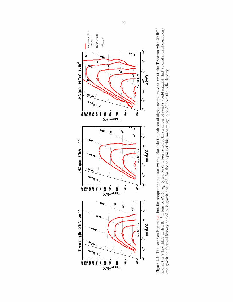
99
10
0
15
0
20
0
25
0
30
0
35
0
40
0
45
0
50
0
55
06
00
65
0
10
-31
0-2
10
-11
00
10
11
02
10
3
mNLSP (GeV)
mG~
(ke
V)
Te
va
tro
n (
p– p
) -
2 T
eV
- 2
0 f
b-1
10 km
10 m
10 mm
10-2 mm
10
0
15
0
20
0
25
0
30
0
35
0
40
0
45
0
50
0
55
06
00
65
0
10
-31
0-2
10
-11
00
10
11
02
10
3
mNLSP (GeV)
mG~
(ke
V)
Te
va
tro
n (
p– p
) -
2 T
eV
- 2
0 f
b-1
10 km
10 m
10 mm
10-2 mm
10
3 10
2 10
1
10
0
15
0
20
0
25
0
30
0
35
0
40
0
45
0
50
0
55
06
00
65
0
10
-31
0-2
10
-11
00
10
11
02
10
3
mNLSP (GeV)
mG~
(ke
V)
Te
va
tro
n (
p– p
) -
2 T
eV
- 2
0 f
b-1
Λ <
80
Te
V
10 km
10 m
10 mm
10-2 mm
10
3 10
2 10
1
Λ > Mmess
103
10
2
10
1
10
0
15
0
20
0
25
0
30
0
35
0
40
0
45
0
50
0
55
06
00
65
0
10
-31
0-2
10
-11
00
10
11
02
10
3
mNLSP (GeV)
mG~
(ke
V)
Te
va
tro
n (
p– p
) -
2 T
eV
- 2
0 f
b-1
Λ <
80
Te
V
10 km
10 m
10 mm
10-2 mm
10
3 10
2 10
1
Λ > Mmess
103
10
2
10
1
10
0
15
0
20
0
25
0
30
0
35
0
40
0
45
0
50
0
55
06
00
65
0
10
-31
0-2
10
-11
00
10
11
02
10
3
mNLSP (GeV)
mG~
(ke
V)
LH
C (
pp
) -
7 T
eV
- 1
fb
-1
104 km
10 km
10 m
10 mm
10-2
mm
10
0
15
0
20
0
25
0
30
0
35
0
40
0
45
0
50
0
55
06
00
65
0
10
-31
0-2
10
-11
00
10
11
02
10
3
mNLSP (GeV)
mG~
(ke
V)
LH
C (
pp
) -
7 T
eV
- 1
fb
-1
104 km
10 km
10 m
10 mm
10-2
mm10
3 1
02
10
1
10
0
15
0
20
0
25
0
30
0
35
0
40
0
45
0
50
0
55
06
00
65
0
10
-31
0-2
10
-11
00
10
11
02
10
3
mNLSP (GeV)
mG~
(ke
V)
LH
C (
pp
) -
7 T
eV
- 1
fb
-1
Λ <
80
Te
V
104 km
10 km
10 m
10 mm
10-2
mm10
3 1
02
10
1
Λ > Mmess
10
3 1
02
10
1
10
0
15
0
20
0
25
0
30
0
35
0
40
0
45
0
50
0
55
06
00
65
0
10
-31
0-2
10
-11
00
10
11
02
10
3
mNLSP (GeV)
mG~
(ke
V)
LH
C (
pp
) -
7 T
eV
- 1
fb
-1
Λ <
80
Te
V
104 km
10 km
10 m
10 mm
10-2
mm10
3 1
02
10
1
Λ > Mmess
10
3 1
02
10
1
10
0
15
0
20
0
25
0
30
0
35
0
40
0
45
0
50
0
55
06
00
65
0
10
-31
0-2
10
-11
00
10
11
02
10
3
mNLSP (GeV)
mG~
(ke
V)
LH
C (
pp)
- 1
4 T
eV
- 1
0 f
b-1
104 km
10 km
10 m
10 mm
10-2
mm
10
0
15
0
20
0
25
0
30
0
35
0
40
0
45
0
50
0
55
06
00
65
0
10
-31
0-2
10
-11
00
10
11
02
10
3
mNLSP (GeV)
mG~
(ke
V)
LH
C (
pp)
- 1
4 T
eV
- 1
0 f
b-1
104 km
10 km
10 m
10 mm
10-2
mm
10
5 1
04
10
3 10
2
10
10
0
15
0
20
0
25
0
30
0
35
0
40
0
45
0
50
0
55
06
00
65
0
10
-31
0-2
10
-11
00
10
11
02
10
3
mNLSP (GeV)
mG~
(ke
V)
LH
C (
pp)
- 1
4 T
eV
- 1
0 f
b-1
Λ <
80
Te
V
104 km
10 km
10 m
10 mm
10-2
mm
10
5 1
04
10
3 10
2
10
Λ > Mmess
10
5
104
103 102
10
1
10
0
15
0
20
0
25
0
30
0
35
0
40
0
45
0
50
0
55
06
00
65
0
10
-31
0-2
10
-11
00
10
11
02
10
3
mNLSP (GeV)
mG~
(ke
V)
LH
C (
pp)
- 1
4 T
eV
- 1
0 f
b-1
Λ <
80
Te
V
no
np
rom
pt
ph
oto
n
eve
nts
SU
SY
eve
nts
< d
decay >
104 km
10 km
10 m
10 mm
10-2
mm
10
5 1
04
10
3 10
2
10
Λ > Mmess
10
5
104
103 102
10
1
Fig
ure
4.5:
Th
esa
me
asF
igu
re4.
4,b
ut
for
non
pro
mp
tp
hoto
nev
ents
.N
ote
that
hu
nd
red
sof
sign
al
even
tsm
ayocc
ur
at
the
Tev
atr
on
wit
h20
fb−
1
and
atth
e7
TeV
LH
Cw
ith
1fb−
1if
ten
sof
eV.mG.
few
keV
.O
bse
rvati
on
of
this
nu
mb
erof
even
tsw
ou
ldsu
gges
tth
at
an
on
stan
dard
cosm
olo
gy
and
grav
itin
oth
erm
alh
isto
ryco
oled
reli
cgr
avit
inos,
an
d,
for
the
top
part
of
this
mass
ran
ge,
als
od
ilu
ted
the
reli
cd
ensi
ty.

100
10
0
15
0
20
0
25
0
30
0
35
0
40
0
45
0
50
0
55
06
00
65
0
10
-31
0-2
10
-11
00
10
11
02
10
3
mNLSP (GeV)
mG~
(ke
V)
Te
va
tro
n (
p– p
) -
2 T
eV
- 2
0 f
b-1
10 km
10 m
10 mm
10-2 mm
10
0
15
0
20
0
25
0
30
0
35
0
40
0
45
0
50
0
55
06
00
65
0
10
-31
0-2
10
-11
00
10
11
02
10
3
mNLSP (GeV)
mG~
(ke
V)
Te
va
tro
n (
p– p
) -
2 T
eV
- 2
0 f
b-1
10 km
10 m
10 mm
10-2 mm
10
2 1
0
1
10
0
15
0
20
0
25
0
30
0
35
0
40
0
45
0
50
0
55
06
00
65
0
10
-31
0-2
10
-11
00
10
11
02
10
3
mNLSP (GeV)
mG~
(ke
V)
Te
va
tro
n (
p– p
) -
2 T
eV
- 2
0 f
b-1
10 km
10 m
10 mm
10-2 mm
10
2 1
0
1
Λ > Mmess
Λ <
30 T
eV
10
2
10 1
10
0
15
0
20
0
25
0
30
0
35
0
40
0
45
0
50
0
55
06
00
65
0
10
-31
0-2
10
-11
00
10
11
02
10
3
mNLSP (GeV)
mG~
(ke
V)
Te
va
tro
n (
p– p
) -
2 T
eV
- 2
0 f
b-1
10 km
10 m
10 mm
10-2 mm
10
2 1
0
1
Λ > Mmess
Λ <
30 T
eV
10
2
10 1
10
0
15
0
20
0
25
0
30
0
35
0
40
0
45
0
50
0
55
06
00
65
0
10
-31
0-2
10
-11
00
10
11
02
10
3
mNLSP (GeV)
mG~
(ke
V)
LH
C (
pp
) -
7 T
eV
- 1
fb
-1
10 km
10 m
10 mm
10-2 mm
10
0
15
0
20
0
25
0
30
0
35
0
40
0
45
0
50
0
55
06
00
65
0
10
-31
0-2
10
-11
00
10
11
02
10
3
mNLSP (GeV)
mG~
(ke
V)
LH
C (
pp
) -
7 T
eV
- 1
fb
-1
10 km
10 m
10 mm
10-2 mm
10
2
10
1
10
0
15
0
20
0
25
0
30
0
35
0
40
0
45
0
50
0
55
06
00
65
0
10
-31
0-2
10
-11
00
10
11
02
10
3
mNLSP (GeV)
mG~
(ke
V)
LH
C (
pp
) -
7 T
eV
- 1
fb
-1
10 km
10 m
10 mm
10-2 mm
10
2
10
1
Λ > Mmess
Λ <
30 T
eV
102 1
0
1
10
0
15
0
20
0
25
0
30
0
35
0
40
0
45
0
50
0
55
06
00
65
0
10
-31
0-2
10
-11
00
10
11
02
10
3
mNLSP (GeV)
mG~
(ke
V)
LH
C (
pp
) -
7 T
eV
- 1
fb
-1
10 km
10 m
10 mm
10-2 mm
10
2
10
1
Λ > Mmess
Λ <
30 T
eV
102 1
0
1
10
0
15
0
20
0
25
0
30
0
35
0
40
0
45
0
50
0
55
06
00
65
0
10
-31
0-2
10
-11
00
10
11
02
10
3
mNLSP (GeV)
mG~
(ke
V)
LH
C (
pp)
- 1
4 T
eV
- 1
0 f
b-1 10 km
10 m
10 mm
10-2 mm
10
0
15
0
20
0
25
0
30
0
35
0
40
0
45
0
50
0
55
06
00
65
0
10
-31
0-2
10
-11
00
10
11
02
10
3
mNLSP (GeV)
mG~
(ke
V)
LH
C (
pp)
- 1
4 T
eV
- 1
0 f
b-1 10 km
10 m
10 mm
10-2 mm
10
4
10
3
10
2 1
0
10
0
15
0
20
0
25
0
30
0
35
0
40
0
45
0
50
0
55
06
00
65
0
10
-31
0-2
10
-11
00
10
11
02
10
3
mNLSP (GeV)
mG~
(ke
V)
LH
C (
pp)
- 1
4 T
eV
- 1
0 f
b-1 10 km
10 m
10 mm
10-2 mm
10
4
10
3
10
2 1
0
Λ > Mmess
Λ <
30 T
eV
104
103
102
10
1
10
0
15
0
20
0
25
0
30
0
35
0
40
0
45
0
50
0
55
06
00
65
0
10
-31
0-2
10
-11
00
10
11
02
10
3
mNLSP (GeV)
mG~
(ke
V)
LH
C (
pp)
- 1
4 T
eV
- 1
0 f
b-1
no
np
rom
pt
lep
ton
eve
nts
SU
SY
eve
nts
< d
decay >
10 km
10 m
10 mm
10-2 mm
10
4
10
3
10
2 1
0
Λ > Mmess
Λ <
30 T
eV
104
103
102
10
1
Fig
ure
4.6:
Con
tou
rp
lots
show
ing
the
exp
ecte
dnum
ber
of
non
pro
mp
tle
pto
nev
ents
ina
mod
elw
ith
ast
au
NL
SP
.N
ote
that
hu
nd
red
sof
sign
al
even
tsm
ayocc
ur
atth
eT
evat
ron
wit
h20
fb−
1an
dat
the
7T
eVL
HC
wit
h1
fb−
1if
ten
sof
eV.mG.
few
keV
.O
bse
rvati
on
of
this
nu
mb
erof
even
tsw
ould
sugg
est
that
an
onst
and
ard
cosm
olo
gy
an
dgra
vit
ino
ther
mal
his
tory
coole
dre
lic
gra
vit
inos,
an
d,
for
the
top
part
of
this
mass
ran
ge,
also
dil
ute
dth
ere
lic
den
sity
.

101
10
0
15
0
20
0
25
0
30
0
35
0
40
0
45
0
50
0
55
06
00
65
0
10
-31
0-2
10
-11
00
10
11
02
10
3
mNLSP (GeV)
mG~
(ke
V)
Te
va
tro
n (
p– p
) -
2 T
eV
- 2
0 f
b-1
10 km
10 m
10 mm
10-2 mm
10
0
15
0
20
0
25
0
30
0
35
0
40
0
45
0
50
0
55
06
00
65
0
10
-31
0-2
10
-11
00
10
11
02
10
3
mNLSP (GeV)
mG~
(ke
V)
Te
va
tro
n (
p– p
) -
2 T
eV
- 2
0 f
b-1
10 km
10 m
10 mm
10-2 mm
10
2 1
0
1
10
0
15
0
20
0
25
0
30
0
35
0
40
0
45
0
50
0
55
06
00
65
0
10
-31
0-2
10
-11
00
10
11
02
10
3
mNLSP (GeV)
mG~
(ke
V)
Te
va
tro
n (
p– p
) -
2 T
eV
- 2
0 f
b-1
10 km
10 m
10 mm
10-2 mm
10
2 1
0
1
Λ > Mmess
Λ <
30 T
eV
10
2
10
1
10
0
15
0
20
0
25
0
30
0
35
0
40
0
45
0
50
0
55
06
00
65
0
10
-31
0-2
10
-11
00
10
11
02
10
3
mNLSP (GeV)
mG~
(ke
V)
Te
va
tro
n (
p– p
) -
2 T
eV
- 2
0 f
b-1
10 km
10 m
10 mm
10-2 mm
10
2 1
0
1
Λ > Mmess
Λ <
30 T
eV
10
2
10
1
10
0
15
0
20
0
25
0
30
0
35
0
40
0
45
0
50
0
55
06
00
65
0
10
-31
0-2
10
-11
00
10
11
02
10
3
mNLSP (GeV)
mG~
(ke
V)
LH
C (
pp
) -
7 T
eV
- 1
fb
-1
10 km
10 m
10 mm
10-2 mm
10
0
15
0
20
0
25
0
30
0
35
0
40
0
45
0
50
0
55
06
00
65
0
10
-31
0-2
10
-11
00
10
11
02
10
3
mNLSP (GeV)
mG~
(ke
V)
LH
C (
pp
) -
7 T
eV
- 1
fb
-1
10 km
10 m
10 mm
10-2 mm
10
2
10
1
10
0
15
0
20
0
25
0
30
0
35
0
40
0
45
0
50
0
55
06
00
65
0
10
-31
0-2
10
-11
00
10
11
02
10
3
mNLSP (GeV)
mG~
(ke
V)
LH
C (
pp
) -
7 T
eV
- 1
fb
-1
10 km
10 m
10 mm
10-2 mm
10
2
10
1
Λ > Mmess
Λ <
30 T
eV
102
10
1
10
0
15
0
20
0
25
0
30
0
35
0
40
0
45
0
50
0
55
06
00
65
0
10
-31
0-2
10
-11
00
10
11
02
10
3
mNLSP (GeV)
mG~
(ke
V)
LH
C (
pp
) -
7 T
eV
- 1
fb
-1
10 km
10 m
10 mm
10-2 mm
10
2
10
1
Λ > Mmess
Λ <
30 T
eV
102
10
1
10
0
15
0
20
0
25
0
30
0
35
0
40
0
45
0
50
0
55
06
00
65
0
10
-31
0-2
10
-11
00
10
11
02
10
3
mNLSP (GeV)
mG~
(ke
V)
LH
C (
pp)
- 1
4 T
eV
- 1
0 f
b-1 10 km
10 m
10 mm
10-2 mm
10
0
15
0
20
0
25
0
30
0
35
0
40
0
45
0
50
0
55
06
00
65
0
10
-31
0-2
10
-11
00
10
11
02
10
3
mNLSP (GeV)
mG~
(ke
V)
LH
C (
pp)
- 1
4 T
eV
- 1
0 f
b-1 10 km
10 m
10 mm
10-2 mm
10
4
10
3
10
2 1
0
10
0
15
0
20
0
25
0
30
0
35
0
40
0
45
0
50
0
55
06
00
65
0
10
-31
0-2
10
-11
00
10
11
02
10
3
mNLSP (GeV)
mG~
(ke
V)
LH
C (
pp)
- 1
4 T
eV
- 1
0 f
b-1 10 km
10 m
10 mm
10-2 mm
10
4
10
3
10
2 1
0
Λ > Mmess
Λ <
30 T
eV
103
10
2
10
1
10
0
15
0
20
0
25
0
30
0
35
0
40
0
45
0
50
0
55
06
00
65
0
10
-31
0-2
10
-11
00
10
11
02
10
3
mNLSP (GeV)
mG~
(ke
V)
LH
C (
pp)
- 1
4 T
eV
- 1
0 f
b-1
me
tasta
ble
sle
pto
n
eve
nts
SU
SY
eve
nts
< d
decay >
10 km
10 m
10 mm
10-2 mm
10
4
10
3
10
2 1
0
Λ > Mmess
Λ <
30 T
eV
103
10
2
10
1
Fig
ure
4.7:
Th
esa
me
asF
igu
re4.
6,b
ut
for
met
ast
ab
lesl
epto
nev
ents
.N
ote
that
hu
nd
red
sof
sign
al
even
tsm
ayocc
ur
at
the
Tev
atr
on
wit
h20
fb−
1
and
atth
e7
TeV
LH
Cw
ith
1fb−
1ifmG&
keV
.O
bse
rvati
on
of
such
anu
mb
erof
even
tsw
ou
ldsu
gges
tth
at
gra
vit
inos
cou
lden
tire
lyco
mp
ose
the
dar
km
atte
r,as
sum
ing
som
en
onst
and
ard
cosm
olo
gy
dil
ute
dre
lic
gra
vit
inos.
Als
o,
note
that
alt
hou
gh
we
on
lyco
nsi
dermG.
MeV
her
e,G
MS
Bm
od
els
allo
wla
rger
grav
itin
om
asse
s,u
ptomG∼
GeV
.T
hu
s,th
ese
plo
tsm
ayb
est
raig
htf
orw
ard
lyex
trap
ola
ted
toh
igh
ergra
vit
ino
mass
esif
des
ired
.H
owev
er,
not
eth
atat
hig
herM
mess
,an
dh
ence
at
hig
hermG
,th
en
eutr
ali
no
again
bec
om
esth
eN
LS
P;
see
Fig
ure
1of
Ref
.[2
60].
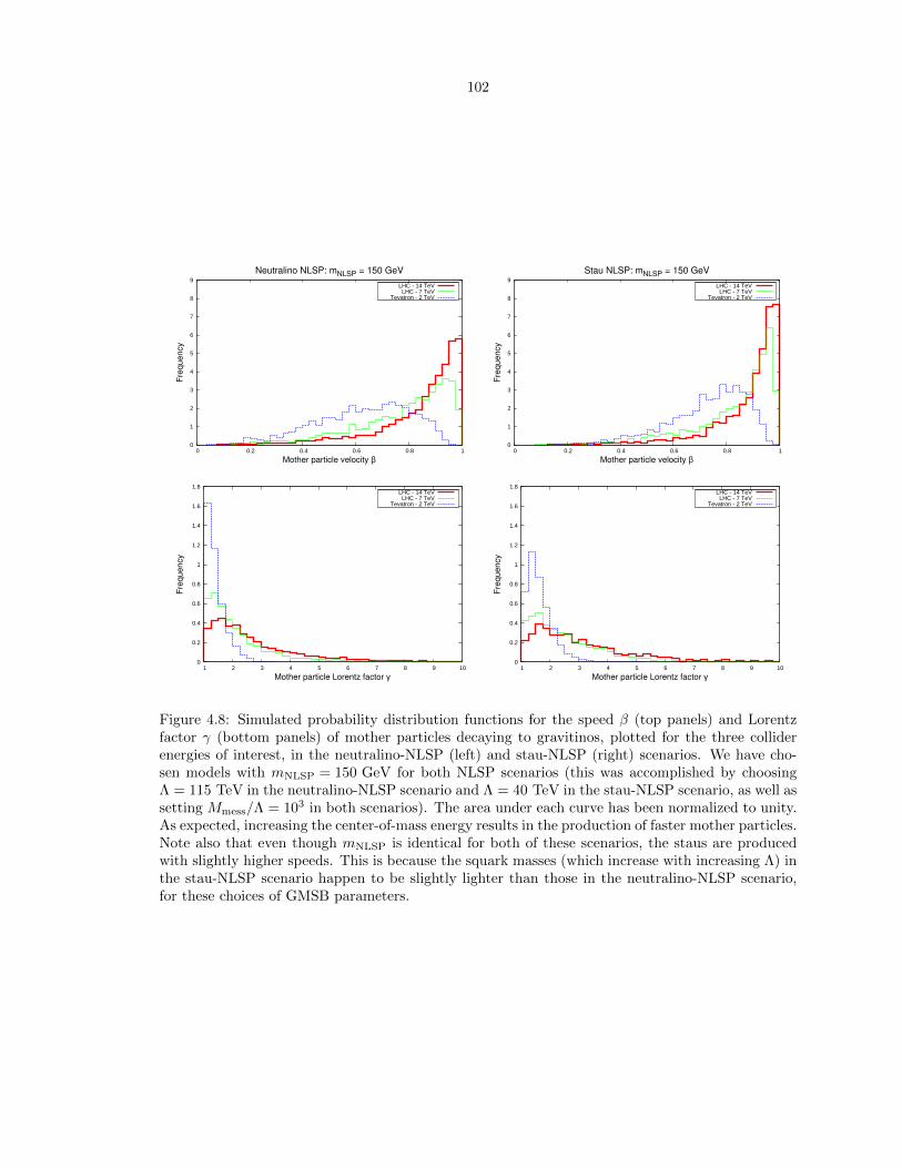
102
0
1
2
3
4
5
6
7
8
9
0 0.2 0.4 0.6 0.8 1
Fre
qu
en
cy
Mother particle velocity β
Neutralino NLSP: mNLSP = 150 GeV
LHC - 14 TeVLHC - 7 TeV
Tevatron - 2 TeV
0
1
2
3
4
5
6
7
8
9
0 0.2 0.4 0.6 0.8 1
Fre
qu
en
cy
Mother particle velocity β
Stau NLSP: mNLSP = 150 GeV
LHC - 14 TeVLHC - 7 TeV
Tevatron - 2 TeV
0
0.2
0.4
0.6
0.8
1
1.2
1.4
1.6
1.8
1 2 3 4 5 6 7 8 9 10
Fre
qu
en
cy
Mother particle Lorentz factor γ
LHC - 14 TeVLHC - 7 TeV
Tevatron - 2 TeV
0
0.2
0.4
0.6
0.8
1
1.2
1.4
1.6
1.8
1 2 3 4 5 6 7 8 9 10
Fre
qu
en
cy
Mother particle Lorentz factor γ
LHC - 14 TeVLHC - 7 TeV
Tevatron - 2 TeV
Figure 4.8: Simulated probability distribution functions for the speed β (top panels) and Lorentzfactor γ (bottom panels) of mother particles decaying to gravitinos, plotted for the three colliderenergies of interest, in the neutralino-NLSP (left) and stau-NLSP (right) scenarios. We have cho-sen models with mNLSP = 150 GeV for both NLSP scenarios (this was accomplished by choosingΛ = 115 TeV in the neutralino-NLSP scenario and Λ = 40 TeV in the stau-NLSP scenario, as well assetting Mmess/Λ = 103 in both scenarios). The area under each curve has been normalized to unity.As expected, increasing the center-of-mass energy results in the production of faster mother particles.Note also that even though mNLSP is identical for both of these scenarios, the staus are producedwith slightly higher speeds. This is because the squark masses (which increase with increasing Λ) inthe stau-NLSP scenario happen to be slightly lighter than those in the neutralino-NLSP scenario,for these choices of GMSB parameters.

103
Chapter 5
A detour: Charged-particle decayat finite temperature
5.1 Introduction
Precise predictions for decay rates of charged particles might be of interest in a variety of cosmological
contexts that introduce long-lived particles with electric charge. These include scenarios for modified
big-bang nucleosynthesis [292–298] and small-scale-power suppression [299–301] and mechanisms for
dark-matter detection wherein a charged quasistable heavier particle is produced [302–310].
In the early Universe, decays of charged particles occur in a thermal bath whose very presence
seems to affect decay rates in a peculiar way. Indeed, consider the decay of a hypothetical charged
particle ψ to two lighter particles χ and φ. The leading-order Feynman diagram is shown in Fig-
ure 5.1. In a thermal bath of photons, the process γψ → χφ also occurs and modifies the vacuum
decay rate. Hence, the vacuum decay rate of a particle ψ must be augmented in the cosmological
context by the inclusion of the rate for the “induced” decay wherein the unstable particle absorbs
a thermal photon (see Figure 5.2). It is easy to see that a naive computation of the diagrams in
Figure 5.2 leads to a divergent result. This divergence is of the infrared type — it appears when
the energy of the absorbed photon becomes very small. In this work we discuss in detail how, when
all possible processes that modify the vacuum decay rate are taken into account, the infrared di-
vergences cancel out. This is a finite-temperature analog of the celebrated cancellation of infrared
divergences in QED pointed out by Bloch and Nordsieck long ago [311].
Although thermal effects have been computed for static thermodynamic quantities such as the
effective potential, the free energy, the pressure, and so on [312], sometimes to very high orders
in the perturbative expansion in QCD and QED (for recent reviews, see Refs. [313, 314]), less is
known about finite-temperature corrections to cross sections and decay rates. Radiative corrections
Material in this chapter was first published in “Charged-particle decay at finite temperature,” Andrzej Czarnecki,Marc Kamionkowski, Samuel K. Lee, and Kirill Melnikov, Phys.Rev. D85, 025018 (2012) [35]. Reproduced here withpermission, c©2012 by the American Physical Society.
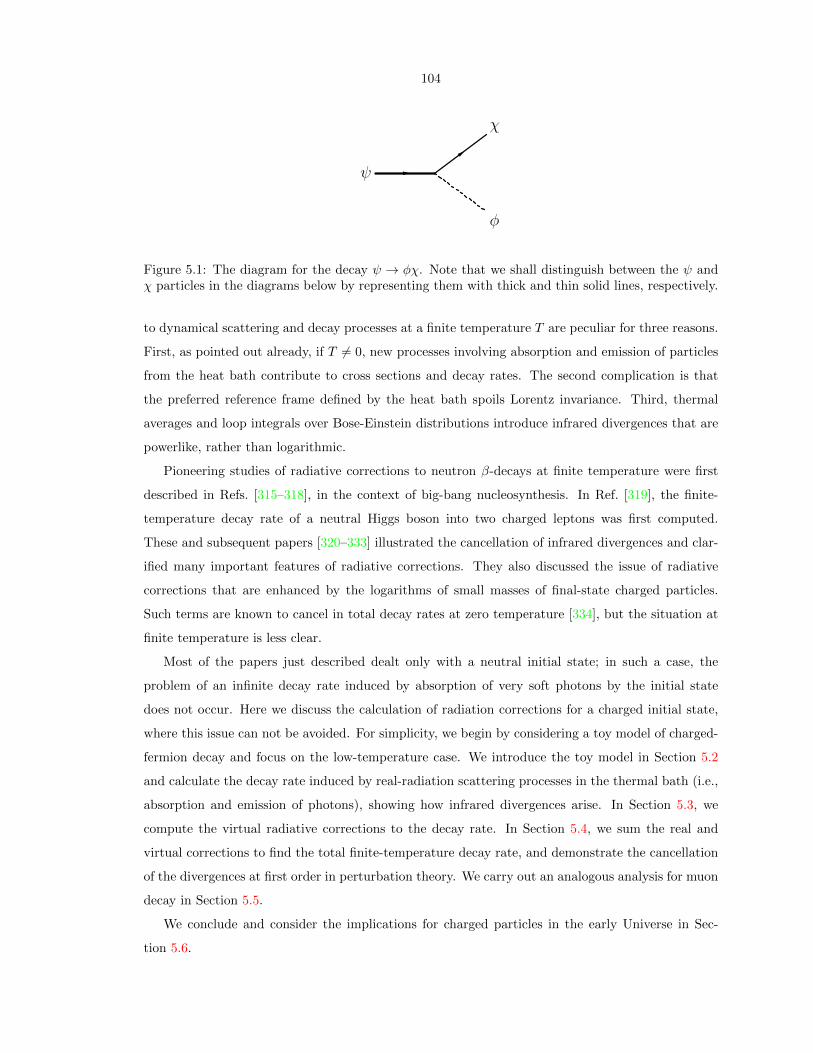
104
ψ
φ
χ
Figure 5.1: The diagram for the decay ψ → φχ. Note that we shall distinguish between the ψ andχ particles in the diagrams below by representing them with thick and thin solid lines, respectively.
to dynamical scattering and decay processes at a finite temperature T are peculiar for three reasons.
First, as pointed out already, if T 6= 0, new processes involving absorption and emission of particles
from the heat bath contribute to cross sections and decay rates. The second complication is that
the preferred reference frame defined by the heat bath spoils Lorentz invariance. Third, thermal
averages and loop integrals over Bose-Einstein distributions introduce infrared divergences that are
powerlike, rather than logarithmic.
Pioneering studies of radiative corrections to neutron β-decays at finite temperature were first
described in Refs. [315–318], in the context of big-bang nucleosynthesis. In Ref. [319], the finite-
temperature decay rate of a neutral Higgs boson into two charged leptons was first computed.
These and subsequent papers [320–333] illustrated the cancellation of infrared divergences and clar-
ified many important features of radiative corrections. They also discussed the issue of radiative
corrections that are enhanced by the logarithms of small masses of final-state charged particles.
Such terms are known to cancel in total decay rates at zero temperature [334], but the situation at
finite temperature is less clear.
Most of the papers just described dealt only with a neutral initial state; in such a case, the
problem of an infinite decay rate induced by absorption of very soft photons by the initial state
does not occur. Here we discuss the calculation of radiation corrections for a charged initial state,
where this issue can not be avoided. For simplicity, we begin by considering a toy model of charged-
fermion decay and focus on the low-temperature case. We introduce the toy model in Section 5.2
and calculate the decay rate induced by real-radiation scattering processes in the thermal bath (i.e.,
absorption and emission of photons), showing how infrared divergences arise. In Section 5.3, we
compute the virtual radiative corrections to the decay rate. In Section 5.4, we sum the real and
virtual corrections to find the total finite-temperature decay rate, and demonstrate the cancellation
of the divergences at first order in perturbation theory. We carry out an analogous analysis for muon
decay in Section 5.5.
We conclude and consider the implications for charged particles in the early Universe in Sec-
tion 5.6.

105
ψ
k
φ
χ
ψ
k
φ
χ
s− channel u− channel
Figure 5.2: The two diagrams via which absorption of a photon can lead to induced ψ decay (or χand φ production)
5.2 Toy model
We shall first discuss a simple model to illustrate the nature of the infrared divergences and their
cancellation. Consider the process ψ → χφ, the decay of a heavy charged fermion ψ to a light
charged fermion χ and a massless neutral scalar φ via the interaction
L ⊃ gφψLχ+ h.c. , (5.1)
depicted in Figure 5.1. Here L = (1 − γ5)/2. We shall assume that the charge of both fermions is
the elementary charge e =√
4πα, and that the mass ratio ε ≡ mχ/mψ is small.
At T = 0, the tree-level amplitude for the decay ψ → χφ is given by
Mtr = guχLuψ . (5.2)
This amplitude gives the O(g2α0) zero-temperature decay rate,
Γ0 = Γ0(1− ε4) , (5.3)
where we have defined Γ0 ≡g2
32πmψ. We will state our subsequent results for the temperature-
dependent decay rate in terms of Γ0.
On account of radiative corrections and finite-temperature effects, the decay rate can be written
as a triple series in τ = T/mψ, ε = mχ/mψ, and the fine-structure constant α. Unless explicitly
stated otherwise, we work in the low-temperature approximation τ ε 1. Our goal is to compute
relative corrections to the decay rate that scale as ατ2. In those terms, we shall set ε → 0. Note
that terms of the form τ/ε do not appear in the total decay rate.

106
5.2.1 Photon absorption
We now consider the process γψ → χφ, the induced decay of ψ in a thermal bath of photons.
This process can occur via the two diagrams shown in Figure 5.2. For a photon with 4-momentum
k = (ω,k), where ω = |k|, the tree-level amplitudes for these channels are
Mabs,s =eg
s−m2ψ
uχL(/pψ + /k +mψ)/εγuψ , (5.4)
Mabs,u =eg
u−m2χ
uχ/εγ(/pχ − /k +mχ)Luψ, (5.5)
giving the total amplitude Mabs = Mabs,s +Mabs,u. We use the amplitude to compute the cross
section for γψ → χφ by the standard procedure. We assume that the ψ particle is at rest with
respect to the photon bath and express the result in terms of the energy of the photon w ≡ ω/mψ.
1 We find
σabs(w) ≡ 1
2mψ
1
2|ω|
∫dLIPSχφ (2π)4δ4(pψ + k − pχ − pφ)〈|Mabs(k)|2〉
= Γ0απ
m3ψw
3ρ(w) , (5.6)
where
ρ(w) ≡(1 + 2w + 2w2
)ln
1 + 2w
ε2−(2 + 4w + 3w2
), (5.7)
at leading order in ε. Note that ρ ∝ w0 and σabs ∝ w−3 as w → 0.
To compute corrections to the decay rate of a particle ψ due to the absorption of thermal photons
from the heat bath, we need to integrate the cross section σabs(w) in Eq. (5.6) multiplied with the
average occupation number for thermal photons. We find
ΓTabs =
∫dw
dnγdw
(w)σabs(w)
= gγ
∫d3k
(2π)3fB(ω)σabs(w)
=α
πΓ0
∫ ∞
0
dw
wfB(ω)ρ(w) , (5.8)
where fB(ω) = 1/(eω/T − 1) = 1/(ew/τ − 1) is the Bose-Einstein distribution function and gγ = 2 is
the number of independent photon polarizations. Since fB ∝ w−1 and ρ ∝ w0 as w → 0, we see that
the integrand in Eq. (5.8) is proportional to w−2 as w → 0, and hence ΓTabs indeed has a powerlike
infrared divergence, implying an infinite decay rate.
1We are implicitly considering a cosmological scenario in which the heavy ψ particle has decoupled from the thermalbath and is out of equilibrium. Furthermore, we assume that the massless φ particle is also not thermalized in thebath (which may be the case if the coupling g is very weak and ψ decay is the dominant mode of φ production, forexample). Similar assumptions will also be made in the case of muon decay discussed in Section 5.5.

107
ψ
φ
χ
k
ψ
φ
χ
k
Figure 5.3: The diagrams for radiative ψ-decays. Note that the topologies of the diagrams areidentical to those for absorption in Figure 5.2, with the exception of the photon line placement.This results in the relation given in Eq. (5.9).
As in the case of infrared divergences at zero temperature, the infinite rate is unphysical. We
arrived at this unphysical result because we considered only the photon absorption process γψ → χφ
in the calculation of the finite-temperature ψ decay rate. However, as we shall demonstrate, we
cannot consider this absorption process independently of other processes that also result in ψ decay.
In particular, we must also take into account the finite-temperature rates of the radiative decay
process ψ → γχφ and the decay process ψ → χφ. At finite temperature, the emission of photons in
the first process is stimulated by the presence of photons in the thermal bath. At the same order in
α, the second process is affected by T -dependent additions to the virtual-photon propagator. When
all of these processes are included in the calculation, all T -dependent infrared divergences cancel to
yield a finite rate. The nature of this cancellation is similar to zero-temperature cancellations of
infrared divergences in QED, as described in a classic paper by Bloch and Nordsieck [311]. We shall
now demonstrate this cancellation to O(g2α).
5.2.2 Photon emission
We begin by considering the photon-emitting radiative decay process ψ → γχφ. The two contribut-
ing diagrams are shown in Figure 5.3. Comparing these diagrams to those in Figure 5.2, we see that
the amplitudes for emission are formally equivalent to those for absorption given in Eq. (5.4) if we
make the substitutions k ↔ −k and εγ ↔ ε∗γ . This crossing symmetry gives the photon-emission
amplitude from the photon-absorption amplitude,
〈|Mem(k)|2〉 = gγ〈|Mabs(−k)|2〉 , (5.9)

108
where the factor of gγ arises because we do not average over photon polarizations on the left-hand
side. The O(g2α) T -dependent part of the rate for this process is then given by
ΓTem =1
2mψ
∫dLIPSγχφ fB(ω)(2π)4δ4(pψ − k − pχ − pφ)〈|Mem(k)|2〉 , (5.10)
where the factor of fB(ω) comes from the T -dependent part of the (1+fB) Bose-enhancement factor
for the final-state photons. Comparing Eq. (5.10) to Eq. (5.8), and using Eqs. (5.6) and (5.9), it can
be shown that the expression for the emission rate is very similar to that for the absorption rate
given in Eq. (5.8),
ΓTem =α
πΓ0
∫ 1/2
0
dw
wfB(ω)ρ(−w) . (5.11)
We see that the only differences are ρ(w) → ρ(−w), arising from the k → −k substitution used to
switch the absorbed photon to an emitted photon, and the limits of integration. The upper limit
reflects that the emitted photon is limited by the kinematics to have w < 1/2 in the final state,
whereas an absorbed photon is allowed to have any energy in the initial state. Note that this is
further reflected in the fact that ρ(w) is defined only for −1/2 < w <∞.
5.2.3 Real-radiation corrections
We are now in position to calculate the total rate of ψ decay due to processes involving either the
absorption or emission of real photons,
ΓTreal = ΓTabs + ΓTem =α
πΓ0
∫ ∞
0
dw
wfB(ω)ρreal(w) , (5.12)
where ρreal(w) = ρ(w) + θ(1/2 − w)ρ(−w). Exact integration over w in the above formula is com-
plicated because of the Bose-Einstein factor. However, if we consider the low-temperature case
τ 1, then fB(ω) is only non-negligible for w . τ 1/2. We can thus use the approximation
θ(1/2−w)→ 1 and integrate Eq. (5.12) by expanding ρreal(w) in a Taylor series in w. This approx-
imation picks up all the terms that are suppressed by powers of τ , but it misses the exponentially
suppressed terms of O(e−1/τ ). The O(g2α) result is then
ΓTreal =α
πΓ0
[(−4− 4 ln ε+O(ε2 ln ε)
)J−1 +
(−2− 8 ln ε+O(ε2)
)J1τ
2 +O(τ4, e−1/τ )], (5.13)
where we have defined the integrals
Jn ≡ limx0→0
∫ ∞
x0
dxxnfB(xT )θ(x− x0) . (5.14)
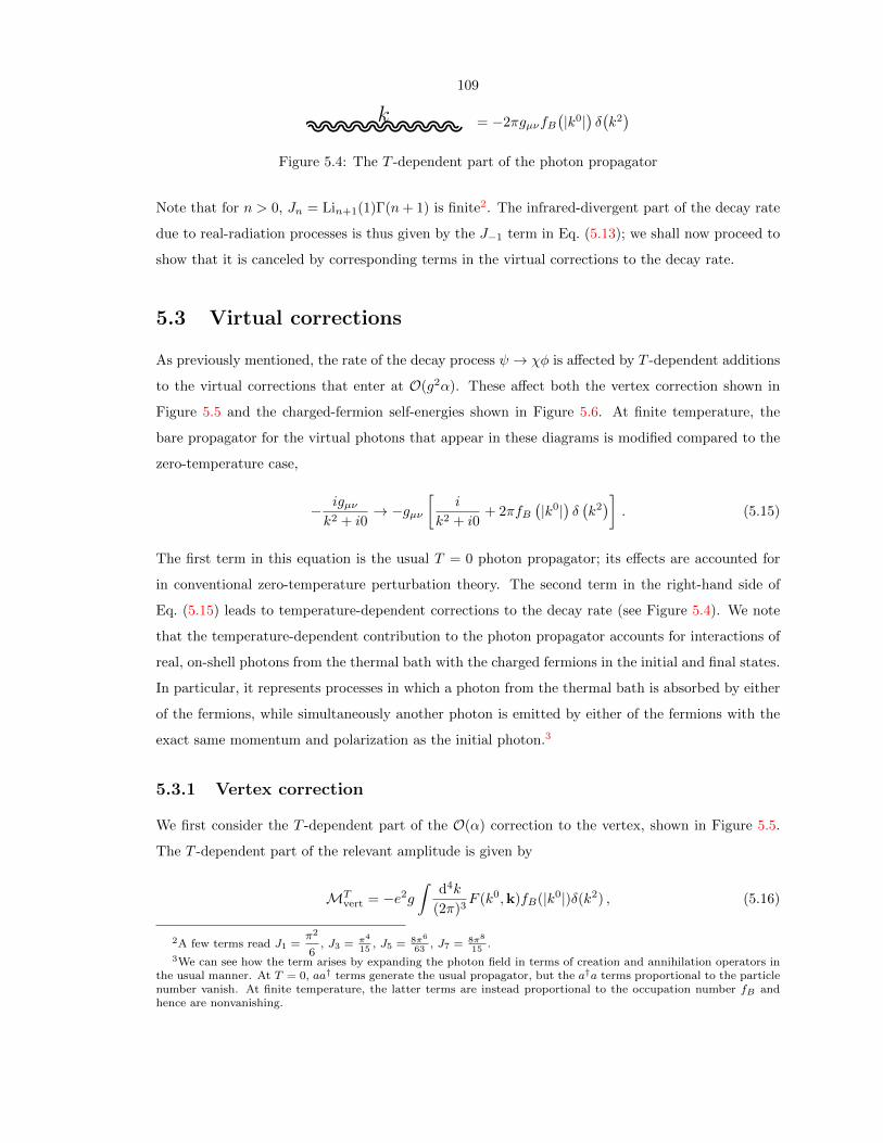
109
k = −2πgµνfB(|k0|)δ(k2)
Figure 5.4: The T -dependent part of the photon propagator
Note that for n > 0, Jn = Lin+1(1)Γ(n+ 1) is finite2. The infrared-divergent part of the decay rate
due to real-radiation processes is thus given by the J−1 term in Eq. (5.13); we shall now proceed to
show that it is canceled by corresponding terms in the virtual corrections to the decay rate.
5.3 Virtual corrections
As previously mentioned, the rate of the decay process ψ → χφ is affected by T -dependent additions
to the virtual corrections that enter at O(g2α). These affect both the vertex correction shown in
Figure 5.5 and the charged-fermion self-energies shown in Figure 5.6. At finite temperature, the
bare propagator for the virtual photons that appear in these diagrams is modified compared to the
zero-temperature case,
− igµνk2 + i0
→ −gµν[
i
k2 + i0+ 2πfB
(|k0|)δ(k2)]
. (5.15)
The first term in this equation is the usual T = 0 photon propagator; its effects are accounted for
in conventional zero-temperature perturbation theory. The second term in the right-hand side of
Eq. (5.15) leads to temperature-dependent corrections to the decay rate (see Figure 5.4). We note
that the temperature-dependent contribution to the photon propagator accounts for interactions of
real, on-shell photons from the thermal bath with the charged fermions in the initial and final states.
In particular, it represents processes in which a photon from the thermal bath is absorbed by either
of the fermions, while simultaneously another photon is emitted by either of the fermions with the
exact same momentum and polarization as the initial photon.3
5.3.1 Vertex correction
We first consider the T -dependent part of the O(α) correction to the vertex, shown in Figure 5.5.
The T -dependent part of the relevant amplitude is given by
MTvert = −e2g
∫d4k
(2π)3F (k0,k)fB(|k0|)δ(k2) , (5.16)
2A few terms read J1 =π2
6, J3 = π4
15, J5 = 8π6
63, J7 = 8π8
15.
3We can see how the term arises by expanding the photon field in terms of creation and annihilation operators inthe usual manner. At T = 0, aa† terms generate the usual propagator, but the a†a terms proportional to the particlenumber vanish. At finite temperature, the latter terms are instead proportional to the occupation number fB andhence are nonvanishing.

110
k
ψ
φ
χ
Figure 5.5: The diagram contributing to the T -dependent part of the O(α) correction to the vertex
where
F (k0,k) ≡uχγ
µ(/pχ − /k +mχ)L(/pψ − /k +mψ)γµuψ[(pχ − k)2 −m2
χ
] [(pψ − k)2 −m2
ψ
] . (5.17)
We may use the properties of the gamma matrices to simplify this expression. Integration over k0
removes δ(k2),
MTvert = −e2g
∫d3k
(2π)32ω[F (ω,k) + F (−ω,k)] fB(ω) , (5.18)
where ω = |k|. Now, by changing the variable of integration from k→ −k in the second term in the
sum enclosed in brackets, the sum becomes [F (k) + F (−k)]. Examining Eq. (5.17), we see that the
numerator of this sum is then independent of k, since k2 = 0 and terms that are linear in k cancel.
However, the denominator of the sum retains its quadratic dependence on k, since it is proportional
to (pχ · k)(pψ · k). By counting powers of ω and recalling that fB ∝ ω−1 at small values of ω, we
observe that the integral in Eq. (5.18) indeed has a powerlike divergence.
We can then take the interference of this amplitude with the tree-level amplitude given in
Eq. (5.2). The T -dependent part of the vertex correction to the decay rate then follows by tak-
ing the usual spin-sum average and evaluating the resulting integral over k, using the appropriate
kinematics of the 2-body decay in the rest frame of the ψ particle. Writing the result in terms of
the integrals Jn as before, we find at O(g2α)
ΓTvert =α
πΓ0
[(4 ln ε+O(ε2 ln ε)
)J−1
]. (5.19)
Comparing to the decay rate due to real-radiation processes in Eq. (5.13), we see that part of the
divergent J−1 term is indeed canceled.
5.3.2 Self-energy corrections
The remaining part of the infrared divergence is canceled by the T -dependent corrections to the
fermion self-energy ΣT (p), which enter via the virtual photon propagator in Figure 5.6 and lead
to T -dependent contributions to the full (dressed) fermion propagator STF (p). At T = 0, these

111
p + k
−k
p p
Figure 5.6: The diagram contributing to the T -dependent part of the fermion self-energy
self-energy contributions are conveniently treated through the mass shift δm, and the wave-function
renormalization factor Z2. The wave function renormalization factors are usually obtained as deriva-
tives of the self-energy Σ with respect to p, evaluated on the mass shell p2 = m2. This treatment
relies on the fact that at T = 0, Σ depends only on the momentum of the particle p. Unfortunately,
this feature is violated at finite temperature because the thermal bath introduces a preferred ref-
erence frame. As a result, the self-energy of a particle at rest and the self-energy of a particle in
motion are not related in an obvious way.
We will need expressions for the self-energy of both the ψ and χ fermions. We can consider
more generally the T -dependent part of the self-energy ΣT (p) of a fermion with electric charge e and
T = 0 physical mass m. This calculation has been discussed extensively in the literature; below, we
loosely follow the formalism laid out in Ref. [335]. Our ultimate goal will be to use the expression
for ΣT to show that, in the limit p2 → m2T , the full finite-temperature fermion propagator takes the
form
STF (p) = ZT2i∑s u
Ts (p)uTs (p)
p2 −m2T
. (5.20)
That is, the pole of the propagator is shifted to the finite-temperature physical mass mT , and the
fermion wave functions are given by Ψs(p) =√ZT2 /2p
0uTs (p)e−ip·x, where ZT2 and uTs (p) are the
finite-temperature wave-function renormalization factor and the finite-temperature spinor, respec-
tively.4 This form implies that self-energy corrections to the decay rate will follow from three distinct
sources: (1) matrix elements will be multiplied by a factor of ZT2 for each external fermion line, (2)
the shift in the physical mass, which will effectively modify the fermion phase-space, and (3) the
spinor completeness relation will be modified, affecting the evaluation of spin sums.
To this end, we start by finding the self-energy ΣT at O(α). We take p to be the off-shell fermion
momentum and −k to be the momentum of the photon in the loop, as shown in Figure 5.6. The
self-energy reads
ΣT (p) = 2e2
∫d4k
(2π)3
/p+ /k − 2m
(p+ k)2 −m2fB(|k0|)δ(k2) . (5.21)
4Note that we assume that renormalization has already been carried out at T = 0.
112
It is convenient to decompose ΣT (p) as
ΣT (p) = /pcB(p)− 2mcB(p) + /K(p) , (5.22)
where
cB(p) ≡ 2e2
∫d4k
(2π)3
fB(|k0|)δ(k2)
(p+ k)2 −m2, (5.23)
Kµ(p) ≡ 2e2
∫d4k
(2π)3kµ
fB(|k0|)δ(k2)
(p+ k)2 −m2
→p2=m2
α
πJ1T 2
|p|
(Lp,
p
|p|
[p0
|p|Lp − 2
]), (5.24)
and Lp = lnp0 + |p|p0 − |p| . We can now use these results for ΣT to find the full (dressed) finite-
temperature fermion propagator STF (p) at O(α) in the usual way,
STF (p) =i
/p−m− ΣT
=i[/p(1− cB) +m(1− 2cB)− /K]
p2(1− 2cB)−m2(1− 4cB)− 2p ·K +O(α2). (5.25)
Examining the denominator of Eq. (5.25), we see that it can be simplified by defining
δm2T ≡ 2e2
∫d4k
(2π)3fB(|k0|)δ(k2)
=2π
3αT 2. (5.26)
Also, since −2p · k = −[(p+ k)2 −m2] + (p2 −m2) + k2, we can write
−2p ·K = −δm2T + (p2 −m2)cB . (5.27)
Finally, we can expand in (p2 −m2) around the on-shell momentum p (which satisfies p2 = m2) by
writing
cB(p) = cB + (p2 −m2)cB′+O
((p2 −m2)2
), (5.28)
where cB ≡ cB(p) = 0 and
cB′ ≡ dcB
dp2(p)
= −2e2
∫d4k
(2π)3
fB(|k0|)δ(k2)
((p+ k)2 −m2)2
(1 +
d(2p · k)
dp2(p)
)
= −απ
J−1
m2. (5.29)
113
We note that the vanishing of the cB coefficient follows from the antisymmetry of the integrand for
cB in Eq. (5.23) at p = p w.r.t. k → −k; for the same reason, the derivative term in the integrand
in Eq. (5.29) vanishes as well.
We are now in position to recover the form of the propagator advertised in Eq. (5.20), by using
Eqs. (5.27) and (5.28) in Eq. (5.25), and keeping only O(α) terms there. We find the result
STF (p) = (1− 2m2cB′)i(/p+m− /K)
p2 −m2 − δm2T
. (5.30)
Comparing this expression with Eq. (5.20) and using Eqs. (5.26) and (5.29), we obtain
ZT2 = 1− 2m2cB′
= 1 + 2α
πJ−1 , (5.31)
m2T = m2 + δm2
T
= m2 +2π
3αT 2 , (5.32)
∑
s
uTs (p)uTs (p) = /p+m− /K(p) , (5.33)
where in the last expression the momentum-dependent results of Eq. (5.23) are to be used in evalu-
ating spin sums. These finite-temperature relations affect the decay rate in the three aforementioned
ways; we shall now calculate each of their contributions separately.
First, the finite-temperature wave-function renormalization factor ZT2 simply affects the tree-
level decay rate Γ0 of Eq. (5.3) as an overall multiplicative factor; one factor enters for each external
fermion line. This yields the O(g2α) temperature-dependent contribution
ΓTZ2=α
πΓ0
[(4 +O(ε4)
)J−1
]. (5.34)
Combining this with Eqs. (5.13) and (5.19), we see that this contribution cancels the remaining
infrared-divergent J−1 part of the total decay rate.
Second, Eq. (5.32) results in a shift of the pole of the fermion propagator to p2 = m2T . Since the
pole masses of the fermions define the leading-order rate, the mass shifts ∆mi ≡ mT,i −mi ≈ δm2T,i/2mi
lead to the following O(g2α) “phase-space” correction
ΓTph =∂Γ0
∂mψ∆mψ +
∂Γ0
∂mχ∆mχ
=α
πΓ0
[(2 +O(ε2)
)J1τ
2]. (5.35)
Finally, the finite-temperature spin-sum relation found in Eq. (5.33) modifies the calculation of
114
matrix elements. Note from Eq. (5.23) that the relation is actually momentum-dependent, and must
be computed for both the ψ particle (at rest) and the χ particle (with energy p0 = mψ(1+ε2)/2). The
leading-order contribution to the decay rate is then found by using the finite-temperature spin-sum
relation in the tree-level calculation, giving the O(g2α) temperature-dependent part,
ΓTK =α
πΓ0
[(−2 + 8 ln ε+O(ε4)
)J1τ
2]. (5.36)
The totalO(g2α) self-energy correction is then given by the sum of these three effects [Eqs. (5.34)–
(5.36)],
ΓTΣ = ΓTZ2+ ΓTph + ΓTK
=α
πΓ0
[(4 +O(ε4)
)J−1 +
(8 ln ε+O(ε2)
)J1τ
2]. (5.37)
5.4 Total decay rate in the toy model
We are now in position to present the final formula for the decay rate of the hypothetical fermion ψ
in a thermal bath. We consider the low-temperature limit T mψ,mχ and include contributions
from processes involving both real photons and virtual photons; the latter category includes the
vertex correction and corrections arising from the self-energy of charged fermions. The total decay
rate is the sum of these contributions given in Eqs. (5.13), (5.19), and (5.37). We remind the reader
that our calculation is performed in the approximation τ ε 1 and that we are interested in the
leading O(ατ2) temperature-dependent correction to the rate. We find
ΓTtot = ΓTreal + ΓTvert + ΓTΣ
= −απ3τ2Γ0 +O(τ2ε4, τ4, e−1/τ ) . (5.38)
We see that all the infrared-divergent terms proportional to the integrals J−1 cancel out in the total
rate. We note that this statement remains valid if exact ε-dependence of the rate is restored. Further-
more, we find in Eq. (5.38) that all the terms that contains logarithms of the mass ratio ln ε cancel
in the correction to the total rate, in contrast to individual contributions in Eqs. (5.13) and (5.36).
Cancellation of such terms in the zero-temperature case follows from the Kinoshita-Lee-Nauenberg
theorem [334,336]. We are not aware of a general proof of a similar cancellation at a finite temper-
ature, so it is important to watch for such terms in explicit T 6= 0 computations.

115
5.5 Muon decay µ→ eνµνe
In this section, we present the temperature-dependent correction to the muon decay rate at low
temperature. The details of the calculation are similar to the preceding discussion of the toy model.
The main difference is that the muon decay is a three-body process, so that integration over the
phase-space of final-state particles is more complex.
The muon decay to electron and neutrinos is described by an effective Lagrangian
L ⊃ 4GF√2eγρLνe νµγρLµ, (5.39)
where GF is the Fermi constant. The leading-order, zero-temperature decay rate reads
Γ0 = Γ0
(1− 8ε2 − 24ε4 ln ε+ 8ε6 − ε8
), (5.40)
where now Γ0 ≡G2Fm
5µ
192π3and ε ≡ me/mµ. Similar to the toy-model case, the radiative corrections to
the rate are given by the sum of real photon emission/absorption corrections, the vertex corrections
and the self-energy corrections. For future reference, we show those corrections separately.
The contribution to the decay rate from real photon emission/absorption reads
ΓTreal =α
πΓ0
[(−17
3− 4 ln ε
)J−1 +
(−70
3− 32 ln ε
)J1τ
2
]. (5.41)
Note that here and below we keep only the leading term in ε for each power of τ ≡ T/mµ, and
consistently neglect all powers of τ beyond τ2. The result for the vertex correction reads
ΓTvert =α
πΓ0
[(5
3+ 4 ln ε
)J−1
]. (5.42)
We note that the temperature dependence in Eq. (5.42) is exact and that higher-order terms in τ
do not appear there.
The self-energy correction to the fermion propagator was discussed in the previous section and
much of that discussion remains valid. For this reason, we just summarize the result. The total
self-energy correction is given by
ΓTΣ =α
πΓ0
[4J−1 +
(64
3+ 32 ln ε
)J1τ
2
]. (5.43)
The final result for temperature-dependent radiative corrections to the muon decay is given
by the sum of the three contributions of Eqs. (5.41)–(5.43). Including also the T = 0 radiative

116
corrections [337,338], we find the final O(α, τ2, ε0) result
Γµ→eνν = Γ0
1 +
α
π
[(25
8− π2
2
)− π2
3τ2
]. (5.44)
We note thatO(ατ2) correction to the rate for the muon decay is identical to the analogous correction
to the two-body fermion decay rate in the toy model, suggesting the possibility of deriving and
understanding this result in a simpler fashion. We also note that our result Eq. (5.44) disagrees with
the one given in Ref. [339].
Part of the discrepancy can be traced to the issue of mass singularities. Indeed, in Ref. [339], the
ln ε terms are present even at O(ατ2) contributions to the rate but, as follows from our analysis, such
terms cancel when all contributions are taken into account. Nevertheless, as pointed out already,
whether mass singularities cancel in the rate if higher-order terms in τ are accounted for is an open
question. When we extend the calculation of the muon decay rate to include O(ατ4) terms, we find
that Eq. (5.44) is modified by
∆Γµ→eνν = −απ
Γ064π4τ4
45
(2 ln ε+
1
3
), (5.45)
which shows the logarithmic sensitivity to the electron-to-muon mass ratio. In the low-temperature
regime τ ε 1 that we consider in this work, there exist more important corrections to Eq. (5.44)
than the ones displayed in Eq. (5.45). However, most of the “more relevant” corrections involve
powers of the mass ratio ε, while Eq. (5.45) shows logarithmic sensitivity to ε, a unique feature in
the low-temperature regime. It is interesting to point out that by relaxing the relationship between
the temperature T and the mass of the charged particle in the final state (the electron), we obtain new
sources of mass logarithms related to the thermal Fermi-Dirac distribution of fermions in the heat
bath. Complete analysis of the corrections to the muon decay rate for the intermediate-temperature
regime me T mµ — where proper interplay of bosonic and fermionic temperature-dependent
corrections becomes important — is beyond the scope of the present discussion, but some details of
the calculation are given in Appendix D.
5.6 Conclusions
Long-lived charged particles appear in a variety of scenarios for early-Universe physics and dark
matter. In all cases, these long-lived particles are bathed for a long time in a gas of photons, giving
rise to the possibility of induced decays through processes such as those shown in Figure 5.2. If
the rate of this induced process is large, then the cosmological effects of these long-lived charged
particles may be substantially modified.
A naive evaluation of the rate for these induced decays leads to a result which diverges as
117
the frequency of the photon in the heat bath that induces the decay vanishes. As with infrared
divergences at zero temperature, a proper calculation of the decay rate requires accounting for all
degenerate processes. Once this is done, the infrared divergences cancel, leading to small correction to
the decay rate. By considering a simple toy model with a two-body final state and a realistic process
— muon decay — with a three-body final state, we found a universal leading finite-temperature
correction δΓ/Γ0 = −απ
π2T 2
3m2, where m is the mass of the decaying particle.
In this study, we focused on discussing infrared divergences in decays of charged particles in
the thermal bath. This issue can be sharply defined by considering temperatures that are small
compared to masses of decaying particles and their decay products. An interesting set of questions
arises if we depart from the low-temperature regime and consider the “intermediate”-temperature
scenario, where the mass of the decaying particle is large and masses of decay products are small,
compared to the heat-bath temperature. In such a case, radiative corrections enhanced by the
logarithms of the mass ratios can become numerically important in the context of a variety of
scenarios that occur in the early Universe. For example, light gravitinos that arise in theories of
supergravity with gauge-mediated supersymmetry breaking may be produced by the decay of short-
lived charged staus to taus [211–216]. Temperatures greater than the tau mass will then fall into
the “intermediate”-temperature scenario. If mass-enhanced corrections are indeed present, large
modifications of the stau decay rate and the production rate of light gravitino dark matter become
conceivable. Such modifications may affect the early-Universe thermal history and have implications
for collider phenomenology [34].
Furthermore, in some regions of the supersymmetric parameter space, the process of coannihila-
tion is important in the determination of the dark-matter relic abundance after freeze-out [340,341].
Freeze-out occurs roughly at temperatures T ∼ mSUSY/20 that may be greater than the masses of
some of the products of supersymmetric particle decay, so this indeed presents another intermediate-
temperature scenario. Finite-temperature effects and mass singularities may then become important
in determining the individual scattering and decay rates for charged particles, which would be impor-
tant if one is interested in the detailed thermal history of these particles. However, note that the final
dark-matter relic abundance is most likely not strongly affected by finite-temperature effects, since
only the coannihilation rates (and not other scattering or decay rates) enter the calculation [342]. For
example, in Ref. [343] it was found that finite-temperature corrections to coannihilation occur only
at the 10−4 level. Finite-temperature effects may also affect neutrino decoupling [344]. It has also
been suggested that the original calculations of temperature-dependent corrections to neutron decay
are incomplete [345]. Clearly, there remains much work to be done concerning finite-temperature
effects in the early Universe.
118
Appendix A
Kinetic decoupling
The kinetic-decoupling temperature Tkd at which the dark matter WIMPs χ decouple from the
radiation in the early Universe sets the small-scale cutoff in the power spectrum and determines
the mass of the first collapsed structures. An estimate in Ref. [49], which considers effects of free-
streaming and acoustic oscillations, gives the relation between the Tkd and the mass of the first
collapsed structures as
Mc ≈ 33.3 (Tkd/10MeV)−3M⊕. (A.1)
The kinetic decoupling process thus links the microscopic scales of particle physics to the macroscopic
scales of astrophysics.
Before deriving the kinetic-decoupling temperature, let us first reexamine the process of chemical
decoupling. Recall that the number of dark matter WIMPs in the early Universe is regulated by
self-annihilation. As we saw in Section 2.1, we can define the chemical-decoupling temperature at
freeze-out by
H(Tcd) = Γan(Tcd). (A.2)
Using the expression for the Hubble expansion rate during the radiation-dominated era, we can write
g1/2∗ T 2
cd/Mpl ∼ nχ〈σanvχ〉. (A.3)
Assuming that the WIMPs are nonrelativistic, we can use the thermal equilibrium relations
nχ ∼ (mχT )3/2e−mχ/T (A.4)
vχ ∼ (T/mχ)1/2. (A.5)
With a weak-scale annihilation cross section σan ∼ |M|2/m2χ ∼ α2/m2
χ, using these relations in
This chapter contains previously unpublished work, which was completed in collaboration with MarcKamionkowski and Stefano Profumo.

119
Eq. (A.3) gives the approximation
mχ
Tcd∼ 30. (A.6)
Let us now examine the process of kinetic decoupling of the WIMPs. After the WIMPs fall out of
chemical equilibrium, they can nevertheless remain in kinetic equilibrium via elastic collisions with
the lighter relativistic particles that compose the radiation. That is, although Eq. (A.4) does not
hold as the temperature of the Universe decreases, Eq. (A.5) may still hold, provided that the rate
of elastic collisions is sufficiently high. When the collision rate falls below that required to maintain
kinetic equilibrium, then the WIMPs are said to be kinetically decoupled from the radiation. We
see from Eq. (A.6) that this happens at a temperature that is at most a few GeV.
To first approximation, we can define the kinetic-decoupling temperature Tkd via an analogue
of Eq. (A.2). However, there is a crucial difference: elastic collisions, unlike annihilations, do not
destroy the particles involved. Thus, a WIMP may collide with multiple relativistic particles in
order to maintain Eq. (A.5). The relevant rate to compare to the Hubble expansion rate is then the
relaxation rate, i.e., the inverse of the timescale for Ncol collisions, the number required to maintain
kinetic equilibrium, to occur. That is, Tkd satisfies
H(Tkd) = Γrlx(Tkd) = N−1col
∑
f
nf 〈σfχ〉, (A.7)
where nf ∼ T 3kd is the thermal equilibrium comoving number density of the relativistic species f ,
σfχ is the cross section for elastic scattering of f particles from the WIMP, and the sum is taken over
all species of light particles that are relativistic at Tkd. Again, all of the variables in this expression
are functions of temperature.
We can estimate Ncol by assuming that a WIMP undergoes a random walk as it scatters off
multiple light particles [60]. The relaxation timescale is then the amount of time needed for the
WIMP to undergo a total momentum change ∆pχ on the order of its own momentum pχ ∼ (mχT )1/2
[given by Eq. (A.5)], thus maintaining kinetic equilibrium. Since the momentum imparted by each
collision is on the order of the momentum of the light particle, ∆p ∼ pf ∼ T for each collision. Then
the total momentum change of the WIMP after Ncol collisions is ∆pχ ∼ N1/2col ∆p ∼ N1/2
col T . Kinetic
equilibrium is thus established when ∆pχ ∼ pχ, or after Ncol ∼ mχ/T collisions.
Using these results, we arrive at an analogue to Eq. (A.3) that serves to define the kinetic-
decoupling temperature Tkd:
1.66g1/2∗ T 2
kd/Mpl = (Tkd/mχ)∑
f
nf 〈σfχ〉. (A.8)

120
fL or fR
χ, 1
f, 2
χ, 3
f, 4
s-channel sfermion exchange
Z
χ, 1
f, 2
χ, 3
f, 4
t-channel Z-boson exchange
fL or fR
χ, 1
f, 2
f, 4
χ, 3
u-channel sfermion exchange
Figure A.1: Feynman diagrams for scattering of a fermion f by a neutralino χ. Double arrowsindicate that the neutralinos are Majorana spinors.
Here, we include a degeneracy factor in the comoving number density nf to account for the multi-
plicity of particle, antiparticle, and spin states. Accordingly, we take σfχ to be the spin-averaged
cross section. Since σfχ will be a function of the energy of the light particles, E ∼ T , the quantity of
interest is 〈σfχ〉, the average of the cross section over the thermal distribution of the light particles.
Note that more exact definitions of Tkd have been formalized; these treatments utilize the Boltz-
mann equation to define more rigorously the conditions at which kinetic decoupling can be said
to occur. Solving Eq. (A.8) nevertheless gives an approximation for Tkd. However, in order to do
this we must first find 〈σfχ〉 as a function of Tkd; i.e., we must calculate cross sections for elastic
scattering of various light particles from WIMPs.
A.1 Elastic-scattering cross sections
We wish to calculate the cross section for elastic scattering between the light relativistic particles
comprising the radiation and the WIMPs, which we take to be the neutralino of the minimally su-

121
persymmetric standard model (MSSM). Since the neutralino is weakly interacting, we are primarily
interested in scattering of light fermions (e.g., quarks and leptons); scattering of photons is sup-
pressed. Since the neutralinos are nonrelativistic and much more massive than these light fermions,
we can also evaluate the cross sections in the fixed-target limit. This approximation should suffice
for the simplified model of kinetic decoupling implied by Eq. (A.8); however, note that the more
rigorous treatments mentioned above can accommodate more sophisticated calculations of the cross
sections.
Let us examine the various ways in which scattering of fermions by neutralinos can occur. The
relevant interaction Lagrangian terms are
Lffχ = fLf(gLfLfχ
PL + gRfLfχ
PR)χ
+ fRf(gLfRfχ
PL + gRfRfχ
PR)χ+ h.c.
≡ fLfKLχ+ fRfKRχ+ h.c. (A.9)
LZff = Zµfγµ(gLZffPL + gRZffPR)f + h.c.
≡ ZµfLµf + h.c. (A.10)
LZχχ =1
2Zµχγ
µ(gLZχχPL + gRZχχPR)χ+ h.c.
≡ ZµχMµχ+ h.c. (A.11)
Here, γµ are the Dirac matrices and PL and PR are the projection matrices; we have also defined
the matrices KL, KR, Lµ and Mµ. The Lorentz indices on Mµ and Lµ follow the Einstein sum-
mation convention, treating the set of Dirac matrices γµ as a 4-vector. The metric is given by
η = diag(1,−1,−1,−1) in this section.
These interactions allow scattering of a fermion f by a neutralino χ by either Z-boson exchange
or sfermion exchange (fL or fR). The corresponding tree-level Feynman diagrams are shown in
Figure A.1.
These diagrams represent the amplitudes
Ms =1
s−m2fL
+ ıΓfLmfL
(u4KLv3)(v1KLu2)
+ (L→ R) (A.12)
Mt = − 1
t−m2Z
(u4Lµu2)(u3Mµu1) (A.13)
Mu =1
u−m2fL
(u4KLu1)(u3KLu2)
+ (L→ R). (A.14)

122
Here, s, t, and u are the Mandelstam variables, C is the charge conjugation matrix, and the u-
spinors and v-spinors are the free-particle and free-antiparticle spinor wave functions. We have also
used the standard Breit-Wigner prescription for s-channel resonances, i.e., Γf is the decay rate of
the sfermion f . Furthermore, we take the low-energy limit of the Z-boson propagator. The total
amplitude M for scattering is given by the sum of these amplitudes; note that
|M|2 = |Ms|2 + |Mt|2 + |Mu|2
+ 2< (MsM∗t +MsM∗u +MtM∗u) . (A.15)
From Eqs. (A.12)–(A.14), we can compute and average the spin sums of each term of Eq. (A.15)
(using the completeness relations of Majorana free-particle spinor wave functions). The averaged
spin sums of the individual terms in Eq. (A.15) are given by:
〈|Ms|2〉 =S
(s−m2fL
+ ıΓfLmfL)(s−m2
fR− ıΓfRmfR
)
× Tr(
(/p4+m4)KL(/p3
−m3)KR
)Tr(
(/p2+m2)KR(/p1
−m1)KL
)
+ (L↔ R) + (L→ R) + (R→ L) (A.16)
〈|Mt|2〉 =S
(t−m2Z)
2 × Tr(
(/p4+m4)Lµ(/p2
+m2)Lν)
Tr(
(/p3+m3)Mµ(/p1
+m1)Mν
)(A.17)
〈|Mu|2〉 =S
(u−m2fL
)(u−m2fR
)
× Tr(
(/p4+m4)KL(/p1
+m1)KR
)Tr(
(/p3+m3)KL(/p2
+m2)KR
)
+ (L↔ R) + (L→ R) + (R→ L) (A.18)
〈MsM∗t 〉 =S
(s−m2fL
+ ıΓfLmfL)(t−m2
Z)
× Tr(
(/p4+m4)KL(/p3
−m3)(CMµTC−1)(/p1−m1)KL(/p2
+m2)Lµ
)
+ (L→ R) (A.19)
〈MsM∗u〉 =S
(s−m2fL
+ ıΓfLmfL)(u−m2
fR)
× Tr(
(/p4+m4)KL(/p3
−m3)KR(/p2−m2)KL(/p1
+m1)KR
)
+ (L↔ R) + (L→ R) + (R→ L) (A.20)
〈MtM∗u〉 = − S
(t−m2Z)(u−m2
fL)
× Tr(
(/p4+m4)Lµ(/p2
+m2)KL(/p3+m3)Mµ(/p1
+m1)KL
)
+ (L→ R) (A.21)

123
Here, (L↔ R) indicates an exchange of indices in the original term, while (L→ R) and (R→ L)
indicate a replacement of indices in the original term. We also use the standard Feynman slash
notation /a ≡ aµγµ. The Lorentz indices on Mµ and Lµ follow the Einstein summation convention,
treating the set of Dirac matrices γµ as a 4-vector. The metric is given by η = diag(1,−1,−1,−1).
One can also note that CMµTC−1 = −ηµνMν† in Eq. (A.19); the placement of indices here is
intended, since γµ is not a true 4-vector. The factor S accounts for the average over the final spin
states, and is given by the reciprocal of the multiplicity of the final spin states; e.g., S = 1/4 for
electron-neutralino scattering, and S = 1/2 for neutrino-neutralino scattering.
We can now find the spin-averaged cross sections for elastic fermion-neutralino scattering. Since
the neutralino is relatively massive, we can approximate the elastic cross sections in the frame of
the neutralino in the limit that the fermions are massless and that the recoil of the neutralino is
negligible. That is, we use the expression
dσfχdΩ
=|M|2f
(8πmχ)2. (A.22)
We can also assume that the particles have the following four-momenta before and after the collision:
p1 = (mχ, 0, 0, 0) (A.23)
p2 = Ef (1, 0, 0, 1) (A.24)
p3 = (mχ, 0, 0, 0) (A.25)
p4 = Ef (1, cos θ, 0, sin θ). (A.26)
Note that this implies that the Mandelstam variables are given by
s = (p1 + p2)2 ≈ m2χ + 2mχEf (A.27)
t = (p1 − p3)2 ≈ 0 (A.28)
u = (p1 − p4)2 ≈ m2χ − 2mχEf . (A.29)
Using these momenta in the expressions given by Eq. (A.16)-A.21 in the Appendix, we can explicitly
compute the traces. Thus, we have all the components needed to evaluate Eq. (A.22), and can find
the spin-averaged cross section for each fermion species.
Finally, we need to compute the thermal average 〈σfχ〉. Since we find that σfχ ∝ E2f (ignoring
corrections of order Ef/mχ), we make the approximation
〈σfχ(Ef )〉 ≈ σfχ(√〈E2
f 〉). (A.30)

124
For a distribution of relativistic fermions at temperature T , we have
√〈E2
f 〉 ≈ 3.60T. (A.31)
Using this in Eq. (A.30), we find the thermally averaged spin-averaged cross section for fermion-
neutralino elastic scattering as a function of temperature. We can now solve Eq. (A.8) to find the
kinetic-decoupling temperature for a given parameterization of the MSSM.
We have merely outlined the calculation of the kinetic-decoupling temperature and the microhalo
cutoff mass here; a more rigorous presentation and complete results are presented in Ref. [70]. For
the MSSM, typical values are Tkd ∼ MeV–GeV and Mmin ∼ 10−11–10−3 M.

125
Appendix B
Derivation of P (F )
Here we derive the relation between the flux-density distribution P1(F ) and the flux PDF P (F ). Such
a calculation is termed “P (D) analysis” in the literature, as it was first performed for observations
of faint radio sources that produced “deflections” of the measuring apparatus. This P (D) analysis
is useful in determining if an observed diffuse background is actually composed of numerous faint
point sources. If this is the case, then there will be fluctuations in the diffuse signal from the
random Poisson clustering of point sources in each beam. The shape of P (F ) thus depends not only
on P1(F ), but also the mean number µ of sources [Eq. (2.49)] in each beam.
We wish to find the probability distribution for a total flux F in a beam, given that it is the
sum F =∑ki Fi of the fluxes Fi from individual microhalos. Each of the Fi is a random variable
with probability distribution P1(Fi). Furthermore, the number k of fluxes Fi entering into the sum
is itself a random variable given by a Poisson distribution with mean µ. Let us call Pk(F ) the
probability that k random variables Fi sum to F ; i.e., the probability that k microhalos emit a total
flux F . Then
P (F ) =
∞∑
k=0
℘ (µ, k)Pk(F ), (B.1)
where ℘ (µ, k) is a Poisson probability distribution for k with mean µ.
It now remains to determine Pk(F ). For k = 0, it is clear that P0(F ) = δ(F ); P1(F ) is given.
For k > 1, Pk(F ) is given by
Pk(F ) =
∫ ∞
0
dF1 . . .
∫ ∞
0
dFk
(k∏
i=1
P1 (Fi)
)δ(F −
k∑
i=1
Fi). (B.2)
The easiest way to compute Eq. (B.2) is to note that the Dirac delta function transforms the
Material in this chapter was first published in “The gamma-ray-flux PDF from Galactic halo substructure,”Samuel K. Lee, Shin’ichiro Ando, and Marc Kamionkowski, JCAP 0907, 007 (2009) [30]. Reproduced here withpermission, c©2009 by IOP Publishing Limited.

126
integral into a convolution [104,113]. To see this, let us examine the integral for k = 2:
P2(F ) =
∫ ∞
0
dF1
∫ ∞
0
dF2 P1(F1)P1(F2) δ(F − (F1 + F2))
=
∫ ∞
0
dF1 P1(F1)P1(F − F1)
= (P1 ∗ P1)(F ). (B.3)
It follows that Pk(F ) = (Pk−1 ∗ P1)(F ); then by induction, Pk(F ) is given by P1(F ) convolved (or
autocorrelated) with itself k times. Using the convolution theorem, it then follows that
Pk(F ) = F−1FP1(F )k
, (B.4)
where F denotes a Fourier transform. Note that Eq. (B.4) also holds for k = 0 (and trivially for
k = 1).
Inserting Eq. (B.4) into Eq. (B.1) and using the linearity of the inverse Fourier transform, we
find
P (F ) =
∞∑
k=0
e−µµk
k!F−1
FP1(F )k
= e−µF−1
∞∑
k=0
(µFP1(F ))kk!
= F−1eµ(FP1(F )−1)
. (B.5)
Eq. (B.5) gives the desired relation for P (F ) in terms of P1(F ) and µ. Although the presence of the
inverse Fourier transform prevents further analytic simplification in general, this expression can be
computed numerically using fast Fourier transforms on a discretized P1(F ).
127
Appendix C
Generation of directional-detectionevents
For simple velocity distributions, Eq. (3.15) may be used to generate random scattering events and
their corresponding nuclear-recoil momentum vectors directly from the analytic form of the recoil
spectrum. However, for more general velocity distributions, an analytic form for the Radon transform
may not be easily found. In such a case, it is then easier to use the velocity distribution to generate
random incoming-WIMP velocity vectors, and then to randomly generate the corresponding nuclear-
recoil momentum distribution by noting that the elastic scattering is isotropic in the center-of-mass
frame of the WIMP-nucleus system.
We first note that the rate for scattering by a WIMP with velocity v is proportional to vf(v),
as can be shown from Eqs. (3.15) and (3.16). We thus draw randomly generated incoming-WIMP
velocity vectors from the distribution proportional to vf(v). This is done using the method given
in Section 7.3 of Ref. [346]. That is, we uniformly sample points in the 4-dimensional space (v, g),
where the range of sampled velocity vectors v is determined by the truncation by the escape speed,
and g ∈ [0,max(vf)] is at most the maximum value of vf(v). If a sampled point fails to satisfy the
criteria vf(v) ≥ g, then the sampled velocity vector v is discarded; otherwise, it is retained. The
retained velocity vectors will then be distributed according to vf(v), as was desired.
We then use these generated incoming-WIMP velocities to generate the corresponding nuclear
recoil momenta. We first note that the recoil direction angular distribution is isotropic in the center-
of-mass frame for nonrelativistic elastic scattering events; however, this clearly implies that that the
lab-frame recoil direction distribution is anisotropic, and will be a function of the incoming velocity
v. To be specific, it is the distribution of the angle between v and q that is anisotropic in the lab
frame. Thus, we could determine the appropriate distribution for each generated v, and then draw
the recoil directions from these anisotropic distributions. However, it is easier to simply randomly
Material in this chapter was first published in “Probing the local velocity distribution of WIMP dark matter withdirectional detectors,” Samuel K. Lee and Annika H. G. Peter, JCAP 1204, 029 (2012) [33]. Reproduced here withpermission, c©2012 by IOP Publishing Limited.
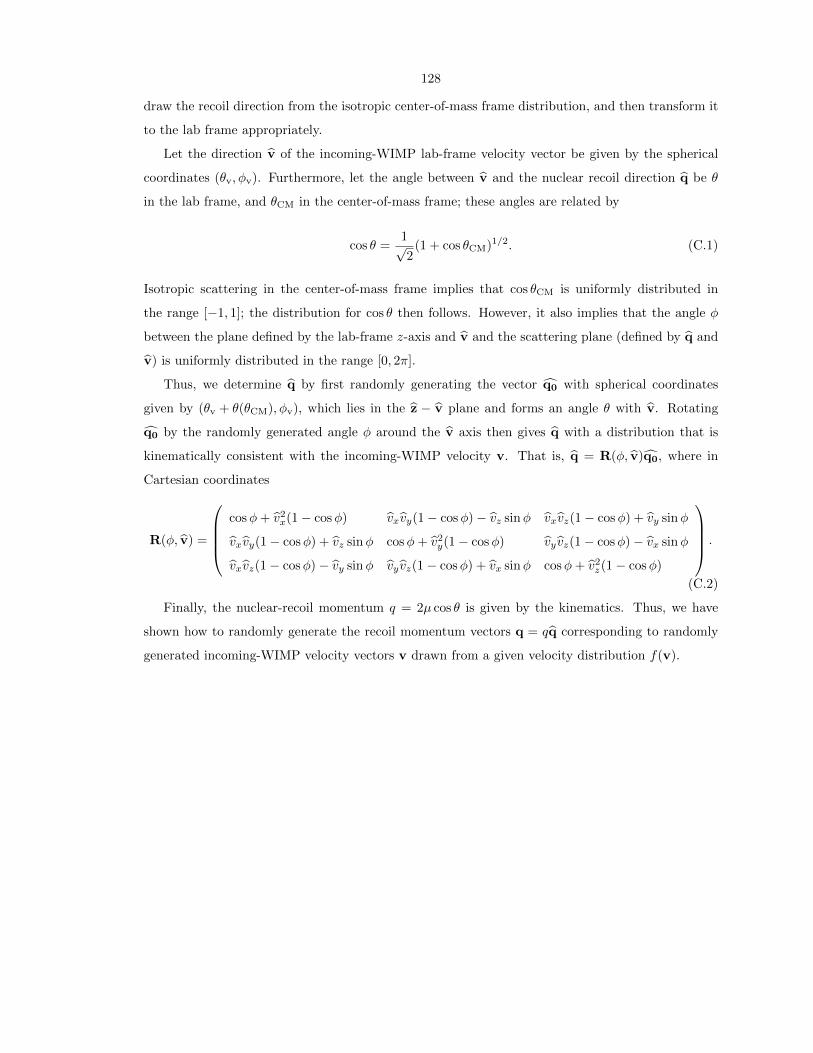
128
draw the recoil direction from the isotropic center-of-mass frame distribution, and then transform it
to the lab frame appropriately.
Let the direction v of the incoming-WIMP lab-frame velocity vector be given by the spherical
coordinates (θv, φv). Furthermore, let the angle between v and the nuclear recoil direction q be θ
in the lab frame, and θCM in the center-of-mass frame; these angles are related by
cos θ =1√2
(1 + cos θCM)1/2. (C.1)
Isotropic scattering in the center-of-mass frame implies that cos θCM is uniformly distributed in
the range [−1, 1]; the distribution for cos θ then follows. However, it also implies that the angle φ
between the plane defined by the lab-frame z-axis and v and the scattering plane (defined by q and
v) is uniformly distributed in the range [0, 2π].
Thus, we determine q by first randomly generating the vector q0 with spherical coordinates
given by (θv + θ(θCM), φv), which lies in the z − v plane and forms an angle θ with v. Rotating
q0 by the randomly generated angle φ around the v axis then gives q with a distribution that is
kinematically consistent with the incoming-WIMP velocity v. That is, q = R(φ, v)q0, where in
Cartesian coordinates
R(φ, v) =
cosφ+ v2x(1− cosφ) vxvy(1− cosφ)− vz sinφ vxvz(1− cosφ) + vy sinφ
vxvy(1− cosφ) + vz sinφ cosφ+ v2y(1− cosφ) vy vz(1− cosφ)− vx sinφ
vxvz(1− cosφ)− vy sinφ vy vz(1− cosφ) + vx sinφ cosφ+ v2z(1− cosφ)
.
(C.2)
Finally, the nuclear-recoil momentum q = 2µ cos θ is given by the kinematics. Thus, we have
shown how to randomly generate the recoil momentum vectors q = qq corresponding to randomly
generated incoming-WIMP velocity vectors v drawn from a given velocity distribution f(v).

129
Appendix D
Mass singularities and thermalfermionic corrections
At zero temperature, mass singularities from real-radiation, vertex, and self-energy diagrams all
cancel [337]. Whether the same is true at finite temperature is still an interesting open question.
As mentioned above, we find in Eq. (5.38) no mass singularities.1 However, we have not yet
proven that the decay rate remains finite in the ε→ 0 limit of a massless χ particle. This is because
we assumed T mχ mψ, so that only the photons had a non-negligible thermal distribution
fB . Again, factors of fB entered into the calculation of the decay rate in two places: (1) in the
calculation of the real-radiation corrections, via the thermal average for absorbed photons and
the Bose-enhancement factor for emitted photons, and (2) the modification of the bare photon
propagator given in Eq. (5.15).
However, at higher temperatures the thermal fermion populations may also be non-negligible. To
illustrate their effect, we return to discussion of the toy model. Let us assume that the temperature
satisfies mχ T mψ, as will be the case in the massless limit under discussion.2 At these
“intermediate” temperatures, we must then consider the Fermi-Dirac distribution for the χ particles,
fF (Eχ) =1
eEχ/T + 1. (D.1)
Factors of fF for the χ particle will then enter the calculation of the decay rate similarly in two
places.
First, a (1 − fF ) Pauli-blocking term for the final-state χ particles will be present, since the
This chapter contains previously unpublished work, which was completed in collaboration with MarcKamionkowski and Kirill Melnikov.
1Note that at this order in perturbation theory, the virtual corrections can only contribute at up to O(τ2), andtherefore can only cancel out infrared divergences and mass singularities from the real corrections that appear at thisorder in the temperature. We do not explicitly give the real corrections at O(τ4) and higher, but they appear tobe free of infrared divergences and mass singularities for the toy model under consideration. However, preliminarycalculations show that this does not appear to be the case for muon decay.
2At even higher temperatures satisfying T mψ , the Fermi-Dirac distribution of the ψ particles would also benon-negligible. In this case, the O(α0τ) correction to the decay rate due to time dilation caused by the thermalmotion of the ψ particles would dominate over the thermal corrections under discussion [347].
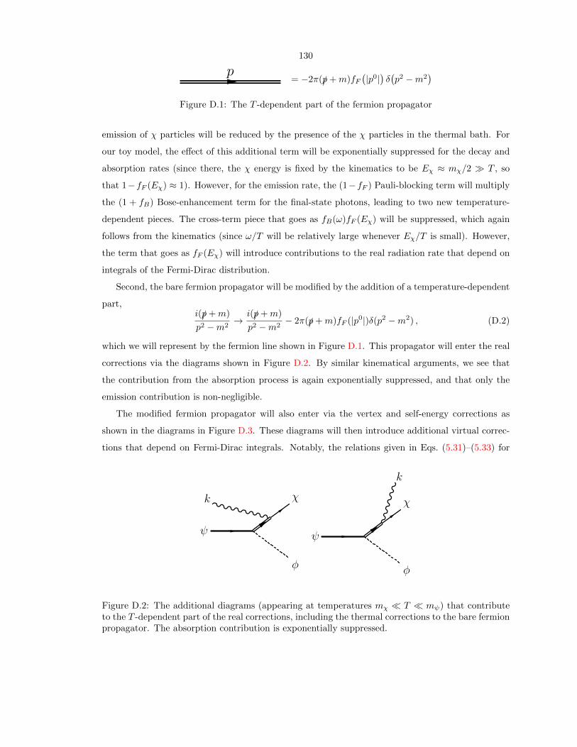
130
p= −2π(/p+m)fF
(|p0|)δ(p2 −m2
)
Figure D.1: The T -dependent part of the fermion propagator
emission of χ particles will be reduced by the presence of the χ particles in the thermal bath. For
our toy model, the effect of this additional term will be exponentially suppressed for the decay and
absorption rates (since there, the χ energy is fixed by the kinematics to be Eχ ≈ mχ/2 T , so
that 1−fF (Eχ) ≈ 1). However, for the emission rate, the (1−fF ) Pauli-blocking term will multiply
the (1 + fB) Bose-enhancement term for the final-state photons, leading to two new temperature-
dependent pieces. The cross-term piece that goes as fB(ω)fF (Eχ) will be suppressed, which again
follows from the kinematics (since ω/T will be relatively large whenever Eχ/T is small). However,
the term that goes as fF (Eχ) will introduce contributions to the real radiation rate that depend on
integrals of the Fermi-Dirac distribution.
Second, the bare fermion propagator will be modified by the addition of a temperature-dependent
part,i(/p+m)
p2 −m2→ i(/p+m)
p2 −m2− 2π(/p+m)fF (|p0|)δ(p2 −m2) , (D.2)
which we will represent by the fermion line shown in Figure D.1. This propagator will enter the real
corrections via the diagrams shown in Figure D.2. By similar kinematical arguments, we see that
the contribution from the absorption process is again exponentially suppressed, and that only the
emission contribution is non-negligible.
The modified fermion propagator will also enter via the vertex and self-energy corrections as
shown in the diagrams in Figure D.3. These diagrams will then introduce additional virtual correc-
tions that depend on Fermi-Dirac integrals. Notably, the relations given in Eqs. (5.31)–(5.33) for
ψ
k
φ
χ
ψ
φ
χ
k
Figure D.2: The additional diagrams (appearing at temperatures mχ T mψ) that contributeto the T -dependent part of the real corrections, including the thermal corrections to the bare fermionpropagator. The absorption contribution is exponentially suppressed.
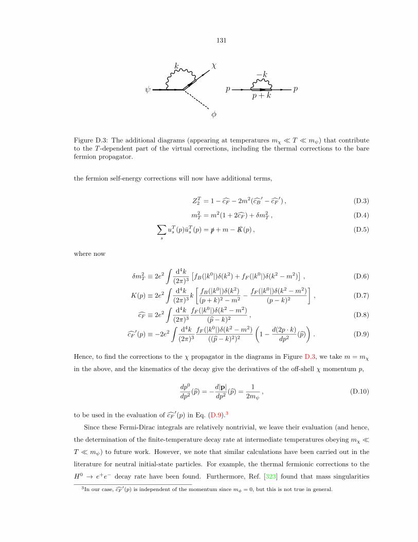
131
k
ψ
φ
χ
p + k
−k
p p
Figure D.3: The additional diagrams (appearing at temperatures mχ T mψ) that contributeto the T -dependent part of the virtual corrections, including the thermal corrections to the barefermion propagator.
the fermion self-energy corrections will now have additional terms,
ZT2 = 1− cF − 2m2(cB′ − cF ′) , (D.3)
m2T = m2(1 + 2cF ) + δm2
T , (D.4)∑
s
uTs (p)uTs (p) = /p+m− /K(p) , (D.5)
where now
δm2T ≡ 2e2
∫d4k
(2π)3
[fB(|k0|)δ(k2) + fF (|k0|)δ(k2 −m2)
], (D.6)
K(p) ≡ 2e2
∫d4k
(2π)3k
[fB(|k0|)δ(k2)
(p+ k)2 −m2− fF (|k0|)δ(k2 −m2)
(p− k)2
], (D.7)
cF ≡ 2e2
∫d4k
(2π)3
fF (|k0|)δ(k2 −m2)
(p− k)2, (D.8)
cF′(p) ≡ −2e2
∫d4k
(2π)3
fF (|k0|)δ(k2 −m2)
((p− k)2)2
(1− d(2p · k)
dp2(p)
). (D.9)
Hence, to find the corrections to the χ propagator in the diagrams in Figure D.3, we take m = mχ
in the above, and the kinematics of the decay give the derivatives of the off-shell χ momentum p,
dp0
dp2(p) = −d|p|
dp2(p) =
1
2mψ, (D.10)
to be used in the evaluation of cF′(p) in Eq. (D.9).3
Since these Fermi-Dirac integrals are relatively nontrivial, we leave their evaluation (and hence,
the determination of the finite-temperature decay rate at intermediate temperatures obeying mχ T mψ) to future work. However, we note that similar calculations have been carried out in the
literature for neutral initial-state particles. For example, the thermal fermionic corrections to the
H0 → e+e− decay rate have been found. Furthermore, Ref. [323] found that mass singularities
3In our case, cF′(p) is independent of the momentum since mφ = 0, but this is not true in general.

132
from the fermionic contributions do not completely cancel out at these intermediate temperatures,
leading to corrections to the decay rate as large as O(10%) when me/T ≈ 5%. Still, a considerable
body of subsequent work has found that mass singularities cancel, even at finite temperature, in a
variety of processes, and it suggests — though by no means proves — that they may always cancel.
If this speculation is correct, then the result of Ref. [323] would need to be revisited.
For the case of muon decay, we find that mass singularities cancel at O(ατ2). This disagrees with
Ref. [339], which found mass singularities at this order from the low-temperature thermal photonic
corrections alone, and claimed that these were cancelled by thermal fermionic corrections at high
temperature. Again, the cancellation of mass singularities in this process needs further investigation.

133
Bibliography
[1] J. H. Jeans, Mon.Not.Roy.Astron.Soc. 82, 122–132 (1922).
[2] F. Zwicky, Helv.Phys.Acta 6, 110–127 (1933).
[3] J. Einasto, arXiv:0901.0632.
[4] N. Jarosik, C. Bennett, J. Dunkley, B. Gold, M. Greason, et al., Astrophys.J.Suppl. 192, 14
(2011), [arXiv:1001.4744].
[5] A. G. Riess, L. Macri, S. Casertano, M. Sosey, H. Lampeitl, et al., Astrophys.J. 699, 539–563
(2009), [arXiv:0905.0695].
[6] R. Kessler, A. Becker, D. Cinabro, J. Vanderplas, J. A. Frieman, et al., Astrophys.J.Suppl.
185, 32–84 (2009), [arXiv:0908.4274].
[7] SDSS Collaboration: W. J. Percival et al., Mon.Not.Roy.Astron.Soc. 401, 2148–2168 (2010),
[arXiv:0907.1660].
[8] M. Roos, arXiv:1001.0316.
[9] D. Clowe, M. Bradac, A. H. Gonzalez, M. Markevitch, S. W. Randall, et al., Astrophys.J.
648, L109–L113 (2006), [astro-ph/0608407].
[10] G. Bertone, D. Hooper, and J. Silk, Phys.Rept. 405, 279–390 (2005), [hep-ph/0404175].
[11] F. D. Steffen, Eur.Phys.J. C59, 557–588 (2009), [arXiv:0811.3347].
[12] L. Bergstrom, New J.Phys. 11, 105006 (2009), [arXiv:0903.4849].
[13] J. L. Feng, Ann.Rev.Astron.Astrophys. 48, 495 (2010), [arXiv:1003.0904].
[14] M. Taoso, G. Bertone, and A. Masiero, JCAP 0803, 022 (2008), [arXiv:0711.4996].
[15] S. D. McDermott, H.-B. Yu, and K. M. Zurek, Phys.Rev. D83, 063509 (2011),
[arXiv:1011.2907].

134
[16] K. Sigurdson, M. Doran, A. Kurylov, R. R. Caldwell, and M. Kamionkowski, Phys.Rev.
D70, 083501 (2004), [astro-ph/0406355].
[17] S. Profumo and K. Sigurdson, Phys.Rev. D75, 023521 (2007), [astro-ph/0611129].
[18] K. Freese, B. Fields, and D. Graff, astro-ph/9904401.
[19] B. D. Fields, K. Freese, and D. S. Graff, Astrophys.J. 534, 265–276 (2000),
[astro-ph/9904291].
[20] MACHO Collaboration: C. Alcock et al., Astrophys.J. 542, 281–307 (2000),
[astro-ph/0001272].
[21] EROS-2 Collaboration: P. Tisserand et al., Astron.Astrophys. 469, 387–404 (2007),
[astro-ph/0607207].
[22] D. N. Spergel and P. J. Steinhardt, Phys.Rev.Lett. 84, 3760–3763 (2000),
[astro-ph/9909386].
[23] J. R. Primack, arXiv:0909.2247.
[24] S. De Lope Amigo, W. M.-Y. Cheung, Z. Huang, and S.-P. Ng, JCAP 0906, 005 (2009),
[arXiv:0812.4016].
[25] A. H. Peter and A. J. Benson, Phys.Rev. D82, 123521 (2010), [arXiv:1009.1912].
[26] A. H. Peter, C. E. Moody, A. J. Benson, and M. Kamionkowski, PoS IDM2010, 084 (2011),
[arXiv:1011.4970].
[27] M. Kesden and M. Kamionkowski, Phys.Rev.Lett. 97, 131303 (2006), [astro-ph/0606566].
[28] M. Kesden and M. Kamionkowski, Phys.Rev. D74, 083007 (2006), [astro-ph/0608095].
[29] http://fermi.gsfc.nasa.gov/.
[30] S. K. Lee, S. Ando, and M. Kamionkowski, JCAP 0907, 007 (2009), [arXiv:0810.1284].
[31] S. Ando, M. Kamionkowski, S. K. Lee, and S. M. Koushiappas, Phys.Rev. D78, 101301
(2008), [arXiv:0809.0886].
[32] S. M. Koushiappas, AIP Conf.Proc. 921, 142–146 (2007), [astro-ph/0703778].
[33] S. K. Lee and A. H. Peter, JCAP 1204, 029 (2012), [arXiv:1202.5035].
[34] J. L. Feng, M. Kamionkowski, and S. K. Lee, Phys.Rev. D82, 015012 (2010),
[arXiv:1004.4213].
135
[35] A. Czarnecki, M. Kamionkowski, S. K. Lee, and K. Melnikov, Phys.Rev. D85, 025018 (2012),
[arXiv:1110.2171].
[36] G. Bertone, Particle Dark Matter: Observations, Models and Searches. Cambridge
University Press, Cambridge, UK, 2010.
[37] E. W. Kolb and M. S. Turner, Front.Phys. 69, 1–547 (1990).
[38] J. Wess and J. Bagger.
[39] S. P. Martin, hep-ph/9709356.
[40] H. Baer and X. Tata, Weak scale supersymmetry: from superfields to scattering events.
Cambridge University Press, Cambridge, UK, 2006.
[41] G. Jungman, M. Kamionkowski, and K. Griest, Phys.Rept. 267, 195–373 (1996),
[hep-ph/9506380].
[42] J. L. Feng, Annals Phys. 315, 2–51 (2005).
[43] J. Ellis and K. A. Olive, arXiv:1001.3651.
[44] S. Ghigna et al., Mon.Not.Roy.Astron.Soc. 300, 146–162 (1998), [astro-ph/9801192].
[45] A. A. Klypin, S. Gottlober, A. V. Kravtsov, and A. M. Khokhlov, Astrophys.J. 516, 530–551
(1999), [astro-ph/9708191].
[46] A. A. Klypin, A. V. Kravtsov, O. Valenzuela, and F. Prada, Astrophys.J. 522, 82–92 (1999),
[astro-ph/9901240].
[47] B. Moore et al., Astrophys.J. 524, L19–L22 (1999), [astro-ph/9907411].
[48] A. Helmi, S. D. M. White, and V. Springel, Phys.Rev. D66, 063502 (2002),
[astro-ph/0201289].
[49] A. Loeb and M. Zaldarriaga, Phys.Rev. D71, 103520 (2005), [astro-ph/0504112].
[50] D. Reed et al., Mon.Not.Roy.Astron.Soc. 359, 1537–1548 (2005), [astro-ph/0406034].
[51] E. Bertschinger, Phys.Rev. D74, 063509 (2006), [astro-ph/0607319].
[52] J. Diemand, M. Kuhlen, and P. Madau, Astrophys.J. 667, 859–877 (2007),
[astro-ph/0703337].
[53] C. Giocoli, L. Pieri, and G. Tormen, arXiv:0712.1476.

136
[54] V. Berezinsky, V. Dokuchaev, and Y. Eroshenko, Phys.Rev. D77, 083519 (2008),
[arXiv:0712.3499].
[55] V. Springel et al., Mon.Not.Roy.Astron.Soc. 391, 1685–1711 (2008), [arXiv:0809.0898].
[56] A. M. Green, S. Hofmann, and D. J. Schwarz, Mon.Not.Roy.Astron.Soc. 353, L23 (2004),
[astro-ph/0309621].
[57] A. M. Green, S. Hofmann, and D. J. Schwarz, JCAP 0508, 003 (2005), [astro-ph/0503387].
[58] A. M. Green, S. Hofmann, and D. J. Schwarz, AIP Conf.Proc. 805, 431–434 (2006),
[astro-ph/0508553].
[59] J. Diemand, M. Kuhlen, and P. Madau, Astrophys.J. 649, 1–13 (2006), [astro-ph/0603250].
[60] T. Bringmann and S. Hofmann, JCAP 0407, 016 (2007), [hep-ph/0612238].
[61] M. Kamionkowski and S. M. Koushiappas, Phys.Rev. D77, 103509 (2008),
[arXiv:0801.3269].
[62] J. Diemand, B. Moore, and J. Stadel, Nature 433, 389–391 (2005), [astro-ph/0501589].
[63] H.-S. Zhao, J. Taylor, J. Silk, and D. Hooper, astro-ph/0502049.
[64] H. Zhao, J. E. Taylor, J. Silk, and D. Hooper, Astrophys.J. 654, 697–701 (2007),
[astro-ph/0508215].
[65] V. Berezinsky, V. Dokuchaev, and Y. Eroshenko, Phys.Rev. D73, 063504 (2006),
[astro-ph/0511494].
[66] T. Goerdt, O. Y. Gnedin, B. Moore, J. Diemand, and J. Stadel, Mon.Not.Roy.Astron.Soc.
375, 191–198 (2007), [astro-ph/0608495].
[67] D. Hooper and S. Profumo, Phys.Rept. 453, 29–115 (2007), [hep-ph/0701197].
[68] X.-l. Chen, M. Kamionkowski, and X.-m. Zhang, Phys.Rev. D64, 021302 (2001),
[astro-ph/0103452].
[69] S. Profumo, K. Sigurdson, and M. Kamionkowski, Phys.Rev.Lett. 97, 031301 (2006),
[astro-ph/0603373].
[70] T. Bringmann, New J.Phys. 11, 105027 (2009), [arXiv:0903.0189].
[71] M. S. Turner, Phys.Rept. 197, 67–97 (1990).
[72] G. G. Raffelt, Phys.Rept. 198, 1–113 (1990).

137
[73] L. J. Rosenberg and K. A. van Bibber, Phys.Rept. 325, 1–39 (2000).
[74] S. J. Asztalos, L. J. Rosenberg, K. van Bibber, P. Sikivie, and K. Zioutas,
Ann.Rev.Nucl.Part.Sci. 56, 293–326 (2006).
[75] M. C. Johnson and M. Kamionkowski, Phys.Rev. D78, 063010 (2008), [arXiv:0805.1748].
[76] E. A. Baltz et al., JCAP 0807, 013 (2008), [arXiv:0806.2911].
[77] L. Bergstrom, J. Edsjo, and P. Ullio, Phys.Rev. D58, 083507 (1998), [astro-ph/9804050].
[78] L. Bergstrom, J. Edsjo, P. Gondolo, and P. Ullio, Phys.Rev. D59, 043506 (1999),
[astro-ph/9806072].
[79] C. Calcaneo-Roldan and B. Moore, Phys.Rev. D62, 123005 (2000), [astro-ph/0010056].
[80] B. Moore et al., Phys.Rev. D64, 063508 (2001), [astro-ph/0106271].
[81] A. Tasitsiomi and A. V. Olinto, Phys.Rev. D66, 083006 (2002), [astro-ph/0206040].
[82] V. Berezinsky, V. Dokuchaev, and Y. Eroshenko, Phys.Rev. D68, 103003 (2003),
[astro-ph/0301551].
[83] A. Tasitsiomi, J. M. Siegal-Gaskins, and A. V. Olinto, New Astron.Rev. 48, 473–475 (2004),
[astro-ph/0306561].
[84] F. Stoehr, S. D. M. White, V. Springel, G. Tormen, and N. Yoshida,
Mon.Not.Roy.Astron.Soc. 345, 1313 (2003), [astro-ph/0307026].
[85] S. M. Koushiappas, A. R. Zentner, and T. P. Walker, Phys.Rev. D69, 043501 (2004),
[astro-ph/0309464].
[86] T. Oda, T. Totani, and M. Nagashima, Astrophys.J. 633, L65–L68 (2005),
[astro-ph/0504096].
[87] S. Ando, Phys.Rev.Lett. 94, 171303 (2005), [astro-ph/0503006].
[88] L. Pieri, E. Branchini, and S. Hofmann, Phys.Rev.Lett. 95, 211301 (2005),
[astro-ph/0505356].
[89] E. A. Baltz, J. E. Taylor, and L. L. Wai, Astrophys.J.Lett. 659, L125–L128 (2007),
[astro-ph/0610731].
[90] J. M. Siegal-Gaskins, V. Pavlidou, A. V. Olinto, C. Brown, and B. D. Fields,
J.Phys.Conf.Ser. 60, 312–314 (2007), [astro-ph/0611273].

138
[91] L. E. Strigari, S. M. Koushiappas, J. S. Bullock, and M. Kaplinghat, Phys.Rev. D75, 083526
(2007), [astro-ph/0611925].
[92] V. Berezinsky, V. Dokuchaev, and Y. Eroshenko, JCAP 0707, 011 (2007),
[astro-ph/0612733].
[93] L. Pieri, G. Bertone, and E. Branchini, Mon.Not.Roy.Astron.Soc. 384, 1627 (2008),
[arXiv:0706.2101].
[94] M. Kuhlen, J. Diemand, and P. Madau, arXiv:0805.4416.
[95] V. Springel et al., arXiv:0809.0894.
[96] S. Ando and E. Komatsu, Phys.Rev. D73, 023521 (2006), [astro-ph/0512217].
[97] S. Ando, E. Komatsu, T. Narumoto, and T. Totani, Phys.Rev. D75, 063519 (2007),
[astro-ph/0612467].
[98] A. Cuoco et al., JCAP 0704, 013 (2007), [astro-ph/0612559].
[99] A. Cuoco, J. Brandbyge, S. Hannestad, T. Haugboelle, and G. Miele, Phys.Rev. D77, 123518
(2008), [arXiv:0710.4136].
[100] J. M. Siegal-Gaskins, JCAP 0810, 040 (2008), [arXiv:0807.1328].
[101] S. Ando, Phys.Rev. D80, 023520 (2009), [arXiv:0903.4685].
[102] D. Hooper and P. D. Serpico, JCAP 0706, 013 (2007), [astro-ph/0702328].
[103] S. M. Koushiappas, Phys.Rev.Lett. 97, 191301 (2006), [astro-ph/0606208].
[104] T. D. Willis, astro-ph/0201515.
[105] http://heasarc.gsfc.nasa.gov/docs/cgro/cossc/egret/.
[106] J. F. Navarro, C. S. Frenk, and S. D. M. White, Astrophys.J. 490, 493–508 (1997),
[astro-ph/9611107].
[107] M. Fornasa, L. Pieri, G. Bertone, and E. Branchini, Phys.Rev. D80, 023518 (2009),
[arXiv:0901.2921].
[108] J. Diemand, M. Kuhlen, and P. Madau, Astrophys.J. 657, 262–270 (2007),
[astro-ph/0611370].
[109] L. Bergstrom, J. Edsjo, and P. Ullio, Phys.Rev.Lett. 87, 251301 (2001), [astro-ph/0105048].

139
[110] EGRET Collaboration: P. Sreekumar et al., Astrophys.J. 494, 523–534 (1998),
[astro-ph/9709257].
[111] A. R. Pullen, R.-R. Chary, and M. Kamionkowski, Phys.Rev. D76, 063006 (2007),
[astro-ph/0610295].
[112] G. D. Mack, T. D. Jacques, J. F. Beacom, N. F. Bell, and H. Yuksel, Phys.Rev. D78, 063542
(2008), [arXiv:0803.0157].
[113] P. A. G. Scheuer, Proc.Cambridge Phil.Soc. 53, 764–773 (1957).
[114] X. Barcons, Astrophys.J. 396, 460–468 (1992).
[115] X. Barcons and A. C. Fabian, Mon.Not.Roy.Astron.Soc. 243, 366–371 (1990).
[116] A. Franceschini, Astrophys.Space Sci. 86, 3–11 (1982).
[117] D. Windridge and S. Phillipps, Mon.Not.Roy.Astron.Soc. 319, 591–605 (2000).
[118] S. Dodelson, A. V. Belikov, D. Hooper, and P. Serpico, Phys.Rev. D80, 083504 (2009),
[arXiv:0903.2829].
[119] D. Tucker-Smith and N. Weiner, Phys.Rev. D64, 043502 (2001), [hep-ph/0101138].
[120] S. Chang, G. D. Kribs, D. Tucker-Smith, and N. Weiner, Phys.Rev. D79, 043513 (2009),
[arXiv:0807.2250].
[121] XENON100 Collaboration: E. Aprile et al., Phys.Rev. D84, 061101 (2011),
[arXiv:1104.3121].
[122] D. N. Spergel, Phys.Rev. 1353–1355 (1988).
[123] P. Gondolo, Phys.Rev. D66, 103513 (2002), [hep-ph/0209110].
[124] F. J. Kerr and D. Lynden-Bell, Mon.Not.Roy.Astron.Soc. 221, 1023–1038 (1986).
[125] A. M. Green, JCAP 1010, 034 (2010), [arXiv:1009.0916].
[126] C.-L. Shan, arXiv:1103.0481.
[127] Y. Akrami, C. Savage, P. Scott, J. Conrad, and J. Edsjo, JCAP 1104, 012 (2011),
[arXiv:1011.4318].
[128] M. Pato et al., Phys.Rev. D83, 083505 (2011), [arXiv:1012.3458].
[129] A. H. G. Peter, Phys.Rev. D83, 125029 (2011), [arXiv:1103.5145].
[130] C. Arina, J. Hamann, and Y. Y. Y. Wong, JCAP 1109, 022 (2011), [arXiv:1105.5121].

140
[131] M. T. Frandsen, F. Kahlhoefer, C. McCabe, S. Sarkar, and K. Schmidt-Hoberg, JCAP 1201,
024 (2012), [arXiv:1111.0292].
[132] C. Strege, R. Trotta, G. Bertone, A. H. G. Peter, and P. Scott, arXiv:1201.3631.
[133] DEAP-CLEAN Collaboration: F. Giuliani, AIP Conf.Proc. 1200, 985–988 (2010).
[134] CDMS-II Collaboration: Z. Ahmed et al., Science 327, 1619–1621 (2010),
[arXiv:0912.3592].
[135] E. Behnke et al., Phys.Rev.Lett. 106, 021303 (2011), [arXiv:1008.3518].
[136] M. Felizardo et al., arXiv:1106.3014.
[137] H. Sekiya, J.Phys.Conf.Ser. 308, 012011 (2011), [arXiv:1006.1473].
[138] ArDM Collaboration: A. Marchionni et al., J.Phys.Conf.Ser. 308, 012006 (2011),
[arXiv:1012.5967].
[139] CDMS Collaboration: Z. Ahmed et al., Phys.Rev. D84, 011102 (2011), [arXiv:1105.3377].
[140] XENON100 Collaboration: E. Aprile et al., Phys.Rev. D84, 052003 (2011),
[arXiv:1103.0303].
[141] XENON100 Collaboration: E. Aprile et al., Phys.Rev.Lett. 107, 131302 (2011),
[arXiv:1104.2549].
[142] D. C. Malling et al., arXiv:1110.0103.
[143] DARWIN Consortium: L. Baudis, arXiv:1201.2402.
[144] R. Bernabei et al., Eur.Phys.J. C67, 39–49 (2010), [arXiv:1002.1028].
[145] C. E. Aalseth et al., Phys.Rev.Lett. 107, 141301 (2011), [arXiv:1106.0650].
[146] G. Angloher et al., arXiv:1109.0702.
[147] C. J. Copi, J. Heo, and L. M. Krauss, Phys.Lett. B461, 43–48 (1999), [hep-ph/9904499].
[148] C. J. Copi and L. M. Krauss, Phys.Rev. D63, 043507 (2001), [astro-ph/0009467].
[149] B. Morgan, A. M. Green, and N. J. C. Spooner, Phys.Rev. D71, 103507 (2005),
[astro-ph/0408047].
[150] B. Morgan and A. M. Green, Phys.Rev. D72, 123501 (2005), [astro-ph/0508134].
[151] C. J. Copi, L. M. Krauss, D. Simmons-Duffin, and S. R. Stroiney, Phys.Rev. D75, 023514
(2007), [astro-ph/0508649].

141
[152] A. M. Green and B. Morgan, Phys.Rev. D77, 027303 (2008), [arXiv:0711.2234].
[153] M. S. Alenazi and P. Gondolo, Phys.Rev. D77, 043532 (2008), [arXiv:0712.0053].
[154] D. P. Finkbeiner, T. Lin, and N. Weiner, Phys.Rev. D80, 115008 (2009), [arXiv:0906.0002].
[155] S. Ahlen et al., Int.J.Mod.Phys. A25, 1–51 (2010), [arXiv:0911.0323].
[156] A. M. Green and B. Morgan, Phys.Rev. D81, 061301 (2010), [arXiv:1002.2717].
[157] M. Lisanti and J. G. Wacker, Phys.Rev. D81, 096005 (2010), [arXiv:0911.1997].
[158] J. Billard, F. Mayet, J. F. Macias-Perez, and D. Santos, Phys.Lett. B691, 156–162 (2010),
[arXiv:0911.4086].
[159] J. Billard, F. Mayet, and D. Santos, Phys.Rev. D82, 055011 (2010), [arXiv:1006.3513].
[160] J. Billard, F. Mayet, and D. Santos, Phys.Rev. D83, 075002 (2011), [arXiv:1012.3960].
[161] J. Billard, F. Mayet, and D. Santos, Phys.Rev. D85, 035006 (2012), [arXiv:1110.6079].
[162] C.-T. Chiang, M. Kamionkowski, and G. Z. Krnjaic, arXiv:1202.1807.
[163] C. Grignon et al., JINST 4, P11003 (2009), [arXiv:0909.0654].
[164] DRIFT Collaboration: M. Pipe, J.Phys.Conf.Ser. 203, 012031 (2010).
[165] K. Miuchi et al., Phys.Lett. B686, 11–17 (2010), [arXiv:1002.1794].
[166] S. Ahlen et al., Phys.Lett. B695, 124–129 (2011), [arXiv:1006.2928].
[167] T. Naka et al., arXiv:1109.4485.
[168] S. E. Vahsen et al., arXiv:1110.3401.
[169] G. Lake, Astron.J. 98, 1554–1556 (1989).
[170] G. Gelmini and P. Gondolo, hep-ph/0405278.
[171] K. Freese, P. Gondolo, and H. J. Newberg, Phys.Rev. D71, 043516 (2005),
[astro-ph/0309279].
[172] C. Savage, K. Freese, and P. Gondolo, Phys.Rev. D74, 043531 (2006), [astro-ph/0607121].
[173] J. I. Read, G. Lake, O. Agertz, and V. P. Debattista, arXiv:0803.2714.
[174] M. Vogelsberger, A. Helmi, V. Springel, S. D. White, J. Wang, et al.,
Mon.Not.Roy.Astron.Soc. 395, 797–811 (2009), [arXiv:0812.0362].
142
[175] J. I. Read, L. Mayer, A. M. Brooks, F. Governato, and G. Lake, arXiv:0902.0009.
[176] M. Kuhlen et al., JCAP 1002, 030 (2010), [arXiv:0912.2358].
[177] R. F. Lang and N. Weiner, JCAP 1006, 032 (2010), [arXiv:1003.3664].
[178] D. S. M. Alves, M. Lisanti, and J. G. Wacker, Phys.Rev. D82, 031901 (2010),
[arXiv:1005.5421].
[179] M. Lisanti and D. N. Spergel, arXiv:1105.4166.
[180] M. Maciejewski, M. Vogelsberger, S. D. White, and V. Springel, Mon.Not.Roy.Astron.Soc.
415, 2475 (2011), [arXiv:1010.2491].
[181] A. Natarajan, C. Savage, and K. Freese, Phys.Rev. D84, 103005 (2011), [arXiv:1109.0014].
[182] D. S. M. Fantin, A. M. Green, and M. R. Merrifield, Mon.Not.Roy.Astron.Soc. 418,
2648–2655 (2011), [arXiv:1108.4411].
[183] M. Kuhlen, M. Lisanti, and D. N. Spergel, arXiv:1202.0007.
[184] J. D. Vergados, arXiv:1202.3105.
[185] K. M. Gorski et al., Astrophys.J. 622, 759–771 (2005), [astro-ph/0409513].
[186] K. Kuijken and G. Gilmore, Mon.Not.Roy.Astron.Soc. 239, 651–664 (1989).
[187] L. Bergstrom, P. Ullio, and J. H. Buckley, Astropart. Phys. 9, 137–162 (1998),
[astro-ph/9712318].
[188] J. Holmberg and C. Flynn, Mon.Not.Roy.Astron.Soc. 313, 209–216 (2000),
[astro-ph/9812404].
[189] R. Catena and P. Ullio, JCAP 1008, 004 (2010), [arXiv:0907.0018].
[190] P. Salucci, F. Nesti, G. Gentile, and C. Frigerio Martins, Astron.Astrophys.
[191] F. Iocco, M. Pato, G. Bertone, and P. Jetzer, JCAP 1111, 029 (2011), [arXiv:1107.5810].
[192] F. Giuliani, Phys.Rev.Lett. 93, 161301 (2004), [hep-ph/0404010].
[193] F. Feroz and M. P. Hobson, Mon.Not.Roy.Astron.Soc. 384, 449 (2008), [arXiv:0704.3704].
[194] F. Feroz, M. P. Hobson, and M. Bridges, Mon.Not.Roy.Astron.Soc. 398, 1601–1614 (2009),
[arXiv:0809.3437].
[195] A. Lewis and S. Bridle, Phys.Rev. D66, 103511 (2002), [astro-ph/0205436].
143
[196] J. Hamann, S. Hannestad, G. G. Raffelt, and Y. Y. Y. Wong, JCAP 0708, 021 (2007),
[arXiv:0705.0440].
[197] D. Santos, O. Guillaudin, T. Lamy, F. Mayet, and E. Moulin, J.Phys.Conf.Ser. 65, 012012
(2007), [astro-ph/0703310].
[198] F. Mayet, O. Guillaudin, D. Santos, and A. Trichet, EAS Publ.Ser. 36, 263 (2009),
[arXiv:0905.4697].
[199] D. Santos et al., J.Phys.Conf.Ser. 309, 012014 (2011), [arXiv:1102.3265].
[200] J. Billard, F. Mayet, and D. Santos, arXiv:1202.3372.
[201] J. Lewin and P. Smith, Astropart.Phys. 6, 87–112 (1996).
[202] Super-Kamiokande Collaboration: T. Tanaka et al., Astrophys.J. 742, 78 (2011),
[arXiv:1108.3384].
[203] IceCube Collaboration: R. Abbasi et al., Phys.Rev. D85, 042002 (2012),
[arXiv:1112.1840].
[204] PICASSO Collaboration: S. Archambault et al., arXiv:1202.1240.
[205] J. I. Read, L. Mayer, A. M. Brooks, F. Governato, and G. Lake, Mon.Not.Roy.Astron.Soc.
397, 44–51 (2009), [arXiv:0902.0009].
[206] C. W. Purcell, J. S. Bullock, and M. Kaplinghat, Astrophys.J. 703, 2275–2284 (2009),
[arXiv:0906.5348].
[207] C. Bidin, G. Carraro, R. Mendez, and W. van Altena, Astrophys.J. 724, L122–L126 (2010),
[arXiv:1011.1289].
[208] N. Bozorgnia, G. B. Gelmini, and P. Gondolo, arXiv:1111.6361.
[209] T. Moroi, hep-ph/9503210.
[210] W. Rarita and J. Schwinger, Phys.Rev. 60, 61 (1941).
[211] M. Dine, W. Fischler, and M. Srednicki, Nucl.Phys. B189, 575–593 (1981).
[212] S. Dimopoulos and S. Raby, Nucl.Phys. B192, 353 (1981).
[213] C. R. Nappi and B. A. Ovrut, Phys.Lett. B113, 175 (1982).
[214] L. Alvarez-Gaume, M. Claudson, and M. B. Wise, Nucl.Phys. B207, 96 (1982).

144
[215] M. Dine, A. E. Nelson, and Y. Shirman, Phys.Rev. D51, 1362–1370 (1995),
[hep-ph/9408384].
[216] M. Dine, A. E. Nelson, Y. Nir, and Y. Shirman, Phys.Rev. D53, 2658–2669 (1996),
[hep-ph/9507378].
[217] D. Volkov and V. Soroka, JETP Lett. 18, 312–314 (1973).
[218] P. Fayet and J. Iliopoulos, Phys.Lett. B51, 461–464 (1974).
[219] B. de Wit and D. Z. Freedman, Phys.Rev.Lett. 35, 827 (1975).
[220] S. Deser and B. Zumino, Phys.Rev.Lett. 38, 1433 (1977).
[221] H. Pagels and J. R. Primack, Phys.Rev.Lett. 48, 223 (1982).
[222] M. Viel, J. Lesgourgues, M. G. Haehnelt, S. Matarrese, and A. Riotto, Phys.Rev. D71,
063534 (2005), [astro-ph/0501562].
[223] N. Cabibbo, G. R. Farrar, and L. Maiani, Phys.Lett. B105, 155 (1981).
[224] S. Weinberg, Phys.Rev.Lett. 48, 1303 (1982).
[225] J. R. Ellis, J. E. Kim, and D. V. Nanopoulos, Phys.Lett. B145, 181 (1984).
[226] T. Moroi, H. Murayama, and M. Yamaguchi, Phys.Lett. B303, 289–294 (1993).
[227] M. Kawasaki and T. Moroi, Prog.Theor.Phys. 93, 879–900 (1995), [hep-ph/9403364].
[228] S. Borgani, A. Masiero, and M. Yamaguchi, Phys.Lett. B386, 189–197 (1996),
[hep-ph/9605222].
[229] M. Bolz, A. Brandenburg, and W. Buchmuller, Nucl.Phys. B606, 518–544 (2001),
[hep-ph/0012052].
[230] J. Pradler and F. D. Steffen, Phys.Rev. D75, 023509 (2007), [hep-ph/0608344].
[231] J. Pradler, arXiv:0708.2786.
[232] V. S. Rychkov and A. Strumia, Phys.Rev. D75, 075011 (2007), [hep-ph/0701104].
[233] E. Pierpaoli, S. Borgani, A. Masiero, and M. Yamaguchi, Phys.Rev. D57, 2089–2100 (1998),
[astro-ph/9709047].
[234] K. Ichikawa, M. Kawasaki, K. Nakayama, T. Sekiguchi, and T. Takahashi, JCAP 0908, 013
(2009), [arXiv:0905.2237].

145
[235] M. Viel, J. Lesgourgues, M. G. Haehnelt, S. Matarrese, and A. Riotto, Phys.Rev.Lett. 97,
071301 (2006), [astro-ph/0605706].
[236] A. Boyarsky, J. Lesgourgues, O. Ruchayskiy, and M. Viel, JCAP 0905, 012 (2009),
[arXiv:0812.0010].
[237] U. Seljak, A. Makarov, P. McDonald, and H. Trac, Phys.Rev.Lett. 97, 191303 (2006),
[astro-ph/0602430].
[238] S. Hannestad, Phys.Rev. D70, 043506 (2004), [astro-ph/0403291].
[239] T. Asaka, K. Hamaguchi, and K. Suzuki, Phys.Lett. B490, 136–146 (2000),
[hep-ph/0005136].
[240] R. Allahverdi, A. Jokinen, and A. Mazumdar, Phys.Rev. D71, 043505 (2005),
[hep-ph/0410169].
[241] E. J. Copeland and O. Seto, Phys.Rev. D72, 023506 (2005), [hep-ph/0505149].
[242] K. Kohri, T. Moroi, and A. Yotsuyanagi, Phys.Rev. D73, 123511 (2006), [hep-ph/0507245].
[243] F. D. Steffen, JCAP 0609, 001 (2006), [hep-ph/0605306].
[244] J. Pradler and F. D. Steffen, Phys.Lett. B648, 224–235 (2007), [hep-ph/0612291].
[245] K.-Y. Choi, L. Roszkowski, and R. Ruiz de Austri, JHEP 04, 016 (2008), [arXiv:0710.3349].
[246] K. Kohri, A. Mazumdar, and N. Sahu, Phys.Rev. D80, 103504 (2009), [arXiv:0905.1625].
[247] D. Gorbunov, A. Khmelnitsky, and V. Rubakov, JHEP 12, 055 (2008), [arXiv:0805.2836].
[248] S. Dimopoulos, G. F. Giudice, and A. Pomarol, Phys.Lett. B389, 37–42 (1996),
[hep-ph/9607225].
[249] K. Choi, K. Hwang, H. B. Kim, and T. Lee, Phys.Lett. B467, 211–217 (1999),
[hep-ph/9902291].
[250] E. A. Baltz and H. Murayama, JHEP 05, 067 (2003), [astro-ph/0108172].
[251] M. Fujii and T. Yanagida, Phys.Lett. B549, 273–283 (2002), [hep-ph/0208191].
[252] K. Jedamzik, M. Lemoine, and G. Moultaka, Phys.Rev. D73, 043514 (2006),
[hep-ph/0506129].
[253] F. Staub, W. Porod, and J. Niemeyer, JHEP 01, 058 (2010), [arXiv:0907.0530].

146
[254] R. Kallosh, L. Kofman, A. D. Linde, and A. Van Proeyen, Phys.Rev. D61, 103503 (2000),
[hep-th/9907124].
[255] I. M. Shoemaker and A. Kusenko, Phys.Rev. D80, 075021 (2009), [arXiv:0909.3334].
[256] A. de Gouvea, T. Moroi, and H. Murayama, Phys.Rev. D56, 1281–1299 (1997),
[hep-ph/9701244].
[257] R. Casalbuoni, S. De Curtis, D. Dominici, F. Feruglio, and R. Gatto, Phys.Lett. B215, 313
(1988).
[258] T. Lee and G.-H. Wu, Phys.Lett. B447, 83–88 (1999), [hep-ph/9805512].
[259] S. Ambrosanio, G. L. Kane, G. D. Kribs, S. P. Martin, and S. Mrenna, Phys.Rev. D54,
5395–5411 (1996), [hep-ph/9605398].
[260] J. L. Feng and T. Moroi, Phys.Rev. D58, 035001 (1998), [hep-ph/9712499].
[261] G. D. Kribs, A. Martin, and T. S. Roy, JHEP 01, 023 (2009), [arXiv:0807.4936].
[262] Y. Santoso, AIP Conf.Proc. 1200, 494–497 (2010), [arXiv:0909.4742].
[263] D. R. Stump, M. Wiest, and C. P. Yuan, Phys.Rev. D54, 1936–1943 (1996),
[hep-ph/9601362].
[264] S. Dimopoulos, M. Dine, S. Raby, and S. D. Thomas, Phys.Rev.Lett. 76, 3494–3497 (1996),
[hep-ph/9601367].
[265] S. Dimopoulos, S. D. Thomas, and J. D. Wells, Phys.Rev. D54, 3283–3288 (1996),
[hep-ph/9604452].
[266] DELPHI Collaboration: P. Abreu et al., Eur.Phys.J. C16, 211–228 (2000),
[hep-ex/0103026].
[267] H. Baer, P. G. Mercadante, X. Tata, and Y.-l. Wang, Phys.Rev. D62, 095007 (2000),
[hep-ph/0004001].
[268] S. Ambrosanio, B. Mele, S. Petrarca, G. Polesello, and A. Rimoldi, JHEP 01, 014 (2001),
[hep-ph/0010081].
[269] CDF and D0 Collaborations: C. Pagliarone, hep-ex/0312005.
[270] K. Hamaguchi, Y. Kuno, T. Nakaya, and M. M. Nojiri, Phys.Rev. D70, 115007 (2004),
[hep-ph/0409248].
[271] J. L. Feng and B. T. Smith, Phys.Rev. D71, 015004 (2005), [hep-ph/0409278].

147
[272] P. Wagner and D. A. Toback, Int.J.Mod.Phys. A20, 3267–3269 (2005), [hep-ph/0410267].
[273] H. U. Martyn, Eur.Phys.J. C48, 15–24 (2006), [hep-ph/0605257].
[274] M. Klasen and G. Pignol, Phys.Rev. D75, 115003 (2007), [hep-ph/0610160].
[275] K. Hamaguchi, S. Shirai, and T. T. Yanagida, Phys.Lett. B663, 86–94 (2008),
[arXiv:0712.2462].
[276] S. Tarem, S. Bressler, H. Nomoto, and A. Di Mattia, Eur.Phys.J. C62, 281–292 (2009).
[277] J. Chen and T. Adams, Eur.Phys.J. C67, 335–342 (2010), [arXiv:0909.3157].
[278] J. L. Feng, J.-F. Grivaz, and J. Nachtman, Rev.Mod.Phys. 82, 699–727 (2010),
[arXiv:0903.0046].
[279] ALEPH Collaboration: A. Heister et al., Eur.Phys.J. C25, 339–351 (2002),
[hep-ex/0203024].
[280] ALEPH, DELPHI, L3, and OPAL Collaborations: LEP SUSY working group et al.,
Note LEPSUSYWG/02-09.2, http: // lepsusy. web. cern. ch/ lepsusy/ Welcome. html/
(2001).
[281] B. C. Allanach et al., Eur.Phys.J. C25, 113–123 (2002), [hep-ph/0202233].
[282] D0 Collaboration: V. M. Abazov et al., Phys.Lett. B659, 856–863 (2008),
[arXiv:0710.3946].
[283] CDF Collaboration: T. Aaltonen et al., Phys.Rev.Lett. 104, 011801 (2010),
[arXiv:0910.3606].
[284] CDF Collaboration: A. Abulencia et al., Phys.Rev.Lett. 99, 121801 (2007),
[arXiv:0704.0760].
[285] D0 Collaboration: V. M. Abazov et al., Phys.Rev.Lett. 102, 161802 (2009),
[arXiv:0809.4472].
[286] CDF Collaboration: T. Aaltonen et al., Phys.Rev.Lett. 103, 021802 (2009),
[arXiv:0902.1266].
[287] A. Brandenburg, L. Covi, K. Hamaguchi, L. Roszkowski, and F. D. Steffen, Phys.Lett. B617,
99–111 (2005), [hep-ph/0501287].
[288] P. Z. Skands et al., JHEP 07, 036 (2004), [hep-ph/0311123].
[289] B. C. Allanach et al., Comp.Phys.Commun. 180, 8–25 (2009), [arXiv:0801.0045].
148
[290] F. E. Paige, S. D. Protopopescu, H. Baer, and X. Tata, hep-ph/0312045.
[291] T. Sjostrand, S. Mrenna, and P. Z. Skands, JHEP 05, 026 (2006), [hep-ph/0603175].
[292] M. Kaplinghat and A. Rajaraman, Phys.Rev. D74, 103004 (2006), [astro-ph/0606209].
[293] K. Kohri and F. Takayama, Phys.Rev. D76, 063507 (2007), [hep-ph/0605243].
[294] M. Kawasaki, K. Kohri, and T. Moroi, Phys.Lett. B649, 436–439 (2007), [hep-ph/0703122].
[295] M. Kusakabe, T. Kajino, R. N. Boyd, T. Yoshida, and G. J. Mathews, Phys.Rev. D76,
121302 (2007), [arXiv:0711.3854].
[296] K. Jedamzik, Phys.Rev. D77, 063524 (2008), [arXiv:0707.2070].
[297] F. Takayama, Phys.Rev. D77, 116003 (2008), [arXiv:0704.2785].
[298] T. Jittoh et al., Phys.Rev. D84, 035008 (2011), [arXiv:1105.1431].
[299] K. Sigurdson and M. Kamionkowski, Phys.Rev.Lett. 92, 171302 (2004), [astro-ph/0311486].
[300] S. Profumo, K. Sigurdson, P. Ullio, and M. Kamionkowski, Phys.Rev. D71, 023518 (2005),
[astro-ph/0410714].
[301] K. Kohri and T. Takahashi, Phys.Lett. B682, 337–341 (2010), [arXiv:0909.4610].
[302] I. Albuquerque, G. Burdman, and Z. Chacko, Phys.Rev.Lett. 92, 221802 (2004),
[hep-ph/0312197].
[303] X.-J. Bi, J.-X. Wang, C. Zhang, and X.-m. Zhang, Phys.Rev. D70, 123512 (2004),
[hep-ph/0404263].
[304] M. Ahlers, J. Kersten, and A. Ringwald, JCAP 0607, 005 (2006), [hep-ph/0604188].
[305] I. F. M. Albuquerque, G. Burdman, and Z. Chacko, Phys.Rev. D75, 035006 (2007),
[hep-ph/0605120].
[306] M. Ahlers, J. I. Illana, M. Masip, and D. Meloni, JCAP 0708, 008 (2007),
[arXiv:0705.3782].
[307] M. H. Reno, I. Sarcevic, and J. Uscinski, Phys.Rev. D76, 125030 (2007), [arXiv:0710.4954].
[308] S. Ando, J. F. Beacom, S. Profumo, and D. Rainwater, JCAP 0804, 029 (2008),
[arXiv:0711.2908].
[309] B. Canadas, D. G. Cerdeno, C. Munoz, and S. Panda, JCAP 0904, 028 (2009),
[arXiv:0812.1067].

149
[310] I. F. M. Albuquerque, G. Burdman, C. A. Krenke, and B. Nosratpour, Phys.Rev. D78,
015010 (2008), [arXiv:0803.3479].
[311] F. Bloch and A. Nordsieck, Phys.Rev. 52, 54–59 (1937).
[312] M. Le Bellac, Thermal field theory. Cambridge University Press, Cambridge, UK, 2000.
[313] U. Kraemmer and A. Rebhan, Rept.Prog.Phys. 67, 351 (2004), [hep-ph/0310337].
[314] J. Moller and Y. Schroder, Nucl.Phys.Proc.Suppl. 205-206, 218–223 (2010),
[arXiv:1007.1223].
[315] D. A. Dicus et al., Phys.Rev. D26, 2694 (1982).
[316] J.-L. Cambier, J. R. Primack, and M. Sher, Nucl.Phys. B209, 372 (1982).
[317] R. Baier, B. Pire, and D. Schiff, Phys.Rev. D38, 2814 (1988).
[318] R. Baier, E. Pilon, B. Pire, and D. Schiff, Nucl.Phys. B336, 157 (1990).
[319] J. F. Donoghue and B. R. Holstein, Phys.Rev. D28, 340 (1983) [Erratum: D29, 3004 (1984)].
[320] J. F. Donoghue, B. R. Holstein, and R. W. Robinett, Ann.Phys. 164, 233 (1985) [Erratum:
172, 483 (1986)].
[321] R. L. Kobes, G. W. Semenoff, and N. Weiss, Z.Phys. C29, 371 (1985).
[322] A. E. I. Johansson, G. Peressutti, and B. S. Skagerstam, Nucl.Phys. B278, 324 (1986).
[323] K. Ahmed and S. S. Masood, Phys.Rev. D35, 1861–1871 (1987).
[324] S. S. Masood, Phys.Rev. D36, 2602–2605 (1987).
[325] T. Grandou, M. Le Bellac, and J. L. Meunier, Z.Phys. C43, 575 (1989).
[326] W. Keil, Phys.Rev. D40, 1176 (1989).
[327] W. Keil and R. Kobes, Physica A158, 47–57 (1989).
[328] T. Grandou, M. Le Bellac, and D. Poizat, Phys.Lett. B249, 478–484 (1990).
[329] T. Altherr, Phys.Lett. B262, 314–319 (1991).
[330] H. A. Weldon, Phys.Rev. D44, 3955–3963 (1991).
[331] A. Niegawa and K. Takashiba, Nucl.Phys. B370, 335–364 (1992).
[332] A. Niegawa, Phys.Rev.Lett. 71, 3055–3058 (1993).
150
[333] D. Indumathi, Annals Phys. 263, 310–339 (1998), [hep-ph/9607206].
[334] T. Kinoshita, J.Math.Phys. 3, 650–677 (1962).
[335] T. Altherr and P. Aurenche, Phys.Rev. D40, 4171 (1989).
[336] T. D. Lee and M. Nauenberg, Phys.Rev. 133, B1549–B1562 (1964).
[337] R. E. Behrends, R. J. Finkelstein, and A. Sirlin, Phys.Rev. 101, 866–873 (1956).
[338] S. M. Berman, Phys.Rev. 112, 267–270 (1958).
[339] K. Jagannathan, Phys.Rev. D41, 1667–1671 (1990).
[340] P. Binetruy, G. Girardi, and P. Salati, Nucl.Phys. B237, 285 (1984).
[341] K. Griest and D. Seckel, Phys.Rev. D43, 3191–3203 (1991).
[342] J. Edsjo and P. Gondolo, Phys.Rev. D56, 1879–1894 (1997), [hep-ph/9704361].
[343] T. Wizansky, Phys.Rev. D74, 065007 (2006), [hep-ph/0605179].
[344] N. Fornengo, C. W. Kim, and J. Song, Phys.Rev. D56, 5123–5134 (1997), [hep-ph/9702324].
[345] L. S. Brown and R. F. Sawyer, Phys.Rev. D63, 083503 (2001), [astro-ph/0006370].
[346] W. H. Press, S. A. Teukolsky, W. T. Vetterling, and B. P. Flannery, Numerical Recipes 3rd
Edition: The Art of Scientific Computing. Cambridge University Press, New York, NY,
USA, 2007.
[347] A. Czarnecki, G. P. Lepage, and W. J. Marciano, Phys.Rev. D61, 073001 (2000),
[hep-ph/9908439].


