Three Methods to Share Joint Costs or Surplus

Journal of Economic Theory 87, 275�312 (1999)

Three Methods to Share Joint Costs or Surplus

Eric Friedman

Rutgers University, New Jerseyfriedman�econ.rutgers.edu

and

Herve� Moulin

Duke University, Durham, North Carolinamoulin�econ.duke.edu

Received September 24, 1997; revised March 5, 1999

We study cost sharing methods with variable demands of heterogeneous goods,additive in the cost function and meeting the dummy axiom. We consider fouraxioms: scale invariance (SI); demand monotonicity (DM); upper bound forhomogeneous goods (UBH) placing a natural cap on cost shares when goods arehomogeneous; average cost pricing for homogeneous goods (ACPH). The randomorder values based on stand alone costs are characterized by SI and DM. Serialcostsharing, by DM and UB; the Aumann�Shapley pricing method, by SI andACPH. No other combination of the four axioms is compatible with additivity anddummy. Journal of Economic Literature Classification Numbers: C71, D62, D63.� 1999 Academic Press

1. ADDITIVE COST SHARING METHODS

The division of joint costs is a central problem in accounting [56],public utility pricing [23] and management [47]. The division of jointsurplus has an even broader scope, encompassing all situations modeled bya cooperative game (in characteristic form): applications include the jointproduction of private [41, 17, 42, 38] or public goods [6, 26], electricitypricing [22], the allocation of waiting time among the users of a computernetwork [44, 45, 8], the allocation of costs among users of a network[15, 14] and more.1

In this paper, we use the axiomatic approach to the cost sharingproblem. We work in the model known as ``axiomatic cost sharing with

Article ID jeth.1999.2534, available online at http:��www.idealibrary.com on

2750022-0531�99 �30.00

Copyright � 1999 by Academic PressAll rights of reproduction in any form reserved.

1 Surveys of the applications of cooperative games to the allocation of joint surplus andjoint costs are in [48, 29].

variable demands.''2 The only available information consists of a costfunction of several heterogeneous and divisible outputs. Given the level ofdemand in each output we ask how total cost should be shared among thevarious outputs? The corresponding formula may use information aboutcost (resp. output) at any potential level of demand (resp. supply) andnothing else. The choice of a specific formula is based on normativearguments of equity and decomposability; it is a robust and easilyapplicable division of costs (or surplus) relying exclusively on ``objective''information about the technology.

Equivalently, the model can be interpreted as a surplus sharing problem,where agents contribute inputs to a production function and share the out-put. There is no difference whatsoever between the cost sharing and surplussharing interpretations of the model; all that matters is a real valued func-tion C defined over Rn

+ and a particular point (q1 , ..., qn) in the domain ofC; the formula then divides C(q1 , ..., qn) between the n ``factors.'' To fixideas, we stick to the cost sharing interpretation throughout the paper (soqi is the demand for output i and C(q) is total cost for producing the vectorq), keeping in mind that the whole theory can be read equivalently in thesurplus-sharing context.3

The seminal work in axiomatic cost sharing is by Shapley [43], in amodel simpler than ours in the sense that the demand of each good isbinary: each variable qi takes only the values zero or one. The two keyaxioms introduced by Shapley are:

(i) Additivity: the cost shares depend additively upon the entire costfunction, and

(ii) Dummy: if the demand of a certain agent does not raise the over-all cost whatever the demands of other agents, then this agent's cost shareis zero.

The combination of additivity and dummy characterizes the family ofrandom order values ([56], see Section 7) within which an additional sym-metry requirement picks the Shapley value formula.

In this paper, we follow Shapley's methodology by adopting withoutfurther justifications its two fundamental postulates, additivity and dummy.If the dummy axiom is normatively compelling, the additivity axiom is not.The latter allows us to decompose a given cost function into an arbitrarysum of cost functions and compute cost shares separately; the resultingtransparency and decentralizibility of the cost sharing method have beennoted by virtually every author in the literature on axiomatic cost sharing

276 FRIEDMAN AND MOULIN

2 Section 4 reviews this literature and contrasts this approach with the Bayesian traditionin mechanism design.

3 Some of the examples discussed in Sections 2 and 3 use the surplus-sharing interpretation.

with variable demands; indeed almost no paper offers a nonadditive costsharing method to our consideration.4

Our first observation is that, in the model where user i may demand anarbitrary amount of the divisible good i, the two axioms additivity anddummy allow for a very rich family of methods, described in our represen-tation theorem. See Lemma 3 and Appendix 1. The goal is to explorethe consequences, within this family, of four additional normativerequirements. Two of them are well known��scale invariance (SI) andaverage cost for homogeneous goods (ACPH). The other two are new��demand monotonicity (DM) and upper bound for homogeneous goods(UBH). No cost sharing method meets any three of these four require-ments; on the other hand three specific pairs of these axioms characterizethree remarkable cost sharing methods.

Announcing the Contents

The formal results of the paper are reviewed in Section 2. Section 3 offersa detailed discussion and interpretation of the four axioms just mentioned,emphasizing the contexts in which they are or are not compelling. Section 4reviews the literature on axiomatic cost sharing. Section 5 defines the costsharing model and introduces the two axioms additivity and dummy.Section 6 provides a crucial representation formula for all cost sharingmethods meeting additivity and dummy. Section 7 characterizes the ran-dom order values by means of demand monotonicity and scale invariance,Theorem 1. Section 8 introduces the upper bound for homogeneous goodsaxiom and characterizes serial cost sharing by the combination of demandmonotonicity and UBH, Theorem 2. Some concluding comments aregathered in Section 9 and all proofs in the Appendix.

2. OVERVIEW OF THE PAPER

The literature on axiomatic cost sharing with variable demands is almostunanimous in recommending one cost sharing method known as theAumann-Shapley pricing method and computed as follows. If q=(q1 , ..., qn)is the demand profile, the cost share of good i is

xi (q; C)=|qi

0�iC \ t

qi} q+ dt (1)

(Note that the above is a revenue, not a price; the literature on Aumann�Shapley pricing usually focuses on the per unit price xi �qi .)

277THREE METHODS TO SHARE COSTS

4 To the best of our knowledge, the only exceptions are [49] and [20].

FIG. 1. The Aumann�Shapley method: xi=�# �i C.

Here the cost share xi imputed to agent i is the integral of the partialderivative of C with respect to good i, along the line from the origin to theprofile q of individual demands. See Fig. 1.

This method is known to be characterized,5 within the family of methodsmeeting additivity and dummy, by the combination of scale invariance andaverage cost pricing for homogeneous goods. The former requires that achange of the unit in which a particular good is measured should have noeffect on cost shares; the latter requires that when the demands qi enteradditively in the cost function (taking the form C(q1+ } } } +qn)), costshares should be proportional to demands. Both axioms are discussed inSection 3.

We challenge this dominant viewpoint in three ways:

(i) we criticize the Aumann�Shapley pricing method because it failsthe natural requirement of demand monotonicity: the cost share of a goodshould not decrease when its demand increases, ceteris paribus.

(ii) we show that the familiar Shapley�Shubik method based onstand alone costs meets the scale invariance and demand monotonicityaxioms, and in a certain sense is the only one with these properties.

(iii) we introduce a new axiom, upper bound for homogeneousgoods, placing a natural upper bound on the cost share of a good when


5 All references to the literature are gathered in Section 4.

goods enter additively in the cost function. This axiom points to a thirdmethod, serial cost sharing, extending to the present model with hetero-geneous goods the method introduced in the homogeneous good model byMoulin and Shenker [32, 33].

To illustrate point (i) we give a numerical example with two goods. TheAumann�Shapley method computes as follows the cost share of agent 1:

x1(q1 , q2 ; C)=|q1

0�1C \t, t

q2

q1+ dt=q1 |1

0�1C(tq1 , tq2) dt

For the cost function C� (q)=(q1 } q2)�(q1+q2) this gives

x1(q1 , q2 ; C� )=q1 } q2

2

(q1+q2)2

which is not monotonic in q1 , so that DM fails.We describe now the two methods mentioned in points (ii) and (iii). The

Shapley-Shubik method applies directly the Shapley value formula to theTU-cooperative game defined by the stand alone costs. Given a set S ofgoods (a nonempty subset of [1, ..., n]), and a profile of demands q=(q1 , ..., qn), the stand alone cost of coalition S at profile q is

c(S; q)=C(q(S)) where q(S) i=qi if i # S and zero otherwise.

Then the Shapley-Shubik formula imputes to good i a convex combinationof its incremental costs c(S _ [i]; q)&c(S; q) where S spans the entire setof coalitions not containing i.6

The serial cost sharing method extends to heterogeneous goods a formulaoriginally introduced in the homogeneous good problem. It is given by anintegral formula similar to (1), namely,

xi (q; C)=|qi

0�iC((te) 7q) dt

where e=(1, ..., 1) and (a 7 b) i=min(ai , bi). (2)

The cost share xi of agent i is the integral of the partial �iC along a pathjoining 0 to q by raising all coordinates at the same speed and freezing acoordinate once it reaches qi . See Fig. 2.


6 The formula is xi (q; C)=�S�N"[i] (s ! (n&s&1)!�n !) [c(S _ [i]; q)&c(S; q)].

FIG. 2. Serial cost sharing: xi=�# �iC.

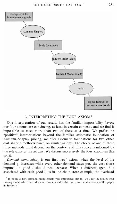
Within the family of methods meeting additivity and dummy, the logicalimplications of the four axioms are striking: there are exactly three costsharing methods meeting more than one axiom (if we count the family ofrandom order values as ``one'' method); each such method meets exactlytwo axioms and is characterized by this pair:

v the random order values are characterized by the pair SI plus DM;adding a mild symmetry requirement picks the Shapley�Shubik method��Theorem 1 and Corollary in Section 7

v serial cost sharing is characterized by the pair DM plus UBH��Theorem 2 in Section 8

v Aumann�Shapley pricing is characterized by the pair SI plus ACPH:this is well known and repeated in Section 8.

Finally, the other three pairs from our four axioms, namely ACPH+DM,ACPH+UBH, SI+UBH, are incompatible; it follows that any three ofthe four axioms are incompatible.

A diagram where axioms are depicted in rectangles and cost sharingmethods in ovals visualizes our findings. A pair of axioms not connected bya line are mutually incompatible; only three pairs of axioms are thus con-nected, each pair characterizing one of the three methods under discussion.


3. INTERPRETING THE FOUR AXIOMS

One interpretation of our results has the familiar impossibility flavor:our four axioms are convincing, at least in certain contexts, and we find itimpossible to meet more than two of these at a time. We prefer the``positive'' interpretation: beyond the familiar axiomatic foundation ofAumann�Shapley pricing, we offer axiomatic foundations for two othercost sharing methods based on similar axioms. The choice of one of thesethree methods must depend on the context and this choice is informed bythe relevance of the axioms. We discuss successively the four axioms in thisspirit.

Demand monotonicity is our first new7 axiom: when the level of thedemand qi increases while every other demand stays put, the cost shareimputed to good i should not decrease. When a different agent i isassociated with each good i, as in the chain store example, the overhead


7 In point of fact, demand monotonicity was introduced first in [30], for the related costsharing model where each demand comes in indivisible units; see the discussion of this paperin Section 4.

sharing among divisions example, or the delay sharing among computers,demand monotonicity is a compelling incentive requirement. If DM fails anagent can manipulate in a particularly wasteful way: raising artificially herdemand in order to decrease her total bill. In a surplus sharing context,failure to meet DM opens the door to ``sabotage.''8 Moreover, DM is aminimal equity requirement, imposing a positive correlation between inputcontribution and output share.9

On the other hand, when the demand of a given good is an aggregateof��small��demands by individual agents, as in the telephone pricingexample, or, more generally, in the problem of pricing a regulatedmonopoly, demand monotonicity is no longer compelling. The aggregatedemand of a particular good does not correspond to a normatively relevantgroup of agents (this is especially true if individual agents may demand apositive quantity of several goods), therefore the equity and incentivesjustifications of the axiom disappear.

Scale invariance is quite convincing when we take seriously the hetero-geneity of the goods. The classical example is the ``telephone pricing amongprofessors'' [5]. We have n classes of phone calls, differentiated by type(local, long distance; peak time, off-peak) and possibly by the telephone setfrom which the call originates. There is no direct way to compare quantitiesof the various phone calls (no obvious exchange rate between local and longdistance calls) and the cost shares should be independent of the units inwhich these different types of good are measured, which is precisely the scaleinvariance requirement (defined in Section 7). Another standard story(similar to the `òverhead division'' story in Shubik [47]) is a surplus sharingmodel. Consider an integrated chain store (e.g., grocery stores) with spe-cialized units supplying the various products offered in the stores (say factori is meat, factor j is produce and so on). Total revenue (net of the cost of dis-tributing the products to the various stores of the chain, and of other over-head costs) C(q1 , ..., qn) must be divided between the units. Quantities ofapples are not intrinsically comparable to quantities of meat, hence the unitsin which apples are measured (kilos, pounds or bushels) should not matter.10


8 `Ìf rewards were negatively correlated with productivity, the organization would besubject to sabotage,'' [2].

9 This is called the `òrdinal equity'' principle in the social psychology literature, e.g.,[16, 11].

10 In fact, there is no reason to limit ourselves to linear changes of unit; maybe even a non-linear redefinition of the scalar measure of any good should not matter. This is desirable whena good has no natural measurement scale invariant to affine transformations; examplesinclude heat, effort, and welfare level. Of the cost sharing methods discussed in this paper,only the random order values are ordinal. Sprumont and Wang [51] show that they arecharacterized by this `òrdinal invariance'' property, in combination with additivity anddummy. Seed also a related result, Proposition 5 in [30], in the ``discrete'' model discussedat the end of Section 4.

In some contexts, on the other hand, scale invariance is not compelling,because the different goods entering the cost or production function aregenuinely comparable, and yet they enter nonadditively in the cost orproduction function.

A simple surplus sharing example is the familiar production cooperative[42, 17] where good i is the effort level provided by worker i. Here dif-ferent workers hold different jobs in the factory, so that their inputs maynot enter symmetrically in the production function (C is not symmetricalin its variables). Yet their respective effort levels are comparable, and thiscomparison, together with the consideration of the entire production func-tion, determine their final shares of output.

Our next example is an important problem in network design. Considera group of agents sharing a single network link.11 Let q i be player i 's(stochastic) transmission rate, i.e., the expected number of packets sent persecond. The choice of service protocol, such as first in first out or roundrobin, determines the probabilistic delays imposed on the players. Let xi bethe average number of player i 's packets residing in the queue, which isrelated to the average queueing delay di by Little's law [19]. When thetransmissions follow a Poisson process and the service times are I.I.D.exponential with rate a (known as the M�M1 queue) work-conservationimplies that for any nonwasteful service protocol �n

i=1 xi=(�ni=1 q i)�

(a&�ni=1 qi)=C(q). In other words, the choice of a service protocol

amounts to the choice of a cost sharing method.12

In the queueing model just described, the demand qi represents the sizeof the service requested by network user i, whereas xi is the delay imposedon agent i by the network. A different problem is scheduling: here user irequests to be served before a certain deadline qi , and the server incurscosts C(q) to meet the deadlines of all the users, so that xi is the monetarycost share of agent i.

The common feature of these queueing, scheduling or productioncooperative stories is that the demands of two different agents are com-parable, so that scale invariance is not compelling. Of course, the weakerproperty requiring that a change in the common unit of the goods shouldhave no effect, is compelling. All the methods discussed in this paper areinvariant to a rescaling of the common unit.


11 This general queueing model applies to many other situations, such as informationrequests from a database or employees sending questions via email to their boss.

12 There are other constraints, � i # S x i�C(qS , 0) for all S/[1, ..., n], that also must besatisfied: [9]. Interestingly, for the M�M�1 queue, all of these are satisfied by the threemethods which we will discuss in this paper. In fact Aumann�Shapley corresponds to first infirst out queueing, incremental cost sharing (the extremal random order values) to preemptivepriority service, and serial cost to fair queueing [45].

The next axiom, ACPH, is a familiar requirement of the literature onAumann�Shapley pricing: it imposes the form of our cost sharing methodon a restricted class of cost functions, namely these cost functionsC(q1+ } } } +qn) where the various goods enter additively. Thus the goodscan be conceived as one single homeogeneous good, because the technologytreats the goods as if they were identical. This axiom, as well as the nextone, UBH, is distinctly less compelling than properties like DM or SI, thatimpose a natural requirement to any cost function in the admissibledomain.

Average cost pricing for homogeneous goods is compelling when thedemand qi of good i is the aggregate of a number of individual demandsthat cannot be individually monitored. In the telephone pricing example,assume that only one type of calls (say local calls) are used, so that thedemands qi emanating from different telephone sets enter additively in thecost; if local calls made from different phones were charged differently,users would have an arbitrage opportunity: e.g., they would transfer someof their demand to the cheap phone set. It is well known that average costpricing for homogeneous goods is the only method immune to manipula-tions by transfers of demands across agents, by merging several demandsinto one, or splitting one demand into several and so on.13

On the other hand, ACPH is not compelling when the agents and theirdemands are easily monitored. In the chain store example above the sup-pliers of a certain kind of apples, whose inputs qi enter additively in theproduction function, cannot easily collude because they are in differentlocations and transferring goods is costly. Or take the cost sharing storytold by Shubik [47]: a firm has n divisions, each division manager requestsqi units of good i from the central unit and C(q1 , ..., qn) is total overheadcost to be allocated between the divisions. Even if the goods i, j enteradditively in the cost function, the actual quantities consumed in each divi-sion are easily monitored so as to prevent collusive transfers; merging andsplitting divisions are simply not feasible. And, finally, in the delay-sharingamong computers story, the decentralized nature of the network makescollusion impractical.

The discussion of the ACPH axiom revolves around the distinctionbetween two stylized cases. In the first context the demand for good i isan anonymous agregate and the mechanism has no way to know who isbehind what fraction of the demand of what good. In the second, good iis impersonated by a specific agent i who consumes the entire amount qi

(and consumes no other good); ACPH is compelling in the former contextbut much less so in the latter. On the other hand, DM is compelling in thelatter context but much less so in the former.


13 See [3, 7, 28, 33].

The fourth axiom is new. Like ACPH, it places a restriction on themethod over the restricted class of cost functions with homogeneous goods.Unlike ACPH, it does not define the method over this subclass; moreoverthe axiom is still meaningful for more general cost functions than homo-geneous ones.

Upper bound for homogeneous goods. When goods are homogeneous, i.e.,enter additively in the cost function, the axiom requires that no agentshould pay more than the cost of producing n times his own demand,where n is the total number of agents. This bound protects the agent witha below average demand from being charged too much: if marginal costsincrease, the low demand agent should not be held responsible for the highmarginal cost generated by demands larger than his own. Symmetrically, inthe surplus sharing interpretation, UBH places a cap on the surplus shareawarded to an agent who contributes less than the average contribution.

For instance, with two goods and the cost function C(q1 , q2)=(q1+q2)2, UBH requires that each agent i be charged no more thanC(qi , qi)=4q2

i , irrespective of the demand qj by agent j. This requirementis not met by average cost pricing, which charges qi } (q1+q2). In general,if the goods i=1, ..., n are different but comparable (as in the queuingproblems described above), and if they enter symmetrically (but notnecessarily additively) in the cost function, the UBH axiom is stillmeaningful.

In the congestion example (delay sharing among computers, see above)UBH is a natural requirement, because we wish to protect the small usersfrom suffering excessive externalities (i.e., delays) from large users. Thisreflects a concern for equity, and has incentives implications as well: usersare less likely to drop from the queue when they know an upper bound ontheir own waiting time that does not depend upon the level of demand byother users.

We show in Section 8 that the axiom UBH is not compatible with scaleinvariance (given that we also require additivity and dummy). In problemswhere the goods are truly heterogeneous and their units incomparable(such as in the chain store or telephone pricing stories), scale invariance iscompelling whereas the UBH requirement must be dropped.

4. RELATION TO THE LITERATURE

Our approach falls squarely in the axiomatic tradition, followingShapley's seminal work in the cooperative game model [43] which inspiredmuch of the social choice and axiomatic bargaining literatures, as well asthe microeconomic theory of distributive justice. For a good survey, see[39]. The choice of a cost or surplus sharing method is conceptually


analogous to the choice of a constitution behind the ``veil of ignorance''[36]. In our model, the mechanism designer can be thought of as a chainstore manager setting up rules for allocating joint costs that will apply toevery particular store with its particular cost structure. Indeed, theaxiomatic analysis hinges on the assumption that cost functions may spana rich domain, in this case any nondecreasing and smooth cost function ofn variables. See Section 5.

A striking feature of the axiomatic approach is to be welfare-blind andincentive-blind: preferences of the users of the technology, over outputand cost shares, are entirely absent from the model. Compare withthe ``Bayesian'' tradition in mechanism design whereby the designer useshis�her incomplete information about the cost function, as well as aboutthe users characteristics, when choosing a particular cost sharing method.See, e.g., [21]. This latter approach is well suited to analyze the allocationof joint costs, or of whatever resources, on a short term basis when infor-mation about (the distribution) of agents' preferences is well known, andis common knowledge among all participants. Such results are often fragile,depending delicately on the detailed structure of the game's priors, andthus can be problematic in the public goods arena, or in situations whenpreferences are not common knowledge, such as on the Internet. In con-trast the axiomatic methodology typically leads to (comparatively) simpleand robust methods which may be more politically acceptable because theydo not rely on any information about preferences. The axiomatic methodis the only route toward uncovering general principles of distributivejustice. In the spirit of Aristotle's ``proportionality principle,'' [16] if offersfair division methods with broad applicability and parsimonious informa-tional requirements.

We now review the literature on axiomatic cost sharing with variabledemands. The first paper directly relevant is Shubik [47] who proposes theShapley-Shubik method discussed above (and of which the corollary toTheorem 1 gives an axiomatic characterization).

The literature on the Aumann�Shapley pricing method starts with theparallel characterizations by [4] and [27]. [24] and [25] discuss non-anonymous versions of the Aumann�Shapley pricing method and offer acharacterization of the random order values related to our Theorem 1. Thecrucial difference is that their strong additivity axiom imposes the require-ment that only stand alone costs should matter, whereas our Theorem 1derives this property. The main point of our paper is to show how variouscombinations of natural axioms such as DM, SI, and UBH force themethod to use information only about a very small subset of the rectangle[0, q], namely a path joining 0 to q or the finite set of vertices. Sprumontand Wang [51] offer an alternative characterization of the random ordervalues related to our Theorem 1: they replace the two requirements DM


and SI by a single axiom called ordinality and requiring cost shares to beinvariant under a nonlinear rescaling of any good.

Serial cost sharing was introduced in Shenker [44] and its incentivesproperties analyzed by Moulin and Shenker [32]: more on these propertiesin the concluding Section 9. More relevant to the current paper is [33],developing an axiomatic comparison of average cost pricing and serialcost sharing when the goods are homogeneous, i.e., on the domain ofcost functions taking the form C(q1+ } } } +qn). There the additivityand separability axioms, the latter being a counterpart to dummy in thehomogeneous good case, play a central role, as does the upper boundaxiom. However scale invariance and demand monotonicity have no coun-terpart. See Remark 2 at the end of Section 8.

This paper is related to (inspired by) [30], developing a parallel theoryof cost sharing with variable demands when goods are heterogeneous andcome in indivisible units (so each demand qi takes integer values). In that``discrete'' model, no topological difficulties stand in the way of systematiccharacterization results. Moulin [30] offers a characterization of serial costsharing in the discrete model that closely resembles our Theorem 3(Proposition 4, statement ii); it offers a characterization of the Shapley�Shubik method by imposing an ordinality requirement, later weakened bySprumont and Wang [52] into a discrete analog of scale invariance. Otherrelated work is [53] and [50], discussing the discrete version of theAumann�Shapley method: the former paper characterizes this methodwhile the latter criticizes it.

A key step in our analysis is the representation result (Lemma 3)describing the set of cost sharing methods satisfying additivity and dummy.It is inspired by the main result in Moulin [30]. Since this paper waswritten, a more elegant representation theorem has been given by Haimanko[13]. It shows that the extreme points of this set consist of taking partialderivatives of the cost function along a monotone path: this result isdescribed in Section 6. Wang [55] establishes its counterpart in the dis-crete model. Finally Friedman [12] exploits the (continuous) representa-tion result to analyze the cost sharing methods satisfying some of theaxioms scale invariance, demand monotonicity and consistency.

5. THE MODEL

We fix the set N=[1, ..., n] of heterogeneous goods (also interpreted asagents) throughout the paper.

Notations. Given p, q, both in Rn and such that p�q, the rectangle[ p, q] is defined by the inequalities p�z�q. Given a subset S of N, we


write (q"Sp) for the vector with ith coordinate qi if i � S and p i if i # S.Given q # Rn

+ we write qN=�n1 qi and qS=�S qi . Given a differentiable

real valued function C with domain Rn+ , we denote by �i C(q) its partial

derivative at q in the i th coordinate. Given an element q of Rn+, we denote

by 1(q) the vector space of real valued continuously differentiable functionswith domain [0, q] such that C(0)=0, and by 1+(q) the subset of itsnon-decreasing elements ( p� p$ O C( p)�C( p$) for all p, p$ in [0, q]). Thenotations 1(�), 1+(�) stand for functions with domain Rn

+ (and thesame regularity�monotonicity properties). Finally the notations 1 &i(q)(resp. 1 &i(�), 1 &i

+ (q), ...) stand for the subset of 1(q) (resp. 1(�),1+(q) . . .) made of functions independent of qi , in other words:

C # 1 &i(q) � C # 1(q) and [�iC( p)=0 for all p # [0, q]].

We now introduce the central concept of this paper: A cost sharing methodis a mapping x from Rn

+_1+(�) into Rn+ associating to each demand

profile q and cost function C a vector x(q; C) of cost shares satisfying thebudget balance property:

:n

i=1

xi (q; C)=C(q)

(note that cost shares are non negative by assumption). The two basicaxioms that we maintain throughout are now defined.

Additivity (ADD). For all C 1, C 2 in 1+(�) and all q # Rn+ ,

x(q; C 1+C 2)=x(q; C 1)+x(q; C 2).

Dummy (DUM). For all C # 1+(�), all i # [1, ..., n],

[C # 1 &i+ (�)] O [xi (q; C)=0 for all q # Rn

+].

We denote by C0 the set of cost sharing methods and by C the subsetdefined by the combination of additivity and dummy. Additivity is a decen-tralizability property: it does not matter whether we compute cost shareson the two separate components C 1 and C 2 of total costs or we apply theformula to the combined cost. Dummy says that a good that can beproduced at no cost, no matter how much of the other goods is produced,should not be charged any cost (the assumption �i C#0 means that goodi is ``free;'' we also say that good i is a dummy good). This is the straight-forward generalization of the original dummy axiom for cooperative games[43].


6. AN INTEGRAL REPRESENTATION UNDERADDITIVITY AND DUMMY

In this section, we present an integral representation of C, on which allsubsequent arguments (and our four theorems) are based.

Throughout this section we fix a cost sharing method x in C.

Lemma 1 (Independence of Irrelevant Costs). Fix q # Rn+ and two cost

functions C 1, C 2 in 1+(�) that coincide on [0, q]. Then x(q; C 1)=x(q; C 2).

Lemma 1 implies that for each fixed q # Rn+ , the cost sharing method x

defines an additive operator C � x(q; C) with domain 1+(q) (as no confu-sion may arise we use the same notation).

Lemma 2. For every fixed q in Rn+ , the operator x(q; } ) extends uniquely

to a linear operator on 1(q). The extended operator is denoted x(q; } ) as well.

In Lemma 1 and 2, only the additivity property of x was used. Dummyis essential for the proof of the next result, namely the integral representa-tion.

Lemma 3. For all q # Rn+ and all i, there exists a nonnegative Radon

measure +i (q) on [0, q] such that for all C # 1(q):

xi (q; C)=|[0, q]

�i C( p) d+i (q)( p). (3)

Moreover the projection of + i (q) on the (one-dimensional ) interval [0, qi] isthe Lebesgue measure:

for all a, b, 0�a�b�qi ,

set 0=[ p # [0, q] | a� pi�b]

then +i (q)(0)=b&a. (4)

The proof is an application of the Riesz representation theorem. SeeAppendix 1.

Note that, as stated, Lemma 3 is not a complete characterization of C,because it does not take into account budget balance. The completerepresentation theorem is significantly more complicated to state and is notrequired for the proofs of this paper; it is presented in Appendix 1. Theconditions that the measures must satisfy to give a valid method in C arequite complex, consisting of 2n restrictions (see (14) in Appendix 1). Sincewe first completed this analysis a more elegant representation has been dis-


covered. It relies on the family of ``path generated'' methods, that computethe cost share of good i as the integral of the i th partial derivative alonga given path.

This representation is based on the fact that the set C is convex and thatthe methods generated by a path are the extreme points of this set. As wenoted in Section 2 the Aumann�Shapley method ((1)) is generated by apath which is the diagonal from 0 to q (Fig. 1), while serial cost sharing((2)) is also generated by a path (Fig. 2). Next consider the followingincremental cost sharing method among two agents

x1(q; C)=C(q1 , 0); x2(q; C)=C(q1 , q2)&C(q1 , 0)

(incremental methods are defined for any N and characterized in Section 7).This method is generated by the path from 0 to x along the lower edge ofthe rectangle [0, x]: this path is denoted #1, 2 on Fig. 3. The symmetricincremental method

x1(q; C)=C(q1 , q2)&C(0, q2); x2(q; C)=C(0, q2)

is similarly generated by the path (denoted #2, 1 on Fig. 3) along the upperedge of this rectangle. Then the Shapley�Shubik method is simply theaverage of these two methods: it is not generated by the average of thesetwo paths (which is a piecewise linear path depicted on Fig. 3), or by anyother path.

FIG. 3. The two incremental methods when N=[1, 2].


It turns out that all cost sharing methods in C can be constructed in asimilar manner, as the convex combination of path methods. First notethat for any path #(t; q) which is continuous and nondecreasing in t, with#(0; q)=0 and #(1; q)=q, the related function

x#i (q; C)=|

1

0�iC(#(t; q)) d#(t; q)

is a cost sharing method in C. These methods form the extreme points ofthe set C, as shown by Haimanko [13].

Theorem. x(q; } ) is an extreme point of the set C ( for fixed q) if andonly if there exists some path #(q; } ) such that x(q; } )=x#(q; } ).

As discussed in Friedman [12] using Lemma 3 and Choqet's theorem[35], we can use this result to get a true representation theorem.

Corollary. If x(q; } ) is a csm in C, there exists a measure & on 1(q)such that

x(q; } )=|1(q)

x#(q; } ) d&(#),

where 1(q) is the set of all paths from 0 to q.

We refer the reader to [12] for the details, such as the definition of themeasure spaces and various topologies. That paper uses the representationby path methods to provide simple representations for various subsets of C,such as those satisfying scale invariance, or demand monotonicity, orconsistency.

Remark 1. By formula (3), all cost sharing methods in C satisfy alsothe marginality property [58]: the cost share imputed to good i dependsonly upon the marginal cost function with respect to good i. In thestandard cooperative game context (where each demand qi equals zero orone), [57] offers a characterization of the Shapley value where marginalityreplaces both additivity and dummy. (This result generalizes to a charac-terization of the random order values: [18]) In the variable demand con-text of this paper, marginality is not enough to replace additivity: it is easyto construct non additive methods meeting marginality.

Remark 2. Lemma 3 implies a robustness of the cost shares: if two costfunctions are close (in the C 1 metric) then the associated cost shares willalso be close. Thus in this metric an approximate knowledge of the costfunction allows one to compute approximate cost shares.


7. SCALE INVARIANCE, DEMAND MONOTONICITY,AND THE RANDOM ORDER VALUES

We define two important axioms for cost sharing methods. The followingnotation will be useful to state SI: for any positive number *, the mapping{ i

* is the *-rescaling of the i th coordinate

{ i*(q)=(q"i*qi) for all q # Rn

+ , all i, all *>0

(where (q"iqi$) equals q except that its i-coordinate is qi$).Given a cost function C it is transformed into the function { i

*[C] by thesaid *-rescaling

{ i*[C](q)=C({ i

1�*(q)).

Scale invariance. For every i, every cost function C # 1+(�), everyq # Rn

+ and every *>0:

x(q; C)=x({ i*(q); { i

*[C]).

Demand monotonicity. For every i, every cost function C # 1+(�) andevery q # Rn

+ :

for any qi$ [qi�qi$] O [x i (q; C)�xi ((q"iqi$); C)]

The SI and DM axioms are discussed in Section 3.We showed in Section 3 that the Aumann�Shapley pricing method is not

demand monotonic. Here we check, also by means of a numerical example,that serial cost sharing fails scale invariance. With two goods and demandsq1 , q2 such that q1�q2 , serial cost sharing yields the cost share:

x1(q1 , q2 ; C)=|q1

0�1 C({, {) d{.

Consider the cost function C(q)=(q1+q2)2, then double the scale of good1 so that the ``new'' demand q~ 1 is worth q~ 1=(1�2) q1 if q1 is the ``old'' one.The new cost function is C� (q~ 1 , q2)=(2q~ 1+q2)2 and we have

x1(1, 1; C)=2

x1( 12 , 1; C� )=|

1�2

04 } (2{+{) d{= 3

2

in violation of scale invariance.If serial cost sharing fails SI, it is easy to see that it is invariant upon a

simultaneous rescaling of all goods.


We now define the random order values [56]. Fix an ordering _ of[1, 2, ..., n] and for every agent i, denote by S(_; i) the set of agents pre-ceding i in this ordering, i.e., j # S(_; i) if _( j)<_(i). Recall the notationc(S; q)=C(q(S)) where q(S) i=qi if i # S and zero otherwise. The incremen-tal cost sharing method associated with _ is defined by

xi (q; C)=c(S(_; i) _ [i]; q)&c(S(_; i); q). (5)

A random order value is an arbitrary convex combination of incrementalc.s.m.s. (the convex weights being independent of both q and C). A randomorder value is an element of C. Naturally, the Shapley�Shubik method isthe arithmetic average of the n ! incremental methods. Figure 3 shows thepaths generating the two incremental methods when N=[1, 2].

The last ingredient of Theorem 1 is a technical continuity requirementfor null demands:

Continuity at zero. For every i, every C # 1+(�) and every q # Rn+ :

limq$i>0, q$i � 0

x((q"iq i$); C)=x(q"i0), C).

Theorem 1. Given N and a cost sharing method x in C (hence satisfyingadditivity and dummy) the two following statements are equivalent:

(i) x is a random order value;

(ii) x satisfies scale invariance, demand monotonicity and continuity atzero.

Corollary. The Shapley�Shubik method is characterized by the com-bination of the five axioms ADD, DUM, SI, DM, Continuity at zero, and thefollowing symmetry property:

Symmetry. If C # 1+(�) is a symmetrical function of the n variables qi

then x(e; C)=(1�n) C(e) where e=(1, 1, ..., 1).

Remark 3. All random order values are continuous in q everywhere. Infact any method in C meeting SI must be continuous in q for any q suchthat qi>0 for all i (this follows easily from Lemma 3). However, if we dropthe requirement of Continuity at zero, new cost sharing methods emerge:they are described in Remark 5 after the proof of Theorem 1 in Appendix 2.

8. UPPER BOUND AND SERIAL COST SHARING

In this section we pay special attention to the important subspace of 1+

containing all cost functions of the form C(q)=C0(�ni=1 q i). For such


technologies, the quantities demanded of the various goods enter additivelyin the cost computation, therefore we may view them as a single homo-geneous good (e.g., blue cars and red cars). We denote by 1 h(q) (resp.1 h

+(q)) the subspace of 1(q) (resp. the cone of 1+(q)) containing all costfunctions of the above form. We call such cost functions homogeneous.

For our second characterization result, we need a slightly more generalfamily of cost functions, for which all goods are either ``dummy goods'' orenter additively in the argument of the function.

Notation. We denote by 1 h* (resp. 1 h*+) the set of all cost functions C

in 1 h such that all nondummy goods are homogeneous: there exists S�Nand C0 , a continuously differentiable real valued function on R withC0(0)=0, such that C(q)=C0(� i # S qi) for all q # Rn

+ (resp. the functionC0 is nondecreasing as well).

The next result hinges on the upper bound axiom, placing a cap on thecost share of all agents when goods are homogeneous (or dummies).

Upper bound for homogeneous goods (UBH). If C is in 1 h*+ and e=

(1, ..., 1) then for all i # N and all q # RN+ : x i (q; C)�C(q ie).

This says that the cost share of agent i cannot exceed the cost of pro-ducing k times his own demand qi , where k is the number of nondummygoods. As discussed in Section 3, UBH protects the below average agent,in the cost sharing context; in the surplus sharing context, it protects theagent with a high (above average) contribution, by limiting the surplusshare of the low contribution agents.

Theorem 2. Given N and a cost sharing method x in C (hence satisfyingadditivity and dummy) the two following statements are equivalent:

(i) x is serial cost sharing:

xi (q; C)=|qi

0�iC((te) 7 q) dt

where e=(1, ..., 1) and (a 7 b) i=min(ai , bi) (2)

(ii) x satisfies demand monotonicity and upper bound for homogeneousgoods.

Note that for the serial cost sharing method the upper bound xi (q; C)�C(qie) holds for any cost function in 1+(�). Indeed, for all t such that0�t�qi , we have

�iC((te) 7 q)�ddt

[C((te) 7 q)].


Hence, by integrating between 0 and qi ,

xi (q; C)�C((qi e) 7q)�C(qie).

This upper bound property has no clear normative meaning for a generalcost function in 1+(�), even if the various goods are expressed in a com-mon unit. However, if C is a symmetrical function of the n goods, thencomparing the quantities of these goods is meaningful and the inequalityxi�C(qie) retains its appeal.

When all goods are homogeneous, the formula (2) yields the familiarserial cost sharing method, discussed in [32, 33, 44]. Fix a cost functionC in 1 h(�) and a profile of demands q. Up to relabeling the coordinates,assume q1�q2� } } } �qn and define the auxiliary quantities qi=(n&i+1) qi

+� i&1j=1 qj for i=1, ..., n. The serial cost shares are now

xi (q; C)=C0(qi )

n&i+1& :

i&1

j=1

C0(q j )(n& j+1)(n& j)

where C(q)=C0(7qi). (6)

We give now an alternative characterization of serial cost sharing (forgeneral heterogeneous cost functions) that follows at once from Theorem 2.

Corollary to Theorem 2. Given N and a cost sharing method x in C,the two following statements are equivalent: (i) x is serial cost sharing ( for-mula (2)); (ii) x satisfies demand monotonicity and equals serial cost sharing( formula (6)) for homogeneous cost functions.

The corollary follows from Theorem 2 upon noticing that if the methodx equals serial cost sharing ((6)) for homogeneous goods, then it meetsUBH.

Remark 4. Theorem 2 is reminiscent of Theorem 3 in Moulin andShenker [33], offering a characterization of serial cost sharing in the spaceof homogeneous cost functions by means of three axioms: additivity, upperbound and a weak form of the familiar consistency axiom. The first twoaxioms are analogs of the ones used in this paper, but the latter is not.Moulin and Shenker [34, Lemma 4] offer yet another characterization ofserial cost sharing in the space of homogeneous cost functions by means ofthree axioms: additivity, upper bound, and the distributivity axiom, requiringthat the computation of cost shares commutes with the composition of(one input, one output) cost functions��just like additivity says that thecomputation of cost shares commutes with the addition of cost functions.

We conclude this section by repeating the classical characterization ofAumann�Shapley pricing and stating the remaining incompatibilitiesbetween our four axioms.


Average Cost Pricing for Homogeneous Goods (ACPH)

If C is in 1 h+ , we have xi (q; C)=qi �qN } C(q).

Theorem 3 [4, 27]. Given N and a cost sharing method x in C, thefollowing statements are equivalent:

(i) x is Aumann�Shapley pricing: formula (1)

(ii) x satisfies scale invariance and average cost pricing for homo-geneous goods.

Note that the dummy axiom is redundant in the above characterization.

Lemma 4. There is no method in C satisfying any one of the followingpairs of axioms:

(i) Average cost pricing for homogeneous goods and demand mono-tonicity.

(ii) Average cost pricing for homogeneous goods and upper bound forhomogeneous goods.

(iii) Scale invariance and upper bound for homogeneous goods.

In fact, scale invariant cost sharing methods do not satisfy any upperbound of the form xi (q; C)�:i (qi ; C) where the upper bound is finiteand does not depend on q&i . This claim is established in the proof ofLemma 4.

9. CONCLUDING COMMENTS

(a) A variant of the model of this paper uses a fixed, finite, capacityQi for each good i. In the variant, the choice of the cost sharing methodmay depend upon the capacity profile Q. In this fashion, we may adapt theserial formula (6) into a scale invariant (and demand monotonic) method,namely,

xi (q; C)=|qi

0�iC \ t

Qie 7

qQ+ dt

with the notation (q�Q)j=qj �Qj . Naturally, the fact that cost shares at q dodepend upon the capacity profile is not very appealing, especially in viewof Lemma 1 (easily generalized). If we introduce an axiom of capacity inde-pendence (requiring that a change of Qi be irrelevant as long as it remainsabove the given demand) then we are back to the current model andresults.


(b) The choice of the domain C of cost functions is an importantaspect of our results. Of particular importance is the fact that C containscost functions with increasing or with decreasing marginal costs (both�ij C>0 or �ijC<0 are possible). If we restrict the domain by imposing, forinstance, the requirement �ijC�0 for all i, j, then our Theorem 1 is nolonger true: [37] shows that on this domain the Aumann�Shapley pricingrule is demand monotonic.

The question of adapting classical axiomatic cost sharing to restricteddomains such as the one just mentioned is wholly open. Note that therestriction to the domain where �ijC is nonnegative everywhere is naturalfrom the point of view of incentives. On this domain, serial cost sharing(and more generally any method generated by a path independent of thedemand q) is incentive compatible in the following sense: its associateddemand game where agents choose qi strategically has an essentially uniqueNash equilibrium which is the only rationalizable outcome for all profilesof convex preferences. The converse is also true, at least in the subdomainof homogeneous goods [32] and in the discrete model where goods comein indivisible units [31]. See also [46].

(c) The familiar Theorem 3 and the corollary to Theorem 2 (and thecomments following it) suggest to investigate the following general ``exten-sion issue.'' Given an additive cost sharing method over 1 h

+(�), there are,in general, several possible ways to extend it into a method in C (a costsharing method over 1+(�) meeting additivity and dummy). The exten-sion problem becomes interesting when we require additional propertiessuch as scale invariance or demand monotonicity. We showed that somemethods for homogeneous goods (e.g., average cost pricing) can beextended to heterogeneous goods so as to meet scale invariance whereassome other methods (e.g., serial cost sharing) cannot. The problem ofcharacterizing the whole set of methods for homogeneous goods that canbe extended while meeting additional properties such as scale invariance ordemand monotonicity is the subject of work in progress by the authors,based on the representation theorem discussed in Section 6.

(d) Both Theorems 2 and 3 rely on a ``restricted domain'' axiom:whenever goods are homogeneous, the method is entirely specified by theaxiom (see ACPH) or it satisfies a specific requirement that is normativelymeaningful only on this restricted domain (see UBH). This is an unappealingfeature of these two axioms; by contrast, Theorem 1 relies on a pair of``full domain'' axioms.14 It is an open question whether either one of theAumann�Shapley and serial methods can be characterized in C by fulldomain axioms.


14 Of course, dummy is a restricted domain axiom, but one that is hardly objectionable.

APPENDIX 1

Proof of Lemmas 1, 2, and 3 and Representation Theorem

Proof of Lemma 1. Fix q, C 1, C 2 as above. We claim that we maychoose a function D in 1+(�) with the following properties:

for all p # [0, q] : D( p)=C 1( p)=C 2( p)

for all p # Rn+ , all i : �iD( p)�max[�iC 1( p), � i C 2( p)].

(We omit the easy proof of the claim.) Then the functions D&C 1 andD&C 2 are both in 1+(�) and, by budget balance, we have

x(q; D&C =)=0 for ==1, 2.

Now additivity yields:

x(q; C 1)+x(q; D&C 1)=x(q; C 2)+x(q; D&C 2). Q.E.D.

Proof of Lemma 2. The operator x(q; } ) being additive on 1+(q) anduniformly bounded below must be linear with respect to positive scalars(by a standard application of Cauchy's theorem: see [1]). That is to saythe equality

x(q; a1C 1+a2C 2)=a1x(q; C 1)+a2x(q; C 2)

must hold for any C = in 1+(q) and any non negative numbers a=, ==1, 2.Next we note that every function C in 1(q) is the difference between two

elements of 1+(q). Indeed for a scalar * large enough, the functionC( p)+* } pN is monotonically increasing, hence the identity

C=(C+* } D)&(* } D) where D is the function D( p)= pN

proves the claim. From the equality

1(q)=1+(q)&1&(q)

it follows that the operator x(q; } ) has a unique additive extension to 1(q).From the linearity of x(q; } ) with respect to positive linear combinations,it follows that the extended operator is linear (we omit the straightforwardargument). Q.E.D.

Proof of Lemma 3. First we state a simple fact. Given arbitrary q # Rn+ ,

i # N, and C # 1(q), there exists a function B in 1+(q) such that

B # 1 &i+ (q) and [for all j{i : � j (C+B)�0] (7)


(i.e., B is independent of qi and C+B is nondecreasing in qj for all j{i).Note that B can even be chosen linear.

Turning to the proof of Lemma 3, we fix a cost sharing method x satisfy-ing additivity and dummy.

Step 1. The cost sharing method x satisfies the following marginal con-tribution upper bound:

for all i, all q # Rn+ , all C # 1+(q) : xi (q; C)�qi max

p # [0, q][�iC( p)].

Fix i, q and C in 1+(q), and set *=max[0, q][�iC]. Define the function B1

with domain [0, q] as follows

B1( p)=* } pi&(C( p)&C( p"i0)) all p # [0, q]

and note that B1 is in 1(q) because C is. Moreover �iB1 is nonnegativeby definition of *. Now we choose a function B2 in 1 &i

+ (q) satisfying (7)where B1 replaces C, and we note that B=B1+B2 is nondecreasing in allvariables. Thus we have

B # 1+(q) and [(C+B)( p)=* } pi+C( p"i0)+B2( p" i0)

for all p # [0, q]].

If D is the function D( p)=*pi , repeated applications of DUM (to allagents but i) gives xi (q; D)=*qi . Therefore, applying DUM one more timeand ADD we get

xi (q; C)+xi (q; B)=xi (q; C+B)=* } qi .

As B is in 1+(q), we have xi (q; B)�0 hence the desired inequalityxi (q; C)�* } qi follows.

Step 2. The marginal contribution upper bound can be extended to1(q) as follows:

for all i, all q # Rn+ , all C # 1(q) : |xi (q; C)|�2qi } max

[0, q]|�iC( p)|. (8)

Fix i, q, and C in 1(q). First we construct C 1, C 2 both in 1+(q) such that

C=C 1&C 2 and max[0, q]

[� iC =]�2 } max[0, q]

|�iC|, for ==1, 2. (9)

We set *=max[0, q] |�iC| and we choose a function B in 1 &i+ (q) satisfying

(7) for the function C. Then we define

C 1( p)=* } pi+C( p)+B( p) for all p # [0, q]

C 2( p)=* } pi+B( p).


By our choice of *, C 1 is nondecreasing in p i , hence by construction of B,C = is in 1+(q) for ==1, 2. Moreover

�iC 1( p)=*+� iC( p)�2*; �iC 2( p)=*

completing the proof of property (9). Now we compute

x1(q; C)=x1(q; C 1)&x1(q, C 2)

�x1(q, C 1)�q1 } max[0, q]

[�1C 1( p)]�2q1 } max[0, q]

|�1C( p)|

and similarly

x1(q, C)�&x1(q, C 2)� &q1 } max[0, q]

[�1 C 2( p)]�&2q1 } max[0, q]

|�1C( p)|

and the proof of Step 2 is now complete.

Step 3 (Applying Riesz's theorem). Partial differentiation with respectto the i th coordinate is a linear operator on 1(q). We denote its range by{(q); thus {(q) is a linear subspace of 4(q), the space of continuous func-tions on [0, q]. Observe that {(q) contains all continuously differentiablefunctions on [0, q] and that the image of 1+(q) contains all non negativeand continuously differentiable functions on [0, q].

(To check the latter claim��the former one is obvious��pick such a func-tion F and define

C( p)=|pi

0F( p"ti) dti .

Clearly C is continuously differentiable and nondecreasing in pi . Addingto C a function of B satisfying (7) we get D=C+B, an element of 1+(q)of which the i th derivative equals F ).

We consider now the linear form C � xi (q; C) (for a fixed choice of i andC) with domain 1(q). By (8) it is zero on 1 &i(q), the kernel of �i in 1(q),hence it decomposes by means of a linear form . with domain {(q):

for all C # 1(q) : xi (q; C)=.(�iC). (10)

By (8) again, .(F) is continuous when {(q) is endowed with the L� norm.By the Hahn�Banach theorem (see e.g., [10]), . can be extended into acontinuous linear form on 4(q), endowed with the L� norm (i.e., theuniform convergence topology). By the Riesz representation theorem (see,e.g., [40]), there exists a Radon measure + on [0, q] such that

for all F # L(q) : .(F )=|[0, q]

F( p) d+( p).

Combining the above with equation (10) yields the desired formula (3).


Step 4. Proving the nonnegativity of + and the normalization property(4) (the index i and vector q remain fixed).

If F is nonnegative and continuously differentiable in [0, q], we noted inStep 3 that F is the image (by �i) of a function C in 1+(q). Therefore .(F )is nonnegative. Now every nonnegative continuous function is the limit (forthe L� norm) of continuously differentiable and non negative functions,hence + is a positive measure.

To check property (4) consider a function C in 1+(q) and independentof all variables but pi . By dummy and budget balance, we have

C(qi)=xi (q; C)=|[0, q]

C$( p1) d+( p).

The desired conclusion follows by applying the above equality to asequence of functions C approximating the (nondifferentiable) function

Ca, b( p1)=min[b&a, max[ p1&a, 0]]

(i.e., the function with derivative one between a and b and zero elsewhere).Q.E.D.

Representation Theorem

Given q, an agent i, and a measure + on [0, q], we define its i th semiprojected density as follows:

*i ( p)=lim= � 0

1=

+ i ([ pi , pi+=]_[ p&i , q&i]).

Lemma. If +=+i (q) is a measure associated with a cost sharing methodas in Lemma 3, then its ith semi projected density *i is defined and satisfies*i ( p)�1 (Lebesgue) almost everywhere on [0, q].

Proof. For all p&i , the measure +̂i on [0, qi] defined by

+̂i ([a, b])=+i ([a, b]_[ p&i , q&i])

is well defined and, by property (4), absolutely continuous with respect to(strictly dominated by) the Lebesgue measure. Now *i ( p), 0� pi�qi , isthe density of +̂i , hence it is defined almost everywhere. Q.E.D.

Lemma. Fix q, and for each i a positive measure +i=+i (q) as in thestatement of Lemma 3 (i.e., satisfying (4)). Then formula (3) defines a costsharing method in C if and only if we have for all S�N

:i # S

*i ( p)=1 a.e. on [0, q(S)], (11)


where q(S)=(q"N "S0) and where a.e. is relative to the |S | dimensionalLebesgue measure on [0, q(S)].

Sketch of the Proof

Step 1 (`ìf ''). We assume (11) and check that formula (3) defines acost sharing method satisfying budget balance (additivity and dummy areobvious). If the cost function C is sufficiently differentiable and �SC is thepartial derivative �i1

} } } �iSC, where S=[i1 , ..., iS] then we have the identity

C( p)= :S�N

|[0, p(S)]

�SC(r) dr, (12)

where ``dr'' is the |S | dimensional Lebesgue measure (this convention ismaintained throughout).

Similarly, if the function f is sufficiently differentiable, repeated integra-tion by parts yields the formula

|[0, q]

f ( p) d+i ( p)= :S�N

|[0, q(S)]

�S"i f ( p) * i ( p) dp.

Applying the above formula to f =�i C (and invoking (3)) yields

xi (q; C)= :S�N

|[0, q(S)]

�S C( p) *i ( p) dp. (13)

Therefore

:N

xi (q; C)= :S�N

|[0, q(S)]

�SC( p) } \ :i # S

* i ( p)+ dp

and budget balance follows at once from (11) and (12). This proves theclaim for all sufficiently differentiable functions C. A straightforward limitingargument extends it to 1(q).

Step 2 (`ònly if ''). Given a family of positive measures +i satisfying(4), we define cost shares xi (q; C) (for fixed q but variable C) by formulas(3). Assuming the budget balance property (for all C), we show thatproperty (11) must be true.

The proof is by contradiction. Let S be a coalition such that (11) doesnot hold. There must exist an interval [ p&, p+] in [0, q(S)], with 0<p&

i < p+i for all i # S, p&

i = p+i =0 for i # N"S and such that

:i # S

|[ p&, p+]

*i ( p) dp{ ì # S

( p+i & p&

i ). (14)


Consider the characteristic function f� of [p&, p+]( f�(p)=1 if p # [p&, p+]and 0 otherwise). We pick a sequence fk of smooth functions on [0, q(S)]such that

v fk( p)=0 if pi=0 for some i # Sv limk � � fk( p)= f�( p) for all p # [0, q].

Define the cost functions

Ck( p)=|[0, p(S)]

fk(r) dr k=1, ..., +�. (15)

For all i # N"S, we have xi (q; Ck)=0 all k=1, ..., +� (this follows fromformula (3) and �i Ck=0. Next we pick i # S; because Ck is smooth when-ever k< +�, we can use formula (13) to compute xi (q; Ck). By construc-tion of Ck all terms in the summation on the right hand side of (13) arezero except the S term; hence

xi (q; Ck)=|[0, q(S)]

fk( p) *i ( p) dp for all k<+�.

By assumption x is budget balanced; therefore,

Ck(q)= :i # N

x i (q; Ck)= :i # S

|[0, q(S)]

fk( p) } *i ( p) dp.

Letting k go to infinity, we get

C(q)= :i # S

|[ p&, p+]

* i ( p) dp

which contradicts (14) since C(q) is computed directly from (15) as theright hand term of formula (14). Q.E.D.

APPENDIX 2

Proof of Theorem 1

Step 1. We let the reader check that a random order value meets allfour axioms listed in the Theorem; clearly the SS method meets symmetryas well. To prove the converse statement, we fix throughout the rest of theproof a cos sharing method x in C: it is represented by n measures +1 , ..., +n

and formulas (3) (4). We examine the consequence on these measures of SIin Step 2 and of DM in Step 3. The rest of the proof is in Step 4.


Step 2. (Characterization of SI) For every q # Rn+ , *>0 and i # [1, ..., n],

for every measure & on [0, q], we denote by { i*[&] the image of & on

[0, { i*(q)] in the expansion { i

* . It is defined as follows: for every continuousfunction F on [0, q]:

|[0, q]

F( p) d+( p)=|[0, {i

*(q)]F({ i

1�*( p)) d{ i*[&]( p). (16)

We claim that the cost sharing method x satisfies SI (in addition to ADDand DUM) if and only if for all q, all *>0 and all i s.t. qi>0 we have

{ i*[+i (q)]=

1*

} +i ({ i*(q))

(17){ i

*[+j (q)]=+j [{ i*(q)] for all j{i.

To check the claim is straightforward: denote &={ i*[+i (q)] and q$={ i

*(q),and apply (19) to F=�iC:

|[0, q]

�i C( p) d+i (q)( p)=|[0, q$]

�i C({ i1�*( p)) d&( p).

On the other hand, SI reads

|[0, q]

�i C( p) d+i (q)( p)=|[0, q$]

1l

� iC({ i1�*( p)) d+i (q$)( p)

and the equality &=(1�*) +i (q$) follows because �i C can be any con-tinuously differentiable function on [0, q]. The second part of (17) isproven similarly.

Step 3. (Characterization of DM) We claim that the cost sharingmethod x satisfies DM (in addition to ADD and DUM) if and only if forall q # Rn

+ and all i # [1, ..., n] we have:

\qi$ [q i$>qi] O + i (q) and +i (q"iqi$) coincide on [0, q]. (18)

To check ``if '', we write q$=(q"iqi$) and 2=[0, q$]"[0, q]. If qi$>q i and if(18) holds, we compute

xi (q$; C)=|[0, q$]

�iC d+i (q$)=x i (q; C)+|2

� iC d+i (q$).

Therefore xi (q; C)�xi (q$; C) follows as �i C and +i (q$) are nonnegative.To prove ``only if '', we fix q, i, and qi$ as in the premises of (18); we write


q$=(q"iqi$); we also pick an arbitrary non negative and continuously dif-ferentiable function F with domain [0, q]. For any = such that qi<qi+=<qi$ we can extend F to a non negative and continuously differentiablefunction with domain [0, q$] and such that F is zero outside [0, (q"iqi

+=)]. As noted in Step 1 of the proof of Lemma 3, there is a function Cin 1+ such that F=�iC. Thus we can apply demand monotonicity to qand q$. Denoting 2(=)=[0, (q"iqi+=)]"[0, q] we get

|[0, q]

F d+i (q)�|[0, q$]

F d+i (q$)=|[0, q]

F d+i (q$)+|2(=)

F d+i (q$).

Letting = go to zero

|[0, q]

F d+i (q)�|[0, q]

F d+i (q$).

As F can be any non negative and continuously differentiable function, anobvious approximation argument shows that +i (q) is bounded above by+i (q$) on [0, q]. In view of (4) these two measures have the same weighton [0, q], whence they coincide as desired.

Step 4. (End of the proof.) We fix an agent i and q # Rn+ such that

qj>0 for all j. Pick an arbitrary Borel set 0 in [0, q&i] (where q&i obtainsfrom q by deleting qi) and a number p i , 0< pi�qi . Denote *=q i �pi andq$={ i

*(q). Applying successively (16) (17) and (18) we get

+i (q)([0, pi]_0)={ i*[+ i (q)]([0, qi]_0)

=1*

+i (q$)([0, qi]_0)=1*

+i (q)([0, qi]_0).

Thus the conditional measure of +i (q) on [0, qi] given 0 satisfies &([0, pi])=: } pi for some constant :: it is proportional to the Lebesgue measure l.We have proven that +i (q) is the product of l on [0, qi] and a probabilitymeasure &i (q) on [0, q&i] (that total mass of &i (q) is 1 follows from (4)).Property (18) implies at once that &i (q) is independent of qi : thus we write&i (q&i).

In order to pin down the form of the measures &i (q&i), we invoke budgetbalance. Fix a vector q and an integer m, m�n. Assume that qi is positivefor all i=1, ..., m and denote T=[m+1, ..., n] and q*=(q"T0) (note thatT is empty if m=n). We consider the function C of the form C(q)=f1(q1)_ } } } _ fm(qm) and we compute for all i=1, ..., m


xi (q*; C)=|[0, q*]

f i$( pi) f1( p1) } } } fm( pm) dpi d&i (q*&i)( p*&i)

= fi (qi*) |[0, q*&i]

f1( p1) } } } fi&1( pi&1)

_fi+1( pi+1) } } } fm( pm) d&i (q*&i)( p*&i).

For each j=1, ..., n, we fix a number rj , 0�rj<qj . We pick = such thatrj+=<qj and the functions fj such that

fj=0 on [0, rj]; fj=1 on [rj+=, qj], 0� fj�1.

As = goes to zero the above integral converges to &j (q*& j)(]r*& j , q*& j])where the notation p # ]a, b] means ai< pi�b i for all i. In the limit,budget balance yields

:m

j=1

&j (q*& j)(]r*& j , q*& j])=1.

As each &j (q*& j) is a positive measure, the weight of ]rj*, q*& j] must beindependent of r& j . Therefore denoting

0i (q; T)=[ p&i | 0< pj�q j for all j{i, j � T; pj=0

for all j # T; p&i{q*&i].

we conclude that &i (q&i)(0i (q; T ))=0. Clearly our choice of T=[m+1, ..., n] did not bring any loss of generality so the conclusion holdsfor any (possibly empty) proper subset T of [1, ..., n] and any i � T (notethat if qj=0 for some j � T, the set 0i (q; T ) is empty).

Varying T over all proper subsets of [1, ..., n] it follows that &i (q&i) canonly charge the stand alone points (q&i"T0). By scale invariance (17) theweight of any such point must be independent of q&i (provided all thecoordinates qj remain strictly positive). Thus the probability measure&i (q&i) takes the form

&i (q&i)= :<{S�N"i

:i (S) } $ (q&i"S c0) where S c=[1, ..., n]"(S _ [i]).

(19)

As the measure +i (q) is the product of &i (q&i) with the Lebesgue measureon [0, qi], the above formula combined with (3) gives

xi (q; C)= :<{S�N"i

: i (S) } (c(S _ [i]; q)&c(S; q)).


This formula holds for all q such that qj>0 for all j. By continuity atzero, it holds for all q # Rn

+ as well. Given budget balance, this is pre-cisely the general form of the random order value, as shown by [56,Theorems 12 and 13]. The Corollary follows at once from Weber'sTheorem 15. Q.E.D.

Remark 5. If we drop the requirement of continuity at zero, the aboveproof is easily adapted to characterize the methods in C meeting SI andDM. They coincide with a random order value on every subset of Rn

+

where the set of nonzero coordinates remains constant, but these randomorder values are not consistent with one another. That is to say, for eachnonempty subset T of N, we can choose an arbitrary random order valuexT among the agents of T, and this defines the cost sharing method x overthe subset P(T ) defined by qi>0 if and only if i # T (of course, agentsoutside T have qj=0 and xj=0).

APPENDIX 3

Proof of Theorem 2

The proof that serial cost sharing meets the upper bound axiom is givenimmediately after the statement of the theorem. That it meets demandmonotonicity is equally straightforward hence omitted.

We prove now the implication ii O i in three steps. First we show, usingdemand monotonicity that for any i and p such that pj> pi for some j{i,that +i (q) is 0 for any small neighborhood of p. Next we show, combiningthe previous result with budget balance, that for any p such that pi> pj forsome j{i, that +i (q) is similarly ``nil'' at p. Finally, combining these twosteps shows that +i (q) is ``nil'' at any point where the measure for the serialmechanism is ``nil.'' Thus the supports of the two must coincide. Budgetbalance then requires that the two methods have the same measure andmust therefore lead to identical mechanisms.

The following approximation of the unit step function will be usefulbelow: let 3=(x)=max[0, min(x�=, 1)], where 3= is 0 for x�0, 1 for x�=,and linear in between.

Step 1. Fix i and q. Now consider any p # [0, q] such that pi< pj for somei{ j. Define qi$= pi and choose =>0 sufficiently small such that pi+=< pj .Set t= pi+ pj&=�2.

Consider the homogeneous cost function C(q)=3=(qi+q j&t), whichis approximately a homogeneous step function: C(q)=0 if qi+qj�t,


C(q)=1 if qi+qj�t+=, and the function is linear in between with slope1�=.15

By assumption xi (qi$, q&i) � C(qi$e) = 0 since 2qi$ < t, and thus�[0, (q$i ; q&i)] �iC( p) d+ i (qi$; q&i)( p)=0. Since �iC( } )=1�= on A_[0, q&ij]where A is any sufficiently small neighborhood of ( pi , pj) this implies that+i (qi$, q&i)(A_[0, q&ij])=0. By demand monotonicity (see (18)), thisimplies that +i (q)(A_[0, q&ij])=0.

Step 2. Now for any i, q consider p such that pi> pj for some j andpj<qj . Let C(z)=D(z)+F(z) where D(z)=(3=(zj& pj+=�2)&3=(zj&pj&=�2)) 3=(zi& pi+=�2) and F(z)=3=(z j& pj&=�2), which is constructedso that �i D(z)=1�= in any sufficiently small neighborhood of ( pi , pj) and�j D(z)=0 when zi�zj . Note that F(z) only depends on zj and thus playerj pays all of F(z) by additivity and dummy (F(z) is only included to makeC(z) nondecreasing). Consider xj (q; C). By the argument in Step 1 wemust have that xj (q; C)=F(q) since + j (q) is nil on the support of �jD( } ).Thus by budget balance xi (q; C)=0 since D(q)=0, but we knowthat xi (q; C)=int&[0, q] �iD(z) d+i (q)(z)�+i (q)(A_[0, q&ij])�=. whereA is a sufficiently small neighborhood of ( pi , pj). This implies that+i (q)(A_[0, q&ij])=0.

Step 3. Completion of Proof. Thus +i (q)(A_[0; q&ij])=0 where A isany small enough neighborhood of p where for some j{i, pi{ pj andpj<qj if pi> pj . Then +i (q)(B)=0 for any neighborhood B included inB/A_[0, q&ij]. This shows that the support of +i (q) must lie along theserial ``path,'' and a computation (similar to the ones above) show thatbudget balance ensures that this is precisely the same measure that definesthe serial method, and thus the two methods must be the same.

APPENDIX 4

Proof of Lemma 4

Proof of Statement (i). Let x be a cost sharing method in C equal toaverage cost pricing for homogeneous cost functions, and demand mono-tonic. We derive a contradiction by means of a counterexample in the casen=2 (this is clearly enough).


15 Note that C( } ) is continuous and differentiable almost everywhere; that it is notcontinuously differentiable and therefore it is not technically an acceptable cost function.However, it can be ``smoothed'' to a continuously differentiable function which is close in thenorm of uniform convergence and works equally well in the remainder of the proof. We omitthe straightforward details.

Consider the function C in 1 h+ :

C(q)=C0(q1+q2) where C0(z)=z2 if z�1,=2z&1 if 1�z.

Denote q=(1, 1) and q$=(2, 1). By assumption x1(q; C)=1.5; x1(q$; C)=3.33. On the other hand, the measures +1(q) (in Lemma 3) satisfy (18)because x is demand monotonic; thus,

x1(q$; C)&x1(q; C)=|2

�1 C d+1(q$)=2+1(q$)(2),

where 2 is the rectangle [0, q$]"[0, q]. By property (4) +1(q$)(2)=1,which is the desired contradiction. Q.E.D.

Proof of Statement (ii). For the cost function C(q)=(qN)2, an elementof 1 h

+ , the properties ACP and UBH are clearly incompatible.

Proof of Statement (iii). Again we derive the contradiction by an examplefor n=2. Let C(q1 , q2)=(q1+q2)2�2. Notice that x1(q; C)=q2

1 �2+x1(q; C� )where C� (q)=q1q2 and �1C� (q)=q2 . Since either x1(e; C� )>0 or x2(e; C� )>0 we will assume w.l.o.g. that x1(e; C� )=#>0. Now assume that q1=1.By the representation lemma,

xi (q; C� )=|[0, q]

p2 d+1(q)( p),

and by scale invariance (using the characterization in the proof of Theorem 1)we get

x1(q; C� )=q2 |[0, e]

p2 d+1(e)( p)

but this is simply q2x1(e; C� ) and therefore x1(q; C)=(q21 �2)+q2# which is

unbounded in q2 .

ACKNOWLEDGMENTS

We gratefully acknowledge stimulating conversations with Scott Shenker, Yves Sprumont,Robert Weber, Roger Myerson and our colleagues in the Mathematics Department at Duke,William Allard and David Schaeffer. The latter in particular gave us key insights into therepresentation result (Lemma 2 and 3) and Sprumont pointed out an error in an earlier state-ment of Theorem 1. The critical comments of two anonymous referees and the Editor havebeen very helpful.


REFERENCES

1. J. Aczel, ``Functional Equations and Their Applications,'' Academic Press, New York,1996.

2. A. Alchian and H. Demsetz, Production, information costs and economic organization,Amer. Econ. Rev. 62 (1972), 77�95.

3. R. Banker, Equity considerations in traditional full cost allocation practices: An axiomaticperspective, in ``Joint Cost Allocations'' (S. Moriarty, Ed.), University of Oklahoma Press,Norman, OK, 1981.

4. L. Billera and D. Heath, Allocation of shared costs: A set of axioms yielding a uniqueprocedure, Math. Oper. Res. 7 (1982), 32�39.

5. L. Billera, D. Heath, and J. Raanan, Internal telephone billing rates: A novel applicationof non atomic game theory, Oper. Res. 26 (1978), 956�965.

6. P. Champsaur, How to share the cost of a public good? Int. J. Game Theory 4 (1975),113�129.

7. Y. Chun, The proportional solution for rights problems, Math. Soc. Sci. 15 (1988),231�246.

8. D. Clarke, S. Shenker, and L. Zhang, Supporting real-time applications in an integratedservices packet network: Architecture and mechanism, Comput. Comm. Rev. 22 (1992),14�26.

9. E. Coffman and I. Mitrani, A characterization of waiting time performance realizable bysingle server queue, Oper. Res. 28 (1980).

10. J. Conway, ``A Course in Functional Analysis,'' Springer-Verlag, New York, 1985.11. M. Deutsch, Equity, equality and need, J. Soc. Issues 31 (1975), 137�149.12. E. J. Friedman, Paths and consistency in additive cost sharing, mimeo, Rutgers Univer-

sity, 1998.13. O. Haimanko, Partially symmetric values, mimeo, Hebrew University, Jerusalem,

1998.14. D. Henriet and H. Moulin, Traffic based cost allocation in a network, RAND J. Econ. 27

(1996), 332�345.15. S. Herzog, S. Shenker, and D. Estrin, Sharing the cost of multicast trees: An axiomatic

analysis, mimeo, University of Southern California, 1995.16. G. Homans, ``Social Behavior, Its Elementary Forms,'' Harcourt, Brace and World, New

York, 1961.17. D. Israelsen, Collectives, communes, and incentives, J. Compar. Econ. 4 (1980), 99�

124.18. A. Khmelnitskaya, Marginalist and efficient values for TU games, forthcoming, Math.

Soc. Sci., 1999.19. L. Kleinrock, ``Queueing Systems,'' Vol. 1, Wiley, New York, 1975.20. M. Koster, S. Tijs, and P. Borm, Serial cost sharing methods for multi-commodity situa-

tions, mimeo, Tilbury University, 1996.21. J. J. Laffont and J. Tirole, ``A Theory of Incentives in Procurement and Regulation,'' MIT

Press, Boston, 1993.22. J. Lima, M. Pereira, and J. Pereira, An integrated framework for cost allocation in a

multi-owned transmission system, IEEE Trans. Power Syst. 10 (1995), 971�977.23. E. Loehman and A. Whinston, An axiomatic approach to cost allocation for public invest-

ment, Public Finance Quart. 2 (1974), 236�251.24. R. McLean and W. Sharkey, Probabilistic value pricing, Math. Oper. Res. 43 (1996),

73�95.25. R. McLean and W. Sharkey, Weighted Aumann�Shapley pricing, Int. J. Game Theory 27

(1998), 511�524.


26. A. Mas-Colell, Remarks on the game theoretic analysis of a simple distribution of surplusproblem, Int. J. Game Theory 9 (1980), 125�40.

27. L. Mirman and Y. Tauman, Demand compatible equitable cost sharing prices, Math.Oper. Res. 7 (1982), 40�56.

28. H. Moulin, Equal or proportional division of a surplus, and other methods, Int. J. GameTheory 16 (1987), 161�186.

29. H. Moulin, ``Cooperative Microeconomics,'' Princeton University Press, Princeton, 1995.30. H. Moulin, On additive methods to share joint costs, Japanese Econ. Rev. 46 (1995),

303�332.31. H. Moulin, Incremental cost sharing: characterization by group strategyproofness, Soc.

Choice Welfare 16 (1999), 279�320.32. H. Moulin and S. Shenker, Serial cost sharing, Econometrica 60 (1992), 1009�1037.33. H. Moulin and S. Shenker, Average cost pricing versus serial cost sharing: An axiomatic

comparison, J. Econ. Theory 64 (1994), 178�201.34. H. Moulin and S. Shenker, Distributive and additive costsharing of an homogeneous

good, Games Econ. Behav. 27 (1999), 299�330.35. R. Phelps, Integral representations for elements of convex sets, in ``Studies in Functional

Analysis'' (R. Bartle, Ed.), pp. 115�157, Mathematical Association of America, Washington,D.C., 1980.

36. J. Rawls, ``A Theory of Justice,'' Harvard University Press, Cambridge, MA, 1971.37. J. Redekop, Conditions for monotonicity of Aumann�Shapley pricing, mimeo, University

of Waterloo, Ontario, 1996.38. J. Roemer, A public ownership resolution of the tragedy of the commons, mimeo, Univer-

sity of California, Davis, 1988.39. J. Roemer, ``Theories of Distributive Justice,'' Harvard University Press, Cambridge, MA,

1996.40. W. Rudin, ``Principles of Mathematical Analysis,'' McGraw�Hill, New York, 1953.41. H. Scarf, Notes on the core of a productive economy, in ``Contributions to Mathematical

Economics in Honor of Gerard Debreu'' (W. Hildenbrand and A. Mas-Colell, Eds.),North-Holland, Amsterdam, 1986. [First circulated 1963]

42. A. Sen, Labour allocation in a cooperative enterprise, Rev. Econ. Stud. 33 (1966), 361�371.43. L. Shapley, A value for n-person games, in ``Contributions to the Theory of Games II''

(H. W. Kuhn and W. Tucker, Eds.), Annals of Mathematical Studies, Vol. 28, PrincetonUniversity Press, Princeton, NJ, 1953.

44. S. Shenker, Making greed work in networks: A game-theoretic analysis of gateway servicedisciplines, IEEE�ACM Trans. Networking 3 (1995, circulated 1989), 819�831.

45. S. Shenker, Efficient network allocations with selfish users, in ``Performance 90'' (P. King,I. Mitrani, and R. Pooley, Eds.), North-Holland, Amsterdam, 1990.

46. S. Shenker, On the strategyproof and smooth allocation of private goods in productioneconomies, mimeo, PARC, Xerox Corporation, Palo Alto, CA, 1992.

47. M. Shubik, Incentives, decentralized control, the assignment of joint costs and internalpricing, Manage. Sci. 8 (1962), 325�343.

48. M. Shubik, ``Game Theory in the Social Sciences,'' MIT Press, Cambridge, MA, 1982.49. Y. Sprumont, Ordinal cost sharing, J. Econ. Theory 81 (1998), 126�162.50. Y. Sprumont, Coherent cost-sharing rules, mimeo, Universite� de Montre� al, 1998.51. Y. Sprumont and Y. Wang, Ordinal additive cost sharing methods must be random order

values, mimeo, Universite� de Montre� al, 1996.52. Y. Sprumont and Y. T. Wang, A note on measurement invariance in discrete cost sharing

problems, mimeo, Universite� de Montre� al, 1996.53. Y. Sprumont and Y. T. Wang, A characterization of the Aumann�Shapley method in the

discrete cost sharing model, mimeo, Universite� de Montre� al, 1998.


54. A. Thomas, ``A Behavioral Analysis of Joint Cost Allocation and Transfer Pricing,''Arthur Anderson and Company Lectures series, Stipes, 1977.

55. Y. T. Wang, The additivity and dummy axioms in the discrete cost sharing model,forthcoming, Econ. Lett., 1999.

56. R. Weber, Probabilistic values for games, in ``The Shapley Value'' (A. Roth, Ed.),Cambridge University Press, Cambridge, UK, 1988.

57. H. P. Young, Monotonicity in cooperative games, Int. J. Game Theory 13 (1985), 65�72.58. H. P. Young, Producer incentives in cost allocation, Econometrica 53 (1985), 757�765.


Three Methods to Share Joint Costs or Surplus

Documents

Transcript of Three Methods to Share Joint Costs or Surplus