THREE ESSAYS ON MONETARY POLICY MODELING: … · Doktora, İktisat Bölümü Tez Yöneticisi: Doç....

THREE ESSAYS ON MONETARY POLICY MODELING: APPLICATIONS

OF INFLATION TARGETING

A Ph.D. Dissertation

by

EBRU YÜKSEL

Department of Economics

Bilkent University

Ankara

February 2008

To My Family

THREE ESSAYS ON MONETARY POLICY MODELING: APPLICATIONS OF INFLATION TARGETING

The Institute of Economics and Social Sciencesof

Bilkent University

by

EBRU YÜKSEL

In Partial Fulfillment of the Requirements for the Degree ofDOCTOR OF PHILOSOPHY

in

THE DEPARTMENT OF ECONOMICS

BILKENT UNIVERSITYANKARA

February 2008

I certify that I have read this thesis and have found that it is fully adequate, in scope and in quality, as a thesis for the degree of Doctor of Philosophy in Economics.

---------------------------------Assoc. Prof. Kıvılcım Metin-ÖzcanSupervisor


---------------------------------Assoc. Prof. Syed F. MahmudExamining Committee Member


---------------------------------Assist. Prof. Nedim AlemdarExamining Committee Member


---------------------------------Assoc. Prof. Levent AkdenizExamining Committee Member


---------------------------------Prof. Serdar SayanExamining Committee Member

Approval of the Institute of Economics and Social Sciences

---------------------------------Prof. Erdal ErelDirector

iii

ABSTRACT

THREE ESSAYS ON MONETARY POLICY MODELING: APPLICATIONS

OF INFLATION TARGETING

Yüksel, Ebru

Ph.D., Department of Economics

Supervisor: Assoc. Prof. Kıvılcım Metin-Özcan

February 2008

This dissertation is made up of three essays on modeling monetary

policy in a New Keynesian framework. The first essay presents an overview of

the evolution of New Keynesian view. Since most of the studies in monetary

policy literature employ New Keynesian models due to their power in

accounting for price rigidities, microeconomic foundations and various

monetary policy rules; such a survey improves our understanding of the type of

theoretical and empirical research that has so far been conducted to analyze

monetary policy within a New Keynesian framework. This first essay also

gives a detailed derivation of structural relationships developed from

microfoundations.

The second essay examines the behavior of Taylor-type monetary

policy rule by introducing interest rate pass-through in a New Keynesian

setting with backward looking components. A simulation is performed to

analyze the behavior of policy instrument and pass-through relationship under

inflation targeting. The main contribution of this essay is the introduction of

interest rate pass-through into a New Keynesian structural model for the first

time. Besides, as differently from the previous literature, the structural model

iv

allows for time-varying parameters (TVP) not only for the parameters of the

monetary policy rule but also for the coefficients of the interest rate pass-

through and other dynamics of the system. This is a salient feature of the

analysis here, since previous studies in this field typically allow for variation

over time of parameters of the monetary policy rule alone. However, having

TVP specification for all parameters of the model provides the flexibility of

examining the impact of policy changes over the monetary policy rule, interest

rate pass-through and other dynamics of the system. The last important aspect

of the second essay is the use of Extended Kalman Filter (EKF) as the

estimation technique. That EKF is not widely employed for estimating non-

linear systems in this field makes this study significant in demonstrating the

strength of EKF in predicting TVP models. The results of the simulations

carried out within this essay revealed that long-term interest rate and interest

rate pass-through specification are essential ingredients to be included in

monetary policy analysis.

The last essay investigates whether inflation targeting programs have

altered the pattern of inflation and its variability for five developed countries

and four emerging economies implementing inflation targeting programs. A

generalized autoregressive conditional heteroscedasticity (GARCH)

specification is used to model inflation variability, which accounts for public

perception of the future levels of inflation variability − conditional variance.

We found that implementation of inflation targeting program has changed the

public perception towards inflation only in Australia, Chile, Sweden and the

UK, indicating limited empirical support for the lower inflation and its

variability for the inflation targeting regimes.

Keywords: EKF, GARCH, Inflation Targeting, Inflation Variability,

Interest Rate Pass-Through, Microfoundations, Monetary Policy Analysis, and

New Keynesian Framework

v

ÖZET

PARA POLİTİKASI MODELLEMESİ ÜZERİNE ÜÇ MAKALE:

ENFLASYON HEDEFLEMESİ UYGULAMALARI

Yüksel, Ebru

Doktora, İktisat Bölümü

Tez Yöneticisi: Doç. Dr. Kıvılcım Metin-Özcan

Şubat 2008

Bu çalışma, para politikası modellemesi üzerine New Keynesian görüş

çerçevesinde şekillendirilmiş üç makaleden oluşmaktadır. İlk makale New

Keynesian görüşün gelişmesine dair genel bir incelemedir. Para politikası

literatüründeki birçok çalışma fiyat katılığını, mikroekonomik yapıtaşlarını ve

değişik para politikası kurallarını açıklamadaki gücünden dolayı New

Keynesian modelleri kullandıkları için, böyle bir inceleme bugüne kadar New

Keynesian görüş çerçevesinde para politikalarını incelemek amacıyla yapılan

teorik ve ampirik çalışmaları daha iyi anlamamıza yardımcı olacaktır. İlk

makale ayrıca mikroekonomik yapıtaşlarından geliştirilen ve ekonomideki

yapısal bağıntıları açıklayan denklemlerin nasıl elde edildiğini ayrıntılı bir

biçimde açıklamaktadır.

İkinci makale New Keynesian görüş çerçevesinde oluşturulan Taylor

para politikası kuralını ve faiz oranı aktarım mekanizmasını kullanan bir

modeli incelemektedir. Para politikası kuralının ve faiz oranı aktarım

mekanizmasının davranışlarını enflasyon hedeflemesi altında inceleyen bir

simülasyon çalışması gerçekleştirilmiştir. Bu çalışmanın literatüre esas katkısı

faiz oranı aktarım mekanizmasının ilk defa bir New Keynesian modelde

vi

kullanılmasıdır. Bunun yanı sıra literatürden farklı olarak, sadece para

politikası kuralındaki katsayıların değil diğer tüm yapısal denklemlerdeki ve

faiz oranı aktarım mekanizmasındaki katsayıların zamana bağlı olarak

değişmesine izin verilmiştir. Bu yapı makalenin en belirgin özelliklerinden

biridir çünkü bu alanda daha önce yapılmış çalışmalar sadece para politikası

kuralındaki katsayıların değişmesine izin vermektedir. Ancak modeldeki bütün

katsayıların zamana bağlı olarak değişmesi politika değişikliklerinin ekonomi

üzerindeki etkilerini incelemek için esneklik sağlamaktadır. Bu makalenin

sonuncu özelliği ise tahmin etme metodu olarak Genişletilmiş Kalman

Filtresinin (EKF) kullanılmasıdır. Bu alanda, lineer olmayan modellerin

tahmininde EKF yaygın bir şekilde kullanılmadığı için bu çalışma EKFnin

zamana bağlı katsayıların olduğu modelleri tahmin etme gücünü göstermesi

bakımından önemlidir. Bu makale çerçevesinde yapılan simülasyonlar, para

politikası analizinde uzun dönemli faiz oranlarının ve faiz oranı aktarım

mekanizmasının önemli elemanlar olduğunu ortaya çıkarmıştır.

Son makale enflasyon hedeflemesi programlarının enflasyon ve

enflasyon oynaklığı üzerindeki etkilerini incelemektedir. Bunun için enflasyon

hedeflemesi programı uygulayan beş gelişmiş, dört gelişmekte olan ülke

seçilmiştir. Enflasyon oynaklığını modellemek için tanım olarak kamunun

enflasyon algılamasını da içeren GARCH metodu kullanılmıştır. Bu çalışmanın

sonucunda sadece Avustralya, Şili, İsveç ve İngiltere’deki enflasyon

hedeflemesi programlarının halkın enflasyon algısını değiştirdiği ve bu yöndeki

ampirik desteğin sınırlı olduğu ortaya çıkmıştır.

Anahtar Kelimeler: Enflasyon Hedeflemesi, Enflasyon Oynaklığı, Faiz

Oranı Aktarım Mekanizması, GARCH, Genişletilmiş Kalman Filresi (EKF),

Mikroekonomik Yapıtaşları, New Keynesian Çerçeve ve Para Politikası

Analizi

vii

ACKNOWLEDGEMENTS

I would like to express my sincere gratitude to my supervisor, Prof. Kıvılcım

Metin-Özcan for her excellent guidance, encouragement and support she

provided throughout the development and improvement of this study. This

dissertation would not have been completed without her invaluable

understanding and patience. She was/will be more than an advisor to me.

I am very grateful to Prof. Hakan Berument who significantly

contributed to this dissertation and my graduate experience. I am indebted to

him for supporting me with his guidance and valuable advices.

I would like to thank Prof. Nedim Alemdar for his valuable

contributions to this dissertation. I also would like to thank the other members

of my committee who are Prof. Levent Akdeniz, Prof. Syed F. Mahmud and

Prof. Serdar Sayan for their noteworthy comments and advices.

I am very grateful to Dr. Vuslat Us for her contribution and support

during my studies. I would like to thank Carl E. Walsh for his help in

completing derivations.

Many thanks also go to my colleagues working at Cankaya University,

in the Department of Industrial Engineering and at Hacettepe University, in the

Department of Industrial Engineering for their friendship, support and advices.

I also would like to thank Meltem Sagturk for her friendship and continuous

support. Lastly, I would like to thank Haluk Cakir for his kind help.

I am absolutely grateful to my family, my father Alaittin Yüksel, my

mother Yüksel Yüksel and my brother Baki Yüksel, for their endless love,

continuous support, encouragement, patience and understanding they have

provided to me in my entire life. Thank you for being always beside me.

viii

TABLE OF CONTENTS

ABSTRACT..................................................................................................iii

ÖZET............................................................................................................. v

ACKNOWLEDGEMENTS ........................................................................vii

TABLE OF CONTENTS ...........................................................................viii

LIST OF TABLES ....................................................................................... xi

CHAPTER 1 INTRODUCTION ................................................................ 1

CHAPTER 2 RE-WORKING ON NEW KEYNESIAN FRAMEWORK

AND RE-EXAMINATION OF MICROFOUNDATIONS.......................... 7

2.1. INTRODUCTION ........................................................................ 7

2.2. HISTORICAL BACKGROUND .................................................. 8

2.3. EMERGENCE OF NEW KEYNESIAN FRAMEWORK ........... 11

2.4. TIME INCONSISTENCY .......................................................... 17

2.5. ANALYSIS OF POLICY RULES .............................................. 21

2.6. INVESTIGATION ON THE EFFECTIVENESS OF POLICY

RULES.............................................................................................. 25

ix

2.7. HISTORICAL ANALYSIS OF POLICY RULES....................... 28

2.8. MICROFOUNDATIONS OF NEW KEYNESIAN MODEL ...... 31

2.8.1. Households................................................................... 33

2.8.2. Firms ............................................................................ 38

2.8.3. Equilibrium .................................................................. 41

2.8.4. Monetary Policy Rule ................................................... 53

2.9. BRIDGING GAP FOR MONETARY POLICY ANALYSIS...... 55

CHAPTER 3 MONETARY POLICY ANALYSIS WITH TVP

INTEREST RATE PASS-THROUGH....................................................... 57

3.1. INTRODUCTION ...................................................................... 57

3.2. STATE SPACE MODELS.......................................................... 71

3.2.1. Linear State Space Models and Kalman Filter............... 72

3.2.2. Non-Linear State Space Models and EKF..................... 74

3.3. THE MODEL AND STATE SPACE REPRESENTATION........ 79

3.3.1. The Baseline Model...................................................... 79

3.3.2. Alternative Model......................................................... 86

3.4. DATA GENERATION AND SIMULATION............................. 90

3.5. SIMULATION RESULTS AND FINDINGS.............................. 93

3.5.1. Coefficients of Monetary Policy Rule ........................... 94

3.5.2. Coefficients of Interest Rate Pass-Through ................... 97

3.6. CONCLUSION........................................................................... 99

CHAPTER 4 EFFECTS OF ADOPTING INFLATION TARGETING

REGIMES ON INFLATION VARIABILITY......................................... 102

4.1. INTRODUCTION .................................................................... 102

x

4.2. METHODOLOGY ................................................................... 107

4.3. EMPIRICAL EVIDENCE ........................................................ 112

4.4. CONCLUSION......................................................................... 121

CHAPTER 5 CONCLUSION................................................................. 124

BIBLIOGRAPHY ..................................................................................... 129

APPENDICES ........................................................................................... 145

APPENDIX A ................................................................................. 146

APPENDIX B.................................................................................. 147

APPENDIX C.................................................................................. 155

xi

LIST OF TABLES

Table 1: Summary of Literature on TVP Policy Rules ................................... 66

Table 2: ARCH-LM Test for the Inflation Series ......................................... 113

Table 3: Estimation Results of the Model 1 ................................................. 114



1

CHAPTER 1

INTRODUCTION

For the last 50 years, there has been a great tendency in working on monetary

policy implemented by a monetary authority and its influence over the

economy. This tendency is motivated by the experience/observation that

monetary policy implemented in a country has significant impact on real

activity of an economy in short run.

Academicians and policymakers interested in monetary economics want to

know/understand the relationship/causality among macroeconomic variables

such as output, interest rates, inflation, employment, money stock and

exchange rates to see what type of behavioral relations construct a stable

economy in a country. Simply, rise of monetary policy is the consequence of a

desire to smooth business cycle fluctuations in an economy. Therefore, the

connection between real aggregate variables and nominal variables is the study

area of monetary economics. Examining long-run and short-run relations

2

between nominal and real variables gives insight to the dynamics of an

economy, monetary policies implemented and welfare of the public, which is a

great concern for the politicians. Investigation of monetary policy rules could

provide us with the advantage of seeing benefits, limitations, implementation

easiness’/difficulties of the policies, propagation mechanisms of the economy,

explanatory power of the policies for the dynamics of economy. Thus, it is

important to study theoretical and empirical aspects of monetary economics

and its evolution.

In the first essay of this dissertation, a brief summary about the development of

New Keynesian framework will be given. The reasoning of this review is

grounded on the fact that currently, most of the studies in monetary economics

rely on New Keynesian view due to its power in explaining/modeling price

rigidities, microeconomic foundations, rational expectations and various

monetary policy rules. Such a literature study provides us to see what type of

theoretical and empirical research has been performed related to monetary

policy analysis under a New Keynesian composition.

In addition to the literature study, the first essay will give details of how to

reach reduced form equations developed from microfoundations. In general,

the articles in this field do not include these derivations and begin their analysis

with the reduced form equations. However, in order to understand inherent

assumptions of the New Keynesian world and direct/form subsequent research,

3

the microfundations of the economy, assumptions and dynamics that shape this

world and the way how linear relationships are derived from such a

microfounded model should be known clearly. Since most of the studies skip

this part, it is not so easy to see properties of these derivations. Therefore, the

last part of the first essay will be allocated to mathematics of formation of a

New Keynesian model. We hope that such an analytical examination could

offer a baseline for many researchers in their studies.

The literature review given in the first essay reveals that recently, inflation

targeting has been favored by most of the studies for stabilizing prices in the

economy. Therefore, the other two essays of this dissertation are shaped around

the implementation of inflation targeting.

The second essay is going to investigate the behavior of Taylor-type monetary

policy rule with interest rate pass-through in a New Keynesian setting with

backward looking components. A simulation study will be performed to

analyze the behavior of policy instrument and pass-through relationship under

inflation targeting. This essay has three distinctive features, which are not

common in the literature:

The main contribution of this essay is the introduction of interest rate pass-

through to a New Keynesian setting with/in addition to a monetary policy rule.

As far as we know, appearance of interest rate pass-through in a simulated

4

structural model is the first time in the literature. The reason of such an

extension is the following: Aggregate demand is affected by long-term interest

rate, regarding the consumption and investment behavior of agents, rather than

short-term policy rate. Thus, it is suggested that monetary transmission

mechanism should have a component that includes long-term interest rates.

Accordingly, interest rate pass-through, which explains the relationship

between policy rate and long-term market rates, is added to the structural

model.

Another significant point of the second essay is that, this article has time-

varying parameter (TVP) property so that, all parameters of the model are

time-dependent. Such a characterization gives us the opportunity of examining

the influence of policy changes over the monetary policy rule, interest rate

pass-through and other dynamics of the system. Here, it is necessary to state

that we allow changes not only in the parameters of the monetary policy rule

but also in the coefficients of the interest rate pass-through and other dynamics

of the system. This is a distinctive property as generally; the studies

accomplished in this area consider time-varying property only for monetary

policy rule. A model with TVP feature provides us with the opportunity of

examining the influence of policy changes over the economy and through

which channels these changes are disseminated.

5

Furthermore, the last important aspect of the second essay is the estimation

technique employed, which is Extended Kalman Filter (EKF). The model has a

non-linear characteristic since we employ time-varying parameters. Therefore,

it is necessary to use an estimation algorithm, which is appropriate for non-

linear systems. Although the usual Kalman Filter is powerful for linear

systems, it looses its strength when the non-linear systems are under

consideration. Thus, we prefer using EKF, which is produced for non-linear

models. Use of EKF in the field of TVP monetary policy analysis is not so

broad hence; our study will be a leading one demonstrating the strength of EKF

in predicting TVP models.

Finally, the third essay of this dissertation will be an empirical study about the

effect of inflation targeting policy on inflation and its variability. In this study,

we are going to investigate whether inflation targeting programs have altered

the perception of public towards inflation and its variability in 5 developed and

4 developing countries implementing inflation targeting programs. In the

literature, there are similar studies investigating the effect of inflation targeting

programs on various macroeconomic variables however, none of them have

attempted to measure public perception about inflation, which was our main

contribution. We will use autoregressive conditional heteroscedasticity

(ARCH)/ generalized autoregressive conditional heteroscedasticity (GARCH)

type of conditional variability to measure inflation variability, which was not

made before in the literature. Our work has two folds: one is whether

6

implementation of these programs, in other words commitment to such a

monetary policy rule, really changed the public assessment of inflation and its

variability. In this respect, our study makes contributions to the rules vs.

discretion debate. That is, it provides a basis for judging the effect of inflation

targeting programs on convincing people’s view about the intentions of the

monetary policy authority. The second point is the comparison of this behavior

between developed and developing countries. We are going to explore whether

opinion of people about inflation variability display differences with respect to

the economic state of the country. As to the consequences of the third essay

shortly, it was found that inflation targeting programs decreased inflation

variability in one developed and one emerging country significantly, and in

some of the other countries insignificantly. The conclusion of the third essay

revealed that implementation of inflation targeting program has really changed

the public perception towards inflation in some countries, that is, expectation

of people about inflation level and its variability has decreased during the

implementation of the program and after. This result was observed both in

developed and developing countries indicating that the economic state of the

country does not create big differences about the effectiveness of inflation

targeting programs in reducing inflation variability.

7

CHAPTER 2

RE-WORKING ON NEW KEYNESIAN FRAMEWORK AND

RE-EXAMINATION OF MICROFOUNDATIONS

2.1. Introduction

In this chapter, a brief summary of the evolution of New Keynesian framework

will be given. The developments that are highly influential in monetary policy

analysis and New Keynesian modeling will be mentioned. Since so many

works are employing structural models based on New Keynesian view for

conducting monetary policy analysis, this literature study presents a summary

of theoretical and empirical research on monetary policy analysis under a New

Keynesian arrangement.

After the literature review, a mathematical model with microfoundations will

be introduced that explains the dynamics, building blocks and assumptions of

8

New Keynesian world. Starting from this microfounded model, linear

structural relationships, which are Phillip’s curve and aggregate demand curve

(in other words, investment-saving, shortly IS, curve) will be derived in detail.

2.2. Historical Background

New Keynesian view takes its roots from the macroeconomic framework of

Keynes (1936) after the period of Great Depression, which was the

consequence of a policy of economic liberalism, proposing that private sector

and markets can act optimally without any government interference. During

Great Depression, aggregate output was at a highly low value with decreasing

employment and capital utilization. From this experience, it was realized that a

liberal market economy was unsuccessful in managing supply and demand.

Therefore, government interference was necessary to control and direct them.

In Keynesian view, behavior of individuals determines the aggregate demand

and hence macroeconomic trends. Consumption and investment behavior of

consumers shape the aggregate demand, which is the driving force of the

economy so that, short run variations in real activity- output and employment-

are figured as the consequence of variations in aggregate demand. At this point,

government intervention has the role of implementing a macroeconomic

stabilization policy to control aggregate demand and smooth business cycle

fluctuations. After World War II, Keynesian view was widely accepted and

9

investment-saving (IS)/liquidity of money (LM) framework with Phillip’s

curve was utilized to study the dynamics of the economy and control economic

activity.

In 1960s, high inflation as well as inflation-output trade off became a central

policy item for governments. Phillip’s curve, a model on the relationship

between inflation and unemployment, was started to be the focus of many

works. Furthermore, policymakers perceived Phillip’s curve as a powerful tool

showing the importance and strong implications of monetary policy. A policy

that favors increasing demand for goods and services results in high inflation

and reduced unemployment in the short-run. However, quantity theory of

money by Friedman (1970, 1971) stated that the trade off between employment

and inflation disappear in the long-run, that is; when the agents adjust to high

inflation rate, unemployment rises again. To keep unemployment at low levels,

continuously increasing inflation is needed. Additionally, Friedman (1968)

discussed the failure of the Phillips’ curve from the microeconomic side and

concluded that the link between unemployment and inflation may not work

since unemployment is affected from not only money growth but also labor

supply and demand, which are not considered in the Phillips’ curve.

In 1970s, oil shocks and other productivity related problems showed that

IS/LM model with Phillip’s curve framework was not sufficient to explain

stagflation, rising inflation together with increasing unemployment. This was

10

due to the vision that Keynesian model was focused on the aggregate demand

side of the economy and supply side was having secondary importance but, the

problems arising in 1970s were related to supply side of the economy. Besides,

Keynesian model was also open to Lucas’ critique due to Lucas (1976)

claiming that Phillips’ curve failed to explain period of stagflation since it was

derived from empirical forecasting models not from a theoretical model with

microfoundations.

Lucas’ critique maintains that the relationships among macroeconomic

variables alter when the macroeconomic policy changes so, using reduced form

equations are not enough to make economic analysis. Macroeconomic models

based on microfoundations are more reliable in assessing the influence of

policy changes on economy assuming that macroeconomic policies do not

change the behavior of micro building blocks of the model like preferences of

the individuals, technology and market structure. Thus, empirically obtained

relationships are subject to policy in effect, that is, the association between

inflation and unemployment in a low inflation environment is different from

the mentioned relationship in a high inflation environment since policy regimes

implemented in these periods are different and empirical correlations are

affected from the policy changes. Since IS/LM framework was composed of

functional equations relating macroeconomics variables such as output,

inflation, unemployment, consumption to each other, this view had the lack of

microeconomic foundations. Furthermore, behavior of individuals and firms

11

were not considered in the IS/LM models so, it was not possible to derive

tough conclusions about the impact of policy on economic activity. In order to

assess the impact of a policy on economy, a microfounded model should be

built in which, the micro blocks such as preferences of individuals, technology,

and budget constraint are not affected from the policy change.

Due to the shortcomings of IS/LM framework and Phillip’s curve, revisions

and some fundamental adjustments were carried out to overcome these

limitations. As a consequence of some major modifications, New Keynesian

framework has emerged, which will be discussed in the next section.

2.3. Emergence of New Keynesian Framework

In the late 1970s, New Keynesian framework was started to be pronounced for

modeling economy with an increasing interest in monetary policy modeling.

New Keynesian framework combines IS/LM and Phillip’s curve models with

microfounded building blocks, that is, household and firm’s behavior are

modeled in micro level and they are aggregated to derive functional

forms/relationships among macroeconomic variables. In this respect, it can be

said that New Keynesian view was a response to Keynesian view due to Lucas’

critique. Furthermore, there were new extensions that make New Keynesian

models operational in policy analysis.

12

One extension is the introduction of rational expectations initiated by Muth

(1961) and later developed by Lucas (1972). Rational expectations hypothesis

is about the way of forecasting future events, which influence the current

actions of the agents. The hypothesis states that agents use all available

information and make predictions with perfect foresight. In this way, the

rational expectations outcomes can be regarded as equilibrium results and if

there is a deviation from the equilibrium, it is not a systematic mistake but

random error. In other words, individuals form their expectations optimally so

that predictions of economic theory are in conformance with the predictions of

agents.

The other expansion is about the nominal rigidities. New Keynesian framework

suggests that prices and wages cannot be adjusted quickly in the short run,

which is considered as a market imperfection leading to inefficiency in the

economy. Then government or central bank, which implements a monetary

policy, can produce more efficient results. This view promotes/increases

interest into design and implementation of optimal monetary policies. In this

picture, it will not be wrong to state that macroeconomic analysis and

macroeconomic policies mostly overlapped with the monetary policy analysis.

Many economists contributed to this area in different directions. Although their

concentration is disseminated in separate branches, they share a common

thought that in the long-run, impact of money on prices decreases and

13

influence on output is little. However, in the short-run, effect of money on real

activity is significant. Initially, most of the studies explored the relationship

between money and output, empirically. Friedman and Schwartz (1963)

presented empirically that money stock growth produces changes in output in

the short-run. Besides the examination of the association between money stock

and output, some articles investigated the factors that are used to forecast

output. For instance, Sims (1980) showed that in addition to money stock,

short-term nominal interest rate can be more effective in forecasting output

since short-term nominal interest rate is more informative about the monetary

policy actions. Friedman and Kuttner (1992) examined the relationship

between output and different money stock definitions with different interest

rates. Similarly, Bernanke and Blinder (1992) showed that federal funds rate is

more efficient in explaining movements in real variables compared to money

stock and bond rates.

After the adoption of rational expectations, many economists used this

approach in their researches. For instance, Sargent and Wallace (1975)

investigated the effectiveness and equilibrium properties of different monetary

policy rules under the assumption that public’s expectations are formed

rationally. They found that money supply rule have some influence on prices

but not on output. Another work that used rational expectations was Fischer’s,

(1977) arguing that monetary policy can affect short-run real output in a sticky-

wage framework. This study is influential for the construction of New

14

Keynesian models with sticky prices. Mankiw (1988, 1990) summarized

advances in macroeconomics including New Keynesian approach with an

emphasis on rational expectations.

Following Lucas’ critique due to Lucas (1976), microfounded models with

rational expectations hypothesis, so called dynamic stochastic general

equilibrium models, were started to be constructed in 1980s and later. The first

study that shapes a general equilibrium model relying on microeconomic

foundations belongs to Kydland and Prescott (1982). Using such a new model,

they contributed to business cycle literature by showing that besides being the

source of long-run growth, technology shocks can also be an important source

of short-run output fluctuations in a perfectly competitive environment without

market frictions. Later, McCallum and Nelson (1999a) attempted to combine

IS/LM framework with microeconomic foundations. It was illustrated that with

a little modification to IS equation, addition of expected future income, the

IS/LM equations can reasonably be used to express aggregate demand side of

the economy, which is drawn from the solution of the optimization problem of

the agents. Moreover, this representation can be merged with various aggregate

supply patterns.

While Kydland and Prescott (1982) introduced the usage of microfoundations

for macroeconomic models, which is one of the essentials for New Keynesian

framework, Taylor (1980) and Gordon (1982) studied on nominal rigidity

15

feature of the economy. They demonstrated that under rational expectations,

wages and prices adjust gradually to aggregate demand shocks, that is, wages

and prices are sticky and they do not adjust in the short-run but they can fully

adjust in the long-run. Rotemberg (1982) verified empirically that prices are

sticky in the US. The nominal rigidity takes its roots from the costly price

adjustment behavior of firms. The concept of price adjustment cost was used

by Schmitt-Grohe and Uribe (2002) to introduce price rigidity into their

microfounded model.

Imperfect market structure, in which wages and prices can not adjust

immediately, was one of the arguments used to explain economic fluctuations.

The other item, which is used to explore the impact of money on output, was

the price setting behavior of firms. Monopolistic competition is more powerful

compared to perfect competition in explaining the price setting behavior of

firms and output fluctuations in response to changes in demand. Hence, interest

was on the behavior of monopolistically competitive firms and differentiated

products. Some works on this issue are Mankiw (1985), Blanchard and

Kiyotaki (1987) and Rotemberg (1987).

The building blocks of New Keynesian models that are used to analyze

monetary policies to stabilize the fluctuations in an economy are outlined

above. These are IS/LM framework, Phillips’ curve, rational expectations,

microeconomic foundations of the structural model, nominal rigidity (sticky

16

prices) and monopolistic competition behavior of firms. In addition to

individuals and private firms, it is certain that an authority, whether central

bank or government, is included in the models to implement monetary policy

rule. Many authors used in the past and still are using, these elements in their

works to study the influence of monetary policy over the economy. One of the

main concerns is to find an optimal monetary policy rule to stabilize inflation

and output growth. This issue also includes the determination of the policy

instrument that will be used to implement the monetary policy. There is a vast

literature on this subject and one part examines the optimal monetary policies

on theoretical grounds with microfounded models (dynamic general

equilibrium models); the remaining part, on the other hand, associates the

conclusions of the former with real data using different econometric

specifications and simulation tools.

In 1980s and later, many studies used the dynamic general equilibrium models

with a New Keynesian perspective to examine dynamics of the economy. Ball

et al. (1988) explored the advances that New Keynesian approach brings into

macroeconomic analysis. They showed that sticky prices and nominal

aggregate demand shocks are the driving force of the fluctuations in real output

in the short-run, which is a support for the theory of New Keynesians about

output fluctuations. Another argument was about the relationship between

slope of the Phillips’ curve and average inflation, in other words inflation-

output trade off, stating that in a low average inflation environment, nominal

17

aggregate demand shocks have sizeable impact on real output while in a high

average inflation environment, price level is the one, which is affected highly

from the nominal shocks.

Elaboration of dynamics in a microfounded New Keynesian model attracted

the attention into the issue of monetary policy design. Many economists

directed their research to monetary policy rules, transmission mechanisms,

policy instruments and properties of these policies both in closed and open

economies. These studies also gave rise to an important issue about monetary

policy implementation: Should monetary policy authority stick to a predefined

policy rule or can discretionary policy create more preferable results? In fact,

exploration of monetary policy rules was carried out with time inconsistency

problem and rule vs. discretion debate, simultaneously. Here, it will be

practical to mention about time inconsistency concept, which is explained in

the next section.

2.4. Time Inconsistency

As it is known from the equilibrium models, stability of the economy (or

equilibrium) depends on current and future behavior of the variables. In this

sense, equilibrium also relies on the monetary policy rule implemented by the

central bank; since expectations of the agents are formed assuming that central

18

bank will obey the policy rule in the future. According to this behavior, a

policy rule can be found for central bank to optimize its objective function.

However, there is a lot of debate on what guarantees that central bank will

obey the policy rule specified before? Sometimes, it can be preferred to deviate

from the policy rule, although agents acted and formed expectations presuming

that central bank will implement the policy rule declared before. If discretion is

possible, that is, deviation from the rule is likely, then agents will be aware of

this scenario and act considering the possibility of this deviation, resultantly

expectations of them will not be based on the policy rule previously

announced. If there are not certain rules ensuring that central bank will obey

the policy rule stated previously, and/or there is the opportunity of deviating

from the rule, then central bank may find it optimal to use incentives, which are

not consistent with the policy rule. Such policies are called time inconsistent

policies, that is, if an action proposed at time � for time ��, is not optimal to

implement when time �� arrives, then these policies are time inconsistent. On

the other hand, if an action proposed at time � for time ��, is still optimal to

implement when time �� arrives, then these are called time consistent policies.

It can be said that time consistent policies are still optimal to implement even

new information arrives and new events happen.

To find and conduct an optimal monetary policy, time inconsistency subject

has great importance to discuss. It was stated that effectiveness of a monetary

policy relies on both current actions and future actions or expectations of the

19

agents about future policy implementations. Then, in order to understand how

policy rules operate and affect economy, we need to understand how agents

react to policy actions so that we can have idea about formation of the

expectations. To do this, policymakers should follow a well-defined policy rule

and the scenarios for potential deviations from the rule can be investigated.

Besides, examination of time inconsistency may provide guidance for

understanding the decision making problems and designing policymaking

bodies such as central banks.

In addition to introduction of microfoundations to macroeconomic models,

other great contribution of Kydland and Prescott is about time consistency of

economic policies. Kydland and Prescott (1977) showed that a government

with rational expectations and forward-looking behavior can find it optimal to

implement discretionary policy when it takes into account expectations of

private sector for policymaking. However, it was proved that welfare loss is

greater under discretionary policy compared to the case when government

announces and sticks to a predefined rule.

Barro and Gordon (1983a, 1983b) supported the view of Kydland and Prescott

(1977) so that commitment to a predefined rule is superior to discretionary

policy with respect to macroeconomic results. Barro and Gordon (1983b)

stressed the importance and credibility of monetary institution, as well.

Another study that underlined the credibility of government is Backus and

20

Driffill (1985). They argued that without full credibility of government, output

loss is too high for keeping inflation at low levels. Rules vs. discretion debate

were also discussed by Taylor (1996). The author pointed out that under the

policy goal of price stability, obeying a policy rule, instead of discretion, is

preferable in responding different shocks concerning different aspects such as

accountability of the performance of the monetary authority, time

inconsistency problem, stipulation of future events of monetary policy,

reducing the uncertainty about the future monetary policy actions, formation of

events for policymakers to achieve policy goals. However, it was argued that

some discretion might still be necessary, to lesser extent, while working with a

policy rule.

Another study, which contributes to discretion vs. rule debate, belongs to

Dwyer (1993). In this study, it was claimed that although they are powerful,

policy rules do not remove discretion totally, that is, there is still room for

discretion. Then, design of monetary authority and monetary policy draws the

attention. As for the policy rules to be implemented, time consistency of

monetary policy, use of feedback rules, response of the monetary authority to

the current state of the economy, effect of feedback policy on the future

behavior of the economy become the main concerns of the discussion.

21

2.5. Analysis of Policy Rules

Having seen the superiority of commitment to policy rules instead of discretion

in producing better economic results, many researchers examined different

monetary policy rules. Henderson and McKibbin (1993) compared alternative

monetary policy rules in a two-country world by the help of scenarios

composed of shocks to money demand/goods demand/productivity, interest

rate tool with full/partial adjustment, different policy targets like money

supply/nominal income/output plus inflation, existence/absence of nominal

wage persistence. It was stated that all these aspects, type of shocks,

adjustment of policy tool, policy target, nominal wage persistence are

important for the design of an effective monetary policy.

A famous monetary policy rule, called Taylor rule, belonged John B. Taylor.

Taylor (1993) suggested this practical policy rule so that policy interest rate

should be responsive to changes in inflation and real output. This

econometrically supported result has been highly influential in monetary policy

literature and Taylor rule was employed in numerous models. Although many

economists discussed pros of this operational rule, it was also criticized in

some works. For instance, Orphanides (1998) pointed out the importance of the

timing of information, which is necessary for implementation of policy rule.

The problems with regard to real-time data, uncertainty inherent in the data,

misleading conclusions obtained due to utilization of ex-post revised data in

22

monetary policy analysis were illustrated via Taylor rule. Having in mind the

concerns related to real-time data, policymakers should use variables with

minimum uncertainty so that the monetary policy can be implemented with

high efficiency. Obviously, monetary policy is designed to stabilize inflation

and output in an economy and monetary policy rule should be respondent to

these variables. Due to this sensitivity, it is clear that any mismeasurement in

output and inflation can have considerable negative impact on the

implementation of policy rules and their consequences.

Starting from the argument of Orphanides (2001), Leitemo and Lønning (2006)

points out that having precise data on output gap can improve the efficiency of

monetary policy rule considerably. Since Taylor rule needs current output gap

data, which cannot be observed currently but is available after some time has

passed, estimation of output gap becomes compulsory. However, due to the

complications about the definition of natural output level, it is difficult to

measure output gap in real-time. This leads to uncertainty in it, which can bring

out problems in implementation of policy rules and deviations from the desired

policy. In order to overcome this problem, Leitemo and Lønning (2006)

proposed the use of proxies, simple and expectation-based proxies, developed

from the relationship between inflation and output gap, in place of output gap

in the Taylor rule as benchmark rule. The results of the study recommended

that proxy-based policy rules considerably decreases the uncertainty of the

model with respect to those based on current estimate of output gap. Levin et

23

al. (1998) proposed that instead of level of the short-term interest rate in the

Taylor rule, using first difference of the policy rate could generate better results

in achieving low inflation-output volatility. Also, it was stated that this type of

rules were more robust with respect to producing the similar results, at least for

the models used in the study.

Design of monetary policy rule was emphasized also by McCallum (1997) by

highlighting the essence of commitment to a policy rule even in the existence

of discretionary pressures. Despite the value of optimal monetary policy rule,

which is a rule specific to a particular model, robust rules, which can suit to

various models, were raised. Growth rate targets for inflation and output were

suggested as central bank’s policy target while both short-term interest rate and

monetary base were discussed for being policy instrument. Finally, monetary

and fiscal policy relationship and collaboration of monetary and fiscal

authorities were mentioned.

Ireland (1997) evaluated various monetary policy rules using a dynamic

general equilibrium model calibrated for the US. It was revealed that aggregate

output fluctuations were mostly due to technology shocks. Besides, decreasing

average inflation rate and achieving price stability would provide gains

regarding to welfare.

24

Issues in the design of monetary policy rules, employing the suitable policy

targets and instruments were also discussed by Ball (1997). The

macroeconomic framework was based on three linear equations, without

dealing with the microfoundations, the IS curve, Phillips’ curve and monetary

policy rule. Three types of monetary policy rules were examined with respect

to their efficiencies in reducing total variances of output and inflation; Taylor

rule, inflation targeting and nominal income targeting. It was stated that the

Taylor rules are efficient but efficiency depends on the parameters used;

moreover, an efficient Taylor rule can be treated as inflation targeting policy.

Tightness of inflation targeting regime depends on the preferences about

inflation and output volatility, that is, if low inflation volatility is desired, then

a strict policy is needed. Nominal income targeting is found to be inefficient in

minimizing the output and inflation variance. Similar and prior to Orphanides

(1998), Ball (1997) criticized the Taylor rule with respect to measurement of

parameters like potential output level and sensitivity of them to policy

variables.

During and after 1990s, desirability of price stability led to rise of inflation

targeting. In conducting monetary policy, adoption of price level path or target

inflation rate were highly popularized. Some countries, Canada, Finland, New

Zealand, Switzerland, and the UK adopted this regime and many studies

elaborated on the consequences of implementation and future policy actions.

Inflation targeting and price level targeting as policy rule/framework,

25

implementation circumstances of these regimes, forward looking behavior in

building inflation expectations, issues related to monetary authority, policy

instruments and policy targets, trade-off regarding to inflation-output volatility

were discussed both theoretically and empirically by many researchers such as

Smith (1994), Cecchetti (1995), Green (1996), Svensson (1996), Bernanke and

Mishkin (1997), Rudebusch and Svensson (1998), Svensson (1995), Mishkin

and Posen (1997), Clarida et al. (1997).

Issues in the design of monetary policy rules were followed by concerns about

the efficiency of these rules in providing price and output stability. Therefore,

some studies started to evaluate monetary policy rules on the basis of

establishing a stable economy. The next section mentions some of the studies

examining the effectiveness of monetary policy rules and transmission

mechanisms.

2.6. Investigation on the Effectiveness of Policy Rules

An assessment on monetary transmission mechanism, which gives important

insights for the design of a policy rule, was made by Taylor (1995). This study

highlighted common crucial characteristics of monetary transmission models,

which are extracted empirically from the relationships existing among the

macroeconomic variables. A transmission mechanism that considers exchange

26

rate, short and long-term interest rates was particularly discussed. A flexible

exchange rate system with Taylor-type interest rate rule, due to Taylor (1993),

was favored according to empirical studies.

Being another extension, Goodfriend and King (1997) explained the

components of the new research field of macroeconomics, new neoclassical

synthesis, which is the combination of neoclassical principles in

microeconomic analysis and Keynesian approach in determination of aggregate

output. In this framework, nature of monetary transmission mechanisms, role

of monetary policies and interaction of inflation with real activity were

illustrated and it was established that in a rational expectations setting, inflation

targeting is the optimal monetary policy. The implementation attributes of

inflation targeting were also stated, such as, response to price shocks, output-

inflation variability trade-off, use of interest rate rules.

Rotemberg and Woodford (1998) contributed to this literature by investigating

effectiveness of different monetary policy rules over the welfare of the public

using an optimization-based model. As for calibration of the theoretical model,

they used vector autoregressive (VAR) specification for modeling actual time

series data. Two monetary policies, Taylor rule and constrained-optimal policy,

were evaluated with respect to a utility based loss function for monetary

authority. Instead of imposing an ad hoc loss function for government, as done

by previous works, a welfare loss function is derived from the households’

27

lifetime utility function. The conclusions were similar to previous studies in

that, Taylor-type monetary policy rule decreases volatility of inflation and

inflation stabilization is the optimal policy. However, such a policy goes along

with high output volatility and high interest rate volatility, which requires high

average inflation leading to a trade-off for the optimal policy. On the other

hand, constrained-optimal policy achieves a better trade-off between inflation

rate variability and interest rate volatility by allowing inflationary shocks,

which rise average inflation, in fact. The latter policy lowers both average

inflation rates, thus interest rate volatility, and inflation variability.

Nonetheless, since constrained-optimal policy permits to supply shocks,

contrary to historical policy, output variability increases under this strategy.

A similar work was accomplished by Clarida et al. (1999). In a New Keynesian

framework, advances in monetary policy design and implementation were

examined using a simple theoretical model.

Schmitt-Grohe and Uribe (2002) investigated both fiscal and monetary policy

(instead of just monetary policy) under sticky prices and imperfect competition

(instead of flexible prices and perfect competition) and the results were

compared both with the flexible price-perfect competition model and flexible

price-imperfect competition model. The results depicted that although

Friedman rule (zero nominal interest rate) was found to be optimal for the

flexible price-perfect competition model, it was not the case anymore for sticky

28

price-imperfect competition model. Also, volatility of inflation highly

decreases in sticky price-imperfect competition model compared to other

models since, it was found optimal for governments to design policies that

support stable prices in order to reduce welfare loss due to price stickiness.

Apart form these, implementation of Taylor-type policy rules in this structure

were not favored.

As the experience in the design and implementation of monetary policy rules

increased, attention was directed, by some authors, to a research field about the

assessment of policy rules in time, in other words ex-post monetary policy

analysis. The subsequent section briefly introduces the advances in historical

monetary policy analysis.

2.7. Historical Analysis of Policy Rules

While some studies investigated efficient monetary policy rules, which are

optimal for the models used, some other works by making historical monetary

policy analysis demonstrated that monetary policy rules alter as dynamics of

the economy changes. For instance, Judd and Rudebusch (1998) performed a

historical analysis associating economic events with Fed’s actions. The study

concluded that Taylor rule framework was a suitable tool for the formation of

an effective monetary policy rule, to some extent.

29

Another study elaborating on the applicability of the Taylor rules was Kozicki

(1999). Although the Taylor rule was inadequate due to problems of real-time

data reliability and problem of robustness to changing specifications of the

variables used, it was pointed in the article that Taylor rule framework is

simple, easy to understand and practical to use as a starting point for monetary

policy analysis and implementation.

Taylor (1999a) examined the monetary policy history of the US based on the

monetary policy rules used. The influences of different monetary policy rules

on the behavior of economy were evaluated and these rules were linked to

political events in time. It is concluded that the short term interest rates should

respond to inflation and output at high degrees. Changes in the monetary policy

directly affect the economic stability and economic outcomes.

Similarly, Clarida et al. (2000) analyzed the monetary policies maintained in

the US. They concluded that one of the factors that should be considered in

formulating monetary policy is the view of policymaker about the state and

dynamics of the economy. Parallel to Taylor (1999a) and Clarida et al. (2000),

McCallum (2000) examined the suitability of different policy instruments and

targets for the US, the UK and Japan using historical ex-post data for monetary

policy analysis. Motivated by McCallum and Nelson (1999b, 1999c) and

Taylor (1993), in McCallum (2000), efficiency of different policy rules

(interest rate rule, monetary base rule and their variants) and target variables

30

(inflation target, nominal income growth hybrid target) were evaluated for each

country separately using ex-post revised data despite the conceptual problems

inherent in definitions and way of gathering these data. The results showed that

monetary base rules can give better policy recommendations to some extent

compared to interest rate instrument based on ex-post data. Furthermore,

efficiency of a rule was found to be more dependent on the right instrument

selection rather than target choice, as long as output gap measure is not used.

Analysis and conduct of monetary policy literature constitutes the implications

of new policy rules, interaction with the fiscal policy, changes in the monetary

transmission mechanism and monetary policy rules, targeting regimes, and

injection of exchange rate dynamics in open economies as well as various

extensions regarding to euro area. However, it is clear that all these works

based on the macroeconomic relationships derived from theoretical models

with microfoundations. In this respect, it is important to understand the

dynamics of a simple theoretical model and derivation of macroeconomic

relationships from these models. The following sections explain the derivation

of the Phillip’s curve and the IS curve from a theoretical microfounded model

and imposing the monetary policy rule.

31

2.8. Microfoundations of New Keynesian Model

The works achieved in the field of monetary policy analysis generally start

directly with baseline structural equations, which are Phillip’s curve and IS

curve, with the explanation of monetary policy rule. After modeling economy

with these equations, they study on the policy implications of the monetary

policy rules under consideration and other aspects of the economy. These

works mostly skip the derivation of structural equations from a microfounded

model and they employ already-developed Phillip’s curve and IS curve.

However, as it was mentioned in the previous sections, it is also of importance

to know the way of acquiring structural relations that explain the economy. On

this ground, this section constitutes the re-derivation of structural equations in

much more detail. Such a thorough study at this level of technicality cannot be

seen in any article.

The theoretical model and the notation that will be used are mostly adapted

from Walsh (2003). As it is inferred from the previous sections, during the

1970s and 1980s, monetary policy analysis were performed mostly using

standard IS/LM framework or through a quantity theory of money with random

disturbances. Although these models were powerful in explaining relationships

among the macroeconomic variables and the dynamics of the economy, the

weak side of them was their theoretical foundations. Later, some work was

carried out to form a theoretical base for these models linking them to

32

optimizing agent behavior and so, contemporary dynamic general equilibrium

models are shaped.

Our baseline macroeconomic framework is described with a dynamic general

equilibrium model containing money. We will simply consider closed economy

case. Frictions in the economy are provided by nominal price rigidities, which

make the model more realistic (and exclude perfectly flexible price setting

behavior). This rigidity is provided using Calvo-type sticky price setting. Firms

are monopolistically competitive and they produce differentiated goods,

implying that goods markets are also monopolistically competitive. Infinitely

lived households are the owner of the firms, that is, we have

producer/consumer agents. The central bank uses short-term nominal interest

rate as the monetary policy instrument. Therefore, money supply is determined

endogenously to achieve determined level of nominal interest rate.

Households buy consumption goods, supply labor and hold bonds (via a

financial agent) and money. Firms hire labor, produce differentiated goods and

sell them in monopolistically competitive goods markets (Simple monopolistic

competition model is given in Dixit and Stiglitz, 1977). Each period some

firms can adjust their prices whereas remaining firms cannot. Firms adjusting

their prices are selected randomly and fraction of them is 1- so, fraction

of all firms cannot be able to adjust their prices. Then, it can be said that for a

firm, the probability of not adjusting the price of a product between two

33

periods, � and �� , is given by � . This price stickiness is introduced by

Calvo (1983). Here the parameter refers to the intensity of price rigidity so

that high means a few of all firms can adjust their prices and degree of price

stickiness is high. Households and firms display optimizing behavior meaning

that households maximize expected present worth of their utility and firms

maximize expected present worth of their profit however, central bank does not

behave optimally in controlling nominal interest rates.

2.8.1. Households

Using the notation of Walsh (2003), utility function of the household is

described as a function of consumption of differentiated goods �� , real money

balances �

�

, and time allocated to employment �� . Objective function of the

household is to maximize present worth of expected future utility, which is

given by

0

111

111�

��

�

��

��

(1)

In this formulation �� is a composite variable consisting of differentiated

goods produced by monopolistically competitive firms. If we locate all firms in

34

an interval of (0, 1), and accept that good �� is produced by firm � then

composite consumption �� becomes

1,11

0

1

�� (2)

where is the price elasticity of demand. Households make their decisions in

two steps; first they minimize cost of purchasing consumption goods for an

implicit level of �� . Second, after finding the cost of any level of �� , they

choose optimally �� , � and �� .

The first step includes the following optimization problem:

1

0

min �� (3)

subject to

��

11

0

1

(4)

where �� represents price of good � at time � . Taking � as the Lagrange

multiplier of the constraint, the following equations make up the solution of the

above optimization problem:

�� 11

0

11

0

(5)

35

with the first order condition

011

111

1

0

1

��

��

��

Solving this first order condition for �� yields

��

��

��

(6)

Substituting equation (6) in the definition of �� , given by equation (2), gives

the following relationship:

�� 11

0

1

(7)

Solving equation (7) for the Lagrange multiplier � gives

��

1

11

0

1 (8)

meaning that the Lagrange multiplier is the price index for consumption goods.

Then, the relation for consumption good �� becomes

��

��

��

(9)

As gets larger, consumption goods become closer substitutes and the market

approaches perfect competition behavior. This concludes the first step of the

decision making process of the households.

36

Given the definition of aggregated price index � , the second stage develops as

follows:

0

111

,,, 111max

�

��

�

��

��

�

��

��

(10)

subject to the budget constraint

��

��

�

��

�

�

�

�

�

��

��

��

�

�

1

11 1 (11)

where �� is the nominal holdings of one-period bonds, �� is the nominal

wage, � real profit transferred from firms and �� is the nominal interest rate

faced by households that bonds pay. Letting � be the Lagrange multiplier,

solution of this optimization problem can be outlined as follows:

0

111

111�

��

�

��

��

�

�

�

�

��

�

��

�

��

�

��

�

��

�

�� 1

11 1 (12)

with the first order conditions

0

��

��

�� (13)

011111 1

1

��

��

�

�

�

��

�

��

� (14)

0

�

��

�

� �

�� (15)

37

0111

11

��

��

� �

�� (16)

Combination of equations (13) and (16) gives the following consumption-price

relationship:

1

11 �

�

��

�� (17)

Combination of equations (13) and (15) yields the real wage-consumption

equation as follows:

�

�

�

��

�

�

(18)

Equations (13), (14) and (16) shape the connection between real money

balances and consumption, which is given below:

�

�

�

�

�

��

�

�

11 (19)

Equation (17) states that intertemporal allocation of consumption goods is

determined by their prices, that is, expected inflation is an important variable

for consumption decision. Equation (18) implies that for any time period � ,

trade-off between consumption and employment depends on the real wage.

Equation (19) indicates that intratemporal substitution between real money

balances and consumption is dependent on the nominal interest rate,

opportunity cost of holding money.

38

2.8.2. Firms

Firm’s problem is simply to maximize profit, which is the difference between

money earned from the sale of the products and money spent for labor input

and production cost. The capital component of production is disregarded for

simplicity hence; the only input for production is labor. The production

function of a firm takes the following form:

�� (20)

where �� is the quantity produced from product � in period � , �� is the

aggregate productivity parameter in period � , �� is the labor input used to

produce product � in period � and � is the parameter used to determine

increasing/constant/decreasing returns to scale property of the production

function. If 1� , then the production function has increasing returns to scale

property; if 1� , it has constant returns to scale and if 1� , decreasing

returns to scale shapes the behavior of production function. It is assumed that

the production function has constant returns to scale property, that is 1� , and

the expected value of the productivity is one, that is, 1)( �� .

Firm’s profit maximization problem is constrained by three restrictions, which

are production function given by equation (20), demand function that the firm

faces for its products given by equation (9) and price stickiness mentioned

before. Similar to the household’s decision making, firm’s problem can be

39

analyzed in two stages, too: The first phase includes cost minimization and is

formulated as follows:

��

��

��

��

min (21)

subject to the production technology introduced by equation (20). Calling �

as the Lagrange multiplier, cost minimization problem is transformed to

��

� ��

�

(22)

The first order condition suggests

0

��

�

��

�

��

which, in turn, means that

�

��

� . (23)

Equation (23) indicates that the lagrange multiplier represents the firm’s real

marginal cost.

The second stage, profit maximization problem, can be called pricing decision

since the firm picks the price level of the goods that maximizes profit, which is

restricted by demand curves of the products and price stickiness. The

formulation of the problem is as follows:

0,,max

��

��

��

�

��

��

�

��

��

(24)

40

where ��

� �� constitutes the discount factor of future profit, � is the

probability of unchanging price of good � from period � to period �� . From

the household’s consumption goods purchasing cost minimization problem, we

can substitute equation (9) in place of �� , . Now, firm’s pricing decision,

equation (24), becomes

0

1

max�

��

��

��

��

�

��

�

�

�

��

��

(25)

for which the first order condition is

010

11

1

��

��

��

��

��

��

�

��

��

�

�

��

�

Rearrangement of the above first order condition results in

0

11�

��

��

�

��

�

��

0

11

��

��

��

�

��

�

��

Carrying the terms without subscript � to the outside of expectation operator

produces

0

11

0

111�

��

��

��

��

Canceling �� and

�� , and dividing both sides of the equality with � leads

to

41

0

11

0

111

� �

��

��

� �

��

��

�

� �

�

Rearranging the above condition yields the following optimal pricing decision

rule for �� :

0

11

0

1

1

� �

��

��

� �

��

��

�

��

�

�

�

(26)

Since all price adjusting firms face the same pricing problem, as expressed by

equation (26), the optimal price set by these firms will be the same. If we

convey the optimal price as *�� , then the equation (26) becomes

0

11

0

1*

1

� �

��

��

� �

��

��

�

�

�

�

�

(27)

2.8.3. Equilibrium

We start with flexible price equilibrium, that is all firms are able adjust the

prices of their products every period hence, there is no price rigidity. This

equilibrium requires that , fraction of firms that do not adjust prices in a

period, equals to zero, 0 . In order to find the flexible price equilibrium, we

42

need to take limit of equation (27) when goes to zero and use L’hospital

rule. The following steps are used to get this equilibrium condition:

0

11

0

1

0

*

lim1

� �

��

��

� �

��

��

�

�

�

�

�

1

111

1

11

0

*

lim1

� �

��

��

� �

��

��

�

�

��

��

�

2

111

111

11

0

2

111111

10

0

*

lim1

� �

��

��

�

��

� �

��

��

�

��

�

�

��

�

��

�

�

0

2

111

111

1

0

2

111111

0

*

lim1

� �

��

��

�

��

� �

��

��

�

��

�

�

��

�

��

�

�

111

1

1111*

1

�

��

�

��

�

�

�

�

�

43

�

��

�

�

� 1

1

*

1

When we impose the equilibrium conditions, �� 1 and �� 1 , the

above expression becomes

��

��

1

*

(28)

Equation (28) establishes the pricing rule of all firms in flexible price

equilibrium. It is clear that when all firms are able to adjust prices, since they

face the same constraints, they will set the same price so that �� * . Then

real marginal cost of firms, � , will be 1 .

Equation (23) states that firm’s real marginal cost also equals to �� ,

resulting in that

�

��

�

1 (29)

This equality produces real wage as a function of productivity, which can be

given by

��

� ��

1

(30)

If we combine equation (30) with equation (18), we have the following flexible

price equilibrium condition

�

��

�

�

�

��

� 1 (31)

44

When we approximate equation (31) around the steady state, it will have the

following functional form (see, Appendix A, for the explanations about

approximation procedure):

��

��

��

��

��

�

��

��

��

��

�ˆ1

ˆ11

ˆ11

Since at steady state

�� 1 , canceling the terms

from both sides and using the approximation rules generate

1

ˆ1ˆ1ˆ1

ˆ1

ˆ1

ˆ1ˆ1

�

��

�

��

��

��

� ��

�

�

��

��

��

�� ˆˆ1ˆ1ˆ1

��

�� ˆˆˆ (32)

The production function given by equation (20) is approximated around steady

state as follows:

��

��

��

�� ˆˆ1ˆ1ˆ1ˆ1

Since at steady state �� , canceling the related terms produces

��

�� ˆˆˆ (33)

Using the fact that at equilibrium ��

�� ˆˆ , equation (33) turns into

��

�� ˆˆˆ (34)

45

When we combine equations (32) and (34) with the equilibrium condition,

��

�� ˆˆ , we end up with the approximation to output around steady state (in a

flexible price framework) as follows:

�� ˆ1ˆ

(35)

After finding output in a flexible price setting, we continue with the sticky

price analysis, that is 0 . As we know, if prices are sticky all firms cannot

adjust their prices every period. Some randomly selected firms, whose fraction

is 1 , can adjust their prices, remaining firms, with the fraction , continue

to use previous period’s prices. Then, the average price in a period will have

two components, as expressed below:

11

1*1 1 �� (36)

Now, we can use equations (27) and (36) to derive a representation for the

deviations of inflation rate around its steady state. For this derivation, the initial

assumption we made is that steady state level of inflation rate is zero. If we let

�� * , ratio of newly selected price to the average price in a period, it

can be inferred that the steady state value of �� is one, 1�� . Here, one thing

should be mentioned: Although we are working with sticky prices,

approximating the expressions around zero inflation steady state requires

1�� and this equality holds also when all firms can adjust their prices every

46

period, i.e. flexible price equilibrium. If we divide both sides of equation (36)

by 1� , we will obtain

11111�

��

� (37)

The following steps show how to approximate equation (37) around a steady

state with zero inflation rate:

1

111

1 ˆ1

ˆ1ˆ111

��

��

��

�

��

111

1 ˆ1ˆ1ˆ111 ��

11 ˆˆ1ˆ1111 ��

At this point, it is clear that we can substitute the inflation rate equation,

1ˆˆ �� . Then, we can continue to approximation as follows:

11 ˆˆ1ˆ1111 ��

11ˆ1111 ��

�� 11ˆ1111

�� 11ˆ11ˆ111

�� 11ˆ11ˆ111

�� ˆ1ˆˆˆ1ˆ10

47

When we arrange the terms in the above equality, we can reach to the

following equilibrium condition, which links inflation to relative price of

products:

��

1ˆ (38)

Using the definition of the term �� , equation (27) becomes

0

1

0

11

1 � �

��

��

� �

��

��

� �

�

(39)

Equation (39) can be approximated around zero inflation steady state as

follows (for this approximation, it should be remembered that for small

numbers ��̂ and ��̂ , 0ˆˆ �� ):

0

111

1 ˆ1

ˆ1ˆ1ˆ1

� ��

��

��

��

�

��

0

11

ˆ1

ˆ1ˆ1ˆ1

1 � ��

��

��

��

��

��

0

1ˆˆ11ˆ11ˆ1

��

��

��

0

1ˆ1ˆˆ1ˆ11

1 ��

��

48

0

1ˆˆ1ˆ11ˆ1

��

��

��

0

1ˆˆˆ1ˆ1

1 ��

��

0)1(1

0

1ˆˆ1ˆ1ˆ1

��

��

�

��

��

0)1(1

0

1ˆˆˆ1ˆ

1 ��

��

�

��

0

11

ˆˆ1ˆ1ˆ11 �

��

�

��

0

1ˆˆˆ1ˆ

11

1 ��

��

(40)

Combining the flexible price equilibrium condition, equation (28), and

definition of �� imposes that 11

�� , at zero inflation steady state.

Using this equality and canceling the terms that are seen on both sides of

equation (40) reduces it to

49

0

ˆˆˆˆ1

1

��

��

(41)

Carrying ��̂ to the left hand side of the equation (41) results in

0ˆˆ1ˆˆ

��

�� (42)

At this point, it is necessary to remember equilibrium condition

11

�� , again. Approximating this equality around the steady state

levels of the variables yields �� ̂ˆ (This approximation can be done as

follows: ��

�� ˆ1

1ˆ1

. At steady state ��

1 then,

�� ˆˆˆ1ˆ1 ). Using this steady state expression, we are able to

write equation (42) for 1,0� as follows:

11 ˆˆˆˆ1ˆˆ ��

�� ˆˆˆˆ1ˆ 11

11ˆˆ1ˆ �� (43)

Equation (38) is used to remove ��̂ from the above expression. Then, we get

111ˆ1

1 ��

111ˆ1

1

��

50

1ˆ11

��

(44)

If we let ~ be )1(1 , then we can obtain forward looking New

Keynesian Phillips curve as follows:

1ˆ~ �� (45)

Here it is worth mentioning that this Phillips curve is a function of real

marginal cost instead of an output gap (difference between actual output and

potential output) measure. However, we can express the Phillips curve as a

function of output gap. For this, equation (23) is approximated around zero

inflation steady state, initially.

��

��

��

��

��

��

ˆ1

ˆ1ˆ1ˆ1

11 ˆ1ˆ1ˆ1ˆ1 ��

��

��

�

�

��

��

��

�

� ˆˆˆ1ˆ1

Since at steady state ��

��

�

� , we can put

�� ˆˆˆˆ (46)

Next, equation (31) should be approximated around zero inflation steady state

as follows:

51

��

��

��

��

��

��

�

��

ˆ1

ˆ1

ˆ1

ˆ1

��

��

��

��

�

�� ˆ1ˆ1ˆ1ˆ1 1

��

��

��

��

�

�� ˆˆ1ˆˆ1

The steady state expression

�� reduces the above

equality to the following:

�� ˆˆˆˆ (47)

In addition to equation (47), if we substitute the other equilibrium conditions

that are equation (34) and �� ˆˆ , into equation (46) we can reach to the

following equality:

�� ˆˆˆˆˆˆˆˆˆˆˆ

�� ˆ1ˆˆ

(48)

Using equation (35), the real marginal cost of the firm can be written as

�� ˆˆˆ . (49)

Accepting the term ��̂ as the potential output (the flexible price equilibrium

output), if we let �� be the output gap, which can be expressed as the

52

difference between actual output and potential output, then the Phillips curve,

equation (45), turns out to be a function of output gap as follows:

1 �� (50)

where 11 .

After deriving Phillips curve that relates current inflation rate to current output

gap and expected future inflation rate, we should also set up the dynamics of

output determination, that is the IS equation.

The IS curve is derived completely from the consumption-price relationship of

the household’s problem, which is equation (17). Here it is convenient to state

equation (17) again with small modifications, which are the substitution of

inflation rate for price terms and introduction of gross real interest rate.

1

11

11

1 11

1111 �

�

��

��

�

��

� � ��

��

1�� (51)

where �� 111 and gross real interest rate, )1()1( 1 �� .

Steady state form of equation (51) implies that

1 ��

(52)

Using the steady state condition, �� ˆˆ , and equation (52), we can end up

with the IS curve by approximating the equation (51) around zero inflation

steady state, as follows:

53

1

1

ˆ1ˆ1ˆ1 ��

��

�� ! ��

11 ˆˆ1ˆˆ1ˆ1 �� ! �! �

11ˆˆˆ ��

11ˆ1ˆˆ

��

(53)

If we substitute the output gap formulation, �� ˆˆ , to equation (53), the

IS curve can be expressed as a function of output gap, too:

�� " ��

11

ˆ1

(54)

where ��

�� " ˆˆ 1 is an exogenous productivity shock defined employing

equation (35).

It can be concluded that structure of an economy can be represented by two

equations, expectations-augmented Phillips curve and forward looking IS curve

given by equations (50) and (54), respectively.

2.8.4. Monetary Policy Rule

It is well established that in an economy, monetary policy that relates nominal

and real macroeconomic variables, influences real activity in short time periods

54

(see for example, Bernanke and Blinder, 1992; Gali, 1992; Bernanke and

Mihov, 1997; Christiano et al., 1996; Christiano et al., 1998; Bernanke et al.,

1997). Thus, monetary policy decisions are used to establish a stable economy

in terms of prices and output growth. In this respect, it is necessary to transmit

monetary policy actions to macroeconomic variables such as inflation, output,

employment, money stock, so that interrelations among these variables can

produce the grounds of a steady economy. For this purpose, different

transmission mechanisms are used to distribute changes in the policy variables

to other real and nominal variables. Some of these transmission channels are

interest rate, exchange rate, asset prices. In our model, we used interest rate as

the monetary policy tool that disseminates actions of monetary authority to the

financial system and real activity.

In order to specify monetary transmission mechanism, it is necessary to

determine the behavior of monetary policy implemented by central bank. The

general tendency in the literature is to use Taylor (1993) type monetary policy

rule, in which short-term interest rate responds to both inflation and output gap.

Then the Taylor-type monetary policy rule is expressed below:

��

(55)

where � stands for the shocks to short-term interest rate. To guarantee the

existence of a unique equilibrium, it is required that the nominal interest rate

should respond greater than one to changes in inflation rate, that is 1 .

55

Otherwise, if policy rate, nominal short-term interest rate, reacts to changes in

inflation less than one-for-one, then an increase in the inflation results in a

decrease in the real interest rate. A fall in the real interest rate leads to an

increase in aggregate demand, which raises the inflation and so forth.

As a result, we can represent a closed economy via three equations derived

from a theoretical model. These are Phillip’s curve, equation (50), IS curve,

equation (54) and monetary policy rule, equation (55). However, although

there are expectation-based variables in these equations, various versions of

them were/are adopted in different studies including lagged variables and

several explanatory variables.

2.9. Bridging Gap for Monetary Policy Analysis

Previous sections of this essay outlined the conventional method of obtaining

structural linear relationships that explain the dynamics of a New Keynesian

economy. After having these equations, the general tendency in the literature is

to perform a simulation and/or empirical study for conducting monetary policy

analysis and extracting policy suggestions using aforementioned structural

equations and monetary policy rule (see for instance, Ball, 1997; Rudebusch

and Svensson, 1998; Clarida et al., 1999; Schmitt-Grohe and Uribe, 2002;

Leitemo and Lønning, 2006). Therefore, the same methodology will be our

56

road map for the next chapter, so that, we will describe a New Keynesian world

with structural relationships and monetary policy rule obtained in this chapter

and then, conduct a research on monetary policy analysis using that

framework.

57

CHAPTER 3

MONETARY POLICY ANALYSIS WITH TVP INTEREST

RATE PASS-THROUGH

3.1. Introduction

Recently, New Keynesian models with microfoundations have gained a lot of

attention. These models raise interest in reducing inflation volatility and

accordingly inflation targeting in order to establish macroeconomic stability.

Today, aims of central banking are to achieve price stability primarily and, to a

lesser extent, output stability. In establishing price stability, design of optimal

monetary policies and theoretically supported monetary policy rules are

essential according to New Keynesian models. In this context, short-term

interest rates, used as policy instruments, are the key variables as suggested by

Taylor (1993) and Woodford (2003). Importance of interest rate pattern for

building efficient monetary policy rules, especially for inflation targeting

58

countries, was further stressed by Taylor (1999a). Hence, it becomes essential

for central banks to determine accurate interest rate rules to reach price stability

in an economy. For this purpose, a lot of effort has been spent to establish

precise policy rules (see, for example, Taylor, 1993; Clarida et al., 1999 and

papers in Taylor, 1999b).

Practically, monetary policy rules are based on the attitude of policymakers

towards the structure of the economy and importance attached by policymakers

to the opposing objectives of the policy. From this perspective, parameters of

the interest rate rules implemented by central banks are subject to change

because of changing nature of the policy objectives and behavior of

policymakers. For instance, central banks do not give the identical responses to

same economic circumstances due to variations in the weights assigned to

policy objectives. These variations result from changes in the

preferences/priorities of policymakers about the implementation of policy

rules.

Besides, central banks utilize broader range of information set while building

policy decisions instead of relying only on a policy rule equation. Thus, for

example, if the policy rule is a Taylor-type interest rate rule, then the same

levels of output gap and inflation may not produce the same level of interest

rate in different periods since the information set used by central banks will be

59

different in these periods. This implies changing behavior of the parameters

employed in the interest rate rule.

Variations in the monetary policy transmission mechanism, that is the structure

of the economy, can be another reason for unstable nature of the coefficients of

a policy rule. In this point of view, interest rate rules should be treated as they

are dynamic instead of being static. Intuitively, it should be noted that, due to

shifts in the coefficients of policy rules, studies that use interest rate rules with

stable parameters may be misleading or inefficient in formulating policy

advices. This statement is also in line with the Lucas (1976) critique (Lucas’

critique maintains that the relationships among macroeconomic variables alter

when the macroeconomic policy changes), so that in order to conduct empirical

policy analysis, changing parameter models, contrary to fixed parameter

models, are appropriate for accounting policy shifts.

A lot of research is devoted to monetary policy changes, their importance and

time-varying parameter (TVP) specification of monetary policy rules. Since

numerous works studied implications of various versions of Taylor rule for

different countries following Taylor (1993), this line of research raised the

utilization of Taylor-type interest rate rules in analyzing policy shifts. Cogley

and Sargent (2001) showed empirically that after World War II, inflation-

unemployment dynamics of the US changed significantly and accordingly they

pointed out the change in conductance of monetary policy using Bayesian

60

vector autoregression (VAR) with time-varying parameters in a nonlinear

stochastic model framework. They demonstrated that policy actions alter

significantly with respect to the status of the economy using time-dependent

parameter models, implying that coefficients in the policy rule are changing

with time.

Judd and Rudebusch (1998) illustrated how the Fed’s reaction function has

changed over time using subsample analysis. They divided monetary policy

history of the US into three periods, which are identified with corresponding

Fed chairman, and econometrically estimated Taylor-type policy rule for each.

The study resulted in that Taylor-type reaction function estimated for each

subperiod significantly differed, implying that monetary policy regime

displayed considerable variations in time. This study was also an interesting

example in revealing the dependency of monetary policy on the attitude of

policymakers towards the structure of the economy.

Similarly, Clarida et al. (2000) presented that the US monetary policy has

changed significantly using a subsample analysis. They considered two periods

for analysis and estimated forward-looking Taylor rule for each of them using

generalized method of moments (GMM). Estimation results were in line with

the work of Judd and Rudebusch (1998) in that monetary policy regime

displayed important differences across the periods considered. Parallel to these

studies, Orphanides (2004) provided evidence that there have been changes in

61

the interest rate rule of the US using the estimations of a forward-looking

Taylor rule for two subperiods.

Apart from the above mentioned works, which are empirical studies about the

monetary policy shifts in the US, recently extensive amount of effort has been

spent on characterization of Taylor-type rules with TVPs. In this line of

research, Boivin (2006) estimated forward-looking Taylor rule with time-

varying coefficients following driftless random walks for the US. TVPs of the

model were estimated through maximum likelihood estimation (MLE)

technique and likelihood function was constructed using Kalman filter. It was

revealed that there are gradual adjustments in the coefficients of the policy rule

in the US, which cannot be captured adequately by sub-sample analysis (A

similar conclusion was stated by Jalil, 2004 using a TVP backward-looking

Taylor rule with ex-post and real-time data for the US.). McCulloch (2007)

also estimated TVP forward-looking Taylor rule for the US. However, this

study differs from the previous one on methodological grounds so that it used

adaptive least squares (Adaptive LS) algorithm to model time-varying

structural VAR framework employed for structural relations and policy rule

(see also McCulloch, 2005 for Adaptive LS algorithm).

Following Boivin (2006), Kim and Nelson (2006) estimated a forward-looking

monetary policy rule with TVP using ex post data. However, besides TVP

property, they also considered the uncertainty included in the forecasts of

62

future inflation and output gap in their estimations. Two-step MLE procedure

was applied using Kalman filter for estimating the model. Their empirical

result was the division of monetary policy history of the US into three periods

instead of two. That is, there are three periods that can be captured in which

monetary policy of the Fed has changed. Partouche (2007) estimated a

forward-looking TVP monetary policy rule for the US, as well. However, this

paper adopted a new technique for estimation procedure, which combined

GMM framework with smoothing splines. Such a technique is not restrictive

on econometric terms in the sense that it imposes no constraints on the form of

heteroscedasticity of the shock terms and the correlations between the

regressors and disturbances.

Orphanides and Williams (2005) adopted time variation in parameters of the

model in a different way, which allows agents to update their expectations

about the structure of the economy and monetary policy. Changes in the view

of policymakers and resultantly changes in the monetary policy conducted in

the US were analyzed empirically.

Canova and Gambetti (2004) examined changes in the structure of the US

economy in terms of inflation and output processes and the changes in the

monetary policy using time-varying coefficients structural VAR framework. It

was found that changes in the coefficients of structural equations and changes

in the variance of structural shocks have explanatory power in the analysis of

63

monetary policy of the US. Parallel to this study, Sims and Zha (2006)

documented inferences about monetary policy changes in the US by allowing

time variation both in the coefficients of the Taylor rule and variances of

disturbances within a structural VAR framework. Among various regime

specifications, the model allowing time-dependence only in the variances of

disturbances and the model allowing time variation only in the parameters of

the monetary policy rule were found to be the best-fit models for the US data.

Time-varying coefficient specification of the Taylor rule was used by Plantier

and Scrimgeour (2002) to reveal that neutral real interest rate of New Zealand

follows a downward trend in recent years. Ordinary least squares (LS) method

and Kalman filter were used to estimate different specifications of TVP Taylor

rule. Similarly, Trehan and Wu (2007) predicted a Taylor rule for the

backward-looking US economy focusing on time-varying equilibrium real

interest rate. In order to estimate the state of the economy in real time, Kalman

filter was used. It was interpreted that taking into account the time-variation in

the equilibrium real interest rate makes substantial difference in the assessment

of monetary policy.

Another study analyzing the time-varying property of equilibrium interest rates

belongs to Horvath (2006). This paper estimated various forms of fixed-

parameter and TVP Taylor-type policy rules for the Czech Republic, using

GMM and Kalman filter in order to evaluate changes in equilibrium interest

64

rate. It was found that equilibrium interest rate has decreased steadily over

time. Time-varying property of natural rate of interest in the euro area was

examined by Mesonnier and Renne (2007). A Taylor-type monetary policy rule

with time-varying natural rate of interest was estimated for the euro area using

Kalman filter.

Mandler (2007) employed Taylor rule with TVPs and unobserved components

model for the output gap together to predict uncertainty in the future values of

the Federal Funds Rate. For the estimation procedure, MLE technique via

Kalman filter was used. It was found that this uncertainty can be divided into

three components, which are uncertainty due to time-dependent coefficients of

the Taylor rule, uncertainty about the future economic events and residual

uncertainty.

Trecroci and Vassalli (2006) estimated forward-looking TVP Taylor rule for

the UK, Germany, France and Italy, in addition to the US, using Kalman filter

(The same analysis was perfomed for the same countries previously by

Wesche, 2003 using a different estimation procedure, which is Markov-

switching model with independent switching processes for the TVPs of the

Taylor rule and variances of disturbances.). It was demonstrated that the

countries analyzed have different interest rate rules and TVP Taylor rules are

preferred, compared to fixed parameter rules, in capturing the variations in the

policy rates for the US, the UK, Germany, France and Italy. Furthermore, the

65

coefficients of the policy rules are changing over time in a gradual fashion as it

was found by Boivin (2006). For Germany, Kuzin (2006) estimated a

backward-looking Taylor rule with time-dependent coefficients using Markov

switching models and Kalman filter. The conclusion was similar to the work of

Trecroci and Vassalli (2006) in the sense that TVP Taylor rule performed well

in capturing the policy shifts and time-varying reactions to inflationary

developments in Germany. A similar research was achieved by Elkhoury

(2006), which examined the TVP monetary policy rule for an open economy,

Switzerland. The study used Kalman filter to embed policy shifts and structural

changes into the model and found that uncertainty associated with the policy

rule was mostly due to time-varying characterization of the parameters and, to

a lesser extent, monetary shocks. The summary of the literature on TVP policy

rules is presented in Table 1.

In the literature, the common practice is to specify TVP characteristic only for

monetary policy rule while parameters of the structural relationships are taken

fixed. However, this paper takes the parameters of both monetary policy rule

and structural equations as variable. Since such an exercise is not common in

the literature, the current study can be regarded as a leading attempt in this

field. That is, being different from the TVP Taylor rule papers, not only

coefficients of the Taylor rule but also coefficients of structural equations are

time dependent.

66

Table 1: Summary of Literature on TVP Policy Rules

Kalman Filter Trehan and Wu (2007)

Trecroci and Vassalli (2006)

Elkhoury (2006)

MLE Boivin (2006)

Jalil (2004)

Kim and Nelson (2006)

Mandler (2007)

VAR Cogley and Sargent (2001)

Canova and Gambetti (2004)

Mesonnier and Renne (2007)

LS Plantier and Scrimgeour (2002)

GMM Horvath (2006)

Markov Switching Kuzin (2006)

Subsample LS Judd and Rudebusch (1998)

Orphanides (2004)

GMM Clarida et.al (2000)

VAR Sims and Zha (2006)

LS Orphanides and Williams (2005)

MLE Markov Switching Wesche (2003)

GMM Partouche (2007)

Adaptive LS Mcculloch (2007)

67

Accordingly, the aim of this paper is to examine changes in inflation targeting

monetary policy in a New Keynesian framework composed of a Taylor rule

with time-varying coefficients, IS curve with time-varying coefficients and

Phillip’s curve with time-varying coefficients. Having TVP specification in

structural relationships allows us to capture changes in the structure of the

economy, which carries crucial information for policymakers in monetary

policymaking.

In the structural models of monetary policy analysis, monetary transmission

mechanism is of importance, too. Since policy decisions impact/manipulate the

economy through these transmission channels, dynamics of propagation

mechanisms should be included in policy analysis. In the literature, the

structural models assume that central bank employs short-term interest rates as

the policy instrument, that is; policy decisions are transmitted to the economy

via short-term policy interest rate. Such a construction implicitly assumes that

households/firms realize policy rate without any media and, macroeconomic

variables such as inflation, aggregate output are affected by policy rate,

directly. Nevertheless, monetary transmission mechanism does not work in this

way because households/investors in the economy do not realize policy rates

directly. On the contrary, short-term policy interest rates are indirectly

recognized by agents. There are financial institutions that buy bonds from the

central bank using deposits collected from the households and, issue credits to

households. Since these deposits and credits, in other words investments,

68

spread on long horizons, investors require high interest rates due to less

liquidity. It is obvious that financial agents (e.g. banks) collect deposits from

and provide loans to households with different maturities according to risk and

time horizon preference of the households. However, we can say that generally

maturity of these deposits and loans are long-term thus, simply it can be

assumed that the market interest rate is a longer-term interest rate compared to

short-term policy rate. Hence, the interest rate faced by the households is not

the short-term policy interest rate but it is the long-term market interest rate.

Changes in the policy rate lead to changes in long-term rate, which results in

changes in investment, consumption and finally aggregate output. Thus, the

monetary transmission mechanism for policy decisions is from policy rate to

long-term rate and then output and inflation.

Up to now, studies related to monetary policy analysis impose that policy

decisions are disseminated through the economy via short-term policy interest

rate. Therefore, it is presumed that aggregate demand is influenced by short-

term policy interest rate. However, it is widely accepted that aggregate demand

is dependent on long-term interest rates rather than short-term interest rates

(see, for instance, Taylor, 1995; Rotemberg and Woodford, 1999; Woodford,

1999). Transmission mechanism uses long-term interest rate, as explained

above. Therefore, since central bank uses only short-term interest rate as the

monetary policy tool, there should be a transition equation between market

interest rate faced by the households and policy rate, with the intention that by

69

changing the latter, central bank can impact the economy according to this

connection. Although interest rate pass-through and term structure of interest

rate literature has elaborated on this issue, no attempt has been made to

consider interest rate pass-through specification in a structural model of

monetary policy analysis, as to our knowledge. Therefore, the main

contribution of the present paper is the inclusion of interest rate pass-through

specification with Taylor-type monetary policy rule in a New Keynesian

model. Particularly, a TVP interest rate pass-through specification is added to

structural model in a simple way to account for monetary transmission

mechanism in the economy. It will not be wrong to claim that such a

composition can provide the chance of examining transition from short-term to

long-term interest rates under different monetary policies.

In order to estimate such a model, extended Kalman filter (EKF) is used, which

is a new application in the field of TVP Taylor rule analysis. The studies listed

above revealed that monetary policy changes are sensitive to the way of how

time variation in the coefficients of the interest rate rule is modeled and the

estimation techniques used. While initial studies were using subsample analysis

to indicate changes in monetary policies, later different techniques were started

to be used like Markov-switching models, GMM, Kalman filter. Especially

Kalman filter is widely utilized as a recursive estimation technique due to its

appropriateness in estimating past, present and future states of a model even

exact form of the model is not known. Although it is an influential technique in

70

addressing the estimation of linear transformations, as stated by Harvey (1990),

it fails to be reliable for non-linear state space forms. While modeling

simultaneously monetary policy rule and structural equations with TVPs, the

system takes a non-linear form and usage of EKF becomes compulsory as the

appropriate estimation tool. As to the knowledge of us, despite being powerful,

use of EKF is not so common in the monetary policy analysis with TVPs.

Hence, our study can be a good preliminary example demonstrating the

strength of EKF in estimating monetary policy models.

The organization of the paper is as follows: In Section 3.2, we briefly explain

linear and non-linear state space models with applications of the Kalman filter

and the EKF, respectively. In Section 3.3, we will describe our baseline model

with Phillip’s curve, IS curve, Taylor-type monetary policy rule and interest

rate pass-through with other structural relationships of the economy. Then an

alternative model without interest rate pass-through specification will be

introduced. Moreover, the state space representations of these two models

(baseline model and alternative model) are given in this section. We simulate

our baseline model (the economy with interest rate pass-through) and

alternative model (the economy without interest rate pass-through) in Section

3.4 by generating artificial data. This section explains the data generation

process initially, and then application of EKF to the simulated models is given.

Section 3.5 discusses the results and findings of estimations about the time-

71

dependent parameters of the monetary policy rule and interest rate pass-

through. Lastly, Section 3.6 concludes the study.

3.2. State Space Models

State space models, in other words dynamic models, are used to associate

observations of a system to unobserved states or parameters of the system.

State space representation is powerful especially for multi-input, multi-output

and/or time-dependent systems. In general, a state space model is composed of

two sets of equations, the system equations and the observation equations. The

system (dynamic) equations represent the evolution of state variables and the

observation (output) equations model the observed state variables. Given the

observations of a system, estimation and prediction of state variables are of

primary concern for state space models. State space models can be both linear

and non-linear. The next two sections will explain the specifications and

estimation procedures of linear and non-linear state space models, sequentially

(Explanations about the Kalman filter and EKF are standard and adopted from

Welch and Bishop, 2006; Pasricha, 2006 and Ribeiro, 2004).

72

3.2.1. Linear State Space Models and Kalman Filter

For the estimation and prediction of linear state space models, Kalman filter,

which was introduced by Kalman (1960) as a recursive linear filter, is widely

used. Kalman filter supplies predictions of state variables for a linear state

space model using system and observation equations. Recent economics

literature includes various applications of Kalman filter, such as Bahmani and

Brown (2004), Ljungqvist and Sargent (2000), Cheung (1993).

Consider a system with linear time-varying dynamics that has the following

state space representation:

01 �#�"��$� �� (56)

�� %�� (57)

where �� is the state vector with n elements, !

� � is the observation

vector with r elements, &� " is the exogenous vector with m elements,

�� and !

� % are Gaussian noises with n and r elements, respectively.

�$ is the �� transition matrix, �� is the !�� observation matrix. The

sequence �" is deterministic while the sequences �� and �% are white,

zero mean disturbances with

0 �� % � (58)

and covariance matrix

73

�

�'�

'�

�

�

�%�

%�

0

0. (59)

The initial state of the system, 0� , is defined as a Gaussian random vector with

mean

00 �� (60)


00000 �� ' . (61)

It is assumed that initial state of the system and shocks hitting the system are

independent so that

000 '�

'� %� �� . (62)

Kalman filter simply predicts the unobserved components of the system, which

is the estimated state vector, ��̂ , given the observation vector

�� ( ,..., 10 . Given the following initial conditions

01|0ˆ �� and 01|0 (63)

estimation of the state vector for the next period is completed by

�� "��$� ||1 ˆˆ (64)

'��

'�� #�#$$ ||1 . (65)

Finally, the filtering procedure is characterized by the following conditions:

�� )�� |1111|11|1 ˆˆˆ (66)

111|111|11

�'��

'�� ) (67)

74

�� )* |1111|1 . (68)

Here, equation (66) is the updated estimate of state vector, equation (67) is the

Kalman gain and equation (68) is the updated estimate of error covariance

matrix for the state vector.

3.2.2. Non-Linear State Space Models and EKF

Non-linear state space models are obtained by dropping linearity assumptions

in equations (56) or (57). Since Kalman filter is restricted with linear models,

such a non-linear system requires a different filtering procedure called EKF.

EKF linearizes the current mean and covariance using the partial derivatives of

the process and measurement functions to compute estimates even within the

non-linear relationships.

Consider the following non-linear state space model without exogenous

variables:

�� )(1 (69)

�� %�+� )( (70)

where �� is the state vector, !

� � is the observation vector, ��

and !� % are disturbances to the system. ��

�� :)( and

75

!�� + :)( are the vector-valued functions representing transition and

observation processes, respectively. The sequences �� and �% are

independent, white Gaussian noises with mean zero

0 �� % � (71)


�

�'�

'�

�

�

�%�

%�

0

0. (72)

The initial state of the system, 0� , is considered as a Gaussian random vector

with the following mean and covariance matrix

),(~ 000 �� . (73)

Given the observation matrix of the system, �� ( ,..., 211 , EKF predicts

state of the system. Iterations of the EKF can be explained in five steps:

1. Take the last filtered state estimate �� |ˆ

2. Linearize the system equation, �� )(1 , around �� |ˆ

3. Employ the prediction algorithm of the Kalman filter to get �� |1ˆ and

�� |1

4. Linearize the observation equation, �� %�+� )( , around �� |1ˆ

5. Apply the filtering algorithm of the Kalman filter to get 1|1ˆ �� and

1|1 �� .

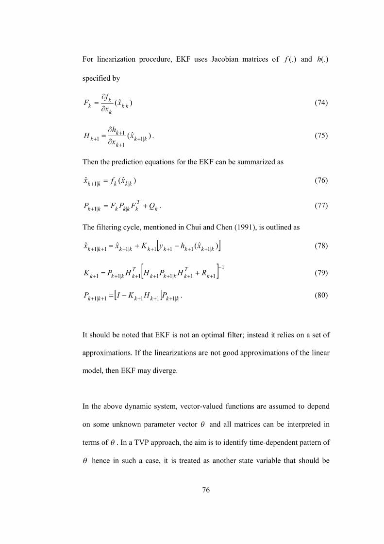
76

For linearization procedure, EKF uses Jacobian matrices of (.)� and (.)+

specified by

)ˆ( |��

��

��

,

(74)

)ˆ( |11

11 ��

�

��

�+

-

. (75)

Then the prediction equations for the EKF can be summarized as

)ˆ(ˆ ||1 �� (76)

�'�� ,, ||1 . (77)

The filtering cycle, mentioned in Chui and Chen (1991), is outlined as

)ˆ(ˆˆ |1111|11|1 �� +�)�� (78)

111|111|11

�'��

'�� ---) (79)

�� -)* |1111|1 . (80)

It should be noted that EKF is not an optimal filter; instead it relies on a set of

approximations. If the linearizations are not good approximations of the linear

model, then EKF may diverge.

In the above dynamic system, vector-valued functions are assumed to depend

on some unknown parameter vector and all matrices can be interpreted in

terms of . In a TVP approach, the aim is to identify time-dependent pattern of

hence in such a case, it is treated as another state variable that should be

77

estimated via EKF. This treatment was used in studies like Ozbek and Efe

(2001, 2004), Ozbek et al. (2003), Bacchetta and Gerlach (1997) as a standard

application. For this algorithm, the following dynamic (transition), observation

and parameter equations constitute the basics of the system:

�� #�$� )()(1 (81)

�� %�� )( (82)

�� 1 (83)

where it is allowed that follows a random walk process; � is a white noise

disturbance with zero mean and 0)( ../�! �� for all � . Here, it is

obvious that if 0. , then will not be time-dependent any longer and EKF

cannot be implemented. Exogenous input �" can also be considered but here it

is ignored for simplicity. Based on the above equations, the non-linear state

space model can be written as

�

��

�

��

�

� �#�$�

)()(

1

1(84)

��

�� %

��

0)(= (85)

Now, EKF algorithm can be applied to the above model in order to estimate

unobserved state variables, which also include parameter vector as one of its

components. The initial state of the system is defined as

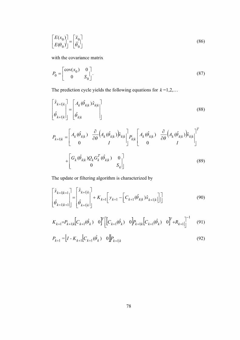
78

0

0

0

0)()(

�

�

(86)

with the covariance matrix

0

00 0

0)cov(.

� . (87)

The prediction cycle yields the following equations for � =1,2,…

��

��

��

�� $�

|

||

1

1

ˆ

ˆ)ˆ(

ˆ

ˆ

(88)

'

��

��

*

�$$*

�$$

0

ˆ)ˆ()ˆ(

0

ˆ)ˆ()ˆ( ||||

||||1

�

��'��

.#�#

00)ˆ()ˆ( || (89)

The update or filtering algorithm is characterized by

��

��

��

��)

��

1|1111

1

1|1

1|1ˆ)ˆ(

ˆ

ˆ

ˆ

ˆ

(90)

1

11|111|11 0)ˆ(0)ˆ(0)ˆ(

�

'��

'�� ) (91)

�� )* 1111 0)ˆ(-= (92)

79

3.3. The Model and State Space Representation

In this part of the study, we will explain the building blocks of our baseline

model and the alternative model with their state space formulations.

3.3.1. The Baseline Model

The baseline model is based on New Keynesian framework so that it consists

of basically three equations, which are Phillip’s curve, IS curve and monetary

policy rule. In order to model inflation process, backward-looking Phillip’s

curve is used in the following form (Backward-looking Phillips curve and IS

curve were adopted in various studies such as Rudebusch and Svensson, 1999;

Rudebusch and Svensson, 2002; Ball, 1997; Ball, 1999; Ball, 2000; Peersman

and Smets, 1999; Goodhart and Hofmann, 2000):

�� 0�� ,4,31,2,11 (93)

where � stands for inflation rate for period � , ��0�� is the output gap for

period � , �� and � are the exogenous input and inflation disturbance for

period � , respectively. In this relationship obviously, �,1 and �,2 are

expected to be positive. �,3 is a coefficient that represents the impact of

output gap on inflation hence, it is also supposed to be positive. �� can be

80

considered as the change in nominal exchange rate to take into account cost-

push inflation. In such a case �,4 is thought to be greater than zero showing

the degree of pass through of exchange rate to inflation.

As it is mentioned previously, a number of studies about monetary

transmission mechanism accept that aggregate demand is affected by long-term

interest rate rather than policy rate determined by central bank (see, for

example, Taylor, 1995; Rotemberg and Woodford, 1999; Woodford, 1999;

Basci et al., 2007; Coricelli et al., 2006). Since consumption and investment

decisions of the agents are affected primarily by long-term interest rate, it can

be said that aggregate output is largely dependent on the long-term interest

rate. However, the common practice in the literature asserts that aggregate

demand is directly affected by short-term policy interest rate so, the IS curve

consists of short-term policy rate instead of long-term interest rate.

Nonetheless, contrary to literature, we follow the claim that aggregate output

depends on mostly long-term interest rate and accordingly, we replace short-

term policy rate with long-term interest rate, in the IS curve. As far as we

know, inclusion of long-term interest rate in the IS curve was not made before

in a New Keynesian framework hence, our study can be considered as a

leading attempt to consider a monetary transmission mechanism via long-term

interest rate in a structural model.

81

The IS curve that characterizes the aggregate demand has the following

components:

�0��

1�� 0��0�� .3,2,11 )( (94)

where �0�� represents the shock hitting the output gap and 1

�� denotes the

long-term market interest rate. �,1 represents the persistence of output gap

and is considered to be greater than zero while �,2 stands for the influence of

real interest rate on output gap, which is negative. �,3 indicating the effect of

nominal exchange rate on output gap is considered to be positive.

After the construction of structural relationships, Taylor-type monetary policy

rule is added, which implies that short-term policy interest rate is a function of

output gap and inflation. Similar to previously cited studies, interest rate

smoothing is maintained and a Taylor-type interest rate rule, which is modeled

below, is reached:

��

��

�� 0��!� ,3,2

*,1

*1 )( (95)

where �� is the short-term policy rate set by central bank for period � , *

�! and

*� are the equilibrium short-term real interest rate and inflation target for

period � and �� is the disturbance term for the policy rate. As it is clear in the

related literature that all coefficients of the policy rule are expected to be

greater than zero. However, since there is debate on the level of �,1 , we do not

82

make a presumption that whether it is greater or less than one. Apart from this

discussion, there are time subscripts for inflation target and equilibrium real

interest rate which means that they can change over time. Such a relationship

also allows us to incorporate changes in targeted inflation and equilibrium real

interest rate, which provides a flexibility to examine time-dependent properties

of these variables as noted by Woodford (2003).

Up to now, the components of standard models of monetary policy analysis

have been given. Our contribution to this model is the inclusion of interest rate

pass through as a different monetary transmission mechanism. While monetary

policy rule determines the short-term policy interest rate, aggregate output is a

function of long-term interest rate. The transition from policy rate to aggregate

output and inflation is realized by means of long-term interest rate. That is,

changes in the policy interest rate lead to changes in the long-term market

interest rate, which is faced by households and firms in the economy. After

then, long-term interest rate affects aggregate output. Our input takes place at

this part and in order to complete the above model, we incorporate interest rate

pass through relationship, which is the first in the literature, as to our

knowledge. The interest rate pass through relationship establishes the link

between short-term policy rate and long-term interest rate. Similar to Kwapil

and Scharler (2006), Crespo-Cuaresma et al. (2004), Sørensen and Werner

(2006), long-term interest rate is modeled as a function of its lag and policy

rate, which is given below:

83

1��

��

1��

1� �� ,2,11 (96)

where 1�� stands for error term for the long-term interest rate. The interest rate

pass through literature states that long-term interest rate is positively dependent

on its lag and policy rate hence; all the coefficients in this equation are

expected to be positive.

In addition to the core equations, given above, there are some other

relationships that explain the dynamics and time-dependent property of the

model. One of these equations is related to output. It is assumed that output

follows the Beveridge-Nelson (1981) decomposition given as

�� 0�� * . (97)

where �� and *�� represent the output and potential output, respectively.

Potential output and equilibrium rate of real interest are assumed to follow a

local linear trend model:

***1

�� (98)

***1

!�� !! (99)

where the two stochastic trends � and � , as well as trend component of

interest rate pass through, � , are assumed to follow autoregressive, AR(1),

process:

84

�� ,1 (100)

�� ,1 (101)

�� ,1 (102)

Clearly, *�

� , *!� , � , � , � are error terms.

After introducing the functional relationships among the macroeconomic

variables of the economy, it is needed to write state space representation of the

model. The state space formulation is necessary for the application of EKF to

estimate TVPs of the model because such a representation forms a basis for the

execution of the filtering and updating algorithm of the EKF. The state space

representation of the model can be given as:

�� "��$� 1 (103)

�� %�� (104)

where �� is the state vector, �� is the observation vector, �" is the vector of

exogenous variables. Besides, $ denotes the transition matrix, � is the matrix

of exogenous variables and � stands for the observation matrix. Furthermore,

�� and �% are the vectors of normally distributed i.i.d shocks, which are

assumed to be uncorrelated and have covariance matrices � and % ,

respectively.

85

Accordingly, the state space model, that is dynamic equations and observation

equations, is written as follows:

�

�

�

�

��

1�

�

�

�

�

�

�

�

��

��

��

��

�

�

�

�

��

1�

�

�

�

�

!��

�0��

!��

�0��

*

*

1

,

,

,

,3,2,1

,2,1

,2,1,2

,3,2,1

1

1

1

*1

1

1

*1

1

1

000000000000000000000000000010100000000010001100000000010001000000000000000000010000000

�

�

�

!�

��

��

��

�0��

�

�

�

�

�

�

�

1�

*

*

0

00000000

000000000

*,1

,3

,4

86

�

�

�

�

��

1�

�

�

�

�

��

1�

�

�

!��

�0��

��

*

*

1

0000100000000001000000000011000000000001

The above state space formulation is used to express our baseline model in the

form of equations (84) and (85) with the parameter vector of � , which was

given in equation (83), specified as:

'�� ,,,,3,2,1,2,1,3,2,1,4,3,2,1

3.3.2. Alternative Model

The alternative model is based on New Keynesian framework, too. The main

difference between our baseline model and the alternative model is the

inclusion of interest rate pass-through relationship. That is, the alternative

model does not consist of interest rate pass-through and related components. In

this way, we can assess the influence of interest rate pass-through over the

economy by comparing the baseline model and the alternative model. In other

words, there will be a chance for evaluating the efficiency of interest rate pass-

87

through in transmitting policy decisions to macroeconomic variables. In this

respect, the alternative model is made up of Phillip’s curve, IS curve and

monetary policy rule. Such a structure is widely used in monetary policy

analysis. Here, one important point should be mentioned regarding the IS

curve: The alternative model assumes that in the IS curve, aggregate demand is

directly affected by short-term policy interest rate as it is common in the

literature. That is to say, policy decisions are disseminated through the

economy via short-term policy interest rate rather than long-term market

interest rate. This is the main difference from the baseline model so that the

alternative model does not need an interest rate pass-through equation for

monetary transmission purposes. The remaining relationships are similar to

those of the baseline model. Resultantly, the following set of equations present

the structure of the alternative model with accompanying relationships:

�� 0�� ,4,31,2,11 (105)

�0��

�� 0��0�� .3,2,11 )( (106)

��

��

�� 0��!� ,3,2

*,1

*1 )( (107)

�� 0�� * . (108)

***1

�� (109)

***1

!�� !! (110)

�� ,1 (111)

88

�� ,1 (112)

where equation (105) is the Phillip’s curve formulating inflation, equation

(106) is the IS curve modeling the aggregate demand, equation (107) is the

monetary policy rule. Beveridge-Nelson (1981) decomposition of output,

potential output and equilibrium real interest rate are given in equations (108),

(109) and (110), respectively. Accordingly, equations (111) and (112) model

the stochastic trends of potential output and equilibrium real interest rate.

Similar to the baseline model, the state space formulation of the alternative

model should be given now for estimation purposes. The state space

representation of the alternative model, that is dynamic equations and

observation equations, can be written as:

89

�

�

�

��

�

�

�

�

�

�

��

��

��

�

�

�

��

�

�

�

�

!��

�0��

!��

�0��

*

*

1

,

,

,3,2,1

,2,1,2

,3,2,1

1

1

*1

1

*1

1

1

000000000000001010000000100101001000000000000000100000

�

�

!�

��

��

�0��

�

�

�

�

�

�

��

*

*

0

000

0000

00000

0

*,1

,3

,4

�

�

�

��

�

�

�

�

��

�

�

!��

�0��

��

*

*

1

000100000000110000000001

The state space formulation given above presents the alternative model in the

form of equations (84) and (85). Accordingly the parameter vector of the

alternative model will be the following:

'�� ,,,3,2,1,3,2,1,4,3,2,1

90

Now, the baseline model and the alternative model will be estimated

separately. Estimation of state variables and unknown parameters requires

application of prediction and filtering cycles of EKF explained in equations

(86) through (92). The next section will explain data generation process and

application of EKF, sequentially.

3.4. Data Generation and Simulation

So far, we have explained dynamics and relationships of our structural models

with their state space representations. Now, we will produce artificial data for

these economies.

Initially, we will simulate the baseline model and obtain the time series of

observed variables. For data generation process, the model described in

equations (93) through (102) are used with the following, arbitrarily selected,

initial values of state variables and parameters:

''�1 !��0�� 1115.5554123000

*000

*0010

'�� ,,,,3,2,1,2,1,3,2,1,4,3,2,1

'200.001.422.351.100.600.479.422.007.158.800.143.186.474.456.

Disturbance terms are produced from normal distribution with mean zero and

variance one so that )1,0(~ �� and )1,0(~ �%� .

91

After data generating process, application of EKF to the artificial data takes

place. This operation requires determination of initial values both for the state

variables and parameters again. For the initiation of EKF, the same starting

values, given above, are selected for state variables and parameters of the

system with following additional parameters:

1.11000.90

1.29285.24

171.16115.35

754.9846.32

188.69000189.69

��

172000011600001050000191

� 1.0*10100 �* and 001.0*15150 �*.

Upon specifying the required starting values, EKF is applied to generated data

using the algorithm given by equations (88) through (92).

Likewise, we will simulate the alternative model. For this, we will generate

artificial data using equations (105) through (112). The following set gives the

starting values of the state variables, coefficients and other parameters of the

alternative model.

92

''� !��0�� 1.1.55.5.4.1.2.3.00

*00

*0010

'0,0,0,30,20,10,30,20,10,40,30,20,1

'001.422.351.100.600.007.158.800.143.186.474.456.

9.00003.1

1.1128.99

5.6613.25

8.730009.73

��

4.1000006.6260007.75

� 1.0*880 �* and 001.0*12120 �*.

Lastly, the error terms are distributed normally, that is, )1,0(~ �� and

)1,0(~ �%� .

The next section elaborates on the results and findings of simulations. It should

be noted that some data points from the beginning and end of the series are

dropped for avoiding start up and termination errors, respectively.

93

3.5. Simulation Results and Findings

The results of the data generation process and application of EKF to this

generated data have been given in Appendix B. The initial five figures (Figures

B1 through B5) compare artificial series produced by means of data generation

process (real value) and estimated series through EKF (estimation) for

inflation, output, output gap policy interest rate and long-term interest rate of

the baseline model. The next four figures (Figures B6 through B9) illustrate the

simulated series (real value) and estimated series (estimation) for the inflation,

output, output gap and policy interest rate of the alternative model. As a

starting point it should be mentioned that when these nine figures (Figures B1

through B9) are examined, it is seen that the EKF algorithm mimics the

behavior of generated data quite well, which means that EKF can be regarded

as a powerful tool for estimating TVP models.

When we compare the corresponding figures of the baseline model and the

alternative model, we can see that the baseline model is superior to the

alternative model in following points: Inflation series of the alternative model

is more volatile compared to inflation series of the baseline model indicating

that interest rate pass-through specification has some role in reducing the

volatility of the inflation. In other words, monetary policy rule alone is not very

efficient in stabilizing inflation. This supports our view such that interest rate

94

pass-through is an influential monetary transmission mechanism that should be

considered in monetary policy analysis.

Also, if we compare output series of both models, we can easily see that output

increases in the baseline model while it falls in the alternative model. This

clearly shows that using monetary policy rule alone shrinks the economy.

Nonetheless, output series of the baseline model follows an increasing pattern

indicating growth in economic activity. This again validate our assumption so

that aggregate demand is dependent more on long-term interest rate so, interest

rate pass-through is significant in transmitting changes in short-term policy

interest rate to long-term market interest rate and resultantly to aggregate

demand. Consequently, we can claim that the baseline model with interest rate

pass-through is preferred over the alternative model without interest rate pass-

through according to inflation and output processes. Having the superiority of

the baseline model in mind, the next subsections elaborates on time varying

parameters of the monetary policy rule and interest rate pass-through of the

baseline model.

3.5.1. Coefficients of Monetary Policy Rule

Figures B10, B11 and B12 display the patterns of time-varying coefficients of

monetary policy rule ( 1 , 2 , 3 ) of the baseline model. These graphs

95

demonstrate that, the parameters of monetary policy rule are greater than zero

as expected. According to Figure B10, the coefficient of inflation on policy

interest rate follows a decreasing pattern but it is greater than zero as expected.

The weight of inflation on policy interest rate, 1 , is falling from 0.62 to 0.56.

Loosely speaking, inflation targeting policy is relaxed a little bit.

Figure B11 shows the effect of output gap on policy interest rate. The weight

of output gap in policy rule, 2 , is first increasing from 0.11 up to 0.19 and

then decreasing back to 0.10. This implies that output gap stability has some

emphasis initially but after the period 700 this policy changes in the opposite

direction. Finally, Figure B12 illustrates that the smoothing parameter of policy

interest rate, 3 , is greater than 0.31 and displays an increasing trend with large

cycles.

When we analyze Figure B10 with Figure B3 contemporaneously, output gap

follows a relatively stable path until period 700 indicating that as 2 rises,

output gap stability can be achieved. However, the weight of inflation in policy

rule, 1 , follows a path with subsequent ups and downs around a decreasing

trend. Examination of Figure B10, 1 , with Figure B1, inflation,

simultaneously shows that as 1 decreases, monetary policy goes away from

inflation targeting, which in turn results in high inflation. Such a configuration

96

may help to explain the growth in output so that, inflation results in rising

output as being a driving force.

On the other hand, after the period 700, although 1 is still decreasing,

inflation begins to go down. When we link this observation with the fall in 2 ,

in Figure B11, it can be argued that inflation targeting policy (in other words,

decrease in inflation) is dependent more on the weight of output gap in policy

rule, 2 , so that fall in 2 goes with the decrease in inflation. As a result, it

can be concluded that if the aim is to decrease inflation, then the gap between

1 and 2 should be high and policy interest rate should be more dependent on

inflation.

Policy interest rate of the baseline model, Figure B4, does follow slightly an

upward trend, but volatility is too high. This volatility can be attributed to the

relatively unstable pattern of output gap transferred via 2 . Examination of

inflation, output gap and policy interest rate series of the baseline model,

Figures B1, B3 and B4, altogether points out that large oscillations in inflation

and output gap are reflected in policy rate indicating that policy interest rate is

highly sensitive to output gap and inflation. The amplitude of oscillations in

policy interest rate is greater compared to those in inflation and output gap,

which means that high value of 1 and growth in 2 amplifies the scale of

97

fluctuations in the inflation and output gap, correspondingly, while transferring

them to policy rate.

High volatility in policy rate indicates also that interest rate smoothing is not so

powerful. Nonetheless, after period 700, the smoothing parameter, 3 , in

Figure B12, begins to rise following a path opposite of 2 . If the decrease in

2 is considered as a sign of inflation targeting policy, or fall in inflation, then

increasing 3 can be regarded as a signal that backward-looking component of

policy rate is remarkable during inflation targeting.

3.5.2. Coefficients of Interest Rate Pass-Through

Time varying paths of the coefficients of the interest rate pass-through ( 1 , 2 )

of the baseline model are demonstrated in Figure B13 and B14. Figure B13

illustrates that long-term interest rate smoothing parameter, 1 , is between 0.34

and 0.48. Figure B14 demonstrates that the parameter displaying the impact of

policy rate on long-term interest rate, 2 , is between 0.45 and 0.54. The

interest rate pass-through relationship asserts that long-term interest rate

positively depends on both its own lag and policy interest rate so, the positive

98

values for 1 and 2 confirms the expectations about the signs of the

parameters of the pass-through relationship.

If the pass-through component of long-term interest rate, 2 , in Figure B14, is

examined, it can be seen that long-term interest rate is highly affected by policy

interest rate implying that pass-through from policy rate to long-term interest

rate is increasing. Hence, it can be claimed that monetary transmission

mechanism is relying also on long-term interest rate so that pass-through is

high. This supports our argument that policy decisions are disseminated to the

economy via long-term interest rate and monetary policy analysis should take

into account interest rate pass-through.

Since volatility of policy rate is transmitted to long-term interest rate via this

parameter, instability in long-term interest rate can be explained with the rise in

2 . Moreover, downward trend in long-term interest rate smoothing parameter,

1 , can be another explanation for the volatility of long-term interest rate.

Nevertheless, after period 700, 1 starts to increase suggesting that inflation

targeting policy increases the weight of smoothing parameter in the pass-

through equation similar to smoothing parameter in the monetary policy rule,

3 . On the other hand, long-term interest rate is a little less volatile than policy

interest rate, suggesting that smoothing parameter for long-term interest rate,

1 , is more effective than the corresponding parameter for policy interest rate,

99

3 . Higher average level of 1 , compared to 3 , indicates that backward

looking behavior of long-term interest rate is stronger than that of policy

interest rate.

Finally, when both of the policy interest rates, in Figure B4, and long-term

interest rates, in Figure B5, are analyzed, it is observed that although their

volatilities are high, there are no clear upward/downward trends in their

pattern. However, a weak upward trend in both of the interest rates is

recognized. High volatility can be attributed partially to disturbance terms and

autoregressive components of the interest rates.

3.6. Conclusion

In this study, we modeled a New Keynesian economy introducing interest rate

pass-through, for the first time, as monetary transmission mechanism. The

model consists of Phillip’s curve, IS curve, monetary policy rule, interest rate

pass-through relationship and other dynamics of the economy. Three points in

this framework are noteworthy:

Firstly, introduction of interest rate pass-through relationship to a New

Keynesian model in this kind of setting is the first, as far as we know. We

imposed a monetary transmission mechanism by claiming that contrary to

100

previous literature, output gap is dependent on long-term interest rate rather

than shot-term policy interest rate. Comparison of the baseline model, which

includes interest rate pass-through, with the alternative model, which does not

have interest rate pass-through, revealed that the baseline model is superior

over the alternative one in reducing the volatility of inflation and in achieving

output growth. Therefore, it can be claimed that interest rate pass-through is an

important ingredient in monetary policy analysis so that attention should be

paid for including long-term interest rate in structural models. However, there

is still room for further research on this issue. Our model is backward-looking

so inclusion of forward-looking components can be the topic of a future study.

Moreover, different forms of interest rate pass-through and policy rule can be

inserted and these models can be tested with real-time data applications.

Secondly, we have used time-varying parameter specification for this system.

Although this feature is not new, we have used this specification not only for

monetary policy rule, as it is common in the related literature, but also for all

parameters of the system. Hence, we have the flexibility of examining time-

dependent pattern of all system dynamics. Even if such a dynamic model may

decrease the estimation power of the technique used, the estimation results

show that the model and estimation tool work quiet well.

Lastly, due to the specification of the relationships among variables and

parameters, the model has a non-linear characteristic and basket of suitable

101

estimation techniques became restricted. Although some tools are powerful for

linear systems, they become improper for nonlinear systems therefore, it is of

importance to employ an appropriate estimation technique, which is EKF.

Similar to the first point, use of EKF in such a setting is new, to the knowledge

of us. The estimation results showed that EKF is highly powerful in capturing

the unobserved state variables and time-dependent parameters of the non-linear

system.

102

CHAPTER 4

EFFECTS OF ADOPTING INFLATION TARGETING

REGIMES ON INFLATION VARIABILITY

4.1. Introduction

In the 1990s, the monetary policy concerns of many countries changed in the

direction of low and stable inflation with the purpose of economic growth, low

inflation uncertainty and growth sustainability. Therefore, many developed and

developing countries started to adopt inflation targeting programs to improve

their economic performance. Although inflation targeting programs have been

mostly successful in achieving the targeted inflation levels, there are various

debates on the performance of these programs.

One of these discussions is about the effect of inflation targeting programs on

inflation variability. It is valuable to analyze the behavior of inflation

uncertainty because it affects macroeconomic variables such as output,

103

investment, interest rate. For example, Friedman (1977), Froyen and Waud

(1987) and Holland (1988) argue the presence of the adverse effect of inflation

uncertainty on output; Hafer (1986) and Holland (1986) elaborate on the

negative effect of inflation uncertainty on employment; Berument (1999)

shows that inflation variability raises UK three-month treasury-bill rates.

There is contradictory evidence about the performance of inflation targeting

programs in achieving lower inflation volatility. Some studies claim that the

adoption of inflation targeting programs does have an impact on reducing the

inflation variability, while some argue that this effect is not present.

Regarding inflation uncertainty, some argue that inflation variability and

inflation expectations decrease after the adoption of inflation targeting

programs. Dittmar et al. (1999) and Gavin (2003) elaborated on the

performance of these programs in reducing the volatility of inflation. The

former study gives evidence from G-10 countries about the behavior of

inflation and its variance, and then explains analytically how inflation targeting

programs can be successful in decreasing inflation variability. Gavin (2003)

further supports this proposition by reviewing the experience of other inflation

targeting countries.

Some studies assert that, in the inflation targeting countries, a decrease in the

inflation expectations and inflation variability should be attributed to the

104

effectiveness of inflation decreasing programs not to the adoption of inflation

targeting regimes. Cecchetti and Ehrman (1999) claimed that inflation targeting

programs are not the sole factor in lowering inflation volatility and inflation

expectations. Cecchetti and Ehrman (1999) discussed both theoretically and

empirically on the link between inflation variability and output volatility under

inflation targeting programs. In this study, data is used from 9 inflation

targeting countries (Australia, Canada, Chile, Finland, Israel, New Zealand,

Spain, Sweden, the UK) and 14 non-inflation targeting countries (Austria,

Belgium, Denmark, France, Germany, Ireland, Italy, Japan, Korea, Mexico,

Netherlands, Portugal, Switzerland, the US). They argued that the monetary

policymakers in these countries preferred to take actions that favor a reduction

in the volatility of inflation compared to a drop in output volatility. Thus, it is

not the inflation targeting programs but the general tendency of the

policymakers to reduce inflation that can be considered the main reason for the

drop in the level of inflation in the countries analyzed (see, for example,

Cecchetti, 1997; Groenveld, 1998; Bernanke et al., 1999; Arestis et al., 2002

and Arestis and Mouratidis, 2004 for further support of this issue).

Two of the other studies elaborating on the effectiveness of inflation targeting

programs on inflation uncertainty are Johnson (2002) and Johnson (2003). In

these works, he used inflation surveys of experts to measure the expected

inflation and variability of inflation and showed that an inflation targeting

regime decreases the level of expected inflation; however, the variability of

105

inflation forecast errors does not decrease significantly in the targeting

countries (Australia, Canada, New Zealand, Sweden, the UK) compared to not

targeting countries (France, Germany, Italy, Japan, Netherlands, the US).

To quantify inflation variability, a variety of measures are employed by

different studies, but none of these studies measures the perception of the

public on inflation risk. In existing studies in the literature, only the observed

variability was measured, only short-run dynamics of the variability were

assessed or the measurement of perception was biased. Cecchetti and Ehrman

(1999) and Dittmar et al. (1999) used the deviation of realized inflation from

the targeted value as a measure of inflation variability. This type of

specification measures observed changes in inflation. In contrast, Johnson

(2002, 2003) employed standard deviation of inflation forecasts collected

through a survey and conducted among professional forecasters. Although this

method is a good measure of variability of expected inflation, as Bomberger

(1996) argued, survey based studies have the problem of biased or unreliable

data. The people, who take part in the survey may be biased, may not give an

objective forecast or may not be able to use all the available information. As a

result, the standard deviation of these forecasts would not be a reliable measure

of the perception toward inflation risk, which is an important measure of the

credibility of the program. Another measure of inflation variability, the

bivariate stochastic volatility framework, is employed by Arestis et al. (2002)

and Arestis and Mouratidis (2004). This type of specification is advantageous

106

for modeling inflation-output variability and is designed to evaluate the short-

run dynamics of inflation-output variability trade-off but fails to capture the

public’s perception of the inflation risk.

Unlike the above models, this study uses ARCH/GARCH type of conditional

inflation variability specification as a measure of inflation variability. This

specification measures the perception of the public on inflation variability

rather than the variance itself. Inflation uncertainty series are examined to

determine whether inflation targeting programs have a significant effect on the

evolution of inflation variability. In this way, we will be able to see whether

inflation targeting programs can really convince the public in the variability of

inflation has been reduced. This is the contribution of this study to the existing

literature, in which public perception has not been considered before.

To perform this analysis, five developed countries and five emerging

economies, which implement inflation targeting programs were selected. The

analysis of both developed and developing country data will serve as a basis

for the comparison of these two groups with respect to the efficiency of the

inflation targeting programs in reducing the inflation variability if there is any

discrepancy. The selection was based on the country classification made by

World Bank and International Monetary Fund (IMF). World Bank classified

the countries with respect to their 2006 gross national income (GNI) per capita

as low income countries, whose 2006 GNI per capita was less than $905; lower

107

middle income countries, whose 2006 GNI per capita was between $906 and

$3595; upper middle income countries, whose between $3596 and $11115; and

high income countries, whose 2006 GNI per capita was greater than $11116

(web site: http://go.worldbank.org/K2CKM78CC0). IMF World Economic

Outlook (2007) also grouped countries mainly as advanced countries and

emerging and developing countries. According to these classifications,

Australia, Canada, New Zealand, Sweden and the UK were selected as

developed countries and Brazil, Chile, Colombia, Mexico and South Africa

were selected as emerging markets. However, for Mexico, the results of the

estimation changed according to the sample used. Due to the instability of the

Mexican estimates, Mexico was eliminated from the study.

The outline of the study is as follows: The next section will explain the

methodology used in this work. Then empirical evidence will be given. The

last section is the conclusion.

4.2. Methodology

Parallel to earlier studies like Engle (1982), Grier and Perry (1998, 2000), we

selected the autoregressive (AR) process to model inflation. Berument (1999)

also included real wage as an explanatory variable in the inflation specification

for the UK, but it was found to be statistically insignificant. Hence, we do not

108

use other variables such as real wages in the inflation specification in order to

avoid over-parameterization. It might have been possible to include additional

variables for the nine countries that we considered. However, the models

would likely not include the same variables for the inflation specification for

the nine countries. Thus, we did not pursue this avenue further for the

parallelism. Consequently, in order to model inflation, we used an ��+ order

autoregressive process, AR(n):

�

�

��

10 (113)

where � is the inflation level at time � , � is the number of lags, � is the

residual term at time � . Here, inflation has an autoregressive expression at the

lag length of � to account for the effect of autocorrelated residuals and we

assume that � has a zero mean and time varying variance of 2�+ . To model the

time varying variance, Engle (1982) used autoregressive conditional

heteroscedastic (ARCH) model, which is a conditional variance of the inflation

equation

�

��2�+

1

22 . (114)

Later, Bollerslev (1986) included past values of 2�+ in addition to the lagged

values of the squared residuals to capture the conditional variance −

generalized autoregressive conditional heteroscedasticity model: GARCH

(p,q).

109

�

��

�

��2� ++

1

22

1

21

2 (115)

In this specification, two points need attention as sufficient conditions; firstly

due to the non-negativity property of variances, the constant and the

coefficients should be positive ),allfor ,0,,( 210 �� . Secondly,

conditional variance should not explode; hence, to provide non-explosiveness,

the sum of the coefficients except the constant should be less than 1:

11

21

1

�

��

�

�� .

In the literature, studies exist that also include some exogenous variables in the

GARCH specification; for instance, Karolyi (1995) included variance of stock

market yields of foreign countries to model the variance of stock market yields

of the home country. As another example, Berument and Kiymaz (2001) and

Kiymaz and Berument (2003) included daily dummies to stock market returns

and its conditional variance to account for the day of the week effect in stock

market conditional variance. With this in mind, in this study, we included some

exogenous variables in the mean inflation and GARCH equations to capture

the impact of inflation targeting programs on inflation volatility.

To differentiate the periods before and after the inflation targeting program

adoption, an exogenous dummy variable is used to represent the time of

110

implementation. The dummy variable �� takes the value of one for the periods

that inflation targeting is adopted, zero otherwise. In addition to this dummy,

eleven monthly dummy variables are included to account for the seasonality in

inflation. Thus, the new inflation equation, formed by employing the dummy

variables (mean equation), is as follows:

�$�!�$�!��!

��!�,3�

�,3��4��

�4��

�� ,,,,00

�.3��.3��$"0

�$"0�4"1

�4"1�4"�

�4"��

�� ,,,,,

�

�

��53�

�53��2%

��2%�6��

�6��

1,,, (116)

�4�� , to �53�� , are the monthly seasonal dummy variables equal to one for the

respective months and zero for the others.

In order to estimate the inflation equation shown by equation (116), three

different GARCH (1,1) specifications are employed separately. Here, it is

noteworthy to clarify why GARCH (1,1) models were selected in the current

analysis. We could also employ different GARCH orders or ARCH type of

classifications. There are two reasons for not doing so. First, GARCH (1,1) is

the most commonly used specification for the conditional variances in general.

Second, a set of robustness statistics that we performed on GARCH (1,1)

specification provides evidence on the adequacy of the specification. We could

adopt more complicated models, which would require additional parameters to

estimate. In this paper we were able to find limited evidence on the decrease in

111

conditional variance of inflation. It would be more difficult to observe the

decrease in conditional variance with more parameters to be estimated. The

first one is the basic GARCH (1,1) model, in which no differentiation is made

for inflation targeting periods, given below:

212

2110

2 �� ++ (117)

The second model has an additive dummy variable for the inflation targeting

era inserted in the GARCH (1,1) specification, in order to see if there is an

exogenous decrease in the conditional variance of inflation:

212

21100

2 ��

�� +�+ (118)

In the third conditional variance expression, besides the additive dummy

variable (used for inflation targeting period) two multiplicative dummy

variables were included. The first multiplicative dummy is employed with the

lagged conditional variance, the second one is used with the lag of squared

residual term. In this way, we are able to observe the behavior of persistence

and impulse variability of inflation, respectively, after the inflation targeting is

adopted. This last conditional variance equation is given as follows:

212

212

211

21100

2 ��

��

��

�� +�+�+ (119)

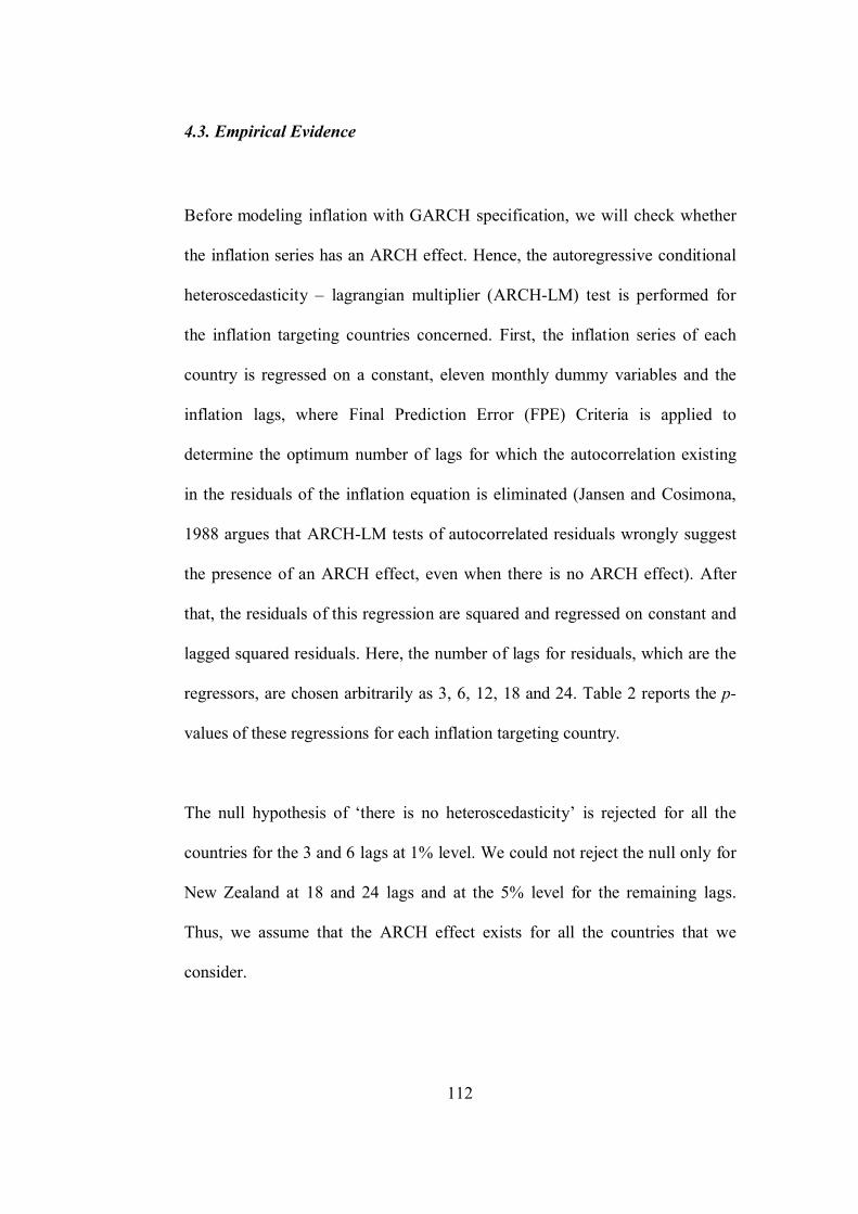
112

4.3. Empirical Evidence

Before modeling inflation with GARCH specification, we will check whether

the inflation series has an ARCH effect. Hence, the autoregressive conditional

heteroscedasticity – lagrangian multiplier (ARCH-LM) test is performed for

the inflation targeting countries concerned. First, the inflation series of each

country is regressed on a constant, eleven monthly dummy variables and the

inflation lags, where Final Prediction Error (FPE) Criteria is applied to

determine the optimum number of lags for which the autocorrelation existing

in the residuals of the inflation equation is eliminated (Jansen and Cosimona,

1988 argues that ARCH-LM tests of autocorrelated residuals wrongly suggest

the presence of an ARCH effect, even when there is no ARCH effect). After

that, the residuals of this regression are squared and regressed on constant and

lagged squared residuals. Here, the number of lags for residuals, which are the

regressors, are chosen arbitrarily as 3, 6, 12, 18 and 24. Table 2 reports the �7

values of these regressions for each inflation targeting country.

The null hypothesis of ‘there is no heteroscedasticity’ is rejected for all the

countries for the 3 and 6 lags at 1% level. We could not reject the null only for

New Zealand at 18 and 24 lags and at the 5% level for the remaining lags.

Thus, we assume that the ARCH effect exists for all the countries that we

consider.

113

Table 2: ARCH-LM Test for the Inflation Series1

Country ARCH-LM (3)

ARCH-LM (6)

ARCH-LM (12)

ARCH-LM (18)

ARCH-LM (24)

Australia 0.000** 0.000** 0.000** 0.000** 0.000**

Brazil 0.000** 0.000** 0.000** 0.000** 0.000**

Canada 0.000** 0.000** 0.000** 0.000** 0.000**

Chile 0.000** 0.000** 0.000** 0.000** 0.000**

Colombia 0.000** 0.000** 0.000** 0.000** 0.000**

New Zealand 0.000** 0.001** 0.034* 0.224 0.552

South Africa 0.000** 0.000** 0.000** 0.000** 0.000**

Sweden 0.000** 0.000** 0.000** 0.000** 0.000**

UK 0.000** 0.000** 0.000** 0.000** 0.000**

In the next step, the variability of the inflation residuals is modeled with a

GARCH specification. Table 3 reports the estimation results of the first model,

specified with equation (116) for the mean inflation and equation (117) for the

conditional variance. In this table, the coefficient of the dummy variable for the

inflation targeting period, �0 , is negative for all the countries except Brazil,

indicating that empirical evidence for Australia, Canada, Chile, Colombia,

New Zealand, South Africa, Sweden and the UK is consistent with the

expectation that implementation of inflation targeting program decreases the

conditional inflation, but it is only significant for Sweden and Chile. Note that

one cannot interpret the estimated coefficient for �0 as an indication of lower

1 ** and * indicate 1% and 5% levels of significance, respectively.

114

inflation. Lower steady state inflation requires that

�

��

�

10 1 be

negative. Negative �0 suggests a lower conditional inflation at a given level

of past inflation, which will be called lower conditional expectation from now

on.

Table 3: Estimation Results of the Model 12, 3

Country �0 0 1 2 Likelihood

-0.116 3894.642 0.029 0.008Australia

(0.161) (447595.088) (1.801) (0.981)-1018.458

0.031 0.061* 0.058 0.674*Brazil

(0.050) (0.029) (0.229) (0.337)36.319

-0.023 0.005 0.875** 0.096**Canada

(0.028) (0.003) (0.041) (0.035)165.362

-0.288** 0.013 0.771** 0.225**Chile

(0.069) (0.007) (0.051) (0.070)-106.702

-0.199 0.000 0.921** 0.076**Colombia

(0.102) (0.001) (0.020) (0.024)-305.753

-0.110 0.524** 0.025 0.144New Zealand (0.073) (0.183) (0.272) (0.084)

-272.071

-0.010 0.002 0.948** 0.049*South Africa (0.067) (0.003) (0.022) (0.024)

-176.572

-0.091* 0.015 0.880** 0.099Sweden

(0.040) (0.010) (0.049) (0.054)26.203

-0.030 0.001 0.948** 0.047**UK

(0.033) (0.001) (0.015) (0.016)39.465

2 ** and * indicate 1% and 5% levels of significance, respectively.3 Values in parenthesis show standard deviations of the coefficients.

115

For the coefficients of conditional variance, 0 , 1 and 2 , the estimation

results satisfy the sufficient condition explained in the methodology part for all

the countries. That is to say, all of the coefficients are positive (non-negativity)

and the sum of 1 and 2 is less than 1 (non-explosiveness). The table also

reports the log likelihood of the estimations in the last column. We did not

report the coefficients of the lagged inflation variables in order to save space.

We also calculated Ljung and Box autocorrelation and ARCH-LM tests for the

standardized residuals ( �� + ) for various lags for the current and other

specifications that are used in this paper. These test statistics are reported in

the Appendix C. Even if the ARCH-LM test fails to reject the ARCH effect for

Chile and Colombia, after allowing conditional variance to change with

adoption of inflation targeting regimes, this problem is mostly eliminated.

Overall, we could reject the presence of autocorrelation and heteroscedasticity

for our specifications. This further supports the validity of our specifications.

After estimating inflation volatility using the general GARCH (1,1)

specification, the second model is estimated, in which the conditional variance

equation has an additive dummy variable for the periods of inflation targeting,

as well. Table 4 reports the estimations of the second model as specified by

equations (116) and (118). The estimated coefficient for �0 is negative again

for all the countries except Australia and Brazil. For the remaining countries,

although the effect of the program is as expected (negative), �0 is significant

116

just for Chile and Sweden. When we look at the effect of the dummy for the

inflation targeting period on the conditional variability of inflation, �0 , it is

negative for all except South Africa, illustrating that conditional inflation

variability decreases after the implementation of an inflation targeting program,

but it is significant only for Chile.


Country �0

�0 0

0.075 -4.273 15023.032Australia

(0.174) (2818.614) (687822.037)

0.023 -0.032 0.083Brazil

(0.054) (0.039) (0.044)

-0.021 -0.002 0.008Canada

(0.027) (0.003) (0.004)

-0.219** -0.112* 0.133*Chile

(0.078) (0.053) (0.058)-0.119 -0.001 0.000

Colombia(0.100) (0.001) (0.001)

-0.140 -0.343 0.674New Zealand (0.073) (0.219) (0.400)

-0.110 0.000 0.003South Africa (0.074) (0.005) (0.003)

-0.106* -0.103 0.152Sweden

(0.043) (0.066) (0.094)

-0.032 -0.003 0.005UK

(0.034) (0.003) (0.004)


117

Table 4 (cont’d)

Country 1 2 Likelihood

0.014 0.080Australia

(1.058) (3.677)-896.937

0.070 0.613*Brazil

(0.220) (0.312)36.590

0.854** 0.100**Canada

(0.051) (0.038)165.852

0.601** 0.320**Chile

(0.075) (0.097)-123.772

0.974** 0.020**Colombia

(0.007) (0.007)-393.581

0.022 0.069New Zealand (0.532) (0.066)

-265.269

0.935** 0.057*South Africa (0.028) (0.028)

-157.611

0.477* 0.212Sweden

(0.229) (0.153)37.384

0.920** 0.063**UK

(0.028) (0.024)40.062

Table 4 also reports the values of the coefficients of conditional variance

equation, 0 , 1 and 2 , and the log likelihood of the estimation. As

explained in Section 4.2, the non-negativity and non-explosiveness conditions

are satisfied, which is required for a good estimation.

Equations (116) and (119) form the specifications of our third model, in which

conditional variance of inflation includes multiplicative dummies in addition to

the additive dummy for the inflation targeting period. Table 5 reports the

118

estimation results of the third model. The impact of the inflation targeting

dummy variable in the mean inflation, �0 , is negative for all countries but

only significant for Australia, Chile and Sweden. Therefore, it can be said that

inflation targeting programs reach their goals to some extent; that is, the

conditional expectation of inflation falls during the inflation targeting period.


Country �0

�0 �

1�2

-1.236** -79.808 0.051 0.278Australia

(0.446) (64146.658) (2.123) (26.502)

-0.019 -0.168 0.634 -0.022Brazil

(0.048) (0.148) (0.669) (0.487)

-0.033 0.081** -1.066** 0.213Canada

(0.028) (0.023) (0.160) (0.176)

-0.268** -0.318** 0.791** -0.788**Chile

(0.079) (0.095) (0.114) (0.262)-0.174 0.062 -1.163 -0.019

Colombia(0.100) (0.061) (1.077) (0.149)

-0.143 -0.297 -0.147 0.041New Zealand (0.073) (0.766) (1.452) (0.143)

-0.103 0.028 -0.283 0.181South Africa (0.075) (0.064) (0.431) (0.293)

-0.109* -0.071 -0.405 -0.001Sweden

(0.043) (0.102) (0.295) (0.324)

-0.034 -0.334** 0.254 0.322UK

(0.036) (0.129) (0.468) (0.307)


119

Table 5 (cont’d)

Country 0 1 2 Likelihood

28108.384 0.045 0.283Australia

(2668281.173) (1.818) (26.965)-957.532

0.218 -0.504 0.421Brazil

(0.144) (0.553) (0.353)38.717

0.002 0.919** 0.071*Canada

(0.002) (0.033) (0.031)167.805

0.321** 0.139 0.821**Chile

(0.095) (0.104) (0.264)-118.174

0.002 0.958** 0.034*Colombia

(0.002) (0.014) (0.014)-390.401

0.670 0.043 0.049New Zealand (0.642) (0.871) (0.075)

-265.223

0.003 0.939** 0.054*South Africa (0.003) (0.027) (0.027)

-156.489

0.191 0.342 0.257Sweden

(0.111) (0.278) (0.195)38.884

0.372** -0.175 0.120UK

(0.130) (0.266) (0.077)33.972

When the effect of the additive dummy variable on the conditional variance of

inflation, �0 , is analyzed, it is negative for all except Canada, Colombia and

South Africa. Importantly for the UK and Chile, the negative effect of the

inflation targeting program on the variability of inflation is significant;

however, for Canada, the positive effect of inflation targeting program is

significant. Hence, the conclusion can be drawn that inflation targeting

programs do not have a uniform effect on the variability of inflation.

120

Not only the level of variance but the persistence of variance might be affected

by inflation targeting. If the coefficient of 21� decreases, this suggests that

impulse variability decreases. If the coefficient of 21�+ decreases, then what we

call the memory of shock also decreases. Accordingly, for Canada, Colombia,

New Zealand, South Africa and Sweden, the effect of the multiplicative

dummy with the lagged value of conditional variance, �1 , is negative, which

indicates that the persistence of inflation variability decreases during the

inflation targeting period but it is significant only for Canada. However, for the

case of Chile, the persistence of inflation volatility during the inflation

targeting period is positive and significant.

The other multiplicative dummy used with the lag of squared residual, �2 , has

a negative influence on the inflation variability of Brazil, Chile, Colombia and

Sweden but is significant only for Chile. This negative coefficient suggests that

the impulse variability of inflation decreases during the inflation targeting

period in these countries. When the values of the remaining coefficients ( 0 ,

1 and 2 ) are analyzed, although the non-explosiveness requirement is

satisfied for all the countries, the non-negativity requirement is not fulfilled for

Brazil and the UK. We did not explore this further since �8 the added interactive

terms were not statistically significant and ��8 when they were dropped, the

conventional restrictions were satisfied (see Table 4). The last column displays

the log likelihood of the estimation.

121

Lower and statistically significant evidence is observed for Chile and the UK

for the conditional evidence. This could not be generalized for other inflation

targeting countries. Therefore, we claim that lower variability is not observed

for all the inflation targeting countries. This is similar to the results of Johnson

(2002, 2003) and others.

4.4. Conclusion

This paper examines whether inflation targeting programs altered the pattern of

inflation and its variability for the five developed countries and the four

emerging economies that have implemented inflation targeting programs. All

three types of models under consideration revealed that in general inflation

targeting programs decrease conditional inflation expectations in both

developed and developing countries. That is, sticking to a monetary policy rule

changes perceptions of public towards inflation however, this result is not

statistically significant for all countries. We find statistically significant lower

conditional inflation expectations only for Australia, Chile and Sweden under

various specifications. This observation points out that economic state of the

country does not make any difference regarding the efficiency of inflation

targeting programs in reducing inflationary expectations.

122

Estimation results of the second model showed that level of conditional

variance decreases for both developed and developing countries, indicating that

inflation targeting programs are efficient in reducing conditional variability of

inflation. In this respect, we can claim that in both developed and developing

countries, monetary authorities have some credibility with respect to reducing

inflation variability however; this result is statistically significant only for

Chile, which is a developing country. If we presume that monetary authorities

in developed countries are more credible than those in developing countries

then our results does not support this line of thought.

Finally, when we analyze the findings of the third model, we can not reach a

general conclusion either for developed countries or for emerging markets with

respect to level of conditional variance, persistence of inflation variability and

impulse variability of inflation. According to estimation results, it seems that

inflation targeting programs reduce inflation variability in some of the

developed and developing countries while these programs increase or do not

affect inflation variability in remaining developed and developing countries.

Moreover, statistical significance can be observed for very few countries. In

general, the conditional variance decreased statistically significantly only for

Chile, a developing country, and the UK, a developed country. Therefore, the

empirical support for the lower inflation and variability for the inflation

targeting regimes is limited. Also, we could not reach a differentiation between

123

developed countries and developing countries with regard to the efficiency of

inflation targeting programs in reducing inflation variability.

124

CHAPTER 5

CONCLUSION

Within years, monetary policies implemented by central banks, their influence

over the economy and monetary transmission mechanism have been the

research topic of several academicians and policymakers. Under the general

tendency of carrying out monetary policy analysis and examining its impact

over the economy, different directions/questions/motivations were adopted for

various investigations.

In the first essay, a brief literature review was given about the evolution of

monetary policy analysis and its future directions in a New Keynesian

framework. Recently, most of the studies in monetary policy analysis have

relied on the building blocks of the New Keynesian world while constructing

their models and performing investigations about monetary policies. Hence, it

is necessary to know the developments in monetary policy analysis and to

understand the basics of New Keynesian models. Starting from the IS/LM

125

framework, today monetary policy field has various analysis subjects including

changes in the monetary policy rules and monetary transmission mechanisms,

implementation of inflation targeting programs, open economy and exchange

rate features, euro area extensions. However, these works have some common

properties related to developments in New Keynesian models, which are

structural relationships derived from microeconomic foundations, rational

expectations, monopolistic competition behavior of firms, nominal rigidities,

different forms of Phillips’ curve, aggregate demand relationship, a monetary

policy rule and policy instrument.

Although many studies do not include the derivation of linear reduced form

equations from microeconomic foundations and they employ directly the linear

relationships that simulates the economy, it is of importance to

know/understand how these equations are derived from microfoundations,

since micro structure of the economy, behavior of households and firms, nature

of connection among different variables and similar aspects are necessary to

conduct future research. Therefore, a stylized closed economy was analyzed

and reduced form equations, which are Phillips’ curve and aggregate demand,

were derived from a structural microfounded model.

The second essay analyzed monetary policy introducing interest rate pass-

through relationship to a New Keynesian world with backward looking

behavior. This study has three important features to mention: The first one is

126

the inclusion of interest rate pass-through relationship between short-term

policy interest rate and long-term market interest rate as a new monetary

transmission mechanism, for the first time in the literature, along with a

Taylor-type monetary policy rule. The second is the use of time-varying

parameter specification not only for coefficients of monetary policy rule, as it

is common in the literature, but also for the coefficients of structural

relationships in the model, which is not observed before in the literature. The

third issue is the application of EKF, which is a new estimation algorithm. The

estimation results showed us that long-term interest rate is an important

component to be considered in structural models of monetary policy analysis

since its influence on aggregate demand is increasing in time and pass-through

from policy rate to long-term interest rate has an increasing weight. Apart from

this result, it is also worth mentioning that performance of EKF in estimating

models with TVPs is quite well. The model adopted in this study is backward-

looking so including forward-looking components can be a valuable extension

for future study. Furthermore, real-time data applications with different interest

rate pass-through and policy rule specifications can be worth exploring. Such

models can be modified for open economies so that exchange rate can be

incorporated as an additional dynamic to the system.

The third essay investigated the impact of inflation targeting policy on inflation

and its variability, empirically. Recently, many countries adopted inflation

targeting policies in order to achieve low and stable inflation with maintaining

127

economic growth. Even though these programs succeed in achieving the

targeted inflation levels, there is no common argument about the effect of them

on inflation variability. Such an examination is worth to conduct since inflation

uncertainty affects macroeconomic variables such as output, investment,

interest rate. There are two main contributions of this essay to the inflation

variability literature: The first input is the measurement of public perception

towards inflation, which has not been made before. The second main

contribution is the investigation of whether commitment to such a monetary

policy rule really changed the public assessment of inflation and its variability.

For this, unlike the existing models, this study used ARCH/GARCH type of

conditional inflation variability specification as a measure of inflation

variability. Another critical issue to be mentioned is the comparison of

performance of inflation targeting programs between developed and

developing countries. This comparison has the advantage of assessing whether

economic state of the country is an important factor in evaluating performance

of the inflation targeting programs in reducing inflation variability. The results

of the study pointed out that inflation targeting programs convince public in

reducing inflation and its variability both in developed and developing

countries, although there are some exceptions and some of the results are not

statistically siginificant. This result revealed that economic state of the

economy does not have much influence on the effectiveness of inflation

targeting programs in decreasing inflation variability. However, this conclusion

can not be generalized to all inflation targeting countries since the conclusion

128

was not valid for some countries examined. For the countries in which inflation

targeting programs are not successful in reducing inflation variability, concerns

about the credibility of the monetary policy authority can be the reason of

failure.

129

BIBLIOGRAPHY

Arestis, P. and K. Mouratidis. 2004, “Is There a Trade-off Between Inflation Variability and Output-Gap Variability in the EMU Countries?,” .�2��+942"!��192�921��19 �2�2&� 51(5): 691-706.

Arestis, P., G. M. Caporale and A. Cipollini. 2002. “Does Inflation Targeting Affect the Trade-off Between Output Gap and Inflation Variability?,” '+39��+3��3!9.�+221 70(4): 528-545.

Bacchetta, P. and S. Gerlach. 1997. "Consumption and Credit Constraints: International Evidence," 42"!��19 2�9 2�3��!�9 �2�2&�� 40(2): 207-238.

Backus, David and John Driffill. 1985. "Rational Expectations and Policy Credibility Following a Change in Regime," 3%�3�9 2�9 �2�2&��9.�"��3� 52(2): 211-221.

Bahmani, Osokee and Ford Brown. 2004. "Kalman Filter Approach to Estimate the Demand for International Reserves," $��1�3�9 �2�2&�� 36(15): 1655-1668.

Ball, Laurence. 1997. "Efficient Rules for Monetary Policy," �� 9�2!��09��3!� 5952.

Ball, Laurence. 1999. "Policy Rules for Open Economies," in John B. Taylor, ed., 2�3��!�9 21��9 "13�. NBER Conference Report Series, University of Chicago Press, 127-144.

130

Ball, Laurence. 2000. "Policy Rules and External Shocks," �� 9 �2!��09��3!� 7910.

Ball, L., N. G. Mankiw and D. Romer. 1988. "The New Keynesian Economics and the Output-Inflation Trade-off," �!22��0�9 ��3!�9 2�9 �2�2&��9$��%�� 1: 1-65.

Banerjee, A, R. L. Lumsdaine and J. H. Stock. 1992. “Recursive and Sequential Tests of the Unit Root and Trend-Break Hypotheses: Theory and International Evidence,” 42"!��192�9�"��3��9:9 �2�2&��9.��10(3): 271-287.

Barro, Robert J. and David B. Gordon. 1983a. "Rules, Discretion and Reputation in a Model of Monetary Policy," 42"!��19 2�9 2�3��!�9 �2�2&�� 12(1): 101-121.

Barro, Robert J. and David B. Gordon. 1983b. "A Positive Theory of Monetary Policy in a Natural Rate Model," 42"!��192�921��19 �2�2&� 91(4): 589-610.

Basci, E., O. Ozel and C. Sarikaya. 2007. "The Monetary Transmission Mechanism in Turkey: New Developments," �3��!�19 ��9 2�9 �+39 3�"�1��9 2�9 '"!�3�;9 3�3�!�+9 ��9 2�3��!�9 21��9 53��!�&3��9�2!��09��3!907/04.

Bernanke, Ben S. and Alan S. Blinder. 1992. "The Federal Funds Rate and the Channels of Monetary Transmission," $&3!��9 �2�2&��9 3%�3�82(4): 901-921.

Bernanke, Ben S. and Frederic S. Mishkin. 1997. "Inflation Targeting: A New Framework for Monetary Policy?," 42"!��19 2�9 �2�2&��93!��3��%3�11(2): 97-116.

Bernanke, Ben S. and Ilian Mihov. 1997. "What Does the Bundesbank Target?," "!2�3��9 �2�2&��9 3%�3� 41(6): 1025-1053.

131

Bernanke, B. S., M. Gertler and M. Watson. 1997. "Systematic Monetary Policy and the Effects of Oil Price Shocks," �!22��0�9 ��3!�9 2�9 �2�2&��9$��%�� 1: 91-157.

Bernanke, B. S., T. Laubach, F. S. Mishkin and A. Posen. 1999. *��1��2�9'�!03��0<9�3��2��9,!2&9'+39*��3!��2��19 ��3!�3��38 Princeton, NJ: Princeton University Press.

Berument, H. 1999. “The Impact of Inflation Uncertainty on the Interest Rates in the UK,” .�2��+942"!��192�921��19 �2�2&� 46(2): 207-218.

Berument, H. and N. Dincer. 2005. “Inflation and Inflation Uncertainty in the G-7 Countries,” +��9$ 348: 371-379.

Berument, H., Z. Kilinc, U. Ozlale. 2005. “The Missing Link Between Inflation Uncertainty and Interest Rates,” .�2��+942"!��192�921��19 �2�2&� 52(2): 222-241.

Berument, H. and H. Kiymaz. 2001. “The Day of the Week Effect on Stock Market Volatility,” 42"!��192�9 �2�2&��9��9,��3 25(2): 181-193.

Beveridge, S. and C. R. Nelson. 1981. "A New Approach to the Decomposition of Economic Time Series into Permanent and Transitory Components with Particular Attention to Measurement of the Business Cycle," 42"!��192�92�3��!�9 �2�2&�� 7(2): 151-174.

Blanchard, Olivier Jean and Nobuhiro Kiyotaki. 1987. "Monopolistic Competition and the Effects of Aggregate Demand," $&3!��9 �2�2&��9 3%�3� 77(4): 647-666.

Blanchard, O. J. and S. Fischer. 1989. �3��"!3�9 2�9 ��!23�2�2&��89Cambridge, MA.: MIT Press.

Boivin, Jean. 2006. "Has U.S. Monetary Policy Changed? Evidence from Drifting Coefficients and Real-Time Data," 42"!��19 2�92�3�;9 �!3��9��9��0 38(5): 1149-1173.

132

Bollerslev, T., R. Chou, and K. Kroner. 1991. “ARCH Modeling in Finance: A Review of the Theory and Empirical Evidence,” 42"!��19 2�9 �2�2&3�!�� 52: 5-59.

Bomberger T. 1996. “Disagreement as a Measure of Uncertainty,” 42"!��192�92�3�;9�!3��9��9��0 28(3): 381-392.

Calvo, Guillermo A. 1983. "Staggered Prices in Utility–Maximizing Framework," 42"!��192�92�3��!�9 �2�2&�� 12(3): 383-398.

Canova, Fabio and Luca Gambetti. 2004. "Structural Changes in the US Economy: Bad Luck or Bad Policy?," �8 88 89 5��"��2�9 ��3!�5457.

Cecchetti, Stephen G. 1995. "Inflation Indicators and Inflation Policy," �� =��!23�2�2&��9$��"�1 10(1): 189-219.

Cecchetti S. G. 1997. “Central Bank Policy Rules: Conceptual Issues and Practical Considerations,” �� 9�2!��09��3!� 6306.

Cecchetti, S. G. and M. Ehrmann. 1999. “Does Inflation Targeting Increase Output Volatility? An International Comparison of Policymakers' Preferences and Outcomes,” �� 9�2!��09��3!�97426.

Cheung, Yin-Wong. 1993. "Exchange Rate Risk Premiums," 42"!��19 2�9*��3!��2��192�3�9��9,��3 12: 182-194.

Christiano, L. J., M. Eichenbaum and C. Evans. 1996. "The Effects of Monetary Policy Shocks: Evidence from the Flow of Funds," 3%�3�92�9 �2�2&��9��9.��978(1): 16-34.

Christiano, L. J., M. Eichenbaum and C. Evans. 1998. "Monetary Policy Shocks: What Have We Learned and To What End?," �� 9�2!��09��3!� 6400.

133

Chui, C. K. and G. Chen. 1991. )�1&��9,�1�3!��09��+9 3�17'�&39$��1��2��. NY: Springer Verlag.

Clarida, R., J. Gali and M. Gertler. 1997. "Monetary Policy Rules in Practice: Some International Evidence," �� 9�2!��09��3!� 6254.

Clarida, R., J. Gali and M. Gertler. 1999. "The Science of Monetary Policy: A New Keynesian Perspective," 42"!��19 2�9 �2�2&��9 ��3!��"!3 37(4): 1661-1707.

Clarida, R., J. Gali and M. Gertler. 2000. "Monetary Policy Rules and Macroeconomic Stability: Evidence and Some Theory," �"�!�3!1�942"!��192�9 �2�2&�� 115(1): 147-180.

Cogley, Timothy and Thomas J. Sargent. 2001. " Evolving Post–World War II U.S. Inflation Dynamics," �� =��!23�2�2&��9$��"�1 16(1): 331-373.

Coricelli, F., B. Egert and R. MacDonald. 2006. "Monetary Transmission Mechanism in Central & Eastern Europe: Gliding on a Wind of Change," '+39��11��&95�%��2�9*��"�39��9�+39>��%3!��92�9��+�0��9�2!��09��3! 850.

Crespo-Cuaresma, J., B. Egert and T. Reininger. 2004. "Interest Rate Pass-Through in New EU Member States: The Case of the Czech Republic, Hungary and Poland," '+39��11��&95�%��2�9*��"�39��9�+39>��%3!��92�9��+�0��9�2!��09��3! 671.

Dittmar, R., W. T. Gavin and F. E. Kydland. 1999. “Price-Level Uncertainty and Inflation Targeting,” ,3�3!�19 3�3!%39 ��9 2�9 .�89 �2"��9 3%�3�81(4): 23-33.

Dixit, Avinash K. and Joseph E. Stiglitz. 1977. " Monopolistic Competition and Optimum Product Diversity," $&3!��9 �2�2&��9 3%�3� 67(3): 297-308.

134

Dwyer Jr., Gerald P. 1993. "Rules and Discretion in Monetary Policy," 3%�3�Federal Reserve Bank of St. Louis, 75(3): 3-13.

Elkhoury, Marwan. 2006. "A Time-Varying Parameter Model of A Monetary Policy Rule for Switzerland. The Case of the Lucas and Friedman Hypothesis," - *9�2!��09��3!� 01-2006.

Engle, R. 1982. “Autoregressive Conditional Heteroscedasticity with Estimates of the Variance of United Kingdom Inflation,” �2�2&3�!��950: 987-1007.

Evans, M. 1991. “Discovering the Links Between Inflation Rates and Inflation Uncertainty,” 42"!��192�92�3�;9�!3��9��9��0 23(2): 169-184.

Fischer, Stanley. 1977. "Long-Term Contracts, Rational Expectations, and the Optimal Money Supply Rule," 42"!��19 2�9 21��19 �2�2&� 85(1): 191-205.

Friedman, Milton. 1968. "The Role of Monetary Policy,"9$&3!�� 2�2&��9 3%�3� 58(1): 1-17.

Friedman, Milton. 1970. "A Theoretical Framework for Monetary Analysis," 42"!��192�921��19 �2�2&� 78(2): 193-238.

Friedman, Milton. 1971. "A Monetary Theory of Nominal Income," 42"!��192�921��19 �2�2&� 79(2): 323-337.

Friedman, Milton. 1977. “Nobel Lecture: Inflation and Unemployment,” 42"!��192�921��19 �2�2&� 85: 451–472.

Friedman, M. and A. Schwartz. 1963. $92�3��!�9-��2!�92�9�+39>��3�9.��3�;9?@AB7?CAD9 Princeton: Princeton University Press.

Friedman, M. and Kenneth N. Kuttner. 1992. "Money, Income, Prices and Interest Rates," $&3!��9 �2�2&��9 3%�3� 82(3): 472-492.

135

Froyen, R. and R. Waud. 1987. “An Examination of Aggregate Price Uncertainty in Four Countries and Some Implications for Real Output,” *��3!��2��19 �2�2&��9 3%�3� 28(2): 353–373.

Gali, Jordi. 1992. "How Well Does the IS/LM Model Fit Post-War U.S. Data?," �"�!�3!1�942"!��192�9 �2�2&�� 92: 709-738.

Gavin, W.T. 2003. “Inflation Targeting: Why It Works and How To Make It Work Better,” ,3�3!�19 3�3!%39��92�9.�89�2"��9�2!��09��3! 2003-027B.

Goodfriend, Marvin and Robert G. King. 1997. "The New Neoclassical Synthesis and the Role of Monetary Policy," �� =��!23�2�2&��9$��"�1 12(1): 231-283.

Goodhart, C. and B. Hofmann. 2000. "Financial Variables and the Conduct of Monetary Policy," .%3!�03�9 ��9�2!��09��3! 112.

Gordon, Robert J. 1982. "Price Inertia and Policy Ineffectiveness in the United States, 1890-1980," 42"!��192�921��19 �2�2&� 90(6): 1087-1117.

Green, John H. 1996. "Inflation Targeting: Theory and Policy Implications," *��3!��2��192�3��!�9,"��9.��9��3!� 43(4): 779-795.

Grier, K. B. and M. J. Perry. 1998. “On Inflation and Inflation Uncertainty in the G- 7 Countries,” 42"!��19 2�9 *��3!��2��19 2�3�9��9 ,��317(4): 671-689.

Grier, K. B. and M. J. Perry. 2000. “The Effects of Real and Nominal Uncertainty on Inflation and Output Growth: Some GARCH-M Evidence,” 42"!��192�9$��1�3�9 �2�2&3�!�� 15: 45-58.

Groenveld, J. M. 1998. *��1��2�9��3!��9��92�3��!�921��<9�3��2��9,2!9'+39 "!2�3��9�3��!�19��8 Cheltenham: Edward Elgar Press.

136

Hafet, R. W. 1986. “Inflation Uncertainty and a Test of the Friedman Hypothesis,” 42"!��192�9��!23�2�2&�� 8(3): 365–372.

Harvey, A. C. 1990. ,2!3��0;9 .�!"��"!�19 '�&39 .3!�3�9 2�31�9 ��9 �+39)�1&��9,�1�3!. Cambridge: Cambridge University Press.

Henderson, Dale W. and Warwick J. McKibbin. 1993. "A Comparison of Some Basic Monetary Policy Regimes for Open Economies: Implications of Different Degrees of Instrument Adjustment and Wage Persistence," ��!�30�37 2�+3��3!9 �2��3!3��39 .3!�3�9 2�9 "�1��9 21��39: 221-317.

Holland, S. 1986. “Wage Indexation and the Effect of Inflation Uncertainty on Employment: An Empirical Analysis,” $&3!��9 �2�2&��9 3%�3�76(1): 235–243.

Holland, S. 1988. “Indexation and the Effect of Inflation Uncertainty on Real GNP,” 42"!��192�9�"��3�� 61(4): 473–484.

Horvath, Roman. 2006. "Real-Time Time-Varying Equilibrium Interest Rates: Evidence on the Czech Republic," $9��3! 845.

IMF. 2007. �2!1�9 �2�2&��9 6"�122�. Washington D.C.: International Monetary Fund, Publication Services.

Ireland, Peter N. 1997. "A Small, Structural, Quarterly Model for Monetary Policy Evaluation," ��!�30�37 2�+3��3!9 �2��3!3��39 .3!�3�9 2�9 "�1��921�� 47: 83-108.

Jalil, Munir A. 2004. "Monetary Policy in Retrospective: A Taylor Rule Inspired Exercise," Manuscript. University of California, San Diego.

Jansen, D. W. and T. F. Cosimona. 1988. “Estimates of the Variance of US Inflation Based Upon the ARCH Model: Comment (in notes, comments, replies),” 42"!��19 2�9 2�3�;9 �!3��9 ��9 ��0 20(3): 409–421.

137

Johnson, D. R. 2002 “The Effect of Inflation Targeting on The Behaviour of Expected Inflation: Evidence From An 11 Country Panel,” 42"!��192�92�3��!�9 �2�2&�� 49(8): 1521-1538.

Johnson, D. R. 2003. “The Effect of Inflation Targets on the Level of Expected Inflation in Five Countries,” 3%�3�92�9 �2�2&��9��9.�� 85(4): 1076-1081.

Judd, John P. and Glenn D. Rudebusch. 1998. "Taylor's Rule and the Fed: 1970-1997," ,3�3!�19 3�3!%39��92�9.��9,!��29 �2�2&��9 3%�3�3: 3-16.

Kalman, R. E. 1960. "A New Approach to Linear Filtering and Prediction Problems," 42"!��192�9��9 �0��33!��0 35-45.

Karolyi, A. 1995. “A Multivariate GARCH Model of International Transmission of Stock Returns and Volatility: The Case of the United States and Canada,” 42"!��192�9�"��3��9��9.�� 13: 11-25.

Keynes, J. M. 1936. '+39#3�3!�19'+32!�92�9 &�12�&3��;9*��3!3��9��92�3�. London: McMillan.

Kim, Chang-Jin and Charles R. Nelson. 2006. "Estimation of a Forward-Looking Monetary Policy Rule: A Time-Varying Parameter Model Using Ex-Post Data," 42"!��19 2�9 2�3��!�9 �2�2&�� 53(8): 1949-1966.

Kiymaz, H. and H. Berument. 2003. “The Day of the Week Effect on Stock Market Volatility and Volume: International Evidence,” 3%�3�9 2�9,��19 �2�2&�� 12: 363-380.

Kontonikas, A. 2004. “Inflation and Inflation Uncertainty in the United Kingdom: Evidence from GARCH Modelling,” �2�2&��9 2�311��021(3): 525-543.

Kozicki, Sharon. 1999. "How Useful Are Taylor Rules for Monetary Policy?," �2�2&��9 3%�3� 84(2): 5-33.

138

Kuzin, Vladimir. 2006. "The Inflation Aversion of the Bundesbank: A State Space Approach," 42"!��19 2�9 �2�2&��9 5��&��9 ��9 �2��!21 30(9-10): 1671-1686.

Kwapil, Claudia and Johann Scharler. 2006. "Interest Rate Pass-Through, Monetary Policy Rules and Macroeconomic Stability," $"��!��9�3��!�19��9�2!��09��3!� 118.

Kydland, Finn E. and Edward C. Prescott. 1977. "Rules Rather Than Discretion: The Inconsistency of Optimal Plans," 42"!��19 2�9 21��19 �2�2&� 85(3): 473-491.

Kydland, Finn E. and Edward C. Prescott. 1982. "Time to Build and Aggregate Fluctuations," �2�2&3�!�� 50(6): 1345-1370.

Leitemo, Kai and Ingunn Lønning. 2006. "Simple Monetary Policymaking without the Output Gap," 42"!��192�92�3�;9�!3��9��9��0 38(6): 1619-1640.

Levin, A. T. and J. M. Piger. 2003. “Is Inflation Persistence Intrinsic in Industrial Economies?,” '+39 ,3�3!�19 3�3!%39 ��9 2�9 .�89 �2"��9�2!��09��3!9.3!�3� 2002-023E.

Levin, A., V. Wieland and J. C. Williams. 1998. "Robustness of Simple Monetary Policy Rules under Model Uncertainty," �� 9 �2!��09��3!� 6570.

Ljungqvist, L. and T. Sargent. 2000. 3�"!��%39 ��!23�2�2&��9 '+32!�. Cambridge and London: MIT Press.

Lucas, R. 1972. "Expectations and the Neutrality of Money," 42"!��19 2�9 �2�2&��9'+32!�94: 103-124.

Lucas, R. 1976. "Econometric Policy Evaluation: A Critique," 42"!��19 2�92�3��!�9 �2�2&�� supplement: 19-46.

139

Mandler, Martin. 2007. "The Taylor Rule and Interest Rate Uncertainty in the U.S. 1955-2006," $9��3! 2340.

Mankiw, N. G. 1985. "Small Menu Costs and Large Business Cycles: A Macroeconomic Model," �"�!�3!1�942"!��192�9 �2�2&�� 100(2): 529-538.

Mankiw, N. G. 1988. "Recent Developments in Macroeconomics: A Very Quick Refresher Course," 42"!��192�92�3�;9�!3��9��9��0 20(3): 436-449.

Mankiw, N. G. 1990. "A Quick Refresher Course in Macroeconomics," 42"!��192�9 �2�2&��9��3!��"!3 28(4): 1645-1660.

McCallum, Bennett T. 1997. "Issues in the Design of Monetary Policy Rules," �� 9�2!��09��3!� 6016.

McCallum, Bennett T. 2000. "Alternative Monetary Policy Rules: A Comparison with Historical Settings for the United States, the United Kingdom, and Japan," �2�2&��9 �"�!�3!1� Federal Reserve Bank of Richmond 86(1): 49-79.

McCallum, Bennett T. and Edward Nelson. 1999a. "An Optimizing IS-LM Specification for Monetary Policy and Business Cycle Analysis," 42"!��192�92�3�;9�!3��9��9��0 31(3): 296-316.

McCallum, Bennett T. and Edward Nelson. 1999b. "Nominal Income Targeting in an Open-Economy Optimizing Model," 42"!��19 2�92�3��!�9 �2�2&�� 43(3): 553-578.

McCallum, Bennett T. and Edward Nelson. 1999c. "Performance of Operational Policy Rules in an Estimated Semiclassical Structural Model," in John B. Taylor, ed., 2�3��!�9 21��9 "13�. NBERConference Report Series, University of Chicago Press, 15-45.

McCulloch, J. Huston. 2005. "The Kalman Foundations of Adaptive Least Squares," 6+�29.��39>��%3!��9�2!��09��3!.

140

McCulloch, J. Huston. 2007. "Adaptive Least Squares Estimation of the Time-Varying Taylor Rule," 6+�29.��39>��%3!��9�2!��09��3!.

Mesonnier, Jean-Stephane and Jean-Paul Renne. 2007. "Does Uncertainty Make a Time-Varying Natural Rate of Interest Irrelevant For the Conduct of Monetary Policy?," ��"39�39,!��39�2!��09��3! 175.

Mishkin, Frederic S. and Adam S. Posen. 1997. "Inflation Targeting: Lessons From Four Countries," �2�2&��921��9 3%�3� 3(3): 9-110.

Muth, John F. 1961. "Rational Expectations and the Theory of Price Movements," �2�2&3�!�� 29(3): 315-335.

Orphanides, Athanasios. 1998. "Monetary Policy Rules Based on Real-Time Data," ,��39��9 �2�2&��95��"��2�9.3!�3� Board of Governors of the Federal Reserve System, 1998-03.

Orphanides, Athanasios. 2001. "Monetary Policy Rules Based on Real-Time Data," $&3!��9 �2�2&��9 3%�3�, 91(4): 964-985.

Orphanides, Athanasios. 2004. "Monetary Policy Rules, Macroeconomic Stability, and Inflation: A View from the Trenches," 42"!��192�92�3�;9�!3��9��9��0 36(2): 151-175.

Orphanides, Athanasios and John C. Williams. 2005. "The Decline of Activist Stabilization Policy: Natural Rate Misperceptions, Learning, and Expectations," 42"!��19 2�9 �2�2&��9 5��&��9 ��9 �2��!21 29(11): 1927-1950.

Ozbek, L. and M. Efe. 2001. "Online Estimation of State and Parameters inCompartmental Models Using Extended Kalman Filter." in W. Sulis and I. Trofimova, eds., �$'69.��3��39 .3!�3�;9�2�1��3�!95��&��9 ��9��39��9.2��19.��3��3�. IOS Press, 320: 262-271.

Ozbek, L. and M. Efe. 2004. "An Adaptive Extended Kalman Filter with Application to Compartment Models," �2&&"��2�9 ��9 .��7.�&"1��2�9��9�2&�"��2� 33(1): 145-158.

141

Ozbek, L., U. Ozlale and M. Efe. 2003. "Employing Extended Kalman Filter in a Simple Macroeconomic Model," �3��!�19��9 3%�3� 3(1): 53-65.

Partouche, Harry. 2007. "Time-Varying Coefficients in a GMM Framework: Estimation of a Forward Looking Taylor Rule for the Federal Reserve," ��"39�39,!��39�2!��09��3! 177.

Pasricha, Gurnain Kaur. 2006. "Kalman Filter and Its Economic Applications." Unpublished. Santa Cruz, CA: University of California, Santa Cruz.

Peersman, G. and F. Smets. 1999. "The Taylor Rule: A Useful Monetary Policy Benchmark for the Euro Area?," *��3!��2��19 ,��3 1: 85-116.

Plantier, L. Christopher and Dean Scrimgeour. 2002. "Estimating a Taylor Rule for New Zealand with a Time-Varying Neutral Real Rate," 3�3!%39��92�9�3�9�3�1��95��"��2�9��3!9.3!�3� DP2002/06.

Ribeiro, Maria Isabel. 2004. "Kalman and Extended Kalman Filters: Concept, Derivation and Properties," Unpublished. Lisboa: Institute for Systems and Robotics, Lisboa.

Rotemberg, Julio J. 1982. "Sticky Prices in the United States," 42"!��19 2�921��19 �2�2&� 90(6): 1187-1211.

Rotemberg, Julio J. 1987. "The New Keynesian Microfoundations," �� =��!23�2�2&��9$��"�1 69-104.

Rotemberg, Julio J. and Michael Woodford. 1998. "An Optimization-Based Econometric Framework for the Evaluation of Monetary Policy: Expanded Version," �� 9'3�+��19�2!��09��3! 233.

Rotemberg Julio J. and Michael Woodford. 1999. "Interest-Rate Rules in an Estimated Sticky-Price Model," in John B. Taylor, ed., 2�3��!�921��9 "13�. NBER Conference Report Series, University of Chicago Press, 57-126.

142

Rudebusch, Glenn D. and Lars E. O. Svensson. 1998. "Policy Rules for Inflation Targeting," �� 9�2!��09��3!� 6512.

Rudebusch, G. D. and L. E. O. Svensson. 1999. "Policy Rules for Inflation Targeting," in John B. Taylor, ed., 2�3��!�9 21��9 "13�. NBER Conference Report Series, University of Chicago Press, 203-253.

Rudebusch, Glenn D. and Lars E. O. Svensson. 2002. "Eurosystem Monetary Targeting: Lessons from U.S. Data," "!2�3��9 �2�2&��9 3%�3� 46(3): 417-442.

Sargent, Thomas J. and Neil Wallace. 1975. "'Rational' Expectations, the Optimal Monetary Instrument, and the Optimal Money Supply Rule," 42"!��192�921��19 �2�2&� 83(2): 241-244.

Schmitt-Grohe, Stephanie and Martin Uribe. 2002. "Optimal Fiscal and Monetary Policy Under Sticky Prices," �� 9�2!��09��3!� 9220.

Sims, Christopher A. 1980. "Comparison of Interwar and Postwar Business Cycles: Monetarism Reconsidered," $&3!��9 �2�2&��9 3%�3� 70(2): 250-257.

Sims, Christopher A. and Tao Zha. 2006. "Were There Regime Switches in U.S. Monetary Policy?,"9$&3!�� 2�2&��9 3%�3� 96 (1): 54-81.

Smith, Bruce D. 1994. "Efficiency and Determinacy of Equilibrium Under Inflation Targeting," �2�2&��9'+32!� 4(3): 327-344.

Sørensen, Christoffer K. and Thomas Werner. 2006. "Bank Interest Rate Pass-Through in the Euro Area: A Cross Country Comparison," "!2�3��9�3��!�19��9�2!��09��3!9.3!�3� 580.

Stock, J. H. and M. W. Watson. 2003. “Forecasting Output and Inflation: The Role of Asset Prices,” 42"!��192�9 �2�2&��9��3!��"!3 41(3): 788-829.

143

Svensson, Lars E. 1995. "The Swedish Experience of an Inflation Target," �8 88 895��"��2�9��3!� 1103.

Svensson, Lars E. 1996. "Price Level Targeting vs. Inflation Targeting: A Free Lunch?," �� 9�2!��09��3!� 5719.

Taylor, John B. 1980. "Aggregate Dynamics and Staggered Contracts," 42"!��192�921��19 �2�2&� 88(1): 1-23.

Taylor, John B. 1993. "Discretion versus Policy Rules in Practice," ��!�30�37 2�+3��3!9�2��3!3��39.3!�3�92�9"�1��921��, 39: 195-214.

Taylor, John B. 1995. "The Monetary Transmission Mechanism: An Empirical Framework," 42"!��192�9 �2�2&��93!��3��%3�, 9(4): 11-26.

Taylor, John B. 1996. "How Should Monetary Policy Respond to Shocks While Maintaining Long-Run Price Stability?--Conceptual Issues," $�+�3%��09 !��39 .��1��9 A symposium sponsored by the Federal Reserve Bank of Kansas City 181-195.

Taylor, John B. 1999a. "A Historical Analysis of Monetary Policy Rules," in John B. Taylor, ed., 2�3��!�921��9 "13�. NBER Conference Report Series, University of Chicago Press, 319-341.

Taylor, John B. (ed.) 1999b. 2�3��!�921��9 "13�. NBER Conference Report Series Chicago and London: University of Chicago Press.

Trecroci, Carmine and Matilde Vassalli. 2006. "Monetary Policy Regime Shifts: New Evidence from Time-Varying Interest Rate Rules," >��%3!��9 2�9 �!3��;9 53��!�&3��9 2�9 �2�2&��9 5��"��2�9 ��3!0602.

Trehan, Bharat and Tao Wu. 2007. "Time-Varying Equilibrium Real Rates and Monetary Policy Analysis," 42"!��19 2�9 �2�2&��9 5��&��9 ��9�2��!21 31(5): 1584-1609.

144

Uhlig, Harald. 1999. "A Toolkit for Analysing Nonlinear Dynamic Stochastic Models Easily," in �2&�"��2��193�+2��9 �2!9 �+39 .�"��9 2�95��&��9 �2�2&�3�. Oxford University Press, 30-61.

Walsh, Carl E. 2003. 2�3��!�9'+32!�9��921��9 (2nd ed.). Cambridge and London: MIT Press.

Welch, Greg and Gary Bishop. 2006. "An Introduction to Kalman Filter." Unpublished. Chapel Hill, NC: Department of Computer Science University of North Carolina, Chapel Hill.

Wesche, Katrin. 2003. "Monetary Policy in Europe: Evidence from Time-Varying Taylor Rules," �2��9 �2�95��"��2�9��3!�9bgse21_2003.

Woodford, Michael. 1999. " Optimal Monetary Policy Inertia," �� 9�2!��09��3!� 7261.

Woodford, Michael. 2003. *��3!3��9 ��9 !��3�. Princeton and Oxford: Princeton University Press.

145

APPENDICES

146

APPENDIX A

For a variable �$ , ��̂ denotes percentage deviation of the variable around

steady state and superscript � represents flexible price equilibrium. Let ��$

be the steady state value of the variable �$ and 1� , then we can write the

following approximations, which are used to obtain approximations of first

order conditions around a steady state (Uhlig, 1999):

�� $3$$ � ˆ1

ˆ

��

��

� ��$3$�$3$$ �� ˆ1ˆ1ˆˆ

When we introduce a second variable �� 3�� ˆ1

ˆ then, for 11 ,

we can write

1�1��

��

1�1��1

�� $3�3$�$ �� ˆ1ˆ1

ˆˆ

�1��

��11�� 1��$3�3$ �� ˆ1ˆ1

ˆˆ

��1��1��1�� 1��$3�$ �� ˆˆ1

ˆˆ

147

APPENDIX B

400 500 600 700 800 900-5

0

5

10

15

20

25

30

35

Time

EstimationReal Value

Figure B1: Inflation Series of the Baseline Model

148

400 500 600 700 800 90020

30

40

50

60

70

80

90

100

110

Time


Figure B2: Output Series of the Baseline Model

400 500 600 700 800 900-10

-5

0

5

10

15

20

25

30

Time


Figure B3: Output Gap Series of the Baseline Model

149

400 500 600 700 800 900-30

-20

-10

0

10

20

30

40

50

Time


Figure B4: Policy Interest Rate Series of the Baseline Model

400 500 600 700 800 900-20

-10

0

10

20

30

40

Time


Figure B5: Long-term Interest Rate Series of the Baseline Model

150

400 500 600 700 800 900-25

-20

-15

-10

-5

0

5

10

15

20

Time


Figure B6: Inflation Series of the Alternative Model

400 500 600 700 800 900-80

-70

-60

-50

-40

-30

-20

-10

0

10

Time


Figure B7: Output Series of the Alternative Model

151

400 500 600 700 800 900-20

-15

-10

-5

0

5

10

15

Time


Figure B8: Output Gap Series of the Alternative Model

400 500 600 700 800 900-40

-30

-20

-10

0

10

20

30

40

Time


Figure B9: Policy Interest Rate Series of the Alternative Model

152

400 500 600 700 800 9000.55

0.56

0.57

0.58

0.59

0.6

0.61

0.62

0.63

Time

Figure B10: Monetary Policy Rule Parameter 1 of the Baseline Model

400 500 600 700 800 9000.08

0.1

0.12

0.14

0.16

0.18

0.2

Time


153

400 500 600 700 800 900

0.31

0.32

0.33

0.34

0.35

0.36

0.37

0.38

0.39

0.4

Time


400 500 600 700 800 9000.34

0.36

0.38

0.4

0.42

0.44

0.46

Time

Figure B13: Interest Rate Pass-Through Parameter 1 of the Baseline Model

154

400 500 600 700 800 9000.45

0.46

0.47

0.48

0.49

0.5

0.51

0.52

0.53

0.54

0.55

Time

Figure B14: Interest Rate Pass-Through Parameter 2 of the Baseline Model

155

APPENDIX C

Table C1: Specification Tests of the Model 1 (�-values)

Panel A: Autocorrelation TestsCountry AR(6) AR(12) AR(24) AR(36)Australia 1.000 0.313 0.853 0.776Brazil 0.733 0.466 0.856 0.295Canada 0.952 0.989 0.748 0.764Chile 0.136 0.420 0.037* 0.174Colombia 0.960 0.967 0.825 0.556New Zealand 0.974 0.990 0.994 0.846South Africa 0.973 0.926 0.185 0.214Sweden 0.780 0.785 0.681 0.361UK 0.728 0.835 0.476 0.372

Panel B: ARCH-LM Tests

Country ARCH-LM(6)

ARCH-LM(12)

ARCH-LM(24)

ARCH-LM(36)

Australia 0.986 0.821 0.999 1.000Brazil 0.961 0.946 0.968 0.988Canada 0.935 0.962 0.997 1.000Chile 0.000** 0.000** 0.999 1.000Colombia 0.906 0.000** 0.000** 0.000**New Zealand 1.000 1.000 1.000 1.000South Africa 0.689 0.907 0.732 0.851Sweden 0.925 0.822 0.977 0.922UK 0.928 0.976 0.999 1.000

** and * indicate 1% and 5% levels of significance, respectively.

156


Panel A: Autocorrelation TestsCountry AR(6) AR(12) AR(24) AR(36)Australia 1.000 0.929 0.980 0.983Brazil 0.725 0.490 0.851 0.294Canada 0.965 0.989 0.772 0.746Chile 0.794 0.835 0.058 0.201Colombia 0.682 0.649 0.277 0.130New Zealand 0.996 1.000 0.999 0.975South Africa 0.956 0.949 0.215 0.217Sweden 0.820 0.865 0.361 0.236UK 0.744 0.797 0.532 0.434


Country ARCH-LM(6)

ARCH-LM(12)

ARCH-LM(24)

ARCH-LM(36)

Australia 0.970 0.818 0.999 1.000Brazil 0.966 0.915 0.985 0.997Canada 0.925 0.928 0.998 1.000Chile 0.668 0.842 0.303 0.632Colombia 0.961 0.000** 0.000** 0.000**New Zealand 1.000 1.000 1.000 1.000South Africa 0.808 0.947 0.918 0.989Sweden 0.940 0.751 0.794 0.663UK 0.796 0.930 0.998 1.000


157


Panel A: Autocorrelation TestsCountry AR(6) AR(12) AR(24) AR(36)Australia 0.999 0.999 0.944 0.979Brazil 0.704 0.406 0.755 0.191Canada 0.905 0.981 0.670 0.663Chile 0.978 0.927 0.179 0.447Colombia 0.718 0.728 0.406 0.262New Zealand 0.996 1.000 0.999 0.974South Africa 0.967 0.932 0.204 0.194Sweden 0.857 0.870 0.559 0.393UK 0.225 0.226 0.091 0.026*


Country ARCH-LM(6)

ARCH-LM(12)

ARCH-LM(24)

ARCH-LM(36)

Australia 0.809 0.746 0.999 1.000Brazil 0.990 0.959 1.000 1.000Canada 0.907 0.962 0.994 1.000Chile 0.692 0.739 0.669 0.934Colombia 0.949 0.000** 0.000** 0.000**New Zealand 1.000 1.000 1.000 1.000South Africa 0.760 0.933 0.888 0.982Sweden 0.991 0.967 0.995 0.867UK 0.175 0.053 0.174 0.347


THREE ESSAYS ON MONETARY POLICY MODELING: … · Doktora, İktisat Bölümü Tez Yöneticisi: Doç....

Documents

Transcript of THREE ESSAYS ON MONETARY POLICY MODELING: … · Doktora, İktisat Bölümü Tez Yöneticisi: Doç....