Three Essays on: Hedging in China's Oil futures market ...etheses.bham.ac.uk/397/1/Chen09PhD.pdf ·...

Three Essays on: Hedging in China's Oil futures market;

Gold, Oil and Stock Market Price Volatility links in the USA;

and, Currency Fluctuations in S.E. and Pacific Asia

By

Wei Chen

A thesis submitted to The University of Birmingham for the degree of

DOCTOR OF PHILOSOPHY

Department of Economics

Business School The University of Birmingham

August 2009

University of Birmingham Research Archive

e-theses repository This unpublished thesis/dissertation is copyright of the author and/or third parties. The intellectual property rights of the author or third parties in respect of this work are as defined by The Copyright Designs and Patents Act 1988 or as modified by any successor legislation. Any use made of information contained in this thesis/dissertation must be in accordance with that legislation and must be properly acknowledged. Further distribution or reproduction in any format is prohibited without the permission of the copyright holder.

Abstract

This thesis empirically evaluates three key financial and macroeconomic issues:

Essay 1 examines the effectiveness of China fuel oil futures in hedging a domestic

spot fuel oil position as well as hedging a spot position in the Singapore fuel oil

market. To the best of our knowledge, this is the first study of this kind. Dynamic

Bi-variate GARCH and constant volatility models are estimated to derive the optimal

hedging ratios and hedging effectiveness of China fuel oil futures. That effectiveness

is assessed by several criteria, for both in- and out-of-sample periods.

Essay 2 aims to investigate the relationship between the oil, gold and US stock

markets. By employing a Tri-variate GARCH(1,1) model, this is the first study to

explore how volatility is transmitted among those three markets. Additionally, this is

the first study to compare Tri-variate GARCH and Bi-variate GARCH modelling

strategies as vehicles for determining the volatility interrelations between these

markets.

Essay 3 explores the power of conventional macroeconomic factors to explain the

currency fluctuations over recent years, including the 1997 crises, in six Asian

countries. Two regimes Markov Switching TGARCH and constant volatility models

are used to determine the causes of market pressures on exchange rates, and the

probability of the timing of a currency attack. The Markov Switching models do not

require an ex-ante definition of a threshold value to distinguish stable and volatile

state like Logit models do, and they can capture the appreciating currency attacks as

well as the depreciating ones. The Markov Switching models are also compared with

Multinomial Logit models in their ability to detect crises.

Dedication

To my dearest parents and the soul of Wei

Acknowledgements

First and foremost I offer my sincerest gratitude to my supervisor, Professor James

Ford, for his continuous encouragement, invaluable suggestions, patient guidance and

supporting me with kindness, sympathy and academic enthusiasm. His forceful

comments and meticulous directions were a constant source of inspiration to my

research that immensely improved the quality of this thesis. I would gratefully

acknowledge his generosity, which often went beyond the call of duty.

I would like to express my deepest acknowledgement to my supervisor Professor

David Dickinson, for his guidance and valuable comments. He had supported me

throughout my thesis with his patience and knowledge. He also helped me in many

ways other than academic matters for which I am highly obliged.

I am also enormously indebted to my examiners Professor Somnath Sen and Professor

Sunil Poshakwale, for their useful discussion and helpful comments. I also would like

to thank Dr Richard Barrett for his kind encouragement and help.

I am deeply indebted to my parents, friends and colleagues who have assisted me with

suggestions and supports. This work was assisted by a scholarship provide by the

University of Birmingham Department of Economics and ORS Awards. I alone take

responsibility for errors and inaccuracies that may remain in this thesis.

ii

TABLE OF CONTENTS

LIST OF FIGURES .............................................................................................VI

LIST OF TABLES.............................................................................................. XII

ABBREVIATIONS ......................................................................................... XVII

INTRODUCTION.................................................................................................. 1

1) THE FIRST STUDY ............................................................................................ 2

2) THE SECOND STUDY........................................................................................ 4

3) THE THIRD STUDY........................................................................................... 6

ESSAY 1 HEDGING EFFECTIVENESS OF CHINA FUEL OIL FUTURES 9

1.1 INTRODUCTION: CHINA FUEL OIL MARKET..................................................... 10

1.2 LITERATURE REVIEW ..................................................................................... 15

1.3 THEORETICAL FRAMEWORK ON OPTIMAL HEDGE RATIOS AND HEDGING

PERFORMANCE EVALUATION................................................................................ 24

1.3.1. Alternative theories for deriving the optimal hedge ratios and criteria for

measuring hedging effectiveness...........................................................................24

1.3.1 a) Minimum variance hedge ratio and risk reduction based on variance ............ 24

1.3.1 b) Expected Utility maximisation hedge ratio and utility maximisation criterion

...................................................................................................................................... 26

1.3.1 c) Sharpe hedge ratio and Sharpe ratio criterion ................................................. 28

1.3.1 d) Minimum Mean extended-Gini coefficient hedge ratio and risk reduction

based on MEG coefficient............................................................................................ 29

1.3.1 e) Optimal Mean extended-Gini coefficient hedge ratio and utility maximisation

based on MEG coefficient............................................................................................ 31

1.3.1 f). Minimum Generalized semivariance hedge ratio and risk reduction based on

the Generalised semivariance....................................................................................... 31

1.3.1 g). Minimum Semivariance hedge ratio and risk reduction based on the

semivariance................................................................................................................. 33

1.3.1 h). Optimal generalized semivariance hedge ratio and utility maximisation based

iii

on the generalised semivariance................................................................................... 35

1.3.1 i) VaR hedge ratio and risk reduction based on VaR .......................................... 35

1.3.2 Approaches to determine the optimal hedge ratio and hedging evaluation

criteria in this study ..............................................................................................37

1.4 DATA AND METHODOLOGY............................................................................ 40

1.4.1 Data..............................................................................................................40

1.4.2 Methodology.................................................................................................42

1.4.2 (A) Estimation of Optimal Hedge Ratios............................................................ 42

1.4.2 (B) Accessing hedging effectiveness in- and out-of-sample............................... 46

1.5 ESTIMATION RESULTS..................................................................................... 52

1.5.1 Descriptive Statistics....................................................................................52

1.5.2 Diagnostic checks on the distributional properties .....................................54

1.5.3 Models Estimation Results ...........................................................................58

1.6 HEDGING PERFORMANCE IN-SAMPLE............................................................. 67

1.6.1 Hedging ratios under different criteria........................................................67

1.6.1 (A) Descriptive statistics of the Covariance matrices and hedge ratios under Risk

Minimisation criterion.................................................................................................. 67

1.6.1 (B) Descriptive statistics of Hedge ratios derived from maximizing expected

utility ............................................................................................................................ 72

1.6.2 Hedging performance Evaluation under different criteria ..........................76

1.6.2 (A) Risk minimisation and variance reduction ................................................... 76

1.6.2 (B) Expected utility maximisation hedge ratios and comparison of the expected

utilities of competing models. ...................................................................................... 82

1.6.2 (C) Risk reduction based on semivariance .......................................................... 83

1.7 OUT-OF-SAMPLE PREDICTIONS OF VOLATILITY AND VARIANCE REDUCTION

AND EXPECTED UTILITY COMPARISONS OVER TIME ............................................. 86

1.7.1 Performance of hedging models out-of-sample: Risk minimisation and

variance reduction ................................................................................................89

1.7.1(A) Estimated hedge ratios under the risk minimisation criterion ....................... 89

1.7.1(B) Out-of-sample variance Reduction ................................................................ 91

1.7.2 Hedge performance under utility maximisation criterion out-of-sample ....97

1.7.3 Hedging performance under risk reduction based on semivariance risk

iv

reduction: out-of-sample.......................................................................................98

1.7.4 Hedging performance: time path of risk reduction based on variance and

semivariance and of expected utility maximisation ............................................100

1.8 SUMMARY AND CONCLUSION ...................................................................... 103

REFERENCES: ..................................................................................................... 108

APPENDIX 1 A.................................................................................................... 113

APPENDIX 1 B.................................................................................................... 149

ESSAY 2 VOLATILITY SPILLOVERS AMONG OIL, GOLD AND US

STOCK MARKET............................................................................................. 151

2.1 BACKGROUND AND LITERATURE................................................................. 152

2.2. DATA AND METHODOLOGY........................................................................ 160

2.2.1 Data............................................................................................................160

2.2.2 Methodology...............................................................................................161

2.3. ESTIMATION RESULTS.................................................................................. 168

2.3.1 Descriptive Statistics for the whole sample ...............................................168

2.3.2 Estimation results for the whole sample period.........................................172

2.3.3 Results for the sub-periods analysis ..........................................................180

2.3.3(A) Descriptive statistics for the three sub-samples........................................... 180

2.3.3(B) Estimation results for the three sub-sample periods. ................................... 183

2.4 CONCLUSION AND FURTHER RESEARCH....................................................... 199

2.4.1 Conclusion .................................................................................................199

2.4.2 Further research ........................................................................................201

REFERENCES: ..................................................................................................... 204

APPENDIX 2 A.................................................................................................... 234

APPENDIX 2 B.................................................................................................... 251

ESSAY 3 RE-EXAMINING THE ASIAN CURRENCY CRISES: A

MARKOV SWITCHING TGARCH APPROACH ........................................ 255

3.1. INTRODUCTION ........................................................................................... 256

v

3.2 THEORETICAL FRAMEWORK FOR CURRENCY CRISIS .................................... 260

3.2.1 First Generation Crisis models: Fundamentals perspective .....................260

3.2.2 The second generation models of currency crisis (Self-fulfilling speculative

attacks) ................................................................................................................267

3.2.3 Summary of the models ..............................................................................272

3.3 PREVIOUS EMPIRICAL STUDIES..................................................................... 275

3.4 EXCHANGE RATE MARKET PRESSURE (MP) AND EXPLANATORY VARIABLE 280

3.5 METHODOLOGY........................................................................................... 288

3.6 EMPIRICAL ANALYSIS................................................................................... 303

3.6.1 Empirical analysis for Korea.....................................................................303

3.6.2 Empirical analysis for Indonesia ...............................................................319

3.6.3 Empirical analysis for Thailand ................................................................329

3.6.4 Empirical analysis for Malaysia ................................................................338

3.6.5 Empirical analysis for Singapore ..............................................................347

3.6.6 Empirical analysis for Philippines.............................................................357

3.6.7 Comparison and summarisation of the empirical results of the six Asian

countries..............................................................................................................365

3.7 THE MULTINOMIAL LOGIT ESTIMATION....................................................... 372

3.7.1 Methodology...............................................................................................372

3.7.2 Estimation results for Multinomial Logit Models ......................................376

3.8 CONCLUSION ............................................................................................... 390

3.8.1 Summary of results.....................................................................................390

3.8.2 Further Research .......................................................................................392

REFERENCES: ..................................................................................................... 394

APPENDIX 3.A DATA ANALYSIS AND DESCRIPTIVE STATISTICS FOR MP AND IT’S

DETERMINANTS.................................................................................................. 400

APPENDIX 3.B NEYMAN’S ( )C TEST .......................................................... 407

vi

LIST OF FIGURES

ESSAY 1 HEDGING EFFECTIVENESS OF CHINA FUEL OIL FUTURES

FIGURE 1. 1 DAILY RETURN SERIES..............................................................................113

FIGURE 1. 2 DAILY LOG PRICE SERIES .........................................................................114

FIGURE 1. 3 PAIRS OF DAILY LOG PRICE SERIES............................................................115

FIGURE 1. 4 CONDITIONAL VARIANCES OF FUTURES RETURNS FOR DOMESTIC HEDGING:

IN-SAMPLE PERIOD...............................................................................................116

FIGURE 1. 5 CONDITIONAL COVARIANCE OF SPOT AND FUTURES RETURNS FOR

DOMESTIC HEDGING: IN-SAMPLE PERIOD ............................................................118

FIGURE 1. 6 CONDITIONAL VARIANCE OF SPOT RETURNS FOR DOMESTIC HEDGING:

IN-SAMPLE PERIOD ..............................................................................................120

FIGURE 1. 7 CONDITIONAL VARIANCE OF FUTURES RETURNS FOR CROSS BORDER

HEDGING: IN-SAMPLE PERIOD ..............................................................................122

FIGURE 1. 8 CONDITIONAL VARIANCE OF SPOT RETURNS FOR CROSS HEDGING:

IN-SAMPLE PERIOD...............................................................................................124

FIGURE 1. 9 CONDITIONAL COVARIANCE OF SPOT AND FUTURES RETURNS FOR CROSS

HEDGING: IN-SAMPLE PERIOD ..............................................................................126

FIGURE 1. 10 ESTIMATED HEDGE RATIOS OF THE DOMESTIC HEDGING: IN-SAMPLE PERIOD

.............................................................................................................................128

FIGURE 1. 11 ESTIMATED HEDGE RATIOS FOR CROSS HEDGING IN THE SINGAPORE

MARKET: IN-SAMPLE PERIOD................................................................................129

FIGURE 1. 12 ESTIMATED HEDGE RATIOS WITH THE TGARH GENERAL MODEL FOR

DOMESTIC HEDGING UNDER UTILITY MAXIMISATION CRITERION: IN-SAMPLE PERIOD

.............................................................................................................................130

FIGURE 1. 13 ESTIMATED HEDGE RATIOS UNDER THE TGARCH-DIAGONAL MODEL FOR

DOMESTIC HEDGING UNDER UTILITY MAXIMISATION CRITERION: IN-SAMPLE PERIOD

.............................................................................................................................131

FIGURE 1. 14 ESTIMATED HEDGE RATIOS USING THE TGARCH GENERAL FOR CROSS

HEDGING UNDER UTILITY MAXIMISATION CRITERION: IN-SAMPLE PERIOD ..........132

FIGURE 1. 15 ESTIMATED HEDGE RATIOS USING THE GARCH GENERAL MODEL FOR THE

CROSS HEDGING UNDER UTILITY MAXIMISATION CRITERION: IN-SAMPLE PERIOD133

FIGURE 1. 16 PREDICTED VARIANCE (PRED VAR) AND THE UNCONDITIONAL VARIANCE

(UNCONDITIONAL VAR) OF FUTURES RETURNS FOR THE DOMESTIC HEDGING:

OUT-OF-SAMPLE ...................................................................................................134

vii


(UNCONDITIONAL VAR) OF THE SPOT RETURNS FOR THE DOMESTIC HEDGING:

OUT-OF-SAMPLE ...................................................................................................135

FIGURE 1. 18 PREDICTED COVARIANCE (PRED COV) AND THE UNCONDITIONAL

COVARIANCE (UNCONDITIONAL COV) OF SPOT AND FUTURES RETURNS FOR THE

DOMESTIC HEDGING: OUT-OF-SAMPLE..................................................................136


(UNCONDITIONAL VAR) OF FUTURES RETURNS FOR THE CROSS HEDGING:

OUT-OF-SAMPLE ...................................................................................................137


(UNCONDITIONAL VAR) OF SPOT RETURNS FOR THE CROSS HEDGING:

OUT-OF-SAMPLE ...................................................................................................138

FIGURE 1. 21 PREDICTED COVARIANCE (PRED COV) AND THE UNCONDITIONAL

COVARIANCE (UNCONDITIONAL COV) OF SPOT AND FUTURES RETURNS FOR THE

CROSS HEDGING: OUT-OF-SAMPLE ........................................................................139

FIGURE 1. 22 PREDICTED HEDGE RATIOS OF HEDGING DOMESTIC SPOT POSITIONS:

OUT-OF-SAMPLE PERIOD.......................................................................................140

FIGURE 1. 23 PREDICTED HEDGE RATIOS OF CROSS HEDGING IN THE SINGAPORE MARKET:

OUT-OF-SAMPLE PERIOD.......................................................................................140

FIGURE 1. 24 RETURN OF HEDGED PORTFOLIOS OF THE DOMESTIC HEDGING UNDER

VARIANCE MINIMISATION: OUT-OF-SAMPLE ..........................................................141

FIGURE 1. 25 RETURN OF HEDGED PORTFOLIOS OF THE CROSS HEDGING IN THE

SINGAPORE MARKET UNDER VARIANCE MINIMISATION: OUT-OF-SAMPLE .............141

FIGURE 1. 26 HISTOGRAM OF HEDGE RATIOS ESTIMATED USING DIFFERENT MODELS FOR

THE DOMESTIC HEDGING: OUT-OF-SAMPLE PERIOD...............................................142

FIGURE 1. 27 HISTOGRAM OF HEDGE RATIOS ESTIMATED USING DIFFERENT MODELS FOR

THE CROSS HEDGING IN THE SINGAPORE MARKET: OUT-OF-SAMPLE PERIOD.........143

FIGURE 1. 28 TIME PATH OF RISK REDUCTION OF THE DOMESTIC HEDGING UNDER RISK

MINIMISATION CRITERION: OUT-OF-SAMPLE PERIOD .............................................144

FIGURE 1. 29 TIME PATH OF RISK REDUCTION OF THE CROSS HEDGING OVER TIME UNDER

RISK MINIMISATION CRITERION: OUT-OF-SAMPLE PERIOD .....................................144

FIGURE 1. 30 EXPECTED UTILITY OF THE DOMESTIC HEDGING OVER TIME UNDER UTILITY

MAXIMISATION CRITERION: OUT-OF-SAMPLE PERIOD............................................145

FIGURE 1. 31 EXPECTED UTILITY OF THE CROSS HEDGING IN THE SINGAPORE MARKET

OVER TIME UNDER UTILITY MAXIMISATION CRITERION: OUT-OF-SAMPLE PERIOD .146

FIGURE 1. 32 TIME PATH OF RISK REDUCTION OF THE DOMESTIC HEDGING BASED ON

SEMIVARIANCE: OUT-OF-SAMPLE PERIOD..............................................................148

viii

FIGURE 1. 33 TIME PATH OF RISK REDUCTION OF THE CROSS HEDGING BASED ON

SEMIVARIANCE: OUT-OF-SAMPLE PERIOD..............................................................148

ESSAY 1 APPENDIX

FIGURE 1.B 1 MONTHLY POSITION OF CHINA FUEL OIL FUTURES (LOT). ......................149

FIGURE 1.B 2 AVERAGE MONTHLY TURN OF CHINA FUEL OIL FUTURES........................149

FIGURE 1.B 3 SALES PRICE AND COST OF SOME OIL REFINERIES ..................................150

FIGURE 1.B 4 CHINA FUEL OIL FUTURES AND SPOT PRICE SERIES.................................150

ESSAY 2 VOLATILITY SPILLOVERS AMONG OIL, GOLD AND US STOCK MARKET

FIGURE 2. 1 OIL AND GOLD PRICE IN LOGARITHM........................................................208 FIGURE 2. 2 PRICE SERIES IN LOGARITHM....................................................................208 FIGURE 2. 3 RETURNS SERIES FOR OIL GOLD AND STOCK INDEX ..................................209 FIGURE 2. 4 CONDITIONAL VARIANCE OF THE OIL RETURNS FOR THE WHOLE SAMPLE

PERIOD .................................................................................................................210 FIGURE 2. 5 CONDITIONAL VARIANCE OF THE GOLD RETURNS FOR THE WHOLE SAMPLE

PERIOD .................................................................................................................211 FIGURE 2. 6 CONDITIONAL VARIANCE OF THE STOCK INDEX (S&P 500) RETURNS FOR THE

WHOLE SAMPLE PERIOD........................................................................................212 FIGURE 2. 7 CONDITIONAL COVARIANCE BETWEEN THE OIL AND GOLD MARKETS FOR

THE WHOLE SAMPLE PERIOD.................................................................................213 FIGURE 2. 8 CONDITIONAL COVARIANCE BETWEEN THE OIL AND STOCK MARKETS FOR

THE WHOLE SAMPLE PERIOD.................................................................................214 FIGURE 2. 9 CONDITIONAL COVARIANCE BETWEEN THE GOLD AND STOCK MARKETS FOR

THE WHOLE SAMPLE PERIOD.................................................................................215 FIGURE 2. 10 CONDITIONAL VARIANCE OF THE OIL RETURNS IN THE PRE-CRISIS PERIOD

(1/04/91—31/03/97). ..........................................................................................216 FIGURE 2. 11 CONDITIONAL VARIANCE OF THE GOLD RETURNS IN THE PRE-CRISIS

PERIOD(1/04/91—31/03/97). ...............................................................................217 FIGURE 2. 12 CONDITIONAL VARIANCE OF THE STOCK RETURNS IN THE PRE-CRISIS

PERIOD (1/04/91—31/03/97). ..............................................................................218 FIGURE 2. 13 CONDITIONAL COVARIANCE BETWEEN THE OIL AND GOLD MARKET IN THE

PRE-CRISIS PERIOD (1/04/91—31/03/97). ............................................................219 FIGURE 2. 14 CONDITIONAL COVARIANCE BETWEEN THE OIL AND STOCK MARKETS IN

THE PRE-CRISIS PERIOD (1/04/91—31/03/97).......................................................220 FIGURE 2. 15 CONDITIONAL COVARIANCE BETWEEN THE GOLD AND STOCK MARKETS IN

THE PRE-CRISIS PERIOD (1/04/91—31/03/97).......................................................221 FIGURE 2. 16 CONDITIONAL VARIANCE OF THE OIL RETURNS IN THE CRISIS PERIOD

(1/04/97—31/07/03). ..........................................................................................222 FIGURE 2. 17 CONDITIONAL VARIANCE OF THE GOLD RETURNS IN THE CRISIS PERIOD

(1/04/97—31/07/03). ..........................................................................................223

ix

FIGURE 2. 18 CONDITIONAL VARIANCE OF THE S&P 500 RETURNS IN THE CRISIS PERIOD

(1/04/97—31/07/03). ..........................................................................................224 FIGURE 2. 19 CONDITIONAL COVARIANCE BETWEEN THE OIL AND GOLD RETURNS IN THE

CRISIS PERIOD (1/04/97—31/07/03).....................................................................225 FIGURE 2. 20 CONDITIONAL COVARIANCE BETWEEN THE OIL AND STOCK RETURNS IN

THE CRISIS PERIOD(1/04/97—31/07/03). .............................................................226 FIGURE 2. 21 CONDITIONAL COVARIANCE BETWEEN THE GOLD AND STOCK RETURNS IN

THE CRISIS PERIOD (1/04/97—31/07/03)..............................................................227 FIGURE 2. 22 CONDITIONAL VARIANCE OF THE OIL RETURNS IN THE POST-CRISIS PERIOD

(1/08/03—5/11/07)..............................................................................................228 FIGURE 2. 23 CONDITIONAL VARIANCE OF THE GOLD RETURNS IN THE POST-CRISIS

PERIOD (1/08/03—5/11/07). ................................................................................229 FIGURE 2. 24 CONDITIONAL VARIANCE OF THE STOCK RETURNS IN THE POST-CRISIS

PERIOD (1/08/03—5/11/07). ................................................................................230 FIGURE 2. 25 CONDITIONAL COVARIANCE BETWEEN THE OIL AND GOLD RETURNS IN THE

POST-CRISIS PERIOD (1/08/03—5/11/07). .............................................................231 FIGURE 2. 26 CONDITIONAL COVARIANCE BETWEEN THE OIL AND STOCK RETURNS IN

THE POST-CRISIS PERIOD (1/08/03—5/11/07). ......................................................232 FIGURE 2. 27 CONDITIONAL COVARIANCE BETWEEN THE GOLD AND STOCK RETURNS IN

THE POST-CRISIS PERIOD (1/08/03—5/11/07). ......................................................233 ESSAY 2 APPENDIX

FIGURE 2.B 1 PERCENTAGE OF OIL PRODUCTION, IMPORTS AND DEMAND IN US TO THE

WORLD ................................................................................................................251

FIGURE 2.B 2 WORLD CRUDE OIL PRICE ($/BBL) FOR PAST 50 YEARS (YEARLY AVERAGE)

.............................................................................................................................251

FIGURE 2.B 3 INFLATION ADJUSTED WORLD OIL PRICES OVER PAST 50 YEARS (YEARLY

AVERAGE, $/BBL) .................................................................................................252

FIGURE 2.B 4 MONTHLY OIL PRICE SERIES FROM 1990S ..............................................252

FIGURE 2.B 5 WORLD GOLD PRICE FOR PAST 50 YEARS (YEARLY AVERAGE, $/OUNCE) 253

FIGURE 2.B 6 PERCENTAGE GOLD HOLDING OF US TO THE WORLD .............................253

FIGURE 2.B 7 OIL AND OIL PRICE OVER THE PAST 50 YEARS (BASED ON YEARLY DATA)

.............................................................................................................................254

FIGURE 2.B 8 OIL AND GOLD MONTHLY PRICE SERIES SINCE 1990S .............................254

ESSAY 3 RE-EXAMINING THE ASIAN CURRENCY CRISES: A MARKOV

SWITCHING TGARCH APPROACH

FIGURE 3. 1 MONEY, DOMESTIC CREDIT AND RESERVES IN A SPECULATIVE ATTACK. ....266

FIGURE 3. 2 ACTUAL AND FITTED VALUE OF MP FROM SINGLE REGIME ESTIMATION:

KOREA .................................................................................................................306

x

FIGURE 3. 3 ACTUAL AND FITTED VALUE OF MP FROM MARKOV SWITCHING MODELS:

KOREA .................................................................................................................311

FIGURE 3. 4 MARKET PRESSURE AND PROBABILITY OF VOLATILE STATE FOR KOREA..312


INDONESIA ...........................................................................................................322


INDONESIA ...........................................................................................................324

FIGURE 3. 7 MARKET PRESSURE AND PROBABILITY OF VOLATILE STATE FOR INDONESIA

.............................................................................................................................325


THAILAND............................................................................................................331


THAILAND............................................................................................................333

FIGURE 3. 10 MARKET PRESSURE AND PROBABILITY OF VOLATILE STATE FOR THAILAND

.............................................................................................................................334


MALAYSIA ...........................................................................................................340


MALAYSIA ...........................................................................................................342

FIGURE 3. 13 MARKET PRESSURE AND PROBABILITY OF VOLATILE STATE FOR MALAYSIA

.............................................................................................................................345


SINGAPORE ..........................................................................................................350


SINGAPORE ..........................................................................................................352

FIGURE 3. 16 MARKET PRESSURE AND PROBABILITY OF VOLATILE STATE FOR

SINGAPORE ..........................................................................................................353


PHILIPPINES .........................................................................................................358


PHILIPPINES .........................................................................................................360

FIGURE 3. 19 MARKET PRESSURE AND PROBABILITY OF VOLATILE STATE FOR

PHILIPPINES .........................................................................................................361

FIGURE 3. 20 MULTINOMIAL LOGIT MODELS: MARKET PRESSURE AND PROBABILITY OF

CRISIS ..................................................................................................................384

ESSAY 3 APPENDIX

FIGURE 3.A 1 MP AND ITS COMPONENTS FOR KOREA..................................................400

xi

FIGURE 3.A 2 MP AND ITS COMPONENTS FOR INDONESIA............................................400

FIGURE 3.A 3 MP AND ITS COMPONENTS FOR THAILAND ............................................401

FIGURE 3.A 4 MP AND ITS COMPONENTS FOR MALAYSIA............................................401

FIGURE 3.A 5 MP AND ITS COMPONENTS FOR SINGAPORE...........................................402

FIGURE 3.A 6 MP AND ITS COMPONENTS FOR PHILIPPINES..........................................402

xii

LIST OF TABLES

ESSAY 1 HEDGING EFFECTIVENESS OF CHINA FUEL OIL FUTURES

TABLE 1. 1DESCRIPTIVE STATISTICS OF RETURN SERIES OF FUTURES AND SPOT RETURNS

...............................................................................................................................52

TABLE 1. 2 CORRELATIONS BETWEEN RF, RS AND RSX................................................54

TABLE 1. 3 UNIT ROOT TEST ..........................................................................................55

TABLE 1. 4 JOHANSON’S COINTEGRATION TEST .............................................................57

TABLE 1. 5 MAXIMUM LIKELIHOOD ESTIMATION FOR THE CHINA FUEL OIL FUTURES

WHEN USED FOR HEDGING THE SPOT POSITION IN THE DOMESTIC MARKET. ............61

TABLE 1. 6 MAXIMUM LIKELIHOOD ESTIMATION FOR THE CHINA FUEL OIL FUTURES

WHEN USED FOR HEDGING THE SPOT POSITION IN THE SINGAPORE MARKET. ..........63

TABLE 1. 7SUMMARY OF LOG LIKELIHOOD RATIO (LR) STATISTICS BETWEEN DIFFERENT

MODELS..................................................................................................................66

TABLE 1. 8 CONDITIONAL AND UNCONDITIONAL VARIANCES AND COVARIANCES FOR THE

DOMESTIC HEDGING: IN-SAMPLE PERIOD................................................................69

TABLE 1. 9 CONDITIONAL AND UNCONDITIONAL VARIANCES AND COVARIANCES FOR

HEDGING IN THE SINGAPORE MARKET: IN-SAMPLE PERIOD.....................................69

TABLE 1. 10 STATISTICS FOR ESTIMATED HEDGE RATIOS FOR DOMESTIC HEDGING:

IN-SAMPLE PERIOD.................................................................................................70

TABLE 1. 11 STATISTICS FOR ESTIMATED HEDGE RATIOS FOR CROSS HEDGING: IN-SAMPLE

PERIOD ...................................................................................................................70

TABLE 1. 12 DESCRIPTIVE STATISTICS OF OHRS DERIVED FROM MAXIMIZING EXPECTED

UTILITY UNDER DIFFERENT RISK AVERSION ASSUMPTION FOR DOMESTIC HEDGING:

IN-SAMPLE PERIOD.................................................................................................73

TABLE 1. 13 DESCRIPTIVE STATISTICS OF OHRS DERIVED FROM MAXIMIZING EXPECTED

UTILITY UNDER DIFFERENT RISK AVERSION ASSUMPTION FOR CROSS HEDGING:

IN-SAMPLE PERIOD.................................................................................................74

TABLE 1. 14 VARIANCE REDUCTION FOR HEDGING IN THE DOMESTIC MARKET:

IN-SAMPLE PERIOD.................................................................................................76

TABLE 1. 15 VARIANCE REDUCTION FOR HEDGING IN THE SINGAPORE MARKET:

IN-SAMPLE PERIOD.................................................................................................76

TABLE 1. 16 STATISTICS SUMMARY OF THE ACTUAL SPOT RETURNS, AND RETURNS OF THE

HEDGED PORTFOLIO CONSTRUCTED USING DIFFERENT MODELS IN THE IN-SAMPLE

xiii

PERIOD FOR DOMESTIC HEDGING ............................................................................80

TABLE 1. 17 STATISTICS SUMMARY OF THE ACTUAL SPOT RETURNS, AND RETURNS OF THE

HEDGED PORTFOLIO CONSTRUCTED USING DIFFERENT MODELS IN THE IN-SAMPLE

PERIOD FOR CROSS HEDGING ..................................................................................80

TABLE 1. 18 EQUALITY TEST OF MEANS AND VARIANCES FOR THE RETURNS OF THE

HEDGED PORTFOLIOS FOR THE DOMESTIC HEDGING: IN-SAMPLE PERIOD ................81

TABLE 1. 19 EQUALITY TEST OF MEANS AND VARIANCES FOR THE RETURNS OF THE

HEDGED PORTFOLIOS FOR THE CROSS HEDGING IN THE SINGAPORE MARKET:

IN-SAMPLE PERIOD .................................................................................................81

TABLE 1. 20 EXPECTED UTILITY OF DOMESTIC HEDGING: IN-SAMPLE ...........................82

TABLE 1. 21 EXPECTED UTILITY OF CROSS HEDGING IN THE SINGAPORE MARKET:

IN-SAMPLE .............................................................................................................82

TABLE 1. 22 IN-SAMPLE VARIANCE REDUCTION FOR DOMESTIC MARKET SPOT RETURNS

BASED ON SEMIVARIANCE MINIMISATION CRITERION..............................................85

TABLE 1. 23 IN-SAMPLE VARIANCE REDUCTION FOR SINGAPORE MARKET SPOT RETURNS

BASED ON SEMIVARIANCE MINIMISATION CRITERION..............................................85

TABLE 1. 24 STATISTICS OF CONDITIONAL AND UNCONDITIONAL VARIANCES AND

COVARIANCES FOR POSITIONS IN THE CHINESE MARKET IN THE OUT-OF-SAMPLE

PERIOD ...................................................................................................................87

TABLE 1. 25 STATISTICS OF CONDITIONAL AND UNCONDITIONAL VARIANCES AND

COVARIANCES FOR POSITIONS IN THE SINGAPORE MARKET IN THE OUT-OF-SAMPLE

PERIOD ...................................................................................................................88

TABLE 1. 26 DESCRIPTIVE STATISTICS FOR ESTIMATED HEDGE RATIOS IN THE

OUT-OF-SAMPLE PERIOD WHEN HEDGING THE DOMESTIC SPOT POSITIONS ..............90

TABLE 1. 27 DESCRIPTIVE STATISTICS FOR ESTIMATED HEDGE RATIOS IN THE

OUT-OF-SAMPLE PERIOD WHEN HEDGING THE SINGAPORE SPOT POSITIONS ............90

TABLE 1. 28 OUT-OF-SAMPLE VARIANCE REDUCTION FOR THE DOMESTIC HEDGING ......92

TABLE 1. 29 OUT-OF-SAMPLE VARIANCE REDUCTION FOR THE CROSS HEDGING IN THE

SINGAPORE MARKET ..............................................................................................92

TABLE 1. 30 SUMMARY OF STATISTICS OF THE ACTUAL SPOT RETURNS, AND RETURNS OF

HEDGED PORTFOLIOS COMPUTED USING DIFFERENT MODELS IN THE OUT-OF-SAMPLE

PERIOD FOR THE CHINESE MARKET.........................................................................95

TABLE 1. 31 SUMMARY STATISTICS OF THE ACTUAL SPOT RETURNS AND RETURNS OF

HEDGED PORTFOLIOS COMPUTED USING DIFFERENT MODELS IN THE OUT-OF-SAMPLE

PERIOD IN THE SINGAPORE MARKET. ......................................................................95

TABLE 1. 32 TEST OF EQUALITY FOR MEANS AND VARIANCES OF THE HEDGED

PORTFOLIO RETURNS IN THE CHINESE MARKET: OUT-OF-SAMPLE PERIOD ..............96

xiv

TABLE 1. 33 TEST OF EQUALITY FOR MEANS AND VARIANCES OF THE HEDGED

PORTFOLIO RETURNS IN THE SINGAPORE MARKET: OUT-OF-SAMPLE PERIOD..........96

TABLE 1. 34 EXPECTED UTILITY OF DOMESTIC HEDGING: OUT-OF-SAMPLE ...................97

TABLE 1. 35 EXPECTED UTILITY OF CROSS HEDGING: OUT-OF-SAMPLE .........................97

TABLE 1. 36 OUT OF SAMPLE VARIANCE REDUCTION FOR DOMESTIC MARKET SPOT

RETURNS BASED ON SEMIVARIANCE MINIMISATION CRITERION.............................100

TABLE 1. 37 OUT OF SAMPLE VARIANCE REDUCTION FOR SINGAPORE MARKET SPOT

RETURNS BASED ON SEMIVARIANCE CRITERION MINIMISATION CRITERION...........100

ESSAY 2 VOLATILITY SPILLOVERS AMONG OIL, GOLD AND US STOCK MARKET

TABLE 2. 1 DESCRIPTIVE STATISTICS FOR RETURN SERIES ...........................................168

TABLE 2. 2 COINTEGRATION TEST FOR THE PRICE SERIES.............................................171

TABLE 2. 4 VOLATILITY SPILLOVERS FOR THE WHOLE SAMPLE PERIOD........................177

TABLE 2. 5 CONDITIONAL VARIANCES ESTIMATED USING DIFFERENT MODELS FOR THE

WHOLE SAMPLE PERIOD........................................................................................177

TABLE 2. 6 STATISTICS FOR CONDITIONAL COVARIANCES ESTIMATED USING DIFFERENT

MODELS FOR THE WHOLE SAMPLE PERIOD ............................................................178

TABLE 2. 7 EQUALITY TEST FOR THE WHOLE SAMPLE PERIOD......................................178

TABLE 2. 8 VOLATILITY SPILLOVERS FOR THE PRE-CRISIS PERIOD (1/04/91—31/03/97).

.............................................................................................................................184

TABLE 2. 9 VOLATILITY SPILLOVERS FOR THE CRISIS PERIOD (1/04/97—31/07/03).....184

TABLE 2. 10 VOLATILITY SPILLOVERS FOR THE POST-CRISIS PERIOD (1/08/03—5/11/07).

.............................................................................................................................185

TABLE 2. 11 STATISTICS FOR THE CONDITIONAL VARIANCES ESTIMATED USING

DIFFERENT MODELS IN THE PRE-CRISIS PERIOD (1/04/91—31/03/97)...................192

TABLE 2. 12 STATISTICS FOR THE CONDITIONAL COVARIANCES ESTIMATED USING

DIFFERENT MODELS IN THE PRE-CRISIS SAMPLE PERIOD (1/04/91—31/03/97)......192

TABLE 2. 13 STATISTICS FOR THE CONDITIONAL VARIANCES ESTIMATED USING

DIFFERENT MODELS IN THE CRISIS PERIOD (1/04/97—31/07/03). .........................193


DIFFERENT MODELS IN THE CRISIS PERIOD (1/04/97—31/07/03). .........................193

TABLE 2. 15 STATISTICS FOR CONDITIONAL VARIANCES ESTIMATED USING DIFFERENT

MODELS IN THE POST CRISIS PERIOD (1/08/03—5/11/07). ....................................194


DIFFERENT MODELS IN THE AFTER CRISIS SAMPLE PERIOD (1/08/03—5/11/07). ...194

TABLE 2. 17 EQUALITY TEST FOR THE PRE-CRISIS PERIOD (1/04/91—31/03/97). ........197

xv

TABLE 2. 18 EQUALITY TEST FOR THE CRISIS PERIOD (1/04/97—31/07/03).................197

TABLE 2. 19 EQUALITY TEST FOR THE POST-CRISIS PERIOD (1/08/03—5/11/07). .........198

ESSAY 2 APPENDIX

TABLE 2.A 1 ESTIMATION RESULTS FROM THE TRI-VARIATE GARCH MODEL IN THE


TABLE 2.A 2 ESTIMATION RESULTS OF THE BI-VARIATE GARCH MODELS FOR THE


TABLE 2.A 3 DESCRIPTIVE STATISTICS OF RETURN SERIES IN PRE-CRISIS PERIOD

(1/04/91—31/03/97). ..........................................................................................237

TABLE 2.A 4 DESCRIPTIVE STATISTICS OF RETURN SERIES IN CRISIS PERIOD

(1/04/97—31/07/03). ..........................................................................................237

TABLE 2.A 5 DESCRIPTIVE STATISTICS OF RETURN SERIES IN POST CRISIS PERIOD

(1/08/03—5/11/07)..............................................................................................238

TABLE 2.A 6 COINTEGRATION TEST FOR LOGARITHM PRICE SERIES IN PRE-CRISIS PERIOD

(1/04/91—31/03/97). ..........................................................................................239

TABLE 2.A 7 COINTEGRATION TEST FOR LOGARITHM PRICE SERIES IN CRISIS PERIOD

(1/04/97—31/07/03). ..........................................................................................240

TABLE 2.A 8 COINTEGRATION TEST FOR LOGARITHM PRICE SERIES IN POST-CRISIS PERIOD

(1/08/03— 5/11/07).............................................................................................241


PRE-CRISIS PERIOD (1/04/91—31/03/97). ............................................................242

TABLE 2.A 10 ESTIMATION RESULTS OF THE BI-VARIATE GARCH MODELS IN THE

PRE-CRISIS PERIOD (1/04/91—31/03/97). ............................................................244


CRISIS PERIOD (1/04/97—31/07/03).....................................................................245

TABLE 2.A 12 ESTIMATION RESULTS OF THE BI-VARIATE GARCH MODELS IN THE CRISIS

PERIOD (1/04/97—31/07/03) ...............................................................................247


POST-CRISIS PERIOD (1/08/03—5/11/07). .............................................................248

TABLE 2.A 14 ESTIMATION RESULTS OF THE BI-VARIATE GARCH MODELS IN THE

POST-CRISIS PERIOD (1/08/03—5/11/07). .............................................................250

ESSAY 3 RE-EXAMINING THE ASIAN CURRENCY CRISES: A MARKOV

SWITCHING TGARCH APPROACH

TABLE 3. 1 ESTIMATION RESULTS FROM SINGLE REGIME MODELS FOR KOREA...........305

TABLE 3. 2 PARAMETER ESTIMATES AND RELATED STATISTICS FOR MARKOV REGIME

xvi

SWITCHING MODELS: KOREA ...............................................................................310

TABLE 3. 3 KOREA: TEST FOR 2 REGIMES VERSUS 1 REGIME. ......................................314

TABLE 3. 4 KOREA: QPS, LPS AND GSB TEST STATISTICS ..........................................318

TABLE 3. 5 ESTIMATION RESULTS FROM SINGLE REGIME MODELS FOR INDONESIA.....321


SWITCHING MODELS: INDONESIA .........................................................................323

TABLE 3. 7 INDONESIA: TEST FOR 2 REGIMES VERSUS 1 REGIME. ................................326

TABLE 3. 8 INDONESIA: QPS, LPS AND GSB TEST STATISTICS ....................................328

TABLE 3. 9 ESTIMATION RESULTS FROM SINGLE REGIME MODELS FOR THAILAND .....330


SWITCHING MODELS: THAILAND..........................................................................332

TABLE 3. 11 THAILAND: TEST FOR 2 REGIMES VERSUS 1 REGIME. ...............................336

TABLE 3. 12 THAILAND: QPS, LPS AND GSB TEST STATISTICS ...................................337

TABLE 3. 13 ESTIMATION RESULTS FROM SINGLE REGIME MODELS FOR MALAYSIA ...339


SWITCHING MODELS: MALAYSIA..........................................................................341

TABLE 3. 15 MALAYSIA: TEST FOR 2 REGIMES VERSUS 1 REGIME................................344

TABLE 3. 16 MALAYSIA: QPS, LPS AND GSB TEST STATISTICS...................................346

TABLE 3. 17 ESTIMATION RESULTS FROM SINGLE REGIME MODELS FOR SINGAPORE ..349


SWITCHING MODELS: SINGAPORE ........................................................................351

TABLE 3. 19 SINGAPORE: TEST FOR 2 REGIMES VERSUS 1 REGIME...............................355

TABLE 3. 20 SINGAPORE: QPS, LPS AND GSB TEST STATISTICS..................................356

TABLE 3. 21 ESTIMATION RESULTS FROM SINGLE REGIME MODELS FOR PHILIPPINES .357


SWITCHING MODELS: PHILIPPINES........................................................................359

TABLE 3. 23 PHILIPPINES: TEST FOR 2 REGIMES VERSUS 1 REGIME..............................363

TABLE 3. 24 PHILIPPINES: QPS, LPS AND GSB TEST STATISTICS.................................364

TABLE 3. 25 MARKOV SWITCHING MODELS CRISIS PREDICTION EVALUATION ...........369

TABLE 3. 26 PARAMETER ESTIMATES AND RELATED STATISTICS FOR MULTINOMIAL

LOGIT MODELS.....................................................................................................378

TABLE 3. 27 CRISIS PREDICTION EVALUATION FOR MULTINOMIAL LOGIT MODELS ....381

xvii

ABBREVIATIONS

ADF Augmented Dickey-Fuller Unite Root Test

ARCH Autoregressive Conditional heteroskedasticity

BHHH Berndt, Hall, Hall, and Hausman Estimation Method

BFGS Broyden, Fletcher, Goldfarb and Shanno Estimation Method

DRM2 First Difference of RM2

DRER First Difference of RER

DGDC First Difference of GDC

ERM European Exchange Rate Mechanism

GARCH Generalized Autoregressive Conditional Heteroscedasticity

GDC Growth of Real Domestic Credit

GSB Global Squared Bias

GSV Generalized Semivariance

IFS International Financial Statistics.

JB Jaque-Bera test

KPSS The Kwiatkowski, Phillips, Schmidt and Shin Unit Root test

LF Price of China Fuel Oil Futures in Logarithm

LG The Price of Gold Futures in Logarithm

LO The Price of Oil Futures in Logarithm

LPM Lower Partial Moment

LPS Log Probability Score

LR Log Likelihood Ratio

LS The Price of China Fuel Oil Spot in Logarithm

LSP The Price of S&P500 Index in Logarithm

LSX The Price of Singapore Platt’s Fuel Oil Spot in Logarithm

MEG Mean Extended-Gini coefficient

M-GSV Optimal Generalized Semivariance

MLogit Multinomial Logit

xviii

M-MEG Optimal Mean Extended-Gini Coefficient

MP Market Pressure

MV Minimum Variance

OHRs Optimal Hedge Ratios

OLS Ordinary Least Squares

PPP Purchasing power parity

QLR Quasi-likelihood Ratio

QPS Quadratic Probability Score

RER Real Exchange Rate

RF The Return of China Fuel Oil Futures

RG The Return of Gold Futures

RM2 Ratio of international reserves to broad money M2

RO The Return of Oil Futures

RS The Return of China Fuel Oil Spot

RSP The Return of S&P500 Index

RSX The Return of Singapore Platt’s Fuel Oil Spot

SHFE The Shanghai Futures Exchanges

TGARCH Threshold GARCH

VaR Value at Risk

VAR Vector Autoregressive Model

1

Introduction

With the development of complex financial markets, inter-related futures markets,

massive cross border capital flows, globalisation and international integration, it is

now widely agreed that financial and real assets’ return volatilities and correlations

are time-varying, interrelated with each other and with persistent dynamics. This is

true across assets, asset classes, time periods, and countries. Variation in market

returns and other economy-wide risk factors is a main feature of asset and portfolio

management and play a key role in asset evaluation, especially in derivatives and

pricing models. Volatility becomes central to finance, whether in asset pricing,

portfolio allocation, or market risk measurement. Considerable evidence indicates that

financial market volatility is related to news (arrival of information). Hence

econometricians have devoted considerable attention to analyse behaviour under

uncertainty, based on an analytical framework with a central feature of modelling the

second moments. One of the most prominent tools used to model the second moments

is due to Engle (1982). Engle (1982) suggested that these unobservable second

moments could be modelled by specifying functional form for the conditional

variance and modelling the first and second moments jointly, giving what is called in

the literature the Autoregressive Conditional Heteroskedasticicity (ARCH) model.

This linear ARCH model was generalized by Bollerslev (1986) and extended in many

other ways, thus called the GARCH type of models. These models have been applied

extensively in the literature. However, given the growing complexity of asset markets,

2

and the changing structure of the transmission mechanism for shocks to the system,

more research needs to be done in particular to test for market efficiency and mean

reversion.

This thesis consists of three different topics, discussing several major issues in the

analyses of financial and commodity markets. Although the topics are different and

disparate, they are united in the common methodological, institutional and globalised

structure discussed above. All of these three studies endogenise market risk and set up

model based on the GARCH framework to take the second moments (volatility) into

consideration, so as to investigate the optimal hedging strategies of futures contract, to

explore the volatility transmission between markets and to detect the timing of

financial crises.

1) The first study

The prices of fuel and its derivatives have risen considerably in recent years, as has

their trend. China is the largest consumer of fuel oil in Asia. Its fuel oil demand has

increased dramatically concomitant with its rapid economic growth. On 25 August

2004, China launched the fuel oil futures at the Shanghai Futures Exchanges (SHFE).

Because hedging has widely been viewed as a major market activity and also the

reason for the existence of futures markets, examining the effectiveness of China fuel

3

oil futures as a vehicle for hedging is of paramount importance.

In Essay 1, in order to derive optimum hedge ratios and hedging strategies in the

futures market, we estimate models that assume dynamic relationships in and between

the volatilities of the returns in the two markets, as well as constancy in those

volatilities. Considering the important role that Singapore fuel oil market plays in the

pricing of China fuel oil futures, cross hedging of China fuel oil futures in the

Singapore market is also examined for comparison. To the best of our knowledge, this

is the first study to investigate the hedging strategies and hedge effectiveness of

China’s fuel oil futures market.

One critical thing in hedging is to derive the optimal hedge ratios. Three approaches

are employed to derive the hedge ratios in our study, which are the minimum variance

hedge ratio, the maximum expected utility hedge ratio and the minimum semivariance

hedge ratio. Accordingly, the hedging effectiveness is evaluated, respectively, by the

variance reduction criterion, expected utility maximisation criterion and the risk

reduction criterion based on the semivariance.

Empirical findings confirm the theoretical advantage of dynamic models over the

constant models in the in-sample period, under all three criteria, for both domestic and

cross hedging. However, in the out-of-sample period, the dynamic models lose their

superiority, especially under the variance reduction criterion. One distinctive finding

4

of this study is the outstanding hedging performance of China fuel oil futures when

using the semivariance risk reduction criterion, in both in- and out-of-sample periods.

Although the China fuel oil futures generates somewhat disappointing hedging

outcome when designed to reduce the total risk, it is an effective tool in reducing the

downside risk, which would be more useful in practice, therefore, should investors

only want to avoid the downside risk whilst maintaining the upside profit potential.

2) The second study

The increasing integration of major financial markets throughout the world has

generated great interest in examining the transmission of financial market shocks

across markets. A particular focus has been the conditional (or predictable) volatility

spills over from one market to another. Essay 2 contributes to the existing literature

by investigating the volatility spillovers between oil, gold and stock markets. Our

research is the first of this kind to investigate the relations between these three

markets. This research, for example, can provide information for risk assessment and

forming optimal hedging strategies across markets and the volatilities derived in the

study can be used as important inputs into macro-econometric models.

Tri-variate GARCH models are employed to capture the interrelationships (which are

shown to exist) between the second moments across the oil, gold and stock markets.

5

Such models allow the conditional variance of one market potentially to be dependent

upon the past information from its own market, as well as from the other two markets.

The conditional variance also depends upon the conditional covariance of each pair of

the three markets. The Tri-variate GARCH estimates for the three markets are

compared with the estimates from Bi-variate GARCH models for each pair of the

markets to discover the “true” relationships across those markets. The data that we use

in this study are for the world oil and gold markets and the US stock market, ranging

from April 1999 to November 2007. Data are split into three sub-sample periods

according to their relative volatility. Such division is warranted by the fact that the

variance-covariance structure of the return series is dynamic, conditional on the past

information in the markets.

We find volatilities spill over from the oil market to the stock market, from the gold

market to the stock market. The gold market is exogenous in terms of its second

moment: its volatility affects both oil market and stock market, but is not affected by

these two markets, confirming that gold is the “safe” investment when market is very

volatile. The volatility spillovers between oil and stock market are bi-directional.

We also discover that, by adding an additional market to the existing Bi-variate

GARCH framework, the Tri-variate GARCH can reveal some otherwise unobserved

breaks in, or break, some existing relationships between the markets. In forecasting

the variance of a market or the covariance between any two markets, taking into

6

consideration of the third market can provide useful information.

3) The third study

The outbreak of the Asian financial crises in 1997-98 triggered a surge in both

theoretical and empirical studies on the factors that contribute to the occurrence of a

currency crisis. The first generation currency crisis models (e.g. Krugman 1979,

Agenor et al., 1992 Flood and Garber, 1984) showed that fiscal and monetary policies

inconsistent with the fixed exchange rate regime lead to a gradual loss in reserves and

ultimately to a speculative attack against the currency. The second generation models

(see, e.g. Obstfeld, 1996) emphasized the importance of market expectation. The

economy can jump from a good, “no attack”, equilibrium to an “attack equilibrium”

triggered by an unexpected shift in market expectation. Thus a crisis can arise mainly

because the macroeconomic fundamentals are in the zone of vulnerability. Economies

with strong fundamentals are impervious to changing market sentiments. Essay 3

evaluates empirically the first and second generation models in explaining 1997-98

Asia crises by exploring the effect of macroeconomic variables on exchange market.

Exchange market pressure, MP, is measured as a weighted average of the change in

the exchange rate, the loss in reserves and the change in domestic interest rate, with

the weights being the inverse of their respective variance. Markov Regime-Switching

7

approaches are adopted to account for the presence of two potential regimes: stable

and volatile. The attractiveness of the Markov Regime-Switching approach is that

there is no need to distinguish ex-ante between stable and volatile states. Such

information will be supplied in the estimation results. By allowing regression

parameters to switch between different regimes, Markov Regime-switching mimics

the existence of multiple equilibria in the exchange market.

Markov models with a TGARCH specification and with constant variance are

examined. Those models are also compared with the Multinomial Logit models in

terms of their ability to detect appreciating and depreciation currency crises. The

empirical findings give credence to the view that fundamental variables can still

explain the market pressure on the exchange rate and the Asian currency crises.

However, we did not find that the Markov Regime-Switching models with dynamic

variance (i.e., with TGARCH specification) completely dominated the Markov

Switching constant models, although in general they were superior.

Our study differs in several ways from previous published studies on currency crises.

For example, we determine the number of potential regimes though Neyman’s ( )C

test, in addition to the conventional (and somewhat inexact) log likelihood ratio test.

More substantially, we test for the presence of more than one regime by determining

whether the residuals from the estimation from the assumption of only one regime are

or are not normally distributed. Any deviation from normality points to distortion

8

arising from the presence of other regimes being embodied in the set of observations.

Bootstrapping methods are used for that purpose. Additionally, having established that

more than one regime exists, using the estimates of the conditional probabilities that

the currency market is in a given regime, we test which regime relates to which state

in the market (for example, volatile or stable) using score based tests, including the

quadratic probability score (QPS) test, the log probability score (LPS) test and the

Global squared bias (GSB) test.

9

Essay 1 Hedging effectiveness of China fuel

oil futures

10

1.1 Introduction: China fuel oil market

Fuel oil is a very important energy source, especially for the fast growing emerging

market. It is mainly used in power generation, transportation and petrochemical

industries. China is the largest consumer of fuel oil in Asia. Its fuel oil demand has

increased dramatically with China’s rapid economic growth. In 2004, China imported

30 million tones of fuel oil, while in 1995 the number was just 6 million tones. Since

2004, the demand for fuel oil in China keeps decreasing, but the amount is still large.

The domestic supply, however, is limited. The increasingly larger demand in domestic

fuel oil market has to be fulfilled by importing. China is the biggest importer of fuel

oil in Asia, whose imports take up to 50% of China’s fuel oil consumption in recent

years.

Fuel oil is regarded as the most liberalised oil product in China, being the least

controlled by the government. On 25 August 2004, the fuel oil futures was launched at

the Shanghai Futures Exchanges (SHFE). For about five years, it has successfully

attracted many domestic investors, and the trading of the fuel oil futures continuously

increasing (see Figures 1.B.1 and 1.B.2). According to the SHFE’s position-hold list,

the majority of fuel oil importers and some end-user have participated in trading.

Among them, speculators hold the majority of long positions, while the bulk of short

positions are held by physical players in oil market who trade in futures market with

the main aim to hedge the risks of trading in physical market.

11

Singapore is one of the main refined product markets and distribution center. It

provides about 30% of fuel oil imports to China. The Mean of Platts Singapore

(MOPS) is the benchmark for Singapore fuel oil price, as well as the benchmark for

China’s fuel oil import price. According to a survey by the National Statistics Bureau,

70% of the China fuel oil prices are determined by the prices in the Singapore fuel oil

market. The Platts 180CST fuel oil has the quality mostly close to China’s fuel oil

futures’s underlying fuel oil commodity. It’s the main constitute in MOPS thus the

base of pricing fuel oil in Singapore, and its price is also an important factor that is

used in pricing of fuel oil futures in China.

Since its launch, the China fuel oil futures were highly correlated with WTI crude oil

futures. However, such correlation was gradually decreasing. According to a report

from SHFE, from 1 Dec 2004 to 15 April 2009, the correlation of Shanghai fuel oil

futures and WTI crude oil futures is 0.93, where the correlation reduced to 0.62 in the

first four months of 2009. The correlation between China fuel oil futures prices and

Singapore 180CST fuel oil spot prices decreases as well, reducing from 0.94 between

Jan 2005 and Dec 2008 to 0.5 in the first four month of 2009. There is a trend that the

China fuel oil futures market is decreasingly impacted by Singapore and the

international oil market passively, but increasingly reflects the supply and demand in

domestic market.

12

In recent years, the fluctuation of fuel oil prices poses a large risk to those companies

that trade or consume large volumes of fuel oil. Volatile fuel prices make budgeting

difficult. The potential increase in fuel costs may exceed the profit margin of the

business. For example, Figure 1.B.3 portrays the influence of the fuel oil price on the

domestic small oil refineries. There are times that the sales price may fall short of the

import prices and therefore generate losses in those oil refinery firms. As risk

management has become one of the most important objectives for enterprises,

hedging of the extensive oil price risk is of paramount importance for those firms.

Futures no doubt is the most wildly used and effective tool for hedging. Using futures

market to hedge is to take opposite positions in these two markets, in order to offset

the price movements and reduce the volatility. Figure 1.B.4 portrays the fuel oil spot

and futures prices1. We can observe that that both spot and futures prices are trending

upward. As the China fuel oil futures is the only oil futures product in the Chinese

market, it is not surprising that trading in that market are increasing, especially with

the big turmoil in the oil market in recent years.

There are other reasons for why the fuel oil futures has become a popular tool for

hedging: first, not like in the spot market with strict short selling restriction, investors

can short sell the futures contracts as well as long in them. Second, same as other

commodity futures, fuel oil futures provide low transaction cost comparing to trading

in physical products. Third, the higher leverage that can be used in futures trading can

1 In the Figure, the Huangpu physical price is used as the representative of fuel oil spot price in China. Such is explained in the Data section.

13

create possible speculative gains (losses) with relative small amount of investment

required.

Because hedging has widely been viewed as a major function and also the reason for

the existence of futures markets, examining the effectiveness of China fuel oil futures

as a tool of hedging is of paramount importance. Hence, in this study, we examine the

effectiveness of China fuel oil futures in hedging a domestic spot position. In addition

to the domestic hedging, this study also investigate the cross hedging of China fuel oil

futures in hedging a corresponding spot position in the Singapore market. As

discussed earlier, Singapore and China’s fuel oil market are closely related, and the

fuel oil spot price in Singapore is an important indicator for the pricing of China fuel

oil futures. Moreover, Singapore, as Asia’s main bunkering port, has decades of

trading experiences together with integrated and expanding network of refineries and

storage facilities. Its fuel oil market is more liberalised, involving less restrictions and

barriers than the China fuel oil market. Though China is ambitious to shrug off

Singapore’s dominance and establish its own pricing system for fuel oil product, that

will take time. Investigating the cross hedging of China fuel oil futures in the

Singapore market can give a hint on the usefulness of China fuel oil futures in the

international market.

Academic studies of China’s fuel oil futures market are limited. To the best of our

knowledge, this is the first study to explore the hedging strategies and hedging

14

effectiveness of the China fuel oil futures, in both domestic hedging as well as cross

hedging in the Singapore market. Moreover, most applications of time-varying models

of hedging have imposed constant variance or dynamic conditional variance with

GARCH process, where positive or negative shocks have the same impact on the

conditional volatility 2 . So far, only Switzer and El-Khoury (2006) incorporate

asymmetries in volatility in the oil market to derive optimal hedge ratios. In this study,

we also incorporate asymmetric information in volatility to generate hedging ratio and

investigate whether incorporating such asymmetric effects can improve the hedging

performance. Differ from most of the studies of hedging effectiveness, we have

specifically included the test of equality for means and variances of the hedged

portfolios, to see if any significant changes exist in the mean and variance of the

hedged portfolio (measured according to Ederington, 1979) when it is constructed

under different hedging models.

The remainder of this study is organized as follows. Section 2 provides a brief review

of the literature. Section 3 lists theoretical framework for deriving optimal hedging

ratios and various criteria for evaluating hedging performances. In Section 4, we

describe our data and methodology. Empirical results for dynamic and constant

variance models are provided in Section 5. In Sections 6 and 7, we present efficiency

tests and hedging analysis for in-sample and out-of-sample period. Summaries and

conclusions are provided in section 8.

2 See the methodology section for more information on the symmetric and asymmetric effects of positive/negative shocks.

15

1.2 Literature review

Among various techniques available for reducing and managing risk, the simplest and

perhaps the most widely used is hedging by means of futures contracts. Traditionally,

investors simply measure the position in the underlying asset and take an equal but

opposite position in the futures contract to hedge risk. This method is nowadays

referred to as a naïve approach. Studies suggest that for hedging effectively, investors

need to determine the proportions of spot to futures positions for an asset, which are

commonly referred to as Optimal Hedge Ratios (OHRs). The optimal hedge ratios

depend on the particular objective function to be optimised. One of the most

widely-used hedging strategies is to employ a minimum-variance (MV) framework,

which is based on minimisation of the variance of the hedged portfolio (e.g., see

Ederington, 1979; Johnson, 1960; Myers & Thompson, 1989).

For several reasons the minimum-variance framework has become the benchmark in

the hedging literature. First, MV hedge ratio is optimal for exceptionally risk averse

traders (Ederington, 1979; Kahl, 1983). Second, as has been verified in several

empirical studies (for example, Baillie and Myers, 1991; Martin and Garcia, 1981) the

MV hedge ratio is still optimal when futures markets are unbiased. However, one

drawback is that the MV hedge ratio completely ignores the expected return of the

hedged portfolio. Therefore, this strategy generally is not consistent with the mean

variance framework unless the individuals are infinitely risk averse or futures prices

16

follow a pure martingale process (i.e., expected futures price change is zero) (Chen et

al., 2003). Moreover, the minimum variance hedge ratio has been criticized because

negative and positive returns are given equal weight, whereas investors may concern

more about the variability in losses rather than in gains. A survey by Adams and

Montesi (1995) points out that corporate managers care about the “downside risk”

much more than the “upside potential”. Investors adopting a hedging strategy may

wish to keep the upside potential whilst eliminating the downside risks. In such case,

the conventional minimum variance hedge strategy is inappropriate.

As a result, strategies that incorporate both the expected return and risk (variance) of

the hedged portfolio and the strategies considering the asymmetry in upside and

downside risk were developed. For the former, these strategies can be consistent with

a mean-variance expected utility framework (e.g., see Cecchetti, Cumby, & Figlewski,

1988; Howard & D’Antonio, 1984; Hsin, Kuo, & Lee, 1994). The maximisation of

expected utility approach (e.g., Cecchetti et al., 1988; Lence, 1995, 1996) requires the

use of a specific utility function and specific return distribution. It can be shown that

if the futures price follows a pure martingale process, then the optimal mean-variance

hedge ratio will be the same as the MV hedge ratio. The latter strategies consist of

minimisation of the mean extended-Gini (MEG) coefficient hedge ratio (e.g., see

Cheung, Kwan, & Yip, 1990; Kolb & Okunev, 1992, 1993; Lien & Luo, 1993a; Lien

& Shaffer, 1999; Shalit, 1995), and the generalized semivariance (GSV) or lower

partial moments (e.g., see Chen, Lee, & Shrestha, 2001; De Jong, De Roon, & Veld,

17

1997; Lien & Tse, 1998, 2000). Most recent development is to derive the OHR based

on the VaR (Value at Risk), which is proposed by Hung, Chin and Lee (2006) and

Cotter and Hanly (2006). Details of these methods are given in Section 1.3.1.

However, in part because of the theoretical justification of finding unbiased markets

and in part because components of the MV hedge ratio may be retrieved from

variance and covariance estimates of underlying spot and futures prices (see, e.g.,

Baillie and Myers, 1991; Kroner and Sultan, 1993), MV has continued to be the most

widely applied methodology.

Early studies in the estimation of OHR provide empirical support for MV using

traditional OLS technique, where OHR is simply derived from the slope coefficient

when the spot price series is regressed against the futures price series. Because the

hedge ratio derived from this method is constant, this is the so called constant model.

Despite its robustness during the early stages, the OLS approach has been subject to

many challenges. Many studies criticized the inefficiency of the residuals in the OLS

method used to estimate the OHRs. For example, Herbst, Kare and Marshall (1989)

argue that the OLS residuals suffer from the problem of serial correlation and are thus

inappropriate to be used in the estimation of OHR. Park and Bera (1987) point out the

simple regression model ignores the heteroskedasticity often encountered in cash and

futures price series. Another obvious shortcoming of the conventional methodology is

that it assumes the covariance matrix of cash and futures prices—and hence the hedge

18

ratio—is constant throughout time. Many studies (for example, Bell and Krasker,

1986; Mers and Thompson, 1989) argue that the covariance between dependent and

explanatory variable and the variance of the explanatory variable under the optimal

hedging rule should be conditional moments which depend on the information set

available at the time the hedging decision is made. Therefore the hedge ratio should

be adjusted continuously based on conditional information and thus on the conditional

variance and covariance which are changing over time.

Introduced by Engle (1982) and generalized by Bollerslev (1986), the Autoregressive

Conditional Heteroskedasticity (ARCH) framework, with various extensions, has

proved to be an effective method to solve the above mentioned problems. The ARCH

and GARCH (Generalised ARCH) specifications take the heteroskedasicity of the

spot and futures prices series into consideration. Instead of searching for possible

information variables, they call upon their own history of spot and futures prices to

explain the variations in variances and covariances in estimating the optimum hedge

ratios. In the early stage of incorporating the GARCH model in OHR estimation, most

studies assume time-varying conditional variances but constant correlation between

the spot returns and futures returns (Cecchetti et al, 1988; Baillie and Myer, 1991;

Kroner and Sultan, 1993; etc.). However, Haigh and Holt (2000) argue that this, while

parsimonious, does not allow the spot-futures covariance (and, therefore, OHRs) to

switch signs in the short run as spot and futures prices move in opposite directions,

implying that such a specification may be overly restrictive.

19

Research has now been extended to finding a dynamic sequence of optimal hedge

ratios while making allowances for time varying conditional variances and also the

covariance of spot and futures returns, using multivariate GARCH models. Given the

apparent theoretical advantages of its dynamic feature over the static ones and over

the dynamic ones with constant correlations, a number of studies have employed the

Bi-variate GARCH framework to examine the hedging performance of various assets.

For example, Gagnon, Lypny and McCurdy (1998) model the time variation in the

variances and covariances between components of a hedge with a Bi-variate GARCH

process. Park and Switzer (1995), using three types of stock index futures, find that

the Bi-variate GARCH-based dynamic hedging strategy provides improvements in

forecasting accuracy over the static hedge. Most of these studies have shown that, by

accounting for the time-variation in the joint distribution of the changes in spot and

futures prices, the dynamic hedging models perform better than the constant or

traditional OLS models. They offer greater risk-reduction and utility maximisation

than the constant hedge models do.

Asymmetry is another feature that typically found in equities, of which negative price

shocks associate with greater volatility than positive price shocks do; resulting in the

so-called leverage effects. Such effects can be modelled by the Threshold GARCH

model (TGARCH model, also called GJR model, after its originators Glosten,

Jagannathan, and Runkle, 1993). Some hedging studies take such asymmetric effects

20

into consideration. Brooks, Henry, and Persand (2002) demonstrate that there are

benefits in allowing for asymmetry effects in volatility when deriving optimal hedge

ratios for commodity futures. Switzer and El-Khoury (2006), for the first time,

incorporate asymmetries in volatility in the oil market to derive optimal hedge ratios

for oil and conclude that hedging performance is improved when such asymmetries

are incorporated into the hedging procedures, based on out-of-sample estimates.

More recently, econometric methods have allowed regime switches to affect the spot

and futures dynamics. They argue that GARCH model tend to impute a high degree of

persistence to the conditional volatility. It is argued that if regime switches occur, the

optimal hedge ratio is also likely to be state dependent, so that by allowing the

volatility to switch stochastically between different processes under different market

conditions, one may obtain more robust estimates of the conditional second moments

and, as a result, more efficient hedge ratios compared to other methods such as

GARCH models or OLS (Alizadeh, Nomikos and Pouliasis, 2007). Despite the

conceptual superiority of utilizing a model that allows for regime switches, there is

mixed support for the use of regime switching models in estimating OHR. For

example, Alizadeth and Nomikos (2004) find that constant volatility Markov

Switching models outperform conventional measures in the in sample period, for the

S&P500 and FTSE100. However, in the out of sample, a multivariate GARCH model

provided the greatest variance reduction for the S&P500. Lee and Yoder (2007) used

a Bivariate Markov Switching GARCH process to estimate dynamic OHRs for corn

21

and nickel contracts. They find that although by allowing the covariance matrix to be

state dependent improves out of sample hedging effectiveness, the improvements are

statistically insignificant. Given the mixed performance of Markov Switching models

and the fact that the oil market is relatively stable in our sample period, we only

experiment with GARCH and constant models in this study.

The performances of these models are assessed by their hedging effectiveness.

Ederington (1979) defines hedging effectiveness as the reduction in variance and

states that the objective of a hedge is to minimise the risk. Howard and D’Antonio

(1984) define hedging effectiveness as the ratio of the excess return per unit of risk of

the optimal portfolio consisting of the spot and the futures instrument, to the excess

return per unit of risk of the portfolio containing the spot position alone. However, it

is argued that the second order conditions derived by Howard and D’Antonio are

incorrect (see, Chang and Shanker, 1987; Satyanarayan, 1998 and Section 1.3.1). Hsin

et al (1994) derive the OHR by considering both risk and returns in the hedging, thus

utility maximisation can be used to gauge the hedging effectiveness. Cotter and Hanly

(2006) illustrate some new developments in evaluating hedging performances, which

include the risk reduction based on semivariance criterion, the Lower Partial Moment

(LPM) criterion and VaR criterion. More detailed theoretical discussion about

hedging performance evaluation methods are given in Section 1.3.2.

Thus far, the dynamic models seem to outperform the conventional models at least in

22

markets “where trading restrictions are minimal, trading information is more readily

available, and timeliness of trading information is high and market liquidity is higher”

(e.g. see, Park and Switzer, 1995; Gagnon and Lypny, 1997; Lypny and Powalla,1998;

and Yang, 2001, Ford, Pok and Poshakwale, 2005). However, despite statistical

soundness of dynamic models and greater risk-reduction they can provide than the

constant hedging models according to the in-sample period comparisons, their

advantage are not as significant in some other cases, especially, in the out-of-sample

period comparisons. A number of explanations have been offered for the inability of

the GARCH models to achieve ex ante superior hedging performance. First, Ghose

and Kroner (1994) suggest common persistence in the conditional variances of spot

and futures prices as a possible explanation for the similar performance between

conventional and GARCH hedge strategies. Second, the long-term forecast

performance of the GARCH model is very poor. Unless the GARCH estimators are

updated frequently, the forecasts of variances and covariances will be unreliable; as,

therefore, will the GARCH hedge ratios. Third, given the persistence in the

conditional covariance matrix and poor long-term forecasting ability, the presence of

an outlier can erroneously affect the investor’s hedging position enormously and for a

number of subsequent time periods. This could very well destabilize the investor’s

portfolio variance. Fourth, the estimated GARCH parameters could be time-varying

leading to possible biases in the assumed hedging position. Also, there is the problem

that the hedging instrument (i.e. the nearby futures contract in most cases) continually

expires. Hence, the futures price series does not describe the behaviour of a single

23

asset.

24

1.3 Theoretical framework on optimal hedge ratios and hedging

performance evaluation

1.3.1. Alternative theories for deriving the optimal hedge ratios and

criteria for measuring hedging effectiveness

One of the main theoretical issues in hedging involves the determination of the

optimal hedge ratio, which is defined by Hull (2003) as “the ratio of the size of the

portfolio taken in futures contracts to the size of the exposure”. Only with correct

hedge ratios, effective hedging can be achieved. The optimal hedge ratio depends on

the particular objective function to be optimized. Based on the objective functions,

optimal hedge ratios are derived and hedging effectiveness are evaluated. Many

different objective functions are currently being used. Here we illustrate several

alternative approaches with the corresponding criteria to assess hedging effectiveness

1.3.1 a) Minimum variance hedge ratio and risk reduction based on variance

The Minimum variance hedging is the most widely-used hedging strategy. It is based

on minimisation of the variance of the hedged portfolio (Johnson, 1960; Ederington,

1979). This is the well-known MV hedge ratio.

25

Assuming that the only hedging instrument available to the investor is the futures

contract, a hedge portfolio consisting of spot and futures is constructed. Let us

consider the following model, which allows for time-varying variances of the spot and

futures prices. Assume an investor purchases one unit of the spot and shorts (short sell)

in t units of the futures at time t, the payoff (return) of the hedged portfolio, 1tX , at

time t+1 is 1tX :

1 1 1t t t tX s f (1.1)

Where 1tf is the changes in the prices of the futures between time t and t+1, and

1ts is the changes in the prices of the spot between time t and t+1.

The variance of the hedged portfolio is

1 1 1

21 1 1, 1

( ) ( )

( ) ( ) 2 ( )

t t t t

t t t t t t

Var X Var s f

Var s Var f Cov s f

(1.2)

To minimise 1( )tVar X , according to the first order condition,

11 1, 1

1

(var( ))2 ( ) 2 ( ) 0

( )t

t t t tt

XVar f Cov s f

(1.3)

Thus we get the optimal hedge ratio:

, 1*2

, 1

sf tt

f t

(1.4)

For the conventional time-varying MV hedge ratio strategy, the hedging effectiveness

of the different portfolios is measured as the percentage reduction in the variance of

the hedged portfolio in comparison to the unhedged portfolio (Ederington1 (1979),

following the work of Working (1953, 1962), Johnson (1960) and Stein (1961)).

26

Hence, the measure of hedging effectiveness ( ) is herein defined as the ratio of the

variance of the unhedged portfolio minus the variance of the hedged position, over the

variance of the unhedged position:

( ) ( )

( )

Var U Var H

Var U (1.5)

Here, ( )Var U denotes the variance of unhedged portfolio (spot position) and

( )Var H represents the variance of the hedged portfolio.

1.3.1 b) Expected Utility maximisation hedge ratio and utility maximisation

criterion

Several models to determine the OHRs are based on the corresponding utility

maximisation of the investors (e.g. Hsin et al., 1994; Lence, 1995). One distinct

advantage of these models is that they have incorporated both risk and return in the

derivation of hedge ratios.

With the payoff of the hedged portfolio is given in Equation (1.1), the investor with a

mean-variance expected utility function will maximize the following function (see,

e.g., Hsin et al, 1994):

21 1 1( ) ( ) ( )t t t t t tE U x E x x (1.6)

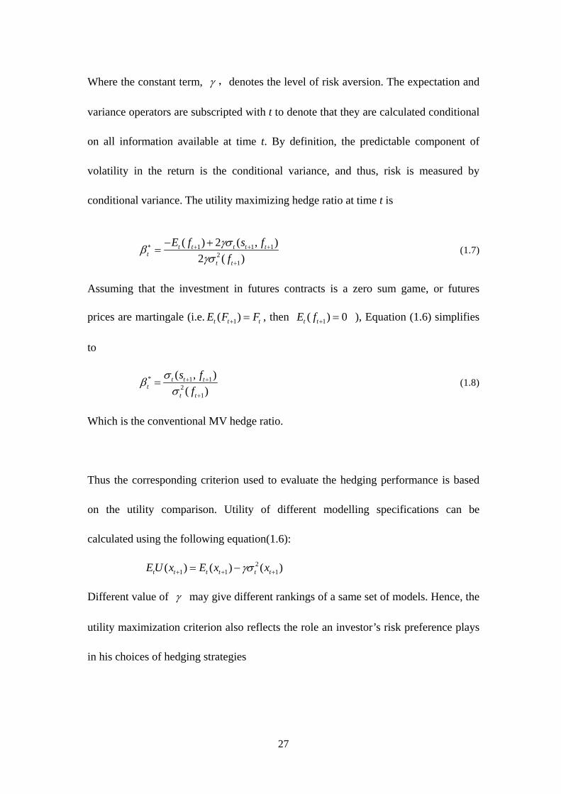
27

Where the constant term, ，denotes the level of risk aversion. The expectation and

variance operators are subscripted with t to denote that they are calculated conditional

on all information available at time t. By definition, the predictable component of

volatility in the return is the conditional variance, and thus, risk is measured by

conditional variance. The utility maximizing hedge ratio at time t is

1 1 12

1

( ) 2 ( , )

2 ( )t t t t t

tt t

E f s f

f

(1.7)

Assuming that the investment in futures contracts is a zero sum game, or futures

prices are martingale (i.e. 1( )t t tE F F , then 1( ) 0t tE f ), Equation (1.6) simplifies

to

* 1 12

1

( , )

( )t t t

tt t

s f

f

(1.8)

Which is the conventional MV hedge ratio.

Thus the corresponding criterion used to evaluate the hedging performance is based

on the utility comparison. Utility of different modelling specifications can be

calculated using the following equation(1.6):

21 1 1( ) ( ) ( )t t t t t tE U x E x x

Different value of may give different rankings of a same set of models. Hence, the

utility maximization criterion also reflects the role an investor’s risk preference plays

in his choices of hedging strategies

28

1.3.1 c) Sharpe hedge ratio and Sharpe ratio criterion

Another way of incorporating the portfolio return in the hedging strategy is to use

Sharpe ratio based criterion, which considers the risk-return tradeoff as well. Howard

and D’Antonio (1984) consider the optimal amount of futures contracts by

maximizing the ratio of the portfolio’s excess return to its volatility:

( )max f

X

E X R

(1.9)

Where 2 ( )X Var X and fR represents the risk-free interest rate. In this case the

optimal hedge ratio is:

*( / ) ( / )( ( ) /( ( ) ))

1 ( / )( ( ) /( ( ) ))

s f s f f

s f f

E f E s R

E f E s R

(1.10)

Where 2 ( )s Var s and 2 ( )f Var f , is the correlation coefficient between s

and f (see Howard and D’Antonio, 1984 for detailed derivations).

Again, if ( ) 0E f , then reduces to:

s

f

(1.11)

which is same as the MV hedge ratio.

One drawback of this approach, as pointed out by Chen et al. (2001), is that the

Sharpe ratio is a highly non-linear function of the hedge ratio. This lead to the

possibility that the hedge ratio derived from first order condition (i.e. the first

derivative with respect to the hedge ratio equal to zero) would minimize the Sharpe

29

ratio, instead of maximizing it, when the second derivative is positive.

The hedging performance of this approach can be evaluated in two ways. First, the

hedging effectiveness can be defined as the ratio of the Sharpe Ratio of the hedged

portfolio over the Sharpe Ratio of the unhedged portfolio.

( ( ) ) /

( ( ) ) /f H

f U

E H R

E U R

(1.12)

The higher the ratio, the better the hedging performance.

Another way is to define the hedge effectiveness as the different between the Sharpe

ratios of the hedged and unhedged portfolio, which is shown as follows:

( ) ( )f f

H U

E H R E U R

(1.13)

1.3.1 d) Minimum Mean extended-Gini coefficient hedge ratio and risk reduction

based on MEG coefficient

Another type of hedge ratio is the Mean extended Gini (MEG) coefficient hedge ratio

(Cheung et al., 1990; Kolb and Okunev, 1992; Lien and Luo, 1993; Shalit, 1995; and

Lien and Shaffer, 1999). This approach of deriving the OHRs is consistent with the

concept of stochastic dominance and involves the use of the MEG coefficient. The

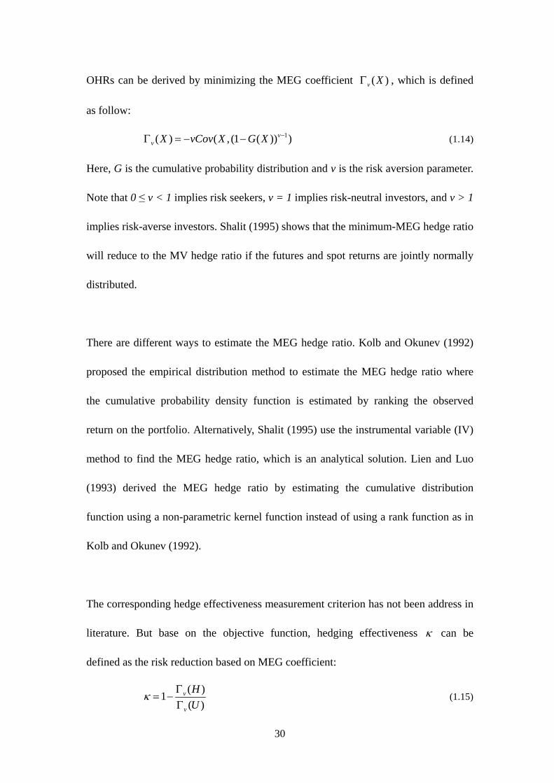
30

OHRs can be derived by minimizing the MEG coefficient ( )v X , which is defined

as follow:

1( ) ( , (1 ( )) )vv X vCov X G X (1.14)

Here, G is the cumulative probability distribution and v is the risk aversion parameter.

Note that 0 ≤ v < 1 implies risk seekers, v = 1 implies risk-neutral investors, and v > 1

implies risk-averse investors. Shalit (1995) shows that the minimum-MEG hedge ratio

will reduce to the MV hedge ratio if the futures and spot returns are jointly normally

distributed.

There are different ways to estimate the MEG hedge ratio. Kolb and Okunev (1992)

proposed the empirical distribution method to estimate the MEG hedge ratio where

the cumulative probability density function is estimated by ranking the observed

return on the portfolio. Alternatively, Shalit (1995) use the instrumental variable (IV)

method to find the MEG hedge ratio, which is an analytical solution. Lien and Luo

(1993) derived the MEG hedge ratio by estimating the cumulative distribution

function using a non-parametric kernel function instead of using a rank function as in

Kolb and Okunev (1992).

The corresponding hedge effectiveness measurement criterion has not been address in

literature. But base on the objective function, hedging effectiveness can be

defined as the risk reduction based on MEG coefficient:

( )

1( )

v

v

H

U

(1.15)

31

1.3.1 e) Optimal Mean extended-Gini coefficient hedge ratio and utility

maximisation based on MEG coefficient

The minimum MEG hedge ratio does not consider the risk return trade-off. To address

this issue, Kolb and Okunev (1993) consider maximizing the utility function based on

GEM coefficient. The objective function is defined as follows:

( ) ( ) ( )vU X E X X (1.16)

The hedge ratio derived from the above objective function is denoted as M-MEG

hedge ratio, which considers the expected return on the hedged portfolio. It manifests

under the condition of joint normal distribution of futures and spot returns or if the

futures returns follow a pure martingale.

Hedging performance is measured by the magnitude of the utility derive based on the

above function (Eq. 1.16). The higher the utility, the better the hedging strategy.

1.3.1 f). Minimum Generalized semivariance hedge ratio and risk reduction

based on the Generalised semivariance

An alternative approach for determining the hedge ratio has been suggested by Chen

et al., 2001; De Jong et al., 1997; Lien & Tse, 1998, 2000, which focus on the

32

downside risk. A survey by Adams and Montesi (1995) also points out that the

managers care about the variability of losses (e.g. the return below a target value)

much more than variability of gains. The variability of losses is normally denominated

as the “downside risk” and the variability of gains as “upside potential” (Lee and Rao,

1988). The investors using hedging instrument with the purpose of minimizing the

downside risk whilst preserving the upside potential will find the conventional

minimum variance hedge strategy inappropriate (lien and Tse, 2000). When an

investors try only to avoid the downside risk, Bawa (1975)’s general definition of

downside risk—the generalized semivariance (GSV) or Lower Partial Moments

(LPM), and Fishburn (1977)’s ( , ) model are more appropriate. The development

of GSV is a milestone in measuring the downside risk. In this case, the optimal hedge

ratio is obtained by minimising the GSV the objective function as follows:

, ( ) ( ) ( ), 0V X X dG X a

(1.17)

where ( )G X is the probability distribution function of the return on the hedged

portfolio. The parameters δ and α are both real numbers, they are used to represent the

target return and risk aversion, respectively. The function assumes that investors

consider the investment as risky only when return is below the target return. It can be

shown (see Fishburn, 1977) that α < 1 represents a risk-seeking investor and α > 1

represents a risk-averse investor. Again, the Minimum GSV hedge ratio would be the

same as the MV hedge ratio if the futures and spot returns are jointly normally

distributed and if the futures price follows a pure martingale process, as shown by

Lien and Tse (1998).

33

Correspondingly, the hedge performance is evaluated by calculation the risk reduction

of the downside risk, GSV of the hedged portfolio comparing to the unhedge

underlying3.

,

,

( )1

( )

V H

V U

(1.18)

The GSV approach has several advantages as an examination of hedging

performances. First, it has been shown by Bawa (1975) that GVS is robust to

non-normalitiy. Thus it does not require the assumption of normality in the return

distribution. Second, analyzing the hedging performance under GSV criterion may

reveal information with respect of the asymmetry of the joint distribution between

spot and futures returns for a given asset. Therefore, it overcomes the primary

shortcoming of conventional variance based on risk reduction measure of hedging

performance which assumes symmetric information. Eftekhari (1998) provides

evidence that the lower partial moment (GSV) hedge ratios are effective in reducing

downside risk and increasing returns.

1.3.1 g). Minimum Semivariance hedge ratio and risk reduction based on the

semivariance

3 This is the LMP hedging effectiveness criterion in Cotter and Hanly (2006).

34

Semivariance is defined as the variability of returns below the mean. The minimum

semivariance approach4 is a special case of the minimum GSV hedge ratio, where

risk aversion parameter is assumed to be equal to 2, and the target return is set to be

the expected return. Thus the objective function to be optimised is:

2( ) ( ), 0SemiVar X dG X a

(1.19)

Where , the target return, is set to be the expected return. As before, the hedge ratio

would be same as the MV hedge ratio if the futures and spot returns are jointly

normally distributed and the futures price follows a pure martingale process.

The hedging performance is then measured by the reduction in the semivariance of the

hedged portfolio to the unhedged position. It is shown as

( )

1( )

SemiVar H

SemiVar U (1.20)

From the Equation (1.19), we can see that the deviations from the target return

( )X are squared. As a result, if the distribution is symmetric and the target return

is set to mean, then the semivariance is just half of the variance. Then the hedging

performance evaluated by risk reduction in semivariance will be the same as that

evaluated by the risk reduction in variance. However, for a non-symmetric

distribution, the results from the two methods are different. The semivariance can

address the primary shortcoming of the variance measure when hedging downside risk

is more of the concern.

4 Following the work by Roy (1952), which proposes the safety-first criterion.

35

1.3.1 h). Optimal generalized semivariance hedge ratio and utility maximisation

based on the generalised semivariance

Chen et al. (2001) extend the GSV hedge ratio to a mean-GSV (M-GSV) hedge ratio

by considering the mean return in the optimal hedge ratio, which enables

incorporating the risk and return trade-off into the GSV strategy. The M-GSV hedge

ratio is obtained by maximising the following utility function:

,( ) ( ) ( )U X E X V X (1.21)

Again, the M-GSV hedge ratio would be the same as the MV hedge ratio if the futures

prices follow a pure martingale process and returns are jointly normal.

The hedging effectiveness is measured by the magnitude of expected utility based on

GSV of the hedged and unhedged positions, using Equation (1.21)

1.3.1 i) VaR hedge ratio and risk reduction based on VaR

In recent years a new approach for determine the hedge ratio has been developed. This

approach uses VaR (Value at Risk) as a measure of downside risk. Due to the

simplicity of quantitative measurement, VaR emerges as the essential and standard

risk management tools of many financial institutions and is widely used for

36

investment decisions, supervisory decisions and capital allocations decisions. Using

Jorion (2000)’s definition of VaR as an absolute size of losses associated with the

hedging strategy, the downside risk of the hedged portfolio over a period and

confidence level as the object function (see, Hung, Chiu and Lee, 2006):

( ) ( )a XminVaR X Z E X

(1.22)

Where ( )VaR X represent the absolute VaR of the hedged portfolio and Z is the

left percentile at for the standard normal distribution. Generally, VaR is the

(100 )th percentile of return distribution of the change in the asset/portfolio over

the period . Therefore, VaR gives the return that is exceeded with (100 )%

probability. It is possible, however, that two portfolios with the same VaR will have

different potential losses. This is because VaR does not account for the magnitude of

losses beyond the (100 )th percentile. Conditional VaR developed by Tasche

(2002) addresses such shortcomings.

The hedge ratio for this kind of VaR approach is (see Chun et al., 2006 for detailed

derivation of the hedge ratio):

2

2 2 2

1( )

( )s s

f f f

E fZ E f

(1.23)

Similarly, the VaR hedge ratio converges to MV hedge ratio if the martingale property

of futures holds.

Cotter and Hanly (2006) give the performance measuring criterion as the percentage

reduction in VaR, using 1% significant level (or 99% confidence level).

37

1%

1%

( )1

( )

VaR H

VaR U (1.24)

1.3.2 Approaches to determine the optimal hedge ratio and hedging

evaluation criteria in this study

This study derives the optimal hedge ratios based on three objective functions: the

traditional risk minimizing, “expected utility” maximisation and semivariance

minimisation5. Accordingly, we access the hedging effectiveness of different models

used to derive the optimal hedge ratio based on three criteria, namely, risk reduction

base on variance (variance reduction), expected utility maximization and risk

reduction based on semivariance. The three methods are chosen for the following

reasons.

First, the variance reduction criterion is the most widely used in the literature.

However, as we discussed before, it has several shortcomings, including that it doesn’t

take the expected mean values into consideration and give positive and negative

returns equal weight, etc. The other two criteria are employed to address these issues.

The expected utility maximization criterion is used to account for the risk and return

trade-offs of the hedged portfolio. Meanwhile, because there is a risk aversion

5 More detailed technical introduction of these is given in next section.

38

parameter in the expected utility function, this criterion also takes into account

investor’s risk preference. The minimum semivariance hedge ratio and the risk

reduction based on semivariance hedging performance evaluation criterion is

employed to address the downside risk for the investor, which is believe to be more

crucial. Such approach seems more practical as most investors tend to avoid the

downside risk but desire to maintain the upside potential.

Second, as shown in the later sections, our empirical estimates show that the futures

prices follow a martingale process. If the futures prices follow a martingale process,

that is, the expected futures return is zero, we know that the Sharpe hedge ratio and

VaR hedge ratio will be the same as the MV hedge ratio. Therefore, the hedged

returns will be the same that derived using Minimum Variance criterion, so will the

rankings of different models.

Third, in theory, the Maximum Utility hedge ratio also reduces to MV hedge ratio

when the expected value of futures return is zero. However, in this study, we still

derive and examine the hedging effectiveness of different hedging strategies using the

utility maximisation criterion by incorporating the actual (expected) mean futures

returns of the sample being examined. We do so because, although those values are

statistically not different from zero, excluding the constant term in the mean equation

of the models6 will make the estimations unable to achieve convergence. Thus we

6 Different models are described in the next section.

39

retain the actual intercept value in deriving the hedge ratios under the Utility

Maximisation criterion. Because the intercept value is very close to zero, the hedge

ratios derived under Utility Maximisation criteria will be only slightly different from

those derived under Variance Minimisation criteria, so should be the rankings.

Moreover, this approach enables us to examine the effect of the investors’ risk

aversion on deriving the hedge ratios and choosing hedging strategies.

Forth, although the futures prices follow a martingale process, the spot and futures

price series are not jointly normally distributed. MEG and M-MEG hedge ratio, GSV

and M-GSV hedge ratio should be different from the MV hedge ratio. However, the

hedge ratios under those objective functions cannot be found mathematically, or could

be very difficult to calculate because the complexity of the mathematical methods.

Most studies on those use approximations. Because of these, we only examine one

special case, that is, the semivariance hedge ratio, where MV hedge ratio is used as

the proxy. We access the ability of those models in reducing downside risk given the

circumstance that hedge ratios are derived with the objective function of minimising

variance of the hedged portfolio.

40

1.4 Data and Methodology

1.4.1 Data

Data for the China fuel oil futures are from Shanghai Futures Exchanges (SFHE). As

any futures contract is associated with expiration, it is necessary to construct a

continuous series of futures prices. The conventional approach relies upon the prices

of the “most nearest to maturity” contracts, because these tend to be the most liquid

and therefore the best delegates for the futures market information, except perhaps

during the maturity month. However, an examination of the Shanghai futures markets

reveals a different story. Peck (2004) finds that the most nearest to maturity futures

contract is hardly the most liquid contract in China. It was reported that the most

liquid contracts are 4 or 5 months to maturity for copper and 3 or 4 months to

maturity for aluminum. For the oil futures, we can determine from the data that the

most liquid contracts are 2 to 3 months to maturity. Thus the futures data we used in

this study corresponds to daily closing prices of the most active nearby contracts. For

the spot prices, we follow the commonly adopted practice in the literature by using the

daily closing prices of the corresponding commodity.

We note that there is no standard fuel oil price series in the Chinese market.

Guangdong province in Huanan area takes 80% of the fuel oil imports and accounts

for 35% of the total oil demand in China, and the Huanan fuel oil market is the most

41

active and closest to a perfectly competitive market in China. Hence we choose

Huanan 180CST fuel oil prices (also called Huagpu 180CST) as the underlining spot

prices for the Chinese market.

The Platts 180CST industry fuel oil has quality mostly similar to the contracted fuel

oil in SHFE. Moreover, it is used as the benchmark of pricing fuel oil prices in

Singapore. Thus we use the Platts 180CST fuel oil as the underlying spot in the cross

hedging, which is compared with the domestic hedging in assessing the China fuel oil

futures. The data for the Huanan (Huangpu) 180CST and Platts 180 CST fuel oil

prices series are taken from Heilongjiang Tianqi Futures Exchange 7

(http://www.tqfutures.com). The data begin on August 25, 2004 (the day when the

futures started to trade) and end on September 29, 20068. Returns of the futures and

spot prices are calculated by computing the first differences in the natural logarithm of

price series multiplied by 100. In total, we have 548 observations of which the first

500 (from August 25 2004 to July 25, 2006) observations are used for estimation

purposes and the remaining 48 observations (from July 26 to September 06) are used

for out-of-sample forecasting.

7 An Exchange for commodity futures in China. 8 Data end on September 2006 because it was the most up-to-date data at the time the research was conducted. In the final revision of the thesis, I attempted to update the data to April 2009, reexamining the hedging effectiveness of China fuel oil futures and comparing the first two years performance with the most recent two years performance. However, data on spot fuel oil prices are no longer available from the source.

http://www.tqfutures.com/�

42

1.4.2 Methodology

1.4.2 (A) Estimation of Optimal Hedge Ratios

To derive the time-varying OHRs for China fuel oil futures, we estimate Bi-variate

GARCH(1,1) and TGARCH(1,1) models to capture time-varying second moment

effects in the joint distribution of spot and futures returns. TGARCH models were

used because of the possibility of capturing the measure of any asymmetric

information effect. Thus we compare five models, Bi-variate GARCH(1,1) general

and diagonal, Bi-variate TGARCH(1,1) general and diagonal and traditional constant

models.

The most general representation of the joint distribution of spot and futures returns

used can be expressed as (Ford, et al, 2005):

),0(~|; 1 ttttttttt HNVGECy (1.25)

Where ( , ) 't t ty f s is a vector of observations of the spot and futures returns

(log-differenced price series), ( , ) 't st ft is a vector of conditional means to be

estimated and ( , ) 't ft st is a vector of residuals. and are column vectors

of parameters,; EC is the error correction term from any cointegrating relationship

between the two prices; G is a (2 2) diagonal matrix with conditional variance

terms from GARCH(1,1) estimation on the diagonal. The term V represents the

possible variables that can determine the returns of spot and futures, multiplied by

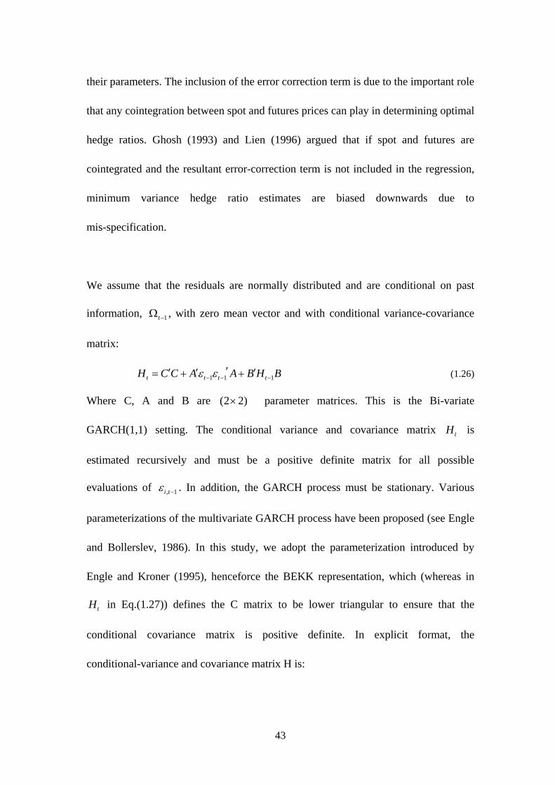
43

their parameters. The inclusion of the error correction term is due to the important role

that any cointegration between spot and futures prices can play in determining optimal

hedge ratios. Ghosh (1993) and Lien (1996) argued that if spot and futures are

cointegrated and the resultant error-correction term is not included in the regression,

minimum variance hedge ratio estimates are biased downwards due to

mis-specification.

We assume that the residuals are normally distributed and are conditional on past

information, 1t , with zero mean vector and with conditional variance-covariance

matrix:

1 1 1t t t tH C C A A B H B (1.26)

Where C, A and B are (2 2) parameter matrices. This is the Bi-variate

GARCH(1,1) setting. The conditional variance and covariance matrix tH is

estimated recursively and must be a positive definite matrix for all possible

evaluations of , 1i t . In addition, the GARCH process must be stationary. Various

parameterizations of the multivariate GARCH process have been proposed (see Engle

and Bollerslev, 1986). In this study, we adopt the parameterization introduced by

Engle and Kroner (1995), henceforce the BEKK representation, which (whereas in

tH in Eq.(1.27)) defines the C matrix to be lower triangular to ensure that the

conditional covariance matrix is positive definite. In explicit format, the

conditional-variance and covariance matrix H is:

44

, , 11 11 12

, , 12 22 22

2, 1 , 1 , 111 21 11 12

2, 1 , 1 , 112 22 21 22

, 1 , 111 21 1

, 1 , 112 22

0

0ff t sf t

tsf t ss t

f t s t f t

f t s t s t

ff t sf t

sf t ss t

h h c c cH

h h c c c

h h

h h

1 12

21 22

(1.27)

This system can be estimated with no restrictions on H and is thus referred to here

as the general model. The diagonal model proposed by Bollerslev, Engle and

Wooldridge (1988) restricts the off-diagonal elements of A and B to be zero,

i.e., 0 12 21 12 21: 0H . Covariance Stationary of the GARCH(1,1) process

requires the eigenvalues of ( )A A B B be less than one in modulus9 (See

Engle and Kroner, 1995).

The static or constant model arises when all elements of A and B are set to zero, i.e.

0 11 22 12 21 11 22 12 21: 0H . The hedge ratio that the static

model produces is constant and equivalent to that obtained by using traditional OLS

estimations. Diagonal and constant models can be seen as nested models: the constant

model is nested in the diagonal model and diagonal in the general. So the competing

structures can be evaluated by likelihood ratio test.

9 For the Bi-variate GARCH(1,1) model, 1 1 1H C C A A B H Bt t t t , hence we have

'( ) ( ' ) ( ) ( ) ( ) ( )1 1 1h vec H vec C C A A vec B B vec Ht t t t t . It follows that the

unconditional covariance matrix is 1[ ( ) ( )] ( )I A A B B vec C C . For the diagonal model,

the stationary condition can be reduced to 2 2 1, 1, 2a b iii ii , because the eigenvalues of a

diagonal matrix are simply the elements along the diagonal and the conditions detailed imply that all other diagonal elements are also less than 1 in absolute value.

45

The general and diagonal models of hedging impose symmetry on the responses of

volatility to positive or negative shocks. This study also examines the asymmetric

effect of oil futures by employing an asymmetric model, the TGARCH specification.

El-Khoury (2006) suggests that incorporating the asymmetric effect could improve

the hedge effectiveness for the NYMEX’s Light Sweet Crude Oil contract. We

examine if this is the case in the Chinese oil market. The asymmetric general model

(TGARCH General) differs from the symmetric general Bi-variate GARCH approach

in that the covariance matrix Eq. (1.26) is replaced by :

1 1 1 1 1t t t t t tH C C A A B H B D D (1.28)

Where D is a (2 2) matrix of coefficients, and t is the additional quadratic form

of the vector of negative return shocks, defined as 1 1t tI , where 1tI if 0t

and 0 otherwise. The inclusion of t in the conditional variance-covariance matrix

not only accounts for any asymmetry effects in the conditional variances but also

allows for possible asymmetric effects in the conditional covariance. The TGARCH

Diagonal model restricts the off-diagonal elements of matrix A, B, D to be zero. The

constant model restricts all elements in matrices A, B and D to be zero. The

stationarity of the TGARCH(1,1) process requires that the eigenvalues of

( )A A B B D D be less than one in modulus.

All these models are estimated through maximum likelihood. Under conditional

normality, the log likelihood function is as follow:

1

1

1( ) log(2 ) (log ( ) ( ) ( ) ( ))

2

T

t t t tt

L T H H

(1.29)

46

Where T is the number of observations of the sample. is the parameter vector to

be estimated. 1 2( , )t t t is a 1x2 vector of residuals at time t. 1cov( )t t tH ,

where the diagonal elements of tH are the conditional variances, the cross diagonal

elements are the conditional covariances of the spot and futures returns. The

log-likelihood function is maximised subject to the constraint that the conditional

variances be positive. Initial values are required for all the parameters and those found

from the univariate GARCH regressions are used for this purpose. For those

parameters for which the initial guesses cannot be obtained from the univariate

GARCH estimations, we used a value 0.05 for all parameters in most of the cases.

1.4.2 (B) Accessing hedging effectiveness in- and out-of-sample

This study derives the optimal hedge ratios based on three objective functions: the

traditional variance minimisation, the “expected utility” maximisation and the

semivariance minimisation10. Accordingly, we access the hedging effectiveness of

different models used to derive the optimal hedge ratio based on three criteria, namely,

risk reduction base on variance (variance reduction), expected utility maximisation

and risk reduction based on semivariance (semivariance reduction).

10 More detailed technical introduction of these is given in the previous section.

47

For the variance minimisation criterion, the MV hedge ratio, 1t will be:

(1) for the constant model

* ( , )

( )

Cov s f

Var f (1.30)

(2) for the dynamic model

,* 1

1 ,

ˆ( , | )ˆ( | )sf tt t t

t t f t

hCov s f

Var f h

(1.31)

where ˆth is the conditional variance estimated at time t-1.

For the “expected utility” maximisation criterion, we use the mean-variance

representation of expected utility following Kroner and Sultan (1993). As a result, the

objective functions to be maximised to obtain the optimal hedge ratios are:

(1) for a constant model

( ) ( ) ( )t t t t tE U R E R Var R (1.32)

(2) for the dynamic models

1 1 1( | ) ( | ) ( | )t t t t t t t tE U R E R Var R (1.33)

Where *1t t t tR s f , is the return of the hedged portfolio, and is the coefficient

of risk aversion. Thus the utility maximisation distinguishes investors who may have

different risk preferences.

The maximisation of expected utility gives the 1t as below:

(1)for the constant model

* ( , ) 1 ( )

( ) 2 ( )

Cov s f E f

Var f Var f

(1.34)

48

(2) for the dynamic model:

1 1

1 1

( , | ) ( | )1*

( | ) 2 ( | )t t t t t

t t t t

Cov s f E f

Var f Var f

(1.35)

There is an additional term in the 1t comparing to MV OHRs, which describes the

speculative demand for futures which reflect the mean and variance trade-off in the

unhedged futures positions as well as the investors’ attitude toward risk.

To derive the optimal hedge ratio under semivariance minimisation objective, the

optimisation of the econometric models should be based on semivariance instead of

variance as we did for the MV hedge ratios. The semivariance assumes that the

positive and negative returns distribute asymmetrically. If the returns are symmetric,

there will be no difference between minimising semivariance and minimising variance

because semivariance is just half of the variance. However, when the residuals are not

normally distributed, the use of maximum likelihood to estimate the GARCH and

constant models is not appropriate. Under such circumstance, derivation of the

optimal hedge ratios under the semivariance minimisation criterion is impossible or

can only be done by incorporating very complex methods11. As a result, most recent

literatures use the MV hedge ratio to approximate the semivariance hedge ratio (e.g.

Cotter and Hanly, 2005, 2006). Therefore, we also use MV hedge ratios as an

approximation and based on these ratios, we examine the hedging performance of

11 For example, kernel density estimation method was used by Lien and Tse (2000), conditional heteroscedastic model was employed by Lien and Tse (1998) to estimate the optimal hedge ratios.

49

those competing models in reducing the downside risk.

Hedging effectiveness of different models is examined in both in- and out-of-sample

periods. The traditional approach measures the hedging as the percentage reduction in

the variance of the hedged position in comparison to the unhedged position

(Ederington, 1979), following the work of Working (1953, 1962), Johnson (1960) and

Stein (1961). The hedge effectiveness ( ) is measured using the formula:

( ) ( )

( )

Var H Var U

Var U (1.36)

Where ( ) ( )tVar U Var s , and *1( ) ( )t t tVar H Var s f .

The variance reduction is on an average basis over the whole of the in-sample and

out-of-sample period and at each day during that latter period. The model that records

the highest percentage variance reduction would be the one considered to be the most

effective. Unlike most of the existing literatures, we also include equality tests for the

means and variances of the hedged portfolio to see if there is any significant change in

means and variances of the hedged portfolio derived from different hedging models,

following Ford et al. (2005).

The expected utility comparisons in assessing the model performance for both in- and

out-of-sample hedging strategies are based on the values of obtained from using Eq.

(1.32) and (1.33). In terms of expected utility the comparison is based on the average

of expected utility values over of the forecast period and also on the time path of

50

expected utility values over each day of the forecast period. The higher value of

expected utility the model can generate the superior the model is relative to other

models. Equality tests for the means and variances of the hedged portfolio under risk

minimisation criterion are employed as well.

The risk reduction based on the semivariance is accessed using the following

equation:

( ) ( )

( )

SemiVar H SemiVar U

SemiVar U (1.37)

Where ( ) ( )tSemiVar U SemiVar s , and *1( ) ( )t t tSemiVar H SemiVar s f .

Same to the variance reduction criterion, we access the semivariance risk reduction

based on both average and time path of the forecast period, and the model that records

the highest percentage semivariance reduction would be the one considered to be the

most effective.

One important issue in accessing the hedging performance is the computation of

hedging ratios in the out-of-sample period. Unlike the in-sample hedge ratios which

are calculated from the conditional variance and covariance, the computation of the

out-of-sample hedge ratios is more complicated. The latter are computed based on the

parameters obtained from the in-sample estimation for the out-of-sample period to

up-date tH continuously. Therefore, the out-of-sample hedge ratios are based on all

information that is available at the time each hedging decision is made. The

51

information set 1t contains the history of spot and futures rates of returns to the

given current time during the forecast period. The predicted hedged portfolio returns

are then obtained based on the calculated hedge ratios to forecast the following day

return of the hedged portfolio.

52

1.5 Estimation results

1.5.1 Descriptive Statistics

Table 1.1 reports some basic statistics for daily returns for the China fuel oil futures

returns (denoted as RF), China Huanan fuel oil spot returns (denoted as RS) and

Singapore Platt’s fuel oil price returns (denoted as RSX). Returns are calculated as the

difference of the nature logarithms of the closing prices multiplied by 100.

Table 1. 1Descriptive Statistics of return series of Futures and Spot returns

RF RS RSX

Mean 0.054093 0.068074 0.065437

Median 0.091827 0.000000 0.000000

Maximum 4.222263 7.020426 8.318446

Minimum -5.016596 -5.706072 -11.21173

Std. Dev. 1.422809 1.194955 1.931239

Skewness -0.207686 0.255625 -0.637181

Kurtosis 4.149266 8.654918 8.361978

Jarque-Bera 34.03585 734.7913 692.2925

Probability 0.000000 0.000000 0.000000

)5(Q 11.741** 6.169 6.7104

22.774*** 16.819*** 16.923***

ARCH-LM 13.3119** 15.0571** 15.98175***

Note: (5)Q and 2

(5)Q denote the Ljung-Box Q statistics for the test of significance of autocorrelations up to 5th

order in return and squared returns series respectively. *, **, *** denote statistical significance at the 10%,5% and

1% level.

From Table 1.1, we can observe that the mean returns of the futures are lower than

that of the spot returns in both of the Chinese and Singapore markets. However, the

2 (5)Q

53

standard deviation for the futures returns is larger than the standard deviation of spot

returns in the Chinese market, which is smaller than that in the Singapore market.

This may due to the fact that trading in The Singapore market is more active.

Skewness12, kurtosis13 and thus Jacque Bera (JB) statistics14 for all three series are

significant, so rejecting the null hypothesis of normal distributions. Kurtosis for the

spot returns is much higher than for the futures return, so that the spot returns have

more peakedness. The Ljung-Box (1987) Q(5) statistics for the futures return series is

significant but not for the two spot return series; while Q(5) statistics for the squared

return series are mostly significant, which indicate that although autocorrelation in

returns series is not strong, it is strong for the squared returns. Thus, the second

moments of returns are time varying and changing in a predictable fashion. This kind

of volatility clustering —large changes tend to be followed by large changes, of either

sign, and small changes tend to be followed by small changes, of either sign—can be

observed in Figure 1.1. In sum, the return series in this study exhibit all the typical

characteristics of high frequency financial return series: skewness, leptokurtosis, and

highly significant linear and nonlinear serial correlations. Moreover, the significance

of the ARCH-LM test (Engle, 1982) statistics also suggests that an ARCH/GARCH

type model is an appropriate specification.

12 Skewness is a measure of asymmetry of the distribution of the series around its mean; the skewness of a symmetric distribution, such as the normal distribution, is zero. 13 Kurtosis measures the peakedness or flatness of the distribution of the series, in other words, how fat the tails of the distribution are. The kurtosis of the normal distribution is 3. 14 A JB statistic for a normal distribution is 0, which indicates that the distribution has a skewness of 0 and a kurtosis of 3. Skewness values other than 0 and a kurtosis values farther away from 3 lead to increasingly large JB values. And the Critical value for normal distribution at 5%level is 5.99.

54

The correlations of the three returns are reported in Table 1.2. We can observe that

those of China’s fuel oil futures are more related to the spot prices changes in the

Singapore market. The price in the Chinese market is largely influenced by the price

changes in the Singapore market.

Table 1. 2 Correlations between RF, RS and RSX

RF RS RSX

RF 1.000000 0.355813 0.467944

RS 0.355813 1.000000 0.324992

RSX 0.467944 0.324992 1.000000

1.5.2 Diagnostic checks on the distributional properties

As discussed in the previous section that the presence of a cointegrating relationship

between spot and futures prices will produce downwardly biased hedge ratios unless

an error correction term is incorporated into the mean equation. Also for an adequate

estimation with Bi-variate GARCH we need to ensure that the components variables

(the mean returns) are stationary. Thus unit root tests are necessary. In this study, we

conduct both the Augmented Dickey-Fuller (ADF) and Kwiatkowski, Phillips,

Schmidt and Shin (KPSS) tests to test for stationary in the natural logarithm of prices

series and also in the return series. The null hypothesis for the ADF test is that the

series has a unit root; while the null hypothesis for KPSS is that the series is stationary.

The test results are reported in Table 1.3.

55

Table 1. 3 Unit root test

(1) Unit Root test for the level series (log of the prices series)

LF LS LSX

ADF KPSS ADF KPSS ADF KPSS

intercept

Lag 1 -1.31614 24.69540* -1.57216 23.88512* -1.67102 22.84567*

Lag 2 -1.34791 16.48799* -1.60328 15.95067* -1.65577 15.2699*

Lag 3 -1.37309 12.38246* -1.60734 11.98272* -1.65825 11.48018*

Lag 4 -1.42362 9.918913* -1.60901 9.601885* -1.71471 9.205771*

Lag 5 -1.39602 8.276574* -1.61353 8.01461* -1.65381 7.689283*

Trend and intercept

Lag 1 -0.28649 2.934404* -0.51119 3.505677* -1.48543 3.543713*

Lag 2 -0.02025 1.975631* -0.68915 2.354065* -1.44472 2.386529*

Lag 3 -0.32942 1.495056* -0.7394 1.777943* -1.43759 1.80712*

Lag 4 -0.29891 1.206754* -0.54393 1.432338* -1.35666 1.459327*

Lag 5 -0.15025 1.014756* -0.50723 1.201965* -1.02593 1.227515*

(2) Unit Root test for the Return series (log differences of the prices series)

RF RS RSX

ADF KPSS ADF KPSS ADF KPSS

None Lag 1 -18.21708* - -14.98325* - -16.44549* -

Lag 2 -13.10897* - -12.32162* - -13.44293* -

Lag 3 -11.34618* - -11.51614* - -11.91796* -

Lag 4 -10.5497* - -10.36032* - -11.69414* -

Lag 5 -10.0398* - -9.341099* - -11.32247* -

intercept

Lag 1 -18.25134* 0.28769 -15.03655* 0.340917 -16.45982* 0.170777

Lag 2 -13.14702* 0.30941 -12.3811* 0.322044 -13.46278* 0.170692

Lag 3 -11.39320* 0.30395 -11.58804* 0.309994 -11.94648* 0.171005

Lag 4 -10.60281* 0.30204 -10.44012* 0.308774 -11.73007* 0.172901

Lag 5 -10.09977* 0.30635 -9.42671* 0.309055 -11.36721* 0.180307

Note: Critical value (for 5% significance) for ADF test: with intercept, - 2.865; with trend and intercept, -3.417.

Critical value (for 5% significance) for KPSS test : with intercept, 0.463, with intercept and trend, 0.146.

Here * indicate rejection of null hypothesis at 5% significance level.

56

Figure 1.2 portrays the three log price series (LF, LS and LSX represent the log of

China fuel oil futures, China fuel oil and Singapore fuel oil spot price series). We can

observe that all the series are upward slopping. Thus the units root tests with intercept

and trend for the log price series. Results from both the ADF test and the KPSS test

reveal that all of the three price series are non-stationary at 5% significant level. For

the return series, we can observe from the figure there is no intercept or trend in the

series. Hence we only perform unit roots test with “none” as well as “with intercept”.

ADF test results for all three series reject the null hypothesis of non-stationarity, and

the KPSS test results show the null hypothesis of stationary should not be rejected at

5% significant level. As the return series is the first difference of log prices series, the

above results indicate that the log futures and spot price series are all following an I(1)

process. We then adopt Johanson’s cointegration test (1991, 1995) to test whether the

cointegration relationships between futures and spot prices exists. The results are

reported in Table 1.4.

As shown in Table 1.4, both the Trace and Max-eigenvalue tests indicate that there is

no cointegrating relationship between the fuel oil futures and China fuel oil spot

prices. While for China fuel oil futures and spot prices in the Singapore market, both

the Trace and Max-eigenvalue tests indicate there exists one cointegrating relationship.

However, we have to cast doubt on such. Cointegration states the long run

co-movements of two series, but we have only two years data available. The time

span is too short for us to draw any meaningful conclusions from the tests. Moreover,

we cannot find consistent cointegration vectors because the residuals are not normally

57

distributed, although in most cases we find that the coefficient on the futures return in

the first cointegration vector was 1 or nearly 1, which is approximately the value in

theory. When we assumed that such a cointegration relation exists and used an error

correction term composed as the difference between the one period lag of the two

prices in the regression for the hedging in the Singapore market, we found that it did

not have a statistically significant impact on the returns. Additionally, the inclusion of

the error correction term made it impossible to obtain estimates of the parameters of

tH sometimes; or making the system singular or non-convergent. Consequently, no

results from using an error correction term are reported here.

Table 1. 4 Johanson’s cointegration test

(1) Cointegration test for China fuel oil futures prices and China Huanan fuel oil spot prices

Hypothesized Trace Test Max-Eigen

No. of CE(s) Statistic Prob. Statistic Prob.

None 14.79088 0.0636 12.40089 0.0965

At most 1 2.389989 0.1221 2.389989 0.1221

(2) Cointegration test for China fuel oil futures prices and Singapore fuel oil spot prices

Hypothesized Trace Test Max-Eigen

No. of CE(s) Statistic Prob. Statistic Prob.

None 26.94548* 0.0006 24.46388* 0.0009

At most 1 2.481599 0.1152 2.481599 0.1152

Note: * denotes rejection of the hypothesis at the 0.05 level

58

1.5.3 Models Estimation Results

We investigate the hedging ability of China fuel oil futures when it is used to hedge

spot positions in the domestic and Singapore markets. We employ different models

with different variance specifications (TGARCH-General, TGARCH-Diagonal,

GARCH-General, GARCH-Diagonal and constant model) in order to unveil the most

appropriate one for deriving the optimum hedging ratios.

Numerous variations of the models were experimented with, for a given structure of

tH , in respect of the specification of each of the mean equations. We found that, for

both the Bi-variate GARCH(1,1) and TGARCH(1,1) models, the most minimal

specifications with random means were generally the most acceptable, statistically

speaking. Such is consistent with Ford et al. (2005). Thus the estimation results we

report here are for GARCH and TGARCH models with the mean structure containing

only intercepts. A further point that might need highlighting is the estimation of

GARCH and TGARCH structure. Engle and Kroner (1995) suggest that the BHHH

(Berndt, Hall, Hall and Hausman, 1974) optimization algorithm15 might be the most

appropriate for estimation of multivariate GARCH models. However, Ford et al (2005)

15 The BHHH algorithm follows Newton-Raphson, but replaces the negative of the Hessian by an approximation formed from the sum of the outer product of the gradient vectors for each observation’s contribution to the objective function. The advantages of approximating the negative Hessian by the outer product of the gradient are that (1) we need to evaluate only the first derivatives, and (2) the outer product is necessarily positive semi-definite. The disadvantage is that, away from the maximum, this approximation may provide a poor guide to the overall shape of the function, so that more iterations may be needed for convergence.

59

point out that the Marquardt algorithm16 provided estimates that were identical to or

better than those obtained from the use of BHHH. Our experiments confirm those

findings.

The maximum likelihood estimation results for the hedging-ability of the China fuel

oil futures in hedging a domestic spot position are reported in Table 1.5 and the

estimation results for hedging a spot position in the Singapore market are reported in

Table 1.6.

First, consider the mean structure for futures and spot returns. From Tables 1.5 and 1.6,

we observe that the estimated mean of futures returns f are not significantly

different from zero at 5% significant level for all the models. The expected means for

Chinese fuel oil spot returns and Singapore fuel oil commodity returns are

insignificantly different from zero as well. Comparing the two tables, we find that the

estimated mean spot returns in the Chinese market are smaller than those in the

Singapore market. Although the estimation results suggest that the futures returns are

not significantly different from zero at a 5% significance level and therefore the

futures prices follows a martingale process, we cannot estimate the dynamic GARCH

models with the mean equations being just dependent upon white noise, because

convergence were not able to be achieve; or even when convergence was ensured, the

16 The Marquart algorithm modifies the Gauss-Newton algorithm in exactly the same manner as quadratic hill climbing modifies the Newton-Raphson method by adding a correction matrix (or ridge factor) to the Hessian approximation. The ridge correction handles numerical problems when the outer product is near singular and may improve the convergence rate. The algorithm pushes the updated parameter values in the direction of the gradient.

60

covariance stationary of the GARCH structures were violated. However, including

those intercept variables will make the coefficients in A, B, and C matrix changed

slightly 17. Thus in calculating the utility maximisation hedge ratios, the actual

expected value is used instead of zero, which make the hedge ratios slightly differ

from the MV hedge ratios, so as the ranking of different models.

Now we turn to the covariance structure for the domestic and cross border hedging.

From Table 1.5 (a) we can observe that for the TGARCH(1,1) general and diagonal

models, all the estimated coefficients ijd , which capture the asymmetric effects

(positive and negative shocks increase the variances by different magnitudes) are

insignificant at 95% significant level. We further perform the Wald exclusion tests for

the asymmetric coefficients. The test result (5.0008 with p-value equal 0.2872) cannot

reject the null hypothesis that these coefficients are jointly zero, implying that markets

react to positive and negative shocks in a similar manner. Such results diverge from

those in the existing literature on the asymmetric effects in equity returns, most of

which indicate the negative shocks have greater and longer effects than positive

shocks. For the general models and diagonal models reported in Table 1.5(b), we

observe most parameters are significant, implying that the distribution of spot and

futures variances and covariances are time-varying. For the constant model, all the

coefficients are significant at a 5% significance level. The Ljung-Box Q-statistics for

residuals and squared residuals in their normalised form are calculated to test the

17 Not their significance, but values.

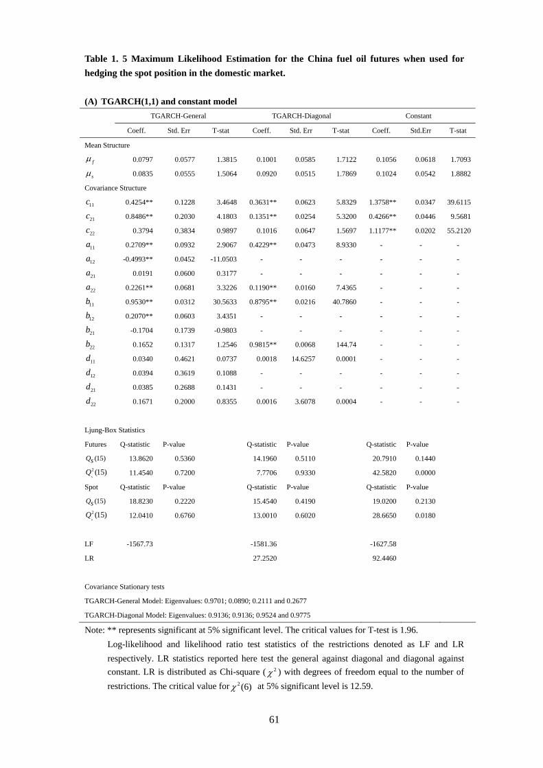
61

Table 1. 5 Maximum Likelihood Estimation for the China fuel oil futures when used for

hedging the spot position in the domestic market.

(A) TGARCH(1,1) and constant model

TGARCH-General TGARCH-Diagonal Constant

Coeff. Std. Err T-stat Coeff. Std. Err T-stat Coeff. Std.Err T-stat

Mean Structure

f 0.0797 0.0577 1.3815 0.1001 0.0585 1.7122 0.1056 0.0618 1.7093

s 0.0835 0.0555 1.5064 0.0920 0.0515 1.7869 0.1024 0.0542 1.8882

Covariance Structure

11c 0.4254** 0.1228 3.4648 0.3631** 0.0623 5.8329 1.3758** 0.0347 39.6115

21c 0.8486** 0.2030 4.1803 0.1351** 0.0254 5.3200 0.4266** 0.0446 9.5681

22c 0.3794 0.3834 0.9897 0.1016 0.0647 1.5697 1.1177** 0.0202 55.2120

11a 0.2709** 0.0932 2.9067 0.4229** 0.0473 8.9330 - - -

12a -0.4993** 0.0452 -11.0503 - - - - - -

21a 0.0191 0.0600 0.3177 - - - - - -

22a 0.2261** 0.0681 3.3226 0.1190** 0.0160 7.4365 - - -

11b 0.9530** 0.0312 30.5633 0.8795** 0.0216 40.7860 - - -

12b 0.2070** 0.0603 3.4351 - - - - - -

21b -0.1704 0.1739 -0.9803 - - - - - -

22b 0.1652 0.1317 1.2546 0.9815** 0.0068 144.74 - - -

11d 0.0340 0.4621 0.0737 0.0018 14.6257 0.0001 - - -

12d 0.0394 0.3619 0.1088 - - - - - -

21d 0.0385 0.2688 0.1431 - - - - - -

22d 0.1671 0.2000 0.8355 0.0016 3.6078 0.0004 - - -

Ljung-Box Statistics

Futures Q-statistic P-value Q-statistic P-value Q-statistic P-value

(15)Qs 13.8620 0.5360 14.1960 0.5110 20.7910 0.1440

2 (15)s

Q 11.4540 0.7200 7.7706 0.9330 42.5820 0.0000

Spot Q-statistic P-value Q-statistic P-value Q-statistic P-value

(15)Qs 18.8230 0.2220 15.4540 0.4190 19.0200 0.2130

2 (15)s

Q 12.0410 0.6760 13.0010 0.6020 28.6650 0.0180

LF -1567.73 -1581.36 -1627.58

LR 27.2520 92.4460

Covariance Stationary tests TGARCH-General Model: Eigenvalues: 0.9701; 0.0890; 0.2111 and 0.2677 TGARCH-Diagonal Model: Eigenvalues: 0.9136; 0.9136; 0.9524 and 0.9775

Note: ** represents significant at 5% significant level. The critical values for T-test is 1.96.

Log-likelihood and likelihood ratio test statistics of the restrictions denoted as LF and LR

respectively. LR statistics reported here test the general against diagonal and diagonal against

constant. LR is distributed as Chi-square ( 2 ) with degrees of freedom equal to the number of

restrictions. The critical value for 2 (6) at 5% significant level is 12.59.

62

(B) GARCH(1,1) and constant model

GARCH-General GARCH-Diagonal Constant

Coeff. Std.Err T-stat Coeff. Std. Err T-stat Coeff. Std.Err T-stat

Mean Structure

f 0.0797 0.0567 1.4045 0.0908 0.0576 1.5780 0.1056 0.0618 1.7093

s 0.0770 0.0530 1.4541 0.0840 0.0518 1.6220 0.1024 0.0542 1.8882


11c 0.4106** 0.1347 3.0484 0.3542** 0.0576 6.1447 1.3758** 0.0347 39.6115

21c 0.9185** 0.2587 3.5507 0.1608** 0.0233 6.8960 0.4266** 0.0446 9.5681

22c -0.2521 0.8338 -0.3024 0.0004 13.2148 0.0000 1.1177** 0.0202 55.2120

11a -0.2834** 0.0811 -3.4947 0.4331** 0.0394 10.9838 - - -

12a 0.4899** 0.0400 12.2316 - - - - - -

21a -0.0059 0.0532 -0.1111 - - - - - -

22a -0.2037** 0.0553 -3.6845 0.1455** 0.0140 10.4178 - - -

11b 0.9485** 0.0299 31.7405 0.8810** 0.0189 46.5407 - - -

12b 0.1993** 0.0601 3.3144 - - - - - -

21b -0.1368 0.1635 -0.8368 - - - - - -

22b 0.1676 0.1388 1.2076 0.9802** 0.0049 200.6259 - - -



(15)Qs 13.7620 0.5440 14.0740 0.5200 20.7910 0.1440

2 (15)s

Q 11.6220 0.7070 7.6953 0.9350 42.5820 0.0000


(15)Qs 18.8660 0.2200 14.8890 0.4590 19.0200 0.2130

2 (15)s

Q 13.2140 0.5860 10.4490 0.7910 28.6650 0.0180

LF -1570.98 -1583.80 -1627.58

LR 25.65 87.5560

Covariance Stationary tests TGARCH-General Model: Eigenvalues: 0.9714; 0.2095; 0.0553 and 0.2469 TGARCH-Diagonal Model: Eigenvalues: 0.9265; 0.9334; 0.9637 and 0.9896

Note: ** represents significant at 5% significant level. The critical values for T-test is 1.96 at 5%

significant level.





63

Table 1. 6 Maximum Likelihood Estimation for the China fuel oil futures when used for

hedging the spot position in the Singapore market.

(A) TGARCH(1,1) and constant models

TGARCH-General TGARCH-Diagonal Constant

Coeff. Std. Err T-stat Coeff. Std. Err T-stat Coeff. Std. Err T-stat

Mean Structure

f 0.0948 0.0621 1.5273 0.1047 0.0603 1.7351 0.1056 0.0620 1.7031

s 0.0957 0.0902 1.0620 0.0991 0.0823 1.2039 0.1131 0.0885 1.2780

covariance Structure

11c 0.3443** 0.0543 6.3439 0.4903** 0.0643 7.6225 1.3758** 0.0353 39.0293

21c -0.0215 0.0898 -0.2390 0.2363** 0.0424 5.5768 0.8873** 0.0777 11.4133

22c -0.0004 74.510 0.0000 0.2206** 0.0684 3.2250 1.6986** 0.0306 55.5574

11a 0.3217** 0.0492 6.5373 0.3788** 0.0492 7.7016 - - -

12a -0.1367** 0.0442 -3.0924 - - - - - -

21a -0.0164 0.0334 -0.4927 - - - - - -

22a 0.2738** 0.0396 6.9223 0.2716** 0.0270 10.0455 - - -

11b 0.9211** 0.0229 40.1847 0.8571** 0.0302 28.3655 - - -

12b 0.1061** 0.0247 4.2935 - - - - - -

21b -0.0059 0.0132 -0.4481 - - - - - -

22b 0.9336** 0.0155 60.4149 0.9499** 0.0094 101.2110 - - -

11d -0.0722 0.2988 -0.2418 -0.0951 0.1884 -0.5049 - - -

12d 0.0001 0.2672 0.0004 - - - - - -

21d 0.0174 0.1445 0.1202 - - - - - -

22d 0.0678 0.1897 0.3575 0.0438 0.1320 0.3313 - - -



(15)Qs 14.5010 0.4880 15.1510 0.4410 20.7910 0.1440

2 (15)s

Q 9.2718 0.8630 9.2723 0.8630 42.5820 0.0000


(15)Qs 23.6210 0.0720 15.3200 0.1210 28.5480 0.0180

2 (15)s

Q 5.0264 0.9920 4.7467 0.9940 38.2260 0.0010

LF -1776.00 -1779.36 -1836.00

LR 6.7100 113.2760

Covariance Stationary tests

TGARCH-General Model: Eigenvalues: 0.9468±0.0685i; 0.9593 and 0.9419

TGARCH-Diagonal Model: Eigenvalues: 0.8871; 0.9128; 0.9593 and 0.9780


significant level..





64

(B) GARCH(1,1) and constant models.

GARCH-General GARCH-Diagonal Constant

Coeff. Std. Err T-stat Coeff. Std. Err T-stat Coeff. Std.Err T-stat

Mean Structure

f 0.0963 0.0611 1.5775 0.1044 0.0594 1.7584 0.1056 0.0620 1.7031

s 0.0926 0.0831 1.1141 0.0990 0.0802 1.2346 0.1131 0.0885 1.2780


11c 0.4172** 0.0619 6.7410 0.4882** 0.0632 7.7221 1.3758** 0.0353 39.0293

21c 0.0273 0.0941 0.2906 0.2256** 0.0401 5.6272 0.8873** 0.0777 11.4133

22c 0.0006 53.6582 0.0000 0.2317** 0.0602 3.8488 1.6986** 0.0306 55.5574

11a 0.3584** 0.0496 7.2192 0.3820** 0.0401 9.5229 - - -

12a -0.1396** 0.0444 -3.1419 - - - - - -

21a -0.0241 0.0359 -0.6710 - - - - - -

22a 0.2917** 0.0406 7.1913 0.2756** 0.0251 10.9872 - - -

11b 0.8910** 0.0289 30.7886 0.8589** 0.0292 29.4055 - - -

12b 0.1039** 0.0282 3.6771 - - - - - -

21b -0.0001 0.0146 -0.0044 - - - - - -

22b 0.9327** 0.0154 60.6049 0.9496** 0.0088 108.5054 - - -



(15)Qs 14.7880 0.4670 15.1150 0.4430 20.7910 0.1440

2 (15)s

Q 8.4913 0.9030 9.0493 0.8750 42.5820 0.0000


(15)Qs 23.5990 0.0720 23.2980 0.0780 28.5480 0.0180

2 (15)s

Q 4.8186 0.9940 4.7225 0.9940 38.2260 0.0010

LF -1776.12 -1779.55 -1836.00

LR 6.8520 112.8980

Covariance Stationary tests

General Model: Eigenvalues: 0.9366±0.0356i; 0.9429 and 0.9321

Diagonal Model: Eigenvalues: 0.8837; 0.9209; 0.9209 and 0.9777


significant level.





65

robustness of these models. We can observe that for the all dynamic models,

Q-statistics for up to 15 lags are insignificant, for both level and squared normalised

residuals, which suggest that the dynamic models can effectively remove the serial

correlations both in levels and in their second movements. However, the Q-statistics

for the constant models are significant, which implies that constant specification

cannot remove the serial correlation in these series; heteroscedasticity still remains in

the residuals. Consequently, we can conclude the dynamic models are more robust

than the constant models and the optimal hedge ratios are indeed time-varying. The

likelihood ratio (LR) tests are employed to test the general specifications against the

diagonal and the diagonal against the constant. LR statistics are given at the bottom of

Table 1.5 and also summarized in Table 1.7. The statistics suggest that the general

models dominate diagonal models and the diagonal models dominate the constant

model. The GARCH General model seems to be the most appropriate and should be

accepted. Covariance stationary tests of these dynamic GARCH models are also

provided. We can observe that for each modelling specifications all the eigenvalues

have modulus less than 1, which indicate stationary in covariance.

For the covariance structure of the futures returns and spot returns in the Singapore

market (shown in Table 1.6), we find similar results. For the asymmetric models, all

the coefficients ( ijd ) capturing asymmetric effects are insignificantly different from

zero. For the coefficient matrix A ( ija ) and coefficient matrix B( ijb ), most of their

components are significant under the dynamic modelling specifications, which

66

provide strong support for the claim that the variances and covariances are time

varying and conditional on past information. For the constant models, all the

parameters are significant at the 5% level. However, the constant models are not

robust because there are serial correlations in the residual series as well as in the

second moment of the residuals, as shown by the Ljung-Box Q statistics. The Q

statistics also show that the dynamic models remove all the serial correlations and

heteroscedasticity in the return series and thus are robust. The Likelihood ratio test for

model restrictions are provided at the bottom of the table and also summarized in

Table 1.7. According to the LR values for joint restrictions between different models

reported in Table 1.7, we see that the LR statistics is not significant for the TGARCH

General model to be nested to TGARCH Diagonal, nor is for GARCH General to be

nested to GARCH Diagonal. This implies that for the cross-hedging of the Singapore

oil spot, the GARCH Diagonal model seems to be the most appropriate. Again, as

suggested by the eigenvalues, all the dynamic modelling specifications are covariance

stationary.

Table 1. 7 Summary of Log Likelihood Ratio (LR) Statistics between different models

Domestic Hedging Cross Hedging

TG-General to TG-Diagonal 27.252 6.71

TG-General to Constant 119.698 119.986

TG-Diagonal to Constant 92.446 113.276

G-General to G-Diagonal 25.650 6.852

G-General to Constant 113.206 119.75

G-Diagonal to Constant 87.556 112.898

TG-Genearl to G-General 6.492 0.236

TG-Diagonal to G-Diagonal 4.89 0.378

Note: At 5% significant level, The critical value for 2 (6) 12.59 , 2 (4) 9.49 , and 2 (2) 5.99

67

1.6 Hedging performance in-sample

1.6.1 Hedging ratios under different criteria

1.6.1 (A) Descriptive statistics of the covariance matrices and hedge ratios under

Risk Minimisation criterion

Figures 1.4(b) to 1.9(b) portray the estimated in-sample conditional variance and

covariance of spot and futures returns from the five different models for both

domestic hedging and cross hedging. At the same time, we also portray the

unconditional variance and covariance of the spot and futures returns together with

their conditional variables, in Figures 1.4(a) to 1.9(a). The descriptive statistics of the

conditional covariance matrices from the five models and the unconditional variance

and covariance of spot and futures returns for the in-sample period are given in Tables

1.8 and 1.9. Table 1.8 reports those statistics for domestic hedging and Table 1.9 for

hedging in the Singapore market. From Figures 1.4 to 1.9, we can see that for almost

all the dynamic models, the properties of the estimated conditional risks are generally

“smoother” than their unconditional counterparts. This is also the case for the constant

model. Relative statistics provided in Tables 1.8 and 1.9 further substantiate such a

view. In addition, we notice there is bigger divergence between the estimated

conditional variances and covariances under different modelling specifications for the

domestic hedging than for hedging in the Singapore market. This implies that there is

68

more unexpected turbulence in the domestic spot market.

Figure 1.10 portrays the estimated in-sample OHRs when China fuel oil futures is

used for hedging the spot positions in the domestic market. Figure 1.11 portrays the

estimated optimal hedge ratios for hedging the spot positions in the Singapore market.

Throughout the period there is a wide divergence between hedge ratios estimated

using dynamic models and constant models, in both markets. The hedge ratios clearly

change as new information arrives and are time-varying. For hedging of domestic spot

risks, we can observe from Figure 1.10 that the OHRs estimated under the GARCH

General model diverge from the hedge ratios estimated under other three dynamic

models throughout. However, for hedging of Singapore spot positions, the estimated

hedge ratios under different dynamic modelling specifications move more or less in

synergy. Comparing the two figures we can also observe that the hedge ratios for

hedging the Singapore spot position are much higher than for the domestic hedging.

These figures only give a general picture of the features of the hedge ratios. We

further examine the dynamics of these hedge ratios, using simple time-series analysis.

Tables 1.10 and 1.11 report the summary statistics for the hedge ratios estimated

in-sample under different model specifications for futures and spot series in both the

domestic and the Singapore market.

For the domestic hedging, Table 1.10 shows that the mean hedge ratio of the diagonal

69

Table 1. 8 Conditional and unconditional variances and covariances for the domestic

hedging: In-sample period

Mean Maximum Minimum Std. Dev. Skewness Kurtosis Jarque-Bera

TG-Gen h11 2.0052 6.1595 0.6421 1.0525 1.1521 4.0519 133.1334

TG-Dia h11 2.0725 7.4015 0.6603 1.2042 1.5380 5.6643 343.6287

G-Gen h11 2.0034 6.0517 0.6503 1.0370 1.1190 3.9266 121.7522

G-Gen h11 2.1406 7.7353 0.6468 1.2719 1.5203 5.5716 329.0538

Const h11 1.8930 1.8930 1.8930 0.0000 NA NA NA

Var(f) 1.8955 25.7266 0.0000 3.3839 3.2900 15.8908 4346.4930

TG-Gen h22 1.4662 5.9917 0.9563 0.7437 3.0061 13.6977 3124.6780

TG-Dia h22 1.3391 2.3200 0.8744 0.3321 0.7392 2.9169 45.4921

G-Gen h22 1.4619 5.8204 1.0006 0.6999 3.0609 14.1319 3348.9230

G-Gen h22 1.4292 2.8937 0.7864 0.4739 0.8326 3.1153 57.8125

Const h2 1.4313 1.4313 1.4313 0.0000 NA NA NA

Var(s) 1.4324 48.3335 0.0000 3.9413 7.1562 68.9965 94627.9400

TG-Gen h12 0.5743 1.5603 -1.6551 0.3678 -2.1305 11.8602 2005.6770

TG-Dia h12 0.5784 1.4969 -0.0339 0.2352 1.2061 4.6882 179.8645

G-Gen h12 0.5685 1.4208 -1.7696 0.3766 -2.4350 13.0331 2580.8710

G-Gen h12 0.6912 1.8456 -0.0706 0.2954 1.2121 4.6784 180.3886

Const h12 0.5869 0.5869 0.5869 0.0000 NA NA NA

Cov(f,s) 0.5886 23.0249 -7.6132 2.2127 4.0361 32.7965 19774.5500

Table 1. 9 Conditional and unconditional variances and covariances for hedging in the

Singapore market: In-sample period


TG-Gen h11 1.9303 5.3975 0.8402 0.8736 1.1948 4.1634 146.5620

TG-Dia h11 1.9598 6.2304 0.9471 0.9086 1.7591 6.8189 559.4629

G-Gen h11 1.9265 5.6482 0.9090 0.8725 1.4390 5.1900 271.3992

G-Gen h11 1.9601 6.1293 0.9516 0.8988 1.7039 6.4834 492.7429

Const h11 1.8930 1.8930 1.8930 0.0000 NA NA NA

Var(f) 1.8955 25.7266 0.0000 3.3839 3.2900 15.8908 4346.4930

TG-Gen h22 3.8079 17.5175 1.4194 2.2729 2.3994 10.4220 1620.8730

TG-Dia h22 3.9022 18.2302 1.5385 2.5331 2.2534 8.9969 1167.6730

G-Gen h22 3.8551 18.3909 1.5365 2.3770 2.4481 10.6073 1698.2480

G-Gen h22 3.9211 18.4469 1.5355 2.5560 2.2571 9.0385 1179.4520

Const h2 3.6725 3.6725 3.6725 0.0000 NA NA NA

Var(s) 3.6745 127.2376 0.0000 10.3940 7.5601 74.9770 112243.1000

TG-Gen h12 1.2022 3.8820 -0.7671 0.5918 0.9589 5.1021 168.0041

TG-Dia h12 1.2825 4.4741 -0.2184 0.6142 1.7167 7.2773 624.2249

G-Gen h12 1.1864 3.8703 -0.9222 0.5633 0.9652 5.7701 236.5462

G-Gen h12 1.2947 4.6917 -0.2534 0.6464 1.7393 7.4071 654.0964

Const h12 1.2208 1.2208 1.2208 0.0000 NA NA NA

Cov(f,s) 1.2231 28.7417 -10.0058 3.3600 3.7522 24.0325 10347.6500

70

Table 1. 10 Statistics for estimated hedge ratios for domestic hedging: In-sample period

TG-Gen TG-Dia G-Gen G-Dia Constant

Mean 0.3652 0.3351 0.3603 0.3908 0.3101

Median 0.3567 0.3212 0.3697 0.3672 0.3101

Maximum 0.7577 0.8043 0.8427 0.9721 0.3101

Minimum -0.0737 -0.0088 -0.4835 -0.0176 0.3101

Std. Dev. 0.1578 0.1482 0.2161 0.1789 0.0000

Skewness -0.0764 0.4284 -0.7206 0.4898 NA

Kurtosis 2.5473 2.8385 4.2802 2.9429 NA

Jarque-Bera 4.7374 15.7742 77.1094 19.9782 NA

Probability 0.0936 0.0004 0.0000 0.0000 NA

ADF -5.2518 -4.1124 -8.1993 -4.0987

[0.0000] [0.0000] [0.0000] [0.0000]

PP -5.4764 -4.2476 -13.2868 -4.2506

[0.0000] [0.0000] [0.0000] [0.0000]

Table 1. 11 Statistics for estimated hedge ratios for cross hedging: In-sample period


Mean 0.6750 0.7079 0.6784 0.7115 0.6449

Median 0.6669 0.6852 0.6699 0.6832 0.6449

Maximum 1.8257 1.8031 1.8611 1.8822 0.6449

Minimum -0.1919 -0.1006 -0.2078 -0.1180 0.6449

Std. Dev. 0.2811 0.2913 0.2955 0.3039 0.0000

Skewness 0.5674 1.0613 0.6334 1.1951 NA

Kurtosis 4.8498 5.3203 4.8707 5.7263 NA

Jarque-Bera 97.7268 205.2026 105.9124 272.7746 NA

Probability 0.0000 0.0000 0.0000 0.0000 NA

ADF with -5.0859 -4.7690 -5.5072 -4.7367

Intercept [0.0000] [0.0000] [0.0000] [0.0000]

PP with -5.0859 -4.7540 -5.6603 -4.7367

Intercept [0.0000] [0.0000] [0.0000] [0.0000]

71

model (0.3908) exceeds that of the TGARCH general model (0.3652) and General

model (0.3603), which exceeds that of the TGARCH Diagonal model (0.3351). The

Constant model generates the lowest hedge ratio (0.3101). The hedge ratios estimated

from the GARCH General model have the largest standard deviation; while hedge

ratios estimated using TGARCH diagonal model have the lowest variation. The

estimated hedging ratios for cross-hedging in the Singapore market which are reported

in Table 1.11, exhibit similar characteristics. The dynamic models yield higher mean

hedge ratio than the constant models; within the dynamic models, diagonal model

yields the largest mean hedge ratio. However, in the Singapore market, hedge ratios

estimated from the TGARH General model have the lowest standard deviation.

Comparing Tables 1.10 and 1.11, we find that the means of hedge ratios for hedging

spot positions in the Singapore market are much higher than their counterparts in the

domestic market, no matter which specification is employed. Meanwhile, the standard

deviations for the hedge ratios in the Singapore market are also higher. Both ADF and

PP unit root tests on the estimated hedge ratios from the dynamic models reject the

null hypothesis of the existence of unit root for all models in both markets, implying

that the hedge ratio are by and large I(0). This suggests that the oil futures hedge

ratios are mean reverting and any impact of a shock to the hedge ratio eventually

becomes negligible. Jarque-Bera statistics are all significant, implying that the hedge

ratios calculated from the conditional information set exhibit a high degree of

non-normality. This may be due to the fact that the returns tend to be clustered

72

through time and thus so are the hedge ratios.

1.6.1 (B) Descriptive statistics of Hedge ratios derived from maximizing expected

utility

Tables 1.12 and 1.13 report the descriptive statistic for the hedge ratios derived from

utility maximisation for domestic and cross hedging, with different risk aversion

assumptions. We can see from the tables that hedge ratios differ with when investors

risk preferences differ. As discussed before that if the futures returns follow a

Martingale process, i.e., if the conditional expected value of futures returns is zero,

then the optimal hedge ratios under variance minimisation criterion are identical to

from those under utility maximisation. However, the actual mean values instead of

zero value for the futures returns are used, thus the hedge ratios estimated under

variance minimisation may be different from those estimated under utility

maximisation. For the same reason, the hedge ratios also change with the different

assumptions of the value of the risk aversion parameter. Figures 1.12 to 1.15 portray

the hedge ratios under different risk aversion assumption when using different models

(we only report two models for domestic and cross-border hedging each; other models

give similar results). We can observe there is divergence between hedge ratios

estimated under different criterion and with different risk aversion assumptions.

73

Table 1. 12 Descriptive statistics of OHRs derived from maximizing expected utility under

different risk aversion assumption for domestic hedging: In-sample period

(1) 0.25

0.25 TG-Gen TG-Dia G-Gen G-Dia Constant

Mean 0.2504 0.2087 0.2594 0.2780 0.1984

Median 0.2566 0.1953 0.2867 0.2560 0.1984

Maximum 0.6066 0.5900 0.6034 0.7718 0.1984

Minimum -0.1104 -0.0610 -0.5337 -0.0629 0.1984

Std. Dev. 0.1238 0.1110 0.1821 0.1431 0.0000

Skewness -0.0022 0.7029 -1.2508 0.6762 NA

Kurtosis 3.0202 3.8804 5.4380 3.7189 NA

Jarque-Bera 0.0089 57.0853 253.1897 48.6718 NA

Probability 0.9956 0.0000 0.0000 0.0000 NA

ADF with -5.3981 -4.0402 -9.8332 -4.0238

Intercept [0.0000] [0.0013] [0.0000] [0.0014]

PP with -5.5804 -4.0463 -15.6522 -4.1255

Intercept [0.0000] [0.0013] [0.0000] [0.0010]

(2) 0.5


Mean 0.3078 0.2719 0.3099 0.3344 0.2542

Median 0.3026 0.2586 0.3289 0.3162 0.2542

Maximum 0.6707 0.6937 0.7202 0.8707 0.2542

Minimum -0.0921 -0.0349 -0.5086 -0.0403 0.2542

Std. Dev. 0.1393 0.1274 0.1984 0.1595 0.0000

Skewness -0.0825 0.5255 -0.9681 0.5599 NA

Kurtosis 2.7311 3.2783 4.7876 3.2754 NA

Jarque-Bera 2.0653 24.5233 144.0993 27.5899 NA

Probability 0.3561 0.0000 0.0000 0.0000 NA

ADF with -5.3533 -4.0354 -8.9393 -4.0421

Intercept [0.0000] [0.0014[ [0.0000] [0.0013]

PP with -5.5892 -4.1742 -14.4758 -4.2037

Intercept [0.0000] [0.0008[ [0.0000] [0.0007]

74

(3) 1

1 TG-Gen TG-Dia G-Gen G-Dia Constant

Mean 0.3365 0.3035 0.3351 0.3626 0.2822

Median 0.3291 0.2879 0.3488 0.3416 0.2822

Maximum 0.7137 0.7490 0.7814 0.9210 0.2822

Minimum -0.0829 -0.0219 -0.4960 -0.0289 0.2822

Std. Dev. 0.1483 0.1374 0.2071 0.1689 0.0000

Skewness -0.0872 0.4675 -0.8395 0.5195 NA

Kurtosis 2.6259 3.0317 4.5167 3.0935 NA

Jarque-Bera 3.5347 18.1576 106.2304 22.5836 NA

Probability 0.1708 0.0001 0.0000 0.0000 NA

ADF with -5.3064 -4.0688 -8.5513 -4.0676

Intercept [0.0000] [0.0012] [0.0000] [0.0012]

PP with -5.5370 -4.1986 -13.8767 -4.2417

Intercept [0.0000] [0.0000] [0.0000] [0.0006]

Table 1. 13 Descriptive statistics of OHRs derived from maximizing expected utility under

different risk aversion assumption for cross hedging: In-sample period

(1) 0.25


Mean 0.5562 0.5792 0.5601 0.5859 0.5333

Median 0.5460 0.5368 0.5409 0.5384 0.5333

Maximum 1.6980 1.7009 1.7354 1.7862 0.5333

Minimum -0.2393 -0.1971 -0.2916 -0.2152 0.5333

Std. Dev. 0.2616 0.2686 0.2738 0.2822 0.0000

Skewness 0.7364 1.3482 0.8027 1.4447 -2.9106

Kurtosis 5.3794 6.4308 5.4638 6.7749 9.4714

Jarque-Bera 178.1456 433.1856 196.7251 514.1136 1723.6390

Probability 0.0000 0.0000 0.0000 0.0000 0.0000

ADF with -5.4466 -5.2388 -5.9267 -5.1963

Intercept [0.0000] [0.0000] [0.0000] [0.0000]

PP with -5.4466 -5.2388 -6.1206 -5.1963

Intercept [0.0000] [0.0000] [0.0000] [0.0000]

75

(2) 0.5


Mean 0.6128 0.6390 0.6157 0.6446 0.5891

Median 0.5956 0.6085 0.6042 0.6050 0.5891

Maximum 1.7618 1.7520 1.7982 1.8311 0.5891

Minimum -0.2156 -0.1488 -0.2497 -0.1666 0.5891

Std. Dev. 0.2677 0.2756 0.2814 0.2883 0.0000

Skewness 0.6581 1.2310 0.7207 1.3476 NA

Kurtosis 5.1653 5.9983 5.2056 6.4052 NA

Jarque-Bera 146.0732 342.4180 157.9293 429.0597 NA

Probability 0.0000 0.0000 0.0000 0.0000 NA

ADF with -5.4453 -5.1468 -5.8978 -5.1104

Intercept [0.0000] [0.0000] [0.0000] [0.0000]

PP with -5.4453 -5.1193 -6.1017 -5.1104

Intercept [0.0000] [0.0000] [0.0000] [0.0000]

(3) 1

1 TG-Gen TG-Dia G-Gen G-Dia Constant

Mean 0.6411 0.6988 0.6434 0.6740 0.6170

Median 0.6281 0.6744 0.6391 0.6391 0.6170

Maximum 1.7938 1.8031 1.8296 1.8567 0.6170

Minimum -0.2037 -0.1006 -0.2288 -0.1423 0.6170

Std. Dev. 0.2715 0.2844 0.2858 0.2920 0.0000

Skewness 0.6153 1.1032 0.6773 1.2923 -2.9106

Kurtosis 5.0358 5.5263 5.0590 6.1920 9.4714

Jarque-Bera 128.74 255.95 138.19 383.76 1723.64

Probability 0.0000 0.0000 0.0000 0.0000 0.0000

ADF with -5.4369 -5.0637 -5.8764 -5.0685

Intercept [0.0000[ [0.0000] [0.0000] [0.0000]

PP with -5.4369 -5.0552 -6.0841 -5.0685

Intercept [0.0000] [0.0000] [0.0000[ [0.0000]

76

1.6.2 Hedging performance Evaluation under different criteria

1.6.2 (A) Risk minimisation and variance reduction

Tables 1.14 and 1.15 report the variance reduction comparisons for the in-sample

hedging of spot positions in the domestic and the Singapore markets. Tables 1.16 and

1.17 report the equality test results for means and variances of the hedged portfolios in

both hedging. Such equality tests enable us to tell if there are any significant changes

across different hedging models.

Table 1. 14 Variance reduction for hedging in the domestic market: In-sample period

No hedge TG-Gen TG-Dia G-Gen G-Dia Constant

Mean 0.10239 0.05641 0.06517 0.05300 0.05889 0.06963

Variance 1.43414 1.18037 1.19003 1.17257 1.18717 1.25179

Variance reduction -0.17695 -0.17021 -0.18239 -0.17221 -0.12715

Ranking (2) (4) (1) (3) (5)

Table 1. 15 Variance reduction for hedging in the Singapore market: In-sample period


Mean 0.11307 0.06276 0.06477 0.06342 0.06591 0.04493

Variance 3.67988 2.76403 2.77491 2.76885 2.77832 2.89097


Ranking (1) (3) (2) (4) (5)

We can observe from Table 1.14 and 1.15 that the hedging effectiveness of China fuel

oil futures in terms of risk reduction is very low. Previous studies show that the risk

77

reduction of commodity futures is normally around 70% to 90% in the developed

markets with little market friction and around 50-70% in the emerging market with

immature regulation and market frictions. However, the risk reduction for the China

fuel oil futures in hedging domestic fuel oil commodity is below 20%, and is around

25% in hedging the Singapore fuel oil price fluctuations. For the hedging of a spot

position in the Singapore market, because it is a cross-border hedging, considering the

regulation restrictions and China’s controlled exchange rate, etc, the 25% risk

reduction is in line with expectation. These administrative obstacles and restrictions

could prevent an efficient hedging across the border. However, the risk reduction of

China’s fuel oil futures in hedging of the domestic spot position was expected to be

higher. There are some reasons for the limited realized gains in domestic hedging:

First, China fuel oil futures prices are largely determined by the price changes of the

fuel oil in the Singapore market. Second, the physical fuel oil price in China is still

largely controlled and adjusted by the government. Thus the spot prices do not reflect

the market demand and supply, nor do they adjust to the information shock effectively.

The adjustments in prices tend to occur with a lag. On the other hand, fuel oil futures

are much more volatile and fluctuated with the international oil prices. Fuel oil futures

are much more volatile than the price of the underlying spot. If a spot position is over

hedged, the hedging strategy may actually introduce additional volatility than desired.

Comparing the unhedged and the hedged positions in Tables 1.14 and 1.15, we find

that the hedged portfolios have lower expected returns than the unhedged positions,

78

but the risk associated is also lower. Ranking of different models are provided in the

bottom of the two tables. We observe that the constant model provides the lowest

degree of variance reduction, no matter domestic hedging or hedging of Singapore

spot positions. The dynamic models are obviously superior to the constant model in

terms of variance reduction.

For the hedge effectiveness within the dynamic modelling framework, we can observe

from Tables 1.14 and 1.15 that the TGARCH General model is better than the

TGARCH Diagonal model, and the GARCH General model is better than the

GARCH Diagonal model, for both domestic and cross hedging. This implies that the

general models, with or without taking the asymmetric information effect into

consideration, provide better performance than when they are restricted to diagonal

models, in terms of risk reduction. Comparing the TGARCH General to the GARCH

General model, the ranking of their risk reduction ability for domestic hedging is

opposite to their ranking for cross hedging. It seems that for cross hedging, taking

asymmetric effects into consideration in calculating conditional variance and

covariance (indicated by ijd s) would help achieve better hedging results, but not for

the domestic hedging. Given that all the asymmetric parameters ( ijd ) are insignificant,

any conclusion about the relative performance of these models would be dubious.

This is also the case for TGARCH Diagonal versus GARCH Diagonal models.

Within the dynamic models, we can also observe from these two tables that the model

79

which generates higher risk reduction (i.e. has smaller variance) has lower mean

return as well. This implies that the dynamic models follow the risk and return

trade-off rule, that the one which generates higher returns is associated with higher

risk. However, when taking the constant model into consideration, the risk-return

trade-off is sometimes violated. In the cross hedging, the mean return for the hedged

portfolio constructed using the constant framework is the lowest but the variance is

the highest. Thus the dynamic models outperform the constant models not only in

terms of risk reduction, but sometimes even in terms of mean return.

Descriptive statistics of the returns of hedged portfolio are given in Tables 1.16 and

1.17, and the equality tests for the means and variances of the returns of the hedged

portfolio are provided in Table 1.18 and 1.19. It is worth noting that no matter which

method we use, the equality test results suggest that the means and variances of the

hedged portfolio by different modeling specifications only marginally different from

each other. Consequently, the disparities between them might not be statistically

significant. Therefore the superiority of any modelling method is not obvious and may

be subject to data and the time period under consideration. For our in-sample period,

all the competing dynamic and constant models are in fact effectively identical.

80

Table 1. 16 Statistics summary of the actual spot returns, and returns of the hedged portfolio

constructed using different models in the in-sample period for domestic hedging

Actual TG-Gen TG-Dia G-Gen G-Dia Constant

Mean 0.1024 0.0564 0.0652 0.0530 0.0589 0.0696

Median 0.0000 0.0455 0.0491 0.0451 0.0364 0.0500

Maximum 7.0204 6.5418 6.5870 6.6370 6.5171 6.3611

Minimum -5.7061 -5.1537 -5.1601 -5.0614 -5.1722 -5.1703

Std. Dev. 1.1976 1.0865 1.0909 1.0829 1.0896 1.1188

Skewness 0.4014 0.3700 0.3833 0.3943 0.3600 0.3755

Kurtosis 8.5187 7.8622 8.1836 7.9716 7.9310 8.0790

Jarque-Bera 645.3322 501.9077 569.7408 525.7799 515.2967 546.9847

Probability 0.0000 0.0000 0.0000 0.0000 0.0000 0.0000

ADF with -21.3502 -24.0044 -23.9834 -23.5330 -24.5584 -23.5119

Intercept [0.0000] [0.0000] [0.0000] [0.0000] [0.0000] [0.0000]

PP with -21.3316 -24.1942 -24.1465 -23.6878 -24.7968 -23.6313

Intercept [0.0000] [0.0000] [0.0000] [0.0000] [0.0000] [0.0000]

Note: Probability of ADF and PP Unite root tests are give in [ ].

Table 1. 17 Statistics summary of the actual spot returns, and returns of the hedged portfolio

constructed using different models in the in-sample period for cross hedging


Mean 0.1131 0.0628 0.0648 0.0634 0.0659 0.0449

Median 0.0000 0.0432 0.0278 0.0458 0.0281 0.0552

Maximum 8.3184 7.0724 7.0073 6.9905 6.9315 7.7681

Minimum -11.2117 -9.1249 -9.2100 -9.2241 -9.2155 -9.6043

Std. Dev. 1.9183 1.6625 1.6658 1.6640 1.6668 1.7003

Skewness -0.6683 -0.6422 -0.6576 -0.6532 -0.6553 -0.6401

Kurtosis 9.0544 8.4093 8.3840 8.4277 8.3343 9.0441

Jarque-Bera 797.6794 641.3797 637.3773 646.7023 626.0668 792.0320

Probability 0.0000 0.0000 0.0000 0.0000 0.0000 0.0000

ADF with -21.2911 -22.6574 -22.7603 -22.6103 -22.7794 -22.9219

Intercept [0.0000] [0.0000] [0.0000] [0.0000] [0.0000] [0.0000]

PP with -21.5401 -23.3067 -23.4500 -23.2075 -23.4533 -24.6449

Intercept [0.0000] [0.0000] [0.0000] [0.0000] [0.0000] [0.0000]

Note: Probability of ADF and PP Unite root tests are give in [ ].

81

Table 1. 18 Equality Test of Means and Variances for the returns of the hedged portfolios for

the domestic hedging: in-sample period

Mean of return Variance of return

F-statistic Probability F-statistic Probability

TGGeneral-TGDiagonal 0.016139 0.8989 1.008182 0.9277

TGDiagonal-Constant -0.063659 0.9493 1.051898 0.5730

TGGeneral-Constant 0.035798 0.8500 1.060505 0.5128

TGGeneral-GGeneral 0.008603 0.9261 1.014295 0.8744

TGDiagonal-GDiagonal 0.091036 0.9275 1.002411 0.9786

TGGeneral-GDiagonal 0.005217 0.9424 1.013626 0.8801

TGDiagonal-GGeneral 0.001289 0.9714 1.005756 0.9490

General-Diagonal 0.003203 0.9549 1.020133 0.8243

General-Constant 0.009699 0.9216 1.075664 0.4165

Diagonal-Constant 0.023584 0.878 1.054435 0.5549

Table 1. 19 Equality Test of Means and Variances for the returns of the hedged portfolios for

the cross hedging in the Singapore market: in-sample period




TGDiagonal-Constant 0.033646 0.8545 1.041917 0.647


TGGeneral-GGeneral -0.004278 0.9966 1.001663 0.9852







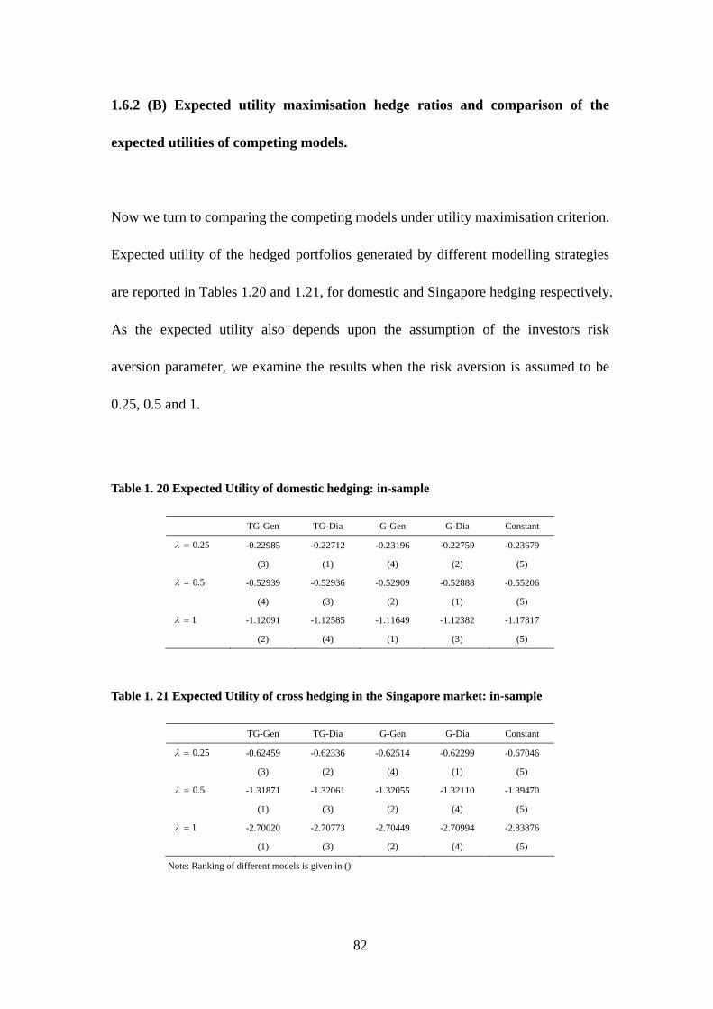
82

1.6.2 (B) Expected utility maximisation hedge ratios and comparison of the

expected utilities of competing models.

Now we turn to comparing the competing models under utility maximisation criterion.

Expected utility of the hedged portfolios generated by different modelling strategies

are reported in Tables 1.20 and 1.21, for domestic and Singapore hedging respectively.

As the expected utility also depends upon the assumption of the investors risk

aversion parameter, we examine the results when the risk aversion is assumed to be

0.25, 0.5 and 1.

Table 1. 20 Expected Utility of domestic hedging: in-sample


0.25 -0.22985 -0.22712 -0.23196 -0.22759 -0.23679

(3) (1) (4) (2) (5)

0.5 -0.52939 -0.52936 -0.52909 -0.52888 -0.55206

(4) (3) (2) (1) (5)

1 -1.12091 -1.12585 -1.11649 -1.12382 -1.17817

(2) (4) (1) (3) (5)

Table 1. 21 Expected Utility of cross hedging in the Singapore market: in-sample

Note: Ranking of different models is given in ()


0.25 -0.62459 -0.62336 -0.62514 -0.62299 -0.67046

(3) (2) (4) (1) (5)

0.5 -1.31871 -1.32061 -1.32055 -1.32110 -1.39470

(1) (3) (2) (4) (5)

1 -2.70020 -2.70773 -2.70449 -2.70994 -2.83876

(1) (3) (2) (4) (5)

83

From Tables 1.20 and 1.21, we can see that the expected utility of the hedged

portfolio under constant model is smaller than those from the dynamic estimation, in

both the domestic and the Singapore market, regardless the assumption on the risk

aversion parameter. Such a result indicates that the dynamic models are superior to

the constant models in term of utility maximisation. This is same as our previous

findings under the risk minimisation criterion. However, within the dynamic

specifications, there is no certain pattern regarding the ranking of their performances.

This is because the expected utility does not only depend on the estimated hedging

ratios, which is influenced by the conditional variance, conditional expected return,

but also on the assumption of the risk aversion factors. The lack of surety in ranking

of the dynamic models further substantiates our findings in the risk minimisation that

all the dynamic models are in fact effectively identical. We cannot conclude which

one is superior to the other.

1.6.2 (C) Risk reduction based on semivariance

Most recent approaches to evaluate hedging performance emphasis investors react

differently to downside risk and upside risk. Investors using futures to hedge their

positions desire to eliminate the downside return but retain the upside potential. In

such case, the MV is inappropriate. More intuitive measures of hedging performance

focusing on downside risk have been developed, including the risk reduction based on

84

the semivariance, the GSV and VaR. In this study, we examine the hedging

performance under semivariance risk reduction criterion.

The semivariance criterion is based on the concept that an investor preferring to

minimize the probability of falling below some predefined level of returns. This return

is the target return or the minimum acceptable return for the investor. Choosing the

target return is critical under the semivariance risk reduction criterion because when

the target return differs, optimal hedging ratio and risk reduction ability of the model

would differ as well. In this study, we set the target value to be zero. For one reason,

investors try to avoid negative returns in practice; for another, the mean of hedged

portfolio returns are quite close to zero.

The risk reduction under semivariance criterion is reported in Tables 3.22 and 3.23,

respectively, for the domestic and cross hedging. We observe that all model perform

quite well, comparing to the variance reductions we examined earlier. The

semivariance reduction of the hedged portfolio in the Chinese market is about 40%,

and for Singapore is about 30%. China fuel oil futures are more affective in hedging

the downside risk than the total risk.

For both domestic and cross hedging, the constant model always ranks at the bottom.

This is consistent with the conclusion drawn from the minimum variance risk

reduction criterion; the dynamic models are superior to the constant model.

85

Within the dynamic model, the GARCH Diagonal model is the most superior and the

GARCH General model is the most inferior one, for both domestic and cross hedging.

Asymmetric models lie in between. Such is different from the minimum variance

reduction. Another distinct feature under semivariance risk reduction criterion is that

the domestic hedging can achieve higher risk reduction than the cross hedging.

Table 1. 22 In-sample variance reduction for domestic market spot returns based on

semivariance minimisation criterion


Mean 0.10239 0.05641 0.06517 0.05300 0.05889 0.06963

Variance 1.94657 1.13075 1.13509 1.13880 1.11428 1.19276


(2) (3) (4) (1) (5)

Table 1. 23 In-sample variance reduction for Singapore market spot returns based on



Mean 0.11307 0.06276 0.06477 0.06342 0.06591 0.04493

Variance 4.51620 3.02324 2.98139 3.02766 2.95527 3.22324


(3) (2) (4) (1) (5)

86

1.7 Out-of-sample predictions of volatility and variance

reduction and expected utility comparisons over time

The parameter estimates of each model from the in-sample period were used to update

tH (except, of course for the constant model) continuously throughout the 48

out-of-sample observations. The subsequent time series of the variances of the two

returns and their covariance for each model, along with the unconditional values of

those variances and covariances, are depicted in Figures 1.16 to 1.21.

Those figures suggest that in general all models tend to underestimate the actual

variances and covariances. Moreover, there are greater divergences between the

estimated variances and covariances under different modelling specifications in the

domestic hedging than they are in the cross hedging in the Singapore market: the

results are more stable for Singapore. This may be due to the fact that the Chinese oil

market is still in an early stage of its development and trading can be influenced by

plenty of noise and speculation. Hence, returns are much harder to predict than that of

the comparatively mature and well-regulated Singapore market. This also implies that

in the out-of-sample periods, it is harder for the hedging models to perform well in the

domestic market than it is in the Singapore market, as confirmed by the risk reduction

results reported later. Detailed descriptive statistics for the estimated conditional and

unconditional variance and covariance of the China fuel oil futures, fuel oil spots in

the Chinese and the Singapore markets are given in Tables 1.24 and 1.25. The

87

predictions do not track the unconditional values well for all the models in the

out-of-sample period.

Table 1. 24 Statistics of conditional and unconditional variances and covariances for

positions in the Chinese market in the out-of-sample period


TG-Gen h11 3.0108 5.7545 1.2907 1.3869 0.5276 1.7147 5.5309

TG-Dia h1 1 3.1512 6.8160 1.0719 1.6579 0.7091 2.1864 5.3460

G-Gen h1 1 2.7326 5.0731 1.4096 1.0924 0.6907 2.1112 5.3969

G-Gen h1 1 3.2638 7.1010 1.0887 1.7412 0.7085 2.1770 5.3705

Cons t h 1 1 1.8930 1.8930 1.8930 0.0000 NA NA NA

Var(f) 3.3490 23.1250 0.0077 5.1574 2.3786 8.3805 103.1637

TG-Gen h22 1.5018 2.0662 1.1773 0.2420 0.8328 2.6338 5.8168

TG-Dia h2 2 1.2821 1.6453 1.1103 0.1478 1.0081 2.8653 8.1665

G-Gen h2 2 1.1342 1.8007 0.8866 0.1853 1.9206 6.5019 54.0357

G-Gen h2 2 1.3684 1.9150 1.1147 0.2187 1.0405 2.9689 8.6629

Cons t h 2 2 1.4313 1.4313 1.4313 0.0000 NA NA NA

Var(s) 1.3810 27.5037 0.0047 4.0835 5.6615 36.4446 2493.5040

TG-Gen h12 0.5959 1.0507 0.1704 0.1864 0.3866 3.3121 1.3904

TG-Dia h1 2 0.6091 1.3192 0.2479 0.3009 0.7131 2.3985 4.7918

G-Gen h1 2 0.6330 1.2702 -0.2927 0.2979 -0.4469 4.4243 5.6547

G-Gen h1 2 0.7294 1.6102 0.2816 0.3741 0.7078 2.3901 4.7523

Cons t h 1 2 0.5869 0.5869 0.5869 0.0000 NA NA NA

Cov(f,s) 0.7731 11.5772 -1.6585 2.2702 3.1868 13.8436 316.4131

88

Table 1. 25 Statistics of conditional and unconditional variances and covariances for

positions in the Singapore market in the out-of-sample period


TG-Gen h11 2.7592 5.3057 1.3156 1.1729 0.6274 1.9699 5.2716

TG-Dia h1 1 2.7719 5.5102 1.1942 1.2559 0.7286 2.2212 5.4593

G-Gen h11 2.7011 5.2656 1.2568 1.1703 0.6423 2.0186 5.2272

G-Gen h11 2.7266 5.4401 1.2011 1.2312 0.7634 2.3037 5.6324

Const h 1 1 1.8930 1.8930 1.8930 0.0000 0.0000 0.0000 0.0000

Var(f) 3.3490 23.1250 0.0077 5.1574 2.3786 8.3805 103.1637

TG-Gen h22 4.0673 6.5453 2.7232 0.9573 0.9733 3.5173 8.1139

TG-Dia h2 2 3.6483 6.1286 1.7464 1.1435 0.2042 2.3055 1.2981

G-Gen h22 3.9416 6.5930 2.4559 1.0277 0.8456 3.2717 5.8679

G-Gen h22 3.6402 6.1493 1.7436 1.1430 0.2377 2.3503 1.2962

Const h 2 2 3.6725 3.6725 3.6725 0.0000 0.0000 0.0000 0.0000

Var(s) 4.2535 30.6032 0.0002 6.7347 2.4745 8.9118 118.8834

TG-Gen h12 1.5531 2.9150 0.4995 0.5698 0.7599 3.3587 4.8765

TG-Dia h1 2 1.5815 3.6139 0.6709 0.6632 0.8855 3.3616 6.5338

G-Gen h12 1.4772 2.9081 0.3357 0.5791 0.5385 3.2441 2.4389

G-Gen h12 1.6077 3.6638 0.6352 0.6961 0.8382 3.1674 5.6772

Const h 1 2 1.2208 1.2208 1.2208 0.0000 0.0000 0.0000 0.0000

Cov(f,s) 1.9117 23.5243 -3.8065 4.5976 2.6738 12.0564 221.2305

89

1.7.1 Performance of hedging models out-of-sample: Risk minimisation

and variance reduction

1.7.1(A) Estimated hedge ratios under the risk minimisation criterion

As there are obvious divergences in the variance and covariance predicted under

different models, it can be reasonable to assume that the minimum variance hedge

ratios estimated by different models will be different in the out-of-sample period. The

forecasted hedge ratios are depicted in Figures 1.22 and 1.23 for domestic and cross

hedging, respectively, and the descriptive statistics for the two predicted hedge ratio

series are reported in Tables 1.26 and 1.27. From Figures 1.22 and 1.23 we observe

that predicted hedge ratio is more different between one and the other for the domestic

hedging. From the descriptive statistics, we observe that, different from the in-sample

findings, constant models give the highest mean hedge ratios in the out-of-sample

forecasting. TGARCH general models have a higher standard deviation than the

TGARCH Diagonal models, and the GARCH general have a higher standard

deviation than the Diagonal model. All the estimated hedge ratio series are not

normally distributed; they are skewed and have large pickedness. For most dynamic

models, the hedge ratio series follow an I(0) process and are thus mean reverting.

However, for the hedge ratios estimated from the TGARCH general and the GARCH

Diagonal models in the domestic market, they exhibit a unit root in the series. This

suggests that the hedge ratios estimated in out-of-sample forecasting are more likely

90

to veer away from its mean.

Table 1. 26 Descriptive statistics for estimated hedge ratios in the out-of-sample period when

hedging the domestic spot positions


Mean 0.2367 0.2078 0.2569 0.2397 0.3101

Median 0.2241 0.1988 0.2778 0.2317 0.3101

Maximum 0.5079 0.3612 0.4115 0.4257 0.3101

Minimum 0.0401 0.0977 -0.0624 0.1132 0.3101

Std. Dev. 0.1082 0.0703 0.1060 0.0843 0.0000

Skewness 0.3004 0.3659 -1.1107 0.3938 NA

Kurtosis 2.7130 2.1266 4.0527 2.1296 NA

ADF -3.1260 -2.6288 -5.9984 -2.5679

[0.0312] [0.0943] [0.0000] [0.1066]

PP -3.1279 -2.4061 -6.1292 -2.3393

[0.0311] [0.1454] [0.0000] [0.1643]

Table 1. 27 Descriptive statistics for estimated hedge ratios in the out-of-sample period when

hedging the Singapore spot positions


Mean 0.6108 0.6034 0.5969 0.6189 0.6449

Median 0.6043 0.5945 0.6003 0.6118 0.6449

Maximum 1.0315 1.0746 1.0833 1.0951 0.6449

Minimum 0.2173 0.2616 0.1355 0.2518 0.6449

Std. Dev. 0.2044 0.1749 0.2223 0.1799 0.0000

Skewness -0.1258 0.3494 -0.0992 0.3212 NA

Kurtosis 1.9728 2.8858 2.2986 2.8977 NA

Jarque-Bera 2.2369 1.0025 1.0626 0.8464 NA

Probability 0.3268 0.6058 0.5878 0.6550 NA

ADF with -2.1350 -2.1576 -2.1806 -2.0800

Intercept [0.2323] [0.2240] [0.2158] [0.2534]

PP with -2.2857 -2.3317 -2.3292 -2.2816

Intercept [0.1806] [0.1665] [0.1673] [0.1819]

91

1.7.1(B) Out-of-sample variance Reduction

For the out-of-sample hedging performance of different models, the results are quite

different from the in-sample findings. Table 1.28 illustrates the variance reduction

comparison for the out-of-sample hedging of spot positions in the domestic market.

All the models underperform in terms of variance reduction in the out-of-sample

period, which reduce the variance by only around 3% to 9%. The mean return of

China’s fuel oil spot is lower than the mean return of any hedged portfolio, no matter

which method is used. Meanwhile, the magnitude of mean returns of the hedged

portfolios is not associated with their variances. For the dynamic models, we can

observe that the two diagonal models, TGARCH diagonal and GARCH diagonal,

outperform their general counterparts, TGARCH general and GARCH General, in

terms of risk reduction based on variance, which is contrary to the in-sample findings.

In general, the diagonal models surpass the constant model and the constant models

surpass the general models in the out-of-sample period, although the reduction is

really small.

Table 1.29 shows the variance reduction comparison for the out-of-sample hedging in

the Singapore market under different model specifications. In general, the hedged

portfolios have higher mean returns and lower variance than the unhedged positions.

Compared with the in-sample variance reduction, all the models have poorer

performance in the out-of-sample period. The constant model reduces the risk to the

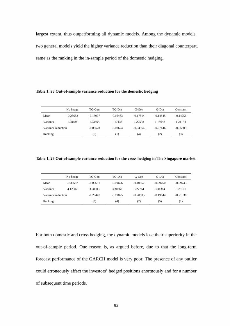
92

largest extent, thus outperforming all dynamic models. Among the dynamic models,

two general models yield the higher variance reduction than their diagonal counterpart,

same as the ranking in the in-sample period of the domestic hedging.

Table 1. 28 Out-of-sample variance reduction for the domestic hedging


Mean -0.28652 -0.15007 -0.16463 -0.17814 -0.14545 -0.14256

Variance 1.28188 1.23665 1.17133 1.22593 1.18643 1.21134


Ranking (5) (1) (4) (2) (3)

Table 1. 29 Out-of-sample variance reduction for the cross hedging in The Singapore market


Mean -0.39687 -0.09631 -0.09696 -0.10567 -0.09260 -0.09743

Variance 4.12307 3.28003 3.30362 3.27764 3.31314 3.23101


Ranking (3) (4) (2) (5) (1)

For both domestic and cross hedging, the dynamic models lose their superiority in the

out-of-sample period. One reason is, as argued before, due to that the long-term

forecast performance of the GARCH model is very poor. The presence of any outlier

could erroneously affect the investors’ hedged positions enormously and for a number

of subsequent time periods.

93

In any case, the risk reduction based on variance for all the constant and dynamic

models is very low. The most plausible reason is that although the fuel oil is the most

liberalised oil product in China with the least control by the government, its prices are

still largely influenced by the government, thus the existence of the lag in price

adjustment compared to the futures. Under such a situation, the futures are far more

volatile than the spot market. Any over-hedged positions might lead to additional risk.

Another reason may be related to the fact that investors trading fuel oil futures are

more likely to be driven by speculative motivations rather than the hedging of risk.

Consequently, markets are influenced by a large stream of trading noise, which make

the power of theoretical forecast very poor. The forecasting results imply that on

average, the fuel oil futures is not a good tool in hedging risk for the investors, at least

in short term. However, this aggregated results do not diminishing the potential

usefulness of fuel oil futures in individual transactions, for either speculating or

hedging.

Overall, the differences in risk reduction between each pair of models are very small.

Any significant differences across different models need to be examined further. We

employ equality tests in dealing with this issue.

Before performing the equality test, we depict the return of hedged portfolio under

different hedging strategies in Figures 1.24 and 1.25. As we can observe, although the

hedge ratios appear to be obviously different from each other, the returns of the

94

hedged portfolio are not. They tend to move in a similar pattern. We give the

descriptive statistics of the returns of different hedged portfolios in Tables 1.30 and

1.31 and also depict their histogram diagram in Figures 1.26 and 1.27, for hedging in

the domestic and Singapore market respectively. From those tables and graphs, it is

clear that the returns of hedged portfolios are moving together and following a similar

pattern. We further perform mean and variance equality tests and the results are

reported in Table 1.32 and 1.33 implying that all the models are actually giving

similar results so we cannot simply conclude which one is outperforming the other.

95

Table 1. 30 Summary of statistics of the actual spot returns, and returns of hedged portfolios

computed using different models in the out-of-sample period for the Chinese market.


Mean -0.2865 -0.1501 -0.1646 -0.1781 -0.1455 -0.1426

Median 0.0000 -0.1884 -0.1213 -0.1987 -0.1215 -0.2571

Maximum 2.2285 2.1198 2.1126 2.0980 2.0925 2.1112

Minimum -5.1762 -5.0971 -4.9033 -4.8559 -4.8549 -4.7351

Std. Dev. 1.1322 1.1120 1.0823 1.1072 1.0892 1.1006

Skewness -1.6524 -1.6309 -1.6021 -1.3327 -1.5403 -1.2919

Kurtosis 8.8702 9.7648 9.2225 8.2168 8.8631 7.8575

Jarque-Bera 90.7628 112.8028 97.9734 68.6383 87.7314 60.5423

Probability 0.0000 0.0000 0.0000 0.0000 0.0000 0.0000

ADF with -5.7776 -6.0109 -6.2425 -6.1167 -6.3592 -6.5340

Intercept [0.0000] [0.0000] [0.0000] [0.0000] [0.0000] [0.0000]

PP with -5.7913 -6.0143 -6.2433 -6.1200 -6.3592 -6.5331

Intercept [0.0000] [0.0000] [0.0000] [0.0000] [0.0000] [0.0000]

Table 1. 31 Summary statistics of the actual spot returns and returns of hedged portfolios

computed using different models in the out-of-sample period in the Singapore market.


Mean -0.3969 -0.0963 -0.0970 -0.1057 -0.0926 -0.0974

Median -0.0373 0.0954 0.0784 0.0517 0.0470 0.1680

Maximum 4.3318 3.9968 3.9709 4.0046 3.9423 3.8685

Minimum -5.4638 -5.4568 -5.4554 -5.4595 -5.4557 -5.4432

Std. Dev. 2.0305 1.8111 1.8176 1.8104 1.8202 1.7975

Skewness -0.3738 -0.4000 -0.4053 -0.4047 -0.4081 -0.4064

Kurtosis 3.1644 3.5571 3.6146 3.5947 3.5992 3.6275

Jarque-Bera 1.1718 1.9008 2.0699 2.0175 2.0502 2.1091

Probability 0.5566 0.3866 0.3552 0.3647 0.3588 0.3484

ADF with -8.1356 -6.7288 -6.5145 -6.6800 -6.4197 -6.1333

Intercept [0.0000] [0.0000] [0.0000] [0.0000] [0.0000] [0.0000]

PP with -8.1333 -6.7269 -6.5199 -6.6778 -6.4267 -6.1238

Intercept [0.0000] [0.0000] [0.0000] [0.0000] [0.0000] [0.0000]

96

Table 1. 32 Test of Equality for Means and Variances of the hedged portfolio returns in the

Chinese market: Out-of-sample period




TGDiagonal-Constant 0.009819 0.9213 1.034163 0.9088





TGDiagonal-GGeneral 3.65E-03 0.9519 1.046619 0.8765




Table 1. 33 Test of Equality for Means and Variances of the hedged portfolio returns in the

Singapore market: Out-of-sample period



TGGeneral-TGDiagonal 3.12E-06 0.9986 1.007191 0.9805

TGDiagonal-Constant 1.60E-06 0.999 1.022472 0.9396

TGGeneral-Constant 9.25E-06 0.9976 1.015172 0.9591








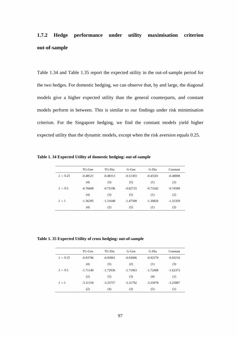
97

1.7.2 Hedge performance under utility maximisation criterion

out-of-sample

Table 1.34 and Table 1.35 report the expected utility in the out-of-sample period for

the two hedges. For domestic hedging, we can observe that, by and large, the diagonal

models give a higher expected utility than the general counterparts, and constant

models perform in between. This is similar to our findings under risk minimisation

criterion. For the Singapore hedging, we find the constant models yield higher

expected utility than the dynamic models, except when the risk aversion equals 0.25.

Table 1. 34 Expected Utility of domestic hedging: out-of-sample


0.25 -0.48521 -0.48313 -0.51303 -0.45501 -0.48008

(4) (3) (5) (1) (2)

0.5 -0.76608 -0.75196 -0.82725 -0.73342 -0.74589

(4) (3) (5) (1) (2)

1 -1.36295 -1.31648 -1.47508 -1.30826 -1.32359

(4) (2) (5) (1) (3)

Table 1. 35 Expected Utility of cross hedging: out-of-sample


0.25 -0.93796 -0.93901 -0.93006 -0.92579 -0.93216

(4) (5) (2) (1) (3)

0.5 -1.71140 -1.72936 -1.71963 -1.72408 -1.62373

(2) (5) (3) (4) (1)

1 -3.31150 -3.33757 -3.31792 -3.33978 -3.25887

(2) (4) (3) (5) (1)

98

For the estimated covariance matrix, the hedge ratios and the hedged portfolio returns

all follow the same pattern as those estimated under risk minimisation; we do not

provide figures of the series and tables for the descriptive statistics. Also we do not

provide the equality test results for the same reason. In fact all the strategies produce

similar performances and the small changes in variance reduction do not significantly

support the existence of a systematically superior optimal hedge ratio estimation

technique.

1.7.3 Hedging performance under risk reduction based on semivariance

risk reduction: out-of-sample

The out-of-sample risk reductions of China oil fuel futures in hedging domestic spot

positions based on semivariance are reported in Table 1.36 and Table 1.37 report that

for hedging of Singapore spot positions.

At a glance, the risk reductions based on semivariance are much higher than that

based on the variance, for both domestic and cross hedging. Although it seems that the

China fuel oil is not a good hedging instrument in reducing the overall risk, at lease

during the first two years since its launches, it is an effective hedging tool in reducing

the downside risk. In practice, avoiding downside risk and maintain upside potential is

99

more important for investors. Thus we argue that the China fuel oil futures is very

successful market wide in hedging downside risks. There is no doubt why the China

fuel oil futures become increasingly popular in the market.

Different from the hedging performance based on variance reduction criterion,

domestic hedging have higher risk reduction based on the semivariance than the cross

hedging in Singapore market. But same as the hedging performance based on variance

reduction criterion, there is no clear pattern which model is more superior to the other

in the out-of-sample period. The dynamic models lose their superiority in the

domestic hedging. Although for the cross hedging in the Singapore market the

constant model still generates the smallest risk reduction, the divergence between

constant and dynamic models is much smaller than in the in-sample period.

Comparing the in-sample and out-of-sample hedging based on semivariance reduction,

we find that the models give even higher reduction in the out-of-sample period for the

domestic hedging. In contrast, for the cross hedging, the models show less effective

performance in the out-of-sample period. Comparing the in-sample and out-of-sample

hedging for both hedging under the two risk reduction criteria, we find that the

hedging in the Singapore market have more stable results, while the risk reduction is

quite different for the fuel oil hedging in domestic market based on the two criteria.

This may be caused by the fact that the returns of fuel oil in the Chinese market,

which is less developed, have larger negative sknewess and asymmetric distribution.

100

On the other hand, the returns are more symmetrically distributed in the Singapore

market.

Table 1. 36 Out of sample variance reduction for domestic market spot returns based on



Mean -0.28652 -0.15007 -0.16463 -0.17814 -0.14545 -0.14256

Variance 2.50095 1.36325 1.42943 1.26795 1.40681 1.32310


(3) (5) (1) (4) (2)

Table 1. 37 Out of sample variance reduction for Singapore market spot returns based on

semivariance criterion minimisation criterion


Mean -0.39687 -0.09631 -0.09696 -0.10567 -0.09260 -0.09743

Variance 5.45792 3.80928 3.84380 3.84016 3.84137 3.90409


(1) (4) (2) (3) (5)

1.7.4 Hedging performance: time path of risk reduction based on variance

and semivariance and of expected utility maximisation

The above provides the performance comparison of average risk reduction and

average expected utility over the out-of-sample period. However, more useful

comparisons between the performances of the models are those between the time

101

paths of the variance reductions under different modelling specifications and between

the time paths of expected utility given a risk aversion parameter. We calculate these

attributes of the models upon a day-by-day revision of the forecasts of variance

reduction and of expected utilities. Thus better information can be provided about the

models than do the average estimates of variance reduction or expected utility over a

given period. Figures 1.28 to 1.29 graph, for domestic and cross hedging respectively,

the time paths of the variance reductions based on variance of different hedging

strategies when hedging decision are updated each day to incorporate all available

information. Accordingly, Figures 1.30 and 1.31 portray the time paths of the

expected utility, and Figure 1.32 and 1.33 depict the time paths of the risk reduction

based on semivariance for the domestic and cross hedging.

On this basis, the dynamic models seem to be superior to the constant model, no

matter under the two risk minimisation criteria or expected utility criterion, for

hedging in both markets. For the domestic hedging, the general model seems to be

superior in terms of variance reduction, and the diagonal model is superior in terms of

utility maximization and semivariance reduction. On the other hand, for hedging in

the Singapore market, the TGARCH General model seems to beat others in terms of

variance reduction and expected utility maximisation, diagonal model is superior in

terms of semivariance reduction.

The best models are seen to possess the GARCH(1,1) dynamic structures. The

102

Constant model is the inferior to them. It performance cannot match the dynamic

models under all three criteria. The plausible reason is that the constant model

ignoring some of the factors that affect the volatility of spot and futures returns.

Investors relay on the dynamic models to formulating hedging strategies should

update the forecast more frequently to generate outstanding performance.

103

1.8 Summary and conclusion

This study investigates the optimal futures hedging using both dynamic and constant

models. As proved in the literature, the distribution of futures and spot returns both

have the characteristics of non-normality. Thus a GARCH framework in the

derivation of OHRs, which are dependent upon to their variance and covariance

structure, has distinct theoretical advantage over the constant models and hence

should provide a better hedging performance. Many previous studies provide

evidences for such statistical and economic improvements of dynamic models,

although most are based on data in the developed market where there are little market

frictions.

In this study, we examined the effectiveness of dynamic hedging models for the fuel

oil futures traded in SHFE, which has only two years history by the time we conduct

the study. To provide the most useful information to market participants, we also take

into consideration of the close relation between the fuel oil market in China and that

in Singapore by comparing the fuel futures hedging for spot positions in both markets.

Our findings provide to the hedgers, speculators and policy makers some insight

information about the performance of the China fuel oil futures as a hedging tool.

The empirical findings for the in-sample period analysis are consistent with those of

previous studies in that the dynamic models surpass the constant model. When

104

investigating the asymmetric effect of positive and negative shocks in influencing the

hedging ability of China fuel oil futures, we find the coefficients capturing the

asymmetric effect for both domestic and cross border hedging are insignificant and

the likelihood ratio test statistics suggest that these parameters should be omitted in

the model specification. However, by including the asymmetric matrix in our

modelling specification, we do get higher variance reductions for cross hedging in the

Singapore market, although this is not the case for the domestic hedging. Results from

likelihood tests suggest that the GARCH General model is the best accepted model

for the domestic hedging and the GARCH Diagonal is superior to other modelling

specifications for the cross hedging in the Singapore Market.

Three different criteria are employed to assess the hedging performance of different

hedging strategies from different perspectives, including the hedging ability to

minimise total risk, to minimise downside risk and to maximise the expected utility.

In terms of variance reduction, we find that GARCH General is the best modelling

strategy for domestic hedging followed by TGARCH General, GARCH Diagonal and

TGARCH Diagonal. For hedging in the Singapore market, TGARCH general is more

superior, followed by the GARCH general, TGARCH Diagonal and GARCH

Diagonal. Under the utility maximisation criterion, we find the constant models are

still always inferior to the dynamic models. However, within the dynamic

specification, there is no certain pattern for the relative ranking of each model, since

the expected value of futures returns are not effectively zero in our sampling period.

105

Moreover, we can conclude that individuals risk preferences also influence their

choice of hedging strategies. Under the semivariance reduction criterion, the GARCH

Diagonal model is the most superior and constant model is the most inferior. Further

evidence is found on that the dynamic models perform better than the constant model.

In the in-sample period, there are some findings that are unique for the China fuel oil

futures. First, the reductions in variance for hedging in both markets are very low,

much lower that the hedging effectiveness of other oil futures in the international oil

market that have been studied so far. Second, the domestic hedging have even lower

variance reduction than the cross border hedging in the Singapore market. Third,

China fuel oil futures are more effective in hedging downside risks based on the

semivariance reduction than total risk reduction. And in terms of hedging downside

risk, domestic hedging is more effective than the cross hedging in the Singapore

market. Fourth, the models do not strictly follow the risk and return trade-off rule; the

model that yields a higher reduction may also generate higher hedged portfolio

returns.

Our empirical findings in the out-of-sample period are somewhat disappointing for

hedging of the spot positions in the Chinese market under variance minimisation

criterion, where all the dynamic and constant models perform extremely poorly. The

risk reduction results based on variance imply the inability of China oil futures in

hedging spot risks, on the market average. For hedging in the Singapore market, all

106

models underperform the in-sample ones, especially the dynamic models. The

Constant model gives a relatively stable variance reduction both in- and out-of-sample.

Such results are consistent with some of the literature in that dynamic hedging

modeling does not have obvious advantages over the constant modeling in terms of

risk reduction in the out-of-sample period due to the limitations of GARCH models in

forecasting. In contrast, the findings of the China fuel oil futures’ ability in hedging

market downside risk are promising, especially for the domestic hedging. The

hedging effectiveness with all the models increases in terms of semivariance reduction

in the out-of-sample period where there is more uncertainty in the market.

Empirically, hedging downside risk is more important to the market participates

because returns below some target value could be disastrous for them; whereas returns

above the target value could be beneficial. In this sense, we believe that the China fuel

oil futures market is an effective hedging instrument, especially for the investors in

domestic fuel oil market. For those who use the China fuel oil futures to hedge the

downside risk, dynamic model is obviously a good choice than the constant model.

In evaluating the out-of-sample hedging performance, this study also provides the

performance comparison of the time path of the risk reduction and of the time path of

the expected utility of different hedging strategies. Different from the out-of-sample

period performance evaluation based on the average risk reduction and average

expected utility, the dynamic models constantly give superior result than the constant

107

models, for both domestic and cross hedging.

Comparing to the existing literature, we take a further step to investigate our findings

by conducting an equality test for means and variances of the hedged portfolios.

According to the insignificance of most results in the equality test, we find that one

hedging strategy is not significantly outperforming the other, for both domestic and

cross hedging.

108

References:

Adams, J. and Montesi, C. J. (1995), “Major Issues Related to Hedge Accounting”,

Financial Accounting Standard, Board, Newark, CT.

Bawa, V. S. (1975), “Optimal rules for ordering uncertain prospects”, Journal of

Financial Economics, 2, 95–121.

Baillie, R.T. and Bollerslev, T. (1990), “A Multivariate Generalised ARCH Approach

to Modelling Risk Premia in Forward Foreign Exchange Rate Markets”, Journal

of International Money and Finance, vol. 9, issue 3, September, pp. 309-324.

Baillie, R.T. and Myers, R.T. (1991), “Bi-variate GARCH Estimation of Optimal

Commodity Futures Hedge”, Journal of Applied Econometrics, vol. 6, issue 2,

April-June, pp. 109-124.

Bell, D. E., & Krasker, W. S. (1986), “Estimating hedge ratios”, Financial

Management, 15, 34–39.

Brooks C, O.T Henry, G. Persand (2002), “The Effect of Asymmetries on Optimal

Hedge Ratios”, Journal of Business, 75 (2), 333-352.

Bollerslev (1986), “A Generalized Autoregressive Conditional Heteroscedasticity”,

Journal of Econometrics. 31, 307-327.

Cecchetti, S.G., Cumby, R.E. and Figlewski, S. (1988), “Estimation of Optimal

Futures, Hedge”, Review of Economics and Statistics, vol. 70, issue 4, December,

pp. 623-630.

Chang, J., and Shanker, L. (1987), “A risk-return measure of hedging effectiveness: a

comment”, Journal of Financial and Quantitative Analysis, 22, 373-376.

Chen, S. S., Lee, C. F., & Shrestha, K. (2001), “On a mean-generalized semivariance

approach to determining the hedge ratio”, Journal of Futures Markets, 21,

581–598.

Cheung, C. S., Kwan, C. C. Y.,& Yip, P. C. Y. (1990), “The hedging effectiveness of

options and futures: A mean-Gini approach”, Journal of Futures Markets, 10,

61–74.

Cotter, J and J. Hanly (2005), “Hedging Effectiveness under Conditions of symmetry”,

109

Center for Financial Markets Mimeo, University college Dublin.

Cotter, J and J. Hanly (2006), “Reevaluating hedging performance”, The Journal of

Futures Markets, 26, No. 7,677-702.

Dark, Jonathan (2004), “Long term hedging of the Australian All Ordinaries Index

using a Bi-variate error correction FIGARCH model”, Working Paper, Monash

University, Australia.

Ederington, L.H. (1979), “The Hedging Performance of the New Futures Markets”,

Journal of Finance, vol. 34, issue 1, March, pp. 157-170.

Eftekhari, B. (1998), “Lower partial moment hedge ratio”, Applied Financial

Economics, 8, 645–52.

Engle, R. F. (1982), “Autoregressive Conditional Heteroscedasticity with Estimates of

Variance of U. K. Inflation”, Econometrica, 50, 987-1008.

Engle, R. F., & Granger, C. W. (1987), “Co-integration and error correction:

Representation, estimation and testing”, Econometrica, 55, 251–276.

Engle. R. F & Kroner K. F (1995), “Multivariate simultaneous generalized ARCH”,

Econometric Theory, 11, 122-150.

Figlewski, S. (1985), “Hedging with Stock Index Futures: Theory and Application in

New Market”, Journal of Futures Markets, vol. 5, issue 2, Summer, pp. 183-199.

Filardo, A. J. (1994), “Business cycle phases and their transition dynamics”, Journal

of Business and Economic Statistics, 12, 299–308.

Fishburn, P. J. (1977), “Mean-risk analysis with risk associated with below-target

returns”, American Economic Review, 67, 116–26.

Ford, Pok and Poshakwale (2005), “Dynamic vs. Static Stock Index Futures Hedging:

A Case Study for Malaysia”, Discussion Papers from Department of Economics,

University of Birmingham (forthcoming: Global Finance Journal, vol.20, no.3,

2009).

Gagnon, L., Lypny, G.J. and McCurdy, T.H. (1998), “Hedging Foreign Currency

Portfolios”, Journal of Empirical Finance, vol. 5, issue 3, pp. 197-220.

Ghosh, A. (1993), “Hedging with Stock Index Futures: Estimation and Forecasting

with Error Correction Model”, The Journal of Futures Markets, 13, 743-752.

http://econpapers.repec.org/paper/birbirmec/�

http://www.economics.bham.ac.uk/�

http://www.economics.bham.ac.uk/�

110

Ghose, D., & Kroner, K. F. (1994), “Common Persistence in Conditional Variances:

Implications for Dynamic Hedging”, Mimeo, Department of Economics,

University of Arizona.

Glosten, L. R., Jagannathan, R. and Runkle, D. E. (1993), “On the relation between

the expected value and the volatility of the nominal excess return on stocks”,

Journal of Finance, 48 (December): 1779–1801.

Herbst, A. F., Kare, D. D. and Caples, S. C. (1989), “Hedging Effectiveness and

Minimum Risk Hedge Ratios in the Presence of Autocorrelation: Foreign

Currency Futures”, Journal of Futures Markets, vol. 9, issue 3, June, pp.

185-197.

Howard, C. T., & D’Antonio, L. J. (1984), “A risk-return measure of hedging

effectiveness”, Journal of Financial and Quantitative Analysis, 19, 101–112.

Hsin, C. W., Kuo, J., & Lee, C. F. (1994), “A new measure to compare the hedging

effectiveness of foreign currency futures versus options”, Journal of Futures

Markets, 14, 685–707.

Huang, J. C., Chiu, C and Lee, M (2006), “Hedging with zero-value at risk hedge

ratio”, Applied Financial Economics, 16, 259-269

Johnson, L. (1960), “The theory of hedging and speculation in commodity futures”,

Review of Economic Studies, 27, 139-151.

Jorion, P. (2000), “Value-at-Risk: The New Benchmark for Controlling Market Risk”,

University of California, Irvine.

Kolb, R.W., & Okunev, J. (1992), “An empirical evaluation of the extended

mean-Gini oefficient for futures hedging”. Journal of Futures Markets, 12,

177–186.

Kolb, R. W., & Okunev, J. (1993), “Utility maximizing hedge ratios in the extended

mean Gini framework”, Journal of Futures Markets, 13, 597–60.

Kroner, K.F. and Sultan, J. (1993), “Time-Varying Distributions and Dynamic

Hedging with Foreign Currency Futures”, Journal of Financial and Quantitative

Analysis, 28, issue 4, December, pp. 535-551.

Kahl, K. (1983), “Determination of the Recommended Hedging Ratio”, American

111

Journal of Agricultural Economics, 65, 603-605.

Koutmos, G. and Pericli, A. (1998), “Dynamic Hedging of Commercial Paper with

T-Bill Futures”, The Journal of Futures Markets, 18, 925-938.

Lence, S. H. (1995), “The economic value of minimum variance hedges”, American

Journal of Agricultural Economics, 77, 353–364.

Lence, S. H. (1996), “Relaxing the assumptions of minimum variance hedging”,

Journal of Agricultural and Resource Economics, 21, 39–55.

Lien, D. (1996), “The Effect of the Cointegration Relationship on Futures Hedging: A

Note”, The Journal of Futures Markets, 16, 773-780.

Lien, D., & Luo, X. (1993a), “Estimating the extended mean-Gini coefficient for

futures hedging”, Journal of Futures Markets, 13, 665–676.

Lien, D., & Luo, X. (1993b), “Estimating multiperiod hedge ratios in cointegrated

markets”, Journal of Futures Markets, 13, 909–920.

Lien, D., & Shaffer, D. R. (1999), “Note on estimating the minimum extended Gini

hedge ratio”, Journal of Futures Markets, 19, 101–113.

Lien, D., & Tse, Y. K. (1998), “Hedging time-varying downside risk”, Journal of

Futures Markets, 18, 705–722.

Lien, D. and Tse, Y. (1999), “Fractional Cointegration and Futures Hedging”, The

Journal of Futures Markets, 19, 457-474.

Lien, D., & Tse, Y. K. (2000), “Hedging downside risk with futures contracts”,

Applied Financial Economics, 10, 163–170.

Lien and Yang, (2006), “Hedging with Chinese Metal Futures”, Working Paper Series,

University of New South Wales

Lypny, G. and Powalla, M. (1998), “The Hedging Effectiveness of DAX Futures”,

European Journal of Finance, vol. 4, issue 4, December, pp. 345-355.

Myers, R. and Thompson, S. (1989), “Generalised Optimal Hedge Ratios Estimation”,

American Journal of Agricultural Economics, vol. 71, issue 4, November, pp.

858-868.

Myers, R.J. (1991), “Estimating Time-Varying Optimal Hedge Ratios on Futures

Markets”, Journal of Futures Markets, vol. 11, issue 1, February, pp. 39-53.

112

Park, T.H. and Switzer, L.N. (1995), “Time-varying Distributions and the Optimal

Hedge Ratios for Stock Index Futures”, Applied Financial Economics, vol. 5,

issue 3, June, pp. 131-137.

Roy, A. (1952), “Safety first and the holding of assets”, Econometrica, 20, 431–449.

Switzer and El-Khoury (2006), “Extreme Volatility, Speculative Efficiency, and the

hedging Effectiveness of the Oil Futures Markets”, Finance Department,

Concordia University.

Sim, A. and Zurbreugg, R. (2000), “The KOSPI 200 and Dynamic Hedging

Effectiveness During the Asian Financial Crisis”, Working Paper, The

University of New South Wales.

Satyanarayan, S. (1998), “A note on a risk-return measure of hedging effectiveness”,

Journal of Futures Markets, 18, 867-870.

Shalit, H. (1995), “Mean-Gini hedging in futures markets”, Journal of Futures

Markets, 15, 617–635.

Tasche, D. (2002), “Expected shortfall and beyond” Journal of Banking and Finance,

26, 1519–1533.

Yang, W. (2001), “M-GARCH Hedge Ratios and Hedging Effectiveness in Australian

Futures Markets”, Edith Cowan University, School of Finance and Economics,

Working Paper Series, January.

113

Appendix 1 A

Figure 1. 1 Daily return series

RF

A S O N D J F M A M J J A S O N D J F M A M J J2005 2006

-6.4

-4.8

-3.2

-1.6

-0.0

1.6

3.2

4.8

RS


-6

-4

-2

0

2

4

6

8

RSX


-12.5

-10.0

-7.5

-5.0

-2.5

0.0

2.5

5.0

7.5

10.0

114

Figure 1. 2 Daily Log price series

7.2

7.4

7.6

7.8

8.0

8.2

8.4

2005M01 2005M07 2006M01 2006M07

LF LS LSX

Note: LF represents the log price of China fuel oil futures. LS represents the log price of China

fuel oil spot and LSX represents the log price of Singapore fuel oil spot.

115

Figure 1. 3 Pairs of daily log price series

(1) LF and LS

7.5

7.6

7.7

7.8

7.9

8.0

8.1

8.2

8.3

2005M01 2005M07 2006M01 2006M07

LF LS

(2) LF and LSX

7.2

7.4

7.6

7.8

8.0

8.2

8.4

2005M01 2005M07 2006M01 2006M07

LF LSX

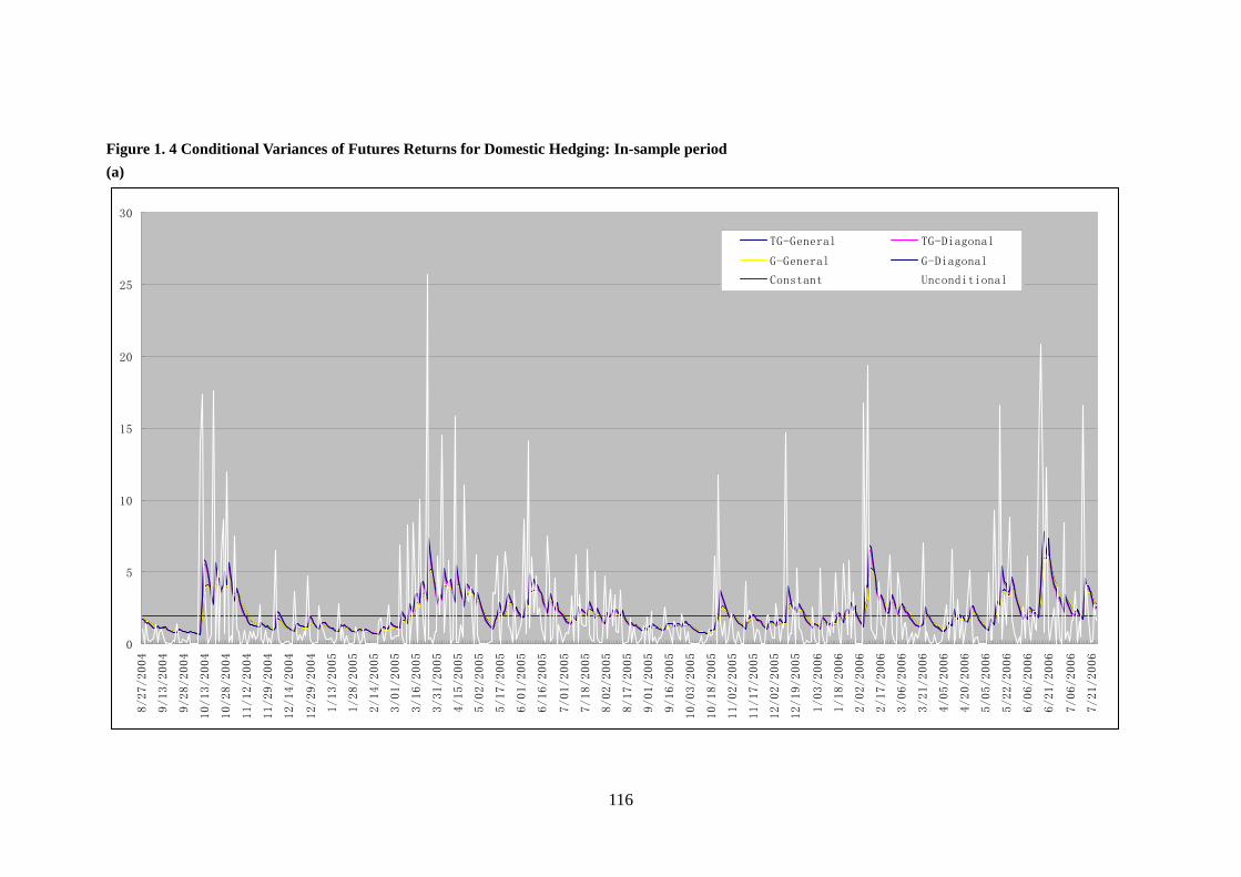
116

Figure 1. 4 Conditional Variances of Futures Returns for Domestic Hedging: In-sample period

(a)

0

5

10

15

20

25

30

8/27/2004

9/13/2004

9/28/2004

10/13/2004

10/28/2004

11/12/2004

11/29/2004

12/14/2004

12/29/2004

1/13/2005

1/28/2005

2/14/2005

3/01/2005

3/16/2005

3/31/2005

4/15/2005

5/02/2005

5/17/2005

6/01/2005

6/16/2005

7/01/2005

7/18/2005

8/02/2005

8/17/2005

9/01/2005

9/16/2005

10/03/2005

10/18/2005

11/02/2005

11/17/2005

12/02/2005

12/19/2005

1/03/2006

1/18/2006

2/02/2006

2/17/2006

3/06/2006

3/21/2006

4/05/2006

4/20/2006

5/05/2006

5/22/2006

6/06/2006

6/21/2006

7/06/2006

7/21/2006

TG-General TG-Diagonal

G-General G-Diagonal

Constant Unconditional

117

(b)

0

1

2

3

4

5

6

7

8

9

8/27/2004

9/13/2004

9/28/2004

10/13/2004

10/28/2004

11/12/2004

11/29/2004

12/14/2004

12/29/2004

1/13/2005

1/28/2005

2/14/2005

3/01/2005

3/16/2005

3/31/2005

4/15/2005

5/02/2005

5/17/2005

6/01/2005

6/16/2005

7/01/2005

7/18/2005

8/02/2005

8/17/2005

9/01/2005

9/16/2005

10/03/2005

10/18/2005

11/02/2005

11/17/2005

12/02/2005

12/19/2005

1/03/2006

1/18/2006

2/02/2006

2/17/2006

3/06/2006

3/21/2006

4/05/2006

4/20/2006

5/05/2006

5/22/2006

6/06/2006

6/21/2006

7/06/2006

7/21/2006

TG-General TG-Diagonal G-General

G-Diagonal Constant

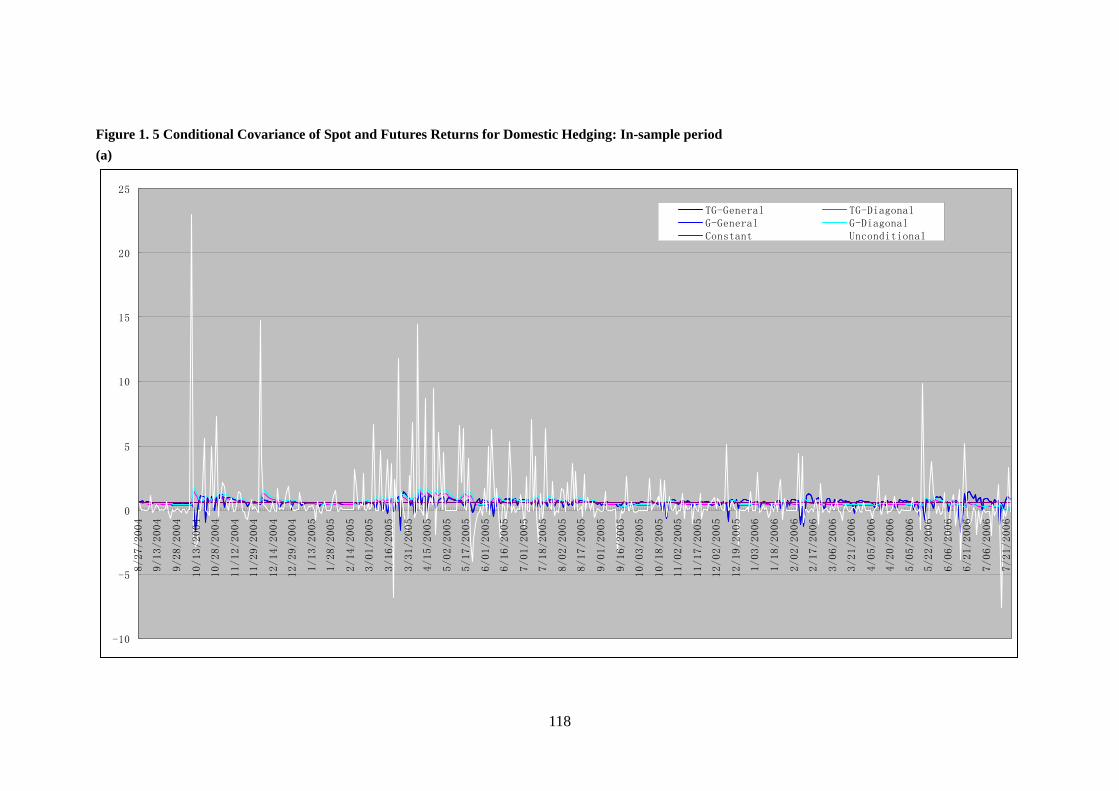
118

Figure 1. 5 Conditional Covariance of Spot and Futures Returns for Domestic Hedging: In-sample period

(a)

-10

-5

0

5

10

15

20

25

8/27/2004

9/13/2004

9/28/2004

10/13/2004

10/28/2004

11/12/2004

11/29/2004

12/14/2004

12/29/2004

1/13/2005

1/28/2005

2/14/2005

3/01/2005

3/16/2005

3/31/2005

4/15/2005

5/02/2005

5/17/2005

6/01/2005

6/16/2005

7/01/2005

7/18/2005

8/02/2005

8/17/2005

9/01/2005

9/16/2005

10/03/2005

10/18/2005

11/02/2005

11/17/2005

12/02/2005

12/19/2005

1/03/2006

1/18/2006

2/02/2006

2/17/2006

3/06/2006

3/21/2006

4/05/2006

4/20/2006

5/05/2006

5/22/2006

6/06/2006

6/21/2006

7/06/2006

7/21/2006

TG-General TG-DiagonalG-General G-DiagonalConstant Unconditional

119

(b)

-2

-1.5

-1

-0.5

0

0.5

1

1.5

2

2.5

8/27/2004

9/13/2004

9/28/2004

10/13/2004

10/28/2004

11/12/2004

11/29/2004

12/14/2004

12/29/2004

1/13/2005

1/28/2005

2/14/2005

3/01/2005

3/16/2005

3/31/2005

4/15/2005

5/02/2005

5/17/2005

6/01/2005

6/16/2005

7/01/2005

7/18/2005

8/02/2005

8/17/2005

9/01/2005

9/16/2005

10/03/2005

10/18/2005

11/02/2005

11/17/2005

12/02/2005

12/19/2005

1/03/2006

1/18/2006

2/02/2006

2/17/2006

3/06/2006

3/21/2006

4/05/2006

4/20/2006

5/05/2006

5/22/2006

6/06/2006

6/21/2006

7/06/2006

7/21/2006



Constant

120

Figure 1. 6 Conditional Variance of Spot Returns for Domestic Hedging: In-sample Period

(a)

0

10

20

30

40

50

60

8/27/2004

9/13/2004

9/28/2004

10/13/2004

10/28/2004

11/12/2004

11/29/2004

12/14/2004

12/29/2004

1/13/2005

1/28/2005

2/14/2005

3/01/2005

3/16/2005

3/31/2005

4/15/2005

5/02/2005

5/17/2005

6/01/2005

6/16/2005

7/01/2005

7/18/2005

8/02/2005

8/17/2005

9/01/2005

9/16/2005

10/03/2005

10/18/2005

11/02/2005

11/17/2005

12/02/2005

12/19/2005

1/03/2006

1/18/2006

2/02/2006

2/17/2006

3/06/2006

3/21/2006

4/05/2006

4/20/2006

5/05/2006

5/22/2006

6/06/2006

6/21/2006

7/06/2006

7/21/2006



Constant Unconditional

121

(b)

0

1

2

3

4

5

6

7

8/27/2004

9/13/2004

9/28/2004

10/13/2004

10/28/2004

11/12/2004

11/29/2004

12/14/2004

12/29/2004

1/13/2005

1/28/2005

2/14/2005

3/01/2005

3/16/2005

3/31/2005

4/15/2005

5/02/2005

5/17/2005

6/01/2005

6/16/2005

7/01/2005

7/18/2005

8/02/2005

8/17/2005

9/01/2005

9/16/2005

10/03/2005

10/18/2005

11/02/2005

11/17/2005

12/02/2005

12/19/2005

1/03/2006

1/18/2006

2/02/2006

2/17/2006

3/06/2006

3/21/2006

4/05/2006

4/20/2006

5/05/2006

5/22/2006

6/06/2006

6/21/2006

7/06/2006

7/21/2006



Constant

122

Figure 1. 7 Conditional Variance of Futures Returns for Cross Border Hedging: In-sample period

(a)

0

5

10

15

20

25

30

8/27/2004

9/13/2004

9/28/2004

10/13/2004

10/28/2004

11/12/2004

11/29/2004

12/14/2004

12/29/2004

1/13/2005

1/28/2005

2/14/2005

3/01/2005

3/16/2005

3/31/2005

4/15/2005

5/02/2005

5/17/2005

6/01/2005

6/16/2005

7/01/2005

7/18/2005

8/02/2005

8/17/2005

9/01/2005

9/16/2005

10/03/2005

10/18/2005

11/02/2005

11/17/2005

12/02/2005

12/19/2005

1/03/2006

1/18/2006

2/02/2006

2/17/2006

3/06/2006

3/21/2006

4/05/2006

4/20/2006

5/05/2006

5/22/2006

6/06/2006

6/21/2006

7/06/2006

7/21/2006



Constant Unconditonal

123

(b)

0

1

2

3

4

5

6

7

8/27/2004

9/13/2004

9/28/2004

10/13/2004

10/28/2004

11/12/2004

11/29/2004

12/14/2004

12/29/2004

1/13/2005

1/28/2005

2/14/2005

3/01/2005

3/16/2005

3/31/2005

4/15/2005

5/02/2005

5/17/2005

6/01/2005

6/16/2005

7/01/2005

7/18/2005

8/02/2005

8/17/2005

9/01/2005

9/16/2005

10/03/2005

10/18/2005

11/02/2005

11/17/2005

12/02/2005

12/19/2005

1/03/2006

1/18/2006

2/02/2006

2/17/2006

3/06/2006

3/21/2006

4/05/2006

4/20/2006

5/05/2006

5/22/2006

6/06/2006

6/21/2006

7/06/2006

7/21/2006



Constant

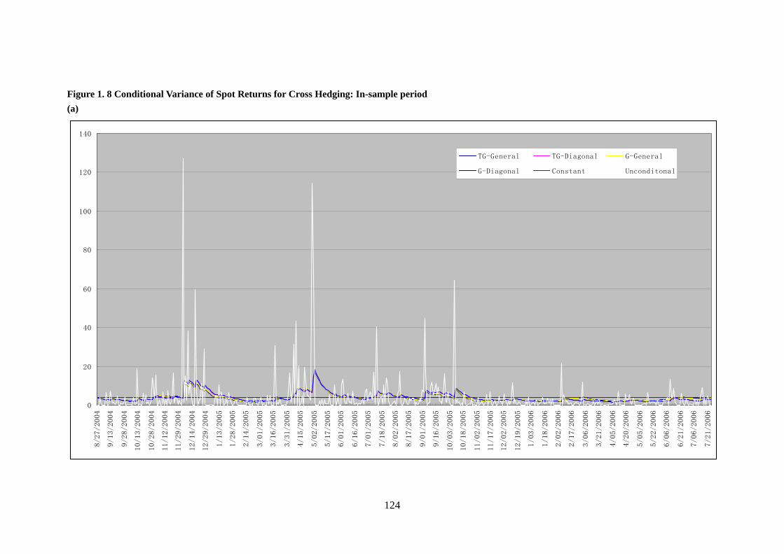
124

Figure 1. 8 Conditional Variance of Spot Returns for Cross Hedging: In-sample period

(a)

0

20

40

60

80

100

120

140

8/27/2004

9/13/2004

9/28/2004

10/13/2004

10/28/2004

11/12/2004

11/29/2004

12/14/2004

12/29/2004

1/13/2005

1/28/2005

2/14/2005

3/01/2005

3/16/2005

3/31/2005

4/15/2005

5/02/2005

5/17/2005

6/01/2005

6/16/2005

7/01/2005

7/18/2005

8/02/2005

8/17/2005

9/01/2005

9/16/2005

10/03/2005

10/18/2005

11/02/2005

11/17/2005

12/02/2005

12/19/2005

1/03/2006

1/18/2006

2/02/2006

2/17/2006

3/06/2006

3/21/2006

4/05/2006

4/20/2006

5/05/2006

5/22/2006

6/06/2006

6/21/2006

7/06/2006

7/21/2006

TG-General TG-Diagonal G-General

G-Diagonal Constant Unconditonal

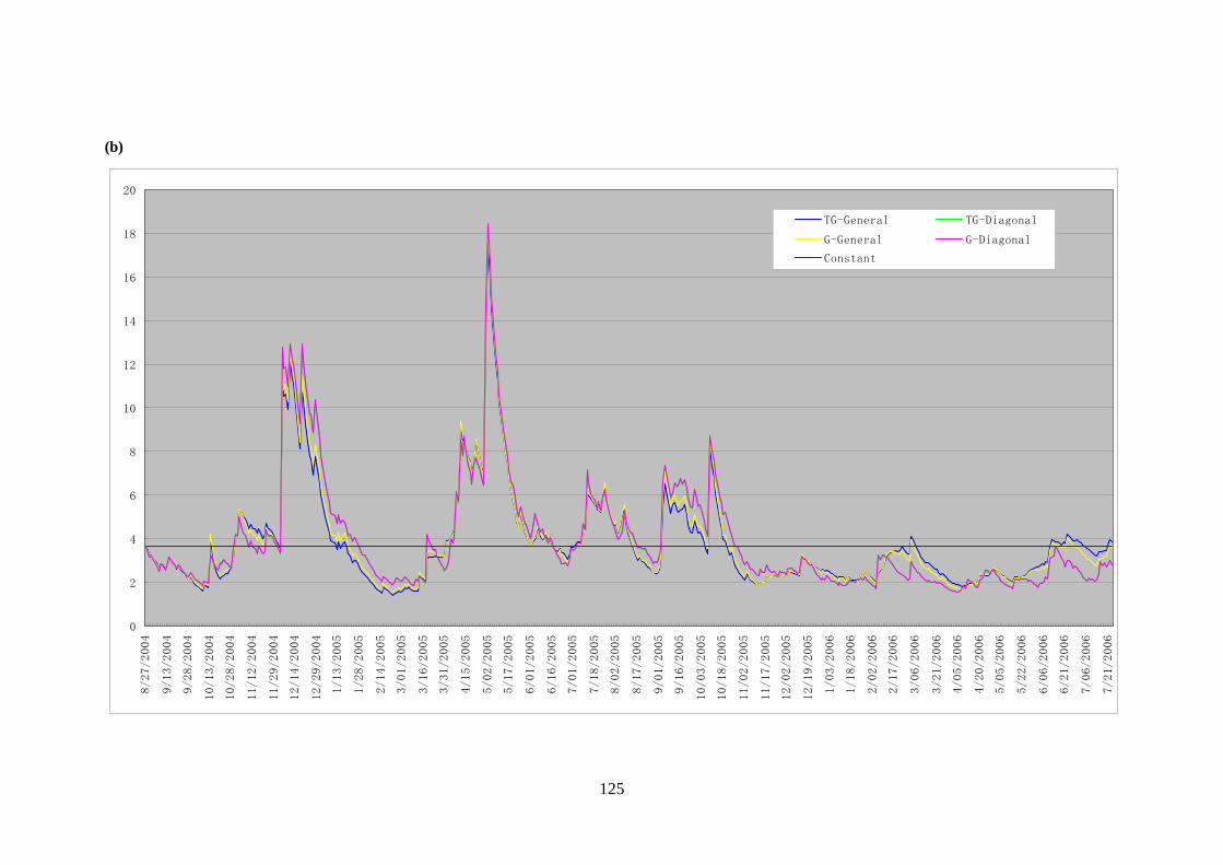
125

(b)

0

2

4

6

8

10

12

14

16

18

20

8/27/2004

9/13/2004

9/28/2004

10/13/2004

10/28/2004

11/12/2004

11/29/2004

12/14/2004

12/29/2004

1/13/2005

1/28/2005

2/14/2005

3/01/2005

3/16/2005

3/31/2005

4/15/2005

5/02/2005

5/17/2005

6/01/2005

6/16/2005

7/01/2005

7/18/2005

8/02/2005

8/17/2005

9/01/2005

9/16/2005

10/03/2005

10/18/2005

11/02/2005

11/17/2005

12/02/2005

12/19/2005

1/03/2006

1/18/2006

2/02/2006

2/17/2006

3/06/2006

3/21/2006

4/05/2006

4/20/2006

5/05/2006

5/22/2006

6/06/2006

6/21/2006

7/06/2006

7/21/2006



Constant

126

Figure 1. 9 Conditional Covariance of Spot and Futures Returns for Cross Hedging: In-sample period

(a)

-15

-10

-5

0

5

10

15

20

25

30

35

8/27/2004

9/13/2004

9/28/2004

10/13/2004

10/28/2004

11/12/2004

11/29/2004

12/14/2004

12/29/2004

1/13/2005

1/28/2005

2/14/2005

3/01/2005

3/16/2005

3/31/2005

4/15/2005

5/02/2005

5/17/2005

6/01/2005

6/16/2005

7/01/2005

7/18/2005

8/02/2005

8/17/2005

9/01/2005

9/16/2005

10/03/2005

10/18/2005

11/02/2005

11/17/2005

12/02/2005

12/19/2005

1/03/2006

1/18/2006

2/02/2006

2/17/2006

3/06/2006

3/21/2006

4/05/2006

4/20/2006

5/05/2006

5/22/2006

6/06/2006

6/21/2006

7/06/2006

7/21/2006



Constant Unconditonal

127

(b)

-2

-1

0

1

2

3

4

5

8/27/2004

9/13/2004

9/28/2004

10/13/2004

10/28/2004

11/12/2004

11/29/2004

12/14/2004

12/29/2004

1/13/2005

1/28/2005

2/14/2005

3/01/2005

3/16/2005

3/31/2005

4/15/2005

5/02/2005

5/17/2005

6/01/2005

6/16/2005

7/01/2005

7/18/2005

8/02/2005

8/17/2005

9/01/2005

9/16/2005

10/03/2005

10/18/2005

11/02/2005

11/17/2005

12/02/2005

12/19/2005

1/03/2006

1/18/2006

2/02/2006

2/17/2006

3/06/2006

3/21/2006

4/05/2006

4/20/2006

5/05/2006

5/22/2006

6/06/2006

6/21/2006

7/06/2006

7/21/2006



Constant

128

Figure 1. 10 Estimated hedge ratios of the domestic hedging: In-sample period

-0.6

-0.4

-0.2

0

0.2

0.4

0.6

0.8

1

1.2

8/27/2004

9/13/2004

9/28/2004

10/13/2004

10/28/2004

11/12/2004

11/29/2004

12/14/2004

12/29/2004

1/13/2005

1/28/2005

2/14/2005

3/01/2005

3/16/2005

3/31/2005

4/15/2005

5/02/2005

5/17/2005

6/01/2005

6/16/2005

7/01/2005

7/18/2005

8/02/2005

8/17/2005

9/01/2005

9/16/2005

10/03/2005

10/18/2005

11/02/2005

11/17/2005

12/02/2005

12/19/2005

1/03/2006

1/18/2006

2/02/2006

2/17/2006

3/06/2006

3/21/2006

4/05/2006

4/20/2006

5/05/2006

5/22/2006

6/06/2006

6/21/2006

7/06/2006

7/21/2006



Constant

129

Figure 1. 11 Estimated hedge ratios for cross hedging in the Singapore market: In-sample period

-0.5

0

0.5

1

1.5

2

8/27/2004

9/13/2004

9/28/2004

10/13/2004

10/28/2004

11/12/2004

11/29/2004

12/14/2004

12/29/2004

1/13/2005

1/28/2005

2/14/2005

3/01/2005

3/16/2005

3/31/2005

4/15/2005

5/02/2005

5/17/2005

6/01/2005

6/16/2005

7/01/2005

7/18/2005

8/02/2005

8/17/2005

9/01/2005

9/16/2005

10/03/2005

10/18/2005

11/02/2005

11/17/2005

12/02/2005

12/19/2005

1/03/2006

1/18/2006

2/02/2006

2/17/2006

3/06/2006

3/21/2006

4/05/2006

4/20/2006

5/05/2006

5/22/2006

6/06/2006

6/21/2006

7/06/2006

7/21/2006



Constant

130

Figure 1. 12 Estimated hedge ratios with the TGARH General model for domestic hedging under Utility Maximisation criterion: In-sample period

-0.2

-0.1

0

0.1

0.2

0.3

0.4

0.5

0.6

0.7

0.8

0.9

8/27/2004

9/13/2004

9/28/2004

10/13/2004

10/28/2004

11/12/2004

11/29/2004

12/14/2004

12/29/2004

1/13/2005

1/28/2005

2/14/2005

3/01/2005

3/16/2005

3/31/2005

4/15/2005

5/02/2005

5/17/2005

6/01/2005

6/16/2005

7/01/2005

7/18/2005

8/02/2005

8/17/2005

9/01/2005

9/16/2005

10/03/2005

10/18/2005

11/02/2005

11/17/2005

12/02/2005

12/19/2005

1/03/2006

1/18/2006

2/02/2006

2/17/2006

3/06/2006

3/21/2006

4/05/2006

4/20/2006

5/05/2006

5/22/2006

6/06/2006

6/21/2006

7/06/2006

7/21/2006

Minimum Variance Risk aversion = 0.5

Risk aversion = 1 Risk aversion =0.25

131

Figure 1. 13 Estimated hedge ratios under the TGARCH-Diagonal model for domestic hedging under Utility Maximisation criterion: In-sample period

-0.2

-0.1

0

0.1

0.2

0.3

0.4

0.5

0.6

0.7

0.8

0.9

8/27/2004

9/13/2004

9/28/2004

10/13/2004

10/28/2004

11/12/2004

11/29/2004

12/14/2004

12/29/2004

1/13/2005

1/28/2005

2/14/2005

3/01/2005

3/16/2005

3/31/2005

4/15/2005

5/02/2005

5/17/2005

6/01/2005

6/16/2005

7/01/2005

7/18/2005

8/02/2005

8/17/2005

9/01/2005

9/16/2005

10/03/2005

10/18/2005

11/02/2005

11/17/2005

12/02/2005

12/19/2005

1/03/2006

1/18/2006

2/02/2006

2/17/2006

3/06/2006

3/21/2006

4/05/2006

4/20/2006

5/05/2006

5/22/2006

6/06/2006

6/21/2006

7/06/2006

7/21/2006

Minimum Variance Risk Aversion = 0.5

Risk Aversion = 1 Risk Aversion = 0.25

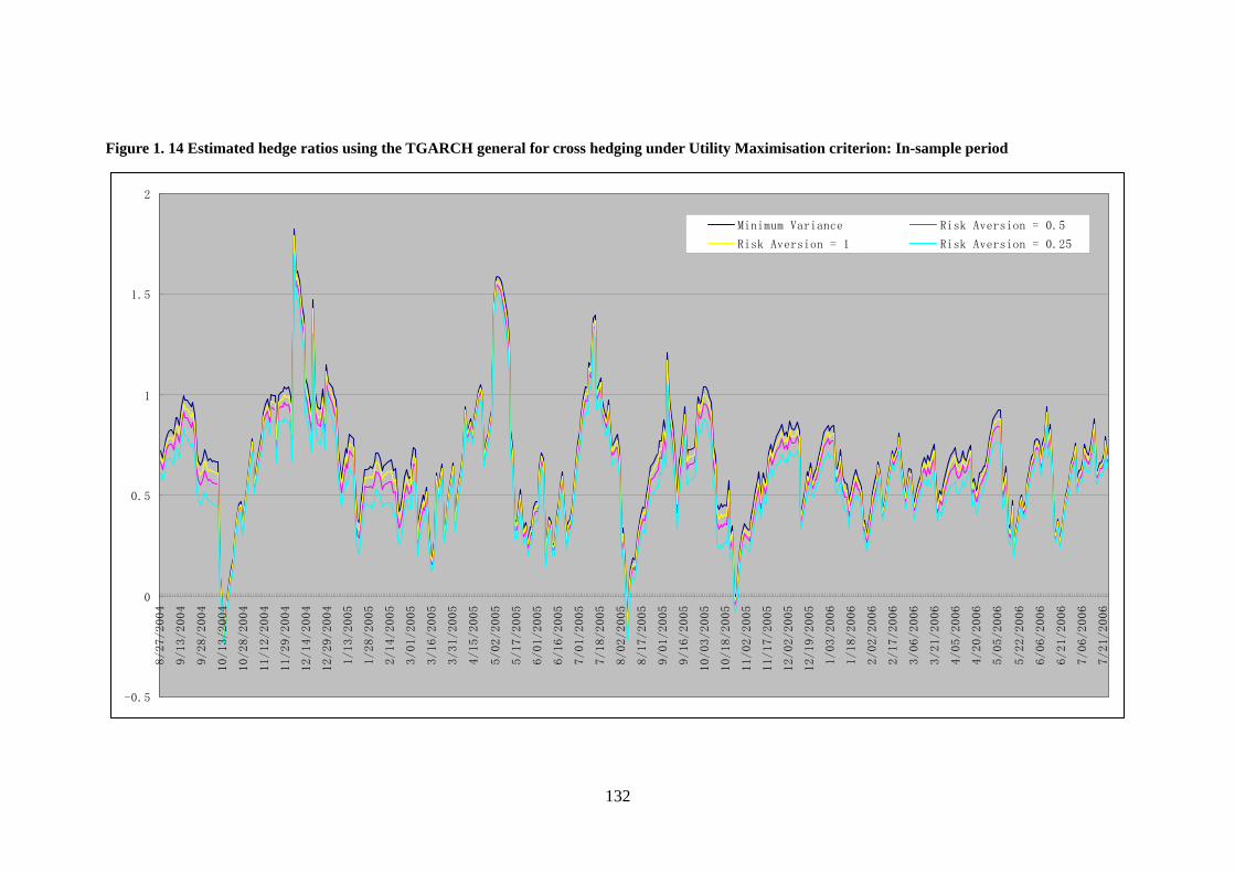
132

Figure 1. 14 Estimated hedge ratios using the TGARCH general for cross hedging under Utility Maximisation criterion: In-sample period

-0.5

0

0.5

1

1.5

2

8/27/2004

9/13/2004

9/28/2004

10/13/2004

10/28/2004

11/12/2004

11/29/2004

12/14/2004

12/29/2004

1/13/2005

1/28/2005

2/14/2005

3/01/2005

3/16/2005

3/31/2005

4/15/2005

5/02/2005

5/17/2005

6/01/2005

6/16/2005

7/01/2005

7/18/2005

8/02/2005

8/17/2005

9/01/2005

9/16/2005

10/03/2005

10/18/2005

11/02/2005

11/17/2005

12/02/2005

12/19/2005

1/03/2006

1/18/2006

2/02/2006

2/17/2006

3/06/2006

3/21/2006

4/05/2006

4/20/2006

5/05/2006

5/22/2006

6/06/2006

6/21/2006

7/06/2006

7/21/2006



133

Figure 1. 15 Estimated hedge ratios using the GARCH General model for the cross hedging under Utility Maximisation criterion: In-sample period

-0.5

0

0.5

1

1.5

2

8/27/2004

9/13/2004

9/28/2004

10/13/2004

10/28/2004

11/12/2004

11/29/2004

12/14/2004

12/29/2004

1/13/2005

1/28/2005

2/14/2005

3/01/2005

3/16/2005

3/31/2005

4/15/2005

5/02/2005

5/17/2005

6/01/2005

6/16/2005

7/01/2005

7/18/2005

8/02/2005

8/17/2005

9/01/2005

9/16/2005

10/03/2005

10/18/2005

11/02/2005

11/17/2005

12/02/2005

12/19/2005

1/03/2006

1/18/2006

2/02/2006

2/17/2006

3/06/2006

3/21/2006

4/05/2006

4/20/2006

5/05/2006

5/22/2006

6/06/2006

6/21/2006

7/06/2006

7/21/2006



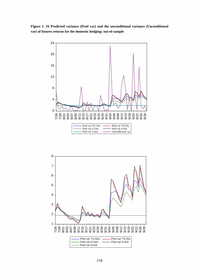
134

Figure 1. 16 Predicted variance (Pred var) and the unconditional variance (Unconditional

var) of futures returns for the domestic hedging: out-of-sample

0

4

8

12

16

20

24

7/26

7/28

8/01

8/03

8/07

8/09

8/11

8/15

8/17

8/21

8/23

8/25

8/29

8/31

9/04

9/06

9/08

9/12

9/14

9/18

9/20

9/22

9/26

9/28

Pred var TG-Gen Rred var TG-DiaPred var G-Gen Pred var G-DiaPred var Const Unconditional var

1

2

3

4

5

6

7

8

7/26

7/28

8/01

8/03

8/07

8/09

8/11

8/15

8/17

8/21

8/23

8/25

8/29

8/31

9/04

9/06

9/08

9/12

9/14

9/18

9/20

9/22

9/26

9/28

Pred var TG-Gen Pred var TG-DiaPred var G-Gen Pred var G-DiaPred var Const

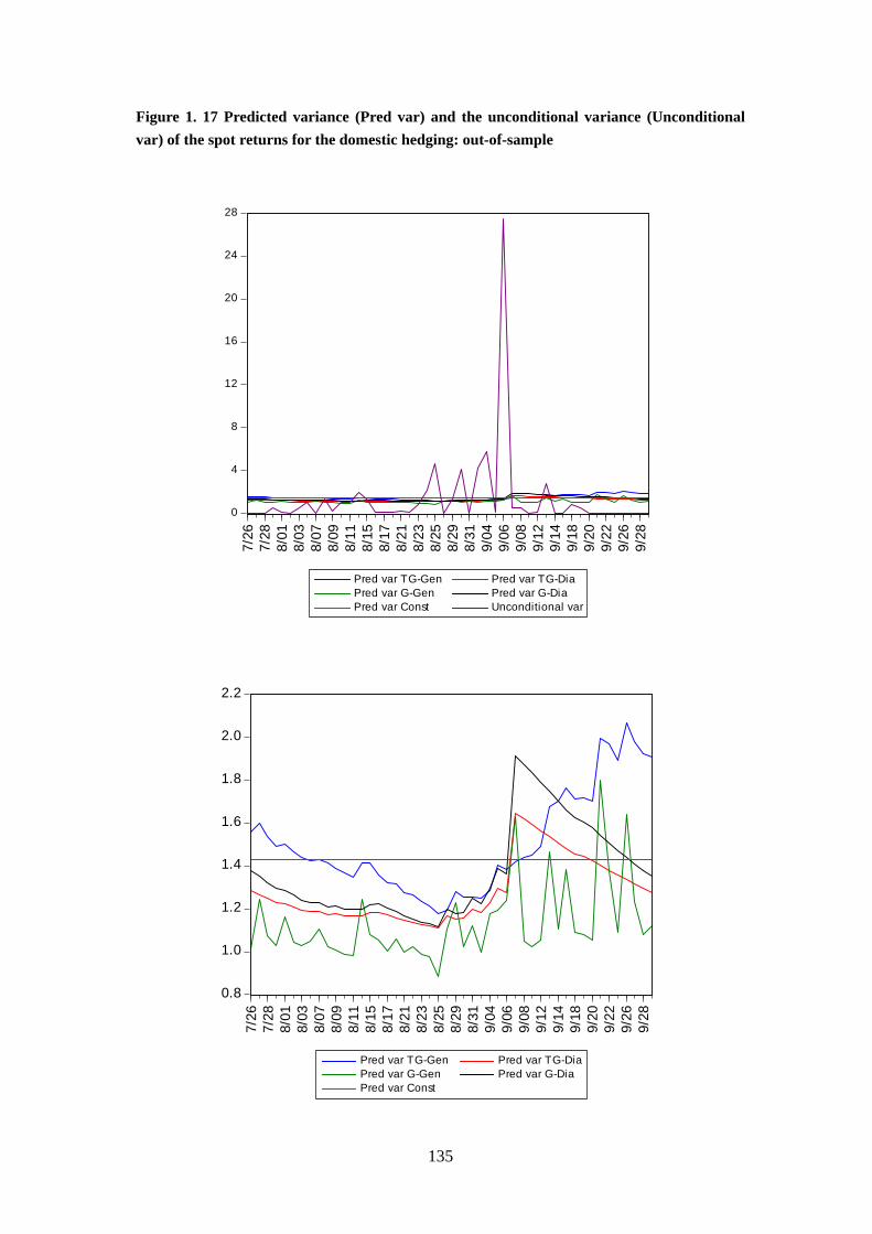
135


var) of the spot returns for the domestic hedging: out-of-sample

0

4

8

12

16

20

24

28

7/26

7/28

8/01

8/03

8/07

8/09

8/11

8/15

8/17

8/21

8/23

8/25

8/29

8/31

9/04

9/06

9/08

9/12

9/14

9/18

9/20

9/22

9/26

9/28

Pred var TG-Gen Pred var TG-DiaPred var G-Gen Pred var G-DiaPred var Const Unconditional var

0.8

1.0

1.2

1.4

1.6

1.8

2.0

2.2

7/26

7/28

8/01

8/03

8/07

8/09

8/11

8/15

8/17

8/21

8/23

8/25

8/29

8/31

9/04

9/06

9/08

9/12

9/14

9/18

9/20

9/22

9/26

9/28


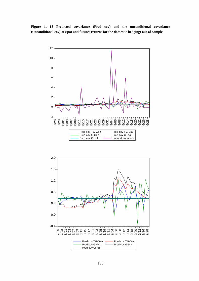
136

Figure 1. 18 Predicted covariance (Pred cov) and the unconditional covariance

(Unconditional cov) of Spot and futures returns for the domestic hedging: out-of-sample

-2

0

2

4

6

8

10

12

7/26

7/28

8/01

8/03

8/07

8/09

8/11

8/15

8/17

8/21

8/23

8/25

8/29

8/31

9/04

9/06

9/08

9/12

9/14

9/18

9/20

9/22

9/26

9/28

Pred cov TG-Gen Pred cov TG-DiaPred cov G-Gen Pred cov G-DiaPred cov Const Unconditional cov

-0.4

0.0

0.4

0.8

1.2

1.6

2.0

7/26

7/28

8/01

8/03

8/07

8/09

8/11

8/15

8/17

8/21

8/23

8/25

8/29

8/31

9/04

9/06

9/08

9/12

9/14

9/18

9/20

9/22

9/26

9/28

Pred cov TG-Gen Pred cov TG-DiaPred cov G-Gen Pred cov G-DiaPred cov Const

137


var) of futures returns for the cross hedging: out-of-sample

0

4

8

12

16

20

24

7/26

7/28

8/01

8/03

8/07

8/09

8/11

8/15

8/17

8/21

8/23

8/25

8/29

8/31

9/04

9/06

9/08

9/12

9/14

9/18

9/20

9/22

9/26

9/28

Pred var TG-Gen Pred var TG-DiaPred var G-Gen Pred var G-DiaPred var Constant Unconditinal var

1

2

3

4

5

6

7/26

7/28

8/01

8/03

8/07

8/09

8/11

8/15

8/17

8/21

8/23

8/25

8/29

8/31

9/04

9/06

9/08

9/12

9/14

9/18

9/20

9/22

9/26

9/28


138


var) of spot returns for the cross hedging: out-of-sample

0

4

8

12

16

20

24

28

32

7/26

7/28

8/01

8/03

8/07

8/09

8/11

8/15

8/17

8/21

8/23

8/25

8/29

8/31

9/04

9/06

9/08

9/12

9/14

9/18

9/20

9/22

9/26

9/28

Pred var TG-Gen Pred var TG-DiaPred var G-Gen Pred var G-DiaPred var Constant Unconditional var

1

2

3

4

5

6

7

7/26

7/28

8/01

8/03

8/07

8/09

8/11

8/15

8/17

8/21

8/23

8/25

8/29

8/31

9/04

9/06

9/08

9/12

9/14

9/18

9/20

9/22

9/26

9/28


139

Figure 1. 21 Predicted covariance (Pred cov) and the unconditional covariance

(Unconditional cov) of Spot and futures returns for the cross hedging: out-of-sample

-5

0

5

10

15

20

25

7/26

7/28

8/01

8/03

8/07

8/09

8/11

8/15

8/17

8/21

8/23

8/25

8/29

8/31

9/04

9/06

9/08

9/12

9/14

9/18

9/20

9/22

9/26

9/28

Pred cov TG-Gen Pred cov TG-DiaPred cov G-Gen Pred cov G-DiaPred cov Constant Unconditional cov

0.0

0.5

1.0

1.5

2.0

2.5

3.0

3.5

4.0

7/26

7/28

8/01

8/03

8/07

8/09

8/11

8/15

8/17

8/21

8/23

8/25

8/29

8/31

9/04

9/06

9/08

9/12

9/14

9/18

9/20

9/22

9/26

9/28

Pred cov TG-Gen Pred cov TG-DiaPred cov G-Gen Pred cov G-DiaPred cov Const

140

Figure 1. 22 Predicted hedge ratios of hedging domestic spot positions: out-of-sample period

-.1

.0

.1

.2

.3

.4

.5

.6

7/26

7/28

8/01

8/03

8/07

8/09

8/11

8/15

8/17

8/21

8/23

8/25

8/29

8/31

9/04

9/06

9/08

9/12

9/14

9/18

9/20

9/22

9/26

9/28

TG-Gen TG-Dia G-GenG-Dia Const

Figure 1. 23 Predicted hedge ratios of cross hedging in the Singapore market: out-of-sample

period

0.0

0.2

0.4

0.6

0.8

1.0

1.2

7/26

7/28

8/01

8/03

8/07

8/09

8/11

8/15

8/17

8/21

8/23

8/25

8/29

8/31

9/04

9/06

9/08

9/12

9/14

9/18

9/20

9/22

9/26

9/28


141

Figure 1. 24 Return of hedged portfolios of the domestic hedging under variance

minimisation: out-of-sample

-6

-5

-4

-3

-2

-1

0

1

2

3

7/26

7/28

8/01

8/03

8/07

8/09

8/11

8/15

8/17

8/21

8/23

8/25

8/29

8/31

9/04

9/06

9/08

9/12

9/14

9/18

9/20

9/22

9/26

9/28

TG-Gen TG-Dia G-GenG-Dia Const RS

Figure 1. 25 Return of hedged portfolios of the cross hedging in the Singapore market under

variance minimisation: out-of-sample

-6

-4

-2

0

2

4

6

7/26

7/28

8/01

8/03

8/07

8/09

8/11

8/15

8/17

8/21

8/23

8/25

8/29

8/31

9/04

9/06

9/08

9/12

9/14

9/18

9/20

9/22

9/26

9/28

TG-Gen TG-Dia G-GenG-Dia Const RSX

142

Figure 1. 26 Histogram of hedge ratios estimated using different models for the domestic

hedging: out-of-sample period

0

5

10

15

20

25

-6 -4 -2 0 2 4

Freq

uenc

y

TG-Gen

0

4

8

12

16

20

-6 -4 -2 0 2 4

Freq

uenc

y

TG-Dia

0

5

10

15

20

25

-6 -4 -2 0 2 4

Freq

uenc

y

G-Gen

0

4

8

12

16

20

-6 -4 -2 0 2 4

Freq

uenc

yG-Dia

0

4

8

12

16

20

-6 -4 -2 0 2 4

Freq

uenc

y

Const

0

4

8

12

16

20

-6 -4 -2 0 2 4

Freq

uenc

y

RS

143

Figure 1. 27 Histogram of hedge ratios estimated using different models for the cross

hedging in the Singapore market: out-of-sample period

0

2

4

6

8

-6 -4 -2 0 2 4

Freq

uenc

y

TG-Gen

0

2

4

6

8

-6 -4 -2 0 2 4

Freq

uenc

y

TG-Dia

0

2

4

6

8

-6 -4 -2 0 2 4 6

Freq

uenc

y

G-Gen

0

1

2

3

4

5

6

7

-6 -4 -2 0 2 4

Freq

uenc

y

G-Dia

0

2

4

6

8

10

-6 -4 -2 0 2 4

Freq

uenc

y

Const

0

2

4

6

8

10

-6 -4 -2 0 2 4 6

Freq

uenc

y

RSX

144

Figure 1. 28 Time path of risk reduction of the domestic hedging under risk minimisation

criterion: out-of-sample period

-.19

-.18

-.17

-.16

-.15

-.14

-.13

-.12

7/25

7/27

7/31

8/02

8/04

8/08

8/10

8/14

8/16

8/18

8/22

8/24

8/28

8/30

9/01

9/05

9/07

9/11

9/13

9/15

9/19

9/21

9/25

9/27

9/29


Figure 1. 29 Time path of risk reduction of the cross hedging over time under risk

minimisation criterion: out-of-sample period

-.26

-.25

-.24

-.23

-.22

-.21

-.20

7/25

7/27

7/31

8/02

8/04

8/08

8/10

8/14

8/16

8/18

8/22

8/24

8/28

8/30

9/01

9/05

9/07

9/11

9/13

9/15

9/19

9/21

9/25

9/27

9/29


145

Figure 1. 30 Expected utility of the domestic hedging over time under utility maximisation

criterion: out-of-sample period

(1) 0.25

-.27

-.26

-.25

-.24

-.23

-.22

-.217/

257/

277/

318/

028/

048/

088/

108/

148/

168/

188/

228/

248/

288/

309/

019/

059/

079/

119/

139/

159/

199/

219/

259/

279/

29


(2) 0.5

-.59

-.58

-.57

-.56

-.55

-.54

-.53

-.52

-.51

7/25

7/27

7/31

8/02

8/04

8/08

8/10

8/14

8/16

8/18

8/22

8/24

8/28

8/30

9/01

9/05

9/07

9/11

9/13

9/15

9/19

9/21

9/25

9/27

9/29


146

(3) 1

-1.22

-1.20

-1.18

-1.16

-1.14

-1.12

-1.10

-1.08

7/25

7/27

7/31

8/02

8/04

8/08

8/10

8/14

8/16

8/18

8/22

8/24

8/28

8/30

9/01

9/05

9/07

9/11

9/13

9/15

9/19

9/21

9/25

9/27

9/29


Figure 1. 31 Expected utility of the cross hedging in The Singapore market over time under

utility maximisation criterion: out-of-sample period (1) 0.25

-.72

-.70

-.68

-.66

-.64

-.62

-.60

7/25

7/27

7/31

8/02

8/04

8/08

8/10

8/14

8/16

8/18

8/22

8/24

8/28

8/30

9/01

9/05

9/07

9/11

9/13

9/15

9/19

9/21

9/25

9/27

9/29

TG-Gen TG-Dia G-GenG-Dia Constant

147

(2) 0.5

-1.44

-1.42

-1.40

-1.38

-1.36

-1.34

-1.32

-1.30

-1.28

7/25

7/27

7/31

8/02

8/04

8/08

8/10

8/14

8/16

8/18

8/22

8/24

8/28

8/30

9/01

9/05

9/07

9/11

9/13

9/15

9/19

9/21

9/25

9/27

9/29


(3) 0.1

-2.92

-2.88

-2.84

-2.80

-2.76

-2.72

-2.68

-2.64

7/25

7/27

7/31

8/02

8/04

8/08

8/10

8/14

8/16

8/18

8/22

8/24

8/28

8/30

9/01

9/05

9/07

9/11

9/13

9/15

9/19

9/21

9/25

9/27

9/29


148

Figure 1. 32 Time path of risk reduction of the domestic hedging based on semivariance:

out-of-sample period

-.44

-.43

-.42

-.41

-.40

-.39

-.38

7/26

7/28

8/01

8/03

8/07

8/09

8/11

8/15

8/17

8/21

8/23

8/25

8/29

8/31

9/04

9/06

9/08

9/12

9/14

9/18

9/20

9/22

9/26

9/28


Figure 1. 33 Time path of risk reduction of the cross hedging based on semivariance:

out-of-sample period

-.35

-.34

-.33

-.32

-.31

-.30

-.29

-.28

-.27

7/26

7/28

8/01

8/03

8/07

8/09

8/11

8/15

8/17

8/21

8/23

8/25

8/29

8/31

9/04

9/06

9/08

9/12

9/14

9/18

9/20

9/22

9/26

9/28


149

Appendix 1 B

Figure 1.B 1 Monthly position of China fuel oil futures (lot).

Figure 1.B 2 Average monthly turn of China fuel oil futures.

150

Figure 1.B 3 Sales price and cost of some oil refineries

Note: Guangdong province in China takes 80% of fuel oil imports.

Figure 1.B 4 China fuel oil futures and spot price series

Source of above figures: Guangzhou Twinace Petroleum and Chemicals Co., Ltd.

151

Essay 2 Volatility spillovers among oil,

gold and US stock market

152

2.1 Background and Literature

Oil and gold are two very important commodities in the financial market. Oil, as one

of goods with substantial volume of trades in world markets, is very essential in every

economy. Its importance as a source of energy and economic growth can hardly be

exaggerated. This is especially true for the world’s leading economy, the U.S., where

oil makes possible the functioning of nearly every component of the economy,

directly or indirectly. It provides 40% of the nation’s power supply—far more than

any other source. Figure 2.B1 in Appendix 2.B shows the percentage of US to the

world oil production, imports and demand. The US oil demand takes up to a quarter of

the world total oil demand, much more than the percentage it can produce. Oil price

have behaved with wide swings in history. Figure 2.B2 depicts the crude oil price for

the past 50 years based on yearly average data. We have witnessed the general upward

trend of the price of oil. The inflation adjusted oil price series portrayed in Figure

2.B3 show that the oil price has picked in 1980 and 200818, following 1997 currency

crisis and 2007 financial crisis, both of which lead to severe economic recession.

The linkage between economic growth (hence, the stock price) and oil markets

appears to be quite natural. Huang et al. (1996) opine that if oil plays an important

role in an economy, it would be expected that changes in the oil price to be correlated

with changes in stock prices. Mussa (2000) argues that by affecting economic activity,

18 Oil price has started to drop from its peak in July 2008 (as shown in Figure 3.B4) and is averaged about 52 dollars a barrel in the first seven month in 2009.

153

corporate earnings, inflation and monetary policy, an increase in the oil price has

implications for asset prices and financial markets. While summing up contemporary

research relating to oil prices and capital markets, Jones et al. (2004) comment that:

“Ideally stock values reflect the market’s best estimate of the future profitability of

firms, so the effect of oil price shocks on the stock market is a meaningful and useful

measure of their likely economic impact. Since asset prices are the present discounted

value of the future net earning of firms, both the current and expected futures impacts

of an oil price shock should be absorbed fairly quickly into stock prices and returns

without having to wait for those impacts to actually occur.”

On the other hand, with the geopolitical uncertainties and some of the turmoil

afflicting the financial markets, the price of gold has been sent soaring as well, as

shown in Figure 2.B5. Gold is a precious metal which is also classed as a commodity

and monetary asset. It has acted as a multi-faceted metal down through the centuries.

It possesses similar characteristics to money in that it acts as a store of wealth,

medium of exchange and a unit of value (Goodman 1956; Solt and Swanson, 1981). It

has also played an important role as a precious metal with significant portfolio

diversification properties (see, e.g., Ciner, 2001). It is used in industrial components,

jewellery, as an investment asset as well as reserve asset. Gold is often used as a

hedge against inflation, political risk, and currency exchange risk. According to Smith

(2002), “when the economic environment becomes more uncertain attention turns to

investing in gold as a safe haven.” The gold holding in the United States is on average

154

up to one quarter of the world total holdings, as shown in Figure 2.B6.

As can be observed in the financial market for the past few decades, it is a general

rule that when the price of crude oil rallies, the price of gold tends to follow suit.

Higher oil prices act like an inflation tax on consumer and producers, whereas

investing in the gold market turns out to be the best hedging strategy. Over the last 50

years or so, gold and oil have generally moved together in terms of price, with a

positive price correlation of over 80 percent (Nick Barisheff, 2005). We depict the last

50 years oil and gold price series in Figure 2.B7 and their monthly price series since

1990s in Figure 2.B8.

From the Figures, we observe strong correlations between the oil and gold markets.

Each of these two markets has significant effects on the economy, which is reflected

in some way by the movement of the stock market in that economy. Despite the

apparent links between the oil and gold markets, there are few studies on their

relationship. For the literature on oil and stock market, while many studies have

examined how changes in oil prices can affect the macroeconomy, especially its

growth, the literature exploring the impact of oil on the stock markets still remains

sparse, with only a few studies. Generally an adverse linkage between the higher oil

prices and economic growth is well documented in the literature (e.g. Hamilton, 1983;

Gisser and Goodwine, 1986; Mussa, 2000; IEA, 2004; Jones et al., 2004). For the

relation between the oil and stock markets, Jones and Kaul (1996) provide evidence

155

that aggregate stock market returns in the USA, Canada, Japan and the UK responsed

negatively to oil price shocks on the economies of these countries. Using a standard

cash-flow dividend valuation model, they found, however, that only in the US and

Canada can this reaction be accounted for completely by the impact of the oil shocks

on real cash flows. Huang, Masulis, and Stoll (1996) examined the relationship

between daily oil futures returns and daily U.S. stock returns. Using a VAR model,

they found that oil futures returns lead some individual oil company stock returns but

they do not have much impact on the broad-based market indices such as the S&P 500.

Sadorsky (1999), utilizing an unrestricted VAR and using US monthly data, examined

the links among fuel oil prices, stock prices, short-term interest rate and industrial

production of the economy. He found, in contrast to Huang et al.’s finding, that oil

price movements are important in explaining movements in broad-based stock returns.

Hammoudeh and Aleisa (2002), using monthly data from 1991 to 2000 and

employing the two-step univariate GARCH models, found mean spillovers from oil

markets to stock markets in the case of Bahrain, Indonesia, Mexico, and Venezuela.

Hammoudeh, Dibooglu and Aleisa (2004) investigate the relationship among U.S. oil

prices and oil industry equity indices based on daily data. They found that the oil

futures market has a matching or echoing volatility effect on the stocks of some oil

sectors and a volatility-dampening effect on the stocks of others. El-Sharif, Brown,

Burton, Nixon and Russell (2005) study the relationship between the price of crude oil

and equity values in the oil and gas sector using data relating to the United Kingdom

and find the volatility in the price of crude oil has a positive and significant impact on

156

share values within the sector.

The existing literature on the relationship between the gold market and stock market is

even sparser. Chan and Faff (1998) investigate the extra-market sensitivity of the

Australian industry equity returns to a gold price factor over the period 1975 to 1994.

They find that there has been a widespread sensitivity of Australian industry returns to

gold price returns, over and above market returns. The sensitivity is found to be

positive for resource and mining sector industries, whereas it is negative for the

industrial sector. They also find that the gold price sensitivities are changing over time.

Blose and Shieh (1995) studied the elasticity of gold mining stocks to the changes in

gold price. Using monthly data over a ten year period from 1981 through 1990, they

found 23 out of 24 publicly traded gold mining companies in their sample have a gold

price elasticity greater than one.

With the ever-increasing integration of financial markets, it is well accepted that the

economic growth benefit from risk sharing, improvements in allocation efficiency and

reductions in macroeconomic volatility and transaction costs (see Prasad et al., 2003;

Baele at al., 2004). Whilst financial market integration encompasses many different

aspects of the complex inter-relationships across various financial markets, we focus

on the interrelation between oil, gold and US stock markets. As far as we know, there

is not a single literature which has studied the linkage between these three markets.

Understanding the links between financial markets is of great importance for a

157

financial hedger, portfolio manager, asset allocator, or other financial analysts. The

study of volatility spillover from one market to another is a crucial part of the issue.

(Martin Agren, 2006). Thus, instead of studying the price and return movements, our

study focuses on the volatilities spillover between these markets, that is, the linkage in

their second moments. Although there is no existing literature exploring such second

moment linkages between these three markets, there are many studies on the volatility

spillover in financial markets, especially among different stock markets and currency

markets. Most of these studies employ the GARCH framework, univariate or

multivariate, as the GARCH model is generally believed to be the best to describe

financial return data. For example, Kearney and Patton (2000) employed a

multivariate GARCH model to study the volatility transmission mechanism among

different exchange rates in the European Monetary System. Ewing, Malik, and

Ozfidan (2002) used a similar model to study the linkage between the oil and natural

gas markets. They find that there exists significant volatility spillover between the two

markets. Malik and Hammoudeh (2005) used a Multivariate GARCH model to study

the volatility and shock transmission mechanism among US equity, global crude oil

market, and equity markets of Saudi Arabia, Kuwait, and Bahrain. They find

significant transmission among second moments. In our study, we investigate the

volatility linkage by employing both Tri-variate GARCH specification for the oil,

gold and stock market returns and Bi-variate GARCH for each of the two markets.

This enables us to examine how the variances of one markets is affected by the shocks

from the another market. Meanwhile, by comparing the variances and covariances

158

estimated from Tri-variate and Bi-variate GARCH models, we can investigate how,

by including a third market to the existing two markets framework, the changes in the

third market can affect the linkage between the two markets being investigated.

Daily data beginning April 1991 to November 200719 are used for the purpose of this

study. Moreover, three sub-samples are examined (reasons of which are given in later

section). We find that, in terms of volatility, the gold market is “exogenous”, despite

the close price or return links between gold and the oil market. The gold market

volatility spills over to the oil and stock markets. The spillovers between the oil and

stock markets are generally bi-directional. This provides evidence of the existence of

the strong linkage between the oil and the stock market, and with the US economy.

Gold, being regarded as a “safe haven” asset and being largely held by individuals and

institutional investors to hedge risk, had a low volatility itself and had not been

affected by oil and stock market shocks. The existence of volatility spillovers between

the oil and gold markets, indicated by the Bi-variate GARCH modelling, actually

emanate from their relations with the third market, the stock market. Similarly, the

volatility spillovers between the gold and stock markets are due to their links with the

oil market.

The remainder of the chapter is organized as follows. Section 2 describes the data and

methodology. Empirical findings are presented in Section 3. A summary and

19 This period is chosen because of the financial integration growing rapidly since the early 1990s.

159

conclusion are provided in Section 4.

160

2.2. Data and Methodology

2.2.1 Data

The data used in this study, namely world oil, gold and US stock prices, are sourced

from DataStream. World oil price is represented by the nearby futures price series of

the world’s most liquid and most actively traded oil futures contract, the NYMEX’s

Light Sweet Crude Oil contract. The futures prices are chosen instead of spot prices

because the futures are far more heavily traded than the commodity itself and also are

far more sensitive to the arrival of new information. The NYMEX’s Light Sweet

Crude oil futures is chosen over other oil futures because this contract is traded in the

US market and is the world’s largest futures contract in terms of trading volume on a

physical commodity. It is widely used as the benchmark for determining crude oil and

refined product prices in the United States and abroad. For similar reasons, we use the

continuous gold futures price series from Chicago Mercantile Exchange as the

indicator of world gold prices. For the stock index, S&P500 is generally used as the

representative of the US stock market and the economy. The data begin on 1 April

1991 and end on 5 November 2007.

We also split our data set into three sub-sample periods for investigative purposes,

which are detailed in Section 2.3. All returns are calculated by computing the

differences in the natural logarithm of the price multiplied by 100.

161

2.2.2 Methodology

To explore the dynamics of the price volatility process, autoregressive conditional

heteroskedasticity (ARCH) and generalised ARCH (GARCH) models that take into

account the time-varying variances of time series data are employed (suitable surveys

of ARCH modelling may be found in Bollerslev, et al. 1992; Bera and Higgins, 1993

and Pagan, 1996). The GARCH type models are more parsimonious than the ARCH

type models and are commonly used to capture the features of financial data and to

explore the volatility and volatility transmission of financial markets. In our study, we

first employ the Tri-variate GARCH (1, 1)20 model to examine the relations between

oil, gold and US stock market. Then we employ a Bi-variate GARCH (1, 1)21 model

to examine the relation between each pair of the three markets. The results obtained

from Tri-variate GARCH model are compared with those obtained from the

Bi-variate GARCH model.

The most general Tri-variate GARCH(1,1) model we postulated to represent the joint

distribution of the oil, gold and stock returns is:

1

n

t t i t i ti

Y Y

; ),0(~| 1 HNtt (2.1)

20 Tri-variate GARCH (m,n) (m>=1, n>=1) models are also experimented for this study. However, we found that when we include higher orders in the GARCH specification, all the parameters for conditional and unconditional variance, except for the first order, are mostly statistically insignificant from zero. 21 Same as Tri-variate GARCH models, higher orders in Bi-variate GARCH specification were also experimented with in the study. The results also suggest that the Bi-variate GARCH (1,1) is the most appropriate.

162

Where ,( , ) 't t tY ro rg rsp is a vector of observations of the log-differenced prices of

oil futures, gold futures and S&P 500 stock index, multiplied by 100,

( , , ) 't ot gt st is a vector of conditional means to be estimated and

( , , ) 't ot gt st is a vector of residuals. This is a general VAR for the mean

equation where one variable is a function of its own lagged values, and lagged values

of all the other variables, from time t - 1 , to time t n . Starting from experiment

with the most general model, we then reduce the mean structure to more parsimonious

specifications. The residuals are assumed to be normally distributed and are

conditional on past information, 1t , with zero mean vector and with conditional

variance-covariance matrix:

1 1 1t t t tH C C A A B H B (2.2)

Where C is (3 3) symmetric parameter matrix, and A and B are (3 3)

parameter matrices. In our estimation, we use the most general form, all full rank A, B

and C matrix for our maximum likelihood estimation. In the cases that estimation is

not possible to obtain because the positive feature of tH is violated, we adopt a

positive definite parameterization following Engle and Kroner (1995), henceforce the

BEKK representation, where 21 31 32 0c c c . Such specification guarantees that

the conditional covariance matrix is positive definite so that conditional variances are

always nonnegative. In explicit format, we can express the conditional

variance-covariance matrix H in the following form:

163

, , , 11 21 31 11 12 13

, , , 12 22 32 21 22 23

, , , 13 23 33 31 32 33

211 21 31 , 1 , 1 , 1 , 1 ,

12 22 32

13 23 33

oo t og t os t

t og t gg t gs t

os t gs t ss t

o t o t g t o t s t

h h h c c c c c c

H h h h c c c c c c

h h h c c c c c c

a a a

a a a

a a a

1 11 12 132

, 1 , 1 , 1 , 1 , 1 21 22 232

, 1 , 1 , 1 , 1 , 1 31 32 33

11 21 31 , 1 , 1 , 1

12 22 32 , 1 , 1 , 1

13 23 33 , 1

o t g t g t g t s t

o t s t g t s t s t

oo t og t os t

og t gg t gs t

os t g

a a a

a a a

a a a

b b b h h h

b b b h h h

b b b h h

11 12 13

21 22 23

, 1 , 1 31 32 33s t ss t

b b b

b b b

h b b b

(2.3)

The Tri-variate GARCH model is estimated using maximum likelihood method.

Under conditional normality, the log likelihood function is as follow:

1

1

1( ) log(2 ) (log ( ) ( ) ( ) ( ))

2

T

t t t tt

L T H H

(2.4)

Where T is the number of observations of the sample. is the parameter vector to

be estimated. 1, 2, 3,( , , )t t t t is a (1 3) vector of residuals at time t.

1cov( )t t tH , with the diagonal elements of tH are the conditional variances,

the cross diagonal elements are the conditional covariances of spot and futures returns.

The log-likelihood function is maximized subject to the constraint that the conditional

variances be positive. The Tri-variate GARCH model is first estimated using the

SIMPLEX22 algorithm. Such preliminary estimation is used to refine the initial

parameter values before switching to our final estimation method. With the values

obtained from Simplex estimation are then used as initial values, the final parameters

22 The Simplex Method is a search procedure which requires only function evaluations, not derivatives. It starts by selecting K+1 points in K-space, where K is the number of parameter. It is normally used as a preliminary estimation method to refine the initial parameter values before switching to one of the other estimation methods.

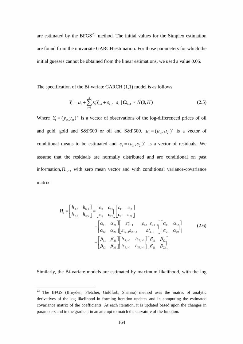
164

are estimated by the BFGS23 method. The initial values for the Simplex estimation

are found from the univariate GARCH estimation. For those parameters for which the

initial guesses cannot be obtained from the linear estimations, we used a value 0.05.

The specification of the Bi-variate GARCH (1,1) model is as follows:

1

n

t t i t i ti

Y Y

, ),0(~| 1 HNtt (2.5)

Where 1 , 2( ) 't t tY y y is a vector of observations of the log-differenced prices of oil

and gold, gold and S&P500 or oil and S&P500. 1 2( , ) 't t t is a vector of

conditional means to be estimated and 1 2( , ) 't t t is a vector of residuals. We

assume that the residuals are normally distributed and are conditional on past

information, 1t , with zero mean vector and with conditional variance-covariance

matrix

11, 12, 11 21 11 12

12, 22, 12 22 21 22

211 21 11 121, 1 1, 1 2, 1

212 22 21 221, 1 2, 1 1, 1

11, 1 12, 111 21

12, 1 22, 112 22

t tt

t t

t t t

t t t

t t

t t

h h c c c cH

h h c c c c

h h

h h

11 12

21 22

(2.6)

Similarly, the Bi-variate models are estimated by maximum likelihood, with the log

23 The BFGS (Broyden, Fletcher, Goldfarb, Shanno) method uses the matrix of analytic

derivatives of the log likelihood in forming iteration updates and in computing the estimated

covariance matrix of the coefficients. At each iteration, it is updated based upon the changes in

parameters and in the gradient in an attempt to match the curvature of the function.

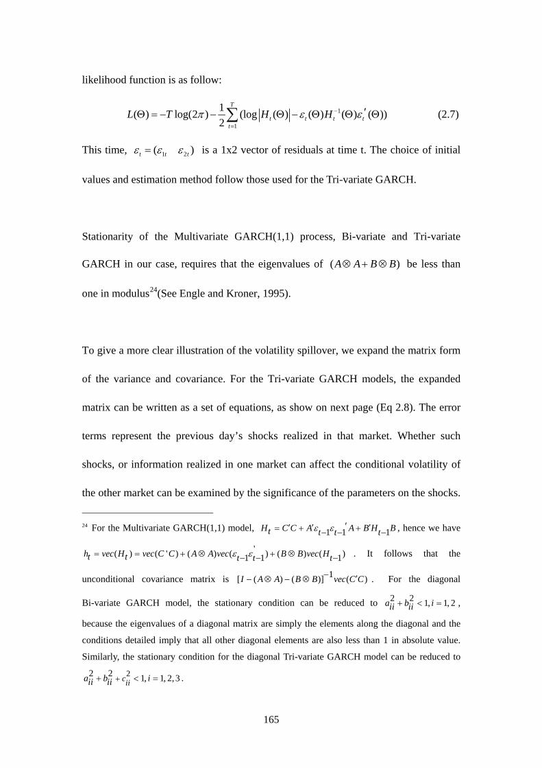
165

likelihood function is as follow:

1

1

1( ) log(2 ) (log ( ) ( ) ( ) ( ))

2

T

t t t tt

L T H H

(2.7)

This time, 1 2( )t t t is a 1x2 vector of residuals at time t. The choice of initial

values and estimation method follow those used for the Tri-variate GARCH.

Stationarity of the Multivariate GARCH(1,1) process, Bi-variate and Tri-variate

GARCH in our case, requires that the eigenvalues of ( )A A B B be less than

one in modulus24(See Engle and Kroner, 1995).

To give a more clear illustration of the volatility spillover, we expand the matrix form

of the variance and covariance. For the Tri-variate GARCH models, the expanded

matrix can be written as a set of equations, as show on next page (Eq 2.8). The error

terms represent the previous day’s shocks realized in that market. Whether such

shocks, or information realized in one market can affect the conditional volatility of

the other market can be examined by the significance of the parameters on the shocks.

24 For the Multivariate GARCH(1,1) model, 1 1 1H C C A A B H Bt t t t , hence we have

'( ) ( ' ) ( ) ( ) ( ) ( )1 1 1h vec H vec C C A A vec B B vec Ht t t t t . It follows that the

unconditional covariance matrix is 1[ ( ) ( )] ( )I A A B B vec C C . For the diagonal

Bi-variate GARCH model, the stationary condition can be reduced to 2 2 1, 1, 2a b iii ii ,

because the eigenvalues of a diagonal matrix are simply the elements along the diagonal and the

conditions detailed imply that all other diagonal elements are also less than 1 in absolute value.

Similarly, the stationary condition for the diagonal Tri-variate GARCH model can be reduced to

22 2 1, 1, 2, 3ciia b iii ii .

166

For example, to investigate whether the oil shocks can affect the volatility of gold, we

need to determine whether the coefficient 212a is significantly different from zero.

Similarly, the significance of coefficients 221a , 2

31a can give indications of how the

past shocks in the gold and stock markets, respectively, affect the conditional

volatility in the oil market. Following the same algorithm, the significance of

coefficients 2ijb represent the conditional variance of market i has significant

impact on the conditional variance of market j . The coefficients 2iia and 2

iib

represent how the conditional variance of one market is affect by its own past shocks

and past conditional variance. Thus there exists spillover from market i to market

j when 2 0ija and/or 2 0ijb . If 2 0ija and 2 0ijb , volatilities do not spill over

from market i to market j . The volatility spillovers for the Bi-variate models can

be identified by the same mechanism. The expanded form of conditional variance and

covariance for the Bi-variate GARCH model is as follows (Eq.2.9).

167

Eq.2.8. The conditional variance-covariance for oil, gold and stock index in an expanded form.

2 2 2 2, 11 11 , 1 21 , 1 31 , 1 11 21 , 1 11 31 , 1 21 31 , 1

2 2 2 2 2 211 , 1 21 , 1 31 , 1 11 21 , 1 , 1 11 31 , 1 , 1 21 31 , 1 , 1

2, 11

2 2 2

2 2 2

oo t oo t gg t ss t og t os t gs t

o t g t s t o t g t o t s t g t s t

gg t

h c b h b h b h b b h b b h b b h

a a a a a a a a a

h c c

2 2 2 222 12 , 1 22 , 1 32 , 1 12 22 , 1 12 32 , 1 22 32 , 1

2 2 2 2 2 212 , 1 22 , 1 32 , 1 12 22 , 1 , 1 12 32 , 1 , 1 22 32 , 1 , 1

2 2, 11 22 33

2 2 2

2 2 2

oo t gg t ss t og t os t gs t

o t g t s t o t g t o t s t g t s t

ss t

b h b h b h b b h b b h b b h

a a a a a a a a a

h c c c

2 2 2 213 , 1 23 , 1 33 , 1 13 23 , 1 13 33 , 1 23 33 , 1

2 2 2 2 2 213 , 1 23 , 1 33 , 1 13 23 , 1 , 1 13 33 , 1 , 1 23 33 , 1 , 1

, 11 12 11 12

2 2 2

2 2 2


o t g t s t o t g t o t s t o t g t

og t o

b h b h b h b b h b b h b b h

a a a a a a a a a

h c c b b h

, 1 21 22 , 1 21 32 , 1 12 21 11 22 , 1 12 31 11 32 , 1 31 22 21 32 , 1

2 2 211 12 21 22 21 32 12 21 11 22 12 31 11 32 31 22 21 32

, 1

( ) ( ) ( )

( ) ( ) ( )

o t gg t ss t og t os t gs t

o g s o g o s g s

gs t

b b h b b h b b b b h b b b b h b b b b h

a a a a a a a a a a a a a a a a a a

h c

2 13 22 23 12 13 , 1 22 23 , 1 32 32 , 1 12 23 22 13 , 1 32 13 12 33 , 1 32 23 22 33 , 1

2 2 212 13 22 23 32 33 12 23 22 13 32 13 12 33 32 23

( ) ( ) ( )

( ) ( ) (


o g s o g o s

c c c b b h b b h b b h b b b b h b b b b h b b b b h

a a a a a a a a a a a a a a a a

22 33

, 11 13 11 13 , 1 21 23 , 1 31 33 , 1 11 23 21 13 , 1 31 13 11 33 , 1 31 23 22 33 , 1

2 2 211 13 21 23 31 33 11 23 21 13 31 13 11 32

)

( ) ( ) ( )

( ) (

g s

os t oo t gg t ss t og t os t gs t

o g s o g

a a

h c c b b h b b h b b h b b b b h b b b b h b b b b h

a a a a a a a a a a a a a a

31 23 22 33 , 1 , 1) ( )o s g t s ta a a a

(2.38)

Eq.2.9. The conditional variance-covariance of a Bi-variate GARCH in an expanded form

2 2 2 2 2 2 211, 11 11 11, 1 21 22, 1 11 21 12, 1 11 1, 1 21 2, 1 11 21 1, 1 2, 1

2 2 2 2 2 2 2 222, 12 22 12 11, 1 22 22, 1 12 22 12, 1 12 1, 1 22 2, 1 12 22 1, 1 2, 1

12, 11

2 2

2 2

t t t t t t t t

t t t t t t t t

t

h c b h b h b b h a a a a

h c c b h b h b b h a a a a

h c

12 11 12 11, 1 21 22 22, 1 11 22 12 21 12, 1( )t t tc b b h b b h a a a a h

(2.39)

168

2.3. Estimation results

2.3.1 Descriptive Statistics for the whole sample

Figure 2.1 and 2.2 in Appendix 2.A portray the price in logarithms for oil and gold

futures and the S&P500 stock index. Table 2.1 reports the basic statistics for daily

returns for the world oil futures returns (denoted as ro), gold futures returns (denoted

as rg) and US stock market index S&P500 returns (denoted as rsp), including

normality tests of the returns series and unit root tests, all of which are to ensure the

modelling specifications we proposed are appropriate.

Table 2. 1 Descriptive statistics for return series

RO RG RSP

Mean 0.0366 0.0187 0.0323

Median 0.0000 0.0000 0.0166

Maximum 14.2309 8.8872 5.5732

Minimum -16.5445 -7.5740 -7.1127

Std. Dev. 2.0859 0.8704 0.9732

Skewness -0.2517 0.0839 -0.1353

Kurtosis 7.0390 12.2394 7.3567

Jarque-Bera 2988.96 15406.51 3437.64

Probability 0.0000 0.0000 0.0000

Q(10) 15.06 21.26** 23.12**

Q2(10) 207.30** 270.14** 1175.20**

ARCH_LM 26.91** 28.84** 85.45**

ADF -65.49** -66.95** -67.15**

KPSS 0.2000 0.6805 0.2290

Note: Critical value ( for 5% significance) for ADF test: with intercept, - 2.865; with trend and intercept, -3.417.

Critical value (for 5% significance) for KPSS test: with intercept, 0.463, with intercept and trend, 0.146.

Here ** indicate rejection of null hypothesis at 5% significance level.

169

From Table 2.1, we observe that the returns for oil gold and stock market are slightly

positive. The oil market has the biggest deviation between maximum and minimum

values. Standard deviations also suggest that the oil returns are more volatile than the

gold futures returns and stock returns. Although we cannot observe noticeable

significance in the skewness25, a considerable significant kurtosis26 is found in each

of the three series, which suggests higher frequencies of extreme peakedness in these

series. The significance of Jarque-Bera27 (JB) statistics suggest that the series are not

normally distributed, thus linear regressions cannot be used. Ljung-Box(1987) Q(10)

statistics are significant for gold and S&P500 return series, which suggest the

existence of serial correlations. Ljung-Box Q-statistics for all squared return series

( 2 (10)Q ) are significant, indicating strong autocorrelation in the squared return series;

thus, the second moments of returns are time varying and changing in a predictable

fashion. This kind of volatility clustering —large changes tend to be followed by large

changes, of either sign, and small changes tend to be followed by small changes, of

either sign— can also be observed in Figure 2.3. In sum, the return series in this study

exhibit all the typical characteristics of high frequency financial return series:

skewness, leptokurtosis, and highly significant linear and nonlinear serial correlations.

Empirical modelling shows that the GARCH type models are adequate for modeling

25 Skewness is a measure of asymmetry of the distribution of the series around its mean; the skewness of a symmetric distribution, such as the normal distribution, is zero. 26 Kurtosis measures the peakedness or flatness of the distribution of the series, in other words, how fat the tails of distribution are. The kurtosis of the normal distribution is 3. 27 A JB statistic for normal distribution is 0, which indicates that the distribution has a skewness of 0 and a kurtosis of 3. Skewness values other than 0 and kurtosis values farther away from 3 lead to increasingly large JB values. And the Critical value for normal distribution at 5%level is 5.99.

170

daily price movements in financial market. The significance of the ARCH-LM test

(Engle, 1982) statistics also suggests that ARCH/GARCH type model is an

appropriate specification. For an adequate estimation with Bi-variate GARCH we

need to ensure that the components variables (the mean returns) are stationary. Thus

unit root tests become necessary. In this study, we conduct the Augmented

Dickey-Fuller (ADF) and the Kwiatkowski, Phillips, Schmidt and Shin (KPSS) test to

examine the existence of stationary in the return series. The null hypothesis for ADF

test is that the series has a unit root; while the null hypothesis for KPSS is that the

series is stationary. The test results are shown at the bottom of Table 2.1. ADF test for

the return series are all significant at 95% significant level, and KPSS are all

insignificant at 95% significant level. Both test results confirm that the three return

series are covariance stationary.

ADF and KPSS tests are also performed on the natural logarithm of the three price

series, with the results indicating that the price series are following an I(1) process. To

ensure the adequacy of our estimation model, we need to test the possible existence of

cointegration between variables. The cointegration relationships are normally

regarded as the long run or stationary relationships between the endogenous variables.

If cointegration relationships exist between variables, the model specifications need to

be adjusted by inclusion of the lagged cointegration vectors ( 1tEC ). If the log price

series are cointegrated and the resultant error correction terms are not included in the

regression, the estimation results will be biased. Johanson’s cointegration test (1991,

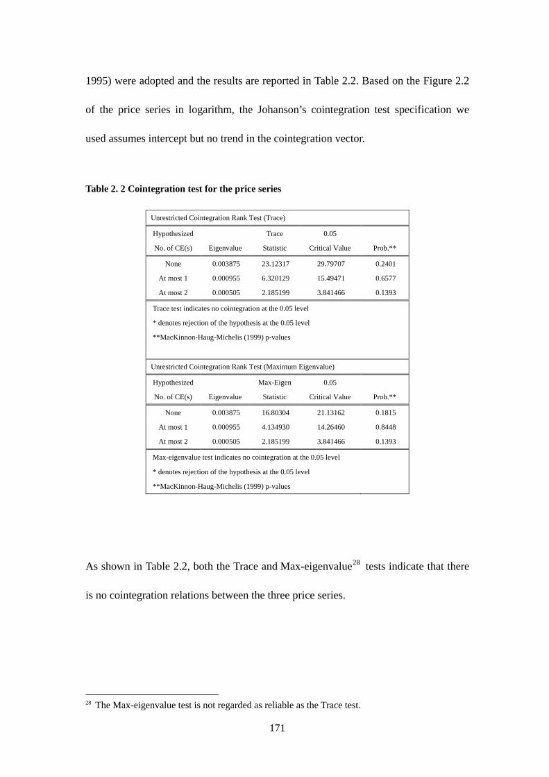
171

1995) were adopted and the results are reported in Table 2.2. Based on the Figure 2.2

of the price series in logarithm, the Johanson’s cointegration test specification we

used assumes intercept but no trend in the cointegration vector.

Table 2. 2 Cointegration test for the price series

As shown in Table 2.2, both the Trace and Max-eigenvalue28 tests indicate that there

is no cointegration relations between the three price series.

28 The Max-eigenvalue test is not regarded as reliable as the Trace test.

Unrestricted Cointegration Rank Test (Trace)

Hypothesized Trace 0.05

No. of CE(s) Eigenvalue Statistic Critical Value Prob.**

None 0.003875 23.12317 29.79707 0.2401

At most 1 0.000955 6.320129 15.49471 0.6577

At most 2 0.000505 2.185199 3.841466 0.1393

Trace test indicates no cointegration at the 0.05 level

* denotes rejection of the hypothesis at the 0.05 level

**MacKinnon-Haug-Michelis (1999) p-values

Unrestricted Cointegration Rank Test (Maximum Eigenvalue)

Hypothesized Max-Eigen 0.05


None 0.003875 16.80304 21.13162 0.1815

At most 1 0.000955 4.134930 14.26460 0.8448

At most 2 0.000505 2.185199 3.841466 0.1393

Max-eigenvalue test indicates no cointegration at the 0.05 level



172

2.3.2 Estimation results for the whole sample period29

In our estimation, we experimented with numerous specification of the mean equation,

for the given structure of conditional variance and covariance (H). For the structure of

the latter, we use full rank in the C matrix. However, when it is impossible to obtain

estimates of the parameters of H, because of singularity or lack of convergence, we

follow the BEKK strategy to set the upper off-diagonal elements equal zero, which

ensures the positive definition of conditional variance and covariance matrix.

From all the permutations of the specification within and across the three returns of

oil, gold futures and stock index for both Tri-variate the Bi-variate GARCH models,

the most minimal specification, of random means, was generally the most acceptable

statistically speaking 30. Where this was not the case, the best mean equations

contained only an intercept or an intercept and one period lagged variables.

The Tri-variate GARCH estimation results are reported in Appendix 2.A. Table 2.A1.

As we can observe, most elements in A and B matrix are significantly different from

zero, indicating that the variance and covariance of each returns series are

time-varying and are impacted by the shocks from its own past and shocks from other

29 Sample period will be divided into three sub-sample periods. Thus we use the whole sample period here. More explanations about the sample splitting are provided later. 30 The appropriate mean settings are chosen by comparing the parameter significance statistics, LR test results for omitting one or more variables and also the log likelihood values for the estimation

173

market, hence the appropriateness of a GARCH framework. The parameters in matrix

A capture the effects from unexpected shocks and the parameters in matrix B capture

the effects from the past conditional volatilities. The diagnostic tests for the maximum

likelihood estimations are provided at the bottom of Table 2.A1. The Ljung-Box Q(10)

Statistics for error terms suggest the autocorrelations in the oil and gold futures

returns have been removed, however, this is not the case for the stock index returns.

Ljung-Box Q statistics for the squared error terms ( 2 (10)Q ) are all significantly

different from zero at 5% significance level, which indicate that the serial correlations

still exist in the second moments of all series. Moreover, we can observe from the

eigenvalues given in the bottom of Table 2.A1 that one of the eigenvalues exceeds 1.

Therefore, the Tri-variate GARCH model for the whole sample period is not

covariance stationary.

To investigate spillovers from Tri-variate GARCH estimation, we also compare these

with the results from Bi-variate GARCH estimation of each pair of variables. The

Bi-variate estimates are reported in Table 2.A2. Again we observe that most elements

in the A and B matrices are significantly different from zero at the 5% significance

level, pointing to the existence of GARCH relations among the error terms. However,

the diagnostic tests suggest that the Bi-variate estimates for the whole sample period

are not covariance stationary for the oil-gold and gold-stock market models (As

reported in at the bottom of the Table 2.A.2, eigenvalues for the two models are not

always smaller than one). The Q(10) statistics for the oil returns series are significant,

174

suggesting the existence of serial correlations. Q(10) statistics for the squared return

series in all of the three markets are strongly significant, so the autocorrelations in the

second moments are not fully removed. Eigenvalues given in Table 2.2 also indicate

the covariance stationary are not satisfied for the Bi-variate estimation of the relations

between oil and gold market, or for the estimation between gold and stock market.

As discussed earlier, the transmission of volatility can be examined by the parameters

in conditional covariance matrix. We summarize the volatility transmission patterns

for Tri- and Bi-variate GARCH estimation of the oil, gold and stock market in Table

2.4. We can conclude from the three Bi-variate estimations that volatilities transmitted

uni-directionally from the gold market to the oil market, from the stock market to the

gold market, and bi-directionally from the oil to the stock market. Except for the

transmission between the oil and stock markets, the relationships are not in line with a

priori expectations. It is normally believed that during the past decade, when the oil

price rallied, the gold price would follow suit. This is because an oil price increase

will raise expected inflation. Investors will buy more gold as it is a reserve asset,

which will raise its price. However, from the volatility point of view, oil market

shocks do not affect gold market volatility directly, at least over a short period. This

indicates that gold is a good hedging asset. On the other hand, the oil market is quite

sensitive to gold market shocks. Gold market volatility is affected by the shocks

emanating from the stock market, but not vice versa.

175

In contrast, the Tri-variate GARCH estimates show that the volatility spillovers are

bi-directional between all three markets, which suggests that oil, gold and stock

markets are intertwined through second moments. The difference between Bi-variate

and Tri-variate GARCH estimation may come from the fact that the Bi-variate results

are obtained when we do not control for any effects from the third market. It seems

that we cannot omit the effect of the third market when we consider the relations

between any pair of markets, at least when describing their second moment

inter-dependence.

The conditional variance and covariance series estimated under different modelling

specification for the three markets are portrayed in Figures 2.4 to 2.9. We can observe

from the Figures 2.4 to 2.6 that the conditional volatility of oil, gold and stock market

estimated by using Tri-variate and two Bi-variate GARCH models follow a similar

pattern. In contrast, the conditional covariances estimated between different methods

obviously diverge from each other, for each of the three markets. This is a

confirmation that the correlations between the two specific markets are largely

affected by the third market.

Descriptive statistics for the conditional variance and covariance series estimated

using different modelling specification are reported in Tables 2.5 and 2.6. In general,

the divergences are very small between different models, especially for the

conditional variance. All the variance and covariance series exhibit non-normality.

176

We can also conclude from Table 2.5 and 2.6 that the variance and covariance

estimated under Bi-variate GARCH models exhibit more peakedness in the estimated

series and consequently larger Jarque-Bera statistics; and the standard deviation for

the covariances estimated using Bi-variate models are higher than those estimated

using the Tri-variate model. All those alternatives bear out the importance of a third,

inter-correlating market.

To investigate whether the variance and covariance series estimated under different

models are statistically similar or not, we perform Equality test for means and

variances for all these series. The results are reported in Table 2.7.

177

Table 2. 3 Volatility spillovers for the whole sample period

ijh

2ij

oil gold stock oil gold stock

oil √ √ √ √ √ √

gold √ √ √ x √ x

stock √ √ √ √ x √

oil gold oil gold

oil √ √ √ √

gold x √ x √

oil stock oil stock

oil √ √ √ √

stock √ √ √ √

gold stock gold stock

gold √ √ √ x

stock x √ x √

Note: √ indicate significant volatility spillover at 5% level

X indicate no significant volatility spillover at 5% level

Table 2. 4 Conditional variances estimated using different models for the whole sample

period

Var(oil) Var(gold) Var(S&P500)

Tri-GARCH

Bi-GARCH

(RO&RG)

Bi-GARCH

(RO&RSP)

Tri-GARCH

Bi-GARCH

(RO & RG)

Bi-GARCH

(RG &RSP)

Tri-GARCH

Bi-GARCH

(RO & RSP)

Bi-GARCH

(RG & RSP)

Mean 4.4547 4.4296 4.4568 0.8137 0.8099 0.8100 0.9544 0.9538 0.9535

Median 4.0836 4.0270 4.0424 0.6446 0.6322 0.6405 0.6454 0.6380 0.6461

Maximum 14.2323 17.9486 15.6205 4.5736 4.8943 4.6511 4.9246 5.2415 5.6397

Minimum 1.1525 1.2879 1.0727 0.0986 0.0964 0.0928 0.1830 0.1707 0.2242

Std. Dev. 2.1904 2.1467 2.3606 0.6549 0.6659 0.6587 0.7807 0.8082 0.8252

Skewness 1.3260 1.3885 1.5499 2.2077 2.3195 2.2327 2.0454 2.1742 2.3649

Kurtosis 5.2664 5.9702 6.1515 9.4735 10.1805 9.6362 7.8883 8.6279 9.7546

Jarque-Bera 2194.13 2980.79 3523.00 11070.29 13175.65 11534.79 7325.30 9119.35 12259.12

Probability 0.0000 0.0000 0.0000 0.0000 0.0000 0.0000 0.0000 0.0000 0.0000

178

Table 2. 5 Statistics for conditional covariances estimated using different models for the

whole sample period

Cov(oil,gold) Cov(oil, sp) Cov(gold, sp)

Tri-GARCH

Bi-GARCH

(RO & RG)

Tri-GARCH

Bi-GARCH

(RO & RSP)

Tri-GARCH

Bi-GARCH

(RG & RSP)

Mean 0.2827 0.2883 -0.0524 -0.0456 -0.0667 -0.0608

Median 0.2126 0.1879 -0.0552 -0.0486 -0.0457 -0.0410

Maximum 1.7707 3.5514 1.4450 1.6626 0.4260 0.4835

Minimum -1.5554 -0.9063 -1.5844 -1.7198 -0.7467 -0.9399

Std. Dev. 0.3571 0.4073 0.2777 0.3061 0.1298 0.1425

Skewness 0.9719 2.3527 0.2985 0.2574 -0.9522 -1.1643

Kurtosis 5.9036 13.3936 8.5007 8.5139 6.1712 8.0714

Jarque-Bera 2201.14 23468.35 5519.54 5529.23 2466.97 5614.42

Probability 0.0000 0.0000 0.0000 0.0000 0.0000 0.0000

Table 2. 6 Equality test for the whole sample period

Mean Variance

Value Probability Value Probability

Var(oil) Tri-(oil,gole, s&p) & Bi-(oil,gold) 0.2895 0.5906 1.0411 0.1853

Tri-(oil,gole, s&p) & Bi-(oil, s&p) 0.0019 0.9652 1.1615 0.0000

Bi-(oil,gold)& Bi-(oil, s&p) 0.3149 0.5747 1.2092 0.0000

Var(gold) Tri-(oil,gole, s&p) & Bi-(oil,gold) 0.0741 0.7854 1.0339 0.2723

Tri-(oil,gole, s&p) & Bi-(gold, s&p) 0.0680 0.7943 1.0118 0.6999

Bi-(oil,gold)& Bi-(gold, s&p) 0.0002 0.9897 1.0219 0.4762

Var(sp) Tri-(oil,gole, s&p) & Bi-(oil,s&p) 0.0012 0.9720 1.0717 0.0228


Bi-(oil,s&p)& Bi-(gold, s&p) 0.0003 0.9868 1.0425 0.1712

Cov(oil,gold) Tri-(oil,gole, s&p) & Bi-(oil,gold) 0.4541 0.5004 1.3008 0.0000

Cov(oil,sp) Tri-(oil,gole, s&p) & Bi-(oil, s&p) 1.1736 0.2787 1.2146 0.0000

Cov(gold,sp) Tri-(oil,gole, s&p) & Bi-(gold, s&p) 4.0415 0.0444 1.2056 0.0000

179

From Table 2.7, we can observe that in most cases, the means of the conditional

variance and covariance series estimated using different models are not significantly

different from each other. However, their variances are different. For the conditional

variance of oil, there is no big divergence between Tri-variate GARCH model and

Bi-variate GARCH model for oil and gold. This suggests that including or not the

stock index return into the endogenous variables group do not affect the estimation

results of the oil variance. On the other hand, the gold shocks cannot be omitted for

the estimation of conditional variance for oil. The variance of gold returns is

somewhat independent from the oil and stock markets. The conditional variance of

S&P returns are both related to oil and gold shocks, as shown by the significance of

the equality test for variance estimated using Tri-variate and Bi-variate GARCH

models. For the conditional covariance of each pair of variables, we can observe that

they largely different between the Tri-variate and Bi-variate specifications. Link back

to the statistic significance of the coefficients on variances and covariances, the

equality tests provide confirmation that the Tri-variate specification is needed for

analyzing the variance and covariance structure of the oil, gold and stock market.

The diagnostic tests for both Tri-variate and Bi-variate GARCH models show that the

serial correlations in squared residuals have not been completely eliminated and

models are not stationary. Thus the models we employed are not appropriate for

describing the whole sample period data. However, we did find the existence of

GARCH effects in the conditional volatility of these three return series. There is a

180

need to redefine the sample period for the models to work. Given the data of

conditional variance and covariance portrayed in Figure 2.4 to Figure 2.9 in Appendix

2.B, the non-stationary estimation results for Tri-variate and Bi-variate GARCH

model are not of surprise. It further suggests that the variance and covariance structure

is affected by the conditions surrounding the markets, which the compartmentalizing

of the data via our three sub-periods aims to capture.

2.3.3 Results for the sub-periods analysis

2.3.3(A) Descriptive statistics for the three sub-samples

From Figure 2.4 and Figure 2.6, we observe that during Oct 1997 to July 2003, the

conditional volatility of oil market and conditional volatility of stock market are much

higher than during the rest of the sample period. Recall that in the late half 1997, there

was huge turmoil in financial markets—the Asia financial crisis. The latter began to

emerge on 2 July 1997 when Thailand abandoned its currency (Baht) peg to the US

dollars. When the financial market opened that day, Baht plunged 15% against the US

dollar and created a currency devaluation panic that spread over the rest of Southeast

Asia. Contagion effects were felt in the whole of the world’s financial markets.

Thereafter, the US financial market experienced a relatively high volatility period, and

the financial market experienced a record expansion after the Asia crisis until 2000.

181

During that period, many stocks had been overvalued, especially those of the internet

companies. In August of 2000, the US stock market experienced a crash, as the

dot-com bubble burst. Then after a short recovery, US stock market slid into a big

Crash from September 11 2001, subsequent to the terrorist attacks on the United

States. Oil prices also declined sharply, largely on increased fear of a sharper

worldwide economic downturn (and therefore sharply lower oil demand). Until the

end of 2001, the stock market began to rally as investors’ confidence came back.

However, staring from March 2002 stock indices started to slid, with dramatic decline

in July and September leading to lows last reaches in 1997 and 1998. At the same

time, oil prices began to increase due to oil production cuts by OPEC and non-OPEC

at the beginning of 2002, plus unrest in the Middle East. At the end of 2003, the US

economy started to resuscitate and the financial markets enter into a relatively low

volatility period.

Thus, we split our whole sample into three sup-samples: pre-crisis period, from 1

April 1991 to 31 March 1997, with relatively low turmoil in the financial market;

crisis period, from 1 April 1997 to 31 July 2003, with relatively high turmoil and thus

high volatility in the financial market; and post-crisis period, 1 August 2003 to 5

November 2007, when volatility in financial market were relatively low.

The descriptive statistics for the three sub-sample periods are reported in Table 2.A3

to 2.A5 in Appendix 2.A, with unit root test results shown at the bottom of each table.

182

The cointegration tests have been performed on the price series to ensure an adequate

modelling specification for our Tri- and Bi-variate GARCH specification. The

Johanson’s cointegration tests results are shown in Table 2.A6 to 2.A8.

Comparing Table 2.A3, 2.A4 and 2.A5, we can conclude that the mean returns for oil

and gold market are increasing during time; the stock market, has its the largest mean

return during the pre-crisis period and the smallest mean in the crisis period. The

standard deviations for oil and stock returns increase in the crisis period, and then

decrease in the post crisis period. For the gold market, the standard deviation is

increasing throughout the three periods, with the post-crisis period exhibiting the

highest volatility. All of the three return series have negative skewness in each period,

expect for the gold return series which has a positive skewness in the crisis period.

The kurtosis statistics are all much higher than the critical value at 5% significance

level, so are the Jarque-Bera statistics. These suggest that the three return series in all

periods have significant peakedness and are not normally distributed. The ADF test

for unit root rejects the null hypothesis that a unit root exist in the series and the KPSS

test result cannot reject the null hypothesis that a unit root does not exist in the return

series. Hence all three series follow an I(0) process in all three sub-periods.

Both Trace and Maximum Eigenvalue test statistics for the Johanson’s cointegration

test shown in Tables 2.A6 to 2.A8 support that there is no cointegrating relationship

between the three price series. These findings together with the fact that return series

183

are all I(0) provide the preconditions for our modelling specification.

2.3.3(B) Estimation results for the three sub-sample periods.

Results for the Tri-variate and Bi-variate GARCH estimates of the conditional

variance and covariance structures are reported in Table 2.A9 to Table 2.A14 in

Appendix 2.A. We observe that the majority of the element in the A and B matrices

are significantly different from zero. The diagnostic checks for both Tri-variate and

Bi-variate GARCH specifications in all the three sub-periods are reported at the

bottom of each table. The Ljung-Box Q(10) statistics show that, for both Bi-variate

and Tri-variate estimation, serial correlations were successfully removed for all

residuals and squared residuals, eliminating potential biases in the estimates. The

eigenvalues for each modelling estimation all have modulus smaller than 1, so that

both types of model are covariance stationary in the three sub-sample periods. Recall

that covariance stationary was not satisfied for the whole sample period; variance and

covariance do change with time and with changes in market conditions.

We summarise the volatility transmission between different markets for the three

sub-sample periods in Table 2.8 to 2.10. In the pre-crisis period, from the Bi-variate

GARCH estimation for oil and gold returns, we can observe that the previous days

184

Table 2. 7 Volatility spillovers for the pre-crisis period (1/04/91—31/03/97).

ijh

2ij

oil gold sp oil gold sp

oil √ x √ √ x √

gold x √ x x √ x

sp x √ √ √ √ √

oil gold oil gold

oil √ √ √ x

gold √ √ √ √

oil sp oil sp

oil √ x √ x

sp x √ x √

gold sp gold sp

gold √ √ √ √

sp √ √ √ √

Note: √ indicate significant volatility spillover at 5% level. X indicate no significant volatility spillover at 5% level

Table 2. 8 Volatility spillovers for the crisis period (1/04/97—31/07/03)

ijh

2ij


oil √ x x √ √ x


sp √ √ √ √ x √

oil gold oil gold

oil √ x √ √

gold √ √ x √

oil sp oil sp

oil √ √ √ x

sp √ √ √ √

gold sp gold sp

gold √ x √ x

sp x √ x √


185

Table 2. 9 Volatility spillovers for the post-crisis period (1/08/03—5/11/07).

ijh

2ij


oil √ x √ √ √ x


sp √ x √ x x √

oil gold oil gold oil √ √ √ √ gold √ √ x √ oil sp oil sp oil x √ √ √ sp √ √ x √ gold sp gold sp gold √ √ √ x sp x √ x √


shocks in the oil market will spill over to the gold market directly, indicated by the

significance of coefficient 212a . The insignificance of coefficient 2

21a implies that

shocks from the gold market in the previous day do not spill over to the oil market

directly. However, the conditional volatility in the oil market is impacted by the

conditional volatility of the gold market, represented by the coefficient 221b . Because

the coefficient 222a is significant, the conditional variance of the gold market is

significantly affected by its own past shocks. Following a similar mechanism, we can

conclude from the Bi-variate GARCH estimates for the oil and gold markets, that the

volatility transmission is bi-directional. Bi-variate estimates for the oil and stock

markets suggest that there is no volatility transmission between them. Bi-variate

186

estimates for gold and S&P returns indicate that the transmission between them is

bi-directional.

Tri-variate GARCH estimates indicate that volatility in the oil market is influenced by

the shocks from its own market as well as by shocks from the stock market. The

lagged gold market shocks have no direct impact on the oil volatility. Gold market

volatility is not affected by shocks from the oil or the stock markets, while the stock

market volatility is affected by the shocks from both gold and stock markets. Thus the

volatility transmission between oil and stock markets is bi-directional. Gold market

volatility looks exogenous. Instead of affect the oil market directly, gold market

volatility transmits to stock market first and then exert impact on the oil market

through its influence on the volatility of the stock market.

Comparing the conclusions we draw from Bi-variate and Tri-variate estimation, we

find that Tri-variate GARCH estimation, which takes into consideration the effect of

conditional and unconditional volatilities of each of the three markets and also the

time varying covariance between each two markets, break the “connections” that

seem to exist between oil and gold, gold and stock market under Bi-variate estimation.

For example, the direct linkage in their second moment between the oil and gold

markets disappear when taking the stock market impact on these two markets into

consideration. In the other way round, we may explain the second moment linkage

between the oil and gold markets as a result of their relations with the stock market. In

187

contrast, the volatility transmission between the oil and stock markets, which is not

obvious when estimated by the Bi-variate GARCH framework, is actually significant

if a Tri-variate GARCH model is used to control the potential gold market impact on

these two markets.

For the crisis period，when the prices for the oil and stock markets are quite volatile,

we can observe from Table 2.9 that, under Bi-variate estimation, volatility between oil

and gold markets is bi-directional. The oil and stock markets also have Bi-variate

volatility transmission. The Bi-variate GRACH estimation results also suggest that

there is no volatility transmission between the gold and stock markets.

The Tri-variate GARCH estimation results reported in Table 2.9 show that volatility

in gold market is exogenous, rather than being affected by the past shocks in oil

market and/or the stock market. Volatility of the oil market is caused by its past

shocks as well as the conditional variance of gold market. Stock market volatility is

determined by its own past shocks, as well as by shocks from the oil and gold markets.

Volatility transmission is uni-directional from the gold market to the oil market, from

the oil market and gold markets to the stock market.

So, Tri-variate estimation gives different structures for the volatility transmission

from the Bi-variate estimation. This again demonstrates that considering the third

market impact can break certain relations that seemed to exist when the third market

188

was excluded. Meanwhile, the Tri-variate estimation may also unveil some of the

relations that seemed not to exist under the Bi-variate framework, for example, the

volatility spillover from the gold market to the stock market.

For the post-crisis period, the volatility of the oil and stock markets become much

smaller than in the crisis period. The volatility transmission relations are shown in

Table 2.10. From the Bi-variate estimation between each pair of markets, we observe

that the volatility transmission between the oil and gold markets are bi-directional, so

is that between the oil and stock markets. Volatility is transmitted from the stock

market to the gold market, but not vice versa. The Tri-variate estimates for the after

crisis period show that the conditional variance, or the volatility of the oil market is

affected by its own past shocks, shocks from stock market as well as shocks from gold

market. The gold market volatility is still exogenous, independent of shocks realized

in either the oil or stock markets. Stock market volatility is affected by its past shocks

as well as shocks from the oil market. So, volatility transmission between the oil and

stock markets is bi-directional. However, volatility spillover is unidirectional from the

gold market to the oil market.

We sum up the volatility transmission mechanism between the three markets using

different modelling specifications in Diagram 2.1. From the three-way volatility

transmission modelled by a Tri-variate GARCH specification, we can observe that,

although generally, in the financial market, when the price of oil goes up the gold

189

price will follow; when it comes to volatility, the gold market takes the lead. There

was insignificant volatility spillover between the oil and gold markets in the pre-crisis

period. With the increasing importance of oil as a resource as well as a financial asset,

we find there are significant volatility spillovers from the gold market to the oil

market in the crisis and post-crisis periods. This suggests that gold is a financial asset

with very low volatility and is not sensitive to the shocks in oil or stock markets. This

explains why gold is one of the most favourable hedging instruments and is normally

regarded as a “safe haven” asset.

Diagram 2.1

Pre Crisis Crisis Post Crisis

Three-way

Volatility

Spillover

(From

Tri-variate

GARCH)

Two-way

Volatility

Spillover

(From

Bi-variate

GARCH)

Represent oil market, represent gold market and represent the US stock market.

Represent the direction of volatility spillover.

190

In contrast to the three-way estimation, the results from Bi-variate GARCH

estimations for the oil and gold markets in the three sub-sample periods all indicate

strong bi-directional linkage in their second moments. Compared with the Tri-variate

estimation, we find that such links between the oil and gold markets is actually

generated from their relations with the stock market. The oil market is very sensitive

to shocks in the gold and stock markets, which accords with expectation. For example,

Gold is a hedging asset largely used by oil companies and international financial

institutions that hold large positions in the oil market. The linkage between the oil and

stock markets is straightforward. Oil, as an extremely important industrial input, is

largely used in every aspect of an economy nowadays. The changes in the economy,

reflected in stock market indices can influence the demand and consumption of oil

substantially.

From Diagram 2.1, we can also observe from the three-way volatility transmission

that stock market volatilities are largely affected by the shocks from the oil and gold

markets. We know that futures markets can normally absorb information quickly.

Thus the spillover from the oil and gold futures markets to the stock market matches

the economic theory. There is substantial hedging in oil and gold markets, altering the

volatility transmission mechanisms across market, thus our results.

The descriptive statistics for the conditional variance and covariance for Tri-variate

and Bi-variate GARCH estimation in the three sub-sample periods are reported in

191

Table 2.11 to Table 2.16, and corresponding data series are portrayed in Figures 2.10

to 2.27.

Comparing the data in Tables 2.11, 2.13 and 2.15, we observe that in the pre-crisis

period, the means of conditional variance for all three series are the lowest. In both the

oil and stock markets, the mean of volatility increased substantially (from around 2.7

to 6.2 for the oil market and from 0.4 to 1.7 for the stock market respectively) during

the crisis period when there were large upheavals in financial markets, then falls after

the crisis, but to a level higher than before the crisis period. Meanwhile, the standard

deviation of the volatility series increases during the crisis period and falls after the

financial market turmoil as well. However, the standard deviation for the oil market in

the post-crisis period is smaller than the pre-crisis period, whereas that for gold

market is higher in the post-crisis than in the pre-crisis period. In the gold market,

mean and standard deviation for the conditional variance of gold returns increase over

time.

The patterns of covariances between each pair of markets also change over time. The

correlation is positive between the oil and gold markets, and negative between the oil

and stock markets. Such findings are consistent with the literature. For example, Nick

Barisheff (2005) state that gold and oil prices moved together with a positive price

correlation. Hammoudeh, Dibooglu and Aleisa (2004) find positive correlation

between the oil market and oil industry equity indices.

192

Table 2. 10 Statistics for the Conditional variances estimated using different models in the

pre-crisis period (1/04/91—31/03/97).

Var (oil) Var (gold) Var (S&P500)

Tri-GARCH

Bi-GARCH

(RO & RG)

Bi-GARCH

(RO & RSP)

Tri-GARCH

Bi-GARCH

(RO & RG)

Bi-GARCH

(RG & RSP)

Tri-GARCH

Bi-GARCH

(RO & RSP)

Bi-GARCH

(RG & RSP)

Mean 2.7667 2.7724 2.7823 0.3642 0.3622 0.3617 0.4173 0.4156 0.4086

Median 2.4612 2.4345 2.3989 0.2774 0.2736 0.2734 0.3922 0.3932 0.3953

Maximum 8.8675 8.4179 10.3275 2.0522 2.1906 2.2826 0.8607 0.8943 0.6714

Minimum 0.9856 1.0017 0.8767 0.0861 0.0808 0.0771 0.2418 0.2302 0.2490

Std. Dev. 1.3204 1.3183 1.4650 0.3038 0.3071 0.3146 0.1092 0.1180 0.0956

Skewness 1.4904 1.4679 1.7156 2.9771 3.0665 3.2002 0.7736 0.6707 0.4220

Kurtosis 5.8638 5.4946 6.8847 13.6892 14.6251 15.5957 3.1122 2.9404 2.2218

Jarque-Bera 1112.03 965.98 1748.42 9743.67 11243.54 12991.66 156.60 117.35 85.78

Probability 0.0000 0.0000 0.0000 0.0000 0.0000 0.0000 0.0000 0.0000 0.0000

Table 2. 11 Statistics for the conditional covariances estimated using different models in the

pre-crisis sample period (1/04/91—31/03/97).

Cov (oil,gold) Cov (oil, sp) Cov (gold, sp)

Tri-GARCH Bi-GARCH

(RO & RG)

Tri-GARCH Bi-GARCH

(RO & RSP)

Tri-GARCH Bi-GARCH

(RG & RSP)

Mean 0.0574 0.0613 -0.0661 -0.0621 -0.0548 -0.0530

Median 0.0384 0.0404 -0.0586 -0.0536 -0.0472 -0.0469

Maximum 0.8014 1.1334 0.3526 0.3923 0.1620 0.0952

Minimum -0.6662 -0.3571 -0.6266 -0.6655 -0.2171 -0.3224

Std. Dev. 0.1766 0.1559 0.1390 0.1397 0.0500 0.0435

Skewness 0.4678 1.6914 -0.2987 -0.4021 -0.3712 -1.7003

Kurtosis 6.0373 9.9716 3.6645 4.0314 4.3080 9.2552

Jarque-Bera 657.38 3908.11 51.97 111.31 147.22 3299.22

Probability 0.0000 0.0000 0.0000 0.0000 0.0000 0.0000

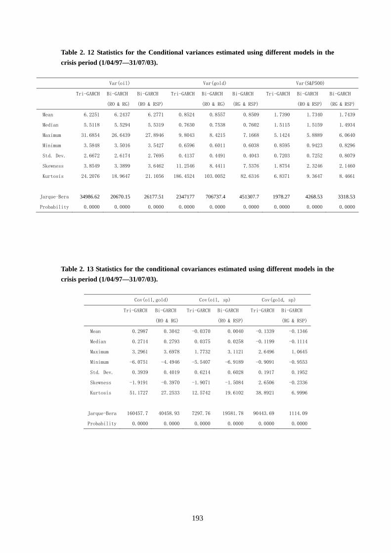
193

Table 2. 12 Statistics for the Conditional variances estimated using different models in the

crisis period (1/04/97—31/07/03).


Bi-GARCH Bi-GARCH Bi-GARCH Bi-GARCH Bi-GARCH Bi-GARCH Tri-GARCH

(RO & RG) (RO & RSP)

Tri-GARCH

(RO & RG) (RG & RSP)

Tri-GARCH

(RO & RSP) (RG & RSP)

Mean 6.2251 6.2437 6.2771 0.8524 0.8557 0.8509 1.7390 1.7340 1.7439

Median 5.5118 5.5294 5.5319 0.7630 0.7538 0.7602 1.5115 1.5159 1.4934

Maximum 31.6854 26.6439 27.8946 9.8043 8.4215 7.1668 5.1424 5.8889 6.0640

Minimum 3.5848 3.5016 3.5427 0.6596 0.6011 0.6038 0.8595 0.9423 0.8296

Std. Dev. 2.6672 2.6174 2.7695 0.4137 0.4491 0.4043 0.7203 0.7252 0.8079

Skewness 3.8549 3.3899 3.6462 11.2546 8.4411 7.5376 1.8754 2.3246 2.1460

Kurtosis 24.2076 18.9647 21.1056 186.4524 103.0052 82.6316 6.8371 9.3647 8.4661

Jarque-Bera 34986.62 20670.15 26177.51 2347177 706737.4 451307.7 1978.27 4268.53 3318.53

Probability 0.0000 0.0000 0.0000 0.0000 0.0000 0.0000 0.0000 0.0000 0.0000


crisis period (1/04/97—31/07/03).


Bi-GARCH Bi-GARCH Bi-GARCH Tri-GARCH

(RO & RG)

Tri-GARCH

(RO & RSP)

Tri-GARCH

(RG & RSP)

Mean 0.2987 0.3042 -0.0370 0.0040 -0.1339 -0.1346

Median 0.2714 0.2793 0.0375 0.0258 -0.1199 -0.1114

Maximum 3.2961 3.6978 1.7732 3.1121 2.6496 1.0645

Minimum -6.0751 -4.4946 -5.5407 -6.9189 -0.9091 -0.9553

Std. Dev. 0.3939 0.4019 0.6214 0.6028 0.1917 0.1952

Skewness -1.9191 -0.3970 -1.9071 -1.5084 2.6506 -0.2336

Kurtosis 51.1727 27.2533 12.5742 19.6102 38.8921 6.9996

Jarque-Bera 160457.7 40458.93 7297.76 19581.78 90443.69 1114.09

Probability 0.0000 0.0000 0.0000 0.0000 0.0000 0.0000

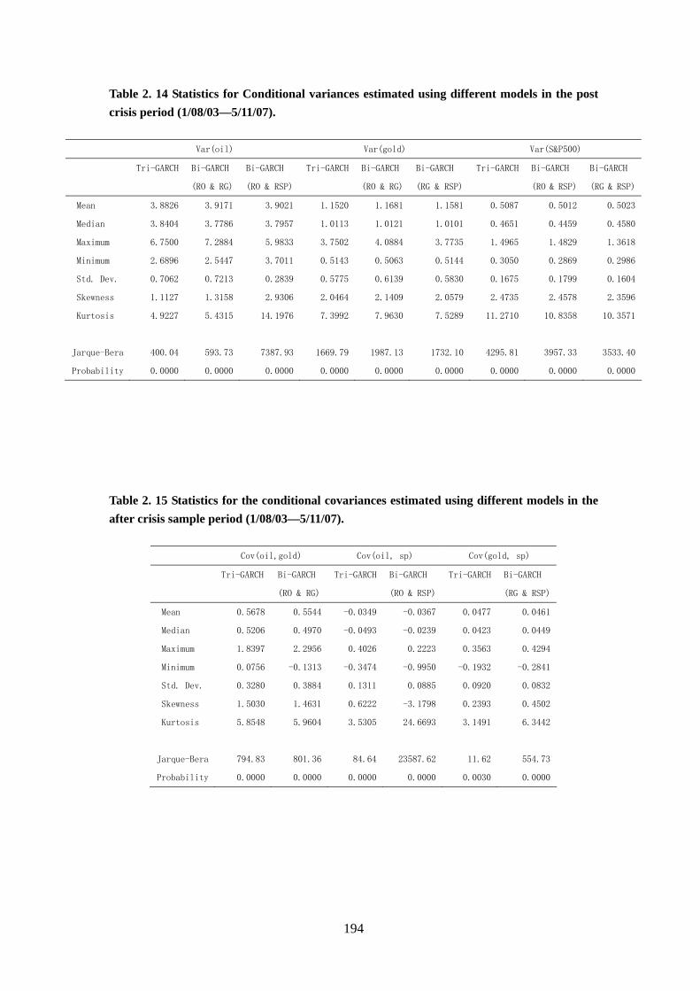
194

Table 2. 14 Statistics for Conditional variances estimated using different models in the post

crisis period (1/08/03—5/11/07).


Bi-GARCH Bi-GARCH Bi-GARCH Bi-GARCH Bi-GARCH Bi-GARCH Tri-GARCH

(RO & RG) (RO & RSP)

Tri-GARCH

(RO & RG) (RG & RSP)

Tri-GARCH

(RO & RSP) (RG & RSP)

Mean 3.8826 3.9171 3.9021 1.1520 1.1681 1.1581 0.5087 0.5012 0.5023

Median 3.8404 3.7786 3.7957 1.0113 1.0121 1.0101 0.4651 0.4459 0.4580

Maximum 6.7500 7.2884 5.9833 3.7502 4.0884 3.7735 1.4965 1.4829 1.3618

Minimum 2.6896 2.5447 3.7011 0.5143 0.5063 0.5144 0.3050 0.2869 0.2986

Std. Dev. 0.7062 0.7213 0.2839 0.5775 0.6139 0.5830 0.1675 0.1799 0.1604

Skewness 1.1127 1.3158 2.9306 2.0464 2.1409 2.0579 2.4735 2.4578 2.3596

Kurtosis 4.9227 5.4315 14.1976 7.3992 7.9630 7.5289 11.2710 10.8358 10.3571

Jarque-Bera 400.04 593.73 7387.93 1669.79 1987.13 1732.10 4295.81 3957.33 3533.40

Probability 0.0000 0.0000 0.0000 0.0000 0.0000 0.0000 0.0000 0.0000 0.0000


after crisis sample period (1/08/03—5/11/07).


Bi-GARCH Bi-GARCH Bi-GARCH Tri-GARCH

(RO & RG)

Tri-GARCH

(RO & RSP)

Tri-GARCH

(RG & RSP)

Mean 0.5678 0.5544 -0.0349 -0.0367 0.0477 0.0461

Median 0.5206 0.4970 -0.0493 -0.0239 0.0423 0.0449

Maximum 1.8397 2.2956 0.4026 0.2223 0.3563 0.4294

Minimum 0.0756 -0.1313 -0.3474 -0.9950 -0.1932 -0.2841

Std. Dev. 0.3280 0.3884 0.1311 0.0885 0.0920 0.0832

Skewness 1.5030 1.4631 0.6222 -3.1798 0.2393 0.4502

Kurtosis 5.8548 5.9604 3.5305 24.6693 3.1491 6.3442

Jarque-Bera 794.83 801.36 84.64 23587.62 11.62 554.73

Probability 0.0000 0.0000 0.0000 0.0000 0.0030 0.0000

195

The correlation between gold and stock market is negative in the pre-crisis and crisis

period, but positive after the crisis period. Chan and Faff (1988) found that gold has a

positive sensitivity to the resource and mining sector industries, but negative

sensitivity in industrial sectors. Thus it is not surprising to find that the correlation

between the gold and stock markets is not constant during time, depending upon the

effects across different sectors. Moreover, the intensive use of gold as a hedging

method in the post-crisis period may also make the correlations between the gold and

stock markets hard to capture. The correlation relationship may change with the

change of time-span in consideration.

The comparison of variances and covariance between different models are portrayed

in Figures 2.10 to 2.27, for pre-crisis, crisis, and post-crisis periods. The divergences

between the conditional variances of oil, gold and stock returns estimated with

different models are not obvious from the figures, except for the conditional variance

of oil in the after crisis period. The conditional variance estimated from Bi-variate

GARCH model for oil and S&P returns largely diverge from that estimated from the

Tri-variate GARCH specification as well as from the Bi-variate GARCH specification

between oil and gold. The divergence between covariance estimated using the

Bi-variate and Tri-variate models is apparent. The graphs give a general idea of the

estimated conditional variance and covariance comparisons. To examine these in a

much clearer manner, we perform the equality test for the means and variances of

those conditional series.

196

The Equality test results are reported in Tables 2.17-2.19 for each of the three

sub-sample periods. The means of the conditional variance and covariance series are

almost equal under different modelling strategies. However, most variances estimated

using different modelling specifications are not equal. For the pre-crisis period, the

conditional variance of oil is not significantly affected by its correlation with the stock

market or by the correlation between the gold and stock markets. The conditional

variance of gold is relatively exogenous. As shown in Table 2.17, the conditional

variance for gold estimated using different models give similar answers. The

conditional variance of oil is affected by shocks from both the oil and gold markets.

The conditional covariance between the oil and gold, the gold and stock markets are

different when estimated by Tri-variate or Bi-variate models. However, the

conditional covariance of the oil and stock markets estimated using different models

are more or less the same. For the crisis period, although the conditional variances

estimated under different modelling strategies are different from each other, the

conditional covariance between each two markets is more or less the same under

Tri-variate and Bi-variate modelling strategy. For the after crisis period, the

conditional covariances show large divergences between the Tri-variate or Bi-variate

models, as they do in the pre-crisis period. Conditional variances generated using

these two modelling strategies are also different in terms of variance equality.

197

Table 2. 16 Equality test for the pre-crisis period (1/04/91—31/03/97).

Mean Probability Variance Probability







Var(sp) Tri-(oil,gole, s&p) & Bi-(oil, s&p) 0.1916 0.6616 1.1680 0.0022


Bi-(oil, s&p) & Bi-(gold, s&p) 3.2642 0.0709 1.5225 0.0000


Cov(oil,sp) Tri-(oil,gole, s&p) & Bi-(gold, s&p) 0.6426 0.4228 1.0100 0.8439


Table 2. 17 Equality test for the crisis period (1/04/97—31/07/03)










Bi-(oil, s&p) & Bi-(oil,gold) 0.1349 0.7134 1.2413 0.0000




198

Table 2. 18 Equality test for the post-crisis period (1/08/03—5/11/07).










Bi-(oil, s&p) & Bi-(oil,gold) 0.0211 0.8845 1.2572 0.0001




199

2.4 Conclusion and further research

2.4.1 Conclusion

This research aims to examine the relationships between the oil, gold and stock

markets. With the integration of financial markets and the increasing importance of oil

and gold as commodities as well as financial instruments, an investigation of the

relations between the three markets is very important. Instead of focusing on the price

and returns relations, we focus on the second moments relationships. Our research is

the first (to the best of our knowledge) of this kind and can be very useful in many

aspects. For example, it can provide information for investors to speculate in financial

markets, for investors or companies to hedge risk, or for decision markers to

understand the market.

Tri-variate GARCH (1,1) models are adopted to examine volatility spillovers between

oil, gold and stock markets. To investigate fully such volatility transmission relations,

we compare the results from Tri-variate GARCH estimation to those from Bi-variate

estimation for each pair of markets. US data are examined because it is the leading

economy in the world and plays an important role in both the oil and gold markets.

We also split the whole sample into three sub-sample periods for investigative

purposes.

200

Our findings are consistent with the past literature in that we find volatility spills over

from the oil market to the stock market, from the gold market to the stock market.

Despite the obvious price and return links between oil and gold markets, the volatility

inter-relations are not so obvious between them. The gold market is kind of

exogenous in terms of volatility. The bi-directional volatility transmission between

the oil and gold markets, which is suggested by the Bi-variate GARCH estimates,

actually results from their linkage with the stock market. The oil market is quite

sensitive to the shocks from both the gold and stock markets, and the stock market is

strongly impacted by the volatility in the oil and gold markets.

Comparing the estimation results from Bi-variate and Tri-variate GARCH models,

our research finds that the Tri-variate GARCH model, by adding an additional

variable to the existing Bi-variate GARCH framework, can break some of the existing

relationships between the variables and can also reveal some of the linkages we

cannot observe in the Bi-variate estimation.

Equality tests are performed on the conditional variance and covariance series

estimated using Tri-variate and Bi-variate modelling strategies to examine whether

these estimated values are statistically different. Over all, the mean equality tests

statistics for the variance are generally not significant at the 5% level. However, most

variance equality tests statistics for the covariance are significantly different from zero.

The mean and variance equality test statistics for the covariances are mostly

201

significance at the 5% level. These indicate that the conditional variances and

covariances estimated using the Tri-variate model and Bi-variate models are

effectively different. The covariance between two markets is significantly affected by

the third market. Tri-variate GARCH models can capture these effects and offer

potentially more information concerning the inter-relationship between the three

markets.

2.4.2 Further research

One possible use of this research is to provide useful information for market hedgers

to hedge risk. For example, assume an investor hold a position in stock market. When

stock market is not performing well, investors tend to buy gold as a means to reserve

value (which may lead to higher gold value when the stock price falls). However,

holding physical gold is costly. For one thing, holding gold in the beginning of the

investment period instead of holding futures would tie up capital that could be

invested in a market with potential higher return, e.g. stock market. This is the

opportunity cost of holding physical gold commodity. For another, holding physical

gold can lead to storage cost. An alternative choice for the investor is to use futures,

which is more flexible and less costly. The investor can go long gold in the futures

market if they expect a slump in the stock market in future. If the stock return does

fall as expected or fall more than expected, the investor can buy gold with the price

202

which has been locked up in the futures contract, which tend to be lower than the

market gold price at that time. If the stock returns do not fall as expected, investors

can just taking an offsetting position in the futures market. This could possibly lead to

some losses in the futures trading, but the loss will be fully or partially offset by the

gain in the stock market. One important issue for the hedging is deciding the number

of gold futures contract to buy. In such case, the investor needs to calculate the

optimal hedge ratios31, which is a function of the variance and covariance of the stock

and gold markets. Traditionally, only these two markets (products) will be considered

to derive the optimal hedging ratio. However, these two markets are both linked to a

third market, the oil market. Our study find that when taking the oil market into

consideration, the conditional variance and covariance between the stock and gold

market will change, and therefore the derived optimal hedge ratios. Such is also true

for hedging strategies in other markets. One further study that may be very interesting

is to investigate whether the hedging effectiveness can be improved when taking a

third market impact into consideration.

This study can also be extended in other ways. For example, with the rapid growth of

developing countries like China and India, their market-shares in the oil consumption

and gold trading are increasing. Our research can be extended to examine how

volatilities are transmitted across the world oil, gold markets and the stock market in

developing countries. Moreover, different sectors have different oil and gold

31 Optimal hedging ratio derivation and hedging effectiveness evaluation are discussed in the Essay 1 of this thesis.

203

sensitivity. To explore how different sectors in an economy are linked to the oil and

gold markets is also a very interesting research topic to work on.

204

References:

Admati, A, and P. P1eiderer (1988), “A Theory of Intraday Patterns: Volume and

Price Variability”, Review of Financial Studies, 1, 3-40.

Alizadeth, A. and Nomikos, N. (2004), “A Markov Regime Switching Approach for

Hedging Stock Indices”, The Journal of Futures Markets, 24 (7), 649-674.

Amir H. Alizadeh, Nikos K. Nomikos and Panos K. Pouliasis (2008), “Markov

regime switching approach for hedging energy commodities”, Journal of

Banking & Finance, Volume 32, Issue 9, 1970-1983

Baele, L., Ferrando, A., Hordahl, P., Krylova, E., and C. Monnet (2004), “Measuring

financial integration in the Euro area”, Occasional Paper 14, European Central

Bank.

Becker, K.G., Finnerty, J.E., and M. Gupta (1990), “The intertemporal relation

between the US and Japanese stock markets”, Journal of Finance, 45,

1297-1306.

Blose and Shieh (1995), “The impact of gold price on the value of gold mining stock”,

Review of financial Economics, 4, 125-193

Booth, G.G., Chowdhury, M., Martikainen, T., and Y, Tse (1997), “Intraday volatility

in international stock index futures markets: meteor showers or heat waves?”

Management Science, 43, 1564-1576.

Booth, G.G., Martikainen, T., and Y. Tse(1997). “Price and volatilities spillovers in

Scandinavian stock markets”, Journal of Banking and Finance, 21, 811-823.

Bollerslev, T., (1986), “Generalized autoregressive conditional heteroskedasticity”,

Journal of Econometrics, 31, 307-327.

Chan, H. and R. Faff (1998), “The sensitivity of Australian industry equity returns to

a gold price factor”, Accounting and Finance, 38, 223-244.

Campbell , J.Y. and L. Hentschel (1992), “No News is Good News: An Asymmetric

Model of Changing Volatility in Stock Returns”, Journal of Financial

Economics, Vol 31 , 281 - 318.

Ciner, C., (2001), “On the longrun relationship between gold and silver: a note”,

http://www.sciencedirect.com/science/journal/03784266�

http://www.sciencedirect.com/science/journal/03784266�

http://www.sciencedirect.com/science?_ob=PublicationURL&_tockey=%23TOC%235967%232008%23999679990%23695729%23FLA%23&_cdi=5967&_pubType=J&view=c&_auth=y&_acct=C000010083&_version=1&_urlVersion=0&_userid=122868&md5=f86cdf3a93606303e3de6425c6907e86�

205

Journal of Global Finance, 12, 299-303.

Dickey, D.A. and W.A.Fuller (1979), “Distribution of the Estimation for

Autoregressive Time Series With a Unit Root”, Journal of the American

Statistical Association, 74,427-31.

Goodman, B., (1956), “The price of gold and international liquidity”, Journal of

finance, 11, 15-28

El-Sharif, Brown, Burton, Nixon and Russell (2005), "Evidence of the Nature and

Extent of the Relationship between Oil Prices and Equity Values in the UK",

Energy Economics, Vol 27, pp.819-830.

Engle, R.F. (1982), “Autoregressive Conditional Heteroscedasticity with Estimates of

the Variance of UK Inflation”, Econometrica. Vol 50. 987-1008.

Engle, R.F., Ito, T., Lin, W., (1990), “Meteor showers or heatwaves? Heteroskedastic

intra-day volatility in the foreign exchange market”, Econometrica, 58,

525-542.

Engle, R. F., and Ng, V. K. (1993), “Measuring and testing the impact of news on

volatility”, Journal of Finance, 48, 1749-1778.

Eun, C.S. and S.Shim (1989), “International Transmission of Stock Market

Movements”, The Journal of Financial and Quantitative Analysis, Vol 24,

241-256

Hamao, Y., Masulis, R.W., Ng, V. (1990), “Correlations in price changes and

volatility across international stock markets”, Review of Financial Studies, 3,

281-307.

Hammoudeh, S., & Aleisa, E. E. (2002), “Relationship between spot/futures prices of

crude oil, and equity indices for oil producing economies and oil-related

industries”, Arab Economic Journal, 11, 37–62.

Hammoudeh, S., S. Dibooglu and E. Aleisa (2004), “Relationships among US Oil

Prices and Oil Industry Equity Indices”, International Review of Economics

and Finance, Vol. 13, no.3.

Hammoudeh, S., and Malik, F. (2005), “Shock and volatility transmission in the oil,

US and Gulf equity markets.” International review of Economics and Finance.

206

16, 357-368

Huang, R., Masulis, R., & Stoll, H. (1996), “Energy shocks and financial markets”,

Journal of Futures Markets, 16, 1–27.

Ito, T., Lin, W.L. (1994), “Price volatility and volume spillovers between the Tokyo

and New York stock markets”, In: Frankel, J.A. (Ed.), The

Internationalization of Equity Markets. National Bureau of Economic

Research, University of Chicago Press, pp. 309–343.

Johansen, S. (1991), “Estimation and hypothesis testing of cointegration vectors in

Gaussian vector autoregressive models”, Econometrica, 59, 1551-1580.

Jones, C., & Kaul, G. (1996), “Oil and stock markets”, Journal of Finance, 51,

463–491.

Jones, D.W., Leiby, P.N., Park, I.K.(2004), “Oil price shocks and the macroeconomy:

what has been learned since 1996”, Energy Journal, 25 (2), 1-32.

Kearney C,Patton A. (2000), “Multivariate GARCH model of exchange rate volatility

in the European monetary system”, The Financial Review, 41, 29-48.

Koutmos, G., Booth, G. (1995), “Asymmetric volatility transmission in international

stock markets”, Journal of International Money and Finance, 14, 747–762.

Koutsoyiannis, A. (1983), “A short-run pricing model for a speculative asset, tested

with data from the gold bullion market”, Applied Economics, 15, 563-581.

Kyle, A.S., (1985), “Continuous auctions and insider trading”, Econometrica, 53,

1315-1335.

Larsen, A.B and G.R. McQueen (1995), “REITS, real estate and inflation: lesson from

the gold market”, Journal of Real Estate Finance and Economics, 10,

563-297.

Lee, H. and Yoder, J. (2007), “A bivariate Markov regime switching GARCH

approach to estimate time varying minimum variance hedge ratios”, Applied

Economics, 39, 1253-1265.

Lin, W., Engle, R.F., Ito, T. (1994), “Do bulls and bears move across borders?

International transmission of stock returns and volatility”, Review of Financial

Studies, 7, 507-538.

207

Mussa, I.A. and Al-Loughani, N.E. (1994), “Unbiasedness and time varying risk

premia in the crude oil futures markets”, Energy Economics, 16, 99-105.

Nelson, D.B. (1991), “Conditional heteroskedasticity in asset returns: A new

approach”, Econometrica, 59, 347–370.

Prasad, E., Rogoff, K., Wei, S.-J., Kose, M.A. (2003), “The effects of financial

globalization on developing countries: Some empirical evidence”, IMF

Occasional paper no. 220.

Rose, S.A. (1989), “Information and volatility: The No-Arbitrage Martingale

Approach to Timing and Resolution Irrelevancy”, Journal of Finance, 45,

1-17.

Sadorsky, P. (1999), “Oil price shocks and stock market activity”, Energy Economics,

21, 449–469.

Shalen, C.T. (1993), “Volume. Volatility, and the Dispersion of Beliefs”, Review of

Financial Studies, 6, 405-434.

Shishko, L. (1977), “Why gold?” Journal of Portfolio Management, 4, 34-40.

Solt, M. & P. Swanson (1981), “On the efficiency of the market for gold and silver”,

Journal of Business, 54, 453-478.

Susmel, R., Engle, R.F., (1994), “Hourly volatility spillovers between international

equity markets”, Journal of International Money Finance, 13, 3-25.

Tse, Y. (1998), “International transmission of information: evidence from the Euroyen

and Eurodollar futures markets.” Journal of International Money and Finance,

17, 909-929.

Wang, S., Rui, O., and M. Firth (2002), “Return and volatility behavior of

dually-traded stocks: the case of Hong Kong.” Journal of International Money

and Finance, 21, 265-293.

208

Figure 2. 1 Oil and gold price in logarithm

2.0

2.5

3.0

3.5

4.0

4.5

5.0

5.2

5.6

6.0

6.4

6.8

91 92 93 94 95 96 97 98 99 00 01 02 03 04 05 06 07

LG LO

LO LG

Figure 2. 2 Price series in logarithm

5.5

6.0

6.5

7.0

7.5

2.0

2.5

3.0

3.5

4.0

4.5

5.0

91 92 93 94 95 96 97 98 99 00 01 02 03 04 05 06 07

LG LO LSP

LOLG/LSP

209

Figure 2. 3 Returns series for oil gold and stock index

-20

-15

-10

-5

0

5

10

15

1991 1992 1993 1994 1995 1996 1997 1998 1999 2000 2001 2002 2003 2004 2005 2006 2007

RO

-8

-6

-4

-2

0

2

4

6

8

10

1991 1992 1993 1994 1995 1996 1997 1998 1999 2000 2001 2002 2003 2004 2005 2006 2007

RG

-8

-6

-4

-2

0

2

4

6

1991 1992 1993 1994 1995 1996 1997 1998 1999 2000 2001 2002 2003 2004 2005 2006 2007

RSP

210

Figure 2. 4 Conditional variance of the oil returns for the whole sample period

0

2

4

6

8

10

12

14

16

18

20

Entry

1991:07:22

1991:11:06

1992:02:21

1992:06:09

1992:09:24

1993:01:11

1993:04:28

1993:08:13

1993:11:30

1994:03:17

1994:07:04

1994:10:19

1995:02:03

1995:05:23

1995:09:07

1995:12:25

1996:04:10

1996:07:26

1996:11:12

1997:02:27

1997:06:16

1997:10:01

1998:01:16

1998:05:05

1998:08:20

1998:12:07

1999:03:24

1999:07:09

1999:10:26

2000:02:10

2000:05:29

2000:09:13

2000:12:29

2001:04:17

2001:08:02

2001:11:19

2002:03:06

2002:06:21

2002:10:08

2003:01:23

2003:05:12

2003:08:27

2003:12:12

2004:03:30

2004:07:15

2004:11:01

2005:02:16

2005:06:03

2005:09:20

2006:01:05

2006:04:24

2006:08:09

2006:11:24

2007:03:13

2007:06:28

2007:10:15

H(ro)-Tri

H(ro)-Bi(ro,rg)

H(ro)-Bi(ro,rsp)

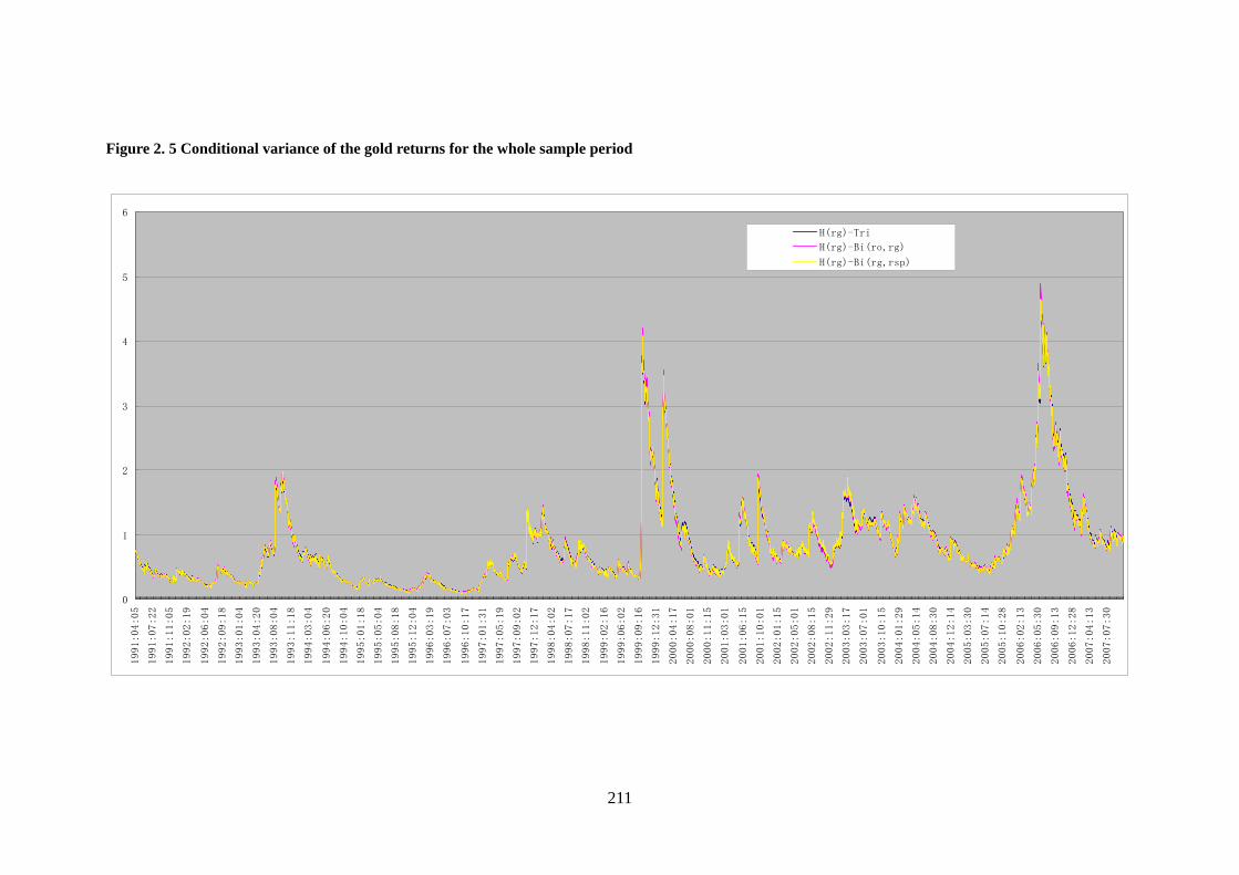
211

Figure 2. 5 Conditional variance of the gold returns for the whole sample period

0

1

2

3

4

5

6

1991:04:05

1991:07:22

1991:11:05

1992:02:19

1992:06:04

1992:09:18

1993:01:04

1993:04:20

1993:08:04

1993:11:18

1994:03:04

1994:06:20

1994:10:04

1995:01:18

1995:05:04

1995:08:18

1995:12:04

1996:03:19

1996:07:03

1996:10:17

1997:01:31

1997:05:19

1997:09:02

1997:12:17

1998:04:02

1998:07:17

1998:11:02

1999:02:16

1999:06:02

1999:09:16

1999:12:31

2000:04:17

2000:08:01

2000:11:15

2001:03:01

2001:06:15

2001:10:01

2002:01:15

2002:05:01

2002:08:15

2002:11:29

2003:03:17

2003:07:01

2003:10:15

2004:01:29

2004:05:14

2004:08:30

2004:12:14

2005:03:30

2005:07:14

2005:10:28

2006:02:13

2006:05:30

2006:09:13

2006:12:28

2007:04:13

2007:07:30

H(rg)-Tri

H(rg)-Bi(ro,rg)

H(rg)-Bi(rg,rsp)

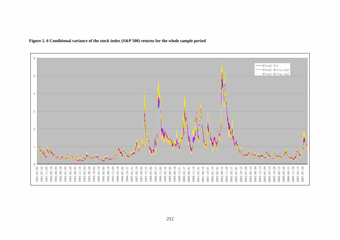
212

Figure 2. 6 Conditional variance of the stock index (S&P 500) returns for the whole sample period

0

1

2

3

4

5

6

1991:04:05

1991:07:22

1991:11:05

1992:02:19

1992:06:04

1992:09:18

1993:01:04

1993:04:20

1993:08:04

1993:11:18

1994:03:04

1994:06:20

1994:10:04

1995:01:18

1995:05:04

1995:08:18

1995:12:04

1996:03:19

1996:07:03

1996:10:17

1997:01:31

1997:05:19

1997:09:02

1997:12:17

1998:04:02

1998:07:17

1998:11:02

1999:02:16

1999:06:02

1999:09:16

1999:12:31

2000:04:17

2000:08:01

2000:11:15

2001:03:01

2001:06:15

2001:10:01

2002:01:15

2002:05:01

2002:08:15

2002:11:29

2003:03:17

2003:07:01

2003:10:15

2004:01:29

2004:05:14

2004:08:30

2004:12:14

2005:03:30

2005:07:14

2005:10:28

2006:02:13

2006:05:30

2006:09:13

2006:12:28

2007:04:13

2007:07:30

H(rsp)-Tri

H(rsp)-Bi(ro,rsp)

H(rsp)-Bi(rg,rsp)

213

Figure 2. 7 Conditional Covariance between the oil and gold markets for the whole sample period

-2

-1

0

1

2

3

4

1991:04:05

1991:08:05

1991:12:03

1992:04:01

1992:07:30

1992:11:27

1993:03:29

1993:07:27

1993:11:24

1994:03:24

1994:07:22

1994:11:21

1995:03:21

1995:07:19

1995:11:16

1996:03:15

1996:07:15

1996:11:12

1997:03:12

1997:07:10

1997:11:07

1998:03:09

1998:07:07

1998:11:04

1999:03:04

1999:07:02

1999:11:01

2000:02:29

2000:06:28

2000:10:26

2001:02:23

2001:06:25

2001:10:23

2002:02:20

2002:06:20

2002:10:18

2003:02:17

2003:06:17

2003:10:15

2004:02:12

2004:06:11

2004:10:11

2005:02:08

2005:06:08

2005:10:06

2006:02:03

2006:06:05

2006:10:03

2007:01:31

2007:05:31

2007:09:28

Cov(ro,rg)-Tri Cov(ro,rg)-Bi

214

Figure 2. 8 Conditional Covariance between the oil and stock markets for the whole sample period

-2

-1.5

-1

-0.5

0

0.5

1

1.5

2

1991:04:05

1991:08:05

1991:12:03

1992:04:01

1992:07:30

1992:11:27

1993:03:29

1993:07:27

1993:11:24

1994:03:24

1994:07:22

1994:11:21

1995:03:21

1995:07:19

1995:11:16

1996:03:15

1996:07:15

1996:11:12

1997:03:12

1997:07:10

1997:11:07

1998:03:09

1998:07:07

1998:11:04

1999:03:04

1999:07:02

1999:11:01

2000:02:29

2000:06:28

2000:10:26

2001:02:23

2001:06:25

2001:10:23

2002:02:20

2002:06:20

2002:10:18

2003:02:17

2003:06:17

2003:10:15

2004:02:12

2004:06:11

2004:10:11

2005:02:08

2005:06:08

2005:10:06

2006:02:03

2006:06:05

2006:10:03

2007:01:31

2007:05:31

2007:09:28

Cov(ro,rsp)-Tri Cov(ro,rsp)-Bi

215

Figure 2. 9 Conditional Covariance between the gold and stock markets for the whole sample period

-1.2

-1

-0.8

-0.6

-0.4

-0.2

0

0.2

0.4

0.6

1991:04:05

1991:08:06

1991:12:05

1992:04:06

1992:08:05

1992:12:04

1993:04:06

1993:08:05

1993:12:06

1994:04:06

1994:08:05

1994:12:06

1995:04:06

1995:08:07

1995:12:06

1996:04:05

1996:08:06

1996:12:05

1997:04:07

1997:08:06

1997:12:05

1998:04:07

1998:08:06

1998:12:07

1999:04:07

1999:08:06

1999:12:07

2000:04:06

2000:08:07

2000:12:06

2001:04:06

2001:08:07

2001:12:06

2002:04:08

2002:08:07

2002:12:06

2003:04:08

2003:08:07

2003:12:08

2004:04:07

2004:08:06

2004:12:07

2005:04:07

2005:08:08

2005:12:07

2006:04:07

2006:08:08

2006:12:07

2007:04:09

2007:08:08

Cov(rg,rsp)-Tri

Cov(rg,rsp)-Bi

216

Figure 2. 10 Conditional variance of the oil returns in the pre-crisis period (1/04/91—31/03/97).

0

2

4

6

8

10

12

1991:04:05

1991:05:21

1991:07:04

1991:08:19

1991:10:02

1991:11:15

1991:12:31

1992:02:13

1992:03:30

1992:05:13

1992:06:26

1992:08:11

1992:09:24

1992:11:09

1992:12:23

1993:02:05

1993:03:23

1993:05:06

1993:06:21

1993:08:04

1993:09:17

1993:11:02

1993:12:16

1994:01:31

1994:03:16

1994:04:29

1994:06:14

1994:07:28

1994:09:12

1994:10:26

1994:12:09

1995:01:24

1995:03:09

1995:04:24

1995:06:07

1995:07:21

1995:09:05

1995:10:19

1995:12:04

1996:01:17

1996:03:01

1996:04:16

1996:05:30

1996:07:15

1996:08:28

1996:10:11

1996:11:26

1997:01:09

1997:02:24

H(ro)-Tri H(ro)-Bi(ro,rg) H(ro)-Bi(ro,rsp)

217

Figure 2. 11 Conditional variance of the gold returns in the pre-crisis period(1/04/91—31/03/97).

0

0.5

1

1.5

2

2.5

1991:04:05

1991:05:21

1991:07:04

1991:08:19

1991:10:02

1991:11:15

1991:12:31

1992:02:13

1992:03:30

1992:05:13

1992:06:26

1992:08:11

1992:09:24

1992:11:09

1992:12:23

1993:02:05

1993:03:23

1993:05:06

1993:06:21

1993:08:04

1993:09:17

1993:11:02

1993:12:16

1994:01:31

1994:03:16

1994:04:29

1994:06:14

1994:07:28

1994:09:12

1994:10:26

1994:12:09

1995:01:24

1995:03:09

1995:04:24

1995:06:07

1995:07:21

1995:09:05

1995:10:19

1995:12:04

1996:01:17

1996:03:01

1996:04:16

1996:05:30

1996:07:15

1996:08:28

1996:10:11

1996:11:26

1997:01:09

1997:02:24

H(rg)-Tri H(rg)-Bi(ro,rg) H(rg)-Bi(rg,rsp)

218

Figure 2. 12 Conditional variance of the stock returns in the pre-crisis period (1/04/91—31/03/97).

0

0.1

0.2

0.3

0.4

0.5

0.6

0.7

0.8

0.9

1

1991:04:05

1991:05:21

1991:07:04

1991:08:19

1991:10:02

1991:11:15

1991:12:31

1992:02:13

1992:03:30

1992:05:13

1992:06:26

1992:08:11

1992:09:24

1992:11:09

1992:12:23

1993:02:05

1993:03:23

1993:05:06

1993:06:21

1993:08:04

1993:09:17

1993:11:02

1993:12:16

1994:01:31

1994:03:16

1994:04:29

1994:06:14

1994:07:28

1994:09:12

1994:10:26

1994:12:09

1995:01:24

1995:03:09

1995:04:24

1995:06:07

1995:07:21

1995:09:05

1995:10:19

1995:12:04

1996:01:17

1996:03:01

1996:04:16

1996:05:30

1996:07:15

1996:08:28

1996:10:11

1996:11:26

1997:01:09

1997:02:24

H(rsp)-Tri H(rsp)-Bi(ro,rsp) H(rsp)-Bi(rg,rsp)

219

Figure 2. 13 Conditional Covariance between the oil and gold market in the pre-crisis period (1/04/91—31/03/97).

-0.8

-0.6

-0.4

-0.2

0

0.2

0.4

0.6

0.8

1

1.2

1.4

Entry

1991:05:17

1991:07:01

1991:08:13

1991:09:25

1991:11:07

1991:12:20

1992:02:03

1992:03:17

1992:04:29

1992:06:11

1992:07:24

1992:09:07

1992:10:20

1992:12:02

1993:01:14

1993:02:26

1993:04:12

1993:05:25

1993:07:07

1993:08:19

1993:10:01

1993:11:15

1993:12:28

1994:02:09

1994:03:24

1994:05:06

1994:06:20

1994:08:02

1994:09:14

1994:10:27

1994:12:09

1995:01:23

1995:03:07

1995:04:19

1995:06:01

1995:07:14

1995:08:28

1995:10:10

1995:11:22

1996:01:04

1996:02:16

1996:04:01

1996:05:14

1996:06:26

1996:08:08

1996:09:20

1996:11:04

1996:12:17

1997:01:29

1997:03:13

Cov(ro,rg)-Tri

Cov(ro,rg)-Bi

220

Figure 2. 14 Conditional Covariance between the oil and stock markets in the pre-crisis period (1/04/91—31/03/97).

-0.8

-0.6

-0.4

-0.2

0

0.2

0.4

0.6

1991:04:05

1991:05:21

1991:07:04

1991:08:19

1991:10:02

1991:11:15

1991:12:31

1992:02:13

1992:03:30

1992:05:13

1992:06:26

1992:08:11

1992:09:24

1992:11:09

1992:12:23

1993:02:05

1993:03:23

1993:05:06

1993:06:21

1993:08:04

1993:09:17

1993:11:02

1993:12:16

1994:01:31

1994:03:16

1994:04:29

1994:06:14

1994:07:28

1994:09:12

1994:10:26

1994:12:09

1995:01:24

1995:03:09

1995:04:24

1995:06:07

1995:07:21

1995:09:05

1995:10:19

1995:12:04

1996:01:17

1996:03:01

1996:04:16

1996:05:30

1996:07:15

1996:08:28

1996:10:11

1996:11:26

1997:01:09

1997:02:24

Cov(ro,rsp)-Tri

Cov(ro,rsp)-Bi

221

Figure 2. 15 Conditional Covariance between the gold and stock markets in the pre-crisis period (1/04/91—31/03/97).

-0.4

-0.3

-0.2

-0.1

0

0.1

0.2

1991:04:05

1991:05:20

1991:07:02

1991:08:14

1991:09:26

1991:11:08

1991:12:23

1992:02:04

1992:03:18

1992:04:30

1992:06:12

1992:07:27

1992:09:08

1992:10:21

1992:12:03

1993:01:15

1993:03:01

1993:04:13

1993:05:26

1993:07:08

1993:08:20

1993:10:04

1993:11:16

1993:12:29

1994:02:10

1994:03:25

1994:05:09

1994:06:21

1994:08:03

1994:09:15

1994:10:28

1994:12:12

1995:01:24

1995:03:08

1995:04:20

1995:06:02

1995:07:17

1995:08:29

1995:10:11

1995:11:23

1996:01:05

1996:02:19

1996:04:02

1996:05:15

1996:06:27

1996:08:09

1996:09:23

1996:11:05

1996:12:18

1997:01:30

1997:03:14

Cov(rg,rsp)-Tri Cov(rg,rsp)-Bi

222

Figure 2. 16 Conditional variance of the oil returns in the crisis period (1/04/97—31/07/03).

0

5

10

15

20

25

30

35

1997:04:07

1997:05:23

1997:07:10

1997:08:27

1997:10:14

1997:12:01

1998:01:16

1998:03:05

1998:04:22

1998:06:09

1998:07:27

1998:09:11

1998:10:29

1998:12:16

1999:02:02

1999:03:22

1999:05:07

1999:06:24

1999:08:11

1999:09:28

1999:11:15

1999:12:31

2000:02:17

2000:04:05

2000:05:23

2000:07:10

2000:08:25

2000:10:12

2000:11:29

2001:01:16

2001:03:05

2001:04:20

2001:06:07

2001:07:25

2001:09:11

2001:10:29

2001:12:14

2002:01:31

2002:03:20

2002:05:07

2002:06:24

2002:08:09

2002:09:26

2002:11:13

2002:12:31

2003:02:17

2003:04:04

2003:05:22

2003:07:09

H(ro)-Tri H(ro)-Bi(ro,rg)

H(ro)-Bi(ro,rsp)

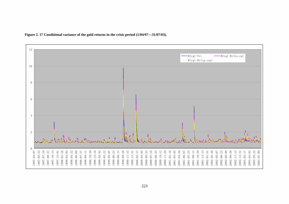
223

Figure 2. 17 Conditional variance of the gold returns in the crisis period (1/04/97—31/07/03).

0

2

4

6

8

10

12

1997:04:07

1997:05:23

1997:07:10

1997:08:27

1997:10:14

1997:12:01

1998:01:16

1998:03:05

1998:04:22

1998:06:09

1998:07:27

1998:09:11

1998:10:29

1998:12:16

1999:02:02

1999:03:22

1999:05:07

1999:06:24

1999:08:11

1999:09:28

1999:11:15

1999:12:31

2000:02:17

2000:04:05

2000:05:23

2000:07:10

2000:08:25

2000:10:12

2000:11:29

2001:01:16

2001:03:05

2001:04:20

2001:06:07

2001:07:25

2001:09:11

2001:10:29

2001:12:14

2002:01:31

2002:03:20

2002:05:07

2002:06:24

2002:08:09

2002:09:26

2002:11:13

2002:12:31

2003:02:17

2003:04:04

2003:05:22

2003:07:09

H(rg)-Tri H(rg)-Bi(ro,rg)

H(rg)-Bi(rg,rsp)

224

Figure 2. 18 Conditional variance of the S&P 500 returns in the crisis period (1/04/97—31/07/03).

0

1

2

3

4

5

6

7

1997:04:07

1997:05:23

1997:07:10

1997:08:27

1997:10:14

1997:12:01

1998:01:16

1998:03:05

1998:04:22

1998:06:09

1998:07:27

1998:09:11

1998:10:29

1998:12:16

1999:02:02

1999:03:22

1999:05:07

1999:06:24

1999:08:11

1999:09:28

1999:11:15

1999:12:31

2000:02:17

2000:04:05

2000:05:23

2000:07:10

2000:08:25

2000:10:12

2000:11:29

2001:01:16

2001:03:05

2001:04:20

2001:06:07

2001:07:25

2001:09:11

2001:10:29

2001:12:14

2002:01:31

2002:03:20

2002:05:07

2002:06:24

2002:08:09

2002:09:26

2002:11:13

2002:12:31

2003:02:17

2003:04:04

2003:05:22

2003:07:09

H(rsp)-Tri H(rsp)-Bi(ro,rsp)

H(rsp)-Bi(rg,rsp)

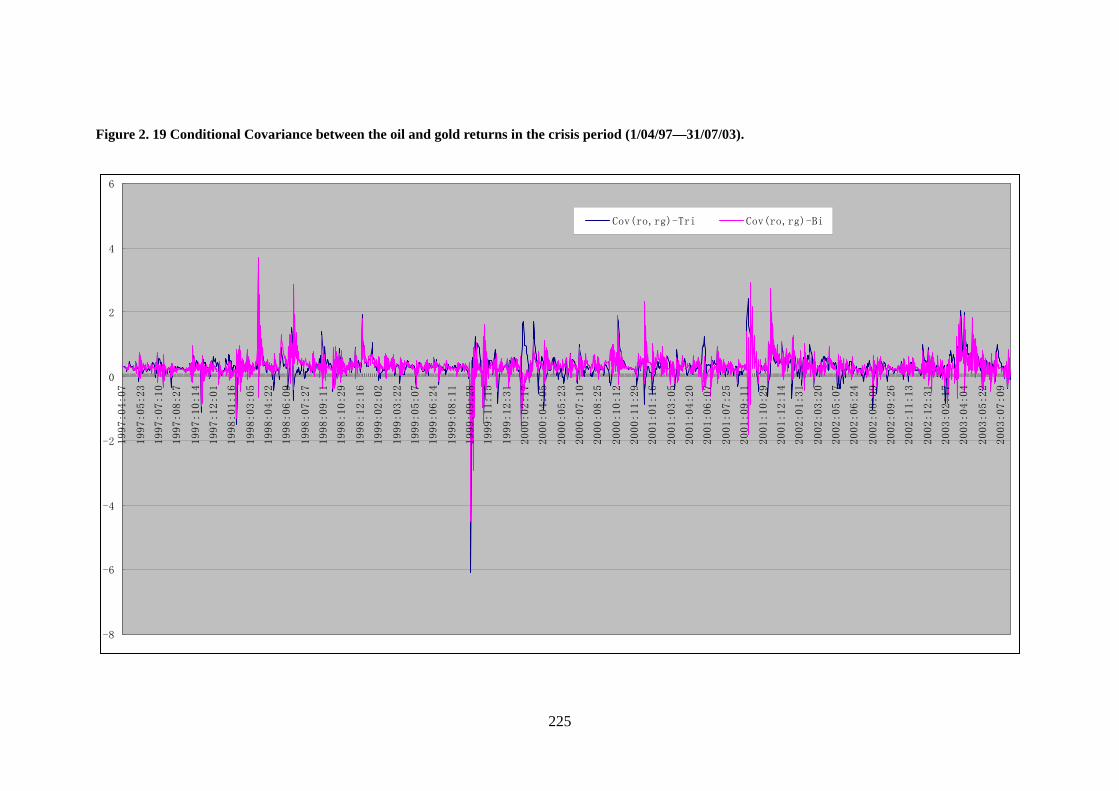
225

Figure 2. 19 Conditional Covariance between the oil and gold returns in the crisis period (1/04/97—31/07/03).

-8

-6

-4

-2

0

2

4

6

1997:04:07

1997:05:23

1997:07:10

1997:08:27

1997:10:14

1997:12:01

1998:01:16

1998:03:05

1998:04:22

1998:06:09

1998:07:27

1998:09:11

1998:10:29

1998:12:16

1999:02:02

1999:03:22

1999:05:07

1999:06:24

1999:08:11

1999:09:28

1999:11:15

1999:12:31

2000:02:17

2000:04:05

2000:05:23

2000:07:10

2000:08:25

2000:10:12

2000:11:29

2001:01:16

2001:03:05

2001:04:20

2001:06:07

2001:07:25

2001:09:11

2001:10:29

2001:12:14

2002:01:31

2002:03:20

2002:05:07

2002:06:24

2002:08:09

2002:09:26

2002:11:13

2002:12:31

2003:02:17

2003:04:04

2003:05:22

2003:07:09


226

Figure 2. 20 Conditional Covariance between the oil and stock returns in the crisis period(1/04/97—31/07/03).

-7

-5

-3

-1

1

3

1997:04:07

1997:05:23

1997:07:10

1997:08:27

1997:10:14

1997:12:01

1998:01:16

1998:03:05

1998:04:22

1998:06:09

1998:07:27

1998:09:11

1998:10:29

1998:12:16

1999:02:02

1999:03:22

1999:05:07

1999:06:24

1999:08:11

1999:09:28

1999:11:15

1999:12:31

2000:02:17

2000:04:05

2000:05:23

2000:07:10

2000:08:25

2000:10:12

2000:11:29

2001:01:16

2001:03:05

2001:04:20

2001:06:07

2001:07:25

2001:09:11

2001:10:29

2001:12:14

2002:01:31

2002:03:20

2002:05:07

2002:06:24

2002:08:09

2002:09:26

2002:11:13

2002:12:31

2003:02:17

2003:04:04

2003:05:22

2003:07:09


227

Figure 2. 21 Conditional Covariance between the gold and stock returns in the crisis period (1/04/97—31/07/03).

-1.5

-1

-0.5

0

0.5

1

1.5

2

2.5

3

1997:04:07

1997:05:23

1997:07:10

1997:08:27

1997:10:14

1997:12:01

1998:01:16

1998:03:05

1998:04:22

1998:06:09

1998:07:27

1998:09:11

1998:10:29

1998:12:16

1999:02:02

1999:03:22

1999:05:07

1999:06:24

1999:08:11

1999:09:28

1999:11:15

1999:12:31

2000:02:17

2000:04:05

2000:05:23

2000:07:10

2000:08:25

2000:10:12

2000:11:29

2001:01:16

2001:03:05

2001:04:20

2001:06:07

2001:07:25

2001:09:11

2001:10:29

2001:12:14

2002:01:31

2002:03:20

2002:05:07

2002:06:24

2002:08:09

2002:09:26

2002:11:13

2002:12:31

2003:02:17

2003:04:04

2003:05:22

2003:07:09


228

Figure 2. 22 Conditional variance of the oil returns in the post-crisis period (1/08/03—5/11/07).

0

1

2

3

4

5

6

7

8

2003:08:05

2003:09:08

2003:10:10

2003:11:13

2003:12:17

2004:01:20

2004:02:23

2004:03:26

2004:04:29

2004:06:02

2004:07:06

2004:08:09

2004:09:10

2004:10:14

2004:11:17

2004:12:21

2005:01:24

2005:02:25

2005:03:31

2005:05:04

2005:06:07

2005:07:11

2005:08:12

2005:09:15

2005:10:19

2005:11:22

2005:12:26

2006:01:27

2006:03:02

2006:04:05

2006:05:09

2006:06:12

2006:07:14

2006:08:17

2006:09:20

2006:10:24

2006:11:27

2006:12:29

2007:02:01

2007:03:07

2007:04:10

2007:05:14

2007:06:15

2007:07:19

2007:08:22

2007:09:25

2007:10:29

H(ro)-Tri H(ro)-Bi(ro,rg)

H(ro)-Bi(ro,rsp)

229

Figure 2. 23 Conditional variance of the gold returns in the post-crisis period (1/08/03—5/11/07).

0

0.5

1

1.5

2

2.5

3

3.5

4

4.5

2003:08:05

2003:09:08

2003:10:10

2003:11:13

2003:12:17

2004:01:20

2004:02:23

2004:03:26

2004:04:29

2004:06:02

2004:07:06

2004:08:09

2004:09:10

2004:10:14

2004:11:17

2004:12:21

2005:01:24

2005:02:25

2005:03:31

2005:05:04

2005:06:07

2005:07:11

2005:08:12

2005:09:15

2005:10:19

2005:11:22

2005:12:26

2006:01:27

2006:03:02

2006:04:05

2006:05:09

2006:06:12

2006:07:14

2006:08:17

2006:09:20

2006:10:24

2006:11:27

2006:12:29

2007:02:01

2007:03:07

2007:04:10

2007:05:14

2007:06:15

2007:07:19

2007:08:22

2007:09:25

2007:10:29

H(rg)-Tri H(rg)-Bi(ro,rg)

H(rg)-Bi(rg,rsp)

230

Figure 2. 24 Conditional variance of the stock returns in the post-crisis period (1/08/03—5/11/07).

0

0.2

0.4

0.6

0.8

1

1.2

1.4

1.6

2003:08:05

2003:09:08

2003:10:10

2003:11:13

2003:12:17

2004:01:20

2004:02:23

2004:03:26

2004:04:29

2004:06:02

2004:07:06

2004:08:09

2004:09:10

2004:10:14

2004:11:17

2004:12:21

2005:01:24

2005:02:25

2005:03:31

2005:05:04

2005:06:07

2005:07:11

2005:08:12

2005:09:15

2005:10:19

2005:11:22

2005:12:26

2006:01:27

2006:03:02

2006:04:05

2006:05:09

2006:06:12

2006:07:14

2006:08:17

2006:09:20

2006:10:24

2006:11:27

2006:12:29

2007:02:01

2007:03:07

2007:04:10

2007:05:14

2007:06:15

2007:07:19

2007:08:22

2007:09:25

2007:10:29

H(rsp)-Tri H(rsp)-Bi(ro,rsp)

H(rsp)-Bi(rg,rsp)

231

Figure 2. 25 Conditional Covariance between the oil and gold returns in the post-crisis period (1/08/03—5/11/07).

-0.5

0

0.5

1

1.5

2

2.5

2003:08:05

2003:09:05

2003:10:08

2003:11:10

2003:12:11

2004:01:13

2004:02:13

2004:03:17

2004:04:19

2004:05:20

2004:06:22

2004:07:23

2004:08:25

2004:09:27

2004:10:28

2004:11:30

2004:12:31

2005:02:02

2005:03:07

2005:04:07

2005:05:10

2005:06:10

2005:07:13

2005:08:15

2005:09:15

2005:10:18

2005:11:18

2005:12:21

2006:01:23

2006:02:23

2006:03:28

2006:04:28

2006:05:31

2006:07:03

2006:08:03

2006:09:05

2006:10:06

2006:11:08

2006:12:11

2007:01:11

2007:02:13

2007:03:16

2007:04:18

2007:05:21

2007:06:21

2007:07:24

2007:08:24

2007:09:26

2007:10:29


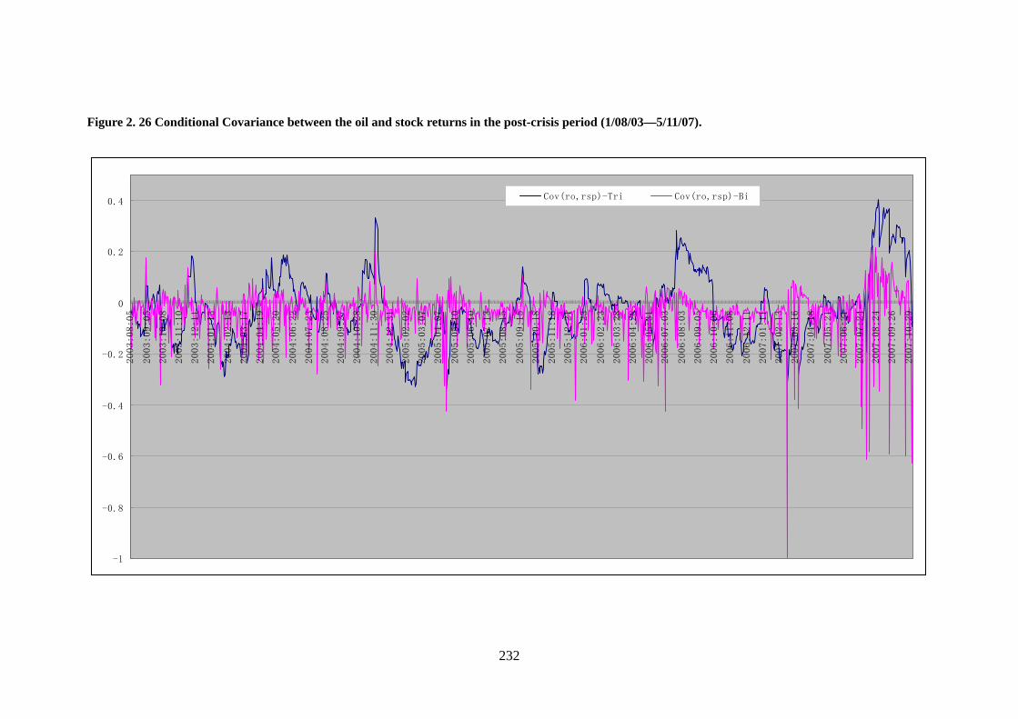
232

Figure 2. 26 Conditional Covariance between the oil and stock returns in the post-crisis period (1/08/03—5/11/07).

-1

-0.8

-0.6

-0.4

-0.2

0

0.2

0.4

2003:08:05

2003:09:05

2003:10:08

2003:11:10

2003:12:11

2004:01:13

2004:02:13

2004:03:17

2004:04:19

2004:05:20

2004:06:22

2004:07:23

2004:08:25

2004:09:27

2004:10:28

2004:11:30

2004:12:31

2005:02:02

2005:03:07

2005:04:07

2005:05:10

2005:06:10

2005:07:13

2005:08:15

2005:09:15

2005:10:18

2005:11:18

2005:12:21

2006:01:23

2006:02:23

2006:03:28

2006:04:28

2006:05:31

2006:07:03

2006:08:03

2006:09:05

2006:10:06

2006:11:08

2006:12:11

2007:01:11

2007:02:13

2007:03:16

2007:04:18

2007:05:21

2007:06:21

2007:07:24

2007:08:24

2007:09:26

2007:10:29


233

Figure 2. 27 Conditional Covariance between the gold and stock returns in the post-crisis period (1/08/03—5/11/07).

-0.4

-0.3

-0.2

-0.1

0

0.1

0.2

0.3

0.4

0.5

2003:08:05

2003:09:05

2003:10:08

2003:11:10

2003:12:11

2004:01:13

2004:02:13

2004:03:17

2004:04:19

2004:05:20

2004:06:22

2004:07:23

2004:08:25

2004:09:27

2004:10:28

2004:11:30

2004:12:31

2005:02:02

2005:03:07

2005:04:07

2005:05:10

2005:06:10

2005:07:13

2005:08:15

2005:09:15

2005:10:18

2005:11:18

2005:12:21

2006:01:23

2006:02:23

2006:03:28

2006:04:28

2006:05:31

2006:07:03

2006:08:03

2006:09:05

2006:10:06

2006:11:08

2006:12:11

2007:01:11

2007:02:13

2007:03:16

2007:04:18

2007:05:21

2007:06:21

2007:07:24

2007:08:24

2007:09:26

2007:10:29


234

Appendix 2 A

Table 2.A 1 Estimation results from the Tri-variate GARCH model in the whole sample

period

2

, , , 11 21 31 11 12 13 11 21 31 , 1 , 1 , 1 , 1 ,

, , , 12 22 32 21 22 23 12 22 32

, , , 13 23 33 31 32 33 13 23 33

oo t og t os t o t o t g t o t s t

t og t gg t gs t

os t gs t ss t

h h h c c c c c c a a a

H h h h c c c c c c a a a


1 11 12 132

, 1 , 1 , 1 , 1 , 1 21 22 232

, 1 , 1 , 1 , 1 , 1 31 32 33

11 21 31 , 1 , 1 , 1

12 22 32 , 1 , 1 , 1

13 23 33 , 1

o t g t g t g t s t

o t s t g t s t s t

oo t og t os t

og t gg t gs t

os t g

a a a

a a a

a a a

b b b h h h

b b b h h h

b b b h h

11 12 13

21 22 23

, 1 , 1 31 32 33s t ss t

b b b

b b b

h b b b

Variable Coeff Std Error T-Stat Signif

11c 0.1325*** 0.0255 5.1866 0.0000

21c ---- ---- ---- ----

31c ---- ---- ---- ----

12c -0.0153 0.0105 -1.4569 0.1451

22c 0.0308*** 0.0119 2.5829 0.0098

32c ---- ---- ---- ----

13c 0.0160 0.0174 0.9173 0.3590

23c -0.0375*** 0.0121 -3.0977 0.0020

33c 0.0001 0.0311 0.0047 0.9962

11b 0.9747*** 0.0077 126.81 0.0000

21b 0.0171*** 0.0052 3.2791 0.0010

31b -0.2533** 0.1101 -2.3011 0.0214

12b 0.0068*** 0.0020 3.4802 0.0005

22b 0.9820*** 0.0030 322.27 0.0000

32b 0.1517*** 0.0231 6.5527 0.0000

13b -0.0807*** 0.0198 -4.0667 0.0000

23b 0.0479*** 0.0111 4.3073 0.0000

33b -0.9698*** 0.0076 -128.45 0.0000

11a 0.1530*** 0.0178 8.6101 0.0000

21a -0.0488* 0.0265 -1.8416 0.0655

31a -0.0858*** 0.0294 -2.9137 0.0036

12a -0.0051 0.0046 -1.0928 0.2745

22a 0.1704*** 0.0188 9.0624 0.0000

32a -0.0106 0.0145 -0.7323 0.4640

13a 0.0180*** 0.0045 3.9861 0.0001

23a 0.0036 0.0066 0.5520 0.5810

33a 0.1702*** 0.0227 7.4807 0.0000


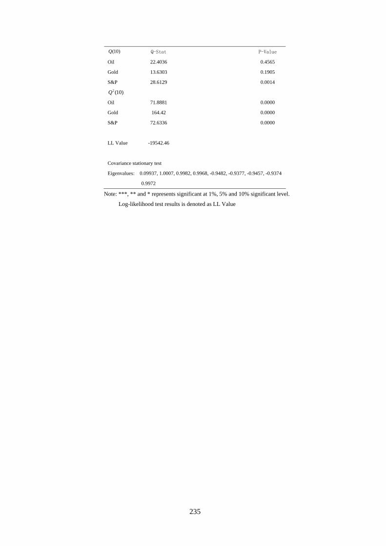
235

(10)Q Q-Stat P-Value

Oil 22.4036 0.4565

Gold 13.6303 0.1905

S&P 28.6129 0.0014

2 (10)Q

Oil 71.8881 0.0000

Gold 164.42 0.0000

S&P 72.6336 0.0000

LL Value -19542.46

Covariance stationary test Eigenvalues: 0.09937, 1.0007, 0.9982, 0.9968, -0.9482, -0.9377, -0.9457, -0.9374

0.9972

Note: ***, ** and * represents significant at 1%, 5% and 10% significant level.

Log-likelihood test results is denoted as LL Value

236

Table 2.A 2 Estimation results of the Bi-variate GARCH models for the whole sample period

2

11, 12, 11, 1 12, 111 21 11 12 11 21 11 12 11 211, 1 1, 1 2, 12

12, 22, 12, 1 22, 112 22 21 22 12 22 21 22 12 221, 1 2, 1 1, 1

t t t tt t tt

t t t tt t t

h h h hc c c cH

h h h hc c c c

11 12

21 22

oil and gold oil and S&P Gold and S&P

Variable Coeff Std Error T-Stat Coeff Std Error T-Stat Coeff Std Error T-Stat

11c -0.0941*** 0.0228 -4.1184 0.1355*** 0.0267 5.0688 0.0345*** 0.0102 3.3939

21c 0.0884*** 0.0231 3.8306 ---- ---- ---- ---- ---- ----

12c 0.0254*** 0.0070 3.6443 0.0167 0.0394 0.4229 -0.0712*** 0.0148 -4.8067

22c -0.0270*** 0.0069 -3.8957 -0.0414 0.0297 -1.3932 -0.0064 0.0254 -0.2503

11b -0.9706*** 0.0105 -92.0648 -0.9732*** 0.0084 -115.77 0.9831*** 0.0054 181.4681

21b 0.8619*** 0.1261 6.8347 0.2555** 0.1258 2.0307 0.1455*** 0.0458 3.1746

12b 0.0270 0.0185 1.4619 0.0741*** 0.0230 3.2171 0.0305 0.0554 0.5503

22b 0.9724*** 0.0092 105.44 0.9716*** 0.0079 123.2103 -0.9732*** 0.0074 -131.17

11a 0.1678*** 0.0207 8.0908 0.1673*** 0.0197 8.5075 0.1722*** 0.0165 10.4366

21a -0.0830*** 0.0244 -3.4049 -0.0970*** 0.0239 -4.0573 -0.0202 0.0166 -1.2181

12a -0.0011 0.0035 -0.3236 0.0177*** 0.0054 3.2652 0.0042 0.0130 0.3203

22a 0.1794*** 0.0201 8.9080 0.1853*** 0.0227 8.1585 0.2082*** 0.0205 10.1429


(10)Q Q-Stat P-Value Q-Stat P-Value Q-Stat P-Value

Oil 10.3549 0.4099 Oil 8.9532 0.5366 Gold 14.1439 0.1665

Gold 12.6294 0.2451 S&P 29.4811 0.0010 S&P 24.3089 0.0068

2 (10)Q

Oil 51.0827 0.0000 Oil 59.6375 0.0000 Gold 170.4528 0.0000

Gold 133.96 0.0000 S&P 61.9162 0.0000 S&P 24.5504 0.0063

LL -14108 LL -14520 LL -10496

Covariance stationary test Eigenvalue of Bi-GARCH for oil and gold market : 0.9940, 1.004, -0.9369; -0.9371

For oil and S&P : 0.9253, 0.9971, -0.9001, -0.8968

For gold and S&P : 1.0007, 0.9260, -0.8900, -0.8899

Note: ***, ** and * represents significant at 1%, 5% and 10% significant level.

237

Table 2.A 3 Descriptive statistics of return series in pre-crisis period (1/04/91—31/03/97).

RO RG RSP

Mean 0.0036 -0.0018 0.0455

Median 0.0000 0.0000 0.0155

Maximum 8.5395 2.6222 2.8962

Minimum -9.1199 -5.7085 -3.7271

Std. Dev. 1.6629 0.5923 0.6452

Skewness -0.1214 -0.6658 -0.2937

Kurtosis 5.6985 11.9599 5.2945

Jarque-Bera 478.68 5350.50 365.80

Probability 0.0000 0.0000 0.0000

(10)Q 20.05** 8.73 16.47

2 (10)Q 102.85** 119.43** 29.38**

ARCH_LM 11.74** 13.22** 4.39**

ADF -38.81** -40.30** -37.86**

KPSS 0.0476 0.0995 0.2014

Note: ** represents significant at 1% significance level.

Table 2.A 4 Descriptive statistics of return series in crisis period (1/04/97—31/07/03).

RO RG RSP

Mean 0.0244 0.0005 0.0162

Median 0.0000 0.0000 0.0000

Maximum 14.2309 8.8872 5.5732

Minimum -16.5445 -5.1049 -7.1127

Std. Dev. 2.4792 0.9299 1.3201

Skewness -0.3464 1.0892 -0.0490

Kurtosis 7.1659 14.5912 5.1359

Jarque-Bera 1228.37 9580.65 314.88

Probability 0.0000 0.0000 0.0000

(10)Q 15.3600 11.1900 10.2700

2 (10)Q 48.97** 97.94** 193.52**

ARCH_LM 7.78** 12.40** 17.25**

ADF -30.40** -40.59** -41.57**

KPSS 0.0796 0.2715 0.4805


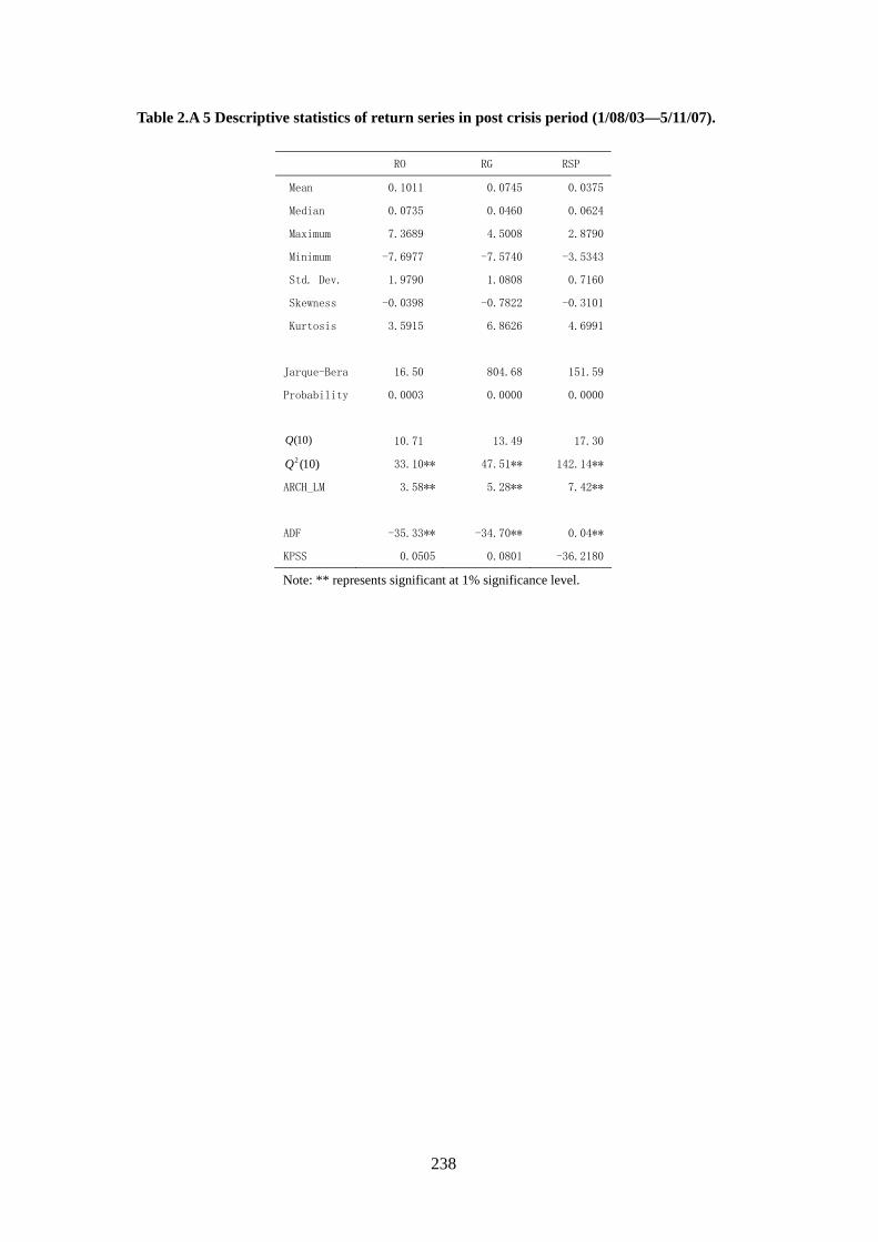
238

Table 2.A 5 Descriptive statistics of return series in post crisis period (1/08/03—5/11/07).

RO RG RSP

Mean 0.1011 0.0745 0.0375

Median 0.0735 0.0460 0.0624

Maximum 7.3689 4.5008 2.8790

Minimum -7.6977 -7.5740 -3.5343

Std. Dev. 1.9790 1.0808 0.7160

Skewness -0.0398 -0.7822 -0.3101

Kurtosis 3.5915 6.8626 4.6991

Jarque-Bera 16.50 804.68 151.59

Probability 0.0003 0.0000 0.0000

(10)Q 10.71 13.49 17.30

2 (10)Q 33.10** 47.51** 142.14**

ARCH_LM 3.58** 5.28** 7.42**

ADF -35.33** -34.70** 0.04**

KPSS 0.0505 0.0801 -36.2180


239

Table 2.A 6 Cointegration test for logarithm price series in pre-crisis period

(1/04/91—31/03/97).




None 0.008597 17.79686 29.79707 0.5811

At most 1 0.002741 4.292770 15.49471 0.8785

At most 2 4.21E-07 0.000658 3.841466 0.9809







None 0.008597 13.50409 21.13162 0.4070

At most 1 0.002741 4.292112 14.26460 0.8273

At most 2 4.21E-07 0.000658 3.841466 0.9809




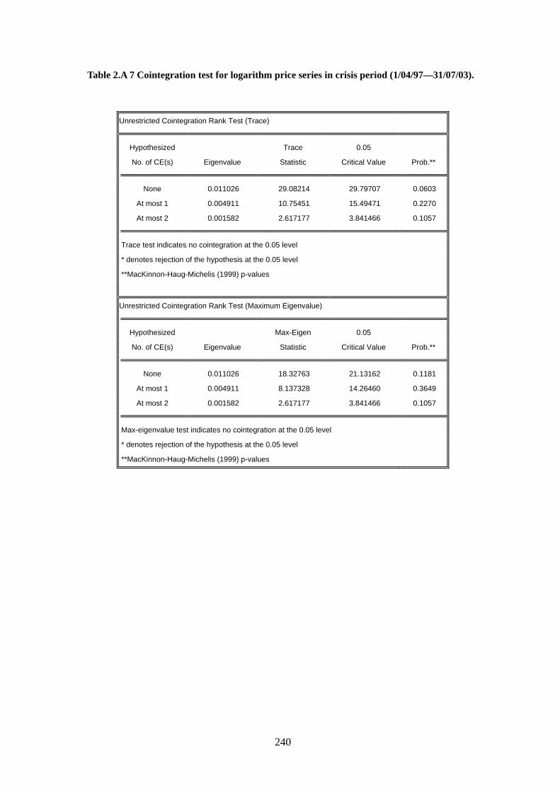
240

Table 2.A 7 Cointegration test for logarithm price series in crisis period (1/04/97—31/07/03).




None 0.011026 29.08214 29.79707 0.0603

At most 1 0.004911 10.75451 15.49471 0.2270

At most 2 0.001582 2.617177 3.841466 0.1057







None 0.011026 18.32763 21.13162 0.1181

At most 1 0.004911 8.137328 14.26460 0.3649

At most 2 0.001582 2.617177 3.841466 0.1057




241

Table 2.A 8 Cointegration test for logarithm price series in post-crisis period (1/08/03—

5/11/07).




None 0.010491 18.49654 29.79707 0.5296

At most 1 0.005910 6.768937 15.49471 0.6047

At most 2 0.000159 0.177183 3.841466 0.6738







None 0.010491 11.72760 21.13162 0.5747

At most 1 0.005910 6.591755 14.26460 0.5385

At most 2 0.000159 0.177183 3.841466 0.6738




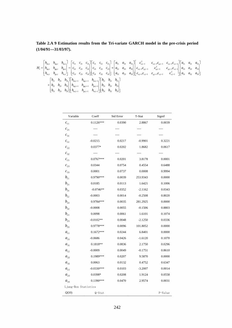
242

Table 2.A 9 Estimation results from the Tri-variate GARCH model in the pre-crisis period

(1/04/91—31/03/97).

2

, , , 11 21 31 11 12 13 11 21 31 , 1 , 1 , 1 , 1 ,

, , , 12 22 32 21 22 23 12 22 32

, , , 13 23 33 31 32 33 13 23 33


t og t gg t gs t

os t gs t ss t




1 11 12 132

, 1 , 1 , 1 , 1 , 1 21 22 232

, 1 , 1 , 1 , 1 , 1 31 32 33

11 21 31 , 1 , 1 , 1

12 22 32 , 1 , 1 , 1

13 23 33 , 1

o t g t g t g t s t

o t s t g t s t s t

oo t og t os t

og t gg t gs t

os t g

a a a

a a a

a a a

b b b h h h

b b b h h h

b b b h h

11 12 13

21 22 23

, 1 , 1 31 32 33s t ss t

b b b

b b b

h b b b


11c 0.1126*** 0.0390 2.8867 0.0039

21c ---- ---- ---- ----

31c ---- ---- ---- ----

12c -0.0215 0.0217 -0.9901 0.3221

22c 0.0377* 0.0202 1.8682 0.0617

32c ---- ---- ---- ----

13c 0.0767*** 0.0201 3.8178 0.0001

23c 0.0344 0.0754 0.4554 0.6488

33c 0.0001 0.0737 0.0008 0.9994

11b 0.9790*** 0.0039 253.9343 0.0000

21b 0.0185 0.0113 1.6421 0.1006

31b -0.0746** 0.0352 -2.1162 0.0343

12b -0.0003 0.0014 -0.2508 0.8020

22b 0.9784*** 0.0035 281.2925 0.0000

32b -0.0008 0.0055 -0.1506 0.8803

13b 0.0098 0.0061 1.6101 0.1074

23b -0.0102** 0.0048 -2.1250 0.0336

33b 0.9778*** 0.0096 101.8052 0.0000

11a 0.1672*** 0.0244 6.8401 0.0000

21a -0.0686 0.0426 -1.6120 0.1070

31a 0.1818** 0.0836 2.1750 0.0296

12a -0.0009 0.0049 -0.1751 0.8610

22a 0.1989*** 0.0207 9.5870 0.0000

32a 0.0063 0.0132 0.4752 0.6347

13a -0.0330*** 0.0103 -3.2007 0.0014

23a 0.0398* 0.0208 1.9124 0.0558

33a 0.1390*** 0.0470 2.9574 0.0031

Ljung-Box Statistics (10)Q Q-Stat P-Value

243

Oil 10.2245 0.4210

Gold 11.6752 0.3074

S&P 12.9007 0.2293

2 (10)Q

Oil 10.8304 0.3709

Gold 16.5473 0.0850

S&P 7.1713 0.7092

LL -5638.65

Covariance stationary test

Eigenvalues: 0.9735±0.0289i, 0.9874±0.0099i, 0.9903, 0.9962, 0.9874±0.0101i

0.9876

244

Table 2.A 10 Estimation results of the Bi-variate GARCH models in the pre-crisis period

(1/04/91—31/03/97).

2

11, 12, 11, 1 12, 111 21 11 12 11 21 11 12 11 211, 1 1, 1 2, 12

12, 22, 12, 1 22, 112 22 21 22 12 22 21 22 12 221, 1 2, 1 1, 1

t t t tt t tt

t t t tt t t

h h h hc c c cH

h h h hc c c c

11 12

21 22



11c 0.1656*** 0.0354 4.674 0.1451*** 0.0475 3.0563 0.0452*** 0.0111 4.0619

21c ---- ---- ---- ---- ---- ---- ---- ---- ----

12c 0.0452*** 0.0107 4.2456 0.0101 0.0654 0.1552 -0.001 0.0225 -0.0423

22c -0.00003 0.0053 -0.0056 0.0759*** 0.0307 2.4698 0.058 0.047 1.2335

11b -0.9768*** 0.0053 -184.09 -0.9752*** 0.0078 -125.44 0.9840*** 0.0056 176.13

21b 0.4210*** 0.1274 3.3057 0.0378 0.0843 0.4485 0.1340*** 0.0315 4.2543

12b 0.0147*** 0.0023 6.3481 -0.0071 0.0112 -0.6324 -0.1379** 0.0565 -2.4394

22b 0.9720*** 0.0036 271.31 -0.9800*** 0.0119 -82.13 -0.9977*** 0.0143 -69.78

11a 0.1745*** 0.0224 7.7817 0.1980*** 0.027 7.3428 0.2168*** 0.0224 9.698

21a 0.0627 0.0448 1.3993 0.1146 0.1881 0.6092 0.0272* 0.0157 1.734

12a -0.0069** 0.0032 -2.1995 -0.0252 0.0272 -0.9237 -0.0306** 0.0137 -2.2442

22a 0.2117*** 0.0195 10.83 0.1501*** 0.0480 3.123 -0.1251** 0.0599 -2.0895



Oil 9.1896 0.5142 Oil 7.8938 0.6392 Gold 11.1324 0.3473

Gold 11.7266 0.3038 sp 21.2177 0.0196 sp 13.7804 0.1832

2 (10)Q

Oil 8.1094 0.6182 Oil 8.5675 0.5736 Gold 11.4232 0.3255

Gold 12.0096 0.2844 SP 7.5956 0.6683 SP 8.6022 0.5702

LL -4167.71 -4416.22 -2725.55 Covariance Stationary Test Eigenvalue of Bi-GARCH for oil and gold market : 0.9911, 0.9953, -0.9190 and -0.9183

For oil and S&P : 0.9912, 0.9821±0.0134i, 0.9886

For gold and S&P : 0.9959, 0.9919, -0.9896, -0.9895

245

Table 2.A 11 Estimation results from the Tri-variate GARCH model in the crisis period

(1/04/97—31/07/03).

2

, , , 11 21 31 11 12 13 11 21 31 , 1 , 1 , 1 , 1 ,

, , , 12 22 32 21 22 23 12 22 32

, , , 13 23 33 31 32 33 13 23 33


t og t gg t gs t

os t gs t ss t




1 11 12 132

, 1 , 1 , 1 , 1 , 1 21 22 232

, 1 , 1 , 1 , 1 , 1 31 32 33

11 21 31 , 1 , 1 , 1

12 22 32 , 1 , 1 , 1

13 23 33 , 1

o t g t g t g t s t

o t s t g t s t s t

oo t og t os t

og t gg t gs t

os t g

a a a

a a a

a a a

b b b h h h

b b b h h h

b b b h h

11 12 13

21 22 23

, 1 , 1 31 32 33s t ss t

b b b

b b b

h b b b


11c 0.5327 0.3562 1.4954 0.1348

21c -0.4604** 0.2088 -2.2052 0.0274

31c 0.1774* 0.1029 1.7235 0.0848

12c 0.2570** 0.1305 1.9686 0.0490

22c 0.4805*** 0.1446 3.3241 0.0009

32c -0.0344 0.0655 -0.5243 0.6001

13c 0.0927 0.0823 1.1265 0.2600

23c 0.1584** 0.0626 2.5316 0.0114

33c 0.1488* 0.0817 1.8222 0.0684

11b 0.8844*** 0.0607 14.5802 0.0000

21b 0.3378 0.2805 1.2045 0.2284

31b 0.0444 0.0581 0.7650 0.4443

12b 0.0021 0.0082 0.2496 0.8029

22b 0.7353*** 0.2015 3.6486 0.0003

32b -0.0293 0.0433 -0.6755 0.4993

13b 0.0186** 0.0089 2.0958 0.0361

23b -0.1729*** 0.0242 -7.1570 0.0000

33b 0.9359*** 0.0160 58.4032 0.0000

11a 0.3004*** 0.0550 5.4571 0.0000

21a -0.1973** 0.0923 -2.1369 0.0326

31a 0.0129 0.0583 0.2204 0.8255

12a 0.0019 0.0140 0.1338 0.8935

22a 0.3132*** 0.1164 2.6910 0.0071

32a 0.0010 0.0635 0.0157 0.9874

13a -0.0271** 0.0129 -2.1011 0.0356

23a 0.1007 0.0655 1.5385 0.1239

33a 0.2214*** 0.0342 6.4733 0.0000

Ljung-Box Statistics (10)Q Q-Stat P-Value

Oil 13.2249 0.2114

Gold 4.7409 0.9078

246

S&P 8.4579 0.5842

2 (10)Q

Oil 19.3644 0.0359

Gold 3.3327 0.9725

S&P 5.5936 0.8482

LL -8648.67

Covariance stationary test Eigenvalues: 0.6006, 0.9678, 0.8822, 0.9197, 0.7231, 0.7448, 0.9204,

0.7232, 0.7465

247

Table 2.A 12 Estimation results of the Bi-variate GARCH models in the crisis period

(1/04/97—31/07/03)

2

11, 12, 11, 1 12, 111 21 11 12 11 21 11 12 11 211, 1 1, 1 2, 12

12, 22, 12, 1 22, 112 22 21 22 12 22 21 22 12 221, 1 2, 1 1, 1

t t t tt t tt

t t t tt t t

h h h hc c c cH

h h h hc c c c

11 12

21 22



11c 0.6815*** 0.1752 3.8905 0.8539*** 0.2152 3.9682 0.3079*** 0.0962 3.2025

21c 0.0839 1.0802 0.0777 -0.0367 0.2849 -0.1287 -0.1851* 0.0982 -1.8844

12c 0.2231 0.4276 0.5217 0.2252*** 0.0695 3.2395 0.2332*** 0.0567 4.1131

22c 0.3670*** 0.0860 4.2676 -0.0097 0.1013 -0.0955 0.1463** 0.0674 2.1719

11b -0.8824*** 0.0912 -9.6748 -0.8615*** 0.0523 -16.4789 0.8824*** 0.0793 11.1281

21b -0.4393 0.5254 -0.8361 0.4382* 0.2473 1.7718 -0.0148 0.0207 -0.7127

12b -0.1160* 0.0597 -1.9438 0.1582** 0.0670 2.3614 -0.0658 0.0581 -1.1316

22b 0.8203*** 0.1997 4.1066 0.9043*** 0.0434 20.8571 0.9376*** 0.0153 61.0846

11a 0.2871*** 0.0755 3.8009 0.2985*** 0.0518 5.7639 0.2538*** 0.0765 3.3188

21a -0.1980*** 0.0645 -3.0674 0.0787 0.0744 1.0581 0.0061 0.0462 0.1332

12a 0.0121 0.0136 0.8903 -0.0262** 0.0129 -2.0293 0.0522 0.0643 0.8117

22a 0.2774** 0.1156 2.3992 0.2417*** 0.0351 6.8789 0.2574*** 0.0296 8.7087



Oil 12.6739 0.2425 Oil 12.7543 0.2377 Gold 3.0667 0.9798

Gold 3.2703 0.9743 SP 8.0699 0.6220 SP 7.6371 0.6642

2 (10)Q

Oil 19.4061 0.0354 Oil 19.0893 0.0391 Gold 2.8843 0.9840

Gold 3.3998 0.9704 SP 5.9706 0.8177 SP 5.6659 0.8425

LL -5937.97 -6527.24 -4874.27

Covariance stationary test Eigenvalue of Bi-GARCH for oil and gold market : 0.9079, 0.8044, -0.6971, -0.6928

For oil and S&P : -0.7754, 0.8955, 0.9454, -0.7718

For gold and S&P : 0.8258, 0.8918, 0.9648, 0.8914

248

Table 2.A 13 Estimation results from the Tri-variate GARCH model in the post-crisis period

(1/08/03—5/11/07). 2

, , , 11 21 31 11 12 13 11 21 31 , 1 , 1 , 1 , 1 ,

, , , 12 22 32 21 22 23 12 22 32

, , , 13 23 33 31 32 33 13 23 33


t og t gg t gs t

os t gs t ss t




1 11 12 132

, 1 , 1 , 1 , 1 , 1 21 22 232

, 1 , 1 , 1 , 1 , 1 31 32 33

11 21 31 , 1 , 1 , 1

12 22 32 , 1 , 1 , 1

13 23 33 , 1

o t g t g t g t s t

o t s t g t s t s t

oo t og t os t

og t gg t gs t

os t g

a a a

a a a

a a a

b b b h h h

b b b h h h

b b b h h

11 12 13

21 22 23

, 1 , 1 31 32 33s t ss t

b b b

b b b

h b b b


11c 0.0928** 0.0383 2.4235 0.0154

21c 0.0000 0.0000 0.0000 0.0000

31c 0.0000 0.0000 0.0000 0.0000

12c 0.0758*** 0.0208 3.6408 0.0003

22c 0.0090 0.0386 0.2319 0.8166

32c 0.0000 0.0000 0.0000 0.0000

13c -0.0252 0.0837 -0.3015 0.7630

23c 0.1230** 0.0374 3.2903 0.0010

33c -0.0418 0.0573 -0.7303 0.4652

11b 0.9940*** 0.0023 434.0444 0.0000

21b -0.0077 0.0089 -0.8665 0.3862

31b 0.0470** 0.0211 2.2253 0.0261

12b 0.0001 0.0018 0.0726 0.9421

22b 0.9856*** 0.0032 312.6862 0.0000

32b 0.0100 0.0154 0.6509 0.5151

13b -0.0051*** 0.0017 -2.9429 0.0033

23b 0.0013 0.0066 0.1920 0.8478

33b 0.9614*** 0.0119 80.6452 0.0000

11a -0.1041*** 0.0191 -5.4530 0.0000

21a 0.1342*** 0.0319 4.2070 0.0000

31a -0.0652 0.0483 -1.3502 0.1770

12a 0.0105 0.0103 1.0244 0.3056

22a 0.1432*** 0.0207 6.9086 0.0000

32a -0.0114 0.0478 -0.2383 0.8117

13a -0.0046 0.0082 -0.5598 0.5756

23a 0.0022 0.0289 0.0775 0.9382

33a 0.2000*** 0.0237 8.4407 0.0000


(10)Q Q-Stat P-Value

Oil 9.1779 0.5153

Gold 4.2583 0.9349

S&P 11.2955 0.3350

249

2 (10)Q

Oil 26.7801 0.0028

Gold 11.5327 0.3175

S&P 11.0184 0.3561

LL -5040.0583

Covariance stationary test

Eigenvalues: 0.9530±0.0170i, 0.9944, 0.9923, 0.9698±0.0108i, 0.9341

0.9701±0.0118i

250

Table 2.A 14 Estimation results of the Bi-variate GARCH models in the post-crisis period

(1/08/03—5/11/07).

2

11, 12, 11, 1 12, 111 21 11 12 11 21 11 12 11 211, 1 1, 1 2, 12

12, 22, 12, 1 22, 112 22 21 22 12 22 21 22 12 221, 1 2, 1 1, 1

t t t tt t tt

t t t tt t t

h h h hc c c cH

h h h hc c c c

11 12

21 22



11c 0.3474** 0.1560 2.2265 1.8908*** 0.1114 16.9767 -0.0885*** 0.0202 -4.3723

21c -0.3640*** 0.1234 -2.9497 0.0000 0.0000 0.0000 0.0000 0.0000 0.0000

12c 0.0509 0.0913 0.5579 -0.0343 0.0214 -1.5990 -0.0909*** 0.0063 -14.3551

22c -0.0527 0.0974 -0.5407 0.0000 0.0448 0.0003 -0.0898*** 0.0056 -16.0573

11b -0.9237*** 0.0265 -34.9179 -0.1764 0.2830 -0.6233 0.9864*** 0.0028 356.48

21b 1.0203*** 0.0949 10.7524 -0.2081** 0.1010 -2.0605 -0.1486** 0.0642 -2.3139

12b 0.0446** 0.0207 2.1519 0.0454*** 0.0097 4.7036 0.0086 0.0060 1.4286

22b 0.9599*** 0.0136 70.5830 -0.9685*** 0.0085 -114.30 -0.9659*** 0.0061 -157.08

11a -0.2015*** 0.0358 -5.6209 -0.1711*** 0.0628 -2.7236 0.1487*** 0.0199 7.4655

21a 0.1509*** 0.0268 5.6288 -0.3895*** 0.1441 -2.7027 0.0015 0.0310 0.0485

12a 0.0123 0.0081 1.5153 -0.0023 0.0130 -0.1747 0.0094 0.0279 0.3369

22a 0.1554*** 0.0180 8.6404 0.1930*** 0.0234 8.2641 -0.1901*** 0.0310 -6.1287



Oil 8.4347 0.5865 Oil 10.7940 0.3738 Gold 4.3601 0.9296

Gold 4.1254 0.9415 SP 10.0421 0.4368 SP 10.6339 0.3867

2 (10)Q

Oil 17.3645 0.0667 Oil 37.4626 0.0000 Gold 11.5329 0.3175

Gold 12.2035 0.2717 SP 8.1964 0.6097 SP 9.6729 0.4696

LL -3882.29 -3494.08 -2770.65

Covariance stationary test Eigenvalue of Bi-GARCH for oil and gold market : 0.9407, 0.9937, -0.9657, -0.9653

For oil and S&P : 0.1012±0.0103i, 0.9625, 0.1464

For gold and S&P :0.9936, 0.9676, -0.9793, 0.9798

251

Appendix 2 B

Figure 2.B 1 Percentage of oil production, imports and demand in US to the World

0

0.05

0.1

0.15

0.2

0.25

0.3

1991 1992 1993 1994 1995 1996 1997 1998 1999 2000 2001 2002 2003 2004 2005

Crude Oil Production Crude Oil Imports Total Oil Demand

Figure 2.B 2 World crude oil price ($/bbl) for past 50 years (yearly average)

0

20

40

60

80

100

60 62 64 66 68 70 72 74 76 78 80 82 84 86 88 90 92 94 96 98 00 02 04 06 08

252

Figure 2.B 3 Inflation adjusted world oil prices over past 50 years (yearly average, $/bbl)

10

20

30

40

50

60

70

80

90

100

60 62 64 66 68 70 72 74 76 78 80 82 84 86 88 90 92 94 96 98 00 02 04 06 08

Figure 2.B 4 Monthly oil price series from 1990s

0

20

40

60

80

100

120

140

160

90 91 92 93 94 95 96 97 98 99 00 01 02 03 04 05 06 07 08 09

253

Figure 2.B 5 World gold price for past 50 years (yearly average, $/ounce)

0

100

200

300

400

500

600

700

800

900

1960 1965 1970 1975 1980 1985 1990 1995 2000 2005

Figure 2.B 6 Percentage gold holding of US to the world

0.2

0.21

0.22

0.23

0.24

0.25

0.26

0.27

0.28

1991

1992

1993

1994

1995

1996

1997

1998

1999

2000

2001

2002

2003

2004

2005

2006

254

Figure 2.B 7 Oil and oil price over the past 50 years (Based on yearly data)

0

20

40

60

80

100

0

200

400

600

800

1,000

1960 1965 1970 1975 1980 1985 1990 1995 2000 2005

GOLD OIL

Figure 2.B 8 Oil and gold monthly price series since 1990s

0

40

80

120

160

200

400

600

800

1,000

1990 1992 1994 1996 1998 2000 2002 2004 2006 2008

GOLD OIL

255

Essay 3 Re-examining the Asian Currency

Crises: A Markov Switching TGARCH

approach

256

3.1. Introduction

The outbreak of the Asia financial crisis in 1997-1998 triggered a surge in both

theoretical and empirical studies on the factors that contribute to the occurrence of a

currency crisis. Some authors claim that the Asia currency crises were predictable and

can be explained by economic fundamentals, whereas others contend that the crises

are self-fulfilling, where speculative attacks on a country are based on the probability

that the attacks will be successful and hence profitable, regardless of the

macroeconomic fundamentals of a country.

Currency crises have been traditionally viewed as retribution for governments that

have mismanaged the economy and/or lack credibility. The basic ‘first generation’

model (see e.g., Krugman, 1979) accentuates domestic fiscal and monetary policies

inconsistent with the fixed exchange rate policy leading to currency overvaluation and

reserve depletion. In these models the presence of inconsistent policies generates a

speculative attack against the local currency, and pushes the economy into a crisis.

The degree of severity of these inconsistencies will determine the timing of the crisis.

The ‘second generation’ model (see e.g., Obstfeld, 1996) emphasizes the importance

of market expectations which can trigger a crisis by shifting the macroeconomy from

a “good” no-crisis equilibrium to a crisis equilibrium, even when macroeconomic

policies are consistent with the exchange rate policy. These models emphasize the role

of policymaker’s preferences, and suggest that the option of abandoning a fixed

257

exchange rate regime may be an ex-ante optimal decision for the policymakers,

considering that economic authorities face tradeoffs. The ‘third generation’ model (see

e.g., Corsetti et al., 1999) focuses on deficiencies in domestic and foreign financial

sectors that result in a ‘feast and famine’ pattern of capital flows. Those models tend

to focus on the financial liberalization in Asia capital markets, accompanied by a

combination of asymmetric information and moral hazard problems and by the

inadequate market regulation, supervision and management in this region, which led

to excessive borrowing (e.g., Mishkin, 1999; Corsetti, Pesenti, & Roubini, 1999).

Rather than following the path of the third generation models we confine ourselves to

the potential of the first and second generation currency crisis models for explaining

(or accounting for) the Asian currency crisis in this study.

A currency crisis is usually identified as an episode in which there is a sharp

depreciation of the currency, a large decline in foreign reserves, a dramatic increase in

domestic interest rate or a combination of these elements. The empirical literature on

currency crisis are vast, and mainly focus on trying to explain and predict crises in the

developing countries.

In this study, we use a Markov Switching approach to account for the presence of two

potential regimes: stable and volatile. We also include an Asymmetric Generalised

Autoregressive Conditional Heteroscedasticity (GARCH) specification to capture the

fact that within each regime, the volatility of market pressure is not constant. The

258

attractiveness of the Markov Switching approach is that we do not need to distinguish

ex-ante between stable and volatile states. Instead, the estimation results will supply

us with such information. By allowing regression parameters to switch between

different regimes, Markov-switching mimics the existence of multiple equilibriums.

Moreover, the mainstream analyses and empirical studies concentrate on depreciating

currency attacks. In reality, however, speculative attacks also take place when

currency appreciates. The Markov Switching models we employed are also able to

capture appreciating currency attacks. In stead of converting the measure of market

pressure on the exchange rate into a binary variable (Eichengreen, Rose and Wyplosz,

1996, Frankel and Rose, 1996, and Kruger, Osakwe, and Page, 1998), we assume a

currency will have higher probability to depreciate if it has high market pressure, and

will appreciate when it has very low market pressure. When market pressure has very

low or high values, it is considered to be potentially in a volatile state. When market

pressure lies in the medium range, it is considered to be in a stable state.

Existing empirical studies have suggested that the deteriorating fundamentals do

increase the probability of a crisis (see, e.g., Kaminsky, Lizondo and Reinhart, 1997;

Berg and Patillo, 1998), but the timing of a crisis cannot be predicted with precision.

In our approach, we examine the explanatory power of several fundamental variables,

including the indicators for international reserves, the real exchange rate and domestic

credit growth. The model can be used for out-of-sample forecasting. Unfortunately,

259

due to the short data sample, we only limit our study to understanding the variables

and modeling specifications.

The remainder of this paper is organized as follows. Section 3.2 and section 3.3

review the theoretical framework and empirical studies on currency crisis. Section 3.4

discusses the measure of market pressure on the exchange rate and the construction of

macroeconomic fundamentals. Section 3.5 discusses the methodology: the Markov

switching models with constant variances and with Asymmetric GARCH

specification in variances. Empirical estimation results are presented in section 3.6. In

section 3.7, we compare our findings from Markov switching model with the results

from Multinomial Logit models. Section 3.8 concludes.

260

3.2 Theoretical Framework for currency crisis

This section provides a review of selected works on explanations for speculative

attacks and currency crisis that have been presented in the theoretical literature. The

aim is to provide some theoretical background and to provide an explanation why a

variety of indicators have been used for currency crisis in our later empirical studies.

3.2.1 First Generation Crisis models: Fundamentals perspective

The first generation models explain currency crisis as a result of unsustainable

development in fundamental macroeconomic variables, which widens the discrepancy

between the promises and the proclaimed goal of the monetary authorities (e.g. Blejer,

1998). Krugman (1979) shows that, under a fixed exchange rate, domestic credit

expansion in excess of money demand growth leads to a gradual but persistent loss of

international reserves and ultimately to a speculative attack on the currency. This

attack immediately depletes reserves and forces the authorities to abandon parity. The

process ends with an attack because economic agents understand that a fixed

exchange rate regime will ultimately collapse, and that in the absence of an attack the

agents would suffer a capital loss on their holdings of domestic money. Krugman’s

analysis parallels obviously the analysis in the theory of exhaustible resources in that

foreign reserves are used to peg an exchange rate. He illustrates a currency crisis from

the viewpoint of monetary model. In this respect, his model predicts that exchange is

261

dependent on the supply of domestic and foreign currency relative to demands. Due to

non-linearities in his model, the Krugman (1979) model was not able to determine the

timing of the collapse of the fixed exchange rate regime. Flood and Garber (1984)

using a linear model provided a solution to the timing of the collapse.

Agenor, Bhandari and Flood (1992) present a framework to analyze the process

leading to a balance of payments crisis, consisting of a simple continuous time and

perfect foresight model. This model is a log linear formulation which can solve

explicitly for the timing of a crisis by assuming that the exchange rate is allowed to

float permanently in the post-crisis regime. We provide an examination of this model.

Consider a small open economy whose residents consume a single traded good whose

domestic supply is exogenously fixed at y . The central bank fixes the exchange rate

of its currency relative to that of a large foreign country. Purchasing power parity

(PPP) holds, so that *P SP ( P is the domestic price level, S is the exchange

rate the *P is the foreign price level). In log notation with *P normalized to 1, the

PPP can be written as p s . p and s are the domestic price level and exchange

rate in logarithms. Assuming there are no private banks in the economy, the money

supply equals the sum of domestic credit issued by the central bank and domestic

currency value of foreign reserves held by the central bank. Domestic credit is

assumed to grow at a constant rate . Finally, agents have perfect foresight. The

model is defined as follow:

262

t t tm p y i , 0a (3.1)

(1 )t t tm d r 0 1 (3.2)

td & 0 (3.3)

t tp s (3.4)

*1t t t ti i E s & (3.5)

All variables except interest are measured in logarithms. tm denotes the nominal

money stock, td is the domestic credit, tr is the domestic currency value of the

government’s holding of foreign reserves, ts is the spot exchange rate, tp is the

domestic price level, ti is the domestic interest rate and *ti is the foreign interest

rate. *ti is assumed to be constant. tE denotes the expectation operator conditional

on information available at time t . A dot over a variable denotes a time derivative.

Equation (3.1) defines real money demand as a positive function of income and a

negative function of the domestic interest rate. Equation (3.2) is a log-linear

approximation of the link between the money stock and reserves and domestic credit.

denotes the share of domestic credit in the money stock32. Equation (3.3) gives that

the domestic credit grows at a constant rate . Purchasing power parity and

uncovered interest parity are assumed to be hold and are defined in Equation (3.4) and

Equation (3.5), respectively. Under perfect foresight, 1 1t t tE s s & & .

32 /t tD M at the point of linearisation, usually the sample mean. tD denotes the domestic

credit and tM denotes the nominal money stock, in level.

263

From this model, the operating properties of a floating exchange rate and fixed

exchange regime can be determined. For convenience, we set 0y . Combining

Equation (3.1), (3.4) and (3.5) yields,

1*t t t ts i m aE s & (3.6)

When the exchange rate is fixed at s , the anticipated rate of change in exchange rate

is zero, 1 0t tE s & . *i is assumed to be constant and so the central bank must

accommodate any change in money demand through the purchase from or sale to the

public of foreign reserves. Using Equation (3.2) and (3.6) yields,

*( ) /(1 )t t tr s d i (3.7)

And under these assumptions

/tr & where (1 ) / (3.8)

When domestic credit is excessive (exceeding the demand for money), the continual

growth in domestic credit will cause reserves to decline steadily as the central bank

intervenes in foreign exchange markets to maintain the fixed exchange rate. If the

central bank will not continue to defend the current exchange rate after the reserves

reach a lower bound, r , the exchange rate will be forced to float or will be devalued.

The rational agents will anticipate that without speculation reserves will at some time

fall to the lower bound and will anticipate the ultimate impending collapse of the

fixed exchange rate. Hence, to avoid a loss of profit at the time of collapse rational

agents will force a crisis before reserves reach r .

In equilibrium under perfect foresight, agents will never expect a discrete jump in the

264

level of exchange rate which will provide a profitable arbitrage opportunity. Arbitrage

in the foreign exchange market fixes the exchange rate at the time of collapse equal to

the fixed exchange rate prevailing at the time of attack. Thus the time of attack can be

determined by two steps. First, from the law of motion of the exchange rate, we solve

for the floating exchange rate given the current level of domestic credit and contingent

on net reserves being at the minimum level of reverse. This contingent exchange rate

is known as the shadow floating exchange rate, s%. Second, we find the time T at

which the shadow floating exchange rate s% equals the fixed exchange rate s .

To find the shadow floating exchange rate, first assume that at the time of collapse,

0r , so Equation (3.2) becomes

t tm d (3.9)

And so

tm d && (3.10)

Substitution in Equation (3.6), the solution for the floating exchange rate is

*t t ts s i d % (3.11)

In the post collapse regime, the exchange rate depreciates steadily and proportionally

to the rate of domestic credit growth.

Assume that domestic credit grows with a deterministic trend: 0td d t and at

the time of collapse, t tm d , then from Equation (3.11) we can determine the time

of collapse

265

*0( ) /cT s i d (3.12)

*0( )

c

s i dT

(3.13)

Given 0 0* (1 )s i d r

0(1 )c

rT

(3.14)

Equation (3.13) shows that the higher initial stock of reserves or the lower the rate of

domestic credit growth, the longer it will take before the collapse occurs in the

absence of a speculative attack. The (semi) interest rate elasticity of money demand

( ) determines the size of the downward shift in money demand and reserves when

the fixed exchange rate collapses and the nominal interest rate rises to reflect the

expected depreciation of the domestic currency. The larger the value of , the sooner

the collapse. Although it is assumed reserves are run down to zero to determine

shadow floating rate, the model indicates that the attack always occurs before the

central bank would have run out of reserves in the absence of speculation.

The model can be depicted in Figure 3.1. Prior to the attack, the exchange rate is fixed

with no anticipated depreciation, so nominal money demand and supply are constant.

Nevertheless, domestic credit is continuously rising, and this is matched by the fall in

reserves. At the time of attack, nominal money demand falls discontinuously to cTD .

The supply of money is reduced accordingly through an attack that drives reserves

discontinuously to zero. From cT onward, the money stock is identical to and grows

266

Figure 3. 1 Money, domestic credit and reserves in a speculative attack.

Source: Agenor, Bhandari and Flood (1992)

Money Stock

Money Stock

Domestic Credit

Reserve

Time

0D

0R

tM tD tm

Exchange rate

T Time

Fixed exchange rate

Shadow exchange rate

s%

s

267

with domestic credit. Note that if the right side of Equation (3.14) is negative, one

should interpret the analysis as showing that a speculative attack must take place

immediately on date 0 (Obstfeld and Rogoff, 1996).

3.2.2 The second generation models of currency crisis (Self-fulfilling

speculative attacks)

The second generation models extend as well as modify the first generation models

whereby dependence on market expectations for the occurrence of a crisis creates an

element of uncertainty and multiple (non-unique) equilibria, rather than the

fundamental macroeconomic variables and their developments cause a currency crisis.

It focus on non-linearities in government behaviour, namely, what happens when

government policy reacts to changes in private behaviour or when the government

faces an explicit trade-off between the fixed exchange rate policy and other goals.

Krugman (1996) point out that the policy dilemma facing by these countries have

centered on such issues as real overvaluation, interest rates and unemployment, rather

than facing a sharply defined foreign reserves constraint, to maintain a fixed exchange

rate regime. Second generation models generally exhibit multiple equilibria so that

speculative attacks can occur because of self-fulfilling expectations. “Then a fixed

exchange rate that would have lasted indefinitely in the absence of a speculative

attack may collapse because financial markets are persuaded, by otherwise irrelevant

268

information, that the rate will not be sustained." (Krugman, 1996). For example, if

private agents expect a high rate of devaluation, interest rate or wage demands can

increase, worsening the prospects for lower debt service, a sounder banking system or

reduced unemployment. The government will be more willing to actually allow for a

high rate of devaluation because the situation implies a high “cost” to be paid by the

government if the government does not actually change the exchange rate. The

government’s decision to devalue validates expectations, making expectations

self-fulfilling (Marion, 1999).

The second generation models assume that the government in every single period of

time evaluates the cost and the benefits from keeping the exchange rate fixed. Such is

achieved by the government to optimise an explicit objective function (see, for

example, Obstfeld, 1994). Consider the case of an agent, the government, which

trying to minimise a loss function must decide whether or not to defend an

exogenously determined exchange parity. We take directly from Krugman (1996) the

reduced form representation, which derives the explicit loss function from a

Mundell-Fleming type of open economy macro model with sticky prices. In such a

model, output is a function of the real exchange rate and real interest rate.

*( ) ( )y s p p i (3.15)

Where *p and p are the foreign and domestic price levels in logarithm, and is

the expected rate of inflation. The money demand is a function of income and interest

rate:

269

( , )m p L y i (3.16)

Assuming perfect capital mobility with equalization of returns

*i i s & (3.17)

Where *i is the foreign interest rate the s& is the expected rate of depreciation. The

government’s loss function is stated in terms of deviation of output from a desired

level:

2( )dH y y (3.18)

Now define the ds as the log of the exchange rate that would leave the output equal

to its target level in the absence of any expected depreciation. (i.e., ds is the desired

exchange rate). Hence:

* *( ) ( )d dy s p p i (3.19)

So that

* *1/ ( ) ( )d ds y p p i (3.20)

Therefore

2( ) ( )dH s s s & (3.21)

Let ds be the exchange rate that government would choose if it faces no credibility

concerns and s be the parity to which it has staked it reputation. s& is the expected

rate of depreciation: es s , where es is the market expectation of the current

exchange rate.

Assume that the government faces a fixed private cost if the government unexpectedly

270

abandon the peg and let the currency devaluate, probability in the form of loss

reputation. Sachs, et al (1996) show that such cost need not be proportional to the size

of the devaluation or any other macroeconomic variable.

Assume the government’s loss function is:

2( ) ( ) ( )dH s s s R & (3.22)

Where ( )R takes the value C when the government allows the exchange rate to

change while ( )R equal 0 when the exchange rate does not change. Thus C is a

fixed “reputation” cost that the government incurs when it abandons the peg.

Assume that the government is currently pegging its exchange rate. The market might

expect that the government will continue to do so: es s , or that the government will

abandon the peg in the next period, then e ds s . Then the decision about whether to

maintain the peg will depend on the comparison of the cost or loss from staying on the

peg with the credibility cost of abandoning the peg, that is, whether

2

min ( ) ( )d eH s s s s C (3.23)

If the market does not expect a depreciation, then the second term in equation (3.23)

will vanish and the government will want to maintain its peg, fulfilling the market

expectations (i.e. es s ) as long as

2( )dH s s C (3.24)

On the other hand, if the market expects a depreciation (i.e., e ds s ), then the second

term will become positive and the government will abandon the peg and fulfill market

271

expectations as long as

2( )( )dH s s C (3.25)

Then we have multiple equilibria as long as

2 2( ) ( )( )d ds s C s s (3.26)

Equation (3.26) shows that self-fulfilling crises are possible when the parameters of

the economy are in a range. Whether the regime survives or collapses will depend on

the government’s reaction to market expectations. In loose terms, the above

government objective function states that the conditions for a crisis-proof fixed

exchange regime include a high cost to abandoning the peg and a peg that is very

close to the desired or “right” level, ds .

Some other versions of second generation models have also been developed (e.g.

Obstfeld, 1996; Masson, 1999, etc). These models generally developed following the

European Exchange Rate Mechanism (ERM) crisis in 1992/1993, when no critical

developments in fundamental macroeconomic variables could be noticed. The second

generation models stress the influence of self-fulfilling expectation and market panics

on a currency, as well as the influence of “triggers” that initiate these panics and shift

all the expectations in the market in the coherent or same direction.

According to second-generation models, a currency crisis occurs due to: 1) coherent

self-fulfilling expectations, 2) rational heard behavior and 3) contagion (Blejer, 1998).

Second generation models accurately describe developments immediately preceding a

272

currency crisis. However, they overestimate the importance of expectation and

triggers in setting off the wave of pessimism and coherent expectations in the market

which results in currency devaluation (Babic and zigman, 2001). When the

second-generation models are used as a complements to first-generation model, more

sound theoretical results for currency crises can be achieved. The current economic

policy of the government as well as its economic objectives and methods for

achieving these objectives are reflected in the fundamental macroeconomic variables.

The greater the deviation of the current economic policy from the optimum policy the

government claimed to maintain the stability of the exchange rate regime (e.g. fixed

exchange rate), the greater the probability of currency attack to take place and thus the

occurrence of currency crisis. Due to various market fractions like transaction costs,

difficulties in arranging credit lines for currency attack and the delay of revealing

government policy indicators, currency crisis may not unfold as soon as the

government policy begins to deviate from the proclaimed optimum policy.

Accordingly, emphasis on the role of various events, especially various political

events, that can trigger and turning point in market expectation has increased.

3.2.3 Summary of the models

First generation currency crisis models have focused on the primacy of deteriorating

fundamentals in triggering a speculative attack. The deterioration of the fundamentals

273

such as a growing budget deficit (perhaps financed by a growing domestic credit) or

real exchange rate appreciation which implies a loss of competitiveness, leads

invariably to a loss of reserves to the threshold level that triggers a speculative attack.

The fixed exchange rate becomes increasingly incompatible with the state of

fundamental, thereby raising the floating exchange rate above the peg. There are

many extended version of first generation model (see, e.g. Floor and Garbet, 1984 and

Santoso, 2001).

The second generation models endogenise government policy on the exchange rate.

The peg is abandoned either as a result of deteriorating fundamental, or as a result of a

speculative attack driven by self-fulfilling. The models focus on the market

expectations which lead to currency crises, rather than the fundamental

macroeconomic variables and their development. However, the fact that the attack is

self-fulfilling does not mean that fundamental variables are no longer important,

because these models require that the fundamentals in a vulnerable range for the

attack to be successful.

Flood and Marion (1998) assert that the first- and second-generation model differ in a

variety of ways, but most of the differences can be traced to one crucial assumption

that first generation models assume the commitment to a fixed exchange rate is state

invariant, whereas second generation models allow it to be state dependent. The

assumption of a state-invariant commitment does not match well with common

274

observation that monetary authority’s commitment to the fixed exchange rate is often

constrained by such factors as unemployment, the fragility of the banking system, the

size of the public debt, or upcoming election. The state dependent behaviour inspires

us to build an empirical model of the currency crisis that incorporates state/regime

switching. The Markov Regime-Switching models are discussed in the section 3.4.

275

3.3 Previous empirical studies

The empirical literature on currency crisis is extensive, and mainly focuses on trying

to explain and predict crises in the developing countries. There are three methods or

approaches for predicting currency crises that have been developed in the literature.

One class of models is the probit/logit regression approach developed by Frankel and

Rose (1996). They apply probit analysis on a panel of annual data for 105 developing

countries for the period between 1971 and 1992 to investigate how international debt

structure and external factors affect the probability of currency crises. Their model

identifies the significant variables as output growth, foreign direct investment/total

debt, reserves, domestic credit growth, external debt and foreign interest rates. Their

findings also suggest that currency crises tend to occur when the growth of domestic

credit and foreign interest rates are high, and foreign direct investment and output

growth are low. Probit approach has also been used by Glick and Moreno (1999).

Based on data from January 1972 to October 1997, they study the crises in Asia and

Latin America. Results of their analysis suggest that reductions in real domestic credit

and foreign reserves, as well as appreciation in the real exchange rate increase the

probability of financial crises. Geochoco-Bautista (2000) uses a probit model based

on data from the Philippines spanning the period between 1980 and 1997. Regression

results indicate that the coefficient of short-term interest rate differential, change in

international reserves, real exchange rate, and the growth of domestic credit to public

276

sector are the significant variables in explaining the financial crisis in the Philippines.

More recently, Bussiere and Fratzscher (2006) develop a new early warning system

model based on a multinomial Logit with three outcomes (tranquil, pre-crisis and

post-crisis) showing that such a specification leads to a better out-of-sample forecast

and solves what they call the“post-crisis bias.”

A second class of models might be termed the “signal approach”, which attributed to

Kaminsky et al. (1998). Macroeconomic series that behave abnormally during periods

prior to a crisis are selected and a warning system based on signals issued by those

variables is produced, normally with a threshold level beyond which a signal would

be generated. Then they assess the individual and combined ability of those variables

to predict crises. Kaminsky et al. (1998) find that the variables that have most

explanatory power based on the noise-to-signal ratio are the deviation of real

exchange rates from a deterministic trend, the occurrence of a banking crisis, the

export growth rate, the stock price index growth rate, M2/reserves growth rate, output

growth, excess M1 balances, growth of international reserves, M2 multiplier growth,

and the growth rate of the domestic credit to GDP ratio. Berg and Pattillo (1999), by

studying five European and eight emerging market economies from April 1970 to

April 1995 under the signal approach, find that the crisis probabilities generated by

this model for the period between May 1995 and December 1996 are statistically

significant predictors of actual crisis occurrence over the following 24 months. They

discover that the probability of a currency crisis increases when domestic credit

277

growth is high, the real exchange rate is overvalued relative to trend, and the ratio of

M2 to reserves is high. Using variants of the signals approach, Kaminsky (1998),

Kaminsky and Reinhart (1999), and Goldstein et al. (2000) claim some success in

predicting the Asian crisis.

A third class of models set up a crisis index and explain the currency crisis based on

traditional linear or non-linear regression approach (for example, Tornell, 1999; IMF,

World Economic Outlook, 1998; Radelet and Sachs, 1998; Corsetti, Pesenti and

Roubini, 1999). Moreno (1995) builds a linear probability model for eight Asian

countries based on monthly data from 1980 to 1994. He finds that depreciation is

positively associated with larger budget deficits and higher growth in domestic credit.

Sachs, Tornell and Velasco's (1996) use cross-country regressions to explain the

Tequila (Mexican) crisis of 1995. Using a crisis index defined as the weighted sum of

the percentage decrease in foreign reserves and the percentage depreciation of the

peso, they conclude that countries have more severe attacks when they have low

foreign reserves, their banking systems are weak and their currencies overvalued.

Tornell’s (1999), using a linear model in studying the Tequila and Asian crises suggest

that the crises did not spread in a purely random way. Rather, there was a set of

fundamentals help to explain cross-country variation of severity of the crises, which

includes the strength of the banking system, the real appreciation and the international

liquidity of the country. He also finds that the same model that explains the spread of

the crisis in Latin American in 1995 also explains the cross-country variation in the

278

1997 crisis. Krkoska (2000) estimates a restricted VAR on quarterly data from 1994 to

1999 to analyze the vulnerability in transition countries. Results of the VAR reveal

that overvaluation, a slowdown in the EU, as well as the gap between the current

account and FDI, are the significant predictors of vulnerability in transition countries.

More recently, Markov Switching approach has been adopted to explain the currency

crisis in different regimes. Abdul Abiad (2003) uses a time-varying transition

probability Markov-switching model on monthly data for five Asian crisis economies

from January 1972 to December 1999. He initially explores 22 indicators of

macroeconomic imbalances, capital flow and financial fragility. The indicators that

can explain the currency crisis for different countries are slightly different.

Furthermore, he suggests that panel data regression models with parameter equality

across countries may lead to incorrect estimates and poor predictive performance.

These approaches have limitations. For example, the signal approach requires the

ex-ante definition of a threshold and the transformation of the variables into binary

variables, with a significant loss of information; the Logit/Probit approach requires

the definition of a crisis dummy, with potential misclassifications (Brunetti, Mariano,

Scotti and Tan, 2007).

In summary, empirical studies suggest that deteriorating fundamentals increase the

probability of a crisis. However, the exact timing of a crisis has not been predicted

with high precision. Speculators will observe that weak fundamentals drive a currency

279

to a vulnerable zone to be attacked. However, the decision to attack is determined by

the probability that speculators will gain profit by attacking the currency.

280

3.4 Exchange Rate Market Pressure (MP) and explanatory

variable

Exchange market pressure has been variously defined in the literature, but the most

commonly used definition sees MP as an excess money phenomenon driven by

abnormally large excess domestic currency demand or supply, which forces the

monetary authorities to take measures to stem disruptive appreciation or depreciation

of the currency. Defined in this way, MP reflects monetary disequilibrium that drives

the demand for a safe-haven currency, and may be exacerbated by foreign exchange

market intervention. Following the pioneering study of Girton and Ruper (1977), the

measure of speculative market pressure on the exchange rate, MP, is measured as a

weighted average of the percentage changes of exchange rate and the percentage

change (loss) in international reserve, where the weights are equal to the inverse of the

(sample period) standard deviation or variance33. Such design is used to capture the

monetary authorities’ interventions in attempting to stabilize the exchange rate. It is

often argued that interest rate changes should be included in the weighted average (see,

e.g., Eichengreen et al., 1996; Kaminsky & Reinhart, 2000), but these are frequently

omitted since data on interest rates for developing economies are not complete34.

Some other studies exclude interest rates as they argue that the increase in interest

rates in the presence of speculative pressure is highly correlated with the

33 In Girton and Ruper (1977) the weights were set at one, given the theoretical underpinnings of their work. 34 In fact, these limitations on the measurement of MP have been faced by many researches (e.g. International Money Fund, 1998; Glick and Rose, 1998; and Tornell, 1999).

281

non-sterilized foreign exchange invention leading to a fall in the reserve. We include

interest rate changes in the measure of MP.

MP is generally a good index of currency crisis as it reflects different manifestations

of speculative attacks, be they successful or otherwise. The MP which consists of a

weighted average of nominal exchange rate, reserves and interest rate changes usually

implies a sample-dependent crisis threshold level which is set (arbitrarily), sometimes,

to ensure a certain percentage of crisis in the sample (e.g., Caramazza et al, 2000).

However, there are drawbacks in this method of identifying crisis: in large samples, a

high volatility regime will tend to dominate the whole sample, and the fixed threshold

will also fail to identify a crisis that happened in a low volatility regime. Therefore, a

fixed threshold tends to ignore the shift in exchange rate regime. To avoid mistakenly

identifying the effect of high inflation for speculative pressure, a separate definition of

crisis is sometimes used for high inflation countries35.

The (weighted average) exchange market pressure index may also be defined by

removing the restriction of a fixed variance for the constituents of MP, thus the

weights are the inverse of the conditional variances of the constituents. By allowing

the conditional variance of the MP be time-varying, MP index will have higher

volatility with this volatility being generated by market uncertainty or shocks36. The

35 Kaminsky et al (1998) uses a different index for subsamples when inflation in the last 6 months exceeded 150%; Corsetti et al (1998) omits the changes in the depreciation component of the crisis index when the rate of depreciation is less than the previous three-year average. 36 By using fixed weights (i.e., a fixed sample period specific variance) shocks and market uncertainty have the same influence.

282

weights (inverse of the conditional variance) may be set to be proportionate or

specific to each constituent37. The one period ahead forecast variance (conditional

variance) may be captured by the changes in nominal exchange rate conditioned on

the macroeconomic variables that have the most impact on MP. Conditional variances

are estimated using a GARCH (Generalized Autoregressive Conditional

Heteroscedasticity) model. However, we find the use of GARCH structures makes it

even harder to use any estimated Markov regime-switching model for “prediction”

purposes. Thus in this study we use the constant weights based on the sample period

data instead of using the time varying weights.

The macroeconomic variables we employed to explain the MP include (1) the ratio of

international reserves to broad money, RM2; (2) the real exchange rate, RER; (3) the

growth of real domestic credit, GDC; and (4) exchange risk premium, Risk. All these

variables are familiar from the literature and will require no further analysis or

rationalizations. Therefore, we provide just a brief description of these variables.

The ratio of international reserves to broad money, RM2, is calculated as foreign

reserves (IFS38 line 1l.d) converted into domestic currency using end of period

exchange rate (IFS line AE) divided by broad money (IFS line 34 plus 35). RM2

serves as a proxy for the government’s contingent liabilities (Sache et al., 1996).

37 For example, Eichengreen et al (1995) use equal conditional variance weights and Lumdaine and Prasad (2003) use proportionate weights of the conditional variance of output growth fluctuations. 38 IFS stands for International Money Fund’s International Financial Statistics.

283

Tornell (1999) argues that if a government is not willing to let the exchange rate to

depreciate, it must be prepared to cover all the liabilities of the banking system with

reserves. During a crisis banks are likely to experience runs. If the central bank does

not act as a lender of last resort, generalized bankruptcies are likely to follow. Since,

in most circumstances, authorities will not find it optimal to allow the economy to

experience generalized bankruptcies, the central bank will have to be prepared to

exchange the amount withdrawn by depositors for foreign exchange. Thus, it is M2,

and not simply the monetary base, that must be the relevant proxy of the central

bank's contingent liabilities. Accordingly, the RM2 represents financial fragility due

to reserves inadequacy. Esquivel and Iarrain (1998) argue that this measure of reserve

availability reflects better the vulnerability of the central bank to possible runs against

currency. An expected decline in RM2, i.e., rising reserves inadequacy tends to

increase MP since the market foresees that the stock of reserves will be inadequate to

defend the exchange rate in the event of a speculative attack. We expect to find a

negative relation between RM2 and MP. However, it may also be possible that a rising

RM2 could enhance the possibility of a crisis, since it may highlight the potential

danger of reversal of capital inflows. The latter may have contributed to increasing

M2 in the first instance.

The real exchange rate, RER, is measured in two steps (following Ford, et al, 2007).

First, we take the natural logarithms of the average exchange rate of domestic

currency against US dollars (IFS line RF) multiplied by US consumer price index

284

(IFS line 64) and divided by domestic consumer price index (IFS line 64). Second, we

subtract the first figure from their past 36 months’ average. This two-step procedure is

a measure of the deviation of real exchange rate from its three years’ previous average.

One benefit of the two step procedure of measuring RER is that the resultant data will

be more likely to be stationary than the unadjusted data. A positive (negative) real

exchange rate indicates a real depreciation (appreciation) of domestic currency. The

real exchange rate effect is ambiguous. An expected increase in the real exchange rate,

i.e., a depreciating real exchange rate will tend to exert upward pressure on MP (e.g.

see, Kaminsky and Reinhart, 1999; Corsetti et al, 1998; Sachs et al, 1996) if the

increase is driven by rising pressure on the nominal exchange rate in a fixed or tightly

managed exchange rate regime, by reducing the price competitiveness of exports,

culminating in large current account deficits and eventually declining economic

growth. This is highly probable if the market perceives rising macroeconomic

imbalances such as credit growth and rising stock of non-performing loans, current

account imbalances and declining reserves sustained over a period of time. Otherwise,

a rising real exchange rate can be beneficial for an economy since it effectively

improves the trade competitiveness of domestic exports. This can happen in normally

high inflation economies where stabilization policies are effective. Another reasons

for the exchange rate impact to be ambiguous is that the exchange rate have a

tendency towards overshooting if the response of output to a currency depreciation is

small following an increase in the money supply, under price rigidities (Obstfeld and

Rogoff, 1995).

285

The growth of real domestic credit, GDC, is calculated as a first difference of the

natural logarithm of total domestic credit (IFS line 32) adjusted for inflation using

consumer price index (IFS line 64). It is widely accepted that linkage between

domestic credit and speculative attacks on the currency exist. Excessive growth of

domestic credit may serve as an indicator of the fragility of the banking system.

Although it is not an ideal indicator for financial fragility, this variable is available on

a timely basis and is comparable across countries39. Domestic Credit usually rises in

the early phase of the banking crisis. It may be that as the crisis unfolds, the central

bank may be injecting money to the banks to improve their financial situation. A

larger amount of credit increases the chances of bad loans and bank failures (see,

Mete Feridun, 2006). The growth of real domestic credit will reflect budgetary policy

and the potential for inflation. Higher credit implies a larger amount of money supply.

Currency crises have been linked to rapid growth in credit and the monetary

aggregates. As the growth rate of domestic credit captures the effects of monetary

policies, it is usually expected to have a positive effect on currency market pressure. A

number of empirical studies in the literature have found that domestic credit is one of

the significant indicators of currency crises (for example, Moreno, 1995; Frankel and

Rose, 1996; Kaminsky et al., 1997; Berg and Patillo, 1999; Glick and Moreno, 1999;

Geochoco-Bautista, 2000; Krkoska, 2000 and Krznar, 2004).

39 According to Aaron Tornell, 1999, ideally, one should measure the weakness of the banking system with the "true" share of bad loans. Unfortunately, this information is available neither on a timely basis nor in data sources that ensure cross-country comparability. First it may not comparable because the accounting rule they adopted, second is the problem arised from misreporting.

286

The risk premium, Risk, is calculated, following Frankel and MacArthur (1988), as

the forward discount rate less the expected (proxied by the one period ahead; as per

rational expectation) rate of depreciation of the domestic currency. The foreign

exchange risk premium represents compensation required by risk-averse investors for

holding an asset whose only risk depends on being issued in a particular currency. A

decrease in the risk premium would produce an increase in the demand for

home-currency denominated assets, thereby, easing or overturning the depreciating

pressure on the domestic currency, therefore, lowering the exchange market pressure.

Data used in this study are monthly data over the period January 1980 to May 2008,

and data source is the International Monetary Fund’s International Financial

Statistics (IFS). Using data from such source makes the data reliable and comparable

across countries.

We plot the Market pressure and its components for the six countries in Figures 3.A.1

to 3.A.6, Appendix 3.A. Descriptive statistics and cross correlations between

dependent and independent variables are reported in Tables 3.A.1 to 3.A.12.

Augmented Dickey-Fuller(ADF) unit root test (1997) and Kwiatkowski Phillips

Schmidt Shin test (KPSS) (1992) test40 are employed to examine the rank of these

variables, which confirms that all the variables are stationary, expect that the GDC

40 The null hypothesis for ADF test is that the series has a unit root; while the null hypothesis for KPSS is that the series is stationary. Intercept but no trend was included in the test equations.

287

and RM2 for Thailand and Malaysia, RM2 for Korea and Philippines are I(1). ADF

and KPSS unit root test statistics and critical values are given in the bottom of the

tables. The equation has potential spurious relations since the dependent variable and

the independent variables seem to contain similar information. However, the zero

order correlation matrix as well as the cross correlation with 36 leads and lags41 show

small correlation coefficients between MP and each of the independent variables.

Thus the concerns are not substantial and as a matter of fact, similar formulation has

been used by International Monetary Fund (1998) and other literature (see for e.g.

Tornell, 1999; Ford et al, 2007 and International Monetary Fund, 1998). Therefore,

we can confirm that we can use the model for our analyses.

41 The resultant extensive tables for the cross correlations are available upon request.

288

3.5 Methodology

Markov Switching models are chosen in this study to explain the exchange market

pressure because it has several theoretical advantages. First, in contrast to OLS and

Probit models, Markov switching allows for nonlinear behavior, that is, behaviour that

varies depending on the state, thus do a better job in describing the speculative attack

than the simple linear models (Jeanne and Masson, 2000; Piard, 1997 and Psaradakis

et al. 1997). Second, Markov Switching can provide an explicit measure of the

probability of a crisis as Probit/Logit models do. Meanwhile, it permits full use of the

continuous dependent variable while endogenously determining the probability of a

switching regime. This could overcome the problem of information loss and sample

bias when using Probit/Logit modelling methods, which involves creation of the a

discrete dependent variable and arbitrary cutoff in the underlying Market Pressure in

defining a period of crisis according to an ex-ante threshold value42.

Since the inception of the state-dependent Markov-switching model, which was

developed by Hamilton (1989) to model time series with changes in regime, various

extensions and empirical tests have been carried out. One development is to combine

Markov-Switching with the ARCH (termed as SWARCH model) and GARCH

42 Flood and Marion (1998) argue that many models of speculative attack indicate that unanticipated devaluations produce the largest jump in the MP. The size of jumps in the MP at the time of attack is reduced by the extent to which the attack is anticipated. Thus, selection of only extreme values of the MP (as inconstruction of the dependent variable for probit models) may reduce the share of predictable crises in the sample and reduce the number of crises that are likely to be correlated with fundamental economic determinant.

289

models, as introduced by Hamilton and Susmel (1994), Cai (1994) and Gray (1996).

For all those models, the conditional volatility process is allowed to switch

stochastically between a finite numbers of regimes. The timing of regime switching is

usually assumed to follow a first-order Markov process. The transition probability of

the Markov process determines the probability of switching to another regime, and

thus the average length of time before a specific other regime is reached. Transition

probabilities may be constant or a time-varying function of exogenous variables,

depending on which is appropriate to describe the data. Hamilton and Susmel (1994)

and Cai (1994) consider regime switching models with ARCH innovations. They

argued that it cannot be extended into a switching GARCH model since the model is

path-dependent and thus difficult to estimate. Gray (1996) introduced

path-independent switching GARCH, which is more general regime switching model

that allows for GARCH dynamics. In our study, we extend Gray’s (1996) Markov

Switching GARCH model by incorporating an asymmetric component in to the model.

One argument about using GARCH type model is that such models can only have

relevance, and indeed be found to be so, when weekly or daily data are being used.

However, weekly and daily data are not available for most explanatory variables of

the exchange market pressure. Although the argument in the literature seems to be

valid, in the empirical work, better results were obtained by using GARCH, than

assuming constant variances for market pressure across and within the two regimes

(see, e.g., Ford, et al., 2007). Baillie and Bollerslev (1989) also shown that the

GARCH type models is able to capture the volatility dynamics of exchange rates at

290

monthly frequencies. Even if the GARCH effect dissipates as the length of the

sampling interval increases, there is still heteroscedasticity and volatility clustering at

monthly frequencies.

Recent studies provide strong evidence that real exchange rates are characterisd by

mean reverting process (Taylor, 2000). It has been shown that adjustment to

equilibrium value is related not only to the size but also to the sign of shocks

(undervaluation and overvaluation, the so called asymmetric effect). Within the

GARCH type models, Threshold GARCH (TGARCH) and Exponential GARCH

(EGARCH) models are normally employed to incorporate the asymmetric effects.

Although it is argued in some literature that EGARCH model is superior in modelling

asymmetric effect by allowing the separation of good news effects from bad news

effects, EGARCH model is too sophisticated that its performance is highly subject to

data frequency. Given only monthly data are the availability for the fundamental

variables to set up the model, the TGARCH model is chosen in this study rather than

the EGARCH model.

Now we turn to the methodology we employed in this study. First, let’s consider the

regression model for currency crisis in a single economic regime. One observation

that emerges from survey of the currency models is that MP rises to the crisis

threshold level when macroeconomic fundamentals deteriorate. The market may

perceive that the fundamentals are becoming increasingly inconsistent with the

291

(implicit) peg, therefore, attack on the currency is launched, which induces reserves

losses and consequently, a high MP. Because of market inefficiency, the market reacts

to the changes in the state of the fundamentals with a lag. However, it is reasonable to

expect that the current level of MP is determined by the “expected” values of the

macroeconomic fundamentals held in the previous period, of the state of the

fundamentals in the next period. The growing market integration makes this even

more likely.

There are several ways to model the impact of market expectations of the

fundamentals43. We adopt the specification of Duesenberry (1958)44. The mechanism

of Duesenberry’s specification is based on the premise that the market forms an

expectation at time t-1 of what the macroeconomic variables will be at time t, by

reference to their experience of the past realized values of those variables and their

recent change. In its simplest form, the expected value of x can be written as

1 1 1 2 1 1( )t t t t t t tE x x x x x x (3.27)

Alternatively, the expected value of x may be determined by its recent past value and

its change at the end of the current period. Therefore, the expected value of x is as

follows:

1 1 1( )t t t t t t tE x x x x x x (3.28)

43 For example, the adaptive expectations mechanism that was first popularized by Cagan (1956), the polynomial distributed lags (PDL) proposed by Almon (1965) and the specification proposed by Duesenberry (1958). 44 Duesenberry’s formulation gives the best statistical results overall among the ones we experimented with.

292

Following the Duesenberry’s type of adaptive expectations, the dynamic equation of

MP can be written as

0 1 1 2 1 3 1 4 1( ) ( ) ( ) ( ) ( ) ( )

5 6 7 8( ) ( ) ( ) ( ) ( ) ( )

2

2

t t t t tor or

t t t t tor or

MP RM RER GDC Risk

DRM DRER DGDC DRisk

(3.29)

where 12 2 2t t tDRM RM RM , 1t t tDRER RER RER

1t t tDGDC GDC GDC , and 1t t tDRisk Risk Risk

Equation (3.29) is the core/base equation for market pressure. We can write the

equation using matrix

t t ty x ),0(...~ 2 Ndiit (3.30)

Where tx is a 1 k vector of exogenous variables (where

1 1 1 1( 2 , , , , 2 , , , )t t t t t t t t tx RM RER GDC Risk DRM DRER DGDC DRisk and t ty MP .

To estimate the parameters of the model, the density and log likelihood functions are

2

1 22

( )1( | , ; ) exp

22t t

t t t

y xf y x

(3.31)

11

ln ( ) ln ( | , ; )T

t t tt

L f y x

(3.32)

The log likelihood function can be maximised with respect to and 2 . 1t

denotes the vector of observations obtained through date t-1 and is the vector of

unknown parameter ( 2( , ) ).

Now we consider modelling the volatility. Following the standard assumption about

the serial dependence of t (Hamilton, 1994), the conditional variance can be

293

modelled as

t t th (3.33)

Where t is an i.i.d sequence with zero mean and unit variance. Hamilton (1994)

maintains that ‘even if those assumptions are invalid, the ARCH specification can still

offer a reasonable result on which to base a linear forecast of the squared value of

t ’.

The behaviour of th in equation (3.33) determines the presence and nature of any

conditional heteroscedasticity. The specifications that we use in this study are:

1. No ARCH effects (constant volatility)

2 constantth (3.34)

2. TGARCH(1,1)45 (Glosten, Jaganathan and Runkle, 1993)

2 20 1 1 2 1 3 1( 0)t t t t th V V V h V (3.35)

In this model, positive shock ( 0)t and negative shock ( 0)t have different

impact on the conditional variance. Positive shock has an impact of 1V , and negative

shock has an impact of 1 3V V . Should 3 0V , asymmetric information shock exists.

The covariance stationary condition is satisfied when 1 2 1V V or 1 2 3 1V V V .

Second, we relax the assumption of a single economic regime and let the regression

coefficients differ in each regime to account for the possibility. Thus we have the

45 Several GARCH-type specifications, including the general GARCH, TGARCH, and Diagonal GARCH, in both single regime models and 2 regimes Markov Switching models, were experimented with in this study. Among them, TGARCH models dominate the others, according to the LR test statistics and significance of the coefficients in the TGARCH specification.

294

regime switching model to account for the possibility that the economic mechanism

that generates the dependent variables may undergo a finite number of changes over

the sample period. In the Markov switching model, although the states are not

observable, their probability of occurrence can be estimated, conditional on the given

information set. In our study, we assume that the model has two states, tS (in our

study, the two states are a stable state and a volatile state). In regime 1, we have

0tS , and in regime 2, we have 1tS . Regime switching is assumed to be directed

by a first-order Markov process with transition probabilities given by

11 21

12 22

1Pr

1

P P P Q

P P P Q

(3.36)

Where

1Pr 0 | 0t tS S P

1Pr 1| 0 1t tS S P

1Pr 1| 1t tS S Q

1Pr 0 | 1 1t tS S Q

tS is the latent Markov chain of order one. P and Q are transitional probabilities,

which determines the probability of the system remaining in the same state. We note

the conditional probability that it is in state i at time t, given the latest observations

on the variables in the system, as i , where 1Pr{ | }i t tS i . 1t denotes the

information on the system at the end of period t-1. The regime probability is thus the

ex-ante probability of a particular state at time t, conditional on the information

available at time t-1 and is a key input for forecasting.

295

A model with a structural break in the parameter (Kim and Nelson, 1999) can be

formulated as

t t ty x ),0(...~ 2 Ndiit (3.37)

0 1(1 ) ( )

tS S t S tS S (3.38)

0 1(1 ) ( )

tS S t S th h S h S (3.39)

0tS or 1tS (3.40)

0S represent parameters in state 0tS , and 1S represent the parameters when

1tS , same for 0S and

1S .

If tS is observable and known a priori, equation (3.37) can be estimated as a model

with the dummy variable, tS . However, if tS is unobserved at time t and is not

known a priori, Markov Switching model offers a way to estimate it (Kim and Nelson,

1999). First, the joint density of ty and the unobserved tS variable is a product of

the conditional and marginal densities as follows:

1 1 1( , | ) ( | , ) ( | )t t t t t t t tf y S f y S f S (3.41)

Second, by summing over all possible values of tS , the marginal density of ty is:

0

00

1

11

2

1 122

2

122

( )1( ,| ) exp Pr 0 |

22

( )1exp Pr 1|

22

t t St t t t

SS

t t St t

SS

y xf y S

y xS

(3.42)

Where

1 1 1 1

1 1 1

1 1 1 1

Pr 0 | Pr 0 | 0 Pr 0 |

Pr 0 | 1 Pr 1|

Pr 0 | (1 ) (1 Pr 0 | )

t t t t t t

t t t t

t t t t

S S S S

S S S

P S Q S

(3.43)

296

and

1 1 1 1

1 1 1

1 1 1 1

Pr 1| Pr 1| 0 Pr 0 |

Pr 1| 1 Pr 1|

(1 ) Pr 0 | (1 Pr 0 |

t t t t t t

t t t t

t t t t

S S S S

S S S

P S Q S

(3.44)

The log likelihood function (L) is given by

1

1 10

0 1 0 1 1 1

ln ln ( | , ) Pr |

ln ( | , ) Pr | ( | , ) Pr |

t

t t t t tS

t t t t t t t t

L f y S S

f y S S f y S S

(3.45)

At the end of time t, when ty is observed, it is possible to make infer which regime

was the more likely to have been responsible for producing the observation

ty (Hamlition, 1994). The filtered probability of regime 0tS is given by (Kim and

Nelson, 1999; Hamilton, 1994)

( | , ) Pr 0 |Pr 0 |

( | )t t t t t

t tt t

f y S SS

f y

(3.46)

Whereas the filtered probability of the state 1tS is given by

Pr 1| 1 Pr 0 |t t t tS S (3.47)

The unconditional or steady state probability of tS is given by

0

1

1

2

1

2

Q

P Q

P

P Q

(3.48)

In this instance, we assume that the transitional probability is constant. The

transitional probability can also be time varying, which was developed by Biebold et

al. (1994). Actually, we estimated the models with time varying transitional

297

probabilities for currency crisis following Peria (2002) and Brunetti et. al (2007)46.

The time varying transitional probabilities were determined by the variables that are

assumed to affect market pressure. However, the estimates produced were chaotic.

There were no clear indications of different states. Moreover, models with constant

transitional probability were preferred than the time varying counterparts as indicated

by various tests. Therefore, this study abandoned the use of time varying transitional

probability and focus on the models with constant transitional probability.

In practice, the log likelihood function is maximised by different non-linear

algorithms 47 . Engle and Kroner (1995) suggest that BHHH is particularly

advantageous for GARCH(1,1) models, by comparing the biasedness, the size and

power of tests between the BHHH and BFGS. In this study, we estimated the models

using both of the above two algorithms, we find that BHHH do not show more

advantage than BFGS methods for the Markov Switching model with TGARCH(1,1)

set up and BFGS methods helps to achieve convergence for the Markov Switching

models.

46 In Peria (2002), instead of modelling MP, the percentage change in the exchange rate itself were modeled by a 3-variable VAR regime switching model. The time varying transitional probabilities are estimated as logistic functions of a conditioning matrix 1tx , as shown below

0

0

1

1

exp( )

1 exp( )t S

t S

xP

x

and 1

1

1

1

exp( )

1 exp( )t S

t S

xQ

x

47 Hamilton (1994) shows that the mixture density in Equation (3.42) has the property that a global maximum of the log likelihood in Equation (3.45) does not exist. A singularity may arise, but normally it does not cause a serious problem, since numerical maximisation procedures typically converge to a reasonable local maximum rather than a singularity. If a numerical maximisation algorithm becomes stuck at a singular solution, we can simply ignore it and try again with different starting values.

298

Maximisation of the log likelihood Equation (3.45) provides a time-path of the

conditional regime probability. By maximising the log likelihood equation, we

estimate the parameters including the transitional probabilities of Markov Switching

Model. Through the estimates of the transitional probabilities, we can estimate several

important characteristics of each regime: (a) their unconditional probabilities, or

“limit”, which is given by ; (b) forecasts of the probability that a given regime

will follow a currency regime in the next period, which is given by Equations (3.42)

and (3.43); (c) when the system is in a given regime, the expected duration of each

regime, which is given by 121 P and 211 P . 48 In addition, which conditional

probability relates to a given state of the economy at a particular period can be

conjectured, by using indicators of when the market pressure is “high” or “low”, as

depictions of “volatile” regime/state, and when market pressure is in the middle range,

as depiction of “stable” regime/state. Which unconditional probability applies to

which type of regime can then be assessed by a probability forecasting statistics of

those indicator, for example, quadratic probability score (QPS) used by Diebold and

Rudebusch (1989). Additional statistics, such as the log probability score (LPS) test

and the global squared bias (GSB) test are also employed in our study to access the

forecast calibration of the probabilities49, so to determine the state of the exchange

market pressure at a given time.

48 “Limit” is the description given in the mathematical literature on Markov chains (see, for example, Kemeny and Snell (1976)). Full detail on the derivations of (a), (c) can be found in that text: the relevant formulae are provided in Goldfeld and Quandt (1973). (b) is covered in Hamilton (1994), as is (a), amongst other sources. 49 Such tests were also used in Ford, et al (2009) in a similar manner.

299

The determination of how many regimes (i.e. one regime versus two regimes) are

there is also accessed in our study. This is not straightforward in these models.

Applying the standard LR statistic to test one versus two regimes is problematic. As

argued by Cho and White (2007), ‘this lead to the geometric growth of the population

variance of the log-likelihood first derivative under the null, ruling out application of

standard central limit results’. Moreover, the power of such a test turns out to be

weaker than in the standard cases (e.g., Hansen, 1992, obtained a lower bound for the

limiting distribution of a standardized LR statistic). Cho and White (2007) attempt to

surmount these problems by formulating a Quasi-likelihood Ratio (QLR) test, which

is sensitive to the mixture aspect of the regime–switching process and thus a test with

appealing power, however, they can provide no general distributions by which we can

evaluate QLR. As a result, most studies of regime-switching models rely upon the

conventional LR test for determine the number of regimes (see, e.g. Peria, 2002).

Lindsay (1995) gave an alternative test for whether more than one regime exists. He

argued that such an assessment can be determined by an evaluation of the normality

of residuals from one regime model. If the residuals from one regime model are not

normally distributed, the assumption of only one regime is distorted by the existence

of other regimes which those residuals cannot accommodate. Therefore, a Jaque-Bera

test (JB) and Lindsay (1995) ( )C score distortion test can be used to test normality.

Bootstrapping methods50 were also employed as a supplement for such purpose. The

50 Bootstrapping is the practice of estimating properties of an estimator (such as its variance) by measuring those properties when sampling from an approximating distribution. In the case where a set of observations can be assumed to be from an independent and identically distributed population, this can be implemented by constructing a number of resamples of the observed dataset (and of equal size to the observed dataset), each of which is obtained by random sampling

300

bootstrapping methods were used to establish that the residuals from the 1 Regime

model estimates are random sample from a given population. Consequently, we assess

the JB statistics for 500 replications of the distribution of the residuals. We do this to

see if the JB statistic obtained can be acceptable at the 95% confidence level. Also, we

use 100 replications to determine the number of modes in the distribution to see if the

distribution to the residuals has more than 1 mode. If it should have more than 1 mode

then the residuals cannot be normally distributed and there is an a priori presumption

that more than 1 regime lies behind the data on the MP variable. Another alternative,

which can be used to detect not only whether more than one regime exists, but also

the number of regimes, is the Neyman’s ( )C test. The test was designed to deal

with hypothesis testing of a parameter of primary interest in the presence of nuisance

parameters. Different from the version of Lindsay (1995) ( )C score distortion test,

which is concerned with a measure of whether the residuals of the one regime model

differ from normality thus we can use it to estimate only for the assumption that there

is a single regime within the Markov switching model, this version of ( )C test is

calculated by means of regressions to circumvent the fact that the second derivatives

of the log likelihood with respect to the parameters will be zero, so making it

impossible to use the Information Equality matrix to arrive at ( )C . As this version

is designed to deal with hypothesis testing of a parameter of primary interest in the

presence of nuisance parameters, therefore can be used as a supplement to the

problematic standard LR test to evaluate the number of regimes. There are two ways

with replacement from the original dataset.

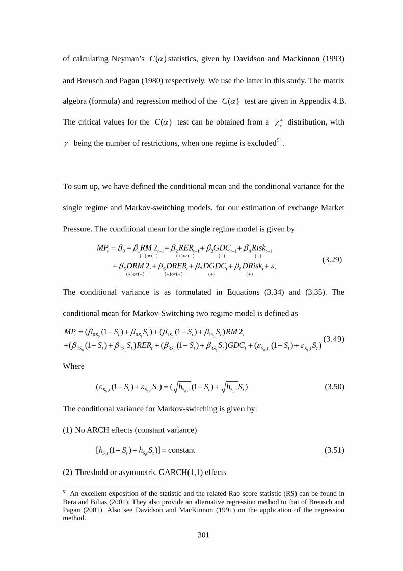
301

of calculating Neyman’s ( )C statistics, given by Davidson and Mackinnon (1993)

and Breusch and Pagan (1980) respectively. We use the latter in this study. The matrix

algebra (formula) and regression method of the ( )C test are given in Appendix 4.B.

The critical values for the ( )C test can be obtained from a 2 distribution, with

being the number of restrictions, when one regime is excluded51.

To sum up, we have defined the conditional mean and the conditional variance for the

single regime and Markov-switching models, for our estimation of exchange Market

Pressure. The conditional mean for the single regime model is given by

0 1 1 2 1 3 1 4 1( ) ( ) ( ) ( ) ( ) ( )

5 6 7 8( ) ( ) ( ) ( ) ( ) ( )

2

2

t t t t tor or

t t t t tor or

MP RM RER GDC Risk

DRM DRER DGDC DRisk

(3.29)

The conditional variance is as formulated in Equations (3.34) and (3.35). The

conditional mean for Markov-Switching two regime model is defined as

0 1 0 1

0 1 0 1 0 1

0 0 1 1

2 2 3 3 , , ,

( (1 ) ) ( (1 ) ) 2

( (1 ) ) ( (1 ) ) ( (1 ) )

t S t S t S t S t t

S t S t t S t S t t S t t S t t

MP S S S S RM

S S RER S S GDC S S

(3.49)

Where

0 1 0 1, , , ,( (1 ) ) ( (1 ) )S t t S t t S t t S t tS S h S h S (3.50)

The conditional variance for Markov-switching is given by:

(1) No ARCH effects (constant variance)

0 1[ (1 ) )] constantS t t S t th S h S (3.51)

(2) Threshold or asymmetric GARCH(1,1) effects

51 An excellent exposition of the statistic and the related Rao score statistic (RS) can be found in Bera and Bilias (2001). They also provide an alternative regression method to that of Breusch and Pagan (2001). Also see Davidson and MacKinnon (1991) on the application of the regression method.

302

0 1 0 1

0 0, 1 1 1, 1 0 0, 1 1 1, 1

0 0, 1 0, 1 1 1, 1 1, 1

, , 0 0

2 21 1 2 2

2 21 1

[ (1 ) )] [ (1 ) ]

[ (1 ) ] [ (1 ) ]

[ (1 ) ( 0) ( 0)]

t t t t

t t t t

S t t S t t S t S t

S t S S t S S t S S t S

S t S S S t S S

h S h S V S V S

V S V S V S h V S h

V S V S

(3.52)

One thing need to be mentioned is that the Markov Switching models we proposed

above and Logit approaches (binary and multinomial Logit models) that we are going

to discuss in section 3.7 which redefine MP in a “threshold” manner all use the market

pressure as an indication of potential currency crisis. Apart from this, there are other

ways to model currency crisis. One possible method is to model the percentage

change in the exchange rate itself rather than MP, as in Peria (2002)’s study. Peria

used a 3-variables VAR regime-switching model, which is based on a 3 equation

VAR for the three constituents of MP (exchange rate change, change in reserves and

interest rate change). It is also possible, of course, just to model the exchange rate

depreciation/appreciation as function of the fundamental variables.

303

3.6 Empirical analysis

In this section, we present the results for the empirical estimations for six Asian

countries, namely, Thailand, Malaysia, Korea, Indonesia, Singapore and Philippines,

for the period from January 1980 to February 2008. For each country, the single

regime constant (OLS) and TGARCH models were first estimated to evaluate the

impact of the fundamental explanatory variables to the currency market pressure.

Markov Switching models with constant variance and with TGARCH specification

are then estimated. We find that when we model the exchange market pressure with

two distinct regimes (stable and volatile), different behaviours for each regime

emerge.

3.6.1 Empirical analysis for Korea

The constant (OLS) and TGARCH estimates for MP ignoring the possibility that

alternative regimes exist, rather than the estimates from Markov-switching model

under the assumption that there is one regime, is given in Table 3.1. For the constant

model, the coefficients on RM2 and Risk are statistically not significantly different

from zero at 5% significance level. For the TGARCH estimates, coefficients on RM2,

GDC and DGDC are insignificant. All other fundamentals and risk variable have

substantial impact on the exchange market pressure. However, the GDC, DGDC and

304

DRisk variables present incorrect expected sign. The Wald coefficient test is

performed to test the joint restriction that the coefficients on the TGARCH conditional

variances are jointly zero (i.e., 1 2 3 0V V V ). The test statistics52 reject the null

hypothesis at 5% significance level. The significance of coefficients in the conditional

variances imply that variance of market pressure is time dependent and conditional on

past information. The significance of 3V imply that asymmetric effect exist in the

conditional variances, with positive shocks have larger effect on the volatility of

market pressure. The conditional variance process is stationary, as 1 2 3 1V V V in

the conditional variance structure.

The graphs depicting the actual and fitted MP and the residuals from the fitted

equations are portrayed on Figure 3.2, with constant model in Figure 3.2 (1) and

TGARCH model in Figure 3.2(2). The estimated equation appears to track the

movement market pressure well. This can also be proved by the estimation fitness,

2R (reported at the bottom in Table 3.1), which indicate the around 80% of the

market pressure can be explained by the fundamental variables in both of the single

regime equation specifications. Jaque-Bera tests are larger than the critical value 5.99

at 5% significant level shows that the residuals from both estimations, which indicate

the residuals are not normally distributed.

The empirical estimation results from the two regimes Markov Switching models for

52 Wald test statistics (for all six countries in our study) are not reported in the table, but available upon request.

305

Table 3. 1 Estimation Results from Single Regime models for Korea

Korea

Constant Variance TGARCH

Coeff Std Error Signif Coeff Std Error Signif

1 0.00237 0.00395 0.54970 0.00235 0.00238 0.32400

2 0.02989 0.00628 0.00000 0.03480 0.00743 0.00000

3 -0.20073 0.06182 0.00130 -0.00067 0.04832 0.98900

4 -0.00390 0.01361 0.77470 0.05123 0.00640 0.00000

5 -0.86115 0.07831 0.00000 -0.68450 0.06840 0.00000

6 0.83101 0.03100 0.00000 0.73579 0.04110 0.00000

7 -0.12518 0.04546 0.00620 -0.04542 0.03471 0.19070

8 -0.06934 0.01908 0.00030 -0.06190 0.02311 0.00740

0V 0.00000 0.00000 0.90350

1V 0.14072 0.03889 0.00030

3V -0.14703 0.03928 0.00020

2V 0.94910 0.01198 0.00000

2R 0.79772 0.77924 2R 0.79342 0.77177

JB 3516.18 1048.80

Log(L) 1022.86 1047.66

LR 49.60

Note: The critical value for 2 (3) 7.81 , 2 (2) 5.99

306

Figure 3. 2 Actual and fitted value of MP from single regime estimation: Korea

(1) Constant (OLS) model

-.15

-.10

-.05

.00

.05

.10

-.2

-.1

.0

.1

.2

.3

.4

1985 1990 1995 2000 2005

Residual Actual Fitted

(2) TGARCH(1,1) model

-.15

-.10

-.05

.00

.05

.10

-.2

-.1

.0

.1

.2

.3

1985 1990 1995 2000 2005


307

Korea are reported in Table 3.2. Those for 1 regime are not reported here but available

upon request. Panel A is for the results from the Regime-Switching model with

constant variances. Our finding confirms that the fundamental and risk variables play

significant roles in triggering currency crisis. Coefficients on RER and Risk are not

significant in the volatile state53, but they are significant in the stable state. The

coefficients on RM2 are not significant at 5% significance level in the stable state. All

other variables have substantial on the market pressure in each state.

Now we turn to examine the Markov Switching TGARCH model for Korea reported

in Table 3.2 Panel B. In the mean structure, majority of fundamental and risk variables

are significant in the volatile state and all the explanatory variables are significant at

5% significant level in the stable state. Every variable has a statistically significant

impact on market pressure in one regime or another.

In the conditional variance structure for the Markov-switching TGARCH model,

coefficient 1V measures the persistence of market pressure shocks and 2V measures

the persistence of shocks on conditional variance. The coefficient 3V measures the

asymmetric effect of positive and negative market pressure shocks. We can observe

that the in the volatile state, all the three coefficients in the conditional variance are

significant at 5% level. For the stable state, only the coefficient on the past squared

53 The volatile and stable state can be readily identified in a 2 regime model, by drawing the probability of one regime against the MP series. However, statistical evidences for which regime represents which state (volatile or stable) is reported and discussed latter in this section. These methods to distinguish regimes of their states are particularly useful when there are more than two regimes, in which case the relationship between regimes and states are not that obvious.

308

residuals is significant. In both states, the 3V coefficients are negative, which suggest

that negative shocks have smaller effect. This means that the positive shocks, which

increase currency market pressure, have larger impact on the market pressure

volatility, though the impact is not significant in the stable state. In both state, we

have 1 2 3 1V V V , and 1 2 1V V . Therefore, the TGARCH process is stationary54.

As reported in Table 3.2, the transition probabilities of one regime switching to

another, 12P and 21P , are significant at 95% confidence level. Since 12 212 1P P ,

we can conclude that the process is likely to be persist in its current state rather than

switching to the other. The average persistence of each state is reported in the bottom

of the table. We can observe that the average persistence of volatile state is much

lower than the persistence of the stable state. Another feature is the average

persistence for the volatile states reduces in the TGARCH model comparing to in the

constant model. In contrast, the average persistence for the stable state increases from

18.33 months under the constant model to 24.59 months under the TGARCH in the

stable state. The unconditional probability of being in each regime (volatile or stable

regime, represented by 0S and

1S respectively), is reported in the bottom of Table 3.2

as well. It is apparent that the unconditional probability of MP to be in the volatile

state at a given time is much lower that the probability it is in the stable state.

We comment now to the comparison of the parameter significance across the constant

54 It is also the case in the single-regime estimation.

309

variance (Panel A) and TGARCH Markov (Panel B) switching models. The likelihood

ratio test is employed for this purpose. The likelihood ratio (LR) statistics are reported

at the bottom of the table. The LR test follows a 2 distribution. Under the null

hypothesis that the parameter for TGARCH ( 1V , 2V and 3V are all zero in both state),

we need to compare the LR Statistics to 2 (6) , with critical value of 12.59 at 5%

significant level. Apparently, the LR statistics for Korea (39.75) is larger than the

critical value, indicating the TGARCH effects are important in the Markov Switching

model for Korea. Same conclusion can also be obtained from examining the

significance of the TGARCH parameters in the variance, most of which are

significant, especially in the volatile state.

Figure 3.3 (1) plots the actual and the fitted value of MP and residuals from the

Markov Switching model with constant variance; and Figure 3.3 (2) for the Markov

Switching TGARCH model. At a glance, we can see that the fitted values track the

actual MP very well, for both constant and TGARCH models. Particularly they can

track the increases in market pressure in Nov 1997 to Jan 1998. However, both

models do not perform as well for the strong reduction in market pressure (possible

appreciation currency crisis), for example, in the early period of 1982. In general, we

can conclude the fundamental variables do have power in explaining the movement of

MP.

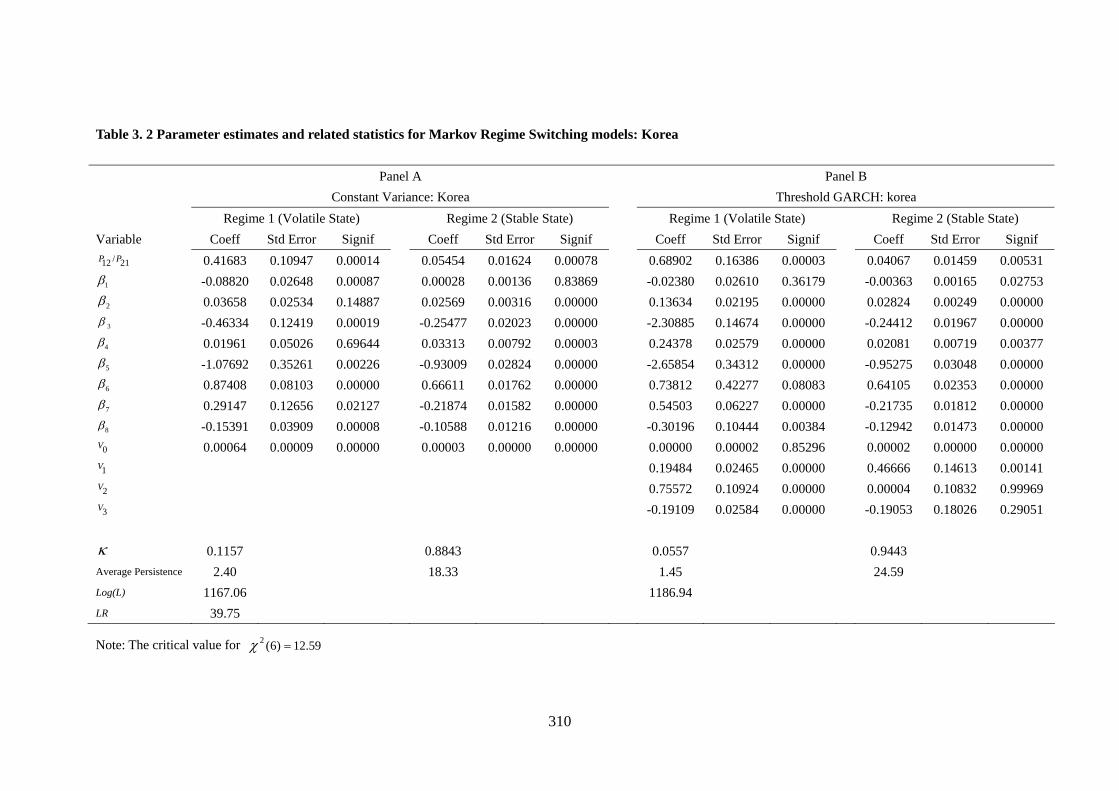
310

Table 3. 2 Parameter estimates and related statistics for Markov Regime Switching models: Korea

Panel A Panel B

Constant Variance: Korea Threshold GARCH: korea

Regime 1 (Volatile State) Regime 2 (Stable State) Regime 1 (Volatile State) Regime 2 (Stable State)

Variable Coeff Std Error Signif Coeff Std Error Signif Coeff Std Error Signif Coeff Std Error Signif /12 21P P 0.41683 0.10947 0.00014 0.05454 0.01624 0.00078 0.68902 0.16386 0.00003 0.04067 0.01459 0.00531

1 -0.08820 0.02648 0.00087 0.00028 0.00136 0.83869 -0.02380 0.02610 0.36179 -0.00363 0.00165 0.02753

2 0.03658 0.02534 0.14887 0.02569 0.00316 0.00000 0.13634 0.02195 0.00000 0.02824 0.00249 0.00000

3 -0.46334 0.12419 0.00019 -0.25477 0.02023 0.00000 -2.30885 0.14674 0.00000 -0.24412 0.01967 0.00000

4 0.01961 0.05026 0.69644 0.03313 0.00792 0.00003 0.24378 0.02579 0.00000 0.02081 0.00719 0.00377

5 -1.07692 0.35261 0.00226 -0.93009 0.02824 0.00000 -2.65854 0.34312 0.00000 -0.95275 0.03048 0.00000

6 0.87408 0.08103 0.00000 0.66611 0.01762 0.00000 0.73812 0.42277 0.08083 0.64105 0.02353 0.00000

7 0.29147 0.12656 0.02127 -0.21874 0.01582 0.00000 0.54503 0.06227 0.00000 -0.21735 0.01812 0.00000

8 -0.15391 0.03909 0.00008 -0.10588 0.01216 0.00000 -0.30196 0.10444 0.00384 -0.12942 0.01473 0.00000

0V 0.00064 0.00009 0.00000 0.00003 0.00000 0.00000 0.00000 0.00002 0.85296 0.00002 0.00000 0.00000

1V 0.19484 0.02465 0.00000 0.46666 0.14613 0.00141

2V 0.75572 0.10924 0.00000 0.00004 0.10832 0.99969

3V -0.19109 0.02584 0.00000 -0.19053 0.18026 0.29051

0.1157 0.8843 0.0557 0.9443

Average Persistence 2.40 18.33 1.45 24.59

Log(L) 1167.06 1186.94

LR 39.75

Note: The critical value for 2 (6) 12.59

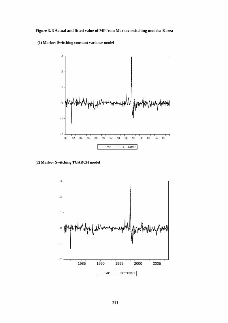
311

Figure 3. 3 Actual and fitted value of MP from Markov switching models: Korea

(1) Markov Switching constant variance model

-.2

-.1

.0

.1

.2

.3

80 82 84 86 88 90 92 94 96 98 00 02 04 06

MP FITTEDMP

(2) Markov Switching TGARCH model

-.2

-.1

.0

.1

.2

.3

1985 1990 1995 2000 2005

MP FITTEDMP

312

Figure 3. 4 Market Pressure and Probability of volatile state for Korea


-.2

-.1

.0

.1

.2

.3

0.0

0.2

0.4

0.6

0.8

1.0

80 82 84 86 88 90 92 94 96 98 00 02 04 06

- 1.5SD

+ 1.5SDMean

p*=0.5

(2)Markov Switching TGARCH model

-.2

-.1

.0

.1

.2

.3

0.0

0.2

0.4

0.6

0.8

1.0

80 82 84 86 88 90 92 94 96 98 00 02 04 06

+ 1.5SD

- 1.5SDMean

p*=0.5

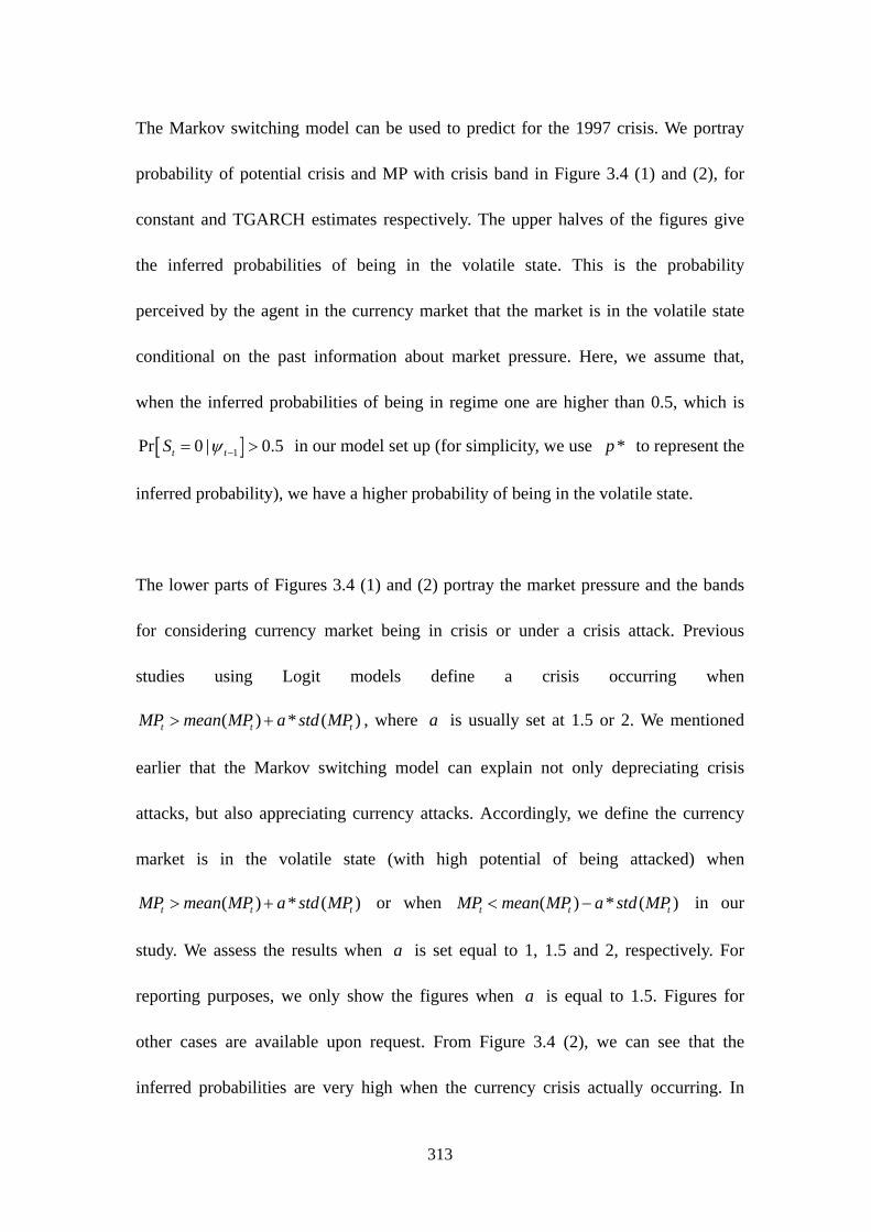
313

The Markov switching model can be used to predict for the 1997 crisis. We portray

probability of potential crisis and MP with crisis band in Figure 3.4 (1) and (2), for

constant and TGARCH estimates respectively. The upper halves of the figures give

the inferred probabilities of being in the volatile state. This is the probability

perceived by the agent in the currency market that the market is in the volatile state

conditional on the past information about market pressure. Here, we assume that,

when the inferred probabilities of being in regime one are higher than 0.5, which is

1Pr 0 | 0.5t tS in our model set up (for simplicity, we use *p to represent the

inferred probability), we have a higher probability of being in the volatile state.

The lower parts of Figures 3.4 (1) and (2) portray the market pressure and the bands

for considering currency market being in crisis or under a crisis attack. Previous

studies using Logit models define a crisis occurring when

( ) * ( )t t tMP mean MP a std MP , where a is usually set at 1.5 or 2. We mentioned

earlier that the Markov switching model can explain not only depreciating crisis

attacks, but also appreciating currency attacks. Accordingly, we define the currency

market is in the volatile state (with high potential of being attacked) when

( ) * ( )t t tMP mean MP a std MP or when ( ) * ( )t t tMP mean MP a std MP in our

study. We assess the results when a is set equal to 1, 1.5 and 2, respectively. For

reporting purposes, we only show the figures when a is equal to 1.5. Figures for

other cases are available upon request. From Figure 3.4 (2), we can see that the

inferred probabilities are very high when the currency crisis actually occurring. In

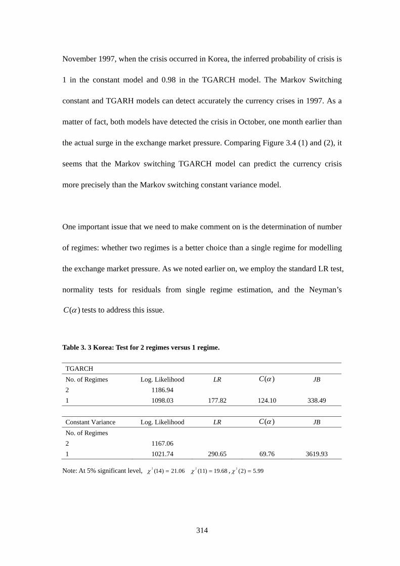
314

November 1997, when the crisis occurred in Korea, the inferred probability of crisis is

1 in the constant model and 0.98 in the TGARCH model. The Markov Switching

constant and TGARH models can detect accurately the currency crises in 1997. As a

matter of fact, both models have detected the crisis in October, one month earlier than

the actual surge in the exchange market pressure. Comparing Figure 3.4 (1) and (2), it

seems that the Markov switching TGARCH model can predict the currency crisis

more precisely than the Markov switching constant variance model.

One important issue that we need to make comment on is the determination of number

of regimes: whether two regimes is a better choice than a single regime for modelling

the exchange market pressure. As we noted earlier on, we employ the standard LR test,

normality tests for residuals from single regime estimation, and the Neyman’s

( )C tests to address this issue.

Table 3. 3 Korea: Test for 2 regimes versus 1 regime.

TGARCH No. of Regimes Log. Likelihood LR ( )C JB

2 1186.94 1 1098.03 177.82 124.10 338.49

Constant Variance Log. Likelihood LR ( )C JB

No. of Regimes 2 1167.06 1 1021.74 290.65 69.76 3619.93

Note: At 5% significant level, 2(14) 21.06 2

(11) 19.68 , 2(2) 5.99

315

Table 3.3 summarises the tests statistics for the presence of one versus two regimes

for Korea. First we perform the normality test on the residuals obtained from one

regime estimation models. The JB statistics is much higher than the critical value

2 (2)=5.99. As stated previously, we also supplement the test using bootstrapping

method to assessing the JB statistics for 500 resampled replications and assessing the

number of modes using 100 replications. Both of these tests based on simulations

indicate that the residuals from the constant single regime model are not normally

distributed, nor did those from the TGARCH single regime model; and hence,

possibly being distorted by the presence of at least another regime.

The log likelihood values for single and two regimes estimates are also quoted in

Table 3.3. Accordingly we calculate the associated Likelihood Ratio (LR) statistics.

LR is 177.82 for the TGARCH model, significantly larger than the critical value

2 (14) 21.06 at 5% significant level. The significance of Neyman’s ( )C test

statistics confirms such results for the TGARCH models (with the critical value

2 (14) 21.06 ). Similar results can be found for the Constant Variance models

between single and two regimes, that LR and Neyman’s ( )C test statistics both

larger than the critical value 2 (11) 19.68 at 5% significance level. All these tests

give consistent implication that more than one regime should be examined. Thus two

regimes Markov switching models should be more suitable than their one regime

counterparts to explain the currency market pressure and the currency crisis.

316

Although by portraying the probability of a regime against MP, it is straightforward to

distinguish which regime relate to which state in a 2 regimes Markov Switching

model: high/low market pressure and thereby probably accompanying a volatile state;

or a stable regime that market pressure fall in the medium range, we provide statistical

evidence for the identification of the regimes in this study55. One method is to

calculate Brier’s (1950) quadratic probability score (QPS). QPS is often used to

evaluate probability forecasts (see Diebold and Rudebush, 1989). The forecast

accuracy, which refers to the closeness, on average, of predicted probabilities and

observed realisations, is measured by a zero-one dummy variable. QPS is a function

of the probability-forecast analog of mean squared error, which is formulated as

2

1

)(2)/1( tt

T

t

RrPTQPS

(3.53)

Here: tPr is the probability that the given regime will occur; and tR is the

realisation (1 or 0) that it has occurred. According to the formula, we need to specify

two things to calculate the QPS: (i) the probability that one regime will occur, which

can be by taking the estimate of the conditional probability for that regime, and (ii)

the outcome, the realized state of a given MP. To capture the state of MP, we follow

the Logit analysis literature, by comparing MP with some threshold values. Here we

take various limiting values: the mean value of MP plus or minus 1 standard deviation,

1.5 standard deviations and 2 standard deviations. When MP exceeds the range of its

mean value plus or minus 1/1.5/2 standard deviation, we refer the realized state as

volatile state. When MP lies within the range, the state is referred to as the stable state.

55 This can be particularly useful when there are more than two regimes.

317

Obviously, the QPS statistics ranges from 0 to 2, with a score of 0 corresponding to

perfect accuracy. The QPS results for Korea are reported in Table 3.4(a). The statistics

clearly indicate the regime 1 is the volatile state and regime 2 is the stable state for

Korea, for both constant variance and TGARCH Markov switching models.

QPS achieves a strict minimum under truthful revelation of the probabilities by the

forecaster. We also consider another strictly proper accuracy-scoring rule, the log

probability score (LPS), given by:

1

1

[(1 ) ln(1 ) ln( )]T

t t t tt

LPS T R R

Pr Pr (3.54)

Still, tPr is the forecasted probability that a given regime will occur; and tR is the

realisation (1 or 0) that it has occurred, defined in the same as in QPS. The LPS range

from 0 to ∞, with a score of 0 corresponding to perfect accuracy. The LPS depends

exclusively on the probability forecast of the event that actually occurred, assigning as

a score of the log of the assessed probability (see Diebold and Rudebush, 1989).

An additional statistic, GSB, which can be appropriate for our purpose, is examined in

our study. GSB is the global squared bias, which assesses the overall forecast

calibration of the probabilities:

22( )GSB R Pr (3.55)

Here rP is the average of the relevant probability values and R is the average of

the realization of the outcome. LPS and GSB statistics are reported in Table 3.4 (b)

and (c) for Korea, which confirm that regime one is the volatile state and regime two

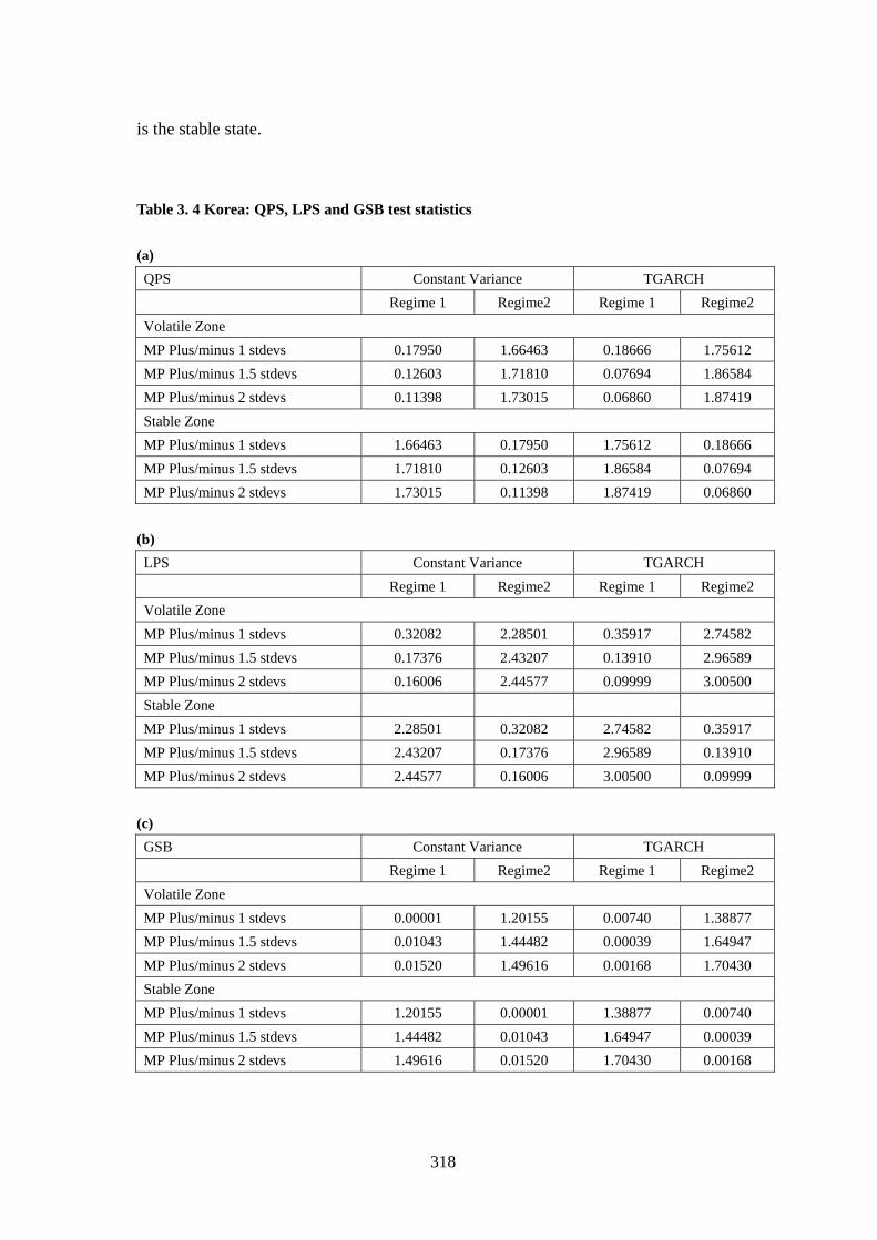
318

is the stable state.

Table 3. 4 Korea: QPS, LPS and GSB test statistics

(a)

QPS Constant Variance TGARCH

Regime 1 Regime2 Regime 1 Regime2

Volatile Zone

MP Plus/minus 1 stdevs 0.17950 1.66463 0.18666 1.75612

MP Plus/minus 1.5 stdevs 0.12603 1.71810 0.07694 1.86584


Stable Zone




(b)

LPS Constant Variance TGARCH


Volatile Zone




Stable Zone




(c)

GSB Constant Variance TGARCH


Volatile Zone




Stable Zone




319

3.6.2 Empirical analysis for Indonesia

Similarly, we perform single regime constant and TGARCH estimations first for the

market pressure in Indonesia and the estimates are reported in Table 3.5. Most

parameters in the two models are significant. For both models, the coefficients on

GDC and DGDC do not differ from zero at 5% significant level. Thus the real

domestic credit growth does not have significant impact on the exchange market

pressure. Besides, it does not have the anticipated sign, in both of its level or first

difference, so as the Risk variable in its first difference. Covariance stationary is

achieved in the TGARCH model specification; however, in the case of Indonesia, the

negative shocks of market pressure have larger impact on its volatility.

Actual and fitted MP and the residuals from the fitted equation are portrayed in Figure

3.5. The estimated equation appears to track the movement market pressure well.

From Table 3.5, we can see that the fitness of estimation equation ( 2R ) is 67.86% for

the constant and 65.05% for the TGARCH model.

The estimation results from 2 regimes Markov Switching Constant and TGARCH

models for Indonesia are reported in Table 3.6 (1) and (2) respectively. For the

constant model, we observe that in the stable state, all the variables are significant,

with GDC, DGDC, and DRisk not having the expected signs; in the volatile state,

GDC has insignificant impact on market pressure in both its level and first difference;

320

however, the signs are consistent with our expectation. Risk in its first difference does

not have significant impact on the market pressure, nor is its sign following

expectation. For the TGARCH model, we found that all the fundamental and risk

variables have significant impact on the market pressure, although the signs for GDC,

DGDC and Risk are not in line with anticipation. Most variables have larger impact in

the volatile state than in the stable state, shows by the absolute value of their

coefficients.

The covariance structure for the TGARCH model is stationary, as indicted by

1 2 3 1V V V in both states. Same as in the single regime model, the coefficient 3V

is positive. This imply that asymmetric effects exist in Indonesia currency market,

with negative shocks have larger impact on the market pressure. From the significance

of LR test between the TGARCH and constant model, as well as the significance of

most coefficients in the TGARCH variances specification, we can conclude that the

variance is time varying and TGARCH specification for the conditionally variance is

necessary in the Markov Switching model for Indonesia.

The transitional probability for each state is significantly different from zero at 95%

confidence level for both constant and TGARCH Regime-Switching estimates.

12 212 1P P confirms the persistence of each state. Average persistence for the

volatile state in Indonesia is under 4 months and under 26 months for the stable state.

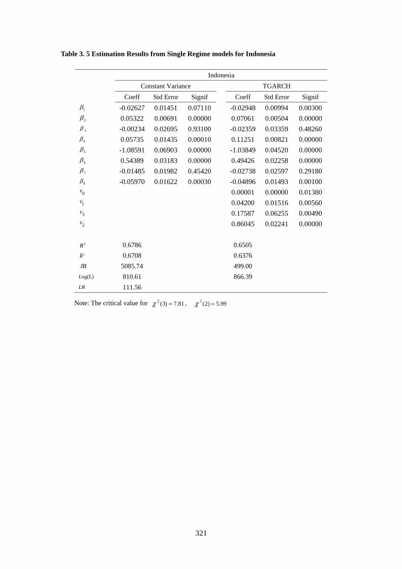
321

Table 3. 5 Estimation Results from Single Regime models for Indonesia

Indonesia



1 -0.02627 0.01451 0.07110 -0.02948 0.00994 0.00300

2 0.05322 0.00691 0.00000 0.07061 0.00504 0.00000

3 -0.00234 0.02695 0.93100 -0.02359 0.03359 0.48260

4 0.05735 0.01435 0.00010 0.11251 0.00821 0.00000

5 -1.08591 0.06903 0.00000 -1.03849 0.04520 0.00000

6 0.54389 0.03183 0.00000 0.49426 0.02258 0.00000

7 -0.01485 0.01982 0.45420 -0.02738 0.02597 0.29180

8 -0.05970 0.01622 0.00030 -0.04896 0.01493 0.00100

0V 0.00001 0.00000 0.01380

1V 0.04200 0.01516 0.00560

3V 0.17587 0.06255 0.00490

2V 0.86045 0.02241 0.00000

2R 0.6786 0.6505 2R 0.6708 0.6376

JB 5085.74 499.00

Log(L) 810.61 866.39

LR 111.56


322

Figure 3. 5 Actual and fitted value of MP from single regime estimation: Indonesia


-.10

-.05

.00

.05

.10

.15

.20

-.2

-.1

.0

.1

.2

.3

1985 1990 1995 2000 2005



-.10

-.05

.00

.05

.10

.15

.20

-.2

-.1

.0

.1

.2

.3

1985 1990 1995 2000 2005


323

Table 3. 6 Parameter estimates and related statistics for Markov Regime Switching models: Indonesia

Panel A Panel B

Constant Variance:Indonesia Threshold GARCH: Indonesia



1 0.18207 0.03160 0.00000 -0.01775 0.00237 0.00000 0.00400 0.00010 0.00000 -0.00376 0.00231 0.10402

2 0.05266 0.02874 0.06693 0.03077 0.00423 0.00000 0.12966 0.01282 0.00000 0.03692 0.00175 0.00000

3 0.23243 0.15249 0.12744 -0.03984 0.01049 0.00015 0.00735 0.00012 0.00000 -0.02785 0.00759 0.00024

4 0.20596 0.06290 0.00106 0.04230 0.00438 0.00000 0.23718 0.01873 0.00000 0.02897 0.00390 0.00000

5 -1.32433 0.20936 0.00000 -1.07729 0.03097 0.00000 -1.25319 0.09856 0.00000 -1.06797 0.02883 0.00000

6 0.45843 0.09117 0.00000 0.54445 0.01472 0.00000 0.48225 0.03231 0.00000 0.58705 0.01235 0.00000

7 0.17500 0.12382 0.15756 -0.03306 0.00694 0.00000 -0.00679 0.00012 0.00000 -0.03043 0.00537 0.00000

8 -0.01765 0.05087 0.72865 -0.08229 0.00936 0.00000 -0.02179 0.03000 0.00000 -0.05756 0.00739 0.00000

0V 0.00222 0.00042 0.00000 0.00012 0.00001 0.00000 0.00238 0.00029 0.00000 0.00009 0.00000 0.00000

1V 0.30825 0.07750 0.00000 0.20169 0.07962 0.01130

2V -0.23974 0.00952 0.00000 -0.00932 0.00373 0.01238

3V 0.21871 0.00511 0.00000 0.11909 0.01905 0.00000

0.1361 0.8639 0.1193 0.8807


Log(L) 921.37 936.40

LR 30.05


324

Figure 3. 6 Actual and fitted value of MP from Markov switching models: Indonesia


-.2

-.1

.0

.1

.2

.3

80 82 84 86 88 90 92 94 96 98 00 02 04 06

MP FITTEDMP


-.15

-.10

-.05

.00

.05

.10

.15

.20

.25

80 82 84 86 88 90 92 94 96 98 00 02 04 06

MP FITTEDMP

325

Figure 3. 7 Market Pressure and Probability of volatile state for Indonesia


-.2

-.1

.0

.1

.2

.3

0.0

0.2

0.4

0.6

0.8

1.0

80 82 84 86 88 90 92 94 96 98 00 02 04 06

- 1.5SD

+ 1.5SD

Mean

p*=0.5


-.2

-.1

.0

.1

.2

.3

0.0

0.2

0.4

0.6

0.8

1.0

80 82 84 86 88 90 92 94 96 98 00 02 04 06

- 1.5SD

+ 1.5SD

Mean

p*=0.5

326

The actual and fitted MP are portrayed in Figure 3.6 (1) and (2), for the Markov

Switching models with constant variance and with TGARCH conditional variance

respectively. Still, the fitted MP tracks the actual MP well. We cannot tell from the

figures whether TGARCH or constant models have better tracking ability than the

other, nor can we tell, by comparing to Figure 3.5, whether the single regime or 2

regimes model is better in tracking the movement of MP. However, the ability of each

model in correctly predicting the state of market pressure is provided and compared in

the later section.

Table 3. 7 Indonesia: Test for 2 regimes versus 1 regime.


2 936.40 1 818.99 234.81 27.40 704.46

Constant Variance No. of Regimes Log. Likelihood LR ( )C JB

2 921.37 1 802.53 237.69 22.87 5549.01


(11) 19.68 , 2(2) 5.99

Information on the criteria used to determine the number of regimes is provided in

Table 3.7. Similarly, we assess JB statistics and using bootstrapping to establish

resampled population of residuals from the single regime estimations to determine if

the residuals are normally distributed. All these diagnostic tests suggest that the

327

residuals are diverged from normal distribution, implying the existence of other

regime/regimes. LR and Neyman’s ( )C tests statistics also provide further

evidence that 2 regimes rather than 1 regime should be used.

Figure 3.7 (1) and (2) depict the market pressure and the inferred probability of

volatile state from the two Markov switching models. Again, both models detect the

currency crisis in August 1997 in Indonesia.

Now we examine the identification of the 2 regimes. The QPS, GSB and LPS

statistics are reported in Table 3.8. All these statistics indicate that regime 1 is the

volatile state for Indonesia.

328

Table 3. 8 Indonesia: QPS, LPS and GSB test statistics

(a)



Volatile Zone




Stable Zone




(b)



Volatile Zone




Stable Zone




(c)



Volatile Zone




Stable Zone




329

3.6.3 Empirical analysis for Thailand

Table 3.9 reports the constant and TGARCH estimates under the assumption that there

is one regime. For the constant model, the RM2 and GDC are not statistically

different from zero at 5% significance level. For the TGARCH model, RM2 and RER

do not significantly different from zero. For both models, two out of four explain

variables have significant impact on market pressure in their levels, with GDC has the

wrong a priori sign. When turning to the changes (first difference) in the macro

variables and risk, all have statistically significant impacts on exchange market

pressure. However, the DGDC and DRisk variables present incorrect expected sign.

The coefficients on the TGARCH conditional variances are all significant, indicating

that variance of market pressure is time dependent and conditional on past

information; and there is asymmetric effect in the conditional variances, with positive

shocks have larger effects on the volatility of market pressure.

The graphs depicting the actual and fitted MP and the residuals from the fitted

equations are portrayed in Figure 3.8. The estimated equation appears to track the

movement of market pressure well. This can also be proved by the estimation fitness,

2R (reported in the bottom of Table 3.1), which indicate that around 80% of the

market pressure can be explained by the fundamental variables in the equations of

single regime models. Jaque-Bera tests are larger than the critical value 5.99 at 5%

significant level shows that the residuals from both estimations, which indicate the

330

Table 3. 9 Estimation Results from Single Regime models for Thailand

Thailand



1 0.00080 0.00286 0.77910 -0.00269 0.00279 0.33520

2 0.02298 0.00569 0.00010 0.00667 0.00547 0.22220

3 -0.07836 0.05482 0.15380 -0.11082 0.04759 0.01990

4 0.04920 0.01675 0.00350 0.02993 0.01337 0.02510

5 -0.87408 0.06482 0.00000 -0.93860 0.06017 0.00000

6 0.79246 0.03219 0.00000 0.67889 0.02783 0.00000

7 -0.11341 0.04587 0.01390 -0.13755 0.03736 0.00020

8 -0.06641 0.01760 0.00020 -0.11566 0.00950 0.00000

0V 0.00002 0.00001 0.00000

1V 0.59028 0.17765 0.00090

3V -0.43661 0.16769 0.00920

2V 0.37769 0.12335 0.00220

2R 0.8175 0.7951 2R 0.8136 0.7881

JB 198.42 71.3318

Log(L) 1101.90 1140.52

LR 77.25


331

Figure 3. 8 Actual and fitted value of MP from single regime estimation: Thailand


-.06

-.04

-.02

.00

.02

.04

-.12

-.08

-.04

.00

.04

.08

.12

.16

1985 1990 1995 2000 2005



-.04

-.02

.00

.02

.04

.06

-.12

-.08

-.04

.00

.04

.08

.12

.16

1985 1990 1995 2000 2005


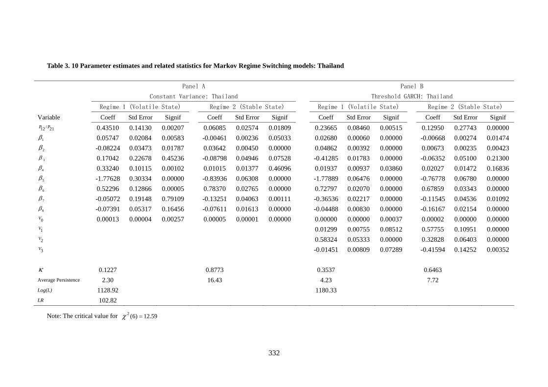
332

Table 3. 10 Parameter estimates and related statistics for Markov Regime Switching models: Thailand

Panel A Panel B

Constant Variance: Thailand Threshold GARCH: Thailand



1 0.05747 0.02084 0.00583 -0.00461 0.00236 0.05033 0.02680 0.00060 0.00000 -0.00668 0.00274 0.01474

2 -0.08224 0.03473 0.01787 0.03642 0.00450 0.00000 0.04862 0.00392 0.00000 0.00673 0.00235 0.00423

3 0.17042 0.22678 0.45236 -0.08798 0.04946 0.07528 -0.41285 0.01783 0.00000 -0.06352 0.05100 0.21300

4 0.33240 0.10115 0.00102 0.01015 0.01377 0.46096 0.01937 0.00937 0.03860 0.02027 0.01472 0.16836

5 -1.77628 0.30334 0.00000 -0.83936 0.06308 0.00000 -1.77889 0.06476 0.00000 -0.76778 0.06780 0.00000

6 0.52296 0.12866 0.00005 0.78370 0.02765 0.00000 0.72797 0.02070 0.00000 0.67859 0.03343 0.00000

7 -0.05072 0.19148 0.79109 -0.13251 0.04063 0.00111 -0.36536 0.02217 0.00000 -0.11545 0.04536 0.01092

8 -0.07391 0.05317 0.16456 -0.07611 0.01613 0.00000 -0.04488 0.00830 0.00000 -0.16167 0.02154 0.00000

0V 0.00013 0.00004 0.00257 0.00005 0.00001 0.00000 0.00000 0.00000 0.00037 0.00002 0.00000 0.00000

1V 0.01299 0.00755 0.08512 0.57755 0.10951 0.00000

2V 0.58324 0.05333 0.00000 0.32828 0.06403 0.00000

3V -0.01451 0.00809 0.07289 -0.41594 0.14252 0.00352

0.1227 0.8773 0.3537 0.6463


Log(L) 1128.92 1180.33

LR 102.82


333

Figure 3. 9 Actual and fitted value of MP from Markov switching models: Thailand


-.12

-.08

-.04

.00

.04

.08

.12

.16

80 82 84 86 88 90 92 94 96 98 00 02 04 06

MP FITTEDMP


-.12

-.08

-.04

.00

.04

.08

.12

.16

80 82 84 86 88 90 92 94 96 98 00 02 04 06

MP FITTEDMP

334

Figure 3. 10 Market Pressure and Probability of volatile state for Thailand


-.12

-.08

-.04

.00

.04

.08

.12

.160.0

0.2

0.4

0.6

0.8

1.0

80 82 84 86 88 90 92 94 96 98 00 02 04 06

+ 1.5SD

- 1.5SD

Mean

p*=0.5


-.12

-.08

-.04

.00

.04

.08

.12

.16

0.2

0.4

0.6

0.8

1.0

80 82 84 86 88 90 92 94 96 98 00 02 04 06

p*=0.5

Mean

+ 1.5SD

- 1.5SD

335

residuals are not normally distributed.

The empirical estimates from the two regimes Markov switching models for Thailand

are reported in Table 3.10. Panel A is for the results from the constant variances mode

and Panel B is for that from the TGARCH model. In the mean structure, our findings

confirm that the fundamental and risk variables play significant roles in triggering

currency crisis, as all variables are significant in at least one regime or another, for

both models. For the variance structure in the Markov switching TGARCH model, we

can observe that asymmetric effects are significant with positive shocks have larger

impact. Moreover, covariance stationary is guaranteed because 1 2 3 1V V V and

1 2 1V V , in both volatile and stable states. Although 1V and 3V differ from zero at

10% instead of 5% significant level, the test for that the coefficients in the conditional

variance structures are jointly zero has a LR statistics equal to 102.82, larger that than

the critical value at the 5% level, implying imposing constraint on the TGARCH

coefficients can be rejected. The TGACH model should not be nested to constant

model.

The transitional probabilities 12P and 21P are significant at 90% confidence level.

Since 12 212 1P P , we conclude that the process is likely to persist in its current

state rather than switching to the other. The average persistence of volatile state

increase from 2.3 months with the constant model to 4.23 with the TGARCH model,

however, the average persistence of stable states reduce from 16.43 to 7.72. The

336

unconditional probabilities are given in the bottom of the table.

Figures 3.9 (1) and (2) depict the actual and fitted MP along with the residuals from

the estimation models for Korea. And Figures 3.10 (1) and (2) present the inferred

probability of volatile state and market pressure. It can be observed that the models

track the MP well and can detect the currency crisis. Both constant and TGARCH

Markov switching model can correctly predict the currency crisis in July 1997 for

Thailand.

Table 3. 11 Thailand: Test for 2 regimes versus 1 regime.

TGARCH

No. of Regimes Log. Likelihood LR ( )C JB

2 1180.33 1 1128.73 103.20 47.90 66.74


2 1128.92 1 1090.89 76.06 20.23 197.92


(11) 19.68 , 2(2) 5.99

Table 3.11 reports the tests for determining the number of regimes. The LR, JB

Newman’s ( )C test statistics, as well as bootstrapping tests all imply that there

should be two regimes rather than one.

The QPS, GSB and LPS statistics are reported in Table 3.12 for identifying each

regime. The statistics all corroborate our observation that regime 1 is the volatile state

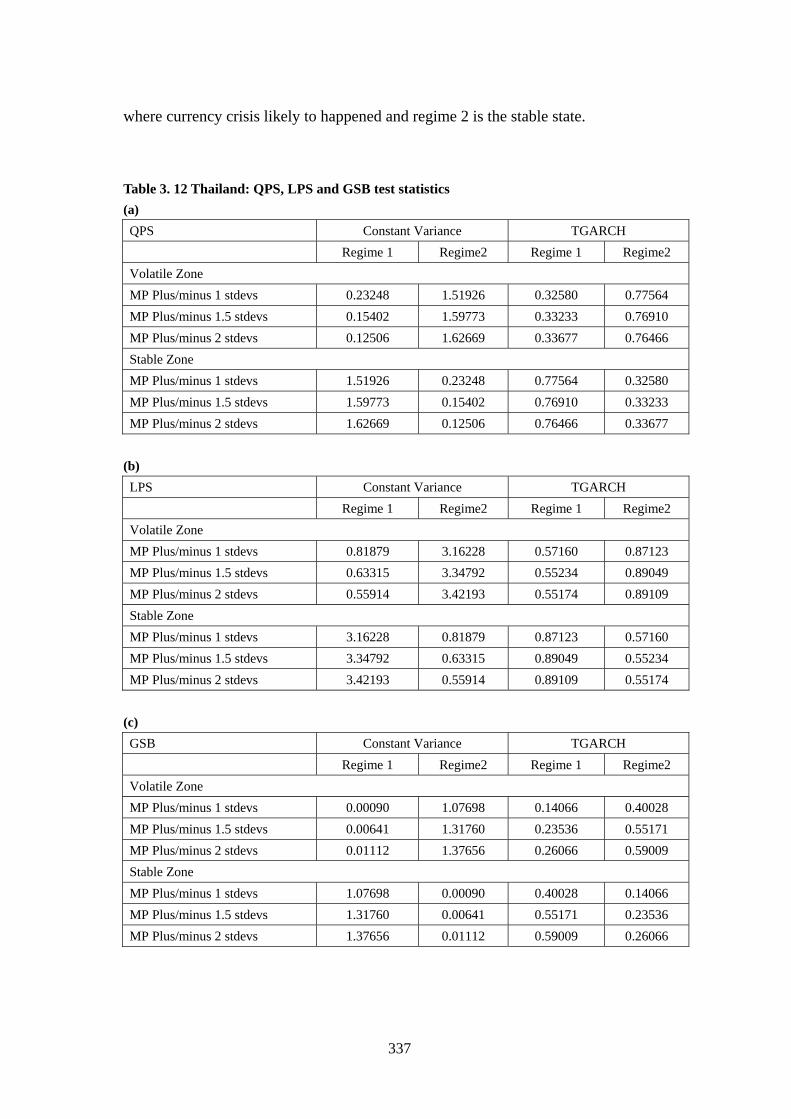
337

where currency crisis likely to happened and regime 2 is the stable state.

Table 3. 12 Thailand: QPS, LPS and GSB test statistics

(a)



Volatile Zone




Stable Zone




(b)



Volatile Zone




Stable Zone




(c)



Volatile Zone




Stable Zone




338

3.6.4 Empirical analysis for Malaysia

Table 3.13 reports the estimation results for Malaysia from single regime constant and

TGARCH models. Actual and fitted MP are portrayed in Figure 3.11. The macro and

risk variables are all significant at 95% confidence level, expect the RM2, in both

models. These variables can explain up to 85% of the MP in Malaysia. Asymmetric

effect in the volatility is not significant for Malaysia in the TGARCH model, indicated

by the insignificance of 3V .

The estimates from 2 regimes Markov Switching constant and TGARCH models are

shown in Table 3.14. From the constant estimates, we found that, in the volatile state,

DGC does not have substantial impact on MP, no matter in its level or first difference.

RER is not significant in its level, but significant in the first difference. In the stable

state, however, all variables expect RM2 are statistically significant. Signs on the

coefficients are not always as anticipation, especially for the DGDC. For the

TAGARCH Markov estimates, we find all variables are significant, expect the RM2

in the stable state. The model is covariance stationary in both volatile and stable state,

as 1 2 3 1V V V . Coefficient 3V is positive in the volatile state and negative in the

stable state, however, both of which are not significantly different from zero. The LR

test for the joint significance of the coefficients in the conditional variances ( 1V , 2V

and 3V are zero in both states) has a statistics of 1.01, smaller than the critical value

2 (6) 12.59 . Thus the null hypothesis that these coefficients are jointly zero cannot

339

Table 3. 13 Estimation Results from Single Regime models for Malaysia

Malaysia



1 -0.00206 0.00149 0.16770 0.00022 0.00132 0.86690

2 0.02653 0.00459 0.00000 0.04066 0.00369 0.00000

3 -0.05032 0.01205 0.00000 -0.08628 0.01252 0.00000

4 0.04213 0.01174 0.00040 0.03062 0.01048 0.00350

5 -0.35652 0.02627 0.00000 -0.45686 0.02305 0.00000

6 0.83603 0.02576 0.00000 0.82125 0.01673 0.00000

7 -0.04749 0.00883 0.00000 -0.08333 0.00756 0.00000

8 -0.03664 0.01530 0.01720 -0.03985 0.00884 0.00000

0V 0.00002 0.00000 0.00000

1V 0.46559 0.15379 0.00250

3V 0.54779 0.21747 0.01180

2V -0.02547 0.04155 0.53980

2R 0.8659 0.84918 2R 0.8630 0.84408

JB 1074.02 23.8504

Log(L) 1201.05 1253.81

LR 108.13


340

Figure 3. 11 Actual and fitted value of MP from single regime estimation: Malaysia


-.06

-.04

-.02

.00

.02 -.15

-.10

-.05

.00

.05

.10

.15

1985 1990 1995 2000 2005



-.06

-.04

-.02

.00

.02

.04

-.15

-.10

-.05

.00

.05

.10

.15

1985 1990 1995 2000 2005


341

Table 3. 14 Parameter estimates and related statistics for Markov Regime Switching models: Malaysia

Panel A Panel B

Constant Variance: Malaysia Threshold GARCH: Malaysia



1 -0.01190 0.00529 0.02411 -0.00014 0.00097 0.88164 -0.00168 0.00065 0.00000 -0.00095 0.00112 0.39469

2 0.00385 0.01010 0.70453 0.03400 0.00299 0.00000 0.02770 0.00131 0.00000 0.03420 0.00379 0.00000

3 0.04690 0.03610 0.19357 -0.08980 0.00840 0.00000 -0.02300 0.00115 0.00000 -0.07560 0.01140 0.00000

4 0.09140 0.03430 0.00775 0.03150 0.00800 0.00008 0.03630 0.00146 0.00000 0.04260 0.01010 0.00003

5 -0.35180 0.06250 0.00000 -0.43580 0.01420 0.00000 -0.38920 0.01120 0.00000 -0.39500 0.01970 0.00000

6 0.93170 0.05910 0.00000 0.72020 0.01750 0.00000 0.98650 0.23744 0.00000 0.73660 0.02060 0.00000

7 0.02450 0.02500 0.32810 -0.08520 0.00366 0.00000 -0.00558 0.00019 0.00000 -0.07280 0.00524 0.00000

8 -0.00888 0.03730 0.81199 -0.08750 0.01470 0.00000 -0.02710 0.00576 0.00000 -0.06060 0.01790 0.00071

0V 0.00008 0.00001 0.00000 0.00002 0.00000 0.00000 0.00007 0.00005 0.00000 0.00001 0.00000 0.00000

1V 0.36320 0.14320 0.01118 0.03250 0.04420 0.46196

2V -0.07540 0.01841 0.00000 0.26270 0.09210 0.00435

3V 0.01800 0.14960 0.90447 -0.02890 0.05400 0.59200

0.2504 0.7496 0.2366 0.7634


Log(L) 1269.45 1269.96

LR 1.01


342

Figure 3. 12 Actual and fitted value of MP from Markov switching models: Malaysia


-.20

-.15

-.10

-.05

.00

.05

.10

.15

80 82 84 86 88 90 92 94 96 98 00 02 04 06

MP FITTEDMP


-.15

-.10

-.05

.00

.05

.10

.15

80 82 84 86 88 90 92 94 96 98 00 02 04 06

MP FITTEDMP

343

be rejected. The LR test indicates the TGARCH structure in the Markov 2 regime

switching model may be not necessary.

For the Markov switching models, we have the transitional probabilities for the

volatile and stable state, 12P and 21P , are significantly differ from zero at 95%

significance level. The average persistence of the volatile state reduces under the

TGARCH modelling specification than under the constant modelling specification, so

as that of the stable state. The unconditional probability of being in the stable state is

more than 70%.

Figure 3.12 graphs the actual and fitted MP and model residuals for the Markov

Switching models. Still, the fitted MP tracks the MP very well, indicating the

explanatory power of the fundamental variables. Comparing Figure 3.12 with the

results from single regime estimation, we cannot claim if the 2 regimes models are

better than their one regime counterpart in terms of tracking MP. However, the LR and

Newman’s ( )C test statistics reported in Table 3.15 shows that the 2 regimes

models rather than the 1 regime ones should be used. JB statistics and bootstrapping

methods also support such conclusion.

Figure 3.13 present market pressure the inferred probability of volatile state and with

presumed crisis band. In July 1997 when the market pressure is high, the inferred

probability of volatile state is higher than 99%, for both constant and TGARCH

344

model. The occurrence of crisis is correctly detected in Malaysia. The figure also

shows that Markov switching TGARCH model can predict the currency crisis in a

more precise manner than the constant variance model.

Finally we examine the identification of the 2 regimes. The QPS, GSB and LPS

statistics are reported in Table 3.16. All these statistics clearly indicate that regime 1 is

the volatile state for Malaysia.

Table 3. 15 Malaysia: Test for 2 regimes versus 1 regime.


2 1269.96 1 1246.48 46.95 25.23 22.45


2 1269.45 1 1199.54 139.83 21.14 1329.92


(11) 19.68 , 2(2) 5.99

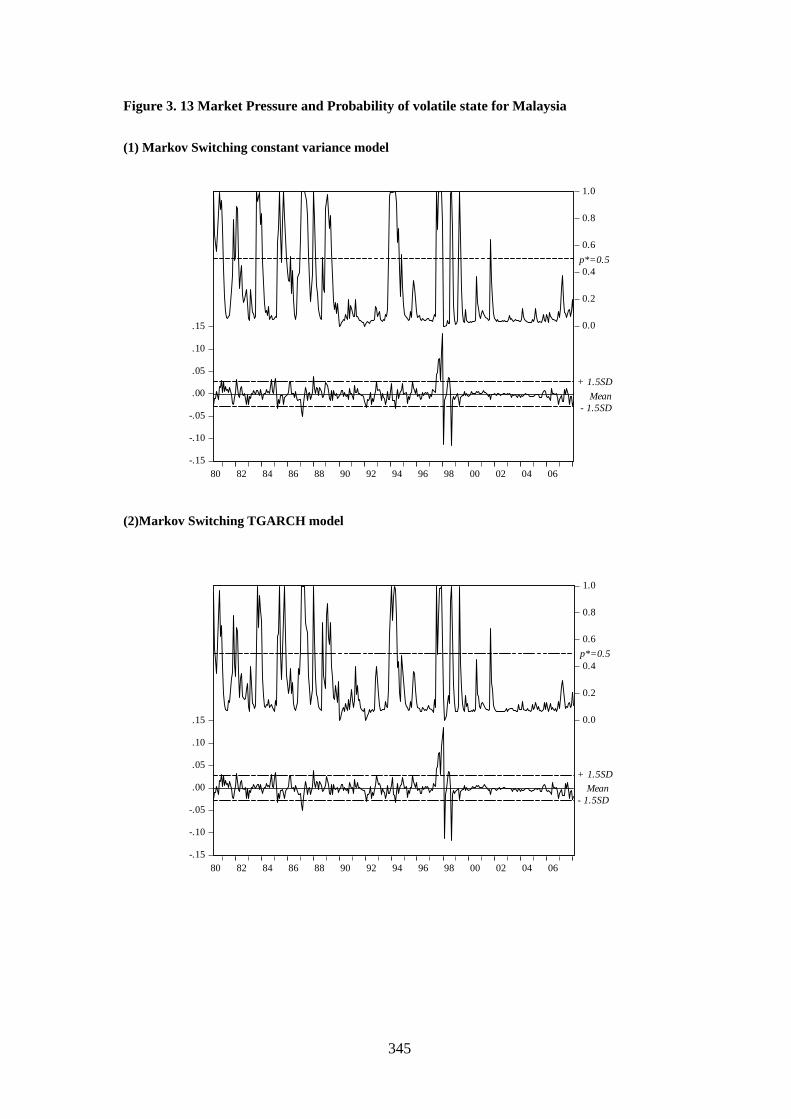
345

Figure 3. 13 Market Pressure and Probability of volatile state for Malaysia


-.15

-.10

-.05

.00

.05

.10

.15 0.0

0.2

0.4

0.6

0.8

1.0

80 82 84 86 88 90 92 94 96 98 00 02 04 06

- 1.5SD

+ 1.5SD

Mean

p*=0.5


-.15

-.10

-.05

.00

.05

.10

.15 0.0

0.2

0.4

0.6

0.8

1.0

80 82 84 86 88 90 92 94 96 98 00 02 04 06

p*=0.5

+ 1.5SD

- 1.5SDMean

346

Table 3. 16 Malaysia: QPS, LPS and GSB test statistics

(a)



Volatile Zone




Stable Zone




(b)



Volatile Zone




Stable Zone




(c)



Volatile Zone




Stable Zone




347

3.6.5 Empirical analysis for Singapore

Table 3.17 reports the estimation results for Singapore from single regime models.

Actual and fitted MP are portrayed in Figure 3.14. We observe that all the macro and

risk variables are significant at 95% confidence level. These variables can explain

more than 80% of the MP. Asymmetric effect in the conditional volatility of market

pressure is not significant in the TAGARCH single regime model.

The empirical estimates from the 2 regimes Markov switching models for Singapore

are reported in Table 3.18. Panel A is for the results from the Markov switching model

with constant variances. Our finding confirms that the fundamental and risk variables

play significant roles in triggering currency crisis, as all the variables are significantly

different from zero at 5% significance level for both states, expect for DGDC in the

volatile state, which is significant at 10% significance level.

The TGARCH Markov Switching estimates are reported in Panel B. Similar to the

constant model, all variables differ from zero at 95% confidence level expect for

DGDC. Signs on the Risk and DGC variables, in their level or first difference, are still

not always consistent with the theoretical expectation. The GARCH process is

stationary in both volatile and stable state, as 1 2 3 1V V V . However, in the volatile

state, 1 2 1V V . This indicate that when 0t , the volatility do not die away after

periods but intent to expand instead. Coefficient 3V is negative and significant in the

348

volatile state, indicating that the asymmetric affect of positive shocks can increase the

next period volatility of market pressure to a larger extent than the negative shocks. In

the stable state, however, 3V is positive, which means that the negative shocks have

large impact on the conditional volatility in the next period. 2V in both state are

indifferent from zero at 5% significant level, implying that the volatility of market

pressure do not depend on the past conditional volatility. However, past shocks has

significant impact on the conditional volatility. The joint significance test for the

TGARCH structure gives 48.34LR , larger than the critical value, suggesting that

the TGARCH structure should not be eliminated.

The transitional probability 12P and 21P , are significant at 95% confidence level in

the constant model, However, for the TGARCH model, the transitional probability is

not significant at 5% significance level for the stable state, but only significant at 10%

level. Since 12 212 1P P , we can conclude that the process is likely to persist in its

current state rather than switching to the other. The average persistent is about 4

months for the volatile state and much larger for the stable state. The persistence of

stable states in the constant model is higher than in the TGARCH model. On the other

hand, the persistence of volatile state from the two modelling specification are more

or less the same. The unconditional probabilities of the market pressure being in each

state are given in the bottom of the table.

349

Table 3. 17 Estimation Results from Single Regime models for Singapore

Singapore



1 -0.00703 0.00055 0.00000 -0.00648 0.00048 0.00000

2 0.03479 0.00490 0.00000 0.03286 0.00460 0.00000

3 -0.04472 0.01172 0.00020 -0.04440 0.01170 0.00010

4 0.07905 0.01408 0.00000 0.06963 0.01284 0.00000

5 -0.12249 0.02053 0.00000 -0.12991 0.01433 0.00000

6 0.72834 0.02472 0.00000 0.68261 0.02278 0.00000

7 -0.03877 0.00768 0.00000 -0.04006 0.00474 0.00000

8 -0.08853 0.01622 0.00000 -0.11910 0.01313 0.00000

0V 0.00000 0.00000 0.02740

1V 0.24683 0.10406 0.01770

3V -0.00159 0.10229 0.98760

2V 0.60859 0.11026 0.00000

2R 0.8413 0.8380 2R 0.8379 0.8325

JB 19.2843 0.0490

Log(L) 1290.81 1310.39

LR 39.15


350

Figure 3. 14 Actual and fitted value of MP from single regime estimation: Singapore


-.03

-.02

-.01

.00

.01

.02

-.08

-.04

.00

.04

.08

1985 1990 1995 2000 2005



-.03

-.02

-.01

.00

.01

.02

-.08

-.04

.00

.04

.08

1985 1990 1995 2000 2005


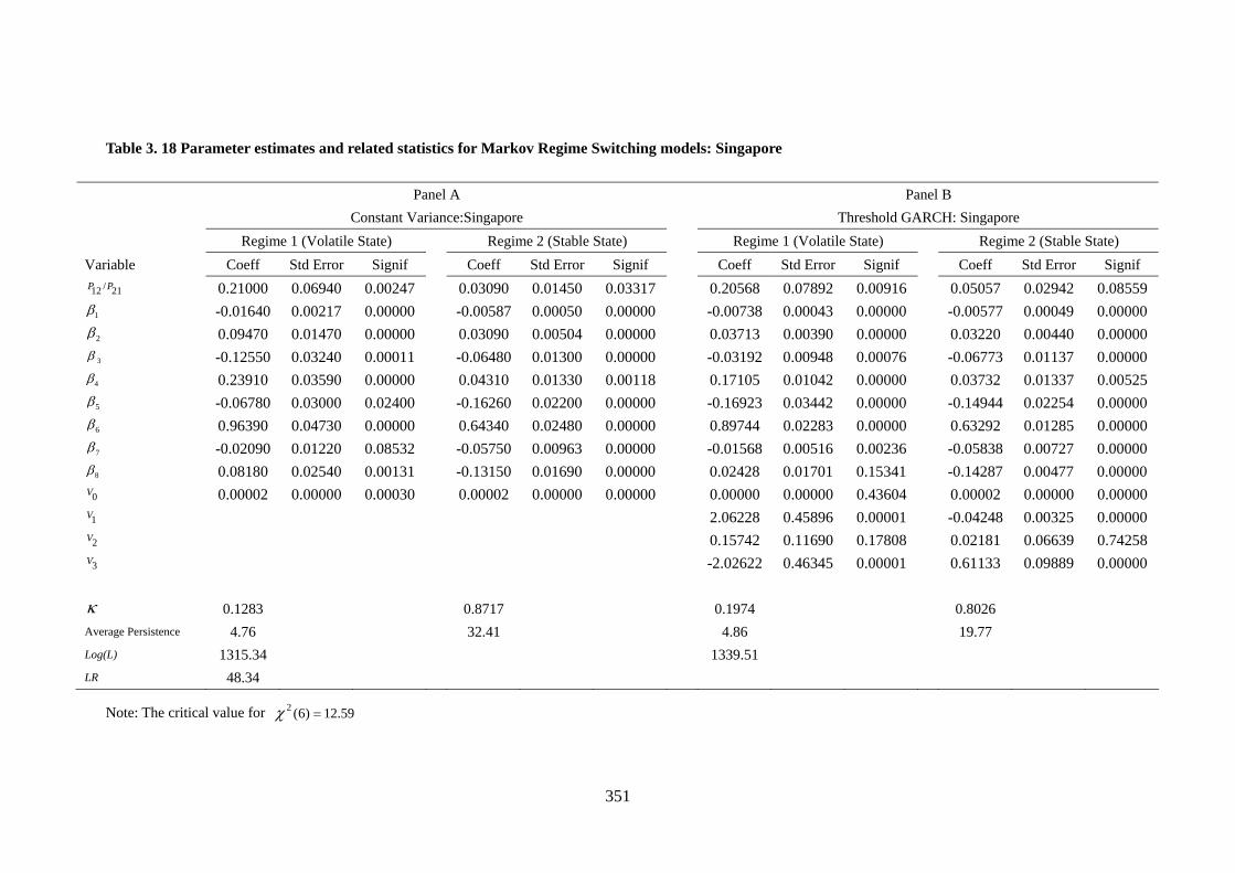
351

Table 3. 18 Parameter estimates and related statistics for Markov Regime Switching models: Singapore

Panel A Panel B

Constant Variance:Singapore Threshold GARCH: Singapore



1 -0.01640 0.00217 0.00000 -0.00587 0.00050 0.00000 -0.00738 0.00043 0.00000 -0.00577 0.00049 0.00000

2 0.09470 0.01470 0.00000 0.03090 0.00504 0.00000 0.03713 0.00390 0.00000 0.03220 0.00440 0.00000

3 -0.12550 0.03240 0.00011 -0.06480 0.01300 0.00000 -0.03192 0.00948 0.00076 -0.06773 0.01137 0.00000

4 0.23910 0.03590 0.00000 0.04310 0.01330 0.00118 0.17105 0.01042 0.00000 0.03732 0.01337 0.00525

5 -0.06780 0.03000 0.02400 -0.16260 0.02200 0.00000 -0.16923 0.03442 0.00000 -0.14944 0.02254 0.00000

6 0.96390 0.04730 0.00000 0.64340 0.02480 0.00000 0.89744 0.02283 0.00000 0.63292 0.01285 0.00000

7 -0.02090 0.01220 0.08532 -0.05750 0.00963 0.00000 -0.01568 0.00516 0.00236 -0.05838 0.00727 0.00000

8 0.08180 0.02540 0.00131 -0.13150 0.01690 0.00000 0.02428 0.01701 0.15341 -0.14287 0.00477 0.00000

0V 0.00002 0.00000 0.00030 0.00002 0.00000 0.00000 0.00000 0.00000 0.43604 0.00002 0.00000 0.00000

1V 2.06228 0.45896 0.00001 -0.04248 0.00325 0.00000

2V 0.15742 0.11690 0.17808 0.02181 0.06639 0.74258

3V -2.02622 0.46345 0.00001 0.61133 0.09889 0.00000

0.1283 0.8717 0.1974 0.8026


Log(L) 1315.34 1339.51

LR 48.34


352

Figure 3. 15 Actual and fitted value of MP from Markov switching models: Singapore


-.08

-.06

-.04

-.02

.00

.02

.04

.06

.08

80 82 84 86 88 90 92 94 96 98 00 02 04 06

MP FITTEDMP


-.08

-.06

-.04

-.02

.00

.02

.04

.06

.08

80 82 84 86 88 90 92 94 96 98 00 02 04 06

MP FITTEDMP

353

Figure 3. 16 Market Pressure and Probability of volatile state for Singapore


-.08

-.04

.00

.04

.08

0.0

0.2

0.4

0.6

0.8

1.0

80 82 84 86 88 90 92 94 96 98 00 02 04 06

- 1.5SD

+ 1.5SD

Mean

p*=0.5


-.08

-.04

.00

.04

.080.0

0.2

0.4

0.6

0.8

1.0

80 82 84 86 88 90 92 94 96 98 00 02 04 06

- 1.5SD

+ 1.5SD

Mean

p*=0.5

354

Figures 3.15 (1) and (2) present the actual and fitted MP along with the residuals from

the estimation models for Singapore; and Figure 3.16 (1) and (2) illustrate the inferred

probability of volatile state and market pressure. From the figures we can see that the

models have predictive power for the currency crisis. Both constant and TGARCH

Markov switching model can correctly predict the 1997 currency crisis.

We turn now to Table 3.19 to comment on the determination of the number of regimes.

The LR test statistics suggest that two regimes rather than one regime should be used.

However, the Newman’s ( )C test statistics is 4.81 for the TGARCH and 4.22 for

the constant model respectively, both of which are less than their critical values. These

results contradict with the LR test results and indicating that one regime may be

proper. The JB statistics for the residuals from one regime model is larger than its

critical value for the constant model, but smaller for the TGARCH model. However,

when we use bootstrapping method to establish a population from the residuals and

then use 500 replications for the JB and 100 replications to test for the number of

modes in the residuals, these simulation test results give that the residuals are not

normally distributed. The results from these tests do not agree with each other. Recall

earlier we find that the transitionally probability in the stable state for the TGARCH

estimation is not significant from zero at 5% significance level. The inconsistent test

statistics together with the estimation results made us to be cautious in claiming the

existence of a second regime in the Singapore exchange market. Further test may be

needed before drawing any conclusion.

355

We turn now to the identification of the 2 regimes (if two 2 regimes are presented and

Markov switching models are used). The QPS, GSB and LPS statistics are reported in

Table 3.20, which all corroborate our observation that regime 1 is the volatile state

where currency crisis likely to happened and regime 2 is the stable state.

Table 3. 19 Singapore: Test for 2 regimes versus 1 regime.


2 1339.51 1 1301.29 76.44 4.81 0.26


2 1315.34 1 1283.02 64.64 4.22 18.68


(11) 19.68 , 2(2) 5.99

356

Table 3. 20 Singapore: QPS, LPS and GSB test statistics

(a)



Volatile Zone




Stable Zone




(b)



Volatile Zone




Stable Zone




(c)



Volatile Zone




Stable Zone




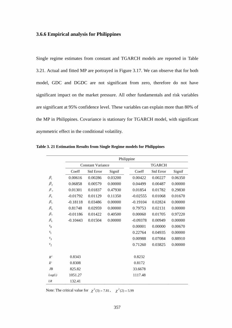
357

3.6.6 Empirical analysis for Philippines

Single regime estimates from constant and TGARCH models are reported in Table

3.21. Actual and fitted MP are portrayed in Figure 3.17. We can observe that for both

model, GDC and DGDC are not significant from zero, therefore do not have

significant impact on the market pressure. All other fundamentals and risk variables

are significant at 95% confidence level. These variables can explain more than 80% of

the MP in Philippines. Covariance is stationary for TGARCH model, with significant

asymmetric effect in the conditional volatility.

Table 3. 21 Estimation Results from Single Regime models for Philippines

Philippine



1 0.00616 0.00286 0.03200 0.00422 0.00227 0.06350

2 0.06858 0.00579 0.00000 0.04499 0.00487 0.00000

3 0.01301 0.01837 0.47930 0.01854 0.01782 0.29830

4 -0.01792 0.01129 0.11350 -0.02555 0.01068 0.01670

5 -0.18118 0.03486 0.00000 -0.19104 0.02824 0.00000

6 0.81748 0.02959 0.00000 0.79753 0.02131 0.00000

7 -0.01186 0.01422 0.40500 0.00060 0.01705 0.97220

8 -0.10443 0.01504 0.00000 -0.09378 0.00949 0.00000

0V 0.00001 0.00000 0.00670

1V 0.22764 0.04935 0.00000

3V 0.00988 0.07084 0.88910

2V 0.71260 0.03825 0.00000

2R 0.8343 0.8232 2R 0.8308 0.8172

JB 825.82 33.6678

Log(L) 1051.27 1117.48

LR 132.41


358

Figure 3. 17 Actual and fitted value of MP from single regime estimation: Philippines


-.04

-.02

.00

.02

.04

.06

.08

-.1

.0

.1

.2

.3

1985 1990 1995 2000 2005



-.04

-.02

.00

.02

.04

.06

.08

-.1

.0

.1

.2

.3

1985 1990 1995 2000 2005


359

Table 3. 22 Parameter estimates and related statistics for Markov Regime Switching models: Philippines

Panel A Panel B

Constant Variance: Philippines Threshold GARCH: Philippines



1 0.00427 0.00875 0.62517 0.00234 0.00169 0.16516 0.00690 0.00024 0.00000 0.00155 0.00162 0.33901

2 0.10950 0.01070 0.00000 0.03690 0.00402 0.00000 0.11750 0.02162 0.00000 0.03110 0.00284 0.00000

3 -0.12660 0.04430 0.00429 0.02460 0.01110 0.02736 0.03110 0.01117 0.00000 0.02070 0.00248 0.00000

4 0.04000 0.01680 0.01687 -0.02410 0.00655 0.00023 0.01410 0.00094 0.00000 -0.02500 0.00293 0.00000

5 -0.25480 0.10830 0.01857 -0.21450 0.02330 0.00000 -0.12910 0.00400 0.00000 -0.22890 0.00966 0.00000

6 0.89530 0.02760 0.00000 0.71610 0.02280 0.00000 0.80910 0.06026 0.00000 0.69810 0.03490 0.00000

7 -0.18800 0.03510 0.00000 0.00813 0.00978 0.40586 -0.06110 0.00205 0.00000 0.00531 0.00189 0.00497

8 -0.06600 0.01450 0.00001 -0.12040 0.01170 0.00000 -0.06870 0.00286 0.00000 -0.14050 0.01260 0.00000

0V 0.00027 0.00004 0.00000 0.00004 0.00000 0.00000 0.00010 0.00001 0.00000 0.00001 0.00000 0.00000

1V 0.86250 0.05085 0.00000 0.06930 0.01390 0.00000

2V -0.07950 0.00528 0.00000 0.69590 0.02300 0.00000

3V -0.01700 0.00049 0.00000 0.09470 0.04880 0.05230

0.2369 0.7631 0.2241 0.7759


Log(L) 1116.13 1128.47

LR 24.68


360

Figure 3. 18 Actual and fitted value of MP from Markov switching models: Philippines


-.10

-.05

.00

.05

.10

.15

.20

.25

80 82 84 86 88 90 92 94 96 98 00 02 04 06

MP FITTEDMP


-.08

-.04

.00

.04

.08

.12

.16

.20

.24

80 82 84 86 88 90 92 94 96 98 00 02 04 06

MP FITTEDMP

361

Figure 3. 19 Market Pressure and Probability of volatile state for Philippines


-.1

.0

.1

.2

.3

0.0

0.2

0.4

0.6

0.8

1.0

80 82 84 86 88 90 92 94 96 98 00 02 04 06

- 1.5SD

+ 1.5SD

Mean

p*=0.5


-.1

.0

.1

.2

.3

0.0

0.2

0.4

0.6

0.8

1.0

80 82 84 86 88 90 92 94 96 98 00 02 04 06

- 1.5SD

+ 1.5SD

Mean

p*=0.5

362

Table 3.22 reports the estimates from 2 regimes Markov Switching constant and

TGARCH models for Philippines. In the constant model, we found that RM2 is not

significant in both states, and DGDC is not significant in stable state. All variables are

significant in the TGARCH switching model expect RM2 in the stable regime.

Markov Switching TGARCH model is covariance stationary in every regime.

For the Markov switching models, the transitional probabilities are significantly

different from zero at 95% significant level. The average persistence of volatile and

stable state both reduces under the TGARCH modelling specification than under the

constant modelling specification. The unconditional probability of being in the stable

state is more than 75%.

Figure 3.18 graphs the actual and fitted MP and the residuals for the Markov

Switching models with constant variance and with TGARCH conditional variance.

Still, the fitted MP tracks the MP very well, indicating the explanatory power of the

fundamental variables. But we can not tell which model perform better only through

the graphs. For the information on 1 v.s. 2 regimes, the LR and Newman’s ( )C test

statistics reported in Table 3.23 give contradicting results. JB statistics and

bootstrapping methods for the residuals from 1 regime estimates show that the

residuals are not normally distributed, which support the 2 regimes rather than a

single regime should be modelled.

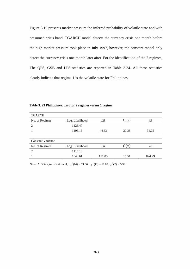
363

Figure 3.19 presents market pressure the inferred probability of volatile state and with

presumed crisis band. TGARCH model detects the currency crisis one month before

the high market pressure took place in July 1997, however, the constant model only

detect the currency crisis one month later after. For the identification of the 2 regimes,

The QPS, GSB and LPS statistics are reported in Table 3.24. All these statistics

clearly indicate that regime 1 is the volatile state for Philippines.

Table 3. 23 Philippines: Test for 2 regimes versus 1 regime.


2 1128.47 1 1106.16 44.63 20.38 31.75


2 1116.13 1 1040.61 151.05 15.51 824.29


(11) 19.68 , 2(2) 5.99

364

Table 3. 24 Philippines: QPS, LPS and GSB test statistics

(a)



Volatile Zone




Stable Zone




(b)



Volatile Zone




Stable Zone




(c)



Volatile Zone




Stable Zone




365

3.6.7 Comparison and summarisation of the empirical results of the six

Asian countries

Now we turn to compare and summarise the empirical results of the six Asian

countries. For all six countries, we find that most of the explanatory variables are

significant in their levels and their first differences. The domestic credit growth, in its

level and in its first difference, has the highest frequency of being insignificant.

Moreover, the signs on the GDC variables violate the theoretical expectation quite

often. Although domestic credit growth is a very important factor in the first and

second generation models for currency crisis, the empirical results in these six Asian

countries are not supportive. Another variable, Risk, in its level and in its first

difference, also frequently have a sign do not match the theoretical anticipation. The

RER variable is always significant in the stable state for all six countries, and mostly

significant in the volatile state except that in the Markov switching constant model for

Korea and Malaysia. RER always has a positive sign, and has larger impact in the

volatile state than in the stable state, with the only exception in the volatile state of

Thailand using constant model.

The covariance structure in the Markov Switching TGARCH model is always

stationary for all six countries. In most cases, the asymmetric effect in the conditional

volatility is significant. For all the countries except Malaysia, the LR test statistics

reject the null hypothesis that parameters on the conditional variance are jointly zero.

366

The TGARCH specification for the conditional variance in the Markov Switching

model should not be restricted to zero.

For Thailand, Indonesia, Malaysia and Philippines, the average persistence of volatile

state is lower in the TGARCH model than in the constant model, so as that of the

stable state. For Singapore, the TGARCH model reduces the average persistence of

stable state but not that of the volatile state; and it is the opposite for Korea. In general,

the TGARCH modelling specification tends to reduce the average persistence of

either state.

All the Markov Switching models can correctly detect the currency crisis in 1997, as

depicted in the market pressure and inferred probability of volatile state figures.

However, it is hard to justify from the figures which model, TGARCH or Constant, is

superior in tracking and detecting currency crisis. We provide further prediction

evaluation for the Markov Switching TGARCH and Constant Variance models.

Assume that the trigger point for a currency attack is ( ) * ( )t tmean MP a std MP .

When the inferred probability p* > 0.5 and at the same time

( ) * ( )t t tMP mean MP a std MP or ( ) * ( )t t tMP mean MP a std MP

the observation is assigned a value one to indicate that the crisis is correctly predicted

at the time. Similarly, when the inferred probability of stable state is bigger than 0.5,

which is equivalent to that (1-p*)>0.5, and at the same time

367

( ) * ( ) ( ) * ( )t t t t tmean MP a std MP MP mean MP a std MP

We assume a non-crisis state is correctly predicted at the time. Because as the value of

a change, the predictive power of the model may change, we set a to equal to different

values (1.5, 1 and 2) for evaluation purpose. The actual and correctly predicted total

number of crisis and non-crisis state using Markov Switching TGARCH and Constant

Variance models are listed in Table 3.25 (1) to (3), for 1.5a , 1a and 2a

respectively. Then the percentages of correct predictions are calculated.

From Table 3.25, we found that the “percentage correct” for non-crisis (stable) state is

higher than for the crisis (or volatile) state, using both constant variance and

TGARCH models, in all the six countries. When a=1.5, the correct percentage of the

non-crisis state is higher than when a=2 but lower than when a=1. In contrast, for the

correct prediction of crisis state, it is highest when a=2 and lowest when a=1, with

when a=1.5 lies in between. We also find that the TGARCH Markov switching

models give better results in focusing non-crisis status and constant model is

somewhat superior in focusing the crisis status. In any case, the correct percentage of

prediction for the currency crisis is low. When a=1.5 , the regime switching models

for Philippines give the highest correct percentage in predicting crisis, with 63.16%

under the TGARCH and 84.21% under the constant variance specifications; whilst the

models give the lowest correct prediction percentage of crisis for Thailand, with only

29.17% under the constant model. The performance of TGARCH and constant models

are mixed, we can not claim one is absolutely superior than the other in explaining

368

and predicting exchange market pressure, albeit we claimed earlier, by considering the

LR statistics, that the asymmetric GARCH specification in the conditional volatility

of the Markov Switching models should not be restricted to constant.

369

Table 3. 25 Markov Switching Models Crisis Prediction Evaluation

(1) a=1.5

Markov Switching Models

TGARCH Constant Variance

Percentage Percentage

Actual Predicted Correct Actual Predicted Correct

Korea

No Crisis 321 314 97.82 321 301 93.77

Crisis 13 7 53.85 13 8 61.54

Sum 334 321 96.11 334 309 92.51

Indonesia

No Crisis 303 288 95.05 303 285 94.06

Crisis 31 15 48.39 31 18 58.06

Sum 334 303 90.72 334 303 90.72

Thailand

No Crisis 312 280 89.74 312 299 95.83

Crisis 22 13 59.09 22 8 36.36

Sum 334 293 87.72 334 307 91.92

Malaysia

No Crisis 310 269 86.77 310 256 82.58

Crisis 24 13 54.17 24 16 66.67

Sum 334 282 84.43 334 272 81.44

Singapore

No Crisis 295 256 86.78 295 279 94.58

Crisis 39 18 46.15 39 21 53.85

Sum 334 274 82.04 334 300 89.82

Philippines

No Crisis 315 266 84.44 315 260 82.54

Crisis 19 12 63.16 19 16 84.21

Sum 334 278 83.23 334 276 82.63

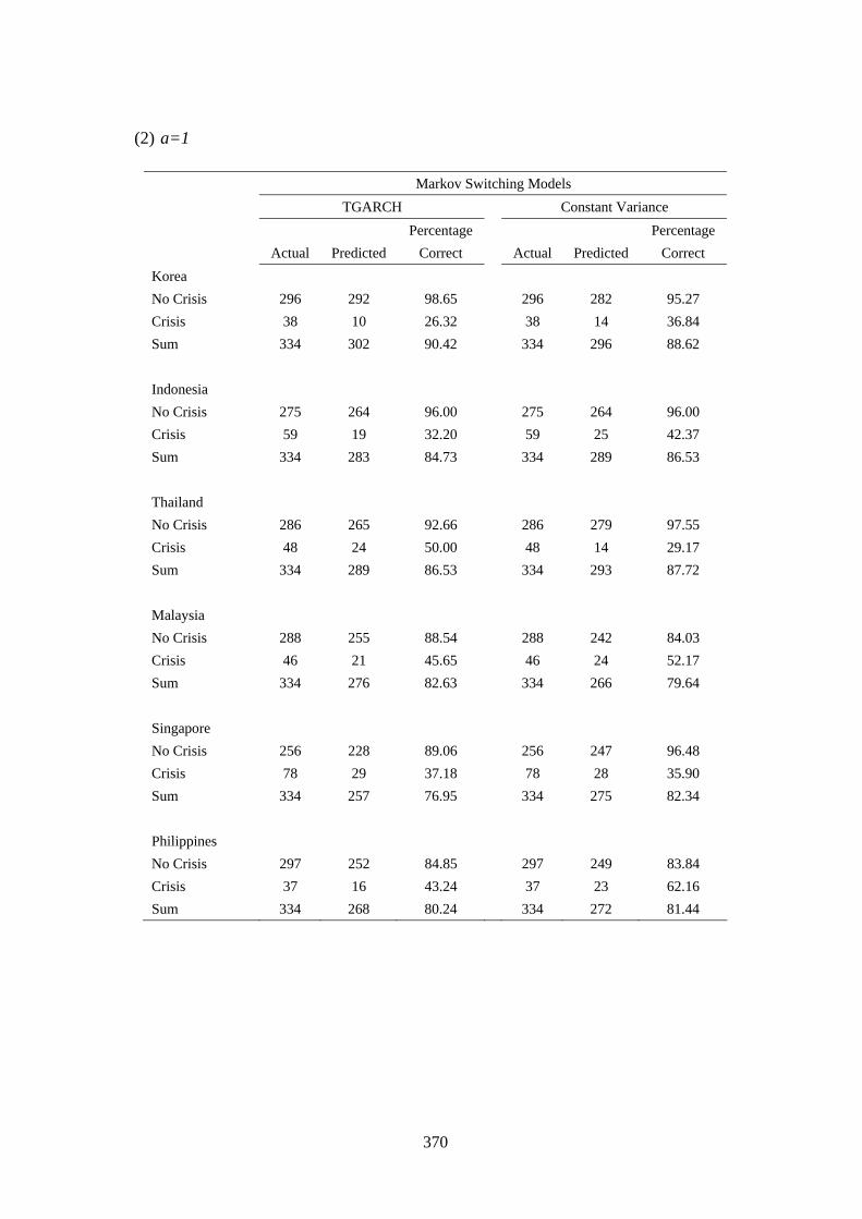
370

(2) a=1





Korea

No Crisis 296 292 98.65 296 282 95.27

Crisis 38 10 26.32 38 14 36.84

Sum 334 302 90.42 334 296 88.62

Indonesia

No Crisis 275 264 96.00 275 264 96.00

Crisis 59 19 32.20 59 25 42.37

Sum 334 283 84.73 334 289 86.53

Thailand

No Crisis 286 265 92.66 286 279 97.55

Crisis 48 24 50.00 48 14 29.17

Sum 334 289 86.53 334 293 87.72

Malaysia

No Crisis 288 255 88.54 288 242 84.03

Crisis 46 21 45.65 46 24 52.17

Sum 334 276 82.63 334 266 79.64

Singapore

No Crisis 256 228 89.06 256 247 96.48

Crisis 78 29 37.18 78 28 35.90

Sum 334 257 76.95 334 275 82.34

Philippines

No Crisis 297 252 84.85 297 249 83.84

Crisis 37 16 43.24 37 23 62.16

Sum 334 268 80.24 334 272 81.44

371

(3) a=2





Korea

No Crisis 326 317 97.24 326 305 93.56

Crisis 8 5 62.50 8 7 87.50

Sum 334 322 96.41 334 312 93.41

Malaysia

No Crisis 323 276 85.45 323 262 81.11

Crisis 11 7 81.82 11 9 81.82

Sum 334 283 84.73 334 271 81.14

Thailand

No Crisis 318 284 89.31 318 305 95.91

Crisis 16 11 68.75 16 8 50.00

Sum 334 295 88.32 334 313 93.71

Indonesia

No Crisis 317 297 93.69 317 292 92.11

Crisis 17 10 58.82 17 11 64.71

Sum 334 307 91.92 334 303 90.72

Singapore

No Crisis 314 267 85.03 314 291 92.68

Crisis 20 10 50.00 20 14 70.00

Sum 334 277 82.93 334 305 91.32

Philippines

No Crisis 320 269 84.06 320 262 81.88

Crisis 14 10 71.43 14 13 92.86

Sum 334 279 83.53 334 275 82.34

372

3.7 The Multinomial Logit Estimation

3.7.1 Methodology

The Binary Logit/Probit regressions have been widely used to examine currency

crises. Such are referred to as the discrete-dependent-variable approaches. In these

approaches, it normally involves converting the exchange market pressure index

(which is used as the currency crises indicator) into a binary variable. Currency crisis

is occurring when market pressure is bigger than a threshold value, which is often

defined as the mean of market pressure plus a times it’s standard deviation. Thus the

binary dependent variable tY is often defined as:

1 if ( ) * ( )

0 otherwiset

t

MP mean MP a Std MPY

The crisis index tY is explained by a set of independent variable tX includes

fundamental variables like RM2, RER, and GDC, Risk, etc. The aim of the model is

to estimate the impact of the indicators tX on the probability of experiencing a

crisis.

The logit model is defined using a logistic distribution:

exp( )( 1) ( )

1 exp( )t

t tt

Xprob Y X

X

(3.54)

Where (.) indicates the logistic cumulative distribution function.

The link function follows a linear regression:

373

t tY X (3.52)

In our study, it can be written as

0 1 1 2 1 3 1 4 1( ) ( ) ( ) ( ) ( ) ( )

5 6 7 8( ) ( ) ( ) ( ) ( ) ( )

2

2

t t t t tor or

t t t t tor or

Y RM RER GDC Risk

DRM DRER DGDC DRisk

(3.53)

The probit model is defined as

( 1) ( )t tprob Y X (3.55)

(.) the cumulative distribution function of the standard normal distribution

There are some defects of the Binary Logit/Probit models. One drawback is that,

using the above settings, they can only detect if there is currency crisis triggered by

currency depreciation. However, as we claimed earlier, the 2 regimes Markov

Switching models in our study can be used to detect not only the depreciation but also

the appreciation currency attacks. To overcome this obvious shortcoming of Binary

Logit/Probit models, Multinomial models are used to study the MP and compared

with the estimation results from the Markov Switching models.

The Multinomial Logit model is used rather than the Multinomial Probit models

because it is more appropriate for our data. Hahn and Soyer (2005) suggest that Logit

provides a better fit in the presence of extreme independent variable levels and

conversely that Probit better fit random effects models with moderate data sets.

Finney (1952) suggests using the Logit over the Probit transformation when data are

http://en.wikipedia.org/wiki/Cumulative_distribution_function�

http://en.wikipedia.org/wiki/Normal_distribution�

374

not normally distributed. Maddala (1992) shows that in the case of disproportionate

sampling in two binary groups, i.e., very few response ( 1tY , tY defined below) or

very few non-response ( 0tY ), the Logit coefficients model is not affected. However,

Probit model is not valid in estimating the disproportionate sample. In our case, there

are very few observations where 1tY , Logit mode is a proper choice.

The Multinomial Logit (Mlogit) model is a straightforward extension of the Binary

Logit model. Suppose dependent variable has M+1 categories. One value (typically

the first, the last or the value with the highest frequency of the dependent variable) is

designated as the reference category. The probability of membership in other

categories is compared to the probability of membership in the reference category.

For a dependent variable with M+1 categories, this requires the calculation of M

equations, or for each category relative to the reference category, to describe the

relationship between dependent variable and the independent variables.

Hence, if the first category is the reference, then, for m= 1, …, M

1

( )

( 0)

Ki

m mk ik miki

P Y mIn a b X Z

P Y

(3.56)

Hence, for each category, there will be M predicted log odds, one for each category

relative to the reference category. The probability is a little more complicated than it

was in logistic regression. For m=1,…,M

375

1

exp( )Pr( )

1 exp( )

mii M

hih

ZY m

Z

(3.57)

For the reference category

1

1Pr( 0)

1 exp( )i M

hih

YZ

(3.58)

For our estimation of currency crises, we assume there are three categories, namely,

the stable state, depreciation state and appreciation state. The stable state is used as

the reference/base state, and the other two states are in a volatile state as defined in the

Markov Switching models.

Hence the Mlogit model can be written as

,

1 if ( ) * ( )

2 if ( ) * ( )

0 otherwise

t t t

i t t t t

MP mean MP a std MP

Y MP mean MP a std MP

(3.59)

The probabilities for each category is

1 1 2 2, ( ) ( )

1Pr( 0)

1 t ti t X XYe e

(3.60)

1 1

1 1 2 2

( )

, ( ) ( )Pr( 1)1

t

t t

X

i t X X

eY

e e

(3.61)

2 2

1 1 2 2

( )

, ( ) ( )Pr( 2)1

t

t t

X

i t X X

eY

e e

(3.62)

376

3.7.2 Estimation results for Multinomial Logit Models

The Multinomial Logit models estimation results, when a=1.5, are reported in Table

3.26. The estimation results for Mlogit models when a=1 and a=1.5 are available

upon request. For the multinomial estimations of the six countries, we find that more

than half the estimated parameters are statistically not significantly different from zero,

for all the six countries; and signs on the GDC, DGDC, Risk and DRisk variables are

not always matching anticipation. Nonetheless, we find the Mlogit model with these

fundamental and risk factors as explanatory variables can describe the market pressure

and detecting crisis well, as shown below.

One objective is to evaluate the ability of the Logit model in predicting a crisis

correctly based on a specified prediction rule. Here we use the conventional cut-off

rule of a probability of 0.5 or 50%. The “correct” predictions of state 1, the high

market pressure (i.e. the depreciation currency attacks/crisis) are obtained when the

predicted probability ˆ( 1) ( )t tprob Y X )

is larger than 0.5 and the observed

1tY . Similar, the “correct” predictions for state 2, (i.e., the appreciation currency

attacks/crisis) are obtained when the predicted probability ˆ( 2) ( )t tprob Y X )

is

larger than 0.5 and the observed 2tY . The “correct” predictions for State 0, or

stable non-crisis state, follow the same mechanism. These are reported in Table 3.26

(1) to (3), for a=1.5, 1 and 2 respectively. Comparing with the results obtained from

Markov Switching models in Table 3.25 (1) to (3), we can observe that the Mlogit

377

model gives overall better prediction for the market pressures than the Markov

switching models. Our results do not provide evidence that 2 regimes switching

models are better for the modelling currency crisis than the Logit models, as claimed

in other literature (e.g. Ford, et al 2007). One argument is that we use 3 states in the

Logit model but only 2 in the Markov Switching model. Using 3 regimes in the

Markov Switching model may improve the results.

Figure 3.20 (1) to (6) charts the predicated probabilities and market pressure dummies.

The upper halves of the graphs are the predicted probabilities of a crisis generated by

the Mlogit model, and the lower halves graph the timing of crises according to the

market pressure dummy. When the upper halves graphs the predicted probability of

being in state 1 (predicated occurrence of depreciation crises), the lower halves of the

figures mark the timing of the depreciation crisis, i.e.,

( ) 1.5* ( )tMP mean mp Std MP . When the upper halves graphs the predicted

probability of being in state 2 (predicated occurrence of appreciation crises), the lower

halves of the figures mark the timing of the depreciation crisis, i.e.,

( ) 1.5* ( )tMP mean mp Std MP . From the figure for the four countries, we can

conclude the Mlogit model does provide a good explanation of cause and timing of

the crises, especially for the depreciating currency crises. When come to explaining

the appreciating market pressures, the model do not give as good results as explaining

the depreciating currency attacks.

378

Table 3. 26 Parameter Estimates and Related Statistics for Multinomial Logit models

Korea Indonesia

Coefficient Std.Error t-prob Coefficient Std.Error t-prob

State (1)

1 -20.9376 17.6300 0.2360 -14.0711 5.4460 0.0100

2 9.2472 11.8000 0.4340 6.9461 2.1260 0.0010

3 -77.7059 73.0000 0.2880 15.7203 7.2640 0.0310

4 -1.1779 23.9700 0.9610 12.6292 4.9330 0.0110

5 -207.4140 125.0000 0.0980 -45.1566 15.2200 0.0030

6 134.2930 62.4700 0.0320 20.5874 10.6200 0.0530

7 -8.9432 33.9600 0.7920 -5.2047 4.2510 0.2220

8 -18.9671 36.5700 0.6040 -13.1312 7.3510 0.0750

State (2)

1 -2.3140 11.0800 0.8350 -11.1159 5.1710 0.0320

2 0.1317 6.5350 0.9840 0.5990 1.9530 0.7590

3 146.1340 117.8000 0.2160 -3.3944 7.2200 0.6390

4 39.5459 40.6600 0.3320 1.9444 3.6030 0.5900

5 461.4340 246.0000 0.0620 93.7569 23.6800 0.0000

6 -235.5530 106.7000 0.0280 -46.0423 11.7300 0.0000

7 -85.3047 64.8800 0.1890 -2.9408 6.1790 0.6340

8 42.5171 26.4000 0.1080 10.5506 5.0160 0.0360

log-likelihood -16.4044 -64.8263

zeroline log-lik -71.7509 -130.9684

Test: Chi^2( 16) 110.69 132.28

AIC 68.8087 165.6525

AIC/T 0.2036 0.4901


379

Table 3.26 continued:

Thailand Malaysia


State (1)

1 -89.8642 44.3600 0.0440 -36.7083 8.4250 0.0000

2 -1.93463 9.3220 0.8360 16.6959 7.6000 0.0290

3 -52.6395 90.7700 0.5620 -34.3530 26.8700 0.2020

4 30.4145 31.2800 0.3320 -2.0497 10.9400 0.8510

5 -163.0070 146.0000 0.2650 -201.6810 61.7100 0.0010

6 627.2510 331.3000 0.0590 195.3750 50.1600 0.0000

7 -202.4310 136.4000 0.1390 0.5644 22.0800 0.9800

8 -20.0897 34.0900 0.5560 -6.3652 16.0200 0.6910

State (2)

1 -33.4229 6.3580 0.0000 -30.6169 7.3970 0.0000

2 -19.4058 8.6420 0.0250 -10.3613 7.3920 0.1620

3 -100.7980 51.8600 0.0530 -5.5259 15.1900 0.7160

4 -7.9427 16.9600 0.6400 -37.3219 22.5700 0.0990

5 38.4748 52.4200 0.4640 -0.0312 56.4200 1.0000

6 -175.1770 46.2100 0.0000 -73.6461 42.3100 0.0830

7 39.1766 42.5800 0.3580 2.0332 9.6160 0.8330

8 15.3195 18.8600 0.4170 147.9890 54.4700 0.0070


zeroline log-lik -371.3310 -371.3310

Test: Chi^2( 16) 689.42 675.37

AIC 85.2434 99.2901

AIC/T 0.2522 0.2938


380

Table 3.26 continued:

Singapore Philippines


State (1)

1 -21.3109 7.9050 0.0070 -29.5624 6.7710 0.0000

2 45.5617 18.4300 0.0140 -0.2455 5.7820 0.9660

3 -26.2597 40.3000 0.5150 -28.2019 25.3800 0.2670

4 120.3760 59.7000 0.0450 24.5317 10.4200 0.0190

5 -49.4505 72.1500 0.4940 54.0947 31.3800 0.0860

6 447.7180 180.4000 0.0140 155.0430 43.4600 0.0000

7 -14.4528 18.8400 0.4440 -2.0390 17.4900 0.9070

8 -135.0380 55.6400 0.0160 -27.3876 10.7000 0.0110

State (2)

1 -6.6467 1.1870 0.0000 -21.0370 4.3300 0.0000

2 -9.4092 5.9310 0.1140 -14.2625 5.6460 0.0120

3 -4.4800 16.8100 0.7900 4.4503 23.0400 0.8470

4 -52.2844 21.9700 0.0180 73.3318 23.0800 0.0020

5 64.9997 32.6900 0.0480 20.6464 26.8300 0.4420

6 -262.4630 56.9500 0.0000 -206.5900 54.5900 0.0000

7 16.5257 14.8800 0.2670 5.7050 22.6000 0.8010

8 43.9516 26.7900 0.1020 -48.5689 17.0900 0.0050


zeroline log-lik -371.3310 -371.3310

Test: Chi^2( 16) 666.96 675.53

AIC 107.7047 99.1305

AIC/T 0.3187 0.2933


381

Table 3. 27 Crisis Prediction Evaluation for Multinomial Logit Models

(1) a=1.5

Korea

State 0 State 1 State 2 Sum actual correct prob

State 0 322 0 1 323 0.9969

State 1 2 5 0 7 0.7143

State 2 2 0 6 8 0.7500

Sum pred 326 5 7 338 0.9852

Indonesia


State 0 300 2 3 305 0.9836

State 1 8 8 0 16 0.5000

State 2 9 0 8 17 0.4706

Sum pred 317 10 11 338 0.9349

Thailand


State 0 314 1 1 316 0.9937

State 1 1 12 0 13 0.9231

State 2 3 0 6 9 0.6667

Sum pred 318 13 7 338 0.9822

Malaysia


State 0 310 3 1 314 0.9873

State 1 5 12 0 17 0.7059

State 2 3 0 4 7 0.5714

Sum pred 318 15 5 338 0.9645

Singapore


State 0 294 2 3 299 0.9833

State 1 3 15 0 18 0.8333

State 2 8 0 13 21 0.6190

Sum pred 305 17 16 338 0.9527

Philippines


State 0 311 4 4 319 0.9749

State 1 3 10 0 13 0.7692

State 2 3 0 3 6 0.5000

Sum pred 317 14 7 338 0.9586

382

(2) a=1

Korea


State 0 286 2 10 298 0.9597

State 1 7 11 0 18 0.6111

State 2 10 0 12 22 0.5455

Sum pred 303 13 22 338 0.9142

Indonesia


State 0 268 4 5 277 0.9675

State 1 12 21 0 33 0.6364

State 2 11 0 17 28 0.6071

Sum pred 291 25 22 338 0.9053

Thailand


State 0 283 2 3 288 0.9826

State 1 6 16 0 22 0.7273

State 2 17 0 11 28 0.3929

Sum pred 306 18 14 338 0.9172

Malaysia


State 0 281 3 7 291 0.9656

State 1 3 22 0 25 0.8800

State 2 12 0 10 22 0.4545

Sum pred 296 25 17 338 0.9260

Singapore


State 0 248 6 6 260 0.9538

State 1 14 24 0 38 0.6316

State 2 16 0 24 40 0.6000

Sum pred 278 30 30 338 0.8757

Philippines


State 0 290 4 6 300 0.9667

State 1 6 13 1 20 0.6500

State 2 14 0 4 18 0.2222

Sum pred 310 17 11 338 0.9083

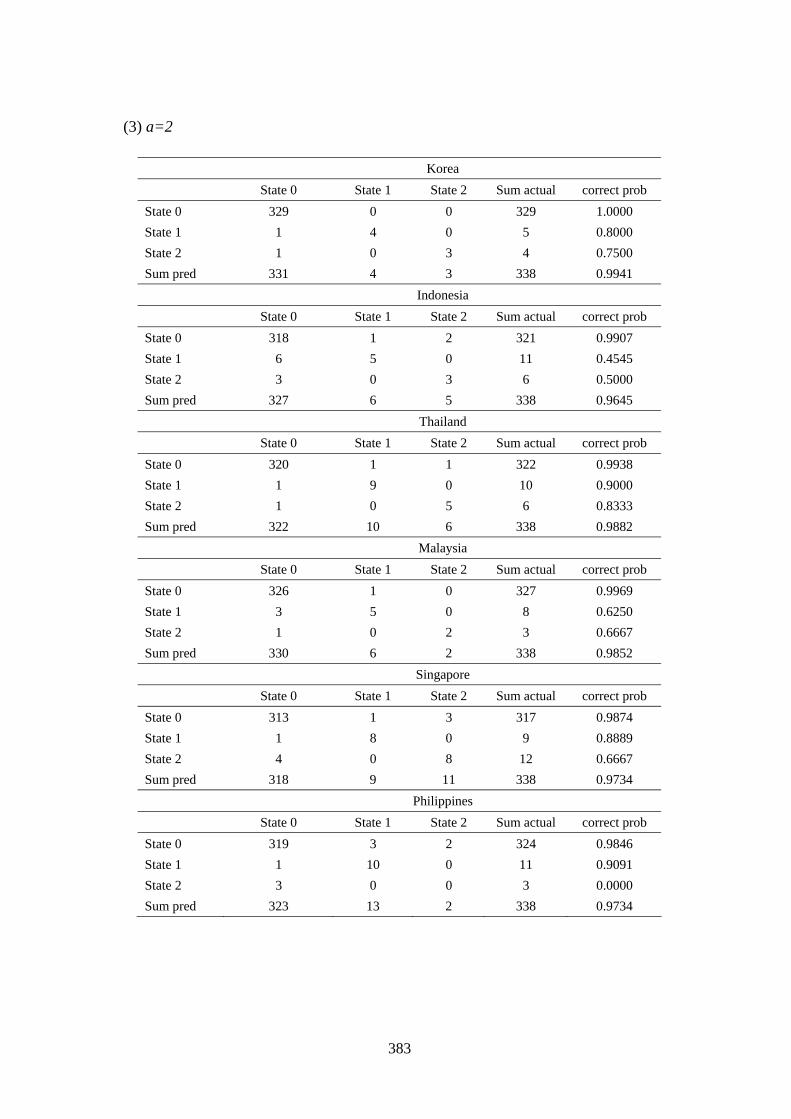
383

(3) a=2

Korea


State 0 329 0 0 329 1.0000

State 1 1 4 0 5 0.8000

State 2 1 0 3 4 0.7500

Sum pred 331 4 3 338 0.9941

Indonesia


State 0 318 1 2 321 0.9907

State 1 6 5 0 11 0.4545

State 2 3 0 3 6 0.5000

Sum pred 327 6 5 338 0.9645

Thailand


State 0 320 1 1 322 0.9938

State 1 1 9 0 10 0.9000

State 2 1 0 5 6 0.8333

Sum pred 322 10 6 338 0.9882

Malaysia


State 0 326 1 0 327 0.9969

State 1 3 5 0 8 0.6250

State 2 1 0 2 3 0.6667

Sum pred 330 6 2 338 0.9852

Singapore


State 0 313 1 3 317 0.9874

State 1 1 8 0 9 0.8889

State 2 4 0 8 12 0.6667

Sum pred 318 9 11 338 0.9734

Philippines


State 0 319 3 2 324 0.9846

State 1 1 10 0 11 0.9091

State 2 3 0 0 3 0.0000

Sum pred 323 13 2 338 0.9734

384

Figure 3. 20 Multinomial Logit models: Market pressure and Probability of Crisis

(1) Korea

0

10.0

0.2

0.4

0.6

0.8

1.0

80 82 84 86 88 90 92 94 96 98 00 02 04 06

Predicted P

robability of State 1

Dum

my

vari

able

Det

ecti

ng S

tate

1

0

10.0

0.2

0.4

0.6

0.8

1.0

80 82 84 86 88 90 92 94 96 98 00 02 04 06

Predicted P


Dum

my

vari

able

Det

ecti

ng S

tate

2

385

(2) Indonesia

0

10.0

0.2

0.4

0.6

0.8

1.0

80 82 84 86 88 90 92 94 96 98 00 02 04 06

Predicted P


Dum

my

vari

able

Det

ecti

ng S

tate

1

0

10.0

0.2

0.4

0.6

0.8

1.0

80 82 84 86 88 90 92 94 96 98 00 02 04 06

Predicted P


Dum

my

vari

able

Det

ecti

ng S

tate

2

386

(3) Thailand

0

10.0

0.2

0.4

0.6

0.8

1.0

80 82 84 86 88 90 92 94 96 98 00 02 04 06

Predicted P


Dum

my

vari

able

Det

ecti

ng S

tate

1

0

10.0

0.2

0.4

0.6

0.8

1.0

80 82 84 86 88 90 92 94 96 98 00 02 04 06

Predicted P


Dum

my

vari

able

Det

ecti

ng S

tate

2

387

(4) Malaysia

0

10.0

0.2

0.4

0.6

0.8

1.0

80 82 84 86 88 90 92 94 96 98 00 02 04 06

Predicted P


Dum

my

vari

able

Det

ecti

ng S

tate

1

0

10.0

0.2

0.4

0.6

0.8

1.0

80 82 84 86 88 90 92 94 96 98 00 02 04 06

Predicted P


Dum

my

vari

able

Det

ecti

ng S

tate

2

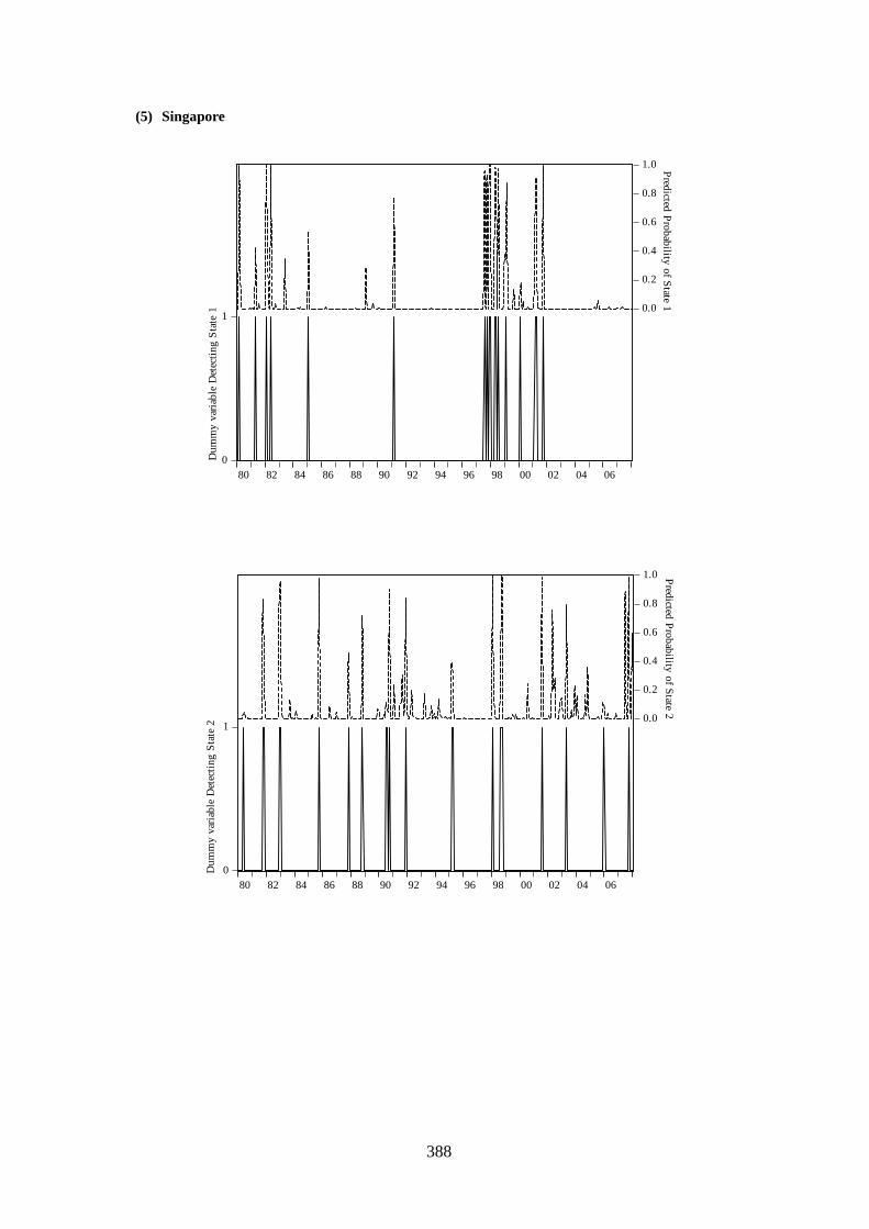
388

(5) Singapore

0

10.0

0.2

0.4

0.6

0.8

1.0

80 82 84 86 88 90 92 94 96 98 00 02 04 06

Predicted P


Dum

my

vari

able

Det

ecti

ng S

tate

1

0

10.0

0.2

0.4

0.6

0.8

1.0

80 82 84 86 88 90 92 94 96 98 00 02 04 06

Predicted P


Dum

my

vari

able

Det

ecti

ng S

tate

2

389

(6) Philippines

0

10.0

0.2

0.4

0.6

0.8

1.0

80 82 84 86 88 90 92 94 96 98 00 02 04 06

Predicted P


Dum

my

varia

ble

Det

ectin

g S

tate

1

0

10.0

0.2

0.4

0.6

0.8

1.0

80 82 84 86 88 90 92 94 96 98 00 02 04 06

Predicted P


Dum

my

vari

able

Det

ecti

ng S

tate

2

390

3.8 Conclusion

3.8.1 Summary of results

This study examines the power of the conventional macroeconomic factors to explain

the 1997-98 Asia currency crises in six countries, namely, Korea, Malaysia, Thailand,

Indonesia, Singapore and Philippines, based on the Markov Switching models. Two

types of Markov switching modelling specifications were examined. One is to assume

that the conditional variance of market pressure follows an asymmetric GARCH

process. The other one is to assume the conditional variance of market pressure is

constant. We can conclude that the Markov Switching specifications have several

advantages: (1) they can explain the appreciating currency attacks as well as

depreciating currency attacks; (2) by allowing regression parameters to switch

between different regimes, they mimic the existence of multiple equilibria relations,

(3) not like Logit/Probit models which require an ex-ante definition of a threshold

value to distinguish stable and volatile state, they can supply us with such

information.

In this study, we model the economy having two regimes, namely, stable state and

volatile state. Different from other studies using Markov switching framework in

modelling currency crises, we provide tests to congregate which regime relate to

which state. The tests we employ include the quadratic probability score (QPS) test,

391

the log probability score (LPS) test and the Global squared bias (GSB) tests. These

statistics measures the accuracy of the probabilities in forecasting the current state.

Although the state of a regime can be readily identified in a 2-regime model through

graphing the inferred probability of being in a certain state against MP, it is not the

case where there are more than two regimes. These statistics can then be very helpful

for detecting regimes in those situations.

Another distinct feature of our study is that we use a more reliable statistics to test for

the number of regimes (1 regime versus 2 regimes). The convention likelihood ratio

test for the same purpose is argued to be questionable because of the problems poised

by the presence of nuisance parameters and the parameter boundary problem. The

Neyman’s ( )C test we employed, however, is design to rectify such problems.

Moreover, we test 1 versus more than 1 regimes by accessing whether the residuals

from one regime models estimation are non-normally distributed which may result

from the distortion of the existence of other regimes. Bootstrapping methods are used

for such purpose.

The empirical estimates from Markov Switching models give credence to the view

that fundamental variables can still explain the market pressure on the behaviour of

the exchange rate and the Asian currency crises. In these models, the majority of those

macroeconomic fundamental variables are significant at 5% significant level. Thus we

believe the crises are not purely self-fulfilling phenomena; detrimental of economic

392

fundamentals do have some impact on the trigging of currency crises. Different from

previously studies on Asian financial crises, we find that the real growth of domestic

credit is not a powerful indicator for currency crises in Asia. The inferred probabilities

for the presence of a volatile state that estimated from the Markov switching models

have substantial informative content in explaining the Asian currency crises in 1997.

We can observe that at, or close to, the time of the currency crises attacks, the filtered

probability increase significantly.

Our results show that, although Markov Regime Switching TGARCH model is by and

large more favourable than the Markov Regime Switching constant model, it is not

necessary always the case. Multinomial Logit model is also examined for its ability to

predict currency crisis. We find that the Mlogit model performs better in predicting

depreciating currency attacks than in predicting the appreciating ones.

3.8.2 Further Research

This study may be extended in two ways. First, this study is based on the first and

second generation currency crises theory. It may be extended by including factors that

capture the deficiencies of banking and financial sectors — the “third generation”

currency crisis model. Financial deregulations, inadequate supervisory, together with

credit market imperfections or distortions that take the form of explicit or implicit

393

government bailout guarantees can create moral hazard. Such financial instability

raise largely through a bank channel mechanism might create or encourage a currency

crisis. Example indicators for the possible role of the bank lending channel and

financial fragility include: the ratio of foreign currency denominated assets to total

assets, the ratio of foreign currency denominated liabilities to total liabilities, the ratio

of non-performing banking loans to total credit grant.

Another extension can be made by assuming three regimes. As we mentioned before,

extreme high exchange market pressure and extreme low exchange market pressure

can both trigger currency attacks and currency crisis. Instead of using two regimes

Markov Switching model, we can experiment with three regimes Markov Switching

model to capture the three possible states in exchange market: an appreciating regime

(possible “speculative”), a stable regime, and a depreciating regime (possible

“speculative”). The latter would be regarded as a text book currency attack, but the

first regime could also be observed in the market.

394

References:

Agenor, Bhandari and Flood (1992), “Speculative Attacks and Models of Balance of

Payment Crises”, IMF Staff Papers, Vol.39, 356-94.

Babic, A. and A. Zigman (2001), “Currency Crises: Theoretical and Empirical

Overview of the 1990s”, Croatian National Bank.

Bera, A. K. and M. L. Higgins (1993), “ARCH Models: Properties, Estimation and

Testing”, Journal of Economic Surveys, 7, 305-362.

Berg, A. and C. Pattillo (1998), “Are Currency Crises Predictable? A Test”, IMF

Working Paper,WP/98/154.

Berg, A. and Patillo, C. (1999), “Are currency crises predictable? A test”, IMF Staff

Papers, 46 (2), 107-38.

Bera, A. K. and Y. Bilias (2001), “Rao’s score, Neyman’s C( ) and Silvey’s LM

tests: an essay on historical developments and some new results”, Journal of

Statistical Planning and Inference, 97, 9-44.

Blejer, M. I. (1998), “The Economics of Currency Crises: Models, Indicators and

Policy Responses: Zagreb”, Journal of Economics, Vol. 2, No. 2, Croatian

Institute for Banking and Insurance, pp. 55-70.

Blejer, M. I. and L. Schumacher (1998), “Central Bank Vulnerability and the

Credibility of Commitments: A Value-at-Risk Approach to Currency Crises”, IMF

Working Paper, WP/98/65, May 1998, Washington D.C.

Bollerslev, T. (1986), “Generalized Autoregressive Conditional Heteroskedasticity”,

Journal of Econometrics, 31: 307-327.

Breusch, T. S. and A. R. Pagan (1980), “The Lagrange Multiplier Test and its

Application to Model Specification in Econometrics”, The Review of Economic

Studies, 47, 239-253.

Breunig R., S. Najarian and A. R. Pagan (2003), “Specification Testing of Markov

395

Switching Models”, Oxford Bulletin of Economics and Statistics, 65, 703-725.

Brunetti, C., R. S. Mariano, C. Scotti and A. H. H. Tan (2007), “Markov Switching

ARCH Models of Currency Turmoil in Southeast Asia”, International Finance

Discussion Papers, Federal Reserve System, Number 889, January,

Cai, J. (1994), “A Markov Model of Switching-Regime ARCH”, Journal of Business

& Economic Statistics 12: 309-316.

Carramaza, F., L. Ricci and R. Saldago (2000),“Trade and Financial Contagion in

Currency Crisis”, IMF Working paper, 00/55.

Cho, Jin Seo and H. White (2007), “Testing For Regime Switching”, Econometrica,

75, 1671-1720.

Corsetti, Giancarlo, P. Pesenti and N. Roubini (1999), “The Asian Crises: An

Overview of the Empirical Evidence and Policy Debate”, In, The Asian Financial

Crisis: Causes, Contagion and Consequences: Pierre Richard Agenor, Marcus

Miller, David Vines and Axel Weber (eds.) Cambridge, UK: Cambridge

University Press.

Davidson R. and J. G. MacKinnon (1991), “Artificial regressions and C(α) tests”,

Economics Letters, 35, 149-153.

Diebold, Z. and G. D. Rudebusch (1989), “Scoring the Leading Indicators”, The

Journal of Business, 62, 369-391.

Eichengreen, B., A. K. Rose and C. Wyplosz (1995), “Exchange Market Mayhem:

The Antecedents and Aftermath of Speculative Attacks”, Economic Policy, 21:

251-312.

Eichengreen, Rose and Wyplosz (1996), “Contagious Currency Crisis: First Tests”,

The Scandinavian Journal of Economics, 98, 463-484

Engle, R. (1982), “Autoregressive Conditional Heteroscedasticity with Estimates of

the Variance of UK inflation”, Econometrica, 50: 987-1008.

Esquivel, G. and F. Larraín (1998), “Explaining Currency Crises”, Development

396

Discussion Paper, No. 666. Harvard Institute for International Development,

Harvard University. November.

Feridun, M. (1996), “How Far Can Domestic Credit Growth Explain Speculative

Attacks? Empirical Evidence from Turkey”, Department of Economics,

Loughborough University, Discussion Paper series, WP 2006 - 23

Frankel, J.A. and A.K. Rose (1996), "Currency Crashes in Emerging Markets: An

Empirical Treatment." Journal of International Economics, 41: 351-366.

Flood, R. P. and Garber, P. M (1984), “Collapsing Exchange Rate Regimes: Some

Linear Example”, Journal of finternational Economics, No. 17, August, 1-13.

Flood. R and N. Marion (1998), “Perspectives on The Recent Currency Crisis

Literature”, NBER Working Paper, No. 6380.

Ford, J. L., B Santoso and N. J. Horsewood, (2007), “Asia Currency Crises: Do

Fundamentals still matter? A Markov-switching approach to causes and timing”,

Department of Economics, University of Birmingham in its series Discussion

Papers with number 07-07.

Ford, J. L., Horsewood, N. J., and G. C. Lim (2009), “Fundamentals, Bank fragility

and Currency volatility: A Study of Indonesia and Taiwan”, Mimeographed Paper,

forthcoming discussion paper in Department of Economics, University of

Birmingham, July.

Geochoco-Bautista, S. M. (2000), “Periods of Currency Pressure: Stylized Facts and

Leading Indicators”, Journal of Macroeconomics, Vol.22 (1).

Glick, R. and A.K. Rose. (1998). “Contagion and Trade: Why are Currency Crises

Regional?”, Haas School of Business, University of California. August.

Glick, R. and Moreno, R. (1999), “Money and Credit, Competitiveness, and Currency

Crises in Asia and Latin America”, Pacific Basin Working Paper Series, No.

PB99-01, Center for Pacific Basin Monetary and Economic Studies, Federal

Reserve Bank of San Francisco.

http://ideas.repec.org/s/bir/birmec.html�

http://ideas.repec.org/s/bir/birmec.html�

397

Glosten, L.R., R. Jagannathan and D. Runkle (1993), “On the Relation between the

Expected Value and the Volatility of the Normal Excess Return on Stocks”,

Journal of Finance, 48: 1779–1801.

Girton, L. and D. Roper (1997), “A monetary model of exchange market pressure

applied to the postwar Canadian experience”, American Economic Review, 67:

231-256.

Goldfeld, S. M. and R. E. Quandt (1973), “A Markov Model for Switching

Regression”, Journal of Econometrics, 1, 3-16.

Goldstein, M. (1998), “The Asian financial Crisis”, International Economics Policy

Briefs, No. 98-1

Gray, S. F. (1996), “Modelling the Conditional Distribution of Interest Rates as a

Regime-switching Process”, Journal of Financial Economics, 42, 27-62.

Hamilton, J.D. (1989), “A New Approach to the Economic Analysis of Nonstationary

Time Series and the Business Cycle”, Econometrica, 57: 357-384.

Hamilton, J. D. (1994), Time Series Analysis, Princeton: Princeton University Press.

Hamilton, J. D. & R. Susmel (1994), “Autoregressive Conditional Heteroskedasticity

and Changes in Regime”, Journal of Econometrics, 64, 307-333.

Hamilton, J. D. (1996), “Specification testing in Markov-switching time-series

models”, Journal of Econometrics, 70, 127-157.

Jeanne, O. and Masson, P. (2000), “Currency Crises, Sunspots and Markov-Switching

Regimes”, Journal of International Economics, Vol. 55, 327-50.

Kaminsky, G, S. Lizondo, and C. M. Reinhart, (1997, 1998), "Leading Indicators of

Currency Crisis," IMF Staff Papers, Vol. 45(1), 1-48.

Kaminsky, Graciela and Carmen M. Reinhart, (1999), " The Twin Crises: the Causes

of Banking and Balance-of-Payments Problems", American Economic Review,

June.

398

Kemeny J. G. and J. L. Snell (1976), Finite Markov Chains, New York:

Springer-Verlag.

Kim, C.J. and C.R. Nelson. (1999), State-Space Models with Regime Switching:

Classical and Gibbs-Sampling Approaches with Applications, London: The MIT

Press.

Krugman, P. (1979), “A Model of Balance of Payment Crises”, Journal of Money,

Credit and Banking, 11:311-325.

Krugman, P. (1999), “Balance Sheets, the Transfer Problem and Financial Crises,” In,

Festschrift Volume: Essays in Honour of Robert P Flood.

Kruger, M., P.N. Osakwe, and J. Page (1998), “Fundamentals, Contagion and

Currency Crises: An Empirical Analysis”, Bank of Canada Working Paper, 98-10:

1-28.

Krkoska, L. (2000), “Assessing Macroeconomic Vulnerability in Central Europe”,

European Bank for Reconstruction and Development, Working Paper, No. 52.

Krznar, Ivo (2004), “Currency crisis: Theory and Practice with Application to

Croatia”, Croatian National Bank Working Papers, August 2004, No: 12.

Lindsay. B. G. (1995), Mixture Models: Theory, Geometry, and Applications,

Hayward, CA: Institute for Mathematical Statistics.

Maddala, G.S. (1992), Introduction to Econometrics. 2nd Edition. New Jersey:

Prentice Hall.

Moreno, R. (1995), “Macroeconomic Behaviour During Periods of Speculative

Pressure or Realignment: Evidence from Pacific Basin Economics”, Federal

Reserve Bank of San Francisco Economic Review, No:3.

Moreno, Ramon and Trehan, Bharat (2000), “Common Shocks and Currency Crises”,

Federal Reserve Bank of San Francisco, April 28, 2000, Unpublished Manuscript.

Obstfeld, M. (1986), “Rational and Self-fulfilling Balance of Payments Crises”,

American Economic Review, Vol.76, Mars, pp. 72-81.

399

Obstfeld, M. and K. Rogoff (1995), “The Mirage of Fixed Exchange Rates,” Journal

of Economic Perpectives, 9:73-96.

Obstfeld, M and Rogoff, K. (1996), Foundations of International Macroeconomics,

Massachusetts, Cambridge, London: The MIT Press.

Obstfeld, M. (1996), “Models of currency Crises with Self-Fulfilling Features”,

European Economic Review, Vol. 43, 61-67.

Peria, M. S. M. (2002), “A regime-switching approach to the study of speculative

attacks: A focus on EMS crises”, Empirical Economics, 27, 299-334.

Perron, P. (1997), “Further evidence on breaking trend functions in macroeconomic

variables”, Journal of Econometrics, 80: 355-85.

Radelet, S. and J. Sachs, (1998), "The Onset of the East Asian Financial Crisis",

Harvard Institute for International Development, mimeo.

Sachs, J.D., A. Tornell, and A. Velasco. (1996), "The Mexican Peso Crisis: Sudden

Death or Death Foretold?", Journal of International Economics, 41: 265-283.

Tornell, A. (1999), “Common Fundamentals in the Tequila and Asian Crises”, NBER

Working Paper, Series No. 7139. May.

400

Appendix 3.A Data Analysis and Descriptive Statistics for MP and it’s determinants Figure 3.A 1 MP and its components for Korea

-.2

-.1

.0

.1

.2

.3

1980 1985 1990 1995 2000 2005

MP

-.1

.0

.1

.2

.3

.4

1980 1985 1990 1995 2000 2005

MP: contribution of domestic currency depreciation

-.3

-.2

-.1

.0

.1

.2

.3

1980 1985 1990 1995 2000 2005

MP: contribution of change in domestic reserves

-.8

-.6

-.4

-.2

.0

.2

.4

1980 1985 1990 1995 2000 2005

MP: contribution of change in domestic interest rate

Figure 3.A 2 MP and its components for Indonesia

-.2

-.1

.0

.1

.2

.3

1980 1985 1990 1995 2000 2005

MP

-.4

-.2

.0

.2

.4

.6

.8

1980 1985 1990 1995 2000 2005


-.6

-.4

-.2

.0

.2

.4

1980 1985 1990 1995 2000 2005


-0.8

-0.4

0.0

0.4

0.8

1.2

1980 1985 1990 1995 2000 2005


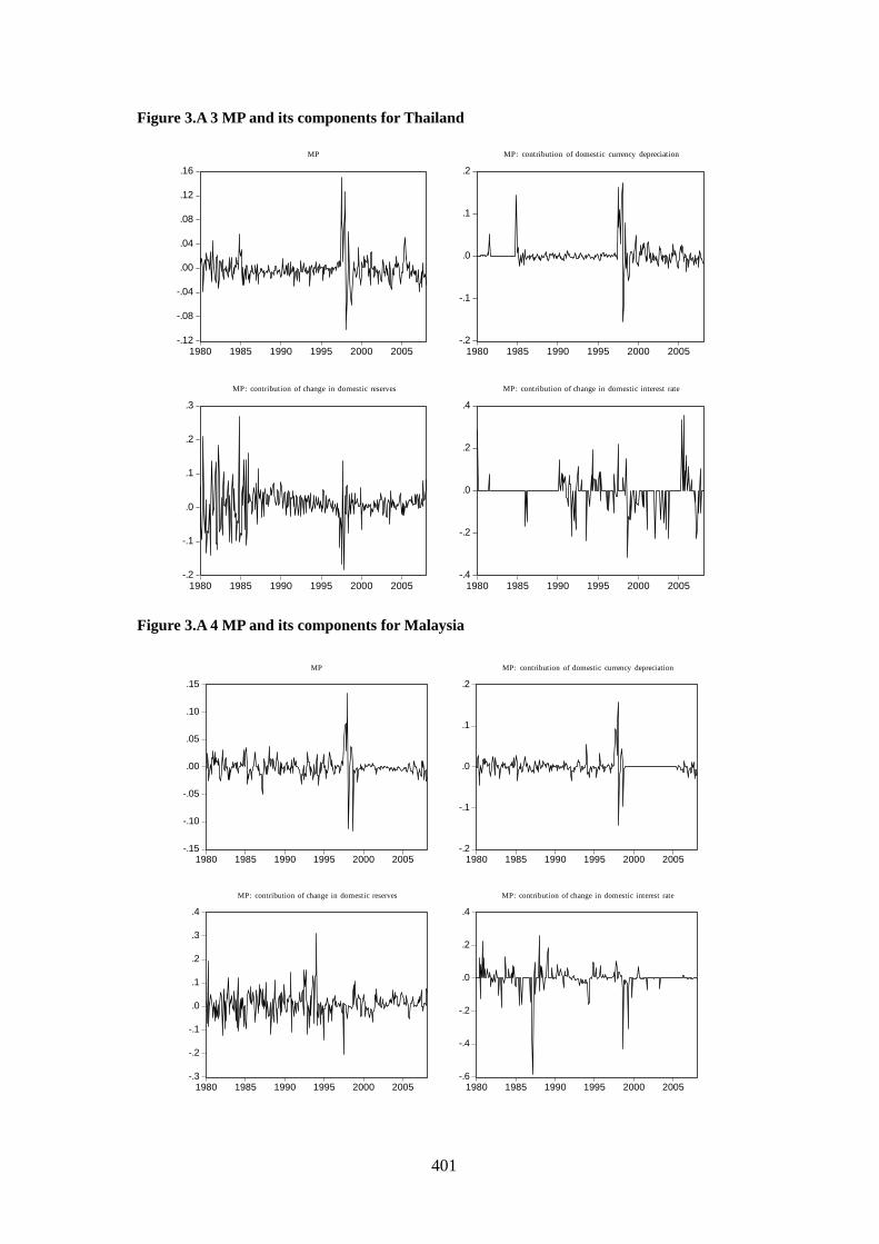
401

Figure 3.A 3 MP and its components for Thailand

-.12

-.08

-.04

.00

.04

.08

.12

.16

1980 1985 1990 1995 2000 2005

MP

-.2

-.1

.0

.1

.2

1980 1985 1990 1995 2000 2005


-.2

-.1

.0

.1

.2

.3

1980 1985 1990 1995 2000 2005


-.4

-.2

.0

.2

.4

1980 1985 1990 1995 2000 2005


Figure 3.A 4 MP and its components for Malaysia

-.15

-.10

-.05

.00

.05

.10

.15

1980 1985 1990 1995 2000 2005

MP

-.2

-.1

.0

.1

.2

1980 1985 1990 1995 2000 2005


-.3

-.2

-.1

.0

.1

.2

.3

.4

1980 1985 1990 1995 2000 2005


-.6

-.4

-.2

.0

.2

.4

1980 1985 1990 1995 2000 2005


402

Figure 3.A 5 MP and its components for Singapore

-.08

-.04

.00

.04

.08

1980 1985 1990 1995 2000 2005

MP

-.06

-.04

-.02

.00

.02

.04

.06

.08

1980 1985 1990 1995 2000 2005


-.08

-.04

.00

.04

.08

.12

1980 1985 1990 1995 2000 2005


-.6

-.4

-.2

.0

.2

.4

1980 1985 1990 1995 2000 2005


Figure 3.A 6 MP and its components for Philippines

-.08

-.04

.00

.04

.08

.12

.16

.20

.24

1980 1985 1990 1995 2000 2005

MP

-.08

-.04

.00

.04

.08

.12

.16

.20

.24

1980 1985 1990 1995 2000 2005


-.8

-.4

.0

.4

.8

1980 1985 1990 1995 2000 2005


-.6

-.4

-.2

.0

.2

.4

.6

1980 1985 1990 1995 2000 2005


403

Table 3.A 1 Descriptive Statistics of MP and its determinants for Korea

MP RM2 RER GDC RISK DRM2 DRER DGDC DRISK

Mean -0.0010 0.1997 0.0064 0.0085 -0.0232 0.0008 0.0002 0.0000 -0.0003

Median -0.0016 0.1639 0.0078 0.0083 -0.0250 0.0011 -0.0004 0.0020 -0.0005

Maximum 0.2965 0.4158 0.6395 0.0920 0.3190 0.0373 0.3379 0.0589 0.2309

Minimum -0.1314 0.0660 -0.2009 -0.0358 -0.2746 -0.0380 -0.1019 -0.0983 -0.4956

Std. Dev. 0.0265 0.0990 0.1120 0.0147 0.0420 0.0092 0.0271 0.0209 0.0435

Skewness 4.2794 0.6368 1.5846 0.6229 0.8056 0.0377 5.7596 -0.8073 -4.1564

Kurtosis 53.3446 2.2499 9.3565 6.5914 20.4000 5.5499 76.0838 5.0795 58.1133

ADF -11.3045 0.4326 -2.7161 -18.5105 -7.3707 -17.6239 -12.6155 -12.8100 -12.3886

KPSS 0.1258 1.8239 0.2201 0.2235 0.3773 0.3255 0.0333 0.0835 0.1543

Note: Critical value for ADF test: 1% level, -3.45; 5% level, -2.87 and 10% level, -2.57

Critical value for KPSS test: 1% level, 0.739; 5% level, 0.463 and 10% level, 0.347.

Table 3.A 2 Correlation of MP and its determinants for Korea


MP 1.0000 -0.0942 0.2125 0.0942 0.0466 -0.1044 0.8491 -0.0538 -0.5102

RM2 -0.0942 1.0000 -0.3319 -0.0965 -0.0208 0.1132 -0.0153 0.0029 0.0027

RER 0.2125 -0.3319 1.0000 0.0585 -0.2119 0.0456 0.1168 -0.0330 -0.1417

GDC 0.0942 -0.0965 0.0585 1.0000 0.2123 -0.3428 0.0879 0.7098 0.0977

RISK 0.0466 -0.0208 -0.2119 0.2123 1.0000 -0.2332 0.0857 0.1693 0.5002

DRM2 -0.1044 0.1132 0.0456 -0.3428 -0.2332 1.0000 0.1491 -0.2170 -0.3370

DRER 0.8491 -0.0153 0.1168 0.0879 0.0857 0.1491 1.0000 -0.0818 -0.5376

DGDC -0.0538 0.0029 -0.0330 0.7098 0.1693 -0.2170 -0.0818 1.0000 0.2395

DRISK -0.5102 0.0027 -0.1417 0.0977 0.5002 -0.3370 -0.5376 0.2395 1.0000

Table 3.A 3 Descriptive Statistics of MP and its determinants for Indonesia


Mean 0.0001 0.2632 0.0565 0.0088 -0.0786 -0.0005 -0.0009 0.0002 -0.0003

Median -0.0032 0.2636 0.0120 0.0099 -0.0880 -0.0006 -0.0028 0.0026 0.0003

Maximum 0.2220 0.5392 1.2151 0.7021 0.6183 0.2019 0.5949 0.7669 0.5855

Minimum -0.1038 0.1038 -0.2330 -0.7415 -0.7674 -0.1030 -0.2885 -0.6789 -0.9617

Std. Dev. 0.0387 0.0920 0.1895 0.0758 0.1175 0.0236 0.0612 0.1099 0.0970

Skewness 1.7532 0.6485 2.8719 -0.8686 -0.4439 1.8271 2.8448 0.1699 -2.5652

Kurtosis 10.8483 3.1072 15.0488 51.9259 11.6911 21.6090 36.7608 23.2127 40.5175

ADF -15.1216 -3.2887 -3.6416 -23.6077 -3.0494 -20.2153 -15.2654 -15.2388 -15.6839

KPSS 0.1323 0.3595 0.3440 0.2211 0.6376 0.3126 0.0214 0.2492 0.0382

404

Table 3.A 4 Correlation of MP and its determinants for Indonesia


MP 1.0000 -0.0236 0.2928 0.1890 0.1272 0.0089 0.6133 0.0878 -0.3773

RM2 -0.0236 1.0000 0.1868 -0.0926 0.1218 0.0952 -0.0029 0.0093 -0.1325

RER 0.2928 0.1868 1.0000 -0.0269 -0.2428 0.1724 0.1616 -0.0037 -0.2496

GDC 0.1890 -0.0926 -0.0269 1.0000 0.0382 0.0138 0.2057 0.7239 -0.1423

RISK 0.1272 0.1218 -0.2428 0.0382 1.0000 -0.0400 0.1547 -0.0299 0.4096

DRM2 0.0089 0.0952 0.1724 0.0138 -0.0400 1.0000 0.6109 0.0256 -0.5230

DRER 0.6133 -0.0029 0.1616 0.2057 0.1547 0.6109 1.0000 0.1242 -0.5685

DGDC 0.0878 0.0093 -0.0037 0.7239 -0.0299 0.0256 0.1242 1.0000 -0.1377

DRISK -0.3773 -0.1325 -0.2496 -0.1423 0.4096 -0.5230 -0.5685 -0.1377 1.0000

Table 3.A 5 Descriptive Statistics of MP and its determinants for Thailand


Mean -0.0015 0.1961 0.0209 0.0062 -0.0183 0.0006 -0.0004 0.0000 -0.0002

Median -0.0030 0.2268 -0.0059 0.0064 -0.0227 0.0007 -0.0016 0.0011 -0.0002

Maximum 0.1500 0.3523 0.6209 0.0529 0.1809 0.0408 0.1579 0.0512 0.2188

Minimum -0.1021 0.0677 -0.1460 -0.0598 -0.3060 -0.0692 -0.1772 -0.0738 -0.3965

Std. Dev. 0.0216 0.0680 0.0937 0.0131 0.0436 0.0096 0.0252 0.0150 0.0381

Skewness 1.7607 -0.5218 2.0435 -0.3377 -0.1443 -0.7235 1.1823 -0.4433 -2.8708

Kurtosis 16.9902 1.9823 10.4908 6.0193 10.2268 14.5148 25.5016 6.0031 43.4154

ADF -11.8306 -0.1717 -3.1336 -1.6501 -3.4408 -9.2239 -13.7019 -13.4081 -15.8925

KPSS 0.1100 1.7540 0.1700 0.9714 0.4196 0.3190 0.0657 0.1630 0.0795

Table 3.A 6 Correlation of MP and its determinants for Thailand


MP 1.0000 -0.0263 0.2601 0.2572 0.0869 0.1418 0.8299 0.1144 -0.5033

RM2 -0.0263 1.0000 -0.2350 -0.1737 -0.0196 0.1240 0.0180 0.0071 -0.0618

RER 0.2601 -0.2350 1.0000 -0.1182 -0.1603 0.0050 0.1517 -0.0300 -0.1825

GDC 0.2572 -0.1737 -0.1182 1.0000 -0.2055 0.1023 0.3898 0.5716 -0.2197

RISK 0.0869 -0.0196 -0.1603 -0.2055 1.0000 -0.0131 0.0841 0.0718 0.4331

DRM2 0.1418 0.1240 0.0050 0.1023 -0.0131 1.0000 0.4768 0.1441 -0.4869

DRER 0.8299 0.0180 0.1517 0.3898 0.0841 0.4768 1.0000 0.2252 -0.5803

DGDC 0.1144 0.0071 -0.0300 0.5716 0.0718 0.1441 0.2252 1.0000 -0.1080

DRISK -0.5033 -0.0618 -0.1825 -0.2197 0.4331 -0.4869 -0.5803 -0.1080 1.0000

405

Table 3.A 7 Descriptive Statistics of MP and its determinants for Malaysia


Mean -0.0003 0.2557 0.0356 0.0073 0.0072 0.0013 -0.0004 0.0000 -0.0002

Median -0.0009 0.2437 0.0211 0.0072 0.0050 0.0004 -0.0013 0.0001 0.0001

Maximum 0.1347 0.5143 0.5085 0.4540 0.1367 0.2509 0.1401 0.6604 0.2064

Minimum -0.1163 0.1001 -0.1106 -0.6549 -0.2530 -0.0998 -0.1698 -0.6701 -0.3774

Std. Dev. 0.0187 0.0977 0.0805 0.0508 0.0376 0.0222 0.0199 0.0746 0.0308

Skewness 0.6617 0.5172 1.9649 -4.6567 -0.5661 5.3373 -0.3116 0.6054 -4.4402

Kurtosis 21.0253 2.4031 9.5510 108.3365 10.2824 59.1347 30.6218 53.7530 75.6270

ADF -13.0690 -1.0708 -2.5567 -19.7787 -3.5531 -17.1921 -14.7237 -11.9792 -14.4153

KPSS 0.1151 1.2591 0.1625 0.1432 0.6398 0.1132 0.0708 0.1696 0.0222

Table 3.A 8 Correlation of MP and its determinants for Malaysia


MP 1.0000 -0.1008 0.2598 0.0574 0.0834 -0.0375 0.8711 0.0411 -0.5541

RM2 -0.1008 1.0000 -0.3125 -0.0714 -0.2057 0.0942 -0.0377 0.0005 -0.0146

RER 0.2598 -0.3125 1.0000 -0.0631 0.0550 0.0362 0.1432 0.0004 -0.1462

GDC 0.0574 -0.0714 -0.0631 1.0000 -0.0411 -0.3973 0.0203 0.7339 -0.0581

RISK 0.0834 -0.2057 0.0550 -0.0411 1.0000 0.0280 0.0257 -0.0069 0.4018

DRM2 -0.0375 0.0942 0.0362 -0.3973 0.0280 1.0000 0.1990 -0.2687 -0.1042

DRER 0.8711 -0.0377 0.1432 0.0203 0.0257 0.1990 1.0000 0.0128 -0.5730

DGDC 0.0411 0.0005 0.0004 0.7339 -0.0069 -0.2687 0.0128 1.0000 -0.0476

DRISK -0.5541 -0.0146 -0.1462 -0.0581 0.4018 -0.1042 -0.5730 -0.0476 1.0000

Table 3.A 9 Descriptive Statistics of MP and its determinants for Singapore


Mean -0.0042 0.8513 0.0087 0.0082 0.0271 -0.0006 -0.0004 -0.0001 -0.0001

Median -0.0036 0.8362 0.0088 0.0038 0.0258 0.0004 -0.0004 0.0002 0.0002

Maximum 0.0605 0.9829 0.2084 0.3211 0.1046 0.0685 0.0628 0.3813 0.0713

Minimum -0.0622 0.6936 -0.1280 -0.2799 -0.0765 -0.1420 -0.0591 -0.5895 -0.1365

Std. Dev. 0.0132 0.0720 0.0608 0.0433 0.0238 0.0158 0.0137 0.0688 0.0211

Skewness 0.1100 0.3118 0.3287 2.2684 0.0108 -2.1425 -0.1837 -1.0767 -0.9229

Kurtosis 6.3546 1.8222 2.9382 26.5659 4.0086 22.5291 5.5891 26.6642 10.1559

ADF -13.0103 -2.1963 -1.9920 -23.9051 -6.7115 -19.3411 -15.2183 -10.9883 -11.8471

KPSS 0.1898 0.1303 0.1814 0.3241 0.5036 0.0703 0.1481 0.3241 0.2577

406

Table 3.A 10 Correlation of MP and its determinants for Singapore


MP 1.0000 0.0750 0.3248 -0.0684 0.0836 -0.0519 0.8575 -0.0205 -0.5380

RM2 0.0750 1.0000 -0.0346 -0.0337 -0.1958 0.0964 0.1413 -0.0096 0.0033

RER 0.3248 -0.0346 1.0000 -0.0098 0.0841 -0.1021 0.1463 0.0094 -0.1079

GDC -0.0684 -0.0337 -0.0098 1.0000 0.0746 -0.4197 -0.0028 0.7930 0.0460

RISK 0.0836 -0.1958 0.0841 0.0746 1.0000 -0.1085 0.0458 -0.0173 0.4399

DRM2 -0.0519 0.0964 -0.1021 -0.4197 -0.1085 1.0000 0.0657 -0.2947 -0.0752

DRER 0.8575 0.1413 0.1463 -0.0028 0.0458 0.0657 1.0000 0.0378 -0.4408

DGDC -0.0205 -0.0096 0.0094 0.7930 -0.0173 -0.2947 0.0378 1.0000 0.0125

DRISK -0.5380 0.0033 -0.1079 0.0460 0.4399 -0.0752 -0.4408 0.0125 1.0000

Table 3.A 11 Descriptive Statistics of MP and its determinants for Philippines


Mean 0.0043 0.2176 0.0173 0.0029 -0.0404 0.0001 -0.0001 -0.0005 0.0000

Median 0.0017 0.2259 0.0103 0.0020 -0.0354 -0.0012 0.0024 -0.0004 0.0011

Maximum 0.2225 0.3911 0.3826 0.5931 0.2010 0.0814 0.5755 0.2026 0.2454

Minimum -0.0655 0.0344 -0.2399 -0.1158 -0.2976 -0.0725 -0.5059 -0.0962 -0.2929

Std. Dev. 0.0263 0.0968 0.1052 0.0446 0.0553 0.0176 0.0564 0.0257 0.0478

Skewness 3.7091 -0.3548 0.5276 6.9150 -0.2408 0.2593 0.6871 2.1832 -0.6991

Kurtosis 28.8064 1.8972 3.4734 92.6242 6.2559 5.5831 53.1439 20.4435 15.0530

ADF -13.7940 -1.6144 -2.2286 -14.9181 -4.1427 -17.5814 -15.2912 -13.7276 -16.7823

KPSS 0.4408 1.0274 0.1734 0.1967 0.2533 0.2846 0.1534 0.1467 0.1488

Table 3.A 12 Correlation of MP and its determinants for Philippines


MP 1.0000 -0.2103 0.4009 0.1726 -0.0095 -0.1159 0.0065 0.8589 -0.5812

RM2 -0.2103 1.0000 -0.1956 0.0258 0.3193 0.0962 0.0095 -0.0410 0.0252

RER 0.4009 -0.1956 1.0000 -0.1134 -0.1150 0.0040 -0.0342 0.1541 -0.1540

GDC 0.1726 0.0258 -0.1134 1.0000 0.1266 -0.1683 0.6318 0.2600 -0.0770

RISK -0.0095 0.3193 -0.1150 0.1266 1.0000 -0.2105 0.0212 0.0712 0.4319

DRM2 -0.1159 0.0962 0.0040 -0.1683 -0.2105 1.0000 -0.0673 -0.0263 -0.1098

DRER 0.0065 0.0095 -0.0342 0.6318 0.0212 -0.0673 1.0000 0.0582 -0.0336

DGDC 0.8589 -0.0410 0.1541 0.2600 0.0712 -0.0263 0.0582 1.0000 -0.5191

DRISK -0.5812 0.0252 -0.1540 -0.0770 0.4319 -0.1098 -0.0336 -0.5191 1.0000

407

Appendix 3.B Neyman’s ( )C test

The ( )C tests were designed to deal with hypothesis testing of a parameter of

primary interest in the presence of nuisance parameter. In particular, Neyman

dispenses with the maximum likelihood estimates and utilizes only n -consistent

estimates that are relatively easy to find. Another attractive feature of the optimal

( )C tests statistics is that by design it satisfies a certain optimality principle; it

maximizes the slope of the limiting power function under “local alternative” to the

null hypothesis.

Assume that there are n independent observations, 1y , 2y ,… ny with identical

density function ( ; )f y where is a 1p parameter vector with p ¡ .

The log-likelihood function, score function, and the information matrix are then

defined, respectively, as

1

( ) ln ( , )n

ii

l f y

(3.B.1)

( )( )

ls

(3.B.2)

and

2 ( )( )

lE

(3.B.3)

Suppose that ( , ) and interest centers on testing the null hypothesis

0 0:H which in practice requires knowledge of the parameter . The parameter

408

is the parameter of primary interest while the parameter is the nuisance

parameter.

Let ( , ) ( , ) /s l and ( , ) ( , ) /s l . Denote the part of

information matrix that corresponds to by ( , ) and the notation ( , )

( , ) and ( , ) have analogous meanings. Neyman’s (1959) finding is that

asymptotic optimality in the sense mentioned above suggests that hypothesis testing

should be based on the statistic

10 0 0 0

110 0 0 0

10 0 0 0

( ) ( , ) ( , ) ( , ) ( , )

( , ) ( , ) ( , ) ( , )

( , ) ( , ) ( , ) ( , )

C s s

s s

(3.B.4)

with all the score and information quantities evaluated at the null value of , 0

and replaced by a n -consistent estimator.

Apart from its relatively easy method of calculation, the matrix algebra expression

itself can be prove difficult to use because the information matrix (essentially the

second derivatives of the likelihood function) would not have zero elements, but

would be singular. Therefore, its generalized inverse would have to be used; but the

key matrix then, that of the eigenvalues, might also be found to be singular. That

means that the generalized inverse of the information matrix have to be obtained

which make the process become one of the infinite regress.

A welcome feature of the ( )C test statistic is that it can be readily obtained from an

409

artificial regression. Breusch and Pagan (1980) suggested one type of artificial

calculation. With some algebraic manipulation, Equation (3.B.4) can be written as

1 10 0 0 0 0( ) ( , ) ( , ) ( , ) ( , ) ( , )C s s s s (3.B.5)

Let ( )S be a n p matrix with ln ( , ) /i jf y as its typical ( , )i j th element.

Note that the first r columns correspond to the parameters of primary interest56 and

the last ( )p r to the nuisance parameters57 .

We use 0

S to denote the n r submatrix of ( )S with parameters of primary

interest (denoted as 0( )S ) , while S to denote the matrix of 0( , )S with the

parameters of primary interest and the nuisance parameters. The statistics can be

obtained in two steps. First, regress 0

S and S

on residuals obtained from

estimates considering the primary interest only, respectively. Save the two 2R s from

the each regression. Second, calculate the ( )C test statistics as n times the

difference of two 2R obtained from regress. The critical values for the ( )C test

can be obtained from a 2 distribution, with being the number of restrictions,

when one regime is excluded.

56 In our study of the Markov Regime Switching models, these are the parameters from the single regime estimation. 57 These are the additional parameters when estimating using 2 regimes Markov Switching model.

Three Essays on: Hedging in China's Oil futures market ...etheses.bham.ac.uk/397/1/Chen09PhD.pdf ·...

Documents

Transcript of Three Essays on: Hedging in China's Oil futures market ...etheses.bham.ac.uk/397/1/Chen09PhD.pdf ·...