Three equations with exponential nonlinearities - ugr.esedp/Ireneo07/JUANlUIS.pdf · Cavallero...
198
Three equations with exponential nonlinearities Juan Luis V ´ azquez Departamento de Matem ´ aticas Universidad Aut ´ onoma de Madrid Three equations with exponential nonlinearities– p. 1/7
Transcript of Three equations with exponential nonlinearities - ugr.esedp/Ireneo07/JUANlUIS.pdf · Cavallero...
Three equations with exponentialnonlinearities
Juan Luis Vazquez
Departamento de Matematicas
Universidad Autonoma de Madrid
Three equations with exponential nonlinearities– p. 1/71

Three equations with exponential nonlinearities– p. 2/71

“Three equations with exponentialnonlinearities”
Three equations with exponential nonlinearities– p. 3/71

“Three equations with exponentialnonlinearities”
Recent T rends in NLPDEs,
Three equations with exponential nonlinearities– p. 3/71
“Three equations with exponentialnonlinearities”
Recent T rends in NLPDEs,
Conferencia çelebrada en Salamanca del nuestro Reyno,en loor del Prof. Ireneo Peral
Three equations with exponential nonlinearities– p. 3/71

“Three equations with exponentialnonlinearities”
Recent T rends in NLPDEs,
Conferencia çelebrada en Salamanca del nuestro Reyno,en loor del Prof. Ireneo Peral
Mio Cid de las Ciencias Matematicas
Three equations with exponential nonlinearities– p. 3/71
“Three equations with exponentialnonlinearities”
Recent T rends in NLPDEs,
Conferencia çelebrada en Salamanca del nuestro Reyno,en loor del Prof. Ireneo Peral
Mio Cid de las Ciencias Matematicas
Cavallero Mayor de los algorismos p-laplaciados e Hardiqueses
Real desfazedor de malos argumentos y calculos erradosen el honrrado Reyno de Castiella
Three equations with exponential nonlinearities– p. 3/71

Three equations with exponential nonlinearities– p. 4/71
IntroductionThe basic problems of Theoretical PDEs are existence,
uniqueness, stability, and qualitative behaviour of the solutions
of relevant classes of equations.
Three equations with exponential nonlinearities– p. 5/71
IntroductionThe basic problems of Theoretical PDEs are existence,
uniqueness, stability, and qualitative behaviour of the solutions
of relevant classes of equations.
Relevant classes of equations can refer to one equation that is
very important itself because of its applications, or to a large
class.
In dealing with large classes it is always difficult to separate
real mathematics from the “exercise” or from the “esoteric”.
Advice for “lost children”: solve really open problems, the simpler the better.
“Critical cases” are the joy of the pure researcher. Some of
them are beautiful, intriguing and important. The exponentials
are examples of interesting critical cases.
♠ I have selected three of my favorite exponentials for Ireneo ♠Three equations with exponential nonlinearities– p. 5/71

Three equations with exponential nonlinearities– p. 6/71
Nonlinear Elliptic and Parabolic PblmsAll these years I have been busy with understanding Diffusion,
and Reaction-Diffusion, both in Evolution and in the Steady
State.
Three equations with exponential nonlinearities– p. 7/71
Nonlinear Elliptic and Parabolic PblmsAll these years I have been busy with understanding Diffusion,
and Reaction-Diffusion, both in Evolution and in the Steady
State.
Populations diffuse, substances (like particles in a solvent)
diffuse, heat propagates, electrons and ions diffuse, the
momentum of a viscous (Newtonian) fluid diffuses (linearly),
there is diffusion in the markets, ...
A main question is: how much of it can be explained with linear
models, how much is essentially nonlinear?
The stationary states of diffusion belong to an important world,
elliptic equations.
Elliptic equations, linear and nonlinear, have many relatives:
diffusion, fluid mechanics, waves of all types, quantum
mechanics, ... Three equations with exponential nonlinearities– p. 7/71

Three equations with exponential nonlinearities– p. 8/71
I. Exponential Elliptic EquationWorking for my doctoral thesis, Profs. Brezis and Bénilan
asked me to investigate the possible existence and properties
of the solutions of the semilinear perturbation of the
Laplace-Poisson equation
−∆u+ eu = f
Three equations with exponential nonlinearities– p. 9/71
I. Exponential Elliptic EquationWorking for my doctoral thesis, Profs. Brezis and Bénilan
asked me to investigate the possible existence and properties
of the solutions of the semilinear perturbation of the
Laplace-Poisson equation
−∆u+ eu = f
The equation is interesting when posed in IR2, and when f is
not a mere integrable function but a Dirac mass, or some other
measure not given by a density in L1. It appeared as a limit case of
the Thomas-Fermi theory; it has its own role in vortex theory.
The simplest case is to put f(x) = f1(x) + cδ(x), f1 smooth.
This was before 1980. I was lucky to find the now well-known
critical value c∗ = 4π. There exist solutions of the problem in
the plane with f1 ∈ L1(IR2), iff c ≤ c∗.Three equations with exponential nonlinearities– p. 9/71

Three equations with exponential nonlinearities– p. 10/71

Exponential Elliptic EquationThe main result I proved was that the problem can be solved if
a certain condition on the measure f is satisfied, but the
condition is unilateral: the atomic part has to have each and every mass
of positive size equal or less than 4πδ(x− xi).
Three equations with exponential nonlinearities– p. 11/71
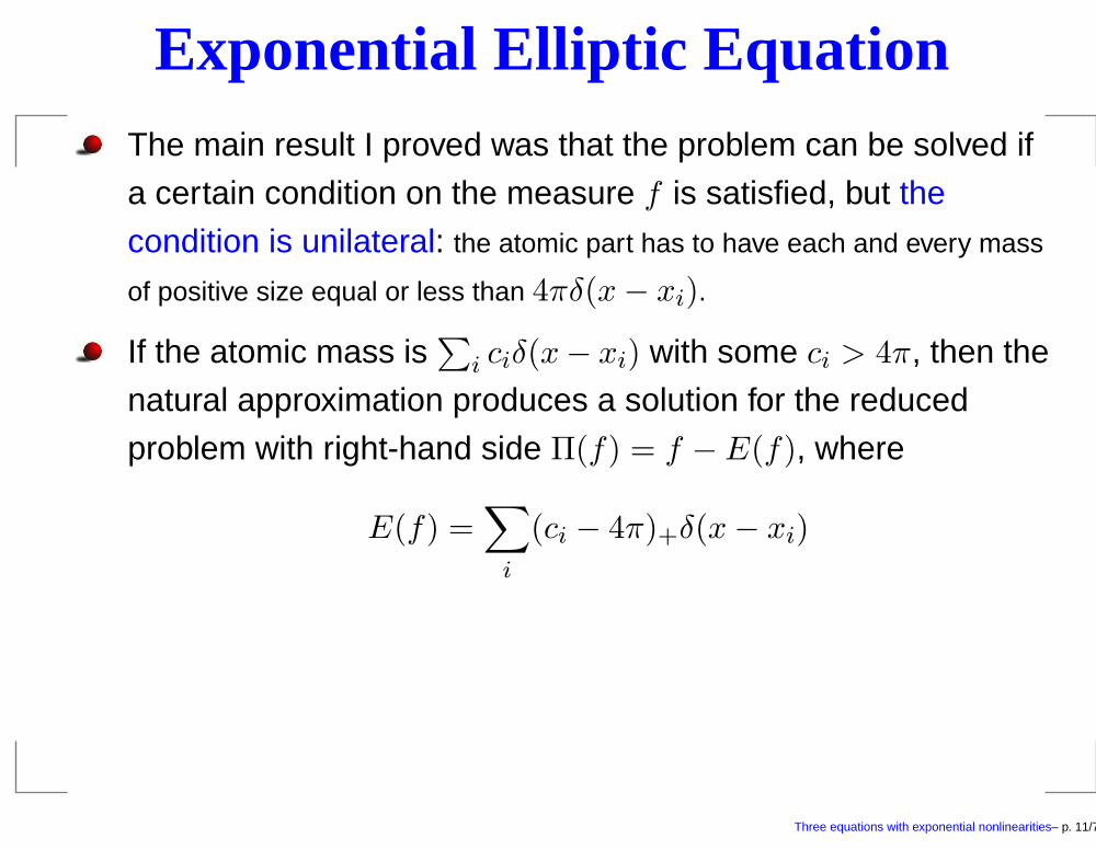
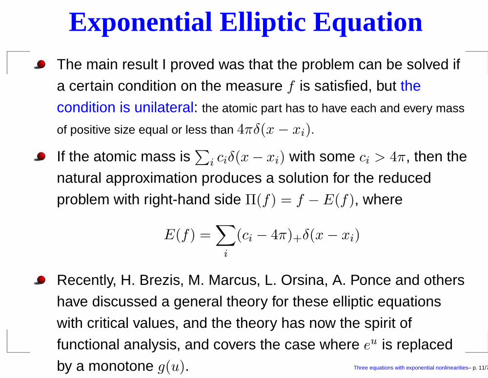
Exponential Elliptic EquationThe main result I proved was that the problem can be solved if
a certain condition on the measure f is satisfied, but the
condition is unilateral: the atomic part has to have each and every mass
of positive size equal or less than 4πδ(x− xi).
If the atomic mass is∑
i ciδ(x− xi) with some ci > 4π, then the
natural approximation produces a solution for the reduced
problem with right-hand side Π(f) = f − E(f), where
E(f) =∑
i
(ci − 4π)+δ(x− xi)
Three equations with exponential nonlinearities– p. 11/71
Exponential Elliptic EquationThe main result I proved was that the problem can be solved if
a certain condition on the measure f is satisfied, but the
condition is unilateral: the atomic part has to have each and every mass
of positive size equal or less than 4πδ(x− xi).
If the atomic mass is∑
i ciδ(x− xi) with some ci > 4π, then the
natural approximation produces a solution for the reduced
problem with right-hand side Π(f) = f − E(f), where
E(f) =∑
i
(ci − 4π)+δ(x− xi)
Recently, H. Brezis, M. Marcus, L. Orsina, A. Ponce and others
have discussed a general theory for these elliptic equations
with critical values, and the theory has now the spirit of
functional analysis, and covers the case where eu is replaced
by a monotone g(u). Three equations with exponential nonlinearities– p. 11/71

Three equations with exponential nonlinearities– p. 12/71
Exponential Elliptic EquationIn case f is excessive, or as they say now non-admissible,
where does the remaining mass go? Here is the magic formula
for the approximations un
g(un) → w1 + w2, w1 ∈ L1, w1 ∈ g(u), w2 = E(f)
Three equations with exponential nonlinearities– p. 13/71

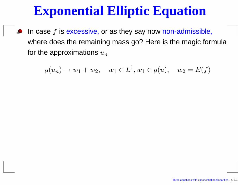
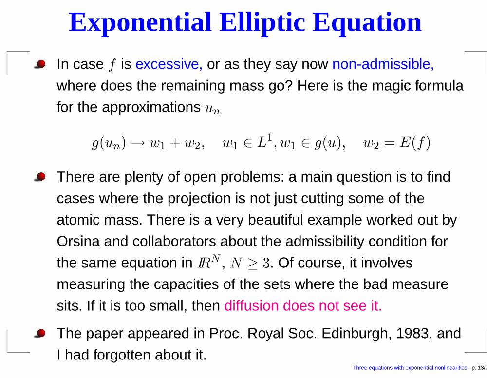
Exponential Elliptic EquationIn case f is excessive, or as they say now non-admissible,
where does the remaining mass go? Here is the magic formula
for the approximations un
g(un) → w1 + w2, w1 ∈ L1, w1 ∈ g(u), w2 = E(f)
There are plenty of open problems: a main question is to find
cases where the projection is not just cutting some of the
atomic mass. There is a very beautiful example worked out by
Orsina and collaborators about the admissibility condition for
the same equation in IRN , N ≥ 3. Of course, it involves
measuring the capacities of the sets where the bad measure
sits. If it is too small, then diffusion does not see it.
Three equations with exponential nonlinearities– p. 13/71
Exponential Elliptic EquationIn case f is excessive, or as they say now non-admissible,
where does the remaining mass go? Here is the magic formula
for the approximations un
g(un) → w1 + w2, w1 ∈ L1, w1 ∈ g(u), w2 = E(f)
There are plenty of open problems: a main question is to find
cases where the projection is not just cutting some of the
atomic mass. There is a very beautiful example worked out by
Orsina and collaborators about the admissibility condition for
the same equation in IRN , N ≥ 3. Of course, it involves
measuring the capacities of the sets where the bad measure
sits. If it is too small, then diffusion does not see it.
The paper appeared in Proc. Royal Soc. Edinburgh, 1983, and
I had forgotten about it.Three equations with exponential nonlinearities– p. 13/71

Three equations with exponential nonlinearities– p. 14/71

End of Part I
At that time I have taken three main decisions for my future:
(i) Getting a position at UAM, where Ireneo Peral with his infinite
enthusiasm made life active every day, just as I needed;
(ii) Emigrating to the USA for long periods. There, I met Luis
Caffarelli, Don Aronson, Mike Crandall, Avner Friedman, ..., people
who helped change our professional life in years to come;
(iii) Going to Italy every year. At the time I was happy to have
learned symmetrization from Giorgio Talenti, and I will need in the
last part all that I can do.
Three equations with exponential nonlinearities– p. 15/71

Three equations with exponential nonlinearities– p. 16/71
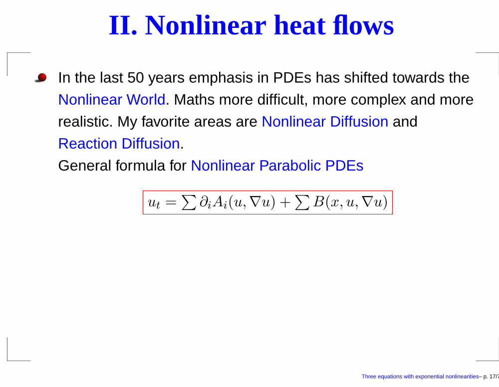
II. Nonlinear heat flows
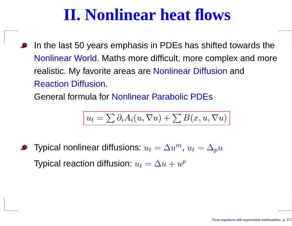
In the last 50 years emphasis in PDEs has shifted towards the
Nonlinear World. Maths more difficult, more complex and more
realistic. My favorite areas are Nonlinear Diffusion and
Reaction Diffusion.
General formula for Nonlinear Parabolic PDEs
ut =∑∂iAi(u,∇u) +
∑B(x, u,∇u)
Three equations with exponential nonlinearities– p. 17/71
II. Nonlinear heat flows
In the last 50 years emphasis in PDEs has shifted towards the
Nonlinear World. Maths more difficult, more complex and more
realistic. My favorite areas are Nonlinear Diffusion and
Reaction Diffusion.
General formula for Nonlinear Parabolic PDEs
ut =∑∂iAi(u,∇u) +
∑B(x, u,∇u)
Typical nonlinear diffusions: ut = ∆um, ut = ∆pu
Typical reaction diffusion: ut = ∆u+ up
Three equations with exponential nonlinearities– p. 17/71

Three equations with exponential nonlinearities– p. 18/71
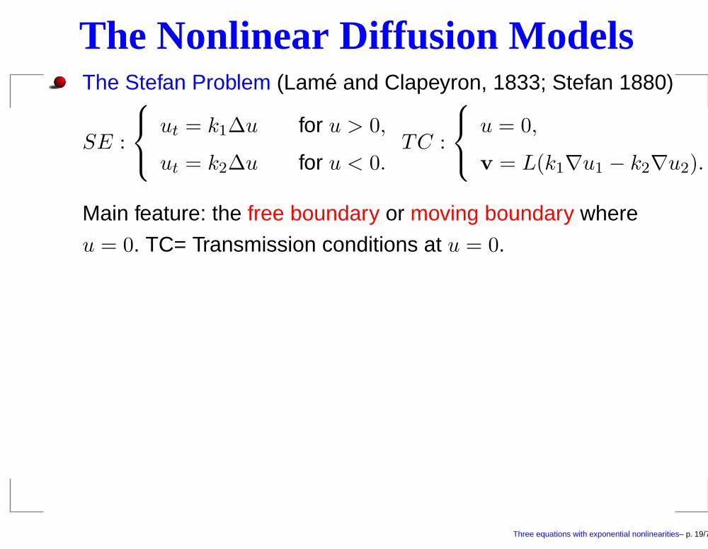
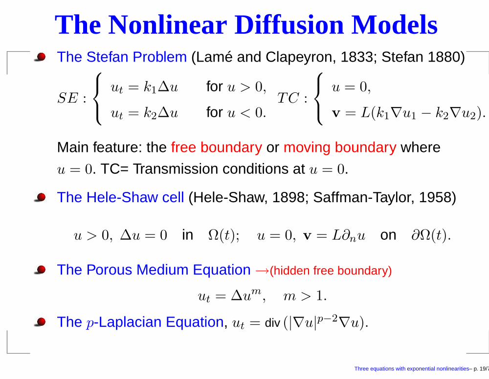
The Nonlinear Diffusion ModelsThe Stefan Problem (Lamé and Clapeyron, 1833; Stefan 1880)
SE :
ut = k1∆u for u > 0,
ut = k2∆u for u < 0.TC :
u = 0,
v = L(k1∇u1 − k2∇u2).
Main feature: the free boundary or moving boundary where
u = 0. TC= Transmission conditions at u = 0.
Three equations with exponential nonlinearities– p. 19/71
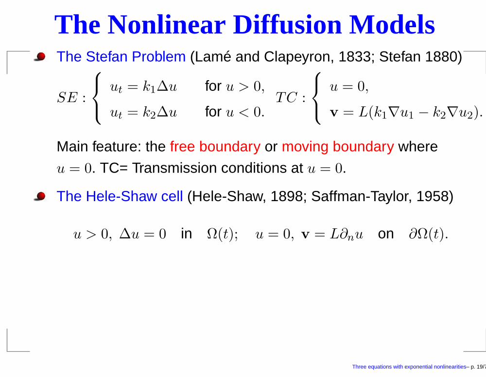
The Nonlinear Diffusion ModelsThe Stefan Problem (Lamé and Clapeyron, 1833; Stefan 1880)
SE :
ut = k1∆u for u > 0,
ut = k2∆u for u < 0.TC :
u = 0,
v = L(k1∇u1 − k2∇u2).
Main feature: the free boundary or moving boundary where
u = 0. TC= Transmission conditions at u = 0.
The Hele-Shaw cell (Hele-Shaw, 1898; Saffman-Taylor, 1958)
u > 0, ∆u = 0 in Ω(t); u = 0, v = L∂nu on ∂Ω(t).
Three equations with exponential nonlinearities– p. 19/71
The Nonlinear Diffusion ModelsThe Stefan Problem (Lamé and Clapeyron, 1833; Stefan 1880)
SE :
ut = k1∆u for u > 0,
ut = k2∆u for u < 0.TC :
u = 0,
v = L(k1∇u1 − k2∇u2).
Main feature: the free boundary or moving boundary where
u = 0. TC= Transmission conditions at u = 0.
The Hele-Shaw cell (Hele-Shaw, 1898; Saffman-Taylor, 1958)
u > 0, ∆u = 0 in Ω(t); u = 0, v = L∂nu on ∂Ω(t).
The Porous Medium Equation →(hidden free boundary)
ut = ∆um, m > 1.
Three equations with exponential nonlinearities– p. 19/71
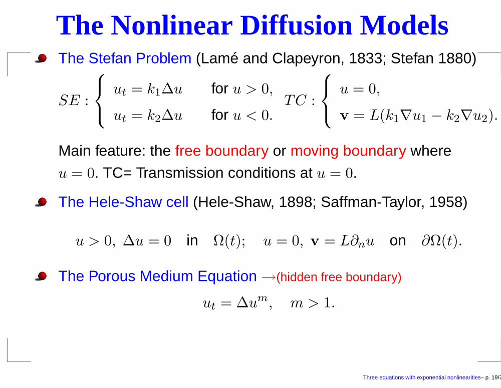
The Nonlinear Diffusion ModelsThe Stefan Problem (Lamé and Clapeyron, 1833; Stefan 1880)
SE :
ut = k1∆u for u > 0,
ut = k2∆u for u < 0.TC :
u = 0,
v = L(k1∇u1 − k2∇u2).
Main feature: the free boundary or moving boundary where
u = 0. TC= Transmission conditions at u = 0.
The Hele-Shaw cell (Hele-Shaw, 1898; Saffman-Taylor, 1958)
u > 0, ∆u = 0 in Ω(t); u = 0, v = L∂nu on ∂Ω(t).
The Porous Medium Equation →(hidden free boundary)
ut = ∆um, m > 1.
The p-Laplacian Equation, ut = div (|∇u|p−2∇u).
Three equations with exponential nonlinearities– p. 19/71
Three equations with exponential nonlinearities– p. 20/71
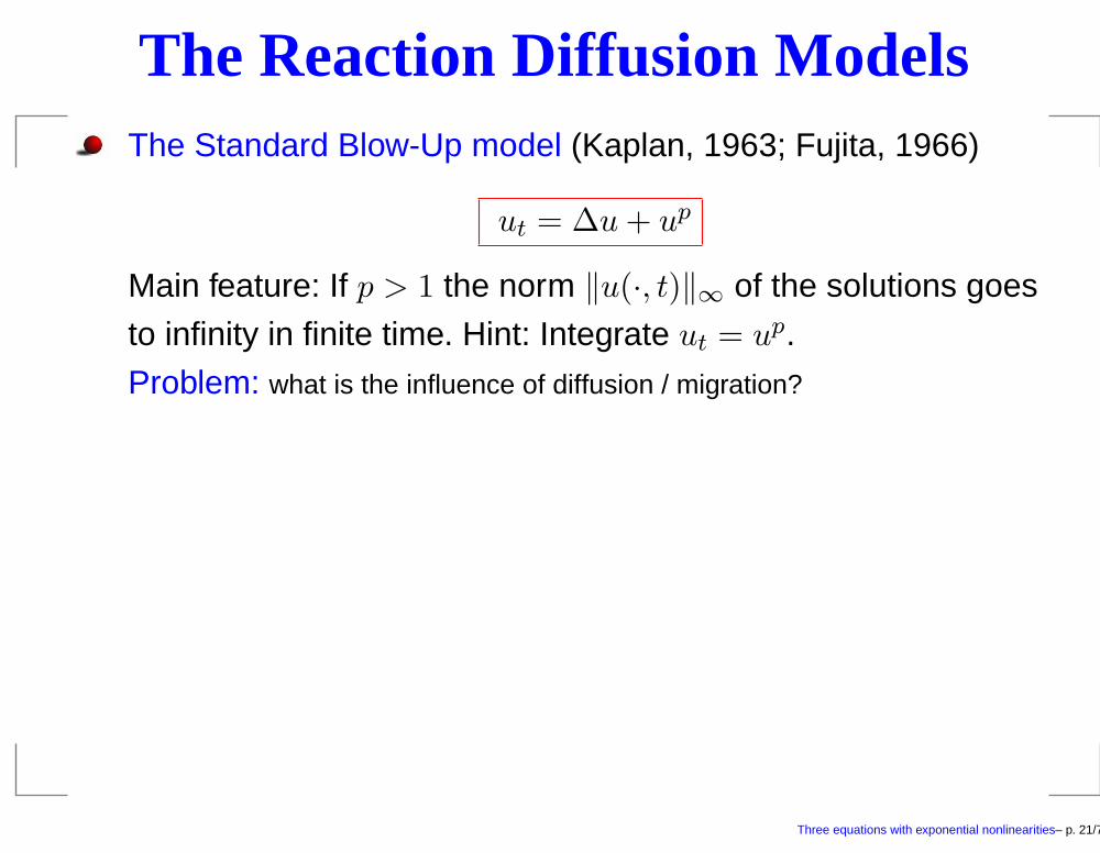
The Reaction Diffusion ModelsThe Standard Blow-Up model (Kaplan, 1963; Fujita, 1966)
ut = ∆u+ up
Main feature: If p > 1 the norm ‖u(·, t)‖∞ of the solutions goes
to infinity in finite time. Hint: Integrate ut = up.
Problem: what is the influence of diffusion / migration?
Three equations with exponential nonlinearities– p. 21/71
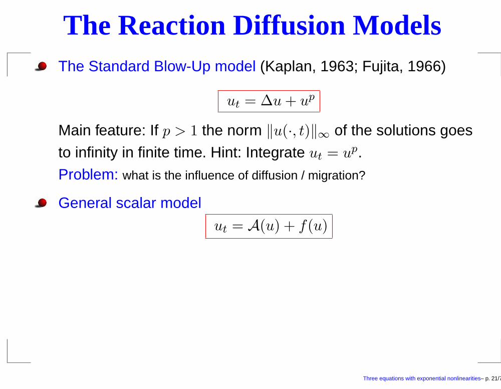
The Reaction Diffusion ModelsThe Standard Blow-Up model (Kaplan, 1963; Fujita, 1966)
ut = ∆u+ up
Main feature: If p > 1 the norm ‖u(·, t)‖∞ of the solutions goes
to infinity in finite time. Hint: Integrate ut = up.
Problem: what is the influence of diffusion / migration?
General scalar model
ut = A(u) + f(u)
The system model: −→u = (u1, · · · , um) → chemotaxis.
The fluid flow models: Navier-Stokes or Euler equation systems
for incompressible flow. Any singularities?
The geometrical models: the Ricci flow: ∂tgij = −Rij .
Three equations with exponential nonlinearities– p. 21/71

Three equations with exponential nonlinearities– p. 22/71

An opinion of John Nash, 1958:
The open problems in the area of nonlinear p.d.e. arevery relevant to applied mathematics and science as awhole, perhaps more so that the open problems in anyother area of mathematics, and the field seems poised forrapid development. It seems clear, however, that freshmethods must be employed...
Little is known about the existence, uniqueness andsmoothness of solutions of the general equations of flow fora viscous, compressible, and heat conducting fluid...
“Continuity of solutions of elliptic and parabolic equations”,paper published in Amer. J. Math, 80, no 4 (1958), 931-954
Three equations with exponential nonlinearities– p. 23/71

Three equations with exponential nonlinearities– p. 24/71
II. Fujita-Gelfand equationIn 1995 Ireneo and myself published a paper on the famous
model known as Gelfand equation in combustion.
ut − ∆u = λf(u), f(u) = eu.
Three equations with exponential nonlinearities– p. 25/71
II. Fujita-Gelfand equationIn 1995 Ireneo and myself published a paper on the famous
model known as Gelfand equation in combustion.
ut − ∆u = λf(u), f(u) = eu.
There are several motivations both for the evolution problem
and for its stationary version. The main one for me is the
application to combustion as model by Frank-Kamenetsky in
1938. The problem attracted much attention after the work of
Fujita in the 1960’s, who carefully examined the question of
blow-up.
Three equations with exponential nonlinearities– p. 25/71

II. Fujita-Gelfand equationIn 1995 Ireneo and myself published a paper on the famous
model known as Gelfand equation in combustion.
ut − ∆u = λf(u), f(u) = eu.
There are several motivations both for the evolution problem
and for its stationary version. The main one for me is the
application to combustion as model by Frank-Kamenetsky in
1938. The problem attracted much attention after the work of
Fujita in the 1960’s, who carefully examined the question of
blow-up.
Dávila has explained in his talk the Joseph-Lundgren analysis,
which separates the types of bifurcation plots in dimensions
N = 1, 2; 3 ≤ N ≤ 9, and finally N ≥ 10. This is one of the
origins of the theories of critical numbers, so popular now.Three equations with exponential nonlinearities– p. 25/71

Three equations with exponential nonlinearities– p. 26/71
Paper on Fujita-Gelfand equationOur paper (ARMA, 1995) is very specific, we wanted to
understand the stability properties of the special singular
solution (again, fundamental solution of the Laplacian)
U(x) = −2 log(|x|)
which corresponds to the value λ = 2(N − 2) when N ≥ 3.
Three equations with exponential nonlinearities– p. 27/71

Paper on Fujita-Gelfand equationOur paper (ARMA, 1995) is very specific, we wanted to
understand the stability properties of the special singular
solution (again, fundamental solution of the Laplacian)
U(x) = −2 log(|x|)
which corresponds to the value λ = 2(N − 2) when N ≥ 3.
The first thing that we did was to show that there is a very good
existence theory for initial data
u(x, 0) ≤ U(x).
Moreover, we did a delicate iterative argument to show that for
all u0 6= U the solution is bounded for all t > 0.
Three equations with exponential nonlinearities– p. 27/71

Three equations with exponential nonlinearities– p. 28/71
Paper on Fujita-Gelfand equationYears later I proved that there is bounded solution even for
u0 = U . Since obviously U is a solution, this means
non-uniqueness. The new minimal solution is selfsimilar and
goes down with time. Actually, the result says that you can
solve the problem with bounded solutions even when
u0(x) ≤ U(x) + c where c is less than the “critical excess".
Reference: J. L. V., Domain of existence and blowup for the exponential
reaction-diffusion equation. Indiana Univ. Math. Journal, 48, 2 (1999),
677–709.
Three equations with exponential nonlinearities– p. 29/71
Paper on Fujita-Gelfand equationYears later I proved that there is bounded solution even for
u0 = U . Since obviously U is a solution, this means
non-uniqueness. The new minimal solution is selfsimilar and
goes down with time. Actually, the result says that you can
solve the problem with bounded solutions even when
u0(x) ≤ U(x) + c where c is less than the “critical excess".
Reference: J. L. V., Domain of existence and blowup for the exponential
reaction-diffusion equation. Indiana Univ. Math. Journal, 48, 2 (1999),
677–709.
The next point is to linearize the equation around the singular solution to
obtain the equation (λ0 = 2(N − 2))
φt = L(φ), L(φ) = ∆φ+λ0
|x|2φ
Three equations with exponential nonlinearities– p. 29/71

Three equations with exponential nonlinearities– p. 30/71
Paper on Fujita-Gelfand equationIndeed, without linearization we have for φ = U − u
φt = ∆φ+λ0
|x|2(1 − e−φ)
which makes these things subsolutions of the linearized
equation.
Three equations with exponential nonlinearities– p. 31/71

Paper on Fujita-Gelfand equationIndeed, without linearization we have for φ = U − u
φt = ∆φ+λ0
|x|2(1 − e−φ)
which makes these things subsolutions of the linearized
equation.
The analysis of the linearized operator is based on knowing
whether −L is positive or not (accretive or not). The Hardy
inequality plays a crucial role, the constant in the energy
formulation is cN = (N − 2)2/4. The constant that we have in
the equation is λ0 = 2(N − 2). Stability holds if N ≥ 10. For
N < 10 the stationary solution is not attractor and the orbit
tends to the minimal solution.
Three equations with exponential nonlinearities– p. 31/71

Three equations with exponential nonlinearities– p. 32/71

Paper on Fujita-Gelfand equationFor N ≥ 10 the orbits “near” U tend to U asymptotically. I have
calculated the rate with a UK-Russian team by doing matched
asymptotics (Dold-Lacey-Galaktionov-JLV) . It says
‖u(t)‖∞ = c1t+ o(t).
Reference: Rate of approach to a singular steady state in
quasilinear reaction-diffusion equations. Ann. Scuola Norm. Sup. Pisa
Cl. Sci. (4) 26 (1998), no. 4, 663–687.
Three equations with exponential nonlinearities– p. 33/71

Paper on Fujita-Gelfand equationFor N ≥ 10 the orbits “near” U tend to U asymptotically. I have
calculated the rate with a UK-Russian team by doing matched
asymptotics (Dold-Lacey-Galaktionov-JLV) . It says
‖u(t)‖∞ = c1t+ o(t).
Reference: Rate of approach to a singular steady state in
quasilinear reaction-diffusion equations. Ann. Scuola Norm. Sup. Pisa
Cl. Sci. (4) 26 (1998), no. 4, 663–687.
The most striking result of the paper is the result on
instantaneous blow-up If u0 ≥ U and u0 6= U and moreover u ≥ U ,
then u(t) ≡ +∞ for every t > 0.
The proof is based on writing the equation for ψ = u− U ,
ψt = ∆ψ +λ0
|x|2(eψ − 1) ≥ L(ψ)
Three equations with exponential nonlinearities– p. 33/71

Three equations with exponential nonlinearities– p. 34/71
Paper on Fujita-Gelfand equationWe compare with the solution u with initial data such that
φ = U − u has same initial data as ψ. We get
ψ(x, t) ≥ φ(x, t)
Therefore,
u(x, t) ≥ 2U(x) − u(x, t)
But φ is bounded, hence the singularity of u is like 2U(x).
Three equations with exponential nonlinearities– p. 35/71

Paper on Fujita-Gelfand equationWe compare with the solution u with initial data such that
φ = U − u has same initial data as ψ. We get
ψ(x, t) ≥ φ(x, t)
Therefore,
u(x, t) ≥ 2U(x) − u(x, t)
But φ is bounded, hence the singularity of u is like 2U(x).
Iterating the argument, we get u(x, t) ≥ cU(x) near x = 0 for
every c > 1. Once this implies that eu(t1) 6∈ L1, we conclude that
u(t) ≡ +∞ for all later times.
♠ End of Part II ♠
Three equations with exponential nonlinearities– p. 35/71

Three equations with exponential nonlinearities– p. 36/71
Intermezzo
Porous Mediumand
Fast Diffusion
Three equations with exponential nonlinearities– p. 37/71

Three equations with exponential nonlinearities– p. 38/71

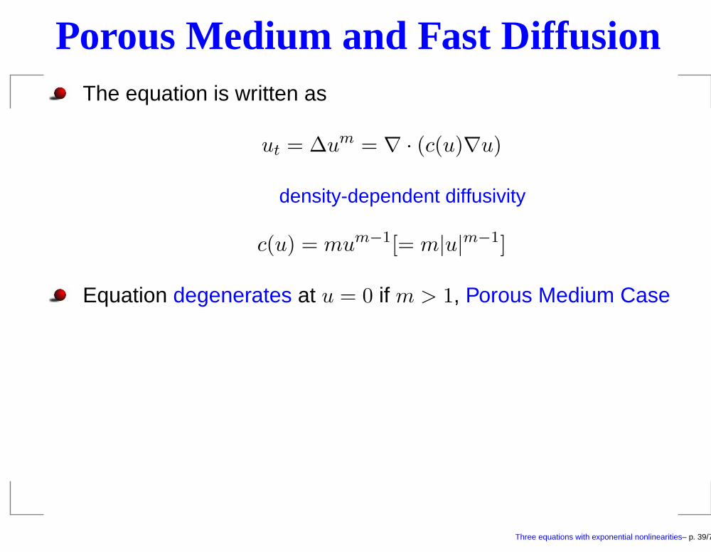
Porous Medium and Fast DiffusionThe equation is written as
ut = ∆um = ∇ · (c(u)∇u)
density-dependent diffusivity
c(u) = mum−1[= m|u|m−1]
Three equations with exponential nonlinearities– p. 39/71
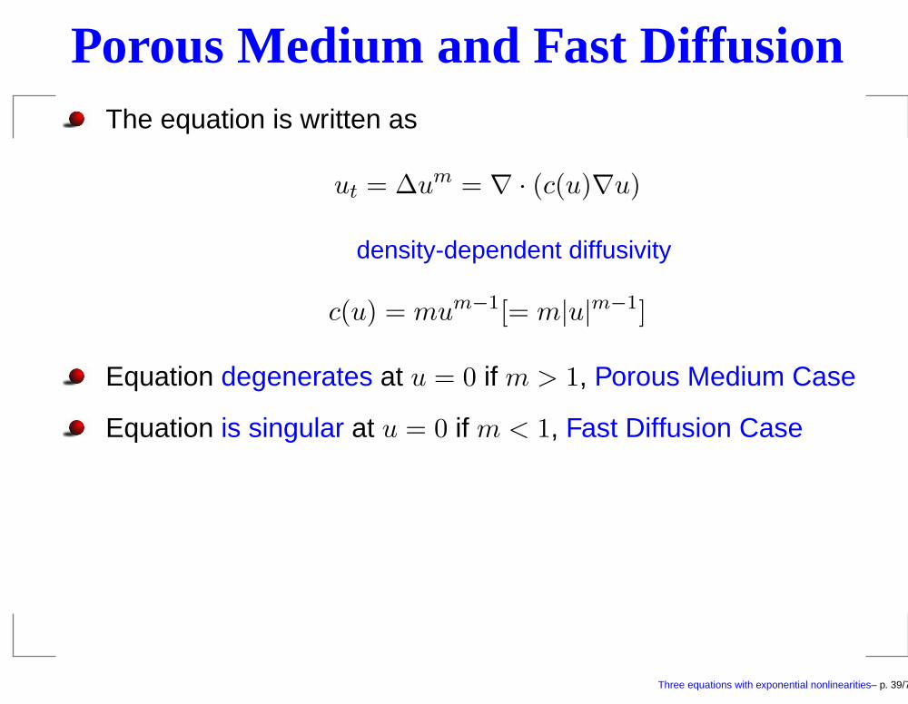
Porous Medium and Fast DiffusionThe equation is written as
ut = ∆um = ∇ · (c(u)∇u)
density-dependent diffusivity
c(u) = mum−1[= m|u|m−1]
Equation degenerates at u = 0 if m > 1, Porous Medium Case
Three equations with exponential nonlinearities– p. 39/71
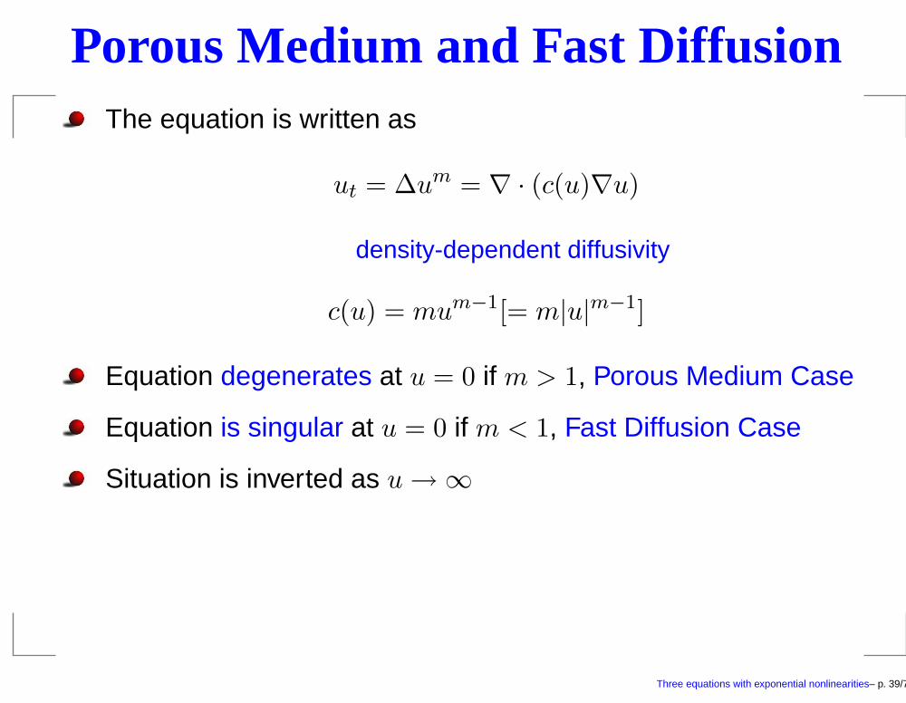
Porous Medium and Fast DiffusionThe equation is written as
ut = ∆um = ∇ · (c(u)∇u)
density-dependent diffusivity
c(u) = mum−1[= m|u|m−1]
Equation degenerates at u = 0 if m > 1, Porous Medium Case
Equation is singular at u = 0 if m < 1, Fast Diffusion Case
Three equations with exponential nonlinearities– p. 39/71
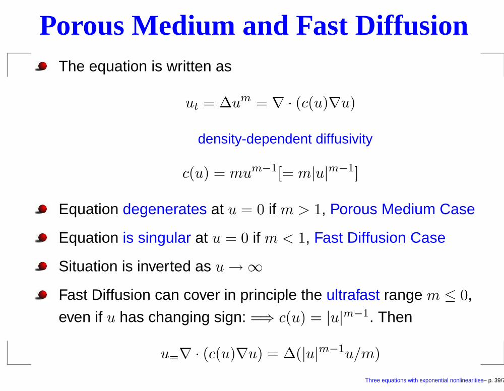
Porous Medium and Fast DiffusionThe equation is written as
ut = ∆um = ∇ · (c(u)∇u)
density-dependent diffusivity
c(u) = mum−1[= m|u|m−1]
Equation degenerates at u = 0 if m > 1, Porous Medium Case
Equation is singular at u = 0 if m < 1, Fast Diffusion Case
Situation is inverted as u→ ∞
Three equations with exponential nonlinearities– p. 39/71
Porous Medium and Fast DiffusionThe equation is written as
ut = ∆um = ∇ · (c(u)∇u)
density-dependent diffusivity
c(u) = mum−1[= m|u|m−1]
Equation degenerates at u = 0 if m > 1, Porous Medium Case
Equation is singular at u = 0 if m < 1, Fast Diffusion Case
Situation is inverted as u→ ∞
Fast Diffusion can cover in principle the ultrafast range m ≤ 0,
even if u has changing sign: =⇒ c(u) = |u|m−1. Then
u=∇ · (c(u)∇u) = ∆(|u|m−1u/m)
Three equations with exponential nonlinearities– p. 39/71

Three equations with exponential nonlinearities– p. 40/71
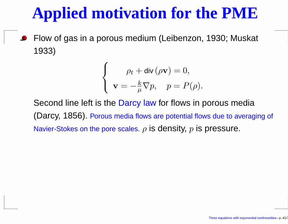
Applied motivation for the PMEFlow of gas in a porous medium (Leibenzon, 1930; Muskat
1933)
ρt + div (ρv) = 0,
v = − kµ∇p, p = P (ρ).
Second line left is the Darcy law for flows in porous media
(Darcy, 1856). Porous media flows are potential flows due to averaging of
Navier-Stokes on the pore scales. ρ is density, p is pressure.
Three equations with exponential nonlinearities– p. 41/71

Applied motivation for the PMEFlow of gas in a porous medium (Leibenzon, 1930; Muskat
1933)
ρt + div (ρv) = 0,
v = − kµ∇p, p = P (ρ).
Second line left is the Darcy law for flows in porous media
(Darcy, 1856). Porous media flows are potential flows due to averaging of
Navier-Stokes on the pore scales. ρ is density, p is pressure.
If P (ρ) is a power, P = ργ ≥ 1, we get the PME with
m = 1 + γ ≥ 2.
If not, we get the general Filtration Equation:
ρt = div (k
µρ∇P (ρ)) := ∆Φ(ρ)
Three equations with exponential nonlinearities– p. 41/71

Three equations with exponential nonlinearities– p. 42/71
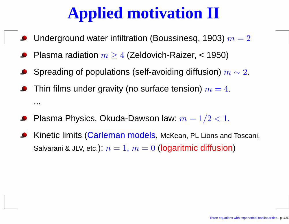
Applied motivation IIUnderground water infiltration (Boussinesq, 1903) m = 2
Three equations with exponential nonlinearities– p. 43/71

Applied motivation IIUnderground water infiltration (Boussinesq, 1903) m = 2
Plasma radiation m ≥ 4 (Zeldovich-Raizer, < 1950)
Three equations with exponential nonlinearities– p. 43/71
Applied motivation IIUnderground water infiltration (Boussinesq, 1903) m = 2
Plasma radiation m ≥ 4 (Zeldovich-Raizer, < 1950)
Spreading of populations (self-avoiding diffusion) m ∼ 2.
Three equations with exponential nonlinearities– p. 43/71
Applied motivation IIUnderground water infiltration (Boussinesq, 1903) m = 2
Plasma radiation m ≥ 4 (Zeldovich-Raizer, < 1950)
Spreading of populations (self-avoiding diffusion) m ∼ 2.
Thin films under gravity (no surface tension) m = 4.
...
Three equations with exponential nonlinearities– p. 43/71

Applied motivation IIUnderground water infiltration (Boussinesq, 1903) m = 2
Plasma radiation m ≥ 4 (Zeldovich-Raizer, < 1950)
Spreading of populations (self-avoiding diffusion) m ∼ 2.
Thin films under gravity (no surface tension) m = 4.
...
Plasma Physics, Okuda-Dawson law: m = 1/2 < 1.
Three equations with exponential nonlinearities– p. 43/71
Applied motivation IIUnderground water infiltration (Boussinesq, 1903) m = 2
Plasma radiation m ≥ 4 (Zeldovich-Raizer, < 1950)
Spreading of populations (self-avoiding diffusion) m ∼ 2.
Thin films under gravity (no surface tension) m = 4.
...
Plasma Physics, Okuda-Dawson law: m = 1/2 < 1.
Kinetic limits (Carleman models, McKean, PL Lions and Toscani,
Salvarani & JLV, etc.): n = 1, m = 0 (logaritmic diffusion)
Three equations with exponential nonlinearities– p. 43/71
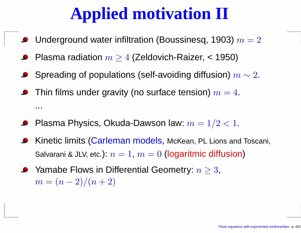
Applied motivation IIUnderground water infiltration (Boussinesq, 1903) m = 2
Plasma radiation m ≥ 4 (Zeldovich-Raizer, < 1950)
Spreading of populations (self-avoiding diffusion) m ∼ 2.
Thin films under gravity (no surface tension) m = 4.
...
Plasma Physics, Okuda-Dawson law: m = 1/2 < 1.
Kinetic limits (Carleman models, McKean, PL Lions and Toscani,
Salvarani & JLV, etc.): n = 1, m = 0 (logaritmic diffusion)
Yamabe Flows in Differential Geometry: n ≥ 3,m = (n− 2)/(n+ 2)
Many more (boundary layers, dopant diffusion,stochastic processes, images, ...); you may find m ≤ −1
Three equations with exponential nonlinearities– p. 43/71

Three equations with exponential nonlinearities– p. 44/71

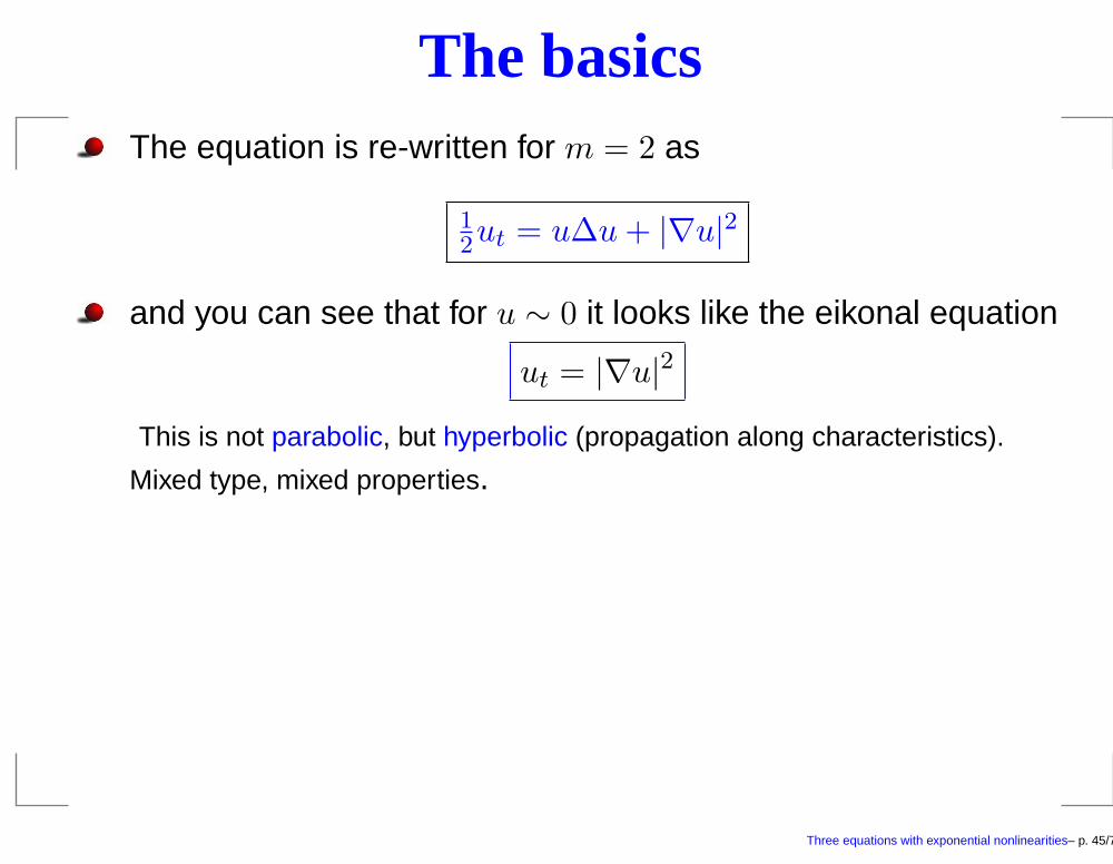
The basicsThe equation is re-written for m = 2 as
12ut = u∆u+ |∇u|2
Three equations with exponential nonlinearities– p. 45/71
The basicsThe equation is re-written for m = 2 as
12ut = u∆u+ |∇u|2
and you can see that for u ∼ 0 it looks like the eikonal equation
ut = |∇u|2
This is not parabolic, but hyperbolic (propagation along characteristics).
Mixed type, mixed properties.
Three equations with exponential nonlinearities– p. 45/71
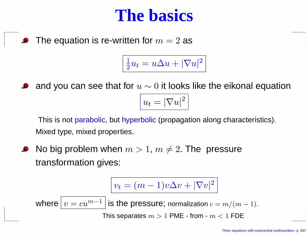
The basicsThe equation is re-written for m = 2 as
12ut = u∆u+ |∇u|2
and you can see that for u ∼ 0 it looks like the eikonal equation
ut = |∇u|2
This is not parabolic, but hyperbolic (propagation along characteristics).
Mixed type, mixed properties.
No big problem when m > 1, m 6= 2. The pressure
transformation gives:
vt = (m− 1)v∆v + |∇v|2
where v = cum−1 is the pressure; normalization c = m/(m− 1).
This separates m > 1 PME - from - m < 1 FDE
Three equations with exponential nonlinearities– p. 45/71

Three equations with exponential nonlinearities– p. 46/71

ReferencesAbout PME
J. L. Vázquez, "The Porous Medium Equation. Mathematical Theory",Oxford Univ. Press, 2006 in press. approx. 600 pages
About estimates and scaling
Three equations with exponential nonlinearities– p. 47/71
ReferencesAbout PME
J. L. Vázquez, "The Porous Medium Equation. Mathematical Theory",Oxford Univ. Press, 2006 in press. approx. 600 pages
About estimates and scaling
J. L. Vázquez, “Smoothing and Decay Estimates for NonlinearParabolic Equations of Porous Medium Type”, Oxford Univ. Press,2006, 234 pages.
About asymptotic behaviour. (Following Lyapunov andBoltzmann)
Three equations with exponential nonlinearities– p. 47/71

ReferencesAbout PME
J. L. Vázquez, "The Porous Medium Equation. Mathematical Theory",Oxford Univ. Press, 2006 in press. approx. 600 pages
About estimates and scaling
J. L. Vázquez, “Smoothing and Decay Estimates for NonlinearParabolic Equations of Porous Medium Type”, Oxford Univ. Press,2006, 234 pages.
About asymptotic behaviour. (Following Lyapunov andBoltzmann)
J. L. Vázquez. Asymptotic behaviour for the Porous Medium Equationposed in the whole space. Journal of Evolution Equations 3 (2003),67–118.
Three equations with exponential nonlinearities– p. 47/71

Three equations with exponential nonlinearities– p. 48/71
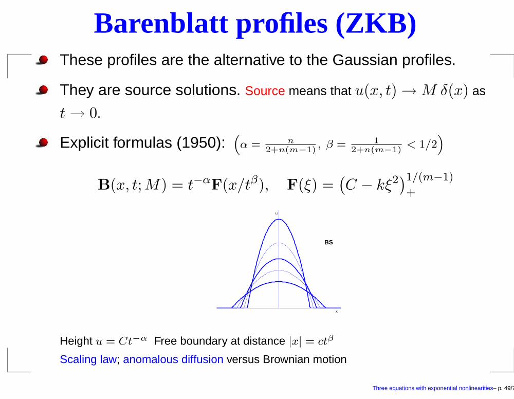
Barenblatt profiles (ZKB)These profiles are the alternative to the Gaussian profiles.
Three equations with exponential nonlinearities– p. 49/71
Barenblatt profiles (ZKB)These profiles are the alternative to the Gaussian profiles.
They are source solutions. Source means that u(x, t) →M δ(x) as
t→ 0.
Three equations with exponential nonlinearities– p. 49/71

Barenblatt profiles (ZKB)These profiles are the alternative to the Gaussian profiles.
They are source solutions. Source means that u(x, t) →M δ(x) as
t→ 0.
Explicit formulas (1950):“
α = n2+n(m−1)
, β = 12+n(m−1)
< 1/2”
B(x, t;M) = t−αF(x/tβ), F(ξ) =(C − kξ2
)1/(m−1)
+
x
u
BS
Height u = Ct−α Free boundary at distance |x| = ctβ
Scaling law; anomalous diffusion versus Brownian motion
Three equations with exponential nonlinearities– p. 49/71

Three equations with exponential nonlinearities– p. 50/71
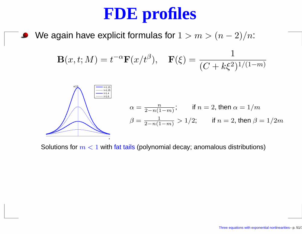
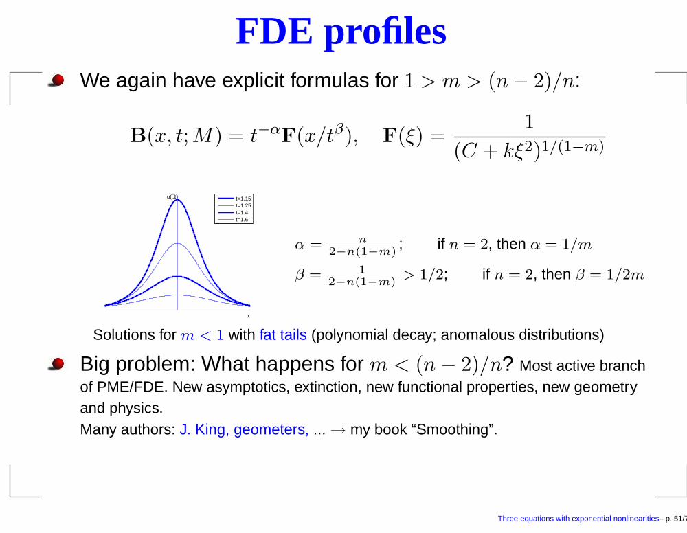
FDE profilesWe again have explicit formulas for 1 > m > (n− 2)/n:
B(x, t;M) = t−αF(x/tβ), F(ξ) =1
(C + kξ2)1/(1−m)
x
u(⋅,t) t=1.15t=1.25t=1.4t=1.6
α = n2−n(1−m)
; if n = 2, then α = 1/m
β = 12−n(1−m)
> 1/2; if n = 2, then β = 1/2m
Solutions for m < 1 with fat tails (polynomial decay; anomalous distributions)
Three equations with exponential nonlinearities– p. 51/71
FDE profilesWe again have explicit formulas for 1 > m > (n− 2)/n:
B(x, t;M) = t−αF(x/tβ), F(ξ) =1
(C + kξ2)1/(1−m)
x
u(⋅,t) t=1.15t=1.25t=1.4t=1.6
α = n2−n(1−m)
; if n = 2, then α = 1/m
β = 12−n(1−m)
> 1/2; if n = 2, then β = 1/2m
Solutions for m < 1 with fat tails (polynomial decay; anomalous distributions)
Big problem: What happens for m < (n− 2)/n? Most active branchof PME/FDE. New asymptotics, extinction, new functional properties, new geometryand physics.Many authors: J. King, geometers, ... → my book “Smoothing”.
Three equations with exponential nonlinearities– p. 51/71

Three equations with exponential nonlinearities– p. 52/71

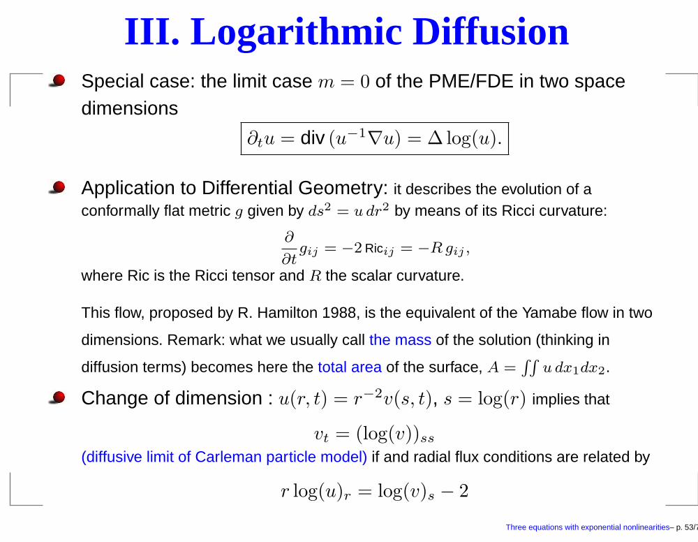
III. Logarithmic DiffusionSpecial case: the limit case m = 0 of the PME/FDE in two spacedimensions
∂tu = div (u−1∇u) = ∆ log(u).
Three equations with exponential nonlinearities– p. 53/71

III. Logarithmic DiffusionSpecial case: the limit case m = 0 of the PME/FDE in two spacedimensions
∂tu = div (u−1∇u) = ∆ log(u).
Application to Differential Geometry: it describes the evolution of aconformally flat metric g given by ds2 = u dr2 by means of its Ricci curvature:
∂
∂tgij = −2 Ricij = −Rgij ,
where Ric is the Ricci tensor and R the scalar curvature.
Three equations with exponential nonlinearities– p. 53/71
III. Logarithmic DiffusionSpecial case: the limit case m = 0 of the PME/FDE in two spacedimensions
∂tu = div (u−1∇u) = ∆ log(u).
Application to Differential Geometry: it describes the evolution of aconformally flat metric g given by ds2 = u dr2 by means of its Ricci curvature:
∂
∂tgij = −2 Ricij = −Rgij ,
where Ric is the Ricci tensor and R the scalar curvature.
This flow, proposed by R. Hamilton 1988, is the equivalent of the Yamabe flow in two
dimensions. Remark: what we usually call the mass of the solution (thinking in
diffusion terms) becomes here the total area of the surface, A =RR
u dx1dx2.
Three equations with exponential nonlinearities– p. 53/71

III. Logarithmic DiffusionSpecial case: the limit case m = 0 of the PME/FDE in two spacedimensions
∂tu = div (u−1∇u) = ∆ log(u).
Application to Differential Geometry: it describes the evolution of aconformally flat metric g given by ds2 = u dr2 by means of its Ricci curvature:
∂
∂tgij = −2 Ricij = −Rgij ,
where Ric is the Ricci tensor and R the scalar curvature.
This flow, proposed by R. Hamilton 1988, is the equivalent of the Yamabe flow in two
dimensions. Remark: what we usually call the mass of the solution (thinking in
diffusion terms) becomes here the total area of the surface, A =RR
u dx1dx2.
Change of dimension : u(r, t) = r−2v(s, t), s = log(r) implies that
vt = (log(v))ss
(diffusive limit of Carleman particle model) if and radial flux conditions are related by
r log(u)r = log(v)s − 2
Three equations with exponential nonlinearities– p. 53/71

Three equations with exponential nonlinearities– p. 54/71
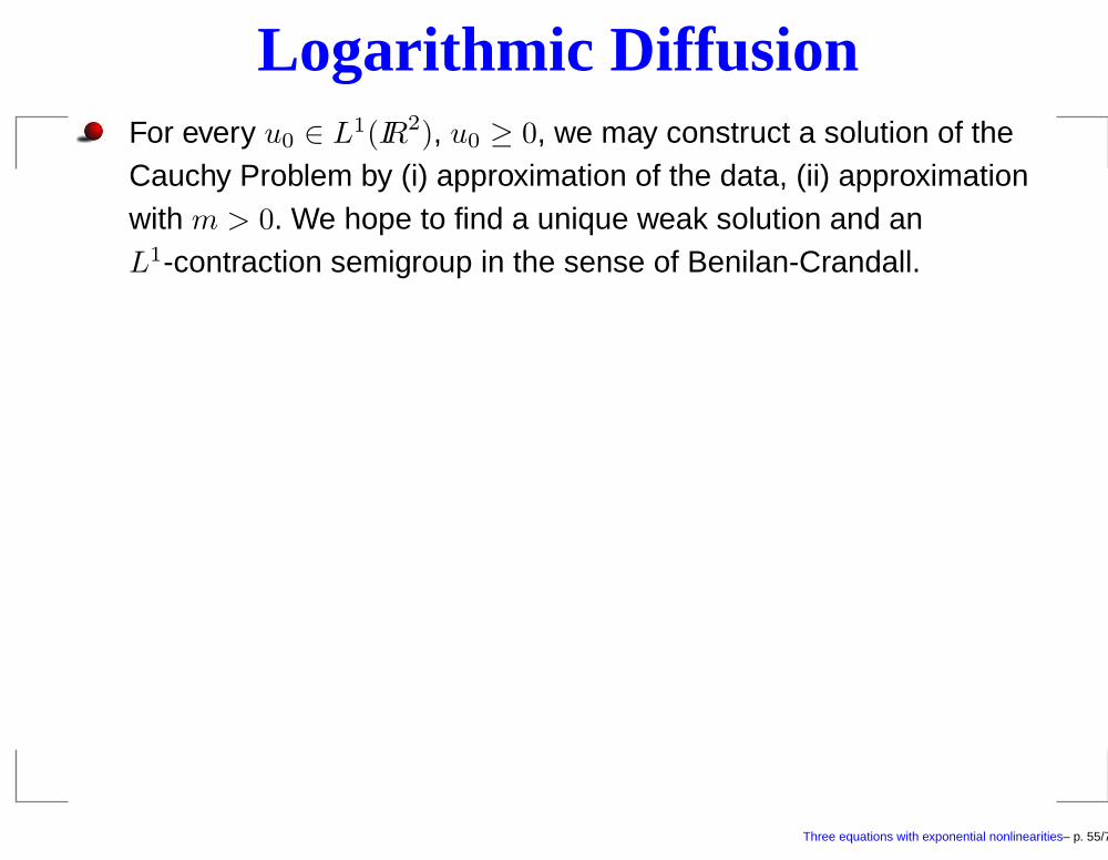
Logarithmic DiffusionFor every u0 ∈ L1(IR2), u0 ≥ 0, we may construct a solution of theCauchy Problem by (i) approximation of the data, (ii) approximationwith m > 0. We hope to find a unique weak solution and anL1-contraction semigroup in the sense of Benilan-Crandall.
Three equations with exponential nonlinearities– p. 55/71
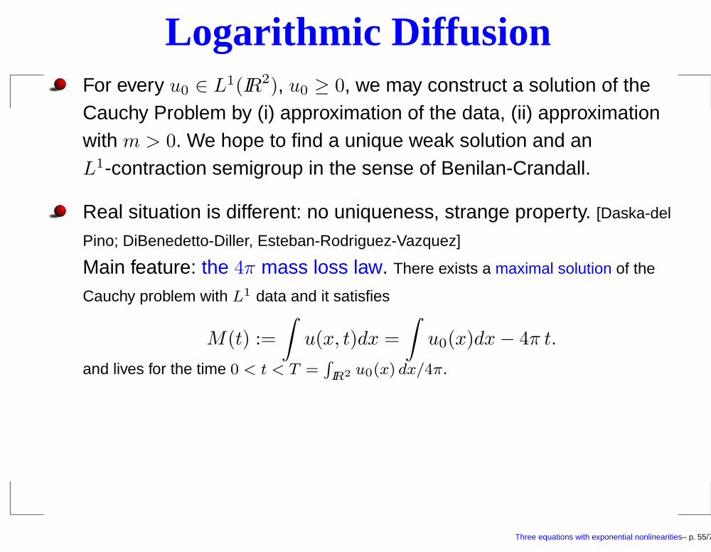
Logarithmic DiffusionFor every u0 ∈ L1(IR2), u0 ≥ 0, we may construct a solution of theCauchy Problem by (i) approximation of the data, (ii) approximationwith m > 0. We hope to find a unique weak solution and anL1-contraction semigroup in the sense of Benilan-Crandall.
Real situation is different: no uniqueness, strange property. [Daska-del
Pino; DiBenedetto-Diller, Esteban-Rodriguez-Vazquez]
Main feature: the 4π mass loss law. There exists a maximal solution of the
Cauchy problem with L1 data and it satisfies
M(t) :=
∫u(x, t)dx =
∫u0(x)dx− 4π t.
and lives for the time 0 < t < T =R
IR2 u0(x) dx/4π.
Three equations with exponential nonlinearities– p. 55/71
Logarithmic DiffusionFor every u0 ∈ L1(IR2), u0 ≥ 0, we may construct a solution of theCauchy Problem by (i) approximation of the data, (ii) approximationwith m > 0. We hope to find a unique weak solution and anL1-contraction semigroup in the sense of Benilan-Crandall.
Real situation is different: no uniqueness, strange property. [Daska-del
Pino; DiBenedetto-Diller, Esteban-Rodriguez-Vazquez]
Main feature: the 4π mass loss law. There exists a maximal solution of the
Cauchy problem with L1 data and it satisfies
M(t) :=
∫u(x, t)dx =
∫u0(x)dx− 4π t.
and lives for the time 0 < t < T =R
IR2 u0(x) dx/4π.
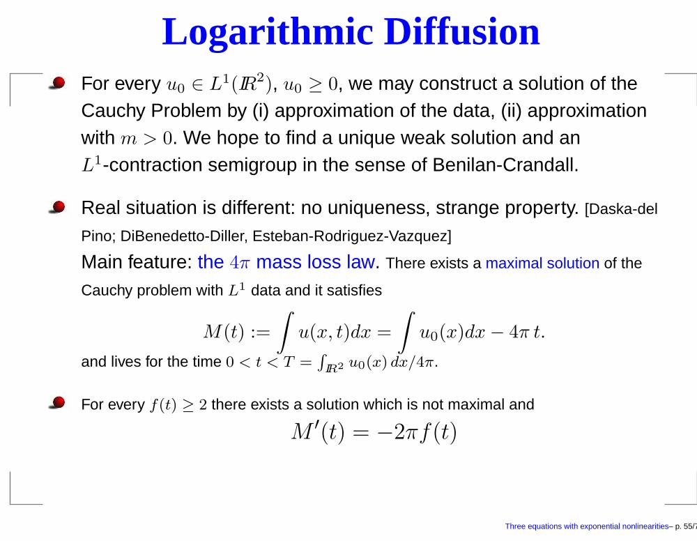
For every f(t) ≥ 2 there exists a solution which is not maximal and
M ′(t) = −2πf(t)
Three equations with exponential nonlinearities– p. 55/71
Logarithmic DiffusionFor every u0 ∈ L1(IR2), u0 ≥ 0, we may construct a solution of theCauchy Problem by (i) approximation of the data, (ii) approximationwith m > 0. We hope to find a unique weak solution and anL1-contraction semigroup in the sense of Benilan-Crandall.
Real situation is different: no uniqueness, strange property. [Daska-del
Pino; DiBenedetto-Diller, Esteban-Rodriguez-Vazquez]
Main feature: the 4π mass loss law. There exists a maximal solution of the
Cauchy problem with L1 data and it satisfies
M(t) :=
∫u(x, t)dx =
∫u0(x)dx− 4π t.
and lives for the time 0 < t < T =R
IR2 u0(x) dx/4π.
For every f(t) ≥ 2 there exists a solution which is not maximal and
M ′(t) = −2πf(t)
There is a special separate variable solution for f = 4 which represents a ball.
Three equations with exponential nonlinearities– p. 55/71

Three equations with exponential nonlinearities– p. 56/71
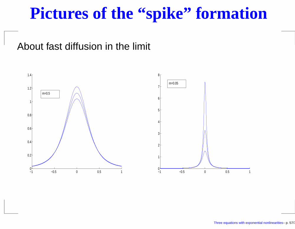
Pictures of the “spike” formation
About fast diffusion in the limit
−1 −0.5 0 0.5 10
0.2
0.4
0.6
0.8
1
1.2
1.4
m=0.5
−1 −0.5 0 0.5 10
1
2
3
4
5
6
7
8
m=0.05
Three equations with exponential nonlinearities– p. 57/71

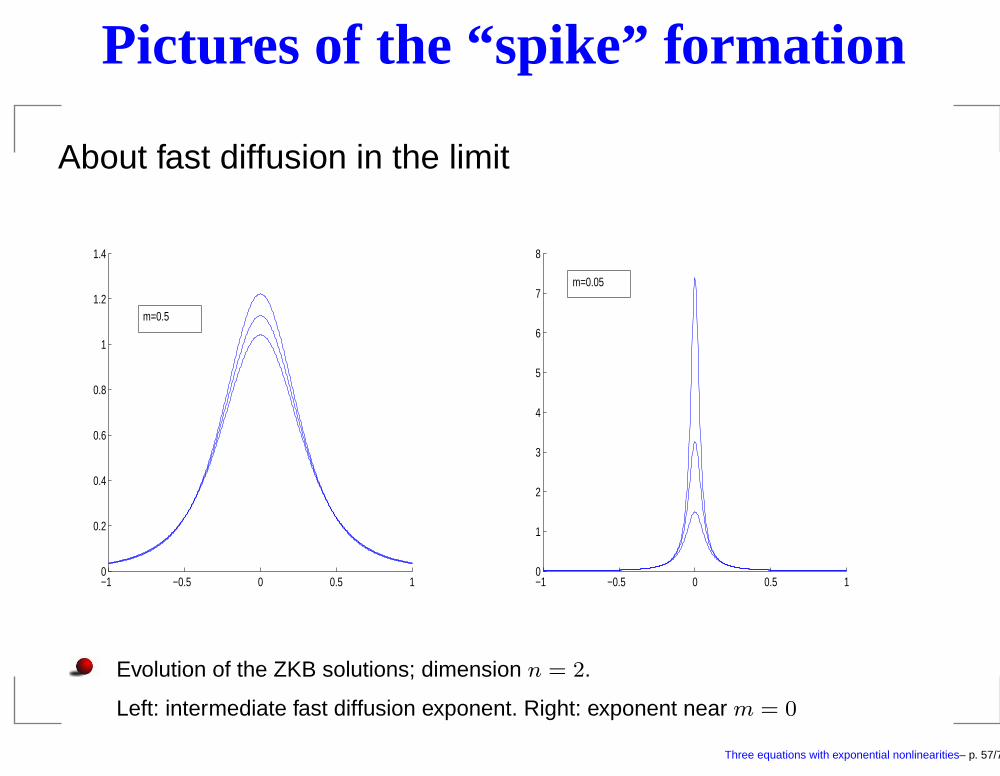
Pictures of the “spike” formation
About fast diffusion in the limit
−1 −0.5 0 0.5 10
0.2
0.4
0.6
0.8
1
1.2
1.4
m=0.5
−1 −0.5 0 0.5 10
1
2
3
4
5
6
7
8
m=0.05
Evolution of the ZKB solutions; dimension n = 2.
Left: intermediate fast diffusion exponent. Right: exponent near m = 0
Three equations with exponential nonlinearities– p. 57/71

Three equations with exponential nonlinearities– p. 58/71
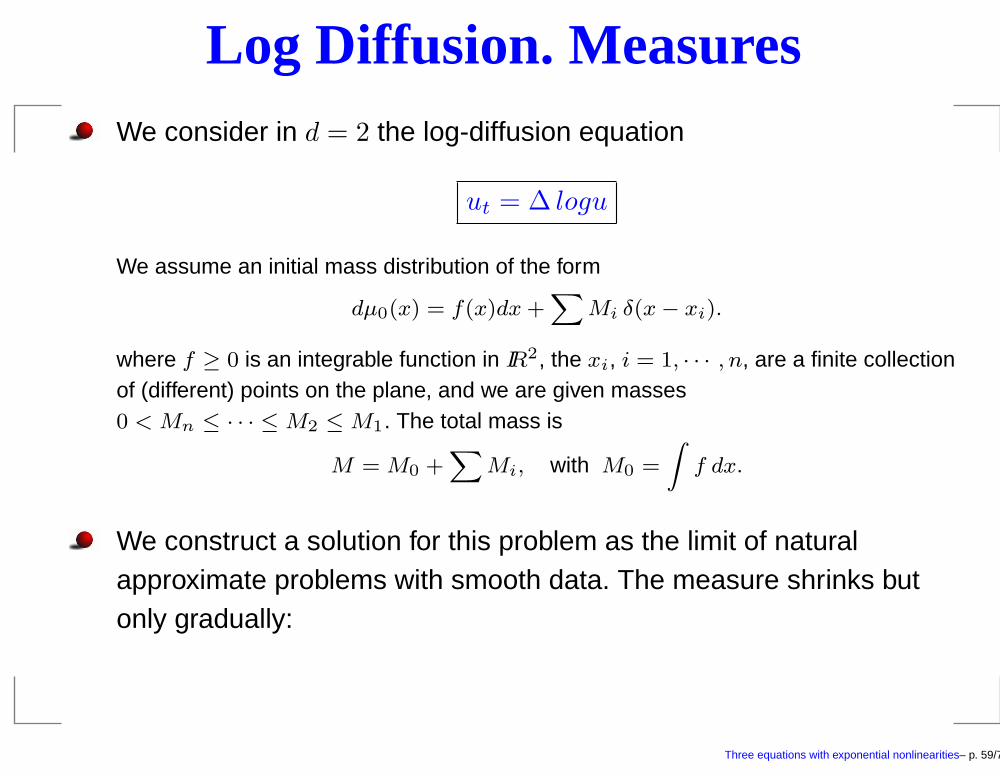
Log Diffusion. MeasuresWe consider in d = 2 the log-diffusion equation
ut = ∆ logu
We assume an initial mass distribution of the form
dµ0(x) = f(x)dx+X
Mi δ(x− xi).
where f ≥ 0 is an integrable function in IR2, the xi, i = 1, · · · , n, are a finite collectionof (different) points on the plane, and we are given masses0 < Mn ≤ · · · ≤M2 ≤M1. The total mass is
M = M0 +X
Mi, with M0 =
Z
f dx.
Three equations with exponential nonlinearities– p. 59/71
Log Diffusion. MeasuresWe consider in d = 2 the log-diffusion equation
ut = ∆ logu
We assume an initial mass distribution of the form
dµ0(x) = f(x)dx+X
Mi δ(x− xi).
where f ≥ 0 is an integrable function in IR2, the xi, i = 1, · · · , n, are a finite collectionof (different) points on the plane, and we are given masses0 < Mn ≤ · · · ≤M2 ≤M1. The total mass is
M = M0 +X
Mi, with M0 =
Z
f dx.
We construct a solution for this problem as the limit of naturalapproximate problems with smooth data. The measure shrinks butonly gradually:
Three equations with exponential nonlinearities– p. 59/71

Three equations with exponential nonlinearities– p. 60/71

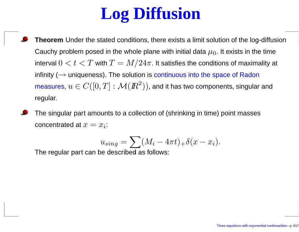
Log DiffusionTheorem Under the stated conditions, there exists a limit solution of the log-diffusion
Cauchy problem posed in the whole plane with initial data µ0. It exists in the time
interval 0 < t < T with T = M/24π. It satisfies the conditions of maximality at
infinity (→ uniqueness). The solution is continuous into the space of Radon
measures, u ∈ C([0, T ] : M(IR2)), and it has two components, singular and
regular.
Three equations with exponential nonlinearities– p. 61/71
Log DiffusionTheorem Under the stated conditions, there exists a limit solution of the log-diffusion
Cauchy problem posed in the whole plane with initial data µ0. It exists in the time
interval 0 < t < T with T = M/24π. It satisfies the conditions of maximality at
infinity (→ uniqueness). The solution is continuous into the space of Radon
measures, u ∈ C([0, T ] : M(IR2)), and it has two components, singular and
regular.
The singular part amounts to a collection of (shrinking in time) point masses
concentrated at x = xi:
using =∑
i
(Mi − 4πt)+δ(x− xi).The regular part can be described as follows:
Three equations with exponential nonlinearities– p. 61/71
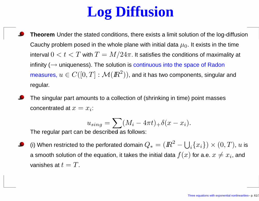
Log DiffusionTheorem Under the stated conditions, there exists a limit solution of the log-diffusion
Cauchy problem posed in the whole plane with initial data µ0. It exists in the time
interval 0 < t < T with T = M/24π. It satisfies the conditions of maximality at
infinity (→ uniqueness). The solution is continuous into the space of Radon
measures, u ∈ C([0, T ] : M(IR2)), and it has two components, singular and
regular.
The singular part amounts to a collection of (shrinking in time) point masses
concentrated at x = xi:
using =∑
i
(Mi − 4πt)+δ(x− xi).The regular part can be described as follows:
(i) When restricted to the perforated domain Q∗ = (IR2 −⋃
ixi) × (0, T ), u is
a smooth solution of the equation, it takes the initial data f(x) for a.e. x 6= xi, and
vanishes at t = T .
Three equations with exponential nonlinearities– p. 61/71

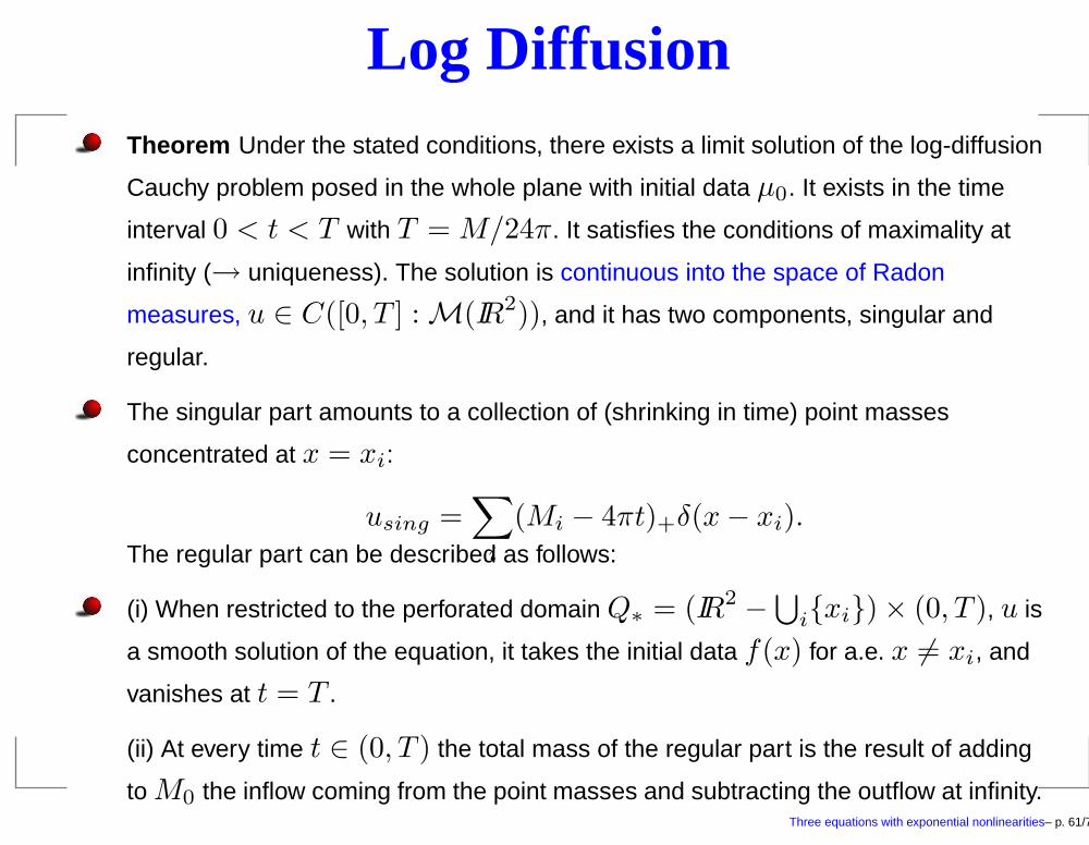
Log DiffusionTheorem Under the stated conditions, there exists a limit solution of the log-diffusion
Cauchy problem posed in the whole plane with initial data µ0. It exists in the time
interval 0 < t < T with T = M/24π. It satisfies the conditions of maximality at
infinity (→ uniqueness). The solution is continuous into the space of Radon
measures, u ∈ C([0, T ] : M(IR2)), and it has two components, singular and
regular.
The singular part amounts to a collection of (shrinking in time) point masses
concentrated at x = xi:
using =∑
i
(Mi − 4πt)+δ(x− xi).The regular part can be described as follows:
(i) When restricted to the perforated domain Q∗ = (IR2 −⋃
ixi) × (0, T ), u is
a smooth solution of the equation, it takes the initial data f(x) for a.e. x 6= xi, and
vanishes at t = T .
(ii) At every time t ∈ (0, T ) the total mass of the regular part is the result of adding
toM0 the inflow coming from the point masses and subtracting the outflow at infinity.Three equations with exponential nonlinearities– p. 61/71

Three equations with exponential nonlinearities– p. 62/71
Log Diffusion(iii) [end of Theorem] Before each point mass disappears, we get a
singular behaviour near the mass location as in the radial case, while later on the
solution is regular around that point.
Three equations with exponential nonlinearities– p. 63/71
Log Diffusion(iii) [end of Theorem] Before each point mass disappears, we get a
singular behaviour near the mass location as in the radial case, while later on the
solution is regular around that point.
Related to singularities in elliptic theory by Brezis, Marcus, Ponceand the author.
ut = ∆Φ(u),un − un−1
h− ∆Φ(un) = 0
Now put f := un−1, u := un, and v = Φ(u), u = β(v):
Three equations with exponential nonlinearities– p. 63/71

Log Diffusion(iii) [end of Theorem] Before each point mass disappears, we get a
singular behaviour near the mass location as in the radial case, while later on the
solution is regular around that point.
Related to singularities in elliptic theory by Brezis, Marcus, Ponceand the author.
ut = ∆Φ(u),un − un−1
h− ∆Φ(un) = 0
Now put f := un−1, u := un, and v = Φ(u), u = β(v):
−h∆Φ(u) + u = f, −h∆v + β(v) = f.
When f is a wrong measure unacceptable by β, then β(v)
accumulates a non-distributed measure component.
Paper: J. L. Vázquez, Evolution of point masses by planarlogarithmic diffusion, Discrete and Continuous Dyn. Systems, toappear in 2007.
Three equations with exponential nonlinearities– p. 63/71

Three equations with exponential nonlinearities– p. 64/71
Log DiffusionThe proof deepends on the local control of the L∞ norm of a solutionaway from the point masses, and for positive times. Such anestimate, L1
loc → L∞
loc is known only in particular cases. The maintechnical result is proving such an estimate here.
Three equations with exponential nonlinearities– p. 65/71
Log DiffusionThe proof deepends on the local control of the L∞ norm of a solutionaway from the point masses, and for positive times. Such anestimate, L1
loc → L∞
loc is known only in particular cases. The maintechnical result is proving such an estimate here.
I use a new tecnhique of symmetrization with respect to a measure,which extends Talenti’s theory. The main idea was developed in apaper with G. Reyes, from Cuba. The paper has appeared inEuropean J. Math., 2006.
The theory of measure-valued solutions of diffusion equations is stillin its beginning.Close questions are: can we solve log-dirffusion with reaction andconvection, with forcing terms, with boundary data, on manifolds?
I did related work for fast diffusion, 1 > m > (n− 2)/n, with E.Chasseigne, a French student of Véron (ARMA, 2003).
Three equations with exponential nonlinearities– p. 65/71

Three equations with exponential nonlinearities– p. 66/71
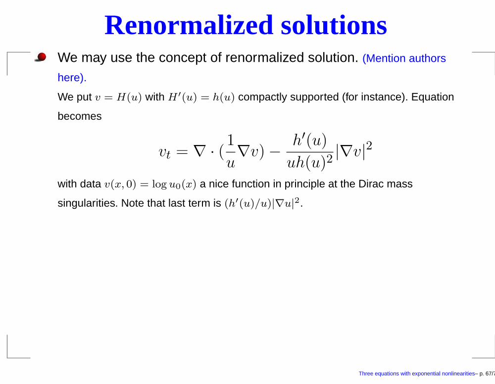
Renormalized solutionsWe may use the concept of renormalized solution. (Mention authors
here).
We put v = H(u) with H′(u) = h(u) compactly supported (for instance). Equation
becomes
vt = ∇ · (1
u∇v) −
h′(u)
uh(u)2|∇v|2
with data v(x, 0) = log u0(x) a nice function in principle at the Dirac mass
singularities. Note that last term is (h′(u)/u)|∇u|2.
Three equations with exponential nonlinearities– p. 67/71
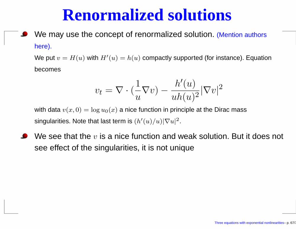
Renormalized solutionsWe may use the concept of renormalized solution. (Mention authors
here).
We put v = H(u) with H′(u) = h(u) compactly supported (for instance). Equation
becomes
vt = ∇ · (1
u∇v) −
h′(u)
uh(u)2|∇v|2
with data v(x, 0) = log u0(x) a nice function in principle at the Dirac mass
singularities. Note that last term is (h′(u)/u)|∇u|2.
We see that the v is a nice function and weak solution. But it does notsee effect of the singularities, it is not unique
Take now v = H(u) = log(u) to get u = ev and
vt = ∆(e−v∇v) + e−v|∇v|2
that we may write as
vt = ∆Φ(v) + |∇Ψ(v)|2
with Φ(v) = C − e−v bounded above, Φ(v) = C − ce−v/2 bounded above .Three equations with exponential nonlinearities– p. 67/71
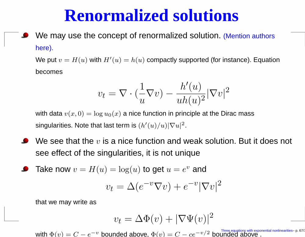

Three equations with exponential nonlinearities– p. 68/71
More open problemsUnderstand the theory of measure-valued solutions, n = 2 or
n ≥ 3. See Book
Three equations with exponential nonlinearities– p. 69/71
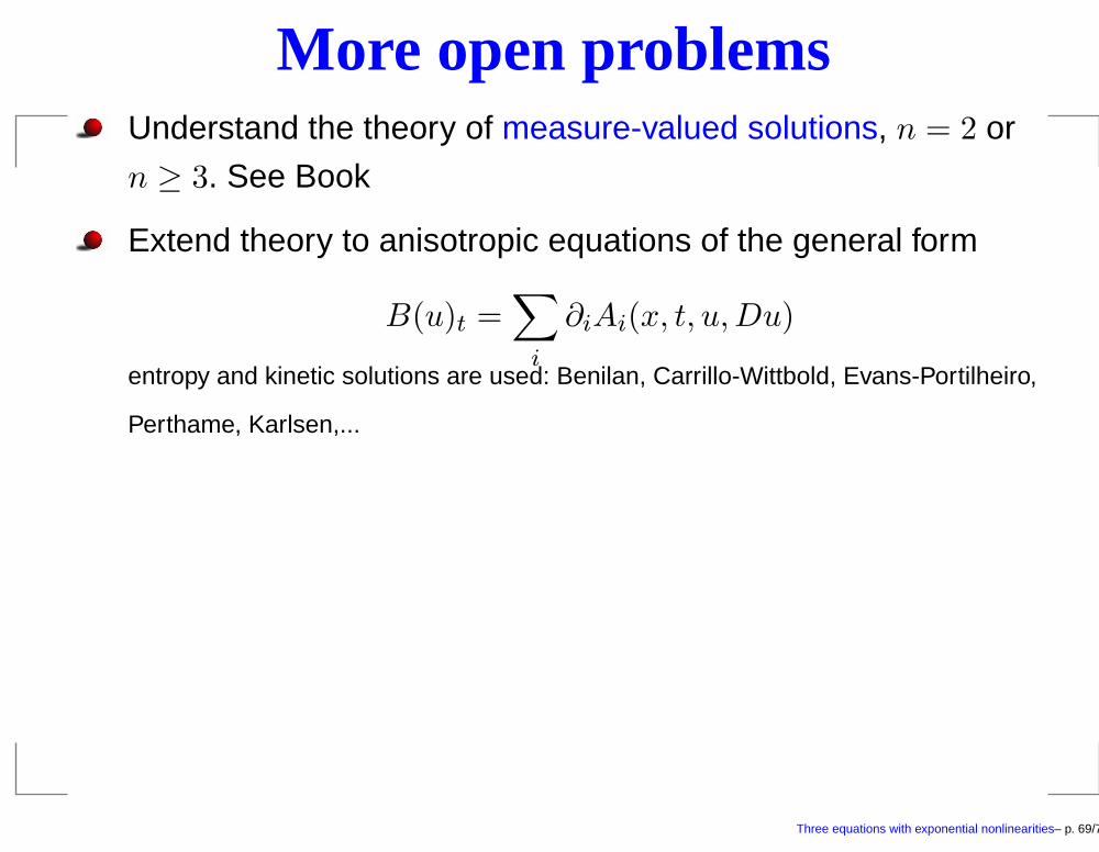
More open problemsUnderstand the theory of measure-valued solutions, n = 2 or
n ≥ 3. See Book
Extend theory to anisotropic equations of the general form
B(u)t =∑
i
∂iAi(x, t, u,Du)
entropy and kinetic solutions are used: Benilan, Carrillo-Wittbold, Evans-Portilheiro,
Perthame, Karlsen,...
Do complete theory for fast diffusion equations, m < 1.
Three equations with exponential nonlinearities– p. 69/71
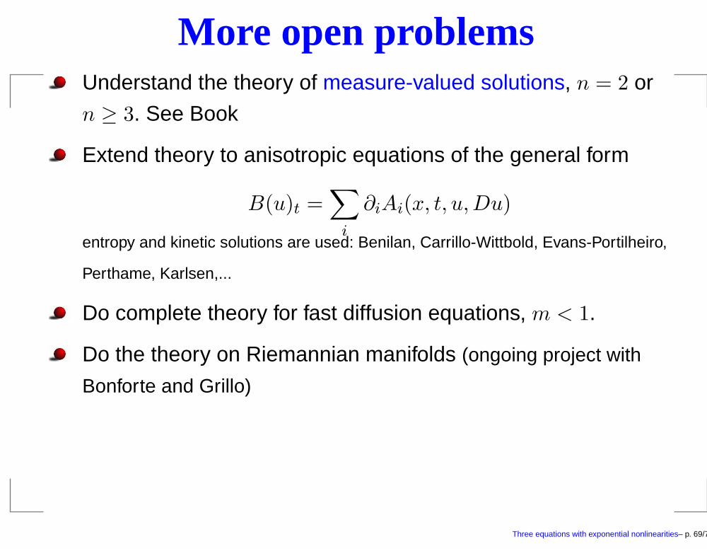
More open problemsUnderstand the theory of measure-valued solutions, n = 2 or
n ≥ 3. See Book
Extend theory to anisotropic equations of the general form
B(u)t =∑
i
∂iAi(x, t, u,Du)
entropy and kinetic solutions are used: Benilan, Carrillo-Wittbold, Evans-Portilheiro,
Perthame, Karlsen,...
Do complete theory for fast diffusion equations, m < 1.
Do the theory on Riemannian manifolds (ongoing project with
Bonforte and Grillo)
Get complete set of decay estimates for asymptotic
convergence to Barenblatt profiles or anomalous profiles.
Three equations with exponential nonlinearities– p. 69/71
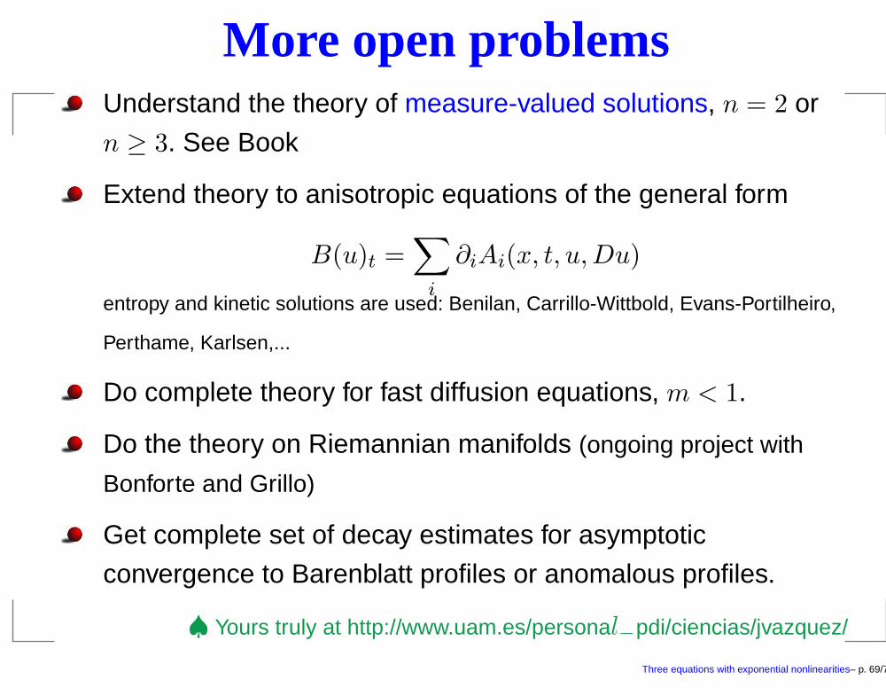
More open problemsUnderstand the theory of measure-valued solutions, n = 2 or
n ≥ 3. See Book
Extend theory to anisotropic equations of the general form
B(u)t =∑
i
∂iAi(x, t, u,Du)
entropy and kinetic solutions are used: Benilan, Carrillo-Wittbold, Evans-Portilheiro,
Perthame, Karlsen,...
Do complete theory for fast diffusion equations, m < 1.
Do the theory on Riemannian manifolds (ongoing project with
Bonforte and Grillo)
Get complete set of decay estimates for asymptotic
convergence to Barenblatt profiles or anomalous profiles.
♠ Yours truly at http://www.uam.es/personal−pdi/ciencias/jvazquez/
Three equations with exponential nonlinearities– p. 69/71

Three equations with exponential nonlinearities– p. 70/71
Finale Maestoso
Felicidades, Ireneo
Three equations with exponential nonlinearities– p. 71/71
Finale Maestoso
Felicidades, Ireneo
Congratulations, sir
Three equations with exponential nonlinearities– p. 71/71
Finale Maestoso
Felicidades, Ireneo
Congratulations, sir
Auguri, signore
Three equations with exponential nonlinearities– p. 71/71
Finale Maestoso
Felicidades, Ireneo
Congratulations, sir
Auguri, signore
Meilleurs voeux, IP
Three equations with exponential nonlinearities– p. 71/71
Finale Maestoso
Felicidades, Ireneo
Congratulations, sir
Auguri, signore
Meilleurs voeux, IP
Parabens, professor
Three equations with exponential nonlinearities– p. 71/71

Finale Maestoso
Felicidades, Ireneo
Congratulations, sir
Auguri, signore
Meilleurs voeux, IP
Parabens, professor
Tahaniya, ya sayidi
Three equations with exponential nonlinearities– p. 71/71
Finale Maestoso
Felicidades, Ireneo
Congratulations, sir
Auguri, signore
Meilleurs voeux, IP
Parabens, professor
Tahaniya, ya sayidi
Three equations with exponential nonlinearities– p. 71/71

Finale Maestoso
Felicidades, Ireneo
Congratulations, sir
Auguri, signore
Meilleurs voeux, IP
Parabens, professor
Tahaniya, ya sayidi
Recommended life planning for Ireneo and friends
60 + STOP FOR CELEBRATIONS+ 60
Three equations with exponential nonlinearities– p. 71/71

Finale Maestoso
Felicidades, Ireneo
Congratulations, sir
Auguri, signore
Meilleurs voeux, IP
Parabens, professor
Tahaniya, ya sayidi
Recommended life planning for Ireneo and friends
60 + STOP FOR CELEBRATIONS+ 60
Three equations with exponential nonlinearities– p. 71/71

Finale Maestoso
Felicidades, Ireneo
Congratulations, sir
Auguri, signore
Meilleurs voeux, IP
Parabens, professor
Tahaniya, ya sayidi
Recommended life planning for Ireneo and friends
60 + STOP FOR CELEBRATIONS+ 60
Three equations with exponential nonlinearities– p. 71/71