Three-dimensional volume analysis of vasculature in ... · Three -d imensional volume analysis of...

Three-dimensional volume analysis of vasculature

in engineered tissues

Mohammed YousefHussien*

a, Kelley Garvin

c, Diane Dalecki

c, Eli Saber

a,b, and María Helguera*

b

aDepartment of Electrical and Microelectronic Engineering, Rochester Institute of Technology,

Rochester, NY 14623 USA; bChester F. Carlson Center for Imaging Science, Rochester Institute of

Technology, Rochester, NY 14623 USA; cBiomedical Engineering Department, University of

Rochester, Rochester, NY 14627 USA

ABSTRACT

Three-dimensional textural and volumetric image analysis holds great potential in understanding the image data

produced by multi-photon microscopy. In this paper, an algorithm that quantitatively analyzes the texture and the

morphology of vasculature in engineered tissues is proposed. The investigated 3D artificial tissues consist of Human

Umbilical Vein Endothelial Cells (HUVEC) embedded in collagen exposed to two regimes of ultrasound standing wave

fields under different pressure conditions. Textural features were evaluated using the normalized Gray-Scale Co-

occurrence Matrix (GLCM) combined with Gray-Level Run Length Matrix (GLRLM) analysis. To minimize error

resulting from any possible volume rotation and to provide a comprehensive textural analysis, an averaged version of

nine GLCM and GLRLM orientations is used. To evaluate volumetric features, an automatic threshold using the gray

level mean value is utilized. Results show that our analysis is able to differentiate among the exposed samples, due to

morphological changes induced by the standing wave fields. Furthermore, we demonstrate that providing more textural

parameters than what is currently being reported in the literature, enhances the quantitative understanding of the

heterogeneity of artificial tissues.

Keywords: Volume quantification, 3D-textural analysis, Multi-photon microscope, Engineered tissues.

1. INTRODUCTION

Tissue engineering is an important multidisciplinary field that combines biology, medicine, and engineering. Its potential

arises from the ability to replace diseased or damaged tissues and organs or even to enhance their function. However, to

successfully create such tissues, an appropriate microenvironment to organize the cells and the proteins into complex

patterns that resemble the natural tissues is needed [1].

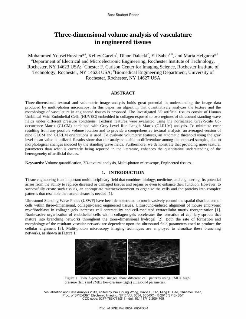
Ultrasound Standing Wave Fields (USWF) have been demonstrated to non-invasively control the spatial distributions of

cells within three-dimensional, collagen-based engineered tissues. Ultrasound-induced alignment of mouse embryonic

myofibroblasts in collagen gels increases cell contractility and cell-mediated extracellular matrix reorganization [1].

Noninvasive organization of endothelial cells within collagen gels accelerates the formation of capillary sprouts that

mature into branching networks throughout the three-dimensional hydrogel [2]. Both the rate of formation and

morphology of the resultant vascular network are dependent upon the ultrasound field parameters used to produce the

cellular alignment [3]. Multi-photon microscopy imaging techniques are employed to visualize these branching

networks, as shown in Figure 1.

Figure 1. Two Z-projected images show different cell patterns using 1MHz high-

pressure (left ) and 2MHz low-pressure (right) ultrasound parameters.

Best Student Paper

Visualization and Data Analysis 2013, edited by Pak Chung Wong, David L. Kao, Ming C. Hao, Chaomei Chen,Proc. of SPIE-IS&T Electronic Imaging, SPIE Vol. 8654, 86540C · © 2013 SPIE-IS&T

CCC code: 0277-786X/13/$18 · doi: 10.1117/12.2004765

Proc. of SPIE Vol. 8654 86540C-1

It was observed that at 1MHz, changing the pressure amplitude from low to high resulted in loosely aggregated cell

bands at low pressure, while dense cell bands were formed at high pressure. Based on these differences in initial cell

band density, we observed that the resulting vascular structure differed. Loosely aggregated cell bands led to the

formation of dense vascular network. On the other hand, densely packed cell bands formed into sprouting networks with

a vascular tree-like morphology. In 2MHz, the USWF pattern differs and the cell bands that are formed are closer

together than those formed at 1 MHz. However, the low and high pressure amplitudes chosen for the 2 MHz exposures

resulted in similar initial cell band density than the 1 MHz pressures used. So the low pressure of 0.08 MPa results in

loosely aggregated cell bands while the high pressure of 0.2 MPa results in densely packed cell bands [2,3].

In this study, we utilize stacks of multi-photon microscopy images to develop three-dimensional textural and volumetric

image analysis techniques to quantitatively characterize the structure of networks formed within various engineered

tissues. To the best of our knowledge, due to the novelty of this technique, there is no preliminary work on quantitative

image analysis of USWF induced vasculature network. We propose to improve previous work developed for other

applications by combining two textural methods encompassing the whole volume. A review of previous work is

discussed in the following paragraphs.

In [4], an algorithm that quantifies biofilm structure by computing textural and areal (volumetric) parameters in two-

dimensional fashion was introduced. In [5], a three-dimensional image analysis of biofilm structures was proposed. As

an improvement over previous work [6,7], the algorithm computed the parameters in three-dimensional fashion. It

evaluated a 256 x 256 normalized gray level co-occurrence matrix (GLCM) in each of the X, Y, and Z directions to

calculate textural parameters. Limiting the analysis to three directions reduces the accuracy of capturing changes that

occur in other directions and makes the results vulnerable to any rotation that might happen to the images [9].

Furthermore, the results reported in this work were single value-type results that describe the whole volume by averaging

the values of the three main orientations, which may not serve as a proper indication of the changes that happened in

each orientation. Other quantization levels that could have shortened computational time were not discussed. Different

volumetric parameters presented in this work were evaluated only in the three main orientations without ensuring volume

connectivity. Their results were validated with digital phantoms, however, in our work we used actual biological samples

as reference.

In [8], the authors demonstrated an algorithm used to extract quantitative structural information about individual collagen

fibers such as length, orientation, and the diameter of the fibers. The algorithm used the medial axis transform and a

tracing technique to connect the fiber branches. By counting the voxels, they determined the length and the diameter of

the fibers. Angles between X and Y and between X and Z were used to determine the orientation of the fibers. No

textural analysis was performed in this work.

In this paper, we present an algorithm that quantifies induced vasculature networks in engineered tissues. Our goal is to

quantitatively differentiate between several pressure and frequency ultrasound field conditions. Our approach provides a

complete three-dimensional quantification that captures the changes in nine different orientations for both textural and

volumetric analysis. We utilize a three-dimensional connected component analysis to extract the volume of interest for

more accurate and comprehensive quantification. A normalized GLCM is estimated from nine orientations to completely

investigate textural information instead of relying only on the three main orientations. Our method combines the GLCM

textural information alongside with GLRLM to provide a comprehensive and detailed overview of the textural

information of the three-dimensional vasculature networks.

The paper is organized as follows. In Section 2, we introduce our experimental data. In Section 3, we discuss the

proposed algorithm in terms of preprocessing and volume quantification. Results are shown and analyzed in Section 4.

Finally, Section 5 draws conclusions and discusses future work.

2. EXPERIMENTAL DATA

Human umbilical vein endothelial cells (HUVEC) were suspended in an unpolymerized type I collagen solution and

were exposed to either a 1 or 2 MHz USWF at various USWF peak positive pressure amplitudes (1 MHz - sham, 0.1

MPa, 0.3 MPa; 2 MHz - sham, 0.08 MPa, 0.2 MPa). Collagen solutions were allowed to polymerize during the 15 min

exposure period to effectively maintain USWF-induced cell alignment after removal of the sound field. Exposure of

HUVEC at the stated pressures resulted in either a homogeneous cell distribution (sham exposure), loosely aggregated

cell bands (0.1 MPa at 1 MHz and 0.08 MPa at 2 MHz), or densely packed cell bands (0.3 MPa at 1 MHz and 0.2 MPa at


2 MHz). Samples were incubated for 10 days post-USWF exposure and then fixed in 4% paraformaldehyde. These

experiments were repeated three times for each condition. Standard immunofluorescence protocols were used to label

HUVEC membranes with an antibody directed against CD31 and cell nuclei were identified by staining with DAPI.

Samples were then examined using multi-photon immunofluorescence microscopy to noninvasively scan through the

three-dimensional volume of the engineered tissue. Images were collected in the Z-direction in 1 µm step size generating

stacks of 300 to 400 images. The spatial dimensions of each voxel are 2.5 x 2.5 x 1 µm3.

3. PROPOSED ALGORITHM

To better understand, compare, and monitor the samples development, a three-dimensional image analysis to quantify the

volume structure is needed. A preprocessing stage is required to enhance the stack of images before any further

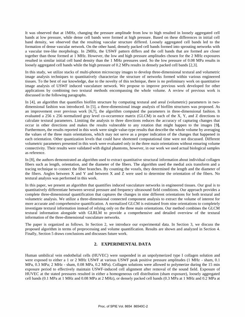
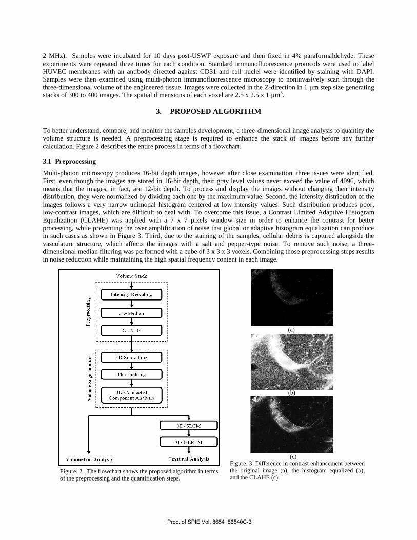
calculation. Figure 2 describes the entire process in terms of a flowchart.

3.1 Preprocessing

Multi-photon microscopy produces 16-bit depth images, however after close examination, three issues were identified.

First, even though the images are stored in 16-bit depth, their gray level values never exceed the value of 4096, which

means that the images, in fact, are 12-bit depth. To process and display the images without changing their intensity

distribution, they were normalized by dividing each one by the maximum value. Second, the intensity distribution of the

images follows a very narrow unimodal histogram centered at low intensity values. Such distribution produces poor,

low-contrast images, which are difficult to deal with. To overcome this issue, a Contrast Limited Adaptive Histogram

Equalization (CLAHE) was applied with a 7 x 7 pixels window size in order to enhance the contrast for better

processing, while preventing the over amplification of noise that global or adaptive histogram equalization can produce

in such cases as shown in Figure 3. Third, due to the staining of the samples, cellular debris is captured alongside the

vasculature structure, which affects the images with a salt and pepper-type noise. To remove such noise, a three-

dimensional median filtering was performed with a cube of 3 x 3 x 3 voxels. Combining those preprocessing steps results

in noise reduction while maintaining the high spatial frequency content in each image.

Figure. 2. The flowchart shows the proposed algorithm in terms

of the preprocessing and the quantification steps.

(b)

Figure. 3. Difference in contrast enhancement between

the original image (a), the histogram equalized (b),

and the CLAHE (c).

(a)

(c)


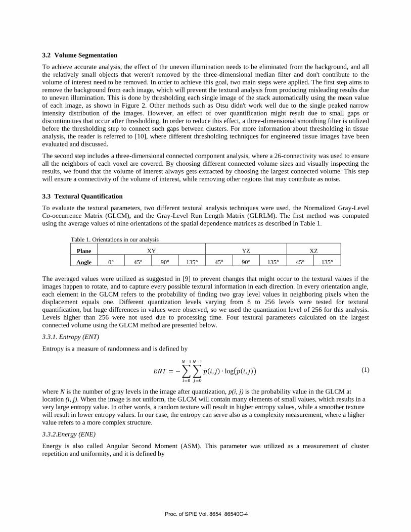
3.2 Volume Segmentation

To achieve accurate analysis, the effect of the uneven illumination needs to be eliminated from the background, and all

the relatively small objects that weren't removed by the three-dimensional median filter and don't contribute to the

volume of interest need to be removed. In order to achieve this goal, two main steps were applied. The first step aims to

remove the background from each image, which will prevent the textural analysis from producing misleading results due

to uneven illumination. This is done by thresholding each single image of the stack automatically using the mean value

of each image, as shown in Figure 2. Other methods such as Otsu didn't work well due to the single peaked narrow

intensity distribution of the images. However, an effect of over quantification might result due to small gaps or

discontinuities that occur after thresholding. In order to reduce this effect, a three-dimensional smoothing filter is utilized

before the thresholding step to connect such gaps between clusters. For more information about thresholding in tissue

analysis, the reader is referred to [10], where different thresholding techniques for engineered tissue images have been

evaluated and discussed.

The second step includes a three-dimensional connected component analysis, where a 26-connectivity was used to ensure

all the neighbors of each voxel are covered. By choosing different connected volume sizes and visually inspecting the

results, we found that the volume of interest always gets extracted by choosing the largest connected volume. This step

will ensure a connectivity of the volume of interest, while removing other regions that may contribute as noise.

3.3 Textural Quantification

To evaluate the textural parameters, two different textural analysis techniques were used, the Normalized Gray-Level

Co-occurrence Matrix (GLCM), and the Gray-Level Run Length Matrix (GLRLM). The first method was computed

using the average values of nine orientations of the spatial dependence matrices as described in Table 1.

Table 1. Orientations in our analysis

Plane XY YZ XZ

Angle 0° 45° 90° 135° 45° 90° 135° 45° 135°

The averaged values were utilized as suggested in [9] to prevent changes that might occur to the textural values if the

images happen to rotate, and to capture every possible textural information in each direction. In every orientation angle,

each element in the GLCM refers to the probability of finding two gray level values in neighboring pixels when the

displacement equals one. Different quantization levels varying from 8 to 256 levels were tested for textural

quantification, but huge differences in values were observed, so we used the quantization level of 256 for this analysis.

Levels higher than 256 were not used due to processing time. Four textural parameters calculated on the largest

connected volume using the GLCM method are presented below.

3.3.1. Entropy (ENT)

Entropy is a measure of randomness and is defined by

∑∑ ( ) ( ( ))

where N is the number of gray levels in the image after quantization, p(i, j) is the probability value in the GLCM at

location (i, j). When the image is not uniform, the GLCM will contain many elements of small values, which results in a

very large entropy value. In other words, a random texture will result in higher entropy values, while a smoother texture

will result in lower entropy values. In our case, the entropy can serve also as a complexity measurement, where a higher

value refers to a more complex structure.

3.3.2.Energy (ENE)

Energy is also called Angular Second Moment (ASM). This parameter was utilized as a measurement of cluster

repetition and uniformity, and it is defined by

(1)


(4)

(5)

∑∑ ( )

For this parameter to reach its maximum value of 1, a few elements in the GLCM should be close to 1, while many

elements should be close to 0. In other words, a higher energy value means more periodic and uniform clusters in the

volume, while the ideal case happens when the volume has a constant intensity level where the energy value equals 1.

3.3.3. Contrast (CON)

Contrast measures the difference between the highest and the lowest intensity values of contiguous pixels and it is

defined by

∑∑ ( ) ( )

where the values range between 0 and (N2). Higher contrast corresponds to busier texture and sharper, more frequent

transitions between the gray levels.

3.3.4. Homogeneity (HOM)

Homogeneity measures the similarity and the smoothness between the intensity values of neighboring pixels. It is

defined by

∑∑ ( )

( )

where higher homogeneity corresponds to smoother and more similar regions in the volume.

The second textural quantification method utilizes the GLRLM to produce five features that describe volumetric textural

information [11,12]. The GLRLM is a matrix with the number of intensity values as its rows, and the run-length values

as the columns. Each entry (i,j) corresponds to the number of times that a certain intensity value i has a run of length j in

a certain orientation. In [12], the authors suggested that the gray-level values to be grouped into 8 sets (levels) for a 64-

levels image, and the run lengths into 6 sets for a 64 by 64 image. We believe the reason behind this is to avoid irrelevant

counting of very small runs and very close values of intensity levels, which may contribute in a negative way to the

analysis. Since our analysis is applied over the largest connected volume with no background intensity variation or

noise, we need every single run length of the volume to be counted. Also, due to having 256 intensity levels, we grouped

the gray-level values into 16 different sets. The advantage of using this method is that it provides textural information

while incorporating some structural information. The following five features are described for further explanation.

3.3.5. Short Run Emphasis (SRE)

This feature measures and emphasizes the short runs in the image, and it is calculated by

∑ ∑ ( )

∑ ∑

( )

where N and M are the row number and the column number of the GLRLM respectively, while p(i,j) is the entry value at

location (i,j). A higher value corresponds to a higher amount of short runs in the image, which indicates that the image

contains a heterogeneous and irregular texture due to a busy structure.

3.3.6. Long Run Emphasis (LRE)

This feature emphasizes the long runs in the image, and it is calculated by

∑ ∑

( )

∑ ∑

( )

(2)

(3)

(6)


where higher values correspond to a higher amount of long runs in the image, which indicates that the image contains a

homogeneous and coarse structural texture.

3.3.7. Gray-Level Non-uniformity (GLN)

The output of this function measures the intensity variation throughout an image, and it is calculated by

∑ (∑ ( )

)

∑ ∑

( )

The lowest value occurs when the runs of the intensity levels are equally distributed throughout the image, higher values

correspond to a fine textural structure.

3.3.8.Run Length Non-uniformity (RLN)

This feature measures the distribution of the runs throughout the lengths in the image, and it is defined by

∑ (∑ ( )

)

∑ ∑

( )

The function has a low value when the image has a single intensity value, since the distribution of the runs is equal

throughout the length.

3.3.9. Run Percentage (RP)

The output of this function is a ratio of the total number of the runs to the total number of pixels K in the image, and it is

calculated by

∑ ∑

( )

where K also known as the total possible runs if the all the intensities have a run length of one.

Combining the two previously mentioned methods, nine different parameters evaluated in nine directions provide us with

a complete picture of how the heterogeneity of samples exposed to different regimes differs among each other.

3.4 Volumetric Quantification

Volumetric parameters were evaluated on the binary version of the images to quantify the morphological information of

the induced vasculature networks. Features such as growth direction and volume percentage are presented in this paper.

3.4.1. Growth Direction

This parameter is computed in order to find in which direction the branching network is growing. To evaluate this

parameter, an average run length algorithm was also utilized in the nine directions mentioned in Table 1. Higher values

result when longer connected regions are examined. For example, if we measure the growth in XY-plane with 0º

between two different objects, the object with the higher value will have a larger connected object in that direction.

3.4.3 Volume Percentage (VP)

This feature measures how much the extracted volume covers from the total size of the sample, and it is calculated by

dividing the number of voxels of the extracted volume of interest over the total number of voxels of the sample. This

analysis gives us an indication of how changes in frequency and pressure regimes will affect the size of the formed

network structures. The actual size of each volume can be found by multiplying the volume of voxels with the spatial

dimension of each voxel mentioned in Section 2.

(7)

(8)

(9)


4. RESULTS

In this paper, we compare different experimental conditions consisting of two different frequency settings and pressure

regimes. We use the sham samples as a reference to compare to. Also, since the experiments are independent, the sham

results from all experiments were averaged. This step was taken after analyzing each sham sample and not finding

noticeable differences among them. Tables 2 and 3 list textural parameters calculated by the GLCM and GLRLM

methods respectively, while Table 4 shows the results calculated for the volumetric analysis.

In Table 2, entropy is highest for the low peak positive pressure cases in both frequency regimes, i.e., 0.1 MPa for 1

MHz, and 0.08 MPa for 2 MHz. These entropy values indicate the disruption of the network appearance compared to the

sham values, which show more complex structure. On the other hand, the entropy value for the high peak positive

pressure cases in both frequency settings is lowest, since the images contain highly packed sprouts with lower structural

complexity. These results are further supported be the fact that energy and homogeneity are lowest, while contrast is

maximum in the low-pressure cases, while the opposite is true for the high-pressure cases.

In Table 3, the high-pressure samples have lower values of short runs and higher long run values compared to the sham

samples. On the other hand, the opposite is true for the low-pressure samples. This indicates that the high-pressure

regime tends to form denser, more uniform, and smoother regions with bands and long sprouts. However, the low

pressure setting wasn't enough to force the cells to form thick bands, but it was enough to form short branches when

comparing to the sham samples. This conclusion is further supported by the difference of the values in the rest of the

features. Other parameters presented in the literature [13,14] which will increase the dimensionality and the complexity

in interpreting the results were not included.

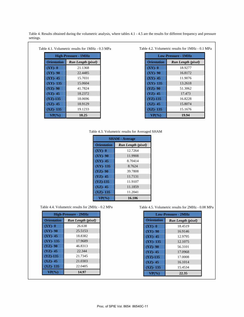
Table 4 shows that the high-pressure cases have higher volumetric run length values than the low-pressure cases

compared to sham samples, except for the Z-direction, due to the morphological structure of the low-pressure setting as

shown in Figure 4 (a). Also, it is worth mentioning that the ratio between the Z-direction run length and the other

directions shows that the high-pressure setting tends to form structures in the center of the plate as shown in Figure 4 (b),

while the low-pressure samples tends to grow vertically compared to sham networks which lay down at the bottom of the

plate as shown in Figure 4 (c).

The absence of USWF on the sham samples result in a lower rate of biological communication between the cells, which

is supported by the fact that they have lower volume percentage (VP) in Table 4. On the other hand, low-pressure

samples have the highest values of VP, since the pressure is enough for the cells to communicate, but not enough to pack

them into thick bands. The values for the high-pressure samples tend to be in-between except for the 2MHz samples,

which we noticed that they were always lower in this case. We relate this observation to the effect of changing the

frequency to a higher setting, which induces the formation of bands more than in the 1MHz samples.

The overall results show that the high-pressure samples have smoother, more uniform, longer, and densely packed

structure, while the low-pressure samples tends to have non-uniform, more heterogeneous, shorter, and unpacked

network structure. Therefore, the quantitative results presented in this work support the qualitative observations made in

[2,3], that different vascular network morphologies are formed when low versus high pressure amplitudes were used to

organize cells within the tissue constructs. The algorithm was written using Matlab environment with a run time varies

between 7 to 12 minutes to finish the analysis of 300 to 400 images.

Figure. 4. The figure shows different projections of cell formation due to the pressure exposure. (a)

shows low-pressure exposure with shorter branches. (b) shows high-pressure exposure which forms

thick bands in the center of the gel, while (c) shows the sham formation with less structure at the

bottom of the gel.

(a) (b) (c)


5. CONCLUSION

In this paper, an algorithm that analyzes three-dimensional vasculature networks in engineered tissues was proposed. The

algorithm used textural and volumetric parameters for quantitative analysis to provide a more objective and reliable

monitoring as well as a quantitative comparison between the structures. We showed that combining two different textural

quantification methods provide a comprehensive overview about the structure's heterogeneity. We also showed that

expanding the analysis to cover nine orientations in quantifying textural and volumetric features, enabled us to capture

full three-dimensional changes happen throughout our samples. Other volumetric parameters such as porosity,

permeability, and diffusion distance were not included, since they don't serve the purpose of comparing totally different

structures. The algorithm is provided with a standalone Graphical User Interface (GUI) written in MATLAB, which will

allow the scientists to interact with the algorithm without the need of understanding the code. The GUI also provides

other functions such as viewing, filtering, or projecting the samples using different techniques. Future work includes

investigating the effect of other three-dimensional volumetric parameters such as 3D-Fractal Dimension (3D-FD), which

is commonly used in medical imaging [15], and 3D-Structural Similarity features in order to provide more structural

information are considered.

ACKNOWLEDGEMENTS

Mohammed YousefHussien would like to thank the American-Mideast Educational and Training Services (AMIDEAST)

and the Institute of International Education (IIE) for funding him through the Fulbright scholarship.

6. REFERENCES

[1] Garvin, K.A., Hocking, D.C., and Dalecki, D., "Controlling the Spatial Organization of Cells and Extracellular

Matrix Proteins in Engineered Tissues Using Ultrasound Standing Wave Fields," Ultrasound in Medicine & Biology,

Elsevier, 1919-1932, (2010).

[2] Garvin, K.A., Dalecki, D., and Hocking, D.C., "Vascularization Of Three-Dimensional Collagen Hydrogels Using

Ultrasound Standing Wave Fields," Ultrasound in Medicine & Biology, Elsevier, 37(11), 1835-1864, (2011).

[3] Garvin, K.A., Dalecki, D., and Hocking, D.C., "Vascular network formation within collagen hydrogels fabricated

with different spatial organizations of endothelial cells using ultrasound-based cell patterning techniques," The North

American Vascular Biology Organization (NAVBO), Hyannis, MA, October (2011).

[4] Yang, X.M., Beyenal, H., Harkin, G., and Lewandowski, Z., "Quantifying Biofilm Structure Using Image Analysis,"

Journal of Microbiological Methods, Elsevier,109-119, (2000).

[5] Beyenal, H., Donovan, C., Lewandowski, Z., and Harkin, G., "Three-dimensional Biofilm Structure Quantification,"

Journal of Microbiological Methods, Elsevier, 395-413, (2004).

[6] Heydron, A., Nielsen, A.T., Hentzer, M., Sternberg, C., Givskov, M., Ersboll, B.K., and Molin, S., "Quantification of

Biofilm Structure by the Novel Computer Program COMSTAT," Journal of Microbiology, 2395-2407, (2000).

[7] Beyenal, H., Lewandowski, Z., and Harkin, G., "Quantifying Biofilm Structure facts and fiction," Biofouling, 1-23,

(2004).

[8] WU, J., Rajwa, B., Filmer, D.L., Hoffmann, C.M., Yuan, B., Chiang, C., Sturgis, J., and Robinson, J.P., "Automated

Quantification and Reconstruction of Collagen Matrix From 3D Confocal Dataset," Journal of Microscopy, 158-165,

(2003).

[9] Haralick, R.M., Shanmuga, K., Dinstein, I., "Textural Features for Image Classification," IEEE Transactions on

Systems, Man and Cybernetics SMC3, 610-621, (1973).

[10] Rajagopalan, S., Yaszemski, M.J., Robb, R., "Evaluation of Thresholding Techniques For Segmenting Scaffold

Images In Tissue Engineering," SPIE Proceedings on Medical Imaging, 1456–1465, (2004).

[11] Sonka, Hlavac, and Boyle, [Digital Image Processing And Computer Vision], Cengage Learning, 571-580 (2008).

[12] Galloway, M.M, "Texture Analysis Using Gray Level Run Lengths", Computer Graphics and Image processing,

Bol. 4, 172-179, (1975).

[13] Tang , X., "Texture information in run-length matrices, "IEEE Transactions on Image Processing, 1602-1609

(1998). [14] Albregtsen, F., Nielsen, B., and Danielsen, H.E., "Adaptive Gray Level Run Length Features from Class Distance

Matrices," Int. Conf. on Pattern Recognition 3, 3746-3749 (2000).

[15] Zhang, L., Liu, J.Z., Dean, D., Sahgal, V., Yue, G.H., "A Three-Dimensional Fractal Analysis Method for

Quantifying White Matter Structure in Human Brain," Journal of Neuroscience Methods, 150(2), 242-253 (2006).


Table 2. Results obtained during the GLCM textural analysis, where tables 2.1 - 2.5 are the results for different frequency and

pressure settings. Please see section 3.3 for abbreviations


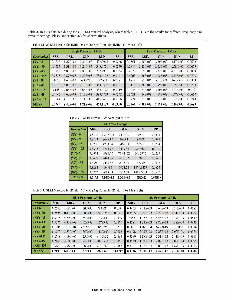
Table 3. Results obtained during the GLRLM textural analysis, where tables 3.1 - 3.3 are the results for different frequency and

pressure settings. Please see section 3.3 for abbreviations


High-Pressure - 1MHz

Orientation Run Length (pixel)

(XY)- 0 21.1368

(XY)- 90 22.4485

(XY)- 45 15.7031

(XY)- 135 15.0604

(YZ)- 90 41.7824

(YZ)- 45 18.2372

(YZ)-135 18.0696

(XZ)- 45 18.9129

(XZ)- 135 19.1233

VP(%) 18.25

Low-Pressure - 1MHz


(XY)- 0 18.9277

(XY)- 90 16.8172

(XY)- 45 11.9076

(XY)- 135 13.2618

(YZ)- 90 51.3062

(YZ)- 45 17.473

(YZ)-135 16.8228

(XZ)- 45 15.8074

(XZ)- 135 15.1676

VP(%) 19.94

SHAM - Average


(XY)- 0 12.7264

(XY)- 90 11.9908

(XY)- 45 8.70414

(XY)- 135 8.7624

(YZ)- 90 39.7808

(YZ)- 45 11.7131

(YZ)-135 11.9107

(XZ)- 45 11.1859

(XZ)- 135 11.2041

VP(%) 16.106

High-Pressure - 2MHz


(XY)- 0 26.638

(XY)- 90 25.5153

(XY)- 45 18.8382

(XY)- 135 17.9689

(YZ)- 90 46.8313

(YZ)- 45 22.344

(YZ)-135 21.7345

(XZ)- 45 21.0303

(XZ)- 135 22.0405

VP(%) 14.97

Low-Pressure - 2MHz


(XY)- 0 18.4519

(XY)- 90 16.9146

(XY)- 45 12.9795

(XY)- 135 12.1075

(YZ)- 90 56.3101

(YZ)- 45 17.0968

(YZ)-135 17.0008

(XZ)- 45 16.1014

(XZ)- 135 15.4534

VP(%) 22.35

Table 4. Results obtained during the volumetric analysis, where tables 4.1 - 4.5 are the results for different frequency and pressure

settings.

Table 4.3. Volumetric results for Averaged SHAM

Table 4.4. Volumetric results for 2MHz - 0.2 MPa Table 4.5. Volumetric results for 2MHz - 0.08 MPa

Table 4.1. Volumetric results for 1MHz - 0.3 MPa Table 4.2. Volumetric results for 1MHz - 0.1 MPa


Three-dimensional volume analysis of vasculature in ... · Three -d imensional volume analysis of...

Documents

Transcript of Three-dimensional volume analysis of vasculature in ... · Three -d imensional volume analysis of...