three-dimensional quantum...

EE 439 three dimensions – 1

The one-dimensional problems we’ve been examining can can carry us a long way — some of these are directly applicable to many nanoelectronics problems — but there are some important problems that are inherently three-dimensional. We need to know how to handle those. Fortunately, the approach is not significantly different from the 1-D approach. Not surprisingly, the math can become more involved.

three-dimensional quantum problems

The extension to 3 dimensions requires a modification of the kinetic energy term, since momentum is, in general, a vector.

S[ � �L� �

�[ �S � �L��

�� =�

�[�D[ +

�

�\�D\ +

�

�]�D]


(For time-independent potentials, the time dependence can be separated out in the 3-D case just as it was in the 1-D case, and the time-dependence will be of the form exp(-iωt).)

With that change, the time-independent Schrödinger equation in 3-D is

� ��P�� ([, \, ]) +8 ([, \, ]) � ([, \, ]) = (� ([, \, ])

�� ([, \, ]) =��

�[� +��

�\� +��

�]�


In 3-D, the free-electron S.E. is

� ��P�� ([, \, ]) = (� ([, \, ])

The simplest solution is still a plane wave, but the form is slightly more complex:

The above solution represents a plane wave traveling in the direction of the wave vector.

The energy still has a familiar form

Exercise: Check that the wave function above is a solution to the 3-D free-electron S.E. with the energy as given. Also, show that the 3-D result reduces to the 1-D if ky = kz = 0.

� (�U) = $ exp�L�N ·�U

� wave vector�N = N[�D[ + N\�D\ + N]�D]

�U = [�D[ + \�D\ + ]�D] position vector

( =��N�

�P N� = N�[ + N�\ + N�]where


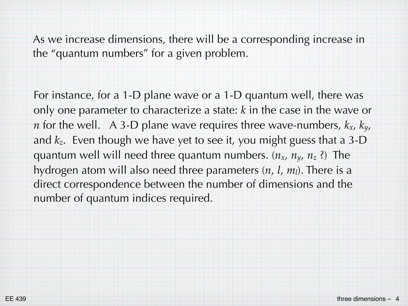
As we increase dimensions, there will be a corresponding increase in the “quantum numbers” for a given problem.

For instance, for a 1-D plane wave or a 1-D quantum well, there was only one parameter to characterize a state: k in the case in the wave or n for the well. A 3-D plane wave requires three wave-numbers, kx, ky, and kz. Even though we have yet to see it, you might guess that a 3-D quantum well will need three quantum numbers. (nx, ny, nz ?) The hydrogen atom will also need three parameters (n, l, ml). There is a direct correspondence between the number of dimensions and the number of quantum indices required.


Solving the 3-D Schroedinger equation looks daunting, but often can be approached using the old separation of variables trick.

If the potential function depends on only one dimension, or can be written as a sum of 3 one-dimensional potentials, then separation of variables will work.

In that case, you would start by writing the full wave-function as the product of three wave-functions, each of which depends on only one variable.

8 ([, \, ]) = 8 ([) + 8 (\) + 8 (])

� ([, \, ]) = �[ ([) �\ (\) �] (])


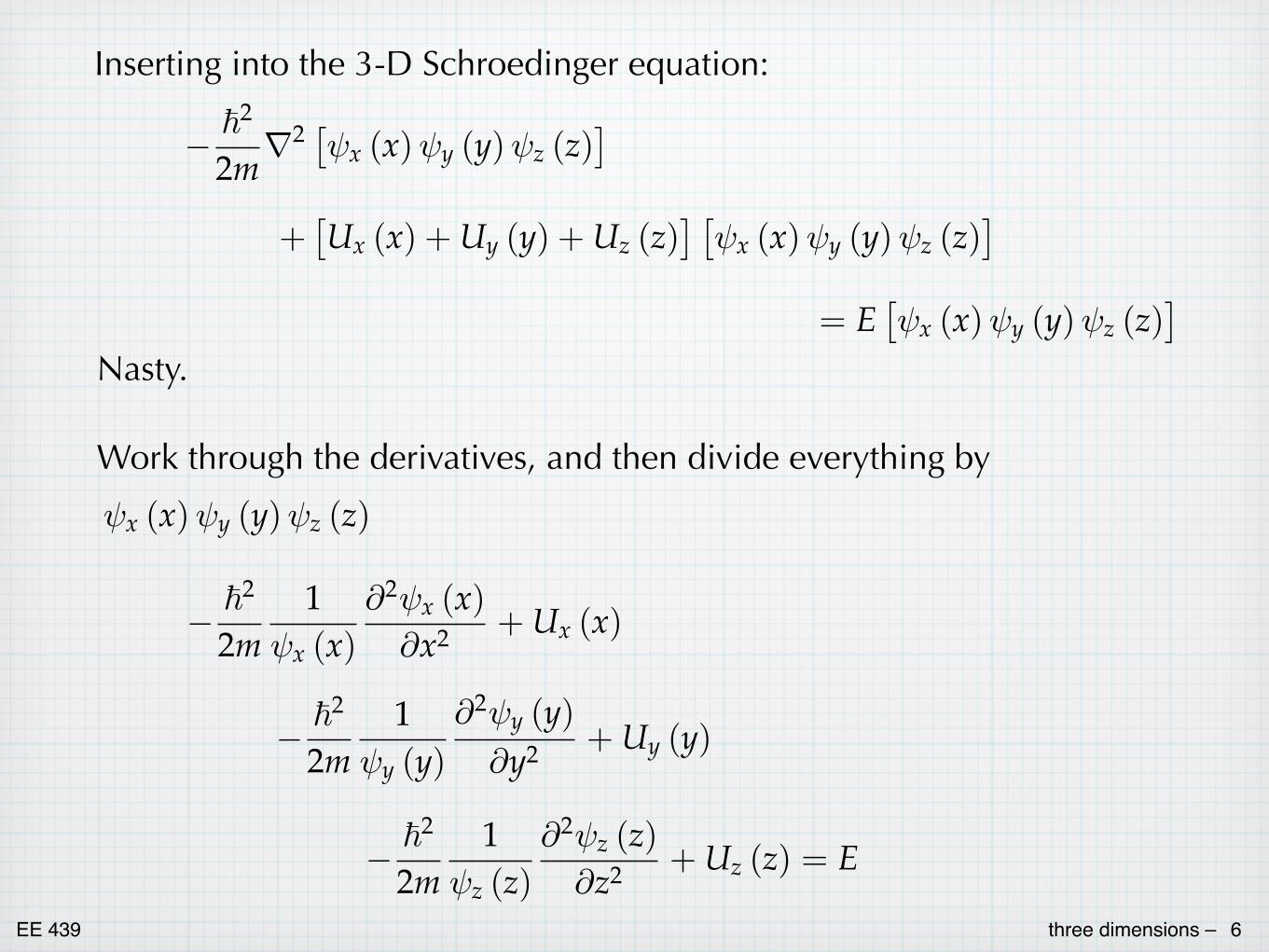
Inserting into the 3-D Schroedinger equation:

Nasty.

Work through the derivatives, and then divide everything by

� ��P��

�[ ([) �\ (\) �] (])�

+�8[ ([) + 8\ (\) + 8] (])

� ��[ ([) �\ (\) �] (])

�

= (��[ ([) �\ (\) �] (])

�

�[ ([) �\ (\) �] (])

� ��P

��[ ([)

��[ ([)�[� +8[ ([)

� ��P

��\ (\)

��\ (\)�\� +8\ (\)

� ��P

��] (])

��] (])�]� +8] (]) = (


The long equation divides into three pieces. Each piece is a function of only one variable. The 3 pieces together sum to a constant.

The only way that this can be true for all values of x, y, z is if each piece is individually equal to a constant.

OK, now we’re getting somewhere. Through separation of variables, we turned one 3-D problem into three 1-D problems. And we know a little bit about solving some 1-D problems.

in x:

and similar for the other dimensions.

I ([) + I (\) + I (]) = (

I ([) = ([ I (\) = (\ I (]) = (] ( = ([ + (\ + (]

� ��P

��[ ([)�[� +8[ ([) �[ ([) = ([�[ ([)


Example: quantum dotAs an example, consider the situation of an electron confined in all three dimensions by infinitely high barriers. The barriers are located at planes defined by x = 0, x = Lx, y = 0, y = Ly, z = 0, and z = Lz. The potential can be viewed as three 1-D barrier problems – one for each dimension – added together.

As we’ve seen, the analysis is made much easier by the fact that we can break this into three identical and well-known 1-D problems.

Using the previously obtained results for the 1-D infinitely deep well.

�[ ([) = $[ sin (N[[) �\ (\) = $\ sin�N\\

��] (]) = $] sin (N]])

N[ =Q[�/[

N\ =Q\�/\

N] =Q]�/]

([ =Q�[��

�P/�[(\ =

Q�\��

�P/�\(] =

Q�]��

�P/�]


Inserting the pieces to form the complete solution:

Each state is characterized by the three quantum numbers, nx, ny, nz. We can denote the different states (nx ny nz)

Note that in some cases, different states will have the same energy. This is known as degeneracy. For example, if the quantum box is a cube (Lx = Ly = Lz), then states with quantum numbers (2 1 1), (1 2 1), and (1 1 2) will all have the same energy and so are degenerate. There are many other degenerate combinations.

( =Q�[��

�P/�[+

Q�\��

�P/�\+

Q�]��

�P/�]

� ([, \, ]) = $ sin (N[[) sin�N\\

�sin (N]])

three-dimensional quantum...

Documents

Transcript of three-dimensional quantum...