Three-Dimensional Modeling of Inelastic Buckling …mceer.buffalo.edu/pdf/report/07-0016.pdf ·...
268
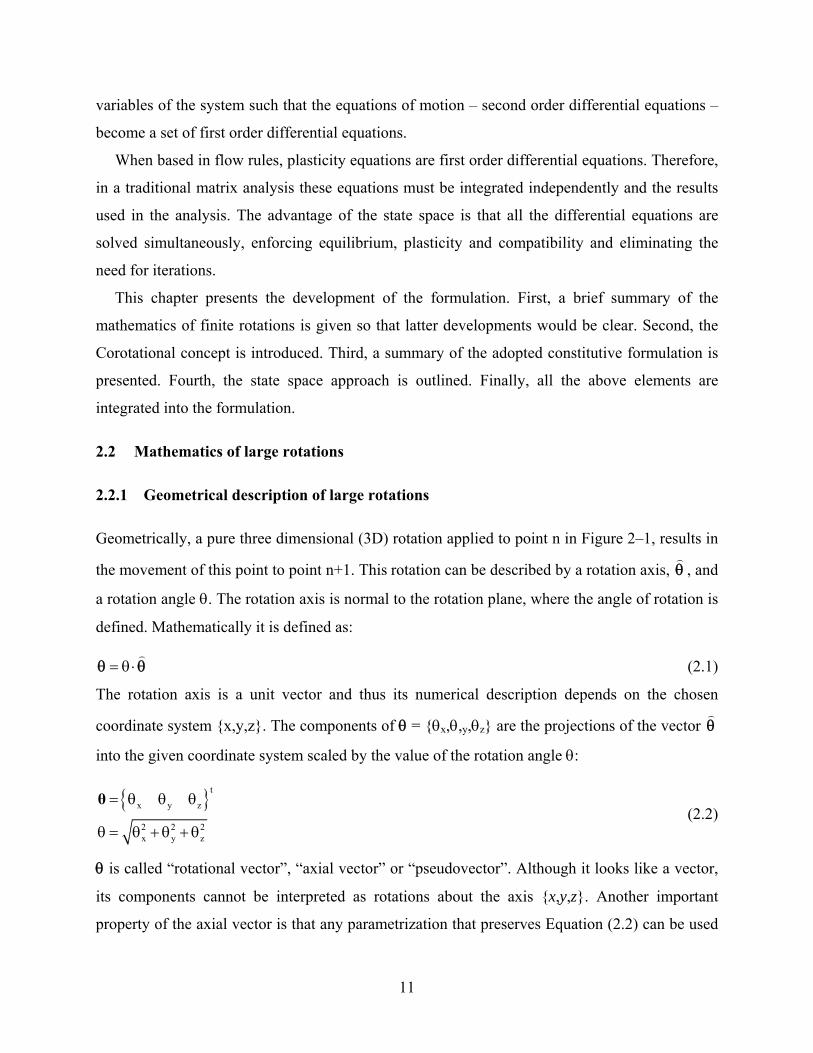
ISSN 1520-295X Three-Dimensional Modeling of Inelastic Buckling in Frame Structures by Macarena Schachter and Andrei M. Reinhorn Technical Report MCEER-07-0016 September 13, 2007 This research was conducted at the University at Buffalo, State University of New York and was supported primarily by the Earthquake Engineering Research Centers Program of the National Science Foundation under award number EEC 9701471 and NSF Award CMS-0324277.
Transcript of Three-Dimensional Modeling of Inelastic Buckling …mceer.buffalo.edu/pdf/report/07-0016.pdf ·...
ISSN 1520-295X
Three-Dimensional Modeling of Inelastic Buckling in Frame Structures
by Macarena Schachter and Andrei M. Reinhorn
Technical Report MCEER-07-0016
September 13, 2007
This research was conducted at the University at Buffalo, State University of New York and was supported primarily by the Earthquake Engineering Research Centers Program of the National Science Foundation under
award number EEC 9701471 and NSF Award CMS-0324277.

NOTICEThis report was prepared by the University at Buffalo, State University of New York as a result of research sponsored by MCEER through a grant from the Earthquake Engineering Research Centers Program of the National Science Foundation under NSF Master Contract Number EEC 9701471 and NSF Award CMS-0324277 and other sponsors. Neither MCEER, associates of MCEER, its sponsors, the University at Buffalo, State University of New York, nor any person acting on their behalf:
a. makes any warranty, express or implied, with respect to the use of any information, apparatus, method, or process disclosed in this report or that such use may not infringe upon privately owned rights; or
b. assumes any liabilities of whatsoever kind with respect to the use of, or the damage resulting from the use of, any information, apparatus, method, or process disclosed in this report.
Any opinions, findings, and conclusions or recommendations expressed in this publication are those of the author(s) and do not necessarily reflect the views of MCEER, the National Science Foundation, or other sponsors.
Three-Dimensional Modeling of Inelastic Buckling in Frame Structures
by
Macarena Schachter1 and Andrei Reinhorn2
Publication Date: September 13, 2007 Submittal Date: August 17, 2007
Technical Report MCEER-07-0016
Task Number 9.2.4
NSF Master Contract Number EEC 9701471and NSF Award CMS-0324277
1 Ph.D. Candidate, Department of Civil, Structural and Environmental Engineering, University at Buffalo, State University of New York
2 Clifford C. Furnas Professor, Department of Civil, Structural and Environmental Engineering, University at Buffalo, State University of New York
MCEERUniversity at Buffalo, The State University of New YorkRed Jacket Quadrangle, Buffalo, NY 14261Phone: (716) 645-3391; Fax (716) 645-3399E-mail: [email protected]; WWW Site: http://mceer.buffalo.edu

iii
Preface
The Multidisciplinary Center for Earthquake Engineering Research (MCEER) is a national center of excellence in advanced technology applications that is dedicated to the reduction of earthquake losses nationwide. Headquartered at the University at Buffalo, State University of New York, the Center was originally established by the National Science Foundation in 1986, as the National Center for Earthquake Engineering Research (NCEER).
Comprising a consortium of researchers from numerous disciplines and institutions throughout the United States, the Center’s mission is to reduce earthquake losses through research and the application of advanced technologies that improve engineering, pre-earthquake planning and post-earthquake recovery strategies. Toward this end, the Cen-ter coordinates a nationwide program of multidisciplinary team research, education and outreach activities.
MCEER’s research is conducted under the sponsorship of two major federal agencies: the National Science Foundation (NSF) and the Federal Highway Administration (FHWA), and the State of New York. Significant support is derived from the Federal Emergency Management Agency (FEMA), other state governments, academic institutions, foreign governments and private industry.
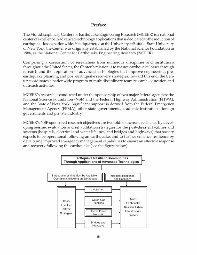
MCEER’s NSF-sponsored research objectives are twofold: to increase resilience by devel-oping seismic evaluation and rehabilitation strategies for the post-disaster facilities and systems (hospitals, electrical and water lifelines, and bridges and highways) that society expects to be operational following an earthquake; and to further enhance resilience by developing improved emergency management capabilities to ensure an effective response and recovery following the earthquake (see the figure below).
-
Infrastructures that Must be Available /Operational following an Earthquake
Intelligent Responseand Recovery
Hospitals
Water, GasPipelines
Electric PowerNetwork
Bridges andHighways
MoreEarthquake
Resilient UrbanInfrastructureSystem
Cost-EffectiveRetrofitStrategies
Earthquake Resilient CommunitiesThrough Applications of Advanced Technologies
iv
A cross-program activity focuses on the establishment of an effective experimental and analytical network to facilitate the exchange of information between researchers located in various institutions across the country. These are complemented by, and integrated with, other MCEER activities in education, outreach, technology transfer, and industry partnerships.
The main purpose of this research is to develop a formulation for three-dimensional frame structures with geometric and material nonlinearities subjected to static and dynamic loads. The first objec-tive is to develop a corotational formulation capable of macro-modeling geometric nonlinearities that considers the plasticity of the cross sections, which facilitates understanding failures due to inelastic buckling. The second objective is to perform an experimental study, using a shake table as the base excitation, for a model where inelastic buckling is expected. The test results provide data for verification of the new formulation and computational model. The frame chosen is the “zipper frame,” which is a chevron braced frame where columns link the midpoints of the beams at the brace connections. The third objective is to test the new formulation against data obtained through testing. By comparing the predictions of the new analytical model with the data obtained from the “zipper frame” experiment, the capability of the formulation to predict inelastic buckling is verified.
v
ABSTRACT
Inelastic buckling is the most important failure mode of a steel beam column element subjected
to compression force. In order to correctly predict this phenomenon, large rotations, large
displacements and the plasticity of the section along the element must be considered.
Several formulations have been proposed to model problems with three dimensional large
displacements and rigid body dynamics. They are usually based in the Lagrangian or the
Corotational methods and are primarily oriented to solve mechanical and aerospace problems,
although some applications to structural stability do exist. Independently, several formulations
have been developed to model plasticity: fiber elements, plastic flow theory and lumped
plasticity are popular choices.
In this report, a novel formulation capable of solving problems with displacement and
material nonlinearities in a unified way is developed. Thus, the State Space approach is selected
because all the basic equations of structures: equilibrium, compatibility and plasticity are solved
simultaneously and thus the global and local states are mutually and explicitly dependent. To
incorporate geometric nonlinearities, the Corotational approach, where rigid body motion and
deformations are described separately, is adopted. To incorporate material nonlinearities, the
formulation developed by Simeonov (1999) and Sivaselvan (2003) is included.
In general, the set of equilibrium, compatibility and plasticity equations constitute a
system of Differential Algebraic Equations (DAE). A procedure to solve such system exists and
is implemented in the package IDA (Implicit Differential Algebraic solver) developed at the
Lawrence Livermore National Laboratory (LLNL), which is used to solve the problem
numerically.
An experimental study on “zipper frames” was conducted to assess the accuracy of the
proposed formulation. A “zipper frame” is a chevron braced frame where the beam to brace
connections are linked through columns, called “zipper columns”. The failure mode of a “zipper
frame” is the successive inelastic buckling of its braces. Three shake table tests of a three stories
“zipper frame” were performed at the UB-NEES laboratory.
A model of the first story of the “zipper frame” was analyzed with the new formulation
and its results compared to experimental data. It is found that the new formulation can reproduce
the features of the test and it is very sensitive to all the model parameters. Results are presented.


vii
ACKNOWLEDGMENTS
This research was conducted by the University at Buffalo and was supported by National Science
Foundation award CMS-0324277. Their support is gratefully acknowledged. All opinions and
remarks are those of the author and do not reflect any opinion of the supporting agency.

ix
TABLE OF CONTENTS
SECTION TITLE PAGE
1 Introduction ..............................................................................................................1
1.1 Objectives ..........................................................................................................1
1.2 Motivation ..........................................................................................................2
1.2.1 Small displacements vs large displacements ............................................2
1.2.2 The problem of large rotations ..................................................................2
1.2.3 Buckling – instability analysis ..................................................................3
1.2.4 Stiffness and flexibility base elements ......................................................6
1.2.5 The plasticity problem ..............................................................................7
1.3 Outline of the report ...........................................................................................8
2 Formulation of a 3D element model for geometric and material nonlinearities ......9
2.1 Introduction ........................................................................................................9
2.2 athematics of large rotations ...........................................................................11
2.2.1 Geometrical description of large rotations ..............................................11
2.2.2 Mathematical description of large rotations ...........................................13
2.2.3 Parametrization of rotations: quaternions ...............................................13
2.2.4 Compound rotations ................................................................................14
2.2.5 Derivatives of the Rotation matrix ..........................................................15
2.2.6 Incremental rotation vector: the update problem ....................................16
2.2.7 Calculation of a rotational vector given an initial vector and its final
configuration ..............................................................................................17
2.3 The corotational concept ..................................................................................18
2.4 Constitutive model ...........................................................................................19
2.4.1 Derivation of the plasticity model ...........................................................19
2.4.2 Elastic stiffness matrix ............................................................................23
2.4.3 Initial elastic stiffness matrix ..................................................................23
2.4.4 Ultimate yield function ...........................................................................24
x
TABLE OF CONTENTS (CONTINUED)
SECTION TITLE PAGE
2.4.5 Yielding criterion parameter ...................................................................25
2.4.6 Unloading criterion .................................................................................25
2.5 The state space approach. ................................................................................27
2.5.1 State variables .........................................................................................27
2.5.2 Evolution equations ................................................................................28
2.6 Development of an element for large displacements and large rotations ........29
2.6.1 Objective .................................................................................................29
2.6.2 Coordinate systems .................................................................................29
2.6.3 Degrees of freedom .................................................................................30
2.6.4 Calculation of rigid body transformation matrices .................................32
2.6.5 Equilibrium Equations ............................................................................33
2.6.6 Compatibility equations ..........................................................................35
2.6.7 Relationship between matrix B* and forces ............................................41
2.6.8 Compatibility equations as functions of state space variables ................43
2.6.9 Plasticity Equations. ................................................................................43
2.7 Summary of the formulation ............................................................................44
3 Numerical implementation of the formulation ......................................................47
3.1 Introduction. .....................................................................................................47
3.2 Solution of DAE equations ..............................................................................47
3.3 Numerical Integration of the formulation ........................................................50
3.4 Brief description of “element.exe” ..................................................................61
4 Experimental study on “zipper frames” .................................................................63
4.1 Introduction ......................................................................................................63
4.2 Description of “zipper frames” ........................................................................63
4.3 Definition of model ..........................................................................................66
4.4 Test setup .........................................................................................................70
xi
TABLE OF CONTENTS (CONTINUED)
SECTION TITLE PAGE
4.5 Test #1 ..............................................................................................................72
4.5.1 Description of frame details in test #1 ....................................................72
4.5.2 Instrumentation .......................................................................................73
4.5.3 Test Protocol ...........................................................................................74
4.5.4 Test results ..............................................................................................74
4.5.4.1 Test observations and data processing ....................................... 74
4.5.4.2 Issues identified in test #1 .......................................................... 76
4.5.5 Lessons and recommendations from test #1 ...........................................77
4.6 Test #2 ..............................................................................................................78
4.6.1 Description of frame details in Test #2 ...................................................78
4.6.2 Instrumentation .......................................................................................79
4.6.3 Test protocol ...........................................................................................79
4.6.4 Test results ..............................................................................................79
4.6.4.1 Test observations and data processing ....................................... 79
4.6.4.2 Low cycle fatigue analysis of frame in test #2. ......................... 83
4.6.5 Lessons and recommendations from test #2 ...........................................85
4.7 Test #3 ..............................................................................................................85
4.7.1 Description of frame details ....................................................................85
4.7.2 Instrumentation .......................................................................................85
4.7.3 Test portocol ...........................................................................................86
4.7.4 Test results ..............................................................................................86
4.7.4.1 Test observations and data processing ....................................... 86
4.7.4.2 Low cycle fatigue analysis ......................................................... 88
4.7.5 Remarks on test #3 ..................................................................................89
4.8 Remarks and conclusions from the experimental study ..................................89
5 Analytical evaluation of the proposed formulation ...............................................91
xii
TABLE OF CONTENTS (CONTINUED)
SECTION TITLE PAGE
5.1 Introduction ......................................................................................................91
5.2 Analytical model ..............................................................................................91
5.3 Analytical Results of test #2 ............................................................................93
5.4 Bounding analysis ............................................................................................97
5.4.1 Connections: variation of the inertia of the connection elements ...........97
5.4.2 Gusset plates: variation of the yield strength of the material ................104
5.4.3 Connections: variation of the length of the element .............................112
5.4.4 Zipper column: variation of the equivalent stiffness ............................119
5.4.5 Lateral restraint .....................................................................................126
5.5 Comparison of analytical models with mixed parameters with test data for
Test #2 ............................................................................................................127
5.6 Conclusions ....................................................................................................134
6 Remarks, conclusions and recommendations ......................................................137
6.1 Summary ........................................................................................................137
6.2 Conclusions ....................................................................................................138
7 References. ...........................................................................................................141
APPENDIX A Details on the deduction of compatibility equations ...........................................147
A.1 Deduction of equation 2.65 ...........................................................................147
A.2 Derivation of Equation 2.68 ..........................................................................148
A.3 Compatibility equations in terms of material curvatures ..............................149
A.4 Derivation of Matrix B ..................................................................................150
A.5 Force transformation from corotated to deformed coordinates ....................153
APPENDIX B ..............................................................................................................................155
B.1 Input file user’s manual .................................................................................155
B.1.1 Introduction ..........................................................................................155
xiii
TABLE OF CONTENTS (CONTINUED)
SECTION TITLE PAGE
B.1.2 General considerations .........................................................................155
B.1.3 Input file format ...................................................................................156
B.2 Example of input file .....................................................................................161
APPENDIX C Design of the “zipper frame” ...............................................................................173
C.1 Suspended “zipper frame” design methodology ...........................................173
C.2 Design of the 3 story prototype .....................................................................174
C.3 Design check of the 1/3 scaled “zipper frame” model ..................................176
APPENDIX D ..............................................................................................................................179
APPENDIX E . ............................................................................................................................189
APPENDIX F ..............................................................................................................................197
APPENDIX G Verification of the formulation with standarized case study: Lateral buckling of
a cantiliver right angle frame under end load ......................................................213

xv
LIST OF FIGURES
FIGURE TITLE PAGE
2–1 Geometrical representation of rotations. ..................................................................... 12
2–2 Mathematical representation of rotation updates. ....................................................... 17
2–3 Corotational concept. .................................................................................................. 19
2–4 Parallel plasticity model (From Simeonov (1999) Figure 2-2 b) ................................ 20
2–5 Ultimate-Yield Surface: a) General View, b) Slice in Plane ymp −
(From Simeonov (1999) Figure 2-4) ........................................................................... 26
2–6 Definition of Global (G), Local (L) and Corotated (E) coordinate systems. .............. 30
2–7 Definition of DOFs in global and local coordinates (a)
and in corotated coordinates (b). ................................................................................. 31
2–8 Description of the deformations in Corotated coordinates. ........................................ 35
2–9 Diagrams to calculate the interpolation of forces in Local deformed coordinates.
Left: interpolation of forces in Corotated coordinates, Right: transformation
to Local deformed coordinates. ................................................................................... 43
4–1 Plastic mechanism of “zipper frame” (left) and “suspended zipper frame” (right). ... 65
4–2 Instantaneous flow of forces in the “zipper frame”. ................................................... 65
4–3 Elevation and plan view of the 3 stories SAC building. ............................................. 66
4–4 Scaled model, dimension (in) and members. .............................................................. 69
4–5 “Zipper frame” alone (left) and with gravity frame (right) ......................................... 70
4–6 Gravity column layout (left) and connection details (right). ...................................... 71
4–7 Detail of beam to brace gusset plate. Designed (a), Constructed (b). ......................... 72
4–8 Restraint implemented in Test #2 for lateral movement. ............................................ 78
4–9 Damage in 1st floor braces after Test #2, “120% LA22yy”. Local buckling and
cracking in West brace (left) and fracture in East brace (right, see circle). ................ 81
4–10 Picture of the rotation of the 1st floor beam after Test #2, “120% LA22yy”. ............. 81
4–11 Picture of the rotation of the 1st story brace to beam gusset plate after
Test #2, “120% LA22yy”. .......................................................................................... 82
xvi
LIST OF FIGURES (CONTINUED)
FIGURE TITLE PAGE
4–12 Picture of the out of plane bending in the 2nd story “zipper column” after Test #2,
“120% LA22yy”. ........................................................................................................ 82
4–13 Picture of the 1st floor West column (left) and East column (right) after Test #2,
“120% LA22yy”. ........................................................................................................ 83
4–14 Picture of the frame’s permanent deformation after Test #3, “160% LA22yy”. ........ 87
4–15 Picture of the beam’s rotation (left) and the brace to beam gusset plate deformation
(right) after Test #3, “160% LA22yy”. ....................................................................... 88
4–16 Picture of the West brace (left) and East brace (right) after Test #3,
“160% LA22yy”. ........................................................................................................ 88
5–1 Schematic of model (black line) and node location (red dots). .................................. 92
5–2 In plane (x) vs. out of plane (z) displacement at top (node 8), middle (node 5) and
bottom (node 2) from Test #2 “80% LA22yy”. .......................................................... 94
5–3 Hysteresis loops of west brace (left) and east brace (right) from Test #2, “80%
LA22yy”. Limits for actual yielding force Py = 50.4 kip and Euler buckling force
PE = -31.77 kip included. ............................................................................................ 95
5–4 Vertical displacements of nodes 8 (top), 5 (middle) and 2 (bottom) for Test #2,
“80% LA22yy”. .......................................................................................................... 96
5–5 Comparison of the in plane (x) vs. out of plane (z) displacement at top (node 8),
middle (node 5) and bottom (node 2) of the WEST brace. Flexible gusset plate
(left), nominal (center), rigid gusset plate (right). ...................................................... 98
5–6 Comparison of the in plane (x) vs. out of plane (z) displacement at top (node 8),
middle (node 5) and bottom (node 2) of the EAST brace. Flexible gusset plate
(left), nominal (center), rigid gusset plate (right). ...................................................... 99
5–7 Comparison of the hysteresis loops of the WEST brace where the axial displacements
considers the gusset plate (top) and does not consider the gusset plate (bottom)
Flexible gusset plate (left), nominal value (center), rigid gusset plate (right) .......... 100
xvii
LIST OF FIGURES (CONTINUED)
FIGURE TITLE PAGE
5–8 Comparison of the hysteresis loops of the EAST brace where the axial displacements
considers the gusset plate (top) and does not consider the gusset plate (bottom).
Flexible gusset plate (left), nominal value (center), rigid gusset plate (right). ......... 101
5–9 Comparison of the vertical displacements at the top ( node 8), middle (node 5) and
bottom (node 2) of the WEST brace. Flexible gusset plate (left), nominal value
(center), rigid gusset plate (right) .............................................................................. 102
5–10 Comparison of the vertical displacements at the top ( node 8), middle (node 5) and
bottom (node 2) of the EAST brace. Flexible gusset plate (left), nominal value
(center), rigid gusset plate (right) .............................................................................. 103
5–11 Comparison of the vertical displacements of the top node (9). Flexible gusset plate
(left), nominal value (center), rigid gusset plate (right) ............................................ 104
5–12 Comparison of the in plane (x) vs. out of plane (z) displacement at top (node 8),
middle (node 5) and bottom (node 2) of the WEST brace. σψ = 36 kip/in2 (left),
σψ = 60 kip/in2 (center), σψ = 100 kip/in2 (right). ..................................................... 105
5–13 Comparison of the in plane (x) vs. out of plane (z) displacement at top (node 8),
middle (node 5) and bottom (node 2) of the EAST brace. σψ = 36 kip/in2 (left),
σψ = 60 kip/in2 (center), σψ = 100 kip/in2 (right). ..................................................... 106
5–14 Comparison of the hysteresis loops of the WEST brace where the axial displacements
considers the gusset plate (top) and does not consider the gusset plate (bottom).
σψ = 36 kip/in2 (left), σψ = 60 kip/in2 (center), σψ = 100 kip/in2 (right). ................. 107
5–15 Comparison of the hysteresis loops of the EAST brace where the axial displacements
considers the gusset plate (top) and does not consider the gusset plate (bottom).
σψ = 36 kip/in2 (left), σψ = 60 kip/in2 (center), σψ = 100 kip/in2 (right). ................. 108
5–16 Comparison of the vertical displacements at the top ( node 8), middle (node 5) and
bottom (node 2) of the WEST brace. σψ = 36 kip/in2 (left), σψ = 60 kip/in2 (center),
σψ = 100 kip/in2 (right). ............................................................................................ 109
xviii
LIST OF FIGURES (CONTINUED)
FIGURE TITLE PAGE
5–17 Comparison of the vertical displacements at the top ( node 8), middle (node 5) and
bottom (node 2) of the EAST brace. σψ = 36 kip/in2 (left), σψ = 60 kip/in2 (center),
σψ = 100 kip/in2 (right). ............................................................................................ 110
5–18 Comparison of the vertical displacements of the top node (9). σψ = 36 kip/in2 (left),
σψ = 60 kip/in2 (center), σψ = 100 kip/in2 (right). ..................................................... 111
5–19 Sketch of gusset plate lengths. .................................................................................. 112
5–20 Comparison of the in plane (x) vs. out of plane (z) displacement at top (node 8),
middle (node 5) and bottom (node 2) of the WEST brace. Small connection element
(left), nominal (center), Large connection element (right). ...................................... 113
5–21 Comparison of the in plane (x) vs. out of plane (z) displacement at top (node 8),
middle (node 5) and bottom (node 2) of the EAST brace. Small connection element
(left), nominal (center), Large connection element (right). ...................................... 114
5–22 Comparison of the hysteresis loops of the WEST brace where the axial displacements
considers the gusset plate (top) and does not consider the gusset plate (bottom). Small
connection element (left), nominal (center), Large connection element (right). ...... 115
5–23 Comparison of the hysteresis loops of the EAST brace where the axial displacements
considers the gusset plate (top) and does not consider the gusset plate (bottom). Small
connection element (left), nominal (center), Large connection element (right). ...... 116
5–24 Comparison of the vertical displacements at the top ( node 8), middle (node 5) and
bottom (node 2) of the WEST brace. Small connection element (left), nominal
(center), Large connection element (right). .............................................................. 117
5–25 Comparison of the vertical displacements at the top ( node 8), middle (node 5) and
bottom (node 2) of the EAST brace. Small connection element (left), nominal
(center), Large connection element (right). .............................................................. 118
5–26 Comparison of the vertical displacements of the top node (9). Small connection
element (left), nominal (center), Large connection element (right). ......................... 119
xix
LIST OF FIGURES (CONTINUED)
FIGURE TITLE PAGE
5–27 Comparison of the in plane (x) vs. out of plane (z) displacement at top (node 8),
middle (node 5) and bottom (node 2) of the WEST brace. Flexible spring (left),
nominal (center), rigid spring (right). ....................................................................... 120
5–28 Comparison of the in plane (x) vs. out of plane (z) displacement at top (node 8),
middle (node 5) and bottom (node 2) of the EAST brace. Flexible spring (left),
nominal (center), rigid spring (right). ....................................................................... 121
5–29 Comparison of the hysteresis loops of the WEST brace where the axial displacements
considers the gusset plate (top) and does not consider the gusset plate (bottom).
Flexible column (left), nominal stiffness (center), rigid column (right). .................. 122
5–30 Comparison of the hysteresis loops of the EAST brace where the axial displacements
considers the gusset plate (top) and does not consider the gusset plate (bottom).
Flexible column (left), nominal stiffness (center), rigid column (right). .................. 123
5–31 Comparison of the vertical displacements at the top ( node 8), middle (node 5) and
bottom (node 2) of the WEST brace Flexible column (left), nominal stiffness
(center), rigid column (right). .................................................................................. 124
5–32 Comparison of the vertical displacements at the top ( node 8), middle (node 5) and
bottom (node 2) of the EAST brace Flexible column (left), nominal stiffness
(center), rigid column (right). ................................................................................... 125
5–33 Comparison of the vertical displacements of the top node (9). Flexible column
(left), nominal stiffness (center), rigid column (right). ............................................. 126
5–34 Comparison of the hysteresis loops of the EAST brace where the axial displacements
considers the gusset plate (top) and does not consider the gusset plate (bottom). No
out of plane restraint (left), rigid restraint (center), infinitely rigid restraint (right) . 126
5–35 Comparison of the hysteresis loops of the WEST brace where the axial displacements
considers the gusset plate (top) and does not consider the gusset plate (bottom). No
out of plane restraint (left), rigid restraint (center), infinitely rigid restraint (right). 127
5–36 Comparison of in plane and out of plane displacement at the middle node (5) of
WEST brace. ............................................................................................................. 130
xx
LIST OF FIGURES (CONTINUED)
FIGURE TITLE PAGE
Figure 5–37: Comparison of in plane and out of plane at the middle node (5) of EAST brace. 131
Figure 5–38: Comparison of hysteresis loops of WEST brace. .................................................. 132
Figure 5–39: Comparison of hysteresis loops of EAST brace (right). ....................................... 133
Figure 5–40: In plane (x) vs. out of plane (z) displacement at middle (node 5) of the
West brace (left) and EAST brace (right). Elastic material for all elements. ........... 135
Figure C–1: Flow chart of the design procedure of a “zipper” braced frame.
(From Yang, 2006 Figure 6.3) .................................................................................. 174
D–1 General view of the model and connection details. .................................................. 179
D–2 Detail 1. ..................................................................................................................... 180
D–3 Detail 2. ..................................................................................................................... 180
D–4 Detail 3. ..................................................................................................................... 181
D–5 Detail 4. ..................................................................................................................... 182
D–6 Detail 5. ..................................................................................................................... 183
D–7 Detail 6. ..................................................................................................................... 184
D–8 Detail 7. ..................................................................................................................... 184
D–9 Detail connection to base plate. ................................................................................ 185
D–10 Front view setup. ....................................................................................................... 185
D–11 Detail of beam to column and gravity frame to zipper frame connection. ............... 186
D–12 Lateral view setup. .................................................................................................... 187
D–13 Detail typ. From lateral view of test setup. ............................................................... 188
E–1 Location of strain gauges. ......................................................................................... 189
E–2 Location f accelerometers and string potentiometers. .............................................. 190
E–3 Location of LED sensors for Krypton camera. ......................................................... 191
F–1: Location of Temposonics and String potentiometers. .............................................. 197
F–2 Location of strain gauges in braces and zipper columns. ......................................... 198
F–3 Location of strain gauges in beams. .......................................................................... 199
F–4 Location of strain gauges in columns. ...................................................................... 200
F–5 Location of LED sensors for Krypton camera. ......................................................... 201
xxi
LIST OF FIGURES (CONTINUED)
FIGURE TITLE PAGE
G–1 Data of the problem. ................................................................................................. 213
G–2 Load displacement diagram. ..................................................................................... 214
G–3 Solutions to the problem by (a) Argyris (1979) and Simo et al. (1986). .................. 215

xxiii
LIST OF TABLES
TABLE TITLE PAGE
2-1 Selection of element state variables at the integration points
(From Simeonov, (1999) Table 4-1) .............................................................................. 28
4–1 Summary of components for prototype ......................................................................... 66
4–2 Scale factors for linear dimensions ................................................................................ 67
4–3 Scale factors for weight per floor. .................................................................................. 67
4–4 List of scale factors of “zipper frame” model. ............................................................... 68
4–5 Summary of components of the model .......................................................................... 69
4–6 Low cycle fatigue analysis for Test #2. ......................................................................... 84
4–7 Low cycle fatigue analysis for Test #3. ......................................................................... 89
5–1 Material properties per coupon testing. ......................................................................... 93
C–1 Demands on the structural members in the strength design phase.
(From Yang, 2006 Table 6.5) ...................................................................................... 175
C–2 Summary of the member sizes for the three stories “zipper” braced frame.
(From Yang, 2006 Table 6.6) ..................................................................................... 176
C–3 Properties of the selected sections of the 1/3 scale model. (From AISC 2005). .......... 177
C–4 Verification of section compactness of the 1/3 scale model (From AISC Seismic
Provisions Table I-8-1). ............................................................................................... 178
C–5 Verification of slenderness for brace members of the 1/3 scale model
(From AISC Seismic Provisions section 13.4a). ......................................................... 178
E–1 List of all instruments, their location and calibration. ................................................. 192
F–1 List of all instruments, their location and calibration. ................................................. 202

1
SECTION 1
INTRODUCTION
1.1 Objectives
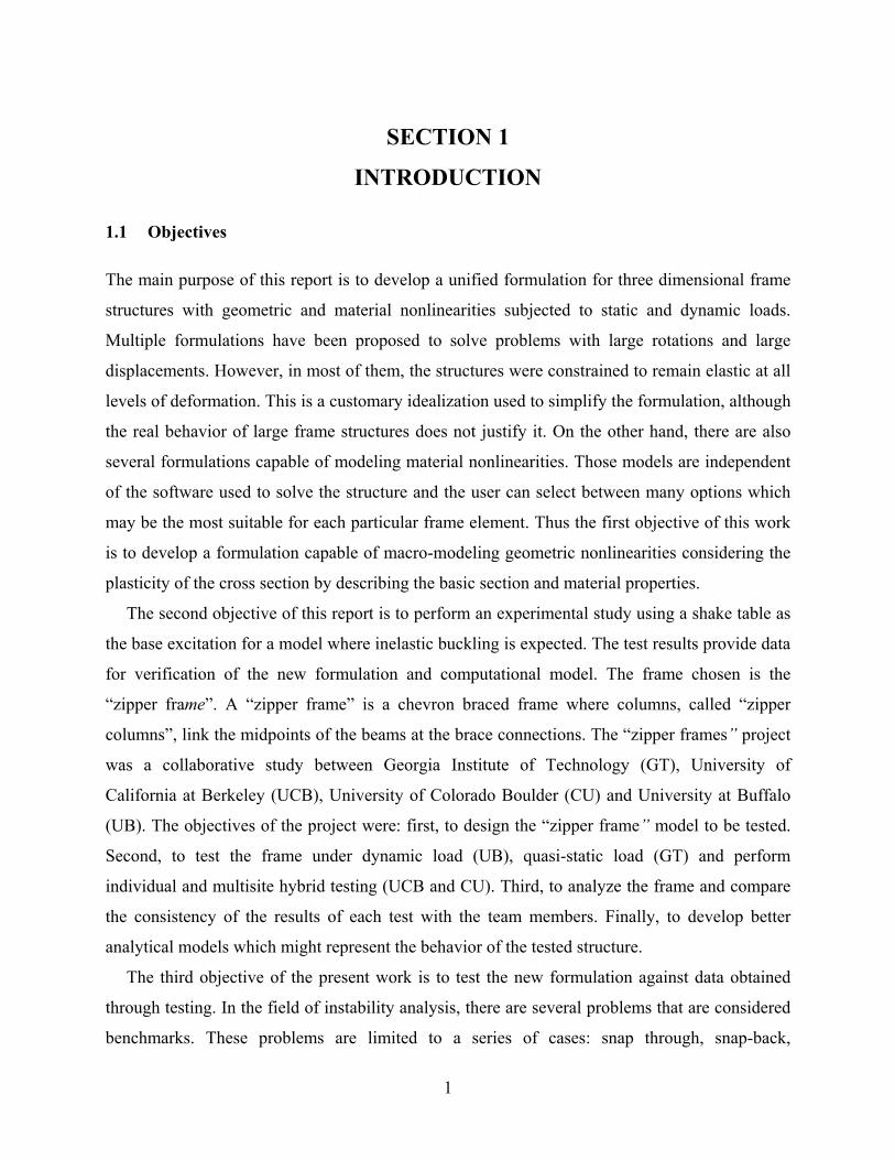
The main purpose of this report is to develop a unified formulation for three dimensional frame
structures with geometric and material nonlinearities subjected to static and dynamic loads.
Multiple formulations have been proposed to solve problems with large rotations and large
displacements. However, in most of them, the structures were constrained to remain elastic at all
levels of deformation. This is a customary idealization used to simplify the formulation, although
the real behavior of large frame structures does not justify it. On the other hand, there are also
several formulations capable of modeling material nonlinearities. Those models are independent
of the software used to solve the structure and the user can select between many options which
may be the most suitable for each particular frame element. Thus the first objective of this work
is to develop a formulation capable of macro-modeling geometric nonlinearities considering the
plasticity of the cross section by describing the basic section and material properties.
The second objective of this report is to perform an experimental study using a shake table as
the base excitation for a model where inelastic buckling is expected. The test results provide data
for verification of the new formulation and computational model. The frame chosen is the
“zipper frame”. A “zipper frame” is a chevron braced frame where columns, called “zipper
columns”, link the midpoints of the beams at the brace connections. The “zipper frames” project
was a collaborative study between Georgia Institute of Technology (GT), University of
California at Berkeley (UCB), University of Colorado Boulder (CU) and University at Buffalo
(UB). The objectives of the project were: first, to design the “zipper frame” model to be tested.
Second, to test the frame under dynamic load (UB), quasi-static load (GT) and perform
individual and multisite hybrid testing (UCB and CU). Third, to analyze the frame and compare
the consistency of the results of each test with the team members. Finally, to develop better
analytical models which might represent the behavior of the tested structure.
The third objective of the present work is to test the new formulation against data obtained
through testing. In the field of instability analysis, there are several problems that are considered
benchmarks. These problems are limited to a series of cases: snap through, snap-back,
2
bifurcation and others. Most of them consist of simple structures with elastic material and have
closed form solutions. The advantage of these solutions are that results from different
methodologies are comparable and errors can be detected. However, the most practical case of
inelastic buckling is not considered. By comparing the predictions of the new analytical model
with the data obtained from the “zipper frame” experiment, the capability of the formulation to
predict inelastic buckling is tested herein.
1.2 Motivation
1.2.1 Small displacements vs large displacements
In matrix analysis of structures with small strains/small deformations there are two main
coordinate systems: “Global”, which is common for all the members in the structure and
“Local”, which is defined in respect to the chord of the member; i.e. the straight line that
connects the two end nodes of an element in its deformed configuration. The hypothesis of small
displacements translates into the assumption that at every step the chord of the member coincides
with its initial position. Thus, the deformations are calculated with respect to the initial
configuration and the matrices that transform from global to local coordinates are constant
throughout the analysis .
When large displacements are considered, the “Local” coordinates coincide with the chord of
the member in its actual position while the “Global” coordinates remain constant. Thus, the
transformation matrices are not constant, but vary with time. The global stiffness matrix,
calculated as the variation of the force given a variation in displacement, is not only sensitive to
the actual nodal displacements but also to the variations of the reference frame. The former is the
elastic stiffness matrix, while the later is the geometric stiffness matrix.
1.2.2 The problem of large rotations
When the analysis in three dimensions (3D) assumes that the rotations are small or infinitesimal,
rotations are treated as vectors, and vectorial mathematics can be used to describe them.
However, large or finite rotations are manifolds and should be described with Lie algebra
(Marsden 1994). Essentially, a rotation has a magnitude (the rotation angle) and a direction or
3
rotation axis (a vector describing the normal to the plane where the rotation takes place). Finite
rotations are not commutative (unless the rotation axis is fixed as in two dimensions (2D)).
There are three ways of describing rotations mathematically:
• Quaternion: The rotation value and its axis in a vector of 4 elements.
• Rotation matrix: a 3x3 orthogonal matrix.
• Pseudovector (Euler angles): the projection of the rotation into a Cartesian coordinate
system.
All these representations are equivalent and the relationships between them are detailed in
Chapter 2. The pseudovector representation is not unique but can be scaled by different factors.
These are called parametrizations of the Euler angles (Crisfield 1991; Felippa and Haugen 2005).
1.2.3 Buckling – instability analysis
There are two main approaches to the problem of instability: The plastic hinge method and the
finite element method.
In the plastic hinge method, the traditional stiffness matrix method is enhanced to
automatically consider second order analysis (the effect of the geometry in the stiffness of the
member) by using stability functions. These functions were first introduced by von Mises and
Ratzersdorfer in 1926 (Bazant and Cedolin 1991). Derived from the differential equations of a
fixed-hinged beam subjected to axial load, these functions are factors that reduce the bending
stiffness of a member due to the presence of axial load. Although popular because of their
simplicity, the description of instability is usually constrained to 2D and to the ideal cases the
differential equations can solve (Chen 2000). Material nonlinearities are added mostly through
plastic hinges or plastic zones. Other options, such as out of plane buckling and local buckling
have also been incorporated (Kim and Lee 2001; Kim and Lee 2002; Kim et al. 2003; Trahair
and Chan 2003; Wongkaew and Chen 2002).
This option is not discussed further since the assumptions made to derive the stability
functions are very rigid. Even though modeling of buckling and instability is the purpose of the
method, no consideration of large displacements is made. Rotations are always treated as
infinitesimal and calculated as the first derivative of the transverse displacements, even though
this is not true in any buckled member. Finally, the method is not general enough to predict local
4
buckling because it just checks the equations provided in the AISC manual (AISC 2003), which
are only mean values of data obtained empirically.
Within the finite element method, there are two main approaches: Lagrangian and
Corotational. The Lagrangian method describes a beam as a continuous element. Each cross
section is completely defined by a position vector and a rotation matrix, which are written with
respect to a Global coordinate system. Axial strain and curvatures are written in terms of these
variables. There are different ways to proceed with the calculations: the strains can be linearized
first to find an admissible variation and then the virtual work principle is applied to find the
equations of motion (Simo and Vu-Quoc 1986); or the virtual work principle is applied first and
the resulting equations are linearized (Cardona and Geradin 1988). In a different approach, the
kinematic equations are solved using a procedure similar to Lagrangian multipliers for all the
unknown variables, resulting in a weak formulation of the equilibrium equations, which are
afterwards discretized and linearized (Jelenic and Saje 1995).
In all the cases described above, the element cannot be integrated as a continuum, so it is
discretized. Since the stiffness matrix is required, displacements and rotations of the internal
nodes are approximated with interpolation functions.
The mathematical details in the above procedures depend on the chosen rotations
parametrization: quaternions (Simo and Vu-Quoc 1985; Simo and Vu-Quoc 1986) and
incremental pseudovectors (Cardona and Geradin 1988; Ibrahimbegovic 1997) are the most
popular choices. The formulation was developed further by proposing strain invariant and path
independent interpolation functions for the rotations (Jelenic and Crisfield 1999). Curvature
interpolation has also been used in an approximated formulation (Schulz and Filippou 2001).
Also, the kinematic equations of the beam, have been extended to include arbitrary cross sections
(Gruttmann et al. 1998) and curved beam elements (Ibrahimbegovic 1995).
The Corotational method works with two coordinate systems: a Global system common for all
members and a Local system for each member. The Local system is defined for every element
and is updated every time step. The method is called Corotational approach because it moves and
rotates following the chord of the member. Translational and rotational deformations are written
with respect to the corotated system, therefore the total movement of a node can be described as
the superposition of a rigid body motion (represented by the movement of the chord of the
5
element and calculated with respect to the Global system) and a deformation (calculated with
respect to the chord).
It is generally assumed that large displacements and rotations are described within the rigid
body motion and that the remaining deformations are small, thus at the corotated level the
hypothesis of small displacements holds and the usual stiffness matrix method can be used to
calculate the local tangent stiffness matrix of the element. However, since the local stiffness
matrix is written with respect to a moving frame, the stiffness matrix of the element in Global
coordinates must consider the variations of the frame with time. (Crisfield 1990; Felippa and
Haugen 2005; Rankin and Nour-Omid 1988). This method has been extended to incorporate
plasticity by considering the von Mises yield criterion (Battini and Pacoste 2002b; Izzuddin and
D.L.Smith 1996; Pi and Trahair 1994; Pi et al. 2001b), and to incorporate second and higher
order terms in the Green strains definition in order to capture flexural-torsional buckling and
warping distortion (Battini and Pacoste 2002a; Hsiao et al. 1999; Pi and Bradford 2001). Also a
combination of Corotational and Lagrangian Methods has been proposed (Hsiao and Lin 2000).
In summary, since the kinematic description of the element in the Lagrangian Method is
mathematically exact, these formulations can handle problems for very large rotations and
displacements as well as for very large strains (plasticity included). In contrast, formulations
based in the Corotational Method assume that the small deformations/small strains theory holds
at the corotated level. On the other hand, while the Corotational concept is simple and the
method can be easily incorporated into existing structural analysis software, the Lagrangian
Methods are mathematically involved and are not compatible with existing software. It has been
proven by various authors (Cardona and Geradin 1988; Crisfield 1990; Felippa and Haugen
2005; Simo and Vu-Quoc 1986) that both methods are successful in solving problems of stability
of structures, although their scope covers mostly the areas of aerospace engineering and
multibody dynamics.
Focusing on a formulation for structural instability, the Corotational Method can be a suitable
choice. The physical meaning of the Corotated frame makes it easy for engineers to understand
the concept behind the mathematics. The objective of the present work is to enhance the
Corotational Method to handle problems of large strains, with both geometric and material
nonlinearities.
6
1.2.4 Stiffness and flexibility base elements
In a formulation using the Corotational Method, stiffness and flexibility based elements can be
used. Stiffness based elements calculate the stiffness matrix of the element by approximating the
deformation field with interpolation functions. Typically, cubic polynomials are used to describe
transverse deformations and linear functions describe axial deformations. This description is
valid only for small displacement analysis, where rotations are calculated as derivatives of the
transverse displacements. In large displacement analyses this corresponds to a first order
approximation and it leads to compatibility inconsistencies (Pi et al. 2001a; Teh and Clarke
1997; Teh and Clarke 1998). Section forces are obtained through the constitutive law. Then,
from the integration of the equilibrium equations (principle of virtual displacements) the global
stiffness matrix is calculated. Finally, the global forces are assembled and compared to the
external forces. In a nonlinear analysis, equilibrium is not satisfied and iterations must be
performed.
In contrast, flexibility based elements approximate the force field. In the case where element
forces are not present, bending moments vary linearly and axial force and torsion are constant,
the interpolation is exact. The section deformations are then obtained through the constitutive
law. By applying the principle of virtual forces, compatibility equations are obtained and after
integrating them, the global flexibility matrix is found. Finally, global compatibility is not
satisfied and iterations at the element level are needed. The formulation is attractive because
equilibrium is always satisfied and there is no need to approximate the displacement field, even
though the numerical implementation is not as simple as with stiffness based elements.
It’s been proven that flexibility based elements have better performance than stiffness based
elements in linear problems solved with matrix methods (Neuenhofer and Filippou 1997;
Spacone et al. 1996) and in the state space (Simeonov 1999); in nonlinear problems of 2D
structures solved with matrix methods (Bäcklund 1976; Neuenhofer and Filippou 1998) and in
the state space (Sivaselvan 2003). It has also been implemented in the program IDARC2D (Park
et al. 1987; Valles et al. 1996), where the flexibility matrix for inelastic elements with small
deformations is determined and then integrated to the global system using its inverse.
The present formulation will combine the Corotational formulation, including mathematics of
large rotations to create a flexibility based element capable of solving 3D nonlinear problems.
7
1.2.5 The plasticity problem
Most of the formulations assume that the material is elastic. They are aimed to model not only
structural problems but also flying planes and mechanical systems where it is undesirable that the
material becomes plastic. Therefore, most of the benchmark problems found in the literature are
elastic, thus plasticity is not needed in the formulations. On the other hand, many of the
instability problems in civil engineering structures involve the plastification of the cross section,
thus it becomes a necessary feature. Plastic flow theories are one choice to model plasticity. A
yield surface is defined along with loading, yielding and unloading rules. The result is a
relationship between the rate of strains and the rate of stresses. Thus, the rate equations must first
be integrated to obtain a relationship between strains and stresses (Crisfield 1991; Lubliner
1990).
It is evident that the traditional stiffness and flexibility matrix methods as well as any of the
above formulations need a strain-stress relationship but it is of no consequence to the formulation
itself how this matrix is calculated. Plasticity is a choice. Thus, none of the above procedures is a
unified approach in the sense that plasticity analysis is treated separately from equilibrium and
compatibility analyses.
Methods based in finite elements, fiber models for instance, solve the problem at a global and
a local level. The global level enforces compatibility and equilibrium while the local level deals
with plasticity. This is possible since the cross section is divided into small sectors where
average strains and stresses are being continuously monitored. The section forces are then
obtained by integrating the stresses of all sectors (Hall and Challa 1995; Izzuddin and D.L.Smith
1996; Zienkiewicz and Taylor 2005). Thus, finite element analysis is a unified approach.
However, the computational costs and time required to solve a complex problem are very high.
Methods based in the state space also solve the problem at a global and a local level. At the
global level the equations of motion become first order differential equations and at the local
level, if plastic flow theories are used, the constitutive laws are also first order differential
equations. The complete system is then solved. As a result, global and local states are mutually
dependent and convergence occurs simultaneously eliminating the need for iterations within a
time step (Simeonov 1999; Sivaselvan 2003). However, if static analysis is being performed,
equations at the global level are algebraic, not differential. Therefore a robust procedure capable
of solving Differential Algebraic Equations (DAEs) is needed. Fortunately, such a procedure
8
exists (Brenan et al. 1989) and it is implemented in a computer software called “Implicit
Differential-Algebraic solver” (IDA) developed at the Lawrence Livermore National Laboratory
(Hindmarsh and Serban 2006).
It is concluded that, for the objectives of this report, the state space approach is the most
suitable option for the development of a unified formulation.
1.3 Outline of the report
Flexibility based element have been combined with the state space approach to create a
formulation for inelastic structures and small displacements (Simeonov 1999). The Corotational
approach mixed with flexibility based elements was used by Sivaselvan (Sivaselvan 2003), to
solve two dimensional (2D) inelastic buckling problems using the state space. However, as
explained in 1.2.2, large rotations in 2D are not different from small rotations since the rotation
axis is fixed. Thus, the challenge is to develop a formulation that mixes the Corotational
approach with a flexibility based element capable of 3D large inelastic displacements and
rotations, to be solved in the state space and to be tested against the results of the “zipper frame”
experiments.
The organization of the work is as follows: in Chapter 2 the mathematical development of the
formulation is explained. Chapter 3 details the numerical implementation of the formulation
derived in Chapter 2. Chapter 4 presents the experimental study and the relevant test results from
the shake table tests of the “zipper frame”. Chapter 5 compares the experimental results with the
analytical results obtained with the new formulation. Finally a summary of the work, conclusions
and recommendations are detailed in Chapter 6.
9
SECTION 2
FORMULATION OF A 3D ELEMENT MODEL FOR GEOMETRIC
AND MATERIAL NONLINEARITIES
2.1 Introduction
The formulation presented in this Chapter is developed for frame structures whose components
are modeled as single elements, also known as macro-models. An “element” can represent a
beam, column, brace or any other structural member where one of its dimensions (length) is
much larger than the other two (cross section). The boundaries of the elements are represented by
“nodes” which also represent connection points between different structural members. The
movement of the member is described solely by the movement of its end nodes and its
centerline. The element’s plasticity is incorporated by monitoring some of the cross sections
along the length of the element, also known as “control sections”. The behavior of the end nodes
is influenced by the integrated behavior of all the control sections.
The objective of the developed formulation is to predict the behavior of an element that
undergoes inelastic buckling i.e. the correct estimation of the buckling load, post buckling
displacement and residual displacements.
Although many procedures capable of analyzing elements subjected to large displacements
and large rotations have been developed (Bäcklund 1976; Battini and Pacoste 2002a; Battini and
Pacoste 2002b; Behdinan et al. 1998; Cardona and Geradin 1988; Crisfield 1990; Gruttmann et
al. 1998; Ibrahimbegovic 1995; Jelenic and Crisfield 1999; Jelenic and Crisfield 2001; Meek and
Xue 1998; Neuenhofer and Filippou 1998; Pacoste and Eriksson 1997; Rankin and Nour-Omid
1988; Simo and Vu-Quoc 1986), most of them assume elastic materials. The inclusion of the
material nonlinearity is an option because the aim of such formulations is the prediction of the
behavior of the elements under large rotations. Those formulations have a broad application
including mechanical systems and aerospace engineering, where rigid body motion is the main
source of geometric nonlinearity and where it is desirable that the material remains elastic. In
civil engineering applications however, it is expected that under a strong ground motion the
material will yield, therefore the inclusion of material nonlinearities is imperative in order to
accurately predict element and structural instabilities.
10
To solve problems with large rotations and large displacements, there are two main
approaches within the finite element method: Lagrangian and Corotational. In the Lagrangian
approach, the displacements and forces are described with respect to a fixed coordinate system,
which can be conveniently placed at the last converged configuration. Rotational increments are
described as finite rotations. In a stiffness based element where the displacement field is
interpolated, the most popular interpolation functions for transverse displacements are the well
known Hermitian polynomials. However, this approximation is valid only when rotations are
infinitesimal because they assume that the rotations can be described as the first derivative of the
transverse displacements. On the other hand, this approach is very efficient handling the rotation
updates from one step to the next and if shear deformations are considered, its strain description
is geometrically exact.
In the Corotational approach, rigid body motion is separated from deformations. Usually
deformations are assumed to be very small so that classical structural analysis is used to evaluate
the element’s stiffness matrix in its corotated coordinates. This is the most popular approach in
Civil Engineering applications because it can be easily integrated to existing structural analysis
software. In this case, the inclusion of material nonlinearity can be implemented with
concentrated plasticity, as in the program DRAIN 2D (Kanaan and Powell 1973), or spread
plasticity formulations, as in IDARC 2D (Valles et al. 1996), and with other finite elements like
fibers, as in DRAIN 3D (Prakash et al. 1994). As long as the rotational deformations are
infinitesimal, they can be treated as vectors and can be interpolated with Hermitian polynomials.
Thus, most of the developed methods within the Corotational approach adopt stiffness based
formulations.
The element described herein is based in the Corotational formulation, thus rigid body motion
and deformations are treated separately. However, the assumption of small deformations is
relaxed and deformational rotations are treated as finite rotations. To avoid compatibility and
interpolation problems, a flexibility based formulation is adopted. In this case, the force field is
interpolated and the resultant interpolation functions are exact. Displacements and rotations need
to be interpolated in order to calculate the flexibility matrix, however these interpolations are
based on compatibility relationships and not on approximated polynomials.
A unified formulation that considers both geometric and material nonlinearities is obtained by
writing the equations of motion in the state space, where displacement and velocities are
11
variables of the system such that the equations of motion – second order differential equations –
become a set of first order differential equations.
When based in flow rules, plasticity equations are first order differential equations. Therefore,
in a traditional matrix analysis these equations must be integrated independently and the results
used in the analysis. The advantage of the state space is that all the differential equations are
solved simultaneously, enforcing equilibrium, plasticity and compatibility and eliminating the
need for iterations.
This chapter presents the development of the formulation. First, a brief summary of the
mathematics of finite rotations is given so that latter developments would be clear. Second, the
Corotational concept is introduced. Third, a summary of the adopted constitutive formulation is
presented. Fourth, the state space approach is outlined. Finally, all the above elements are
integrated into the formulation.
2.2 Mathematics of large rotations
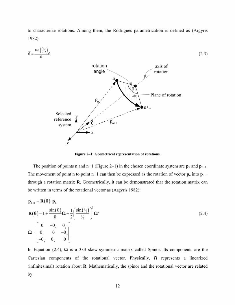
2.2.1 Geometrical description of large rotations
Geometrically, a pure three dimensional (3D) rotation applied to point n in Figure 2–1, results in
the movement of this point to point n+1. This rotation can be described by a rotation axis, θ , and
a rotation angle θ. The rotation axis is normal to the rotation plane, where the angle of rotation is
defined. Mathematically it is defined as:
= θ⋅θ θ (2.1)
The rotation axis is a unit vector and thus its numerical description depends on the chosen
coordinate system x,y,z. The components of θ = θx,θ,y,θz are the projections of the vector θ
into the given coordinate system scaled by the value of the rotation angle θ:
t
x y z
2 2 2x y z
θ = θ θ θ
θ = θ + θ + θ (2.2)
θ is called “rotational vector”, “axial vector” or “pseudovector”. Although it looks like a vector,
its components cannot be interpreted as rotations about the axis x,y,z. Another important
property of the axial vector is that any parametrization that preserves Equation (2.2) can be used
12
to characterize rotations. Among them, the Rodrigues parametrization is defined as (Argyris
1982):
( )tan 2θ
=θ
θ θ (2.3)
z
y
x
^
axis ofrotation
rotationangle
n
n+1
pn+1
pn
Plane of rotation
Selected reference
system
Figure 2–1: Geometrical representation of rotations.
The position of points n and n+1 (Figure 2–1) in the chosen coordinate system are pn and pn+1.
The movement of point n to point n+1 can then be expressed as the rotation of vector pn into pn+1
through a rotation matrix R. Geometrically, it can be demonstrated thar the rotation matrix can
be written in terms of the rotational vector as (Argyris 1982):
( )
( ) ( ) ( )n 1 n
22 2
2
z y
z x
y x
sin sin12
00
0
p R p
R I
+
θ
θ
= ⋅
θ ⎛ ⎞= + + ⎜ ⎟θ ⎝ ⎠
⎡ ⎤−θ θ⎢ ⎥= θ −θ⎢ ⎥⎢ ⎥−θ θ⎣ ⎦
θ
θ Ω Ω
Ω
(2.4)
In Equation (2.4), Ω is a 3x3 skew-symmetric matrix called Spinor. Its components are the
Cartesian components of the rotational vector. Physically, Ω represents a linearized
(infinitesimal) rotation about R. Mathematically, the spinor and the rotational vector are related
by:
13
p p p× = ⋅ = − ×θ Ω θ (2.5)
for any vector p (p can represent the position of a point in space, but the definition in Equation
(2.5) is very general). If Equation (2.4) is expanded into Taylor series, it is possible to
demonstrate that (Argyris 1982):
eR = Ω (2.6)
Equation (2.6) represents the “exponential map”. Although this compact format is very popular
for mathematical derivations, it is very difficult to implement numerically. Instead, a
parametrization of the rotational vector is used to calculate R (Felippa and Haugen 2005).
2.2.2 Mathematical description of large rotations
Mathematically, large (finite) rotations in three dimensions (3D) are represented by rotation
matrices R which constitute the group of Special Orthogonal linear transformations SO(3). This
is a subgroup where all matrices are orthogonal i.e. R Rt = I3 (I3 is the 3x3 identity matrix) and
their determinants are 1 i.e. the rotation matrix preserves the orientation of the vectors it rotates.
The mathematical structure of the SO(3) group is a nonlinear differentiable manifold, not a
linear space. In general, a differentiable manifold is defined by an open subspace where linear
tangent spaces can be defined at each point and maps (or functions) relate the points in the
manifold with those of the tangent space. In the finite rotations problem, each rotation matrix is a
point in the manifold space. Thus, at each rotation matrix, a tangent linear space can be defined
and it is composed by the set of all possible axial vectors. The relationship between the axial
vector and the manifold is the “exponential map”. Since it is very difficult to develop
mathematics for nonlinear spaces, the existence of a tangent linear space where linear algebra is
valid transforms a complex problem into a conventional problem and a space mapping.
2.2.3 Parametrization of rotations: quaternions
The most practical description of finite rotations for numerical analysis is the quaternion
definition. A quaternion q is a rotation parametrization that uses 4 parameters: one for the
rotation angle and 3 for the rotation axis with the restriction that the quaternion’s modulus has to
be unitary.
14
0
t1 2 3
2 2 2 20 1 2 3
q
q q q
q q q q 1
*
*
q
⎛ ⎞= ⎜ ⎟
⎝ ⎠
=
+ + + =
(2.7)
In terms of the rotational vector, the quaternion is written as (Simo and Vu-Quoc 1986):
( )
( )
0
t1 2 3
q cos 2
sin 2q q q
θ=
θ=
θθ
(2.8)
And the rotation matrix in terms of the quaternion components is:
2 2 1o 1 2 1 3 o 3 1 2 o2
2 2 11 2 3 o o 2 3 2 1 o2
2 2 11 3 2 o 2 3 1 o o 3 2
q q q q q q q q q q2 q q q q q q q q q q
q q q q q q q q q qR =
⎡ ⎤+ − + −⎢ ⎥− + − +⎢ ⎥⎢ ⎥+ − + −⎣ ⎦
(2.9)
The inverse operation: to extract the quaternions from a rotation matrix, can be done with the
following formulas:
( )( )
( )
( )
1 1o 11 22 332 2
32 2311 4
o
13 3112 4
o
21 1213 4
o
q 1 Tr 1 R R R
R Rq
qR R
R Rq
q
R= ± + = ± + + +
−= ±
−= ±
−= ±
(2.10)
2.2.4 Compound rotations
Compound rotations are the result of successive rotations. To calculate them, it is very important
to define the reference frame in which the calculation is being done. The results obtained for
different coordinate systems will be numerically different but geometrically equivalent. Given
two successive rotations, there are two ways of calculating the resultant rotation matrix (Argyris
1982). First, when the reference frame is constant, the final rotation is:
m1R R R= ⋅ (2.11)
15
where R is the resultant rotation matrix, R1 is the first rotation and Rm is the second rotation.
This operation is called material rotation or right translation. R1 and Rm share the same reference
system.
Second, when the reference frame moves and rotates with the body, the final rotation is:
s1R R R= ⋅ (2.12)
where R is the resultant rotation matrix and Rs is the second rotation. This operation is called
spatial rotation or left translation. In this case, the reference frame rotates first with R1 and Rs is
written with respect to the rotated coordinate system.
Denoting θm the axial vector associated with Rm and θs the axial vector associated with Rs, the
relationship between the axial vectors is:
m1
s = R ⋅θ θ (2.13)
From Equation (2.12) it can be concluded that rotations are “path-sensitive” i.e. θs is affected by
all previous rotations. Unless the reference and rotation axes are kept fixed, finite rotations
cannot be added like true vectors.
2.2.5 Derivatives of the Rotation matrix
The variations of the rotation matrix with respect to time and position are very useful during the
development of the formulation. The material and spatial forms are (Cardona and Geradin 1988;
Simo and Vu-Quoc 1986):
s mddsddt
s m
R R = R
R R = R
= ⋅ ⋅
= ⋅ ⋅
Ψ Ψ
Ω Ω (2.14)
where R is any rotation matrix, s is the arc-length variable and t is the time variable. Ψ and Ω are
skew-symmetric matrices representing the curvatures and instantaneous angular velocities
respectively. The superscripts “s” denotes spatial and “m” denotes material forms. As explained
in 2.2.4, the result of the compound rotation (Ψs R) is the same as (R Ψm), and the difference
between the matrices Ψs and Ψm is that the reference frame in the later is fixed while the
reference frame in the former rotates with R.
16
Equation (2.14) is obtained after the application of the directional Fréchet derivative on the
rotation matrix. Geometrically, it is equivalent to superimpose an infinitesimal rotation on to a
finite rotation.
2.2.6 Incremental rotation vector: the update problem
From 2.2.4 it was concluded that finite rotations cannot be added like real numbers, nor can axial
vectors be added like true vectors unless the reference frame and rotation axes remain fixed.
However, this is a very desirable feature in the context of an update process in a numerical
method, where the rotations at some step n (θn) are known, the increments (δθR) are obtained
through some type of Newton method and their values at the step n+1 (θn+1) have to be
determined. Usually, the update procedure will be through the composition of their respective
rotation matrices:
n 1 nR R R+ = ∆ ⋅ (2.15)
where Rn+1 is the rotation matrix at step n+1, Rn is the rotation matrix at step n and ∆R is the
rotation matrix of the incremental rotation δθR. It is very difficult to implement Equation (2.15)
in the context of a Newton method, thus the incremental rotation vector (Cardona and Geradin
1988; Ibrahimbegovic 1997) was introduced. The idea is to write the incremental rotation always
in respect to the same reference frame so that the axial vectors can be added like true vectors:
1 1 1n 1 n+ = + δθ θ θ (2.16)
Mathematically, Equation (2.16) means that the axial vector θn1, the increment δθ1 and the final
axial vector θn+11 belong to the same tangent linear space, see Figure 2–2. To obtain the
respective rotation matrices, the “exponential map” is used. Recalling Equation (2.6):
1n 1
n 1 eR ++ = Ω (2.17)
where Ωn+11 is the skew symmetric matrix whose components are the components of the axial
vector θn+11.
It is possible to obtain a transformation between the incremental rotation vector δθ1 and the
axial vector of the rotation matrix ∆R: δθR (Cardona and Geradin 1988; Ibrahimbegovic 1997):
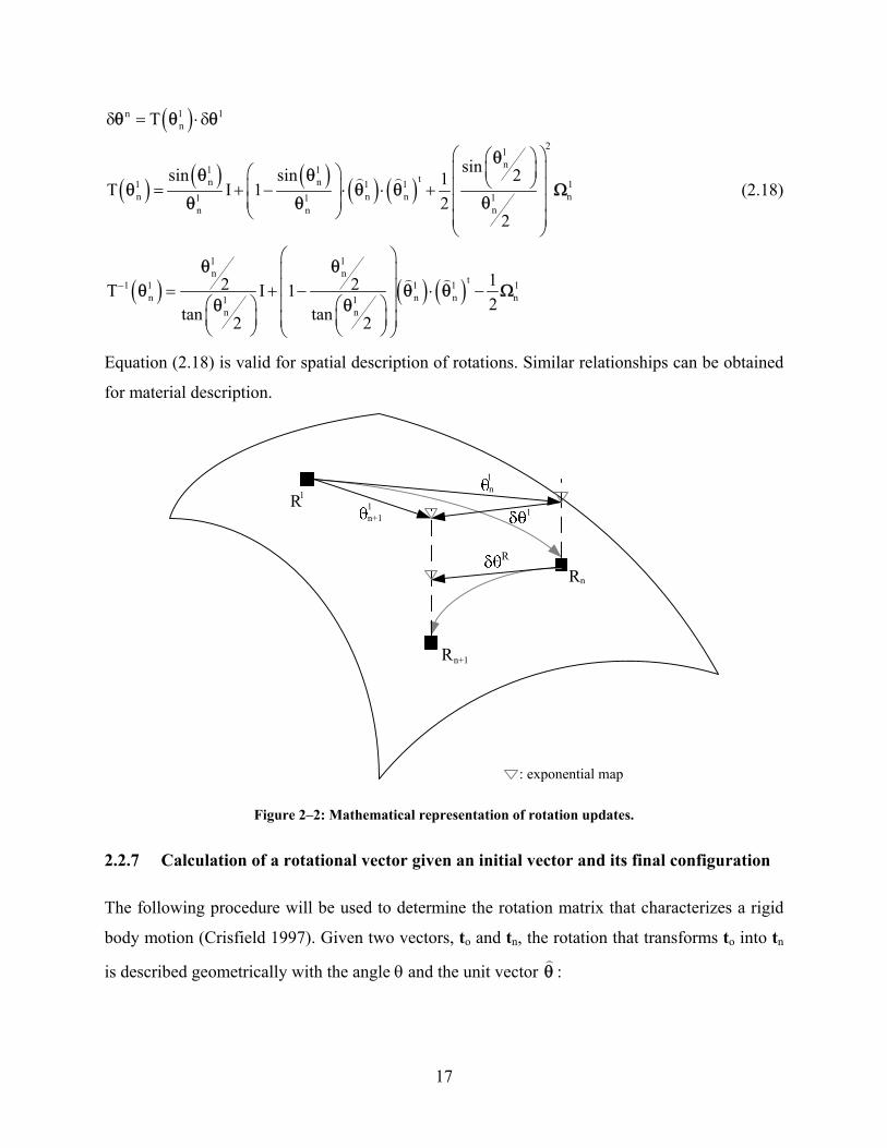
17
( )
( ) ( ) ( ) ( ) ( )
( ) ( ) ( )
n 1 1n
21n1 1
tn n1 1 1 1n n n n11 1
nn n
1 1n n t1 1 1 1 1
n n n n1 1n n
T
sinsin sin 21T I 12
2
12 2T I 12tan tan2 2
−
δ = ⋅δ
⎛ ⎞⎛ ⎞⎜ ⎟⎜ ⎟⎛ ⎞ ⎝ ⎠⎜ ⎟⎜ ⎟= + − ⋅ ⋅ +
⎜ ⎟ ⎜ ⎟⎝ ⎠ ⎜ ⎟⎝ ⎠
⎛ ⎞⎜ ⎟⎜ ⎟= + − ⋅ −
⎛ ⎞ ⎛ ⎞⎜ ⎟⎜ ⎟ ⎜ ⎟⎜ ⎟⎝ ⎠ ⎝ ⎠⎝ ⎠
θ θ θ
θθ θ
θ θ θ Ωθθ θ
θ θθ θ θ Ω
θ θ
(2.18)
Equation (2.18) is valid for spatial description of rotations. Similar relationships can be obtained
for material description.
R 1n1
n+11
R n+1
R n
1
: exponential map
R
Figure 2–2: Mathematical representation of rotation updates.
2.2.7 Calculation of a rotational vector given an initial vector and its final configuration
The following procedure will be used to determine the rotation matrix that characterizes a rigid
body motion (Crisfield 1997). Given two vectors, to and tn, the rotation that transforms to into tn
is described geometrically with the angle θ and the unit vector θ :
18
( )( )
to n
o n
o n
cos
sin
t t
t tt t
θ = ⋅
θ×= =
× θθ θ
(2.19)
Thus the rotation matrix becomes:
( ) ( ) ( ) ( )o n o n o nto n
11 t t
R I t t t t t t= + × + × ⋅ ×+ ⋅
θ Ω Ω Ω (2.20)
where Ω(t0×tn) represents the Spinor of the resultant vector from the cross product (t0×tn).
2.3 The corotational concept
The movement of an element in a body can be separated into two components: a rigid body
motion (displacement and rotation) and a deformation (strains and curvatures). To describe the
rigid body motion, a reference frame located outside of the element is needed. In general, the
same external reference is used for all elements in the body and it is called “Global coordinate
system” (G).
A rigid body motion is composed of (i) a rigid body translation: the displacement of the center
of gravity of the element; and (ii) a rigid body rotation: the relative displacements of the nodes of
the elements with respect to the center of the element. The same description can be made by
considering the movement of the nodes in Global coordinates. In structural analysis, this is called
the “chord of the element”, see Figure 2–3.
In the Corotational approach, the element’s deformations are described with respect to the
chord; therefore a Local reference system has to be defined and a relationship with the Global
reference system has to be found. Since the Local coordinate system describes the position of the
chord in the space, moving and rotating with it, this Local system is known as Corotated (E). It is
arbitrarily chosen that the x axis of the Corotated system coincides with the direction of the
element’s chord and that the y and z axis coincide with the principal directions of the section.
The Corotated axes (E) are related to the global axes (G) through a rotation matrix.
In the context of stability analysis, a common assumption is that large displacements are
described within the rigid body motion so that deformations are small. If this assumption is not
valid for a particular element, it is always possible to break it into more elements until the
assumption holds true. Thus, at the corotated level, the small strains theory is used to describe
the deformations. The main advantage of this assumption is that existing formulation and
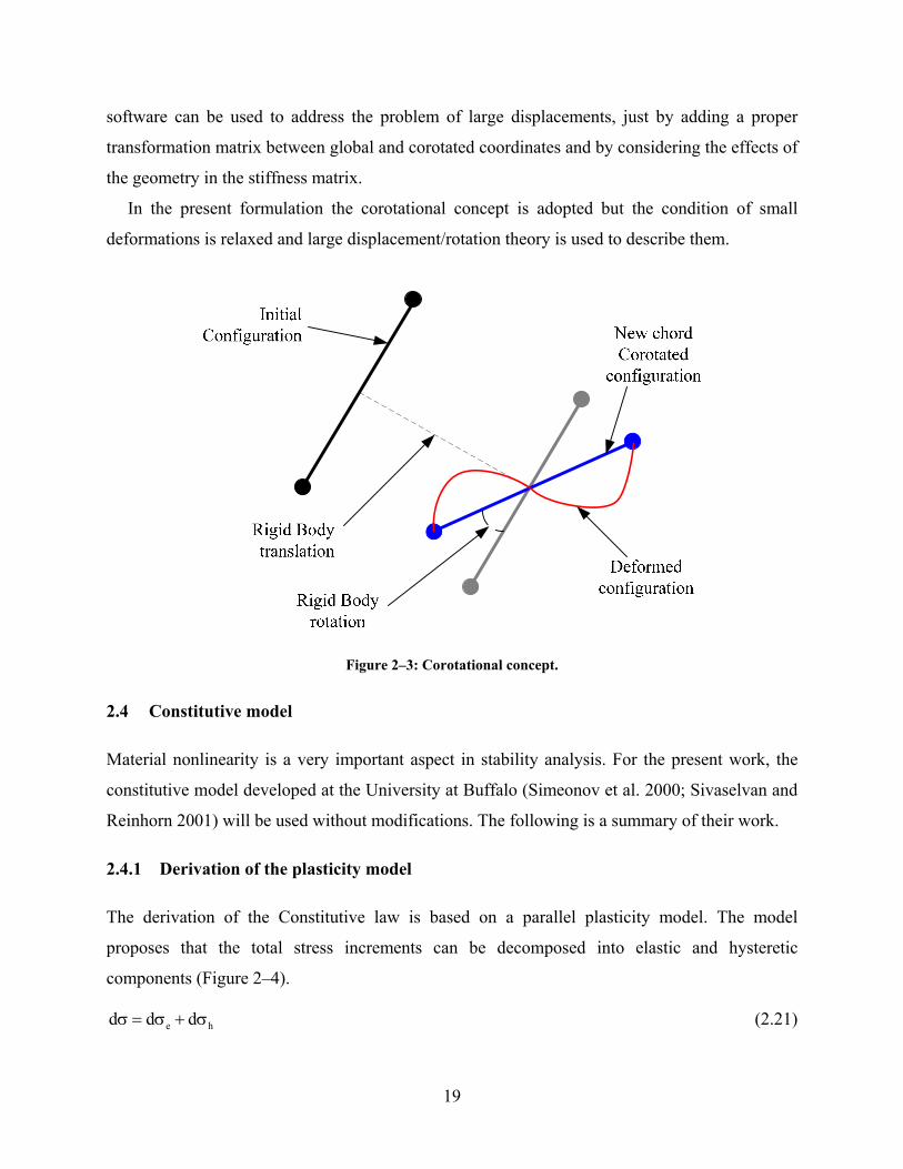
19
software can be used to address the problem of large displacements, just by adding a proper
transformation matrix between global and corotated coordinates and by considering the effects of
the geometry in the stiffness matrix.
In the present formulation the corotational concept is adopted but the condition of small
deformations is relaxed and large displacement/rotation theory is used to describe them.
Figure 2–3: Corotational concept.
2.4 Constitutive model
Material nonlinearity is a very important aspect in stability analysis. For the present work, the
constitutive model developed at the University at Buffalo (Simeonov et al. 2000; Sivaselvan and
Reinhorn 2001) will be used without modifications. The following is a summary of their work.
2.4.1 Derivation of the plasticity model
The derivation of the Constitutive law is based on a parallel plasticity model. The model
proposes that the total stress increments can be decomposed into elastic and hysteretic
components (Figure 2–4).
e hd d dσ = σ + σ (2.21)
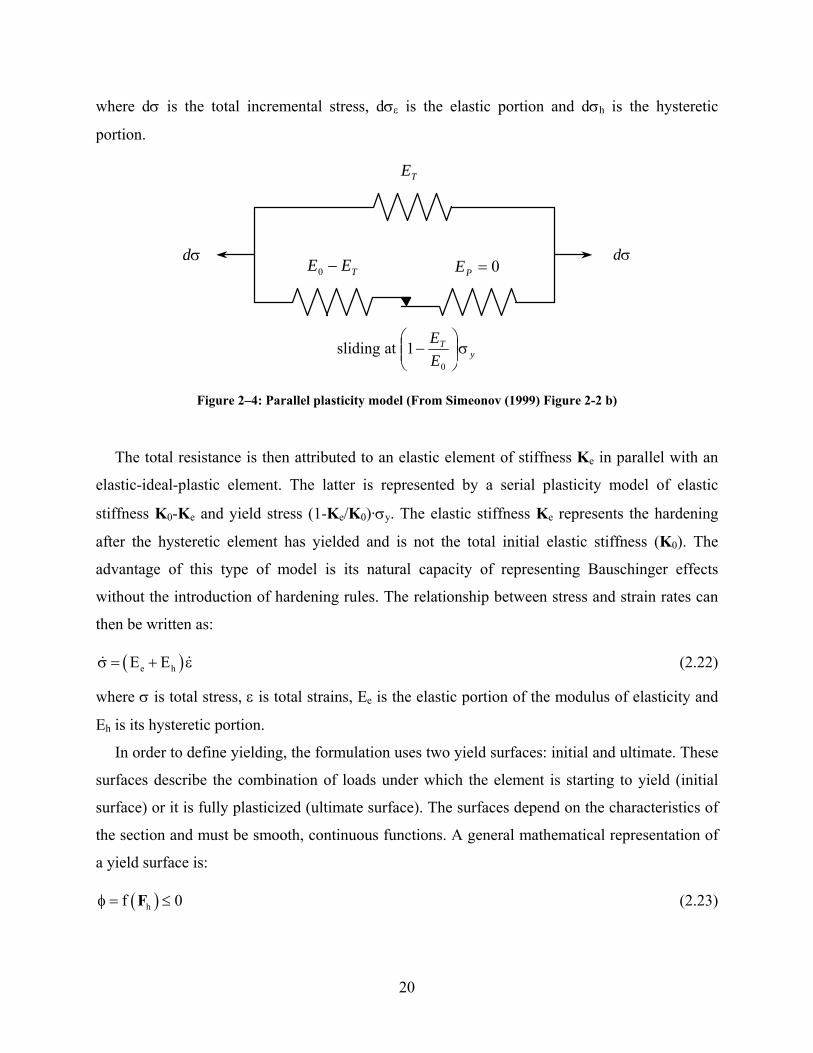
20
where dσ is the total incremental stress, dσε is the elastic portion and dσh is the hysteretic
portion.
TEE −0σd
0=PE
TE
σd
yT
EE
σ⎟⎟⎠
⎞⎜⎜⎝
⎛−
0
1atsliding
Figure 2–4: Parallel plasticity model (From Simeonov (1999) Figure 2-2 b)
The total resistance is then attributed to an elastic element of stiffness Ke in parallel with an
elastic-ideal-plastic element. The latter is represented by a serial plasticity model of elastic
stiffness K0-Ke and yield stress (1-Ke/K0)·σy. The elastic stiffness Ke represents the hardening
after the hysteretic element has yielded and is not the total initial elastic stiffness (K0). The
advantage of this type of model is its natural capacity of representing Bauschinger effects
without the introduction of hardening rules. The relationship between stress and strain rates can
then be written as:
( )e hE Eσ = + ε (2.22)
where σ is total stress, ε is total strains, Ee is the elastic portion of the modulus of elasticity and
Eh is its hysteretic portion.
In order to define yielding, the formulation uses two yield surfaces: initial and ultimate. These
surfaces describe the combination of loads under which the element is starting to yield (initial
surface) or it is fully plasticized (ultimate surface). The surfaces depend on the characteristics of
the section and must be smooth, continuous functions. A general mathematical representation of
a yield surface is:
( )hf 0Fφ = ≤ (2.23)
21
Equation (2.23) describes the yield function φ as a function of Fh, the elastic-ideal plastic
component of the total force FT. It is always non-positive. When the yield function is equal to 0,
the section is yielding.
It is also assumed that the total strains ε can be written as the sum of the elastic and hysteretic
parts. In rate form:
e p= +ε ε ε (2.24)
where εe is the elastic and εp is the plastic component of the total strains ε.
When the element is flowing: φ=0, the rate of the elastic strain is zero and the rate of total
strains is the rate of hysteretic strains. On the other hand, the rate of the hysteretic force can be
written solely in terms of the rate of the elastic strains since after yielding the force is constant,
thus its rate is zero.
( )h 0 e eF K K= − ⋅ε (2.25)
The plastic strain εp is calculated using plastic flow rules. The direction of the plastic flow is
perpendicular to the yielding surface and its magnitude is proportional to the gradient of the
surface at the point of yielding:
phF
∂φ= λ
∂ε (2.26)
where ∂φ/∂Fh = ∂φ/∂Fx* ∂φ/∂My
* ∂φ/∂Mz*t is the gradient of the yield function and the rate of
λ is a proportionality scalar. Fx*, My* and Mz* are defined in Equation (2.36) To calculate the
proportionality scalar and the plastic strains, the following rules known as Kuhn-Tucker
conditions must be enforced:
• The plastic flow is always directed outwards the yielding surface.
• No flow occurs for load combinations outside the yielding surface.
t
hh
00
0FF
λ ≥
φ⋅λ =
⎛ ⎞∂φλ ≥⎜ ⎟∂⎝ ⎠
(2.27)
The plastic multiplier can be calculated from the consistency equation:
22
t
hh
0FF
⎛ ⎞∂φ=⎜ ⎟∂⎝ ⎠
(2.28)
It expresses the fact that a force combination which has caused plastic strains, will continue to do
so until unloading.
Replacing the value of the rate of Fh into the consistency equation:
( )t
0 eh h
0K KF F
⎛ ⎞ ⎛ ⎞∂φ ∂φ− ⋅ − λ =⎜ ⎟ ⎜ ⎟∂ ∂⎝ ⎠ ⎝ ⎠
ε (2.29)
And solving for the plastic multiplier and the plastic strains:
( )
( )
( )
( )
t
0 eht
0 eh h
t
0 eh
p th
0 eh h
K KF
K KF F
K KF
FK K
F F
⎛ ⎞∂φ−⎜ ⎟∂⎝ ⎠λ =
⎛ ⎞ ⎛ ⎞∂φ ∂φ−⎜ ⎟ ⎜ ⎟∂ ∂⎝ ⎠ ⎝ ⎠
⎛ ⎞∂φ−⎜ ⎟∂ ∂φ⎝ ⎠=
∂⎛ ⎞ ⎛ ⎞∂φ ∂φ−⎜ ⎟ ⎜ ⎟∂ ∂⎝ ⎠ ⎝ ⎠
ε
εε
(2.30)
The relationship between the force rate and the strain rate is:
( )( )
( )
t
0 eh
h 0 e 1 2th
0 eh h
H HK K
FF K K
FK K
F F
⎡ ⎤⎛ ⎞∂φ−⎢ ⎥⎜ ⎟∂ ∂φ⎢ ⎥⎝ ⎠= − −⎢ ⎥∂⎛ ⎞ ⎛ ⎞∂φ ∂φ⎢ ⎥−⎜ ⎟ ⎜ ⎟⎢ ⎥∂ ∂⎝ ⎠ ⎝ ⎠⎣ ⎦
εε (2.31)
H1 represents the yielding condition and H2 the unloading condition.
The yielding condition, or plastic flow, occurs only if the force combination defines a point in
the yielding surface. Mathematicaly, this can be represented by a Heaviside function, that is
always 0 when there is no yielding and 1 when there is yielding. Numerically, this Heaviside
function can be smoothed to have a continuous function:
( ) ( )n1H 1φ = φ + (2.32)
When the value of the yield function is close to zero, at the onset of yielding, the value of H1
approaches asymptotically to 1, equaling to 1 after yielding.
23
The unloading criterion is modeled through another smoothed Heaviside function:
2 h 1 2 hh h
H sgnF FF F
⎛ ⎞ ⎛ ⎞∂φ ∂φ= η + η ⋅⎜ ⎟ ⎜ ⎟∂ ∂⎝ ⎠ ⎝ ⎠
(2.33)
where η1+η2=1. η1 and η2 can take any value between 0 and 1. Here it will be considered
η1=η2=0.5. When the section is yielding, the gradient of the yield function ∂φ/∂Fh and the rate of
the forces hF have the same sign (outwards the yield surface) and therefore η1+η2=1. When the
section is unloading, the flow gradient and the force rates have opposite signs, therefore H2=0.
This means that at the unloading stage, the total stiffness becomes the total initial elastic
stiffness.
The rate of the total force is then written as:
( )( )
( )( )
t
0 enh
e 0 e 1 2 hth h
0 eh h
1 sgnK K
FF K K K F
F FK K
F F
∂φ−
∂ ∂φ ∂φ= + − ε − φ + η + η ⋅
∂ ∂∂φ ∂φ−
∂ ∂
⎡ ⎤⎛ ⎞⎢ ⎥⎜ ⎟ ⎡ ⎤⎛ ⎞⎝ ⎠⎢ ⎥⎡ ⎤ ⎜ ⎟⎢ ⎥⎣ ⎦⎢ ⎥⎛ ⎞ ⎛ ⎞ ⎝ ⎠⎣ ⎦⎢ ⎥⎜ ⎟ ⎜ ⎟⎢ ⎥⎝ ⎠ ⎝ ⎠⎣ ⎦
ε
ε (2.34)
Note: This can be viewed as a generalized multidimensional inelastic hysteretic model that in
unidimensional form reduces to the Sivaselvan-Reinhorn model (Sivaselvan and Reinhorn 2001),
which can be further reduced to Bouc-Wen model (Bouc 1967; Wen 1976). Or one can look at
this model as the “generalized Bouc-Wen model” for multidimensional surfaces.
2.4.2 Elastic stiffness matrix
The elastic stiffness matrix Ke is the hardening slope in a force-displacement relationship.
Usually, the hardening is written in terms of a percentage of the total initial elastic stiffness: Ke =
a K0. Where a can be 3%, 5% or any value defined by a material coupon test.
2.4.3 Initial elastic stiffness matrix
Since the relationship above links the force rate to the strains, a typical total initial elastic
stiffness matrix would look like:
24
0y
z
EA 0 0 00 GJ 0 00 0 EI 00 0 0 EI
K
⎡ ⎤⎢ ⎥⎢ ⎥=⎢ ⎥⎢ ⎥⎣ ⎦
(2.35)
where E: modulus of elasticity; A: area; G: shear modulus; J: torsional constant; Iy: inertia in the
weak direction; Iz: inertia in the strong direction.
2.4.4 Ultimate yield function
The ultimate yield function depends on the cross section shape. However, in general it can be
written as (Figure 2–5):
( ) ( )
( )( )
( )
y z
y zy z
y z
* * *y z x
y z* * *yu zu xu
* *y y y y yu y y
* *z z z z zu y z
* *x x x xu y
m m1
1 p 1 p
M M Fm m pM M F
M M aEI M 1 a Z
M M aEI M 1 a Z
F F aEA F 1 a A
α α
α αβ βφ = + −
− −
= = =
= − φ = − σ
= − φ = − σ
= − ε = − σ
(2.36)
In Equation (2.36) Mx, My and Mz are the moments in the x, y and z directions respectively; φy
and φz are the curvatures in the y and z directions; Fx is the axial force (in x direction); εx is the
axial strain; the exponents α and β are particular to each section and have to be determined from
a finite element analysis or experimental results. All other quantities have been defined
elsewhere.
The yield function depends on non-dimensional quantities p, my and mz that are always less
than unity. These quantities represent the proportion of the hysteretic forces, total forces minus
elastic forces, with respect to the ultimate capacities.
The equation above assumes that the section is doubly-symmetric. If the section in the model
is not symmetric, appropriate changes have to be made to the axial force axis representation
(Sivaselvan and Reinhorn 2001).
From Equation (2.36), a general gradient of the hysteretic force can be obtained:
25
* *x xu
* *y y yu
* *z z zu
1F p F
1M m M
1M m M
∂φ ∂φ=
∂ ∂
∂φ ∂φ=
∂ ∂
∂φ ∂φ=
∂ ∂
(2.37)
2.4.5 Yielding criterion parameter
The parameter n in the exponent of the yielding criterion defines how smooth is the transition
between the elastic and inelastic portions of the hysteretic curve. Values between 6 and 10 are
normally used. A value of 10 is considered high which means that the transition is sharp or
sudden. A lower exponent is better for numerical purposes. The drawback of this formulation is
that it is allowing plastic deformations from the beginning of the analysis, which is not correct.
An initial yield surface can be used to define incipient yielding, using an elastic stiffness matrix
or a very high exponent up to that surface and switching to a lower exponent until reaching full
plasticity. Numerical problems may arise when using this approach because the distance between
incipient yielding and fully plastic surfaces is, in general, small.
2.4.6 Unloading criterion
Equation (2.33) depends on the yield function gradients and the hysteretic force rates. However,
the hysteretic force rate is the variable that is being calculated through the above procedure. It is
not desirable to have its value in the unloading function because traditional methods for solving
differential equations cannot be applied. The product of the elastic stiffness matrix and the total
strains vector was suggested to replace it (Simeonov et al. 2000):
2 h 1 2 eh h
H sgnF KF F
⎛ ⎞ ⎛ ⎞∂φ ∂φ= η + η ⋅ ⋅⎜ ⎟ ⎜ ⎟∂ ∂⎝ ⎠ ⎝ ⎠
ε (2.38)
The reason for the above change is that since the unloading is elastic, the force rate and the strain
rate are related through the elastic stiffness matrix. The dot product ensures that the sign of the
function is preserved.
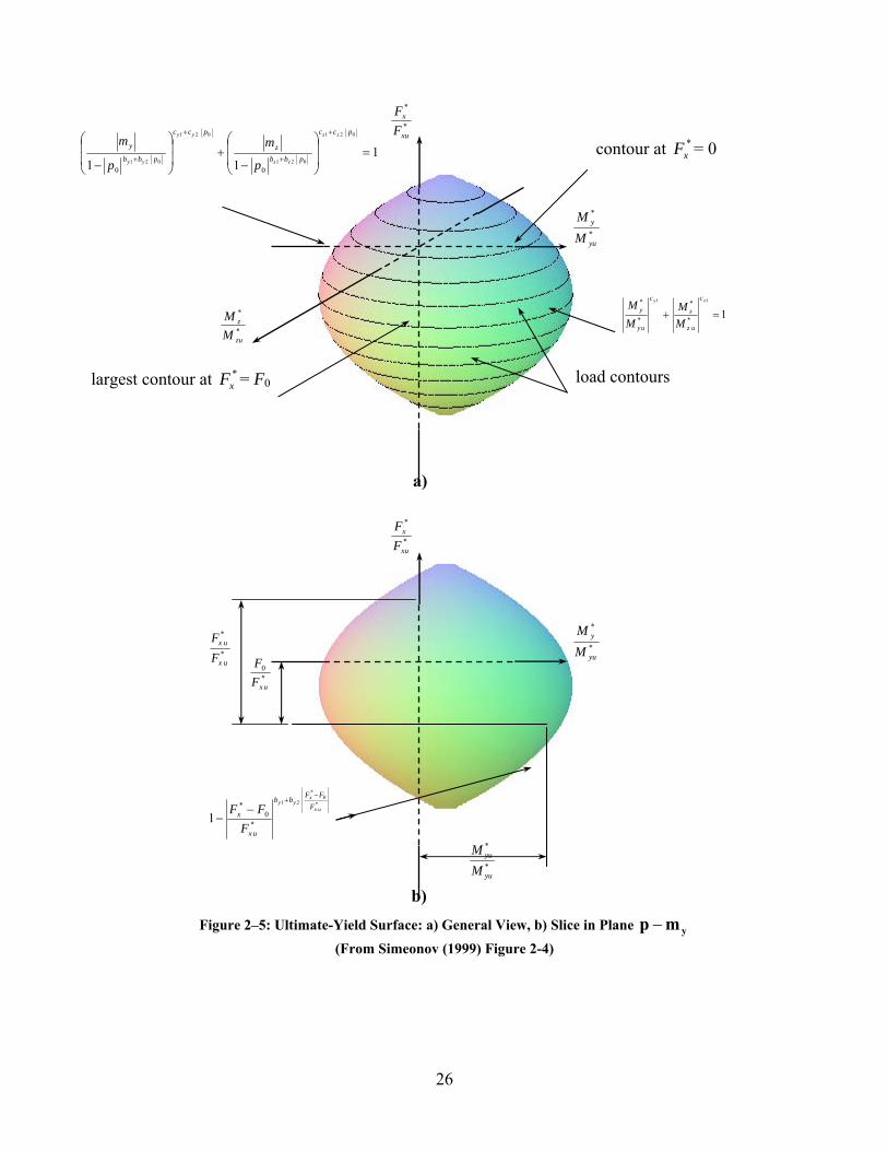
26
Figure 2–5: Ultimate-Yield Surface: a) General View, b) Slice in Plane ymp −
(From Simeonov (1999) Figure 2-4)
b)
*
*
xu
x
FF
*
*
yu
y
MM
*0
uxFF
*
*
ux
ux
FF
*0
*
21
*0
*
1ux
xyy F
FFbb
ux
x
FFF
−+
−−
*
*
yu
yu
MM
load contours
a)
*
*
yu
y
MM
*
*
zu
z
MM
*
*
xu
x
FF
111
021
021
021
021
00
=⎟⎟
⎠
⎞
⎜⎜
⎝
⎛
−+⎟
⎟
⎠
⎞
⎜⎜
⎝
⎛
−
+
+
+
+
pcc
pbbz
pcc
pbb
yzz
zz
yy
yy p
m
p
m
111
*
*
*
*
=+zy c
uz
z
c
uy
y
MM
MM
largest contour at *xF = F0
contour at *xF = 0
27
2.5 The state space approach.
For solving a system of nonlinear equations of motion that represents a structural system, the
traditional approach has been to write these equations in an incremental way, thus solving a
nonlinear transient analysis as a sequence of quasi-static analyses. The system is solved in
Global coordinates, therefore during a step, equilibrium, internal plasticity rules and/or
compatibility between elements can be violated and iterations within a step are necessary to
enforce them.
By contrast, the state space approach uses a set of variables: global nodal displacements and
velocities their rates, element internal forces and their rates, total strains at pre-defined control
sections along the length of the element and their rates. These variables completely define the
state of each element in the structure at any time. The solution of the structural problem consists
in solving a set of equations that represent the “evolution” of all these variables with time
(evolution equations). Those equations are the fundamental equations of a structural system:
Equilibrium, Compatibility and Plasticity. Written in rate form this set constitutes, in general, a
system of Differential Algebraic Equations (DAE). The simultaneous solution of all the
equations ensures that the all the basic laws (equilibrium, compatibility and plasticity) are
satisfied at all times, eliminating the need for iterations within a step. The framework of this
approach was developed by Simeonov (Simeonov et al. 2000).
2.5.1 State variables
First, the set of variables and their rates have to be defined.
Denoting u the displacement, m the mass, c the damping constant, k the stiffness and P the
external force, the traditional equation of motion, a second order differential equation, is:
m u + c u + k u = P⋅ ⋅ ⋅ (2.39)
Using displacements and velocities (or displacements rates) as the independent variables,
Equation (2.39) is re-written as a set of two first order differential equations:
1 2
2 1 1
2 1
y u y um y c y k y Py y
= =⋅ + ⋅ + ⋅ ==
(2.40)
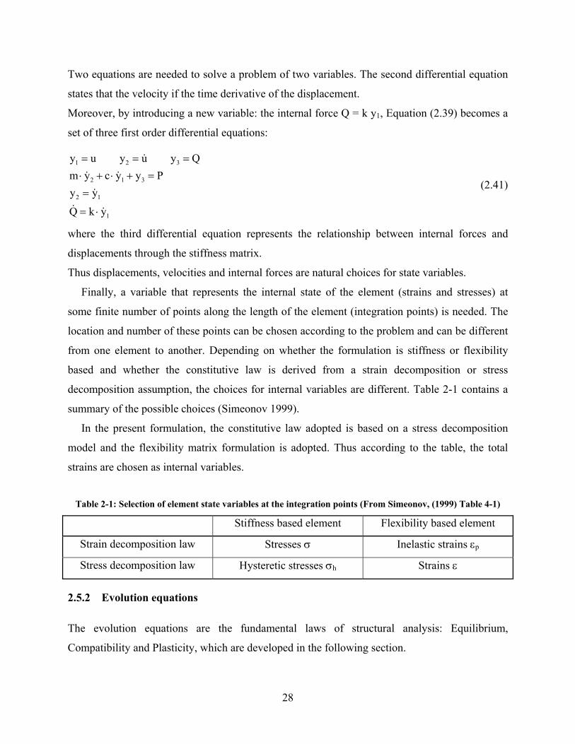
28
Two equations are needed to solve a problem of two variables. The second differential equation
states that the velocity if the time derivative of the displacement.
Moreover, by introducing a new variable: the internal force Q = k y1, Equation (2.39) becomes a
set of three first order differential equations:
1 2 3
2 1 3
2 1
1
y u y u y Qm y c y y Py y
Q k y
= = =
⋅ + ⋅ + =
=
= ⋅
(2.41)
where the third differential equation represents the relationship between internal forces and
displacements through the stiffness matrix.
Thus displacements, velocities and internal forces are natural choices for state variables.
Finally, a variable that represents the internal state of the element (strains and stresses) at
some finite number of points along the length of the element (integration points) is needed. The
location and number of these points can be chosen according to the problem and can be different
from one element to another. Depending on whether the formulation is stiffness or flexibility
based and whether the constitutive law is derived from a strain decomposition or stress
decomposition assumption, the choices for internal variables are different. Table 2-1 contains a
summary of the possible choices (Simeonov 1999).
In the present formulation, the constitutive law adopted is based on a stress decomposition
model and the flexibility matrix formulation is adopted. Thus according to the table, the total
strains are chosen as internal variables.
Table 2-1: Selection of element state variables at the integration points (From Simeonov, (1999) Table 4-1)
Stiffness based element Flexibility based element
Strain decomposition law Stresses σ Inelastic strains εp
Stress decomposition law Hysteretic stresses σh Strains ε
2.5.2 Evolution equations
The evolution equations are the fundamental laws of structural analysis: Equilibrium,
Compatibility and Plasticity, which are developed in the following section.
29
2.6 Development of an element for large displacements and large rotations
2.6.1 Objective
The objective of the present formulation is to develop a procedure capable of solving structural
problems with material as well as geometrical nonlinearities.
The formulation solves the problem in the state space, using the Corotational formulation to
describe each element independently. Deformations are calculated with respect to the Corotated
system of coordinates and they can be large. The goal is to develop appropriate equations of
Equilibrium, Compatibility and Plasticity for every element. The result is a set of Differential
Algebraic Equations (DAE) equations that are being solved using the Implicit Differential
Algebraic solver (IDA) from the Lawrence Livermore National Laboratory (LLNL) (Hindmarsh
and Serban 2006).
The procedure can be summarized in the following steps:
1. Definition of Coordinate systems.
2. Definition of DOFs.
3. Calculation of rigid body transformation matrices.
4. Equilibrium equations.
5. Compatibility equations.
6. Plasticity equations.
7. Numerical integration methods.
2.6.2 Coordinate systems
There are 3 coordinate systems needed for understanding the present development (Figure 2–6):
• G: Global coordinate system. Fixed and common for all the elements, the equations of
motions of the structure are solved in this system.
• L: Local coordinate system. Defines the position of the element in its original unstressed
position. This system serves as a reference for the calculation of nodal rotations.
• E: Corotated coordinate system. Defines the position of the chord of the element at each
time step. This system changes with each iteration.
G, L and E are 3x3 orthogonal matrices whose rows are the three axes that define the
coordinate system. Each axis has 3 components: the projections in the Global system. Therefore,
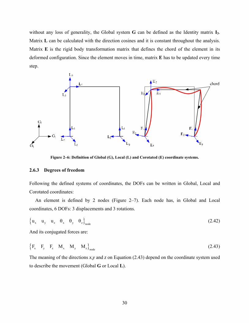
30
without any loss of generality, the Global system G can be defined as the Identity matrix I3.
Matrix L can be calculated with the direction cosines and it is constant throughout the analysis.
Matrix E is the rigid body transformation matrix that defines the chord of the element in its
deformed configuration. Since the element moves in time, matrix E has to be updated every time
step.
Figure 2–6: Definition of Global (G), Local (L) and Corotated (E) coordinate systems.
2.6.3 Degrees of freedom
Following the defined systems of coordinates, the DOFs can be written in Global, Local and
Corotated coordinates:
An element is defined by 2 nodes (Figure 2–7). Each node has, in Global and Local
coordinates, 6 DOFs: 3 displacements and 3 rotations.
x y z x y z nodeu u u θ θ θ (2.42)
And its conjugated forces are:
x y z x y z nodeF F F M M M (2.43)
The meaning of the directions x,y and z on Equation (2.43) depend on the coordinate system used
to describe the movement (Global G or Local L).
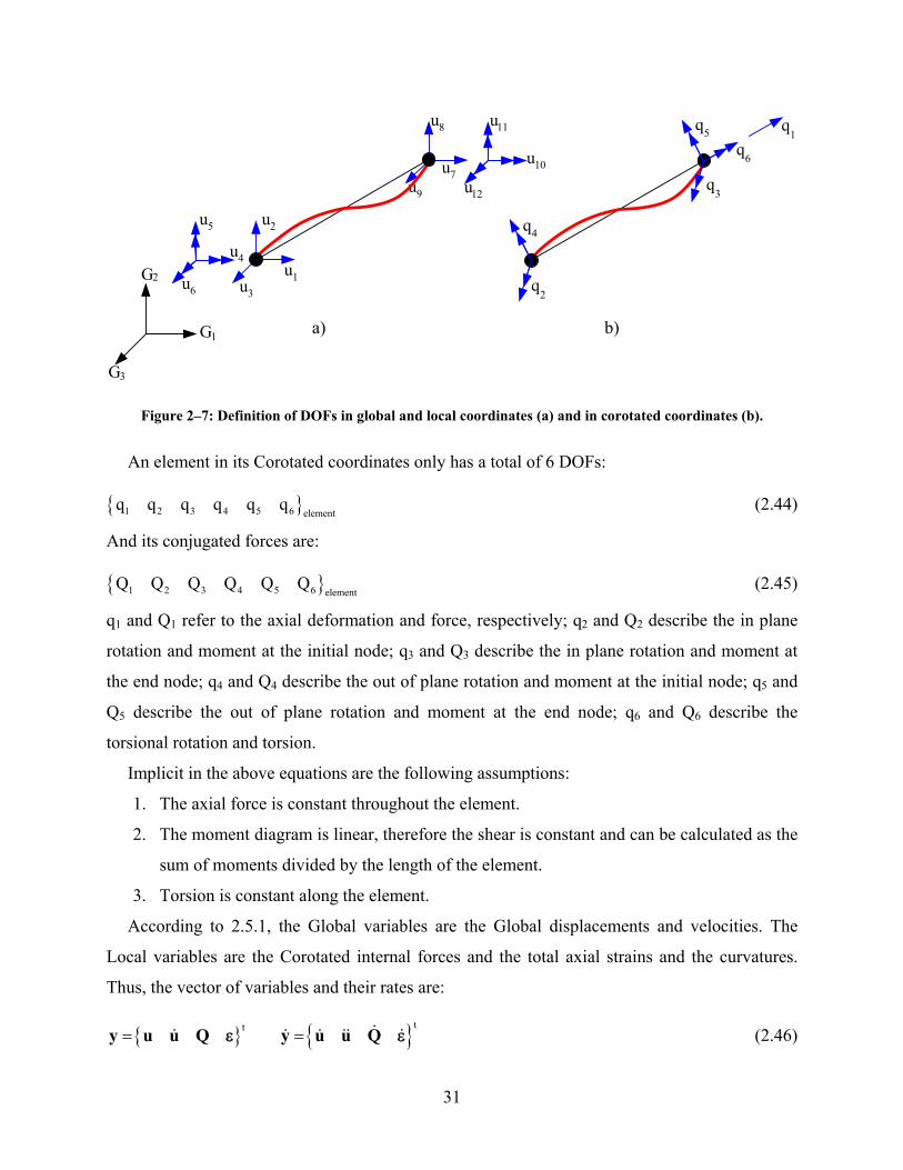
31
G
G
G
1
2
3
u1
u2
u3
u4
u5
u6
u7
u8 u11
u10
u12u9
q4
q2
q5
q3
q6
q1
Figure 2–7: Definition of DOFs in global and local coordinates (a) and in corotated coordinates (b).
An element in its Corotated coordinates only has a total of 6 DOFs:
1 2 3 4 5 6 elementq q q q q q (2.44)
And its conjugated forces are:
1 2 3 4 5 6 elementQ Q Q Q Q Q (2.45)
q1 and Q1 refer to the axial deformation and force, respectively; q2 and Q2 describe the in plane
rotation and moment at the initial node; q3 and Q3 describe the in plane rotation and moment at
the end node; q4 and Q4 describe the out of plane rotation and moment at the initial node; q5 and
Q5 describe the out of plane rotation and moment at the end node; q6 and Q6 describe the
torsional rotation and torsion.
Implicit in the above equations are the following assumptions:
1. The axial force is constant throughout the element.
2. The moment diagram is linear, therefore the shear is constant and can be calculated as the
sum of moments divided by the length of the element.
3. Torsion is constant along the element.
According to 2.5.1, the Global variables are the Global displacements and velocities. The
Local variables are the Corotated internal forces and the total axial strains and the curvatures.
Thus, the vector of variables and their rates are:
tt y u u Q y u u Q= =ε ε (2.46)
a) b)
32
where u is defined in Equation (2.42), Q is defined in Equation (2.45) and ε is defined by:
t
x y z= ε φ φ φε (2.47)
ε is the set of vectors of total axial strain and curvatures of every section of the element. In
Equation (2.47), ε represents axial strains and φx, φy, φz are the curvatures.
In a general structure, not all its DOFs are dynamics i.e. have an associated mass. Those
DOFs are called “static” and their associated equation of motion is simply:
k u = P⋅ (2.48)
For these DOFs, there are only two state variables: u and Q. Therefore, in Equation (2.46), the
velocity is a state variable of dynamic DOFs only. For instance, when a static analysis is
performed Equation (2.46) becomes:
tt y u Q y u Q= =ε ε (2.49)
2.6.4 Calculation of rigid body transformation matrices
For each element, a matrix E: the rigid body transformation matrix that defines the chord and
principal axes of the element in its deformed configuration, has to be calculated. At each time
step, the actual position of each node of the element in Global coordinates is calculated from its
original position and actual displacement:
i 0 ip p u= +
where pi is the vector of the actual position of node i, p0 and ui are the original position and
actual displacement of node i. The actual displacement ui=uxi uyi uzit at any time step is a
known quantity and can be retrieved from the state variable u. The vector describing the chord of
the element can then be calculated as:
i j1
i j
p pE
p p−
=−
(2.51)
where the variables i and j represent the initial and end nodes of the element. The vector E1 is the
Corotated x coordinate.
The next step is to obtain a rotation matrix RL-E that rotates the vector L1 (the Local x
coordinate) into vector E1. Using Equation (2.20):
33
( ) ( ) ( )1 1 1 1 1 1t1 1
11L-ER I L E L E L E
L E= + × + × ⋅ ×
+ ⋅Ω Ω Ω (2.52)
Recalling that Ω(L1×E1) is the spinor of the resultant vector of the cross product L1×E1.
Matrix RL-E also rotates the vectors L2 into E2 and L3 into E3. Vectors L2 and L3 represent the
directions of the principal axes of the cross section in its original configuration, while E2 and E3
represent the directions of the principal axes of the cross section in its Corotated configuration.
Thus, matrix E is obtained by rotating matrix L with RL-E:
L-EE R L= ⋅ (2.53)
Vectors L1, L2 and L3 are rows of the transformation matrix L (that rotates the Global
coordinates into Local coordinates). These vectors are also known as cosine directors (Weaver,
1990 #123). Similarly, Vectors E1, E2 and E3 are rows of the rotation matrix E.
Because the Global system is arbitrarily chosen as the identity matrix G = I3, the coordinate
system L coincides with the rotation matrix L i.e. L = L·G and the coordinate system E
coincides with the rotation matrix E i.e. E = E G.
The origin of the Corotated coordinate system E can be located anywhere along the element.
It is convenient to place it at one of the end nodes, say node i, for reasons that will become
apparent latter in the development of the formulation.
2.6.5 Equilibrium Equations
Global equilibrium equations are the evolution equations of Global variables.
The internal forces Q of each element in Corotated coordinates are known variables (Equation
(2.46)). Global equilibrium is calculated by transforming the internal forces into Global
Coordinates, summing all the contributions from different elements in each node and comparing
these values to the applied external force.
The transformation into Global variables is done through a transformation matrix Tt. This
matrix is specific to each element and is the resultant of the composition of the rigid body
rotation matrix TCG and the matrix of change of variables TEC.
EC CGT T T= (2.54)
TEC is the matrix representing equilibrium at the Corotated level using the assumptions listed in
part 2.6.3. TEC transforms 12 DOFs (Local) into 6 DOFs (Corotated) (See Figure 2–7):
34
L L
L LEC
L L
L L
1 0 0 0 0 0 1 0 0 0 0 01 10 0 0 0 1 0 0 0 0 0
1 10 0 0 0 0 0 0 0 0 1
1 10 0 0 1 0 0 0 0 0 0
1 10 0 0 0 0 0 0 0 1 0
0 0 0 1 0 0 0 0 0 1 0 0
T
−⎡ ⎤⎢ ⎥
−⎢ ⎥ξ ξ⎢ ⎥⎢ ⎥−ξ ξ⎢ ⎥= ⎢ ⎥−⎢ ⎥ξ ξ⎢ ⎥⎢ ⎥− ξ ξ⎢ ⎥⎢ ⎥−⎣ ⎦
(2.55)
where ξL is the actual length of the element.
Transformation matrix TCG is an expanded version of matrix E to allow the transformation of
12 DOFs simultaneously from Global to Corotated coordinates. Matrix E transforms 3 DOFs
(displacements u and rotations θ) from Global to Corotated coordinates:
CR G
CR G
u = E u= E
⋅
⋅θ θ (2.56)
Thus, to transform all the DOFs of a node the following matrix form can be used:
CR G
CR G
E 0u u=
0 E⎡ ⎤ ⎡ ⎤⎡ ⎤
⋅⎢ ⎥ ⎢ ⎥⎢ ⎥⎣ ⎦⎣ ⎦ ⎣ ⎦θ θ
(2.57)
Since an element has 2 end nodes, Equation (2.57) can be written as:
CR Gi i
CR Gi i
CR Gj j
CR Gj j
u uE 0 0 00 E 0 0
u u0 0 E 00 0 0 E
⎡ ⎤ ⎡ ⎤⎡ ⎤⎢ ⎥ ⎢ ⎥⎢ ⎥⎢ ⎥ ⎢ ⎥⎢ ⎥= ⋅⎢ ⎥ ⎢ ⎥⎢ ⎥⎢ ⎥ ⎢ ⎥⎢ ⎥⎢ ⎥ ⎢ ⎥⎣ ⎦⎣ ⎦ ⎣ ⎦
θ θ
θ θ
(2.58)
where the subscript i denotes node i and the subscript j denotes node j. Finally, matrix TCG is:
CG
E 0 0 00 E 0 0
T0 0 E 00 0 0 E
⎡ ⎤⎢ ⎥⎢ ⎥=⎢ ⎥⎢ ⎥⎣ ⎦
(2.59)
Matrix T transforms Global displacement and rotation rates into Corotated coordinates and, by
virtual work, its transpose transforms Corotated forces Q into Global coordinates F:
t
q T uF T Q
= ⋅
= ⋅ (2.60)
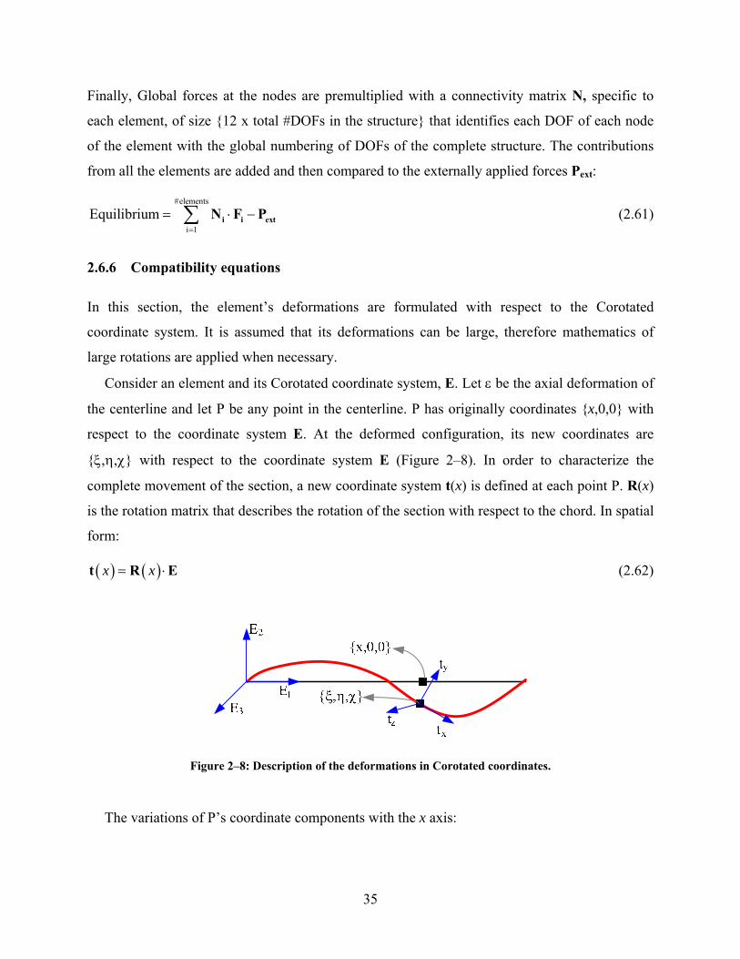
35
Finally, Global forces at the nodes are premultiplied with a connectivity matrix N, specific to
each element, of size 12 x total #DOFs in the structure that identifies each DOF of each node
of the element with the global numbering of DOFs of the complete structure. The contributions
from all the elements are added and then compared to the externally applied forces Pext:
#elements
i 1Equilibrium i i extN F P
=
= ⋅ −∑ (2.61)
2.6.6 Compatibility equations
In this section, the element’s deformations are formulated with respect to the Corotated
coordinate system. It is assumed that its deformations can be large, therefore mathematics of
large rotations are applied when necessary.
Consider an element and its Corotated coordinate system, E. Let ε be the axial deformation of
the centerline and let P be any point in the centerline. P has originally coordinates x,0,0 with
respect to the coordinate system E. At the deformed configuration, its new coordinates are
ξ,η,χ with respect to the coordinate system E (Figure 2–8). In order to characterize the
complete movement of the section, a new coordinate system t(x) is defined at each point P. R(x)
is the rotation matrix that describes the rotation of the section with respect to the chord. In spatial
form:
( ) ( )t R E= ⋅x x (2.62)
Figure 2–8: Description of the deformations in Corotated coordinates.
The variations of P’s coordinate components with the x axis:
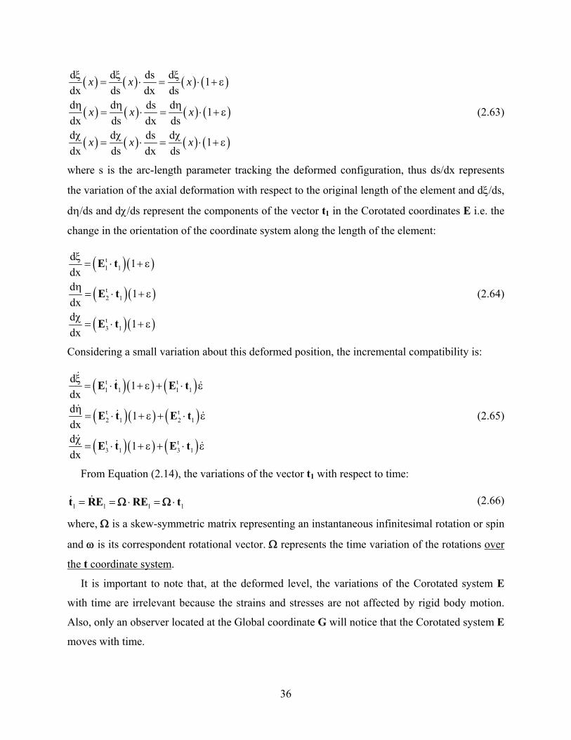
36
( ) ( ) ( ) ( )
( ) ( ) ( ) ( )
( ) ( ) ( ) ( )
d d ds d 1dx ds dx dsd d ds d 1dx ds dx dsd d ds d 1dx ds dx ds
ξ ξ ξ= ⋅ = ⋅ + ε
η η η= ⋅ = ⋅ + ε
χ χ χ= ⋅ = ⋅ + ε
x x x
x x x
x x x
(2.63)
where s is the arc-length parameter tracking the deformed configuration, thus ds/dx represents
the variation of the axial deformation with respect to the original length of the element and dξ/ds,
dη/ds and dχ/ds represent the components of the vector t1 in the Corotated coordinates E i.e. the
change in the orientation of the coordinate system along the length of the element:
( )( )
( )( )
( )( )
t1 1
t2 1
t3 1
d 1dxd 1dxd 1dx
E t
E t
E t
ξ= ⋅ + ε
η= ⋅ + ε
χ= ⋅ + ε
(2.64)
Considering a small variation about this deformed position, the incremental compatibility is:
( )( ) ( )
( )( ) ( )
( )( ) ( )
t t1 1 1 1
t t2 1 2 1
t t3 1 3 1
d 1dxd 1dxd 1dx
E t E t
E t E t
E t E t
ξ= ⋅ + ε + ⋅ ε
η= ⋅ + ε + ⋅ ε
χ= ⋅ + ε + ⋅ ε
(2.65)
From Equation (2.14), the variations of the vector t1 with respect to time:
1 1 1 1t RE RE t= = ⋅ = ⋅Ω Ω (2.66)
where, Ω is a skew-symmetric matrix representing an instantaneous infinitesimal rotation or spin
and ω is its correspondent rotational vector. Ω represents the time variation of the rotations over
the t coordinate system.
It is important to note that, at the deformed level, the variations of the Corotated system E
with time are irrelevant because the strains and stresses are not affected by rigid body motion.
Also, only an observer located at the Global coordinate G will notice that the Corotated system E
moves with time.
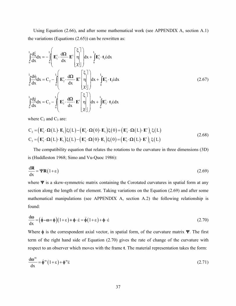
37
Using Equation (2.66), and after some mathematical work (see APPENDIX A, section A.1)
the variations (Equations (2.65)) can be rewritten as:
L L Lt t t1 1 1
0 0 0
L L Lt t t
2 2 2 10 0 0
L L Lt t t
3 3 3 10 0 0
d ddx dx dxdx dx
d ddx C dx dxdx dx
d ddx C dx dxdx dx
E E E t
E E E t
E E E t
⎛ ξ ⎞⎡ ⎤ξ ⎜ ⎟⎢ ⎥= − ⋅ ⋅ η + ⋅ ε⎜ ⎟⎢ ⎥
⎜ ⎟⎢ ⎥χ⎣ ⎦⎝ ⎠⎛ ξ ⎞⎡ ⎤
η ⎜ ⎟⎢ ⎥= − ⋅ ⋅ η + ⋅ ε⎜ ⎟⎢ ⎥⎜ ⎟⎢ ⎥χ⎣ ⎦⎝ ⎠⎛ ξ ⎞⎡ ⎤
χ ⎜ ⎟⎢ ⎥= − ⋅ ⋅ η + ⋅ ε⎜ ⎟⎢ ⎥⎜ ⎟⎢ ⎥χ⎣ ⎦⎝ ⎠
∫ ∫ ∫
∫ ∫ ∫
∫ ∫ ∫
Ω
Ω
Ω
(2.67)
where C2 and C3 are:
( )( ) ( ) ( )( ) ( ) ( )( ) ( )( )( ) ( ) ( )( ) ( ) ( )( ) ( )
t t t t2 2 1 2 1 2 1
t t t t3 3 1 3 1 3 1
C L L 0 0 L L
C L L 0 0 L L
E E E E E E
E E E E E E
= ⋅ ⋅ ξ − ⋅ ⋅ ξ = ⋅ ⋅ ξ
= ⋅ ⋅ ξ − ⋅ ⋅ ξ = ⋅ ⋅ ξ
Ω Ω Ω
Ω Ω Ω (2.68)
The compatibility equation that relates the rotations to the curvature in three dimensions (3D)
is (Huddleston 1968; Simo and Vu-Quoc 1986):
( )d 1dxR R= + εΨ (2.69)
where Ψ is a skew-symmetric matrix containing the Corotated curvatures in spatial form at any
section along the length of the element. Taking variations on the Equation (2.69) and after some
mathematical manipulations (see APPENDIX A, section A.2) the following relationship is
found:
( )( ) ( )d 1 1dx
-= × + ε ⋅ε = + ε + ⋅εω
φ ω φ + φ φ φ (2.70)
Where φ is the correspondent axial vector, in spatial form, of the curvature matrix Ψ. The first
term of the right hand side of Equation (2.70) gives the rate of change of the curvature with
respect to an observer which moves with the frame t. The material representation takes the form:
( )m
m md 1dx
= + ε + εω
φ φ (2.71)
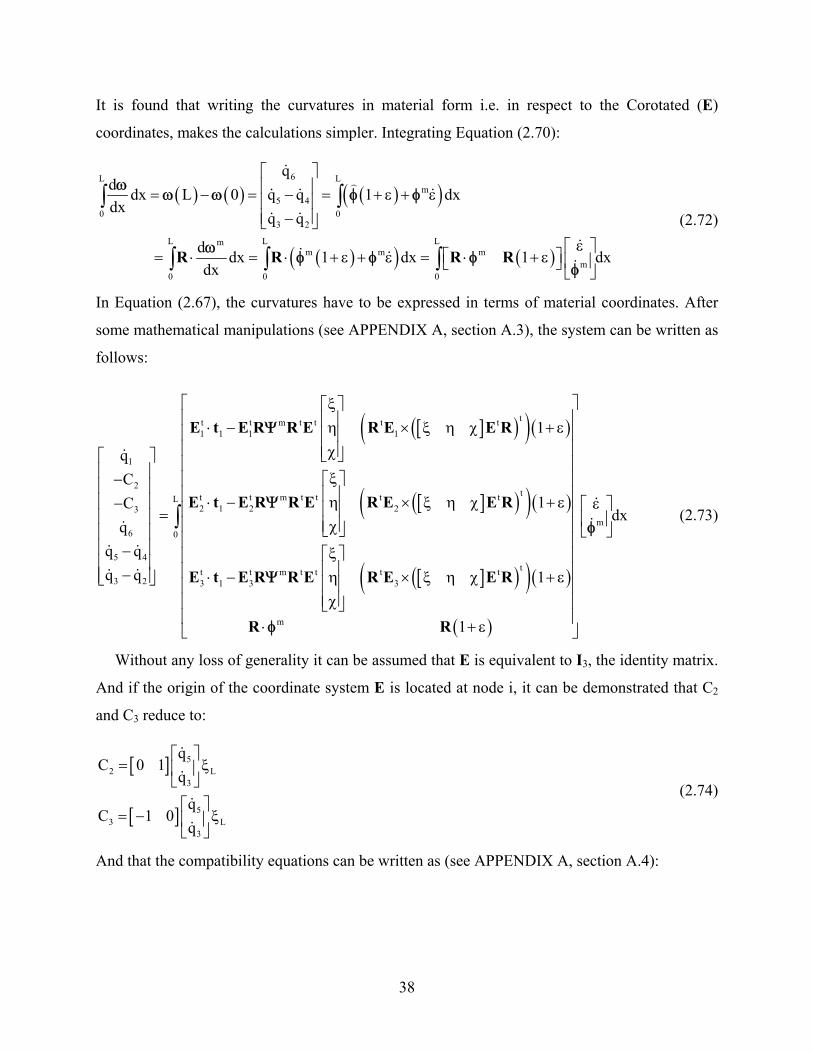
38
It is found that writing the curvatures in material form i.e. in respect to the Corotated (E)
coordinates, makes the calculations simpler. Integrating Equation (2.70):
( ) ( ) ( )( )
( )( ) ( )
6L Lm
5 40 0
3 2
L L Lmm m m
m0 0 0
qd dx L 0 q q 1 dxdx
q q
d dx 1 dx 1 dxdx
R R R R
⎡ ⎤⎢ ⎥= − = − = + ε + ε⎢ ⎥⎢ ⎥−⎣ ⎦
ε⎡ ⎤⎡ ⎤= ⋅ = ⋅ + ε + ε = ⋅ + ε ⎢ ⎥⎣ ⎦ ⎣ ⎦
∫ ∫
∫ ∫ ∫
ωω ω φ φ
ωφ φ φ
φ
(2.72)
In Equation (2.67), the curvatures have to be expressed in terms of material coordinates. After
some mathematical manipulations (see APPENDIX A, section A.3), the system can be written as
follows:
[ ]( )( )( )
[ ]( )( )( )
[ ]( )( )( )
( )
tt t m t t t t1 1 1 1
1
2tt t m t t t t
2 1 2 23
6
5 4tt t m t t t t
3 2 3 1 3 3
m
1
qC
1Cq
q qq q 1
1
E t E R R E R E E R
E t E R R E R E E R
E t E R R E R E E R
R R
⎡ ξ⎡ ⎤⎢ ⎢ ⎥⋅ − η × ξ η χ + ε⎢ ⎢ ⎥⎢ ⎢ ⎥χ⎣ ⎦⎡ ⎤ ⎢⎢ ⎥ ξ− ⎡ ⎤⎢⎢ ⎥ ⎢ ⎥⎢ ⋅ − η × ξ η χ + ε⎢ ⎥− ⎢ ⎥⎢=⎢ ⎥ ⎢ ⎥⎢ χ⎣ ⎦⎢ ⎥
⎢ ⎥− ξ⎡ ⎤⎢ ⎥ ⎢ ⎥−⎢ ⎥ ⋅ − η × ξ η χ + ε⎣ ⎦ ⎢ ⎥⎢ ⎥χ⎣ ⎦
⋅ + ε⎣
Ψ
Ψ
Ψ
φ
L
m0
dx
⎤⎥⎥⎥⎥⎥⎥ ε⎡ ⎤⎥ ⎢ ⎥⎥ ⎣ ⎦
⎢ ⎥⎢ ⎥⎢ ⎥⎢ ⎥⎢ ⎥⎢ ⎥
⎦
∫ φ (2.73)
Without any loss of generality it can be assumed that E is equivalent to I3, the identity matrix.
And if the origin of the coordinate system E is located at node i, it can be demonstrated that C2
and C3 reduce to:
[ ]
[ ]
52 L
3
53 L
3
qC 0 1
q
qC 1 0
q
⎡ ⎤= ξ⎢ ⎥
⎣ ⎦⎡ ⎤
= − ξ⎢ ⎥⎣ ⎦
(2.74)
And that the compatibility equations can be written as (see APPENDIX A, section A.4):
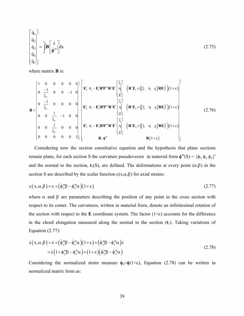
39
1
2 L
3 m0
4
5
qqq dxqq
B
⎡ ⎤⎢ ⎥⎢ ⎥ ε⎡ ⎤⎢ ⎥ = ⎢ ⎥⎢ ⎥ ⎣ ⎦⎢ ⎥⎢ ⎥⎣ ⎦
∫ φ (2.75)
where matrix B is:
[ ]( )( )( )
[ ]( )( )( )
tt t m t t t1 1 1 1
L
tt t m t t t2 1 2 2L
L
t t m t t3 1 3
L
1 0 0 0 0 0110 0 0 1 0
10 0 0 0 01
10 0 1 0 0
10 0 0 0 0
0 0 0 0 0 1
E t E R R E R E RE
E t E R R E R E REB
E t E R R E
ξ⎡ ⎤⎡ ⎤ ⎢ ⎥⎢ ⎥ ⋅ − η × ξ η χ + ε− ⎢ ⎥⎢ ⎥− ⎢ ⎥χ⎣ ⎦ξ⎢ ⎥⎢ ⎥ ξ⎡ ⎤−⎢ ⎥ ⎢ ⎥⎢ ⎥ ⋅ − η × ξ η χ + εξ ⎢ ⎥= ⋅⎢ ⎥ ⎢ ⎥χ⎣ ⎦⎢ ⎥−⎢ ⎥ξ ξ⎡ ⎤⎢ ⎥ ⎢ ⎥⋅ − η⎢ ⎥ ⎢ ⎥⎢ ⎥ξ ⎢χ⎣ ⎦⎢ ⎥⎢ ⎥⎣ ⎦
Ψ
Ψ
Ψ [ ]( )( )( )
( )
tt3
m
1
1
R E RE
R R
⎡ ⎤⎢ ⎥⎢ ⎥⎢ ⎥⎢ ⎥⎢ ⎥⎢ ⎥⎢ ⎥⎢ ⎥⎢ ⎥⎢ ⎥⎢ ⎥× ξ η χ + ε⎢ ⎥
⎥⎢ ⎥⎢ ⎥
⋅ + ε⎢ ⎥⎣ ⎦φ
(2.76)
Considering now the section constitutive equation and the hypothesis that plane sections
remain plane, for each section S the curvature pseudovector in material form φm(S) = φx φy φzt
and the normal to the section, t1(S), are defined. The deformations at every point (α,β) in the
section S are described by the scalar function ε(x,α,β) for axial strains:
( ) ( )( )m my zx, , 1ε α β = ε + φ β − φ α + ε (2.77)
where α and β are parameters describing the position of any point in the cross section with
respect to its center. The curvatures, written in material form, denote an infinitesimal rotation of
the section with respect to the E coordinate system. The factor (1+ε) accounts for the difference
in the chord elongation measured along the normal to the section (t1). Taking variations of
Equation (2.77):
( ) ( )( ) ( )( ) ( )( )
m m m my z y z
m m m my z y z
x, , 1
1 1
ε α β = ε + φ β − φ α + ε + φ β − φ α ε
= ε + φ β − φ α + + ε φ β − φ α (2.78)
Considering the normalized strain measure φn=φ(1+ε), Equation (2.78) can be written in
normalized matrix form as:
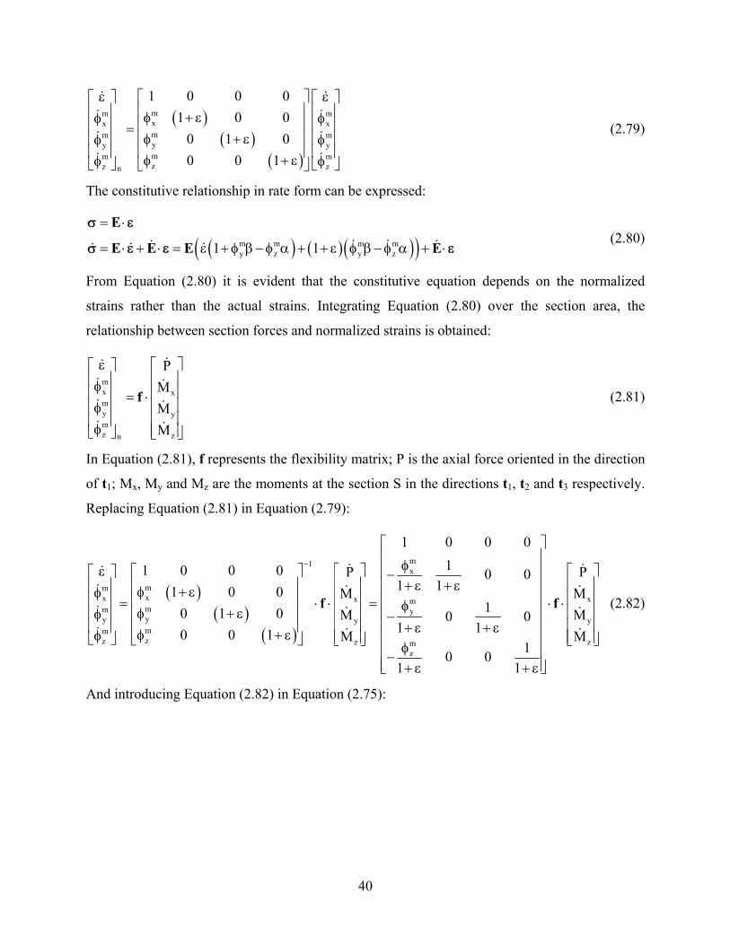
40
( )( )
( )
mm mxx xmm myy ymm mzz zn
1 0 0 01 0 0
0 1 00 0 1
ε ε⎡ ⎤⎡ ⎤ ⎡ ⎤⎢ ⎥⎢ ⎥ ⎢ ⎥φ + εφ φ⎢ ⎥⎢ ⎥ ⎢ ⎥=⎢ ⎥⎢ ⎥ ⎢ ⎥φ + εφ φ⎢ ⎥⎢ ⎥ ⎢ ⎥φ + εφ φ⎣ ⎦ ⎣ ⎦⎣ ⎦
(2.79)
The constitutive relationship in rate form can be expressed:
( ) ( )( )( )m m m my z y z1 1
E
E E E E
= ⋅
= ⋅ + ⋅ = ε + φ β − φ α + + ε φ β − φ α + ⋅
σ ε
σ ε ε ε (2.80)
From Equation (2.80) it is evident that the constitutive equation depends on the normalized
strains rather than the actual strains. Integrating Equation (2.80) over the section area, the
relationship between section forces and normalized strains is obtained:
mx xmy ymz zn
PMMM
f
ε ⎡ ⎤⎡ ⎤⎢ ⎥⎢ ⎥φ ⎢ ⎥⎢ ⎥ = ⋅⎢ ⎥⎢ ⎥φ⎢ ⎥⎢ ⎥φ ⎢ ⎥⎣ ⎦ ⎣ ⎦
(2.81)
In Equation (2.81), f represents the flexibility matrix; P is the axial force oriented in the direction
of t1; Mx, My and Mz are the moments at the section S in the directions t1, t2 and t3 respectively.
Replacing Equation (2.81) in Equation (2.79):
( )( )
( )
m1x
mmxx x xmmm yyy y ymmzz z zm
z
1 0 0 011 0 0 0 P P0 0
1 11 0 0 M M10 1 0 M M0 0
1 10 0 1 M M10 0
1 1
f f
−
⎡ ⎤⎢ ⎥φ⎢ ⎥ε ⎡ ⎤ ⎡ ⎤⎡ ⎤⎡ ⎤ −⎢ ⎥⎢ ⎥ ⎢ ⎥⎢ ⎥ + ε + ε⎢ ⎥ φ + εφ ⎢ ⎥⎢ ⎥ ⎢ ⎥⎢ ⎥⎢ ⎥ = ⋅ ⋅ = ⋅ ⋅φ⎢ ⎥⎢ ⎥ ⎢ ⎥⎢ ⎥⎢ ⎥ φ + εφ −⎢ ⎥⎢ ⎥ ⎢ ⎥⎢ ⎥⎢ ⎥ + ε + εφ + εφ ⎢ ⎥ ⎢ ⎥⎣ ⎦ ⎢ ⎥⎣ ⎦ ⎣ ⎦ ⎣ ⎦φ⎢ ⎥−⎢ ⎥+ ε + ε⎣ ⎦
(2.82)
And introducing Equation (2.82) in Equation (2.75):
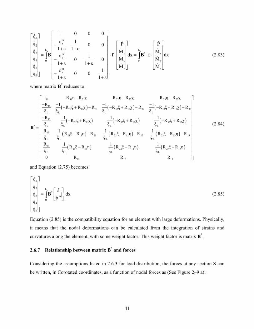
41
1mx
2L L
3 x xmy
4 y y0 0
5 z zmz
6
1 0 0 0q1q P P0 0
1 1q M Mdx dx1q M M0 0
1 1q M M10 0q
1 1
*B f B f
⎡ ⎤⎡ ⎤ ⎢ ⎥⎢ ⎥ φ⎢ ⎥ ⎡ ⎤ ⎡ ⎤−⎢ ⎥ ⎢ ⎥ ⎢ ⎥ ⎢ ⎥+ ε + ε⎢ ⎥ ⎢ ⎥ ⎢ ⎥ ⎢ ⎥= ⋅ ⋅ = ⋅ ⋅⎢ ⎥ φ⎢ ⎥ ⎢ ⎥ ⎢ ⎥−⎢ ⎥ ⎢ ⎥ ⎢ ⎥ ⎢ ⎥+ ε + ε⎢ ⎥ ⎢ ⎥ ⎢ ⎥⎢ ⎥ ⎣ ⎦ ⎣ ⎦⎢ ⎥ φ⎢ ⎥−⎢ ⎥⎣ ⎦ ⎢ ⎥+ ε + ε⎣ ⎦
∫ ∫ (2.83)
where matrix B* reduces to:
( ) ( ) ( )
( ) ( ) ( )
( ) ( ) ( )
11 31 21 32 22 33 23
1231 11 31 32 12 32 33 13 33
L L L L
1231 11 32 12 33 13
L L L L
1321 11 21 22 12 22 23 13 23
L L L L
13
L
t R R R R R RR 1 1 1R R R R R R R R R
R 1 1 1R R R R R R
R 1 1 1R R R R R R R R R
R 1
*B
η − χ η − χ η − χ− − − −
− ξ + χ − − ξ + χ − − ξ + χ −ξ ξ ξ ξ
− − − −− ξ + χ − ξ + χ − ξ + χ
ξ ξ ξ ξ=
ξ − η − ξ − η − ξ − η −ξ ξ ξ ξ
ξ( ) ( ) ( )21 11 22 12 23 13
L L L
11 12 13
1 1R R R R R R
0 R R R
⎡ ⎤⎢ ⎥⎢ ⎥⎢ ⎥⎢ ⎥⎢ ⎥⎢ ⎥⎢ ⎥⎢ ⎥⎢ ⎥⎢ ⎥⎢ ⎥ξ − η ξ − η ξ − η⎢ ⎥ξ ξ ξ⎢ ⎥⎢ ⎥⎣ ⎦
(2.84)
and Equation (2.75) becomes:
1
2 L
3 m0 n
4
5
qqq dxqq
*B
⎡ ⎤⎢ ⎥⎢ ⎥ ε⎡ ⎤⎢ ⎥ = ⎢ ⎥⎢ ⎥ ⎣ ⎦⎢ ⎥⎢ ⎥⎣ ⎦
∫ φ (2.85)
Equation (2.85) is the compatibility equation for an element with large deformations. Physically,
it means that the nodal deformations can be calculated from the integration of strains and
curvatures along the element, with some weight factor. This weight factor is matrix B*.
2.6.7 Relationship between matrix B* and forces
Considering the assumptions listed in 2.6.3 for load distribution, the forces at any section S can
be written, in Corotated coordinates, as a function of nodal forces as (See Figure 2–9 a):
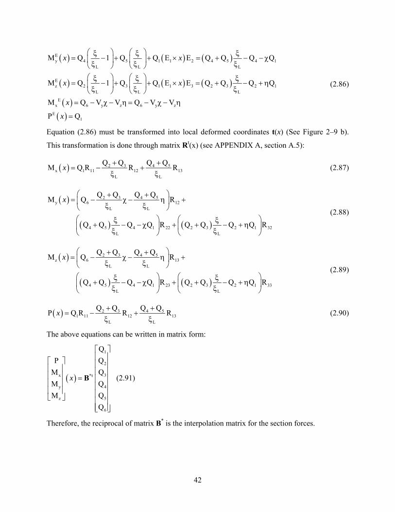
42
( ) ( ) ( )
( ) ( ) ( )
( )( )
Ey 4 5 1 1 2 4 5 4 1
L L L
Ez 2 3 1 1 3 2 3 2 1
L L L
Ex 6 y z 6 y z
E1
M Q 1 Q Q E E Q Q Q Q
M Q 1 Q Q E E Q Q Q Q
M Q V V Q V V
P Q
⎛ ⎞ ⎛ ⎞ξ ξ ξ= − + + × = + − − χ⎜ ⎟ ⎜ ⎟ξ ξ ξ⎝ ⎠ ⎝ ⎠
⎛ ⎞ ⎛ ⎞ξ ξ ξ= − + + × = + − + η⎜ ⎟ ⎜ ⎟ξ ξ ξ⎝ ⎠ ⎝ ⎠= − χ − η = − χ − η
=
x x
x x
x
x
(2.86)
Equation (2.86) must be transformed into local deformed coordinates t(x) (See Figure 2–9 b).
This transformation is done through matrix Rt(x) (see APPENDIX A, section A.5):
( ) 2 3 4 5x 1 11 12 13
L L
Q Q Q QM Q R R R+ += − +
ξ ξx (2.87)
( )
( ) ( )
2 3 4 5y 6 12
L L
4 5 4 1 22 2 3 2 1 32L L
Q Q Q QM Q R
Q Q Q Q R Q Q Q Q R
⎛ ⎞+ += − χ − η +⎜ ⎟ξ ξ⎝ ⎠
⎛ ⎞ ⎛ ⎞ξ ξ+ − − χ + + − + η⎜ ⎟ ⎜ ⎟ξ ξ⎝ ⎠ ⎝ ⎠
x (2.88)
( )
( ) ( )
2 3 4 5z 6 13
L L
4 5 4 1 23 2 3 2 1 33L L
Q Q Q QM Q R
Q Q Q Q R Q Q Q Q R
⎛ ⎞+ += − χ − η +⎜ ⎟ξ ξ⎝ ⎠
⎛ ⎞ ⎛ ⎞ξ ξ+ − − χ + + − + η⎜ ⎟ ⎜ ⎟ξ ξ⎝ ⎠ ⎝ ⎠
x (2.89)
( ) 2 3 4 51 11 12 13
L L
Q Q Q QP Q R R R+ += − +
ξ ξx (2.90)
The above equations can be written in matrix form:
( )
1
2
3x *t
4y
5z
6
QQPQMQMQMQ
B
⎡ ⎤⎢ ⎥⎡ ⎤ ⎢ ⎥⎢ ⎥ ⎢ ⎥⎢ ⎥ = ⎢ ⎥⎢ ⎥ ⎢ ⎥⎢ ⎥ ⎢ ⎥⎣ ⎦ ⎢ ⎥⎢ ⎥⎣ ⎦
x (2.91)
Therefore, the reciprocal of matrix B* is the interpolation matrix for the section forces.
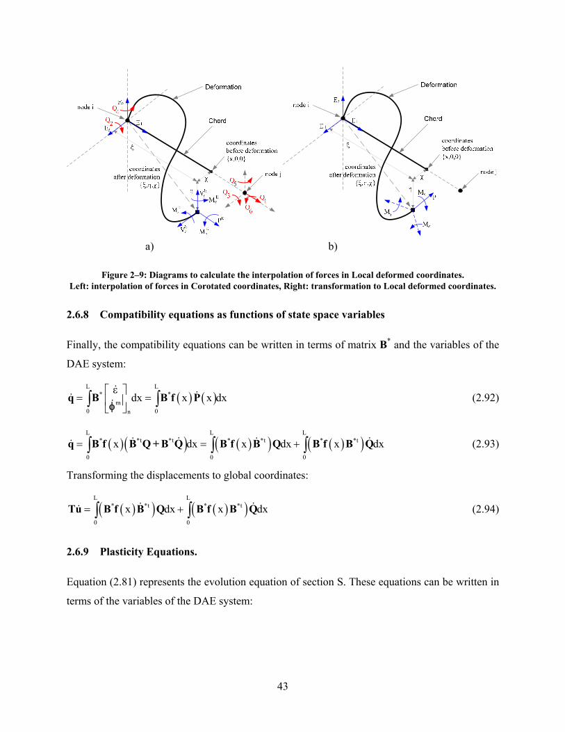
43
Figure 2–9: Diagrams to calculate the interpolation of forces in Local deformed coordinates. Left: interpolation of forces in Corotated coordinates, Right: transformation to Local deformed coordinates.
2.6.8 Compatibility equations as functions of state space variables
Finally, the compatibility equations can be written in terms of matrix B* and the variables of the
DAE system:
( ) ( )L L
* *m
0 0n
dx x x dxq B B f Pε⎡ ⎤
= =⎢ ⎥⎣ ⎦
∫ ∫φ (2.92)
( )( ) ( )( ) ( )( )L L L
* *t *t * *t * *t
0 0 0
x dx x dx x dxq B f B Q + B Q B f B Q B f B Q= = +∫ ∫ ∫ (2.93)
Transforming the displacements to global coordinates:
( )( ) ( )( )L L
* *t * *t
0 0
x dx x dxTu B f B Q B f B Q= +∫ ∫ (2.94)
2.6.9 Plasticity Equations.
Equation (2.81) represents the evolution equation of section S. These equations can be written in
terms of the variables of the DAE system:
a) b)
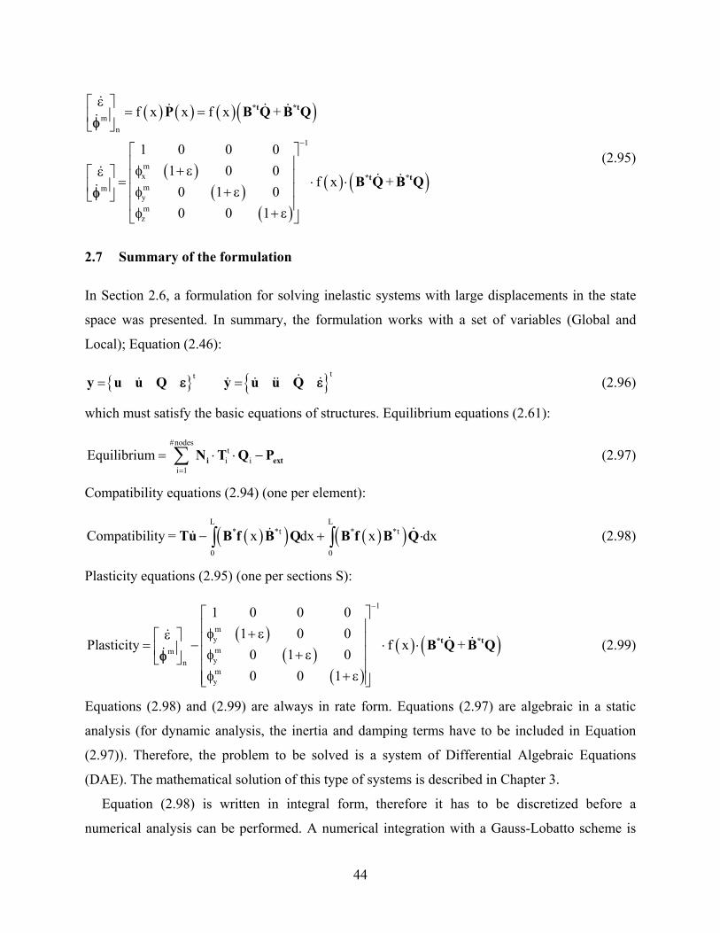
44
( ) ( ) ( )( )
( )( )
( )
( ) ( )
mn
1
mxmmymz
f x x f x +
1 0 0 01 0 0
f x +0 1 00 0 1
*t *t
*t *t
P B Q B Q
B Q B Q
−
ε⎡ ⎤= =⎢ ⎥
⎣ ⎦
⎡ ⎤⎢ ⎥φ + εε⎡ ⎤ ⎢ ⎥= ⋅ ⋅⎢ ⎥ ⎢ ⎥φ + ε⎣ ⎦⎢ ⎥φ + ε⎣ ⎦
φ
φ
(2.95)
2.7 Summary of the formulation
In Section 2.6, a formulation for solving inelastic systems with large displacements in the state
space was presented. In summary, the formulation works with a set of variables (Global and
Local); Equation (2.46):
tt y u u Q y u u Q= =ε ε (2.96)
which must satisfy the basic equations of structures. Equilibrium equations (2.61):
#nodest
i ii 1
Equilibrium i extN T Q P=
= ⋅ ⋅ −∑ (2.97)
Compatibility equations (2.94) (one per element):
( )( ) ( )( )L L
* *t * *t
0 0
Compatibility = x dx x dxTu B f B Q B f B Q− + ⋅∫ ∫ (2.98)
Plasticity equations (2.95) (one per sections S):
( )( )
( )
( ) ( )
1
mymmynmy
1 0 0 01 0 0
Plasticity f x +0 1 00 0 1
*t *tB Q B Q
−⎡ ⎤⎢ ⎥φ + εε⎡ ⎤ ⎢ ⎥= − ⋅ ⋅⎢ ⎥ ⎢ ⎥φ + ε⎣ ⎦ ⎢ ⎥φ + ε⎢ ⎥⎣ ⎦
φ (2.99)
Equations (2.98) and (2.99) are always in rate form. Equations (2.97) are algebraic in a static
analysis (for dynamic analysis, the inertia and damping terms have to be included in Equation
(2.97)). Therefore, the problem to be solved is a system of Differential Algebraic Equations
(DAE). The mathematical solution of this type of systems is described in Chapter 3.
Equation (2.98) is written in integral form, therefore it has to be discretized before a
numerical analysis can be performed. A numerical integration with a Gauss-Lobatto scheme is

45
adopted because it makes use of the values at the nodes, which are known state variables. Thus, a
number of points, “Integration Points” are defined along the length of the member. At these
Integration Points the total strains are known at each time step (because they are local state
variables) and the plasticity equations are evaluated. Thus, matrix B* and its rate are evaluated at
each Integration Point and therefore the following variables need to be interpolated along the
length of the element: coordinates and coordinate rates; rotations and rotation rates (or spins).
These values are only known at the nodes. Details of the implemented interpolation scheme are
presented in Chapter 3.
Once all the variables are known, the equations are evaluated and the residuals are compared
to the pre-defined error tolerance. If the residuals are smaller than the tolerance, the values for
the step are accepted and a new step is attempted. When the errors are large, the step size is
reduced and the step is recalculated.

47
SECTION 3
NUMERICAL IMPLEMENTATION OF THE FORMULATION
3.1 Introduction.
The formulation developed in Chapter 2 results in a set of Differential Algebraic Equations
(DAE). The unknown variables the system is solved for are: displacements and velocities at the
nodes, local Corotated forces of all elements and strains and curvatures along the length of each
element. The set of equations are: global equilibrium at all nodes, compatibility conditions at
each element and plasticity equations along the length of the member. From this set of equations,
in a dynamic analysis, only the equilibrium equations for all DOFs with no associated mass are
algebraic or, in a static analysis, all the equilibrium equations are algebraic. The compatibility
and plasticity equations are always differential. This set of equations can be solved with a DAE
solver. Based on recent research on DAE solutions (Brenan et al. 1989), researchers at the
Lawrence Livermore National Laboratory (LLNL) have developed a mathematical software
called “Implicit Differential Algebraic” (IDA) capable of solving such systems (Hindmarsh and
Serban 2006). The present chapter summarizes the procedure implemented in IDA.
This Chapter also includes a step by step summary of the numerical implementation of the
procedure presented in Chapter 2 along with the assumption, approximations and interpolation
functions used.
3.2 Solution of DAE equations
As explained in Chapter 2, the equations of equilibrium, compatibility and plasticity form a DAE
system. In general such system can be written as:
( )t, , 0f y y = (3.1)
where f(·) represents a function where the set of equations are evaluated, t is an independent
variable (time), y is the vector of variables. In a DAE system, the rates of the variables are also
variables in the system and thus their values are known at every time step.
In order to solve this problem, a set of initial conditions must be known:
( )( )
0 0
0 0
t
t
y y
y y
=
= (3.2)
48
where t0 is the initial time and y0 is the vector of the variables evaluated at time t0. This set must
be consistent i.e. it has to satisfy Equation (3.1):
( )0 0 0t , ,f y y 0= (3.3)
The system in Equation (3.1) is coupled and singular due to the algebraic components. A
measure of the singularity of the problem is the index, which counts the number of times the
system must be differentiated with respect to t in order to determine the rate of y explicitly as a
function of y and t. In other words, to obtain a set of Ordinary Differential Equations (ODE) of
the form:
( )g t,y = y (3.4)
Algorithms exist to solve systems like Equation (3.1) of index 1, however problems of higher
index don’t have a simple numerical solution yet. In a structural problem, the equations of static
equilibrium are algebraic:
k u P⋅ = (3.5)
Writing Equation (3.5) in the state space with y1 = u and y2 = Q:
2
1 2
y Pk y y
=⋅ =
(3.6)
The algebraic equation in the set of Equations (3.6) needs to be differentiated only once to
become an explicit ODE:
2
1 2
y Pk y y
=⋅ =
(3.7)
Therefore, the structural problem is a DAE of order 1.
As in any numerical analysis, the values for the variables are approximated:
( )( )
n n
n n
t
t
y y
y y
≈
≈ (3.8)
where yn is the approximated value for the exact evaluation y(tn). DAEs of index 1 are solved
using the Backward Differentiation Formula (BDF), where the rate of y is calculated in terms of
the values for the variable y at tn and at previous times: k
n n n,i n ii 0
h y y −=
⋅ = α ⋅∑ (3.9)
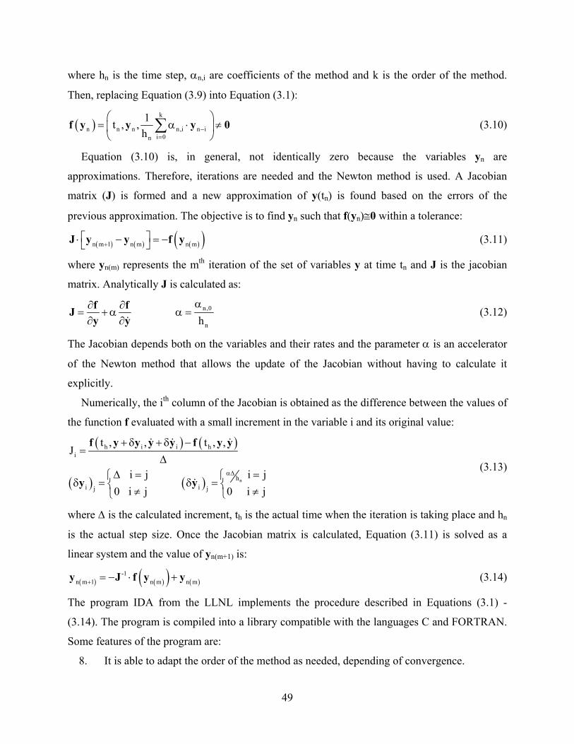
49
where hn is the time step, αn,i are coefficients of the method and k is the order of the method.
Then, replacing Equation (3.9) into Equation (3.1):
( )k
n n n n,i n ii 0n
1t , ,h
f y y y 0−=
⎛ ⎞= α ⋅ ≠⎜ ⎟
⎝ ⎠∑ (3.10)
Equation (3.10) is, in general, not identically zero because the variables yn are
approximations. Therefore, iterations are needed and the Newton method is used. A Jacobian
matrix (J) is formed and a new approximation of y(tn) is found based on the errors of the
previous approximation. The objective is to find yn such that f(yn)≅0 within a tolerance:
( ) ( ) ( )( )n m 1 n m n mJ y y f y+⎡ ⎤⋅ − = −⎣ ⎦ (3.11)
where yn(m) represents the mth iteration of the set of variables y at time tn and J is the jacobian
matrix. Analytically J is calculated as:
n,0
nhf fJ y y
α∂ ∂= + α α =
∂ ∂ (3.12)
The Jacobian depends both on the variables and their rates and the parameter α is an accelerator
of the Newton method that allows the update of the Jacobian without having to calculate it
explicitly.
Numerically, the ith column of the Jacobian is obtained as the difference between the values of
the function f evaluated with a small increment in the variable i and its original value:
( ) ( )
( ) ( ) n
h i i hi
hi ij j
t , , t , ,J
i j i j0 i j 0 i j
f y y y y f y y
y y
α∆
+ δ + δ −=
∆∆ = =⎧ ⎧
δ = δ =⎨ ⎨≠ ≠⎩ ⎩
(3.13)
where ∆ is the calculated increment, th is the actual time when the iteration is taking place and hn
is the actual step size. Once the Jacobian matrix is calculated, Equation (3.11) is solved as a
linear system and the value of yn(m+1) is:
( ) ( )( ) ( )-1
n m 1 n m n my J f y y+ = − ⋅ + (3.14)
The program IDA from the LLNL implements the procedure described in Equations (3.1) -
(3.14). The program is compiled into a library compatible with the languages C and FORTRAN.
Some features of the program are:
8. It is able to adapt the order of the method as needed, depending of convergence.
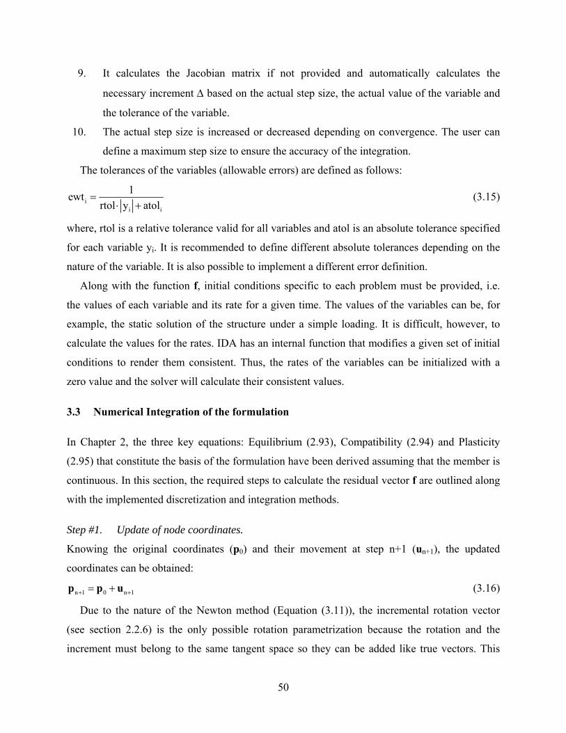
50
9. It calculates the Jacobian matrix if not provided and automatically calculates the
necessary increment ∆ based on the actual step size, the actual value of the variable and
the tolerance of the variable.
10. The actual step size is increased or decreased depending on convergence. The user can
define a maximum step size to ensure the accuracy of the integration.
The tolerances of the variables (allowable errors) are defined as follows:
ii i
1ewtrtol y atol
=⋅ +
(3.15)
where, rtol is a relative tolerance valid for all variables and atol is an absolute tolerance specified
for each variable yi. It is recommended to define different absolute tolerances depending on the
nature of the variable. It is also possible to implement a different error definition.
Along with the function f, initial conditions specific to each problem must be provided, i.e.
the values of each variable and its rate for a given time. The values of the variables can be, for
example, the static solution of the structure under a simple loading. It is difficult, however, to
calculate the values for the rates. IDA has an internal function that modifies a given set of initial
conditions to render them consistent. Thus, the rates of the variables can be initialized with a
zero value and the solver will calculate their consistent values.
3.3 Numerical Integration of the formulation
In Chapter 2, the three key equations: Equilibrium (2.93), Compatibility (2.94) and Plasticity
(2.95) that constitute the basis of the formulation have been derived assuming that the member is
continuous. In this section, the required steps to calculate the residual vector f are outlined along
with the implemented discretization and integration methods.
Step #1. Update of node coordinates.
Knowing the original coordinates (p0) and their movement at step n+1 (un+1), the updated
coordinates can be obtained:
n 1 0 n 1p p u+ += + (3.16)
Due to the nature of the Newton method (Equation (3.11)), the incremental rotation vector
(see section 2.2.6) is the only possible rotation parametrization because the rotation and the
increment must belong to the same tangent space so they can be added like true vectors. This
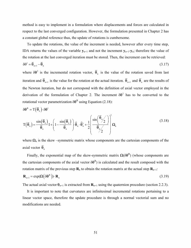
51
method is easy to implement in a formulation where displacements and forces are calculated in
respect to the last converged configuration. However, the formulation presented in Chapter 2 has
a constant global reference thus, the update of rotations is cumbersome.
To update the rotations, the value of the increment is needed, however after every time step,
IDA returns the values of the variable yn+1 and not the increment yn+1-yn; therefore the value of
the rotation at the last converged iteration must be stored. Then, the increment can be retrieved: 1
n 1 n+δθ = −θ θ (3.17)
where δθ1 is the incremental rotation vector, nθ is the value of the rotation saved from last
iteration and n 1+θ is the value for the rotation at the actual iteration. n 1+θ and nθ are the results of
the Newton iteration, but do not correspond with the definition of axial vector employed in the
derivation of the formulation of Chapter 2. The increment δθ1 has to be converted to the
rotational vector parametrization δθR using Equation (2.18):
( )
( ) ( ) ( )
R 1n
2
n
n n tn n n n
nn n
T
sinsin sin 21T I 12
2
δ = ⋅δ
⎛ ⎞⎛ ⎞⎜ ⎟⎜ ⎟⎛ ⎞ ⎝ ⎠⎜ ⎟⎜ ⎟= + − ⋅ ⋅ +
⎜ ⎟ ⎜ ⎟⎝ ⎠ ⎜ ⎟⎝ ⎠
θ θ θ
θθ θ
θ θ θ Ωθθ θ
(3.18)
where Ωn is the skew –symmetric matrix whose components are the cartesian components of the
axial vector nθ
Finally, the exponential map of the skew-symmetric matrix Ω(δθR) (whose components are
the cartesian components of the axial vector δθR) is calculated and the result composed with the
rotation matrix of the previous step Rn to obtain the rotation matrix at the actual step Rn+1:
( )Rn 1 nexp( )R R+ = δ ⋅Ω θ (3.19)
The actual axial vector θn+1 is extracted from Rn+1 using the quaternion procedure (section 2.2.3).
It is important to note that curvatures are infinitesimal incremental rotations pertaining to a
linear vector space, therefore the update procedure is through a normal vectorial sum and no
modifications are needed.
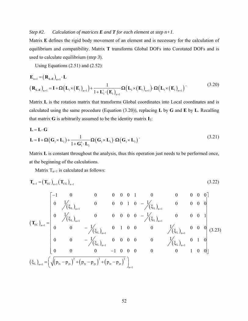
52
Step #2. Calculation of matrices E and T for each element at step n+1.
Matrix E defines the rigid body movement of an element and is necessary for the calculation of
equilibrium and compatibility. Matrix T transforms Global DOFs into Corotated DOFs and is
used to calculate equilibrium (step 3).
Using Equations (2.51) and (2.52):
( )
( ) ( )( ) ( ) ( )( ) ( )( )n 1 n 1
1 1 1 1 1 1tn 1 n 1 n 1 n 11 1 n 1
11
L-E
L-E
E R L
R I L E L E L EL E
+ +
+ + + ++
= ⋅
= + × + × ⋅ ×+ ⋅
Ω Ω Ω. (3.20)
Matrix L is the rotation matrix that transforms Global coordinates into Local coordinates and is
calculated using the same procedure (Equation (3.20)), replacing L by G and E by L. Recalling
that matrix G is arbitrarily assumed to be the identity matrix I3:
( ) ( ) ( )1 1 1 1 1 1t1 1
11
L L G
L I G L G L G LG L
= ⋅
= + × + × ⋅ ×+ ⋅
Ω Ω Ω. (3.21)
Matrix L is constant throughout the analysis, thus this operation just needs to be performed once,
at the beginning of the calculations.
Matrix Tn+1 is calculated as follows:
( ) ( )n 1 EC CGn 1 n 1T T T+ + +
= (3.22)
( )
( ) ( )
( ) ( )
( ) ( )
( ) ( )
( ) ( ) ( ) ( )
L Ln 1 n 1
L Ln 1 n 1EC n 1
L Ln 1 n 1
L Ln 1 n 1
2 2 2
L ix jx iy jy iz jzn 1n 1
1 0 0 0 0 0 1 0 0 0 0 01 10 0 0 0 1 0 0 0 0 0
1 10 0 0 0 0 0 0 0 0 1
1 10 0 0 1 0 0 0 0 0 0
1 10 0 0 0 0 0 0 0 1 0
0 0 0 1 0 0 0 0 0 1 0 0
p p p p p p
T
+ +
+ +
+
+ +
+ +
++
−⎡ ⎤⎢ ⎥
−⎢ ⎥ξ ξ⎢ ⎥⎢ ⎥−ξ ξ⎢ ⎥
= ⎢ ⎥−⎢ ⎥ξ ξ⎢ ⎥
⎢ ⎥−⎢ ⎥ξ ξ⎢ ⎥
−⎢ ⎥⎣ ⎦⎛ ⎞ξ = − + − + −⎜ ⎟⎝ ⎠
(3.23)
53
( )
n 1
n 1CG n 1
n 1
n 1
E 0 0 00 E 0 0
T0 0 E 00 0 0 E
+
++
+
+
⎡ ⎤⎢ ⎥⎢ ⎥=⎢ ⎥⎢ ⎥⎣ ⎦
(3.24)
In Equations (3.23) (ξL)n+1 is the actual length of the element, calculated as the norm of the
vectorial difference between the actual positions of its end nodes pi and pj.
Step #3. Calculate Equilibrium.
Using Equation (2.58), the forces in global coordinates are found:
tn 1 n 1 n 1F T Q+ + += ⋅ (3.25)
In Equation (3.25), the local Corotated forces Qn+1 of each element (extracted from the known
vector yn+1) are transformed into Global Coordinates with the correspondent matrix Tn+1
(calculated in Step #2).
Using Equation (2.59):
( ) ( )#elements
n 1 n 1 n 1i 1
Equilibrium i i extN F P+ + +=
= ⋅ −∑ (3.26)
Step #4. Calculation of deformational rotation matrices at nodes.
In the formulation, the rigid body motion is calculated with matrix E (step #2). To calculate the
compatibility equations, the deformational part of the total rotation is needed because the
equations were deduced with respect to the Corotated system of coordinates.
The directions of the rotational DOFs coincide with the Global reference frame. However,
rotations are measured with respect to the initial configuration. Therefore, the updated rotations
obtained in Step 1 will be rigidly rotated into Local coordinates: Ln 1 n 1L+ += ⋅θ θ (3.27)
where θn+1L is the axial vector of the total rotations at any node with respect to the Local
coordinate system and matrix L was calculated in Step #2. Then, the correspondent rotation
matrix R(θn+1L) is found using the quaternion procedure (section 2.2.3). Finally, the
deformational part of the rotations is obtained using compound rotations:
( ) ( )L td n 1 n 1n 1
R R L E+ ++= ⋅ ⋅θ (3.28)
54
where the product (R L) represents the total rotations in Global coordinates. The product (Rd E)
also represents the total rotations in Global coordinates, but in this case, the rigid body motion is
completely represented by E, thus Rd contains only the deformational part of the rotations.
Equation (3.28) is written in spatial form so that Rd is described with respect to the E system of
coordinates.
Step #5. Calculate the rotational vector associated with the deformational rotation matrix.
The rotational vectors will be needed to interpolate the deformational rotations along the length
of the element.
Using the quaternion procedure (section 2.2.3), the quaternion qd that corresponds to each
deformational rotation matrix found in Step #4 is found:
( ) ( ) ( )( ) ( )( )
( )( ) ( )( ) ( )
( ) ( )( )
d d32 231 1d d d2 40 1
o
d d d d13 31 21 121 1d d4 42 3
o o
R Rq 1 Tr ; q
q
R R R Rq ; q
q q
R−
= ± + = ±
− −= ± = ±
(3.29)
Using the inverse of Equation (2.8), the axial vector θd is found:
( )
1d 0
tdd 1 2 3
d
2 cos q
q q qsin 2
−θ = ×
θθ⎛ ⎞⎜ ⎟
⎝ ⎠
θ = (3.30)
To evaluate the compatibility equations, a discretization procedure is needed to perform a
numerical integration. Thus, a number of “Integration Points” (IP) are selected along the length
of the member according to the Gauss-Lobatto rule (given the number of IPs, it provides the
position and weight of each IP). Matrix B* (Equation (2.82)) and its rate (derived below) are
needed for the calculation of compatibility and plasticity equations. Matrix B* depends on:
• The actual deformed position in respect to the Corotated coordinates at each IP.
• The actual deformational rotation matrix at each IP.
The rate of matrix B* depends on the above quantities plus:
• The rates of the positions at each IP.
• The rates of the deformational rotation matrices (or spins) at each IP.
55
Thus, an interpolation scheme must be implemented for the above 4 quantities. Step 6 to Step 12
detail the procedure to evaluate both matrix B* and its rate.
Step #6. Interpolate the nodal deformational rotations to obtain rotations at the integration
points.
The undeformed coordinates of the IPs are constant and determined by the number of points
considered in the interpolation. With respect to the E coordinate system, located at one of the
nodes, the original coordinates of each integration point (IP) can be described as:
t
ip ipx 0 0x = (3.31)
The rotational vectors at the nodes (θd)i and (θd)j have been obtained in Step #5. To calculate the
values of the rotational vectors along the length of the member, a simplified procedure is
adopted. The interpolation is done independently for each coordinate (r) and the curvatures are
assumed to be constant between two consecutive IPs:
( )
( ) ( )( )
( ) ( ) ( ) ( ) ( ) ( ) ( )( )i
mrr
mr rr r
x xm m
r i r r ip 1 ip ip 1 r ip ipx 0
d sdsd d ds dss s 1dx ds dx dx
x s 1 dx x x x x 1 x=
− −=
θ= φ
θ θ= ⋅ = φ ⋅ = φ + ε
θ = φ ⋅ + ε ⋅ ≈ θ + − ⋅φ + ε∫
(3.32)
Because the deformational axial vectors are known at both nodes, two integrations are
performed: the first starts at node i and the second starts at node j. The final value adopted is the
average of both integration procedures:
( ) ( ) ( ) ( ) ( )( )( ) ( ) ( ) ( ) ( )( )
( ) ( ) ( )
1 1 mdx ip dx i 1 ip ip 1 dx ip ip
2 2 mdx ip dx i 1 ip ip 1 dx ip ip
1 2dx ip dx ip
dx ip
x x x x x 1 x
x x x x x 1 x
x xx
2
− −
+ +
θ = θ + − φ + ε
θ = θ + − φ + ε
θ + θθ =
(3.33)
( ) ( ) ( ) ( ) ( )( )( ) ( ) ( ) ( ) ( )( )
( ) ( ) ( )
1 1 mdy ip dy i 1 ip ip 1 dy ip ip
2 2 mdy ip dy i 1 ip ip 1 dy ip ip
1 2dy ip dy ip
dy ip
x x x x x 1 x
x x x x x 1 x
x xx
2
− −
+ +
θ = θ + − φ + ε
θ = θ + − φ + ε
θ + θθ =
(3.34)
56
( ) ( ) ( ) ( ) ( )( )( ) ( ) ( ) ( ) ( )( )
( ) ( ) ( )
1 1 mdz ip dz i 1 ip ip 1 dz ip ip
2 2 mdz ip dz i 1 ip ip 1 dz ip ip
1 2dz ip dz ip
dz ip
x x x x x 1 x
x x x x x 1 x
x xx
2
− −
+ +
θ = θ + − φ + ε
θ = θ + − φ + ε
θ + θθ =
(3.35)
In Equation (3.33), φm(xip)=φxm(xip) φy
m(xip) φzm(xip)t is the axial vector of material curvatures
at the IP xip. These values are known quantities because they are the local state variables of the
system and can be extracted from the complete vector of variables yn at each step.
Having found the rotational vectors at each IP, the rotation matrices Rd(xip) are obtained, for
each IP, with the quaternion procedure.
Step #7. Calculate the deformed coordinates of the Integration Points.
Upon deformation, the coordinates of the IPs are:
tnewip ip ip ipx = ξ η χ (3.36)
The chord of the element links the deformed positions of its 2 end nodes. Therefore the nodal
coordinates are:
ti
tj L
0 0 0
0 0
x
x
=
= ξ (3.37)
where ξL is the actual length of the chord obtained in Step #2. The coordinates of the IPs are
interpolated using Equation (2.62):
( ) ( ) ( ) ( ) ( )( )( ) ( ) ( ) ( ) ( )( )
( ) ( ) ( )
1 1ip ip 1 ip ip 1 11 ip ip
2 2ip ip 1 ip ip 1 11 ip ip
1 2ip ip
ip
x x x x t x 1 x
x x x x t x 1 x
x xx
2
− −
+ +
ξ = ξ + − + ε
ξ = ξ + − + ε
ξ + ξξ =
(3.38)
( ) ( ) ( ) ( ) ( )( )( ) ( ) ( ) ( ) ( )( )
( ) ( ) ( )
1 1ip ip 1 ip ip 1 12 ip ip
2 2ip ip 1 ip ip 1 12 ip ip
1 2ip ip
ip
x x x x t x 1 x
x x x x t x 1 x
x xx
2
− −
+ +
η = η + − + ε
η = η + − + ε
η + ηη =
(3.39)
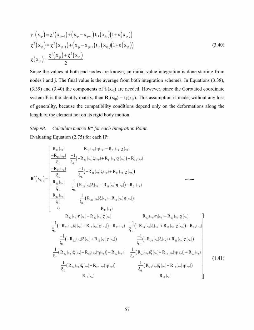
57
( ) ( ) ( ) ( ) ( )( )( ) ( ) ( ) ( ) ( )( )
( ) ( ) ( )
1 1ip ip 1 ip ip 1 13 ip ip
2 2ip ip 1 ip ip 1 13 ip ip
1 2ip ip
ip
x x x x t x 1 x
x x x x t x 1 x
x xx
2
− −
+ +
χ = χ + − + ε
χ = χ + − + ε
χ + χχ =
(3.40)
Since the values at both end nodes are known, an initial value integration is done starting from
nodes i and j. The final value is the average from both integration schemes. In Equations (3.38),
(3.39) and (3.40) the components of t1(xip) are needed. However, since the Corotated coordinate
system E is the identity matrix, then R1(xip) = t1(xip). This assumption is made, without any loss
of generality, because the compatibility conditions depend only on the deformations along the
length of the element not on its rigid body motion.
Step #8. Calculate matrix B* for each Integration Point.
Evaluating Equation (2.75) for each IP:
( )
( ) ( ) ( ) ( ) ( )( ) ( ) ( ) ( ) ( )( ) ( )
( ) ( ) ( ) ( ) ( )( )
( ) ( ) ( ) ( ) ( )( ) ( )
( ) ( ) ( ) ( ) ( )( )
( )
x x x x xip ip ip ip ip
xipx x x x xip ip ip ip ip
xipx x x xip ip ip ip
xipx x x x xip ip ip ip ip
xipx x x xip ip ip ip
xip
11 31 21
1231 11 31
L L
1231 11
L Lip
1321 11 21
L L
1321 11
L L
11
R R RR 1 R R R
R 1 R Rx
R 1 R R R
R 1 R R
0 R
*B
η − χ⎡⎢− −⎢ − ξ + χ −
ξ ξ⎢⎢− −⎢ − ξ + χ⎢ ξ ξ
= ⎢⎢ ξ − η −⎢ ξ ξ⎢
ξ − ηξ ξ
⎣( ) ( ) ( ) ( ) ( ) ( ) ( ) ( )
( ) ( ) ( ) ( )( ) ( ) ( ) ( ) ( ) ( )( ) ( )
( ) ( ) ( )
x x x x x x x xip ip ip ip ip ip ip ip
x x x x x x x x x xip ip ip ip ip ip ip ip ip ip
x x x xip ip ip i
32 22 33 23
32 12 32 33 13 33L L
32 12L
R R R R1 1R R R R R R
1 R R
........
⎢⎢⎢⎢
η − χ η − χ− −
− ξ + χ − − ξ + χ −ξ ξ
−− ξ + χ
ξ( )( ) ( ) ( ) ( ) ( )( )
( ) ( ) ( ) ( )( ) ( ) ( ) ( ) ( ) ( )( ) ( )
( ) ( ) ( ) ( )( ) ( ) ( ) ( ) ( )( )
( ) ( )
x x x xp ip ip ip ip
x x x x x x x x x xip ip ip ip ip ip ip ip ip ip
x x x x x x x xip ip ip ip ip ip ip ip
x xip ip
33 13L
22 12 22 23 13 23L L
22 12 23 13L L
12 13
1 R R
1 1R R R R R R
1 1R R R R
R R
⎤⎥⎥⎥⎥− ⎥− ξ + χ⎥ξ⎥⎥ξ − η − ξ − η −⎥ξ ξ⎥⎥ξ − η ξ − η⎥ξ ξ⎥⎥⎦
(1.41)
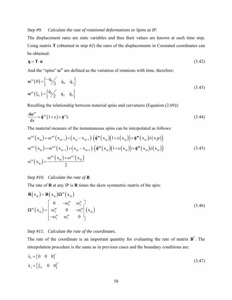
58
Step #9. Calculate the rate of rotational deformations or Spins at IP.
The displacement rates are state variables and thus their values are known at each time step.
Using matrix T (obtained in step #2) the rates of the displacements in Corotated coordinates can
be obtained:
q T u= ⋅ (3.42)
And the “spins” ωm are defined as the variation of rotations with time, therefore:
( ) ( )
m 64 2
m 6L 5 3
q0 q q2
q q q2
−=
ξ =
ω
ω (3.43)
Recalling the relationship between material spins and curvatures (Equation (2.69)):
( )m
m md 1dx
= + ε + εω
φ φ (3.44)
The material measure of the instantaneous spins can be interpolated as follows:
( ) ( ) ( ) ( ) ( )( ) ( ) ( )( )( ) ( ) ( ) ( ) ( )( ) ( ) ( )( )
( ) ( ) ( )
m1 m1ip ip 1 ip ip 1 ip ip ip i
m2 m2ip ip 1 ip ip 1 ip ip ip ip
m1 m2ip ipm
ip
x x x x x 1 x x x p
x x x x x 1 x x x
x xx
2
m m
m m
− −
− +
ω = ω + − ⋅ + ε + ε
ω = ω + − ⋅ + ε + ε
ω + ωω =
φ φ
φ φ (3.45)
Step #10. Calculate the rate of R.
The rate of R at any IP is R times the skew symmetric matrix of the spin:
( ) ( ) ( )
( ) ( )
mip ip ip
m m3 2
m m mip 3 1 ip
m m2 1
x x x
0x 0 x
0
R R=
⎡ ⎤−ω ω⎢ ⎥= ω −ω⎢ ⎥⎢ ⎥−ω ω⎣ ⎦
Ω
Ω (3.46)
Step #11. Calculate the rate of the coordinates.
The rate of the coordinate is an important quantity for evaluating the rate of matrix B*. The
interpolation procedure is the same as in previous cases and the boundary conditions are:
ti
t
j L
x 0 0 0
x 0 0
=
= ξ (3.47)
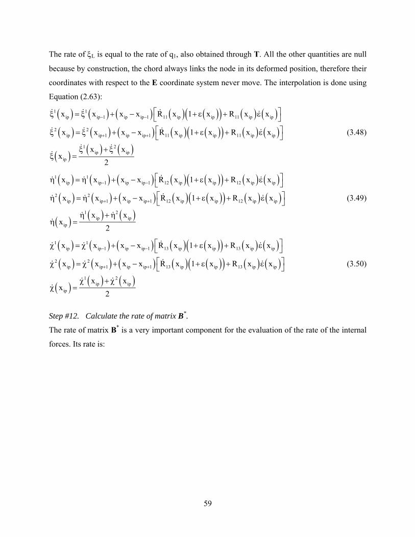
59
The rate of ξL is equal to the rate of q1, also obtained through T. All the other quantities are null
because by construction, the chord always links the node in its deformed position, therefore their
coordinates with respect to the E coordinate system never move. The interpolation is done using
Equation (2.63):
( ) ( ) ( ) ( ) ( )( ) ( ) ( )( ) ( ) ( ) ( ) ( )( ) ( ) ( )
( ) ( ) ( )
1 1ip ip 1 ip ip 1 11 ip ip 11 ip ip
2 2ip ip 1 ip ip 1 11 ip ip 11 ip ip
1 2ip ip
ip
x x x x R x 1 x R x x
x x x x R x 1 x R x x
x xx
2
− −
+ +
⎡ ⎤ξ = ξ + − + ε + ε⎣ ⎦⎡ ⎤ξ = ξ + − + ε + ε⎣ ⎦
ξ + ξξ =
(3.48)
( ) ( ) ( ) ( ) ( )( ) ( ) ( )( ) ( ) ( ) ( ) ( )( ) ( ) ( )
( ) ( ) ( )
1 1ip ip 1 ip ip 1 12 ip ip 12 ip ip
2 2ip ip 1 ip ip 1 12 ip ip 12 ip ip
1 2ip ip
ip
x x x x R x 1 x R x x
x x x x R x 1 x R x x
x xx
2
− −
+ +
⎡ ⎤η = η + − + ε + ε⎣ ⎦⎡ ⎤η = η + − + ε + ε⎣ ⎦
η + ηη =
(3.49)
( ) ( ) ( ) ( ) ( )( ) ( ) ( )( ) ( ) ( ) ( ) ( )( ) ( ) ( )
( ) ( ) ( )
1 1ip ip 1 ip ip 1 13 ip ip 13 ip ip
2 2ip ip 1 ip ip 1 13 ip ip 13 ip ip
1 2ip ip
ip
x x x x R x 1 x R x x
x x x x R x 1 x R x x
x xx
2
− −
+ +
⎡ ⎤χ = χ + − + ε + ε⎣ ⎦⎡ ⎤χ = χ + − + ε + ε⎣ ⎦
χ + χχ =
(3.50)
Step #12. Calculate the rate of matrix B*.
The rate of matrix B* is a very important component for the evaluation of the rate of the internal
forces. Its rate is:
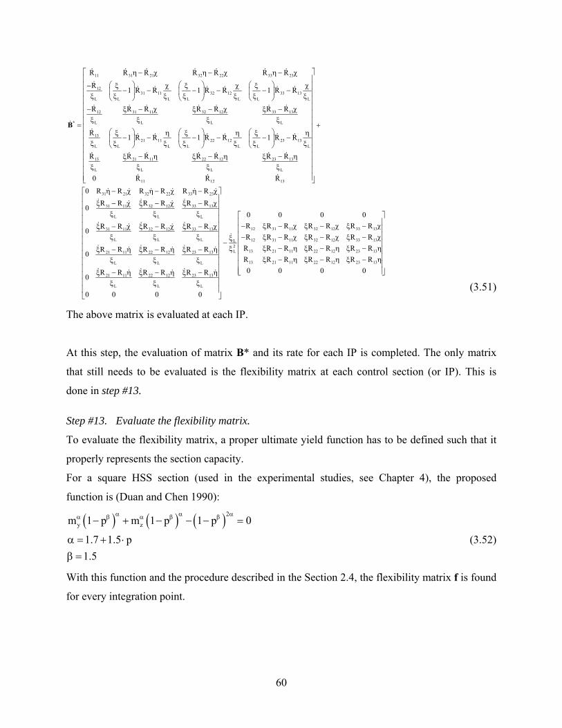
60
11 31 21 32 22 33 23
1231 11 32 12 33 13
L L L L L L L
12 31 11 32 12 33 13
L L L L
1321 11
L L L L
R R R R R R R
R 1 R R 1 R R 1 R R
R R R R R R R
R 1 R R 1
*B
η − χ η − χ η − χ
⎛ ⎞ ⎛ ⎞ ⎛ ⎞− ξ χ ξ χ ξ χ− − − − − −⎜ ⎟ ⎜ ⎟ ⎜ ⎟
ξ ξ ξ ξ ξ ξ ξ⎝ ⎠ ⎝ ⎠ ⎝ ⎠− ξ − χ ξ − χ ξ − χξ ξ ξ ξ
=⎛ ⎞ ⎛ξ η ξ
− − −⎜ ⎟ ⎜ξ ξ ξ ξ⎝ ⎠ ⎝
22 12 23 13L L L
13 21 11 22 12 23 13
L L L L
11 12 13
31 21 32 22 33 23
31 11 32 12
L L
R R 1 R R
R R R R R R R
0 R R R
0 R R R R R RR R R R0
⎡ ⎤⎢ ⎥⎢ ⎥⎢ ⎥⎢ ⎥⎢ ⎥⎢ ⎥⎢ ⎥ +⎢ ⎥⎞ ⎛ ⎞η ξ η⎢ ⎥− − −⎟ ⎜ ⎟⎢ ⎥ξ ξ ξ⎠ ⎝ ⎠⎢ ⎥
ξ − η ξ − η ξ − η⎢ ⎥⎢ ⎥ξ ξ ξ ξ⎢ ⎥⎢ ⎥⎣ ⎦
η − χ η − χ η − χ
ξ − χ ξ − χξ ξ
33 13
L
12 31 11 32 1231 11 32 12 33 13
L L L L2L21 11 22 12 23 13
L L L
21 11 22 12 23 13
L L L
R R0 0 0 0R R R R RR R R R R R0
R R R R R R0
R R R R R R0
0 0 0 0
⎡ ⎤⎢ ⎥
ξ − χ⎢ ⎥⎢ ⎥ξ⎢ ⎥
− ξ − χ ξ − χ ξξ − χ ξ − χ ξ − χ⎢ ⎥⎢ ⎥ξ ξ ξ ξ⎢ ⎥ −⎢ ⎥ ξξ − η ξ − η ξ − η⎢ ⎥
ξ ξ ξ⎢ ⎥⎢ ⎥ξ − η ξ − η ξ − η⎢ ⎥⎢ ⎥ξ ξ ξ⎢ ⎥⎣ ⎦
33 13
12 31 11 32 12 33 13
13 21 11 22 12 23 13
13 21 11 22 12 23 13
R RR R R R R R R
R R R R R R RR R R R R R R0 0 0 0
⎡ ⎤⎢ ⎥− χ⎢ ⎥⎢ ⎥− ξ − χ ξ − χ ξ − χ⎢ ⎥
ξ − η ξ − η ξ − η⎢ ⎥⎢ ⎥ξ − η ξ − η ξ − η⎢ ⎥⎢ ⎥⎣ ⎦
(3.51)
The above matrix is evaluated at each IP.
At this step, the evaluation of matrix B* and its rate for each IP is completed. The only matrix
that still needs to be evaluated is the flexibility matrix at each control section (or IP). This is
done in step #13.
Step #13. Evaluate the flexibility matrix.
To evaluate the flexibility matrix, a proper ultimate yield function has to be defined such that it
properly represents the section capacity.
For a square HSS section (used in the experimental studies, see Chapter 4), the proposed
function is (Duan and Chen 1990):
( ) ( ) ( )2
y zm 1 p m 1 p 1 p 0
1.7 1.5 p1.5
α α αα β α β β− + − − − =
α = + ⋅β =
(3.52)
With this function and the procedure described in the Section 2.4, the flexibility matrix f is found
for every integration point.
61
Finally, all the information required for the evaluation of the equations of compatibility (2.94)
and plasticity (2.95). is available for each IP of every element of the complete structure. This is
done in step #14.
Step #14. Evaluate the compatibility equation for each element.
The compatibility equation in integral form reproduced below:
( ) ( )L L
* *t * *t
0 0
dx dxq B fB Q B fB Q= +∫ ∫ (3.53)
Is discretized as follows:
( )( ) ( )( ) ( )( ) ( )( ) ( )
( )( ) ( )( ) ( )( ) ( )( ) ( )
NIP* *t
n 1 n 1 ip ip ip ip ipn 1 n 1 n 1 n 11NIP
* *tip ip ip ip ipn 1 n 1 n 1 n 1
compatibility x x x x x
x x x x x1
T u - B f B Q W
B f B Q W
+ + + + + +
+ + + +
= ⋅ +∑
∑ (3.54)
Where xip represents the integration point and W(xip) is the weight of that particular point into
the integral according to the Gauss-Lobatto rule. All the other components have been found in
previous steps.
Step #15. Evaluate the plasticity equations at each Integration Point.
Recalling the local evolution equations:
( ) ( ) ( )( )mn
x x x +*t *tf P f B Q B Qε⎡ ⎤
= =⎢ ⎥⎣ ⎦φ
(3.55)
The discretization is:
( )( ) ( )( ) ( )( ) ( )( ) ( )( ) ( )( )( )n 1 n 1 n 1 n 1 n 1
*t *tn ip ip ip ip ip ipn 1
plasticity x - x x x x xf B Q B Q+ + + + ++
= +ε (3.56)
Step #16. Solve the problem.
Once all the equations have been formulated, a call to IDA solver will use the numerical
procedure of section 3.2 to determine the values of the variables y = u Q ε and their rates for a
given time.
3.4 Brief description of “element.exe”
The procedure described in Section 3.3 has been implemented in a computer program called
“Element.exe”. The program is written in C language. The library IDA is already built in the
62
executable file, therefore the user does not need to install it unless a modification to the code is
done.
The program reads an input file of name “InputFile.dat” where the user describes the problem
to be solved, the forcing functions and the initial conditions. The input file’s name cannot be
changed; otherwise the program will not work.
To describe the structural problem, a description of the nodes’ location, the elements’
connectivity and the materials’ parameters are needed. The restraints are assigned to the nodal
DOFs with a 1 or 0 entry (1=restrained, 0=not restrained). A restrained DOF is equivalent to a
fixed support in that DOF. It is not possible to define hinges.
The loading can be a force, a prescribed displacement or a base acceleration. In all the cases,
an independent file must be provided with the time history of the loading (even if the loading is a
single number).
Finally, the Initial Conditions of each node, element and integration point must be provided.
A complete user’s manual is described in APPENDIX B.
63
SECTION 4
EXPERIMENTAL STUDY ON “ZIPPER FRAMES”
4.1 Introduction
An experimental study was needed to generate data for validation of the analytical model
presented in Chapter 2 and Chapter 3. The experimental study on “zipper frames” was an ideal
project because the main failure mode of this type of frame is the inelastic buckling of its braces.
The experimental study on “zipper frames” was part of a multi-site NEES collaborative project
between Georgia Institute of Technology (GT), University of California at Berkeley (UCB),
University of Colorado Boulder (CU) and the University at Buffalo (UB).
The global objectives of the experimental study were to test for the first time the “zipper
frames” concept and to demonstrate that a multi-site experimental study is advantageous and
useful. In addition, the specific objective of the tests at UB was to obtain detailed data about the
three dimensional inelastic behavior of the structure under dynamic loading. This data is
compared to analytical predictions obtained from an analytical “zipper frames” model using the
formulation described in previous Chapters.
The experiments were performed at all the NEES Equipment Sites according to the capacities
of each laboratory, thus at Georgia Institute of Technology quasi-static tests were performed
(Yang et al. 2006a; Yang et al. 2007a), at University of California at Berkeley (Yang et al.
2006b) and University of Colorado Boulder (Stavridis and Shing 2006), hybrid simulations were
carried out and at the University at Buffalo shake table tests were conducted. This chapter
includes only the experimental study done at the University at Buffalo.
4.2 Description of “zipper frames”
Concentrically Braced Frames (CBF) are frames where diagonal elements resist lateral loads
through the development of high axial forces and small moments. The Inverted V-braced frame
or Chevron is the most popular configuration, however it has an important design problem.
When subjected to lateral force, the braces resist in tension and compression. For steel structures,
the capacity in compression is, in general, smaller than the capacity in tension and its value
depends both on the properties of the cross section and the boundary conditions. When the
64
compression capacity is attained, the brace buckles and a plastic hinge develops at midheight. At
this stage, the midpoint of the brace undergoes large displacements, generating even larger
moments. Since the section is fully plastic, the axial capacity of the member reduces to
accommodate a larger moment capacity. On the other hand, the brace in tension attracts even
more load to compensate for the loss in capacity of the compression brace. This generates an
unbalanced vertical force that is transmitted to the beam at its midpoint. Thus, the capacity
design of the beam becomes very costly due to the big section size required to resist such a force.
As a solution for this problem, the idea to link every beam to brace intersection point with
columns, called “zipper columns”, was proposed (Khatib et al. 1988). In this case, when a brace
buckles, the unbalanced vertical force is transmitted to the “zipper column” as tension force. The
column re-distributes the force to the upper story braces as an extra compression force, forcing
the upper story compression brace to buckle. A new unbalanced vertical force is then generated
and transmitted to the next level through another “zipper column”. This mechanism, called the
“zipper mechanism”, will repeat itself at all levels forcing all the compression braces to buckle
almost simultaneously, resulting in a better energy dissipation distribution over the height of the
building and avoiding concentration of damage in just one story. Plastic hinges also develop at
the base of the columns and at the midspan of the beams (Figure 4–1, left). This is the plastic
collapse mechanism of the “zipper frame”. To improve the performance of the frame, the
“suspended zipper frame” concept was proposed (Leon and Yang 2003; Yang 2006). In this
configuration, the last story braces are purposely designed to remain elastic at all times. The
“zipper columns” are designed to yield shortly after the yielding of the brace in tension. This is
achieved by considering only Py (nominal yield force) instead of RyPy (expected yield force) in
the capacity design. The yielding of the “zipper columns” delays the development of plastic
hinges in the beams, which will develop at the beam to column connections instead (Figure 4–1,
right). The objective of the design procedure developed by Yang (Yang 2006; Yang et al. 2007b)
is to ensure that the desired plastic mechanism develops.
On occasions, the “zipper columns” could be loaded in compression, thus the compression
capacity of the selected section must be checked to meet the load requirements. However, in a
properly designed frame, the “zipper columns” are expected to be loaded primarily in tension. A
drawing with the expected distribution of forces in all the elements of the “suspended zipper
frame” is presented in Figure 4–2.
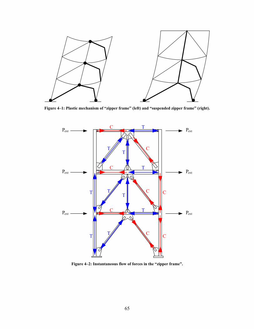
65
Figure 4–1: Plastic mechanism of “zipper frame” (left) and “suspended zipper frame” (right).
TT
T TT
T
T
T
TT
C
C
C
C
C
C
C
CPext
Pext
Pext Pext
Pext
Pext
Figure 4–2: Instantaneous flow of forces in the “zipper frame”.
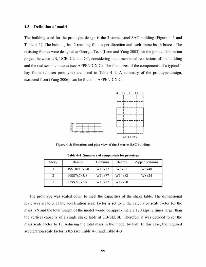
66
4.3 Definition of model
The building used for the prototype design is the 3 stories steel SAC building (Figure 4–3 and
Table 4–1). The building has 2 resisting frames per direction and each frame has 6 braces. The
resisting frames were designed at Georgia Tech (Leon and Yang 2003) for the joint collaboration
project between UB, UCB, CU and GT, considering the dimensional restrictions of the building
and the real seismic masses (see APPENDIX C). The final sizes of the components of a typical 1
bay frame (chosen prototype) are listed in Table 4–1. A summary of the prototype design,
extracted from (Yang 2006), can be found in APPENDIX C.
Figure 4–3: Elevation and plan view of the 3 stories SAC building.
Table 4–1: Summary of components for prototype
Story Braces Columns Beams Zipper columns
3 HSS10x10x5/8 W10x77 W8x21 W8x48
2 HSS7x7x3/8 W10x77 W14x82 W8x24
1 HSS7x7x3/8 W10x77 W12x50
The prototype was scaled down to meet the capacities of the shake table. The dimensional
scale was set to 3. If the acceleration scale factor is set to 1, the calculated scale factor for the
mass is 9 and the total weight of the model would be approximately 120 kips, 2 times larger than
the vertical capacity of a single shake table at UB-SEESL. Therefore it was decided to set the
mass scale factor to 18, reducing the total mass in the model by half. In this case, the required
acceleration scale factor is 0.5 (see Table 4–1 and Table 4–3).
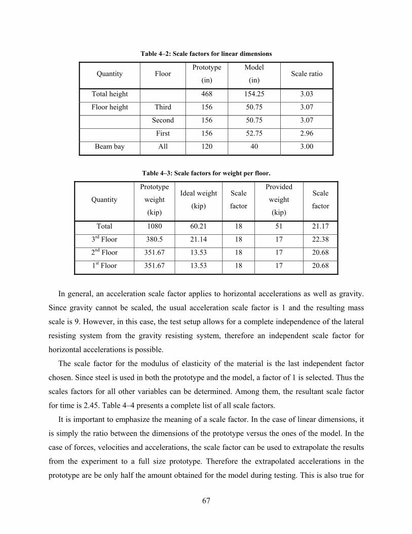
67
Table 4–2: Scale factors for linear dimensions
Quantity Floor Prototype
(in)
Model
(in) Scale ratio
Total height 468 154.25 3.03
Floor height Third 156 50.75 3.07
Second 156 50.75 3.07
First 156 52.75 2.96
Beam bay All 120 40 3.00
Table 4–3: Scale factors for weight per floor.
Quantity
Prototype
weight
(kip)
Ideal weight
(kip)
Scale
factor
Provided
weight
(kip)
Scale
factor
Total 1080 60.21 18 51 21.17
3rd Floor 380.5 21.14 18 17 22.38
2nd Floor 351.67 13.53 18 17 20.68
1st Floor 351.67 13.53 18 17 20.68
In general, an acceleration scale factor applies to horizontal accelerations as well as gravity.
Since gravity cannot be scaled, the usual acceleration scale factor is 1 and the resulting mass
scale is 9. However, in this case, the test setup allows for a complete independence of the lateral
resisting system from the gravity resisting system, therefore an independent scale factor for
horizontal accelerations is possible.
The scale factor for the modulus of elasticity of the material is the last independent factor
chosen. Since steel is used in both the prototype and the model, a factor of 1 is selected. Thus the
scales factors for all other variables can be determined. Among them, the resultant scale factor
for time is 2.45. Table 4–4 presents a complete list of all scale factors.
It is important to emphasize the meaning of a scale factor. In the case of linear dimensions, it
is simply the ratio between the dimensions of the prototype versus the ones of the model. In the
case of forces, velocities and accelerations, the scale factor can be used to extrapolate the results
from the experiment to a full size prototype. Therefore the extrapolated accelerations in the
prototype are be only half the amount obtained for the model during testing. This is also true for
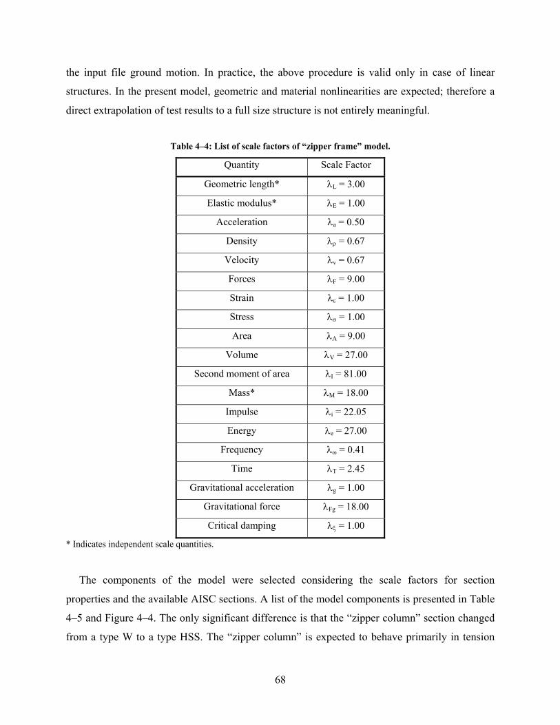
68
the input file ground motion. In practice, the above procedure is valid only in case of linear
structures. In the present model, geometric and material nonlinearities are expected; therefore a
direct extrapolation of test results to a full size structure is not entirely meaningful.
Table 4–4: List of scale factors of “zipper frame” model.
Quantity Scale Factor
Geometric length* λL = 3.00
Elastic modulus* λE = 1.00
Acceleration λa = 0.50
Density λρ = 0.67
Velocity λv = 0.67
Forces λF = 9.00
Strain λε = 1.00
Stress λσ = 1.00
Area λA = 9.00
Volume λV = 27.00
Second moment of area λI = 81.00
Mass* λM = 18.00
Impulse λi = 22.05
Energy λe = 27.00
Frequency λω = 0.41
Time λT = 2.45
Gravitational acceleration λg = 1.00
Gravitational force λFg = 18.00
Critical damping λξ = 1.00
* Indicates independent scale quantities.
The components of the model were selected considering the scale factors for section
properties and the available AISC sections. A list of the model components is presented in Table
4–5 and Figure 4–4. The only significant difference is that the “zipper column” section changed
from a type W to a type HSS. The “zipper column” is expected to behave primarily in tension
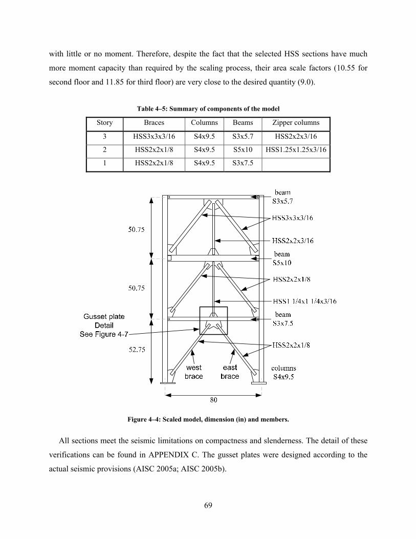
69
with little or no moment. Therefore, despite the fact that the selected HSS sections have much
more moment capacity than required by the scaling process, their area scale factors (10.55 for
second floor and 11.85 for third floor) are very close to the desired quantity (9.0).
Table 4–5: Summary of components of the model
Story Braces Columns Beams Zipper columns
3 HSS3x3x3/16 S4x9.5 S3x5.7 HSS2x2x3/16
2 HSS2x2x1/8 S4x9.5 S5x10 HSS1.25x1.25x3/16
1 HSS2x2x1/8 S4x9.5 S3x7.5
Figure 4–4: Scaled model, dimension (in) and members.
All sections meet the seismic limitations on compactness and slenderness. The detail of these
verifications can be found in APPENDIX C. The gusset plates were designed according to the
actual seismic provisions (AISC 2005a; AISC 2005b).
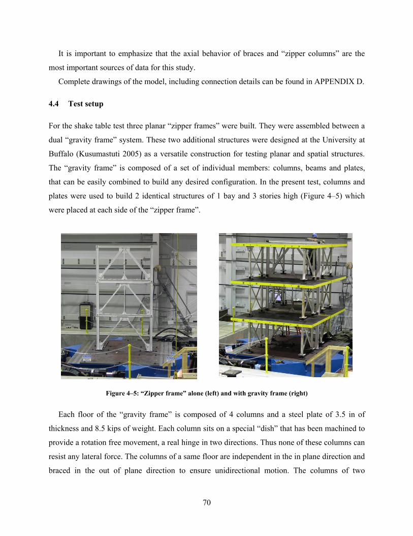
70
It is important to emphasize that the axial behavior of braces and “zipper columns” are the
most important sources of data for this study.
Complete drawings of the model, including connection details can be found in APPENDIX D.
4.4 Test setup
For the shake table test three planar “zipper frames” were built. They were assembled between a
dual “gravity frame” system. These two additional structures were designed at the University at
Buffalo (Kusumastuti 2005) as a versatile construction for testing planar and spatial structures.
The “gravity frame” is composed of a set of individual members: columns, beams and plates,
that can be easily combined to build any desired configuration. In the present test, columns and
plates were used to build 2 identical structures of 1 bay and 3 stories high (Figure 4–5) which
were placed at each side of the “zipper frame”.
Figure 4–5: “Zipper frame” alone (left) and with gravity frame (right)
Each floor of the “gravity frame” is composed of 4 columns and a steel plate of 3.5 in of
thickness and 8.5 kips of weight. Each column sits on a special “dish” that has been machined to
provide a rotation free movement, a real hinge in two directions. Thus none of these columns can
resist any lateral force. The columns of a same floor are independent in the in plane direction and
braced in the out of plane direction to ensure unidirectional motion. The columns of two
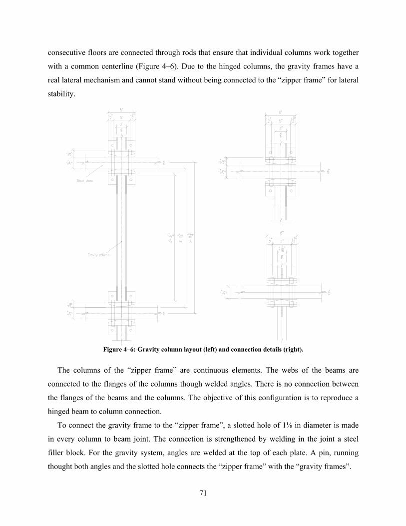
71
consecutive floors are connected through rods that ensure that individual columns work together
with a common centerline (Figure 4–6). Due to the hinged columns, the gravity frames have a
real lateral mechanism and cannot stand without being connected to the “zipper frame” for lateral
stability.
Figure 4–6: Gravity column layout (left) and connection details (right).
The columns of the “zipper frame” are continuous elements. The webs of the beams are
connected to the flanges of the columns though welded angles. There is no connection between
the flanges of the beams and the columns. The objective of this configuration is to reproduce a
hinged beam to column connection.
To connect the gravity frame to the “zipper frame”, a slotted hole of 1⅛ in diameter is made
in every column to beam joint. The connection is strengthened by welding in the joint a steel
filler block. For the gravity system, angles are welded at the top of each plate. A pin, running
thought both angles and the slotted hole connects the “zipper frame” with the “gravity frames”.
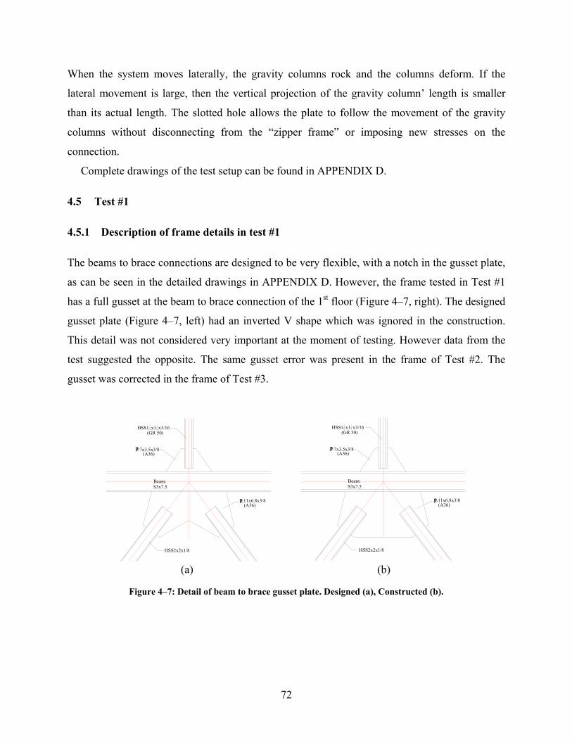
72
HSS2x2x1/8
P
(GR 50)
7x3.5x3/8LP(A36)
Beam: S3x7.5
HSS1 x1 x3/16
L11x6.8x3/8(A36)
(GR 50)
(A36)11x6.8x3/8L
Beam: S3x7.5
(A36)PL7x3.5x3/8
P
HSS2x2x1/8
HSS1 x1 x3/16
When the system moves laterally, the gravity columns rock and the columns deform. If the
lateral movement is large, then the vertical projection of the gravity column’ length is smaller
than its actual length. The slotted hole allows the plate to follow the movement of the gravity
columns without disconnecting from the “zipper frame” or imposing new stresses on the
connection.
Complete drawings of the test setup can be found in APPENDIX D.
4.5 Test #1
4.5.1 Description of frame details in test #1
The beams to brace connections are designed to be very flexible, with a notch in the gusset plate,
as can be seen in the detailed drawings in APPENDIX D. However, the frame tested in Test #1
has a full gusset at the beam to brace connection of the 1st floor (Figure 4–7, right). The designed
gusset plate (Figure 4–7, left) had an inverted V shape which was ignored in the construction.
This detail was not considered very important at the moment of testing. However data from the
test suggested the opposite. The same gusset error was present in the frame of Test #2. The
gusset was corrected in the frame of Test #3.
Figure 4–7: Detail of beam to brace gusset plate. Designed (a), Constructed (b).
(a) (b)
73
4.5.2 Instrumentation
The quantities that needed to be measured were:
- Axial force in the braces.
- Axial force in beams and columns.
- Moments in braces.
- Moments in beam and columns.
- Axial force in “zipper columns”.
Strain gauges were provided in form of half bridges (moments) and full bridges (axial) to read
strains (which are directly related to forces through a stress-strain curve) at particular points
along the members. In braces, axial force measurements were located far from the buckling point
(midheight of the element), at approximately ¼ of its length in all three stories. Meanwhile, in
plane moments were measured only in the first floor in 4 locations near the ends of the elements.
In columns, only in plane moments were measured. The strain gauges were located 4” away
from the beam to column connections. In “zipper columns”, axial strains were recorded at
midheight of the element. In beams, axial forces were measured at quarter length and in plane
moments were measured near the ends but at least 3” away from beam to column and beam to
brace connections.
In addition to strain gauges, accelerometers were attached to each level of the structure to
record lateral accelerations and were also attached to the extremes of the plates to record out of
plane accelerations or possible torsion. Potentiometers were located at each level to record
possible differences in lateral movement between the “zipper frame” and the “gravity frames”.
String potentiometers were placed along each brace and each “zipper column” to record the axial
displacements. They were also placed along the first floor beam to record its midpoint axial and
vertical displacement. Finally, they were attached to each floor to measure the total
displacements with respect to a reference frame.
Finally, the Krypton tracking system was also used during the test. The system consists of a
camera capable of detecting and recording the spatial coordinate of a point in the structure. The
points are defined by LEDs and the coordinate system can be defined anywhere in the range of
view of the camera. For this test, the first story braces were instrumented with 7 LEDs each.
A complete list of instruments and drawings can be found in APPENDIX E.
74
4.5.3 Test Protocol
The chosen ground motion was LA22yy from the SAC set of scaled records for the L.A. area for
the 2% probability of exceedance in 50 years (Somerville et al. 1997). This record corresponds to
1.15 times the Kobe earthquake. The peak ground acceleration (PGA) of the original Kobe
ground motion is 0.8g and the PGA of LA22yy ground motion is 0.92g.
LA22yy was scaled in time according to Table 4–4 reducing its duration to approximate 12
seconds. The amplitude of the motion should be doubled to 1.84g however, the total weight of
the model (51 kips) is very close to the maximum weight limit, therefore the maximum
acceleration the shake table can reproduce is around 1.1g. It is not possible to perform a test with
the 100% amplitude of the scaled LA22yy ground motion.
Since the real capacity of the frame before testing is not well known (only numerical analyses
on an ideal 2D “zipper frame” model were performed before testing); it was decided to perform
several tests amplifying the amplitude of the motion each time: incremental dynamic testing
(IDT).
The sequence in Test #1 was: 0.138g, 0.276g, 0.414g, 0.552g. 0.736g and 0.920g (equivalent
to the 7.5%, 15%, 22.5%, 30%, 40% and 50% of the PGA of the scaled LA22yy ground motion).
For identification purposes, the individual tests are named after the “% PGA” of the original
LA22yy record. Thus for Test #1, the sequence was: “15% LA22yy”, “30% LA22yy”, “45%
LA22yy”, “60% LA22yy”, “80% LA22yy” and “100% LA22yy” .
4.5.4 Test results
4.5.4.1 Test observations and data processing
During the “15% LA22yy” and the “30% LA22yy”, the system remained elastic, as expected.
In the “45% LA22yy”, the west brace in the 1st floor buckled elastically, while the east brace
remained elastic. The buckled brace pulled the 1st floor beam down. As a consequence, both
braces showed permanent compression strains, being those of the buckled brace greater than
those of the elastic one. Braces in the 2nd floor remained elastic. No measurement of importance
was registered in the “zipper column”. The vertical potentiometer was not sensitive enough to
record the beam displacement.
75
During the “60% LA22yy”, both braces in the first floor buckled and yielded, remaining with
an important permanent deformation in tension. Even though the vertical string potentiometer
was not sensitive enough to record the beam movement with accuracy, its sign showed that the
bottom part of the gusset plate moved upwards, therefore, the bottom flange of the beam also
moved upwards, coinciding with the fact that both braces were in tension at the end of the test.
The “zipper column”, again did not record any axial strains of the magnitude of the calculated
unbalanced vertical force from the braces, however it sign showed that it is in tension. Therefore,
the top flange of the beam must have gone down. The only possible explanation for the beam
movement is a rotation.
During the same test, the second floor east brace buckled inelastically, remaining with some
compressive deformation. The time at which the braces on the east side at the first and second
floor level buckled, was exactly the same. Therefore, the second floor brace did not require the
addition of a big unbalanced axial force to buckle.
The second story “zipper column” showed to be engaged but the magnitude of the forces was
very small.
The columns of the first floor both at the base and top showed signs of yielding.
During the “80% LA22yy” and “100% LA22yy” strain gauges at first story level either
exceeded their maximum range or peeled off. At “80% LA22yy” the first story west brace was
severely damaged and reached its axial compression capacity. During the same test, the east
brace still showed buckling behavior. Both braces remained permanently in tension.
Accordingly, the vertical string potentiometer showed that the bottom flange of the beam moved
upwards. This again proves the importance of the rotation of the beam in the global behavior of
the braces. The “zipper column” reached its largest force during this test, due to the fact that the
west brace had already reached its minimum capacity, however the measured magnitude was
again very small compared to the expected value.
The second story braces also buckled, remaining both in compression at the end of the
motion. The beam at the second floor was considerably larger than the beam at the first floor and
can resist the imposed torsion without substantial rotation. For the braces to remain in
compression, the beam must have moved downwards. This is the expected behavior of the beam.
Only at “100% LA22yy” the buckling in the second story braces was large enough to activate the
76
third story “zipper column”. However, even in this case, the readings from strain measurements
are very small, indicating that very small forces were present in the member.
4.5.4.2 Issues identified in test #1
The calibration of the full bridge strain gauges was found to have an error during testing. The
calibration was 2.0 times larger than intended; reaching saturation (10 Volts max.) at 2500
µstrains when the expected value was 5000 µstrains. This is why, at the “80% LA22yy” level
test, the readings from the gauges “saturated” at 2500 µstrains. Thus valuable data from the
behavior of the braces was not properly recorded. This error was corrected in subsequent tests.
The data recorded with the “Krypton”coordinate tracking system presented problems. This
was the first time that this instrument was used in the laboratory. The readings from the first 4
LEDs, numbers 1 to 4 on the west brace were correct, but all others were just a copy of the data
for LED #4. This was due to a saturation of series scanned LEDs. This error was corrected in
subsequent tests.
Moreover, the buckling of the braces occurred out of plane, thus the braces were subjected to
a much larger out of plane moment (which was not recorded) than in plane moment. Although,
the braces are designed such that the axial forces do not produce moments at the connections, in
practice, a real hinge cannot be achieved. Thus, there are always moments at the ends of the
braces and, depending on the gusset plate flexibility, these moments are transmitted to the beam.
Since the braces buckle out of plane, the beam is subjected to torsion.
Preliminary numerical analysis and the design of the frame itself were done in two
dimensions. Although the final design of the gusset plates considered the fact that the braces
were going to buckle out of plane and provided enough room for the development of plastic
hinges, the beam was not designed to carry any torsion because the connections were assumed
“pinned”. The test setup did not use any lateral restraint and as a consequence, during the “80%
LA22yy” test, the beam was subjected to torsion, yielded in shear and remained twisted when the
test finished. The lateral displacements of the beam’ flanges were not recorded, since the beam
was not instrumented to record such motion; however its rotation was evident from simple visual
inspection.
The rotations of the beam had a major influence on the behavior of the “zipper column”. The
gusset plate connecting these two elements is very rigid, thus it followed the rotation of the beam
77
like a rigid body. As a consequence, the “zipper column” was also bent out of plane but did not
elongate sufficiently to transfer axial loading to the upper braces.
4.5.5 Lessons and recommendations from test #1
Test #1 presented numerous problems with the strain gauges. The advantage of working with full
or half Wheatstone bridges instead of individual gauges (quarter bridges) is the reduction in the
number of channels and the simplification of the numerical analysis. However, with a full or half
bridge is possible to record only one type of information: axial strains, in plane moments or out
of plane moments. If individual gauges are used as independent channels, then all the above
information can be obtained for the same section through data processing. With a consistent
numbering of the channels it is easy to build a function that can do the calculations
automatically. Therefore, for Test #2 it was decided to use single gauges instead of half or full
bridges.
The insufficient redundancy of instrumentation was also a problem in Test #1. This is evident
in the case of the “zipper columns”. It was not possible to conclude unequivocally from this test,
that the “zipper columns” worked properly because there was not a second set of gauges along
the member to measure axial strains. Therefore, for Test #2, two sets of gauges were used to
record strains at the “zipper columns”.
The instrumentation did not include any shear measurement in beams to detect torsion or
shear, therefore in Test #2, shear rosettes were placed along the beam.
It was found that the string potentiometers were not sufficiently sensitive to the small axial
displacements of the braces. It was decided to replace them by high sensitivity rigid
TemposonicsTM transducers .
Since the objective of the general work is to have comparable data to experimental results
done at the other NEES Equipment Sites, it was decided to brace the beam against torsion in Test
#2.
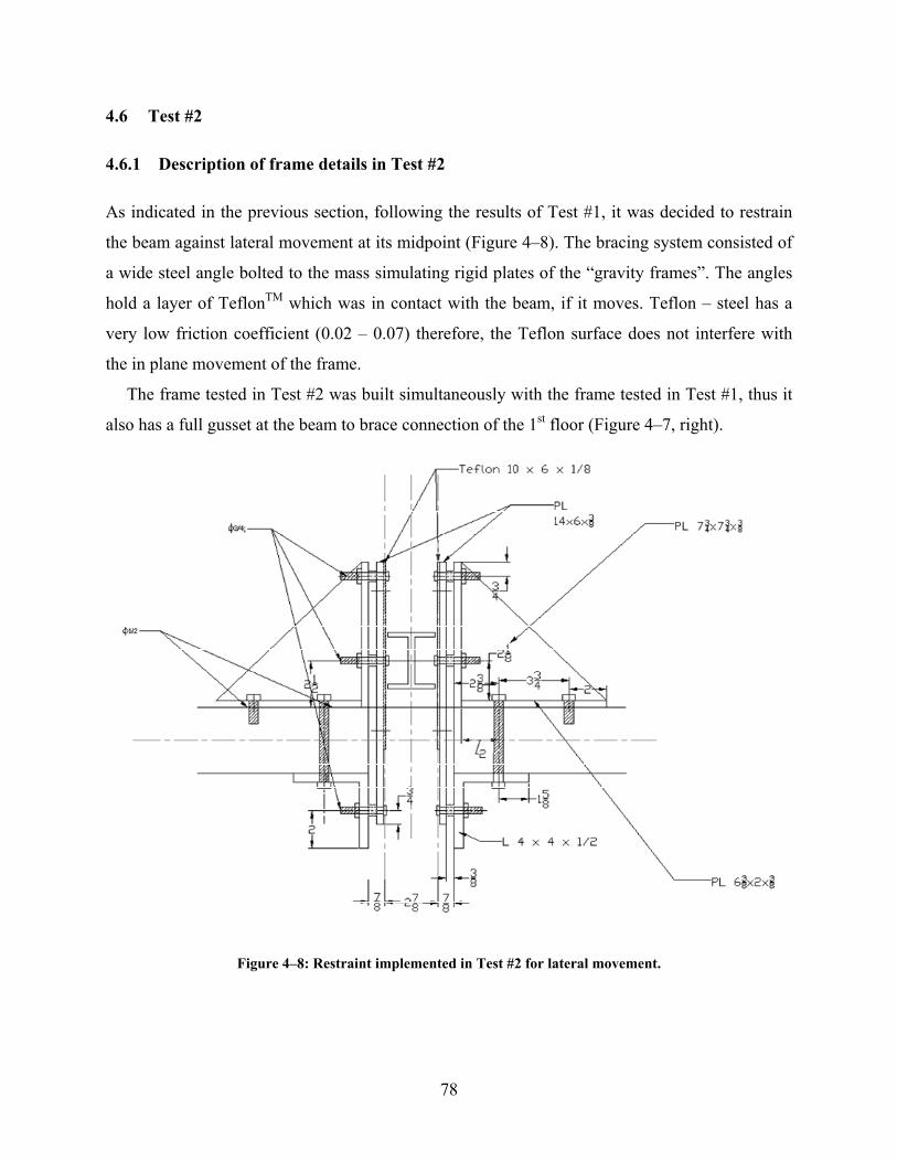
78
4.6 Test #2
4.6.1 Description of frame details in Test #2
As indicated in the previous section, following the results of Test #1, it was decided to restrain
the beam against lateral movement at its midpoint (Figure 4–8). The bracing system consisted of
a wide steel angle bolted to the mass simulating rigid plates of the “gravity frames”. The angles
hold a layer of TeflonTM which was in contact with the beam, if it moves. Teflon – steel has a
very low friction coefficient (0.02 – 0.07) therefore, the Teflon surface does not interfere with
the in plane movement of the frame.
The frame tested in Test #2 was built simultaneously with the frame tested in Test #1, thus it
also has a full gusset at the beam to brace connection of the 1st floor (Figure 4–7, right).
Figure 4–8: Restraint implemented in Test #2 for lateral movement.
79
4.6.2 Instrumentation
The quantities measured in this test were the same as in Test #1. After the instrumentation
problems of Test #1, it was decided to connect every strain gauge as an individual channel
(quarter bridge) and to perform the required processing after the test in order to obtain axial or
moment strains.
The 1st floor braces had 4 sets of strain gauges along their length, while the braces of the 2nd
floor had only 2 sets located near the ends. The 3rd floor braces had only 1 set of gauges and they
were hooked into a full bridge because only the axial force was of interest in this floor.
Beams were instrumented with 4 sets of gauges located in the same places where the half
bridges were in Test #1. At quarter points, strain rosettes were placed for shear measurements.
String potentiometers were used to record lateral movement and TemposonicsTM were used
for recording the brace’s axial displacements and 1st floor beam vertical movement
The Krypton camera was used again. The location of LEDs was the same as in Test #1. Two
additional LEDs were place at the bottom gusset plates to detect out of plane motion.
Instrumentation in columns was not changed and accelerometers were used in the same way
as in Test #1.
A complete list of instruments and its locations as well as drawings can be found in
APPENDIX F.
4.6.3 Test protocol
As in Test #1, the ground motion for Test #2 was LA22yy. The sequence applied was: “30%
LA22yy”, “80% LA22yy”, “100% LA22yy” and “120% LA22yy”. The objective of this
sequence was to minimize the effect of low cycle fatigue in the braces’ performance.
4.6.4 Test results
4.6.4.1 Test observations and data processing
The first run scheduled for Test #2 was “30% LA22yy”. During this run, the structure was
expected to behave elastically. However, in a first attempt to perform “30% LA22yy”, problems
with the control of the shake table due to the weight of the specimen, created an input greater
than the desirable, triggering buckling at the west brace. The east brace remained elastic. The
80
loading was not large enough to create important permanent displacements in the brace but it did
move the frame horizontally so that the east brace remained with some permanent tensile stress.
In a second attempt, the frame performed elastically.
During the “80% LA22yy”, both braces in the first floor buckled and yielded. During this test,
the Krypton camera worked very well and its readings show very clearly the buckling at the first
story braces. As expected, the “zipper column” was engaged just after the braces buckled and it
remained elastic during the entire ground motion. Readings from both sets of strain gauges were
consistent and the calculated values of forces were in good agreement with what was expected.
The vertical TemposonicTM placed at the bottom of the 1st floor beam showed that the beam
moved downwards, as expected. Braces in the second floor remained elastic. Readings from
strain rosettes in the beam revealed that the beam was being subjected to some torsion, however
its value was very small. When the beam moved out of plane, the sides of the flanges were in
contact with the Teflon surface of the restraint, thus a large amount of the torsional moment was
being transmitted to the bracing plates instead of to the beam itself.
During the “100% LA22yy”, the shake table exceeded its controllable rocking range, resulting
in substantial base rotation. These additional vertical accelerations have to be considered in any
numerical analysis that try to reproduce the results from this test. The 1st story braces showed a
very small capacity in compression and extensive yielding while the 2nd story braces buckled.
The 3rd floor “zipper column” was engaged when the 2nd floor braces buckled and remained with
a permanent deformation in tension when the motion stopped. Consequently, the east brace of
the 2nd floor remained in tension while the west brace of the 2nd floor remained in compression.
However, the amount of permanent deformation in the 2nd floor was very small compared to 1st
floor.
An additional test of amplitude “120% LA22yy” was performed because the frame was in
good conditions after the “100% LA22yy”. During this test, the 1st story east brace ruptured in
tension and the west brace had an important fracture (Figure 4–9). This test had to be stopped
due to instability of the setup after the rupture of the brace.
After the “120% LA22yy”, the structure was inspected for signs of beam rotation and general
frame displacements. It was found that the beam did rotate as shown in Figure 4–10. The 1st
story brace to beam gusset plate also rotated (Figure 4–10 and Figure 4–11). The “zipper
column” had some permanent deformation in the out of plane direction (Figure 4–12). The
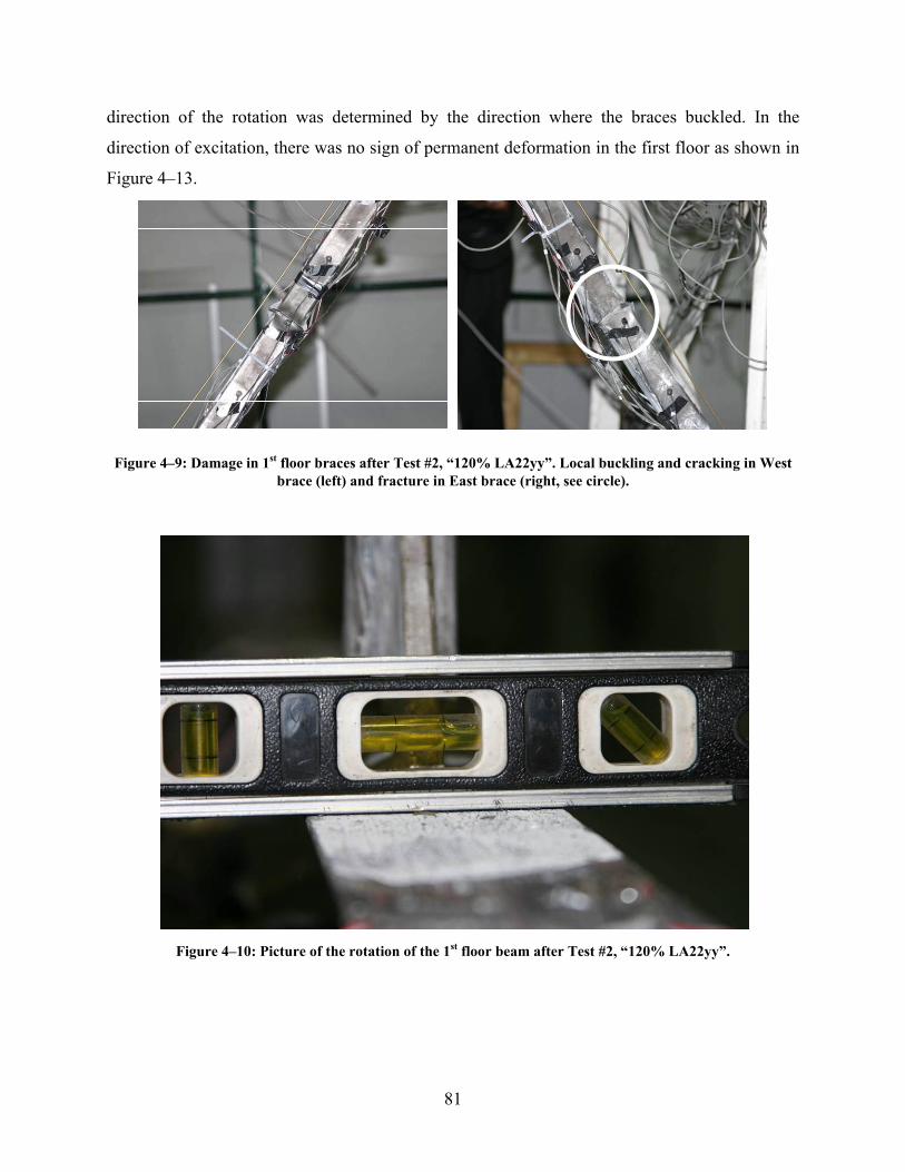
81
direction of the rotation was determined by the direction where the braces buckled. In the
direction of excitation, there was no sign of permanent deformation in the first floor as shown in
Figure 4–13.
Figure 4–9: Damage in 1st floor braces after Test #2, “120% LA22yy”. Local buckling and cracking in West brace (left) and fracture in East brace (right, see circle).
Figure 4–10: Picture of the rotation of the 1st floor beam after Test #2, “120% LA22yy”.

82
Figure 4–11: Picture of the rotation of the 1st story brace to beam gusset plate after Test #2, “120% LA22yy”.
Figure 4–12: Picture of the out of plane bending in the 2nd story “zipper column” after Test #2, “120% LA22yy”.
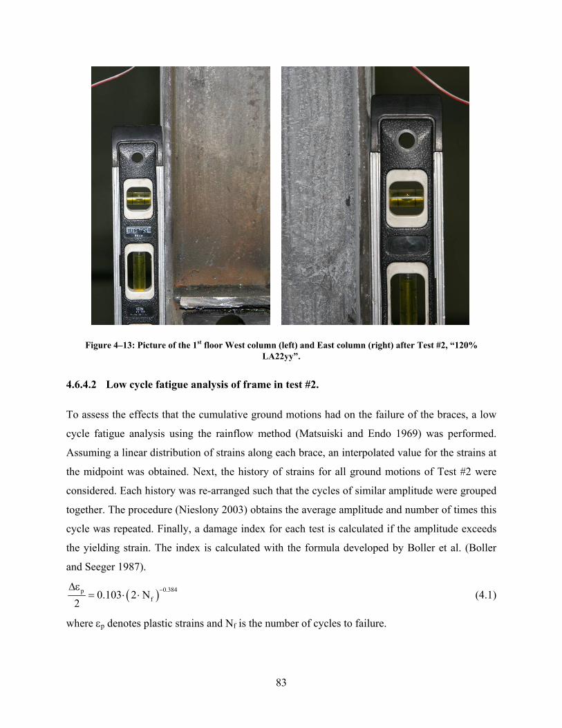
83
Figure 4–13: Picture of the 1st floor West column (left) and East column (right) after Test #2, “120% LA22yy”.
4.6.4.2 Low cycle fatigue analysis of frame in test #2.
To assess the effects that the cumulative ground motions had on the failure of the braces, a low
cycle fatigue analysis using the rainflow method (Matsuiski and Endo 1969) was performed.
Assuming a linear distribution of strains along each brace, an interpolated value for the strains at
the midpoint was obtained. Next, the history of strains for all ground motions of Test #2 were
considered. Each history was re-arranged such that the cycles of similar amplitude were grouped
together. The procedure (Nieslony 2003) obtains the average amplitude and number of times this
cycle was repeated. Finally, a damage index for each test is calculated if the amplitude exceeds
the yielding strain. The index is calculated with the formula developed by Boller et al. (Boller
and Seeger 1987).
( ) 0.384pf0.103 2 N
2−∆ε
= ⋅ ⋅ (4.1)
where εp denotes plastic strains and Nf is the number of cycles to failure.
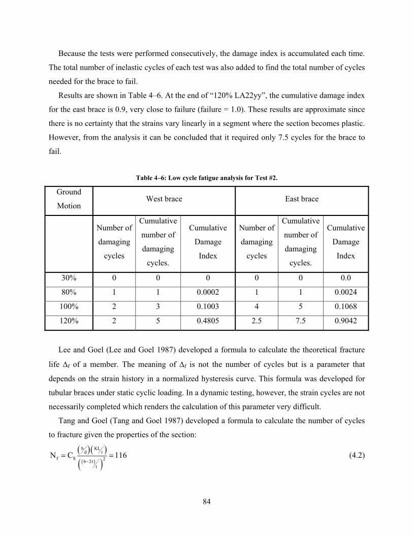
84
Because the tests were performed consecutively, the damage index is accumulated each time.
The total number of inelastic cycles of each test was also added to find the total number of cycles
needed for the brace to fail.
Results are shown in Table 4–6. At the end of “120% LA22yy”, the cumulative damage index
for the east brace is 0.9, very close to failure (failure = 1.0). These results are approximate since
there is no certainty that the strains vary linearly in a segment where the section becomes plastic.
However, from the analysis it can be concluded that it required only 7.5 cycles for the brace to
fail.
Table 4–6: Low cycle fatigue analysis for Test #2.
Ground
Motion West brace East brace
Number of
damaging
cycles
Cumulative
number of
damaging
cycles.
Cumulative
Damage
Index
Number of
damaging
cycles
Cumulative
number of
damaging
cycles.
Cumulative
Damage
Index
30% 0 0 0 0 0 0.0
80% 1 1 0.0002 1 1 0.0024
100% 2 3 0.1003 4 5 0.1068
120% 2 5 0.4805 2.5 7.5 0.9042
Lee and Goel (Lee and Goel 1987) developed a formula to calculate the theoretical fracture
life ∆f of a member. The meaning of ∆f is not the number of cycles but is a parameter that
depends on the strain history in a normalized hysteresis curve. This formula was developed for
tubular braces under static cyclic loading. In a dynamic testing, however, the strain cycles are not
necessarily completed which renders the calculation of this parameter very difficult.
Tang and Goel (Tang and Goel 1987) developed a formula to calculate the number of cycles
to fracture given the properties of the section:
( )( )( )( )b KL
d rf S 2b 2t
t
N C 116−
= = (4.2)
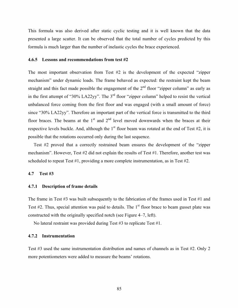
85
This formula was also derived after static cyclic testing and it is well known that the data
presented a large scatter. It can be observed that the total number of cycles predicted by this
formula is much larger than the number of inelastic cycles the brace experienced.
4.6.5 Lessons and recommendations from test #2
The most important observation from Test #2 is the development of the expected “zipper
mechanism” under dynamic loads. The frame behaved as expected: the restraint kept the beam
straight and this fact made possible the engagement of the 2nd floor “zipper column” as early as
in the first attempt of “30% LA22yy”. The 3rd floor “zipper column” helped to resist the vertical
unbalanced force coming from the first floor and was engaged (with a small amount of force)
since “30% LA22yy”. Therefore an important part of the vertical force is transmitted to the third
floor braces. The beams at the 1st and 2nd level moved downwards when the braces at their
respective levels buckle. And, although the 1st floor beam was rotated at the end of Test #2, it is
possible that the rotations occurred only during the last sequence.
Test #2 proved that a correctly restrained beam ensures the development of the “zipper
mechanism”. However, Test #2 did not explain the results of Test #1. Therefore, another test was
scheduled to repeat Test #1, providing a more complete instrumentation, as in Test #2.
4.7 Test #3
4.7.1 Description of frame details
The frame in Test #3 was built subsequently to the fabrication of the frames used in Test #1 and
Test #2. Thus, special attention was paid to details. The 1st floor brace to beam gusset plate was
constructed with the originally specified notch (see Figure 4–7, left).
No lateral restraint was provided during Test #3 to replicate Test #1.
4.7.2 Instrumentation
Test #3 used the same instrumentation distribution and names of channels as in Test #2. Only 2
more potentiometers were added to measure the beams’ rotations.
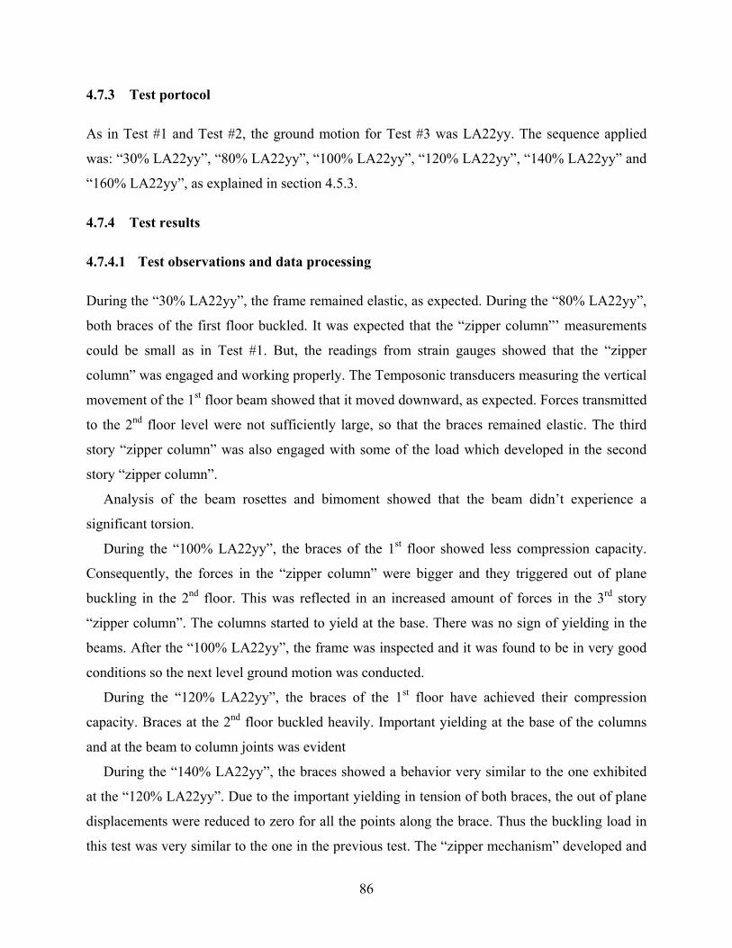
86
4.7.3 Test portocol
As in Test #1 and Test #2, the ground motion for Test #3 was LA22yy. The sequence applied
was: “30% LA22yy”, “80% LA22yy”, “100% LA22yy”, “120% LA22yy”, “140% LA22yy” and
“160% LA22yy”, as explained in section 4.5.3.
4.7.4 Test results
4.7.4.1 Test observations and data processing
During the “30% LA22yy”, the frame remained elastic, as expected. During the “80% LA22yy”,
both braces of the first floor buckled. It was expected that the “zipper column”’ measurements
could be small as in Test #1. But, the readings from strain gauges showed that the “zipper
column” was engaged and working properly. The Temposonic transducers measuring the vertical
movement of the 1st floor beam showed that it moved downward, as expected. Forces transmitted
to the 2nd floor level were not sufficiently large, so that the braces remained elastic. The third
story “zipper column” was also engaged with some of the load which developed in the second
story “zipper column”.
Analysis of the beam rosettes and bimoment showed that the beam didn’t experience a
significant torsion.
During the “100% LA22yy”, the braces of the 1st floor showed less compression capacity.
Consequently, the forces in the “zipper column” were bigger and they triggered out of plane
buckling in the 2nd floor. This was reflected in an increased amount of forces in the 3rd story
“zipper column”. The columns started to yield at the base. There was no sign of yielding in the
beams. After the “100% LA22yy”, the frame was inspected and it was found to be in very good
conditions so the next level ground motion was conducted.
During the “120% LA22yy”, the braces of the 1st floor have achieved their compression
capacity. Braces at the 2nd floor buckled heavily. Important yielding at the base of the columns
and at the beam to column joints was evident
During the “140% LA22yy”, the braces showed a behavior very similar to the one exhibited
at the “120% LA22yy”. Due to the important yielding in tension of both braces, the out of plane
displacements were reduced to zero for all the points along the brace. Thus the buckling load in
this test was very similar to the one in the previous test. The “zipper mechanism” developed and
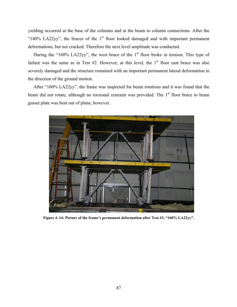
87
yielding occurred at the base of the columns and at the beam to column connections. After the
“140% LA22yy”, the braces of the 1st floor looked damaged and with important permanent
deformations, but not cracked. Therefore the next level amplitude was conducted.
During the “160% LA22yy”, the west brace of the 1st floor broke in tension. This type of
failure was the same as in Test #2. However, at this level, the 1st floor east brace was also
severely damaged and the structure remained with an important permanent lateral deformation in
the direction of the ground motion.
After “160% LA22yy”, the frame was inspected for beam rotations and it was found that the
beam did not rotate, although no torsional restraint was provided. The 1st floor brace to beam
gusset plate was bent out of plane, however.
Figure 4–14: Picture of the frame’s permanent deformation after Test #3, “160% LA22yy”.
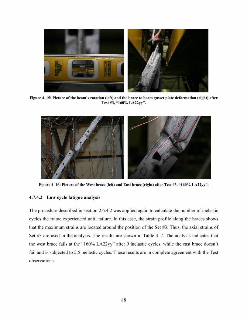
88
Figure 4–15: Picture of the beam’s rotation (left) and the brace to beam gusset plate deformation (right) after
Test #3, “160% LA22yy”.
Figure 4–16: Picture of the West brace (left) and East brace (right) after Test #3, “160% LA22yy”.
4.7.4.2 Low cycle fatigue analysis
The procedure described in section 2.6.4.2 was applied again to calculate the number of inelastic
cycles the frame experienced until failure. In this case, the strain profile along the braces shows
that the maximum strains are located around the position of the Set #3. Thus, the axial strains of
Set #3 are used in the analysis. The results are shown in Table 4–7. The analysis indicates that
the west brace fails at the “160% LA22yy” after 9 inelastic cycles, while the east brace doesn’t
fail and is subjected to 5.5 inelastic cycles. These results are in complete agreement with the Test
observations.
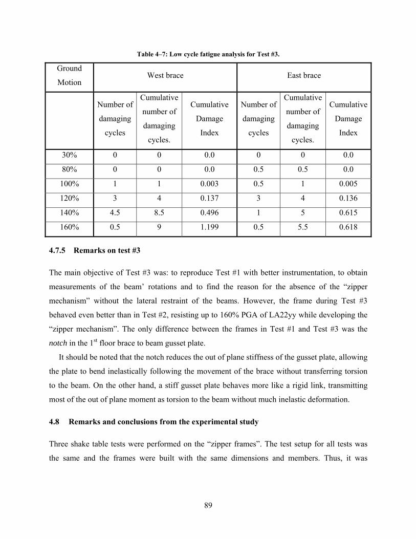
89
Table 4–7: Low cycle fatigue analysis for Test #3.
Ground
Motion West brace East brace
Number of
damaging
cycles
Cumulative
number of
damaging
cycles.
Cumulative
Damage
Index
Number of
damaging
cycles
Cumulative
number of
damaging
cycles.
Cumulative
Damage
Index
30% 0 0 0.0 0 0 0.0
80% 0 0 0.0 0.5 0.5 0.0
100% 1 1 0.003 0.5 1 0.005
120% 3 4 0.137 3 4 0.136
140% 4.5 8.5 0.496 1 5 0.615
160% 0.5 9 1.199 0.5 5.5 0.618
4.7.5 Remarks on test #3
The main objective of Test #3 was: to reproduce Test #1 with better instrumentation, to obtain
measurements of the beam’ rotations and to find the reason for the absence of the “zipper
mechanism” without the lateral restraint of the beams. However, the frame during Test #3
behaved even better than in Test #2, resisting up to 160% PGA of LA22yy while developing the
“zipper mechanism”. The only difference between the frames in Test #1 and Test #3 was the
notch in the 1st floor brace to beam gusset plate.
It should be noted that the notch reduces the out of plane stiffness of the gusset plate, allowing
the plate to bend inelastically following the movement of the brace without transferring torsion
to the beam. On the other hand, a stiff gusset plate behaves more like a rigid link, transmitting
most of the out of plane moment as torsion to the beam without much inelastic deformation.
4.8 Remarks and conclusions from the experimental study
Three shake table tests were performed on the “zipper frames”. The test setup for all tests was
the same and the frames were built with the same dimensions and members. Thus, it was
90
expected that the results from the different tests would be similar. However, a small detail in the
1st floor brace to beam gusset plate significantly changed the behavior of the system.
During Test #1 a stiff gusset plate was used with no lateral restraint on the beam. As a result,
the beam rotated and yielded in torsion, the “zipper column” was bent out of plane and the
“zipper mechanism” was compromised, although it is not possible to conclude that it did not
develop entirely.
During Test #2, a stiff gusset plate and a lateral restraint for the beams were used. As a result
the “zipper mechanism” developed and the frame behaved as expected until the “120% LA22yy”
amplitude test when the east brace broke in tension.
During Test #3, a flexible gusset and no lateral restraint for the beams were used. As a result,
the “zipper mechanism” also developed properly and the frame showed larger capacity than in
Test #2. The west brace broke in tension at the “160% LA22yy” amplitude test after severe
buckling in compression.
From the experimental study it can be concluded that:
4. The “zipper mechanism” can develop as expected if the system is built with adequate
details.
5. The system is sensitive to the construction details which may render the system
ineffective.
6. If the system is built with sufficient redundancy (such as lateral restraint) the “zipper
mechanism” is ensured.
7. The flexibility of the gusset plates connecting braces and beams is an important factor in
the development of the “zipper mechanism”.
It should be noted that the tests produced data on 3D buckling in dynamic conditions, as
recorded by the coordinate tracking system, Krypton, which uses digital imagery technology.
Finally, all data from this experimental study is available in the NEES repository:
https://central.nees.org/.
91
SECTION 5
ANALYTICAL EVALUATION OF THE PROPOSED FORMULATION
5.1 Introduction
The main objective of the following analysis is to verify that the new formulation is capable to
analyze the structural models (such as the “zipper frame”) and it is sufficiently sensitive to detect
the influence of various parameters consistent with observations from experiments and from
structural mechanics theory.
To test the performance of the element developed in Chapter 2, a model of the first story of
the zipper frame is built and analyzed. While a full size model would be desirable, due to the
high computational demands, a reduced size model was selected to explore the sensitivity of the
modeling parameters. The objective of this model is to reproduce the 3D movement of the
braces, like the one observed in the experimental work presented in Chapter 4.
The input motion is the 1st story lateral displacements obtained from string potentiometers at
the beam level and from the beam axial deformations obtained from strain gauges readings.
The formulation is not capable of modeling a hinge because it cannot condense the rotational
DOFs therefore, the connections are assumed fixed. The gusset plates are modeled with an
element of equivalent section and material properties - a connection element. Because these
properties are very difficult to determine, a bounding analysis is performed to assess the
influence of each parameter in the global behavior of the braces. Then, the structure is analyzed
with a combination of values for the parameters and the results are compared. In this Chapter, the
results of the analysis of the model subjected to the input motion obtained from data of Test #2
are shown.
5.2 Analytical model
The analytical model consists of the 1st floor braces and 1st floor beam (Figure 5–1). The nodes
are located at the same places were the sensors of the Krypton tracking system were placed
during the experiment. This allows for a direct comparison of the analytical and experimental
displacements. The only difference between the model and the experiment are the locations of
nodes 2 and 8. In the model, they define the boundary between the gusset plate and the brace
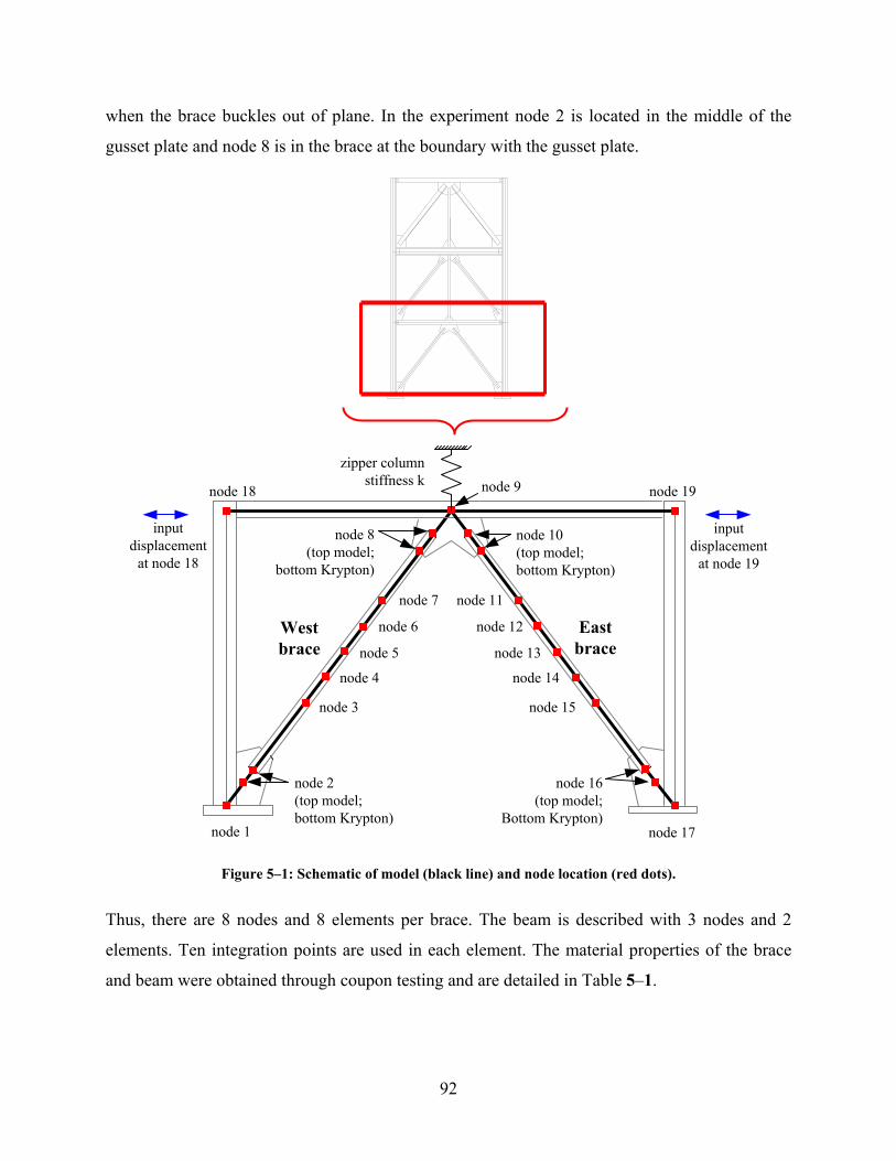
92
when the brace buckles out of plane. In the experiment node 2 is located in the middle of the
gusset plate and node 8 is in the brace at the boundary with the gusset plate.
node 1
node 2 (top model; bottom Krypton)
node 3
node 4
node 5
node 6
node 7
node 8(top model;
bottom Krypton)
node 10(top model; bottom Krypton)
node 11
node 12
node 13
node 14
node 15
node 16(top model;
Bottom Krypton)node 17
node 18 node 9 node 19
zipper columnstiffness k
Westbrace
Eastbrace
inputdisplacement
at node 18
inputdisplacement
at node 19
Figure 5–1: Schematic of model (black line) and node location (red dots).
Thus, there are 8 nodes and 8 elements per brace. The beam is described with 3 nodes and 2
elements. Ten integration points are used in each element. The material properties of the brace
and beam were obtained through coupon testing and are detailed in Table 5–1.
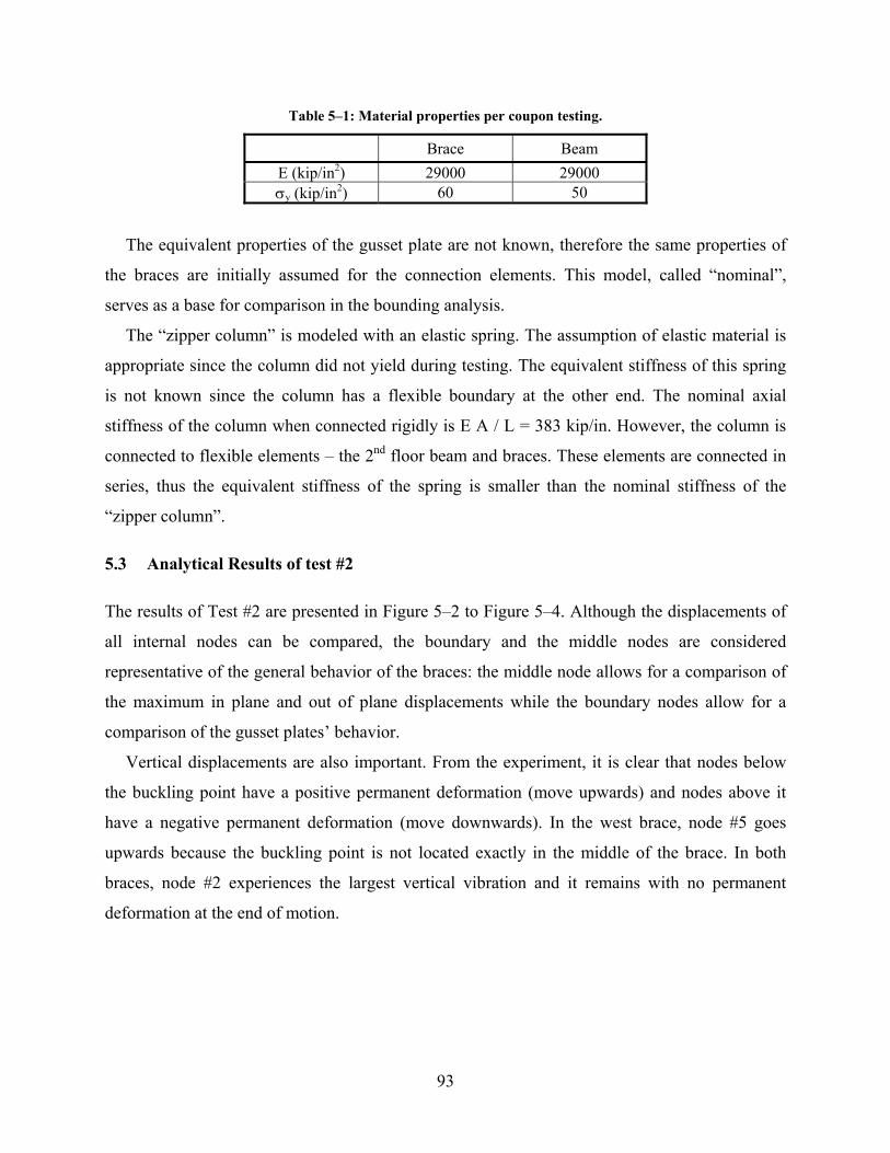
93
Table 5–1: Material properties per coupon testing.
Brace Beam E (kip/in2) 29000 29000 σy (kip/in2) 60 50
The equivalent properties of the gusset plate are not known, therefore the same properties of
the braces are initially assumed for the connection elements. This model, called “nominal”,
serves as a base for comparison in the bounding analysis.
The “zipper column” is modeled with an elastic spring. The assumption of elastic material is
appropriate since the column did not yield during testing. The equivalent stiffness of this spring
is not known since the column has a flexible boundary at the other end. The nominal axial
stiffness of the column when connected rigidly is E A / L = 383 kip/in. However, the column is
connected to flexible elements – the 2nd floor beam and braces. These elements are connected in
series, thus the equivalent stiffness of the spring is smaller than the nominal stiffness of the
“zipper column”.
5.3 Analytical Results of test #2
The results of Test #2 are presented in Figure 5–2 to Figure 5–4. Although the displacements of
all internal nodes can be compared, the boundary and the middle nodes are considered
representative of the general behavior of the braces: the middle node allows for a comparison of
the maximum in plane and out of plane displacements while the boundary nodes allow for a
comparison of the gusset plates’ behavior.
Vertical displacements are also important. From the experiment, it is clear that nodes below
the buckling point have a positive permanent deformation (move upwards) and nodes above it
have a negative permanent deformation (move downwards). In the west brace, node #5 goes
upwards because the buckling point is not located exactly in the middle of the brace. In both
braces, node #2 experiences the largest vertical vibration and it remains with no permanent
deformation at the end of motion.
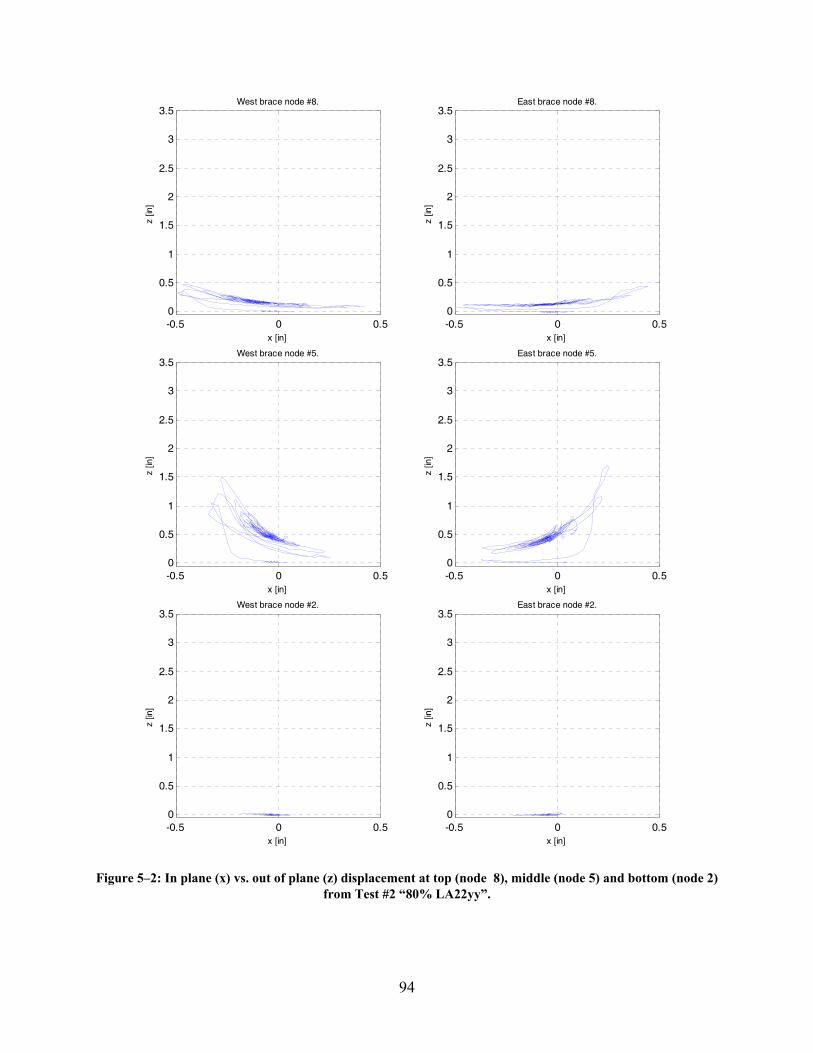
94
-0.5 0 0.50
0.5
1
1.5
2
2.5
3
3.5
x [in]
z [in
]
West brace node #8.
-0.5 0 0.50
0.5
1
1.5
2
2.5
3
3.5
x [in]
z [in
]
East brace node #8.
-0.5 0 0.50
0.5
1
1.5
2
2.5
3
3.5
x [in]
z [in
]
West brace node #5.
-0.5 0 0.50
0.5
1
1.5
2
2.5
3
3.5
x [in]
z [in
]
East brace node #5.
-0.5 0 0.50
0.5
1
1.5
2
2.5
3
3.5
x [in]
z [in
]
West brace node #2.
-0.5 0 0.50
0.5
1
1.5
2
2.5
3
3.5
x [in]
z [in
]
East brace node #2.
Figure 5–2: In plane (x) vs. out of plane (z) displacement at top (node 8), middle (node 5) and bottom (node 2) from Test #2 “80% LA22yy”.
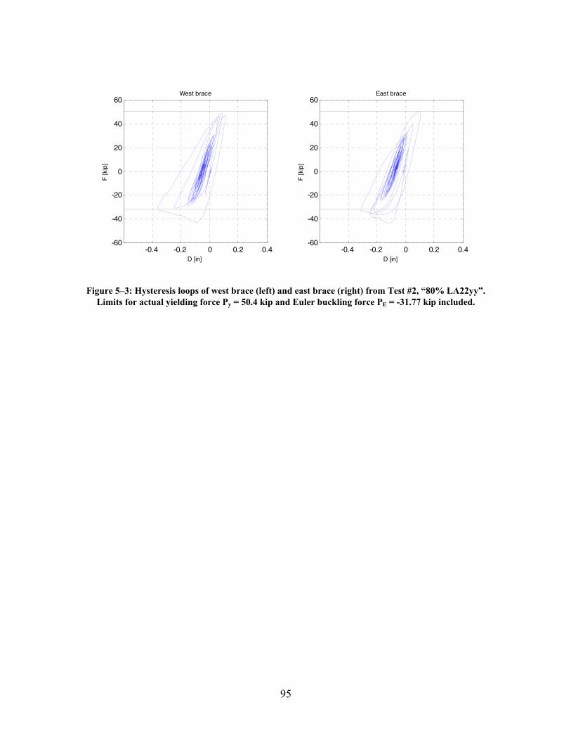
95
-0.4 -0.2 0 0.2 0.4-60
-40
-20
0
20
40
60
D [in]
F [k
ip]
West brace
-0.4 -0.2 0 0.2 0.4-60
-40
-20
0
20
40
60
D [in]
F [k
ip]
East brace
Figure 5–3: Hysteresis loops of west brace (left) and east brace (right) from Test #2, “80% LA22yy”. Limits for actual yielding force Py = 50.4 kip and Euler buckling force PE = -31.77 kip included.
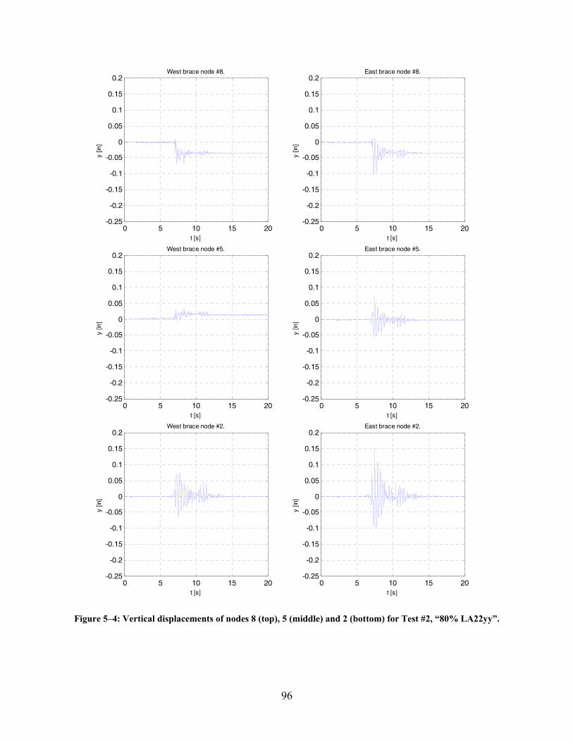
96
0 5 10 15 20-0.25
-0.2
-0.15
-0.1
-0.05
0
0.05
0.1
0.15
0.2
t [s]
y [in
]
West brace node #8.
0 5 10 15 20-0.25
-0.2
-0.15
-0.1
-0.05
0
0.05
0.1
0.15
0.2
t [s]
y [in
]
East brace node #8.
0 5 10 15 20-0.25
-0.2
-0.15
-0.1
-0.05
0
0.05
0.1
0.15
0.2
t [s]
y [in
]
West brace node #5.
0 5 10 15 20-0.25
-0.2
-0.15
-0.1
-0.05
0
0.05
0.1
0.15
0.2
t [s]
y [in
]
East brace node #5.
0 5 10 15 20-0.25
-0.2
-0.15
-0.1
-0.05
0
0.05
0.1
0.15
0.2
t [s]
y [in
]
West brace node #2.
0 5 10 15 20-0.25
-0.2
-0.15
-0.1
-0.05
0
0.05
0.1
0.15
0.2
t [s]
y [in
]
East brace node #2.
Figure 5–4: Vertical displacements of nodes 8 (top), 5 (middle) and 2 (bottom) for Test #2, “80% LA22yy”.

97
5.4 Bounding analysis
5.4.1 Connections: variation of the inertia of the connection elements
The inertia of the “nominal” model is assumed as the inertia of the brace’s section: I = 0.486 in4.
Two variations were analyzed: a flexible and a rigid connection element. The flexible connection
has an assumed inertia ten times smaller than the nominal Iflexible = I/10, and the rigid connection
has an assumed inertia ten times bigger than nominal Irigid = I×10. The yield function used was
HSS. When the inertia is 10 times smaller, the area of the section has to increase at least 10
times, otherwise the capacity of the section is very small compared to the brace and controls the
behavior of the complete structure. It is expected that the end moments would be reduced when
the gusset plates are more flexible and that the model would approach a hinged behavior.
Accordingly, the calculated end moments in the flexible model are smaller than in the nominal
model which in turn are slightly smaller than in the rigid model.
Figure 5–5 and Figure 5–6 show the in plane vs. out of plane displacements of node 2, 5 and 8
for west and east brace, respectively. When the connection is more flexible, the maximum out of
plane displacements at all nodes increase significantly. Also, the curve becomes smoother and
the residual out of plane displacement after buckling is considerably smaller, especially after the
first cycle. The connection elements remain elastic, allowing the brace to recover all its out of
plane deformation. As a consequence, the buckling loads of the first and second cycles are
almost identical in the case of a flexible connection while they are clearly different when the
gussets are rigid. This result is consistent with the theory: if the brace yields in tension such that
it completely recovers its original out of plane imperfection, its buckling capacity remains
unchanged.
From Figure 5–7 and Figure 5–8, it is observed that the value of the buckling load decreases
when the connections are more flexible. This is consistent with the fact that stronger boundary
conditions improve the capacity of a member to carry axial loads. The theoretical buckling load
with hinge connections is 30 kip (see APPENDIX C) and the recorded experimental value is 42
kip, therefore, the gusset plates in the experimental model have some flexibility and do not
behave like hinges.
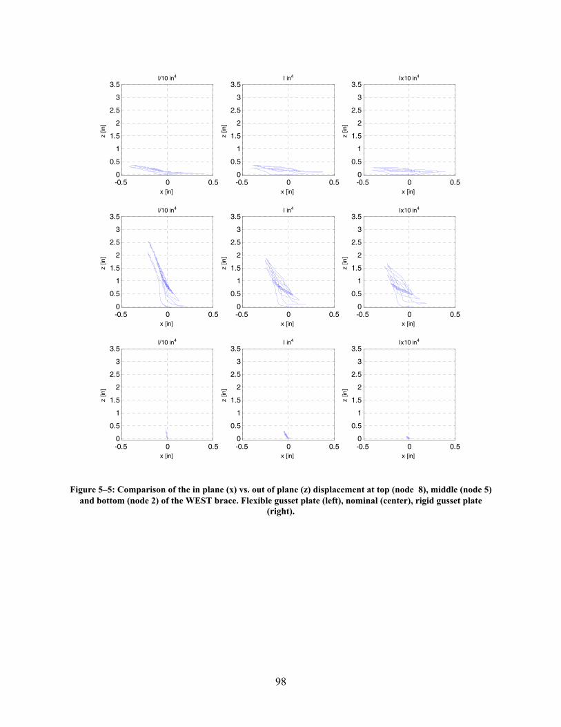
98
-0.5 0 0.50
0.5
1
1.5
2
2.5
3
3.5
x [in]
z [in
]
I/10 in4
-0.5 0 0.50
0.5
1
1.5
2
2.5
3
3.5
x [in]
z [in
]
I in4
-0.5 0 0.50
0.5
1
1.5
2
2.5
3
3.5
x [in]
z [in
]
Ix10 in4
-0.5 0 0.50
0.5
1
1.5
2
2.5
3
3.5
x [in]
z [in
]
I/10 in4
-0.5 0 0.50
0.5
1
1.5
2
2.5
3
3.5
x [in]
z [in
]
I in4
-0.5 0 0.50
0.5
1
1.5
2
2.5
3
3.5
x [in]
z [in
]
Ix10 in4
-0.5 0 0.50
0.5
1
1.5
2
2.5
3
3.5
x [in]
z [in
]
I/10 in4
-0.5 0 0.50
0.5
1
1.5
2
2.5
3
3.5
x [in]
z [in
]
I in4
-0.5 0 0.50
0.5
1
1.5
2
2.5
3
3.5
x [in]
z [in
]Ix10 in4
Figure 5–5: Comparison of the in plane (x) vs. out of plane (z) displacement at top (node 8), middle (node 5) and bottom (node 2) of the WEST brace. Flexible gusset plate (left), nominal (center), rigid gusset plate
(right).
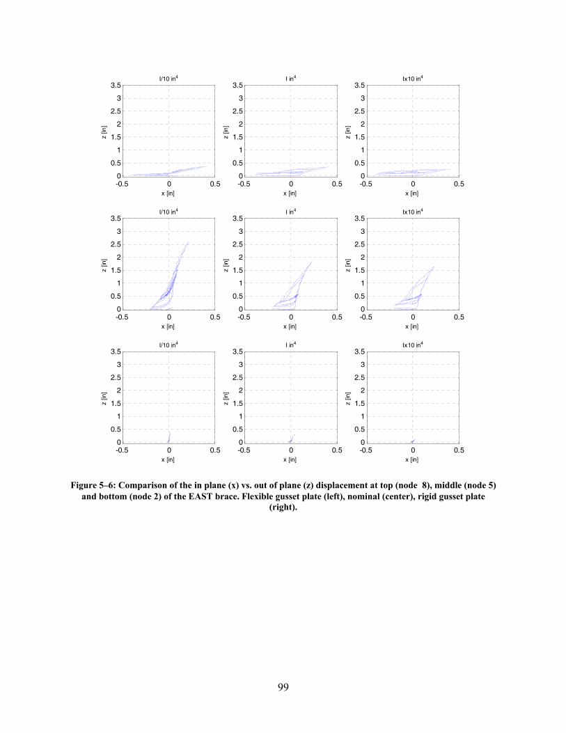
99
-0.5 0 0.50
0.5
1
1.5
2
2.5
3
3.5
x [in]
z [in
]
I/10 in4
-0.5 0 0.50
0.5
1
1.5
2
2.5
3
3.5
x [in]
z [in
]
I in4
-0.5 0 0.50
0.5
1
1.5
2
2.5
3
3.5
x [in]
z [in
]
Ix10 in4
-0.5 0 0.50
0.5
1
1.5
2
2.5
3
3.5
x [in]
z [in
]
I/10 in4
-0.5 0 0.50
0.5
1
1.5
2
2.5
3
3.5
x [in]
z [in
]
I in4
-0.5 0 0.50
0.5
1
1.5
2
2.5
3
3.5
x [in]
z [in
]
Ix10 in4
-0.5 0 0.50
0.5
1
1.5
2
2.5
3
3.5
x [in]
z [in
]
I/10 in4
-0.5 0 0.50
0.5
1
1.5
2
2.5
3
3.5
x [in]
z [in
]
I in4
-0.5 0 0.50
0.5
1
1.5
2
2.5
3
3.5
x [in]
z [in
]Ix10 in4
Figure 5–6: Comparison of the in plane (x) vs. out of plane (z) displacement at top (node 8), middle (node 5) and bottom (node 2) of the EAST brace. Flexible gusset plate (left), nominal (center), rigid gusset plate
(right).
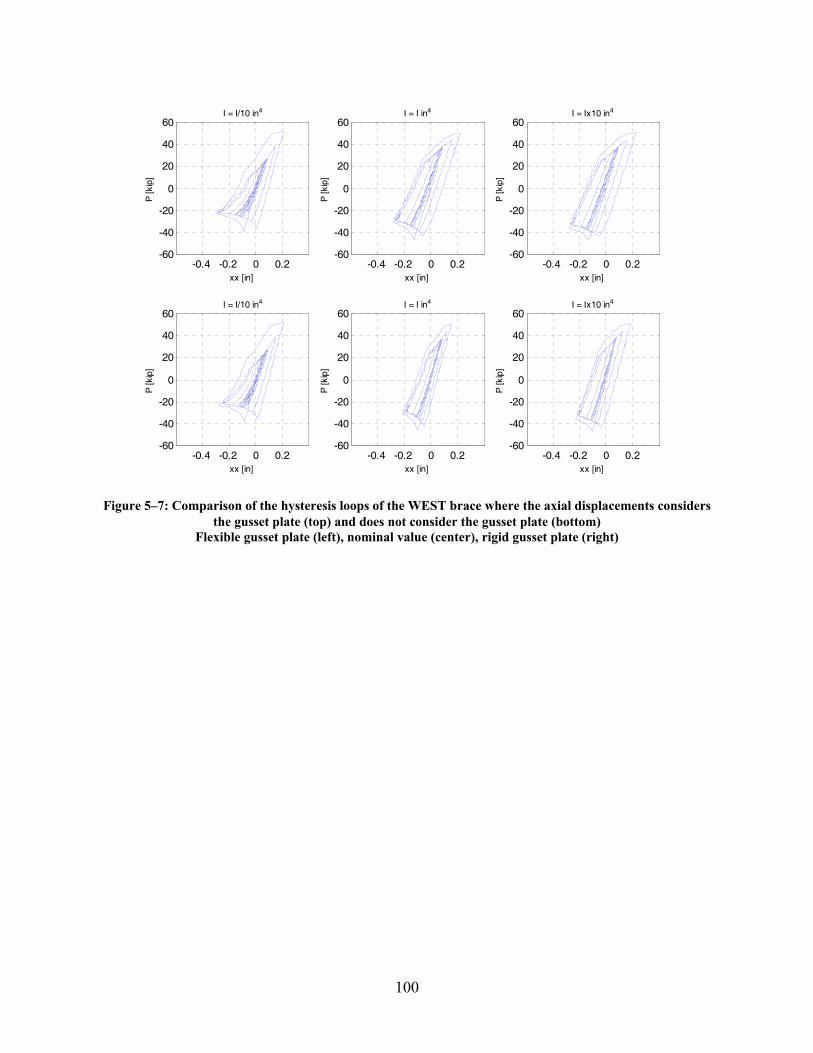
100
-0.4 -0.2 0 0.2-60
-40
-20
0
20
40
60
xx [in]
P [k
ip]
I = I/10 in4
-0.4 -0.2 0 0.2-60
-40
-20
0
20
40
60
xx [in]
P [k
ip]
I = I in4
-0.4 -0.2 0 0.2-60
-40
-20
0
20
40
60
xx [in]
P [k
ip]
I = Ix10 in4
-0.4 -0.2 0 0.2-60
-40
-20
0
20
40
60
xx [in]
P [k
ip]
I = I/10 in4
-0.4 -0.2 0 0.2-60
-40
-20
0
20
40
60
xx [in]
P [k
ip]
I = I in4
-0.4 -0.2 0 0.2-60
-40
-20
0
20
40
60
xx [in]
P [k
ip]
I = Ix10 in4
Figure 5–7: Comparison of the hysteresis loops of the WEST brace where the axial displacements considers the gusset plate (top) and does not consider the gusset plate (bottom)
Flexible gusset plate (left), nominal value (center), rigid gusset plate (right)
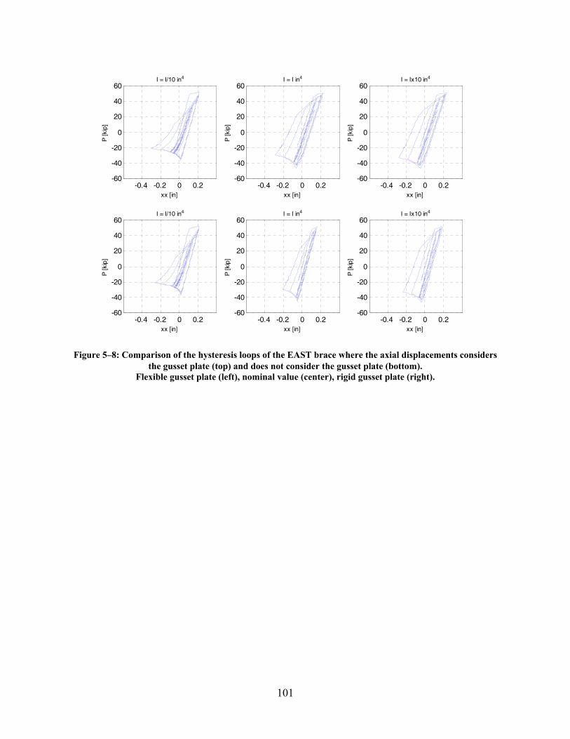
101
-0.4 -0.2 0 0.2-60
-40
-20
0
20
40
60
xx [in]
P [k
ip]
I = I/10 in4
-0.4 -0.2 0 0.2-60
-40
-20
0
20
40
60
xx [in]
P [k
ip]
I = I in4
-0.4 -0.2 0 0.2-60
-40
-20
0
20
40
60
xx [in]
P [k
ip]
I = Ix10 in4
-0.4 -0.2 0 0.2-60
-40
-20
0
20
40
60
xx [in]
P [k
ip]
I = I/10 in4
-0.4 -0.2 0 0.2-60
-40
-20
0
20
40
60
xx [in]
P [k
ip]
I = I in4
-0.4 -0.2 0 0.2-60
-40
-20
0
20
40
60
xx [in]
P [k
ip]
I = Ix10 in4
Figure 5–8: Comparison of the hysteresis loops of the EAST brace where the axial displacements considers the gusset plate (top) and does not consider the gusset plate (bottom).
Flexible gusset plate (left), nominal value (center), rigid gusset plate (right).
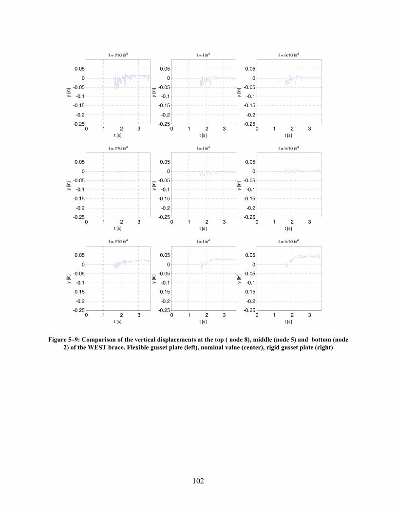
102
0 1 2 3-0.25
-0.2
-0.15
-0.1
-0.05
0
0.05
t [s]
y [in
]
I = I/10 in4
0 1 2 3-0.25
-0.2
-0.15
-0.1
-0.05
0
0.05
t [s]
y [in
]
I = I in4
0 1 2 3-0.25
-0.2
-0.15
-0.1
-0.05
0
0.05
t [s]
y [in
]
I = Ix10 in4
0 1 2 3-0.25
-0.2
-0.15
-0.1
-0.05
0
0.05
t [s]
y [in
]
I = I/10 in4
0 1 2 3-0.25
-0.2
-0.15
-0.1
-0.05
0
0.05
t [s]
y [in
]I = I in4
0 1 2 3-0.25
-0.2
-0.15
-0.1
-0.05
0
0.05
t [s]
y [in
]
I = Ix10 in4
0 1 2 3-0.25
-0.2
-0.15
-0.1
-0.05
0
0.05
t [s]
y [in
]
I = I/10 in4
0 1 2 3-0.25
-0.2
-0.15
-0.1
-0.05
0
0.05
t [s]
y [in
]
I = I in4
0 1 2 3-0.25
-0.2
-0.15
-0.1
-0.05
0
0.05
t [s]
y [in
]I = Ix10 in4
Figure 5–9: Comparison of the vertical displacements at the top ( node 8), middle (node 5) and bottom (node 2) of the WEST brace. Flexible gusset plate (left), nominal value (center), rigid gusset plate (right)
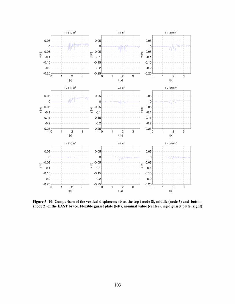
103
0 1 2 3-0.25
-0.2
-0.15
-0.1
-0.05
0
0.05
t [s]
y [in
]
I = I/10 in4
0 1 2 3-0.25
-0.2
-0.15
-0.1
-0.05
0
0.05
t [s]
y [in
]
I = I in4
0 1 2 3-0.25
-0.2
-0.15
-0.1
-0.05
0
0.05
t [s]
y [in
]
I = Ix10 in4
0 1 2 3-0.25
-0.2
-0.15
-0.1
-0.05
0
0.05
t [s]
y [in
]
I = I/10 in4
0 1 2 3-0.25
-0.2
-0.15
-0.1
-0.05
0
0.05
t [s]
y [in
]I = I in4
0 1 2 3-0.25
-0.2
-0.15
-0.1
-0.05
0
0.05
t [s]
y [in
]
I = Ix10 in4
0 1 2 3-0.25
-0.2
-0.15
-0.1
-0.05
0
0.05
t [s]
y [in
]
I = I/10 in4
0 1 2 3-0.25
-0.2
-0.15
-0.1
-0.05
0
0.05
t [s]
y [in
]
I = I in4
0 1 2 3-0.25
-0.2
-0.15
-0.1
-0.05
0
0.05
t [s]
y [in
]I = Ix10 in4
Figure 5–10: Comparison of the vertical displacements at the top ( node 8), middle (node 5) and bottom (node 2) of the EAST brace. Flexible gusset plate (left), nominal value (center), rigid gusset plate (right)
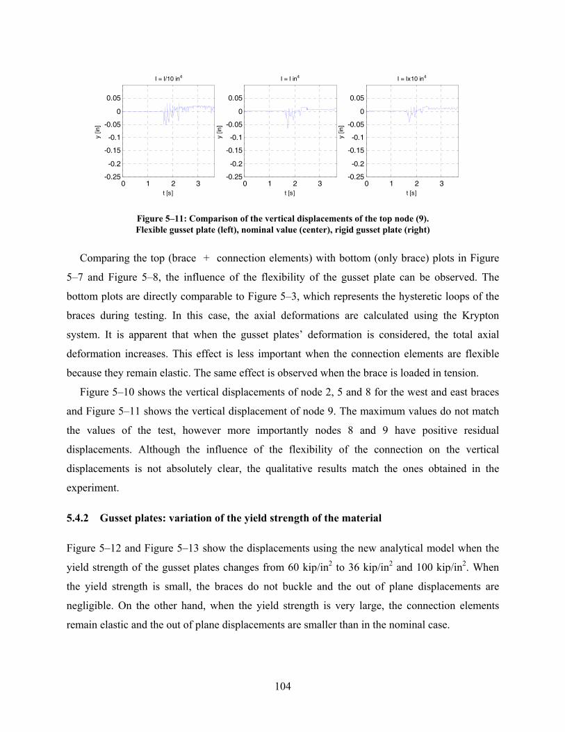
104
0 1 2 3-0.25
-0.2
-0.15
-0.1
-0.05
0
0.05
t [s]
y [in
]
I = I/10 in4
0 1 2 3-0.25
-0.2
-0.15
-0.1
-0.05
0
0.05
t [s]
y [in
]
I = I in4
0 1 2 3-0.25
-0.2
-0.15
-0.1
-0.05
0
0.05
t [s]
y [in
]
I = Ix10 in4
Figure 5–11: Comparison of the vertical displacements of the top node (9). Flexible gusset plate (left), nominal value (center), rigid gusset plate (right)
Comparing the top (brace + connection elements) with bottom (only brace) plots in Figure
5–7 and Figure 5–8, the influence of the flexibility of the gusset plate can be observed. The
bottom plots are directly comparable to Figure 5–3, which represents the hysteretic loops of the
braces during testing. In this case, the axial deformations are calculated using the Krypton
system. It is apparent that when the gusset plates’ deformation is considered, the total axial
deformation increases. This effect is less important when the connection elements are flexible
because they remain elastic. The same effect is observed when the brace is loaded in tension.
Figure 5–10 shows the vertical displacements of node 2, 5 and 8 for the west and east braces
and Figure 5–11 shows the vertical displacement of node 9. The maximum values do not match
the values of the test, however more importantly nodes 8 and 9 have positive residual
displacements. Although the influence of the flexibility of the connection on the vertical
displacements is not absolutely clear, the qualitative results match the ones obtained in the
experiment.
5.4.2 Gusset plates: variation of the yield strength of the material
Figure 5–12 and Figure 5–13 show the displacements using the new analytical model when the
yield strength of the gusset plates changes from 60 kip/in2 to 36 kip/in2 and 100 kip/in2. When
the yield strength is small, the braces do not buckle and the out of plane displacements are
negligible. On the other hand, when the yield strength is very large, the connection elements
remain elastic and the out of plane displacements are smaller than in the nominal case.
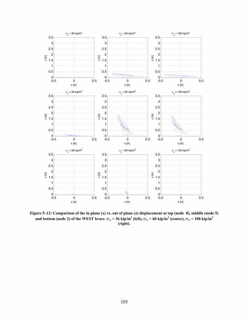
105
-0.5 0 0.50
0.5
1
1.5
2
2.5
3
3.5
x [in]
z [in
]
σy = 36 kip/in2
-0.5 0 0.50
0.5
1
1.5
2
2.5
3
3.5
x [in]
z [in
]
σy = 60 kip/in2
-0.5 0 0.50
0.5
1
1.5
2
2.5
3
3.5
x [in]
z [in
]
σy = 100 kip/in2
-0.5 0 0.50
0.5
1
1.5
2
2.5
3
3.5
x [in]
z [in
]
σy = 36 kip/in2
-0.5 0 0.50
0.5
1
1.5
2
2.5
3
3.5
x [in]
z [in
]
σy = 60 kip/in2
-0.5 0 0.50
0.5
1
1.5
2
2.5
3
3.5
x [in]
z [in
]
σy = 100 kip/in2
-0.5 0 0.50
0.5
1
1.5
2
2.5
3
3.5
x [in]
z [in
]
σy = 36 kip/in2
-0.5 0 0.50
0.5
1
1.5
2
2.5
3
3.5
x [in]
z [in
]
σy = 60 kip/in2
-0.5 0 0.50
0.5
1
1.5
2
2.5
3
3.5
x [in]
z [in
]σ
y = 100 kip/in2
Figure 5–12: Comparison of the in plane (x) vs. out of plane (z) displacement at top (node 8), middle (node 5) and bottom (node 2) of the WEST brace. σψ = 36 kip/in2 (left), σψ = 60 kip/in2 (center), σψ = 100 kip/in2
(right).
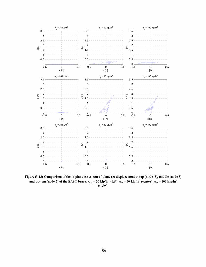
106
-0.5 0 0.50
0.5
1
1.5
2
2.5
3
3.5
x [in]
z [in
]
σy = 36 kip/in2
-0.5 0 0.50
0.5
1
1.5
2
2.5
3
3.5
x [in]
z [in
]
σy = 60 kip/in2
-0.5 0 0.50
0.5
1
1.5
2
2.5
3
3.5
x [in]
z [in
]
σy = 100 kip/in2
-0.5 0 0.50
0.5
1
1.5
2
2.5
3
3.5
x [in]
z [in
]
σy = 36 kip/in2
-0.5 0 0.50
0.5
1
1.5
2
2.5
3
3.5
x [in]
z [in
]
σy = 60 kip/in2
-0.5 0 0.50
0.5
1
1.5
2
2.5
3
3.5
x [in]
z [in
]
σy = 100 kip/in2
-0.5 0 0.50
0.5
1
1.5
2
2.5
3
3.5
x [in]
z [in
]
σy = 36 kip/in2
-0.5 0 0.50
0.5
1
1.5
2
2.5
3
3.5
x [in]
z [in
]
σy = 60 kip/in2
-0.5 0 0.50
0.5
1
1.5
2
2.5
3
3.5
x [in]
z [in
]σ
y = 100 kip/in2
Figure 5–13: Comparison of the in plane (x) vs. out of plane (z) displacement at top (node 8), middle (node 5) and bottom (node 2) of the EAST brace. σψ = 36 kip/in2 (left), σψ = 60 kip/in2 (center), σψ = 100 kip/in2
(right).
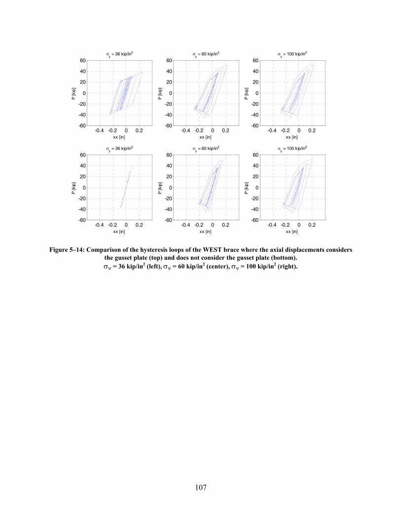
107
-0.4 -0.2 0 0.2-60
-40
-20
0
20
40
60
xx [in]
P [k
ip]
σy = 36 kip/in2
-0.4 -0.2 0 0.2-60
-40
-20
0
20
40
60
xx [in]
P [k
ip]
σy = 60 kip/in2
-0.4 -0.2 0 0.2-60
-40
-20
0
20
40
60
xx [in]
P [k
ip]
σy = 100 kip/in2
-0.4 -0.2 0 0.2-60
-40
-20
0
20
40
60
xx [in]
P [k
ip]
σy = 36 kip/in2
-0.4 -0.2 0 0.2-60
-40
-20
0
20
40
60
xx [in]
P [k
ip]
σy = 60 kip/in2
-0.4 -0.2 0 0.2-60
-40
-20
0
20
40
60
xx [in]
P [k
ip]
σy = 100 kip/in2
Figure 5–14: Comparison of the hysteresis loops of the WEST brace where the axial displacements considers the gusset plate (top) and does not consider the gusset plate (bottom). σψ = 36 kip/in2 (left), σψ = 60 kip/in2 (center), σψ = 100 kip/in2 (right).
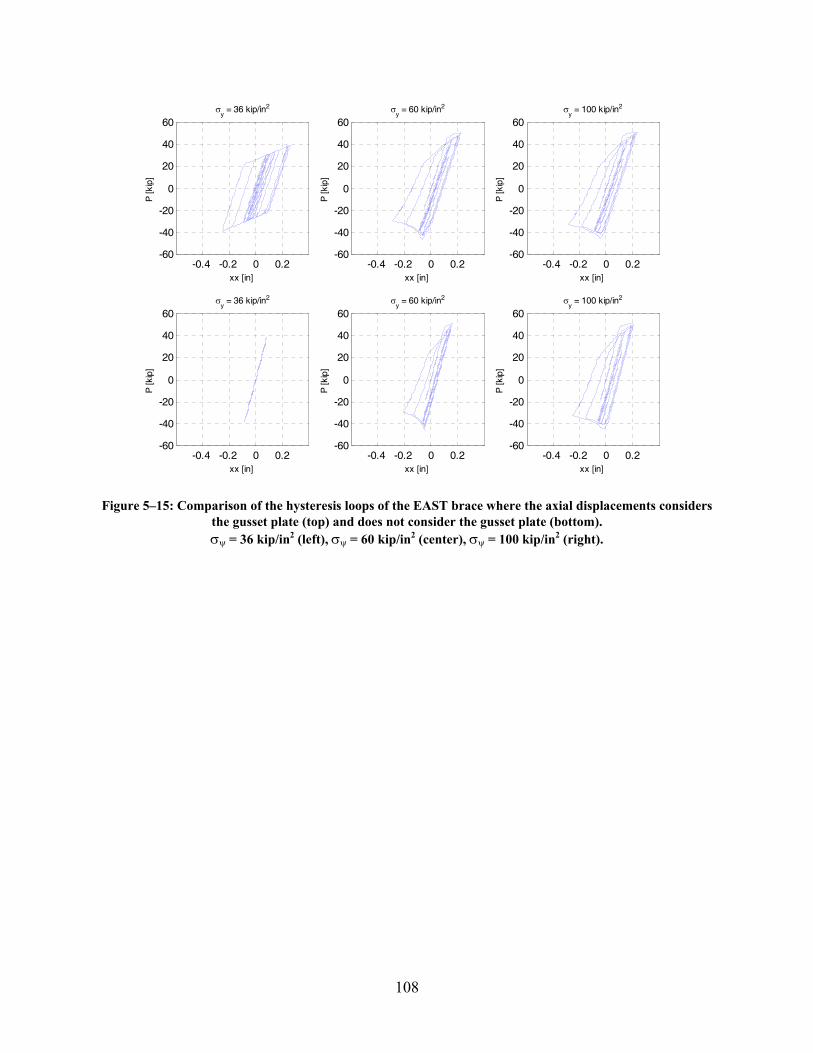
108
-0.4 -0.2 0 0.2-60
-40
-20
0
20
40
60
xx [in]
P [k
ip]
σy = 36 kip/in2
-0.4 -0.2 0 0.2-60
-40
-20
0
20
40
60
xx [in]
P [k
ip]
σy = 60 kip/in2
-0.4 -0.2 0 0.2-60
-40
-20
0
20
40
60
xx [in]
P [k
ip]
σy = 100 kip/in2
-0.4 -0.2 0 0.2-60
-40
-20
0
20
40
60
xx [in]
P [k
ip]
σy = 36 kip/in2
-0.4 -0.2 0 0.2-60
-40
-20
0
20
40
60
xx [in]
P [k
ip]
σy = 60 kip/in2
-0.4 -0.2 0 0.2-60
-40
-20
0
20
40
60
xx [in]
P [k
ip]
σy = 100 kip/in2
Figure 5–15: Comparison of the hysteresis loops of the EAST brace where the axial displacements considers the gusset plate (top) and does not consider the gusset plate (bottom). σψ = 36 kip/in2 (left), σψ = 60 kip/in2 (center), σψ = 100 kip/in2 (right).
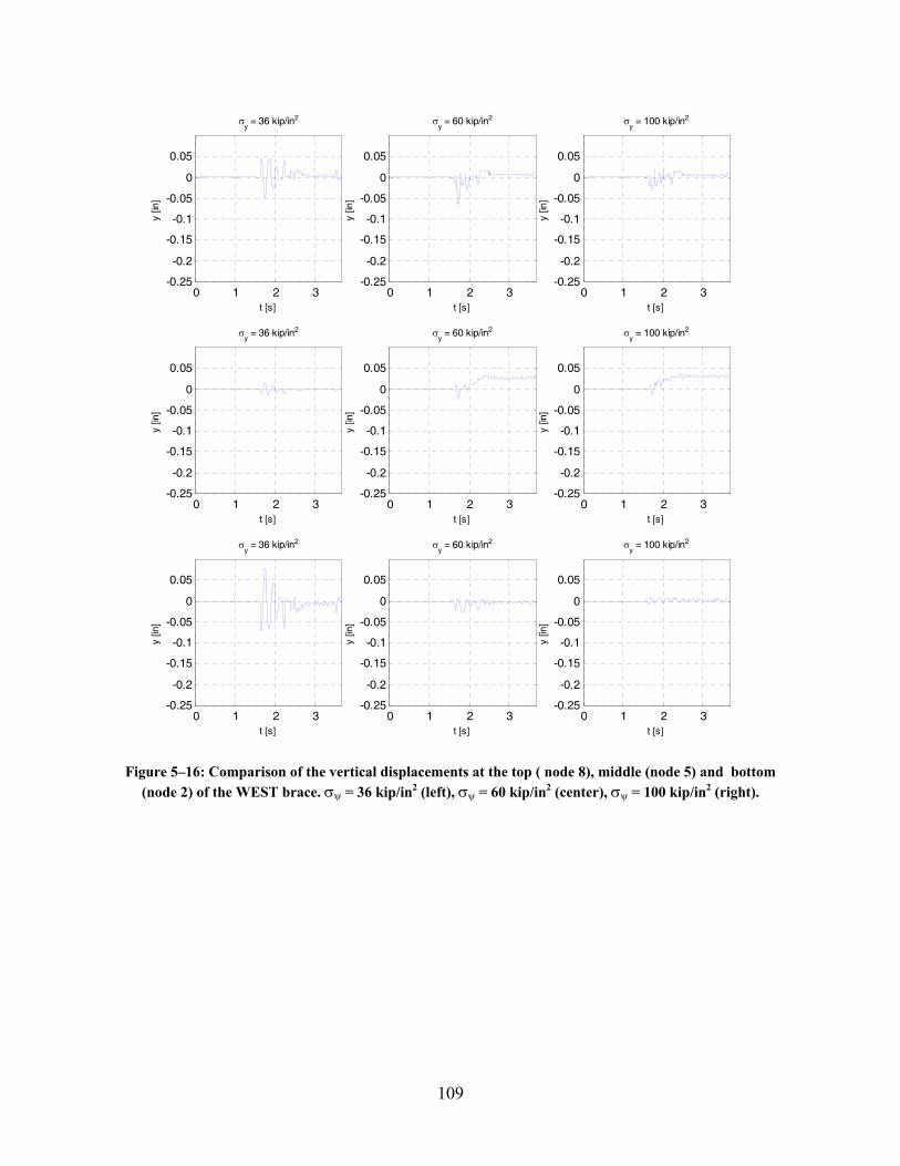
109
0 1 2 3-0.25
-0.2
-0.15
-0.1
-0.05
0
0.05
t [s]
y [in
]
σy = 36 kip/in2
0 1 2 3-0.25
-0.2
-0.15
-0.1
-0.05
0
0.05
t [s]
y [in
]
σy = 60 kip/in2
0 1 2 3-0.25
-0.2
-0.15
-0.1
-0.05
0
0.05
t [s]
y [in
]
σy = 100 kip/in2
0 1 2 3-0.25
-0.2
-0.15
-0.1
-0.05
0
0.05
t [s]
y [in
]
σy = 36 kip/in2
0 1 2 3-0.25
-0.2
-0.15
-0.1
-0.05
0
0.05
t [s]
y [in
]
σy = 60 kip/in2
0 1 2 3-0.25
-0.2
-0.15
-0.1
-0.05
0
0.05
t [s]
y [in
]
σy = 100 kip/in2
0 1 2 3-0.25
-0.2
-0.15
-0.1
-0.05
0
0.05
t [s]
y [in
]
σy = 36 kip/in2
0 1 2 3-0.25
-0.2
-0.15
-0.1
-0.05
0
0.05
t [s]
y [in
]
σy = 60 kip/in2
0 1 2 3-0.25
-0.2
-0.15
-0.1
-0.05
0
0.05
t [s]
y [in
]σ
y = 100 kip/in2
Figure 5–16: Comparison of the vertical displacements at the top ( node 8), middle (node 5) and bottom (node 2) of the WEST brace. σψ = 36 kip/in2 (left), σψ = 60 kip/in2 (center), σψ = 100 kip/in2 (right).
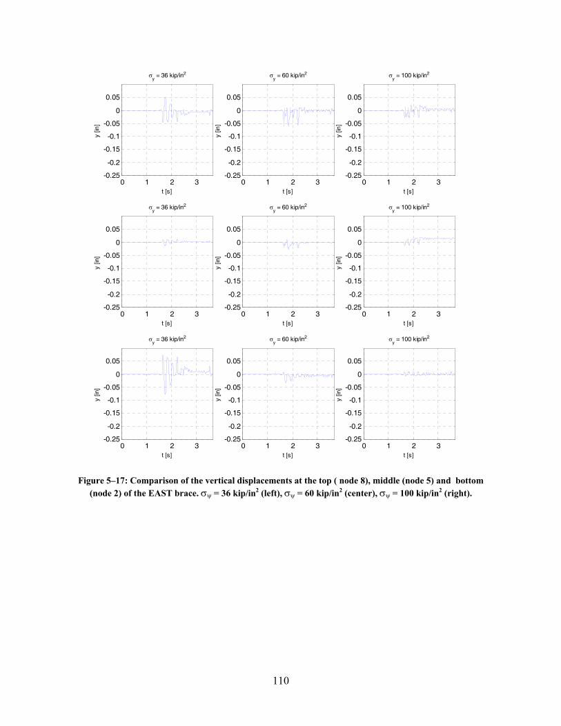
110
0 1 2 3-0.25
-0.2
-0.15
-0.1
-0.05
0
0.05
t [s]
y [in
]
σy = 36 kip/in2
0 1 2 3-0.25
-0.2
-0.15
-0.1
-0.05
0
0.05
t [s]
y [in
]
σy = 60 kip/in2
0 1 2 3-0.25
-0.2
-0.15
-0.1
-0.05
0
0.05
t [s]
y [in
]
σy = 100 kip/in2
0 1 2 3-0.25
-0.2
-0.15
-0.1
-0.05
0
0.05
t [s]
y [in
]
σy = 36 kip/in2
0 1 2 3-0.25
-0.2
-0.15
-0.1
-0.05
0
0.05
t [s]
y [in
]
σy = 60 kip/in2
0 1 2 3-0.25
-0.2
-0.15
-0.1
-0.05
0
0.05
t [s]
y [in
]
σy = 100 kip/in2
0 1 2 3-0.25
-0.2
-0.15
-0.1
-0.05
0
0.05
t [s]
y [in
]
σy = 36 kip/in2
0 1 2 3-0.25
-0.2
-0.15
-0.1
-0.05
0
0.05
t [s]
y [in
]
σy = 60 kip/in2
0 1 2 3-0.25
-0.2
-0.15
-0.1
-0.05
0
0.05
t [s]
y [in
]σ
y = 100 kip/in2
Figure 5–17: Comparison of the vertical displacements at the top ( node 8), middle (node 5) and bottom (node 2) of the EAST brace. σψ = 36 kip/in2 (left), σψ = 60 kip/in2 (center), σψ = 100 kip/in2 (right).
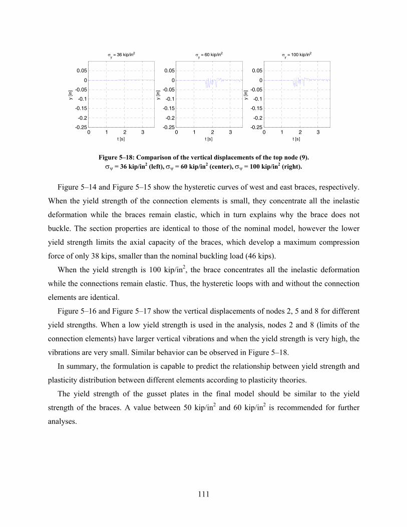
111
0 1 2 3-0.25
-0.2
-0.15
-0.1
-0.05
0
0.05
t [s]
y [in
]
σy = 36 kip/in2
0 1 2 3-0.25
-0.2
-0.15
-0.1
-0.05
0
0.05
t [s]
y [in
]
σy = 60 kip/in2
0 1 2 3-0.25
-0.2
-0.15
-0.1
-0.05
0
0.05
t [s]
y [in
]
σy = 100 kip/in2
Figure 5–18: Comparison of the vertical displacements of the top node (9). σψ = 36 kip/in2 (left), σψ = 60 kip/in2 (center), σψ = 100 kip/in2 (right).
Figure 5–14 and Figure 5–15 show the hysteretic curves of west and east braces, respectively.
When the yield strength of the connection elements is small, they concentrate all the inelastic
deformation while the braces remain elastic, which in turn explains why the brace does not
buckle. The section properties are identical to those of the nominal model, however the lower
yield strength limits the axial capacity of the braces, which develop a maximum compression
force of only 38 kips, smaller than the nominal buckling load (46 kips).
When the yield strength is 100 kip/in2, the brace concentrates all the inelastic deformation
while the connections remain elastic. Thus, the hysteretic loops with and without the connection
elements are identical.
Figure 5–16 and Figure 5–17 show the vertical displacements of nodes 2, 5 and 8 for different
yield strengths. When a low yield strength is used in the analysis, nodes 2 and 8 (limits of the
connection elements) have larger vertical vibrations and when the yield strength is very high, the
vibrations are very small. Similar behavior can be observed in Figure 5–18.
In summary, the formulation is capable to predict the relationship between yield strength and
plasticity distribution between different elements according to plasticity theories.
The yield strength of the gusset plates in the final model should be similar to the yield
strength of the braces. A value between 50 kip/in2 and 60 kip/in2 is recommended for further
analyses.
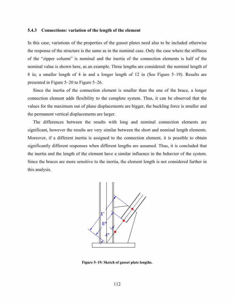
112
5.4.3 Connections: variation of the length of the element
In this case, variations of the properties of the gusset plates need also to be included otherwise
the response of the structure is the same as in the nominal case. Only the case where the stiffness
of the “zipper column” is nominal and the inertia of the connection elements is half of the
nominal value is shown here, as an example. Three lengths are considered: the nominal length of
8 in; a smaller length of 4 in and a longer length of 12 in (See Figure 5–19). Results are
presented in Figure 5–20 to Figure 5–26.
Since the inertia of the connection element is smaller than the one of the brace, a longer
connection element adds flexibility to the complete system. Thus, it can be observed that the
values for the maximum out of plane displacements are bigger, the buckling force is smaller and
the permanent vertical displacements are larger.
The differences between the results with long and nominal connection elements are
significant, however the results are very similar between the short and nominal length elements.
Moreover, if a different inertia is assigned to the connection element, it is possible to obtain
significantly different responses when different lengths are assumed. Thus, it is concluded that
the inertia and the length of the element have a similar influence in the behavior of the system.
Since the braces are more sensitive to the inertia, the element length is not considered further in
this analysis.
Figure 5–19: Sketch of gusset plate lengths.
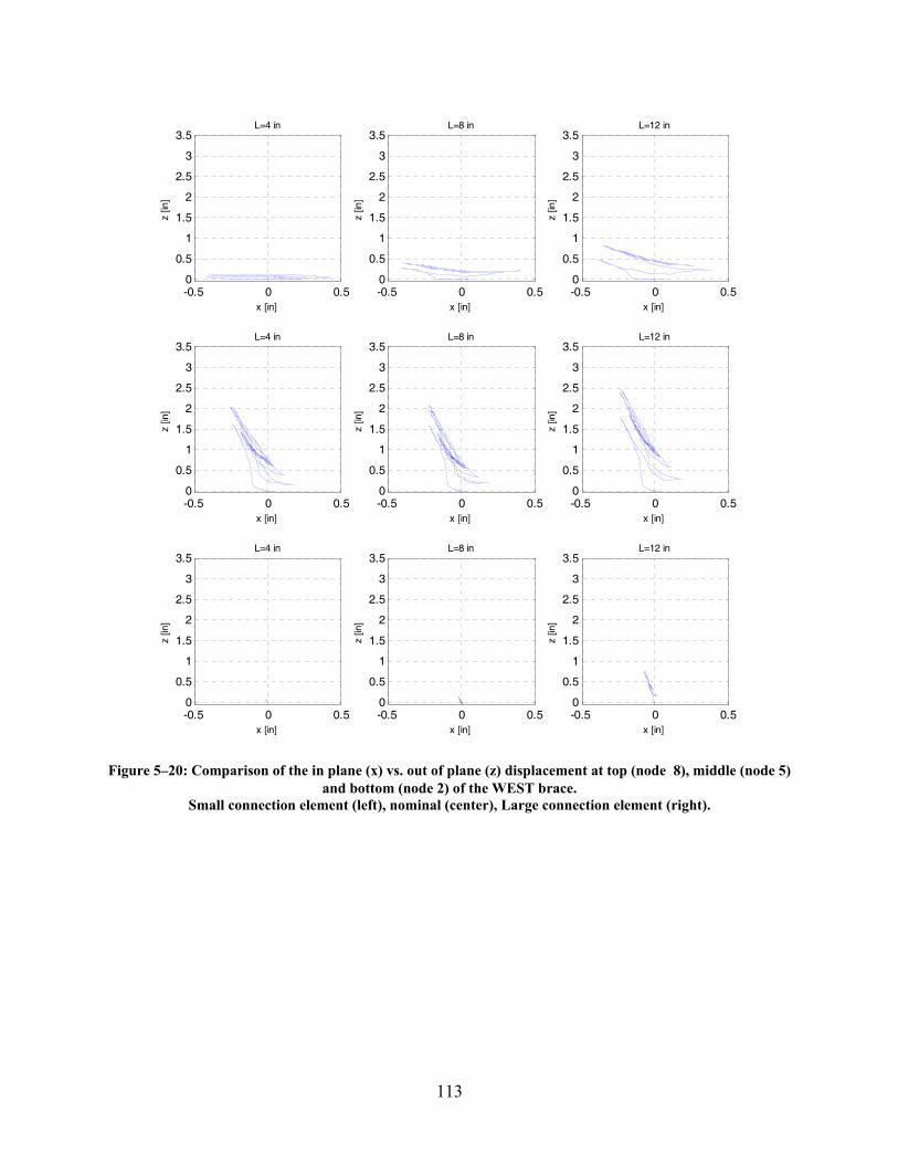
113
-0.5 0 0.50
0.5
1
1.5
2
2.5
3
3.5
x [in]
z [in
]
L=4 in
-0.5 0 0.50
0.5
1
1.5
2
2.5
3
3.5
x [in]
z [in
]
L=8 in
-0.5 0 0.50
0.5
1
1.5
2
2.5
3
3.5
x [in]
z [in
]
L=12 in
-0.5 0 0.50
0.5
1
1.5
2
2.5
3
3.5
x [in]
z [in
]
L=4 in
-0.5 0 0.50
0.5
1
1.5
2
2.5
3
3.5
x [in]
z [in
]
L=8 in
-0.5 0 0.50
0.5
1
1.5
2
2.5
3
3.5
x [in]
z [in
]
L=12 in
-0.5 0 0.50
0.5
1
1.5
2
2.5
3
3.5
x [in]
z [in
]
L=4 in
-0.5 0 0.50
0.5
1
1.5
2
2.5
3
3.5
x [in]
z [in
]
L=8 in
-0.5 0 0.50
0.5
1
1.5
2
2.5
3
3.5
x [in]
z [in
]L=12 in
Figure 5–20: Comparison of the in plane (x) vs. out of plane (z) displacement at top (node 8), middle (node 5) and bottom (node 2) of the WEST brace.
Small connection element (left), nominal (center), Large connection element (right).
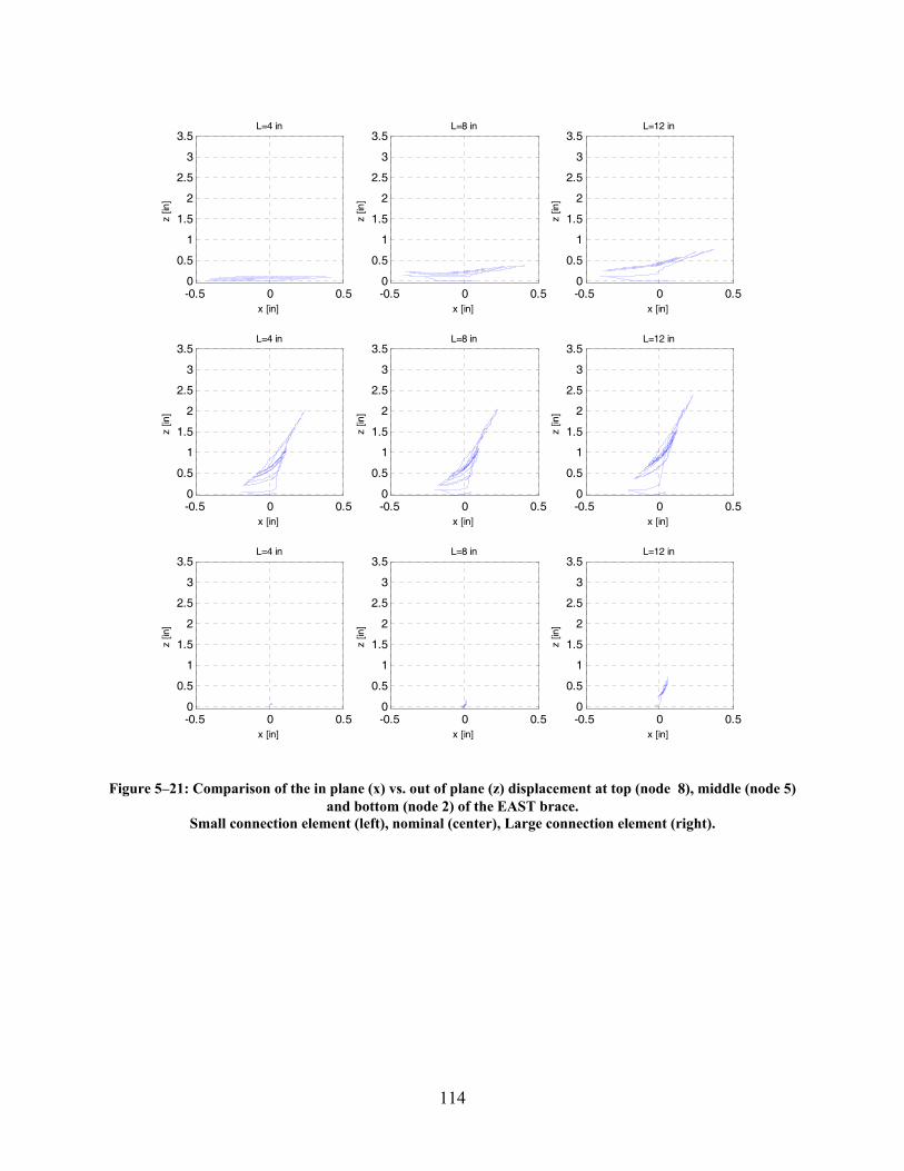
114
-0.5 0 0.50
0.5
1
1.5
2
2.5
3
3.5
x [in]
z [in
]
L=4 in
-0.5 0 0.50
0.5
1
1.5
2
2.5
3
3.5
x [in]
z [in
]
L=8 in
-0.5 0 0.50
0.5
1
1.5
2
2.5
3
3.5
x [in]
z [in
]
L=12 in
-0.5 0 0.50
0.5
1
1.5
2
2.5
3
3.5
x [in]
z [in
]
L=4 in
-0.5 0 0.50
0.5
1
1.5
2
2.5
3
3.5
x [in]
z [in
]
L=8 in
-0.5 0 0.50
0.5
1
1.5
2
2.5
3
3.5
x [in]
z [in
]
L=12 in
-0.5 0 0.50
0.5
1
1.5
2
2.5
3
3.5
x [in]
z [in
]
L=4 in
-0.5 0 0.50
0.5
1
1.5
2
2.5
3
3.5
x [in]
z [in
]
L=8 in
-0.5 0 0.50
0.5
1
1.5
2
2.5
3
3.5
x [in]
z [in
]L=12 in
Figure 5–21: Comparison of the in plane (x) vs. out of plane (z) displacement at top (node 8), middle (node 5) and bottom (node 2) of the EAST brace.
Small connection element (left), nominal (center), Large connection element (right).
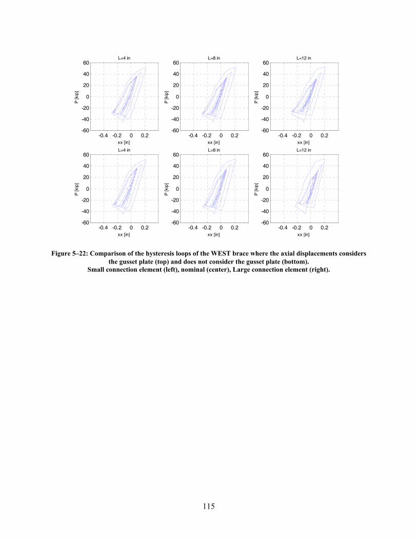
115
-0.4 -0.2 0 0.2-60
-40
-20
0
20
40
60
xx [in]
P [k
ip]
L=4 in
-0.4 -0.2 0 0.2-60
-40
-20
0
20
40
60
xx [in]
P [k
ip]
L=8 in
-0.4 -0.2 0 0.2-60
-40
-20
0
20
40
60
xx [in]
P [k
ip]
L=12 in
-0.4 -0.2 0 0.2-60
-40
-20
0
20
40
60
xx [in]
P [k
ip]
L=4 in
-0.4 -0.2 0 0.2-60
-40
-20
0
20
40
60
xx [in]
P [k
ip]
L=8 in
-0.4 -0.2 0 0.2-60
-40
-20
0
20
40
60
xx [in]
P [k
ip]
L=12 in
Figure 5–22: Comparison of the hysteresis loops of the WEST brace where the axial displacements considers the gusset plate (top) and does not consider the gusset plate (bottom).
Small connection element (left), nominal (center), Large connection element (right).
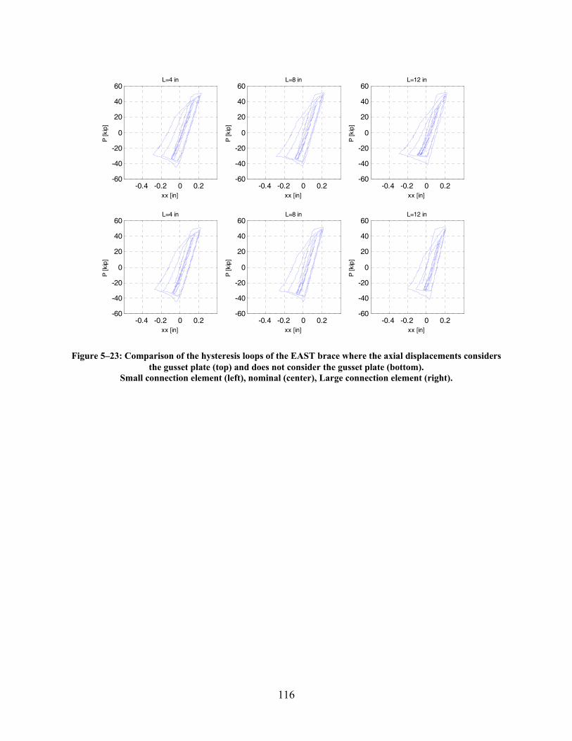
116
-0.4 -0.2 0 0.2-60
-40
-20
0
20
40
60
xx [in]
P [k
ip]
L=4 in
-0.4 -0.2 0 0.2-60
-40
-20
0
20
40
60
xx [in]
P [k
ip]
L=8 in
-0.4 -0.2 0 0.2-60
-40
-20
0
20
40
60
xx [in]
P [k
ip]
L=12 in
-0.4 -0.2 0 0.2-60
-40
-20
0
20
40
60
xx [in]
P [k
ip]
L=4 in
-0.4 -0.2 0 0.2-60
-40
-20
0
20
40
60
xx [in]
P [k
ip]
L=8 in
-0.4 -0.2 0 0.2-60
-40
-20
0
20
40
60
xx [in]
P [k
ip]
L=12 in
Figure 5–23: Comparison of the hysteresis loops of the EAST brace where the axial displacements considers the gusset plate (top) and does not consider the gusset plate (bottom).
Small connection element (left), nominal (center), Large connection element (right).
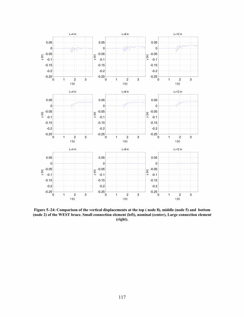
117
0 1 2 3-0.25
-0.2
-0.15
-0.1
-0.05
0
0.05
t [s]
y [in
]
L=4 in
0 1 2 3-0.25
-0.2
-0.15
-0.1
-0.05
0
0.05
t [s]
y [in
]
L=8 in
0 1 2 3-0.25
-0.2
-0.15
-0.1
-0.05
0
0.05
t [s]
y [in
]
L=12 in
0 1 2 3-0.25
-0.2
-0.15
-0.1
-0.05
0
0.05
t [s]
y [in
]
L=4 in
0 1 2 3-0.25
-0.2
-0.15
-0.1
-0.05
0
0.05
t [s]
y [in
]L=8 in
0 1 2 3-0.25
-0.2
-0.15
-0.1
-0.05
0
0.05
t [s]
y [in
]
L=12 in
0 1 2 3-0.25
-0.2
-0.15
-0.1
-0.05
0
0.05
t [s]
y [in
]
L=4 in
0 1 2 3-0.25
-0.2
-0.15
-0.1
-0.05
0
0.05
t [s]
y [in
]
L=8 in
0 1 2 3-0.25
-0.2
-0.15
-0.1
-0.05
0
0.05
t [s]
y [in
]L=12 in
Figure 5–24: Comparison of the vertical displacements at the top ( node 8), middle (node 5) and bottom (node 2) of the WEST brace. Small connection element (left), nominal (center), Large connection element
(right).
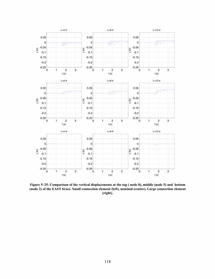
118
0 1 2 3-0.25
-0.2
-0.15
-0.1
-0.05
0
0.05
t [s]
y [in
]
L=4 in
0 1 2 3-0.25
-0.2
-0.15
-0.1
-0.05
0
0.05
t [s]
y [in
]
L=8 in
0 1 2 3-0.25
-0.2
-0.15
-0.1
-0.05
0
0.05
t [s]
y [in
]
L=12 in
0 1 2 3-0.25
-0.2
-0.15
-0.1
-0.05
0
0.05
t [s]
y [in
]
L=4 in
0 1 2 3-0.25
-0.2
-0.15
-0.1
-0.05
0
0.05
t [s]
y [in
]L=8 in
0 1 2 3-0.25
-0.2
-0.15
-0.1
-0.05
0
0.05
t [s]
y [in
]
L=12 in
0 1 2 3-0.25
-0.2
-0.15
-0.1
-0.05
0
0.05
t [s]
y [in
]
L=4 in
0 1 2 3-0.25
-0.2
-0.15
-0.1
-0.05
0
0.05
t [s]
y [in
]
L=8 in
0 1 2 3-0.25
-0.2
-0.15
-0.1
-0.05
0
0.05
t [s]
y [in
]L=12 in
Figure 5–25: Comparison of the vertical displacements at the top ( node 8), middle (node 5) and bottom (node 2) of the EAST brace. Small connection element (left), nominal (center), Large connection element
(right).
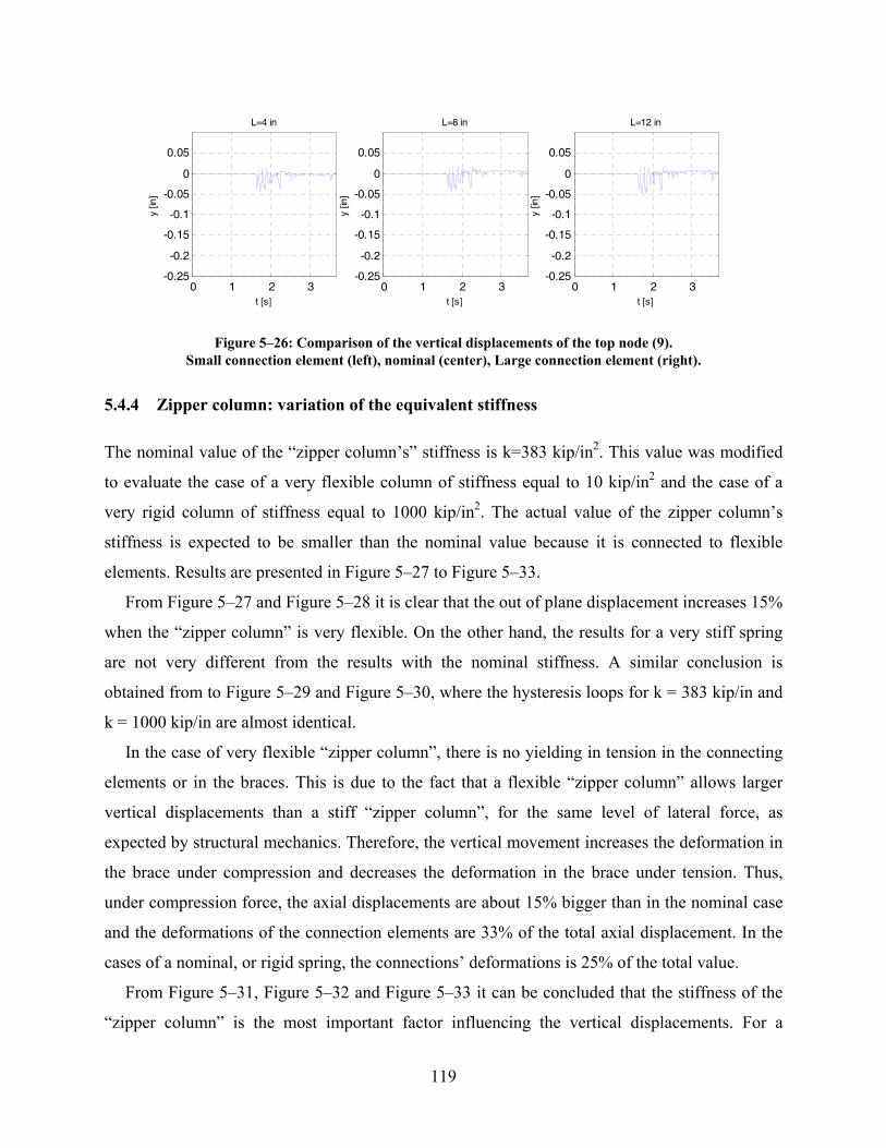
119
0 1 2 3-0.25
-0.2
-0.15
-0.1
-0.05
0
0.05
t [s]
y [in
]
L=4 in
0 1 2 3-0.25
-0.2
-0.15
-0.1
-0.05
0
0.05
t [s]
y [in
]
L=8 in
0 1 2 3-0.25
-0.2
-0.15
-0.1
-0.05
0
0.05
t [s]
y [in
]
L=12 in
Figure 5–26: Comparison of the vertical displacements of the top node (9). Small connection element (left), nominal (center), Large connection element (right).
5.4.4 Zipper column: variation of the equivalent stiffness
The nominal value of the “zipper column’s” stiffness is k=383 kip/in2. This value was modified
to evaluate the case of a very flexible column of stiffness equal to 10 kip/in2 and the case of a
very rigid column of stiffness equal to 1000 kip/in2. The actual value of the zipper column’s
stiffness is expected to be smaller than the nominal value because it is connected to flexible
elements. Results are presented in Figure 5–27 to Figure 5–33.
From Figure 5–27 and Figure 5–28 it is clear that the out of plane displacement increases 15%
when the “zipper column” is very flexible. On the other hand, the results for a very stiff spring
are not very different from the results with the nominal stiffness. A similar conclusion is
obtained from to Figure 5–29 and Figure 5–30, where the hysteresis loops for k = 383 kip/in and
k = 1000 kip/in are almost identical.
In the case of very flexible “zipper column”, there is no yielding in tension in the connecting
elements or in the braces. This is due to the fact that a flexible “zipper column” allows larger
vertical displacements than a stiff “zipper column”, for the same level of lateral force, as
expected by structural mechanics. Therefore, the vertical movement increases the deformation in
the brace under compression and decreases the deformation in the brace under tension. Thus,
under compression force, the axial displacements are about 15% bigger than in the nominal case
and the deformations of the connection elements are 33% of the total axial displacement. In the
cases of a nominal, or rigid spring, the connections’ deformations is 25% of the total value.
From Figure 5–31, Figure 5–32 and Figure 5–33 it can be concluded that the stiffness of the
“zipper column” is the most important factor influencing the vertical displacements. For a
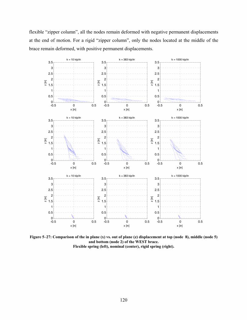
120
flexible “zipper column”, all the nodes remain deformed with negative permanent displacements
at the end of motion. For a rigid “zipper column”, only the nodes located at the middle of the
brace remain deformed, with positive permanent displacements.
-0.5 0 0.50
0.5
1
1.5
2
2.5
3
3.5
x [in]
z [in
]
k = 10 kip/in
-0.5 0 0.50
0.5
1
1.5
2
2.5
3
3.5
x [in]
z [in
]
k = 383 kip/in
-0.5 0 0.50
0.5
1
1.5
2
2.5
3
3.5
x [in]
z [in
]
k = 1000 kip/in
-0.5 0 0.50
0.5
1
1.5
2
2.5
3
3.5
x [in]
z [in
]
k = 10 kip/in
-0.5 0 0.50
0.5
1
1.5
2
2.5
3
3.5
x [in]
z [in
]
k = 383 kip/in
-0.5 0 0.50
0.5
1
1.5
2
2.5
3
3.5
x [in]
z [in
]
k = 1000 kip/in
-0.5 0 0.50
0.5
1
1.5
2
2.5
3
3.5
x [in]
z [in
]
k = 10 kip/in
-0.5 0 0.50
0.5
1
1.5
2
2.5
3
3.5
x [in]
z [in
]
k = 383 kip/in
-0.5 0 0.50
0.5
1
1.5
2
2.5
3
3.5
x [in]
z [in
]
k = 1000 kip/in
Figure 5–27: Comparison of the in plane (x) vs. out of plane (z) displacement at top (node 8), middle (node 5) and bottom (node 2) of the WEST brace.
Flexible spring (left), nominal (center), rigid spring (right).
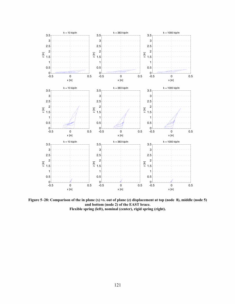
121
-0.5 0 0.50
0.5
1
1.5
2
2.5
3
3.5
x [in]
z [in
]
k = 10 kip/in
-0.5 0 0.50
0.5
1
1.5
2
2.5
3
3.5
x [in]
z [in
]
k = 383 kip/in
-0.5 0 0.50
0.5
1
1.5
2
2.5
3
3.5
x [in]
z [in
]
k = 1000 kip/in
-0.5 0 0.50
0.5
1
1.5
2
2.5
3
3.5
x [in]
z [in
]
k = 10 kip/in
-0.5 0 0.50
0.5
1
1.5
2
2.5
3
3.5
x [in]
z [in
]
k = 383 kip/in
-0.5 0 0.50
0.5
1
1.5
2
2.5
3
3.5
x [in]
z [in
]
k = 1000 kip/in
-0.5 0 0.50
0.5
1
1.5
2
2.5
3
3.5
x [in]
z [in
]
k = 10 kip/in
-0.5 0 0.50
0.5
1
1.5
2
2.5
3
3.5
x [in]
z [in
]
k = 383 kip/in
-0.5 0 0.50
0.5
1
1.5
2
2.5
3
3.5
x [in]
z [in
]k = 1000 kip/in
Figure 5–28: Comparison of the in plane (x) vs. out of plane (z) displacement at top (node 8), middle (node 5) and bottom (node 2) of the EAST brace.
Flexible spring (left), nominal (center), rigid spring (right).
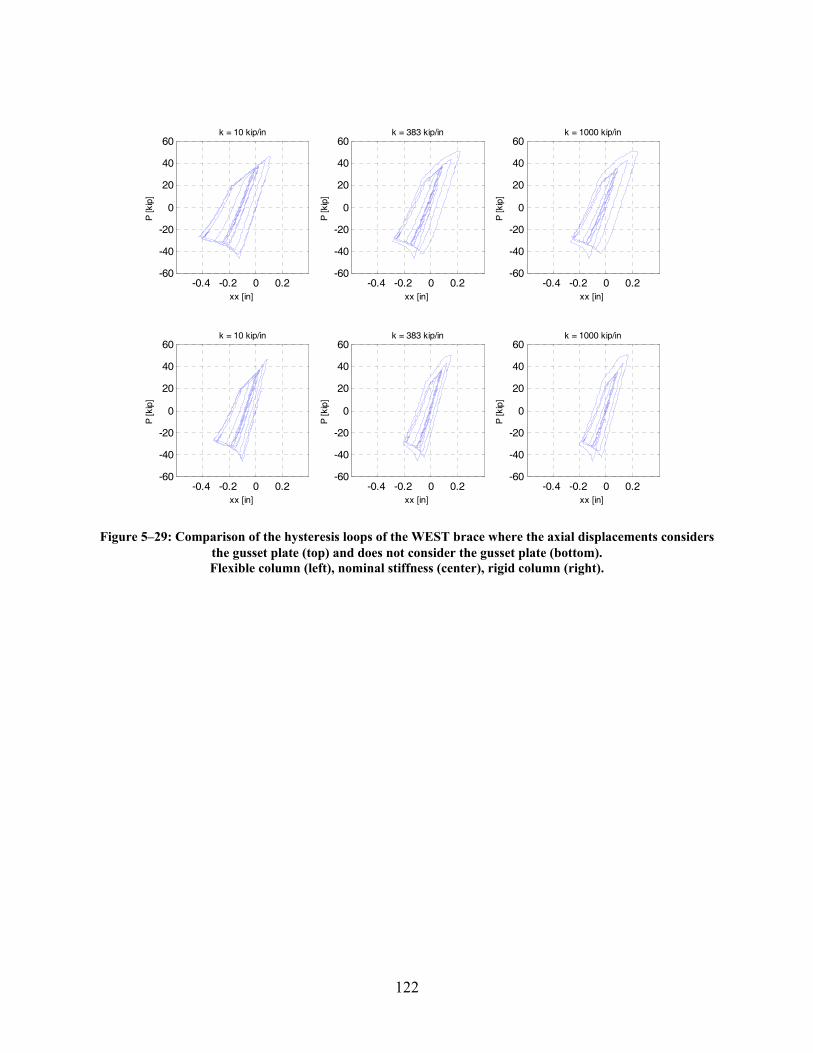
122
-0.4 -0.2 0 0.2-60
-40
-20
0
20
40
60
xx [in]
P [k
ip]
k = 10 kip/in
-0.4 -0.2 0 0.2-60
-40
-20
0
20
40
60
xx [in]
P [k
ip]
k = 383 kip/in
-0.4 -0.2 0 0.2-60
-40
-20
0
20
40
60
xx [in]
P [k
ip]
k = 1000 kip/in
-0.4 -0.2 0 0.2-60
-40
-20
0
20
40
60
xx [in]
P [k
ip]
k = 10 kip/in
-0.4 -0.2 0 0.2-60
-40
-20
0
20
40
60
xx [in]
P [k
ip]
k = 383 kip/in
-0.4 -0.2 0 0.2-60
-40
-20
0
20
40
60
xx [in]P
[kip
]
k = 1000 kip/in
Figure 5–29: Comparison of the hysteresis loops of the WEST brace where the axial displacements considers the gusset plate (top) and does not consider the gusset plate (bottom). Flexible column (left), nominal stiffness (center), rigid column (right).
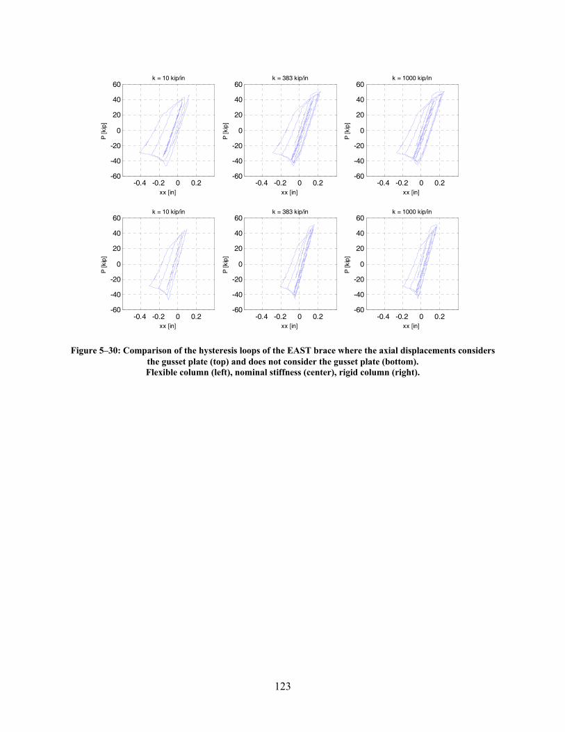
123
-0.4 -0.2 0 0.2-60
-40
-20
0
20
40
60
xx [in]
P [k
ip]
k = 10 kip/in
-0.4 -0.2 0 0.2-60
-40
-20
0
20
40
60
xx [in]
P [k
ip]
k = 383 kip/in
-0.4 -0.2 0 0.2-60
-40
-20
0
20
40
60
xx [in]
P [k
ip]
k = 1000 kip/in
-0.4 -0.2 0 0.2-60
-40
-20
0
20
40
60
xx [in]
P [k
ip]
k = 10 kip/in
-0.4 -0.2 0 0.2-60
-40
-20
0
20
40
60
xx [in]
P [k
ip]
k = 383 kip/in
-0.4 -0.2 0 0.2-60
-40
-20
0
20
40
60
xx [in]
P [k
ip]
k = 1000 kip/in
Figure 5–30: Comparison of the hysteresis loops of the EAST brace where the axial displacements considers the gusset plate (top) and does not consider the gusset plate (bottom). Flexible column (left), nominal stiffness (center), rigid column (right).
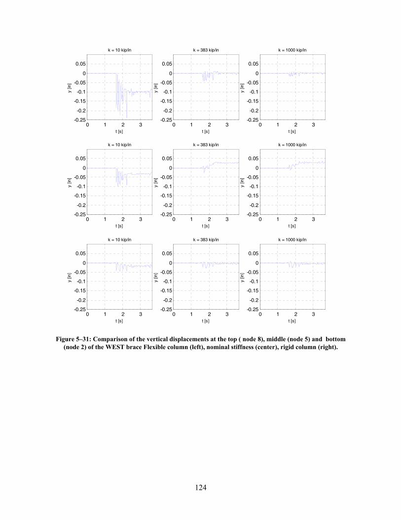
124
0 1 2 3-0.25
-0.2
-0.15
-0.1
-0.05
0
0.05
t [s]
y [in
]
k = 10 kip/in
0 1 2 3-0.25
-0.2
-0.15
-0.1
-0.05
0
0.05
t [s]
y [in
]
k = 383 kip/in
0 1 2 3-0.25
-0.2
-0.15
-0.1
-0.05
0
0.05
t [s]
y [in
]
k = 1000 kip/in
0 1 2 3-0.25
-0.2
-0.15
-0.1
-0.05
0
0.05
t [s]
y [in
]
k = 10 kip/in
0 1 2 3-0.25
-0.2
-0.15
-0.1
-0.05
0
0.05
t [s]
y [in
]
k = 383 kip/in
0 1 2 3-0.25
-0.2
-0.15
-0.1
-0.05
0
0.05
t [s]
y [in
]
k = 1000 kip/in
0 1 2 3-0.25
-0.2
-0.15
-0.1
-0.05
0
0.05
t [s]
y [in
]
k = 10 kip/in
0 1 2 3-0.25
-0.2
-0.15
-0.1
-0.05
0
0.05
t [s]
y [in
]
k = 383 kip/in
0 1 2 3-0.25
-0.2
-0.15
-0.1
-0.05
0
0.05
t [s]
y [in
]k = 1000 kip/in
Figure 5–31: Comparison of the vertical displacements at the top ( node 8), middle (node 5) and bottom (node 2) of the WEST brace Flexible column (left), nominal stiffness (center), rigid column (right).
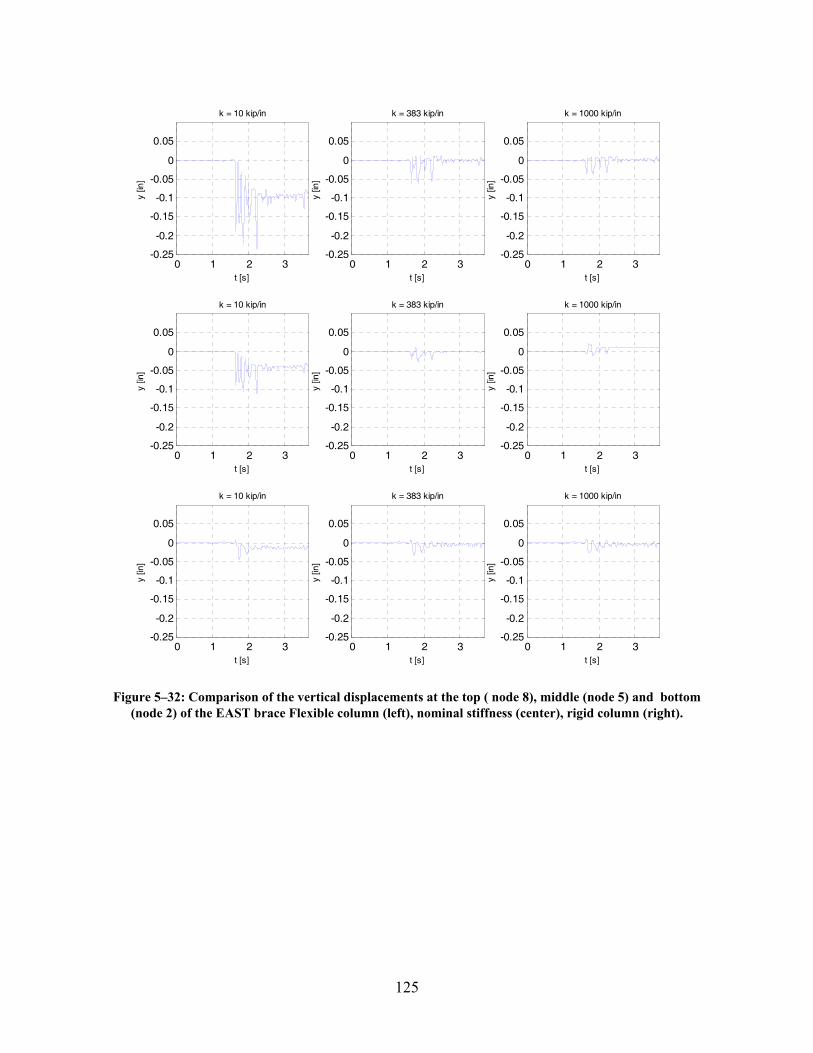
125
0 1 2 3-0.25
-0.2
-0.15
-0.1
-0.05
0
0.05
t [s]
y [in
]
k = 10 kip/in
0 1 2 3-0.25
-0.2
-0.15
-0.1
-0.05
0
0.05
t [s]
y [in
]
k = 383 kip/in
0 1 2 3-0.25
-0.2
-0.15
-0.1
-0.05
0
0.05
t [s]
y [in
]
k = 1000 kip/in
0 1 2 3-0.25
-0.2
-0.15
-0.1
-0.05
0
0.05
t [s]
y [in
]
k = 10 kip/in
0 1 2 3-0.25
-0.2
-0.15
-0.1
-0.05
0
0.05
t [s]
y [in
]k = 383 kip/in
0 1 2 3-0.25
-0.2
-0.15
-0.1
-0.05
0
0.05
t [s]
y [in
]
k = 1000 kip/in
0 1 2 3-0.25
-0.2
-0.15
-0.1
-0.05
0
0.05
t [s]
y [in
]
k = 10 kip/in
0 1 2 3-0.25
-0.2
-0.15
-0.1
-0.05
0
0.05
t [s]
y [in
]
k = 383 kip/in
0 1 2 3-0.25
-0.2
-0.15
-0.1
-0.05
0
0.05
t [s]
y [in
]k = 1000 kip/in
Figure 5–32: Comparison of the vertical displacements at the top ( node 8), middle (node 5) and bottom (node 2) of the EAST brace Flexible column (left), nominal stiffness (center), rigid column (right).
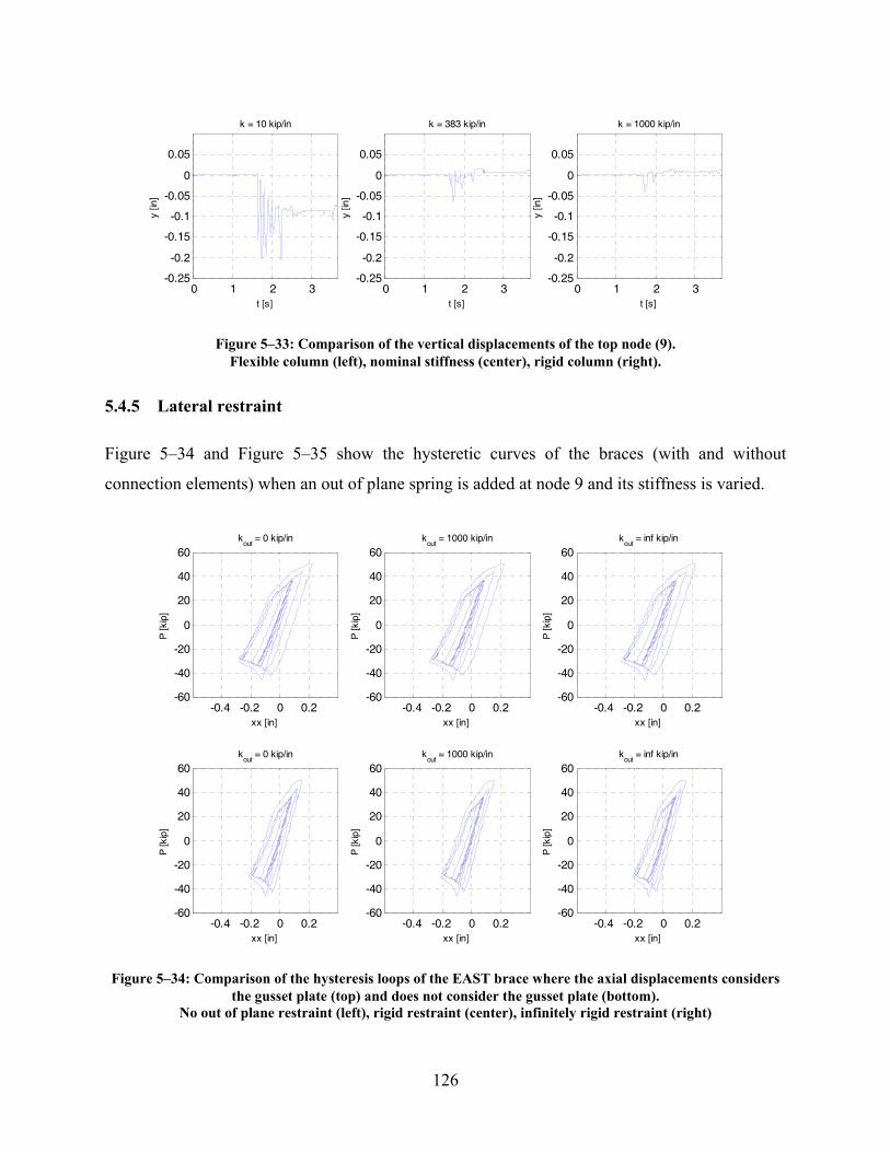
126
0 1 2 3-0.25
-0.2
-0.15
-0.1
-0.05
0
0.05
t [s]
y [in
]
k = 10 kip/in
0 1 2 3-0.25
-0.2
-0.15
-0.1
-0.05
0
0.05
t [s]
y [in
]
k = 383 kip/in
0 1 2 3-0.25
-0.2
-0.15
-0.1
-0.05
0
0.05
t [s]
y [in
]
k = 1000 kip/in
Figure 5–33: Comparison of the vertical displacements of the top node (9). Flexible column (left), nominal stiffness (center), rigid column (right).
5.4.5 Lateral restraint
Figure 5–34 and Figure 5–35 show the hysteretic curves of the braces (with and without
connection elements) when an out of plane spring is added at node 9 and its stiffness is varied.
-0.4 -0.2 0 0.2-60
-40
-20
0
20
40
60
xx [in]
P [k
ip]
kout
= 0 kip/in
-0.4 -0.2 0 0.2-60
-40
-20
0
20
40
60
xx [in]
P [k
ip]
kout
= 1000 kip/in
-0.4 -0.2 0 0.2-60
-40
-20
0
20
40
60
xx [in]
P [k
ip]
kout
= inf kip/in
-0.4 -0.2 0 0.2-60
-40
-20
0
20
40
60
xx [in]
P [k
ip]
kout
= 0 kip/in
-0.4 -0.2 0 0.2-60
-40
-20
0
20
40
60
xx [in]
P [k
ip]
kout
= 1000 kip/in
-0.4 -0.2 0 0.2-60
-40
-20
0
20
40
60
xx [in]
P [k
ip]
kout
= inf kip/in
Figure 5–34: Comparison of the hysteresis loops of the EAST brace where the axial displacements considers the gusset plate (top) and does not consider the gusset plate (bottom).
No out of plane restraint (left), rigid restraint (center), infinitely rigid restraint (right)
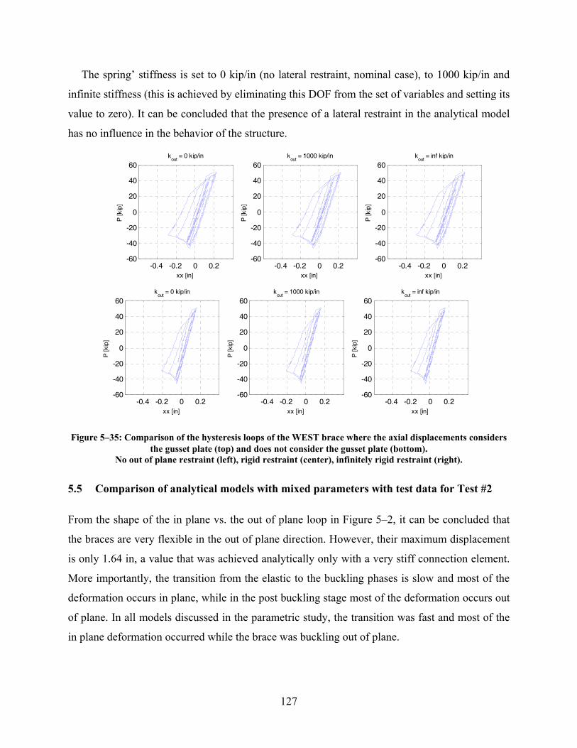
127
The spring’ stiffness is set to 0 kip/in (no lateral restraint, nominal case), to 1000 kip/in and
infinite stiffness (this is achieved by eliminating this DOF from the set of variables and setting its
value to zero). It can be concluded that the presence of a lateral restraint in the analytical model
has no influence in the behavior of the structure.
-0.4 -0.2 0 0.2-60
-40
-20
0
20
40
60
xx [in]
P [k
ip]
kout
= 0 kip/in
-0.4 -0.2 0 0.2-60
-40
-20
0
20
40
60
xx [in]
P [k
ip]
kout
= 1000 kip/in
-0.4 -0.2 0 0.2-60
-40
-20
0
20
40
60
xx [in]
P [k
ip]
kout
= inf kip/in
-0.4 -0.2 0 0.2-60
-40
-20
0
20
40
60
xx [in]
P [k
ip]
kout
= 0 kip/in
-0.4 -0.2 0 0.2-60
-40
-20
0
20
40
60
xx [in]
P [k
ip]
kout
= 1000 kip/in
-0.4 -0.2 0 0.2-60
-40
-20
0
20
40
60
xx [in]
P [k
ip]
kout
= inf kip/in
Figure 5–35: Comparison of the hysteresis loops of the WEST brace where the axial displacements considers the gusset plate (top) and does not consider the gusset plate (bottom).
No out of plane restraint (left), rigid restraint (center), infinitely rigid restraint (right).
5.5 Comparison of analytical models with mixed parameters with test data for Test #2
From the shape of the in plane vs. the out of plane loop in Figure 5–2, it can be concluded that
the braces are very flexible in the out of plane direction. However, their maximum displacement
is only 1.64 in, a value that was achieved analytically only with a very stiff connection element.
More importantly, the transition from the elastic to the buckling phases is slow and most of the
deformation occurs in plane, while in the post buckling stage most of the deformation occurs out
of plane. In all models discussed in the parametric study, the transition was fast and most of the
in plane deformation occurred while the brace was buckling out of plane.
128
Several combinations of parameters were analyzed and the results are shown from Figure 5–
36 to Figure 5–39. The experimental results are also shown for comparison purposes.
The properties of the connection elements are:
• Model 1: stiffness of “zipper column” 200 kip/in
yield strength 60 kip/in2
out of plane inertia Ibrace/2
• Model 2: stiffness of “zipper column” 200 kip/in
yield strength 60 kip/in2
out of plane inertia Ibracex2
• Model 3: stiffness of “zipper column” 100 kip/in
yield strength 60 kip/in2
out of plane inertia Ibracex2
• Model 4: stiffness of “zipper column” 100 kip/in
yield strength 60 kip/in2
out of plane inertia Ibrace
• Model 5: stiffness of “zipper column” 383 kip/in
yield strength 60 kip/in2
out of plane inertia Ibrace/2
Figure 5–36 and Figure 5–37 show the results for displacement loops of the west and east
brace for the models detailed above. Comparing the results of Model 1 and Model 5, it can be
concluded that when the connection elements are flexible, a variation in the “zipper column’s”
flexibility has an impact on the values of maximum displacements. However, when a very stiff
connection element is used (model 2 and Model 3), a variation of the flexibility of the “zipper
column” has no impact on the values of the maximum displacements and has a minimum
influence in the shape of the curve. Therefore, the major parameter affecting the in plane and out
of plane displacements of the braces is the stiffness of the connection elements.
Figure 5–38 and Figure 5–39 show the hysteretic loops of the west and east braces under the
same combination of parameters. In this case, the stiffness of the spring is important because it
controls the vertical displacements of the brace, thus it controls its total axial displacement. This
is especially relevant when the brace is loaded in tension. When a soft spring is attached to the
129
braces, the nodes move more freely in the vertical direction, thus for the brace under
compression force the vertical displacements translate into more compression deformation. This
brace will have larger buckling and permanent deformations. When the brace is under tension
force, the vertical displacements also translate into compression deformation, thus reducing the
amount of axial tension displacement. It is concluded that the models with a softer spring
representing the “zipper column” approximate better the test results.
It appears also that a system with a soft spring dissipates less energy, but this conclusion must
be wrong because the axial displacement is calculated as the length of the chord of the complete
brace and does not account for permanent out of plane deformations.
Finally, a complete model of the “zipper frame” was not analyzed for the sensitivity study due
to the high computational time required.
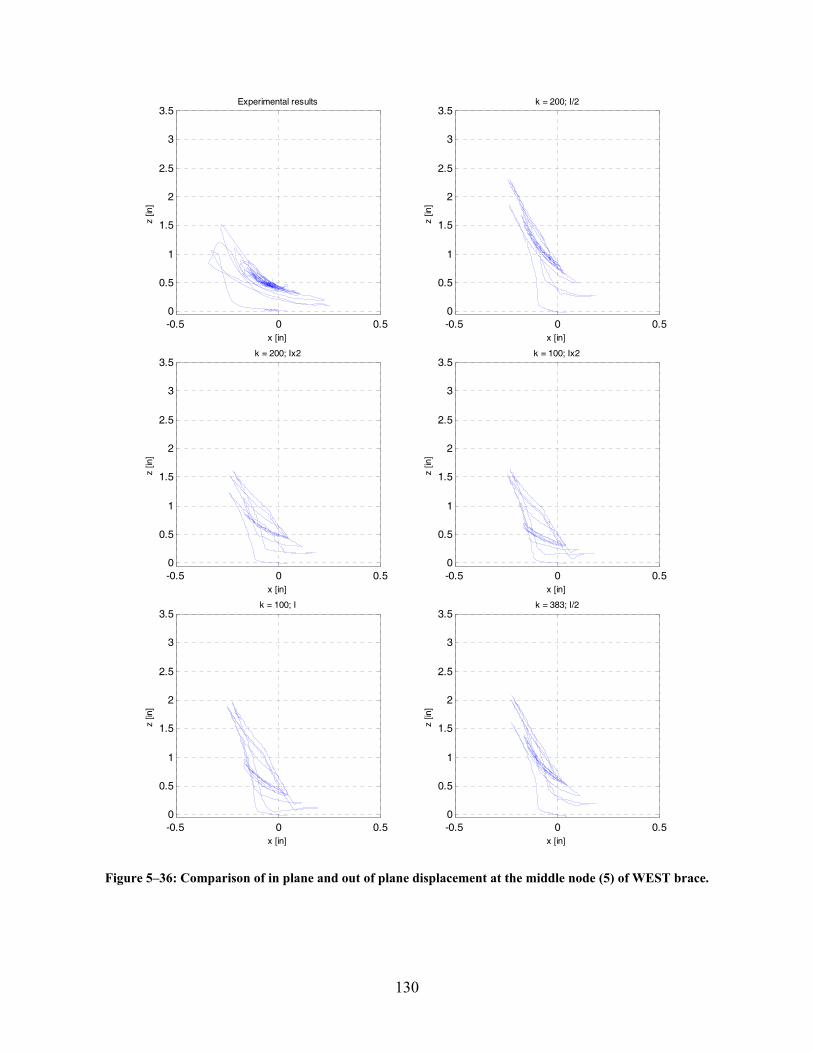
130
-0.5 0 0.50
0.5
1
1.5
2
2.5
3
3.5
x [in]
z [in
]
Experimental results
-0.5 0 0.50
0.5
1
1.5
2
2.5
3
3.5
x [in]
z [in
]
k = 200; I/2
-0.5 0 0.50
0.5
1
1.5
2
2.5
3
3.5
x [in]
z [in
]
k = 200; Ix2
-0.5 0 0.50
0.5
1
1.5
2
2.5
3
3.5
x [in]
z [in
]
k = 100; Ix2
-0.5 0 0.50
0.5
1
1.5
2
2.5
3
3.5
x [in]
z [in
]
k = 100; I
-0.5 0 0.50
0.5
1
1.5
2
2.5
3
3.5
x [in]
z [in
]
k = 383; I/2
Figure 5–36: Comparison of in plane and out of plane displacement at the middle node (5) of WEST brace.
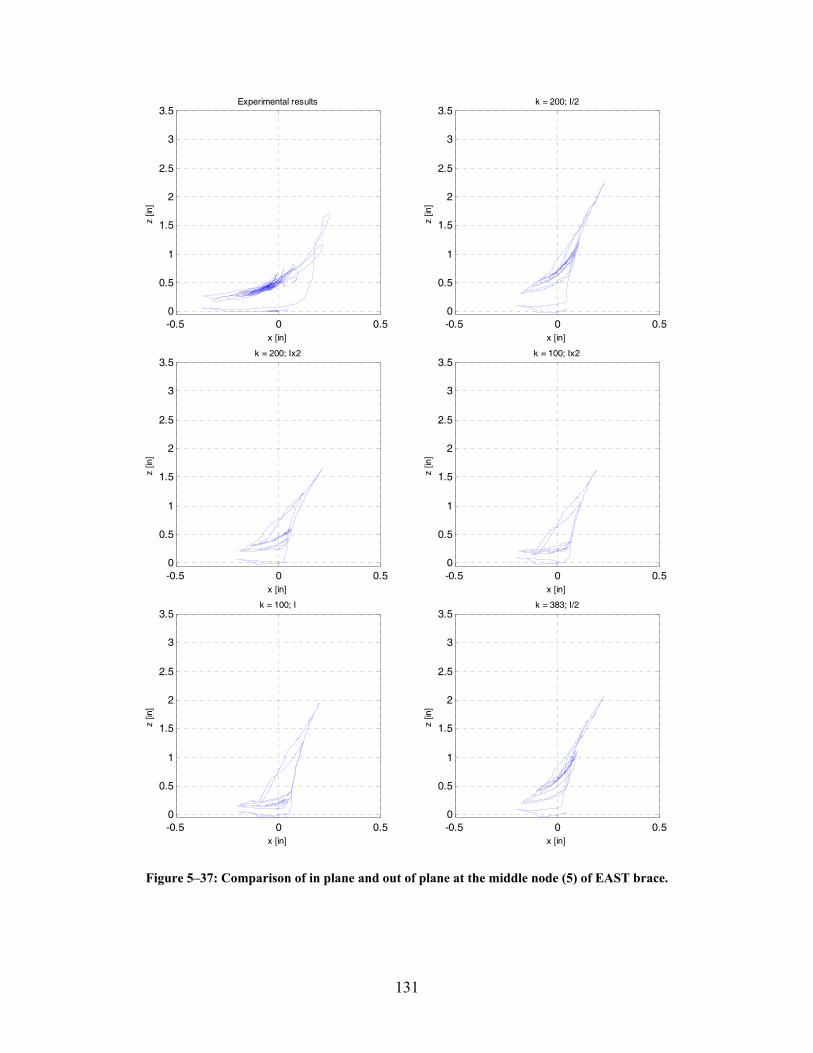
131
-0.5 0 0.50
0.5
1
1.5
2
2.5
3
3.5
x [in]
z [in
]
Experimental results
-0.5 0 0.50
0.5
1
1.5
2
2.5
3
3.5
x [in]
z [in
]
k = 200; I/2
-0.5 0 0.50
0.5
1
1.5
2
2.5
3
3.5
x [in]
z [in
]
k = 200; Ix2
-0.5 0 0.50
0.5
1
1.5
2
2.5
3
3.5
x [in]
z [in
]
k = 100; Ix2
-0.5 0 0.50
0.5
1
1.5
2
2.5
3
3.5
x [in]
z [in
]
k = 100; I
-0.5 0 0.50
0.5
1
1.5
2
2.5
3
3.5
x [in]
z [in
]
k = 383; I/2
Figure 5–37: Comparison of in plane and out of plane at the middle node (5) of EAST brace.
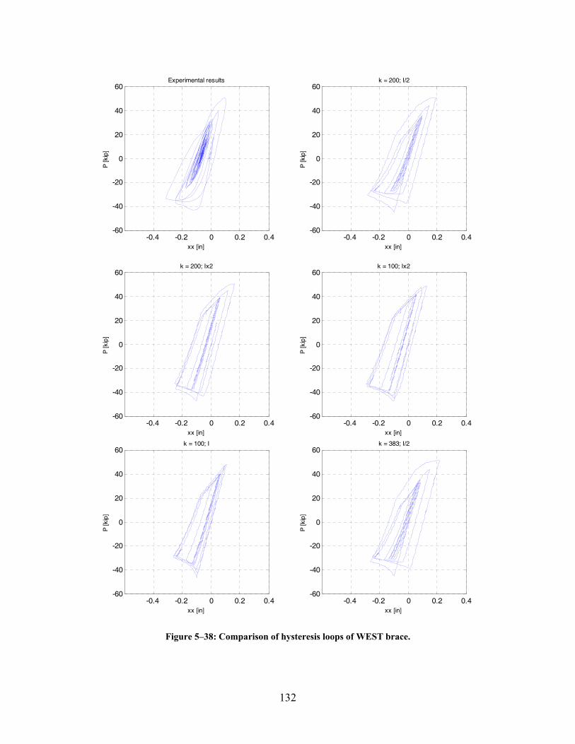
132
-0.4 -0.2 0 0.2 0.4-60
-40
-20
0
20
40
60
xx [in]
P [k
ip]
Experimental results
-0.4 -0.2 0 0.2 0.4-60
-40
-20
0
20
40
60
xx [in]
P [k
ip]
k = 200; I/2
-0.4 -0.2 0 0.2 0.4-60
-40
-20
0
20
40
60
xx [in]
P [k
ip]
k = 200; Ix2
-0.4 -0.2 0 0.2 0.4-60
-40
-20
0
20
40
60
xx [in]
P [k
ip]
k = 100; Ix2
-0.4 -0.2 0 0.2 0.4-60
-40
-20
0
20
40
60
xx [in]
P [k
ip]
k = 100; I
-0.4 -0.2 0 0.2 0.4-60
-40
-20
0
20
40
60
xx [in]
P [k
ip]
k = 383; I/2
Figure 5–38: Comparison of hysteresis loops of WEST brace.
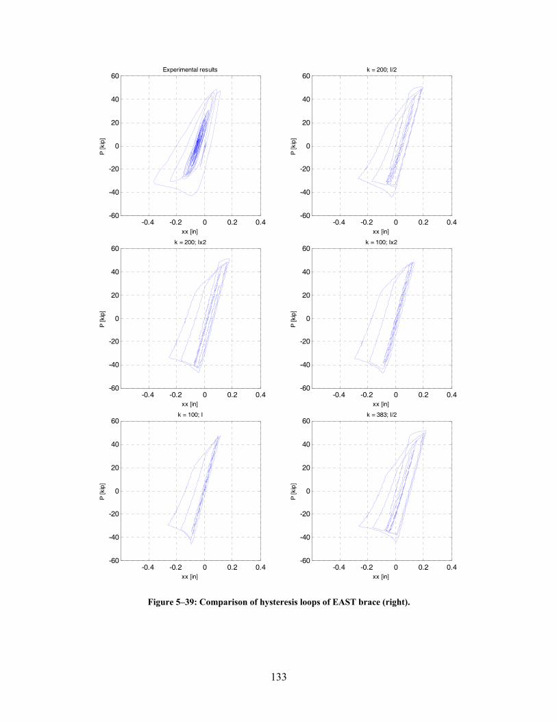
133
-0.4 -0.2 0 0.2 0.4-60
-40
-20
0
20
40
60
xx [in]
P [k
ip]
Experimental results
-0.4 -0.2 0 0.2 0.4-60
-40
-20
0
20
40
60
xx [in]
P [k
ip]
k = 200; I/2
-0.4 -0.2 0 0.2 0.4-60
-40
-20
0
20
40
60
xx [in]
P [k
ip]
k = 200; Ix2
-0.4 -0.2 0 0.2 0.4-60
-40
-20
0
20
40
60
xx [in]
P [k
ip]
k = 100; Ix2
-0.4 -0.2 0 0.2 0.4-60
-40
-20
0
20
40
60
xx [in]
P [k
ip]
k = 100; I
-0.4 -0.2 0 0.2 0.4-60
-40
-20
0
20
40
60
xx [in]
P [k
ip]
k = 383; I/2
Figure 5–39: Comparison of hysteresis loops of EAST brace (right).
134
5.6 Conclusions
It can be concluded that the formulation developed in Chapter 2 reproduces all the important
details that characterizes the inelastic buckling. The formulation is numerically stable and
extremely sensitive to all modeling parameters. All the results obtained for each variation of each
modeling parameter are consistent with structural mechanics theory.
Among the sources for discrepancies in the prediction are:
• Uncertain modeling parameters:
o The gusset plates are modeled with connection elements of uncertain equivalent
properties
o The “zipper column” and the frame’s upper stories are modeled with an elastic
spring of uncertain equivalent stiffness.
• Uncertain yield functions: There are smooth continuous functions available in the
literature that approximate the theoretical ultimate yield curves for typical sections.
However, in the examples shown, a plate is being modeled with a conventional element
and an appropriate equivalent yield function is not perfectly modeled. This is a key aspect
in the solution of the system because the flexibility of the connection elements control the
out of plane displacement of the braces and the relationship between the moment capacity
of the connection and the moment capacity of the brace defines the shape of the hysteric
loop.
• The implemented relationship between strains and forces (flexibility matrix) controls the
relationship between the in plane and out of plane displacement. By allowing plastic
deformations from the beginning of the ground motion, the brace moves in plane and out
of plane simultaneously however, during the test, these displacements were almost
independent. Figure 5–40 shows the in plane and out of plane displacements of the
middle node of west and east braces when an elastic relationship between strains and
forces is used in both braces and connection elements. The braces still buckle out of
plane, although elastically. In that case, the shape of the displacement plots is very
similar to the shapes in Figure 5–2 i.e. the braces develop most of their in plane
displacement before buckling. The description of the material nonlinearity also controls
the maximum and permanent lateral and vertical displacements and the distribution of the
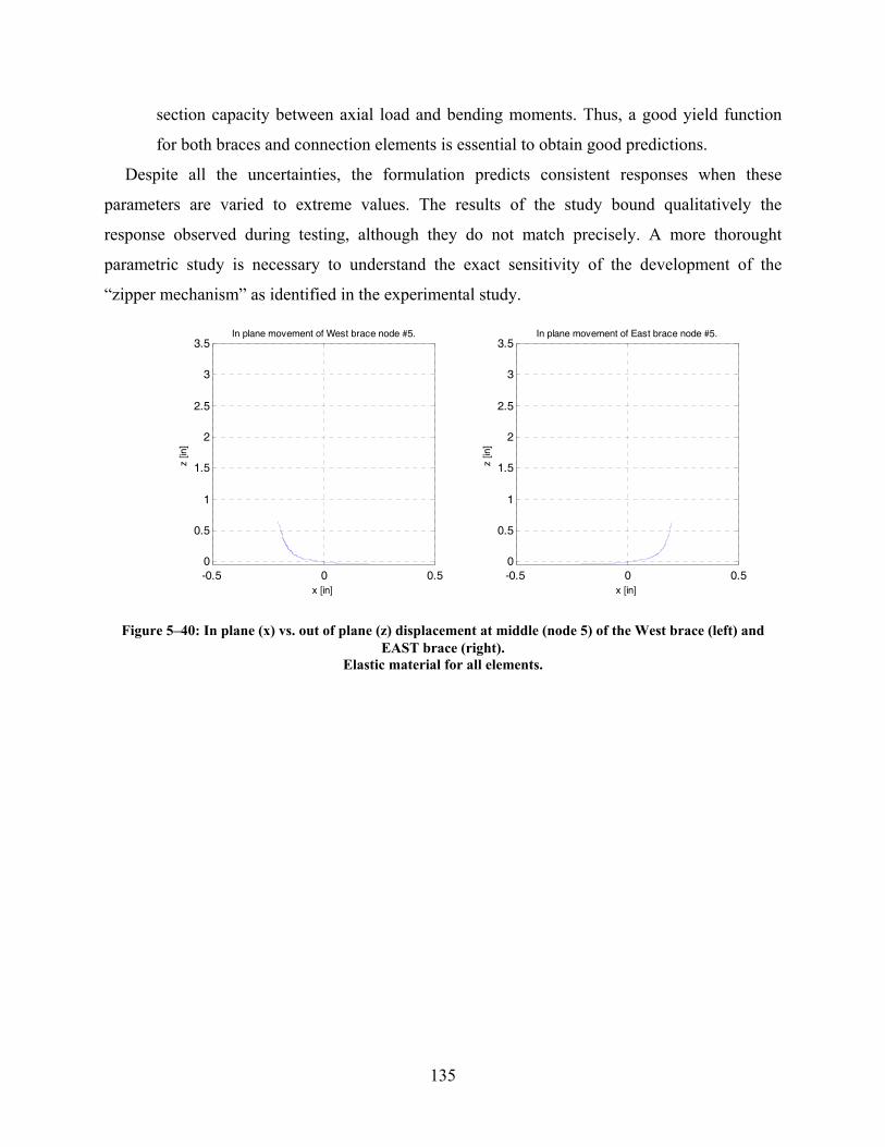
135
section capacity between axial load and bending moments. Thus, a good yield function
for both braces and connection elements is essential to obtain good predictions.
Despite all the uncertainties, the formulation predicts consistent responses when these
parameters are varied to extreme values. The results of the study bound qualitatively the
response observed during testing, although they do not match precisely. A more thorought
parametric study is necessary to understand the exact sensitivity of the development of the
“zipper mechanism” as identified in the experimental study.
-0.5 0 0.50
0.5
1
1.5
2
2.5
3
3.5
x [in]
z [in
]
In plane movement of West brace node #5.
-0.5 0 0.50
0.5
1
1.5
2
2.5
3
3.5
x [in]
z [in
]
In plane movement of East brace node #5.
Figure 5–40: In plane (x) vs. out of plane (z) displacement at middle (node 5) of the West brace (left) and EAST brace (right).
Elastic material for all elements.

137
SECTION 6
REMARKS, CONCLUSIONS AND RECOMMENDATIONS
6.1 Summary
A new unified formulation capable of solving problems of large rotations and large deformations
in inelastic frame structures was developed. An experimental study was carried out on a “zipper
frame”. The frame was subjected to earthquake motion using the shake tables. Data from the
inelastic behavior of the frame was collected for comparison with the analytical model
predictions. Finally, an analytical model of the first story of the zipper frame was built and
analyzed with the new formulation. A parametric study was performed and a few combinations
of modeling parameters were selected to match the test results.
In order to incorporate large rotations and displacements, the formulation is based on the
corotational method, where the rigid body motion and deformations are separated and analyzed
independently by defining a local corotated coordinate system at the chord of the element in its
deformed configuration. All the information needed to calculate the variations in strains and
stresses is contained in the deformational part of the motion because a rigid body movement just
changes the orientation of the strains. Usually deformations are assumed to be infinitesimal,
however in the present formulation this hypothesis is relaxed and P-∆ effects are also accounted
for at the chord level.
The proposed new formulation uses a flexibility based element and it is implemented in the
state space. The main advantage of a flexibility based element is its exact interpolation of the
forces along the length of the element while interpolating displacements using compatibility
equations instead of approximated polynomials. In the state space, local and global variables and
their evolution equations are defined. Global variables are total displacements and local variables
are the elements' local forces and total strains at the Integration Points. The rates of all these
variables are also variables of the system. The evolution equations for global variables are
equilibrium equations and for local variables are plasticity equations. For a flexibility based
element, the compatibility equations need to be considered explicitly because the internal forces
are interpolated. In a stiffness based element, the compatibility is already accounted for when the
138
strains (or displacement field) is approximated with interpolation functions. By solving all these
equations simultaneously, convergence is achieved for all variables at the same time, thus
eliminating the need for iterations between time steps.
The formulation derived therein combines the state space approach, the corotational method
and a flexibility based element. Thus, after selecting the global and local variables, the equations
of equilibrium compatibility and plasticity must be derived as rate equations, or algebraic
equations. Equilibrium is readily obtained with the transformation of the element local forces.
These equations are differential when mass is associated with a DOF and algebraic for all others
DOFs. Incremental compatibility equations are based on a differential description of the
deformed shape with respect to the chord. Both rotational and displacement deformations are
considered to be finite. Plasticity equations are based on flow theory and are derived as rate
equations linking force rates and strain rates. Therefore, the state space is an ideal framework to
develop a unified formulation because it naturally integrates all the basics structural equations
and ensures that convergence is achieved in all of them.
Finally, a comparison of the sensitivity of the analytical predictions from a model of the first
story of a “zipper frame” with data from shaking table tests was performed. The primarily failure
mode of the structure is inelastic buckling of its braces thus; this comparison is a good test of the
capabilities of the developed formulation, which can handle problems of large rotations and
inelastic material with great sensitivity.
6.2 Conclusions
From the comparison between analytical prediction and test results it can be concluded that:
• The formulation successfully solves problems of large rotations and displacements in
three dimensions, like out of plane buckling of braces. A small imperfection of 1/500 of
the length of the element is enough to trigger buckling.
• As a general conclusion, it can be said that the new formulation is sensitive to all
parameters studied above and the variations of the response is always in agreement with
structural principles.
• The formulation proved to be very sensitive to parameters that characterize the gusset
plates (connection elements). The most sensitive parameters found are: the stiffness of
139
the vertical spring that models the influence of the zipper column and upper stories and
the stiffness of the connection elements.
• It was found that the stiffness of the vertical spring controls the vertical displacement of
the nodes, thus it controls the total axial deformation of the member and influences the
shape of the hysteretic loop. Compared to a nominal stiffness calculated as (EA/L) with
zipper column properties, the required stiffness of this element is much smaller. This
result is in agreement with the fact that the nominal stiffness corresponds to an element
that is rigidly supported at one end and that the actual zipper column is attached to
flexible elements, thus the equivalent stiffness is smaller than the nominal.
• It was found that the stiffness of the connection elements controls the out of plane
displacement of the nodes and thus controls the shape of the in plane vs. out of plane
loop. The stiffness of these elements can be changed by changing the value of the
equivalent inertia or by changing the length of the element. These possibilities were
explored in the parametrical study performed. It was found that with flexible connection
elements, the out of plane displacements are larger and the shapes of the loops are
smoother. This behavior was the expected one. From the test results, the connection
elements should be very flexible but the out of plane displacements are smaller than
predicted.
• The variation in the response when the connection elements had different yield strengths
was studied. It was found that if the connections’ strength is very small compared to the
braces, they yield first and do not allow the braces to develop all the axial force. Thus, by
limiting the capacity of the connection elements, the overall capacity of the brace is also
limited. In contrast, when their yield strength is much larger than the rest of the element,
the connections remain elastic and the braces concentrate all plastic deformation.
• An important parameter not studied in this work is the yield function of the connection
elements. The function used corresponds to a HSS section. Clearly, this is inadequate
(because the gussets are plates not tubes) and a yield function that can replicate the
plastic behavior of a plate is needed. During testing, the gusset plates yielded with a
combination of axial force and bending moments, thus it is expected that a better
description of the plate’s plasticity will improve the overall response of the system.
140
• One of the most important differences between the predicted and recorded responses is
the shape of the in plane/out of plane displacement. While the maximum in plane
displacements are very similar, in the test during the pre-buckling phase most of the
displacement occurs in the in plane direction and during the post-buckling phase the
displacement is mostly in the out of plane direction. In the analytical response, however
both displacements occur simultaneously. The explanation for this behavior lays in the
adopted plasticity description. When the model is analyzed with an elastic material, a
similar shape for in plane/out of plane loop is obtained although the maximum values are
very different.
• In general, the new formulation and the experimental study indicate that the “zipper
frame” is sensitive to the construction details which, if not properly considered, may
render the system ineffective.
• The new formulation can identify the sensitive spots and can lead to better detail
considerations and addition of redundancies.
In conclusion, the formulation can predict inelastic buckling and its accuracy depends on the
knowledge of model details.
141
SECTION 7
REFERENCES.
AISC. (2003). Manual of steel construction LRFD, AISC, Chicago, IL.
AISC. (2005a). "Seismic provisions for structural steel buildings."
AISC. (2005b). "Specification for structural steel buildings."
Argyris, J. (1982). "An excursion into large rotations." Computer Methods in Applied Mechanics and Engineering, 32(1-3), 85-155.
Argyris, J. H., Balmer, H., Doltsinis, J. S., Dunne, P. C., Haase, M., Kleiber, M., Malejannakis, G. A., Mlejnek, H. P., Muller, M., and Scharpf, D. W. (1979). "Finite element method -- the natural approach." Computer Methods in Applied Mechanics and Engineering, 17-18(Part 1), 1-106.
ASCE. (2005). "Minimum design loads for buildings and other structures."
Bäcklund, J. (1976). "Large deflection analyis of elasto-plastic beams and frames." International Journal of Mechanical Science, 18, 269-277.
Battini, J.-M., and Pacoste, C. (2002a). "Co-rotational beam elements with warping effects in instability problems." Computer Methods in Applied Mechanics and Engineering, 191(17-18), 1755-1789.
Battini, J.-M., and Pacoste, C. (2002b). "Plastic instability of beam structures using co-rotational elements." Computer Methods in Applied Mechanics and Engineering, 191(51-52), 5811-5831.
Bazant, Z., and Cedolin, L. (1991). Stability of structures., Oxford University Press., New York.
Behdinan, K., Stylianou, M. C., and Tabarrok, B. (1998). "Co-rotational dynamic analysis of flexible beams." Computer Methods in Applied Mechanics and Engineering, 154(3-4), 151-161.
Boller, C., and Seeger, T. (1987). Material data for cyclic loading, part A: unalloyed steels, Elsevier, Amsterdam.
Bouc, R. "Forced vibration of mechanical systems with hysteresis." Proc., 4th Conference on Non-linear Oscillations.
Brenan, K. E., Campbell, S. L., and Petzold, L. R. (1989). Numerical solution of initial-value problems in differential-algebraic equations., SIAM, Philadelphia.
Cardona, A., and Geradin, M. (1988). "A beam finite element non-linear theory with finite rotations." International Journal for Numerical Methods in Engineering, 26(11), 2403-2438.
Chen, W. F. (2000). "Structural stability: from theory to practice." Engineering Structures, 22(2), 116-122.
142
Crisfield, M. A. (1990). "A consistent co-rotational formulation for non-linear, three-dimensional, beam-elements." Computer Methods in Applied Mechanics and Engineering, 81(2), 131-150.
Crisfield, M. A. (1991). Non linear finite element analysis of solids and structures. v1: Essentials, Wiley, Chichester.
Crisfield, M. A. (1997). Non linear finite element analysis of solids and structures. v2: Advanced topics, Wiley, Chichester.
Duan, L., and Chen, W.-F. (1990). "A yield surface equation for doubly symmetrical sections." Engineering Structures, 12(2), 114-119.
Felippa, C. A., and Haugen, B. (2005). "A unified formulation of small-strain corotational finite elements: I. Theory." Computer Methods in Applied Mechanics and Engineering, 194(21-24), 2285-2335.
FEMA. (2000). 355C: State of the art report on systems performance of steel moment frames subject to earthquake ground shaking, Washington, DC, Prepared by the SAC joint venture for the Federal Emergency Management Agency.
Gruttmann, F., Sauer, R., and Wagner, W. (1998). "A geometrical nonlinear eccentric 3D-beam element with arbitrary cross-sections." Computer Methods in Applied Mechanics and Engineering, 160(3-4), 383-400.
Hall, J. F., and Challa, R. M. (1995). "Beam-Column Modeling." Journal of Engineering Mechanics, 121(2), 1284-1291.
Hindmarsh, A. C., and Serban, R. (2006). User documentation for IDA v2.4.0, LLNL.
Hsiao, K. M., Lin, J. Y., and Lin, W. Y. (1999). "A consistent co-rotational finite element formulation for geometrically nonlinear dynamic analysis of 3-D beams." Computer Methods in Applied Mechanics and Engineering, 169(1-2), 1-18.
Hsiao, K. M., and Lin, W. Y. (2000). "A co-rotational finite element formulation for buckling and postbuckling analyses of spatial beams." Computer Methods in Applied Mechanics and Engineering, 188(1-3), 567-594.
Huddleston, J. V. (1968). "Effect of axial strain on buckling and postbuckling behavior of elastic columns." Developments in theoretical and applied mechanics, Proceedings of the fourth southeastern conference on theoretical and applied mechanics, New Orleans, Louisiana, 263-273.
Ibrahimbegovic, A. (1995). "On finite element implementation of geometrically nonlinear Reissner's beam theory: three-dimensional curved beam elements." Computer Methods in Applied Mechanics and Engineering, 122(1-2), 11-26.
Ibrahimbegovic, A. (1997). "On the choice of finite rotation parameters." Computer Methods in Applied Mechanics and Engineering, 149(1-4), 49-71.
Izzuddin, B. A., and D.L.Smith. (1996). "Large-Displacement Analysis of Elastoplastic Thin-Walled Frames. I: Formulation and Implementation." Journal of Structural Engineering, 122(8), 905-914.
143
Jelenic, G., and Crisfield, M. A. (1999). "Geometrically exact 3D beam theory: implementation of a strain-invariant finite element for statics and dynamics." Computer Methods in Applied Mechanics and Engineering, 171(1-2), 141-171.
Jelenic, G., and Crisfield, M. A. (2001). "Dynamic analysis of 3D beams with joints in presence of large rotations." Computer Methods in Applied Mechanics and Engineering, 190(32-33), 4195-4230.
Jelenic, G., and Saje, M. (1995). "A kinematically exact space finite strain beam model - finite element formulation by generalized virtual work principle." Computer Methods in Applied Mechanics and Engineering, 120, 131-161.
Kanaan, A. E., and Powell, G. H. (1973). "DRAIN 2D - A general purpose computer program for dynamic analysis of inelastic plane structures." University of California, Berkeley.
Khatib, I. F., Mahin, S. A., and Pister, K. S. (1988). Seismic Behavior of Concentrically Braced Steel Frames., Report No. UCB/EERC-88/01, Berkeley: Earthquake Engineering Research Center, University of California at Berkeley.
Kim, S.-E., and Lee, J. (2001). "Improved refined plastic-hinge analysis accounting for local buckling." Engineering Structures, 23(8), 1031-1042.
Kim, S.-E., and Lee, J. (2002). "Improved refined plastic-hinge analysis accounting for lateral torsional buckling." Journal of Constructional Steel Research, 58(11), 1431-1453.
Kim, S.-E., Lee, J., and Park, J.-S. (2003). "3-D second-order plastic-hinge analysis accounting for local buckling." Engineering Structures, 25(1), 81-90.
Kusumastuti, D. (2005). A versatile experimentation model for study of structures near collapse, PhD Dissertation, The State University of New York at Buffalo.
Lee, S., and Goel, S. C. (1987). "Seismic behavior of hollow and concrete filled square tubular bracing members." Ann Arbor, Michigan, The University of Michigan.
Leon, T. R., and Yang, C. S. (2003). "Special Inverted-V-braced Frames with Suspended Zipper Struts." International Workshop on Steel and Concrete Composite Construction, IWSCCC, National Center for Research on Earthquake, Taipei, Taiwan.
Lubliner, J. (1990). Plasticity theory., Macmillan., New York.
Marsden, J. a. H., T. (1994). Mathematical foundations of elasticity., Dover publications, Mineola.
Matsuiski, M., and Endo, T. (1969). Fatigue of metals subjected to varying stress, Japan Soc. Mech. Engrg.
Meek, J. L., and Xue, Q. (1998). "A study on the instability problem for 3D frames." Computer Methods in Applied Mechanics and Engineering, 158(3-4), 235-254.
Neuenhofer, A., and Filippou, F. C. (1997). "Evaluation of Nonlinear Frame Finite-Element Models." Journal of Structural Engineering, 123(7), 958-966.
Neuenhofer, A., and Filippou, F. C. (1998). "Geometrically Nonlinear Flexibility-Based Frame Finite Element." Journal of Structural Engineering, 124(6), 704-711.
Nieslony, A. (2003). "RainFlow Counting Method." Matlab Central.
144
Pacoste, C., and Eriksson, A. (1997). "Beam elements in instability problems." Computer Methods in Applied Mechanics and Engineering, 144(1-2), 163-197.
Park, Y., Reinhorn, A. M., and Kunnath, S. K. (1987). "IDARC: Inelastic damage analysis of reinforced concrete frame-shear wall structures." National Center for Earthquake Engineering Research, Buffalo, NY.
Pi, Y. L., and Bradford, M. A. (2001). "Effects of approximations in analyses of beams of open thin-walled cross-section - part I: Flexural-torsional stability." International Journal for Numerical Methods in Engineering, 51(7), 757-772.
Pi, Y. L., and Trahair, N. S. (1994). "Beam-Columns. I: Theory." Journal of Structural Engineering, 120(7), 2041-2061.
Pi, Y. L., Trahair, N. S., and Bradford, M. A. (2001a). "Effects of approximations in analyses of beams of open thin walled cross section-part I: Flexural-torsional stability." International Journal for Numerical Methods in Engineering, 51, 757-772.
Pi, Y. L., Trahair, N. S., and Bradford, M. A. (2001b). "Effects of approximations in analyses of beams of open thin walled cross section-part II: 3-D non-linear behaviour." International Journal for Numerical Methods in Engineering, 51, 773-790.
Prakash, V., Powell, G. H., and Campbell, S. D. (1994). "DRAIN-3DX: Base program description and user guide Version 1.10." Dept. of Civil Engineering, University of California, Berkeley.
Rankin, C. C., and Nour-Omid, B. (1988). "The use of projectors to improve finite element performance." Computers & Structures, 30(1-2), 257-267.
Schulz, M., and Filippou, F. C. (2001). "Non-linear spatial Timoshenko beam element with curvature interpolation." International Journal for Numerical Methods in Engineering, 50(4), 761-785.
Simeonov, V. (1999). Three dimensional inelastic dynamic structural analysis of frame systems., PhD Dissertation, The State University of New York at Buffalo.
Simeonov, V., Sivaselvan, M. V., and Reinhorn, A. M. (2000). "Nonlinear analysis of structural frame systems by the state-space approach." Computer-Aided Civil and Infrastructure Engineering, 15(2), 76-89.
Simo, J. C., and Vu-Quoc, L. (1985). "A finite strain beam formulation. The three-dimensional dynamic problem. Part I." Computer Methods in Applied Mechanics and Engineering, 49(1), 55-70.
Simo, J. C., and Vu-Quoc, L. (1986). "A three-dimensional finite-strain rod model. part II: Computational aspects." Computer Methods in Applied Mechanics and Engineering, 58(1), 79-116.
Sivaselvan, M. V. (2003). Nonlinear analysis towards collapse simulation – a dynamical systems approach., PhD dissertation., State University of New York at Buffalo.
Sivaselvan, M. V., and Reinhorn, A. M. (2001). "Hysteretic models for deteriorating inelastic structures." Journal of Engineering Mechanics, 126(6), 633-640.
145
Somerville, P. G., Smith, N., Punyamurthula, S., and Sun, J. (1997). "Development of ground motion time histories for phase 2 of the FEMA/SAC steel project."
Spacone, E., Ciampi, V., and Filippou, F. C. (1996). "Mixed formulation of nonlinear beam finite element." Computers & Structures, 58(1), 71-83.
Stavridis, A., and Shing, P. B. (2006). "Validation of a fast hybrid test system with substructure tests." 17th Analysis and computation specialty conference, St. Louis, Missouri.
Tang, X., and Goel, S. C. (1987). "Seismic analysis and design considerations of braced steel structures." Ann Arbor, Michigan, The University of Michigan.
Teh, L. H., and Clarke, M. J. (1997). "New Definition of Conservative Internal Moments in Space Frames." Journal of Engineering Mechanics, 123(2), 97-106.
Teh, L. H., and Clarke, M. J. (1998). "Co-rotational and Lagrangian formulations for elastic three-dimensional beam finite elements." Journal of Constructional Steel Research, 48(2-3), 123-144.
Trahair, N. S., and Chan, S. L. (2003). "Out of plane advanced analysis of steel structures." Engineering Structures, 25, 1627-1637.
Valles, R. E., Reinhorn, A. M., Kunnath, S. K., and Madan, A. (1996). "IDARC2D version 4.0: A computer program for the inelastic damage analysis of buildings." National Center for Earthquake Engineering Research, Buffalo, New York.
Wen, Y. K. (1976). "Method for random vibration of hysteretic systems." Journal Engineering Mechanical Division, ASCE, 102(2), 249-263.
Wongkaew, K., and Chen, W. F. (2002). "Consideration of out-of-plane buckling in advanced analysis for planar steel frame design." Journal of Constructional Steel Research, 58(5-8), 943-965.
Yang, C. S. (2006). Analytical and experimental study of concentrically braced frames with zipper struts, PhD Dissertation, Georgia Institute of Technology.
Yang, C. S., Leon, T. R., and DesRoches, R. (2006a). "Pushover test and analysis of a braced frame with zipper struts." Journal of Structural Engineering, in review.
Yang, C. S., Leon, T. R., and DesRoches, R. (2007a). "Cyclic behavior of zipper braced-frames." Journal of Structural Engineering, in review.
Yang, C. S., Leon, T. R., and DesRoches, R. (2007b). "Design and behavior of zipper braced frames." Submitted for publication to Engineering Structures.
Yang, T. Y., Stojadinovic, B., and Moehle, J. (2006b). "Hybrid simulation evaluation of innovative steel braced frame system." 8th NCEE, San Francisco, California.
Zienkiewicz, O. C., and Taylor, R. L. (2005). The finite element method for solid and structural mechanics. 6th Edition., Elsevier, Boston.

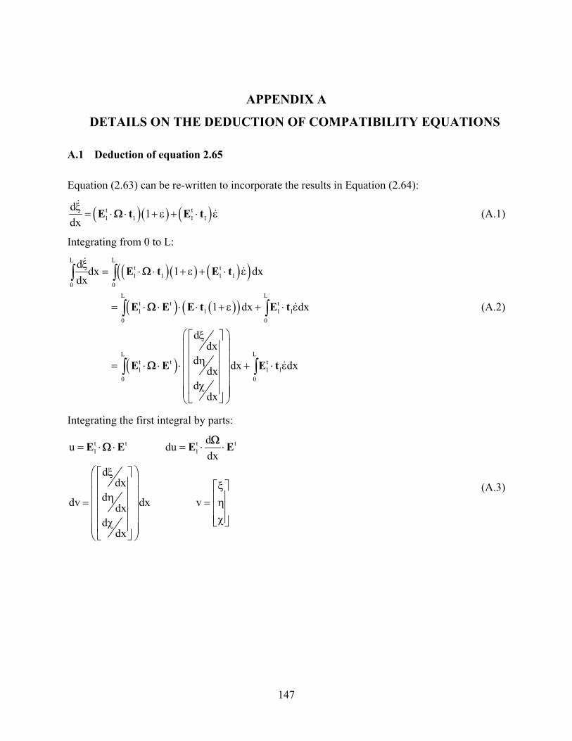
147
APPENDIX A
DETAILS ON THE DEDUCTION OF COMPATIBILITY EQUATIONS
A.1 Deduction of equation 2.65
Equation (2.63) can be re-written to incorporate the results in Equation (2.64):
( )( ) ( )t t1 1 1 1
d 1dx
E t E tξ= ⋅ ⋅ + ε + ⋅ εΩ (A.1)
Integrating from 0 to L:
( )( ) ( )( )
( ) ( )( )
( )
L Lt t1 1 1 1
0 0L L
t t t1 1 1 1
0 0
L Lt t t1 1 1
0 0
d dx 1 dxdx
1 dx dx
ddx
d dx dxdxd
dx
E t E t
E E E t E t
E E E t
ξ= ⋅ ⋅ + ε + ⋅ ε
= ⋅ ⋅ ⋅ ⋅ + ε + ⋅ ε
⎛ ξ ⎞⎡ ⎤⎜ ⎟⎢ ⎥⎜ ⎟⎢ ⎥η= ⋅ ⋅ ⋅ + ⋅ ε⎜ ⎟⎢ ⎥⎜ ⎟⎢ ⎥χ⎜ ⎟⎢ ⎥⎜ ⎟⎣ ⎦⎝ ⎠
∫ ∫
∫ ∫
∫ ∫
Ω
Ω
Ω
(A.2)
Integrating the first integral by parts:
t t t t1 1
du dudx
ddx
ddv dx vdxd
dx
E E E E
= ⋅ ⋅ = ⋅ ⋅
⎛ ξ ⎞⎡ ⎤⎜ ⎟⎢ ⎥ ξ⎡ ⎤⎜ ⎟⎢ ⎥ ⎢ ⎥η= = η⎜ ⎟⎢ ⎥ ⎢ ⎥⎜ ⎟⎢ ⎥ ⎢ ⎥χ⎣ ⎦χ⎜ ⎟⎢ ⎥⎜ ⎟⎣ ⎦⎝ ⎠
ΩΩ
(A.3)
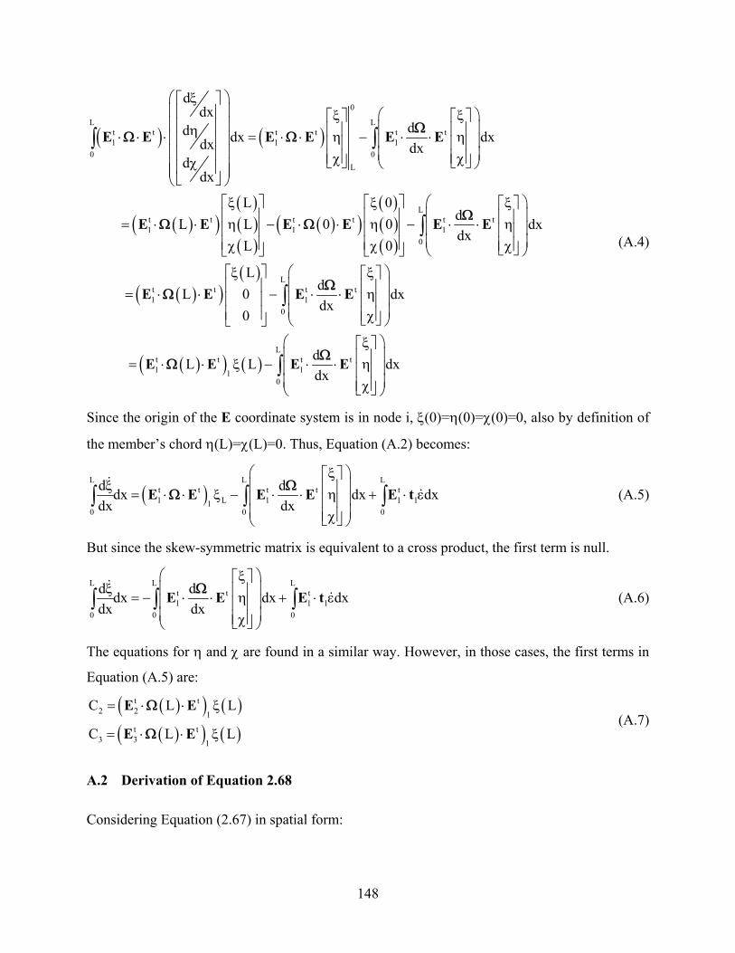
148
( ) ( )
( )( )( )( )( )
( )( )( )( )( )
0
L Lt t t t t t1 1 1
0 0L
t t t t t t1 1 1
ddx
dd dx dxdx dxd
dx
L 0dL L 0 0dx
L 0
E E E E E E
E E E E E E
⎛ ξ ⎞⎡ ⎤⎜ ⎟⎢ ⎥ ξ ⎛ ξ ⎞⎡ ⎤ ⎡ ⎤⎜ ⎟⎢ ⎥ ⎜ ⎟⎢ ⎥ ⎢ ⎥η⋅ ⋅ ⋅ = ⋅ ⋅ η − ⋅ ⋅ η⎜ ⎟⎢ ⎥ ⎜ ⎟⎢ ⎥ ⎢ ⎥⎜ ⎟⎢ ⎥ ⎜ ⎟⎢ ⎥ ⎢ ⎥χ χ⎣ ⎦ ⎣ ⎦χ ⎝ ⎠⎜ ⎟⎢ ⎥⎜ ⎟⎣ ⎦⎝ ⎠
ξ ξ ξ⎡ ⎤ ⎡ ⎤ ⎡⎢ ⎥ ⎢ ⎥ ⎢= ⋅ ⋅ η − ⋅ ⋅ η − ⋅ ⋅ η⎢ ⎥ ⎢ ⎥ ⎢⎢ ⎥ ⎢ ⎥ ⎢χ χ χ⎣⎣ ⎦ ⎣ ⎦
∫ ∫Ω
Ω Ω
ΩΩ Ω
( )( )( )
( )( ) ( )
L
0
Lt t t t1 1
0
Lt t t t1 11
0
dx
LdL 0 dxdx
0
dL L dxdx
E E E E
E E E E
⎛ ⎞⎤⎜ ⎟⎥⎜ ⎟⎥⎜ ⎟⎥⎦⎝ ⎠
ξ ⎛ ξ ⎞⎡ ⎤ ⎡ ⎤⎜ ⎟⎢ ⎥ ⎢ ⎥= ⋅ ⋅ − ⋅ ⋅ η⎜ ⎟⎢ ⎥ ⎢ ⎥⎜ ⎟⎢ ⎥ ⎢ ⎥χ⎣ ⎦⎣ ⎦ ⎝ ⎠
⎛ ξ ⎞⎡ ⎤⎜ ⎟⎢ ⎥= ⋅ ⋅ ξ − ⋅ ⋅ η⎜ ⎟⎢ ⎥⎜ ⎟⎢ ⎥χ⎣ ⎦⎝ ⎠
∫
∫
∫
ΩΩ
ΩΩ
(A.4)
Since the origin of the E coordinate system is in node i, ξ(0)=η(0)=χ(0)=0, also by definition of
the member’s chord η(L)=χ(L)=0. Thus, Equation (A.2) becomes:
( )L L L
t t t t t1 L 1 1 11
0 0 0
d ddx dx dxdx dx
E E E E E t⎛ ξ ⎞⎡ ⎤
ξ ⎜ ⎟⎢ ⎥= ⋅ ⋅ ξ − ⋅ ⋅ η + ⋅ ε⎜ ⎟⎢ ⎥⎜ ⎟⎢ ⎥χ⎣ ⎦⎝ ⎠
∫ ∫ ∫Ω
Ω (A.5)
But since the skew-symmetric matrix is equivalent to a cross product, the first term is null.
L L Lt t t1 1 1
0 0 0
d ddx dx dxdx dx
E E E t⎛ ξ ⎞⎡ ⎤
ξ ⎜ ⎟⎢ ⎥= − ⋅ ⋅ η + ⋅ ε⎜ ⎟⎢ ⎥⎜ ⎟⎢ ⎥χ⎣ ⎦⎝ ⎠
∫ ∫ ∫Ω (A.6)
The equations for η and χ are found in a similar way. However, in those cases, the first terms in
Equation (A.5) are:
( )( ) ( )( )( ) ( )
t t2 2 1
t t3 3 1
C L L
C L L
E E
E E
= ⋅ ⋅ ξ
= ⋅ ⋅ ξ
Ω
Ω (A.7)
A.2 Derivation of Equation 2.68
Considering Equation (2.67) in spatial form:
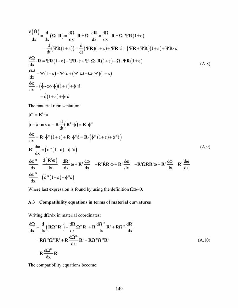
149
( ) ( ) ( )
( )( ) ( )( ) ( )( )
( ) ( ) ( )
( ) ( )( )
( )( )
( )
d d d d d 1+dx dx dx dx dx
d d1 1 1dt dt
d 1 1dxd 1 1dxd 1dx
1
R RR R + R + R
R R R R R R
R R R R R 1+
-
= ⋅ = ⋅ ⋅ = ⋅ ⋅ ε
= + ε = + ε + ⋅ε = + + ε + ⋅ε
⋅ = + ε + ⋅ε + ⋅ ⋅ + ε − ⋅ ε
= + ε + ⋅ε + ⋅ − ⋅ + ε
= × + ε + ⋅ε
= + ε + ⋅ε
Ω ΩΩ Ω Ω Ψ
Ψ Ψ Ψ Ψ Ψ Ψ
ΩΨ Ψ Ψ Ω Ω Ψ
ΩΨ Ψ Ψ Ω Ω Ψ
ωφ ω φ φ
φ φ
(A.8)
The material representation:
( )
( ) ( )( )
( )( )( )
( )( )
m t
t m
m m m m
t m m
tm tt t t t t t t t
mm m
d= -dt
d 1 1dx
d 1dx
dd d d d d ddx dx dx dx dx dx dx
d 1dx
R
= R R R
R R R
R
R R R R RR R R RR R R
= ⋅
× ⋅ = ⋅
= ⋅ + ε + ⋅ ε = ⋅ + ε + ε
= + ε + ε
= = + = − + = − + =
= + ε + ε
φ φ
φ φ ω φ φ φ
ωφ φ φ φ
ωφ φ
ωω ω ω ω ωω ω Ω ω
ωφ φ
(A.9)
Where last expression is found by using the definition Ωω=0.
A.3 Compatibility equations in terms of material curvatures
Writing dΩ/dx in material coordinates:
( )m t
m t m t t m
mm m t t m m t
mt
d d d d ddx dx dx dx dx
ddx
ddx
R RR R R R R R
R R R R R R
R R
= = + +
= + −
=
Ω ΩΩ Ω Ω
ΩΩ Ω Ω Ω
Ω
(A.10)
The compatibility equations become:
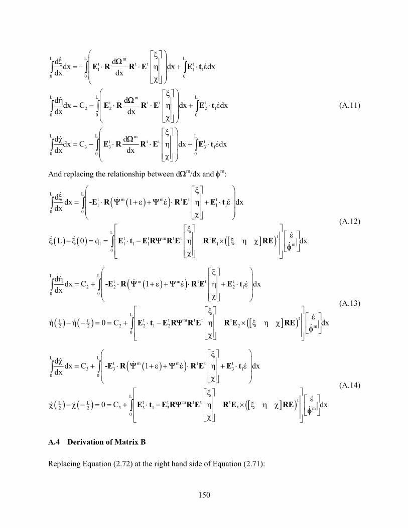
150
L L Lmt t t t1 1 1
0 0 0
L L Lmt t t t
2 2 2 10 0 0
L L mt t t
3 3 30 0
d ddx dx dxdx dx
d ddx C dx dxdx dx
d ddx C dxdx dx
E R R E E t
E R R E E t
E R R E E
⎛ ξ ⎞⎡ ⎤ξ ⎜ ⎟⎢ ⎥= − ⋅ ⋅ η + ⋅ ε⎜ ⎟⎢ ⎥
⎜ ⎟⎢ ⎥χ⎣ ⎦⎝ ⎠⎛ ξ ⎞⎡ ⎤
η ⎜ ⎟⎢ ⎥= − ⋅ ⋅ η + ⋅ ε⎜ ⎟⎢ ⎥⎜ ⎟⎢ ⎥χ⎣ ⎦⎝ ⎠⎛ ξ ⎞⎡ ⎤
χ ⎜ ⎟⎢ ⎥= − ⋅ ⋅ η +⎜ ⎟⎢ ⎥⎜ ⎟⎢ ⎥χ⎣ ⎦⎝ ⎠
∫ ∫ ∫
∫ ∫ ∫
∫ ∫
Ω
Ω
Ω Lt
10
dxt⋅ ε∫
(A.11)
And replacing the relationship between dΩm/dx and φm:
( )( )
( ) ( ) [ ]( )
L Lt m m t t t1 1 1
0 0
Ltt t m t t t
1 1 1 1 1 m0
d dx 1 dxdx
L 0 q dx
-E R R E E t
E t E R R E R E RE
⎛ ξ ⎞⎡ ⎤ξ ⎜ ⎟⎢ ⎥= ⋅ + ε + ε ⋅ η + ⋅ ε⎜ ⎟⎢ ⎥
⎜ ⎟⎢ ⎥χ⎣ ⎦⎝ ⎠⎡ ξ ⎤⎡ ⎤
ε⎡ ⎤⎢ ⎥⎢ ⎥ξ − ξ = = ⋅ − η × ξ η χ ⎢ ⎥⎢ ⎥⎢ ⎥ ⎣ ⎦⎢ ⎥⎢ ⎥χ⎣ ⎦⎣ ⎦
∫ ∫
∫
Ψ Ψ
Ψφ
(A.12)
( )( )
( ) ( ) [ ]( )
L Lt m m t t t
2 2 2 10 0
Ltt t m t t tL L
2 2 1 2 22 2 m0
d dx C 1 dxdx
0 C dx
-E R R E E t
E t E R R E R E RE
⎛ ξ ⎞⎡ ⎤η ⎜ ⎟⎢ ⎥= + ⋅ + ε + ε ⋅ η + ⋅ ε⎜ ⎟⎢ ⎥
⎜ ⎟⎢ ⎥χ⎣ ⎦⎝ ⎠⎡ ξ ⎤⎡ ⎤
ε⎡ ⎤⎢ ⎥⎢ ⎥η − η − = = + ⋅ − η × ξ η χ ⎢ ⎥⎢ ⎥⎢ ⎥ ⎣ ⎦⎢ ⎥⎢ ⎥χ⎣ ⎦⎣ ⎦
∫ ∫
∫
Ψ Ψ
Ψφ
(A.13)
( )( )
( ) ( ) [ ]( )
L Lt m m t t t
3 3 3 10 0
Ltt t m t t tL L
3 3 1 3 32 2 m0
d dx C 1 dxdx
0 C dx
-E R R E E t
E t E R R E R E RE
⎛ ξ ⎞⎡ ⎤χ ⎜ ⎟⎢ ⎥= + ⋅ + ε + ε ⋅ η + ⋅ ε⎜ ⎟⎢ ⎥
⎜ ⎟⎢ ⎥χ⎣ ⎦⎝ ⎠⎡ ξ ⎤⎡ ⎤
ε⎡ ⎤⎢ ⎥⎢ ⎥χ − χ − = = + ⋅ − η × ξ η χ ⎢ ⎥⎢ ⎥⎢ ⎥ ⎣ ⎦⎢ ⎥⎢ ⎥χ⎣ ⎦⎣ ⎦
∫ ∫
∫
Ψ Ψ
Ψφ
(A.14)
A.4 Derivation of Matrix B
Replacing Equation (2.72) at the right hand side of Equation (2.71):
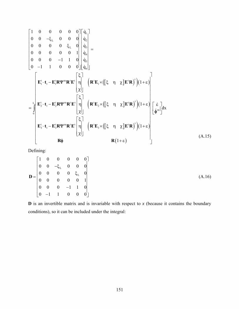
151
[ ]( )( )( )
[ ]( )( )( )
1
2L
3L
4
5
6
tt t m t t t t1 1 1 1
tt t m t t t t2 1 2 2
t t3 1 3
q1 0 0 0 0 0q0 0 0 0 0q0 0 0 0 0q0 0 0 0 0 1q0 0 0 1 1 0
0 1 1 0 0 0 q
1
1
E t E R R E R E E R
E t E R R E R E E R
E t E R
⎡ ⎤⎡ ⎤⎢ ⎥⎢ ⎥−ξ ⎢ ⎥⎢ ⎥⎢ ⎥⎢ ⎥ξ
=⎢ ⎥⎢ ⎥⎢ ⎥⎢ ⎥⎢ ⎥⎢ ⎥−⎢ ⎥⎢ ⎥
− ⎢ ⎥⎣ ⎦ ⎣ ⎦ξ⎡ ⎤
⎢ ⎥⋅ − η × ξ η χ + ε⎢ ⎥⎢ ⎥χ⎣ ⎦
ξ⎡ ⎤⎢ ⎥⋅ − η × ξ η χ + ε⎢ ⎥=⎢ ⎥χ⎣ ⎦
⋅ −
Ψ
Ψ
[ ]( )( )( )
( )
L
m0
tm t t t t3
dx
1
1
R E R E E R
R R
⎡ ⎤⎢ ⎥⎢ ⎥⎢ ⎥⎢ ⎥⎢ ⎥⎢ ⎥ ε⎡ ⎤⎢ ⎥ ⎢ ⎥⎢ ⎥ ⎣ ⎦⎢ ⎥
ξ⎡ ⎤⎢ ⎥⎢ ⎥⎢ ⎥η × ξ η χ + ε⎢ ⎥⎢ ⎥⎢ ⎥χ⎢ ⎥⎣ ⎦
⎢ ⎥+ ε⎣ ⎦
∫ φ
Ψ
φ (A.15)
Defining:
L
L
1 0 0 0 0 00 0 0 0 00 0 0 0 00 0 0 0 0 10 0 0 1 1 00 1 1 0 0 0
D
⎡ ⎤⎢ ⎥−ξ⎢ ⎥⎢ ⎥ξ
= ⎢ ⎥⎢ ⎥⎢ ⎥−⎢ ⎥
−⎣ ⎦
(A.16)
D is an invertible matrix and is invariable with respect to x (because it contains the boundary
conditions), so it can be included under the integral:
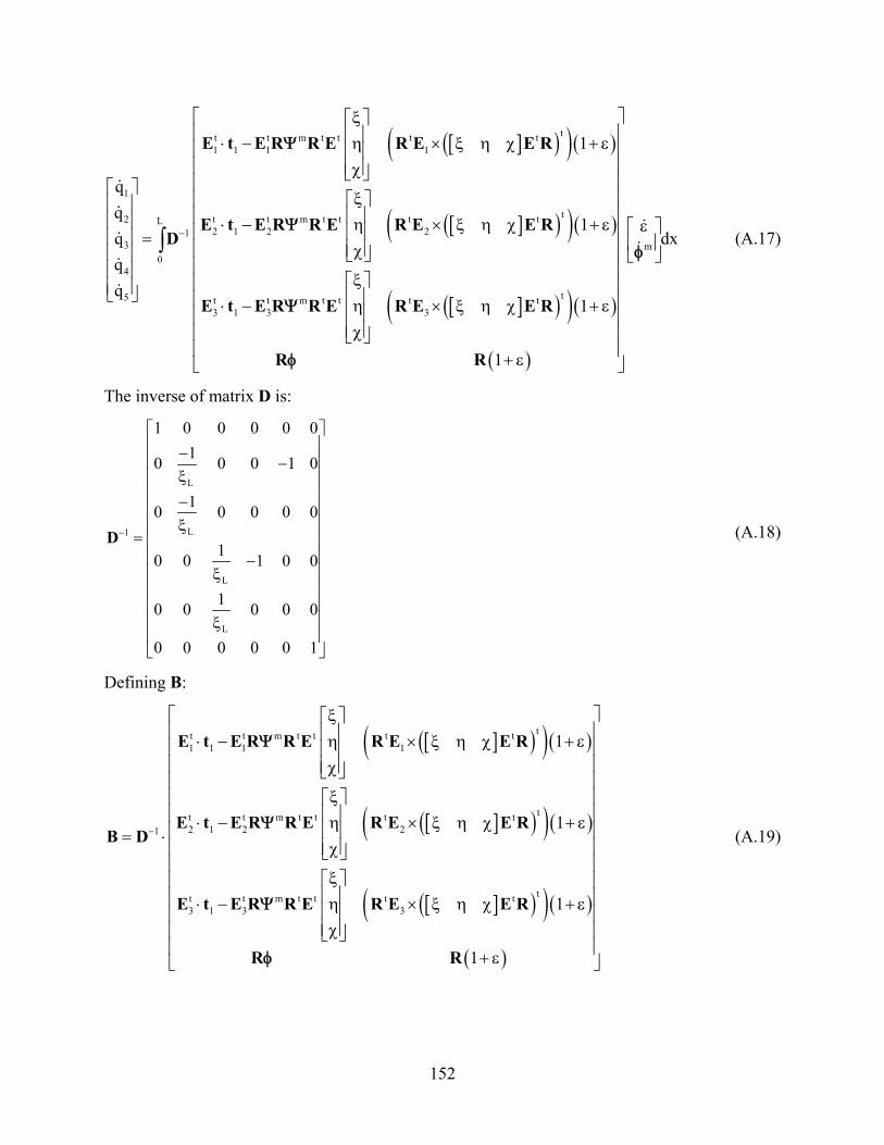
152
[ ]( )( )( )
[ ]( )( )( )
[ ]( )( )( )
( )
tt t m t t t t1 1 1 1
1
tt t m t t t t22 1 2 21
3
4
t5 t t m t t t t3 1 3 3
1
1qqq
1
1
E t E R R E R E E R
E t E R R E R E E RD
E t E R R E R E E R
R R
−
⎡ ⎤ξ⎡ ⎤⎢ ⎥⎢ ⎥⋅ − η × ξ η χ + ε⎢ ⎥⎢ ⎥⎢ ⎥⎢ ⎥χ⎣ ⎦⎢ ⎥⎡ ⎤
ξ⎡ ⎤⎢ ⎥⎢ ⎥⎢ ⎥⎢ ⎥⎢ ⎥ ⋅ − η × ξ η χ + ε⎢ ⎥⎢⎢ ⎥ =⎢ ⎥⎢ χ⎢ ⎥ ⎣ ⎦
⎢⎢ ⎥ ξ⎡ ⎤⎢⎢ ⎥⎣ ⎦ ⎢ ⎥⎢ ⋅ − η × ξ η χ + ε⎢ ⎥⎢⎢ ⎥χ⎢ ⎣ ⎦
⎢ + ε⎣ ⎦
Ψ
Ψ
Ψ
φ
L
m0
dxε⎡ ⎤⎥ ⎢ ⎥⎥ ⎣ ⎦
⎥⎥⎥⎥⎥⎥
∫ φ (A.17)
The inverse of matrix D is:
L
L1
L
L
1 0 0 0 0 010 0 0 1 0
10 0 0 0 0
10 0 1 0 0
10 0 0 0 0
0 0 0 0 0 1
D−
⎡ ⎤⎢ ⎥−⎢ ⎥−
ξ⎢ ⎥⎢ ⎥−⎢ ⎥⎢ ⎥ξ
= ⎢ ⎥⎢ ⎥−⎢ ⎥ξ⎢ ⎥⎢ ⎥⎢ ⎥ξ⎢ ⎥⎣ ⎦
(A.18)
Defining B:
[ ]( )( )( )
[ ]( )( )( )
[ ]( )( )( )
( )
tt t m t t t t1 1 1 1
tt t m t t t t2 1 2 21
tt t m t t t t3 1 3 3
1
1
1
1
E t E R R E R E E R
E t E R R E R E E RB D
E t E R R E R E E R
R R
−
⎡ ⎤ξ⎡ ⎤⎢ ⎥⎢ ⎥⋅ − η × ξ η χ + ε⎢ ⎥⎢ ⎥⎢ ⎥⎢ ⎥χ⎣ ⎦⎢ ⎥
ξ⎡ ⎤⎢ ⎥⎢ ⎥⎢ ⎥⋅ − η × ξ η χ + ε⎢ ⎥⎢ ⎥= ⋅⎢ ⎥⎢ ⎥χ⎣ ⎦
⎢ ⎥ξ⎡ ⎤⎢ ⎥
⎢ ⎥⎢ ⎥⋅ − η × ξ η χ + ε⎢ ⎥⎢ ⎥⎢ ⎥χ⎢ ⎥⎣ ⎦
⎢ ⎥+ ε⎣ ⎦
Ψ
Ψ
Ψ
φ
(A.19)
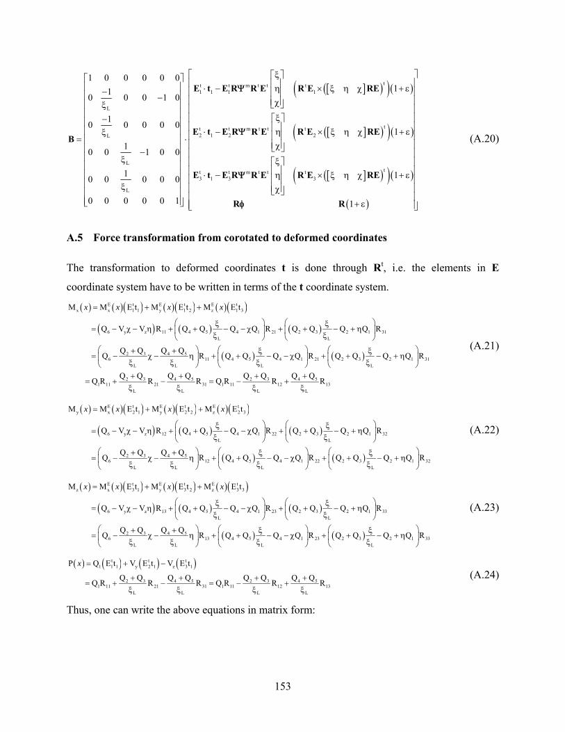
153
[ ]( )( )( )
[ ]( )( )( )
tt t m t t t1 1 1 1
L
tt t m t t t2 1 2 2L
L
t t m t t3 1 3
L
1 0 0 0 0 0110 0 0 1 0
10 0 0 0 01
10 0 1 0 0
10 0 0 0 0
0 0 0 0 0 1
E t E R R E R E RE
E t E R R E R E REB
E t E R R E
ξ⎡ ⎤⎡ ⎤ ⎢ ⎥⎢ ⎥ ⋅ − η × ξ η χ + ε− ⎢ ⎥⎢ ⎥− ⎢ ⎥χ⎣ ⎦ξ⎢ ⎥⎢ ⎥ ξ⎡ ⎤−⎢ ⎥ ⎢ ⎥⎢ ⎥ ⋅ − η × ξ η χ + εξ ⎢ ⎥= ⋅⎢ ⎥ ⎢ ⎥χ⎣ ⎦⎢ ⎥−⎢ ⎥ξ ξ⎡ ⎤⎢ ⎥ ⎢ ⎥⋅ − η⎢ ⎥ ⎢ ⎥⎢ ⎥ξ ⎢χ⎣ ⎦⎢ ⎥⎢ ⎥⎣ ⎦
Ψ
Ψ
Ψ [ ]( )( )( )
( )
tt3 1
1
R E RE
R R
⎡ ⎤⎢ ⎥⎢ ⎥⎢ ⎥⎢ ⎥⎢ ⎥⎢ ⎥⎢ ⎥⎢ ⎥⎢ ⎥⎢ ⎥⎢ ⎥× ξ η χ + ε⎢ ⎥
⎥⎢ ⎥⎢ ⎥
+ ε⎢ ⎥⎣ ⎦φ
(A.20)
A.5 Force transformation from corotated to deformed coordinates
The transformation to deformed coordinates t is done through Rt, i.e. the elements in E
coordinate system have to be written in terms of the t coordinate system.
( ) ( )( ) ( )( ) ( )( )
( ) ( ) ( )
( ) ( )
E t E t E tx x 1 1 y 1 2 z 1 3
6 y z 11 4 5 4 1 21 2 3 2 1 31L L
2 3 4 56 11 4 5 4 1 21 2 3 2 1 31
L L L L
M M E t M E t M E t
Q V V R Q Q Q Q R Q Q Q Q R
Q Q Q QQ R Q Q Q Q R Q Q Q Q R
= + +
⎛ ⎞ ⎛ ⎞ξ ξ= − χ − η + + − − χ + + − + η⎜ ⎟ ⎜ ⎟
ξ ξ⎝ ⎠ ⎝ ⎠⎛ ⎞ ⎛ ⎞ ⎛ ⎞+ + ξ ξ
= − χ − η + + − − χ + + − + η⎜ ⎟ ⎜ ⎟ ⎜ ⎟ξ ξ ξ ξ⎝ ⎠ ⎝ ⎠ ⎝ ⎠
x x x x
2 3 4 5 2 3 4 51 11 21 31 1 11 12 13
L L L L
Q Q Q Q Q Q Q QQ R R R Q R R R + + + += + − = − +
ξ ξ ξ ξ
(A.21)
( ) ( )( ) ( )( ) ( )( )
( ) ( ) ( )
( ) ( )
E t E t E ty x 2 1 y 2 2 z 2 3
6 y z 12 4 5 4 1 22 2 3 2 1 32L L
2 3 4 56 12 4 5 4 1 22 2 3 2 1 32
L L L L
M M E t M E t M E t
Q V V R Q Q Q Q R Q Q Q Q R
Q Q Q QQ R Q Q Q Q R Q Q Q Q R
= + +
⎛ ⎞ ⎛ ⎞ξ ξ= − χ − η + + − − χ + + − + η⎜ ⎟ ⎜ ⎟
ξ ξ⎝ ⎠ ⎝ ⎠⎛ ⎞ ⎛ ⎞ ⎛ ⎞+ + ξ ξ
= − χ − η + + − − χ + + − + η⎜ ⎟ ⎜ ⎟ ⎜ ⎟ξ ξ ξ ξ⎝ ⎠ ⎝ ⎠ ⎝ ⎠
x x x x
(A.22)
( ) ( )( ) ( )( ) ( )( )
( ) ( ) ( )
( ) ( )
E t E t E tz x 3 1 y 3 2 z 3 3
6 y z 13 4 5 4 1 23 2 3 2 1 33L L
2 3 4 56 13 4 5 4 1 23 2 3 2 1 33
L L L L
M M E t M E t M E t
Q V V R Q Q Q Q R Q Q Q Q R
Q Q Q QQ R Q Q Q Q R Q Q Q Q R
= + +
⎛ ⎞ ⎛ ⎞ξ ξ= − χ − η + + − − χ + + − + η⎜ ⎟ ⎜ ⎟
ξ ξ⎝ ⎠ ⎝ ⎠⎛ ⎞ ⎛ ⎞ ⎛ ⎞+ + ξ ξ
= − χ − η + + − − χ + + − + η⎜ ⎟ ⎜ ⎟ ⎜ ⎟ξ ξ ξ ξ⎝ ⎠ ⎝ ⎠ ⎝ ⎠
x x x x
(A.23)
( ) ( ) ( ) ( )t t t1 1 1 y 2 1 z 3 1
2 3 4 5 2 3 4 51 11 21 31 1 11 12 13
L L L L
P Q E t V E t V E t
Q Q Q Q Q Q Q QQ R R R Q R R R
= + −
+ + + += + − = − +
ξ ξ ξ ξ
x (A.24)
Thus, one can write the above equations in matrix form:
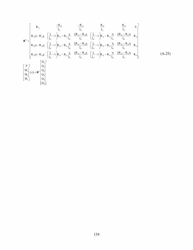
154
12 12 13 1311
L L L L
31 11 21 1131 21 31 11 21 11 11
L L L L L L*t
32 12 22 1232 22 32 12 22 12 12
L L L L L L
33 23L
R R R RR 0
R R R RR R 1 R R 1 R R R
R R R RR R 1 R R 1 R R R
R R 1
B
− −ξ ξ ξ ξ
⎛ ⎞ ⎛ ⎞ξ χ ξ − χ ξ η ξ − ηη − χ − − − −⎜ ⎟ ⎜ ⎟
ξ ξ ξ ξ ξ ξ⎝ ⎠ ⎝ ⎠=
⎛ ⎞ ⎛ ⎞ξ χ ξ − χ ξ η ξ − ηη − χ − − − −⎜ ⎟ ⎜ ⎟
ξ ξ ξ ξ ξ ξ⎝ ⎠ ⎝ ⎠⎛ ⎞ξ
η − χ −⎜ξ⎝
( )
33 13 23 1333 13 23 13 13
L L L L L
1
2
3x *t
4y
5z
6
R R R RR R 1 R R R
QQPQMQMQMQ
B
⎡ ⎤⎢ ⎥⎢ ⎥⎢ ⎥⎢ ⎥⎢ ⎥⎢ ⎥⎢ ⎥⎢ ⎥⎢ ⎥⎢ ⎥⎛ ⎞χ ξ − χ ξ η ξ − η
− − −⎢ ⎥⎟ ⎜ ⎟ξ ξ ξ ξ ξ⎢ ⎥⎠ ⎝ ⎠⎣ ⎦
⎡ ⎤⎢ ⎥⎡ ⎤ ⎢ ⎥⎢ ⎥ ⎢ ⎥⎢ ⎥ = ⎢ ⎥⎢ ⎥ ⎢ ⎥⎢ ⎥ ⎢ ⎥⎣ ⎦ ⎢ ⎥⎢ ⎥⎣ ⎦
x
(A.25)
155
APPENDIX B
This appendix contains the description of the input file to Element.exe and an example.
B.1 Input file user’s manual
B.1.1 Introduction
Element.exe is a program capable of solving 3-dimensional structures with large displacements
and large rotations. The nodes’ initial position, the elements’ connectivity,
materials’ definition, initial conditions, restraints, loads and output information
are contained in an “input file”, which has a strict format. The objective of this
format is to guide the program through the different options and ensure the proper
interpretation of the data. The user’s manual is a description of the input file
format.
B.1.2 General considerations
• The input file has to be named “InputFile.dat”.
• Input file, load files and executable file must be in the same folder to run properly.
Output files are also written in the same folder, therefore if more than 1 output file is to
be written, they have to have different names or the information will be written in a
single file. If the file already exists, it will not be overwritten, it will be appended.
• Each line is preceded by a few words (written in bold letters below) that tells the program
what part of the input file is reading. These words are essential to the correct
interpretation of the input file.
• The input file is case sensitive.
• The loading can be static or dynamic. For static analysis, a history of displacements or
forces can be prescribed at any node and in any direction. When a static analysis is being
performed, the time step is still needed and can be set to a very large quantity (100). This
ensures that the rates of the variables remain constant after the initial velocity required to
get to the initial conditions is reached. For dynamic analysis, the frequency of the
156
recorded motion can be used as time step. Sometimes, if the structure is highly nonlinear,
a very small time step will prompt the solver into numerical errors and it will fail.
• Initial conditions: the program is set such that the user needs only to input the initial
conditions for the variables, not for its rates. Even in the case of dynamic analysis, where
the velocities are part of the variable vector, its initial conditions are not needed. In
general, the set of initial conditions must be a good approximation of the actual
deformations, forces and strains under the specified loads. If the solver fails in the initial
conditions calculation is because there is an error in the user’s input. The loads for initial
conditions must also be provided so that equilibrium can be satisfied. The loads can be
prescribed displacements or forces, not accelerations and must be defined separately from
the analysis loads. It is a good idea to use gravity loads for initial conditions purposes
because the structure is easy to solve for them. Also, the loads can be carried as constant
loads through the analysis. The user can always skip the verification of the initial
conditions but must provide the complete set for both the variables and its rates. It is
recommended to let the solver compute these values. If an initial condition of no loading
(a vector of zero valued variables) is used, the program will not converge.
• Damping: damping in this program is considered to be only mass proportional. Because
the program lacks the procedure to calculate the frequencies of the structure, the first
frequency must be input by the user along with the damping ratio associated to that
frequency. Since this program is based on a formulation in the state space, no mass,
stiffness or damping matrices are created. The damping is considered in every
equilibrium equation that has mass, the damping coefficient “c” is then calculated as the
mass factor a0 = 2ζω times the mass at that dof: c = a0 m.
B.1.3 Input file format
title: 1 line with no more than 128 characters
Example: Program description The actual word “title” is not needed but the program
expects the first sentence to be an explanatory note.
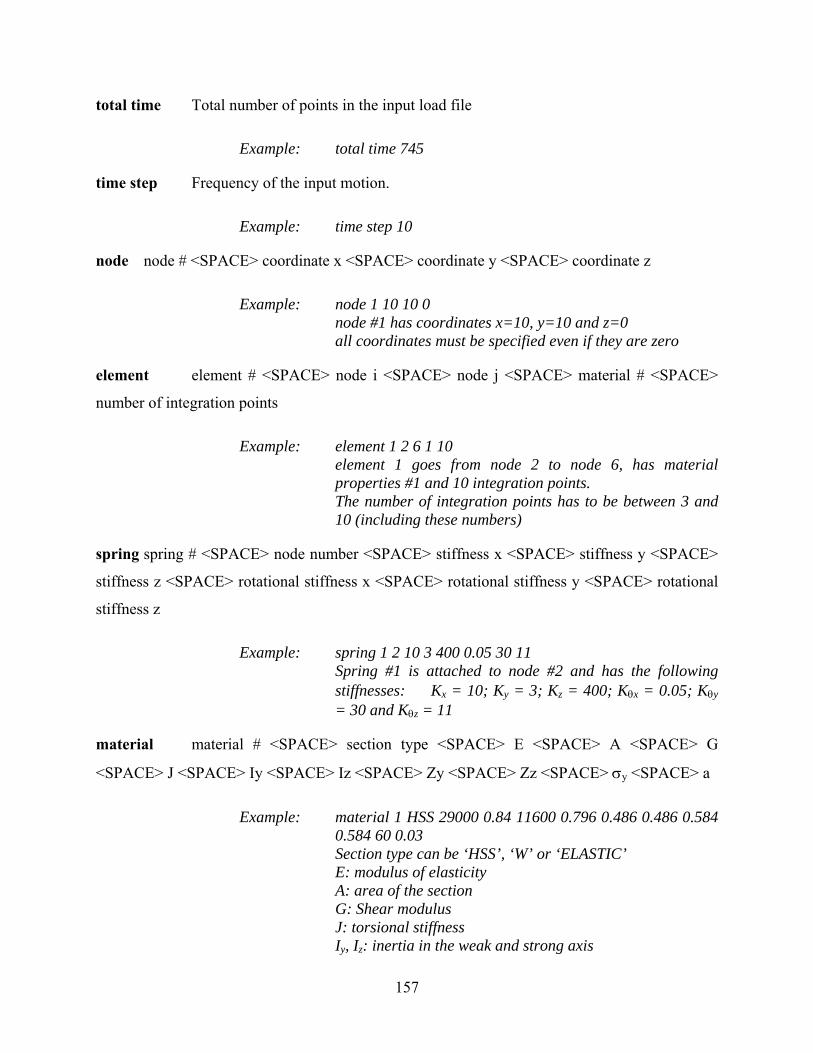
157
total time Total number of points in the input load file
Example: total time 745
time step Frequency of the input motion.
Example: time step 10
node node # <SPACE> coordinate x <SPACE> coordinate y <SPACE> coordinate z
Example: node 1 10 10 0 node #1 has coordinates x=10, y=10 and z=0 all coordinates must be specified even if they are zero
element element # <SPACE> node i <SPACE> node j <SPACE> material # <SPACE>
number of integration points
Example: element 1 2 6 1 10 element 1 goes from node 2 to node 6, has material
properties #1 and 10 integration points. The number of integration points has to be between 3 and
10 (including these numbers)
spring spring # <SPACE> node number <SPACE> stiffness x <SPACE> stiffness y <SPACE>
stiffness z <SPACE> rotational stiffness x <SPACE> rotational stiffness y <SPACE> rotational
stiffness z
Example: spring 1 2 10 3 400 0.05 30 11 Spring #1 is attached to node #2 and has the following
stiffnesses: Kx = 10; Ky = 3; Kz = 400; Kθx = 0.05; Kθy = 30 and Kθz = 11
material material # <SPACE> section type <SPACE> E <SPACE> A <SPACE> G
<SPACE> J <SPACE> Iy <SPACE> Iz <SPACE> Zy <SPACE> Zz <SPACE> σy <SPACE> a
Example: material 1 HSS 29000 0.84 11600 0.796 0.486 0.486 0.584 0.584 60 0.03
Section type can be ‘HSS’, ‘W’ or ‘ELASTIC’ E: modulus of elasticity A: area of the section G: Shear modulus J: torsional stiffness Iy, Iz: inertia in the weak and strong axis
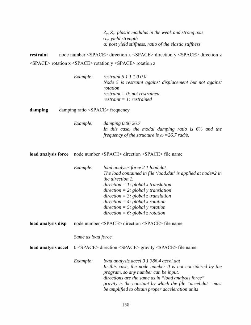
158
Zy, Zz: plastic modulus in the weak and strong axis σy: yield strength a: post yield stiffness, ratio of the elastic stiffness
restraint node number <SPACE> direction x <SPACE> direction y <SPACE> direction z
<SPACE> rotation x <SPACE> rotation y <SPACE> rotation z
Example: restraint 5 1 1 1 0 0 0 Node 5 is restraint against displacement but not against
rotation restraint = 0: not restrained restraint = 1: restrained
damping damping ratio <SPACE> frequency
Example: damping 0.06 26.7 In this case, the modal damping ratio is 6% and the
frequency of the structure is ω =26.7 rad/s.
load analysis force node number <SPACE> direction <SPACE> file name
Example: load analysis force 2 1 load.dat The load contained in file ‘load.dat’ is applied at node#2 in
the direction 1. direction = 1: global x translation direction = 2: global y translation direction = 3: global z translation direction = 4: global x rotation direction = 5: global y rotation direction = 6: global z rotation
load analysis disp node number <SPACE> direction <SPACE> file name
Same as load force.
load analysis accel 0 <SPACE> direction <SPACE> gravity <SPACE> file name
Example: load analysis accel 0 1 386.4 accel.dat In this case, the node number 0 is not considered by the
program, so any number can be input. directions are the same as in “load analysis force” gravity is the constant by which the file “accel.dat” must
be amplified to obtain proper acceleration units
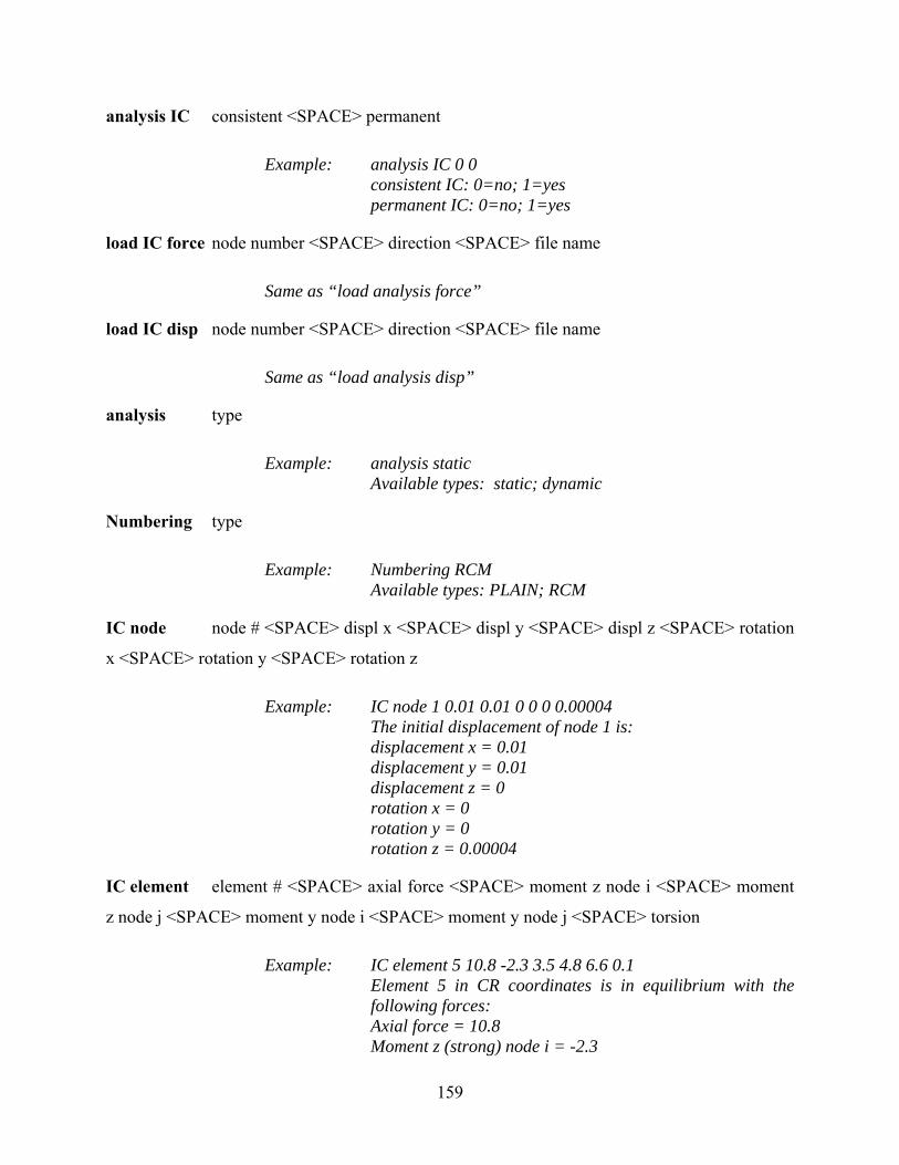
159
analysis IC consistent <SPACE> permanent
Example: analysis IC 0 0 consistent IC: 0=no; 1=yes permanent IC: 0=no; 1=yes
load IC force node number <SPACE> direction <SPACE> file name
Same as “load analysis force”
load IC disp node number <SPACE> direction <SPACE> file name
Same as “load analysis disp”
analysis type
Example: analysis static Available types: static; dynamic
Numbering type
Example: Numbering RCM Available types: PLAIN; RCM
IC node node # <SPACE> displ x <SPACE> displ y <SPACE> displ z <SPACE> rotation
x <SPACE> rotation y <SPACE> rotation z
Example: IC node 1 0.01 0.01 0 0 0 0.00004 The initial displacement of node 1 is: displacement x = 0.01 displacement y = 0.01 displacement z = 0 rotation x = 0 rotation y = 0 rotation z = 0.00004
IC element element # <SPACE> axial force <SPACE> moment z node i <SPACE> moment
z node j <SPACE> moment y node i <SPACE> moment y node j <SPACE> torsion
Example: IC element 5 10.8 -2.3 3.5 4.8 6.6 0.1 Element 5 in CR coordinates is in equilibrium with the
following forces: Axial force = 10.8 Moment z (strong) node i = -2.3
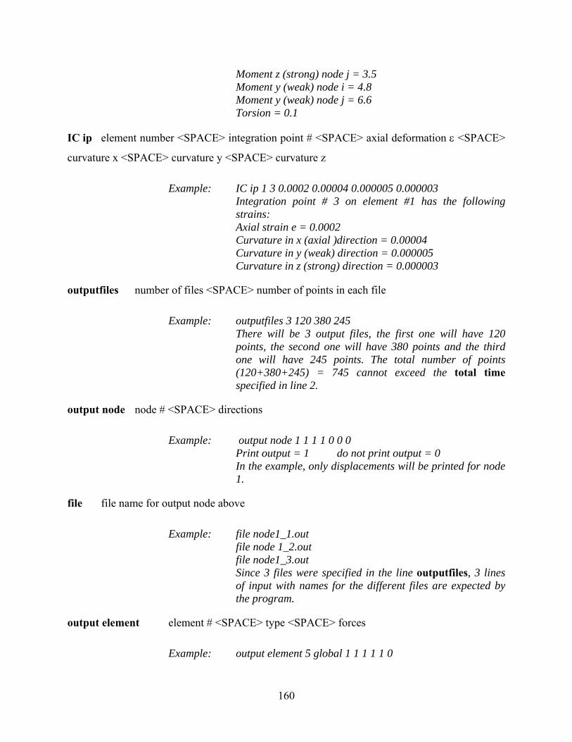
160
Moment z (strong) node j = 3.5 Moment y (weak) node i = 4.8 Moment y (weak) node j = 6.6 Torsion = 0.1
IC ip element number <SPACE> integration point # <SPACE> axial deformation ε <SPACE>
curvature x <SPACE> curvature y <SPACE> curvature z
Example: IC ip 1 3 0.0002 0.00004 0.000005 0.000003 Integration point # 3 on element #1 has the following
strains: Axial strain e = 0.0002 Curvature in x (axial )direction = 0.00004 Curvature in y (weak) direction = 0.000005 Curvature in z (strong) direction = 0.000003
outputfiles number of files <SPACE> number of points in each file
Example: outputfiles 3 120 380 245 There will be 3 output files, the first one will have 120
points, the second one will have 380 points and the third one will have 245 points. The total number of points (120+380+245) = 745 cannot exceed the total time specified in line 2.
output node node # <SPACE> directions
Example: output node 1 1 1 1 0 0 0 Print output = 1 do not print output = 0 In the example, only displacements will be printed for node
1.
file file name for output node above
Example: file node1_1.out file node 1_2.out file node1_3.out Since 3 files were specified in the line outputfiles, 3 lines
of input with names for the different files are expected by the program.
output element element # <SPACE> type <SPACE> forces
Example: output element 5 global 1 1 1 1 1 0
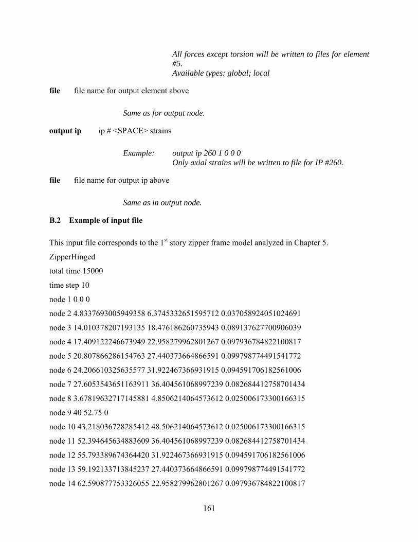
161
All forces except torsion will be written to files for element #5.
Available types: global; local
file file name for output element above
Same as for output node.
output ip ip # <SPACE> strains
Example: output ip 260 1 0 0 0 Only axial strains will be written to file for IP #260.
file file name for output ip above
Same as in output node.
B.2 Example of input file
This input file corresponds to the 1st story zipper frame model analyzed in Chapter 5.
ZipperHinged
total time 15000
time step 10
node 1 0 0 0
node 2 4.8337693005949358 6.3745332651595712 0.037058924051024691
node 3 14.010378207193135 18.476186260735943 0.089137627700906039
node 4 17.409122246673949 22.958279962801267 0.097936784822100817
node 5 20.807866286154763 27.440373664866591 0.099798774491541772
node 6 24.206610325635577 31.922467366931915 0.094591706182561006
node 7 27.6053543651163911 36.404561068997239 0.082684412758701434
node 8 3.67819632717145881 4.8506214064573612 0.025006173300166315
node 9 40 52.75 0
node 10 43.218036728285412 48.506214064573612 0.025006173300166315
node 11 52.394645634883609 36.404561068997239 0.082684412758701434
node 12 55.793389674364420 31.922467366931915 0.094591706182561006
node 13 59.192133713845237 27.440373664866591 0.099798774491541772
node 14 62.590877753326055 22.958279962801267 0.097936784822100817
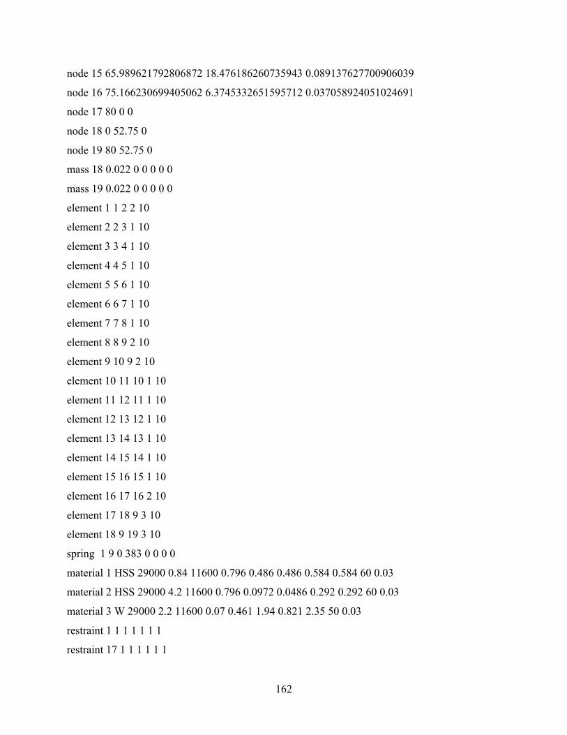
162
node 15 65.989621792806872 18.476186260735943 0.089137627700906039
node 16 75.166230699405062 6.3745332651595712 0.037058924051024691
node 17 80 0 0
node 18 0 52.75 0
node 19 80 52.75 0
mass 18 0.022 0 0 0 0 0
mass 19 0.022 0 0 0 0 0
element 1 1 2 2 10
element 2 2 3 1 10
element 3 3 4 1 10
element 4 4 5 1 10
element 5 5 6 1 10
element 6 6 7 1 10
element 7 7 8 1 10
element 8 8 9 2 10
element 9 10 9 2 10
element 10 11 10 1 10
element 11 12 11 1 10
element 12 13 12 1 10
element 13 14 13 1 10
element 14 15 14 1 10
element 15 16 15 1 10
element 16 17 16 2 10
element 17 18 9 3 10
element 18 9 19 3 10
spring 1 9 0 383 0 0 0 0
material 1 HSS 29000 0.84 11600 0.796 0.486 0.486 0.584 0.584 60 0.03
material 2 HSS 29000 4.2 11600 0.796 0.0972 0.0486 0.292 0.292 60 0.03
material 3 W 29000 2.2 11600 0.07 0.461 1.94 0.821 2.35 50 0.03
restraint 1 1 1 1 1 1 1
restraint 17 1 1 1 1 1 1
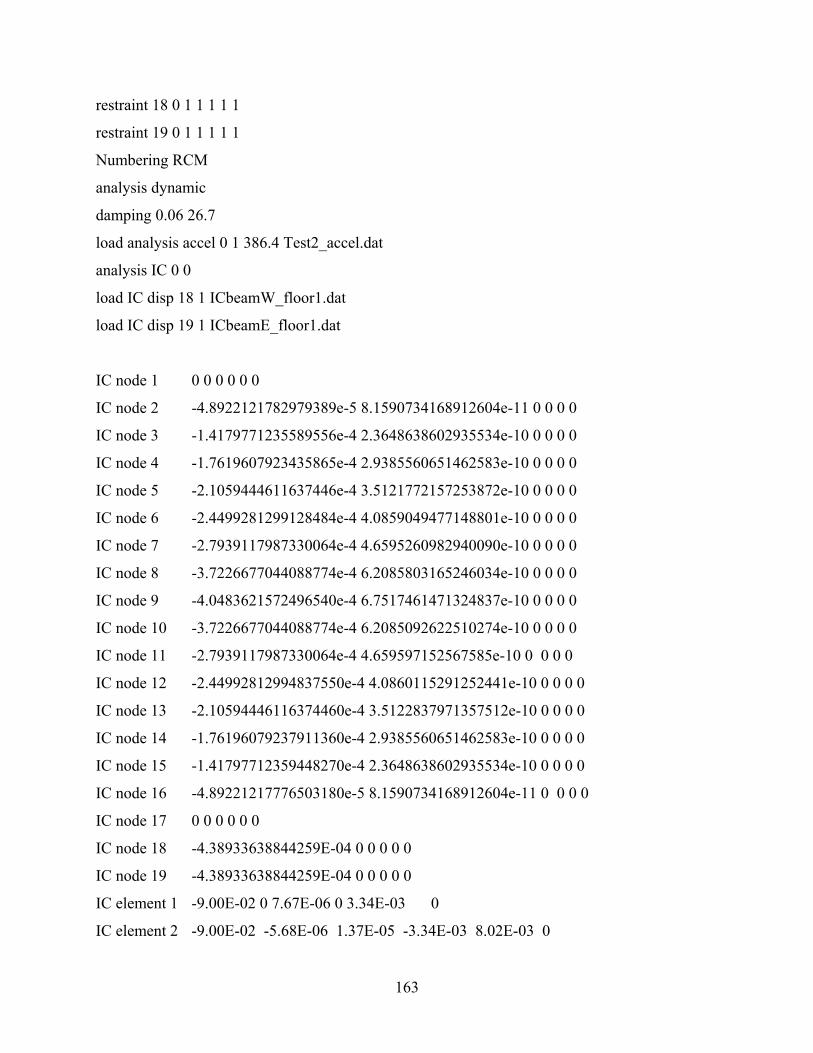
163
restraint 18 0 1 1 1 1 1
restraint 19 0 1 1 1 1 1
Numbering RCM
analysis dynamic
damping 0.06 26.7
load analysis accel 0 1 386.4 Test2_accel.dat
analysis IC 0 0
load IC disp 18 1 ICbeamW_floor1.dat
load IC disp 19 1 ICbeamE_floor1.dat
IC node 1 0 0 0 0 0 0
IC node 2 -4.8922121782979389e-5 8.1590734168912604e-11 0 0 0 0
IC node 3 -1.4179771235589556e-4 2.3648638602935534e-10 0 0 0 0
IC node 4 -1.7619607923435865e-4 2.9385560651462583e-10 0 0 0 0
IC node 5 -2.1059444611637446e-4 3.5121772157253872e-10 0 0 0 0
IC node 6 -2.4499281299128484e-4 4.0859049477148801e-10 0 0 0 0
IC node 7 -2.7939117987330064e-4 4.6595260982940090e-10 0 0 0 0
IC node 8 -3.7226677044088774e-4 6.2085803165246034e-10 0 0 0 0
IC node 9 -4.0483621572496540e-4 6.7517461471324837e-10 0 0 0 0
IC node 10 -3.7226677044088774e-4 6.2085092622510274e-10 0 0 0 0
IC node 11 -2.7939117987330064e-4 4.659597152567585e-10 0 0 0 0
IC node 12 -2.44992812994837550e-4 4.0860115291252441e-10 0 0 0 0
IC node 13 -2.10594446116374460e-4 3.5122837971357512e-10 0 0 0 0
IC node 14 -1.76196079237911360e-4 2.9385560651462583e-10 0 0 0 0
IC node 15 -1.41797712359448270e-4 2.3648638602935534e-10 0 0 0 0
IC node 16 -4.89221217776503180e-5 8.1590734168912604e-11 0 0 0 0
IC node 17 0 0 0 0 0 0
IC node 18 -4.38933638844259E-04 0 0 0 0 0
IC node 19 -4.38933638844259E-04 0 0 0 0 0
IC element 1 -9.00E-02 0 7.67E-06 0 3.34E-03 0
IC element 2 -9.00E-02 -5.68E-06 1.37E-05 -3.34E-03 8.02E-03 0
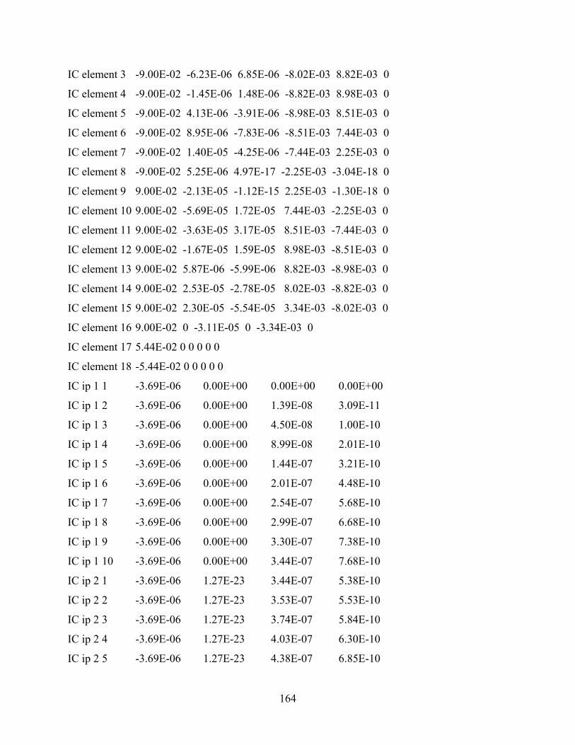
164
IC element 3 -9.00E-02 -6.23E-06 6.85E-06 -8.02E-03 8.82E-03 0
IC element 4 -9.00E-02 -1.45E-06 1.48E-06 -8.82E-03 8.98E-03 0
IC element 5 -9.00E-02 4.13E-06 -3.91E-06 -8.98E-03 8.51E-03 0
IC element 6 -9.00E-02 8.95E-06 -7.83E-06 -8.51E-03 7.44E-03 0
IC element 7 -9.00E-02 1.40E-05 -4.25E-06 -7.44E-03 2.25E-03 0
IC element 8 -9.00E-02 5.25E-06 4.97E-17 -2.25E-03 -3.04E-18 0
IC element 9 9.00E-02 -2.13E-05 -1.12E-15 2.25E-03 -1.30E-18 0
IC element 10 9.00E-02 -5.69E-05 1.72E-05 7.44E-03 -2.25E-03 0
IC element 11 9.00E-02 -3.63E-05 3.17E-05 8.51E-03 -7.44E-03 0
IC element 12 9.00E-02 -1.67E-05 1.59E-05 8.98E-03 -8.51E-03 0
IC element 13 9.00E-02 5.87E-06 -5.99E-06 8.82E-03 -8.98E-03 0
IC element 14 9.00E-02 2.53E-05 -2.78E-05 8.02E-03 -8.82E-03 0
IC element 15 9.00E-02 2.30E-05 -5.54E-05 3.34E-03 -8.02E-03 0
IC element 16 9.00E-02 0 -3.11E-05 0 -3.34E-03 0
IC element 17 5.44E-02 0 0 0 0 0
IC element 18 -5.44E-02 0 0 0 0 0
IC ip 1 1 -3.69E-06 0.00E+00 0.00E+00 0.00E+00
IC ip 1 2 -3.69E-06 0.00E+00 1.39E-08 3.09E-11
IC ip 1 3 -3.69E-06 0.00E+00 4.50E-08 1.00E-10
IC ip 1 4 -3.69E-06 0.00E+00 8.99E-08 2.01E-10
IC ip 1 5 -3.69E-06 0.00E+00 1.44E-07 3.21E-10
IC ip 1 6 -3.69E-06 0.00E+00 2.01E-07 4.48E-10
IC ip 1 7 -3.69E-06 0.00E+00 2.54E-07 5.68E-10
IC ip 1 8 -3.69E-06 0.00E+00 2.99E-07 6.68E-10
IC ip 1 9 -3.69E-06 0.00E+00 3.30E-07 7.38E-10
IC ip 1 10 -3.69E-06 0.00E+00 3.44E-07 7.68E-10
IC ip 2 1 -3.69E-06 1.27E-23 3.44E-07 5.38E-10
IC ip 2 2 -3.69E-06 1.27E-23 3.53E-07 5.53E-10
IC ip 2 3 -3.69E-06 1.27E-23 3.74E-07 5.84E-10
IC ip 2 4 -3.69E-06 1.27E-23 4.03E-07 6.30E-10
IC ip 2 5 -3.69E-06 1.27E-23 4.38E-07 6.85E-10
165
IC ip 2 6 -3.69E-06 1.27E-23 4.75E-07 7.43E-10
IC ip 2 7 -3.69E-06 1.27E-23 5.11E-07 7.98E-10
IC ip 2 8 -3.69E-06 1.27E-23 5.40E-07 8.44E-10
IC ip 2 9 -3.69E-06 1.27E-23 5.60E-07 8.76E-10
IC ip 2 10 -3.69E-06 1.27E-23 5.69E-07 8.90E-10
IC ip 3 1 -3.69E-06 3.23E-23 5.69E-07 4.42E-10
IC ip 3 2 -3.69E-06 3.23E-23 5.72E-07 4.44E-10
IC ip 3 3 -3.69E-06 3.23E-23 5.77E-07 4.48E-10
IC ip 3 4 -3.69E-06 3.23E-23 5.84E-07 4.54E-10
IC ip 3 5 -3.69E-06 3.23E-23 5.93E-07 4.61E-10
IC ip 3 6 -3.69E-06 3.23E-23 6.02E-07 4.68E-10
IC ip 3 7 -3.69E-06 3.23E-23 6.11E-07 4.75E-10
IC ip 3 8 -3.69E-06 3.23E-23 6.18E-07 4.80E-10
IC ip 3 9 -3.69E-06 3.23E-23 6.23E-07 4.84E-10
IC ip 3 10 -3.69E-06 3.23E-23 6.25E-07 4.86E-10
IC ip 4 1 -3.69E-06 -8.86E-23 6.25E-07 1.03E-10
IC ip 4 2 -3.69E-06 -8.86E-23 6.26E-07 1.03E-10
IC ip 4 3 -3.69E-06 -8.86E-23 6.27E-07 1.03E-10
IC ip 4 4 -3.69E-06 -8.86E-23 6.29E-07 1.03E-10
IC ip 4 5 -3.69E-06 -8.86E-23 6.30E-07 1.04E-10
IC ip 4 6 -3.69E-06 -8.86E-23 6.32E-07 1.04E-10
IC ip 4 7 -3.69E-06 -8.86E-23 6.34E-07 1.04E-10
IC ip 4 8 -3.69E-06 -8.86E-23 6.36E-07 1.05E-10
IC ip 4 9 -3.69E-06 -8.86E-23 6.37E-07 1.05E-10
IC ip 4 10 -3.69E-06 -8.86E-23 6.37E-07 1.05E-10
IC ip 5 1 -3.69E-06 -1.59E-23 6.37E-07 -2.93E-10
IC ip 5 2 -3.69E-06 -1.59E-23 6.36E-07 -2.92E-10
IC ip 5 3 -3.69E-06 -1.59E-23 6.33E-07 -2.91E-10
IC ip 5 4 -3.69E-06 -1.59E-23 6.29E-07 -2.89E-10
IC ip 5 5 -3.69E-06 -1.59E-23 6.23E-07 -2.87E-10
IC ip 5 6 -3.69E-06 -1.59E-23 6.18E-07 -2.84E-10
166
IC ip 5 7 -3.69E-06 -1.59E-23 6.13E-07 -2.82E-10
IC ip 5 8 -3.69E-06 -1.59E-23 6.08E-07 -2.80E-10
IC ip 5 9 -3.69E-06 -1.59E-23 6.05E-07 -2.78E-10
IC ip 5 10 -3.69E-06 -1.59E-23 6.04E-07 -2.78E-10
IC ip 6 1 -3.69E-06 -1.19E-22 6.04E-07 -6.35E-10
IC ip 6 2 -3.69E-06 -1.19E-22 6.01E-07 -6.32E-10
IC ip 6 3 -3.69E-06 -1.19E-22 5.94E-07 -6.25E-10
IC ip 6 4 -3.69E-06 -1.19E-22 5.84E-07 -6.14E-10
IC ip 6 5 -3.69E-06 -1.19E-22 5.72E-07 -6.02E-10
IC ip 6 6 -3.69E-06 -1.19E-22 5.60E-07 -5.89E-10
IC ip 6 7 -3.69E-06 -1.19E-22 5.48E-07 -5.76E-10
IC ip 6 8 -3.69E-06 -1.19E-22 5.38E-07 -5.66E-10
IC ip 6 9 -3.69E-06 -1.19E-22 5.31E-07 -5.58E-10
IC ip 6 10 -3.69E-06 -1.19E-22 5.28E-07 -5.55E-10
IC ip 7 1 -3.69E-06 -1.81E-22 5.28E-07 -9.34E-10
IC ip 7 2 -3.69E-06 -1.81E-22 5.18E-07 -9.16E-10
IC ip 7 3 -3.69E-06 -1.81E-22 4.95E-07 -8.76E-10
IC ip 7 4 -3.69E-06 -1.81E-22 4.62E-07 -8.17E-10
IC ip 7 5 -3.69E-06 -1.81E-22 4.22E-07 -7.46E-10
IC ip 7 6 -3.69E-06 -1.81E-22 3.80E-07 -6.72E-10
IC ip 7 7 -3.69E-06 -1.81E-22 3.40E-07 -6.02E-10
IC ip 7 8 -3.69E-06 -1.81E-22 3.07E-07 -5.43E-10
IC ip 7 9 -3.69E-06 -1.81E-22 2.84E-07 -5.02E-10
IC ip 7 10 -3.69E-06 -1.81E-22 2.74E-07 -4.84E-10
IC ip 8 1 -3.69E-06 -2.65E-22 2.74E-07 -6.24E-10
IC ip 8 2 -3.69E-06 -2.65E-22 2.62E-07 -5.99E-10
IC ip 8 3 -3.69E-06 -2.65E-22 2.38E-07 -5.42E-10
IC ip 8 4 -3.69E-06 -2.65E-22 2.02E-07 -4.61E-10
IC ip 8 5 -3.69E-06 -2.65E-22 1.59E-07 -3.63E-10
IC ip 8 6 -3.69E-06 -2.65E-22 1.14E-07 -2.60E-10
IC ip 8 7 -3.69E-06 -2.65E-22 7.14E-08 -1.63E-10
167
IC ip 8 8 -3.69E-06 -2.65E-22 3.57E-08 -8.15E-11
IC ip 8 9 -3.69E-06 -2.65E-22 1.10E-08 -2.51E-11
IC ip 8 10 -3.69E-06 -2.65E-22 -1.85E-22 1.47E-20
IC ip 9 1 3.69E-06 2.22E-22 -2.73E-07 2.53E-09
IC ip 9 2 3.69E-06 2.22E-22 -2.62E-07 2.43E-09
IC ip 9 3 3.69E-06 2.22E-22 -2.38E-07 2.20E-09
IC ip 9 4 3.69E-06 2.22E-22 -2.02E-07 1.87E-09
IC ip 9 5 3.69E-06 2.22E-22 -1.59E-07 1.47E-09
IC ip 9 6 3.69E-06 2.22E-22 -1.14E-07 1.06E-09
IC ip 9 7 3.69E-06 2.22E-22 -7.14E-08 6.60E-10
IC ip 9 8 3.69E-06 2.22E-22 -3.57E-08 3.30E-10
IC ip 9 9 3.69E-06 2.22E-22 -1.10E-08 1.02E-10
IC ip 9 10 3.69E-06 2.22E-22 -1.85E-22 -3.69E-20
IC ip 10 1 3.69E-06 2.68E-22 -5.28E-07 3.79E-09
IC ip 10 2 3.69E-06 2.68E-22 -5.18E-07 3.71E-09
IC ip 10 3 3.69E-06 2.68E-22 -4.95E-07 3.55E-09
IC ip 10 4 3.69E-06 2.68E-22 -4.62E-07 3.31E-09
IC ip 10 5 3.69E-06 2.68E-22 -4.22E-07 3.03E-09
IC ip 10 6 3.69E-06 2.68E-22 -3.80E-07 2.72E-09
IC ip 10 7 3.69E-06 2.68E-22 -3.40E-07 2.44E-09
IC ip 10 8 3.69E-06 2.68E-22 -3.07E-07 2.20E-09
IC ip 10 9 3.69E-06 2.68E-22 -2.84E-07 2.04E-09
IC ip 10 10 3.69E-06 2.68E-22 -2.73E-07 1.96E-09
IC ip 11 1 3.69E-06 5.42E-22 -6.04E-07 2.57E-09
IC ip 11 2 3.69E-06 5.42E-22 -6.01E-07 2.56E-09
IC ip 11 3 3.69E-06 5.42E-22 -5.94E-07 2.53E-09
IC ip 11 4 3.69E-06 5.42E-22 -5.84E-07 2.49E-09
IC ip 11 5 3.69E-06 5.42E-22 -5.72E-07 2.44E-09
IC ip 11 6 3.69E-06 5.42E-22 -5.60E-07 2.39E-09
IC ip 11 7 3.69E-06 5.42E-22 -5.48E-07 2.34E-09
IC ip 11 8 3.69E-06 5.42E-22 -5.38E-07 2.29E-09
168
IC ip 11 9 3.69E-06 5.42E-22 -5.31E-07 2.26E-09
IC ip 11 10 3.69E-06 5.42E-22 -5.28E-07 2.25E-09
IC ip 12 1 3.69E-06 -3.71E-22 -6.37E-07 1.19E-09
IC ip 12 2 3.69E-06 -3.71E-22 -6.36E-07 1.19E-09
IC ip 12 3 3.69E-06 -3.71E-22 -6.33E-07 1.18E-09
IC ip 12 4 3.69E-06 -3.71E-22 -6.29E-07 1.17E-09
IC ip 12 5 3.69E-06 -3.71E-22 -6.23E-07 1.16E-09
IC ip 12 6 3.69E-06 -3.71E-22 -6.18E-07 1.15E-09
IC ip 12 7 3.69E-06 -3.71E-22 -6.13E-07 1.14E-09
IC ip 12 8 3.69E-06 -3.71E-22 -6.08E-07 1.13E-09
IC ip 12 9 3.69E-06 -3.71E-22 -6.05E-07 1.13E-09
IC ip 12 10 3.69E-06 -3.71E-22 -6.04E-07 1.13E-09
IC ip 13 1 3.69E-06 -1.93E-22 -6.25E-07 -4.17E-10
IC ip 13 2 3.69E-06 -1.93E-22 -6.26E-07 -4.17E-10
IC ip 13 3 3.69E-06 -1.93E-22 -6.27E-07 -4.18E-10
IC ip 13 4 3.69E-06 -1.93E-22 -6.29E-07 -4.19E-10
IC ip 13 5 3.69E-06 -1.93E-22 -6.30E-07 -4.20E-10
IC ip 13 6 3.69E-06 -1.93E-22 -6.32E-07 -4.21E-10
IC ip 13 7 3.69E-06 -1.93E-22 -6.34E-07 -4.23E-10
IC ip 13 8 3.69E-06 -1.93E-22 -6.36E-07 -4.24E-10
IC ip 13 9 3.69E-06 -1.93E-22 -6.37E-07 -4.24E-10
IC ip 13 10 3.69E-06 -1.93E-22 -6.37E-07 -4.25E-10
IC ip 14 1 3.69E-06 -5.45E-22 -5.69E-07 -1.79E-09
IC ip 14 2 3.69E-06 -5.45E-22 -5.72E-07 -1.80E-09
IC ip 14 3 3.69E-06 -5.45E-22 -5.77E-07 -1.82E-09
IC ip 14 4 3.69E-06 -5.45E-22 -5.84E-07 -1.84E-09
IC ip 14 5 3.69E-06 -5.45E-22 -5.93E-07 -1.87E-09
IC ip 14 6 3.69E-06 -5.45E-22 -6.02E-07 -1.90E-09
IC ip 14 7 3.69E-06 -5.45E-22 -6.11E-07 -1.92E-09
IC ip 14 8 3.69E-06 -5.45E-22 -6.18E-07 -1.95E-09
IC ip 14 9 3.69E-06 -5.45E-22 -6.23E-07 -1.96E-09
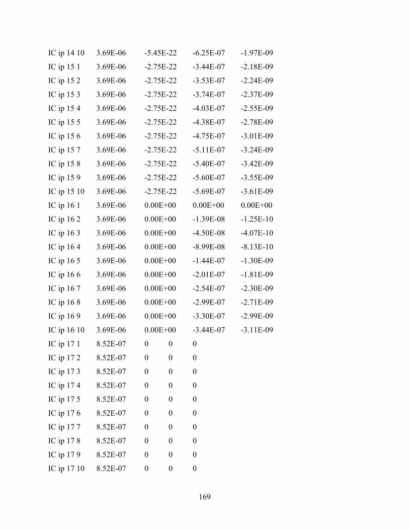
169
IC ip 14 10 3.69E-06 -5.45E-22 -6.25E-07 -1.97E-09
IC ip 15 1 3.69E-06 -2.75E-22 -3.44E-07 -2.18E-09
IC ip 15 2 3.69E-06 -2.75E-22 -3.53E-07 -2.24E-09
IC ip 15 3 3.69E-06 -2.75E-22 -3.74E-07 -2.37E-09
IC ip 15 4 3.69E-06 -2.75E-22 -4.03E-07 -2.55E-09
IC ip 15 5 3.69E-06 -2.75E-22 -4.38E-07 -2.78E-09
IC ip 15 6 3.69E-06 -2.75E-22 -4.75E-07 -3.01E-09
IC ip 15 7 3.69E-06 -2.75E-22 -5.11E-07 -3.24E-09
IC ip 15 8 3.69E-06 -2.75E-22 -5.40E-07 -3.42E-09
IC ip 15 9 3.69E-06 -2.75E-22 -5.60E-07 -3.55E-09
IC ip 15 10 3.69E-06 -2.75E-22 -5.69E-07 -3.61E-09
IC ip 16 1 3.69E-06 0.00E+00 0.00E+00 0.00E+00
IC ip 16 2 3.69E-06 0.00E+00 -1.39E-08 -1.25E-10
IC ip 16 3 3.69E-06 0.00E+00 -4.50E-08 -4.07E-10
IC ip 16 4 3.69E-06 0.00E+00 -8.99E-08 -8.13E-10
IC ip 16 5 3.69E-06 0.00E+00 -1.44E-07 -1.30E-09
IC ip 16 6 3.69E-06 0.00E+00 -2.01E-07 -1.81E-09
IC ip 16 7 3.69E-06 0.00E+00 -2.54E-07 -2.30E-09
IC ip 16 8 3.69E-06 0.00E+00 -2.99E-07 -2.71E-09
IC ip 16 9 3.69E-06 0.00E+00 -3.30E-07 -2.99E-09
IC ip 16 10 3.69E-06 0.00E+00 -3.44E-07 -3.11E-09
IC ip 17 1 8.52E-07 0 0 0
IC ip 17 2 8.52E-07 0 0 0
IC ip 17 3 8.52E-07 0 0 0
IC ip 17 4 8.52E-07 0 0 0
IC ip 17 5 8.52E-07 0 0 0
IC ip 17 6 8.52E-07 0 0 0
IC ip 17 7 8.52E-07 0 0 0
IC ip 17 8 8.52E-07 0 0 0
IC ip 17 9 8.52E-07 0 0 0
IC ip 17 10 8.52E-07 0 0 0
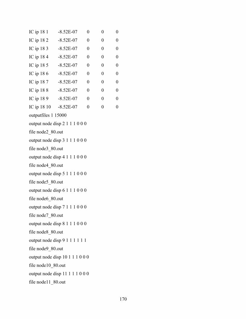
170
IC ip 18 1 -8.52E-07 0 0 0
IC ip 18 2 -8.52E-07 0 0 0
IC ip 18 3 -8.52E-07 0 0 0
IC ip 18 4 -8.52E-07 0 0 0
IC ip 18 5 -8.52E-07 0 0 0
IC ip 18 6 -8.52E-07 0 0 0
IC ip 18 7 -8.52E-07 0 0 0
IC ip 18 8 -8.52E-07 0 0 0
IC ip 18 9 -8.52E-07 0 0 0
IC ip 18 10 -8.52E-07 0 0 0
outputfiles 1 15000
output node disp 2 1 1 1 0 0 0
file node2_80.out
output node disp 3 1 1 1 0 0 0
file node3_80.out
output node disp 4 1 1 1 0 0 0
file node4_80.out
output node disp 5 1 1 1 0 0 0
file node5_80.out
output node disp 6 1 1 1 0 0 0
file node6_80.out
output node disp 7 1 1 1 0 0 0
file node7_80.out
output node disp 8 1 1 1 0 0 0
file node8_80.out
output node disp 9 1 1 1 1 1 1
file node9_80.out
output node disp 10 1 1 1 0 0 0
file node10_80.out
output node disp 11 1 1 1 0 0 0
file node11_80.out
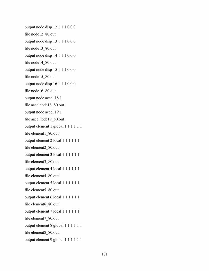
171
output node disp 12 1 1 1 0 0 0
file node12_80.out
output node disp 13 1 1 1 0 0 0
file node13_80.out
output node disp 14 1 1 1 0 0 0
file node14_80.out
output node disp 15 1 1 1 0 0 0
file node15_80.out
output node disp 16 1 1 1 0 0 0
file node16_80.out
output node accel 18 1
file aacelnode18_80.out
output node accel 19 1
file aacelnode19_80.out
output element 1 global 1 1 1 1 1 1
file element1_80.out
output element 2 local 1 1 1 1 1 1
file element2_80.out
output element 3 local 1 1 1 1 1 1
file element3_80.out
output element 4 local 1 1 1 1 1 1
file element4_80.out
output element 5 local 1 1 1 1 1 1
file element5_80.out
output element 6 local 1 1 1 1 1 1
file element6_80.out
output element 7 local 1 1 1 1 1 1
file element7_80.out
output element 8 global 1 1 1 1 1 1
file element8_80.out
output element 9 global 1 1 1 1 1 1
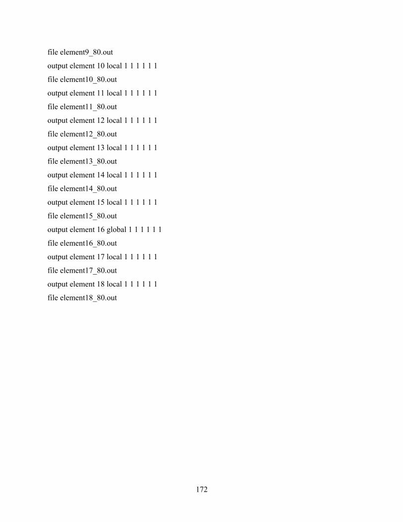
172
file element9_80.out
output element 10 local 1 1 1 1 1 1
file element10_80.out
output element 11 local 1 1 1 1 1 1
file element11_80.out
output element 12 local 1 1 1 1 1 1
file element12_80.out
output element 13 local 1 1 1 1 1 1
file element13_80.out
output element 14 local 1 1 1 1 1 1
file element14_80.out
output element 15 local 1 1 1 1 1 1
file element15_80.out
output element 16 global 1 1 1 1 1 1
file element16_80.out
output element 17 local 1 1 1 1 1 1
file element17_80.out
output element 18 local 1 1 1 1 1 1
file element18_80.out
173
APPENDIX C
DESIGN OF THE “ZIPPER FRAME”
This Appendix contains information about the general design procedure of a full scale “zipper
frame” prototype as developed by Yang (Yang 2006) (all the information presented here has
been kindly provided by Walter Yang). In addition, seismic requirements on compactness,
slenderness and bracing length for the 1/3 scaled “zipper frame” model are also presented.
C.1 Suspended “zipper frame” design methodology
The methodology proposed by Yang (Yang 2006) is a two step design procedure. Step I is a
design by strength where the frame is analyzed without considering the contribution from the
“zipper columns” i.e. like a conventional chevron braced frame. All the frame members, except
for the top story braces, are designed to resist the actions from combined gravity and lateral
loads.
Step II is a design by capacity where the frame is analyzed considering the “zipper columns”.
The introduction of these new elements will change the design of all the other structural
members except for the braces below the top story.
The “zipper column” is designed to resist the vertical unbalanced forces generated by the
braces below the floor under consideration, assuming Py (not Ry Py ) for the braces in tension and
0.3 times φc Pn for the braces in compression. The use of a tension brace force of Py in the
capacity calculation prevents excessive deformations in the tension brace and forces the “zipper
column” to yield soon after the brace under tension force yields, preventing drift concentration in
a single floor. The value used for the compression capacity is in accordance with current codes,
and reflects the capacity of a moderately slender brace after buckling. The shear capacity of the
beams is ignored.
The top-story braces need to resist both the vertical unbalanced forces and the top-floor level
equivalent lateral earthquake force. A factor of 1.7 times the top-floor level equivalent
earthquake force is used because the top-story braces need to be elastic throughout the load
history. As mentioned by Yang (Yang 2006), this value needs further research.
A flow chart of the design procedure is found in Figure C–1.
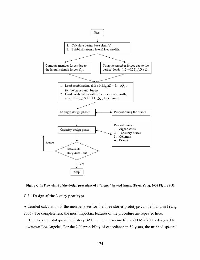
174
Figure C–1: Flow chart of the design procedure of a “zipper” braced frame. (From Yang, 2006 Figure 6.3)
C.2 Design of the 3 story prototype
A detailed calculation of the member sizes for the three stories prototype can be found in (Yang
2006). For completeness, the most important features of the procedure are repeated here.
The chosen prototype is the 3 story SAC moment resisting frame (FEMA 2000) designed for
downtown Los Angeles. For the 2 % probability of exceedance in 50 years, the mapped spectral
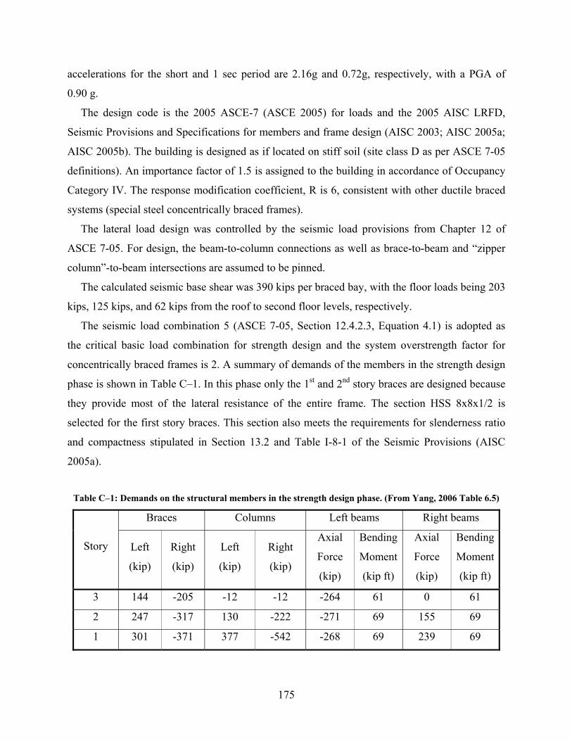
175
accelerations for the short and 1 sec period are 2.16g and 0.72g, respectively, with a PGA of
0.90 g.
The design code is the 2005 ASCE-7 (ASCE 2005) for loads and the 2005 AISC LRFD,
Seismic Provisions and Specifications for members and frame design (AISC 2003; AISC 2005a;
AISC 2005b). The building is designed as if located on stiff soil (site class D as per ASCE 7-05
definitions). An importance factor of 1.5 is assigned to the building in accordance of Occupancy
Category IV. The response modification coefficient, R is 6, consistent with other ductile braced
systems (special steel concentrically braced frames).
The lateral load design was controlled by the seismic load provisions from Chapter 12 of
ASCE 7-05. For design, the beam-to-column connections as well as brace-to-beam and “zipper
column”-to-beam intersections are assumed to be pinned.
The calculated seismic base shear was 390 kips per braced bay, with the floor loads being 203
kips, 125 kips, and 62 kips from the roof to second floor levels, respectively.
The seismic load combination 5 (ASCE 7-05, Section 12.4.2.3, Equation 4.1) is adopted as
the critical basic load combination for strength design and the system overstrength factor for
concentrically braced frames is 2. A summary of demands of the members in the strength design
phase is shown in Table C–1. In this phase only the 1st and 2nd story braces are designed because
they provide most of the lateral resistance of the entire frame. The section HSS 8x8x1/2 is
selected for the first story braces. This section also meets the requirements for slenderness ratio
and compactness stipulated in Section 13.2 and Table I-8-1 of the Seismic Provisions (AISC
2005a).
Table C–1: Demands on the structural members in the strength design phase. (From Yang, 2006 Table 6.5)
Braces Columns Left beams Right beams
Story Left
(kip)
Right
(kip)
Left
(kip)
Right
(kip)
Axial
Force
(kip)
Bending
Moment
(kip ft)
Axial
Force
(kip)
Bending
Moment
(kip ft)
3 144 -205 -12 -12 -264 61 0 61
2 247 -317 130 -222 -271 69 155 69
1 301 -371 377 -542 -268 69 239 69
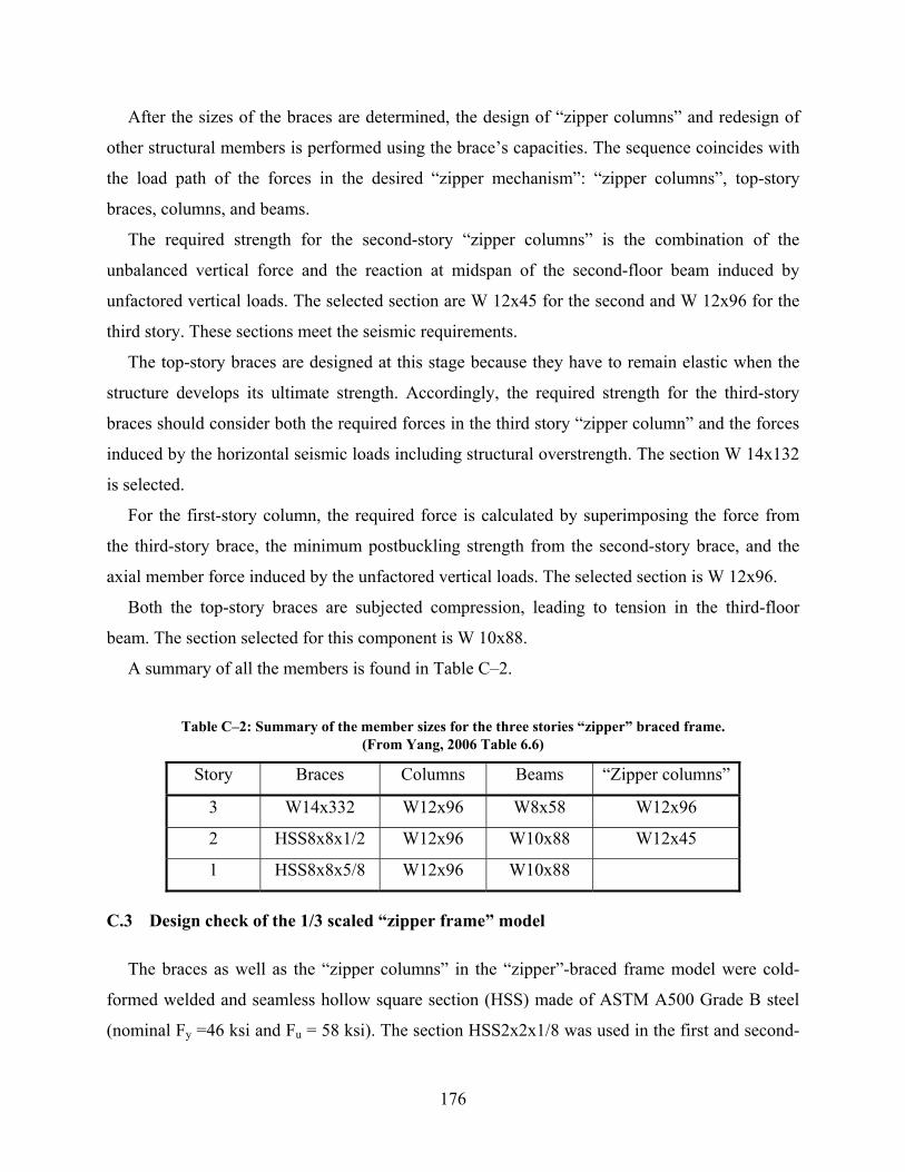
176
After the sizes of the braces are determined, the design of “zipper columns” and redesign of
other structural members is performed using the brace’s capacities. The sequence coincides with
the load path of the forces in the desired “zipper mechanism”: “zipper columns”, top-story
braces, columns, and beams.
The required strength for the second-story “zipper columns” is the combination of the
unbalanced vertical force and the reaction at midspan of the second-floor beam induced by
unfactored vertical loads. The selected section are W 12x45 for the second and W 12x96 for the
third story. These sections meet the seismic requirements.
The top-story braces are designed at this stage because they have to remain elastic when the
structure develops its ultimate strength. Accordingly, the required strength for the third-story
braces should consider both the required forces in the third story “zipper column” and the forces
induced by the horizontal seismic loads including structural overstrength. The section W 14x132
is selected.
For the first-story column, the required force is calculated by superimposing the force from
the third-story brace, the minimum postbuckling strength from the second-story brace, and the
axial member force induced by the unfactored vertical loads. The selected section is W 12x96.
Both the top-story braces are subjected compression, leading to tension in the third-floor
beam. The section selected for this component is W 10x88.
A summary of all the members is found in Table C–2.
Table C–2: Summary of the member sizes for the three stories “zipper” braced frame. (From Yang, 2006 Table 6.6)
Story Braces Columns Beams “Zipper columns”
3 W14x332 W12x96 W8x58 W12x96
2 HSS8x8x1/2 W12x96 W10x88 W12x45
1 HSS8x8x5/8 W12x96 W10x88
C.3 Design check of the 1/3 scaled “zipper frame” model
The braces as well as the “zipper columns” in the “zipper”-braced frame model were cold-
formed welded and seamless hollow square section (HSS) made of ASTM A500 Grade B steel
(nominal Fy =46 ksi and Fu = 58 ksi). The section HSS2x2x1/8 was used in the first and second-
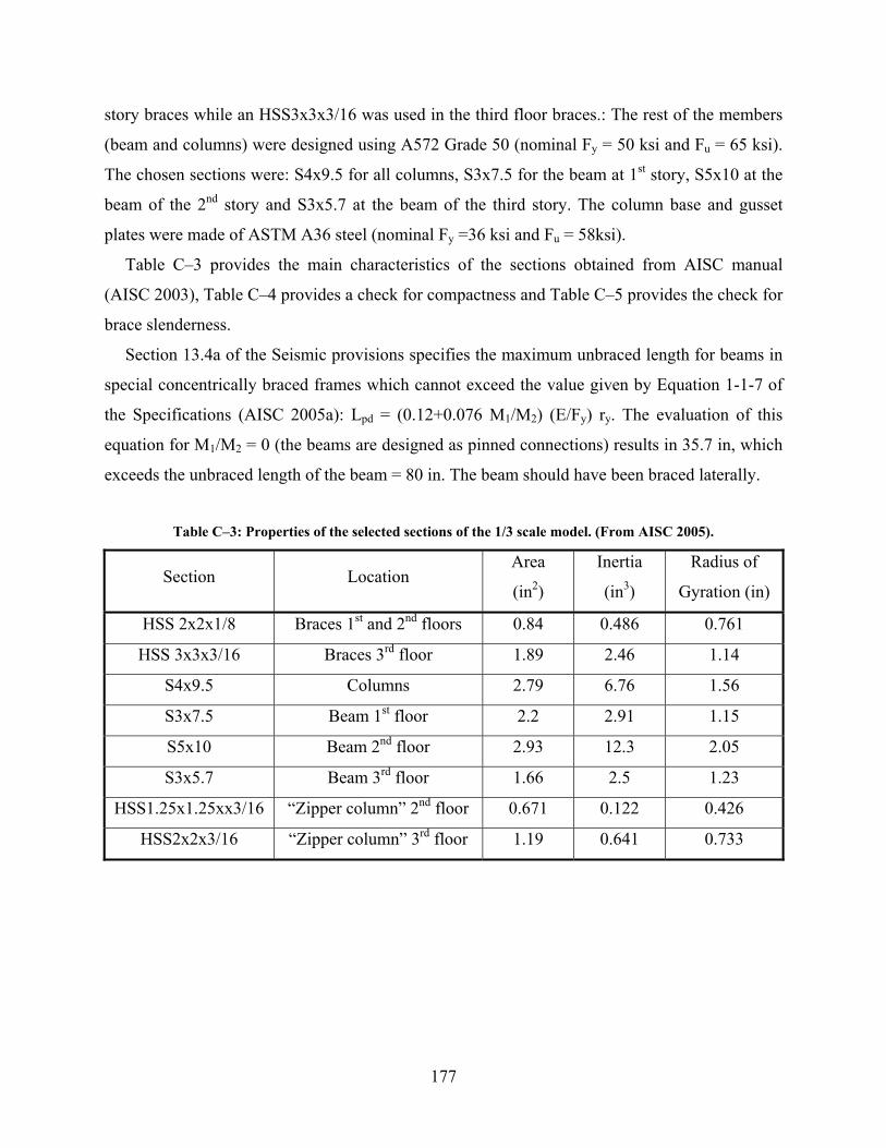
177
story braces while an HSS3x3x3/16 was used in the third floor braces.: The rest of the members
(beam and columns) were designed using A572 Grade 50 (nominal Fy = 50 ksi and Fu = 65 ksi).
The chosen sections were: S4x9.5 for all columns, S3x7.5 for the beam at 1st story, S5x10 at the
beam of the 2nd story and S3x5.7 at the beam of the third story. The column base and gusset
plates were made of ASTM A36 steel (nominal Fy =36 ksi and Fu = 58ksi).
Table C–3 provides the main characteristics of the sections obtained from AISC manual
(AISC 2003), Table C–4 provides a check for compactness and Table C–5 provides the check for
brace slenderness.
Section 13.4a of the Seismic provisions specifies the maximum unbraced length for beams in
special concentrically braced frames which cannot exceed the value given by Equation 1-1-7 of
the Specifications (AISC 2005a): Lpd = (0.12+0.076 M1/M2) (E/Fy) ry. The evaluation of this
equation for M1/M2 = 0 (the beams are designed as pinned connections) results in 35.7 in, which
exceeds the unbraced length of the beam = 80 in. The beam should have been braced laterally.
Table C–3: Properties of the selected sections of the 1/3 scale model. (From AISC 2005).
Section Location Area
(in2)
Inertia
(in3)
Radius of
Gyration (in)
HSS 2x2x1/8 Braces 1st and 2nd floors 0.84 0.486 0.761
HSS 3x3x3/16 Braces 3rd floor 1.89 2.46 1.14
S4x9.5 Columns 2.79 6.76 1.56
S3x7.5 Beam 1st floor 2.2 2.91 1.15
S5x10 Beam 2nd floor 2.93 12.3 2.05
S3x5.7 Beam 3rd floor 1.66 2.5 1.23
HSS1.25x1.25xx3/16 “Zipper column” 2nd floor 0.671 0.122 0.426
HSS2x2x3/16 “Zipper column” 3rd floor 1.19 0.641 0.733
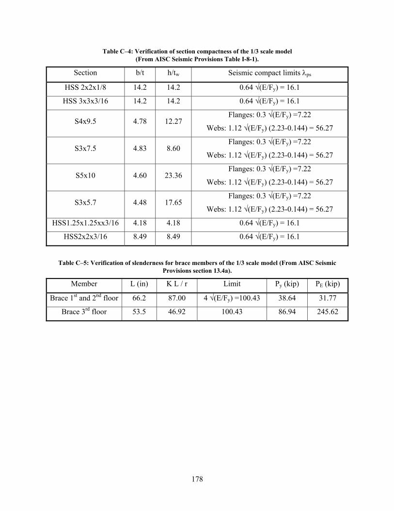
178
Table C–4: Verification of section compactness of the 1/3 scale model (From AISC Seismic Provisions Table I-8-1).
Section b/t h/tw Seismic compact limits λps
HSS 2x2x1/8 14.2 14.2 0.64 √(E/Fy) = 16.1
HSS 3x3x3/16 14.2 14.2 0.64 √(E/Fy) = 16.1
S4x9.5 4.78 12.27 Flanges: 0.3 √(E/Fy) =7.22
Webs: 1.12 √(E/Fy) (2.23-0.144) = 56.27
S3x7.5 4.83 8.60 Flanges: 0.3 √(E/Fy) =7.22
Webs: 1.12 √(E/Fy) (2.23-0.144) = 56.27
S5x10 4.60 23.36 Flanges: 0.3 √(E/Fy) =7.22
Webs: 1.12 √(E/Fy) (2.23-0.144) = 56.27
S3x5.7 4.48 17.65 Flanges: 0.3 √(E/Fy) =7.22
Webs: 1.12 √(E/Fy) (2.23-0.144) = 56.27
HSS1.25x1.25xx3/16 4.18 4.18 0.64 √(E/Fy) = 16.1
HSS2x2x3/16 8.49 8.49 0.64 √(E/Fy) = 16.1
Table C–5: Verification of slenderness for brace members of the 1/3 scale model (From AISC Seismic Provisions section 13.4a).
Member L (in) K L / r Limit Py (kip) PE (kip)
Brace 1st and 2nd floor 66.2 87.00 4 √(E/Fy) =100.43 38.64 31.77
Brace 3rd floor 53.5 46.92 100.43 86.94 245.62
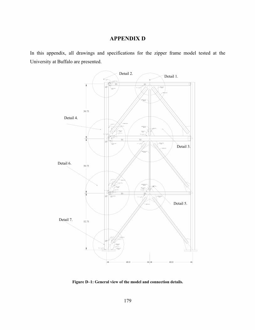
179
APPENDIX D
In this appendix, all drawings and specifications for the zipper frame model tested at the
University at Buffalo are presented.
Column: S4x9.5
3.516
5.5FE70XX 316
2L2.5x1x5/16(A36)
E70XX3 F
14
(GR 50)HSS1 x1 x3/16
41E70XXF
9
163 13
Beam: S5x10
FE70XX
FE70XX7
Beam: S5x10
P
FE70XX94
1
(GR 50)HSS2x2x3/163
16
HSS3x3x3/16
F6
E70XX
L9x7x1/2
3F3
16E70XXE70XX
163 F
LP 11x6.8x3/8(A36)
HSS2x2x1/8
(A36)13x6.7x3/8PL
316163 FE70XXE70XXF
5
Column: S4x9.5 F
(A36)2L1.5x1x1/4
HSS2x2x3/16(GR 50)
E70XX
41
316
163
2
E70XXF 4
FE70XX
Beam: S3x5.7
Beam: S3x5.7
CL
LP 16x9x1/2(A36)
HSS3x3x3/16
16
16
(A36)12x8x1.25
E70XX
10x4x3/8
PLE70XXF60°
F41 4
(A36)PL
52.75
E70XX
Column: S4x9.5
43
F163 10 HSS2x2x1/8
E70XXF
HSS2x2x1/8
50.75
4
3
1.5
163FE70XX
F316
E70XX
(A36)2L1.5x1.0x5/16
7
4
316
E70XXF316
E70XX316
F
Column: S4x9.5
LP 7x4x3/8(A36)
113
Beam: S3x7.5
7
HSS1 x1 x3/16
E70XXF
E70XXF 316
FE70XX
(GR 50)
7x3.5x3/8LP(A36)
Beam: S3x7.5
HSS2x2x1/8
50.75
9x5.5x1/2(A36)(A36)
40.0 40.0
Detail 1.Detail 2.
Detail 3.
Detail 5.
Detail 7.
Detail 6.
Detail 4.
Figure D–1: General view of the model and connection details.
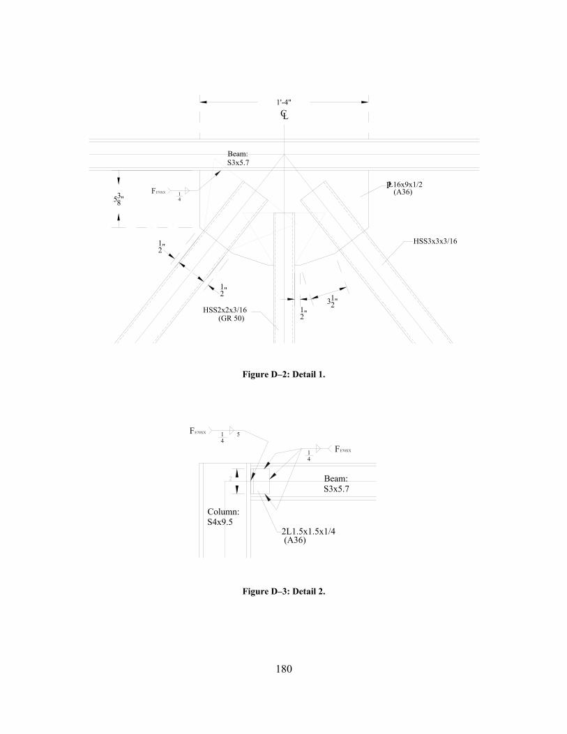
180
F
HSS2x2x3/16(GR 50)
E70XX
41
Beam: S3x5.7
CL
LP 16x9x1/2(A36)
HSS3x3x3/16
538"
12"
12"
312"
12"
1'-4"
Figure D–2: Detail 1.
2
14
14
Beam: S3x5.7
E70XXF 5
(A36)
FE70XX
Column: S4x9.5
2L1.5x1.5x1/4
Figure D–3: Detail 2.
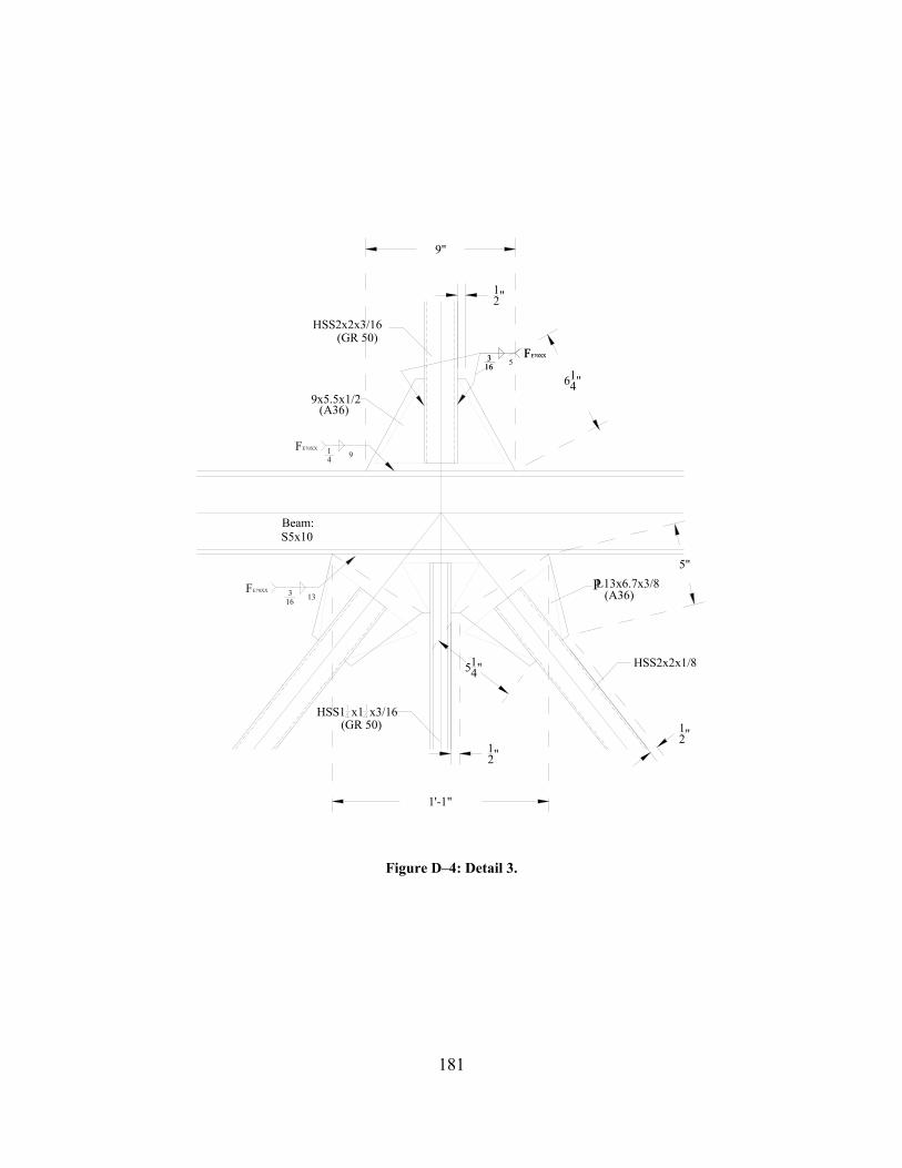
181
(A36)9x5.5x1/2
HSS1 x1 x3/16
E70XXF
Beam: S5x10
13316
9FE70XX 1
4
(GR 50)
LP 13x6.7x3/8(A36)
HSS2x2x1/8
HSS2x2x3/16(GR 50)
5FE70XXE70XXF3
16163
9"
12"
614"
5"
12"
514"
12"
1'-1"
Figure D–4: Detail 3.
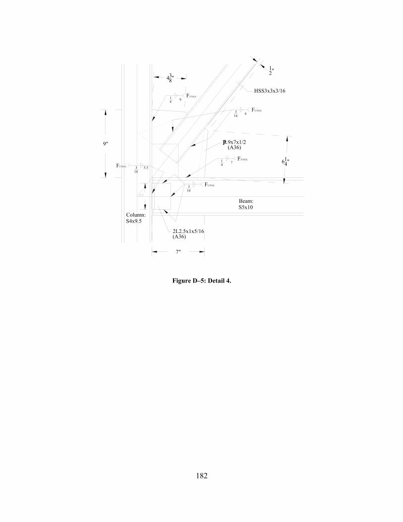
182
(A36)
Column: S4x9.5
16
5.5FE70XX 316
2L2.5x1x5/16(A36)
E70XX3 F
14
FE70XX7
Beam: S5x10
P
FE70XX94
1
316
HSS3x3x3/16
F6
E70XX
L9x7x1/2
614"
3.5
438"
12"
9"
7"
Figure D–5: Detail 4.
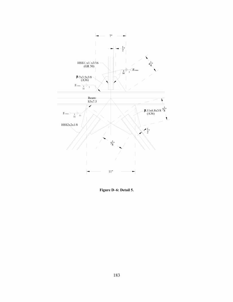
183
16
HSS2x2x1/8
HSS1 x1 x3/16
Beam: S3x7.5
(A36)PL7x3.5x3/8
(GR 50)
163FE70XX
FE70XX
7
3 11(A36)11x6.8x3/8PL
F316
E70XXE70XX
163 F
3
414"
518"
12"
518"
11"
7"
12"
Figure D–6: Detail 5.
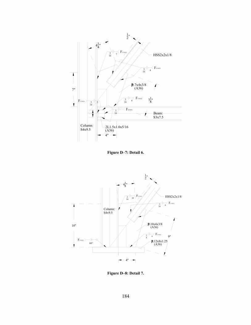
184
(A36)7x4x3/8
E70XX
PL
Column: S4x9.5
F163 E70XX
163 F
4
7
2L1.5x1.0x5/16(A36)
E70XX
163 F
E70XXF 316
1.5
3
HSS2x2x1/8
Beam: S3x7.5
E70XXF163 4
718"
4"
7"
414"
12"
Figure D–7: Detail 6.
(A36)
F
10x4x3/8
12x8x1.25(A36)
LP
414
60°FE70XX LP
E70XX
10316
F
Column: S4x9.5
E70XX
FE70XX
HSS2x2x1/8
3 416
418"
10"
4"
9"
12"
Figure D–8: Detail 7.
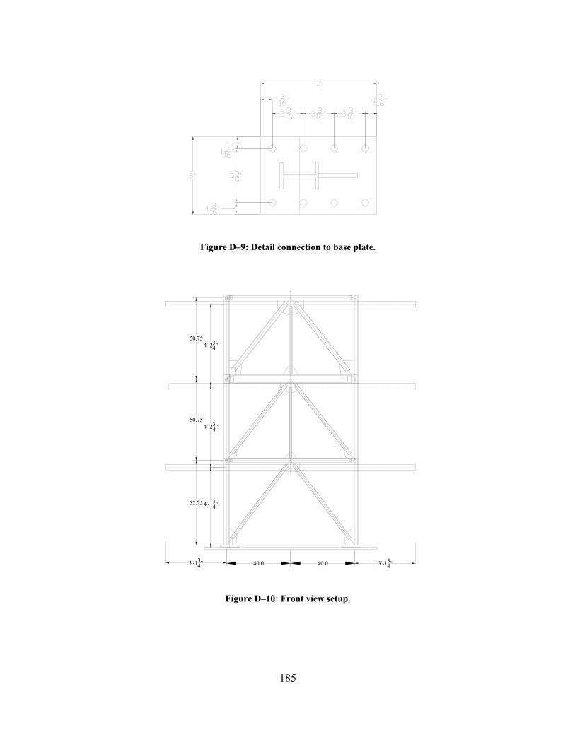
185
Figure D–9: Detail connection to base plate.
4'-134"
4'-234"
4'-234"
3'-134"3'-13
4" 40.0 40.0
52.75
50.75
50.75
CL
Figure D–10: Front view setup.
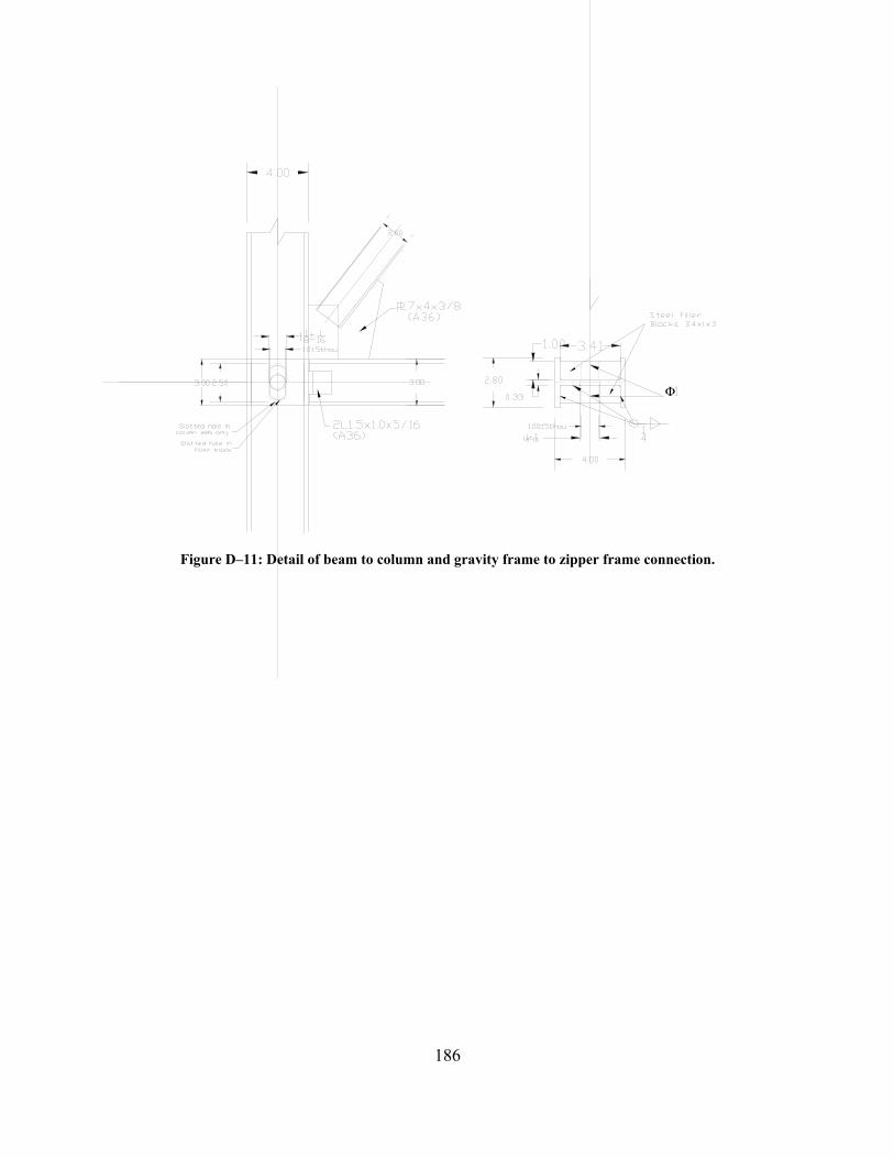
186
Φ
Figure D–11: Detail of beam to column and gravity frame to zipper frame connection.
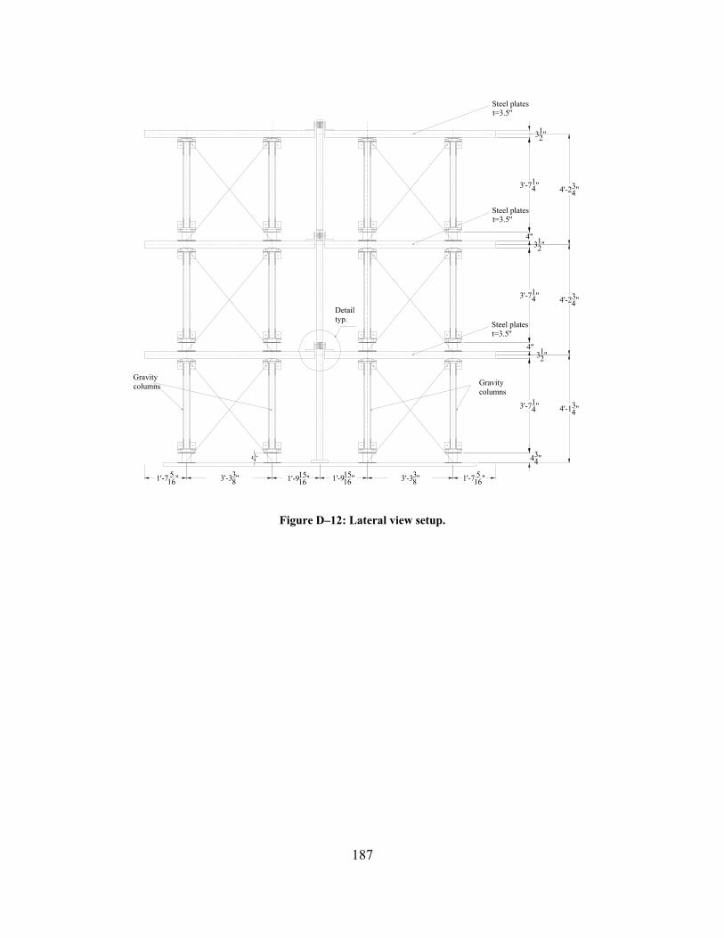
187
3'-714"
434"
3'-714"
4"312"
3'-714"
4"312"
312"
4'-134"
4'-234"
4'-234"
1'-91516" 1'-7 5
16"3'-338"1'-7 5
16" 3'-338" 1'-915
16"
Detail typ.
Gravity columns
Gravity columns
Steel platest=3.5''
Steel platest=3.5''
Steel platest=3.5''
434"
Figure D–12: Lateral view setup.
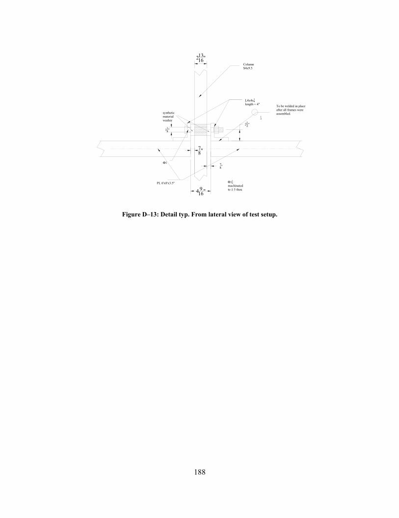
188
21316"
4 916"
78"
ColumnS4x9.5
L4x4x34
length = 4''
PL 6'x8'x3.5'' Φ118
machinated to ± 5 thou
Φ1
To be welded in place after all frames were assembled.
12
synthetic materialwasher
212"
78"
118"
Figure D–13: Detail typ. From lateral view of test setup.
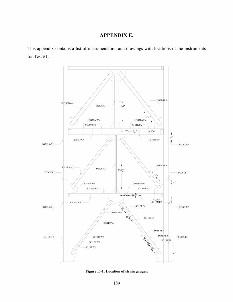
189
APPENDIX E.
This appendix contains a list of instrumentation and drawings with locations of the instruments
for Test #1.
714"7"
3"
1'-2"
SG2BREA
SG3BREA
SG2BRWA
SG3BMWA
SG1CLW1
SG1CLW2
SG1CLE1
SG1CLE2
SG2ZCA
SG3ZCA
SG2BMWw SG2BMEw
SG1BMWw
SG1BMWe
4"
SG2CLE1
SG2CLE2SG2CLW2
SG2CLW1
SG2BMWe SG2BMEe
4"
5"
4"
1058"
1014"
518"
518"
518"
518"
1034"6"
1'-734"
1'-4"
1012"
SG1BRW2
SG1BMEw
SG1BMEe
SG1BRWA
SG1BREA
SG1BRW3
SG1BRW4
SG1BRE4
SG1BRE3
SG1BRE2
SG1BRE1
SG1BRW1
SG2BMWA SG2BMEA
SG1BMWA SG1BMEA
Figure E–1: Location of strain gauges.
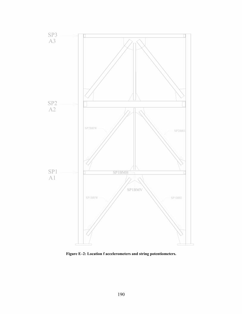
190
SP2
SP3
SP1
SP1BMV
SP1BMHA1
A2
A3
SP1BRW SP1BRE
SP2BRWSP2BRE
Figure E–2: Location f accelerometers and string potentiometers.
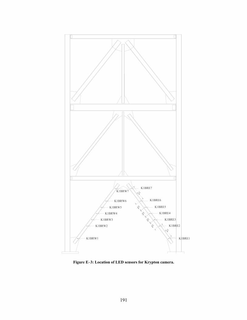
191
K1BRW1
K1BRW2
K1BRW3
K1BRW4
K1BRW5
K1BRW6
K1BRW7 K1BRE7
K1BRE6
K1BRE5
K1BRE4
K1BRE3
K1BRE2
K1BRE1
558"
558"
558"
558"
1114"
1114"
Figure E–3: Location of LED sensors for Krypton camera.
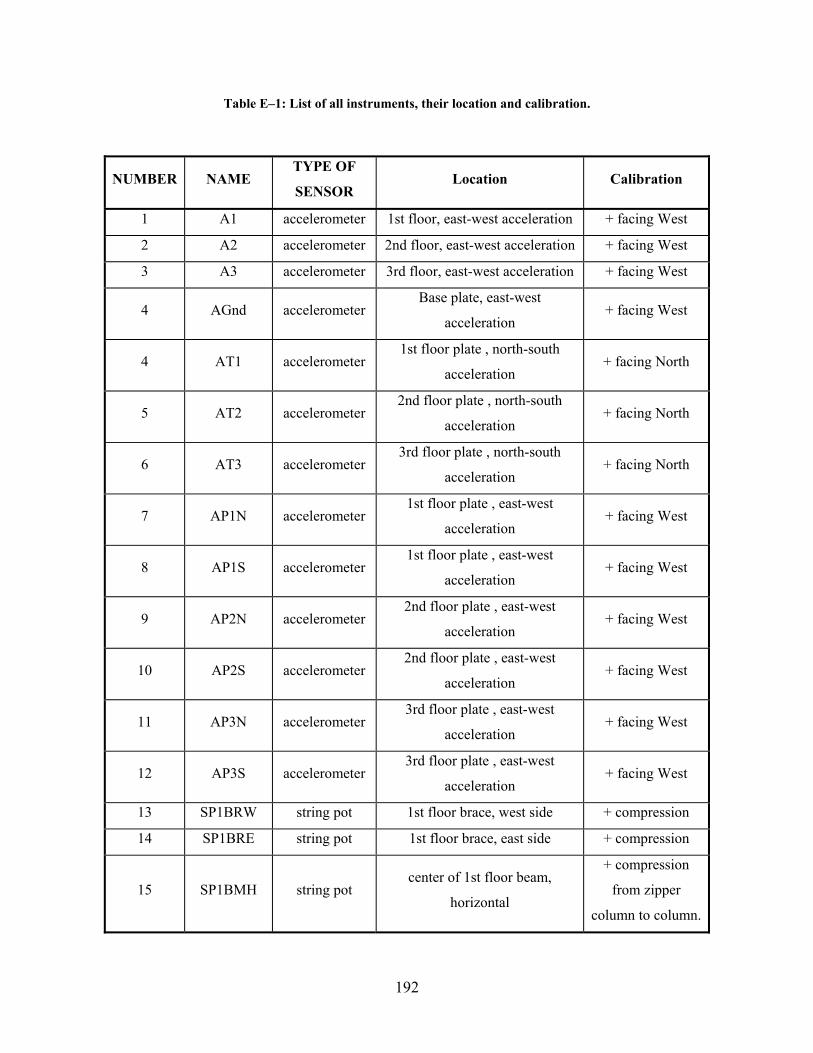
192
Table E–1: List of all instruments, their location and calibration.
NUMBER NAME TYPE OF
SENSOR Location Calibration
1 A1 accelerometer 1st floor, east-west acceleration + facing West
2 A2 accelerometer 2nd floor, east-west acceleration + facing West
3 A3 accelerometer 3rd floor, east-west acceleration + facing West
4 AGnd accelerometer Base plate, east-west
acceleration + facing West
4 AT1 accelerometer 1st floor plate , north-south
acceleration + facing North
5 AT2 accelerometer 2nd floor plate , north-south
acceleration + facing North
6 AT3 accelerometer 3rd floor plate , north-south
acceleration + facing North
7 AP1N accelerometer 1st floor plate , east-west
acceleration + facing West
8 AP1S accelerometer 1st floor plate , east-west
acceleration + facing West
9 AP2N accelerometer 2nd floor plate , east-west
acceleration + facing West
10 AP2S accelerometer 2nd floor plate , east-west
acceleration + facing West
11 AP3N accelerometer 3rd floor plate , east-west
acceleration + facing West
12 AP3S accelerometer 3rd floor plate , east-west
acceleration + facing West
13 SP1BRW string pot 1st floor brace, west side + compression
14 SP1BRE string pot 1st floor brace, east side + compression
15 SP1BMH string pot center of 1st floor beam,
horizontal
+ compression
from zipper
column to column.
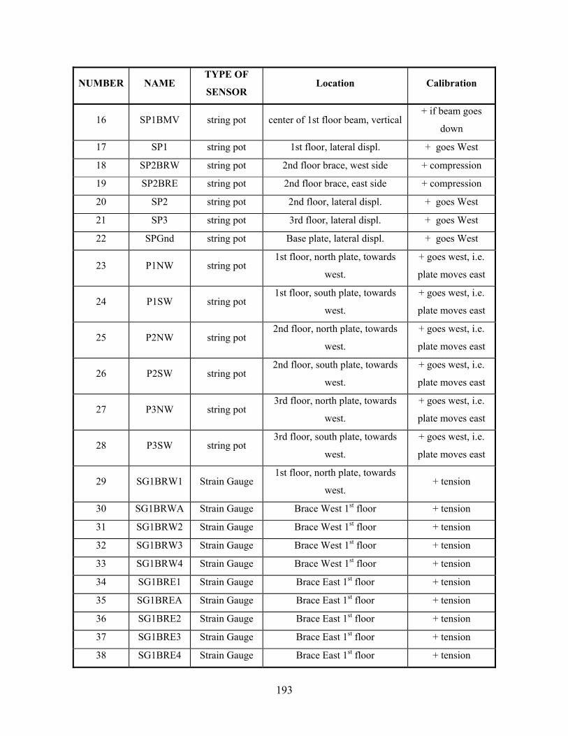
193
NUMBER NAME TYPE OF
SENSOR Location Calibration
16 SP1BMV string pot center of 1st floor beam, vertical + if beam goes
down
17 SP1 string pot 1st floor, lateral displ. + goes West
18 SP2BRW string pot 2nd floor brace, west side + compression
19 SP2BRE string pot 2nd floor brace, east side + compression
20 SP2 string pot 2nd floor, lateral displ. + goes West
21 SP3 string pot 3rd floor, lateral displ. + goes West
22 SPGnd string pot Base plate, lateral displ. + goes West
23 P1NW string pot 1st floor, north plate, towards
west.
+ goes west, i.e.
plate moves east
24 P1SW string pot 1st floor, south plate, towards
west.
+ goes west, i.e.
plate moves east
25 P2NW string pot 2nd floor, north plate, towards
west.
+ goes west, i.e.
plate moves east
26 P2SW string pot 2nd floor, south plate, towards
west.
+ goes west, i.e.
plate moves east
27 P3NW string pot 3rd floor, north plate, towards
west.
+ goes west, i.e.
plate moves east
28 P3SW string pot 3rd floor, south plate, towards
west.
+ goes west, i.e.
plate moves east
29 SG1BRW1 Strain Gauge 1st floor, north plate, towards
west. + tension
30 SG1BRWA Strain Gauge Brace West 1st floor + tension
31 SG1BRW2 Strain Gauge Brace West 1st floor + tension
32 SG1BRW3 Strain Gauge Brace West 1st floor + tension
33 SG1BRW4 Strain Gauge Brace West 1st floor + tension
34 SG1BRE1 Strain Gauge Brace East 1st floor + tension
35 SG1BREA Strain Gauge Brace East 1st floor + tension
36 SG1BRE2 Strain Gauge Brace East 1st floor + tension
37 SG1BRE3 Strain Gauge Brace East 1st floor + tension
38 SG1BRE4 Strain Gauge Brace East 1st floor + tension
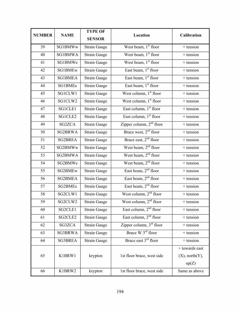
194
NUMBER NAME TYPE OF
SENSOR Location Calibration
39 SG1BMWw Strain Gauge West beam, 1st floor + tension
40 SG1BMWA Strain Gauge West beam, 1st floor + tension
41 SG1BMWe Strain Gauge West beam, 1st floor + tension
42 SG1BMEw Strain Gauge East beam, 1st floor + tension
43 SG1BMEA Strain Gauge East beam, 1st floor + tension
44 SG1BMEe Strain Gauge East beam, 1st floor + tension
45 SG1CLW1 Strain Gauge West column, 1st floor + tension
46 SG1CLW2 Strain Gauge West column, 1st floor + tension
47 SG1CLE1 Strain Gauge East column, 1st floor + tension
48 SG1CLE2 Strain Gauge East column, 1st floor + tension
49 SG2ZCA Strain Gauge Zipper column, 2nd floor + tension
50 SG2BRWA Strain Gauge Brace west, 2nd floor + tension
51 SG2BREA Strain Gauge Brace east, 2nd floor + tension
52 SG2BMWw Strain Gauge West beam, 2nd floor + tension
53 SG2BMWA Strain Gauge West beam, 2nd floor + tension
54 SG2BMWe Strain Gauge West beam, 2nd floor + tension
55 SG2BMEw Strain Gauge East beam, 2nd floor + tension
56 SG2BMEA Strain Gauge East beam, 2nd floor + tension
57 SG2BMEe Strain Gauge East beam, 2nd floor + tension
58 SG2CLW1 Strain Gauge West column, 2nd floor + tension
59 SG2CLW2 Strain Gauge West column, 2nd floor + tension
60 SG2CLE1 Strain Gauge East column, 2nd floor + tension
61 SG2CLE2 Strain Gauge East column, 2nd floor + tension
62 SG3ZCA Strain Gauge Zipper column, 3rd floor + tension
63 SG3BRWA Strain Gauge Brace W 3rd floor + tension
64 SG3BREA Strain Gauge Brace east 3rd floor + tension
65 K1BRW1 krypton 1st floor brace, west side
+ towards east
(X), north(Y),
up(Z)
66 K1BRW2 krypton 1st floor brace, west side Same as above
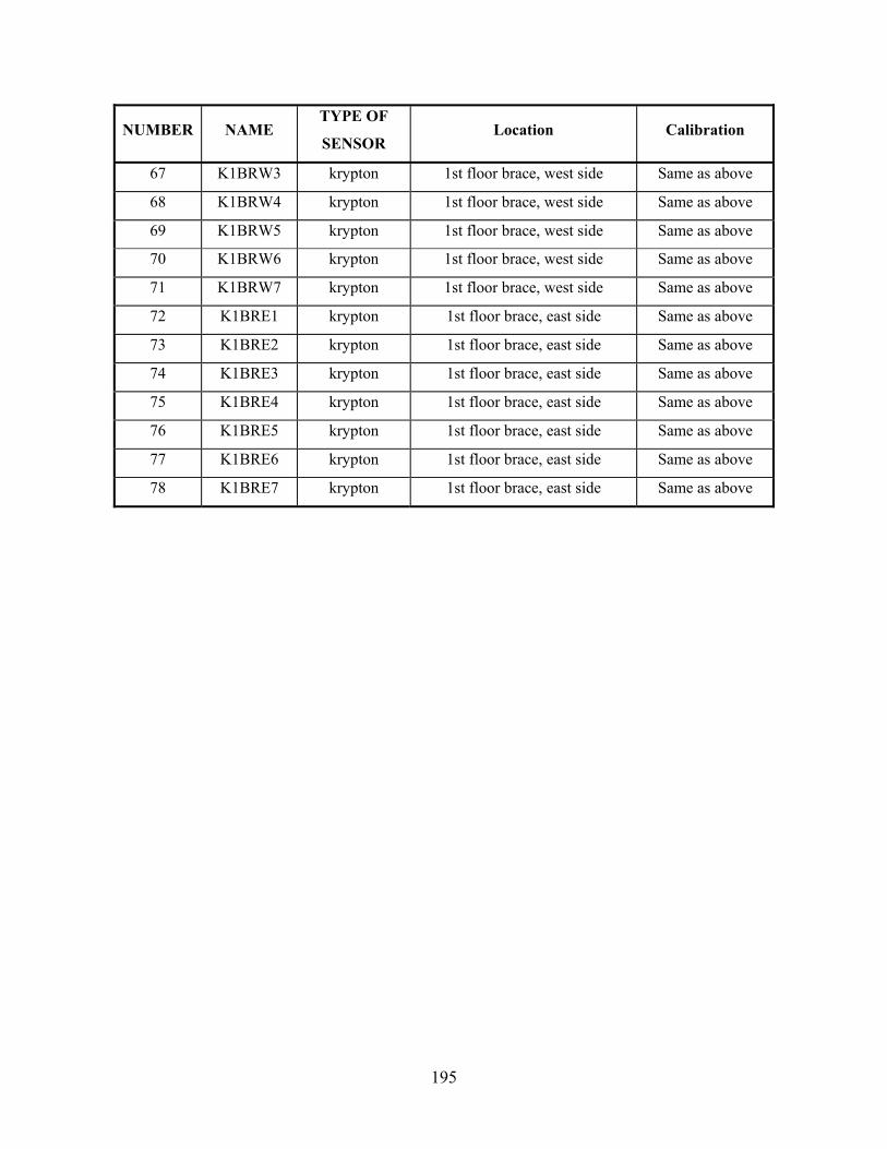
195
NUMBER NAME TYPE OF
SENSOR Location Calibration
67 K1BRW3 krypton 1st floor brace, west side Same as above
68 K1BRW4 krypton 1st floor brace, west side Same as above
69 K1BRW5 krypton 1st floor brace, west side Same as above
70 K1BRW6 krypton 1st floor brace, west side Same as above
71 K1BRW7 krypton 1st floor brace, west side Same as above
72 K1BRE1 krypton 1st floor brace, east side Same as above
73 K1BRE2 krypton 1st floor brace, east side Same as above
74 K1BRE3 krypton 1st floor brace, east side Same as above
75 K1BRE4 krypton 1st floor brace, east side Same as above
76 K1BRE5 krypton 1st floor brace, east side Same as above
77 K1BRE6 krypton 1st floor brace, east side Same as above
78 K1BRE7 krypton 1st floor brace, east side Same as above

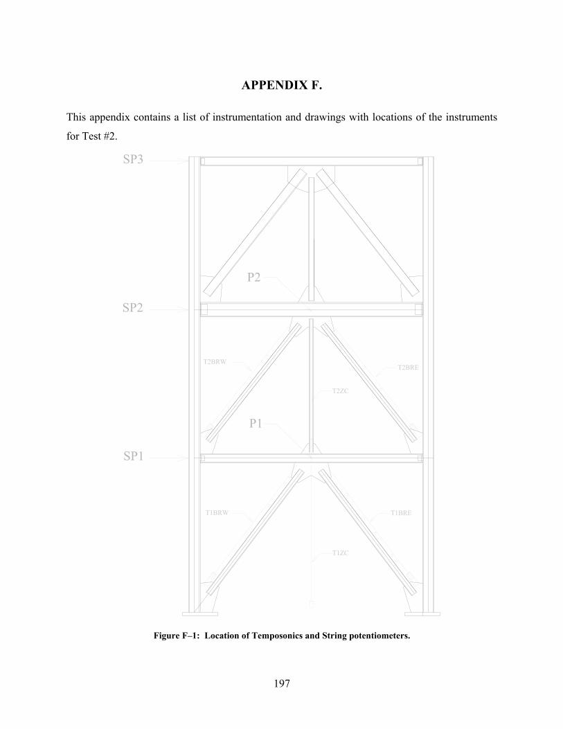
197
APPENDIX F.
This appendix contains a list of instrumentation and drawings with locations of the instruments
for Test #2.
SP2
SP3
SP1
T1BRW T1BRE
T2BRWT2BRE
T1ZC
T2ZC
P1
P2
Figure F–1: Location of Temposonics and String potentiometers.
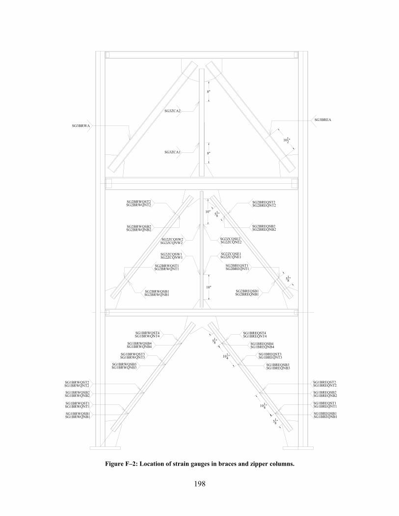
198
1012"
SG3BREASG3BRWA
518"
SG1BREQST4
SG1BREQST3
SG1BREQST2
SG1BREQST1
518"
SG2ZCQSW2
10"
10"
8"
8"
SG3ZCA2
SG3ZCA1
SG2BREQSB2
SG2BREQSB1
SG2BREQST2
518"
SG2BREQST1
SG2ZCQSE2
SG2ZCQSE1
SG2BRWQSB2
SG2BRWQSB1
SG2BRWQST2
SG2BRWQST1
SG2ZCQSW1
518"
1014"
1014"
SG1BREQSB4
SG1BREQSB3
SG1BREQSB2
SG1BREQSB1
SG1BRWQST4
SG1BRWQST3
SG1BRWQST2
SG1BRWQST1
SG1BRWQSB4
SG1BRWQSB3
SG1BRWQSB2
SG1BRWQSB1
SG1BREQNT4
SG1BREQNT3
SG1BREQNT2
SG1BREQNT1
SG2ZCQNW2
SG2BREQNB2
SG2BREQNB1
SG2BREQNT2
SG2BREQNT1
SG2ZCQNE2
SG2ZCQNE1
SG2BRWQNB2
SG2BRWQNB1
SG2BRWQNT2
SG2BRWQNT1
SG2ZCQNW1
SG1BREQNB4
SG1BREQNB3
SG1BREQNB2
SG1BREQNB1
SG1BRWQNT4
SG1BRWQNT3
SG1BRWQNT2
SG1BRWQNT1
SG1BRWQNB4
SG1BRWQNB3
SG1BRWQNB2
SG1BRWQNB1
Figure F–2: Location of strain gauges in braces and zipper columns.
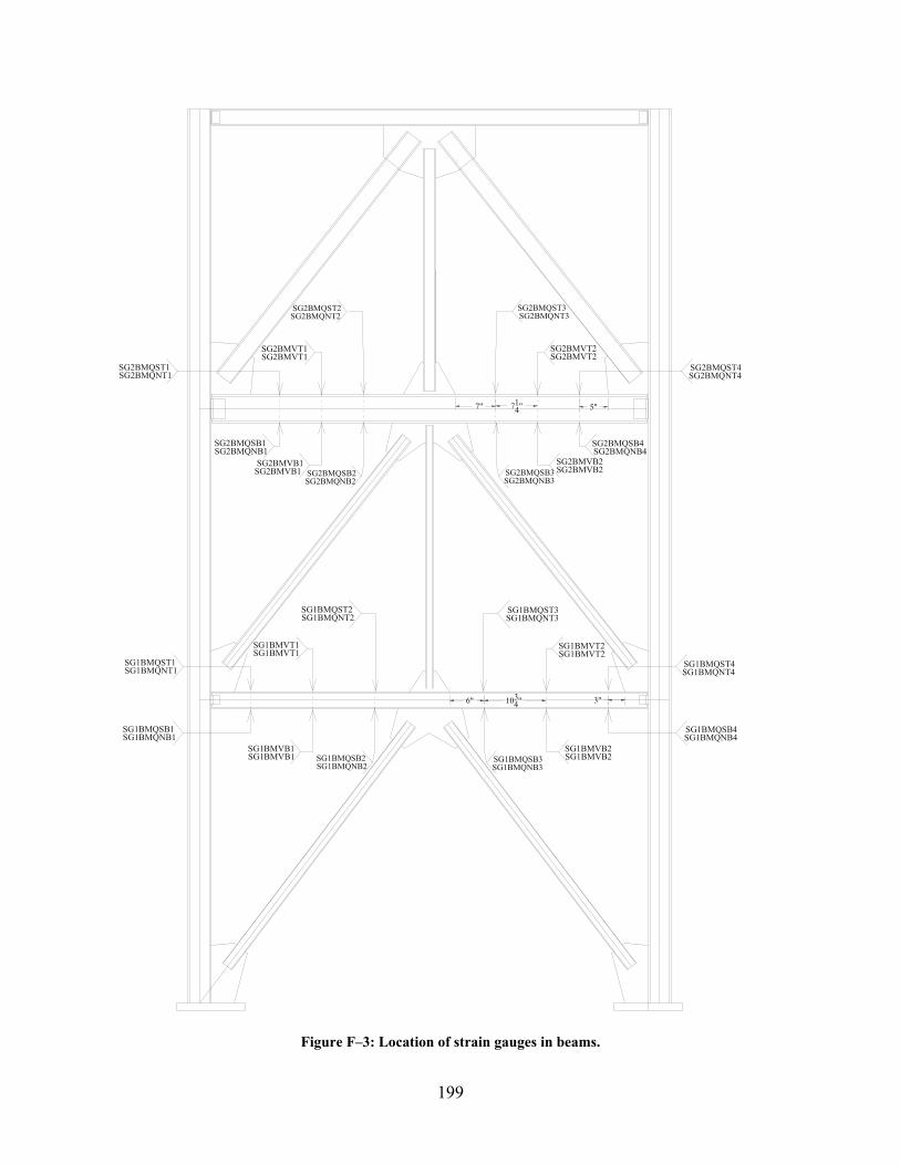
199
SG1BMQST2
6" 3"
7" 5"
SG2BMVB1
714"
1034"
SG2BMQSB2
SG2BMQSB1
SG2BMVB2SG2BMQSB3
SG2BMQSB4
SG1BMVB2SG1BMQSB3
SG1BMVB1
SG1BMQSB1
SG1BMQSB2
SG1BMQSB4
SG1BMQST3
SG1BMQST1
SG1BMVT1 SG1BMVT2
SG1BMQST4
SG2BMVT1
SG2BMQST1
SG2BMQST2
SG2BMQST4
SG2BMQST3
SG2BMVT2
SG1BMQNT2
SG2BMVB1SG2BMQNB2
SG2BMQNB1
SG2BMVB2SG2BMQNB3
SG2BMQNB4
SG1BMVB2SG1BMQNB3
SG1BMVB1
SG1BMQNB1
SG1BMQNB2
SG1BMQNB4
SG1BMQNT3
SG1BMQNT1
SG1BMVT1 SG1BMVT2
SG1BMQNT4
SG2BMVT1
SG2BMQNT1
SG2BMQNT2
SG2BMQNT4
SG2BMQNT3
SG2BMVT2
Figure F–3: Location of strain gauges in beams.
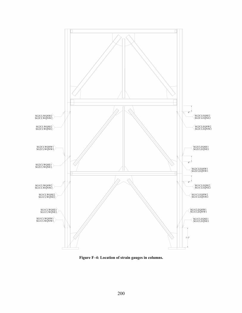
200
SG1CLWQSW1
SG1CLWQSW2
1'-2"
4"
SG2CLWQSW2
SG2CLWQSW1
4"
4"
SG1CLWQSE1
SG1CLWQSE2
SG2CLWQSE1
SG2CLWQSE2
SG1CLEQSE1
SG1CLEQSE2
SG2CLEQSE2
SG2CLEQSE1
SG1CLEQSW1
SG1CLEQSW2
SG2CLEQSW1
SG2CLEQSW2
SG1CLWQNW1
SG1CLWQNW2
SG2CLWQNW2
SG2CLWQNW1
SG1CLWQNE1
SG1CLWQNE2
SG2CLWQNE1
SG2CLWQNE2
SG1CLEQNE1
SG1CLEQNE2
SG2CLEQNE2
SG2CLEQNE1
SG1CLEQNW1
SG1CLEQNW2
SG2CLEQNW1
SG2CLEQNW2
Figure F–4: Location of strain gauges in columns.
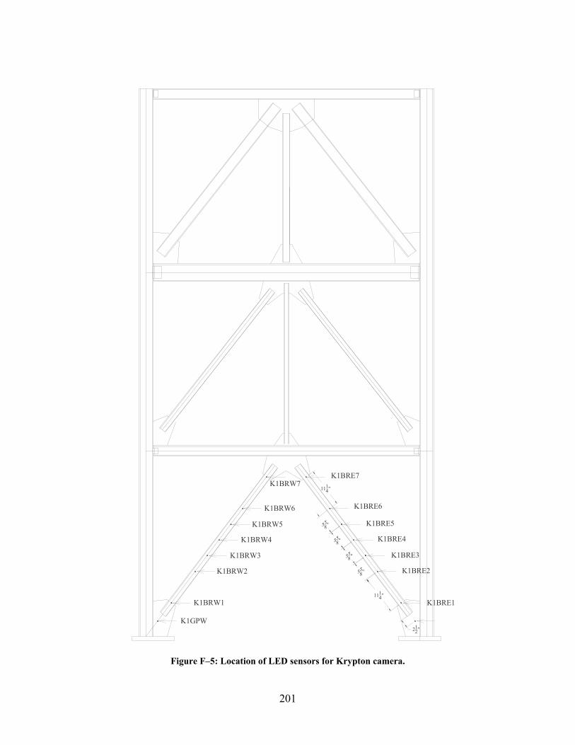
201
1114"
1114"
K1BRW1
K1BRW2
K1BRW3
K1BRW4
K1BRW5
K1BRW6
K1BRW7 K1BRE7
K1BRE6
K1BRE5
K1BRE4
K1BRE3
K1BRE2
K1BRE1
558"
558"
558"
558"
K1GPW212"
Figure F–5: Location of LED sensors for Krypton camera.
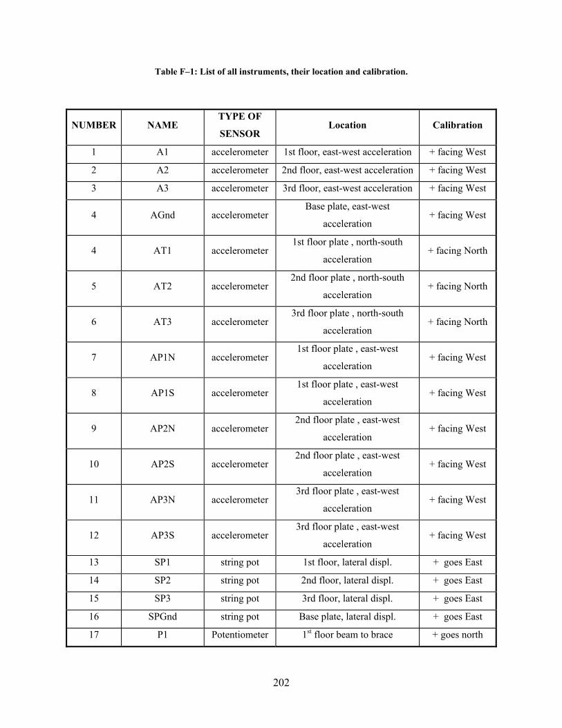
202
Table F–1: List of all instruments, their location and calibration.
NUMBER NAME TYPE OF
SENSOR Location Calibration
1 A1 accelerometer 1st floor, east-west acceleration + facing West
2 A2 accelerometer 2nd floor, east-west acceleration + facing West
3 A3 accelerometer 3rd floor, east-west acceleration + facing West
4 AGnd accelerometer Base plate, east-west
acceleration + facing West
4 AT1 accelerometer 1st floor plate , north-south
acceleration + facing North
5 AT2 accelerometer 2nd floor plate , north-south
acceleration + facing North
6 AT3 accelerometer 3rd floor plate , north-south
acceleration + facing North
7 AP1N accelerometer 1st floor plate , east-west
acceleration + facing West
8 AP1S accelerometer 1st floor plate , east-west
acceleration + facing West
9 AP2N accelerometer 2nd floor plate , east-west
acceleration + facing West
10 AP2S accelerometer 2nd floor plate , east-west
acceleration + facing West
11 AP3N accelerometer 3rd floor plate , east-west
acceleration + facing West
12 AP3S accelerometer 3rd floor plate , east-west
acceleration + facing West
13 SP1 string pot 1st floor, lateral displ. + goes East
14 SP2 string pot 2nd floor, lateral displ. + goes East
15 SP3 string pot 3rd floor, lateral displ. + goes East
16 SPGnd string pot Base plate, lateral displ. + goes East
17 P1 Potentiometer 1st floor beam to brace + goes north
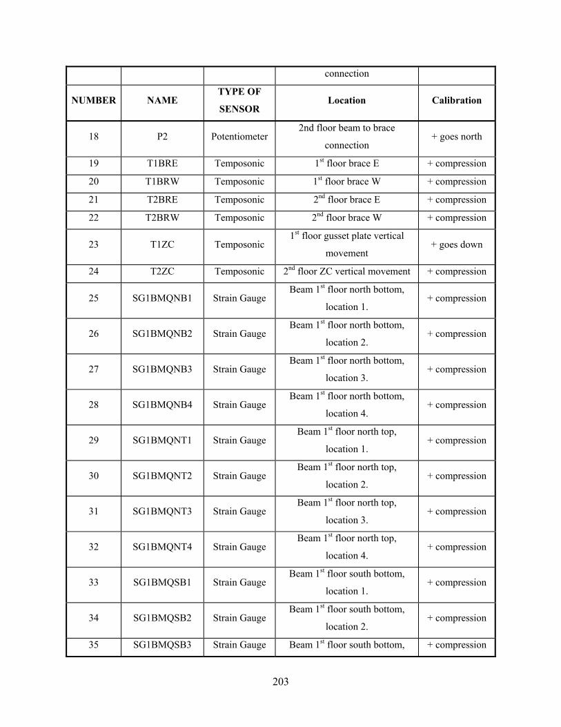
203
connection
NUMBER NAME TYPE OF
SENSOR Location Calibration
18 P2 Potentiometer 2nd floor beam to brace
connection + goes north
19 T1BRE Temposonic 1st floor brace E + compression
20 T1BRW Temposonic 1st floor brace W + compression
21 T2BRE Temposonic 2nd floor brace E + compression
22 T2BRW Temposonic 2nd floor brace W + compression
23 T1ZC Temposonic 1st floor gusset plate vertical
movement + goes down
24 T2ZC Temposonic 2nd floor ZC vertical movement + compression
25 SG1BMQNB1 Strain Gauge Beam 1st floor north bottom,
location 1. + compression
26 SG1BMQNB2 Strain Gauge Beam 1st floor north bottom,
location 2. + compression
27 SG1BMQNB3 Strain Gauge Beam 1st floor north bottom,
location 3. + compression
28 SG1BMQNB4 Strain Gauge Beam 1st floor north bottom,
location 4. + compression
29 SG1BMQNT1 Strain Gauge Beam 1st floor north top,
location 1. + compression
30 SG1BMQNT2 Strain Gauge Beam 1st floor north top,
location 2. + compression
31 SG1BMQNT3 Strain Gauge Beam 1st floor north top,
location 3. + compression
32 SG1BMQNT4 Strain Gauge Beam 1st floor north top,
location 4. + compression
33 SG1BMQSB1 Strain Gauge Beam 1st floor south bottom,
location 1. + compression
34 SG1BMQSB2 Strain Gauge Beam 1st floor south bottom,
location 2. + compression
35 SG1BMQSB3 Strain Gauge Beam 1st floor south bottom, + compression
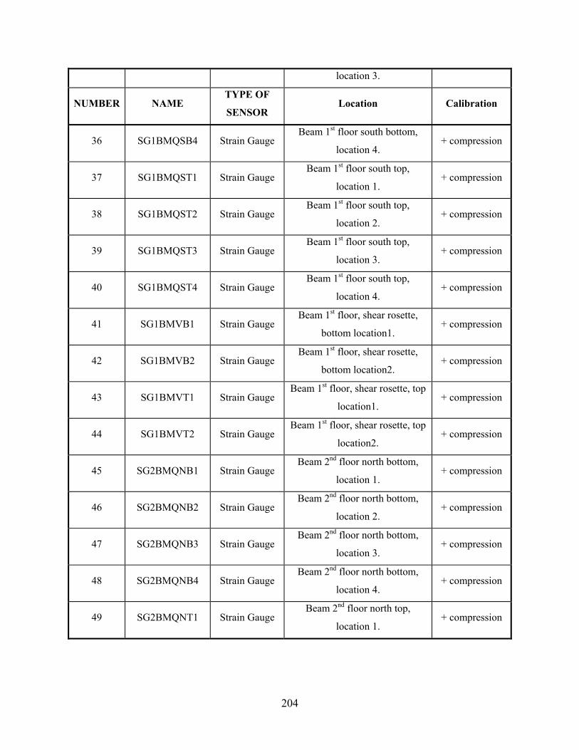
204
location 3.
NUMBER NAME TYPE OF
SENSOR Location Calibration
36 SG1BMQSB4 Strain Gauge Beam 1st floor south bottom,
location 4. + compression
37 SG1BMQST1 Strain Gauge Beam 1st floor south top,
location 1. + compression
38 SG1BMQST2 Strain Gauge Beam 1st floor south top,
location 2. + compression
39 SG1BMQST3 Strain Gauge Beam 1st floor south top,
location 3. + compression
40 SG1BMQST4 Strain Gauge Beam 1st floor south top,
location 4. + compression
41 SG1BMVB1 Strain Gauge Beam 1st floor, shear rosette,
bottom location1. + compression
42 SG1BMVB2 Strain Gauge Beam 1st floor, shear rosette,
bottom location2. + compression
43 SG1BMVT1 Strain Gauge Beam 1st floor, shear rosette, top
location1. + compression
44 SG1BMVT2 Strain Gauge Beam 1st floor, shear rosette, top
location2. + compression
45 SG2BMQNB1 Strain Gauge Beam 2nd floor north bottom,
location 1. + compression
46 SG2BMQNB2 Strain Gauge Beam 2nd floor north bottom,
location 2. + compression
47 SG2BMQNB3 Strain Gauge Beam 2nd floor north bottom,
location 3. + compression
48 SG2BMQNB4 Strain Gauge Beam 2nd floor north bottom,
location 4. + compression
49 SG2BMQNT1 Strain Gauge Beam 2nd floor north top,
location 1. + compression
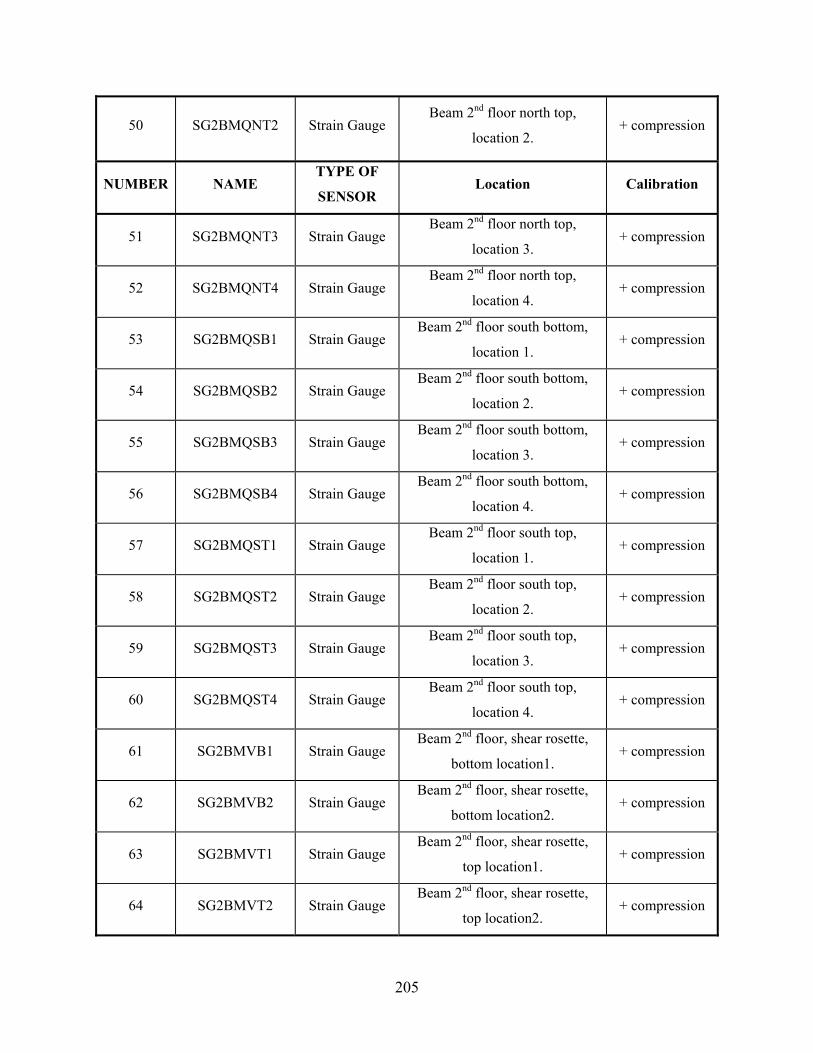
205
50 SG2BMQNT2 Strain Gauge Beam 2nd floor north top,
location 2. + compression
NUMBER NAME TYPE OF
SENSOR Location Calibration
51 SG2BMQNT3 Strain Gauge Beam 2nd floor north top,
location 3. + compression
52 SG2BMQNT4 Strain Gauge Beam 2nd floor north top,
location 4. + compression
53 SG2BMQSB1 Strain Gauge Beam 2nd floor south bottom,
location 1. + compression
54 SG2BMQSB2 Strain Gauge Beam 2nd floor south bottom,
location 2. + compression
55 SG2BMQSB3 Strain Gauge Beam 2nd floor south bottom,
location 3. + compression
56 SG2BMQSB4 Strain Gauge Beam 2nd floor south bottom,
location 4. + compression
57 SG2BMQST1 Strain Gauge Beam 2nd floor south top,
location 1. + compression
58 SG2BMQST2 Strain Gauge Beam 2nd floor south top,
location 2. + compression
59 SG2BMQST3 Strain Gauge Beam 2nd floor south top,
location 3. + compression
60 SG2BMQST4 Strain Gauge Beam 2nd floor south top,
location 4. + compression
61 SG2BMVB1 Strain Gauge Beam 2nd floor, shear rosette,
bottom location1. + compression
62 SG2BMVB2 Strain Gauge Beam 2nd floor, shear rosette,
bottom location2. + compression
63 SG2BMVT1 Strain Gauge Beam 2nd floor, shear rosette,
top location1. + compression
64 SG2BMVT2 Strain Gauge Beam 2nd floor, shear rosette,
top location2. + compression
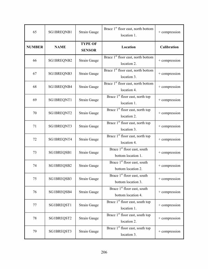
206
65 SG1BREQNB1 Strain Gauge Brace 1st floor east, north bottom
location 1. + compression
NUMBER NAME TYPE OF
SENSOR Location Calibration
66 SG1BREQNB2 Strain Gauge Brace 1st floor east, north bottom
location 2. + compression
67 SG1BREQNB3 Strain Gauge Brace 1st floor east, north bottom
location 3. + compression
68 SG1BREQNB4 Strain Gauge Brace 1st floor east, north bottom
location 4. + compression
69 SG1BREQNT1 Strain Gauge Brace 1st floor east, north top
location 1. + compression
70 SG1BREQNT2 Strain Gauge Brace 1st floor east, north top
location 2. + compression
71 SG1BREQNT3 Strain Gauge Brace 1st floor east, north top
location 3. + compression
72 SG1BREQNT4 Strain Gauge Brace 1st floor east, north top
location 4. + compression
73 SG1BREQSB1 Strain Gauge Brace 1st floor east, south
bottom location 1. + compression
74 SG1BREQSB2 Strain Gauge Brace 1st floor east, south
bottom location 2. + compression
75 SG1BREQSB3 Strain Gauge Brace 1st floor east, south
bottom location 3. + compression
76 SG1BREQSB4 Strain Gauge Brace 1st floor east, south
bottom location 4. + compression
77 SG1BREQST1 Strain Gauge Brace 1st floor east, south top
location 1. + compression
78 SG1BREQST2 Strain Gauge Brace 1st floor east, south top
location 2. + compression
79 SG1BREQST3 Strain Gauge Brace 1st floor east, south top
location 3. + compression

207
80 SG1BREQST4 Strain Gauge Brace 1st floor east, south top
location 4. + compression
NUMBER NAME TYPE OF
SENSOR Location Calibration
81 SG1BRWQNB1 Strain Gauge Brace 1st floor west, north
bottom location 1. + compression
82 SG1BRWQNB2 Strain Gauge Brace 1st floor west, north
bottom location 2. + compression
83 SG1BRWQNB3 Strain Gauge Brace 1st floor west, north
bottom location 3. + compression
84 SG1BRWQNB4 Strain Gauge Brace 1st floor west, north
bottom location 4. + compression
85 SG1BRWQNT1 Strain Gauge Brace 1st floor west, north top
location 1. + compression
86 SG1BRWQNT2 Strain Gauge Brace 1st floor west, north top
location 2. + compression
87 SG1BRWQNT3 Strain Gauge Brace 1st floor west, north top
location 3. + compression
88 SG1BRWQNT4 Strain Gauge Brace 1st floor west, north top
location 4. + compression
89 SG1BRWQSB1 Strain Gauge Brace 1st floor west, south
bottom location 1. + compression
90 SG1BRWQSB2 Strain Gauge Brace 1st floor west, south
bottom location 2. + compression
91 SG1BRWQSB3 Strain Gauge Brace 1st floor west, south
bottom location 3. + compression
92 SG1BRWQSB4 Strain Gauge Brace 1st floor west, south
bottom location 4. + compression
93 SG1BRWQST1 Strain Gauge Brace 1st floor west, south top
location 1. + compression
94 SG1BRWQST2 Strain Gauge Brace 1st floor west, south top
location 2. + compression
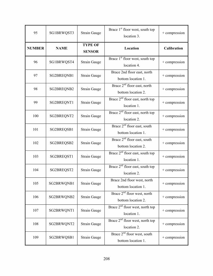
208
95 SG1BRWQST3 Strain Gauge Brace 1st floor west, south top
location 3. + compression
NUMBER NAME TYPE OF
SENSOR Location Calibration
96 SG1BRWQST4 Strain Gauge Brace 1st floor west, south top
location 4. + compression
97 SG2BREQNB1 Strain Gauge Brace 2nd floor east, north
bottom location 1. + compression
98 SG2BREQNB2 Strain Gauge Brace 2nd floor east, north
bottom location 2. + compression
99 SG2BREQNT1 Strain Gauge Brace 2nd floor east, north top
location 1. + compression
100 SG2BREQNT2 Strain Gauge Brace 2nd floor east, north top
location 2. + compression
101 SG2BREQSB1 Strain Gauge Brace 2nd floor east, south
bottom location 1. + compression
102 SG2BREQSB2 Strain Gauge Brace 2nd floor east, south
bottom location 2. + compression
103 SG2BREQST1 Strain Gauge Brace 2nd floor east, south top
location 1. + compression
104 SG2BREQST2 Strain Gauge Brace 2nd floor east, south top
location 2. + compression
105 SG2BRWQNB1 Strain Gauge Brace 2nd floor west, north
bottom location 1. + compression
106 SG2BRWQNB2 Strain Gauge Brace 2nd floor west, north
bottom location 2. + compression
107 SG2BRWQNT1 Strain Gauge Brace 2nd floor west, north top
location 1. + compression
108 SG2BRWQNT2 Strain Gauge Brace 2nd floor west, north top
location 2. + compression
109 SG2BRWQSB1 Strain Gauge Brace 2nd floor west, south
bottom location 1. + compression
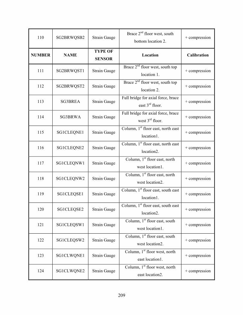
209
110 SG2BRWQSB2 Strain Gauge Brace 2nd floor west, south
bottom location 2. + compression
NUMBER NAME TYPE OF
SENSOR Location Calibration
111 SG2BRWQST1 Strain Gauge Brace 2nd floor west, south top
location 1. + compression
112 SG2BRWQST2 Strain Gauge Brace 2nd floor west, south top
location 2. + compression
113 SG3BREA Strain Gauge Full bridge for axial force, brace
east 3rd floor. + compression
114 SG3BRWA Strain Gauge Full bridge for axial force, brace
west 3rd floor. + compression
115 SG1CLEQNE1 Strain Gauge Column, 1st floor east, north east
location1. + compression
116 SG1CLEQNE2 Strain Gauge Column, 1st floor east, north east
location2. + compression
117 SG1CLEQNW1 Strain Gauge Column, 1st floor east, north
west location1. + compression
118 SG1CLEQNW2 Strain Gauge Column, 1st floor east, north
west location2. + compression
119 SG1CLEQSE1 Strain Gauge Column, 1st floor east, south east
location1. + compression
120 SG1CLEQSE2 Strain Gauge Column, 1st floor east, south east
location2. + compression
121 SG1CLEQSW1 Strain Gauge Column, 1st floor east, south
west location1. + compression
122 SG1CLEQSW2 Strain Gauge Column, 1st floor east, south
west location2. + compression
123 SG1CLWQNE1 Strain Gauge Column, 1st floor west, north
east location1. + compression
124 SG1CLWQNE2 Strain Gauge Column, 1st floor west, north
east location2. + compression
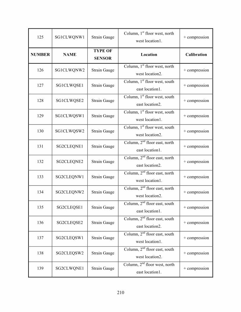
210
125 SG1CLWQNW1 Strain Gauge Column, 1st floor west, north
west location1. + compression
NUMBER NAME TYPE OF
SENSOR Location Calibration
126 SG1CLWQNW2 Strain Gauge Column, 1st floor west, north
west location2. + compression
127 SG1CLWQSE1 Strain Gauge Column, 1st floor west, south
east location1. + compression
128 SG1CLWQSE2 Strain Gauge Column, 1st floor west, south
east location2. + compression
129 SG1CLWQSW1 Strain Gauge Column, 1st floor west, south
west location1. + compression
130 SG1CLWQSW2 Strain Gauge Column, 1st floor west, south
west location2. + compression
131 SG2CLEQNE1 Strain Gauge Column, 2nd floor east, north
east location1. + compression
132 SG2CLEQNE2 Strain Gauge Column, 2nd floor east, north
east location2. + compression
133 SG2CLEQNW1 Strain Gauge Column, 2nd floor east, north
west location1. + compression
134 SG2CLEQNW2 Strain Gauge Column, 2nd floor east, north
west location2. + compression
135 SG2CLEQSE1 Strain Gauge Column, 2nd floor east, south
east location1. + compression
136 SG2CLEQSE2 Strain Gauge Column, 2nd floor east, south
east location2. + compression
137 SG2CLEQSW1 Strain Gauge Column, 2nd floor east, south
west location1. + compression
138 SG2CLEQSW2 Strain Gauge Column, 2nd floor east, south
west location2. + compression
139 SG2CLWQNE1 Strain Gauge Column, 2nd floor west, north
east location1. + compression
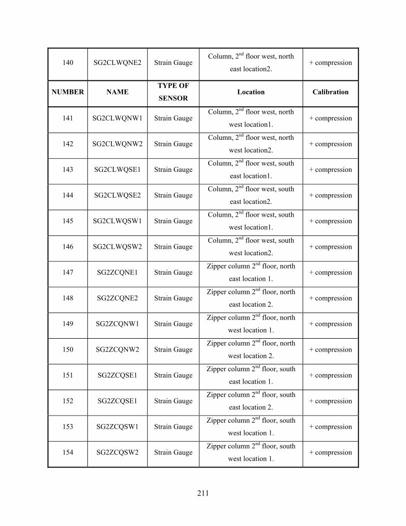
211
140 SG2CLWQNE2 Strain Gauge Column, 2nd floor west, north
east location2. + compression
NUMBER NAME TYPE OF
SENSOR Location Calibration
141 SG2CLWQNW1 Strain Gauge Column, 2nd floor west, north
west location1. + compression
142 SG2CLWQNW2 Strain Gauge Column, 2nd floor west, north
west location2. + compression
143 SG2CLWQSE1 Strain Gauge Column, 2nd floor west, south
east location1. + compression
144 SG2CLWQSE2 Strain Gauge Column, 2nd floor west, south
east location2. + compression
145 SG2CLWQSW1 Strain Gauge Column, 2nd floor west, south
west location1. + compression
146 SG2CLWQSW2 Strain Gauge Column, 2nd floor west, south
west location2. + compression
147 SG2ZCQNE1 Strain Gauge Zipper column 2nd floor, north
east location 1. + compression
148 SG2ZCQNE2 Strain Gauge Zipper column 2nd floor, north
east location 2. + compression
149 SG2ZCQNW1 Strain Gauge Zipper column 2nd floor, north
west location 1. + compression
150 SG2ZCQNW2 Strain Gauge Zipper column 2nd floor, north
west location 2. + compression
151 SG2ZCQSE1 Strain Gauge Zipper column 2nd floor, south
east location 1. + compression
152 SG2ZCQSE1 Strain Gauge Zipper column 2nd floor, south
east location 2. + compression
153 SG2ZCQSW1 Strain Gauge Zipper column 2nd floor, south
west location 1. + compression
154 SG2ZCQSW2 Strain Gauge Zipper column 2nd floor, south
west location 1. + compression
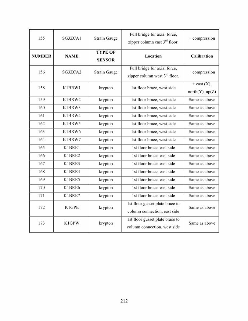
212
155 SG3ZCA1 Strain Gauge Full bridge for axial force,
zipper column east 3rd floor. + compression
NUMBER NAME TYPE OF
SENSOR Location Calibration
156 SG3ZCA2 Strain Gauge Full bridge for axial force,
zipper column west 3rd floor. + compression
158 K1BRW1 krypton 1st floor brace, west side + east (X),
north(Y), up(Z)
159 K1BRW2 krypton 1st floor brace, west side Same as above
160 K1BRW3 krypton 1st floor brace, west side Same as above
161 K1BRW4 krypton 1st floor brace, west side Same as above
162 K1BRW5 krypton 1st floor brace, west side Same as above
163 K1BRW6 krypton 1st floor brace, west side Same as above
164 K1BRW7 krypton 1st floor brace, west side Same as above
165 K1BRE1 krypton 1st floor brace, east side Same as above
166 K1BRE2 krypton 1st floor brace, east side Same as above
167 K1BRE3 krypton 1st floor brace, east side Same as above
168 K1BRE4 krypton 1st floor brace, east side Same as above
169 K1BRE5 krypton 1st floor brace, east side Same as above
170 K1BRE6 krypton 1st floor brace, east side Same as above
171 K1BRE7 krypton 1st floor brace, east side Same as above
172 K1GPE krypton 1st floor gusset plate brace to
column connection, east side Same as above
173 K1GPW krypton 1st floor gusset plate brace to
column connection, west side Same as above
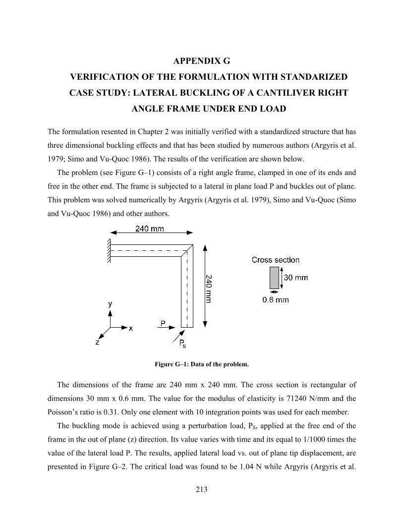
213
APPENDIX G
VERIFICATION OF THE FORMULATION WITH STANDARIZED
CASE STUDY: LATERAL BUCKLING OF A CANTILIVER RIGHT
ANGLE FRAME UNDER END LOAD
The formulation resented in Chapter 2 was initially verified with a standardized structure that has
three dimensional buckling effects and that has been studied by numerous authors (Argyris et al.
1979; Simo and Vu-Quoc 1986). The results of the verification are shown below.
The problem (see Figure G–1) consists of a right angle frame, clamped in one of its ends and
free in the other end. The frame is subjected to a lateral in plane load P and buckles out of plane.
This problem was solved numerically by Argyris (Argyris et al. 1979), Simo and Vu-Quoc (Simo
and Vu-Quoc 1986) and other authors.
240 mm
Figure G–1: Data of the problem.
The dimensions of the frame are 240 mm x 240 mm. The cross section is rectangular of
dimensions 30 mm x 0.6 mm. The value for the modulus of elasticity is 71240 N/mm and the
Poisson’s ratio is 0.31. Only one element with 10 integration points was used for each member.
The buckling mode is achieved using a perturbation load, PS, applied at the free end of the
frame in the out of plane (z) direction. Its value varies with time and its equal to 1/1000 times the
value of the lateral load P. The results, applied lateral load vs. out of plane tip displacement, are
presented in Figure G–2. The critical load was found to be 1.04 N while Argyris (Argyris et al.
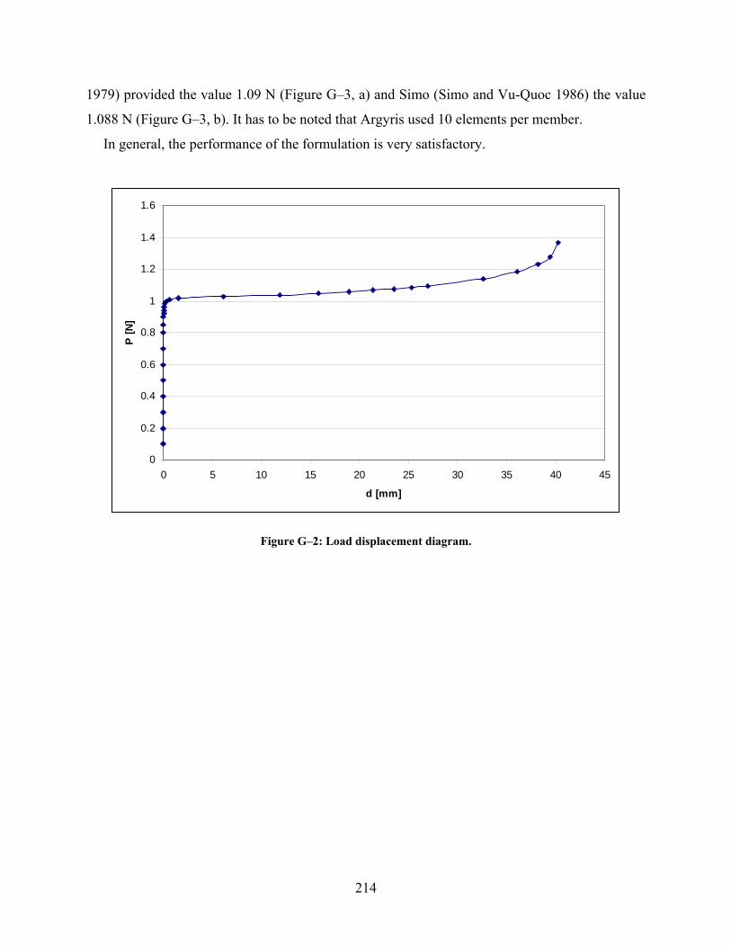
214
1979) provided the value 1.09 N (Figure G–3, a) and Simo (Simo and Vu-Quoc 1986) the value
1.088 N (Figure G–3, b). It has to be noted that Argyris used 10 elements per member.
In general, the performance of the formulation is very satisfactory.
0
0.2
0.4
0.6
0.8
1
1.2
1.4
1.6
0 5 10 15 20 25 30 35 40 45
d [mm]
P [N
]
Figure G–2: Load displacement diagram.
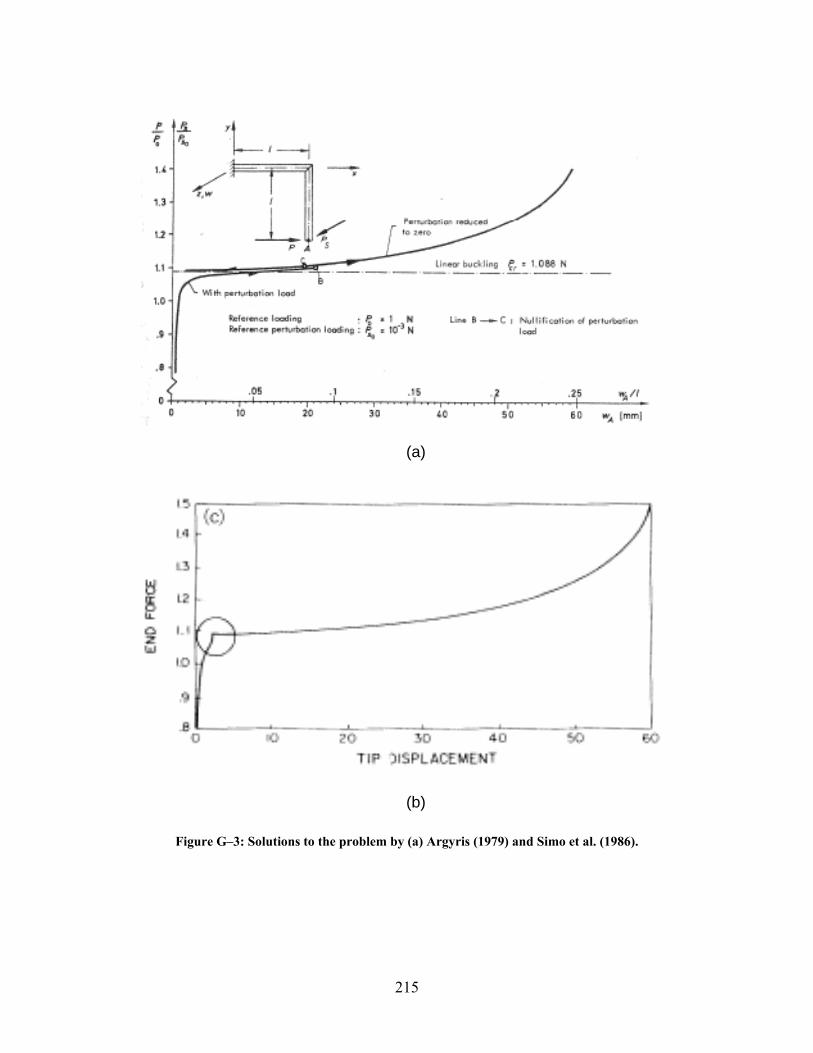
215
(a)
(b)
Figure G–3: Solutions to the problem by (a) Argyris (1979) and Simo et al. (1986).


217
MCEER Technical Reports
MCEER publishes technical reports on a variety of subjects written by authors funded through MCEER. These reports are available from both MCEER Publications and the National Technical Information Service (NTIS). Requests for reports should be directed to MCEER Publications, MCEER, University at Buffalo, State University of New York, Red Jacket Quadrangle, Buffalo, New York 14261. Reports can also be requested through NTIS, 5285 Port Royal Road, Springfield, Virginia 22161. NTIS accession numbers are shown in parenthesis, if available. NCEER-87-0001 "First-Year Program in Research, Education and Technology Transfer," 3/5/87, (PB88-134275, A04, MF-
A01). NCEER-87-0002 "Experimental Evaluation of Instantaneous Optimal Algorithms for Structural Control," by R.C. Lin, T.T.
Soong and A.M. Reinhorn, 4/20/87, (PB88-134341, A04, MF-A01). NCEER-87-0003 "Experimentation Using the Earthquake Simulation Facilities at University at Buffalo," by A.M. Reinhorn
and R.L. Ketter, to be published. NCEER-87-0004 "The System Characteristics and Performance of a Shaking Table," by J.S. Hwang, K.C. Chang and G.C.
Lee, 6/1/87, (PB88-134259, A03, MF-A01). This report is available only through NTIS (see address given above).
NCEER-87-0005 "A Finite Element Formulation for Nonlinear Viscoplastic Material Using a Q Model," by O. Gyebi and G.
Dasgupta, 11/2/87, (PB88-213764, A08, MF-A01). NCEER-87-0006 "Symbolic Manipulation Program (SMP) - Algebraic Codes for Two and Three Dimensional Finite Element
Formulations," by X. Lee and G. Dasgupta, 11/9/87, (PB88-218522, A05, MF-A01). NCEER-87-0007 "Instantaneous Optimal Control Laws for Tall Buildings Under Seismic Excitations," by J.N. Yang, A.
Akbarpour and P. Ghaemmaghami, 6/10/87, (PB88-134333, A06, MF-A01). This report is only available through NTIS (see address given above).
NCEER-87-0008 "IDARC: Inelastic Damage Analysis of Reinforced Concrete Frame - Shear-Wall Structures," by Y.J. Park,
A.M. Reinhorn and S.K. Kunnath, 7/20/87, (PB88-134325, A09, MF-A01). This report is only available through NTIS (see address given above).
NCEER-87-0009 "Liquefaction Potential for New York State: A Preliminary Report on Sites in Manhattan and Buffalo," by
M. Budhu, V. Vijayakumar, R.F. Giese and L. Baumgras, 8/31/87, (PB88-163704, A03, MF-A01). This report is available only through NTIS (see address given above).
NCEER-87-0010 "Vertical and Torsional Vibration of Foundations in Inhomogeneous Media," by A.S. Veletsos and K.W.
Dotson, 6/1/87, (PB88-134291, A03, MF-A01). This report is only available through NTIS (see address given above).
NCEER-87-0011 "Seismic Probabilistic Risk Assessment and Seismic Margins Studies for Nuclear Power Plants," by Howard
H.M. Hwang, 6/15/87, (PB88-134267, A03, MF-A01). This report is only available through NTIS (see address given above).
NCEER-87-0012 "Parametric Studies of Frequency Response of Secondary Systems Under Ground-Acceleration Excitations,"
by Y. Yong and Y.K. Lin, 6/10/87, (PB88-134309, A03, MF-A01). This report is only available through NTIS (see address given above).
NCEER-87-0013 "Frequency Response of Secondary Systems Under Seismic Excitation," by J.A. HoLung, J. Cai and Y.K.
Lin, 7/31/87, (PB88-134317, A05, MF-A01). This report is only available through NTIS (see address given above).
NCEER-87-0014 "Modelling Earthquake Ground Motions in Seismically Active Regions Using Parametric Time Series
Methods," by G.W. Ellis and A.S. Cakmak, 8/25/87, (PB88-134283, A08, MF-A01). This report is only available through NTIS (see address given above).
NCEER-87-0015 "Detection and Assessment of Seismic Structural Damage," by E. DiPasquale and A.S. Cakmak, 8/25/87,
(PB88-163712, A05, MF-A01). This report is only available through NTIS (see address given above).
218
NCEER-87-0016 "Pipeline Experiment at Parkfield, California," by J. Isenberg and E. Richardson, 9/15/87, (PB88-163720,
A03, MF-A01). This report is available only through NTIS (see address given above). NCEER-87-0017 "Digital Simulation of Seismic Ground Motion," by M. Shinozuka, G. Deodatis and T. Harada, 8/31/87,
(PB88-155197, A04, MF-A01). This report is available only through NTIS (see address given above). NCEER-87-0018 "Practical Considerations for Structural Control: System Uncertainty, System Time Delay and Truncation of
Small Control Forces," J.N. Yang and A. Akbarpour, 8/10/87, (PB88-163738, A08, MF-A01). This report is only available through NTIS (see address given above).
NCEER-87-0019 "Modal Analysis of Nonclassically Damped Structural Systems Using Canonical Transformation," by J.N.
Yang, S. Sarkani and F.X. Long, 9/27/87, (PB88-187851, A04, MF-A01). NCEER-87-0020 "A Nonstationary Solution in Random Vibration Theory," by J.R. Red-Horse and P.D. Spanos, 11/3/87,
(PB88-163746, A03, MF-A01). NCEER-87-0021 "Horizontal Impedances for Radially Inhomogeneous Viscoelastic Soil Layers," by A.S. Veletsos and K.W.
Dotson, 10/15/87, (PB88-150859, A04, MF-A01). NCEER-87-0022 "Seismic Damage Assessment of Reinforced Concrete Members," by Y.S. Chung, C. Meyer and M.
Shinozuka, 10/9/87, (PB88-150867, A05, MF-A01). This report is available only through NTIS (see address given above).
NCEER-87-0023 "Active Structural Control in Civil Engineering," by T.T. Soong, 11/11/87, (PB88-187778, A03, MF-A01). NCEER-87-0024 "Vertical and Torsional Impedances for Radially Inhomogeneous Viscoelastic Soil Layers," by K.W. Dotson
and A.S. Veletsos, 12/87, (PB88-187786, A03, MF-A01). NCEER-87-0025 "Proceedings from the Symposium on Seismic Hazards, Ground Motions, Soil-Liquefaction and Engineering
Practice in Eastern North America," October 20-22, 1987, edited by K.H. Jacob, 12/87, (PB88-188115, A23, MF-A01). This report is available only through NTIS (see address given above).
NCEER-87-0026 "Report on the Whittier-Narrows, California, Earthquake of October 1, 1987," by J. Pantelic and A.
Reinhorn, 11/87, (PB88-187752, A03, MF-A01). This report is available only through NTIS (see address given above).
NCEER-87-0027 "Design of a Modular Program for Transient Nonlinear Analysis of Large 3-D Building Structures," by S.
Srivastav and J.F. Abel, 12/30/87, (PB88-187950, A05, MF-A01). This report is only available through NTIS (see address given above).
NCEER-87-0028 "Second-Year Program in Research, Education and Technology Transfer," 3/8/88, (PB88-219480, A04, MF-
A01). NCEER-88-0001 "Workshop on Seismic Computer Analysis and Design of Buildings With Interactive Graphics," by W.
McGuire, J.F. Abel and C.H. Conley, 1/18/88, (PB88-187760, A03, MF-A01). This report is only available through NTIS (see address given above).
NCEER-88-0002 "Optimal Control of Nonlinear Flexible Structures," by J.N. Yang, F.X. Long and D. Wong, 1/22/88, (PB88-
213772, A06, MF-A01). NCEER-88-0003 "Substructuring Techniques in the Time Domain for Primary-Secondary Structural Systems," by G.D.
Manolis and G. Juhn, 2/10/88, (PB88-213780, A04, MF-A01). NCEER-88-0004 "Iterative Seismic Analysis of Primary-Secondary Systems," by A. Singhal, L.D. Lutes and P.D. Spanos,
2/23/88, (PB88-213798, A04, MF-A01). NCEER-88-0005 "Stochastic Finite Element Expansion for Random Media," by P.D. Spanos and R. Ghanem, 3/14/88, (PB88-
213806, A03, MF-A01).
219
NCEER-88-0006 "Combining Structural Optimization and Structural Control," by F.Y. Cheng and C.P. Pantelides, 1/10/88, (PB88-213814, A05, MF-A01).
NCEER-88-0007 "Seismic Performance Assessment of Code-Designed Structures," by H.H-M. Hwang, J-W. Jaw and H-J.
Shau, 3/20/88, (PB88-219423, A04, MF-A01). This report is only available through NTIS (see address given above).
NCEER-88-0008 "Reliability Analysis of Code-Designed Structures Under Natural Hazards," by H.H-M. Hwang, H. Ushiba
and M. Shinozuka, 2/29/88, (PB88-229471, A07, MF-A01). This report is only available through NTIS (see address given above).
NCEER-88-0009 "Seismic Fragility Analysis of Shear Wall Structures," by J-W Jaw and H.H-M. Hwang, 4/30/88, (PB89-
102867, A04, MF-A01). NCEER-88-0010 "Base Isolation of a Multi-Story Building Under a Harmonic Ground Motion - A Comparison of
Performances of Various Systems," by F-G Fan, G. Ahmadi and I.G. Tadjbakhsh, 5/18/88, (PB89-122238, A06, MF-A01). This report is only available through NTIS (see address given above).
NCEER-88-0011 "Seismic Floor Response Spectra for a Combined System by Green's Functions," by F.M. Lavelle, L.A.
Bergman and P.D. Spanos, 5/1/88, (PB89-102875, A03, MF-A01). NCEER-88-0012 "A New Solution Technique for Randomly Excited Hysteretic Structures," by G.Q. Cai and Y.K. Lin,
5/16/88, (PB89-102883, A03, MF-A01). NCEER-88-0013 "A Study of Radiation Damping and Soil-Structure Interaction Effects in the Centrifuge," by K. Weissman,
supervised by J.H. Prevost, 5/24/88, (PB89-144703, A06, MF-A01). NCEER-88-0014 "Parameter Identification and Implementation of a Kinematic Plasticity Model for Frictional Soils," by J.H.
Prevost and D.V. Griffiths, to be published. NCEER-88-0015 "Two- and Three- Dimensional Dynamic Finite Element Analyses of the Long Valley Dam," by D.V.
Griffiths and J.H. Prevost, 6/17/88, (PB89-144711, A04, MF-A01). NCEER-88-0016 "Damage Assessment of Reinforced Concrete Structures in Eastern United States," by A.M. Reinhorn, M.J.
Seidel, S.K. Kunnath and Y.J. Park, 6/15/88, (PB89-122220, A04, MF-A01). This report is only available through NTIS (see address given above).
NCEER-88-0017 "Dynamic Compliance of Vertically Loaded Strip Foundations in Multilayered Viscoelastic Soils," by S.
Ahmad and A.S.M. Israil, 6/17/88, (PB89-102891, A04, MF-A01). NCEER-88-0018 "An Experimental Study of Seismic Structural Response With Added Viscoelastic Dampers," by R.C. Lin, Z.
Liang, T.T. Soong and R.H. Zhang, 6/30/88, (PB89-122212, A05, MF-A01). This report is available only through NTIS (see address given above).
NCEER-88-0019 "Experimental Investigation of Primary - Secondary System Interaction," by G.D. Manolis, G. Juhn and
A.M. Reinhorn, 5/27/88, (PB89-122204, A04, MF-A01). NCEER-88-0020 "A Response Spectrum Approach For Analysis of Nonclassically Damped Structures," by J.N. Yang, S.
Sarkani and F.X. Long, 4/22/88, (PB89-102909, A04, MF-A01). NCEER-88-0021 "Seismic Interaction of Structures and Soils: Stochastic Approach," by A.S. Veletsos and A.M. Prasad,
7/21/88, (PB89-122196, A04, MF-A01). This report is only available through NTIS (see address given above).
NCEER-88-0022 "Identification of the Serviceability Limit State and Detection of Seismic Structural Damage," by E.
DiPasquale and A.S. Cakmak, 6/15/88, (PB89-122188, A05, MF-A01). This report is available only through NTIS (see address given above).
NCEER-88-0023 "Multi-Hazard Risk Analysis: Case of a Simple Offshore Structure," by B.K. Bhartia and E.H. Vanmarcke,
7/21/88, (PB89-145213, A05, MF-A01).
220
NCEER-88-0024 "Automated Seismic Design of Reinforced Concrete Buildings," by Y.S. Chung, C. Meyer and M. Shinozuka, 7/5/88, (PB89-122170, A06, MF-A01). This report is available only through NTIS (see address given above).
NCEER-88-0025 "Experimental Study of Active Control of MDOF Structures Under Seismic Excitations," by L.L. Chung,
R.C. Lin, T.T. Soong and A.M. Reinhorn, 7/10/88, (PB89-122600, A04, MF-A01). NCEER-88-0026 "Earthquake Simulation Tests of a Low-Rise Metal Structure," by J.S. Hwang, K.C. Chang, G.C. Lee and
R.L. Ketter, 8/1/88, (PB89-102917, A04, MF-A01). NCEER-88-0027 "Systems Study of Urban Response and Reconstruction Due to Catastrophic Earthquakes," by F. Kozin and
H.K. Zhou, 9/22/88, (PB90-162348, A04, MF-A01). NCEER-88-0028 "Seismic Fragility Analysis of Plane Frame Structures," by H.H-M. Hwang and Y.K. Low, 7/31/88, (PB89-
131445, A06, MF-A01). NCEER-88-0029 "Response Analysis of Stochastic Structures," by A. Kardara, C. Bucher and M. Shinozuka, 9/22/88, (PB89-
174429, A04, MF-A01). NCEER-88-0030 "Nonnormal Accelerations Due to Yielding in a Primary Structure," by D.C.K. Chen and L.D. Lutes,
9/19/88, (PB89-131437, A04, MF-A01). NCEER-88-0031 "Design Approaches for Soil-Structure Interaction," by A.S. Veletsos, A.M. Prasad and Y. Tang, 12/30/88,
(PB89-174437, A03, MF-A01). This report is available only through NTIS (see address given above). NCEER-88-0032 "A Re-evaluation of Design Spectra for Seismic Damage Control," by C.J. Turkstra and A.G. Tallin, 11/7/88,
(PB89-145221, A05, MF-A01). NCEER-88-0033 "The Behavior and Design of Noncontact Lap Splices Subjected to Repeated Inelastic Tensile Loading," by
V.E. Sagan, P. Gergely and R.N. White, 12/8/88, (PB89-163737, A08, MF-A01). NCEER-88-0034 "Seismic Response of Pile Foundations," by S.M. Mamoon, P.K. Banerjee and S. Ahmad, 11/1/88, (PB89-
145239, A04, MF-A01). NCEER-88-0035 "Modeling of R/C Building Structures With Flexible Floor Diaphragms (IDARC2)," by A.M. Reinhorn, S.K.
Kunnath and N. Panahshahi, 9/7/88, (PB89-207153, A07, MF-A01). NCEER-88-0036 "Solution of the Dam-Reservoir Interaction Problem Using a Combination of FEM, BEM with Particular
Integrals, Modal Analysis, and Substructuring," by C-S. Tsai, G.C. Lee and R.L. Ketter, 12/31/88, (PB89-207146, A04, MF-A01).
NCEER-88-0037 "Optimal Placement of Actuators for Structural Control," by F.Y. Cheng and C.P. Pantelides, 8/15/88,
(PB89-162846, A05, MF-A01). NCEER-88-0038 "Teflon Bearings in Aseismic Base Isolation: Experimental Studies and Mathematical Modeling," by A.
Mokha, M.C. Constantinou and A.M. Reinhorn, 12/5/88, (PB89-218457, A10, MF-A01). This report is available only through NTIS (see address given above).
NCEER-88-0039 "Seismic Behavior of Flat Slab High-Rise Buildings in the New York City Area," by P. Weidlinger and M.
Ettouney, 10/15/88, (PB90-145681, A04, MF-A01). NCEER-88-0040 "Evaluation of the Earthquake Resistance of Existing Buildings in New York City," by P. Weidlinger and M.
Ettouney, 10/15/88, to be published. NCEER-88-0041 "Small-Scale Modeling Techniques for Reinforced Concrete Structures Subjected to Seismic Loads," by W.
Kim, A. El-Attar and R.N. White, 11/22/88, (PB89-189625, A05, MF-A01). NCEER-88-0042 "Modeling Strong Ground Motion from Multiple Event Earthquakes," by G.W. Ellis and A.S. Cakmak,
10/15/88, (PB89-174445, A03, MF-A01).
221
NCEER-88-0043 "Nonstationary Models of Seismic Ground Acceleration," by M. Grigoriu, S.E. Ruiz and E. Rosenblueth, 7/15/88, (PB89-189617, A04, MF-A01).
NCEER-88-0044 "SARCF User's Guide: Seismic Analysis of Reinforced Concrete Frames," by Y.S. Chung, C. Meyer and M.
Shinozuka, 11/9/88, (PB89-174452, A08, MF-A01). NCEER-88-0045 "First Expert Panel Meeting on Disaster Research and Planning," edited by J. Pantelic and J. Stoyle, 9/15/88,
(PB89-174460, A05, MF-A01). NCEER-88-0046 "Preliminary Studies of the Effect of Degrading Infill Walls on the Nonlinear Seismic Response of Steel
Frames," by C.Z. Chrysostomou, P. Gergely and J.F. Abel, 12/19/88, (PB89-208383, A05, MF-A01). NCEER-88-0047 "Reinforced Concrete Frame Component Testing Facility - Design, Construction, Instrumentation and
Operation," by S.P. Pessiki, C. Conley, T. Bond, P. Gergely and R.N. White, 12/16/88, (PB89-174478, A04, MF-A01).
NCEER-89-0001 "Effects of Protective Cushion and Soil Compliancy on the Response of Equipment Within a Seismically
Excited Building," by J.A. HoLung, 2/16/89, (PB89-207179, A04, MF-A01). NCEER-89-0002 "Statistical Evaluation of Response Modification Factors for Reinforced Concrete Structures," by H.H-M.
Hwang and J-W. Jaw, 2/17/89, (PB89-207187, A05, MF-A01). NCEER-89-0003 "Hysteretic Columns Under Random Excitation," by G-Q. Cai and Y.K. Lin, 1/9/89, (PB89-196513, A03,
MF-A01). NCEER-89-0004 "Experimental Study of `Elephant Foot Bulge' Instability of Thin-Walled Metal Tanks," by Z-H. Jia and R.L.
Ketter, 2/22/89, (PB89-207195, A03, MF-A01). NCEER-89-0005 "Experiment on Performance of Buried Pipelines Across San Andreas Fault," by J. Isenberg, E. Richardson
and T.D. O'Rourke, 3/10/89, (PB89-218440, A04, MF-A01). This report is available only through NTIS (see address given above).
NCEER-89-0006 "A Knowledge-Based Approach to Structural Design of Earthquake-Resistant Buildings," by M. Subramani,
P. Gergely, C.H. Conley, J.F. Abel and A.H. Zaghw, 1/15/89, (PB89-218465, A06, MF-A01). NCEER-89-0007 "Liquefaction Hazards and Their Effects on Buried Pipelines," by T.D. O'Rourke and P.A. Lane, 2/1/89,
(PB89-218481, A09, MF-A01). NCEER-89-0008 "Fundamentals of System Identification in Structural Dynamics," by H. Imai, C-B. Yun, O. Maruyama and
M. Shinozuka, 1/26/89, (PB89-207211, A04, MF-A01). NCEER-89-0009 "Effects of the 1985 Michoacan Earthquake on Water Systems and Other Buried Lifelines in Mexico," by
A.G. Ayala and M.J. O'Rourke, 3/8/89, (PB89-207229, A06, MF-A01). NCEER-89-R010 "NCEER Bibliography of Earthquake Education Materials," by K.E.K. Ross, Second Revision, 9/1/89,
(PB90-125352, A05, MF-A01). This report is replaced by NCEER-92-0018. NCEER-89-0011 "Inelastic Three-Dimensional Response Analysis of Reinforced Concrete Building Structures (IDARC-3D),
Part I - Modeling," by S.K. Kunnath and A.M. Reinhorn, 4/17/89, (PB90-114612, A07, MF-A01). This report is available only through NTIS (see address given above).
NCEER-89-0012 "Recommended Modifications to ATC-14," by C.D. Poland and J.O. Malley, 4/12/89, (PB90-108648, A15,
MF-A01). NCEER-89-0013 "Repair and Strengthening of Beam-to-Column Connections Subjected to Earthquake Loading," by M.
Corazao and A.J. Durrani, 2/28/89, (PB90-109885, A06, MF-A01). NCEER-89-0014 "Program EXKAL2 for Identification of Structural Dynamic Systems," by O. Maruyama, C-B. Yun, M.
Hoshiya and M. Shinozuka, 5/19/89, (PB90-109877, A09, MF-A01).
222
NCEER-89-0015 "Response of Frames With Bolted Semi-Rigid Connections, Part I - Experimental Study and Analytical Predictions," by P.J. DiCorso, A.M. Reinhorn, J.R. Dickerson, J.B. Radziminski and W.L. Harper, 6/1/89, to be published.
NCEER-89-0016 "ARMA Monte Carlo Simulation in Probabilistic Structural Analysis," by P.D. Spanos and M.P. Mignolet,
7/10/89, (PB90-109893, A03, MF-A01). NCEER-89-P017 "Preliminary Proceedings from the Conference on Disaster Preparedness - The Place of Earthquake
Education in Our Schools," Edited by K.E.K. Ross, 6/23/89, (PB90-108606, A03, MF-A01). NCEER-89-0017 "Proceedings from the Conference on Disaster Preparedness - The Place of Earthquake Education in Our
Schools," Edited by K.E.K. Ross, 12/31/89, (PB90-207895, A012, MF-A02). This report is available only through NTIS (see address given above).
NCEER-89-0018 "Multidimensional Models of Hysteretic Material Behavior for Vibration Analysis of Shape Memory Energy
Absorbing Devices, by E.J. Graesser and F.A. Cozzarelli, 6/7/89, (PB90-164146, A04, MF-A01). NCEER-89-0019 "Nonlinear Dynamic Analysis of Three-Dimensional Base Isolated Structures (3D-BASIS)," by S.
Nagarajaiah, A.M. Reinhorn and M.C. Constantinou, 8/3/89, (PB90-161936, A06, MF-A01). This report has been replaced by NCEER-93-0011.
NCEER-89-0020 "Structural Control Considering Time-Rate of Control Forces and Control Rate Constraints," by F.Y. Cheng
and C.P. Pantelides, 8/3/89, (PB90-120445, A04, MF-A01). NCEER-89-0021 "Subsurface Conditions of Memphis and Shelby County," by K.W. Ng, T-S. Chang and H-H.M. Hwang,
7/26/89, (PB90-120437, A03, MF-A01). NCEER-89-0022 "Seismic Wave Propagation Effects on Straight Jointed Buried Pipelines," by K. Elhmadi and M.J. O'Rourke,
8/24/89, (PB90-162322, A10, MF-A02). NCEER-89-0023 "Workshop on Serviceability Analysis of Water Delivery Systems," edited by M. Grigoriu, 3/6/89, (PB90-
127424, A03, MF-A01). NCEER-89-0024 "Shaking Table Study of a 1/5 Scale Steel Frame Composed of Tapered Members," by K.C. Chang, J.S.
Hwang and G.C. Lee, 9/18/89, (PB90-160169, A04, MF-A01). NCEER-89-0025 "DYNA1D: A Computer Program for Nonlinear Seismic Site Response Analysis - Technical
Documentation," by Jean H. Prevost, 9/14/89, (PB90-161944, A07, MF-A01). This report is available only through NTIS (see address given above).
NCEER-89-0026 "1:4 Scale Model Studies of Active Tendon Systems and Active Mass Dampers for Aseismic Protection," by
A.M. Reinhorn, T.T. Soong, R.C. Lin, Y.P. Yang, Y. Fukao, H. Abe and M. Nakai, 9/15/89, (PB90-173246, A10, MF-A02). This report is available only through NTIS (see address given above).
NCEER-89-0027 "Scattering of Waves by Inclusions in a Nonhomogeneous Elastic Half Space Solved by Boundary Element
Methods," by P.K. Hadley, A. Askar and A.S. Cakmak, 6/15/89, (PB90-145699, A07, MF-A01). NCEER-89-0028 "Statistical Evaluation of Deflection Amplification Factors for Reinforced Concrete Structures," by H.H.M.
Hwang, J-W. Jaw and A.L. Ch'ng, 8/31/89, (PB90-164633, A05, MF-A01). NCEER-89-0029 "Bedrock Accelerations in Memphis Area Due to Large New Madrid Earthquakes," by H.H.M. Hwang,
C.H.S. Chen and G. Yu, 11/7/89, (PB90-162330, A04, MF-A01). NCEER-89-0030 "Seismic Behavior and Response Sensitivity of Secondary Structural Systems," by Y.Q. Chen and T.T.
Soong, 10/23/89, (PB90-164658, A08, MF-A01). NCEER-89-0031 "Random Vibration and Reliability Analysis of Primary-Secondary Structural Systems," by Y. Ibrahim, M.
Grigoriu and T.T. Soong, 11/10/89, (PB90-161951, A04, MF-A01).
223
NCEER-89-0032 "Proceedings from the Second U.S. - Japan Workshop on Liquefaction, Large Ground Deformation and Their Effects on Lifelines, September 26-29, 1989," Edited by T.D. O'Rourke and M. Hamada, 12/1/89, (PB90-209388, A22, MF-A03).
NCEER-89-0033 "Deterministic Model for Seismic Damage Evaluation of Reinforced Concrete Structures," by J.M. Bracci,
A.M. Reinhorn, J.B. Mander and S.K. Kunnath, 9/27/89, (PB91-108803, A06, MF-A01). NCEER-89-0034 "On the Relation Between Local and Global Damage Indices," by E. DiPasquale and A.S. Cakmak, 8/15/89,
(PB90-173865, A05, MF-A01). NCEER-89-0035 "Cyclic Undrained Behavior of Nonplastic and Low Plasticity Silts," by A.J. Walker and H.E. Stewart,
7/26/89, (PB90-183518, A10, MF-A01). NCEER-89-0036 "Liquefaction Potential of Surficial Deposits in the City of Buffalo, New York," by M. Budhu, R. Giese and
L. Baumgrass, 1/17/89, (PB90-208455, A04, MF-A01). NCEER-89-0037 "A Deterministic Assessment of Effects of Ground Motion Incoherence," by A.S. Veletsos and Y. Tang,
7/15/89, (PB90-164294, A03, MF-A01). NCEER-89-0038 "Workshop on Ground Motion Parameters for Seismic Hazard Mapping," July 17-18, 1989, edited by R.V.
Whitman, 12/1/89, (PB90-173923, A04, MF-A01). NCEER-89-0039 "Seismic Effects on Elevated Transit Lines of the New York City Transit Authority," by C.J. Costantino,
C.A. Miller and E. Heymsfield, 12/26/89, (PB90-207887, A06, MF-A01). NCEER-89-0040 "Centrifugal Modeling of Dynamic Soil-Structure Interaction," by K. Weissman, Supervised by J.H. Prevost,
5/10/89, (PB90-207879, A07, MF-A01). NCEER-89-0041 "Linearized Identification of Buildings With Cores for Seismic Vulnerability Assessment," by I-K. Ho and
A.E. Aktan, 11/1/89, (PB90-251943, A07, MF-A01). NCEER-90-0001 "Geotechnical and Lifeline Aspects of the October 17, 1989 Loma Prieta Earthquake in San Francisco," by
T.D. O'Rourke, H.E. Stewart, F.T. Blackburn and T.S. Dickerman, 1/90, (PB90-208596, A05, MF-A01). NCEER-90-0002 "Nonnormal Secondary Response Due to Yielding in a Primary Structure," by D.C.K. Chen and L.D. Lutes,
2/28/90, (PB90-251976, A07, MF-A01). NCEER-90-0003 "Earthquake Education Materials for Grades K-12," by K.E.K. Ross, 4/16/90, (PB91-251984, A05, MF-
A05). This report has been replaced by NCEER-92-0018. NCEER-90-0004 "Catalog of Strong Motion Stations in Eastern North America," by R.W. Busby, 4/3/90, (PB90-251984, A05,
MF-A01). NCEER-90-0005 "NCEER Strong-Motion Data Base: A User Manual for the GeoBase Release (Version 1.0 for the Sun3)," by
P. Friberg and K. Jacob, 3/31/90 (PB90-258062, A04, MF-A01). NCEER-90-0006 "Seismic Hazard Along a Crude Oil Pipeline in the Event of an 1811-1812 Type New Madrid Earthquake,"
by H.H.M. Hwang and C-H.S. Chen, 4/16/90, (PB90-258054, A04, MF-A01). NCEER-90-0007 "Site-Specific Response Spectra for Memphis Sheahan Pumping Station," by H.H.M. Hwang and C.S. Lee,
5/15/90, (PB91-108811, A05, MF-A01). NCEER-90-0008 "Pilot Study on Seismic Vulnerability of Crude Oil Transmission Systems," by T. Ariman, R. Dobry, M.
Grigoriu, F. Kozin, M. O'Rourke, T. O'Rourke and M. Shinozuka, 5/25/90, (PB91-108837, A06, MF-A01). NCEER-90-0009 "A Program to Generate Site Dependent Time Histories: EQGEN," by G.W. Ellis, M. Srinivasan and A.S.
Cakmak, 1/30/90, (PB91-108829, A04, MF-A01). NCEER-90-0010 "Active Isolation for Seismic Protection of Operating Rooms," by M.E. Talbott, Supervised by M.
Shinozuka, 6/8/9, (PB91-110205, A05, MF-A01).
224
NCEER-90-0011 "Program LINEARID for Identification of Linear Structural Dynamic Systems," by C-B. Yun and M. Shinozuka, 6/25/90, (PB91-110312, A08, MF-A01).
NCEER-90-0012 "Two-Dimensional Two-Phase Elasto-Plastic Seismic Response of Earth Dams," by A.N. Yiagos, Supervised
by J.H. Prevost, 6/20/90, (PB91-110197, A13, MF-A02). NCEER-90-0013 "Secondary Systems in Base-Isolated Structures: Experimental Investigation, Stochastic Response and
Stochastic Sensitivity," by G.D. Manolis, G. Juhn, M.C. Constantinou and A.M. Reinhorn, 7/1/90, (PB91-110320, A08, MF-A01).
NCEER-90-0014 "Seismic Behavior of Lightly-Reinforced Concrete Column and Beam-Column Joint Details," by S.P.
Pessiki, C.H. Conley, P. Gergely and R.N. White, 8/22/90, (PB91-108795, A11, MF-A02). NCEER-90-0015 "Two Hybrid Control Systems for Building Structures Under Strong Earthquakes," by J.N. Yang and A.
Danielians, 6/29/90, (PB91-125393, A04, MF-A01). NCEER-90-0016 "Instantaneous Optimal Control with Acceleration and Velocity Feedback," by J.N. Yang and Z. Li, 6/29/90,
(PB91-125401, A03, MF-A01). NCEER-90-0017 "Reconnaissance Report on the Northern Iran Earthquake of June 21, 1990," by M. Mehrain, 10/4/90, (PB91-
125377, A03, MF-A01). NCEER-90-0018 "Evaluation of Liquefaction Potential in Memphis and Shelby County," by T.S. Chang, P.S. Tang, C.S. Lee
and H. Hwang, 8/10/90, (PB91-125427, A09, MF-A01). NCEER-90-0019 "Experimental and Analytical Study of a Combined Sliding Disc Bearing and Helical Steel Spring Isolation
System," by M.C. Constantinou, A.S. Mokha and A.M. Reinhorn, 10/4/90, (PB91-125385, A06, MF-A01). This report is available only through NTIS (see address given above).
NCEER-90-0020 "Experimental Study and Analytical Prediction of Earthquake Response of a Sliding Isolation System with a
Spherical Surface," by A.S. Mokha, M.C. Constantinou and A.M. Reinhorn, 10/11/90, (PB91-125419, A05, MF-A01).
NCEER-90-0021 "Dynamic Interaction Factors for Floating Pile Groups," by G. Gazetas, K. Fan, A. Kaynia and E. Kausel,
9/10/90, (PB91-170381, A05, MF-A01). NCEER-90-0022 "Evaluation of Seismic Damage Indices for Reinforced Concrete Structures," by S. Rodriguez-Gomez and
A.S. Cakmak, 9/30/90, PB91-171322, A06, MF-A01). NCEER-90-0023 "Study of Site Response at a Selected Memphis Site," by H. Desai, S. Ahmad, E.S. Gazetas and M.R. Oh,
10/11/90, (PB91-196857, A03, MF-A01). NCEER-90-0024 "A User's Guide to Strongmo: Version 1.0 of NCEER's Strong-Motion Data Access Tool for PCs and
Terminals," by P.A. Friberg and C.A.T. Susch, 11/15/90, (PB91-171272, A03, MF-A01). NCEER-90-0025 "A Three-Dimensional Analytical Study of Spatial Variability of Seismic Ground Motions," by L-L. Hong
and A.H.-S. Ang, 10/30/90, (PB91-170399, A09, MF-A01). NCEER-90-0026 "MUMOID User's Guide - A Program for the Identification of Modal Parameters," by S. Rodriguez-Gomez
and E. DiPasquale, 9/30/90, (PB91-171298, A04, MF-A01). NCEER-90-0027 "SARCF-II User's Guide - Seismic Analysis of Reinforced Concrete Frames," by S. Rodriguez-Gomez, Y.S.
Chung and C. Meyer, 9/30/90, (PB91-171280, A05, MF-A01). NCEER-90-0028 "Viscous Dampers: Testing, Modeling and Application in Vibration and Seismic Isolation," by N. Makris
and M.C. Constantinou, 12/20/90 (PB91-190561, A06, MF-A01). NCEER-90-0029 "Soil Effects on Earthquake Ground Motions in the Memphis Area," by H. Hwang, C.S. Lee, K.W. Ng and
T.S. Chang, 8/2/90, (PB91-190751, A05, MF-A01).
225
NCEER-91-0001 "Proceedings from the Third Japan-U.S. Workshop on Earthquake Resistant Design of Lifeline Facilities and Countermeasures for Soil Liquefaction, December 17-19, 1990," edited by T.D. O'Rourke and M. Hamada, 2/1/91, (PB91-179259, A99, MF-A04).
NCEER-91-0002 "Physical Space Solutions of Non-Proportionally Damped Systems," by M. Tong, Z. Liang and G.C. Lee,
1/15/91, (PB91-179242, A04, MF-A01). NCEER-91-0003 "Seismic Response of Single Piles and Pile Groups," by K. Fan and G. Gazetas, 1/10/91, (PB92-174994,
A04, MF-A01). NCEER-91-0004 "Damping of Structures: Part 1 - Theory of Complex Damping," by Z. Liang and G. Lee, 10/10/91, (PB92-
197235, A12, MF-A03). NCEER-91-0005 "3D-BASIS - Nonlinear Dynamic Analysis of Three Dimensional Base Isolated Structures: Part II," by S.
Nagarajaiah, A.M. Reinhorn and M.C. Constantinou, 2/28/91, (PB91-190553, A07, MF-A01). This report has been replaced by NCEER-93-0011.
NCEER-91-0006 "A Multidimensional Hysteretic Model for Plasticity Deforming Metals in Energy Absorbing Devices," by
E.J. Graesser and F.A. Cozzarelli, 4/9/91, (PB92-108364, A04, MF-A01). NCEER-91-0007 "A Framework for Customizable Knowledge-Based Expert Systems with an Application to a KBES for
Evaluating the Seismic Resistance of Existing Buildings," by E.G. Ibarra-Anaya and S.J. Fenves, 4/9/91, (PB91-210930, A08, MF-A01).
NCEER-91-0008 "Nonlinear Analysis of Steel Frames with Semi-Rigid Connections Using the Capacity Spectrum Method,"
by G.G. Deierlein, S-H. Hsieh, Y-J. Shen and J.F. Abel, 7/2/91, (PB92-113828, A05, MF-A01). NCEER-91-0009 "Earthquake Education Materials for Grades K-12," by K.E.K. Ross, 4/30/91, (PB91-212142, A06, MF-
A01). This report has been replaced by NCEER-92-0018. NCEER-91-0010 "Phase Wave Velocities and Displacement Phase Differences in a Harmonically Oscillating Pile," by N.
Makris and G. Gazetas, 7/8/91, (PB92-108356, A04, MF-A01). NCEER-91-0011 "Dynamic Characteristics of a Full-Size Five-Story Steel Structure and a 2/5 Scale Model," by K.C. Chang,
G.C. Yao, G.C. Lee, D.S. Hao and Y.C. Yeh," 7/2/91, (PB93-116648, A06, MF-A02). NCEER-91-0012 "Seismic Response of a 2/5 Scale Steel Structure with Added Viscoelastic Dampers," by K.C. Chang, T.T.
Soong, S-T. Oh and M.L. Lai, 5/17/91, (PB92-110816, A05, MF-A01). NCEER-91-0013 "Earthquake Response of Retaining Walls; Full-Scale Testing and Computational Modeling," by S.
Alampalli and A-W.M. Elgamal, 6/20/91, to be published. NCEER-91-0014 "3D-BASIS-M: Nonlinear Dynamic Analysis of Multiple Building Base Isolated Structures," by P.C.
Tsopelas, S. Nagarajaiah, M.C. Constantinou and A.M. Reinhorn, 5/28/91, (PB92-113885, A09, MF-A02). NCEER-91-0015 "Evaluation of SEAOC Design Requirements for Sliding Isolated Structures," by D. Theodossiou and M.C.
Constantinou, 6/10/91, (PB92-114602, A11, MF-A03). NCEER-91-0016 "Closed-Loop Modal Testing of a 27-Story Reinforced Concrete Flat Plate-Core Building," by H.R.
Somaprasad, T. Toksoy, H. Yoshiyuki and A.E. Aktan, 7/15/91, (PB92-129980, A07, MF-A02). NCEER-91-0017 "Shake Table Test of a 1/6 Scale Two-Story Lightly Reinforced Concrete Building," by A.G. El-Attar, R.N.
White and P. Gergely, 2/28/91, (PB92-222447, A06, MF-A02). NCEER-91-0018 "Shake Table Test of a 1/8 Scale Three-Story Lightly Reinforced Concrete Building," by A.G. El-Attar, R.N.
White and P. Gergely, 2/28/91, (PB93-116630, A08, MF-A02). NCEER-91-0019 "Transfer Functions for Rigid Rectangular Foundations," by A.S. Veletsos, A.M. Prasad and W.H. Wu,
7/31/91, to be published.
226
NCEER-91-0020 "Hybrid Control of Seismic-Excited Nonlinear and Inelastic Structural Systems," by J.N. Yang, Z. Li and A. Danielians, 8/1/91, (PB92-143171, A06, MF-A02).
NCEER-91-0021 "The NCEER-91 Earthquake Catalog: Improved Intensity-Based Magnitudes and Recurrence Relations for
U.S. Earthquakes East of New Madrid," by L. Seeber and J.G. Armbruster, 8/28/91, (PB92-176742, A06, MF-A02).
NCEER-91-0022 "Proceedings from the Implementation of Earthquake Planning and Education in Schools: The Need for
Change - The Roles of the Changemakers," by K.E.K. Ross and F. Winslow, 7/23/91, (PB92-129998, A12, MF-A03).
NCEER-91-0023 "A Study of Reliability-Based Criteria for Seismic Design of Reinforced Concrete Frame Buildings," by
H.H.M. Hwang and H-M. Hsu, 8/10/91, (PB92-140235, A09, MF-A02). NCEER-91-0024 "Experimental Verification of a Number of Structural System Identification Algorithms," by R.G. Ghanem,
H. Gavin and M. Shinozuka, 9/18/91, (PB92-176577, A18, MF-A04). NCEER-91-0025 "Probabilistic Evaluation of Liquefaction Potential," by H.H.M. Hwang and C.S. Lee," 11/25/91, (PB92-
143429, A05, MF-A01). NCEER-91-0026 "Instantaneous Optimal Control for Linear, Nonlinear and Hysteretic Structures - Stable Controllers," by J.N.
Yang and Z. Li, 11/15/91, (PB92-163807, A04, MF-A01). NCEER-91-0027 "Experimental and Theoretical Study of a Sliding Isolation System for Bridges," by M.C. Constantinou, A.
Kartoum, A.M. Reinhorn and P. Bradford, 11/15/91, (PB92-176973, A10, MF-A03). NCEER-92-0001 "Case Studies of Liquefaction and Lifeline Performance During Past Earthquakes, Volume 1: Japanese Case
Studies," Edited by M. Hamada and T. O'Rourke, 2/17/92, (PB92-197243, A18, MF-A04). NCEER-92-0002 "Case Studies of Liquefaction and Lifeline Performance During Past Earthquakes, Volume 2: United States
Case Studies," Edited by T. O'Rourke and M. Hamada, 2/17/92, (PB92-197250, A20, MF-A04). NCEER-92-0003 "Issues in Earthquake Education," Edited by K. Ross, 2/3/92, (PB92-222389, A07, MF-A02). NCEER-92-0004 "Proceedings from the First U.S. - Japan Workshop on Earthquake Protective Systems for Bridges," Edited
by I.G. Buckle, 2/4/92, (PB94-142239, A99, MF-A06). NCEER-92-0005 "Seismic Ground Motion from a Haskell-Type Source in a Multiple-Layered Half-Space," A.P. Theoharis, G.
Deodatis and M. Shinozuka, 1/2/92, to be published. NCEER-92-0006 "Proceedings from the Site Effects Workshop," Edited by R. Whitman, 2/29/92, (PB92-197201, A04, MF-
A01). NCEER-92-0007 "Engineering Evaluation of Permanent Ground Deformations Due to Seismically-Induced Liquefaction," by
M.H. Baziar, R. Dobry and A-W.M. Elgamal, 3/24/92, (PB92-222421, A13, MF-A03). NCEER-92-0008 "A Procedure for the Seismic Evaluation of Buildings in the Central and Eastern United States," by C.D.
Poland and J.O. Malley, 4/2/92, (PB92-222439, A20, MF-A04). NCEER-92-0009 "Experimental and Analytical Study of a Hybrid Isolation System Using Friction Controllable Sliding
Bearings," by M.Q. Feng, S. Fujii and M. Shinozuka, 5/15/92, (PB93-150282, A06, MF-A02). NCEER-92-0010 "Seismic Resistance of Slab-Column Connections in Existing Non-Ductile Flat-Plate Buildings," by A.J.
Durrani and Y. Du, 5/18/92, (PB93-116812, A06, MF-A02). NCEER-92-0011 "The Hysteretic and Dynamic Behavior of Brick Masonry Walls Upgraded by Ferrocement Coatings Under
Cyclic Loading and Strong Simulated Ground Motion," by H. Lee and S.P. Prawel, 5/11/92, to be published. NCEER-92-0012 "Study of Wire Rope Systems for Seismic Protection of Equipment in Buildings," by G.F. Demetriades,
M.C. Constantinou and A.M. Reinhorn, 5/20/92, (PB93-116655, A08, MF-A02).
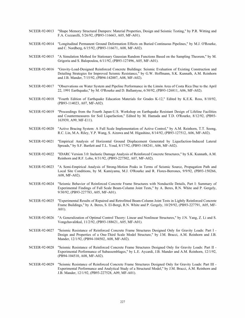
227
NCEER-92-0013 "Shape Memory Structural Dampers: Material Properties, Design and Seismic Testing," by P.R. Witting and F.A. Cozzarelli, 5/26/92, (PB93-116663, A05, MF-A01).
NCEER-92-0014 "Longitudinal Permanent Ground Deformation Effects on Buried Continuous Pipelines," by M.J. O'Rourke,
and C. Nordberg, 6/15/92, (PB93-116671, A08, MF-A02). NCEER-92-0015 "A Simulation Method for Stationary Gaussian Random Functions Based on the Sampling Theorem," by M.
Grigoriu and S. Balopoulou, 6/11/92, (PB93-127496, A05, MF-A01). NCEER-92-0016 "Gravity-Load-Designed Reinforced Concrete Buildings: Seismic Evaluation of Existing Construction and
Detailing Strategies for Improved Seismic Resistance," by G.W. Hoffmann, S.K. Kunnath, A.M. Reinhorn and J.B. Mander, 7/15/92, (PB94-142007, A08, MF-A02).
NCEER-92-0017 "Observations on Water System and Pipeline Performance in the Limón Area of Costa Rica Due to the April
22, 1991 Earthquake," by M. O'Rourke and D. Ballantyne, 6/30/92, (PB93-126811, A06, MF-A02). NCEER-92-0018 "Fourth Edition of Earthquake Education Materials for Grades K-12," Edited by K.E.K. Ross, 8/10/92,
(PB93-114023, A07, MF-A02). NCEER-92-0019 "Proceedings from the Fourth Japan-U.S. Workshop on Earthquake Resistant Design of Lifeline Facilities
and Countermeasures for Soil Liquefaction," Edited by M. Hamada and T.D. O'Rourke, 8/12/92, (PB93-163939, A99, MF-E11).
NCEER-92-0020 "Active Bracing System: A Full Scale Implementation of Active Control," by A.M. Reinhorn, T.T. Soong,
R.C. Lin, M.A. Riley, Y.P. Wang, S. Aizawa and M. Higashino, 8/14/92, (PB93-127512, A06, MF-A02). NCEER-92-0021 "Empirical Analysis of Horizontal Ground Displacement Generated by Liquefaction-Induced Lateral
Spreads," by S.F. Bartlett and T.L. Youd, 8/17/92, (PB93-188241, A06, MF-A02). NCEER-92-0022 "IDARC Version 3.0: Inelastic Damage Analysis of Reinforced Concrete Structures," by S.K. Kunnath, A.M.
Reinhorn and R.F. Lobo, 8/31/92, (PB93-227502, A07, MF-A02). NCEER-92-0023 "A Semi-Empirical Analysis of Strong-Motion Peaks in Terms of Seismic Source, Propagation Path and
Local Site Conditions, by M. Kamiyama, M.J. O'Rourke and R. Flores-Berrones, 9/9/92, (PB93-150266, A08, MF-A02).
NCEER-92-0024 "Seismic Behavior of Reinforced Concrete Frame Structures with Nonductile Details, Part I: Summary of
Experimental Findings of Full Scale Beam-Column Joint Tests," by A. Beres, R.N. White and P. Gergely, 9/30/92, (PB93-227783, A05, MF-A01).
NCEER-92-0025 "Experimental Results of Repaired and Retrofitted Beam-Column Joint Tests in Lightly Reinforced Concrete
Frame Buildings," by A. Beres, S. El-Borgi, R.N. White and P. Gergely, 10/29/92, (PB93-227791, A05, MF-A01).
NCEER-92-0026 "A Generalization of Optimal Control Theory: Linear and Nonlinear Structures," by J.N. Yang, Z. Li and S.
Vongchavalitkul, 11/2/92, (PB93-188621, A05, MF-A01). NCEER-92-0027 "Seismic Resistance of Reinforced Concrete Frame Structures Designed Only for Gravity Loads: Part I -
Design and Properties of a One-Third Scale Model Structure," by J.M. Bracci, A.M. Reinhorn and J.B. Mander, 12/1/92, (PB94-104502, A08, MF-A02).
NCEER-92-0028 "Seismic Resistance of Reinforced Concrete Frame Structures Designed Only for Gravity Loads: Part II -
Experimental Performance of Subassemblages," by L.E. Aycardi, J.B. Mander and A.M. Reinhorn, 12/1/92, (PB94-104510, A08, MF-A02).
NCEER-92-0029 "Seismic Resistance of Reinforced Concrete Frame Structures Designed Only for Gravity Loads: Part III -
Experimental Performance and Analytical Study of a Structural Model," by J.M. Bracci, A.M. Reinhorn and J.B. Mander, 12/1/92, (PB93-227528, A09, MF-A01).
228
NCEER-92-0030 "Evaluation of Seismic Retrofit of Reinforced Concrete Frame Structures: Part I - Experimental Performance of Retrofitted Subassemblages," by D. Choudhuri, J.B. Mander and A.M. Reinhorn, 12/8/92, (PB93-198307, A07, MF-A02).
NCEER-92-0031 "Evaluation of Seismic Retrofit of Reinforced Concrete Frame Structures: Part II - Experimental
Performance and Analytical Study of a Retrofitted Structural Model," by J.M. Bracci, A.M. Reinhorn and J.B. Mander, 12/8/92, (PB93-198315, A09, MF-A03).
NCEER-92-0032 "Experimental and Analytical Investigation of Seismic Response of Structures with Supplemental Fluid
Viscous Dampers," by M.C. Constantinou and M.D. Symans, 12/21/92, (PB93-191435, A10, MF-A03). This report is available only through NTIS (see address given above).
NCEER-92-0033 "Reconnaissance Report on the Cairo, Egypt Earthquake of October 12, 1992," by M. Khater, 12/23/92,
(PB93-188621, A03, MF-A01). NCEER-92-0034 "Low-Level Dynamic Characteristics of Four Tall Flat-Plate Buildings in New York City," by H. Gavin, S.
Yuan, J. Grossman, E. Pekelis and K. Jacob, 12/28/92, (PB93-188217, A07, MF-A02). NCEER-93-0001 "An Experimental Study on the Seismic Performance of Brick-Infilled Steel Frames With and Without
Retrofit," by J.B. Mander, B. Nair, K. Wojtkowski and J. Ma, 1/29/93, (PB93-227510, A07, MF-A02). NCEER-93-0002 "Social Accounting for Disaster Preparedness and Recovery Planning," by S. Cole, E. Pantoja and V. Razak,
2/22/93, (PB94-142114, A12, MF-A03). NCEER-93-0003 "Assessment of 1991 NEHRP Provisions for Nonstructural Components and Recommended Revisions," by
T.T. Soong, G. Chen, Z. Wu, R-H. Zhang and M. Grigoriu, 3/1/93, (PB93-188639, A06, MF-A02). NCEER-93-0004 "Evaluation of Static and Response Spectrum Analysis Procedures of SEAOC/UBC for Seismic Isolated
Structures," by C.W. Winters and M.C. Constantinou, 3/23/93, (PB93-198299, A10, MF-A03). NCEER-93-0005 "Earthquakes in the Northeast - Are We Ignoring the Hazard? A Workshop on Earthquake Science and
Safety for Educators," edited by K.E.K. Ross, 4/2/93, (PB94-103066, A09, MF-A02). NCEER-93-0006 "Inelastic Response of Reinforced Concrete Structures with Viscoelastic Braces," by R.F. Lobo, J.M. Bracci,
K.L. Shen, A.M. Reinhorn and T.T. Soong, 4/5/93, (PB93-227486, A05, MF-A02). NCEER-93-0007 "Seismic Testing of Installation Methods for Computers and Data Processing Equipment," by K. Kosar, T.T.
Soong, K.L. Shen, J.A. HoLung and Y.K. Lin, 4/12/93, (PB93-198299, A07, MF-A02). NCEER-93-0008 "Retrofit of Reinforced Concrete Frames Using Added Dampers," by A. Reinhorn, M. Constantinou and C.
Li, to be published. NCEER-93-0009 "Seismic Behavior and Design Guidelines for Steel Frame Structures with Added Viscoelastic Dampers," by
K.C. Chang, M.L. Lai, T.T. Soong, D.S. Hao and Y.C. Yeh, 5/1/93, (PB94-141959, A07, MF-A02). NCEER-93-0010 "Seismic Performance of Shear-Critical Reinforced Concrete Bridge Piers," by J.B. Mander, S.M. Waheed,
M.T.A. Chaudhary and S.S. Chen, 5/12/93, (PB93-227494, A08, MF-A02). NCEER-93-0011 "3D-BASIS-TABS: Computer Program for Nonlinear Dynamic Analysis of Three Dimensional Base Isolated
Structures," by S. Nagarajaiah, C. Li, A.M. Reinhorn and M.C. Constantinou, 8/2/93, (PB94-141819, A09, MF-A02).
NCEER-93-0012 "Effects of Hydrocarbon Spills from an Oil Pipeline Break on Ground Water," by O.J. Helweg and H.H.M.
Hwang, 8/3/93, (PB94-141942, A06, MF-A02). NCEER-93-0013 "Simplified Procedures for Seismic Design of Nonstructural Components and Assessment of Current Code
Provisions," by M.P. Singh, L.E. Suarez, E.E. Matheu and G.O. Maldonado, 8/4/93, (PB94-141827, A09, MF-A02).
NCEER-93-0014 "An Energy Approach to Seismic Analysis and Design of Secondary Systems," by G. Chen and T.T. Soong,
8/6/93, (PB94-142767, A11, MF-A03).
229
NCEER-93-0015 "Proceedings from School Sites: Becoming Prepared for Earthquakes - Commemorating the Third
Anniversary of the Loma Prieta Earthquake," Edited by F.E. Winslow and K.E.K. Ross, 8/16/93, (PB94-154275, A16, MF-A02).
NCEER-93-0016 "Reconnaissance Report of Damage to Historic Monuments in Cairo, Egypt Following the October 12, 1992
Dahshur Earthquake," by D. Sykora, D. Look, G. Croci, E. Karaesmen and E. Karaesmen, 8/19/93, (PB94-142221, A08, MF-A02).
NCEER-93-0017 "The Island of Guam Earthquake of August 8, 1993," by S.W. Swan and S.K. Harris, 9/30/93, (PB94-
141843, A04, MF-A01). NCEER-93-0018 "Engineering Aspects of the October 12, 1992 Egyptian Earthquake," by A.W. Elgamal, M. Amer, K.
Adalier and A. Abul-Fadl, 10/7/93, (PB94-141983, A05, MF-A01). NCEER-93-0019 "Development of an Earthquake Motion Simulator and its Application in Dynamic Centrifuge Testing," by I.
Krstelj, Supervised by J.H. Prevost, 10/23/93, (PB94-181773, A-10, MF-A03). NCEER-93-0020 "NCEER-Taisei Corporation Research Program on Sliding Seismic Isolation Systems for Bridges:
Experimental and Analytical Study of a Friction Pendulum System (FPS)," by M.C. Constantinou, P. Tsopelas, Y-S. Kim and S. Okamoto, 11/1/93, (PB94-142775, A08, MF-A02).
NCEER-93-0021 "Finite Element Modeling of Elastomeric Seismic Isolation Bearings," by L.J. Billings, Supervised by R.
Shepherd, 11/8/93, to be published. NCEER-93-0022 "Seismic Vulnerability of Equipment in Critical Facilities: Life-Safety and Operational Consequences," by
K. Porter, G.S. Johnson, M.M. Zadeh, C. Scawthorn and S. Eder, 11/24/93, (PB94-181765, A16, MF-A03). NCEER-93-0023 "Hokkaido Nansei-oki, Japan Earthquake of July 12, 1993, by P.I. Yanev and C.R. Scawthorn, 12/23/93,
(PB94-181500, A07, MF-A01). NCEER-94-0001 "An Evaluation of Seismic Serviceability of Water Supply Networks with Application to the San Francisco
Auxiliary Water Supply System," by I. Markov, Supervised by M. Grigoriu and T. O'Rourke, 1/21/94, (PB94-204013, A07, MF-A02).
NCEER-94-0002 "NCEER-Taisei Corporation Research Program on Sliding Seismic Isolation Systems for Bridges:
Experimental and Analytical Study of Systems Consisting of Sliding Bearings, Rubber Restoring Force Devices and Fluid Dampers," Volumes I and II, by P. Tsopelas, S. Okamoto, M.C. Constantinou, D. Ozaki and S. Fujii, 2/4/94, (PB94-181740, A09, MF-A02 and PB94-181757, A12, MF-A03).
NCEER-94-0003 "A Markov Model for Local and Global Damage Indices in Seismic Analysis," by S. Rahman and M.
Grigoriu, 2/18/94, (PB94-206000, A12, MF-A03). NCEER-94-0004 "Proceedings from the NCEER Workshop on Seismic Response of Masonry Infills," edited by D.P. Abrams,
3/1/94, (PB94-180783, A07, MF-A02). NCEER-94-0005 "The Northridge, California Earthquake of January 17, 1994: General Reconnaissance Report," edited by
J.D. Goltz, 3/11/94, (PB94-193943, A10, MF-A03). NCEER-94-0006 "Seismic Energy Based Fatigue Damage Analysis of Bridge Columns: Part I - Evaluation of Seismic
Capacity," by G.A. Chang and J.B. Mander, 3/14/94, (PB94-219185, A11, MF-A03). NCEER-94-0007 "Seismic Isolation of Multi-Story Frame Structures Using Spherical Sliding Isolation Systems," by T.M. Al-
Hussaini, V.A. Zayas and M.C. Constantinou, 3/17/94, (PB94-193745, A09, MF-A02). NCEER-94-0008 "The Northridge, California Earthquake of January 17, 1994: Performance of Highway Bridges," edited by
I.G. Buckle, 3/24/94, (PB94-193851, A06, MF-A02). NCEER-94-0009 "Proceedings of the Third U.S.-Japan Workshop on Earthquake Protective Systems for Bridges," edited by
I.G. Buckle and I. Friedland, 3/31/94, (PB94-195815, A99, MF-A06).

230
NCEER-94-0010 "3D-BASIS-ME: Computer Program for Nonlinear Dynamic Analysis of Seismically Isolated Single and Multiple Structures and Liquid Storage Tanks," by P.C. Tsopelas, M.C. Constantinou and A.M. Reinhorn, 4/12/94, (PB94-204922, A09, MF-A02).
NCEER-94-0011 "The Northridge, California Earthquake of January 17, 1994: Performance of Gas Transmission Pipelines,"
by T.D. O'Rourke and M.C. Palmer, 5/16/94, (PB94-204989, A05, MF-A01). NCEER-94-0012 "Feasibility Study of Replacement Procedures and Earthquake Performance Related to Gas Transmission
Pipelines," by T.D. O'Rourke and M.C. Palmer, 5/25/94, (PB94-206638, A09, MF-A02). NCEER-94-0013 "Seismic Energy Based Fatigue Damage Analysis of Bridge Columns: Part II - Evaluation of Seismic
Demand," by G.A. Chang and J.B. Mander, 6/1/94, (PB95-18106, A08, MF-A02). NCEER-94-0014 "NCEER-Taisei Corporation Research Program on Sliding Seismic Isolation Systems for Bridges:
Experimental and Analytical Study of a System Consisting of Sliding Bearings and Fluid Restoring Force/Damping Devices," by P. Tsopelas and M.C. Constantinou, 6/13/94, (PB94-219144, A10, MF-A03).
NCEER-94-0015 "Generation of Hazard-Consistent Fragility Curves for Seismic Loss Estimation Studies," by H. Hwang and
J-R. Huo, 6/14/94, (PB95-181996, A09, MF-A02). NCEER-94-0016 "Seismic Study of Building Frames with Added Energy-Absorbing Devices," by W.S. Pong, C.S. Tsai and
G.C. Lee, 6/20/94, (PB94-219136, A10, A03). NCEER-94-0017 "Sliding Mode Control for Seismic-Excited Linear and Nonlinear Civil Engineering Structures," by J. Yang,
J. Wu, A. Agrawal and Z. Li, 6/21/94, (PB95-138483, A06, MF-A02). NCEER-94-0018 "3D-BASIS-TABS Version 2.0: Computer Program for Nonlinear Dynamic Analysis of Three Dimensional
Base Isolated Structures," by A.M. Reinhorn, S. Nagarajaiah, M.C. Constantinou, P. Tsopelas and R. Li, 6/22/94, (PB95-182176, A08, MF-A02).
NCEER-94-0019 "Proceedings of the International Workshop on Civil Infrastructure Systems: Application of Intelligent
Systems and Advanced Materials on Bridge Systems," Edited by G.C. Lee and K.C. Chang, 7/18/94, (PB95-252474, A20, MF-A04).
NCEER-94-0020 "Study of Seismic Isolation Systems for Computer Floors," by V. Lambrou and M.C. Constantinou, 7/19/94,
(PB95-138533, A10, MF-A03). NCEER-94-0021 "Proceedings of the U.S.-Italian Workshop on Guidelines for Seismic Evaluation and Rehabilitation of
Unreinforced Masonry Buildings," Edited by D.P. Abrams and G.M. Calvi, 7/20/94, (PB95-138749, A13, MF-A03).
NCEER-94-0022 "NCEER-Taisei Corporation Research Program on Sliding Seismic Isolation Systems for Bridges:
Experimental and Analytical Study of a System Consisting of Lubricated PTFE Sliding Bearings and Mild Steel Dampers," by P. Tsopelas and M.C. Constantinou, 7/22/94, (PB95-182184, A08, MF-A02).
NCEER-94-0023 “Development of Reliability-Based Design Criteria for Buildings Under Seismic Load,” by Y.K. Wen, H.
Hwang and M. Shinozuka, 8/1/94, (PB95-211934, A08, MF-A02). NCEER-94-0024 “Experimental Verification of Acceleration Feedback Control Strategies for an Active Tendon System,” by
S.J. Dyke, B.F. Spencer, Jr., P. Quast, M.K. Sain, D.C. Kaspari, Jr. and T.T. Soong, 8/29/94, (PB95-212320, A05, MF-A01).
NCEER-94-0025 “Seismic Retrofitting Manual for Highway Bridges,” Edited by I.G. Buckle and I.F. Friedland, published by
the Federal Highway Administration (PB95-212676, A15, MF-A03). NCEER-94-0026 “Proceedings from the Fifth U.S.-Japan Workshop on Earthquake Resistant Design of Lifeline Facilities and
Countermeasures Against Soil Liquefaction,” Edited by T.D. O’Rourke and M. Hamada, 11/7/94, (PB95-220802, A99, MF-E08).
231
NCEER-95-0001 “Experimental and Analytical Investigation of Seismic Retrofit of Structures with Supplemental Damping: Part 1 - Fluid Viscous Damping Devices,” by A.M. Reinhorn, C. Li and M.C. Constantinou, 1/3/95, (PB95-266599, A09, MF-A02).
NCEER-95-0002 “Experimental and Analytical Study of Low-Cycle Fatigue Behavior of Semi-Rigid Top-And-Seat Angle
Connections,” by G. Pekcan, J.B. Mander and S.S. Chen, 1/5/95, (PB95-220042, A07, MF-A02). NCEER-95-0003 “NCEER-ATC Joint Study on Fragility of Buildings,” by T. Anagnos, C. Rojahn and A.S. Kiremidjian,
1/20/95, (PB95-220026, A06, MF-A02). NCEER-95-0004 “Nonlinear Control Algorithms for Peak Response Reduction,” by Z. Wu, T.T. Soong, V. Gattulli and R.C.
Lin, 2/16/95, (PB95-220349, A05, MF-A01). NCEER-95-0005 “Pipeline Replacement Feasibility Study: A Methodology for Minimizing Seismic and Corrosion Risks to
Underground Natural Gas Pipelines,” by R.T. Eguchi, H.A. Seligson and D.G. Honegger, 3/2/95, (PB95-252326, A06, MF-A02).
NCEER-95-0006 “Evaluation of Seismic Performance of an 11-Story Frame Building During the 1994 Northridge
Earthquake,” by F. Naeim, R. DiSulio, K. Benuska, A. Reinhorn and C. Li, to be published. NCEER-95-0007 “Prioritization of Bridges for Seismic Retrofitting,” by N. Basöz and A.S. Kiremidjian, 4/24/95, (PB95-
252300, A08, MF-A02). NCEER-95-0008 “Method for Developing Motion Damage Relationships for Reinforced Concrete Frames,” by A. Singhal and
A.S. Kiremidjian, 5/11/95, (PB95-266607, A06, MF-A02). NCEER-95-0009 “Experimental and Analytical Investigation of Seismic Retrofit of Structures with Supplemental Damping:
Part II - Friction Devices,” by C. Li and A.M. Reinhorn, 7/6/95, (PB96-128087, A11, MF-A03). NCEER-95-0010 “Experimental Performance and Analytical Study of a Non-Ductile Reinforced Concrete Frame Structure
Retrofitted with Elastomeric Spring Dampers,” by G. Pekcan, J.B. Mander and S.S. Chen, 7/14/95, (PB96-137161, A08, MF-A02).
NCEER-95-0011 “Development and Experimental Study of Semi-Active Fluid Damping Devices for Seismic Protection of
Structures,” by M.D. Symans and M.C. Constantinou, 8/3/95, (PB96-136940, A23, MF-A04). NCEER-95-0012 “Real-Time Structural Parameter Modification (RSPM): Development of Innervated Structures,” by Z.
Liang, M. Tong and G.C. Lee, 4/11/95, (PB96-137153, A06, MF-A01). NCEER-95-0013 “Experimental and Analytical Investigation of Seismic Retrofit of Structures with Supplemental Damping:
Part III - Viscous Damping Walls,” by A.M. Reinhorn and C. Li, 10/1/95, (PB96-176409, A11, MF-A03). NCEER-95-0014 “Seismic Fragility Analysis of Equipment and Structures in a Memphis Electric Substation,” by J-R. Huo and
H.H.M. Hwang, 8/10/95, (PB96-128087, A09, MF-A02). NCEER-95-0015 “The Hanshin-Awaji Earthquake of January 17, 1995: Performance of Lifelines,” Edited by M. Shinozuka,
11/3/95, (PB96-176383, A15, MF-A03). NCEER-95-0016 “Highway Culvert Performance During Earthquakes,” by T.L. Youd and C.J. Beckman, available as
NCEER-96-0015. NCEER-95-0017 “The Hanshin-Awaji Earthquake of January 17, 1995: Performance of Highway Bridges,” Edited by I.G.
Buckle, 12/1/95, to be published. NCEER-95-0018 “Modeling of Masonry Infill Panels for Structural Analysis,” by A.M. Reinhorn, A. Madan, R.E. Valles, Y.
Reichmann and J.B. Mander, 12/8/95, (PB97-110886, MF-A01, A06). NCEER-95-0019 “Optimal Polynomial Control for Linear and Nonlinear Structures,” by A.K. Agrawal and J.N. Yang,
12/11/95, (PB96-168737, A07, MF-A02).
232
NCEER-95-0020 “Retrofit of Non-Ductile Reinforced Concrete Frames Using Friction Dampers,” by R.S. Rao, P. Gergely and R.N. White, 12/22/95, (PB97-133508, A10, MF-A02).
NCEER-95-0021 “Parametric Results for Seismic Response of Pile-Supported Bridge Bents,” by G. Mylonakis, A. Nikolaou
and G. Gazetas, 12/22/95, (PB97-100242, A12, MF-A03). NCEER-95-0022 “Kinematic Bending Moments in Seismically Stressed Piles,” by A. Nikolaou, G. Mylonakis and G. Gazetas,
12/23/95, (PB97-113914, MF-A03, A13). NCEER-96-0001 “Dynamic Response of Unreinforced Masonry Buildings with Flexible Diaphragms,” by A.C. Costley and
D.P. Abrams,” 10/10/96, (PB97-133573, MF-A03, A15). NCEER-96-0002 “State of the Art Review: Foundations and Retaining Structures,” by I. Po Lam, to be published. NCEER-96-0003 “Ductility of Rectangular Reinforced Concrete Bridge Columns with Moderate Confinement,” by N. Wehbe,
M. Saiidi, D. Sanders and B. Douglas, 11/7/96, (PB97-133557, A06, MF-A02). NCEER-96-0004 “Proceedings of the Long-Span Bridge Seismic Research Workshop,” edited by I.G. Buckle and I.M.
Friedland, to be published. NCEER-96-0005 “Establish Representative Pier Types for Comprehensive Study: Eastern United States,” by J. Kulicki and Z.
Prucz, 5/28/96, (PB98-119217, A07, MF-A02). NCEER-96-0006 “Establish Representative Pier Types for Comprehensive Study: Western United States,” by R. Imbsen, R.A.
Schamber and T.A. Osterkamp, 5/28/96, (PB98-118607, A07, MF-A02). NCEER-96-0007 “Nonlinear Control Techniques for Dynamical Systems with Uncertain Parameters,” by R.G. Ghanem and
M.I. Bujakov, 5/27/96, (PB97-100259, A17, MF-A03). NCEER-96-0008 “Seismic Evaluation of a 30-Year Old Non-Ductile Highway Bridge Pier and Its Retrofit,” by J.B. Mander,
B. Mahmoodzadegan, S. Bhadra and S.S. Chen, 5/31/96, (PB97-110902, MF-A03, A10). NCEER-96-0009 “Seismic Performance of a Model Reinforced Concrete Bridge Pier Before and After Retrofit,” by J.B.
Mander, J.H. Kim and C.A. Ligozio, 5/31/96, (PB97-110910, MF-A02, A10). NCEER-96-0010 “IDARC2D Version 4.0: A Computer Program for the Inelastic Damage Analysis of Buildings,” by R.E.
Valles, A.M. Reinhorn, S.K. Kunnath, C. Li and A. Madan, 6/3/96, (PB97-100234, A17, MF-A03). NCEER-96-0011 “Estimation of the Economic Impact of Multiple Lifeline Disruption: Memphis Light, Gas and Water
Division Case Study,” by S.E. Chang, H.A. Seligson and R.T. Eguchi, 8/16/96, (PB97-133490, A11, MF-A03).
NCEER-96-0012 “Proceedings from the Sixth Japan-U.S. Workshop on Earthquake Resistant Design of Lifeline Facilities and
Countermeasures Against Soil Liquefaction, Edited by M. Hamada and T. O’Rourke, 9/11/96, (PB97-133581, A99, MF-A06).
NCEER-96-0013 “Chemical Hazards, Mitigation and Preparedness in Areas of High Seismic Risk: A Methodology for
Estimating the Risk of Post-Earthquake Hazardous Materials Release,” by H.A. Seligson, R.T. Eguchi, K.J. Tierney and K. Richmond, 11/7/96, (PB97-133565, MF-A02, A08).
NCEER-96-0014 “Response of Steel Bridge Bearings to Reversed Cyclic Loading,” by J.B. Mander, D-K. Kim, S.S. Chen and
G.J. Premus, 11/13/96, (PB97-140735, A12, MF-A03). NCEER-96-0015 “Highway Culvert Performance During Past Earthquakes,” by T.L. Youd and C.J. Beckman, 11/25/96,
(PB97-133532, A06, MF-A01). NCEER-97-0001 “Evaluation, Prevention and Mitigation of Pounding Effects in Building Structures,” by R.E. Valles and
A.M. Reinhorn, 2/20/97, (PB97-159552, A14, MF-A03). NCEER-97-0002 “Seismic Design Criteria for Bridges and Other Highway Structures,” by C. Rojahn, R. Mayes, D.G.
Anderson, J. Clark, J.H. Hom, R.V. Nutt and M.J. O’Rourke, 4/30/97, (PB97-194658, A06, MF-A03).
233
NCEER-97-0003 “Proceedings of the U.S.-Italian Workshop on Seismic Evaluation and Retrofit,” Edited by D.P. Abrams and
G.M. Calvi, 3/19/97, (PB97-194666, A13, MF-A03). NCEER-97-0004 "Investigation of Seismic Response of Buildings with Linear and Nonlinear Fluid Viscous Dampers," by
A.A. Seleemah and M.C. Constantinou, 5/21/97, (PB98-109002, A15, MF-A03). NCEER-97-0005 "Proceedings of the Workshop on Earthquake Engineering Frontiers in Transportation Facilities," edited by
G.C. Lee and I.M. Friedland, 8/29/97, (PB98-128911, A25, MR-A04). NCEER-97-0006 "Cumulative Seismic Damage of Reinforced Concrete Bridge Piers," by S.K. Kunnath, A. El-Bahy, A.
Taylor and W. Stone, 9/2/97, (PB98-108814, A11, MF-A03). NCEER-97-0007 "Structural Details to Accommodate Seismic Movements of Highway Bridges and Retaining Walls," by R.A.
Imbsen, R.A. Schamber, E. Thorkildsen, A. Kartoum, B.T. Martin, T.N. Rosser and J.M. Kulicki, 9/3/97, (PB98-108996, A09, MF-A02).
NCEER-97-0008 "A Method for Earthquake Motion-Damage Relationships with Application to Reinforced Concrete Frames,"
by A. Singhal and A.S. Kiremidjian, 9/10/97, (PB98-108988, A13, MF-A03). NCEER-97-0009 "Seismic Analysis and Design of Bridge Abutments Considering Sliding and Rotation," by K. Fishman and
R. Richards, Jr., 9/15/97, (PB98-108897, A06, MF-A02). NCEER-97-0010 "Proceedings of the FHWA/NCEER Workshop on the National Representation of Seismic Ground Motion
for New and Existing Highway Facilities," edited by I.M. Friedland, M.S. Power and R.L. Mayes, 9/22/97, (PB98-128903, A21, MF-A04).
NCEER-97-0011 "Seismic Analysis for Design or Retrofit of Gravity Bridge Abutments," by K.L. Fishman, R. Richards, Jr.
and R.C. Divito, 10/2/97, (PB98-128937, A08, MF-A02). NCEER-97-0012 "Evaluation of Simplified Methods of Analysis for Yielding Structures," by P. Tsopelas, M.C. Constantinou,
C.A. Kircher and A.S. Whittaker, 10/31/97, (PB98-128929, A10, MF-A03). NCEER-97-0013 "Seismic Design of Bridge Columns Based on Control and Repairability of Damage," by C-T. Cheng and
J.B. Mander, 12/8/97, (PB98-144249, A11, MF-A03). NCEER-97-0014 "Seismic Resistance of Bridge Piers Based on Damage Avoidance Design," by J.B. Mander and C-T. Cheng,
12/10/97, (PB98-144223, A09, MF-A02). NCEER-97-0015 “Seismic Response of Nominally Symmetric Systems with Strength Uncertainty,” by S. Balopoulou and M.
Grigoriu, 12/23/97, (PB98-153422, A11, MF-A03). NCEER-97-0016 “Evaluation of Seismic Retrofit Methods for Reinforced Concrete Bridge Columns,” by T.J. Wipf, F.W.
Klaiber and F.M. Russo, 12/28/97, (PB98-144215, A12, MF-A03). NCEER-97-0017 “Seismic Fragility of Existing Conventional Reinforced Concrete Highway Bridges,” by C.L. Mullen and
A.S. Cakmak, 12/30/97, (PB98-153406, A08, MF-A02). NCEER-97-0018 “Loss Asssessment of Memphis Buildings,” edited by D.P. Abrams and M. Shinozuka, 12/31/97, (PB98-
144231, A13, MF-A03). NCEER-97-0019 “Seismic Evaluation of Frames with Infill Walls Using Quasi-static Experiments,” by K.M. Mosalam, R.N.
White and P. Gergely, 12/31/97, (PB98-153455, A07, MF-A02). NCEER-97-0020 “Seismic Evaluation of Frames with Infill Walls Using Pseudo-dynamic Experiments,” by K.M. Mosalam,
R.N. White and P. Gergely, 12/31/97, (PB98-153430, A07, MF-A02). NCEER-97-0021 “Computational Strategies for Frames with Infill Walls: Discrete and Smeared Crack Analyses and Seismic
Fragility,” by K.M. Mosalam, R.N. White and P. Gergely, 12/31/97, (PB98-153414, A10, MF-A02).
234
NCEER-97-0022 “Proceedings of the NCEER Workshop on Evaluation of Liquefaction Resistance of Soils,” edited by T.L. Youd and I.M. Idriss, 12/31/97, (PB98-155617, A15, MF-A03).
MCEER-98-0001 “Extraction of Nonlinear Hysteretic Properties of Seismically Isolated Bridges from Quick-Release Field
Tests,” by Q. Chen, B.M. Douglas, E.M. Maragakis and I.G. Buckle, 5/26/98, (PB99-118838, A06, MF- A01).
MCEER-98-0002 “Methodologies for Evaluating the Importance of Highway Bridges,” by A. Thomas, S. Eshenaur and J.
Kulicki, 5/29/98, (PB99-118846, A10, MF-A02). MCEER-98-0003 “Capacity Design of Bridge Piers and the Analysis of Overstrength,” by J.B. Mander, A. Dutta and P. Goel,
6/1/98, (PB99-118853, A09, MF-A02). MCEER-98-0004 “Evaluation of Bridge Damage Data from the Loma Prieta and Northridge, California Earthquakes,” by N.
Basoz and A. Kiremidjian, 6/2/98, (PB99-118861, A15, MF-A03). MCEER-98-0005 “Screening Guide for Rapid Assessment of Liquefaction Hazard at Highway Bridge Sites,” by T. L. Youd,
6/16/98, (PB99-118879, A06, not available on microfiche). MCEER-98-0006 “Structural Steel and Steel/Concrete Interface Details for Bridges,” by P. Ritchie, N. Kauhl and J. Kulicki,
7/13/98, (PB99-118945, A06, MF-A01). MCEER-98-0007 “Capacity Design and Fatigue Analysis of Confined Concrete Columns,” by A. Dutta and J.B. Mander,
7/14/98, (PB99-118960, A14, MF-A03). MCEER-98-0008 “Proceedings of the Workshop on Performance Criteria for Telecommunication Services Under Earthquake
Conditions,” edited by A.J. Schiff, 7/15/98, (PB99-118952, A08, MF-A02). MCEER-98-0009 “Fatigue Analysis of Unconfined Concrete Columns,” by J.B. Mander, A. Dutta and J.H. Kim, 9/12/98,
(PB99-123655, A10, MF-A02). MCEER-98-0010 “Centrifuge Modeling of Cyclic Lateral Response of Pile-Cap Systems and Seat-Type Abutments in Dry
Sands,” by A.D. Gadre and R. Dobry, 10/2/98, (PB99-123606, A13, MF-A03). MCEER-98-0011 “IDARC-BRIDGE: A Computational Platform for Seismic Damage Assessment of Bridge Structures,” by
A.M. Reinhorn, V. Simeonov, G. Mylonakis and Y. Reichman, 10/2/98, (PB99-162919, A15, MF-A03). MCEER-98-0012 “Experimental Investigation of the Dynamic Response of Two Bridges Before and After Retrofitting with
Elastomeric Bearings,” by D.A. Wendichansky, S.S. Chen and J.B. Mander, 10/2/98, (PB99-162927, A15, MF-A03).
MCEER-98-0013 “Design Procedures for Hinge Restrainers and Hinge Sear Width for Multiple-Frame Bridges,” by R. Des
Roches and G.L. Fenves, 11/3/98, (PB99-140477, A13, MF-A03). MCEER-98-0014 “Response Modification Factors for Seismically Isolated Bridges,” by M.C. Constantinou and J.K. Quarshie,
11/3/98, (PB99-140485, A14, MF-A03). MCEER-98-0015 “Proceedings of the U.S.-Italy Workshop on Seismic Protective Systems for Bridges,” edited by I.M. Friedland
and M.C. Constantinou, 11/3/98, (PB2000-101711, A22, MF-A04). MCEER-98-0016 “Appropriate Seismic Reliability for Critical Equipment Systems: Recommendations Based on Regional
Analysis of Financial and Life Loss,” by K. Porter, C. Scawthorn, C. Taylor and N. Blais, 11/10/98, (PB99-157265, A08, MF-A02).
MCEER-98-0017 “Proceedings of the U.S. Japan Joint Seminar on Civil Infrastructure Systems Research,” edited by M.
Shinozuka and A. Rose, 11/12/98, (PB99-156713, A16, MF-A03). MCEER-98-0018 “Modeling of Pile Footings and Drilled Shafts for Seismic Design,” by I. PoLam, M. Kapuskar and D.
Chaudhuri, 12/21/98, (PB99-157257, A09, MF-A02).
235
MCEER-99-0001 "Seismic Evaluation of a Masonry Infilled Reinforced Concrete Frame by Pseudodynamic Testing," by S.G. Buonopane and R.N. White, 2/16/99, (PB99-162851, A09, MF-A02).
MCEER-99-0002 "Response History Analysis of Structures with Seismic Isolation and Energy Dissipation Systems:
Verification Examples for Program SAP2000," by J. Scheller and M.C. Constantinou, 2/22/99, (PB99-162869, A08, MF-A02).
MCEER-99-0003 "Experimental Study on the Seismic Design and Retrofit of Bridge Columns Including Axial Load Effects,"
by A. Dutta, T. Kokorina and J.B. Mander, 2/22/99, (PB99-162877, A09, MF-A02). MCEER-99-0004 "Experimental Study of Bridge Elastomeric and Other Isolation and Energy Dissipation Systems with
Emphasis on Uplift Prevention and High Velocity Near-source Seismic Excitation," by A. Kasalanati and M. C. Constantinou, 2/26/99, (PB99-162885, A12, MF-A03).
MCEER-99-0005 "Truss Modeling of Reinforced Concrete Shear-flexure Behavior," by J.H. Kim and J.B. Mander, 3/8/99,
(PB99-163693, A12, MF-A03). MCEER-99-0006 "Experimental Investigation and Computational Modeling of Seismic Response of a 1:4 Scale Model Steel
Structure with a Load Balancing Supplemental Damping System," by G. Pekcan, J.B. Mander and S.S. Chen, 4/2/99, (PB99-162893, A11, MF-A03).
MCEER-99-0007 "Effect of Vertical Ground Motions on the Structural Response of Highway Bridges," by M.R. Button, C.J.
Cronin and R.L. Mayes, 4/10/99, (PB2000-101411, A10, MF-A03). MCEER-99-0008 "Seismic Reliability Assessment of Critical Facilities: A Handbook, Supporting Documentation, and Model
Code Provisions," by G.S. Johnson, R.E. Sheppard, M.D. Quilici, S.J. Eder and C.R. Scawthorn, 4/12/99, (PB2000-101701, A18, MF-A04).
MCEER-99-0009 "Impact Assessment of Selected MCEER Highway Project Research on the Seismic Design of Highway
Structures," by C. Rojahn, R. Mayes, D.G. Anderson, J.H. Clark, D'Appolonia Engineering, S. Gloyd and R.V. Nutt, 4/14/99, (PB99-162901, A10, MF-A02).
MCEER-99-0010 "Site Factors and Site Categories in Seismic Codes," by R. Dobry, R. Ramos and M.S. Power, 7/19/99,
(PB2000-101705, A08, MF-A02). MCEER-99-0011 "Restrainer Design Procedures for Multi-Span Simply-Supported Bridges," by M.J. Randall, M. Saiidi, E.
Maragakis and T. Isakovic, 7/20/99, (PB2000-101702, A10, MF-A02). MCEER-99-0012 "Property Modification Factors for Seismic Isolation Bearings," by M.C. Constantinou, P. Tsopelas, A.
Kasalanati and E. Wolff, 7/20/99, (PB2000-103387, A11, MF-A03). MCEER-99-0013 "Critical Seismic Issues for Existing Steel Bridges," by P. Ritchie, N. Kauhl and J. Kulicki, 7/20/99,
(PB2000-101697, A09, MF-A02). MCEER-99-0014 "Nonstructural Damage Database," by A. Kao, T.T. Soong and A. Vender, 7/24/99, (PB2000-101407, A06,
MF-A01). MCEER-99-0015 "Guide to Remedial Measures for Liquefaction Mitigation at Existing Highway Bridge Sites," by H.G.
Cooke and J. K. Mitchell, 7/26/99, (PB2000-101703, A11, MF-A03). MCEER-99-0016 "Proceedings of the MCEER Workshop on Ground Motion Methodologies for the Eastern United States,"
edited by N. Abrahamson and A. Becker, 8/11/99, (PB2000-103385, A07, MF-A02). MCEER-99-0017 "Quindío, Colombia Earthquake of January 25, 1999: Reconnaissance Report," by A.P. Asfura and P.J.
Flores, 10/4/99, (PB2000-106893, A06, MF-A01). MCEER-99-0018 "Hysteretic Models for Cyclic Behavior of Deteriorating Inelastic Structures," by M.V. Sivaselvan and A.M.
Reinhorn, 11/5/99, (PB2000-103386, A08, MF-A02).
236
MCEER-99-0019 "Proceedings of the 7th U.S.- Japan Workshop on Earthquake Resistant Design of Lifeline Facilities and Countermeasures Against Soil Liquefaction," edited by T.D. O'Rourke, J.P. Bardet and M. Hamada, 11/19/99, (PB2000-103354, A99, MF-A06).
MCEER-99-0020 "Development of Measurement Capability for Micro-Vibration Evaluations with Application to Chip
Fabrication Facilities," by G.C. Lee, Z. Liang, J.W. Song, J.D. Shen and W.C. Liu, 12/1/99, (PB2000-105993, A08, MF-A02).
MCEER-99-0021 "Design and Retrofit Methodology for Building Structures with Supplemental Energy Dissipating Systems,"
by G. Pekcan, J.B. Mander and S.S. Chen, 12/31/99, (PB2000-105994, A11, MF-A03). MCEER-00-0001 "The Marmara, Turkey Earthquake of August 17, 1999: Reconnaissance Report," edited by C. Scawthorn;
with major contributions by M. Bruneau, R. Eguchi, T. Holzer, G. Johnson, J. Mander, J. Mitchell, W. Mitchell, A. Papageorgiou, C. Scaethorn, and G. Webb, 3/23/00, (PB2000-106200, A11, MF-A03).
MCEER-00-0002 "Proceedings of the MCEER Workshop for Seismic Hazard Mitigation of Health Care Facilities," edited by
G.C. Lee, M. Ettouney, M. Grigoriu, J. Hauer and J. Nigg, 3/29/00, (PB2000-106892, A08, MF-A02). MCEER-00-0003 "The Chi-Chi, Taiwan Earthquake of September 21, 1999: Reconnaissance Report," edited by G.C. Lee and
C.H. Loh, with major contributions by G.C. Lee, M. Bruneau, I.G. Buckle, S.E. Chang, P.J. Flores, T.D. O'Rourke, M. Shinozuka, T.T. Soong, C-H. Loh, K-C. Chang, Z-J. Chen, J-S. Hwang, M-L. Lin, G-Y. Liu, K-C. Tsai, G.C. Yao and C-L. Yen, 4/30/00, (PB2001-100980, A10, MF-A02).
MCEER-00-0004 "Seismic Retrofit of End-Sway Frames of Steel Deck-Truss Bridges with a Supplemental Tendon System:
Experimental and Analytical Investigation," by G. Pekcan, J.B. Mander and S.S. Chen, 7/1/00, (PB2001-100982, A10, MF-A02).
MCEER-00-0005 "Sliding Fragility of Unrestrained Equipment in Critical Facilities," by W.H. Chong and T.T. Soong, 7/5/00,
(PB2001-100983, A08, MF-A02). MCEER-00-0006 "Seismic Response of Reinforced Concrete Bridge Pier Walls in the Weak Direction," by N. Abo-Shadi, M.
Saiidi and D. Sanders, 7/17/00, (PB2001-100981, A17, MF-A03). MCEER-00-0007 "Low-Cycle Fatigue Behavior of Longitudinal Reinforcement in Reinforced Concrete Bridge Columns," by
J. Brown and S.K. Kunnath, 7/23/00, (PB2001-104392, A08, MF-A02). MCEER-00-0008 "Soil Structure Interaction of Bridges for Seismic Analysis," I. PoLam and H. Law, 9/25/00, (PB2001-
105397, A08, MF-A02). MCEER-00-0009 "Proceedings of the First MCEER Workshop on Mitigation of Earthquake Disaster by Advanced
Technologies (MEDAT-1), edited by M. Shinozuka, D.J. Inman and T.D. O'Rourke, 11/10/00, (PB2001-105399, A14, MF-A03).
MCEER-00-0010 "Development and Evaluation of Simplified Procedures for Analysis and Design of Buildings with Passive
Energy Dissipation Systems," by O.M. Ramirez, M.C. Constantinou, C.A. Kircher, A.S. Whittaker, M.W. Johnson, J.D. Gomez and C. Chrysostomou, 11/16/01, (PB2001-105523, A23, MF-A04).
MCEER-00-0011 "Dynamic Soil-Foundation-Structure Interaction Analyses of Large Caissons," by C-Y. Chang, C-M. Mok,
Z-L. Wang, R. Settgast, F. Waggoner, M.A. Ketchum, H.M. Gonnermann and C-C. Chin, 12/30/00, (PB2001-104373, A07, MF-A02).
MCEER-00-0012 "Experimental Evaluation of Seismic Performance of Bridge Restrainers," by A.G. Vlassis, E.M. Maragakis
and M. Saiid Saiidi, 12/30/00, (PB2001-104354, A09, MF-A02). MCEER-00-0013 "Effect of Spatial Variation of Ground Motion on Highway Structures," by M. Shinozuka, V. Saxena and G.
Deodatis, 12/31/00, (PB2001-108755, A13, MF-A03). MCEER-00-0014 "A Risk-Based Methodology for Assessing the Seismic Performance of Highway Systems," by S.D. Werner,
C.E. Taylor, J.E. Moore, II, J.S. Walton and S. Cho, 12/31/00, (PB2001-108756, A14, MF-A03).
237
MCEER-01-0001 “Experimental Investigation of P-Delta Effects to Collapse During Earthquakes,” by D. Vian and M. Bruneau, 6/25/01, (PB2002-100534, A17, MF-A03).
MCEER-01-0002 “Proceedings of the Second MCEER Workshop on Mitigation of Earthquake Disaster by Advanced
Technologies (MEDAT-2),” edited by M. Bruneau and D.J. Inman, 7/23/01, (PB2002-100434, A16, MF-A03).
MCEER-01-0003 “Sensitivity Analysis of Dynamic Systems Subjected to Seismic Loads,” by C. Roth and M. Grigoriu,
9/18/01, (PB2003-100884, A12, MF-A03). MCEER-01-0004 “Overcoming Obstacles to Implementing Earthquake Hazard Mitigation Policies: Stage 1 Report,” by D.J.
Alesch and W.J. Petak, 12/17/01, (PB2002-107949, A07, MF-A02). MCEER-01-0005 “Updating Real-Time Earthquake Loss Estimates: Methods, Problems and Insights,” by C.E. Taylor, S.E.
Chang and R.T. Eguchi, 12/17/01, (PB2002-107948, A05, MF-A01). MCEER-01-0006 “Experimental Investigation and Retrofit of Steel Pile Foundations and Pile Bents Under Cyclic Lateral
Loadings,” by A. Shama, J. Mander, B. Blabac and S. Chen, 12/31/01, (PB2002-107950, A13, MF-A03). MCEER-02-0001 “Assessment of Performance of Bolu Viaduct in the 1999 Duzce Earthquake in Turkey” by P.C. Roussis,
M.C. Constantinou, M. Erdik, E. Durukal and M. Dicleli, 5/8/02, (PB2003-100883, A08, MF-A02). MCEER-02-0002 “Seismic Behavior of Rail Counterweight Systems of Elevators in Buildings,” by M.P. Singh, Rildova and
L.E. Suarez, 5/27/02. (PB2003-100882, A11, MF-A03). MCEER-02-0003 “Development of Analysis and Design Procedures for Spread Footings,” by G. Mylonakis, G. Gazetas, S.
Nikolaou and A. Chauncey, 10/02/02, (PB2004-101636, A13, MF-A03, CD-A13). MCEER-02-0004 “Bare-Earth Algorithms for Use with SAR and LIDAR Digital Elevation Models,” by C.K. Huyck, R.T.
Eguchi and B. Houshmand, 10/16/02, (PB2004-101637, A07, CD-A07). MCEER-02-0005 “Review of Energy Dissipation of Compression Members in Concentrically Braced Frames,” by K.Lee and
M. Bruneau, 10/18/02, (PB2004-101638, A10, CD-A10). MCEER-03-0001 “Experimental Investigation of Light-Gauge Steel Plate Shear Walls for the Seismic Retrofit of Buildings”
by J. Berman and M. Bruneau, 5/2/03, (PB2004-101622, A10, MF-A03, CD-A10).
MCEER-03-0002 “Statistical Analysis of Fragility Curves,” by M. Shinozuka, M.Q. Feng, H. Kim, T. Uzawa and T. Ueda, 6/16/03, (PB2004-101849, A09, CD-A09).
MCEER-03-0003 “Proceedings of the Eighth U.S.-Japan Workshop on Earthquake Resistant Design f Lifeline Facilities and
Countermeasures Against Liquefaction,” edited by M. Hamada, J.P. Bardet and T.D. O’Rourke, 6/30/03, (PB2004-104386, A99, CD-A99).
MCEER-03-0004 “Proceedings of the PRC-US Workshop on Seismic Analysis and Design of Special Bridges,” edited by L.C.
Fan and G.C. Lee, 7/15/03, (PB2004-104387, A14, CD-A14). MCEER-03-0005 “Urban Disaster Recovery: A Framework and Simulation Model,” by S.B. Miles and S.E. Chang, 7/25/03,
(PB2004-104388, A07, CD-A07). MCEER-03-0006 “Behavior of Underground Piping Joints Due to Static and Dynamic Loading,” by R.D. Meis, M. Maragakis
and R. Siddharthan, 11/17/03, (PB2005-102194, A13, MF-A03, CD-A00). MCEER-03-0007 “Seismic Vulnerability of Timber Bridges and Timber Substructures,” by A.A. Shama, J.B. Mander, I.M.
Friedland and D.R. Allicock, 12/15/03. MCEER-04-0001 “Experimental Study of Seismic Isolation Systems with Emphasis on Secondary System Response and
Verification of Accuracy of Dynamic Response History Analysis Methods,” by E. Wolff and M. Constantinou, 1/16/04 (PB2005-102195, A99, MF-E08, CD-A00).

238
MCEER-04-0002 “Tension, Compression and Cyclic Testing of Engineered Cementitious Composite Materials,” by K. Kesner and S.L. Billington, 3/1/04, (PB2005-102196, A08, CD-A08).
MCEER-04-0003 “Cyclic Testing of Braces Laterally Restrained by Steel Studs to Enhance Performance During Earthquakes,”
by O.C. Celik, J.W. Berman and M. Bruneau, 3/16/04, (PB2005-102197, A13, MF-A03, CD-A00). MCEER-04-0004 “Methodologies for Post Earthquake Building Damage Detection Using SAR and Optical Remote Sensing:
Application to the August 17, 1999 Marmara, Turkey Earthquake,” by C.K. Huyck, B.J. Adams, S. Cho, R.T. Eguchi, B. Mansouri and B. Houshmand, 6/15/04, (PB2005-104888, A10, CD-A00).
MCEER-04-0005 “Nonlinear Structural Analysis Towards Collapse Simulation: A Dynamical Systems Approach,” by M.V.
Sivaselvan and A.M. Reinhorn, 6/16/04, (PB2005-104889, A11, MF-A03, CD-A00). MCEER-04-0006 “Proceedings of the Second PRC-US Workshop on Seismic Analysis and Design of Special Bridges,” edited
by G.C. Lee and L.C. Fan, 6/25/04, (PB2005-104890, A16, CD-A00). MCEER-04-0007 “Seismic Vulnerability Evaluation of Axially Loaded Steel Built-up Laced Members,” by K. Lee and M.
Bruneau, 6/30/04, (PB2005-104891, A16, CD-A00). MCEER-04-0008 “Evaluation of Accuracy of Simplified Methods of Analysis and Design of Buildings with Damping Systems
for Near-Fault and for Soft-Soil Seismic Motions,” by E.A. Pavlou and M.C. Constantinou, 8/16/04, (PB2005-104892, A08, MF-A02, CD-A00).
MCEER-04-0009 “Assessment of Geotechnical Issues in Acute Care Facilities in California,” by M. Lew, T.D. O’Rourke, R.
Dobry and M. Koch, 9/15/04, (PB2005-104893, A08, CD-A00). MCEER-04-0010 “Scissor-Jack-Damper Energy Dissipation System,” by A.N. Sigaher-Boyle and M.C. Constantinou, 12/1/04
(PB2005-108221). MCEER-04-0011 “Seismic Retrofit of Bridge Steel Truss Piers Using a Controlled Rocking Approach,” by M. Pollino and M.
Bruneau, 12/20/04 (PB2006-105795). MCEER-05-0001 “Experimental and Analytical Studies of Structures Seismically Isolated with an Uplift-Restraint Isolation
System,” by P.C. Roussis and M.C. Constantinou, 1/10/05 (PB2005-108222). MCEER-05-0002 “A Versatile Experimentation Model for Study of Structures Near Collapse Applied to Seismic Evaluation of
Irregular Structures,” by D. Kusumastuti, A.M. Reinhorn and A. Rutenberg, 3/31/05 (PB2006-101523). MCEER-05-0003 “Proceedings of the Third PRC-US Workshop on Seismic Analysis and Design of Special Bridges,” edited
by L.C. Fan and G.C. Lee, 4/20/05, (PB2006-105796). MCEER-05-0004 “Approaches for the Seismic Retrofit of Braced Steel Bridge Piers and Proof-of-Concept Testing of an
Eccentrically Braced Frame with Tubular Link,” by J.W. Berman and M. Bruneau, 4/21/05 (PB2006-101524).
MCEER-05-0005 “Simulation of Strong Ground Motions for Seismic Fragility Evaluation of Nonstructural Components in
Hospitals,” by A. Wanitkorkul and A. Filiatrault, 5/26/05 (PB2006-500027). MCEER-05-0006 “Seismic Safety in California Hospitals: Assessing an Attempt to Accelerate the Replacement or Seismic
Retrofit of Older Hospital Facilities,” by D.J. Alesch, L.A. Arendt and W.J. Petak, 6/6/05 (PB2006-105794). MCEER-05-0007 “Development of Seismic Strengthening and Retrofit Strategies for Critical Facilities Using Engineered
Cementitious Composite Materials,” by K. Kesner and S.L. Billington, 8/29/05 (PB2006-111701). MCEER-05-0008 “Experimental and Analytical Studies of Base Isolation Systems for Seismic Protection of Power
Transformers,” by N. Murota, M.Q. Feng and G-Y. Liu, 9/30/05 (PB2006-111702). MCEER-05-0009 “3D-BASIS-ME-MB: Computer Program for Nonlinear Dynamic Analysis of Seismically Isolated
Structures,” by P.C. Tsopelas, P.C. Roussis, M.C. Constantinou, R. Buchanan and A.M. Reinhorn, 10/3/05 (PB2006-111703).

239
MCEER-05-0010 “Steel Plate Shear Walls for Seismic Design and Retrofit of Building Structures,” by D. Vian and M. Bruneau, 12/15/05 (PB2006-111704).
MCEER-05-0011 “The Performance-Based Design Paradigm,” by M.J. Astrella and A. Whittaker, 12/15/05 (PB2006-111705). MCEER-06-0001 “Seismic Fragility of Suspended Ceiling Systems,” H. Badillo-Almaraz, A.S. Whittaker, A.M. Reinhorn and
G.P. Cimellaro, 2/4/06 (PB2006-111706). MCEER-06-0002 “Multi-Dimensional Fragility of Structures,” by G.P. Cimellaro, A.M. Reinhorn and M. Bruneau, 3/1/06
(PB2007-106974, A09, MF-A02, CD A00). MCEER-06-0003 “Built-Up Shear Links as Energy Dissipators for Seismic Protection of Bridges,” by P. Dusicka, A.M. Itani
and I.G. Buckle, 3/15/06 (PB2006-111708). MCEER-06-0004 “Analytical Investigation of the Structural Fuse Concept,” by R.E. Vargas and M. Bruneau, 3/16/06
(PB2006-111709). MCEER-06-0005 “Experimental Investigation of the Structural Fuse Concept,” by R.E. Vargas and M. Bruneau, 3/17/06
(PB2006-111710). MCEER-06-0006 “Further Development of Tubular Eccentrically Braced Frame Links for the Seismic Retrofit of Braced Steel
Truss Bridge Piers,” by J.W. Berman and M. Bruneau, 3/27/06 (PB2007-105147). MCEER-06-0007 “REDARS Validation Report,” by S. Cho, C.K. Huyck, S. Ghosh and R.T. Eguchi, 8/8/06 (PB2007-106983). MCEER-06-0008 “Review of Current NDE Technologies for Post-Earthquake Assessment of Retrofitted Bridge Columns,” by
J.W. Song, Z. Liang and G.C. Lee, 8/21/06 06 (PB2007-106984). MCEER-06-0009 “Liquefaction Remediation in Silty Soils Using Dynamic Compaction and Stone Columns,” by S.
Thevanayagam, G.R. Martin, R. Nashed, T. Shenthan, T. Kanagalingam and N. Ecemis, 8/28/06 06 (PB2007-106985).
MCEER-06-0010 “Conceptual Design and Experimental Investigation of Polymer Matrix Composite Infill Panels for Seismic
Retrofitting,” by W. Jung, M. Chiewanichakorn and A.J. Aref, 9/21/06 (PB2007-106986). MCEER-06-0011 “A Study of the Coupled Horizontal-Vertical Behavior of Elastomeric and Lead-Rubber Seismic Isolation
Bearings,” by G.P. Warn and A.S. Whittaker, 9/22/06 (PB2007-108679). MCEER-06-0012 “Proceedings of the Fourth PRC-US Workshop on Seismic Analysis and Design of Special Bridges:
Advancing Bridge Technologies in Research, Design, Construction and Preservation,” Edited by L.C. Fan, G.C. Lee and L. Ziang, 10/12/06.
MCEER-06-0013 “Cyclic Response and Low Cycle Fatigue Characteristics of Plate Steels,” by P. Dusicka, A.M. Itani and I.G.
Buckle, 11/1/06 06 (PB2007-106987). MCEER-06-0014 “Proceedings of the Second US-Taiwan Bridge Engineering Workshop,” edited by W.P. Yen, J. Shen, J-Y.
Chen and M. Wang, 11/15/06. MCEER-06-0015 “User Manual and Technical Documentation for the REDARSTM Import Wizard,” by S. Cho, S. Ghosh, C.K.
Huyck and S.D. Werner, 11/30/06. MCEER-06-0016 “Hazard Mitigation Strategy and Monitoring Technologies for Urban and Infrastructure Public Buildings:
Proceedings of the China-US Workshops,” edited by X.Y. Zhou, A.L. Zhang, G.C. Lee and M. Tong, 12/12/06.
MCEER-07-0001 “Static and Kinetic Coefficients of Friction for Rigid Blocks,” by C. Kafali, S. Fathali, M. Grigoriu and A.S.
Whittaker, 3/20/07. MCEER-07-0002 “Hazard Mitigation Investment Decision Making: Organizational Response to Legislative Mandate,” by L.A.
Arendt, D.J. Alesch and W.J. Petak, 4/9/07.
240
MCEER-07-0003 “Seismic Behavior of Bidirectional-Resistant Ductile End Diaphragms with Unbonded Braces in Straight or Skewed Steel Bridges,” by O. Celik and M. Bruneau, 4/11/07.
MCEER-07-0004 “Modeling Pile Behavior in Large Pile Groups Under Lateral Loading,” by A.M. Dodds and G.R. Martin,
4/16/07. MCEER-07-0005 “Experimental Investigation of Blast Performance of Seismically Resistant Concrete-Filled Steel Tube
Bridge Piers,” by S. Fujikura, M. Bruneau and D. Lopez-Garcia, 4/20/07. MCEER-07-0006 “Seismic Analysis of Conventional and Isolated Liquefied Natural Gas Tanks Using Mechanical Analogs,”
by I.P. Christovasilis and A.S. Whittaker, 5/1/07. MCEER-07-0007 “Experimental Seismic Performance Evaluation of Isolation/Restraint Systems for Mechanical Equipment –
Part 1: Heavy Equipment Study,” by S. Fathali and A. Filiatrault, 6/6/07. MCEER-07-0008 “Seismic Vulnerability of Timber Bridges and Timber Substructures,” by A.A. Sharma, J.B. Mander, I.M.
Friedland and D.R. Allicock, 6/7/07. MCEER-07-0009 “Experimental and Analytical Study of the XY-Friction Pendulum (XY-FP) Bearing for Bridge
Applications,” by C.C. Marin-Artieda, A.S. Whittaker and M.C. Constantinou, 6/7/07. MCEER-07-0010 “Proceedings of the PRC-US Earthquake Engineering Forum for Young Researchers,” Edited by G.C. Lee
and X.Z. Qi, 6/8/07. MCEER-07-0011 “Design Recommendations for Perforated Steel Plate Shear Walls,” by R. Purba and M. Bruneau, 6/18/07. MCEER-07-0012 “Performance of Seismic Isolation Hardware Under Service and Seismic Loading,” by M.C. Constantinou,
A.S. Whittaker, Y. Kalpakidis, D.M. Fenz and G.P. Warn, 8/27/07. MCEER-07-0013 “Experimental Evaluation of the Seismic Performance of Hospital Piping Subassemblies,” by E.R. Goodwin,
E. Maragakis and A.M. Itani, 9/4/07. MCEER-07-0014 “A Simulation Model of Urban Disaster Recovery and Resilience: Implementation for the 1994 Northridge
Earthquake,” by S. Miles and S.E. Chang, 9/7/07. MCEER-07-0015 “Statistical and Mechanistic Fragility Analysis of Concrete Bridges,” by M. Shinozuka, S. Banerjee and S-H.
Kim, 9/10/07. MCEER-07-0016 “Three-Dimensional Modeling of Inelastic Buckling in Frame Structures,” by M. Schachter and AM.
Reinhorn, 9/13/07.


ISSN 1520-295X
University at Buffalo The State University of New York