Théophile Chaumont-Frelet, Alexandre Ern, Martin Vohralík
105
Polynomial-degree-robust a posteriori error estimation for the curl-curl problem Théophile Chaumont-Frelet, Alexandre Ern, Martin Vohralík Inria Paris & Ecole des Ponts RANAPDE, June 24, 2021
Transcript of Théophile Chaumont-Frelet, Alexandre Ern, Martin Vohralík

Polynomial-degree-robust a posteriori error estimationfor the curl-curl problem
Théophile Chaumont-Frelet, Alexandre Ern, Martin Vohralík
Inria Paris & Ecole des Ponts
RANAPDE, June 24, 2021

I H1-case H(curl)-case Equilibration Polynomial extensions Numerics C
Outline
1 Introduction
2 Reminder on the H1-case
3 The H(curl)-case
4 H(curl) patchwise equilibration
5 Stable (broken) H(curl) polynomial extensions
6 Numerical experiments
7 Conclusions
M. Vohralík p-robust a posteriori estimation for the curl-curl problem 1 / 29

I H1-case H(curl)-case Equilibration Polynomial extensions Numerics C
The curl-curl problem (current density j ∈ H0,N(div,Ω) with ∇·j = 0)
The curl–curl problem
Find the magnetic vector potential A : Ω→ R3 such that∇×(∇×A) = j , ∇·A = 0 in Ω,
A×nΩ = 0, on ΓD,
(∇×A)×nΩ = 0, A·nΩ = 0 on ΓN.
Weak formulation (consequence)
A ∈ H0,D(curl,Ω) satisfies(∇×A,∇×v) = (j ,v) ∀v ∈ H0,D(curl,Ω).
Nédélec finite element discretization (consequence)
V h := Np(Th) ∩ H0,D(curl,Ω), p ≥ 0; Ah ∈ V h satisfies(∇×Ah,∇×vh) = (j ,vh) ∀vh ∈ V h.
M. Vohralík p-robust a posteriori estimation for the curl-curl problem 2 / 29

I H1-case H(curl)-case Equilibration Polynomial extensions Numerics C
BibliographyResidual estimates
Monk (1998)Beck, Hiptmair, Hoppe, & Wohlmuth (2000)Nicaise & Creusé (2003)
Functional estimatesRepin (2007)Hannukainen (2008)Neittaanmäki & Repin (2010)
Equlibrated estimatesBraess & Schöberl (2008): patchwise minimizations (lowest-order case p = 0)Licht (2019): a conceptual discussionGedicke, Geevers, & Perugia (2020): equilibrated-residual-style constructionGedicke, Geevers, Perugia, & Schöberl (2020): p-robust modification
M. Vohralík p-robust a posteriori estimation for the curl-curl problem 3 / 29

I H1-case H(curl)-case Equilibration Polynomial extensions Numerics C
Outline
1 Introduction
2 Reminder on the H1-case
3 The H(curl)-case
4 H(curl) patchwise equilibration
5 Stable (broken) H(curl) polynomial extensions
6 Numerical experiments
7 Conclusions
M. Vohralík p-robust a posteriori estimation for the curl-curl problem 3 / 29

I H1-case H(curl)-case Equilibration Polynomial extensions Numerics C
The hat function and the partition of unity, Ω ⊂ Rd
−1
−0.50
0.51−1
−0.5
0
0.5
1
00.5
1
xy
z
0
0.2
0.4
0.6
0.8
1
The hat function ψa, d = 2
Partition of unity
∑a∈Vh
ψa = 1|Ω
M. Vohralík p-robust a posteriori estimation for the curl-curl problem 4 / 29

I H1-case H(curl)-case Equilibration Polynomial extensions Numerics C
The Laplacian −∆u = f in Ω, u = 0 on ∂Ω
Weak solution u ∈ H10 (Ω) is such that
(∇u,∇v) = (f , v) ∀v ∈ H10 (Ω)
Approximation uh ∈ H10 (Ω) satisfies
(∇uh,∇ψa) = (f , ψa) ∀a ∈ V inth
Residual R(uh) ∈ H−1(Ω) is defined by〈R(uh), v〉 := (f , v)− (∇uh,∇v)
Norm characterization‖∇(u−uh)‖ = ‖R(uh)‖−1 = sup
v∈H10 (Ω)
‖∇v‖=1
〈R(uh), v〉
H1
∗ (ωa) :=
v ∈ H1(ωa); (v ,1)ωa = 0 for interior vertex a ∈ V int
h
v ∈ H1(ωa); v = 0 on faces sharing a for boundary vertex a ∈ Vexth
ψa-weighted residual on H1∗ (ωa)′
‖∇(u − uh)‖ ≤ (d + 1)1/2∑a∈Vh
supv∈H1
∗(ωa)‖∇v‖ωa =1
〈R(uh), ψav〉
2
1/2
Unweighted residual on H10 (ωa)′
‖∇(u − uh)‖ ≤ (d + 1)1/2Ccont,PF∑a∈Vh
supv∈H1
0 (ωa)‖∇v‖ωa =1
〈R(uh), v〉
2
1/2
M. Vohralík p-robust a posteriori estimation for the curl-curl problem 5 / 29

I H1-case H(curl)-case Equilibration Polynomial extensions Numerics C
Bound by ψa-weighted residuals on H1∗ (ωa)′
v ∈ H10 (Ω), ‖∇v‖ = 1:
〈R(uh), v〉 PU=⟨R(uh),
∑a∈Vh
(ψav)⟩
GO=∑a∈Vh
⟨R(uh), ψa(v − Π0v)
⟩=∑a∈Vh
〈R(uh), ψa(v − Π0v)〉‖∇v‖ωa
‖∇v‖ωa
CS≤
∑a∈Vh
supw∈H1
∗(ωa)‖∇w‖ωa =1
〈R(uh), ψaw〉
2
1/2∑a∈Vh
‖∇v‖2ωa
1/2
overlaps≤ (d + 1)1/2
∑a∈Vh
supw∈H1
∗(ωa)‖∇w‖ωa =1
〈R(uh), ψaw〉
2
1/2
M. Vohralík p-robust a posteriori estimation for the curl-curl problem 6 / 29

I H1-case H(curl)-case Equilibration Polynomial extensions Numerics C
Bound by unweighted residuals on H10 (ωa)′
for v ∈ H1∗ (ωa):
‖∇(ψav)‖ωa ≤ ‖∇ψav‖ωa + ‖ψa∇v‖ωa ≤ (1 + CPFhωa‖∇ψa‖∞,ωa )︸ ︷︷ ︸≤Ccont,PF
‖∇v‖ωa
bound for the ψa-weighted residual on H1∗ (ωa)′, since ψav ∈ H1
0 (ωa) forv ∈ H1
∗ (ωa):
supv∈H1
∗(ωa)‖∇v‖ωa =1
〈R(uh), ψav〉 = supv∈H1
∗(ωa)
〈R(uh), ψav〉‖∇v‖ωa
= supv∈H1
∗(ωa)
〈R(uh), ψav〉‖∇(ψav)‖ωa
‖∇(ψav)‖ωa
‖∇v‖ωa
≤ Ccont,PF supv∈H1
0 (ωa)‖∇v‖ωa =1
〈R(uh), v〉
M. Vohralík p-robust a posteriori estimation for the curl-curl problem 7 / 29

I H1-case H(curl)-case Equilibration Polynomial extensions Numerics C
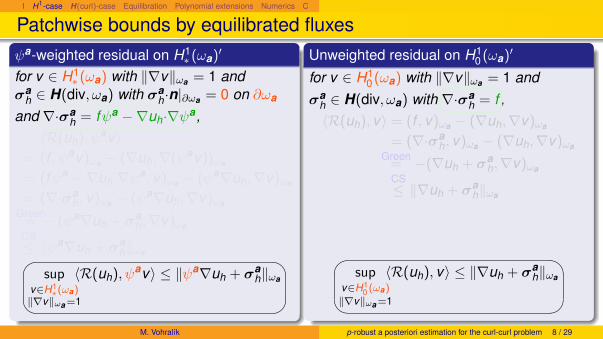
Patchwise bounds by equilibrated fluxesψa-weighted residual on H1
∗ (ωa)′
for v ∈ H1∗ (ωa) with ‖∇v‖ωa = 1 and
σah ∈ H(div, ωa) with σa
h·n|∂ωa = 0 on ∂ωa
and ∇·σah = fψa −∇uh·∇ψa,
〈R(uh), ψav〉= (f , ψav)ωa − (∇uh,∇(ψav))ωa
= (fψa −∇uh·∇ψa, v)ωa − (ψa∇uh,∇v)ωa
= (∇·σah, v)ωa − (ψa∇uh,∇v)ωa
Green= − (ψa∇uh + σa
h,∇v)ωaCS≤ ‖ψa∇uh + σa
h‖ωa
supv∈H1
∗(ωa)‖∇v‖ωa =1
〈R(uh), ψav〉 ≤ ‖ψa∇uh + σah‖ωa
Unweighted residual on H10 (ωa)′
for v ∈ H10 (ωa) with ‖∇v‖ωa = 1 and
σah ∈ H(div, ωa) with ∇·σa
h = f ,〈R(uh), v〉 = (f , v)ωa − (∇uh,∇v)ωa
= (∇·σah, v)ωa − (∇uh,∇v)ωa
Green= −(∇uh + σa
h,∇v)ωaCS≤ ‖∇uh + σa
h‖ωa
supv∈H1
0 (ωa)‖∇v‖ωa =1
〈R(uh), v〉 ≤ ‖∇uh + σah‖ωa
M. Vohralík p-robust a posteriori estimation for the curl-curl problem 8 / 29

I H1-case H(curl)-case Equilibration Polynomial extensions Numerics C
Patchwise bounds by equilibrated fluxesψa-weighted residual on H1
∗ (ωa)′
for v ∈ H1∗ (ωa) with ‖∇v‖ωa = 1 and
σah ∈ H(div, ωa) with σa
h·n|∂ωa = 0 on ∂ωa
and ∇·σah = fψa −∇uh·∇ψa,
〈R(uh), ψav〉= (f , ψav)ωa − (∇uh,∇(ψav))ωa
= (fψa −∇uh·∇ψa, v)ωa − (ψa∇uh,∇v)ωa
= (∇·σah, v)ωa − (ψa∇uh,∇v)ωa
Green= − (ψa∇uh + σa
h,∇v)ωaCS≤ ‖ψa∇uh + σa
h‖ωa
supv∈H1
∗(ωa)‖∇v‖ωa =1
〈R(uh), ψav〉 ≤ ‖ψa∇uh + σah‖ωa
Unweighted residual on H10 (ωa)′
for v ∈ H10 (ωa) with ‖∇v‖ωa = 1 and
σah ∈ H(div, ωa) with ∇·σa
h = f ,〈R(uh), v〉 = (f , v)ωa − (∇uh,∇v)ωa
= (∇·σah, v)ωa − (∇uh,∇v)ωa
Green= −(∇uh + σa
h,∇v)ωaCS≤ ‖∇uh + σa
h‖ωa
supv∈H1
0 (ωa)‖∇v‖ωa =1
〈R(uh), v〉 ≤ ‖∇uh + σah‖ωa
M. Vohralík p-robust a posteriori estimation for the curl-curl problem 8 / 29

I H1-case H(curl)-case Equilibration Polynomial extensions Numerics C
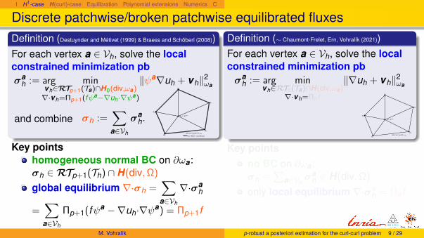
Discrete patchwise/broken patchwise equilibrated fluxesDefinition (Destuynder and Métivet (1999) & Braess and Schöberl (2008))For each vertex a ∈ Vh, solve the localconstrained minimization pbσa
h := arg minvh∈RTp+1(Ta)∩H0(div,ωa)∇·vh=Πp+1(fψa−∇uh·∇ψa)
‖ψa∇uh + vh‖2ωa
and combine σh :=∑a∈Vh
σah.
a ∈ V int
interior patch ωa
no-flow conditiona1
a2
a3
a4
a5
Key pointshomogeneous normal BC on ∂ωa:σh ∈RTp+1(Th) ∩ H(div,Ω)
global equilibrium ∇·σh =∑a∈Vh
∇·σah
=∑a∈Vh
Πp+1(fψa −∇uh·∇ψa) = Πp+1f
Definition (∼ Chaumont-Frelet, Ern, Vohralík (2021))For each vertex a ∈ Vh, solve the localconstrained minimization pbσa
h := arg minvh∈RTp(Ta)∩H(div,ωa)
∇·vh=Πp f
‖∇uh + vh‖2ωa
Key pointsno BC on ∂ωa:σh =
∑a∈Vh
σah 6∈ H(div,Ω)
only local equilibrium ∇·σah = Πpf
M. Vohralík p-robust a posteriori estimation for the curl-curl problem 9 / 29

I H1-case H(curl)-case Equilibration Polynomial extensions Numerics C
Discrete patchwise/broken patchwise equilibrated fluxesDefinition (Destuynder and Métivet (1999) & Braess and Schöberl (2008))For each vertex a ∈ Vh, solve the localconstrained minimization pbσa
h := arg minvh∈RTp+1(Ta)∩H0(div,ωa)∇·vh=Πp+1(fψa−∇uh·∇ψa)
‖ψa∇uh + vh‖2ωa
and combine σh :=∑a∈Vh
σah.
a ∈ V int
interior patch ωa
no-flow conditiona1
a2
a3
a4
a5
Key pointshomogeneous normal BC on ∂ωa:σh ∈RTp+1(Th) ∩ H(div,Ω)
global equilibrium ∇·σh =∑a∈Vh
∇·σah
=∑a∈Vh
Πp+1(fψa −∇uh·∇ψa) = Πp+1f
Definition (∼ Chaumont-Frelet, Ern, Vohralík (2021))For each vertex a ∈ Vh, solve the localconstrained minimization pbσa
h := arg minvh∈RTp(Ta)∩H(div,ωa)
∇·vh=Πp f
‖∇uh + vh‖2ωa
Key pointsno BC on ∂ωa:σh =
∑a∈Vh
σah 6∈ H(div,Ω)
only local equilibrium ∇·σah = Πpf
M. Vohralík p-robust a posteriori estimation for the curl-curl problem 9 / 29
I H1-case H(curl)-case Equilibration Polynomial extensions Numerics C
Discrete patchwise/broken patchwise equilibrated fluxesDefinition (Destuynder and Métivet (1999) & Braess and Schöberl (2008))For each vertex a ∈ Vh, solve the localconstrained minimization pbσa
h := arg minvh∈RTp+1(Ta)∩H0(div,ωa)∇·vh=Πp+1(fψa−∇uh·∇ψa)
‖ψa∇uh + vh‖2ωa
and combine σh :=∑a∈Vh
σah.
a ∈ V int
interior patch ωa
no-flow conditiona1
a2
a3
a4
a5
Key pointshomogeneous normal BC on ∂ωa:σh ∈RTp+1(Th) ∩ H(div,Ω)
global equilibrium ∇·σh =∑a∈Vh
∇·σah
=∑a∈Vh
Πp+1(fψa −∇uh·∇ψa) = Πp+1f
Definition (∼ Chaumont-Frelet, Ern, Vohralík (2021))For each vertex a ∈ Vh, solve the localconstrained minimization pbσa
h := arg minvh∈RTp(Ta)∩H(div,ωa)
∇·vh=Πp f
‖∇uh + vh‖2ωa
a ∈ V int
interior patch ωaa1
a2
a3
a4
a5
Key pointsno BC on ∂ωa:σh =
∑a∈Vh
σah 6∈ H(div,Ω)
only local equilibrium ∇·σah = Πpf
M. Vohralík p-robust a posteriori estimation for the curl-curl problem 9 / 29

I H1-case H(curl)-case Equilibration Polynomial extensions Numerics C
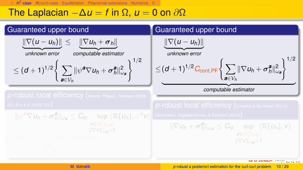
The Laplacian −∆u = f in Ω, u = 0 on ∂Ω
Guaranteed upper bound
‖∇(u − uh)‖︸ ︷︷ ︸unknown error
≤ ‖∇uh + σh‖︸ ︷︷ ︸computable estimator
≤ (d + 1)1/2
∑a∈Vh
‖ψa∇uh + σah‖2ωa
1/2
p-robust local efficiency (Braess, Pillwein, Schöberl (2009;
2D), Ern & V. (2020; 3D))
‖ψa∇uh + σah‖ωa ≤ Cst sup
v∈H1∗(ωa)
‖∇v‖ωa =1
〈R(uh), ψav〉
≤CstCcont,PF supv∈H1
0 (ωa)‖∇v‖ωa =1
〈R(uh), v〉
Guaranteed upper bound
‖∇(u − uh)‖︸ ︷︷ ︸unknown error
≤(d + 1)1/2Ccont,PF
∑a∈Vh
‖∇uh + σah‖2ωa
1/2
︸ ︷︷ ︸computable estimator
p-robust local efficiency (Costabel & Mc-Intosh (2010);
Demkowicz, Gopalakrishnan, & Schöberl (2012))
‖∇uh + σah‖ωa ≤ Cst sup
v∈H10 (ωa)
‖∇v‖ωa =1
〈R(uh), v〉
≤ Cst‖∇(u − uh)‖ωa
M. Vohralík p-robust a posteriori estimation for the curl-curl problem 10 / 29
I H1-case H(curl)-case Equilibration Polynomial extensions Numerics C
The Laplacian −∆u = f in Ω, u = 0 on ∂Ω
Guaranteed upper bound
‖∇(u − uh)‖︸ ︷︷ ︸unknown error
≤ ‖∇uh + σh‖︸ ︷︷ ︸computable estimator
≤ (d + 1)1/2
∑a∈Vh
‖ψa∇uh + σah‖2ωa
1/2
p-robust local efficiency (Braess, Pillwein, Schöberl (2009;
2D), Ern & V. (2020; 3D))
‖ψa∇uh + σah‖ωa ≤ Cst sup
v∈H1∗(ωa)
‖∇v‖ωa =1
〈R(uh), ψav〉
≤CstCcont,PF supv∈H1
0 (ωa)‖∇v‖ωa =1
〈R(uh), v〉
Guaranteed upper bound
‖∇(u − uh)‖︸ ︷︷ ︸unknown error
≤(d + 1)1/2Ccont,PF
∑a∈Vh
‖∇uh + σah‖2ωa
1/2
︸ ︷︷ ︸computable estimator
p-robust local efficiency (Costabel & Mc-Intosh (2010);
Demkowicz, Gopalakrishnan, & Schöberl (2012))
‖∇uh + σah‖ωa ≤ Cst sup
v∈H10 (ωa)
‖∇v‖ωa =1
〈R(uh), v〉
≤ Cst‖∇(u − uh)‖ωa
M. Vohralík p-robust a posteriori estimation for the curl-curl problem 10 / 29

I H1-case H(curl)-case Equilibration Polynomial extensions Numerics C
The Laplacian −∆u = f in Ω, u = 0 on ∂Ω
Guaranteed upper bound
‖∇(u − uh)‖︸ ︷︷ ︸unknown error
≤ ‖∇uh + σh‖︸ ︷︷ ︸computable estimator
≤ (d + 1)1/2
∑a∈Vh
‖ψa∇uh + σah‖2ωa
1/2
p-robust local efficiency (Braess, Pillwein, Schöberl (2009;
2D), Ern & V. (2020; 3D))
‖ψa∇uh + σah‖ωa ≤ Cst sup
v∈H1∗(ωa)
‖∇v‖ωa =1
〈R(uh), ψav〉
≤CstCcont,PF supv∈H1
0 (ωa)‖∇v‖ωa =1
〈R(uh), v〉 ≤ ‖∇(u − uh)‖ωa
Guaranteed upper bound
‖∇(u − uh)‖︸ ︷︷ ︸unknown error
≤(d + 1)1/2Ccont,PF
∑a∈Vh
‖∇uh + σah‖2ωa
1/2
︸ ︷︷ ︸computable estimator
p-robust local efficiency (Costabel & Mc-Intosh (2010);
Demkowicz, Gopalakrishnan, & Schöberl (2012))
‖∇uh + σah‖ωa ≤ Cst sup
v∈H10 (ωa)
‖∇v‖ωa =1
〈R(uh), v〉
≤ Cst‖∇(u − uh)‖ωa
M. Vohralík p-robust a posteriori estimation for the curl-curl problem 10 / 29

I H1-case H(curl)-case Equilibration Polynomial extensions Numerics C
Outline
1 Introduction
2 Reminder on the H1-case
3 The H(curl)-case
4 H(curl) patchwise equilibration
5 Stable (broken) H(curl) polynomial extensions
6 Numerical experiments
7 Conclusions
M. Vohralík p-robust a posteriori estimation for the curl-curl problem 10 / 29

I H1-case H(curl)-case Equilibration Polynomial extensions Numerics C
The curl-curl problem (current density j ∈ H0,N(div,Ω) with ∇·j = 0)
The curl–curl problem
Find the magnetic vector potential A : Ω→ R3 such that∇×(∇×A) = j , ∇·A = 0 in Ω,
A×nΩ = 0, on ΓD,
(∇×A)×nΩ = 0, A·nΩ = 0 on ΓN.
Weak formulation (consequence)
A ∈ H0,D(curl,Ω) satisfies(∇×A,∇×v) = (j ,v) ∀v ∈ H0,D(curl,Ω).
Nédélec finite element discretization (consequence)
V h := Np(Th) ∩ H0,D(curl,Ω), p ≥ 0; Ah ∈ V h satisfies(∇×Ah,∇×vh) = (j ,vh) ∀vh ∈ V h.
M. Vohralík p-robust a posteriori estimation for the curl-curl problem 11 / 29

I H1-case H(curl)-case Equilibration Polynomial extensions Numerics C
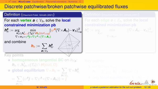
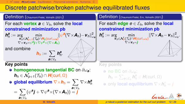
Discrete patchwise/broken patchwise equilibrated fluxesDefinition (Chaumont-Frelet, Vohralík (2021))For each vertex a ∈ Vh, solve the localconstrained minimization pbha
h := arg minvh∈Np+1(Ta)∩H0(curl,ωa)∇×vh=ψaj+∇ψa×(∇×Ah)
‖ψa(∇×Ah)−vh‖2ωa
and combinehh :=
∑a∈Vh
hah.
• a Ta
Key pointshomogeneous tangential BC on ∂ωa:hh ∈Np+1(Th) ∩ H(curl,Ω)
global equilibrium ∇×hh =∑a∈Vh
∇×hah
=∑a∈Vh
(ψaj +∇ψa×(∇×Ah)) = j
Definition (Chaumont-Frelet, Ern, Vohralík (2021))For each edge e ∈ Eh, solve the localconstrained minimization pbhe
h := arg minvh∈Np(Te)∩H(curl,ωe)
∇×vh=j
‖∇×Ah−vh‖2ωe .
Key pointsno BC on ∂ωe:hh =
∑e∈Eh
heh 6∈ H(curl,Ω)
only local equilibrium ∇×heh = j
M. Vohralík p-robust a posteriori estimation for the curl-curl problem 12 / 29

I H1-case H(curl)-case Equilibration Polynomial extensions Numerics C
Discrete patchwise/broken patchwise equilibrated fluxesDefinition (Chaumont-Frelet, Vohralík (2021))For each vertex a ∈ Vh, solve the localconstrained minimization pbha
h := arg minvh∈Np+1(Ta)∩H0(curl,ωa)∇×vh=ψaj+∇ψa×(∇×Ah)
‖ψa(∇×Ah)−vh‖2ωa
and combinehh :=
∑a∈Vh
hah.
• a Ta
Key pointshomogeneous tangential BC on ∂ωa:hh ∈Np+1(Th) ∩ H(curl,Ω)
global equilibrium ∇×hh =∑a∈Vh
∇×hah
=∑a∈Vh
(ψaj +∇ψa×(∇×Ah)) = j
Definition (Chaumont-Frelet, Ern, Vohralík (2021))For each edge e ∈ Eh, solve the localconstrained minimization pbhe
h := arg minvh∈Np(Te)∩H(curl,ωe)
∇×vh=j
‖∇×Ah−vh‖2ωe .
Key pointsno BC on ∂ωe:hh =
∑e∈Eh
heh 6∈ H(curl,Ω)
only local equilibrium ∇×heh = j
M. Vohralík p-robust a posteriori estimation for the curl-curl problem 12 / 29

I H1-case H(curl)-case Equilibration Polynomial extensions Numerics C
Discrete patchwise/broken patchwise equilibrated fluxesDefinition (Chaumont-Frelet, Vohralík (2021))For each vertex a ∈ Vh, solve the localconstrained minimization pbha
h := arg minvh∈Np+1(Ta)∩H0(curl,ωa)∇×vh=ψaj+∇ψa×(∇×Ah)
‖ψa(∇×Ah)−vh‖2ωa
and combinehh :=
∑a∈Vh
hah.
• a Ta
Key pointshomogeneous tangential BC on ∂ωa:hh ∈Np+1(Th) ∩ H(curl,Ω)
global equilibrium ∇×hh =∑a∈Vh
∇×hah
=∑a∈Vh
(ψaj +∇ψa×(∇×Ah)) = j
Definition (Chaumont-Frelet, Ern, Vohralík (2021))For each edge e ∈ Eh, solve the localconstrained minimization pbhe
h := arg minvh∈Np(Te)∩H(curl,ωe)
∇×vh=j
‖∇×Ah−vh‖2ωe .
e
Te
Key pointsno BC on ∂ωe:hh =
∑e∈Eh
heh 6∈ H(curl,Ω)
only local equilibrium ∇×heh = j
M. Vohralík p-robust a posteriori estimation for the curl-curl problem 12 / 29

I H1-case H(curl)-case Equilibration Polynomial extensions Numerics C
Discrete patchwise/broken patchwise equilibrated fluxesDefinition (Chaumont-Frelet, Vohralík (2021))For each vertex a ∈ Vh, solve the localconstrained minimization pbha
h := arg minvh∈Np+1(Ta)∩H0(curl,ωa)∇×vh=ψaj+∇ψa×(∇×Ah)
‖ψa(∇×Ah)−vh‖2ωa
and combinehh :=
∑a∈Vh
hah.
• a Ta
Key pointshomogeneous tangential BC on ∂ωa:hh ∈Np+1(Th) ∩ H(curl,Ω)
global equilibrium ∇×hh =∑a∈Vh
∇×hah
=∑a∈Vh
(ψaj +∇ψa×(∇×Ah)) = j
Definition (Chaumont-Frelet, Ern, Vohralík (2021))For each edge e ∈ Eh, solve the localconstrained minimization pbhe
h := arg minvh∈Np(Te)∩H(curl,ωe)
∇×vh=j
‖∇×Ah−vh‖2ωe .
well-posed for j|ωe ∈RTp(Te) ∩ H(div, ωe) with∇·j = 0
e
Te
Key pointsno BC on ∂ωe:hh =
∑e∈Eh
heh 6∈ H(curl,Ω)
only local equilibrium ∇×heh = j
M. Vohralík p-robust a posteriori estimation for the curl-curl problem 12 / 29

I H1-case H(curl)-case Equilibration Polynomial extensions Numerics C
Discrete patchwise/broken patchwise equilibrated fluxesDefinition (Chaumont-Frelet, Vohralík (2021))For each vertex a ∈ Vh, solve the localconstrained minimization pbha
h := arg minvh∈Np+1(Ta)∩H0(curl,ωa)∇×vh=ψaj+∇ψa×(∇×Ah)
‖ψa(∇×Ah)−vh‖2ωa
ψa j ∈RTp+1(Ta) ∩ H0(div, ωa) but∇ψa×(∇×Ah) 6∈ H(div, ωa)
hh :=∑a∈Vh
hah.
• a Ta
Key pointshomogeneous tangential BC on ∂ωa:hh ∈Np+1(Th) ∩ H(curl,Ω)
global equilibrium ∇×hh =∑a∈Vh
∇×hah
=∑a∈Vh
(ψaj +∇ψa×(∇×Ah)) = j
Definition (Chaumont-Frelet, Ern, Vohralík (2021))For each edge e ∈ Eh, solve the localconstrained minimization pbhe
h := arg minvh∈Np(Te)∩H(curl,ωe)
∇×vh=j
‖∇×Ah−vh‖2ωe .
well-posed for j|ωe ∈RTp(Te) ∩ H(div, ωe) with∇·j = 0
e
Te
Key pointsno BC on ∂ωe:hh =
∑e∈Eh
heh 6∈ H(curl,Ω)
only local equilibrium ∇×heh = j
M. Vohralík p-robust a posteriori estimation for the curl-curl problem 12 / 29

I H1-case H(curl)-case Equilibration Polynomial extensions Numerics C
Bottom line
Continuous caseWhen there exist v ∈ H(curl,Ω) such that ∇×v = j?When j ∈ H(div,Ω) with ∇·j = 0.
Discrete caseWhen there exist vh ∈Np(Th) ∩ H(curl,Ω) such that ∇×vh = j?When j ∈RTp(Th) ∩ H(div,Ω) with ∇·j = 0.
We supposej ∈ H0,N(div,Ω) with ∇·j = 0j ∈RTp(Th) (no data oscillation, simplicity of presentation)
M. Vohralík p-robust a posteriori estimation for the curl-curl problem 13 / 29

I H1-case H(curl)-case Equilibration Polynomial extensions Numerics C
The curl–curl case
Guaranteed upper bound
‖∇×(A− Ah)‖︸ ︷︷ ︸unknown error
≤ ‖∇×Ah − hh‖︸ ︷︷ ︸computable estimator
≤ 2
∑a∈Vh
‖ψa(∇×Ah)− hah‖2ωa
1/2
p-robust local efficiency (Costabel & Mc-Intosh (2010);
Demkowicz, Gopalakrishnan, & Schöberl (2009, 2012); Chaumont-Frelet & V.
(2021))
‖ψa(∇×Ah)−hah‖ωa≤Cst sup
v∈H∗(curl,ωa)‖∇×v‖ωa =1
〈R(Ah), ψav〉
≤CstCcont,PFW‖∇×(A− Ah)‖ωa
Guaranteed upper bound
‖∇×(A− Ah)‖︸ ︷︷ ︸unknown error
≤CL 61/2Ccont,PF
∑e∈Eh
‖∇×Ah − heh‖2ωe
1/2
︸ ︷︷ ︸computable estimator
p-robust local efficiency (Costabel & Mc-Intosh (2010);
Demkowicz, Gopalakrishnan, & Schöberl (2009); Ern, Chaumont-Frelet, & V.
(2021))
‖∇×Ah − heh‖ωe ≤ Cst sup
v∈H0(curl,ωe)‖∇×v‖ωe =1
〈R(Ah),v〉
≤ Cst‖∇×(A− Ah)‖ωe
M. Vohralík p-robust a posteriori estimation for the curl-curl problem 14 / 29

I H1-case H(curl)-case Equilibration Polynomial extensions Numerics C
Patchwise/broken patchwise flux equilibration
Patchwise flux equilibrationglobally equilibrated fluxPrager–Synge constant-free upperboundequilibration in several stages, moreexpensiveadditional layer for efficiencyp-robust
Broken patchwise flux equilibrationlocally equilibrated flux61/2, Ccont,PF, and CL in the upper bound;CL = 1 if Ω is convex and no mixed BCsequilibration in a single stage, cheaper,explicit for p = 0both estimator and efficiency on ωe
p-robust
Lift constant CL such that for all v ∈ H0,D(curl,Ω), there exists w ∈ H1(Ω) suchthat w ∈ H0,D(curl,Ω), ∇×w = ∇×v , and
‖∇w‖ ≤ CL‖∇×v‖
M. Vohralík p-robust a posteriori estimation for the curl-curl problem 15 / 29

I H1-case H(curl)-case Equilibration Polynomial extensions Numerics C
Outline
1 Introduction
2 Reminder on the H1-case
3 The H(curl)-case
4 H(curl) patchwise equilibration
5 Stable (broken) H(curl) polynomial extensions
6 Numerical experiments
7 Conclusions
M. Vohralík p-robust a posteriori estimation for the curl-curl problem 15 / 29

I H1-case H(curl)-case Equilibration Polynomial extensions Numerics C
Stage 1: overconstrained Raviart–Thomas projection
Projection of ∇ψa×(∇×Ah) to a Raviart–Thomas space
For all vertices a ∈ Vh, consider p′ := minp,1-degree patchwise minimizations:
θah := arg min
vh∈RTp′ (Ta)∩H0(div,ωa)
∇·vh=−∇ψa·j(vh,rh)K =(∇ψa×(∇×Ah),rh)K ∀rh∈[P0(K )]3, ∀K∈Ta
‖∇ψa×(∇×Ah)− vh‖2ωa .
Comments∇ψa×(∇×Ah) 6∈RTp′(Ta) ∩ H0(div, ωa)additional orthogonality constraint
crucial for stage 2only possible thanks the lowest-order Galerkin orthogonality of Ahrequests minp,1
remainder δh :=∑
a∈Vhθa
hshould be zero (∼ partition of unity) but is notδh ∈RTp′(Th) ∩ H0,N(div,Ω) and ∇·δh = 0
M. Vohralík p-robust a posteriori estimation for the curl-curl problem 16 / 29

I H1-case H(curl)-case Equilibration Polynomial extensions Numerics C
Stage 2: divergence-free decomposition of the given divergence-freeRaviart-Thomas piecewise polynomial δh
Divergence-free decomposition of δh
For all tetrahedra K ∈ Th, consider (p + 1)-degree elementwise minimizations:
δah|K := arg min
vh∈RT1(K )∇·vh=0
vh·nK =IRT1 (ψaδh)·nK on ∂K
‖vh − IRT1 (ψaδh)‖2K ∀a ∈ VK when p = 0,
δah|K := arg min
vh∈RTp+1(K )∇·vh=0
vh·nK =ψaδh·nK on ∂K
‖vh − ψaδh‖2K ∀a ∈ VK when p ≥ 1.
Commentspatchwise contributions
δah ∈RTp+1(Ta) ∩ H0(div, ωa) and ∇·δa
h = 0 ∀a ∈ Vh
δah form a divergence-free decomposition of δh, δh =
∑a∈Vh
δah
M. Vohralík p-robust a posteriori estimation for the curl-curl problem 17 / 29

I H1-case H(curl)-case Equilibration Polynomial extensions Numerics C
Stage 2: divergence-free decomposition of the given divergence-freecurrent density j
Divergence-free decomposition of the current density jSet
jah := ψaj + θa
h − δah.
Then
jah ∈RTp+1(Ta) ∩ H0(div, ωa),
∇·jah = 0,∑
a∈Vh
jah = j .
M. Vohralík p-robust a posteriori estimation for the curl-curl problem 18 / 29

I H1-case H(curl)-case Equilibration Polynomial extensions Numerics C
Stage 3: discrete patchwise equilibrated fluxes
Definition (Chaumont-Frelet, Vohralík (2021))For each vertex a ∈ Vh, solve the local constrained minimization problem
hah := arg min
vh∈Np+1(Ta)∩H0(curl,ωa)
∇×vh=jah
‖ψa(∇×Ah)− vh‖2ωa
and combinehh :=
∑a∈Vh
hah.
• a Ta
Key pointshomogeneous tangential BC on ∂ωa: hh ∈Np+1(Th) ∩ H(curl,Ω)
global equilibrium ∇×hh =∑a∈Vh
∇×hah =
∑a∈Vh
jah = j
M. Vohralík p-robust a posteriori estimation for the curl-curl problem 19 / 29

I H1-case H(curl)-case Equilibration Polynomial extensions Numerics C
Outline
1 Introduction
2 Reminder on the H1-case
3 The H(curl)-case
4 H(curl) patchwise equilibration
5 Stable (broken) H(curl) polynomial extensions
6 Numerical experiments
7 Conclusions
M. Vohralík p-robust a posteriori estimation for the curl-curl problem 19 / 29

I H1-case H(curl)-case Equilibration Polynomial extensions Numerics C
H(curl) polynomial extension on a tetrahedron
Theorem (H(curl) polynomial extension on a tetrahedron Costabel & Mc-Intosh (2010); Demkowicz,
Gopalakrishnan, & Schöberl (2009); Chaumont-Frelet, Ern, & V. (2020))
Let ∅ ⊆ F ⊆ FK be a (sub)set of faces of a tetrahedron K . Then, for everypolynomial degree p ≥ 0, for all rK ∈RTp(K ) such that ∇·rK = 0, and for allrF ∈Nτ
p (ΓF ) such that rK ·nF = curlF (rF ) for all F ∈ F , there holds
minvp∈Np(K )∇×vp=rKvp|τF=rF
‖vp‖K ≤ Cst minv∈H(curl,K )∇×v=rKv |τF=rF
‖v‖K .
CommentsCst only depends on the shape-regularity of Kfor (pw) p-polynomial data rK , rF , minimization over Np(K ) is up to Cst asgood as minimization over the entire H(curl,K )extension to an edge patch: Chaumont-Frelet, Ern, & V. (2021)extension to a vertex patch: conjecture
M. Vohralík p-robust a posteriori estimation for the curl-curl problem 20 / 29

I H1-case H(curl)-case Equilibration Polynomial extensions Numerics C
Outline
1 Introduction
2 Reminder on the H1-case
3 The H(curl)-case
4 H(curl) patchwise equilibration
5 Stable (broken) H(curl) polynomial extensions
6 Numerical experiments
7 Conclusions
M. Vohralík p-robust a posteriori estimation for the curl-curl problem 20 / 29

I H1-case H(curl)-case Equilibration Polynomial extensions Numerics C
Broken patchwise equilibration, smooth solution, h-refinement
1 1/2 1/4 1/8 1/16 1/32
10−4
10−2
100
h
h2
h3
h4
h/√
3
‖∇×(A− Ah)‖
1 1/2 1/4 1/8 1/16 1/32
1
1.5
2
h/√
3
maxe∈Eh ηe/‖∇×(A− Ah)‖ωe
1 1/2 1/4 1/8 1/16 1/3225
30
35
40
45
h/√
3
η/‖∇×(A− Ah)‖
p = 0 p = 1 p = 2 p = 3
M. Vohralík p-robust a posteriori estimation for the curl-curl problem 21 / 29

I H1-case H(curl)-case Equilibration Polynomial extensions Numerics C
Broken patchwise equilibration, smooth solution, p-refinement
0 1 2 3 4 5 6 710−10
10−5
100
e−3p
p
‖∇×(A− Ah)‖
0 1 2 3 4 5 6 7
1
1.5
2
p
maxe∈Eh ηe/‖∇×(A− Ah)‖ωe
0 1 2 3 4 5 6 7
102
103
p
η/‖∇×(A− Ah)‖
N = 1 N = 2 N = 4 Unstrucutred
M. Vohralík p-robust a posteriori estimation for the curl-curl problem 22 / 29

I H1-case H(curl)-case Equilibration Polynomial extensions Numerics C
Broken patchwise equilibration, singular solution, adap. refinement
103 104 105
10−1
N2/3dofs
N1/3dofs
Ndofs
‖∇×(A− Ah)‖
103 104 105
1
1.5
2
Ndofs
maxe∈Eh ηe/‖∇×(A− Ah)‖ωe
103 104 105
2
2.5
Ndofs
ηcfree/‖∇×(A− Ah)‖
p = 0 p = 1 p = 2 p = 3
M. Vohralík p-robust a posteriori estimation for the curl-curl problem 23 / 29

I H1-case H(curl)-case Equilibration Polynomial extensions Numerics C
Broken patchwise equilibration, singular solution, adap. refinement
0
1.1e-3
2.2e-3
Estimated (left) and actual error (right), p = 3
M. Vohralík p-robust a posteriori estimation for the curl-curl problem 24 / 29
I H1-case H(curl)-case Equilibration Polynomial extensions Numerics C
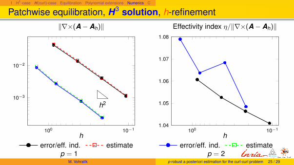
Patchwise equilibration, H3 solution, h-refinement
10−1100
10−3
10−2
h2
h
‖∇×(A− Ah)‖
10−11001.04
1.05
1.06
1.07
1.08
h
Effectivity index η/‖∇×(A− Ah)‖
error/eff. ind. estimatep = 1
error/eff. ind. estimatep = 2
M. Vohralík p-robust a posteriori estimation for the curl-curl problem 25 / 29

I H1-case H(curl)-case Equilibration Polynomial extensions Numerics C
Patchwise equilibration, H3 solution, p-refinement
1 2 3 4 5 6
10−4
10−3
10−2
p
‖∇×(A− Ah)‖
1 2 3 4 5 6
1.05
1.1
1.15
p
Effectivity index η/‖∇×(A− Ah)‖
error estimatestructured mesh
error estimateunstructured mesh
M. Vohralík p-robust a posteriori estimation for the curl-curl problem 26 / 29
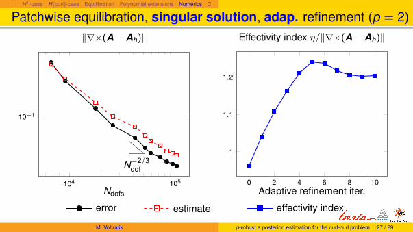
I H1-case H(curl)-case Equilibration Polynomial extensions Numerics C
Patchwise equilibration, singular solution, adap. refinement (p = 2)
104 105
10−1
N−2/3dof
Ndofs
‖∇×(A− Ah)‖
0 2 4 6 8 10
1
1.1
1.2
Adaptive refinement iter.
Effectivity index η/‖∇×(A− Ah)‖
error estimate effectivity index
M. Vohralík p-robust a posteriori estimation for the curl-curl problem 27 / 29

I H1-case H(curl)-case Equilibration Polynomial extensions Numerics C
Patchwise equilibration, singular solution, adap. refinement (p = 2)
0.0
3.3e-3
6.6e-3
Estimated (left) and actual error (right), adaptive mesh refinement iteration #10.Top view (top) and side view (bottom)
M. Vohralík p-robust a posteriori estimation for the curl-curl problem 28 / 29

I H1-case H(curl)-case Equilibration Polynomial extensions Numerics C
Outline
1 Introduction
2 Reminder on the H1-case
3 The H(curl)-case
4 H(curl) patchwise equilibration
5 Stable (broken) H(curl) polynomial extensions
6 Numerical experiments
7 Conclusions
M. Vohralík p-robust a posteriori estimation for the curl-curl problem 28 / 29

I H1-case H(curl)-case Equilibration Polynomial extensions Numerics C
ConclusionsConclusions
reliable, locally efficient, p-robust, and possibly constant-free estimatesdivergence-free decompositions of Raviart–Thomas piecewise polynomials
M. Vohralík p-robust a posteriori estimation for the curl-curl problem 29 / 29

I H1-case H(curl)-case Equilibration Polynomial extensions Numerics C
ConclusionsConclusions
reliable, locally efficient, p-robust, and possibly constant-free estimatesdivergence-free decompositions of Raviart–Thomas piecewise polynomials
CHAUMONT-FRELET T., ERN A., VOHRALÍK M., Polynomial-degree-robustH(curl)-stability of discrete minimization in a tetrahedron, C. R. Math. Acad. Sci. Paris358 (2020), 1101–1110.
CHAUMONT-FRELET T., ERN A., VOHRALÍK M., Stable broken H(curl) polynomialextensions and p-robust a posteriori error estimates by broken patchwise equilibrationfor the curl–curl problem, Math. Comp. (2021), accepted for publication.
CHAUMONT-FRELET T., VOHRALÍK M., p-robust equilibrated flux reconstruction inH(curl) based on local minimizations. Application to a posteriori analysis of thecurl–curl problem, HAL Preprint 03227570, submitted for publication.
Thank you for your attention!M. Vohralík p-robust a posteriori estimation for the curl-curl problem 29 / 29