Approximation properties of isogeometric

function spaces on singularly parameterized

domains

Thomas Takacs

Department of Mathematics

University of Pavia, Italy

thomas.takacs@unipv.it

October 24, 2021

Abstract

We study approximation error bounds of isogeometric function spaces

on a specific type of singularly parameterized domains. In this context

an isogeometric function is the composition of a piecewise rational func-

tion with the inverse of a piecewise rational geometry parameterization.

We consider domains where one edge of the parameter domain is mapped

onto one point in physical space. To be more precise, in our configuration

the singular patch is derived from a reparameterization of a regular trian-

gular patch. On such a domain one can define an isogeometric function

space fulfilling certain regularity criteria that guarantee optimal conver-

gence. The main contribution of this paper is to prove approximation error

bounds for the previously defined class of isogeometric discretizations.

1 Introduction

Isogeometric analysis as presented by Hughes et al. (2005) starts from a dis-

cretization based on a B-spline or NURBS geometry parameterization. The

standard theory, as developed in Bazilevs et al. (2006) relies on the regularity of

the geometry mapping. If the geometry mapping is singular, the standard the-

ory does not apply. Therefore, in the standard setting, the underlying geometry

has to be diffeomorphic to a rectangle. Singular parameterizations have been

1

arX

iv:1

507.

0809

5v1

[m

ath.

NA

] 2

9 Ju

l 201

5

studied in the context of isogeometric analysis in e.g. Lu (2009); Cohen et al.

(2010); Lipton et al. (2010) The regularity theory has already been partially ex-

tended to singularly parameterized domains in Takacs and Juttler (2011, 2012).

However, the study of approximation properties of isogeometric spaces over sin-

gular patches still remains an open problem, which we study in more detail in

this paper. In the context of finite elements there exist several related studies

concerning degenerate Q1 isoparametric elements, such as Jamet (1977); Acosta

and Monzon (2006).

In Section 2 we present the notation and the underlying setting that we

consider throughout this paper. In Section 3 we introduce the hierarchical

mesh as well as the corresponding function space on it. In Section 3.3 we

define an L2-stable projection operator onto the hierarchical function space.

We briefly mention how the construction can be generalized to locally quasi-

uniform refinements in Section 3.4 and present approximation error bounds in

Section 4. Finally, we conclude the paper in Section 5.

2 Preliminaries

Isogeometric function spaces V, as they are present in isogeometric analysis

introduced in Hughes et al. (2005), are built from an underlying B-spline or

NURBS space. Hence, to introduce the notation needed, we start this prelimi-

nary section with recalling the notion of B-splines and NURBS. We do not give

detailed definitions here but refer to standard literature for further reading, see

Piegl and Tiller (1995); Prautzsch et al. (2002).

2.1 B-splines, NURBS and isogeometric functions

Throughout this paper we consider the simple configuration of an isogeometric

function space based on a single NURBS patch with uniform knots. Note that

this simplification is not necessary, as we point out in Section 3.4.

For simplicity we consider uniform B-splines over the parameter domain

]0, 1[. Given a degree p ∈ Z+ and a mesh size h = 1/2n, with n ∈ Z+0 , the i-th

B-spline, for i = 1, . . . , 2n + p, is denoted by bni (s). Here n refers to the level of

(dyadic) refinement. We assume that the knot vector is open and has uniformly

distributed interior knots. We moreover denote by bni,j(s, t) the product of bni (s)

and bnj (t). Let Sn be the tensor-product B-spline space spanned by bni,j(s, t).

We have given a weight function w ∈ Sn∗ on some coarse level n∗, with w > 0

uniformly. For all n ≥ n∗ we define the NURBS space as Nn = vnw : vn ∈ Sn.

2

Moreover, let G ∈ (Nn∗)2 be a geometry parameterization, with

G : B = ]0, 1[2 → Ω ⊂ R2.

For n ≥ n∗, the h-dependent spaces Vn of isogeometric functions over the open

domain Ω = G(B) are defined by

Vn =ϕn : Ω→ R | ϕn = fn G−1, with fn ∈ Nn

.

The goal of this paper is to prove approximation error bounds for h-refined

isogeometric functions over singularly parameterized domains. In the following

section we introduce a simple configuration of singularly parameterized domains.

2.2 Singular tensor-product patches derived from trian-

gular patches

In this section we construct smooth isogeometric function spaces on singular

patches, where the singular patches are derived from triangular Bezier patches.

The configuration presented here is developed in more detail in Takacs (2015),

which is based on Hu (2001).

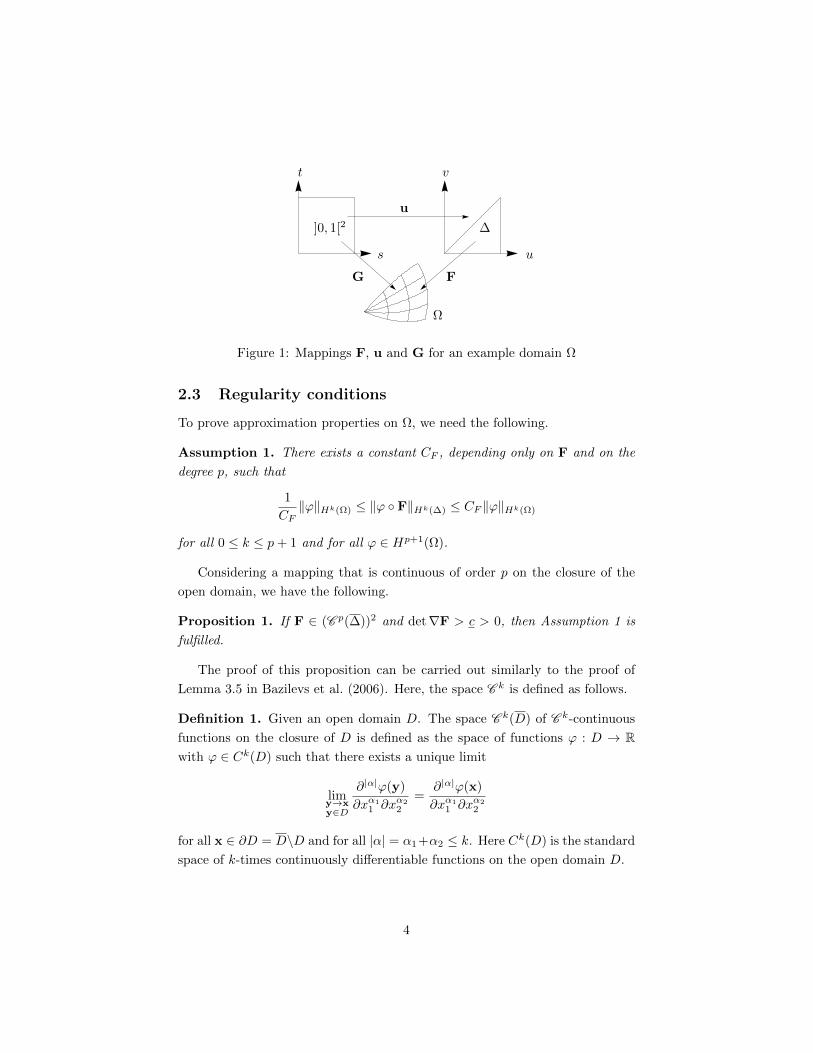
Let u be the mapping

u : ]0, 1[2 → ∆ = (u, v) : 0 < u < 1, 0 < v < u

(s, t)T 7→ (s, s t)T,

and let F : ∆→ R2 be a regular mapping. We assume that the parameterization

G is given as

G = F u.

All mappings u, F and G are defined on an open parameter domain and can

be extended continuously to the boundary. Here, G is singular at a part of

the boundary, i.e. det∇G(s, t) = 0 for all (s, t) ∈ 0 × [0, 1]. Let Wn be the

isogeometric B-spline space on ∆, i.e.

Wn =ϕn : ∆→ R | ϕn = fn u−1, with fn ∈ Sn

,

where the inverse of the singular mapping u is equal to

u−1(u, v) =(u,v

u

)T.

The various introduced mappings and domains are depicted in Figure 1.

3

s u

t v

FG

u

Ω

]0, 1[2 ∆

Figure 1: Mappings F, u and G for an example domain Ω

2.3 Regularity conditions

To prove approximation properties on Ω, we need the following.

Assumption 1. There exists a constant CF , depending only on F and on the

degree p, such that

1

CF‖ϕ‖Hk(Ω) ≤ ‖ϕ F‖Hk(∆) ≤ CF ‖ϕ‖Hk(Ω)

for all 0 ≤ k ≤ p+ 1 and for all ϕ ∈ Hp+1(Ω).

Considering a mapping that is continuous of order p on the closure of the

open domain, we have the following.

Proposition 1. If F ∈ (C p(∆))2 and det∇F > c > 0, then Assumption 1 is

fulfilled.

The proof of this proposition can be carried out similarly to the proof of

Lemma 3.5 in Bazilevs et al. (2006). Here, the space C k is defined as follows.

Definition 1. Given an open domain D. The space C k(D) of C k-continuous

functions on the closure of D is defined as the space of functions ϕ : D → Rwith ϕ ∈ Ck(D) such that there exists a unique limit

limy→xy∈D

∂|α|ϕ(y)

∂xα11 ∂xα2

2

=∂|α|ϕ(x)

∂xα11 ∂xα2

2

for all x ∈ ∂D = D\D and for all |α| = α1+α2 ≤ k. Here Ck(D) is the standard

space of k-times continuously differentiable functions on the open domain D.

4

3 Spaces and operators on the triangle

In this section we introduce a hierarchical mesh refinement and corresponding

spline spaces Wn on the triangle ∆. In this configuration Wn is a subspace of

Wn. Then we introduce a projection operator ΠWn: L2(∆) → Wn, that is

locally bounded in L2.

3.1 Hierarchical mesh and refinement

Let Tn be the Bezier mesh corresponding to the function space Wn on ∆, i.e.

it is a regular mesh mapped by u. We consider a sequence of meshes Tn, such

that T0 = ∆ and

Tn = δ : δ ∈ Tn ∩ (∆\∆1/2) ∪ δ/2 : δ ∈ Tn−1,

where

∆γ = (u, v) : 0 < u < γ, 0 < v < u

and δ/2 = (u2 ,v2 ) : (u, v) ∈ δ. Here, with a slight abuse of notation, we have

Tn ∩ (∆\∆1/2) = δ : δ ∈ Tn and δ ⊆ ∆\∆1/2.

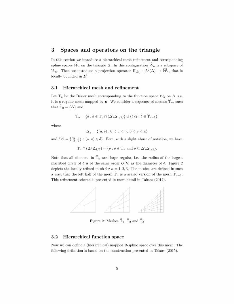
Note that all elements in Tn are shape regular, i.e. the radius of the largest

inscribed circle of δ is of the same order O(h) as the diameter of δ. Figure 2

depicts the locally refined mesh for n = 1, 2, 3. The meshes are defined in such

a way, that the left half of the mesh Tn is a scaled version of the mesh Tn−1.

This refinement scheme is presented in more detail in Takacs (2012).

Figure 2: Meshes T1, T2 and T3

3.2 Hierarchical function space

Now we can define a (hierarchical) mapped B-spline space over this mesh. The

following definition is based on the construction presented in Takacs (2015).

5

Definition 2. The basis Sn over ]0, 1[2 is defined via

Sn =bni,j = bni (s)Bij(t) : 1 ≤ i ≤ p+ 1 and 1 ≤ j ≤ i+ 1

∪

bni,j = bni (s)b1j (t) : p+ 1 + 1 ≤ i ≤ p+ 2 and 1 ≤ j ≤ p+ 2

∪

bni,j = bni (s)b2j (t) : p+ 2 + 1 ≤ i ≤ p+ 4 and 1 ≤ j ≤ p+ 4

. . .

∪bni,j = bni (s)bnj (t) : p+ 2n−1 + 1 ≤ i ≤ p+ 2n and 1 ≤ j ≤ p+ 2n

,

where Bij(t) is the j-th Bernstein polynomial of degree i. This defines a function

space Wn over ∆ via

Wn = spanβni,j = bni,j u−1 : bni,j ∈ Sn

.

Lemma 1. The space Wn and the corresponding basis fulfill the following prop-

erties.

(A) The space Wn is a subspace of Wn ∩ C p(∆).

(B) For all δ ∈ Tn the space fulfills Pp ⊆ Wn |δ ⊆ Qp, where Pp is the space of

bivariate polynomials of total degree ≤ p and Qp is the space of bivariate

polynomials of maximum degree ≤ p.

(C) The basis functions fulfill

βni,j(u, v) = βn−1i,j (2u, 2v)

for all 1 ≤ i ≤ 2n−1 and for all j.

(D) The basis forms a partition of unity.

We omit the simple proof of this lemma.

3.3 Stable projection operator

Let n0 = dlog2(8p)e. Then we have h0 = 1/2n0 . In the following we consider

n ≥ n0. This is necessary for the proofs of Lemma 2 and Theorem 7, to be able

to properly split the contributions from the singular point at the left and the

regular part at the right of the parameter domain. We consider the standard

dual basis for univariate B-splines, see e.g. Schumaker (2007); da Veiga et al.

(2014) for more details.

Definition 3. Let λnk : L2(0, 1)→ R be the dual basis for bni with λnk (bni ) = δki ,

for i, k ∈ 1, . . . , 2n + p.

6

Moreover, consider a dual basis for polynomials on ∆h0 .

Definition 4. Let µn0

k,l : L2(∆h0)→ R be dual functionals, with

µn0

k,l(βn0i,j ) = δki δ

lj ,

for k = 1, . . . , p+ 1 and l = 1, . . . , k.

We assume that all the functionals in Definitions 3 and 4 are bounded in L2.

This is no restriction, see Schumaker (2007).

Let cI be the mapping from R2 → R2 with (u, v) 7→ (c u, c v). Then we can

define a global dual basis for all n > n0.

Definition 5. Let n > n0. Given ϕ ∈ L2(∆), we set

Λnk,l(ϕ) = µn0

k,l(ϕ (2n0−n)I)

for all k = 1, . . . , p+ 1 and all l = 1, . . . , k. Moreover, we set

Λnk,l(ϕ) = λnk ⊗ λm(k)l (ϕ u)

for all k = p+ 2, . . . , 2n + p and all l = 1, . . . , 2m(k) + p. Here m(k) = dlog2(k−p+ 1)e.

It is easy to see, that Λnk,l is in fact a dual basis for the basis βni,j on ∆.

Definition 6. The dual functionals naturally define a projection operator from

L2(∆) onto Wn, with

ΠWn(ϕ) =

2n+p∑k=1

∑l

Λnk,l(ϕ)βnk,l,

where we appropriately sum over all l.

Before we prove our main Theorem 7, we recall two preliminary results.

Lemma 2. Let n ≥ n0. There exists a constant CR > 0, depending only on p,

such that for all ϕ ∈ L2(∆\∆h0) and for all δ ∈ Tn ∩ (∆\∆3/8) we have∥∥∥ΠWnϕ∥∥∥L2(δ)

≤ CR ‖ϕ‖L2(δ) , (1)

where δ is the support extension of δ as presented in Bazilevs et al. (2006).

7

Proof. A proof of this lemma follows directly from the standard theory for

regularly parameterized domains (see e.g. Bazilevs et al. (2006); da Veiga et al.

(2014)), since ∆\∆h0is parameterized via u0 : ]h0, 1[ × ]0, 1[ → ∆\∆h0

and

the support extension of any δ ∈ ∆\∆3/8 remains in ∆\∆(3/8−ph). Since n0

is chosen large enough, we have 38 − ph ≥ h0 for all h ≤ h0, and therefore

δ ⊂ ∆\∆h0. In that case, the constant CR depends on the degree p and on the

Jacobian determinant of the mapping u0, which depends on n0 only. Since n0

is fully determined by p, the constant CR depends on p only.

On the refinement level n0 it is obvious that the operator is bounded.

Lemma 3. There exists a constant C0 > 0, depending only on p, such that for

all ϕ ∈ L2(∆) and for all δ ∈ Tn0we have∥∥∥ΠWn0

ϕ∥∥∥L2(δ)

≤ C0 ‖ϕ‖L2(δ) . (2)

Proof. This lemma follows directly from the boundedness of the dual function-

als. There is no condition on the scaling needed, since we consider the coarse

level n0 only. The constant C0 depends on p and n0 only. Again, n0 is fully

determined by p, which concludes the proof.

Now we can prove the main result, the stability of the projection operator.

Theorem 7. Let n ≥ n0. There exists a constant CS > 0, depending only on

p, such that for all ϕ ∈ L2(∆) and for all δ ∈ Tn we have∥∥∥ΠWnϕ∥∥∥L2(δ)

≤ CS ‖ϕ‖L2(δ) . (3)

Proof. We split the proof into three parts.

(A) Let δ ⊂ ∆\∆3/8. Then this statement follows directly from Lemma 2.

(B) Let δ ⊂ ∆3/8 and there exists an m ∈ Z+, with m ≤ n − n0, such that

2mI(δ) ⊂ ∆3/4\∆3/8. Due to Lemma 1 (C) we have

Wn|∆3/8= Wn−1|∆3/4

2I

for all n ≥ log2(8p). Hence we conclude∥∥∥ΠWnϕ∥∥∥2

L2(δ)= 2−m

∥∥∥ΠWn−m(ϕ (2−mI))

∥∥∥2

L2(2mI(δ)).

The desired result follows from Lemma 2 and because

2−m∥∥ϕ ((2−m)I)

∥∥2

L2(2mI(δ))= ‖ϕ‖2L2(δ) .

8

(C) We have∥∥∥ΠWnϕ∥∥∥2

L2(δ)= 2n0−n

∥∥∥ΠWn0(ϕ (2n0−nI))

∥∥∥2

L2(2n−n0I(δ)).

Here, the bound is fulfilled because of Lemma 3.

This concludes the proof with CS = max(CR, C0).

Having a stable projection operator, we can prove approximation error bounds

on Ω for a special class of geometry mappings G. But before we present the

proof, we discuss a possible generalization.

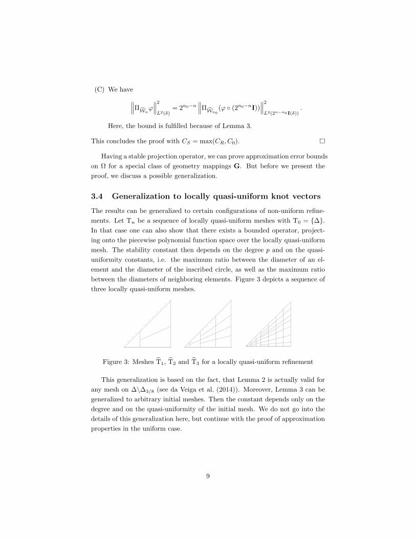
3.4 Generalization to locally quasi-uniform knot vectors

The results can be generalized to certain configurations of non-uniform refine-

ments. Let Tn be a sequence of locally quasi-uniform meshes with T0 = ∆.In that case one can also show that there exists a bounded operator, project-

ing onto the piecewise polynomial function space over the locally quasi-uniform

mesh. The stability constant then depends on the degree p and on the quasi-

uniformity constants, i.e. the maximum ratio between the diameter of an el-

ement and the diameter of the inscribed circle, as well as the maximum ratio

between the diameters of neighboring elements. Figure 3 depicts a sequence of

three locally quasi-uniform meshes.

Figure 3: Meshes T1, T2 and T3 for a locally quasi-uniform refinement

This generalization is based on the fact, that Lemma 2 is actually valid for

any mesh on ∆\∆3/8 (see da Veiga et al. (2014)). Moreover, Lemma 3 can be

generalized to arbitrary initial meshes. Then the constant depends only on the

degree and on the quasi-uniformity of the initial mesh. We do not go into the

details of this generalization here, but continue with the proof of approximation

properties in the uniform case.

9

4 Approximation error bounds

We first prove approximation error bounds on the triangle ∆ and then show

bounds on Ω, using the equivalence of norms presented in Assumption 1.

4.1 Approximation on ∆

On ∆ we have the following approximation error bound.

Theorem 8. Let n ≥ n0. Then there exists a constant C > 0, depending only

on the degree p, such that for all ϕ ∈ Hp+1(∆), for all q ≤ p + 1, and for all

δ ∈ Tn we have ∣∣∣ϕ−ΠWnϕ∣∣∣Hq(δ)

≤ Chp−q+1|ϕ|Hp+1(δ).

Proof. We show this result only for q = 0. The statement for general q follows

immediately. According to Bramble and Hilbert (1970), there exists a constant

CA, depending only on p, and a polynomial ψ ∈ Pp, such that

‖ϕ− ψ‖L2(δ) ≤ CAhp+1|ϕ|Hp+1(δ).

The constant is uniformly bounded, due to the quasi-uniformity of the support

extension δ of the element δ. Due to Lemma 1 (B) we have ψ ∈ Wn, hence∥∥∥ϕ−ΠWnϕ∥∥∥2

L2(δ)≤ ‖ϕ− ψ‖2L2(δ) +

∥∥∥ΠWn(ϕ− ψ)

∥∥∥2

L2(δ).

From Theorem 7 it follows that∥∥∥ΠWn(ϕ− ψ)

∥∥∥2

L2(δ)≤ C2

S ‖ϕ− ψ‖2L2(δ) .

Hence, we conclude∥∥∥ϕ−ΠWnϕ∥∥∥2

L2(δ)≤ (1 + C2

S) ‖ϕ− ψ‖2L2(δ) ≤ (1 + C2S)C2

Ah2p+2|ϕ|2Hp+1(δ)

,

which concludes the proof with C = CA√

1 + C2S .

We can now apply this theorem to prove bounds on the mapped physical

domain Ω.

4.2 Approximation on Ω

This bound can be extended directly to some geometry mapping G fulfilling

additional regularity criteria.

10

Theorem 9. Let n ≥ max(n0, n∗), let G = F u, where F = 1

F0(F1, F2)T with

F0, F1, F2 ∈ Wn∗ and det∇F > c > 0, and let

ΠVn(ϕ) =ΠWn

((ϕ F).F0)

F0 F−1.

Then there exists a constant C > 0, depending only on the degree p and on the

geometry parameterization G, such that for all ϕ ∈ Hp+1(Ω), for all q ≤ p+ 1,

and for all ω = F(δ), with δ ∈ Tn, we have

|ϕ−ΠVnϕ|Hq(ω) ≤ Chp−q+1‖ϕ‖Hp+1(ω).

Proof. The proof of this theorem is a direct consequence of Theorem 8 and the

equivalence of norms as stated in Assumption 1. The assumption is fulfilled

because of Lemma 1 (A) and Proposition 1.

Note that the condition on the geometry mapping G is a real restriction. A

general NURBS mapping G cannot be represented as a composition of a singu-

lar bilinear mapping u with a regular mapping F = 1F0

(F1, F2)T which fulfills

F0, F1, F2 ∈ Wn. Hence, for general NURBS parameterizations, the equivalence

of norms in Assumption 1 is not fulfilled. However, numerical evidence shows,

that in many cases the equivalence of norms is not necessary for optimal order

of approximation. This phenomenon may be studied in more detail.

5 Conclusion

In this paper we could prove approximation error bounds for isogeometric func-

tion spaces over singularly parameterized domains, thus extending known results

in isogeometric analysis to singular patches. We show these bounds for a hierar-

chically refined subspace of the full tensor product spline space. The refinement

is considered to be uniform with h, which is not a necessary condition, as we

pointed out in Section 3.4. We however restricted our study to a certain type of

singular patches that are derived from regularly mapped triangular domains. In

the framework we presented, this is necessary in order to guarantee the equiv-

alence of norms between the triangle ∆ and the mapped domain Ω. It is not

clear yet, how these results extend to more general configurations where this

equivalence is not satisfied near the singularity.

11

References

Acosta, G. and Monzon, G. (2006), ‘Interpolation error estimates in W 1,p for

degenerate Q1 isoparametric elements’, Numerische Mathematik 104(2), 129–

150.

Bazilevs, Y., da Veiga, L. B., Cottrell, J. A., Hughes, T. J. R. and Sangalli, G.

(2006), ‘Isogeometric analysis: approximation, stability and error estimates

for h-refined meshes’, Mathematical Models and Methods in Applied Sciences

16(7), 1031 – 1090.

Bramble, J. H. and Hilbert, S. R. (1970), ‘Estimation of linear functionals on

Sobolev spaces with application to Fourier transforms and spline interpola-

tion’, SIAM Journal on Numerical Analysis 7(1), pp. 112–124.

Cohen, E., Martin, T., Kirby, R. M., Lyche, T. and Riesenfeld, R. F. (2010),

‘Analysis-aware modeling: Understanding quality considerations in model-

ing for isogeometric analysis’, Computer Methods in Applied Mechanics and

Engineering 199(5-8), 334 – 356.

da Veiga, L. B., Buffa, A., Sangalli, G. and Vazquez, R. (2014), ‘Mathematical

analysis of variational isogeometric methods’, Acta Numerica 23, 157–287.

Hu, S.-M. (2001), ‘Conversion between triangular and rectangular Bezier

patches’, Computer Aided Geometric Design 18(7), 667 – 671.

Hughes, T. J. R., Cottrell, J. A. and Bazilevs, Y. (2005), ‘Isogeometric anal-

ysis: CAD, finite elements, NURBS, exact geometry and mesh refinement’,

Computer Methods in Applied Mechanics and Engineering 194(39-41), 4135

– 4195.

Jamet, P. (1977), ‘Estimation of the interpolation error for quadrilateral finite

elements which can degenerate into triangles’, SIAM Journal on Numerical

Analysis 14(5), 925–930.

Lipton, S., Evans, J. A., Bazilevs, Y., Elguedj, T. and Hughes, T. J. R. (2010),

‘Robustness of isogeometric structural discretizations under severe mesh dis-

tortion’, Computer Methods in Applied Mechanics and Engineering 199(5-

8), 357 – 373.

Lu, J. (2009), ‘Circular element: Isogeometric elements of smooth boundary’,

Computer Methods in Applied Mechanics and Engineering 198(30-32), 2391

– 2402.

12

Piegl, L. and Tiller, W. (1995), The NURBS book, Springer, London.

Prautzsch, H., Boehm, W. and Paluszny, M. (2002), Bezier and B-Spline Tech-

niques, Springer, New York.

Schumaker, L. L. (2007), Spline Functions: Basic Theory, Cambridge University

Press, Cambridge.

Takacs, T. (2012), ‘Singularities in isogeometric analysis’, In B.H.V. Topping,

(Editor), Proceedings of the Eighth International Conference on Engineering

Computational Technology, Civil-Comp Press, Stirlingshire, UK Paper 45.

Takacs, T. (2015), ‘Construction of smooth isogeometric function spaces on

singularly parameterized domains’, J.-D. Boissonnat et al. (Eds.): Curves

and Surfaces 2014, LNCS 9213 pp. 433–451.

Takacs, T. and Juttler, B. (2011), ‘Existence of stiffness matrix integrals for sin-

gularly parameterized domains in isogeometric analysis’, Computer Methods

in Applied Mechanics and Engineering 200(49-52), 3568–3582.

Takacs, T. and Juttler, B. (2012), ‘H2 regularity properties of singular param-

eterizations in isogeometric analysis’, Graphical Models 74(6), 361–372.

13