A Measurement ofgp2 and the

Longitudinal-Transverse Spin Polarizability

(Resubmission of E07-001 to Jefferson Lab PAC-33)

A. Camsonne (Spokesperson), P. Bosted, E. Chudakov,J.-P. Chen (Spokesperson), J. Gomez, D. Gaskell, J.-O. Hansen,

D. Higinbotham, J. Lerose, S. Nanda, A. Saha, V. SulkoskyThomas Jefferson National Accelerator Facility, Newport News VA, 23606

H. Baghdasaryan, D. Crabb, D. Day, R. Lindgren, N. Liyanage,B. Norum, O.A. Rondon, J. Singh, K. Slifer† (Spokesperson),

C. Smith, R. Subedi, S. Tajima, K. Wang, X. ZhengUniversity of Virginia, Charlottesville, VA, Charlottesville, VA 22903

X. Li, S. ZhouChina Institute of Atomic Energy, Beijing China

T. Averett, R. J. Feuerbach, K. GriffioenThe College of William and Mary, Williamsburg, VA 23187

P. MarkowitzFlorida International University, Miami, Fl 33199

E. Cisbani, F. Cusanno, S. Frullani, F. GaribaldiINFN Roma1 gr. coll. Sanita’, Rome, Italy

G.M. UrciuoliINFN Roma1, Rome, Italy

R. De Leo, L. Lagamba, S. MarroneINFN Bari, Bari, Italy

M. IodiceINFN Roma3, Rome, Italy

W. KorschUniversity of Kentucky, Lexington, Kentucky 40506

N. KochelevJoint Institute for Nuclear Research, Dubna, Moscow Region, 141980, Russia

M. Mihovilovic, M. Potokar, S.SircaJozef Stefan Institute and Dept. of Physics, University of Ljubljana, Slovenia

W. Bertozzi, S. Gilad,J. Huang, B. Moffit, P. Monaghan,

N. Muangma, A. Puckett, Y. Qiang, X.-H. ZhanMassachusetts Institute of Technology, Cambridge, MA 02139

M. Khandaker, F. R. WesselmannNorfolk State University, Norfolk, VA 23504

K. McCormickPacific Northwest National Laboratory, Richland, WA 99352

R. Gilman⋆, G. KumbartzkiRutgers, The State University of New Jersey, Piscataway, NJ08854

⋆alsoThomas Jefferson National Accelerator Facility, Newport News VA, 23606

Seonho Choi, Ho-young Kang, Hyekoo Kang,Byungwuek Lee, Yoomin Oh, Jeongseog Song

Seoul National University, Seoul 151-747, Korea

G. RonTel Aviv University, Tel Aviv, 69978 Israel

B. SawatzkyTemple University, Philadelphia PA, 19122

H. Lu, X. Yan, Y. Ye, Y. JiangUniversity of Sci. and Tech. of China , Hefei, Anhui, China

and

The Jefferson Lab Hall A Collaboration

Abstract

JLab has been at the forefront of a program to measure the nucleonspin-dependent structure functions over a wide kinematic range, and dataof unprecedented quality has been extracted in all three experimental halls.Higher moments of these quantities have proven to be powerful tools to testQCD sum rules and will provide benchmark tests of Lattice QCDand Chi-ral Perturbation Theory. Precision measurements ofgn

1,2 andgp1

have beenperformed as part of the highly successful ‘extended GDH program’, butmeasurements of thegp

2structure function remain scarce. This is particularly

surprising given the intriguing results found in the transverse data. Namely,a three sigma deviation from the Burkhardt-Cottingham sum rule was foundat largeQ2 for the proton, while it is satisfied for the neutron at lowQ2.In addition, it was found that NLOχPT calculations are in agreement withdata for the generalized polarizabilityγn

0at Q2 = 0.1 GeV2, but exhibit a

significant discrepancy with the longitudinal-transversepolarizabilityδnLT at

the same momentum transfer. Clearly, there are serious questions about ourunderstanding of the transverse spin structure function.

24 days of beam in Hall A will allow a measurement ofgp2

in the reso-nance region. This data will be used to test the Burkhardt-Cottingham sumrule and to extract the fundamental quantitiesδp

LT (Q2) anddp2(Q2) with high

precision. TheQ2 range0.02 < Q2 < 0.4 GeV2 is chosen to provide un-ambiguous benchmark tests ofχPT calculations on the lower end, while stillprobing the transition region where parton-like behaviourbegins to emerge.This data will also have a significant impact on our theoretical understandingof the hyperfine structure of the proton, and reduce the systematic uncertaintyof CLAS experiments which extract thegp

1structure from purely longitudinal

measurements.

†Contact person: Karl Slifer, slifer@jlab.org

Foreword

This document is an update to conditionally approved experiment E07-001. Itis meant to address the request of PAC31 to strengthen the physics case for thehigherQ2 portion of the run. Specifically, we address three issues raised by thePAC report:

1. Projected results for the BC sum rule anddp2 are displayed in Figs. 25 and 26

of section 7.2.

2. A discussion of the impact of this data on ongoing calculations of the hyper-fine structure of hydrogen is covered in section 4.1.

3. The impact of this data on the systematic error of CLAS experiment EG4 isnow discussed in section 4.2.

In addition, we review the relation of the spin polarizability δLT measured in thisexperiment to the VCS polarizabilities in section 3.4.1.

Excerpt from PAC31 Report

Measurement and Feasibility:The proposed experiment constitutes a ma-jor installation in Hall A requiring significant technical resources. However,none are felt to be insurmountable, and no particular technical obstacles wereidentified.

Issues: The PAC feels that to justify the resources and time requested, thephysics case should be more solidly established. The proposal presently pro-vides little support for the data points atQ2 > 0.1 GeV2 which account formuch of the requested beam time, and where XPT calculations (at modest or-der) may be expected to break down. The PAC finds these kinematic pointsof importance, but that their value lies elsewhere. One example is the preciseBCSR measurements, particularly as SLAC data at higher Q2 suggest a vio-lation of this sum rule. A second important motivation is thesystematic-errorreduction the proposed data can provide for the generalizedGDH measure-ments at CLAS. This error reduction is mentioned in the proposal, but theinfluence ofg2 is not quantified. Further, one PAC member pointed out theimportance of preciseg2 data on the proton, especially at lowQ2, to ongoingcalculations of the hyperfine structure of hydrogen – a physics case whichshould be explored.

Recommendation:C1=Conditionally Approve w/Technical Review

Contents1 Introduction 6

2 Theoretical Background 62.1 Theg2 Structure Function . . . . . . . . . . . . . . . . . . . . . . . . . . . . . . . . . .. . 62.2 Sum Rules and Moments . . . . . . . . . . . . . . . . . . . . . . . . . . . . . .. . . . . . . 82.3 Chiral Perturbation Theory . . . . . . . . . . . . . . . . . . . . . . . .. . . . . . . . . . . . 10

3 Existing Data 113.1 Theg2 Structure Function . . . . . . . . . . . . . . . . . . . . . . . . . . . . . . . . . .. . 113.2 The Burkhardt-Cottingham Sum Rule . . . . . . . . . . . . . . . . . .. . . . . . . . . . . . 163.3 Higher Momentd2(Q2) . . . . . . . . . . . . . . . . . . . . . . . . . . . . . . . . . . . . . 163.4 Spin Polarizabilitiesγ0 andδLT . . . . . . . . . . . . . . . . . . . . . . . . . . . . . . . . . 18

3.4.1 Relation ofδLT to the VCS polarizabilities . . . . . . . . . . . . . . . . . . . . . . . 213.5 Thegp

1Structure Function . . . . . . . . . . . . . . . . . . . . . . . . . . . . . . . . . .. . 22

3.6 Ongoing Analyses . . . . . . . . . . . . . . . . . . . . . . . . . . . . . . . . .. . . . . . . 243.7 Experimental Status Summary . . . . . . . . . . . . . . . . . . . . . . .. . . . . . . . . . . 24

4 Additional Motivations 254.1 Calculations of the Proton Hyperfine Structure . . . . . . . .. . . . . . . . . . . . . . . . . . 254.2 Impact on EG4 Extraction ofgp

1. . . . . . . . . . . . . . . . . . . . . . . . . . . . . . . . . 28

5 Proposed Experiment 305.1 Polarized Target . . . . . . . . . . . . . . . . . . . . . . . . . . . . . . . . .. . . . . . . . 315.2 Chicane . . . . . . . . . . . . . . . . . . . . . . . . . . . . . . . . . . . . . . . . .. . . . 315.3 Raster . . . . . . . . . . . . . . . . . . . . . . . . . . . . . . . . . . . . . . . . . .. . . . 335.4 Secondary Emission Monitor . . . . . . . . . . . . . . . . . . . . . . . .. . . . . . . . . . . 335.5 Exit beam pipe and beam dump . . . . . . . . . . . . . . . . . . . . . . . . .. . . . . . . . 335.6 Beamline Instrumentation . . . . . . . . . . . . . . . . . . . . . . . . .. . . . . . . . . . . 34

5.6.1 Beam Current and Beam Charge Monitor . . . . . . . . . . . . . . .. . . . . . . . . 345.6.2 Beam Polarimetry . . . . . . . . . . . . . . . . . . . . . . . . . . . . . . .. . . . . 35

5.7 The Spectrometers . . . . . . . . . . . . . . . . . . . . . . . . . . . . . . . .. . . . . . . . 355.7.1 Septa Magnet . . . . . . . . . . . . . . . . . . . . . . . . . . . . . . . . . . .. . . 355.7.2 Detector Stack . . . . . . . . . . . . . . . . . . . . . . . . . . . . . . . . .. . . . . 355.7.3 Optics . . . . . . . . . . . . . . . . . . . . . . . . . . . . . . . . . . . . . . . .. . 365.7.4 Data Acquisition . . . . . . . . . . . . . . . . . . . . . . . . . . . . . . .. . . . . . 36

6 Analysis Method 426.1 Extraction of theg2 Structure Function . . . . . . . . . . . . . . . . . . . . . . . . . . . . . . 426.2 The Generalized Spin PolarizabilityδLT . . . . . . . . . . . . . . . . . . . . . . . . . . . . . 446.3 Interpolation to ConstantQ2 . . . . . . . . . . . . . . . . . . . . . . . . . . . . . . . . . . . 456.4 Systematic Uncertainties . . . . . . . . . . . . . . . . . . . . . . . . .. . . . . . . . . . . . 45

7 Rates and Beam Time Request 477.1 Overhead . . . . . . . . . . . . . . . . . . . . . . . . . . . . . . . . . . . . . . . .. . . . . 487.2 Projected Results . . . . . . . . . . . . . . . . . . . . . . . . . . . . . . . .. . . . . . . . . 49

8 Summary 49

A Beam Time Request Tables 54

1 Introduction

The experimental and theoretical study [1] of the spin structure of the nucleon hasprovided many exciting results over the years, along with several new challenges.Probes of QCD in the perturbative regime, such as tests of theBjorken sum rule [2]have afforded a greater understanding of how the spin of the composite nucleonarises from the intrinsic degrees of freedom of the theory. Recently, results havebecome available from a new generation of JLab experiments that seek to probethe theory in its non-perturbative and transition regimes.Distinct features seen inthe nucleon response to the electromagnetic probe indicatethat complementary de-scriptions of the interaction are possible, depending on the resolution of the probe.The low momentum transfer results offer insight into the coherent region, wherethe collective behavior of the nucleon constituents give rise to the static proper-ties of the nucleon, in contrast to higherQ2 where quark-gluon correlations aresuppressed and parton-like behavior is observed.

There’s been a strong commitment at JLab to extract the spin structure func-tions gn

1 , gn2 andgp

1 and their moments over a wide kinematic range [3–12]. Butat low and moderateQ2, data on thegp

2 structure function is absent. The lowestmomentum transfer that has been investigated is1.3 GeV2 by the RSS collab-oration [4]. This proposal aims to fill the gap in our knowledge of the protonspin structure by performing a high precision measurement of gp

2 in the range0.02 < Q2 < 0.4 GeV2. This experiment will address intriguing discrepan-cies between data and theory for the Burkhardt-Cottingham Sum Rule (see Sec-tion 3.2) and the longitudinal-transverse generalized spin polarizability δLT (seeSection 3.4). It will also have significant impact on ongoingcalculations of thehyperfine structure of hydrogen (Section 4.1), and substantially reduce one of theleading systematic uncertainties of the EG4 experiment (Section 4.2).

2 Theoretical Background

2.1 Theg2 Structure Function

If we defineqf (x)dx andqf (x)dx as the expectation value for the number ofquarks and anti-quarks of flavorf in the hadron whose momentum fraction liesin the interval[x, x + dx], then in the parton model it can be shown that:

F1(x) =1

2

∑

f

z2f

(

qf (x) + qf (x))

(1)

6

and

g1(x) =1

2

∑

f

z2f

(

qf (x) − qf (x))

(2)

where the quark chargezf enters due to the fact that the cross section is propor-tional to the squared charge of the target. The Callan-Gross[13] relation showsthat F2 can be defined entirely in terms ofF1, but there is no such simple phys-ical interpretation of g2. This spin-dependent structure function is determined bythe x-dependence of the quarks’ transverse momenta and the off-shellness, both ofwhich are unknown in the parton model [14].

Ignoring quark mass effect of orderO(mq/ΛQCD), g2 can be separated intoleading and higher-twist components as:

g2(x,Q2) = gWW2 (x,Q2) + g2(x,Q2) (3)

where

g2(x,Q2) = −

∫ 1

x

∂

∂y

[

mq

MhT (y,Q2) + ζ(y,Q2)

]

dy

y(4)

To twist-3, there are three contributions tog2:

1. gWW2 : The leading twist-2 term, which depends only ong1.

2. hT : Arises from the quark transverse polarization distribution. Also twist-2,this term is suppressed by the smallness of the quark mass.

3. ζ : The twist-3 part which arises from quark-gluon interactions.

The Wandzura–Wilczek [15] relation:

gWW2 (x,Q2) = −g1(x,Q2) +

∫ 1

x

dy

yg1(y,Q2) (5)

describes the leading twist part of the g2 completely in terms of g1. In reality, Eq. 5is a good approximation only in the limitQ2 → ∞. At typical JLab kinematics,g2 exhibits strong deviations from leading twist behaviour asdiscussed in Sec. 3.1.This givesg2 a unique sensitivity to higher twist,i.e. interaction-dependent effectsin QCD [14].

7

2.2 Sum Rules and Moments

Sum rules involving the spin structure of the nucleon offer an important oppor-tunity to study QCD. In recent years the Bjorken sum rule at large Q2, and theGerasimov-Drell-Hearn (GDH) sum rule [16] atQ2 = 0, have attracted a con-certed experimental and theoretical effort (see for example [17]). Another class ofsum rules address the generalized GDH sum [18] and the spin polarizabilities [19].These sum rules which are based on unsubtracted dispersion relations and the op-tical theorem relate the moments of the spin structure functions to real or virtualCompton amplitudes, which can be calculated theoretically.

Considering the forward spin-flip doubly-virtual Compton scattering (VVCS)amplitudegTT , and assuming it has an appropriate convergence behavior athighenergy, an unsubtracted dispersion relation leads to the following equation forgTT [9, 19]:

Re[gTT (ν,Q2) − gpoleTT (ν,Q2)] = (

ν

2π2)P

∫ ∞

ν0

K(ν ′, Q2)σTT (ν ′, Q2)

ν ′2 − ν2dν ′, (6)

wheregpoleTT is the nucleon pole (elastic) contribution,P denotes the principal value

integral andK is the virtual photon flux factor. The lower limit of the integrationν0 is the pion-production threshold on the nucleon. A low-energy expansion gives:

Re[gTT (ν,Q2) − gpoleTT (ν,Q2)] = (

2α

M2)ITT (Q2)ν + γ0(Q

2)ν3 + O(ν5). (7)

Combining Eqs. (1) and (2), theO(ν) term yields a sum rule for the generalizedGDH integral [17, 18]:

ITT (Q2) =M2

4π2α

∫ ∞

ν0

K(ν,Q2)

ν

σTT

νdν

=2M2

Q2

∫ x0

0

[

g1(x,Q2) −4M2

Q2x2g2(x,Q2)

]

dx. (8)

The low-energy theorem relates I(0) to the anomalous magnetic moment of thenucleon,κ, and Eq. (8) becomes the original GDH sum rule [16]:

I(0) =

∫ ∞

ν0

σ1/2(ν) − σ3/2(ν)

νdν = −

2π2ακ2

M2, (9)

where2σTT ≡ σ1/2 − σ3/2. TheO(ν3) term yields a sum rule for the generalizedforward spin polarizability [19]:

γ0(Q2) = (

1

2π2)

∫ ∞

ν0

K(ν,Q2)

ν

σTT (ν,Q2)

ν3dν

=16αM2

Q6

∫ x0

0x2

[

g1(x,Q2) −4M2

Q2x2g2(x,Q2)

]

dx. (10)

8

Considering the longitudinal-transverse interference amplitudegLT , theO(ν2)term leads to the generalized longitudinal-transverse polarizability [19]:

δLT (Q2) = (1

2π2)

∫ ∞

ν0

K(ν,Q2)

ν

σLT (ν,Q2)

Qν2dν

=16αM2

Q6

∫ x0

0x2

[

g1(x,Q2) + g2(x,Q2)]

dx. (11)

The Burkhardt-Cottingham Sum Rule

Alternatively, we can consider the covariant spin-dependent VVCS amplitudesS1

andS2, which are related to the spin-flip amplitudesgTT andgLT . The unsub-tracted dispersion relations forS2 andνS2 lead to a super-convergence relationbased on Regge asymptotics which is valid for allQ2:

∫ 1

0g2(x,Q2)dx = 0, (12)

where the integration includes the elastic peak. This sum rule was originally pro-posed by Burkhardt and Cottingham (BC) [20]. At first glance,it appears to be atrivial consequence of then = 1 term of the operator product expansion (OPE) ofΓ2 (See for example [21]). But the expansion is valid only forn ≥ 3. The OPEactually gives no information about the BC sum rule [14].

The validity of the BC sum rule depends on convergence of the integral, whichwould fail [22] for example, ifg2 exhibits non-Regge behaviour at lowx, or ex-hibits a delta function singularity atx = 0. It is these criteria for a possible viola-tion that have lead some authors to conclude [23] that “the B.C. integral is eitherzero or infinite”.

Higher Moment d2(Q2)

At large Q2, thed2 matrix element is related to the color polarizabilities, whichdescribe how the color electric and magnetic fields respond to the nucleon spin(see for example [35]). At lower momentum transfer,d2(Q

2) provides a means tostudy the transition from perturbative to non-perturbative behaviour and to quantifyhigher twist effects via:

d2(Q2) = 3

∫ 1

0x2

[

g2(x,Q2) − gWW2 (x,Q2)

]

dx (13)

The lowest twist component ind2 is twist-3, although higher twists can also con-tribute at lowQ2. And althoughd2 is a higher-twist OPE object, the definition

9

holds for allQ2. Thend2 is just thex2 moment of the difference betweeng2 andgWW2 even at low momentum transfer. It must vanish forQ2 → 0, andQ2 → ∞

but peaks around 1 GeV2. In this sense, it represents a measure of QCD complex-ity. Therefore, it’s of crucial importance to map outd2 over allQ2.

2.3 Chiral Perturbation Theory

For low energy interactions, it is impractical to deal directly with quarks and glu-ons in QCD. Instead, processes are best studied in terms of aneffective theory thataddresses composite hadrons as the degrees of freedom. In the low energy limit, aneffective lagrangian can be formed which still reproduces the symmetries and sym-metry breaking patterns of the fundamental theory [25]. Forthis to be a reasonableapproach, the eigenvalues of the quark mass matrix have to besmall compared tothe typical energy scale of any system under consideration.

The central idea of Chiral Perturbation Theory (χPT) is that the massless leftand right handed quarks do not interact with each other so that the theory admits aU(3)L × U(3)R symmetry. Explicit breaking of this symmetry is then treated as aperturbation. As with all effective field theories, at some scale the approximationwill fail and must be superseded by a more fundamental approach. The applicabil-ity range ofχPT is an open question, with estimates ranging as high asQ2 = 0.2GeV2 [18]. This issue can only be resolved by benchmark measurements of theQ2

evolution of quantities calculable inχPT.Chiral perturbation theory calculations are now being usedto help Lattice QCD

extrapolate to the physical region. One example is the use ofthe Chiral extrapola-tion in π mass from a few hundred MeV to the physical mass scale, and from finiteto infinite volume. Because of this it is very important to have benchmark tests ofthe reliability of these calculations to ensure any error does not propagate.

A measurement ofδLT would testχPT by measuring a nucleon observablethat is insensitive to contributions from virtualπ-∆ intermediate states [46]. Thesestates affect most other nucleon observables, and limit theapplicability ofχPT forpractical purposes. TheχPT predictions forδLT in LO and NLO are parameter-freepredictions, the accuracy of which is determined only by theconvergence proper-ties of the chiral expansion. A significant disagreement of these ChPT predictionswith the measured values ofδLT would indicate substantial short-distance con-tributions in this observable, and might force theorists toreconsider the relativeimportance of long-distance (chiral) and short-distance contributions also in otherchannels, where this issue is overshadowed by the model dependence introducedby theπ∆ contributions. Indirectly, these results would impact also on applicationsof χPT to the study of the quark mass dependence of other observables in latticeQCD simulations (“chiral extrapolation”), where the relative importance of long-

10

distance and short-distance contributions is often a matter of debate and dependse.g. on the regularization scheme adopted in evaluating thepion loop contribu-tions [46].

3 Existing Data

3.1 Theg2 Structure Function

SLAC experiment E155x [26] represents the most precise DIS measurement ofg2 for the proton and deuteron. The kinematic range was0.02 ≤ x ≤ 0.8 and0.7 ≤ Q2 ≤ 20 GeV2. The results (see Fig. 2) are consistent with the leadingtwist gWW

2 prediction, but with large error bars that don’t exclude thepossibilityof higher twist effects. Also in DIS, JLab experiment E97-103 [27] reported a twostandard deviation difference from the leading twist expectation for gn2 . See Fig. 1.The neutron results were extracted from the measured3He g2 structure function atx ≈ 0.2.

The resonance region at lowerQ2 was investigated by the RSS and the E94-010 collaborations at JLab. Fig. 3 shows preliminary protong2 data atQ2 ≈ 1.3GeV2 from RSS [4] compared togWW

2 , the Simula model [28], Hall B model [29]and MAID [17]. Fig. 4 shows3He g2 data from E94-010 [3] compared togWW

2 .The constantQ2 value is indicated in GeV2 in each panel. While leading twistbehaviour gives a reasonable description of the data at large Q2, it is clearly insuf-ficient to describe the data at lowQ2.

11

Figure 1: Neutrongn2 as a function ofQ2 for x ≈ 0.2. Error bars are statistical. Systematic

uncertainties indicated by the lower, dark gray band. The dark solid line, with gray uncertainty band,and the light gray line are calculations ofgWW

2 using NLO fits to worldgn1 data, evolved to the

measuredQ2. Reproduced from [27].

Figure 2:Q2 averaged (0.8–8.2 GeV2) xg2 from E155x (solid circle), E143 (open diamond) andE155 (open square). Error bars are statistical. Also shown is gWW

2 (solid line) at the averageQ2 ofE155x. Curves are the bag model calculations of Stratmann[30] (dash-dot) and Song[31] (dot) andthe chiral soliton models of Weigel and Gamberg[32] (short dash) and Wakamatsu[33] (long dash).Reproduced from [26].

12

0.3 0.4 0.5 0.6 0.7 0.8X

-0.25

-0.20

-0.15

-0.10

-0.05

0.00

0.05

0.10

Simula ModelHall B modelMaid Modelg2

WW

g2

RSS PRELI

MIN

ARY

Q2=1.3 GeV

2

∆

Figure 3: Preliminary protong2 at Q2 ≈ 1.3 GeV2 from RSS [4] compared togWW2 , Simula model [28], Hall B model [29] and MAID [17]. Locationof the

∆(1232) resonance indicated at largex.

13

1000 1500 2000 2500W (MeV)

−0.3

−0.1

0.1

0.3

−0.20

−0.10

0.00

0.10

0.20

−0.15

−0.05

0.05

0.15−0.09

−0.04

0.01

0.06

−0.05

0.00

0.05

−0.05−0.03−0.01

0.010.030.05

0.90

0.74

0.58

0.42

0.26

0.10

Figure 4: 3He g2 (filled circle) from E94-010 [3] compared togWW2 (band). Sta-

tistical error only. The constantQ2 value is indicated in GeV2 in each panel.

14

0 0.2 0.4 0.6 0.8 1 0.02

0

0.02

0.04

Γ 2

Resonance

Full Integral SLAC E155x MAID

10 Q

2 (GeV

2 )

0.1 1 10

Q2 (GeV

2)

-0.04

-0.02

0

0.02

0.04

Elastic Maid (W<1.9 GeV) E155x (0.02<x<0.8) E155x (0.00<x<0.8)

0.1 1 10

Q2 (GeV

2)

-0.04

-0.02

0

0.02

0.04

Γ 2p

RSS Preliminary (W<1.9GeV) Res + DIS Res + DIS + Elastic

Figure 5:Γ2(Q2) =

∫

g2dx. Top: Neutron . E94010 [3] Full circle is the reso-nance contribution, compared with the MAID model [17]. Opendiamonds are thefull (0 < x < 1) integral, including estimates for the elastic and low-x contribu-tions. Upper, lower bands correspond to the experimental systematic errors, andthe systematic error of the low-x extrapolation, respectively. SLAC E155x [34]data atQ2 = 5 GeV2 is also shown.Bottom: Proton. Preliminary RSS [4], mea-sured (open squared). Including estimate of elastic and unmeasured region (filledcircle). E155x [26]. 15

3.2 The Burkhardt-Cottingham Sum Rule

Fig. 5 (top panel) shows the Burkhardt-Cottingham integralΓ2(Q2) =

∫

g2dx forthe neutron, which was extracted from Hall A experiment E94-010 [3], from pionthreshold toW = 2 GeV. The capability to transversely polarize the Hall A3Hetarget allowed for the precise measurements ofg2 needed for the BC sum. Themeasured region is shown with solid circles, and the MAID estimate should becompared directly to these resonance region points. The open diamonds representthe full (0 < x < 1) integral, which is evaluated using the well know elastic formfactors for thex = 1 contribution, and assumingg2 = gWW

2 in the unmeasuredlow-x region. The upper, lower bands correspond to the experimental system-atic errors, and the estimate of the systematic error for thelow-x extrapolation,respectively. The total integral exhibits a striking cancellation of the inelastic (res-onance+DIS) and elastic contributions, leading to an apparent satisfaction of theBurkhardt-Cottingham sum rule within uncertainties. The SLAC E155x collabo-ration [34] previously reported a neutron result at highQ2 (open square), which isconsistent with zero but with a rather large error bar.

On the other hand, the SLAC proton result deviated from the BCsum rule pre-diction by 3 standard deviations [34]. Their result is shownin Fig. 5 (bottom).E155x covered thex-range0.02− 0.8. The extendedQ2 coverage (0.8–8.2 GeV2)was averaged to 5 GeV2. For the unmeasured contribution asx → 0, they assumedg2 = gWW

2 . Also shown along are the preliminary results from RSS [4] which cov-eredW < 1.910 MeV at Q2 ≈ 1.3 GeV2. Open square represents the measureddata, while the circular symbols include estimates of the unmeasured region (open)and the elastic contribution atx = 1. Inner (outer) error bars represent statistical(total) uncertainty. At thisQ2, the BC sum rule appears to be satisfied within theexperimental error.

3.3 Higher Moment d2(Q2)

Recent neutrond2 data‡ is shown in Fig. 6 (top). The experimental results are theopen circles, while the grey band represents the systematicuncertainty. The worldneutron results from SLAC [34] (open square) and from JLab E99-117 [47] (solidsquare) are also shown. At lowQ2, the Heavy Baryon (HB)χPT calculation of Kaoet al. [39] is shown with a dashed line. The Relativisitc BaryonχPT calculation ofBernardet al. [38] is very close to the HB curve at this scale, regardless ofwhetherthe authors include vector mesons and the∆ contributions. It is not shown on thefigure for clarity. The Lattice QCD prediction [49] atQ2 = 5 GeV2 is negative but

‡To signify that the entire range (0 < x < 1) is not measured, and the factQ2 is finite, the symbold2 is often used.

16

0.01 0.1 10Q

2 (GeV

2)

–0.005

0.000

0.005

0.010

0.015

d2

E94010 Neutron

E155x Neutron

ChPT

MAID

Lattice QCD

1

E99-117 + E155x Neutron

0.1 1

Q2 (GeV

2)

-0.01

-0.005

0

0.005

0.01

0.015

0.02

0.025

0.03

d 2p

Wakamatsu WGR pQCD MAID QCDSF E155x RSS

SANE

PRD 71, 054007(2005)

Osipenko, et al.

Figure 6: d2(Q2) Top: Neutron Results from JLab [3, 47] and SLAC [34], to-

gether with Lattice QCD calculations [49] and the MAID [17] model. Bottom:Proton RSS [4], E155x [26], and expected SANE uncertainties [53]. PQCDfrom [48]. Also shown are a Lattice QCD calculation [49], andthe chiral soli-ton models of WGR [32], and Wakamatsu [33]. The large shaded area is the globalanalysis from Osipenko et al. [51], with inner (outer) band representing statistical(systematic) uncertainty.

17

close to zero, and represents a2σ deviation from the experimental result. We notethat all available models (not shown) predict a negative or zero value at largeQ2.As Q2 increases, the E94010 data reveal a positive, but decreasing dn

2 .Fig. 6 (bottom) reveals that theQ2 evolution of the protond2 is not known

nearly as well as for the neutron. E155x [26] provides one point at an averageQ2

of 5.0 GeV2 and RSS [4] measureddp2 at Q2 ≈ 1.3 GeV2. The large shaded area

represents the global analysis of Osipenko et al. [51] usingthe existinggp1 data [8]

and the MAID [17] model. However, the MAID model disagrees strongly with theexisting data, and the authors of [51] note that ‘new experimental data ong2 in theresonance region at differentQ2 values are clearly needed’.

3.4 Spin Polarizabilitiesγ0 and δLT

The nucleon polarizabilities are fundamental observablesthat characterize nucleonstructure, and are related to integrals of the nucleon excitation spectrum. The elec-tric and magnetic polarizabilities measure the nucleon’s response to an externalelectromagnetic field. Because the polarizabilities can belinked to the forwardCompton scattering amplitudes, real photon Compton scattering experiments [40]were performed to measure them. Another polarizability, associated with a spin-flip, is the forward spin polarizabilityγ0. It has been measured in an experiment atMAMI (Mainz) [41] with a circularly polarized photon beam ona longitudinallypolarized proton target.

The extension of these quantities to the case of virtual photon Compton scat-tering with finite four-momentum-squared,Q2, leads to the concept of the gen-eralized polarizabilities. See for example Ref. [42]. Generalized polarizabilitiesare related to the forward virtual Compton scattering (VCS)amplitudes and theforward doubly-virtual Compton scattering (VVCS) amplitudes [19]. With this ad-ditional dependence onQ2, the generalized polarizabilities provide a powerful toolto probe the nucleon structure covering the whole range fromthe partonic to thehadronic region. Some generalized polarizabilities data has recently become avail-able for the first time: At MAMI, there is the real photon measurement ofγ0 forthe proton [41], and the doubly polarized VCS experiment A1/01-00 [86] has beenapproved to run. At JLab an extraction ofγn

0 (Q2) andδnLT (Q2) was performed by

E94010 [3], and the EG1b collaboration [8] is finalizing their analysis of data forγp0(Q2).

Since the generalized polarizabilities defined in Eqs. 10 and 11 have an extra1/ν2 weighting compared to the first moments, these integrals have only a smallcontribution from the large-ν region and converge quickly, which minimizes theuncertainty due to extrapolation. Measurements of the generalized spin polariz-abilities are an important step in understanding the dynamics of QCD in the chiral

18

-5

0

γ 0 (10

-4 fm

4 )

0 0.1 0.2 0.3

Q2 (GeV

2)

0

1

2

3

δ LT (

10-4

fm4 )

MaidBernard et al. (VM+∆)Bernard et al.

Kao et al. O(p3) + O(p

4)

E94010

Figure 7: The neutron spin polarizabilitiesγ0 (top) andδLT (bottom). Solid squaresrepresent the results from [3] with statistical uncertainties. The light grey bandon the axis represents systematic uncertainties. The heavydashed curve is theHBχPT calculation of Kaoet al. [39]. The dot-dashed curve (blue band) is theRBχPT calculation of Bernardet al. [38] without (with) the∆ and vector mesoncontributions. The solid curve is the MAID model [17].

19

0 Q

2 (GeV

2)

0

0.002

Q6 δ LT

/(16

αM2 )

E94010

MAID Kao et al. O(p

3)+O(p

4)

Bernard et al. Bernard et al. (VM+∆)

SLAC Lattice QCD

−0.01

0

Q6 γ 0/

(16α

M2 )

1 10

Figure 8: Neutron Forward spin polarizabilityγ0 (top panel) andδLT (bottompanel) withQ6 weighting. E94010 [3] solid squares are the results with statis-tical uncertainties. The light bands are the systematic uncertainties. The opensquares are the SLAC data [26] and the open diamonds are the Lattice QCD calcu-lations [49].

perturbation region. At lowQ2, the generalized polarizabilities have been eval-uated with next-to-leading orderχPT calculations [38, 39]. One issue in thesecalculations is how to properly include the nucleon resonance contributions, espe-cially the∆ resonance. As was pointed out in Refs. [38, 39], whileγ0 is sensitiveto resonances,δLT is insensitive to the∆ resonance.

The first results for the neutron generalized forward spin polarizabilitiesγ0(Q2)

andδLT (Q2) were obtained at Jefferson Lab Hall A [3]. The results forγn0 (Q2) are

shown in the top panel of Fig. 7. The statistical uncertainties are smaller than thesize of the symbols. The data are compared with a next-to-leading order (O(p4))HBχPT§ calculation [39], a next-to-leading order RBχPT¶ calculation [38], andthe same calculation explicitly including both the∆ resonance and vector mesoncontributions. Predictions from the MAID model [17] are also shown. At the low-estQ2 point, the RBχPT calculation including the resonance contributions is ingood agreement with the experimental result. For the HBχPT calculation withoutexplicit resonance contributions, discrepancies are large even atQ2 = 0.1 GeV2.This might indicate the significance of the resonance contributions or a problem

§Heavy Baryon Chiral Perturbation Theory¶Relativistic Baryon Chiral Perturbation Theory

20

with the heavy baryon approximation at thisQ2. The MAID model reproduces thehigherQ2 data point but underestimates the strength atQ2 = 0.1 GeV2.

SinceδLT is insensitive to the∆ resonance contribution, it was believed thatδLT should be more suitable thanγ0 to serve as a testing ground for the chiraldynamics of QCD [38, 39]. Fig. 7 showsδLT compared toχPT calculations andthe MAID predictions. While the MAID predictions are in goodagreement withthe results, it is surprising to see that the data are in significant disagreement withtheχPT calculations even at the lowestQ2, 0.1 GeV2. This disagreement presentsa significant challenge to the present implementation of Chiral Perturbation Theory.

From discussions with theorists, this discrepancy might originate from the shortrange part of the interaction. Some possible mechanisms which might be respon-sible are t-channel axial vector meson exchange [44, 45], oran effect of QCDvacuum structure [46]. It is essential to separate different isospins in the t-channelin order to understand the mechanism.

Fig. 8 reveals theQ2 evolution of the neutron spin polarizabilities. It is ex-pected that at largeQ2, theQ6-weighted spin polarizabilities become independentof Q2 (scaling) [19]. No evidence for scaling is observed in the neutron data. Itis interesting to note that the deep-inelastic-scattering(DIS) Wandzura-Wilczekrelation [15] leads to a relation betweenγ0 andδLT :

δLT (Q2) →1

3γ0(Q

2) as Q2 → ∞. (14)

which implies a sign change of one of the polarizabilities atfinite Q2.

3.4.1 Relation ofδLT to the VCS polarizabilities

Generalized Polarizabilities [42] are fundamental observables that characterize thenucleon properties. There are a number of independent Generalized Spin Polariz-abilities. VCS experiments, especially doubly polarized VCS experiment, such asA1/01-00 [86] which was approved to run for 300 hours at MAINZ, access somecombination of these observables. The expected sensitivity of these measurementsis shown in Fig. 9 for 2000 hours.

The Forward Generalized Spin Polarizabilities,γ0 andδLT , can be accessedwith polarized inclusive electron scattering via the sum rules. The forward longitudinal-longitudinal spin polarizability,γ0, is closely related to the VCS accessible gener-alized spin polarizabilities. In the limitQ2 = 0:

γ0 = γ1 − γ3 − 2γ4 (15)

whereγi, (i = 1 . . . 4) are the generalized spin polarizabilities. The unique com-binationγ0 measures is not accessible with VCS experiments, and therefore mea-surements ofγ0 are complementary to the VCS experiments.

21

Figure 9: Angular evolutions of the 3 relevant quantities obtained inan in-plane measurement at Mainz,Ψ0, ∆Ψ0(h, z) and∆Ψ0(h, x). The investigated angular range with the accuracy obtainedin 2000 hours atq′ = 111.5 MeV/c would allow to extract the individual GPs.Reproduced from Ref. [86].

The longitudinal-transverse spin polarizabilityδLT to be measured in this pro-posal (E07-001), is very special and does not have a simple relation to the otherVCS generalized spin polarizabilities. Since it is the L-T interference, it exhibitsunique sensitivity. For example, it has very little contribution from the N-to-∆transition, and allows us to access some physics aspects which would otherwise bemasked. In addition, it is much easier to measure and with much higher precisionthan the doubly polarized VCS experiments as demonstrated in Fig. 9.

Sect 3.3 of Ref. [87] further discusses the relationship between the VVCS spinpolarizabilitiesγ0 andδLT , and the VCS polarizabilities. We quote directly below:

It must be emphasized that the Generalized Polarizabilities [ed: γ0 andδLT ] are not the same as the ones introduced in the previous sections.In VCS we have only one virtual photon, whereas in VVCS . . . wehave two virtual photons, with identical virtuality. Thesetwo types ofpolarizabilities are however connected in the limitQ2 → 0.

3.5 Thegp1 Structure Function

Thegp1 structure function has been measured with high precision inthe resonance

region over a wide range ofQ2 [4, 8, 11]. Due to space constraints we will not dis-cuss this data in detail other than to give an indication of the data quality in Fig. 10,

22

-0.025

0

0.025

0.05

0.075

0.1

0.125

0.15

0 1 2 3

Burkert-Ioffe

Soffer-Teryaev

CLAS EG1b

CLAS EG1a

HERMES

SLAC E143

Γp 1

0 0.1 0.2 0.3

-0.05

-0.04

-0.03

-0.02

-0.01

0

0.01

0.02

GDH slope

Ji, χPt

Bernard, χPt

EG1b Fit

Q2(GeV/c)2

-0.05

-0.04

-0.03

-0.02

-0.01

0

0.01

0.02

0.03

0 0.05 0.1 0.15 0.2

Ji et al.

Bernard et al.

Burkert and Ioffe

Soffer and Teryaev

This experiment

CLAS preliminary results

Q2(GeV2)Γ 1

GDH Sum Rule

Figure 10: Left: Preliminary protonΓ1(Q2) from EG1b [8], together with pub-

lished results from EG1a [5], SLAC [34] and HERMES [37]. Model predictionsfrom the Soffer-Teryaev [54] and Burkert-Ioffe [55]. The insets show comparisonswith the NLO χPT predictions by Jiet al. [56], and Bernardet al. [38]. Right:Projected protonΓ1(Q

2) for EG4 at lowQ2. Reproduced from [11].

which displays the preliminary proton results forΓ1(Q2) from the EG1b [8] ex-

periment, together with the published results from EG1a [5,6], SLAC [34] andHERMES [37]. The error bar indicates the statistical uncertainty while the bandon the axis represents the systematic uncertainty. AtQ2 = 0, the slope ofΓ1 ispredicted by the GDH sum rule.χPT calculations by Jiet al. [56] using HBχPT,and by Bernardet al. [38] with and without the inclusion of vector mesons and∆degrees of freedom are also shown. The calculations are in reasonable agreementwith the data in the range0.05 < Q2 < 0.1 GeV2. TheχPT calculations start toshow disagreement with the data aboveQ2 ≈ 0.06 GeV2. At moderate and largeQ2, the data are compared with two model calculations [54, 55],both of whichreproduce the data reasonably well.

At the low Q2 relevent to this proposalgp1 has been measured with high pre-

cision by the EG4 [11] collaboration and the projected results are also shownin Fig. 10 (right panel). For further discussion of the stateof measurements ofgp1 , we refer the interested reader to the reviews in Refs. [9, 51] and the experi-

ments [4, 8, 43].

23

3.6 Ongoing Analyses

Several recent spin structure experiments are in the process of analyzing existingdata. These results should be available soon. For example, an extraction ofγp

0 willbe performed from the EG1b longitudinal asymmetry data [8] down toQ2 ≈ 0.05GeV2. The preliminary results [5] show a large deviation from theχPT calcula-tions of Refs. [38, 39]. Neutron(3He) longitudinal and transverse data [10] hasalso been taken atQ2 down to 0.02 GeV2. A longitudinal measurement aimed atextractingg1 for the proton and deuteron [11] reached similarQ2. Preliminary re-sults [4] for the protond2 and BC integral atQ2 ≈ 1.3, will also soon be available.

3.7 Experimental Status Summary

In summary, a large body of nucleon spin-dependent cross-section and asymmetrydata has been collected at low to moderateQ2 in the resonance region. Thesedata have been used to evaluate theQ2 evolution of moments of the nucleon spinstructure functionsg1 andg2, including the GDH integral, the Bjorken sum, theBC sum and the spin polarizabilities. The BC sum rule for the neutron is observedto be satisfied within uncertainties due to a cancellation between the inelastic andelastic contributions. The situation for the proton is lessclear, with a three sigmaviolation found atQ2 = 5 GeV2, and preliminary data from [4] in final analysis atQ2 ≈ 1.3 GeV2.

At low Q2, available next-to-leading orderχPT calculations have been testedagainst data and found to be in reasonable agreement for0.05 < Q2 < 0.1 GeV2

for the GDH integralI(Q2), Γ1(Q2) and the forward spin polarizabilityγ0(Q

2).Although it was expected that theχPT calculation ofδLT would offer a fasterconvergence because of the absence of the∆ contribution, the experimental datashow otherwise. None of the available calculations can reproduceδLT at Q2 of0.1 GeV2. This discrepancy presents a significant challenge to our theoretical un-derstanding ofχPT. To better understand theδLT puzzle, or more importantly, tobetter understand what the puzzle means in terms of the Chiral dynamics, we needboth theoretical and experimental efforts. A natural question is whether this dis-crepancy also exists in the proton case. Testing the isospindependence would helpshed light on the problem. It is of great interest to have a measurement ofδp

LT inthe lowQ2 region where the Chiral Perturbation Theory calculations are expectedto work.

Overall, we find the case that the neutron spin structure functions gn1 andgn

2

have been measured to a high degree of precision. This has stimulated an intenseamount of theoretical work and has led to many interesting insights. The caseis equally impressive for thegp

1 structure function, where high quality data exists

24

over a wide range inQ2. However, data is lacking forgp2 for Q2 < 1.3 GeV2. For

a complete understanding of the nucleon spin structure,gp2 data in this region is

needed.

4 Additional Motivations

4.1 Calculations of the Proton Hyperfine Structure

As recently discussed by Nazaryan, Carlson and Griffioen(NCG) [77], the hyper-fine splitting in the hydrogen ground state has been measuredto a relative accuracyof 10−13:

∆E = 1420.405 751 766 7(9) MHz

but calculations of this fundamental quantity are only accurate to a few parts permillion. The splitting is conventionally expressed in terms of the Fermi energyEF

as∆E = (1 + δ)EF where the correctionδ is given by:

δ = 1 + (δQED + δR + δsmall) + ∆S (16)

Here,∆S is the proton structure correction and has the largest uncertainty. TheδR

term accounts for recoil effects, andδQED represents the QED radiative correction,which is known to very high accuracy. We’ve collected the hadronic and muonicvacuum polarizations and the weak interaction correction into δsmall. Numericalvalues for all these quantities are given in Table 1.

∆S depends on ground state and excited properties of the proton. It is conven-tionally split into two terms:

∆S = ∆Z + ∆pol (17)

where the first term can be determined from elastic scattering† :

∆Z = −2αmerZ

(

1 + δradZ

)

(18)

The Zemach [79] radiusrZ depends on the electric and magnetic form factors ofthe proton, and is given by:

rZ = −4

π

∫ ∞

0

dQ

Q2

[

GE(Q2)GM (Q2)

1 + κp− 1

]

(19)

whereδradZ is the radiative correction.

25

EF [MHz] 1 418.840 08 ± 0.000 02δQED 0.001 056 21 ± 0.000 000 001δR 0.000 005 84 ± 0.000 000 15δµvp 0.000 000 07 ± 0.000 000 02δhvp 0.000 000 01δweak 0.000 000 06

Table 1: Numerical values from [77] and [85] and references therein.

0 1 2 3 4 5

0

0.025

0.05

Γ2

p

B2

0.01 0.1 1

Q2 (GeV

2)

-20

-10

0

Integrand of ∆2

Figure 11: MAID [17] model prediction forΓ2, B2 and the integrand of∆2. Toppanel horizontal axis is linear while bottom panel is logarithmic.

26

The second term,∆pol, which is of interest to this proposal, involves contribu-tions where the proton is excited. See Refs. [80–84].

∆pol =αme

πgpmp(∆1 + ∆2), (20)

∆1 involves the Pauli form factor and theg1 structure function, while∆2 dependsonly on theg2 structure function:

∆2 = −24m2p

∫ ∞

0

dQ2

Q4B2(Q

2). (21)

where

B2(Q2) =

∫ xth

0dxβ2(τ)g2(x,Q2) , (22)

and

β2(τ) = 1 + 2τ − 2√

τ(τ + 1) , (23)

Hereτ = ν2/Q2, andxth represents the pion production threshold.NCG [77] utilized the latest data available [5], to determine∆1. But to evaluate

∆2 they were forced to rely heavily on models since there is little g2 data forthe proton: E155 measuredgp

2 at largeQ2 [26], and the RSS collaboration [4]pushed down to1.3 GeV2 but otherwise the data is lacking. This is significantsince theQ2 weighting of Eq. 21 emphasizes the low momentum transfer regionas demonstrated in Fig. 11.

Figs. 1 to 4 showed comparisons ofg2 data togWW2 and to several models, and

revealed that while leading twist behaviour gives a reasonable description of thedata at largeQ2, it is clearly insufficient to describe the data at lowQ2. The inher-ent uncertainty in the models is reflected in the predictionsfor |∆2/∆1| presentedin NCG [77]. The CLAS model predicts a 9% contribution to∆pol, while in theSimula model it is 52%. Neither model is strongly favored when compared to theexisting data as shown in Fig. 3. Precision data at lowQ2 is needed to clarify thissituation. Fig. 11 reveals that∆2 is dominated by the contribution below0.4 GeV2

where this experiment will measuregp2 .

For this proposal, we evaluated∆2 = −1.98 from the MAID model∗∗, whilethe CLAS model [29] and the Simula model predict∆2 = −0.57 ± 0.57, and

†See the update to JLab proposal PR-07-004 [78] for discussion of Zemach radius determination.∗∗Integrated over the regionW ≤ 2 GeV andQ2

≤ 5 GeV2.

27

−1.86±0.37 respectively. NCG [77] utilized the CLAS model with 100% assumeduncertainty ong2 to obtain:

∆pol = (1.3 ± 0.3) ppm

The total uncertainty projected for this experiment is better than 10%, so wecan expect the published error on∆2 to improve by an order of magnitude from±0.57 to ±0.06, and the error contribution ofg2 to ∆pol to decrease from 0.13ppm to 0.013 ppm. However, we note that the disparity among model predictionsis large, which is natural considering the lack of data in this region. For this reason,100% uncertainty may have been optimistic for the unmeasured quantitygp

2 .

4.2 Impact on EG4 Extraction of gp1

The Hall B EG4 [11] experiment ran in 2006, and will extractgp1 at low Q2 from

a longitudinally polarized cross section measurement. Thesystematic uncertaintyarising from the unmeasured transverse contribution tog1 is detailed along withthe full error budget of EG4 in Table 2.

The EG4 uncertainty arising from the unknowng2 was estimated in Ref. [11]by noting that the longitudinal polarized cross section∆σ‖ depends ong2 as fol-lows:

∆σ‖ ∝(

E + E′ cos θ)

g1 − 2Mxg2 (24)

Then, the kinematically weighted contribution ofg2

c2

c1=

2Mxg2

(E + E′ cos θ) g1(25)

was evaluated†† from a model [29] and is shown in Fig. 12. Theg2 contribution issmall for the lowest Q2, but increases with the momentum transfer and is a leadinguncertainty at largeQ2. Assuming the 7-9% projected error of this experiment(detailed in Table 4), EG4 can expect a reduction of the systematic due tog2 to lessthan 1 percent for allQ2.

††We note that although models can give an estimate of theg2 contribution, the difference betweenavailable models in this region is large and the the only way to actually quantify the transversecontribution is to experimentally measureg2 or the transversely polarized cross section.

28

EG4 Systematic Uncertainty Value(%)

Beam charge asymmetry -Beam and target polarization 1-215N background 1-2Luminosity and filling factor 3.0Electron efficiency ≤ 5Radiative Corrections 5.0Modeling ofg2 1-10†

Extrapolation (x → 0) 1-10†

Table 2: Summary of systematic errors on the generalized GDHintegral for EG4experiment. Values are from Ref. [11]. Dagger† indicates that value isQ2-dependent.

-0.04-0.02

00.020.04

0.006 0.008 0.01 0.012 0.014 0.016 0.018 0.02 0.022 0.024

-0.02

-0.015

-0.01

0.45 0.5 0.55 0.6 0.65x 10

-2

xB

c 2/c 1

xB

c 2/c 1

xB

c 2/c 1

0.41

0.42

0.43

0.44

x 10-2

0.255 0.26 0.265 0.27 0.275 0.28 0.285x 10

-2

-0.1

-0.08

-0.06

-0.04

-0.02

0

0.02

0.04

0.03 0.04 0.05 0.06 0.07 0.08 0.09 0.1

xB

c 2/c 1

xB

c 2/c 1

0.050.0550.06

0.0650.07

0.0750.08

0.0850.09

0.0950.1

0.1 0.105 0.11 0.115 0.12 0.125 0.13 0.135 0.14x 10

-1

Figure 12: Ratio between theg2 andg1 term of the spin dependent cross section forQ2 = 0.01 GeV2 (left) and beam energy of 1.1, 1.6, and 2.4 GeV (top to bottom),and forQ2 = 0.05 GeV2 (right) and beam energy of 2.4 GeV and 3.2 GeV (top tobottom).Reproduced from [11].

29

Figure 13: Kinematic coverage. Specific beam energies and angles are detailed inTable 6. Dashed lines represent the interpolation to constant Q2.

5 Proposed Experiment

We plan to perform an inclusive measurement at forward angleof the proton spin-dependent cross sections in order to determine thegp

2 structure function in the res-onance region for0.02 < Q2 < 0.4 GeV2. The kinematic coverage, shown inFig. 13, complements experiment EG4 [11]. Data will be measured in the trans-verse configuration for all energies. In addition, beamtimewill be dedicated to thelongitudinal configuration for one energy, in order to provide some overlap andcross check of the EG4 data. Kinematic details are listed in Table 6.

This experiment will require the baseline Hall A equipment,with the additionof the septa magnets, and the JLab/UVa polarized target. Adapting the polarizedtarget to Hall A will require extensive technical support from JLab. In particular,we will request:

1. Installation of the UVA/JLab 5 T polarized target.

2. Installation of an upstream chicane and associated support structures.

3. Installation of the slow raster, and the Basel Secondary Emission Monitor(SEM).

30

4. Installation of a local beam dump.

5. Operation of the beamline instrumentation for 50-100 nA beam.

We examine these requirements in detail in the following sections.

5.1 Polarized Target

The polarized target has been successfully used in experiments E143/E155/E155xat SLAC and E93-026 and E01-006 at JLab. This target operateson the princi-ple of Dynamic Nuclear Polarization, to enhance the low temperature (1 K), highmagnetic field (5 T) polarization of solid materials (ammonia, lithium hydrides) bymicrowave pumping. The polarized target assembly containsseveral target cellsof variable length (0.5-3.0 cm) that can be selected individually by remote con-trol to be located in the uniform field region of a superconducting Helmholtz pair.The permeable target cells are immersed in a vessel filled with liquid Helium andmaintained at 1 K by use of a high power evaporation refrigerator.

The target material is exposed to 140 GHz microwaves to drivethe hyperfinetransition which aligns the nucleon spins. The DNP technique produces protonpolarizations of up to 90% in the NH3 target. The heating of the target by the beamcauses a drop of a few percent in the polarization, and the polarization slowlydecreases with time due to radiation damage. Most of the radiation damage can berepaired by annealing the target at about 80 K, until the accumulated dose reachedis greater than about17 × 1015 e−/cm2, at which time the target material needs tobe replaced. The luminosity of the polarized material in theuniform field region isapproximately85 × 1033 cm−2 Hz.

5.2 Chicane

To accessgp2 , the polarization direction will be held perpendicular to the beam axis

for the majority of the experiment. This will create a non-negligible deflection oflow energy electrons, so to ensure proper transport of the beam, a chicane will beemployed. The design, (courtesy of J. Benesch [74]), utilizes the existing Hall CHKS magnets and is shown in Fig. 14. The first dipole will be located 10 metersupstream of the target and gives the beam a kick out of the horizontal plane. Thesecond dipole, which is 4 meters upstream, is mounted on a hydraulic support witha vertical range of 85 cm, and is used to bend the beam back on the target with therequired angle to compensate for the 5 Tesla field. Beam Position Monitors (BPMs)will be placed along the chicane line before and after each magnet to ensure propertransport of the beam. Table 3 lists the deflection angles that will be created by the5 T target field for each incident energy.

31

10 m

SEM BPM

2nd dipole 4m

85 cm

Fast raster

tungsten

calorimeter

BCM

Slow raster

Figure 14: Beamline schematic indicating the location of the fast/slow rasters, Secondary Emission Monitor (SEM), tungstencalorimeter and the chicane magnets. The second dipole is located on a hydraulic stand in order to accommodate the rangeof vertical displacements needed (see Table 3). Distances are with respect to the polarized target center, at the far right ofthe diagram.

32

Energy Deflection Angle(GeV) (deg)

1.1 11.71.7 7.62.2 5.93.3 3.94.4 2.9

Table 3: Vertical deflection of the incident electron beam due to the 5 T target field.

5.3 Raster

The existing Hall A fast raster will be used to generate a pattern up to 4 mm x 4mm and will remain in its standard location (see Fig. 14). Theslow raster will belocated just upstream of the target, and can increase the final size up to 2.5 cm x2.5 cm, although we will use a smaller spotsize. A 2 inch wide beam pipe will beused starting after the slow raster.

5.4 Secondary Emission Monitor

To ensure proper reconstruction of target variables given the large raster size, wewill utilize the Basel Secondary Emission Monitor (SEM)‡‡. This device was usedunder similar conditions in Hall C and provided an accuracy of better than 1 mmfor currents as low as 10 nA. It is insensitive to the target magnetic field.

5.5 Exit beam pipe and beam dump

The low currents employed in this experiment allow for the use of a local beamdump just downstream of the target. The connection from the vacuum chamber tothe exit beam pipe will need to be modified to accommodate the vertical deflectionof the beam, and the coupling to the beam pipe going to the beamdump. We planto move the target position upstream by 25 cm, in order to produce a two inchgap between the two septa at six degrees. A two inch beam pipe is sufficient toaccommodate the rastered beam and expected multiple scattering.

A helium bag will be used to transport the beam past the septa.This allowsfor different exit angles. Connection to the usual beam pipewill be made at 5meters downstream, in order to allow for ‘straight-thru’ passage of the beam to thestandard beam dump when necessary: for example during Moller measurements

‡‡Also referred to as SEE forsecondaryelectronemission.

33

stacked

concrete

blocks

2nd

helium

bag1st

helium

bag

Figure 15: Schematic of beam exit and local dump.

and beam tuning. A 10 inch diameter beam pipe will accommodate all plannedscenarios. The beam dump (see Fig. 15) will be constructed above the beam lineby stacking concrete blocks movable with the crane.

Similarly configured local dumps were utilized for the Hall CRSS and Genexperiments, and will be used again in 2008 for the SANE groupof polarizedtarget experiments. Recently, a Helium bag was also tested in Hall A for the E04-007 experiment which is scheduled to run in March 2008. It successfully withstoodapproximately 10 times the radiation expected to be produced during E07-001.

5.6 Beamline Instrumentation

5.6.1 Beam Current and Beam Charge Monitor

Beam currents less than 100 nA are typically used with the polarized target in orderto limit depolarizing effects and large variations in the density. Standard BCMcavities have a linearity good to 0.2% for currents ranging from 180 down to 1 uA.High accuracy at even lower currents will be possible due to ongoing upgrades,which will be complete before this experiment might be scheduled. Most notably,the Happex III [73] and Lead Parity experiments will requireaccurate knowledge ofthe charge and beam position down to 50 nA. We plan to use the low current cavitymonitor BCM/BPM sets that were initially tested in 2005. In addition, experiment

34

E05-004[71] has just recently commissioned a tungsten beamcalorimeter, in orderto have a good calibration forI < 3µA. Preliminary results show an absolutecalibration of the Hall A BCM with 1% accuracy for currents ranging from 3µAdown to 0.5µA. The calorimeter will be located just after the first BPM and beforethe first dipole (see Fig. 14). In the worst-case scenario, the tungsten calorimeterwill allow at least 2% accuracy [72] on the charge determination all the way downto 50 nA.

5.6.2 Beam Polarimetry

We will utilize the Moeller polarimeter as part of the standard Hall A equipment.During operation, 0.3 to 0.5µA of current are incident on a foil of iron polarizedby a magnetic field. The expected systematic uncertainty [76] of the Moeller mea-surement is 3.5% or better. An upgrade is planned for the LeadParity experimentwith the goal of reaching 1% systematic. Moeller runs will bescheduled at leastonce per energy change, and will will be performed with the (non-chicaned) beampassing to the standard hall A dump.

The Compton polarimeter normally is used for a continuous non-invasive beampolarization monitor. However, it is not very well suited torun at low energy orlow current. To provide a cross check of the Moller polarimeter, we may dedicatesome high current beam time (without polarized target) specifically for Comptonpolarimeter measurements.

5.7 The Spectrometers

5.7.1 Septa Magnet

The Hall A spectrometers will be fitted with septa magnets allowing to reach scat-tering angles of 6 and 9 degrees. They have been used successfully for the Hyper-nuclear experiment, Happex and small angle GDH, so their optical properties arewell understood.

5.7.2 Detector Stack

The standard detector stack will be used for detecting electrons. We will re-quire the usual VDC, scintillators S1 and S2, the gas Cerenkov and pion rejec-tor/shower counter for particle identification. Performance of the spectrometersare well known so we can expect the same accuracies as for the GDH experimentson the polarized He3 target E94-010 and E97-110. We note thatpion contami-nation at these kinematics is negligible, as indicated fromthe epc [88] simulationcode.

35

5.7.3 Optics

A study of the change of the optics coming from the target fieldwas done byJohn Lerose for the lowest anticipated electron momentum (400 MeV/c). Fig. 16shows the scattered electrons without field. Fig. 17 displays the effect of the 5Tesla field. Fig. 18 shows the incident beam corrected by the chicane so that it ishorizontal at the target. Except for an approximate 5 mm vertical offset, (whichwould give about10−3 offset in detected momentum), the shifted envelope looksvery much like the no-field situation when it gets to the entrance of the septum. Theeffect would diminish linearly with either an increase in momentum, or a decreasein the magnetic field. The situation, from an optics point of view, appears to bemanageable even in this worst case scenario.

For further detail, Figs. 19 to 22 demonstrate the effect of the 5 T target field onthe reconstruction [64]. These plots represent a montecarlo simulation of the targetvariablesδ, θ, φ, andyt. Overall, as the scattered electron momentum decreases,there is a slight degradation in resolution. Shifts inθ (vertical) are also seen alongwith much smaller shifts inδ andφ. The offsets do not have a significant effectsince the variables remain in the well known region of the acceptance. The degra-dation of resolution should result in no worse than a factor of two [64] increase inthe systematic uncertainty of the acceptance.

5.7.4 Data Acquisition

We will utilize the standard Hall A data acquisition (DAQ) system which is basedon Fastbus 1877 TDC and Fastbus 1881 ADC. The DAQ will be run intwo singlearm mode which allows up to 4 KHz rate of data for each arm. We will be DAQrate limited for the lowest few energies.

36

Figure 16: The vertical envelope of 400 MeV/c electron trajectories that wouldnormally go through the spectrometer and septum setup (+-50mrad).

Figure 17: The same envelope of 400 MeV/c trajectories but with the 5 Tesla targetfield turned on.

Figure 18: 5 Tesla field remains on but the set of trajectoriesis vertically shiftedby 275 mrad.

37

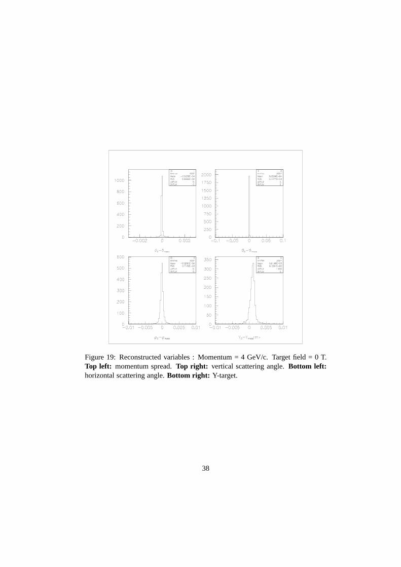
Figure 19: Reconstructed variables : Momentum = 4 GeV/c. Target field = 0 T.Top left: momentum spread.Top right: vertical scattering angle.Bottom left:horizontal scattering angle.Bottom right: Y-target.

38

Figure 20: Reconstructed variables : Momentum = 4 GeV/c. Target field = 5 T.Top left: momentum spread.Top right: vertical scattering angle.Bottom left:horizontal scattering angle.Bottom right: Y-target.

39

Figure 21: Reconstructed variables : Momentum = 1 GeV/c. Target field = 5 T.Top left: momentum spread.Top right: vertical scattering angle.Bottom left:horizontal scattering angle.Bottom right: Y-target.

40

Figure 22: Reconstructed variables : Momentum = 0.4 GeV/c. Target field = 5 T.Top left: momentum spread.Top right: vertical scattering angle.Bottom left:horizontal scattering angle.Bottom right: Y-target.

41

6 Analysis Method

6.1 Extraction of the g2 Structure Function

We will perform a polarized cross section measurement in order to determine thespin structure functiongp

2 . The spin structure functions are related to the spin-dependent cross sections via:

g1 =MQ2

4α2e

y

(1 − y)(2 − y)

[

∆σ‖ + tanθ

2∆σ⊥

]

g2 =MQ2

4α2e

y2

2(1 − y)(2 − y)

[

−∆σ‖ +1 + (1 − y) cos θ

(1 − y) sin θ∆σ⊥

]

(26)

wherey = ν/E.Here, the polarized cross section differences are represented by∆σ‖ and∆σ⊥.

Measuring polarized cross section differences results in the cancellation of the con-tribution from any unpolarized target material and obviates the need for any exter-nal model input.

We can recast Eq. 26 in the form:

g1 = K1(a1∆σ‖ + b1∆σ⊥)

g2 = K2(c1∆σ‖ + d1∆σ⊥) (27)

where

K1 =MQ2

4α2e

y

(1 − y)(2 − y)

K2 =MQ2

4α2e

y2

2(1 − y)(2 − y)= K1

y

2

a1 = 1

b1 = tanθ

2c1 = −1

d1 =1 + (1 − y) cos θ

(1 − y) sin θ

Equation 27 reveals that the parallel contribution tog2 is highly suppressed(See Fig. 23). In fact, the relative weight of the∆σ‖ contribution tog2 ranges from2 to 8% for all proposed kinematics. For the kinematics wherewe will not measure∆σ‖, we will use the high precision data from Hall B experiment EG4 [11], which

42

1000 1200 1400 1600 1800 2000W (GeV)

0

0.02

0.04

0.06

0.08

0.1

|c1/d1|

9o settings

6o settings

Figure 23: Relative weighting of the∆σ‖ contribution tog2. See Eq. 27.

0.01 0.1

Q2 (GeV

2)

0

0.2

0.4

0.6

0.8

1

δLT

(Q2) W

max = 2.0 GeV

δLT

(Q2) W

max = 1.7 GeV

ratio

Figure 24: MAID model prediction forδLT (Q2) evaluated with a maximum W of1.7 and 2.0 GeV, along with the ratio. Over 90% of the integralstrength comesfrom W less than 1.7 GeV.

43

expects an uncertainty of approximately 10%. Given the ratio of |c1/d1|, this leadsto less than 1% error contribution to ourg2 for all kinematics.

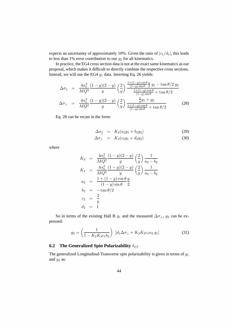
In practice, the EG4 cross section data is not at the exact same kinematics as ourproposal, which makes it difficult to directly combine the respective cross sections.Instead, we will use the EG4g1 data. Inverting Eq. 26 yields:

∆σ‖ =4α2

e

MQ2

(1 − y)(2 − y)

y

(

2

y

)

1+(1−y) cos θ(1−y) sin θ

y2 g1 − tan θ/2 g2

1+(1−y) cos θ(1−y) sin θ + tan θ/2

∆σ⊥ =4α2

e

MQ2

(1 − y)(2 − y)

y

(

2

y

) 2yg1 + g2

1+(1−y) cos θ(1−y) sin θ + tan θ/2

(28)

Eq. 28 can be recast in the form:

∆σ‖ = K3(a2g1 + b2g2) (29)

∆σ⊥ = K4(c2g1 + d2g2) (30)

where

K3 =4α2

e

MQ2

(1 − y)(2 − y)

y

(

2

y

)

1

a2 − b2

K4 =4α2

e

MQ2

(1 − y)(2 − y)

y

(

2

y

)

1

a2 − b2

a2 =1 + (1 − y) cos θ

(1 − y) sin θ

y

2

b2 = − tan θ/2

c2 =2

y

d2 = 1

So in terms of the existing Hall Bg1 and the measured∆σ⊥, g2 can be ex-pressed:

g2 =

(

1

1 − K2K3c1b2

)

[d1∆σ⊥ + K2K3c1a2 g1] (31)

6.2 The Generalized Spin PolarizabilityδLT

The generalized Longitudinal-Transverse spin polarizability is given in terms ofg1

andg2 as:

44

δLT (Q2) =16αM2

Q6

∫ x0

0x2

[

g1(x,Q2) + g2(x,Q2)]

dx. (32)

For the kinematics where we do not measureg1 directly we will utilize the re-sults of EG4 [11]. Our proposal includes settings (see Table6) where we will rotatethe target and measure∆σ‖ in addition to∆σ⊥ in order to cross check the Hall Bdata. Table 9 details the projected EG4 statistical uncertainties [70]. Our beamtime request typically aims to match or improve on these errors so that the com-bined data set is consistent. As for systematic uncertainties, EG4 projects about10% error, which includes a contribution from their lack of knowledge of trans-verse data. The effect of our transverse data on the EG4 systematic is discussed inSection 4.2.

6.3 Interpolation to Constant Q2

The data measured at constant incident energy and scattering angle will be inter-polated† to constantQ2 as shown in Fig. 13. The good kinematic coverage andoverlap should facilitate a straight forward interpolation.

6.4 Systematic Uncertainties

Several JLab experiments have performed measurements similar to what we pro-pose here (for example, see Refs. [3, 4, 10, 11]). From these previous endeavors,we can make an estimate of the systematic uncertainty. Table4 gives an estimateof the most significant sources of error, while Table 5 gives further detail on thecontributions to the cross section uncertainty which will be the dominant error.Previous experience in Hall A [3] has shown that we can obtain4-5% systematicuncertainty [66–68] on cross section measurements, with the largest uncertainty(2-3%) coming from the knowledge of the acceptance. Discussion with the HallA septum/optics expert [64], indicates that, in the worst case, the presence of the5 Tesla target field and the use of the septum will only increase the acceptanceuncertainty by a factor of 2.

An 8%‡ systematic uncertainty on the moments is assumed in Figs. 25to 28of section 7.2. Eq. 32 reveals that the unmeasured low-x contribution to δLT issuppressed asx2. In fact, over 90% of the total integral strength (as predicted fromthe MAID model) is covered in the range from pion threshold toW = 1.7 GeV foreach of our incident energies. The unmeasured contributionaboveW = 2 GeV isvery small and introduces a negligible uncertainty (See Fig. 24).

†as has been done in experiments E94010, E97110 and E01012.‡relative to the MAID model prediction.

45

Source (%)

Cross section 5-7Target Polarization 3.0Beam Polarization 3.0Radiative Corrections 3.0Parallel Contribution ≤ 115N asymmetry [69] ≤ 1

Total 7-9

Table 4: Total Systematic Uncertainties.

Source (%)

Acceptance 4-6Packing fraction 3.0Charge determination 1.0VDC efficiency 1.0PID detector efficiencies ≤1Software cut efficiency ≤1Energy 0.5Deadtime 0.0

Total 5-7

Table 5: Major contributions to the cross section systematic of Table 4.

46

7 Rates and Beam Time Request

The count rate of scattered electrons from the polarized target is given by:

N =L∆Ω∆E′σ

f(33)

whereL is the luminosity,∆Ω is the angular acceptance,∆E′ is the momentumbite, σ represents the proton cross section, andf is the dilution factor which ac-counts for scattering from unpolarized nucleons in the target.

We estimate the experimental cross section by combining proton, nitrogen andhelium cross sections from the quasifree scattering model QFS [59, 88]. Inelasticand elastic radiative effects are also included. Table 10 shows the assumed mate-rial thickness for a 3 cm target. At the lowest plannedQ2, the elastic radiative tailbecomes large and we switch to a thinner (0.5 cm) target cell.Cross-checks withthe longer standard cell will help to reduce the systematic uncertainty of the radia-tive corrections, and ensure we have a good understanding ofour target packingfraction. A representative spin-independent cross section is shown in Fig. 29.

The time needed for a given uncertaintyδA is given by:

T =1

N(fPbPT δA)2(34)

The relevent statistical uncertainty is for the asymmetry,even though this is a crosssection measurement, because in the productσA the dominant error arises fromA.

The running time and spectrometer configurations are summarized in Table 6.The sixth column represents the rate (in each bin) from the proton, while the sev-enth shows the total prescaled rate seen by the spectrometer. When the momentumof the scattered electron is accessible by both spectrometers, we double our DAQrate. We assume a maximum accessible momentum of 3.1 and 4.3 GeV for theright and left HRS respectively. We also assume both spectrometers can reach 0.4GeV minimum momentum, and that the DAQ limit is 4 kHz per arm§.

Transverse data will be measured for every kinematic. Table6 specifies thesettings where we plan to also take data with the target polarization held parallelto the beam momentum. This is in order to directly extractg1 and provide a crosscheck with the EG4 data. This effectively doubles the time needed for this setting,so the kinematic to perform the longitudinal measurement has been chosen to beat the largestQ2 for which both arms can simultaneously take data for all chosenmomentum settings.

§More than 5 kHz rate with manageable deadtime was demonstrated with the existing DAQ duringE97110 [10].

47

To reach the highestQ2 will require the septum to run 391 A at 6 degrees(P0=4.15 GeV) and almost 530 A at 9 degrees (P0=4.0 GeV). Discussion withHall A septum experts [64, 65] indicate that all of the planned 6 degree settingsshould be achievable, although the septum must be trained toreach a few of thehigher currents required. All of the 9 degree settings are also within the nominallimits, but the 9 degree, 4.0 GeV setting in particular may prove difficult. This hasminimal impact on the physics goals of this experiment, since it affects only onekinematic setting at the highestQ2 (see Fig. 13). To adjust to this circumstance wecan perform an extrapolation for the small affected region,or simply reduce ourhighest expectedQ2 by a small amount.

The choice of parameters used in our rate calculation is summarized in Ta-ble 10. We assume an angular acceptance of 4 msr and a momentumacceptanceof ±4%, both slightly reduced from the nominal values due to the presence ofthe septa, and beam and target polarizations of 80 and 75% respectively. We notethat higher polarization values are routinely achieved. Finally, we assume that theminimum time that we would reasonably spend at each setting is one half hour,regardless of how high the rate is.

With this beam request, we achieveδA⊥ = 0.004 for each 20 MeV bin.

7.1 Overhead

The incident beam causes radiation damage in the frozen ammonia, which leadsto the creation [60, 61] of atomic hydrogen in the target material. This providesan additional relaxation path for the nuclear spins, and thebuildup of these freeradicals leads to a gradual decay of the target polarization. The concentration ofthese unwanted radicals can be reduced significantly by raising the temperature ofthe target to 80-90K, in a process known as annealing. Given the proposed beamcurrent and raster size, we expect to require an anneal aboutonce every 14 hours ofbeam time. The anneal itself typically requires 2.5 hours from start to beam backon target. The target stick holds two ammonia batches. Each batch can absorbapproximately 17·1015 e-/cm2, at which point the material must be replaced. Weexpect to swap out target inserts about once every 5 days of accumulated (100% ef-ficient) beam. To replace the stick and calibrate the NMR instrumentation requiresabout a shift.

Measuringg1 will require physically rotating the target can from the perpen-dicular to parallel configuration, a process which we estimate will take two shifts.One final overhead arising from the target comes from the needfor dedicated emptycell and carbon target runs, which are used to determine the granular target pack-ing fraction and dilution factor. These high rate unpolarized runs can be completedin about one half hour, and we plan to perform them for every other momentum

48

setting.Pass changes and linac changes are estimated to require 4 and8 hours respec-

tively. Changing the spectrometer momentum settings requires approximately 15minutes each on average, while changes to the septa angle typically takes one shift.We will perform one Moller measurement for each beam energy,each of whichrequires two hours. Finally, we have included an additional8 hours of overheadto measure the elastic cross section and asymmetry for the lowest two energies,as a cross check of our beam and target polarizations, and to help ensure we fullyunderstand all cross section systematics.

The overhead requirement is summarized in Table 8. We note that previousexperience has shown that many overhead tasks can be performed in parallel, orscheduled to coincide with non-delivery of beam. In this sense, our overhead esti-mate should be conservative.

7.2 Projected Results

Figs. 25 to 27 show the projected accuracy we can obtain with the beam time re-quest of Table 6. The systematic error bands on the axes represent the total fromTable 4. The projected uncertainties have been evaluated assuming the centralvalues predicted by the MAID model [17]. The integralIB(Q2) in Fig. 28 corre-sponds to Eq. 8 when the Gilman convention [89] is chosen for the virtual photonflux factorK.

8 Summary

We request 24 days in order to perform a precision measurement of gp2 at low and

moderateQ2 using a transversely polarized proton (NH3) target, together with theHall A HRS and septa. This measurement is needed to provide data on the trans-verse spin structure of the proton and to resolve several outstanding issues. TheQ2−evolution ofdp

2(Q2), the BC and extended GDH Sum will be obtained, along

with the longitudinal-transverse spin polarizabilityδLT , a fundamental quantitywhich characterizes the nucleon’s structure. This data will fill the gap in our knowl-edge of the proton spin structure functiongp

2 , and address intriguing discrepanciesbetween data and theory for the BC Sum Rule and the longitudinal-transverse gen-eralized spin polarizability. It will also have significantimpact on ongoing calcu-lations of the hyperfine structure of hydrogen, and substantially reduce one of theleading systematic uncertainties of the EG4 experiment.

49

0.01 0.1 1 10

Q2 (GeV

2)

-0.03

0

0.03

0.06

0.09E07-001 projectedSyst (unmeas region)Syst (meas region) Elastic Maid E155x (Total) RSS (Resonance) RSS + DIS + Elastic

Preliminary

E07-001 Projected

Figure 25: Projected results forΓp2. Statistical errors are shown on the symbols.

Systematic for measured region is represented by the light band. Systematic forunmeasured region is represented by the dark band. Uncertainties for the measuredregion are evaluated assuming the central value predicted by the MAID [17] model.Systematic for the unmeasured region is 100% of the model prediction assumingBC sum rule holds. Elastic curve is from Ref. [62].

50

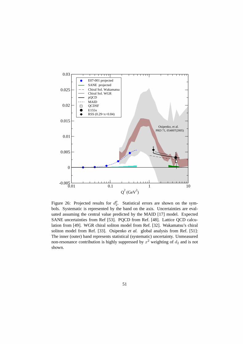
0.01 0.1 1 10

Q2 (GeV

2)

-0.005

0

0.005

0.01

0.015

0.02

0.025

0.03

E07-001 projected SANE projected Chiral Sol. Wakamatsu Chiral Sol. WGR pQCD MAID QCDSF E155x RSS (0.29<x<0.84)

Osipenko, et al. PRD 71, 054007(2005)

Figure 26: Projected results fordp2. Statistical errors are shown on the sym-

bols. Systematic is represented by the band on the axis. Uncertainties are eval-uated assuming the central value predicted by the MAID [17] model. ExpectedSANE uncertainties from Ref [53]. PQCD from Ref. [48]. Lattice QCD calcu-lation from [49]. WGR chiral soliton model from Ref. [32]. Wakamatsu’s chiralsoliton model from Ref. [33]. Osipenkoet al. global analysis from Ref. [51]:The inner (outer) band represents statistical (systematic) uncertainty. Unmeasurednon-resonance contribution is highly suppressed byx2 weighting ofd2 and is notshown.

51

0.1

Q2 (GeV

2)

-1

0

1

2

3

δ LT [

10-4

fm4 ]

Bernard et al. (VM+∆)Bernard et al.

Kao et al. O(p3 + p

4)

MAIDE07-001 Projected

Figure 27: Projected results forδLT . Statistical errors are shown on the symbols.Systematic is represented by the grey band on the axis. Uncertainties are evaluatedassuming the central value predicted by the MAID [17] model.χPT predictionsfrom Bernardet al. [38], and Kaoet al. [39].

52

0.01 0.1 1

Q2 (GeV

2)

-300

-200

-100

0

I B

(µb)

MAIDHermes (Tot)Hermes (Res)Preliminary RSS (Res)Preliminary RSS (Tot)E07-001 projected

Figure 28: Projected results for the GDH IntegralITT (Q2). Statistical errors areshown on the symbols. Systematic is represented by the band on the axis. Un-certainties are evaluated assuming the central value predicted by the MAID [17]model, scaled here to satisfy the GDH Sum Rule prediction (star). Also shown isHERMES [36], and RSS [4] preliminary data.

53

A Beam Time Request Tables

In this section we detail the proposed kinematics and beam time request. In Table 6,all energies and momenta are in GeV, while the luminosity is given in (cm2-s)−1.

Table 8 summarizes the expected overhead, which was discussed in section 7.1.The expected statistical error is given in Table 9. Table 6 specifies whether we willmeasure data in the perpendicular configuration alone, or inboth perpendicular andparallel configuration for each kinematic. Finally, for reference, in Table 10 we listthe relevent experimental parameters that we have assumed in the rate calculation.

Table 6: Beam Time Request.

E0 Θ P0 W Q2 Rate P Rate Pre L PbPt I Time(Hz) (kHz) (nA) (h)

1.1 6 0.950 1.07 0.011 55 4.0 6 0.1E+35 0.60 85 6.71.1 6 0.871 1.14 0.010 58 4.0 4 0.1E+35 0.60 85 6.51.1 6 0.800 1.20 0.010 70 4.0 3 0.1E+35 0.60 85 5.31.1 6 0.734 1.25 0.009 82 4.0 3 0.1E+35 0.60 85 4.51.1 6 0.674 1.29 0.008 86 4.0 2 0.1E+35 0.60 85 4.31.1 6 0.618 1.33 0.007 93 4.0 2 0.1E+35 0.60 85 4.01.1 6 0.567 1.37 0.007 103 4.0 2 0.1E+35 0.60 85 3.61.1 6 0.521 1.40 0.006 113 4.0 2 0.1E+35 0.60 85 3.31.1 6 0.478 1.43 0.006 125 4.0 2 0.1E+35 0.60 85 3.01.1 6 0.439 1.45 0.005 139 4.0 2 0.1E+35 0.60 85 2.71.1 6 0.403 1.48 0.005 154 4.0 2 0.1E+35 0.60 85 2.41.1 6 0.369 1.50 0.004 170 4.0 2 0.1E+35 0.60 85 2.2

1.0 days

1.7 6 1.540 1.07 0.029 46 4.0 2 0.1E+35 0.60 85 8.01.7 6 1.414 1.18 0.026 54 4.0 2 0.1E+35 0.60 85 6.91.7 6 1.297 1.27 0.024 66 4.0 1 0.1E+35 0.60 85 5.61.7 6 1.191 1.35 0.022 65 4.0 1 0.1E+35 0.60 85 5.71.7 6 1.093 1.41 0.020 72 4.0 1 0.1E+35 0.60 85 5.11.7 6 1.003 1.47 0.019 83 4.0 1 0.1E+35 0.60 85 4.51.7 6 0.920 1.53 0.017 93 4.0 1 0.1E+35 0.60 85 4.01.7 6 0.845 1.57 0.016 96 4.0 1 0.1E+35 0.60 85 3.91.7 6 0.775 1.61 0.014 98 3.9 1 0.1E+35 0.60 85 3.81.7 6 0.712 1.65 0.013 103 3.8 1 0.1E+35 0.60 85 3.61.7 6 0.653 1.68 0.012 113 4.0 1 0.1E+35 0.60 85 3.31.7 6 0.599 1.71 0.011 122 4.0 1 0.1E+35 0.60 85 3.11.7 6 0.550 1.74 0.010 129 4.0 1 0.1E+35 0.60 85 2.91.7 6 0.505 1.76 0.009 138 4.0 1 0.1E+35 0.60 85 2.71.7 6 0.463 1.79 0.009 147 4.0 1 0.1E+35 0.60 85 2.51.7 6 0.425 1.81 0.008 158 4.0 1 0.1E+35 0.60 85 2.41.7 6 0.390 1.83 0.007 170 4.0 1 0.1E+35 0.60 85 2.2

1.5 days

2.2 6 2.030 1.07 0.049 45 4.0 13 0.8E+35 0.60 85 8.22.2 6 1.863 1.21 0.045 54 4.0 11 0.8E+35 0.60 85 6.92.2 6 1.709 1.33 0.041 58 4.0 8 0.8E+35 0.60 85 6.42.2 6 1.569 1.42 0.038 65 4.0 6 0.8E+35 0.60 85 5.72.2 6 1.440 1.51 0.035 77 4.0 5 0.8E+35 0.60 85 4.92.2 6 1.321 1.58 0.032 80 4.0 5 0.8E+35 0.60 85 4.72.2 6 1.213 1.64 0.029 83 4.0 4 0.8E+35 0.60 85 4.5

continued on next page

54

Table 6: Beam Time Request.

E0 Θ P0 W Q2 Rate P Rate Pre L PbPt I Time(Hz) (kHz) (nA) (h)

2.2 6 1.113 1.70 0.027 87 4.0 4 0.8E+35 0.60 85 4.32.2 6 1.022 1.75 0.025 89 4.0 4 0.8E+35 0.60 85 4.22.2 6 0.938 1.80 0.023 93 4.0 4 0.8E+35 0.60 85 4.02.2 6 0.860 1.84 0.021 96 4.0 5 0.8E+35 0.60 85 3.92.2 6 0.790 1.87 0.019 101 4.0 5 0.8E+35 0.60 85 3.72.2 6 0.725 1.91 0.017 107 4.0 5 0.8E+35 0.60 85 3.52.2 6 0.665 1.94 0.016 113 4.0 5 0.8E+35 0.60 85 3.32.2 6 0.610 1.96 0.015 120 4.0 6 0.8E+35 0.60 85 3.12.2 6 0.560 1.99 0.013 128 4.0 6 0.8E+35 0.60 85 2.92.2 6 0.514 2.01 0.012 137 4.0 7 0.8E+35 0.60 85 2.7

1.6 days

3.3‡ 6 3.096 1.07 0.112 29 4.0 7 0.8E+35 0.60 85 12.73.3‡ 6 2.841 1.28 0.103 39 4.0 6 0.8E+35 0.60 85 9.43.3‡ 6 2.608 1.44 0.094 42 4.0 4 0.8E+35 0.60 85 8.73.3‡ 6 2.393 1.58 0.087 50 4.0 3 0.8E+35 0.60 85 7.53.3‡ 6 2.196 1.69 0.079 54 4.0 2 0.8E+35 0.60 85 6.93.3‡ 6 2.016 1.79 0.073 57 4.0 2 0.8E+35 0.60 85 6.53.3‡ 6 1.850 1.88 0.067 61 4.0 2 0.8E+35 0.60 85 6.13.3‡ 6 1.698 1.96 0.061 65 4.0 1 0.8E+35 0.60 85 5.73.3‡ 6 1.558 2.02 0.056 69 4.0 1 0.8E+35 0.60 85 5.4

2.9 days

4.4 6 4.149† 1.07 0.200 22 4.0 5 0.8E+35 0.60 85 16.74.4 6 3.808† 1.34 0.184 29 4.0 4 0.8E+35 0.60 85 12.94.4 6 3.495† 1.55 0.168 33 4.0 2 0.8E+35 0.60 85 11.44.4 6 3.207† 1.72 0.155 34 4.0 2 0.8E+35 0.60 85 10.74.4 6 2.944 1.86 0.142 36 4.0 1 0.8E+35 0.60 85 10.34.4 6 2.701 1.98 0.130 40 4.0 1 0.8E+35 0.60 85 9.44.4 6 2.479 2.09 0.120 44 4.0 1 0.8E+35 0.60 85 8.4

2.7 days

4.4 9 4.023† 1.07 0.436 14 2.5 1 0.8E+35 0.60 85 25.24.4 9 3.692† 1.34 0.400 17 2.2 1 0.8E+35 0.60 85 21.44.4 9 3.389† 1.55 0.367 16 2.0 1 0.8E+35 0.60 85 22.44.4 9 3.110† 1.72 0.337 14 1.7 1 0.8E+35 0.60 85 25.64.4 9 2.854 1.86 0.309 12 1.4 1 0.8E+35 0.60 85 31.24.4 9 2.620 1.98 0.284 11 1.2 1 0.8E+35 0.60 85 33.14.4 9 2.404 2.09 0.260 11 1.1 1 0.8E+35 0.60 85 33.7

6.0 days

† signifies that only the left spectrometer can access this momentum.‡ signifies that longitudinal data will be taken in addition totransverse.

55

Table 7: Beam Request Summary.

Days using 1 (2) arms 25.2 (15.7)Days for Overhead 8.4 ( 8.4)Total Days using 1 (2) arms 33.6 (24.1)

Table 8: Overhead

Overhead Number Time Per (hr) (hr)Target anneal 27 2.5 67.5Target rotation 2 16.0 32.0Target swap 2 8.0 16.0Pass change 6 4.0 24.0Packing Fraction 34 0.50 17.0Linac change 0 8.0 0.0Momentum change 69 0.25 17.2Moller measurement 6 2.0 12.0Septum angle change 1 8.0 8.0Elastic calibration 2 4.0 8.0

201.8

Table 9: Statistical Uncertainty

Kinematic A‖ error A⊥ error1 0.004⋆ 0.0042 0.004⋆ 0.0043 0.004⋆ 0.0044 0.004 0.0045 0.004⋆ 0.0046 0.004⋆ 0.004

⋆ EG4 expected uncertainty.

Table 10: Experiment Parameters

Parameter Value∆Ω [msr] 4.0±δP [%] 4.0PTarget [%] 75.0PBeam [%] 80.0Tb radiation length 0.026Ta radiation length 0.026Minimum time per setting [hr] 0.5Minimum Momentum [MeV] 400.0Maximum Momentum (L) [MeV] 4300.0Maximum Momentum (R) [MeV] 3100.0Daq Limit [kHz] 4.0Packing Fraction 0.55

56

1000 1200 1400 1600 1800 2000W (MeV)

100

101

102

103

104

nb/M

eV−

sr

σtotal

σNit inel

σNit elas

σH3 inel

σH3 elas

σHe inel

σHe elas

Figure 29: NH3 cross section atE0 = 2.2 GeV,6.

57

References

[1] See,e.g., B. W. Filippone and X. Ji, Adv. Nucl. Phys.26, 1 (2001).

[2] J. D. Bjorken, Phys. Rev.148, 1467 (1966).

[3] M. Amarianet al., Phys. Rev. Lett.89, 242301 (2002);92, 022301 (2004);93,152301 (2004); K. Slifer,et al., [E94010 Collaboration] in preparation.

[4] JLab RSS experiment, M. Jones and O Rondon, spokespersons ; F. R. Wes-selmannet al. Phys. Rev. Lett.98, 132003 (2007). K. Slifer,et al., [RSSCollaboration] in preparation.

[5] R. Fatemiet al., Phys. Rev. Lett.91, 222002 (2003).

[6] J. Yunet al., Phys. Rev.C 67, 055204 (2003).

[7] A. Deur et al., Phys. Rev. Lett.93, 212001 (2004).

[8] K.V. Dharmawardaneet al., Phys. Lett.B 64111 (2006); Y. Proket al., to bepublished.

[9] J.-P. Chen, A. Deur and Z.-E. Meziani, Mod. Phys. Lett.A 20, 2745 (2005);J.-P. Chen, nucl-ex/0611024 (2006).

[10] JLab experiment E97-110, J. P. Chen, A. Deur, F. Garibaldi, spokespersons.

[11] JLab run group Eg4, M. Battaglieri, R. De Vita, A. Deur, M. Ripanispokespersons. http://www.jlab.org/expprog/proposals/03/PR03-006.pdf

[12] JLab E01-012, J. P. Chen, S. Choi and N. Liyanage, spokespersons.

[13] J. Callan, G. Curtis. and D. J. Gross, Phys. Rev. Lett.22, 156 (1969).

[14] R. L. Jaffe, Comments Nucl. Part. Phys.19, 239 (1990).

[15] S. Wandzura and F. Wilczek, Phys. Lett.B72, 195 (1977).

[16] S. B. Gerasimov, Sov. J. Nucl. Phys.2, 598 (1965); S. D. Drell and A. C.Hearn, Phys. Rev. Lett.16, 908 (1966).

[17] D. Drechsel, S. S. Kamalov and L. Tiator, Phys. Rev.D 63, 114010 (2001).

[18] X. Ji and J. Osborne, J. of Phys. G27, 127 (2001).

[19] D. Drechsel, B. Pasquini and M. Vanderhaeghen, Phys. Rep. 378, 99 (2003);D. Drechsel and L. Tiator, Ann. Rev. Nucl. Part. Sci.54, 69 (2004).

[20] H. Burkhardt and W. N. Cottingham, Ann. Phys. (N.Y.)56, 453 (1970).

[21] A. V. Manohar, arXiv:hep-ph/9204208.

[22] R. L. Jaffe and X.-D. Ji, Phys. Rev.D43, 724 (1991).

[23] J. Soffer and O. V. Teryaev, Phys. Lett.B545, 323 (2002) .

58

[24] V. Bernard, N. Kaiser, and U.-G. Meissner, Int. J. Mod. Phys.E4, 193 (1995).

[25] A. W. Thomas and W. Weise,The Structure of the Nucleon(Wiley-Vch,Berlin, 2001).

[26] P. L. Anthony et al. [E155 Collaboration], Phys. Lett. B553, 18 (2003)[arXiv:hep-ex/0204028].

[27] K. Kramer et al., Phys. Rev. Lett.95, 142002 (2005) [arXiv:nucl-ex/0506005].

[28] S. Simula, M. Osipenko, G. Ricco and M. Taiuti, Phys. Rev. D 65, 034017(2002) [arXiv:hep-ph/0107036].

[29] J. Yunet al., Phys. Rev. C67 055204, (2003); S. Kuhn, private communica-tion.

[30] M. Stratmann, Z. Phys. C60, 763 (1993).

[31] X. Song, Phys. Rev. D54, 1955 (1996).

[32] H. Weigel and L. Gamberg, Nucl. Phys. A680, 48 (2000); Weigel, Gambergand Reinhardt, Phys. Rev.D55 (1997) 6910.

[33] M. Wakamatsu, Phys. Lett. B487, 118 (2000).

[34] K. Abe et al., Phys. Rev.D 58,112003 (1998).

[35] Z. E. Mezianiet al., Phys. Lett. B613, 148 (2005) [arXiv:hep-ph/0404066].

[36] A. Airapetianet al. [HERMES Collaboration], Eur. Phys. J. C26, 527 (2003)

[37] K. Ackerstaffet al., Phys. Lett.B 404, 383 (1997);B 444, 531 (1998).

[38] V. Bernard, T. Hemmert and Ulf-G. Meissner, Phys. Lett.

[39] C. W. Kao, T. Spitzenberg and M. Vanderhaeghen, Phys. Rev. D 67, 016001(2003).

[40] V. Olmos de Leonet al., Eur. Phys. J.A 10, 207 (2001); J. Tonnisonet al.,Phys. Rev. Lett.80, 4382 (1998).

[41] J. Ahrenset al., Phys. Rev. Lett.87, 022003 (2001).

[42] P. A. M. Guichon, G. Q. Liu and A. W. Thomas, Nucl. Phys.A 591, 606(1995).

[43] P. E. Bostedet al. [CLAS Collaboration], Phys. Rev. C75, 035203 (2007)[arXiv:hep-ph/0607283].

[44] N. I. Kochelev et al, Phys. Rev. D67, 074014 (2003), and private communi-cation.

[45] Marc Vanderhaeghen, JLab Theory Division, private communication.

59

[46] Christian Weiss, JLab Theory Division, private communication.

[47] X. Zhenget al., Phys. Rev.C 70, 065207 (2004).

[48] Edward V. Shuryak and A.I. Vainshtein. Nucl. Phys.B201(1982) 141.

[49] M. Gockeleret al.Phys. Rev.D 63, 074506 (2001). hep-lat/0011091

[50] M. Stratmann, Z. Phys.C60 (1993) 763.

[51] M. Osipenkoet al., Phys. Rev. D71, 054007 (2005).

[52] P. L. Anthonyet al., Phys. Lett.B553(2003) 18.

[53] Hall C Sane experiment. O. Rondon, Z.-E. Meziani and S. Choi spokesmen.Scheduled to run in 2008.

[54] J. Soffer and O. V. Teryaev, Phys. Rev.D 70, 116004 (2004).

[55] V. D. Burkert and B. L. Ioffe, Phys. Lett.B 296, 223 (1992).

[56] X. Ji, C. Kao, and J. Osborne, Phys. Lett. B472, 1 (2000).

[57] JLab experiment E06-014, S. Choi, X. Jiang, Z.E. Meziani and B. Sawatzkyspokespersons.

[58] JLab experiment E12-06-121, T. Averett, W. Korsch, Z.E. Meziani and B.Sawatzky, spokespersons.

[59] K. Slifer, E94010 Technical Note #44: “Modifications tothe QFS and RAD-COR Codes”, (2003).

[60] P. M. McKee NIM A526 (2004) 60-64.

[61] L. De Marco, A, Brill, D. Crabb, J. Chem. Phys. 108 (1998)1423.

[62] E. L. Lomon , PRC 66 04501 (2002).

[63] M. Amarian et al. [Jefferson Lab E94-010 Collaboration], Phys. Rev. Lett.92, 022301 (2004) [arXiv:hep-ex/0310003].

[64] J. Lerose, Hall A Staff. Private communication.

[65] R. Feuerbach, Hall A Staff. Private communication.

[66] K. Slifer, E94010 Technical Note #37 : “Dependence of the Cross-Section onAcceptance Cuts for E94010”, (2001)

[67] K. Slifer, E94010 Technical Note #38 : “E94010 Unpolarized 3He CrossSections”, (2001)

[68] K. Slifer, Ph.D. Thesis. Temple University (2004).

[69] Mark Jones, “The15N correction to the measured asymmetries”, RSS techni-cal note 2005-01 (2005).

60

[70] M. Ripani’s EG4 analysis webpage :http://www.jlab.org/Hall-B/secure/eg4/ripani/analysis.html

[71] JLab E05-004 : R. Gilman, D.W. Higinbotham, X. Jiang, spokespersons.‘A(Q) at lowQ in eD Elastic Scattering’.

[72] Private communication, Arne Freyberger.

[73] L. Kaufman, K. Pascke, R. Michaels, “Cavity Monitor Performance in2005”, http://hallaweb.jlab.org/experiment/HAPPEX/docs/, HAPPEX tech-note, (2006).

[74] J. Benesch, JLab Center for Advanced Studies of Accelerators (CASA). pri-vate communication.

[75] C. Yan, R. Carlini, “Chicane and raster system for Hall C”, CEBAF-R-92-004, (1992).

[76] J. Alcornet al., Nucl. Instrum. Meth. A522, 294 (2004).

[77] V. Nazaryan, C. E. Carlson and K. A. Griffioen, Phys. Rev.Lett. 96, 163001(2006) [arXiv:hep-ph/0512108].

[78] PR-07-004 : J. Arrington, D. Day, R. Gilman, G. Ron(contact). Update sub-mitted to PAC33.

[79] A. C. Zemach, Phys. Rev.104, 1771 (1956 ).

[80] C. K. Iddings, Phys. Rev.138, B446 (19 65).

[81] R. N. Faustov and A. P. Martynenko, Eur. Phys. J. C24, 281 (2002);R. N. Faustov and A. P. Martynenko, Phys. Atom. Nucl.65, 265 (2002) [Yad.Fiz. 65, 291 (2002)].

[82] E. De Rafael, Phys. Lett. B37, 201 (1971).

[83] P. Gnadig and J. Kuti, Phys. Lett. B42, 241 (1972).

[84] S. D. Drell and J. D. Sullivan, Phys. Rev.154, 1477 (1967).

[85] A. V. Volotka, V. M. Shabaev, G. Plunien and G. Soff, Eur.Phys. J. D33, 23(2005).

[86] Mainz Proposal A1/01-00: “Double polarization Virtual Compton Scatteringin the threshold regime”. http://wwwa1.kph.uni-mainz.de/A1/publications/proposals/

[87] H. Fonvieille, “Virtual Compton scattering at low energy and the general-ized polarizabilities of the nucleon,” Prog. Part. Nucl. Phys. 55, 198 (2005)[arXiv:hep-ph/0412074].

[88] J.W. Lightbody Jr. and J.S. O’Connell, Computers in Physics,57 May/June1988.

[89] F. J. Gilman, Phys. Rev.167, 1365 (1968).

61