Terms and Conditions of Use:

this document downloaded from

vulcanhammer.infothe website about Vulcan Iron Works Inc. and the pile driving equipment it manufactured

All of the information, data and computer software (“information”) presented on this web site is for general information only. While every effort will be made to insure its accuracy, this information should not be used or relied on for any specific application without independent, competent professional examination and verification of its accuracy, suit-ability and applicability by a licensed professional. Anyone making use of this information does so at his or her own risk and assumes any and all liability resulting from such use. The entire risk as to quality or usability of the information contained within is with the reader. In no event will this web page or webmaster be held liable, nor does this web page or its webmaster provide insurance against liability, for any damages including lost profits, lost savings or any other incidental or consequential damages arising from the use

or inability to use the information contained within.

This site is not an official site of Prentice-Hall, Pile Buck, or Vulcan Foundation Equipment. All references to sources of software, equipment, parts, service or

repairs do not constitute an endorsement.

Visit our companion sitehttp://www.vulcanhammer.org

CIVIL ENGINEERING STUDIES Illinois Center for Transportation Series No. 14-021

UILU-ENG-2014-2023 ISSN: 0197-9191

IMPROVED DESIGN FOR DRIVEN PILES BASED ON A PILE LOAD TEST PROGRAM

IN ILLINOIS: PHASE 2 Prepared By

Jim Long University of Illinois at Urbana-Champaign

Andrew Anderson University of Illinois at Urbana-Champaign

Research Report No. FHWA-ICT-14-019

A report of the findings of ICT-R27-122

Improvement of Driven Pile Installation and Design in Illinois: Phase 2

Illinois Center for Transportation

September 2014

Technical Report Documentation Page 1. Report No.FHWA-ICT-14-019

2. Government Accession No. 3. Recipient's Catalog No.

4. Title and Subtitle

Improvement of Driven Pile Installation and Design in Illinois: Phase 2

5. Report DateSeptember 2014

6. Performing Organization Code

7. Author(s)James Long, Andrew Anderson

8. Performing Organization Report No.ICT-14-021 UILU-2014-2023

9. Performing Organization Name and AddressIllinois Center for Transportation Department of Civil and Environmental Engineering University of Illinois at Urbana-Champaign 205 N. Mathews Ave., MC-250 Urbana, IL 61801

10. Work Unit No. (TRAIS)

11. Contract or Grant No.R27-122

12. Sponsoring Agency Name and AddressIllinois Department of Transportation Bureau of Materials and Physical Research 126 E. Ash St. Springfield, IL 62704

13. Type of Report and Period Covered

14. Sponsoring Agency Code

15. Supplementary Notes

16. AbstractA dynamic load test program consisting of 38 sites and 111 piles with restrikes was conducted throughout Illinois to improve the Illinois Department of Transportation design of driven piling. Pile types included steel H-piles and closed-ended pipe (shell) piles. Piles were driven into all soil types including clay, silt, sand, shale, and limestone. Predictive methods for estimating pile capacity were investigated and include the K-IDOT (static) method, WSDOT (dynamic formula), WEAP, PDA, and CAPWAP. Pile capacities were taken as the capacity estimated using CAPWAP for beginning of restrike conditions. Piles were monitored during initial driving. Piles were re-driven several days later to assess the amount of setup to assess the effect of time, pile type and soil type. Restrikes were conducted typically between 3 -15 days after initial driving. Modifying WSDOT to include effects of setup explicitly with specific equations (Skov and Denver, 1988) for time dependent setup was not any more precise than the original WSDOT formula with adjustments for pile type. Accordingly recommendations are made for adjusting WSDOT estimates based on whether the pile is an H-pile or a shell pile. Adjustments were made to the simplified stress formula (SSF) to refine predictions of stresses in driven H- and Shell piles driven with diesel hammers. Resistance factors were determined using the First Order Second Moment method for the static method (K-IDOT) and the dynamic formula (WSDOT). Pile types included H-piles and shell piles for both end of driving conditions and for beginning of restrike. Resistance factors were also determined for WEAP and PDA. These resistance factors were determined using the CAPWAP (BOR) capacity as the static capacity for the pile, although it is preferable that the resistance factors be based on static load test. Accordingly, adjustments were made to the resistance factors accounting for the average agreement between capacity determined by CAPWAP(BOR) and capacity determined with a static load test. 17. Key Wordspiles, driven piling, pile capacity, pile setup, LRFD, pile stresses, driving stresses, dynamic formula, bearing capacity

18. Distribution StatementNo restrictions. This document is available to the public through the National Technical Information Service, Springfield, Virginia 22161

19. Security Classif. (of this report)Unclassified

20. Security Classif. (of this page)Unclassified

21. No. of Pages79 + appendices

22. Price

Form DOT F 1700.7 (8-72) Reproduction of completed page authorized

CONTENTS

CHAPTER 1 INTRODUCTION AND DOCUMENTATION OF COLLECTION ....................................... 1

1.1 INTRODUCTION .......................................................................................................................... 1

1.2 COLLECTION EFFORT AND DOCUMENTATION ...................................................................... 1

CHAPTER 2 PREDICTIVE METHODS ................................................................................................. 8

2.1 INTRODUCTION .......................................................................................................................... 8

2.2 STATIC METHODS ..................................................................................................................... 9

2.2.1 Introduction ............................................................................................................................ 9

2.2.2 K-IDOT Method .................................................................................................................... 10

2.3 DYNAMIC FORMULAS ............................................................................................................. 14

2.2.1 WSDOT Formula ................................................................................................................. 14

2.4 WAVE EQUATION ..................................................................................................................... 15

2.5 DYNAMIC TESTING .................................................................................................................. 16

2.5.1 PDA ..................................................................................................................................... 16

2.5.2 CAPWAP ............................................................................................................................. 20

CHAPTER 3 TIME EFFECTS ............................................................................................................. 21

3.1 ASSESSMENT OF SETUP MAGNITUDE AND GENERAL TRENDS ....................................... 21

3.2 DETERMINATION OF RATE OF SETUP .................................................................................. 24

3.3 NORMALIZATION TO 14-DAY CAPACITY ............................................................................... 29

3.4 TIME EFFECTS APPLIED TO WSDOT ..................................................................................... 29

3.5 LIMITATIONS ............................................................................................................................ 30

3.6 ASSESSING RELAXATION POTENTIAL OF END-BEARING PILES IN SHALE ..................... 30

CHAPTER 4 PERFORMANCE OF METHODS ................................................................................... 34

4.1 METHOD STATISTICS (CHARTS AND TABLES) .................................................................... 35

4.2 SUMMARY TABLES ................................................................................................................. 46

CHAPTER 5 DEVELOPMENT OF A SIMPLFIED STRESS FORMULA ............................................. 48

5.1 INTRODUCTION ........................................................................................................................ 48

5.2 LIMITATIONS ............................................................................................................................ 48

5.3 REQUIRED INPUT ..................................................................................................................... 49

5.4 SIMPLIFIED STRESS METHOD ................................................................................................ 49

5.4.1 Correction Factors ............................................................................................................... 51

5.4.2 Detailed Discussion for Calculating Step 3 ........................................................................... 51

CHAPTER 6 DYNAMIC PILE STRESSES DURING DRIVING ........................................................... 54

i

CHAPTER 7 DEVELOPMENT OF RESISTANCE FACTORS FOR LRFD ......................................... 64

7.1 INTRODUCTION ........................................................................................................................ 64

7.2 REFINEMENT OF WSDOT AND K-IDOT PREDICTIVE METHODS ......................................... 64

7.3 FOSM ......................................................................................................................................... 67

7.4 CALCULATED RESISTANCE FACTORS ................................................................................. 68

7.5 RESISTANCE FACTORS MODIFIED TO ACCOUNT FOR STATIC LOAD TESTS .................. 70

7.6 DISCUSSION ............................................................................................................................. 72

CHAPTER 8 CONCLUSIONS ............................................................................................................. 74

8.1 RECOMMENDED CHANGES TO CURRENT PRACTICE ......................................................... 74

8.1.1 K-IDOT ................................................................................................................................ 74

8.1.2 WSDOT ............................................................................................................................... 75

8.1.3 PDA ..................................................................................................................................... 75

8.1.4 CAPWAP ............................................................................................................................. 75

8.1.5 Simplified Stress Formula (SSF) .......................................................................................... 76

8.2 SUMMARY OF SELECTED FINAL RESULTS .......................................................................... 76

8.2.1 Setup Magnitude and Setup Rate ........................................................................................ 76

8.2.2 Relaxation Potential of End-Bearing Piles in Shale .............................................................. 76

8.2.3 K-IDOT ................................................................................................................................ 76

8.2.4 WSDOT ............................................................................................................................... 77

REFERENCES .................................................................................................................................... 78

APPENDIX A PROCEDURE USED TO REPRESENT PREDICTED VERSUS MEASURED RELATIONSHIP .................................................................................................................................. 80

A.1 INTRODUCTION ....................................................................................................................... 80

A.2 LOG-NORMAL DISTRIBUTION ................................................................................................ 80

A.3 PROCEDURE FOR DETERMINING STATISTICAL PARAMETERS ........................................ 80

A.4 DISCUSSION ............................................................................................................................ 81

APPENDIX B SAMPLE CALCULATIONS ......................................................................................... 82

B.1 SAMPLE CALCULATIONS FOR WSDOT ............................................................................... 82

ii

FIGURES

Figure 1-1.Test site locations: 38 sites, 111 piles, 222 tests................................................................... 3 Figure 1-2. Distribution of pile-soil category by research phase. ............................................................ 4 Figure 1-3. Pile-soil category distribution: Total piles tested (%), linear feet driven (%). ......................... 4 Figure 1-4. Distribution of soil category and pile type tested. ................................................................. 5 Figure 1-5. Distribution of pile sections tested. ....................................................................................... 6 Figure 1-6. Single-acting diesel hammers: Manufacturer and model. ..................................................... 7 Figure 2-1. Modified sandy gravel soil strength curve. ......................................................................... 13 Figure 2-2. Model simulating the hammer pile-soil system for one-dimensional wave equation (after Smith 1960). ............................................................................................................................... 16 Figure 2-3. PDA Instrumentation and installation on H-pile (Ng et al. 2011). ........................................ 17 Figure 2-4. Stress-wave propagation (Randolph 2003). ....................................................................... 18 Figure 2-5. Example PDA record: Force and velocity with time. ........................................................... 18 Figure 3-1. Setup ratio (total capacity) vs. setup duration. ................................................................... 22 Figure 3-2. Setup ratio (side resistance) vs. setup duration. ................................................................ 22 Figure 3-3. Setup ratio (total capacity) vs. NSPT average, Na (along embedment length). ..................... 23 Figure 3-4. Setup ratio (side resistance) vs. NSPT average, Na (along embedment length). .................. 23 Figure 3-5. Setup factor C and constants a and b back-calculated for pile-soil category. ..................... 27 Figure 3-6. Setup factor C and selected constants a and b for H-piles and shell piles. ........................ 28 Figure 3-7. Total capacity setup ratio vs. setup period, piles to shale. .................................................. 32 Figure 3-8. End-bearing setup ratio vs. setup period, piles to shale. .................................................... 32 Figure 3-9. Total capacity setup ratio vs. NSPT average, piles to shale. ................................................ 33 Figure 4-1. K-IDOT vs. CAPWAP(BOR_14). ........................................................................................ 37 Figure 4-2. WSDOT(EOD) vs. CAPWAP(BOR_14). ............................................................................ 38 Figure 4-3. WSDOT(BOR) vs. CAPWAP(BOR_14). ............................................................................ 39 Figure 4-4. WSDOT(EOD_14) vs. CAPWAP(BOR_14). ....................................................................... 40 Figure 4-5. WSDOT(BOR_14) vs. CAPWAP(BOR_14). ....................................................................... 41 Figure 4-6. WEAP(EOD) vs. CAPWAP(BOR_14). ............................................................................... 42 Figure 4-7. WEAP(BOR) vs. CAPWAP(BOR_14). ............................................................................... 43 Figure 4-8. PDA(EOD) vs. CAPWAP(BOR_14). .................................................................................. 44 Figure 4-9. PDA(BOR) vs. CAPWAP(BOR_14). .................................................................................. 45 Figure 6-1. Maximum stress vs. CSX at EOD. ..................................................................................... 55 Figure 6-2. Maximum stress vs. CSX at BOR. ..................................................................................... 56 Figure 6-3. WEAP(EOD) maximum stress, (σmax)WEAP(EOD).................................................................... 58 Figure 6-4. WEAP(BOR) maximum stress, (σmax)WEAP(BOR).................................................................... 59 Figure 6-5. SSF(EOD) Co = 0.9, maximum stress, (σmax)SSF(EOD). .......................................................... 60 Figure 6-6. SSF(BOR) Co = 0.9, maximum stress, (σmax)SSF(BOR). .......................................................... 61 Figure 6-7. SSF(EOD) Co = 0.944, maximum stress, (σmax)SSF(EOD). ...................................................... 62 Figure 6-8. SSF(BOR) Co = 0.953, maximum stress, (σmax)SSF(BOR). ...................................................... 63

iii

TABLES

Table 1-1. Test Pile Properties: Pile-Soil Category by Research Phase ................................................. 4 Table 1-2. Test Pile Properties: Soil Type and Pile Type ....................................................................... 5 Table 1-3. Pile Properties: Pile Sections Tested .................................................................................... 6 Table 1-4. Single-Acting Diesel Hammers: Manufacturer and Model ..................................................... 7 Table 2-1. Summary of Capacity Methods Presented ............................................................................ 9 Table 2-2. Summary of Stress Methods Examined ................................................................................ 9 Table 2-3. Kinematic Correction Factors for Side and Tip Resistance .................................................. 12 Table 2-4. Phase 1 K-IDOT Bias Factor and LRFD Resistance Factor ................................................ 13 Table 2-5. Phase 2 K-IDOT Bias Factors and LRFD Resistance Factors ............................................. 14 Table 3-1. Shale Setup Ratio Summary Table ..................................................................................... 31 Table 3-2. Shale Setup Ratio for All Piles to Shale .............................................................................. 33 Table 4-1. K-IDOT Method Statistics by Pile and Soil Type ................................................................. 37 Table 4-2. WSDOT(EOD) Method Statistics by Pile and Soil Type ...................................................... 38 Table 4-3. WSDOT(BOR) Method Statistics by Pile and Soil Type ...................................................... 39 Table 4-4. WSDOT(EOD_14) Method Statistics by Pile and Soil Type ................................................ 40 Table 4-5. WSDOT(BOR_14) Method Statistics by Pile and Soil Type ................................................ 41 Table 4-6. WEAP(EOD) Method Statistics by Pile and Soil Type ......................................................... 42 Table 4-7. WEAP(BOR) Method Statistics by Pile and Soil Type ......................................................... 43 Table 4-8. PDA(EOD) Method Statistics by Pile and Soil Type ............................................................ 44 Table 4-9. PDA(BOR) Method Statistics by Pile and Soil Type ............................................................ 45 Table 4-10. Capacity Method Statistics Summary: H-Piles .................................................................. 46 Table 4-11. Capacity Method Statistics Summary: Shell Piles ............................................................. 46 Table 4-12. Capacity Method Statistics Summary: All Piles ................................................................. 46 Table 4-13. Capacity Method Statistics Summary: Piles in Soil (No Rock) ........................................... 47 Table 6-1. WEAP(EOD) Maximum Stress Statistics, (σmax)WEAP(EOD) ..................................................... 58 Table 6-2. WEAP(BOR) Maximum Stress Statistics, (σmax)WEAP(BOR) ..................................................... 59 Table 6-3. SSF(EOD) Maximum Stress Statistics, Co = 0.9, (σmax)SSF(EOD) ............................................ 60 Table 6-4. SSF(BOR) Maximum Stress Statistics, Co = 0.9, (σmax)SSF(BOR) ............................................ 61 Table 6-5. SSF(EOD) Statistics, Co = 0.944, (σmax)SSF(EOD) ................................................................... 62 Table 6-6. Comparison of WEAP and SSF Maximum Stress Prediction (EOD).................................... 62 Table 6-7. SSF(BOR) Maximum Stress Statistics, Co = 0.953, (σmax)SSF(BOR) ........................................ 63 Table 6-8. Comparison of WEAP and SSF Maximum Stress Prediction (BOR).................................... 63 Table 7-1. WSDOT Recommended Feff Values .................................................................................... 65 Table 7-2. WSDOT(EOD) Statistics with Recommendations Applied ................................................... 65 Table 7-3. WDOT(BOR) Statistics with Recommendations Applied ..................................................... 66 Table 7-4. K-IDOT Statistics with Recommendations Applied .............................................................. 66

iv

Table 7-5. Values of φ for Comparison of Predicted Capacity with CAPWAP(BOR_14) ...................... 70 Table 7-6. Values of φ Adjusted for Comparison with Static Load Test ................................................ 72 Table 8-1. Recommended K-IDOT Kinematic Factors ......................................................................... 74 Table 8-2. WSDOT Recommended Values for Feff for Single-Acting Diesel Hammers ......................... 75

v

ACKNOWLEDGMENT, DISCLAIMER, MANUFACTURERS’ NAMES

This publication is based on the results of ICT-R27-122, Improvement of Driven Pile Installation and Design in Illinois. ICT-R27-122 was conducted in cooperation with the Illinois Center for Transportation; the Illinois Department of Transportation; and the U.S. Department of Transportation, Federal Highway Administration.

Members of the Technical Review Panel are the following:

William Kramer, IDOT (chair) Dan Brydl, FHWA Tom Casey, S.C.I. Engineering Greg Heckel, IDOT Brad Hessing, IDOT Chad Hodel, WHKS Gary Kowalski, IDOT Justan Mann, IDOT Terry McCleary, McCleary Engineering Veniecy Pearman-Green, IDOT Heather Shoup, IDOT Dan Tobias, IDOT

The contents of this report reflect the view of the authors, who are responsible for the facts and the accuracy of the data presented herein. The contents do not necessarily reflect the official views or policies of the Illinois Center for Transportation, the Illinois Department of Transportation, or the Federal Highway Administration. This report does not constitute a standard, specification, or regulation.

Trademark or manufacturers’ names appear in this report only because they are considered essential to the object of this document and do not constitute an endorsement of product by the Federal Highway Administration, the Illinois Department of Transportation, or the Illinois Center for Transportation.

vi

EXECUTIVE SUMMARY

Results are presented for the project, “Improvement of Driven Pile Installation and Design in Illinois: Phase 2.” This phase of research continued to add and interpret dynamic load tests conducted in Phase 1 (Project R27-069). A total of 111 dynamic pile tests and one static load test was performed for Phase 1 and Phase 2 research. The overall project objective was to improve the design of driven piling in Illinois. This included reducing the difference between estimated and driven pile lengths, accounting for the type of pile and soil or rock to assess their effect on developing capacity, to reduce the risk of damage during installation by developing a predictive method for estimating stresses during pile driving, and developing resistance factors based on the results of the dynamic load tests conducted throughout the state of Illinois.

The Phase 2 research effort included traveling throughout the state to jobsites at which driven piling was being installed. Piles were instrumented, and data recorded during the installation were analyzed to provide the best estimates of pile capacity at the end of driving. Piles were retested after a delay of typically 3 to 14 days to determine the change in capacity with time. Estimates using the current IDOT method for predicting pile capacity (WSDOT) can be used with a more appropriate resistance factor because restricting the database to the pile types, soil conditions, and installation methods commonly used in Illinois results in a specific and relevant database with less scatter between predicted and measured behavior.

A significant effort was made to incorporate time-dependent change in pile capacity (pile setup) into the WSDOT method. Relationships to quantify and model the magnitude and the rate of pile setup are assessed in Chapter 3. The relationships exhibit considerable scatter. Estimates of pile capacity based on WSDOT(EOD) with functions specifically modeling the time-dependent behavior were found to be less precise than WSDOT methods based on EOD and pile type. Accordingly, it was observed that installation effects are better accounted for using WSDOT(EOD) with separate factors for H-pile and shell piles. WSDOT uses a factor, Feff (Equation {2.8}), in the formula for pile capacity. Currently, a value of 0.47 is used for Feff for all steel piles driven with an open-ended diesel hammer. New recommendations for determining pile capacity are as follows:

Pile Type Ground

Conditions EOD/BOR Feff H Soil EOD 0.38

Shell Soil EOD 0.46 H Rock EOD 0.47 H Shale EOD 0.38 H Soil BOR 0.33

Shell Soil BOR 0.33 H Rock BOR 0.47 H Shale BOR 0.34

Piles driven to shale indicated that over a period of up to about 2 weeks, the end-bearing capacity decreased an average of 26% of the initial end bearing. However, in most cases the side capacity increased sufficiently to compensate for the reduction in end bearing, resulting in little to no change in total bearing capacity with time.

The K-IDOT method exhibits the highest degree of scatter for all the methods investigated. COV values of greater than 0.55 were observed for K-IDOT, while the WSDOT method exhibited significantly lower

vii

COV values, at around 0.3. Accordingly, the K-IDOT predicts capacity with significantly less precision than WSDOT.

Estimates of pile capacity (K-IDOT) for H-piles were improved by increasing the estimate by a factor of 1.265; therefore, new values for Fs and Fp (in Equation {2.7}) are increased for portions of the pile embedded in cohesionless soil and for portions of the pile embedded in cohesive soil as follows: H-piles in cohesionless soil, Fs = 0.19, Fp = 0.38; H-piles in cohesive soil, Fs = 0.94, Fp = 1.89.

Resistance factors were developed for the predictive methods investigated in this study. The recommended resistance factor for K-IDOT is 0.37. Resistance factors for WSDOT in soil profiles are 0.58, 0.63for H-piles and shell piles respectively for EOD and 0.61 for both H-piles and shell piles for BOR. Resistance factors for H-piles driven to shale are 0.56 for EOD and BOR. Resistance factors are reported for more conditions and predictive methods in Table 6-6.

The simplified stress formula (SSF) was modified to predict pile damage using the maximum pile stress, σmax along the pile length. The overall correction factor Co has been updated to Co = 0.95 for EOD and BOR.

viii

CHAPTER 1 INTRODUCTION AND DOCUMENTATION OF COLLECTION

1.1 INTRODUCTION The primary objective of this project (Phase 1 and Phase 2) was to increase foundation efficiency by improving pile design for driven pile bridge foundations in Illinois. A high-strain dynamic pile load test program provided the basis by which pile design methods and installation guidelines are evaluated and improved. In addition to providing a basis for evaluation of current practice, a dynamic pile load test program provides the most effective, direct, and economical approach to determining the LRFD resistance factors for axial pile capacity calibrated to local conditions. The performance of static methods, dynamic formulas, and wave equation were evaluated for capacity prediction. The performance of wave equation and the simplified stress formula (SSF), developed in Phase 1, were evaluated for prediction of driving stresses and used to refine driving criteria to minimize pile damage. Phase 2 field data collection increased the number of piles tested from 45 to 111 with tests conducted at end-of-driving (EOD) and beginning-of-restrike (BOR). Primary objectives in Phase 2 were to collect additional dynamic testing data from under sampled analysis categories, revise driving and acceptance criteria for end bearing piles driven to rock, determine potential end bearing relaxation of piles driven to shale, to determine time effects (setup) for friction piles, and to incorporate setup into design methods.

Chapter 1 describes the character of the dynamic load test database with respect to test site location, soil category, pile category, pile-soil category, pile section, and hammer type. Equations and background information for each of the capacity methods analyzed in this study are presented in Chapter 2. The static axial capacity methods examined in this report are the K-IDOT static method, WSDOT dynamic formula, WEAP wave equation analysis, and PDA and CAPWAP dynamic testing. Time effects on pile capacity are discussed in Chapter 3. Magnitude and rate of soil setup are determined by examining setup ratios (BOR/EOD capacity) for total and side resistance. Setup constants are back-calculated, and relationships are developed and evaluated. Statistics based on predicted capacity/measured capacity are calculated in Chapter 4 for all capacity methods. Chapters 5 and 6 update the comparison of stresses measured during driving with stresses predicted using the simplified stress formula (SSF). Resistance factors using the first order second moment (FOSM) method are developed for all the predictive methods in Chapter 7. Some additional adjustments to the K-IDOT and WSDOT methods are developed to allow more precise predictions of capacity. A summary and conclusions are provided in Chapter 8.

1.2 COLLECTION EFFORT AND DOCUMENTATION A dynamic load test program was performed to establish a dynamic load test database of driven pile behavior to improve pile design and pile installation practice. The dynamic load test program was conducted over a 4-year period and included 38 test sites with a total of 111 test piles (Figure 1-1). Each test pile was monitored with a pile driving analyzer (PDA) during initial driving and had at least one restrike (222 tests, piles to rock have retaps at different fuel settings to assess pile stresses). The second phase of the data collection added an additional 66 piles to the 45 piles tested in Phase 1 and broadened the test area. The site locations are geographically distributed throughout the state from north to south and from east to west. Soil profiles at test sites were rarely uniform; thus, soil categories of clay, mixed, and sand were made to provide general categories of soil type and behavior. Test sites in Phase 2 were also selected to provide a variety of soil categories. A number of sites were included where piles were driven to shale. H-piles and shell piles were tested with a wide distribution of length, size, capacity, and percent end bearing.

1

Two pile types, H- and shell piles, were included in the study. Shell piles are closed-ended pipe piles driven to capacity, and then later filled with concrete. Soil profiles were identified as clay, sand, or mixed (Table 1-1). A soil profile was considered clay if greater than 70% of the pile capacity is contributed by fine-grained soil. A soil profile is considered sand if greater than 70% of the capacity is contributed by coarse grained soil. A soil profile is considered mixed if neither soil type provides greater than 70% to overall capacity. Piles driven to rock refer to cases where H-piles driven to rock or shale are categorized as H-rock. No shell piles were driven to rock or shale for this study.

The distribution of pile types (H- and shell) across the three different soil profiles is shown in Figure 1-2 and Figure 1-3. About 20% of the total number of piles were H-piles in sand, and about another 20% were shell piles in mixed soil. About 15% of all piles were H-piles to shale. H-piles in clay and H-piles to rock each contributed about 5% of the total number of piles; the remaining combinations contributed 7% to 10%.

About 60% of the driven piling was H-piles, as shown in Figure 1-4 and quantified in Table 1-2. Thirty-one percent of all piles were driven into primarily sand, approximately 19% were in clay, and about 28% were in mixed soil. Twenty-two percent of piles were driven into rock or shale.

The specific distribution of pile type and size is shown in Figure 1-5 and Table 1-3. HP 12x53 and HP 14x73 were the more common H-pile sizes used. The most common shell pile was the 14x0.25.

A summary of the hammer size and manufacture for piles driven in this study is given in Figure 1-6 and Table 1-4. The four most common hammers were the Delmag D30-3.2 (24%), the Delmag D19-42 (24%), the APE D19-42 (12%), and the Delmag D19-3.2 (11%). All piles were driven using single-acting diesel hammers.

2

Figure 1-1.Test site locations: 38 sites, 111 piles, 222 tests.

3

Figure 1-2. Distribution of pile-soil category by research phase.

Figure 1-3. Pile-soil category distribution: Total piles tested (%), linear feet driven (%).

Table 1-1. Test Pile Properties: Pile-Soil Category by Research Phase

Pile/Soil Type Phase 1 Phase 2 Piles Piles (%) Linear ft H-clay 2 5 7 6.3 341 H-mix 7 3 10 9.0 531

H-sand 6 17 23 20.7 1440 H-rock 4 4 8 7.2 251 H-shale 0 17 17 15.3 796 S-clay 5 9 14 12.6 725 S-mix 14 7 21 18.9 926

S-sand 7 4 11 9.9 661 Total: 45 66 111 100.0 5671

4

Figure 1-4. Distribution of soil category and pile type tested.

Table 1-2. Test Pile Properties: Soil Type and Pile Type

Pile/Soil Type Piles (%) Linear ft (%) Piles All clay 18.9 18.8 21 All mix 27.9 25.7 31

All sand 30.6 37.0 34 All H-piles 58.6 59.2 65 All S-piles 41.4 40.8 46

5

Figure 1-5. Distribution of pile sections tested.

Table 1-3. Pile Properties: Pile Sections Tested

Pile Type Piles (%) Linear ft (%) Piles HP 12x53 0.90 0.31 1 HP 10x57 0.90 0.70 1 HP 12x53 21.62 19.42 24 HP 12x63 4.50 3.88 5 HP 14x73 1.80 1.45 2

HP 14x102 0.90 1.27 1 HP 14x73 20.72 24.61 23 HP 14x89 7.21 7.60 8

Shell 12x0.25 6.31 6.46 7 Shell 14x0.25 22.52 20.93 25 Shell 14x0.312 12.61 13.37 14

6

Figure 1-6. Single-acting diesel hammers: Manufacturer and model.

Table 1-4. Single-Acting Diesel Hammers: Manufacturer and Model

Hammer Type Number (%) Linear ft (%) Number APE D19-42 11.7 13.0 13

Delmag D12-43 1.8 1.4 2 Delmag D-15 0.9 0.3 1

Delmag D19-3.2 10.8 8.8 12 Delmag D19-42 24.3 23.9 27 Delmag D25-3.2 3.6 2.1 4

Delmag D30 0.9 0.7 1 Delmag D30-3.2 24.3 31.4 27 Delmag D36-3.2 0.9 1.1 1 Delmag D8-22 0.9 0.5 1

ICE 40-S 2.7 2.4 3 ICE 42-S 5.4 3.7 6

MKT DE-42 3.6 3.3 4 MKT DE-42/35 3.6 3.3 4 PileCo D19-42 4.5 4.1 5

7

CHAPTER 2 PREDICTIVE METHODS

2.1 INTRODUCTION Of the 14 methods used in Phase 1 to calculate pile capacity and presented in the Phase 1 report (R27-069), only the nine methods of primary interest are presented here. These methods can be divided into four main categories: static methods, dynamic formulas, wave equation, and dynamic testing (see Table 2-1). Method categories are listed in order of increasing computational effort:

• Static methods use data from a subsurface investigation (NSPT and su) to calculate sidefriction and end bearing, the sum of which is equal to total capacity.

• Dynamic formulas rely on EOD field data (specifically, pile penetration resistance [bpi] andhammer stroke [ft] to calculate total capacity). Dynamic formulas are empirically based andrelate hammer energy imparted to the pile and pile driving resistance to static capacity.

• Wave equation analysis of piles (WEAP) also relies on EOD field data. It simulates thedriving process by modeling the hammer system, pile, and soil resistance. WEAP relatespile capacity and pile stress to hammer energy and pile resistance (PDI 2005).

• Dynamic testing is defined in this study as pile monitoring using a pile driving analyzer(PDA) to record pile acceleration and stress-time histories for each hammer impact. PDAstatic capacity is calculated in real time during pile driving using the Case method, whichassumes a homogeneous soil profile with damping constant only applied at the pile toe. Inthis study, a damping constant of 0.6 was used. Additional refinement of PDA capacity isachieved by performing a CAPWAP analysis (CAse Pile Wave Analysis Program), enablingpile resistance to be divided into end bearing and side resistance and to provide an estimateof the side-resistance distribution along the pile embedment length. CAPWAP analysisemploys signal matching between a calculated theoretical response (stress-wavepropagation for each hammer impact) and the measured response spectra in an iterativeprocess to converge to a solution. The CAPWAP series of equations is underdetermined(more unknowns than equations) resulting in a non-unique solution and therefore requiresengineering judgment to verify the solution.

Methods investigated for determining pile capacity are listed in Table 2-1 and are organized by design stage in order of increasing investigative effort.

8

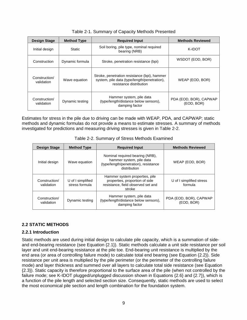
Table 2-1. Summary of Capacity Methods Presented

Design Stage Method Type Required Input Methods Reviewed

Initial design Static Soil boring, pile type, nominal required bearing (NRB) K-IDOT

Construction Dynamic formula Stroke, penetration resistance (bpi) WSDOT (EOD, BOR)

Construction/ validation Wave equation

Stroke, penetration resistance (bpi), hammer system, pile data (type/length/penetration),

resistance distribution WEAP (EOD, BOR)

Construction/ validation Dynamic testing

Hammer system, pile data (type/length/distance below sensors),

damping factor

PDA (EOD, BOR), CAPWAP (EOD, BOR)

Estimates for stress in the pile due to driving can be made with WEAP, PDA, and CAPWAP; static methods and dynamic formulas do not provide a means to estimate stresses. A summary of methods investigated for predictions and measuring driving stresses is given in Table 2-2.

Table 2-2. Summary of Stress Methods Examined

Design Stage Method Type Required Input Methods Reviewed

Initial design Wave equation

Nominal required bearing (NRB), hammer system, pile data

(type/length/penetration), resistance distribution

WEAP (EOD, BOR)

Construction/ validation

U of I simplified stress formula

Hammer system properties, pile properties, proportion of side

resistance, field observed set and stroke

U of I simplified stress formula

Construction/ validation Dynamic testing

Hammer system, pile data (type/length/distance below sensors),

damping factor

PDA (EOD, BOR), CAPWAP (EOD, BOR)

2.2 STATIC METHODS 2.2.1 Introduction Static methods are used during initial design to calculate pile capacity, which is a summation of side- and end-bearing resistance (see Equation {2.1}). Static methods calculate a unit side resistance per soil layer and unit end-bearing resistance at the pile toe. End-bearing unit resistance is multiplied by the end area (or area of controlling failure mode) to calculate total end bearing (see Equation {2.2}). Side resistance per unit area is multiplied by the pile perimeter (or the perimeter of the controlling failure mode) and layer thickness and summed over all layers to calculate total side resistance (see Equation {2.3}). Static capacity is therefore proportional to the surface area of the pile (when not controlled by the failure mode; see K-IDOT plugged/unplugged discussion shown in Equations {2.6} and {2.7}), which is a function of the pile length and selected section size. Consequently, static methods are used to select the most economical pile section and length combination for the foundation system.

9

The ultimate capacity, Qu, of a pile under axial load is generally accepted to be equal to the sum of the net pile tip capacity, Qp, and the shaft capacity, Qs:

u p sQ Q Q= + {2.1}

These terms can be further broken down and defined as follows:

p p pQ q A= ⋅ {2.2} and

1

n

s si i ii

Q f C l=

= ∑ {2.3}

where

qp = unit net bearing capacity of pile tip [F/L2] Ap = area of pile tip [L2] fsi = ultimate skin resistance per unit area of pile shaft segment i [F/L2] Ci = perimeter of pile segment i [L] li = length of pile segment i [L] n = number of pile segments

Thus, evaluating the ultimate pile capacity, Qu, reduces to estimating the magnitude of fs for each pile segment and qp at the pile tip. A number of methods are available for evaluating the ultimate pile capacity, most of which are based on empirical methods, derived from correlations of measured pile capacity with soil data. One method is described in the following section.

The static methods examined in this study are the kinematic IDOT method (K-IDOT), DRIVEN, Olson, and ICP method; however, only K-IDOT is presented because the primary focus of this research phase is to improve existing methods used by IDOT. The K-IDOT applies kinematic correction factors accounting for pile type (shell or HP) and dominant soil type along embedment length (granular or cohesive). The K-IDOT method was presented and developed in ICT Report R27-024.

2.2.2 K-IDOT Method IDOT currently uses the K-IDOT method to estimate the capacity of a pile (Long et al. 2009). The user inputs information based on the soil profile and pile type to determine pile capacity. Specifically, for each layer of the soil profile, the user must input the layer thickness, soil type (either hard till, very fine silty sand, fine sand, medium sand, clean medium to coarse sand, or sandy gravel), the SPT N-value, and, if applicable, the undrained shear strength. The total pile capacity is determined as the sum of the base capacity and side capacity.

For granular (cohesionless) soils, the unit base capacity is determined as

( )p b lq 0.8 N D / D qSPT= ⋅ ⋅ ≤ {2.4}

where

NSPT = SPT N-value as measured in the field and indicated on log [dimensionless]

10

Db = depth from the ground surface to the pile tip [ft] D = pile diameter [ft] qp = unit base capacity [kips/ft2] ql = limiting unit base capacity [kips/ft2]

where

for sands and gravel

for fine silty sand and hard till qp is multiplied by the area of the base of the pile to determine the pile’s base capacity. For cohesive soils, the unit base capacity is determined based on the undrained shear strength as

p uq 4.5 q= ⋅ {2.5} where qu is the unconfined compressive strength [tsf]. The unit base capacity, qp, is multiplied by the area of the base of the pile to determine the pile’s base capacity.

The side capacity of a pile is determined on a layer-by-layer basis. For a granular soil, the unit side capacity is determined based on the soil type and the N-value input. The formulas used are empirical. There are 17 different formulas used to determine the unit side capacity of a granular soil, depending on the soil type and NSPT value of the soil. For cohesive soils, the unit side resistance is based on Qu. Depending on the value of Qu, one of four empirical formulas is used. Also, for very stiff soils (Qu > 3 tsf and N > 30), the soil is treated as a granular soil with the hard-till soil type.

The K-IDOT method applies an empirical correction factor determined for combinations of pile type and dominant soil type along the embedment length (kinematic factors, side (FS) and end (FP)) (Table 2-3.).

Two conditions are considered for a non-displacement pile; plugged and unplugged. These conditions refer to the effective surface areas, side and end, to which a unit side resistance and unit end bearing resistance are applied respectively. The plugged or unplugged condition is applied to the entire pile. The unplugged condition exists when the failure plane along the pile length is assumed to exactly follow the pile perimeter (e.g. H-piles result in an ‘H’ shape, areas: ASAu, APu). The plugged condition represents a soil plug situated in the pile web moving with the pile. Therefore, the effective surface area is taken as the rectangular prism surrounding the pile (areas: ASAp, APp). The plugged condition will result in a smaller surface area per unit length of the pile; however, the H-pile will have a larger end bearing area. Capacity is determined for both plugged and unplugged conditions, and the lesser capacity is used as the capacity of the H-pile. The K-IDOT method calculates the plugged and unplugged capacity (for both side and end bearing) on a per-layer basis. Therefore, the controlling condition may change with increasing embedment depth. Note, the displacement piles examined (closed-end shell piles) are always unplugged and tip area is equal to the area of the bottom plate.

For displacement piles (closed-ended shell piles, precast concrete piles, timber piles) and non-displacement piles (H-piles, open shell piles) capacity is calculated as follows:

( )N S S SAp P P Pp GR F q A F q A I= + ⋅ {2.6}

lq 8 NSPT= ⋅

lq 6 NSPT= ⋅

11

and displacement piles (closed-end shell piles) capacity is calculated as follows:

( )N S S SAu P p Pu GR F q A F q A I= + ⋅ {2.7} where

Fs = pile type correction factor for side resistance (see Table 2-3. for value) [dimensionless] Fp = pile type correction factor for tip resistance (see Table 2-3. for value) [dimensionless] ASAu = unplugged surface area (4 x flange-width + 2 x member-depth) x pile

length [ft2] ASAp = plugged surface area (2 x flange-width + 2 x member-depth) x pile length [ft2] APu = the cross-sectional area of steel member [ft2] APp = the flange-width x member-depth [ft2] IG = bias factor ratio (1.04) [dimensionless]

Table 2-3. Kinematic Correction Factors for Side and Tip Resistance

Fs Fp

Displacement Piles

Cohesionless 0.758 0.758

Cohesive 1.174 1.174

Rock NA NA

Non-Displacement Piles

Cohesionless 0.15 0.3

Cohesive 0.75 1.5

Rock 1 1.0

To facilitate the use of the K-IDOT method, a spreadsheet was created by IDOT and circulated to the public as “Estimating Pile Length” on the IDOT Bridges and Structures—Foundations and Geotechnical Unit website. The K-IDOT method and spreadsheet are discussed in AGMU Memo 10.2—Geotechnical Pile Design. Note that all references to (N1)60 in AGMU Memo 10.2 should be NSPT. The current values for kinematic factors (FS and FP) are shown in Table 2-3.

2.2.2.1 Interim Modifications to K-IDOT Method This research project was organized to allow for interim reports and regular progress meetings with its technical review panel. Applying this format enabled the research project to incorporate feedback from IDOT and allow IDOT to implement changes to design methods and installation guidelines throughout the project duration due to preliminary research findings. Implementation of these changes throughout the data collection phase has no effect on the measured data collected and consequently does not affect the character of the dynamic pile load test database. When a design method in the dynamic pile load test database is modified, the method is recalculated for all piles.

Several modifications were made by IDOT to the K-IDOT static method to account for observed field performance, particularly to compensate for lower driving resistance than predicted for H-piles in sand and sandy gravel. At particular sites with difficult driving conditions, driven lengths of 50% to 100% longer than predicted were observed (St. Charles, McLean). To account for this behavior, the correlation curve between SPT blow count and unit side resistance in sandy gravel was decreased. Study results consistently show that piles driven in soil identified as sandy gravel in SPT borings

12

provided significantly less resistance than calculated by the K-IDOT method. Therefore, the correlation curve for sandy gravel is conservative and was reduced by 14% over the entire range of NSPT values, as seen in Figure 2-1.

Figure 2-1. Modified sandy gravel soil strength curve.

The resistance, load factors, and bias factor applied in the K-IDOT method for Phase 1 calculations are shown in Table 2-4.

Table 2-4. Phase 1 K-IDOT Bias Factor and LRFD Resistance Factor

Cohesive DD load factor 1.05 Granular DD load factor 1.05

Seismic resistance factor 1.0 LRFD resistance factor 0.55 ASD factor of safety 3.0 Bias factor ratio 1.04 Modified IDOT static bias factor 1.09

13

On the basis of the results of the Phase 1 study, the resistance and bias factors were modified. The modified factors applied to all piles for Phase 2 calculations are shown in Table 2-5.

Table 2-5. Phase 2 K-IDOT Bias Factors and LRFD Resistance Factors

Cohesive DD load factor 1.00 Granular DD load factor 1.00 Seismic resistance factor 1.0 Extreme event φ 1.0 LRFD φ (WSDOT soil) 0.60 LRFD φ (WSDOT shale) 0.65 LRFD φ (WSDOT rock except shale) 0.7 ASD factor of safety 2.4 Bias factor ratio (soil) 0.87 Bias factor ratio (rock) 1.0 Modified IDOT static bias factor 1.00 Maximum driving stress factor 0.9 Required check of boring location No

During the Phase 2 project, the bias factor for soil was changed from 1.04 to 0.87. Additionally, the resistance factor for all soil types (φ = 0.55) was changed to φsoil = 0.6, φshale = 0.65, and φrock = 0.7. The research team used these latest values for estimates of pile capacity. Additionally, the K-IDOT method used in this study uses NSPT values rather than previous (N1)60 values.

2.3 DYNAMIC FORMULAS 2.2.1 WSDOT Formula The WSDOT dynamic formula uses observations of ram weight, ram stroke height, and rate of pile penetration at the end of driving to estimate the capacity of the pile. Calibrations of dynamic formulas are made using results of static load tests, which are typically tested several days to several weeks after initial driving. It is well known that the capacity of a driven pile can change with time; therefore, there is an inherent assumption that the dynamic formula (based on observations made during EOD) can be related to the static capacity of a pile that is tested several days to several weeks later. Therefore, dynamic formulas include in an approximate way, the change of capacity after initial driving.

The State of Washington uses the following formula (Allen 2005) to determine pile capacity:

6.6 ln(10 )n effR F WH N= {2.8}

where

Rn = ultimate pile capacity [kips] Feff = hammer efficiency factor based on hammer and pile type W = weight of hammer [kips] H = drop of hammer [ft] N = average pile penetration resistance [blows/in.]

14

Currently, the parameter is Feff = 0.55 for air/steam hammers with all pile types, 0.37 for open-ended diesel hammers with concrete or timber piles, 0.47 for open-ended diesel hammers with steel piles, and 0.35 for closed-ended diesel hammers with all pile types. The WSDOT formula is used currently by IDOT for EOD capacity verification.

2.4 WAVE EQUATION Wave equation analyses use the one-dimensional wave equation to estimate pile stresses and pile capacity during driving (Goble and Rausche 1986). Isaacs (1931) first suggested that the one-dimensional wave equation analyses can model the hammer-pile-soil system more accurately than dynamic formulas based on Newtonian mechanics.

Wave equation analyses model the pile hammer, pile, and soil resistance as a discrete set of masses, springs, and viscous dashpots. Smith's discrete model for the hammer-pile-soil system is shown in Figure 2-2.

A finite difference method is used to model the stress wave through the hammer-pile-soil system. The basic wave equation is:

2 2

2 2p

p s bp

Su uE fx A t

ρ∂ ∂− =

∂ ∂{2.9}

where

Ep= modulus of elasticity [F/L2] u = axial displacement of the pile [L] x = distance along axis of pile [L] Sp = pile circumference [L] Ap = pile area [L2] fs = frictional stress along the pile [F/L2] ρb = unit density of the pile material [M/L3] t = time [T]

Wave equation analyses may be conducted before piles are driven to assess the behavior expected for the hammer-pile selection. Wave equation analyses provide a rational means to evaluate the effect of change in pile properties or pile driving systems on pile driving behavior and driving stresses (FHWA 1995). Furthermore, better estimates of pile capacity and pile behavior have been reported if the field measurement of energy delivered to the pile is used as direct input into the analyses (FHWA 1995) (Long and Maniaci 2000).

15

Figure 2-2. Model simulating the hammer pile-soil system for one-dimensional wave equation (after Smith 1960).

2.5 DYNAMIC TESTING 2.5.1 PDA PDA dynamic testing refers to a procedure for determining pile capacity based on the temporal variation of pile head force and velocity (Case method). PDA dynamic monitoring requires the use of a minimum of two accelerometers and two strain gauges typically mounted a minimum distance of two to three pile diameters below the top of the pile. Gauges are used in pairs to account for eccentricity in the hammer blow. Each accelerometer and strain gauge pair is attached to a Bluetooth radio that wirelessly transmits the response spectra from each hammer blow to the PDA (a wired setup is required for use of more than two sets of gauges; see Figure 2-3.).

16

Figure 2-3. PDA Instrumentation and installation on H-pile (Ng et al. 2011).

The PDA provides real-time analysis of the measured response with a calculated pile capacity, pile stress, and related data. Strain measurements are converted to pile force by multiplying by the pile cross-sectional area (A) and elastic modulus (E), and acceleration measurements are integrated to find velocities. The measured force and velocity are related by the pile impedance:

F Zv= {2.10} where ; and for a uniform pile:

Mc EAL c

= {2.11}

allowing the Case method to be expressed in terms of pile impedance, where

F = measured force [kip] Z = pile impedance [kip] v = pile velocity (particle velocity) [ft/s] E = Elastic modulus [ksi] A = pile cross-sectional area [in2] c = wave speed [ft/s] M = total mass of pile of length L [kips-s2] L = pile length below sensor location (typ. ) [ft]

Using the relationship in Equation {2.10}, the velocity can be scaled by the pile impedance, Z, to coincide with the plot of measured force at the start of the time-history record (see Figure 2-5). The time and magnitude of the divergence of the force and velocity traces indicate the magnitude and position of soil resistance (side resistance before t = 2L/c or pile tip resistance after t = 2L/c; see Figure 2-4 and Figure 2-5). The travel time for a stress wave to propagate from the gauge location to the pile toe is ttoe = L/c and total travel time for the reflected wave to return to the sensor location is t = 2L/c. A simple

( )Z EA c=

3tot pileL L D= −

17

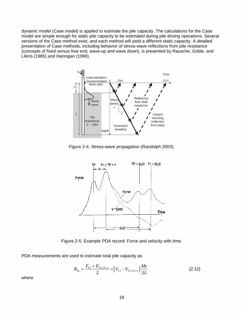
dynamic model (Case model) is applied to estimate the pile capacity. The calculations for the Case model are simple enough for static pile capacity to be estimated during pile driving operations. Several versions of the Case method exist, and each method will yield a different static capacity. A detailed presentation of Case methods, including behavior of stress-wave reflections from pile resistance (concepts of fixed versus free end, wave-up and wave down), is presented by Rausche, Goble, and Likins (1985) and Hannigan (1990).

Figure 2-4. Stress-wave propagation (Randolph 2003).

Figure 2-5. Example PDA record: Force and velocity with time.

PDA measurements are used to estimate total pile capacity as

[ ]1 1 2 /1 1 2 /2 2

T T L cTL T T L c

F F McR V VL

++

+= + − {2.12}

where

18

RTL = total pile resistance FT1 = measured force at the time T1 FT1+2L/c = measured force at the time T1 plus 2L/c VT1 = measured velocity at the time T1 VT1+2L/c = measured velocity at the time T1 plus 2L/c L = length of the pile c = speed of wave propagation in the pile M = pile mass per unit length.

Terms for force and velocity are illustrated in Figure 2-5. The total pile resistance, RTL, includes a static and dynamic component of resistance. Therefore, the total pile resistance is

TL static dynamicR R R= + {2.13}

where Rstatic is the static resistance and Rdynamic is the dynamic resistance. The dynamic resistance is assumed viscous and therefore is velocity dependent. The dynamic resistance is estimated as

( )dynamic toe c toeMcR J V j VL

= ≈ {2.14}

where

J = linear viscous damping coefficient [kip-s/ft] jc = Case damping factor [dimensionless] Vtoe = velocity of pile toe [ft/s]

The velocity at the toe of the pile can be estimated from PDA measurements of force and velocity as

11

T TLtoe T

F RV V EAc

−= + {2.15}

Substituting Equations {2.14} and {2.15} into Equation {2.13} and rearranging terms results in the expression for static load capacity of the pile as

1 1static TL T T TLMcR R J V F RL

= − + − {2.16}

The calculated value of RTL can vary depending on the selection of T1. T1 can occur at some time after initial impact:

1T TP δ= + {2.17}

where TP = time of impact peak and δ = time delay. The two most common Case methods are the RSP method and the RMX method. The RSP method uses the time of impact as T1 (corresponds to δ = 0 in Equation {2.17}). The RMX method varies δ to obtain the maximum value of Rstatic. The RMX method is recommended over the RSP method (PDA-W User’s Manual 2004) and was used throughout this study.

19

2.5.2 CAPWAP CAPWAP signal matching analysis is an iterative solution process whereby a calculated theoretical pile response is converged to match the observed force-time and velocity-time records. The convergence procedure is required as the CAPWAP series of equations is underdetermined, thereby making the solution non-unique and requiring engineering judgment to determine the appropriate solution. The PDA provides a single estimate of ultimate static axial capacity, whereas CAPWAP resolves the axial capacity into a side-resistance distribution and an end-bearing capacity.

20

CHAPTER 3 TIME EFFECTS

It is well known that the capacity of a driven pile can change after initial installation. Usually the capacity of a driven pile will increase with time, and this increase in capacity is termed setup. If the rate and magnitude of setup can be quantified reliably, then estimates of pile capacity based on pile behavior at end of driving can be modified to include the effect of setup.

This chapter uses field observations of pile capacity at end of driving and pile capacity after several days to quantify setup as a function of time, soil type, and pile type. Effects of setup are then applied to adjust capacities estimated with CAPWAP at beginning of restrike to the pile capacity at 14 days. These estimates of CAPWAP(BOR_14) are compared with estimates of capacity from WSDOT based on EOD, WSDOT based on BOR, and WSDOT modified to include time effects specifically. Finally, observations are made for the change in capacity observed for piles driven into shale.

3.1 ASSESSMENT OF SETUP MAGNITUDE AND GENERAL TRENDS The magnitude of pile setup is shown in terms of setup ratio (BOR/EOD capacity) for both total capacity and side resistance (Figures 3-1 and 3-2). Piles driven to competent rock do not exhibit a significant change in mobilized end-bearing capacity with time and therefore restrikes were not performed in the field study (accordingly, these piles are absent from the figures based on setup ratio). Piles driven to soft rock such as shale do exhibit time-dependent capacity change for both side and end bearing resistance; therefore, restrikes were performed and appear in the figures shown in this chapter. Piles driven to shale will be specifically discussed in Section 3.6.

As indicated by Figure 3-1 and Figure 3-2, pile capacity typically increases with time, as is evident by the setup ratio for total capacity and for side resistance. The increase in pile capacity is typically the result of increased shaft resistance (see Figure 3-2), while the end-bearing capacity remains approximately constant. The notable exception to this trend in end-bearing resistance is piles driven to shale, in which significant relaxation at the pile toe may be observed.

A field test program was conducted on driven piles to ascertain the rate and magnitude of pile setup in a recent study by the Iowa Department of Transportation (Ng et al. 2011). An inverse relationship was found between the thickness-weighted average SPT blow count along the pile embedment length, Na, and pile setup in clays. The Na values did not exceed 16 (piles driven in soft clays) and was not calculated for granular or mixed soil types because these soil categories were shown to contribute less than cohesive layers to soil setup (Ng et al. 2011).

The relationship between Na and the total capacity setup ratio, and Na versus side-resistance setup ratio is shown for the piles in the Illinois dynamic load test database (see Figure 3-3 and Figure 3-4). Results show for Illinois soil conditions significant average setup ratios for sand (27%) and for mixed (36%) soil categories in addition to clay (45%). Therefore, an approach for estimating pile setup based on Na was extended to all soil types. The average N-value for piles to rock and shale is calculated using only the soil profile above the top of shale/rock. This acknowledges that only the soil profile will be experiencing setup and eliminates the effect of an N-value equal to refusal (N = 100) at the pile toe in the calculation of Na, which would disrupt the ability to make potential correlations (e.g., for a pile socketed into shale). It will be shown in section 3.6 that setup should not be applied to piles driven to rock or to shale. Time dependent capacity change occurs for piles driven to shale; however, the observed increase in side resistance is often offset by an approximately equivalent relaxation in end bearing capacity resulting in no net change in total capacity.

21

Figure 3-1. Setup ratio (total capacity) vs. setup duration.

Figure 3-2. Setup ratio (side resistance) vs. setup duration.

22

Figure 3-3. Setup ratio (total capacity) vs. NSPT average, Na (along embedment length).

Figure 3-4. Setup ratio (side resistance) vs. NSPT average, Na (along embedment length).

23

Trends for soil type, pile type, and soil category are difficult to determine solely from these figures; however, some general trends are observed from calculation of the setup factor, C, discussed in the following section.

3.2 DETERMINATION OF RATE OF SETUP The rate of setup was quantified by estimating the capacity at EOD using CAPWAP, and then by estimating the capacity at a later time using CAPWAP(BOR). Time delays between EOD and BOR were typically greater than 24 hours. The change in capacity with time provides a means to quantify setup. A commonly applied approach to describe the rate of pile setup is with a linear log time relationship. The general form of the pile setup estimation formula is based on Skov and Denver (1988):

log 1t

o o

R tAR t

= +

{3.1}

Following the Iowa DOT variable nomenclature the equation can be rewritten as

1min

log 1BOR BOR

EOD

R tCR t

= +

{3.2}

Pile setup rate (C) is defined as

( )ba

aCN

= {3.3}

where

a = method-dependent scale factor (regression curve-fitting term) b = method-dependent concave factor (regression curve-fitting term)

aN = average SPT N-value

The pile setup factor, C, is the slope of the pile setup curve at any given time, where aN is the thickness-weighted average SPT N-value along the pile embedment length defined as

1

1

n

i ii

a n

ii

N lN

l

=

=

=∑

∑{3.4}

where

iN = SPT N-value for layer i

il = thickness for layer l [ft]

24

Substituting for C into Equation {3.2}:

( ) 1min

log 1BOR BORb

EOD a

R taR tN

= +

{3.5}

Comparing Equation {3.5} to the Iowa SPT method, which is defined as

( )

10log1EODt

bEOD EODa

tatR L

R LN

= +

{3.6}

there is an additional length term. The L/LEOD term in Equation {3.6} reflects the increase in pile capacity from the additional embedment length driven during pile restrike. For the majority of cases, piles are driven less than 4 in. during restrike, which produces a negligible change in capacity compared with the capacity obtained for the initial pile embedment length (L/LEOD = 1). Therefore, a value of unity was used for the length term in Equation {3.5}.

The capacity ratio in Equation {3.5} is expressed in terms of total capacity and was used to initially back-calculate the setup constants a and b (which define the resulting function of the setup parameter C with Na). Therefore, this method applies the setup factor to both end bearing and side resistance. As previously shown in Figure 3-1 and Figure 3-2 and is commonly recognized, setup occurs primarily along the embedded length of the pile shaft and not the pile toe. Therefore, a more accurate representation is to apply the setup parameters only to the side resistance.

The back-calculated values for constants a and b are shown for each pile-soil category in Figure 3-5 for side resistance. Setup constants are back-calculated for all categories including rock, although setup factors are not applied for piles to rock or shale for design recommendations or normalization of setup period (determination of 14-day capacity). Normalization is discussed in the following section.

Accordingly, the setup equation in terms of side resistance is defined as

( )( )

( )1min

log 1BORBOR EOD EODbside end

a

taR R RtN

= + +

{3.7}

The approach shown in Equation {3.7} reflects a more rigorous treatment of setup and resulted in lower COVs for capacity methods when compared with estimates of BOR from EOD total capacity (even though side resistance exhibits significantly higher scatter than total capacity). The distribution of side and end-bearing resistance and the side-resistance profile is determined from CAPWAP analysis.

The back-calculation of constants a and b shown in Figure 3-5 exhibits significant scatter. Therefore, engineering judgment was used to create two sets of design curves: one for H-piles (a = 2.92, b = 1.17, max = 0.4) and one for shell piles (a = 2.63, b = 0.85, max = 0.5) (see Figure 3-6). The setup factor, C, is not constant with time, and piles of the same soil type will not have the same setup curve unless the piles have the same Na value.

25

An additional method applied by the Iowa Department of Transportation, the CPT&SPT method, used the following definition of constant C, derived by Ng et al. (2011):

2h

c ra p

CC f fN r

= +

{3.8}

where

cf = consolidation factor [min-1]

rf = remolding recovery factor

hC = horizontal coefficient of consolidation [in2/min]

pr = equivalent pile radius [in.]

The CPT&SPT method could not be applied because the back-calculated consolidation factor, fc, and remolding recovery factor, fr, resulted in significant scatter, which prevented the determination of these constants using a linear regression (as conducted by Iowa DOT). The scatter may be due to attempting to extend the application of this formula to granular and mixed soil conditions because the formula was initially applied only to cohesive soils. Additionally, the Iowa case study had a much smaller average SPT blow count, Na (approximately 2 to 16), whereas the soil profiles for the piles in the dynamic load test program had an Na range of approximately 6 to 65. Lastly, an empirical formula for estimation of the coefficient of horizontal permeability established by the Iowa DOT for cohesive soil and specific site conditions is not applicable. For the Iowa study, the CPT&SPT formula did provide a bias closer to unity and a lower COV in comparison with the SPT method.

26

Figure 3-5. Setup factor C and constants a and b back-calculated for pile-soil category.

a 2.92b 1.17a 10.51b 3.71a 0.09b 0.00a 1.22b 0.53

a 0.82b 0.19a 0.39b 0.10a 2.63b 0.85

S-sand

H-clay

H-mix

H-sand

H-rock

S-clay

S-mix

-0.2

0

0.2

0.4

0.6

0.8

1

0 10 20 30 40 50 60 70

Setu

p Fa

ctor

, C

N-spt

H-clay

back calc

a: 2.92, b: 1.17

-0.2

0

0.2

0.4

0.6

0.8

1

0 10 20 30 40 50 60 70

Setu

p Fa

ctor

, C

N-spt

H-mix

back calc

a: 10.51, b: 3.71

-0.2

0

0.2

0.4

0.6

0.8

1

0 10 20 30 40 50 60 70

Setu

p Fa

ctor

, C

N-spt

H-sand

back calc

a: 0.09, b: 0

-0.2

0

0.2

0.4

0.6

0.8

1

0 10 20 30 40 50 60 70

Setu

p Fa

ctor

, C

N-spt

H-rock

back calc

a: 1.22, b: 0.53

-0.2

0

0.2

0.4

0.6

0.8

1

0 10 20 30 40 50 60 70

Setu

p Fa

ctor

, C

N-spt

S-clay

back calc

a: 0.82, b: 0.19

-0.2

0

0.2

0.4

0.6

0.8

1

0 10 20 30 40 50 60 70

Setu

p Fa

ctor

, C

N-spt

S-mix

back calc

a: 0.39, b: 0.1

-0.2

0

0.2

0.4

0.6

0.8

1

0 10 20 30 40 50 60 70

Setu

p Fa

ctor

, C

N-spt

S-sand

back calc

a: 2.63, b: 0.85

27

Figure 3-6. Setup factor C and selected constants a and b for H-piles and shell piles.

a 2.92b 1.17a 2.63b 0.85

Upper Limit = 0.4

Upper Limit = 0.5

H-piles

S-piles

-0.2

0

0.2

0.4

0.6

0.8

1

0 10 20 30 40 50 60 70

Setu

p Fa

ctor

, C

Na

H-clay

selected

a: 2.92, b: 1.17

-0.2

0

0.2

0.4

0.6

0.8

1

0 10 20 30 40 50 60 70

Setu

p Fa

ctor

, C

Na

H-mix

selected

a: 2.92, b: 1.17

-0.2

0

0.2

0.4

0.6

0.8

1

0 10 20 30 40 50 60 70

Setu

p Fa

ctor

, C

Na

H-sand

selected

a: 2.92, b: 1.17

-0.2

0

0.2

0.4

0.6

0.8

1

0 10 20 30 40 50 60 70

Setu

p Fa

ctor

, C

Na

H-rock

selected

a: 2.92, b: 1.17

-0.2

0

0.2

0.4

0.6

0.8

1

0 10 20 30 40 50 60 70

Setu

p Fa

ctor

, C

Na

S-clay

selected

a: 2.63, b: 0.85

-0.2

0

0.2

0.4

0.6

0.8

1

0 10 20 30 40 50 60 70

Setu

p Fa

ctor

, C

Na

S-mix

selected

a: 2.63, b: 0.85

-0.2

0

0.2

0.4

0.6

0.8

1

0 10 20 30 40 50 60 70

Setu

p Fa

ctor

, C

Na

S-sand

selected

a: 2.63, b: 0.85

28

3.3 NORMALIZATION TO 14-DAY CAPACITY Pile capacity changes with time. It is common for static load tests to be delayed as long as practical (after initial driving) to allow for as much setup to occur as possible. From the beginning of the project a target setup period of 14 days or greater was specified as a balance between observation of the majority of pile setup which will occur and delay to the contractor potentially resulting in increased project costs. A 14-day capacity was chosen as a reasonable time to use for pile capacity as this represents a time period at which the majority of setup has occurred and is near the mean and median setup period for the database.

The BOR capacity data presented in the Phase 1 report was not normalized based on the duration of the setup period. Therefore, the setup magnitude data subset of interest (e.g. shell piles in clay) was be qualified by noting the average setup period observed for the piles in this category. Therefore it is difficult to compare observed setup from different data subsets as each subset has a different corresponding average setup period. Consequently, in this report the Phase 1 and Phase 2 capacities determined at pile restrike, CAPWAP(BOR) is normalized to 14 days, CAPWAP(BOR_14) to enable comparison of pile setup between piles with different setup periods. Normalization of all CAPWAP(BOR) capacities to CAPWAP(BOR_14) was performed by developing a time rate of setup formula. The formula is back calculated from quantifying average setup magnitudes and rates (Figure 3-5, 3-6). Equation {3.7} was used to determine RBOR_14 by using Rside and Rend from CAPWAP analysis at the time of BOR, and then correcting for time by using the ratio (14 days/tBOR) instead of (tBOR/1min). For piles with a setup duration less than 14 days the CAPWAP(BOR) capacity is increased by the setup factor C (defined by curve fitting parameters ‘a’ and ‘b’, for either h-piles or shell piles). If the setup duration is greater than 14 days than CAPWAP(BOR) capacity is not modified. The capacities for piles driven to rock and to shale were not changed (for rock EOD = BOR_14 and for shale BOR = BOR_14) under the observation that no setup occurs. The change in capacity between CAPWAP(BOR) and CAPWAP(BOR_14) will depend on the 1) setup period (a time period << 14 days will result in a larger capacity increase) 2) Na (an increase in Na will result in a decrease in C and result in a smaller increase in capacity) 3) the proportion of side resistance to end bearing resistance (setup is only applied to side resistance; if the side resistance is larger than calculated setup will increase). The database contains 111 piles. Of the 111 pile 94 have reliable test data. Of the 94 piles, 43 piles had a setup period less than 14 days. For the 43 piles which had a setup correction to a 14 day strength the average capacity increase was 3.3 percent (min = 0.02% and max = 14.6%). Of the 111 piles, 94 had reliable test data. Of the 94 piles, 43 piles had a setup period less than 14 days. For the 43 piles that had a setup correction to a 14-day strength, the average capacity increase was 3.3% (min = 0.02% and max = 14.6%).

3.4 TIME EFFECTS APPLIED TO WSDOT An investigation was conducted to determine whether the WSDOT method could be improved by including effects of setup. Three versions of WSDOT were evaluated and compared:

1. WSDOT method using EOD driving behavior,

29

2. WSDOT (EOD_14) = WSDOT(EOD) + Setup Factor, WSDOT method using EOD driving behavior and modifying capacities based on Equation {3.7} with setup factors based on the thickness weighted average of NSPT, Na and

3. WSDOT method using BOR driving information.

Values of pile capacity were predicted using all three methods and compared with CAPWAP(BOR_14) capacities. The ratios of WSDOT/CAPWAP(BOR_14) were determined for each pile in the database and for each variation of the WSDOT method. The coefficient of variation (COV), was compared for each case as follows:

1. WSDOT(EOD) COV = 0.314 (Figure 4-2, Table 4-2) 2. WSDOT(EOD_14) COV = 0.320 (Figure 4-4, Table 4-4) 3. WSDOT(BOR) COV = 0.330 (Figure 4-3, Table 4-3)

The proportion of side resistance was obtained from the K-IDOT formula (side resistance was not obtained from CAPWAP because that information would not be available at this design stage). The results of this test showed an increase in COV and bias for WSDOT(EOD_14). Therefore, it is not recommended that predictive methods be normalized in this manner.

It can be observed that the WSDOT(EOD) has the smallest COV and therefore exhibits the least amount of scatter. The WSDOT(EOD_14) method did not show tangible benefit from including the setup factors directly. The WSDOT(BOR) method also exhibited a greater scatter (higher COV) than the original WSDOT formula. Accordingly, it was concluded that including setup factors into the WSDOT method did not improve its ability to predict capacity precisely.

3.5 LIMITATIONS Most of the tests occur with a setup period of less than 20 days (75 of 86 piles with restrikes, 87%). The number of piles with setup periods less than 14 days which require BOR capacity adjustments to normalize capacity to a 14-day capacity are 51 of 86 piles (59%). The majority of piles were restruck between 3 and 20 days and therefore it is recommended that the application of the Skov and Denver (1988) method, with constants back-calculated from the dynamic testing field study, be limited to setup periods between 3 days and 20 days. Additionally, the back-calculated constants are applicable only for the soil conditions and pile sections included in the tests. Also, the method is based on average setup for the dynamic load test database and therefore observed setup at any given site may be different.

3.6 ASSESSING RELAXATION POTENTIAL OF END-BEARING PILES IN SHALE Relaxation potential in shale is assessed by examining the setup ratio for total capacity and the setup ratio for end-bearing resistance determined by CAPWAP(BOR)/CAPWAP(EOD). A slight majority (10) of the 17 piles tested in shale exhibited a total capacity on restrike less than or equal to unity (mean, μ < 1); however, the setup ratio for all piles to shale has a mean 0.99 (μ ≈ 1), indicating an essentially constant total resistance with time (see Figure 3-7 and Table 3-1). The minimum observed setup ratio of 0.81 indicates a 19% reduction in total capacity, and the maximum setup ratio 1.14 indicates a 14% increase in capacity. Total resistance remains essentially constant due to an increase in side resistance that offsets the decrease in end-bearing resistance at the pile toe resulting from relaxation in the shale. Several of the piles exhibited a significant increase in side resistance (large setup ratio) due to low EOD driving resistance and subsequent pile setup. This was particularly true for the soft riparian clays overlying shale at the Big Muddy site, in which piles penetrated 15 to 25 ft under the weight of hammer (hammer seated on the top of the pile, no hammer blows). The setup ratio in terms of total capacity

30

versus the NSPT average along the pile embedment length is shown in Figure 3-9. Piles driven to shale with lower NSPT average values do exhibit the largest setup ratio; however, the majority of piles which exhibit a relaxation greater than 10% have NSPT average values less than 15 (low NSPT average value). Therefore, there is no clear correlation between NSPT average and a decrease or increase in total capacity with time.

The end-bearing capacity of piles decreased in 14 of the 17 piles tested (Figure 3-8, Table 3-2). The average decrease in end-bearing resistance was 26% with a maximum of 74%. Some pile cases exhibited unusually high values of setup and are considered outliers.

Table 3-1. Shale Setup Ratio Summary Table

Parameter Setup Ratio

Side End Bearing Total min 0.35 0.26 0.81 max 12.08 2.53 1.14

μ 2.23 0.84 0.99 μ (no outliers) 1.62 0.74 0.99

In summary, total capacity on average decreased by 1%, while end-bearing resistance decreased by 26% therefore indicating that significant relaxation in shale occurs but is typically offset with an approximately equal increase in side resistance. The increase in side-resistance setup has been found to be largest in clay soils followed by mixed profiles and then sand. Setup has also been found to be inversely related to the average SPT blow count along the pile length. In examination of plots of total resistance (see Figure 3-3.) and end-bearing resistance (see Figure 3-4) versus NSPT average, there does not appear to be a correlation between average overburden strength and total capacity on restrike.

Dynamic formulas for end-bearing piles driven to shale will tend to yield unconservative results because, according to the results of this study, setup does not occur and dynamic formulas implicitly include a setup factor in their formulation to relate EOD resistance to a longer-duration capacity. Therefore, it may be necessary for WSDOT analysis to treat piles driven to shale and rock differently than piles in soil (see Chapter 7).

31

Figure 3-7. Total capacity setup ratio vs. setup period, piles to shale.

Figure 3-8. End-bearing setup ratio vs. setup period, piles to shale.

32

Figure 3-9. Total capacity setup ratio vs. NSPT average, piles to shale.

Table 3-2. Shale Setup Ratio for All Piles to Shale

Pile ID # Site & Pile Location Setup Ratio

Side End Total 24 Carmi East Abt. 1.11 0.96 0.99 25 Carmi Pier 4 0.52 0.88 0.81 26 Carmi Pier 2 1.17 0.81 0.90 27 Carmi West Abt. 1.05 0.81 0.87 68 Marion I-57 N. Abt (SB) 1.47 0.31 0.97 69 Marion Ramp J - W. Abt 4.88 0.26 1.00 70 Marion Ramp J - Pier 1 0.35 2.53 0.90 71 Marion Ramp I - S. Abt 1.17 1.05 1.08 72 Marion Ramp I - Pier 2 1.32 0.96 1.00 80 Big Muddy East Abt. 12.08 0.36 1.08 81 Big Muddy Pier 1 1.38 0.89 1.04 82 Big Muddy Pier 2 1.05 0.85 0.88 83 Big Muddy Pier 3 1.68 0.94 1.00 84 Big Muddy Pier 4 2.64 0.35 1.06 85 Big Muddy West Abt. 3.08 0.41 1.14

106 Pontiac (East) South Abt 1.05 1.10 1.09 111 Middlegrove West Abt. 1.99 0.84 0.99

33

CHAPTER 4 PERFORMANCE OF METHODS

The primary goal of the dynamic testing program is to provide measured values for capacity and stress at end of driving and beginning of restrike. PDA measurements serve as the basis of comparison for evaluating the static, dynamic, and wave equation capacity methods. Stress predictions are obtained using a wave equation analysis performed by the GRL WEAP software program and the simplified stress formula (SSF).

PDA records are analyzed using CAse Pile Wave Analysis Program (CAPWAP) which provides refined estimates of pile capacity and pile stress. The CAPWAP(EOD_14) and CAPWAP(BOR_14) capacities are considered the measured capacities for EOD and BOR in this research project and include a normalization to a 14 day capacity (section 3.3).

Method performance is expressed in terms of method accuracy, (bias (λ), or mean (μ)) and method precision, coefficient of variation (COV). The ratio of QP/QM or its inverse, QM/QP is used as the metric to quantify the agreement between predicted and measured capacity. The distribution of QP/QM (and QM/QP) is lognormal (Long and Maniaci 2000). Accordingly, mean and standard deviation are determined for ln(QP/QM) and then converted to their arithmetic equivalents. The mean of a method is defined as the average natural log ratio of measured to predicted capacity (Equation 4.2).

The performance of a method is quantified statistically with the following parameters:

The mean, μ, is defined as

1

1 n

ii

xn

µ=

= ⋅∑ {4.1}

The lognormal mean, μln, when applied to quantifying the performance of a method is defined as

ln1

1 lnn

i

QPn QM

µ=

=

∑

{4.2}

where QP = predicted value (capacity or stress) and QM = measured value (capacity or stress) for the method being analyzed for each pile (n = number of piles). The mean, μ, represents the average trend to over- or underpredict for a given method examined in this study.

Standard deviation, σ, is defined as

( )2

1

11

n

ii

xn

σ µ=

= ⋅ −− ∑ {4.3}

Lognormal standard deviation, σln, when applied to quantifying the performance of a method is defined as

2

ln ln1

1 ln1

n

i

QPn QM

σ µ=

= − −

∑ {4.4}

34

The measure of method precision (scatter) is quantified as the standard deviation divided by the mean and is termed the coefficient of variation (COV). The COV is used as a normalized metric to quantify scatter for the arithmetic values of QP/QM and QM/QP. The coefficient of variation, COV is applied to the arithmetic equivalents of standard deviation and mean (see Appendix A for lognormal to arithmetic conversion calculation) and is calculated as

COV σµ

= {4.5}

Alternatively, some LRFD formulations such as those used to determine LRFD resistance factors are expressed in terms of bias, λ, which for lognormal distributions is the negative of the mean and is defined as

ln ln1

1 lnn

i

QMn QP

λ µ=

= − =

∑

{4.6}

with the same definitions of standard deviation, σ, and coefficient of variation, COV, applied with values of QM/QP replacing values of QP/QM in Equations {4.4} and {4.2}. Further discussion of statistical parameters if discussed in Appendix A.

The performance of a method is evaluated by comparing the predicted value with the value obtained from CAPWAP signal matching analysis of PDA records at the time of restrike normalized to 14 days (CAPWAP(BOR_14)) (section 3.3). Method performance is further investigated by filtering the data on the basis of pile type, soil type, and pile-soil combinations.

4.1 METHOD STATISTICS (CHARTS AND TABLES) The performance of the predictive methods: static (K-IDOT), dynamic (WSDOT), wave equation WEAP), dynamic measurement (PDA) are presented for EOD and BOR. All statistics are presented for the 14 day normalized capacity CAPWAP(BOR_14).

The K-IDOT method results are presented in Figure 4-1 and Table 4-1. The K-IDOT method has a high COV (0.55) compared with other methods; however, a large COV is often observed for static methods because such methods are based solely on boring information. The K-IDOT method has the largest COV for piles in sand (shell piles COV = 0.771 and H-piles COV = 0.752) with an average COV = 0.591; whereas in Phase 1, the average COV = 0.492. The K-IDOT method also overpredicts pile capacity for shell piles on average by 22%, while H-pile capacity at a given depth is underpredicted by 16%.

WSDOT results for EOD are shown in Figure 4-2 and Table 4-2, and BOR data are presented in Figure 4-3. and Table 4-3. The WSDOT equation was calibrated using EOD measurements of stroke height and penetration resistance and therefore should not be used for BOR without recalibration. Direct use of WSDOT restrike observations leads to a mean much greater than unity. However, the COV of WSDOT(BOR) can be compared with WSDOT(EOD) to determine whether applying BOR stroke and penetration resistance improves the method scatter. WSDOT(BOR) has a COV = 0.330, whereas WSDOT(EOD) COV = 0.314; therefore, despite using EOD data, WSDOT(EOD) predicts BOR capacity more consistently than WSDOT(BOR). The COV for WSDOT(EOD) increased from 0.252 in Phase 1 to 0.314. The procedure to model time effects was presented in Chapter 3. This procedure was applied to the WSDOT method using driving performance data at EOD (Figure 4-4, Table 4-4) and

35

at BOR (Figure 4-5, Table 4-5) to investigate if applying the effect of time improves the ability of the WSDOT method to predict capacity consistently. In both cases the COV was greater than the COV based on WSDOT(EOD). Accordingly, WSDOT(EOD) predicts capacity with better consistency than modifying WSDOT values to model time effects.

WEAP results for EOD are shown in Figure 4-6 and Table 4-6, and BOR data are presented in Figure 4-7 and Table 4-7. For both EOD and BOR, shell piles in clay have the largest COV 0.507 and 0.426, respectively. The lowest COV for EOD is H-piles in mixed (COV = 0.098) and for BOR is shell piles in mixed (COV = 0.201). The very high COV for shell piles in clay contributes significantly to increasing the COV for EOD = 0.360 from 0.316 in Phase 1 and BOR = 0.330 from COV = 0.238 in Phase 1.

PDA data for Phase 1 and Phase 2 are reported for a case damping constant of jc = 0.6 (EOD: Figure 4-8, Table 4-8; BOR: Figure 4-9, Table 4-9). For the PDA data in the Phase 1 report (ICT R27-069), a Case damping constant of jc = 0.5 was applied. Back-calculation of a PDA Case damping constant to provide the best agreement with CAPWAP results indicates that a jc = 0.9 provides the best agreement (a factor larger than 0.9 would provide better agreement; however, 0.9 is the maximum value). The Case damping constant of 0.9 is not representative of the soil damping but is an empirical correction factor improving agreement between PDA and CAPWAP capacity. This correction factor accounts for PDA capacity typically overpredicting CAPWAP capacity (increased Case damping lowers calculated PDA resistance). Therefore, as applied to Illinois soil conditions and installation techniques, a PDA Case damping factor of jc = 0.9 is recommended for monitoring real-time capacity while driving. Once collected, PDA records can be analyzed with iCAP (automated, rapid, approximate CAPWAP analysis) on the PAX data collection unit for further capacity refinement in the field. A full CAPWAP analysis performed on a personal computer is recommended for final analysis.

The summary tables for the methods examined are grouped by soil pile type (for all piles) in Table 4-10 through Table 4-12 and are presented for soil profiles only (no rock) in Table 4-13. In general, shell piles (Table 4-11) have a lower COV than H-piles (Table 4-10). Additionally, compared with results for all piles, excluding piles driven to rock from the database (Table 4-13) did not significantly improve results (Table 4-12).

36

Figure 4-1. K-IDOT vs. CAPWAP(BOR_14).

Table 4-1. K-IDOT Method Statistics by Pile and Soil Type

K-IDOT Clay Mixed Sand Rock Shale All Soil All

H-Piles μ 0.747 1.071 0.963 0.792 0.771 0.916 0.837

COV 0.417 0.541 0.752 0.650 0.465 0.583 0.552 n 7 7 9 10 17 23 50

Shell Piles μ 1.246 1.042 1.714 NA NA 1.219 1.219

COV 0.617 0.422 0.771 NA NA 0.558 0.558 n 8 21 9 NA NA 38 38

All μ 0.998 1.045 1.323 0.792 0.771 1.103 1.000

COV 0.568 0.442 0.822 0.650 0.465 0.586 0.591 n 15 28 18 10 17 61 88

37

Figure 4-2. WSDOT(EOD) vs. CAPWAP(BOR_14).

Table 4-2. WSDOT(EOD) Method Statistics by Pile and Soil Type

WSDOT (EOD) Clay Mixed Sand Rock Shale All Soil All

H-Piles μ 1.275 1.232 1.378 0.977 1.257 1.306 1.228

COV 0.466 0.204 0.317 0.424 0.219 0.328 0.337 n 7 7 12 10 17 26 53

Shell Piles μ 0.990 1.100 1.078 NA NA 1.070 1.070

COV 0.361 0.286 0.137 NA NA 0.269 0.269 n 8 21 11 NA NA 40 40

All μ 1.115 1.132 1.231 0.977 1.257 1.161 1.159

COV 0.414 0.271 0.264 0.424 0.219 0.306 0.314 n 15 28 23 10 17 66 93

38

Figure 4-3. WSDOT(BOR) vs. CAPWAP(BOR_14).

Table 4-3. WSDOT(BOR) Method Statistics by Pile and Soil Type

WSDOT (BOR) Clay Mixed Sand Rock Shale All Soil All

H-Piles μ 1.338 1.317 1.651 1.048 1.409 1.475 1.377

COV 0.400 0.257 0.192 0.491 0.213 0.295 0.351 n 7 7 12 10 17 26 53

Shell Piles μ 1.301 1.624 1.468 NA NA 1.514 1.514

COV 0.364 0.278 0.224 NA NA 0.293 0.293 n 8 21 11 NA NA 40 40

All μ 1.312 1.545 1.562 1.048 1.409 1.498 1.436

COV 0.366 0.284 0.213 0.491 0.213 0.292 0.330 n 15 28 23 10 17 66 93

39

Figure 4-4. WSDOT(EOD_14) vs. CAPWAP(BOR_14).

Table 4-4. WSDOT(EOD_14) Method Statistics by Pile and Soil Type

WSDOT (EOD_14) Clay Mixed Sand Rock Shale All Soil All

H-Piles μ 1.293 1.276 1.429 0.977 1.257 1.346 1.248

COV 0.462 0.200 0.334 0.424 0.219 0.334 0.344 n 7 7 12 10 17 26 53

Shell Piles μ 1.006 1.133 1.097 NA NA 1.096 1.096

COV 0.376 0.295 0.128 NA NA 0.277 0.277 n 8 21 11 NA NA 40 40

All μ 1.132 1.168 1.266 0.977 1.257 1.193 1.181

COV 0.419 0.278 0.275 0.424 0.219 0.314 0.320 n 15 28 23 10 17 66 93

40

Figure 4-5. WSDOT(BOR_14) vs. CAPWAP(BOR_14).

Table 4-5. WSDOT(BOR_14) Method Statistics by Pile and Soil Type

WSDOT (BOR_14) Clay Mixed Sand Rock Shale All Soil All

H-Piles μ 1.355 1.364 1.705 1.048 1.409 1.517 1.398

COV 0.389 0.254 0.199 0.491 0.213 0.295 0.354 n 7 7 12 10 17 26 53

Shell Piles μ 1.320 1.673 1.501 NA NA 1.553 1.553

COV 0.375 0.288 0.239 NA NA 0.305 0.305 n 8 21 11 NA NA 40 40

All μ 1.330 1.594 1.606 1.048 1.409 1.538 1.464

COV 0.367 0.289 0.225 0.491 0.213 0.299 0.338 n 15 28 23 10 17 66 93

41

Figure 4-6. WEAP(EOD) vs. CAPWAP(BOR_14).

Table 4-6. WEAP(EOD) Method Statistics by Pile and Soil Type

WEAP (EOD) Clay Mixed Sand Rock Shale All Soil All

H-Piles μ 0.808 0.906 1.153 0.742 1.005 0.993 0.951

COV 0.252 0.098 0.214 0.433 0.165 0.252 0.303 n 7 7 12 10 17 26 53

Shell Piles μ 0.649 0.662 0.833 NA NA 0.706 0.706

COV 0.507 0.308 0.181 NA NA 0.347 0.347 n 8 21 11 NA NA 40 40

All μ 0.724 0.725 0.999 0.742 1.005 0.820 0.847

COV 0.424 0.313 0.256 0.433 0.165 0.364 0.360 n 15 28 23 10 17 66 93

42

Figure 4-7. WEAP(BOR) vs. CAPWAP(BOR_14).

Table 4-7. WEAP(BOR) Method Statistics by Pile and Soil Type

WEAP (BOR) Clay Mixed Sand Rock Shale All Soil All

H-Piles μ 1.008 1.009 1.366 0.799 1.101 1.173 1.082

COV 0.369 0.266 0.212 0.475 0.126 0.315 0.348 n 7 7 12 10 17 26 53

Shell Piles μ 0.802 0.897 1.163 NA NA 0.951 0.951

COV 0.426 0.201 0.185 NA NA 0.295 0.295 n 8 21 11 NA NA 40 40

All μ 0.895 0.923 1.268 0.799 1.101 1.038 1.025

COV 0.409 0.219 0.211 0.475 0.126 0.318 0.330 n 15 28 23 10 17 66 93

43

Figure 4-8. PDA(EOD) vs. CAPWAP(BOR_14).

Table 4-8. PDA(EOD) Method Statistics by Pile and Soil Type

PDA (EOD) Clay Mixed Sand Rock Shale All Soil All

H-Piles μ 0.993 0.910 1.120 1.037 1.099 1.027 1.052

COV 0.361 0.099 0.211 0.105 0.146 0.247 0.197 n 7 7 12 10 17 26 53

Shell Piles μ 0.874 0.891 0.889 NA NA 0.886 0.886

COV 0.394 0.221 0.230 NA NA 0.258 0.258 n 8 21 11 NA NA 40 40

All μ 0.926 0.896 1.009 1.037 1.099 0.941 0.981

COV 0.372 0.196 0.248 0.105 0.146 0.263 0.243 n 15 28 23 10 17 66 93

44

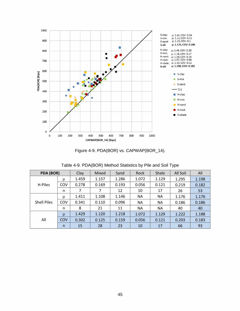
Figure 4-9. PDA(BOR) vs. CAPWAP(BOR_14).

Table 4-9. PDA(BOR) Method Statistics by Pile and Soil Type

PDA (BOR) Clay Mixed Sand Rock Shale All Soil All

H-Piles μ 1.459 1.157 1.286 1.072 1.129 1.295 1.198

COV 0.278 0.169 0.193 0.056 0.121 0.219 0.182 n 7 7 12 10 17 26 53

Shell Piles μ 1.411 1.108 1.146 NA NA 1.176 1.176

COV 0.341 0.110 0.096 NA NA 0.186 0.186 n 8 21 11 NA NA 40 40

All μ 1.429 1.120 1.218 1.072 1.129 1.222 1.188

COV 0.302 0.125 0.159 0.056 0.121 0.203 0.183 n 15 28 23 10 17 66 93

45

4.2 SUMMARY TABLES

Table 4-10. Capacity Method Statistics Summary: H-Piles

Predicted Mean COV n K-IDOT 0.837 0.552 50

WSDOT (EOD) 1.228 0.337 53 WSDOT (BOR) 1.377 0.351 53

WSDOT (EOD) 14 days 1.248 0.344 53 WSDOT (BOR) 14 days 1.398 0.354 53

WEAP (EOD) 0.951 0.303 53 WEAP (BOR) 1.082 0.348 53 PDA (EOD) 1.052 0.197 53 PDA (BOR) 1.198 0.182 53

Table 4-11. Capacity Method Statistics Summary: Shell Piles

Predicted Mean COV n K-IDOT 1.219 0.558 38

WSDOT (EOD) 1.070 0.269 40 WSDOT (BOR) 1.514 0.293 40

WSDOT (EOD) 14 days 1.096 0.277 40 WSDOT (BOR) 14 days 1.553 0.305 40

WEAP (EOD) 0.706 0.347 40 WEAP (BOR) 0.951 0.295 40 PDA (EOD) 0.886 0.258 40 PDA (BOR) 1.176 0.186 40

Table 4-12. Capacity Method Statistics Summary: All Piles

Predicted Mean COV n K-IDOT 1.000 0.591 88

WSDOT (EOD) 1.159 0.314 93 WSDOT (BOR) 1.436 0.330 93

WSDOT (EOD) 14 days 1.181 0.320 93 WSDOT (BOR) 14 days 1.464 0.338 93

WEAP (EOD) 0.847 0.360 93 WEAP (BOR) 1.025 0.330 93 PDA (EOD) 0.981 0.243 93 PDA (BOR) 1.188 0.183 93

46

Table 4-13. Capacity Method Statistics Summary: Piles in Soil (No Rock)

Predicted Mean COV n K-IDOT 1.103 0.586 61

WSDOT (EOD) 1.161 0.306 66 WSDOT (BOR) 1.498 0.292 66

WSDOT (EOD) 14 days 1.193 0.314 66 WSDOT (BOR) 14 days 1.538 0.299 66

WEAP (EOD) 0.820 0.364 66 WEAP (BOR) 1.038 0.318 66 PDA (EOD) 0.941 0.263 66 PDA (BOR) 1.222 0.203 66

47

CHAPTER 5 DEVELOPMENT OF A SIMPLFIED STRESS FORMULA

5.1 INTRODUCTION An introduction to the Simplified Stress Formula (SSF) is presented in this chapter. A complete derivation of the SSF can be found in Appendix B of the Phase 1 report (ICT R27-069). The SSF method has been incorporated into the IDOT spreadsheet for verification of field capacity by the dynamic formula (WSDOT). The SSF method identifies stroke heights on an inspector’s table, for which overstressing is a concern (for the corresponding penetration resistance and selected hammer).

The purpose for developing a simplified method for estimating stresses during driving is to provide a simple and reasonably accurate estimation of pile stress during driving. The simple method can be used in a spreadsheet along with WSDOT pile driving formulas. When the simplified method predicts stresses near 0.85fy, it is recommended to perform a more accurate analysis using the wave equation (e.g. WEAP analysis).

The SSF is an empirically corrected version of the peak stress driving formula proposed by Parola (1970). Correction factors were derived by comparing stress formula predictions with WEAP stress predictions (over 5,000 cases) for single-acting diesel hammers including Delmag, select ICE, and MKT manufacturers. Piles were driven in a homogeneous sand profile with a triangular resistance distribution with the proportion of side to end bearing varied. The final solution is obtained by calculating the corrected peak compressive strength (see Equation {5.8}), which is the product of the peak compressive stress (see Equation {5.7}) and the inverse of the correction factors. Simplified stress formula performance for the WEAP cases used in its derivation is presented in the Phase 1 report Appendix B.

5.2 LIMITATIONS The simplified stress method was developed using a limited number of cases and therefore is appropriate for the following conditions only:

1. Blow count between 2 and 20 bpi (blows per in.)

2. Cohesionless dense sand; homogeneous soil profile

3. Triangular resistance distribution

4. H-piles section range: (HP 12x55 to HP 14x117)

5. Shell piles range: (12x0.179 to 14x0.312)

6. Pile lengths between 20 and 90 ft

7. Embedment length between 20 and 90 ft (with 10 ft of additional pile length above groundsurface)

8. Hammer manufacturer (energy range): Delmag (22.0 to 212.5 kip-ft), ICE (excluding xx–sseries) (17.6 to 264.5 kip-ft), MKT (28 to 150 kip-ft)

9. No pile cushion

10. Hammer cushion was used according to manufacturer recommendations

11. Hammer selected using IDOT BBS Foundations and Geotechnical Unit recommendationsbased on WSDOT pile-bearing equations

48

5.3 REQUIRED INPUT Specific pile, hammer, and soil information needed to estimate stresses during driving is as follows:

1. Hammer cushion stiffness (see kC) or elastic modulus and thickness(s) of hammer cushion material(s) (see E1, E2, t1, t2)

2. Area of cushion (see AC): hammer specific; obtain from hammer specification sheets or GRL WEAP hammer database

3. Weight of ram (see WH)

4. Field observations: ram stroke (see ST) and pile set (see s)

5. Pile properties: cross-sectional area (see AP) and embedment length (see L)

6. Resistance: proportion of total resistance in side friction; obtain from K-IDOT static analysis (see PS)

5.4 SIMPLIFIED STRESS METHOD The SSF is readily applied via a spreadsheet. The equation

pc O

S W L R

CC C C C

σσ

=

{5.1}

calculates theoretical peak compressive stress, σP, and using empirical factors developed from WEAP analysis to calculate a corrected peak stress, σc. The steps necessary to calculate σP are shown in Steps 1 through 5 and Equations {5.2} through {5.25}. Equation variables are defined and required input dimensions presented immediately following Equation {5.8}.

Step 1: Calculate the hammer impedance using Equations {5.2} through {5.4}

Composite modulus for two-material pile cushion:

( ) ( )

1 2

1 2 2 1C

E E tEE t E t

⋅ ⋅=

⋅ + ⋅ {5.2}

Hammer cushion stiffness (axial stiffness):

C CC

A Ekt⋅

= {5.3}

Hammer impedance:

12C H

H

ink Wft

Ig

⋅

= {5.4}

49

Step 2: Calculate ram impact velocity:

2H TV g eff S= ⋅ ⋅ ⋅ {5.5} Step 3: Calculate the peak force coefficient, CF (see Equations {5.15} through {5.25}).

Step 4: Calculate peak force:

11000P F H H

kipF C V Ilbs

= ⋅ ⋅

{5.6}

Step 5: Calculate peak compressive stress [ksi]:

pp

p

FA

σ = {5.7}

Step 6: Solution: Calculate corrected peak compressive stress [ksi]:

pc O

S W L R

CC C C C

σσ

=

{5.8}

where LC and RC depend on pile type: shell or H-pile

and where

EC = combined elastic modulus of cushion materials [ksi] E1 = elastic modulus of cushion material 1 [ksi] E2 = elastic modulus of cushion material 2 [ksi] t = total cushion thickness [in.] t1 = thickness of cushion material 1 [in.] t2 = thickness of cushion material 2 [in.] kC = stiffness of hammer cushion [kips/in.] AC = area of cushion [in2]—hammer specific; obtain from hammer specification sheets or GRL WEAP hammer database IH = hammer impedance [lb-sec/ft] WH = weight of ram [kips] g = acceleration of gravity [32.2 ft/sec2] VH = ram impact velocity [ft/sec] eff = hammer efficiency [fraction] = 0.80 (default GRL WEAP value) ST = ram stroke [ft] FP = peak pile force [kips] CF = peak force coefficient [dimensionless] σp = peak pile stress [ksi]

50

Ap = pile area [in2] σc = corrected peak pile stress [ksi] CS = set correction factor [dimensionless] CW = ram weight correction factor [dimensionless] CL = length correction factor [dimensionless] CR = side-resistance proportion correction factor [dimensionless] CO = overall correction factor [dimensionless] = 0.9

5.4.1 Correction Factors Correction factors and associated input parameters with dimensions are given for set, ram weight, pile embedment, and proportion of side resistance.

2SC 0.6281 s - 0.0058 s + 0.6956= ⋅ ⋅ {5.9}

2W H P H PC 1.395 ( W A ) - 2.869 ( W A ) + 2.106= ⋅ ⋅ {5.10}

For shell piles, determine CL and CR as follows:

LC 0.0046 L + 0.7265= ⋅ {5.11} 2

R S SC -0.5006 P + 0.8226 P + 0.8105= ⋅ ⋅ {5.12}

For H-piles, determine CL and CR as follows:

LC 0.0011 L + 0.8953= ⋅ {5.13} 2

R S SC -0.9767 P + 1.233 P + 0.7044= ⋅ ⋅ {5.14}

where

s = pile set [in] WH = weight of ram [kips] AP = pile cross-sectional area [in2] PS = proportion of total resistance in side friction [fraction] L = embedment length [ft]

5.4.2 Detailed Discussion for Calculating Step 3 The peak force hammer coefficient (CF) is obtained from the closed form solution by Clough and Penzien 1975 (note: angles are expressed in radians (Equations {5.20} through {5.25}). The following steps are necessary to determine the state of damping for the system as either underdamped, critically damped, or overdamped.

The pile impedance is defined as

PP

E AIc⋅

= {5.15}

51

where

IP = pile impedance [lb*sec/ft] E = elastic modulus of pile material [psi] c = wave speed of pile material [ft/s]

Note: if the wave speed is unknown, it can be estimated by

E gc

ρ⋅

= {5.16}

where

ρ = density of the material [pcf] g = gravitational constant [32.2 ft/sec2]

The impedance ratio, IR is defined as

PR

H

III

= {5.17}

where IH = hammer impedance [lb-sec/ft] The damping ratio, ξ is a function of the impedance ratio and is defined as

12 RI

ξ =⋅

{5.18}

Defining an additional term, WD, allows for the following equations to be simplified:

2 1DW ξ= − {5.19} 1. Underdamped system (IR > 0.5, or equivalently ξ < 1):

1 tan D

XD

WT aW ξ

= ⋅

{5.20}

( ) ( )1 exp sinXTF D X

D

C W TW

ξ− ⋅= ⋅ ⋅ ⋅ {5.21}

2. Critically damped system (IR = 0.5, or equivalently ξ = 1):

1XT = {5.22}

( )1 1exp 0.368FCe

−= = = {5.23}

52

3. Overdamped system (IR < 0.5, or equivalently ξ >1):

1 tanh D

XD

WT aW ξ

= ⋅

{5.24}

( ) ( )1 exp sinhXTF D X

D

C W TW

ξ− ⋅= ⋅ ⋅ ⋅ {5.25}

The calculated value for CF can now be substituted into Equation {5.6}. The intensive properties of wave speed, modulus, and stiffness dominate the magnitude of the impedance ratio. Applying the material constants for steel piles and open-ended diesel hammers used in this study usually results in an overdamped system and therefore Equations {5.24} and {5.25} are applied.

53

CHAPTER 6 DYNAMIC PILE STRESSES DURING DRIVING Stress predictions are obtained from four methods: SSF (EOD, BOR), WEAP (EOD, BOR), PDA (EOD, BOR), and CAPWAP (EOD, BOR). The maximum stress calculated by CAPWAP is used as a baseline for method comparison and is assumed to be equivalent to the actual maximum stress generated in the pile during driving, σmax. This stress will be used as an indicator for potential pile damage by overstressing. End-of-driving (EOD) methods are compared with CAPWAP(EOD) stress estimates and beginning-of-restrike conditions are compared with CAPWAP(BOR) stress estimates. PDA stresses are based on field measurements of strain and acceleration during driving, whereas WEAP and the SSF predict stress based on field observations of stroke and penetration resistance.

PDA testing lacks the ability to directly measure or calculate (using the Case method) the maximum pile stress observed along the pile length per hammer blow. The magnitude of the maximum pile stress, σmax, will determine whether the pile will likely experience damage during driving if exposed to this stress level for multiple hammer blows. PDA stress data provide an indication of the magnitude of the maximum driving stress in the field; however, a CAPWAP analysis is required to obtain the actual maximum stress.

Dynamic measurements collected and recorded using a PAX (PDA field computer and base station (PDI 2004)) (Figure 2-3.) and measured using strain gauges and accelerometers enable the stress-wave time-history from each hammer blow to be analyzed. The following discussion will refer to the standard sensor configuration as was applied throughout the dynamic load test program (two accelerometers, two strain gauges, two radio units). The measured strain is converted to stress by multiplying by the modulus of steel and the cross-sectional area of the pile. Stress per hammer blow is reported in real time by the PAX and can be displayed in terms of variables CSX (maximum average stress of both strain gauges), CSI (maximum stress recorded by either gauge), CSB (calculated stress at the pile toe), maximum stress σmax (maximum stress at any location along the pile length). Note, CSI is not equal to σmax. CSX is a measured stress; therefore, the CSX stress reported by the PAX and the CSX stress reported in CAPWAP (after data adjustment) are essentially equivalent (Phase 1, μ = 0.994, COV = 0.048 for EOD for all piles, μ = 1.01, COV = 0.079). The CSX values presented here are obtained from CAPWAP. The difference between these stresses, the implications for the SSF, reinterpretation of Phase 1 stress data, new stress data from Phase 2, and a revised SSF method will be discussed.

The measured stresses CSX and CSI are typically in good agreement for H-piles because the strain gauges are mounted on each side of the web directly opposite one another and share mounting bolts (gauges are offset from the centerline of the pile by only half the thickness of the web) (see Figure 2-3.). This sensor arrangement contrasts with placement of strain gauges (and accelerometers) on shell piles that have a centerline offset of 5 to 7 in. (10 to 14 in. pile diameter) for the sections tested in this study. Therefore, a high ratio of measured stresses (gauge_1:gauge_2) will be observed for eccentric hammer blows. High stress ratios may also be measured if the top of the shell pile is not flush (e.g., torch cut pile top) even with concentric hammer blows.

To provide an estimate of the maximum stress, σmax along the pile length, the maximum of CSX and CSB can be selected; however, it is likely that the maximum stress will be observed at a location other than these points thereby underestimating σmax. The strain gauges are able to measure pile stress at the gauge location only and do not provide stress information for any other position along the pile length. According to Pile Dynamics Inc. (PDI) estimates, σmax may be under estimated by up to 5% (PDI engineer, personal communication, May 5, 2014) if estimated by PDA stresses. This is in good agreement with stress results from the dynamic load test database. A comparison of CSX with σmax

54

indicates that σmax is on average 7% larger than CSX for both EOD and BOR (see Figure 6-1 and Figure 6 -2). This observed stress difference does not account for CSB and therefore predicts a larger stress difference than if the maximum of CSX and CSB was compared with σmax (CSB will control for piles driven to rock); consequently, the actual stress difference will be less than 7%.

Figure 6-1. Maximum stress vs. CSX at EOD.

55

Figure 6-2. Maximum stress vs. CSX at BOR.

WEAP one-dimensional wave equation analysis provides a direct calculation of maximum pile stress. WEAP estimates of maximum stress for EOD and BOR are found in Figure 6-3. and Figure 6-4, respectively.

The SSF was developed and has been incorporated into the IDOT spreadsheet for verification of field capacity by dynamic formula (WSDOT) to provide engineers and inspectors a method to estimate dynamic stresses in steel piles produced by driving with single-acting diesel hammers and assess risk for potential damage. The SSF method identifies stroke heights on an inspector’s table for which overstressing is a concern (for the corresponding penetration resistance and selected hammer).

The SSF was developed by calibrating the formula developed by Parola (1970) to WEAP by running over 5,000 cases to encompass the range of driving systems (hammers and piles) and soil conditions observed in the dynamic load test database. Use of the SSF method should be limited to those cases for which the equation is calibrated (see Chapter 5; see derivation in Long and Anderson 2012). The SSF method contains an overall correction factor Co to correct the stress calculated by the SSF method to a CAPWAP calculated stress (assumed equal to actual). In Phase 1 of this project, the CAPWAP stress used for calibration was CSX and therefore the SSF method overpredicted observed pile stress (without an overall correction factor). The SSF formula is based on WEAP, which calculates the value of σmax. The CSX stress obtained from CAPWAP is always smaller than σmax. Because the SSF method was developed using σmax, a calibration of σmax to CSX results in a correction factor less than unity, Co = 0.9. As stated previously, the maximum driving stress σmax will provide the best indication of the risk of pile damage by over stressing and is therefore applied instead of CSX for all piles (EOD and BOR). The

56

recommended overall correction factors based on CAPWAP maximum observed stress, σmax for the updated SSF method are calculated as follows:

Since CO is a scalar, the updated overall correction factor for σmax, ( )max

OCσ

, can be obtained from the

overall correction factor for CSX, ( )O CSXC and mean, ( )_SSF EOD CSX

µ .

The mean of SSF for EOD with 1OC = is calculated as:

( ) ( )( )

__ 1O

SSF EOD CSXSSF EOD C

O CSXC

µµ

== {6.1}

The overall correction factor for σmax, ( )

maxOC

σwill adjust the mean of the SSF with 1oC = to unity as

shown: ( ) ( )

max_ 1

1O

SSF EOD OCC

σµ

== {6.2}

Therefore the updated overall correction factor for CSI at EOD is calculated as:

( ) ( )( )

( )max

1

_

_ 1

1 0.900 0.9440.953

O

SSF EOD CSXo

OSSF EOD CSXC

CCσ

µ

µ

−

=

= = = =

{6.3}

Similarly the overall correction factor for CSI at BOR is calculated as:

( ) ( )( )

( )max

1

_BOR

_BOR 1

1 0.900 0.9530.944

O

SSF CSXo

OSSF CSXC

CCσ

µ

µ

−

=

= = = =

{6.4}

Changing from a ( )O CSX

C = 0.9 to ( )max

OCσ

=0.944 for EOD and ( )max

OCσ

=0.953 for BOR result in a 5%

to 6% increase in predicted stress for EOD and BOR respectively. The correction factor moved closer to unity as the stress obtained from WEAP and CAPWAP are both σmax whereas formerly the CAPWAP stress applied was CSX and required a larger correction to convert between stress types. The increase in calculated stress reflects the change from using an average maximum stress recorded near the pile top (CSX) as an indicator of potential pile overstressing to a CAPWAP calculated maximum stress, σmax occurring at any point along the pile length. The magnitude of change in predicted stress also is in good agreement with PDI’s experience, which indicates a 5% increase in pile stress will be observed when moving from the approximating the maximum pile stress by selecting the maximum of CSX and CSB to the CAPWAP calculated maximum stress, σmax.

Method performance of stress methods are compared to measured values of CAPWAP maximum stress for EOD or BOR. The performance of WEAP can be observed for EOD in Figure 6-3. and Table 6-1 and is shown for BOR in Figure 6-4 and Table 6-2. The performance of the SSF with an

57

overall correction factor, Co = 0.9, for EOD is shown in Table 6-3. and Figure 6-5 and for BOR in Table 6-4 and Figure 6-6. The correction factor Co = 0.9 was for predicting pile damage using the average stress at the strain gauge location, CSX. Therefore, the results for the correct CAPWAP stress, σmax and corresponding Co = 0.944 and 0.953 are shown in Table -6 5 and Figure 6-7 and in Table 6-7 and Figure 6-8 for EOD and BOR, respectively. Summary tables for EOD (Table 6-6) and BOR (Table 6-8) indicate very good agreement between WEAP and SSF, with each method performing better in some pile-soil categories.

Figure 6-3. WEAP(EOD) maximum stress, (σmax)WEAP(EOD).

Table 6-1. WEAP(EOD) Maximum Stress Statistics, (σmax)WEAP(EOD)

WEAP (EOD) Sand Mixed Clay Rock All Soil All

H-Piles μ 1.087 0.926 0.925 1.107 0.992 1.043

COV 0.173 0.174 0.218 0.412 0.209 0.311 n 12 10 7 24 29 53

Shell Piles μ 1.135 0.928 1.011 NA 1.007 1.007

COV 0.309 0.203 0.132 NA 0.243 0.243 n 11 18 8 NA 37 37

All μ 1.109 0.927 0.971 1.107 1.000 1.028

COV 0.240 0.190 0.185 0.412 0.227 0.284 n 23 28 15 24 66 90

58

Figure 6-4. WEAP(BOR) maximum stress, (σmax)WEAP(BOR).

Table 6-2. WEAP(BOR) Maximum Stress Statistics, (σmax)WEAP(BOR)

WEAP (BOR) Sand Mixed Clay Rock All Soil All

H-Piles μ 1.013 0.866 0.988 1.123 0.966 1.041

COV 0.174 0.128 0.102 0.255 0.164 0.227 n 12 7 7 24 26 50

Shell Piles μ 1.129 0.943 0.967 NA 0.997 0.997

COV 0.336 0.245 0.321 NA 0.293 0.293 n 11 21 8 NA 40 40

All μ 1.067 0.924 0.976 1.123 0.985 1.021

COV 0.260 0.221 0.240 0.255 0.248 0.260 n 23 28 15 24 66 90

59

Figure 6-5. SSF(EOD) Co = 0.9, maximum stress, (σmax)SSF(EOD).

Table 6-3. SSF(EOD) Maximum Stress Statistics, Co = 0.9, (σmax)SSF(EOD)

SSF (EOD) Sand Mixed Clay Rock All Soil All

H-Piles μ 0.977 1.001 0.809 0.954 0.944 0.948

COV 0.160 0.215 0.217 0.311 0.220 0.262 n 12 10 7 24 29 53

Shell Piles μ 0.970 0.977 0.912 NA 0.961 0.961

COV 0.174 0.324 0.175 NA 0.259 0.259 n 11 21 8 NA 40 40

All μ 0.973 0.984 0.863 0.954 0.954 0.953

COV 0.163 0.291 0.206 0.311 0.242 0.260 n 23 31 15 24 69 93

60

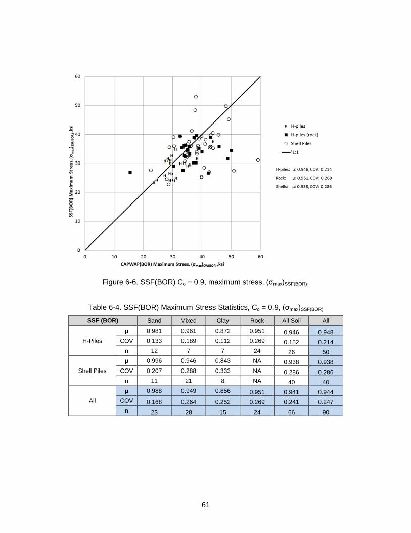
Figure 6-6. SSF(BOR) Co = 0.9, maximum stress, (σmax)SSF(BOR).

Table 6-4. SSF(BOR) Maximum Stress Statistics, Co = 0.9, (σmax)SSF(BOR)

SSF (BOR) Sand Mixed Clay Rock All Soil All

H-Piles μ 0.981 0.961 0.872 0.951 0.946 0.948

COV 0.133 0.189 0.112 0.269 0.152 0.214 n 12 7 7 24 26 50

Shell Piles μ 0.996 0.946 0.843 NA 0.938 0.938

COV 0.207 0.288 0.333 NA 0.286 0.286 n 11 21 8 NA 40 40

All μ 0.988 0.949 0.856 0.951 0.941 0.944

COV 0.168 0.264 0.252 0.269 0.241 0.247 n 23 28 15 24 66 90

61

Figure 6-7. SSF(EOD) Co = 0.944, maximum stress, (σmax)SSF(EOD).

Table 6-5. SSF(EOD) Statistics, Co = 0.944, (σmax)SSF(EOD)

SSF (EOD), Final Sand Mixed Clay Rock All Soil All

H-Piles μ 1.025 1.050 0.848 1.001 0.991 0.995

COV 0.165 0.221 0.221 0.320 0.226 0.269 n 12 10 7 24 29 53

Shell Piles μ 1.018 1.025 0.957 NA 1.008 1.008

COV 0.179 0.334 0.179 NA 0.267 0.267 n 11 21 8 NA 40 40

All μ 1.021 1.033 0.906 1.001 1.001 1.000

COV 0.168 0.300 0.210 0.320 0.248 0.267 n 23 31 15 24 69 93

Table 6-6. Comparison of WEAP and SSF Maximum Stress Prediction (EOD)

WEAP EOD SSF EOD

Rock Soil All Rock Soil All μ 1.107 1.000 1.028 1.001 1.001 1.000

COV 0.412 0.227 0.284 0.320 0.248 0.267 n 24 66 90 24 69 93

62

Figure 6-8. SSF(BOR) Co = 0.953, maximum stress, (σmax)SSF(BOR).

Table 6-7. SSF(BOR) Maximum Stress Statistics, Co = 0.953, (σmax)SSF(BOR)

SSF (BOR), Final Sand Mixed Clay Rock All Soil All

H-Piles μ 1.039 1.018 0.924 1.007 1.002 1.004

COV 0.137 0.196 0.115 0.278 0.157 0.221 n 12 7 7 24 26 50

Shell Piles μ 1.055 1.002 0.893 NA 0.994 0.994

COV 0.215 0.297 0.342 NA 0.295 0.295 n 11 21 8 NA 40 40

All μ 1.046 1.006 0.907 1.007 0.997 1.000

COV 0.174 0.273 0.258 0.278 0.249 0.255 n 23 28 15 24 66 90

Table 6-8. Comparison of WEAP and SSF Maximum Stress Prediction (BOR)

WEAP BOR SSF BOR

Rock Soil All Rock Soil All μ 1.123 0.985 1.021 1.007 0.997 1.000

COV 0.255 0.248 0.260 0.278 0.249 0.255 n 24.000 66.000 90 24 66 90

63

CHAPTER 7 DEVELOPMENT OF RESISTANCE FACTORS FOR LRFD

7.1 INTRODUCTION Load resistance factor design (LRFD) is being used more frequently in the design of foundations for bridge structures. LRFD accounts for the uncertainty associated with the prediction of load and resistance by assigning load factors and resistance factors necessary to achieve a target level of reliability (reliability index).

The technique to apply LRFD to geotechnical design used herein requires quantifying the uncertainty of load and resistance with a bias and a coefficient of variation (COV). Bias is defined as the average ratio of measured/predicted and represents how well predicted and measured agree, on the average. The COV identifies how consistently the method predicts capacity, and therefore COV quantifies the scatter associated with ratio of measured/predicted. The COV is defined as the standard deviation divided by the bias. Specific definitions and equations for COV are given in Chapter 4.

The overall target reliability of the pile foundation is affected by the uncertainties (bias and COV) in load and resistance. Furthermore, the overall target reliability is controlled by selecting appropriate values for load and resistance factors. Mathematically, the target reliability index (β) is a function of live load (bias, COV, and load factor), dead load (bias, COV, and load factor), and pile capacity (bias, COV, and resistance factor). The first order second moment (FOSM) method and the first order reliability method (FORM) can be used to quantify the target reliability index as a function of the load and resistance variables (Long and Anderson 2012).

7.2 REFINEMENT OF WSDOT AND K-IDOT PREDICTIVE METHODS Most piling driven for IDOT requires that the K-IDOT method be used for estimating length and WSDOT be used to verify pile capacity in the field. Statistical results presented in Chapter 4 show there is a slight tendency, on average, for the WSDOT method to overpredict capacity.

The approach applied to refine K-IDOT and WSDOT is presented in the following example. Consider a predictive method in which all the load tests result in an average ratio of predicted/measured capacity equal to 1.2 with a COV of 0.3. It can be correctly stated that the method overpredicts pile capacity an average of 20%. However, the distribution of predicted/measured values is a log-normal distribution rather than a normal distribution, which means the distribution of predicted/measured values is not symmetric and, as a result, the median and the mean are not the same value. The median is defined at the value at which half the predicted/measured ratios are greater and the other half are less. Therefore, it is more appropriate to calibrate predictive methods so that the median value equals to unity. The median value (x50) can be determined from the mean and COV from a log-normal distribution by using the following relationship: x50 = µ / sqrt(1+COV2).

Continuing with this example, the median equals 1.2/sqrt(1+0.3^2), which is 1.149. All predicted capacities are divided by 1.149, which results in a new set of statistics in which the new mean is 1.044 and the COV remains at 0.3. The new median is 1.044/sqrt(1+0.3^2) = 1.00. This adjustment results in a calibrated method that overpredicts capacity half the time and underpredicts capacity half the time, which is the desired outcome of the calibration procedure.

Now consider the statistics for WSDOT. WSDOT(EOD) reports an average value for the ratio of predicted/measured capacity to be 1.31 for H-piles and 1.07 for shell piles. Adjusting the parameter Feff in the WSDOT formula (see Equation {2.8}) provides a simple means to adjust WSDOT predictions so that the median x50, will be closer to unity. Feff in Equation {2.8} is stated as 0.47 for steel piles driven

64

with an open-ended diesel hammer. Based on the values of x50 for these cases, an Feff = 0.38 is recommended for H-piles, and an Feff = 0.46 is recommended for shell piles.

The average predicted/measured capacity ratio for WSDOT(BOR) is about 1.5 for both H- and shell piles; therefore, it is recommended to use Feff = 0.33 for WSDOT(BOR). Piles driven into rock and shale exhibited mean and COV values different enough to warrant separate Feff values as shown in Table 7-1. The resulting statistics for the WSDOT with the newly recommended Feff values are given in Table 7-1 for driving steel piles with an open-ended diesel hammer and resulting statistics for EOD and BOR are shown in Table 7-2 and Table 7-3. respectively.

Table 7-1. WSDOT Recommended Feff Values

WSDOT Category Feff μ COV EOD

H-piles 0.38 1.06 0.328 Shell piles 0.46 1.05 0.269

H-piles (rock) 0.47 1.16 0.34 H-piles (shale) 0.38 1.02 0.219

BOR H-piles 0.33 1.04 0.292

Shell piles 0.33 1.06 0.292 H-piles (rock) 0.47 1.28 0.384 H-piles (shale) 0.34 1.02 0.213

The updated statistics for the modified method are presented in Table 7-2.

Table 7-2. WSDOT(EOD) Statistics with Recommendations Applied

WSDOT(EOD) Clay Mixed Sand Rock Shale All Soil All

H-Piles μ 1.031 0.996 1.156 0.977 1.016 1.056 1.105

COV 0.466 0.204 0.340 0.424 0.219 0.328 0.334 n 7 7 27 10 17 26 53

Shell Piles μ 0.969 1.076 NA NA NA 1.048 1.048

COV 0.361 0.286 NA NA NA 0.269 0.269 n 8 21 NA NA NA 40 40

All μ 0.992 1.055 1.156 0.977 1.016 1.050 1.080

COV 0.396 0.266 0.340 0.424 0.219 0.291 0.306 n 15 28 27 10 17 66 93

65

Table 7-3. WDOT(BOR) Statistics with Recommendations Applied

WSDOT(BOR) Clay Mixed Sand Rock Shale All Soil All

H-Piles μ 0.940 0.924 1.282 1.048 1.02 1.036 1.158

COV 0.400 0.257 0.384 0.491 0.213 0.295 0.353 n 7 7 27 10 17 26 53

Shell Piles μ 0.913 1.140 NA NA NA 1.063 1.063

COV 0.364 0.278 NA NA NA 0.293 0.293 n 8 21 NA NA NA 40 40

All μ 0.921 1.085 1.282 1.048 1.02 1.052 1.117

COV 0.366 0.284 0.384 0.491 0.213 0.292 0.329 n 15 28 27 10 17 66 93

K-IDOT estimates capacity of a driven pile based on the stratigraphy and strength characteristics of the ground and the size, length, and shape (H- or shell) of the pile. Details of the predictive method are presented in Section 2.2.2 of this report. Statistical values for the ratio of predicted capacity (K-IDOT) to measured capacity (CAPWAP(BOR_14)) were presented in Chapter 4 and are as follows:

H-piles in soil: μ = 0.916, COV = 0.583 Shell piles in soil: μ = 1.219, COV = 0.558

These values suggest that the K-IDOT method, on the average, overpredicts capacity for shell piles by a factor of 1.22 and underpredicts capacity of H-piles by a factor of 0.92 (8%). Values for the median, x50, are 0.79 for H-piles and 1.06 for shell piles. The COV values are very high for both pile types, which indicates the K-IDOT predictive method is less precise than the other methods investigated in the this report.

The tendency for K-IDOT to underpredict capacity for H-piles can be adjusted by increasing all K-IDOT estimates of capacity (for H-piles) by a factor of 1.26. This adjustment corrects the median value close to 1.0, but the COV remains the same. Results of H- and shell piles can now be combined to develop one set of summary statistics for K-IDOT for all piles. Combining the two pile types results in a mean of 1.192 and a COV of 0.563 for K-IDOT. Updated statistics for including suggested modifications are shown in Table 7-4.

Table 7-4. K-IDOT Statistics with Recommendations Applied

K-IDOT Clay Mixed Sand Rock All Soil All

H-Piles μ 0.941 1.349 1.214 0.976 1.155 1.054

COV 0.417 0.541 0.752 0.525 0.583 0.552 n 7 7 9 27 23 50

Shell Piles μ 1.246 1.042 1.714 NA 1.219 1.219

COV 0.617 0.422 0.771 NA 0.558 0.558 n 8 21 9 NA 38 38

All μ 1.090 1.112 1.445 0.976 1.192 1.123

COV 0.522 0.453 0.765 0.525 0.563 0.557 n 15 28 18 27 61 88

66

7.3 FOSM The FOSM method as defined in NCHRP 507 (Paikowsky et al. 2004) uses the following expression to determine the resistance factor, φ:

( )( )

( )( ){ }

2 2

2

2 2 2

1

1

exp ln 1 1

D L

D

L D L

Q QD DR L

L R

Q DQ T R Q Q

L

COV COVQQ COV

QCOV COV COV

Q

γλ γ

ϕλ

λ β

+ + +

+ = + + + +

{7.1}

where

λR = bias factor (which is the mean value of QM/QP) for resistance (input)

DQCOV = coefficient of variation for the dead load (0.1)

LQCOV = coefficient of variation for the live load (0.2)

COVR = coefficient of variation for the resistance (input) βT = target reliability index (2.33) γD = load factor for dead loads (1.25) γL = load factor for live loads (1.75) QD/QL = ratio of dead load to live load (2.0)

DQλ = bias factor for dead load (1.05)

LQλ = bias factor for live load (1.15)

However, Equation {7.1} uses an incomplete definition for the covariance of the total load, Q, as follows:

2 2 2Q QD QLCOV COV COV= + {7.2}

As a result, a conservative estimate for the resistance factor (Equation {7.1}) is determined. A more accurate estimate of the overall COV for load accounts for both the COV for live and dead load, but it also accounts for the proportion of dead load to live load. Bloomquist et al. (2007) derived a more accurate formulation for COV that includes the ratio of dead load to live load:

22 2 2 2

22

22 2

2 2

D D L L

D D L L

DQ Q Q Q

LQ

D DQ Q Q Q

L L

Q COV COVQCOVQ QQ Q

λ λ

λ λ λ λ

⋅ ⋅ + ⋅=

⋅ + ⋅ ⋅ +{7.3}

which can be substituted into the resistance factor equation to yield

67

( )

( )

22 2 2 2

2

22 2

2

2

22 2 2 2

22

22 2

2

2

1

exp ln 12

D D L L

D D L L

D D L L

D L

D D L L

DQ Q Q Q

L

D DQ Q Q Q

D L LR D L

L R

DQ Q Q Q

D LQ Q T R

D DLQ Q Q Q

L L

Q COV COVQQ Q

Q Q QQ COV

Q COV COVQ QCOV

Q QQQ Q

λ λ

λ λ λ λλ γ γ

φ

λ λλ λ β

λ λ λ λ

⋅ ⋅ + ⋅

⋅ + ⋅ ⋅ +

⋅ ⋅ + +

≥

⋅ ⋅ + ⋅ ⋅ + ⋅ + ⋅ ⋅ + ⋅ ⋅ +

{7.4}

The corrected FOSM approach shown in Equation {7.4} agrees well with more rigorous iterative procedures such as the FORM. Equation {7.4} is used to calculate the resistance factor for all methods examined in this study.

The equations presented use the term bias (λ), which is defined as the average ratio of measured capacity/predicted capacity. The term bias is often used in statistical formulas such as Equation {7.4}. However, this report primarily uses the term mean (µ) to represent the average ratio of predicted capacity/measured capacity. Mean (µ) has been used because it is a simple and direct measure to assess predictive capability for a method. A value (µ) greater than unity corresponds to predicting capacity greater than measured (overprediction), and a mean value less than one corresponds to underprediction of capacity. Accordingly, all statistics based on mean values provided previously in this report were converted to the equivalent value of bias.

7.4 CALCULATED RESISTANCE FACTORS Resistance factors are determined using Equation {7.4} and are presented in Table 7-5. Within Equation {7.4} the dominant parameter relating the predictive ability of a given method is the COV (standard deviation normalized by the mean), which is a measure of precision. The accuracy of the method as related by the bias (λ), is of less relative importance because the method bias can be easily corrected by multiplying the predicted capacity by a constant. The bias (λ) and COV are calculated using log-normal distributions and then converted back to arithmetic; this process is more statistically rigorous than calculating arithmetic parameters directly (see Appendix A).

A review of the summary statistics suggests that the WSDOT(EOD) method performed differently for H- and shell piles in soil. While the bias values for H- and shell piles are similar (1.06 and 1.05), the COV for H-piles is greater (0.33) than for shell piles (0.27). The differences in mean and COV were enough to justify development of independent resistance factors for H-piles and shell piles. Additionally, differences were significant enough in mean and COV for H-piles driven to shale and rock to be considered separately. Individual resistance factors for H- and shell piles for other methods were developed when the differences in mean and COV were significant.

It is a common misinterpretation to assume more precise methods will have higher resistance factors. The resistance factor depends on both the bias (accuracy) and COV (precision). Method bias reflects the tendency of a method to over- or under-predict and therefore indicates if a method is, on the average, conservative (λ > 1) or unconservative (λ < 1). For example, consider two methods (method

68

1, method 2) with a bias of 1.3 and 0.9 respectively which have the same COV (0.3). Both methods have exactly the same precision (COV) and therefore, are equally effective and efficient equations to use for design. The resultant resistance factors are 0.80 and 0.55 for methods 1 and 2 respectively. Thus, two predictive methods identical in precision can have different resistance factors to compensate for the methods' bias. Accordingly, a higher resistance factor is not an indicator of a more efficient method.

The most effective and efficient predictive methods are the methods that exhibit the greatest precision. A method's precision can be selected on the basis of COV (smaller COV, greater precision) or “efficiency”. Efficiency is defined as the ratio of the resistance factor to the method bias (φ/λ), and thus the effect of bias is removed. Efficiencies for all the methods considered are included in Tables 7-5 and 7-6. A higher efficiency value corresponds to a more precise method and to a more efficient design. Similarly, the COV can also be used to identify more efficient methods. Smaller values of COV represent less scatter in the predictive method, which indicates in a more efficient method.

Efficiencies for all methods ranged from 0.33 to 1.01. The highest efficiency for piles driven into soil was 0.77 for PDA(BOR). The statistics for the WSDOT method are based on the updated method with updated values of Feff applied. The efficiency for WSDOT(EOD) was 0.57 for H-piles and 0.66 for shell piles.

The statistics presented for the K-IDOT method are based on the updated K-IDOT method correcting for method bias for H-piles. K-IDOT exhibited the lowest efficiency of all predicative methods. Several factors contribute to this low efficiency, such as the difference between the soil profile determined from the soil boring and the actual soil profile at the exact location of the driven pile.

69

Table 7-5. Values of φ for Comparison of Predicted Capacity with CAPWAP(BOR_14) Predictive

Method Soil

Conditions Pile Type Bias COV φ Efficiency

(φ/λ) K-IDOT Soil H & Shell 1.10 0.56 0.36 0.33

WSDOT(EOD) Soil H 1.05 0.33 0.60 0.57

WSDOT(EOD) Soil Shell 1.02 0.27 0.67 0.66

WSDOT(BOR) Soil H & Shell 1.03 0.29 0.64 0.62

WEAP(EOD) Soil H 1.07 0.25 0.73 0.69

WEAP(EOD) Soil Shell 1.59 0.35 0.87 0.55

WEAP(BOR) Soil H 0.94 0.32 0.55 0.59

WEAP(BOR) Soil Shell 1.14 0.30 0.71 0.62

PDA(EOD) Soil H & Shell 1.14 0.26 0.76 0.67

PDA(BOR) Soil H & Shell 0.85 0.20 0.65 0.77

WSDOT(EOD) Shale H 1.03 0.219 0.76 0.74

WSDOT(BOR) Shale H 1.02 0.213 0.77 0.75

WEAP(EOD) Shale H 1.02 0.165 0.85 0.83

WEAP(BOR) Shale H 0.92 0.126 0.83 0.90

PDA(EOD) Shale H 0.93 0.146 0.81 0.87

PDA(BOR) Shale H 0.90 0.121 0.82 0.91

WSDOT(EOD) Rock H 1.21 0.424 0.55 0.46

WSDOT(BOR) Rock H 1.18 0.491 0.46 0.39

WEAP(EOD) Rock H 1.60 0.433 0.72 0.45

WEAP(BOR) Rock H 1.53 0.475 0.62 0.41

PDA(EOD) Rock H 0.97 0.105 0.92 0.94

PDA(BOR) Rock H 0.94 0.056 0.95 1.01

7.5 RESISTANCE FACTORS MODIFIED TO ACCOUNT FOR STATIC LOAD TESTS All the resistance factors that were determined are based on the agreement between predicted pile capacity and the pile capacity as established from dynamic load tests conducted at the beginning of restrike and interpreted with CAPWAP. A more appropriate assessment would compare predicted pile capacity with results from static load tests, but unfortunately, only one static load test was conducted (Long and Anderson 2012), which prevents statistical treatment of the database of pile capacities collected in this study. Therefore, an approach was used to relate the predicted capacity with pile capacity as determined by CAPWAP, and then to relate the CAPWAP capacity to the capacity expected from a static load test.

The relationship (bias and COV) for all predictive methods compared with CAPWAP were presented in the previous section (Table 7-5). The bias and COV for each of these methods need to be adjusted to

70

relate the predictive capacity with the static load test capacity. The adjustment can be explained mathematically as follows:

capacity capacity capacity( ) capacity( ) capacity( ) measured capacity(SLT)

predicted predicted measured CWmeasured SLT measured CW

= • {7.5}

where measured capacity (SLT) is the measured capacity from a static load test, and measured capacity (CW) is the estimate of pile capacity from a restrike analysis with CAPWAP. Values for the numerator (predicted/measured(CW)) are reported for several predictive methods in the previous section. Values for the measured(CW)/measured(SLT) are obtained from a study reported by Rausche et al. (1996), who conducted a study of 99 pile load tests in which both static load tests and CAPWAP analyses were performed. Statistical analyses of the results indicate an average ratio of predicted to measured capacity of 0.92 with a COV = 0.22.

Equation {7.5} demonstrates the method to get the ratio of predicted to measured/(SLT), however, this ratio is a statistical function with a mean and COV. Likewise, the other two parameters, predicted/measured(CW) and measured(CW)/measured(SLT), are also statistical functions with means and COVs. The two functions on the right-hand side of Equation {7.5} were combined by determining the mean of the log-normal values, and then adding the two means to get the combined average as follows:

( ) ( ) ( )/ (SLT) / ( ) ( )/ (SLT)ln ln lnpredicted measured predicted measured CW measured CW measuredµ µ µ= + {7.6}

Log-normal values for mean were then converted back to arithmetic values. The COV for predicted capacity/measured capacity (SLT) was calculated by taking the square root of the sum of the squares of the (log-normal) standard deviations for each of the two parameters on the right hand side of Equation {7.5} as follows:

( ) ( ) ( )2 2

( / ( ) ( / ( ) ( ( )/ ( )ln ln lnpredicted measured SLT predicted measured CW measured CW measured SLTσ σ σ= + {7.7}

Log-normal values for standard deviation were then converted to the arithmetic equivalent. Equation {7.7} for the combined standard deviation from the two distributions assumes there is no covariance between the two methods, predicted capacity/measured capacity (CW) and measured capacity (CW)/measured capacity(SLT). This is a prudent assumption and results in upper-bound estimates for the combined standard deviation. If there is covariance between the two distributions, then estimates of combined standard deviation would be less in magnitude.

All values for mean and COV presented in the previous section (predicted/measured(CW)) were adjusted as outlined in Equations {7.1} through {7.7} to determine the mean and COV values for predicted/measured(SLT) and are given in Table 7-6. Also given in Table 7-6 are the resistance values, φ, and efficiency for each of the methods. In most cases, adjusted φ values are less than φ values based on CW(BOR).

Resistance factors for WSDOT(EOD) are 0.58 for H-piles and 0.63 for shell piles driven into soil. The resistance factor for K-IDOT is 0.37. As stated earlier, resistance factors in Table 7-6 are considered to be lower-bound values because there is no covariance assumed for Equation {7.7}.

71

Table 7-6. Values of φ Adjusted for Comparison with Static Load Test Predictive

Method Soil

Conditions Pile Type Bias COV φ Efficiency

(φ/λ)

K-IDOT Soil H & Shell 1.26 0.62 0.37 0.29

WSDOT(EOD) Soil H 1.20 0.40 0.58 0.48

WSDOT(EOD) Soil Shell 1.17 0.35 0.63 0.54

WSDOT(BOR) Soil H & Shell 1.18 0.37 0.61 0.52

WEAP(EOD) Soil H 1.22 0.34 0.68 0.56

WEAP(EOD) Soil Shell 1.81 0.42 0.84 0.46

WEAP(BOR) Soil H 1.07 0.39 0.53 0.49

WEAP(BOR) Soil Shell 1.30 0.37 0.67 0.51

PDA(EOD) Soil H & Shell 1.29 0.35 0.71 0.55

PDA(BOR) Soil H & Shell 0.97 0.30 0.59 0.61

WSDOT(EOD) Shale H 0.95 0.314 0.56 0.59

WSDOT(BOR) Shale H 0.94 0.310 0.56 0.60

WEAP(EOD) Shale H 0.94 0.277 0.61 0.65

WEAP(BOR) Shale H 0.85 0.255 0.58 0.68

PDA(EOD) Shale H 0.85 0.266 0.57 0.66

PDA(BOR) Shale H 0.83 0.252 0.57 0.68

WSDOT(EOD) Rock H 1.11 0.487 0.44 0.39

WSDOT(BOR) Rock H 1.09 0.549 0.37 0.34

WEAP(EOD) Rock H 1.47 0.495 0.57 0.39

WEAP(BOR) Rock H 1.41 0.534 0.50 0.35

PDA(EOD) Rock H 0.90 0.245 0.63 0.70

PDA(BOR) Rock H 0.86 0.227 0.62 0.73

7.6 DISCUSSION Statistics for each predictive method were developed and summarized with a mean and COV for the parameter predicted capacity/measured capacity (CW). These statistics were used with parameters for dead load, live load, and target reliability index, as recommended in NCHRP 507, to determine the resistance factor for each predictive method. Pile capacities were determined from dynamic load tests conducted during restrike on driven piling. CAPWAP was used to interpret capacity from the dynamic load test results.

Additional adjustments were made to the statistics to account for the fact that all “measured” pile capacities were estimated using CAPWAP on results of dynamic tests conducted for restrike conditions several days after initial driving. The result of these adjustments was to decrease slightly the estimates for resistance factors.

The WSDOT(EOD) method exhibited a tendency to overpredict capacity for H-piles and to exhibit slightly more scatter than shell piles. Accordingly, statistics and resistance factors were determined

72

separately for H-piles and shell piles, and for piles driven to rock and shale. The results are given in tables 7-5 and 7-6. Table 7-6 represents lower bound values of φ because combining the statistics (section 7.5) required the assumption that there is no covariance between the distributions of QP/QCAPWAP and QCAPWAP/QStaticLoadTest. Therefore, it is reasonable to use a value between the two bounds. The resistance factor range between upper and lower bounds for WSDOT are 0.6 to 0.58 for H-piles and 0.67 to 0.63 for shell piles. A value of 0.60 for the resistance factor for both H-piles and shell piles fits within bounds and has the advantage of being appropriate for both shell and H-piles. Alternatively, separate resistance factors of 0.60 for H-piles and 0.65 for shell piles could be used.

A resistance factor for H-piles driven to shale (WSDOT(EOD)) is between 0.76 and 0.56 (Tables 7.5 and 7.6), therefore a factor of 0.6 is appropriate. H-piles driven to rock exhibit resistance factors between 0.55 and 0.44. However, the statistics for H-piles driven to rock are unreliable because CAPWAP estimates are typically lower than real capacity Lower-bound estimates of pile capacity in rock is not uncommon with PDA measurements typically because the pile driving hammer cannot deliver sufficient energy to fail the pile. Accordingly, rock should be considered lower bound values.

73

CHAPTER 8 CONCLUSIONS Dynamic load tests on driven piling were conducted in the state of Illinois for IDOT. Dynamic tests were conducted on steel H- and shell piles driven for IDOT structures. Dynamic measurements were conducted for end-of-driving conditions. Most of the piles were retested (restrike) after a delay of 3 days or more. The collection of dynamic load tests was used to improve the ability and efficiency with which IDOT estimates pile capacity. The methods for predicting capacity include the static method used by IDOT (K-IDOT) and the dynamic formula used by IDOT (WSDOT). Other methods were also investigated and compared (WEAP, PDA, CAPWAP). The effect of time on bearing capacity of piles was investigated and modeled. Recommendations are provided for improving K-IDOT and WSDOT, and resistance factors are developed for all methods investigated in this report. The simplified stress formula (SSF) developed in Phase 1 predicted driving stresses well for the additional cases collected in Phase 2.

8.1 RECOMMENDED CHANGES TO CURRENT PRACTICE 8.1.1 K-IDOT Based on the findings from this study, it is recommended that the K-IDOT method be modified slightly. The modifications improve the overall agreement between K-IDOT and the dynamic load tests as well as the agreement between K-IDOT and the WSDOT dynamic formula. The K-IDOT kinematic factors are shown in Table 8-1. The values for Fs and Fp for H-piles have been increased by a factor of 1.26 for both cohesionless and cohesive soil, whereas the kinematic factors for H-piles are unchanged. Updated statistics for the K-IDOT method with suggested recommendations applied are shown in Table 7-4.

Table 8-1. Recommended K-IDOT Kinematic Factors

Fs Fp

Displacement Piles (Shell Piles)

Cohesionless 0.750 0.758

Cohesive 1.174 1.174

Rock NA NA

Non-Displacement Piles (H-Piles)

Cohesionless 0.19 0.38

Cohesive 0.94 1.89

Rock 1.0 1.0

The final recommended resistance factor for K-IDOT is φ = 0.37 for all piles types and all soil types (see Table 7-5 and Table 7-6). Previously, K-IDOT applied separate resistance factors for soil, shale, and rock (excluding shale) (see Long and Anderson 2012).

In addition to the recommendations for the K-IDOT method, it is helpful to review the changes made to the K-IDOT method after publication of the Phase 1 report and included in current statistics:

1. The strength curve relating unit side resistance to NSPT for sandy gravel was reduced by 14% for all values of NSPT. This reduction was made due to the observation of piles in sandy gravel driving significantly longer then the estimated pile length.

74

2. Separate resistance factors were applied for soil, shale, and rock (excluding shale) (Table 2-4, Table 2-5). Note that the resistance factor does not change calculated capacity by K-IDOT but changes the factored resistance available.

3. The K-IDOT method is now based on NSPT values and not (N1)60, allowing the method tomore accurately account for depth effects in SPT penetration resistances.

8.1.2 WSDOT It is recommended that the WSDOT method use different Feff values based on pile type and soil category (soil, shale, or rock) for EOD and BOR. The constant Feff as seen in Equation {2.8} is equal to 0.47 for open-ended diesel hammers with steel piles. The Feff constant is used to modify WSDOT estimates to correct for bias with respect to CAPWAP(BOR_14). The correction factors proposed for BOR will allow estimates for pile capacity to be made for restrike with any setup duration. The correction factors for pile type and soil category are listed in Table 8-2 and should be applied for open-ended diesel hammers only.

Table 8-2. WSDOT Recommended Values for Feff for Single-Acting Diesel Hammers

WSDOT Category Feff μ COV EOD

H-piles 0.38 1.06 0.328 Shell piles 0.46 1.05 0.269

H-piles (rock) 0.47 1.16 0.34 H-piles (shale) 0.38 1.02 0.219

BOR H-piles 0.33 1.04 0.292

Shell piles 0.33 1.06 0.292 H-piles (rock) 0.47 1.28 0.384 H-piles (shale) 0.34 1.02 0.213

8.1.3 PDA All PDA capacity estimates were reported using a Case damping constant, jc = 0.5, in Phase 1. The PDA capacity for all piles in this report used jc = 0.6.

8.1.4 CAPWAP CAPWAP capacity at BOR, CAPWAP(BOR) was used in Phase 1 to represent measured static axial capacity and was therefore used as the metric from which all statistics were calculated. Static axial pile capacity is, however, time dependent as demonstrated in Chapter 3. Consequently, all statistics in Phase 1 were presented in conjunction with the average setup period for each analysis subcategory. Therefore, to enable capacities obtained from pile restrikes with different setup periods to be compared, capacities were normalized to a 14-day strength. The setup period between EOD and BOR range from less than 1 day to 155 days and the majority of piles had a setup period less than 20 days. The time rate of the setup procedure described in Section 3.2 was used to increase CAPWAP(BOR) capacities for periods less than 14 days, whereas piles with setup periods greater than 14 days were unchanged. The normalized 14-day strength is referred to as CAPWAP(BOR_14) and is used as the measured capacity for calculating statistics for method performance (predicted/measured) in this report.

75

The CAPWAP(BOR) capacity according to the findings of Rausche et al. (1996) predict on average 92% of the capacity measured from a static load test. Therefore, to enable comparison of method statistics to those obtained from static load tests, an overall correction factor can be applied (see Table 7-6).

8.1.5 Simplified Stress Formula (SSF) The simplified stress formula (SSF) has been modified to use the maximum stress at any position along the pile length, σmax as an indicator of potential pile damage due to overstressing. Formerly, overstressing was assessed using the maximum average stress of both strain gauges at the gauge location, CSX. The potential for overstressing is better represented using the maximum pile stress and results in a 5% to 6% increase in predicted pile stress. The overall correction factor applied in the SSF method, Co (formerly, Co = 0.9), is adjusted to reflect the change in stress modeled: Co = 0.944 for EOD and Co = 0.953 for BOR. Note, σmax is maximum stress at any point along the pile and is calculated by CAPWAP. The only point at which stress is measured is at the guage location (maximum average stress CSX, maximum stress of either gauge, CSI). Therefore, for monitoring dynamic stresses in the field it is recommended that CSX and CSB (calculated stress at pile toe) be observed noting that the maximum stress, σmax will be approximately 5% larger.

8.2 SUMMARY OF SELECTED FINAL RESULTS 8.2.1 Setup Magnitude and Setup Rate In addition to expanding the dynamic pile load test database, a primary focus of this research phase was to accurately characterize pile setup magnitude (see Section 3.1) and rate (see Section 3.2) for Illinois soil conditions. Setup was examined in terms of a setup ratio (BOR/EOD capacity) for total capacity and side resistance and analyzed with respect to pile type, soil type, pile-soil category, and average NSPT value along pile embedment length, Na. Calibrating the setup formula proposed by Skov and Denver (1988) and applying a modified version of the procedure recently implemented by the Iowa DOT, a time rate of setup formula was developed based on Na and with separate recommended values (setup factor C) for H- and shell piles (see Section 3.2). The final recommended equation based on side resistance is shown in Equation {3.7}. The predictive method that modifies the WSDOT(EOD) based on setup equations exhibited greater scatter than the WSDOT(EOD). Therefore, the simpler WSDOT(EOD) is preferred.

8.2.2 Relaxation Potential of End-Bearing Piles in Shale Relaxation in shale was assessed by examining the setup ratio CAPWAP(BOR)/CAPWAP(EOD) for total capacity and side resistance. For the 17 end-bearing piles driven to shale, the average total capacity decreased by 1%, while end-bearing resistance decreased on average by 26% with a maximum of 74%. End-bearing resistance decreased in 14 of the17 piles tested, as determined by CAPWAP. Therefore, end-bearing relaxation occurred in the majority of piles tested; however, the total pile capacity on average remained approximately constant due to an increase in side resistance of similar magnitude. WSDOT(EOD) exhibited about the same scatter as WSDOT(BOR).

8.2.3 K-IDOT The K-IDOT method was updated by increasing Fp and Fs for H-piles in soil. Statistics for the K-IDOT method with suggested recommendations applied are shown in Table 7-4. Applying these recommendations resulted in the overall method bias, λ = 1.10, COV = 0.563, and resistance factor, φ = 0.37 with respect to CAPWAP(BOR_14). CAPWAP predicts approximately 90% of the typical capacity obtained from a static load test (92% reported by Rausche et al. 1996). Therefore the statistics

76

for all methods including K-IDOT are adjusted to a static load test equivalent capacity (see Section 7.5 for procedure). Accordingly, the final K-IDOT statistics are λ = 1.26, COV = 0.620, and resistance factor, φ = 0.37, with respect to static load test capacity.

8.2.4 WSDOT Resistance factors recommended for the WSDOT method are as follows:

φ = 0.6 for H- and shell piles in soil driven with open-ended diesel hammer (EOD) φ = 0.62 for H- and shell piles in soil driven with open-ended diesel hammer (BOR) φ = 0.60 for H-piles driven to shale with open-ended diesel hammer (EOD)

77

REFERENCES Allen, T. M., “Development of the WSDOT Pile Driving Formula and Its Calibration for Load and

Resistance Factor Design (LRFD).” Prepared for Washington State Department of Transportation and in cooperation with U.S. Department of Transportation, Federal Highway Administration, March 2005.

Bloomquist, D., McVay, M., and Hu, Z. “Updating Florida Department of Transportation’s (FDOT) Pile/Shaft Design Procedures Based on CPT & DTP Data.” BD-545, RPWO #43, UF Project #00005780, Florida Department of Transportation, September 2007.

Clough, R. and Penzien, J. (1975). Dynamics of Structures. McGraw Hill, New York, pp. 364-389.

Federal Highway Administration, U.S;. Department of Transportation. “Research and Procurement, Design and Construction of Driven Pile Foundations.” F HWA Contract No. DTFH61-93-C-00115, September 1995 (I, II). Washington, DC.

Goble, G. G. and F. Rausche. “Wave Equation Analysis of Pile Driving—WEAP86 Program.” U.S. Department of Transportation, Federal Highway Administration, Implementation Division, McLean, VA, Volumes I-IV. 1986.

Isaacs, D. V. (1931). “Reinforced Concrete Pile Formulas.” Transactions, Institute of Engineers, Sydney, Australia, Volume 12, pp. 305-323.

Long, J.H. and Anderson, A.C. (2012). “Improved Design for Driven Piles on a Pile Load Test Program in Illinois.” Research Report FHWA-ICT-12-011, Project R27-069. Rantoul: Illinois Center for Transportation.

Long, J., Hendrix, J., and Baratta, A. (2009). “Evaluation/Modification of IDOT Foundation Piling Design and Construction Policy.” ICT-09-037, Findings of ICT-R27-024, Rantoul: Illinois Center for Transportation, March 2009.

Long, J., and M. Maniaci. “Friction Bearing Design of Steel H-Liles.” IDOT ITRC 1-5-38911, Illinois Transportation Research Center, Edwardsville, December 2000.

Ng, K. W., Suleiman, M. T., Roling, M. J., Abdel Salam, S. S., and Sritharan, S. (2011). “Development of LRFD Design Procedures for Bridge Piles in Iowa—Volume II: Field Testing of Steel H-Piles in Clay, Sand, and Mixed Soils and Data Analysis.” Iowa State University—Institute for Transportation, Ames, IA.

Paikowsky, S.G. et al. (2004). “Load and Resistance Factor Design (LRFD) for Deep Foundations.” NCHRP Report 507, Transportation Research Board, Washington, DC.

Parola, J. (1970). “Mechanics of Impact Pile Driving.” Ph.D. Dissertation, University of Illinois at Urbana-Champaign.

PDI (Pile Dynamics, Inc.) (2005). GRLWEAP Procedures and Models. Cleveland, OH. www.pile.com.

PDI (Pile Dynamics, Inc.) (2004). PDA-W Users Manual. Cleveland, OH. www.pile.com.

Rausche, F., Thendean, G., Abou-matar, H., Likins. G.E. and Goble, G.G. (1996). “Determination of Pile Driveability and Capacity from Penetration Tests.” Final Report, U.S. Department of Transportation, Federal Highway Administration Research Contract DTFH61-91-C-00047.

Skov, R., and Denver, H. (1988). “Time-Dependence of Bearing Capacity of Piles.” Proceedings of the 3rd International Conference on Application of Stress-Waves Theory to Piles (pp. 879-888). Ottawa, ON.

78

Smith, E.A.L. (1960), “Pile driving by the wave equation,” American Society of Civil Engineers, Journal of Soil Mechanics and Foundation Division, 86(4), pp. 35-61.

State of Illinois Department of Transportation (2014) Geotechnical Manual Users (AGMU) Design Guide 10.2, http://www.dot.il.gov/bridges/Design Guides/AGMU 10.2-Geotechnical Pile Design Guide.pdf State of Illinois Department of Transportation (2014) K-IDOT static method, pile length estimation spreadsheet, http://www.dot.il.gov/bridges/dcspreadsheets.html U.S. Department of Transportation, FHWA (Federal Highway Administration), Research and

Procurement, Design and Construction of Driven Pile Foundations. (Washington, D.C. :FHWA Contract No. DTFH61-93-C-00115, September 1995) I, II.

Rausche, F., Goble, G. G., Likins, G. E., (1985). “Dynamic Determination of Pile Capacity. ASCE Journal of Geotechnical Engineering, 111(3), pp. 367-383.

Hannigan, P. (1990). “Dynamic Monitoring and Analysis of Pile Foundation Installations,” Deep

Foundation Institute Short Course Text, First Edition, 69 pp. Randolph, M. F. (2003). Science and Empiricism in Pile Foundation Design, 43rd Rankine Lecture,

Geotechnique 53 (10), 847-875.

79

APPENDIX A PROCEDURE USED TO REPRESENT PREDICTED VERSUS MEASURED RELATIONSHIP

A.1 INTRODUCTION This appendix identifies how the average, standard deviation, and COV are determined for the ratio of QP/QM (mean) and the ratio of QM/QP (bias).

The value of predicted capacity divided by measured capacity (QP/QM) is used throughout this report as a metric to quantify agreement between the predicted axial capacity of a driven pile and its measured capacity. When multiple are available in which both predicted and measured capacities are available, an overall sense of how well the predictive method performs can be quantified by averaging the values of QP/QM. Equation 4.5 in Chapter 4 identifies the average of QP/QM with the symbol, µ. Further statistics identify the standard deviation with the symbol, σ, and the coefficient of variation as COV, as given in Equations 4.4 and 4.5, respectively.

The ratio of QP/QM is straightforward to understand. Over-prediction of capacity results in a ratio of greater than unity while underprediction results in a ratio less than unity. The ratio of QP/QM is used as the primary metric for determining the overall behavior of the method because of its straightforward relationship. However, some statistical treatments require that the statistics quantifying the predictive method be expressed as QM/QP which is the inverse of the predicted/measured ratio. The value of QM/QP is termed “bias” and is represented with the symbol, λ.

A.2 LOG-NORMAL DISTRIBUTION The distribution of QP/QM and its inverse, QM/QP is log normal rather than arithmetic (Long and Maniaci, 2000). However, values for λ, σ, and COV are determined using the arithmetic ratio of QM/QP. Equations to determine the resistance factor (Equations 7.1 and 7.4) use the arithmetic statistical parameters λ and COV, but the equations are formulated in a way that recognizes the distribution is log normal. The values λ and COV are used to express the log normal distribution.

The computation for statistical parameters is conducted in a manner to best represent the log normal distribution. Accordingly, log normal statistics (mean and standard deviation) are determined first, and then the log normal parameters are converted to the arithmetic equivalent.

A.3 PROCEDURE FOR DETERMINING STATISTICAL PARAMETERS Outlined herein is the procedure and commentary for determining the statistical parameters in this report.

1. Determine the mean and standard deviation for all values of ln(QP/QM). The parameters from this step will be called µln and σln. These two terms are representative of the mean and standard deviation of the natural logarithm of QP/QM and are the best representation for a log normal distribution. The value of statistical parameters for the inverse of QP/QM (bias) are simple, the bias is the negative of the mean (λln = -µln) and the standard deviations for both QP/QM and QM/QP are identical.

2. Determine the mean, standard deviation, and COV for QP/QM. Values for µ, σ, and COV based on the arithmetic formulas (Equations 4.2–4.5). The arithmetic mean is determined as follows:

80

2ln ln

12e

µ σµ

+ = A.1

The arithmetic standard deviation is determined as

( )2ln 1eσσ µ= − A.2

Finally, the equation for determining COV is the same as Equation 4.5 (COV = σ/µ).

3. Determine the bias, standard deviation, and COV for QM/QP. Values for λ, σ, and COV basedon the same arithmetic formulas in Chapter 4. Similar to Equations A.1 and A.2, we have thefollowing expressions:

2ln ln

12e

λ σλ

+ = A.3

The arithmetic standard deviation is determined as

( )2ln 1eσσ λ= − A.3

Finally, the equation for determining COV is the same as Equation 4.5 (COV = σ/λ). It is worthwhile to note that in the last sentence of procedure 1 above states that the value of mean for ln(QP/QM) is the negative of the value of mean for ln(QP/QM) (λln = -µln), while the standard deviations are exactly the same.

A.4 DISCUSSION If there were a large number of data (values of QP/QM or QM/QP) and if the data were distributed in a perfectly log normal distribution, then the procedure given above would not be necessary. The statistics in Chapter 4 would be sufficient. However, the number of data points are typically between 10 and 30 and the distribution is neither normal nor log normal (but closer to log normal).

The consequence of smaller data and a distribution that is not exactly log normal is that the COV for QP/QM and the COV for QM/QP are different. Furthermore, back calculated values of µln and σln based on µ and COV (for QP/QM) will not agree with back calculated values of µln and σln calculated from λ and COV (for QM/QP), although for consistency they should.

The procedure followed above ensures consistency and is more representative of the log normal distribution than using the arithmetic equivalents as given in Chapter 4. It is also a more robust representation. By first determining µln and σln and then back calculating equivalent µ and λ, and COV, the log normal distribution is represented more accurately and consistently in the arithmetic equivalents of µ, λ, and COV.

81

APPENDIX B SAMPLE CALCULATIONS

B.1 SAMPLE CALCULATIONS FOR WSDOT The State of Washington uses the following formula (Allen 2005) to determine pile capacity:

{B.1} where

Rn = ultimate pile capacity [kips] Feff = hammer efficiency factor based on hammer and pile type W = weight of hammer [kips] H = drop of hammer [ft] N = average pile penetration resistance [blows/in.]

Only, open-ended diesel hammers were included in the dynamic load test program and therefore, the WSDOT equation was calibrated to reflect field performance by adjusting the Feff factor. The Feff factor formerly equal to 0.47 for open-ended diesel hammers in now determined with the following table:

WSDOT Category Feff μ COV EOD

H-piles 0.38 1.06 0.328 Shell piles 0.46 1.05 0.269

H-piles (rock) 0.47 1.16 0.34 H-piles (shale) 0.38 1.02 0.219

BOR H-piles 0.33 1.04 0.292

Shell piles 0.33 1.06 0.292 H-piles (rock) 0.47 1.28 0.384 H-piles (shale) 0.34 1.02 0.213

Calculation 1: WSDOT(EOD)

Given the following data: SPT soil profile, EOD driving log, hammer type, pile type the WSDOT(EOD) method can be calculated. Given for EOD: stroke = 9, bpi = 4, Delmag D19-42 (4.015 kip ram weight), h-pile in sand (Feff = 0.38).

6.6*0.38*4.015 *9 *ln(10*3 ) 308nR kip ft bpi kips= = {B.2}

6.6 ln(10 )n effR F WH N=

82

Calculation 2: WSDOT(BOR)

Given the following data: SPT soil profile, BOR driving log, hammer type, pile type the WSDOT(BOR) method can be calculated. Given for EOD: stroke = 9.5, bpi = 5.5, Delmag D19-42 (4.015 kip ram weight), h-pile in sand (Feff = 0.33).

6.6*0.33*4.015 *9.5 *ln(10*5.5 ) 333nR kip ft bpi kips= = {B.3}

Calculation 3: WSDOT(BOR_14)

Given the following data: SPT soil profile, BOR driving log, hammer type, pile type the WSDOT(BOR) method can be calculated. Given for EOD: stroke = 9.5, bpi = 5.5, Delmag D19-42 (4.015 kip ram weight), h-pile in sand (Feff = 0.33), Restrike conducted at 2 days.

Steps:

1. Calculate WSDOT(BOR): (see calculation 2). WSDOT(BOR) = 333 kips

2. Calculate K-IDOT method using SPT soil profile. For this example the following K-IDOT datawere obtained: total capacity = 350 kips, side resistance = 225 kips, end resistance = 125 kips.

3. Determine percent side resistance: 225 kips/350 kips = 64%

4. Determine side resistance portion of WSDOT: WSDOT(BOR)*(%side)K-IDOT = 333 kips * 0.64 =213 kips.

5. Determine the thickness weighted average NSPT value along pile length, Na using SPT soilprofile:

1

1

n

i ii

a n

ii

N lN

l

=

=

=∑

∑{B.4}

For this example Na = 18

6. Determine setup constant, C:

( )ba

aCN

= {B.5}

where: Cmax = 0.4 H-piles, 0.5 shell piles a = 2.92, b = 1.17 for H-piles a = 2.63, b = 0.85 for shell piles

Substituting into Equation {B.5} yields:

83

( )1.172.92 0.099 0.518

C = = < {B.6}

7. Apply Skov & Denver approach to side resistance:

( )( )

( )14log 1daysBOR EOD EODbside end

EODa

taR R RtN

= + +

{B.7}

( )1.172.92 14213 log 1 125 356

218BOR

daysR kips kipsdays

= + + = {B.8}

The capacity incorporating setup increased the calculated capacity from 355 kips to 356 kips for an H-pile in sand with a setup period of 2 days. Full setup is assumed to occur at 14 days.

84