This article was originally published in Treatise on ... · PDF fileThis article was...
33
This article was originally published in Treatise on Geophysics, Second Edition, published by Elsevier, and the attached copy is provided by Elsevier for the author's benefit and for the benefit of the author's institution, for non-commercial research and educational use including without limitation use in instruction at your institution, sending it to specific colleagues who you know, and providing a copy to your institution’s administrator. All other uses, reproduction and distribution, including without limitation commercial reprints, selling or licensing copies or access, or posting on open internet sites, your personal or institution’s website or repository, are prohibited. For exceptions, permission may be sought for such use through Elsevier's permissions site at: http://www.elsevier.com/locate/permissionusematerial Blewitt G GPS and Space-Based Geodetic Methods. In: Gerald Schubert (editor-in- chief) Treatise on Geophysics, 2 nd edition, Vol 3. Oxford: Elsevier; 2015. p. 307-338.
Transcript of This article was originally published in Treatise on ... · PDF fileThis article was...

This article was originally published in Treatise on Geophysics, Second Edition, published by Elsevier, and the attached copy is provided by Elsevier for the author's benefit and for the benefit of the author's institution, for non-commercial research and educational use including without limitation use in instruction at your institution, sending it to specific colleagues who you know, and providing a copy to your institution’s administrator.
All other uses, reproduction and distribution, including without limitation commercial reprints, selling or licensing copies or access, or posting on open internet sites, your
personal or institution’s website or repository, are prohibited. For exceptions, permission may be sought for such use through Elsevier's permissions site at:
http://www.elsevier.com/locate/permissionusematerial
Blewitt G GPS and Space-Based Geodetic Methods. In: Gerald Schubert (editor-in-chief) Treatise on Geophysics, 2nd edition, Vol 3. Oxford: Elsevier; 2015. p. 307-338.

Tre
Author's personal copy
3.11 GPS and Space-Based Geodetic MethodsG Blewitt, University of Nevada, Reno, NV, USA
ã 2015 Elsevier B.V. All rights reserved.
3.11.1 The Development of Space Geodetic Methods 3073.11.1.1 Introduction 3073.11.1.2 The Limitations of Classical Surveying Methods 3083.11.1.3 The Impact of Space Geodesy 3093.11.1.4 Lunar Laser Ranging Development 3103.11.1.5 Satellite Laser Ranging Development 3103.11.1.6 VLBI Development 3113.11.1.7 Global Positioning System Development 3113.11.1.8 Comparing GPS with VLBI and SLR 3133.11.1.9 GPS Receivers in Space: LEO GPS 3143.11.1.10 Global Navigation Satellite Systems 3143.11.1.11 International GNSS Service 3153.11.2 GPS and Basic Principles 3163.11.2.1 Basic Principles 3163.11.2.2 GPS Design and Consequences 3183.11.2.3 Introducing High-Precision GPS 3193.11.2.4 GPS Observable Modeling 3213.11.2.5 Data Processing Software 3243.11.2.6 Real-Time GPS and Accuracy Versus Latency 3263.11.3 Global and Regional Measurement of Geophysical Processes 3263.11.3.1 Introduction 3263.11.3.2 Estimation of Station Velocity 3283.11.3.3 Plate Tectonic Rotations 3293.11.3.4 Plate Boundary Strain Accumulation 3303.11.3.5 The Earthquake Cycle 3323.11.3.6 Surface Mass Loading 334References 335
3.11.1 The Development of Space Geodetic Methods
3.11.1.1 Introduction
Geodesy is the science of accurately measuring and understand-
ing three fundamental properties of the Earth: (1) its gravit-
ational field, (2) its geometric shape, and (3) its orientation in
space (Torge, 2001). In recent decades, the growing emphasis
has been on the time variation of these ‘three pillars of geodesy’
(Beutler et al., 2004), which has become possible owing to the
accuracy of new space-based geodetic methods and also owing
to a truly global reference system that only space geodesy can
realize (Altamimi et al., 2001, 2002). As each of these three
properties is connected by physical laws and is forced by natural
processes of scientific interest (Lambeck, 1988), thus, space
geodesy has become a highly interdisciplinary field, intersecting
with a vast array of geophysical disciplines, including tectonics,
Earth structure, seismology, oceanography, hydrology, atmo-
spheric physics, meteorology, and climate change. This richness
of diversity has provided the impetus to develop space geodesy
as a precise geophysical tool that can probe the Earth and its
interacting spheres in ways never before possible (Smith and
Turcotte, 1993).
Borrowing from the fields of navigation and radio astron-
omy and classical surveying, space geodetic methods were
atise on Geophysics, Second Edition http://dx.doi.org/10.1016/B978-0-444-538
Treatise on Geophysics, 2nd edition
introduced in the early 1970s with the development of lunar
laser ranging (LLR), satellite laser ranging (SLR), and very long
baseline interferometry (VLBI) and soon to be followed by the
Global Positioning System (GPS) (Smith and Turcotte, 1993).
The near future promises other new space geodetic systems
similar to GPS, which can be more generally called Global
Navigation Satellite Systems (GNSSs). In recent years, the GPS
has become commonplace, serving a diversity of applications
from car navigation to surveying. Originally designed for few
meter-level positioning for military purposes, GPS is now rou-
tinely used in many areas of geophysics (Bilham, 1991; Dixon,
1991; Hager et al., 1991; Segall and Davis, 1997), for example,
to monitor the movement of the Earth’s surface between points
on different continents with millimeter-level precision, essen-
tially making it possible to observe plate tectonics as it happens.
The stringent requirementsof geophysics arepart of the reason
as towhyGPS has become as precise as it is today (Blewitt, 1993).
As will be described here, novel techniques have been developed
by researchers working in the field of geophysics and geodesy,
resulting in an improvement of GPS precision by four orders of
magnitude over the original design specifications. Owing to this
high level of precision and the relative ease of acquiringGPSdata,
GPS has revolutionized geophysics, aswell asmany other areas of
human endeavor (Minster et al., 2010).
02-4.00060-9 307, (2015), vol. 3, pp. 307-338

308 GPS and Space-Based Geodetic Methods
Author's personal copy
Whereas perhaps the general public may be more familiar
with the georeferencing applications of GPS, say, to locate a
vehicle on a map, this chapter introduces space geodetic
methods with a special focus on GPS as a high-precision geo-
detic technique and introduces the basic principles of geophys-
ical research applications that this capability enables. As an
example of the exacting nature ofmodernGPS geodesy, Figure 1
shows a geodetic GPS station of commonplace (but leading-
edge) design now in the western United States, installed for
purposes of measuring tectonic deformation across the bound-
ary between the North American and Pacific plates. This station
was installed in 1996 at Slide Mountain, Nevada, as part of the
BARGEN network (Bennett et al., 1998, 2003; Wernicke et al.,
2000). To mitigate the problem of very local, shallow surface
motions (Wyatt, 1982), this station has a deep brace Wyatt-type
monument design, by which the antenna is held fixed to the
Earth’s crust by four welded braces that are anchored �10 m
below the surface (and are decoupled by padded boreholes from
the surface). Tests have shown that suchmonuments exhibit less
environmentally caused displacement than those installed to a
(previously more common) depth of �2 m (Langbein et al.,
1995). Time series of daily coordinate estimates from such
sites indicate repeatability at the level of 1 mm horizontal, and
3 mm vertical, with a velocity uncertainty of 0.2 mm year�1
(Davis et al., 2003). This particular site detected �10 mm of
transient motion for 5 months in late 2003, concurrent with
unusually deep seismicity below Lake Tahoe that was likely
caused by intrusion of magma into the lower crust (Smith
et al., 2004).
3.11.1.2 The Limitations of Classical Surveying Methods
It is useful to consider the historical context of terrestrial sur-
veying at the dawn of modern space geodesy around 1970
(Bomford, 1971). Classical geodetic work of the highest
(�mm) precision was demonstrated in the 1970s for purposes
of measuring horizontal crustal strain over regional scales (e.g.,
Savage, 1983). However, the limitations of classical geodesy
discussed in the succeeding text implied that it was essentially
impossible to advance geodetic research on the global scale.
Figure 1 Permanent IGS station at Slide Mountain, Nevada, the UnitedStates. Photo by Jean Dixon.
Treatise on Geophysics, 2nd edition,
Classical surveying methods were not truly three-dimen-
sional. This is because geodetic networks were distinctly sepa-
rated into horizontal networks and height networks, with poor
connections between them. Horizontal networks relied on the
measurement of angles (triangulation) and distances (trilatera-
tion) between physical points (or ‘benchmarks’) marked on
top of triangulation pillars, and vertical networks mainly
depended on spirit leveling between height benchmarks. In
principle, height networks could be loosely tied to horizontal
networks by collocation of measurement techniques at a subset
of benchmarks, together with geometric observations of verti-
cal angles. Practically, this was difficult to achieve, because of
the differing requirements on the respective networks. Hori-
zontal benchmarks could be separated further apart on hill
tops and peaks, but height benchmarks were more efficiently
surveyed along valleys wherever possible. Moreover, the mea-
surement of angles is not particularly precise and is subject to
significant systematic error, such as atmospheric refraction.
Fundamentally, however, the height measured with respect
to the gravitational field (by spirit leveling) is not the same
quantity as the geometric height, which is given relative to
some conventional ellipsoid (that in some average sense rep-
resents sea level). Thus, the horizontal and height coordinate
systems (often called a ‘2þ1’ system) could never be made
entirely consistent.
A troublesome aspect of terrestrial surveying methods was
that observations were necessarily made between benchmarks
that were relatively close to each other, typically between near-
est neighbors in a network. Because of this, terrestrial methods
suffered from increase in errors as the distance increased across
a network. Random errors would add together across a net-
work, growing as a random walk process, proportional to the
square root of distance.
Even worse, systematic errors in terrestrial methods (such as
errors correlated with elevation, temperature, latitude, etc.) can
grow approximately linearly with distance. For example, wave
propagation for classical surveying occurs entirely within the
troposphere, and thus, errors due to refraction increase with
the distance between stations. In contrast, no matter how far
apart the stations are, wave propagation for space geodetic
techniques occurs almost entirely in the approximate vacuum
of space and is only subject to refraction within �10 km opti-
cal thickness of the troposphere (and within the ionosphere in
the case of microwave techniques, although ionospheric refrac-
tion can be precisely calibrated by dual-frequency measure-
ments). Furthermore, by modeling the changing slant depth
through the troposphere (depending on the source position in
the sky), tropospheric delay can be accurately estimated as part
of the positioning solution.
There were other significant problems with terrestrial survey-
ing that limited its application to geophysical geodesy. One was
the requirement of interstation visibility, not onlywith respect to
intervening terrain but also with respect to the weather at the
time of observation. Furthermore, the precision and accuracy of
terrestrial surveying depended a lot on the skill and experience of
the surveyors making the measurements and the procedures
developed to mitigate systematic error while in the field (i.e.,
errors that could not readily be corrected after the fact).
Finally, the spatial extent of classical terrestrial surveying
was limited by the extent of continents. In practice, different
(2015), vol. 3, pp. 307-338

GPS and Space-Based Geodetic Methods 309
Author's personal copy
countries often adopted different conventions to define the
coordinates of their national networks. As a consequence,
each nation typically had a different reference system. More
importantly from a scientific viewpoint, connecting continen-
tal networks across the ocean was not feasible without the use
of satellites. So in the classical geodetic era, it was possible to
characterize the approximate shape of the Earth; however, the
study of the change of the Earth’s shape in time was for all
practical purposes out of the question.
3.11.1.3 The Impact of Space Geodesy
Space geodetic techniques have since solved all the aforemen-
tioned problems of terrestrial surveying. Therefore, the impact
of space geodetic techniques can be summarized as follows (as
will be explained in detail later):
• They allow for true three-dimensional positioning.
• They allow for relative positioning that does not degrade
significantly with distance.
• They do not require interstation visibility and can tolerate a
broader range of weather conditions.
• The precision and accuracy are far superior and position
estimates are more reproducible and repeatable than for
terrestrial surveying, where for space geodesy, the quality
is determined more by the quality of the instruments and
data processing software than by the skill of the operator.
• They allow for global networks that can define a global
reference frame; thus, the position coordinates of stations
in different continents can be expressed in the same system.
From a geophysical point of view, the advantages of space
geodetic techniques can be summarized as follows:
• The high precision of space geodesy (now at the �1 mm
level), particularly over very long distances, allows for the
study of Earth processes that could never be observed with
classical techniques.
• The Earth’s surface can be surveyed in one consistent refer-
ence frame, so geophysical processes can be studied in a
consistent way over distance scales ranging ten orders of
magnitude from 10� to 1010 m (Altamimi et al., 2002).
Global surveying allows for the determination of the
largest-scale processes on Earth, such as plate tectonics
and surface mass loading.
• Geophysical processes can be studied in a consistent way
over timescales ranging ten orders of magnitude from 10�1
to 109 s. Space geodetic methods allow for continuous
acquisition of data using permanent stations with commu-
nications to a data processing center. This allows for geo-
physical processes to be monitored continuously, which is
especially important for the monitoring of natural hazards
but is also important for the characterization of errors and
for the enhancement of precision in the determination of
motion. Sample rates from GPS can be as high as 50 Hz.
Motion is fundamentally determined by space geodesy as a
time series of positions relative to a global reference frame.
Precise timing of the sampled positions in a global time-
scale (<0.1 ms UTC in even the most basic form of GPS and
<0.1 ns for geodetic GPS) is an added bonus for some
applications, such as seismology and SLR.
Treatise on Geophysics, 2nd edition
• Space geodetic surveys are more cost-efficient than classical
methods; thus, more points can be surveyed over a larger
area than was previously possible.
The benefits that space geodesy could bring to geophysics
are precisely the reason why space geodetic methods were
developed. For example, NASA’s interest in directly observing
the extremely slow motions (centimeters per year) caused by
plate tectonics was an important driver in the development of
SLR, geodetic VLBI, and geodetic GPS (Smith and Turcotte,
1993). SLR was initially a NASA mission dedicated to geodesy.
VLBI and GPS were originally developed for other purposes
(astronomy and navigation, respectively), though with some
research and development (motivated by the potential geo-
physical reward) they were adapted into high-precision geo-
detic techniques for geophysical research.
The following are just a few examples of geophysical appli-
cations of space geodesy:
• Plate tectonics, by tracking the relative rotations of clusters
of space geodetic stations on different plates.
• Interseismic strain accumulation, by tracking the relative
velocity between networks of stations in and around plate
boundaries.
• Earthquake rupture parameters, by inverting measurements
of coseismic displacements of stations located within a few
rupture lengths of the fault.
• Postseismic processes and rheology of the Earth’s topmost
layers, by inverting the decay signature (exponential, loga-
rithmic, etc.) of station positions in the days to decades
following an earthquake.
• Magmatic processes, by measuring time variation in the
position of stations located on volcanoes or other regions
of magmatic activity, such as hot spots.
• Rheology of the Earth’s mantle and ice-sheet history, by mea-
suring the vertical and horizontal velocities of stations in the
area of postglacial rebound (glacial isostatic adjustment).
• Mass redistribution within the Earth’s fluid envelope, by
measuring time variation in the Earth’s shape, the velocity
of the solid Earth’s center of mass, the Earth’s gravitational
field, and the Earth’s rotation in space.
• Global change in sea level, by measuring vertical movement
of the solid Earth at tide gauges, by measuring the position
of spaceborne altimeters in a global reference frame, and by
inferring exchange of water between the oceans and conti-
nents from mass redistribution monitoring.
• Hydrology of aquifers by monitoring aquifer deformation
inferred from time variation in 3-D coordinates of a net-
work of stations on the surface above the aquifer.
• Providing a global reference frame for consistent geo-
referencing and precision time tagging of nongeodetic mea-
surements and sampling of the Earth, with applications in
seismology, airborne and spaceborne sensors, and general
fieldwork.
What characterizes modern space geodesy is the broadness
of its application to almost all branches of geophysics and the
pervasiveness of geodetic instrumentation and data used by
geophysicists who are not necessarily experts in geodesy. GPS
provides easy access to the global reference frame, which in
turn fundamentally depends on the complementary benefits of
, (2015), vol. 3, pp. 307-338

310 GPS and Space-Based Geodetic Methods
Author's personal copy
all space geodetic techniques (Herring and Perlman, 1993). In
this way, GPS provides access to the stability and accuracy
inherent in SLR and VLBI without the need for coordination
on the part of the field scientist. Moreover, GPS geodesy has
benefited tremendously from earlier developments in SLR and
VLBI, particularly in terms of modeling the observations.
3.11.1.4 Lunar Laser Ranging Development
Geodesy was launched into the space age by LLR, a pivotal exper-
iment in the history of geodesy. The basic concept of LLR is to
measure the distance to the Moon from an Earth-based telescope
by timing the flight of a laser pulse that is emitted by the telescope,
reflects off the Moon’s surface, and is received back into the same
telescope. LLRwas enabled by the Apollo 11mission in July 1969,
when Buzz Aldrin deployed a laser retroreflector array on the
Moon’s surface in the Sea of Tranquility (Dickey et al., 1994).
Later, Apollo 14 and 15 and a Soviet Lunokhod mission carrying
French-built retroreflectors have expanded the number of sites on
the Moon. Since initial deployment, several LLR observatories
have recorded measurements around the globe, although most
of the routine observations have been made at only two observa-
tories:McDonaldObservatory in Texas, the United States, and the
CERGA station in France. Today, the McDonald Observatory
uses a 0.726 m telescope with a frequency-doubled neodymium-
doped–YAG laser, producing 1500 mJ pulses of 200 ps width at
532 nm wavelength, at a rate of 10 Hz.
The retroreflectors on the lunar surface are corner cubes,
which have the desirable property that they reflect light in
precisely the opposite direction, independent of the angle of
incidence. Laser pulses take between 2.3 and 2.6 s to complete
the 385000 km journey. The laser beam width expands from
7 mm on Earth to several km at the Moon’s surface (a few km),
and so in the best conditions, only one photon of light will
return to the telescope every few seconds. By timing the flight
of these single photons, ranges to the Moon can now be
measured with a precision approaching 1 cm.
The LLR experiment has produced the following important
research findings fundamental to geophysics (Williams et al.,
2001, 2004), all of which represent the most stringent tests
to date:
• The Moon is moving radially away from the Earth at
38 mm year�1, an effect attributed to tidal friction, which
slows down the Earth’s rotation, hence increasing the
Moon’s distance so as to conserve angular momentum of
the Earth–Moon system.
• The moon likely has a liquid core.
• The Newtonian gravitational constant G is stable to
<10�12.
• Einstein’s theory of general relativity correctly explains the
Moon’s orbit to within the accuracy of LLR measurements.
For example, the equivalence principle is verified with a
relative accuracy of 10�13, and geodetic precession is veri-
fied to within <0.2% of general relativistic expectations.
3.11.1.5 Satellite Laser Ranging Development
SLR was developed in parallel with LLR and is based on similar
principles, with the exception that the retroreflectors (corner
Treatise on Geophysics, 2nd edition,
cubes) are placed on artificial satellites (Degnan, 1993). Exper-
iments with SLR began in 1964 with NASA’s launch of the
Beacon-B satellite, tracked by Goddard Space Flight Center
with a range accuracy of several meters. Following a succession
of demonstration tests, operational SLR was introduced in
1975 with the launch of the first dedicated SLR satellite, Starl-
ette, launched by the French Space Agency, soon followed in
1976 by NASA’s Laser Geodynamics Satellite (LAGEOS-1) in a
near-circular orbit of 6000 km radius. Since then, other SLR
satellites now include LAGEOS-II, Stella, Etalon-1 and -2, and
AJISAI. There are now approximately ten dedicated satellites
that can be used as operational SLR targets for a global network
of more than 40 stations, most of them funded by NASA for
purposes of investigating geodynamics, geodesy, and orbital
dynamics (Tapley et al., 1993).
SLR satellites are basically very dense reflecting spheres
orbiting the Earth. For example, LAGEOS-II launched in 1992
is a 0.6 m sphere of mass 411 kg. The basic principle of SLR is
to time the round-trip flight of a laser pulse shot from the Earth
to the satellite. Precise time tagging of the measurement is
accomplished with the assistance of GPS. The round-trip time
of flight measurements can be made with centimeter-level
precision, allowing for the simultaneous estimation of the
satellite orbits, gravitational field parameters, tracking station
coordinates, and Earth rotation parameters. The reason the
satellites have been designed with a high mass to surface area
ratio is to minimize accelerations due to nonconservative
forces such as drag and solar radiation pressure. This produces
a highly stable and predictable orbit and hence a stable
dynamic frame from which to observe the Earth’s rotation
and station motions.
SLR made early contributions to the confirmation of the
theory of plate tectonics (Smith et al., 1993) and toward mea-
suring and understanding contemporary crustal deformation
in plate boundary zones ( Jackson et al., 1994; Wilson and
Reinhart, 1993). To date, SLR remains the premier technique
for determining the location of the center of mass of the Earth
system and its motion with respect to the Earth’s surface (Chen
et al., 1999; Ray, 1998; Watkins and Eanes, 1997). As an
optical technique that is relatively less sensitive to water
vapor in the atmosphere, SLR has also played a key role in
the realization of reference frame scale (Dunn et al., 1999). The
empirical realization of scale and origin is very important for
the testing of dynamic Earth models within the rigorous frame-
work of the International Terrestrial Reference System (ITRS)
(McCarthy, 1996).
Today, SLR is used in the following research (Perlman et al.,
2002):
• Mass redistribution in the Earth’s fluid envelope, allowing
for the study of atmosphere–hydrosphere–cryosphere–
solid Earth interactions. SLR can sense the Earth’s changing
gravitational field (Bianco et al., 1997; Cheng and Tapley,
1999, 2004; Gegout and Cazenave, 1993; Nerem et al.,
1993; Devoti et al., 2001), the location of the solid Earth’s
center of mass with respect to the center of mass of the
entire Earth system (Chen et al., 1999). Also, SLR determi-
nation of the Earth’s rotation in the frame of the stable
satellite orbits reveals the exchange of angular momentum
between the solid Earth and fluid components of the Earth
(2015), vol. 3, pp. 307-338

GPS and Space-Based Geodetic Methods 311
Author's personal copy
system (Chao et al., 1987). SLR stations can sense the
deformation of the Earth’s surface in response to loading
of the oceans, atmosphere, and hydrosphere and can infer
mantle dynamics from response to the unloading of ice
from past ice ages (Argus et al., 1999).
• Long-term dynamics of the solid Earth, oceans, and ice
fields (Sabadini et al., 2002). SLR can sense surface eleva-
tions unambiguously with respect to the Earth’s center of
mass, such as altimeter satellite height and hence ice-sheet
and sea surface height. Thus, SLR is fundamental to the
terrestrial reference frame and the long-term monitoring
of sea level change.
• Mantle–core interaction through long-term variation in the
Earth’s rotation (Eubanks, 1993).
• General relativity, specifically the Lense–Thirring effect of
frame dragging (Cuifolini and Pavlis, 2004).
SLR is a relatively expensive and cumbersome technique
and so has largely been superseded by the GPS technique for
most geophysical applications. SLR is still necessary for main-
taining the stability of the International Terrestrial Reference
Frame (ITRF), in particular, to aligning the ITRF origin with the
specifications of ITRS (Altamimi et al., 2002). SLR is also
necessary to determine long-term variation in the low-degree
components of the Earth’s gravitational field. SLR is main-
tained by NASA to support high-precision orbit determination
(such as for satellite altimetry), though GPS is also now being
used for that purpose.
3.11.1.6 VLBI Development
VLBI, originally a technique designed for observing distant
celestial radio sources with high angular resolution, was from
the late 1970s developed for high-precision geodetic applica-
tions by applying the technique ‘in reverse’ (Rogers et al.,
1978). Much of this development of geodetic VLBI was per-
formed by the NASA Crustal Dynamics Project initiated in
1979 (Bosworth et al., 1993) with the idea to have an alterna-
tive technique to SLR to provide independent confirmation of
scientific findings.
Conceptually, geodetic VLBI uses radio waves from distant
quasars at known positions on the celestial sphere and mea-
sures the difference in the time of arrival of signals from those
quasars at stations (radio observatories) on the Earth’s surface.
Such data provide information on how the geometry of a
network of stations evolves in time. This time-variable geome-
try can be inverted to study geophysical processes such as the
Earth’s rotation and plate tectonics and can be used to define a
global terrestrial reference frame with high precision. Unique
to VLBI is that it can provide an unambiguous, stable tie
between the orientation of the terrestrial reference frame and
the celestial reference frame, that is, Earth orientation. How-
ever, as a purely geometric technique, it is not directly sensitive
to the Earth’s center of mass and gravitational field, although
inferences by VLBI on gravity can bemade throughmodels that
connect gravity to Earth’s shape, such as tidal and loading
models.
Comparisons between VLBI and SLR proved to be impor-
tant for making improvements in both methods. As a radio
technique, VLBI is more sensitive to errors in atmospheric
Treatise on Geophysics, 2nd edition
refraction (Davis et al., 1985; Niell, 1996; Truehaft and Lanyi,
1987) than the optical SLR technique; however, VLBI has the
advantage that the sources are quasars that appear to be essen-
tially fixed in the sky, thus providing the ultimate in celestial
reference frame stability. VLBI is therefore the premier tech-
nique for determining parameters describing the Earth
rotation’s in inertial space, namely, precession, nutation, and
UT1 (the angle of rotation with respect to UTC) (Eubanks,
1993). VLBI ultimately has proven to be more precise than
SLR in measuring distances between stations.
However, VLBI has never been adapted for tracking Earth-
orbiting platforms and is highly insensitive to the Earth’s
gravitational field and thus cannot independently realize the
Earth’s center of mass as the origin of the global reference
frame. On the other hand, the stability of scale in VLBI is
unsurpassed. For most geophysical applications, GPS has
superseded VLBI, except for the important reference frame
and Earth orientation tasks described earlier. VLBI remains
important for characterizing long-wavelength phenomena
such as postglacial rebound, with the highest precision
among all techniques today, and therefore is integral to the
stability of global terrestrial reference frames.
To summarize, geodetic VLBI’s main contributions to sci-
entific research involve (Schlueter et al., 2002)
• unambiguous Earth orientation parameters, which can be
used to study angular momentum exchange between the
solid Earth and its fluid reservoirs and provides a service to
astronomy and space missions by connecting the terrestrial
reference frame to the celestial reference frame (Eubanks,
1993);
• providing a stable scale for the global terrestrial reference
frame (Boucher and Altamimi, 1993);
• providing the highest-precision measurements of long-
wavelength Earth deformations, thus providing stability to
the global frame, and constraints on large-scale geody-
namics such as postglacial rebound and plate tectonics
(Argus et al., 1999; Stein, 1993).
3.11.1.7 Global Positioning System Development
As of September 2006, the GPS consists of 29 active satellites
that can be used to position a geodetic receiver with an accu-
racy of millimeters within the ITRF. To do this requires
geodetic-class receivers (operating at two frequencies, and
with antennas designed to suppress signal multipath), cur-
rently costing a few thousand US dollars, and geodetic
research-class software (developed by various universities and
government institutions around the world). Such software
embody leading-edge models (of the solid Earth, atmosphere,
and satellite dynamics) and data processing algorithms (signal
processing and stochastic parameter estimation). Many of the
models have been developed as a result of much research
conducted by the international geodetic and geophysical com-
munity, often specifically to improve the accuracy of GPS.
Today, it is even possible for a nonexpert to collect GPS data
and produce receiver positions with centimeter accuracy by
using an Internet service for automatic data processing.
The geodetic development of the GPS has been driven by a
number of related factors (Blewitt, 1993):
, (2015), vol. 3, pp. 307-338

312 GPS and Space-Based Geodetic Methods
Author's personal copy
• The foundation for many of the research-class models was
already in place owing to the similarities between GPS and
VLBI (as radio techniques) and GPS and SLR (as satellite
dynamic techniques), thus giving an early boost to GPS
geodesy. Continued collaboration with the space geodetic
community has resulted in standard models such as those
embodied by the ITRS Conventions (McCarthy, 1996),
which aim to improve the accuracy and compatibility of
results from the various space geodetic techniques.
• GPS is of relatively low cost and yet has comparable preci-
sion to VLBI and SLR. Whereas the GPS itself is paid for by
the US taxpayer, the use of the system is free to all as a
public good. This has made GPS accessible to university
researchers, and the resulting research has further improved
GPS accuracy through better models.
• GPS stations are easy to deploy and provide a practical way
to sample the deformation field of the Earth’s surface more
densely, thus allowing space geodesy to address broader
diversity scientific questions. This has opened up interdis-
ciplinary research within geophysics, leading to discoveries
in unforeseen areas and to further improvements in GPS
accuracy through improved observation models.
• GPS was readily adopted because of the ease of access to the
ITRF on an ad hoc basis, without the need for special global
coordination from the point of view of an individual inves-
tigator. Furthermore, the ITRF gives implicit access to the
best possible accuracy and stability that can be achieved by
SLR and VLBI (Herring and Pearlman, 1993).
Following closely the historical perspectives of Evans et al.
(2002) and Blewitt (1993), GPS has its roots as a successor to
military satellite positioning systems developed in the 1960s,
though the first geophysical applications of GPS were not
realized until the early 1980s. In the run-up to the space age
in 1955, scientists at the Naval Research Laboratory first pro-
posed the application of satellite observations to geodesy. By
optical observation methods, the first geodetic satellites were
quickly used to refine parameters of the Earth’s gravitational
field. Optical methods were eventually made obsolete by the
Doppler technique employed by the Navy Navigation Satellite
System (TRANSIT). As the name implies, Doppler positioning
was based on measuring the frequency of the satellite signal as
the relative velocity changed between the satellite and the
observer. By the early 1970s, Doppler positioning with 10 m
accuracy became possible on the global scale, leading to the
precise global reference frame ‘World Geodetic System 1972’
(WGS 72), further improved by WGS 84, which was internally
accurate at the 10 cm level. Having a global network of known
coordinates together with the success of radiometric tracking
methods set the stage for the development of a prototype GPS
in the late 1970s.
The US Department of Defense launched its first prototype
Block I GPS satellite, NAVSTAR 1, in February 1978. By 1985,
ten more Block 1 satellites had been launched, allowing for the
development and testing of prototype geodetic GPS data proces-
sing software that used dual-frequency carrier phase observ-
ables. In February 1989, the first full-scale operational GPS
satellite known as Block II was deployed, and by January
1994, a nominally full constellation of 24 satellites was com-
pleted, ensuring that users could see satellites of a sufficient
Treatise on Geophysics, 2nd edition,
number (at least 5) at anytime, anywhere in the world. Initial
operational capability was officially declared in December 1993,
and full operational capability was declared in April 1995. From
July 1997, Block IIRs began to replace GPS satellites. The first
modified version Block IIR-M satellite was launched in 2005
(for the first time emitting the L2C signal, which allows civilian
users to calibrate for ionospheric delay). The current constella-
tion of 29 satellites includes extra satellites as ‘active spares’ to
ensure seamless and rapid recovery from a satellite failure. The
first Block IIF satellite was scheduled to launch in 2008 and may
transmit a new civil signal at a third frequency.
The GPS design built on the success of Doppler by enabling
the measurement of a biased range (‘pseudorange’) to the
satellite, which considerably improved positioning precision.
Carrier phase tracking technology further improved the signal
measurement precision to the few millimeter level. As a radio
technique, VLBI technology was adapted in NASA’s prototype
geodetic GPS receivers. The SERIES receiver, developed by
MacDoran (1979) at the Jet Propulsion Laboratory (JPL),
pointed at one source at a time using a directional antenna
(a technique no longer used). Many key principles and benefits
of the modern GPS geodesy were based on the omnidirectional
instrument, MITES, proposed by Counselman and Shapiro
(1979). This was developed by the Massachusetts Institute of
Technology (MIT) group into the Macrometer instrument,
which provided centimeter-level accuracy using the innovative
double-difference method for eliminating clock bias, a method
that has its origins in radio navigation of the Apollo mission
(Counselman et al., 1972).
By the mid 1980s, commercial receivers such as the Texas
Instrument TI 4100 became available (Henson et al., 1985)
and were quickly deployed by geophysicists in several pioneer-
ing experiments to measure the slow motions associated with
plate tectonics (Dixon et al., 1985; Freymueller and Kellogg,
1990; Prescott et al., 1989); such experiments spurred the
development of analysis techniques to improve precision at
the level required by geophysics (Larson and Agnew, 1991;
Larson et al., 1991; Tralli et al., 1988). Important develop-
ments during these early years include ambiguity resolution
over long distances (Blewitt, 1989; Dong and Bock, 1989),
precise orbit determination (Beutler et al., 1985; King et al.,
1984; Lichten and Border, 1987; Swift, 1985), and troposphere
modeling (Davis et al., 1987; Lichten and Border, 1987; Tralli
and Lichten, 1990).
The development of geodetic GPS during the 1980s was
characterized by intensive hardware and software development
with the goal of sub-centimeter positioning accuracy, over
increasingly long distances. A prototype digital receiver
known as ‘Rogue’ was developed by the JPL (Thomas, 1988),
which produced high-precision pseudorange data that could
be used to enhance data processing algorithms, such as ambi-
guity resolution. Several high-precision geodetic software pack-
ages that were developed around this time are still in use and
far exceed the capabilities of commercial packages. These
included the Bernese developed at the University of Bern
(Beutler et al., 1985; Gurtner, 1985; Rothacher et al., 1990),
GAMIT-GLOBK developed at MIT (Bock et al., 1986; Dong and
Bock, 1989; Herring et al., 1990), and GIPSY-OASIS developed
at JPL (Blewitt, 1989, 1990; Lichten and Border, 1987; Sovers
and Border, 1987).
(2015), vol. 3, pp. 307-338

GPS and Space-Based Geodetic Methods 313
Author's personal copy
GPS became fully operational in 1994, with the completion
of a full constellation of 24 satellites. Developments toward
high precision in the 1990s include (1) truly global GPS solu-
tions made possible by the completion of the Block II GPS
constellation and, simultaneously, installation and operation
of the global network in 1994 (shown in its current configura-
tion in Figure 2) by the International GPS Service (IGS, since
renamed the International GNSS Service) (Beutler et al.,
1994a); (2) global-scale ambiguity resolution (Blewitt and
Lichten, 1992); (3) further refinement to tropospheric model-
ing and the inclusion of tropospheric gradient parameters
(Bar-Sever et al., 1998; Chen and Herring, 1997; Davis et al.,
1993; McMillan, 1995; Niell, 1996; Rothacher et al., 1998); (4)
adoption of baseband-digital GPS receivers with the low-
multipath choke ring antenna developed originally at JPL
(Meehan et al., 1992), which remains the IGS standard design
today; (5) improved orbit models, particularly with regard to
GPS satellite attitude, and the tuning of stochastic models
for solar radiation pressure (Bar Sever, 1996; Beutler et al.,
1994b; Fliegel and Gallini, 1996; Fliegel et al., 1992; Kuang
et al., 1996); (6) improved reference system conventions
(McCarthy, 1996); and (7) simultaneous solution for both
orbits and station positions (fiducial-free global analysis)
(Heflin et al., 1992).
The focus of developments in the decade includes (1)
building on earlier work by Schupler et al. (1994), antenna
phase center variation modeling and calibrations for both
stations and the GPS satellites themselves (Ge et al., 2005;
Mader, 1999; Mader and Czopek, 2002; Schmid and
Rothacher, 2003; Schmid et al., 2005); (2) densification of
stations in the ITRF and the installation of huge regional
networks of geodetic GPS stations, such as the �1000 station
Plate Boundary Observatory currently being installed in the
western North America (Silver et al., 1999); (3) improved
analysis of large regional networks of stations through
Figure 2 The global network of the International GPS Service. Courtesy of A
Treatise on Geophysics, 2nd edition
common-mode signal analysis (Wdowinski et al., 1997) and
faster data processing algorithms ((Bertiger et al., 2010;
Zumberge et al., 1997); (4) the move toward real-time geodetic
analysis with applications such as GPS seismology (Larson
et al., 2003; Nikolaidis et al., 2001) and tsunami warning
systems (Blewitt et al., 2006), including signal processing algo-
rithms to filter out sidereally repeating multipath (Bock et al.,
2000, 2004; Choi et al., 2004); and (5) further improvements
in orbit determination (Ziebart et al., 2002), tropospheric
modeling (Boehm et al., 2006), and higher-order ionospheric
models (Kedar et al., 2003).
With the significant improvements to modeling since the
inception of the IGS in 1994, data reprocessing of global GPS
data sets has begun in earnest. Early results indicate superior
quality of the GPS data products, such as station coordinate
time series, orbit and clock accuracy, and Earth orientation
parameters (Steinberger et al., 2006).
3.11.1.8 Comparing GPS with VLBI and SLR
GPS geodesy can be considered a blend of the two earlier space
geodetic techniques: VLBI and SLR. The most obvious similar-
ities are that (1) SLR and GPS are satellite systems and so are
sensitive to Earth’s gravitational field and (2) VLBI and GPS are
radio techniques and so the observables are subject to atmo-
spheric refraction in a similar way. Due to these similarities,
GPS geodesy has benefited from earlier work on both VLBI and
SLR observation modeling and from reference system conven-
tions already established through a combination of astronom-
ical observation, VLBI and SLR observation, and geodynamic
modeling. Moreover, Earth models such as tidal deformation
are required by all global geodetic techniques, so GPS geodesy
was in a position to exploit what had already been learned.
Today, the improvements in modeling any of the techniques
can often be exploited by another technique.
. Moore.
, (2015), vol. 3, pp. 307-338

314 GPS and Space-Based Geodetic Methods
Author's personal copy
The similarities between certain aspects of the different
techniques lead to an overlap of strengths and weaknesses,
error sources, and sensitivity to geophysical parameters of
interest. The strengths and weaknesses can be summarized as
follows:
• The main strength of SLR is the stability of the orbits due to
custom-designed satellites. This leads to high sensitivity to
the low-degree gravitational field harmonics and their long-
term changes in time. This includes the degree-one term
(characterizing geocenter motion, the motion of the solid
Earth with respect to the center of mass of the entire Earth
system), which is important for realizing the origin of the
ITRF. As an optical technique, SLR is insensitive to moisture
in the atmosphere and so has relatively small systematic
errors associated with signal propagation. This inherently
leads to more robust estimation of station height. On the
other hand, SLR has problems working during daylight
hours and in cloudy conditions. It is also an expensive
and bulky technique and so suffers from a lack of
geographic coverage.
• The main strength of VLBI is the stability and permanency of
the sources, which are quasars. This leads to two important
qualities: (1) VLBI is insensitive to systematic error in orbit
dynamic models and can potentially be the most stable
system for detecting the changes over the longest observed
time periods, and (2) VLBI is strongly connected to an
external, celestial reference frame, a vantage point from
which Earth orientation and rotation can be properly deter-
mined. A major weakness of VLBI is (similar to SLR) its
expensiveness and bulkiness. Moreover, some VLBI observa-
tories are used for astronomical purposes and so cannot be
dedicated to continuous geodetic measurement. VLBI anten-
nas are very large structures that have their own set of prob-
lems, including the challenge to relate the observations to a
unique reference point, and the stability of the structure with
respect to wind and gravitational stress, and aging.
The main advantage of GPS is its low cost and ease of
deployment and all-weather capability. Thus, GPS can provide
much better geographic coverage, continuously. The flexibility
of deployment allows for ties to be made between the terres-
trial reference frames of the various techniques through collo-
cation at SLR and VLBI sites. The disadvantage of GPS is that it
is subject to both the systematic error associated with orbit
dynamics and atmospheric moisture. Furthermore, the omni-
directional antennas of GPS lead to multipath errors. Thus,
geodetic GPS is essential for improved sampling of the Earth
in time and space but ultimately depends on SLR and VLBI to
put such measurements into a reference frame that has long-
term stability. This synergy lies at the heart of the emerging
concept GGOS, the Global Geodetic Observing System, under
the auspices of the International Association of Geodesy (IAG)
(Rummel et al., 2005).
3.11.1.9 GPS Receivers in Space: LEO GPS
GPS has proved extremely important for positioning space-
borne scientific instruments in low-Earth orbit (sometimes
called LEO GPS). Evans et al. (2002) provided an overview of
Treatise on Geophysics, 2nd edition,
spaceborne GPS, which is only briefly summarized here. The
Landsat 4 satellite launched in 1982 was the first to carry a GPS
receiver, called GPSPAC. This was followed by three more
missions using GPSPAC, including Landsat 5 in 1984 and
DoD satellites in 1983 and 1984. As the GPS satellite constel-
lation grew during the 1980s, so the precision improved,
enabling decimeter-level accuracy for positioning spaceborne
platforms. Following Evans et al. (2002), the applications of
spaceborne GPS can be categorized as (1) precise orbit deter-
mination of the host satellite for applications such as altimetry;
(2) measurement of the Earth’s gravitational field, such as the
missions CHAMP and GRACE; (3) ionospheric imaging; and
(4) indirect enhancements to global geodesy and remote sens-
ing. In addition to these categories, spaceborne GPS is also
being used to invert for the refractivity of the Earth’s neutral
atmosphere by occultation measurements, which can be used,
for example, to infer stratospheric temperatures for studies of
global climate change.
3.11.1.10 Global Navigation Satellite Systems
The success of GPS has led to the development of similar future
systems, generically referred to as GNSS. To achieve global
coverage, each GNSS system generally has a constellation of
20–30 satellites in roughly 12 h orbits. Some systems are aug-
mented with a few satellites in either geostationary or inclined
geosynchronous orbit.
The Russian system GLONASS (a Russian acronym that
literally translates to GNSS) was actually developed in parallel
with GPS and achieved global coverage with 24 satellites in
orbit by 1995. After a subsequent period of degradation, the
GLONASS system was restored back to a full constellation of
24 satellites by the end of 2011 and, as of 2013, has 29 satellites
in orbit. Many modern GNSS receivers can track both GPS and
GLONASS. Like GPS, the GLONASS satellite orbits and clocks
are modeled by the IGS. However, in part due to the different
transmission frequencies of the GLONASS satellites, which
hinder the application of carrier phase ambiguity resolution
techniques, the system has not proven to deliver geodetic
solutions with such high precision as GPS. Nevertheless,
GLONASS data can enhance GPS in situations where the
sky is not completely visible, such as in an urban canyon
environment.
An example of a GNSS under development is the European
Galileo system, which has been scheduled to have full opera-
tional capability with 30 satellites before 2020, following sev-
eral years of initial operational capability. By October 2012,
four Galileo satellites had become operational, enabling the
first production of 3-D position solutions.
The Chinese experimental regional BeiDou Navigation Sat-
ellite System (BDS) of five geostationary satellites is being
expanded to have global coverage. BDS plans to add 30 non-
geostationary satellites to the constellation, including three
that are in inclined geosynchronous orbit. By 2013, BDS had
15 operational satellites and is planned to have a full global
constellation by 2020.
Regional enhancement systems are being developed too. In
Japan, the Quasi-Zenith Satellite System (QZSS) is planned to
have three satellites in inclined geosynchronous orbit to
enhance GPS in that region. As of 2012, one QZSS satellite
(2015), vol. 3, pp. 307-338
GPS and Space-Based Geodetic Methods 315
Author's personal copy
was in operation. Similarly, the Indian Regional Navigation
Satellite System (IRNSS) is planned to have seven satellites to
augment GPS (with three in geostationary orbit and four in
inclined geosynchronous orbit), with the first launch planned
for summer 2013.
The main reason for the development of alternative systems
to GPS is to ensure access to GNSS signals that are not under
the control of any single nation, with implications for the
military in times of war and national emergencies and for
civilian institutions such as national aviation authorities that
have stringent requirements on guaranteed access to a suffi-
cient number of GNSS signals at all times.
Thus, the future of GNSS is essentially guaranteed. By anal-
ogy with the Internet, navigation and geospatial referencing
has become such an embedded part of the world’s infrastruc-
ture and economy that it is now difficult to imagine a future
world where GNSS is not pervasive. As GPS has proved, a GNSS
system does not necessarily have to be designed with high-
precision geodesy in mind in order for it to be used successfully
as a high-precision geophysical tool. However, it is likely that
future GNSS systems will take more into account the high-
precision applications in their design and thus may be even
better suited to geophysical applications than GPS currently is.
Much can be done to mitigate errors, for example, in the
calibration of the phase center variation in the satellite trans-
mitting antenna or the transmission of signals at several differ-
ent frequencies.
Satellite geodesy in the future will therefore use multiple
GNSS systems interoperably and simultaneously. This will lead
to improved precision and robustness of solutions. It will also
allow for new ways to probe and hopefully mitigate systematic
errors associated with specific GNSS systems and satellites. The
continued downward spiral in costs of GNSS receiver systems
will undoubtedly result in the deployment of networks with
much higher density (reduced station spacing), which will
benefit geophysical studies. For example, it would allow for
higher-resolution determination of strain accumulation due to
crustal deformation in plate boundary zones.
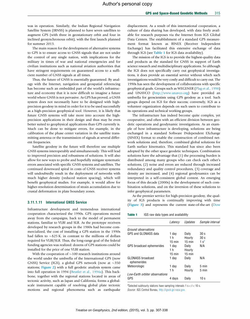
Table 1 IGS raw data types and availability
Latency Updates Sample interval
Ground observationsGPS and GLONASS data 1 day Daily 30 s
1 h Hourly 30 s15 min 15 min 1 sa
GPS broadcast ephemerides 1 day Daily N/A1 h Hourly15 min 15 min
GLONASS broadcastephemerides
1 day Daily N/A
Meteorologic 1 day Daily 5 min1 h Hourly 5 min
Low-Earth orbiter observationsGPS 4 days Daily 10 s
aSelected subhourly stations have sampling intervals 1 s< t<10 s.
Source : IGS Central Bureau, http://igscb.jpl.nasa.gov.
3.11.1.11 International GNSS Service
Infrastructure development and tremendous international
cooperation characterized the 1990s. GPS operations moved
away from the campaigns, back to the model of permanent
stations, familiar to VLBI and SLR. As the prototype receivers
developed by research groups in the 1980s had become com-
mercialized, the cost of installing a GPS station in the 1990s
had fallen to �$25 K, in contrast to the millions of dollars
required for VLBI/SLR. Thus, the long-range goal of the federal
funding agencies was realized: dozens of GPS stations could be
installed for the price of one VLBI station.
With the cooperation of �100 research institutions around
the world under the umbrella of the International GPS (now
GNSS) Service (IGS), a global GPS network (now at �350
stations; Figure 2) with a full geodetic analysis system came
into full operation in 1994 (Beutler et al., 1994a). This back-
bone, together with the regional stations located in areas of
tectonic activity, such as Japan and California, forms a global-
scale instrument capable of resolving global plate tectonic
motions and regional phenomena such as earthquake
Treatise on Geophysics, 2nd edition
displacement. As a result of this international cooperation, a
culture of data sharing has developed, with data freely avail-
able for research purposes via the Internet from IGS Global
Data Centers. The establishment of a standard GPS measure-
ment format known as RINEX (Receiver Independent
Exchange) has facilitated this extensive exchange of data
through IGS (see Table 1 for IGS data availability).
The mission of the IGS is to provide the highest-quality data
and products as the standard for GNSS in support of Earth
science research andmultidisciplinary applications. So although
the IGS does not specifically carry out geophysical investiga-
tions, it does provide an essential service without which such
investigations would be very costly and difficult to carry out. The
1990s has seen the development of collaborations with specific
geophysical goals. Groups such as WEGENER (Plag et al., 1998)
and UNAVCO (http://www.unavco.org) have provided an
umbrella for geoscientists using GPS geodesy as a tool. Such
groups depend on IGS for their success; conversely, IGS as a
volunteer organization depends on such users to contribute to
its operations and technical working groups.
The infrastructure has indeed become quite complex, yet
cooperative, and often with an efficient division between geo-
detic operations and geodynamic investigations. As an exam-
ple of how infrastructure is developing, solutions are being
exchanged in a standard Software INdependent EXchange
(SINEX) format to enable the construction of combined net-
work solutions and, therefore, combined global solutions for
Earth surface kinematics. This standard has since also been
adopted by the other space geodetic techniques. Combination
solutions have the advantage that (1) the processing burden is
distributed among many groups who can check each other’s
solutions, (2) noise and errors are reduced through increased
redundancy and quality control procedures, (3) coverage and
density are increased, and (4) regional geodynamics can be
interpreted in a self-consistent global context. An emerging
focus of this decade (2000s) is the development of such com-
bination solutions, and on the inversion of these solutions to
infer geophysical parameters.
As the premier service for high-precision geodesy, the qual-
ity of IGS products is continually improving with time
(Figure 3) and represents the current state-of-the-art (Dow
, (2015), vol. 3, pp. 307-338

Final Orbits (AC solutions compared to IGS Final)
CODEMRESAGFZJPLMITNGSSIOIGR
(smoothed)
Time (GPS weeks)
Wei
ghte
d R
MS
(mm
)
7000
50
100
150
200
250
300
750 800 850 900 950 1000 1050 1100 1150 1200 1250 1300
GFZ Potsdarn, 30.12.2008 18:17 (GMT)
1350 1400
Figure 3 Plot showing the improvement of IGS orbit quality with time. Courtesy of G. Gendt.
316 GPS and Space-Based Geodetic Methods
Author's personal copy
et al., 2005b; Moore, 2007). The levels of accuracy claimed by
the IGS for its various products are reproduced in Table 2.
Analogous to the IGS, geodetic techniques are organized as
scientific services within the IAG. The IAG services are as
follows:
• International Earth Rotation and Reference Systems Service
(IERS) (IERS, 2004).
• International GNSS Service, formerly the International GPS
Service (IGS) (Dow et al., 2005b).
• International VLBI Service (IVS) (Schluter et al., 2002).
• International Laser Ranging Service (ILRS) (Pearlman et al.,
2002).
• International DORIS Service (IDS) (Tavernier et al., 2005).
These scientific services, as well as gravitational field ser-
vices and an expected future altimetry service, are integral
components of the future ‘Global Geodetic Observing System’
(GGOS) (Rummel et al., 2005; http://www.ggos.org). Closer
cooperation and understanding through GGOS are expected to
bring significant improvements to the ITRF and to scientific
uses of geodesy in general (Dow et al., 2005a).
Figure 4 shows the current status of colocated space geodetic
sites, which forms the foundation for ITRF and GGOS. Co-
location is essential to exploit the synergy of the various tech-
niques, and so increasing the number and quality of colocated
sites will be a high priority for GGOS. In addition, the IGS
adapts to incorporate new GNSS systems as they come online.
Treatise on Geophysics, 2nd edition,
3.11.2 GPS and Basic Principles
3.11.2.1 Basic Principles
GPS positioning is based on the principle of ‘trilateration,’
which is the method of determining position by measuring
distances to points of known positions (not to be confused
with triangulation, which measures angles between known
points). At a minimum, trilateration requires three ranges to
three known points. In the case of GPS, the known points
would be the positions of the satellites in view. The measured
ranges would be the distances between the GPS satellites and a
user’s GPS receiver. (Note that GPS is a completely passive
system from which users only receive signals.) GPS receivers,
on the other hand, cannot measure ranges directly, but rather
‘pseudoranges.’ A pseudorange is a measurement of the differ-
ence in time between the receiver’s local clock and an atomic
clock on board a satellite. The measurement is multiplied by
the speed of light to convert it into units of range (meters):
pseudorange¼ receiver_time� satellite_timeð Þ� speed_of_light [1]
The satellite effectively sends its clock time by an encoded
microwave signal to a user’s receiver. It does this by multiply-
ing a sinusoidal carrier wave by a known sequence (‘code’)
of þ1 and �1, where the timing of the signal (both code and
carrier wave) is controlled by the satellite clock. The receiver
generates an identical replica code and then performs a cross
(2015), vol. 3, pp. 307-338
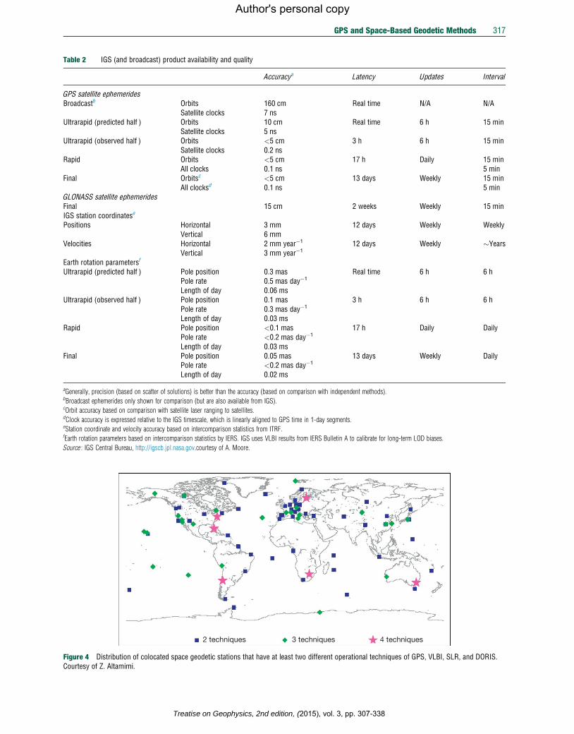
Table 2 IGS (and broadcast) product availability and quality
Accuracya Latency Updates Interval
GPS satellite ephemeridesBroadcastb Orbits 160 cm Real time N/A N/A
Satellite clocks 7 nsUltrarapid (predicted half ) Orbits 10 cm Real time 6 h 15 min
Satellite clocks 5 nsUltrarapid (observed half ) Orbits <5 cm 3 h 6 h 15 min
Satellite clocks 0.2 nsRapid Orbits <5 cm 17 h Daily 15 min
All clocks 0.1 ns 5 minFinal Orbitsc <5 cm 13 days Weekly 15 min
All clocksd 0.1 ns 5 minGLONASS satellite ephemeridesFinal 15 cm 2 weeks Weekly 15 minIGS station coordinatese
Positions Horizontal 3 mm 12 days Weekly WeeklyVertical 6 mm
Velocities Horizontal 2 mm year�1 12 days Weekly �YearsVertical 3 mm year�1
Earth rotation parametersf
Ultrarapid (predicted half ) Pole position 0.3 mas Real time 6 h 6 hPole rate 0.5 mas day�1
Length of day 0.06 msUltrarapid (observed half ) Pole position 0.1 mas 3 h 6 h 6 h
Pole rate 0.3 mas day�1
Length of day 0.03 msRapid Pole position <0.1 mas 17 h Daily Daily
Pole rate <0.2 mas day�1
Length of day 0.03 msFinal Pole position 0.05 mas 13 days Weekly Daily
Pole rate <0.2 mas day�1
Length of day 0.02 ms
aGenerally, precision (based on scatter of solutions) is better than the accuracy (based on comparison with independent methods).bBroadcast ephemerides only shown for comparison (but are also available from IGS).cOrbit accuracy based on comparison with satellite laser ranging to satellites.dClock accuracy is expressed relative to the IGS timescale, which is linearly aligned to GPS time in 1-day segments.eStation coordinate and velocity accuracy based on intercomparison statistics from ITRF.fEarth rotation parameters based on intercomparison statistics by IERS. IGS uses VLBI results from IERS Bulletin A to calibrate for long-term LOD biases.
Source : IGS Central Bureau, http://igscb.jpl.nasa.gov.courtesy of A. Moore.
2 techniques 3 techniques 4 techniques
Figure 4 Distribution of colocated space geodetic stations that have at least two different operational techniques of GPS, VLBI, SLR, and DORIS.Courtesy of Z. Altamimi.
GPS and Space-Based Geodetic Methods 317
Treatise on Geophysics, 2nd edition, (2015), vol. 3, pp. 307-338
Author's personal copy

Perigee
SatelliteOrbital ellipse
318 GPS and Space-Based Geodetic Methods
Author's personal copy
correlation with the incoming signal to compute the required
time shift to align the codes. This time shift multiplied by the
speed of light gives the pseudorange measurement.
The reason the measurement is called a ‘pseudorange’ is
that the range is biased by error in the receiver’s clock (typically
a quartz oscillator). However, this bias at any given time is the
same for all observed satellites, and so it can be estimated as
one extra parameter in the positioning solution. There are also
(much smaller) errors in the satellites’ atomic clocks, but GPS
satellites handle this by transmitting another code that tells the
receiver the error in its clock (which is routinely monitored and
updated by the US Department of Defense).
Putting all this together, point positioning with GPS there-
fore requires pseudorange measurements to at least four satel-
lites, where information on the satellite positions and clocks is
also provided as part of the GPS signal. Three coordinates of
the receiver’s position can then be estimated simultaneously
along with the receiver’s clock offset. By this method, GPS
positioning with few meter accuracy can be achieved by a
relatively low-cost receiver.
Hence, GPS also allows the user to synchronize time to the
globally accessible atomic standard provided by GPS. In fact,
the GPS atomic clocks form part of the global clock ensemble
that define Universal Coordinated Time (UTC). Note that since
GPS time began (6 January 1980), there have accumulated a
number of leap seconds (16 s as of July 2012) between GPS
time (a continuous timescale) and UTC (which jumps occa-
sionally to maintain approximate alignment with the variable
rotation of the Earth). Synchronization to GPS time (or UTC)
can be achieved to <0.1 ms using a relatively low-cost receiver.
This method is suitable for many time-tagging applications,
such as in seismology, in SLR, and even for GPS receivers
themselves. That is, by using onboard point positioning soft-
ware, GPS receivers can steer their own quartz oscillator clocks
through a feedback mechanism such that observations are
made within a certain tolerance of GPS time.
A fundamental principle to keep in mind is that GPS is a
timing system. By the use of precise timing information on
radio waves transmitted from the GPS satellite, the user’s
receiver can measure the range to each satellite in view and
hence calculate its position. Positions can be calculated at every
measurement epoch, which may be once per second when
applied to car navigation (and in principle as frequently as
50 Hz). Kinematic parameters such as velocity and acceleration
are secondary, in that they are calculated from the measured
time series of positions.
Equator
Vernalequinox
a(l – e)
Ascendingnode
IEllipse center
Geocenterf(t)
ae
g
W
w
Figure 5 Diagram illustrating the Keplerian orbital elements: semimajoraxis a, eccentricity e, inclination I, argument of perigee (closestapproach) o, right ascension of the ascending node O, and true anomalyf as a function of time t. The geocenter is the Earth’s center of mass;hence, satellite geodesy can realize the physical origin of the terrestrialreference system. This diagram is exaggerated, as GPS orbits are almostcircular.
3.11.2.2 GPS Design and Consequences
The GPS has three distinct segments:
1. The space segment, which includes the constellation of
�30 GPS satellites that transmit the signals from space
down to the user, including signals that enable a user’s
receiver to measure the biased range (pseudorange) to
each satellite in view and signals that tell the receiver the
current satellite positions, the current error in the satellite
clock, and other information that can be used to compute
the receiver’s position.
Treatise on Geophysics, 2nd edition,
2. The control segment (in the US Department of Defense),
which is responsible for the monitoring and operation of
the space segment, including the uploading of information
that can predict the GPS satellite orbits and clock errors into
the near future, which the space segment can then transmit
down to the user.
3. The user segment, which includes the user’s GPS hardware
(receivers and antennas) and GPS data processing software
for various applications, including surveying, navigation,
and timing applications.
The satellite constellation is designed to have at least four
satellites in view anywhere, anytime, to a user on the ground.
For this purpose, there are nominally 24 GPS satellites distrib-
uted in six orbital planes. In addition, there is typically an
active spare satellite in each orbital plane, bringing the total
number of satellites closer to 30. The orientation of the satel-
lites is always changing, such that the solar panels face the sun
and the antennas face the center of the Earth. Signals are
transmitted and received by the satellite using microwaves.
Signals are transmitted to the user segment at frequencies
L1¼1575.42 MHz and L2¼1227.60 MHz in the direction of
the Earth. This signal is encoded with the ‘navigation message,’
which can be read by the user’s GPS receiver. The navigation
message includes orbit parameters (often called the ‘broadcast
ephemeris’), from which the receiver can compute satellite
coordinates (X,Y,Z). These are Cartesian coordinates in a geo-
centric system, known as WGS 84, which has its origin at the
Earth’s center of mass, Z-axis pointing toward the North Pole,
X pointing toward the prime meridian (which crosses Green-
wich), and Y at right angles to X and Z to form a right-handed
orthogonal coordinate system. The algorithm that transforms
the orbit parameters into WGS 84 satellite coordinates at any
specified time is called the ‘Ephemeris Algorithm’ (e.g., Leick,
2004). For geodetic purposes, precise orbit information is
available over the Internet from civilian organization such as
the IGS in the Earth-fixed reference frame.
According to Kepler’s laws of orbital motion, each orbit takes
the approximate shape of an ellipse, with the Earth’s center of
mass at the focus of the ellipse (Figure 5). For a GPS orbit, the
(2015), vol. 3, pp. 307-338

GPS and Space-Based Geodetic Methods 319
Author's personal copy
eccentricity of the ellipse is so small (0.02) that it is almost
circular. The semimajor axis (largest radius) of the ellipse is
approximately 26600 km, or approximately 4 Earth radii.
The six orbital planes rise over the equator at an inclination
angle of 55�. The point at which they rise from the Southern to
Northern Hemisphere across the equator is called the ‘right
ascension of the ascending node.’ Since the orbital planes are
evenly distributed, the angle between the six ascending nodes
is 60�.Each orbital plane nominally contains four satellites, which
are generally not spaced evenly around the ellipse. Therefore, the
angle of the satellite within its own orbital plane, the ‘true
anomaly,’ is only approximately spaced by 90�. The true anom-
aly is measured from the point of closest approach to the Earth
(the perigee). Instead of specifying the satellite’s anomaly at
every relevant time, it is equivalent to specify the time that the
satellite had passed perigee and then compute the satellite’s
future position based on the known laws of motion of the
satellite around an ellipse. Finally, the argument of perigee
specifies the angle between the equator and perigee. Since the
orbit is nearly circular, this orbital parameter is not well defined,
and alternative parameterization schemes are often used.
Taken together (the eccentricity, semimajor axis, inclina-
tion, right ascension of the ascending node, time of perigee
passing, and argument of perigee), these six parameters define
the satellite orbit (according to the Keplerian model). These
parameters are known as Keplerian elements. Given the Kep-
lerian elements and the current time, it is possible to calculate
the coordinates of the satellite.
However, GPS satellites do not move in perfect ellipses, so
additional parameters are necessary. Nevertheless, GPS does
use Kepler’s laws to its advantage, and the orbits are described
in the broadcast ephemeris by parameters that are Keplerian in
appearance. Additional parameters must be added to account
for non-Keplerian behavior. Even this set of parameters has to
be updated by the control segment every hour for them to
remain sufficiently valid.
Several consequences of the orbit design can be deduced
from the previously mentioned orbital parameters and Kepler’s
laws of motion. First of all, the satellite speed is �4 km s�1
relative to the Earth’s center. All the GPS satellite orbits are
prograde, which means the satellites move in the direction of
the Earth’s rotation. Therefore, the relative motion between the
satellite and a user on the ground must be less than 4 km s�1.
Typical values around 1 km s�1 can be expected for the relative
speed along the line of sight (range rate).
The second consequence is the phenomena of ‘repeating
ground tracks’ every day. The orbital period is approximately
T¼11 h 58 min; therefore, a GPS satellite completes two revo-
lutions in 23 h 56 min. This is intentional, as it equals one
sidereal day, the time it takes for the Earth to rotate 360�.Therefore, every day (minus 4 min), the satellite appears over
the same geographic location on the Earth’s surface. The ‘ground
track’ is the locus of points on the Earth’s surface that is traced
out by a line connecting the satellite to the center of the Earth.
The ground track is said to repeat. From the user’s point of view,
the same satellite appears in the same direction in the sky every
day minus 4 min. Likewise, the ‘sky tracks’ repeat.
So from the point of view of a ground user, the entire
satellite geometry repeats every sidereal day. Consequently,
Treatise on Geophysics, 2nd edition
any errors correlated with satellite geometry will repeat from
one day to the next. An example of an error tied to satellite
geometry is ‘multipath,’ which is due to the antenna also
sensing signals from the satellite that reflect and refract from
nearby objects. In fact, it can be verified that, because of multi-
path, observation residuals do have a pattern that repeats every
sidereal day. Therefore, such errors will not significantly affect
the repeatability of coordinates estimated each day. However,
the accuracy can be significantly worse than the apparent pre-
cision for this reason.
Another consequence of this is that the same subset of the
24 satellites will be observed every day by someone at a fixed
geographic location. Generally, not all 24 satellites will be seen
by a user at a fixed location. This is one reason why there needs
to be a global distribution of receivers around the globe to be
sure that every satellite is tracked sufficiently well.
The inclination angle of 55� also has consequences for the
user. Note that a satellite with an inclination angle of 90�
would orbit directly over the poles. Any other inclination
angle would result in the satellite never passing over the
poles. From the user’s point of view, the satellite’s sky track
would never cross over the position of the celestial pole in the
sky. In fact, there would be a ‘hole’ in the sky around the
celestial pole where the satellite could never pass. For a satellite
constellation with an inclination angle of 55�, there would
therefore be a circle of radius at least 35� around the celestial
pole, through which the sky tracks would never cross. This has
a big effect on the satellite geometry as viewed from different
latitudes. An observer at the pole would never see a GPS
satellite rise above 55� elevation. Most of the satellites would
hover close to the horizon. Therefore, vertical positioning is
slightly degraded near the poles. An observer at the equator
would see some of the satellites passing overhead but would
tend to deviate away from points on the horizon directly to the
north and south.
Due to a combination of the Earth’s rotation and the fact
that the GPS satellites are moving faster than the rotation of the
Earth, the satellites actually appear to move approximately
north–south or south–north to an observer at the equator,
with very little east–west motion. Therefore, the closer the
observer is to the equator, the better determined the north
component of relative position becomes as compared with
the east component. An observer at midlatitudes in the North-
ern Hemisphere would see satellites anywhere in the sky to the
south, but there would be a large void toward the north. This
has consequences for site selection, where a good view is
desirable to the south, and the view to the north is less critical.
For example, one might want to select a site in the Northern
Hemisphere that is on a south-facing slope (and vice versa for
an observer in the Southern Hemisphere).
3.11.2.3 Introducing High-Precision GPS
By measuring pseudoranges to at least four satellites with rel-
atively low-cost equipment, GPS can readily provide users with
a positioning accuracy of meters and a timing accuracy of
0.1 ms. On the other hand, geodetic GPS positioning with an
accuracy of a few millimeters requires a number of significant
improvements to the technique described in the preceding text,
which will be emphasized in this section. For example,
, (2015), vol. 3, pp. 307-338

320 GPS and Space-Based Geodetic Methods
Author's personal copy
accurate positioning requires accurate knowledge of the GPS
satellite positions and satellite clock offsets. For standard GPS
positioning, this ‘ephemeris’ information is broadcast by the
GPS satellites in the so-called navigation message; however, it
is not sufficiently accurate for geodetic applications.
In addition to the three GPS segments listed earlier, one
could informally include the ‘service segment’ consisting of
civilian networks that provide the user segment with data and
services to enhance positioning accuracy. This information can
be transmitted to the user in a variety of ways, such as by the
Internet, cell phone, and geostationary satellite. The part of this
service segment that is relevant to geodetic positioning would be
the International GNSS Service (IGS), an international collabo-
ration of geodesists that provides high-accuracy data on satellite
orbits and clocks. IGS also provides data from reference stations
around the globe, at accurately known coordinates that account
for plate tectonics and other geophysical movements such as
earthquakes. Thus, the IGS enables users to position their
receivers anywhere on the globe with an accuracy of millimeters
in a consistent terrestrial reference frame. But this is only solves
one of the many problems toward achieving geodetic precision.
In practice, high-precision GPS geodesy requires a mini-
mum of five satellites in view, because it is essential to estimate
parameters to model tropospheric refraction. At an absolute
minimum, one zenith delay is estimated, which can be
mapped to delay at any elevation angle using a ‘mapping
function’ based on tropospheric models.
Geodetic applications require much more sophisticated
GPS receivers that measure not only the pseudorange
observable but also the so-called ‘carrier phase’ observable.
The carrier phase observable is the difference between (1) the
phase of the incoming carrier wave (upon which the codes are
transmitted) and (2) the phase of a signal internally generated
by the receiver, which is synchronized with the receiver clock.
When multiplied by the �20 cm wavelength of the carrier
wave, the result is a biased distance to the satellite. Indeed,
this is a type of pseudorange that is about 100 times more
precise than the coded pseudoranges. The downside to the
carrier phase observable is that in addition to the receiver
clock bias, there is an additional bias of an unknown number
of wavelengths. It is possible to resolve this bias exactly by the
so-called ‘ambiguity resolution’ techniques. Ambiguity resolu-
tion is essential to achieve the highest possible precision for
geodetic applications. Hence, in units of range, the observed
carrier phase can be expressed as
carrier_phase¼ reference_phase� signal_phaseþ integerð Þ� carrier_wavelength
[2]
Note that the signal phase is generated by the satellite clock
and that the reference phase is generated by the receiver clock;
hence, eqn [2] is just a very precise form of eqn [1] for the
pseudorange, except that it has an integer–wavelength ambi-
guity. (In fact, this is why the sign of the phase difference was
chosen by subtracting the incoming signal phase from the
reference phase.) Therefore, the observable models for eqns
[1] and [2] are very similar and relate to the theoretical differ-
ence between the reading of the receiver clock (time of recep-
tion) and the satellite clock (time of transmission), including
clock biases.
Treatise on Geophysics, 2nd edition,
This similarity of models has enabled the development of
automatic signal processing algorithms to check the integrity of
the data, such as the detection of data outliers and jumps in the
integer ambiguity (the so-called cycle slips), which occur when
the receiver loses lock on the signal, for example, due to a
temporary obstruction between the ground antenna and the
satellite. In fact, the pseudorange data can be used together
with the carrier phase data to correct for the initial integer
ambiguity (Blewitt, 1989) and for subsequent cycle slips
(Blewitt, 1990).
For geodetic positioning, both pseudoranges and carrier
phases are measured at two different frequencies (L1 at
19.0 cm wavelength and L2 at 24.4 cm), to provide a self-
calibration of delay in the Earth’s ionosphere. So in total,
there are four observations that are fundamental to high-
precision GPS geodesy: two pseudoranges and two carrier
phases. This enables more algorithms to assure the integrity
of the data and allows for monitoring of the ionosphere itself.
Another requirement for geodetic positioning is the use of
highly specialized stochastic multiparameter estimation soft-
ware by modeling the carrier phase data, including modeling
of the satellite–station geometry, Earth’s atmosphere, solid
Earth tides, Earth’s rotation, antenna effects, circular polariza-
tion effects (phase windup), and relativistic effects (both spe-
cial and general). In addition, the software must be capable of
detecting and correcting integer offsets in the carrier phase
observables (cycle slips) and must be capable of resolving the
integer ambiguity in the initial phase measurements.
In summary, therefore, geodetic GPS requires
• geodetic-class GPS receivers capable of acquiring dual-
frequency carrier phase data;
• geodetic-class satellite orbit and clock information, which is
available from the IGS;
• simultaneous observations to a minimum of five satellites;
• specialized postprocessing software (not on the receiver
itself ) that embodies high-accuracy observable models,
carrier phase data processing algorithms, and simultaneous
parameter estimation.
The quality of the IGS orbit and clock data depends on their
latency, so generally, there is a trade-off between latency and
accuracy. Currently, the ultrarapid IGS product is actually a
prediction from 3 to 9 h ago. Even though there are atomic
clocks on board the GPS satellites, the clock time is much more
difficult to predict than the satellite orbits. In the case that
sufficiently accurate clock data are not yet available, it is nev-
ertheless possible to produce geodetic-class solutions for rela-
tive positions between ground stations. This is achieved either
by (1) solving for satellite clock biases at every epoch as part of
the positioning solution or equivalently by (2) differencing
data between ground stations to cancel out the clock bias.
Furthermore, data can be differenced again (‘double
difference’) between satellites to cancel out the receiver clock
bias rather than estimate it as a parameter (Figure 6).
In practice, the following different approaches to estimating
positions all give results that are of geodetic quality (with errors
measured in millimeters) and typically agree very well:
• Precise point positioning (PPP) of single stations using
precise orbit and clock data.
(2015), vol. 3, pp. 307-338

Satellite k
D LABkDLAB
j
DLAB jkD
DLAB jk = DLAB
j —DLABkD
Double differencing
Station BStation A
At each epoch, difference the single difference data between satellites:
Satellite jPrinciples: At any time,(1) clock bias at aspecific satellite is thesame for all stations; (2)clock bias at a specificstation is the same for allsatellites being tracked.
Figure 6 Diagram illustrating double differencing of GPS data. The idea is to differentiate away the satellite and station clock biases. Doubledifferencing is equivalent to estimating the clock biases explicitly when processing undifferenced data.
GPS and Space-Based Geodetic Methods 321
Author's personal copy
• Relative positioning of networks by clock estimation, using
precise orbit data.
• Relative positioning of networks by double-difference data
(Figure 6), using precise orbit data.
All of these three methods are in common use today for
geophysical research purposes. In each case, dual-frequency
pseudorange and carrier phase data types are used.
3.11.2.4 GPS Observable Modeling
This section describes how GPS observables are typically mod-
eled by geodetic-quality software packages. First, however, a
few more specific details on the GPS signals are required. The
signals from a GPS satellite are fundamentally driven by an
atomic clock precisely at frequency 10.23 MHz. Two sinusoidal
carrier signals are generated from this signal by multiplying
the frequency by 154 for the L1 channel (frequency¼1575.42 MHz; wavelength¼19.0 cm) and 120 for the L2 chan-
nel (frequency¼1227.60 MHz; wavelength¼24.4 cm). Infor-
mation is encoded in the form of binary bits on the carrier
signals by a process known as phase modulation. The binary
digits 0 and 1 are actually represented by multiplying the
electrical signals by either þ1 or �1.
For purposes of observable modeling, here, the observables
(all in units of meters) will be called L1 and L2 for the two
types of carrier phase and P1 and P2 for the two types of
pseudorange. The actual observable types are numerous due
to different methods of correlating the signals; however, the
fundamental observation equations can be written in the same
generic way, with the exception that there is generally a bias
associated with each observable types, including instrumental
bias and, in the case of the carrier phase, an integer wavelength
bias. (For some older signal-squaring receivers, the bias is a
half-integer wavelength.) Here, it is simply assumed that such
biases are not problematic, which is typically the case, and so
the interobservable biases are not explicitly modeled.
Treatise on Geophysics, 2nd edition
Taking eqns [1] and [2], the generic (pseudorange or carrier
phase) GPS observation Pji at receiver j (subscript, on the
ground) from satellite i (superscript, up in space) can be
modeled:
Pij ¼ c Tj�T
i� �
þBij [3]
Since special relativity and general relativity prove to be
important in the model, care must be taken to define each
term with respect to a reference frame. Thus, Tj is the time
according to the receiver clock coincident with signal reception
(used as the time tag, recorded with the observation), Tiis the
time according to the satellite clock coincident with signal
transmission (which imprints its signature on the signal,
hence the bar, which denotes time local to the satellite), Bji is
a frame-invariant bias associated with this type of observation,
and c is the frame-invariant speed of light in a vacuum. In
addition, this observation is recorded at an epoch with time
tag Tj (the same for all satellites observed at that epoch).
The clock difference can be rewritten as the sum of four
time differences:
Pij ¼ c Tj� tj
� �þ tj� ti� �þ ti� ti
� �þ ti�T
i� �n o
þBij [4]
where tj is the coordinate time at the receiver, ti is the coordinate
time at the satellite, and ti is the proper time at the satellite (the
time kept by a perfect clock on board the satellite). ‘Coordinate
time’ simply means the timescale that is actually used to com-
pute the models. It is convenient to take coordinate time in the
‘local Earth’ frame (that of a perfect clock on the geoid) (Ashby
and Allan, 1984). Appropriate timescales for this purpose
include Terrestrial Dynamic Time (TDT) and International
Atomic Time (TIA), but for the discussion here, it is convenient
to choose GPS time. The important thing to keep inmind (to cut
through the confusion of all these conventions) is that all these
timescales ideally run at the same rate as UTC, with the unit of
time being the SI second (Kaplan, 1981), and so all these scales
only differ by conventional constant offsets (and leap seconds).
, (2015), vol. 3, pp. 307-338

322 GPS and Space-Based Geodetic Methods
Author's personal copy
The four time-difference terms found in eqn [4] can be
written as follows. First, the difference in receiver clock time
and coordinate time is simply the receiver clock bias, which we
will model as an independent parameter tj at every epoch (at
every value of Tj):
Tj� tj� �¼ tj [5]
The clock bias includes the sum of a clock error (with
respect to proper time) plus a minor relativistic bias due to
the geodetic location of the receiver clock.
The second term is the difference between coordinate time
at the receiver and satellite, the so-called light-time equation
(here expressed as a range):
c tj� ti� �¼ rijþ
Xprop
Drprop ij
¼ rj tj� �� ri tið Þ�� ��þDrGR ijþDrionij þDrtrop ij
þDrpcv ijþDrcircij þ��� [6]
where rji is the Euclidean distance between the satellite and
receiver and Drpropji represent various propagation delays,
which are a function of satellite–station geometry, arising
from space–time curvature (general relativity); ionosphere,
troposphere, and antenna phase center variations; circular
polarization effects; and other propagation terms as necessary.
In eqn [6], rj is the geocentric receiver position at the time of
reception and ri is the geocentric satellite position at the time of
transmission. The reference frame for the light-time equation is
taken to be J2000, the conventional Earth-centered inertial
(ECI) frame (so the axes do not corotate with the Earth),
because the speed of light is a constant in all directions in an
inertial frame. In addition, the ECI frame is most convenient
for integrating the satellite equations of motion, if the goal is to
estimate satellite orbits. However, it can be more convenient to
solve the light-time equation in a rotating, Earth-centered,
Earth-fixed (ECEF) reference frame, given that satellite orbit
positions and velocities are typically distributed in the ECEF
frame. In this case, the equation would also need to account for
the Sagnac effect (e.g., Ashby, 2004), which accounts for the
effect of the Earth’s rotation on light propagation when viewed
in the ECEF frame. A simple way to handle this is to consider
the ECEF and ECI frames as being instantaneously aligned at
reception time. Thus, all that is required is to compute the
satellite velocity in the ECI frame by adding the velocity due
to the Earth’s rotation at the satellite to the ECEF velocity and
then compute the ECI position of the satellite at transmit time
using this ECI velocity. Thus, the Sagnac effect can be consid-
ered simply as a correction for the Earth’s rotation.
The general relativistic delay can be computed as
DrGRij ¼2GM�c2
lnrjþ riþ r
ji
rjþ ri� rji
[7]
where GM� is the Earth’s gravitational constant and, in general,
r� |r|. This is sometimes called the Shapiro delay after Shapiro
(1964) and is typically at the 10 mm level for signals from
satellites in medium Earth orbit. It accounts for the distance
traveled, being longer than the Euclidean distance, caused by
space–time curvature in the Earth’s gravitational field. Equa-
tion [7] is a sufficiently good approximation, derived by inte-
grating the effect of the Earth’s gravitational potential along a
Treatise on Geophysics, 2nd edition,
straight light path; so the term ‘space–time curvature’ should not
be confused with gravitational bending of the direction of light,
which is negligible. Rather, the curvature can be thought of
primarily as the ‘stretching’ of space along the direction of travel.
Antenna effects such asphase center variationDrpcvji [Schupler
et al., 1994] and circular polarization Drcircji (‘phase windup’)
(Wu et al., 1993) are examples of important effects that have
been researched and applied to improve positioning accuracy,
but as nongeophysical effects, they are beyond the scope of this
text. Antenna calibrations for both the GPS satellite and station
antennas are available from the IGS and should be applied
(Schmid et al., 2005).
Ionospheric delay can be adequately modeled as being
inversely proportional to the squared frequency f of the carrier
wave:
Drionij fð Þ¼kTECi
j
f 2[8]
where the positive sign is taken for pseudoranges and the
negative sign for carrier phase observations. The term TEC
refers to ‘total electron content,’ which is excited by solar
radiation and so is highly variable through the day and is
sensitive to geographic location. The constant k can be derived
from the theory of electromagnetic (EM) wave propagation in
plasmas. Delays at GPS frequencies can be as large as 100 m
near the equator, peaking around 2 pm local time, and can be
as small as centimeters at midlatitudes between midnight and
dawn. In contrast, higher-order terms are of the order of mil-
limeters and are typically ignored, although including them in
the model is one of many themes of current research (Kedar
et al., 2003). An appropriate linear combination of observa-
tions eliminates the frequency-squared term exactly, leaving all
nondispersive terms in the model unchanged. In fact, the
‘ionosphere-free’ combination of carrier phases can be so
defined (and similarly for the pseudoranges):
LC¼ f 12L1� f 2
2L2
f 12� f 2
2� �
ffi 2:546L1�1:546L2
[9]
Hence, k and TEC are not explicitly needed to compute the
ionosphere-free data. The coefficients in the preceding text can
be computed exactly by substituting f1¼154 and f2¼120,
owing to the properties of the GPS signals described at the
beginning of this section. As an aside, if the ionosphere is
the geophysical scientific target of interest, then differencing
the observations at two different frequencies results in a
‘geometry-free’ observation from which TEC can be estimated:
PI¼ P1�P2
¼ kTEC1
f 12�
1
f 22
!þbias
[10]
Using GPS stations located around the globe, this method is
now routinely used to map ionospheric TEC. A side benefit of
this method is the estimation of the interchannel bias between
observables at L1 and L2 frequency, which can be monitored
for long-term variability and used as input to ambiguity reso-
lution algorithms.
The tropospheric delay (a fraction of which actually occurs
in the stratosphere) is almost entirely nondispersive
(2015), vol. 3, pp. 307-338

GPS and Space-Based Geodetic Methods 323
Author's personal copy
(independent of frequency) at GPS L-band frequencies and so
must be handled in a different way. Whereas it is possible in
principle to model tropospheric delay based on ground-based
meteorologic observations, in practice, this has not proven to
be sufficiently accurate. The key to successful tropospheric
modeling is the estimation of the delay at zenith, by accurately
modeling the relationship between zenith delay Z and delay at
lower elevations e, for example,
Drtropij ¼Zj
sineij[11]
where the inverse signof elevationangle is the simplest example of
a ‘mapping function,’ which can be derived by assuming a hori-
zontally layered troposphere over a flat Earth. This model breaks
down rapidly for e<20�. More accurate modeling (Truehaft and
Lanyi, 1987) requiresmodifying themapping function to account
for Earth curvature and partitioning the delay into a so-called dry
and wet components, which have different characteristic scale
heights (�10 km and �2 km, respectively):
Drtropij ¼Drdry ijþDrwet ij
¼ZdryFdry eij� �
þZwetFwet eij� � [12]
Due to the inherent weakness in the determination of
height with both GPS and VLBI, accurate modeling of mapping
functions has always been and remains an active area of
research. The wet delay is caused by the interaction of the EM
wave with the static dipole of molecular water. The dry delay is
due to the dynamic dipole induced by the EM wave on all
component molecules in the atmosphere, including a (small)
contribution from water (and so ‘dry’ is just a conventional,
perhaps, misleading term). Typical values for the dry and wet
delay are 2.1 and 0.1 m, respectively, to within �10 cm.
The dry component can be adequately modeled as a func-
tion of hydrostatic pressure at the altitude of the receiver.
Nominal values can be computed in the absence of
meteorologic data by assuming a nominal surface pressure at
sea level and then subtracting a correction for altitude, assum-
ing that pressure decays exponentially with altitude. The wet
component is typically assumed to have a nominal value of
zero, and Zwet is then estimated from the GPS data along with
the positioning solution. Note that in this case, the estimated
value of Zwet would absorb most (but not all) of the obvious
inadequacies of the nominal model for Zdry. Whereas this is
currently the standard method in high-precision GPS geodesy,
the limitations of this approach are an active area of research
(Tregoning and Herring, 2006).
The tropospheric delay model is important not only for
solving for geodetic position but also for the study of the tropo-
sphere itself. For this application, estimates of troposphere delay
can be converted into precipitable water vapor in the atmo-
sphere, which can then be used as input for weather forecasting
and climate modeling. For this application, surface
meteorologic data are essential to more accurately partition the
dry and wet components of delay (Bevis et al., 1992).
Now, returning to the light-time equation, even if we had
perfect propagation models, the light-time equation needs to
be solved iteratively rather than simply computed, because at
first, we do not have a nominal value for ti, the coordinate time
of signal transmission. The procedure is as follows:
Treatise on Geophysics, 2nd edition
• Starting with the observation time tag Tj, use eqn [5] and a
nominal value for the receiver clock bias tj (which may be
zero or a preliminary estimate) to compute the coordinate
time of signal reception tj. Note that the assumed clock bias
affects the subsequent computation of geometric range,
indicating the need for iterative estimation. (This problem
can be more conveniently addressed by accounting for the
range rate in the partial derivative with respect to the
receiver clock parameter.)
• Given a modeled station position rj at time tj, and an
interpolated table of modeled satellite positions ri as a
function of coordinate time ti, iteratively compute the coor-
dinate time of transmission using
ctj� ctj n½ �� rij n½ ��Xprop
Drpropij n½ �
ctj nþ1½ � ¼ ctj n½ �þ1� _ri n½ �� rij n½ �=c [13]
where rij ¼ rij=rij are the direction cosines to the receiver from
the satellite. It is to be understood that at the nth iteration, for
example, the satellite position ri and ECI velocity _ri are both
interpolated to time ti[n]. By virtue of this equation converging
very quickly, it is sufficient to initialize the transmission time to
the reception time ti[0]¼ tj.
Being in the ECI frame (J2000), the receiver position must
account for the Earth’s rotation and geophysical movements of
the Earth’s surface:
rj tj� �¼PNUXY x0 jþ
XkDxkj tj
� ���[14]
Here, PNUXY is the multiple of 3�3 rotation matrices that
account (respectively) for precession, nutation, rate of rotation,
and polar motion (in two directions). The bracketed term
represents the receiver position in the (corotating) conven-
tional Earth-fixed terrestrial reference frame known as ITRF.
Conventional station position x0j is specified by station coor-
dinates in ITRF at some conventional epoch, and Dxkj(tj) rep-resents the displacement from the epoch position due to
geophysical process k, for example, accounting for the effects
of plate tectonics, solid Earth tides, etc. Equation [14] together
with [6] forms the fundamental basis of using GPS as a geo-
physical tool, and this will be explored later.
Returning now to the original observation eqn [4], the third
term is the difference between coordinate time and proper time
at the satellite. According to special relativity, GPS satellite
clocks run slow relative to an observer on the Earth’s surface
due to relative motion. In contrast, general relativity predicts
that the satellite clocks will appear to run faster when observed
from the Earth’s surface due to the photons gaining energy
(gravitational blue shift) as they fall into a gravitational well.
These two effects do not entirely cancel. With appropriate
foresight in the design of GPS, the satellite clocks operate at a
slightly lower frequency than 10.23 MHz to account for both
special relativity and general relativity, so that their frequency
would be 10.23 MHz (on average) as viewed on the Earth’s
surface. The residual relativistic term can be computed from
ti� ti� �
¼ 2ri ti� �� _ri ti� �=c2 [15]
It is inconsequential as to whether eqn [15] is computed in
the ECI or ECEF frame. This result assumes an elliptical orbit
, (2015), vol. 3, pp. 307-338

324 GPS and Space-Based Geodetic Methods
Author's personal copy
about a point (or spherically layered) mass and assumes that
additional relativistic effects are negligible. The expected accu-
racy is at the level of 10�12, comparable with the level of
stability of the satellite atomic clocks.
The fourth term is the difference between proper time and
clock time at the satellite, which is simply the negative error in
the satellite clock:
ti�Ti
� �¼�ti [16]
Unlike errors in the station clock, errors in the satellite clock
do not affect the model of geometric range (in the light-time
equation) and so are not required in advance to compute that
part of the model. However, they do affect the observable itself,
and so not accounting for satellite clock error would result in an
error in estimated receiver position. Despite the satellite clocks
being atomic, they are not sufficiently stable to be predicted
forward in time for geodetic applications (though this is the
method for standard positioning with GPS). Therefore, this
term is estimated independently at every epoch as part of the
positioning solution (or alternatively, observations equations
can be differenced between pairs of observing receivers to elim-
inate this parameter). As a consequence, geodetic-quality PPP of
individual stations in real time presents a challenge that is the
topic of current research.
Finally, each observation type has an associated bias.
Typically, receivers are designed so that these biases either
should be calibrated or are stable in time. Like the case for
the satellite clock error, these biases have no effect on the
computed geometric range and so do not need to be known
in advance; however, they are present in the observations
themselves and so can affect positioning accuracy unless they
are absorbed by parameters in the least-squares solution. It
turns out for the most part that biases between observable
types can be ignored for purposes of positioning, because
they can be absorbed into the station or satellite clock bias
parameters as part of the least-squares positioning solution.
For purposes of accurate timing, however, special consider-
ations are required to calibrate such biases. Some of the inter-
observable biases are monitored by major GPS analysis centers
and made routinely available if needed.
The most important bias to consider for geodetic applica-
tions is the carrier phase bias, for which its double difference
has an integer ambiguity (Blewitt, 1989). The carrier phase bias
is not predictable from models and can vary by integer jumps
occasionally (Blewitt, 1990). For an initial solution, the carrier
phase biases can be nominally assumed to be zero (because
they do not affect the light-time equation) and then estimated
as real-valued parameters. If the real-valued carrier phase bias
parameters are sufficiently precise, then their double differ-
ences can be resolved to their correct integer values. The solu-
tion can then be computed again by holding these integer
values fixed, or more efficiently, the change to the solution
can be computed using least-squares adjustment theory.
For undifferenced data processing, such as PPP, ambiguity
resolution presents a conundrum. A solution to this problem
lies in the stability of undifferenced phase biases. It turns out
that the double difference in the estimates of the phase biases
can be resolved to integer numbers of cycles (Blewitt, 1989). In
the case of PPP with a single receiver (Zumberge et al., 1997),
Treatise on Geophysics, 2nd edition,
we also need estimates of biases from at least one other station
with the same satellites in view. A successful method now in
common use, which was proposed and demonstrated by
Bertiger et al. (2010), is known as the wide-lane and phase
bias (WLPB) method. The WLPB method estimates biases for
the IGS network during the GPS orbit estimation procedure.
These phase bias estimates are then made available to the
single-receiver user along with the GPS orbit and clock param-
eters. Thus, the user can perform ambiguity resolution when
PPP with a single receiver.
In summary, this has been a key section, in that the light
eqn [6] represents the heart of GPS observable modeling and a
very specific component given by eqn [14] is the source of all
geophysical applications that relate to precise positioning.
3.11.2.5 Data Processing Software
Geodetic GPS data processing as implemented by research
software packages can typically be generalized as a modular
scheme (Figure 7). In this processing model, the input is raw
data from GPS receivers, and the processing stops with the
production of a set of station coordinates. Before discussing
data processing in detail, it should be noted that the data
processing does not stop with the initial production of station
coordinates, but rather this is the first step toward time series
analysis, velocity estimation, and kinematic analysis, all lead-
ing to dynamic analysis and geophysical interpretation. It is
convenient to separate the actual processing of GPS data
shown in the preceding text from the subsequent kinematic
analysis, though for some geophysical applications (e.g., ocean
tidal loading), this division is not correct, and geophysical
parameters must be estimated directly in the solution.
Several software packages have been developed since the
1980s that are capable of delivering high-precision geodetic
estimates over long baselines. These days, the processing of
GPS data by these software packages is, to a large degree,
automatic, or at least a ‘black-box’ approach is common. The
black box can of course be tampered with for purposes of
research into GPS methodology, but one big advantage of
automation is reproducibility and consistency of results pro-
duced in an objective way.
Geodetic data processing software is a result of intensive
geodetic research, mainly by universities and government
research laboratories. Typical features of such software include
• orbit integration with appropriate force models;
• accurate observation model (Earth model, media delay,
etc.) with rigorous treatment of celestial and terrestrial ref-
erence systems;
• reliable data editing (cycle slips and outliers);
• estimation of all coordinates, orbits, tropospheric bias,
receiver clock bias, polar motion, and Earth spin rate;
• ambiguity resolution algorithms applicable to long
baselines;
• estimation of reference frame transformation parameters
and kinematic modeling of station positions to account
for plate tectonics and coseismic displacements.
The typical quality of geodetic results from processing 24 h
of data can be summarized as follows (IGS, http://igscb.jpl.
nasa.gov):
(2015), vol. 3, pp. 307-338

User network/campaignIERS
conventions
Metadata Calibrations
Planetaryephemeris
Earthorientation
ITRFrealization
Observational model
Estimationstrategy
Transform
Solution
Iterate model
Ambiguityresolution
Post-editing
Parameterestimation
Observationmodeling
Pre-editing
Differencing(optional)
RINEX data
Pre-fit data
Pre-fit residuals &partial derivatives
Post-fit residuals& estimatedparameters
Orbits &clocks
Geodetic Services (IGS, IERS, Regional Networks, UNAVCO...)
Raw data
Pre-assessment& formatting
Figure 7 Generic modular scheme for geodetic GPS data processing.
GPS and Space-Based Geodetic Methods 325
Author's personal copy
• Relative positioning at the level of few parts per billion of
baseline length
• Geocentric (global) positioning to �6 mm vertical and
�3 mm horizontal in the ITRF
• Tropospheric delay estimated to �4 mm
• GPS orbits determined to �25 mm
• Earth pole position determined to �2 mm
• Clock synchronization (relative bias estimation) to<0.1 ns
• Ionospheric TEC maps to <10 TEC units
Two features of commercial software are often conspicu-
ously absent from more advanced packages: (1) Sometimes,
double differencing is not implemented, but instead, un-
differenced data are processed, and clock biases are estimated;
(2) network adjustment using baseline solutions is unneces-
sary, since advanced packages do a rigorous, one-step, simul-
taneous adjustment of station coordinates directly from all
available GPS observations.
Treatise on Geophysics, 2nd edition
Some precise software packages incorporate a Kalman filter
(or an equivalent formulism) (Bierman, 1977; Herring et al.,
1990; Lichten and Border, 1987). This allows for certain
selected parameters to vary in time, according to a statistical
(‘stochastic’) model. Typically, this is used for the tropospheric
bias, which can vary as a random walk in time (Tralli and
Lichten, 1990). A filter can also be used to estimate clock
biases, where ‘white noise’ estimation of clock bias approaches
the theoretical equivalent of double differencing.
Although many more packages have been developed, there
are three ultrahigh-precision software packages, which are
widely used around the world by researchers and are com-
monly referenced in the scientific literature:
• Bernese software, by Astronomical Institute, University of
Bern, Switzerland (Rothacher et al., 1990);
• GAMIT-GLOBK software, by Massachusetts Institute of
Technology, the United States (King and Bock, 2005);
, (2015), vol. 3, pp. 307-338

326 GPS and Space-Based Geodetic Methods
Author's personal copy
• GIPSY-OASIS II software, by JPL, California Institute of
Technology, the United States (Webb and
Zumberge, 1993).
There are several other packages, but they tend to be limited
to the institutions that wrote them. It should be noted that,
unlike commercial software packages, the use of the previously
mentioned software can require a considerable investment in
time to understand the software and how best to use it under
various circumstances. Expert training is essential.
3.11.2.6 Real-Time GPS and Accuracy Versus Latency
The most accurate GPS geodetic solutions result from a simul-
taneous estimation for satellite orbit and clock parameters,
Earth rotation parameters, and station coordinates. One the
other hand, solutions that very closely approximate those from
simultaneous estimation are possible in a two-step process,
where an analysis center first computes the satellite orbit and
clock parameters and Earth rotation parameters and then dis-
tributes these to users who simply solve for their own station
coordinates (along with the station clock, tropospheric delay,
and carrier phase biases). This is basically the model used by
IGS and its analysis centers to serve its users.
One consequence of the two-step model is that there is a
delay for the user, who must wait until the orbit parameters
become available. In the extreme case of real-time positioning,
the two-step model becomes challenging to implement accu-
rately. In this case, the orbit positions must be predicted ahead
in time, and the satellite clocks must be handled in real time,
either by the user differencing data or by the analysis center
providing real-time estimates of the satellite clock biases.
In this section, we consider the effect of latency on accuracy
and precision of point positioning for the user with one of the
best software packages available. We also consider the effect of
positioning interval, for example, whether the position repre-
sents a 24 h average or a new position every data epoch, which
could be every 5 min, every 1 s, or even shorter intervals.
Positioning at every data epoch is sometimes called
‘kinematic positioning,’ which is somewhat of a misnomer,
as positions are directly estimated rather than kinematic
parameters such as velocity (which can be subsequently
inferred from the position time series). Nevertheless, we use
the term ‘kinematic positioning’ because it has become a
de facto standard.
The most accurate ‘final’ orbits and clocks are available with
12–18 day latency (some as low as 5 days). These allow the
user to perform daily PPP in the ITRF to a precision of �2 mm
horizontal and �6 mm vertical using 24 h RINEX files. For
kinematic positioning, the precision degrades to �7 mm
horizontal and �20 mm vertical, as measured by RMS scatter
over a day. However, the RMS precision can be much better
than this over shorter time windows, so it is possible to track
very accurately the variations in position caused by seismolog-
ical waves. When using the term ‘precision,’ therefore, one
must be careful to consider the time window relevant to the
problem at hand.
GPS analysis centers also produce the so-called rapid orbits
with 1–2 day latency. These products are almost as good as
final orbits but can differ to the extent that quality control may
Treatise on Geophysics, 2nd edition,
not be as effective at shorter latency. But as a consequence,
positioning precision using rapid orbits is of similar quality to
that using final orbits.
Pushing to lower latencies, GPS analysis centers also pro-
duce the so-called ultrarapid orbits with several-hour latency
(some as low as 1–2 h latency). These tend to be based on the
analysis of hourly RINEX files that have been concatenated
over the last day or so. Ultrarapid orbits are useful for low-
latency kinematic positioning problems, such as measuring the
permanent displacement of stations following a large
earthquake, and for rapidly inferring earthquake rupture
parameters. Kinematic positioning using ultrarapid orbits is
generally only slightly worse than using rapid orbits, at the
10 mm level horizontal and 30 mm level vertical. However,
solutions can suffer because of several effects: (1) quality con-
trol becomes more difficult at lower latency; (2) toward the
end of the ultrarapid orbit (closer to real time), the solution is
based on data from the past, but not from the future, and so are
degraded; (3) moreover, toward the end of the ultrarapid orbit,
it becomes more difficult to detect and correct for the effect of
cycle slips and to resolve integer ambiguities. As a conse-
quence, the quality of positioning using ultrarapid orbits and
clocks can be quite good but can also be sporadically poor in a
rather unpredictable way.
Finally, at the extreme of real-time point positioning, it is
sufficient to predict the future position of the ultrarapid orbits.
However, the satellite clocks cannot be predicted accurately,
and the issue of quality control becomes paramount. More-
over, the user is faced with the problem of having very poor
initial estimates of carrier phase biases whenever new satellites
come into view or whenever a cycle slip is detected. Carrier
phase bias resets can cause systematic deviations of kinematic
positions that do not reflect the actual motion of the station.
Current real-time position precision is typically better than one
decimeter but can be better or worse depending on the multi-
path and sky-view environment of the both the user’s station
and the stations used to determine the satellite clocks. Needless
to say, improving real-time positioning is an emerging area of
intense research.
3.11.3 Global and Regional Measurementof Geophysical Processes
3.11.3.1 Introduction
Geodesy is the science of the shape of the Earth, its gravitational
field, and orientation in space and is therefore intrinsically
connected to geophysics (Lambeck, 1988; Torge, 2001).
Indeed, space geodetic techniques, such as GPS, can be used
to observe the Earth and hence probe geodynamic processes on
a global scale (Figure 8). GPS contributes to geophysics
through comparing the observed and modeled motion of the
Earth’s surface. Since the observedmotion of the Earth’s surface
will represent the sum of the various effects, it is clear that
geophysics must be modeled as a whole, even when investigat-
ing a specific problem. This creates a rich area of interdisciplin-
ary research.
As the precision and coverage of GPS stations have
improved over the last two decades, the depth and breadth of
GPS geodesy’s application to geodynamics have increased
(2015), vol. 3, pp. 307-338

Land loadsurface densityHydrology
Satellitealtimetry
Geocentricsea level
Relativesea level
–+
Mass exchangeTide gauges &
bottom pressure
Global loadsurface density
Equipotentialsea surface
Gravitation
Loadpotential
Geocenterdisplacement
Frame theoryLLN theory
Solid earthdeformation
Geoiddeformation
Satellitegravimetry
Stationgravimetry
Stationpositioning
Momentum Sea floordeformation
Figure 8 Schematic model of surface mass loading that incorporates self-consistency of the reference frame, loading dynamics, and passive oceanresponse. Closed-form inversion solutions have been demonstrated (Blewitt and Clarke, 2003; Gross et al., 2004). Note that everything is a functionof time, so ‘continental water’ in its most general sense would include the entire past history of ice sheets responsible for postglacial rebound.(Arrows indicate the direction toward the computation of measurement models, phenomena are in round boxes, measurements are in rectangles,and physical principles label the arrows.)
GPS and Space-Based Geodetic Methods 327
Author's personal copy
correspondingly. It has now matured to the point that it is
viewed as an important and often primary tool for understand-
ing the mechanics of Earth processes.
On the other hand, geophysical models are essential to GPS
geodesy; as such, models are embedded in the reference sys-
tems we use to define high-accuracy positions. For example, if
the reference system did not account for the tidal deformation
of the solid Earth, the coordinates of some stations could vary
as much as �10 cm in the time frame of several hours. There-
fore, reference systems to enable high-accuracy geodetic posi-
tioning have developed in parallel with progress in
geodynamics, which in turn depends on geodetic positioning.
Thus, this interdependent relationship between geodesy and
geophysics is inextricable.
Table 3 shows examples of the various geophysical pro-
cesses that affect space geodetic observables and thus are
Treatise on Geophysics, 2nd edition
subject to investigation using space geodesy. Most of the appli-
cations assume the ability to track the position of geodetic
stations with sub-centimeter precision, but other possibilities
include the determination of the Earth’s polar motion and rate
of rotation, low-degree gravitational field coefficients, and
atmospheric delay in the troposphere and ionosphere. For
example, global climate change not only could affect both
the shape and gravitational field through mass redistribution
(e.g., melting polar ice caps) but also could affect large-scale
tropospheric delay.
In this section, the focus will be on providing examples of
geodetic applications across the spatiotemporal spectrum,
ranging from coseismic rupture and seismic waves to plate
rotations.
The subsequent section will then focus on how geodesy can
be used to address large-scale loading problems.
, (2015), vol. 3, pp. 307-338

Table 3 Geophysical processes that affect geodetic observations as a function of spatial and temporal scale
Scale Temporal
Spatial 10�2–103 s 100–101 h 100–102 day 100–102 year 102–106 year
100–101 km Coseismic ruptureVolcanism
Creep eventsVolcanism
AfterslipPoroelastic relaxationDike injection
Viscoelastic relaxationInterseismic strain
Earthquake cycle
101–102 km M 6–7.5 seismic strainrelease
Tropospheric moisture
Storm-surge loadingTsunami loadingTroposphericmoisture
Rifting eventsAquifer deformationPoroelastic relaxationLower crustal
magmatismLake loadingSnow loading
Viscoelastic relaxationBlock rotationStrain partitionMountain growthGlacial loadingSedimentary
loading
Fault activation andevolution
Mountain rangebuildingDenudationRegional topographySedimentary loading
102–103 km M 7.5–9 seismic strainrelease
Traveling ionosphericdisturbances
Seismic waves
Coastal ocean loading Atmospheric loadingRegional hydrologic
loading
Mantle–crust couplingIce-sheet loading
Plateau riseMountain rangebuildingGlacial cycle
103–104 km M 9þ seismic strainrelease
Seismic wavesFree oscillations
Earth tidesTidal loading
Seasonal fluidtransport
Ocean bottompressure
Core–mantle couplingClimate changeSolar cycle
Plate rotationsMantle flowContinental evolution
328 GPS and Space-Based Geodetic Methods
Author's personal copy
3.11.3.2 Estimation of Station Velocity
All of the following examples use a time series of discrete
station positions (whether they be relative station positions
or with respect to the reference frame origin). For many appli-
cations, it is convenient to first fit a 3-D station velocity to each
time series. If the velocity is intended to represent the secular
motion of a station but the time series spans less than �4.5
years, then it is important to simultaneously fit an empirical
seasonal signal (Blewitt and Lavallee, 2002). The simplest sea-
sonal model would fit amplitudes for an annual sine and
cosine wave. In some locations, the semiannual signal may
also be important, for example,
xi tj� �¼ xi0þ _xi tj� t0
� �þaC1 icos 2ptj� �þaS1 isin 2ptj
� �þaC2 icos ptj
� �þaC2 isin ptj� �þvij [17]
where xi(tj) is the observed vector position of station i at epoch
tj (in Julian years); t0 is an arbitrary user-specified time to
define the modeled epoch position xi0; _xi is the station velocity
(independent of the choice of t0); the harmonic vector ampli-
tude a2Ci , for example, indicates the cosine amplitude of fre-
quency two cycles per year at station i; and vij represents the
vector error. When using geocentric Cartesian coordinates, it is
especially important to use a full 3�3 weight matrix in the
inversion, because of the large difference (�factor of 3) in the
magnitude of formal error in the vertical direction.
If the geophysical signals under investigation are seasonal
in nature, then of course, the harmonic amplitudes are inter-
esting in their own right, and the velocity term may be consid-
ered the ‘nuisance parameter.’ It should be always kept in mind
that the parameter estimates will absorb the sum of all relevant
geophysical processes and errors that affect the specified data
set. Seasonal systematic errors are particularly difficult to quan-
tify. In the case of simultaneous geophysical processes, it is
Treatise on Geophysics, 2nd edition,
often the case that the larger-scale processes (e.g., global-scale
plate tectonics) can be characterized first and used as a calibra-
tion or as boundary conditions for a smaller-scale study (e.g.,
plate boundary deformation).
For some applications, it may be sufficient to study the
postfit residual time series (i.e., estimates of vij). However,
caution is warranted if the form of the signal under investiga-
tion significantly is likely to correlate with the velocity or
harmonic amplitude parameters. If the exact form of the signal
is known (e.g., a step function in the case of a coseismic
displacement field), then it is always better to augment the
model in the preceding text and estimate the extra parameters
simultaneously with the previously mentioned base set of
parameters. On the other hand, if the exact form is not
known but the signal is assumed to start with an event at a
given time T, then a reasonable approach is to estimate the base
parameters using only data prior to time T and then form the
residuals time series for all data using this model.
Finally, it should be noted that for some inversion problems,
it would be more rigorous to incorporate a stochastic model that
accounts for temporal correlations in the position time series.
There have been several attempts to infer the stochastic nature
of errors in the time domain from spectral analysis (Mao et al.,
1999; Williams, 2003). The consensus conclusion of such inves-
tigations is that GPS time series has the characteristics of flicker
noise. The presence of random walk noise, which is quite dam-
aging to the determination of station velocity, for example, is
much less conclusive. The importance of thesemodels has proven
to lie largely in the realistic assignment of error bars on the
estimated geophysical parameters and not somuch on the actual
estimates themselves. Ultimately, the accuracy of geophysical
parameter estimates is better inferred by other external means,
such as the smoothness of the inverted velocity field in regions
where smoothness is expected from geologic considerations.
(2015), vol. 3, pp. 307-338

GPS and Space-Based Geodetic Methods 329
Author's personal copy
As a general rule, estimationof station velocity canbe achieved
with precision <1 mm year�1 using >2.5 years of continuous
data. Onemeasure of precision is to infer it from the smoothness
of a velocity field across a network (Davis et al., 2003). In some
sense, this approach gives a measure of ‘accuracy,’ because the
results are being compared with an assumed truth (the smooth-
ness of the velocity field). Another method, which assesses the
level of systematic error, is to compare results using different
software packages. For example, Hill and Blewitt (2006)
compared velocities produced using the GAMIT and GIPSY soft-
ware packages, where GAMIT processes double-difference data
and GIPSY processes undifferenced data. Using 4 years of data
from a 30-station regional GPS network, they found that the RMS
difference in GPS horizontal velocity is <0.1 mm year (after
accounting for a 14-parameter reference frame transformation
between the two solutions). Thedata processingby both packages
was done in a black-box fashion, withminimal user intervention.
This result indicates that errors in GPS station velocities are more
than likely to be dominated by biases in common to both GIPSY
and GAMIT, for example, multipath error, antenna phase center
mismodeling, and nonsecular Earth deformations.
3.11.3.3 Plate Tectonic Rotations
Once geodetic station velocities havebeen estimated (as outlined
earlier), plate tectonic rotations can be estimated using the
following classical kinematic model (Larson et al., 1997):
_xpj ¼Vp�xj [18]
where Vp is the angular velocity (sometimes called the ‘Euler
vector’) of a plate called ‘p’ associated with station j. The
180�
-60�
-30�
0�
30�
60�
REVE
240�Rigid plate site
Velocities are with re30 mm year-1 30 m
300� 0
Figure 9 The REVEL-2000 plate motion model derived from GPS velocities.recent plate velocities from space geodesy. Journal of Geophysical Research
Treatise on Geophysics, 2nd edition
magnitude Op¼ |Vp| is the ‘rate of rotation’ of plate p (often
expressed as degrees per million years but computationally as
radians per year), and the direction Vp ¼Vp=Op is called the
‘Euler pole’ (often expressed as a spherical latitude and
longitude but computationally as Cartesian components,
i.e., direction cosines) (Minster and Jordan, 1978). The
Euler pole can be visualized as the fixed point on the Earth’s
surface (not generally within the plate itself ) about which the
plate rotates. This rotation model essentially constrains the
plate to move rigidly on the Earth’s surface (no radial
motion). The cross product is taken between the angular
velocity and station position in a geocentric reference frame;
therefore, the velocity is also expressed in the geocentric ref-
erence frame. The label p on _xpj simply identifies the assumed
plate (not the reference frame). This notation becomes useful
later when considering the relative motion at a plate
boundary.
Figure 9 shows an example of an inversion of GPS
velocities for rigid plate rotations from the REVEL model
(Sella et al., 2002). In this figure, only the stations so
indicated were used to invert for plate rotations, on the
assumption that they are located on stable plate interiors.
Stations that fall within deforming plate boundaries must
be treated differently, as will be explained in the following
subsection.
Several points are worth noting about the classical kine-
matic model of plate tectonics:
• The motions are instantaneous, in the sense that the time of
observation is sufficiently short that the angular velocities
are assumed to be constant in time. As the equation appar-
ently works well for paleomagnetic data over a few million
L-2000
spect to ITRF-97
Sella, Dixon, and Mao J. Geophys. Res., 107, 10.1029/2000JB000033, 2002
m year-1
Non-rigid plate site� 60� 120� 180�
Reproduced from Sella G, Dixon T, and Mao A (2002) REVEL: A model for107(B4), http://dx.doi.org/10.1029/2000JB000033.
, (2015), vol. 3, pp. 307-338

330 GPS and Space-Based Geodetic Methods
Author's personal copy
years (DeMets et al., 1990, 1994; Minster and Jordan,
1978), such an assumption is essentially perfect for geo-
detic observation periods of decades. Indeed, discrepancies
between angular velocities from geodesy and pale-
omagnetic inversions can test whether plates might have
significant angular accelerations.
• Plate tectonic theory here assumes that plate motions are
rigid and that the motion is a rotation about a fixed point in
common to all the Earth’s surface. Thus, the motions are
purely horizontal on a spherical Earth.
• The assumption of plate rigidity can be tested indepen-
dently of the previously mentioned model, for example,
by observing changes of distance between stations suppos-
edly on the same plate. Thus, by using geodesy (together
with independent evidence), the ‘stable plate interior’ can
be defined empirically as the domain within a plate that, to
within the errors of observations, is consistent with having
zero deformation. The earlier equation is therefore more
properly applied to such defined ‘stable plate interiors.’ The
relative motions between neighboring plate interiors there-
fore impose boundary conditions on the deformational
processes that are taking place in the plate boundary region
(Stein, 1993).
• Since the Earth is only approximately spherical, the
earlier equation gives long systematic errors at the level
of �0.2 mm year�1, including in the vertical direction
(with respect to the WGS 84 reference ellipsoid). Because
the errors have a very long wavelength, the induced
artificial strain rates are negligible (<0.1 nstrain year�1).
• Even though vertical motions are predicted to be zero in the
model, it is convenient to invert the earlier equation using
Cartesian coordinates and using the full weight matrix
(inverse covariance) associated with the Cartesian compo-
nents of velocity. In any case, the resulting estimate of
angular velocity will not be sensitive to errors in vertical
velocity.
• If the true plate motions (for the part of plates exposed
on the Earth’s surface) are on average gravitationally
horizontal (with respect to the geoid), then on average,
the motion must also be horizontal with respect to the
reference ellipsoid (which is defined to align with the
geoid on average). Such a reference ellipsoid is necessar-
ily centered on the center of mass of the entire Earth
system, CM. Therefore, the fixed point of rotation can be
taken to be CM, which is the ideal origin of ITRF. Due to
the (verifiable) assumption that plate motions are con-
stant, it is therefore important to use the long-term
average CM rather than the instantaneous CM, which
can move by millimeters relative to the mean Earth’s
surface (CF) over tidal and seasonal timescales (caused
by redistribution of fluid mass).
• Any systematic error in the realization of CM will map into
errors in the model for plate motions and hence errors in
estimates of plate angular velocities. Significantly, this will
also affect model predictions of the relative velocities of
stations across plate boundaries. Considering the velocity
of station j, which resides nominally on plate p (e.g.,
Pacific), in a reference frame corotating with plate n (e.g.,
North America), then this can be expressed as the following
relative velocity:
Treatise on Geophysics, 2nd edition,
_xpj ¼Vp�xj
_xpj � _xnj ¼Vp�xj�Vn�xj [19]
D _xpnj ¼DVpn�xj
• Here, DVpq is the relative angular velocity between plates p
and n, and D _xpnj is the relative velocity between plates p and n
at station j, in other words, the relative velocity of station j on
plate p as viewed by an observer fixed to plate n. Note that if
station j actually lies in the stable interior of plate p, then D _xpnj
represents the path integral of deformation plus rotation
crossing the entire plate boundary going from the stable inte-
riorof platen to station j.Hence, systematic errors inDVpqwill
negatively impact geophysical inferences on plate boundary
deformation. This proves that it is important to plate tectonic
applications of geodesy to realize the origin of the reference
frame as the long-term center of mass of the entire Earth
system. Thus, from a physical standpoint, the SLR technique
is essential (to realize the origin), even if it is not the primary
tool for observing relative motions between plates. It is possi-
ble to realize an appropriateorigin geometrically, by assuming
that, after accounting for known geophysical processes that
cause vertical motion (e.g., glacial isostatic adjustment), there
should be no residual vertical motion in some average sense.
There are various possibleways to define such an origin, and it
remains a promising topic of research to understand which
types of global reference frames (in terms of their realization
of the velocity reference at the origin) aremost appropriate for
determining plate angular velocities.
• The angular velocity parameters for any given plate are going
to be best constrained by a network thatmaximally spans the
rigid plate interior. This presents a problem if the plate is
small. For very small plates (e.g., blocks in plate boundary
zones), the motion can be characterized by a horizontal
translation to within the sensitivity of geodetic measure-
ments. In this case, there is a high correlation between the
rate of rotation and the location of the Euler pole normal to
the direction plate motion, and so the concepts of rate of
rotation and Euler pole essentially lose their meaning. Nev-
ertheless, what is important to geophysical processes is not
the precision of the Euler pole and rate or rotation, but rather
the precision to which relative motion is known across plate
boundaries. Generally, this will be constrained very well if
the geodetic network spans those boundaries.
3.11.3.4 Plate Boundary Strain Accumulation
Approximately 85% of the Earth’s surface can be characterized
by rigid plate tectonics. The remaining 15% can be character-
ized as plate boundary zones, within which the Earth’s crust
deforms to accommodate the relative rotation between neigh-
boring plates (Holt et al., 2005). As these zones are responsible
for generating destructive earthquakes, they are the subject of
intense geodetic research. To accommodate crustal deforma-
tion, the model for rigid plate rotations can be modified to a
continuum velocity field _x xð Þ as follows:_x xð Þ¼V xð Þ�x [20]
where _x xð Þ has been parameterized in terms of a continuum
angular velocity field V(x), otherwise known as the ‘rotational
(2015), vol. 3, pp. 307-338

75�
195�210�225�240� 255� 270� 285� 300� 315� 330� 345� 360� 15� 30� 45� 60� 75� 90� 105� 120� 135� 150� 165�180�
60�
45�
30�
15�
0�
-15�
-30�
-45�
-60�
75�
60�
45�
30�
15�
0�
-15�
-30�
-45�
-60�
195�
Kreemer et al. (2003)GSRM v.1.2
210� 225� 240� 255� 270� 285� 300� 315� 330� 345� 360� 15� 30� 45�
0
Second invariant strain rate, 1x10⁻⁹year-1
3 31 316 3162
60� 75� 90� 105� 120� 135� 150� 165� 180�
Figure 10 A global strain-rate map, derived from space geodetic data. Adapted from Kreemer C, Holt WE, and Haines AJ (2003). An integrated globalmodel of present-day plate motions and plate boundary deformation. Geophysical Journal International 154, 8–34.
GPS and Space-Based Geodetic Methods 331
Author's personal copy
vector function’ (Haines and Holt, 1993). The advantage of
this reparameterization is that the angular velocity field is a
constant within a stable plate interior, unlike the velocity field,
which appears as a rotation, depending on the defined refer-
ence frame. If a region can be defined a priori as being on a
stable plate interior, then V(x) can be constrained as a con-
stant parameter in the model: V(x)¼Vp, and in these regions,
the formula reduces to the plate rotation model. Otherwise,
spatial gradients of V(x) correspond to deformation rates.
Specifically, the three horizontal components of the deforma-
tional (symmetrical and nonrotating) strain-rate tensor on a
sphere can be written as
_«’’ ¼ Q
cosy�@V@’
_«yy ¼�F�@V@y
_«’y ¼ 1
2Q�@O
@y� F
cosy�@V@’
! [21]
where Q and F are unit vectors that point in the north and east
directions, respectively. The contribution of vertical velocity to
horizontal strain rates is neglected, because this is <2% for
even rapid uplift rates of 10 mm year�1. Similarly, the vertical
component of the rotation rate (the symmetrical strain-rate
tensor component) is
w¼ 1
2Q�@V
@yþ F
cosy�@V@’
![22]
TheGlobal Strain RateMap (GSRM) Project has implemented
this approach to invert GPS station velocities for a global map of
Treatise on Geophysics, 2nd edition
strain (Holt et al., 2005; Kreemer et al., 2000, 2003). The GSRM
website (http://www.world-strain-map.org) is housed and main-
tained at UNAVCO facility in Boulder, Colorado. The GSRM
website has an introduction page where one can access informa-
tion on the methodology used, the data and references, model
results, and acknowledgments. A sample of a global strain-rate
map is presented in Figure 10. Areas with no color (white) are
constrained a priori to be stable (zero strain, corresponding to
rigid plate rotation, as in the classical plate tectonic model).
Haines (1982) showed that if the spatial distribution of
strain rates is everywhere defined, then the full velocity gradi-
ent tensor is uniquely defined. Given that geodetic stations
only sample the continuum velocity field at a discrete set of
locations, additional constraints are required to invert the
equations. In early work, the rotation vector function was
expanded as polynomials (Holt and Haines, 1993; Holt et al.,
1991; Jackson et al., 1992), but in all later work, the bicubic
Bessel interpolation on a curvilinear grid has been used for the
Aegean Sea ( Jackson et al., 1994), Asia (Holt et al., 1995), Iran
( Jackson et al., 1995), Japan (Shen-Tu et al., 1995), the Indian
Ocean (Tinnon et al., 1995), the western United States (Shen-
Tu et al., 1999), New Zealand (Holt and Haines, 1995), and
the Tonga subduction zone (Holt, 1995).
The art of designing appropriate constraint methods is a
fertile area of research. In general, the constraints should be
data-driven where there are data but should be averse to gen-
erating artifacts in sparsely sampled regions. Ideally, the con-
straints should adapt the spatial resolution to the extreme
nonhomogeneity that is the case for today’s global network
of continuous GPS stations. However, it should be kept in
mind that no matter what the constraints, they will generally
smooth the observed velocity field to some extent and will
, (2015), vol. 3, pp. 307-338

332 GPS and Space-Based Geodetic Methods
Author's personal copy
generally generate anomalous spatially distributed artifacts
around stations with velocity errors. Such is the nature of
underdetermined inversion problems. The key to successful
geophysical interpretation is to not overanalyze the results
and to use only information at wavelengths longer than a
spatial resolution appropriate to the expected errors. One
exception to this is the case where anomalous motion of a
station is truly geophysical and related to an interesting local-
ized process. Strain-rate mapping can be used to help identify
such candidates for further investigation.
One method of imposing constraints is using independent
strain-rate inferences from earthquake moment tensors and
geologic fault slip data, through Kostrov’s relation (Kostrov,
1974). Observed average seismic strain rates for any grid area
can be obtained by summing moment tensors in the volume
described by the product of the grid area and the assumed
seismogenic thickness:
_eij ¼ 1
2mVT
XNk¼1
M0mij [23]
where N is the number of events in the grid area, m is the shear
modulus, V the cell volume, T is the time period of the earth-
quake record, M0 is the seismic moment, and mij is the unit
moment tensor. Similarly, average horizontal strain-rate com-
ponents from Quaternary fault slip data can be obtained by a
variant of Kostrov’s summation (Kostrov, 1974) over N fault
segments k within a grid area A :
_eij ¼ 1
2
XNk¼1
Lk _ukAsindk
mkij [24]
where mijk is the unit moment tensor defined by the fault
orientation and unit slip vector and the fault segment has
length Lk, dip angle dk, and slip rate _uk.
In this combined (geodeticþ seismicþgeologic) scheme,
an objective minimization function can then be defined that
accommodates all three data types (e.g., Kreemer et al., 2000).
Typically, geodetic data are given a strong weight in such
schemes because, unlike the case for geodetic data, it is not
clear to what extent a limited sample of earthquake moment
tensors or Quaternary geologic data represent strain rates
today. Whereas this approach can be applied to produce a
combined (geodetic plus seismic) solution for strain-rate map-
ping, an alternative approach is to produce an independent
empirical geodetic solution from which to compare other geo-
physical data types.
A different approach to strain mapping is based on the
concept of 2-D tomography. The idea is that the relative veloc-
ity between distant geodetic stations must equal the path inte-
gral of strain no matter what the path. Therefore, faults can be
assigned slip rates and block domains can be assigned rota-
tions such that path integrals that cross these structures agree
with the geodetic data. This approach requires the user to
construct a variety of path integrals that will ensure a well-
conditioned solution. Although this introduces an additional
level of nonuniqueness (due to the user’s choices of path
integral), the resulting strain-rate maps are insensitive to the
choices made so long as their choice overdetermines the prob-
lem. Implicitly, the rotation function approach also ensures
that the path integral agrees in a least-squares sense with
Treatise on Geophysics, 2nd edition,
relative velocities between stations, and so both methods lead
to similar solutions, assuming the a priori constraints (from
nongeodetic evidence) are approximately equivalent.
The applications of strain-rate mapping in plate boundary
zones are numerous, ranging from understanding mantle-scale
processes to identifying areas of enhanced seismic hazard. The
general pattern of the style of strain can point to the larger-scale
picture of the driving dynamics. Deformations can be under-
stood as the sum of dilatational strain (increase in surface area)
and shear strain (distortion of shape). Regions of strain that are
predominantly represented by shear relate to strike-slip fault-
ing, which typically accommodates strain across transform
boundaries, such as the North America–Pacific plate boundary.
Positive dilatational strain is associated with zones of exten-
sion, which can be driven by a combination of gravitational
collapse and boundary conditions on a region, as is the case of
the Great Basin in western North America. Gravitational col-
lapse is a predominant factor in the Himalayas and the broader
zone of deformation in Southeast Asia. Negative dilatational
strain is of course associated with convergent plate boundaries.
Whereas these examples are largely related to mantle-scale
processes, on the smaller-scale, combinations of all styles of
strains can arise from inhomogeneities in the crust. For exam-
ple, kinks in a strike-slip fault can create either a compressional
fold or pull-apart basins.
Clearly, all these processes can be and have been studied
with nongeodetic techniques and geodesy should be consid-
ered as just one tool that can be brought to bear. Broadly
speaking, what geodesy brings to the table are the following
two basic advantages:
• Geodesy can provide a seamless, consistent map of strain
rates spanning a broad range of distance scales, ranging
from seismogenic thickness (�15 km) to the global scale
(�10000 km). As such,
o geodesy can provide a spatial framework within which
other types of geophysical evidence can be better
interpreted,
o geodesy can indicate to what extent strain can be attrib-
uted to broader mantle-scale processes versus more
localized crustal-scale structures,
o a geodetic map of strain rate can provide boundary
conditions for a study area within which more detailed
fieldwork can be preformed and understood in the
broader context.
• Geodesy can provide a seamless, consistent characterization
of changes in strain- rates over the timescales of seconds to
decades. As such,
o geodesy clearly represents what is happening today
(differences with other techniques may point to tempo-
ral evolution in recent geologic time),
o geodesy is an appropriate tool to study all phases of the
earthquake cycle (the topic of the next section), ranging
from coseismic rupture, through postseismic relaxation,
to steady-state interseismic strain accumulation.
3.11.3.5 The Earthquake Cycle
As pointed out in the previous section, geodesy can be used to
investigate motions of the Earth’s surface on timescales of
(2015), vol. 3, pp. 307-338

GPS and Space-Based Geodetic Methods 333
Author's personal copy
seconds to decades and so is an appropriate tool to study all
phases of the earthquake cycle (Hammond, 2005).
Figure 11 schematically illustrates the expected characteris-
tics of geodetic position time series as a function of time and
distance from a fault through the earthquake cycle. In this
specific example, the fault is strike-slip with two stations on
either side of the fault located at equal distance normal to the
fault strike (Figure 12). ‘Displacement’ is defined as the relative
position of the two stations in the direction parallel to the
strike of the fault. Each curve represents a different distance
1000 km
Rel
ativ
e d
isp
lace
men
t
100 km
10 km
100 km
EQ1 EQ2Time
(d)
(c)
(b)
(a)
Figure 11 Schematic illustration of the effect of the earthquake cycle ongeodetic station positions (see text for explanation).
Full plate motionfar from fault
Surface deformation30 km of locked fault
Figure 12 Deformation around a transform plate boundary, such as the Sa
Treatise on Geophysics, 2nd edition
from the fault (i.e., half the distance between stations). For
purposes of illustration, the plot is not to scale. The plot shows
the time of characteristic earthquakes EQ1 and EQ2, which are
of the largest magnitude that can typically occur on this par-
ticular fault, such that smaller earthquakes produce displace-
ments so small that they can be neglected for purposes of
illustrating the earthquake cycle. Thus, EQ1 and EQ2 represent
the start and end of an earthquake cycle. The size of these
earthquakes (MW�7) is sufficient that they rupture from seis-
mogenic depth through to the surface, with coseismic slip
approximately constant with depth.
Case (a) at distance 100 m shows a displacement equal to
the coseismic slip on the rupture plane. In between earth-
quakes, the distance between stations is so small that no defor-
mation is detected. Hence, case (a) is effectively equivalent to a
geologic determination of coseismic fault slip. In the opposite
extreme, case (d) at 1000 km from the fault in the far field
shows no detectable coseismic displacement. (This assumes
naively that this is only active fault in the region of this
scale.) This displacement represents the far-field driving force
transmitted through the crust that ultimately causes the earth-
quakes. In a sense, the earthquake represents the crust ‘catching
up’ to where it would be if the fault were continuously sliding
as a frictionless plane. Thus, case (d) shows the same average
displacement per year as would a regression to curve (a) over a
sufficient number of earthquake cycles. Thus, case (d) also
represents (1) the slip rate at depth below the locked (seismo-
genic) portion of the crust, assuming the crust behaves per-
fectly elastically, and (2) the mean slip rate inferred by geologic
observations of recent Quaternary earthquakes over several
earthquake cycles, assuming that the activity of this fault is in
steady-state equilibrium and is not evolving in time.
Case (b) represents the strain accumulation and release
where strain rates are highest in the near field of the fault. In
this case, the coseismic displacement is slightly damped due to
the coseismic rupture being of finite depth. On the other hand,
the time series captures subsequent near-field postseismic
effects following each earthquake (Pollitz, 1997, 2003). These
processes include afterslip (creep) caused by a velocity-
hardening rheology and poroelastic relaxation in response to
coseismic change in pore pressure. Significant aftershock might
Full plate motionat depth
Lower crustfreely slipping onthe fault anddeformingviscoelastically
Seismogenic zonelocked to 15 kmand deformingelastically
Full plate motionfar from fault
n Andreas Fault.
, (2015), vol. 3, pp. 307-338
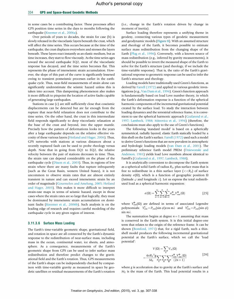
334 GPS and Space-Based Geodetic Methods
Author's personal copy
in some cases be a contributing factor. These processes affect
GPS position time series in the days to months following the
earthquake (Kreemer et al., 2006a).
Over periods of years to decades, the strain for case (b) is
slowly released in the viscoelastic layers beneath the crust, which
will affect the time series. This occurs because at the time of the
earthquake, the crust displaces everywhere and stresses the layers
beneath. These layers react instantly as an elastic medium, but as
time increases, they start to flow viscously. As the time series ages
toward the second earthquake EQ2, most of the viscoelastic
response has decayed, and the time series becomes flat. This
represents the phase of interseismic strain accumulation. How-
ever, the slope of this part of the curve is significantly lessened
owing to transient postseismic processes earlier in the earth-
quake cycle. Thus, near-field measurements of strain alone can
significantly underestimate the seismic hazard unless this is
taken into account. This dampening phenomenon also makes
it more difficult to pinpoint the location of active faults capable
of generating large earthquakes.
Stations in case (c) are still sufficiently close that coseismic
displacements can be detected but are far enough from the
rupture that near-field relaxation does not contribute to the
time series. On the other hand, the crust in this intermediate
field responds significantly to deep viscoelastic relaxation at
the base of the crust and beyond, into the upper mantle.
Precisely how the pattern of deformations looks in the years
after a large earthquake depends on the relative effective vis-
cosity of these various layers (Hetland and Hager, 2006). Thus,
GPS networks with stations at various distances about a
recently ruptured fault can be used to probe rheology versus
depth. Note that in going from EQ1 to EQ2, the relative
velocity between the pair of stations decreases in time. Thus,
the strain rate can depend considerably on the phase of the
earthquake cycle (Dixon et al., 2003). Thus, in regions of low
strain where there are many faults that rupture infrequently
(such as the Great Basin, western United States), it is not
uncommon to observe strain rates that are almost entirely
transient in nature and can exceed interseismic strain by an
order of magnitude (Gourmelen and Amelung, 2005; Hetland
and Hager, 2003). This makes it more difficult to interpret
strain-rate maps in terms of seismic hazard, except in those
cases where the strain rates are so large that logically, they must
be dominated by interseismic strain accumulation on domi-
nant faults (Kreemer et al., 2006b). Such analysis is on the
leading edge of research and requires careful modeling of the
earthquake cycle in any given region of interest.
3.11.3.6 Surface Mass Loading
The Earth’s time-variable geometric shape, gravitational field,
and rotation in space are all connected by the Earth’s dynamic
response to the redistribution of near-surface mass, including
mass in the ocean, continental water, ice sheets, and atmo-
sphere. As a consequence, measurements of the Earth’s
geometric shape from GPS can be used to infer surface mass
redistribution and therefore predict changes to the gravit-
ational field and the Earth’s rotation. Thus, GPS measurements
of the Earth’s shape can be independently checked by compar-
ison with time-variable gravity as measured in space by geo-
detic satellites or residual measurements of the Earth’s rotation
Treatise on Geophysics, 2nd edition,
(i.e., change in the Earth’s rotation driven by change in
moment of inertia).
Surface loading therefore represents a unifying theme in
geodesy, connecting various types of geodetic measurement
and geodynamic models (Figure 8). With an assumed structure
and rheology of the Earth, it becomes possible to estimate
surface mass redistribution from the changing shape of the
Earth (Plag et al., 1996). Conversely, with a known source of
mass redistribution (e.g., inferred by gravity measurements), it
should be possible to invert the measured shape of the Earth to
solve for the Earth’s structure (and rheology, if we include the
time-variable response). That is, the ratio of the Earth’s gravi-
tational response to geometric response can be used to infer the
Earth’s structure and rheology.
Loadingmodels have traditionally used Green’s functions, as
derived by Farrell (1972) and applied in various geodetic inves-
tigations (e.g., VanDam et al., 1994). Green’s function approach
is fundamentally based on load Love number theory, in which
the Earth’s deformation response is a function of the spherical
harmonic components of the incremental gravitational potential
created by the surface load. To study the interaction between
loading dynamics and the terrestrial reference frame, it is conve-
nient to use the spherical harmonic approach (Grafarend et al.,
1997; Lambeck, 1988; Mitrovica et al., 1994) (therefore, the
conclusions must also apply to the use of Green’s functions).
The following ‘standard model’ is based on a spherically
symmetrical, radially layered, elastic Earth statically loaded by a
thin shell on the Earth’s surface. Farrell (1972) used such amodel
to deriveGreen’s functions that are nowprevalent in atmospheric
and hydrologic loading models (van Dam et al., 2001). The
preliminary reference Earth model PREM (Dziewonski and
Anderson, 1981) yields load Love numbers almost identical to
Farrell’s (Grafarend et al., 1997; Lambeck, 1988).
It is analytically convenient to decompose the Earth system
as a spherical solid Earth of radius RE, plus surface mass that is
free to redistribute in a thin surface layer (<<RE) of surface
density s(O), which is a function of geographic position O(latitude ’ and longitude l). Let us express the total redistrib-
uted load as a spherical harmonic expansion:
s Oð Þ¼X1n¼1
Xnm¼0
XSF¼C
sFnmYFnm Oð Þ [25]
where YnmF (O) are defined in terms of associated Legendre
polynomials: YnmC ¼Pnm(sin f)cos ml and Ynm
S ¼Pnm(sin f)sin ml.
The summation begins at degree n¼1 assuming that mass
is conserved in the Earth system. It is this initial degree-one
term that relates to the origin of the reference frame. It can be
shown (Bomford, 1971) that, for a rigid Earth, such a thin-
shell model produces the following incremental gravitational
potential at the Earth’s surface, which we call the ‘load
potential’:
V Oð Þ¼Xn
Vn Oð Þ
¼ 4pRE3g
ME
Xn
Xm
XF
sFnmYFnm Oð Þ
2nþ1ð Þ[26]
where g is acceleration due to gravity at the Earth’s surface and
ME is the mass of the Earth. This load potential results in a
(2015), vol. 3, pp. 307-338

GPS and Space-Based Geodetic Methods 335
Author's personal copy
displacement of the geoid called the ‘equilibrium tide.’ As shall
be addressed later, the load deforms the solid Earth and, in
doing so, creates an additional potential.
According to load Love number theory, solutions for sur-
face displacements Dsh(O) in the local height direction and
Dsl(O) in any lateral direction specified by unit vector l Oð Þ aregiven by (Lambeck, 1988)
Dsh Oð Þ¼Xn
h0nVn Oð Þ=g
Dsl Oð Þ¼Xn
l0n l Oð Þ:∇Vn Oð Þ=g [27]
and the additional potential caused by the resulting deforma-
tion is
DV Oð Þ¼Xn
k0nVn Oð Þ [28]
where hn0 , ln0 , and kn
0 are degree-n load Love numbers, with the
prime distinguishing Love numbers used in loading theory
from those used in tidal theory. The surface gradient operator
is defined as ∇¼ w@’þ l 1=cos’ð Þ@l, where f and l are unit
vectors pointing northward and eastward, respectively.
The net loading potential (load plus additional potential)
relative to Eulerian observer (the ‘space potential’ as observed
on a geocentric reference surface) is
U Oð Þ¼V Oð ÞþDV Oð Þ¼Xn
1þk0n� �
Vn Oð Þ [29]
The net loading potential relative to Lagrangian observer
(the ‘body potential’ as observed on the deforming Earth’s
surface) must also account for the lowering of the Earth’s
surface due to loading. From eqns [5] and [3], the body poten-
tial is
U0 Oð Þ¼U Oð Þ� gDsh Oð Þ¼Xn
1þk0n�h0n� �
Vn Oð Þ [30]
Therefore, the ‘space’ and ‘body’ combinations of load Love
number, (1þkn0) and (1þkn
0 �hn0), are relevant to computing
gravity acting on Earth-orbiting satellites and Earth-fixed
instruments, respectively.
Solutions for surface deformations of the thin-shell loading
model are found by substituting [2] into [3] and [5]:
Dsh Oð Þ¼ 4pRE3
ME
Xn
Xm
XF
h0n2nþ1
sFnmYFnm Oð Þ
Dsl Oð Þl ¼ 4pRE3
ME
Xn
Xm
XF
l0n2nþ1
sFnm l:∇YFnm Oð Þ
U Oð Þ¼ 4pRE3
ME
Xn
Xm
XF
1þk0n2nþ1
sFnmYFnm Oð Þ [31]
Thus, GPS data on station coordinate variations around the
globe can be used to invert eqn [7] for the surface mass coef-
ficients (up to some degree and order n) and hence the surface
mass field by substitution into eqn [1] (Blewitt and Clarke,
2003). Truncation of the expansion is of course necessary due
to the discrete and finite coverage of GPS data, especially
considering the sparsity of data in certain areas such as over
the ocean. This implies that the surface mass field will be
Treatise on Geophysics, 2nd edition
smoothed. Nevertheless, the long-wavelength information
from geodesy is in principle useful to constrain the
continental-scale integral of basin-scale hydrologic models.
While it is in widespread use, the previously mentioned
standard loading model might be improved by incorporating
the Earth’s ellipticity (Wahr, 1981), mantle heterogeneity
(Dziewonski et al., 1977; Plag et al., 1996; Su et al., 1994;
van Dam et al., 1994), and Maxwell rheology (Lambeck,
1988; Mitrovica et al., 1994; Peltier, 1974). There is no con-
sensus model to replace PREM yet; however, the general
approach to reference frame considerations described here
would be applicable to improved models.
To date, surface mass loading has primarily been investi-
gated by gravimetric methods (e.g., GRACE and SLR, see else-
where in this volume), and the application of geometric
measurements from GPS is still in its infancy. The most prom-
ising application of GPS in this respect is to the lower-degree
harmonic components of the global surface mass field, to
which satellite missions such as GRACE are least sensitive.
References
Altamimi Z, Angermann D, Argus D, et al. (2001) The terrestrial reference frame and thedynamic Earth. EOS. Transactions of the American Geophysical Union 82: 273–279.
Altamimi Z, Sillard P, and Boucher C (2002) ITRF2000: A new release of theInternational Terrestrial Reference Frame for Earth science application. Journal ofGeophysical Research 107(B10): 2214. http://dx.doi.org/10.1029/2001JB000561.
Argus DF, Peltier WR, and Watkins MM (1999) Glacial isostatic adjustment observedusing very long baseline interferometry and satellite laser ranging geodesy. Journalof Geophysical Research 104(B12): 29077–29093.
Ashby N (2004) The Sagnac effect in the Global Positioning System. In: Rizzi G andRuggiero ML (eds.) Relativity and Rotating Frames (Fundamental Theories ofPhysics), vol. 135, pp. 11–28. Dordrecht: Springer.
Ashby N and Allan D (1984) Coordinate time on and near the Earth. Physical ReviewLetters 53(19): 1858.
Bar-Sever Y (1996) A new model for GPS yaw attitude. Journal of Geodesy 70: 714–723.Bar-Sever YE, Kroger PM, and Borjesson JA (1998) Estimating horizontal gradients of
tropospheric path delay with a single GPS receiver. Journal of Geophysical Research103: 5019–5035.
Bennett RA, Wernicke BP, and Davis JL (1998) Continuous GPS measurements ofcontemporary deformation across the northern Basin and Range province.Geophysical Research Letters 25: 563–566.
Bennett RA, Wernicke BP, Niemi NA, Friedrich AM, and Davis JL (2003) Contemporarystrain rates in the northern Basin and Range province from GPS data. Tectonics22(2): 1008. http://dx.doi.org/10.1029/2001TC001355.
Bertiger WI, Desai SD, Haines B, et al. (2010) Single receiver phase ambiguityresolution with GPS data. Journal of Geophysical Research 84(5): 327–337.
Beutler G, Brockmann E, Gurtner W, Hugentobler U, Mervart L, and Rothacher M (1994)Extended orbit modeling techniques at the CODE Processing Center of theInternational GPS Service for Geodynamics (IGS): Theory and initial results.Manuscripta Geodaetica 19: 367–386.
Beutler G, Drewes H, and Verdun A (2004) The new structure of the InternationalAssociation of Geodesy (IAG) viewed from the perspective of history. Journal ofGeodesy 77: 560–575.
Beutler G, Gurtner W, Bauersima I, and Langley R (1985) Modeling and estimating theorbits of GPS satellites. In: Proceedings of the 1st International Symposium onPrecise Positioning with the Global Positioning System Rockville, MD: U.S. Dept. ofCommerce.
Beutler G, Mueller II, and Neilan RE (1994) The International GPS Service forGeodynamics: Development and start of official service on January 1, 1994. BulletinGeodesique 68: 39–70.
Bevis M, Businger S, Herring TA, Rocken C, Anthes RA, and Ware RH (1992) GPSmeteorology: Remote sensing of atmospheric water vapor using the GlobalPositioning System. Journal of Geophysical Research 97(D14): 15787–15801.
Bianco G, Devoti R, Fermi M, Luceri V, Rutigliano P, and Sciarretta C (1997) Estimationof low degree geopotential coefficients using SLR data. Planetary and Space Science46: 1633–1638.
, (2015), vol. 3, pp. 307-338

336 GPS and Space-Based Geodetic Methods
Author's personal copy
Bierman G (1977) Factorization Methods for Discrete Sequential Estimation. New York,NY: Academic Press.
Bilham R (1991) Earthquakes and sea level: Space and terrestrial metrology onchanging planet. Reviews of Geophysics 29: 1–29.
Blewitt G (1989) Carrier phase ambiguity resolution for the Global Positioning Systemapplied to geodetic baselines up to 2000 km. Journal of Geophysical Research94(B8): 10187–10283.
Blewitt G (1990) An automatic editing algorithm for GPS data. Geophysical ResearchLetters 17(3): 199–202.
Blewitt G (1993) Advances in Global Positioning System technology for geodynamicsinvestigations. In: Smith DE and Turcotte DL (eds.) Contributions of Space Geodesyto Geodynamics: Technology, pp. 195–213. Washington, DC: AmericanGeophysical Union.
Blewitt G and Clarke P (2003) Inversion of Earth’s changing shape to weigh sea level instatic equilibrium with surface mass redistribution. Journal of Geophysical Research108(B6): 2311. http://dx.doi.org/10.1029/2002JB002290.
Blewitt G, Kreemer C, Hammond WC, Plag H-P, Stein S, and Okal E (2006) Rapiddetermination of earthquake magnitude using GPS for tsunami warning systems.Geophysical Research Letters 33: L11309. http://dx.doi.org/10.1029/2006GL026145.
Blewitt G and Lavallee D (2002) Effect of annual signals on geodetic velocity. Journal ofGeophysical Research 107(B7). http://dx.doi.org/10.1029/2001JB000570.
Blewitt G and Lichten SM (1992) Carrier phase ambiguity resolution up to 12000 km:Results from the GIG’91 experiment. In: Proceedings of the 6th InternationalSymposium on Satellite Positioning, Columbus: Ohio State University.
Bock Y, Gourevitch SA, Counselman CC, King RW, and Abbot RI (1986) Interferometricanalysis of GPS phase observations. Manuscripta Geodaetica 11: 282–288.
Bock Y, Nikolaidis RM, de Jonge PJ, and Bevis M (2000) Instantaneous geodeticpositioning at medium distances with the Global Positioning System. Journal ofGeophysical Research 105(B12): 28223–28253.
Bock Y, Prawirodirdjo L, and Melbourne TI (2004) Detection of arbitrarily dynamicground motions with a dense high-rate GPS network. Geophysical Research Letters31(B10): L06604. http://dx.doi.org/10.1029/2003GL019150.
Boehm J, Niell A, Tregoning P, and Schuh H (2006) Global Mapping Function (GMF):A new empirical mapping function based on numerical weather model data.Geophysical Research Letters 33: L07304. http://dx.doi.org/10.1029/2005/GL025546.
Bomford G (1971) Geodesy, third rev. ed Oxford, UK: Oxford University Press. ISBN978-0198519195.
Bosworth JM, Coates RJ, and Fischetti TL (1993) The Development of NASA’s CrustalDynamics Project. In: Smith DE and Turcotte DL (eds.) Contributions of SpaceGeodesy to Geodynamics: Technology, pp. 1–20. Washington, DC: AmericanGeophysical Union.
Boucher C and Altamimi Z (1993) Development of a conventional terrestrial referenceframe. In: Smith DE and Turcotte DL (eds.) Contributions of Space Geodesy toGeodynamics: Earth Dynamics, pp. 89–98. Washington, DC: American GeophysicalUnion.
Chao BF, O’Connor WP, Chang ATC, Hall DK, and Foster JL (1987) Snow load effect onthe Earth’s rotation and gravitational field, 1979–1985. Journal of GeophysicalResearch 92: 9415–9422.
Chen G and Herring TA (1997) Effects of atmospheric azimuthal asymmetry on theanalysis of space geodetic data. Journal of Geophysical Research102: 20489–20502.
Chen JL, Wilson CR, Eanes RJ, and Nerem RS (1999) Geophysical interpretation ofobserved geocenter variations. Journal of Geophysical Research 104(B2):2683–2690.
Cheng MK and Tapley BD (1999) Seasonal variations in low degree zonal harmonics ofthe Earth’s gravity field from satellite laser ranging observations. Journal ofGeophysical Research 104(B2): 2667–2681, February 10.
Cheng M and Tapley BD (2004) Variations in the Earth’s oblateness during the past28 years. Journal of Geophysical Research 109. http://dx.doi.org/10.1029/2004JB003028.
Choi K, Bilich A, Larson K, and Axelrad P (2004) Modified sidereal filtering: Implicationsfor high-rate GPS positioning. Geophysical Research Letters 31(22), L22608.
Ciufolini I and Pavlis EC (2004) A confirmation of the general relativistic prediction ofthe Lense-Thirring effect. Nature 431: 958–960.
Counselman CC, Hinteregger HF, and Shapiro II (1972) Astronomical applications ofdifferential interferometry. Science 178: 607–608.
Counselman CC and Shapiro II (1979) Miniature interferometer terminals for Earthsurveying. Bulletin Geodesique 53(2): 139–163.
Davis JL, Bennett RA, and Wernicke BP (2003) Assessment of GPS velocity accuracy forthe Basin and Range Geodetic Network (BARGEN). Geophysical Research Letters30(7): 1411. http://dx.doi.org/10.1029/2003GL016961.
Treatise on Geophysics, 2nd edition,
Davis JL, Elgered G, Niell AE, and Kuehn CE (1993) Ground-based measurement ofgradients in the “wet” radio refractivity of air. Radio Science 28: 1003–1018.
Davis JL, Herring TA, Shapiro II, Rogers AEE, and Elgered G (1985) Geodesy by radiointerferometry: Effects of atmospheric modeling errors on estimates of baselinelength. Radio Science 20: 1593–1607.
Davis JL, Murray MH, King RW, and Bock Y (1987) Assessing the effects ofatmospheric errors on estimates of relative position obtained from GPS data. Eos,Transactions American Geophysical Union 68(16): 286.
Degnan JJ (1993) Millimeter accuracy satellite laser ranging: A review. In: Smith DE andTurcotte DL (eds.) Contributions of Space Geodesy to Geodynamics: Technology(Geodynamics Series), vol. 25, pp. 133–162. Washington, DC: AmericanGeophysical Union.
DeMets C, Gordon RG, Argus DF, and Stein S (1990) Current plate motions.Geophysical Journal International 101: 425–478.
DeMets C, Gordon RG, Argus DF, and Stein S (1994) Effect of recent revisions of thegeomagnetic reversal time scale on estimates of current plate motions. GeophysicalResearch Letters 21: 2191–2194.
Devoti R, Luceri V, Sciarretta C, et al. (2001) The SLR secular gravity variations andtheir impact on the inference of mantle rheology and lithospheric thickness.Geophysical Research Letters 28(5): 855–858.
Dickey JO, Bender PL, Faller JE, et al. (1994) Lunar laser ranging: A continuing legacyof the Apollo Program. Science 265: 482–490. http://dx.doi.org/10.1126/science.265.5171.482.
Dixon TH (1991) An introduction to the Global Positioning System and some geologicalapplications. Reviews of Geophysics 29(2): 249–276.
Dixon TH, Golombek MP, and Thornton CL (1985) Constraints on Pacific platekinematics and dynamics with Global Positioning System measurements. IEEETransactions on Geoscience and Remote Sensing GE-23(4): 491–501.
Dixon TH, Norabuena E, and Hotaling L (2003) Paleoseismology and GPS: Earthquakecycle effects and geodetic versus geologic fault slip rates in the eastern Californiashear zone. Geology 31: 55–58.
Dong D and Bock Y (1989) GPS network analysis with phase ambiguity resolutionapplied to crustal deformation studies in California. Journal of GeophysicalResearch 94(B4): 3949–3966.
Dow JM, Gurtner W, and Schluter W (2005a) The IGGOS viewed from the SpaceGeodetic Services. Journal of Geodynamics 40(4–5): 375–386.
Dow JM, Neilan RE, and Gendt G (2005b) The International GPS Service (IGS):Celebrating the 10th anniversary and looking to the next decade. Advances in SpaceResearch 36(3): 320–326. http://dx.doi.org/10.1016/j.ast.2005.05.125.
Dunn P, Torrence M, Kolenkiewicz R, and Smith D (1999) Earth scale defined bymodern satellite ranging observations. Journal of Geophysical Research 26(10):1489–1492.
Dziewonski AM and Anderson DL (1981) Preliminary reference Earth model. Physics ofthe Earth and Planetary Interiors 25: 297–356.
Dziewonski AM, Hager BH, and O’Connell RJ (1997) Large-scale heterogeneities in thelower mantle. Journal of Geophysical Research 82: 239–255. http://dx.doi.org/10.1029/JB082i002p00239.
Eubanks TM (1993) Variations in the orientation of the Earth. In: Smith DE andTurcotte DL (eds.) Contributions of Space Geodesy to Geodynamics: EarthDynamics, pp. 1–54. Washington, DC: American Geophysical Union.
Evans AG, Hill RW, Blewitt G, et al. (2002) The Global Positioning System geodesyodyssey, navigation. Journal of the Institute of Navigation 49(1): 7–34.
Farrell WE (1972) Deformation of the Earth by surface loads. Reviews of Geophysics10: 761–797.
Fliegel HF and Gallini TE (1996) Solar force modeling of Block IIR Global PositioningSystem satellites. Journal of Spacecraft and Rockets 33(6): 863–866.
Fliegel HF, Gallini TE, and Swift ER (1992) Global Positioning System radiation forcemodel for geodetic applications. Journal of Geophysical Research 97: 559–568.
Freymueller JT and Kellogg JN (1990) The extended tracking network and indications ofbaseline precision and accuracy in the North Andes. Geophysical Research Letters17: 207–210.
Ge M, Gendt G, Dick G, Zhang FP, and Reigber C (2005) Impact of GPS satellite antennaoffsets on scale changes in global network solutions. Geophysical Research Letters32(6): L06310. http://dx.doi.org/10.1029/2004GL022224.
Gegout P and Cazenave A (1993) Temporal variations of the Earth gravity field for1985–1989 derived from LAGEOS. Geophysical Journal International114: 347–359.
Gourmelen N and Amelung F (2005) Post-seismic mantle relaxation in the CentralNevada Seismic Belt. Science 310: 1473–1476. http://dx.doi.org/10.1126/science.1119798.
Grafarend EW, Engels J, and Varga P (1997) The spacetime gravitational field of adeforming body. Journal of Geodesy 72: 11–30.
(2015), vol. 3, pp. 307-338

GPS and Space-Based Geodetic Methods 337
Author's personal copy
Gross RS, Blewitt G, Clarke PJ, and Lavallee (2004) Degree-2 harmonics of the Earth’smass load estimated from GPS and Earth rotation data. Geophysical ResearchLetters 31: L07601. http://dx.doi.org/10.1029/2004GL019589.
Gurtner W, Beutler G, Bauersima I, and Schildknecht T (1985) Evaluation of the GPScarrier difference observations: The BERNESE second generation software package.In: Goad Clyde (ed.), 1st Int. Symp. on Precise Positioning with the GlobalPositioning System, Rockville, MD: U.S. Dept. of Commerce.
Hager BH, King RW, and Murray MH (1991) Measurement of crustal deformationusing the Global Positioning System. Annual Reviews of Planetary Science19: 351–382.
Haines AJ (1982) Calculating velocity fields across plate boundaries from observedshear rates. Geophysical Journal of the Royal Astronomical Society 68: 203–209.
Haines AJ and Holt WE (1993) A procedure for obtaining the complete horizontalmotions within zones of distributed deformation from the inversion of strain ratedata. Journal of Geophysical Research 98: 12057–12082.
Hammond WC (2005) The ghost of an earthquake. Science 310: 1440–1442.Heflin MB, Bertiger WI, Blewitt G, et al. (1992) Global geodesy using GPS without
fiducial sites. Geophysical Research Letters 19: 131–134.Henson DJ, Collier EA, and Schneider KR (1985) Geodetic applications of the Texas
Instruments TI-4100 GPS navigator. In: Goad C (ed.), Proceedings of the 1stInternational Symposium on Precise Positioning with the Global PositioningSystem, pp. 191–200. Rockville, MD: U.S. Dept. of Commerce.
Herring TA, Davis JL, and Shapiro II (1990) Geodesy by radio interferometry: Theapplication of Kalman filtering to the analysis of very long baseline interferometrydata. Journal of Geophysical Research 95: 12561–12581.
Herring TA and Pearlman MR (1993) Future developments and synergism of spacegeodetic measurement techniques. In: Smith DE and Turcotte DL (eds.)Contributions of Space Geodesy to Geodynamics: Technology, pp. 21–22.Washington DC: American Geophysical Union.
Hetland EA and Hager BH (2003) Postseismic relaxation across the Central NevadaSeismic Belt. Journal of Geophysical Research 108: 2394. http://dx.doi.org/10.1029/2002JB002257.
Hetland EA and Hager BH (2006) The effect of rheological layering on postseismic andinterseismic displacements. Geophysical Journal International 166: 277–292.
Hill EM and Blewitt G (2006) Testing for fault activity at Yucca Mountain, Nevada, usingindependent GPS results from the BARGEN network. Geophysical Research Letters33: L14302. http://dx.doi.org/10.1029/2006GL026140.
Holt WE (1995) Flow fields in the Tonga slab determined from the moment tensors ofdeep earthquakes. Geophysical Research Letters 22: 989–992.
Holt WE and Haines AJ (1993) Velocity fields in deforming Asia from the inversion ofearthquake-released strains. Tectonics 12: 1–20.
Holt WE and Haines AJ (1995) The kinematics of northern South Island New Zealanddetermined from geologic strain rates. Journal of Geophysical Research100: 17991–18010.
Holt WE, Kreemer C, Haines AJ, et al. (2005) Project helps constrain continentaldynamics and seismic hazards. Eos, Transactions of the American GeophysicalUnion 86: 383–387.
Holt WE, Li M, and Haines AJ (1995) Earthquake strain rates and instantaneous relativemotions within central and east Asia. Geophysical Journal International122: 569–593.
Holt WE, Ni JF, Wallace TC, and Haines AJ (1991) The active tectonics of the EasternHimalayan Syntaxis and Surrounding Regions. Journal of Geophysical Research96: 14595–14632.
IERS (2004) McCarthy DD and Petit G (eds.), IERS Conventions 2003, IERS TechnicalNote 32, Frankfurt am Main: Verlag des Bundesamts fur Kartographie und Geodasie,127 pp., paperback, ISBN 3-89888-884-3.
Jackson J, Haines AJ, and Holt WE (1992) Determination of the complete horizontalvelocity field in the deforming Aegean Sea region from the moment tensors ofearthquakes. Journal of Geophysical Research 97: 17657–17684.
Jackson JA, Haines AJ, and Holt WE (1994) Combined analysis of strain rate data fromsatellite laser ranging and seismicity in the Aegean region. Geophysical ResearchLetters 21: 2849–2852.
Jackson JA, Haines AJ, and Holt WE (1995) The accommodation of Arabia–Eurasiaplate convergence in Iran. Journal of Geophysical Research 100: 15205–15219.
Kaplan GH (1981) The IAU Resolutions on Astronomical Constants, Time Scale and theFundamental Reference Frame, U. S. Naval Observatory Circular No. 163.
Kedar S, Hajj GA, Wilson BD, and Heflin MB (2003) The effect of the second order GPSionospheric correction on receiver positions. Geophysical Research Letters 30(16):1829. http://dx.doi.org/10.1029/2003GL017639.
King RW, Abbot RI, Counselman CC, Gourevitch SA, Rosen BJ, and Bock Y (1984)Interferometric determination of GPS satellite orbits. Eos, Transactions of AmericanGeophysical Union 65: 853.
Treatise on Geophysics, 2nd edition
King RW and Bock Y (2005) Documentation for the GAMIT GPS Processing SoftwareRelease 10.2. Cambridge, MA: Mass Inst of Technol.
Kostrov VV (1974) Seismic moment and energy of earthquakes, and seismic flow ofrocks. Izvestiya, Academy of Sciences, USSR, Physics of Solid Earth 1: 23–44, Eng.Transl.
Kreemer C, Blewitt G, and Hammond WC (2006) Using geodesy to explore correlationsbetween crustal deformation characteristics and geothermal resources. GeothermalResources Council Transactions 30: 441–446.
Kreemer C, Blewitt G, and Maerten F (2006) Co- and postseismic deformation of the28 March 2005 Nias Mw 8.7 earthquake from continuous GPS data. GeophysicalResearch Letters 33: L07307. http://dx.doi.org/10.1029/2005GL025566.
Kreemer CJ, Haines WE, Holt G Blewitt, and Lavallee D (2000) On the determination of aglobal strain rate model. Earth, Planets and Space 52: 765–770.
Kreemer C, Holt WE, and Haines AJ (2003) An integrated global model of present-dayplate motions and plate boundary deformation. Geophysical Journal International154: 8–34.
Kuang D, Rim HJ, Schutz BE, and Abusali PAM (1996) Modeling GPS satellite attitudevariation for precise orbit determination. Journal of Geodesy 70: 572–580.
Lambeck K (1988) Geophysical Geodesy: The Slow Deformations of the Earth. Oxford,UK: Clarendon Press.
Langbein JL, Wyatt F, Johnson H, Hamann D, and Zimmer P (1995) Improved stabilityof a deeply anchored geodetic monument for deformation monitoring. GeophysicalResearch Letters 22: 3533–3536.
Larson KM and Agnew D (1991) Application of the Global Positioning System to crustaldeformation measurement: 1. Precision and accuracy. Journal of GeophysicalResearch 96(B10): 16547–16565.
Larson K, Bodin P, and Gomberg J (2003) Using 1 Hz GPS data to measuredeformations caused by the Denali Fault Earthquake. Science 300: 1421–1424.
Larson KM, Freymueller JT, and Philipsen S (1997) Global plate velocities from theGlobal Positioning System. Journal of Geophysical Research 102: 9961–9981.
Larson KM, Webb FH, and Agnew D (1991) Application of the Global Positioning Systemto crustal deformation measurement: 2. The influence of errors in orbit determinationnetworks. Journal of Geophysical Research 96(B10): 16567–16584.
Leick A (2004) GPS Satellite Surveying, 3rd ed. Hoboken, NJ: Wiley ISBN: 978-0-471-05930-1.
Lichten SM and Border JS (1987) Strategies for high-precision Global PositioningSystem orbit determination. Journal of Geophysical Research 92: 12751–12762.
MacDoran PF (1979) Satellite Emission Radio Interferometric Earth Surveying, SERIES-GPS geodetic system. Bulletin Geodesique 53: 117–138.
Mader GL (1999) GPS antenna calibration at the National Geodetic Survey. GPSSolutions 3(1): 50–58.
Mader GL and Czopek FM (2002) The Block IIA satellite—Calibrating antenna phasecenters. GPS World 13(5): 40–46.
Mao A, Harrison CGA, and Dixon TH (1999) Noise in GPS coordinate time series.Journal of Geophysical Research 104: 2797–2816.
McCarthy D (ed.) (1996) IERS Conventions, IERS Tech. Note 21. Paris: IERS CentralBureau, Observatory of Paris.
McMillan DS (1995) Atmospheric gradients from very long baseline interferometryobservations. Geophysical Research Letters 22(9): 1041–1044.
Meehan T, Srinivasan J, Spitzmesser D, et al. (1992) The TurboRogue GPS receiver.In: Proc. of the 6th Intl, Symp. on Satellite Positioning, Columbus, Ohio, 1, pp.209–218.
Minster JB, Altamimi Z, Blewitt G, et al. (2010) Precise Geodetic Infrastructure: NationalRequirements for a Shared Resource. Washington, DC: The National AcademiesPress, ISBN-10:0-309-15811-7, ISBN-13: 978-0-309-15811-4, 142 pp.
Minster JB and Jordan TH (1978) Present-day plate motions. Journal of GeophysicalResearch 83: 5331–5354.
Mitrovica JX, Davis JL, and Shapiro II (1994) A spectral formalism for computing three-dimensional deformations due to surface loads: 1. Theory. Journal of GeophysicalResearch 99: 7057–7073.
Moore AW (2007) The International GNSS Service: Any questions? GPS World 18(1):58–64.
Nerem RS, Chao BF, Au AY, et al. (1993) Time variations of the Earth’s gravitational fieldfrom satellite laser ranging to LAGEOS. Geophysical Research Letters 20(7):595–598.
Niell A (1996) Global mapping functions for the atmospheric delay at radio wavelengths.Journal of Geophysical Research 101(B2): 3227–3246.
Nikolaidis RM, Bock Y, de Jonge PJ, Agnew DC, and Van Domselaar M (2001) Seismicwave observations with the Global Positioning System. Journal of GeophysicalResearch 106(B10): 21897–21916.
Pearlman MR, Degnan JJ, and Bosworth JM (2002) The international laser rangingservice. Advances in Space Research 30(2): 135–143.
, (2015), vol. 3, pp. 307-338

338 GPS and Space-Based Geodetic Methods
Author's personal copy
Peltier WR (1974) The impulse response of a Maxwell Earth. Reviews of Geophysics andSpace Physics 12: 649–669.
Plag HP, Ambrosius B, Baker TF, et al. (1998) Scientific objectives of current and futureWEGENER activities. Tectonophysics 294: 177–223.
Plag H-P, Juttner H-U, and Rautenberg V (1996) On the possibility of global andregional inversion of exogenic deformations for mechanical properties of the Earth’sinterior. Journal of Geodynamics 21: 287–309.
Pollitz FF (1997) Gravitational-viscoelastic postseismic relaxation on a layeredspherical Earth. Journal of Geophysical Research 102: 17921–17941.
Pollitz FF (2003) Post-seismic relaxation theory on a laterally heterogeneousviscoelastic model. Geophysical Journal International 154: 1–22.
Prescott WH, Davis JL, and Svarc JL (1989) Global Positioning System measurementsfor crustal deformation: Precision and accuracy. Science 244: 1337–1340.
Ray J (ed.) (1998) IERS Analysis Campaign to Investigate Motions of the Geocenter,International Earth Rotation Service Tech. Note 25, Obs. Paris.
Rogers AEE, Knight CA, Hinteregger HF, et al. (1978) Geodesy by radio interferometry:Determination of a 1.24-km base line vector with �5-mm repeatability. Journal ofGeophysical Research 83: 325–334.
Rothacher M, Beutler G, Gurtner W, Schildknecht T, and Wild U (1990) BERNESE GPSSoftware Version 3.2. Switzerland: Printing Office Univ of Berne.
Rothacher M, Springer TA, Schaer S, and Beutler G (1998) Processing Strategies forRegional Networks. In: Brunner FK (ed.) Advances in Positioning and ReferenceFrames, IAG Symposium No. 118, pp. 93–100.
Rummel R, Rothacher M, and Beutler G (2005) Integrated Global Geodetic ObservingSystem (IGGOS)—Science rationale. Journal of Geodynamics 40(4–5): 357–362.
Sabadini R, Di Donato G, Vermeersen LLA, Devoti R, Luceri V, and Bianco G (2002) Icemass loss in Antarctica and stiff lower mantle viscosity inferred from the longwavelength time dependent gravity field. Geophysical Research Letters 29(10).
Savage JC (1983) Strain accumulation in the Western United States. Annual Review ofEarth and Planetary Sciences 11: 11–41. http://dx.doi.org/10.1145/annurev.ea.11.0501083.000303.
Schluter W, Himwich E, Nothnagel A, Vandenberg N, and Whitney A (2002) IVS and itsimportant role in the maintenance of the global reference systems. Advances inSpace Research 30(2): 145–150.
Schmid R and Rothacher M (2003) Estimation of elevation-dependent satellite antennaphase center variations of GPS satellites. Journal of Geodesy 77: 440–446. http://dx.doi.org/10.1007/s00190-003-0339-0.
Schmid R, Rothacher M, Thaller D, and Steigenberger P (2005) Absolute phase centercorrections of satellite and receiver antennas impact on GPS solutions andestimation of azimuthal phase center variations of the satellite antenna. GPSSolutions 9(4): 283–293.
Schupler BR, Allshouse RL, and Clark TA (1994) Signal characteristics of GPS userantennas. Journal of the Institute of Navigation 41: 277–295.
Segall P and Davis JL (1997) GPS applications for geodynamics and earthquakestudies. Annual Reviews of Earth and Planetary Sciences 25: 301–336.
Sella G, Dixon T, and Mao A (2002) REVEL: A model for recent plate velocities fromspace geodesy. Journal of Geophysical Research 107(B4). http://dx.doi.org/10.1029/2000JB000033.
Shapiro II (1964) Fourth test of general relativity. Physical Review Letters 13(26):789–791. http://dx.doi.org/10.1103/PhysRevLett.13.789.
Shen-Tu B, Holt WE, and Haines AJ (1995) Intraplate deformation in the JapaneseIslands: A Kinematic study of intraplate deformation at a convergent plate margin.Journal of Geophysical Research 100: 24275–24293.
Shen-Tu B, Holt WE, and Haines AJ (1999) The kinematics of the western United Statesestimated from Quaternary rates of slip and space geodetic data. Journal ofGeophysical Research 104: 28927–28955.
Silver PG, Bock Y, Agnew D, et al. (1999) A plate boundary observatory. IRIS Newsletter16: 3–9.
Smith DE and Turcotte DL (eds.) (1993) Contributions of Space Geodesy toGeodynamics: Technology. Washington, DC: American Geophysical Union.
Smith KD, von Seggern D, Blewitt G, et al. (2004) Evidence for deep magma injectionbeneath Lake Tahoe, Nevada-California. Science 305: 1277–1280. http://dx.doi.org/10.1126/science.1101304.
Sovers OJ and Border JS (1987) Observation Model and Parameter Partials for the JPLGeodetic Software, “GPSOMC". Pasadena, CA: JPL Pub Jet Propulsion Laboratory,87–21.
Steigenberger P, Rothacher M, Dietrich R, Fritsche M, Rulke A, and Vey S (2006)Reprocessing of a global GPS network. Journal of Geophysical Research111: B05402. http://dx.doi.org/10.1029/2005JB003747.
Stein S (1993) Space geodesy and plate motions. In: Smith DE and Turcotte DL (eds.)Contributions of Space Geodesy to Geodynamics: Crustal Dynamics, pp. 5–20.Washington, DC: American Geophysical Union.
Treatise on Geophysics, 2nd edition,
Su W, Woodward RL, and Dziewonski AD (1994) Degree 12 model of shear velocityheterogeneity in the mantle. Journal of Geophysical Research 99: 6945–6980.
Swift ER (1985) NSWC’s GPS orbit/clock determination system. In: Proc. of the 1stSymp. on Prec. Positioning with the Global Positioning System, U.S. Dept. ofCommerce, Rockville, MD .
Tapley BD, Schutz BE, Eanes RJ, Ries JC, and Watkins MM (1993) LAGEOS laserranging contributions to geodynamics, geodesy and orbital dynamics. In: Smith DEand Turcotte DL (eds.) Contributions of Space Geodesy to Geodynamics: EarthDynamics, pp. 147–174. Washington, DC: American Geophysical Union.
Tavernier G, Fagard H, Feissel-Vernier M, et al. (2005) The International DORIS Service,IDS. Advances in Space Research 36(3): 333–341.
Thomas JB (1988) Functional Description of Signal Processing in the Rogue GPSReceiver. Pasadena, CA: JPL, pp 88–15.
Tinnon M, Holt WE, and Haines AJ (1995) Velocity gradients in the northern IndianOcean inferred from earthquake moment tensors and relative plate velocities.Journal of Geophysical Research 100: 24315–24329.
Torge W (2001) Geodesy, 3rd ed. Berlin, Germany: Gruyte ISBN: 978-3110170726,400 pp.
Tralli DM, Dixon TH, and Stephens SA (1988) The effect of wet tropospheric pathdelays on estimation of geodetic baselines in the Gulf of California usingthe Global Positioning System. Journal of Geophysical Research 93(B6):6545–6557.
Tralli DM and Lichten SM (1990) Stochastic estimation of tropospheric path delays inGlobal Positioning System geodetic measurements. Bulletin Geodesique64: 127–159.
Tregoning P and Herring TA (2006) Impact of a priori zenith hydrostatic delay errors onGPS estimates of station heights and zenith total delays. Geophysical ResearchLetters 33: L23303. http://dx.doi.org/10.1029/2006GL027706.
Truehaft RN and Lanyi GE (1987) The effects of the dynamic wet troposphere on radiointerferometric measurements. Radio Science 22: 251–265.
Van Dam T, Blewitt G, and Heflin MB (1994) Atmospheric pressure loading effectson GPS coordinate determinations. Journal of Geophysical Research99: 23939–23950.
Van Dam TM, Wahr J, Milly PCD, Shmakin AB, Blewitt G, and Larson KM (2001)Crustal displacements due to continental water loading. Geophysical ResearchLetters 28: 651–654.
Wahr JM (1981) Body tides on an elliptical, rotating, elastic and oceanless Earth.Geophysical Journal 64: 677–703.
Watkins MM and Eanes RJ (1997) Observations of tidally coherent diurnaland semidiurnal variations in the geocenter. Geophysical Research Letters24: 2231–2234.
Wdowinski S, Bock Y, Zhang J, Fang P, and Genrich J (1997) Southern CaliforniaPermanent GPS Geodetic Array; spatial filtering of daily positions for estimatingcoseismic and postseismic displacements induced by the 1992 Landers earthquake.Journal of Geophysical Research 102(B8): 18057–18070.
Webb FH and Zumberge JF (1993) An Introduction to GIPSY-OASIS II. Pasadena, CA:Jet Propulsion Laboratory, JPL Publication D-11088.
Wernicke BP, Friedrich AM, Niemi NA, Bennett RA, and Davis JL (2000) Dynamics ofplate boundary fault systems from Basin and Range Geodetic Network (BARGEN)and geologic data. GSA Today 10(11): 1–7.
Williams SDP (2003) The effect of coloured noise on the uncertainties of rates estimatedfrom geodetic time series. Journal of Geodesy 76: 483–494. http://dx.doi.org/10.1007/s00190-002-0283-4.
Williams JG, Boggs DH, Yoder CF, Ratcliff JT, and Dickey JO (2001) Lunar rotationaldissipation in solid body and molten core. Journal of Geophysical Research106(E11): 27933–27968.
Williams JG, Tunyshev S, and Boggs DH (2004) Progress in lunar laser ranging tests ofrelativistic gravity. Physical Review Letters 93. http://dx.doi.org/10.1103/PhysRevLett.93.261101.
Wilson P and Reinhart E (1993) The Wegener-Medlas Project preliminary results on thedetermination of the geokinematics of the Eastern Mediterranean. In: Smith DE andTurcotte DL (eds.) Contributions of Space Geodesy to Geodynamics: CrustalDynamics, pp. 299–310. Washington, DC: American Geophysical Union.
Wu JT, Wu SC, Hajj GA, Bertiger WI, and Lichten SM (1993) Effects of antennaorientation on GPS carrier phase. Manuscripta Geodaetica 18: 91–93.
Wyatt F (1982) Displacement of surface monuments; horizontal motion. Journal ofGeophysical Research 87: 979–989.
Ziebart M, Cross P, and Adhya S (2002) Modeling photon pressure, the key to high-precision GPS satellite orbits. GPS World 13(1): 43–50.
Zumberge JF, Heflin MB, Jefferson DC, Watkins MM, and Webb FH (1997) Precisepoint positioning for the efficient and robust analysis of GPS data from largenetworks. Journal of Geophysical Research 102(B3): 5005–5018.
(2015), vol. 3, pp. 307-338