Forschungsinstitut zur Zukunft der ArbeitInstitute for the Study of Labor

DI

SC

US

SI

ON

P

AP

ER

S

ER

IE

S

Third-Party vs. Second-Party Control:Disentangling the Role of Autonomy and Reciprocity

IZA DP No. 9251

August 2015

Gabriel BurdinSimon HallidayFabio Landini

Third-Party vs. Second-Party Control: Disentangling the Role of Autonomy

and Reciprocity

Gabriel Burdin Leeds University Business School,

IECON-FCEA, Universidad de la Republica and IZA

Simon Halliday

Smith College

Fabio Landini

SEP, LUISS University and CRIOS, Bocconi University

Discussion Paper No. 9251 August 2015

IZA

P.O. Box 7240 53072 Bonn

Germany

Phone: +49-228-3894-0 Fax: +49-228-3894-180

E-mail: iza@iza.org

Any opinions expressed here are those of the author(s) and not those of IZA. Research published in this series may include views on policy, but the institute itself takes no institutional policy positions. The IZA research network is committed to the IZA Guiding Principles of Research Integrity. The Institute for the Study of Labor (IZA) in Bonn is a local and virtual international research center and a place of communication between science, politics and business. IZA is an independent nonprofit organization supported by Deutsche Post Foundation. The center is associated with the University of Bonn and offers a stimulating research environment through its international network, workshops and conferences, data service, project support, research visits and doctoral program. IZA engages in (i) original and internationally competitive research in all fields of labor economics, (ii) development of policy concepts, and (iii) dissemination of research results and concepts to the interested public. IZA Discussion Papers often represent preliminary work and are circulated to encourage discussion. Citation of such a paper should account for its provisional character. A revised version may be available directly from the author.

IZA Discussion Paper No. 9251 August 2015

ABSTRACT

Third-Party vs. Second-Party Control: Disentangling the Role of Autonomy and Reciprocity

This paper studies the role of autonomy and reciprocity in explaining control averse responses in principal-agents interactions. While most of the social psychology literature emphasizes the role of autonomy, recent economic research has provided an alternative explanation based on reciprocity. We propose a simple model and an experiment to test the relative strength of these two motives. We compare two treatments: one in which control is exerted directly by the principal (second-party control); and the other in which it is exerted by a third party enjoying no residual claimancy rights (third-party control). If control aversion is driven mainly by autonomy, then it should persist in the third-party treatment. Our results, however, suggest that this is not the case. Moreover, when a third party instead of the principal exerts control, control results in a greater expected profit for the principal. The implications of these results for organizational design are discussed. JEL Classification: C72, C91, D23, M54 Keywords: third party, second party, control aversion, autonomy, principal-agent game, social preferences, trust, reciprocity Corresponding author: Simon Halliday Department of Economics Smith College Northampton, MA 01063 USA E-mail: shalliday@smith.edu

2

1. Introduction

In contemporary societies, significant resources are devoted to control people's actions.

For instance, a substantial fraction of the labor force is allocated to supervisory tasks in

both developed and developing countries (Acemoglu and Newman, 2002; Jayadev and

Bowles, 2006; Fafchamps and Söderbom, 2006). According to figures computed from

the European Working Condition Survey (EWCS), more than half (57%) of non-

supervisory employees lack procedural autonomy at work in at least one dimension (i.e.

the ability to change or choose the order of tasks, the speed or rate of work and the

method of work) and 42% perceive that their work rate depends on the direct control of

their bosses. 1 Hence, understanding the precise behavioral mechanisms underlying

people's reactions to control and their economic consequences remain important

concerns.

Traditionally, two main streams of literature have focused on people’s reactions to

control. On the one hand social psychologists have emphasized the role of individual

orientations towards autonomy and control. According to Self-Determination Theory

(SDT), human beings have a basic psychological need for autonomy (Deci and Ryan,

1985). That is, humans require “a form of freedom in which a party experiences himself

to be the locus of causality for his own behavior ” (Gagné and Deci, 2005, p. 333). This

approach sees people’s wellbeing as inseparable from their experience of personal and

motivational autonomy (Chirkov et al, 2011) and considers the quest for autonomy as

one of the main drivers of individual reactions to control.2

On the other hand, behavioral economists have focused primarily on intention-based

social preferences, in particular reciprocity (Falk and Fischbacher, 2006; Dufwenberg

and Kirchsteiger, 2004; Von Siemens, 2013). Nowadays, there is ample evidence that

many agents behave in a reciprocal manner even when acting on reciprocal preferences

is costly and yields no future rewards (see, for instance, Fehr and Gächter, 2000). On

this basis Falk and Kosfeld (2006, henceforth, F&K) have provided a reciprocity-based

1 Own calculations from EWCS wave 2010.2 Several experiments conducted by psychologists in highly differentiated contexts have shown thatenvironments supporting autonomy (control) to significantly increase (decrease) intrinsic motivations andprosocial behavior, and therefore that autonomy and control can severely affect task performance (seeGagné, 2003; Greene-Demers et al., 1997; Pelletier et al., 1998; Fabes et al., 1989; Kunda and Schwartz,1983; Upton, 1974; Batson et al., 1978; Sobus,1995).

3

explanation for individual reactions to control. In a principal-agent game they explore

the phenomena of hidden costs of control and the idea that ‘control aversion’ may be

one of the reasons why incentives sometimes degrade performance. They found a

sizeable fraction of agents react negatively to control and that control is not profitable,

i.e. principals earn more if they leave agents to decide freely than if they control. F&K

explain their result in terms of negative reciprocity on the side of the agents who punish

the controlling principals for their distrust.3

Although both the autonomy and the reciprocity explanations are plausible, there is still

no clear evidence that help to disentangle them. F&K explored the agents’ emotional

perception of control in their experiment and the most frequent answers among those

agents who react negatively to control were distrust and lack of autonomy. However,

the experimental design does not allow the authors to separate the explanatory role of

these two motives and thus leaves their relative importance unexplained. Distinguishing

between these two motives is important as it affects the way in which control practices

ought to be implemented. If reciprocity is the main driver, then third-party control (i.e.

through salaried supervisors enjoying no residual claimancy rights) is to be preferred

over second-party control (i.e. through supervisors entitled with residual claimancy

rights). On the contrary, if autonomy is the strongest motive, then control is always

perceived in a negative way and it may thus degrade performance independently of

whom is exerting it.

In this paper we extend F&K’s experimental design to disentangle the role of autonomy

and reciprocity in explaining how individuals react to control in a principal-agent

relationship. We vary their experiment to permit it to include three parties: the principal,

who benefits from the effort of the agent, the agent, and a third party who is given a

show-up fee and chooses whether or not to exert control over the agent, but does not

directly benefit from the agent’s actions (i.e. he does not have any claim over the

residual). On this basis, we obtain three main results: (1) in the presence of a third party

who can exert control we find no hidden costs of control; (2) when a third party instead

of the principal exerts control, the fraction of control averse agents dramatically

3 Recent experimental evidence also suggests that individuals intrinsically value decisional autonomyover their own and others’ outcomes (Bartling et al, 2014; Owens et al, 2014). Moreover, greaterprocedural autonomy and lower monitoring intensity appear to correlate positively with greater jobsatisfaction (Bartling et al, 2013).

4

decreases and control results in a greater expected profit for the principal; (3)

independently of the type of control, a relatively high degree of heterogeneity in

behavioral responses to control exist. Regression analysis shows no correlation between

the probability of being control averse and a psychological measure of autonomy

orientation (General Causality Orientation Scale; GCOS). In contrast, we find a

significantly negative correlation between this probability and individuals' controlled

orientation as measured by GCOS. Overall, control aversion appears to be driven (at

least in this very specific and highly stylized experimental setting) by negative

reciprocity rather than by agents' preference for autonomy.

The paper contributes to the growing experimental economics literature on authority

and control in organizations (Falk and Kosfeld, 2006; Ziegelmeyer et al, 2012; Fehr et

al., 2013; Charness et al., 2011; Schnedler and Vadovic, 2011). The study also adds to

the literature on crowding out (in) effects of incentives on intrinsic motives (see Frey

and Jegen, 2000; Bowles and Polanía, 2012). Finally, the paper contributes to the

research agenda in organizational economics trying to improve the mapping of

individual preferences and assessing the consequences of the mismatch between

preferences and organization design (Ben Ner, 2013). By disentangling the precise

behavioral motives underlying reactions to control, the results presented in this paper

may have implications for key aspects of organizational design, such as the optimal

level of employees' discretion and monitoring practices. Specifically, our results may

provide a rationale for why fixed wage contracts are still dominant in supervisory

occupations, despite standard economic reasoning would suggest to couple monitoring

responsibilities and residual claimancy (Alchian and Demsetz, 1972).4 The reason is

that in the presence of reciprocal types, the exercise of control combined with residual

claimancy rights may trigger workers' control averse dispositions.

The rest of the paper is structured as follows. In Section 2 we sketch a simple model to

rationalize the role of reciprocal preferences and autonomy preferences in explaining

costs of control. In section 3, we present the experimental design, including the original

F&K design and our third-party treatment. Section 4 describes practical procedures

4 According to own calculations from EWCS wave 2010, only 29% of supervisory employees are paidthrough performance-contingent schemes (price rates, profit sharing, company shares). This fraction isslightly lower for non-supervisory employees (20.3%).

5

related to the experiment. Section 5 presents the main results. Finally, in section 6 we

conclude and discuss potential extensions.

2. Reciprocity and Autonomy: A Simple Model

Consider a principal-agent interaction in which the principal (P) chooses the degree of

control c and the agent (A) chooses the level of a productive activity x. P’s payoff is

monotonically increasing in x, whereas for A x is costly. Control is modeled as a

minimum threshold on x, which we call x. For the sake of simplicity we model control

as a binary choice: either P chooses to control – i.e. c = 1 , or P chooses not to control –

i.e. when P sets c = 0. A’s choice set is bounded on x and A can choose only x ≥ x.

When P sets 0c , A can choose any x ≥ 0.

P’s payoff takes the following form:

(1) πP = qx

where q is the marginal product of activity x. In line with F&K we assume that the

behavior of A is motivated by social preferences. In particular we focus on two main

types of such motives: autonomy and reciprocity. Autonomy is assumed to affect the

disutility that A experiences in performing the activity x (i.e. intrinsic motivation).

Reciprocity is assumed to affect the extent to which A evaluates the payoff of P in her

own utility function. As a way to distinguish between these two motives, we assume

A’s utility function takes the following form:

(2)

where w is the wage (exogenous in this model), )(c where γ’ > 0 captures the increase

in the disutility of x as a result of control (preference for Autonomy) and β is the weight

with which A evaluates P’s payoff. In particular we assume that β takes the following

form:

(3)

PA

xcwU

2)(

2

)(cq

x F

6

where xF is a fair level of x which depends on an agent-specific social norm, and )(c

with 0' is a function capturing the extent to which A conditions their evaluation of

P’s payoff on P’s decision to control (Reciprocity). In order to make clear predictions

we assume )(c and )(c have the following form:

(4)

(5)

where γ ≥ 1.

The timing of the interaction is as follows. At stage 1, for a given level of w, P chooses

whether to exercise control, i.e. sets 0c or 1c . At stage 2, having observed P’s

control decision, A chooses the level of x. We solve the model by backward induction.

From equations (2) and (3) together we obtain the following first order condition (FOC)

for A:

(6)

Equation (6) provides A’s optimal level of x as a function of c. By substituting equation

(6) into equation (1) we have the following maximization problem for P:

(7)

Given the binary nature of P’s choice we can directly compare the payoff for each value

of c. From equations (4), (5) and (6) we obtain the following:

1

01)(

cif

cifc

1

00)(

cif

cifc

)(

)()(

c

cqxcx

F

)(

)()(max

}1,0{ c

cqxqc

F

Pc

7

(8) ܿ= 0 ⟺ ∗ݔ� = ிݔ ⟺ ()ߨ� = ிݔݍ�

(9) c = 1 ⟺

By comparing equations (8) and (9) we can see that the optimal choice for P is to

control if and only if .

In our paper, the main focus is on the behavior of A. While SDT explains the negative

effect of control on A's actions mainly in terms of autonomy, i.e. it tends to assume that

γ >1 and λ = 0 for any c, F&K primarily focus on reciprocity, i.e. they assume 1 and

λ > 0 for any c. According to our model, however, both motives can be relevant and

distinguishing between them is important. If reciprocity is the predominant factor there

could be a rationale for designing control in such a way that negative signals on the side

of the principal are somewhat attenuated, for instance by decoupling monitoring and

residual claimancy rights. On the contrary, if autonomy is the prevalent force control

per se may be perceived in a negative way, independently on whom is exerting it. Our

experiment is expressly aimed at disentangling these effects.

3. Experimental Design

Principal-agent Game

In order to test the extent to which control aversion depends on both reciprocity and

autonomy we rely on a simple laboratory experiment. The experiment is based on the

two-stage principal-agent game used in F&K and replicated in Ziegelmeyer et al (2012),

which are similar to the setting of our model. The agent chooses a productive activity x,

which is costly to him but beneficial for the principal. The monetary cost for the agent is

c(x) = x, while the benefit for the principal is 2x; i.e., the marginal cost of providing the

productive activity is always smaller than the marginal benefit. The agent has an initial

endowment of 120 experimental currency units (ECUs), while the endowment of the

principal is 0. The payoff functions are thus given by:

xq

qxq

qxxifx

qxxif

qx

x

P

F

P

F

FF

)1(

)1(

*

Fxx

8

(10) πP = 2x

(11) πA = 120 – x

Before the agent decides on x, the principal determines the agent's choice set. The

principal can either restrict the agent's choice set, in which case the agent can choose

any integer value ∋ݔ ൛ݔ,ݔ+ 1, … , 120ൟ, or the principal can leave the choice set

unrestricted to ∋ݔ {0, 1, … , 120}. Thus the principal can control the agent’s decision

environment, thereby guaranteeing a minimal payoff of 2x, or the principal can leave

the decision completely up to the agent, trusting that the agent will not choose an x

below x.

Treatment

In line with the model of Section 1, we conjecture that the principal’s choice to control

has two main effects. First, as conjectured by F&K, it signals distrust and thus motivates

reciprocity on the side of the agent ( )(c ). Second, as a consequence of a reduction in

decisional autonomy, it crowds out the agent’s intrinsic motivation to contribute ( )(c ).

We call the first the reciprocity effect, and the second the autonomy effect. In order to

disentangle these two effects we consider 2 distinct experiments: Experiment 1 (C10)

and Experiment 2 (TP10). In C10, the principal chooses whether or not to control

(replicating F&K’s baseline treatment with 10x . In TP10 the decision to control is

taken by a neutral third party (i.e. a subject outside the main principal-agent interaction)

whose payoff is not affected by the agent’s choice as the third party is only paid a show-

up fee. The third party chooses whether or not to set 10 xx . Each agent makes their

decision using the strategy method specifying the level of x in the condition when the

principal exerts control and the level of x when the principal does not exert control, or,

in the TP10 treatment, the level of x in the condition when the third party exerts control

and the level of x when the third party does not exert control. Since in TP10 the

principal is only a passive player, no reciprocity motive can explain the agent’s behavior

in this treatment.

On this basis, if we were to find that in TP10 control significantly reduces the level of x

chosen by the agent (comparing across the conditions), there would be room to argue

9

that it is not solely reciprocity that explains the hidden cost of control, and the

autonomy effect holds. Referring to our model the result would imply 1 that.

Alternatively, if in TP10 control did not affect performance, that is, were the agents to

transfer the same level of x when controlled relative to when not controlled, then the

results would support the existence of reciprocity motives. Referring to our model, the

result would imply λ=1.

The treatment TP10 is different from the treatment EX10 included in F&K’s original

design. In EX10 the principal and the agent play only the sub-game of the game in

treatment C10. Such a treatment is thus used to control for the effects associated with an

exogenously given smaller size of the agent’s choice set. By fixing the size of the choice

set ex-ante, however, EX10 cannot control for the effect associated with an exogenous

variation in the size of the choice set, i.e. an exogenous variation in decisional

autonomy. Finally, the design is between subjects as in F&K.

Questionnaire study

In addition to the experiment we conduct a questionnaire study to help evaluating the

subjects’ motivations. In contrast with previous research on control aversion, we do not

use F&K’s standard questionnaire. Rather, we use a psychological questionnaire aimed

at measuring the strength of individuals’ considerations for choices considering the

roles of impersonal, autonomous or controlling forces (Deci and Ryan, 1985). The

questionnaire is called the General Causality Orientation Survey (GCOS) and it has

been used and verified in a variety of circumstances to understand peoples’ preferences

for self-determination or autonomy. In the GCOS, subjects answer questions relating to

their preferences for an autonomy orientation, impersonal orientation, or control

orientation. As the study focuses on adults' decisions in an economic setting, we employ

the original 12-vignette version of the GCOS.

Deci and Ryan define each of the orientations in the following ways. A person’s

autonomy orientation involves, “a high degree of experiences choice in the initiation

and regulation of one’s own behavior” and people who rate highly on the autonomy

orientation “seek out opportunities for self-determination and choice” (p. 111) or they

are more likely to experience intrinsic motivation. With the control orientation, people

“seek out, select or interpret events as controlling” with a person who is rated highly on

10

the scale being motivated significantly by extrinsic benefits and rewards. Lastly, with

the impersonal orientation people experience their behavior as “beyond their intentional

control.” A person who rates highly on the impersonal orientation may view himself or

herself as incompetent, or see their behavior as subject to the whims of impersonal

forces.

4. Practical Procedures

As in F&K and Ziegelmeyer et al (2012), all experiments were facilitated with the use

of z-Tree experimental economics software (Fischbacher, 2007). We used a modified

version of the official English-language translations of the F&K instructions, with the

minor modifications proposed by the Institutional Review Board of Smith College to

make certain differences clear to home language English-speakers.

All sessions were conducted at the Cleve E. Willis Experimental Economics Laboratory

at the University of Massachusetts, Amherst. Subjects were invited using the ORSEE

recruitment system (Greiner, 2004). All subjects were students at the University of

Massachusetts, Amherst. Subjects did not participate in more than one session. Most

subjects had participated in at least one other economics experiment, but all were

inexperienced in that they had not participated in an experiment of this type before. The

subjects interacted only once and each session lasted 45 minutes on average (including

time for private payment). Table 1 summarizes the experimental conditions of the two

experiments.

At the start of each experimental session subjects arrived and randomly drew a cubicle

number. Cubicles are separated from each other visually and physically. Subjects are

prohibited from speaking. In experiment 1, half of the subjects were assigned the role of

principal and half of the subjects were assigned the role of agent. In experiment 2, one

third of the subjects were assigned to the role of principal, one third to the role of agent,

and one third to the role of third party. All subjects received a common set of

instructions and all questions were answered privately.

As in F&K and Ziegelmeyer et al (2012), the subjects’ understanding of the players’

choice sets and payoffs were assured by three control questions. Once all subjects had

11

answered the control questions correctly (with opportunities to ask questions privately),

the subjects played the principal-agent experiment (Experiment 1) or principal-agent-

third party experiment (Experiment 2) once. After they had played and before they

received information about their payoffs, they filled out the General Causality

Orientation Scale discussed in section 2 and a basic demographic survey. Responding to

the questionnaire was not incentivized and subjects were told that their responses on the

survey were not connected to their final payments. After completing the survey, a

payment screen showed final earnings in the experiment. Once payment information

was revealed, subjects were called to a cubicle in order to privately receive their final

earnings (including the show-up fee).

5. Results

In this section, we present our findings about the replication of the F&K experiment

(Experiment 1 or C10) and discuss the subject’s answers to the questionnaires. We

proceed to discuss the results from the third-party variation (Experiment 2 or TP10) and

the answers to the questionnaires in that experiment.

We report results from two-sided statistical tests and we either reject or do not reject the

relevant null hypotheses based on a 5 percent level of significance. We refer to the

agents’ choices as occurring in either the “control” or “no-control” setting, consistent

with Ziegelmeyer et al (2012). Consequently, any reference to “significance” in this

section should be read as referring to statistical rather than economic or substantive

significance.

The sample comprises 235 subjects: 76 subjects in the C10 treatment with 38 subjects

playing the role of the principal and 38 the role of the agent; 159 subjects in the TP10

treatment with 53 subjects playing the role of the principal, 53 the agent and 53 the third

party. Much of the analysis refers either to transfers (by the agent to the principal) or to

experimental currency units (ECUs). We use either term where appropriate. One ECU

was equivalent to $0.20.

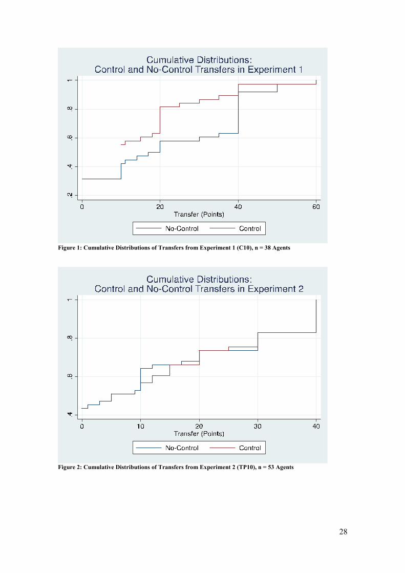
[Figures 1 and 2 here]

12

5.1 The replication

Result 1: We observe significant hidden costs of control in Experiment 1.

In Experiment 1, we observe significant costs of control. First, consistent with F&K, we

present the cumulative distributions of the players’ transfers where equal transfers were

given the same probability weight. The no-control distribution is depicted in blue and

the control distribution is depicted in red. Were there no hidden costs of control then the

two distributions would coincide for all x ≥ x. On the contrary, the distributions differ.

For each value of xx there are more agents in the no-control condition who choose at

least that value of x than in the control condition. For instance, more than 40% of agents

choose 20x when they are not controlled. In contrast, less than 20% of agents choose

20x if controlled and, hence, forced to choose at least 10. A greater mass of x-choices

is centered at 10x if the principal restricts agent's actions.

Second, examining the distributions in greater detail, we follow F&K and Ziegelmeyer

et al (2012) by constructing a modified distribution for the no-control condition, such

that all xx in the no-control condition are set equal to .ݔ In experiment 1, we reject

the null hypothesis that the modified distribution from the no-control setting and the

distribution from the control setting have the same medians (Wilcoxon signed-rank test

for paired observations, z = -3.385, p=0.007).

We can therefore confirm the results from F&K and from Ziegelmeyer et al, that there

are significant costs of control in dyadic principal-agent relationships. But, as

Ziegelmeyer et al argue, we should be particularly concerned about hidden costs of

control if they are economically substantial and large enough to undermine the use of

incentives in relevant settings. That is, do the costs of control outweigh the benefits of

control? Consistent with Ziegelmeyer et al (2012), but inconsistent with F&K, in our

replication we find that the costs of control do not outweigh the benefits.

Result 2: Hidden Costs do not outweigh benefits of control in Experiment 1

Table 2 presents the agents’ transfers as a function of the principals’ decisions in the

two experiments. The first row presents the average transfers for each of the control

(column 1) and no-control (column 2) conditions in the experiments and the difference

13

between the two (column 3). The second row for each experiment reports the standard

deviation, followed by the 1st quartile, the median, and the 3rd quartile. For the

difference between xNC and xC, the 95% bootstrap confidence interval is reported in the

second row based on 105 replications.5

[Tables 2 and 3 About Here]

In Experiment 1, the mean number of ECUs is higher in the no-control condition than in

the control condition. Furthermore, though the median number of ECUs initially may

appear larger in the no-control condition than in the control condition, the median is not

significantly larger (Wilcoxon signed-rank z=-1.001, p=0.32). The 95% bootstrap

confidence interval of the difference xNC – xC includes zero suggesting that the hidden

costs of control do not significantly outweigh the benefits of control. The sign of the

difference in principal's average profits between control and no-control conditions

remains undetermined.

5.2 The third-party treatment (Experiment 2)

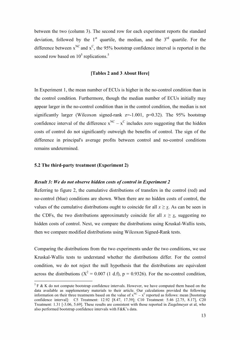
Result 3: We do not observe hidden costs of control in Experiment 2

Referring to figure 2, the cumulative distributions of transfers in the control (red) and

no-control (blue) conditions are shown. When there are no hidden costs of control, the

values of the cumulative distributions ought to coincide for all x ≥ x. As can be seen in

the CDFs, the two distributions approximately coincide for all x ≥ x, suggesting no

hidden costs of control. Next, we compare the distributions using Kruskal-Wallis tests,

then we compare modified distributions using Wilcoxon Signed-Rank tests.

Comparing the distributions from the two experiments under the two conditions, we use

Kruskal-Wallis tests to understand whether the distributions differ. For the control

condition, we do not reject the null hypothesis that the distributions are equivalent

across the distributions (Χ2 = 0.007 (1 d.f), p = 0.9326). For the no-control condition,

5 F & K do not compute bootstrap confidence intervals. However, we have computed them based on thedata available as supplementary materials to their article. Our calculations provided the followinginformation on their three treatments based on the value of xNC – xC reported as follows: mean [bootstrapconfidence interval]: C5 Treatment: 12.92 [8.47, 17.39]; C10 Treatment: 5.46 [2.75, 8.17], C20Treatment: 1.31 [-3.06, 5.69]. These results are consistent with those reported in Ziegelmeyer et al, whoalso performed bootstrap confidence intervals with F&K’s data.

14

we reject the null hypothesis that the distributions are equivalent (Χ2 = 4.048 (1 d.f.) p =

0.0442).

Using the modified distribution for the no-control condition, such that all xx in the

no-control condition are set equal to .ݔ In experiment 2, we do not reject the null

hypothesis that the modified distribution from the no-control setting and the distribution

from the control setting have the same medians (Wilcoxon signed-rank test for paired

observations, z = 0.840, p=0.4007).

In contrast with F&K and Ziegelmayer et al, the result above suggests that when a third-

party exerts control instead of a principal, then significant costs of control do not

emerge. To understand whether control by a third-party on behalf of a principal might

result in benefits of control outweighing costs of control, we go into greater detail in

examining the behavior of agents in the third-party treatment.

Result 4: The benefits of control outweigh the costs of control in Experiment 2

The properties of Table 2 were discussed in detail in Result 2. In Experiment 2, the

mean number of ECUs is lower in the no-control condition than in the control condition.

The median number of ECUs transferred by the agent is significantly lower in the no-

control condition than in the control condition (Wilcoxon signed-rank z = 5.030,

p<0.001). The mean difference xNC – xC is negative and the bootstrap confidence

interval around the mean excludes zero. Referring to Table 3, the expected payoff to a

principal when a third party exerts control is greater than the expected payoff to a

principal when a third party does not exert control. This suggests that hidden costs of

control are eliminated when a third a third party rather than a principal exerts control.

As a consequence of using the strategy method to elicit the agents’ choices, we can

observe whether the players are heterogeneous in their types by gaining greater

understanding of whether players react positively, neutrally or negatively to control.

[Table 3 About Here]

15

5.3 Comparing C10 (experiment 1) and TP10 (experiment 2)

Result 5: Players react to control heterogeneously in both experiments; far fewer

players react negatively to control in Experiment 2

Table 3 summarizes the agent’s responses to control in each of the experiments. In

experiment 1, our result where 42.10% of agents react negatively (control aversely) are

consistent with Ziegelmeyer et al who found a proportion of agents who react

negatively in the range 40.62% to 45.45%. This result contrasts with F&K who found

that a majority of agents (56.94%) reacted negatively. The proportion of agents who

react positively to control (36.84%) is consistent with Ziegelmeyer et al (39.40% to

60.00% in various C10 experiments) rather than relative to F&K (25% in C10). In

experiment 1, the minority of subjects responds neutrally to control (21.05%). Control-

averse agents transfer approximately the same in experiment 1 as they do in C10 in

F&K and in Experiment 1 by Ziegelmeyer et al, that is, control-averse agents transfer

roughly double in the no-control condition relative to the control condition. Agents who

respond neutrally to control transfer (25.13) within the range of what they did in F&K

(22.3)) and Ziegelmeyer et al (range: 14.8 to 30.71).

In experiment 2, on the other hand, few agents respond negatively to control (3.77%), a

large proportion responds neutrally to control (41.51%) and the majority of agents

respond positively to control (54.72%). These results are consistent with the preceding

results examining the distributions of transfers and the difference between control and

no-control transfers in Experiment 2. Fisher’s exact tests contrasting differences in

proportions between the treatments suggest the following: we reject the null hypothesis

that the proportions are the same for neutral responses to control (p=0.045) and negative

responses to control (p<0.001), but we cannot reject the null that the proportions are the

same for positive responses to control (p=0.136).6

[Tables 4 and 5 About Here]

6 Comparisons of Fisher’s exact tests between our proportions and those in Ziegelmeyer et al (2012) andF&K are available upon request.

16

We interrogate these results further using regression analysis, the results of which are

presented in Tables 4 and 5. The data are pooled from the data from the C10

experiments in F&K and Ziegelmeyer et al (2012) with permission from the authors.

Column 1 presents an OLS regression where the independent variable is the difference

between the agent’s transfer in the no-control condition and their transfer in the control

condition: xNC – xC. Standard errors are corrected using the MacKinnon & White (1985)

residual-variance estimator HC3. Columns 2 through 4 are logistic regressions where

the agent is classified as having either a positive, neutral or negative reaction to control

depending on whether the differences between their transfers in the no-control vs.

control conditions were negative, zero or positive (i.e. xNC – xC < 0 for positive response

to control, xNC – xC = 0 for control-neutral and xNC – xC > 0 for negative response to

control). In each regression, the explanatory variables are the dummies for each of the

C10 experiments, though the very first explanatory variable is a dummy variable for our

TP10 experiment. For the logistic regressions, the marginal effects are reported. In the

bottom half of the table, p-values from Wald tests for the equivalence of the coefficients

are reported for our TP10 experiment against each of the C10 experiments from F&K

and ZSP’s experiments 1 through 5. In all cases, linear probability models and

heteroskedastic probit models have also been specified and the results are consistent

across all the models.

First, were there no differences in positive (neutral, negative) responses to control

across our experiment 1 and experiment 2, then the treatment dummy for TP10 would

be small and not statistically significantly different from zero. Second, if the results

from our replication are consistent with preceding C10 experiments, then the other

experimental dummies for other C10 experiments ought not to be statistically

significantly different from zero.

In regression 1, the TP10 dummy is negative, large and statistically significant. The

coefficient suggests that an average agent in experiment 2 has a difference xNC – xC =

-5.14 in contrast with a difference of 3.76 in the baseline experiment 1 (as shown by the

constant). This result is reinforced by the outcomes of regressions 2 and 3 where

subjects are significantly more likely to respond positively to control (column 2) or be

control-neutral in experiment 2 than in experiment 1 (columns 3) and significantly less

likely to respond negatively to control (column 4). These results are borne out in the

17

Wald tests, where the coefficient on the TP10 treatment dummy is shown consistently

not to equal the F&K dummy’s coefficient and, for negative responses to control

specifically, the TP10 treatment is shown to be consistently statistically significantly

different to the other coefficients.

As a further robustness check for the result on the third-party treatment, we use a

multinomial logit model where the three categories are Positive, Neutral and Negative.

The marginal effects of the model are reported in Table 5. The results are consistent

with the logit regressions, suggesting that subjects in the TP10 treatments were

significantly less likely to respond negatively to control and significantly more likely to

respond neutrally to control.

The results from Tables 4 and 5 suggest that, though hidden costs of control emerge in

the dyadic principal-agent interaction, the addition of the third party significantly

decreases the likelihood that hidden costs will emerge or that they will outweigh the

benefits of control. As principal's signal of distrust cannot play any role under TP10, the

fact that the fraction of control averse agents dramatically vanishes in this treatment

suggests reciprocity rather than preferences for autonomy to be the main behavioral

mechanisms underlying control aversion.

[Tables 6, 7 and 8 About Here]

For robustness across the treatments, we confirm that the samples are not statistically

significantly different with respect to the subjects’ reported attitudes using the GCOS

The means and standard deviations for the subjects’ reported preference for each scale

in each of the experiments are reported in Table 6. The means in the scales are not

statistically significantly different across the experiments, as shown by the t-statistics of

the difference between their values by treatment.7 Standardized values for each scale

were incorporated into the regressions replicating those in Tables 4 and 5. The

regressions report results for our data only as F&K or Ziegelmeyer et al did not gather

the GCOS attitudes. These results are reported in Tables 7 and 8.

7 Regarding the internal consistency of each of the three subscales, the Cronbach’s α nonstandarized values were autonomy, 0.8469; impersonal, 0.7394; and control, 0.6218.

18

As with Table 4, in Table 7 the first column represents an OLS regression with the

difference xNC – xC as the dependent variable. In specifications 2 through 4, the

dependent variable was a dummy variable indicating whether a subject displayed a

positive (neutral or negative) response to control. The standardized control variable was

statistically significant and negative in the xNC – xC regression (column 1), the positive

response to control logit regression (column 2) and the negative response to control

logit regression (column 3). A one standard deviation increase in the standardized

control GCOS corresponds with a decrease in the probability a subject will respond

negatively to control by 6.4%, an increase in the probability the subject will respond

positive by 16.6% and an increase in the difference between xNC and xC by -2.17 ECUs.

These results are borne out by the multinomial logit regressions in Table 8, which show

that the third-party treatment dummy significantly decreases the probability of a

negative response to control and significantly increases the probability of a neutral or

positive response to control. The standardized control scale is also significant once

again for the negative response to control and positive response to control. Other things

equal, one standard deviation increase in the control scale corresponds with a decrease

in the probability of a negative response by about 7% and an increase in the probability

of a positive response by about 16.3%. This result is consistent with the psychological

interpretation given to the controlled orientation, which assesses the extent to which a

person is oriented toward being controlled by rewards and the directives of others (Deci

and Ryan, 1985). In line with the idea that control-averse reactions in this setting are

mainly driven by reciprocity rather than individuals' preferences for self-determination,

the standardized autonomy GCOS does not show significant correlation neither with the

probability the subject will respond negatively to control nor with the difference

between xNC and xC.

Result 6: The proportions of principals (in experiment 1) and third parties (in

experiment 2) who exert control are not significantly different

In experiment 1, the 63.15%. of principals exert control. In experiment 2, 77.34%. of

third parties exert control. A 95% bootstrap confidence interval of the difference in the

proportions contains zero (-0.051 < pC10 – pTP10 < 0.335). These results are consistent

with Ziegelmeyer et al who found proportions of control ranging from 57% to 83% in

their C10 experiments. Both our results and Ziegelmeyer et al’s results suggest

19

significantly higher proportions of control than F&K who found 29% of principals

choosing control in their C10 experiment.

6. Conclusion

Our third-party treatment offers an opportunity to understand the behavioral motives

underlying control averse reactions. First, in the presence of a third party rather than a

principal who exerts control, we did not find significant hidden costs of control. Second,

when the third party exerts control it results in greater expected profits for the principal

than when the third party does not control. But, this should not be viewed as a form of

delegation or the third party acting on behalf of (or at the orders of) the principal, rather

it suggests that the agents respond reciprocally toward the principals in C10, but do not

have that incentive in TP10. Third, substantial heterogeneity remains among subjects in

the third-party experiment: subjects who respond neutrally to control consistently

transfer a substantial proportion of their endowment to the principal, the puzzle though

surrounds the ways in which types change given the decision context in the two

treatments, suggesting that the subjects’ choices may be endogenous (Bowles, 1998).

Social preferences, which we employ in our model, may be more or less active

depending on the decision context (Carpenter & Seki, 2011). Correspondingly, the

results from our experiments suggest a parameterization of our model in which

reciprocity, rather than preferences for autonomy, strongly affects the decision-making

process in principal-agent decisions. Control-averse agents reciprocate trust by the

principal with higher effort and they reciprocate distrust by the principal with lower

effort. Control-neutral agents do not alter their behavior and the small subset of control-

loving agents exert greater effort when controlled than when not controlled by a

principal. The behavior of the agents appears to be consistent with models of reciprocity

that include considerations for the intentions of the principal, rather than any agent

exerting control (Falk & Fischbacher, 2006; Von Siemens, 2013).

That reciprocity, rather than preferences for autonomy, drives the behavior of agents in

these interactions is the main contribution of this paper. In demonstrating this result, we

contribute to a wider literature engaged with understanding the employment relation,

hierarchy, coercion and the exercise of power (Fehr et al, 2013; Nikiforakis et al, 2014).

20

Of course, the limited role played by autonomy preferences in our experiment should

not be interpreted as a general claim about the irrelevance of this type of preferences,

which have been proven to be very salient in other settings (see, for instance, Bartling et

al, 2014). Future work should examine the extent to which preferences evolve over

repeated principal-agent interactions and interactions in which the hierarchical

relationship between subjects in the experiments may be made clearer either through

framing or through changes in experimental design where the loci of control for the

principal are more diverse. This may permit researchers to examine more

unambiguously the extent to which autonomy and reciprocity may complement or

substitute for each other in principal-agent interactions and, therefore, the extent to

which extrinsic benefits may crowd out or in the effort of agents.

Acknowledgements

The experiments were funded by the Santa Fe Institute Cowan Fund. Additional support

was provided by the Smith College Committee on Faculty Compensation and

Development.

21

References:

Acemoglu, D. and F. Newman, Andrew, 2002. "The labor market and corporate structure," EuropeanEconomic Review, Elsevier, vol. 46(10), pages 1733-1756, December.

Alchian, Armen A & Demsetz, Harold, 1972. "Production , Information Costs, and EconomicOrganization," American Economic Review, American Economic Association, vol. 62(5), pages 777-95, December.

Bartling, B., Ernst Fehr, Klaus M. Schmidt, 2013. "Discretion, Productivity, and WorkSatisfaction," Journal of Institutional and Theoretical Economics (JITE), Mohr Siebeck, Tübingen,vol. 169(1), pages 4-22, March.

Bartling B., Ernst Fehr & Holger Herz, 2014. "The Intrinsic Value of Decision Rights," Econometrica,Econometric Society, vol. 82, pages 2005-2039, November.

Batson, C. D., Coke, J. S., Jasnoski, M. L., and Hanson, M. (1978), “Buying kindness: effect of anextrinsic incentive for helping on perceived altruism”, Personality and Social Psychology Bulletin,4:86–91.

Ben-Ner, A. (2013), “Preferences and Organization Structure: Towards Behavioral Economics Micro-Foundations of Organizational Analysis", Journal of Socio-Economics, 46 (2013) 87-96.

Bowles, S. and S. Polania (2012), “Economic Incentives and Social Preferences: Substitutes orComplements?”, Journal of Economic Literature, American Economic Association, vol. 50(2),pages 368-425, June.

Charness, G., Cobo-Reyes, R., Jinénez, N., Lacomba, J. A, Lagos, F. (2012), “The Hidden Advantage ofDelegation: Pareto-improvements in a Gift-exchange Game”, American Economic Review, AmericanEconomic Association, vol. 102(5), pages 2358-79, August.

Chirkov, V. I., R. M. Ryan and K.M. Sheldon (2010) “Human Autonomy in Cross-Cultural Context”,Perspectives on the Psychology of Agency, Freedom, and Well-Being. Cross-Cultural Advancementsin Positive Psychology, Vol 1. Springer.

Deci, E. L. and R. M. Ryan (1985), Intrinsic Motivation and Self-Determination in Human Behavior,New York: Plenum Press.

Fabes, R. A., Fultz, J., Eisenberg, N., May-Plumlee, T., and Christopher, F. S. (1989), “Effects of rewardson children’s prosocial motivation: a socialization study”, Developmental Psychology, 25:509–515.

Fafchamps, M. and Måns Söderbom, 2006. "Wages and Labor Management in AfricanManufacturing," Journal of Human Resources, University of Wisconsin Press, vol. 41(2).

Falk, A. and Fischbacher, U., 2006. “A theory of reciprocity.” Games and Economic Behavior 54, 293–315.

Falk, A. and M. Kosfeld (2006), “The Hidden Costs of Control”, American Economic Review, 96(5):1611-1630.

Fehr, Ernest, and Simon Gächter. 2000. “Fairness and Retaliation: The Economics of Reciprocity.”Journal of Economic Perspectives 14(3): 159–181.

Fehr, Ernst, Holger Herz, and Tom Wilkening. 2013. "The Lure of Authority: Motivation and IncentiveEffects of Power." American Economic Review, 103(4): 1325-59.

Fischbacher, U., (2007), “z-Tree: Zurich toolbox for ready-made economic experiments”, ExperimentalEconomics, 10(2): 171-178

Frey, B. S. and R. Jegen (2000), “Motivation Crowding Theory: A Survey of Empirical Evidence”,CESifo Working Paper No. 245

Gagné, M. (2003), “The role of autonomy support and autonomy orientation in the engagement ofprosocial behavior”, Motivation and Emotion, 27:199–223.

Gagné, M. and E.L. Deci (2005), “Self-determination Theory and Work Motivation”, Journal ofOrganizational Behavior, 26:331-362

Greiner, B., (2004), “An Online Recruitment System for Economic Experiments,” In: Kurt Kremer,Volker Macho (Hrsg.): Forschung und wissenschaftliches Rechnen. GWDG Bericht 63. Ges. für

22

Wiss. Datenverarbeitung, Göttingen, 79-93.

Greene-Demers, I., Pelletier, L. G., and Ménard, S. (1997), “The impact of behavioral difficult on thesaliency of the association between self-determined motivation and environmental behaviors”,Canadian Journal of Behavioural Science, 29:157–166.

Jayadev, Arjun and Bowles, Samuel, 2006. "Guard labor," Journal of Development Economics, Elsevier,vol. 79(2), 328-348, April.

Kunda, Z., and Schwartz, S. H. (1983), “Undermining intrinsic moral motivation: external reward andself-presentation”, Journal of Personality and Social Psychology, 45:763–771

Owens Jr. D., Zachary Grossman Jr., and Ryan Fackler Jr., 2014. "The Control Premium: A Preferencefor Payoff Autonomy," American Economic Journal: Microeconomics, American EconomicAssociation, vol. 6(4), 138-61, November.

Nikiforakis, Nikos, Oechssler, Jörg and Shah, Anwar, 2014. "Hierarchy, coercion, and exploitation: Anexperimental analysis," Journal of Economic Behavior & Organization, Elsevier, vol. 97(C), 155-168.

Pelletier, L. G., Tuson, K. M., Greene-Demers, I., Noels, K., and Beaton, A. M. (1998), “Why are youdoing things for the environment? The Motivation Toward the Environmental Scale (MTES)”,Journal of Applied Social Psychology, 28:437–468.

Ryan, R.M. and Deci, E. L. (2000), “Self-Determination Theory and the Facilitation of IntrinsicMotivation, Social Development, and Well-Being”, American Psychologist, 55(1):68-78

Schnedler, W. and Radovan Vadovic, 2011. "Legitimacy of Control," Journal of Economics &Management Strategy, Wiley Blackwell, vol. 20(4), 985-1009, December.

Sobus, M. S. (1995), “Mandating community service: psychological implications of requiring prosocialbehaviour”, Law and Psychology Review, 19:153–182.

Upton, W. E. III. (1974), “Altruism, attribution and intrinsic motivation in the recruitment of blooddonors”, in Selected readings in donor recruitment (Vol. 2, pp. 7–38). Washington, DC: AmericanNational Red Cross.

Von Siemens, F. 2013, “Intention-based reciprocity and the hidden costs of control.” Journal of EconomicBehavior and Organization, 92, 55-56

Ziegelmeyer, A, Schmelz, K., and. Ploner, M., (2012), “Hidden Costs of Control: Four Repetitions and an

Extension”, Experimental Economics, Springer, vol. 15(2), 323-340, June.

23

Table 1 Experimental Conditions

Notes: Earnings are stated in dollars net of the show-up fee with standard deviations in parentheses. Third

parties were simply paid the show-up fee and therefore would have no payoff net of the show-up fee.

Experiment 1 Number of Sessions 4

Number of Subjects 76

Gender (% Female) 44%*

Average age 21.02 (2.34)*

Agents’ Average Earnings 20.14 (2.9486)

Principals’ Average Earnings 7.73 (5.8972)

Experiment 2 Number of Sessions 7

Number of Subjects 159

Gender (% Female) 54%*

Average age 20.75 (4.2)*

Agents’ Average Earnings 20.66 (2.5930)

Principals’ Average Earnings 6.69 (5.1860)

Third Party’s Average Earnings 0

24

Table 2: Agents' Transfers as a function of the principal's decision

Control Condition No-control condition xNC – xC

Experiment 117.47

(11.76, 10, 10, 20)

21.24

(19.03, 0, 18.5, 40)

3.76

[-.71, 8.24]

Experiment 218

(11.62, 10, 10, 25)

12.87

(15.50, 0, 5, 30)

-5.13

[-6.53, -3.73]

Table 3: Agents' behavioral reactions to control, n = 38 in Experiment 1 and n = 53 in Experiment 2; ExpectedPayoff to P is calculated as an weighted average where the mean transfer in each condition is multiplied by theproportion of each type

Positive Neutral Negative ExpectedPayoff to P

Experiment 1 Relative Share 36.84% 21.05% 42.11%

Mean ControlTransfer

11.64(4.40)

25.13(19.16)

18.75(9.40)

17.38

Mean no-controlTransfer

1.93(5.09)

25.13(19.16)

36.19(10.23)

21.22

Experiment 2 Relative Share 54.72% 41.51% 3.77%

Mean ControlTransfer

10.76(2.21)

27.36(12.67)

20(7.07)

18.05

Mean no-controlTransfer

1.14(2.70)

27.36(12.67)

23.5(9.19)

16.07

25

Table 4: Regressions on Differences between transfers and reactions to control

(1) (2) (3) (4)

VARIABLES xNC - xC Positive Neutral Negative

D: = 1 for our TP10 -8.895*** 0.178* 0.203* -0.383***(2.448) (0.107) (0.111) (0.0448)

D: = 1 for FK Exp 1.695 -0.126 -0.0331 0.136(2.729) (0.0914) (0.0844) (0.0961)

D: = 1 for ZSP Exp 1 -4.591 0.218* -0.0808 -0.124(3.351) (0.123) (0.0924) (0.0886)

D: = 1 for ZSP Exp 2 -6.730** 0.231* -0.0481 -0.160**(2.870) (0.121) (0.0984) (0.0814)

D: = 1 for ZSP Exp 3 -1.612 0.0258 -0.0654 0.0299(3.053) (0.118) (0.0926) (0.108)

D: = 1 for ZSP Exp 4 3.447 -0.170* 0.124 0.0313(3.436) (0.0903) (0.104) (0.0944)

D: = 1 for ZSP Exp 5 -3.585 0.0605 0.0418 -0.0859(3.056) (0.125) (0.116) (0.0960)

Constant 3.763 - - -(2.337)

Observations 340 340 340 340R-squared 0.107 - - -Log Likelihood - -212.4 -180.7 -196.6TP10 Dummy = FK Dummy p < 0.01 p < 0.01 P < 0.01 p < 0.01TP10 Dummy = ZSP E1 Dummy p = 0.09 p = 0.734 p = 0.0142 p < 0.01TP10 Dummy = ZSP E2 Dummy p = 0.234 p = 0.642 p = 0.0249 p < 0.01TP10 Dummy = ZSP E3 Dummy p < 0.01 p = 0.169 p = 0.0139 p < 0.01TP10 Dummy = ZSP E4 Dummy p < 0.01 p < 0.01 p = 0.377 p < 0.01TP10 Dummy = ZSP E5 Dummy p = 0.0118 p = 0.312 p = 0.145 p < 0.01

Notes: Standard errors in parentheses, *** p<0.01, ** p<0.05, * p<0.1. Data from Ziegelmeyer et al andF&K used with permission of the authors.

26

Table 5: Pooled Data Multinomial Logit Regressions of Agents’ Responses to Control (n=340)

(1) (2) (3)

VARIABLES Positive Neutral Negative

D: = 1 for our Exp 2 (TP10) 0.179 0.212* -0.390***(0.118) (0.117) (0.0457)

D: = 1 for FK Exp -0.118 -0.0191 0.137(0.0977) (0.0939) (0.0968)

D: = 1 for ZSP Exp 1 0.218* -0.0974 -0.121(0.121) (0.0990) (0.0918)

D: = 1 for ZSP Exp 2 0.223* -0.0638 -0.159*(0.121) (0.105) (0.0842)

D: = 1 for ZSP Exp 3 0.0381 -0.0709 0.0328(0.122) (0.102) (0.109)

D: = 1 for ZSP Exp 4 -0.185* 0.149 0.0361(0.0965) (0.111) (0.0970)

D: = 1 for ZSP Exp 5 0.0501 0.0372 -0.0873(0.129) (0.123) (0.0978)

Observations 340 340 340Notes: Robust standard errors in parentheses, *** p<0.01, ** p<0.05, * p<0.1

Table 6: Summary of General Causality Orientation Scale Indexes

Experiment 1 Experiment 2 t-stat/

(Mann-Whitney z)

GCOS: Autonomy Scale 71.80 70.52 1.150075

(6.23) (8.74) (0.495)

GCOS: Impersonal Scale 43.42 45.41 -1.349482

(10.83) (10.43) (-1.487)

GCOS: Control Scale 58.43 58.93 -.4760745

(6.97) (7.71) (-0.758)

Observations 76 159 235

27

Table 7: Regressions from our Subject Pool Only (n=91) with GCOS variables

(1) (2) (3) (4)

VARIABLES xNC - xC Positive Neutral Negative

D: TP10 Treatment = 1 -8.864*** 0.193* 0.216** -0.403***(2.444) (0.111) (0.0961) (0.0830)

Standardized AutonomyScale

1.198 -0.105 0.0800 0.00241

(1.363) (0.0676) (0.0615) (0.0320)Standardized ImpersonalScale

-0.611 -0.0465 0.0343 0.0149

(1.259) (0.0644) (0.0533) (0.0294)Standardized Control Scale -2.177* 0.166** -0.0675 -0.0641**

(1.303) (0.0701) (0.0514) (0.0299)Constant 3.551 - - -

(2.324)

Observations 91 91 91 91R-squared 0.212 - - -Log Likelihood - -57.47 -54.16 -32.22

Notes: Standard errors in parentheses.*** p<0.01, ** p<0.05, * p<0.1

Table 8: Multinomial Logit Regressions of Agents’ Responses to Control with GCOS variables (n=91)

(1) (2) (3)VARIABLES Positive Neutral Negative

D: TP10 Treatment = 1 0.202* 0.209** -0.411***(0.113) (0.0972) (0.0846)

Standardized Autonomy Scale -0.105 0.102 0.00292(0.0700) (0.0672) (0.0330)

Standardized Impersonal Scale -0.0492 0.0328 0.0163(0.0646) (0.0585) (0.0314)

Standardized Control Scale 0.163** -0.0926 -0.0699**(0.0715) (0.0623) (0.0336)

Observations 91 91 91Log Likelihood -78.85 -78.85 -78.85

Notes: Robust standard errors in parentheses. *** p<0.01, ** p<0.05, * p<0.1

28

Figure 1: Cumulative Distributions of Transfers from Experiment 1 (C10), n = 38 Agents

Figure 2: Cumulative Distributions of Transfers from Experiment 2 (TP10), n = 53 Agents

29

Figure 3: Kernel Density Estimates of the General Causality Orientation Scale Surveys, n=91 agents