swimlessons@thinkorswim.com

ThinkScript In this document you will find information on the thinkScript language. Using the price data in conjunction with functions, variables, and operators allows you to build up a whole system of your own studies and strategies. Being integrated into various features of the thinkorswim platform, thinkScript can be used for issuing alerts, scanning the market, customizing quotes, and submitting orders automatically. The Getting Started section will help you get acquainted with thinkScript and start writing your first scripts. The Reference section provides you with information on constants, data types, declarations, functions, operators, and reserved words, explaining how to use them when writing scripts with thinkScript. The thinkScript Integration section contains articles demonstrating usage of thinkScript integration features.

ThinkScript

• Getting Started 4 o Writing Your First Script 5 o Advanced Topics 19

• Reference 35

o Reserved Words 37 o Declarations 68 o Functions 78 o Constants 256 o Data Types 312 o Operators 315

• thinkScript Integration 324

o Conditional Orders 325 o Custom Quotes 327 o Study Alerts 329 o Study Filters 331

Getting Started This section contains tutorials that will help you get acquainted with thinkscript and start writing your first scripts.

• Getting Started

o Writing Your First Script 5 Defining Plots 5 Defining Variables 6

Def Variables 7 Rec Variables 8 Rec Enumerations 10

Using Functions 12 Formatting Plots 13 Adjusting Parameters Using Inputs 16 Accessing Data 17 Using Strategies 18

o Advanced Topics 19 Concatenating Strings 20 Creating Local Alerts 22 Referencing Data 23

Referencing Secondary Aggregation 24 Referencing Historical Data 27 Referencing Other Price Type Data 28 Referencing Other Studies 29 Referencing Other Symbol's Data 31 Past Offset 32

Using Profiles 34

o Writing Your First Script This section contains tutorials that will help you write your first thinkscript study or strategy. o Defining Plots In order to visualize data calculated by studies, you can use plots. plot SMA = Average(close, 10); This example script plots a 10 period simple moving average of the Close price. When working with charts, you might need to use several plots. The following example script plots two moving averages of the Close price: the 10 period simple moving average and the 10 period exponential moving average. plot SMA = Average(close, 10); plot EMA = ExpAverage(close, 10); In case you only need one plot and don't need any inputs or intermediate variables, you can use short syntax: Average(close, 10) This example script plots a 10 period simple moving average of the Close price. Note that if you use the short syntax, your script must be a single expression. See also: Reserved Words: plot; Formatting Plots.

o Defining Variables Thinkscript provides different types of variables to work with. This section contains tutorials that will teach you to work with these variables.

• Def Variables 7 • Rec Variables 8 • Rec Enumerations 10

Def Variables The def reserved word defines a variable you'd like to work with. For example, you can define something called MyClosingPrice as: def MyClosingPrice = Close; By using the def reserved word, you can create a variable that can be used in another formula in the study. This let's you construct complex formulas from simpler elements. For example, if you want to divide the range of a stock price by the closing price, you can create a variable for the range: def range = high - low; then create another variable: def percentrange = range / close; Doing it this way lets you re-use variables and gives you the power to combine complex variables in your formulas more easily. By defining a variable such as: def SMA = average(close, 20); You can use that variable sma in your code as part of another calculation. For instance, plot doubleSMA = SMA * 2; plot tripleSMA = SMA * 3;

Rec Variables Rec variables are used to store floating point data. Values of such variables are calculated one after another in a chronological manner. When you assign a value to the rec variable you can use its values calculated for the previous bars. If you use data related to the period prior to the beginning of the time period then the rec variable is also calculated for the period. Before the calculation, the rec value is set to 0 for all moments of time. rec x = x[1] + (random() - 0.5); plot RandomWalk = x; Shows random walk. input drop = 5.0; rec x = if close >= (1 - drop / 100) * x[1] then Max(close, x[1]) else close; plot MaxPrice = x; plot Drops = close < (1 - drop / 100) * x[1]; Drops.SetPaintingStrategy(PaintingStrategy.BOOLEAN_ ARROW_UP); In this example the rec variable holds the maximum close value starting from the moment of the last fall. When the price reduces on the defined percentage from the maximum, the maximum value resets. declare lower; rec x = x[1] + x[10] * 0 + 1; plot line = x; This script takes data for the previous 10 bars. Thus, the rec calculation starts 10 bars prior to the beginning of the time period. As a result, the first drawn value of the plot line is 11.

declare lower; rec x = x[1] + 1; plot line = x; Similarly, in this example the calculation starts 1 bar prior to the beginning of the time period. This is why the first visible value equals 2. rec x = x[-1] + close; plot data = x; This script refers to data that has not been calculated yet. Thus, it will produce an error. This applies to any calculation of a rec variable which attempts to use its current or future value.

Rec Enumerations You can use rec enumeration constructions to create something like a usual rec in thinkScript but with limited possible values. Note that rec enumerations can contain only string values. rec a = {default neutral, up, down}; a = if (close == close[1]) then a.neutral else if (close > close[1]) then a.up else a.down; plot q; switch(a) { case up: q = low; case down: q = high; case neutral: q = close; } The first line of the script is a declaration of a rec enumeration a having neutral, up, and down values. The default keyword indicates the default value of the rec enumeration. If you do not assign a value to a, it will always be equal to its default neutral value . rec a = {default neutral, up, down}; The second line of this script is the assignment statement. Note that a rec enumeration can have only one assignment statement. a = if (close == close[1]) then a.neutral else if (close > close[1]) then a.up else a.down; The third line is just a plot declaration. plot q;

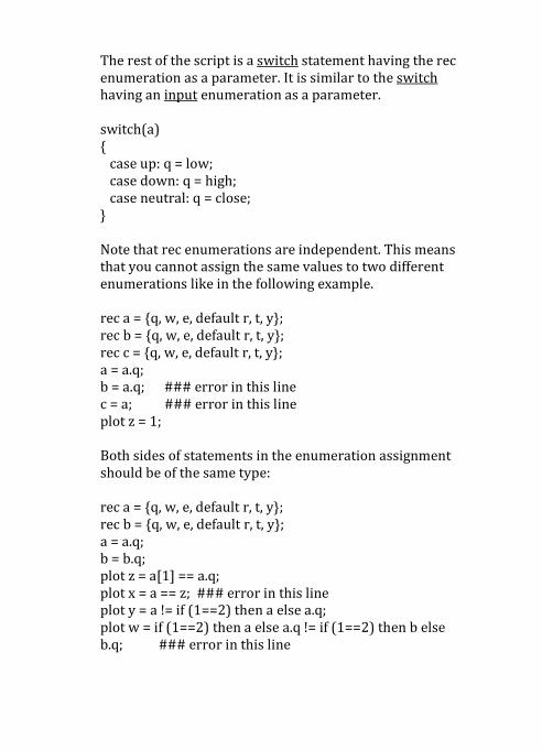
The rest of the script is a switch statement having the rec enumeration as a parameter. It is similar to the switch having an input enumeration as a parameter. switch(a) { case up: q = low; case down: q = high; case neutral: q = close; } Note that rec enumerations are independent. This means that you cannot assign the same values to two different enumerations like in the following example. rec a = {q, w, e, default r, t, y}; rec b = {q, w, e, default r, t, y}; rec c = {q, w, e, default r, t, y}; a = a.q; b = a.q; ### error in this line c = a; ### error in this line plot z = 1; Both sides of statements in the enumeration assignment should be of the same type: rec a = {q, w, e, default r, t, y}; rec b = {q, w, e, default r, t, y}; a = a.q; b = b.q; plot z = a[1] == a.q; plot x = a == z; ### error in this line plot y = a != if (1==2) then a else a.q; plot w = if (1==2) then a else a.q != if (1==2) then b else b.q; ### error in this line

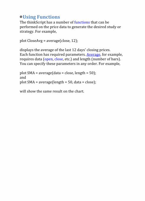
o Using Functions The thinkScript has a number of functions that can be performed on the price data to generate the desired study or strategy. For example, plot CloseAvg = average(close, 12); displays the average of the last 12 days' closing prices. Each function has required parameters. Average, for example, requires data (open, close, etc.) and length (number of bars). You can specify these parameters in any order. For example, plot SMA = average(data = close, length = 50); and plot SMA = average(length = 50, data = close); will show the same result on the chart.

o Formatting Plots The thinkscript contains lots of Look & Feel functions used to format a plot: define a plot type (histogram, line, point, etc.), color, line style and other. Here is the common syntax for that: <plot_name>.<L&F_function_name>(L&F_function_parameters) In order to specify a plot type, use the SetPaintingStrategy function. Note that you can use this function only in combination with Painting Strategy constants. In case this function is not called, then the Line Painting Strategy is used. Note that plots from the following "signal" painting strategy category are drawn above plots from the common category:

• PaintingStrategy.ARROW_DOWN • PaintingStrategy.ARROW_UP • PaintingStrategy.POINTS • PaintingStrategy.BOOLEAN_ARROW_DOWN • PaintingStrategy.BOOLEAN_ARROW_UP • PaintingStrategy.BOOLEAN_POINTS • PaintingStrategy.DASHES • PaintingStrategy.HORIZONTAL • PaintingStrategy.SQUARES • PaintingStrategy.TRIANGLES

Plots defined first are drawn above plots defined later in the same painting strategy category. declare lower; plot AvgVolume = Average(volume, 7); AvgVolume.SetPaintingStrategy(PaintingStrategy.HISTOGRAM);

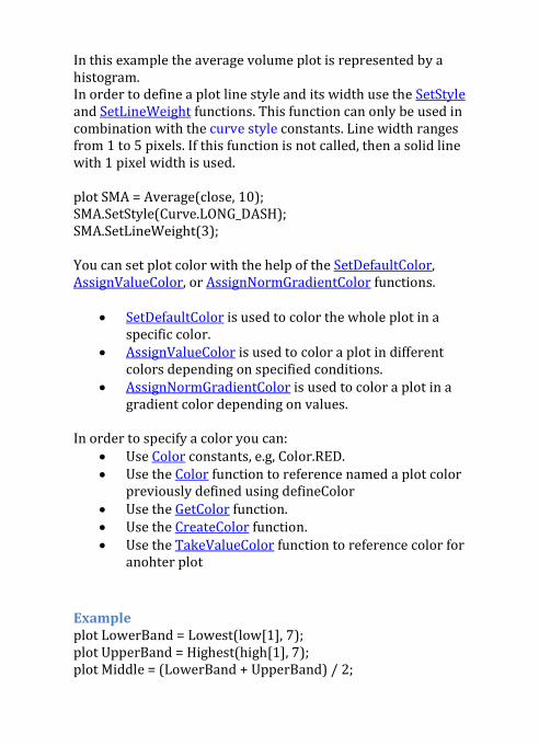
In this example the average volume plot is represented by a histogram. In order to define a plot line style and its width use the SetStyle and SetLineWeight functions. This function can only be used in combination with the curve style constants. Line width ranges from 1 to 5 pixels. If this function is not called, then a solid line with 1 pixel width is used. plot SMA = Average(close, 10); SMA.SetStyle(Curve.LONG_DASH); SMA.SetLineWeight(3); You can set plot color with the help of the SetDefaultColor, AssignValueColor, or AssignNormGradientColor functions.

• SetDefaultColor is used to color the whole plot in a specific color.

• AssignValueColor is used to color a plot in different colors depending on specified conditions.

• AssignNormGradientColor is used to color a plot in a gradient color depending on values.

In order to specify a color you can:

• Use Color constants, e.g, Color.RED. • Use the Color function to reference named a plot color

previously defined using defineColor • Use the GetColor function. • Use the CreateColor function. • Use the TakeValueColor function to reference color for

anohter plot Example plot LowerBand = Lowest(low[1], 7); plot UpperBand = Highest(high[1], 7); plot Middle = (LowerBand + UpperBand) / 2;

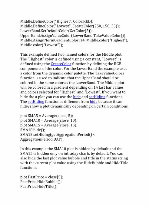
Middle.DefineColor("Highest", Color.RED); Middle.DefineColor("Lowest", CreateColor(250, 150, 25)); LowerBand.SetDefaultColor(GetColor(5)); UpperBand.AssignValueColor(LowerBand.TakeValueColor()); Middle.AssignNormGradientColor(14, Middle.color("Highest"), Middle.color("Lowest")); This example defined two named colors for the Middle plot. The "Highest" color is defined using a constant, "Lowest" is defined using the CreateColor function by defining the RGB components of the color. For the LowerBand the example uses a color from the dynamic color palette. The TakeValueColors function is used to indicate that the UpperBand should be colored in the same color as the LowerBand. The Middle plot will be colored in a gradient depending on 14 last bar values and colors selected for "Highest" and "Lowest". If you want to hide the a plot you can use the hide and setHiding functions. The setHiding function is diffenent from hide because it can hide/show a plot dynamically depending on certain conditions. plot SMA5 = Average(close, 5); plot SMA10 = Average(close, 10); plot SMA15 = Average(close, 15); SMA10.hide(); SMA15.setHiding(getAggregationPeriod() < AggregationPeriod.DAY); In this example the SMA10 plot is hidden by default and the SMA15 is hidden only on intraday charts by default. You can also hide the last plot value bubble and title in the status string with the current plot value using the HideBubble and HideTitle functions. plot PastPrice = close[5]; PastPrice.HideBubble(); PastPrice.HideTitle();

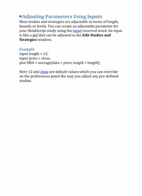
o Adjusting Parameters Using Inputs Most studies and strategies are adjustable in terms of length, bounds or levels. You can create an adjustable parameter for your thinkScript study using the input reserved word. An input is like a def that can be adjusted in the Edit Studies and Strategies window. Example input length = 12; input price = close; plot SMA = average(data = price, length = length); Here 12 and close are default values which you can override on the preferences panel the way you adjust any pre-defined studies.

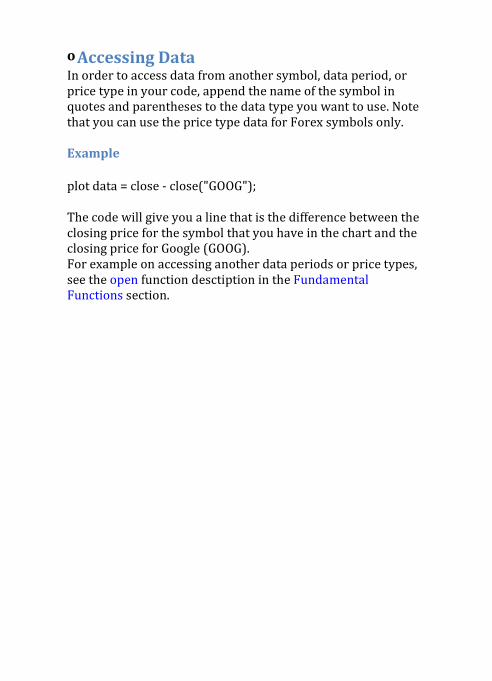
o Accessing Data In order to access data from another symbol, data period, or price type in your code, append the name of the symbol in quotes and parentheses to the data type you want to use. Note that you can use the price type data for Forex symbols only. Example plot data = close - close("GOOG"); The code will give you a line that is the difference between the closing price for the symbol that you have in the chart and the closing price for Google (GOOG). For example on accessing another data periods or price types, see the open function desctiption in the Fundamental Functions section.

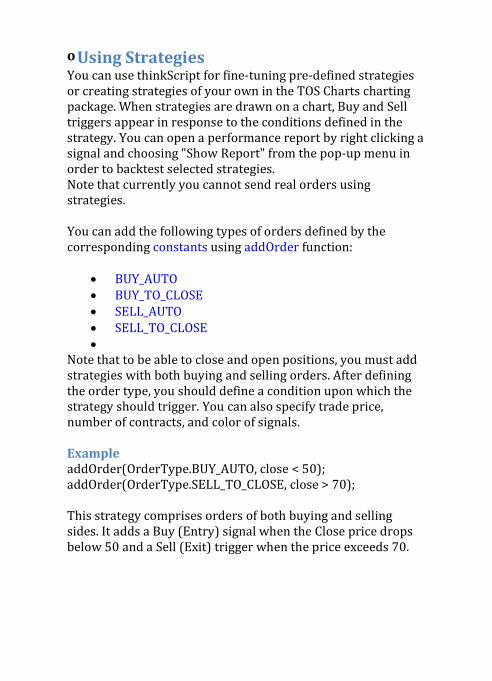
o Using Strategies You can use thinkScript for fine-tuning pre-defined strategies or creating strategies of your own in the TOS Charts charting package. When strategies are drawn on a chart, Buy and Sell triggers appear in response to the conditions defined in the strategy. You can open a performance report by right clicking a signal and choosing "Show Report" from the pop-up menu in order to backtest selected strategies. Note that currently you cannot send real orders using strategies. You can add the following types of orders defined by the corresponding constants using addOrder function:

• BUY_AUTO • BUY_TO_CLOSE • SELL_AUTO • SELL_TO_CLOSE •

Note that to be able to close and open positions, you must add strategies with both buying and selling orders. After defining the order type, you should define a condition upon which the strategy should trigger. You can also specify trade price, number of contracts, and color of signals. Example addOrder(OrderType.BUY_AUTO, close < 50); addOrder(OrderType.SELL_TO_CLOSE, close > 70); This strategy comprises orders of both buying and selling sides. It adds a Buy (Entry) signal when the Close price drops below 50 and a Sell (Exit) trigger when the price exceeds 70.

o Advanced Topics This section contains tutorials that will help you write your first thinkscript study or strategy. Here is a list of the tutorials:

• Concatenating Strings • Creating Local Alerts • Referencing Data • Using Profiles

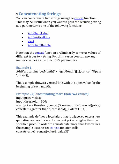
o Concatenating Strings You can concatenate two strings using the concat function. This may be useful when you want to pass the resulting string as a parameter to one of the following functions:

• AddChartLabel • AddVerticalLine • alert • AddChartBubble

Note that the concat function preliminarily converts values of different types to a string. For this reason you can use any numeric values as the function's parameters. Example 1 AddVerticalLine(getMonth() <> getMonth()[1], concat("Open: ", open)); This example draws a vertical line with the open value for the beginning of each month. Example 2 (Concatenating more than two values) input price = close; input threshold = 100; alert(price > threshold, concat("Current price ", concat(price, concat(" is greater than ", threshold))), Alert.TICK); This example defines a local alert that is triggered once a new quotation arrives in case the current price is higher that the specified price. In order to concatenate more than two values the example uses nested concat function calls: concat(value1, concat(value2, value3))

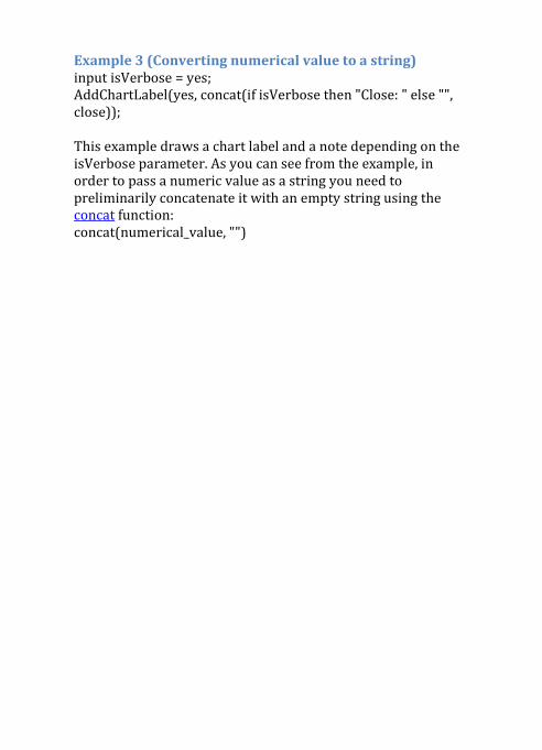
Example 3 (Converting numerical value to a string) input isVerbose = yes; AddChartLabel(yes, concat(if isVerbose then "Close: " else "", close)); This example draws a chart label and a note depending on the isVerbose parameter. As you can see from the example, in order to pass a numeric value as a string you need to preliminarily concatenate it with an empty string using the concat function: concat(numerical_value, "")

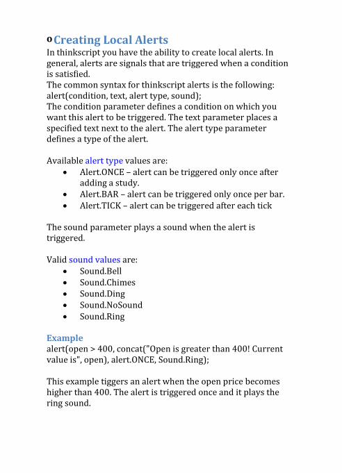
o Creating Local Alerts In thinkscript you have the ability to create local alerts. In general, alerts are signals that are triggered when a condition is satisfied. The common syntax for thinkscript alerts is the following: alert(condition, text, alert type, sound); The condition parameter defines a condition on which you want this alert to be triggered. The text parameter places a specified text next to the alert. The alert type parameter defines a type of the alert. Available alert type values are:

• Alert.ONCE – alert can be triggered only once after adding a study.

• Alert.BAR – alert can be triggered only once per bar. • Alert.TICK – alert can be triggered after each tick

The sound parameter plays a sound when the alert is triggered. Valid sound values are:

• Sound.Bell • Sound.Chimes • Sound.Ding • Sound.NoSound • Sound.Ring

Example alert(open > 400, concat("Open is greater than 400! Current value is", open), alert.ONCE, Sound.Ring); This example tiggers an alert when the open price becomes higher than 400. The alert is triggered once and it plays the ring sound.

o Referencing Data In this section you will find tutorials that describe ways of referencing data in the thinkscript. Here is a list of the tutorials:

• Referencing Secondary Aggregation 24 • Referencing Historical Data 27 • Referencing Other Price Type Data 28 • Referencing Other Studies 29 • Referencing Other Symbol's Data 31 • Past Offset 32

Referencing Secondary Aggregation In order to access data of a different aggregation period in your code, specify the period parameter using the corresponding Aggregation Period constant. You can also use a pre-defined string value for this purpose: 1 min, 2 min, 3 min, 4 min, 5 min, 10 min, 15 min, 20 min, 30 min, 1 hour, 2 hours, 4 hours, Day, 2 Days, 3 Days, 4 Days, Week, Month, Opt Exp, and <current period>. Example plot dailyOpen = open(period = AggregationPeriod.DAY); This code plots daily Open price for the current symbol. plot weeklyClose = close("IBM", period = AggregationPeriod.WEEK); This code plots weekly Close price for IBM. plot yesterdayHigh = High(period = AggregationPeriod.DAY)[1]; This code plots the High price reached on the previous day. All indexers with such price functions use secondary aggregation period until you save it in some variable. Example plot Data = Average(close(period = AggregationPeriod.DAY), 10); This code returns a 10 day average of the Close price. However, plot dailyClose = close(period = AggregationPeriod.DAY); plot Data = Average(dailyClose, 10); will return an average of the Close price calculated for the last ten bars (the aggregation period used in calculation will depend on the current chart settings).

Note that two different secondary aggregation periods cannot be used within a single variable. In addition, the secondary aggregation period cannot be less than the primary aggregation period defined by chart settings. Example plot Data = close(period = AggregationPeriod.MONTH) + close(period = AggregationPeriod.WEEK); This code will not work on a daily chart. The correct script is: def a = close(period = AggregationPeriod.MONTH); def b = close(period = AggregationPeriod.WEEK); plot Data = a + b; Example declare lower; input KPeriod = 10; input DPeriod = 10; input slowing_period = 3; plot FullK = Average((close(period = AggregationPeriod.WEEK) - Lowest(low(period = AggregationPeriod.WEEK), KPeriod)) / (Highest(high(period = AggregationPeriod.WEEK), KPeriod) - Lowest(low(period = AggregationPeriod.WEEK), KPeriod)) * 100, slowing_period); plot FullD = Average(Average((close(period = AggregationPeriod.WEEK) - Lowest(low(period = AggregationPeriod.WEEK), KPeriod)) / (Highest(high(period = AggregationPeriod.WEEK), KPeriod) - Lowest(low(period = AggregationPeriod.WEEK), KPeriod)) * 100, slowing_period), DPeriod);

Example shows the Stochastic Full study using weekly price regardless of the current chart aggregation period. See the Stochastic Full for a detailed study description.

Referencing Historical Data To access data in the past and in the future, you can use each of the two possible ways. Indexing Positive indexes are used to refer to data in the past and negative indexes to refer to data in the future. For example, close[1] returns the Close price from one bar ago, close[2] returns the Close price 2 bars ago, etc. At the same time, close[-1] returns the Close price 1 bar forward, close[-2] returns the Close price 2 bars forward, etc. Example plot momentum = close - close[5]; The example will plot a line that is the difference between the current Close price and the Close price 5 bars ago. Verbal Syntax Verbal syntax allows using reserved human-readable sentences in the script. For example, close from 2 bars ago returns the Close price from two bars ago, close from 1 bar ago returns the Close price one bar ago, etc. Negative numbers refer to data in the future. For example, close from -1 bar ago returns the Close price one bar forward, low from -2 bars ago returns the Low price two bars forward, etc. Example plot scan = close from 4 bars ago + high from 1 bar ago; The example will plot a line that is the sum of the Close price 5 bars ago and the High price 1 bar ago.

Referencing Other Price Type Data In order to access data from another price type in your code, put the priceType parameter with the name of the aggregation period in parentheses to the Fundamentals you want to use. Note that only Forex symbols support different price type data, all other symbols support only data based on the "LAST" price. Example plot ask = close(priceType = "ASK"); plot bid = close(priceType = "BID"); On the "MARK" price type chart for some Forex symbol this code will give you a ask and bid plots.

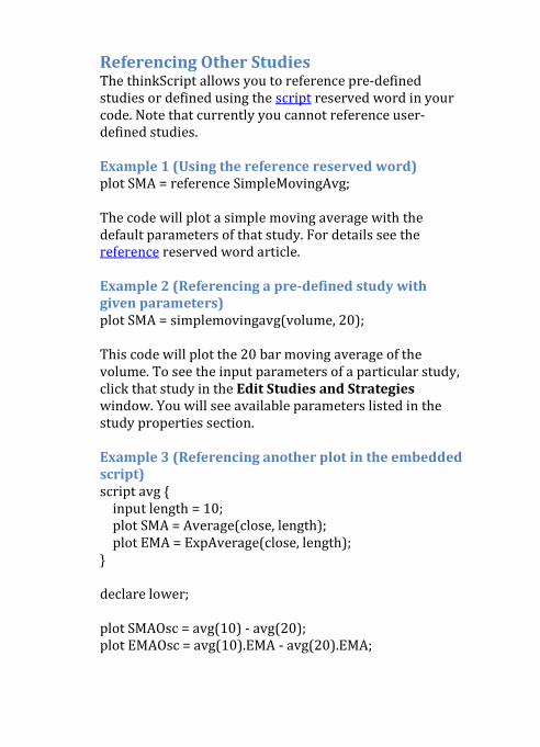
Referencing Other Studies The thinkScript allows you to reference pre-defined studies or defined using the script reserved word in your code. Note that currently you cannot reference user-defined studies. Example 1 (Using the reference reserved word) plot SMA = reference SimpleMovingAvg; The code will plot a simple moving average with the default parameters of that study. For details see the reference reserved word article. Example 2 (Referencing a pre-defined study with given parameters) plot SMA = simplemovingavg(volume, 20); This code will plot the 20 bar moving average of the volume. To see the input parameters of a particular study, click that study in the Edit Studies and Strategies window. You will see available parameters listed in the study properties section. Example 3 (Referencing another plot in the embedded script) script avg { input length = 10; plot SMA = Average(close, length); plot EMA = ExpAverage(close, length); } declare lower; plot SMAOsc = avg(10) - avg(20); plot EMAOsc = avg(10).EMA - avg(20).EMA;

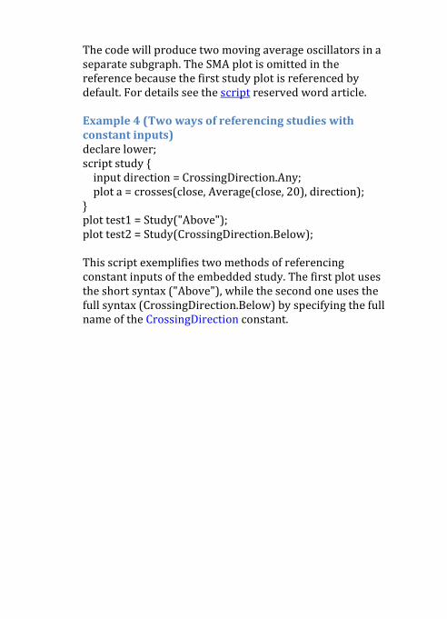
The code will produce two moving average oscillators in a separate subgraph. The SMA plot is omitted in the reference because the first study plot is referenced by default. For details see the script reserved word article. Example 4 (Two ways of referencing studies with constant inputs) declare lower; script study { input direction = CrossingDirection.Any; plot a = crosses(close, Average(close, 20), direction); } plot test1 = Study("Above"); plot test2 = Study(CrossingDirection.Below); This script exemplifies two methods of referencing constant inputs of the embedded study. The first plot uses the short syntax ("Above"), while the second one uses the full syntax (CrossingDirection.Below) by specifying the full name of the CrossingDirection constant.

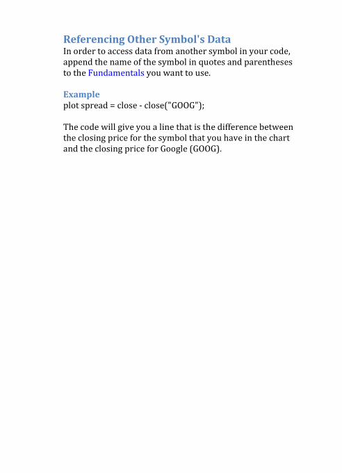
Referencing Other Symbol's Data In order to access data from another symbol in your code, append the name of the symbol in quotes and parentheses to the Fundamentals you want to use. Example plot spread = close - close("GOOG"); The code will give you a line that is the difference between the closing price for the symbol that you have in the chart and the closing price for Google (GOOG).

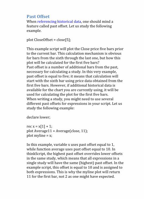
Past Offset When referencing historical data, one should mind a feature called past offset. Let us study the following example. plot CloseOffset = close[5]; This example script will plot the Close price five bars prior to the current bar. This calculation mechanism is obvious for bars from the sixth through the last one, but how this plot will be calculated for the first five bars? Past offset is a number of additional bars from the past, necessary for calculating a study. In this very example, past offset is equal to five; it means that calculation will start with the sixth bar using price data obtained from the first five bars. However, if additional historical data is available for the chart you are currently using, it will be used for calculating the plot for the first five bars. When writing a study, you might need to use several different past offsets for expressions in your script. Let us study the following example: declare lower; rec x = x[1] + 1; plot Average11 = Average(close, 11); plot myline = x; In this example, variable x uses past offset equal to 1, while function average uses past offset equal to 10. In thinkScript, the highest past offset overrides lower offsets in the same study, which means that all expressions in a single study will have the same (highest) past offset. In the example script, this offset is equal to 10 and is assigned to both expressions. This is why the myline plot will return 11 for the first bar, not 2 as one might have expected.

Note that past offset might affect calculation mechanism of some studies due to setting a single intialization point for all expressions. However, if for some reason you need an independent initialization point for an expression, you can use the compoundValue function: declare lower; rec x = compoundValue(1, x[1]+1, 1); plot ATR = average(TrueRange(high, close, low), 10); plot myline = x; This would explicitly set the value for the myline plot for the first bar, and all the other values of this plot will be calculated corresponding to it.

o Using Profiles The TPO, Volume, and Monkey Bars profiles can be created in thinkScript using corresponding Profile functions. You can find the detailed description of these functions in the Profiles section. In order to demonstrate the use of the functions, let's create a TPO profile study (colored blue) that aggregates all chart data on the right expansion. Here is the code: def allchart = 0; profile tpo = timeProfile("startnewprofile" = allchart); tpo.show("color" = Color.BLUE);

Reference The reference describes thinkscript elements (functions, constants, declarations, etc.) required to create studies and strategies. The items are distributed alphabetically among the following sections: Constants, Declarations, Functions, and Reserved Words. Each article provides the syntax, description, and an example of use of the selected item. All interrelated thinkscript items are cross-linked to ensure you have the fullest information about the relations inside the thinkscript. Here is the list of the reference sections:

• Reserved Words 37 • Declarations 68 • Functions 78 • Constants 256 • Data Types 312 • Operators 315

• Reference o Reserved Words 37 o Declarations 68 o Functions 78

Fundamentals 79 Option Related 92 Technical Analysis 104 Mathematical and Trigonometrical 132 Statistical 156 Date and Time 170 Corporate Actions 185 Look and Feel 191 Profiles 220 Others 234

o Constants 256 Aggregation Period 257 Alert 268 ChartType 269 Color 273 CrossingDirection 283 Curve 285 Double 289 EarningTime 291 FundamentalType 293 OrderType 297 PaintingStrategy 299 PricePerRow 309 Sound 310

o Data Types 312 o Operators 315

o Reserved Words The thinkScript supports a number of simple commands such as for example: declare, plot, and input. These commands control the basic behavior of your thinkScript study. Choose your command from the list:

o above Syntax See the crosses reserved word article. Description The above reserved word is used with the crosses operator to test if a value gets higher than another value. o ago Syntax <value> from 1 bar ago <value> from <length> bars ago Description This reserved word is used to specify a time offset in a human-friendly syntax. For more information, see the Referencing Historical Data article.

o and Syntax <condition1> and <condition2> Description The and logical operator is used to define complex conditions. For a complex condition to be true it is required that each condition from it is true. In order to define the operator you can also use &&. This reserved word is also used to define an interval in the between expression. Example plot InsideBar = high <high[1] and low > low[1]; InsideBar.SetPaintingStrategy(PaintingStrategy.BOOLEAN _POINTS); Draws a dot near each inside price bar. o bar Syntax <value> from 1 bar ago Description This reserved word is used to specify a time offset in a human-friendly syntax. For more information, see the Referencing Historical Data article. Note that bar and bars reserved words can be used interchangeably.

o bars Syntax <value> from <length> bars ago Description This reserved word is used to specify a time offset in a human-friendly syntax. For more information, see the Referencing Historical Data article. Note that bar and bars reserved words can be used interchangeably. o below Syntax See the crosses reserved word article. Description The below reserved word is used with the crosses operator to test if a value becomes less than another value. o between Syntax <parameter> between <value1> and <value2> Description This reserved word is used in the between logical expression. It tests if the specified parameter is within the range of value1 and value2 (inclusive). The thinkscript also has the between function with a different syntax and usage. Example declare lower; def isIn = close between close[1] * 0.9 and close[1] * 1.1; plot isOut = !isIn; In this example between is used to check whether the current closing price hits the 10% channel of the previous closing price. The isOut plot reflects the opposite condition.

o case Syntax See the switch statement. Description The reserved word is used in combination with the switch statement to define a condition.

o crosses Syntax <value1> crosses above <value2> <value1> crosses below <value2> <value1> crosses <value2> Description This reserved word is used as a human-readable version of the Crosses function. It tests if value1 gets higher or lower than value2. Example plot Avg = Average(close, 10); plot ArrowUp = close crosses above Avg; plot ArrowDown = close crosses below Avg; plot Cross = close crosses Avg; ArrowUp.SetPaintingStrategy(PaintingStrategy.BOOLEAN_ARROW_UP); ArrowDown.SetPaintingStrategy(PaintingStrategy.BOOLEAN_ARROW_DOWN); Cross.SetPaintingStrategy(PaintingStrategy.BOOLEAN_POINTS); This code plots up arrows indicating the bars at which the Close price gets higher than its 10 period average, and down arrows at which the Close price gets lower than its 10 period average.

The same result can be achieved by using the Crosses function: plot Avg = Average(close, 10); plot ArrowUp = Crosses(close, Avg, CrossingDirection.Above); plot ArrowDown = Crosses(close, Avg, CrossingDirection.Below); plot Cross = Crosses(close, Avg, CrossingDirection.Any); ArrowUp.SetPaintingStrategy(PaintingStrategy.BOOLEAN_ARROW_UP); ArrowDown.SetPaintingStrategy(PaintingStrategy.BOOLEAN_ARROW_DOWN); Cross.SetPaintingStrategy(PaintingStrategy.BOOLEAN_POINTS); Example plot Avg = Average(close, 10); plot Cross = close crosses Avg; Cross.SetPaintingStrategy(PaintingStrategy.BOOLEAN_POINTS); This code plots arrows indicating the bars at which the Close price gets higher or lower than its 10 period average. The equivalent code is: plot Avg = Average(close, 10); plot Cross = close crosses above Avg or close crosses below Avg; Cross.SetPaintingStrategy(PaintingStrategy.BOOLEAN_POINTS);

o declare Syntax declare <supported_declaration_name> Description The declare keyword is a method for telling the chart something basic about the appearance of the study or strategy you are creating. You can find the list of supported declarations in the Declarations section. Example declare lower; plot PriceOsc = Average(close, 9) - Average(close, 18); The example shows how to use one of the most commonly used declations called lower. For other examples on declarations, see the Declarations section.

o def Syntax def <variable_name>=<expression>; or def <variable_name>; <variable_name>=<expression>; Description Defines a variable you would like to work with. Example def base = Average(close, 12); plot UpperBand = base * 1.1; plot LowerBand = base * 0.9; This example shows a simplified SMAEnvelope study, where the def reserved word is used to define the base. The rational of defining this variable is to avoid double calculations (increase performance) in UppderBand and LowerBand plots, because def variable values are cached (by means of increasing memory usage). You can separate the variable definition from its value assignment as shown in the following example where a variable value is assigned depending on the selected averageType input value. See the Defining Variables section for more details. input averageType = {default SMA, EMA}; def base; switch (averageType) { case SMA: base = Average(close, 12); case EMA: base = ExpAverage(close, 12); } plot UpperBand = base * 1.1; plot LowerBand = base * 0.9;

o default Syntax See the enum rec, enum input, and switch statements. Description The default reserved word is used in combination with the enum rec, enum input, and switch statements to specify a default value. o do Syntax def <result> = fold <index> = <start> to <end> with <variable> [ = <init> ] [ while <condition> ] do <expression>; Description This reserved word defines an action to be performed when calculating the fold function. For more information, see the fold reserved word article. o else Syntax See the if reserved word article. Description The else reserved word is used to specify an additional condition in the if-expression and if-statement.

o equals Syntax equals Description The reserved word is used as a logic operator to test equality of values. In order to define this operator you can also use the double equals sign ==. Example plot Doji = open equals close; Doji.SetPaintingStrategy(PaintingStrategy.BOOLEAN_POINTS); The code draws points on bars having the Doji pattern (equal close and open).

o fold Syntax def <result> = fold <index> = <start> to <end> with <variable> [ = <init> ] [ while <condition> ] do <expression>; Description The fold operator allows you to perform iterated calculations similarly to the for loop. It uses variable to store the result of the calculation. The initial value of variable is defined by init; if it is omitted, variable is initialized to zero. The index is iterated from start (inclusive) to end (exclusive) with step 1. At each iteration, expression is calculated and assigned to variable. Value of index and previous value of variable can be used in expression. The value of variable after the last iteration is returned and can be used in assignments and expressions. You can also specify a condition upon violation of which the loop is terminated. Example 1 input n = 10; plot factorial = fold index = 1 to n + 1 with p = 1 do p * index; Calculates the factorial of a number. Example 2 input price = close; input length = 9; plot SMA = (fold n = 0 to length with s do s + getValue(price, n, length - 1)) / length; Calculates the simple moving average using fold. Example 3 plot NextHigh = fold i = 0 to 100 with price = Double.NaN while IsNaN(price) do if getValue(high, -i) > 40 then getValue(high, -i) else Double.NaN; Finds the next High price value greater than 40 among the following 100 bars.

o from Syntax <value> from 1 bar ago <value> from <length> bars ago Description This reserved word is used to specify a time offset in a human-friendly syntax. For more information, see the Referencing Historical Data article.

o if Syntax (if-expression) plot <plot_name> = if <condition> then <expression1> else <expression2>; plot <plot_name> = if <condition1> then <expression1> else if <condition2> then <expression2> else <expression3>; Syntax (if-statement) plot <plot_name>; if <condition> [then] { <plot_name> = <expression1>; } else { <plot_name> = <expression2>; } plot <plot_name>; if <condition1> [then] { <plot_name > = <expression1>; } else { if <condition2> [then] { <plot_name> = <expression2>; } else { <plot_name> = <expression3>; } } Description As a reserved word, if is used in if-expressions and if-statements to specify a condition. If-expression always calculates both then and else branches, while if-statement calculates either of these, depending on the condition. In thinkScript, there is also if-function having syntax and usage different from those of the reserved word. The if-expression

can also be used in other functions such as, for example, AssignValueColor, AssignPriceColor, etc. Note that you can also use the def and rec instead of plot in the syntax provided above. Example input price = close; input long_average = yes; plot SimpleAvg = Average(price, if long_average then 26 else 12); plot ExpAvg; if long_average { ExpAvg = ExpAverage(price, 26); } else { ExpAvg = ExpAverage(price, 12); } In this example, if-expression and if-statement are used to control the length parameter of moving averages.

o input Most studies are adjustable in terms of length, bounds, or levels. You can create an adjustable parameter for your thinkScript study using the input reserved word. When defining inputs take the following notes into consideration: • Inputs are displayed on the GUI in the same order as they

appear in the source code. • Inputs titles are always displayed on the GUI in the

lowercase. The following two definitions are similar on the GUI. Code snippet 1 input test = "test in lowercase"; Code snippet 2 input TEST = "test in uppercase";

• Inputs can't have empty spaces in their definitions. The following code will result in compilation error. input "input name with spaces" = "ERROR"; In order to have titles displayed on the GUI with spaces you can do one of the following: Code snippet 3 input inputNameWithSpaces = "OK"; Code snippet 4 input input_name_with_spaces = "OK";

Find the full list of inputs in the following list: • boolean • constant • enum • float • integer • price • string

boolean Profile: Studies and Strategies Syntax input <input name>=<boolean_value_used_by_default>; Description Defines a boolean input. The default value of the input can either be "yes" or "no". Example input useHighLow = yes; plot HighPrice = if useHighLow then Highest(high, 10) else Highest(close, 10); plot LowPrice = if useHighLow then Lowest(low, 10) else Lowest(close, 10); Draws the channel based on the highest and lowest price for the length equal to 10. Whether to use or not the high and low prices instead of the closing price can be defined using the correspondent input, which is set to "yes" by default.

constant Profile: Studies and Strategies Syntax input <input name>=<constant_used_by_default>; Description Defines an input expressed by a constant of particular type. For the full list of supported constants, see the Constants section. Note that color constants cannot be used for input definition. Example input secondaryPeriod = AggregationPeriod.DAY; plot SecondaryPeriodOpen = open(period = secondaryPeriod); This example script draws the Open price plot with specified aggregation period.

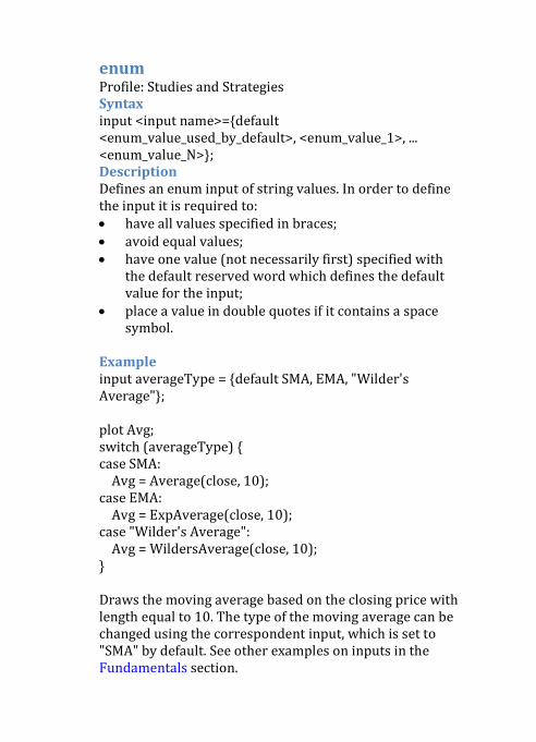
enum Profile: Studies and Strategies Syntax input <input name>={default <enum_value_used_by_default>, <enum_value_1>, ... <enum_value_N>}; Description Defines an enum input of string values. In order to define the input it is required to: • have all values specified in braces; • avoid equal values; • have one value (not necessarily first) specified with

the default reserved word which defines the default value for the input;

• place a value in double quotes if it contains a space symbol.

Example input averageType = {default SMA, EMA, "Wilder's Average"}; plot Avg; switch (averageType) { case SMA: Avg = Average(close, 10); case EMA: Avg = ExpAverage(close, 10); case "Wilder's Average": Avg = WildersAverage(close, 10); } Draws the moving average based on the closing price with length equal to 10. The type of the moving average can be changed using the correspondent input, which is set to "SMA" by default. See other examples on inputs in the Fundamentals section.

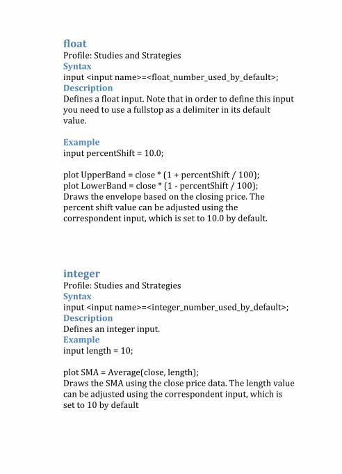
float Profile: Studies and Strategies Syntax input <input name>=<float_number_used_by_default>; Description Defines a float input. Note that in order to define this input you need to use a fullstop as a delimiter in its default value. Example input percentShift = 10.0; plot UpperBand = close * (1 + percentShift / 100); plot LowerBand = close * (1 - percentShift / 100); Draws the envelope based on the closing price. The percent shift value can be adjusted using the correspondent input, which is set to 10.0 by default. integer Profile: Studies and Strategies Syntax input <input name>=<integer_number_used_by_default>; Description Defines an integer input. Example input length = 10; plot SMA = Average(close, length); Draws the SMA using the close price data. The length value can be adjusted using the correspondent input, which is set to 10 by default

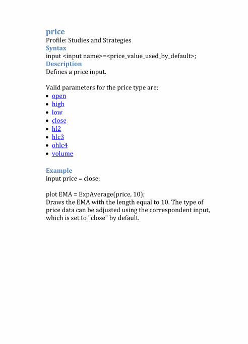
price Profile: Studies and Strategies Syntax input <input name>=<price_value_used_by_default>; Description Defines a price input. Valid parameters for the price type are: • open • high • low • close • hl2 • hlc3 • ohlc4 • volume

Example input price = close; plot EMA = ExpAverage(price, 10); Draws the EMA with the length equal to 10. The type of price data can be adjusted using the correspondent input, which is set to "close" by default.

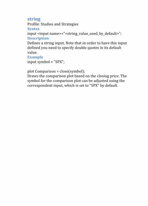
string Profile: Studies and Strategies Syntax input <input name>="<string_value_used_by_default>"; Description Defines a string input. Note that in order to have this input defined you need to specify double quotes in its default value. Example input symbol = "SPX"; plot Comparison = close(symbol); Draws the comparison plot based on the closing price. The symbol for the comparison plot can be adjusted using the correspondent input, which is set to "SPX" by default.

o no Syntax no Description The no reserved word is used as a value for the boolean input or as the false condition. In order to define the false condition, you can also use the 0 value. Example plot Price = if no then high else low; Since the condition is always false, the low plot is always displayed. o or Syntax or Description The reserved word is used to define complex conditions. For a complex condition to be true it is required that at least one condition from it is true. Example input NumberOfBars = 3; rec barsUp = if close > close[1] then barsUp[1] + 1 else 0; rec barsDown = if close < close[1] then barsDown[1] + 1 else 0; plot ConsecutiveBars = barsUp >= NumberOfBars or barsDown >= NumberOfBars; ConsecutiveBars.SetPaintingStrategy(PaintingStrategy.BOOLEAN_POINTS); This example highlights bars having the closing price lower than the closing price of the specified number of previous bars with a dot.

o plot Syntax plot <plot_name>=<expression>; or plot <plot_name>; <plot_name>=<expression>; Description Renders the data you are working with on the chart. For more information about the reserved word, see the Formatting Plots tutorial. Example plot SMA = Average(close, 12); This example draws a simple moving average study plot. You can separate the plot definition from its value assignment as shown in the following example where a plot value is assigned depending on the selected averageType input value. input averageType = {default SMA, EMA}; plot MA; switch (averageType) { case SMA: MA = Average(close, 12); case EMA: MA = ExpAverage(close, 12); }

o profile Syntax profile <variable_name>=<expression>; or profile <variable_name>; <variable_name>=<expression>; Description Defines a profile to be displayed on the chart. o rec Syntax rec Description Enables you to reference a historical value of a variable that you are calculating in the study or strategy itself. Rec is short for "recursion". See the Defining Variables section for more details. Example rec C = C[1] + volume; plot CumulativeVolume = C; This example plots the cumulative volume starting from the beginning of the time period.

o reference Syntax reference <StudyName>(parameter1=value1,.., parameterN=valueN).<PlotName> Description References a plot from another script. Note that the reference reserved word can be dropped but in this case parenthesis are necessary. Full form: plot MyMACD = reference MACDHistogram; Compressed form: plot MyMACD = MACDHistogram(); The reference reserved work is required to distinguish the VWAP study from the vwap function, MoneyFlow study from the moneyflow function. Calling the vwap function: plot MyVWAP1 = vwap; Referenicing the VWAP study: plot MyVWAP1 = reference VWAP; If the plot name is not defined, study's main plot should be referenced (main is the first declared in the source code). If parameters values are not defined, default values should be used. Inputs' names can be dropped only for ThinkScript studies, because they have fixed order of inputs in the code: Full form: plot MyBB2 = BollingerBandsSMA(price = open, displace = 0, length = 30); Compact form: plot MyBB = BollingerBandsSMA(open, 0, 30);

Example The following example references def and rec instead of the plot as shown at the top of the article. def st = ATRTrailingStop().state; AssignPriceColor(if st == 1 then GetColor(1) else if st == 2 then GetColor(0) else Color.CURRENT); def bs = !IsNaN(close) and ATRTrailingStop().BuySignal == yes; def ss = !IsNaN(close) and ATRTrailingStop().SellSignal == yes; AddVerticalLine(bs or ss, if bs then "Buy!" else "Sell!", if bs then GetColor(0) else GetColor(1)); st is the reference to the state enum rec from the ATRTrailingStop study, bs and ss are references to the BuySignal and SellSignal def from the same study.

o script Syntax script <script_name> { <script_code>; } Description This reserved word is used to define new scripts you may need to reference later within a certain study or strategy. Example script MyEMA { input data = close; input length = 12; rec EMA = compoundValue(1, 2 / (length + 1) * data + (length - 1) / (length + 1) * EMA[1], Average(data, length)); plot MyEma = EMA; } declare lower; plot Osc = MyEMA(close, 25) - MyEMA(close, 50); This code defines the MyEma script where the first EMA value is calculated as SMA in contrast to the ExpAverage function whose first value is assigned the closing price. The main section of the code creates an oscillator based on the MyEMA difference for different lenghts.

o switch Syntax plot <plot_name>; switch (<enum input or enum_rec>) { case <enum value1>: <plot_name> = <expression1>; ... default: <plot_name> = <expression>; } Description The switch statement is used to control the flow of program execution via a multiway branch using the enum rec, and enum input. In the switch statement you either need to define the case with all values from the enum. Or you can use the default statement to define actions for all enums that are not defined using the case. Note that in this approach you cannot use case with equal enums. Example input price = close; input plot_type = {default SMA, "Red EMA", "Green EMA", WMA}; plot Avg; switch (plot_type) { case SMA: Avg = Average(price); case WMA: Avg = wma(price); default: Avg = ExpAverage(price); } Avg.SetDefaultColor( if plot_type == plot_type."Red EMA" then color.RED else if plot_type == plot_type."Green EMA" then color.GREEN else color.BLUE);

This example illustrates the usage of the switch reserved word to assign different values to plots. The default keyword must be used unless all possible values of variable are explicitly listed.

o then Syntax See the if reserved word article. Description The reserved word is used to specify an action to be performed when the if condition is satisfied. This reserved word is used only in combination with the if statement. o to Syntax def <result> = fold <index> = <start> to <end> with <variable> [ = <init> ] [ while <condition> ] do <expression>; Description The reserved word is used to define an interval to be used when calculating the fold function. For more information, see the fold reserved word article. o while Syntax def <result> = fold <index> = <start> to <end> with <variable> [ = <init> ] [ while <condition> ] do <expression>; Description This reserved word defines a condition upon violation of which the loop is terminated when calculating the fold function. For more information, see the fold reserved word article.

o with Syntax def <result> = fold <index> = <start> to <end> with <variable> [ = <init> ] [ while <condition> ] do <expression>; Description The reserved word is used to define an iteration step value in the fold function. For more information, see the fold reserved word article. o yes Syntax yes Description The yes reserved word is used as a value for the boolean input or as the true condition. In order to define the true condition, you can also use 1 or any non-zero number. Example input DisplayPlot = yes; plot Data = close; Data.SetHiding(!DisplayPlot); In this study, DisplayPlot input controls visibility of plot. Its default value is yes.

o Declarations Declarations are responsible for basic operations performed with charts such as changing the recalculation mode or setting the minimal chart value to zero. An important difference of declarations from other thinkscript items is that in order to define a declaration you need to use the declare reserved word. The section contains the following declarations: • all_for_one • hide_on_daily • hide_on_intraday • lower • on_volume • once_per_bar • real_size • upper • weak_volume_dependency • zerobase

o all_for_one Syntax declare all_for_one; Description Keeps the volume value either in all price inputs or in none of them. This function is used to prevent visualizing irrelevant data in case the volume value does not combine with other price input values. Example (Price Envelopes) declare all_for_one; input HighPrice = high; input LowPrice = low; plot UpperBand = Average(HighPrice) * 1.1; plot LowerBand = Average(LowPrice) * 0.9; This example plots the high and low price envelopes at 10 percent above and below for the 12 day simple moving average. If you change the inputs to close and volume, the all_for_one declaration will automatically change the HighPrice and LowPrice inputs to the two volumes because the close and volume in combination lead to irrelevant data. As a result, the two volume values will be plotted. Usage in: SMAEnvelope; StochasticFast; StochasticFull; StochasticSlow.

o hide_on_daily Syntax declare hide_on_daily; Description Hides a study on charts with aggregation periods equal to or greater than 1 day. Example declare hide_on_daily; plot SMA = average(close); SMA.AssignValueColor(GetColor(secondsFromTime(0) / 3600)); This study plots SMA of Close price and assigns a different color to the plot each hour. Due to declaration, this study will be hidden on daily charts. o hide_on_intraday Syntax declare hide_on_intraday; Description Hides a study on intraday charts (time charts with aggregation period less than 1 day and tick charts). Example (Implied Volatility) declare hide_on_intraday; declare lower; plot ImpVol = IMP_VOLATILITY(); By definition, data for implied volatility is not available for intraday charts. Therefore, you can use the declaration to automatically hide studies on this type of charts. Usage in: ImpVolatility; OpenInterest.

o lower Syntax declare lower; Description Places a study on the lower subgraph. This declaration is used when your study uses values that are considerably lower or higher than price history or volume values. Example (Price Oscillator) declare lower; input price = close; input fastLength = 9; input slowLength = 18; plot PriceOsc = Average(price, fastLength) - Average(price, slowLength); The example plots the difference between the two average values calculated on 9 and 18-bar intervals. The result value is lower compared to the price value. Therefore, it is reasonable to put the plot on the lower subgraph to avoid scaling the main chart. Usage in: Multiple

o on_volume Syntax declare on_volume; Description Places a plot on the volume subgraph. General Information By default, the application automatically defines where to place a study. If the study contains volume values and values not related to the base subgraph, then this study is displayed on the volume subgraph, otherwise it is displayed on the base subgraph. However, it may be required to forcibly place the study on the volume subgraph regardless of the values you are using. Example (Volume Accumulation on the Volume Subgraph) declare on_volume; plot VolumeAccumulation = (close - (high + low) / 2) * volume; The code in the example contains both volume and base subgraph related values. In order to place the study on the volume subgraph, the code uses the on_volume declaration. To study an example that uses only non-volume values, see the real_size function article. Usage in: OpenInterest.

o once_per_bar Syntax declare once_per_bar; Description Changes the recalculation mode of a study. By default, last study values are recalculated after each tick. If this declaration is applied, the study is forced to recalculate the last values only once per bar. This declaration can be used to reduce CPU usage for studies which do not need to be recalculated per each tick. Example declare once_per_bar; input time = 0930; AddVerticalLine(secondsFromTime(time)[1] < 0 && secondsFromTime(time) >= 0, concat("", time)); This study plots a verical line at the specified time point in EST time zone for each day. Since the time value is fixed, there is no need to recalculate the study after each tick.

o real_size Syntax declare real_size; Description Forces a study to use axis of either base subgraph or volume subgraph. Note that the axis of the volume subgraph can be used in case you use only volume values in your study. General Information Studies always use the axis of the subgraph where you plot them except for the following two cases when the native plot axis are used:

• Study that is created for a separate subgraph (using the lower declaration) is moved to the base or volume subgraph using the On base subgraph check box;

• Study that is placed on the base subgraph by default is forcibly moved to the volume subgraph (using the on_volume declaration).

For the described two cases it may be required to use the axis of the volume or base subgraph, instead of the native plot axis. Example declare real_size; declare on_volume; declare hide_on_intraday; plot Data = open_interest(); In the code above, in order to use the axis of the volume subgraph, you specify the real_size declaration. Usage in: OpenInterest; ProbabilityOfExpiringCone.

o upper Syntax declare upper; Description Enables you to place a study either on the base subgraph or on the volume subgraph. Note that a study is placed on the volume subgraph in case only volume values are used in the study. This declaration is applied by default to all studies not containing the lower and on_volume declarations. Example (Price Oscillator) declare upper; input price = close; input length = 9; plot AvgWtd = wma(price, length); In this example, the upper declaration places the weighted moving average plot on the main chart.

o weak_volume_dependency Syntax declare weak_volume_dependency; Description Places a study on the volume subgraph when at least one volume value is used. Example (Keltner Channels) declare weak_volume_dependency; input factor = 1.5; input length = 20; input price = close; def shift = factor * AvgTrueRange(high, close, low, length); def average = Average(price, length); plot Avg = average; plot Upper_Band = average + shift; plot Lower_Band = average - shift; Consider you are analyzing data that contains both volume and base subgraph related values using the code provided above. You want to display the plot on the base subgraph except for cases when you use at least one volume value. For the latter case, you would like to use the volume subgraph. In order to implement the logics, you use the weak_volume_declaration. If you use the close price input in the code, the study will be displayed on the base subgraph. If you use the volume price input, then there is a weak volume dependency and the study will be displayed on the volume subgraph. Usage in: KeltnerChannels; STARCBands.

o zerobase Syntax declare zerobase; Description Sets the minimal value on a study axis to zero if there are no negative values in the study. Example (Price Oscillator) declare zerobase; declare lower; plot Vol = Volume; In this example, the Vol plot contains no negative values. It is reasonable to set the minimum value on the study axis to zero using the zerobase declaration. Usage in: AwesomeOscillator; SpectrumBars; Volume; VolumeAvg.

o Functions Similar to functions in programming languages, each thinkscript function receives input parameters and produces a result. In thinkscript the parameters can be specified in any order. For example plot SMA = average(data = close, length = 50) and plot SMA = average(length = 50, data = close) produce the same result. All the functions are spread among the following sections: • Fundamentals 79 • Option Related 92 • Technical Analysis 104 • Mathematical and Trigonometrical 132 • Statistical 156 • Date and Time 170 • Corporate Actions 185 • Look and Feel 191 • Profiles 220 • Others 234

o Fundamentals Trading analysis tightly relates to close, open, low, or high values. The thinkscript contains functions to work with these values. In addition, there are functions to work with data such as implied volatility, open interest, volume weighted average, and volume. All of them are collected in this section. Here is the full list: • ask • bid • close • high • hl2 • hlc3 • imp_volatility • low • ohlc4 • open • open_interest • volume • vwap

ask Syntax ask Description Returns current value of ask price for current symbol. This function is only available in thinkScript integration features: Custom Quotes, Study Alerts, and Conditional Orders. Example plot spread = ask - bid; AssignBackgroundColor(if spread < 0.05 then Color.GREEN else if spread < 0.25 then Color.YELLOW else Color.RED); This example script is used as a custom quote. It calculates a bid-ask spread and assigns different colors according to its value. Note that you cannot reference historical data using this function, e.g. ask[1] is an invalid expression.

bid Syntax bid Description Returns current value of bid price for current symbol. This function is only available in thinkScript integration features: Custom Quotes, Study Alerts, and Conditional Orders. Example plot "Diff, %" = round(100 * ((bid + ask) / 2 - close) / close, 2); AssignBackgroundColor(if "Diff, %" > 0 then Color.UPTICK else if "Diff, %" < 0 then Color.DOWNTICK else Color.GRAY); This example script is used as a custom quote. It calculates percentage difference between mark and last prices and assigns colors according to its sign. Note that you cannot reference historical data using this function, e.g. bid[1] is an invalid expression.

close Syntax close(String symbol, Any period, String priceType); Default values: • symbol: "<currently selected symbol>" • period: "<current period>" • priceType: "<current type>"

Description Returns the Close price for the specific symbol, aggregation period and price type. You can use both Aggregation Period constants and pre-defined string values (e.g. Day, 2 Days, Week, Month, etc.) as valid parameters for the aggregation period. The full list of the pre-defined string values can be found in the Referencing Secondary Aggregation article. Valid parameters for the price type are: • LAST • MARK, ASK, BID (for Forex symbols only)

Example declare lower; input symbol = {default "IBM", "GOOG/3", "(2*IBM - GOOG/6 + GE)/2"} ; plot PriceClose = close(symbol); Draws the close plot of either IBM, GOOG divided by three, or a composite price consisting of IBM, GOOG, and GE. Each of the symbols can be selected in the Edit Studies dialog. Usage in: AdvanceDecline; Alpha2; AlphaJensen; Beta; Beta2; Correlation; CumulativeVolumeIndex; DailyHighLow; McClellanOscillator; McClellanSummationIndex; PairCorrelation; PairRatio; PersonsPivots; RelativeStrength; Spreads; WoodiesPivots.

high Syntax high(String symbol, Any period, String priceType); Default values: • symbol: "<currently selected symbol>" • period: "<current period>" • priceType: "<current type>"

Description Returns the High price for the specific symbol, aggregation period and price type. You can use both Aggregation Period constants and pre-defined string values (e.g. Day, 2 Days, Week, Month, etc.) as valid parameters for the aggregation period. The full list of the pre-defined string values can be found in the Referencing Secondary Aggregation article. Valid parameters for the price type are: • LAST • MARK, ASK, BID (for Forex symbols only)

Example declare lower; input symbol = "IBM"; plot PriceHigh = high(symbol); This example script plots High price for IBM. Usage in: DailyHighLow; PersonsPivots; WoodiesPivots.

hl2 Syntax hl2(String symbol, Any period, String priceType); Default values: • symbol: "<currently selected symbol>" • period: "<current period>" • priceType: "<current type>"

Description Returns (High + Low)/2. You can use both Aggregation Period constants and pre-defined string values (e.g. Day, 2 Days, Week, Month, etc.) as valid parameters for the aggregation period. The full list of the pre-defined string values can be found in the Referencing Secondary Aggregation article. Example declare lower; input symbol = "IBM"; input period = AggregationPeriod.WEEK; plot MedianPrice = hl2(symbol, period); This example script plots weekly median price for IBM.

hlc3 Syntax hlc3(String symbol, Any period, String priceType); Default values: • symbol: "<currently selected symbol>" • period: "<current period>" • priceType: "<current type>"

Description Returns the typical price (arithmetical mean of High, Low, and Close price values) for the specific symbol, aggregation period and price type. You can use both Aggregation Period constants and pre-defined string values (e.g. Day, 2 Days, Week, Month, etc.) as valid parameters for the aggregation period. The full list of the pre-defined string values can be found in the Referencing Secondary Aggregation article. Valid parameters for the price type are: • LAST • MARK, ASK, BID (for Forex symbols only)

Example plot TypicalPrice = hlc3; This example script draws the typical price plot.

imp_volatility Syntax imp_volatility(String symbol, Any period, String priceType); Default values: • symbol: "<currently selected symbol>" • period: "<current period>" • priceType: "<current type>"

Description Returns the implied volatility for the specific symbol, aggregation period and price type. You can use both Aggregation Period constants and pre-defined string values (e.g. Day, 2 Days, Week, Month, etc.) as valid parameters for the aggregation period. The full list of the pre-defined string values can be found in the Referencing Secondary Aggregation article. Valid parameters for the price type are: • LAST • MARK, ASK, BID (for Forex symbols only)

Example declare lower; plot ImpliedVolatility = imp_volatility(); Draws the implied volatility plot for the current symbol. Usage in: ImpVolatility.

low Syntax low(String symbol, Any period, String priceType); Default values: • symbol: "<currently selected symbol>" • period: "<current period>" • priceType: "<current type>"

Description Returns the Low price for the specific symbol, aggregation period and price type. You can use both Aggregation Period constants and pre-defined string values (e.g. Day, 2 Days, Week, Month, etc.) as valid parameters for the aggregation period. The full list of the pre-defined string values can be found in the Referencing Secondary Aggregation article. Valid parameters for the price type are: • LAST • MARK, ASK, BID (for Forex symbols only)

Example plot LowDaily = low(period = AggregationPeriod.DAY); plot LowWeekly = low(period = AggregationPeriod.WEEK); plot LowMonthly = low(period = AggregationPeriod.MONTH); This example script draws daily, weekly, and monthly Low price plots for the current symbol. Usage in: DailyHighLow; PersonsPivots; WoodiesPivots.

ohlc4 Syntax ohlc4(String symbol, Any period, String priceType); Default values: • symbol: "<currently selected symbol>" • period: "<current period>" • priceType: "<current type>"

Description Returns the (Open + High + Low + Close)/4 value for the specific symbol, aggregation period and price type. You can use both Aggregation Period constants and pre-defined string values (e.g. Day, 2 Days, Week, Month, etc.) as valid parameters for the aggregation period. The full list of the pre-defined string values can be found in the Referencing Secondary Aggregation article. Example plot OHLCMean = ohlc4; This example script plots the arithmetical mean of Open, High, Low and Close price values.

open Syntax open(String symbol, Any period, String priceType); Default values: • symbol: "<currently selected symbol>" • period: "<current period>" • priceType: "<current type>"

Description Returns the Open price for the specific symbol, aggregation period and price type. You can use both Aggregation Period constants and pre-defined string values (e.g. Day, 2 Days, Week, Month, etc.) as valid parameters for the aggregation period. The full list of the pre-defined string values can be found in the Referencing Secondary Aggregation article. Valid parameters for the price type are: • LAST • MARK, ASK, BID (for Forex symbols only)

Example input symbol = "EUR/USD"; input period = AggregationPeriod.MONTH; input price_type = {default "LAST", "BID", "ASK", "MARK"}; plot Data = open(symbol, period, price_type); This example script plots daily Open price plot for EUR/USD with LAST price type. Usage in: DailyOpen; WoodiesPivots.

open_interest Syntax open_interest(String symbol, Any period, String priceType); Default values: • symbol: "<currently selected symbol>" • period: "<current period>" • priceType: "<current type>"

Description Returns the open interest value for the specific symbol, aggregation period and price type. You can use both Aggregation Period constants and pre-defined string values (e.g. Day, 2 Days, Week, Month, etc.) as valid parameters for the aggregation period. The full list of the pre-defined string values can be found in the Referencing Secondary Aggregation article. Valid parameters for the price type are: • LAST • MARK, ASK, BID (for Forex symbols only)

Example declare lower; plot OpenInterest = open_interest(); This example script draws the open interest plot for the current symbol. Usage in: OpenInterest.

volume Syntax volume(String symbol, Any period, String priceType); Default values: • symbol: "<currently selected symbol>" • period: "<current period>" • priceType: "<current type>"

Description Returns the volume value for the specific symbol, aggregation period and price type. You can use both Aggregation Period constants and pre-defined string values (e.g. Day, 2 Days, Week, Month, etc.) as valid parameters for the aggregation period. The full list of the pre-defined string values can be found in the Referencing Secondary Aggregation article. Valid parameters for the price type are: • LAST • MARK, ASK, BID (for Forex symbols only)

Example declare lower; input divider = 1000000; plot VolumeDivided = volume / divider; VolumeDivided.SetPaintingStrategy(PaintingStrategy. HISTOGRAM); This example script plots the histogram of volume value divided by a specified number. By default, the divider is equal to 1000000.

vwap Syntax vwap(String symbol, Any period, String priceType); Default values: • symbol: "<currently selected symbol>" • period: "<current period>" • priceType: "<current type>"

Description Returns the volume weighted average price value for the specific symbol, aggregation period and price type. You can use both Aggregation Period constants and pre-defined string values (e.g. Day, 2 Days, Week, Month, etc.) as valid parameters for the aggregation period. The full list of the pre-defined string values can be found in the Referencing Secondary Aggregation article. Valid parameters for the price type are: • LAST • MARK, ASK, BID (for Forex symbols only)

Example plot DailyVWAP = vwap(period = AggregationPeriod.DAY); plot WeeklyVWAP = vwap(period = AggregationPeriod.WEEK); plot MonthlyVWAP = vwap(period = AggregationPeriod.MONTH); This example script plots daily, weekly, and monthly VolumeWeightedAveragePrice values for the current symbol.

o Option Related This section contains functions to work with options. Here is the full list: • delta • gamma • getDaysToExpiration • getStrike • getUnderlyingSymbol • isEuropean • isOptionable • isPut • optionPrice • rho • theta • vega

delta Syntax delta(IDataHolder Underlying Price, IDataHolder Volatility); Default values: • Underlying Price: close(getUnderlyingSymbol()) • Volatility: imp_volatility(getUnderlyingSymbol())

Description Calculates the delta option greek. Example declare lower; def epsilon = 0.01 * close(getUnderlyingSymbol()); plot approxDelta = (optionPrice(underlyingPrice = close(getUnderlyingSymbol()) + epsilon) - optionPrice()) / epsilon; plot Delta = delta(); This example illustrates the approximate calculation of delta by dividing a change in the theoretical option price by a change in the underlying symbol price. Usage in: OptionDelta.

gamma Syntax gamma(IDataHolder Underlying Price, IDataHolder Volatility); Default values: • Underlying Price: close(getUnderlyingSymbol()) • Volatility: imp_volatility(getUnderlyingSymbol())

Description Calculates the gamma option greek. Example def shift = 0.1*close(getUnderlyingSymbol()); plot theoreticalprice = optionPrice(underlyingPrice = close(getUnderlyingSymbol()) + shift); plot firstorder = optionPrice() + shift * delta(); plot secondorder = firstorder + shift*shift/2 * gamma(); This example illustrates the use of the gamma function to calculate changes in the theoretical option price when the underlying symbol price changes significantly. While the expression using delta is only a rough estimate of the resulting price, taking gamma into account results in much better approximation. Usage in: OptionGamma.

getDaysToExpiration Syntax getDaysToExpiration(); Description Returns the number of days till the expiration of the current option. Example declare hide_on_intraday; input weeks = 4; AddChartBubble( getDaysToExpiration() == 7 * weeks + 1, high, concat("Weeks till expiration: ", weeks), color.YELLOW, yes ); AddChartBubble( getDaysToExpiration() == 1, high, "Expiration Friday", color.RED, yes ); This script shows two bubbles on the option chart: the red one indicating the Expiration Friday and the yellow one indicating a bar four weeks prior to the Expiration Friday.

getStrike Syntax getStrike(); Description Returns the strike price for the current option. Example input strike_price_interval = 5; input steps = 1; plot OtherPrice = optionPrice(getStrike() + steps * strike_price_interval); This example plots the theoretical price of an option with a different strike. getUnderlyingSymbol Syntax getUnderlyingSymbol(); Description Returns the underlying symbol for the current option. Example AddChartLabel(yes, concat(concat(getSymbolPart(), " is an option for "), getUnderlyingSymbol())); This script adds a chart label showing the underlying symbol for the current option.

isEuropean Syntax isEuropean(); Description Returns true if the current option is European, false if American. Example AddChartLabel(yes, concat(concat("This is ", if isEuropean() then "a European" else "an American"), " style option.")); For option symbols, this example displays a label informing whether it is an American or a European style option. isOptionable Syntax isOptionable(); Description Returns true if the current symbol is optionable, false - otherwise. Example AddChartLabel(isOptionable(), concat("IV: ", concat(imp_volatility() * 100, "%"))); Displays a label for optionable symbols showing the implied volatility in percentage.

isPut Syntax isPut(); Description Returns true if the current option is PUT, false if CALL. Example plot Opposite = optionPrice(isPut = !isPut()); This example plots theoretical price of an option with the same underlying, strike price, and expiration but the opposite right.

optionPrice Syntax optionPrice(IDataHolder strike, IDataHolder isPut, IDataHolder daysToExpiration, IDataHolder underlyingPrice, IDataHolder Volatility, double isEuropean, double yield, double interestRate); Default values: • strike: getStrike() • isPut: isPut() • daysToExpiration: getDaysToExpiration() • underlyingPrice: close(getUnderlyingSymbol()) • Volatility: imp_volatility(getUnderlyingSymbol()) • isEuropean: isEuropean() • yield: getYield() • interestRate: getInterestRate()

Description Calculates the theoretical option price. By default, this function uses implied volatility averaged over different options for the underlying, so the returned result is approximate. Example input underlying = "ORCL"; input strike = 21.0; input expiration_date = 20101220; input is_put = no; input interest_rate = 0.06; input yield = 0.0; input is_european = no; plot TheoOptPrice = optionPrice(strike, is_put, daysTillDate(expiration_date), close(underlying), imp_volatility(underlying), is_european, yield, interest_rate);

This script plots the theoretical price of Oracle December 2010 call option with $21 strike and interest rate of 6%. Usage in: TheoreticalOptionPrice. rho Syntax rho(IDataHolder Underlying Price, IDataHolder Volatility); Default values: • Underlying Price: close(getUnderlyingSymbol()) • Volatility: imp_volatility(getUnderlyingSymbol())

Description Calculates the rho option greek. Example declare lower; def epsilon = 0.0001; plot approxRho = (optionPrice(interestRate = getInterestRate() + epsilon) - optionPrice()) / epsilon / 100; plot Rho = rho(); This example illustrates the approximate calculation of rho by dividing a change in the theoretical option price by a change in the risk-free interest rate. Usage in: OptionRho.

theta Syntax theta(IDataHolder Underlying Price, IDataHolder Volatility); Default values: • Underlying Price: close(getUnderlyingSymbol()) • Volatility: imp_volatility(getUnderlyingSymbol())

Description Calculates the theta option greek. Example declare lower; plot approxTheta = (optionPrice() - optionPrice(daysToExpiration = getDaysToExpiration() + 1)); plot Theta = theta(); This example illustrates the approximate calculation of theta by finding a change in the theoretical option price produced by increasing the time to expiration by one day. Usage in: OptionTheta.

vega Syntax vega(IDataHolder Underlying Price, IDataHolder Volatility); Default values: • Underlying Price: close(getUnderlyingSymbol()) • Volatility: imp_volatility(getUnderlyingSymbol())

Description Calculates the vega option greek. Example declare lower; def epsilon = 0.01 * imp_volatility(getUnderlyingSymbol()); plot approxVega = (optionPrice(Volatility = imp_volatility(getUnderlyingSymbol()) + epsilon) - optionPrice()) / epsilon / 100; plot Vega = vega(); This example illustrates the approximate calculation of vega by dividing a change in the theoretical option price by a change in implied volatility of the underlying. Usage in: OptionVega.

o Technical Analysis Functions featured in the adjacent sections relate to analysis indirectly. For example, the look and feel functions help you paint a chart to achieve better visualization, fundamentals provide functions to work with data and so on. However, these functions cannot solve direct technical analysis tasks. Technical analysis functions address this task. Here is the full list of the functions:

• AccumDist • Average • AvgTrueRange • BodyHeight • Ema2 • ExpAverage • FastKCustom • GetMaxValueOffset • GetMinValueOffset • Highest • HighestAll • HighestWeighted • IsAscending • IsDescending • IsDoji • IsLongBlack • IsLongWhite • Lowest • LowestAll • LowestWeighted • MidBodyVal • moneyflow • TrueRange • Ulcer • WildersAverage • wma

AccumDist Syntax AccumDist(IDataHolder high, IDataHolder close, IDataHolder low, IDataHolder open, IDataHolder volume); Description Returns the Accumulation/Distribution value. General Information Some studies, for example the AccDist, use the simplified formula to calculate the Accumulation/Distribution. The formula does not contain open prices. Example script AccumDistTS { input high = high; input close = close; input low = low; input open = open; input volume = volume; plot AccumDistTS = TotalSum(if high - low > 0 then (close - open) / (high - low) * volume else 0); } declare lower; plot AccumDist1 = AccumDist(high, close, low, open, volume); plot AccumDist2 = AccumDistTS(high, close, low, open, volume); The example calculates the Accumulation/Distribution with the help of the AccumDist and AccumDistTS functions. The AccumDistTS function is implemented using the thinkScript and the AccumDist is a regular built-in function. Both the functions provide equal results that are represented by a single plot. Usage in: AccumDistPrVol; ChaikinOsc.

Average Syntax Average(IDataHolder data, int length); Default values: • length: 12

Description Returns the average value of a set of data for the last length bars. If the length of the data set is not specified, the default value is used. See the following example to learn how the average is calculated. Example 1 script AverageTS { input data = close; input length = 12; plot AverageTS = sum(data, length) / length; } input price = close; input length = 12; plot SMA1 = Average(price, length); plot SMA2 = AverageTS(price, length); The example plots an average value using the thinkScript implementation called AverageTS and the built-in function. Since both the implementations produce the same result the plots coincide with each other forming a single curve. Example 2 plot SMA = average(close, 20); The example displays the moving average for the last 20 closing prices. Usage in: Multiple

AvgTrueRange Syntax AvgTrueRange(IDataHolder high, IDataHolder close, IDataHolder low, int length); Default values: • length: 12

Description Returns the average of the TrueRange function. General Information Some studies (e.g. ATRWilder) use Wilder's smoothing instead of simple moving average to calculate the TrueRange average. Example 1 script AvgTrueRangeTS { input high = high; input close = close; input low = low; input length = 15; plot AvgTrueRangeTS = Average(TrueRange(high, close, low), length); } input length = 14; plot AvgTrueRange1 = AvgTrueRange(high, close, low, length); plot AvgTrueRange2 = AvgTrueRangeTS(high, close, low, length); The code provides two approaches to calculate and plot the average of the true range. The first approach is implemented through the built-in AvgTrueRange function. The second approach uses a manual implementation. The results of the approaches are equal which means that both the calculations result in equal plots that coincide with each other.

Usage in: ATRTrailingStop; KeltnerChannels; LBR_PaintBars; VoltyExpanCloseLX.

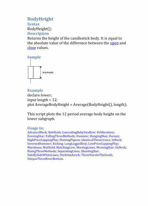
BodyHeight Syntax BodyHeight(); Description Returns the height of the candlestick body. It is equal to the absolute value of the difference between the open and close values. Sample

Example declare lower; input length = 12; plot AverageBodyHeight = Average(BodyHeight(), length); This script plots the 12 period average body height on the lower subgraph. Usage in: AdvanceBlock; BeltHold; ConcealingBabySwallow; Deliberation; EveningStar; FallingThreeMethods; Hammer; HangingMan; Harami; HighPriceGappingPlay; HomingPigeon; IdenticalThreeCrows; InNeck; InvertedHammer; Kicking; LongLeggedDoji; LowPriceGappingPlay; Marubozu; MatHold; MatchingLow; MeetingLines; MorningStar; OnNeck; RisingThreeMethods; SeparatingLines; ShootingStar; SideBySideWhiteLines; StickSandwich; ThreeStarsInTheSouth; UniqueThreeRiverBottom.

Ema2 initialization, so adding more initialization data by increasing additionalBars input has little impact on the study. Syntax Ema2(IDataHolder data, int prefetch, double smoothing factor, int First Bar); Default values: • prefetch: 0 • First Bar: 0

Description Returns the Exponential Moving Average (EMA) of data with smoothing factor. The prefetch parameter controls the number of historical data points used to initialize EMA for the first bar. The First Bar parameter is deprecated and should not be used. Example input additionalBars = 0; plot ExpAvg = Ema2(close, additionalBars, 0.2); The code plots the exponential average of a security Close price with a smoothing factor of 0.2. Note that studies using ema2 fetch a necessary number of additional bars for correct

ExpAverage Syntax ExpAverage(IDataHolder data, int length); Default values: • length: 12

Description Returns the Exponential Moving Average (EMA) of data with length. Example input price = close; input length = 12; plot ExpAvg = ExpAverage(price, length); The example plots an exponential moving average of a security's Close price. Usage in: ATRTrailingStop; BalanceOfMarketPower; BollingerBandsEMA; ChaikinOsc; ChaikinOscillator; DEMA; DisparityIndex; DisplacedEMA; DoubleSmoothedStochastics; EMAEnvelope; ElderRay; ElderRayBearPower; ElderRayBullPower; ForceIndex; KeltnerChannels; KlingerOscillator; MACD; MassIndex; MovAvgExpRibbon; MovAvgExponential; MovAvgTwoLines; MovingAvgCrossover; PolarizedFractalEfficiency; PriceAverageCrossover; PriceZoneOscillator; PriceZoneOscillatorLE; PriceZoneOscillatorLX; PriceZoneOscillatorSE; PriceZoneOscillatorSX; RSI_EMA; RangeIndicator; RelativeMomentumIndex; RelativeVolatilityIndex; ReverseEngineeringRSI; StochasticFull; StochasticMomentumIndex; TEMA; TRIX; TrendPeriods; TrueStrengthIndex; VolumeFlowIndicator; VolumeWeightedMACD; VolumeZoneOscillator; WoodiesCCI.

FastKCustom Syntax FastKCustom(IDataHolder data, int length); Default values: • length: 14

Description Returns values from 0 through 100 depending on a price. If the price is the lowest for the last length bars then 0 is returned. If the price is the highest for the last length bars then 100 is returned. The function is calculated according to the following algorithm: FastKCustom = if highest(close, 12) - lowest(close, 12) > 0 then (close - lowest(close, 12)) / (highest(close, 12) - lowest(close, 12))*100 else 0 Example declare lower; input colorNormLength = 14; plot Price = close; def abs = AbsValue(Price); def normVal = FastKCustom(abs, colorNormLength); Price.AssignValueColor( CreateColor(255, 2.55 * normVal, 0) ); The example plots the EMA using the manual thinkScript implementation and the built-in function. The resulting plots coincide forming a single curve. The FastKCustom function is used to assign a normVal value to each bar depending on its price. Zero value is assigned if the current closing price is the lowest on the last 14 bars, 100 is assigned if the current closing price is the highest on the last 14 bars. The normVal is used in the AssignValueColor function to paint a plot with colors ranging from red (255, 0,0) to yellow (255, 255, 0). The green component of the color varies depending on the current value of normVal.

GetMaxValueOffset Syntax GetMaxValueOffset(IDataHolder data, int length); Default values: • length: 25

Description Returns the offset of the highest value of data for the last length bars. Example declare lower; input length = 25; def upIndex = GetMaxValueOffset(high, length); def downIndex = GetMinValueOffset(low, length); plot AroonUp = (length - upIndex) * 100.0 / length; plot AroonDown = (length - downIndex) * 100.0 / length; The example calculates the Aroon Indicator. The GetMaxValueOffset is used to calculate the upIndex variable that defines the number of bars appeared starting from the maximum value for the last length bars. When drawing the AroonUp, the upIndex is recorded as a percentage from the overall number of length bars. Usage in: AroonIndicator; AroonOscillator; LookUpHighest.

GetMinValueOffset Syntax GetMinValueOffset(IDataHolder data, int length); Default values: • length: 25

Description Returns the offset of the lowest value of data for the last length bars. Example declare lower; input length = 25; def upIndex = GetMaxValueOffset(high, length); def downIndex = GetMinValueOffset(low, length); plot AroonOsc = (downIndex - upIndex) * 100.0 / length; The example calculates the Aroon Oscillator. The GetMinValueOffset is used to calculate the downIndex variable that defines the number of bars appeared starting from the minimum value for the last length bars. Then the downIndex value and the upIndex values are used to draw the resulting AroonOsc plot. Usage in: AroonIndicator; AroonOscillator; LookUpLowest.

Highest Syntax Highest(IDataHolder data, int length); Default values: • length: 12

Description Returns the highest value of data for the last length bars. Example input length = 20; plot LowerBand = Lowest(low[1], length); plot UpperBand = Highest(high[1], length); plot MiddleBand = (LowerBand + UpperBand) / 2; The plots in the example illustrate the Donchian Channels system where the Lower Band and the Upper Band are calculated as the minimum low and maximum high for the previous length bars. Note that the low and high for the current bar are left out of account. In order to implement this approach the [1] index is applied to the corresponding parameters. Usage in: BollingerBandwidth; DailyHighLow; DemandIndex; FisherTransform; HighPriceGappingPlay; Ichimoku; KeyRevLX; LBR_PaintBars; LowPriceGappingPlay; PercentR; PriceChannel; RangeIndicator; StochasticFull; StochasticMomentumIndex; VerticalHorizontalFilter; WilliamsPercentR.

HighestAll Syntax HighestAll(IDataHolder data); Description Returns the highest value of data for all bars in the chart. Example input price = close; plot MiddleLR = InertiaAll(price); def dist = HighestAll(AbsValue(MiddleLR - price)); plot UpperLR = MiddleLR + dist; plot LowerLR = MiddleLR - dist; The code draws a regression channel where the highest and the lowest borders are defined with the help of the maximum deviation between the price and regression line. The deviation is calculated for all bars using the HighestAll function. Usage in: DarvasBox; LinearRegCh100; LinearRegCh50; LinearRegChVar; MajorGannLevels; SemiCupFormation; ZigZagPercent; ZigZagSign.

HighestWeighted Syntax HighestWeighted(IDataHolder data, int length, IDataHolder coefficient); Default values: • length: 14

Description Returns the highest value of data weighted with the coefficient for the last length bars. Example declare lower; input price1 = close; input price2 = open; def delta = price2 - price1; plot HWBuiltin = HighestWeighted(price1, 3, delta); plot HW = Max(Max(price1, price1[1] + delta), price1[2] + 2 * delta); This example shows how the HighestWeighted is constructed by taking maximum of several values. The two plots coincide. Usage in: ProjectionBands; ProjectionOscillator.

IsAscending Syntax IsAscending(IDataHolder value, int length); Default values: • length: 3

Description Tests if the trend is ascending by calculating the average slope coefficient of trendlines whose start points are MidBodyVal for a specified number of bars and end points are value for current bar. If the slope is positive then the trend is considered ascending. Example AssignPriceColor(if IsAscending(close, 10) then Color.GREEN else Color.RED); This example paints price bars in green color if the closing price in comparison to the MidBodyVal for the last 10 bars is considered ascending and in red color otherwise. Usage in: AbandonedBaby; AdvanceBlock; BeltHold; Breakaway; DarkCloudCover; Deliberation; Engulfing; EveningDojiStar; EveningStar; HangingMan; Harami; HaramiCross; HighPriceGappingPlay; IdenticalThreeCrows; LongLeggedDoji; MatHold; MeetingLines; RisingThreeMethods; SeparatingLines; ShootingStar; SideBySideWhiteLines; ThreeBlackCrows; ThreeLineStrike; TriStar; TwoCrows; UpsideGapThreeMethods; UpsideGapTwoCrows; UpsideTasukiGap.

IsDescending Syntax IsDescending(IDataHolder value, int length); Default values: • length: 3

Description Tests if the trend is descending by calculating the average slope coefficient of trendlines whose start points are MidBodyVal for a specified number of bars and end points are value for current bar. If the slope is negative then the trend is considered descending. Example plot DescBar = IsDescending(close, 10); DescBar.SetPaintingStrategy(PaintingStrategy.BOOLEAN_POINTS); This example draws points at the closing prices for all bars considered as descending in comparison to the MidBodyValfor the last 10 bars. Usage in: AbandonedBaby; BeltHold; Breakaway; ConcealingBabySwallow; DownsideGapThreeMethods; DownsideTasukiGap; Engulfing; FallingThreeMethods; Hammer; Harami; HaramiCross; HomingPigeon; InNeck; InvertedHammer; LongLeggedDoji; LowPriceGappingPlay; MatchingLow; MeetingLines; MorningDojiStar; MorningStar; OnNeck; PiercingLine; SeparatingLines; SideBySideWhiteLines; StickSandwich; ThreeLineStrike; ThreeStarsInTheSouth; ThreeWhiteSoldiers; Thrusting; TriStar.

IsDoji Syntax IsDoji(int length, double bodyFactor); Default values: • length: 20 • bodyFactor: 0.05

Description Returns true if the current candle is Doji (i.e. its Close price and Open price are equal or almost the same) and false otherwise. Note that a candle is considered Doji if its body height does not exceed average body height multiplied by the specified factor. The average body height is calculated for a specified number of preceding candles. Example input length = 25; def IsDoji = IsDoji(length); plot ThreeDoji = IsDoji[2] and IsDoji[1] and IsDoji; ThreeDoji.SetPaintingStrategy(PaintingStrategy.BOOLEAN_POINTS); This example marks the last of three consecutive Doji candles. In this case, a candle will be considered Doji if its body height does not exceed 5% (default value) of the average body height calculated for last 25 candles. Usage in: AbandonedBaby; Doji; Engulfing; EveningDojiStar; HaramiCross; LongLeggedDoji; MorningDojiStar; TriStar.

IsLongBlack Syntax IsLongBlack(int length); Default values: • length: 20

Description Returns true for the current candle if: • Its Close price is lower than the Open price; • Its body is longer than each shadow; • Its body is longer than the average body size

calculated for the specified number of preceding candles.

Example input length = 20; def IsLongBlack = isLongBlack(length); plot TwoLongBlack = IsLongBlack[1] and IsLongBlack; TwoLongBlack.SetPaintingStrategy(PaintingStrategy.BOOLEAN_ARROW_DOWN); This example draws an arrow marking the last of two consecutive long bearish candles. Usage in: AbandonedBaby; BeltHold; Breakaway; DownsideGapThreeMethods; FallingThreeMethods; Harami; HaramiCross; HomingPigeon; IdenticalThreeCrows; InNeck; LowPriceGappingPlay; Marubozu; MatchingLow; MeetingLines; MorningDojiStar; MorningStar; OnNeck; PiercingLine; SeparatingLines; ThreeBlackCrows; ThreeLineStrike; ThreeStarsInTheSouth.

IsLongWhite Syntax IsLongWhite(int length); Default values: • length: 20

Description Returns true for the current candle if: • Its Close price is higher than the Open price; • Its body is longer than each shadow; • Its body is longer than the average body size

calculated for the specified number of preceding candles.

Example input length = 20; def IsLongWhite = isLongWhite(length); plot TwoLongWhite = IsLongWhite[1] and IsLongWhite; TwoLongWhite.SetPaintingStrategy(PaintingStrategy.BOOLEAN_ARROW_UP); This example draws an arrow marking the last of two consecutive long bullish candles. Usage in: AbandonedBaby; BeltHold; Breakaway; DarkCloudCover; Deliberation; EveningDojiStar; EveningStar; Harami; HaramiCross; HighPriceGappingPlay; Marubozu; MatHold; MeetingLines; RisingThreeMethods; SeparatingLines; ThreeLineStrike; ThreeWhiteSoldiers; TwoCrows; UpsideGapThreeMethods; UpsideGapTwoCrows.

Lowest Syntax Lowest(IDataHolder data, int length); Default values: • length: 12

Description Returns the lowest value of data for the last length bars. Example declare lower; input length = 10; def HH = Highest(high, length); def LL = Lowest(low, length); plot "Williams %R" = if HH == LL then -100 else (HH - close) / (HH - LL) * (-100); The example shows the Williams %R calculation. In particular, it is required to define the minimum low for the last length bars including the current bar. Therefore, to define the minimum, the example uses the Lowest function. Usage in: BollingerBandwidth; DailyHighLow; DemandIndex; FisherTransform; HighPriceGappingPlay; Ichimoku; KeyRevLE; LBR_PaintBars; LowPriceGappingPlay; PercentR; PriceChannel; RangeIndicator; StochasticFull; StochasticMomentumIndex; VerticalHorizontalFilter; WilliamsPercentR.

LowestAll Syntax LowestAll(IDataHolder data); Description Returns the lowest value of data for all bars in the chart. Example def HH = HighestAll(high); def LL = LowestAll(low); plot G1 = HH / 2; plot G2 = (HH + LL) / 2; plot G3 = HH / 4; plot G4 = (HH - LL) / 4 + LL; The example shows the Major Gann Levels which uses all chart bars to calculate the maximum high and minimum low values. Usage in: MajorGannLevels; ZigZagPercent; ZigZagSign.

LowestWeighted Syntax LowestWeighted(IDataHolder data, int length, IDataHolder coefficient); Default values: • length: 14

Description Returns the lowest value of data weighted with the coefficient for the last length bars. Example declare lower; input price1 = close; input price2 = open; def delta = price2 - price1; plot LWBuiltin = LowestWeighted(price1, 3, delta); plot LW = Min(Min(price1, price1[1] + delta), price1[2] + 2 * delta); This example shows how the LowestWeighted is constructed by taking minimum of several values. The two plots coincide. Usage in: ProjectionBands; ProjectionOscillator.

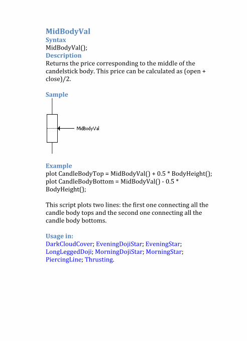
MidBodyVal Syntax MidBodyVal(); Description Returns the price corresponding to the middle of the candelstick body. This price can be calculated as (open + close)/2. Sample

Example plot CandleBodyTop = MidBodyVal() + 0.5 * BodyHeight(); plot CandleBodyBottom = MidBodyVal() - 0.5 * BodyHeight(); This script plots two lines: the first one connecting all the candle body tops and the second one connecting all the candle body bottoms. Usage in: DarkCloudCover; EveningDojiStar; EveningStar; LongLeggedDoji; MorningDojiStar; MorningStar; PiercingLine; Thrusting.

moneyflow Syntax moneyflow(IDataHolder high, IDataHolder close, IDataHolder low, IDataHolder volume, int length); Default values: • length: 12

Description Returns the money flow value. Example script moneyflowTS { input high = high; input close = close; input low = low; input volume = volume; input length = 14; def price = high + close + low; def moneyFlow = price * volume; def positiveMoneyFlow = sum(if price >price[1] then moneyFlow else 0, length); def totalMoneyFlow = sum(moneyFlow, length); plot moneyflowTS = if totalMoneyFlow != 0 then 100 * positiveMoneyFlow / totalMoneyFlow else 0; } declare lower; input length = 14; plot moneyflow1 = moneyflow(high, close, low, volume, length); plot moneyflow2 = moneyflowTS(high, close, low, volume, length); In this example the money flow is calculated and plotted based on two different implementations that have equal results. The first implementation is based on the moneflowTS function, the second one is based on the built-in moneyflow function. Usage in: MoneyFlowIndex.

TrueRange Syntax TrueRange(IDataHolder high, IDataHolder close, IDataHolder low); Description Returns the true range (TR). TR is the greatest of the following: • the difference between the current high and current

low • the difference between the current high and previous

close • the difference between the previous close and current

low

Example script TrueRangeTS { input high = high; input close = close; input low = low; plot TrueRangeTS = max(close[1], high) - min(close[1], low); } plot TrueRange1 = TrueRange(high, close, low); plot TrueRange2 = TrueRangeTS(high, close, low); The example plots the TR using the manual thinkScript implementation and the built-in function. The resulting plots coincide forming a single curve. Usage in: ATRWilder; AverageTrueRange; CSI; DMI; RandomWalkIndex; RangeIndicator; STARCBands; TrueRangeIndicator; TrueRangeSpecifiedVolume; UltimateOscillator; VortexIndicator.

Ulcer Syntax Ulcer(IDataHolder data, int length); Default values: • length: 14

Description Returns the Ulcer Index of data for the last length bars. Example declare lower; input length = 100; input risk_free_rate = 0.01; def somedate = 20000101; def growth = close - close[length]; def days = daysFromDate(somedate) - daysFromDate(somedate)[length]; def annualreturn = growth / close[length] * 365 / days; plot MartinRatio = (annualreturn - risk_free_rate) * 100 / Ulcer(close, length); This example calculates the Martin Ratio for an instrument. Usage in: UlcerIndex.

WildersAverage Syntax WildersAverage(IDataHolder data, int length); Default values: • length: 12

Description Returns the Wilder's Moving Average of data with smoothing factor that equals 1 / length. The first value is calculated as the simple moving average and then all values are calculated as the exponential moving average. Example input length = 10; plot WildersAvg = WildersAverage(close, length); plot ExpAvg = Ema2(close, 0, 1 / length); This code draws two plots: the first is a Wilder's average of the Close price, and the second is the exponential moving average with the corresponding smoothing factor. The two plots differ to a certain extent due to variance in initialization. Usage in: ATRWilder; BalanceOfMarketPower; CSI; DMI; MovingAvgCrossover; PriceAverageCrossover; RSIWilder; ReverseEngineeringRSI; WildersSmoothing.

wma Syntax wma(IDataHolder data, int length); Default values: • length: 9

Description Returns the Weighted Moving Average value. The Weighted Moving Average is calculated by multiplying each of the previous days' data by a weight factor. That factor is equal to the number of days past the first day. The total is then divided by the sum of the factors. Example plot WMA = wma(close, 20); The example displays the weighted moving average for the last 20 closing prices. Usage in: BalanceOfMarketPower; HullMovingAvg; LinearRegressionSlope; MovAvgWeighted; MovingAvgCrossover; PriceAverageCrossover; RSquared; TrueStrengthIndex.

o Mathematical and Trigonometrical As appears from the section title, this section collects mathematical and trigonometrical functions. Besides traditional functions such as sine, cosine, or logarithm the section also contains some more specific ones. For example, it has the isNaN function that defines if a parameter is a number, or the round function that rounds a value to a certain number of digits. • AbsValue • ACos • ASin • ATan • Ceil • Cos • Crosses • exp • Floor • isInfinite • IsNaN • lg • log • Max • Min • Power • Random • round • roundDown • roundUp • Sign • Sin • Sqr • Sqrt • sum • Tan • TotalSum

AbsValue Syntax AbsValue(double value); Description Returns the absolute value of an argument. If the argument is positive, the argument is returned. If the argument is negative, the negation of the argument is returned. Example declare lower; plot Absolute = AbsValue(open - close); The example plots the absolute value of difference between the open and close price which can be either positive, or negative. Usage in: AdvanceDecline; BeltHold; DMI; DemandIndex; DynamicMomentumIndex; IdenticalThreeCrows; KlingerOscillator; LinearRegCh100; LinearRegCh50; LinearRegChVar; MESASineWave; MatchingLow; MeetingLines; MovAvgAdaptive; OnNeck; RSIWilder; RSI_EMA; RangeExpansionIndex; SemiCupFormation; SeparatingLines; SideBySideWhiteLines; StickSandwich; SwingIndex; TrendNoiseBalance; TrendQuality; TrueStrengthIndex; VariableMA; VerticalHorizontalFilter; VortexIndicator; WoodiesCCI; ZigZagPercent; ZigZagSign.

ACos Syntax ACos(double value); Description Returns the arc cosine of an angle in the range from 0 through pi. Example declare lower; plot Data = Acos(0.5) == Double.Pi / 3; The expression in the second line of code compares two values and draws a plot. If the two values are equal, it draws the unit (true) plot . Otherwise, it draws the zero (false) plot. The arc cosine of 0.5 equals pi/3. So the example draws the unit plot.

ASin Syntax ASin(double value); Description Returns the arc sine of an angle in the range from -pi/2 through pi/2. Example 1 declare lower; plot Data = Asin(0.5) == Double.Pi / 3; Similar to the ACos example, the code above compares two values and draws the unit (true) plot if they are equal. In case the values are not equal, the zero (false) plot is drawn. The arc sine of 0.5 is not equal pi/3. The example draws the zero plot. Example 2 declare lower; input length = 3; def height = close - close[length]; def hypotenuse = sqrt( sqr(length) + sqr(height) ); plot "Angle, deg" = Asin(height/hypotenuse) * 180 / Double.Pi; The code draws a line that connects the current close value with the close value on the desired bar in the past. The Asin function is used to calculate the angle of slope of the line.

ATan Syntax ATan(double value); Description Returns the arc tangent of an angle in the range of -pi/2 through pi/2. Example declare lower; input length = 3; def avg = Average(close, length); def height = avg - avg[length]; plot "Angle, deg" = Atan(height/length) * 180 / Double.Pi; The code calculates the angle of slope of the simple moving average with the given length. The angle itself is calculated using the ATan function. Usage in: MESASineWave; WoodiesCCI.

Ceil Syntax Ceil(double value); Description Rounds a value up to the nearest integer (which is not less than the value). Example plot data = ceil(close); The example returns the integer that is equal to or next higher than the close price. Usage in: DynamicMomentumIndex; HullMovingAvg; MovAvgTriangular.

Cos Syntax Cos(double angle); Description Returns the trigonometric cosine of an angle. Example declare lower; input a = 0; input b = 10; input periodBars = 20; def w = 2 * Double.Pi / periodBars; rec x = compoundValue(1, x[1] + 1, 0); plot F = a + b * Cos(w * x); The code draws the cosine function depending on a variable which starts from one and increments by one on each bar. The cyclic frequency(w) is calculated based on the periodBars input. Usage in: MESASineWave.

Crosses Syntax Crosses(IDataHolder data1, IDataHolder data2, double direction); Default values: • direction: CrossingDirection.Any

Description The Crosses function tests if data1 gets higher or lower than data2. It returns true when data1 becomes greater than data2 if the direction parameter is CrossingDirection.Above. Conversely, the function returns true when data1 becomes less than data2 if the direction parameter is CrossingDirection.Below. The function can also indicate a crossover irrespective of its direction if the direction parameter is CrossingDirection.Any. Example 1 plot avg = Average(close, 10); plot crossing1 = close > avg and close[1] <= avg[1]; plot crossing2 = Crosses(close, avg, CrossingDirection.Above); crossing1.SetPaintingStrategy(PaintingStrategy.BOOLEAN_ARROW_UP); crossing2.SetPaintingStrategy(PaintingStrategy.BOOLEAN_ARROW_DOWN); The crossing1 and crossing2 variables are equal definitions of a condition when the Close price crosses the simple moving average with the length equal to 10. In other words, the Crosses function serves as a more compact and flexible way of defining intersections.

Example 2 input crossingType = {default above, below}; def avg = Average(close, 10); plot Crossing = Crosses(close, avg, crossingType == CrossingType.above); Crossing.SetPaintingStrategy(if crossingType == CrossingType.above then PaintingStrategy.BOOLEAN_ARROW_UP else PaintingStrategy.BOOLEAN_ARROW_DOWN, yes); The example first determines the crossing type of the Close price and the simple moving average for the last 10 bars. Depending on whether the crossing is up or down, the code draws either the arrow up or arrow down mark below and above the corresponding bars. Note that above and below here are enumeration constants. Usage in: ADXCrossover; ATRTrailingStop; BollingerBandsCrossover; MACDHistogramCrossover; MomentumCrossover; MoneyFlowIndexCrossover; MovingAvgCrossover; ParabolicSARCrossover; PriceAverageCrossover; RSIWilderCrossover; RateOfChangeCrossover; StochasticCrossover; WoodiesCCI.

exp Syntax exp(double number); Description Returns the exponential value of a number. Example 1 declare lower; input x = 3; plot Calculate1 = exp(x); plot Calculate2 = power(Double.E, x); The example calculates the value of the exponent raised to the power of x using two different approaches. The results of the calculations are equal. Example 2 declare lower; def temp = 0.1 * (RSIWilder() - 50); def x = wma(temp, 9); plot IFT_RSI = (exp(2 * x) - 1) / (exp(2 * x) + 1); The code plots the Inversed Fisher Transform indicator based on the smoothed RSI value. Initially, the code subtracts the standart RSIWilder by 50 and multiplies the result by 0.1 to get values starting from -5 and through 5. Then it smoothes the values using the wma function. Finally, it calculates the IFT for the values. Usage in: DemandIndex; SemiCupFormation.

Floor Syntax Floor(double value); Description Rounds a value down to the nearest integer (which is not greater than the value). Example plot Lower = Floor(low); plot Upper = Ceil(high); This example draws a channel at integer levels which fits high and low prices. Usage in: DynamicMomentumIndex; MonkeyBars; MonkeyBarsExpanded; SeriesCount; TPOProfile; VWAP; VolumeProfile.

isInfinite Syntax isInfinite(double value); Description Returns true if the specified number is infinitely large in magnitude. Example 1 declare lower; input dividend = 10; input divisor = 0; def tempResult = dividend / divisor; plot Result = if isInfinite(tempResult) then 0 else tempResult; The example draws the result of division the dividend by the divisor on a separate subgraph. If the divisor is equal to zero then the division produces the infine number. The isInfinite returns true as a result of verifying the infinite number and the result is assigned 0. Example 2 declare lower; input dividend = 10; input divisor = 0; plot Result = if divisor == 0 then 0 else dividend / divisor; This example is similar to the previous one. But here the validation is performed before the division which makes the code simplier.

IsNaN Syntax IsNaN(double value); Description Returns true if the specified parameter is not a number, returns false otherwise. Example 1 def onExpansion = if IsNaN(close) then yes else no; plot HighestClose = if onExpansion then HighestAll(close) else double.NaN; plot LowestClose = if onExpansion then LowestAll(close) else double.NaN; The example draws the highest close and open on the right expansion of the subgraph. For more information about the expansion chart, see thinkDesktop User Manual. Example 2 declare lower; input symbol = "IBM"; def closeSymbol = close(symbol); rec closeSymbolWithOutNaN = CompoundValue(1, if IsNaN(closeSymbol) then closeSymbolWithOutNan[1] else closeSymbol, closeSymbol); plot Data = closeSymbolWithOutNaN; The code draws the comparison close chart replacing gaps containing no data with lines. If the plot contains the NaN value then the last available non-NaN value is used. Usage in: ATRTrailingStop; AdvanceDecline; CumulativeVolumeIndex; DailyHighLow; DailyOpen; DailySMA; DarvasBox; DemandIndex; DynamicMomentumIndex; FisherTransform; McClellanOscillator; McClellanSummationIndex; MonkeyBars; Next3rdFriday; PersonsPivots; RelativeStrength; SemiCupFormation; SpectrumBarsLE; TPOProfile; ThreeBarInsideBarLE; ThreeBarInsideBarSE; TrailingStopLX; TrailingStopSX; TrendNoiseBalance; TrendQuality; VariableMA; VolumeProfile; WoodiesCCI; WoodiesPivots; ZigZagPercent; ZigZagSign; ZigZagTrendPercent; ZigZagTrendSign.

lg Syntax lg(double number); Description Returns the base-10 logarithm of an argument. Example declare lower; plot data = lg(close); The example draws the base-10 logarithm plot of the close values. Usage in: DynamicMomentumIndex. log Syntax log(double number); Description Returns the natural logarithm of an argument. Example declare lower; plot data = log(close); The code draws the plot of the logarithm of the closing price of a stock. Usage in: FisherTransform; HistoricalVolatility; SemiCupFormation; SeriesCount; TRIX; VolatilityStdDev; VolumeFlowIndicator.

Max Syntax Max(double value1, double value2); Description Returns the greater of two values. Example def SMA = SimpleMovingAvg(); plot data = Max(close, SMA); This example displays the higher value of either the closing price or the simple moving average. Usage in: ATRTrailingStop; AccumDistBuyPr; BeltHold; BollingerBandsLE; DynamicMomentumIndex; Engulfing; Hammer; HangingMan; Harami; HaramiCross; InvertedHammer; LongLeggedDoji; MarkerIndicator; MomentumLE; ParabolicSAR; RandomWalkIndex; RangeExpansionIndex; RelativeMomentumIndex; ReverseEngineeringRSI; SemiCupFormation; ShootingStar; SwingIndex; TrailingStopLX; VWAP; ZigZagPercent; ZigZagSign; ZigZagTrendPercent; ZigZagTrendSign.

Min Syntax Min(double value1, double value2); Description Returns the smaller of two values. Example plot data = Min(close, open); The code draws the smaller value of the close and open values. Usage in: ATRTrailingStop; AccumDistBuyPr; BeltHold; BollingerBandsSE; Deliberation; DemandIndex; Engulfing; Hammer; HangingMan; Harami; HaramiCross; InvertedHammer; LongLeggedDoji; MonkeyBars; MonkeyBarsExpanded; ParabolicSAR; RangeExpansionIndex; SemiCupFormation; ShootingStar; SwingIndex; TPOProfile; TrailingStopSX; UltimateOscillator; VoltyExpanCloseLX; VolumeFlowIndicator; VolumeProfile; ZigZagPercent; ZigZagSign; ZigZagTrendPercent; ZigZagTrendSign.

Power Syntax Power(double number, double power); Description Returns the value of the first argument raised to the power of the second argument. Example declare lower; plot Close1_5 = power(close, 1.5); The example draws the plot of the close value raised to the power of 1.5. Usage in: MovAvgExpRibbon; SemiCupFormation. Random Syntax Random(); Description Returns a value with a positive sign, greater than or equal to 0.0 and less than 1.0 Example declare lower; input limit = 10; plot Noise = Random() * limit; The code draws a plot of random values ranging from 0. to 10.

round Syntax round(double number, int numberOfDigits); Default values: • numberOfDigits: 2

Description Rounds a number to a certain number of digits. Example plot SMA = round(Average(close, 12) / tickSize(), 0) * tickSize(); This example script plots 12 period SMA rounded to the nearest tick size value. Usage in: AdvanceDecline; SemiCupFormation; WoodiesCCI. roundDown Syntax roundDown(double number, int numberOfDigits); Default values: • numberOfDigits: 2

Description Rounds a number towards zero to a certain number of digits. Example See the roundUp function example. Usage in: VWAP.

roundUp Syntax roundUp(double number, int numberOfDigits); Default values: • numberOfDigits: 2

Description Rounds a number up to a certain number of digits. Example input price = close; input digits = 0; plot ceiling = roundup(price, digits); plot floor = rounddown(price, digits); This example plots bands representing a price of the instrument rounded up and down to a certain number of digits.

Sign Syntax Sign(double number); Description Returns the algebraic sign of a number: 1 if the number is positive, 0 if zero and -1 if negative. Example 1 declare lower; plot Trend = sign( ExpAverage(close, 15) - ExpAverage(close, 30) ); The example draws a plot showing the current trend as 1(bullish), 0(neutral), or -1(bearish) values depending on the difference between two EMAs. Example 2 declare lower; plot Data = Average(Sign(close - close[1]) * (high - low), 15); The example draws the average range for 15 bars considering the closing price change as compared to the previous bar. Usage in: MESASineWave; PriceZoneOscillator; TrendPeriods; VolumeZoneOscillator.

Sin Syntax Sin(double angle); Description Returns the trigonometric sine of an angle. Example declare lower; input a = 0; input b = 10; input periodBars = 20; def w = 2 * Double.Pi / periodBars; rec x = compoundValue(1, x[1] + 1, 0); plot F = a + b * Sin(w * x); The code draws the sine function depending on the variable which starts from one and increments by one on each bar. The cyclic frequency(w) is calculated based on the periodBars constant. Usage in: MESASineWave.

Sqr Syntax Sqr(double value); Description Calculates the square of an argument. Example declare lower; plot Data = Sqr(stdev(close, 10)); The example draws the variance of close for the last 10 bars. Variance by definition is a square of the standard deviation. Usage in: Beta; Beta2; CyberCyclesOscillator; MovAvgAdaptive; PolarizedFractalEfficiency; RSquared; VWAP. Sqrt Syntax Sqrt(double value); Description Calculates the square root of an argument. Example declare lower; plot data = Sqrt(close); The draws the plot of the square root of the closing price of a stock. Usage in: CSI; HistoricalVolatility; HullMovingAvg; PolarizedFractalEfficiency; PolychromMtm; RandomWalkIndex; SeriesCount; TrendNoiseBalance; TrendQuality; VWAP; VolatilityStdDev; WoodiesCCI.

sum Syntax sum(IDataHolder data, int length); Default values: • length: 12

Description Returns the sum of values for the specified number of bars. The default value of length is 12. Example 1 declare lower; plot data = sum(close, 20); The example displays a line that is the sum of the last 20 days' closing prices. Example 2 plot data = sum(close, 20)/20; This example returns the sum of the last 20 days' closing prices divided by 20. This value is called 20 day moving average. Usage in: Alpha2; AlphaJensen; ChaikinMoneyFlow; ChandeMomentumOscillator; EhlersDistantCoefficientFilter; MassIndex; MovAvgAdaptive; PolarizedFractalEfficiency; RangeExpansionIndex; UltimateOscillator; VariableMA; VerticalHorizontalFilter; VolumeFlowIndicator; VolumeWeightedMACD; VortexIndicator.

Tan Syntax Tan(double angle); Description Returns the trigonometric tangent of an angle. Example declare lower; input length = 5; input min = 30; input max = 90; plot CheckingTangentHit = between((close - close[length]) / length, Tan(min * double.Pi / 180), Tan(max * double.Pi / 180)); The code checks if the tangle of the closing price angle of slope is within the defined limits.

TotalSum Syntax TotalSum(IDataHolder data); Description Returns the sum of all values from the first bar to the current. Example declare lower; plot data = TotalSum(volume); The example returns the total accumulated volume for the time frame of the current chart. Usage in: AccDist; AccumDistBuyPr; AccumulationSwingIndex; CumulativeVolumeIndex; DarvasBox; McClellanSummationIndex; MoneyFlow; OnBalanceVolume; PriceAndVolumeTrend; TradeVolumeIndex.

o Statistical Statistics is the area that closely relates to trading analysis. For this reason the thinkscript also includes statistical functions. If you lack for the general understanding of functions from the section, refer to the General Information sub-section featured in the articles. In order to provide a better understanding, the section also contains formulas for the functions. Here is the full list of the statistical functions: • correlation • covariance • Inertia • InertiaAll • lindev • stdev • stdevAll • sterr • sterrAll

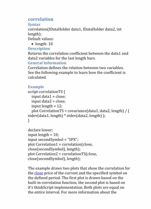
correlation Syntax correlation(IDataHolder data1, IDataHolder data2, int length); Default values: • length: 10

Description Returns the correlation coefficient between the data1 and data2 variables for the last length bars. General Information Correlation defines the relation between two variables. See the following example to learn how the coefficient is calculated. Example script correlationTS { input data1 = close; input data2 = close; input length = 12; plot CorrelationTS = covariance(data1, data2, length) / ( stdev(data1, length) * stdev(data2, length) ); } declare lower; input length = 10; input secondSymbol = "SPX"; plot Correlation1 = correlation(close, close(secondSymbol), length); plot Correlation2 = correlationTS(close, close(secondSymbol), length); The example draws two plots that show the correlation for the close price of the current and the specified symbol on the defined period. The first plot is drawn based on the built-in correlation function, the second plot is based on it's thinkScript implementation. Both plots are equal on the entire interval. For more information about the

covariance function, see the covariance function in this section. Usage in: Correlation; PairCorrelation.

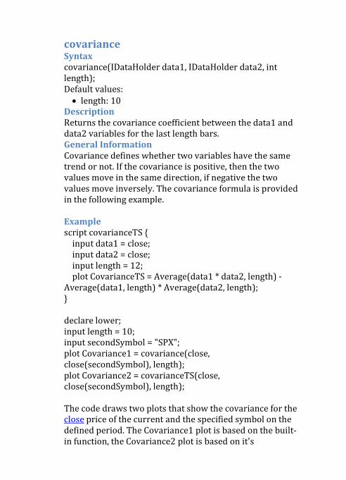
covariance Syntax covariance(IDataHolder data1, IDataHolder data2, int length); Default values: • length: 10

Description Returns the covariance coefficient between the data1 and data2 variables for the last length bars. General Information Covariance defines whether two variables have the same trend or not. If the covariance is positive, then the two values move in the same direction, if negative the two values move inversely. The covariance formula is provided in the following example. Example script covarianceTS { input data1 = close; input data2 = close; input length = 12; plot CovarianceTS = Average(data1 * data2, length) - Average(data1, length) * Average(data2, length); } declare lower; input length = 10; input secondSymbol = "SPX"; plot Covariance1 = covariance(close, close(secondSymbol), length); plot Covariance2 = covarianceTS(close, close(secondSymbol), length); The code draws two plots that show the covariance for the close price of the current and the specified symbol on the defined period. The Covariance1 plot is based on the built-in function, the Covariance2 plot is based on it's

thinkScript implementation. Both the plots coincide with each other forming a single plot. For more information about the Average function, see the Average function in the Tech Analysis section. Usage in: Beta; Beta2.

Inertia Syntax Inertia(IDataHolder data, int length); Description Draws the linear regression curve using the least-squares method to approximate data for each set of bars defined by the length parameter. The resulting interpolation function for each set of bars is defined by the y = a * current_bar + b equation. See the following example for details. Example script inertiaTS { input y = close; input n = 20; rec x = x[1] + 1; def a = (n * sum(x * y, n) - sum(x, n) * sum(y, n) ) / ( n * sum(Sqr(x), n) - Sqr(sum(x, n))); def b = (sum(Sqr(x), n) * sum(y, n) - sum(x, n) * sum(x * y, n) ) / ( n * sum(Sqr(x), n) - Sqr(sum(x, n))); plot InertiaTS = a * x + b; } input length = 20; plot LinReg1 = Inertia(close, length); plot LinReg2 = InertiaTS(close, length); Draws the linear regression plot for the close value for the defined set of bars. Usage in: ForecastOscillator; Inertia; LinearRegCurve; LinearRegrIndicator; LinearRegrReversal; StandardErrorBands; TimeSeriesForecast; WoodiesCCI.

InertiaAll Syntax InertiaAll(IDataHolder data, int length, int startDate, int startTime, double extendToLeft, double extendToRight); Default values: • length: all chart • startDate: 0 • startTime: 0 • extendToLeft: no • extendToRight: no

Description Draws the linear regression function either for the entire plot or for the interval defined by the length parameter. If you specify length, the approximation is applied only for the last length bars of the plot, otherwise the approximation is applied for the entire plot and it is calculated based on all bars from the plot. See the Inertia function for more information. The startDate (specified in the YYYYMMDD format) and startTime (specified in the HHMM format) define the date and time for the starting point of linear regression. These parameters override any value of the length if the startDate is non-zero. By default, the function will return Double.NaN at any moment in time outside the interval used for calculation of linear regression. This behavior can be changed by using non-zero values of extendToLeft and extendToRight parameters. Example input length = 20; plot MiddleLR = InertiaAll(close, length); The example draws the linear recession for the close value for the defined number of last bars. Usage in: LinearRegCh100; LinearRegCh50; LinearRegChVar; LinearRegTrendline; StandardDevChannel; StandardErrorChannel.

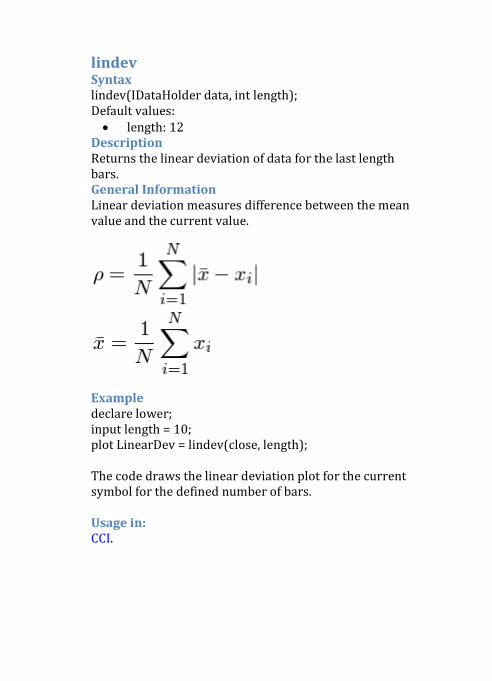
lindev Syntax lindev(IDataHolder data, int length); Default values: • length: 12

Description Returns the linear deviation of data for the last length bars. General Information Linear deviation measures difference between the mean value and the current value.

Example declare lower; input length = 10; plot LinearDev = lindev(close, length); The code draws the linear deviation plot for the current symbol for the defined number of bars. Usage in: CCI.

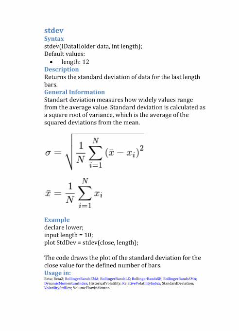
stdev Syntax stdev(IDataHolder data, int length); Default values: • length: 12

Description Returns the standard deviation of data for the last length bars. General Information Standart deviation measures how widely values range from the average value. Standard deviation is calculated as a square root of variance, which is the average of the squared deviations from the mean.

Example declare lower; input length = 10; plot StdDev = stdev(close, length); The code draws the plot of the standard deviation for the close value for the defined number of bars. Usage in: Beta; Beta2; BollingerBandsEMA; BollingerBandsLE; BollingerBandsSE; BollingerBandsSMA; DynamicMomentumIndex; HistoricalVolatility; RelativeVolatilityIndex; StandardDeviation; VolatilityStdDev; VolumeFlowIndicator.

stdevAll Syntax stdevAll(IDataHolder data, int length, int startDate, int startTime, double extendToLeft, double extendToRight); Default values: • length: all chart • startDate: 0 • startTime: 0 • extendToLeft: no • extendToRight: no

Description Returns the standard deviation of data for the entire plot or for the interval of the last bars defined by the length parameter. The difference of the function from the stdev function is that the output result for the last bar is used for the whole calculated interval. If the length parameter is not specified, the function is calculated for the entire plot. The startDate (specified in the YYYYMMDD format) and startTime (specified in the HHMM format) define the date and time for the starting point of linear regression. These parameters override any value of the length if the startDate is non-zero. By default, the function will return Double.NaN at any moment in time outside the interval used for calculation of linear regression. This behavior can be changed by using non-zero values of extendToLeft and extendToRight parameters. Example input price = close; def regression = InertiaAll(price, 30); def stdDeviation = stdevAll(price, 30); plot UpperLine = regression + stdDeviation; plot LowerLine = regression - stdDeviation;

The example draws the Standard Deviation Channel, which is the linear regression channel spaced by standard deviation. The deviation channel is based on price data for the last 30 bars. Usage in: StandardDevChannel.

sterr Syntax sterr(IDataHolder data, int length); Default values: • length: 12

Description Returns the standard error calculated for the last length bars from current bar. Returns the standard deviation between data and linear regression of data. Example declare lower; input length = 10; plot StdError = sterr(close, length); The example calculates the standard error of close values for the defined number of bars. Usage in: StandardError; StandardErrorBands.

sterrAll Syntax sterrAll(IDataHolder data, int length, int startDate, int startTime, double extendToLeft, double extendToRight); Default values: • length: all chart • startDate: 0 • startTime: 0 • extendToLeft: no • extendToRight: no

Description Returns the standard error of data around the regression line for the entire plot or for the interval of last bars defined by the length parameter. The difference of the function from the sterr function is that the output result for the last bar is used for the whole calculated interval. If the length parameter is not specified, the function is calculated for the entire plot. The startDate (specified in the YYYYMMDD format) and startTime (specified in the HHMM format) define the date and time for the starting point of linear regression. These parameters override any value of the length if the startDate is non-zero. By default, the function will return Double.NaN at any moment in time outside the interval used for calculation of linear regression. This behavior can be changed by using non-zero values of extendToLeft and extendToRight parameters. Example input price = close; def regression = InertiaAll(price); def stdError = sterrAll(price); plot UpperLine = regression + stdError; plot LowerLine = regression - stdError;

The example draws the Standard Error Channel which is the linear regression channel spaced by a standard error. The error channel is based on the price data for the last 30 bars. Usage in: StandardErrorChannel.

Date and Time During analysis you often work with quote historical data. For this reason you will find useful the date and time functions featured in this section. For example, with the help of the functions you can draw the close plot for the last three years or draw the open plot for the first half of each year. Here is the full list of the functions:

• countTradingDays • daysFromDate • daysTillDate • getDay • getDayOfMonth • getDayOfWeek • getLastDay • getLastMonth • getLastWeek • getLastYear • getMonth • getWeek • getYear • getYyyyMmDd • regularTradingEnd • regularTradingStart • secondsFromTime • secondsTillTime

countTradingDays Syntax countTradingDays(int fromDate, int toDate); Description Returns the number of trading days in the specified time period (including both starting and ending dates) for the current symbol. Note that fromDate and toDate parameters should be specified in the YYYYMMDD format. Example def yearstart = getYear() * 10000 + 101; AddChartLabel(yes, concat(countTradingDays(yearstart, getYyyyMmDd()), " trading days since year start")); This script displays a chart label indicating the number of trading days from the first day of the year to the current day for the chosen symbol. Usage in: MonkeyBars; MonkeyBarsExpanded; TPOProfile; VolumeProfile.

daysFromDate Syntax daysFromDate(IDataHolder fromDate); Description Returns the number of days from the specified date. Note that the fromDate argument is specified in the EST timezone and has the YYYYMMDD format. Example input BeginDate = 20090101; plot Price = if daysFromDate(BeginDate) >= 0 and daysFromDate(BeginDate) <= 50 then close else double.NaN; This example script draws the close plot for bars in the 50 days interval starting from BeginDate. Usage in: MonkeyBars; MonkeyBarsExpanded; SeriesCount; TPOProfile; VWAP; VolumeProfile.

daysTillDate Syntax daysTillDate(IDataHolder tillDate); Description Returns the number of days till the specified date. Note that the tillDate argument is specified in the EST timezone and has the YYYYMMDD format. Example input EndDate = 20090101; plot price = if daysTillDate(EndDate) >= 0 and daysTillDate(EndDate) <= 50 then close else double.NaN; The example draws the close plot for bars in the 50 days interval ending on EndDate. Usage in: Next3rdFriday. getDay Syntax getDay(); Description Returns the number of the current bar day in the CST timezone. The output is returned in the range from 1 through 365 (366 for leap years). Example plot Price = if getDay() <= 100 then close else Double.NaN; The code draws the close plot for the first 100 days of each year.

getDayOfMonth Syntax getDayOfMonth(int yyyyMmDd); Description Returns the day of a month based on the given YYYYMMDD parameter. Example input first_day = 10; input last_day = 20; plot Data = if getDayofMonth(getYyyyMmDd()) between first_day and last_day then close else double.NaN; Displays the close price only for days of month falling into a specified interval. Usage in: MonkeyBars; MonkeyBarsExpanded; Next3rdFriday; TPOProfile; VolumeProfile.

getDayOfWeek Syntax getDayOfWeek(int yyyyMmDd); Description Returns the day of week based on the given YYYYMMDD parameter. The return value ranges from from 1 (Monday) to 7 (Sunday). Example declare hide_on_intraday; input day_of_week = {default Monday, Tuesday, Wednesday, Thursday, Friday, Saturday, Sunday}; AddChartBubble(getDayofWeek(getYyyyMmDd()) == day_of_week + 1, high, "Here it is"); Displays bubbles with text for a certain day of week. Usage in: MonkeyBars; MonkeyBarsExpanded; Next3rdFriday; TPOProfile; VWAP; VolumeProfile. getLastDay Syntax getLastDay(); Description Returns the number of the last bar day in the CST timezone. The output is returned in the range from 1 through 365 (366 for leap years). Example plot Price = if getLastDay() == getDay() and getLastYear() == getYear() then close else Double.NaN; This example draws the close plot for the last bar day of the current year.

getLastMonth Syntax getLastMonth(); Description Returns the number of the last bar month in the CST timezone. The output is returned in the range from 1 through 12. Example 1 plot Price = if getLastMonth() == getMonth() and getLastYear() == getYear() then close else Double.NaN; The example draws the close plot for the last month of the current year. Example 2 plot Price = if getLastMonth() == getMonth() then open else Double.NaN; This code draws the open plot for the last month of each year.

getLastWeek Syntax getLastWeek(); Description Returns the number of the last bar week in the CST timezone. The output is returned in the range from 1 through 53. Example plot Price = if getLastWeek() == getWeek() and getLastYear() == getYear() then high else Double.NaN; This example draws the high plot for the last week of the current year. getLastYear Syntax getLastYear(); Description Returns the number of the last bar year in the CST timezone. Example plot Price = if getLastYear() == getYear() then close else Double.NaN; The code draws the close plot for the current year.

getMonth Syntax getMonth(); Description Returns the number of the current bar month in the CST timezone. The output is returned in the range from 1 through 12. Example plot Price = if getMonth() <= 6 then close else Double.NaN; The example draws the close plot for the first half of each year. Usage in: MonkeyBars; MonkeyBarsExpanded; Next3rdFriday; TPOProfile; VolumeProfile.

getWeek Syntax getWeek(); Description Returns the number of the current bar week in the CST timezone. The output is returned in the range from 1 through 53. Example plot Price = if getWeek() % 2 == 1 then close else Double.NaN; The example draws the close plot for odd weeks of each year. getYear Syntax getYear(); Description Returns the number of the current bar year in the CST timezone. Example plot Price = if getYear() > getLastYear() - 3 then open else Double.NaN; The example draws the close plot for the last three years. Usage in: MonkeyBars; MonkeyBarsExpanded; Next3rdFriday; TPOProfile; VolumeProfile.

getYyyyMmDd Syntax getYyyyMmDd(); Description Returns the date of the current bar in the YYYYMMDD format. This date corresponds to the day whose trading session contains the current bar. Note that on intraday charts, this date and the actual date might not be the same for Forex and Futures symbols. Example declare lower; input endDate = 20100101; def cond = getYyyyMmDd() < endDate; plot Price = if cond then close else Double.NaN; This example plots closing price only when the date of the current bar is less than the one specified in the endDate input. Usage in: MonkeyBars; MonkeyBarsExpanded; Next3rdFriday; TPOProfile; VWAP; VolumeProfile; WoodiesCCI.

regularTradingEnd Syntax regularTradingEnd(int yyyyMmDd); Description Returns the end of the regular trading hours for the current symbol on the trading day specified in the YYYYDDMM format. This value is the number of milliseconds since the epoch (January 1, 1970, 00:00:00 GMT). Example See the regularTradingStart function example. Usage in: WoodiesCCI.

regularTradingStart Syntax regularTradingStart(int yyyyMmDd); Description Returns the start of the regular trading hours for the current symbol on the trading day specified in the YYYYDDMM format. This value is the number of milliseconds since the epoch (January 1, 1970, 00:00:00 GMT). Example AddChartLabel(yes, concat("RTH duration (hrs): ", (regularTradingEnd(getYyyyMmDd()) - regularTradingStart(getYyyyMmDd())) / AggregationPeriod.HOUR)); This example script displays a chart label with duration of a regular trading session in hours. Usage in: WoodiesCCI.

secondsFromTime Syntax secondsFromTime(int fromTime); Description Returns the number of seconds from the specified time (24-hour clock notation) in the EST timezone. Note that this function always returns zero when chart's aggregation period is greater than or equal to 1 day. Example input OpenTime = 0930; input DurationHours = 1; def durationSec = DurationHours * 60 * 60; def secondsPassed = secondsFromTime(OpenTime); plot Price = if secondsPassed >= 0 and secondsPassed <= durationSec then close else double.NaN; The plot displays the close value based on the specified duration and the beginning in the EST timezone format. Usage in: MonkeyBars; MonkeyBarsExpanded; SeriesCount; TPOProfile; VolumeProfile.

secondsTillTime Syntax secondsTillTime(int tillTime); Description Returns the number of seconds till the specified time (24-hour clock notation) in the EST timezone. Note that this function always returns zero when chart's aggregation period is greater than or equal to 1 day. Example input CloseTime = 1600; input DurationHours = 1; def durationSec = DurationHours * 60 * 60; def secondsRemained = secondsTillTime(closeTime); plot Price = if secondsRemained >= 0 and secondsRemained <= durationSec then close else double.NaN; This example draws the close plot based on the defined duration and through the specified time in EST.

o Corporate Actions This section contains functions related to corporate actions. Here is the full list: • getActualEarnings • getDividend • getEstimatedEarnings • getSplitDenominator • getSplitNumerator • hasConferenceCall • hasEarnings

getActualEarnings Syntax getActualEarnings(); Description Returns actual earnings for the current symbol. Example 1 declare lower; rec AECont = if IsNaN(getActualEarnings()) then AECont [1] else getActualEarnings(); plot DilutedEarnings = if AECont <> 0 then AECont else Double.NaN; The example draws values of diluted earnings for the current symbol. Values between earnings are saved using the AECont rec. Example 2 declare lower; rec AE = if IsNaN(getActualEarnings()) then 0 else getActualEarnings(); plot EPS_TTM = sum(AE, 252); AddChartLabel(yes, concat("P/E Ratio: ", close / EPS_TTM)); The code draws values of diluted earnings for approximately twelve months. Also it shows the current Price-Earnings Ratio in the chart label. Note that this example works only for daily charts because it uses an assumption that there are 252 daily bars in a year.

getDividend Syntax getDividend(); Description Returns a dividend amount for the current symbol. Example 1 declare lower; rec DCont = if IsNaN(getDividend()) then DCont[1] else getDividend(); plot Dividend = if DCont <> 0 then DCont else Double.NaN; The example plots dividends for the current symbol on a separate subgraph. Values between different Ex-Dividend dates are saved using the DCont rec. Example 2 declare lower; rec DCont = if IsNaN(getDividend()) then DCont[1] else getDividend(); plot DivA = if DCont <> 0 then DCont * 4 else Double.NaN; AddChartLabel(yes, concat(DivA / close * 100, "% Yield"), DivA.takeValueColor()); The example draws the annual dividend plot (considering that dividends are quarterly and they remain on the same level through the year). Also the code in this example defines a chart label that indicates the calculated dividend yield value in percentage and draws it using the same color as the main plot.

getEstimatedEarnings Syntax getEstimatedEarnings(); Description Returns estimate earnings for the current symbol. Example declare lower; plot EstEarning = getEstimatedEarnings(); EstEarning.SetPaintingStrategy(PaintingStrategy.POINTS); The example draws estimated earnings for the current symbol as points on a separate subgraph. getSplitDenominator Syntax getSplitDenominator(); Description Returns the split denominator for the current symbol. Example AddVerticalLine(!IsNaN(getSplitDenominator()), if getSplitNumerator() > getSplitDenominator() then "Split!" else "Reverse Split!", Color.GRAY); The code draws a gray vertical line with the "Split!" or "Reverse Split!" label for days when a corresponding split took place. For more information, see the AddVerticalLine function.

getSplitNumerator Syntax getSplitNumerator(); Description Returns a split numerator for the current symbol. Example declare lower; input initialPosition = 100; rec position = CompoundValue(1, if !IsNaN(getSplitDenominator()) then position[1] * getSplitNumerator() / getSplitDenominator() else position[1], initialPosition); plot CurrentPosition = position; This example shows trader position changes taking into account the splits presented on the chart. hasConferenceCall Syntax hasConferenceCall(); Description Returns true if there is an earnings conference call, false - otherwise. Example plot ConfCall = hasConferenceCall(); ConfCall.SetPaintingStrategy(PaintingStrategy.BOOLEAN_POINTS); The code draws a dot based on the close price when the current symbol has a conference call. For more information, see the PaintingStrategy.BOOLEAN_POINTS constant.

hasEarnings Syntax hasEarnings(int type); Default values: • type: EarningTime.ANY

Description Returns true if there are announced earnings, and false otherwise. Use an EarningTime constant to specify the time of announcement. Example plot isBefore = hasEarnings(EarningTime.BEFORE_MARKET); plot isAfter = hasEarnings(EarningTime.AFTER_MARKET); plot isDuringOrUnspecified = hasEarnings() and !isBefore and !isAfter; isBefore.SetPaintingStrategy(PaintingStrategy.BOOLEAN_ARROW_UP); isAfter.SetPaintingStrategy(PaintingStrategy.BOOLEAN_ARROW_DOWN); isDuringOrUnspecified.SetPaintingStrategy(PaintingStrategy.BOOLEAN_POINTS); This example script marks announced earnings with an up arrow if they are expected before market open, down arrow if they are expected after market close, and a dot if they are expected during market trading hours or the time is not specified.

o Look and Feel The thinkscript enables you to adjust the look and feel of charts you analyse. Although the majority of these settings can be made through the application GUI, some of them can be done only with the help of the thinkscript. One of these functions is AddCloud that highlights the area between charts, or AssignNormGradientColor that paints a chart with a gradient. The full set of the functions is provided in the following list:

• AddChartBubble • AddChartLabel • AddCloud • AddVerticalLine • AssignBackgroundColor • AssignNormGradientColor • AssignPriceColor • AssignValueColor • color • CreateColor • DefineColor • DefineGlobalColor • EnableApproximation • GetColor • globalColor • hide • HideBubble • hidePricePlot • HideTitle • setChartType • SetDefaultColor • setHiding • SetLineWeight • SetPaintingStrategy • SetStyle • TakeValueColor

AddChartBubble Syntax AddChartBubble(boolean time condition, double price location, Any text, CustomColor color, boolean up); Default values: • color: Color.RED • up: yes

Description Adds a bubble with a text to the specified location. Bubbles are displayed next to bars for which the time condition is true. The tip of the bubble is at the point specified by the price location parameter. The text parameter defines the text to be displayed in the bubble. The color parameter defines the color of the bubble. The bubble will be displayed above the specified point if the up parameter is true and below the specified point if it is false. Example input timeFrame = {default DAY, "2 DAYS", "3 DAYS", "4 DAYS", WEEK, MONTH, "OPT EXP"}; AddChartBubble(high == high(period = timeFrame), high, concat("High of ", concat(timeFrame, concat(": ", high))), color.green, yes); AddChartBubble(low == low(period = timeFrame), low, concat("Low of ", concat(timeFrame, concat(": ", low))), color.red, no); This example shows bubbles with values and a description on the selected time frame extremums.

AddChartLabel Profile: Studies Syntax AddChartLabel(boolean visible, Any text, CustomColor color); Default values: • color: Color.RED

Description Adds a label with a text to the top-left graph corner. Example AddChartLabel(yes, concat("Last price is ", close)); Displays a label with the last price. Usage in: AdvanceDecline; Next3rdFriday; SemiCupFormation; WoodiesCCI.

AddCloud Profile: Studies Syntax AddCloud(IDataHolder data1, IDataHolder data2, CustomColor color1, CustomColor color2); Default values: • color1: Color.YELLOW • color2: Color.RED

Description Visualizes the difference between two values by filling the intermediate area with a translucent background. The sections where data1 value exceeds data2 value are assigned color1, otherwise color2 is used. The AddCloud function can use both defined variables and plots as parameters. Example 1 def OpenPrice = open; def ClosePrice = close; AddCloud(OpenPrice, ClosePrice, color.RED, color.GREEN); In this example, the AddCloud function draws a translucent "cloud" that highlights the difference between the OpenPrice and ClosePrice values. Green cloud corresponds to bull candles, while red cloud corresponds to bear candles. Example 2 plot CurrentPrice = close; plot PastPrice = close[10]; AddCloud(CurrentPrice, PastPrice, Color.VIOLET, Color.PINK); In this example, the AddCloud draws the translucent "cloud" and paints it according to the following rule: • if CurrentPrice > PastPrice then the cloud is violet;

• if CurrentPrice < PastPrice then the cloud is pink. Note that the order in which the arguments appear in the AddCloud function affects the logics. For example, if you swap over the PastPrice and the CurrentPrice: plot CurrentPrice = close; plot PastPrice = close[10]; AddCloud(PastPrice, CurrentPrice, Color.VIOLET, Color.PINK); the rule will be: • if PastPrice > CurrentPrice then the cloud is violet; • if PastPrice < CurrentPrice then the cloud is pink.

Usage in: Ichimoku.

AddVerticalLine Profile: Studies Syntax AddVerticalLine(boolean visible, Any text, CustomColor color, int stroke); Default values: • color: Color.RED • stroke: 3

Description Adds a vertical line with specified text. Parameters Specify the following parameters for this function: • visible: defines a condition controlling line visibility.

Lines are only displayed before bars for which this parameter is true.

• text: defines a text to be shown with the line. This text is displayed vertically to the left from the line.

• color: defines the color of the line. • stroke: defines the style of the line. Any of the Curve

constants can be used for this parameter.

Example input period = {WEEK, default MONTH}; AddVerticalLine((period == period.WEEK and getWeek() <> getWeek()[1]) or (period == period.MONTH and getMonth() <> getMonth()[1]), "", Color.ORANGE, curve.SHORT_DASH); The code draws orange short-dashed vertical lines with a defined frequency. Usage in: SeriesCount.

AssignBackgroundColor Profile: Studies Syntax AssignBackgroundColor(CustomColor color); Description Sets a background color. Note that when used in script for a custom quote, this function sets the background color of the quote cell. Example AssignBackgroundColor(color.DARK_RED); Sets the background color to dark red.

AssignNormGradientColor Profile: Studies Syntax AssignNormGradientColor(int length, CustomColor lowestColor, CustomColor highestColor); Description Fills a plot with a gradient using the current, the lowest, and the highest values of the last length bars to define a specific color. If the current plot value is positive and the highest, then it is painted with the highestColor. If the current plot value is negative and the lowest, then it is painted with the lowestColor. The center color of the gradient is always situated on the zero level which means that the positive part of the plot uses the higher colors of the gradient, and the negative part uses the lower colors. Example declare lower; input colorNormLength = 14; input fastLength = 9; input slowLength = 18; plot PriceOsc = Average(close, fastLength) - Average(close, slowLength); PriceOsc.AssignNormGradientColor(colorNormLength, Color.LIGHT_RED, Color.YELLOW); The example shows the Price Oscillator study which is a momentum study calculated as the difference between two moving averages. The biggest positive difference for the last colorNormLength is painted yellow, the smallest is painted light red. The rest of the values are painted using intermediate colors depending on how far they are located from the two extreme points. Usage in: ChaikinOsc; DetrendedPriceOsc; EaseOfMovement; PriceOsc; RateOfChange; TRIX; VolumeOsc; VolumeRateOfChange.

AssignPriceColor Profile: Studies Syntax AssignPriceColor(CustomColor color); Description Sets a color of the price bar. Example declare lower; plot MFI = MoneyFlowIndex(); plot OverBought = 80; plot OverSold = 20; MFI.DefineColor("OverBought", Color.ORANGE); MFI.DefineColor("OverSold", Color.BLUE); OverBought.SetDefaultColor(Color.GRAY); OverSold.SetDefaultColor(Color.GRAY); AssignPriceColor(if MFI >= OverBought then MFI.color("OverBought") else if MFI <= OverSold then MFI.color("OverSold") else Color.CURRENT); In this example price bars are colored depending on the MFI plot which refers to the MoneyFlowIndex study. If the MFI is greater or equals 80 then the price plot is colored orange, if the MFI is lower or equals 20 then it is colored blue. In the rest of cases the color will not change and will remain grey which is defined by the Color.CURRENT constant. In order to be able to change colors for the AssignPriceColor function without actually changing the code, the example refers to colors of the MFI plot. Note that you cannot paint the same price bar using multiple studies simultaneously.

Usage in: LBR_PaintBars; SpectrumBars; TTM_Trend.

AssignValueColor Profile: Studies Syntax AssignValueColor(CustomColor color); Description Paints intervals of a plot with desired colors depending on a condition. The specified colors override the default color set for the plot. Note that when used in script for a custom quote, this function sets the color of the quote value. Example plot Diff = close - close[1]; Diff.AssignValueColor(if Diff >= 0 then Color.UPTICK else Color.DOWNTICK); In this example, if the difference between the current closing value and the closing value for the previous bar is positive, the Diff plot is painted green, otherwise it is painted red. Colors can be specified in the following ways: • Explicitly, for example Color.RED. • Using the Color.UPTICK and the Color.DOWNTICK

constants. Color.UPTICK is a green color, Color.DOWNTICK is red. For more information about the color constants, see the Color constant in the Constants section.

• Using the color function. • Using the GetColor function. • Using the CreateColor function. •

Note that you can change colors of a plot in the Edit Studies dialog only if you use the color function to define these colors. In the rest of cases you can change the colors only by editing the source code of a study.

Usage in: ADXCrossover; ATRTrailingStop; AccelerationDecelerationOsc; AdvanceDecline; AwesomeOscillator; BalanceOfMarketPower; BollingerBandsCrossover; ElliotOscillator; ErgodicOsc; HullMovingAvg; KlingerHistogram; LBR_SmartADX; LBR_ThreeTenOscillator; MACD; MACDHistogram; MACDHistogramCrossover; MomentumCrossover; MoneyFlowIndex; MoneyFlowIndexCrossover; MovingAvgCrossover; ParabolicSARCrossover; PercentChg; PercentR; PersonsPivots; PriceAverageCrossover; RSIWilder; RSIWilderCrossover; RateOfChangeCrossover; SpectrumBars; StochasticCrossover; TrendQuality; VolumeAvg; VolumeWeightedMACD; WoodiesCCI.

color Profile: Studies Syntax color(String name); Description Gets a plot color using the title of the color. Note that the color should be defined using the DefineColor function. Example declare lower; plot Price = close; Price.DefineColor("Up", Color.UPTICK); Price.DefineColor("Down", Color.DOWNTICK); Price.AssignValueColor(if Price >= Price[1] then Price.color("Up") else Price.color("Down")); The code paints the closing plot with "Up" and "Down" colors depending on the price change as compared to the previous bar. Usage in: ADXCrossover; ATRTrailingStop; AccelerationDecelerationOsc; AdvanceDecline; AwesomeOscillator; BollingerBandsCrossover; ChaikinOsc; DetrendedPriceOsc; EaseOfMovement; ElliotOscillator; ErgodicOsc; HullMovingAvg; KlingerHistogram; LBR_SmartADX; LBR_ThreeTenOscillator; MACD; MACDHistogram; MACDHistogramCrossover; MomentumCrossover; MoneyFlowIndex; MoneyFlowIndexCrossover; MovingAvgCrossover; ParabolicSARCrossover; PercentChg; PercentR; PersonsPivots; PriceAverageCrossover; PriceOsc; RSIWilder; RSIWilderCrossover; RateOfChange; RateOfChangeCrossover; SpectrumBars; StochasticCrossover; TRIX; TrendQuality; VolumeAvg; VolumeOsc; VolumeRateOfChange; VolumeWeightedMACD; WoodiesCCI.

CreateColor Profile: Studies Syntax CreateColor(double red, double green, double blue); Description Generates a color based on its rgb code. Example plot Price = close; Price.SetDefaultColor(CreateColor(255, 220, 210)); This example paints the Price chart in color that has the 255, 220, 210 rgb code. Usage in: BeltHold; DarvasBox; Doji; MovAvgExpRibbon; RibbonStudy.

DefineColor Profile: Studies Syntax DefineColor(String name, CustomColor color); Description Defines a named color for a plot with the default color value. This color can be changed in the Edit Studies dialog. Example declare lower; input length = 12; plot Momentum = close - close[length]; Momentum.DefineColor("Positive", Color.UPTICK); Momentum.DefineColor("Negative", Color.DOWNTICK); Momentum.AssignValueColor(if Momentum >= 0 then Momentum.color("Positive") else Momentum.color("Negative")); This example paints the Momentum plot in different colors according to its trend. The DefineColor function defines Positive and Negative color names as aliases for Color.UPTICK and Color.DOWNTICK constants. You can change the colors in the Edit Studies dialog and their order is the same as in the source code. If the trend of the plot is positive then it is painted in Positive (Uptick) color. If the trend is negative, the plot is painted in Negative (Downtick) color. Note that in order to refer to a specific color the code uses the color function. Usage in: Multiple

DefineGlobalColor Profile: Studies Syntax DefineGlobalColor(String name, CustomColor color); Description Defines a named color for a plot with a default color value. This color can be changed in the menu. Example DefineGlobalColor("Global1", CreateColor(128, 0, 128)); plot signal = high > highest(high[1]); plot NinetyPercent = 0.9*close; signal.SetPaintingStrategy(PaintingStrategy.BOOLEAN_ARROW_DOWN); signal.SetDefaultColor(globalColor("Global1")); NinetyPercent.SetDefaultColor(globalColor("Global1")); This example defines and uses a global color. This color can be changed in the Globals sub-tab of the Study Properties. Usage in: Ichimoku; LBR_PaintBars; MonkeyBars; MonkeyBarsExpanded; SeriesCount; SpectrumBars; TPOProfile; VolumeProfile.

EnableApproximation Profile: Studies Syntax EnableApproximation(); Description Connects adjacent non-NaN values. Example plot ZZ = ZigZagSign(); ZZ.EnableApproximation(); The first line of the code defines the ZZ plot as a reference to the ZigZagSign plot. The second line enables the approximation for the plot in order to connect separate reversal points with lines. Usage in: FourPercentModel; ZigZagPercent; ZigZagSign.

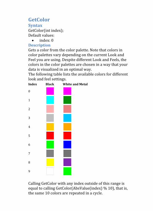
GetColor Syntax GetColor(int index); Default values: • index: 0

Description Gets a color from the color palette. Note that colors in color palettes vary depending on the current Look and Feel you are using. Despite different Look and Feels, the colors in the color palettes are chosen in a way that your data is visualized in an optimal way. The following table lists the available colors for different look and feel settings. Index Black White and Metal

0

1

2

3

4

5

6

7

8

9

Calling GetColor with any index outside of this range is equal to calling GetColor(AbsValue(index) % 10), that is, the same 10 colors are repeated in a cycle.

Example input length = 12; plot SMA = SimpleMovingAvg(close, length); plot EMA = MovAvgExponential(close, length); SMA.SetDefaultColor(GetColor(1)); EMA.SetDefaultColor(GetColor(5)); This script plots two lines: the 12 period simple moving average and exponential moving average of the Close price using colors 1 and 5 from the predefined palette respectively. Usage in: Multiple

globalColor Profile: Studies Syntax globalColor(String name); Description Gets a plot color by name. The color should be defined by the plot.DefineColor(name, color) statement. Example See the DefineGlobalColor function example. Usage in: Ichimoku; LBR_PaintBars; MonkeyBars; MonkeyBarsExpanded; SeriesCount; SpectrumBars; TPOProfile; VolumeProfile.

hide Profile: Studies Syntax hide(); Description Makes a plot hidden by default. This function may be required to hide plot data that is not used in the analysis at the moment. Example plot PriceClose = close; plot PriceOpen = open; PriceOpen.hide(); This example makes the PriceOpen plot invisible by default. Usage in: BalanceOfMarketPower; LBR_PaintBars; MonkeyBars; MonkeyBarsExpanded; PersonsPivots; TPOProfile; TrueStrengthIndex; VolumeProfile.

HideBubble Profile: Studies Syntax HideBubble(); Description Makes the last value bubble of a plot invisible. Example plot Data = volume; Data.HideBubble(); The example hides the last value bubble of the Data plot. Usage in: WoodiesCCI.

hidePricePlot Profile: Studies Syntax hidePricePlot(double hide price); Default values: • hide price: yes

Description Hides the price plot for the current symbol if the Boolean condition value is yes. Example plot closeOnly = close; hidePricePlot(yes); The example code solely displays the Close price plot.

HideTitle Profile: Studies Syntax HideTitle(); Description Removes the plot value from the graph title. Example declare lower; plot PriceOsc = Average(close, 9) - Average(close, 18); plot PriceOscLine = PriceOsc; plot ZeroLine = 0; PriceOsc.SetDefaultColor(Color.VIOLET); PriceOsc.SetPaintingStrategy(PaintingStrategy.HISTOGRAM); PriceOscLine.SetDefaultColor(Color.LIGHT_GRAY); PriceOscLine.HideTitle(); ZeroLine.SetDefaultColor(Color.PINK); ZeroLine.HideTitle(); The example draws the Price Oscillator study consisting of two plots - a histogram and line. The HideTitle function is used to deallocate equal values of PriceOsc and PriceOscLine plots and a permanent zero value for the ZeroLine plot from the status string. Usage in: LBR_ThreeTenOscillator; WoodiesCCI.

setChartType Profile: Studies Syntax setChartType(double chart type); Description Sets a desirable non-Monkey chart type directly from the script. Note that you can also set the chart type along with its color settings within the Chart Settings window, for more information on that, see the Appearance Settings article. Valid parameters are: • ChartType.AREA • ChartType.BAR • ChartType.CANDLE • ChartType.CANDLE_TREND • ChartType.HEIKIN_ASHI • ChartType.LINE

For more information about the constants, see the ChartType constants section. Example plot price = close; setChartType(ChartType.AREA); This code sets the Area chart type and outlines it with the Close price plot.

SetDefaultColor Profile: Studies Syntax SetDefaultColor(CustomColor color); Description Sets the default color of a plot. This setting affects the color of the plot when the study is first initialized or added to the chart. Example plot Data = close; Data.SetDefaultColor(color.RED); The example sets the default color of the Data plot to red. Usage in: Multiple

setHiding Profile: Studies Syntax setHiding(double condition); Description Controls visibility of a plot depending on a condition. If this condition is true, the plot is hidden; otherwise the plot is visible. Example plot DailyClose = close(period = AggregationPeriod.DAY); plot WeeklyClose = close(period = AggregationPeriod.WEEK); plot MonthlyClose = close(period = AggregationPeriod.MONTH); DailyClose.SetHiding(getAggregationPeriod() >= AggregationPeriod.DAY); WeeklyClose.SetHiding(getAggregationPeriod() >= AggregationPeriod.WEEK); MonthlyClose.SetHiding(getAggregationPeriod() >= AggregationPeriod.MONTH); In this example, the daily plot is hidden if the aggregation period is greater than or equal to one day. The weekly plot is hidden if the aggregation period is not less than one week week. The monthly plot is hidden if the aggregation period is greater than or equal to one month. For more information about the aggregation period, see the AggregationPeriod article in the Constants section. Usage in: PersonsPivots.

SetLineWeight Profile: Studies Syntax SetLineWeight(int lineWeight); Description Sets a weight of a line. Example plot Price = close; Price.SetLineWeight(5); This code sets the weight of a line to 5. The value is measured in pixels and ranges from 1 to 5 inclusively. Usage in: Multiple SetPaintingStrategy Profile: Studies Syntax SetPaintingStrategy(int paintingStrategy); Description Controls a painting style of a line. For a list of valid style parameters, see the PaintingStrategy constant in the Constants section. Example plot Data = open; Data.setPaintingStrategy(PaintingStrategy.HISTOGRAM); In this example, the painting style of the Data plot is a histogram. Usage in: Multiple

SetStyle Profile: Studies Syntax SetStyle(int curve); Description Controls a style of a curve. Valid parameters are: • Curve.FIRM • Curve.LONG_DASH • Curve.MEDIUM_DASH • Curve.SHORT_DASH • Curve.POINTS

For more information about the constants, see the Curve constant in the Constants section. Example plot Data = low; Data.setStyle(Curve.SHORT_DASH); This example script draws the Low price plot using a short-dashed curve. Usage in: BollingerBandwidth; PersonsPivots; WoodiesPivots.

TakeValueColor Profile: Studies Syntax TakeValueColor(); Description Returns the color of the current bar. Example input price = close; input length = 12; plot Avg = Average(price, length); AddChartBubble(Avg == HighestAll(Avg), Avg, "Max. Average", Avg.TakeValueColor()); In this example, the TakeValueColor is called to ensure that the bubble is the same color as the SMA plot. Usage in: Next3rdFriday; WoodiesCCI.

o Profiles This section contains articles on profile functions used in thinkScript. The list of functions: • getHighest • getHighestValueArea • getLowest • getLowestValueArea • getPointOfControl • monkeyBars • show • timeProfile • volumeProfile

getHighest Profile: Studies Syntax getHighest(); Description Returns the highest price value reached by the instrument within the time period for which the profile is accumulated. Example def yyyymmdd = getYyyyMmDd(); def day_number = daysFromDate(first(yyyymmdd)) + getDayOfWeek(first(yyyymmdd)); def period = Floor(day_number / 7); def cond = 0 < period - period[1]; profile vol = volumeProfile("startNewProfile" = cond, "onExpansion" = no); vol.show(); plot b = vol.getHighest(); This script plots the High price for each weekly Volume profile. Usage in: MonkeyBars; MonkeyBarsExpanded; TPOProfile; VolumeProfile.

getHighestValueArea Profile: Studies Syntax getHighestValueArea(); Description Returns the highest price of the profile's Value Area. Example def yyyymmdd = getYyyyMmDd(); def day_number = daysFromDate(first(yyyymmdd)) + getDayOfWeek(first(yyyymmdd)); def period = Floor(day_number / 7); def cond = 0 < period - period[1]; profile vol = volumeProfile("startNewProfile" = cond, "onExpansion" = no); vol.show("va color" = Color.YELLOW); plot b = vol.getHighestValueArea(); This script plots the highest price of each weekly Volume profile's Value Area. Usage in: MonkeyBars; MonkeyBarsExpanded; TPOProfile; VolumeProfile.

getLowest Profile: Studies Syntax getLowest(); Description Returns the lowest price value reached by the instrument within the time period for which the profile is accumulated. Example def yyyymmdd = getYyyyMmDd(); def day_number = daysFromDate(first(yyyymmdd)) + getDayOfWeek(first(yyyymmdd)); def period = Floor(day_number / 7); def cond = 0 < period - period[1]; profile vol = volumeProfile("startNewProfile" = cond, "onExpansion" = no); vol.show(); plot b = vol.getLowest(); This script plots the Low price for each weekly Volume profile. Usage in: MonkeyBars; MonkeyBarsExpanded; TPOProfile; VolumeProfile.

getLowestValueArea Profile: Studies Syntax getLowestValueArea(); Description Returns the lowest price of the profile's Value Area. Example def yyyymmdd = getYyyyMmDd(); def day_number = daysFromDate(first(yyyymmdd)) + getDayOfWeek(first(yyyymmdd)); def period = Floor(day_number / 7); def cond = 0 < period - period[1]; profile vol = volumeProfile("startNewProfile" = cond, "onExpansion" = no); vol.show("va color" = Color.YELLOW); plot b = vol.getLowestValueArea(); This script plots the lowest price of each weekly Volume profile's Value Area. Usage in: MonkeyBars; MonkeyBarsExpanded; TPOProfile; VolumeProfile.

getPointOfControl Profile: Studies Syntax getPointOfControl(); Description Returns the price value of the Point of Control level closest to the middle of profile's price range. Example def yyyymmdd = getYyyyMmDd(); def day_number = daysFromDate(first(yyyymmdd)) + getDayOfWeek(first(yyyymmdd)); def period = floor(day_number / 7); def cond = 0 < period - period[1]; profile tpo = timeProfile("startNewProfile" = cond, "onExpansion" = no); tpo.show(); plot b = tpo.getPointOfControl(); This script displays the Point of Control plot for weekly TPO profiles. Usage in: MonkeyBars; MonkeyBarsExpanded; TPOProfile; VolumeProfile.

monkeyBars Profile: Studies Syntax monkeyBars(IDataHolder timeInterval, String symbol, double pricePerRow, IDataHolder startNewProfile, int onExpansion, int numberOfProfiles, double the playground percent, boolean emphasize first digit); Default values: • symbol: "<currently selected symbol>" • pricePerRow: PricePerRow.AUTOMATIC • startNewProfile: all chart • onExpansion: yes • numberOfProfiles: "all" • the playground percent: 70.0 • emphasize first digit: 0

Description Calculates the Monkey Bars profile with user-defined paramaters. The timeInterval parameter defines an ordinal number of aggregation period. The first decade is displayed as digits 0-9 in the first palette color, the second decade is displayed as digits 0-9 in the second palette color, and so on. Note that a named variable must be used for this parameter. The symbol parameter defines a symbol to calculate Monkey Bars for. The pricePerRow parameter defines the "height" (price range) of each row of Monkey Bars. This value can be defined by an actual price range or a PricePerRow constant. The startNewProfile parameter defines a condition; when it is true, the monkeyBars function is given a trigger signal to calculate the new profile. Note that a named variable must be used for this parameter.

The onExpansion parameter defines whether or not to show Monkey Bars on the expansion area of the chart. The numberOfProfiles parameter defines the number of profiles to be displayed if onExpansion is set to no. If onExpansion is set to yes then this parameter is ignored and only one profile is shown. The the playground percent parameter sets the percentage of the trading activity for which The Playground is determined. The emphasize first digit parameter defines whether or not to highlight the opening digit of each period in bold. Example def yyyymmdd = getYyyyMmDd(); def timeInterval = getDayOfMonth(yyyymmdd); def allchart = 0; profile monkey = monkeyBars(timeInterval, "startNewprofile"=allchart); monkey.show(); This script displays Monkey Bars with 1 day aggregation period for the whole chart. Usage in: MonkeyBars.

show Profile: Studies Syntax show(CustomColor color, CustomColor poc color, CustomColor va color, double opacity, CustomColor open color, CustomColor close color); Default values: • color: Color.PLUM • poc color: Color.CURRENT • va color: Color.CURRENT • opacity: 50.0 • open color: Color.CURRENT • close color: Color.CURRENT

Description Controls visibility and color scheme of Time, Volume, and Monkey Bars profiles. Note that profiles calculated by the corresponding functions will only be visible if the show function is applied to them. The color parameter defines the main color of Time and Volume profile bars. The poc color parameter defines the color of the Point of Control. The va color parameter defines the color of the Value Area. The opacity parameter sets the degree of histogram opacity, in percent. The open color parameter defines the color of the square marking the Monkey Bars' Open price. The close color parameter defines the color of the arrow marking the Monkey Bars' Close price. Note that when Color.CURRENT is used for any of the elements (profile itself, point of control, value area), that element is not displayed.

Example def yyyymmdd = getYyyyMmDd(); def day_number = daysFromDate(first(yyyymmdd)) + getDayOfWeek(first(yyyymmdd)); def period = Floor(day_number / 7); def cond = 0 < period - period[1]; profile vol = volumeProfile("startNewProfile" = cond, "onExpansion" = no); vol.show("va color" = Color.YELLOW); This script displays weekly Volume profiles with Value Area highlighted in yellow. Usage in: MonkeyBars; MonkeyBarsExpanded; TPOProfile; VolumeProfile.

timeProfile Profile: Studies Syntax timeProfile(String symbol, double pricePerRow, IDataHolder startNewProfile, int onExpansion, int numberOfProfiles, double value area percent); Default values: • symbol: "<currently selected symbol>" • pricePerRow: PricePerRow.AUTOMATIC • startNewProfile: all chart • onExpansion: yes • numberOfProfiles: "all" • value area percent: 70.0

Description Displays the time price opportunity (TPO) profile with user-defined calculation parameters. The symbol parameter defines a symbol to calculate the TPO profile for. The pricePerRow parameter defines the "height" (price range) of each row of the profile. This value can be defined by an actual price range or a PricePerRow constant. The startNewProfile parameter defines a condition; when it is true, the function is given a trigger signal to calculate the new TPO profile. Note that a named variable must be used for this parameter. The onExpansion parameter defines whether or not the profile is shown on the expansion area of the chart. The numberOfProfiles parameter defines the number of profiles to be displayed if onExpansion is set to no. If onExpansion is set to yes then this parameter is ignored and only one profile is shown. The value area percent parameter sets the percentage of the trading activity for which the Value Area is determined.

Example def allchart = 0; profile tpo = timeProfile("startnewprofile"=allchart); tpo.show("color"=Color.BLUE); This script plots TPO profile study (colored blue) that aggregates all chart data on the right expansion. Usage in: TPOProfile.

volumeProfile Profile: Studies Syntax volumeProfile(String symbol, double pricePerRow, IDataHolder startNewProfile, int onExpansion, int numberOfProfiles, double value area percent); Default values: • symbol: "<currently selected symbol>" • pricePerRow: PricePerRow.AUTOMATIC • startNewProfile: all chart • onExpansion: yes • numberOfProfiles: "all" • value area percent: 70.0

Description Displays the volume profile with user-defined calculation parameters. The symbol parameter defines a symbol to calculate the volume profile for. The pricePerRow parameter defines the "height" (price range) of each row of the profile. This value can be defined by an actual price range or a PricePerRow constant. The startNewProfile parameter defines a condition; when it is true, the function is given a trigger signal to calculate the new volume profile. Note that a named variable must be used for this parameter. The onExpansion parameter defines whether or not the profile is shown on the expansion area of the chart. The numberOfProfiles parameter defines the number of profiles to be displayed if onExpansion is set to no. If onExpansion is set to yes then this parameter is ignored and only one profile is shown. The value area percent parameter sets the percentage of the trading activity for which the Value Area is determined.

Example def allchart = 0; profile vol = volumeProfile("startnewprofile"=allchart); vol.show("color"=Color.YELLOW); This script plots Volume profile study (colored yellow) that aggregates all chart data on the right expansion. Usage in: VolumeProfile.

o Others This section contains functions not fitting the rest of the sections. Each of the functions is used as a supplement for technical analysis. Here is the full list: • addOrder • alert • barNumber • between • compoundValue • concat • entryPrice • first • fundamental • getAggregationPeriod • getInterestRate • getSymbolPart • getValue • getYield • if • tickSize • tickValue

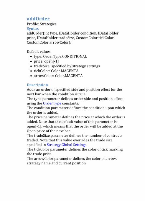
addOrder Profile: Strategies Syntax addOrder(int type, IDataHolder condition, IDataHolder price, IDataHolder tradeSize, CustomColor tickColor, CustomColor arrowColor); Default values: • type: OrderType.CONDITIONAL • price: open[-1] • tradeSize: specified by strategy settings • tickColor: Color.MAGENTA • arrowColor: Color.MAGENTA

Description Adds an order of specified side and position effect for the next bar when the condition is true. The type parameter defines order side and position effect using the OrderType constants. The condition parameter defines the condition upon which the order is added. The price parameter defines the price at which the order is added. Note that the default value of this parameter is open[-1], which means that the order will be added at the Open price of the next bar. The tradeSize parameter defines the number of contracts traded. Note that this value overrides the trade size specified in Strategy Global Settings. The tickColor parameter defines the color of tick marking the trade price. The arrowColor parameter defines the color of arrow, strategy name and current position.

Example addOrder(OrderType.BUY_AUTO, close > close[1], open[-2], 50, Color.ORANGE, Color.ORANGE); If the current Close price is higher than the previous, the code opens the long position or closes the short one at the Open price of the second bar from the current. The trade size will be equal to 50, and the signals will be colored orange. Usage in: ATRTrailingStopLE; ATRTrailingStopSE; BollingerBandsLE; BollingerBandsSE; ConsBarsDownSE; ConsBarsUpLE; GapDownSE; GapUpLE; InsideBarLE; InsideBarSE; KeyRevLE; KeyRevLX; MomentumLE; PriceZoneOscillatorLE; PriceZoneOscillatorLX; PriceZoneOscillatorSE; PriceZoneOscillatorSX; ProfitTargetLX; ProfitTargetSX; SpectrumBarsLE; StopLossLX; StopLossSX; ThreeBarInsideBarLE; ThreeBarInsideBarSE; TrailingStopLX; TrailingStopSX; VoltyExpanCloseLX.

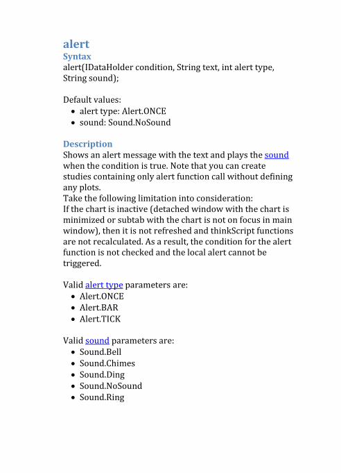
alert Syntax alert(IDataHolder condition, String text, int alert type, String sound); Default values: • alert type: Alert.ONCE • sound: Sound.NoSound

Description Shows an alert message with the text and plays the sound when the condition is true. Note that you can create studies containing only alert function call without defining any plots. Take the following limitation into consideration: If the chart is inactive (detached window with the chart is minimized or subtab with the chart is not on focus in main window), then it is not refreshed and thinkScript functions are not recalculated. As a result, the condition for the alert function is not checked and the local alert cannot be triggered. Valid alert type parameters are: • Alert.ONCE • Alert.BAR • Alert.TICK

Valid sound parameters are: • Sound.Bell • Sound.Chimes • Sound.Ding • Sound.NoSound • Sound.Ring

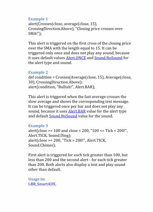
Example 1 alert(Crosses(close, average(close, 15), CrossingDirection.Above), "Closing price crosses over SMA!"); This alert is triggered on the first cross of the closing price over the SMA with the length equal to 15. It can be triggered only once and does not play any sound, because it uses default values Alert.ONCE and Sound.NoSound for the alert type and sound. Example 2 def condition = Crosses(Average(close, 15), Average(close, 30), CrossingDirection.Above); alert(condition, "Bullish!", Alert.BAR); This alert is triggered when the fast average crosses the slow average and shows the corresponding text message. It can be triggered once per bar and does not play any sound, because it uses Alert.BAR value for the alert type and default Sound.NoSound value for the sound. Example 3 alert(close >= 100 and close < 200, "100 <= Tick < 200!", Alert.TICK, Sound.Ding); alert(close >= 200, "Tick > 200!", Alert.TICK, Sound.Chimes); First alert is triggered for each tick greater than 100, but less than 200 and the second alert - for each tick greater than 200. Both alerts also display a text and play sound other than default. Usage in: LBR_SmartADX.

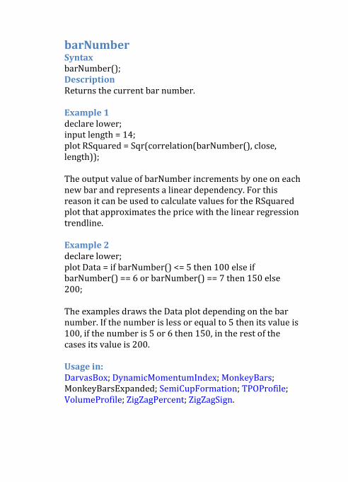
barNumber Syntax barNumber(); Description Returns the current bar number. Example 1 declare lower; input length = 14; plot RSquared = Sqr(correlation(barNumber(), close, length)); The output value of barNumber increments by one on each new bar and represents a linear dependency. For this reason it can be used to calculate values for the RSquared plot that approximates the price with the linear regression trendline. Example 2 declare lower; plot Data = if barNumber() <= 5 then 100 else if barNumber() == 6 or barNumber() == 7 then 150 else 200; The examples draws the Data plot depending on the bar number. If the number is less or equal to 5 then its value is 100, if the number is 5 or 6 then 150, in the rest of the cases its value is 200. Usage in: DarvasBox; DynamicMomentumIndex; MonkeyBars; MonkeyBarsExpanded; SemiCupFormation; TPOProfile; VolumeProfile; ZigZagPercent; ZigZagSign.

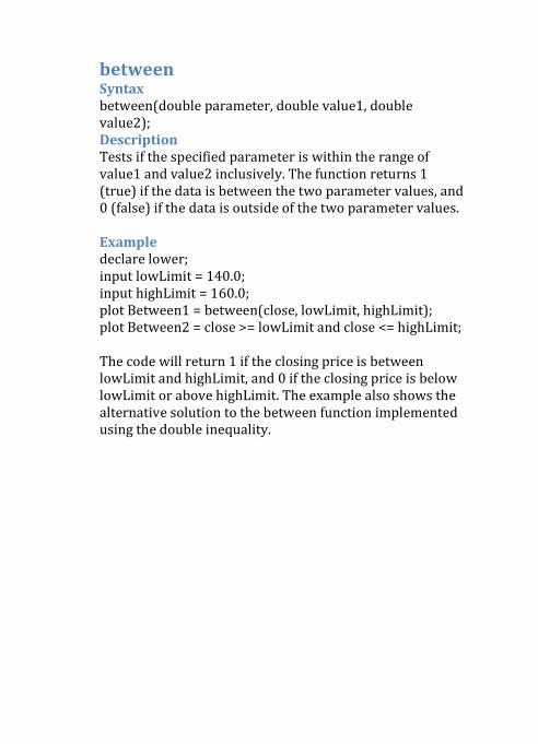
between Syntax between(double parameter, double value1, double value2); Description Tests if the specified parameter is within the range of value1 and value2 inclusively. The function returns 1 (true) if the data is between the two parameter values, and 0 (false) if the data is outside of the two parameter values. Example declare lower; input lowLimit = 140.0; input highLimit = 160.0; plot Between1 = between(close, lowLimit, highLimit); plot Between2 = close >= lowLimit and close <= highLimit; The code will return 1 if the closing price is between lowLimit and highLimit, and 0 if the closing price is below lowLimit or above highLimit. The example also shows the alternative solution to the between function implemented using the double inequality.

compoundValue Syntax compoundValue(int length, IDataHolder visible data, IDataHolder historical data); Default values: • length: 1

Description Calculates a compound value according to following rule: if a bar number is bigger than length then the visible data value is returned, otherwise the historical data value is returned. This function is used to initialize studies with recursion. Example declare lower; rec x = compoundValue(2, x[1] + x[2], 1); plot FibonacciNumbers = x; The example calculates the Fibonacci sequence. Starting from the third bar each following number is calculated as the sum of the previous two numbers while the numbers for the first two bars are equal to one. As a result you will get a plot containing values 1, 1, 2, 3, 5, etc. Usage in: CyberCyclesOscillator; DarvasBox; HeikinAshiDiff; LegacyEMA; MonkeyBars; MonkeyBarsExpanded; MovAvgAdaptive; NegativeVolumeIndex; PositiveVolumeIndex; RelativeStrength; ReverseEngineeringRSI; TPOProfile; VWAP; VariableMA; VolumeProfile.

concat Syntax concat(Any value1, Any value2); Description Concatenates two string values. If the values' type is not string it is first converted to a string (for doubles it saves four decimal places) Example input symbol = "IBM"; AddChartLabel(yes, concat("SMA (", concat(symbol, concat(", 10): ", round(Average(close(symbol), 10), 1))))); This example displays a constantly visible chart label with the SMA of the given symbol with the length equal to 10 rounded to one decimal place. Usage in: AdvanceDecline; Next3rdFriday; SemiCupFormation; WoodiesCCI.

entryPrice Profile: Strategies Syntax entryPrice(); Description Returns the price of the entry order. For several entry orders in the same direction as the currently held position the function returns the average price for all of them. Example declare LONG_EXIT; addOrder(close > entryPrice() + 3 or close < entryPrice() - 9); Defines a selling strategy for closing a long position when either the closing price is greater than the entry price by 3 for taking profits or less by 9 for safety. Usage in: ProfitTargetLX; ProfitTargetSX; SpectrumBarsLE; StopLossLX; StopLossSX; ThreeBarInsideBarLE; ThreeBarInsideBarSE; TrailingStopLX; TrailingStopSX.

first Syntax first(IDataHolder data); Description Returns the value of the parameter expression in the first bar. Example declare lower; def close1 = first(close); plot Data = (close - close1) / close1 * 100; The code calculates the close price percentage move on the analogy of the Percentage View mode for charts. In this example the parameter expression for the first function is close. This means that the close1 variable always holds close for the first bar. Usage in: MonkeyBars; MonkeyBarsExpanded; TPOProfile; VWAP; VolumeProfile.

fundamental Syntax fundamental(int fundamentalType, String symbol, Any period, String priceType); Default values: • symbol: "<currently selected symbol>" • period: "<current period>" • priceType: "<current type>"

Description This function is generalization of fundamental functions, i.e. it returns the specified price for the chosen symbol, aggregation period, and price type. This function should be used with one of the Fundamental Type constants to perform as the corresponding fundamental function. For more information about these constants, see the Fundamental Type constants section. You can use both Aggregation Period constants and pre-defined string values (e.g. Day, 2 Days, Week, Month, etc.) as valid parameters for the aggregation period. The full list of the pre-defined string values can be found in the Referencing Secondary Aggregation article. Valid parameters for the price type are: • LAST • MARK, ASK, BID (for Forex symbols only)

Example declare lower; input price = FundamentalType.CLOSE; input relationWithSecurity = "SPX"; def price1 = fundamental(price); def price2 = fundamental(price, relationWithSecurity);

plot Relation = if price2 == 0 then Double.NaN else price1 / price2; Relation.SetDefaultColor(GetColor(1)); This script exemplifies usage of the fundamental function in the Symbol Relation study. Usage in: DailySMA; SymbolRelation.

getAggregationPeriod Syntax getAggregationPeriod(); Description Returns the current aggregation period in milliseconds for time charts and in ticks for tick charts. The aggregation period is the number of milliseconds (ticks) required to complete a candle on the current chart time frame. You can use this function in combination with aggregation period constants. For more information about the constants see the Constants section. Example input lengthIntraday = 20; input lengthDaily = 10; plot data; if getAggregationPeriod() < AggregationPeriod.DAY { data = Average(close, lengthIntraday); } else { data = Average(close, lengthDaily); } The example plots the simple moving average depending on an aggregation period. If the aggregation period is shorter than day, then it calculates the average on the lengthIntraday period. For daily and longer aggregations it calculates the average on the lengthDaily period. Usage in: VWAP; WoodiesCCI.

getInterestRate Syntax getInterestRate(); Description Returns the global interest rate. Example declare lower; input loan = 1000; plot Charge = loan * getInterestRate(); AddChartLabel(yes, concat("Interest Rate: ", getInterestRate() * 100)); This example draws a charge for the loan at the current interest rate displayed in the chart label.

getSymbolPart Syntax getSymbolPart(int position); Default values: • position: 1

Description Returns a part of the composite symbol. Example declare lower; plot Spreads = close(getSymbolPart(1)) - close(getSymbolPart(2)); The code calculates the spread between the first and second parts of the composite symbol. Note that the normalized form of representation is used when defining parts a composite index. The form implies the sorting in the ascending order. For example, if you specify the "KO+GE" composite then it will be represented as "GE+KO" and it's first part will be "GE", not "KO", as it was during the input. Usage in: PairCorrelation; PairRatio.

getValue Syntax getValue(IDataHolder data, IDataHolder dynamic offset, int max offset); Default values: • max offset: 0

Description Returns the value of data with the specified dynamic offset. AbsValue('dynamic offset') should be less or equal than max offset. Example plot ClosingPriceForHighestHigh = getValue(close, GetMaxValueOffset(high, 12), 12); The example draws a closing price plot for a bar where the high price was at its maximum for the last 12 bars. Usage in: DarvasBox; DynamicMomentumIndex; LookUpHighest; LookUpLowest; MESASineWave; PolychromMtm; RandomWalkIndex; SemiCupFormation; ZigZagPercent; ZigZagSign.

getYield Syntax getYield(); Description Returns the yield of the current stock or the underlying symbol for the current option. Example declare lower; plot CurrentYield = getYield() * 100; AddChartLabel(yes, concat("Annual Dividends: ", getYield() * close)); This script plots the current yield line and places a chart label indicating annual dividends.

if Syntax if(double condition, double true value, double false value); Description Returns true value if condition is true and false value otherwise. There are two ways to use the function. First, you can use it as the right side of an equation with 3 parameters: a condition, a true value and a false value. Secondly, you can use it in a conjunction with else to create more complex conditions. Note that input arguments can only be numerical of type double. If other values are needed (e.g. Color constants), use the if-expression. E.g. for CustomColor arguments, the following code is valid: AssignPriceColor(if close > open then Color.UPTICK else Color.DOWNTICK); The following script will result in compilation error as type CustomColor is not compatible with type double: AssignPriceColor(if(close > open, Color.UPTICK, Color.DOWNTICK)); Example plot Maximum1 = if(close > open, close, open); plot Maximum2 = if close > open then close else open; plot Maximum3; if close > open { Maximum3 = close; } else { Maximum3 = open; } The code draws either close or open value depending on the condition in the if-statement. If close is higher than open, then close is drawn, otherwise open is drawn.

Maximum2 and Maximum3 plots use alternative solutions such as if-expression and if-statement correspondingly. Usage in: DarvasBox.

tickSize Syntax tickSize(String symbol); Default values: • symbol: "<currently selected symbol>"

Description Returns the minimum possible tick size for the current symbol. Example input numberOfTicks = 3; plot OverBought = Highest(high)[1] + numberOfTicks * tickSize(); plot OverSold = Lowest(low)[1] - numberOfTicks * tickSize(); plot BreakOut = if Close >= OverBought then Close else if Close <= OverSold then Close else Double.NaN; Breakout.SetPaintingStrategy(PaintingStrategy.POINTS); Breakout.SetLineWeight(3); Breakout.HideBubble(); Initially the example draws the OverBought and OverSold plots. The OverBought plot is calculated by adding the given number of ticks to the highest price for the last 12 bars starting from previous bar. The OverSold plot is calculated the same way but by subtracting the ticks from the lowest price. If the close price is out of the area of the first two plots the code displays the BreakOut plot. Usage in: ProfitTargetLX; ProfitTargetSX; StopLossLX; StopLossSX; TrailingStopLX; TrailingStopSX; WoodiesCCI.

tickValue Syntax tickValue(String symbol); Default values: • symbol: "<currently selected symbol>"

Description Returns the dollar value of a symbol tick. Example AddChartLabel(yes, concat("Contract size is ", tickValue()/tickSize())); In this example the contract size is calculated using the tick size and value.

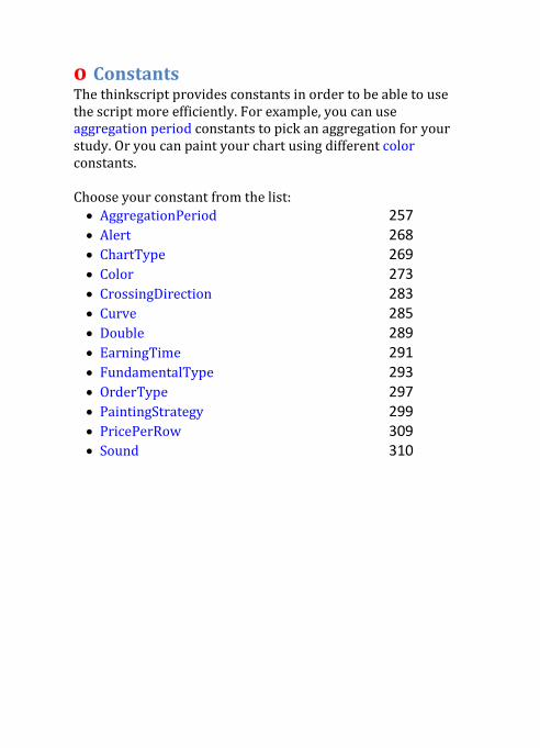
o Constants The thinkscript provides constants in order to be able to use the script more efficiently. For example, you can use aggregation period constants to pick an aggregation for your study. Or you can paint your chart using different color constants. Choose your constant from the list: • AggregationPeriod 257 • Alert 268 • ChartType 269 • Color 273 • CrossingDirection 283 • Curve 285 • Double 289 • EarningTime 291 • FundamentalType 293 • OrderType 297 • PaintingStrategy 299 • PricePerRow 309 • Sound 310

o AggregationPeriod Aggregation period constants define a specific aggregation period for your studies and strategies. The period length varies from one minute to option expiration. Choose an aggregation period from the list:

• MIN • TWO_MIN • THREE_MIN • FOUR_MIN • FIVE_MIN • TEN_MIN • FIFTEEN_MIN • TWENTY_MIN • THIRTY_MIN • HOUR • TWO_HOURS • FOUR_HOURS • DAY • TWO_DAYS • THREE_DAYS • FOUR_DAYS • WEEK • MONTH • OPT_EXP

MIN Syntax AggregationPeriod.MIN Description Defines the aggregation period equal to one minute (60,000 milliseconds). Example def agg = AggregationPeriod.MIN; plot data = close(period = agg); This example script draws the Close price plot with aggregation period equal to one minute. Note that aggregation period used in this example cannot be less than chart aggregation period. See also getAggregationPeriod function in the Others section. TWO_MIN Syntax AggregationPeriod.TWO_MIN Description Defines the aggregation period equal to two minutes (120,000 milliseconds). Example def agg = AggregationPeriod.TWO_MIN; plot data = close(period = agg); This example script draws the Close price plot with aggregation period equal to two minutes. Note that aggregation period used in this example cannot be less than chart aggregation period. See also getAggregationPeriod function in the Others section.

THREE_MIN Syntax AggregationPeriod.THREE_MIN Description Defines the aggregation period equal to three minutes (180,000 milliseconds). Example def agg = AggregationPeriod.THREE_MIN; plot data = close(period = agg); This example script draws the Close price plot with aggregation period equal to three minutes. Note that aggregation period used in this example cannot be less than chart aggregation period. See also getAggregationPeriod function in the Others section. FOUR_MIN Syntax AggregationPeriod.FOUR_MIN Description Defines the aggregation period equal to four minutes (240,000 milliseconds). Example def agg = AggregationPeriod.FOUR_MIN; plot data = close(period = agg); This example script draws the Close price plot with aggregation period equal to four minutes. Note that aggregation period used in this example cannot be less than chart aggregation period. See also getAggregationPeriod function in the Others section.

FIVE_MIN Syntax AggregationPeriod.FIVE_MIN Description Defines the aggregation period equal to five minutes (300,000 milliseconds). Example def agg = AggregationPeriod.FIVE_MIN; plot data = close(period = agg); This example script draws the Close price plot with aggregation period equal to five minutes. Note that aggregation period used in this example cannot be less than chart aggregation period. See also getAggregationPeriod function in the Others section. TEN_MIN Syntax AggregationPeriod.TEN_MIN Description Defines the aggregation period equal to ten minutes (600,000 milliseconds). Example def agg = AggregationPeriod.TEN_MIN; plot data = close(period = agg); This example script draws the Close price plot with aggregation period equal to ten minutes. Note that aggregation period used in this example cannot be less than chart aggregation period. See also getAggregationPeriod function in the Others section.

FIFTEEN_MIN Syntax AggregationPeriod.FIFTEEN_MIN Description Defines the aggregation period equal to fifteen minutes (900,000 milliseconds). Example def agg = AggregationPeriod.FIFTEEN_MIN; plot data = close(period = agg); This example script draws the Close price plot with aggregation period equal to fifteen minutes. Note that aggregation period used in this example cannot be less than chart aggregation period. See also getAggregationPeriod function in the Others section. TWENTY_MIN Syntax AggregationPeriod.TWENTY_MIN Description Defines the aggregation period equal to twenty minutes (1,200,000 milliseconds). Example def agg = AggregationPeriod.TWENTY_MIN; plot data = close(period = agg); This example script draws the Close price plot with aggregation period equal to twenty minutes. Note that aggregation period used in this example cannot be less than chart aggregation period. See also getAggregationPeriod function in the Others section.

THIRTY_MIN Syntax AggregationPeriod.THIRTY_MIN Description Defines the aggregation period equal to thirty minutes (1,800,000 milliseconds). Example def agg = AggregationPeriod.THIRTY_MIN; plot data = close(period = agg); This example script draws the Close price plot with aggregation period equal to thirty minutes. Note that aggregation period used in this example cannot be less than chart aggregation period. See the getAggregationPeriod function in the Others section. HOUR Syntax AggregationPeriod.HOUR Description Defines the aggregation period equal to one hour (3,600,000 milliseconds). Example def agg = AggregationPeriod.HOUR; plot data = close(period = agg); This example script draws the Close price plot with aggregation period equal to one hour. Note that aggregation period used in this example cannot be less than chart aggregation period. See also getAggregationPeriod function in the Others section.

TWO_HOURS Syntax AggregationPeriod.TWO_HOURS Description Defines the aggregation period equal to two hours (7,200,000 milliseconds). Example def agg = AggregationPeriod.TWO_HOURS; plot data = close(period = agg); This example script draws the Close price plot with aggregation period equal to two hours. Note that aggregation period used in this example cannot be less than chart aggregation period. See also getAggregationPeriod function in the Others section. FOUR_HOURS Syntax AggregationPeriod.FOUR_HOURS Description Defines the aggregation period equal to four hours (14,400,000 milliseconds). Example def agg = AggregationPeriod.FOUR_HOURS; plot data = close(period = agg); This example script draws the Close price plot with aggregation period equal to four hours. Note that aggregation period used in this example cannot be less than chart aggregation period. See also getAggregationPeriod function in the Others section.

DAY Syntax AggregationPeriod.DAY Description Defines the aggregation period equal to one day (86,400,000 milliseconds). Example def agg = AggregationPeriod.DAY; plot data = close(period = agg); This example script draws the daily Close price plot. Note that aggregation period used in this example cannot be less than chart aggregation period. See also getAggregationPeriod function in the Others section. TWO_DAYS Syntax AggregationPeriod.TWO_DAYS Description Defines the aggregation period equal to two days (172,800,000 milliseconds). Example def agg = AggregationPeriod.TWO_DAYS; plot data = close(period = agg); This example script draws the Close price plot with aggregation period equal to two days. Note that aggregation period used in this example cannot be less than chart aggregation period. See also getAggregationPeriod function in the Others section.

THREE_DAYS Syntax AggregationPeriod.THREE_DAYS Description Defines the aggregation period equal to three days (259,200,000 milliseconds) Example def agg = AggregationPeriod.THREE_DAYS; plot data = close(period = agg); This example script draws the Close price plot with aggregation period equal to three days. Note that aggregation period used in this example cannot be less than chart aggregation period. See also getAggregationPeriod function in the Others section. FOUR_DAYS Syntax AggregationPeriod.FOUR_DAYS Description Defines the aggregation period equal to four days (345,600,000 milliseconds). Example def agg = AggregationPeriod.FOUR_DAYS; plot data = close(period = agg); This example script draws the Close price plot with aggregation period equal to four days. Note that aggregation period used in this example cannot be less than chart aggregation period. See also getAggregationPeriod function in the Others section.

WEEK Syntax AggregationPeriod.WEEK Description Defines the aggregation period equal to one week (604,800,000 milliseconds) Example def agg = AggregationPeriod.WEEK; plot data = close(period = agg); This example script draws the weekly Close price plot. Note that aggregation period used in this example cannot be less than chart aggregation period. See also getAggregationPeriod function in the Others section. MONTH Syntax AggregationPeriod.MONTH Description Defines the aggregation period equal to one month (2,592,000,000 milliseconds). Example def agg = AggregationPeriod.MONTH; plot data = close(period = agg); This example script draws the Close price plot with aggregation period equal to one month. Note that aggregation period used in this example cannot be less than chart aggregation period. See also getAggregationPeriod function in the Others section.

OPT_EXP Syntax AggregationPeriod.OPT_EXP Description Defines the aggregation period equal to option expiration (2,678,400,000 milliseconds). Example def agg = AggregationPeriod.OPT_EXP; plot data = close(period = agg); This example script draws the Close price plot with aggregation period equal to option expiration. Note that aggregation period used in this example cannot be less than chart aggregation period. See also getAggregationPeriod function in the Others section.

o Alert Alert constants represent different types of alerts for the alert function. Choose an alert constant from the list: • BAR • ONCE • TICK

BAR Syntax Alert.BAR Description Defines the alert that can be triggered only once per bar. Example See the alert function in the Others section. ONCE Syntax Alert.ONCE Description Defines the alert that can be triggered only once after adding a study. Example See the alert function in the Others section. TICK Syntax Alert.TICK Description Defines the alert that can be triggered after each tick. Example See the alert function in the Others section.

o ChartType In this section you will find information on the constants used in setChartType function. • BAR • CANDLE • CANDLE_TREND • HEIKIN_ASHI • LINE • AREA

BAR Syntax ChartType.BAR Description Used in setChartType function to set the Bar chart type. Example See the setChartType article in the Look and Feel functions section. CANDLE Syntax ChartType.CANDLE Description Used in setChartType function to set the Candle chart type. Example See the setChartType article in the Look and Feel functions section.

CANDLE_TREND Syntax ChartType.CANDLE_TREND Description Used in setChartType function to set the Candle Trend chart type. Example See the setChartType article in the Look and Feel functions section. HEIKIN_ASHI Syntax ChartType.HEIKIN_ASHI Description Used in setChartType function to set the Heikin Ashi chart type. Example See the setChartType article in the Look and Feel functions section. LINE Syntax ChartType.LINE Description Used in setChartType function to set the Line chart type. Example See the setChartType article in the Look and Feel functions section.

AREA Syntax ChartType.AREA Description Used in setChartType function to set the Area chart type. Example See the setChartType article in the Look and Feel functions section.

o Color The thinkScript provides the set of constants for colors. Here is the full list of the colors: • BLACK • BLUE • CURRENT • CYAN • DARK_GRAY • DARK_GREEN • DARK_ORANGE • DARK_RED • DOWNTICK • GRAY • GREEN • LIGHT_GRAY • LIGHT_GREEN • LIGHT_ORANGE • LIGHT_RED • LIME • MAGENTA • ORANGE • PINK • PLUM • RED • UPTICK • VIOLET • WHITE • YELLOW

Example See the SetDefaultColor function in the Look and Feel functions section.

BLACK Syntax Color.BLACK Description Defines the black color. Its RGB representation is (0, 0, 0). Sample

BLUE Syntax Color.BLUE Description Defines the blue color. Its RGB representation is (0, 0, 255). Sample

CURRENT Syntax Color.CURRENT Description Refers to the default plot color (or redefined color in case it was changed on the UI). When using the AssignPriceColor function the constant is responsible for price bars color. In combintaion with the AssignBackgroundColor function the constant defines the corresponding background color.

CYAN Syntax Color.CYAN Description Defines the cyan color. Its RGB representation is (0, 255, 255). Sample

DARK_GRAY Syntax Color.DARK_GRAY Description Defines the dark gray color. Its RGB representation is (64, 64, 64). Sample

DARK_GREEN Syntax Color.DARK_GREEN Description Defines the dark green color. Its RGB representation is (0, 100, 0). Sample

DARK_ORANGE Syntax Color.DARK_ORANGE Description Defines the dark orange color. Its RGB representation is (255, 127, 0). Sample

DARK_RED Syntax Color.DARK_RED Description Defines the dark red color. Its RGB representation is (128, 0, 0). Sample

DOWNTICK Syntax Color.DOWNTICK Description Defines the downtick color. Its RGB representation is (204, 0, 0). Sample

GRAY Syntax Color.GRAY Description Defines the gray color. Its RGB representation is (128, 128, 128). Sample

GREEN Syntax Color.GREEN Description Defines the green color. Its RGB representation is (0, 255, 0). Sample

LIGHT_GRAY Syntax Color.LIGHT_GRAY Description Defines the light gray color. Its RGB representation is (192, 192, 192). Sample

LIGHT_GREEN Syntax Color.LIGHT_GREEN Description Defines the light green color. Its RGB representation is (144, 238, 114). Sample

LIGHT_GREEN Syntax Color.LIGHT_GREEN Description Defines the light green color. Its RGB representation is (144, 238, 114). Sample

LIGHT_RED Syntax Color.LIGHT_RED Description Defines the light red color. Its RGB representation is (255, 63, 0). Sample

LIME Syntax Color.LIME Description Defines the lime color. Its RGB representation is (191, 255, 0). Sample

MAGENTA Syntax Color.MAGENTA Description Defines the magenta color. Its RGB representation is (255, 0, 255). Sample

ORANGE Syntax Color.ORANGE Description Defines the orange color. Its RGB representation is (255, 200, 0). Sample

PINK Syntax Color.PINK Description Defines the pink color. Its RGB representation is (255, 175, 175). Sample

PLUM Syntax Color.PLUM; Description Defines the plum color. Its RGB representation is (128, 0, 128). Sample

RED Syntax Color.RED Description Defines the red color. Its RGB representation is (255, 0, 0). Sample

UPTICK Syntax Color.UPTICK Description Defines the uptick color. Its RGB representation is (3, 128, 0). Sample

VIOLET Syntax Color.VIOLET Description Defines the violet color. Its RGB representation is (153, 153, 255). Sample

WHITE Syntax Color.WHITE Description Defines the white color. Its RGB representation is (255, 255, 255). Sample

YELLOW Syntax Color.YELLOW Description Defines the yellow color. Its RGB representation is (255, 255, 0). Sample

o CrossingDirection Crossing direction constants define a specific switch of the relationship between arguments of the Crosses function. Choose a crossing direction constant from the list:

• Above • Below • Any

Above Syntax CrossingDirection.Above Description This constant is used with the Crosses function to find when the first value becomes greater than the second. Note that this constant can be replaced with reserved word yes. Example plot avg = Average(close, 10); plot crossing = Crosses(close, avg, CrossingDirection.Above); crossing.SetPaintingStrategy(PaintingStrategy.BOOLEAN_ARROW_UP); This code marks the bars at which the Close price gets higher than its 10 period average.

Below Syntax CrossingDirection.Below Description This constant is used with the Crosses function to find when the first value becomes less than the second. Note that this constant can be replaced with reserved word no. Example plot avg = Average(close, 10); plot crossing = Crosses(close, avg, CrossingDirection.Below); crossing.SetPaintingStrategy(PaintingStrategy.BOOLEAN_ARROW_DOWN); This code marks the bars at which the Close price becomes less than its 10 period average. Any Syntax CrossingDirection.Any Description Defines the change of relation of two values in the Crosses function irrespective of its direction. Example plot avg = Average(close, 10); plot crossing = Crosses(close, avg, CrossingDirection.Any); crossing.SetPaintingStrategy(PaintingStrategy.BOOLEAN_ARROW_UP); This code marks the bars at which the Close price becomes greater or less than its 10 period average.

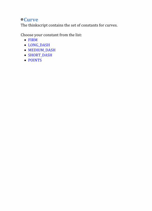
o Curve The thinkscript contains the set of constants for curves. Choose your constant from the list: • FIRM • LONG_DASH • MEDIUM_DASH • SHORT_DASH • POINTS

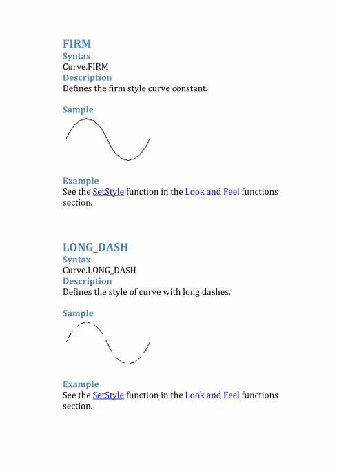
FIRM Syntax Curve.FIRM Description Defines the firm style curve constant. Sample

Example See the SetStyle function in the Look and Feel functions section. LONG_DASH Syntax Curve.LONG_DASH Description Defines the style of curve with long dashes. Sample

Example See the SetStyle function in the Look and Feel functions section.

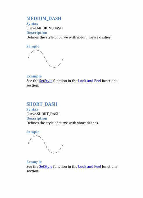
MEDIUM_DASH Syntax Curve.MEDIUM_DASH Description Defines the style of curve with medium-size dashes. Sample

Example See the SetStyle function in the Look and Feel functions section. SHORT_DASH Syntax Curve.SHORT_DASH Description Defines the style of curve with short dashes. Sample

Example See the SetStyle function in the Look and Feel functions section.

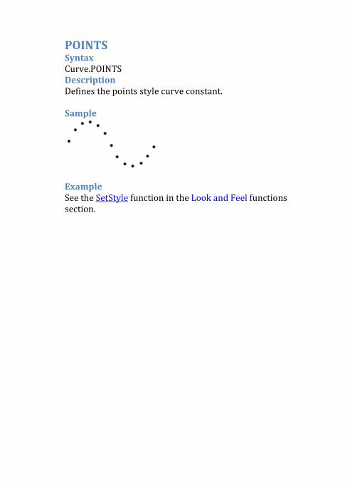
POINTS Syntax Curve.POINTS Description Defines the points style curve constant. Sample

Example See the SetStyle function in the Look and Feel functions section.

o Double This section describes mathematical constants such as exponent or pi. Choose a constant from the list:

• E • NaN • Pi

E Syntax Double.E Description Returns the value of the exponent constant. Example (Price Oscillator) See the exp function in the Mathematical and Trigonometrical functions section. NaN Syntax Double.NaN Description Returns the value that indicates that the result of an operation is not a number. Example (Price Oscillator) See the isNaN function in the Mathematical and Trigonometrical functions section. Pi Syntax Double.Pi Description Returns the value of the pi constant. Example (Price Oscillator) See the ASin, ACos, Sin, and Cos functions in the Mathematical and Trigonometrical functions section.

o EarningTime In this section you will find information on the constants used with hasEarnings function.

• ANY • BEFORE_MARKET • AFTER_MARKET

ANY Syntax EarningTime.ANY Description Used with hasEarnings function to query whether there are announced earnings. The announcement can take place before market open, or after market close, or during market hours, or at unspecified time. Example See the hasEarnings article in the Corporate Actions functions section. BEFORE_MARKET Syntax EarningTime.BEFORE_MARKET Description Used with hasEarnings function to query whether the earnings announcement takes place before market open. Example See the hasEarnings article in the Corporate Actions functions section.

AFTER_MARKET Syntax EarningTime.AFTER_MARKET Description Used with hasEarnings function to query whether the earnings announcement takes place after market close. Example See the hasEarnings article in the Corporate Actions functions section.

o FundamentalType In this section you will find information on the constants used in fundamental function.

• HIGH • LOW • CLOSE • OPEN • HL2 • HLC3 • OHLC4 • VWAP • VOLUME • OPEN_INTEREST • IMP_VOLATILITY

HIGH Syntax FundamentalType.HIGH Description Used with fundamental function to return the High price. Example See the fundamental function article in the Others section. LOW Syntax FundamentalType.LOW Description Used with fundamental function to return the Low price. Example See the fundamental function article in the Others functions section.

CLOSE Syntax FundamentalType.CLOSE Description Used with fundamental function to return the Close price. Example See the fundamental function article in the Others section. OPEN Syntax FundamentalType.OPEN Description Used with fundamental function to return the Open price. Example See the fundamental function article in the Others section. HL2 Syntax FundamentalType.HL2 Description Used with fundamental function to return the arithmetical mean of High and Low prices. Example See the fundamental function article in the Others section.

HLC3 Syntax FundamentalType.HLC3 Description Used with fundamental function to return the arithmetical mean of High, Low, and Close prices. Example See the fundamental function article in the Others section. OHLC4 Syntax FundamentalType.OHLC4 Description Used with fundamental function to return the arithmetical mean of High, Low, Open, and Close prices. Example See the fundamental function article in the Others section. VWAP Syntax FundamentalType.VWAP Description Used with fundamental function to return the volume weighted average price value. Example See the fundamental function article in the Others section.

VOLUME Syntax FundamentalType.VOLUME Description Used with fundamental function to return the volume value. Example See the fundamental function article in the Others section. OPEN_INTEREST Syntax FundamentalType.OPEN_INTEREST Description Used with fundamental function to return the open interest value. Example See the fundamental function article in the Others section. IMP_VOLATILITY Syntax FundamentalType.IMP_VOLATILITY Description Used with fundamental function to return the implied volatility value. Example See the fundamental function article in the Others section.

o OrderType In this section you will find information on the constants used in addOrder function.

• BUY_AUTO • BUY_TO_CLOSE • SELL_AUTO • SELL_TO_CLOSE

BUY_AUTO Syntax OrderType.BUY_AUTO Description Used in addOrder function to add a buying order for entering a new long position or closing a short position. Note that you can switch order to BUY_TO_CLOSE by customizing strategy properties; see the Strategy Properties article for details. Example See the addOrder article in the Others section. BUY_TO_CLOSE Syntax OrderType.BUY_TO_CLOSE Description Used in addOrder function to add a buying order for closing a short position. Note that you can switch order to BUY_AUTO by customizing strategy properties; see the Strategy Properties article for details. Example See the addOrder article in the Others section.

SELL_AUTO Syntax OrderType.SELL_AUTO Description Used in addOrder function to add a selling order for entering a new short position or closing a long position. Note that you can switch order to SELL_TO_CLOSE by customizing strategy properties; see the Strategy Properties article for details. Example See the addOrder article in the Others section. SELL_TO_CLOSE Syntax OrderType.SELL_TO_CLOSE Description Used in addOrder function to add a selling order for closing a long position. Note that you can switch order to SELL_AUTO by customizing strategy properties; see the Strategy Properties article for details. Example See the addOrder article in the Others section.

o PaintingStrategy The constants in this section define painting strategy styles. Here is the list of the constants:

• ARROW_DOWN • ARROW_UP • BOOLEAN_ARROW_DOWN • BOOLEAN_ARROW_UP • BOOLEAN_POINTS • DASHES • HISTOGRAM • HORIZONTAL • LINE • LINE_VS_POINTS • LINE_VS_SQUARES • LINE_VS_TRIANGLES • POINTS • SQUARED_HISTOGRAMadded • SQUARES • TRIANGLES • VALUES_ABOVE • VALUES_BELOW

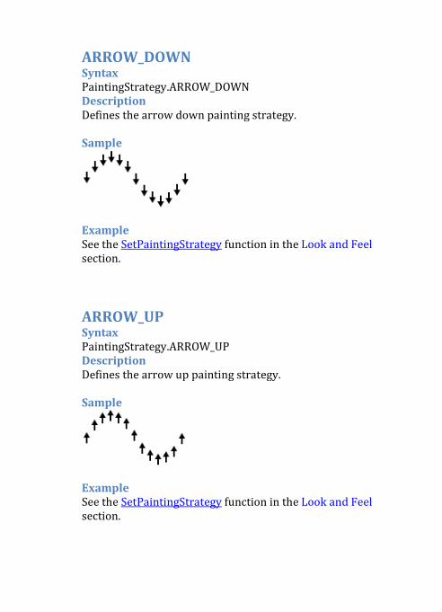
ARROW_DOWN Syntax PaintingStrategy.ARROW_DOWN Description Defines the arrow down painting strategy. Sample

Example See the SetPaintingStrategy function in the Look and Feel section. ARROW_UP Syntax PaintingStrategy.ARROW_UP Description Defines the arrow up painting strategy. Sample

Example See the SetPaintingStrategy function in the Look and Feel section.

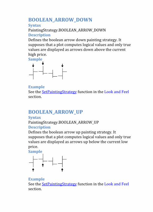
BOOLEAN_ARROW_DOWN Syntax PaintingStrategy.BOOLEAN_ARROW_DOWN Description Defines the boolean arrow down painting strategy. It supposes that a plot computes logical values and only true values are displayed as arrows down above the current high price. Sample

Example See the SetPaintingStrategy function in the Look and Feel section. BOOLEAN_ARROW_UP Syntax PaintingStrategy.BOOLEAN_ARROW_UP Description Defines the boolean arrow up painting strategy. It supposes that a plot computes logical values and only true values are displayed as arrows up below the current low price. Sample

Example See the SetPaintingStrategy function in the Look and Feel section.

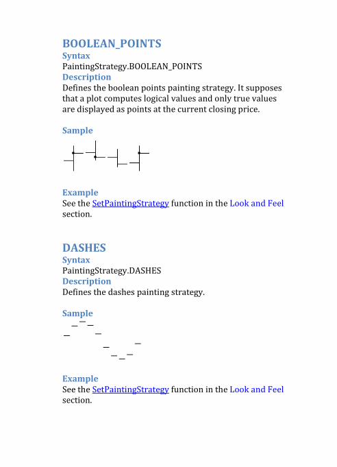
BOOLEAN_POINTS Syntax PaintingStrategy.BOOLEAN_POINTS Description Defines the boolean points painting strategy. It supposes that a plot computes logical values and only true values are displayed as points at the current closing price. Sample

Example See the SetPaintingStrategy function in the Look and Feel section. DASHES Syntax PaintingStrategy.DASHES Description Defines the dashes painting strategy. Sample

Example See the SetPaintingStrategy function in the Look and Feel section.

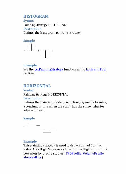
HISTOGRAM Syntax PaintingStrategy.HISTOGRAM Description Defines the histogram painting strategy. Sample

Example See the SetPaintingStrategy function in the Look and Feel section. HORIZONTAL Syntax PaintingStrategy.HORIZONTAL Description Defines the painting strategy with long segments forming a continuous line when the study has the same value for adjacent bars. Sample

Example This painting strategy is used to draw Point of Control, Value Area High, Value Area Low, Profile High, and Profile Low plots by profile studies (TPOProfile, VolumeProfile, MonkeyBars).

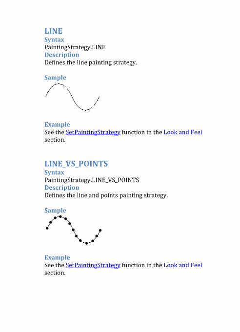
LINE Syntax PaintingStrategy.LINE Description Defines the line painting strategy. Sample

Example See the SetPaintingStrategy function in the Look and Feel section. LINE_VS_POINTS Syntax PaintingStrategy.LINE_VS_POINTS Description Defines the line and points painting strategy. Sample

Example See the SetPaintingStrategy function in the Look and Feel section.

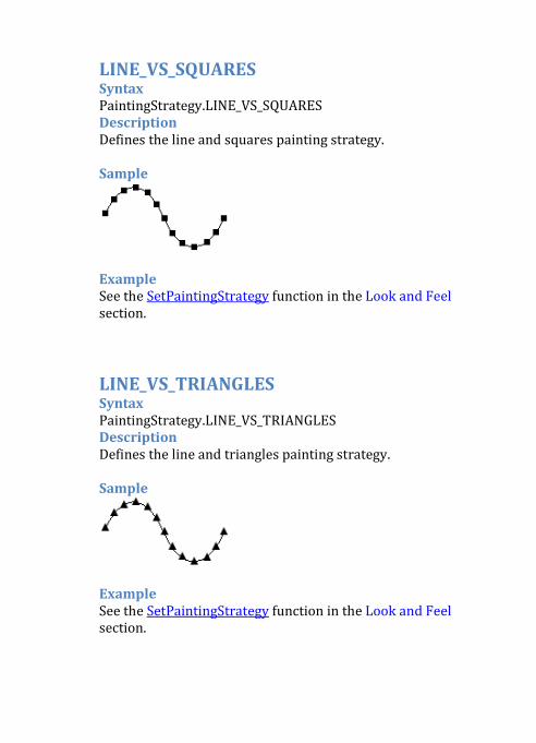
LINE_VS_SQUARES Syntax PaintingStrategy.LINE_VS_SQUARES Description Defines the line and squares painting strategy. Sample

Example See the SetPaintingStrategy function in the Look and Feel section. LINE_VS_TRIANGLES Syntax PaintingStrategy.LINE_VS_TRIANGLES Description Defines the line and triangles painting strategy. Sample

Example See the SetPaintingStrategy function in the Look and Feel section.

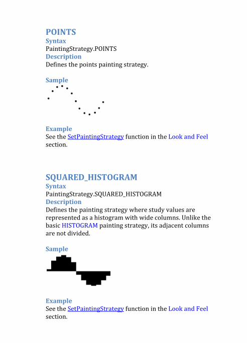
POINTS Syntax PaintingStrategy.POINTS Description Defines the points painting strategy. Sample

Example See the SetPaintingStrategy function in the Look and Feel section. SQUARED_HISTOGRAM Syntax PaintingStrategy.SQUARED_HISTOGRAM Description Defines the painting strategy where study values are represented as a histogram with wide columns. Unlike the basic HISTOGRAM painting strategy, its adjacent columns are not divided. Sample

Example See the SetPaintingStrategy function in the Look and Feel section.

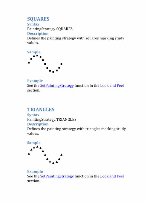
SQUARES Syntax PaintingStrategy.SQUARES Description Defines the painting strategy with squares marking study values. Sample

Example See the SetPaintingStrategy function in the Look and Feel section. TRIANGLES Syntax PaintingStrategy.TRIANGLES Description Defines the painting strategy with triangles marking study values. Sample

Example See the SetPaintingStrategy function in the Look and Feel section.

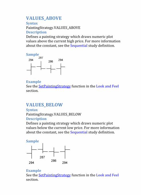
VALUES_ABOVE Syntax PaintingStrategy.VALUES_ABOVE Description Defines a painting strategy which draws numeric plot values above the current high price. For more information about the constant, see the Sequential study definition. Sample

Example See the SetPaintingStrategy function in the Look and Feel section. VALUES_BELOW Syntax PaintingStrategy.VALUES_BELOW Description Defines a painting strategy which draws numeric plot values below the current low price. For more information about the constant, see the Sequential study definition. Sample

Example See the SetPaintingStrategy function in the Look and Feel section.

o PricePerRow The constants described in this section are used in combination with the profile functions to define a price range. Choose a constant from the list:

• AUTOMATIC • TICKSIZE

AUTOMATIC Syntax PricePerRow.AUTOMATIC Description Defines the "height" (price range) of each row of the profile. When this constant is specified, the height of a row is computed to have a total number of rows equal to 50 for Monkey Bars and 85 for others. Note that this constant can only be used in conjunction with the Profile functions. TICKSIZE Syntax PricePerRow.TICKSIZE Description Defines the "height" (price range) of each row of the profile. When this constant is specified, the height of a row is equal to the minimal price change for the current symbol. Note that this constant can only be used in conjunction with the Profile functions.

o Sound The thinkscript provides the set of constants for sounds. The constants can be used in combination with alert constants to create alerts. Choose a sound from the list: • NoSound • Bell • Ding • Ring • Chimes

NoSound Syntax Sound.NoSound Description Defines the no sound constant. Example See the alert function in the Others section. Bell Syntax Sound.Bell Description Defines the bell sound constant. Example See the alert function in the Others section.

Ding Syntax Sound.Ding Description Defines the ding sound constant. Example See the alert function in the Others section. Ring Syntax Sound.Ring Description Defines the ring sound constant. Example See the alert function in the Others section. Chimes Syntax Sound.Chimes Description Defines the chimes sound constant. Example See the alert function in the Others section.

o Data Types Thinkscript functions receive arguments of different data types as parameters. Here is the full list of the data types: • Any • boolean 313 • CustomColor 313 • double 313 • IDataHolder 313 • int 313 • String 313 • Data Conversion 314

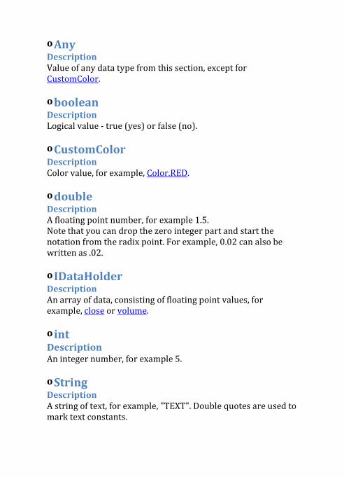
o Any Description Value of any data type from this section, except for CustomColor. o boolean Description Logical value - true (yes) or false (no). o CustomColor Description Color value, for example, Color.RED. o double Description A floating point number, for example 1.5. Note that you can drop the zero integer part and start the notation from the radix point. For example, 0.02 can also be written as .02. o IDataHolder Description An array of data, consisting of floating point values, for example, close or volume. o int Description An integer number, for example 5. o String Description A string of text, for example, "TEXT". Double quotes are used to mark text constants.

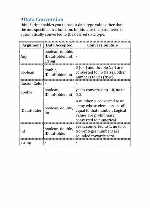
o Data Conversion thinkScript enables you to pass a data type value other than the one specified in a function. In this case the parameter is automatically converted to the desired data type.

Argument Data Accepted Conversion Rule

Any boolean, double, IDataHolder, int, String

-

boolean double, IDataHolder, int

0 (0.0) and Double.NaN are converted to no (false), other numbers to yes (true).

CustomColor - -

double boolean, IDataHolder, int

yes is converted to 1.0, no to 0.0.

IDataHolder boolean, double, int

A number is converted to an array whose elements are all equal to that number. Logical values are preliminary converted to numerical.

int boolean, double, IDataHolder

yes is converted to 1, no to 0. Non-integer numbers are rounded towards zero.

String - -

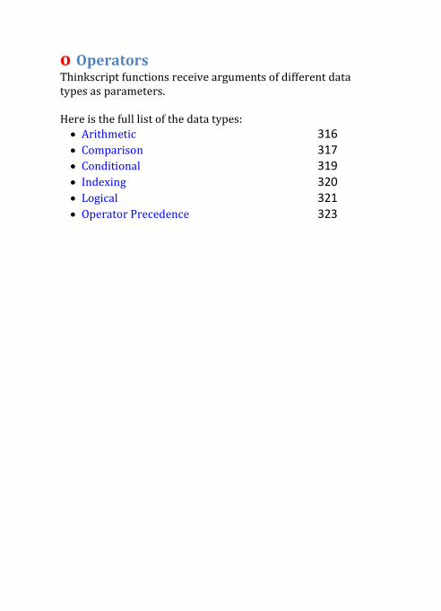
o Operators Thinkscript functions receive arguments of different data types as parameters. Here is the full list of the data types: • Arithmetic 316 • Comparison 317 • Conditional 319 • Indexing 320 • Logical 321 • Operator Precedence 323

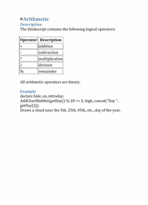
o Arithmetic Description The thinkscript contains the following logical operators: Operator Description

+ addition - subtraction * multiplication / division % remainder All arithmetic operators are binary. Example declare hide_on_intraday; AddChartBubble(getDay() % 20 == 5, high, concat("Day ", getDay())); Draws a cloud near the 5th, 25th, 45th, etc., day of the year.

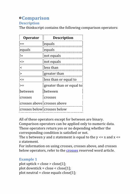
o Comparison Description The thinkscript contains the following comparison operators:

Operator Description

== equals equals equals != not equals <> not equals < less than > greater than <= less than or equal to >= greater than or equal to between between crosses crosses crosses above crosses above crosses below crosses below All of these operators except for between are binary. Comparison operators can be applied only to numeric data. These operators return yes or no depending whether the corresponding condition is satisfied or not. The x between y and z statement is equal to the y <= x and x <= z statement. For information on using crosses, crosses above, and crosses below operators, refer to the crosses reserved word article. Example 1 plot uptick = close > close[1]; plot downtick = close < close[1]; plot neutral = close equals close[1];

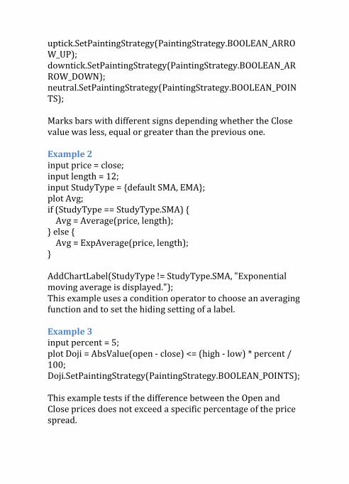
uptick.SetPaintingStrategy(PaintingStrategy.BOOLEAN_ARROW_UP); downtick.SetPaintingStrategy(PaintingStrategy.BOOLEAN_ARROW_DOWN); neutral.SetPaintingStrategy(PaintingStrategy.BOOLEAN_POINTS); Marks bars with different signs depending whether the Close value was less, equal or greater than the previous one. Example 2 input price = close; input length = 12; input StudyType = {default SMA, EMA}; plot Avg; if (StudyType == StudyType.SMA) { Avg = Average(price, length); } else { Avg = ExpAverage(price, length); } AddChartLabel(StudyType != StudyType.SMA, "Exponential moving average is displayed."); This example uses a condition operator to choose an averaging function and to set the hiding setting of a label. Example 3 input percent = 5; plot Doji = AbsValue(open - close) <= (high - low) * percent / 100; Doji.SetPaintingStrategy(PaintingStrategy.BOOLEAN_POINTS); This example tests if the difference between the Open and Close prices does not exceed a specific percentage of the price spread.

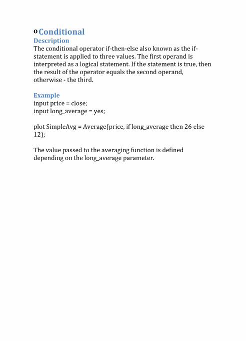
o Conditional Description The conditional operator if-then-else also known as the if-statement is applied to three values. The first operand is interpreted as a logical statement. If the statement is true, then the result of the operator equals the second operand, otherwise - the third. Example input price = close; input long_average = yes; plot SimpleAvg = Average(price, if long_average then 26 else 12); The value passed to the averaging function is defined depending on the long_average parameter.

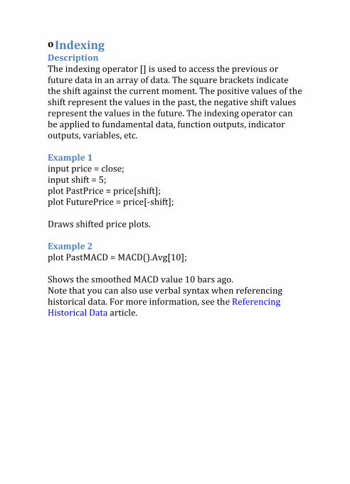
o Indexing Description The indexing operator [] is used to access the previous or future data in an array of data. The square brackets indicate the shift against the current moment. The positive values of the shift represent the values in the past, the negative shift values represent the values in the future. The indexing operator can be applied to fundamental data, function outputs, indicator outputs, variables, etc. Example 1 input price = close; input shift = 5; plot PastPrice = price[shift]; plot FuturePrice = price[-shift]; Draws shifted price plots. Example 2 plot PastMACD = MACD().Avg[10]; Shows the smoothed MACD value 10 bars ago. Note that you can also use verbal syntax when referencing historical data. For more information, see the Referencing Historical Data article.

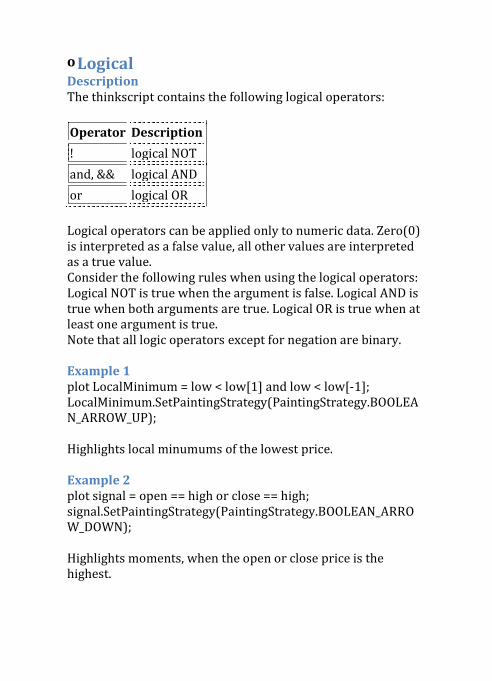
o Logical Description The thinkscript contains the following logical operators: Operator Description

! logical NOT and, && logical AND or logical OR Logical operators can be applied only to numeric data. Zero(0) is interpreted as a false value, all other values are interpreted as a true value. Consider the following rules when using the logical operators: Logical NOT is true when the argument is false. Logical AND is true when both arguments are true. Logical OR is true when at least one argument is true. Note that all logic operators except for negation are binary. Example 1 plot LocalMinimum = low < low[1] and low < low[-1]; LocalMinimum.SetPaintingStrategy(PaintingStrategy.BOOLEAN_ARROW_UP); Highlights local minumums of the lowest price. Example 2 plot signal = open == high or close == high; signal.SetPaintingStrategy(PaintingStrategy.BOOLEAN_ARROW_DOWN); Highlights moments, when the open or close price is the highest.

Example 3 input bubble = yes; AddChartBubble(bubble and barNumber() == 1, high, "Displaying a bubble"); AddChartLabel(!bubble, "Displaying a label"); Draws a cloud or label near the first bar depending on the parameter. The label is displayed when the the bubble parameter is set to no.

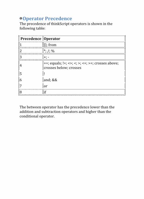
o Operator Precedence The precedence of thinkScript operators is shown in the following table: Precedence Operator

1 []; from 2 *; /; % 3 +; -

4 ==; equals; !=; <>; <; >; <=; >=; crosses above; crosses below; crosses

5 ! 6 and; && 7 or 8 if The between operator has the precedence lower than the addition and subtraction operators and higher than the conditional operator.

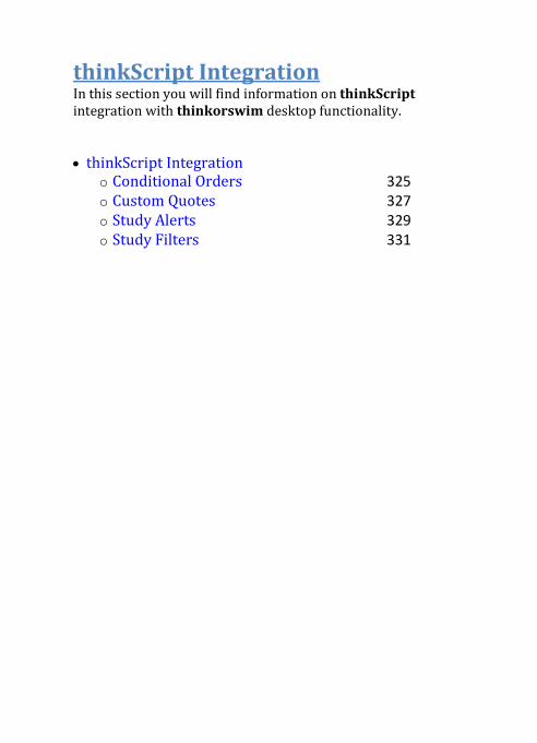
thinkScript Integration In this section you will find information on thinkScript integration with thinkorswim desktop functionality. • thinkScript Integration

o Conditional Orders 325 o Custom Quotes 327 o Study Alerts 329 o Study Filters 331

o Conditional Orders Conditional Orders are automatically placed when a study-based condition is fulfilled. You can use both pre-defined and custom studies whose values will be analyzed to place the order. How to Find It: 1. Click the "gear-and-plus" icon on the right-hand side of the Order Entry form. The Order Rules window will appear. 2. Rules for the order submission can be set in the Submit at Specified Market Condition form. After typing in the desirable symbol name, click on the Method cell and choose "STUDY" from the drop-down list. Use one of the pre-defined studies from the quick list or choose "Edit..." to open the Study Order Condition window. 3. Now you are ready to set order rules. If you prefer to use a pre-defined (or previously created) study for that purpose, make sure that Trigger Type is Study Value and choose a desirable study from the Study list. The interface allows you to specify the study plot whose values will be analyzed, input parameters, and aggregation period. For numerical plots, you can choose triggering direction relative to threshold value. For boolean plots, you can specify whether to submit the order when the value is true or false. Note that Look and Feel inputs (e.g. colors, painting strategies, etc.) are not available in Conditional Orders; constant plots are not included in the Plots list. However, you are not restricted to use a single pre-defined study to place conditional orders. You can also use a combination of studies or implement a new one right away. For that purpose, choose Complex Formula from the Trigger Type list. The editor window will appear.

Example Consider the following script: close > expaverage(close, 60) and ADX(length = 14) > 18 This condition is used in the Volume Zone Oscillator study; it checks whether the price is above the 60 period EMA and 14 period ADX value is higher than 18, which could possibly mean that the market is in strong uptrend. If you would like to automatically place an order when this condition fulfills, choose TRUE from the Trigger If list. If you however prefer to place the order when the condition is not satisfied, choose FALSE. Once you have set the rules for the conditional order, click OK in the lower right corner of the window. Specific Usage In Conditional Orders, you can use either a regular study or an expression. Here is a list of thinkScript usage peculiarities when applied to Conditional Orders:

• You are free to use bid and ask functions; • Range-dependent functions (dealing with data from the

whole chart, such as HighestAll) are not allowed; • Studies must have exactly one plot; • rec variables are not allowed.

o Custom Quotes When watching market quotes, you might need immediate calculation of certain studies for one or several symbols. You can use thinkScript integration feature in Custom Quotes for that purpose. How to Find It: 1. Click the MarketWatch tab and choose Quote from the sub-tab row. 2. Add as many symbols as you wish to the Symbol column. In order to do that, click the empty cell in the bottom of the column and type symbol's name in it. 3. Right-click on the upper row of the watchlist and choose Customize... from the menu appeared. 4. Add a Custom item (or several) to the current set - one for each value to be calculated. Click the "script" icon next to it to call the Custom Quote Formula editor window. Now you are ready to create a study whose values will be displayed in your watchlist. For pre-defined studies, the interface allows you to specify the study plot whose values will be analyzed, input parameters, and aggregation period - these can be set in the right section of the editor window. For custom studies, aggregation period can be set using the Aggregation list. Also, make sure you are using a convenient name for the study, which can be specified within the Column name string. Example To add a 60 day simple moving average, use the following script: SimpleMovingAvg() After that, choose "Day" from the Aggregation list and set the length input parameter equal to 60. Note that once a pre-defined study is added, you can replace it with another one by

choosing the corresponding name from the Study list which is now active. You can also use a custom study. Consider the following example: def period1 = 40; def period2 = 10; plot a = Momentum(length = period1) - Momentum(length = period2); This script calculates the difference between 40 and 10 period Momentum values. As you can see, the standard thinkScript syntax is also supported in Custom Quotes formulas. Once you have set the Custom Quote formula, click OK; study values will appear in the column with the corresponding name. Note that you can adjust calculation rules by right-clicking the column name and choosing Edit formula from the menu. Custom Quotes are also available for watchlists in Watchlist gadget, Scan results, and Option view at All Products under the Trade tab. Specific Usage When in Custom Quotes, thinkScript usage is somewhat different from that in studies and strategies. Here is the list of peculiarities:

• You are free to use bid and ask functions; • Range-dependent functions (dealing with data from the

whole chart, such as HighestAll) are not allowed; • Functions AssignValueColor(), SetDefaultColor(), and

AssignBackgroundColor() have specific usage; • Studies must have exactly one plot; • rec variables are not allowed.

o Study Alerts Study Alerts are signals generated when a study-based condition is fulfilled. You can use both pre-defined and custom studies whose values will be analyzed to issue the alert. How to Find It: 1. Click the MarketWatch tab and choose Alerts from the sub-tab row. 2. Choose the symbol to issue alerts for. 3. Click the Study Alert button. The Study Alerts window will appear. Now you are ready to set alert rules. If you prefer to use a pre-defined (or previously created) study for that purpose, choose a desirable one from the Study list. The interface allows you to specify the study plot whose values will be analyzed, input parameters, and aggregation period. For numerical plots, you can choose triggering direction relative to threshold value. For boolean plots, you can specify whether to issue the alert when the value is true or false. Note that Look and Feel inputs (e.g. colors, painting strategies, etc.) are NOT available in "Study Alerts"; constant plots are not included in the Plots list. However, you are not restricted to using a single pre-defined study to generate alert signals. You can also use a combination of studies or implement a new one right away. For that purpose, choose Complex Formula from the Trigger Type list. The thinkScript editor will appear. Example Consider the following script: close > expaverage(close, 60) and ADX(length = 14) > 18 This condition is used in the Volume Zone Oscillator study; it checks whether the price is above the 60 period EMA and 14 period ADX value is higher than 18, which could possibly mean

that the market is in strong uptrend. If you would like to be notified when this condition fulfills, choose TRUE from the Trigger If list. If you however prefer to place the order when the condition is not satisfied, choose FALSE. Once you have set the rules for the alert, click Create Alert in the lower right corner of the window. Specific Usage In Study Alerts, you can use either a regular study or an expression. Here is a list of thinkScript usage peculiarities when applied to Study Alerts:

• You are free to use bid and ask functions; • Range-dependent functions (dealing with data from the

whole chart, such as HighestAll) are not allowed; • Studies must have exactly one plot; • rec variables are not allowed.

o Study Filters The Stock Hacker Scanning Tool allows you to search for symbols meeting certain criteria. Study filters are criteria based on study values: adding one or several study filters will help you narrow the search range when looking for symbols. You can use up to ten filters to scan the market. How to Find It: 1. Click the Scan tab and choose Stock Hacker from the sub-tab row. 2. Click the Add Study Filter button. A new filter editor will appear. 3. The first field of the editor allows you to choose a custom or pre-defined study to filter the results. Choose the desirable study, adjust input parameters, and click Scan afterwards. Search results will be shown in the watchlist form below the Criteria section. 4. However, pre-defined study filters might be insufficient to your search. Choose Custom from the study list; this will open the Scanner Custom Filter editor window. Now you are ready to set the custom filter rules using thinkScript. Example Consider the following script: close > expaverage(close, 60) and ADX(length = 14) > 18 This condition is used in the Volume Zone Oscillator study; it checks whether the price is above the 60 period EMA and 14 period ADX value is higher than 18, which could possibly mean that the market is in strong uptrend. Click OK save the filter and then press Scan to display all symbols meeting this criterion.

You can also use plot values in Study Filters: def SMA = Average(close, 15); plot condition = close[2] > SMA[2] and close[1] < SMA[1] and close < SMA; This example script searches for symbols which were above simple moving average two days ago, but have fallen below since then. Note that search criteria can be adjusted by pressing the "pencil" icon in the filter. To delete a filter, press the "cross" icon. Note also that search results are displayed in the watchlist form, which means that you can display custom quotes along with standard values. For more information on that, refer to the Custom Quotes article. Specific Usage When in Stock Hacker, thinkScript usage is somewhat different from that in studies and strategies. Here is the list of peculiarities:

• Secondary aggregation is not allowed: all studies have aggregation period equal to one day;

• Scripts using standard thinkScript syntax must have exactly one plot.

• Getting Started 4 o Writing Your First Script 5

Defining Plots Defining Variables

Def Variables Rec Variables Rec Enumerations

Using Functions Formatting Plots Adjusting Parameters Using Inputs Accessing Data Using Strategies

o Advanced Topics 19 Concatenating Strings Creating Local Alerts Referencing Data

Referencing Secondary Aggregation Referencing Historical Data Referencing Other Price Type Data Referencing Other Studies Referencing Other Symbol's Data Past Offset

Using Profiles

• Reference 35 o Reserved Words 37 above ago and bar bars below between case crosses declare

def default do else equals fold from if input boolean

constant enum float integer price string no or plot profile

rec reference script switch then to while with yes

o Declarations 68

all_for_one hide_on_daily hide_on_intraday lower on_volume

once_per_bar real_size upper weak_volume_dependency zerobase

o Functions 78 Fundamentals 79

ask bid close high hl2

hlc3 imp_volatility low ohlc4 open

open_interest volume vwap

Option Related 92 delta gamma getDaysToExpiration getStrike getUnderlyingSymbol isEuropean

isOptionable isPut optionPrice rho theta vega

Technical Analysis 104 AccumDist Average AvgTrueRange BodyHeight Ema2 ExpAverage FastKCustom GetMaxValueOffset GetMinValueOffset Highest HighestAll HighestWeighted IsAscending

IsDescending IsDoji IsLongBlack IsLongWhite Lowest LowestAll LowestWeighted MidBodyVal moneyflow TrueRange Ulcer WildersAverage wma

Mathematical and Trigonometrical 132

AbsValue ACos ASin ATan Ceil Cos Crosses exp Floor isInfinite

IsNaN lg log Max Min Power Random round roundDown roundUp

Sign Sin Sqr Sqrt sum Tan TotalSum

Statistical 156

correlation covariance Inertia InertiaAll lindev

stdev stdevAll sterr sterrAll

Date and Time 170 countTradingDays daysFromDate daysTillDate getDay getDayOfMonth getDayOfWeek getLastDay getLastMonth getLastWeek

getLastYear getMonth getWeek getYear getYyyyMmDd regularTradingEnd regularTradingStart secondsFromTime secondsTillTime

Corporate Actions 185

getActualEarnings getDividend getEstimatedEarnings getSplitDenominator

getSplitNumerator hasConferenceCall hasEarnings

Look and Feel 191

AddChartBubble AddChartLabel AddCloud AddVerticalLine AssignBackgroundColor AssignNormGradientColor AssignPriceColor AssignValueColor color CreateColor DefineColor DefineGlobalColor EnableApproximation GetColor

globalColor hide HideBubble hidePricePlot HideTitle setChartType SetDefaultColor setHiding SetLineWeight SetPaintingStrategy SetStyle TakeValueColor

Profiles 220

getHighest getHighestValueArea getLowest getLowestValueArea getPointOfControl

monkeyBars show timeProfile volumeProfile

Others 234 addOrder alert barNumber between compoundValue concat entryPrice first fundamental

getAggregationPeriod getInterestRate getSymbolPart getValue getYield if tickSize tickValue

o Constants 256

AggregationPeriod MIN TWO_MIN THREE_MIN FOUR_MIN FIVE_MIN TEN_MIN FIFTEEN_MIN TWENTY_MIN THIRTY_MIN

HOUR TWO_HOURS FOUR_HOURS DAY TWO_DAYS THREE_DAYS FOUR_DAYS WEEK MONTH OPT_EXP

o AggregationPeriod 257

• MIN • TWO_MIN • THREE_MIN • FOUR_MIN • FIVE_MIN • TEN_MIN • FIFTEEN_MIN • TWENTY_MIN • THIRTY_MIN • HOUR

• TWO_HOURS • FOUR_HOURS • DAY • TWO_DAYS • THREE_DAYS • FOUR_DAYS • WEEK • MONTH • OPT_EXP

Alert 268

BAR ONCE

TICK

ChartType 269 BAR CANDLE CANDLE_TREND

HEIKIN_ASHI LINE AREA

Color 273

BLACK BLUE CURRENT CYAN DARK_GRAY DARK_GREEN DARK_ORANGE DARK_RED DOWNTICK GRAY GREEN LIGHT_GRAY LIGHT_GREEN

LIGHT_ORANGE LIGHT_RED LIME MAGENTA ORANGE PINK PLUM RED UPTICK VIOLET WHITE YELLOW

CrossingDirection 283

Above Below

Any

Curve 285

FIRM LONG_DASH MEDIUM_DASH

SHORT_DASH POINTS

Double 289

E NaN Pi

EarningTime 291

ANY BEFORE_MARKET AFTER_MARKET

FundamentalType 293 HIGH LOW CLOSE OPEN HL2 HLC3 OHLC4 VWAP

VOLUME OPEN_INTEREST IMP_VOLATILITY OrderType BUY_AUTO BUY_TO_CLOSE SELL_AUTO SELL_TO_CLOSE

o OrderType 297

• BUY_AUTO • BUY_TO_CLOSE • SELL_AUTO • SELL_TO_CLOSE

PaintingStrategy 299

ARROW_DOWN ARROW_UP BOOLEAN_ARROW_DOWN BOOLEAN_ARROW_UP BOOLEAN_POINTS DASHES HISTOGRAM HORIZONTAL LINE LINE_VS_POINTS

LINE_VS_SQUARES LINE_VS_TRIANGLES POINTS SQUARED_HISTOGRAM SQUARES TRIANGLES VALUES_ABOVE VALUES_BELOW

PricePerRow 309

AUTOMATIC TICKSIZE

Sound 310

NoSound Bell Ding

Ring Chimes

o Data Types 312 Any boolean CustomColor double

IDataHolder int String Data Conversion

o Operators 323 Arithmetic Comparison Conditional

Indexing Logical Operator Precedence

• thinkScript Integration 324

o Conditional Orders 325 o Custom Quotes 327 o Study Alerts 329 o Study Filters 331