THIEM WOH MUN UNIVERSITY TUNKU ABDUL RAHMAN

INVESTIGATE THE FEASIBILITY OF

IMPLEMENTING EARTH-TO-AIR HEAT

EXCHANGER (EAHE) AS A

SUSTAINABLE COOLING SYSTEM

IN MALAYSIA

THIEM WOH MUN

UNIVERSITY TUNKU ABDUL RAHMAN

INVESTIGATE THE FEASIBILITY OF IMPLEMENTING

EARTH-TO-AIR HEAT EXCHANGER (EAHE) AS A

SUSTAINABLE COOLING SYSTEM IN MALAYSIA

THIEM WOH MUN

A project report submitted in partial fulfilment of the

requirements for the award of Bachelor of Engineering

(Hons.) Mechanical Engineering

Faculty of Engineering and Science

Universiti Tunku Abdul Rahman

May 2015

iii

DECLARATION

I hereby declare that this progress report is based on my original work except for

citations and quotations which have been duly acknowledged. I also declare that it

has not been previously and concurrently submitted for any other degree or award at

UTAR or other institutions.

Signature :

Name : Thiem Woh Mun

ID No. : 10UEB05467

Date : 8 May 2015

iv

APPROVAL FOR SUBMISSION

I certify that this progress report entitled “INVESTIGATE THE FEASIBILITY

OF IMPLEMENTING EARTH-TO-AIR HEAT EXCHANGER (EAHE) AS A

SUSTAINABLE COOLING SYSTEM IN MALAYSIA” was prepared by

THIEM WOH MUN has met the required standard for submission in partial

fulfilment of the requirements for the award of Bachelor of Engineering (Hons.)

Mechanical Engineering at Universiti Tunku Abdul Rahman.

Approved by,

Signature :

Supervisor :

Date :

v

The copyright of this report belongs to the author under the terms of the

copyright Act 1987 as qualified by Intellectual Property Policy of Universiti Tunku

Abdul Rahman. Due acknowledgement shall always be made of the use of any

material contained in, or derived from, this report.

© 2015, Thiem Woh Mun. All right reserved.

vi

Specially dedicated to

my beloved mother, father, brother and sister.

vii

ACKNOWLEDGEMENTS

I would like to thank everyone who had contributed to the successful completion of

this project report. I would like to express my gratitude to my research supervisor,

Dr. Tan Yong Chai for his invaluable advice, guidance and his enormous patience

throughout the development of the research.

In addition, I would also like to express my gratitude to my loving parent and

family members and friends who had helped and given me encouragement

throughout this progress report. I am thankful to all my final year project group

members for sharing valuable knowledge with me.

viii

INVESTIGATE THE FEASIBILITY OF IMPLEMENTING

EARTH-TO-AIR HEAT EXCHANGER (EAHE) AS A

SUSTAINABLE COOLING SYSTEM IN MALAYSIA

ABSTRACT

This project aims to evaluate the potential of implementing Earth-to-Air Heat

Exchanger (EAHE) to provide space cooling and air conditioning in Malaysia. The

benefit of this passive cooling technology in tropical climate such as Malaysia is

unrecognized at current time due to lack of development in this field. Based on

experimental measurement, the suitable depth for the installation of the pipe of

EAHE prototype system in this project was determined to be 1.5 m. The difference

of ground temperature at the depth of 1.5 m and 2.0 m was also determined to be

very small with a difference of only 0.1 C.

To design the EAHE prototype system for this studies, a cooling load analysis

based on Residential Load Factor (RLF) method has been conducted on the

experimental residential room. The cooling load determined from RLF method was

952 W. The EAHE prototype system designed in this project intended to reject heat

of the amount imposed by the determined cooling load under the worst condition.

The EAHE prototype system finalized and tested in this project has selected PVC

pipe of 3 in (80 mm) nominal diameter. The pipe length of the EAHE prototype has

been designed to be 11.6 m long.

Besides, a centrifugal exhaust has been designed and fabricated in this project

that was used in the EAHE prototype system. The centrifugal fan was designed by a

trial-and-error approach using Flow Simulation of SolidWorks. The simulated and

experimental suction velocity was determined to be 17.1 m/s and 16.5 m/s with a

percentage difference of 3.64 %.

ix

Experimental studies performed on the EAHE prototype system has shown

that the average ideal and actual percentage reduction of cooling load achieved were

37.57 % and 16.21 % respectively. The average heat rejected by the EAHE and from

the room were 357.70 W and 154.28 W respectively. The results obtained also

shown that the EAHE efficiency stays in the range of 30 – 50 % for most of the time

and the prototype had achieved an average EAHE efficiency of 48.87 %. The

average ideal and actual Coefficients of Performance (COPs) achieved by the EAHE

prototype were 7.15 and 3.09 respectively. It was also shown that the actual COP of

the EAHE prototype stays in the range of 3.0 – 4.4 for most of the time.

In conclusion, the EAHE prototype did reasonably well performance in terms

of COPs. However, it did not achieved very well performance in percentage

reduction of cooling load and EAHE efficiency due to the effect of heat gained by

the insulation. Therefore, it can be concluded that it is feasible to implement EAHE

cooling system in Malaysia if thermal insulation of the system could be carefully

designed.

x

TABLE OF CONTENTS

DECLARATION iii

APPROVAL FOR SUBMISSION iv

ACKNOWLEDGEMENTS vii

ABSTRACT viii

TABLE OF CONTENTS x

LIST OF TABLES xiv

LIST OF FIGURES xvi

LIST OF SYMBOLS / ABBREVIATIONS xx

LIST OF APPENDICES xxiii

CHAPTER

1 INTRODUCTION 1

1.1 Background 1

1.2 Problem Statements 5

1.3 Aim and Objectives 7

2 LITERATURE REVIEW 8

2.1 Undisturbed Ground Temperature by Experiment

Investigation 8

2.2 EAHE Pipe Diameter Selection 10

2.3 EAHE Pipe Length Selection 11

2.4 Evaluation of Cooling Performance of EAHE in Different

Climate 11

xi

3 METHODOLOGY 15

3.1 Experimental Location and Setup 15

3.1.1 Experimental Location 15

3.1.2 Experimental Residential Room 16

3.2 Measurement of Ground, Room and Environment

Temperature 17

3.2.1 Preparation of the K-type Thermocouples 17

3.2.2 Drilling of Hole by JKR Probe and Insertion of

Thermocouples 18

3.2.3 On-site Measurement of Ground, Room (before

EAHE) and Environment Temperature 19

3.3 Cooling Load Analysis 21

3.3.1 Cooling Load due to Heat Gain through Opaque

Surfaces 21

3.3.2 Cooling Load due to Infiltration/Ventilation 22

3.3.3 Cooling Load due to Internal Heat Gains 24

3.4 EAHE Prototype Design 25

3.4.1 EAHE Prototype Design Strategy 25

3.4.2 Fan Design and Fabrication 25

3.4.3 Pipe Diameter and Length Selection of EAHE

Prototype 28

3.5 Data Collection and Analysis of the EAHE Prototype

System 33

3.5.1 Data Collection of the EAHE Prototype System 33

3.5.2 Temperature Data Analysis of the EAHE

Prototype System 33

3.5.3 Heat Analysis of the EAHE Prototype System 34

3.5.4 Cooling Performance of EAHE Prototype 35

4 RESULTS AND DISCUSSION 38

4.1 Ground, Room and Environment Temperature Profile 38

4.2 Cooling Load Analysis with Residential Load Factor

(RLF) Method 43

xii

4.3 EAHE Prototype Design 54

4.3.1 Fan Design and Fabrication 54

4.3.2 Pipe Diameter and Length Selection of EAHE

Prototype 62

4.3.3 Full View of Designed EAHE Prototype System 69

4.4 Data Collection of the EAHE Prototype System 73

4.5 Temperatures Data Analysis of the EAHE Prototype

System 77

4.5.1 Mean Room and Environment Temperatures with

EAHE 77

4.5.2 Mean Room and EAHE Outlet Temperatures 78

4.5.3 Mean Room and EAHE Inlet Temperatures 80

4.5.4 Mean EAHE Inlet and Outlet Temperature 82

4.5.5 Mean Room Inlet and Outlet Temperature 84

4.5.6 Mean Room Temperature without and with

EAHE 86

4.6 Heat Analysis of the EAHE Prototype System 88

4.6.1 Heat Gained by the Insulation – Inlet Segment 88

4.6.2 Heat Gained by the Insulation – Outlet Segment 89

4.6.3 Heat Rejected by the EAHE 91

4.6.4 Heat Rejected from the Room 93

4.7 Cooling Performance of the EAHE Prototype System 94

4.7.1 Summarized of Heat Analysis 94

4.7.2 Percentage Reduction of Cooling Load Analysis 96

4.7.3 EAHE Efficiency Analysis 98

4.7.4 Coefficient of Performance (COP) Analysis 100

5 CONCLUSION AND RECOMMENDATIONS 103

5.1 Conclusion 103

5.2 Recommendation 105

REFERENCES 106

xiii

APPENDICES 109

xiv

LIST OF TABLES

TABLE TITLE PAGE

3.1 Technical Specification of K-type Thermocouple 20

4.1 Mean Ground, Room and Environment

Temperatures 39

4.2 Mean Daily Ground, Room and Environment

Temperatures 47

4.3 Experimental Residential Room Design Conditions 49

4.4 Experimental Residential Room Component

Parameter 50

4.5 Experimental Residential Room Opaque Surface

Factors 50

4.6 Experimental Residential Room Cooling Loads 53

4.7 Specification of Designed Centrifugal Exhaust Fan 59

4.8 Result of Calculation of Required Length and

Total Cost for PVC with Different Nominal

Diameter 67

4.9 Simulated and Experimental Values of Flow

Properties of EAHE Prototype 74

4.10 Various Mean Temperatures of the EAHE

Prototype System 75

4.11 Mean Room and Environment Temperatures with

EAHE Prototype 77

4.12 Mean Room and EAHE Outlet Temperatures with

EAHE Prototype 79

xv

4.13 Mean Room and EAHE Inlet Temperatures with

EAHE Prototype 81

4.14 Mean EAHE Inlet and Outlet Temperatures with

EAHE Prototype 83

4.15 Mean Room Inlet and Outlet Temperatures with

EAHE Prototype 84

4.16 Room Temperatures without and with EAHE

Prototype 86

4.17 Heat Gained by the Insulation – Inlet Segment 89

4.18 Heat Gained by the Insulation – Outlet Segment 90

4.19 Heat Rejected by the EAHE Prototype 92

4.20 Heat Rejected from the Room 93

4.21 Ideal and Actual Percentage Reduction of Cooling

Load 96

4.22 Heat Rejected and EAHE Efficiency 98

4.23 Ideal and Actual COP of EAHE Prototype 100

xvi

LIST OF FIGURES

FIGURE TITLE PAGE

1.1 International Energy Outlook 2013 on World

Energy Consumption by Fuel Type (EIA U.S.

Energy information Administration, 2013) 2

1.2 Electricity Consumption of Residential and

Commercial Sectors of Malaysia (Energy

Commission, 2013) 2

1.3 Open loop EAHE System (Peretti, et al., 2013) 4

1.4 Closed loop EAHE System (Ozgener and Ozgener,

2011) 5

2.1 Effect of Depth of Ground on Indoor Air

Temperature (Ghosal and Tiwari, 2006) 9

2.2 Experimental Setup of EAHE (Mongkon, et al.,

2013) 12

2.3 Experimental Setup of EAHE (Ghosal and Tiwari,

2003) 13

2.4 CoolTek house with integrated EAHE layout

(Reimann, 2007) 14

3.1 Bird-eye view of experiment location through

Google Maps (2015) 15

3.2 Experimental Residential Room View 1 16

3.3 Experimental Residential Room View 2 16

3.4 Marking by Duct Tape for Thermocouples 17

3.5 Shaping of Hot Junction of the Thermocouple 17

3.6 JKR Probe 18

xvii

3.7 Hole Drilled by using JKR Probe 19

3.8 K-type/Infra-red Thermometer 20

3.9 Opaque Surface Cooling Factor Coefficients

(ASHRAE, 2009) 22

3.10 Roof Solar Absorptance (ASHRAE, 2009) 22

3.11 Typical Values of IDF (ASHRAE, 2009) 24

3.12 Unit Leakage Area Factor (ASHREA, 2009) 24

3.13 Maximum Recommended Air Flow Velocity

(ASHREA, 2009) 27

3.14 Microsoft Excel Spreadsheet for Pipe Diameter

and Length Selection 28

3.15 PVC Pipe Catalogue (ATKC e-Commerce

Warehouse, 2015) 29

4.1 Mean Ground, Room and Environment

Temperatures 40

4.2 Mean Ground Temperatures at Different Depth 41

4.3 Detail Dimensions of the Experimental Residential

Room 44

4.4 Roof tiles of the Experimental Residential Room 45

4.5 Concrete ceiling of the Experimental Residential

Room 45

4.6 Walls of the Experimental Residential Room 45

4.7 Door and Wood Covered Window of the

Experimental Residential Room 46

4.8 Roof Type of the Experimental Residential Room

with Suggested U-factor (Tan, 2013) 46

4.9 Wall Type of the Experimental Residential Room

with Suggested U-factor (Tan, 2013) 47

4.10 Mean Maximum Temperature Distribution of

Malaysia at March (Malaysia Metrological

Department, 2015) 48

xviii

4.11 Mean Minimum Temperature Distribution of

Malaysia at March (Malaysia Metrological

Department, 2015) 49

4.12 Finalized Centrifugal Exhaust Fan in Solid

Modelling 54

4.13 Impeller of Finalized Centrifugal Exhaust Fan in

Solid Modelling 55

4.14 Casing of Finalized Centrifugal Exhaust Fan in

Solid Modelling 55

4.15 Actual Appearance of the Fabricated Centrifugal

Exhaust Fan 56

4.16 Impeller of the Fabricated Centrifugal Exhaust Fan 56

4.17 Casing/Housing of the Fabricated Centrifugal

Exhaust Fan 57

4.18 Supporting Structure of the Fabricated Centrifugal

Exhaust Fan 57

4.19 Determination of Experimental Suction Velocity

by Anemometer 60

4.20 Velocity Flow Trajectory in Flow Simulation 60

4.21 Pressure Flow Trajectory in Flow Simulation 61

4.22 Velocity Cut Plot in Flow Simulation 61

4.23 Pressure Cut Plot in Flow Simulation 62

4.24 Calculation for 25 mm PVC pipe by Microsoft

Excel Spreadsheet 65







4.28 Required Length and Total Cost for PVC pipe of

Different Nominal Diameter 68

xix

4.29 Pipe Layout of the EAHE Prototype with

Dimensions Labelled 69

4.30 EAHE Pipe Layout with Insulation in Solid

Modeling 70

4.31 Top View of EAHE Prototype System in Solid

Modeling 70

4.32 Isometric View of EAHE Prototype System in

Solid Modeling 71

4.33 Side View of EAHE Prototype System in Solid

Modeling 71

4.34 Actual EAHE Pipe Layout on Site 72

4.35 Actual EAHE Prototype on Site 72

4.36 Various Mean Temperatures of the EAHE

Prototype System 76

4.37 Mean Room and Environment Temperatures with

EAHE Prototype 78

4.38 Mean Room and EAHE Outlet Temperatures with

EAHE Prototype 79

4.39 Mean Room and EAHE Inlet Temperatures with

EAHE Prototype 81

4.40 Mean EAHE Inlet and Outlet Temperatures with

EAHE Prototype 83

4.41 Mean Room Inlet and Outlet Temperature with

EAHE Prototype 85

4.42 Room Temperature without and with EAHE

Prototype 87

4.43 Heat Gained and Rejected at Various Segments 95

4.44 Ideal and Actual Percentage Reduction of Cooling

Load 97

4.45 Heat Rejected and EAHE Efficiency 99

4.46 Ideal and Actual COP of EAHE Prototype 101

xx

LIST OF SYMBOLS / ABBREVIATIONS

A net surface area, ft2

Acf conditioned floor area of building, ft2

Aes building exposed surface area, ft2

AL building effective leakage area, ft2

Aul unit leakage area factor, in2/ft2

qopq opaque surface cooling load, Btu/h

CFopq surface cooling factor, Btu/h.ft2

COPactual actual coefficient of performance of the EAHE

COPideal ideal coefficient of performance of the EAHE

Cs air sensible heat factor, Btu/h·cfm

Di inner diameter of the pipe, m

Do outer diameter of the pipe, m

DR daily cooling range, ℉

f friction factor

ha convective heat transfer coefficient of air, W/m2·K

k thermal conductivity of the component, W/m ·K

ka thermal conductivity of the air, W/m·K

kp thermal conductivity of the PVC pipe, W/m·K

L length of the pipe, m

am mass flow rate of air, kg/s

Noc number of occupants

Nu Nusselt number

OFb opaque surface cooling factors

OFr opaque surface cooling factors

OFt, opaque surface cooling factors

xxi

Pfan rated power of the fan, W

Pr Prandlt number

Qbal,hr balanced ventilation flow rate via HRV/ERV equipment, cfm

Qbal,oth other balanced ventilation supply airflow rate, cfm

Qi infiltration leakage rate assuming no mechanical pressurization, cfm

Qunbal unbalanced airflow rate, cfm

Qv required ventilation flow rate, cfm

Qvi combine infiltration/ventilation flow rate, cfm

qgained/rejected heat gained or rejected, W

qig cooling load (sensible) due to internal heat gains, Btu/h

qload total heat gain of the room from cooling load analysis, W

EAHErejectedq , heat rejected by the EAHE prototype, W

rooomrejectedq , heat rejected from the room, W

qvi ventilation/infiltration cooling load, Btu/h

Rconductive conductive thermal resistance of the pipe, K/W

Rconvective convective thermal resistance from air to inner pipe surface, K/W

Re Reynolds number

Rtotal total thermal resistance, K/W

t thickness of the component, m

U construction U-factor, Btu/h·ft2·oF

Vavg average velocity in the EAHE pipe system, m/s

Vo outlet velocity of the EAHE system or suction inlet velocity of the

fan, m/s

Vi inlet velocity of the EAHE system

∆T difference of temperature, K

∆Troom-ground temperature difference of room and ground temperature, K

∆t cooling design temperature difference, ℉

εs HRV/ERV sensible effectiveness

μ dynamic viscosity of the air, kg/m s

ηEAHE EAHE efficiency

ρ density of air, kg/m3

xxii

EAHE Earth-to-Air Heat Exchanger

℃ degree Celsius

s second

m meter

J Joule

W Watt

Pa Pascal

kg kilogram

xxiii

LIST OF APPENDICES

APPENDIX TITLE PAGE

A Tables and Graph of Ground, Room and

Environment Temperature 109

B Calculation of Required Length for Different

Diameter 119

C Tables and Graph Various Temperature of the

EAHE Prototype System 129

1

CHAPTER 1

1 INTRODUCTION

1.1 Background

The world energy consumption is increasing over the time horizon while the fossil

fuels are still expected to be the largest supply of the worldwide energy consumption.

Nevertheless, nuclear and renewable energy are growing fast due to the relatively

high price of fossil fuels especially petroleum and other liquid fuels as shown in

Figure 1.1 (EIA U.S. Energy information Administration, 2013). In Malaysia, the

energy demand of residential and commercial sectors has increased by over 118 and

124 percent from year 2000 to 2012. Most of the energy consumed in these two

sectors are used in cooling and conditioning the indoor air of a building as shown in

Figure 1.2 (Energy Commission, 2013). Renewable energy combine with energy

efficient design suggested a sustainable and reliable solution for the worldwide

energy crisis.

There is a growing interest in heating, ventilation and air conditioning

(HVAC) based on renewable energy particularly in the development of green

building. Geothermal energy which exploits the use of renewable energy stored in

the ground is one of the energy sources currently in demand (Geothermal Panel of

the European Technology Platform on Renewable Heating and Cooling, 2012).

There are generally three types of geothermal energy that could be extracted or

harvested corresponding to three level of depth of the ground which are deep,

swallow and very swallow (or near-surface). Deep geothermal energy can be

extracted using deep drilling holes for electricity generation. Geothermal power plant

2

utilizes steam (over 150oC) produced from reservoir of hot water found three to six

km below the surface of ground for this purpose (Germany Energy Agency, 2002).

Figure 1.1: International Energy Outlook 2013 on World Energy Consumption

by Fuel Type (EIA U.S. Energy information Administration, 2013)

Figure 1.2: Electricity Consumption of Residential and Commercial Sectors of

Malaysia (Energy Commission, 2013)

3

Swallow geothermal energy can be extracted using deep bore heat exchangers,

a closed system for geothermal energy production consists of a single borehole at a

depth of over 400 m. Double pipe heat exchangers are inserted into it and heat is then

extracted and delivered to a heat pump circuit at the surface through a circulating hot

water. This kind of geothermal heat wells finds it application in the industrial and

agriculture heating process (Germany Energy Agency, 2002). The third type of

geothermal energy is near-surface geothermal energy which exploits the heat from

the upper layers of ground and ground water. At sufficient depth of about 2 m from

the ground surface, the ground temperature remains relatively constant, the

temperature fluctuations at the surface is attenuated by the high thermal inertia of the

soil. The ground temperature at this depth is warmer than air in winter and cooler

than the air in summer for a seasonal country.

Passive cooling and heating of a building to a comfortable level can be

achieved through buried pipes in the ground, a mechanism called earth-to-air heat

exchanger (EAHE). When ambient air is drawn through these buried pipes, the air

will be cooled in the summer because the ground temperature is lower. Conversely,

the ambient air is heated during winter because the ground temperature is relatively

higher. For many years since its discovery, EAHE was well-known as a potent and

viable solution to achieve comfort and space cooling whilst reducing energy

consumption in a building (Al-Ajmi, Loveday and Hanby, 2006). Besides being

emission-free and environment friendly, the main advantages of the EAHE is low

operational and maintenance costs and high pre-cooling and pre-heating potential.

The main focus of this study is to investigate the effectiveness of the EAHE

in terms of cooling potential in Malaysia which has a tropical climate. Generally, an

EAHE consists of a network of buried pipes where hot air is sucked in at the inlet

end by the blower or fan to the outlet end of the pipes. The ground function as a heat

sink absorbing the thermal energy given out by the transfer medium of air through

heat transfer. Subsequently, the hot ambient air in tropical climate will be cooled

down at EAHE outlet ends. In some instances, if the air temperature at the EAHE

outlet is sufficiently low, the outlet air from the EAHE can be straightaway used for

space cooling. Otherwise, it could be further cooled down by means of an external

refrigeration unit. Therefore, EAHE reduced the cooling load and energy consumed

4

of the building in either case of direct cooling or pre-cooling (Wu, Wang and Zhu,

2007).

Generally, there are two type of EAHE system which are open or closed loop

EAHE (Ozgener and Ozgener, 2011). Both open and closed loop EAHE have

network of buried pipes connected to the inlet and outlet ends they differentiated

from each other by the location of the inlet end. Open loop EAHE typically has an

inlet shaft with filter located outside of the building and an outlet located inside the

building. It is so called open loop EAHE because the system is open at the inlet end

and takes in air from the outdoor as shown in Figure 1.3. Alternatively, a closed loop

EAHE typically has both inlet and outlet ends located inside the building. It is so

called closed loop EAHE because the buried pipes, inlet and outlet ends and the

building space formed a closed system as referred to Figure 1.4. In this study, a

closed loop EAHE with the network of buried pipes installed in open spaces (rather

than beneath buildings) has been constructed for investigation.

Figure 1.3: Open loop EAHE System (Peretti, et al., 2013)

5

Figure 1.4: Closed loop EAHE System (Ozgener and Ozgener, 2011)

1.2 Problem Statements

This study intended to determine the potential of implementing Earth-to-Air Heat

Exchangers (EAHE) in Malaysia as a sustainable option for the purpose of space

cooling and air conditioning. It was shown that the cooling performance of several

EAHE in other climates are greatly influenced by the ambient air temperature and

undisturbed ground temperature where the pipe being buried. (Pretti, et al., 2013).

The fact that this passive cooling technology (EAHE) lack of implementation data

and records in Malaysia makes the evaluation process rather challenging.

The ground temperature at the depth where EAHE is buried does not always

remain constant due to the heat transfer convection and radiation with the

surrounding at the surface. By designing the depth of buried pipe as deep as possible

will not solve this problem because of the increase in installation cost due to soil

digging will not necessary be justified by the increase in cooling performance.

Therefore, the main problem in this study was to determine the undisturbed ground

temperature profile and suitable depth of ground for EAHE in Malaysia. One of the

6

feasible solutions to resolve this issue could be by conducting an on-site

experimental measurement of ground temperature at various depth.

In general, the EAHE prototype shall be designed and built based on the

cooling load imposed by the experimental room or space to be conditioned. It was

crucial that cooling load to be known so that the EAHE designed would not be

undersized or oversized in terms of cooling capacity. There are many methods

available to determine the cooling load some of which as complicated as using

computerized numerical solutions while other could be as simple as using empirical

factor. Therefore, the next problem was to determine cooling load imposed by the

experimental residential room with the chosen method before the EAHE prototype

could be designed and built.

The optimization of the cooling performance of the EAHE depends greatly on

its operating parameters such as pipe length, diameter, air flow rate and depth of

ground (Wu, Wang and Zhu, 2007). Therefore, the next problem in this project was

to design and built an EAHE prototype and to determine the optimum size of the

prototype in terms of its pipe diameter and length. In addition, an exhaust fan has to

be designed and built to provide the static pressure, air flow rate and velocity

required by the prototype EAHE system. The process of fan design was also very

important because the EAHE prototype should be well balanced in cooling and

acoustics performances at the same time. Thus, another problem in this project was

to design and fabricate the suitable exhaust fan using the available design methods.

Although there are plenty EAHEs in operation in Europe and other regions of

the world, this technology was not yet being commercialized in Malaysia. The

determination of the cooling performance and economic considerations of

implementation were the foremost issues restraining the development of this

technology in Malaysia. Therefore, the last problem in this project was to determine

the experimental cooling performance of a designed and built EAHE prototype so as

to access its feasibility of implementation in Malaysia.

7

1.3 Aim and Objectives

Based on the problems identified in the previous section, this project was carried out

to resolve all these problems with the aim to access the feasibility of implementing

EAHE in Malaysia. In short, the five (5) objectives that were to be achieved through

this final year project include:

1. To determine the suitable depth for the installation of earth-to-air heat

exchanger (EAHE) pipe by experimental measurement.

2. To determine the cooling load of the experimental residential room using

Residential Load Factor (RLF) method proposed by ASHRAE.

3. To design and fabricate a centrifugal exhaust fan that can provide the static

pressure, air flow rate and velocity required by the prototype EAHE system.

4. To design an EAHE prototype system in terms of pipe diameter and length to

output the cooling capacity imposed by the experimental residential room’s

cooling load.

5. To analyse and evaluate the experimental cooling performance of the EAHE

prototype system.

8

CHAPTER 2

2 LITERATURE REVIEW

2.1 Undisturbed Ground Temperature by Experiment Investigation

The undisturbed ground temperature is the main operating parameter during the

EAHE design process. It was proposed that the undisturbed ground temperature will

be affected by the depth of ground. Although the deeper into the ground the more

constant the ground temperature, installing EAHE too deep will not be justified by

the increase of installation cost. Therefore, finding the suitable depth of ground for

the EAHE installation is very important during the design process.

In practice, most of the EAHE in operation was installed at a depth of 3 m to

4 m. Ghosal and Tiwari (2006) performed a parametric studies by conducting

experiments in Delhi, India to illustrate the effects of operating parameters including

the depth of ground on the thermal performance. This study has demonstrated that

the cooling performance of the integrated EAHE increased with increasing depth of

ground up to 4 m in a hot and dry climate as shown in Figure 2.1. However, this

result might not be applicable in other region of the world with different climate.

Pfafferott (2003) evaluated the energy efficiency with a standardized method of three

EAHEs in Germany with the depth of pipe of 2-3 m, 2 m and 2.3 m below the

ground.

Sanusi, Li and Zamri (2014) analysed the potential of EAHE in Malaysia in

terms of ground temperature and ambient temperature. The ambient temperature,

ground surface temperature, and ground temperature at the depth of 1 m, 2m, 3 m, 4

9

m and 5 m were measured during the first stage of the investigation. Then, soil

temperature at the depth of 0.5 m, 1.0 m and 1.5 m were investigated for one year.

The results of this study shown that at a depth of below 1 m, the soil temperature

increases with depth up to 5 m. The annual amplitude or the fluctuation of the soil

temperature decreases from 0.5 m to 1.0 m and then 1.5 m. The optimum depth of

ground for EAHE installation obtained in this study was 1 m below the ground. At

the depth of 1 m, the maximum differences between the outdoor ambient temperature

and the soil temperature was determine to be about 7 ℃.

Figure 2.1: Effect of Depth of Ground on Indoor Air Temperature (Ghosal and

Tiwari, 2006)

Another factor that is also affecting the undisturbed ground temperature is

whether there is shading effect on the ground surface. In Malaysia, Nik, Kasran and

Hassan (1986) shown that the soil temperature under shading such as forest were

regularly lower than that of the open area by about 4 to 6 ℃ . For open area,

significant differences in soil temperature were observed at various depth (up to

30cm from the ground surface). It was also shown in this study that the soil

temperature for open area shown high fluctuation at the depth of 5 cm. In other

10

words, the “shading effect” of the forest cover caused a lower soil temperature

amplitude. Besides, the soil temperature decreased with depth in the open area whilst

not obvious under forest. The presence of a “shading effect” was the most important

modifying factor in soil temperature besides other factors such as slope and elevation

as demonstrated in this research.

2.2 EAHE Pipe Diameter Selection

The pipe diameter is the most critical and important aspect in the design of EAHE

system. This is because an oversizing EAHE system would not be economical as the

system was not fully utilized the cooling capacity offered but cause the system to be

over-cost. On the other hand, an undersized system would not be able to attain the

required cooling capacity (heat rejection) imposed by the cooling load of the

conditioned spaced.

Typical pipe diameters for the EAHE system are 10 cm to 30 cm but could be

as large as 1 m in some cases for larger commercial building (Peretti, et al., 2013).

By using software simulation it was shown that an increase in the pipe diameter

results in a decrease in the difference between outlet air temperature and environment

temperature for constant average air velocity. However, it was shown that with the

increased of pipe diameter the cooling capacity of the EAHE system would also be

increased which has an important role in EAHE design (Wu, Wang and Zhu, 2007).

However, one parametric study conducted in tropical climate (Thailand) had

demonstrated that increasing pipe diameter, lengths and air velocity could improve

the performance of EAHE system particularly on pipe diameter and air velocity. It

was found out in this study that the Coefficient of Performance (COP) of the EAHE

system could be improved or enlarged significantly with the increased of pipe

diameter and air velocity. Increasing pipe diameter was found to have effect in

reducing the air velocity through EAHE system and hence would also reduce the heat

transfer rate but the cooling capacity was increased. Therefore, the average COP

11

would be higher, however, the outlet temperature would be higher as well. (Mongkon,

et al., 2014).

2.3 EAHE Pipe Length Selection

It is important that the length of the EAHE to be sufficiently long so that

outlet temperature could be as close to the ground temperature as possible which

means a more complete heat transfer process could took place. It would be desirable

if the pipe length could be made as long as possible so that the outlet temperature

could be as low as possible, however, the additional cost might not be able to

justifiable by the improvement in cooling performance.

A transient and implicit model developed by Wu, Wang and Zhu (2007)

predicted that increasing the pipe length could increases the cooling capacity of the

EAHE system. This numerical and computational mathematical model predictd that

the longer the pipe length the lower the outlet temperature could be. The average

outlet temperature obtained for three different pipe length obtained were 29.85℃ for

20 m pipe, 27.95 ℃ for 40 m and 26.65 ℃ for 60 m (Wu, Wang and Zhu, 2007).

However, there would be no significant advantage in using EAHE with pipe length

more than 70 m long and the exact optimum pipe length would mostly depends on

local climate condition as reported in one literature review of EAHE cooling system

(Peretti, et al., 2013).

2.4 Evaluation of Cooling Performance of EAHE in Different Climate

The cooling performance of the EAHE can be evaluated using a range of approaches

depending requirements of the researchers. Generally, cooling performance could be

evaluated with the specific cooling energy supply per annum, heat transfer NTU

and ℎ𝑚𝑒𝑎𝑛, temperature ratio Θ, cooling capacity Q and coefficient of performance

(or energy efficiency) COP of the EAHE system.

12

Mongkon, et al. (2014) evaluated the cooling performance of an EAHE

system in the agriculture greenhouse under the tropical climate of Thailand. It was

found in this study that the operating nature of the EAHE system could be divided

into two periods: heating and cooling periods. The cooling period was from

approximately 10 am to 5 pm with high inlet temperature. The maximum COP of this

cooling period from the prediction of mathematical model was 2.41 whilst the actual

COP attained was observed to be 1.9. The experimental setup of this study was as

shown in Figure 2.5.

Figure 2.2: Experimental Setup of EAHE (Mongkon, et al., 2013)

Ghosal and Tiwari (2004) conducted an experimental validation to investigate

the cooling and heating performance of an EAHE buried under the bare and covered

(under greenhouse) surface at Delhi, India. This study reported 3-4℃ decrease of

greenhouse air temperature in summer with integrated EAHE buried under bare

surface. This study shows that EAHE pipes buried under covered surface reduces the

cooling performance as compared to those under bare surface. The air temperature

inside the greenhouse increased by 1-2℃ due to the increase of outlet temperature by

3-4 ℃ with EAHE buried under covered surface. This study demonstrated the

evaluation of the cooling performance of EAHE based on thermal load leveling

(TLL). It gives an indication about the temperature fluctuation inside the greenhouse.

The highest TLL value obtained by the system was 0.67 at January.

13

Wu, Wang and Zhu (2007) evaluated the mathematical model of soil and

EAHE against the experimental system installed in Guangzhou, Southern China. It

was reported that a maximum daily cooling capacity of 74.6 kWh could be obtained

from the EAHE system installed in the mentioned region of China. The maximum

cooling capacity was achieved by pipe of 60 m in length and 0.3m in diameter. This

study also shown that the cooling capacity or performance of the EAHE could be

increased by increasing the length and the diameter of the buried pipe. The maximum

cooling capacity achieved by the EAHE in this study was 74.6 kWh daily.

Figure 2.3: Experimental Setup of EAHE (Ghosal and Tiwari, 2003)

Al-Ajmi, Loveday and Hanby (2006) conducted a theoretical study on the

cooling potential of EAHE for desert climate in Kuwait. Based on the theoretical

model developed, it was concluded that the optimal EAHE configuration required a

pipe length of 60 m, pipe diameter of 0.25 m, buried depth of 4 m, and air mass flow

rate of 100 kg/h. This configuration when integrated to a 300 m2 building was able to

give a reduction of 2.8 ℃ when the ambient temperature was at the peak value of

45 ℃ in the summer. However, it was also concluded that the EAHE system alone

was not sufficient to maintain the indoor temperature within comfort range. In other

words, EAHE could reduce the cooling load but it must be combined with traditional

air conditioning unit in order to be implemented in extreme desert climate.

14

Reimann (2007) has presented a paper of experimental investigation of

CoolTek house in Melaka, Malaysia integrated with EAHE. There were no windows

in the air-conditioned region of the CoolTek house as shown in the Figure 2.4. There

was a solar chimney that expelled out the warm light air from the house and drained

in ground cooled EAHE air from the two inlets at the floor. These two upper portion

of EAHE pipes will be connected to a sub-soil chamber which then will be connected

to the lower portion of the EAHE pipe at sub-soil depth. Then, a small fan was

mounted in the solar chimney opening to mechanically drawn in cooled EAHE air

and force expel air from the solar chimney. The EAHE outlet temperature was able

to achieve a stable temperature of approximately 27.7 ℃ both at day and night time.

This system was able to provide sufficient cooling capacity by reducing the sensible

cooling load by 9.8%.

Figure 2.4: CoolTek house with integrated EAHE layout (Reimann, 2007)

15

CHAPTER 3

3 METHODOLOGY

3.1 Experimental Location and Setup

3.1.1 Experimental Location

The EAHE study has been conducted in University Tunku Abdul Rahman (UTAR)

Lee Kong Chian Faculty of Engineering and Science (LKC FES) as shown in Figure

3.1. The coordinate location of the experiment site is 3o13’00.60’’ N 101o43’57.01’’

E. The exact location of the experiment site location is shows as the area within the

blue circle in Figure 3.1.

Figure 3.1: Bird-eye view of experiment location through Google Maps (2015)

16

3.1.2 Experimental Residential Room

The experimental residential room is a small room that has a dimension of 2970mm

(length), 4470mm (width) and 3230mm (height). The wall of this room was built

with lightweight concrete and covered with clay roof tiles. This experimental

residential room consists of a plastic door and an opened window area in default. The

window area was later being covered with plywood to eliminate the heat gain

through fenestration. Figure 3.2 and 3.3 show the room in different view point.

Figure 3.2: Experimental Residential Room View 1

Figure 3.3: Experimental Residential Room View 2

17

3.2 Measurement of Ground, Room and Environment Temperature

3.2.1 Preparation of the K-type Thermocouples

The undisturbed ground temperature, 𝑇𝑔 at the depth of 0.5m, 1.0m, 1.5m and 2.0m

was measured for 3 days. After cutting the thermocouples into desired length for

each depth of ground, one of the end which left on the ground was marked with duct

tape marking. This allows us to differentiate one thermocouple from another after all

of them were buried into the same holes. Then, the hot junction of the thermocouples

(the end buried into the ground) were also twisted together and shaped as shown in

Figure 3.6.

Figure 3.4: Marking by Duct Tape for Thermocouples

Figure 3.5: Shaping of Hot Junction of the Thermocouple

18

3.2.2 Drilling of Hole by JKR Probe and Insertion of Thermocouples

Thermocouples were inserted into the ground to measure the ground temperature at

different depth aforementioned. To drill a hole into the ground for the insertion of the

thermocouples, an apparatus called JKR probe was borrowed from Civil Lab of

UTAR. JKR probe is a tool that can be used to create a small hole on the ground

deep into the desired depth up to 30 feet (9m).

The process of drilling a hole for the insertion of thermocouples began with

the assembling of the JKR probe. The drilling head was connected to the metal rod

along the screw thread. Next, the weight hammer was attached to the other end of the

metal. After placing the assembly on the spot where hole was to be drilled, the

weight hammer was lifted up and allowed to free fall to punch the metal rod by its

inertia into the ground. This process of punching was continued until most of the

length of metal rod has gone into the ground. Then, the weight hammer was removed

temporary and connector was attached to allow another metal rod to join on the

previous metal rod. The weight hammer was then re-attached and the process of

punching the ground continued until the desired maximum depth of 2.0 m was

reached.

Finally, K-type thermocouples that has been prepared for each depth was

inserted into the ground one by one started from the deepest one to the shallowest

one. Last but not least, the hole with thermocouple inserted were filled up with soil to

ensure there was a direct contact of thermocouples with the soil at each depth.

Figure 3.6: JKR Probe

19

Figure 3.7: Hole Drilled by using JKR Probe

3.2.3 On-site Measurement of Ground, Room (before EAHE) and

Environment Temperature

Before the cooling analysis and EAHE prototype design can be done, three

temperature profiles were needed to be taken which are the ground, room and

environment temperatures. These temperatures has been measured for three sunny

days and the average temperature reading were obtained and used in the subsequent

cooling load analysis and EAHE prototype design. For each day, temperatures were

measured for every hour from 8am to 6pm, for a total of 11 hours.

The ground temperature at each depth of 0.5m, 1.0m, 1.5m and 2.0m were

measured after the thermocouple has been inserted into the ground as described in

Section 3.2.2 for three days. The room temperature profile before the installation of

the EAHE was also taken for three days to determine the temperature profile of the

room without the EAHE system. Then, this room temperature profile were compared

to the room temperature profile with EAHE installed to evaluate the cooling

performance of the system. Besides, the highest room temperature was also recorded

which is needed in the cooling load analysis. Finally, the environment temperature

was also measured for three days.

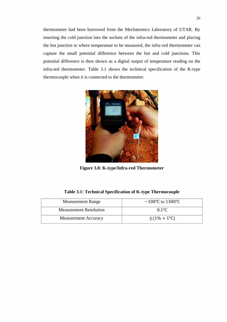
The instrument that was used to measure the temperatures was the infra-red

thermometer (Model: TM-909AL) as shown in Figure 3.8. This infra-red

20

thermometer had been borrowed from the Mechatronics Laboratory of UTAR. By

inserting the cold junction into the sockets of the infra-red thermometer and placing

the hot junction to where temperature to be measured, the infra-red thermometer can

capture the small potential difference between the hot and cold junctions. This

potential difference is then shown as a digital output of temperature reading on the

infra-red thermometer. Table 3.1 shows the technical specification of the K-type

thermocouple when it is connected to the thermometer.

Figure 3.8: K-type/Infra-red Thermometer

Table 3.1: Technical Specification of K-type Thermocouple

Measurement Range −100℃ to 1300℃

Measurement Resolution 0.1℃

Measurement Accuracy ±(1% + 1℃)

21

3.3 Cooling Load Analysis

Cooling load of the experimental residential room was calculated using Residential

Load Factor (RLF) method as suggested by ASHRAE. This method is a simplified

version of the more detailed Residential Heat Balance (RHB) method. However, this

method could provide sufficient accuracy and especially useful in situation where

detailed analysis is impractical.

3.3.1 Cooling Load due to Heat Gain through Opaque Surfaces

Heat gains through opaque surfaces such as walls, floor slabs ceiling and door can be

caused by the difference of air temperature across these surfaces. Besides, heat gains

through these surfaces could also because of solar gains which incident on the

surfaces. The equation used to estimate the cooling load due to heat gains through

opaque surfaces using RLF method are given as shown in below.

opqopq CFAq (3.1)

)( DROFOFtOFUCF rbtopq (3.2)

where

qopq = opaque surface cooling load, Btu/h

A = net surface area, ft2

CFopq = surface cooling factor, Btu/h.ft2

U = construction U-factor, Btu/h·ft2·oF

∆t = cooling design temperature difference, ℉

OFt, OFb, OFr = opaque surface cooling factors

DR = daily cooling range, ℉

Figure 3.9 shows the opaque surface factors for different situation. These

factors represent the construction specific physical characteristics associated with

each surfaces. Figure 3.10 shows that roof solar absorptance, 𝛼𝑟𝑜𝑜𝑓.

22

Figure 3.9: Opaque Surface Cooling Factor Coefficients (ASHRAE, 2009)

Figure 3.10: Roof Solar Absorptance (ASHRAE, 2009)

3.3.2 Cooling Load due to Infiltration/Ventilation

The cooling load as a result of ventilation and infiltration can be calculated based on

equations shown below.

tQQQCq othbalhrbalsvisvi ,,1 (3.3)

where

qvi = ventilation/infiltration cooling load, Btu/h

Cs = air sensible heat factor, 1.1 Btu/h·cfm at sea level

Qvi = combine infiltration/ventilation flow rate, cfm

εs = HRV/ERV sensible effectiveness

Qbal,hr = balanced ventilation flow rate via HRV/ERV equipment, cfm

[assumed 𝑄𝑏𝑎𝑙,ℎ𝑟 = 0]

Qbal,oth = other balanced ventilation supply airflow rate, cfm

23

[assumed 𝑄𝑏𝑎𝑙,𝑜𝑡ℎ = 0]

∆𝑡 = cooling design temperature difference, ℉

unbaliunbalvvi QQQQQ 5.0max , (3.4)

where

Qvi = combine infiltration/ventilation flow rate, cfm

Qv = required ventilation flow rate, cfm [assumed 𝑄𝑣= 0 for single

zone]

Qunbal = unbalanced airflow rate, cfm [assumed 𝑄𝑢𝑛𝑏𝑎𝑙 = 0]

Qi = infiltration leakage rate assuming no mechanical pressurization,

cfm

Therefore

ivi QQ (3.5)

while

IDFAQ Li (3.6)

where

AL = building effective leakage area

IDF = infiltration driving force, cfm/in2 (refer Figure 3.11)

ulesL AAA (3.7)

where

Aes = building exposed surface area, ft2

Aul = unit leakage area factor, in2/ft2 (refer Figure 3.12)

24

Figure 3.11: Typical Values of IDF (ASHRAE, 2009)

Figure 3.12: Unit Leakage Area Factor (ASHREA, 2009)

3.3.3 Cooling Load due to Internal Heat Gains

According to the ASHRAE Handbook-Fundamentals, the cooling load contributed

by internal heat gains sources such as occupants, lighting and equipment (or

appliances) can be estimated by the following equation. For the purpose of cooling

load estimation for the EAHE design, it will be assumed that the room is occupied by

two people throughout the whole day.

25

occfig NAq 757.0464 (3.8)

where

qig = cooling load (sensible) due to internal heat gains, Btu/h

Acf = conditioned floor area of building, ft2

Noc = number of occupants [assumed 𝑁𝑜𝑐 = 2]

3.4 EAHE Prototype Design

3.4.1 EAHE Prototype Design Strategy

The procedures involved in the designing of the EAHE prototype system was based

on a trial-and-error approach. This is necessary because the requirement of static

pressure of the fan depends on the pressure drop of the EAHE pipe. This pressure

drop was only known after the pipe diameter and length of the EAHE prototype has

been designed. However, the design of the pipe diameter and length required the

mass flow rate and velocity of the fan that was going to supply to the system.

Therefore, it forms a cycle and required a trial-and-error approach to design the

EAHE prototype system.

3.4.2 Fan Design and Fabrication

The previous version of EAHE prototype system being designed have chosen axial

exhaust fan to drive the air through the pipe of the system. However, axial fan used

in the system lacks the static pressure to overcome the pressure loss of the pipe

system required. For this reason, a centrifugal fan was designed and fabricated in this

project.

26

A stand fan motor of rated power 50W has been used as the prime mover to

drive the designed centrifugal fan impeller. The centrifugal fan casing and impeller

was fabricated from hard-cardboard and plywood. These material were chosen to

minimize the additional loading on the motor especially for the fan impeller that

could be caused by its weight.

Since the suction inlet of the centrifugal exhaust fan was connected directly

to the outlet end of the EAHE pipe system, it is reasonable to assume that the outlet

air velocity of the EAHE pipe system to be equal to the suction inlet air velocity of

the centrifugal exhaust fan. Therefore, we can set a design value for the outlet air

velocity for the EAHE pipe system and let it equal to the suction inlet air velocity of

the centrifugal fan to start the trial-and-error procedures.

As the air flow from the one end to the other, its velocity will dropped as a

result of friction and losses. The common practise was to set the average velocity

between the inlet and outlet value based on the ASHREA recommendation. This

recommendation suggested certain maximum air velocity in the main and branch

duct to avoid unnecessary acoustic problem, which is to control the sound and

vibration of the system. Figure 3.13 shows the recommended air velocity in our

project’s case which is 2600 fpm or 13.6 m/s. Then, a higher value is set as the

design value at the suction inlet of the centrifugal fan for example, 16 m/s so that an

average velocity of about 13.6 m/s can be achieved in the EAHE pipe system. The

following equation was used to calculate the average velocity of the EAHE pipe

system.

6.132

ioavg

VVV m/s (recommended) (3.9)

where

Vavg = average velocity in the EAHE pipe system, m/s

Vo = outlet velocity of the EAHE system or suction inlet velocity of the fan, m/s

Vi = inlet velocity of the EAHE system

27

Figure 3.13: Maximum Recommended Air Flow Velocity (ASHREA, 2009)

The centrifugal exhaust fan used in the EAHE prototype was designed based

on a trial-and-error approach using Flow Simulation of SolidWorks. Those steps

involved in the designing of the centrifugal exhaust fan were as listed below.

1. The impeller and casing of the centrifugal was first designed to give a trial

value of air velocity, mass flow rate and static pressure.

2. The air velocity and mass flow rate parameters were used to design the

optimum pipe diameter and length of the EAHE pipe system as shown in

Section 3.4.3.

3. The EAHE pipe design determined from Step 2 was modelled in SolidWorks

and simulated with the exhaust centrifugal fan.

4. The average velocity in the EAHE pipe as provided by the result of the

simulation was compared with the recommended average velocity of 13.6 m/s.

5. If the average velocity acquired was less than the recommended value, then

the process was repeated by altering the fan design to give a higher air

velocity, mass flow rate and static pressure else the design will be finalized if

the average velocity was almost equal and slightly higher than the

recommended value.

28

3.4.3 Pipe Diameter and Length Selection of EAHE Prototype

The required pipe length of EAHE prototype was calculated for five different

nominal diameters which were 1 in (25mm), 2 in (50mm), 3 in (80mm), 4 in (100mm)

and 5 in (125 mm). By fixing the material of pipe as PVC and with the determined

heat rejection rate from the cooling load analysis, the selection of which diameter of

PVC pipe to be used was based on the shortest required pipe length because this will

minimize the area of ground used. Figure 3.14 shows the Microsoft Excel

Spreadsheet used for the calculation of required pipe length. Figure 3.15 is the

catalogue of PVC pipe from ATKC e-Commerce Warehouse which shows the

standard PVC pipe with grade and dimension available in the market.

The lowest grade with the thinnest pipe wall was selected for each of the

different nominal diameters which were input into the Microsoft Excel Spreadsheet

for the calculation of pipe length required. This is because the thinnest pipe wall will

give the lowest possible conductive resistance associated with the pipe for each of

the different nominal diameters. The heat transfer equations that were used to

calculate the required pipe length for each of the different nominal diameters were

listed in the following pages.

Figure 3.14: Microsoft Excel Spreadsheet for Pipe Diameter and Length

Selection

29

Figure 3.15: PVC Pipe Catalogue (ATKC e-Commerce Warehouse, 2015)

p

io

conductivekL

DDR

2

)/ln( (3.10)

where

Rconductive = conductive thermal resistance of the pipe, K/W

Do = outer diameter of the pipe, m

Di = inner diameter of the pipe, m

L = length of the pipe, m

kp = thermal conductivity of the PVC pipe, W/m·K

It was assumed that fully developed turbulent flow of air was provided inside

the ground pipe. The convective thermal resistance associated with the convection

heat transfer between the air flowing in the ground pipe and the pipe inner surface

can be expressed as Equation 3.11.

LhD

Rai

convective

1 (3.11)

30

where

Rconvective = convective thermal resistance from air to inner pipe surface, K/W

ha = convective heat transfer coefficient of air, W/m2·K

Di = inner radius of the soil annulus/nominal radius of the ground pipe, m


The convective heat transfer coefficient, ℎ𝑎 of the above formula can be calculated

by the formula below provided that Nusselt number, 𝑁𝑢 was known

i

a

aD

kNuh (3.12)

where

ha = convective heat transfer coefficient of air, W/m2·K

Nu = Nusselt number

Di = inner diameter of the ground pipe, m

ka = thermal conductivity of the air, W/m·K

The Nusselt number for a fully developed laminar and turbulent flow in a

circular pipe can be obtained by a correlation valid over large Reynold number and

Prantl number ranges as proposed by Gnielinski (Incopera, 2002). This correlation is

valid for 0.5 ≤ Pr ≤ 2000 and 300 ≤ Re ≤ 5× 106.

)1(Pr8

7.121

Pr1000Re8

3/2

5.0

f

f

Nu (3.13)

where

Nu = Nusselt number

f = friction factor

Pr = Prandlt number

Re = Reynolds number

31

Friction factor appears in the above equation can be determined using

Petukhov’s relationship which is particularly valid for smooth pipe as shown in

Equation 3.14.

264.1Reln79.0

f (3.14)

where

f = friction factor


a

pa

k

c Pr (3.15)

where

Pr = Prantl number

Cpa = specific heat capacity of air, J/kg·K

ka = thermal conductivity of air, W/m·K

Reynolds number appear in the above equation can be determined by the following

Equation 3.16.

i

a

D

m4Re (3.16)

where



μ = dynamic viscosity of the air, kg/m s

am = mass flow rate of air, kg/s

4

2

avgi

a

VDm

(3.17)

32

where


ρ = density of air, kg/m3


Vavg = average velocity in the EAHE pipe system, m/s

The total thermal resistance, 𝑅𝑡𝑜𝑡𝑎𝑙 associated with this heat transfer can be

calculated by Equation 3.18.

convectiveconductivetotal RRR (3.18)

where

Rtotal = total thermal resistance, K/W

Rconvective = convective thermal resistance between air flowing and pipe inner surface,

K/W

Rconductive = conductive thermal resistance of the pipe, K/W

Finally, the required length of the EAHE can be calculated as shown in Equation

3.19.

groundroom

totalload

T

RqL

(3.19)

where


qload = total heat gain of the room from cooling load analysis, W

∆Troom-ground = temperature difference of room and ground temperature, K

Rtotal = total thermal resistance, K/W

33

3.5 Data Collection and Analysis of the EAHE Prototype System

3.5.1 Data Collection of the EAHE Prototype System

Data collection was conducted on the EAHE prototype system that was designed and

built. The collection of temperature readings were accomplished by using K-type

thermocouple and K-type/infra-red thermometer similar to Section 3.2. The

following temperature readings were collected to conduct the data analysis

1. Room temperature, 𝑇𝑟

2. EAHE inlet temperature, 𝑇𝑖

3. EAHE outlet temperature, 𝑇𝑜

4. Room inlet temperature before insulation, 𝑇𝑖′

5. Room outlet temperature after insulation, 𝑇𝑜′

6. Environment temperature, 𝑇𝑒𝑛𝑣𝑖𝑟𝑜𝑛

The exact location on the EAHE prototype system where each of the above

mentioned temperature will be taken can be found in Figure 4.30 of Section 4.4 in

which the full view of the finalized EAHE prototype system design was given.

3.5.2 Temperature Data Analysis of the EAHE Prototype System

After the collection of various temperature data of the EAHE prototype system has

been conducted for three days, the collected data were then analysed. Each and every

of the temperature profile mentioned in the previous section was analysed in terms of

trends, peak values and temperature difference with another temperature profile to

get a more in-depth understanding of the EAHE prototype system.

34

3.5.3 Heat Analysis of the EAHE Prototype System

There was heat rejected by the EAHE prototype along the pipe length buried

underground. However, it was also important to analyse the portion heat rejected by

the room over the total heat rejected by the EAHE prototype system. Besides, there

was heat gained between the room inlet before insulation and EAHE inlet after

insulation and between the EAHE outlet before insulation and room outlet after

insulation due to imperfect insulation. Furthermore, there was also heat gained that

was analysed.

Therefore, heat analysis was carried out on two different heat gained and

rejected on four different segments of the EAHE prototype system which were listed

here.

1. Heat gained by the insulation at the inlet segment. This heat gained based on

the temperature difference between the room inlet temperature before

insulation, 𝑇𝑖′ and EAHE inlet temperature after insulation, 𝑇𝑖.

2. Heat gained by the insulation at the outlet segment. This heat gained was

based on the temperature difference EAHE outlet temperature before

insulation, 𝑇𝑜 and room outlet temperature after insulation, 𝑇𝑜′

3. Heat rejected by the EAHE system. This heat rejected was based on the

temperature difference between EAHE inlet after insulation, 𝑇𝑖 and EAHE

outlet temperature before insulation, 𝑇𝑜.

4. Heat rejected from the room. This heat rejected was based on the temperature

difference between room inlet temperature before insulation, 𝑇𝑖′ and room

outlet temperature after insulation, 𝑇𝑜′.

The heat gained or rejected on different segment of the EAHE prototype can

be defined as the heat transfer rate as a result of the temperature differences of that

particular segment. The equation that expressed heat gained or rejected in terms of

these variables can be expressed as shown in Equation 3.20.

Tcmq paarejectedgained

/ (3.20)

where

35

qgained/rejected = heat gained or rejected, W

cpa = specific heat capacity of the air, J/kg K


∆T = difference of temperature, K

3.5.4 Cooling Performance of EAHE Prototype

The first parameters that can be used to evaluate the cooling performance of a

cooling system such as the EAHE prototype system under study is percentage of

cooling effect. The percentage of cooling effect can be expressed as shown in

Equation 3.21 and 3.22.

% Reduction of Cooling Load (ideal) %100,

load

EAHErejected

q

q (3.21)

% Reduction of Cooling Load (actual) %100,

load

rooomrejected

q

q (3.22)

where

qload = total cooling load, W

EAHErejectedq , = heat rejected by the EAHE prototype, W

rooomrejectedq , = heat rejected from the room, W

The ideal percentage reduction of cooling load is the fraction of heat rejected

by the EAHE over the total cooling load without the consideration of imperfect

insulation. On the other hand, actual percentage reduction of cooling is the fraction

of heat rejected from the room over the total cooling load with the consideration of

imperfect insulation.

36

The second parameter that can be used to evaluate the cooling performance of

an EAHE cooling system is called the EAHE efficiency. EAHE efficiency was

defined as the fraction of heat rejected from the room to the total heat rejected by the

EAHE into the ground. Therefore, EAHE efficiency can be calculated by the

following Equation 3.23.

%100,

,

EAHErejected

rooomrejected

EAHEq

q (3.23)

where

ηEAHE = EAHE efficiency

rooomrejectedq , = heat rejected from the room, W

EAHErejectedq , = heat rejected by the EAHE prototype, W

Besides, the cooling performance of the EAHE prototype could also be

evaluated by its energy efficiency which can be described by the dimensionless

parameter called coefficient of performance (COP). Two different COPs of the

EAHE prototype were analysed which are the COPideal and COPactual. COPideal is the

ideal coefficient of performance of the EAHE prototype without the consideration of

imperfect insulation. It is defined as the ratio of heat rejected by the EAHE system

over the power dissipated which is fan power. On the other hand, COPactual actual

coefficient of performance of the EAHE prototype with the consideration of

imperfect insulation. It is defined as the ratio of heat rejected from the room over the

power dissipated which is also the fan power. The equation for the calculation of

COPideal and COPactual are shown in Equation 3.24 and 3.25.

fan

oipaa

fan

EAHErejected

idealP

TTcm

P

qCOP

, (3.24)

where

COPideal = ideal coefficient of performance of the EAHE

qrejected,EAHE = cooling capacity/heat transfer rate from the air to the ground, W

Pfan = rated power of the fan, W

37

fan

oipaa

fan

roomrejected

actualP

TTcm

P

qCOP

''

,

(3.25)

where

COPactual = actual coefficient of performance of the EAHE

qrejected,room = cooling capacity/heat transfer rate from the air to the ground, W

Pfan = rated power of the fan, W

38

CHAPTER 4

4 RESULTS AND DISCUSSION

4.1 Ground, Room and Environment Temperature Profile

Using the procedures mentioned in Section 3.2, the ground temperatures at different

depth, room temperatures without EAHE system, and environment temperatures had

been measured and recorded for 3 days continuously. The measurement had been

conducted from 8am in the morning until 6pm in the evening each day. The full

detail of these measurement for these three days had been tabulated in tables and

presented in graphs in Appendix A.

In order to analyse the variation and trends of the ground, room and

environment temperature profile captured, these temperature has been sum up and

averaged to get the mean temperatures at the specific period of time. The mean daily

ground, room and environment temperature obtained for these three days was

tabulated and presented in Table 4.1. Besides, the mean daily ground, room and

temperature for these three days was also plotted into a graph as shown in Figure 4.1.

From the temperature data obtained and shown in Figure 4.1 and 4.2, it could

be observed that the room temperature mostly influenced by the environment

temperature. As can be observed from the aforementioned figures, the room

temperature increased as the environment temperature increased from morning 8am

to afternoon 1pm. At 1pm in the afternoon, the environment temperatures reached its

peak or maximum temperature.

39

Table 4.1: Mean Ground, Room and Environment Temperatures

Description

Time

0.5 m

( C)

1.0 m

( C)

1.5 m

( C)

2.0 m

( C)

Room temperature,

𝑻𝒓′ ( C)

Environment

temperature, 𝑻𝒆𝒏𝒗 ( C)

08:00 AM 27.9 27.7 27.4 27.4 28.5 27.0

09:00 AM 27.8 27.6 27.3 27.3 29.8 27.8

10:00 AM 28.4 27.9 27.2 27.2 31.1 32.0

11:00 AM 29.2 28.1 27.1 27 32.3 34.0

12:00 PM 29.8 28.5 27.6 27.3 33.8 35.6

01:00 PM 30.6 28.8 28.3 27.9 35.2 37.0

02:00 PM 31.1 29.4 28.6 28.4 36.5 36.7

03:00 PM 31.5 30.5 29 28.7 37.3 36.2

04:00 PM 30.6 30.8 29.3 29.2 36.8 35.5

05:00 PM 29.5 29.9 29.5 29.4 35.9 33.5

06:00 PM 28.8 29.0 29.0 28.9 35.0 30.7

Max temperature 31.5 30.8 29.5 29.4 37.3 37.0

Min temperature 27.8 27.6 27.1 27.0 28.5 27.0

Temperature range 3.7 3.2 2.4 2.4 8.8 10.0

40

Figure 4.1: Mean Ground, Room and Environment Temperatures

25

27

29

31

33

35

37

39

Tem

peratu

re (

C)

Time

Mean Ground, Room and Environment Temperatures

0.5m

1.0m

1.5m

2.0m

Room

Temperature

without EAHE,

Tr'Environment

Temperature,

Tenviron

41

Figure 4.2: Mean Ground Temperatures at Different Depth

42

However, the room temperature did not reaches its maximum temperatures at

this time of the day. The room temperature continued to increase until it reaches its

peak temperature at about 3pm in the afternoon. Therefore, a delayed or shifted

response can be observed from the variation of room temperature as compared to the

environment temperature. Although there was a shift of response between room and

environment temperature, both of these temperature decreased almost linearly

together after the shift which is 4pm onwards.

This shift in the temperature response of the room temperature could be due

to the heat accumulation in the room after its peak temperature. This is because the

room lacks ventilation as compared to the environment in which heat could be

carried away by the convective heat transfer of the ambient air. By relying solely on

the conductive heat transfer through the room’s wall, the room temperature only

started to decrease after a period of time when the environment temperatures had

already decreased. Therefore, it could be concluded that the room temperature

without the EAHE was directly influenced by the environment temperature whereby

both of them have the same temperature trends while the room temperature had a

damped response from the environment temperature at late afternoon due to heat

accumulation.

On the other hand, it could be observed that the ground temperature at all the

depth decreases slightly in the morning from 8am to 9am in the morning until the

minimum temperature attained. The minimum ground temperature at the depth of

0.5m, 1.0 m, 1.5 m and 2.0m were 27.8 C, 27.6 C, 27.1 C and 27.0 C respectively.

After the minimum ground temperature had been attained, the ground temperature at

each depth will start to increase with different rate of increment. As could be

observed from the Figure 4.3 above, the rate of increment in ground temperature

decreases as the depth of ground increased.

Beside this, the maximum temperature attained by the ground at different

depth also decreased as the depth of ground increased as shown in Figure 4.2. The

maximum ground temperature at the depth of 0.5m, 1.0 m, 1.5 m and 2.0m were

31.5 C, 30.8 C, 29.5 C and 29.4 C respectively. Besides, the mean daily range of the

ground temperature was also decreased as the depth of ground increased as shown in

43

Table 4.1. After the maximum temperature had been attained, the ground

temperature started to decrease at a different rate. The rate of decrement in

temperature decreased as the depth of ground increases as shown in Figure 4.2 above.

Therefore, it could be concluded that the fluctuation of ground temperature in terms

of mean daily temperature range decreased as the depth of the ground increases. This

could be due to the effect of fluctuating solar radiation on the ground (which

contribute to the radiation heat gain) would decrease as we go deeper into the ground.

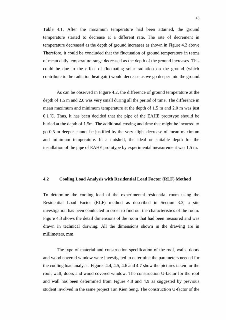
As can be observed in Figure 4.2, the difference of ground temperature at the

depth of 1.5 m and 2.0 was very small during all the period of time. The difference in

mean maximum and minimum temperature at the depth of 1.5 m and 2.0 m was just

0.1 C. Thus, it has been decided that the pipe of the EAHE prototype should be

buried at the depth of 1.5m. The additional costing and time that might be incurred to

go 0.5 m deeper cannot be justified by the very slight decrease of mean maximum

and minimum temperature. In a nutshell, the ideal or suitable depth for the

installation of the pipe of EAHE prototype by experimental measurement was 1.5 m.

4.2 Cooling Load Analysis with Residential Load Factor (RLF) Method

To determine the cooling load of the experimental residential room using the

Residential Load Factor (RLF) method as described in Section 3.3, a site

investigation has been conducted in order to find out the characteristics of the room.

Figure 4.3 shows the detail dimensions of the room that had been measured and was

drawn in technical drawing. All the dimensions shown in the drawing are in

millimeters, mm.

The type of material and construction specification of the roof, walls, doors

and wood covered window were investigated to determine the parameters needed for

the cooling load analysis. Figures 4.4, 4.5, 4.6 and 4.7 show the pictures taken for the

roof, wall, doors and wood covered window. The construction U-factor for the roof

and wall has been determined from Figure 4.8 and 4.9 as suggested by previous

student involved in the same project Tan Kien Seng. The construction U-factor of the

44

plastic door and wood covered windows was calculated based on the following

formula.

t

kU (4.1)

Where

𝑈 = construction U-factor, W/m2·K

𝑘 = thermal conductivity of the component, W/m ·K

𝑡 = thickness of the component, m

Figure 4.3: Detail Dimensions of the Experimental Residential Room

45

Figure 4.4: Roof tiles of the Experimental Residential Room

Figure 4.5: Concrete ceiling of the Experimental Residential Room

Figure 4.6: Walls of the Experimental Residential Room

46

Figure 4.7: Door and Wood Covered Window of the Experimental Residential

Room

Figure 4.8: Roof Type of the Experimental Residential Room with Suggested U-

factor (Tan, 2013)

47

Figure 4.9: Wall Type of the Experimental Residential Room with Suggested U-

factor (Tan, 2013)

Table 4.2 summarizes the characteristics of the experimental residential room

of this project along with the associated construction U-factors.

Table 4.2: Mean Daily Ground, Room and Environment Temperatures

Component Description Factors

Roof Concrete flat roof with wood frame

ceiling and light clay tiles

𝑈 = 0.232 Btu/h ∙ ft2 ∙ ℃

Exterior

walls

Light weight concrete block walls

with three (3) walls exposed to

solar radiation while one (1) was

shaded.

𝑈 = 0.155 Btu/h ∙ ft2 ∙ ℃

Door Plastic door made of PVC of 𝑘 =

0.19 W/m ∙ K with a thickness of

𝑡 = 27 𝑚𝑚

𝑈 = 1.24 Btu/h ∙ ft2 ∙ ℃

Window Plywood wood, 𝑘 = 0.13 W/m ∙ K

covered window with a thickness of

𝑡 = 10 mm that is being shaded

from solar.

𝑈 = 2.29 Btu/h ∙ ft2 ∙ ℃

Construction Leaky 𝐴𝑢𝑙 = 0.08 in2/ft2

48

To define the indoor and outdoor design condition for the cooling system, the

common practice suggested by the ASHRAE Handbook – Fundamental of 2009 has

been taken into consideration. The typical practice for cooling purpose is to design

the indoor conditions at 75 F (23. 8 C) to 85 F (29.4 C) dry bulb temperature as

suggested by ASHRAE. As decided by our project team the design indoor

temperature was set to 85 F. On the other hand, the outdoor design conditions for

cooling load calculation should be selected from the climate data of the specific

location. The outdoor design temperature should be the mean maximum air

temperature taken from the warmest month of Kuala Lumpur, Malaysia which is

March. To find the daily range for the designed EAHE cooling system, the difference

between the mean maximum and minimum temperatures of the warmest month

should be used. Based on the climate data obtained from website of Malaysia

Metrological Department, the mean maximum and minimum temperature of March

are 35 C (95 F) 25 C (77 F) and as shown in Figure 4.10 and 4.11.

Figure 4.10: Mean Maximum Temperature Distribution of Malaysia at March

(Malaysia Metrological Department, 2015)

49

Figure 4.11: Mean Minimum Temperature Distribution of Malaysia at March

(Malaysia Metrological Department, 2015)

Table 4.3 summarized the design condition of the EAHE cooling system for

the experimental residential room. Table 4.4 summarized the experimental residential

room component parameters for the calculation of cooling load using RLF method.

Table 4.5 summarized the experimental residential room opaque surface factors.

Table 4.3: Experimental Residential Room Design Conditions

Item Values

Latitude 3o13’00.60’’ N

Indoor temperature 85 F

Outdoor

temperature

95 F

Daily range 18 F

Wind speed 7.5 mph (suggested by ASHRAE)

Design ∆𝒕 10 F

50

Table 4.4: Experimental Residential Room Component Parameter

Component Quantity

Ceiling 15.1984 m2 = 163.94 ft2

Door 1.7723 m2 = 19.07 ft2

Window 1.44 m2 = 15.5 ft2

Walls

30.412 m2 = 327.35 ft2 (unshaded)

14.4381 m2 = 155.41 ft2 (shaded)

Floor area 15.1984 m2 = 163.94 ft2

Total exposed surface 63.2608 m2 = 680.93 ft2

Volume 42.8816 m2 = 461.57 ft2

Wall height 3.23 m = 10 ft

Table 4.5: Experimental Residential Room Opaque Surface Factors

Component U-factor,

Btu/h·ft· F

OFt OFb OFr CFopq

Ceiling 0.232 1.0 14.96 -0.36 4.2874

Door 1.24 1.0 14.8 -0.36 22.7168

Window 2.29 1.0 14.8 -0.36 8.0608

Wall (unshaded) 0.155 1.0 14.8 -0.36 2.8396

Wall (shaded) 0.155 1.0 0 -0.36 8.0608

A sample calculation for the opaque surface cooling load due to heat gains at

these opaque surfaces was given below.

For ceiling,

)( DROFOFtOFUCF rbtopq

)]1836.0(96.14)10(0.1232.0

2874.4

opqopq CFAq

2874.46.163

51

41.701 Btu/h

For door,


)]1836.0(8.14)10(0.124.1

7168.22

opqopq CFAq

7168.2208.19

44.433 Btu/h

For window,


)]1836.0(0)10(0.129.2

0608.8

opqopq CFAq

0608.85.15

94.124 Btu/h

For wall (unshaded)


)]1836.0(8.14)10(0.1155.0

8396.2

opqopq CFAq

8396.235.327

54.929 Btu/h

For wall (shaded),


)]1836.0(0)10(0.1155.0

5456.0

52

opqopq CFAq

5456.041.155

79.84 Btu/h

Total opaque surfaces cooling load, qopq,total

12.274,279.8494.12444.43341.701, totalopqq Btu/h

A sample calculation for the infiltration/ventilation cooling load that was

contributing to the total cooling load was given below. Since there was no ventilator

in the experimental residential room, therefore we have assumed that

ivi QQ

Building total exposed area, 93.680esA ft2

Unit leakage area factor, 04.0ulA cfm/in2 (according to Figure 3.12)

Thus,

ulesL AAA

08.093.680

47.54 cfm

Infiltration driving force, IDF = 0.41 (according to Figure 3.11)

Thus,

IDFAQ Li

41.047.54

33.22 cfm

33.22 ivi QQ cfm

53

Ventilation/infiltration cooling load, qvi

tQQQCq othbalhrbalsvisvi ]1[ ,,

10]00)1(33.22[1.1 s

63.245 Btu/h

A sample calculation for the cooling load due to internal heat gains that was

contributing to the total cooling load was given below. For the purpose of cooling

load estimation for the EAHE design, it will be assumed that the room is occupied by

two people throughout the whole day.

Cooling load due to internal heat gains, qig

occfig NAq 757.0464

)2(75)94.163(7.0464

76.728 Btu/h

Table 4.6 shows the cooling load contributed by opaque surfaces,

infiltration/ventilation and internal heat gains along with the total cooling load. The

total cooling load as calculated and tabulated in Table 4.5 was 952 W. To sum up,

the cooling load of the experimental residential room as determined by using

Residential Load Factor (RLF) method was 952 W.

Table 4.6: Experimental Residential Room Cooling Loads

Component Cooling Load, Btu/h

Opaque surfaces 12.274,2 Btu/h

Infiltration/ventilation 63.245 Btu/h

Internal gain 76.728 Btu/h

Total Cooling Load 𝟑, 𝟐𝟒𝟖. 𝟓𝟏 𝐁𝐭𝐮 𝐡⁄ = 𝟗𝟓𝟐 𝐖

54

4.3 EAHE Prototype Design

4.3.1 Fan Design and Fabrication

Three most important parameters to be determined in the design of centrifugal

exhaust fan for the EAHE prototype was the mass flow rate, suction velocity and

static pressure. The mass flow rate and velocity at the suction inlet of the centrifugal

exhaust fan was required as an input parameter during the designing of pipe diameter

and length for the EAHE prototype system. Based on the designed pipe diameter and

length, the pressure drop of the EAHE pipe layout must not exceed the static pressure

provided by the designed centrifugal exhaust fan as well.

Figure 4.12 shows the solid modelling of the finalized centrifugal exhaust fan

in SolidWorks. Figure 4.13 and 4.14 shows the impeller and casing of the finalized

centrifugal exhaust fan in solid modelling. Figure 4.15 shows the actual appearance

of the fabricated centrifugal exhaust fan. Figure 4.16 shows the fan impeller of the

fabricated centrifugal exhaust fan. Figure 4.17 shows the casing of the fabricated

centrifugal exhaust fan. Figure 4.18 shows the supporting structure of the fabricated

centrifugal exhaust fan.

Figure 4.12: Finalized Centrifugal Exhaust Fan in Solid Modelling

55

Figure 4.13: Impeller of Finalized Centrifugal Exhaust Fan in Solid Modelling

Figure 4.14: Casing of Finalized Centrifugal Exhaust Fan in Solid Modelling

56

Figure 4.15: Actual Appearance of the Fabricated Centrifugal Exhaust Fan

Figure 4.16: Impeller of the Fabricated Centrifugal Exhaust Fan

57

Figure 4.17: Casing/Housing of the Fabricated Centrifugal Exhaust Fan

Figure 4.18: Supporting Structure of the Fabricated Centrifugal Exhaust Fan

58

The finalized design of the centrifugal exhaust fan was simulated in Flow

Simulation of SolidWorks and tested experimentally after it was fabricated to

determine and verify some of its important specifications. The finalized design of the

centrifugal exhaust fan has the following specification as shown in Table 4.7. Note

that the static pressure of the centrifugal exhaust fan could not be determined

experimentally because the testing equipment was not available in UTAR. Figure

4.19 shows that the suction velocity of the centrifugal exhaust fan was being tested

using an anemometer. Since the diameter of suction opening of the centrifugal fan

was known, the mass flow rate can be calculated based on the determined suction

velocity.

4

2

suctionopening

a

VDm

(4.2)

where

am = mass flow rate of the centrifugal fan, kg/s

2

openingD = diameter of suction opening, m

suctionV = suction velocity of centrifugal fan, m/s

For simulated result,

suctionV = 17.1 m/s

openingD = 100 mm = 0.1 m

Thus,

4

2

suctionopening

a

VDm

4

1.1710.0205.1 2

16186.0 kg/s

59

For experimental result,

suctionV = 16.5 m/s

openingD = 100 mm = 0.1 m

Thus,

4

2

suctionopening

a

VDm

4

5.161.0205.1 2

15618.0 kg/s

The percentage difference of the simulation and experimental value for

suction velocity and mass flow rate could be calculated.

% Difference of Velocity

5.16

5.161.17100 % = 3.64 %

% Difference of Mass Flow Rate

15618.0

15618.016186.0100 % = 3.64 %

Table 4.7: Specification of Designed Centrifugal Exhaust Fan

Component Simulation value Experimental value

Suction velocity 17.1 m/s 16.5 m/s

Mass flow rate 0.16186 kg/s 0.15618 kg/s

Static Pressure 263 Pa NA

60

Figure 4.19: Determination of Experimental Suction Velocity by Anemometer

Figure 4.20 shows the simulation results of the velocity flow trajectory inside

the centrifugal exhaust fan. Figure 4.21 shows the simulation results of the pressure

flow trajectory inside the centrifugal exhaust fan. Figure 4.22 shows the simulation

result of velocity cut plot of the centrifugal exhaust fan at the suction inlet which is

showing the suction inlet velocity. Figure 4.23 shows the simulation result of relative

pressure of the centrifugal exhaust fan at the suction inlet which is showing the static

pressure provided by the fan.

Figure 4.20: Velocity Flow Trajectory in Flow Simulation

61

Figure 4.21: Pressure Flow Trajectory in Flow Simulation

Figure 4.22: Velocity Cut Plot in Flow Simulation

62

Figure 4.23: Pressure Cut Plot in Flow Simulation

4.3.2 Pipe Diameter and Length Selection of EAHE Prototype

To design the pipe diameter and length of the EAHE prototype system, the air

velocity and mass flow rate of the centrifugal exhaust fan designed in the previous

Section 4.3.1 was used as the input data in the developed Microsoft Excel

Spreadsheet. This developed Microsoft Excel Spread will calculate the required

length of the EAHE prototype with the provided data of air velocity, mass flow rate,

pipe material characteristics, cooling load and the trial diameter.

The required pipe length of EAHE prototype was calculated for five different

nominal diameters which were 1 in (25mm), 2 in (50mm), 3 in (80mm) and 4 in (100

mm) and 5 in (125 mm). By fixing the material of the pipe as PVC and with the pre-

determined cooling load, the selection of which nominal diameter of PVC pipe to be

used was based on the shortest required pipe length because this will minimize the

63

area of ground used. The difference of room (without EAHE) and ground

temperature, ∆Troom-ground used in Equation 3.16 given in Section 3.4.3 have taken the

value of 8.3 C which was the worst condition recorded in Section 4.1.

A sample calculation for the selected 3 in (80 mm) nominal diameter pipe

used in the finalized EAHE prototype design was presented below. The rest of the

calculation for different diameter can be found in Appendix B. The standard inner

and outer diameter for PVC pipe of different nominal diameter can be found in

Figure 3.15 given above.

From Figure 3.15,

oD = 88.7 mm = 0.0887 m

iD = 86.9 mm = 0.0869 m

Conductive thermal resistance of the pipe, conductiveR

p

ioconductive

kL

DDR

2

)/ln(

19.02

)0869.0/0887.0ln(

L

L/01717.0

Mass flow rate of air, 𝑚𝑎

4

2

avgi

a

VDm

4

8.130869.0205.12

09864.0 kg/s

Reynolds number of the pipe flow, Re

i

a

D

m4Re

64

000015573.00869.0

09864.04

793,92

Friction factor, f

264.1Reln79.0

f

264.1793,92ln79.0

01828.0

Prantl number, Pr

a

pa

k

c Pr

0257.0

000015573.01005

61.0

Nusselt number, Nu

)1(Pr8

7.121

Pr1000Re8

3/2

5.0

f

f

Nu

)161.0(8

01828.07.121

61.01000793,928

01828.0

3/2

5.0

59.155

Convective heat transfer coefficient, ha

i

aa

D

kNuh

0869.0

0257.059.155

0159.46 W/m2 ∙ K

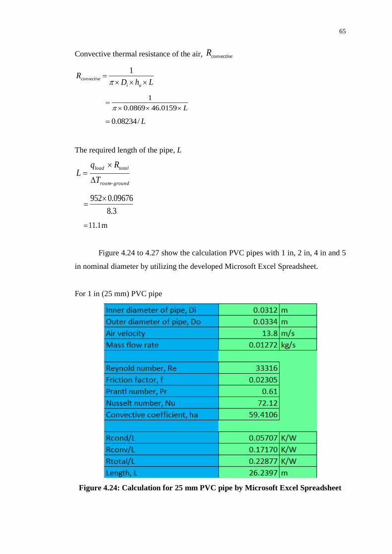
65

Convective thermal resistance of the air, convectiveR

LhDR

ai

convective

1

L

0159.460869.0

1

L/08234.0

The required length of the pipe, L

groundroom

totalload

T

RqL

3.8

09676.0952

1.11 m

Figure 4.24 to 4.27 show the calculation PVC pipes with 1 in, 2 in, 4 in and 5

in nominal diameter by utilizing the developed Microsoft Excel Spreadsheet.

For 1 in (25 mm) PVC pipe

Figure 4.24: Calculation for 25 mm PVC pipe by Microsoft Excel Spreadsheet

66





67



Table 4.8 summarized the result of calculation of the required length for PVC

pipe with different diameter if were to be used in the EAHE prototype. Figure 4.28

shows the chart of required length of pipe and total cost for PVC pipe of different

nominal diameter.

Table 4.8: Result of Calculation of Required Length and Total Cost for PVC

with Different Nominal Diameter

Nominal pipe

diameter, D (m)

Required length,

L (m)

Cost per Meter

(RM)

Total Cost

(RM)

1 in (25 mm) 26.24 7.5 196.80

2 in (50 mm) 16.54 20.5 338.97

3 in (80 mm) 11.10 21.0 233.07

4 in (100 mm) 9.48 32.1 304.24

5 in (125 mm) 8.21 46.8 384.33

68

Figure 4.28: Required Length and Total Cost for PVC pipe of Different

Nominal Diameter

For the finalized EAHE prototype design, PVC pipe with nominal diameter

of 3 inch (80 mm) was selected because it hit the sweet spot of short required length

and low total cost. PVC pipe with nominal diameter of 4 in (100 mm) and 5 in (125

mm) were not chosen because the total cost was too high. On the other hand, PVC

pipe of diameter 1 in (25 mm) and 2 in (50 mm) were not chosen as well because it

would be very impractical to dig a hole of 1.5 m depth that can fit in the required

pipe length of 26.24 m and 16.54 m. Although the calculated pipe length required by

the EAHE prototype to remove the imposed cooling load was 11.1 m. However, for

the simplicity of design the length of the pipe has been designed to be 11.6 m

(including the vertical portion being buried underground) as shown in Figure 4.29. In

a nutshell, the pipe diameter and length of the designed EAHE prototype were 3 in

(80 mm) and 11.6 m respectively based on the cooling load of the experimental

residential room.

0

50

100

150

200

250

300

350

400

450

0

5

10

15

20

25

30

25mm 50mm 80mm 100mm 125mm

Tota

l C

ost

(R

M)

Req

uir

ed

Len

gth

, L

(m

)

Nominal Pipe Diameter

Required Length and Total Cost of PVC Pipe

Required Length, L Total Cost

69

Figure 4.29: Pipe Layout of the EAHE Prototype with Dimensions Labelled

4.3.3 Full View of Designed EAHE Prototype System

The full view of the finalized EAHE prototype system was given in actual photo and

solid modelling pictures in this section. Figure 4.30 shows the EAHE prototype’s

pipe layout along with the location where the temperature mentioned in Section 3.5

was collected being labelled on it. Figures 4.31 to 4.33 shows the EAHE system in

solid modelling at different views. Figures 4.34 and 4.35 shows the actual EAHE

pipe layout and prototype system on site.

70

Figure 4.30: EAHE Pipe Layout with Insulation in Solid Modeling

Figure 4.31: Top View of EAHE Prototype System in Solid Modeling

71

Figure 4.32: Isometric View of EAHE Prototype System in Solid Modeling

Figure 4.33: Side View of EAHE Prototype System in Solid Modeling

72

Figure 4.34: Actual EAHE Pipe Layout on Site

Figure 4.35: Actual EAHE Prototype on Site

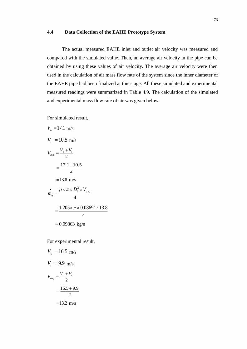
73

4.4 Data Collection of the EAHE Prototype System

The actual measured EAHE inlet and outlet air velocity was measured and

compared with the simulated value. Then, an average air velocity in the pipe can be

obtained by using these values of air velocity. The average air velocity were then

used in the calculation of air mass flow rate of the system since the inner diameter of

the EAHE pipe had been finalized at this stage. All these simulated and experimental

measured readings were summarized in Table 4.9. The calculation of the simulated

and experimental mass flow rate of air was given below.

For simulated result,

1.17oV m/s

5.10iV m/s

2

ioavg

VVV

2

5.101.17

8.13 m/s

4

2

avgi

a

VDm

4

8.130869.0205.1 2

09863.0 kg/s

For experimental result,

5.16oV m/s

9.9iV m/s

2

ioavg

VVV

2

9.95.16

2.13 m/s

74

4

2

avgi

a

VDm

4

2.130869.0205.1 2

09434.0 kg/s

Table 4.9: Simulated and Experimental Values of Flow Properties of EAHE

Prototype

Description EAHE Outlet

velocity, Vo

(m/s)

EAHE Inlet

Velocity, Vi

(m/s)

Average

Velocity, Vavg

(m/s)

Mass Flow

Rate, 𝒎𝒂

(kg/s)

Simulated 17.1 10.5 13.80 0.09863

Experimental 16.5 9.9 13.20 0.09434

The following temperatures were collected on the EAHE prototype system

each day from 8am to 6pm for three days.

1. Room temperature, 𝑇𝑟

2. EAHE inlet temperature, 𝑇𝑖

3. EAHE outlet temperature, 𝑇𝑜

4. Room Inlet temperature before insulation, 𝑇𝑖′

5. Room Outlet temperature after insulation, 𝑇𝑜′

6. Environment temperature, Tenviron

These temperatures had been summed up and averaged to get the mean

temperatures at the specific time. The aforementioned mean temperatures collected

were tabulated in Table 4.10. Figure 4.36 shows the graph of the aforementioned

mean temperatures plotted against time from 8am to 6pm. The particular temperature

readings collected for each of the three days can be found in Appendix C. In the

following Section 4.5, temperatures will be compared in the form of table and chart

where it is relevant to relate them together. By doing so would allow a more in-depth

analysis and discussion as compared to analysing and discussing all the temperatures

collected in once.

75

Table 4.10: Various Mean Temperatures of the EAHE Prototype System

Description

Time Ti ( C) To ( C) Ti' ( C) To' ( C) Tr ( C) Tenviron ( C)

8:00 AM 28.1 27.4 28 27.5 28 27

9:00 AM 29.2 27.4 29.1 27.8 29.1 29.8

10:00 AM 29.7 27.4 29.5 27.9 29.6 32.1

11:00 AM 31.4 28 30.2 28.5 30.1 34

12:00 PM 32.7 29 31.1 29.5 31.1 35.6

1:00 PM 34.4 29.9 32.3 30.6 32.2 37

2:00 PM 35.4 30.5 32.9 31.1 32.7 36.8

3:00 PM 36.9 31.3 33.6 31.9 33.4 36.5

4:00 PM 37.4 31.9 34 32.2 33.8 35.7

5:00 PM 35.5 29.8 33.6 30.3 33.5 33.8

6:00 PM 34.3 29.2 33.1 29.7 33 31.9

76

Figure 4.36: Various Mean Temperatures of the EAHE Prototype System

25

27

29

31

33

35

37

39

Tem

peratu

re (

C)

Time

Various Mean Temperature of the EAHE Prototype System

EAHE Inlet

Temperature, Ti

EAHE Outlet

Temperature, To

Inlet Temperature

before Insulation,

Ti'

Outlet Temperature

after Insulation, To'

Room Temperature

with EAHE, Tr

Environment

Temperature,

Tenviron

Room Temperature

without EAHE

77

4.5 Temperatures Data Analysis of the EAHE Prototype System

4.5.1 Mean Room and Environment Temperatures with EAHE

Table 4.11 shows the tabulated mean room and environment temperature with the

implementation of EAHE prototype system that was collected. On the other hand,

Figure 4.37 shows the chart of mean room and environment temperature with EAHE

prototype system against time that was plotted according to the tabulated data.

Table 4.11: Mean Room and Environment Temperatures with EAHE Prototype

Description

Time

Room Temperature

with EAHE System,

Tr ( C)

Environment

Temperature,

Tenviron ( C)

Temperature

Difference,

Tenviron - Tr ( C)

8:00 AM 28.0 27.0 -1

9:00 AM 29.1 29.8 0.7

10:00 AM 29.6 32.1 2.5

11:00 AM 30.1 34.0 3.9

12:00 PM 31.1 35.6 4.5

1:00 PM 32.2 37.0 4.8

2:00 PM 32.7 36.8 4.1

3:00 PM 33.4 36.5 3.1

4:00 PM 33.8 35.7 1.9

5:00 PM 33.5 33.8 0.3

6:00 PM 33.0 31.9 -1.1

As shown in the Table 4.11, Figure 4.36 and 4.37 that the room temperature

is almost always lower than the environment temperature. At early in the morning of

8am and late evening in the 6pm, the room temperature was slight higher than the

environment temperature by about 1 ℃ and 1.1 ℃ . The largest temperature

difference between environment and room temperature was 4.8℃ which occurred at

1pm in the afternoon. The EAHE prototype system was able to keep the room at

about 30 ℃ from 8am in the early morning until 11am in the late morning. Then, the

78

room temperature kept increased from 31.1 ℃ at 12pm and reached the highest room

temperature of 33.8 ℃ at 4pm. The increased in the room temperature was due to

heat accumulation that caused by insufficient heat rejected by the EAHE prototype

system as compared to the heat gained by the room.

Figure 4.37: Mean Room and Environment Temperatures with EAHE

Prototype

4.5.2 Mean Room and EAHE Outlet Temperatures

Table 4.12 shows the tabulated mean room and EAHE outlet temperature with the

implementation of EAHE prototype system that was collected. On the other hand,

Figure 4.38 shows the chart of mean room and EAHE outlet temperature with the

implementation of EAHE prototype system against time that was plotted according

to the tabulated data.

79

Table 4.12: Mean Room and EAHE Outlet Temperatures with EAHE Prototype

Description

Time

Room Temperature

with EAHE System,

Tr ( C)

EAHE Outlet

Temperature, To

( C)

Temperature

Difference, Tr - To

( C)

8:00 AM 28.0 27.4 0.6

9:00 AM 29.1 27.4 1.7

10:00 AM 29.6 27.4 2.2

11:00 AM 30.1 28 2.1

12:00 PM 31.1 29 2.1

1:00 PM 32.2 29.9 2.3

2:00 PM 32.7 30.5 2.2

3:00 PM 33.4 31.3 2.1

4:00 PM 33.8 31.9 1.9

5:00 PM 33.5 30.8 2.7

6:00 PM 33.0 29.9 3.1

Figure 4.38: Mean Room and EAHE Outlet Temperatures with EAHE

Prototype

80

As shown in the Table 4.12, Figure 4.36 and 4.38, the EAHE outlet

temperature was lower than the room temperature at all the time. However, both the

room and EAHE outlet temperature shown an increasing trend from 8am to 4pm.

From 5pm onward, the outlet temperature decreases drastically and this trends was

carried on until 6pm in the late evening. The largest temperature difference between

room and EAHE outlet temperature occurred during 6pm in which a temperature

difference of 3.1 ℃ was achieved. EAHE outlet temperature was able to remains

below 30 ℃ until 1pm in the afternoon. After 1pm, the EAHE outlet temperature

rises above 30 ℃ and reaches its peak value of 31.9 ℃ at 4pm in the afternoon. Then,

the EAHE outlet temperature decreased until 6pm was reached.

The increased in EAHE outlet temperature could be due to the heat

accumulation in the ground or in other words reservoir degradation. This can happen

if the ground does not transfer the heat fast enough away and subsequently the

ground temperature increases and would reduce the total amount of heat being

rejected into the ground. A solution that could solve this problem is to increase the

air velocity and pipe length of the EAHE system together. By having a longer pipe

length, the rate of heat transfer could be reduced but still maintaining the same total

heat rejection (or cooling capacity) if the air velocity was increased at the same time.

As a result, the ground would not be saturated with heat and the ground temperature

could be more stable all the time.

4.5.3 Mean Room and EAHE Inlet Temperatures

Table 4.13 shows the tabulated mean room and EAHE inlet temperature with EAHE

prototype system that was collected. On the other hand, Figure 4.39 shows the chart

of mean room and EAHE inlet temperature with the implementation of EAHE

prototype system against time that was plotted according to the tabulated data.

81

Table 4.13: Mean Room and EAHE Inlet Temperatures with EAHE Prototype

Description

Time

Room Temperature

with EAHE System,

Tr ( C)

EAHE Inlet

Temperature, Ti

( C)

Temperature

Difference, Ti - Tr

( C)

8:00 AM 28 28.1 0.1

9:00 AM 29.1 29.2 0.1

10:00 AM 29.6 29.7 0.1

11:00 AM 30.1 31.4 1.3

12:00 PM 31.1 32.7 1.6

1:00 PM 32.2 34.4 2.2

2:00 PM 32.7 35.4 2.7

3:00 PM 33.4 36.9 3.5

4:00 PM 33.8 37.4 3.6

5:00 PM 33.5 35.5 2.0

6:00 PM 33 34.3 1.3

Figure 4.39: Mean Room and EAHE Inlet Temperatures with EAHE Prototype

82

As shown in the Table 4.13, Figure 4.36 and 4.39, the EAHE inlet

temperature was higher than the room temperature almost all the time. However,

both the EAHE inlet and room temperatures shown an increasing trend from 8am to

4pm. From 5pm onward, the EAHE inlet temperature decreased and this trend was

carried on until 6pm in the late evening. The largest temperature difference between

EAHE inlet and room temperature was 3.6 ℃ which occurred at 4pm. The highest

EAHE inlet temperature recorded was 37.4 ℃ which occurred at 4pm. The lowest

EAHE inlet temperature recorded was 28.1 ℃ which occurred at 8am.

The location where the measurement of EAHE inlet temperature was right

after the insulation but before the pipe enter the ground as can be seen in Figure 4.30

above. The temperature difference between EAHE inlet temperature and room

temperature could be caused by the heat gained by the insulation at the inlet segment

as air flow through it. The heat gained by the insulation at the inlet segment was

presented in Section 4.6.1.

4.5.4 Mean EAHE Inlet and Outlet Temperature

Table 4.14 shows the tabulated mean EAHE inlet and outlet temperature measured at

the locations shown in Figure 4.30 which were just before and after the pipe enter

into the ground. On the other hand, Figure 4.40 shows the chart of mean EAHE inlet

and EAHE outlet temperatures against time that was plotted according to the

tabulated data.

As shown in the Table 4.14, Figure 4.36 and 4.40 above, the EAHE inlet

temperature was always above EAHE outlet temperature for all the time. Although

both the EAHE inlet and outlet temperatures increases from 8am until 4pm, EAHE

outlet temperature shown lesser increment as compared to EAHE inlet temperature.

The peak EAHE inlet temperature recorded was 37.4 ℃ that occurred at 4pm. The

peak EAHE outlet temperature recorded was 31.9 ℃ which also occurred at 4pm.

83

Table 4.14: Mean EAHE Inlet and Outlet Temperatures with EAHE Prototype

Description

Time

EAHE Inlet

Temperature, Ti

( C)

EAHE Outlet

Temperature, To

( C)

Temperature

Difference, Ti - To

( C)

8:00 AM 28.1 27.4 0.7

9:00 AM 29.2 27.4 1.8

10:00 AM 29.7 27.4 2.3

11:00 AM 31.4 28 3.4

12:00 PM 32.7 29 3.7

1:00 PM 34.4 29.9 4.5

2:00 PM 35.4 30.5 4.9

3:00 PM 36.9 31.3 5.6

4:00 PM 37.4 31.9 5.5

5:00 PM 35.5 30.8 4.7

6:00 PM 34.3 29.9 4.4

Figure 4.40: Mean EAHE Inlet and Outlet Temperatures with EAHE Prototype

84

As can be observed from Figure 4.40, the temperature difference of the

EAHE inlet and outlet temperature increased steadily from 8am until 5pm. The peak

temperature difference recorded was 5.7 ℃ which occurred at 5pm. Besides, it can be

observed that the temperature difference stay in the range of 4.9 to 5.7 ℃ throughout

the afternoon from 1pm until 6pm. The temperature difference mentioned in here is

an indication of the amount of heat rejected by the EAHE into the ground. Thus, the

heat rejected by the EAHE prototype system increased and stayed in a maximum

range in the afternoon.

4.5.5 Mean Room Inlet and Outlet Temperature

Table 4.15 shows the tabulated mean room inlet and outlet temperature measured at

the locations as shown in Figure 4.30 which were just before and after the insulation.

On the other hand, Figure 4.41 shows the chart of mean EAHE inlet and EAHE

outlet temperatures against time that was plotted according to the tabulated data.

Table 4.15: Mean Room Inlet and Outlet Temperatures with EAHE Prototype

Description

Time

Room Inlet

Temperature, Ti’

( C)

Room Outlet

Temperature, To’

( C)

Temperature

Difference, Ti’ - To

’

( C)

8:00 AM 28 27.5 0.5

9:00 AM 29.1 27.8 1.3

10:00 AM 29.5 27.9 1.6

11:00 AM 30.2 28.5 1.7

12:00 PM 31.1 29.5 1.6

1:00 PM 32.3 30.6 1.7

2:00 PM 32.9 31.1 1.8

3:00 PM 33.6 31.9 1.7

4:00 PM 34.0 32.5 1.5

5:00 PM 33.6 31.3 2.3

6:00 PM 33.1 30.9 2.2

85

Figure 4.41: Mean Room Inlet and Outlet Temperature with EAHE Prototype

As shown in the Table 4.15, Figure 4.36 and 4.41 above, the room inlet

temperature was above the room outlet temperature for all the time. The room inlet

temperature constantly increased from 8am and reached its peak value of 34.0 ℃ at

4pm. On the other hand, the room outlet temperature stayed at a range of 27.5 to

27.9 ℃ from 8am to 10am. The room outlet temperature started to increase steadily

from 11am until 4pm. Then, the room outlet temperature started to fall down from

5pm to 6pm. The highest room outlet temperature recorded was 32.5 ℃. Generally,

the room inlet and outlet temperatures have the same increase trend from 11am to

4pm. Besides, the room inlet and outlet temperatures also have the same decrease

trend from 5pm to 6pm. Therefore, it can be concluded that the room inlet and outlet

temperatures are highly dependent on each other.

As can be observed from Figure 4.41, the temperature difference of the

EAHE inlet and outlet temperature increases steadily from 8am to 10am. After that,

the temperature difference stay in a relative constant range of 1.6 to 1.8 ℃ from

86

11am to 5pm. The peak temperature difference recorded was 2.3 ℃ which occurred

at 5pm. The temperature difference mentioned in here is an indication of the amount

of heat extracted from the room that is rejected to the ground. Thus, the heat

extracted from the room by the EAHE prototype system stays in a constant range in

from 11am to 5pm. The detail calculation and analysis of heat extraction from the

room can be found in Section 4.6.4.

4.5.6 Mean Room Temperature without and with EAHE

Table 4.16 shows the tabulated mean room temperature with and without EAHE

measured before and after the EAHE was being installed. On the other hand, Figure

4.42 shows the chart of mean room temperatures with and without EAHE against

time that was plotted according to the tabulated data.

Table 4.16: Room Temperatures without and with EAHE Prototype

Description

Time

Room Temperature

without EAHE, Tr’

( C)

Room Temperature

with EAHE, Tr

( C)

Temperature

Difference, Tr’–Tr

( C)

8:00 AM 28.5 28 0.5

9:00 AM 29.8 29.1 0.7

10:00 AM 31.1 29.6 1.5

11:00 AM 32.3 30.1 2.2

12:00 PM 33.8 31.1 2.7

1:00 PM 35.2 32.2 3.0

2:00 PM 36.5 32.7 3.8

3:00 PM 37.3 33.4 3.9

4:00 PM 36.8 33.8 3.0

5:00 PM 35.9 33.5 2.4

6:00 PM 35 33 2.0

87

Figure 4.42: Room Temperature without and with EAHE Prototype

As can be observed from Table 4.16, Figure 4.36 and 4.21, the room

temperature with EAHE prototype system was always lower than the room

temperature without the system. Thus, the EAHE prototype system did reduced the

room temperature at all the time. Both the room temperatures with and without

EAHE increased from 8am but reached their peak value at different time. The room

temperature with EAHE prototype system reached its peak temperature of 33.8 ℃ at

4pm. On the other hand, the room temperature without EAHE prototype system

reached its peak value of 37.3 ℃ at 3pm.

The highest temperature difference between the room temperature with and

without the EAHE prototype system was 3.9 ℃ which occurred at 3pm. During the

afternoon from 12pm to 4pm the temperature difference stays in the range of 2.7 to

3.9 ℃. The temperature difference increased from 8am to 3pm and reached its peak

value before it started to decrease again from 4pm to 6pm. Thus, it can be concluded

that the EAHE prototype did reduced the room temperature significantly especially

88

during afternoon. It was also shown that at most the EAHE prototype system was

able to bring down the room temperature by 3.9 ℃.

4.6 Heat Analysis of the EAHE Prototype System

4.6.1 Heat Gained by the Insulation – Inlet Segment

Heat gained by the insulation can be calculated based on the Equation 3.20 given in

Section 3.5.3. Firstly, heat gained by the insulation at the inlet segment has been

presented here. It can be calculated based on temperature difference of the room inlet

temperature before insulation, Ti’ and EAHE inlet temperature after insulation, Ti. A

sample calculation of heat gained at 3pm had been provided here. Heat gained from

8am to 6pm were summarized in Table 4.17.

At 3pm,

9.36iT ℃

6.33' iT ℃

From Section 4.4,

09434.0

am kg/s

while

1005pac kJ/kg ∙ K

Therefore, heat gained by the insulation at the inlet segment is

', iipaaingained TTcmq

)6.339.36)(1005(09434.0

88.312 W

89

Table 4.17: Heat Gained by the Insulation – Inlet Segment

Description

Time

Temperature Difference,

Ti – Ti’ ( C)

Heat Gained - Inlet,

qgained,in (W)

8:00 AM 0.1 9.48

9:00 AM 0.1 9.48

10:00 AM 0.2 18.96

11:00 AM 1.2 113.77

12:00 PM 1.6 151.70

1:00 PM 2.1 199.10

2:00 PM 2.5 237.03

3:00 PM 3.3 312.88

4:00 PM 3.4 322.36

5:00 PM 1.9 180.14

6:00 PM 1.2 113.77

Average 1.6 151.70

As can be observed from Table 4.17 above, the heat gained by the insulation

at the inlet segment increases from 9am to 4pm and then it started to decrease until

6pm. The maximum heat gained by insulation at the inlet segment was 322.36 W

which occurred at 4pm. This increasing and decreasing trends of the heat gained

were because the sunlight start to shine on the inlet segment’ insulation starting from

9am and the solar energy increased throughout the afternoon. The heat gained started

to decrease when the sunlight finally moved away from the inlet segment’ insulation

which only occur after 5pm in the late evening. Last but not least, the average heat

gained by insulation at inlet segment was calculated to be 151.70W.

4.6.2 Heat Gained by the Insulation – Outlet Segment

Heat gained by the insulation at the outlet segment has been presented here. It can be

calculated by the temperature difference between the EAHE outlet temperature

90

before insulation, To and room outlet temperature after insulation, To’. A sample

calculation of heat gained by the insulation at 3pm has been provided here. Heat

gained by insulation at the outlet segment from 8am to 6pm were summarized in

Table 4.18.

At 3pm,

3.31oT ℃

9.31' oT ℃

From Section 4.4,

09434.0

am kg/s

while

1005pac kJ/kg ∙ K

Therefore, heat gained by the insulation at the outlet segment is

oopaaoutgained TTcmq

'

,

)3.319.31)(1005(09434.0

89.56 W

Table 4.18: Heat Gained by the Insulation – Outlet Segment

Description

Time


To’ – To ( C)

Heat Gained -

Outlet, qgained,out (W)

8:00 AM 0.1 9.48

9:00 AM 0.4 37.92

10:00 AM 0.5 47.41

11:00 AM 0.5 47.41

12:00 PM 0.5 47.41

1:00 PM 0.7 66.37

2:00 PM 0.6 56.89

3:00 PM 0.6 56.89

4:00 PM 0.6 56.89

5:00 PM 0.5 47.41

6:00 PM 1.0 94.81

91

Average 0.6 51.72 W

As can be observed from Table 4.18 above, heat gained by the insulation at

the outlet segment increased abruptly from 9am to 1pm and then it starts to decrease

gradually and slowly until 6pm. The maximum heat gained by insulation at the outlet

segment was 66.37 W which occurred at 1pm. This increasing trends of the heat

gained was because the sunlight start to shine on the outlet segment’ insulation

starting from 9am and the solar energy reached its peak value at 1pm. The heat

gained starts to decrease from 4pm to 5pm when the sunlight finally moved away

from the outlet segment’s insulation. However, there was an outlier in this set of data

which was the heat gained at 6pm. Last but not least, the average heat gained by

insulation at the outlet segment was calculated to be 51.72 W.

4.6.3 Heat Rejected by the EAHE

Heat rejected by the EAHE prototype system can also be calculated based on the

Equation 3.20 given in Section 3.5.3. It can be calculated by the temperature

difference between the EAHE inlet temperature after insulation, Ti and EAHE outlet

temperature before insulation, To. A sample calculation of heat rejected by the EAHE

prototype at 3pm has been provided here. Heat rejected by the EAHE prototype from

8am to 6pm were summarized in Table 4.19.

At 3pm,

9.36iT ℃

3.31oT ℃

From Section 4.4,

09434.0

am kg/s

while

1005pac kJ/kg ∙ K

92

Therefore, heat rejected by the EAHE prototype is

oipaaEAHErejected TTcmq

,

)3.319.36)(1005(09434.0

95.530 W

Table 4.19: Heat Rejected by the EAHE Prototype

Description

Time


Ti – To ( C)

Heat Rejected by EAHE,

qrejected,EAHE (W)

8:00 AM 0.7 66.37

9:00 AM 1.8 170.66

10:00 AM 2.3 218.07

11:00 AM 3.4 322.36

12:00 PM 3.7 350.80

1:00 PM 4.5 426.65

2:00 PM 4.9 464.58

3:00 PM 5.6 530.95

4:00 PM 5.5 521.46

5:00 PM 4.7 445.61

6:00 PM 4.4 417.17

Average 3.8 357.70

As can be observed from Table 4.19 above, the heat rejected by the EAHE

prototype into the ground increased abruptly from 9am to 3pm and then it starts to

decrease until 6pm. The maximum heat rejected by the EAHE prototype was 530.95

W which occurred at 3pm On the other hand, the minimum heat rejected by the

EAHE prototype was 66.37 W which occurred at 8am. From 12pm to 6pm, the heat

rejected by the EAHE prototype stayed in the range of 322.36 to 530.95 W. The

average temperature difference and heat rejected by the EAHE prototype were

calculated to be 3.8 C and 357.70 W respectively.

93

4.6.4 Heat Rejected from the Room

Heat rejected by the room which appear to be part of the heat rejected by the

EAHE can also be calculated based on the equation given in Section 3.5.3 above.

This can be calculated by the temperature difference between the room inlet

temperature before insulation, Ti’ and room outlet temperature after insulation, To

’. A

sample calculation of heat rejected by the room at 3pm will be provided below. Heat

rejected by the room from 8am to 6pm were summarized in Table 4.20.

At 3pm,

6.33' iT ℃

9.31' oT ℃

From Section 4.4,

09434.0

am kg/s

while

1005pac kJ/kg ∙ K

Therefore, heat rejected by the EAHE prototype is

''

, oipaaEAHErejected TTcmq

)9.316.33)(1005(09434.0

18.161 W

Table 4.20: Heat Rejected from the Room

Description

Time


Ti’ – To

’ ( C)

Heat Rejected from

Room , qrejected,room (W)

8:00 AM 0.5 47.41

9:00 AM 1.3 123.26

10:00 AM 1.6 151.70

11:00 AM 1.7 161.18

12:00 PM 1.6 151.70

1:00 PM 1.7 161.18

94

2:00 PM 1.8 170.66

3:00 PM 1.7 161.18

4:00 PM 1.5 142.22

5:00 PM 2.3 218.07

6:00 PM 2.2 208.59

Average 1.63 154.28

As can be observed from Table 4.20 above, the heat rejected from the room

also increased suddenly from 9am to 2pm and then it started to decrease from 3pm to

4pm. However, the heat rejected from the room start to increase back from 5pm to

6pm. The maximum heat rejected from the room was 218.07 W which occurred at

5pm. From 10am to 3pm, the heat rejected from the room stayed within the range of

151.70 to 170.66 W. The average temperature difference and heat rejected from the

room were calculated to be 2.2 C and 208.59 W respectively.

4.7 Cooling Performance of the EAHE Prototype System

4.7.1 Summarized of Heat Analysis

Figure 4.43 shows the chart that summarized heat gained and rejected at various

segments against time determined in Section 4.6. As can be observed from Figure

4.43, the portion of heat gained by the insulation at the inlet segment over the total

heat rejected by the EAHE prototype shown an increasing trend from 10am to 4pm.

After that, it also shown a decreasing trend from 5pm to 6pm. On the other hand, the

heat gained by the insulation at outlet segment remain relatively constant as

compared to its inlet segment counterpart. As can be observed from Figure 4.43, the

portion of heat rejected from the room over the total heat rejected by the EAHE

prototype remained relatively constant throughout the day from 10am to 4pm. There

was an increase in the portion of heat rejected by the room from 8am to 9am and

5pm to 6pm only.

95

Figure 4.43: Heat Gained and Rejected at Various Segments

The portion of heat gained by the insulation at outlet segment remained

almost constant because most of the segment was always shaded by the inlet segment

when sunlight shone on it. However, the heat gained by the insulation at the inlet

segment was being shone by sunlight that constantly increased its solar radiation

intensity throughout the day from late morning until evening. After 5pm in the late

evening, heat gained by the insulation at inlet segment start to decrease while the

heat rejected from the room increased although the heat rejected by EAHE did not

increased. Therefore, it could be concluded that heat rejected from the room was

highly dependent on the heat gained at the insulation.

0

100

200

300

400

500

600

Hea

t G

ain

er/R

ejec

ted

(W

)

Time

Heat Gained and Rejected at Various Segments

qgain,in qgain,out qrej,room qrej,EAHE

96

4.7.2 Percentage Reduction of Cooling Load Analysis

Percentage reduction of cooling load was defined as the fraction of heat rejected over

the total cooling load either with or without the consideration of imperfect insulation.

The ideal percentage reduction of cooling load is the fraction of heat rejected by the

EAHE over the total cooling load without the consideration of imperfect insulation.

On the other hand, actual percentage reduction of cooling is the fraction of heat

rejected from the room over the total cooling load with the consideration of imperfect

insulation. These can be calculated by Equation 3.21 and 3.22 that was given in

Section 3.5.4. The maximum ideal and actual percentage reduction of cooling load

has been provided here while the others were summarized in Table 4.21.

Max % Reduction of Cooling Load (ideal) %100)( ,

load

EAHErejected

q

qMax

%100952

95.530

%77.55

Max % Reduction of Cooling Load (actual) %100)( ,

load

roomrejected

q

qMax

%100952

07.218

%91.22

Table 4.21: Ideal and Actual Percentage Reduction of Cooling Load

Description

Time

Ideal Percentage

Reduction of Cooling

Load (%)

Actual Percentage

Reduction of Cooling

Load (%)

8:00 AM 6.97 4.98

9:00 AM 17.93 12.95

10:00 AM 22.91 15.93

11:00 AM 33.86 16.93

12:00 PM 36.85 15.93

1:00 PM 44.82 16.93

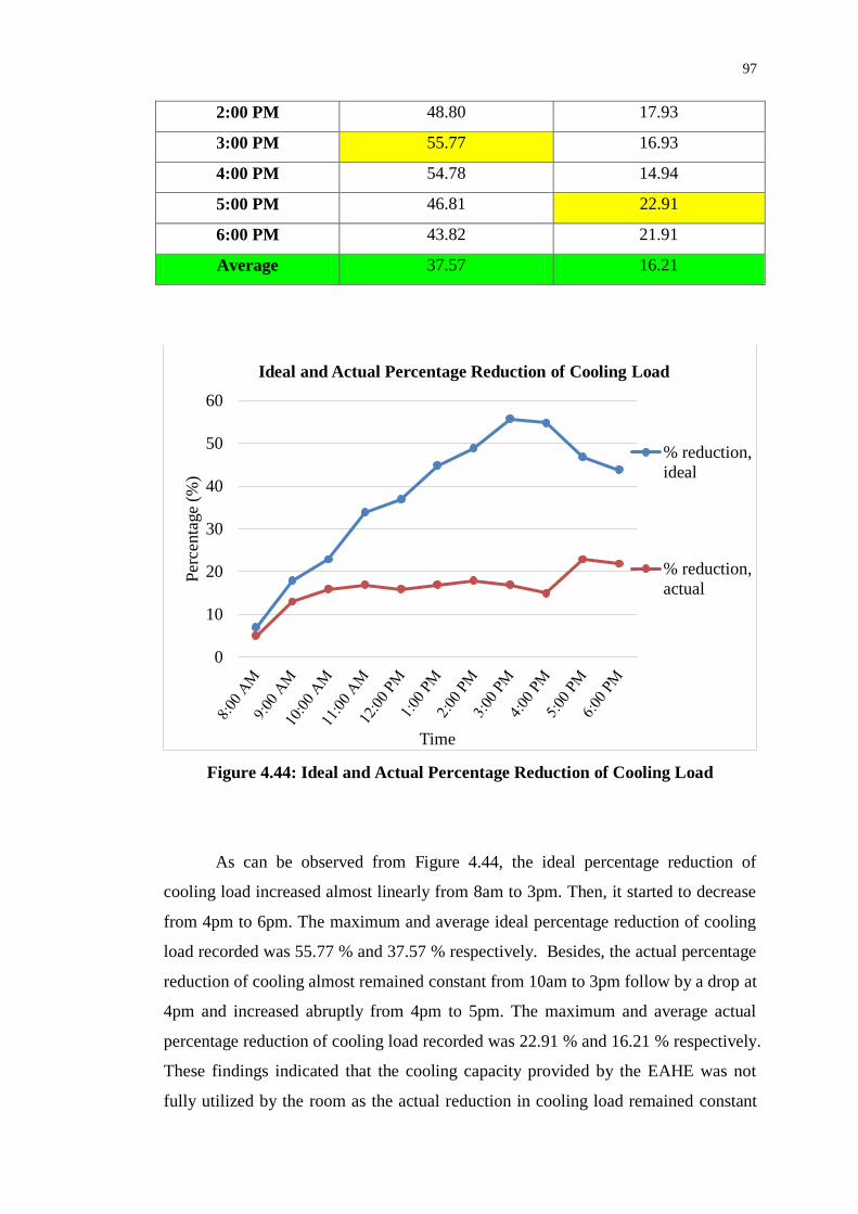
97

2:00 PM 48.80 17.93

3:00 PM 55.77 16.93

4:00 PM 54.78 14.94

5:00 PM 46.81 22.91

6:00 PM 43.82 21.91

Average 37.57 16.21

Figure 4.44: Ideal and Actual Percentage Reduction of Cooling Load

As can be observed from Figure 4.44, the ideal percentage reduction of

cooling load increased almost linearly from 8am to 3pm. Then, it started to decrease

from 4pm to 6pm. The maximum and average ideal percentage reduction of cooling

load recorded was 55.77 % and 37.57 % respectively. Besides, the actual percentage

reduction of cooling almost remained constant from 10am to 3pm follow by a drop at

4pm and increased abruptly from 4pm to 5pm. The maximum and average actual

percentage reduction of cooling load recorded was 22.91 % and 16.21 % respectively.

These findings indicated that the cooling capacity provided by the EAHE was not

fully utilized by the room as the actual reduction in cooling load remained constant

0

10

20

30

40

50

60

Per

centa

ge

(%)

Time

Ideal and Actual Percentage Reduction of Cooling Load

% reduction,

ideal

% reduction,

actual

98

when the ideal reduction in cooling load actually increased. Therefore, the actual

percentage of reduction of cooling load could have been increased provided that a

better insulation had been done.

4.7.3 EAHE Efficiency Analysis

EAHE efficiency was defined as the fraction of heat rejected from the room to the

total heat rejected by the EAHE into the ground and can be calculated by Equation

3.21 given in Section 3.5.4. Table 4.22 tabulated the heat rejected by the room and

EAHE and the associated EAHE efficiency at various time. Figure 4.45 shows the

chart of heat rejected and EAHE efficiency.

Table 4.22: Heat Rejected and EAHE Efficiency

Description

Time

Heat Rejected by

EAHE, qrejected,EAHE

(W)

Heat Rejected

from Room ,

qrejected,room (W)

EAHE Efficiency

%100,

,

EAHErejected

roomrejected

q

q

(%)

8:00 AM 66.37 47.41 71.43

9:00 AM 170.66 123.26 72.22

10:00 AM 218.07 151.70 69.57

11:00 AM 322.36 161.18 50.00

12:00 PM 350.80 151.70 43.24

1:00 PM 426.65 161.18 37.78

2:00 PM 464.58 170.66 36.73

3:00 PM 530.95 161.18 30.36

4:00 PM 521.46 142.22 27.27

5:00 PM 445.61 218.07 48.94

6:00 PM 417.17 208.59 50.00

Average 357.70 154.28 48.87

99

Figure 4.45: Heat Rejected and EAHE Efficiency

EAHE efficiency shown a decreasing trend from 10am to 4pm as shown in

Table 4.22 and Figure 4.45. After that, the EAHE efficiency started to recover back

from 5pm to 6pm. The maximum EAHE efficiency achieved by the prototype was

72.22 % at 9am in the morning while the lowest EAHE efficiency recorded was

27.27 % at 4pm. This trend was due to the increased of heat gained by the insulation

which caused lesser portion of the heat rejected from room as the heat rejected by the

EAHE had to remain at its maximum constant value. Besides, the average EAHE

efficiency achieved by the EAHE prototype was 48.87 %. Last but not least, the

result obtained also shown that the EAHE efficiency stayed in the range of 30 - 50 %

for most of the time.

0

10

20

30

40

50

60

70

80

0

100

200

300

400

500

600

EA

HE

Eff

icie

ncy

(%

)

Heat

Reje

cte

d (

W)

Time

Heat Rejected and EAHE Efficiency

qrej,EAHE qrej,room Eff

100

4.7.4 Coefficient of Performance (COP) Analysis

Two different COPs of the EAHE prototype were analysed which are the COPideal

and COPactual. COPideal is the ideal coefficient of performance of the EAHE prototype

without the consideration of imperfect insulation. It was defined as the ratio of heat

rejected by the EAHE system over the power dissipated which was fan power. On

the other hand, COPactual is the actual coefficient of performance of the EAHE

prototype with the consideration of imperfect insulation. It was defined as the ratio of

heat rejected from the room over the power dissipated. The formula for the

calculation of COPideal and COPactual were shown in Section 3.5.4 and had been

provided again here.

oipaa

fan

EAHErejected

ideal TTcmP

qCOP

,

'',

oipaa

fan

roomrejected

actual TTcmP

qCOP

Table 4.23 summarized the ideal and actual coefficient of performance of the

EAHE prototype at various time. Figure 4.46 shown the graph of ideal and actual

coefficient of performance of the EAHE prototype plotted against time according to

the tabulated data in Table 4.23.

Table 4.23: Ideal and Actual COP of EAHE Prototype

Description

Time

Ideal COP,

COPideal

Actual COP,

COPactual

8:00 AM 1.33 0.95

9:00 AM 3.41 2.47

10:00 AM 4.36 3.03

11:00 AM 6.45 3.22

12:00 PM 7.02 3.03

1:00 PM 8.53 3.22

2:00 PM 9.29 3.41

101

3:00 PM 10.62 3.22

4:00 PM 10.43 2.84

5:00 PM 8.91 4.36

6:00 PM 8.34 4.17

Average 7.15 3.09

Figure 4.46: Ideal and Actual COP of EAHE Prototype

Based on Table 4.23 and Figure 4.46, the maximum ideal and actual COPs

achieved by the EAHE prototype were 10.62 and 4.36. These maximum ideal and

actual COPs were achieved at 3pm and 5pm respectively. Both the ideal and actual

COP of the EAHE prototype attained the lowest value at 8am in the morning. The

lowest ideal and actual COPs attained were 1.33 and 0.95 respectively. Although

ideal COP of the EAHE prototype increased throughout the day from morning to late

afternoon, actual COP stayed in the range of 3.0 – 4.4 for most of the time. The ideal

and actual average COPs achieved by the EAHE prototype were 7.15 and 3.09

respectively.

102

As can be observed from Figure 4.46, the difference between the ideal and

actual COPs increased as time progressed from 10am to 4pm. This could be due to

the decreased of heat rejected from the room that caused by increased of heat gained

by insulation as explained previously in Section 4.6.4. On the other hand, the

difference between the ideal and actual COPs reduced as time progress from 5pm to

6pm. This could be due to increase of heat rejected from the room as a result of the

decreased of heat gained by insulation as the solar radiation intensity reduced in the

evening.

Another reason that might have caused the increased of difference between

ideal and actual COPs was the heat accumulation in the ground after prolong period

of EAHE operation. The ground temperature near the EAHE pipe might have

increased throughout the day rather than staying at a constant value as assumed due

to heat rejected by the EAHE prototype. The maximum heat rejected by EAHE

would be reduced if the ground temperature have increased. Thus, a detail

investigation are required to determine whether there were heat accumulated and the

effect corresponding effects on EAHE prototype.

In a nutshell, the actual COP of the EAHE could theoretically be increased if

the heat gained by the insulation and heat accumulation in the ground could be

reduced. These and the aforementioned findings again further reinforced the insight

that cooling performance of the EAHE prototype system could be increased if the

heat gained by the insulation could be reduced to a reasonable extent. Although the

actual average COP (3.09) achieved was not low, there was plentiful of room for

improvement to get it closer to the ideal average COP recorded (7.15).

103

CHAPTER 5

5 CONCLUSION AND RECOMMENDATIONS

5.1 Conclusion

One of the most important design aspect of the Earth-to-Air Heat Exchanger (EAHE)

system was the determination of the suitable depth for the installation of the pipe. By

experimental measurement, the most ideal or suitable depth for the installation of the

EAHE prototype was determined to be 1.5m. The difference of ground temperature

at the depth of 1.5 m and 2.0 m was very small during all the period of the time. The

measured difference in mean maximum and minimum temperature at the depth of 1.5

m and 2.0 m was just 0.1 C. Thus, it would be impractical to go for another 0.5 m

deeper for the slight improvement in mean daily temperature range because it cannot

be justified by the additional costing and time that might be incurred.

To design the EAHE prototype system, the cooling load imposed by the

experimental residential room at UTAR LKCFES has been determined before others

design parameters of the EAHE prototype could be established. For the

aforementioned purpose, the Residential Load Factor (RLF) method has been used to

conduct a cooling load analysis. The indoor and outdoor design temperature has been

defined to be 29.4 C and 35 C. The total cooling load determined using RLF method

was 952 W. The EAHE prototype was designed to reject heat imposed by the cooling

load determined under the worst condition recorded with temperature difference of

room and ground, ∆Troom-ground of 8.3 C. The finalized EAHE prototype design has

selected PVC pipe of 3 in (80 mm) nominal diameter because it was well balanced in

terms of space saving and total cost. The required pipe length of the EAHE prototype

104

using 3 in (80 mm) nominal diameter PVC pipe was calculated to be 11.1 m.

However, the pipe length has been designed to be 11.6 m for simplicity of design.

A centrifugal exhaust fan has been designed and fabricated in this project that

was being used in the EAHE prototype system to provide the static pressure, air

velocity and mass flow rate required by the system. The centrifugal exhaust fan was

designed through a trial-and-error approach using Flow Simulation of SolidWorks.

Some of the important aforementioned specifications of the finalized centrifugal fan

design was simulated using Flow Simulation and experimentally tested after it is

fabricated. The simulated and experimental suction velocity was determined to be

17.1 m/s and 16.5 m/s with a percentage difference of 3.64%. The simulated and

experimental mass flow rate was determined to be 0.16186 kg/s and 0.15618 kg/s

with a percentage difference of 3.64% as well.

From the result obtained from experiment, the ideal and actual maximum

percentage reduction of cooling load achieved were 55.77 % and 22.91 %. The

average ideal and actual percentage reduction of cooling load achieved were 37.57 %

and 16.21 % respectively. The maximum heat rejected by the EAHE and from the

room were 530.95 W and 218.07 W. The average heat rejected by EAHA and from

the room achieved were 357.70 W and 154.28 W respectively. On the other hand, the

maximum and minimum EAHE efficiency achieved by the designed EAHE

prototype were 72.22 % and 27.27% respectively. However, the result obtained

shown that the EAHE efficiency stays in the range of 30 - 50 % only for most of the

time and had achieved an average EAHE efficiency of 48.87 %.

The maximum ideal and actual COPs achieved by the EAHE prototype were

10.62 and 4.36. The lowest ideal and actual COPs attained by the EAHE prototype

were 1.33 and 0.95. Although ideal COP of the EAHE prototype increased

throughout the day from morning to late afternoon, actual COP stays in the range of

3.0 – 4.4 for most of the time. Besides, the average ideal and actual COPs achieved

by the EAHE prototype were 7.15 and 3.09 respectively. In conclusion, the EAHE

did achieve reasonably good cooling performance in terms of COP. However, it did

not perform very well in terms of percentage of reduction of cooling load and EAHE

efficiency due to too much heat gained by the insulation. Therefore, it is feasible to

105

implement EAHE cooling system in Malaysia if thermal insulation of the system

could be carefully designed and monitored.

5.2 Recommendation

The thermal insulation on the pipe exposed to solar radiation could be improved in

order to improve the cooling performance of the EAHE prototype. This is because

result of the experiment has shown that the increases of heat gained by the insulation

reduced the heat rejected from the room and hence reduced the actual coefficient of

performance. To solve this problem, the EAHE pipes that is exposing to solar

radiation could be covered with rock wool blanket or neoprene insulation foam.

Besides this, a larger centrifugal exhaust fan with a larger rated power could

be used in place of the 50 W fan but with the condition that it must be placed outside

the building to avoid unnecessary heat dissipation. By using a larger centrifugal

exhaust fan, the air velocity and pipe length could be increased in the EAHE design.

This will increase the amount of heat rejected in to the ground by the EAHE system

and at the same will avoid heat accumulation in the ground. This is because higher

air velocity means lower heat transfer as the air would have lesser time to transfer

heat across the pipe but the loss in that amount of heat transfer can be made up by

having a longer pipe. The benefit of having higher air velocity is that heat will not

accumulate easily in the ground near where the EAHE pipes were buried.

106

REFERENCES

ASHRAE, 2009. 2009 ASHRAE Handbook – Fundamentals. Chapter 14.

Al-Ajmi, A., Loveday, D.L., Hanby, V.I., 2006. The cooling potential of earth-air

heat exchangers for domestic buildings in a desert climate. Building and

Environment, 41(3), pp. 235-244.

ATKC e-Commerce Warehouse, 2015. PVC Pipes & Fittings. [online]. Available at:

<http://www.ewarehouse.atkc.com.my/plumbing/pvc-pipe-fittings&filter=161>

[Assessed 1 January 2015].

EIA U.S. Energy Information Administration, 2013. International Energy Outlook

2013. [online] Available at: <http://www.eia.gov/forecasts/ieo/world.cfm>

[Accessed 5 August 2014]

Energy Commission, 2011. Malaysia Energy Information Hub: Electricity - Final

Electricity Consumption. [online] Available at < http://meih.st.gov.my/statistics>


Germany Energy Agency, 2002. Geothermal energy. [online] Available at: <

http://www.renewables-made-in-germany.com/en/renewables-made-in-germany-

start/geothermal.html> [Accessed 7 August 2014]

Ghosal, M.K., Tiwari, G.N., 2006. Modeling and parametric studies for thermal

performance of earth to air heat exchanger integrated with a greenhouse. Energy

Conversion and Management, 47(13-14), pp. 1779-1798.

http://www.ewarehouse.atkc.com.my/plumbing/pvc-pipe-fittings&filter=161

http://www.eia.gov/forecasts/ieo/world.cfm

http://meih.st.gov.my/statistics

http://www.renewables-made-in-germany.com/en/renewables-made-in-germany-start/geothermal.html

http://www.renewables-made-in-germany.com/en/renewables-made-in-germany-start/geothermal.html

107

Incopera, F. P., 2002. Introduction to Heat Transfer. 4th ed. Singapore: John Wiley

& Sons.

Malaysia Metrological Department, 2015. Buletin Cuaca Bulanan. [online].

Available at:

<http://www.met.gov.my/index.php?option=com_content&task=view&id=842&It

emid=1586> [Assessed 29 February 2015].

Mongkon, S., Thepa, S., Namprakai, P., Pratinthong, N., 2014. Cooling performance

assessment of horizontal earth tube system and effect on planting in tropical

greenhouse. Energy Conversion and Management, 78, pp. 225-236.

Nik, A.R., Kasran, B. and Hassan, A., 1986. Soil Temperature Regimes under Mixed

Dipterocarp Forests of Peninsular Malaysia. Pertanika, 9(3), 277-284.

Ozgener, L., 2011. Ozgener, O., 2011. A review on the experimental and analytical

analysis of the earth to air heat exchanger (EAHE) systems in Turkey. Renewable

and Sustainable Energy Reviews, 15(9), pp. 4483-4490.

Peretti, C., Zarella, A., Carli, M.D., Zecchin, R., 2013. The design and environmental

evaluation of earth-to-air heat exchangers (EAHE). A literature review.

Renewable and Sustainable Energy Reviews, 28, pp. 107-116.

Pfafferott, J., 2003. Evaluation of earth-to-air heat exchangers with a standardised

method to calculate energy efficiency. Energy and Building, 35(10), pp. 971-983.

Reimann, G., 2007. Ground Cooling of Ventilation Air for energy Efficient House in

Malaysia: A Case Study of the CoolTek House. In: Conference on Sustainable

Building South East Asia. Malaysia, 5-7 November 2007. Johor, Malaysia:

Institute Sultan Iskandar of Urban Habitat and Highrise. Available at

<http://www.irbnet.de/daten/iconda/CIB11369.pdf> Accessed date [19 August

2014].

http://www.met.gov.my/index.php?option=com_content&task=view&id=842&Itemid=1586

http://www.met.gov.my/index.php?option=com_content&task=view&id=842&Itemid=1586

http://www.irbnet.de/daten/iconda/CIB11369.pdf

108

Sanusi, A.N.Z., Li, S. and Zamri, A.A.A., 2014. Seeking Underground for Potential

Heat Sink in Malaysia for Earth Air Heat Exchanger (EAHE) Application.

Australian Journal of Basic and Applied Sciences, 8 (8), pp. 54-57.

Tan, K. S., 2013. Investigation into Effectiveness of Heat Transfer for Water-

Circulated Geothermal Cooling System with Polyethylene Ground Heat Exchange

Loop.

The European Technology Platform on Renewable Heating and Cooling, 2012.

Strategic Research Priorities for Geothermal Technology. [online] Available at:

<http://www.rhc-platform.org/fileadmin/Publications/Geothermal_SRA.pdf>


Woodson, T., Coulibaly, Y. and Traore, E.S., 2012. Earth-air Heat Exchangers for

Passive Air Conditioning: Case Study Burkina Faso. Journals of Construction in

Developing Countries, 17(1), pp. 21-32.

Wu, H., Wang, S., Zhu, D., 2007. Modelling and evaluation of cooling capacity of

earth-air-pipe systems. Energy Conversion and Management, 48(5), pp. 1462-

1471.

http://www.rhc-platform.org/fileadmin/Publications/Geothermal_SRA.pdf

109

APPENDICES

APPENDIX A: Tables and Graph of Ground, Room and Environment Temperature

110

Table A-1: Ground, Room and Environment Temperature on 1 March 2015 (Day 1)

Description

Time

0.5 m

( C)

1.0 m

( C)

1.5 m

( C)

2.0 m

( C)

Room temperature,

𝑻𝒓′ ( C)

Environment


08:00 AM 28.1 27.9 27.6 27.6 27.2 28.7

09:00 AM 28 27.8 27.5 27.5 28 30

10:00 AM 28.6 28.1 27.4 27.4 32.2 31.3

11:00 AM 29.5 28.4 27.4 27.3 34.3 32.6

12:00 PM 30.2 28.9 28 27.7 36 34.2

01:00 PM 30.9 29.1 28.6 28.2 37.3 35.5

02:00 PM 31.4 29.7 28.9 28.7 37 36.8

03:00 PM 31.9 30.9 29.4 29.1 36.6 37.7

04:00 PM 31 31.2 29.7 29.6 35.9 37.2

05:00 PM 30 30.4 30 29.9 34 36.4

06:00 PM 28.9 29.1 29.1 29 30.8 35.1

111

Figure A-1: Ground, Room and Environment Temperature on 1 March 2015 (Day 1)

25

27

29

31

33

35

37

39T

em

peratu

re (

C)

Time

Ground, Room and Environment Temperature of Day 1

0.5m

1.0m

1.5m

2.0m

Environment

Temperature,

Tenviron

Room

Temperature

without EAHE,

Tr

112

Figure A-2: Ground Temperature at Different Depth on 1 March 2015 (Day 1)

25

26

27

28

29

30

31

32

33

Tem

peratu

re (

C)

Time

Ground Temperature at Different Depth of Day 1

0.5m

1.0m

1.5m

2.0m

113


Description

Time

0.5 m

( C)

1.0 m

( C)

1.5 m

( C)

2.0 m

( C)

Room temperature,

𝑻𝒓′ ( C)

Environment


08:00 AM 27.9 27.7 27.4 27.4 27 28.5

09:00 AM 27.8 27.6 27.3 27.3 27.8 29.8

10:00 AM 28.4 27.9 27.2 27.2 32 31.1

11:00 AM 29.2 28.1 27.1 27 34 32.3

12:00 PM 29.7 28.4 27.5 27.2 35.5 33.7

01:00 PM 30.6 28.8 28.3 27.9 37 35.2

02:00 PM 31 29.3 28.5 28.3 36.6 36.4

03:00 PM 31.4 30.4 28.9 28.6 36.1 37.2

04:00 PM 30.5 30.7 29.2 29.1 35.4 36.7

05:00 PM 29.2 29.6 29.2 29.1 33.2 35.6

06:00 PM 28.8 29 29 28.9 30.7 35

114


25

27

29

31

33

35

37

39T

em

peratu

re (

C)

Time


0.5m

1.0m

1.5m

2.0m

Environment

Temperature,

Tenviron

Room

Temperature

without EAHE,

Tr

115


25

26

27

28

29

30

31

32

Tem

peratu

re (

C)

Time


0.5m

1.0m

1.5m

2.0m

116


Description

Time

0.5 m

( C)

1.0 m

( C)

1.5 m

( C)

2.0 m

( C)

Room temperature,

𝑻𝒓′ ( C)

Environment


08:00 AM 27.7 27.5 27.2 27.2 26.8 28.3

09:00 AM 27.6 27.4 27.1 27.1 27.6 29.6

10:00 AM 28.2 27.7 27 27 31.8 30.9

11:00 AM 28.9 27.8 26.8 26.7 33.7 32

12:00 PM 29.5 28.2 27.3 27 35.3 33.5

01:00 PM 30.3 28.5 28 27.6 36.7 34.9

02:00 PM 30.9 29.2 28.4 28.2 36.5 36.3

03:00 PM 31.2 30.2 28.7 28.4 35.9 37

04:00 PM 30.3 30.5 29 28.9 35.2 36.5

05:00 PM 29.3 29.7 29.3 29.2 33.3 35.7

06:00 PM 28.7 28.9 28.9 28.8 30.6 34.9

117


25

27

29

31

33

35

37

39T

em

peratu

re (

C)

Time


0.5m

1.0m

1.5m

2.0m

Environment

Temperature,

Tenviron

Room

Temperature

without EAHE,

Tr

118


25

26

27

28

29

30

31

32T

em

peratu

re (

C)

Time


0.5m

1.0m

1.5m

2.0m

119

APPENDIX B: Calculation of Required Length for Different Diameter

1. For nominal diameter of 25 mm

From Figure 3.15,

oD = 31.2 mm = 0.0312 m

iD = 33.4 mm = 0.0334 mm


p

ioconductive

kL

DDR

2

)/ln(

19.02

)0312.0/0334.0ln(

L

L/05707.0


4

2

avgi

a

VDm

4

8.130312.0205.12

01272.0 kg/s


i

a

D

m4Re

120

000015573.00312.0

01272.04

316,33

Friction factor, f

264.1Reln79.0

f

264.1312,33ln79.0

02305.0

Prantl number, Pr

a

pa

k

c Pr

0257.0

000015573.01005

61.0

Nusselt number, Nu

)1(Pr8

7.121

Pr1000Re8

3/2

5.0

f

f

Nu

)161.0(8

02305.07.121

61.01000316,338

02305.0

3/2

5.0

12.72


i

aa

D

kNuh

121

0334.0

0257.012.72

4106.59 W/m2 ∙ K


LhDR

ai

convective

1

L

4106.590312.0

1

L/17170.0


groundroom

totalload

T

RqL

3.8

22877.0952

24.26 m


From Figure 3.15,

oD = 57.7 mm = 0.0577 m

iD = 60.2 mm = 0.0602 m


p

ioconductive

kL

DDR

2

)/ln(

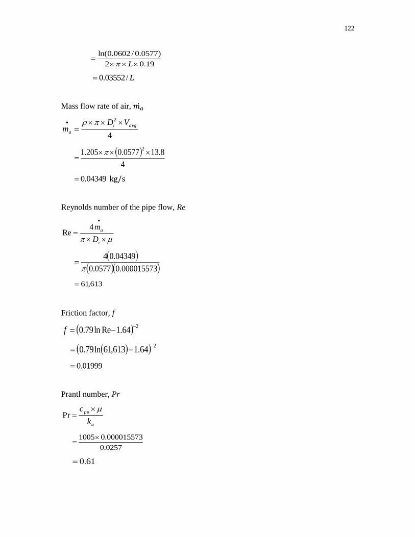
122

19.02

)0577.0/0602.0ln(

L

L/03552.0


4

2

avgi

a

VDm

4

8.130577.0205.12

04349.0 kg/s


i

a

D

m4Re

000015573.00577.0

04349.04

613,61

Friction factor, f

264.1Reln79.0

f

264.1613,61ln79.0

01999.0

Prantl number, Pr

a

pa

k

c Pr

0257.0

000015573.01005

61.0

123

Nusselt number, Nu

)1(Pr8

7.121

Pr1000Re8

3/2

5.0

f

f

Nu

)161.0(8

01999.07.121

61.01000613,618

01999.0

3/2

5.0

99.113


i

aa

D

kNuh

0577.0

0257.099.113

7733.50 W/m2 ∙ K


LhDR

ai

convective

1

L

7733.500577.0

1

L/10864.0


groundroom

totalload

T

RqL

3.8

10864.0952

124

54.16 m


From Figure 3.15,

oD = 111.8 mm = 0.1118 m

iD = 114.1 mm = 0.1141 m


p

ioconductive

kL

DDR

2

)/ln(

19.02

)1118.0/1141.0ln(

L

L/01706.0


4

2

avgi

a

VDm

4

8.131118.0205.12

16327.0 kg/s


i

a

D

m4Re

000015573.01118.0

16327.04

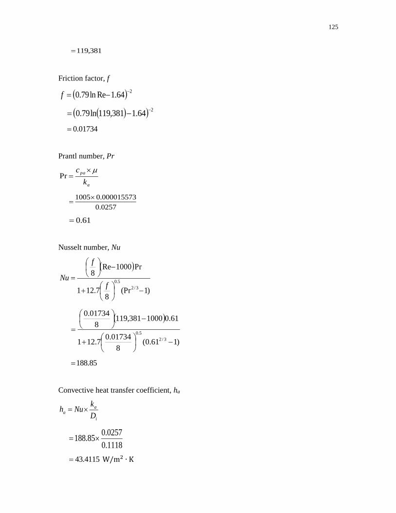
125

381,119

Friction factor, f

264.1Reln79.0

f

264.1381,119ln79.0

01734.0

Prantl number, Pr

a

pa

k

c Pr

0257.0

000015573.01005

61.0

Nusselt number, Nu

)1(Pr8

7.121

Pr1000Re8

3/2

5.0

f

f

Nu

)161.0(8

01734.07.121

61.01000381,1198

01734.0

3/2

5.0

85.188


i

aa

D

kNuh

1118.0

0257.085.188

4115.43 W/m2 ∙ K

126


LhDR

ai

convective

1

L

4115.431118.0

1

L/06558.0


groundroom

totalload

T

RqL

3.8

08263.0952

48.9 m


From Figure 3.15,

oD = 134.7 mm = 0.1374 m

iD = 140.0 mm = 0.1400 m


p

ioconductive

kL

DDR

2

)/ln(

19.02

)1400.0/1374.0ln(

L

L/01570.0

127


4

2

avgi

a

VDm

4

8.131374.0205.12

24660.0 kg/s


i

a

D

m4Re

000015573.01374.0

24660.04

717,146

Friction factor, f

264.1Reln79.0

f

264.1717,146ln79.0

01661.0

Prantl number, Pr

a

pa

k

c Pr

0257.0

000015573.01005

61.0

Nusselt number, Nu

128

)1(Pr8

7.121

Pr1000Re8

3/2

5.0

f

f

Nu

)161.0(8

01661.07.121

61.01000717,1468

01661.0

3/2

5.0

55.221


i

aa

D

kNuh

1374.0

0257.055.221

4404.41 W/m2 ∙ K


LhDR

ai

convective

1

L

4404.411374.0

1

L/05590.0


groundroom

totalload

T

RqL

3.8

07160.0952

21.8 m

129

APPENDIX C: Tables and Graph Various Temperature of the EAHE Prototype System

Table A-4: Various Temperature of the EAHE Prototype System on 26 March 2015 (Day 1)

Description


8:00 AM 28.1 27.4 28 27.5 28 27

9:00 AM 29.1 27.4 29.1 27.8 29.1 29.8

10:00 AM 29.8 27.5 29.6 28 29.7 32.2

11:00 AM 31.3 27.9 30.1 28.4 30 33.9

12:00 PM 32.2 28.5 30.6 29 30.6 35.1

1:00 PM 34 29.5 31.9 30.2 31.8 36.6

2:00 PM 35.1 30.2 32.6 30.8 32.4 36.5

3:00 PM 36.7 31.1 33.4 31.7 33.2 36.3

4:00 PM 37.1 31.6 33.7 32.6 33.5 35.4

5:00 PM 35.5 30.7 33.6 31.2 33.5 33.8

6:00 PM 34.4 29.7 33.2 30.8 33.1 32

130

Figure A-7: Various Temperature of the EAHE Prototype System on 26 March 2015 (Day 1)

25

27

29

31

33

35

37

39

Tem

peratu

re (

C)

Time

Various Temperature of the EAHE Prototype System

EAHE Inlet

Temperature, Ti

EAHE Outlet

Temperature, To

Inlet Temperature

before Insulation,

Ti'

Outlet Temperature


Room Temperature

with EAHE, Tr

Environment

Temperature,

Tenviron

131


Description


8:00 AM 27.9 27.2 27.8 27.3 27.8 26.8

9:00 AM 29.4 27.2 28.9 27.6 28.9 29.6

10:00 AM 29.8 27.6 29.7 28.1 29.8 32.3

11:00 AM 31.6 28.2 30.4 28.7 30.3 34.2

12:00 PM 32.9 29.2 31.3 29.7 31.3 35.8

1:00 PM 34.7 30.2 32.6 30.9 32.5 37.3

2:00 PM 35.6 30.7 33.1 31.3 32.9 37

3:00 PM 37.1 31.5 33.8 32.1 33.6 36.7

4:00 PM 37.5 32 34.1 32.6 33.9 35.8

5:00 PM 35.7 30.9 33.8 31.4 33.7 34

6:00 PM 34.9 30.1 33.7 31 33.6 32.5

132


25

27

29

31

33

35

37

39

Tem

peratu

re (

C)

Time

Mean Temperature of the EAHE Prototype System

EAHE Inlet

Temperature, Ti

EAHE Outlet

Temperature, To

Inlet Temperature

before Insulation,

Ti'

Outlet Temperature


Room Temperature

with EAHE, Tr

Environment

Temperature,

Tenviron

133


Description


8:00 AM 28.3 27.6 28.2 27.7 28.2 27.2

9:00 AM 29.1 27.6 29.3 28 29.3 30

10:00 AM 29.5 27.1 29.2 27.6 29.3 31.8

11:00 AM 31.3 27.9 30.1 28.4 30 33.9

12:00 PM 33 29.3 31.4 29.8 31.4 35.9

1:00 PM 34.5 30 32.4 30.7 32.3 37.1

2:00 PM 35.5 30.6 33 31.2 32.8 36.9

3:00 PM 36.9 31.3 33.6 31.9 33.4 36.5

4:00 PM 37.6 32.1 34.2 32.3 34 35.9

5:00 PM 35.3 30.8 33.4 31.3 33.3 33.6

6:00 PM 33.6 29.9 32.4 30.9 32.3 31.2

134


25

27

29

31

33

35

37

39

Tem

peratu

re (

C)

Time

Mean Temperature of the EAHE Prototype System

EAHE Inlet

Temperature, Ti

EAHE Outlet

Temperature, To

Inlet Temperature

before Insulation,

Ti'

Outlet Temperature


Room Temperature

with EAHE, Tr

Environment

Temperature,

Tenviron

THIEM WOH MUN UNIVERSITY TUNKU ABDUL RAHMAN

Documents

Transcript of THIEM WOH MUN UNIVERSITY TUNKU ABDUL RAHMAN