THESIS TECHNOECONOMIC ANALYSIS OF A STEAM GENERATION SYSTEM WITH CARBON

CAPTURE

Submitted by

Luke Giugliano

Department of Mechanical Engineering

In partial fulfillment of the requirements

For the Degree of Master of Science

Colorado State University

Fort Collins, Colorado

Summer 2019

Master’s Committee: Adviser: Todd M. Bandhauer Shantanu Jathar Tiezheng Tong

Copyright Luke Giugliano 2019

All Rights Reserved

ii

ABSTRACT

TECHNOECONOMIC ANALYSIS OF A STEAM GENERATION SYSTEM WITH CARBON

CAPTURE

Industrial steam generation consumes large amounts of natural gas (NG) and contributes

significantly to CO2 emissions. Existing boiler technology is relatively inefficient, and its

continued adoption could potentially be hampered by carbon emissions taxes due to the difficulty

in CO2 separation from the dilute exhaust gas stream. This paper presents an alternative approach

to steam generation that combines a membrane reactor (MR) to produce hydrogen from steam

methane reforming (SMR), resulting in a concentrated CO2 exhaust. The performance of the

system is evaluated using a coupled thermodynamic and technoeconomic analysis of an industrial-

scale SMR plant to produce hydrogen in a MR used primarily for the purpose of steam generation

(SG). The proposed SMR-MR-SG system converts NG to clean-burning hydrogen (H2), burns H2

to generate steam, and captures and concentrates CO2. Unused NG and H2 are recycled back into

the system with uncaptured CO2 to increase efficiency.

The SMR-MR-SG is compared to two baseline systems: a natural gas industrial boiler

system (BS), and the same boiler system with integrated CO2 capture (BSC). The SMR-MR-SG

improves on the BS by increasing efficiency from 86% to 97% and reducing NG and water

consumption by 14% and 55%, respectively. Additionally, the SMR-MR-SG uses cryogenic

separation and gas recycling to completely eliminate CO2 emissions with a 3.0% energy penalty,

much less than comparable systems with carbon capture.

iii

The SMR-MR-SG has a capital cost about three times the BS and twice the BSC, but makes

up for it quickly with reducing operating costs. Using a conservative prediction of carbon tax, the

SMR-MR-SG has a payback period of 1.86 and 1.26 years and a discounted lifetime cost reduction

of 42% and 43% relative to the BS and BSC, respectively. A sensitivity analysis showed that the

results are most heavily influenced by the amount of carbon tax implemented in the future, with

no carbon tax corresponding to a payback period of 8.05 years relative to the BS. The results of

this modelling study show that the SMR-MR-SG could be a direct replacement for common

industrial boiler systems as a new, efficient, and clean steam generation system.

iv

ACKNOWLEDGEMENTS

I would like to thank Dr. Todd Bandhauer for pushing me to work harder, think more

critically, and achieve greater accomplishments. In particular, he has taught me how to always

make progress by trusting my own engineering judgement. I sincerely appreciate his great

flexibility with my pursuits outside the ITS lab, be it running, tiny house living, or moving out of

town. I may have had an easier time with another advisor, but I certainly would not have learned

as much.

I would like to thank our collaborators, formerly of Mines but now of Worcester

Polytechnic Institute: Simona Liguori, Cyrus Kian, and Jen Wilcox. These are the masterminds

behind everything “membrane reactor”. To say they taught me everything I know about membrane

reforming is not far from the truth. Thank you for helping to guide a frequently lost mechanical

engineer in a chemical world.

The students (and former students) of the ITS lab are the heart of this experience. I could

easily write pages about all that they have done for me, but this is technical writing so I will keep

it short. Thank you to: Josh, for putting up with me in house and lab; John, for being my go-to

“can you help me with...” guy; Shane, for his patience helping me with the many things I’ve asked

of him; Derek, for showing me the ropes of thesis writing; Alex, for TIG welding along with the

best of them; Katie, for her mastery of zip-ties and fiberglass insulation; James, for dedicating his

life to the study of gas chromatography and smoked meats; David, for always making time to help

at a minute’s notice; Zach, for the comedy, intentional or not; Caleb, for keeping me up to date on

current events; Will, for removing 126 cubic inches of masonry; Jensen, for building dozens of

steel menorahs. You guys made the memories I will remember.

v

To my family: M, DA, Swa, and Shark, thank you for answering my phone calls every day

between 4:30 and 6:30pm MT. I have had nothing but support from each of you and cannot wait

for all of you to move out here. Finally, I would like to thank Chrissy. My world is made brighter

by your smile. Thank you for keeping me going. I thought about proposing in this thesis, but that

would almost be too romantic. Instead, please enjoy the following ~150 pages on steam methane

reforming.

vi

TABLE OF CONTENTS

ABSTRACT .................................................................................................................................. ii ACKNOWLEDGEMENTS .......................................................................................................... iii LIST OF TABLES ........................................................................................................................ vii LIST OF FIGURES ..................................................................................................................... viii NOMENCLATURE ....................................................................................................................... x

Introduction ......................................................................................................... 1 1.1. Background ..................................................................................................................... 1

1.2. Steam Methane Reforming ............................................................................................. 2

1.3. Application to Steam Generation .................................................................................... 8

1.4. Research Objectives ...................................................................................................... 11

1.5. Thesis Organization ...................................................................................................... 12

Literature Review.............................................................................................. 13 2.1. State-of-the-Art Steam Methane Reforming ................................................................. 15

2.1.1. Membrane Reactors .............................................................................................. 15

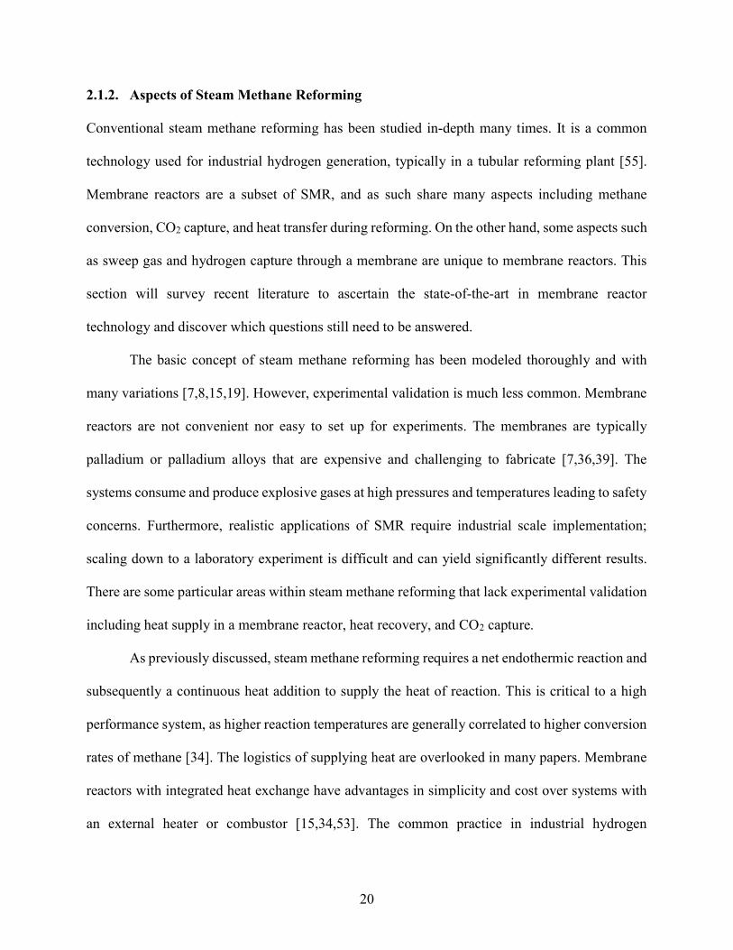
2.1.2. Aspects of Steam Methane Reforming ................................................................. 20

2.1.3. CO2 Capture .......................................................................................................... 25

2.1.4. Summary ............................................................................................................... 26

2.2. Steam Methane Reforming Applications ...................................................................... 27

2.3. Competitive Steam Generation Technologies .............................................................. 32

2.4. Research Needs for Steam Methane Reforming ........................................................... 35

2.5. Specific Aims of this Study .......................................................................................... 37

Modeling Approach .......................................................................................... 39 3.1. Boiler Systems .............................................................................................................. 45

3.2. SMR-MR-SG System ................................................................................................... 50

3.2.1. Model Overview ................................................................................................... 51

3.2.2. Assumptions and Input Parameters ....................................................................... 57

3.2.3. Thermodynamic Analysis ..................................................................................... 63

3.2.4. Cost Calculations .................................................................................................. 75

3.3. CO2 Capture .................................................................................................................. 79

3.4. Technoeconomic Comparison ...................................................................................... 80

3.4.1. Baseline for Comparison....................................................................................... 80

3.4.2. Cash Flow Analysis .............................................................................................. 83

Results and Discussion ..................................................................................... 86

vii

4.1. Thermodynamic Results ............................................................................................... 86

4.1.1. Process States and Energy Balances ..................................................................... 86

4.1.2. Comparison of Energy Consumption.................................................................... 89

4.2. Technoeconomic Results .............................................................................................. 95

4.3. Sensitivity Analysis .................................................................................................... 100

4.3.1. Basic Analysis ..................................................................................................... 100

4.3.2. Monte Carlo Simulation ...................................................................................... 104

Conclusions and Recommendations for Further Work ................................... 111 5.1. Recommendations for Future Work............................................................................ 112

5.1.1. SMR-MR-SG Cycle Variants ............................................................................. 112

5.1.2. Summary ............................................................................................................. 114

REFERENCES ........................................................................................................................... 115 APPENDIX A. Representative Calculation ......................................................................... 122

A.1. Thermodynamic State Points Calculation ................................................................... 125

A.2. Energy Balance Calculation ........................................................................................ 134

A.3. Capital and Operating Cost Calculation ..................................................................... 137

A.4. Cash Flow Analysis Calculation ................................................................................. 139

APPENDIX B. Heat Exchanger Sizing ................................................................................ 141 B.1. Single Phase ................................................................................................................ 141

B.2. Two Phase ................................................................................................................... 145

viii

LIST OF TABLES Table 2-1: Large-scale membrane reactor plants. ......................................................................... 19

Table 2-2: Scale of typical hydrogen consumers and producers. ................................................. 19

Table 2-3: Boiler Inventory in the United States [40]. ................................................................. 33

Table 2-4: Summary of recent studies on membrane reforming technologies. ............................ 36

Table 3-1: List of major assumptions and input variables in thermodynamic model. .................. 40

Table 3-2: List of major thermodynamic modeling assumptions ................................................. 41

Table 3-3: Enthalpy reference states for fluids used in Engineering Equation Solver. ................ 42

Table 3-4: International currency exchange rates in January 2019. ............................................. 45

Table 3-5: List of major input variables in technoeconomic model. ............................................ 47

Table 3-6: Parameters for estimating capital costs using the scaling method. ............................. 49

Table 3-7: Temperature and pressure of states set directly by input parameters. ......................... 69

Table 3-8: Example of heat exchanger temperatures crossing during thermodynamic model

development. ................................................................................................................................. 71

Table 4-1: Thermodynamic state points for SMR steam generation system. ............................... 87

Table 4-2: Relative thermodynamic comparison of SMR-MR-SG and boiler systems. .............. 89

Table 4-3: Comparison of CO2 capture and concentration energy penalties. ............................... 93

Table 4-4: Key results of technoeconomic analysis. .................................................................... 95

Table 4-5: Input parameters varied and range of variation for sensitivity analysis. ................... 101

Table 4-6: Input parameters varied and PERT probability distribution parameters used in Monte

Carlo simulation. ......................................................................................................................... 105 (delete lin k break)

ix

Table A-1: State point descriptions for integrated steam methane reformer and steam generation

system. ........................................................................................................................................ 123

Table A-2: Definition of enthalpy terms used in calculations. ................................................... 124

Table A-3: Hand calculations versus EES results to verify thermodynamic state points. .......... 125

Table A-4: Hand calculations versus EES results to verify energy balance parameters. ........... 134

Table A-5: Hand calculations versus EES results to verify capital and operating costs. ........... 137

Table A-6: Hand calculations versus EES results to verify cash flow analysis results. ............. 139

x

LIST OF FIGURES Figure 1-1: Carbon emissions flow diagram for United States in 2014 [3]. ................................... 1

Figure 1-2: Simplified process flow diagram of steam methane reforming. .................................. 5

Figure 1-3: Industrial boiler quantity and boiler capacity by primary fuel [40]. ............................ 9

Figure 1-4: Size distribution of industrial boilers sold between 1992 and 2002 [40]................... 10

Figure 1-5: Simplified steam methane reformer process flow diagram with steam generation. .. 11

Figure 2-1: Simplified process flow diagram of steam methane reforming with sweep gas. ....... 23

Figure 2-2: Tube-in-tube membrane reactor with sweep gas. ...................................................... 24

Figure 2-3: Simplified process flow diagram of steam methane reforming with a hydrogen turbine.

....................................................................................................................................................... 29

Figure 3-1: Process flow diagram for coupled SMR in a MR and steam generation system (SMR-

MR-SG)......................................................................................................................................... 50

Figure 3-2: Simplified process flow diagram of a coupled SMR and steam generation system. . 53

Figure 3-3: Closest approach temperature (CAT) of fluids in a counter-flow heat exchanger. ... 54

Figure 3-4: United States natural gas industrial price history [5]. ................................................ 81

Figure 4-1: Pinch points of heat exchangers in steam methane reformer steam generation cycle.

....................................................................................................................................................... 88

Figure 4-2: Energy flows for SMR-MR-SG system. .................................................................... 90

Figure 4-3: Energy flows for boiler system with CO2 capture (BSC). ......................................... 91

Figure 4-4: Discounted lifetime cost comparison between boiler and SMR-MR-SG systems. ... 97

Figure 4-5: Cash flow diagram comparing SMR-MR-SG to baseline steam generation systems.99

xi

Figure 4-6: Results of sensitivity analysis for SMR-MR-SG system compared to BS (a) and BSC

(b). ............................................................................................................................................... 103

Figure 4-7: Tornado chart showing Monte Carlo simulation of payback period of the SMR-MR-

SG vs. BS (a) and vs. BSC (b). ................................................................................................... 107

Figure 4-8: Histogram showing Monte Carlo simulation of payback period of the SMR-MR-SG

vs. BS (a) and vs. BSC (b). ......................................................................................................... 109

xii

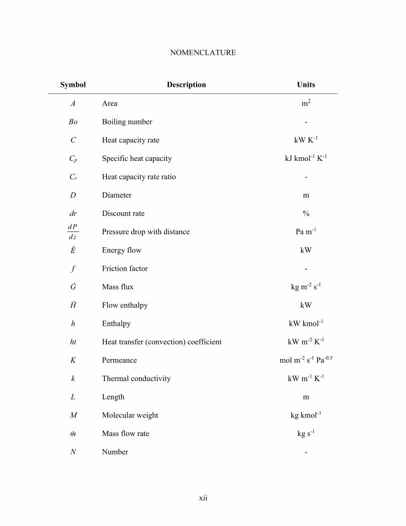
NOMENCLATURE

Symbol Description Units

A Area m2

Bo Boiling number -

C Heat capacity rate kW K-1

Cp Specific heat capacity kJ kmol-1 K-1

Cr Heat capacity rate ratio -

D Diameter m

dr Discount rate % d Pd z

Pressure drop with distance Pa m-1 �̇� Energy flow kW

f Friction factor -

Ġ Mass flux kg m-2 s-1

Ḣ Flow enthalpy kW

h Enthalpy kW kmol-1

ht Heat transfer (convection) coefficient kW m-2 K-1

K Permeance mol m-2 s-1 Pa-0.5

k Thermal conductivity kW m-1 K-1

L Length m

M Molecular weight kg kmol-1

ṁ Mass flow rate kg s-1

N Number -

xiii

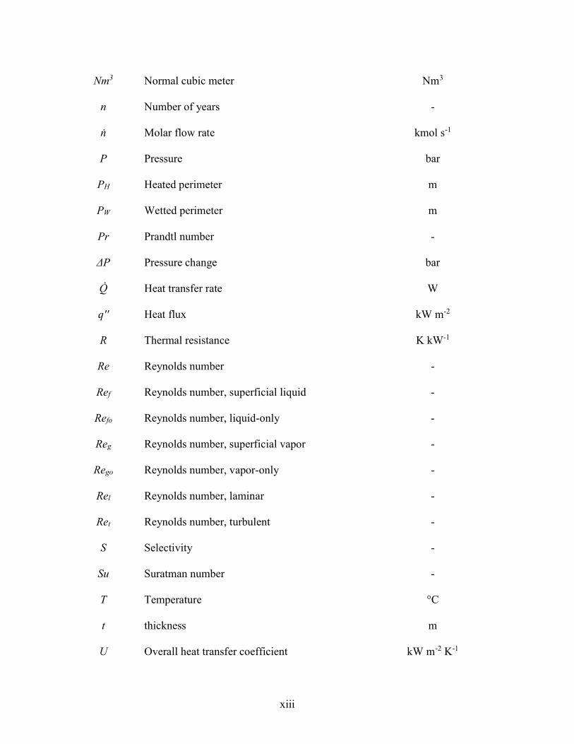
Nm3 Normal cubic meter Nm3

n Number of years -

ṅ Molar flow rate kmol s-1

P Pressure bar

PH Heated perimeter m

PW Wetted perimeter m

Pr Prandtl number -

ΔP Pressure change bar

Q̇ Heat transfer rate W

q'' Heat flux kW m-2

R Thermal resistance K kW-1

Re Reynolds number -

Ref Reynolds number, superficial liquid -

Refo Reynolds number, liquid-only -

Reg Reynolds number, superficial vapor -

Rego Reynolds number, vapor-only -

Rel Reynolds number, laminar -

Ret Reynolds number, turbulent -

S Selectivity -

Su Suratman number -

T Temperature °C

t thickness m

U Overall heat transfer coefficient kW m-2 K-1

xiv

u Velocity m s-1

UA Heat transfer conductance kW K-1

V Volumetric flow rate m3 s-1

Ẇ Work kW

We Weber number -

X Fluid quality -

XLM Lockhart-Martinelli parameter -

Xtt Turbulent-turbulent Martinelli parameter -

Y Mole fraction -

Greek Symbols

α Thermal diffusivity m2 s-1

ε Heat exchanger effectiveness -

η Efficiency -

μ Dynamic viscosity Pa s

ρ Density kg m-3

δ Surface roughness m

σ Surface tension N m-1

Two-phase multiplier -

Subscripts and Superscripts

act Actual -

adj Adjustment -

amb Ambient -

avail Available -

xv

avg Average -

boil Boiling -

boiler (Baseline) boiler system -

c Cross-sectional -

capt Capture -

CH4 Methane -

CO2 Carbon dioxide -

check Check (of original calculation) -

Churchill Churchill correlation -

cold Cold fluid -

comb Combustion -

comp Compressor -

cond Condenser -

conduc Conduction -

conv Conversion -

convec Convection -

cryo Cryogenic separation unit -

elec Electricity -

exh Exhaust -

export Export -

F Frictional -

f Formation -

Feed Feed -

xvi

fg Liquid to gas phase change -

fuel Fuel -

fluid Fluid -

gas Gas phase -

H Heated -

h Hydraulic -

HE Heat exchanger -

high High pressure (feed) side of membrane -

highP High pressure -

hot Hot fluid -

ht Heat transfer -

H2 Hydrogen -

H2O Water -

i Placeholder state number -

ij From gas i to gas j -

in In (to component) -

input Input -

known Known -

liq Liquid phase -

load Load -

low Low pressure (permeate) side of membrane -

max Maximum -

mem Membrane -

xvii

membrane Membrane only (not reactor) -

min Minimum -

NG Natural gas -

nb Non-boiling -

new New -

N2 Nitrogen -

o Reference conditions -

overall Overall -

O2 Oxygen -

out Out (to fluid) -

per Permeate -

preheat Preheating section -

pump Pump -

r Ratio -

reac Reaction -

reactor Reactor only (not membrane) -

ret Retentate -

ref Reference conditions (25°C, 1 bar) -

reform Reforming conditions -

retentate Retentate -

sat Saturation -

sens Sensible -

sep Separation -

xviii

shell Shell -

SMR Steam methane reformer system -

steam Steam -

steamGen Steam generation -

supply Supply -

system System -

total Total -

tube Tube -

wall Wall -

water Water -

1 One shell pass -

298K Referenced to 298 K -

ΔP Change in pressure -

* Modified -

Abbreviations

BCE Boiler combustion exhaust -

BS Boiler system -

BSC Boiler system with CO2 capture -

CapEx Capital expense k$

CAT Closest approach temperature °C

CCC Carbon capture and concentration -

cCO2 Compressed carbon dioxide -

CSU Cryogenic separation unit -

xix

DCR Discounted cost reduction k$

FV Future value k$

HE Heat exchanger -

HHV Higher heating value kJ kg-1

ICE Internal combustion engine -

ID Inner diameter m

k$ Thousand US Dollars k$

LHV Lower heating value kJ kg-1

M$ Million U.S. dollars -

MBtu Thousand Btu -

MMBtu Million Btu -

MR Membrane reactor -

NG Natural gas -

NPB Net present benefit k$

NPV Net present value k$

NTU Number of transfer units -

O&M Operating and maintenance (excluding commodity purchases and sales) k$

OD Outer diameter m

OpEx Operating expense $ yr-1

PV Present value k$

SC Steam to carbon ratio kmol kmol-1

scf Standard cubic feet (60°F, 1 atm) scf

SMR Steam methane reforming -

xx

SMR-MR-SG

Steam methane reforming in a membrane reactor steam generation system -

ton Short ton ton

Val Value -

WGS Water-gas shift -

1

Introduction 1.1. Background

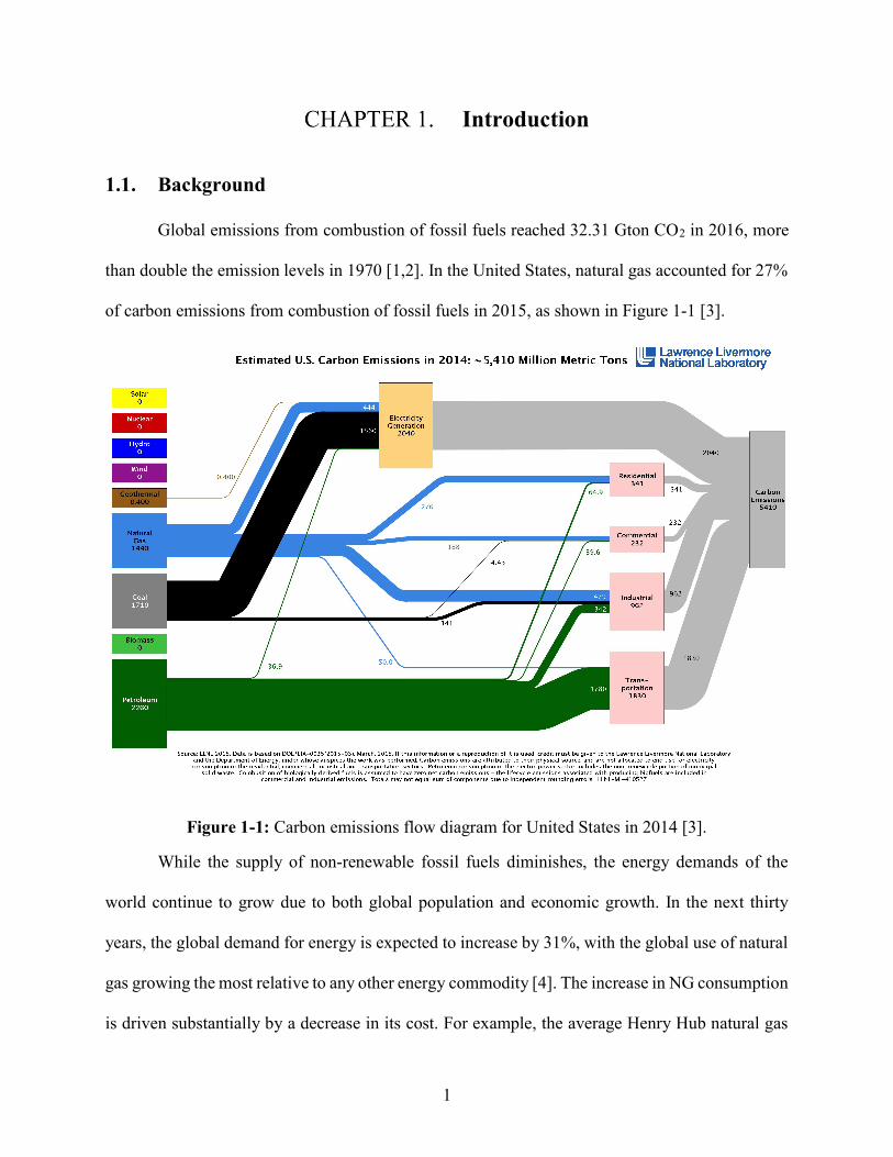
Global emissions from combustion of fossil fuels reached 32.31 Gton CO2 in 2016, more

than double the emission levels in 1970 [1,2]. In the United States, natural gas accounted for 27%

of carbon emissions from combustion of fossil fuels in 2015, as shown in Figure 1-1 [3].

Figure 1-1: Carbon emissions flow diagram for United States in 2014 [3].

While the supply of non-renewable fossil fuels diminishes, the energy demands of the

world continue to grow due to both global population and economic growth. In the next thirty

years, the global demand for energy is expected to increase by 31%, with the global use of natural

gas growing the most relative to any other energy commodity [4]. The increase in NG consumption

is driven substantially by a decrease in its cost. For example, the average Henry Hub natural gas

2

spot price in 2018 ($3.15 per MMBtu) is 36% of its average price in 2008 [5]. The realistic

medium-term solution is not to stop using natural gas, but to use it in a cleaner and more efficient

way. As regulations governing carbon emissions tighten [6], a significant and increasing tax will

be placed on industrial carbon emissions in the near future. The development of efficient natural

gas technology simultaneously decreases CO2 emissions and provides a financial advantage.

One interesting pathway for clean and efficient natural gas consumption is the production

of hydrogen. The use of hydrogen as a fuel for combustion is fundamentally clean with water as

the only product. Hydrogen can be used in many ways, including in fuel cells for power generation

or in electric vehicles [7]. However, hydrogen gas has low volumetric energy density and is

challenging to store and transport [8]. It is also difficult to use as a standalone fuel due to lack of

infrastructure and high cost [9].

A logical conclusion is to create hydrogen from natural gas. It takes advantage of the low

price and availability of natural gas. Production of hydrogen from natural gas allows existing

natural gas infrastructure to be used, which mitigates the need for new hydrogen infrastructure [9].

With hydrogen as a fuel, the usual emissions associated with natural gas are vastly reduced. The

next section discusses a technologically and economically realistic method for producing hydrogen

from natural gas.

1.2. Steam Methane Reforming

The most common method of hydrogen production in the United States today is natural gas

reforming, accounting for 95% of total hydrogen production [10]. A specialized subset of natural

gas reforming is steam methane reforming (SMR), which uses a more refined fuel that is composed

primarily or completely of methane. Although the details differ, the fundamental concepts of

3

natural gas reforming and steam methane reforming are the same. In the context of this study,

“natural gas reforming” and “steam methane reforming” will be used interchangeably.

Currently the SMR reaction takes place in a conventional reformer in which methane reacts

with high-temperature steam under very harsh operating conditions (800 - 1000°C and 1.5 - 2.0

MPa) to generate H2 [11]. In order to maximize the H2 yield, the intermediate product, CO, is later

introduced into two high and low temperature water-gas shift (HT-WGS and LT-WGS) reactors

[12,13]. The generated H2 is later separated and purified via various techniques such as pressure

swing adsorption (PSA), cryogenic distillation, physical scrubbing [14], or palladium (Pd)-based

membrane [7,8,15]. PSA, a highly energy-intensive process, is the most common method for H2

separation and purification in the industry [16,17].

In the SMR process, the steam and methane react over a catalyst, forming hydrogen and

carbon monoxide via Equation (1.1) [10,18]:

4 2 23 CH H O CO H (1.1)

It is important to note that Equation (1.1) is strongly endothermic, so a method for adding heat

during the reaction is essential. Following, or often simultaneously with, this reaction, the carbon

monoxide undergoes a water-gas shift reaction, converting carbon monoxide to carbon dioxide

and producing more hydrogen via Equation (1.2):

2 2 2 CO H O CO H (1.2)

Assuming both reactions go to completion in the forward direction, Equations (1.1) and (1.2) can

be condensed into Equation (1.3) [19]:

4 2 2 22 4 CH H O H CO (1.3)

Disadvantages of the current SMR process include harsh operating conditions, catalyst

deactivation due to coking, blockage of reformer tubes, and high pressure drop within the reactor.

4

High-temperature, expensive alloy reformer tubes and a complex PSA design contribute to high

capital and operational costs [13,17,20]. These drawbacks make the development of an alternative

method of H2 production via SMR a necessity.

Membrane reactor (MR) technology is an alternative method that can be used to perform

the SMR reaction at milder operating temperatures. MR combines the advantages of catalytic

reactors such as catalyst bed uniformity, and improved heat and mass transfer rates, with the

advantages of selective membranes to increase methane conversion and hydrogen recovery.

Specifically, by placing a metallic membrane inside the reactor, hydrogen is continuously removed

from the reaction zone (retentate side) through the membrane [21]. The continuous withdrawal of

H2 from the permeate side shifts the reaction equilibrium further toward production of hydrogen

according to Le Chatelier’s principle [22]. A membrane with infinite permeability toward H2 will

allow for a collection of a pure stream of H2 on the permeate side. Utilizing MR technology will

allow for production of H2 and capture of a highly concentrated CO2 stream in a single unit. As a

result, WGS reactors and H2 purification units will be eliminated. Furthermore, high conversion

values of methane to H2 can be achieved at temperatures (around 400°C) that are much lower than

the current industry values. Low operating temperatures result in lower energy intensity of the

SMR process and higher-grade alloy steels can be replaced with lower grade and less expensive

materials. MR technology will prevent coke formation and catalyst fouling in the reactor. Finally,

since the partial pressure of CO2 on the retentate side is much higher, more pure CO2 can be

captured with lower thermodynamic work [23].

Membranes used for H2 separation can be divided into four categories based on the

materials used in the fabrication of membranes: polymeric, metallic (dense and porous), carbon,

and ceramic. Polymeric membranes are considered organic while the other three categories are

5

inorganic membranes [24]. Dense metallic membranes are of special interest due to their capability

to produce pure H2 in one single separation step with low energy penalty [25]. Palladium-based

(Pd) metallic membranes are the best candidates for production of high purity hydrogen due to

their ‘infinite’ selectivity towards H2 permeation [26]. Pd-based separation and purification

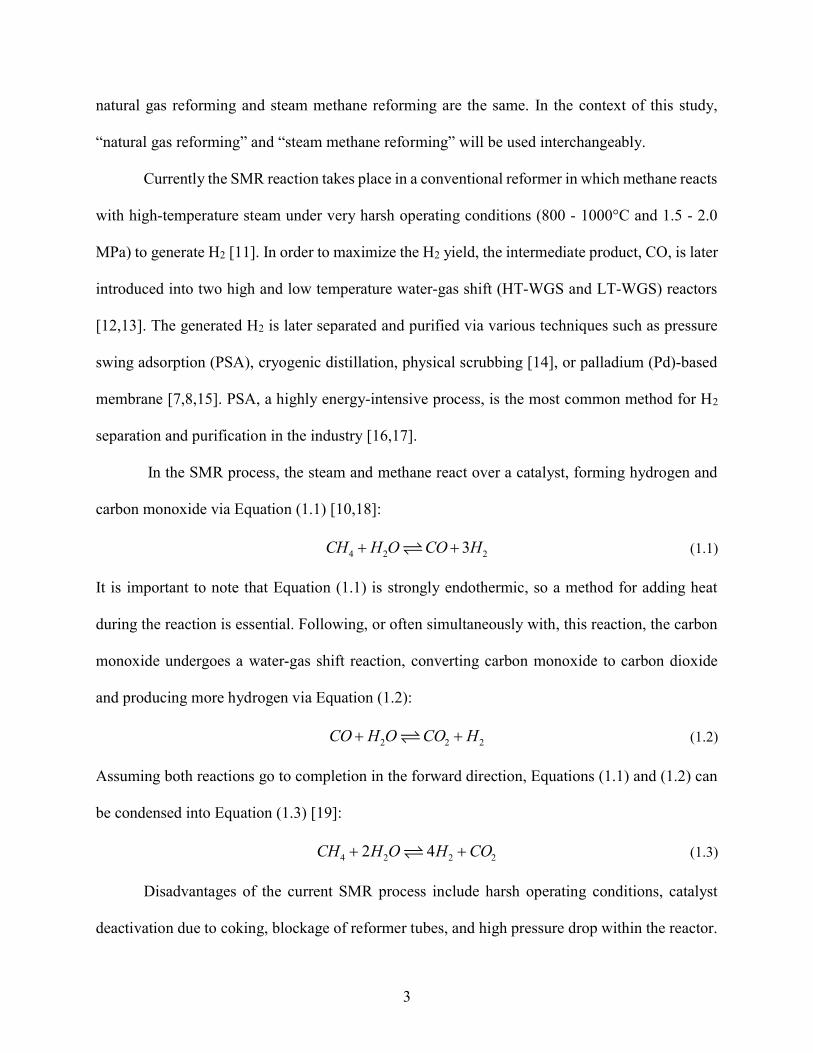
process can further be facilitated by using a sweep gas (Figure 1-2) [27–29].

Ideal products of SMR are just H2 and CO2. In reality, the reaction doesn’t reach

completion, so the products also contain CH4, H2O, and CO in addition to any impurities or higher

hydrocarbons in the fuel. The hydrogen is separated from the rest of the products through a

hydrogen-selective membrane. On the side of the membrane with the products (retentate), the

partial pressure of hydrogen is high relative to on the other (permeate) side of the membrane. The

pressure and concentration gradients force hydrogen through the membrane, creating a stream of

pure hydrogen on the permeate side. Figure 1-2 shows the ideal steam methane reforming process,

where ideal indicates the simple case of complete conversion of CH4 and perfect separation of H2.

Figure 1-2: Simplified process flow diagram of steam methane reforming.

Steam methane reforming is not the only way to create hydrogen. In general, hydrogen is

produced in two sub-processes: generation and separation [7]. One alternative method to SMR is

electrolysis of water, which is a simple yet power-intensive process that uses an electrical power

sources to generate hydrogen by separating water molecules. The produced hydrogen and oxygen

6

are separated by to their separate generation on the anode and cathode of the system, respectively.

After separation, another energy-intensive process is required in compression of the hydrogen gas.

Electrolysis is rarely used in industrial hydrogen generation due to its significantly higher cost

[30,31]. Coal gasification is another method of hydrogen production, where underground coal is

converted to syngas and then refined into pure hydrogen [32]. This method promises reduced

greenhouse gas emissions over traditional methane reforming, but still has significantly higher

emissions than the membrane reactor technology proposed in this study.

On the other end of the complexity spectrum are protonic membrane reactors (PMR).

PMRs are a specialized type of steam methane reformer which use a proton-conducting electrolyte

to function as both an electrode and reforming catalyst. Produced hydrogen is simultaneously

separated and compressed electrochemically through a nickel membrane. Protonic membrane

reactors show promise of nearly full methane conversion, simultaneous hydrogen compression,

and near zero net energy loss [33]. The downside is that they are significantly more complex and

expensive, and have not been proven outside of academic investigations [33,34].

Steam methane reforming also has its drawbacks. Hydrogen-selective membranes are most

often Palladium or Palladium alloys [7,8,15]. Even at typical membrane thicknesses of 10 to 50

µm, material cost of the Pd can be prohibitive [9,33,35]. Steam is often flowed on the permeate

side of the membrane to facilitate better permeation of hydrogen through the membrane [27–29].

This “sweep steam” adds complexity in that the hydrogen must then be separated from the sweep

steam and often compressed before use. For example, fuel cells require nearly perfectly dry

hydrogen for correct operation [36]. Steam methane reforming is used primarily for industrial

hydrogen production, which only takes advantage of only one of its several outputs. In the correct

7

application, compressed CO2, waste heat, and low-grade steam could also be used to increase

system efficiency and effectively reduce cost.

As with most competing technologies, all have their pros and cons. Steam methane

reforming is the most effective method for hydrogen production from natural gas. It is better than

any other method in energy efficiency, size, and cost [7,33]. It offers the opportunity to separate

CO2 in an integrated system, dramatically reducing carbon emissions. Even considering upstream

processes, hydrogen produced through SMR and used to power fuel cell electric vehicles cuts

greenhouse gas emissions and petroleum use by 50% and 90%, respectively [10]. Although steam

methane reforming uses only methane as its fuel source, many sources show the efficacy of other

fuels including natural gas of various compositions, methanol, ethanol, propane, and even gasoline

[7,8,10]. There are complications that arise from different fuels. For example, methanol and

ethanol used as fuel in membrane reforming can reverse the water gas shift reaction, reducing

system efficiency [37]. This study will focus only on natural gas as a reforming fuel. As mentioned

earlier, SMR is by far the most common industrial method for producing hydrogen from natural

gas [10,15]. This is tangible evidence that steam methane reforming with natural gas is the best

technology in this category.

Despite SMR’s ubiquitous application to hydrogen production, its application to other

areas in industry is somewhat limited. Hundreds of studies in the last decade have continued to

develop the state-of-the-art in membrane reformer technology. While there are many promising

results, the use of industrial SMR has remained more or less unchanged. There are several barriers

to the acceptance of this relatively new technology, including lack of a single study unifying all

desirable aspects of SMR and missing proof of additional, economically realistic, applications of

SMR.

8

An important distinction of this study is that it aims to go beyond theoretical modeling by

supplying an appropriate application of the proposed technology. In industry, new technology is

seldom introduced unless it can make a solid business case. In this context, the business case is

that (a) there is a logical application of SMR, and (b) SMR can be applied in a cost-effective way.

Steam methane reforming is already widely used in industry for hydrogen production. Several

authors, including this one, have investigated using SMR in power generation with gas turbines

and combined cycle plants [18,34,38,39]. After testing the waters with modeling in several fields

of industry, this study chose to focus on steam generation.

1.3. Application to Steam Generation

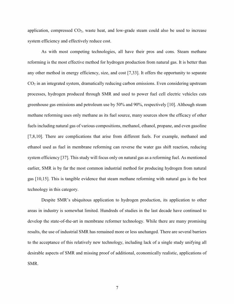
Steam generation relies heavily on natural gas as a fuel source. Energy and Environmental

Analysis, Inc (EEA) estimates that there are 163,000 industrial and commercial boilers in the U.S.

These boilers consume 8,100 TBtu per year, which equates to 40% of energy use in the industrial

and commercial sectors [40]. Combining the industrial and commercial sectors, Figure 1-3 shows

that roughly 73% of all boiler fuel comes from natural gas. This equates to 5,900 TBtu, or 5.69

Trillion cubic feet of natural gas per year [41]. To put this into perspective, the energy in natural

gas used just in U.S. steam boilers could supply about half of New York City’s electricity

continuously [42].

Clearly, the United States relies heavily on natural gas in steam generation. Recalling an

earlier conclusion, it is imperative to work towards using natural gas in a more clean and efficient

way. Steam generation provides an excellent application upon which to focus this effort. The sheer

volume of energy involved in steam generation throughout the country gives potential for

significant cost, energy, and emissions savings.

9

Figure 1-3: Industrial boiler quantity and boiler capacity by primary fuel [40].

Existing boiler technology is largely outdated: 76% of boilers currently operating in the

United States are at least 30 years old. Of those, even the largest scale industrial boilers achieve

only 80-86% efficiency [40]. It’s not surprising that boilers are not updated to a newer technology;

the design of boilers hasn’t changed significantly in the last 30 years, they work reliably, and it

would be expensive to replace them with a new technology. However, updating steam generation

technology could have profoundly positive consequences. Steam methane reforming provides a

realistic path to improving efficiency and reducing emissions associated with steam generation.

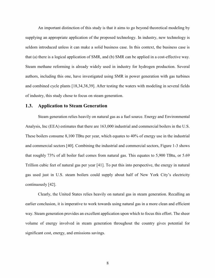
Steam generation is a large market. Approximately 7,200 industrial boilers are sold each

year in the United States, with an estimated total of 163,000 boilers currently in operation [40].

Figure 1-4 shows the size distribution of these boilers. Boilers in the 1 – 10 MMBtu h-1 account

10

for the largest number of boiler sales by far. The average unit size in that range is 3.5 MMBtu h-1;

this size will be the focus of this study.

Figure 1-4: Size distribution of industrial boilers sold between 1992 and 2002 [40].

There are many possible ways to improve upon the current steam generation process, but

steam methane reforming is the most effective. An important barrier to new energy technology is

the additional infrastructure required to support it. SMR allows for the benefits of clean-burning

hydrogen fuel without the need to move away from natural gas. At the same time, SMR mitigates

many of the potential problems of hydrogen fuel, chiefly transport and storage, by taking

advantage of the well-developed natural gas infrastructure.

11

1.4. Research Objectives

The goal of this study was to explore a new application of steam methane reforming: steam

generation. The process lends itself to steam generation: Figure 1-5 shows a simplified process

flow diagram for steam generation using SMR in a membrane reactor (SMR-MR-SG).

Figure 1-5: Simplified steam methane reformer process flow diagram with steam generation.

Note that the only two inputs are the same as for a traditional boiler: natural gas and water.

The largest difference is that, if the system is designed and executed correctly, the only outputs are

generated steam, cold nitrogen exhaust, and compressed CO2. The compressed CO2 can be sold or

used instead of rejected as emissions. In this configuration, there is also reduced water

consumption if the generated steam from H2 combustion is recycled back into the system. The

concept of recycling steam and water throughout the system will be discussed further in the

thermodynamic modeling sections.

The proposed system uses natural gas as a fuel as in conventional SMR, but the main

product of the system is steam rather than H2. Hydrogen is generated as an intermediate product

in the membrane reactor, then burned to generate steam without the carbon emissions associated

with conventional natural gas combustion. Based on the results of this investigation, the new

12

technology could be a direct replacement for industrial steam boilers, offering better efficiency,

lower cost, and reduced CO2 emissions.

This study developed a coupled thermodynamic and economic model in Engineering

Equation Solver (EES) to evaluate performance of the proposed system. The model was compared

to two other baseline technologies: a state-of-the-art industrial boiler system, and the same boiler

system with the addition of CO2 capture. Results of the proposed system were compared to the

two baselines on a thermodynamic and economic basis

1.5. Thesis Organization

The remainder of this thesis expands on the concept of a steam methane reformer system

in an industrial context. Chapter 2 provides a detailed review of the current literature, addressing

state-of-the-art reforming technology and the suitability of steam generation as an application.

Chapter 3 dives into the development of a thermodynamic and coupled technoeconomic model.

Chapter 4 discusses the results of modeling and the highlights of the study. Finally, Chapter 5

summarizes the main points of the study and provides recommendations for future work.

Appendix A contains representative calculations which help to prove the results of the

model reasonable. The calculations also served as a careful check to catch typos or other errors in

the modelling program. Appendix B contains detailed calculations for sizing heat exchangers. This

was necessary to determine the cost of heat exchangers in the technoeconomic analysis, but was

moved to an appendix to avoid distracting the reader from the system-level analysis.

13

Literature Review

This study will focus on a practical application of steam methane reforming to industrial

steam generation. Steam methane reforming is a technique to produce hydrogen from natural gas.

There are other methods to produce hydrogen from natural gas, but SMR has been shown to be

superior due to ultra-high efficiency and potential for carbon capture. Although SMRs produce

hydrogen from natural gas (or methane), they can vary widely in the process, effectiveness, and

additional features of the system. The following will explain several details of steam methane

reforming, including their desirability and consequences. Next, the metrics of comparison in this

study will be discussed. Following the overview, a literature review will be presented to establish

what is known and what this study has to offer.

At its most basic, steam methane reforming converts methane into hydrogen according to

the net reaction given by Equation (2.1):

4 2 2 22 4 CH H O H CO (2.1)

Methane conversion is defined as the percentage of methane that is converted to hydrogen.

Methane conversion is defined in Equation (2.2):

4

4

4

CH ,retCH ,conv

CH ,feed

1

nn

(2.2)

The ideal methane conversion is 100%, where there is no methane left in the retentate. Hydrogen

recovery is defined by Equation (2.3) as the ratio of permeated hydrogen to available hydrogen on

the feed side:

2

2

2

H ,perH ,capt

H ,avail

nn

(2.3)

14

It is important to note that methane conversion and hydrogen recovery are not directly linked. For

example, with perfect (100%) methane conversion, it is possible that all, none, or any amount of

the hydrogen permeates through the membrane. Any produced hydrogen that does not permeate

through the membrane exits the reactor in the retentate stream.

Steam methane reforming requires several processes at minimum: two chemical reactions

(reforming and water-gas shift), heat transfer to support the highly endothermic reforming

reaction, and separation of hydrogen from the retentate to the permeate stream. These processes

may be carried out in separate steps or in parallel. This study defines an integrated membrane

reactor as one where all three processes (two reactions, heat transfer, and hydrogen) are achieved

in a single step and single physical device. There are many benefits of using a membrane reactor

over conventional steam methane reforming such as a lower reforming temperature and a less

complicated system.

Waste heat recovery is a broad term because it can vary depending on the application. In

this thesis, it refers to capturing the sensible energy from the retentate, permeate, and heating

streams coming out of the membrane reactor. CO2 separation is defined as the separation of CO2

from the rest of the retentate stream. This may be accomplished cryogenically, via compression,

or by other methods. In reality, SMRs don’t achieve perfect methane conversion or hydrogen

recovery. Therefore, it makes sense to mix the retentate stream back into the feed. In most

instances, the retentate stream contains CH4, H2, CO2, CO, and H2O (assuming imperfect water

and CO2 separation/condensation as well). This is referred to in this study as gas recycling.

The essence of this study is a comparison between steam methane reforming and other

steam generation technologies. The comparison will be quantified both thermodynamically and

economically. Thermodynamic metrics of comparison include amount of waste heat, fuel

15

consumption, and overall system efficiency. Economic metrics include capital cost, total cost of

ownership, and payback period. To achieve a fair comparison, the systems will be set at the same

scale with the same net output.

The remainder of this chapter will describe and compare literature relevant to state-of-the-

art steam methane reformer technology and competitive steam generation technology. The

literature will help guide and give context for the modeling approach, and discussion of SMR

technologies as applied to steam generation. This review will highlight the gaps in current research,

showcase the importance of filling those gaps, and explain how this study will round out the

knowledge in this field.

2.1. State-of-the-Art Steam Methane Reforming

2.1.1. Membrane Reactors

In conventional steam methane reforming, methane reacts with high-temperature steam

under very harsh operating conditions (800 - 1000°C and 15 - 20 bar) to generate H2 in the

reforming reaction given by Equation (3.24) [18]:

04 2 2 298K3 206 / CH H O CO H H kJ mol (2.4)

To maximize the H2 yield, the intermediate product, CO, is later introduced into two high and low

temperature water-gas shift (WGS) reactors [12,13] which perform the reaction of Equation (3.25)

[18]:

02 2 2 298K 41 / CO H O CO H H kJ mol (2.5)

These two reactions can be combined into an overall reaction, The overall SMR reaction that

includes WGS is given by Equation (3.26) [18,19]:

04 2 2 2 298K2 4 165 / CH H O H CO H kJ mol (2.6)

16

The generated H2 is later separated and purified via various techniques such as pressure swing

adsorption (PSA), cryogenic distillation, physical scrubbing [14], or a palladium (Pd)-based

membrane [7,8,15]. PSA, a highly energy-intensive process, is the most common method for H2

separation and purification in the industry [16,17].

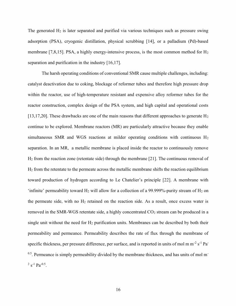
The harsh operating conditions of conventional SMR cause multiple challenges, including:

catalyst deactivation due to coking, blockage of reformer tubes and therefore high pressure drop

within the reactor, use of high-temperature resistant and expensive alloy reformer tubes for the

reactor construction, complex design of the PSA system, and high capital and operational costs

[13,17,20]. These drawbacks are one of the main reasons that different approaches to generate H2

continue to be explored. Membrane reactors (MR) are particularly attractive because they enable

simultaneous SMR and WGS reactions at milder operating conditions with continuous H2

separation. In an MR, a metallic membrane is placed inside the reactor to continuously remove

H2 from the reaction zone (retentate side) through the membrane [21]. The continuous removal of

H2 from the retentate to the permeate across the metallic membrane shifts the reaction equilibrium

toward production of hydrogen according to Le Chatelier’s principle [22]. A membrane with

‘infinite’ permeability toward H2 will allow for a collection of a 99.999%-purity stream of H2 on

the permeate side, with no H2 retained on the reaction side. As a result, once excess water is

removed in the SMR-WGS retentate side, a highly concentrated CO2 stream can be produced in a

single unit without the need for H2 purification units. Membranes can be described by both their

permeability and permeance. Permeability describes the rate of flux through the membrane of

specific thickness, per pressure difference, per surface, and is reported in units of mol m m-2 s-1 Pa-

0.5. Permeance is simply permeability divided by the membrane thickness, and has units of mol m-

2 s-1 Pa-0.5.

17

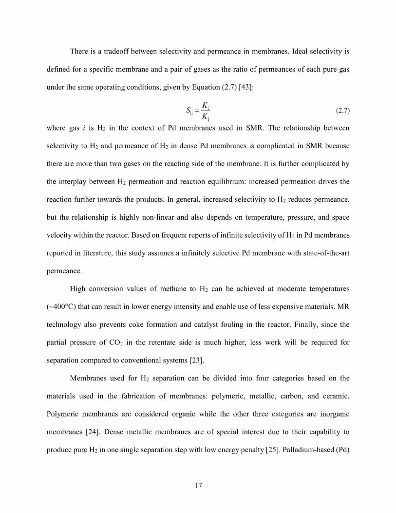
There is a tradeoff between selectivity and permeance in membranes. Ideal selectivity is

defined for a specific membrane and a pair of gases as the ratio of permeances of each pure gas

under the same operating conditions, given by Equation (2.7) [43]:

iij

j

KSK

(2.7)

where gas i is H2 in the context of Pd membranes used in SMR. The relationship between

selectivity to H2 and permeance of H2 in dense Pd membranes is complicated in SMR because

there are more than two gases on the reacting side of the membrane. It is further complicated by

the interplay between H2 permeation and reaction equilibrium: increased permeation drives the

reaction further towards the products. In general, increased selectivity to H2 reduces permeance,

but the relationship is highly non-linear and also depends on temperature, pressure, and space

velocity within the reactor. Based on frequent reports of infinite selectivity of H2 in Pd membranes

reported in literature, this study assumes a infinitely selective Pd membrane with state-of-the-art

permeance.

High conversion values of methane to H2 can be achieved at moderate temperatures

(~400°C) that can result in lower energy intensity and enable use of less expensive materials. MR

technology also prevents coke formation and catalyst fouling in the reactor. Finally, since the

partial pressure of CO2 in the retentate side is much higher, less work will be required for

separation compared to conventional systems [23].

Membranes used for H2 separation can be divided into four categories based on the

materials used in the fabrication of membranes: polymeric, metallic, carbon, and ceramic.

Polymeric membranes are considered organic while the other three categories are inorganic

membranes [24]. Dense metallic membranes are of special interest due to their capability to

produce pure H2 in one single separation step with low energy penalty [25]. Palladium-based (Pd)

18

metallic membranes are the best candidates for production of high purity hydrogen due to their

‘infinite’ selectivity towards H2 permeation [26]. The Pd-based separation and purification process

can further be facilitated by using a sweep gas [27–29].

Due to the presence of the membrane, the generated H2 is continually separated and

transported to the permeate side. As a result, excess steam in the retentate is used to facilitate the

water-gas shift reaction (Equation (2.5)) to generate additional H2 that permeates through the

membrane. The net reaction (Equation (2.6)) yields concentrated CO2 in the retentate, which can

be readily captured through removal of excess H2O.

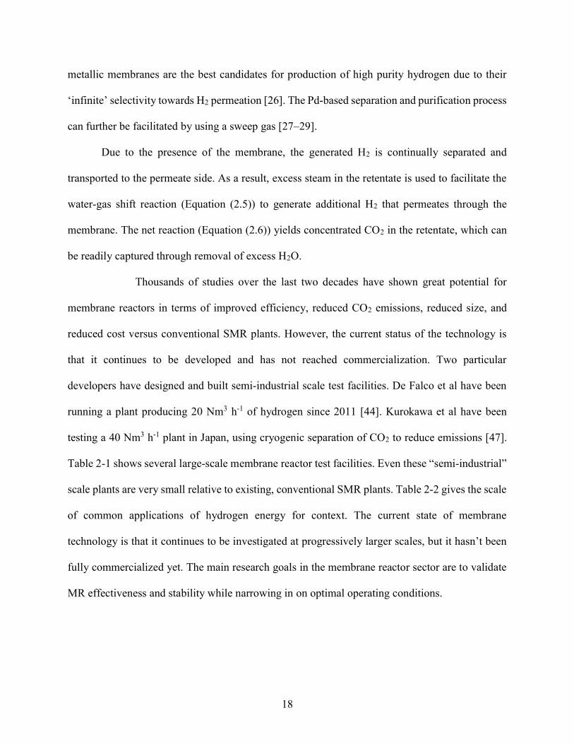
Thousands of studies over the last two decades have shown great potential for

membrane reactors in terms of improved efficiency, reduced CO2 emissions, reduced size, and

reduced cost versus conventional SMR plants. However, the current status of the technology is

that it continues to be developed and has not reached commercialization. Two particular

developers have designed and built semi-industrial scale test facilities. De Falco et al have been

running a plant producing 20 Nm3 h-1 of hydrogen since 2011 [44]. Kurokawa et al have been

testing a 40 Nm3 h-1 plant in Japan, using cryogenic separation of CO2 to reduce emissions [47].

Table 2-1 shows several large-scale membrane reactor test facilities. Even these “semi-industrial”

scale plants are very small relative to existing, conventional SMR plants. Table 2-2 gives the scale

of common applications of hydrogen energy for context. The current state of membrane

technology is that it continues to be investigated at progressively larger scales, but it hasn’t been

fully commercialized yet. The main research goals in the membrane reactor sector are to validate

MR effectiveness and stability while narrowing in on optimal operating conditions.

19

Table 2-1: Large-scale membrane reactor plants.

Developer Location

Membrane Thickness

[µm]

Scale

Novelty

Surface Area [m2]

Hydrogen Production [Nm3 h-1]

Kurokawa et al. a Japan N/A N/A 40 Large scale

De Falco et al. b Italy 3 – 25

0.13 – 0.6 20 Large scale, operation >10 yr

ECN b The Netherlands 3 – 9 0.4 N/A Alumina support

MRT b Canada 8 - 15 0.6 N/A Rolled foil or deposited film membranes

JC b Japan N/A 0.00283 N/A Al2O3 support

SINTEF b Norway 2 – 3 N/A N/A Macroporous substrate support

ACKTAR b Israel 3 – 5 N/A N/A Steel substrate support a Kurokawa et al. [47] b De Falco et al. [44]

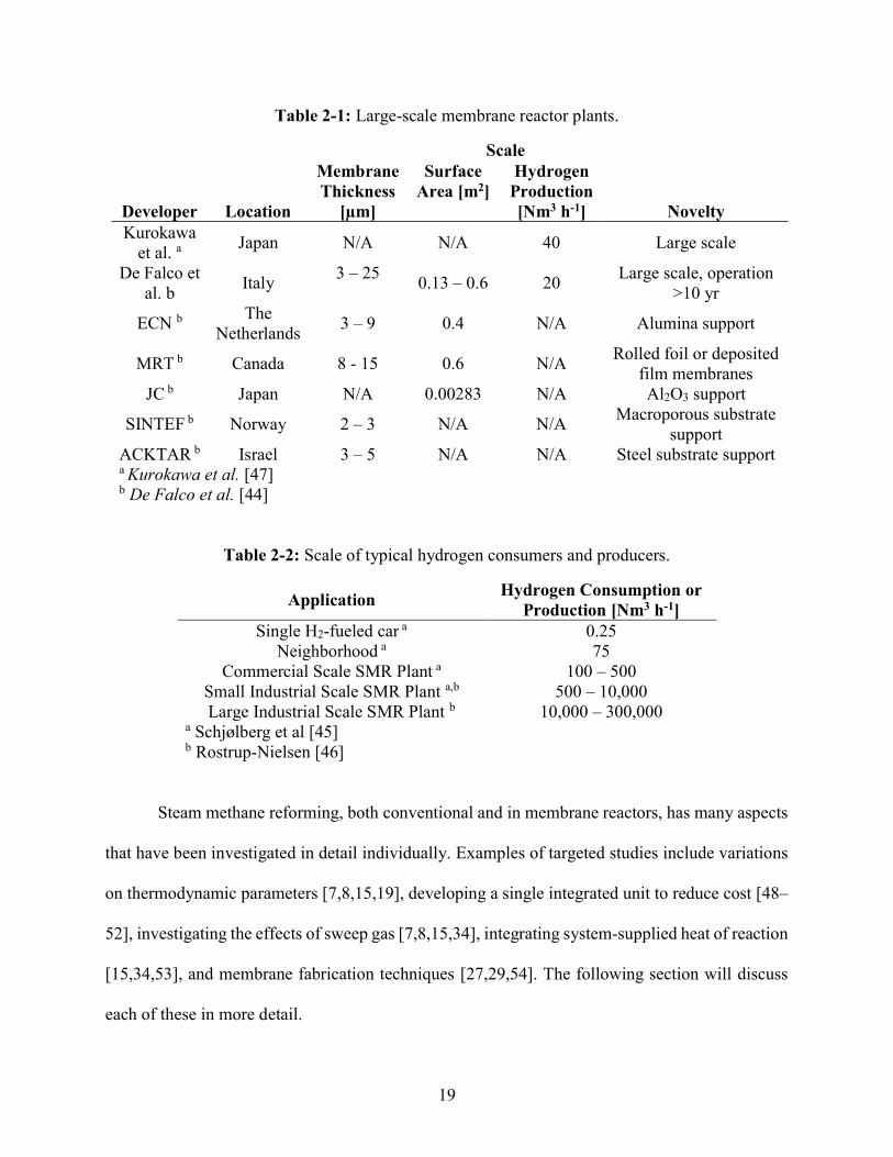
Table 2-2: Scale of typical hydrogen consumers and producers.

Application Hydrogen Consumption or Production [Nm3 h-1]

Single H2-fueled car a 0.25 Neighborhood a 75

Commercial Scale SMR Plant a 100 – 500 Small Industrial Scale SMR Plant a,b 500 – 10,000 Large Industrial Scale SMR Plant b 10,000 – 300,000

a Schjølberg et al [45] b Rostrup-Nielsen [46]

Steam methane reforming, both conventional and in membrane reactors, has many aspects

that have been investigated in detail individually. Examples of targeted studies include variations

on thermodynamic parameters [7,8,15,19], developing a single integrated unit to reduce cost [48–

52], investigating the effects of sweep gas [7,8,15,34], integrating system-supplied heat of reaction

[15,34,53], and membrane fabrication techniques [27,29,54]. The following section will discuss

each of these in more detail.

20

2.1.2. Aspects of Steam Methane Reforming

Conventional steam methane reforming has been studied in-depth many times. It is a common

technology used for industrial hydrogen generation, typically in a tubular reforming plant [55].

Membrane reactors are a subset of SMR, and as such share many aspects including methane

conversion, CO2 capture, and heat transfer during reforming. On the other hand, some aspects such

as sweep gas and hydrogen capture through a membrane are unique to membrane reactors. This

section will survey recent literature to ascertain the state-of-the-art in membrane reactor

technology and discover which questions still need to be answered.

The basic concept of steam methane reforming has been modeled thoroughly and with

many variations [7,8,15,19]. However, experimental validation is much less common. Membrane

reactors are not convenient nor easy to set up for experiments. The membranes are typically

palladium or palladium alloys that are expensive and challenging to fabricate [7,36,39]. The

systems consume and produce explosive gases at high pressures and temperatures leading to safety

concerns. Furthermore, realistic applications of SMR require industrial scale implementation;

scaling down to a laboratory experiment is difficult and can yield significantly different results.

There are some particular areas within steam methane reforming that lack experimental validation

including heat supply in a membrane reactor, heat recovery, and CO2 capture.

As previously discussed, steam methane reforming requires a net endothermic reaction and

subsequently a continuous heat addition to supply the heat of reaction. This is critical to a high

performance system, as higher reaction temperatures are generally correlated to higher conversion

rates of methane [34]. The logistics of supplying heat are overlooked in many papers. Membrane

reactors with integrated heat exchange have advantages in simplicity and cost over systems with

an external heater or combustor [15,34,53]. The common practice in industrial hydrogen

21

production is for an external furnace to the heat of reaction [53]. In the integrated reactor approach,

methane conversion, hydrogen recovery, and heat transfer to support reforming all occur

simultaneously in a single reactor module. This paper refers to an integrated reactor as a

“membrane reactor”, as opposed to a “membrane reformer”.

Membrane reactors have more benefits besides supplying heat. They combine the

reforming reaction (including the water-gas shift) and hydrogen separation into one volumetrically

compact unit [48]. Integration the reforming reaction and separation of produced hydrogen has

been shown to reduce capital cost [49]. Additionally, membrane reactors reduce capital cost

compared to a conventional reformer and non-membrane separator because the reactors don’t

require a pressure-swing adsorption system to separate hydrogen [50].

Another important facet of steam methane reforming is waste heat recovery. SMR lends

itself to recovering waste heat; the outlet streams besides the desired hydrogen permeate are

typically at high temperature and pressure. In addition to recovering the enthalpy of outlet streams,

the fluid composition often carries energy. The permeate in particular can contain significant

amounts of unburned natural gas [56–58]. This leftover natural gas can be burned to produce heat

and remove it from the stream so that carbon dioxide may be separated more easily. Two useful

places to use recovered waste heat are in the reactor itself to help supply the heat of reaction and

in steam generation for both the reaction and sweep gas.

Another method for recovering energy from the retentate stream is to recycle the “leftover”

gas into the feed. In a real-life implementation, imperfect methane conversion, hydrogen

separation, and carbon dioxide sequestration leave those three gases left in the retentate stream.

Instead of exhausting those net products, gas recycling creates a closed loop for methane,

hydrogen, and carbon dioxide in the system. This ensures that there is no exhaust from the system

22

other than generated steam; everything else is simply recycled back to the feed side of the reactor

for a second pass.

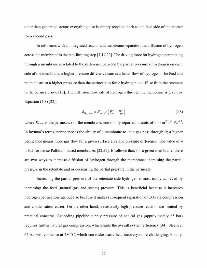
In reformers with an integrated reactor and membrane separator, the diffusion of hydrogen

across the membrane is the rate-limiting step [7,19,22]. The driving force for hydrogen permeating

through a membrane is related to the difference between the partial pressure of hydrogen on each

side of the membrane; a higher pressure difference causes a faster flow of hydrogen. The feed and

retentate are at a higher pressure than the permeate to force hydrogen to diffuse from the retentate

to the permeate side [18]. The diffusion flow rate of hydrogen through the membrane is given by

Equation (2.8) [22]:

2H ,mem mem ret per n nn K A P P (2.8)

where Kmem is the permeance of the membrane, commonly reported in units of mol m-2 s-1 Pa-0.5.

In layman’s terms, permeance is the ability of a membrane to let a gas pass through it; a higher

permeance means more gas flow for a given surface area and pressure difference. The value of n

is 0.5 for dense Pallidum based membranes [22,59]. It follows that, for a given membrane, there

are two ways to increase diffusion of hydrogen through the membrane: increasing the partial

pressure in the retentate and or decreasing the partial pressure in the permeate.

Increasing the partial pressure of the retentate-side hydrogen is most easily achieved by

increasing the feed (natural gas and steam) pressure. This is beneficial because it increases

hydrogen permeation rate but also because it makes subsequent separation of CO2 via compression

and condensation easier. On the other hand, excessively high-pressure reactors are limited by

practical concerns. Exceeding pipeline supply pressure of natural gas (approximately 65 bar)

requires further natural gas compression, which hurts the overall system efficiency [34]. Steam at

65 bar will condense at 280°C, which can make waste heat recovery more challenging. Finally,

23

high pressure requires stronger materials. With expensive palladium alloy membranes in the 1-10

µm thickness range, membrane failure due to high pressure is a real concern. On the other hand, a

higher feed pressure allows a higher permeate pressure, which reduces the high energy penalty of

compressing hydrogen after separation if needed [53]. The conclusion is that there is an optimal

range of pressures for the feed side to balance the benefits with the additional cost and complexity.

Manzolini et al. suggest an optimized cost near natural gas pipeline pressure [34].

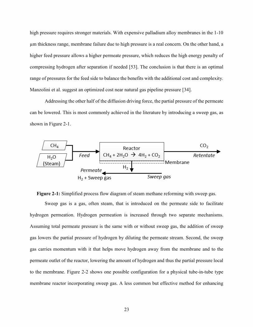
Addressing the other half of the diffusion driving force, the partial pressure of the permeate

can be lowered. This is most commonly achieved in the literature by introducing a sweep gas, as

shown in Figure 2-1.

Figure 2-1: Simplified process flow diagram of steam methane reforming with sweep gas.

Sweep gas is a gas, often steam, that is introduced on the permeate side to facilitate

hydrogen permeation. Hydrogen permeation is increased through two separate mechanisms.

Assuming total permeate pressure is the same with or without sweep gas, the addition of sweep

gas lowers the partial pressure of hydrogen by diluting the permeate stream. Second, the sweep

gas carries momentum with it that helps move hydrogen away from the membrane and to the

permeate outlet of the reactor, lowering the amount of hydrogen and thus the partial pressure local

to the membrane. Figure 2-2 shows one possible configuration for a physical tube-in-tube type

membrane reactor incorporating sweep gas. A less common but effective method for enhancing

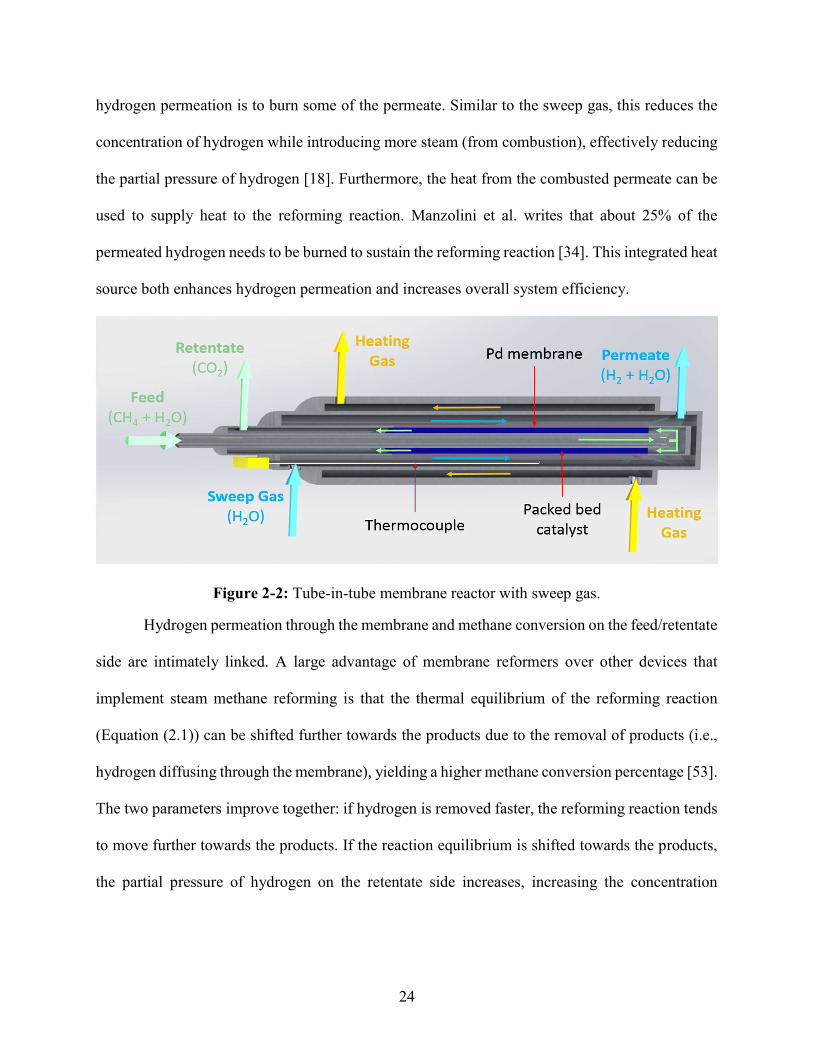
24

hydrogen permeation is to burn some of the permeate. Similar to the sweep gas, this reduces the

concentration of hydrogen while introducing more steam (from combustion), effectively reducing

the partial pressure of hydrogen [18]. Furthermore, the heat from the combusted permeate can be

used to supply heat to the reforming reaction. Manzolini et al. writes that about 25% of the

permeated hydrogen needs to be burned to sustain the reforming reaction [34]. This integrated heat

source both enhances hydrogen permeation and increases overall system efficiency.

Figure 2-2: Tube-in-tube membrane reactor with sweep gas.

Hydrogen permeation through the membrane and methane conversion on the feed/retentate

side are intimately linked. A large advantage of membrane reformers over other devices that

implement steam methane reforming is that the thermal equilibrium of the reforming reaction

(Equation (2.1)) can be shifted further towards the products due to the removal of products (i.e.,

hydrogen diffusing through the membrane), yielding a higher methane conversion percentage [53].

The two parameters improve together: if hydrogen is removed faster, the reforming reaction tends

to move further towards the products. If the reaction equilibrium is shifted towards the products,

the partial pressure of hydrogen on the retentate side increases, increasing the concentration

25

gradient and driving force for hydrogen diffusion through the membrane. This effect has been

modeled and validated thoroughly in literature [7,8,15,34].

A more straight-forward method of improving methane conversion and hydrogen recovery

is to reduce the thickness of the membrane. Recalling Equation (2.8), the flow rate of hydrogen

through the membrane is inversely proportional to its thickness. An additional benefit is financial;

the cost of membranes is driven by the material cost of precious metals (Pd, Au, Ag), so using less

material reduces membrane capital cost. State-of-the-art membranes are palladium alloys with

thicknesses under 3µm thickness [60,61]. There is a need for mechanical strength to support the

pressure difference between the feed and permeate sides, which can be over 100 bar difference.

Membranes are often deposited on a porous, ceramic or metallic substrate to provide mechanical

support. An ideal membrane support offers no resistance to hydrogen (or other gas) permeation.

The membrane may be attached or deposited on the support material by several methods including

electroless plating [27,29,54].

2.1.3. CO2 Capture

Transitioning from methods to increase conversion and permeation efficiencies, carbon

dioxide separation and storage is a key component of most SMR systems. Carbon dioxide is

present in the retentate stream in a significant concentration, along with H2O, H2, and CH4. This

assumes that the water-gas shift has converted all of the CO and that pure methane (as opposed to

natural gas) is used as a fuel. The concentration of carbon dioxide in the retentate (after hydrogen

separation) is typically above 30% by mole. If the products were perfectly separated, the H2O

would be recycled, CO2 compressed and stored, CH4 recycled into the feed, and H2 either recycled

to the feed or burned to produce heat. There are three popular methods of separating CO2 from the

retentate stream.

26

The first method of separating CO2 is by introducing air or oxygen into the retentate stream

and combusting it. This eliminates the CH4 and H2, producing more steam and CO2 [18,34]. The

steam can easily be then be condensed out by cooling, leaving only CO2 gas. Depending on the

retentate pressure, the CO2 can then be compressed, creating a high purity, compressed CO2 stream

for storage [34]. The second method is to liquefy the CO2. The water is first condensed out of the

other gases, which can be done easily and effectively by dropping the temperature while holding

temperature constant. Then, additional cooling and or compression liquefies the CO2, which can

be separated from the remaining CH4 and H2. The heat duty of water and CO2 cooling can be

recovered in a heat exchanger to increase the overall system efficiency. The third method of

separating CO2 is to pass it through a CO2-selective membrane [8]. This method is simple and

passive, but does not achieve as high separation percentages as the first two.

Particularly in steam methane reforming systems with high feed and retentate pressures,

carbon dioxide sequestration can be accomplished with little economic or thermodynamic penalty

relative to other carbon-free technology [53]. CO2 capture and hydrogen separation can be

combined into one integrated reactor to mitigate the need for additional equipment or size [51,52].

Carbon capture ratios up to 100% have been modeled and validated [34]. Carbon dioxide

sequestration is important, as SMR is branded as a “clean” technology of the future. The strategies

for CO2 sequestration discussed here have been proven to be effective with an overall system

efficiency loss of less than 1 percentage point [22].

2.1.4. Summary

Section 2.1 has discussed the state-of-the-art in steam methane reforming. The technology

is relatively new but has been investigated in detail in the literature. Reactors have been developed

with integrated thermal management to supply heat for the reforming reaction. Methods of waste

27

heat recovery and gas recycling have been modeled, optimized, and validated. There are many

ways to increase methane conversion and hydrogen recovery, most of them with tradeoffs in cost

and complexity. The details and methods of carbon dioxide sequestration have been analyzed and

compared.

The next section will investigate commercial and industrial applications of steam methane

reforming. It will address both existing and proposed technologies, evaluating the feasibility of

each. Then, steam generation will be introduced as a proposed application of steam methane

reforming that optimizes its thermodynamic and economic potential.

2.2. Steam Methane Reforming Applications

While steam methane reforming has been studied extensively, it has been limited in number of

practical applications. The only significant industrial or commercial practice of steam methane

reforming is in plant-scale hydrogen production. Although SMR has the capability of capturing

CO2, SMR used for hydrogen production is usually associated with greenhouse gas emissions due

to insufficient CO2 capture [62]. Academic studies have investigated SMR’s use in electricity

generation via several methods. It has also explored on-board (small scale, mobile system)

hydrogen production for automotive applications, but none of these have implanted at scale beyond

academia. This section will cover commercial, industrial, and academic applications of steam

methane reforming, then compare them to a proposed new application: steam generation via SMR.

Hydrogen production via steam methane reforming is a tried and true process. It works

well thermodynamically and is cost effective. However, it only utilizes part of potential of SMR.

The main product of steam methane reforming is high purity hydrogen, but there are other products

as well. Compressed, high purity CO2 is a common byproduct. It is valuable to capture CO2 instead

of releasing it to the environment as exhaust, but even more value can be derived from selling it

28

or using it directly. Steam is an integral part of the SMR process. In certain configurations, a system

can produce net steam by generating more water than it consumes. Again, heat can be recovered

and the water can be recycled, but it would be more beneficial to choose an application where

steam is desired. Hydrogen is usually carried by a sweep gas, which is often steam. The hydrogen

can be separated and compressed for the end goal of hydrogen production, but there are other

pathways with more direct use of the fluid streams and less thermodynamic losses. Steam methane

reforming is a promising technology but is not currently being utilized to its fullest potential.

One potential application for steam methane reforming is electricity production. For an

apples to apples comparison, SMR should be compared to other electricity generation technologies

that don’t exhaust carbon dioxide: solar electric, wind turbines, hydroelectric, etc. There are

limitless variations of process flows to incorporate SMR and electricity generation This review

will focus on the two most common in literature: hydrogen turbines and fuel cells.

On a fundamental level, most studies involving SMR and hydrogen turbines consist of a

few main components: a membrane reformer (converts NG to H2), turbine (converts H2 to shaft

work and heat), waste heat recovery (moves heat from turbine exhaust to steam and NG heating),

and a condenser (separates out water and CO2). A conceptual process flow for such a system is

shown in Figure 2-3.

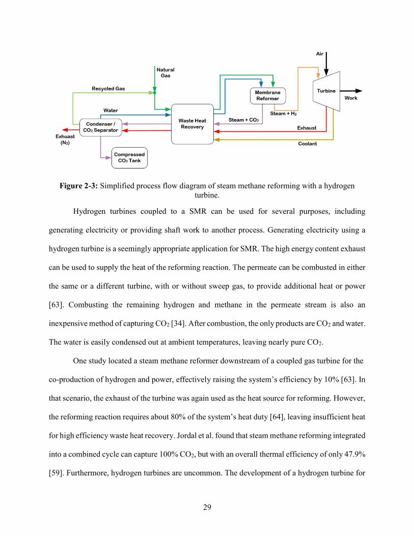
29

Figure 2-3: Simplified process flow diagram of steam methane reforming with a hydrogen turbine.

Hydrogen turbines coupled to a SMR can be used for several purposes, including

generating electricity or providing shaft work to another process. Generating electricity using a

hydrogen turbine is a seemingly appropriate application for SMR. The high energy content exhaust

can be used to supply the heat of the reforming reaction. The permeate can be combusted in either

the same or a different turbine, with or without sweep gas, to provide additional heat or power

[63]. Combusting the remaining hydrogen and methane in the permeate stream is also an

inexpensive method of capturing CO2 [34]. After combustion, the only products are CO2 and water.

The water is easily condensed out at ambient temperatures, leaving nearly pure CO2.

One study located a steam methane reformer downstream of a coupled gas turbine for the

co-production of hydrogen and power, effectively raising the system’s efficiency by 10% [63]. In

that scenario, the exhaust of the turbine was again used as the heat source for reforming. However,

the reforming reaction requires about 80% of the system’s heat duty [64], leaving insufficient heat

for high efficiency waste heat recovery. Jordal et al. found that steam methane reforming integrated

into a combined cycle can capture 100% CO2, but with an overall thermal efficiency of only 47.9%

[59]. Furthermore, hydrogen turbines are uncommon. The development of a hydrogen turbine for

30

this specific application would be prohibitively expensive [63]. One study of electricity generation

via SMR showed that it resulted in a 30% increase in the price of electricity compared to a

conventional natural gas combined cycle without CO2 capture [34]. This result is not used as a

direct comparison but rather to show that SMR implemented in electricity generation significantly

increases the operating costs. Another possible application of SMR is coupled to fuel cells.

As “clean” technologies such as fuel cells evolve, the demand for clean vehicle fuels

increases. Hydrogen is an attractive fuel, either used directly for combustion or for electricity

generation. For example, a fuel cell vehicles running on hydrogen can be 3 times more efficient

than an internal combustion engine vehicle with only water vapor as exhaust [22]. The demand for

hydrogen as a potential alternative automotive fuel is constantly increasing [65]. Specifically,

Sanusi et al. predict that demand for hydrogen in the transportation sector could reach 275 million

ton per year by 2050 [62].

The largest problem with hydrogen as a fuel is the transport and storage of the volatile and

non-dense fuel. On-board hydrogen production via steam methane reforming has been proposed

as a solution [9]. An on-board reformer would provide a compact and efficient hydrogen source

relative to hydrogen storage or a separate reactor and membrane separator [7]. A coupled SMR

and fuel cell would work well together: fuel cells require the near-pure hydrogen that can be

achieved through Pd-alloy membrane separation [8]. Small scale membrane reactors have even

been proposed as a means of reducing fuel cost [53]. One study modeled a steam methane reformer

with CO2 capture, potentially producing hydrogen as low as $30 per GJ [62]. For reference, a

consumer price of $2.50 per gallon of gasoline comes out to $20.7 per GJ. Stated another way,

assuming hydrogen has the same combustion efficiency, the consumer cost of hydrogen would be

roughly equivalent to a gasoline price of $3.63 gal. This competitive price is intriguing. However,

31

the system producing hydrogen achieved an overall efficiency below 40%, did not fully capture

CO2 emissions, and added significantly complexity. One experimental on-board SMR system for

hydrogen production achieved 2.65 L volume, 129 kW hydrogen energy production, but again a

low efficiency at 44% [37]. In the near future, it is likely that that the added complexity in capital

cost and maintenance will outweigh the potential benefits of coupled on-board SMR and fuel cells.

New technology, especially that proposed in academia, often fails to be implemented due

to lack of economic benefit. For a new application of steam methane reforming to be feasible, it

must not only break-even but far out-compete current technology. While there are many factors

that go into this, high thermodynamic efficiency and modern emissions control are two important

considerations. With that in mind, consider industrial steam generation, an industry that has

persisted for several centuries. Steam generation is fundamentally simple: a fuel is burned to

produce hot exhaust, and that exhaust is used to heat and boil water. Of course efficiency has

improved greatly since the need for steam began, but overall system efficiency has plateaued in

the last 20-30 years around 86% [66–69]. With steam being such a widely used commodity, fuel

prices increasing, and a recent push to quickly regulate combustion emissions, it is a logical time

to propose an alternative steam generation technology.

Steam methane reforming applied to a steam generation application is a perfect fit. SMR

requires significant amounts of high temperature (roughly 400 – 600 ºC) heat to preheat reactants

and replace the enthalpy of the reforming reaction. This results in still relatively high temperature

heat that is often exhausted in hydrogen production applications, wasting energy and lowering

system efficiency. In low-pressure steam applications (roughly 15 bar pressure), the saturation

temperature of water is less than 200 ºC, meaning that the otherwise waste heat can be easily used

to preheat and boil water. Remaining waste heat can be recovered in low temperature preheating

32

of reactants. High purity permeated hydrogen can be burned with no CO2 emissions to provide

excess heat. The heat from hydrogen combustion can be split towards multiple sinks, providing

heat for steam generation as well as for the reforming reaction [53]. Additionally, the SMR process

usually produces excess steam due to the combustion of hydrogen [63]. Near-perfect methane

conversion rates of 98% [64] and permeated hydrogen purity above 99.9% [35] can be

supplemented by recycling of unconverted fuel to further raise system efficiency and reduce

overall fuel consumption compared to a traditional boiler used for steam generation.

The next section will survey literature to identify competitors in the steam generation

industry. This thesis will focus on low-pressure, natural gas fired steam boilers. Specifically,

competitive technologies will be compared based on overall efficiency, lifetime cost, carbon

dioxide emissions, and system complexity.

2.3. Competitive Steam Generation Technologies

Steam methane reforming applied to steam generation is an excellent fit from a

thermodynamic perspective. Arguably the more important question is whether it can compete

economically with existing technology for steam generation. This section will summarize

competing technologies in the steam generation industry and justify a choice for the most

appropriate system to compare to SMR.

There are countless methods of generating steam. The only truly essential component is a

high temperature source that can transfer heat to water. In order to narrow the window of

investigation into alternative technology, several constraints are imposed. First, the system must

generate low-pressure steam, where low pressure steam typically refers to saturated steam between

10 and 20 bar absolute [40]. Another constraint is that the system must use natural gas as its

primary fuel. As explained in the Introduction, natural gas is inexpensive, has robust infrastructure,

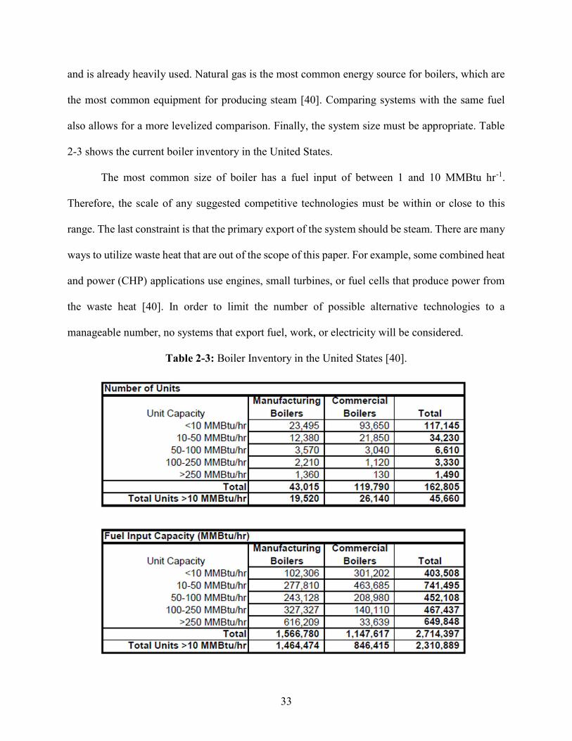
33

and is already heavily used. Natural gas is the most common energy source for boilers, which are

the most common equipment for producing steam [40]. Comparing systems with the same fuel

also allows for a more levelized comparison. Finally, the system size must be appropriate. Table

2-3 shows the current boiler inventory in the United States.

The most common size of boiler has a fuel input of between 1 and 10 MMBtu hr-1.

Therefore, the scale of any suggested competitive technologies must be within or close to this

range. The last constraint is that the primary export of the system should be steam. There are many

ways to utilize waste heat that are out of the scope of this paper. For example, some combined heat

and power (CHP) applications use engines, small turbines, or fuel cells that produce power from

the waste heat [40]. In order to limit the number of possible alternative technologies to a

manageable number, no systems that export fuel, work, or electricity will be considered.

Table 2-3: Boiler Inventory in the United States [40].

34

Within these constraints, the only alternative to SMR is a natural gas fired boiler system.

This is a logical outcome: boiler technology has been developed over several centuries and is

simple and robust. At its most simple, a boiler burns a fuel to create hot exhaust, and heat is

transferred from the exhaust to water to produce steam. Boiler efficiency is typically defined in

the “Input-Output” method: efficiency is the ratio of the heat delivered to the water to the heat

supplied to the system from fuel [66]. In a simple boiler, a significant amount of energy leaves the

system in the still moderately hot exhaust. Modern, more efficient boilers use several methods to

capture more heat and raise thermodynamic efficiency [66]. Optimized heat exchangers create

increased surface area to yield more heat transfer from the exhaust. Precise air/fuel controls help

control combustion of the fuel to achieve complete combustion. Heat recovery devices such as

feed water heaters take advantage of low temperature exhaust to preheat incoming water, reducing

the load on the main burner. With all the stops pulled, a high efficiency, natural gas fired steam

boiler in the 1 – 10 MMBtu h-1 size range has a peak efficiency of 83-86% [66–69].

Boilers have been in widespread use for hundreds of years; why replace them? Natural gas

boilers are typically associated with high levels of emissions including NOx, SO2, particulate

matter, volatile organic compounds, and CO2 [70]. The efficiency of even state-of-the-art boiler

systems has plateaued around 86%, which includes expensive heat recovery equipment. There are

challenges associated with trace amounts of Sulphur in natural gas; acid condensates can form

during combustion, fouling heat exchangers and contributing to acid rain.

This section has identified literature sufficient to conclude that a high efficiency natural

gas fired boiler is an appropriate comparison for the proposed SMR steam generation system. In

the Technoeconomic Comparison section, 3.4, a detailed analysis and comparison will be

explained. It will establish a baseline for comparison using a fixed mass and state of steam, provide

35

data for a technoeconomic comparison, and quantitatively prove whether SMR is an economic

competitor to other steam generation technologies.

The literature review presented here shows that there are significant gaps in current work

on steam methane reforming. While there have been many detailed studies of specific facets of

SMR such as enhancing hydrogen recovery or recycling gas to increase efficiency, no one study

has unified all the major factors discussed here. In academia, steam methane reforming is confined

to a narrow application window in plant scale hydrogen production, on-board scale hydrogen

production, and electricity generation. In industry, that window is even narrower, with the only

significant application of SMR being hydrogen production. There is an opportunity to fully utilize

the net exports of SMR in the appropriate context of steam generation, but it has not been addressed

in literature. Furthermore, for the applications that have been studied, there is insufficient analysis

to prove that a given technology is can be implemented in a cost-effective way. This study aims to

fill these gaps in the literature by developing an integrated steam methane reforming and steam

generation system. A detailed thermodynamic and technoeconomic analysis determine whether

the proposed technology has a favorable economic case over existing technology.

2.4. Research Needs for Steam Methane Reforming

The literature review presented here shows that there are several key areas of research

lacking exploration. Many studies have shown novel designs or aspects of membrane reformers,

but only Martin et al. [18] and Manzolini et al. [34] unify all of the discussed aspects of steam

methane reforming in a single study (Table 2-4). No papers were found that apply SMR to steam

generation as the primary goal.

Steam methane reforming is a proven technology, but only in the limited application of

hydrogen production. SMR naturally aligns well with the requirements and goals of steam

36

generation. This new application shows the potential for higher system efficiency and reduced

cost, but a focused study is needed to prove those points from a thermodynamic and

technoeconomic perspective.

Table 2-4: Summary of recent studies on membrane reforming technologies.

a b c d e f g h i j k This Study

Thermodynamic Modeling

Technoeconomic Modeling

Methane as fuel Heat Exchange within Reactor

Waste Heat Recovery Sweep gas

Hydrogen Recovery CO2 Separation Recycled Gas

Application to Steam Generation

a: Spallina et al. [53] b: Malerod-Fjeld et al. [33] c: Martin et al. [18] d: Manzolini et al. [34] e: Gallucci et al. [71] f: Shigarov et al. [72]

g: Mokheim et al. [73] h: Sheintuch [74] i: Vigneault and Grace [75] j: Eveloy [76] k: De Falco et al. [77]

This literature review focused on membrane reactors and steam generation. It shows that

there are several specific needs for further research in the field:

Create and analyze a thermodynamic model for an integrated steam methane reformer

steam generation system that combines all aspects of the technology described in Table

2-4.

37

Explore the options for carbon capture in steam methane reforming, taking into account

the high CO2 concentration in the retentate and other effects of incorporating steam

generation.

Perform a technoeconomic analysis of steam methane reforming applied to steam

generation to determine economic feasibility.

Compare the proposed steam generation system to existing technology – i.e. a high

efficiency natural gas boiler.

Investigate the possibility of adding carbon capture onto existing boilers instead of

introducing an entirely new system for steam generation.

Put the results of carbon capture in context using data from existing power and energy

conversion plants.

Using the developed models, perform a sensitivity analysis to help guide future research

on steam generation via steam methane reforming.

2.5. Specific Aims of this Study

This literature review has identified several key gaps in current research on steam methane

reforming. Many key aspects of steam methane reforming have been studied separately, but there

is a lack of modeling and validation for a system that integrates all aspects. Additionally, most

literature addresses theoretical improvements and understanding of the technology without

offering a specific application. The goal of this study is to fill those gaps through execution of the

following:

Develop and refine a detailed thermodynamic model of an integrated steam methane

reformer system, combining state-of-the-art technology in multiple aspects of the

technology.

38

Choose the best technology for CO2 capture in the proposed steam generation system

based on minimizing energy consumption and costs.

Couple the thermodynamic model to a technoeconomic analysis at a relevant industrial

scale to determine economic performance of the proposed system.

Discuss the relative merits of the proposed system against a baseline for steam

generation: industrial natural gas boilers that are currently in widespread use.

Develop a model for a boiler system with integrated carbon capture as an alternative to

the proposed steam generation system.

Collect and discuss energy penalties and technologies associated with carbon capture

in existing systems, including power plants and conventional steam methane reforming.

Develop a sensitivity analysis to help discuss important factors that drive

thermodynamic and economic performance.

39

Modeling Approach

The literature review showed that there are several key points missing from the current

literature on steam methane reforming. Specifically, there are many more thermodynamic

modeling studies than technoeconomic investigations. Furthermore, few studies combine all

aspects of SMR found in Table 2-4: methane conversion, hydrogen recovery, heat exchange within

the reactor, waste heat recovery, carbon dioxide sequestration, recycled gas, and an integrated

membrane reactor. Also, the literature generally focuses on the technology itself, rather than

practical methods of implementation, whereas this study has selected and analyzed a proposed

application in steam generation.

The modeling effort in this study develops and compares models for three NG-fueled steam

generation systems: a high efficiency boiler system (BS), the same boiler system with carbon

capture (BSC), and the SMR-MR-SG. The models were developed using Engineering Equation

Solver (EES) version 10.441-3D,50 allowing relevant equations to be solved simultaneously with

embedded thermophysical properties. The thermodynamic models incorporate chemical reactions,

thermodynamic states, energy balances, and heat exchanger design variables necessary to estimate

system performance. For a direct, levelized comparison, the boiler and SMR-MR-SG systems were

sized to produce (export) the same mass flow rate of steam at a set temperature and pressure of

200°C and 15 bar, respectively, corresponding to a typical low-pressure steam system [40]. The

condensate return rate is the mass of liquid water that returns from steam export; a rule of thumb

is 80% return for steam generation plants [78].

Table 3-1 shows the key assumptions and input parameters to the thermodynamic model.

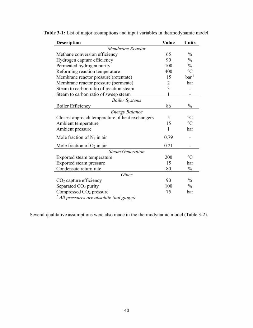
40

Table 3-1: List of major assumptions and input variables in thermodynamic model.

Description Value Units Membrane Reactor

Methane conversion efficiency 65 % Hydrogen capture efficiency 90 % Permeated hydrogen purity 100 % Reforming reaction temperature 400 °C Membrane reactor pressure (retentate) 15 bar 1

Membrane reactor pressure (permeate) 2 bar Steam to carbon ratio of reaction steam 3 - Steam to carbon ratio of sweep steam 1 -

Boiler Systems Boiler Efficiency 86 %

Energy Balance Closest approach temperature of heat exchangers 5 °C Ambient temperature 15 °C Ambient pressure 1 bar Mole fraction of N2 in air 0.79 - Mole fraction of O2 in air 0.21 -

Steam Generation Exported steam temperature 200 °C Exported steam pressure 15 bar Condensate return rate 80 %

Other CO2 capture efficiency 90 % Separated CO2 purity 100 % Compressed CO2 pressure 75 bar 1 All pressures are absolute (not gauge).

Several qualitative assumptions were also made in the thermodynamic model (Table 3-2).

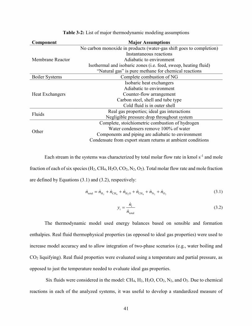
41

Table 3-2: List of major thermodynamic modeling assumptions

Component Major Assumptions

Membrane Reactor

No carbon monoxide in products (water-gas shift goes to completion) Instantaneous reactions

Adiabatic to environment Isothermal and isobaric zones (i.e. feed, sweep, heating fluid)

“Natural gas” is pure methane for chemical reactions Boiler Systems Complete combustion of NG

Heat Exchangers

Isobaric heat exchangers Adiabatic to environment Counter-flow arrangement

Carbon steel, shell and tube type Cold fluid is in outer shell

Fluids Real gas properties; ideal gas interactions Negligible pressure drop throughout system

Other

Complete, stoichiometric combustion of hydrogen Water condensers remove 100% of water

Components and piping are adiabatic to environment Condensate from export steam returns at ambient conditions

Each stream in the systems was characterized by total molar flow rate in kmol s-1 and mole

fraction of each of six species (H2, CH4, H2O, CO2, N2, O2). Total molar flow rate and mole fraction

are defined by Equations (3.1) and (3.2), respectively:

2 4 2 4 2 2total H CH H O CH N O n n n n n n n (3.1)

ii

total

ny

n (3.2)

The thermodynamic model used energy balances based on sensible and formation

enthalpies. Real fluid thermophysical properties (as opposed to ideal gas properties) were used to

increase model accuracy and to allow integration of two-phase scenarios (e.g., water boiling and

CO2 liquifying). Real fluid properties were evaluated using a temperature and partial pressure, as

opposed to just the temperature needed to evaluate ideal gas properties.

Six fluids were considered in the model: CH4, H2, H2O, CO2, N2, and O2. Due to chemical

reactions in each of the analyzed systems, it was useful to develop a standardized measure of

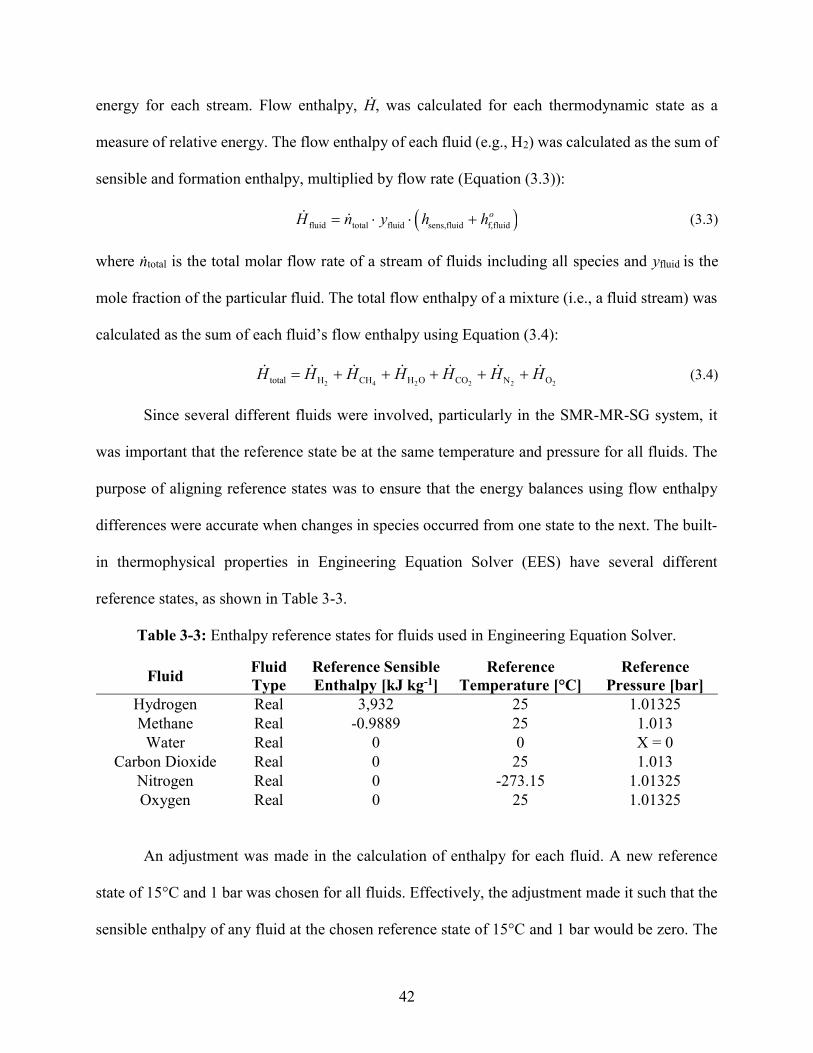
42

energy for each stream. Flow enthalpy, Ḣ, was calculated for each thermodynamic state as a

measure of relative energy. The flow enthalpy of each fluid (e.g., H2) was calculated as the sum of

sensible and formation enthalpy, multiplied by flow rate (Equation (3.3)):

fluid total fluid sens,fluid f,fluid oH n y h h (3.3)

where ṅtotal is the total molar flow rate of a stream of fluids including all species and yfluid is the

mole fraction of the particular fluid. The total flow enthalpy of a mixture (i.e., a fluid stream) was

calculated as the sum of each fluid’s flow enthalpy using Equation (3.4):

2 4 2 2 2 2total H CH H O CO N O H H H H H H H (3.4)

Since several different fluids were involved, particularly in the SMR-MR-SG system, it

was important that the reference state be at the same temperature and pressure for all fluids. The

purpose of aligning reference states was to ensure that the energy balances using flow enthalpy

differences were accurate when changes in species occurred from one state to the next. The built-

in thermophysical properties in Engineering Equation Solver (EES) have several different

reference states, as shown in Table 3-3.

Table 3-3: Enthalpy reference states for fluids used in Engineering Equation Solver.

Fluid Fluid Type

Reference Sensible Enthalpy [kJ kg-1]

Reference Temperature [°C]

Reference Pressure [bar]

Hydrogen Real 3,932 25 1.01325 Methane Real -0.9889 25 1.013

Water Real 0 0 X = 0 Carbon Dioxide Real 0 25 1.013

Nitrogen Real 0 -273.15 1.01325 Oxygen Real 0 25 1.01325

An adjustment was made in the calculation of enthalpy for each fluid. A new reference

state of 15°C and 1 bar was chosen for all fluids. Effectively, the adjustment made it such that the

sensible enthalpy of any fluid at the chosen reference state of 15°C and 1 bar would be zero. The

43

adjustment also standardized the enthalpy of formation reference of each fluid to the new reference

state. First, the pressure and temperature were adjusted to match the new reference state. The

temperature and pressure adjustments were calculated by Equations (3.5) and (3.6):

adj ref,new ref,fluid T T T (3.5)

adj ref,new ref,fluid P P P (3.6)

where Tref,new and Pref,new were equal to the reference state: 15°C and 1 bar, respectively. For

example, “Nitrogen” in Table 3-3 had Tref,fluid equal to -273.15°C and Pref,fluid equal to 1.01325 bar.

Then, each of the fluids required an additional adjustment to set the sensible enthalpy to zero at

the new reference state. The sensible enthalpy of each fluid was ultimately evaluated as in Equation

(3.7):

sens,fluid fluid fluid adj fluid adj adj( , ) h h T T T P P P h (3.7)

Similar to the lower heating value (LHV) method of Spallina et al. [53], flow enthalpy of each

state was used as the primary metric for calculating changes in energy between states, even with a

change in chemical composition. A brief example is included to explain the concept of flow

enthalpy in energy balances. Consider H2 combustion in a boiler: H2 is combusted with air (N2 and

O2) to produce heat, and the heat is transferred to liquid water to boil it into steam. For simplicity,

assume a 100% efficient boiler, such that all extracted heat from combustion enters the water. The

flow enthalpy of the combustion reactants is given by the sum of hydrogen and air as in Equation

(3.8):

2 2 2reactants H N

OH H H H (3.8)

where the flow enthalpy of each reactant H2, N2, and O2 are evaluated at their particular

temperature, partial pressure, and mole fraction according to Equation (3.3). Assuming complete

stoichiometric combustion, the flow enthalpy of the products is given by Equation (3.9):

44

2 2products H O N H H H (3.9)

The net energy produced in the combustion is simply the difference in flow enthalpy, given by

Equation (3.10):

boiler products reactants Q H H (3.10)

Referring to the definition of flow enthalpy in Equation (3.3), the calculated Q̇boiler includes the

heat of combustion due to the chemical reaction (enthalpy of formation) as well as energy involved

in change in temperature and pressure (sensible enthalpy). Assuming 100% efficiency, all of the

heat from combustion is transferred to the water as in Equation (3.11):

boiler water Q Q (3.11)

On the water side of the boiler, the flow enthalpy in and out of the boiler are calculated in the same

way because there is no change in species. Flow enthalpy is calculated using Equations (3.12) and

(3.13):

2water,in H O H H (3.12)

2water,out H O H H (3.13)

Then, the heat entering the water is given by the difference in flow enthalpy, given by Equation

(3.14):

water water,out water,in Q H H (3.14)

In the case of Equation (3.14), the enthalpy of formation in each term cancels because flow rate

and species have remained the same. The difference is that ḢH2O in Equation (3.12) is evaluated at

liquid water state (e.g., 15°C and 15 bar), but ḢH2O in Equation (3.13) is steam (e.g., 200°C and 15

bar). Thus, Equation (3.14) captures only the change in sensible enthalpy because there is no

change in enthalpy of formation.

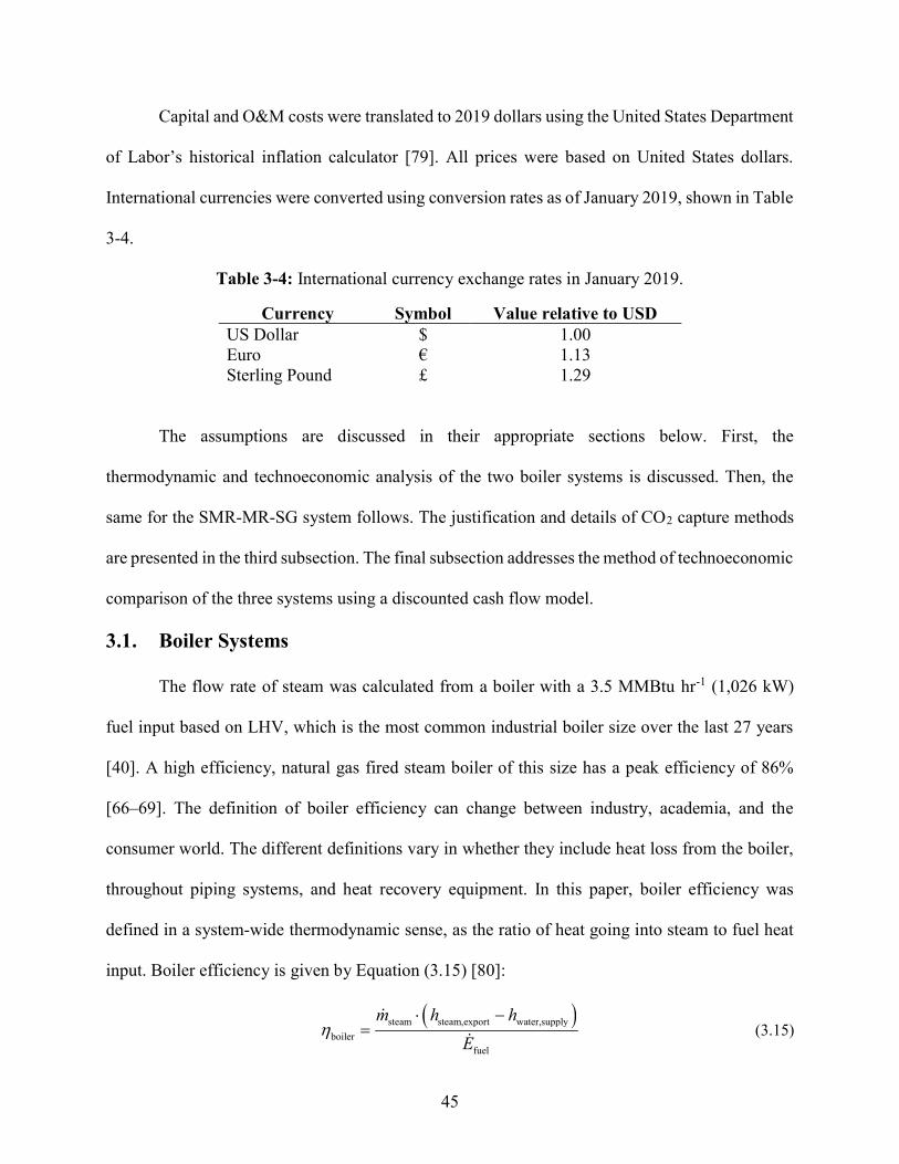
45

Capital and O&M costs were translated to 2019 dollars using the United States Department

of Labor’s historical inflation calculator [79]. All prices were based on United States dollars.

International currencies were converted using conversion rates as of January 2019, shown in Table

3-4.

Table 3-4: International currency exchange rates in January 2019.

Currency Symbol Value relative to USD US Dollar $ 1.00 Euro € 1.13 Sterling Pound £ 1.29

The assumptions are discussed in their appropriate sections below. First, the

thermodynamic and technoeconomic analysis of the two boiler systems is discussed. Then, the

same for the SMR-MR-SG system follows. The justification and details of CO2 capture methods

are presented in the third subsection. The final subsection addresses the method of technoeconomic

comparison of the three systems using a discounted cash flow model.

3.1. Boiler Systems

The flow rate of steam was calculated from a boiler with a 3.5 MMBtu hr-1 (1,026 kW)

fuel input based on LHV, which is the most common industrial boiler size over the last 27 years

[40]. A high efficiency, natural gas fired steam boiler of this size has a peak efficiency of 86%

[66–69]. The definition of boiler efficiency can change between industry, academia, and the

consumer world. The different definitions vary in whether they include heat loss from the boiler,

throughout piping systems, and heat recovery equipment. In this paper, boiler efficiency was

defined in a system-wide thermodynamic sense, as the ratio of heat going into steam to fuel heat

input. Boiler efficiency is given by Equation (3.15) [80]:

steam steam,export water,supply

boilerfuel

m h h

E (3.15)

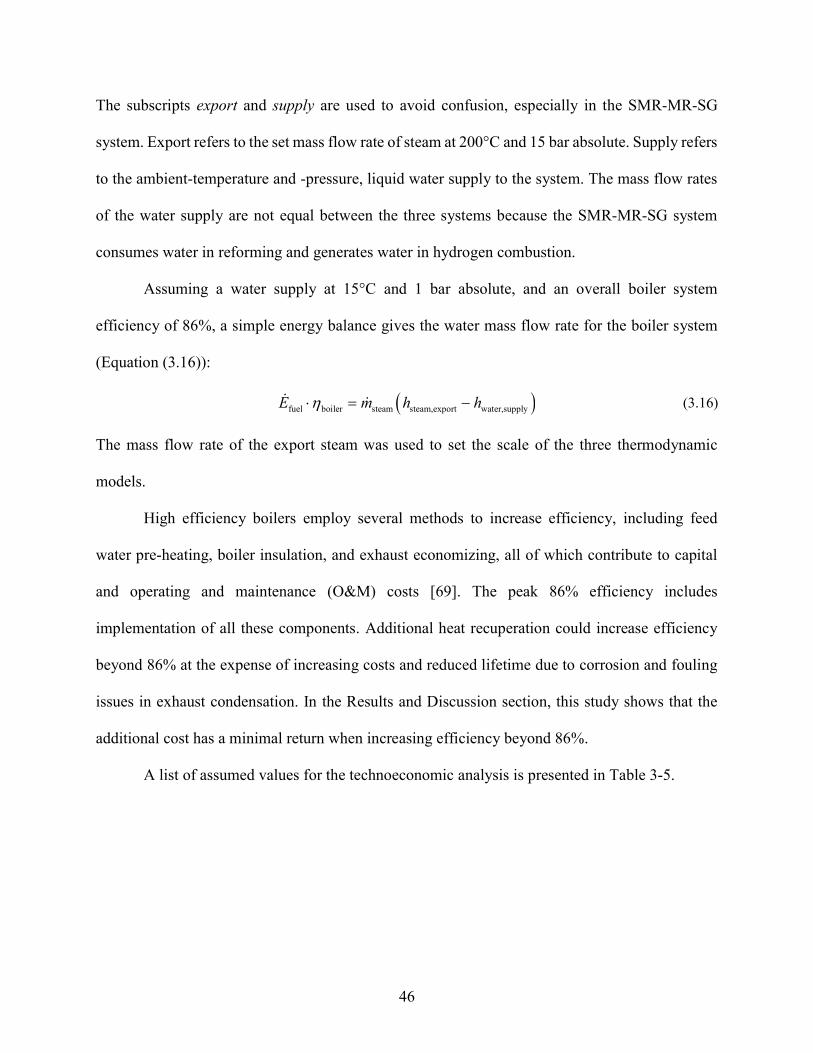
46

The subscripts export and supply are used to avoid confusion, especially in the SMR-MR-SG

system. Export refers to the set mass flow rate of steam at 200°C and 15 bar absolute. Supply refers

to the ambient-temperature and -pressure, liquid water supply to the system. The mass flow rates

of the water supply are not equal between the three systems because the SMR-MR-SG system

consumes water in reforming and generates water in hydrogen combustion.

Assuming a water supply at 15°C and 1 bar absolute, and an overall boiler system

efficiency of 86%, a simple energy balance gives the water mass flow rate for the boiler system

(Equation (3.16)):

fuel boiler steam steam,export water,supply E m h h (3.16)

The mass flow rate of the export steam was used to set the scale of the three thermodynamic

models.

High efficiency boilers employ several methods to increase efficiency, including feed

water pre-heating, boiler insulation, and exhaust economizing, all of which contribute to capital

and operating and maintenance (O&M) costs [69]. The peak 86% efficiency includes

implementation of all these components. Additional heat recuperation could increase efficiency

beyond 86% at the expense of increasing costs and reduced lifetime due to corrosion and fouling

issues in exhaust condensation. In the Results and Discussion section, this study shows that the

additional cost has a minimal return when increasing efficiency beyond 86%.

A list of assumed values for the technoeconomic analysis is presented in Table 3-5.

47

Table 3-5: List of major input variables in technoeconomic model.

Parameter Value Units Commodity Pricing

Natural gas purchase price 4.1 $ 1000 scf-1

Electricity purchase price 0.0688 $ kWh-1

CO2 sale price 20 $ ton-1

Water purchase price 0.282 $ m-3

Cash Flow Analysis Discount rate 12 % Lifespan 20 yr Carbon tax 50.5 $ tonCO2

-1 Scale (boiler fuel input) 3.5 MMBtu h-1

Boiler Systems System capital cost 35,000 $ per MMBtu h-1

Boiler efficiency 86 % System O&M Cost 0.95 $ MMBtu-1 MEA CapEx 1.178 M$ per kgCO2 s

-1 MEA O&M Cost 0.141 $ kmolCO2

-1

SMR Steam Generation System Membrane thickness 2.8 µm Membrane permeance 6.48x10-3 mol m-2 s-1 Pa-0.5 Membrane cost (no reactor) 1,076 $ m-2

System O&M Cost 5 % of total CapEx CSU CapEx 0.440 M$ per kgCO2 s

-1

CSU O&M Cost 4 % of CSU CapEx

The capital cost for the high efficiency natural gas boiler system was calculated using

$35,000 per MMBtu h-1 ($119.42 per kW) of fuel input [70] by Equation (3.17):

1BS 1

$35,000 3.5

CapEx MMBtu h

MMBtu h (3.17)

Note that the selected boiler scale of 3.5 MMBtu h-1 for this study and the capital cost of $35,000

per MMBtu h-1 are neat multiples by coincidence; one was not calculated using the other. The

O&M cost (excluding commodity consumption) of the baseline system was calculated using a cost

of $0.95 per MMBtu ( $0.003242 per kWh) of fuel input [70] using Equation (3.18):

48

1 1BS load

$0.95 3.5 8760

OpEx MMBtu h F h yrMMBtu

(3.18)

where Fload is the load factor, or the percentage of time the plant is in operation, as opposed to

offline for maintenance, defined by Equation (3.19) [69]:

loadOperational hours per year

Total hours per yearF (3.19)

As validation of the calculated values, other sources suggested an alternative method of

cost estimation. For an industrial steam generation system the O&M, capital cost, and fuel cost

should equal 1%, 3%, and 96% of the lifetime cost, respectively [69,81,82]. Using the cost per

MMBtu methods, the O&M, capital cost, and fuel cost came out to 0.7%, 3.2%, and 61%,

respectively. The reason for the disparity in fuel cost percentage is that this study included the cost

of carbon tax and water supply in addition to fuel.

The BSC is the same as the BS but with the addition of CCC components: a condenser,

amine absorber, and compressor for dehydration of exhaust, CO2 separation, and CO2

compression, respectively. The costs of the BSC were calculated as the sum of the BS costs plus

the additional costs of CCC. The capital cost of the amine absorber was calculated using Equation

(3.20) [83]:

2

2

COMEA CO ,BSC

$1.178

kg

CapEx ms

(3.20)

Several authors make use of a scaling factor to predict capital cost at a different scale

[22,84,85]. For example, if the price of a 100 kW compressor is known but a cost estimate is

required for a 500 kW compressor, the scaling factor can be used to estimate the price of the

unknown component. The scaling equation is given by Equation (3.21):

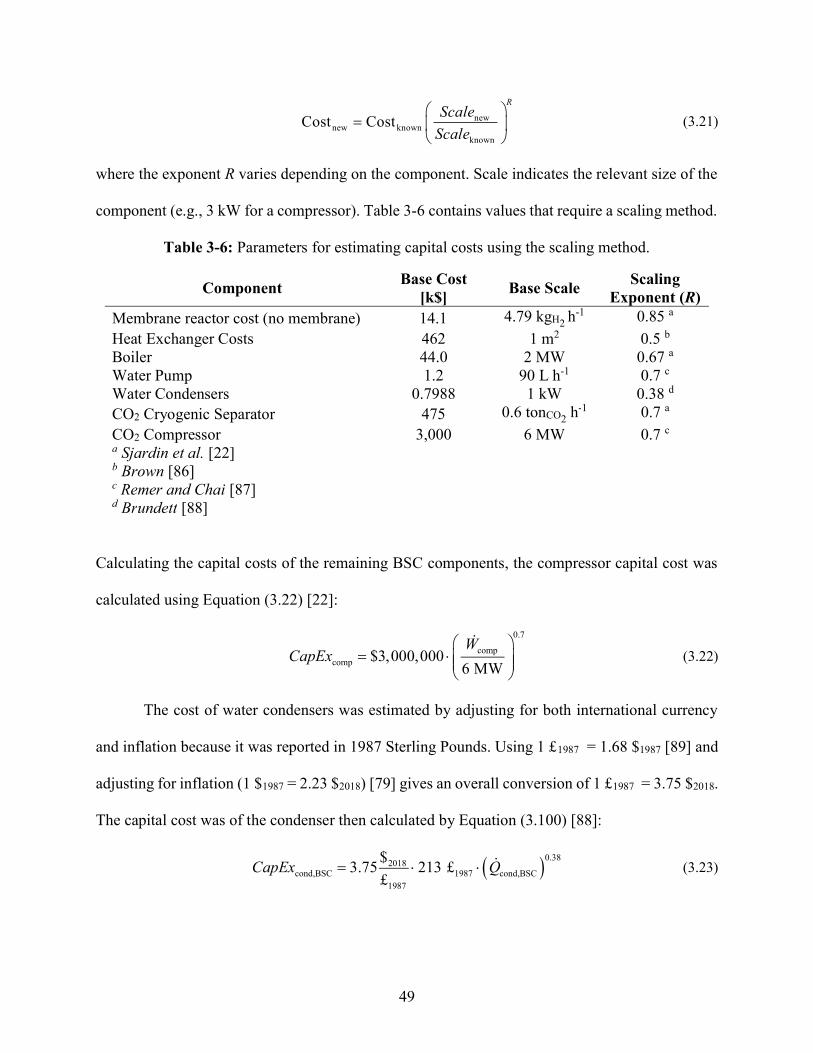
49

newnew known

known

Cost Cost

RScale

Scale (3.21)

where the exponent R varies depending on the component. Scale indicates the relevant size of the

component (e.g., 3 kW for a compressor). Table 3-6 contains values that require a scaling method.

Table 3-6: Parameters for estimating capital costs using the scaling method.

Component Base Cost [k$] Base Scale Scaling

Exponent (R) Membrane reactor cost (no membrane) 14.1 4.79 kgH2

h-1 0.85 a Heat Exchanger Costs 462 1 m2 0.5 b

Boiler 44.0 2 MW 0.67 a Water Pump 1.2 90 L h-1 0.7 c

Water Condensers 0.7988 1 kW 0.38 d CO2 Cryogenic Separator 475 0.6 tonCO2 h

-1 0.7 a CO2 Compressor 3,000 6 MW 0.7 c a Sjardin et al. [22] b Brown [86] c Remer and Chai [87] d Brundett [88]

Calculating the capital costs of the remaining BSC components, the compressor capital cost was

calculated using Equation (3.22) [22]:

0.7

compcomp $3,000,000

6 MW

WCapEx (3.22)

The cost of water condensers was estimated by adjusting for both international currency

and inflation because it was reported in 1987 Sterling Pounds. Using 1 £1987 = 1.68 $1987 [89] and

adjusting for inflation (1 $1987 = 2.23 $2018) [79] gives an overall conversion of 1 £1987 = 3.75 $2018.

The capital cost was of the condenser then calculated by Equation (3.100) [88]:

0.3820181987 cond,BSC

198cond

7,BSC 3. $ 213 £

£75 QCapEx (3.23)

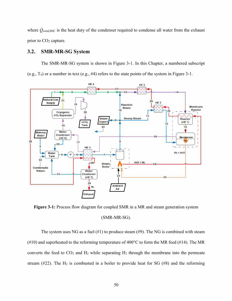
50

where Q̇cond,BSC is the heat duty of the condenser required to condense all water from the exhaust

prior to CO2 capture.

3.2. SMR-MR-SG System

The SMR-MR-SG system is shown in Figure 3-1. In this Chapter, a numbered subscript

(e.g., T4) or a number in text (e.g., #4) refers to the state points of the system in Figure 3-1.

Figure 3-1: Process flow diagram for coupled SMR in a MR and steam generation system

(SMR-MR-SG).

The system uses NG as a fuel (#1) to produce steam (#9). The NG is combined with steam

(#10) and superheated to the reforming temperature of 400°C to form the MR feed (#14). The MR

converts the feed to CO2 and H2 while separating H2 through the membrane into the permeate

stream (#22). The H2 is combusted in a boiler to provide heat for SG (#8) and the reforming

51

reaction (#24). Waste heat is captured in recuperative heat exchangers (HE 2 through HE 5). Water

is condensed from the boiler exhaust (#28) and retentate (#17) for recycling. A cryogenic

separation unit (CSU) separates CO2 from the retentate stream (#18). The unreacted CH4, un-

permeated H2, and un-captured CO2 are recycled back into the feed (#21). It is important to note

that the H2-fueled boiler in the SMR-MR-SG is a simple boiler without integrated heat

recuperation and economizing, whereas the boiler systems of the BS and BSC have additional

components that increase efficiency but add cost.

3.2.1. Model Overview

Steam methane reforming reacts steam and methane over a catalyst to form hydrogen and

carbon dioxide. In a membrane reactor, the hydrogen is separated from the chemical products in

real-time. The chemical reaction occurs in two steps: steam methane reforming, given by Equation

(3.24) [18]:

04 2 2 298K3 206 / CH H O CO H H kJ mol (3.24)

and water-gas shift, given by Equation (3.25) [18]:

02 2 2 298K 41 / CO H O CO H H kJ mol (3.25)

These two reactions can be combined into an overall reaction, given by Equation (3.26) [18,19]:

04 2 2 2 298K2 4 165 / CH H O H CO H kJ mol (3.26)

The heat of reaction given in Equation (3.3) is the sum of the two reaction steps. It’s important to

note that this is a highly endothermic reaction, the implication being that a physical reactor must

have a significant and constant supply of heat to operate correctly.

The goal of the thermodynamic analysis was to provide an accurate model for a fluid

process coupling steam methane reforming and steam generation. Specifically, the process flow

diagram of Figure 3-1 was developed and then modeled in detail. The desired outputs were the

52

fully defined state points, including flow rates of each gas, mole fractions, temperature, pressure,

enthalpy, and phase if applicable. On a system level, the flow and states of each input and output

was calculated, as well as the heat duty of each heat exchanger.

The secondary goal of the thermodynamic model was to be able to couple it directly to a

technoeconomic model. The technoeconomic model models the SMR-MR-SG and compares it to

the BS and BSC to determine its economically feasibility. The technoeconomic comparison will

be discussed in the next major section, 3.4. A sensitivity analysis is detailed in section 4.3 to show

the effects of input parameters, thermodynamic and economic, on technoeconomic outputs.

The thermodynamic model was purposefully kept to a system level as much as possible.

Many models and experiments have varied pressure, temperature, and steam to carbon ratio in

order to optimize methane conversion and hydrogen recovery [7]. That was not the focus of this

thesis, so parameters were assumed based on recent literature and the model proceeded. On the

other hand, topics such as heat balances within the membrane reactor and heat exchangers in the

system were lacking in literature [15]. Those aspects that were not well developed in the literature

were given more attention.

In the ideal SMR process, the reactions given in Equations (3.24) through (3.26) go to

completion, i.e., the only remaining species are H2 and CO2. In reality, only a percentage of the

CH4 is reacted, the water-gas shift reaction does not completely consume all CO, and not all H2 is

separated. The net effect is that the products contain CH4, H2O, CO, CO2, and H2.

The primary tool used for modeling was the program Engineering Equation Solver (EES).

There are two large advantages to EES in the context of thermodynamic modeling. First, it has

integrated thermophysical properties. Instead of spending time finding and interpolating from

tables, built-in functions were used to evaluate all properties. Unlike most other programming

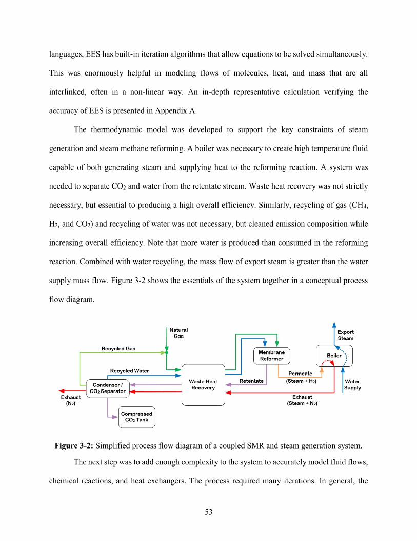
53

languages, EES has built-in iteration algorithms that allow equations to be solved simultaneously.

This was enormously helpful in modeling flows of molecules, heat, and mass that are all

interlinked, often in a non-linear way. An in-depth representative calculation verifying the

accuracy of EES is presented in Appendix A.

The thermodynamic model was developed to support the key constraints of steam

generation and steam methane reforming. A boiler was necessary to create high temperature fluid

capable of both generating steam and supplying heat to the reforming reaction. A system was

needed to separate CO2 and water from the retentate stream. Waste heat recovery was not strictly

necessary, but essential to producing a high overall efficiency. Similarly, recycling of gas (CH4,

H2, and CO2) and recycling of water was not necessary, but cleaned emission composition while

increasing overall efficiency. Note that more water is produced than consumed in the reforming

reaction. Combined with water recycling, the mass flow of export steam is greater than the water

supply mass flow. Figure 3-2 shows the essentials of the system together in a conceptual process

flow diagram.

Figure 3-2: Simplified process flow diagram of a coupled SMR and steam generation system.

The next step was to add enough complexity to the system to accurately model fluid flows,

chemical reactions, and heat exchangers. The process required many iterations. In general, the

54

challenge was to recover sufficient heat to supply the reforming reaction while respecting the

limitations of real heat exchangers. In counter-flow heat exchangers, the hot fluid outlet

temperature cannot be colder than the cold fluid inlet. Similarly, the cold fluid outlet temperature

cannot be warmer than the hot fluid inlet temperature. Counter-flow heat exchangers were used

instead of parallel flow in all modeling because they allow temperatures to “cross”: the hot fluid

outlet can be colder than the cold fluid outlet [90]. The closest approach temperature (CAT) was

introduced at this point. All these concepts are depicted in Figure 3-3.

Figure 3-3: Closest approach temperature (CAT) of fluids in a counter-flow heat exchanger.

The introduction of the closest approach temperature complicated the process flow diagram

further. Part of the difficulty was that there was no single goal; it could be to minimize waste heat,

minimize natural gas input required, or maximize the overall system efficiency. Several iterations

on a detailed process flow diagram yielded Figure 3-1, which is a compromise between waste heat

recovery, natural gas input, and system efficiency. This system supplies just enough heat for

generating the required amount of export steam, preheating reactants, and supplying the heat of

55

reaction to the membrane reactor. Steam was chosen for sweep gas composition; it is convenient

due to the large amount of steam in the system already, and literature shows a marked improvement

in hydrogen permeation using steam instead of other gases such as nitrogen [71].

The system uses NG as a fuel (#1) to produce steam (#9). The NG is combined with steam

(#10) and superheated to the reforming temperature of 400°C to form the MR feed (#14). The MR

converts the feed to CO2 and H2 while separating H2 through the membrane into the permeate

stream (#22). The H2 is combusted in a boiler to provide heat for SG (#8) and the reforming

reaction (#24). Waste heat is captured in recuperative heat exchangers (e.g., HE 2). Water is

condensed from the boiler exhaust (#28) and retentate (#17) for recycling. A cryogenic separation

unit separates CO2 from the retentate stream (#18). The unreacted CH4, un-permeated H2, and un-

captured CO2 are recycled back into the feed (#21). It’s important to note that the boiler in the

SMR-MR-SG is a simple boiler, whereas the boiler systems in the BS and BSC have complicated

economizing and heat recuperation components.

In addition to producing process steam, the SMR-MR-SG system creates a concentrated

CO2 stream on the retentate side of the reactor (#16). Because some of the incoming methane is

not reacted and some of the generated hydrogen remains in the retentate, the CO2 must go through

a purification process. Recent studies argue that a cryogenic separation unit (CSU) is the most

energy- and cost-effective way to separate CO2 from a high concentration CO2 stream [22,91]. The

CSU will be discussed in more detail in the CO2 capture section.

The inputs and outputs of the system in Figure 3-1 are shown in bolded boxes. Inputs

include natural gas as the fuel source (#1), liquid water to be heated into steam (#4), and air for

hydrogen combustion in the boiler (#23). Outputs of the system are steam for export (#9),

compressed CO2 (abbreviated cCO2) for sale (#20), and ambient temperature nitrogen as exhaust

56

(#30). The steam export is the same temperature, pressure, and flow rate as the high efficiency

boiler system being used as a benchmark for comparison. Where the steam goes or what it is used

for is not the focus of this thesis; the focus is how to generate the export steam in a more efficient,

clean, and cost-effective way than the current technology. Stream (#33) is the condensate return,

or the cold water left over from some steam consuming application.

Continuing through the system, the membrane reactor is shown on the far right, inside the

large dashed box. The unit is shown as two separate components (reactor and separator) for

modeling purposes, but is intended to be one physical unit. Stream (#24) to (#25) is high

temperature exhaust from the boiler; it provides heat for the reforming reaction. Stream (#14) is

the feed, consisting primarily of CH4 and H2O, but also with lesser amounts of H2 and CO2 that

have been recycled. Stream (#12) is the sweep gas, in this case pure steam, superheated to the

reforming temperature. Stream (#15) is an intermediate within the reactor, representing the feed

after the reforming reaction but before hydrogen permeating through the membrane. In reality, the

reforming reaction happens simultaneously with the hydrogen removal; again, this was a technique

for modeling. Stream (#22) is the low pressure permeate, which includes all the sweep steam from

Stream (#12) plus the permeated hydrogen. Stream (#16) is the retentate: everything left over on

the high-pressure side of the membrane.

Following Stream (#22), the hydrogen is combusted stoichiometrically with air in the

boiler. The boiler is purposefully inefficient in the sense that only about 50% of the heat from

combustion goes into the steam, with the rest leaving in the exhaust. The reason for this is that a

significant amount of energy is required in the exhaust to heat the membrane reactor and preheat

the reactants. Heat exchanger 1 (HE 1) supplies the heat of reaction for the steam methane

reforming reaction. HE 2 superheats sweep steam from the export steam temperature to the

57

reforming temperature. HE 3 superheats the feed entering the membrane reactor. HE 4 preheats

the supply natural gas and recycled gases. HE 5 captures the low temperature energy from the

exhaust by preheating water before it enters the steam boiler. HE 7 condenses and recycles water

out of the exhaust, leaving only nitrogen to be exhausted to the environment.

Following the retentate, Stream (#16), its high temperature energy is recovered in HE 5,

also preheating water for the boiler. HE 6 condenses and recycles water out of Stream (#17),

leaving Stream (#18) dry. This is an important step that allows the cryogenic separator to achieve

low temperatures without freezing water. Most of the CO2 in stream (#18) is liquefied and

separated into Stream (#19), with the remaining gases (CH4, H2, and CO2) being recycled into the

fuel stream via Stream (#21).

Returning to the beginning, Stream (#1) is a compressed natural gas supply that provides

energy to the system. Stream (#2) is the combination of (#1) and (#21), now including recycled

CH4, H2, and CO2. Stream (#10) is the steam required for the reforming reaction. The flow rate of

Stream (#10) is defined by the steam to carbon ratio (SC) which typically has a value between 2.5

and 3.5 in literature. The following section will go into detail of the thermodynamic analysis of

the SMR-MR-SG process flow diagram shown in Figure 3-1.

3.2.2. Assumptions and Input Parameters

The thermodynamic model was based on a set of important inputs and assumptions that

were supplied by literature. All assumptions and calculations are guided by results in the published

literature, including experimental results generated by the author and collaborators on the project.

These results include: heat exchanger area, membrane surface area, methane conversion, hydrogen

permeation, capital costs, NG and CO2 market pricing, and carbon taxes [14,23,29,43,92]. Some

assumptions, such as the methane conversion, were made as temporary assumptions pending

58

experimental validation in a future study by this author. The quantifiable assumed and input

variable are shown in Table 3-1.

In this analysis, it was assumed that the natural gas supplied to the system is composed of

pure methane with no impurities. Although this assumption introduced some error, it greatly

simplifies the chemistry. Literature shows that true natural gas reforming can achieve similar fuel

conversion as with pure methane, with conversion of higher hydrocarbons above 85% [12].

Furthermore, palladium-based membranes are not poisoned by CO2 or higher hydrocarbons, which

shows that natural gas of varying composition is a possible option, even if experimental work is

performed with pure methane [48]. Future studies will incorporate relevant impurities.

The key assumptions for the MR include reactor temperature, methane conversion,

hydrogen permeability, operating pressures, and steam-carbon feed and sweep ratios. Prior studies

have shown that a reactor temperature of 400°C provides sufficient reaction stability [53].

Operating at this low temperature also provides a key advantage over traditional SMR by enabling

sufficient heat recuperation in the reactor from the boiler exhaust (#24). The use of low-

temperature MR technology also has a significantly longer life expectancy than conventional

SMR.

Methane conversion varies widely throughout literature. It is a strong function of reforming

temperature and pressure, although the relationship is not well defined. For example, experimental

studies with reforming temperatures between 450 and 500°C and pressures from 1 to 20 bar

showed an average methane conversion of 75.1% with a standard deviation of 18.5% [14]. This

study used a conservative value of 65%, which is close to various estimates [12] and highlights

the efficacy of unconverted methane recycling.

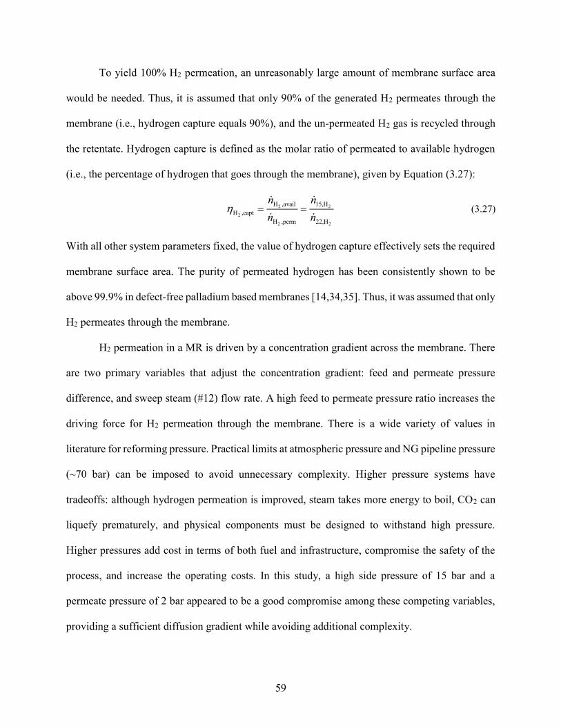
59

To yield 100% H2 permeation, an unreasonably large amount of membrane surface area

would be needed. Thus, it is assumed that only 90% of the generated H2 permeates through the

membrane (i.e., hydrogen capture equals 90%), and the un-permeated H2 gas is recycled through

the retentate. Hydrogen capture is defined as the molar ratio of permeated to available hydrogen

(i.e., the percentage of hydrogen that goes through the membrane), given by Equation (3.27):

2 2

2

2 2

H ,avail 15,HH ,capt

H ,perm 22,H

n nn n

(3.27)

With all other system parameters fixed, the value of hydrogen capture effectively sets the required

membrane surface area. The purity of permeated hydrogen has been consistently shown to be

above 99.9% in defect-free palladium based membranes [14,34,35]. Thus, it was assumed that only

H2 permeates through the membrane.

H2 permeation in a MR is driven by a concentration gradient across the membrane. There

are two primary variables that adjust the concentration gradient: feed and permeate pressure

difference, and sweep steam (#12) flow rate. A high feed to permeate pressure ratio increases the

driving force for H2 permeation through the membrane. There is a wide variety of values in

literature for reforming pressure. Practical limits at atmospheric pressure and NG pipeline pressure

(~70 bar) can be imposed to avoid unnecessary complexity. Higher pressure systems have

tradeoffs: although hydrogen permeation is improved, steam takes more energy to boil, CO2 can

liquefy prematurely, and physical components must be designed to withstand high pressure.

Higher pressures add cost in terms of both fuel and infrastructure, compromise the safety of the

process, and increase the operating costs. In this study, a high side pressure of 15 bar and a

permeate pressure of 2 bar appeared to be a good compromise among these competing variables,

providing a sufficient diffusion gradient while avoiding additional complexity.

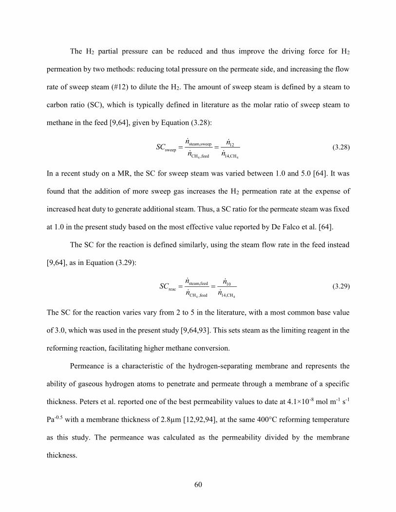
60

The H2 partial pressure can be reduced and thus improve the driving force for H2

permeation by two methods: reducing total pressure on the permeate side, and increasing the flow

rate of sweep steam (#12) to dilute the H2. The amount of sweep steam is defined by a steam to

carbon ratio (SC), which is typically defined in literature as the molar ratio of sweep steam to

methane in the feed [9,64], given by Equation (3.28):

4 4

steam,sweep 12sweep

CH ,feed 14,CH

n nSCn n

(3.28)

In a recent study on a MR, the SC for sweep steam was varied between 1.0 and 5.0 [64]. It was

found that the addition of more sweep gas increases the H2 permeation rate at the expense of

increased heat duty to generate additional steam. Thus, a SC ratio for the permeate steam was fixed

at 1.0 in the present study based on the most effective value reported by De Falco et al. [64].

The SC for the reaction is defined similarly, using the steam flow rate in the feed instead

[9,64], as in Equation (3.29):

4 4

steam,feed 10reac

CH ,feed 14,CH

n nSCn n

(3.29)

The SC for the reaction varies vary from 2 to 5 in the literature, with a most common base value

of 3.0, which was used in the present study [9,64,93]. This sets steam as the limiting reagent in the

reforming reaction, facilitating higher methane conversion.

Permeance is a characteristic of the hydrogen-separating membrane and represents the

ability of gaseous hydrogen atoms to penetrate and permeate through a membrane of a specific

thickness. Peters et al. reported one of the best permeability values to date at 4.1×10-8 mol m-1 s-1

Pa-0.5 with a membrane thickness of 2.8µm [12,92,94], at the same 400°C reforming temperature

as this study. The permeance was calculated as the permeability divided by the membrane

thickness.

61

For the heat exchangers, the closest approach temperature (CAT) is defined as the

minimum temperature difference in a counter-flow heat exchanger between the hot fluid outlet and

the cold fluid inlet (Figure 3-3). Similar to the pressure difference across the membrane reactor,

larger values of CAT reduce the capital cost by increasing the driving force for heat transfer, which

reduces the surface area required. However, these higher CATs reduce energy recovery, and lower

system efficiency. This study assumes a CAT of 5°C.

Ambient conditions of 15°C and 1 bar were chosen as realistic for an implemented plant.

The molar concentrations of nitrogen and oxygen in air were given by Cengel et al. [95]. It was

assumed that no other species were present in the ambient air.

This study focused on low-pressure steam boilers as opposed to hot water boilers or high-

pressure boilers. Oak Ridge National Laboratory defines low-pressure steam boilers as producing

steam at 350 - 400°F (177 - 204°C) and 125 - 250 psig (8.6 to 17.2 bar) [40]. The exported steam

temperature and pressure of 200°C and 15 bar were selected within those limits as a realistic output

of a low-pressure natural gas fired steam boiler. The values are towards the upper limits to provide

additional driving force for hydrogen permeation and closer match the reforming temperature of

400°C. The reforming pressure, which is nominally the same as the feed and retentate pressures,

was chosen to match the steam export pressure. This simplified the system significantly by

avoiding several different steam pressures. In a typical steam generation application such as district

heating, steam is used to supply heat, and the cool water returns to be recycled in the steam

generation plant. The amount of cool water that returns is approximately 80% of the export steam

by mass [78].

There are several methods of separating CO2 from the retentate stream in the SMR-MR-

SG system. Recent literature agrees that cryogenic separation is the most cost-effective way to

62

separate CO2 from the retentate stream [22,91]. In the thermodynamic cycle proposed in Figure

3-1, the CO2 is processed in three steps: liquification via cryogenic cooling to -51°C, distillation

to separate the liquid CO2 from the gases, and compression to 75 bar to raise the liquid above its

critical pressure for storage [91]. State-of-the-art cryogenic separation can achieve 99.9% CO2

purity after separation with a 90% CO2 capture efficiency [91]. Chiesa et al. have shown examples

of cryogenic CO2 separation after water condensation for the purpose of separating CO2 from

exhaust gases [96].

Chemical reactions have a propensity to become extremely complicated with increasing

model fidelity. This study focused on a system level view and thus simplified chemistry to a single

reforming reaction. It is possible in steam methane reforming to have carbon monoxide in the

retentate stream if the water-gas shift reaction doesn’t go to completion. It was assumed that any

carbon monoxide formed was converted to carbon dioxide immediately. No chemical reaction

rates were considered; it was assumed that all reactions occurred infinitely fast. The membrane

reactor was assumed adiabatic to the environment, which could be closely mirrored in a physical

system with sufficient insulation. Each zone in the membrane reactor was treated as isobaric,

isothermal, and otherwise homogenous. Solsvik et al. proved that isobaric and isothermal

conditions can be assumed for the permeation zone without significantly hurting the accuracy of

the model accuracy [15]. This study uses natural gas and methane interchangeably. In the

thermodynamic analysis, all properties and reactions involving natural gas are evaluated using

pure methane.

Heat exchangers were modeled as isobaric and adiabatic to the environment, assuming they

would be well insulated in an industrial plant. They were modeled in a counter-flow arrangement

to maximize amount of heat recovery from low temperature fluids. For estimating capital costs,

63

the heat exchangers were modeled as carbon steel, shell and tube type heat exchangers with the

cold fluid in the outer shell.

Fluids were assumed to have real fluid properties. This was important as water and carbon

dioxide exist as both liquids and gases in the proposed system. For consistency, all fluids were

modeled as real fluids as opposed to ideal gases. The fluids were treated as ideal in that a mixture

of gases did not interact with itself except for the intended reforming reaction. Properties of a

mixture of gases were calculated as the molar weighted average of the properties. Fluids were

assumed to have negligible pressure drops throughout the system.

The combustion of hydrogen was assumed to be complete and stoichiometric. This defined

the flow rate of the ambient air inlet as well as the combustion of the combustion exhaust. Water

condensers were assumed to be 100% effective at removing water and only water. In general, the

system was assumed to be adiabatic to the environment except where components (condensers,

compressor, pump, and cryogenic unit) explicitly rejected heat. This section outlined the inputs

and assumptions that drove the thermodynamic model. The next section will discuss the

development of the model in detail.

3.2.3. Thermodynamic Analysis

This section will explain the development process and methodology of the thermodynamic

analysis of the SMR-MR-SG system shown in Figure 3-1. The conceptual modeling process was

as follows: the export steam (#9) temperature, pressure, and mass flow rate were set based on input

parameters. The heat duty required to generate the export steam set the flow rate of hydrogen

needed for combustion, which then set the size of the membrane reactor. Working iteratively, the

flow rates of the entire system were set. Then, an energy balance on each component set enthalpies

of flows. Analyzing the temperatures in each heat exchanger, further adjustments were made to

64

prevent temperatures from crossing in heat exchangers. This set final state points (temperature,

pressure, quality if applicable, flow rate, mole fractions, and flow enthalpy) of each stream.

The ultimate goal of this study was to compare the proposed SMR-MR-SG against the

state-of-the-art in steam generation: high-efficiency natural gas fired boiler systems, with and

without CO2 capture. The SMR-MR-SG system scale was set by using the same steam export mass

flow rate as the BS and BSC systems.

The first step in developing the model was to define flow rates and mole fractions for every

stream. The state of (#9) was set completely by the input parameters for export steam: temperature,

pressure, and mass flow rate. A simple mass balance, Equation (3.30), balanced the flow of steam:

2 2 2 28,H O 9,H O 10,H O 11,H O n n n n (3.30)

This equation was under defined at this point: the flow rate at 9 was known, but two more equations

were needed. The reaction steam (#10) and sweep steam (#11) could be defined by the steam to

carbon ratios in the input parameters, but the “carbon” part of the ratio (i.e., the flow rate of

methane in (#14)) was not yet known. Hence, the model development advanced using

placeholders, or approximate values entered as inputs until enough information was available to

solve for the true value. Putting in placeholders for the reaction steam (#10) and sweep steam (#11)

flow rates allowed the model to solve for flow (#8). Defining a boiler efficiency as the ratio of heat

into steam to heat from fuel, the flow enthalpy of hydrogen (#22) was calculated using Equation

(3.31):

2

boiler,steam 8 7boiler,H

boiler,fuel,input 22 23 24,amb

Q H H

Q H H H (3.31)

where Ḣ24,amb is the flow enthalpy of the boiler exhaust at ambient temperature and pressure. This

is the same definition as the previously discussed boiler efficiency for evaluating system

performance, with the exception that the fuel in the SMR-MR-SG’s boiler is H2. Also, the boiler

65

efficiency in the SMR-MR-SG system was set lower at approximately 50% in order to balance

required heat for steam generation with required heat for the membrane reactor and preheating

reactants. Boiler efficiency was another placeholder parameter at this point, so the value was set

at 50% with a note to solve for the actual value later.

Continuing to work backwards, the flow rate of (#22) was calculated from the flow

enthalpy of (#22). Using the known permeation rate of H2 through the membrane, the flow rate of

stream (#15) was set by Equation (3.32):

2 2 215,H H ,capt 22,H n n (3.32)

The flow rates of the permeate (#16) and intermediate reaction step (#15) were set using the known

chemical reactions and extent of methane conversion. Again, placeholders had to be introduced

temporarily due to circular dependencies. For instance, some amount of H2 was present in stream

(#14) due to the recycled gases at (#21), but the amount wasn’t known yet. The net chemical

reaction relating stream (#14) to (#15) is given by Equation (3.33):

4 4

4 4

4 2 CH ,conv 2 CH ,conv 2

CH ,conv 2 CH ,conv 4

4

2

aCH bH O a H a CO

b H O a a CH (3.33)

This chemical reaction was translated into EES via Equations (3.34) through (3.37):

4 4 415,CH CH ,conv 14,CH1 n n (3.34)

2 2 4 415,H O 14,H O CH ,conc 14,CH2 n n n (3.35)

2 2 4 415,CO 14,CO CH ,conc 14,CH1 n n n (3.36)

4 4 2 214,CH CH ,conc 14,H 15,H4 n n n (3.37)

Continuing to work backwards, the flow rate of methane in the feed (#14) allowed steam flow rates

at the feed (#14) and sweep steam (#12) to be set using the definition of the two steam to carbon

66

ratios in Equations (3.29) and (3.28). Most flow rates were set in a more straightforward way: the

flow rate and composition of the sweep steam after (#12) and before pressure drop (#11) are equal;

the superheated feed (#14) and feed before superheating (#13) are also equal. The flow rate and

composition of the retentate (#16) was set as what was left from 15 after hydrogen permeation

through the membrane, using Equations (3.38) through (3.41):

4 416,CH 15,CH n n (3.38)

2 2 216,H 15,H 22,H n n n (3.39)

2 216,H O 15,H O n n (3.40)

2 216,CO 15,CO n n (3.41)

Following the permeate stream (#16), flow and composition were unchanged from (#16)

to (#17) through HE 5. All water was condensed out from the retentate (#17) in the water condenser

(HE 6), with the condensed water in stream (#32) and the remaining gases in the dehydrated

retentate (#18). This was represented by Equations (3.42) through (3.45):

2 232,H O 17,H O n n (3.42)

4 418,CH 17,CH n n (3.43)

2 218,H 17,H n n (3.44)

2 218,CO 17,CO n n (3.45)

From there, the dehydrated retentate (#18) was cryogenically cooled, liquefying and separating

most of the CO2 to the captured CO2 (#19) while the remaining gases left via the recycled gas

stream (#21). In EES, this process was described by Equations (3.46) through (3.49):

2 2 219,CO CO ,sep 18,CO n n (3.46)

2 2 221,CO 18,CO 19,CO n n n (3.47)

67

2 221,H 18,H n n (3.48)

4 421,CH 18,CH n n (3.49)

The composition and molar flow of the captured CO2 before (#19) and after compression (#20)

are identical; stream (#20) is just at an increased pressure.

Working backwards from the feed prior to superheat (#13), the steam in (#13) comes from

the reaction steam (#10); all other gases are supplied from the preheated mixed gas supply (#3). In

EES, this was modeled with Equations (3.50) through (3.53)

2 210,H O 13,H O n n (3.50)

4 43,CH 13,CH n n (3.51)

2 23,H 13,H n n (3.52)

2 23,CO 13,CO n n (3.53)

With the composition and flow of the cold mixed gas supply (#2) set equal to the preheated mixed

gas supply (#3), and the recycled gases (#21) known, the natural gas supply (#1) was set as the

difference in methane between the two streams, calculated using Equation (3.54):

4 4 41,CH 21,CH 2,CH n n n (3.54)

Although it doesn’t show up here, the recycled hydrogen in the recycled gases (#21) does reduce

the makeup methane required from the natural gas supply (#1) by reducing the amount of methane

that is needed for conversion from the superheated feed (#14) to the reformed products before

separation (#15).

The composition of the ambient air (#23) was set from input parameters; the flow rate was

set using the chemical reaction for combustion of hydrogen, Equation (3.55):

12 2 22 H O H O (3.55)

68

This reaction assumed that the nitrogen present in the ambient air (#23) and the steam present in

the permeated hydrogen (#22) did not participate in the chemical reaction. The nitrogen and steam

were considered in the energy balance which later set the heat duty of the boiler and the

temperature of the boiler exhaust (#24). Translating Equation (3.55) into EES, the ambient air

(#23) flows were set using Equations (3.56) and (3.57):

2 2

123,O 22,H2 n n (3.56)

2

2 2

2

23,N23,N 23,O

23,O

y

n ny

(3.57)

The flow of the exhaust was also set based on Equation (3.55), translated into EES as Equations

(3.58) and (3.59):

2 2 224,H O 22,H 22,H O1 n n n (3.58)

2 224,N 23,N n n (3.59)

The flow of the boiler exhaust through the system was simple to set, with the flow and composition

being equal from (#24) through (#29). In the water condenser (HE 7), the water is removed from

the boiler exhaust (#29), expressed by Equations (3.60) and (3.61):

2 231,H O 29,H O n n (3.60)

2 230,N 29,N n n (3.61)

Working backwards from the boiler, the flow and composition of the total generated steam (#8),

preheated boiler feed (#7), pressurized water supply (#6), and ambient water supply (#5) are equal.

The flows of water from each condenser (#31) and (#32) were previously set by the amount of

water in the boiler exhaust (#29) and retentate (#17), respectively. A mass balance on the water

tank set the amount of makeup water (#4) needed using Equation (3.62):

2 2 2 24,H O 31,H O 32,H O 5,H O n n n n (3.62)

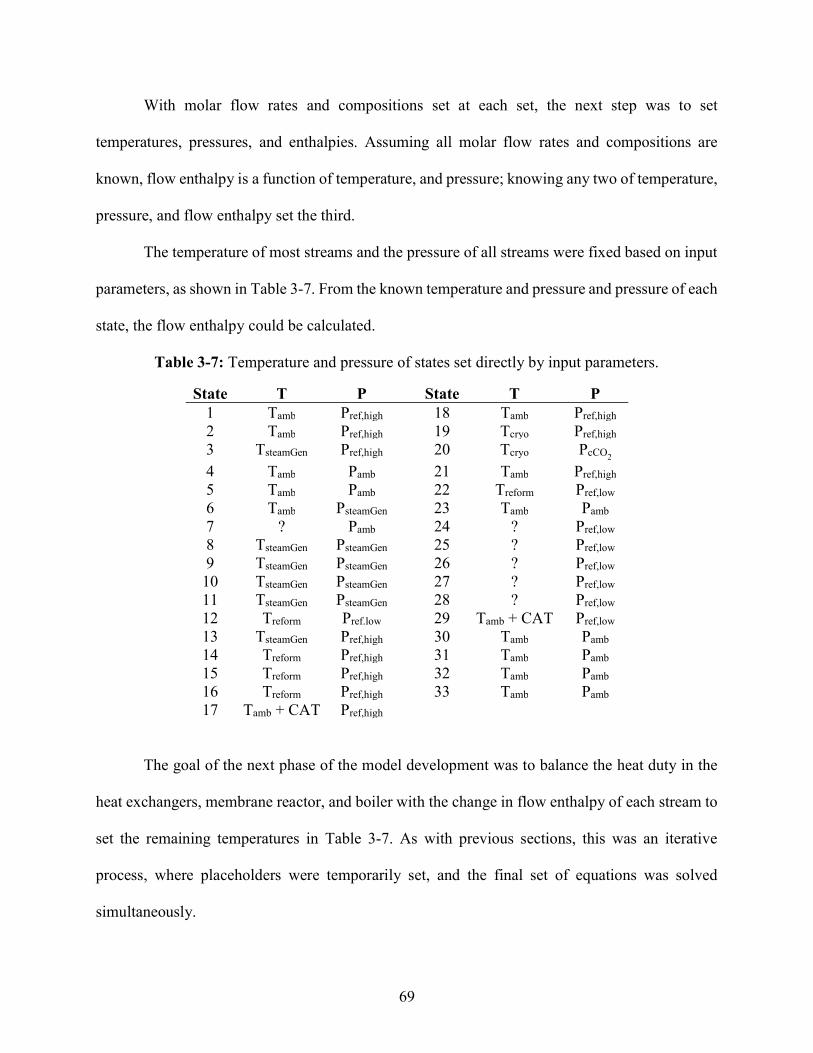
69

With molar flow rates and compositions set at each set, the next step was to set

temperatures, pressures, and enthalpies. Assuming all molar flow rates and compositions are

known, flow enthalpy is a function of temperature, and pressure; knowing any two of temperature,

pressure, and flow enthalpy set the third.

The temperature of most streams and the pressure of all streams were fixed based on input

parameters, as shown in Table 3-7. From the known temperature and pressure and pressure of each

state, the flow enthalpy could be calculated.

Table 3-7: Temperature and pressure of states set directly by input parameters.

State T P State T P 1 Tamb Pref,high 18 Tamb Pref,high 2 Tamb Pref,high 19 Tcryo Pref,high 3 TsteamGen Pref,high 20 Tcryo PcCO2 4 Tamb Pamb 21 Tamb Pref,high 5 Tamb Pamb 22 Treform Pref,low 6 Tamb PsteamGen 23 Tamb Pamb 7 ? Pamb 24 ? Pref,low 8 TsteamGen PsteamGen 25 ? Pref,low 9 TsteamGen PsteamGen 26 ? Pref,low

10 TsteamGen PsteamGen 27 ? Pref,low 11 TsteamGen PsteamGen 28 ? Pref,low 12 Treform Pref.low 29 Tamb + CAT Pref,low 13 TsteamGen Pref,high 30 Tamb Pamb 14 Treform Pref,high 31 Tamb Pamb 15 Treform Pref,high 32 Tamb Pamb 16 Treform Pref,high 33 Tamb Pamb 17 Tamb + CAT Pref,high

The goal of the next phase of the model development was to balance the heat duty in the

heat exchangers, membrane reactor, and boiler with the change in flow enthalpy of each stream to

set the remaining temperatures in Table 3-7. As with previous sections, this was an iterative

process, where placeholders were temporarily set, and the final set of equations was solved

simultaneously.

70

Returning to the H2 boiler in the SMR-MR-SG system, an energy balance was performed

to balance three heat flows: total heat input to the boiler in the form of hydrogen, heat out to steam,

and heat out to exhaust. The three were related by Equation (3.31) as well as Equations (3.63)

through (3.65):

boiler,fuel,input boiler,steam boiler,exh Q Q Q (3.63)

boiler,fuel,input 22 23 24,amb Q H H H (3.64)

boiler,steam 8 7 Q H H (3.65)

where Ḣ24,amb is the flow enthalpy of the boiler exhaust at ambient temperature and pressure. The

energy balance on HE 1 was expressed as a difference of enthalpies as in Equations (3.66) and

(3.67):

HE1 22 16 14 12 Q H H H H (3.66)

HE1 24 25 Q H H (3.67)

Similarly, the energy balance on heat exchanger 2 was performed by Equations (3.68) and (3.69):

HE2 12 11 Q H H (3.68)

HE2 25 26 Q H H (3.69)

The energy balance on heat exchanger 3 was calculated by Equations (3.70) and (3.71):

HE3 14 13 Q H H (3.70)

HE3 26 27 Q H H (3.71)

The energy balance on heat exchanger 4 was calculated by Equations (3.72) and (3.73):

HE4 3 2 Q H H (3.72)

HE4 27 28 Q H H (3.73)

71

The energy balance on HE 5 was different than the previous heat exchangers due to it being a

three-fluid heat exchanger. It was assumed that there was no interaction between the two hot fluids

(#16-17) and (#28-29). In other words, the increase in heat from the pressurized water supply (#6)

to the preheated boiler feed (#7) was calculated as the sum of heat loss from the retentate (#16) to

(#17) and from the boiler exhaust (#28) to (#29). The energy balance was calculated using

Equations (3.74) through (3.77):

HE5,total HE5,ret HE5,exh Q Q Q (3.74)

HE5,total 7 6 Q H H (3.75)

HE5,ret 16 17 Q H H (3.76)

HE5,exh 28 29 Q H H (3.77)

where the subscript ret refers to the retentate (#16-17) and exh refers to the boiler exhaust (#28-

29). The temperature and pressure of every state was now set, but not at quite the correct value:

the next section of the model ensured that no temperatures crossed within heat exchangers.

The inlet and outlet temperatures at each heat exchanger were checked. If temperatures

crossed, that was a problem that needed to be resolved. For example, the temperatures in HE 2 at

this point in the model development, before it was revised are shown in Table 3-8.

Table 3-8: Example of heat exchanger temperatures crossing during thermodynamic model development.

Inlet temperature [°C] (State Point)

Outlet temperature [°C] (State Point)

Cold Fluid 200 (#11)

400 (#12)

Hot Fluid 390 (#25)

365.1 (#26)

72

Here, the hot fluid inlet is less than the cold fluid outlet. Heat can only flow naturally from

a hot to cold temperature, so this represented an impossible condition. Since both cold fluid

temperatures were set permanently by model inputs, the problem was resolved by setting the hot

inlet to the cold outlet, plus the closest approach temperature (CAT). This is shown in Equation

(3.78):

26 14 T T CAT (3.78)

Adjustments like Equation (3.78) were made until no heat exchanger temperatures crossed. The

adjustments in the boiler exhaust temperature worked their way back upstream (#26, #25, #24,

etc.), effectively varying the H2 boiler efficiency iteratively until both the energy balances and

temperature constraints were satisfied.

At this point, every thermodynamic state in the system was fully defined. Next, several

calculations were made to evaluate parameters of interest such as overall efficiency and mass flow

rate of imports and exports. Some additional parameters were also calculated as inputs to the

technoeconomic model, such as total electrical work input.

The natural gas energy input was calculated with an enthalpy difference rather than lower

heating value (LHV) for consistency with the rest of the program. The energy input was based on

the stoichiometric, complete combustion of methane, given in Equation (3.79):

4 2 2 22 2 CH O H O CO (3.79)

The heat supplied by the natural gas supply (#1) was calculated based on the difference of flow

enthalpy (#1) and the ambient combustion products, shown in Equation (3.80):

NG,in 1 1,comb,amb Q H H (3.80)

where Ḣ1 was evaluated based on the known flow ṅ1,CH4 and the hypothetical amount of oxygen

needed to fully combust the methane, at temperature and pressure (#1). Ḣ1,comb,amb was evaluated

73

based on the molar flows of H2O and CO2 calculated by Equation (3.79), at ambient temperature

and pressure. As a check, the heat input from natural gas was also calculated using the higher

heating value (HHV) in Equation (3.81):

4 4NG,input,check 1,CH CH Q m HHV (3.81)

The heat from Equation (3.81) matched the heat from the heat from Equation (3.80) to within 1.7%

difference. The HHV was used instead of the LHV because the energy from steam condensation

was accounted for and utilized in the SMR-MR-SG system.

Likewise, a check was performed to ensure that the energy balance in the boiler was

accurate. Equation (3.82) evaluated the heat input to the H2 boiler using the higher heating value

(HHV) of hydrogen:

2 2boiler,fuel,input 22,H H Q m HHV (3.82)

Again, this check showed less than 2% deviation from Equation (3.63). Values for higher heating

value were supplied internally by EES.

The work output of the water pump and CO2 compressor were calculated based on enthalpy

changes, as in Equations (3.83) and (3.84):

pump,out 6 5 W H H (3.83)

comp,out 20 19 W H H (3.84)

The efficiencies of the pump, compressor, and cryogenic unit set the electrical input required for

the SMR-MR-SG system based on the calculated work out to the fluid, as in Equations (3.85) and

(3.86):

pump,outpump

pump,elec,in

W

W (3.85)

74

comp,outcomp

comp,elec,in

W

W (3.86)

The work of the cryogenic CO2 separation unit was evaluated based on Xu et al.’s model in

Equation (3.87) [91]:

2 2 2

1cryo,elec,in 19,CO CO425 COW MJ kg n M (3.87)

The actual work imparted to the fluid by the CSU was calculated by Equation (3.88):

cryo,out 18 19 21 W H H H (3.88)

The total electrical work into the system was calculated as the sum of the work inputs for pump,

compressor, and CSU via Equation (3.89):

elec,in,total pump,elec,in comp,elec,in cryo,elec,in W W W W (3.89)

The actual energy delivered to the fluid for the purpose of CO2 separation and compression was

defined by Equation (3.90):

2CO ,export 20,amb 20 Q H H (3.90)

where Ḣ20,amb was calculated the same way as Ḣ20,amb except at ambient temperature and pressure.

The pressure was dropped in the sweep steam from 15 bar (#10) to 2 bar (#11) without

recovering energy from the expansion. The energy lost was calculated by Equation (3.91):

sweep,ΔP 11,highP 11 Q H H (3.91)

where Ḣ11,highP was calculated the same as Ḣ11¸but at a pressure of 15 bar instead of 2 bar. This is

a source of waste heat that could be captured by a small steam turbine. However, the energy lost

in the sweep steam expansion is approximately 0.2% of the natural gas input. The additional

complexity and expense of adding a small turbine would vastly outweigh the potential energy

savings.

75

An overall boiler efficiency for the SMR-MR-SG was used as the most direct comparison

to the benchmark natural gas boiler, and was defined by Equation (3.92):

steam,exportoverall,boiler

NG,in elec,in

QQ W

(3.92)

where overall boiler efficiency is a simple indication of the percentage of utilized energy from the fuel

input. This is different than the H2 boiler efficiency, which characterized just the H2 boiler within the SMR-

MR-SG system.

3.2.4. Cost Calculations

The capital cost of the SMR-MR-SG system was calculated as the sum of its components.

Install factors for all three systems were neglected due to the comparative nature of the study. The

capital cost of the membrane reactor was calculated based on its surface area. The thickness of the

Pd-alloy membrane largely drives surface area, and hence the cost, of the membrane. A thicker

membrane obviously requires more Pd-alloy, but the effect is further compounded: for a given

hydrogen flux, a thicker membrane requires more surface area. As mentioned in the literature

review, membrane thicknesses as low as 0.93 µm have been achieved with no defects

[60,61,94,97]. This study used a conservative thickness of 2.8 µm, corresponding to a state-of-the-

art permeance of 6.48x10-3 mol m-2 s-1 Pa-0.5, calculated from the permeability of 4.1×10-8 mol m-

1 s-1 Pa-0.5 divided by membrane thickness [12,92,94].

The membrane surface area was calculated using H2 permeating flux through the

membrane, H2 partial pressure on both sides of the membrane, and membrane thickness. Assuming

that solution-diffusion is the governing transport mechanism for hydrogen flux, the surface area is

calculated by rearranging Equation (2.8) into Equation (3.93) [22]:

2H ,memmem

mem ret per

n n

nA

K P P (3.93)

76

The dependent factor n is a parameter that correlates the permeating flux with the driving

force. When the membrane is defect-free and it shows ‘infinite’ perm-selectivity towards H2, n

assumes a value of 0.5. Note that any degradation factor requiring additional membrane surface

area because of recycled gas is implicit in the thermodynamic model. Additional recycled gas

(from inefficiency in methane conversion, hydrogen recovery, or carbon dioxide capture) dilutes

the hydrogen on the feed side of the membrane, changing the partial pressure of hydrogen and thus

the driving force for permeation. Therefore, an increase in amount of recycled gas does have an

effect on the required membrane surface area and thus on the capital cost. The effect is not

necessarily negative; un-permeated hydrogen can be recycled, which increases driving force

through the membrane.

This study uses a combination of “best-case” values of MR parameters from literature. It

is assumed that, at a larger scale implementation of the SMR-MR-SG, scaling factors would allow

for reduced material and fabrication costs. For example, a tube in tube configuration for a

membrane reactor is useful for laboratory scale experiments, but new designs to increase surface

area to volume ratio are necessary at the industrial scale [48].

The capital cost of Pd-based membranes is significantly affected by both material cost and

fabrication method. The material cost of Palladium is relatively unpredictable, ranging between

$3,500 and $45,000 per kg over the last 20 years [98]. Recently, novel fabrication techniques have

rapidly dropped Pd membrane costs down to as low as $100 per ft2 ($1,076 per m2) [50,99,100].

The membrane cost was calculated by Equation (3.94):

membrane mem 2

$1,076 CapEx A

m (3.94)

The reactor (i.e., the membrane reactor minus the membrane) cost was calculated using a scaling

factor and a known cost of $14,100 corresponding to 4.79 kgH2 h-1 [22] via Equation (3.95):

77

2

0.7H

reactor 1$14,1004.79

mCapEx

kg h (3.95)

The cost of each heat exchanger was calculated based on its required heat transfer area

using the method of Brown [86]. The calculations to determine required heat transfer area were

completed using the epsilon-NTU method described by Bergman et al. [90]. The working units of

flow were kmol s-1 rather than the more customary kg s-1 due to the modeling of chemical reactions

throughout the model. As a result, fluid properties were in molar units (e.g., units of specific heat

were kJ kmol-1 K-1). The process of calculating required heat exchanger surface areas is described

in detail in APPENDIX B to avoid distraction from the cost calculations. The capital cost of each

heat exchanger was calculated directly from the heat transfer surface area (in square feet), using

Equation (3.96):

0.52

HE ht,hot 2

10.76$462

ftCapEx Am

(3.96)

Heat exchanger 5 was more complicated for two reasons: it involved flow boiling, and it

used three fluids (instead of two). Heat exchanger 5 was split up into two sections: preheating

liquid water to saturation temperature, and boiling from saturated liquid to two-phase with 0 < X

< 1. Each section of the heat exchanger was sized independently, and a cost for each was calculated

using Equation (3.96). The separate parts of heat exchanger 5 (preheating and boiling) were added

and multiplied by a factor of 1.5 to account for the added complexity of a three-fluid heat

exchanger [101]. The total capital cost of heat exchanger 5 was calculated by Equation (3.97):

HE5,total HE5,preheat HE5,boil1.5 CapEx CapEx CapEx (3.97)

The capital cost for the H2 boiler within the SMR-MR-SG system was calculated using

Equation (3.98) [22]:

78

0.67

boiler,inputboiler $44,000

2

QCapEx

MW (3.98)

Similarly, the capital cost of the water pump was calculated by Equation (3.99) [22]:

0.7

waterpump 1$1,200

90

VCapExL h

(3.99)

The capital cost of each condenser was calculated by Equation (3.100) [88]:

0.3820181987 cond

198cond

7

$ 213 £3.£

75 CapEx Q (3.100)

The capital cost of the cryogenic CO2 separator was calculated using Equation (3.101) [22]:

2

2

0.7

COCryo 1

CO

$475,0000.6 t

mCapEx

h (3.101)

Similarly, the cost of the CO2 compressor was calculated using Equation (3.102) [22]:

0.7

compcomp $3,000,000

6 MW

WCapEx (3.102)

The operating cost of the cryogenic CO2 separator, CO2 compressor, and water pump were

calculated based on their required input work and the cost of electricity using Equations (3.103)

through (3.105):

Cryo cryo,in elecPrice OpEx W (3.103)

comp comp,in elecPrice OpEx W (3.104)

pump pump,in elecPrice OpEx W (3.105)

The operating and maintenance cost of the membrane reactor system in $ yr-1 was assumed to be

5% of the total capital expense in $ [50], calculated in Equation (3.106):

SMR,system SMR,system0.05 OpEx CapEx (3.106)

79

This operating expense includes the cost of replacing membranes approximately every three years

[22]. The cost of procurement, assembly, and installation can add an additional 42.5% on top of

the base capital cost [101,102]; these costs weren’t considered for all three systems because similar

values would be anticipated for similar system functions

3.3. CO2 Capture

In the SMR-MR-SG system, the combination of high pressure (15 bar) and high CO2

concentration (53.1%) in the dehydrated retentate (#18) allows an extremely low energy penalty

for CO2 capture via cryogenic separation [91]. Cryogenic separation uses a series of simple,

industry proven steps (i.e., refrigeration and distillation) to cool the gas mix until CO2 liquifies,

then separate CO2 out by distillation. In addition to achieving a low energy penalty, cryogenic

separation has been shown to achieve 99.9% CO2 purity after separation with a 90% CO2 capture

efficiency [91].

A large difference between the SMR-MR-SG and the BSC is the concentration of CO2

prior to capture: 53.1% in the SMR-MR-SG retentate versus 11.5% in the BSC exhaust. The

penalty for CCC using a CSU increases exponentially with decreasing CO2 concentration due to

lowered phase transition temperature and increasingly expensive cold-tolerant equipment. Thus,

cryogenic separation is not a reasonable choice for the BSC because of its low CO2 concentration.

Additionally, attempting cryogenic separation on low CO2 concentration gas would result in high

levels of impurities, preventing the CO2 from being sold [91].

The most effective method of CO2 separation from the BSC is a form of amine scrubbing:

monoethanolamine absorption (MEA) [103]. MEA is a mature technology used for removing CO2

from flue gas or other low temperature, low concentration sources via chemical absorption. It can

capture 90% of CO2 with 98% purity in the product, but at great cost: the energy penalty of MEA

80

for the BSC is 3.9 MJ kg CO2-1, 818% more than the cryogenic penalty of 0.425 MJ kg CO2

-1 in the

SMR-MR-SG. The large difference in energy penalty is due to the disparity in CO2 concentration

in the gas to be separated.

Both CO2 separation systems, CSU and MEA, add additional capital, O&M and operating

cost in the form of electricity purchased from the grid. However, the most profound difference

between the two is the large energy penalty of MEA. Technoeconomic modeling assumed that the

entire energy penalty of CCC in each system was incurred in additional electricity usage.

3.4. Technoeconomic Comparison

A technoeconomic model was developed to determine whether the proposed SMR-MR-

SG system could compete economically with a state-of-the-art steam boiler, with and without CO2

capture. The technoeconomic model was also utilized to perform a sensitivity analysis, detailed in

Section 4.3. Membrane reactor technology studies often include sensitivity analyses, but they are

rarely tied to economics. This technoeconomic model, coupled with the thermodynamic model

from the previous section, provides a useful tool for directing future research on a financially

beneficial route.

3.4.1. Baseline for Comparison

The three systems were compared economically using a discounted cash flow model.

Commodity costs were defined using historical data and forecasts. The electricity, NG, and water

prices were set at the current industrial costs, with historical variations accounted for in the

sensitivity analysis. This paper defines “purchase price” as the price a plant would pay to acquire

the commodity and “sale price” as the amount of money a plant would receive for selling a

commodity to another entity. All prices were considered at the industrial scale, as opposed to

commercial or residential.

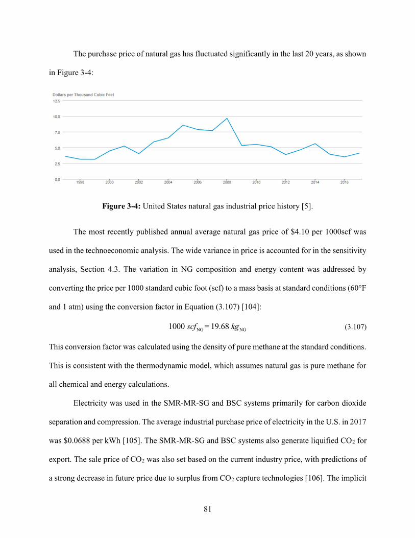
81

The purchase price of natural gas has fluctuated significantly in the last 20 years, as shown

in Figure 3-4:

Figure 3-4: United States natural gas industrial price history [5].

The most recently published annual average natural gas price of $4.10 per 1000scf was

used in the technoeconomic analysis. The wide variance in price is accounted for in the sensitivity

analysis, Section 4.3. The variation in NG composition and energy content was addressed by

converting the price per 1000 standard cubic foot (scf) to a mass basis at standard conditions (60°F

and 1 atm) using the conversion factor in Equation (3.107) [104]:

NG NG1000 = 19.68 scf kg (3.107)

This conversion factor was calculated using the density of pure methane at the standard conditions.

This is consistent with the thermodynamic model, which assumes natural gas is pure methane for

all chemical and energy calculations.

Electricity was used in the SMR-MR-SG and BSC systems primarily for carbon dioxide

separation and compression. The average industrial purchase price of electricity in the U.S. in 2017

was $0.0688 per kWh [105]. The SMR-MR-SG and BSC systems also generate liquified CO2 for

export. The sale price of CO2 was also set based on the current industry price, with predictions of

a strong decrease in future price due to surplus from CO2 capture technologies [106]. The implicit

82

assumption is that all captured CO2 can be readily sold at the assumed market price of $20 per ton.

Alternatively, the CO2 could be used directly for another in-house application instead of

purchasing CO2, effectively reducing the operating cost by the same $20 per ton.

Carbon tax is a financial cost imposed on a plant that produces CO2 emissions,

incentivizing reduced emissions. A mid-case prediction of carbon tax came in at an average of

$50.50 per ton of CO2 between 2020 and 2050 [107]. This study assumed that, rather than the

consumers of electricity being responsible for carbon emissions due to electricity generation, the

electricity plant would pay the direct costs. The same was assumed for NG: the tax on carbon

emissions due to the production and refinement of NG would be paid by the third party producers.

This assumption is consistent with the thermodynamic models where each system pays a carbon

tax only on the CO2 emissions that it produces directly. The social cost implications will be

discussed in the technoeconomic results, section 4.24.1.

Steam generation plants require a supply of water to generate steam. The cost of water was

set at $0.282 per m3 ($2.828x10-3 per kg) [22]. It was assumed that process steam was a required

commodity, and the system that can produce it with the least cost was most beneficial. Thus, no

sale price of steam is considered, and the three systems are compared based on relative cost of

steam production.

The annual discount rate and lifespan were chosen based on a similar technoeconomic

analysis of MRs by Sjardin et al. [22]. A 20-year lifespan is reasonable for industrial boilers, but

not for MRs. A typical MR has a life span of 1.3 - 4.7 years [22], but the O&M cost for the SMR-

MR-SG includes the cost of replacing the MR every three years as well as regular maintenance on

the rest of the system [22]. The load factor determines how many hours per year each system

operates. The International Energy Agency suggests a load factor of 90.5% [69].

83

3.4.2. Cash Flow Analysis

The economic comparison used a discounted cash flow analysis. Operating expenses and

income due to sale or purchase of commodities were calculated for each system. The price of

natural gas was converted from standard cubic feet to kilograms based on the conversion of

Equation (3.107), rearranged into Equation (3.108):

1NG

1000Price 4.10 $ 100019.68

scfscfkg

(3.108)

The cost associated with consumption of natural gas, water, and electricity, as well as taxed exhaust

of carbon dioxide were calculated for each system as applicable. The value of each cost or revenue

is just a positive magnitude here for simplification; the proper signs will be applied in the net

income calculations below. Equations (3.109) through (3.112) show the operating cost and revenue

calculations that were applied to each system:

2 2 2CO sale cCO operating cCORev Price m t (3.109)

NG NG operating NGPrice OpEx m t (3.110)

water water operating waterPrice OpEx m t (3.111)

elec elec operating elecPrice OpEx W t (3.112)

2 2CO ,tax CO ,exh operating CarbonTaxPrice OpEx m t (3.113)

Next, the total operating cost for each system was calculated in $ yr-1 using Equations (3.115) and

(3.114):

SMR,total SMR,system SMR,NG SMR,water SMR,elec& OpEx O M OpEx OpEx OpEx (3.114)

2BS,total BS,system BS,NG BS,CO tax BS,water& OpEx O M OpEx OpEx OpEx (3.115)

2BSC,total BSC,system BSC,NG BSC,CO tax BSC,water& OpEx O M OpEx OpEx OpEx (3.116)

84

The net income per year is given by revenues minus expenses, calculated in Equations (3.117)

through (3.119):

2SMR,net SMR,CO sale SMR,totalRev Income OpEx (3.117)

BS,net BS,totalIncome OpEx (3.118)

2BSC,net BSC,CO sale BSC,totalRev Income OpEx (3.119)

With all variations of input parameters, the SMR system had the highest capital cost but

the lowest operating costs due to its high efficiency. Therefore, the metrics used to quantify the

desirability of the SMR-MR-SG system relative to the other systems were the payback period, net

present value (NPV), and discounted cost reduction (DCR). The payback period is defined as the

time in years when the SMR-MR-SG surpasses the other systems in value. For a lifetime longer

than the payback period, the SMR-MR-SG system is more desirable. The NPV represents the

lifetime cost of each system, accounting for the time value of money. The DCR is the difference

in NPV of the SMR-MR-SG versus each of the other two systems, normalized by original (higher)

cost.

In the discounted cash flow analysis, the future value (FV) of each system was calculated

each year as the sum of revenues minus expenses. In year 0, the capital expense was the only

transaction, given in Equations (3.120):

0 totalFV CapEx (3.120)

The future value for each subsequent year was equal to the net income, shown in Equations (3.121)

:

n netFV Income (3.121)

The equation used for present value at each year is given by Equation (3.122):

85

nn 1

nFVPV

dr (3.122)

where n is the year number and the discount rate (dr) was assumed to be 12% based on a similar

technoeconomic study by Sjardin et al. [22]. The NPV was calculated as the sum of present values

of each year, as in Equation (3.123):

n0

lifespan

nNPV PV (3.123)

DCR relative to the BS is defined as the percent reduction in NPV, given in Equation (3.124):

BS DCRBS

BS

NPV NPVDCRNPV

(3.124)

The DCR relative to the BSC is defined similarly. DCR is a key parameter: it shows the economic

benefit of the SMR-MR-SG, normalized by discounted lifetime cost of the BS or BSC. The results

of the technoeconomic are presented in section 4.2. The following chapter will explain results of

the coupled models and discuss the implications.

86

Results and Discussion

The coupled thermodynamic and technoeconomic model described in Chapter 3 fully

defined the SMR-MR-SG process flow cycle shown in Figure 3-1. Most academic studies of

membrane reformer and steam methane reforming technology focuses on a small aspect of the

thermodynamic performance. This work performed a system level analysis with an emphasis on

economic feasibility. This chapter will discuss the thermodynamic results first, highlighting the

performance of the SMR-MR-SG system, the relative energy use of each of the three SG systems,

and possible variations on the SMR-MR-SG cycle. The technoeconomic results follow, with a

comparison of the three systems’ lifetime costs. Finally, a sensitivity analysis discusses the key

assumptions and parameters that have large effects on the model.

4.1. Thermodynamic Results

4.1.1. Process States and Energy Balances

The full list of state points corresponding to the process flow diagram of Figure 3-1 is

shown in Table 4-1. The state points were significantly influenced by the temperature and pressure

of the export steam. This is a development in SMR and MR technology: traditional systems

optimize reforming and H2 separation, while this study focused on the steam generation process

and worked in a SMR-MR system around those constraints.

87

Table 4-1: Thermodynamic state points for SMR steam generation system.

State T P Ḣ ṅtotal yH2 yCH4 yH2O yCO2 yN2 yO2

No. °C bar kW mol s-1 - - - - - - 1 15 15 -75.8 1.01 0 1 0 0 0 0 2 15 15 -153.6 2.11 0.212 0.735 0 0.053 0 0 3 200 15 -138.8 2.11 0.212 0.735 0 0.053 0 0 4 15 1 -451.7 1.62 0 0 1 0 0 0 5 15 1 -6798.5 24.37 0 0 1 0 0 0 6 15 15 -6798 24.37 0 0 1 0 0 0

7 198.3 15 (X=0.369) -6278.4 24.37 0 0 1 0 0 0

8 200 15 -5615.4 24.37 0 0 1 0 0 0 9 200 15 -4186.9 18.17 0 0 1 0 0 0

10 200 15 -1071.4 4.65 0 0 1 0 0 0 11 200 2 -355.5 1.55 0 0 1 0 0 0 12 400 2 -344.1 1.55 0 0 1 0 0 0 13 200 15 -1208.2 6.76 0.066 0.229 0.688 0.017 0 0 14 400 15 -1152.6 6.76 0.066 0.229 0.688 0.017 0 0 15 400 15 -918.3 8.77 0.51 0.062 0.3 0.128 0 0 16 400 15 -1026.6 4.74 0.094 0.114 0.555 0.236 0 0 17 20 15 -1208.3 4.74 0.094 0.114 0.555 0.236 0 0 18 15 15 -475 2.11 0.212 0.257 0 0.531 0 0 19 -51.14 7.959 -414.8 1.01 0 0 0 1 0 0 20 15 75 -408.5 1.01 0 0 0 1 0 0 21 15 15 -77.8 1.1 0.406 0.492 0 0.102 0 0 22 400 2 -236 5.58 0.722 0 0.278 0 0 0 23 15 1 261.7 9.59 0 0 0 0 0.79 0.21 24 912.6 2 -637.4 13.16 0 0 0.424 0 0.576 0 25 429.9 2 -871.4 13.16 0 0 0.424 0 0.576 0 26 405 2 -882.8 13.16 0 0 0.424 0 0.576 0 27 281.4 2 -938.4 13.16 0 0 0.424 0 0.576 0 28 247.8 2 -953.3 13.16 0 0 0.424 0 0.576 0 29 20 2 -1291.1 13.16 0 0 0.424 0 0.576 0 30 15 1 262.2 7.58 0 0 0 0 1 0 31 15 1 -1556.5 5.58 0 0 1 0 0 0 32 15 1 -735 2.63 0 0 1 0 0 0 33 15 1 -4055.2 14.53 0 0 1 0 0 0

After adjusting temperatures to avoid pinch points by a margin of the CAT, the temperature

changes in each heat exchanger are shown in Figure 4-1.

88

Figure 4-1: Pinch points of heat exchangers in steam methane reformer steam generation cycle.

The two most significant pinch points are at the hot side of heat exchanger 2 and cold side

of heat exchanger 5. In heat exchanger 2, the states (#12) and (#25) are separated only by the CAT.

This effectively set the energy balance in the boiler: state (#24) must be at a high enough

temperature for (#25) to remain above the reforming temperature of (#12) while supplying the heat

of the reforming reaction. The implication is that the low reforming temperature, 400°C, is key to

allow heat recovery from low temperature sources and achieve a high system efficiency. For

example, a conventional SMR uses a reforming temperature of ~900°C and would be able to

extract only 1.4% of the available boiler exhaust heat (#24) to supply the reforming reaction [11],

compared to 56.6% in the SMR-MR-SG system. There is a practical upper limit on the boiler

exhaust temperature due to the high concentration of steam mixed with the H2 entering the boiler

for combustion.

89

4.1.2. Comparison of Energy Consumption

Key results of the thermodynamic analysis are shown in Table 4-2.

Table 4-2: Relative thermodynamic comparison of SMR-MR-SG and boiler systems.

BS System BSC System

Parameter Units SMR-MR-SG System Result SMR-MR-SG

Improvement Result SMR-MR-SG Improvement

Equivalent boiler efficiency % 97.0 86 12.8% 72.4 34.0%

Water Use ton yr-1 1,014 2,276 55.4% 809 -25.3% Energy Use kW 910 1,026 11.3% 1,218 25.2%

Natural Gas Use ton yr-1 883 1,026 13.9% 1,026 13.9% Electricity Use kW 27 0 - 192 85.9% CO2 Emissions ton yr-1 0 1,791 - 179 -

cCO2 Sale ton yr-1 1,541 0 - 1,612 -0.4%

The improvement of the SMR-MR-SG over the BS for each parameter was calculated as

the change in value divided by the baseline (BS or BSC), shown in Equation (4.1):

SMR BS

BS

Improvement

Val ValVal

(4.1)

The appropriate sign was applied to the numerator of Equation (4.1) depending on the value in

question. The improvement relative to the BSC was calculated similarly. Equivalent boiler

efficiency refers to the system-level definition of output energy (export steam) divided by input

energy. The SMR-MR-SG shows large improvements over both the BS and BSC in efficiency

(12.8% and 34.0% improvement) and thus total energy use (11.3% and 25.2%), respectively.

Water use is improved by 55.4% over the BS, but the SMR-MR-SG uses 25.3% more water than

the BSC. This is because the BSC has the water-recycling benefits of CCC (i.e., the exhaust is

completely dehydrated before CO2 separation), plus there is no need for excess steam for

reforming. The SMR-MR-SG is the only system to achieve zero CO2 emissions. This is made

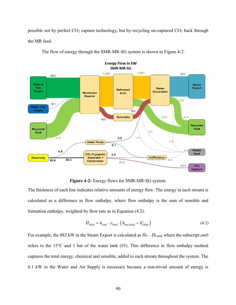
90

possible not by perfect CO2 capture technology, but by recycling un-captured CO2 back through

the MR feed.

The flow of energy through the SMR-MR-SG system is shown in Figure 4-2.

Figure 4-2: Energy flows for SMR-MR-SG system.

The thickness of each line indicates relative amounts of energy flow. The energy in each stream is

calculated as a difference in flow enthalpy, where flow enthalpy is the sum of sensible and

formation enthalpy, weighted by flow rate as in Equation (4.2):

fluid total fluid sens,fluid f,fluid oH n y h h (4.2)

For example, the 882 kW in the Steam Export is calculated as Ḣ9 – Ḣ9,amb where the subscript amb

refers to the 15°C and 1 bar of the water tank (#5). This difference in flow enthalpy method

captures the total energy, chemical and sensible, added to each stream throughout the system. The

6.1 kW in the Water and Air Supply is necessary because a non-trivial amount of energy is

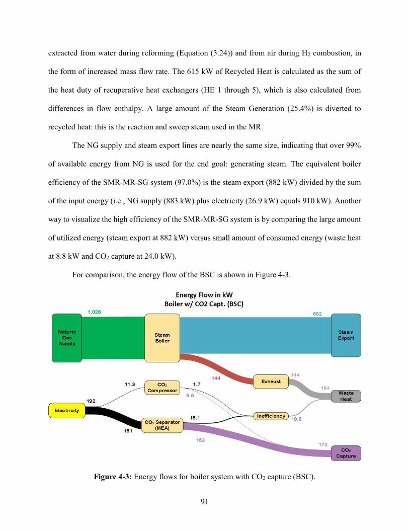
91

extracted from water during reforming (Equation (3.24)) and from air during H2 combustion, in

the form of increased mass flow rate. The 615 kW of Recycled Heat is calculated as the sum of

the heat duty of recuperative heat exchangers (HE 1 through 5), which is also calculated from

differences in flow enthalpy. A large amount of the Steam Generation (25.4%) is diverted to

recycled heat: this is the reaction and sweep steam used in the MR.

The NG supply and steam export lines are nearly the same size, indicating that over 99%

of available energy from NG is used for the end goal: generating steam. The equivalent boiler

efficiency of the SMR-MR-SG system (97.0%) is the steam export (882 kW) divided by the sum

of the input energy (i.e., NG supply (883 kW) plus electricity (26.9 kW) equals 910 kW). Another

way to visualize the high efficiency of the SMR-MR-SG system is by comparing the large amount

of utilized energy (steam export at 882 kW) versus small amount of consumed energy (waste heat

at 8.8 kW and CO2 capture at 24.0 kW).

For comparison, the energy flow of the BSC is shown in Figure 4-3.

Figure 4-3: Energy flows for boiler system with CO2 capture (BSC).

92

Both energy flow figures use the same steam export energy (882 kW) to allow for a direct

comparison. The water and air supply term is not included in the BSC energy flow because there

is no reforming reaction. The input energy in the BSC (NG and electricity at 1,026 + 192 = 1,218

kW) is 33% higher than the SMR-MR-SG. Again, efficiency is calculated as steam export (882

kW) divided by input energy (1,218 kW), which results in a 72.4% efficiency for the BSC system.

This is simply the BS efficiency of 86%, reduced by the CCC energy penalty.

The large difference in efficiency between the SMR-MR-SG and BSC is due to more

effective heat recovery and lower CCC energy penalty in the SMR-MR-SG. Heat recovery could

be improved in the BSC; this will be addressed below in the technoeconomic subsection. The CCC

energy penalty is defined by Equation (4.3):

out,w/ CCC out,w/o CCCCCC

out,w/o CCC

E E

PE

(4.3)

The CCC energy penalty indicates the reduction in net output power of the plant due to CCC,

normalized by the original output power. The SMR-MR-SG and BSC have CCC energy penalties

of 3.0% and 16.4%, respectively. This is a key point: the high CO2 concentration in the SMR-MR-

SG retentate (#18) allows the use of CSU, whereas the BSC system requires MEA for CO2 capture

due to low CO2 concentration in the exhaust. Cryogenic separation is simple and efficient, with

most of the energy penalty incurred running a refrigeration cycle. On the other hand, MEA is more

complex, requiring electricity for solvent regeneration (accounting for 55% of MEA energy

consumption), CO2 compression, process pumping, and blowers [83]. These factors add up to

make the CCC energy penalty via MEA over 9 times more than via CSU.

Table 4-3 shows a comparison of state-of-the-art technologies that use a fossil fuel source

and capture CO2 to put these energy penalties into context.

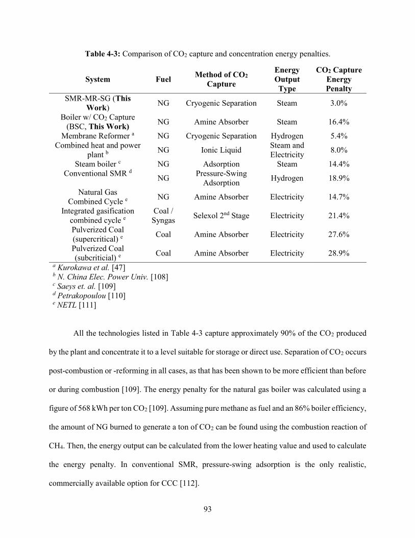
93

Table 4-3: Comparison of CO2 capture and concentration energy penalties.

System Fuel Method of CO2 Capture

Energy Output Type

CO2 Capture Energy Penalty

SMR-MR-SG (This Work) NG Cryogenic Separation Steam 3.0%

Boiler w/ CO2 Capture (BSC, This Work) NG Amine Absorber Steam 16.4%

Membrane Reformer a NG Cryogenic Separation Hydrogen 5.4% Combined heat and power

plant b NG Ionic Liquid Steam and Electricity 8.0%

Steam boiler c NG Adsorption Steam 14.4% Conventional SMR d

NG Pressure-Swing Adsorption Hydrogen 18.9%

Natural Gas Combined Cycle e NG Amine Absorber Electricity 14.7%

Integrated gasification combined cycle e

Coal / Syngas Selexol 2nd Stage Electricity 21.4%

Pulverized Coal (supercritical) e Coal Amine Absorber Electricity 27.6%

Pulverized Coal (subcriticial) e Coal Amine Absorber Electricity 28.9%

a Kurokawa et al. [47] b N. China Elec. Power Univ. [108] c Saeys et. al. [109] d Petrakopoulou [110] e NETL [111]

All the technologies listed in Table 4-3 capture approximately 90% of the CO2 produced

by the plant and concentrate it to a level suitable for storage or direct use. Separation of CO2 occurs

post-combustion or -reforming in all cases, as that has been shown to be more efficient than before

or during combustion [109]. The energy penalty for the natural gas boiler was calculated using a

figure of 568 kWh per ton CO2 [109]. Assuming pure methane as fuel and an 86% boiler efficiency,

the amount of NG burned to generate a ton of CO2 can be found using the combustion reaction of

CH4. Then, the energy output can be calculated from the lower heating value and used to calculate

the energy penalty. In conventional SMR, pressure-swing adsorption is the only realistic,

commercially available option for CCC [112].

94

Several coal fired plants were considered to show that the CCC energy penalty is

significantly worse than in natural gas fired plants. As an interesting aside, the addition of CCC

almost doubles water usage in coal and NG power plants [111], while the SMR-MR-SG reduces

water consumption relative to the baseline boiler system by 55.5%.

The system with the energy penalty closest to the SMR-MR-SG system is a membrane

reformer with cryogenic separation of CO2 developed by Kurokawa et al [47]. The authors report

a 3% energy penalty resulting in over 90% CO2 capture in reactor off-gas, but only a 50% reduction

in total CO2 emissions. The penalty of 5.4% was extrapolated by setting total CO2 emissions to

90%. The SMR-MR-SG achieves a much lower energy penalty than Kurokawa’s system by

recycling un-captured CO2 via stream (#21). After water is removed from the retentate (#18), the

majority of the remaining gas is CO2. Rather than focus on maximizing CO2 separation with

diminishing returns of capture efficiency versus cost, only ~90% of CO2 is captured via the CSU,

and the rest (#21) is mixed with the natural gas supply (#1). Diluting the feed with CO2 reduces

methane conversion and hydrogen capture, but the effect is minimal at 90% CO2 capture. With

CO2 recycling, the SMR-MR-SG system has 100% effective CO2 capture because the CO2 is

recycled until it is captured.

One major difference between the SMR-MR-SG and most other systems in Table 4-3 is

that the SMR-MR-SG produces heat for steam, while others produce electricity or hydrogen. In

these cases, heat is an intermediate product and the additional energy conversion from heat to

energy output is a source of energy loss that is avoided in the SMR-MR-SG. This is an important

point to consider when developing energy systems that utilize NG: co-location of end use and NG

consumption could be critical in providing economic benefit for systems that capture carbon.

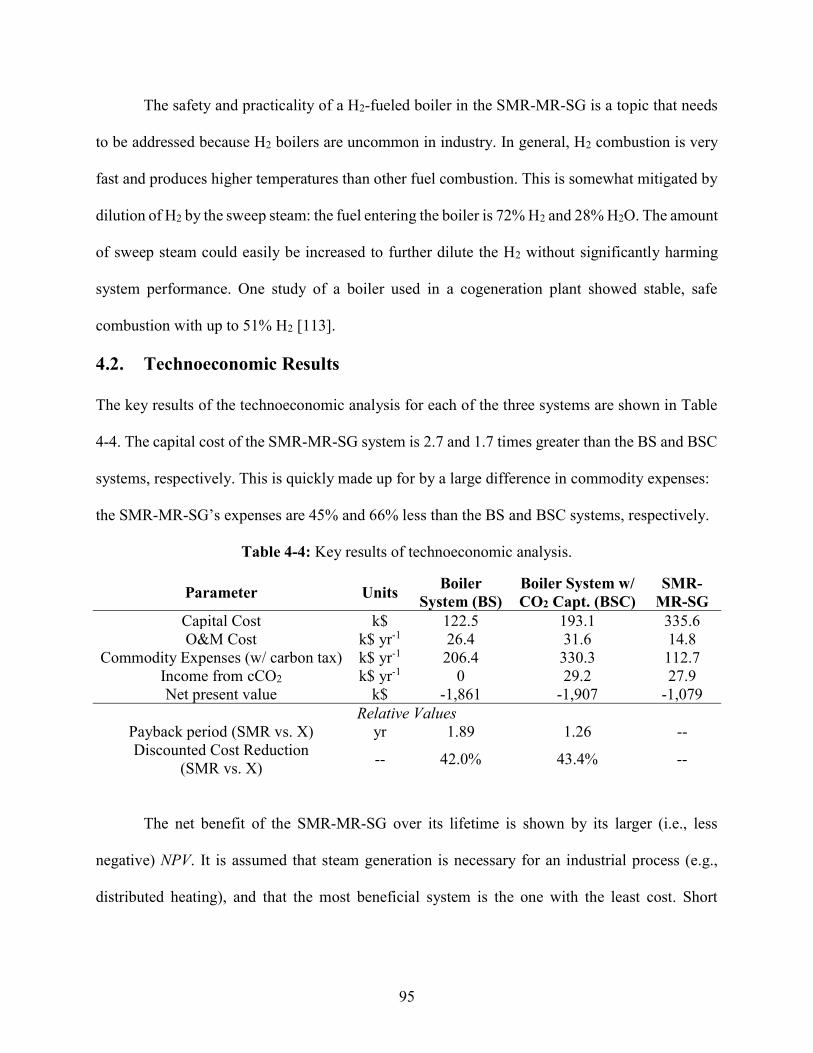
95

The safety and practicality of a H2-fueled boiler in the SMR-MR-SG is a topic that needs

to be addressed because H2 boilers are uncommon in industry. In general, H2 combustion is very

fast and produces higher temperatures than other fuel combustion. This is somewhat mitigated by

dilution of H2 by the sweep steam: the fuel entering the boiler is 72% H2 and 28% H2O. The amount

of sweep steam could easily be increased to further dilute the H2 without significantly harming

system performance. One study of a boiler used in a cogeneration plant showed stable, safe

combustion with up to 51% H2 [113].

4.2. Technoeconomic Results

The key results of the technoeconomic analysis for each of the three systems are shown in Table

4-4. The capital cost of the SMR-MR-SG system is 2.7 and 1.7 times greater than the BS and BSC

systems, respectively. This is quickly made up for by a large difference in commodity expenses:

the SMR-MR-SG’s expenses are 45% and 66% less than the BS and BSC systems, respectively.

Table 4-4: Key results of technoeconomic analysis.

Parameter Units Boiler System (BS)

Boiler System w/ CO2 Capt. (BSC)

SMR-MR-SG

Capital Cost k$ 122.5 193.1 335.6 O&M Cost k$ yr-1 26.4 31.6 14.8

Commodity Expenses (w/ carbon tax) k$ yr-1 206.4 330.3 112.7 Income from cCO2 k$ yr-1 0 29.2 27.9 Net present value k$ -1,861 -1,907 -1,079

Relative Values Payback period (SMR vs. X) yr 1.89 1.26 -- Discounted Cost Reduction

(SMR vs. X) -- 42.0% 43.4% --

The net benefit of the SMR-MR-SG over its lifetime is shown by its larger (i.e., less

negative) NPV. It is assumed that steam generation is necessary for an industrial process (e.g.,

distributed heating), and that the most beneficial system is the one with the least cost. Short

96

payback periods versus both boiler systems show that an investment in SMR-MR-SG instead of a

boiler would yield financial benefit in under 2 years.

The capital cost of the CSU in the SMR-MR-SG system was very high relative to other

components, making up 59.9% of the total system capital cost. To ensure that this estimate was

reasonable, another source was used to verify the calculation of the CSU CapEx. Xu et al. reported

a total cryogenic system cost of $29.872M at a scale of 76.18 kg s-1 captured CO2, with a scale

factor of 0.67 [91]. The calculated cost using Xu’s method differed from the calculation in this

study by only 0.8%.

The capital expense of the SMR-MR-SG could be reduced by pursuing less expensive CSU

development. Alternatively, higher values of methane conversion and hydrogen permeation would

create a higher concentration of CO2 in the retentate. For example, setting both parameters to 95%

would increase the CO2 concentration in the dehydrated retentate (stream #18) to 81%. Depending

on the application that the captured CO2 is intended for, very high values of methane conversion

and hydrogen permeation might produce a CO2 concentration high enough that it does not require

separation, eliminating the CSU. Future investigations will explore this possibility.

The cost breakdown of each system is shown in Figure 4-4.

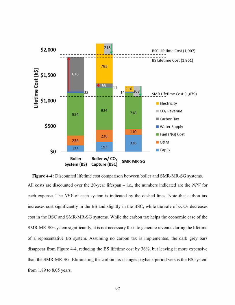
97

Figure 4-4: Discounted lifetime cost comparison between boiler and SMR-MR-SG systems.

All costs are discounted over the 20-year lifespan – i.e., the numbers indicated are the NPV for

each expense. The NPV of each system is indicated by the dashed lines. Note that carbon tax

increases cost significantly in the BS and slightly in the BSC, while the sale of cCO2 decreases

cost in the BSC and SMR-MR-SG systems. While the carbon tax helps the economic case of the

SMR-MR-SG system significantly, it is not necessary for it to generate revenue during the lifetime

of a representative BS system. Assuming no carbon tax is implemented, the dark grey bars

disappear from Figure 4-4, reducing the BS lifetime cost by 36%, but leaving it more expensive

than the SMR-MR-SG. Eliminating the carbon tax changes payback period versus the BS system

from 1.89 to 8.05 years.

98

An interesting effect of carbon capture is that it reduces the lifetime cost of the SMR-MR-

SG system. This is the result of a two-fold effect of CO2 capture: without it, there is a large cost

increase due to carbon tax, plus the lost revenue from sale of cCO2. This is partially offset by

avoiding the capital cost of the CSU, but the difference in operating costs far outweighs the capital

cost. This is not true for most other systems (i.e., BSC system), because the energy and economic

penalties are much higher.

The efficiency of the boiler systems could be improved beyond 86% by adding additional

heat exchangers and more complicated system flow paths to capture low temperature heat. A

hypothetical BSC with higher efficiency (BSC-H) could have a 97% efficiency to match the SMR-

MR-SG with an optimistic increase in capital cost of only 10% [66,68]. The effect on the BSC

column of Figure 4-4 would be that the light blue, capital expense, would increase by $19k while

the green, fuel cost, would decrease by $116k. The BSC-H discounted lifetime cost would be

reduced to $1,810k, still 68% more expensive than the SMR-MR-SG. The MEA energy and

economic penalties for CO2 capture in the BSC are very high and increases in boiler efficiency

only slightly offsets the cost of CCC. The same hypothetical, high-efficiency scenario was

analyzed for the BS system (BS-H) with a similar result: the discounted lifetime cost of the BS-H

is $1,757k, which is a significant improvement, but not enough to make the BS-H more beneficial

than the SMR-MR-SG ($1,079k).

A discounted cash flow diagram is presented in Figure 4-5.

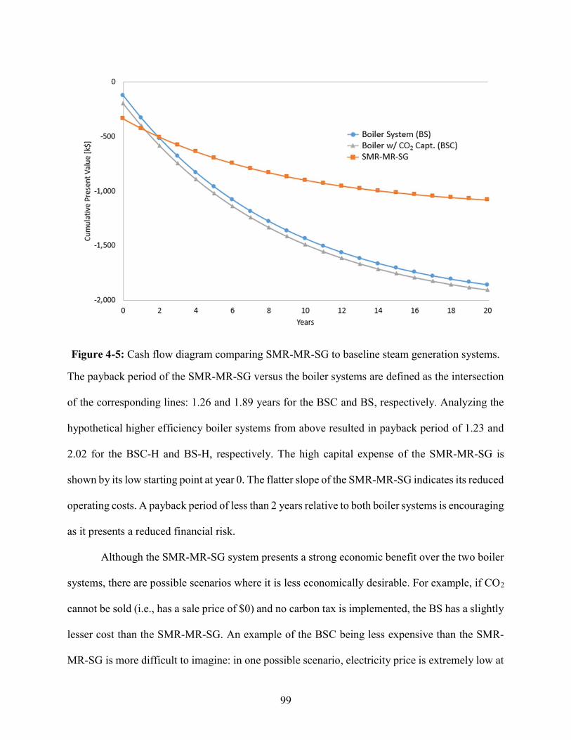
99

Figure 4-5: Cash flow diagram comparing SMR-MR-SG to baseline steam generation systems.

The payback period of the SMR-MR-SG versus the boiler systems are defined as the intersection

of the corresponding lines: 1.26 and 1.89 years for the BSC and BS, respectively. Analyzing the

hypothetical higher efficiency boiler systems from above resulted in payback period of 1.23 and

2.02 for the BSC-H and BS-H, respectively. The high capital expense of the SMR-MR-SG is

shown by its low starting point at year 0. The flatter slope of the SMR-MR-SG indicates its reduced

operating costs. A payback period of less than 2 years relative to both boiler systems is encouraging

as it presents a reduced financial risk.

Although the SMR-MR-SG system presents a strong economic benefit over the two boiler

systems, there are possible scenarios where it is less economically desirable. For example, if CO2

cannot be sold (i.e., has a sale price of $0) and no carbon tax is implemented, the BS has a slightly

lesser cost than the SMR-MR-SG. An example of the BSC being less expensive than the SMR-

MR-SG is more difficult to imagine: in one possible scenario, electricity price is extremely low at

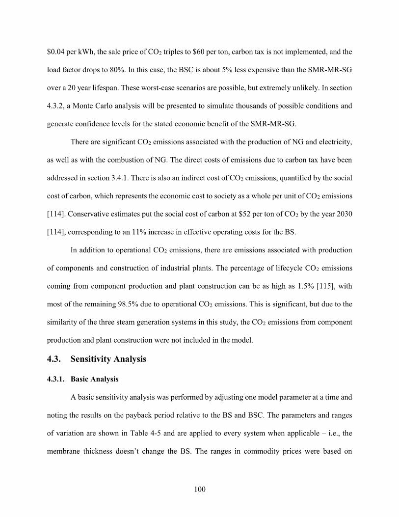
100

$0.04 per kWh, the sale price of CO2 triples to $60 per ton, carbon tax is not implemented, and the

load factor drops to 80%. In this case, the BSC is about 5% less expensive than the SMR-MR-SG

over a 20 year lifespan. These worst-case scenarios are possible, but extremely unlikely. In section

4.3.2, a Monte Carlo analysis will be presented to simulate thousands of possible conditions and

generate confidence levels for the stated economic benefit of the SMR-MR-SG.

There are significant CO2 emissions associated with the production of NG and electricity,

as well as with the combustion of NG. The direct costs of emissions due to carbon tax have been

addressed in section 3.4.1. There is also an indirect cost of CO2 emissions, quantified by the social

cost of carbon, which represents the economic cost to society as a whole per unit of CO2 emissions

[114]. Conservative estimates put the social cost of carbon at $52 per ton of CO2 by the year 2030

[114], corresponding to an 11% increase in effective operating costs for the BS.

In addition to operational CO2 emissions, there are emissions associated with production

of components and construction of industrial plants. The percentage of lifecycle CO2 emissions

coming from component production and plant construction can be as high as 1.5% [115], with

most of the remaining 98.5% due to operational CO2 emissions. This is significant, but due to the

similarity of the three steam generation systems in this study, the CO2 emissions from component

production and plant construction were not included in the model.

4.3. Sensitivity Analysis

4.3.1. Basic Analysis

A basic sensitivity analysis was performed by adjusting one model parameter at a time and

noting the results on the payback period relative to the BS and BSC. The parameters and ranges

of variation are shown in Table 4-5 and are applied to every system when applicable – i.e., the

membrane thickness doesn’t change the BS. The ranges in commodity prices were based on

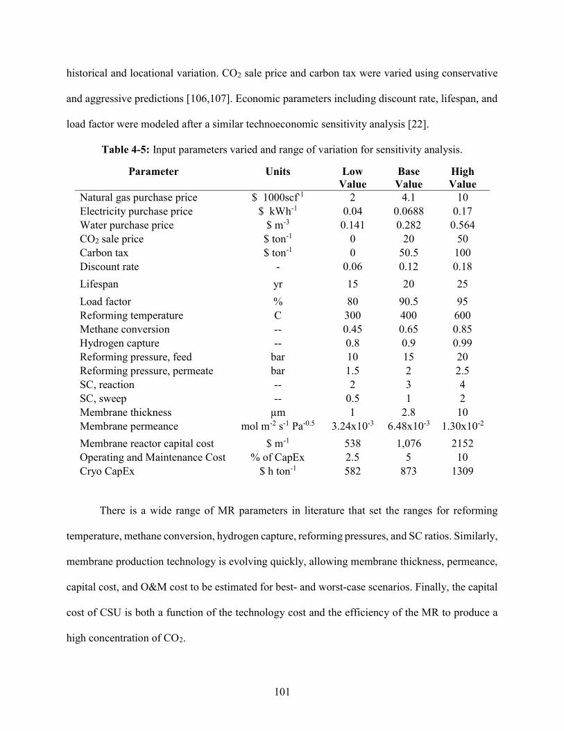
101

historical and locational variation. CO2 sale price and carbon tax were varied using conservative

and aggressive predictions [106,107]. Economic parameters including discount rate, lifespan, and

load factor were modeled after a similar technoeconomic sensitivity analysis [22].

Table 4-5: Input parameters varied and range of variation for sensitivity analysis.

Parameter Units Low Value

Base Value

High Value

Natural gas purchase price $ 1000scf-1 2 4.1 10 Electricity purchase price $ kWh-1 0.04 0.0688 0.17 Water purchase price $ m-3 0.141 0.282 0.564 CO2 sale price $ ton-1 0 20 50 Carbon tax $ ton-1 0 50.5 100 Discount rate - 0.06 0.12 0.18 Lifespan yr 15 20 25 Load factor % 80 90.5 95 Reforming temperature C 300 400 600 Methane conversion -- 0.45 0.65 0.85 Hydrogen capture -- 0.8 0.9 0.99 Reforming pressure, feed bar 10 15 20 Reforming pressure, permeate bar 1.5 2 2.5 SC, reaction -- 2 3 4 SC, sweep -- 0.5 1 2 Membrane thickness µm 1 2.8 10 Membrane permeance mol m-2 s-1 Pa-0.5 3.24x10-3 6.48x10-3 1.30x10-2 Membrane reactor capital cost $ m-1 538 1,076 2152 Operating and Maintenance Cost % of CapEx 2.5 5 10 Cryo CapEx $ h ton-1 582 873 1309

There is a wide range of MR parameters in literature that set the ranges for reforming

temperature, methane conversion, hydrogen capture, reforming pressures, and SC ratios. Similarly,

membrane production technology is evolving quickly, allowing membrane thickness, permeance,

capital cost, and O&M cost to be estimated for best- and worst-case scenarios. Finally, the capital

cost of CSU is both a function of the technology cost and the efficiency of the MR to produce a

high concentration of CO2.

102

The results of the sensitivity analysis relative to the BS and BSC are reported in

(b)

Figure 4-6. Note that the scale in payback period is very different for the BS and BSC

figures: the SMR MR-SG system pays back very quickly when compared to the BSC system.

(a)

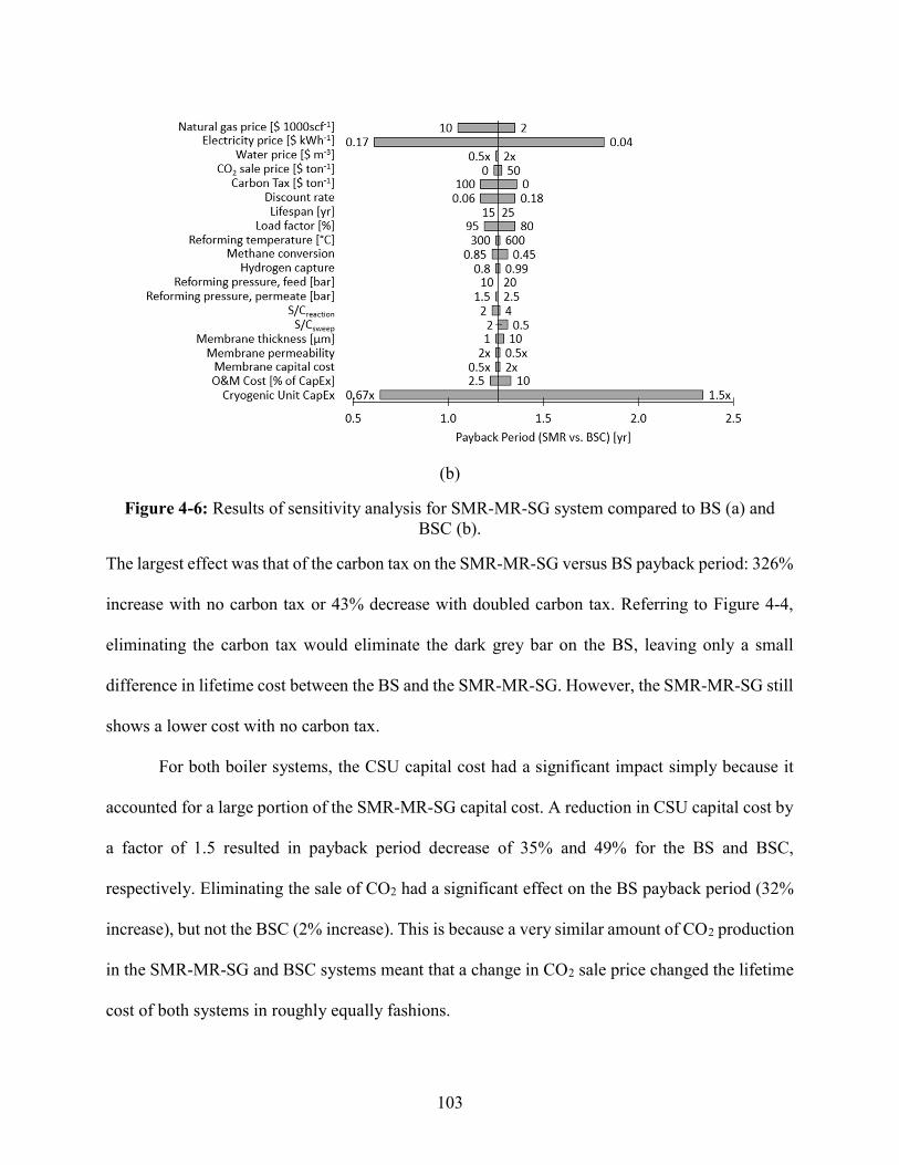
103

(b)

Figure 4-6: Results of sensitivity analysis for SMR-MR-SG system compared to BS (a) and BSC (b).

The largest effect was that of the carbon tax on the SMR-MR-SG versus BS payback period: 326%

increase with no carbon tax or 43% decrease with doubled carbon tax. Referring to Figure 4-4,

eliminating the carbon tax would eliminate the dark grey bar on the BS, leaving only a small

difference in lifetime cost between the BS and the SMR-MR-SG. However, the SMR-MR-SG still

shows a lower cost with no carbon tax.

For both boiler systems, the CSU capital cost had a significant impact simply because it

accounted for a large portion of the SMR-MR-SG capital cost. A reduction in CSU capital cost by

a factor of 1.5 resulted in payback period decrease of 35% and 49% for the BS and BSC,

respectively. Eliminating the sale of CO2 had a significant effect on the BS payback period (32%

increase), but not the BSC (2% increase). This is because a very similar amount of CO2 production

in the SMR-MR-SG and BSC systems meant that a change in CO2 sale price changed the lifetime

cost of both systems in roughly equally fashions.

104

Electricity cost has a significant impact on the relative merits of the BSC system: increasing

electricity price to $0.17 per kWh (147% increase) resulted in a 52% decrease in payback period.

This is due to the high electricity demand of the MEA system use for CCC. The relative size of

the energy cost can be seen easily by the large yellow bar in the BSC column of Figure 4-4. On

the other hand, electricity price was one of the most widely varied parameters due to a large

variation in local electricity price throughout the U.S.

The thermodynamic reforming properties have relatively small influence over the system’s

economic performance. Part of this may be due to the recycling aspect of the system. For example,

better methane conversion is not critical to improving efficiency, as the “leftover” is just recycled

rather than wasted. Also, the true impact of the thermodynamic parameters may have been lost: a

high-fidelity sensitivity analysis would adjust one parameter and then completely redesign the

system to support that change. For example, if the reforming temperature could be set to 250°C

and the export steam adjusted to 250°C, at least two heat exchangers could be eliminated from the

system, reducing complexity. However, this could make it more difficult to capture low

temperature waste heat because smaller temperature differences would reduce heat exchanger

efficiency. The thermodynamic parameters in the model affect one another enough that it is not

trivial to predict response to a parameter change, and future studies will address this challenge.

4.3.2. Monte Carlo Simulation

A Monte Carlo simulation was performed to validate the basic sensitivity analysis,

investigate the effects of varying multiple parameters simultaneously, and provide additional

information on the probability distribution of different outcomes. The simulation was performed

in Microsoft Excel, using ModelRisk add-in software, version 6.1.3 [116]. The Monte Carlo

simulation varied input variables using a PERT probability distribution based on the most likely,

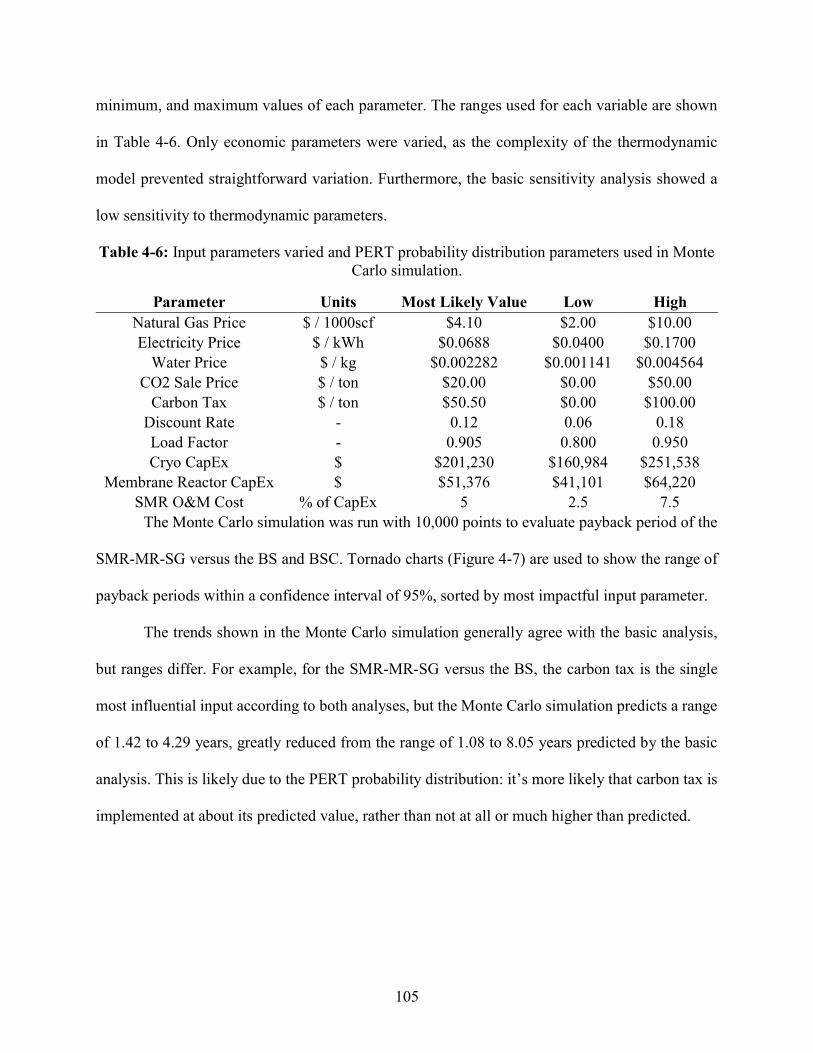
105

minimum, and maximum values of each parameter. The ranges used for each variable are shown

in Table 4-6. Only economic parameters were varied, as the complexity of the thermodynamic

model prevented straightforward variation. Furthermore, the basic sensitivity analysis showed a

low sensitivity to thermodynamic parameters.

Table 4-6: Input parameters varied and PERT probability distribution parameters used in Monte Carlo simulation.

Parameter Units Most Likely Value Low High Natural Gas Price $ / 1000scf $4.10 $2.00 $10.00 Electricity Price $ / kWh $0.0688 $0.0400 $0.1700

Water Price $ / kg $0.002282 $0.001141 $0.004564 CO2 Sale Price $ / ton $20.00 $0.00 $50.00

Carbon Tax $ / ton $50.50 $0.00 $100.00 Discount Rate - 0.12 0.06 0.18 Load Factor - 0.905 0.800 0.950 Cryo CapEx $ $201,230 $160,984 $251,538

Membrane Reactor CapEx $ $51,376 $41,101 $64,220 SMR O&M Cost % of CapEx 5 2.5 7.5

The Monte Carlo simulation was run with 10,000 points to evaluate payback period of the

SMR-MR-SG versus the BS and BSC. Tornado charts (Figure 4-7) are used to show the range of

payback periods within a confidence interval of 95%, sorted by most impactful input parameter.

The trends shown in the Monte Carlo simulation generally agree with the basic analysis,

but ranges differ. For example, for the SMR-MR-SG versus the BS, the carbon tax is the single

most influential input according to both analyses, but the Monte Carlo simulation predicts a range

of 1.42 to 4.29 years, greatly reduced from the range of 1.08 to 8.05 years predicted by the basic

analysis. This is likely due to the PERT probability distribution: it’s more likely that carbon tax is

implemented at about its predicted value, rather than not at all or much higher than predicted.

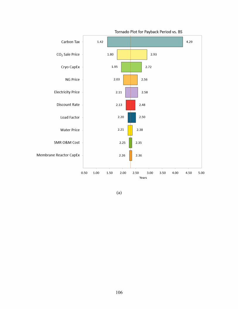
106

(a)

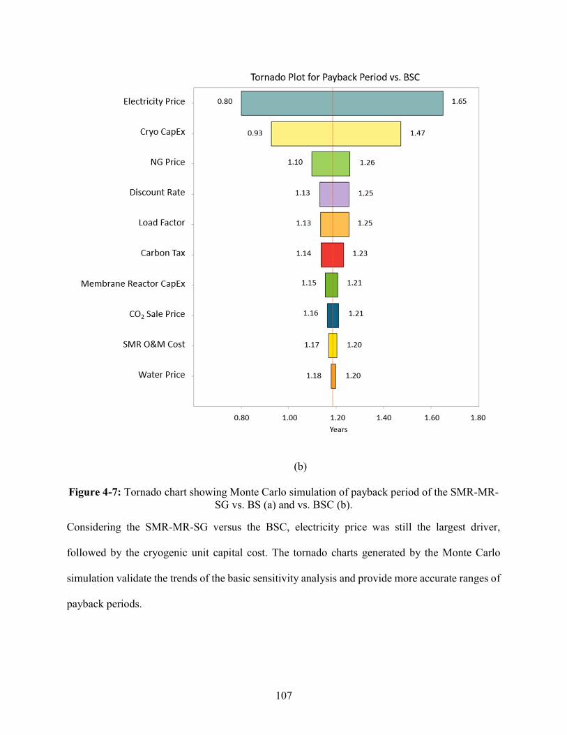
107

(b)

Figure 4-7: Tornado chart showing Monte Carlo simulation of payback period of the SMR-MR-SG vs. BS (a) and vs. BSC (b).

Considering the SMR-MR-SG versus the BSC, electricity price was still the largest driver,

followed by the cryogenic unit capital cost. The tornado charts generated by the Monte Carlo

simulation validate the trends of the basic sensitivity analysis and provide more accurate ranges of

payback periods.

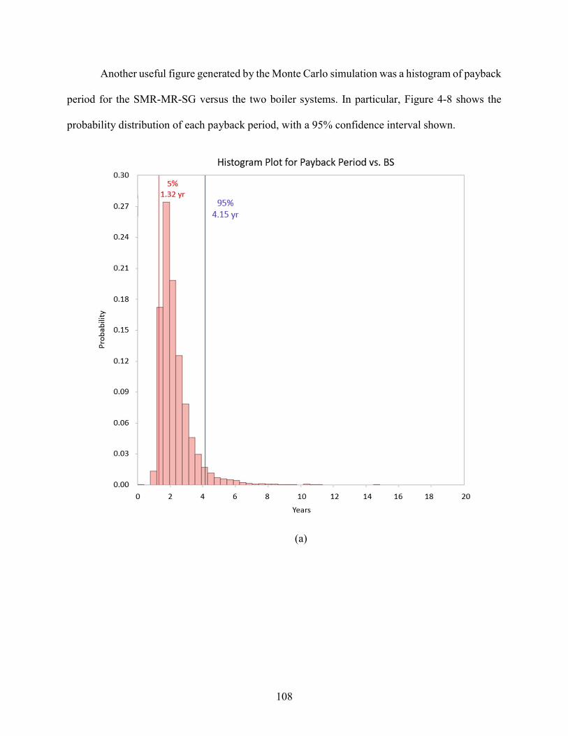
108

Another useful figure generated by the Monte Carlo simulation was a histogram of payback

period for the SMR-MR-SG versus the two boiler systems. In particular, Figure 4-8 shows the

probability distribution of each payback period, with a 95% confidence interval shown.

(a)

109

(b)

Figure 4-8: Histogram showing Monte Carlo simulation of payback period of the SMR-MR-SG vs. BS (a) and vs. BSC (b).

Based on these histograms, a concise summary of the sensitivity analysis can be formed:

accounting for the variability and probability distribution of input parameters, the SMR-MR-SG

system shows a payback period of 2.74 ± 1.42 yr versus the BS and 1.26 ± 0.51 yr versus the BSC

with 95% confidence. It is also worth noting that, in all 10,000 repetitions of the Monte Carlo

simulation, the SMR-MR-SG had a finite payback period, i.e., it was the least expensive option

110

every time. This chapter has presented and discussed the results of modeling and the sensitivity

analysis. The following chapter will summarize the conclusions of this study and provide

guidelines for future work.

111

Conclusions and Recommendations for Further Work

The current study investigated a steam generation system using steam methane reforming in a

membrane reactor (SMR-MR-SG). A technoeconomic model was developed using an enthalpy-

based energy balance method with a discounted cash flow analysis. The SMR-MR-SG was

compared to a high efficiency NG boiler system, with (BSC) and without CO2 capture (BS), and

evaluated as an alternative technology for steam generation.

Modeling results show an increase of boiler efficiency from 86% to 97.0% is possible for

the SMR-MR-SG system, with a reduction of water and NG use of 55% and 14% relative to the

BS system, respectively. The combination of gas recycling and a cryogenic separation unit (CSU)

effectively reduced CO2 emissions to zero with a 3.0% energy penalty, substantially lower than

other representative systems with carbon capture.

The economic benefit of the SMR-MR-SG is derived largely from CO2 capture and

concentration. This eliminates the cost of carbon tax on emissions while also raising revenue from

sale of CO2. Additionally, the co-location of products (CO2 and steam) with the SMR-MR-SG

plant effectively eliminates export costs relative to other plants with carbon capture, yielding

significant economic advantage.

The capital cost of the new system is ~3 times higher than the conventional boiler without

CO2 capture, but the payback period is a short 1.89 years if a reasonable carbon tax system is

employed. Payback period showed the highest sensitivity to carbon tax: eliminating it complete

increasing payback period to 8.05 years relative to the BS system, but still leaving the SMR-MR-

SG desirable over the other two systems. Other factors with large impacts on payback period were

112

CSU capital cost, CO2 sale price, and electricity cost. The SMR-MR-SG showed a reduction in

discounted lifetime cost of 42.0% and 43.4% relative to the BS and BSC systems, respectively.

The results of this study show that the SMR-MR-SG could be a direct replacement for an

industrial boiler system. The SMR-MR-SG can offer significantly reduced cost and energy use

while completely eliminating CO2 emissions. The author intends to continue the development of

this technology in the near future, targeting commercialization as an end goal.

5.1. Recommendations for Future Work

Future work will involve experimental validation of assumed thermodynamic parameters

and increased detail in the thermodynamic model to understand the effect of operating conditions.

5.1.1. SMR-MR-SG Cycle Variants

There are several interesting variants to the proposed SMR-MR-SG system that were not

investigated fully in this study. The topics listed would constitute meaningful future work. To start,

there are several ways to capture CO2 from the retentate stream:

Cryogenic CO2 separation, as in this study. CSU combines high capital expense with

simple and effective operation and low energy penalties, but energy cost increases

quickly with decreasing CO2 concentration.

Burn retentate to remove CH4 and H2, recover waste heat, condense water, and end up

with a high purity CO2 stream that may require little or no CO2 capture technology.

Separate CO2 from retentate via chemical adsorption.

Separate CO2 through a membrane (different than the H2 membrane). This is relatively

unproven technology and likely expensive, but could offer very simple and inexpensive

operation [8].

113

Any or all these technologies could be combined with cooling and or compression to create

compressed or liquefied CO2 for sale or export. The CO2 production could also be used in a process

where it is directly needed. For example, a brewing plant may need large amounts of steam for

brewing and building heating in addition to CO2 for carbonation.

Another area of interest is the amount and composition of sweep gas. Two potential variations

in sweep gas are to:

Use air for sweep gas instead of steam, especially if the permeate will be burned as in this

system. Spallina et al. performed work on this concept [53], but it has not been applied to

a steam generation application.

Increase the flow rate of sweep gas dramatically. This would greatly increase the driving

force for H2 permeation through the membrane, at the expense of using more heat to

superheat more sweep gas. However, if heat is recovered efficiently as in this study, then

the downside may be insignificant.

Hydrogen capture is an interesting parameter: the intuitive thought process is that it would be

optimized at 100% such that no hydrogen is left on the retentate side. However, there are

diminishing returns in flow rate of hydrogen per membrane surface area, as additional surface area

adds to the system’s capital cost. This suggests that, if un-permeated hydrogen gas is recycled, the

optimal hydrogen capture is a finite number less than 100%. Methane conversion may also be

optimized at some value below 100% with recycled retentate gas. With the working

thermodynamic and technoeconomic model developed in this study, it would be interesting to

perform an optimization of the system’s lifetime cost. The optimization should be based on

independent variables including both steam to carbon ratios, methane conversion efficiency,

114

hydrogen capture efficiency, reformer temperature, feed pressure, and permeate pressure. This

would require a significantly more detailed model to execute properly.

5.1.2. Summary

This study lays the groundwork for a potentially lucrative future technology as a direct

replacement for industrial boilers. Several items should be addressed to help transition this study

towards proof of concept and commercialization:

A small-scale test facility should be designed and operated to validate the key

assumptions of the thermodynamic model.

More detailed should be added to the thermodynamic model, including pressure

losses, detailed heat exchanger models, and more realistic heat losses.

A plate and frame configuration membrane reactor should be built and tested to

validate scaling costs and thermodynamic parameters of the reactor.

The variations of the thermodynamic cycle discussed in section 5.1.1 should be

modeled and optimized.

A high-fidelity sensitivity analysis should be conducted to identify any high-

influence thermodynamic parameters that were not identified in this study.

115

REFERENCES

[1] United States Environmental Protection Agency (EPA), 2017, “Global Greenhouse Gas Emissions Data.”

[2] International Energy Agency (IEA), 2018, CO2 Emissions from Fuel Combustion. [3] Lawrence Livermore National Laboratory, and United States Department of Energy (DoE),

2015, “Carbon Flow Charts,” LLNL Flow Charts [Online]. Available: https://flowcharts.llnl.gov/commodities/carbon.

[4] U.S. EIA, 2018, Annual Energy Outlook 2018 with Projections to 2050. [5] U.S. Energy Information Administration, 2018, “U.S. Natural Gas Prices” [Online].

Available: https://www.eia.gov/dnav/ng/ng_pri_sum_dcu_nus_a.htm. [Accessed: 08-Feb-2019].

[6] 2015, “The Way Forward: Second-Best Solutions,” Econ. [7] Sharma, R., Kumar, A., and Upadhyay, R. K., 2017, “Performance Comparison of Methanol

Steam Reforming Integrated to Pd-Ag Membrane: Membrane Reformer vs. Membrane Separator,” Sep. Purif. Technol., 183, pp. 194–203.

[8] Ribeirinha, P., Abdollahzadeh, M., Boaventura, M., and Mendes, A., 2017, “H2 Production with Low Carbon Content via MSR in Packed Bed Membrane Reactors for High-Temperature Polymeric Electrolyte Membrane Fuel Cell,” Appl. Energy, 188, pp. 409–419.

[9] Tribioli, L., Cozzolino, R., and Chiappini, D., 2017, “Technical Assessment of Different Operating Conditions of an On-Board Autothermal Reformer for Fuel Cell Vehicles,” Energies, 10(839), pp. 1–17.

[10] “Hydrogen Production: Natural Gas Reforming,” Fuel Cell Technol. Off. [11] Nakajima, T., Kume, T., Ikeda, Y., Shiraki, M., Kurokawa, H., Iseki, T., Kajitani, M.,

Tanaka, H., Hikosaka, H., Takagi, Y., and Ito, M., 2015, “Effect of Concentration Polariation on Hydrogen Production Performance of Ceramic-Support Pd Membrane Module,” Int. J. Hydrogen Energy, 40, pp. 11451–11456.

[12] Anzelmo, B., 2016, On-Board Hydrogen Production from Natural Gas via a Metallic Pd-Based Membrane Reactor.

[13] Song, C., Liu, Q., Ji, N., Kansha, Y., and Tsutsumi, A., 2015, “Optimization of Steam Methane Reforming Coupled with Pressure Swing Adsorption Hydrogen Production Process by Heat Integration,” Appl. Energy, 154, pp. 392–401.

[14] Iulianelli, A., Liguori, S., Wilcox, J., and Basile, A., 2016, “Advances on Methane Steam Reforming to Produce Hydrogen through Membrane Reactors Technology: A Review,” Catal. Rev., 58(1), pp. 1–35.

[15] Solsvik, J., and Jakobsen, H. A., 2017, “On the Modeling of One-Dimensional Membrane Reactors: Application to Hydrogen Production in Fixed Packed Bed,” Fuel, 202, pp. 595–612.

[16] Uehara, I., 2008, “Separation and Purification of Hydrogen,” Energy carriers Convers. Syst. with Emphas. Hydrog., 1, pp. 268–282.

[17] Barelli, L., Bidini, G., Gallorini, F., and Servili, S., 2008, “Hydrogen Production through Sorption-Enhanced Steam Methane Reforming and Membrane Technology: A Review,” Energy, 33, pp. 554–570.

[18] Zaragoza Martin, F., Dijkstra, J. W., Boon, J., and Meuldijk, J., 2011, “Energy Procedia A Membrane Reformer with Permeate Side Combustion for CO 2 Capture: Modeling and

116

Design,” Energy Procedia, 4, pp. 707–714. [19] Murmura, M. A., Cerbelli, S., and Annesini, M. C., 2017, “Modelling and Optimization of

Hydrogen Yield in Membrane Steam Reforming Reactors,” Can. J. Chem. Eng., 95, pp. 1676–1682.

[20] Johnsen, K., Ryu, H. J., Grace, J. R., and Lim, C. J., 2006, “Sorption-Enhanced Steam Reforming of Methane in a Fluidized Bed Reactor with Dolomite as CO 2-Acceptor,” Chem. Eng. Sci., 61, pp. 1195–1202.

[21] Adris, A.-E. M., 1994, “A Fluidized Bed Membrane Reactor for Steam Methane Reforming: Experimental Verification and Model Validation,” University of British Columbia.

[22] Sjardin, M., Damen, K., and Faaij, A., 2006, “Techno-Economic Prospects of Membrane Reactors in a Future Hydrogen-Driven Transportation Sector,” Energy, 31, pp. 2523–2555.

[23] Wilcox, J., 2012, Carbon Capture, Springer Science & Business Media. [24] Adhikari, S., and Fernando, S., 2006, “Hydrogen Membrane Separation Techniques,” Ind.

Eng. Chem. Res., 45(3), pp. 875–881. [25] Conde, J. J., Maroño, M., and Sánchez-Hervás, J. M., 2017, “Pd-Based Membranes for

Hydrogen Separation: Review of Alloying Elements and Their Influence on Membrane Properties,” Sep. Purif. Rev., 46(2), pp. 152–177.

[26] Catalano, J., Giacinti Baschetti, M., and Sarti, G. C., 2009, “Influence of the Gas Phase Resistance on Hydrogen Flux through Thin Palladium–silver Membranes,” J. Memb. Sci., 339(1–2), pp. 57–67.

[27] Chen, Y., Wang, Y., Xu, H., and Xiong, G., 2008, “Efficient Production of Hydrogen from Natural Gas Steam Reforming in Palladium Membrane Reactor,” Appl. Catal. B Environ., 81(3–4), pp. 283–294.

[28] Patel, K. S., and Sunol, A. K., 2007, “Modeling and Simulation of Methane Steam Reforming in a Thermally Coupled Membrane Reactor,” Int. J. Hydrogen Energy, 32(13), pp. 2344–2358.

[29] Anzelmo, B., Wilcox, J., and Liguori, S., 2017, “Natural Gas Steam Reforming Reaction at Low Temperature and Pressure Conditions for Hydrogen Production via Pd/PSS Membrane Reactor,” J. Memb. Sci., 522, pp. 343–350.

[30] Brown, L. F., 2001, A Comparative Study of Fuels for On-Board Hydrogen Production for Fuel-Cell-Powered Automobiles.

[31] Rostrup-Nielsen, J. R., 2001, “Conversion of Hydrocarbons and Alcohols for Fuel Cells,” Phys. Chem. Chem. Phys., 3, pp. 283–288.

[32] Burchart-Korol, D., Korol, J., and Czaplicka-Kolarz, K., 2016, “Life Cycle Assessment of Heat Production from Underground Coal Gasification,” Int. J. Life Cycle Assess., 21(10), pp. 1391–1403.

[33] Malerød-Fjeld, H., Clark, D., Yuste-Tirados, I., Zanón, R., Catalán-Martinez, D., Beeaff, D., Morejudo, S. H., Vestre, P. K., Norby, T., Haugsrud, R., Serra, J. M., and Kjølseth, C., 2017, “Thermo-Electrochemical Production of Compressed Hydrogen from Methane with near-Zero Energy Loss,” Nat. Energy, 2, pp. 923–931.

[34] Manzolini, G., Dijkstra, J. W., Macchi, E., and Jansen, D., 2006, “Technical Economic Evaluation of a System for Electricity Production with CO2 Capture Using a Membrane Reformer with Permeate Side Combustion,” ASME Turbo Expo 2006: Power for Land, Sea, and Air.

[35] Leimert, J. M., Dillig, M., and Karl, J., 2018, “Hydrogen Production from Solid Feedstock by Using a Nickel Membrane Reformer,” J. Memb. Sci., 548, pp. 11–21.

117

[36] Miller, J. B., Morreale, B. D., and Smith, M. W., 2014, “Pd-Alloy Membranes for Hydrogen Separation,” Reactor and Process Design in Sustainable Energy Technology, Elsevier B.V., pp. 135–161.

[37] Jiwanuruk, T., Putivisutisak, S., Vas-Umnuay, P., Bumroongsakulsawat, P., Cheng, C. K., and Assabumrungrat, S., 2017, “Modeling of Thermally-Coupled Monolithic Membrane Reformer for Vehicular Hydrogen Production,” Int. J. Hydrogen Energy, 42, pp. 26308–26319.

[38] Iaquaniello, G., Giacobbe, F., Morico, B., Cosenza, S., and Farace, A., 2008, “Membrane Reforming in Converting Natural Gas to Hydrogen: Production Costs, Part II,” 33, pp. 6595–6601.

[39] De Falco, M., Salladini, A., Palo, E., and Iaquaniello, G., 2015, “Pd-Alloy Membrane Reactor for Natural Gas Steam Reforming: An Innovative Process Design for the Capture of CO2,” Ind. Eng. Chem. Res., 54, pp. 6950–6958.

[40] 2005, Characterization of the U.S. Industrial/Commercial Boiler Population. [41] 2018, “Converting Natural Gas Prices in Dollars per Ccf or Mcf to Dollars per Btu or

Therm,” U.S. Energy Inf. Adm. [Online]. Available: https://www.eia.gov/tools/faqs/faq.php?id=45&t=8. [Accessed: 23-Jan-2019].

[42] Steinberg, L., 2012, “How Much Electricity Does New York Use?,” Leonard Steinb. Team [Online]. Available: http://theleonardsteinbergteam.com/how-much-electricity-does-new-york-use/.

[43] Kian, K., Woodall, C., Wilcox, J., Liguori, S., Kian, K., Woodall, C. M., Wilcox, J., and Liguori, S., 2018, “Performance of Pd-Based Membranes and Effects of Various Gas Mixtures on H2 Permeation,” Environments, 5(12), p. 128.

[44] Falco, M. De, Marrelli, L., and Iaquaniello, G., 2011, Membrane Reactors for Hydrogen Production Processes, Springer.

[45] Schjølberg, I., Calo, E., Dijk, E. van, Ersöz, A., Fernandez, E. O., Hulteberg, C., Lieftink, D., Nelsson, C., Saint-Just, J., Silversand, F., Stauss, R., and Yasuda, I., 2011, IEA HIA Task 23: Small Scale Reformers for On-Site Hydrogen Supply.

[46] Rostrup-Nielsen, J. R., and Rostrup-Nielsen, T., 2004, Large-Scale Hydrogen Production. [47] Kurokawa, H., Shirasaki, Y., and Yasuda, I., 2011, “Energy-Efficient Distributed Carbon

Capture in Hydrogen Production from Natural Gas,” Energy Procedia, 4, pp. 674–680. [48] Gallucci, F., Fernandez, E., Corengia, P., and van Sint Annaland, M., 2013, “Recent

Advances on Membranes and Membrane Reactors for Hydrogen Production,” Chem. Eng. Sci., 92, pp. 40–66.

[49] Murmura, M. A., Cerbelli, S., and Annesini, M. C., 2017, “Designing the Optimal Geometry of a Membrane Reactor for Hydrogen Production from a Pre-Reformed Gas Mixture Based on the Extent of the Reaction Boundary Layer,” Chem. Eng. Process. Process Intensif., 120, pp. 148–160.

[50] Roses, L., Manzolini, G., Campanari, S., De Wit, E., and Walter, M., 2013, “Techno-Economic Assessment of Membrane Reactor Technologies for Pure Hydrogen Production for Fuel Cell Vehicle Fleets,” Energy and Fuels, 27(8), pp. 4423–4431.

[51] Prasad, P., and Elnashaie, S. S. E. H., 2004, “Novel Circulating Fluidized-Bed Membrane Reformer Using Carbon Dioxide Sequestration,” Ind. Eng. Chem. Res., 43, pp. 494–501.

[52] Chen, Z., Po, F., Grace, J. R., Lim, C. J., Mahecha-Botero, A., Rakib, M., Shirasaki, Y., and Yasuda, I., 2008, “Sorbent-Enhanced/Membrane-Assisted Steam-Methane Reforming,” Chem. Eng. Sci., 63, pp. 170–182.

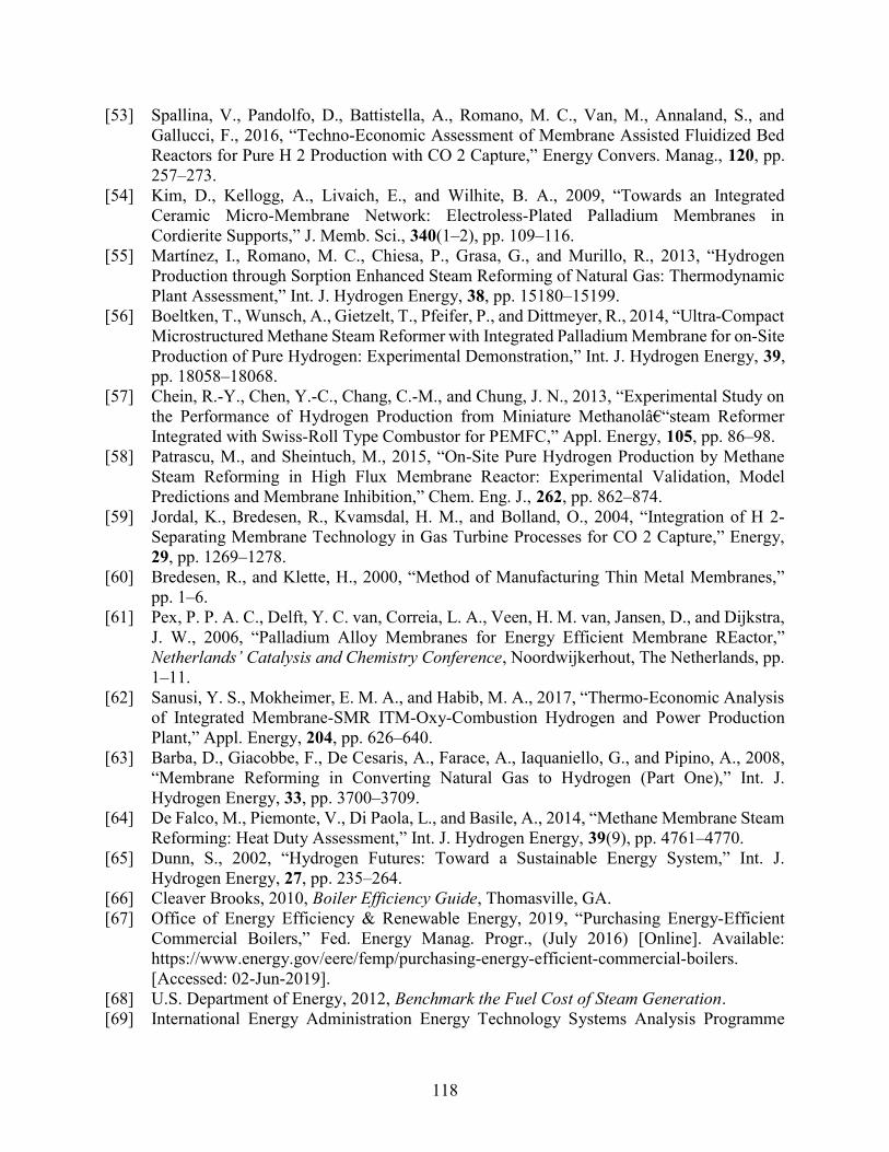
118

[53] Spallina, V., Pandolfo, D., Battistella, A., Romano, M. C., Van, M., Annaland, S., and Gallucci, F., 2016, “Techno-Economic Assessment of Membrane Assisted Fluidized Bed Reactors for Pure H 2 Production with CO 2 Capture,” Energy Convers. Manag., 120, pp. 257–273.

[54] Kim, D., Kellogg, A., Livaich, E., and Wilhite, B. A., 2009, “Towards an Integrated Ceramic Micro-Membrane Network: Electroless-Plated Palladium Membranes in Cordierite Supports,” J. Memb. Sci., 340(1–2), pp. 109–116.

[55] Martínez, I., Romano, M. C., Chiesa, P., Grasa, G., and Murillo, R., 2013, “Hydrogen Production through Sorption Enhanced Steam Reforming of Natural Gas: Thermodynamic Plant Assessment,” Int. J. Hydrogen Energy, 38, pp. 15180–15199.

[56] Boeltken, T., Wunsch, A., Gietzelt, T., Pfeifer, P., and Dittmeyer, R., 2014, “Ultra-Compact Microstructured Methane Steam Reformer with Integrated Palladium Membrane for on-Site Production of Pure Hydrogen: Experimental Demonstration,” Int. J. Hydrogen Energy, 39, pp. 18058–18068.

[57] Chein, R.-Y., Chen, Y.-C., Chang, C.-M., and Chung, J. N., 2013, “Experimental Study on the Performance of Hydrogen Production from Miniature Methanol–steam Reformer Integrated with Swiss-Roll Type Combustor for PEMFC,” Appl. Energy, 105, pp. 86–98.

[58] Patrascu, M., and Sheintuch, M., 2015, “On-Site Pure Hydrogen Production by Methane Steam Reforming in High Flux Membrane Reactor: Experimental Validation, Model Predictions and Membrane Inhibition,” Chem. Eng. J., 262, pp. 862–874.

[59] Jordal, K., Bredesen, R., Kvamsdal, H. M., and Bolland, O., 2004, “Integration of H 2-Separating Membrane Technology in Gas Turbine Processes for CO 2 Capture,” Energy, 29, pp. 1269–1278.

[60] Bredesen, R., and Klette, H., 2000, “Method of Manufacturing Thin Metal Membranes,” pp. 1–6.

[61] Pex, P. P. A. C., Delft, Y. C. van, Correia, L. A., Veen, H. M. van, Jansen, D., and Dijkstra, J. W., 2006, “Palladium Alloy Membranes for Energy Efficient Membrane REactor,” Netherlands’ Catalysis and Chemistry Conference, Noordwijkerhout, The Netherlands, pp. 1–11.

[62] Sanusi, Y. S., Mokheimer, E. M. A., and Habib, M. A., 2017, “Thermo-Economic Analysis of Integrated Membrane-SMR ITM-Oxy-Combustion Hydrogen and Power Production Plant,” Appl. Energy, 204, pp. 626–640.

[63] Barba, D., Giacobbe, F., De Cesaris, A., Farace, A., Iaquaniello, G., and Pipino, A., 2008, “Membrane Reforming in Converting Natural Gas to Hydrogen (Part One),” Int. J. Hydrogen Energy, 33, pp. 3700–3709.

[64] De Falco, M., Piemonte, V., Di Paola, L., and Basile, A., 2014, “Methane Membrane Steam Reforming: Heat Duty Assessment,” Int. J. Hydrogen Energy, 39(9), pp. 4761–4770.

[65] Dunn, S., 2002, “Hydrogen Futures: Toward a Sustainable Energy System,” Int. J. Hydrogen Energy, 27, pp. 235–264.

[66] Cleaver Brooks, 2010, Boiler Efficiency Guide, Thomasville, GA. [67] Office of Energy Efficiency & Renewable Energy, 2019, “Purchasing Energy-Efficient

Commercial Boilers,” Fed. Energy Manag. Progr., (July 2016) [Online]. Available: https://www.energy.gov/eere/femp/purchasing-energy-efficient-commercial-boilers. [Accessed: 02-Jun-2019].

[68] U.S. Department of Energy, 2012, Benchmark the Fuel Cost of Steam Generation. [69] International Energy Administration Energy Technology Systems Analysis Programme

119

(IEA ETSAP), 2010, “Industrial Combustion Boilers,” Energy Technol. Netw., (May), pp. 1–5.

[70] US Environmental Protection Agency, 2013, “Fact Sheet: CHP as a Boiler Replacement Opportunity,” pp. 1–6.

[71] Gallucci, F., Paturzo, L., Famà, A., and Basile, A., 2004, “Experimental Study of the Methane Steam Reforming Reaction in a Dense Pd/Ag Membrane Reactor,” Ind. Eng. Chem. Res., 43(4), pp. 928–933.

[72] Shigarov, A., Kirillov, V., and Landgraf, I., 2014, “Computational Study of Pd-Membrane CH4 Steam Reformer with Fixed Catalyst Bed: Searching for a Way to Increase Membrane Efficiency,” Int. J. Hydrogen Energy, 39, pp. 20072–20093.

[73] Mokheimer, E. M. A., Ibrar Hussain, M., Ahmed, S., Habib, M. A., and Al-Qutub, A. A., 2014, “On the Modeling of Steam Methane Reforming,” J. Energy Resour. Technol.

[74] Sheintuch, M., 2015, “Pure Hydrogen Production in a Membrane Reformer: Demonstration, Macro-Scale and Atomic Scale Modeling,” Chem. Eng. J.

[75] Vigneault, A., and Grace, J. R., 2015, “Hydrogen Production in Multi-Channel Membrane Reactor via Steam Methane Reforming and Methane Catalytic Combustion,” Int. J. Hydrogen Energy.

[76] Eveloy, V., 2012, “Numerical Analysis of an Internal Methane Reforming Solid Oxide Fuel Cell with Fuel Recycling,” Appl. Energy, 93, pp. 107–115.

[77] Huang, Y. M., Xu, J. H., Ling, W., Li, Y., Zhang, X. X., Dai, Z. K., Sui, Y., and Zhao, H. L., 2015, “Efficacy of the Wen Dan Decoction, a Chinese Herbal Formula, for Metabolic Syndrome,” Altern. Ther. Health Med., 21(4), pp. 54–67.

[78] Boyd, B., 2010, Guidelines for Estimating Unmetered Industrial Water Use. [79] U.S. Department of Labor, “CPI Inflation Calculator” [Online]. Available:

https://data.bls.gov/cgi-bin/cpicalc.pl?cost1=1&year1=198701&year2=201801. [Accessed: 08-Feb-2019].

[80] Lieberman, N. P., and Lieberman, E. T., 2009, Working Guide to Process Equipment. [81] Advanced Manufacturing Office, Improving Steam System Performance : A Sourcebook for

Industry Second Edition. [82] Harrell, G., and Ph, D., 2001, Steam System Survey Guide. [83] Abu-Zahra, M. R. M., Niederer, J. P. M., Feron, P. H. M., and Versteeg, G. F., 2007, “CO2

Capture from Power Plants,” Int. J. Greenh. Gas Control, 1(2), pp. 135–142. [84] Brennan, D., 1998, Process Industry Economics: An International Perspective. [85] Perry, R. H., 1997, Chemical Engineers’ Handbook, McGraw-Hill. [86] Brown, T., Engineering Economics and Economic Design for Process Engineers, CRC

Press. [87] Remer, D. S., and Chai, L. H., 1990, “Design Cost Factors for Scaling-Up Engineering

Equipment,” Chem. Eng. Prog., 86(8), pp. 77–82. [88] Brundett, G. W., 1987, “Economics,” Handbook of Dehumidification Technology,

Butterworths, Essex, Great Britain, pp. 202–214. [89] “British Pound to US Dollar Spot Exchange Rates for 1987 from the Bank of England”

[Online]. Available: https://www.poundsterlinglive.com/bank-of-england-spot/historical-spot-exchange-rates/gbp/GBP-to-USD-1987. [Accessed: 08-Feb-2019].

[90] Incropera, F. P., Dewitt, D. P., Bergman, T. L., and Lavine, A. S., 2017, Fundamentals of Heat and Mass Transfer, John Wiley and Sons.

[91] Xu, G., Liang, F., Yang, Y., Hu, Y., Zhang, K., and Liu, W., 2014, “An Improved CO2

120

Separation and Purification System Based on Cryogenic Separation and Distillation Theory,” Energies, 7, pp. 3484–3502.

[92] Liguori, S., Iulianelli, A., Dalena, F., Pinacci, P., Drago, F., Broglia, M., Huang, Y., and Basile, A., 2014, “Performance and Long-Term Stability of Pd/PSS and Pd/Al2O3 Membranes for Hydrogen Separation,” Membranes (Basel)., 4(1), pp. 143–162.

[93] Roses, L., Gallucci, F., Manzolini, G., and van Sint Annaland, M., 2013, “Experimental Study of Steam Methane Reforming in a Pd-Based Fluidized Bed Membrane Reactor,” Chem. Eng. J., 222, pp. 307–320.

[94] Peters, T. A., Stange, M., and Bredesen, R., 2011, “On the High Pressure Performance of Thin Supported Pd-23%Ag Membranes-Evidence of Ultrahigh Hydrogen Flux after Air Treatment,” J. Memb. Sci., 378(1–2), pp. 28–34.

[95] Cengel, Y. A., and Boles, M. A., 2015, Thermodynamics: An Engineering Approach, McGraw Hill.

[96] Chiesa, P., Campanari, S., and Manzolini, G., 2011, “CO2 Cryogenic Separation from Combined Cycles Integrated with Molten Carbonate Fuel Cells,” Int. J. Hydrogen Energy, 36, pp. 10355–10365.

[97] Hatlevik, Ø., Gade, S. K., Keeling, M. K., Thoen, P. M., Davidson, A. P., and Way, J. D., 2010, “Palladium and Palladium Alloy Membranes for Hydrogen Separation and Production: History, Fabrication Strategies, and Current Performance,” Sep. Purif. Technol., 73(1), pp. 59–64.

[98] Money Metals LLC, 2019, “Palladium Price Charts: Check Live &amp; Historical Bullion Prices Today” [Online]. Available: https://www.moneymetals.com/precious-metals-charts/palladium-price. [Accessed: 08-Feb-2019].

[99] Acquaviva, J., 2009, High-Performance, Durable, Palladium Alloy Membrane for Hydrogen Separation and Purification, New York, NY.

[100] Emerson, S., Dardas, Z., Hebert, R., Janowsky, G., Magdefrau, N., She, Y., Wittenzellner, J., and Technologies, U., 2011, Advanced Palladium Membrane Scale-up for Hydrogen Separation, East Hartford, CT.

[101] Couper, J. R., Emeritus, D. S., Ralph, T., Hertz, D. W., Manager, B. S., Loading, F., Practices, V., Smith, F. L., Ph, D., Principal, M. E., and Associates, W. C., 2008, “Process Economics,” Perry’s Checmical Engineers’ Handbook.

[102] Myers, D. B., Ariff, G. D., James, B. D., Lettow, J. S., Thomas, C. E. S., and Kuhn, R. C., 2002, “Cost and Performance Comparison Of Stationary Hydrogen Fueling Appliances,” U.S. DOE Hydrogen Program Review, pp. 1–8.

[103] Jiangzhou, S., Wang, R. Z., Lu, Y. Z., Xu, Y. X., and Wu, J. Y., 2005, “Experimental Study on Locomotive Driver Cabin Adsorption Air Conditioning Prototype Machine,” Energy Convers. Manag., 46(9–10), pp. 1655–1665.

[104] International Gas Union (IGU), 2012, Natural Gas Conversion Guide. [105] U.S. Energy Information Administration, 2019, Electric Power Monthly with Data for

November 2018. [106] Global CCS Institute, 2019, The CO2 Market. [107] Luckow, P., Stanton, E. A., Fields, S., Ong, W., Biewald, B., Jackson, S., and Fisher, J.,

2016, Spring 2016 National Carbon Dioxide Price Forecast, Cambridge, MA. [108] North China Electric Power University, and North China Electric Power University, 2014,

People’s Republic of China: Study on Carbon Capture and Storage in Natural Gas-Based Power Plants.

121

[109] Saeys, M., Quah, M. C. G., Agrawal, R., Farooq, S., Karimi, I. A., and Vasudevan, S., 2016, “Energy Penalty Estimates for CO2 Capture: Comparison between Fuel Types and Capture-Combustion Modes,” Energy, 103, pp. 709–714.

[110] Petrakopoulou, F., and Tsatsaronis, G., 2012, “Production of Hydrogen-Rich Fuels for Pre-Combustion Carbon Capture in Power Plants: A Thermodynamic Assessment,” Int. J. Hydrogen Energy, 37(9), pp. 7554–7564.

[111] Gür, T. M., 2017, “Perspective—Low-Carbon Electricity Is Great: What about ‘Less-Carbon’?,” J. Electrochem. Soc., 164(14), pp. F1587–F1590.

[112] Soltani, R., Rosen, M. A., and Dincer, I., 2014, “Assessment of CO2 Capture Options from Various Points in Steam Methane Reforming for Hydrogen Production,” Int. J. Hydrogen Energy, 39(35), pp. 20266–20275.

[113] Jou, C. J. G., Lee, C. li, Tsai, C. H., Wang, H. P., and Lin, M. L., 2008, “Enhancing the Performance of a High-Pressure Cogeneration Boiler with Waste Hydrogen-Rich Fuel,” Int. J. Hydrogen Energy, 33(20), pp. 5806–5810.

[114] Nordhaus, W. D., 2017, “Revisiting the Social Cost of Carbon,” Proceedings of the National Academy of Sciences, pp. 1518–1523.

[115] Wu, X. D., Guo, J. L., and Chen, G. Q., 2018, “The Striking Amount of Carbon Emissions by the Construction Stage of Coal-Fired Power Generation System in China,” Energy Policy, 117(July 2017), pp. 358–369.

[116] Voses Software, 2007, “ModelRisk.” [117] Kim, S. M., and Mudawar, I., 2013, “Universal Approach to Predicting Saturated Flow

Boiling Heat Transfer in Mini/Micro-Channels – Part II. Two-Phase Heat Transfer Coefficient,” Int. J. Heat Mass Transf., 64, pp. 1239–1256.

[118] Kim, S. M., and Mudawar, I., 2012, “Flow Condensation in Parallel Micro-Channels - Part 2: Heat Transfer Results and Correlation Technique,” Int. J. Heat Mass Transf., 55(4), pp. 984–994.

122

APPENDIX A. Representative Calculation

The purpose of this appendix is to verify the results obtained using Engineering Equation

Solver (EES). EES was used as the primary tool for the thermodynamic and technoeconomic

analyses discussed in Chapter 3. This calculation will step through the process, equations, and

assumptions required to completely model the steam generation cycle shown in Figure 3-1.

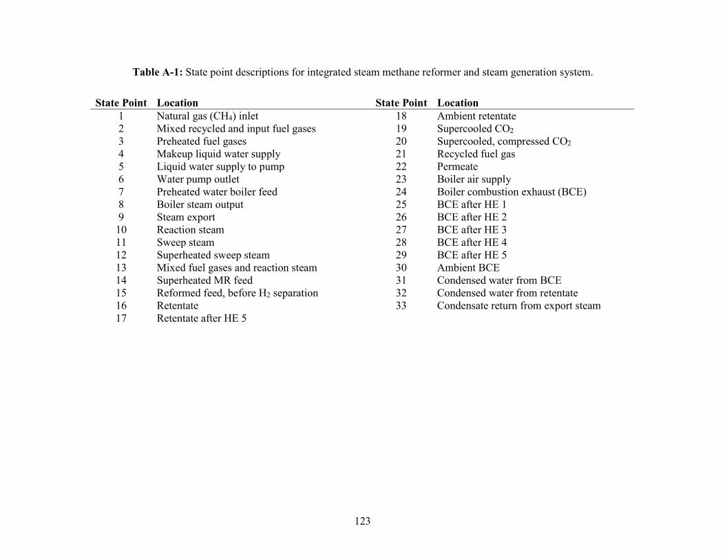
123

Table A-1: State point descriptions for integrated steam methane reformer and steam generation system.

State Point Location State Point Location 1 Natural gas (CH4) inlet 18 Ambient retentate 2 Mixed recycled and input fuel gases 19 Supercooled CO2 3 Preheated fuel gases 20 Supercooled, compressed CO2 4 Makeup liquid water supply 21 Recycled fuel gas 5 Liquid water supply to pump 22 Permeate 6 Water pump outlet 23 Boiler air supply 7 Preheated water boiler feed 24 Boiler combustion exhaust (BCE) 8 Boiler steam output 25 BCE after HE 1 9 Steam export 26 BCE after HE 2 10 Reaction steam 27 BCE after HE 3 11 Sweep steam 28 BCE after HE 4 12 Superheated sweep steam 29 BCE after HE 5 13 Mixed fuel gases and reaction steam 30 Ambient BCE 14 Superheated MR feed 31 Condensed water from BCE 15 Reformed feed, before H2 separation 32 Condensed water from retentate 16 Retentate 33 Condensate return from export steam 17 Retentate after HE 5

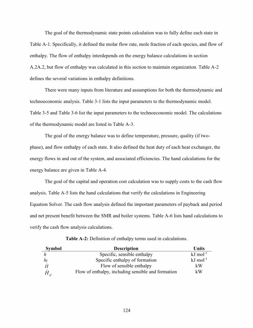
124

The goal of the thermodynamic state points calculation was to fully define each state in

Table A-1. Specifically, it defined the molar flow rate, mole fraction of each species, and flow of

enthalpy. The flow of enthalpy interdepends on the energy balance calculations in section

A.2A.2, but flow of enthalpy was calculated in this section to maintain organization. Table A-2

defines the several variations in enthalpy definitions.

There were many inputs from literature and assumptions for both the thermodynamic and

technoeconomic analysis. Table 3-1 lists the input parameters to the thermodynamic model.

Table 3-5 and Table 3-6 list the input parameters to the technoeconomic model. The calculations

of the thermodynamic model are listed in Table A-3.

The goal of the energy balance was to define temperature, pressure, quality (if two-

phase), and flow enthalpy of each state. It also defined the heat duty of each heat exchanger, the

energy flows in and out of the system, and associated efficiencies. The hand calculations for the

energy balance are given in Table A-4.

The goal of the capital and operation cost calculation was to supply costs to the cash flow

analysis. Table A-5 lists the hand calculations that verify the calculations in Engineering

Equation Solver. The cash flow analysis defined the important parameters of payback and period

and net present benefit between the SMR and boiler systems. Table A-6 lists hand calculations to

verify the cash flow analysis calculations.

Table A-2: Definition of enthalpy terms used in calculations.

Symbol Description Units h Specific, sensible enthalpy kJ mol-1

hf Specific enthalpy of formation kJ mol-1 H Flow of sensible enthalpy kW

sfH Flow of enthalpy, including sensible and formation kW

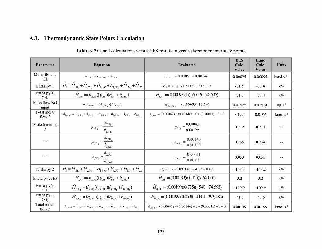
125

A.1. Thermodynamic State Points Calculation

Table A-3: Hand calculations versus EES results to verify thermodynamic state points.

Parameter Equation Evaluated EES Calc. Value

Hand Calc. Value

Units

Molar flow 1, CH4 4 4 41,CH 21,CH 2,CH n n n

41,CH 0.00051 0.00146 n 0.00095 0.00095 kmol s-1

Enthalpy 1 2 4 2 2 2 21 1,H 1,CH 1,H O 1,CO 1,N 1,O H H H H H H H 1 0 ( 71.5) 0 0 0 0 H -71.5 -71.4 kW

Enthalpy 1, CH4 2 2 2 21,H 1,total 1,H 1,H f,1,H( )( )( ) H n y h h

21,H (0.00095)(1)( 607.6 74,595) H -71.5 -71.4 kW

Mass flow NG input 4 4NG,input 1,CH CH( )( ) m n M

NG,input (0.00095)(16.04)m 0.01525 0.01524 kg s-1

Total molar flow 2 2 4 2 2 2 22,total 2,H 2,CH 2,H O 2,CO 2,N 2,O n n n n n n n

2,total (0.00042) (0.00146) 0 (0.00011) 0 0 n 0199 0.0199 kmol s-1

Mole fractions 2

2

2

2,H2,H

2,total

n

yn 22,H

0.000420.00199

y 0.212 0.211 --

“ ” 4

4

2,CH2,CH

2,total

n

yn 42,CH

0.001460.00199

y 0.735 0.734 --

“ ” 2

2

2,CO2,CO

2,total

n

yn 22,CO

0.000110.00199

y 0.053 0.055 --

Enthalpy 2 2 4 2 2 2 2i i,H i,CH i,H O i,CO i,N i,O H H H H H H H i 3.2 109.9 0 41.5 0 0 H -148.3 -148.2 kW

Enthalpy 2, H2 2 2 2 2i,H i,total i,H i,H f,i,H( )( )( ) H n y h h 2i,H (0.00199)(0.212)(7,640 0) H 3.2 3.2 kW

Enthalpy 2, CH4 4 4 4 4i,CH i,total i,CH i,CH f,i,CH( )( )( ) H n y h h

4i,CH (0.00199)(0.735)( 540 74,595) H -109.9 -109.9 kW

Enthalpy 2, CO2 2 2 2 2i,CO i,total i,CO i,CO f,i,CO( )( )( ) H n y h h

2i,CO (0.00199)(0.053)( 403.4 393,486) H -41.5 -41.5 kW

Total molar flow 3 2 4 2 2 2 2i,total i,H i,C H i,H O i,C O i,N i,O n n n n n n n

i,total (0.00042) (0.00146) 0 (0.00011) 0 0 n 0.00199 0.00199 kmol s-1

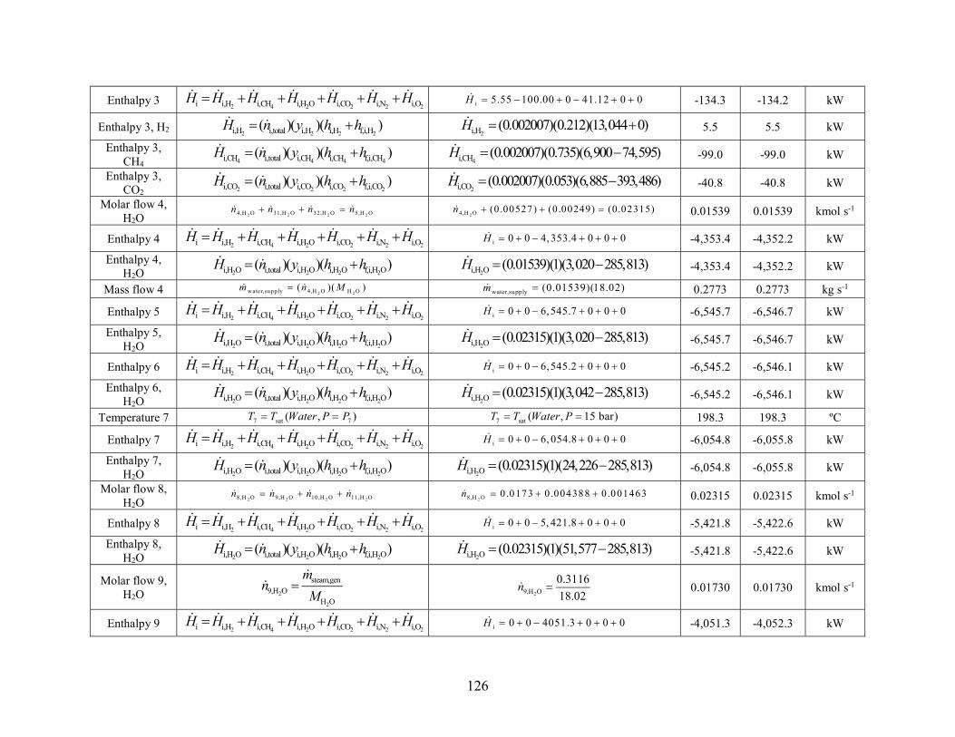
126

Enthalpy 3 2 4 2 2 2 2i i,H i,CH i,H O i,CO i,N i,O H H H H H H H i 5.55 100.00 0 41.12 0 0 H -134.3 -134.2 kW

Enthalpy 3, H2 2 2 2 2i,H i,total i,H i,H f,i,H( )( )( ) H n y h h 2i,H (0.002007)(0.212)(13,044 0) H 5.5 5.5 kW

Enthalpy 3, CH4 4 4 4 4i,CH i,total i,CH i,CH f,i,CH( )( )( ) H n y h h

4i,CH (0.002007)(0.735)(6,900 74,595) H -99.0 -99.0 kW

Enthalpy 3, CO2 2 2 2 2i,CO i,total i,CO i,CO f,i,CO( )( )( ) H n y h h

2i,CO (0.002007)(0.053)(6,885 393,486) H -40.8 -40.8 kW

Molar flow 4, H2O 2 2 2 24,H O 31,H O 32,H O 5,H O n n n n

24,H O (0 .00527) (0.00249) (0.02315) n 0.01539 0.01539 kmol s-1

Enthalpy 4 2 4 2 2 2 2i i,H i,CH i,H O i,CO i,N i,O H H H H H H H i 0 0 4, 353.4 0 0 0 H -4,353.4 -4,352.2 kW

Enthalpy 4, H2O 2 2 2 2i,H O i,total i,H O i,H O f,i,H O( )( )( ) H n y h h

2i,H O (0.01539)(1)(3,020 285,813) H -4,353.4 -4,352.2 kW

Mass flow 4 2 2w ater,supply 4,H O H O( )( ) m n M water,supply (0.01539)(18.02)m 0.2773 0.2773 kg s-1

Enthalpy 5 2 4 2 2 2 2i i,H i,CH i,H O i,CO i,N i,O H H H H H H H i 0 0 6,545.7 0 0 0 H -6,545.7 -6,546.7 kW

Enthalpy 5, H2O 2 2 2 2i,H O i,total i,H O i,H O f,i,H O( )( )( ) H n y h h

2i,H O (0.02315)(1)(3,020 285,813) H -6,545.7 -6,546.7 kW

Enthalpy 6 2 4 2 2 2 2i i,H i,CH i,H O i,CO i,N i,O H H H H H H H i 0 0 6,545.2 0 0 0 H -6,545.2 -6,546.1 kW

Enthalpy 6, H2O 2 2 2 2i,H O i,total i,H O i,H O f,i,H O( )( )( ) H n y h h

2i,H O (0.02315)(1)(3,042 285,813) H -6,545.2 -6,546.1 kW

Temperature 7 7 sat 7( , ) T T Water P P 7 sat ( , 15 bar) T T Water P 198.3 198.3 ºC

Enthalpy 7 2 4 2 2 2 2i i,H i,CH i,H O i,CO i,N i,O H H H H H H H i 0 0 6, 054.8 0 0 0 H -6,054.8 -6,055.8 kW

Enthalpy 7, H2O 2 2 2 2i,H O i,total i,H O i,H O f,i,H O( )( )( ) H n y h h

2i,H O (0.02315)(1)(24,226 285,813) H -6,054.8 -6,055.8 kW

Molar flow 8, H2O 2 2 2 28,H O 9,H O 10,H O 11,H O n n n n

28,H O 0.0173 0.004388 0.001463 n 0.02315 0.02315 kmol s-1

Enthalpy 8 2 4 2 2 2 2i i,H i,CH i,H O i,CO i,N i,O H H H H H H H i 0 0 5, 421.8 0 0 0 H -5,421.8 -5,422.6 kW

Enthalpy 8, H2O 2 2 2 2i,H O i,total i,H O i,H O f,i,H O( )( )( ) H n y h h

2i,H O (0.02315)(1)(51,577 285,813) H -5,421.8 -5,422.6 kW

Molar flow 9, H2O 2

2

steam,gen9,H O

H O

m

nM 29,H O

0.311618.02

n 0.01730 0.01730 kmol s-1

Enthalpy 9 2 4 2 2 2 2i i,H i,CH i,H O i,CO i,N i,O H H H H H H H i 0 0 4051.3 0 0 0 H -4,051.3 -4,052.3 kW

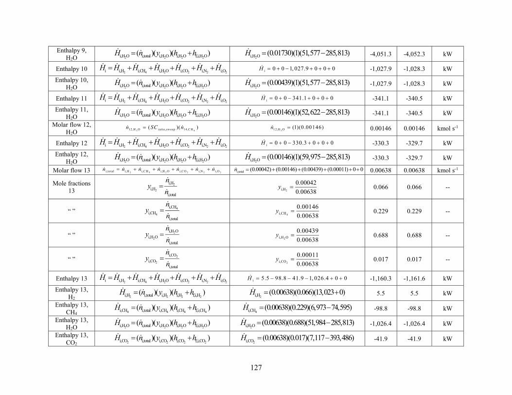
127

Enthalpy 9, H2O 2 2 2 2i,H O i,total i,H O i,H O f,i,H O( )( )( ) H n y h h

2i,H O (0.01730)(1)(51,577 285,813) H -4,051.3 -4,052.3 kW

Enthalpy 10 2 4 2 2 2 2i i,H i,CH i,H O i,CO i,N i,O H H H H H H H i 0 0 1, 027.9 0 0 0 H -1,027.9 -1,028.3 kW

Enthalpy 10, H2O 2 2 2 2i,H O i,total i,H O i,H O f,i,H O( )( )( ) H n y h h

2i,H O (0.00439)(1)(51,577 285,813) H -1,027.9 -1,028.3 kW

Enthalpy 11 2 4 2 2 2 2i i,H i,CH i,H O i,CO i,N i,O H H H H H H H i 0 0 341.1 0 0 0 H -341.1 -340.5 kW

Enthalpy 11, H2O 2 2 2 2i,H O i,total i,H O i,H O f,i,H O( )( )( ) H n y h h

2i,H O (0.00146)(1)(52,622 285,813) H -341.1 -340.5 kW

Molar flow 12, H2O 2 412,H O ratio,sw eep 14,C H( )( ) n SC n

212,H O (1)(0.00146)n 0.00146 0.00146 kmol s-1

Enthalpy 12 2 4 2 2 2 2i i,H i,CH i,H O i,CO i,N i,O H H H H H H H i 0 0 330.3 0 0 0 H -330.3 -329.7 kW

Enthalpy 12, H2O 2 2 2 2i,H O i,total i,H O i,H O f,i,H O( )( )( ) H n y h h

2i,H O (0.00146)(1)(59,975 285,813) H -330.3 -329.7 kW

Molar flow 13 2 4 2 2 2 2i,total i,H i,C H i,H O i,C O i,N i,O n n n n n n n i,total (0.00042) (0.00146) (0.00439) (0.00011) 0 0 n 0.00638 0.00638 kmol s-1

Mole fractions 13

2

2

i,Hi,H

i,total

n

yn 2i,H

0.000420.00638

y 0.066 0.066 --

“ ” 4

4

i,CHi,CH

i,total

n

yn 4i,CH

0.001460.00638

y 0.229 0.229 --

“ ” 2

2

i,H Oi,H O

i,total

n

yn 2i,H O

0.004390.00638

y 0.688 0.688 --

“ ” 2

2

i,COi,CO

i,total

n

yn 2i,CO

0.000110.00638

y 0.017 0.017 --

Enthalpy 13 2 4 2 2 2 2i i,H i,CH i,H O i,CO i,N i,O H H H H H H H i 5.5 98.8 41.9 1, 026.4 0 0 H -1,160.3 -1,161.6 kW

Enthalpy 13, H2 2 2 2 2i,H i,total i,H i,H f,i,H( )( )( ) H n y h h

2i,H (0.00638)(0.066)(13,023 0) H 5.5 5.5 kW

Enthalpy 13, CH4 4 4 4 4i,CH i,total i,CH i,CH f,i,CH( )( )( ) H n y h h

4i,CH (0.00638)(0.229)(6,973 74,595) H -98.8 -98.8 kW

Enthalpy 13, H2O 2 2 2 2i,H O i,total i,H O i,H O f,i,H O( )( )( ) H n y h h

2i,H O (0.00638)(0.688)(51,984 285,813) H -1,026.4 -1,026.4 kW

Enthalpy 13, CO2 2 2 2 2i,CO i,total i,CO i,CO f,i,CO( )( )( ) H n y h h

2i,CO (0.00638)(0.017)(7,117 393,486) H -41.9 -41.9 kW

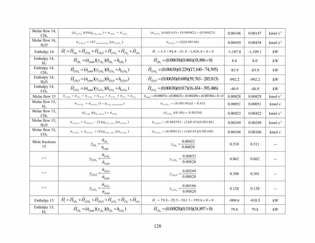
128

Molar flow 14, CH4 4 4 2 214 ,C H C H ,conv 14 ,H 15 ,H( )(4)( ) n n n

414,CH( )(4)(0.65) (0.00042) (0.00423) n 0.00146 0.00147 kmol s-1

Molar flow 14, H2O 2 414,H O ratio,reaction 14,C H( )( ) n SC n

214,H O (3)(0.00146)n 0.00439 0.00438 kmol s-1

Enthalpy 14 2 4 2 2 2 2i i,H i,CH i,H O i,CO i,N i,O H H H H H H H i 5.5 98.8 41.9 1, 026.4 0 0 H -1,107.8 -1,109.1 kW

Enthalpy 14, H2 2 2 2 2i,H i,total i,H i,H f,i,H( )( )( ) H n y h h

2i,H (0.00638)(0.066)(18,886 0) H 8.0 8.0 kW

Enthalpy 14, CH4 4 4 4 4i,CH i,total i,CH i,CH f,i,CH( )( )( ) H n y h h

4i,CH (0.00638)(0.229)(17,160 74,595) H -83.9 -83.9 kW

Enthalpy 14, H2O 2 2 2 2i,H O i,total i,H O i,H O f,i,H O( )( )( ) H n y h h

2i,H O (0.00638)(0.688)(59,763 285,813) H -992.2 -992.2 kW

Enthalpy 14, CO2 2 2 2 2i,CO i,total i,CO i,CO f,i,CO( )( )( ) H n y h h

2i,CO (0.00638)(0.017)(16,434 393,486) H -40.9 -40.9 kW

Molar flow 15 2 4 2 2 2 2i,total i,H i,C H i,H O i,C O i,N i,O n n n n n n n i,total (0.00051) (0.00423) (0.00249) (0.00106) 0 0 n 0.00828 0.00829 kmol s-1

Molar flow 15, H2 4 4 415,C H 14,C H C H ,conversion(1 ) n n

415 ,C H (0 .00146)(1 0 .65) n 0.00051 0.00051 kmol s-

Molar flow 15, CH4 2 2 215,H H ,recov 22,H( )( ) n n

215 ,H( )(0 .90) 0 .00380n 0.00423 0.00422 kmol s-1

Molar flow 15, H2O 2 2 4 415,H O 14,H O C H ,conv 14,CH(2)( )( ) n n n

215,H O (0.00439) (2)(0.65)(0.00146) n 0.00249 0.00249 kmol s-1

Molar flow 15, CO2 2 2 4 415,C O 14 ,C O C H ,conv 14,C H(1)( )( ) n n n

215,CO (0.00011) (1)(0.65)(0.00146) n 0.00106 0.00106 kmol s-

Mole fractions 15

2

2

i,Hi,H

i,total

n

yn 2i,H

0.004230.00828

y 0.510 0.511 --

“ ” 4

4

i,CHi,CH

i,total

n

yn 4i,CH

0.000510.00828

y 0.062 0.062 --

“ ” 2

2

i,H Oi,H O

i,total

n

yn 2i,H O

0.002490.00828

y 0.300 0.301 --

“ ” 2

2

i,COi,CO

i,total

n

yn 2i,CO

0.001060.00828

y 0.128 0.128 --

Enthalpy 15 2 4 2 2 2 2i i,H i,CH i,H O i,CO i,N i,O H H H H H H H i 79.8 29.5 561.1 399.6 0 0 H -909.6 -910.5 kW

Enthalpy 15, H2 2 2 2 2i,H i,total i,H i,H f,i,H( )( )( ) H n y h h

2i,H (0.00828)(0.510)(18,897 0) H 79.8 79.8 kW

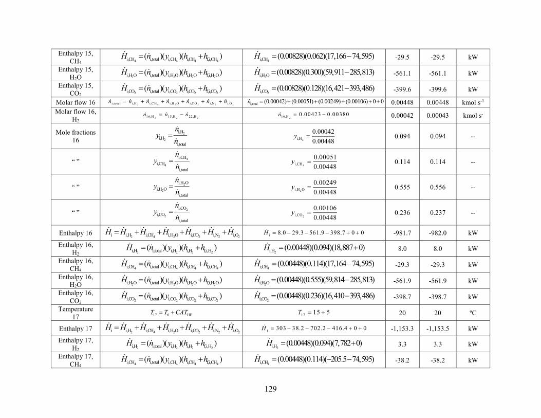
129

Enthalpy 15, CH4 4 4 4 4i,CH i,total i,CH i,CH f,i,CH( )( )( ) H n y h h

4i,CH (0.00828)(0.062)(17,166 74,595) H -29.5 -29.5 kW

Enthalpy 15, H2O 2 2 2 2i,H O i,total i,H O i,H O f,i,H O( )( )( ) H n y h h

2i,H O (0.00828)(0.300)(59,911 285,813) H -561.1 -561.1 kW

Enthalpy 15, CO2 2 2 2 2i,CO i,total i,CO i,CO f,i,CO( )( )( ) H n y h h

2i,CO (0.00828)(0.128)(16,421 393,486) H -399.6 -399.6 kW

Molar flow 16 2 4 2 2 2 2i,total i,H i,C H i,H O i,C O i,N i,O n n n n n n n i,total (0.00042) (0.00051) (0.00249) (0.00106) 0 0 n 0.00448 0.00448 kmol s-1

Molar flow 16, H2 2 2 216,H 15,H 22 ,H n n n

216,H 0.00423 0.00380 n 0.00042 0.00043 kmol s-

Mole fractions 16

2

2

i,Hi,H

i,total

n

yn 2i,H

0.000420.00448

y 0.094 0.094 --

“ ” 4

4

i,CHi,CH

i,total

n

yn 4i,CH

0.000510.00448

y 0.114 0.114 --

“ ” 2

2

i,H Oi,H O

i,total

n

yn 2i,H O

0.002490.00448

y 0.555 0.556 --

“ ” 2

2

i,COi,CO

i,total

n

yn 2i,CO

0.001060.00448

y 0.236 0.237 --

Enthalpy 16 2 4 2 2 2 2i i,H i,CH i,H O i,CO i,N i,O H H H H H H H i 8.0 29.3 561.9 398.7 0 0 H -981.7 -982.0 kW

Enthalpy 16, H2 2 2 2 2i,H i,total i,H i,H f,i,H( )( )( ) H n y h h

2i,H (0.00448)(0.094)(18,887 0) H 8.0 8.0 kW

Enthalpy 16, CH4 4 4 4 4i,CH i,total i,CH i,CH f,i,CH( )( )( ) H n y h h

4i,CH (0.00448)(0.114)(17,164 74,595) H -29.3 -29.3 kW

Enthalpy 16, H2O 2 2 2 2i,H O i,total i,H O i,H O f,i,H O( )( )( ) H n y h h

2i,H O (0.00448)(0.555)(59,814 285,813) H -561.9 -561.9 kW

Enthalpy 16, CO2 2 2 2 2i,CO i,total i,CO i,CO f,i,CO( )( )( ) H n y h h

2i,CO (0.00448)(0.236)(16,410 393,486) H -398.7 -398.7 kW

Temperature 17 17 6 HE T T CAT 17 15 5 T 20 20 ºC

Enthalpy 17 2 4 2 2 2 2i i,H i,CH i,H O i,CO i,N i,O H H H H H H H i 303 38.2 702.2 416.4 0 0 H -1,153.3 -1,153.5 kW

Enthalpy 17, H2 2 2 2 2i,H i,total i,H i,H f,i,H( )( )( ) H n y h h

2i,H (0.00448)(0.094)(7,782 0) H 3.3 3.3 kW

Enthalpy 17, CH4 4 4 4 4i,CH i,total i,CH i,CH f,i,CH( )( )( ) H n y h h

4i,CH (0.00448)(0.114)( 205.5 74,595) H -38.2 -38.2 kW

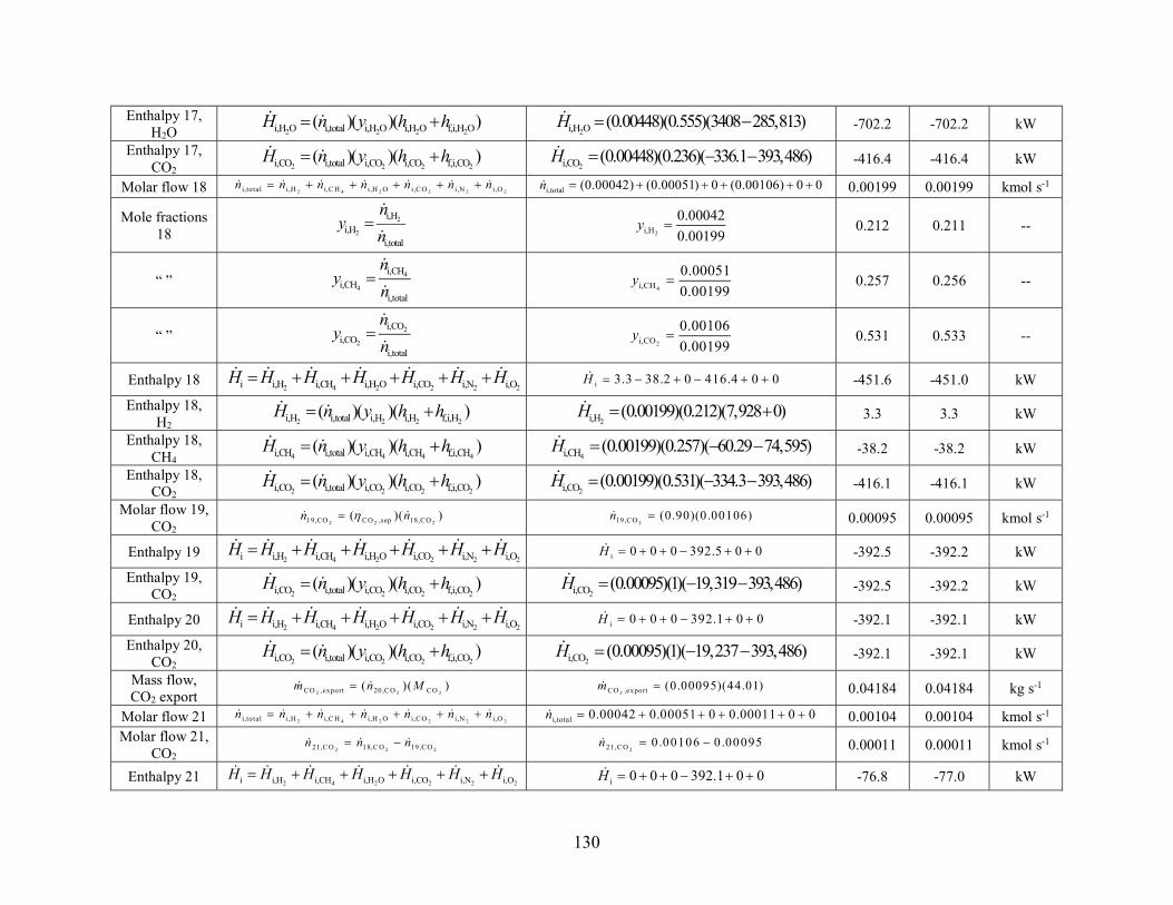
130

Enthalpy 17, H2O 2 2 2 2i,H O i,total i,H O i,H O f,i,H O( )( )( ) H n y h h

2i,H O (0.00448)(0.555)(3408 285,813) H -702.2 -702.2 kW

Enthalpy 17, CO2 2 2 2 2i,CO i,total i,CO i,CO f,i,CO( )( )( ) H n y h h

2i,CO (0.00448)(0.236)( 336.1 393,486) H -416.4 -416.4 kW

Molar flow 18 2 4 2 2 2 2i,total i,H i,C H i,H O i,C O i,N i,O n n n n n n n i,total (0.00042) (0.00051) 0 (0.00106) 0 0 n 0.00199 0.00199 kmol s-1

Mole fractions 18

2

2

i,Hi,H

i,total

n

yn 2i,H

0.000420.00199

y 0.212 0.211 --

“ ” 4

4

i,CHi,CH

i,total

n

yn 4i,CH

0.000510.00199

y 0.257 0.256 --

“ ” 2

2

i,COi,CO

i,total

n

yn 2i,CO

0.001060.00199

y 0.531 0.533 --

Enthalpy 18 2 4 2 2 2 2i i,H i,CH i,H O i,CO i,N i,O H H H H H H H i 3.3 38.2 0 416.4 0 0 H -451.6 -451.0 kW

Enthalpy 18, H2 2 2 2 2i,H i,total i,H i,H f,i,H( )( )( ) H n y h h

2i,H (0.00199)(0.212)(7,928 0) H 3.3 3.3 kW

Enthalpy 18, CH4 4 4 4 4i,CH i,total i,CH i,CH f,i,CH( )( )( ) H n y h h

4i,CH (0.00199)(0.257)( 60.29 74,595) H -38.2 -38.2 kW

Enthalpy 18, CO2 2 2 2 2i,CO i,total i,CO i,CO f,i,CO( )( )( ) H n y h h

2i,CO (0.00199)(0.531)( 334.3 393,486) H -416.1 -416.1 kW

Molar flow 19, CO2 2 2 219,CO CO ,sep 18,CO( )( ) n n

219,CO (0.90)(0.00106)n 0.00095 0.00095 kmol s-1

Enthalpy 19 2 4 2 2 2 2i i,H i,CH i,H O i,CO i,N i,O H H H H H H H i 0 0 0 392.5 0 0 H -392.5 -392.2 kW

Enthalpy 19, CO2 2 2 2 2i,CO i,total i,CO i,CO f,i,CO( )( )( ) H n y h h

2i,CO (0.00095)(1)( 19,319 393,486) H -392.5 -392.2 kW

Enthalpy 20 2 4 2 2 2 2i i,H i,CH i,H O i,CO i,N i,O H H H H H H H i 0 0 0 392.1 0 0 H -392.1 -392.1 kW

Enthalpy 20, CO2 2 2 2 2i,CO i,total i,CO i,CO f,i,CO( )( )( ) H n y h h

2i,CO (0.00095)(1)( 19,237 393,486) H -392.1 -392.1 kW

Mass flow, CO2 export 2 2 2CO ,export 20,CO CO( )( ) m n M

2CO ,export (0.00095)(44.01)m 0.04184 0.04184 kg s-1

Molar flow 21 2 4 2 2 2 2i,total i,H i,C H i,H O i,C O i,N i,O n n n n n n n i,total 0.00042 0.00051 0 0.00011 0 0 n 0.00104 0.00104 kmol s-1

Molar flow 21, CO2 2 2 221,C O 18,C O 19,CO n n n

221,C O 0.00106 0.00095 n 0.00011 0.00011 kmol s-1

Enthalpy 21 2 4 2 2 2 2i i,H i,CH i,H O i,CO i,N i,O H H H H H H H i 0 0 0 392.1 0 0 H -76.8 -77.0 kW

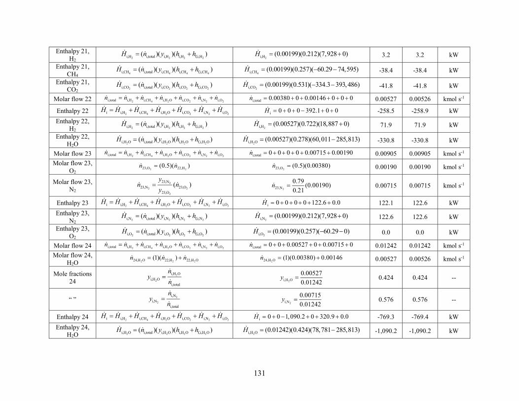
131

Enthalpy 21, H2 2 2 2 2i,H i,total i,H i,H f,i,H( )( )( ) H n y h h

2i,H (0.00199)(0.212)(7,928 0) H 3.2 3.2 kW

Enthalpy 21, CH4 4 4 4 4i,CH i,total i,CH i,CH f,i,CH( )( )( ) H n y h h

4i,CH (0.00199)(0.257)( 60.29 74,595) H -38.4 -38.4 kW

Enthalpy 21, CO2 2 2 2 2i,CO i,total i,CO i,CO f,i,CO( )( )( ) H n y h h

2i,CO (0.00199)(0.531)( 334.3 393,486) H -41.8 -41.8 kW

Molar flow 22 2 4 2 2 2 2i,total i,H i,CH i,H O i,CO i,N i,O n n n n n n n i,total 0.00380 0 0.00146 0 0 0 n 0.00527 0.00526 kmol s-1

Enthalpy 22 2 4 2 2 2 2i i,H i,CH i,H O i,CO i,N i,O H H H H H H H i 0 0 0 392.1 0 0 H -258.5 -258.9 kW Enthalpy 22,

H2 2 2 2 2i,H i,total i,H i,H f,i,H( )( )( ) H n y h h 2i,H (0.00527)(0.722)(18,887 0) H 71.9 71.9 kW

Enthalpy 22, H2O 2 2 2 2i,H O i,total i,H O i,H O f,i,H O( )( )( ) H n y h h

2i,H O (0.00527)(0.278)(60,011 285,813) H -330.8 -330.8 kW

Molar flow 23 2 4 2 2 2 2i,total i,H i,CH i,H O i,CO i,N i,O n n n n n n n i,total 0 0 0 0 0.00715 0.00190 n 0.00905 0.00905 kmol s-1 Molar flow 23,

O2 2 223,O 22,H(0.5)( ) n n 223,O (0.5)(0.00380)n 0.00190 0.00190 kmol s-1

Molar flow 23, N2

2

2 2

2

23,N23,N 23,O

23,O

( ) y

n ny

223,N

0.79 (0.00190)0.21

n 0.00715 0.00715 kmol s-1

Enthalpy 23 2 4 2 2 2 2i i,H i,CH i,H O i,CO i,N i,O H H H H H H H i 0 0 0 0 122.6 0.0 H 122.1 122.6 kW Enthalpy 23,

N2 2 2 2 2i,N i,total i,N i,N f,i,N( )( )( ) H n y h h 2i,N (0.00199)(0.212)(7,928 0) H 122.6 122.6 kW

Enthalpy 23, O2 2 2 2 2i,O i,total i,O i,O f,i,O( )( )( ) H n y h h

2i,O (0.00199)(0.257)( 60.29 0) H 0.0 0.0 kW

Molar flow 24 2 4 2 2 2 2i,total i,H i,CH i,H O i,CO i,N i,O n n n n n n n i,total 0 0 0.00527 0 0.00715 0 n 0.01242 0.01242 kmol s-1 Molar flow 24,

H2O 2 2 224,H O 22,H 22,H O(1)( ) n n n 224,H O (1)(0.00380) 0.00146 n 0.00527 0.00526 kmol s-1

Mole fractions 24

2

2

i,H Oi,H O

i,total

n

yn

2i,H O

0.005270.01242

y 0.424 0.424 --

“ ” 2

2

i,Ni,N

i,total

n

yn

2i,N

0.007150.01242

y 0.576 0.576 --

Enthalpy 24 2 4 2 2 2 2i i,H i,CH i,H O i,CO i,N i,O H H H H H H H i 0 0 1,090.2 0 320.9 0.0 H -769.3 -769.4 kW Enthalpy 24,

H2O 2 2 2 2i,H O i,total i,H O i,H O f,i,H O( )( )( ) H n y h h 2i,H O (0.01242)(0.424)(78,781 285,813) H -1,090.2 -1,090.2 kW

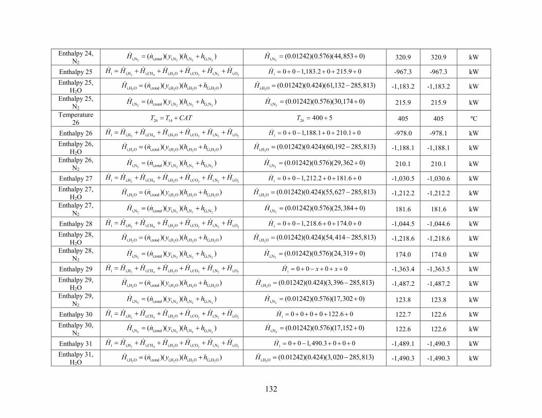
132

Enthalpy 24, N2 2 2 2 2i,N i,total i,N i,N f,i,N( )( )( ) H n y h h

2i,N (0.01242)(0.576)(44,853 0) H 320.9 320.9 kW

Enthalpy 25 2 4 2 2 2 2i i,H i,CH i,H O i,CO i,N i,O H H H H H H H i 0 0 1,183.2 0 215.9 0 H -967.3 -967.3 kW Enthalpy 25,

H2O 2 2 2 2i,H O i,total i,H O i,H O f,i,H O( )( )( ) H n y h h 2i,H O (0.01242)(0.424)(61,132 285,813) H -1,183.2 -1,183.2 kW

Enthalpy 25, N2 2 2 2 2i,N i,total i,N i,N f,i,N( )( )( ) H n y h h

2i,N (0.01242)(0.576)(30,174 0) H 215.9 215.9 kW

Temperature 26 26 14 T T CAT 26 400 5 T 405 405 ºC

Enthalpy 26 2 4 2 2 2 2i i,H i,CH i,H O i,CO i,N i,O H H H H H H H i 0 0 1,188.1 0 210.1 0 H -978.0 -978.1 kW Enthalpy 26,

H2O 2 2 2 2i,H O i,total i,H O i,H O f,i,H O( )( )( ) H n y h h 2i,H O (0.01242)(0.424)(60,192 285,813) H -1,188.1 -1,188.1 kW

Enthalpy 26, N2 2 2 2 2i,N i,total i,N i,N f,i,N( )( )( ) H n y h h

2i,N (0.01242)(0.576)(29,362 0) H 210.1 210.1 kW

Enthalpy 27 2 4 2 2 2 2i i,H i,CH i,H O i,CO i,N i,O H H H H H H H i 0 0 1, 212.2 0 181.6 0 H -1,030.5 -1,030.6 kW Enthalpy 27,

H2O 2 2 2 2i,H O i,total i,H O i,H O f,i,H O( )( )( ) H n y h h 2i,H O (0.01242)(0.424)(55,627 285,813) H -1,212.2 -1,212.2 kW

Enthalpy 27, N2 2 2 2 2i,N i,total i,N i,N f,i,N( )( )( ) H n y h h

2i,N (0.01242)(0.576)(25,384 0) H 181.6 181.6 kW

Enthalpy 28 2 4 2 2 2 2i i,H i,CH i,H O i,CO i,N i,O H H H H H H H i 0 0 1, 218.6 0 174.0 0 H -1,044.5 -1,044.6 kW Enthalpy 28,

H2O 2 2 2 2i,H O i,total i,H O i,H O f,i,H O( )( )( ) H n y h h 2i,H O (0.01242)(0.424)(54,414 285,813) H -1,218.6 -1,218.6 kW

Enthalpy 28, N2 2 2 2 2i,N i,total i,N i,N f,i,N( )( )( ) H n y h h

2i,N (0.01242)(0.576)(24,319 0) H 174.0 174.0 kW

Enthalpy 29 2 4 2 2 2 2i i,H i,CH i,H O i,CO i,N i,O H H H H H H H i 0 0 0 0 H x x -1,363.4 -1,363.5 kW Enthalpy 29,

H2O 2 2 2 2i,H O i,total i,H O i,H O f,i,H O( )( )( ) H n y h h 2i,H O (0.01242)(0.424)(3,396 285,813) H -1,487.2 -1,487.2 kW

Enthalpy 29, N2 2 2 2 2i,N i,total i,N i,N f,i,N( )( )( ) H n y h h

2i,N (0.01242)(0.576)(17,302 0) H 123.8 123.8 kW

Enthalpy 30 2 4 2 2 2 2i i,H i,CH i,H O i,CO i,N i,O H H H H H H H i 0 0 0 0 122.6 0 H 122.7 122.6 kW Enthalpy 30,

N2 2 2 2 2i,N i,total i,N i,N f,i,N( )( )( ) H n y h h 2i,N (0.01242)(0.576)(17,152 0) H 122.6 122.6 kW

Enthalpy 31 2 4 2 2 2 2i i,H i,CH i,H O i,CO i,N i,O H H H H H H H i 0 0 1, 490.3 0 0 0 H -1,489.1 -1,490.3 kW Enthalpy 31,

H2O 2 2 2 2i,H O i,total i,H O i,H O f,i,H O( )( )( ) H n y h h 2i,H O (0.01242)(0.424)(3,020 285,813) H -1,490.3 -1,490.3 kW

133

Enthalpy 32 2 4 2 2 2 2i i,H i,CH i,H O i,CO i,N i,O H H H H H H H i 0 0 1, 490.3 0 0 0 H -703.2 -704.2 kW Enthalpy 32,

H2O 2 2 2 2i,H O i,total i,H O i,H O f,i,H O( )( )( ) H n y h h 2i,H O (0.01242)(0.424)(3,020 285,813) H -704.2 -704.2 kW

134

A.2. Energy Balance Calculation

Table A-4: Hand calculations versus EES results to verify energy balance parameters.

Parameter Equation Evaluated EES Calc. Value

Hand Calc. Value

Units

Ambient enthalpy 9 2 4 2 2 2 2i i,H i,CH i,H O i,CO i,N i,O H H H H H H H i 0 0 4,892.3 0 0 0 H -4,891.1 -4,892.3 kW

Ambient enthalpy 9,

H2O 2 2 2 2i,H O i,total i,H O i,H O f,i,H O( )( )( ) H n y h h

2i,H O (0.01730)(1)(3,020 285,813) H -4,892.3 -4,892.3 kW

Heat to export steam steam,export 9 9,amb Q H H steam,export ( 4,051.3) ( 4,891.1) Q 839.8 839.8 kW

Enthalpy of NG, available 2 4 2 2 2 2i i,H i,CH i,H O i,CO i,N i,O H H H H H H H 0 71.2 0 0 0 0.7

iH -72.0 -72.1 kW

“ “, CH4 4 4 4 4i,CH i,total i,CH i,CH f,i,CH( )( )( ) H n y h h 4i,CH (0.00285)(0.333)( 438.4 74.595) H -71.2 -71.2 kW

“ “, O2 2 2 2 2i,O i,total i,O i,O f,i,O( )( )( ) H n y h h 2i,O (0.00285)(0.333)( 369 0) H -0.7 -0.7 kW

Enthalpy of NG,

combusted 2 4 2 2 2 2i i,H i,CH i,H O i,CO i,N i,O H H H H H H H i 0 0 537.6 373.9 0 0 H -912.2 -911.5 kW

“ “, H2O 2 2 2 2i,H O i,total i,H O i,H O f,i,H O( )( )( ) H n y h h 2i,H O (0.00285)(0.667)(3,030 285,813) H -537.6 -537.6 kW

“ “, CO2 2 2 2 2i,CO i,total i,CO i,CO f,i,CO( )( )( ) H n y h h 2i,CO (0.00285)(0.333)( 531.7 393,486) H -373.9 -373.9 kW

Heat of NG in NG,in NG,in NG,out Q H H NG,in ( 72.0) ( 912.2) Q 840.2 840.2 kW Electricity

input 2 2elec CO ,comp,in CO ,cryo,in pump,in W W W W elec 0.09 17.78 0.61 W 18.48 18.48 kW

Ambient enthalpy 20 2 4 2 2 2 2i i,H i,CH i,H O i,CO i,N i,O H H H H H H H i 0 0 0 374.5 0 0 H -374.5 -374.2 kW

Ambient enthalpy 20,

CO2 2 2 2 2i,CO i,total i,CO i,CO f,i,CO( )( )( ) H n y h h

2i,CO (0.00199)(0.531)( 334.3 393,486) H -374.5 -374.2 kW

Heat of CO2 export 2CO ,export 20 20,amb Q H H

2CO ,export ( 392.4) ( 374.5) Q -17.9 -17.9 kW

Efficiency, overall system

steam,exportoverall,system

NG,in elec,in

QQ W

overall,system839.8

840.2 18.48

0.9781 0.97801 --

135

Efficiency, overall boiler

steam,export CO2,exportoverall,boiler

NG,in elec,in

Q Q

Q W overall,boiler

839.8 17.9840.2 18.48

0.9989 0.99886 --

Enthalpy 11, before

pressure drop 2 4 2 2 2 2i i,H i,CH i,H O i,CO i,N i,O H H H H H H H 11,highP 0 0 341.1 0 0 0 H -342.6 -342.0 kW

Enthalpy 11, H2O, before

pressure drop 2 2 2 2i,H O i,total i,H O i,H O f,i,H O( )( )( ) H n y h h

2i,H O (0.00146)(1)(51,577 285,813) H -342.6 -342.0 kW

Heat lost in pressure drop

of 11 11, 11, 11

P highPQ H H 11, ( 342.6) ( 341.1) PQ -1.53 -1.5 kW

Boiler heat to steam boiler,steam 8 7 Q H H boiler,steam ( 5,421.8) ( 6,054.8) Q 633.02 633.00 kW

Boiler input (fuel) heat boiler,input boiler boiler,steam Q Q boiler,input (0.5146) 633.02Q 1,230.12 1,230.12 kW

Boiler input (fuel) heat boiler,input 22 23 24,amb Q H H H 221, 230.12 (122.1) ( 1,366.4) H -258.5 -258.38 kW

Ambient enthalpy 24 2 4 2 2 2 2i i,H i,CH i,H O i,CO i,N i,O H H H H H H H i 0 0 1, 488.0 0 122.6 0 H -1,366.4 -1,365.4 kW

Ambient enthalpy 24,

H2O 2 2 2 2i,H O i,total i,H O i,H O f,i,H O( )( )( ) H n y h h

2i,H O (0.01730)(1)(3,020 285,813) H -1,488.0 -1,488.0 kW

Ambient enthalpy 24,

N2 2 2 2 2i,N i,total i,N i,N f,i,N( )( )( ) H n y h h

2i,N (0.01242)(0.576)(24,319 0) H 122.6 122.6 kW

Boiler heat to steam boiler,steam 22 23 24 Q H H H boiler,steam ( 258.5) (122.1) ( 769.3) Q 633.02 632.9 kW

Boiler heat to exhaust boiler,exh boiler,input boiler,steam Q Q Q boiler,exh (1,230.12) (633.02) Q 597.1 597.1 kW

Heat exchanger 1,

cold side HE1 22 16 14 12 Q H H H H HE1 ( 258.5) ( 981.7) ( 1,107.8) ( 330.3) Q 197.9 197.9 kW

Heat exchanger 1,

hot side HE1 24 25 Q H H HE1 ( 769.3) ( 967.3) Q 197.9 198 kW

Heat exchanger 2,

cold side HE2 12 11 Q H H HE2 ( 330.3) ( 341.1) Q 10.75 10.8 kW

136

Heat exchanger 2,

hot side HE2 25 26 Q H H HE2 ( 967.3) ( 978.0) Q 10.75 10.7 kW

Heat exchanger 3,

cold side HE3 14 13 Q H H HE3 ( 1,107.8) ( 1,160.3) Q 52.5 52.5 kW

Heat exchanger 3,

hot side HE3 26 27 Q H H HE3 ( 978.0) ( 1,030.5) Q 52.5 52.5 kW

Heat exchanger 4,

cold side HE4 3 2 Q H H HE4 ( 134.3) ( 148.3) Q 13.99 14.0 kW

Heat exchanger 4,

hot side HE4 27 28 Q H H HE4 ( 1,030.5) ( 1,044.5) Q 13.99 14.0 kW

Heat exchanger 5,

cold side HE5 7 6 Q H H HE5 ( 6,054.8) ( 6,545.2) Q 490.4 490.4 kW

Heat exchanger 5,

retentate HE5,ret 16 17 Q H H HE5,ret ( 981.7) ( 1,153.3) Q 171.5 171.6 kW

Heat exchanger 5,

boiler exhaust HE5,exh 28 29 Q H H HE5,exh ( 1,044.5) ( 1,363.4) Q 318.9 318.9 kW

Heat exchanger 5,

hot side HE5 HE5,ret HE5,exh Q Q Q HE5 171.5 318.9 Q 490.4 490.4 kW

Heat exchanger 6 HE6 18 32 17 Q H H H HE6 ( 451.6) ( 703.2) ( 1,153.3) Q -1.552 -1.5 kW

Heat exchanger 7 HE7 30 31 29 Q H H H HE7 (122.7) ( 1, 489.1) ( 1,363.4) Q -3.056 -3.0 kW

Work, CO2 compressor, to

fluid 2CO ,comp,out 20 19 W H H

2CO ,comp,out ( 392.4) ( 392.5) W 0.078 0.1 kW

Work, CO2 compressor, electricity in

2 2 2CO ,comp,in CO ,comp CO ,comp,out( )( ) W W 2CO ,comp,in( )(0.85) 0.078W 0.0914 0.092 kW

Work, CO2 cryo, to fluid 2CO ,cryo,out 18 19 21 W H H H

2,CO cryo,in ( 451.6) ( 392.5) ( 76.8) W 17.78 17.7 kW

137

Work, CO2 cryo,

electricity in 2 2 2

1CO ,cryo,in 19,CO CO(425 )( )( ) W kJ kg n M

2CO ,cryo,out (425)(0.00095)(44.01)W 17.78 17.77 kW

Work, water pump, to fluid pump,out 6 5 W H H pump,out ( 6,545.2) ( 6,545.7) W 0.5171 0.5 kW

Work, water pump,

electricity in pump,in pump pump,out( )( ) W W pump,in( )(0.85) 0.5171W 0.6084 0.6084 kW

A.3. Capital and Operating Cost Calculation

Table A-5: Hand calculations versus EES results to verify capital and operating costs.

Parameter Equation Evaluated EES Calc. Value

Hand Calc. Value

Units

Membrane permeance

63 2 1 0.5

memmem

2.8 10 6.48 10

x mK x mol m s Pat

mem2.8 -66.48 -32.8 -6

eK ee

6.48x10-3 6.48x10-3 mol m-2 s-1 Pa-0.5

Retentate H2 partial

pressure 2 2

100,000 PaH ,ret 15 15,H( )( ) barP P y bar

2H ,ret (15)(0.510) 100,000P 765,456 765,000 Pa

Permeate H2 partial

pressure 2 2

100,000 PaH ,per 22 22,H( )( ) barP P y bar

2H ,per (2)(0.722) 100,000P 144,444 144,400 Pa

Membrane surface area 2 2 2

0.5 0.51000 22,H mem mem H ,ret H ,per( )( ) kmol mol

s kmoln K A P P 0.5 0.5mem(0.00380) 1000 (6.48 -6)( ) 765, 456 144, 444 e A 1.186 1.185 m2

Cost, HE1, membrane HE1,membrane membrane$1,076C A HE1,membrane 1,076 1.186C 1,276 1,276 $

Mass flow 22, H2 2 2 222,H 22,H H( )( ) m n M

222,H (0.00380)(2.002)m 0.007667 0.00761 kg s-1

Cost, HE1, reactor 2

0.73600 22,H

HE1,reactor $14,1004.79

sh

kgh

mC

0.7

HE1,reactor(0.007667)(3600)14,100

4.79

C 48,043 48,043 $

Cost, HE1, total HE1,total HE1,membrane HE1,reactor C C C 1, 12,76 48,043 HE totalC 49,319 49,319 $

Cost HE2 2

2

0.510.76 ft

HE2 ht,HE2$462m

C A 0.5HE2 $462 22.73 10.76 C 7,226 7,225 $

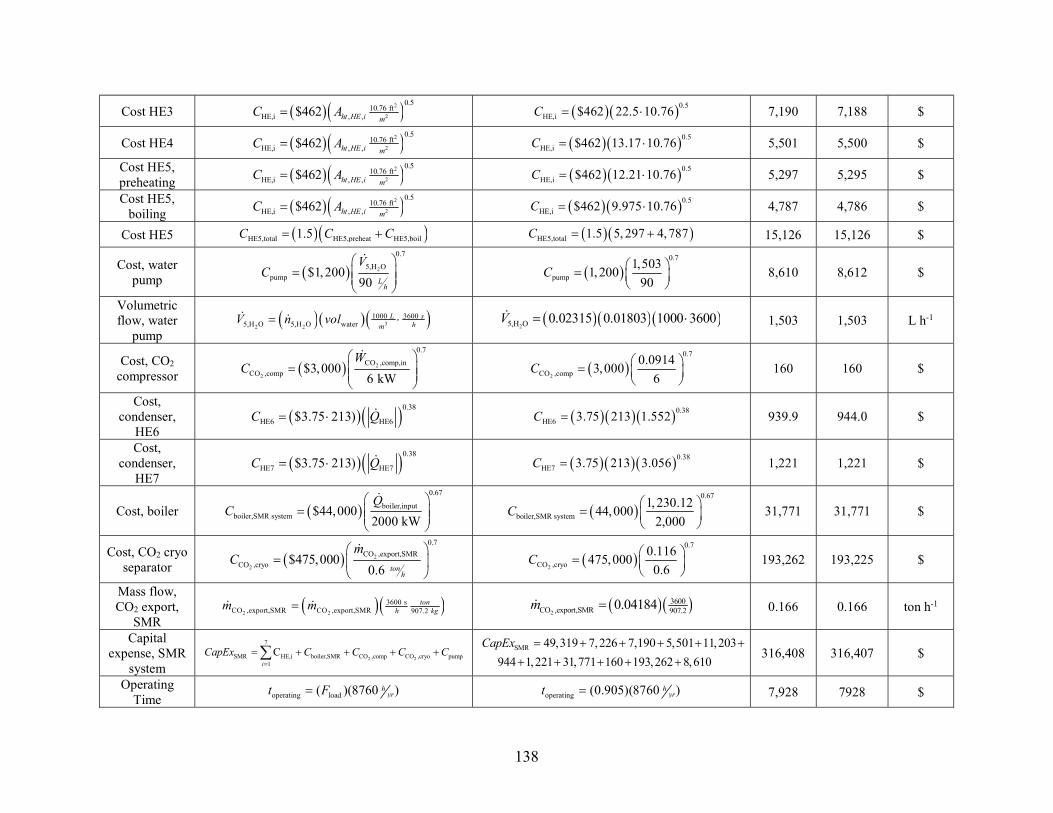
138

Cost HE3 2

2

0.510.76 ft

HE,i , ,$462 ht HE i mC A 0.5

HE,i $462 22.5 10.76 C 7,190 7,188 $

Cost HE4 2

2

0.510.76 ft

HE,i , ,$462 ht HE i mC A 0.5

HE,i $462 13.17 10.76 C 5,501 5,500 $

Cost HE5, preheating 2

2

0.510.76 ft

HE,i , ,$462 ht HE i mC A 0.5

HE,i $462 12.21 10.76 C 5,297 5,295 $

Cost HE5, boiling 2

2

0.510.76 ft

HE,i , ,$462 ht HE i mC A 0.5

HE,i $462 9.975 10.76 C 4,787 4,786 $

Cost HE5 HE5,total HE5,preheat HE5,boil1.5 C C C HE5,total 1.5 5, 297 4,787 C 15,126 15,126 $

Cost, water pump 2

0.7

5,H Opump $1,200

90

L

h

VC

0.7

pump1,5031, 200

90

C 8,610 8,612 $

Volumetric flow, water

pump 32 2

1000 3600 5,H O 5,H O water L s

hmV n vol

25,H O 0.02315 0.01803 1000 3600 V 1,503 1,503 L h-1

Cost, CO2 compressor 2

2

0.7

CO ,comp,inCO ,comp $3,000

6 kW

WC

2

0.7

CO ,comp0.09143,000

6

C 160 160 $

Cost, condenser,

HE6 0.38

HE6 HE6$3.75 213) C Q 0.38HE6 3.75 213 1.552C 939.9 944.0 $

Cost, condenser,

HE7 0.38

HE7 HE7$3.75 213) C Q 0.38HE7 3.75 213 3.056C 1,221 1,221 $

Cost, boiler 0.67

boiler,inputboiler,SMR system $44,000

2000 kW

QC

0.67

boiler,SMR system1,230.1244,000

2,000

C 31,771 31,771 $

Cost, CO2 cryo separator 2

2

0.7CO ,export,SMR

CO ,cryo $475,0000.6

ton

h

mC

2

0.7

CO ,cryo0.116475,000

0.6

C 193,262 193,225 $

Mass flow, CO2 export,

SMR 2 2

3600 sCO ,export,SMR CO ,export,SMR 907.2 ton

h kgm m 2

3600CO ,export,SMR 907.20.04184m 0.166 0.166 ton h-1

Capital expense, SMR

system 2 2

7

SMR HE,i boiler,SMR CO ,comp CO ,cryo pump1

C

i

CapEx C C C C SMR 49,319 7,226 7,190 5,501 11,203 944 1,221 31,771 160 193,262 8,610

CapEx 316,408 316,407 $

Operating Time operating load( )(8760 ) h

yrt F operating (0.905)(8760 ) hyrt 7,928 7928 $

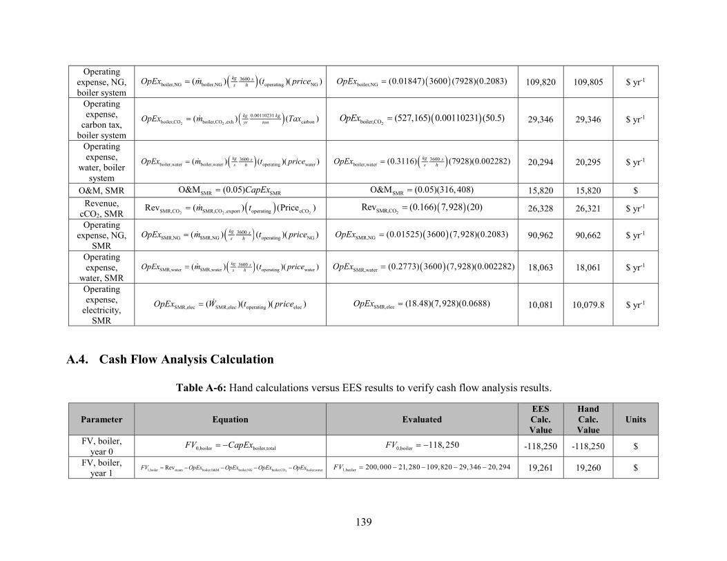
139

Operating expense, NG, boiler system

3600 boiler,NG boiler,NG operating NG( ) ( )( ) kg s

s hOpEx m t price boiler,NG (0.01847) 3600 (7928)(0.2083)OpEx 109,820 109,805 $ yr-1

Operating expense,

carbon tax, boiler system

2 2

0.00110231 boiler,CO boiler,CO ,exh carbon( ) ( ) kg kg

yr tonOpEx m Tax 2boiler,CO (527,165) 0.00110231 (50.5)OpEx 29,346 29,346 $ yr-1

Operating expense,

water, boiler system

3600 boiler,water boiler,water operating water( ) ( )( ) kg s

s hOpEx m t price 3600 boiler,water (0.3116) (7928)(0.002282) kg s

s hOpEx 20,294 20,295 $ yr-1

O&M, SMR SMR SMRO&M (0.05) CapEx SMRO&M (0.05)(316,408) 15,820 15,820 $ Revenue,

cCO2, SMR 2 2 2SMR,CO SMR,CO ,export operating cCORev ( ) (Price ) m t

2SMR,CORev (0.166) 7,928 (20) 26,328 26,321 $ yr-1

Operating expense, NG,

SMR 3600

SMR,NG SMR,NG operating NG( ) ( )( ) kg ss hOpEx m t price SMR,NG (0.01525) 3600 (7,928)(0.2083)OpEx 90,962 90,662 $ yr-1

Operating expense,

water, SMR 3600

SMR,water SMR,water operating water( ) ( )( ) kg ss hOpEx m t price SMR,water (0.2773) 3600 (7,928)(0.002282)OpEx 18,063 18,061 $ yr-1

Operating expense,

electricity, SMR

SMR,elec SMR,elec operating elec( )( )( ) OpEx W t price SMR,elec (18.48)(7,928)(0.0688)OpEx 10,081 10,079.8 $ yr-1

A.4. Cash Flow Analysis Calculation

Table A-6: Hand calculations versus EES results to verify cash flow analysis results.

Parameter Equation Evaluated EES Calc. Value

Hand Calc. Value

Units

FV, boiler, year 0 0,boiler boiler,total FV CapEx 0,boiler 118, 250 FV -118,250 -118,250 $

FV, boiler, year 1 21,boiler steam boiler,O&M boiler,NG boiler,CO boiler,waterRev FV OpEx OpEx OpEx OpEx

1,boiler 200, 000 21, 280 109,820 29,346 20, 294 FV 19,261 19,260 $

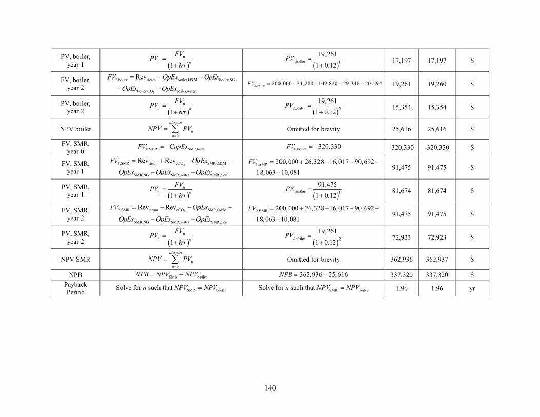
140

PV, boiler, year 1

nn

1

n

FVPVirr

1,boiler 1

19,2611 0.12

PV 17,197 17,197 $

FV, boiler, year 2

2

2,boiler steam boiler,O&M boiler,NG

boiler,CO boiler,water

Rev

FV OpEx OpExOpEx OpEx

2,boiler 200, 000 21, 280 109,820 29,346 20, 294 FV 19,261 19,260 $

PV, boiler, year 2

nn

1

n

FVPVirr

2,boiler 2

19,2611 0.12

PV 15,354 15,354 $

NPV boiler n0

lifespan

nNPV PV Omitted for brevity 25,616 25,616 $

FV, SMR, year 0 0,SMR SMR,total FV CapEx 0,boiler 320,330 FV -320,330 -320,330 $

FV, SMR, year 1

21,SMR steam cCO SMR,O&M

SMR,NG SMR,water SMR,elec

Rev Rev

FV OpEx

OpEx OpEx OpEx 1,SMR 200,000 26,328 16,017 90,692

18,063 10,081

FV 91,475 91,475 $

PV, SMR, year 1

nn

1

n

FVPVirr

1,boiler 1

91,4751 0.12

PV 81,674 81,674 $

FV, SMR, year 2

22,SMR steam cCO SMR,O&M

SMR,NG SMR,water SMR,elec

Rev Rev

FV OpEx

OpEx OpEx OpEx 2,SMR 200,000 26,328 16,017 90,692

18,063 10,081

FV 91,475 91,475 $

PV, SMR, year 2

nn

1

n

FVPVirr

2,boiler 2

19,2611 0.12

PV 72,923 72,923 $

NPV SMR n0

lifespan

nNPV PV Omitted for brevity 362,936 362,937 $

NPB SMR boiler NPB NPV NPV 362,936 25,616 NPB 337,320 337,320 $ Payback Period SMR boilerSolve for such that n NPV NPV SMR boilerSolve for such that n NPV NPV 1.96 1.96 yr

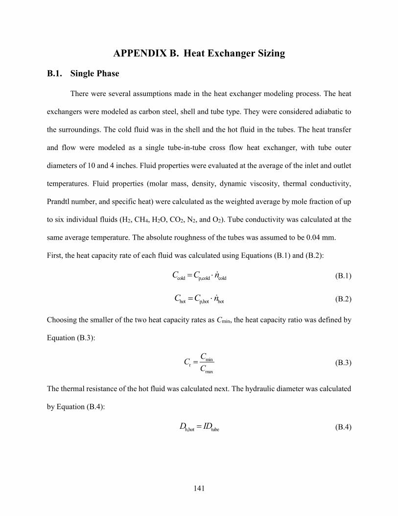
141

APPENDIX B. Heat Exchanger Sizing B.1. Single Phase

There were several assumptions made in the heat exchanger modeling process. The heat

exchangers were modeled as carbon steel, shell and tube type. They were considered adiabatic to

the surroundings. The cold fluid was in the shell and the hot fluid in the tubes. The heat transfer

and flow were modeled as a single tube-in-tube cross flow heat exchanger, with tube outer

diameters of 10 and 4 inches. Fluid properties were evaluated at the average of the inlet and outlet

temperatures. Fluid properties (molar mass, density, dynamic viscosity, thermal conductivity,

Prandtl number, and specific heat) were calculated as the weighted average by mole fraction of up

to six individual fluids (H2, CH4, H2O, CO2, N2, and O2). Tube conductivity was calculated at the

same average temperature. The absolute roughness of the tubes was assumed to be 0.04 mm.

First, the heat capacity rate of each fluid was calculated using Equations (B.1) and (B.2):

cold p,cold coldC C n (B.1)

hot p,hot hotC C n (B.2)

Choosing the smaller of the two heat capacity rates as Cmin, the heat capacity ratio was defined by

Equation (B.3):

minr

max

CCC

(B.3)

The thermal resistance of the hot fluid was calculated next. The hydraulic diameter was calculated

by Equation (B.4):

h,hot tubeD ID (B.4)

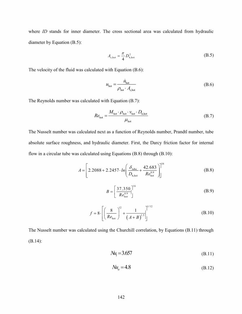
142

where ID stands for inner diameter. The cross sectional area was calculated from hydraulic

diameter by Equation (B.5):

2c,hot h,hot4

A D (B.5)

The velocity of the fluid was calculated with Equation (B.6):

hothot

hot c,hot

nuA

(B.6)

The Reynolds number was calculated with Equation (B.7):

hot hot hot h,hothot

hot

M v DRe (B.7)

The Nusselt number was calculated next as a function of Reynolds number, Prandtl number, tube

absolute surface roughness, and hydraulic diameter. First, the Darcy friction factor for internal

flow in a circular tube was calculated using Equations (B.8) through (B.10):

16

tube0 9

h,hot hot

42 6832 2088 2 2457

.

.A . . lnD Re

(B.8)

16

0 9hot

37 350

.

,BRe

(B.9)

1 1212

1 5hot

8 18

/

.fRe A B

(B.10)

The Nusselt number was calculated using the Churchill correlation, by Equations (B.11) through

(B.14):

l 3.657Nu (B.11)

o 4.8Nu (B.12)

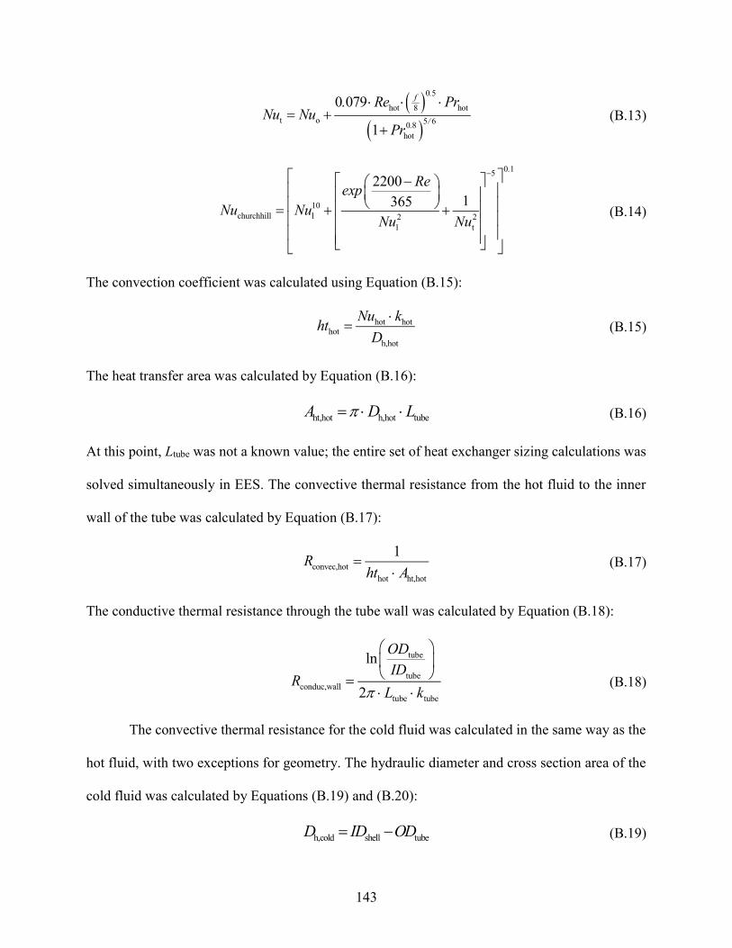
143

0 5

hot hot8t o 5 60 8

hot

0 079

1

.f

/.

. Re PrNu Nu

Pr (B.13)

0 15

10churchhill l 2 2

l t

22001365

.

ReexpNu Nu

Nu Nu (B.14)

The convection coefficient was calculated using Equation (B.15):

hot hothot

h,hot

Nu khtD

(B.15)

The heat transfer area was calculated by Equation (B.16):

ht,hot h,hot tubeA D L (B.16)

At this point, Ltube was not a known value; the entire set of heat exchanger sizing calculations was

solved simultaneously in EES. The convective thermal resistance from the hot fluid to the inner

wall of the tube was calculated by Equation (B.17):

convec,hothot ht,hot

1Rht A

(B.17)

The conductive thermal resistance through the tube wall was calculated by Equation (B.18):

tube

tubeconduc,wall

tube tube

ln

2

ODID

RL k

(B.18)

The convective thermal resistance for the cold fluid was calculated in the same way as the

hot fluid, with two exceptions for geometry. The hydraulic diameter and cross section area of the

cold fluid was calculated by Equations (B.19) and (B.20):

h,cold shell tubeD ID OD (B.19)

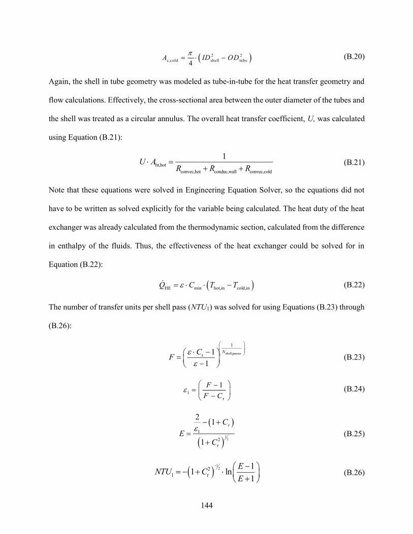
144

2 2c,cold shell tube4

A ID OD (B.20)

Again, the shell in tube geometry was modeled as tube-in-tube for the heat transfer geometry and

flow calculations. Effectively, the cross-sectional area between the outer diameter of the tubes and

the shell was treated as a circular annulus. The overall heat transfer coefficient, U, was calculated

using Equation (B.21):

ht,hotconvec,hot conduc,wall convec,cold

1U AR R R

(B.21)

Note that these equations were solved in Engineering Equation Solver, so the equations did not

have to be written as solved explicitly for the variable being calculated. The heat duty of the heat

exchanger was already calculated from the thermodynamic section, calculated from the difference

in enthalpy of the fluids. Thus, the effectiveness of the heat exchanger could be solved for in

Equation (B.22):

HE min hot,in cold,inQ C T T (B.22)

The number of transfer units per shell pass (NTU1) was solved for using Equations (B.23) through

(B.26):

shell,passes

1

r 11

NCF

(B.23)

1r

1FF C

(B.24)

1

2

1

2r

2 1

1

rCE

C

(B.25)

1

221 r

11 ln1

ENTU CE

(B.26)

145

The total number of transfer units was calculated using Equation (B.27):

shell,passes 1NTU n NTU (B.27)

Using the definition of NTU, the overall heat transfer area (and thus Ltube) was solved for iteratively

by Equation (B.28):

ht,hot

min

ANTU U

C (B.28)

B.2. Two Phase

The method of section B.1 was applied for heat exchangers 1 through 4. Heat exchanger 5

was more complicated for two reasons: it involved flow boiling, and it used three fluids (instead

of two). Heat exchanger 5 was split up into two sections: preheating liquid water to saturation

temperature, and boiling from saturated liquid to two-phase with 0 < X < 1. The preheating section

of heat exchanger 5 was modeled in the same way as heat exchangers 1 through 4.

The boiling section of heat exchanger 5 was more complicated. The same assumptions

about geometry were made as with the previous heat exchangers. The hydraulic diameters and

cross-sectional areas were calculated in the same way as before. The heat transfer correlations used

in the sizing of the boiling section of the heat exchanger were from Kim and Mudawar [117]. In

order to accurately capture the behavior of flow boiling, the heat exchanger was discretized into N

sections using Equations (B.29) and (B.30):

cold,out cold,inX X

XN

(B.29)

hot,in hot,out

hot

T TT

N

(B.30)

The first discretized section was the hot fluid entry (highest temperature) and cold fluid exit

(highest quality). The boundary conditions were initialized by Equations (B.31) and (B.32):

146

0,hot hot,inT T (B.31)

0,cold cold,outX X (B.32)

The following (Equations (B.33) through (B.79)) occurred within a duplicated loop, where i

represents the section of heat exchanger. Fluid properties were evaluated separately in each section

of the heat exchanger. First, the known conditions were set by Equations (B.33) and (B.34):

i,cold coldT T (B.33)

i,cold 0,coldX X i X (B.34)

The convection coefficient of the boiling (“cold”) fluid was calculated using the Kim and

Mudawar correlation as a function of temperature, quality, molar flow rate, and hydraulic diameter

[117,118]. Several fluid properties were calculated for both the saturated liquid (subscript liq) and

saturated vapor (subscript gas). The mass flux was calculated using Equations (B.35) and (B.37):

2c h4

A D (B.35)

m M n (B.36)

c

mGA

(B.37)

The Reynolds number of liquid and vapor were calculated using Equations (B.38) and (B.39):

hliq

liq

1

G X D

Re (B.38)

hgas

gas

G X DRe (B.39)

147

The fanning friction factor was calculated depending on the Reynolds number. The same equations

apply to both liquid and vapor, but were calculated separately for each, using Equations (B.40)

through (B.42):

116 for < 2,000 f Re Re (B.40)

0250079 for 2,000 < 20,000 .f . Re Re (B.41)

020046 for 20 000 .f . Re Re , (B.42)

The frictional pressure drop of the liquid and vapor were calculated using Equations (B.43) and

(B.44):

2liq 2

liqliq

liq

2 1

h

vf G X

Mdpdz D

(B.43)

gas 2 2gas

gas

gas h

2v

f G XMdp

dz D

(B.44)

The next step was to calculate total frictional pressure drop of the fluid by Equation (B.45):

2liq

F liq

dP dPdz dz

(B.45)

where ϕliq is given by Equation (B.46):

2liq 2

LM LM

11 CX X

(B.46)

The symbol XLM is a Lockhart-Martinelli parameter and should not be confused with fluid quality,

X. The Lockhart-Martinelli parameter XLM was calculated by Equation (B.47):

liq2LM

gas

dPdz

dPdz

X (B.47)

148

Another Lockhart-Martinelli parameter was calculated based on liquid and vapor Reynolds

numbers, by Equations (B.48) through (B.51):

0 35

liq0.03 0.10nb fo go liq gas

gas

0 39 for 2 000 and 2 000

.

C . Re Su Re , Re , (B.48)

0 14

liq0.17 0.50nb fo go liq gas

gas

8 7 -4 for 2 000 and 2 000

.

C . e Re Su Re , Re , (B.49)

0 36

liq0.59 0.19nb fo go liq gas

gas

0 0015 for 2 000 and 2 000

.

C . Re Su Re , Re , (B.50)

0 48

liq0.44 0.50nb fo go liq gas

gas

3 5 -5 for 2 000 and 2 000

.

C . e Re Su Re , Re , (B.51)

Based on the non-boiling parameter, Cnb, the parameter C was calculated using Equations (B.52)

and (B.53):

0 78

0.32 Hnb fo liq

W

1 60 for 2 000

.PC C We Bo Re ,P

(B.52)

1 09

0.52 Hnb fo liq

W

1 530 for 2 000

.PC C We Bo Re ,P

(B.53)

In Equations (B.52) and (B.53), PH is the heated perimeter of the channel and PF is the wetted

perimeter of the channel. Bo is the boiling number, given by Equation (B.54):

fg

HqBoG h

(B.54)

Wefo is the Weber number for liquid, given by Equation (B.55):

2

hfo

liq

G DWe

(B.55)

149

The turbulent-turbulent Martinelli parameter, Xtt, was calculated using Equation (B.56):

0.1 0.9

liq gastt

gas liq

1 XXX

(B.56)

The modified Weber number was calculated depending on the liquid Reynolds number by

Equations (B.57) and (B.58):

0.64gas

liq0 40.3 0.039go tt

2 45 for 1 2501 1 09

*.

ReWe . Re ,

Su . X (B.57)

0 08420.79 0.157gas tt gas gas

liq0 40.3 0.039liq liqgo tt

0 85 for 1 250

1 1 09

.

*.

. Re X vWe Re ,

vSu . X (B.58)

Finally, the convection coefficient was calculated using Equations (B.59) and (B.60):

liq g0.69 0.34 0.2boil liq liq tt

h tt

0 048 for 7

*kht . Re Pr We X

D X (B.59)

0 522g0.69 0.34 7 -0.38 1.39

boil liq liq liq gott

0.2tt

0 048 3 2x10

for 7

.

*

ht . Re Pr . Re SuX

We X

(B.60)

After calculating the convection coefficient, the heat exchanger model was resumed with the new

convection coefficient set in Equation (B.61):

i,cold boilht ht (B.61)

The heat transfer surface area was calculated by Equation (B.62):

i,ht,cold tube i,tubeA OD L (B.62)

Again, the length of the tube segment Li,tube is not known if solving this set of equations linearly;

the heat exchanger modeling equations, including each discretized segment, are solved

150

simultaneously as a set. The thermal resistance of the cold fluid was calculated with Equation

(B.63):

i,convec,coldi,cold i,ht,cold

1Rht A

(B.63)

The thermal resistance to conduction through the tube wall was calculated with Equation (B.64):

tube

tubei,conduc,wall

i,tube tube

ln

2

ODID

RL k

(B.64)

The average temperature of the hot fluid in the current segment was calculated with Equation

(B.65):

i,hot i-1,hot

i,avg,hot 2T T

T

(B.65)

This average segment temperature was used to evaluate properties of the hot fluid in each segment

separately. The velocity of the hot fluid was calculated with Equation (B.66):

hoti,hot

i,hot c,hot

nuA

(B.66)

The Reynolds number of the hot fluid was calculated with Equation (B.67):

i,hot i,hot i,hot h,hoti,hot

i,hot

M v DRe (B.67)

Mi,hot, the molar mass of the hot fluid in the current segment, is constant. The subscript i was added

because all fluid properties were evaluated together in each loop iteration. The Nusselt number

was calculated using Equations (B.11) to (B.14). The convection coefficient was calculated using

Equation (B.68):

i,hot i,hoti,hot

h,hot

Nu kht

D

(B.68)

151

The heat transfer area was calculated using Equation (B.69):

i,ht,hot h,hot i,tubeA D L (B.69)

The convective thermal resistance of the hot fluid was calculated using Equation (B.70):

i,convec,hoti,hot i,ht,hot

1Rht A

(B.70)

Beginning the epsilon-NTU method, the total thermal resistance between fluids was calculated

using Equation (B.71):

i,total i,convec,cold i,conduc,wall i,convec,hotR R R R (B.71)

The overall heat transfer coefficient was calculated using Equation (B.72):

i i,ht,hoti,total

1U AR

(B.72)

The heat capacity rate of the hot fluid was calculated using Equation (B.73):

i,hot i,min hot i,hotC C n Cp (B.73)

The heat capacity rate of the hot fluid is the minimum because the heat capacity rate of a phase-

change fluid is effectively infinite. It follows that the heat capacity ratio is equal to zero, shown in

Equation (B.74):

i,min i,hoti,r

i,max

0C C

CC

(B.74)

The number of transfer units (NTU) was calculated using Equation (B.75):

i i,ht,hoti

i,hot

U ANTU

C

(B.75)

The effectiveness of the segment was calculated using Equation (B.76):

i i1 exp NTU (B.76)

152

Finally, the following three equations allow the system to be solved simultaneously. They set the

heat transfer in a given segment equal to: Equation (B.77): enthalpy difference due to hot fluid’s

temperature change; Equation (B.78): enthalpy difference due to cold fluid’s change in quality;

and Equation (B.79): heat transfer predicted by the epsilon-NTU method.

i hot i,hot i-1,hot i,hotQ n Cp T T (B.77)

i cold fg,cold i-1,cold i,coldQ n h X X (B.78)

i i i,hot i-1,hot coldQ C T T (B.79)

After the set of equations for the segments was calculated, the sum of the heat transfer area was

calculated using Equation (B.80):

ht,hot,total i,ht,hot1

N

iA A

(B.80)