MODELLING CHEMOTACTIC MOTION OF CELLS

IN BIOLOGICAL TISSUE WITH

APPLICATIONS TO EMBRYOGENESIS

THESIS SUBMITTED IN ACCORDANCE WITH THE REQUIREMENTS OF THE

UNIVERSITY OF LIVERPOOL FOR THE DEGREE OF DOCTOR OF PHILOSOPHY

BY

NIGEL CLIFFORD HARRISON

SEPTEMBER 2012

2 | P a g e

TABLE OF CONTENTS

General Introduction ................................................................................................................................. 5

Motivation ................................................................................................................................................... 5

Thesis Outline ............................................................................................................................................. 6

Chapter 1 Background Review ..................................................................................................................... 8

1.1 Background Review ......................................................................................................................... 8

1.1.1 Developmental Biology .......................................................................................................... 8

1.1.2 Mechanisms Of Cell Migration ........................................................................................... 13

1.2 Mathematical Modelling in Developmental Biology ................................................................ 17

1.2.1 Introduction ........................................................................................................................... 17

1.2.2 Modeling Morphogen Concentrations and Pattern Formation ..................................... 18

1.2.3 Chemotaxis ............................................................................................................................. 21

1.2.4 Numerical Methods .............................................................................................................. 25

1.3 The Cellular Potts Model .............................................................................................................. 29

1.3.1 The Ising Model .................................................................................................................... 29

1.3.2 The Potts (Clock) model ...................................................................................................... 33

1.3.3 The Extended Large-q Potts Model ................................................................................... 34

1.3.4 The Monte Carlo Method. ................................................................................................... 35

1.3.5 The Cellular Potts Model ..................................................................................................... 39

1.3.6 Implementation Of The CPM............................................................................................. 42

Chapter 2 1D Continuous Models for Chemotactically Moving Cells ............................................... 43

2.1 Introduction .................................................................................................................................... 43

2.2 Homogenous Model of a Migrating Group Of Cells ............................................................... 44

2.2.1 Concentration profile of Internally Produced Chemotactic Agent ............................... 44

2.2.2 Motion due to chemotaxis ................................................................................................... 47

2.2.3 Existence of Travelling Solutions ....................................................................................... 50

2.2.4 Concentration profile of an Externally Produced Chemotactic Agent ........................ 53

2.2.5 Motion Due To Chemotaxis ............................................................................................... 54

2.3 Model for the Heterogeneous Migrating Group ....................................................................... 55

3 | P a g e

2.3.1 Concentration profile of an Internally Produced Chemotactic Agent ......................... 55

2.3.2 Motion Due To Chemotaxis ............................................................................................... 57

2.3.3 Concentration profile of an Externally Produced Chemotactic Agent ........................ 60

2.3.4 Motion Due To Chemotaxis. .............................................................................................. 60

2.3.5 Generalisation of the Heterogeneous Model .................................................................... 63

2.4 Chapter Summary ........................................................................................................................... 65

Chapter 3 2D Modeling of a Migrating Group of Cells ......................................................................... 67

3.1 Introduction .................................................................................................................................... 67

3.2 2D Continuous Model of Homogenous Migrating Group ..................................................... 67

3.2.1 2D Model of a Migrating Group ........................................................................................ 68

3.2.2 2D Polar Coordinate Representation of 1D Model ........................................................ 69

3.2.3 Solutions to the 2D Polar System ....................................................................................... 70

3.2.4 Comparison between 1D and 2D Profiles ........................................................................ 71

3.2.5 Chemotactic Motion of a Circular Group: Numerical Implementation ...................... 73

3.2.6 Travelling Solution of a 2D Migrating Group. ................................................................. 74

3.3 Preliminaries Of CPM Models Of Group Migration: .............................................................. 75

3.4 CPM Homogenous Model of a Migrating Group .................................................................... 77

3.4.1 Concentration Profiles for an Internally Produced Chemotactic Agent ...................... 77

3.4.2 Motion Due To Chemotaxis On The CPM. ..................................................................... 78

3.4.3 Group Motion for an Internally Produced Chemotactic Agent .................................... 79

3.4.4 Group Motion for an Externally Produced Chemotactic Agent ................................... 85

3.5 Heterogeneous Model of a Migrating Group ............................................................................ 87

3.5.1 Group Migration for an Internally Produced Chemotactic Agent ................................ 88

3.5.2 Group Migration for an Externally Produced Chemotactic Agent ............................... 90

3.6 Chapter Summary ........................................................................................................................... 90

Chapter 4 Coordination of Cell Differentiation and Migration In Mathematical Models of

Embryonic Axis Extension ...................................................................................................................................... 92

4.1 Abstract ............................................................................................................................................ 93

4.2 Introduction .................................................................................................................................... 93

4.3 Results .............................................................................................................................................. 98

4 | P a g e

4.3.1 Concentration profiles in the continuous one-dimensional model ............................... 98

4.3.2 Self-regulation of the size of the DoT via negative feedback ........................................ 99

4.3.3 Size regulation of the FGF8 domain of transcription ................................................... 101

4.3.4 Maintenance of the migrating DoT size in GGHM ...................................................... 103

4.3.5 Promotion of cell migration by a caudal morphogen .................................................... 104

4.3.6 Chemotactic mechanism for the DoT migration ........................................................... 105

4.3.7 Chemo-repulsion in GGHM ............................................................................................. 107

4.3.8 Experimental study of regulative properties of the FGF8 DoT ................................. 109

4.4 Discussion...................................................................................................................................... 111

4.5 Materials and Methods ................................................................................................................ 114

4.5.1 One-dimensional continuous model ................................................................................ 114

Chapter 5 Discussion and Conclusions ................................................................................................... 124

5.1 Summary Of Thesis ..................................................................................................................... 124

5.2 Discussion...................................................................................................................................... 125

5.3 Conclusion ..................................................................................................................................... 129

Appendix A Derivation of Solution for a homogenous group with an internally produced

chemotactic agent. ................................................................................................................................................... 130

Appendix B Derivation of Cubic Approximation to the Chemotaxis Function .............................. 134

Appendix C Cartesian to Polar Coordinate of The 1D Model Equation. ......................................... 141

Bibliography ................................................................................................................................................. 145

5 | P a g e

General Introduction

Motivation

Perhaps one of the most amazing events that occurs in nature, is in the emergence and growth of

biological life. Emergence speaks of the well-coined phrase Primordial ooze from which the chemical

building blocks of life first gave rise to the complicated molecular structure of Deoxyribonucleic acid

(DNA), that has the mind boggling task of encoding every chemical and physical attribute and trait of the

organism for which it is encoded. This incredible feat of nature is only equalled by the ability of single

fertilized cell (zygote) to undergo a seemingly magical transformation through enlargement, growth and

change to give rise to a fully formed animal (or plant). The study and body of knowledge of this latter

process is called Developmental Biology, and it seeks to define and explain all of the intricate sub-stages

and bio-chemical, molecular and physical processes along the time-line of this transformation, that is from

fertilization to birth, hatching or germination and beyond.

One might consider, and quite reasonably, that the variety of different processes leading to the

development of a complete biological organism would be so vast as to render the problem untenable.

Indeed the almost inconceivable amount of genetic information contained within the nucleus of the

simplest of cells would seem to corroborate this assumption. However when one takes a more holistic

view, we can see that the development of any complex biological organism can be reduced to a set of five

distinct processes, all of which are orchestrated to define structures from a body of cells. Viewed in this

light the generation of any complex multi-cellular organism, be it small or large, must involve: cell-division,

differentiation, pattern formation, change in form and growth [1].

To mediate and orchestrate these different processes during the development of the embryo are a

enumerable number of bio-chemicals that are produced within the cells that can diffuse into the

surrounding environment, activating (and de-activating) inter/intra-cellular signalling pathways that trigger

further productions and possibly one or more of the processes suggested above. One such case of this,

and which is of particular interest in this thesis, is in the role of morphogens in the growth of vertebrate

embryos, where it is known that interacting morphogen gradients can give rise to spatially stable

concentrations [2] that are known to be involved in organ growth [3], primitive streak formation [4] and

the extension and patterning of the primary body axis [5, 6, 7].

In this thesis we are considering one such problem involving these mechanisms/processes, during

the primary body axis extension in the chick embryo. During this phase of development the early brain is

beginning to form and the central nervous system (CNS) is beginning to extend unilaterally in a posterior

direction defining the main anteroposterior (head to tail) body axis; in simple terms one may see this as the

generation of the spinal cord and surrounding structures. Extension of this axis is known to be

orchestrated by a small cellular structure located at the posterior-most tip of the extension, encompassing

what is known as the primary organising centre in the chick embryo: Hensen’s node. This structure

6 | P a g e

including the node is known to move independently/autonomously of the rest of the embryo and as it

does so the cells in the region are growing and proliferating, and ultimately differentiating and leaving this

region to literally fuel the axial extension.

This broad description leads us to the heart of our thesis, and which will preoccupy the rest of this

dissertation. We postulate that the motile behaviour of the group is as a result of biochemical gradients to

which the group is attracted toward areas of highest concentration or towards areas of lowest

concentration of some as yet unnamed morphogen. That is we assume that the group moves as a result of

a chemotaxis. Furthermore, the growth and subsequent differentiation of cells exiting the group,

contributing to the growth of the CNS, are also regulated by the same morphogen. Therefore we propose

that a singular bio-chemical mechanism can account for the motile and growth behaviour observed during

CNS extension.

Thesis Outline

In the course of this dissertation we shall set out to show that a singular, elegant biochemical

mechanism is sufficient to describe the complicated process of primary body axis extension during the

development of the central nervous system, as orchestrated by the organizing centre, Hensen’s node.

Throughout we make some large assumptions concerning the composition of the node and the nature of

its migration and growth, and the bio-chemicals that we assert are responsible for the migration due to

chemotaxis. However we also draw upon experimental observations and unique experiments performed

during the course of this project to support any of these assumptions, but inevitably there are aspects of

this work that are still open to conjecture. In any event the thesis outline is as follows:

Chapter 1: In this current chapter we review the mathematical and biological background of the

thesis, with reference to significant contributions and developments. We will also consider the

models and numerical methods we will employ and their respective derivations.

Chapter 2: In this chapter we abstract the problem to a one-dimensional continuous model to

investigate the chemical dynamics in and around the group. We consider chemical concentrations

that can either be produced within the group or by a surrounding population of cells. The cell

structure of the group is also investigated in terms of homogenous and heterogeneous

compositions, for example where one sub-population produces the chemical and another reacts.

To aid this analysis we consider permutations using analytic methods and numerical simulations

using our proprietary simulator, BioChemSim.

Chapter 3: Using the results of Chapter 2 we next consider extending the problem to two-

dimensions with a proprietary implementation of the Cellular Potts Model (CPM) we call

BioCellSim, taking a more qualitative approach to corroborate the one-dimensional findings of

7 | P a g e

Chapter 2. The distinguishing feature of the CPM is that now the group is represented as a

recognisable cellular structure composed of individual cells. Thus while we seek to corroborate

previous findings, we also reveal features and results not present or accounted for in one-

dimension.

Chapter 4: In this chapter we introduce a experimental work in association with R. D. del-Coral,

where we illustrate through numerical simulations and analytical models a plausible mechanism

based on interacting morphogen gradients that can control migration of Hensen’s node and

growth, proliferation and differentiation of the extending vertebrate primary body axis.

Chapter 5: In this chapter we present our conclusions and a discussion of the findings presented

throughout this work, demonstrating strengths, weaknesses and outstanding areas of possible

research.

8 | P a g e

Chapter 1

BACKGROUND REVIEW

1.1 Background Review

In this chapter we review both the mathematical and biological backgrounds to the problems outlined

during the rest of this thesis. At a broad level we consider the field that encompasses the development of

biological life, with an overview of the historical events that have construed to give us the ever growing

field that is Developmental Biology. In particular we shall give a review of developmental context, or if

you will the physiological setting for our project, the model organism Gallus gallus (the chicken).

Mathematically the background is given in terms the development of our governing equations, described

by reaction-diffusion systems, necessarily implying the emergence of steady-state or travelling wave fronts,

which are assumed to give rise to pattern formation and/or positional information in the cellular structure

constituting our physiological problem. In addition we shall review the numerical techniques we applied

and the implementation of our proprietary software: BioChemSim and BioCellSim.

1.1.1 Developmental Biology

A Brief Historical Overview of Developmental Biology

Studying the development of biological life from the zygote to the fully fledged animal is a

remarkable process, a process which has preoccupied mankind and sparked his imaginations to conjure

theories that could explain such a seemingly magical process. Indeed in a time dating back several

thousand years to the ancient Greeks, clearly a time without microscopy, one could be forgiven to bare

any theory that could, at least in some part, explain how a seemingly invisible egg could give rise a chicken,

mouse or even human.

The earliest of these theories was proposed by the great Greek philosopher Aristotle around 600

BC who postulated two, and necessarily competing theories, to explain how this transformation might

occur. These two ideas, he termed epigenesis and preformation, sought to explain the formation of the

early embryo. Epigenesis describes the progressive development of the different structures in the embryo

in time, while preformation the idea that the embryo was a miniature version of the fully formed animal

that merely grew in size. It is known that Aristotle preferred the theory of epigenesis, and clearly given our

current understanding he was right. However it was preformation that was to dominate science for the

two thousand years (attributed to the prevailing ideas of creationism supported through religious doctrine)

until a resurgence in the 18th century, notably by the German physiologist Caspar Friedrich Wolff,

attributed as one of the founders of modern embryology, who indicated that the organs of the embryo are

derived from different layers of undifferentiated cells; layers which we now refer to a Germ Layers.

9 | P a g e

This cell-centred conceptualisation was to become very important, and indeed it is the prevailing

theory in biology that living organisms are complex organisations of cellular structures, a theory that

developed during the 19th century, notably by German botanist Matthias Schleiden and physiologist

Theodor Schwann. The idea that all living organisms are seen as diverse cell populations, and more

importantly the observation that the egg itself was but a single highly specialized cell, became known as

Cell Theory, and it marked the death knell (at least within the scientific community) for preformationism.

While Cell Theory had given a plausible explanation for the structure of living things being entirely

composed families of cell types making up the whole organism, it raised the question of how these

different families of cells came about? One of the fundamental tenets of Cell Theory is that new cells are

created from old ones, of course beginning with a single zygote. If this is true then how do different

families of cells arise, that is by what mechanism we explain creation of bone, skin, liver or any type of cell

for that matter?

An answer to this question was proposed by the German botanist August Weismann, who

suggested that as cells enlarged and divided to create two daughter cells (cleavage), the contents of the

parent cell, he called determinants, would be unequally divided amongst the daughter cells. Thus seen as a

continual process, this would give rise to many distinct cell types in each successive cleavage, a process

that was termed mosaic development. However this theory was shown to be incorrect by German

biologist Hans Adolf Eduard Driesch. During experiments on sea urchin embryos he showed that at the

first stage of cleavage of the zygote, if one of the first daughter cells was removed, then a still complete

lava would result, albeit slightly smaller in size. This clearly implies that each daughter cell of the zygote

contains within it all that is required to develop a complete organism, and indeed implies the contents of

the zygote are replicated and distributed equally to its daughters, clearly contradicting Weismann’s claim.

The implication of Driesch’s experiment is that there must be some form of self-regulatory

mechanism at work, which necessarily implies there must be some form of communication between cells

in the embryo. Put another way, if we assume that the two original daughter cells of the zygote were left to

their developmental fates, the lineages of these daughters would lead to a fully developed embryo.

However if we remove one of these lineages/daughters, then the remaining lineage must reorganise to

compensate for this loss. Therefore the fates of individual cells, in terms of the future body plan of the

organism, are not controlled by the cells themselves but by some other extracellular control, thus implying

some form of communication between cells.

Evidence of this communication was ultimately found during a famous transplant experiment

performed by Hans Spemann and Hilde Mangold [8], that lead to the principle of induction, which states

that tissues or cells can induce or direct the development of cells around them. To demonstrate this

Spemann and Mangold had identified a small region on the newt embryo that seemed to be controlling its

development. They took a small graft from this region and transplanted it into a second newt embryo, and

startlingly it developed a second partial embryo. They named this region an organiser for obvious reasons,

10 | P a g e

and today it is referred to as the Spemann-Mangold Organiser and for their work they received a Nobel

Prize.

Much of the work that continued through the rest of the 19th century and indeed has continued to

the current day, was/is concerned with the connection between genetics and development and principally

how the expression of genetic information in terms of proteins could control this. Initially it was

conceived that genetics and development were separate functions of the organism. Genetics was

concerned with aspects of inheritance of particular features and traits from the parents that manifested in

the child, such as demonstrated by Gregor Mendel and his famous pea experiments. On the other hand

development was only concerned with the development of the embryo, and differentiation of cells

forming the early germ layers. It wasn’t until the finding that cells produced proteins that are expressions

of genes, and that these expressions could activate or inhibit the production of proteins in other cells or

tissue, that can ultimately control the development cells and ultimately the embryo. Thus the modern

definition of developmental biology is the development of an organism from fertilization to birth, via the

progressive development and refinement of cellular structures, controlled and governed by the expression

of genetic information referred to as gene action.

Chick Embryo As A Model Of Vertebrate Development

The challenge in choosing any developing biological organism for analysis is driven by the

requirements of the research that specifies the characteristics of an organism one is interested in. The

selection of such an organism is based on several factors, such as rate of reproduction, amenability to

genetic modification, physiological interference such as grafting or transplantation and/or visualisation of

early of development, lifecycle behaviours and in some cases historical reasons. For example Escherichia

coli (E. Coli) has long been used in molecular genetics in the study of bacteriophages in studying gene

regulation and gene structure, as it has very short life-cycle implying one can see over very short time

periods successive generational effects of genetic manipulation. At a larger scale, investigation of cell-level

behaviour and signaling, such as in Dictyostelium discoideum, is used due its restricted number of cell

types and it simplistic life-cycle. Sea urchins and amphibians such as frogs where chosen because of their

ease of acquisition and robustness to experimentation over long time scales of their development.

Amongst the vertebrate family, perhaps the most useful organism is the chicken (Gallus gallus). Since

most of its development takes place after laying inside the egg, it can be easily visualised with lamp and

microscope by careful remove of a section of egg shell. Further it is very robust during interference, where

the entire embryo can be transplanted from the egg and its growth observed in-vitro. These organisms, by

either historical fate or amenability to experiment in some context, are known as model organisms.

11 | P a g e

Key Developmental Stages In Chick Embryo Development

Vertebrates share very similar developmental stages after fertilisation, from initial growth,

emergence of important organising centres to large scale cell migrations leading to changes in form know

as morphogenesis. In the chick embryo these changes take place geographically on the surface of the egg

yolk, which can be seen macroscopically as a small opaque ring in any fertilised egg (Figure 1-1).

Figure 1-1: Basic structure of a chicken egg (Wolpert 2007). The common features are shown where the embryo is situated on top of the yolk as a small opaque disc.

Cleavage. The first stage of development is concerned with growth as the newly fertilised cell (zygote)

undergoes rapid cell divisions during the stage known as cleavage, that increases the number of cells in the

embryo to form the a densely packed, multi layered group of cells called the Blastodisc, containing

approximately 60,000 cells. At this point a cavity appears underneath the Blastodisc, separating it from the

yolk to develop a subgerminal cavity, which is translucent and is given the name the area pellucida.

Surrounding this translucent area is an opaque ring of cells that define the outer border of the embryo,

given the name area opaca. As development proceeds a new layer of cell develops over the surface of the

yolk called the hypoblast, that together with the topmost layer (now given the name the epiblast),

completely surrounds the subgerminal space. It is on this surface, the epiblast, that the embryo proper will

develop.

Gastrulation. At this point a critical feature of development emerges, that is the first visible indicator the

embryo is viable and marks the marks the beginning of the gastrulation stage. Gastrulation marks large-

scale cell migrations and morphological changes in the structure of the embryo that culminates in the

formation of the main body axes, and the central nervous system giving the familiar impression of an early

vertebrate embryonic foetus. At the beginning of gastrulation, at the posterior (lower edge) of the embryo

between the area opaca and area pellucida, a small crescent-like formation of cells appears called Koller’s

Sickle. From within the sickle a small condensation of cells appears centrally within the sickle that begins

to migrate anteriorly (upward or head-wise) over the surface of the area pellucida. As it does so it produces

in its wake a small invagination in the surface of the epiblast called the primitive streak, and it is this

structure that defines the early anteroposterior (head to tail), and by implication, dorsoventral (back to

front) body axes. Hensen’s node, together with the primitive streak, forms the primary organizing centre

within avian embryos, analogous to the Spemann-Mangold organiser in amphibians. Shortly after the

12 | P a g e

formation of the primitive streak it begins to regress, together with Hensen’s node posteriorly, with cells

from the lateral epiblast converging on the streak and ingressing through it into the subgerminal cavity as

mesenchyme cells (loosely connected), eventually forming the future mesoderm and endoderm germ layers

(see Figure 1-2).

Figure 1-2: Illustration of the early stages in vertebrate embryonic development through to the formation of the primitive streak (Wolpert 2007). In the early stages the embryo undergoes rapid cell divisions to form the Blastodisc of approximately 60,000 cells (A). As development continues a subgerminal cavity appear separating it from the yolk (B), over which a unicellular of cells forms the hypoblast (C). The hypoblast together with the newly formed upper ceiling, the epiblast, now completely enclose the subgerminal cavity (D). At the posterior marginal zone a small crescent-like group of cells appears (D) the gives rise to a small condensation of cells known as Hensen’s node that begins to migrate over the surface of the epiblast to near the centre of the embryo, and as is does it leaves in its wake an invagination in the surface of the epiblast (E). Cells on the lateral epiblast converge on the streak and ingress through it to give rise to the future mesoderm and endoderm germ layers. The primitive streak, together with Hensen’s node make up the primary organiser of the developing organism, and define the primary body axes.

Neurulation. The regression of the primitive streak is coupled with the formation of the notochord,

which one can refer to as the early backbone, which defines the so-called neural plate on which the early

nervous system will develop. At the anterior end the notochord cells laterally convergence at the centre of

the plate and begin to fold to form the early head process (encompassing the early brain) and the neural

tube. Collectively one can visualise this process as the formation of the early central nervous system, with

the early brain forming at the anterior and the development of the “backbone” being fuelled and

organised by the regression of Hensen’s node.

Organogenesis And Beyond. Much of the rest of the development is concerned with development of

internal organs and eyes, and largely signified by growth and enlargement until hatching.

A

B

C

E

D

13 | P a g e

1.1.2 Mechanisms Of Cell Migration Despite the large amount of experimental observations and data, there is still relatively little known

about the forces and mechanisms that control the migrations of cells during early development of the

chick embryo. The ability of a single cell to move is well understood, in terms of it physiology and bio-

molecular signaling that motivates such movement. However in more complicated systems, such as during

gastrulation in the chick embryo during formation of the primitive streak, a number of factors could be

brought to bear. In such system there are large and diverse cell populations contained within densely

packed medium exhibiting cellular flows, where it is not clear which cells are actively moving and which

are being moved passively [9]. That is, some cells maybe actively moving in response to some signal, but in

such a dense medium, there will inevitably other cells that are moving as a result of adhesive bonds with

active cells, literally pushing and pulling surrounding cells. Further the forces and sources that cause such

motion are also in question. However there seems to be agreement that in general, there are some

fundamental mechanisms that describe cell motion/migration: cellular intercalation, cellular growth, apical

constriction and chemotaxis.

Apical Constriction

In a unicellular layer of cells that are assumed to share reciprocal bilateral adhesion with their

neighbours, apical constriction can be seen as the contraction on the upper or lower surface of the cells.

The surface that contracts is referred to as the apical layer, and it contracts by the action of compression in

the actin filaments that make up the cytoskeletal structure of the cell walls. As the apical layer contracts the

upper basal layer begins to expand and a local curvature is observed.

14 | P a g e

Figure 1-3: Apical constriction. (A) Illustration of a unicellular layer of cells undergoing constriction of the apical layer by causing surrounding cells move inwards as the local curvature increases. (B) Example of the apical constriction within the sea urchin (Lytechinus variegates) from Morrill and Santos 1985; C and D after Lane et al. 1993) as seen by scanning electron microscope. (C-D) Illustration of the structure and process leading to apical constriction.

This mechanism is clearly demonstrated within the early gastrula of the sea urchin (Lytechinus

variegates), where the invagination is referred to as blastopore. However while it does describe evidence

on cell movements, it is not considered to be involved in larger scale migratory behaviour of cells.

15 | P a g e

Cellular Intercalation

This is the process by which two groups of cells become spatially integrated. In one case there are

two layers of cells stacked on top of each other, then by some mechanism the layers breaks the adhesive

bonds between the cells their respective layers and begin to merge together thereby causing a radial cell

flow or migration in the plain of intercalation. This type intercalation is referred to as radial intercalation,

which typically reduces three-dimensional bodies of cells into a unicellular two-dimensional layer (Figure

1-4A).

Figure 1-4: Intercalation is the process by which two populations of cells spatially integrate to form new cellular structures. There are, in general, two ways this can happen: (A) multiple layers of cells can intercalate to form an expanding two-dimensional sheet, known as radial intercalation or (B) two-dimensional sheet converges bilaterally to form a single one dimensional row of cells, a process biologically referred to as convergent extension. (C) (Glickman N S et al. Development 2003;130:873-887) illustrates these principles within the development of the dorsal mesoderm of the zebra fish were the sub-panel (A) shows the actual cells of the embryo (B) the extension of the mesoderm and (C,D) coaxial views illustrating the shearing effects of the extension. The cells in sub-panels B, C and D are colour-coded according to their eventual fates with green the notochord-forming cells, dark blue adaxial cells, yellow and red cells associated with somite formation.

The second mechanism, Mediolateral intercalation, is similar to that of radial intercalation, however

two layers appear to have a common one-dimensional interface, like sliding two pieces of paper together

on a table (Figure 1-4B). This kind of intercalation occurs in many species during gastrulation, and is

sometimes referred to as convergent extension, and is typical of axial extension in one-dimension such as

in zebra fish development.

Chemotaxis

Chemotaxis is the behavioural response of biological organisms to exhibit a motile response in the

presence of a chemical gradient, quite literally taxis meaning to move and chemo pertaining to chemical.

There is an abundance of research within the literature for chemotaxis as the underlying mechanism that

drives numerous processes in embryological development, too many to mention within this thesis.

However there are select model cases that illustrate such chemotactic behaviour dramatically, notably the

aggregation of slime-mold namely Dictyostelium discoideum, travelling bacteria Escherichia Coli and

more centrally to this dissertation in the regression of Hensen’s node during gastrulation in the chick

embryo (see Section 1.2.3).

16 | P a g e

A B

Figure 1-5: Panel A illustrates both simulated dynamics (sub-labelled A,B,C,D) and actual images of aggregations and mound formation (sub-labelled E,F,G,H). In sub-panel A-A the ameobae (yellow) are randomly distributed on a substrate and a spiral wave of cyclic adenosine monophosphate (cAMP) is initiated with colour-coded concentrations from high (red ~0.8) to low (0.0 blue). Sub-panel A-B illustrates streak formation as the amoebae aggregate towards the centre of the spiral as they are periodically excited by the wave eventually leading to the formation of the mound illustrated in sub-panel A-D. B: Current Opinion suggests that during gastrulation the primitive streak dynamics are controlled via chemo-repulsion by FGF8 and chemo-attraction of FGF4 giving rise to observed cell flows in and around the streak.

Dictyostelium discoideum is a type of amoebae that become chemotactically active as they struggle

to find nourishment in their environment. To solve this problem they begin to secrete a signaling

molecule, cyclic adenosine monophosphate (cAMP), into the environment, which is picked up by

surrounding amoeba that amplify and relay this chemical signal and begin to travel to it source. In time the

amoebae aggregate at this source and develop into a multicellular slug in an attempt to find new feeding

grounds. Bacteria, such as E. Coli being a much simpler organism, has a more fundamental mechanism to

respond to reduction in nutrients and it has long been known to move freely within a substrate in search

of oxygen and mineral nutrients by travelling up the gradients of these nutrients to their source. The

mechanisms underlying the regression of Hensen’s node is not so easily discernible, but it is generally

accepted that the production of certain fibroblast growth factors in and around the node are involved in

its motility [4, 10, 9, 11].

17 | P a g e

1.2 Mathematical Modelling in Developmental Biology

1.2.1 Introduction Much of the early work involved in developmental biology centered on observation, were given a

model organism physiologists and biologists would make detailed notes and drawings of the various stages

of development. From these detailed observations hypotheses were formed on the likely mechanisms or

processes that drive the intricate stages of development. In the absence of genetic sequencing and/or

advanced microscopy to identify regulatory networks of bio-molecules or bio-physical mechanisms,

invariably these hypotheses would be investigated by interference with the normal developmental

processes, such as by grafting, transplantation or even complete removal of whole sections of the embryo.

Over the millennia a vast amount of data had been collected and catalogued from such experimentation,

however much of the mechanisms involved in development biology still elude us to this day, primarily

because of the incredible complexity that underlies even the most primitive biological organism.

It would appear that the classical approach of reductionism leads to us to an intractable problem.

That is since the underlying complexity is so great, inevitably we would be lead to correlating an almost

insurmountable number observations over vastly different spatiotemporal scales. This has lead to the

development of fields such as System Biology that draw upon interdisciplinary research across the sub-

fields of biology to draw conclusions at a more holistic level. Underpinning much of this research is the

application of computational and mathematical models in a manner that captures the essential processes

that give rise observable behaviour. In this respect, and quite ironically, mathematics does follow a

reductionist approach, however, and as remarked by Murray [12]:

“The aim ... is not to derive a mathematical model that takes into

account every single process because, even if this were possible, the

resulting model would yield little or no insight on the crucial interactions

within the (biological) system”

Collectively the field that encompasses the mathematical applications and tools that are used to

give insight into complex biological systems is Mathematical Biology. The introduction and application of

mathematics to understanding biological systems was first proposed by D’Arcy Thompson [13], who

expounded that the underlying geometry of form and growth could be explained in terms of principles of

mechanics and physical laws. Investigation into population dynamics and bioenergetics by Lotka [14] is

regarded by many as the first text on Mathematical Biology, with robust models of predator-prey systems

that are still used to this day to demonstrate the principle dynamics of such systems. In developmental

biology the discovery of the Spemann-Mangold organiser in amphibians, and the consensus that cell

differentiation leading to pattern formation was a function of positional information due to morphogen

gradients [15], was first indicated by Turing [16] where he coined the term “gradient” in describing

reaction-diffusion (or activator-inhibitor) systems that could describe pattern formation by fast and slow

diffusing morphogen concentrations.

18 | P a g e

Within the remit of this thesis, we consider such systems in the context embryological

development in the chicken. During early development of the central nervous system, the anteroposterior

body axis extends, orchestrated and regulated by the organising centre Hensen’s node. It is known that

this self-regulating behaviour allows for the node to move independently of the rest of the embryo,

inducing pattern formation of the extending body axis controlled via intra-cellular signaling by the

morphogen families of fibroblast growth factors (FGF) and retinoic acid (RA) [5, 7]. The central question

we seek to answer, and indeed model, is what mechanism accounts for this regulation that allows the node

to move? As we have suggested in the previous section there several mechanisms that can account

migrations of tissue or cells within the embryo, however we propose that a single chemotactic mechanism

is responsible. Thus at the heart of this project is the problem associated with understanding the origins

and dynamics of experimentally observed morphogens, and the resultant dynamical behaviour of the node

in terms uniform motion.

For the remainder of this section we shall consider some of these mathematical models as they

contribute to the project at hand, namely embryonic development within the chick egg, with a view to

understanding methods of cell migrations in around Hensen’s node leading to its regression.

1.2.2 Modeling Morphogen Concentrations and Pattern Formation The term morphogen, as coined by Turing [16], speaks of a bio-chemical that can be involved in

change of form and shape within developing biological systems. These changes can be associated with

reorganisation of cellular structures whereby cells migrate into new positions, typically during development

of the early body plan of the organism, but continue throughout the developmental process. Morphogens

are also known to be involved in patterning that is not necessarily connected with reorganisation, but with

molecular cell differentiation, whereby a group of cells are exposed to the distribution of one or more

morphogens that trigger differentiation of cells within the group according to level of the morphogen they

exposed to. The resultant type after differentiation is dependent on the developmental history of each cell,

so that coupled with the exposure to the morphogen, spatial patterns in cell type will emerge.

At a broader level one can see that there is a fundamental link between cell differentiation and migration,

and the spatial distribution in morphogen concentration profiles in producing spatial cell patterns. In the

sections that follow we shall briefly review some of these mechanisms.

19 | P a g e

French Flag Model Of Pattern Formation

The interpretation and subsequent differentiation according to the spatial positioning within the

morphogen concentration, was termed positional information by Wolpert [15] and is characterised in his

French flag problem as illustrated in Figure 1-6.

Figure 1-6: A group of cells exposed to a morphogen concentration can differentiate according to the exposure at

specific gradients or thresholds of the morphogen. Assume a homogeneous linear arrangement of cells of width . At

gradients in the concentration, and , differentiation can give rise to spatial patterns of different cell types corresponding to

bands of the colours blue, white and red at exact position over the group, , and .

In the classic setting Wolpert suggested that a simple linear passive distribution of a morphogen

over the group of cells of length , that at thresholds in its concentrations ( ), could signal

differentiation of cells, defining differentiation threshold boundaries. Cells in the group with a

concentration greater than the threshold for would differentiate to become blue, while

below for would become white and below for red, giving a simplistic

model:

( ) ( ) (1.1)

with the concentration of the morphogen, the diffustion coefficient and and the values at the

boundaries representing source and sink concentrations respectively, implying a linear solution (Figure

1-6A):

( )

(1.2)

While such a formulation allows for size invariance, implying we can double the size of the group,

to , and similar pattern would result, albeit slightly larger, such distributions do not correlate well with

experimental observations. However a similar result can be achieved by assuming a non-linear distribution

with active diffusion (Figure 1-6B):

( )

|

|

(1.3)

where the concentration decays proportional to its own concentration with rate , and its production is

given by the characteristic function:

( ) {

(1.4)

20 | P a g e

with an arbitrary positive production constant defined in the domain of size . In this setting it

assumed that the cells within the group are sensitive not to threshold value of the morphogen, but its

gradient ( ). However it should be clear that this second model does not possess size invariance, as

the distribution of the morphogen in this case is only dependent on the diffusion coefficient and the

decay rate . This implies that if we double the size of them medium in this case, the relative horizontal

dimensions of each part of the flag would differ.

In either case the French flag problem illustrates quite elegantly how relatively simplistic

mechanisms can bring about complex pattern formation, due to the dynamics of a single morphogen. In

the next section we shall see that adding a secondary morphogen to the system can lead spatially stable

patterns in the morphogens.

Pattern Formation in a Two Component System

In a landmark paper “The Chemical Basis of Morphogenesis” Alan Turing [16] proposed that

spatially stable patterns could occur in a two-morphogen system if they possessed different diffusion rates.

Such systems have come to be known as reaction-diffusion systems. In principle there are two

morphogens, one the activator, , and the second the inhibitor, . The activator exhibits an autocatalytic

reaction that self-enhances its own production, while simultaneously catalysing the production of the

inhibitor. The inhibitor also has an autocatalytic reaction but in addition acts to down-regulate, or catalyses

decay, of the activator. In its most general form, such a system can be given by the following system in

one-dimension:

( ) (1.5)

( ) (1.6)

The coefficients and are constants representing the rate of diffusion, and ( ) and

( ) the associated kinetics terms, that assumed to be both a function of the activator and inhibitor

concentrations, collectively describing the interdependent rates of production and decay.

Thus the essences of Turing’s idea was that instability would occur in an otherwise stable

homogenous distribution if . This seemingly simplistic idea has been shown to be able to explain

a plethora of pattern forming phenomena in biological systems, depending on how one prescribes and

. In linear setting and can describe the mutual activation and inhibition that can create spatially

stable concentration of interacting gradients, that can give rise to structures such as those illustrated in the

French flag model. By introducing non-linearities in and , a much richer set of behaviours can result.

21 | P a g e

Figure 1-7: Examples of pattern forming behavior in a Fitzhugh-Nagumo type reaction-diffusion system (images sourced from Wikipedia). Depending on the reaction kinetics of the equation various patterns can form such spiral waves (A) circular propagating waves (B) or stationary spots (C) and in hysteresis where from a seemingly chaotic (noisey) system distributed irregular patterns can forms.

For example the well-known Fitzhugh-Nagumo (a qualitative generalization of the Hodgkin-

Huxley model) model involves excitable or fast variable, typically given as a non-linear cubic equation, and

a slow refactory variable, typically linear as a model of squid axon induction of excitation. The form of

these equations have become widespread in the modeling of reaction-diffusion system due to the variety

of travelling, propagating or stationary patterns can result (Figure 1-7) such spiral waves, pulsating or

stationary spots and spatially distributed patterns (See proceeding section Figure 1-6).

1.2.3 Chemotaxis Chemotaxis is a phenomenon whereby somatic cells, bacteria and other single-cell organisms direct

their movements according to certain chemicals in their environment. History of chemotaxis research is

indeed well known. Migration of cells was detected from the early days of the development of microscopy

but erudite description of chemotaxis was first made by TW. Engelmann and WF. Pfeifer in bacteria and

H.S. Jennings in ciliates. The significance of chemotaxis in biology and clinical pathology was widely

accepted in the 1930s [17]. Chemotaxis is important for bacteria to find food (for example glucose) by

swimming towards the highest concentration of food molecules, or to flee from poisons (for example

phenol). In multicellular organisms, chemotaxis is critical to early development (for example the

movement of sperm towards the egg during fertilization) and subsequent phases of development (for

example the migration of neurons and lymphocytes) as well as in normal function. In addition, it has been

recognised that mechanisms that allow chemotaxis in animals can be subverted during cancer metastasis.

In eukaryotic chemotaxis, the mechanism employed is quite different from that in bacteria.

However the sensing of chemical gradients is still a crucial step in the process. Due to their size,

prokaryotes cannot detect effective concentration gradients, therefore these cells scan and evaluate their

environment by a constant swimming (consecutive steps of straight swims and tumbles). In contrast to

prokaryotes, the size of eukaryotic cells allows the possibility of detecting gradients, which results in a

dynamic and polarised distribution of receptors. Induction of these receptors by chemo-attractants or

chemo-repellents results in migration towards or away from the chemotactic substance [17]. Study of

eukaryotic cell migration and chemotaxis are processes which are fundamental to cell growth, survival and

death. Chemotaxis in particular is essential during embryonic development, immune cell function and

22 | P a g e

cancer metastasis. It has high significance in the early phases of embryogenesis as development of germ

layers is guided by gradients of signal molecules [18].

The use of mathematical techniques for classification and understanding of the ever-growing

amount of experimental data and possible help in designing new experiments is now more profound than

ever. Recently, mathematical modelling played an growing role in biological studies in general and in

particular, in developmental biology. Mathematical modelling in developmental biology has an important

role in helping us discover biophysical mechanics driving the development. It is a unique tool which

allows a rigorous check of hypotheses concerning these mechanisms as they emerge from the

experimental observations. Several mathematical models of chemotaxis were developed depending

(among which) on the type of

a) migration (for examples the basic differences of bacterial swimming, movement of

unicellular eukaryotes with cilia/flagellum and amoeboid migration),

b) assay systems applied to evaluate chemotaxis (to see incubation times, development and

stability of concentration gradients) and

c) other environmental effects possessing direct or indirect influence on the migration

(lighting, temperature, magnetic fields, etc.).

Other publications written in genetics, biochemistry, cell physiology, pathology and clinical

sciences can also incorporate data about migration or especially the chemotaxis of cells. A curiosity of

migration research is that among several works investigating taxes (for examples thermotaxis, geotaxis and

phototaxis), chemotaxis research shows a significantly high ratio, which point to the underlined

importance of chemotaxis research both in biology and medicine [17]. For chemotaxis, a mathematical

description for it requires a model to describe the cells ability to sense a gradient of ambient chemo-

attractant and its interaction with a physical model of cell migration. It is also now appreciated that it is

important to model the feedback from the evolving cell shape and the intra and extra cell signalling

pathways which lead to directed cell motion. The computational challenge therefore involves the solution

of partial differential equations (PDEs) on evolving surfaces where the computed solution state is used to

derive movement and changes in cell shape.

Further chemotaxis is modelled by non-linear equations or systems of equations. Contrary to linear

models, which have a limited range of possible solutions, non-linear models can be used to reproduce

virtually any kind of known dynamics in concentration fields of morphogens. This is especially true if

more than one morphogen is considered. In general these are represented by so called reaction-diffusion

equations (It is used to derive the equation for the flux of cells whose motion is affected by variations in

the ambient concentration of certain chemicals) [7].

23 | P a g e

An individual cell path can result in an average cell flux which is proportional to the macroscopic

chemical gradient. If we let ( ) denote the density of cells centred at and ( ) the net flux of cells per

unit time in the direction of increasing . Then the dependence of cell density ( ) on position and

time is described by the differential equation:

( ) (1.7)

where the vector flux is given by:

(1.8)

The first term is the diffusion term, describing the non-chemotactic, random motion of cells, and the

second term describes the chemotactic response.

Chemotaxis has been used in the detailed study of the developing population of Dictyostelium

discoideum (Dd) amoebae. This biological organism cooperates with and shows striking social behaviour

when they are deprived of food. The starving cells then communicate by means of chemical signal to

synchronise their otherwise random and unorganised movement.

The molecular machinery for cell motility is currently best understood in Dd. This is because it is

an organism which spends most of its life as a chemotactic amoeboid phagocyte but which also uses

chemotaxis to form a multicellular organism during subsequent stages of development. In this process of

transformation, there is both production of and a chemotactic response to cyclic adenosine –

monophosphate (cAMP); the result is aggregation [19].

Aggregation of Dd amoebae is an example of a phenomenon whereby the wave of excitation can

change the properties of excitable media and cause the formation of spatial patterns. The monolayer of

the starving amoebae is an excitable medium which conducts excitation waves of the intracellular mediator

i.e. the cAMP. Since cAMP is a chemotactic attractant for the amoebae, the waves of cAMP cause motion

of the amoebae. As a result of this motion amoebae are organized into streams which usually form

branching radial multicellular structures. There are two major types of cAMP sources forming aggregates:

a point source and a spiral wave. Figure 1-8: shows streams which were induced by a spiral wave of cAMP.

Figure 1-8: View of aggregative structure formed by a starving population of Dictyostelium discoideum due to chemotactic response of the amoebae as illustrated in Figure 1-5 [19].

24 | P a g e

The process of aggregation of Dd amoebae was numerically studied in a continuous model and

thus the reaction-diffusion model [19] was proposed for the simulation of the process. The model is based

on FitzHugh-Nagumo-type equations for cAMP waves and a continuity equation for amoebae motion.

The process of aggregation induced was simulated by a periodic point source and by a spiral wave. It was

shown that an aggregation pattern is formed as a result of front instabilities due to dependence of wave

velocity on density of amoebae. This instability can also result in formation of wave breaks and generation

of spiral waves.

For calculations, the following model was used:

( ( ) )

( ( ) )

(1.9)

The first two equations are a Fitzhugh-Nagumo model which describes the propagation of cAMP

waves. represents the extracellular concentration of cAMP and , the refactory period. Instead of

ordinary cubic function, ( ), in the second equation, the piecewise linear function is used instead:

( ) {

( )

( )

(1.10)

( is infinite, ( ) is only defined on the interval ) . It was suggested that in normal

conditions, the production and decay of cAMP are proportional to the cell density ( ).

The third equation in (1.9) describes the chemotactic motion of amoebae. is the local

concentration of amoebae, and ( ) is their motility. In the model (as ), reaches its maximum at

and decreases to , with increasing . Biologically, this means that cells move if they are not

refractory (i.e. not able to respond to additional stimulation).

From an initially random distribution of amoebae, the formation of the aggregation pattern will

occur. They will form the pattern of branching streams. Therefore a necessary condition for stream

formation is non-uniformity in the initial distribution of amoebae density. If we perform a simulation, but

with an initially uniform distribution of amoebae, the streams will not formed. Amoebae collect in the

stimulated area and form a circular spot with high density. This mechanism of stream formation is

associated with the fact that the velocity of the cAMP waves depends on the local density of the amoebae.

25 | P a g e

The reaction-diffusion model proposed describes fairly well the aggregation process in natural

population of Dd. The aggregation pattern obtained by numerical simulation looks similar to the pattern

in amoebae populations (Figure 1-8). In addition, the technical features which makes Dd amoebae

attractive as a model includes [9]:

a) The cells exist as a homogeneous population in culture,

b) They can be induced by physiologic stimuli to undergo normal morphogenesis in vitro

thus permitting direct observation of the role of chemotaxis in organogenesis,

c) Cells can be grown in suspension culture to high density to generate kilogram quantities of

material for biochemical analysis,

d) Amoeboid cells are haploid and are readily manipulated by molecular genetic techniques

and

e) The physiological response to chemotactic stimulation is synchronous in a cell population

and can, therefore, be correlated with biochemical measurements.

1.2.4 Numerical Methods Much of the analysis of this thesis involves the development of two numerical/computational

tools: BioCellSim and BioChemSim. BioCellSim, as its name suggests is a two-dimensional cell-centered

computational model based of the Cellular Potts Model of Glazier & Graner [20], which we implemented

and modified to satisfy our modelling needs. BioChemSim on the other hand is an entirely novel model

we derived for simulation of chemical and chemotactic dynamics. In this section we wish to briefly set out

the numerical methods we employed in these models, primarily in terms of reaction-diffusion. It should be

noted that we will not be discussing here the CPM per-se, rather we will only outline the numerical

implementations of the chemical models we use. In all of our models we used a forward-time centered-

space (FTCS) explicit Euler finite differencing scheme.

Numerical Reaction-Diffusion Equations

In all numerical modelling of chemicals we can see, both one and two-dimensions, that our

diffusion equation is given as a standard parabolic equation with added kinetics expressed in (1.11) as

( ). From the point of view of deriving a numerical model, the only difference between one and two

dimensions is in the expression for the Laplacian differential operator , where in one dimension it takes

the form ⁄ and in two dimensions ( ⁄ ⁄ ) . The kinetics term can be

considered equivalent in both models and as it is linear it does not affect the derivation of the numerical

form, thus we can state the governing equation for both one and two dimensional models as:

( )

( ) ( ) ( ) ) (1.11)

Our aim is to find an explicit numerical representation of (1.11), that is, to find representations for

both its spatial and temporal derivatives. The temporal derivative gives us the rate of change of chemicals

in time, whereas the spatial derivative gives us the rate of diffusion of the chemicals with respect to space.

26 | P a g e

In other words the spatio-temporal derivatives can be seen as taking approximations for small

perturbations in both space and time. In this way we can see that we can see that we can represent

derivatives as Taylor series expansions about these small differences/perturbations, which can be visually

illustrated as stencils in Figure 1-9.

Figure 1-9: Numerical stencils for one and two-dimensional explicit Euler, forward-time centered-space differencing scheme in one dimension (A) and two dimensions (B).

Considering the spatial variation, , in one-dimension of the chemical concentration ( ) due

to diffusion at a discrete numerical grid point , we can approximate this by the Taylor expansion:

( ) ( ) ( )

( )( ) ( ) (1.12)

and

( ) ( ) ( )

( )( ) ( ) (1.13)

If we now take the superposition of (1.12) and (1.13) and rearrange we find:

( ) ( ) ( ) ( )

( ) (1.14)

is an approximation to the second order derivative with respect to space, , where it should be clear that

we can perform an equivalent derivation for a second spatial dimension, , as:

( ) ( ) ( ) ( )

( ) (1.15)

Then by superposition of (1.14) and (1.15) we can an approximation to the Laplacian differential

operator in two-dimensions as:

( ) (

) ( ( ) ( ) ( )

(1.16)

( ) ( ) ( )

)

where for simplicity we have assumed that the grid is isotropic, and in one-dimension as:

( ) (

) ( ( ) ( ) ( )

) (1.17)

27 | P a g e

The representation of the temporal derivative can be derived by equivalent means and be shown to

be of the form:

(

( ) ( )

) (1.18)

Now if we substitute (1.16) and (1.18) in (1.11), and make a symbolic change of ( ) then we

have:

( ) (1.19)

which after simplification we find the FTCS finite differencing approximation to (1.11) in two dimensions:

{

( )} (1.20)

and in one-dimension:

{

( )} (1.21)

Stability of FTCS Numerical Scheme

The stability, or instability, of the numerical schemes given by (1.20) and (1.21) is seen as a

function of the numerical error associated with the scheme and is attributed to the rate at which spatial

information contributes to each grid point from time to time . In each time step, , in (1.20) or

(1.21) the contributing information for a grid point, , comes from

, and

. If neglect

the kinetics terms ( ) in (1.21) and re-write it as:

( )

(1.22)

where , the standard condition for stability is given by for (1.22). Formally we can

derive the condition for stability by the method of Von-Neumann stability analysis, where we assume that

coefficients of the difference equation are varying so slowly in space and time as to make them

approximately constant. In this way we can assume that the eigenmodes of the difference equation are all

of the from

(1.23)

where is the wave number and ( ) is a complex number where the importance lies is in the fact

that the difference between modes is linear, given by successive integer powers of the complex number

( ). Therefore the numerical scheme can be shown to be unstable if there are exponentially growing

modes, that is | ( )| .

28 | P a g e

Substituting (1.23) into (1.22) we find:

( ) ( )

( )

( ) (1.24)

now using the identities:

( )

(

)

( )

(1.25)

we can rewrite (1.25) as

( )

(

) (1.26)

where we have written ( ) which is referred to as the amplification factor, and therefore to

satisfy | ( )| we require:

|

(

)|

, (1.27)

for the numerical scheme to remain stable, and this conditions is known as the famous Courant condition.

In essence (1.26) states that for any specification of the we are required to ensure that is set such that

the condition in (1.27) holds.

Accuracy Of Numerical Scheme

We shall only note here the method we have used to ensure the accuracy of our simulations and we

will only be considering details that warrant a justification for our simulations. The accuracy, or more

accurately, the inaccuracy of the numerical scheme, can be seen to be caused two different problems:

boundary size and incorrect specification or spatio-temporal scales used.

Boundary size is important in that in a diffusive scheme, if the boundary of the domain of the

problem are set too close, then the numerical simulation will not (literally) have enough space to for the

solutions to saturate properly. In the context our problem, if boundary is too close to the domain of

transcription, given in one-dimension as a segment and in two dimension a disk, then the chemicals will

have a limited into which they can diffuse, and so the resultant chemical profiles will not be accurate. To

account for this problem, we can simply ensure that the boundary size is large enough, however in practice

it is not readily clear what “large enough” translates to in any given simulation. Our solutions was quite

simple, when obtaining results from simulations we always sought to check the results by doubling the size

of the medium to determine if the boundary was having any appreciable effect.

Spatio-Temporal scales were covered in the previous section, however when we include kinetics

terms into the standard heat/diffusion equation, we must account for this contribution by rescaling both

time in space, such that condition (1.27) is satisfied. A simple check we used to determine is the scales we

used were accurate, was note the relation between the spatio-temporal scales: if we double the spatial step,

we should reduce the time step by a factor of 4. So in our numerical results to determine accuracy we

29 | P a g e

would increase the segment/disk twice, double the spatial step and divide the temporal step by a factor of

four and adjust boundaries dimensions if need be. If we found a less than 3% difference in numerical

results we would accept this as being reasonably accurate.

1.3 The Cellular Potts Model

The CPM has its origins in mathematical physics as a mathematical model used to study phase

transitions that occur in physical systems. While not self-evident why research into phase transitions allows

us to model cellular phenomena, we shall see in the following sections how (and a common practice in

science) the development of a model in one discipline can have broad applicability in others. In terms of

the CPM this originates with the work of Ernst Irving, in the study of magnetic properties of

ferromagnetic materials. Therefore we shall begin at the beginning, so to speak, and show the

development of the Ising Model into CPM we will be using for the rest of this chapter.

1.3.1 The Ising Model The Ising model was developed by Ernst Ising for his 1925 PhD Thesis, in an attempt to derive a

mathematical model whose solution could predict spontaneous magnetization in ferromagnetic materials

such as iron, nickel, cobalt or their alloys. This spontaneous change in behaviour, or “phase transition” in

these materials from paramagnetic to ferromagnetic was/is of significant interest, as the production of

magnets on an industrial scale clearly has large ranging applications throughout all sectors of industry and

society. While there was a great deal of intuition for what phase transitions were, and even how they

occur, there was no mathematical tools/models that could demonstrate this analytically. Thus Ising’s work

was a first attempt to derive a closed-from analytical expression that could describe conditions, using weak

assumptions, on system parameters for such phase transitions to occur. In Ising’s original work in one-

dimension (referred to as one-dimensional chains, the term Ising Model was coined by Perierls [21]) he

failed to demonstrate such transitions which, in very broad terms, he incorrectly concluded that similar

results would occur in higher dimensions. It wasn’t until nearly a decade later through the work of Perirels

[21] and Kramers & Wannier [22] that it was shown that a phase transition can occur in two-dimensions,

and several years later Onsager [23] derived an analytical solution to the model in the absence of an

external magnetic field, the so called zero-field.

Phase transitions are intuitive physical/chemical processes and they occur in numerous settings

throughout nature, characterised by the change in the qualitative behaviour of some substance/material in

response to a change in a parameter in the system. A common example to most of us is the transition of

water into vapour or ice, dependent on a critical temperature value of the system. Changes or transitions

occur abruptly and typically manifest as discontinuities in the governing mathematical system or one of its

derivatives. The so-called Ehrenfest classification, named after 20th century Dutch physicist Paul

Ehrenfest, classifies transitions by the order of the derivative of the system that first displays such a

discontinuity. For example water freezes and boils at temperatures and , that

30 | P a g e

notwithstanding variations in surrounding atmospheric pressure or temperature (an idealised system) mark

precise conditions for the transition from liquid to solid or liquid to vapour. These changes manifests as a

discontinuous change in the density of the water, which is given to be the first derivative of the free energy

with respect to the chemical potential, and therefore a first-order transition.

For Ising’s work, magnetism, we know from classical electrodynamics that spinning electrically

charged bodies will produce a magnetic dipole with poles having equal magnitude and opposite polarity.

In terms of atoms the concept of “spin” is given to be a collective analogy of the angular and orbital

moment of electrons about the nucleus. Clearly if two locally and equally interacting atoms have opposite

spin, necessarily implying opposite polarity, then the net magnetic moment will be zero. Therefore if a

material is to exhibit a useful measurable magnetic field, the configuration of atoms within the material

must favour interactions between atoms with equal polarity/spin; the greater the degree of alignment, the

greater the net force. Practically this is achieved by re-organising the materials microcrystalline structure,

by heating the material and exposing it to a powerful magnetic field. As the magnetic field is reduced, and

assuming the temperature of the material is at a critical (constant) value (less than the materials Currie

point), the material will undergo a ferromagnetic phase transition to exhibit spontaneous magnetisation. In

this sense the magnetisation of the material is given by a first derivative of the free energy with respect to

the applied magnetic field, which is a continuously increasing function as the temperature is lowered below

its Currie point. However the magnetic susceptibility of the material is given by the second derivate, which

exhibits a discontinuity in the onset of spontaneous magnetisation, and therefore is described as a second-

order phase transition.

To model the problem Ising made the assumption that localised interactions between spin states

can give rise to long-term correlative behaviour that could help to predict the onset of a ferromagnetic

phase transition. To aid this assumption, Ising suggested that the material be discretised onto a lattice, ,

of uniformly distributed sites, with each site representing the spin state of an individual atom. The state of

each spin is given by the state variable for which there can be possible states, each taking on

a value , representing the physical assumption that each site can be only one of two possible

states: spin-up or spin-down. In Ising’s original one-dimensional case, can be visualised as line of equally

spaced , however it can be easily extended to higher physical dimensions such as grid in two-dimensions

of cube in three (Figure 1-10).

31 | P a g e

Figure 1-10: Illustrations of Ising lattices ( ) in one, two and three spatial dimensions. The Ising model in its inception

was described by the arrangement of equally spin states, , on a line (A), however the model can be easily generalised to higher dimensions where in two dimensions we have a grid (B) and in three dimension we have cube (C).

Local interactions on can now be seen as what one might term as nearest neighbour interactions,

or first order interactions, that occur between sites that are at most one lattice site away from the site of

interest . It is possible to consider higher order interactions, but for the rest of this work only first order

interactions will be considered. If we let be the dimension of the then we can see that for a given

there will be interactions (or local atomic bonds) forming a stencil of interacting sites as illustrated in

Figure 1-11.

Figure 1-11: Energy is computed on by interactions with nearest neighbour sites about the site of interest . These nearest neighbour interactions can be defined in higher dimensions and form stencil of sorts that can be considered as the

smallest computational unit of energy on when calculating the Hamiltonian of the system.

These interaction stencils are taken to be the smallest unit of energy computation and they form

the basis of the Hamiltonian, of the system. That is gives us function from which we determine the

current energy state of . At this point we should note that this highlights Ising’s largest assumption for

the model, as generally speaking a Hamiltonian gives the total energy state of a system, whereas here the

assumption is that only first order interactions contribute to the final state. Therefore for Ising

introduced the following Hamiltonian:

( ) ∑ ( )

∑ ( )

(1.28)

which expresses the summation over all lattice sites on ( ).

The first sum in (1.28) represents the first order interaction at each site proportional to the

parameter , which prescribes the strength of the interaction energy, and the second sum the influence of

the magnetic field on the interacting sites. Recalling that , then if we consider we can see

that the system will favour anti-aligned or higher energy states, whereas for lower energy states or

energy minimization, the latter being favourable for spontaneous magnetisation. Clearly as the

32 | P a g e

orientation of the magnetic field should tend to align states, and therefore should contribute to the

minimization of energy.

As suggested earlier, an important aspect of phase transitions is that changes in the qualitative

behaviour of the thermodynamic system manifest as abrupt, discontinuous changes, which in the case of

ferromagnetic transitions is described as spontaneous magnetisation. We can infer from this description

that transitions are not deterministic in nature, moreover they are characterised by stochastic processes,

which brings us to the central object used by the Ising model, the partition function from statistical

mechanics:

( ) ∑ ( )

(1.29)

where parameter with the absolute temperature and is the Boltzmann factor that relates

temperature and energy at the microscopic particle level, and the minus sign suggest that lower energy

states are preferred.

In general (1.29) is the sum over all configuration microstates on which for a lattice of sites

equates to possible spin state configurations. Its use becomes apparent when we consider the

probability of one such a spin state configuration, , that is a specific assignment of states ,

then the probability of occuring is given by the so-called Boltzmann probability distribution:

( ) ( )

(1.30)

More generally (1.30) encodes statistical information about the thermodynamic features of the

system, such as heat, magnetism, etc. For example the expected internal free energy is given to be the

weighted probability:

( )

∑ ( )

( ) (1.31)

which we can see can be expressed as the derivative with respect to the temperature of the system

( )

(1.32)

This brings us to the central question in the Ising model: if we define the free energy per lattice site as

( )

( ) (1.33)

where is called the thermodynamic limit, then Ising sought a closed form analytical solution for

( ). The reasoning for this is that if phase transitions do occur, then they would manifest as

discontinuities in or one of its derivatives. However there is no guarantee that such a limit exists.

For our purposes this essentially completes the description of the Ising model in one-dimension,

and we will not be considering this problem in any further detail. Next we shall consider the contributions

of Potts in generalising this model.

33 | P a g e

1.3.2 The Potts (Clock) model In this section we acknowledge the work of Renfrey Potts in generalizing the Ising model in his

1952 PhD thesis under the supervision of C. Domb. The Potts Model, as it has now come to be known,

was first suggested to Potts by his supervisor Cyral Domb for his PhD thesis. The principle was that the

Ising model could be generalized to more than two spin states. That is, can phase transitions be found in

lattice where there are different spin states? As stated earlier, the Ising model for was solved for a

zero field [23] and indeed the Potts Model is equivalent to the Ising Model for this value of . The

problem was to consider the spins as equally spaced spins confined to the plane or as Domb suggested,

spins equally spaced around a circle, with angles

(1.34)

which gives symmetric spin states, which lead to the construction sometimes being referred to as the

Clock Model, as one can see in Figure 1-12.

Figure 1-12: Potts’s extension of the Ising model was to suggest that spin states could be generalised so as to allow an

arbitrary number of states to occur. The construction of this model assumed that the spin states can be considered as -

symmetric angular subdivisions of a two-dimensional circle, with each state given by an angle where . Thus this model was sometimes referred to as the clock model for its similarity to a clock face, illustrated above for

and . One should note that corresponds to the so-called Ising value as for this value the Potts model is equivalent to the Ising’s.

In addition, Domb suggested the following interaction Hamiltonian,

∑ ( )

(1.35)

where ( ) is the angle between two spins at neighbouring sites, and on the lattice and is the

strength of the interaction. The factor under the summation, , is taken to be shorthand for the

summation over all nearest neighbours. However, in solving the problem, Potts used the following

simplified Hamiltonian:

∑ ( )

(1.36)

where ( ) is the Kroenecker delta function defined in the usual way, ( ) { }

and again is the strength of the interaction of the states. With these Potts was able solve the problem in

2D for & , that is find phase transitions for the system, but unable to find any solution for

.

34 | P a g e

1.3.3 The Extended Large-q Potts Model In the previous discussion the main efforts in the development of the Potts model were concerned

with analytical techniques, to derive closed-form solutions that can describe statistical properties of the

material. At this juncture the development diverges and the models evolution is now concerned with the

qualitative rather than the quantitative. To understand this let us refresh with a mental picture of what

come so far. If we consider the Ising (and Potts) model, the spontaneous magnetisation is the occurrence

of a dominant set of co-aligned atomic spin states that lead to a net permanent magnetic moment in the

material. However if we were to visualise such a configuration, then we would see that rather than a

uniform distribution of alignments, we would see small pockets of moments irregularly distributed over

the materials microcrystalline ( ) structure as illustrated in Figure 1-13.

Figure 1-13: Graphical representations of the Ising model for probabilistic distribution of two-dimensional an

lattice (courtesy of Linas Vepstas 2006). For possible states implies a pixel image with each pixel representing a single spin state. The colours are chosen as black such that the probability of a spin state is not likely to occur

as, ( ) , grey such that the state has a borderline probability of acceptance, ( ) , and white for ( ) implying state is highly likely.

This perceived irregularity is a function of the degeneracy of the ground/spin states in the model

which is prescribed by which clearly for low , as is the case for the Ising value , is what one

might expect given that random spin flips occur without regard spin orientations of it neighbours beyond

the Boltzmann probability. However the situation becomes more interesting when we consider higher

degeneracy for , as suggested by Anderson and Grest [24].

In their model Anderson et al were considering the domain-growth kinetics of grain structures on a

lattice, where the central feature was given to be dependent on the degeneracy of the so-called ground

states, or the prescription of size of , and temperature. In practical terms to achieve such grain growth in

real poly-crystalline alloy, one would raise the temperature of the alloy significantly beyond its melting

point and then rapidly quench it to . At which point one can observe a growth in grain

structures as domains of similarly oriented crystals increase in size. The driving force of this process can

be seen as an energy minimisation process as a result of nucleation of precipitates on the boundaries

between anti-aligned crystals that minimize the overall boundary length, and as a consequence reduce the

number of grains. In other words the small grains will coalesce to form larger grains that grow in size

reducing boundary length thereby maximising entropy in the system.

35 | P a g e

The latter observation is central to the development of the CPM, specifically Anderson et al made

the distinction that energy of the system is a function of temperature, but more importantly, energy

fluctuations are only significant at nucleation sites. In terms of the Potts model this is reflected in their

modified Hamiltonian:

∑ ( ( ))

(1.37)

where again ( ) is the Kroenecker delta function, is the interactions energy and is the

summation over all nearest neighbours. Clearly (1.37) is zero when and when . Like the

Ising/Potts models they suggested that consists of regularly arranged spin states where ,

however in addition each state can have multiplicity such that leading to a degeneracy

of . This degeneracy of states on , coupled with (1.37) leads to homogenised domains of like states or

as they put it “...higher ground-state degeneracy had an effect on the growth kinetics, the microstructure,

and the topology.” . This can clearly be seen when we consider domain-growth for increasing (Figure

1-14), where for low the domains are irregular and asymmetric, but as is increased the grain structure

becomes more pronounced and equiaxed.

Figure 1-14: Simulations of grain structures growing and becoming more pronounced and equiaxed as the

degeneracy, , of the spin states increases. The solid black curves represent the boundaries between domains of like spin states, on which energetic interactions take place representing the physical phenomena in real alloys of nucleation of precipitates

that takes place during quenching from above the alloy’s melting point to [24]. Simulations illustrated above show

that after quenching we can see clearly that as the degeneracy increases from to the topology of the structure exhibits clear grain like structures.

1.3.4 The Monte Carlo Method. In the discussion so far we can see that most of the early work in the development leading to the

CPM was (and largely still is) concerned with analytical techniques, that attempt to derive closed-form

solutions to describe qualitative features of large particle system, classically referred to as an ensemble, in

the “thermodynamic limit”. However problems emerge when we try to simulate such systems that exhibit

correlative behaviour over vastly different velocity or spatio-temporal scales. One historically significant

example of this was outlined by Fermi & Richtmyer [25] while investigating neutron chain reactions of

fissionable materials at the Los Alamos National laboratory, were thermal and fast neutrons have a

signification impact on critical reactivity in a nuclear reactor. Here “thermal” is given to mean neutrons

36 | P a g e

that are in thermodynamic equilibrium with the surrounding environment, and are much less energetic

than fast neutrons, and therefore have smaller velocities; thermal neutrons 1ev and fast neutrons 1Mev.

If we consider a nuclear fission chain reaction in an atom, the net result of the reaction is the

ejection of fast neutrons (and other particles such as gamma rays). If there is sufficient supply of fissile

material then these neutrons will collide (absorbed) with other atoms, causing further nuclear reaction

leading to a critical, and unstoppable, self-sustaining reaction such as witnessed in a nuclear bomb or

nuclear power plant reactor melt-down. If power production is the goal, then clearly this reaction needs to

be controlled in some manner, and to do this a moderator is added to slow the reaction by reducing the

velocities of the fast neutrons. This is achieved by adding thermal neutrons into the reaction, such that

collisions between thermal and fast neutrons are elastic. That is the mass of the thermal neutrons should

be equal to that of the fast neutrons, ensuring kinetic energy between the collisions is conserved, in this

way slowing down the fast neutrons and controlling the reaction.

If we now consider developing a model simulation of the above process, we might suggest that to

capture the underlying behaviour we need to model the spatio-temporal dynamics of both types of

neutron, essentially capturing the mean free paths, or the velocity and position of each neutron in

successive time intervals, in what Fermi & Richtmyer [25] referred to as “census time”. The problem with

this approach is clear. Since the mean free paths of both fast and thermal neutrons are considered to be

of the same order of magnitude, if we allow a time interval length sufficient for a thermal neutron to make

a several collisions, then a fast neutron would have made several thousand, and clearly the simulation

would be become intractable. In other words, a brute-force approach will not work.

To overcome this problem Fermi & Richtmyer employed a probabilistic approach conceived by

Stanislaw Ulam at the Los Alamos laboratory while studying neutron diffusion, which he later described as

the problem of “...how to change processes described by certain differential equations into an equivalent

form interpretable as a succession of random operations.” [26]. Ulam conveyed this idea to John von

Neumann, (also at Los Alamos) who saw the importance of the idea and immediately began work to

implement it. Given the secrecy surrounding their work at the time, they decided to give it the codename

which has endured to this day, the Monte Carlo Method. Incidentally the idea for the name has been

widely reported as von Neumann’s suggestion, however Metropolis recounted in a publication much later

how he “...suggested an obvious name for the statistical method-a suggestion not unrelated to the fact that

Stan had an uncle who would borrow money from relatives because he ‘just had to go to Monte Carlo’”

[27]. Be that as it may, the approach can be summarised by the following algorithm:

1. Define a domain of possible inputs.

2. Generate inputs randomly from a probability distribution over the domain.

3. Perform a deterministic computation on the inputs.

4. Aggregate the results.

Algorithm 1

37 | P a g e

We should note at this point, that this algorithm/approach was by no means new, and indeed an

early variant of this approach was given in the 18th century by Georges-Louis Leclerc, Comte de Buffon’s

needle experiment to approximate the value of . Since Buffon’s experiment is probably the most intuitive

description of how the so-called Monte Carlo algorithm works, so we shall briefly describe it here. Let us

take a unit square and inscribe it with a unit circle (I). Now sprinkle grains of sand uniformly over the

square and circle (II). Now take the count of the total number of grains and the count of those

contained exclusively within the circle (III). Finally take the ratio of the two counts and equate it to the

ratio of the area of the square to the area of the circle, that is ⁄ ⁄ which implies ⁄

(IV). We can see that if we iterate this approach, adding more and more grains of sand, then we should

expect this process to converge, for all practical purposes, on an the true value of .

The true power of the approach however, is given by its applicability to computational processing

by computer, first sketched in 1949 by Metropolis & Ulam [28] in what is considered to be paper that first

alluded to this method, where they themselves point out that “...modern computing machines are

extremely well suited to performing the procedures described [the Monte Carlo Method]”. However it

was until 1953 in a subsequent paper by Metropolis et al [29] that provided the first complete general

Monte Carlo technique of which they propose “... a general method, suitable for fast electronic computing

machines, of calculating the properties of any substance which may be considered as composed of

interacting individual molecules.”.

In their paper they considered a system of identical moving particles with spherically symmetric

potentials, arranged on a regular two-dimensional lattice (here we can take to be equivalent to the

two-dimensional Ising lattice), and assumed the system is given as a canonical ensemble, implying that the

system is in a state of thermodynamic equilibrium with its environment. Generally speaking, if the

positions of the particles are known, it is possible to calculate the potential energy of the system by

∑∑ ( )

(1.38)

where is the potential energy between particles and is given as the minimum distance between

particles and . To calculate a specific property, , of the system one integrates the weighted probability

of that quantity over the sum of all possible microstates in configuration space:

⟨ ⟩ ∫ ∫

⁄ (1.39)

where is taken to be the volume element (note the comparisons between (1.38) and (1.39) with

Ising’s model (1.29) and (1.30)). However, and equally with Fermi & Richtmyer, (1.39) quickly becomes

intractable when becomes large, say several hundred particles. To solve this problem they of course

suggested a Monte Carlo algorithm, however rather than randomly sampling a configuration and weighting

it against its Boltzmann probability (as suggested in (II) in the above algorithm), they picked

configurations with Boltzmann probability and weighted them evenly.

38 | P a g e

To demonstrate this, consider a single particle on a two-dimensional initial lattice

configuration, , at a starting positions ] , and assume that it attempts to move to a new

position such that

[

] (1.40)

where is the lattice constant that represents the maximum arbitrary distance the particle is allowed to

travel in one step of the simulation, and and are numbers generated at random such that is

between and ; the particle will attempt to move in a purely random direction in each step a distance

no greater than in any direction from its original position. If we now calculate the difference in the

energy, ( ) , of this new configuration, , then the change will be accepted or rejected

according to the Boltzmann probability:

{

(1.41)

were is a random number between and . If we iterate this process for each of the particles,

recording the state of the configuration in each move attempt (regardless of the outcome), then one can

see that the properties of the system can now be given by a statistical average:

⟨ ⟩

∑

(1.42)

where is the value of the property of the system after the iteration. We can assume this if we

appeal to the law of large numbers, which implies that the configuration will conform to the Boltzmann

distribution within a finite number of iterations, and therefore so should any statistical measure we make

on it. Put another way, if we assume that then the relative probability of the system being in

these two energy states is given by

( )

( )

( ) (1.43)

then the probability outcome can be seen to be a function of the temperature of the system. That is for

very high temperatures if | ( )|, then the states and are equally likely to exist, since

in a thermally agitated state the positions are random. Conversely for low temperatures if |

( )| it is more probable that the system will tend to lower energy states, and therefore, as long as

we specify an appropriate temperature in any simulation, one can see the system will conform to the

canonical distribution.

39 | P a g e

1.3.5 The Cellular Potts Model Through the work of Ising and Potts and the development of sophisticated computational

machines to model neutron chain reactions in the development of “the bomb”, and tractable methods to

solve such problems, namely the Monte Carlo method, we arrive at the last key stage that marks the

introduction of the these models into the world of biological cell simulations. In this regard it was through

the work of Graner & Glazier in researching biological cell sorting [20, 30], that showed how large scale

spatial cell relocation could be simulated using the extended Potts model of Anderson and Grest.

The fundamental difference between the models of Anderson & Grest and Graner & Glazier, is

that in the former domain growth in the granular structure is a function of grain boundary growth, that is

metallic grains grow by increasing their boundary length by coalescing of smaller grains and absorbing

boundary segments of other equally sized neighbouring grains. In the latter however biological cells do not

appreciably changes their volumes during their life-cycles. The implication of this difference is in the

effective manipulation of system energy. Both will attempt to maximise the entropy of their respective

systems (given their Ising/Potts derivation), however one achieves this by domain coarsening of a granular

structure (Figure 1-14) and thereby reducing the boundary length, while the other by spatial reorganisation

of cells into a configuration that minimises contact energy between dissimilar cell types, they termed as

differential adhesivity. Thus the advancements to the Potts model made by Graner & Glazier, were firstly

to impose a volume constraint on what where previously termed grains to what are now termed cells, and

that each cell can have a “type” with each type having the ability to define its own attributes.

To put this in perspective of the large- Potts Model, let us assume again we have a two-

dimensional Ising lattice, , and that lattice sites are given by the state variable having possible

states such that where refers to the lattice coordinates in two-dimensions and are

arranged such that refers to the site at the top-left-most coordinate and the bottom-right-most.

Again are not unique on , that is, there is a degeneracy of states and this degeneracy implies identity

with respect to a specific grain or cell. That is the cell has a number of , collectively

defined as , such that ∑ ∑ ∑

. Put another way, each cell has an area defined as

the sum of all .

Figure 1-15: Illustration of an Ising lattice showing several cells represented as shades of grey with each grid state given

as an integer identifier to which a grid (pixel) belongs (here ). The volume of each cell will on average be

equal, meaning each shaded region will contain a similar number of integer identifiers, although given that the CPM uses a random probabilistic decision algorithm, these areas will vary during a simulation.

40 | P a g e

The calculation of the current energy state of can be defined similarly to (1.37), but now we take

into account that energy calculations on the boundaries between cells are now a function of type,

∑ ( ) ( ( ( ) ( )))

(1.44)

were we see that the contribution between like are zero, and ( ) otherwise, implying as

suggested that the contribution between dissimilar are not constant, but a function of boundary

interactions between cells. More specifically this expresses that for any given on , the energy

contribution to the system at this site is the sum of the energies of all its nearest neighbours such that

.

Differential Adhesion

The exact contribution of each neighbour satisfying this inequality is given by a triangular adhesion

matrix that describes the adhesive relationships, or contact energies, between the cell types on the lattice,

which implies that adhesion forces between cells types are symmetric, and indeed this is true of all forces

in the CPM; energetic interactions between cells of differing types on conform to Newton’s third law.

Considering Glazier & Graner [20] they defined three cell types: Substrate (S), Dark (D) and Light (L), to

demonstrate how a random configuration of these cell types would sort themselves into homogenous,

homotypic domains. That is, Dark cells would preferentially adhere to Dark, and Light would equally

adhere to Light, with the Substrate acting as a special medium on which the Light and Dark cells interact

as illustrated in Figure 1-16.

Figure 1-16: Results of a cell simulation for Dark and Light cells from [20] that demonstrates how differential adhesion between the differing cell types can lead to cell sorting. An initial random configuration of Dark and Light cells (A) on the CPM lattice is presented, then after 10,000 Monte Carlo steps the two cell populations have been spatially rearranged so as to minimise contact energy (or maximise adhesive bonds) leading to the two populations sorting into two homotypic groups.

To achieve this result Glazier & Graner specified the following adhesion matrix, were the entries in

the first matrix of the form #,# demonstrate the interactions between cell types. In this example the

adhesive bonds between Dark and Dark cells are given as ( ) and between Dark and Light by ( )

with the second matrix giving the actual integer adhesive bonding values used in [20].

( ) [

] [

] (1.45)

41 | P a g e

Considering these values, and the fact that the CPM will attempt to minimise contact energy, we

can see directly the following relationships are prescribed: Dark cells will adhere to Dark cells

preferentially over all interactions since . Light cells will prefer to adhere to

Dark cells rather than themselves as . However Dark and Light cells will avoid contacts with

Substrate cells as . But since Dark to Dark cells have the smallest contact energy, Light

cells will be forced to interact with the Substrate ( ) which can be seen in Figure 1-16B as the

Light cells engulfing the Dark.

Incompressibility and Volume Constraint

Affecting this influence of adhesive bonding, or contact energies, is the other addition by Glazier

& Graner, namely a volume constraint. In the absence of such a constraint, the cell structure on the lattice

would coarsen [24], eventually to a single large cell with area equal to sum of the areas of the initial cells.

This is because the CPM evolves to maximise the entropy of the system, implemented as boundary level

interactions whereby cells contract or expand said boundaries, such that changes would cause a lowering

of system energy. In terms of the adhesion matrix in equation (1.45), we can see that this would imply that

we would be left with a single large Dark cell, as all intracellular interactions would occur preferentially for

Dark cells and thus the Light cells would be consumed and disappear.

Thus the aim of the volume constraint is to maintain, on average, cells at a constant area, or in

other words we impose an incompressibility constraint. This was achieved by exacting an energetic penalty

for any boundary level interaction that would cause a cell’s area to deviate from a specific target value.

Glazier & Graner defined this penalty by first defining the area of the cell as ( ) and giving it a

type dependent target area ( ( )) and then suggesting that the penalty grows quadraticaly as

the ( ) deviates from ( ( )). However this penalty should not be imposed for the surrounding

substrate, referred to as in the definition of the adhesion matrix (1.45). Biologically the substrate can be

thought of as a surrounding fluid medium, for example a growth culture as found in petri dishes, or a

surrounding extracellular matrix. Therefore they did not impose a volume constraint for this special cell

type. Thus the total penalty exacted for one energy computation is expressed as,

∑ [ ( ) ( ( ))] ( ( ))

(1.46)

were is a shorthand notation for the summation of all interacting cells in the current computation,

and ( ) { } and is a model parameter specifying the strength of the area constraint.

The effect of the area constraint can be seen as the elasticity or an incompressibility factor of cell

boundaries. For example when for very small the cells would grow unbounded, effectively turning

off the area constraint and reducing the model to that of Anderson & Grest. For very large the

constraint would freeze cells on the lattice at their current area, pinning the cells and revealing the

underlying discretization of the lattice structure. Thus there is an intermediate that allows for cell

42 | P a g e

boundaries to fluctuate in a manner similar to their biological counterparts. Lastly the current energy state

of is given by the sum of local nearest neighbour interactions and is defined as follows:

( ) ∑ ( ) ( ( ( ) ( )))

∑ [ ( ) ( ( ))] ( ( ))

(1.47)

1.3.6 Implementation Of The CPM What remains is of an algorithmic nature in describing how one would implement (1.47) within a

software program. In general equation (1.47) prescribes exactly how we should calculate the energy

associated with single lattice point from the sum of contributions from nearest neighbours . Given

an arbitrary lattice such as that illustrated in Figure 1-15, we follow a Monte-Carlo scheme, whereby we

make random changes on cell boundaries, that is we pick at random a then attempt to change its

identity to that of another adjacent cell. That is we pick a nearest neighbour of at random say, , and

for both of the sites we compute the energy before and after the attempted change in identity, that is

( ) ( ) (1.48)

and accept this change with Boltzmann probability as in (1.41), reproduced here for convenience:

{

This process continues until all of the sites on the lattice have attempted such a change, at such

time we say a Monte-Carlo step has been computed, and we repeat the whole process again.

As suggested previously, it might take tens of thousands of such steps to converge on an outcome

that sufficiently resembles any observable behavior we are modelling. In terms of our problems, biological

cell dynamics behaviour, this can be readily seen by direct observation, however we should note that

herein lies the largest problem with the CPM. There has been no formal analysis carried out on it to

determine an optimal configuration of model parameters that have a consensus amongst its adopters. In

the literature it is usual to find justification by morphological characteristics (as we do here), or by

association with other applications by different adopters, therefore the CPM can only be considered as a

qualitative model at best.

43 | P a g e

Chapter 2

1D CONTINUOUS MODELS

FOR CHEMOTACTICALLY MOVING CELLS

2.1 Introduction

In this chapter we describe the definition and analysis of a one-dimensional continuous model,

designed for the study of motile dynamics of a group/population of cells and to analyse travelling

solutions. In deriving the model we do not assume any biological factors pertaining to cellular dynamics,

such as intracellular adhesion, cellular density or include any experimental observations. In particular we

are only interested in deriving conditions for the group to move given an applied force, which results in

the group moving (potentially) with constant, uniform velocity. The applied force, termed chemotaxis, is

the reaction of the group to move along (attract) or against (repel) the gradient of a locally produced

chemical, which we define to be produced either within the group or one of its sub-populations (internal),

or by the surrounding environment (external). Further we make the distinction that the composition of

the group may vary in terms of how sub-populations of the group react to the chemical. That is, we

assume that the group may be composed of two sub-populations, with one population reacting to the

chemical, while the other does not. Or in the simpler case, the group is comprised of a single population

all reacting equivalently. We will use homogenous to represent a group composed of a single population of

equivalently reacting cells, and heterogeneous to represent the composition of two unequally reacting sub-

populations.

For the remainder of this chapter we shall investigate the construction and analysis of these

models, with the primary focus of understanding the behaviour of dynamical systems that result, to

analyse the stability and existence of travelling solutions. The mathematical model we derive here is based

on reaction diffusion systems implemented as a system of linear piecewise partial-differential equations,

the solutions of which describes the chemical dynamics, and the associated chemotaxis, or if you will,

velocity function. We shall proceed by dividing modification of the model, in terms of heterogeneous and

homogenous dynamics, defining the respective equations (and solutions) and analysing the dynamical

systems that result.

44 | P a g e

2.2 Homogenous Model of a Migrating Group Of Cells

As suggested the homogenous model is composed of a group of homotypic cells (of the same

type), all of which share an equivalent motile response to the chemotactic chemical. The model describes

the concentration ( ) of a chemical (morphogen, chemotactic agent) which is produced within a

domain of constant size, , moving with constant speed ( ) . This chemical can diffuse outside the

production domain and degrade. This implies that in the homogenous model, the group is reacting

chemotactically to a chemical it produces, resulting in a closed autonomous chemotactic system, an auto-

chemotaxis if you will. As one would expect the emergence of travelling solution within such a system

would require special initial conditions, such as a perturbation or agitation of the group from the

‘dominant’ stationary equilibrium. Thus the challenge of the homogeneous system, and something not in

the heterogeneous model, is what chemotactic force is necessary for the group to move uniformly with

constant speed, given an initial perturbation.

2.2.1 Concentration profile of Internally Produced Chemotactic Agent From a biological point of view we can consider the production domain as a domain of

transcription (DoT) expressing intracellular mRNA, which in general is held at a constant concentration

within cells and does not permeate through cell membranes. Thus the production domain can be

considered as a source for the diffusing chemical, ( ), defined in the interval ( ) ( ) (see

Appendix A), representing the width of the activating domain of ( ) . We assume a constant

concentration within ( ) ( ) (grey shaded region in Figure 2-1A), and is zero concentration

everywhere else. Therefore we can model the diffusing chemical ( ) as:

( ) (2.1)

where ( ) and ), is the constant rate of decay proportional to the concentration of

, is the coefficient of diffusion, the Laplacian differential operator in one dimension and ( ) is

defined as:

( ) { ( ) ( )

(2.2)

where is a constant describing production rate within production domain and zero everywhere else.

Further if the size of the production domain is , and moves with constant speed , we have

symmetrically posed about the origin by setting and . We shall derive

models in their general form in terms of or and express solutions, when it simplifies the result, in

terms of . Thus the chemical, ( ) , diffuses from the production domain, ( ) , into the

surrounding environment and acts as a chemotactic agent.

We can, through a suitable change of variables, repose our problem if we assume that solutions to

(2.1) are given as travelling waves. Then in a co-moving frame of reference the profiles of such waves do

not change in time and therefore (2.1) becomes independent of time. Thus if we introduce the variable

and substitute into (2.1) and (2.2) our problem becomes,

45 | P a g e

( )

( )

( ) ( ) (2.3)

and our problem is now independent of time and has gained an advective term proportional to .

( ) { (2.4)

However we can make a symbolic change for convenience and assume that and the piecewise

solution to (2.3)-(2.4) can be stated as:

{

| | | |

(2.5)

where is the speed of the frame and we have substituted directly the definition (2.4). Solutions of the

system (2.5) can be shown to be of the form (See Appendix A):

{

(2.6)

where

√

(2.7)

and the unknown coefficients: and can be determined by application of boundary

conditions. For clarity we will use the subscript, ], to identify the intervals defined in (2.5)

ordered from left to right on the -axis. Using this subscript we can prescribe the boundary condition at

the extremes of the spatial domain as,

( ) ( ) (2.8)

and at the boundaries of the intervals, which by necessity of continuity we require ( ), giving

the conditions on as:

( ) ( )

( ) ( ) (2.9)

and

|

|

|

|

(2.10)

Therefore we can solve for the coefficients in (2.6) by employing the boundary conditions ((2.8-

(2.10), and derive the piecewise solutions for the system (2.5) as (See Appendix A for solution):

{

( ) (

( ) ( ))

( )(

( ) ( ) ( ))

( ) (

( ) ( ))

(

(2.11)

46 | P a g e

for which we can illustrate both stationary (Figure 2-1A) and travelling segments (Figure 2-1B).

Figure 2-1: Plots of stationary and travelling segments for the homogenous model. A: For a group/segment of width on

the spatial -axis we show a stationary ( ) solution profile of the (solid black profile) illustrating a symmetric distribution.

B: For the same group we can show a travelling solution ( ) illustrating an asymmetric distribution with the maximum concentration lags the mid-point and the concentration on the back of the domain is above the concentration on the front.

Considering ((2.11) the first observation we can make is that it is a symmetric function when ,

the location of maximum concentration, , is located at the origin. However in a travelling solution,

shifts away from the origin in either the positive or negative -direction depending on whether the

domain moves to the right ( ) or to the left ( ) The magnitude of the shift increases with the

speed of the group. The exact location can be found by equating the spatial derivative of to zero, giving

( )

[

( )(

( ) ( ) ( ))]

( )(

( ) ( ))

( )( ( ) ( ))

(2.12)

then the condition for (2.12) to be equal to zero can only be true when

( ) ( )

( ) ( )

( ) ( )

( )

( )

which gives, after putting the expression for and , the location of the maximum concentration of ,

√ (2.13)

Considering (2.13) we can see that for the location of shifts to the left and for

shifts to the right, that is the sign of describes the group’s direction of motion, and trivially for

implies indicating a stationary solution. In addition we should note that for any speed the

47 | P a g e

definition (2.13) ensures the location of the maximum is always located within domain,

with when and when .

2.2.2 Motion due to chemotaxis Chemotaxis as a chemo-mechanical process is observed throughout nature in both plants and

animals, in many diverse situations such as in the probing behaviour of plant meristems, aggregation of the

amoebae Dictyostelium discoideum, travelling bands of bacteria and in particular importance in this work,

axial migration of cells during embryogenesis.

Due to chemotaxis, the organism will attempt to move towards areas of higher concentrations of

the chemotactic agent, termed attraction, or towards areas of lower concentrations, termed chemo-

repulsion. The mechanisms by which they determine the gradient varies from organism to organism. For

example, certain amoebae are of insufficient size and/or complexity to determine the gradient of the

substance, so their response is to perform random walks, literally sampling the substance periodically.

Conversely larger cells, such as eukaryotic cells, can determine the differential concentration over the

length of their bodies, and thus can determine the gradient of the substance at a specific point.

Characteristically the implication is that organisms have a motile response to the local gradient of a

substance, regardless of the mechanism they employ, and this is the premise of our chemotaxis model.

Thus the question becomes how do we implement, or describe this in terms of solution ((2.11)? We could

take the gradient at some specific point within the group:

|

where (2.14)

where is the strength of chemotiaxis, or if you will, the sensitivity of the group to the chemical gradient.

This raises the question of which point is most appropriate within the group, and of course we could

arbitrarily pick a point, say , and use this consistently throughout the analysis. However we take a

more “representative” approach, and consider the total gradient to be calculated as an average in (2.14)

over the group for which we can show:

∫

( ( ) ( ))

(2.15)

Since the concentrations on the boundaries of the group are equal at the boundaries of ((2.11), the

choice of which to substitute depends only on where is defined. Substituting the expression for from ((2.11) into (2.15) we find:

( ) ( )

| |

( )

( ( ) ( ))

( ) ( ( ) ( ))

| |

| | ( )( ( ( )) (

( ) ))

48 | P a g e

Which, after substituting in terms of a production domain of width , leads to the definition of

the chemotaxis function:

( )( ( ) ( )) (2.16)

Thus the dynamical behaviour of the group, specifically in terms of travelling solutions, is given by

the equation (2.16). However the analysis of this is non-trivial since are both functions of , which

not only implies (2.16) is a non-linear function, but is also implicit in . Therefore we have a non-linear

dynamical system where concentration ( ) given by ((2.11) depends on speed and is defined by the

current has on changes to (2.16), which we can write as:

( ) (2.17)

The consequence of the implicit and non-linear nature of the system (2.3)-(2.16), as is the case with

many non-linear dynamical systems, is that determining analytical solutions is either at best non-trivial

and/or intractable or at worst insoluble. In the case of (2.16) we can see by direct observation, that there is

at least one solution when the right-hand side of (2.16) that corresponds to a stationary solution,

and another is that . However beyond these superficial observations, we cannot determine

(analytically) the existence of any further solution(s). Therefore if we are to determine any further

solutions, and indeed the dynamical behavior governed by (2.16), we will need to employ qualitative

techniques.

As stated above there is one stationary solution when , and we can show this to be true for the entire

parameter space of the model,

√ (√

(

√ ) √

(

√ )) (2.18)

whereas on the other hand travelling solutions correspond to 0. We can determine if such solutions

exist by graphical considerations if we plot functions of the left and right-hand sides of (2.16) as

independent functions:

( ) (2.19)

and

( )

( )( ( ) ( )) (2.20)

against each other on the same axis. Travelling solutions will correspond to non-zero graphical points of

intersection between these two functions as illustrated Figure 2-2A. These solutions represent a segment

moving with constant and uniform speed.

49 | P a g e

t

Figure 2-2: Illustration of travelling solutions for the chemotactically moving segment. A: Plots of ( ) and ( ) for

chemo-repulsion ( , solid black profiles) and chemo-attraction ( , dotted lines). For both chemo-repulsion and

attraction there always exists a travelling solution when located at the origin of the graph. However for chemo-attraction

( ) two further travelling solutions occur with the condition that ( ) . This is illustrated as points of intersection

between ( ) and ( ), describing two symmetric solutions interpreted as the segment travelling right-wise (B) or left-wise (C)

on the -axis with equal but opposite velocity. The asymptotic behaviour for , can be seen by noting and

as and and as . Substituting these expressions into (2.16) we can see directly that ( )

as . Model parameters where chosen such that: , , and .

An important observation we can make from the plots illustrated in Figure 2-2A, is that the

chemotaxis function is odd, and therefore we can expect not one but two solutions, that are equal in

magnitude and opposite in sign. The physical interpretation of these solutions can be seen as the segment

moving in opposite directions. If there is a travelling solution to the right, then there will also be a

travelling solution to the left, illustrated respectively in Figure 2-2B and Figure 2-2C. We can determine

whether such solutions exist as condition on from the observation that travelling solutions exist only at

intersections between ( )and ( ), and further, this can be true only when ( )

|

>1, that is:

( )

(

( )( ( ) ( )))

((

( )

( )

( )

( )))

{

( ( )

( ))

( ( )

( ))}

{( )

( )

( )

( ) (

)

( )

( )

( )

( )

( ) (

)

( ) }

50 | P a g e

evaluating , and their derivatives at we can show that,

| √

|

(2.21)

and substituting these values back into ( ) gives:

( )

|

(

( √

)

( √

)

√

√

( √

)

( √

)

( √

)

√

√

( √

)

)

which after simplification we have

( )

|

√

( √

(√

) ) (2.22)

However while (2.22) is a necessary condition for travelling solutions to exist, it is not sufficient to

enable a stationary group to become motile. Considering Figure 2-1A we can conclude that this is a

consequence of the symmetric distribution of the chemotactic agent about the group, that from definition

(2.16) we can see clearly results in a zero net force/velocity. Therefore if travelling solutions are to exist

then we need to break this symmetry, and this can be achieved in several ways. In numerical simulations

we gave the group an initial push or perturbation from its stationary equilibrium for an initial time period,

essentially given as an initial velocity of , we used as a fixed parameter in (2.16) for sufficient

time to allow to saturate to a travelling concentration profile. Subsequently the initial velocity was

removed the chemotactic force applied, which if condition (2.22) was upheld, resulted in travelling

solutions. Alternatively we considered that asymmetry could be a result of diffusion driven molecular

fluctuations in the chemotactic agent, essentially manifesting as noise in the agent’s concentration,

implemented numerically as Gaussian noise.

2.2.3 Existence of Travelling Solutions In our model of chemotactic motion we defined the velocity function to be a function of the

concentrations on the boundaries of the segment given as , where is taken as the difference

over the segment. The free parameter models the strength of segments motile reaction to the

chemotactic gradient, and in this sense it can be seen as a parameter that determines the existence of

travelling solutions. Put more simply the sensitivity of the group to the chemotactic agent has to be greater

than some minimum threshold in order for the group to move. Thus let us re-write (2.22) to account for

this and re-state the condition on which travelling solutions will emerge as:

51 | P a g e

√

( √

(√

) )

(2.23)

As previously suggested we cannot determine non-trivial solutions of (2.16) because of its implicit

and non-linear nature, however we can draw some interesting conclusions from the observation that it

appears to be cubic function, as illustrated in Figure 2-2A. Further we can take advantage of this fact and

take a cubic approximation to (2.16), and note that since by definition of being odd then even derivatives

of an odd function are identically zero,

( ) ( ) ( )

|

(2.24)

so when we take the cubic Taylor approximation:

( ) ( ) ∑ ( )( )

( )

( )( )

( )

( )( )

( )

( )( )

( )

( )( )

( )

and we can show that ( ) ( )( ) then,

( )

|

( )

|

and we see that quadratic term does not appear, (see Appendix B for derivation)

( )

√

( √

( √

) )

√

(

√

(

√

( )

)

)

(2.25)

and clearly this has led to a much simpler approximation and further analysis of this in terms of analytical

(and numerical) solutions is straight forward. If we now let

√ (

√ ( √

) ),

√

(

√

(

√

( )

)

)

and substitute into (2.16) we have:

( ) (2.26)

solutions are then given by

( ) (2.27)

or equivalently

( ) ;

, (2.28)

which gives

√ (2.29)

52 | P a g e

This suggests there are only three possible solutions: travelling symmetric pair or non-travelling/

stationary. If this is the case then there must exist a transition or bifurcation point. That is, there exists a

point at which a qualitative change in solutions occurs, namely from stationary to travelling (or vice versa),

and this point can be found from (2.23) as the condition that where

. This

leads us to the conclusion that the behavior being described is prescriptive of a Pitchfork bifurcation.

Pitchfork bifurcations are found in dynamical systems that contain symmetry and where the

bifurcation/transition point is a symmetry breaking event, for example the buckling of a axially

constrained beam that under a critical load will cause the beam to buckle in one direction or another with

equal displacement. In our setting this symmetry breaking event has the physical interpretation of the

segment moving positively or negatively on the -axis. We illustrate this in Figure 2-3A where we plot

(2.16) and (2.26) in the parameter plane vs , and we see that for there are only stationary

solutions, , and when travelling solutions emerge in pairs, which corroborates the

observations made in the previous section.

Figure 2-3: Plots illustrating the presence of a pitchfork bifurcation in the chemotaxis equation. A: Plots of vs for analytical (solid black line) and Taylor approximation (dash-dot line) of the chemotaxis function illustrate that a single stationary

solution exists above a critical value of the bifurcation parameter . Below this value, , travelling solutions emerge in

pairs, with equal magnitude but opposite sign describing the group moving left-wise ( ) or right-wise ( ) on the -axis.

Model where chosen such that: , , and . B-C: Diagrams illustrating sub-critical and super-critical stability respectively with thick dashed lines representing unstable points and solid thick black line stable points.

We have found that for certain values of parameter we have 3 travelling wave solutions and for

others only one and transition between these two cases is described by pitch-fork bifurcation. Therefore

concerning the stability of all these solutions there are only two possibilities: the bifurcation occurs sub-

critically, i.e. single solution is unstable before bifurcation and stable afterwards and two other

traveling wave solutions are unstable; or it occurs super-critically when the single solution is stable

before bifurcation and unstable afterwards while two other traveling wave solutions are stable (see Figure

2-3B-C). The important consequence of this is that if we can determine the stability of stationary solution

for a certain value of we can deduce on stability of all traveling wave solutions for any value of

. It is intuitively clear that if the protein produced in the segment is an attractor ( ) then the

segment should be stationary, since any shift of segment with respect to the u-profile will results to

formation of forces pushing it backward. Therefore stationary solution is stable when

meaning that it will be stable for all values of satisfying inequality (2.23). Therefore it becomes unstable

53 | P a g e

when (2.23) is not satisfied while two traveling solutions which appear through pitch-fork bifurcation are

stable (supercritical bifurcation).

2.2.4 Concentration profile of an Externally Produced Chemotactic Agent In the previous section we considered a homogenous group that is attracted or repelled by a

diffusing chemotactic agent it produces, and showed that the dynamical behaviour, in terms of travelling

solutions and governed by (2.16), is prescriptive of a Pitchfork bifurcation as illustrated in Figure 2-3A. In

this section we will consider the same homogenous group, however we shall consider that the chemotactic

agent is produced by a surrounding population of cells, rather than the group itself. The analysis that

follows will mirror the previous sections for an internally produced chemical, beginning with the

production of the diffusing agent that is equivalent to (2.2), re-produced here for convenience,

( )

( ) (2.30)

Where ( ) is the velocity of motion depending on which is the difference in on the left and

right boundaries of the segment and is chemotactic forcing parameter measing the sensitiy of the group

to the chemotactic gradient. However the kinetics in (2.2) prescribed by (2.1) are changed to describe

external production:

( ) { ( ) ( )

(2.31)

To accommodate this change in the production characteristics we can redefine the piecewise system given

by (2.5) and describing travelling wave solutions in the following way,

{

(2.32)

where the production term in the diffusion equation, , is now expressed outside of the group | |

| |, and zero within, and whose general solution can be determined equivalently to (2.6) as:

{

(2.33)

Again to determine the unknown coefficients we apply the same boundary and continuity conditions

defined by ((2.8)-(2.10)), which leads us to the solution of (2.33) for a homogeneous group with an

externally produced chemotactic agent:

{

( )( (

( ) ( )) ( ))

( )(

( ) ( ))

( )( (

( ) ( )) ( ))

(2.34)

for which we can illustrate both stationary (Figure 2-4A) and travelling (Figure 2-4B) frames.

54 | P a g e

Figure 2-4: Plots of stationary and travelling solutions for a homogenous group with an externally produced

chemotactic agent. The group is represented by the grey shaded segment of width that reacts to the production of an

externally produced chemotactic agent, , that in a stationary solution (A) displays a symmetric profile with respect to the group.

In a travelling solution (B) the group moves to the right on the spatial -axis mirroring the behaviour of an internally produced chemical in Figure 2-2.

As with (2.7) the system (2.34) displays a symmetric distribution with respect to the group in a

stationary solution, with its minimum concentration located centrally within the group. And further for a

travelling solution the minimum concentration lags behind this central position proportional to the

velocity of the frame given by . Again we can determine the location of the minimum by evaluating the

spatial derivative within the group in exactly the same manner for (2.13):

( )

[

( )(

( ) ( ))]

( )(

( ) ( )) (2.35)

where again ( ) is the concentration profile inside the group and the condition for (2.35) to be

identically zero can only be true when (

)

(

) , which is identical to the condition

required for the derivation of (2.13). Thus the derivation and expression of the location of the

maximum, , for (2.34) is also identical.

2.2.5 Motion Due To Chemotaxis Let us now derive the chemotaxis function for the solution (2.34). We will again follow the same

derivation as for (2.8). As before the boundary conditions are such that the expressions in (2.34) we

employ to take the difference in concentration over the entire group can be chosen arbitrarily, so again we

follow the derivation for (2.16):

( ) ( ) ( )

( )

( ( (

) –

(

)) ( ))

( )

( ( (

)

(

)) ( ))

( ){

(

)

(

)

(

)

(

)}

( ){

}

55 | P a g e

leading to the chemotaxis function for a homogenous group with an externally produced chemotactic

agent:

( )

( )( ( ) ( )) (2.36)

Clearly (2.36) is identical to (2.16) and so we conclude that while the production dynamics of the

chemotactic agent have changed from internal to external (or vice versa), the dynamical behaviour of the

group of cells in terms of travelling solutions are equivalent.

2.3 Model for the Heterogeneous Migrating Group

In this section we consider the case of a migrating group that is composed of two cell types. We

assume that one of these types is attracted or repelled by the gradient of a locally produced, diffusing

chemotactic agent, and another type within the same group that is not. As before the dynamics of the

diffusing chemotactic agent is described by (2.1), however we will need to redefine the domain of

production as given by (2.2) to account for the inhomogeneity of the group. Let us assume once again that

the group is defined in the interval ( ). Further for simplicity let us assume that the group is divided

equally down the vertical axis, composing two halves defined symmetrically about the origin. We consider

again that production can be internal or external to the group, however we make the distinction that one

half of the group reacts chemotactically while the other half does not. As in the preceding section, we shall

proceed by dividing the analysis into scenarios of external and internal production and investigate the

permutations of the reacting half of the group and the dynamical systems that result.

In the cases we have analysed so far we have assumed the group is composed of a single

population of cells, all reacting equivalently to the chemotactic agent. However in this variation of the

model we have two sub-populations with one part reacting actively to the chemotactic agent and the other

part is producing. For clarity, let us term the part that is producing the chemotactic agent as and the

part that is reacting to the agent as . Clearly then or can be either to the left or right of the origin.

Therefore let us redefine the definition of and to take into account spatial positioning by defining:

{ ( )

( ) (2.37)

and

{ ( )

( ) (2.38)

2.3.1 Concentration profile of an Internally Produced Chemotactic Agent

For now we shall only consider and delay consideration of until the next section when we

consider chemotactic motion. In terms of concentration profiles then, there are two configurations given

by (2.37): one profile when and another profile when . These two configurations give rise

to two reaction-diffusion systems, which for :

56 | P a g e

( ) {

(2.39)

{

(

( ( ) ) ( ))

( )

( )(

( ( ) ) ( ) ( )) ( )

( ( ( ) ) ( ))

( ) ( )

(2.40)

and for

( ) {

( )

( )

(2.41)

{

(

( ) ( ( ) ))

( ) ( )

( )(

( ) ( ( ) ) ( )) ( )

( ( ) ( ( ) ))

( )

(2.42)

While it is not necessarily clear that the systems form a symmetric pair, given by rotating either

about the vertical axis, which can be seen more readily if consider plots as illustrated in Figure 2-5. Beyond

this symmetry the concentration profiles are equivalent to those illustrated in Figure 2-1A for the

homogenous system ((2.11), with the only difference being how the concentrations are distributed about

the mid-point of the group. However this will play an important role when we consider chemotactic

motion in the next section when we consider the permutations of and .

Figure 2-5: Concentration profiles for an heterogeneous group. We divide the group evenly down the vertical axis and

assume that half of the group is producing the chemotactic agent . In terms of there are two symmetric variations: the left-

hand part of the group is producing the agent we call (A) or the right-hand part of the group is producing the agent (B).

57 | P a g e

2.3.2 Motion Due To Chemotaxis In line with the previous analysis we will derive the chemotaxis function from (2.15) and substitute

from the heterogeneous systems (2.39)-(2.40) and (2.41)-(2.42). Unlike the previous models of chemotaxis

we have considered so far, the part of the group that is reacting to the chemotactic agent is not necessarily

the same as the part that is producing it. To differentiate these scenarios we introduced in the last section

the quantities and , defined respectively in (2.37) and (2.38), with the rather obvious assignment of

for the part that produces the chemotactic agent and for the part that reacts to it. If we now recall that

the chemotactic force can either act to repel or attract , and noting that we can either have or

, then there are eight cases we can consider.

Consider now the case when we have four permutations: two when and

and two when and for chemo-repulsion or chemo-attraction, illustrated in Figure 2-6.

Clearly the distinguishing factor in this case, is that the part of the group that reacts to the chemotactic

agent is different from the part that produces it. However unlike the previous analysis there is an implied

asymmetry in the chemotaxis function in this case, since will always be situated within an asymmetric

distribution of the agent. Practically this implies that for we will always have travelling solutions, or

in other words, there will always be one trivial stationary solution when or there will always be

travelling solutions when . This is in direct contrast to the dynamical behaviour of previous

chemotaxis functions, were dual travelling solutions emerged at a bifurcation point when ,

were is the expressed as the right-hand side of inequality (2.23).

Figure 2-6: Concentration profiles of travelling wave solutions for an heterogeneous system when . When the

group is divided equally into two parts about the origin with one part producing the chemotactic agent, (grey shaded rectangle),

and another being chemo-repelled or chemo-attracted to the gradient of the agent, , then we have four permutations when

: two when and and two when and for attraction or repulsion. However it can be shown that there only exists two distinct cases that, since (A,B) and (C,D) are merely symmetric variations of the same problem and thus (A,B) is qualitatively and quantitatively equivalent to (C,D).

Since in this case we have the choice to substitute from either (2.39) and (2.40) or (2.41)

and (2.42), that is the group is composed of either and or and . Let us first consider the case

of and , and derive the associated chemotaxis function, noting that we can only substitute for

from (2.40), then:

( ) (( ) )

| ( )

|

58 | P a g e

( )| ( )

|(

( ( )

) ( )

(( )

( )

)

(( )

)

)

and when the group is symmetric with respect to the vertical axis:

( )(

(

)

(

—(

))

( ) ( —(

))

( )(

)

and we find the chemotaxis function:

( )(

)

(2.43)

Clearly the sign of ( ) is given by difference in the concentration over . If we neglect the

contribution from this difference will be negative implying the group will have the tendency to move

left-wise (Figure 2-7B). More generally it can be shown that is attracted by when . It should

also be clear that ( ) and conversely ( ) , which we can show by

noting that , ( ) and the model parameters , , and are strictly positive and clearly

( )

. Therefore only changes sign when changes sign, and further it follows that (2.43)

admits travelling solutions whenever , with direction of motion given by the sign of , and

stationary solutions when . We can illustrate these points by considering Figure 2-7.

Figure 2-7: Motile dynamics of a heterogeneous group when . Concentration profiles in a travelling frame for

repulsion (A) and attraction (B) illustrate the group moving either positively or negatively on the -axis given by the sign of .

Unlike the homogenous system, the heterogeneous system will always exhibit travelling solutions when and these will

appear in pairs, with a trivial solution when . However the implied asymmetry brought about by the difference in

concentration profiles over , manifest as asymmetries in the velocity of the group for attraction (solid black line) and repulsion

(dashed black lines)(C). We can summarise this behaviour by plotting solutions in the parametric plane vs (D) were repelling

solutions (dashed black line) exist when and attracting solutions (solid black line) when , and a trivial stationary

solution when . Model parameters where chosen such that: , , and .

Figure 2-7(A-B) shows the concentration profiles for the system (2.40) in a travelling frame

( ) for chemo-repulsion, , (A) and chemo-attraction, , (B). Travelling solutions can be

seen to exist by using the same argument as for (2.19) and (2.20), by plotting the left and right-hand sides

of (2.43) on the same axis, and again solutions are given by intersections that appear in pairs (Figure 2-7C).

Unlike the homogenous case we observe that the solutions are asymmetric about the vertical, that is the

59 | P a g e

velocity of the group, ( ), is greater for repulsion than for attraction. The observed asymmetry is a result

of the definition of the chemotaxis function, which is given as the difference in concentration over .

Depending on the direction of motion, i.e. attraction or repulsion, we can see that the difference is either

taken at the front or the rear of what can be seen as a travelling wave. Therefore one would expect the

difference to be more precipitous at the front of the wave than at the rear, thus implying a differential in

the gradients of the pairs of travelling solutions.

However it is possible to show that the asymmetry in (2.43) can be overcome, and further that

attraction or repulsion can be maximised by scaling the size of the group. We can see this more clearly if

re-write (2.43) to express the dependence of travelling solutions on the group’s size,

( )(

)

(2.44)

and plot solutions in plane vs . Such solutions, as illustrated in Figure 2-8A, are shown as profiles for

attraction (solid) and repulsion (dashed), demonstrating how the velocity of the group varies as the size of

the group is increased symmetrically.

Figure 2-8: Velocity characteristics of the group. The chemotaxis equation (2.44) for an heterogeneous group when exhibits asymmetry in its velocity between the forces of attraction and repulsion. However we can show that if we consider the

velocity to be dependent on the size of the group and plot solutions to (2.44) for symmetric variations in its size (A), then we

can show that it is possible for these force to be not only equal, , but we can also be maximised for attraction, , or repulsion

. Further if we vary the size of the group asymmetrically, that is vary while holding (or vice versa) by moving the boundary

between them (B), then the velocity of the group changes equivalently for a change of or , illustrating a symmetric

distribution. Model parameters where chosen such that: , , and .

When the size of the group is then the force of repulsion is greater than that of attraction

and maximises for until when both forces become equal. Then as the force

attraction is greater than that of repulsion until it reaches its maximum at beyond which both

forces decay. Therefore we can show qualitatively that we can maximize (2.43) for attraction or repulsion

and further the two forces can be equal. Lastly, if we vary the size of the group asymmetrically, that is if

we vary the size of while holding constant (or vice versa) (Figure 2-8B) by moving the boundary

between and , then the velocity of the group varies symmetrically.

60 | P a g e

2.3.3 Concentration profile of an Externally Produced Chemotactic Agent In this section we again consider a heterogeneous group of cells with only one part reacting

chemotactically and . However we now assume that the agent is produced by a surrounding

population of cells and not the cells in the group, and so in this case can be defined as

{ } where the subscript denotes the external population of cells. The distribution of the

agent, for this configuration can be seen to be distributed symmetrically about the stationary group,

implying the concentrations at the left ( ) and right ( ) boundaries of group are equal and will have a

minimum concentration located at the group's centre with coordinate ( ) , illustrated in

Figure 2-9.

Figure 2-9: Concentration profiles of an externally produced chemotactic agent for a heterogeneous group. The

production domain of the chemotactic agent is produced by a surrounding population of cells, , with a profile distributed

symmetrically about the group with equal concentrations at the left and right boundaries given respectively as and with a

minimum concentration loacted at the centre of the group with coordinate ( ) . The Inhomogeneity of the group is

once again given as a bisection with one part reacting to the agent, which can either be on the right-hand or left-hand.

The composition of the group, in terms of inhomogeneity, is once again given by the bisection of

the group about the centre point of the group. This bisection defines two equally sized halves with one

part chemotactically sensitive to the gradient of the chemotactic agent, while the other part is not,

identified by the term .

2.3.4 Motion Due To Chemotaxis.

As before we define to define whether the left or right part of the group is reacting to

the chemotactic agent described by (2.34), and analyse the motile dynamics by deriving the chemotaxis

equation from (2.40) for and (2.42) for . Given that there are two possible configurations

for the group and that there are two possibilities for forces, chemo-attraction and chemo-repulsion, then

there are four cases we can consider. Specifically for attraction when and repulsion when

. As before the chemotaxis function is essentially given by the difference in concentration over the

reacting part of the group, and we again consider a stationary solution (Figure 2-9) and further assume that

, then for we should expect the group to move right-wise and for left-wise; in other words

the group will be attracted for and when . Further since the difference in attraction or

61 | P a g e

repulsion is a change of sign of , then appealing to intuition we can see that there only two qualitatively

unique cases for travelling solutions (consider Figure 2-10) due to symmetry.

Figure 2-10: Travelling solutions of a heterogeneous group for an externally produced chemotactic agent. For travelling

solutions there are four possible outcomes that depend on which part of the group is reacting, , and whether it is attracted or

repelled by the concentration gradient of the chemotactic agent (solid black profile). For the group will move left-wise for

repulsion (A) and right-wise (B) for attraction, whereas for the opposite is true and the group will move left-wise (C) for attraction and right-wise for repulsion (D).

To see this more clearly let us derive the chemotaxis functions for and by substituting ( )

from (2.34) for ( ) in (2.40) we find:

( ) (( ) ) ( )

|( )

|

( )

( ( ) ( ))|

( )

( )( ( ) ( ))|

|( )

|

( )|( )

|

( (

( )

)

(

( )

)

( )

( ))

which for a symmetrically posed group of width :

( )|( )

|

(

)

we find the chemotaxis equation for an heterogeneous group when :

( )

( )( (

) (

)) (2.45)

And substituting ( ) from (2.34) for ( ) in (2.42), we can show by an equivalent derivation when

that:

( )

( )( (

) (

)) (2.46)

Now assuming that there are only two equivalent travelling solutions, then is should be the case

that (2.45) and (2.46) can be shown to be equivalent for attraction and repulsion respectively. That is it

should be true that there are conditions on the model parameters that satisfy ( ) ( ).

From direct observation we can see this can only be true when , implying and

, that is they are equivalent for a change in chemotactic response and direction of motion. Therefore

for attraction is equivalent to for repulsion and vice versa. For either of these cases we wish to

62 | P a g e

analyse the existence of, and conditions for, travelling solutions to emerge. However we cannot directly

determine an analytical derivation given their implicit and non-linear nature, and thus we shall fall back on

qualitative techniques.

To determine existence and conditions for travelling solutions we could follow the analysis

outlined in 2.2.2 for a homogenous group. In that section we demonstrated that solutions can be seen to

exist if we plot the left and right-hand sides of the chemotaxis equation against each other on the same

axis, and that the condition for such travelling solutions is given by taking the derivative at and

solving for the bifurcation parameter . It should be clear however, that unlike the homogenous case,

travelling solutions will always exist for a heterogeneous group, regardless of how or where the

chemotactic agent is produced for non-zero as a result of the asymmetric distribution of the agent

over . The implication of this is that the chemotactic functions are non-zero for , and therefore the

derivative condition suggested in 2.1.2 is meaningless for an heterogeneous group. To see this more clearly

let us re-write (2.45) and (2.46) so as to plot the left and right-hand sides against each other on the same

axis:

;

( )( (

) (

)) (2.47)

and let us assume that ; the reacting part of the group will be attracted to the chemotactic agent.

Clearly travelling solutions in (2.47) correspond with the equality , which we can see respectively

as graphical intersections between the solid or dashed profiles and the dotted line in Figure 2-11C. The

two profiles for each case are for two values of the model parameter , where we see that in both cases at

least one solution will always exist when ( ) , with two further solutions emerging if is of

sufficient magnitude.

Figure 2-11: Attraction for a heterogeneous with the chemotactic agent produced externally will always produce

travelling solutions. A-B: if we assume that , that is chemo-attraction, then regardless of which sub-population of the

group is reacting, , the difference in concentration over will always be non-zero due asymmetry with respect to the

chemotactic agent’s profile where we see two cases: one where is on the right (A) and is on the left (B). C: We illustrate here

two pairs of profiles for two values of the parameter to demonstrate the effect of increasing its value, where we see that there

will always be one solution (intersection of solid black like and small dotted line) and two further solutions emerging when

increases with one stable and the other unstable. Further we note that there is a case when ( ) and , that we can

interpret as limiting cases when the velocity, , such that the difference in concentrations of either side of becomes equal; we will consider this case in the proceeding section.

63 | P a g e

2.3.5 Generalisation of the Heterogeneous Model In the preceding section we again found that the condition for travelling solutions is dependent on

the prescription of , but as we can see from Figure 2-11C the derivative condition of 2.1.2 does not

hold. Moreover we cannot find a condition on that is independent of the variable , and thus we

cannot derive any meaningful results in this respect. However we can make some interesting observations

regarding Figure 2-11C, where we see that the right-hand sides of (2.47) are zero for non-zero on the

left-hand side. We can interpret these two points as limiting cases when the chemotactic mechanism is

attraction. To understand this, let us first reconsider the definition of the chemotaxis function given by

(2.15), reproduced here for convenience:

∫

{ ( ) ( )}

Clearly the velocity of the group, , is given as the difference in the concentration of the

chemotactic agent between the left and right boundaries of the group, given respectively as and .

Given this definition is easy to see that if ( ) ( ), then by definition . The condition under

which this can happen can be seen with respect to the maximum in the concentration of the agent.

As previously suggested, for a symmetrically posed group in a stationary frame, the maximum

coincides with the origin. As the velocity of the frame increases (due to chemo-attraction in this

discussion), the maximum moves away from the origin contrary to the direction of motion, and takes on

the characteristics of a travelling wave (Figure 2-12); the concentration drops away at the front of the wave

and rises behind it. Now if we note that for an attracting group the position of the maximum will move

toward, and indeed enter the group of attracting cells, then this fact in tandem with the wave like

characteristics implies that ( ) ( ) for some critical velocity (see Figure 2-12).

Figure 2-12: The chemotactic agent is produced by all cells in the group with only a part reacting. A: In a stationary frame

the chemotactic agent is symmetrically distributed about the producing group (grey shaded region), , with the chemotactic

mechanism defined such that velocity of the group, , is given as a gradient, taken as the difference over the reacting group

(dashed outline segment), . B: as the velocity of the frame increases the maximum concentration of the agent moves contrary to the group direction of motion, exhibiting a wave-like characteristic that causes the concentrations on either side of the reacting

group to increase on one side and decrease on the other. Thus for sufficient we can see that the concentrations will become

equal and therefore we expect the velocity of the group to approach a limiting velocity .

64 | P a g e

Accepting this explanation it should be clear that this will only occur when the chemotactic

mechanism is attraction, moreover it occurs only for heterogeneous configurations were the agent is

produced externally or internally when the whole group is producing the agent with a sub-population

reacting. This latter point speaks to the equivalence between the chemotactic mechanisms for these

configurations as previously described in 2.2.5 Motion Due To Chemotaxis

However we can bring together some of the mechanisms we have studied so far into a generalized

model. If we consider again a group that is producing the chemotactic agent and now introduce a border,

, within the group, such that it defines what part of the group is reacting, then there are three cases that

exist (Figure 2-13). If the border is within the group, for example at the midpoint , then this is

simply the definition of heterogeneity, and we note that it produces equivalent analytical results for both

internal and external production of the chemotactic agent. Secondly if the border coincides with the right-

hand boundary of the group ( ), then this is the definition of homogeneity and again we note that,

analytically, it is equivalent for both internal and external production. And finally there is the possible we

have not considered, that is, what happens when the border extends beyond the size of the group, say

at .

Figure 2-13:Illustration of how the different mechanisms of heterogeneity and homogeneity can be shown by suitable prescription of a varying border defining the division of the group that is reacting. In all panels the red dotted rectangle represents the part of the group that is reacting and the grey rectangle the part that is producing. A: the chemotactically reacting

part is smaller than the producing group (border is inside ). B: the whole group is producing the chemotacitic agent and the

whole of reacting ( ). C: The chemotactically reacting part is larger than the producing part ( ).

In this case it is neither heterogeneous nor homogeneous, however it can be shown to be

fundamentally linked to the first case as an inversion of the chemotactic mechanism. Putting a slightly

different way, we can see that by simply specifying a varying border we can make a fundamental link

between to the dynamical systems we have considered throughout this chapter. These systems are

illustrated in Figure 2-14.

65 | P a g e

Figure 2-14: Illustration of the three fundamental bifurcations resulting from heterogeneity and homogeneity for a

varying border. If we make plots in the parametric plane vs. there are three phase diagrams relating to the three border cases outlined in Figure 2-13. A: When the whole group is producing and sub part reacting we can see that there is always a travelling

solution except in the trivial case when . However as is increased two new solutions appear one stable (solid black line) and one unstable (dashed black line) separated by a jump in graph, which is clear example of a fold bifurcation. B: when the border is coincident with the right-hand border we have a homogenous case which we have previously analysed and is clearly prescriptive of a pitchfork bifurcation. C: when the border extends beyond the right-hand boundary, we have a previously unseen case, however it can be seen as an inversion of A, reversing the direction of motion and therefore is also prescriptive of a fold bifurcation. Therefore we can see that all together these mechanisms can be represented one of these three dynamical systems as

illustrated in A, B and C. Model parameters for all of the systems were chosen such that , , and

.

2.4 Chapter Summary

In the previous sections we derived a model describing a group of hypothetical biological cells,

which move in response to the concentration of a locally produced chemotactic agent, and derived

conditions using, where possible, a qualitative stability analysis that allow the group to move. In one case

we assumed that the cells were homotypic (cells of the same type), which we described as a homogenous

group. The implication of the group being homogenous, is that we assume that all cells in the group will

respond equivalently to the chemotactic agent and therefore the force, and the resulting velocity , will be

uniform over the group; in simpler terms the group will move coherently given an applied force. We

further considered a secondary case where we assumed the group was now composed of two distinct

populations of cells, we referred to as heterogeneous, and investigated the various permutations in

production of the chemotactic agent, and the population that reacted to it.

To describe the chemotactic agent we employed a two chemical reaction-diffusion system of linear

partial differential equations, with one acting as an activator to model the concentration of a hypothetical

intracellular -mRNA, and the other its reacting extracellular diffusing transcript . Thus the dynamics of

the chemical system can be seen to be dependent on where -mRNA is produced. Consequently we

investigated two scenarios, one where -mRNA is produced by a surrounding population of cells, and the

other where it was produced by the cells in the group.

Given these two scenarios we separately defined and derived the corresponding chemotaxis

functions, defined as the average in concentration over the group, taken as the difference in

concentrations between its left and right boundaries. Defining the chemotaxis functions in this way lead us

to a non-linear dynamical system prescribed by an implicit function. The analysis of this system in terms of

66 | P a g e

conditions for motion, were investigated using a qualitative stability analysis and we showed that the

systems that resulted followed canonical bifurcation of Pitchfork and Fold.

The results of this chapter are that under various configurations, group of cells can move

uniformly under the influence of a chemotactic force, and we showed/derived conditions showing

whether the group will move and whether such movement is stable, that is will continue to move

indefinitely. Further we found that the production dynamics of the chemical system, whether the

chemicals were produced internally or externally, does not display a qualitative or quantitative change in

the results of the analysis of the chemotaxis function or its stability properties. More importantly we have

showed a rich variety of chemotactic conditions that can give rise to self-regulating motion of a group of

cells, both within a tissue and independently on a substrate.

67 | P a g e

Chapter 3

2D MODELING OF A MIGRATING GROUP OF

CELLS

3

3.1 Introduction

In the previous chapter we considered a 1D caricature model based on a group of cells abstracted

as a segment of the real line, defining the production domain of a theoretical intracellular mRNA that

gives rise to an externally diffusing protein, which we suggested acts to chemotactically attract or repel the

group. The advantage of this model is that it afforded us a reduction in complexity, by neglecting

biological factors such as intracellular adhesion and cell motility, in favour of analysis of chemical

dynamics and the motile dynamical behaviour of the group described by the derivation and analysis of

chemotaxis functions. In this chapter we seek to continue this analysis by modelling the group of cells as a

two dimensional population of cells, implemented using a modified Cellular Potts Models (CPM). That is,

rather than representing the group as an abstract segment, we shall now model it as a discrete,

morphologically realistic population of cells. First however we shall consider extending the 1D continuous

to a 2D numerical continuous model. In this way we can, in slightly simplified setting, consider the

chemical dynamics to compare and contrast with the 1D continuous model before we demonstrate the

qualitative results in the CPM.

3.2 2D Continuous Model of Homogenous Migrating Group

In the one-dimensional continuous model we observed chemical dynamics in an advection system,

illustrative of Turing wave solutions (or travelling wave solutions) that do not change the shape of their

profile in time. The characteristics of these travelling waves are given due to an advective term that is

proportional to a chemotactic force, prescribed as the integration of the gradient of the chemotactic

chemical over the activating region, or a group as we referred to it. In this section we will consider again

this formulation but extend the problem to two dimensions, and consider the group to be represented as a

circular domain or disk. In this sense the 2D model allows to take a step closer to the more physiologically

realistic representation given by the Cellular Potts Model.

68 | P a g e

3.2.1 2D Model of a Migrating Group As suggested above our principal motivation in this section is to analyse the velocity and chemical

dynamics of the group with respect to a more relevant model structure, while still overlooking the

dynamical nature of group morphology when represented as group of cells. As with the one-dimensional

model we again assume that there is a stationary, activating region that is an abstract representation of a

group of cells that gives rise to an externally diffusing chemotactic agent . Let us define the activating

region or group in the -plane as a two dimensional disk of radius or equivalently the

diameter , to correspond with the width of the line segment in the one-dimensional model repeated

here for convenience:

( )

( )

where we assume that group only moves on the -axis. The two dimensional model of the chemotactic

profile, , is given as an extension of the one-dimensional model to two spatial dimensions, which we note

is trivially a change to the diffusive term, given as the first term on the right hand side of the above

equation. Where we note that a change of the Laplacian operator, , from one to two dimensions

respectively is:

(

) (

) (3.1)

In addition the characteristic function, ( ), describing the group is also extended to two dimensions to

reflect the circular structure of the group, and thus the two-dimensional representation of the one-

dimensional model can be given as:

(

) ( )

( ) (3.2)

and the associated characteristic function:

( ) { √

√ (3.3)

Again we assume that the function is continuous in its first derivatives, , to ensure that the two

solutions to (3.2), defined on the domains prescribed by (3.3), have equal concentration and curvature on

the boundary of the disk. Figure 3-1 illustrates the chemical profiles of for both one and two-

dimensional system for the case when .

69 | P a g e

Figure 3-1: Illustrative comparison between profiles of the chemotactic agent in one and two-dimensional systems. A:

In the one-dimensional case the group is given to be segment width . B: In a two dimensional model we show the circular group,

with the activating region (black contour circle) centered on the -axis giving rise to two-dimensional chemical profile (grey 3D surface).

Given the radially symmetric nature of the two-dimensional model it would seem a logical step to

transform (3.2) to different coordinate system such as spherical or cylindrical coordinates. Thus as next

step we considered converting to polar a coordinate system.

3.2.2 2D Polar Coordinate Representation of 1D Model

We can restate our two dimensional model in a polar coordinate system , where is the

radial component centered about an arbitrary pole (or origin if you will), with the angular component of

rotation. In such a system, it is usual to impose uniqueness given the rotational nature of the coordinates,

and this is typically given to be , and ). The coordinate transformation relies on the

trigonometric relationships between the two systems, given by the following:

( ) ( ) (3.4)

and correspondingly the reverse substitution,

√ ( ) (3.5)

The transformation occurs in two parts: firstly we will need to make the above variable

substitutions to re-write the derivatives, then secondly repose the characteristic function ( )

( ). Re-writing the derivates can be a little involved so we shall forgo this lengthy process here

(interested readers are directed to Appendix C) and instead we can go directly to it two-dimensional polar

representation of the derivative terms:

(

) (3.6)

which we can see is entirely dissimilar to that of its Cartesian counterpart, and it follows from the

derivation of the above that the transformation of the advective term is:

( ( )

( )

) (3.7)

and lastly the characteristic function:

( ) {

(3.8)

70 | P a g e

and thus we have the two-dimensional polar equivalent of our one dimensional model

(

) ( ( )

( )

) ( ) ( ) (3.9)

3.2.3 Solutions to the 2D Polar System We are now faced with the problem that (3.9) may not admit any analytical solution. Solutions may

be possible however when , that is for a stationary system. In this situation we note that (3.9)

becomes a circularly symmetric problem, independent of and , therefore we can re-write (3.9) as:

(

) ( ) ( ) (3.10)

The general solution to (3.10) is give as the superposition of the particular and complementary

solutions, . The complementary, or homogenous solution, can be seen to be equivalent to a

modified Bessel’s equation:

( ) (3.11)

which we can see that if we divide throughout by and assume that becomes:

(3.12)

which differs from (3.10) by only a factor in the last term. However we can account for this by

making the substitution in (3.10) then:

( ) (3.13)

and now multiplying through by :

( ) (3.14)

which is clearly equivalent to (3.11) for , were we take . Given this, solutions are known

to be in terms of two linearly independent modified Bessel functions of the first ( ) and second kind ( )

( ) ( ) ( ) (3.15)

dependent of the order, , in this case assumed to be zero, and and are constant coefficients to be

determined from boundary, initial and continuity conditions. The definitions of these modified Bessel

function are given to be

( ) ∑

( )

( )

( ) ( )

( )

( )

( ) ( )

( )

(3.16)

71 | P a g e

where ( ) is a Bessel function of the first kind:

( ) ∑ ( )

( )

(3.17)

Thus using these definitions we can show directly that the solution (3.15) can be written in the rather

cumbersome form:

( )

{

( )

( ) ( ) ( ) ( ) ( )

( )

( ) ( ) ( ) ( ) ( )

(3.18)

where the solution to the particular integral for (3.10) is trivially defined as and √ .

3.2.4 Comparison between 1D and 2D Profiles Bringing together the solutions to the 2D polar Bessel function, 2D numerical and 1D analytical

problems we can plot the steady states, that is non-travelling solutions without chemotaxis, to illustrate

how the profile of changes between these different implementations of the model.

In the first instance when we consider Figure 3-2A, we note that the profiles in all cases are

illustrative of a diffusive profile, or in a more physical sense the dissipation of heat in a 1D rod with

constant heat source at its centre. However there is a significant difference in the maximum value of

between the 1D and 2D models, where we see an approximate doubling of the maximum in the 1D model

as compared to that of 2D.

This difference can be accounted for when we consider the difference in how each model

represents the group. In the 1D model the group is represented as line segment and in 2D a disk. The

implication of this seemingly innocuous difference brings about a fundamental change in how chemicals

spatially diffuse in either system.

Figure 3-2: Stationary steady-state solutions of the 1D and 2D models illustrating diffusive profiles. In both cases the

model parameters where equivalent such that: , , , . 1D (red profile) is a solution to

((2.11) for a steady state ( ). 2D Bessel solution is a solution to (3.18) and 2D numeric is a solution given by the description in section 3.2.5.

To understand this difference first let us consider the process of diffusion in the 1D model. If we

restrict our view to only consider diffusion with respect to the boundary of the group, that is, the diffusion

72 | P a g e

in the concentration of ( ) (or equivalently ), then we can see that will reduce for

and will increase for until the equilibrium state is reached. In other words, and referring

to the previous heat analogy, there is a net thermal flux on the boundary of the heat source as the

temperature in the rod tends to thermal equilibrium. Considering this as a spatially discrete process, then it

is clear that the flux flows between discrete segments of equal volume/area. However when we consider

the 2D model, this is not the case.

Figure 3-3: Diffusive Flux is affected by curvature that occurs when we introduce a circular domain that is producing the chemotactic agent. A: In the 1D model the segment is arranged as a rectilinear segment such that when we consider the

diffusive flux between segments, it passes between areas of equal are where it is assumed that . B: when we introduce curvature due to the circular nature imposed by both the 2D numerical model and the CPM, we can see directly that the diffusive flux passes between areas of unequal size essentially causing a dilution effect that increases the gradient between the areas which

can readily be seen by the changes in arc length .

Again if we restrict our view to diffusion on the boundary, a disk in the 2D model, then flux will

proceed in an equivalent fashion to that of 1D. However in 2D there is a diluting effect, brought about by

the fact that the flux does not flow between discrete segments of equal volume/area (Figure 3-1). That is

to say, the flux at the boundary of the disk flow from ( ) to ( ), were is a unit spatial

increase in the radius of the disk, from an area of size to an area of causing a spatial

diluting effect not present in the 1D model.

Figure 3-4: Analytical results of continually increasing the groups in 1D and 2D models so as to reduce the diluting effect of curvature in the 2D model. The effect of curvature on the boundary of the 2D group causes a spatial diluting effect as the flux from smaller to a larger volume over the boundary proportional to the curvature. The curvature effect can be reduced by

increasing the size of the groups and thereby reducing local curvature. Therefore we see that there is a value of for which both models have equal concentrations on the boundary. A: The size at which the two models saturate are grossly different, and in terms of the 2D model these sizes become computationally intractable in numerical in simulations and therefore we call upon the Bessel solution derived above. B: As with the 2D case the 1D also saturates to a value at which both concentrations become equal implying the boundary curvature effect due to diffusion is negligible. Model parameters where equivalent to those used in Figure

3-3 such that: , , , .

73 | P a g e

From a slightly different point of view, this can be seen as a problem of curvature on the boundary

with respect to diffusion, and therefore we can reduce the diluting effect by reducing the curvature. Since

the curvature at a point on the boundary is given to be the reciprocal of the radius, that is . Then

if we continually increase the size of the disk then reduces and thus , or one would expect

the curvature to disappear completely. To illustrate this we can consider a single value of on the

boundary in both the 1D and 2D models, and continually increase the size of both groups equally, that is

the width of the line segment in 1D and the radius of the disk in 2D, then we should find that

these values will become equal at some value of as the curvature effect becomes negligible. Indeed this is

the case and is illustrated in Figure 3-4.

3.2.5 Chemotactic Motion of a Circular Group: Numerical Implementation In this section we shall consider the implementation of the two-dimensional model with reference

to chemotaxis as it translates from one dimension to two dimensions. The numerical methods we will

apply are based on an explicit Euler scheme, where we implement a forward time centered space scheme

(FTCS). The implementation of chemotaxis follows a direct extension from the one-dimensional model,

where we will integrate the gradient of the chemotactic chemical, , over the circumference of the group.

That is, we are taking the difference in the chemical concentration of bilaterally about the vertical axis

(Figure 3-5A) of disk of constant radius .

∫ ( ) ( )

( ) ( ) (3.19)

where is the difference in for all values of . In addition there is now a dependence

on the area of the group, , which in the one-dimensional model was taken to be the length of a line

segment, . As before is a constant of proportionality that can be taken as the effective sensitivity of

the group to the gradient of . In all subsequent simulations it will always be the case that when

correlating between the models.

Figure 3-5: Illustration of the implementation of chemotaxis in the two-dimensional model: A: The mechanism of chemotaxis, as in the one-dimensional model, is prescribed as a bilateral difference about the spatial axis transverse to the groups

direction of motion, that for a given angle takes the form ( ). We assume that the diameter of the group is of fixed size

and that the sum of all differences for – represents the total chemotactic force acting on the boundary of the group. B: The illustration of the numerical implementation demonstrates how we discretise the model onto a grid and how

we take the difference in concentration, , of the chemotactic agent between the gridpoint ( ) and its vertical reflection at

( ).

74 | P a g e

For the numerical implementation of (3.19) we discretize the group/disk onto a grid which

approximates the disks with increasing accuracy as we increase the grids resolution (Figure 3-5B).

Recalling that the chemotactic force acting on the disk is given by the difference in concentration of the

chemotactic agent between the right- and left-hand boundaries, and further that we assume that the

direction of motion is confined to the horizontal axis, then the concentration profile of the agent is

symmetric with respect to this axis. Therefore the interpretation of (3.19) in a numerical setting is an

iteration over the right-hand plane of the grid, and determining the concentrations at points on that half-

plane/half-grid that satisfy , where is given to be the radius of the disk. Since we assumed

axial symmetry we can calculate the mirror difference in the opposite half-grid by subtracting the width of

the grid, , from the coordinate (Figure 3-5B) and thus the difference in concentration on the

boundary about the vertical axis is at grid-points( ) and (( ) ), for and

, such that .

3.2.6 Travelling Solution of a 2D Migrating Group. In this section we investigate the travelling solutions that arise for a circular group, given the

definition of chemotaxis in the previous section, and attempt to correlate these finding with those found

in one-dimension. In one-dimension we showed that when we fix all model parameters except and

make plots in the parametric plane vs , we find that the dynamical behaviour is consistent with a sub-

critical pitchfork bifurcation. At small values of the parameter , less than a critical bifurcation value ,

we find that no travelling solutions exist. However for values travelling solutions emerge in pairs,

with equal magnitude and opposite sign, with the physical interpretation that the solutions are travelling in

either a positive or negative direction on the -axis. When we applied a similar analysis to the 2D model

we found a qualitatively equivalent behaviour, with the notable exception that there is a discrepancy in the

value of between the models, specifically in 1D

and in 2D a difference of ~63%

(Figure 3-6A).

The apparent difference in between the one and two dimensional models can be explained as a

result of the curvature in the profiles of , which was discussed in the previous section. However from a

slightly different point of view, we know that the curvature due to diffusion is a function of the radius, ,

of the group (or width of the line segment in 1D). An increase in necessarily implies an increase in the

production/activation domain leading to an increase in the production of the chemotactic agent . It

follows then that the velocity of the group, , will also increase proportional to this change. Naively one

might expect that such a process might continue without limit that is, as . However this

is not the case, since if we do not scale diffusion ( ) and the chemotactic response ( ), then as

.

.

75 | P a g e

Figure 3-6: Comparison between 1D analytical and 2D numerical velocity ( ) characteristics for identical model

paramters. A: In the parametric plane vs the behaviour in 1D is descriptive of a sub-critical pitchfork bifurcation were non-

zero velocities only occurred above a critical value, , of the bifurcation parameter . Following a similar analysis in the 2D

numerical model we can show a qualitatively equivalent result, with the exception that the value of is slightly higher:

in 1D and in 2D. The apparent difference is due to local curvature introduced when representing the group as disk, that

effectively increases the diffusion effect by what one might call dilution due to the chemical flux between unequal volumes/area. B: We can negate this effect by increasing the sizes of the 1D and 2D groups, which will ultimately have the effect of decreasing

local curvature and therefore we should expect both models to saturate to equal velocities for an ideal size of the groups ( in 1D

or in 2D). Model parameters were such that: in A and , , for both A & B.

In physical terms this is quite intuitive: The chemotactic force on the group of a given size

produces a motile response . If we increase the size of group, for example twice, then we should expect

to increase the force proportionally to scale the system. This is nothing more than a consequence of

Newton’s second law , from which we can infer that as the size of the group increases, the

influence of the advective term reduces. Similarly as diffusion is a constant and independent of the size of

the group, it will also become negligible as the size of the group gets very large and so from these two

arguments we find:

( ) ( )

( )

(3.20)

and therefore, given the definition of chemotaxis we should expect as (Figure 3-6B).

3.3 Preliminaries Of CPM Models Of Group Migration:

The purpose of this is to give a basic set of terminology for the proceeding material, in that we

shall use simple mnemonics to refer to the different CPM configurations. Thus to aid subsequent

discussions, let us first consider the visual construction of the models we will be using. This will make

discussion simpler at least in terms of naming conventions. Considering Figure 3-7 we have two initial

CPM lattices: one illustrating a heterogeneous model of three distinct populations of cells (Figure 3-7A)

and the other a homogeneous model of two (Figure 3-7B). The red cells are taken to be a surrounding

cellular medium representing a tissue in which the group will travel. In the heterogeneous case the group

itself is composed of a four by four square of cells, divided equally into eight green and eight blue cells,

while the homogeneous, a single four by four square of green cells. The square nature of the cells are a

consequence of the underlying structure of the CPM lattice as a regular square tessellation, which can be

taken as an initial condition.

76 | P a g e

Figure 3-7: Illustration BioCell of initial conditions for simulation of a heterogeneous and homogenous migrating group using BioCellSim (http://pcwww.liv.ac.uk/~mf0u4027/biocellsim.html). The above are screenshots taken directly from our proprietary software implementation of the Cellular Potts Model, illustrating lattice configurations of a cell mediums (red squares) in which a heterogeneous (A) and homogenous (B) group is located, in the heterogeneous case the group is composed of 4x4 square of cells divided equally into two sub-populations of eight green and eight blue cells (green and blue squares). In the homogeneous case the group is composed a 4x4 homotypic cells (all of the same type). It can be the case the size of the group (and of course their respective sub-populations) can be composed of more or less cells, but these illustrations are typical of the dimensions we will typically use.

On all occasions when we use the term lattice, it will unambiguously imply all cells of all types

constituting a CPM simulation from which there are two illustrated in Figure 3-7. Once again, and in-line

with its previous use, the group will represent all cells that are distinct from the surrounding medium of

red cells. That is the group may be heterogeneous or homogeneous, but we refer to it is a group

nevertheless. A further distinction may be made when we consider chemicals. Since any population can

potentially be responsible for production of the chemotactic agent, we may refer to such a population as

an activator, since it is the internal concentration of a non-diffusing chemical that gives rise, or activates,

the externally diffusing chemical we have referred to as a chemotactic agent, or simply .

Since fundamentally we are dealing with permutations of a population of cells reacting to the agent

( ), and a population producing it, we shall refer to a particular mechanism with the shorthand form:

[Producer][Chemotactic Mechanism][Reactor]. For example in a simulation where the green cells are

producing a chemical that attracts the red cells, we shall simply write , or when the blue cells are

producing a chemical that repels the green cells we shall write , and so on, where clearly and are

the chemotactic mechanisms of attraction and repulsion respectively.

The parameter space of the CPM has within a set that is applicable to all simulations that follow.

These are the Boltzmann temperature of the system that defines the rate of evolutions of the

system and the elasticity or compressibility of cells . The ratio of these parameters, , defines

the fluctuation rate of cell boundaries (or cell membranes), where for large or small the system will

tend to freeze and conversely for small and large the system becomes chaotic and the cellular

structure would become unrecognizable. Thus the specification of these parameters is chosen on a

qualitative basis due to characteristic morphology one might observe actual biological cells, but also

optimally for migratory behavior in the group.

Finally there are parameters associated with differential adhesion, however these parameters are

not necessarily fixed for simulations, and this is especially true when we consider the heterogeneous

model. We can make an important observation however, in that there are fundamental relationships

77 | P a g e

between adhesive parameters that define important bonding behavior. We know from the introduction

that the CPM uses a symmetric triangular matrix to define the adhesive relationships between cells types,

and that the entries are given by the shorthand notation, .

The subscripts identify the indices of matrix entries identifying a particular cell type when ,

or the relationship between two differing types when , where . With this definition if

we want two cell types to form a connected tissue we require that , and for two cell types to

remain connected but to not dissociate into each other, we require at least and

. However we must note that the rules are predicated on the absence of any other external forces

(for example chemotaxis) which we should consider as guidelines.

3.4 CPM Homogenous Model of a Migrating Group

As in the 1D case, here we assume the group of cells is composed of a population that are of the

same type (homotypic). Being of the same type necessarily implies that individuals in the group will react

equivalently to any environmental stimuli, which in this case is the gradient of a locally produced

chemotactic agent . Further we again assume that this agent can be produced internally or externally

by/to the group. That is either cells in the group or a surrounding population, contains -mRNA that

promotes the production of the externally diffusing agent. In the former case referred to as an auto-

chemotaxis.

3.4.1 Concentration Profiles for an Internally Produced Chemotactic Agent The simulation of chemical in the CPM is all but equivalent to that of the one-dimensional models,

save two notable differences: Firstly simulations are conducted in a stationary frame of reference, implying

we do not need an advection term, and secondly the diffusion term is extended to two dimensions. As in

the one-dimensional model we assume that cells give rise to a diffusing chemical , and do so proportional

the concentration of an internal non-diffusing chemical denoted by the characteristic function ( ), we

previously defined respectively as and mRNA. Thus we can rewrite (1.2) as

(

) ( ) (3.21)

where chemical decays proprotional to its own concentration with rate and is produced with rate

and is the constant coefficient of diffusion.

The prescription of is trivially extended to two dimensions with little modification. However the

concentration of is not so trivial. In the one-dimensional model ( ) was confined to a static line

segment, however in the CPM the group is composed of moving cells, implying that the production

domain described by ( ) is non-static and is updated on a continual basis as the producing cells move.

Therefore we cannot give a precise mathematical description of ( ), it is given as a function of the

CPMs underlying stochastic process. However in general we could describe it in the following way,

78 | P a g e

( ) { ( )

(3.22)

were ( ) is the lattice site at point on with cell type , and is the type of cell that is producing

( ), as in the one-dimensional model, is held at a constant concentration of . Using these equations

we ran simulations on the CPM to illustrate the concentration profiles of and ( ) for a stationary and

travelling group of cells (Figure 3-8). Note here that when we say stationary we are referring to a group

which is not moving rather than its frame of reference, and equivalently for the travelling group.

Figure 3-8: Concentration profiles of both a stationary and travelling group of 25 cells. For a stationary group we can see

that production (solid black) is held constant with the cell boundaries (red outlines) and gives rise to diffusing chemical (B)

producing an approximately circularly symmetric distribution (grey shade). For a travelling group (C) the diffusing chemical (D) now shows a distinct trailing profile that lags behind the group. Compare and contrast these with Figure 2.1. Model where chosen

such that , , , volume constraint , temperature , and differential adhesion

and and where the subscript denotes red cells and the surrounding substrate.

Considering Figure 3-8 we can see that we have an analogous result to the one-dimensional

equivalent, where again we see an approximately symmetric distribution of for a stationary group.

Further for a travelling group ’s concentration displays a distinct asymmetry in the form of a travelling

wave, with the maximum in concentration displaced contrary to the group’s direction of motion,

equivalent to the one-dimensional case. We also note that the group of cells also shares this asymmetry,

that is, the group is deformed as individual cells in the group react differently to the varying

concentrations of they are exposed to. Therefore it should be clear that as the chemotactic force on the

cells increases, we should expect this type of deformation to increase. However we shall consider this in a

subsequent section. In summary the concentration profiles observed in the one-dimensional model are

mirrored in the two-dimensional case, with spatial variations brought about by individual cell motility in

the group.

3.4.2 Motion Due To Chemotaxis On The CPM. In the one-dimensional model chemotaxis was implemented as the difference in concentrations

over the reacting population of cells, be they the cells comprising the group or an external population.

Clearly we are afforded this simplification because we do not consider the populations to have any

physiological variances; we do not consider characteristics such as cell density or changes in morphology

(shape), for example. However the CPM is a discrete model with an evolving cellular morphology, which

implies that the domain of integration for calculating the chemotactic affect over the reacting population is

constantly changing, and more importantly it does so stochastically. In addition the discreteness comes

79 | P a g e

from the fact that the CPM only considers energetic interactions that take place on the boundaries

between cells. Putting it a slightly different way, cells are delineated on the CPM surface/lattice as

boundary representations, where the spaces contained within boundaries are only considered

volumetrically. Therefore to influence the outcome of a CPM simulation, we are required to modify this

interaction energy on these boundaries.

Energy in this context can be seen from a mechanical point of view as the concept of work,

given as the product of a force, , and a spatial displacement , such that . In this sense is

the sum of all the forces acting on a cell boundary, equalling the kinetic energy associated with the cell,

with the spatial displacements on cell boundaries due to the underlying stochastic process of the

CPM. Thus we can see that the kinetic energy associated with cell boundary fluctuations can be

manipulated to produce a motile response, by specification of the vector quantity , such that spatial

displacements on cell boundaries occurs preferentially in some direction, say . Putting this in the

context of the CPM, changes in the work done by the system, , follows a minimization scheme such

that a spatial displacement, , of a unit length of a cell’s boundary must act to reduce the energy of the

system, otherwise it is rejected. In its basic setting this change in energy is,

, (3.23)

given as the sum of the forces associated with intracellular adhesion, , and the

incompressibility of the cells, implemented as a volumetric constraint. Therefore we can

influence this change by the addition of a chemotactic force,

, (3.24)

that is proportional to the gradient of . That is the work done by the chemotactic force can be

defined as , where is a constant coefficient that for implies

attraction and for repulsion. Thus boundary displacements acting in the direction of will

maximise energy minimisation, which on average will compel cells to move towards or away from the

areas of highest concentration of depending on the specification of .

3.4.3 Group Motion for an Internally Produced Chemotactic Agent The first case we consider is when a compact group of cells is producing the externally diffusing

chemotactic agent . Recalling that the chemotactic force can either repel or attract cells, and further this

force can act on the cells in the group or a surrounding population, we have, at least theoretically, four

different scenarios to consider: two for attraction and repulsion of and external population of cells, and

two for self-attraction and self-repulsion of the group. However, and informed by the one-dimensional

analysis, we know that self-attraction is not feasible since we have shown in 1D that no travelling solutions

exist for . In addition we have an reacting, external population we have found no results in one-

dimension, since we have assumed that chemotactic force is given as an average of the gradient over the

group.

80 | P a g e

However we don’t any such problems in the CPM since the force acts over the boundaries of the

cells and hence there is no equivalent averaging taking placing, implying the chemotactic force is

independent of the size of the group. Therefore the CPM admits new solutions in terms of external

population not present in the 1D model. Thus we are left with self-repulsion of the group and attraction

or repulsion of the external population. We will consider each of these mechanisms in the following

sections.

Motion For an Isolated Self-Repelling Group (GrG).

In the simplest setting the one-dimensional analysis demonstrated that a group of cells can self-

repel if the value chemotactic forcing parameter (or bifurcation parameter) was of sufficient magnitude.

Above this value two travelling solutions would emerge that are equal in magnitude and opposite in sign,

describing the a positive or negative direction of motion on the horizontal spatial axis, . In the CPM we

are faced with two possibilities, one when an isolated group is self-repelling on a substrate, and the second

when there is a surrounding or external population; we shall consider the external case in the subsequent

section.

In the first case we constructed a CPM simulation with parameters equivalent to those in the 1D

model, and showed that such a group can give results that clearly demonstrate the mechanism of self-

repulsion (Figure 3-9). However to achieve this result we had to change the total kinetics rates, and

by a factor of and increase the chemotactic coefficient by several orders of magnitude.

Figure 3-9: Simulation of a self-repelling group. A group of nine cells initially arranged as a 3 by 3 square (A) at simulation step zero that diffuses a chemotactic agent into the surrounding environment is given an initial condition such that the chemical it produces is shifted fifteen lattice points left of it true position (B) shown here at step 300. At step 1000 the condition is removed and then the cells become chemotactically sensitive to the chemotactic agent, shown here at 4500 steps after the condition has been removed (C). Subsequently the simulation is allowed to run for a further 4500 steps where we note that the cells have continued to be repelled as predicted in the one-dimensional model (D). To produce this simulation the kinetics coefficients of

production and decay were given values equivalent to the one-dimensional model, and . However to enable a similar outcome the overall kinetics rate was lowered by a factor of 0.7 (or 30%). The coefficient of chemotaxis was also

adjusted so that it was four orders of magnitude greater than that in 1D, .

The explanation of this apparent change is once again due to changes in local curvature on the

boundaries of cells in the group. Recalling that chemotaxis is implemented as an energy quantity, that for

random boundary fluctuations due to the stochastic process of the CPM, causes such displacement to

occur preferentially with the gradient of , be that attraction or repulsion. This clearly implies that the

morphology of the group is directly affected by ’s gradient, which is of course a rather obvious

81 | P a g e

statement. However, when we factor in the effect of curvature, we can see that for areas of high or low

local curvature the diffusive flux increases or decreases respectively, which in turn so does the local

gradient of . Thus in areas of high curvature the local chemotactic effect is amplified, and the net result is

deformation of the group, which in extreme can cause total dissociation of the cells.

In this sense the reduction of the kinetics rates serves two purposes: firstly reducing the overall rate

of kinetics is equivalent to increasing diffusion, which in turn flattens the gradient of , and therefore

reduces the effect of chemotactic amplification associated high curvature. And secondly all local curvature

effects become near equal to the total boundary average, implying that deformation is reduced and the

group will maintain an approximately circular morphology. Given this explanation it would seem that an

increase in is inevitable since if we are flattening the overall gradient of by reducing kinetics, it merely

is logical to assume that we will need to increase the chemotactic response of the cells in the group, by

increasing their sensitivity to this change in the gradient.

Motion for a Group In a Tissue.

In this section we introduce a homogeneous population of cells, which one can refer to as a tissue,

that surrounds our group of cells. We consider that this tissue is homotypic, in that the cells constituting it

are all of the same type. However to differentiate them from the group they are distinct in one important

way, differential adhesion. Differential adhesion is a fundamental quantity in the CPM that allows us to

differentiate between cell types (other than colour that is). Its purpose, as indicated in the introducing

chapter, is to allow cells of equivalent types to preferentially adhere to one another. This is clearly

important for the cells in our group, since in the absence of any other differentiating factor, there would

be no reason for the cells in the group to maintain contact with one another, and therefore they would

quickly dissociate when exposed to the chemotactic force. However this not merely a phenomenological

aspect of the CPM, in a biological setting this is an analogue of trans-membrane cadherin (calcium-

dependent adhesion) bonds that are responsible for essentially gluing biological cells together, consider

skin cells or tissue constituting the stomach wall for example.

The addition of an external tissue thus brings with at least two extra forces that will come to bear

when consider motile dynamics of the group: viscous forces due to incompressible nature of the tissue,

and adhesion forces due to differential adhesion properties between the surrounding tissue and the group.

Given this, it is clear that we should expect there to be a significant difference between the motion

observed in the previous section this one, at the very least in terms of velocity.

Having a surrounding population of cells also brings with it new possibilities for group motion that

are not theoretically possible in the 1D model, which is due to how we derived the chemotactic

mechanism as an averaged gradient over the whole group. If we consider active group motion, that is, the

chemotactic force is acting on the group and not the surrounding population, we defined this as:

∫ ( )

( ) ( )

(3.25)

82 | P a g e

When we consider passive motion, that is, the external population is reacting to the agent, then it would

follow that:

| |

∫ ( )

| |

∫ ( )

(

) (

)

(3.26)

and we can see that the integration leads to zero net force, assuming we could evaluate (2.2). When we

consider the CPM implementation as described in Section 3.4.2, the integration of the force is now a

discrete summation over the cell boundaries, and therefore we have no such dependence on the area of

the cells, and therefore the chemotactic force for active and passive movement is given as:

(3.27)

that states that the passive and active mechanisms rely only on the difference on the concentrations on the

boundaries of the group, and that a change from active to passive motion results in the direction of

motion being reversed. More specifically, and for a potentially travelling group, if we change the

population that is reacting, then to maintain to the same direction of motion we must change chemotactic

mechanism from attraction to repulsion or vice versa.

From this it is clear that are at least two scenarios to consider, and using the naming conventions

suggested, these are and . However there is clearly a third scenario which we have not

mentioned and this is . From the arguments given above we know that travelling solutions exist

when , and indeed this was shown in the analysis of the 1D model. And clearly must also if we

are to believe (3.27). However it is not necessarily clear if will also admit travelling solutions. To

demonstrate that no solutions exist when , consider the following scenario, illustrated in Figure 3-10:.

Consider the simple case of a stationary group, in a tissue, that is diffusing a chemotactic agent into

the surrounding environment. In this setting, regardless of who is reacting, it should be clear the net result

of the chemotactic force acting on the tissue or the group is clearly zero. In other words the group is

positioned symmetrically within the agent, and in the absence of symmetry breaking event, such as a

spatial perturbation, the chemotactic force acts equally in all directions (Figure 3-10:B).

Assume now that we impose some initial condition, such that we force the group to move through

the tissue, for example mechanically drag it, and subsequently let it go. At the instant of release, and

depending on whether we dragged it to the left (Figure 3-10:A) or to the right (Figure 3-10:C), the

concentration profile of the agent would exhibit wave-like characteristic. We now ask the question will the

group continue to move? In more formal terms, will the perturbation from the stationary equilibrium lead

to an instability in the form a travelling solution.

83 | P a g e

Figure 3-10: Illustration of whether a chemotactic mechanism can lead to instability of the stationary group and cause its migration.

In simple terms the answer will be yes if the resulting chemotactic force acts in the direction of

motion imposed by the initial condition, in this case either positively or negatively on the -axis; will it

become unstable? In the active case, that is , we know from all previous definitions that chemo-

repulsion is given (in the simplest sense) as the negative of the difference in concentration of the boundary

of the group, that is . From this it is clear to see that this results in a travelling solution.

Further it follows from (3.27) that will also admit a travelling solution. However if we consider ,

recalling this is a passive chemo-repulsion mechanism, then it equivalent to , and it is clear

that the group will return to its stationary state, and thus the mechanism of is not feasible.

To corroborate these findings we ran two CPM simulations, one and the other . In both

simulations the parameters of the model were identical, and further they were identical to those used in

the 1D model except for a relative decrease in the overall kinetics as explained in section 0. Specifically we

set , , and . The size of the surrounding population was set at 55

cells wide by 31 cells high, and the group as square of 3 by 3 cells. As indicated in the previous scenario, in

the absence of any symmetry breaking event, the cells will not move appreciably from their starting

position, and so we provide this by offsetting the group spatially from the chemotactic agent it produces,

more simply a shift in the profile of relative to the group. This represents an initial condition of sorts

that introduces asymmetry, and thereby instigates motion in the group (see Figure 3-9B). We allow the

initial condition to run for 1200 simulation steps, at which point we remove “shift” and the simulation is

allowed to continue naturally, that is in the absence of any artificial conditions. The results for and

are illustrated in Figure 3-11.

84 | P a g e

Figure 3-11: Passive ( ) and active ( ) motion for a homogenous group in a tissue. The group, represented by green cells, is placed in a cell medium (or tissue) represented by red cells, give rise to an externally diffusing, chemotactic agent which

acts to either repel the cells in the group, (B), or attract the cell of the surrounding tissue, (A). In both mechanisms the

cells are given an initial condition at (as given in Figure 3-9B) and motion forced to travel form left to right (as in Figure 3-9B). All model parameters are identical with the exception of chemotactic mechanism changing from attraction to repulsion and the cell type that reacts from red to green. In both cases it can be seen that indeed that both mechanisms result in uniform direct motion, indicated by both groups reaching the same spatial end point. However there is a clear discrepancy in the time it took

each mechanism to reach this end point. For it took ~2900 steps and for it took ~8000 steps, this is a time difference of ~70%. In a purely mathematical sense, these two mechanisms should be identical as shown in (3.27), but this is simply not the case. We shall delay consideration of this problem until later, in this context of this result, it is only important to note that both mechanisms achieve the same result, and more importantly using an identical parameter set. Model parameters were chosen such

that , , , volume constraint , temperature , and differential adhesion ,

and and where the subscript denotes red cells and the

surrounding substrate.

From Figure 3-11 it is clear that and both produce the desired result of a directed,

uniformly travelling group of cells. However there is a clear discrepancy between the chemotactic

mechanisms in the amount of time group it takes the group to reach the spatial end point, here arbitrarily

set at grid units on the lattice. Accounting for this discrepancy is clearly important as (3.27)

demonstrates that there should be no such difference, moreover the mechanisms should be equivalent for

an identical set of parameters, but this clearly is not the case.

Our initial investigation centered on the boundary representation of the cells on the lattice, and the

effect of integrating the forces over such boundaries. However the problem arises, and indeed a solution

becomes more elusive, when one considers the group and surrounding tissue to be an incompressible

medium, such as fluid. And of course in this sense, we negate any effect(s) that compressibility might have

on the cellular structure. Of course what we alluding to, is that the time discrepancy we see between

and , is entirely due to the compressible nature of the CPM.

In practice incompressibility in the CPM is function of the volume of each cell, which is imposed

as a quadratically increasing energy penalty as the volume of each cell deviates from its pre-assigned target

volume. To understand how this works in practice, one needs to consider that the CPM evolves

simulations as attempts of a cell’s boundary to expand or contract due to randomly imposed fluctuations

that will succeed or fail depending on how the system energy is affected. In short the fluctuations

manifest as changes in the volumes of the cells as unit lengths of each cells boundary is gained or lost

according simple energy based rules. Thus it is entirely possible for cells to maintain a marginal increase or

decrease in their volume over time, if that increase or decrease is energetically beneficial to the energy state

of the system; energy minimization.

85 | P a g e

Figure 3-12: The chemotactic force on the group can affect it’s velocity due to compression or expansion of cell

volumes that increase or decrease the size of the group. A: When the mechanism is there is a net increase in the size of

the group which in turn enlarges the production domain. C: when the mechanism is there is a net reduction in the size of the

group leading a reduction in production domain of . B-D: We can get clearer picture of how the concentrations of are affected

when we view the concentration profiles from a side elevation, where we see significant relative drop in the concentration of

between (B) and (D). E: If we set symmetric initial conditions then the group is symmetrically posed within the profile

and will remain stationary. This allows us to increase the chemotactic force to observe the effect on the group’s volume .

Over the range of shown we observe an decrease of ~17% in the groups volume.

If we consider again the two chemotactic mechanisms of and in light of this, then for

it should be clear that the force acts to expand the volume of the cells in the group, while for

the force acts compress the volume. More specifically, when the mechanism is then force acts

predominantly from inside to outside of the group, as the maximum concentration of will always be

within its outer boundary. Inversely when the mechanism is the force acts from outside to inside, for

exactly the same argument: ’s maximum is with the group’s outer boundary.

The net effect of compression and expansion on the velocity of the group then, or the time it takes

the group to reach the end-point, is revealed when we recall that the group represents an activating region

for . If the group maintains an increase or decrease in volume, then so does the activating region of ,

and consequentially there will be, respectively, an increase or decrease in the chemotactic forces

proportional this change. Therefore the discrepancy in time, is function of compression/expansion and

the chemotactic force. These points are illustrated in Figure 3-12.

3.4.4 Group Motion for an Externally Produced Chemotactic Agent In this section we are again concerned with active and passive mechanisms of motion for the

group. As before the active mechanism is where the cells in the group are responsible for their own

motion, that is, they are chemotactically reacting to the chemotactic agent , the passive mechanism is

where the group moves as a result of chemotactic forces acting on an external population, referred to as a

tissue. We will continue this analysis, but with the difference that the agent is now produced by the

surrounding tissue.

86 | P a g e

As with the previous section we are informed by our 1D analysis that is a feasible mechanism

for motion of the group, and by arguments of symmetry given by (3.27) this implies that must also

admit travelling solutions. If this point is not necessarily clear, then it is suggested to once again consider

the scenario illustrated in Figure 3-10, but with the chemical externally produced. In addition there is a

mechanism of , however this mechanism can again be shown to be not feasible, by arguments of the

previous section.

Figure 3-13: Passive ( ) and active ( ) motion for a homogeneous group for an externally produced chemotactic

agent. Initially the cells in the simulation are allowed to relax before the simulation begins proper at . To initiate motion the group is initially attracted to a distant attracting point (white encircled cross) with constant force to allow the agent to saturate to a

travelling profile until , after which the group is allowed to move independently. In both cases the parameter set is identical to those for an internally produced as, with changes only to who produces to the agent, the chemotactic mechanism, and who is reacting. In all other respects these simulations are identical to used in Figure 3-11. For passive (A) and active (B) motion we see once again that the group moves independently and uniformly from left to right marked by three time periods representing the beginning middle and end of each simulation. Again we notice that there is a distince difference in time elapsed between the two mechanisms, however as suggested this can be explained by compression/expansion effects due to the chemotactic forces on the group. Model parameters are as in Figure 3-11.

In general then it would seem that for a change from internal to external production, we are merely

inverting the problem, and this is clear when we consider, for example, that for internal we have and

and for external we have and . Clearly there is only an inversion of the type of cell that is

reacting, and the type of cell that is producing, but not the chemotactic mechanism. From this point of

view the story of a heterogeneous model is complete, and it remains to demonstrate the final mechanisms

of and (Figure 3-13).

Once again we constructed two simulations, one for and one for , using parameters

identical to those used in the homogenous group with an internally produced chemotactic agent.

Practically this literally entailed copying the simulation files and simply changing the population that

produces the agent and the population that reacts to it. In both simulations we found almost identical

results to those where the chemical is produced internally by the group, with a single exception that in the

external case the simulations are apparently slightly faster than those of the internal case by ~30%.

87 | P a g e

Figure 3-14: Compression and expansion of the cells in the group due to the chemotactic force can increase or decrease production of the chemotactic agent and therefore affect velocity of the group. As with the case of internal production there is a net change in the volume of cells in the group due to the chemotactic force, that shows when the mechanism is active (A), there is a net increase in volume leading to an increase in chemotactic gradient (C) which consequently increase the velocity of the group. Inversely when the mechanism is passive (B) there is a net decrease in the volume of the group leading to decrease in the chemotactic gradient (C), consequently decreasing the velocity of the group.

However we account for this once again by arguments of compression and expansion due to the

chemotactic force, and this is corroborated when we see that the relative differences between active and

passive mechanisms, for both internal and external cases, shows an approximate four-fold difference in

the time elapsed. Therefore if it were possible to remove the compression effects we would expect to see

four identical results. For completeness the dynamics of the chemicals are illustrated to demonstrate the

effects compression and expansion has on the group Figure 3-14, where we see clearly the significant drop

in concentration for relative to .

3.5 Heterogeneous Model of a Migrating Group

Possibly the most interesting feature of the heterogeneous models is that there is no permutation

for which we cannot find a travelling solution, that is, no matter who is producing the chemotactic agent,

or who is reacting to it the group can move coherently and uniformly. This is direct contrast the

homogenous model where we showed that not all mechanisms are feasible, for example the two

symmetric cases and . However the heterogeneous model brings with it problems associated

with differential adhesion, which is due in no small part to what we define a successful simulation to be.

Since the group is bisected into two distinct cell populations, we know from previous discussion

that the primary differentiating factor of cell type in the CPM is differential adhesion, which allows us, by

simple energy rules, to determine what one might call affinity between cells of differing types. However

the group, regardless of heterogeneity, is still a group and specification of this “affinity” by differential

adhesion needs to account for the sub-populations affinity to the group and affinity to their own

populations. In other words, a successful simulation is one where the group (and by necessity is sub-

populations) moves as a coherent whole, while preventing the sub-populations from dissociating into

surrounding tissue, or indeed another sup-population.

88 | P a g e

In the all the simulations that follow we began with a parameter set identical to the 1D analytical

model, with the single exception that the chemotactic forcing parameter was found to optimal for

. This disparity can be explained by several factors include frictional forces due to contacts with

a surrounding tissue, and of course effects of compression and expansion. Model parameters specific to

the CPM will be identical to all previous simulations, with the exception of cell adhesion as suggested

previously.

3.5.1 Group Migration for an Internally Produced Chemotactic Agent In this section we consider that a sub-population of the group is responsible for the production of

the chemotactic agent that can react with either another population in the group, itself, or the surrounding

tissue. Unlike the homogeneous models, we do not require any initial conditions for the group to begin

moving, such as an initial shift in the chemotactic agent relative the position of the group or a distant

attracting point. In those models it was required to break the symmetry that occurs naturally. When the

group is heterogeneous however, asymmetry is defined explicitly due to the composition of the group. Put

another way, we can see that in all configurations we will have one population producing the agent,

another reacting to it, and a third population that essentially breaks the symmetry, either by differential

adhesion, opposing chemotactic forces or the approximately incompressible nature of the cellular

medium.

From a physical point of view the compressible nature of the cellular medium, as we have shown,

causes significant changes in volume of the group from increased pressure due to the chemotactic forces

being applied. In those cases however, the forces were acting almost symmetrically on the whole group,

which implies that as the force increases, the pressure increases, and without any means of releasing that

pressure the volume decreases. In this case however, the chemotactic force is applied asymmetrically. In

this sense when the chemotactic force acts to compress the reacting cells there is an equal and opposite

expansion effect in another population, analogous to squeezing one half of a balloon.

Since we know that these mechanisms will always produce travelling solutions, all that remains is to

illustrate such solutions which can be seen in Figure 3-15.

89 | P a g e

Figure 3-15: Simulations illustrating travelling solutions of the homogeneous group with an internally produced chemotactic agent. Here we demonstrate the four possible mechanisms of travelling solutions for an internally produced chemotactic agent, in each pair(left and right panels) illustrate both the cells at the beginning middle and end of the simulation, and the concentration field of the agent. (A-B): Blue cell producing the chemotactic agent that attracts the green cells. (C-D): Green cells producing the agent that repels the blue cells. (E-F): Blue cells producing the agent that repels the red cells. (G-H): Green cells producing the agent that attracts the red cells.

90 | P a g e

3.5.2 Group Migration for an Externally Produced Chemotactic Agent When the chemical is produced by the external population then we have an inverted problem,

however since we have already shown that solutions exist we will only illustrate solutions as we did in the

previous section.

Figure 3-16: Simulations illustrating travelling solutions of the heterogeneous group with an externally produced chemotactic agent. (A-B): Cells in the surrounding medium (red cells) are producing the chemotactic agent which acts to attract the blue cells in the group. (C-D): Again the red cells are producing the agent, but this time the green cells in the group are repelled.

3.6 Chapter Summary

The primary motivation of this chapter was to demonstrate, albeit on a qualitative basis, that we

could corroborate the analysis of the previous chapter where we considered a 1D continuous model. To

do this we first introduced a continuous numerical model to first illustrate the chemical dynamics and

chemotaxis functions when the group is represented by a more realistic geometry that is a disk.

Using this representation we showed clearly that the dynamics are equivalent in both models, with

the exception that when we extend our model to this new geometry, there is an inevitable change in the

diffusive characteristics of the chemotactic agent. This change manifested as a discrepancy in the

bifurcation point at which the travelling solutions emerge (Figure 3-6A). However the difference in the

bifurcation, and indeed the resultant velocity profiles, was demonstrated to be a difference in the rates of

diffusion we referred to as a diluting effect, due to the group being represented as a disk giving a

volumetric difference due to curvature on the disk boundary. However we accounted for this showing that

if the size of the disk (and line segment in 1D) are steadily enlarged then the effect of this curvature would

become negligible, and both 1D and 2D models would become equal (Figure 3-6B).

Due to computational complexity in the 2D model, increasing the size of the disk quickly become

computationally intractable, and so we turn to a polar representation that admitted solutions in the form

of modified Bessel functions. Using this solution we could demonstrate how the concentration values

changed on the boundaries between 1 and 2D models, in a steady state solution, which clearly showed that

91 | P a g e

as both the sizes of the groups were increased in both models, the concentrations on the boundaries of

the groups saturated to a common value, indicating that the effect of curvature had become negligible

(Figure 3-4), and therefore the velocities will become equal.

Notwithstanding these differences the biggest difference between the 1D and 2D model was due

to the introduction of an external surrounding population of cells. In the 1D model we had derived an

expression for the chemotactic function that was dependent on the size of the group, and this became

insoluble when considered the external population to be reacting to the chemotactic agent (3.26).

However in the CPM we had no such barriers and so we could introduce two new simulations that were

not possible in the 1D models, which gave four mechanisms of group motion, given by two pairs

symmetric problems: / and / . In all cases we demonstrated again that for identical

parameter sets, all of these models produce travelling solutions for the group.

However while we could demonstrate that such solutions exist, there was a significant difference in

each symmetric pair when the external population was reacting or the group itself. This manifested as a

near four-fold increase in velocity of the group relative to when the external population was reacting,

(compare Figure 3-11 and Figure 3-13). However this was shown to be a function of compression and

expansion between the mechanisms. When the group is reacting to an external chemical there is a net

reduction in volume of the group, directly affecting the production domain of the agent, leading to drop in

velocity. Conversely when the group is reacting to an internal chemical there is a net increase in the

volume of the group which increases the production domain of the agent and of course increasing the

velocity.

When we introduced heterogeneity into group, we found that there were no permutations we

could not find a travelling solution for. And in a simple sense there is very little to say about these

simulations, however they do have far reaching implications in other studies, such in primitive streak

progression in gastrulation in the chick embryo, however in the context of this chapter we merely illustrate

the results verbatim, as dynamically these results are quite trivial.

Finally we have demonstrated that there are a variety of chemotactic mechanisms that can lead to

group motion, and in a more morphologically realistic setting (CPM), demonstrated all that was predicted

in the 1D analysis and realized new mechanisms previously thought not possible. In the proceeding

chapter we will see through an experimental study, how the mechanisms we have demonstrated here and

in the previous chapter, can explain early developmental processes in the embryogenesis of chick egg.

92 | P a g e

Chapter 4

COORDINATION OF CELL DIFFERENTIATION

AND MIGRATION IN MATHEMATICAL

MODELS OF EMBRYONIC AXIS EXTENSION

Nigel C. Harrison1, Ruth Diez del Corral2, Bakhtier Vasiev1 (2011)

1Department of Mathematical Sciences, University of Liverpool, United Kingdom

2Instituto Cajal, Consejo Superior de Investigaciones Cientìficas, Madrid, Spain

PLoS ONE 6(7): e22700. doi:10.1371/journal.pone.0022700

93 | P a g e

4.1 Abstract

Vertebrate embryos display a predominant head-to-tail body axis whose formation is associated

with the progressive development of post-cranial structures from a pool of caudal undifferentiated cells.

This involves the maintenance of active FGF signaling in this caudal region as a consequence of the

restricted production of the secreted factor FGF8. FGF8 is transcribed specifically in the caudal precursor

region and is down-regulated as cells differentiate and the embryo extends caudally. We are interested in

understanding the progressive down-regulation of FGF8 and its coordination with the caudal movement

of cells which is also known to be FGF-signaling dependent. Our study is performed using mathematical

modeling and computer simulations. We use an individual-based hybrid model as well as a caricature

continuous model for the simulation of experimental observations (ours and those known from the

literature) in order to examine possible mechanisms that drive differentiation and cell movement during

the axis elongation. Using these models we have identified a possible gene regulatory network involving

self-repression of a caudal morphogen coupled to directional domain movement that may account for

progressive down-regulation of FGF8 and conservation of the FGF8 domain of expression. Furthermore,

we have shown that chemotaxis driven by molecules, such as FGF8 secreted in the stem zone, could

underlie the migration of the caudal precursor zone and, therefore, embryonic axis extension. These

mechanisms may also be at play in other developmental processes displaying a similar mode of axis

extension coupled to cell differentiation.

4.2 Introduction

During embryonic development, generation of cell diversity needs to be coordinated with tissue

growth in order to achieve the right size, cell number and shape of the different organs. Depending on the

developmental context this is implemented differently. Several developmental systems with predominant

growth along one axis share a similar strategy: cells at one end of the domain remain undifferentiated and

give rise progressively in time and space to cells that have a more restricted fate and can differentiate

further. This occurs for example during growth of plant root meristemes, caudal extension of short germ

band insects and worms, extension of the vertebrate limb bud, growth of bones, and caudal extension of

the vertebrate body axis [31, 32, 33, 34, 35, 7]. In this paper we focus on the latter process, namely we are

interested in understanding how the migration and differentiation of cells associated with the caudal

extension are controlled at the molecular and cellular level.

Vertebrate embryos display very important differences along their rostro-caudal (head-to-tail) axis

from very early stages of development which are manifested, for example, by the orientation and

movement of the primitive streak along the rostro-caudal axis. This is a transient structure, composed of

cells that form a groove in the epiblast, through which cells ingress to form the mesoderm and the

endoderm. The primitive streak displays a rostral tip (named Hensen’s node), which has an important

pattern organizing role on the cells that develop in its vicinity and influences the primitive streak

94 | P a g e

dynamics. Primitive streak development goes through an initial phase of rostral elongation followed by

caudal regression.

Formation and rostral elongation of the primitive streak is associated with cell movements that

may have a lateral intercalation component [36] or be of chemotactic nature [4, 9]. Regression of the

primitive streak is associated with the movement of a group of cells surrounding and including Hensen’s

node, that behaves as a precursor region for postcranial mesoderm and neural tube. Although some stem-

like cells giving rise to several lineages may reside in this caudal precursor region, different populations

have been discovered to give rise preferentially to distinct lineages. The mesodermal layer of Hensen’s

node gives rise to the notocord while the rostral primitive streak gives rise to somites. The ectodermal

layer of Hensen’s node gives rise to the floorplate of the neural tube while the ectoderm adjacent to the

primitive streak gives rise mainly to lateral (non-floorplate) neural tube [37] and some somitic tissue [38,

39, 40, 41]. Cells in this region proliferate and their daughter cells can either continue to move caudally

and remain in the caudal precursor region as the streak regresses or can be left behind and consequently

exit this region (Figure 4-1).

Figure 4-1: Progressive down-regulation of FGF8 at the caudal precursor zone. Schematic drawing showing expression of FGF8 (purple) in embryos of 10 (A) and 14 (B) somites respectively. Transcription of FGF8 (red) only occurs at the primitive streak and adjacent epiblast but FGF8 mRNA extends into the presomitic mesoderm and adjacent neural tube due to maintenance of the transcript as the embryo extends. Cells which are left behind the moving caudal neural precursor zone (blue dot) do not regress caudally and stop transcribing FGF8.

In general, it is thought that cells either remain in the caudal precursor region or transit to a more

differentiated state depending on the degree of activation of signaling pathways which in turn depends on

their exposure to specific morphogens produced by particular cell populations. A precise molecular

marker for this precursor population has not been described, but in the epiblast layer, according to fate

maps, it may correspond to cells that transcribe FGF8 as detected with the FGF8 intronic probe [6]. We

95 | P a g e

will refer to this population as the caudal neural precursor region (CNPR) (which includes the caudal

lateral epiblast [42], and the epiblast layer of the node and gives rise primarily to neural tube although it

also contains mesoderm precursors). FGF8 is not just a marker of the caudal precursor region but it is also

a crucial player in the regulation of cell maturation within its domain of influence. Cells with active FGF

signaling pathway remain undifferentiated, both in the neural plate and in the mesoderm, while those with

low or no activation of FGF signaling can progress to a more differentiated state (if the right signals are

present) [5, 43]. It is therefore important to understand how this signaling pathway is regulated and in

particular how the production of FGF8 at both the protein and mRNA levels is controlled.

Some aspects of the regulation of FGF8 expression are known. FGF8 mRNA is characterized by

high stability so that cells that have stopped transcription of the gene can maintain its expression for a

considerable time interval resulting in a graded distribution of the RNA in the extending axis [6]. Figure

4-1 illustrates that although FGF8 transcription takes place in the CNPR, the area where FGF8 mRNA is

present extends further rostrally. FGF8 levels can be down-regulated by retinoic acid (RA) that is secreted

from somites and this could in theory be sufficient for the progressive down-regulation of FGF8 [5].

However, in the absence of RA, FGF8 mRNA is still progressively down-regulated [5] although its region

of expression is expanded.

Although mechanisms responsible for the control of FGF8 transcription remain unknown, it is

clear that they must be coupled to caudal extension of the embryonic axis, a crucial process that takes

place as FGF8 is down-regulated. Caudal extension involves movements in all three embryonic layers that

rely on different cellular behaviors that are region and embryo dependent. Many efforts have been made

to understand the mechanisms that regulate convergence and extension of the mesodermal layer in fish

and frogs where region-specific cellular behavior such as directed migration towards the midline (due to

cellular intercalation) have been described [44]. More recently, a random cell motility gradient has been

observed in chick presomitic mesoderm that contributes to axial elongation [45]. In addition, other

phenomena such as stem-cell like mode of growth [46] reviewed in [42] and active movement of cells

towards the caudal end [47] have been identified for neural plate and notocord elongation respectively.

Extension of the embryo constitutes, therefore, a multi-factorial process where all these aspects of cell

behavior are coordinated [44].

In this paper we will focus on two main features of vertebrate embryonic axis extension, namely

progressive generation of cells not producing FGF8 and migration of the caudal precursor zone. We will

use mathematical methods to analyze these processes.

Concentration dynamics of FGF8 and RA during caudal extension in chick embryo have been

modeled previously in [48]. It was shown there that the dynamics of the concentration profiles of FGF8

and RA could, in theory, be explained by specific interactions (mutual inhibition) between FGF8 and RA

which can be described by the system of nonlinear partial-differential equations having a propagating front

solution.

96 | P a g e

The ability of local self-enhancement and long-ranging inhibition of morphogen gradients to give

rise to a propagating front-like behavior has also been addressed in [49], where it was suggested that

stationary patterns (Turing) form due to the growth of the medium (tissue grow due to cell proliferation).

The main feature of our approach is that we take into account the movement of the FGF8

production domain and consider its effect on the dynamics of the FGF8 concentration profile, as well as

the effect of FGF8 concentration profile on the differentiation and movement of cells. We perform our

study using two distinct models. First, we develop and consider different modifications of a continuous

one-dimensional model to check hypotheses concerning dynamics of morphogens and mechanisms of cell

motion. Then we verify the obtained results by use of a multi-cell simulation method (the Glazier-Graner

Hogeweg model, the GGHM, aka the Cellular Potts model or CPM) originally developed by Glazier and

Graner [20, 30]and recently used to simulate and analyze the migration of cells in various biological tissues

[50] including the formation of cell flows at the early stages of the chick embryo gastrulation [4].

Furthermore, with new experimental observations, we analyze modeling outcomes and further

explore the mechanisms that underlie progressive down-regulation of FGF8 and its role in the caudal

precursor zone migration. We focus on the events that occur in the epiblast region that will give rise to the

spinal cord (the CNPR) as this is a tissue where the regulation of FGF8 transcription occurs but similar

interactions may be relevant for mesoderm maturation. Based on our modeling and experimental results

we suggest that the movement of the caudal precursor region is essential for the observed dynamics of the

concentration patterns of involved morphogens, and that the interplay between these morphogens and the

cells producing them is responsible for the progressive generation of differentiated cells as well as for the

migration of the CNPR. We also show that the integration of cell proliferation, differentiation and

movement allows the CNPR to maintain a constant size and preconditions the constant speed of its

migration so that the moving stem zone regulates regression of the primitive streak. Table S1 outlines the

summary of our models.

97 | P a g e

Table 1: Summary of models used. Using continuous one-dimensional and individual-based two-dimensional models we have considered migration of the domain of transcription (DoT) under a few distinct sets of assumptions concerning proliferation, differentiation and movement of cells forming the DoT. Summary of the mechanisms with references to the figures and

supplementary movies demonstrating simulation outcomes has been provided. Again is the externally diffusing chemotactic

agent/transcript of an intracellular gene -mRNA and is a constant representing the threshold of at which differentiation occurs.

The mechanisms of embryonic axis extension we propose here may also be applicable to different

systems where production of a morphogen by a domain of moving cells is responsible for progressive

differentiation.

98 | P a g e

4.3 Results

4.3.1 Concentration profiles in the continuous one-dimensional model We posed the general theoretical problem of what simple regulatory network could account for the

restricted transcription of a gene within a domain of constant size considering that cells that transcribe the

gene proliferate and move as the main axis of the embryo extends. To address this problem we first

developed a continuous one-dimensional model (installation, templates for basic simulations and source

codes are available from the web site: http://pcwww.liv.ac.uk/~mf0u4027/biochemsim.html). The

simplest version of the model includes two variables: one for dynamics of hypothetical A-mRNA,

transcribed exclusively in a fixed-sized domain that moves (say to the right) with constant speed ( ), and

one for the secreted protein it encodes (protein ). The basic model therefore considers concentrations of

the following two species:

1) mRNA (non-diffusible) which is maintained (produced) at a constant level exclusively in a

domain of constant size moving with a constant speed. Further on we will refer to the

domain of mRNA transcription as to the DoT.

2) Protein A (diffusible) whose production rate is proportional to the level of A-mRNA.

Figure 4-2 shows the stationary concentration profiles of both species with the assumption that the

decay rates are given by linear functional terms (see the description of 1D model in the Materials and

Methods Section). The transition process from the initial conditions (when both concentrations are zero

everywhere except for the DoT where the concentration of A-mRNA is one) to the stationary solution is

shown in Movie S1. Also, since the DoT is moving, the concentration profiles of A-mRNA and protein A

do not form symmetric pattern with respect to each other: A-mRNA decays gradually behind the DoT

and the maximum in protein profile lags behind (shifted to the left in the graph) the midpoint of the

DoT. This shift becomes more pronounced with the increase of the DoT speed, , and depends on the

kinetic rates of A-mRNA and protein (see equation (4.6), Material and Methods). Due to this shift the

maximum in concentration of the protein can lie outside the DoT (see Figure 4-2, also Figure 4-3B). The

condition for this is given by inequality (4.7) in the Materials and Methods Section.

99 | P a g e

Figure 4-2: Stationary concentration profiles of -mRNA and its corresponding protein in one-dimensional model of a migrating DoT (see equations (4.1)-(4.2) Materials and Methods). The solid red line denotes the concentration of A-mRNA

along the embryo’s axis while the dashed red line denotes the concentration of protein . -mRNA is produced in the DoT, i.e.

in the red hatched area which has a preset size and moves to the right (the -coordinate points to the posterior side) with speed .

Production of protein A is proportional to the level of -mRNA. The schematic gene regulatory network diagram explaining the underlying molecular model is also presented. The detailed description of the model is given in the Materials an Methods Section. Here we presume that the DoT is located in the segment (420, 455) of the medium of total size 600 (space units) and moves with

speed to the right. Other parameters: , , , .

4.3.2 Self-regulation of the size of the DoT via negative feedback

So far in our model the size of the DoT (which reflects the number of cells transcribing -mRNA)

has been fixed. Now we would like to take into account that the cells forming the DoT proliferate and

differentiate (i.e. can stop transcribing -mRNA under the appropriate conditions). When proliferation is

taken into account the DoT size should gradually increase over time unless a regulative mechanism

ensures this does not occur. The shape of the concentration profile of protein in Figure 4-2 gives an

idea of a possible and simple mechanism for regulating the size of the DoT that would not involve any

component external to the system. If we assume that cells stop transcription of -mRNA when the level

of protein rises above some threshold, , (see the diagram on Figure 4-3A), this would define the

position of the left side border of the DoT (as a coordinate of the point where the level of protein gets

above ) while the position of the right side border is predefined and given as a coordinate of a point

moving to the right with speed (see Figure 4-3B). Now the size of the DoT is defined by the negative

feedback loop where protein inhibits the transcription of -mRNA

100 | P a g e

Figure 4-3: The model with cell differentiation. The basic model (Figure 4-2) is extended by imposing the condition that

production of -mRNA stops when the concentration of protein reaches the threshold value ( in all presented simulations). This defines the location of back (left) side of the moving DoT and therefore provides the mechanism controlling its size. A: The schematic gene regulatory network diagram explaining the used version of the model, for further details see the

Materials and Methods Section equation (4.1)-(4.2). B: Concentration profiles of A-mRNA (solid red) and protein (dashed red) with respect to the moving DoT (red hatched). Parameter values are the same as in Figure 4-2. C: The DoT size versus the DoT speed in simulations (blue markers) and in analytics (solid red line, given by the equation (4.9) in the Materials and Methods

Section). D: Domains corresponding to the stationary and oscillating dynamics of the DoT size on the parameter plane ‘‘ versus

’’ in simulations (blue markers) and in analytics (red line) as described in the systems in panels A-B. is the velocity of the DoT

migration and is the kinetics rate ( is a relaxation time) of protein (here and everywhere else ).

In this version of the model the size of the DoT is defined by the value of the threshold : when

the concentration of the protein gets above , transcription of the -mRNA stops and this eventually

defines the DoT size. This mechanism of the DoT size regulation works if the value of parameter is

below the maximum possible value of protein concentration (which is , see equations (4.2) and

(4.4) in the Materials and Methods section). Obviously, the size of the DoT is small for low values of

and increases with . Simulations and analysis of the model show that the size of the DoT is generally an

increasing function of the DoT’s speed (see Figure 4-3C). Simulations also indicate that this size is not

necessarily a constant and can oscillate over time (compare Movies S2 and S3 showing formation of a

101 | P a g e

DoT of stationary and oscillating sizes). Oscillations are observed when the kinetics rate of -mRNA ( )

or protein (note that for simplicity we presume that in all simulations, i.e. the rates of protein

production and decay are varied in a proportional manner) are too small with the transition (bifurcation)

value depending on the speed of migration of the active transcription domain (Figure 4-3D). Comparison

of the numerical and analytical results indicates that the domain in the model parameter space, where

oscillations are observed numerically, strongly correlates when no stationary solution exists according to

analytics (compare dashed blue and solid red lines in Figure 4-3D and see inequality (4.10) in the Materials

and Methods Section).

4.3.3 Size regulation of the FGF8 domain of transcription So far, we have kept our model general and have not named the molecules that would be

represented as morphogen . Going back to the CNPR, we are interested in understanding the

mechanisms that regulate the size of the FGF8 transcription domain and therefore the CNPR. The

simplest possibility would be that FGF8 corresponds to morphogen . In this case, based on the results

presented in Figure 4-3, we could suggest that high FGF8 levels stop transcription of its own gene and

thus regulates the size of its domain of transcription.

Figure 4-4: FGF8 transcription is not altered by FGF signaling. A–B: FGF8 transcription at the caudal precursor zone in control (A) and FGFR antagonist treated (B) chick embryos. No changes in FGF8 transcription are observed following a blockade of FGF signaling. C: Schematic drawing showing the origin of the explants shown in D–E. D–E: FGF8 transcription in caudal precursor zone chick explants following culture in the presence of control (D) and FGF4 containing media (E).

Previous reports suggest that FGF8 may be able to promote the stability of its own mRNA

transcript [6], but no experimental evidence for its influence on the rate of its own transcription has been

found. In order to examine the dependence of FGF8 transcription on FGFR signaling, we treated chick

embryos with the FGFR antagonist PD173074 for 4h [51]. This treatment did not change significantly the

102 | P a g e

domain of FGF8 transcription (compare panels A and B in Figure 4-4) ( ). In addition, the treatment

of cultures of the caudal precursor zone with FGF4 (which activates FGF receptors more efficiently than

FGF8 [52]) for 9h did not alter FGF8 transcription ( , Figure 4-4 panels D and E). These results in

the chick embryo are consistent with the phenotype of FGFR1 mutant mouse embryos where the

expression of FGF8 in the caudal precursor region is not altered [53]. Therefore we conclude that FGF8 is

not self- repressing.

Figure 4-5: Possible mechanisms of the involvement of FGF8 in the caudal gene regulatory network.

A-B: as before the concentration of protein is proportional to its transcript -mRNA given my equations (4.1) and (4.2) (see the Materials and Methods Section for details). However we now impose a feedback control on transcription by regulating the size

of the A-mRNA DoT due to a threshold of protein ’s concentration ( ) modeled in equation (4.8), where the size of the DoT is now a function of model parameters and not constant and is given by equation (4.9). The rate of FGF8 transcription is

proportional to the level of protein (see equations (4.11) and (4.12)). Note that the FGF8 DoT extends behind the -mRNA DoT. C–D: the transcription of FGF8 and A-mRNA are launched independently in (roughly) the same group of cells, while both down-regulated by the same signal provided by protein A (again see equations (4.1)-(4.2) and (4.11)-(4.12) coupled with condition

(4.8)). Note that the concentration profiles for FGF8 DoT and -mRNA DoT in this case basically coincide. Values of parameters (in equations (4.1) and (4.2)) are the same as in Figure 4-2. For extra parameters (equations (4.11) and (4.12)):

,

In terms of our model this means that FGF8 dynamics could be regulated by the caudal self-

repressing morphogen . We have explored several possible relationships between this self-repressing

morphogen (protein ) and FGF8. If FGF8 transcription was activated by protein then the profile of

FGF8 transcription (and therefore the extent of the CNPR) would lag behind the domain of the -mRNA

transcription (Figure 4-5A–B). Alternatively, if the transcription of -mRNA and is initiated in a

similar caudal domain and protein is repressing simultaneously the transcription of both, then the DoT

of FGF8 would coincide with (or at least will not significantly differ from) the DoT of -mRNA (Figure

4-5 C–D). Both possibilities are feasible in principle but for simplicity, in the following sections, we will

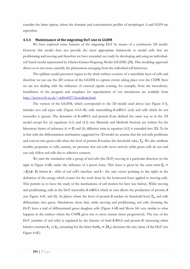
103 | P a g e

consider the latter option, where the domains and concentration profiles of morphogen A and FGF8 are

equivalent.

4.3.4 Maintenance of the migrating DoT size in GGHM We have explored some features of the migrating DoT by means of a continuous 1D model.

However this model does not provide the most appropriate framework to model cells that are

proliferating and moving and therefore we have extended our study by developing and using an individual-

cell based model represented by Glazier-Graner-Hogeweg Model (GGHM) [28]. This modeling approach

allows us to test more carefully the phenomena emerging from the individual cell behaviors.

The epiblast caudal precursor region in the chick embryo consists of a unicellular layer of cells and

therefore we can use the 2D version of the GGHM to capture events taking place over the CNPR (here

we are not dealing with the influence of external signals coming, for example, from the mesoderm).

Installation of the program and templates for reproduction of our simulations are available from

http://pcwww.liv.ac.uk/~mf0u4027/biocellsim.html.

The version of the GGHM, which corresponds to the 1D model used above (see Figure 4-3),

includes two cell types only (Figure 4-6A–B): cells transcribing -mRNA (red) and cells which do not

transcribe it (green). The dynamics of -mRNA and protein are defined the same way as in the 1D

model except for: (a) equations (4.1) and (4.2) (see Materials and Methods Section) are written for the

laboratory frame of reference ( ) and (b) diffusion term in equation (4.2) is extended into 2D. To be

in line with the differentiation mechanism suggested for 1D model we assume that the red cells proliferate

and convert into green cells when the level of protein reaches the threshold value, . We also attribute

motility properties to cells, namely, we presume that red cells move actively while green cells do not and

can only follow red cells due to adhesive contacts.

We start the simulation with a group of red cells (the DoT) moving in a particular direction (to the

right in Figure 4-6B) under the influence of a preset force. This force is given by the extra term

( ) (where - shift of red cell’s interface and – the unit vector pointing to the right) in the

definition of the energy which counts for the work done by the horizontal force applied to moving cells.

This permits us to leave the study of the mechanisms of cell motion for later (see below). While moving

and proliferating, cells in the DoT transcribe -mRNA which in turn allows the production of protein

(see Figure 4-6C and D). In places where the level of protein reaches its threshold level, , red cells

differentiate into green. Simulations show that, while moving and proliferating, red cells (forming the

DoT) leave a trail of differentiated green daughter cells (Figure 4-6B and Movie S4) very similar to what

happens in the embryo where the CNPR gives rise to more mature tissue progressively. The size of the

DoT (number of red cells) is regulated by the kinetics of both -RNA and protein : increasing either

kinetics constant or (assuming for the latter that ) decreases the size (area) of the DoT (see

Figure 4-6E).

104 | P a g e

4.3.5 Promotion of cell migration by a caudal morphogen The simulations presented in Figures Figure 4-2, Figure 4-3, Figure 4-5 and Figure 4-6 were

performed under the assumption that the ability of cells to move correlates strongly with their ability to

transcribe the -mRNA gene so that the high level of protein switches off both abilities of a cell.

However other mechanisms that relate motility of cells to morphogen concentration may fit better to

experimental results and known signaling molecules produced in the caudal precursor zone, in particular

FGF8. Our 2D (GGHM) model can be used to check some of these mechanisms.

In our model we were dealing with a hypothetical protein rather than FGF8, but as we have

previously explained, if protein down-regulates the transcription of both -mRNA and FGF8, the

concentration profile of protein is equivalent to that of FGF8. The signaling pathways that regulate the

movement of cells in the caudal precursor zone are not well established, although it is known that FGF

signaling controls the ability of spinal cord precursor cells to move [54]. Down-regulation of FGFR

signaling in one cell promotes its exit from the CNPR which suggests that FGF signaling keeps cells

moving and allows them to accompany the regressing Hensen’s node [55].

Figure 4-6: The DoT migration in the GGHM. A: Schematic diagram of the used model (identical to the diagram in Figure 4-3). B: Three consecutive images from the simulation of primitive streak regression. Initially there is a group of 25 red cells (the

DoT) forming a square tissue. The level of -mRNA is high and constant in all red cells. Red cells move (to the right), proliferate and differentiate, i.e. red cell transforms into the green cell when the level of protein A at any point inside the red cell gets above

the threshold value TA = 0.8. Green cells do not move nor produce -mRNA, for simplicity we have also assumed that they do

not proliferate. Cell differentiation is regulated by the level of morphogen (as in Figure 4-3). Parameters: , , . C, D: Concentrations of -mRNA (C) and protein (D) are shown in shades of red. The border line between

red and green zones is along an isoline in the concentration field of protein corresponding to the threshold value . E:

Increase in the rate of kinetics, , (assuming that ) reduces the size of the DoT (or number of cells forming the DoT) exponentially.

105 | P a g e

To incorporate this feature into our model we decouple the ability of cells to transcribe -mRNA

from their ability to move and we introduce an intermediate cell type: cells that do not transcribe -

mRNA but can move (blue cells in Figure 4-7). Therefore differentiation of red cells into green cells takes

place in two steps. Step 1: we assume that transcription of -mRNA is down-regulated by protein A, i.e.

production is stopped when the level of protein achieves some threshold level (analogous to 1D

model represented in Figure 4-3A and Figure 4-5C). Step 2: all cells transcribing -mRNA move and

those that do not transcribe -mRNA keep moving until the level of protein gets below another

threshold ( , ). The shape of tissue formed by cells forming the DoT and their descendants (all

daughter cells) is given on Figure 4-7B (see also Movie S5). Comparing Figure 4-6B and Figure 4-7B we

can see that both modifications of the model allow regulation (stabilization) of the DoT size.

4.3.6 Chemotactic mechanism for the DoT migration Up to now we were presuming that the DoT is moving and that the speed of its motion is given by

the preset parameter . Examination of Figure 4-3 reveals a possible mechanism of this motion. Assume

that the cells forming the DoT are chemotactic to a morphogen they produce. For example, we can

assume that the speed of the DoT migration is proportional to the gradient of A

. The gradient

can be taken at some specific point, for example at the right border of the DoT, or we could use an

average gradient over the entire DoT, i.e. the difference between concentrations of the protein on two

borders of the DoT divided by the size of the DoT. Computer simulations show that both these

assumptions can cause the DoT migration with constant speed and therefore the motion of the CNPR can

have a chemotactic nature. Simulations with the first assumption, i.e. the speed of the DoT is defined by

the gradient of on one particular side, show that starting from a wide range of initial conditions (and

also for a wide range of values of ), we obtain (after some transition period) a DoT migrating moving

with constant speed (see Movie S6). Simulations with the second assumption, i.e. that the speed is defined

by the average gradient of morphogen over the DoT, also show the desired behavior, but we need to

apply special initial conditions: for example, we force the DoT to move for some initial time and then

switch this force off and chemotaxis on (see Movie S7).

106 | P a g e

Figure 4-7: The DoT migration in the GGHM with 3 cell types. A: Schematic diagram of the used model. B: Snapshots from

the simulation: red cells – move and produce -mRNA, blue cells move but don’t produce -mRNA and green cells do not move

and do not produce -mRNA. Red cells transform into blue when the level of protein A rises above TA = 0.75, blue cells – to

green when the level of protein drops below . Only red cells proliferate. Parameters , ,

. C, D: concentration profiles of -mRNA (C) and protein A (D) after 20500 time steps of simulation.

Thus the migration of the DoT can be due, in theory, to chemo-repulsion of its constituent cells by

protein A. This mechanism of migration is very similar to that of so called ‘‘ballistic’’ motion of a point

which is a source of its own chemo-repellent [56]. In our case this ‘‘ballistic’’ effect is even more profound:

the chemorepellent is produced not only inside the DoT but also behind it (where the concentration of -

mRNA is nonzero) and this adds to the difference between concentrations of the chemo-repellent at the

front and back sides of the DoT. Simulations as well as analytical studies of the model show that the

migration (with constant speed) of a self-repelled DoT is only possible when the parameter , defining

the strength of chemotaxis, is above a certain threshold (see Figure 4-8A, where this threshold is roughly

0.6). The concentration profiles of A-mRNA and protein A, as well as the size of the DoT, depend on the

parameter c0 similar to their dependences on the parameter c in the non-chemotactic version of the model

(equations (4.8)–(4.10)) with fixed speed of the DoT migration (compare Figure 4-3C with Figure 4-8B).

107 | P a g e

Figure 4-8: The DoT migration due to chemotaxis in 1D model. The speed of the DoT migration is defined by the formula

( ) where and are concentrations of protein on the left and right borders of the DOT. A: The version of

the model where the DoT size is fixed (chemotaxis without -mRNA self-repressive production control). The domain in the

parameter plane ‘‘ versus ’’ where the travelling DoT should definitely exist according to the analysis of the model is on the right side of the solid red line (this line represents the border of the domain defined by inequality (4.16) in the Materials and Methods section. Transition points (between existence and nonexistence) of migrating DoT’s in simulations are given by blue markers, dished blue line connecting these markers gives the numerically obtained border. B: The version of the model where the

DoT size is controlled by the protein (chemotaxis with -mRNA self-repressive production control). The size of the DoT

depends on the parameter . The difference depends on and saturates when giving a linear asymptotic (red)

for the dependence of the DoT size on .

The role of chemotaxis in the migration of caudal precursor zone has not yet been addressed

experimentally, but it is known that FGF8 can act as a chemo-repellent upon mesenchyme cells during

gastrulation in the chick embryo [9], and that down-regulation of FGF signalling does not allow the caudal

movement of cells following node regression [54]. Although, in our model, we consider the self-repressing

morphogen as the chemo-repellent for cells forming the DoT, the same result would be obtained if we

consider that the actual repellent is FGF8 whose dynamics coincides with that of protein (as discussed

above).

4.3.7 Chemo-repulsion in GGHM As we have noted in the previous section, the migration of the DoT can have a chemotactic nature

and, in addition, there is strong evidence that FGF8 can act as a chemorepellent in several contexts [57].

Using GGHM we can analyze this problem to a much greater extent than was possible in the framework

of the 1D model.

Let us first consider a simplified problem by ignoring cell proliferation and differentiation. Assume

that the DoT is represented by a group of (non-proliferating) cells which produce some chemotactic agent

(protein or FGF8, in our case), such that the cells are repelled by this agent. Is it possible that this group

of cells will migrate (move along a straight line) due to this repulsion and thus reproduce migration of the

DoT? Our simulations show that the group of cells repelled by a chemical they produce can exhibit three

types of behavior (Figure 4-9). Cells can stay as a compact group and move randomly or meander with

little net relocation (Figure 4-9B, Movies S8) or exhibit oriented motion, as in the case of the CNPR

(Figure 4-9C, Movie S9). Movement of cells can deform the shape of the DoT (Figure 4-9D, Movie S10)

or even break it so that they form a few smaller groups of cells each moving independently. The type of

108 | P a g e

observed behaviour is defined by model parameters and can be altered by varying the number of cells,

their adhesiveness (defined by the adhesion matrix ), kinetics rates of protein (production and

decay ), -mRNA (decay ) and chemotactic forcing, , (see Materials and Methods Section).

Generally, the model’s parameter space can be represented as a collection of domains corresponding to

each type of observed dynamic behavior. Figure 4-9E shows the location of these domains on a

parametric plane corresponding to two key parameters (responsible for the type of dynamics exhibited by

self-repelling group of cells), namely chemotactic force as defined by parameter and protein decay

rate, (see Materials and Methods Section). When the chemotactic forcing is weak ( is less than some

threshold value, and this threshold depends on ) the group of cells meanders and shows no net

migration. The meandering behaviour is intrinsic to GGHM (corresponds to thermal fluctuations when

) and it is a counterpart of the resting DoT in continuous 1D model: as we saw previously the DoT

in 1D model does not migrate (or no travelling solutions exist) when is below than some threshold

value (see inequality (4.16)) and this threshold depends on the DoT size (see Figure 4-8A). A meandering

group of cells starts to move along a straight line when we increase the chemotactic forcing (by increasing

the parameter ) or the protein decay rate, . This type of behaviour is also in a line with our

observations on 1D model where the DoT starts to migrate when chemotactic forcing c0 is above some

threshold value (Figure 8A). On the other hand further increase in either of these parameters results in

deformation of moving tissue so that rounded tissue transforms into an umbrella-like shape. There is no

1D counterpart for this kind of behaviour.

109 | P a g e

Figure 4-9: Migration of the DoT due to chemotaxis in GGHM. A–E: Simulation of the movement of a group of cells

transcribing -mRNA (DoT) that are repelled by a protein they produce. Three types of behavior can be found in GGHM. Here we assume that cells forming the DoT do not grow, proliferate or differentiate. A: Initial shape of the DoT. The DoT was ‘‘forced’’ to move to the right (see about a preset motion of the DoT in Figure 4-7) for the first 2000 time steps to provide initial

conditions for chemotactic motion. ‘‘Self-repelled’’ DoT can: B: meander ( ). C: move along straight line (migrate)

( ). D: move and elongate (deform into ‘‘umbrella’’-shaped tissue) ( ). E: domains on a parameter plane

( ) corresponding to each kind of behavior. Blue dots in B, C and D show location of the DoT’s center of mass every

200 time steps. Parameters: , . F: Simulation of the movement of a group of red cells transcribing -mRNA

(DoT) that are chemotactically repelled by a protein they produce and that, in addition, grow, proliferate and differentiate into green non-actively moving cells (as it was in the case of Figure 4-6). Initially the DoT is represented by a group of 25 cells. These cells are ‘‘forced’’ to move to the right for the first 2000 time step computations to provide the direction for further chemotactic

movement. After , red cells are repelled by protein , and (as directed by the initial conditions) they move to the right leaving the trail of differentiated daughter cells (green).

Thus, the migration of the -mRNA DoT can be explained by the chemotactic response of its

constituent cells to protein (i.e. the FGF8 DoT migrates due to repulsion by FGF8). Now we can put

proliferation and differentiation of cells back into this model and adjust model parameters so that we

observe oriented motion of tightly packed red cells leaving the trail of differentiated daughter cells (Figure

4-9F, see also Movie S11). The result from this simulation mimics the regression of the CNPR indicating

that the interactions we have considered are sufficient to account for the observed maintenance of a

compact group of cells that proliferate, migrate and differentiate during vertebrate embryonic axis

extension.

4.3.8 Experimental study of regulative properties of the FGF8 DoT In order to challenge the ability of the model to reproduce experimental results, we have

performed an experiment where the FGF8 DoT (which in our model is equivalent to the -mRNA DoT)

was split into two and the changes in the expression of FGF8 were analyzed after 20h culture (Figure

4-10A, B). In the rostral moiety, FGF8 was maintained caudally suggesting that FGF8 does not require

signals from the caudal-most region of the embryo for its maintenance. In addition, this experiment also

110 | P a g e

shows that the capacity of FGF8 to progressively down-regulate is also intrinsic to the caudal moiety

(Figure 4-10B).

Figure 4-10: Regulative properties of the FGF8 DoT. FGF8 expression can be maintained in the absence of caudal-most signals and can be progressively down-regulated in the absence of rostral signals. A: Schematic diagram showing the experimental separation of the rostral and caudal parts of the FGF8 DoT (cutting experiment). B: FGF8 expression following the experimental separation of the caudal precursor zone into two. White arrows show how FGF8 is maintained at both the rostral and caudal moieties and black arrow shows the progressive down-regulation of FGF8 in the caudal moiety. C: Simulation of cutting experiment: the chemotactically moving DoT is cut into two pieces (see images at T=0 and T = 650). We allow the piece corresponding to the caudal moiety to move while the movement in the rostral moiety is arrested by the cut. The concentration of

-mRNA (shown by shades) which is associated with the location of the DoT reproduces the corresponding pattern for FGF8

shown in B. Parameters: , , .

Using our complete model, we have performed simulations where we split the DoT into two

(Movie S12) and follow the behavior of the two moieties. As shown in Figure 4-10C we find the

maintenance of a caudal population of red cells (those producing -mRNA or the equivalent FGF8-

mRNA) in the rostral moiety and the progressive generation of a green population (that have stopped

producing A-RNA) in the caudal moiety, very similar to what is observed in experiments (Figure 4-10A,

B).

This result suggest that our model captures essential features of the biological network regulating

FGF8 expression and encourage the search for a morphogen with both the ability to self-repress

transcription of its encoding RNA and of FGF8. In addition, it posses the possibility that chemotaxis may

play a role in caudal elongation of the embryo.

111 | P a g e

4.4 Discussion

The aim of this work is to explore possible mechanisms of progressive differentiation and

regression of the caudal neural precursor region (CNPR, as defined by the region where cells transcribe

FGF8 mRNA) in the chick embryo. We have focused on essential features of regression of this region

such as progressive differentiation and the conservation of its size and speed of migration. These features

were incorporated into two distinct modeling approaches which we used to evaluate a set of hypotheses

concerning the mechanisms of differentiation and motion of cells in the CNPR. Our results are

summarized in the Table S1.

The regulation of FGF8 dynamics during the regression of the caudal precursor zone was

previously addressed using a mathematical model [48] where it was suggested that a mechanism involving

FGF8 self-activation could, in theory, account for the progressive down-regulation of FGF8 provided a

high FGF8 degradation rate was considered. According to this model the dynamics of FGF8 can be

described as a propagating concentration wave, which is one of the patterns that form in nonlinear

reaction-diffusion systems [58].

In the present work we have also addressed the regulation of FGF8 dynamics but we consider

both intracellular (mRNA) and diffusing (protein) species of FGF8 and most importantly we take into

account the movement of the domain of FGF8 transcription.

Cells in the precursor region proliferate and differentiate in such a way that the size of the region

(identified by FGF8 transcription) does not change significantly over time. The size of a growing tissue

usually involves control of proliferation such that when the tissue reaches a certain size, cells stop dividing.

This may involve a mechanism which is able to measure population size as has been described in bacteria

quorum sensing in Dictyostelium population, the Drosophila imaginal disc [59] or for the mesoderm

community effect [60]. It is generally hypothesized that the concentration of signaling factors change as

the size of the tissue increases until they reach a threshold value that dictates an arrest in cell proliferation.

In our scenario, maintenance of a population with constant size is not due to an arrest of proliferation but

to the balance of proliferation versus differentiation that is spatially controlled such that only cells at the

rostral end of the domain differentiate (i.e. stop transcribing FGF8). This involves a mechanism where the

strength of the signal regulating cell differentiation correlates with the size of the cell population, i.e. the

signal is provided by a morphogen whose overall production is related to the size of the zone. In terms of

our model this could be morphogen A produced from A-mRNA which in turn is produced exclusively in

the precursor region. This is reflected by our model assumption that cell differentiation takes place when

the level of morphogen rises above some threshold, . This assumption allows the control of the DoT

size, although (depending on parameter values) the size can be stationary or oscillating (see Figure 4-3). An

interesting problem is whether the DoT size is stationary or oscillating in experimental conditions.

Another important problem is what morphogen is actually under self-repression control and can

be involved in the regulation of the DoT size. One possibility would be that FGF8 is actually able to

repress transcription of FGF8 mRNA, however this is not supported by our experimental evidence as

112 | P a g e

manipulations of the level of FGFR activation in experimental conditions do not seem to affect the size of

the area where FGF8 mRNA is expressed. This brings us to an alternative assumption that, for example,

another morphogen is responsible for the regulation of FGF8 transcription. Two possibilities have been

considered: morphogen activates FGF8 transcription or it represses FGF8 transcription (see Figure 5).

Both are able to maintain a domain of FGF8 transcription of constant size; however the latter network

would account more easily for the maintenance of FGF8 expression in the rostral fragment following the

splitting of its domain of expression.

Several secreted proteins are present in the caudal zone that could correspond to -mRNA such as

WNTs (WNT3A, WNT8C) and BMPs (BMP7, BMP4). They could participate in the mechanisms

presented in Figure 4-5. Independently of the particular mechanism that regulates production of FGF8 in

our models, the relevant feature of the regulatory networks that allows the maintenance of a constant size

of the domain transcribing -mRNA is the presence of a negative feed-back loop involving protein .

It is known that retinoid acid signalling from the somites is involved in down-regulation of FGF8:

in the absence of RA the domain of FGF8 is expanded. However, down-regulation of FGF8 still occurs in

RA-deficient embryos and our experiments of embryo sectioning show that progressive down-regulation

can occur in the absence of rostral signals. In our model we did not take into account the influence of the

rostro/caudal gradient of RA in shaping the FGF8 pattern. Future work will be required to incorporate

into the models more elements concerning the gene regulatory network involved in FGF8 regulation such

as the influence of RA, which is itself influenced by FGF signaling and Wnt8C, which is regulated by RA

and FGF8 [7, 61].

Our models assume the existence of concentration thresholds of morphogen that determine

whether A-RNA (or FGF8) is transcribed or not. Several molecular mechanisms underlying such an all-or-

nothing response of cells could be relevant in this context, such as nonlinear saturating autocatalytic

feedback of a gene product [2] or mutual inhibition [49]. It has been suggested that mutual inhibition of

FGF8 and RA gradients may be involved in setting a bi-stability switch of FGFR versus Retinoic acid

receptor activation. However so far, no experimental evidence indicates that such a switch could be

involved in controlling whether FGF8 is transcribed or not [62].

Coordination of differentiation and axis extension can be found during growth of plant meristemes

and in vertebrate limb bud development. In these cases, however, the mechanism involved must be

different to caudal extension as differentiation coupled to axis extension relies on an external cell

population that secretes a morphogen that regulates proliferation and maintains neighboring cells in an

undifferentiated state. In the case of the root meristeme this is the quiescent center, in the case of the

apical shoot meristeme it is the organizing center [33, 34]and in the case of the limb it is the apical

ectodermal ridge that secretes FGFs [35].

The other feature that we have explored using our models is the mechanism of domain migration.

Several cellular behaviors have been shown to contribute to regression of the primitive streak-node and

extension of the embryo. Convergence (at the midline) and extension seem to be at play in mesoderm.

113 | P a g e

Besides, stem-cell like mode of growth and caudal movement of cells has also been observed in the neural

tube and axial mesoderm [54, 55]. At the caudal neural plate, FGF signaling is required for cells to

accompany the regressing primitive streak and precocious down-regulation of the pathway results in cells

exiting the node-streak region. The version of the GGHM with differentiation (incorporating the

influence of FGF8 on FGF8 transcription and cell motility) shows that such a mechanism is able to

maintain a cohesive group of cells moving at constant speed (Figure 4-6). Further extension of the model

with the assumption that the reason why cells move caudally is related to FGF8 concentration (FGF8 acts

as a chemo-repellent) allows us to simulate the correct behaviour of cells that can move coherently in one

direction provided there is an initial cause for the migration. A stationary group of cells producing a

chemotactic agent maintains a symmetric condition with respect to the agent’s concentration profile and

will not move unless other events (such as noise) are involved. Indeed, Hensen’s node (which we

considered here as a part of stem zone) changes direction of its motion when the progression of primitive

streak is replaced by its regression. We don’t know what is responsible for reversing the motion of

Hensen’s node but most likely it is due to some external signals, while the repulsion by morphogen A in

our model is rather an internal process as the production of this morphogen is closely associated with the

processes in the caudal precursor region itself.

In summary, we have used mathematical models to explore possible mechanisms for the

progressive differentiation of the caudal stem zone coordinated with the embryonic rostro-caudal

extension. We have found that the self-repression of a caudal morphogen could be involved in driving

progressive differentiation of the caudal stem zone and that chemo-repulsion here may be part of the

mechanism responsible for the axis extension. Further experimental evidence is required to assess the role

of FGF in regulating motility of ectodermal cells and to find out the signalling pathways that may be at the

core of these mechanisms.

114 | P a g e

4.5 Materials and Methods

In this section we describe the mathematical models as well as the experimental techniques used

for obtaining the results presented in this work. For our study we have developed two models: continuous

(1D) and cell-based (2D, Glazier-Graner Hogeweg model also known as Cellular Potts model). Dynamics

of morphogens was modelled in the same way in both models while the migration of the DoT - using

different techniques. In the 2D model we have considered a tissue consisting of a single layered group of

cells. Each cell can produce and/or degrade genes and proteins and, in addition, move in response to the

forces (adhesive, chemotactic) acting upon it. Also, the 2D model incorporates the ability of cells to grow

and proliferate.

4.5.1 One-dimensional continuous model 1D simulations were performed in a medium of fixed size in a frame of reference moving with the

DoT. To describe the dynamics of morphogens we have used reaction-diffusion equations with an added

advection term to take into account the DoT migration.

Basic Model.

The basic model is represented by two equations: one – for the dynamics of the concentration of a

non-diffusible agent which we call -mRNA and the second – for the concentration dynamics of

corresponding protein . The concentration of -mRNA (denoted as ) is equal to 1 (i.e. constant)

inside the DoT of fixed size, a, while outside is given by the equation:

(4.1)

Parameter defines the rate of A-mRNA decay while parameter defines the speed of DoT

migration or the speed of the frame of reference. The concentration of protein (denoted as ) is

defined by the equation:

(4.2)

where parameter defines its diffusion constant while and are the rates of protein decay and

production. Production of the protein is assumed to be proportional to the concentration of -mRNA

while its decay is proportional to its own concentration. The stationary solution of the system (4.2) can be

found analytically. One can check directly that the solution:

{

(4.3)

115 | P a g e

satisfies (4.1) while the solution:

{

( ){(

( )( )) (

) }

( ){

( )

}

( )(

)

(4.4)

where

√

(4.5)

satisfies (4.2). Figure 2 shows typical concentration profiles given by ((4.3)–(4.4)).

Since the DoT is moving, the maximum of the concentration of protein A lags behind the middle

of the DoT, i.e. where is the location of the maximum. For a slowly moving DoT the

maximum is located inside the DoT ( ) with its coordinate defined by the condition that

the derivative of the u2-solution inside the DoT, (see (4.4)), is zero. This gives:

√

[ (

)] (4.6)

his coordinate is when and decreases with the increase of . When the DoT’s speed is too high

the maximum lags behind the DoT, i.e. . The condition for this case can be given, for example,

by the following inequality:

(

) (4.7)

when defined by (6) becomes negative. This condition is also confirmed by consideration of the

maximum for solution behind the DoT ( in (4.4)).

Model for the regulation of the DoT size.

In order to consider the proliferation and differentiation of cells in the DoT we extend the basic

model by the assumption that the location of the left side (or back side in respect to the direction of

motion) of the DoT is controlled by the signal provided by protein . That is, the maintenance of -

mRNA, whose concentration is constant inside the DoT, is switched off (cells forming the DoT

differentiate) when the concentration of protein achieves the threshold value . In terms of the model

((4.1)- (4.2)) and its stationary solution ((4.3)–(4.4)) this gives:

( )

( ){

} (4.8)

and, therefore, the size of the DoT, , is not a preset parameter but a function of other model parameters,

including :

[ (

( )

)] (4.9)

116 | P a g e

Furthermore, the threshold value, , is generally achieved in two points (on the either side of the

maximum whose location is given by (4.6). As the concentration of should not get above in the

DoT the differentiation should take place before the maximum is achieved, i.e. condition (4.7) is to be

held. Combining equation (4.9) with the inequality (4.7) we define the condition when the stationary

solution to the stated problem exists:

(

( )

) (4.10)

An important case to consider is when the concentration of the protein A is low and doesn’t reach

the threshold value, TA, anywhere in the medium. In the simulations we presume for this case that the

size of the DoT is increasing over time (due to proliferation of cells) and the coordinate of the DoT’s left

border is gradually decreasing (the degree of ‘‘graduality’’ represents the proliferation rate). Simulations

show that the size of the DoT is fixed and stable under the condition given by the equation (4.10).

Furthermore, simulations show that if this condition does not hold the size of the DoT oscillates over

time (see Figure 4-3 and Movies S2 and S3).

For Variable Models.

Modelled protein down-regulates its own transcription while experimental results shown in

Figure 4-4 indicates that is not involved in the control of its own transcription. Thus protein does

not correspond to and we need to analyze possible relationships between these two morphogens.

We have examined two possibilities:

Transcription of FGF8 is proportional to the concentration of protein (see Figure 4-5 A, B).

This is expressed in the following equation for the concentration ( ) of mRNA:

(4.11)

Transcription of -mRNA and -mRNA take place in the (nearly) same group of cells: they

have been switched on independently from each other but both switched off by the signal provided by

protein . In this scenario the concentration of -mRNA is calculated the same way as the

concentration of -mRNA in the basic model (see above, equation (4.1)).

In both cases the concentration of protein ( ) is given by the equation:

(4.12)

i.e. similarly to the concentration of protein , , (see equation (4.2)) it is a diffusible agent and its

production is proportional to the level of its corresponding gene ( -mRNA, equation (4.11)) and

decays proportional to its own concentration.

Modeling chemotaxis.

In this version of the model, parameter , defining the DoT migration speed, is calculated with the

assumption that the migration is taking place due to chemotaxis, i.e. the speed is proportional to the

117 | P a g e

gradient of the chemotactic agent [63, 19]. We have assumed that protein acts as a chemo-repellent on

cells forming the DoT and the speed of migration is defined either by its gradient in some specific point,

say on the front (right-side, ) of the DoT:

|

(4.13)

(see Movie S6) or by the average gradient over the DoT,

( ) ( )

(4.14)

(see Movie S7).

The analysis of conditions when the DoT can migrate due to self-repulsion is relatively simple

when we consider the chemotactic movement of a DoT of fixed size, , i.e. consider solution ((4.3)–(4.4))

remove condition (4.8) and add condition (4.14) which gives:

( )(

( ) ( )

( )) (4.15)

Where the right hand side is also function of ( , and are functions of , see the definitions

given by (4.5)). When the right hand side of (4.15) is zero, i.e. one stationary solution (with )

exists for all sets of parameters. One can show that the right hand side of (4.15) is positive and tends to

zero when tends to infinity. Travelling solutions correspond to the points where and plots of

functions

and

( )(

( ) ( )

( )) (4.16)

intersect. At least one such point exists, if the derivative of the function (the derivative of the

RHS of (4.15)) is more than 1 at . This condition can be expressed by the formula:

√

(

(

√

) √

) (4.17)

Therefore for sets of model parameters satisfying (4.16) (see Figure 8A) we can expect the

existence of a moving DoT, moving with constant speed. Whether more than one such solution exists and

whether such solutions exist when condition (4.16) is violated should be rigorously analyzed in a more

detailed study. We have plotted the function given by the RHS of (4.15) versus variable for various sets

of model parameters. It looks that this function always has only one maximum. Therefore we expect that

inequality (4.16) gives the condition for the Pitch-Fork bifurcation, i.e. we have only one solution

(corresponding to ) when model parameters do not satisfy (4.16) and two extra solutions appear

(corresponding to the DoTs moving in opposite directions) when (4.16) is satisfied. But indeed this

conclusion should be verified by proper analysis.

118 | P a g e

Details of simulations and verification of parameters.

For simulations we used the explicit Euler’s method with central differencing scheme for diffusion

and alternating up- and down-wind schemes for advection. Typical initial conditions: all concentrations are

equal to zero with the only exception: in the DoT which has a predefined location and size.

Default values of the parameters: diffusion coefficients ; kinetics rates

, , , ; speed , chemotaxis .

Default values for the time and space steps and for which we found the

simulations to be fairly accurate: two-fold reduction of space step together with four-fold reduction of

time step ( and ) was altering measured quantities (such as maximums in

concentration profiles, the DoT size when differentiation is on, and the DoT speed when it is drove by

chemotaxis) by less than 3%. Also the simulations were performed in sufficiently large domain to reduce

the influence of medium boundaries (doubling the size of the medium has changed measured quantities by

less than 1%).

To scale the model parameters we estimate the DoT size to be and its speed to be

. Comparing this with the simulations shown on Figure 4-3 where (space units over time

units) and the DoT size is 40 (space units) we conclude that the space unit corresponds to about 20 m

and the time unit – to 10 seconds. This means that corresponds to and

kinetics coefficient – to sec.

A few words about justification of the parameter values used in our simulations. Firstly, the

analysis of the model represented by equations (4.1) and (4.2) with extra conditions (4.8) and/or (4.14)

indicates that qualitatively the solution is the same for any set of parameters represented by positive

numbers. Furthermore, we can take three arbitrary numbers to represent the values of three parameters

appropriate for scaling dimensions associated with time, distance and concentration. In our case we

decided that the concentration of A-mRNA inside the DoT is 1, the DoT is represented by about 40 grid

points (or its size is 40 space units if the grid size is 1) and the speed of the DoT is something between 0.1

and 0.01. The choices for the DoT size and speed are dictated by the accuracy issue. We have checked that

40 grids for the DoT gave considerably more accurate solutions than say 10 grids and, on the other hand,

approximately the same accuracy as 100 grids. Similarly, if we assume that the time step is 1 then speed

should be less than 0.1 (say 1/40) to provide enough accuracy in numerical calculation of concentration

profiles. Diffusion is convenient when it comes to the numerical scheme (the highest possible

value when the explicit Euler scheme with time and space steps is still stable) and still in a

range of diffusion coefficients known for proteins. Kinetic rate has been chosen in a way that the space

scale for the mRNA degradation is comparable with the size of the DoT: this is done to fit with the

observations concerning the sizes of -mRNA transcription and expression (Figure 4-1 and Figure

4-4). Other kinetic constants have been chosen to be of the same order as . And finally, concerning

and : the ratio of these two constants is only important for the choice of the threshold value : the ratio

119 | P a g e

has been chosen only to bring concentrations of -mRNA and protein to the same scale (Figure 4-2,

Figure 4-3, Figure 4-5).

Glazier-Graner-Hogeweg Model.

This is a computational individual-based model originally developed by Graner and Glazier [20,

30]. In this model we consider the DoT as a group (25 by default) of cells, each, in turn, is represented by

a number of grid points (50 grid points per cell in our simulations) on a regular (square-shaped 2D in our

case) lattice (see also Methods Section in [4]). Movement of a cell (or change in its shape) means that the

cell looses or gains some grid points on the lattice. In terms of the underlying tissue this implies that the

grid points are associated with different cells at different times. To calculate whether a particular grid point

will be associated with a different cell at next time step a variation principle is used to minimize a quantity

representing ‘‘the energy’’ of the system.

Contrary to the original implementation of the GGHM which was based on Monte Carlo

algorithm involving the random choice of the pixel followed by the random choice of its neighbor and

following calculations of probability of change [20] we have implemented a synchronous model: at each

time step we calculate the probability to change the state for all grid points. For each grid point, we

randomly select a neighbor (one out of the eight nearest) and calculate how the energy of the system will

change after changing the state of the grid point to that of its neighbor. If this change results in an energy

decrease we allow the change to occur; if the energy is increased we calculate the probability of that

change, , using the Boltzmann function: ( ) where the parameter can be referred to as

the ‘‘temperature’’ of the system.

The energy is defined in a way that its change accounts for the work done by different forces acting

upon moving or deforming cells. The definition of energy used in our implementation of the model takes

into account three forces, the adhesive forces between cells, the force associated with the incompressibility

of cells (pressure) and forces developed by chemotactically moving cells:

(4.18)

The following definitions of the terms on the right hand side of equation (4.17) are commonly

used in various modifications of GGHM [4, 50]:

An adhesive energy associated with cell-to-cell contacts is defined by the adhesion matrix

( ) which refers to an interface between neighbouring grid points which belong to different cells

(numbers and represent cell types of these cells). The energy, , characterizes the strength of a

particular cell’s adhesive contacts (stronger contacts correspond to smaller energies). To consider adhesive

contacts between cells and the surroundings we treat the letter as a special cell of its own type. In our

simulations we, as a rule, consider 3 cell types: the surrounding was considered as a cell of its own type –

cell type ; cell type – cells which form the DoT; cell type – cells which form the DoT trail or the

differentiated daughter cells. The default adhesion matrix for adhesive bonds between each pair of

different cell types is:

120 | P a g e

[

] (4.19)

To control the size of a cell (say cell), ( ), a target area (in case of our 2D cells number of

grid points forming the cell can be considered as its area), , is introduced. The cell is given an

energy ( ( ) ) , where is a positive constant ( in all our simulations).

Constant a represents the cell’s resistance to compression and we can call it the ‘‘incompressibility’’

coefficient (it had different names such as ‘‘Lagrange multiplier specifying the strength of the area

constraint’’ in [20], or ‘‘volume elasticity’’ in [64]) referring to another approach when the motion of cells

in a tissue is seen as a flow in incompressible viscous liquid described by Navier-Stokes equation [65, 66]

and where this term would correspond to the gradient of pressure. The ‘‘incompressibility’’ energy reaches

its minimum (zero) when the cell’s actual and target areas are equal. To take into account the growth of

cells the target area, , is considered to be an increasing function of time. To model cell proliferation we

split big cells (which contain 100 or more grid points) into two small cells. The split is performed along a

straight line (having a random orientation) crossing the cell’s centre of mass.

To implement the chemotactic effect of the agent, whose concentration is denoted as ‘u’, to a

moving (or deforming) cell we introduce the change in chemotactic energy ( ( )),

where is a constant describing the chemotactic response of cells of type to the chemotactic agent

and is a vector representing the local displacement of the given cell’s boundary. This energy change

refers to the work done by chemotactic force and therefore corresponds to the

chemotactic force, ( ) , exerted by chemotactically responding cell. The identical

definition of the chemotactic force was introduced and used earlier in the hydrodynamic model of

Dictyostelium development [67]. The most common implementation of chemotaxis in our model:

if and ( ) for or for ‘‘red’’ cells forming the DoT. This means that there is an

energy gain or loss in the system related to the relocation of the red cell’s boundary which depends on the

local gradient of chemotactic agent. We note that a positive value for the parameter corresponds to the

process of chemo-repulsion while a negative value for - to chemo-attraction.

Detailed description of the GGHM model and its modifications and applications to various

problems in developmental biology are given in [50]. One of the greatest advantages of GGHM is that it

allows modeling the dynamics of biological tissue while being focused on behavior of individual cells. The

simplicity of the model allows modeling of tissue which contains up to 105 cells on a single PC. Parallel

implementation of the software [64] allows an increase in this number up to 107–108 which is close to the

actual number of cells in many real tissues. Furthermore, the GGHM allows relatively simple

modifications to address various problems associated with mechanics and deformations of cells. For

example the GGHM allows consideration of cells of different shapes. Cells in the version of the GGHM

which we use here are predominantly round-shaped. To model, for example, elongated cells the GGHM

can be extended by the introduction of the anisotropy in adhesive properties of cells [68] or by the

121 | P a g e

introduction of cellular subunits which compose cells of desired shape and stiffness [69]. The GGHM has

also been extended to address three-dimensional problems [70] and its simulation code is available

publically (the CompuCell3D package at http://www.compucell3d.org).

Details of simulations.

We have implemented a synchronous model: at each time step we calculate the probability to

change the state for all grid points. For each grid point, we randomly select a neighbour (one out of the

eight nearest) and calculate how the energy of the system will change after changing the state of the grid

point to that of its neighbour. If this change results in an energy decrease we allow the change to occur; if

the energy is increased we calculate the probability of that change, , using the Boltzmann function:

( ) where the parameter can be referred to as the ‘‘temperature’’ of the system (we set

in all our simulations).

All simulations start with a group of 25 cells (forming an artificial square-shaped tissue)

representing the DoT. In the simulations where we do not consider cell proliferation, we assume that all

cells have a constant target volume ( ) which does not depend on the cell age. In the

simulations where we take into account cell growth and proliferation, we assume that the initial target

volumes of cells are randomly distributed among the cells in the range (30–70) and then the target volume

of each cell is increased by one unit every 10 time steps with probability 1/3. When the actual volume of a

cell reaches 100, the cell divides along a line crossing through the cell’s centre of mass with a random

direction of the cleavage plane. After division the target volumes of both daughter cells are reset to 50 and

they start to increase again over time. This implies that the average time required for a cell to double in

size and proliferate is equal to 1500 time steps. One time step scales as 70 seconds (as it derived in the

next section) and therefore the effective proliferation rate in the model is one division per 30 hours. In

experimental conditions the proliferation rate is much higher (one division per 6 hours) but on the other

hand,, in experimental conditions, many cells leave the stem zone (and epiblast) and transform into

mesenchyme cells. Since in our model we don’t consider formation of mesenchyme cells (this would

require three-dimensional version of the model) we have to reduce the proliferation rate of cells in the

epiblast (to compensate the mesenchyme formation). Furthermore we did not consider the proliferation

of differentiated (green) daughter cells as this would not influence the phenomena which we are interested

in but add unnecessary details into simulations and graphical outputs used in the figures.

Verification of parameter values in GGHM.

Parameters used in the GGHM can be split into two sets. One set is used for the definition of

energy in the system and is associated with adhesiveness (entries in the adhesion matrix),

incompressibility (parameter a defining incompressibility) and chemotactic responses of cells (parameter b

defining chemotactic response) as well as temperature T in Boltzmann function. The second set of

parameters is used to define the dynamics of morphogen concentrations (kinetics and diffusion of

morphogens). The First set of parameters forms a core of the GGHM and verification of the parameter

122 | P a g e

values used for this set can be found in the literature ( [30, 50] including more references in [50]). Here we

can briefly note that the most important point concerning the entries in the adhesion matrix is their

ratios: for cells to stay together and form a tissue. Also

and for cells of types and to sort out or to stay sorted out. The values of the entries

are scaled with the values of parameters and in order to scale all three considered forces

(associated with adhesion, pressure and chemotaxis) relative to each other. The value of parameter

defining the rate of the evolution in the system is also scaled with the values of , and . The ratio

defines the amplitude of the cell shape fluctuations (or cell membrane fluctuations). These

fluctuations freeze at high values of a as well as at low values of the Boltzmann temperature . If we will

keep all parameters of the model constant and vary only the temperature we will see that the rate of

dynamics in the model will be low at low temperatures, then the processes accelerate with the increase of

the temperature and eventually they slow down again when the temperature becomes too high. We have

measured the speed of migrating group of cells as a function of the Boltzmann temperature (keeping all

other model parameters at their ‘‘default’’ values) and found that the highest speed is observed at

(see Figure S1). It was noted in [71] that the Boltzmann temperature, , defines the intrinsic cell motility in

GGHM. Therefore (which we have chosen for our simulations) corresponds to the highest

possible intrinsic cell motility for the given set of other model parameter values.

It was shown on many occasions that the GGHM is robust: small variations in the values of model

parameters do not alter qualitatively the outcome of simulations. Besides, it was shown that the GGHM

parameters can be rescaled so that the outcome of simulations is absolutely the same. For example, the

simulation of the primitive streak progression was performed in [4] in tissues containing 625 and 15000

cells without any notable difference in the outcome.

The concentration fields of morphogens were calculated in a way similar to that for the 1D model.

The level of -mRNA was set equal to 1 in all (red) cells forming the DoT and was decaying in

differentiated (green) cells according to the equation: similar to what was in the 1D (compare

with the equation 1 where ). The equation for protein includes diffusion, production and decay

and is given by the equation (4.2) (see above) where . There are no advection terms in the 2D model

as the events are considered in the laboratory frame of reference. As the GGHM is considerably slower (as

compared with our 1D model) we have increased the speed of computations by ensuring slightly faster

processes (faster moving DoT and faster kinetics for chemicals). For , and

(see Figure 4-6) the speed of the DoT is roughly 60 space steps per 1000 time steps (should

correspond to ) and the DoT size is roughly 32 grid points (should correspond to ).

This means that 1 space unit roughly corresponds to , 1 time step to 70 seconds causing for

dimensional diffusion and kinetic coefficients to be slightly (2 to 3 times) less than for the set of

parameters used in the 1D model.

123 | P a g e

Experimental Methods.

Stage Hamburger and Hamilton (HH) 9–10 chick embryos were obtained from fertilized eggs

(Granja Santa Isabel, Cordoba, Spain) and dissected in L15 culture medium (Invitrogen).

Embryos were cultured in 4 well dishes on top of collagen beds and with of culture

medium (Optimem (Invitrogen), fetal calf serum, glutamax and gentamicine) containing 0.1% DMSO

(control) or PD173074 ( in 0.1% DMSO, Sigma). Caudal explants (including 3 embryonic layers)

were cultured in collagen as described in [72] in the presence of BSA (control) or (330 ng/ml,

Sigma). For splitting the caudal domain into two, embryos were prepared following the EC culture

method [73], a cut was performed caudal to the node with a microsurgical knife and embryos where

cultured for another 20h. Embryos and explants were fixed in 4% PFA and processed for in situ

hybridization with probes to detect either nascent [6] or total FGF8 following standard methods.

Acknowledgments.

RDC is grateful to K. Storey and M. Chaplain for their support and encouragement during the

initial stages of the project, to K. Storey for comments on the manuscript, Inmaculada Ocan˜a for

technical assistance with the experimental procedures and to A. Morales, JM Frade and P. Bovolenta for

their help and support. BV is grateful to Prof Vladimir Maz’ya for his help with analysis of 1D model and

to Manou Rasolonjanahary for his assistance with analytical solutions. RDC and BV acknowledge the

British Council for their participation in the Workshop ‘‘Development: at the crossroads of Systems

Biology’’.

Author Contributions.

Conceived and designed the experiments: RDC BV. Performed the experiments: NCH RDC BV.

Analyzed the data: NCH RDC BV. Contributed reagents/materials/analysis tools: RDC BV. Wrote the

paper: NCH RDC BV.

124 | P a g e

Chapter 5

DISCUSSION AND CONCLUSIONS

In this thesis we have set out to understand (and explain) mechanisms of self-regulated motion of a

group cells due to reaction of the group to the gradient of locally produced chemical, referred to as

chemotaxis. Such problems are abound in nature with examples appearing in both plant and animal

kingdoms, illustrating the ubiquitous nature of chemotaxis as a mechanism for migration and

reorganisation in biological cellular systems. However while vast amounts of data has been collected over

protracted period of time, it is only relatively recently that computational power and techniques have

advanced to the state where these data can be analysed and correlated. Further, advances in microscopy

and genetic sequencing to show how the expression of genes controls the development of biological

organisms at the cellular level, that bridge the gap between the microscopic and macroscopic, that is, gene

expression and cell behaviour. It is in this context, molecular and cellular dynamics, that this thesis

attempts to explain self-regulation of migratory behaviour (cellular dynamics), due to local gene expression

(molecular dynamics).

For the rest of this chapter we shall briefly summarize the preceding work, and consider how what

steps we can take next to further the work, and end with and short conclusion.

5.1 Summary Of Thesis

In the most basic setting, we consider a small group of cell that is chemotactically reacting to a

locally produced chemical. This chemical in a biological context, is the product of a gene expression within

some population of cells, translating into an externally diffusing protein. The diffusive nature gives rise to

a spatial distribution, that in a stationary setting can visualised as the normalised probability curve (the bell

curve). If our group of cells are exposed to such a curve then depending on how they reacted to the

gradient of this protein, they could either move towards (chemo-attraction) or away (chemo-repulsion)

from the point of highest concentration. This raises two fundamental questions in the thesis: who is

producing the chemical and who is reacting to it? And under what conditions will the group move, or will

not as the case may be?

In chapter 2 we began with a reduced one-dimensional analytical model, essentially a caricature

representation of the group of cells, as a segment of the real line. This allowed us to neglect the

physiological aspects of the cells in the group in order analyse the chemical and chemotactic dynamics in a

simplified setting. Using this simplified model we demonstrated a variety of mechanisms for group

migration, for different assumptions about where the chemical was produced and what cells reacting to it.

The results of this chapter where that there are essentially two dynamical systems that can result, that

depend on the composition of the group being homogeneous or heterogeneous. From these dynamical

systems we were able to derive analytical expressions/conditions that result in travelling solutions, that

125 | P a g e

were shown to be dependent on chemotactic forcing parameter . Thus we were able to derive the

fundamental characteristics of group motion.

In chapter 3 we extended our model to two-dimensions, with a numerical analytical model where

we represented the group as a circle (or disk), and found there are fundamental differences between one

and two-dimensional representations due to how the geometry of the group affects the diffusive

characteristics of the chemotactic agent. Regardless of this difference we demonstrated a strong qualitative

and quantitative agreement between these models. With this in hand we then showed, using a modified

Cellular Potts Model, that when we introduce a more realistic morphology, and indeed more realistic

physiology, we can demonstrated all of the results of the analytical/numerical model, essentially

corroborating the robustness of the self-regulatory mechanism of chemotaxis.

In the final chapter 4 we performed an extensive experimental study that brings together the

analytical, numerical and computational techniques illustrated in the previous chapters, applied to a study

of early growth in the central nervous system in the chick egg. In this work [11] we demonstrated how

coordination of proliferation, differentiation and regulation of morphogens bringing about self-regulated

migratory behaviour observed in axial extension of the central nervous system, during neurulation. While

there are still questions relating to identity of specific morphogen responsible processes, the underlying

mechanisms of self-regulated chemotaxis is elegant and relies on few assumptions, specifically those

outlined in Chapters 2 & 3.

5.2 Discussion

In general the mechanisms underlying biological migratory behavior or spatial reorientation of an

object, can be a function of several different mechanisms that are dependent on numerous factors such as:

environment, motivation, physiology and stimulus, to name but a few. Clearly the specification of these

factors for a given object is governed by its size and/or complexity. For example if we suggest the object

in question is a hungry lion, we could prescribe a set of values for the above factors with ease. However if

we suggest that object is the organizing centre Hensen’s node in gastrulation in the chick embryo, few

could, with certainty, prescribe values for all of the above factors. Hence we are forced to take a

reductionist view and consider the problem in terms of one or two varying factors, while holding all the

others constant if you will.

In this context of this thesis we only consider stimulus, that is, what signal compels the object to

migrate, and physiology, how the object responds to the signal. Hopefully by now it is clear that by

stimulus we mean the presence of diffusing chemical, and by physiology, we mean chemotactic

movement.

The choice of chemotaxis was not taken arbitrarily, indeed the literature is abound with it as a

fundamental mechanism in many systems of growth, development and survival throughout the plant and

animal kingdoms. Mathematical models of chemotaxis tend to focus on an arbitrary point source [56],

while mathematical biological models focus on a select set of model organisms such a bacterium [63] and

ameobae [65, 67, 19], due their relative simplicity and having their behavior macroscopically visible to the

126 | P a g e

naked eye. In our thesis however, our experimental work is in the very early stages of embryogenesis,

where there are literally innumerable regulatory networks of chemicals involved, not to mention the

physiological aspect of motility itself in such a compact cellular medium [9], that are not so easily

discernible by macroscopic observation. However there is evidence in the literature that suggests there are

certain morphogens [5, 7] that are coupled with the ability of cell population to move. Specifically we

consider extension of the primitive streak as coordinated/orchestrated by Hensen’s node, a small compact

group composed of approximately 20,000 cells that appears to maintain a consistent size while migrating

uniformly during primary body axis extension. Given this it is reasonable to assume that the primary

mechanism involved in migration of the node is chemotaxis, however there are question relating to other

local and global forces due to passive and active cellular flows [9] that could also have a dramatic impact

on migration, however we largely neglect these in this thesis. In addition it not clear exactly which

chemical/morphogen is responsible directly or indirectly for node migration [11], however our models

were designed such that, were it to be found, it would not change the outcomes of our results.

When we considered the composition of the group in our models, that is the model representation

of Hensen’s, we assumed it was either homogeneous or heterogeneous, in that was either a homotypic or

heterotypic population of cells. In a sense we can consider the homogeneity as a base case in our analysis,

that is, the simplest assumption we can make is that the node is composed of single type of cell. In this

case we showed using various mechanisms of chemo-attraction and chemo-repulsion, with itself and a

surrounding population, that there are symmetries arising between the group and an external population

that lead to pairs of travelling solutions, however we also showed that there are symmetric cases that do

not, the results of which we correlated between analytical (1D model) and numerical methods (CPM).

When we consider heterogeneity, we found that there was no configuration for which we could not

find traveling solutions, and in the sense the results of these simulations were rather uninteresting.

However when initially investigating cellular models we reproduced results [4] where heterogeneity plays a

crucial role in the dynamics of progression of the primitive streak; a preceding event to regression we

studied in Chapter 4.

During the early stages of development of the chick embryo a small condensation of cells arises in

the posterior marginal zone of the embryo within a region known as Koller’s sickle (Figure 5-1). This

small condensation is the first emergence of Hensen’s node and it progresses over the surface of the

embryo, and as it does so Koller’s sickle follows and forms a streak behind the node. The dynamics of this

process are assumed to be a function of both passive and active cell motility, where passive is due to cell

flows that occur in the other cell population (such as Koller’s sickle) and active chemotactic force acting

on the node. In this setting the heterogeneity of the simulations seems to be a determining factor for

successful streak progression, and therefore its role in embryogenesis could be an important mechanism

underlying primitive streak regression.

127 | P a g e

Figure 5-1: Primitive streak progression during the early stages of embryogenesis may rely on heterogeneity between cell populations in the embryo in determining successful streak progression. A: Initial conditions for simulations with Hensen’s node (yellow cells) located with Koller’s sickly (blue cells) are opaca (green cells) and area pullicada (red cells) and black and white cells above where chemical dynamics can be observed. B: Hensen’s node diffuses a morphogen that acts to attract Koller’s sickly cells. C: Hensen’s node diffuses morphogen that repels area pellucida cells. D: Area pellucida diffuses chemical that attracts the cells in Hensen’s node. E: Keller’s sickle diffuses morphogen that repel cells in Hensen’s node.

In addition to these simulations we also undertook a minor study with Prof Weijer lab in Dundee

to produce simulations that could corroborate analysis that he had found in investigating a morphogen

suspected (FGF8) of playing a role in chemotaxis during streak progression (Figure 5-2). The

configuration of the experiment was such that, just prior to the progression of the streak, a bead saturated

with the morphogen was implanted into the embryo lateral to the streaks normal progression, to

determine its effect on the streak. The results showed clearly that the expected behavior of the morphogen

on the streak was contrary to its previously known effects, that is, it was previously assumed that it acts as

a chemo-repellent. However it clearly demonstrates that cells in the streak where chemo-attracted to the

bead, illustrating that if it didn’t have a differential effect then we would not have observed any reaction.

Figure 5-2: Bead simulations illustrating differential FGF8 signalling of motility. Experiments were conducted to determine the effect of FGF8 on cell motility in cell populations on the surface of the embryo where a bead saturated in FGF8 was placed adjacent to the primitive streak. The streak was attracted to the bead (A,B,C) indicating that FGF8 seems to act as an attractor which is counter to FGF8s known effect as an repellent, and secondly that FGF8 must have a differential effect on cell populations otherwise the bead would have a negligible effect. Simulations were conducted to understand the mechanisms involved where different scenarios of attraction and repulsion where investigated. D: Initial conditions. E: Yellow attracts blue and grey repel yellow. F: Yellow repels red and grey repel yellow. G: Blue and Grey repels yellow.

128 | P a g e

The discussion wouldn’t be complete without reference to competing models, or at least models by

their definition lend themselves to problems of the kind we have described in Chapter 4. In this sense

there are two models that are generally accepted as being involved in the emergence of spatially complex

structures and patterns in biological organisms. The first of these is based upon the work of Alan Turing

[16] in the so-called reaction-diffusion systems, where it has been shown that in a two-component (and

possible more) activator-inhibitor system complex stationary patterns can emerge between interacting

morphogen gradients as a result of growth within tissue [2, 74, 49, 35], that stimulates instabilities as the

concentrations of the morphogens rise.

The reaction begins when the concentration of a morphogen begins to increase at some point,

and as it does so it catalyses the production of a secondary morphogen , which in turn acts to down-

regulate . If diffuses at a faster rate than then locally the concentration of will be less than that of

and thus its ability to down-regulate locally will be small. However at a longer range the concentration

of will exceed that of and thus will act to totally down-regulate down ; put another way we will have

short range activation and long range inhibition. At furthermost range degrades in the absence of and

in this way new instabilities may arise by the same mechanism outlined above. In such a context it easy to

see how different spatial patterns can arise, such as spots or stripes, dependent of diffusion and kinetics

rates of the morphogens.

The second model assumes that there are propagating waves [48] that develop mutual interactions,

whereby both morphogenes catalyse the decay and production of each other while still enhancing their

own production by autocatalysis. The interaction of these morphogens can give rise to spatially stable

travelling wave-fronts (not to be confused with Turing waves) in the concentrations of one or more

morphogens, such that they travel along a spatial axis.

In both of these models it is assumed that the morphogens involved illicit programs of

differentiation in the cell populations that are exposed to them. In a stationary setting of the first case, it

has been shown in many developmental contexts such as the patterning on the bodies of zebra fish,

correspond to expressions of morphogen concentrations defining skin pigmentation. In the travelling

setting of the second case wave-fronts can describe a similar program of cellular differentiation due to

thresholding as the wave-fronts travel over a development field (populations of cells exposed to the

waves), similar to that described in positional information [15], albeit in 1a non-stationary setting.

The latter mechanism of travelling wave-fronts would seem to be more relevant to the models we

propose in this thesis, since it is not necessarily clear how stationary morphogen concentrations can lead

to migratory behavior. Bringing things back to the setting of primitive streak regression of Chapter 4

travelling wave-fronts could in theory be responsible for migratory behavior of the node, in that the wave-

front could act as a chemo-attraction or chemo–repellent depending on the directionality of the waves

propagation. In this sense the nodes migration is an active response the chemicals gradient of the wave,

that in simple terms literally pushes (or drags) the node along in front of the wave, analogous to a surfer

1 [48]

129 | P a g e

on an ocean wave. This is in direction contrast to our models where we assume that it is the motion of the

node that brings about the wave, initiating a travelling solution.

5.3 Conclusion

In this thesis we derived a novel caricature one-dimensional model for the analysis of chemical and

chemotactic dynamics of an abstract representation of a group of cells (Hensen’s node). We demonstrated

that heterogeneity and homogeneity play a key role in what type of motile dynamics occurs, in that the

composition of the group, and the resultant chemotactic mechanism, produces two types of non-linear

dynamical systems (pitchfork and fold bifurcations). We showed directly that solutions to these systems

depend on exact conditions that determine whether the segment will move, that is travelling solutions

emerge, under the assumption that such solutions manifest as travelling waves and whether these waves

remained stable. That is, once travelling (wave) solution emerged, the profile of the wave would remain

constant in time.

To corroborate this analysis we investigated a cell-centered computational model (Cellular Potts

Model) that takes into account a physiology and morphology of cells in more realistic manner. Using this

model we encountered several phenomenological features intrinsic to two-dimensional modeling not

present in our one-dimensional model, however we were able to account for these features and

demonstrated conditions that could mitigate these differences. Further we were able to demonstrate all

that had been demonstrated in our one-dimensional analysis, and found that other mechanisms or

travelling solutions can occur. However while it evident that the CPM based modeling corroborates our

1D analysis, it is also true that there remains a question mark over the CPMs, as there has been no formal

analysis of its parameter space (by ourselves or others) and therefore, at best, it can only be considered a

qualitative model.

Bringing together the analysis of both one and two-dimensional modeling, we applied what we had

learnt to an experimental setting of migration of Hensen’s node and regression of the primitive streak

during embryogenesis in the chick embryo. Through unique experiments, performed by Dr R.D del-

Corral, we correlated our numerical and analytical results with experimental observations and

demonstrated, that there is indeed good agreement in terms of morphogen dynamics and nodal migratory

behavior. These experiments also concluded that a specific morphogen that has been identified with

regulating migratory behavior of cells during gastrulation (FGF8), a morphogen we assumed could be

responsible for nodal/streak regression, did not correlate with experimental evidence. However our

models were made sufficiently general that if such a morphogen were to be found, we could incorporate it

into our models with equivalent results. Notwithstanding this small contradiction, our results clearly

demonstrated an elegant biophysical model that requires few assumptions, and produced robust

reproducible results

130 | P a g e

Appendix A

DERIVATION OF SOLUTION FOR A

HOMOGENOUS GROUP WITH AN INTERNALLY

PRODUCED CHEMOTACTIC AGENT.

We start by considering the production of a chemical over the spatial domain as a reaction-

diffusion system of equations as defined in the manuscript as (2.3) and (2.4), repeated here for

convenience:

and

( ) { (A.2)

where when we converted to a co-moving frame of reference. If we consider the system for a group

with an internally produced chemical as given in (A.2), where the partitions of the spatial axis are given by

the arbitrary constants and :

{

(A.3)

then solutions are given by solving each equation independently and then employing boundary conditions

to solve for the unknown coefficients. Let us refer to each equation by the subscript { }, where

each index corresponds to the intervals defined left to right on the -axis thus giving three equations:

{

(A.4)

with corresponding boundary conditions:

( ) ( ) (A.5)

( ) ( ) (A.6)

( ) ( ) (A.7)

|

|

(A.8)

|

|

(A.9)

The equations are clearly second order linear partial differential equations, where are homogenous

and is inhomogeneous. The derivation of the homogenous solution is equivalent for all 3 equations,

which differ only in their unknown coefficients. Therefore we can consider the homogenous solution for

all 3 equations,

(A.10)

( )

( )

( ) ( ) (A.1)

131 | P a g e

were from the form of (A.1) we can see the solutions will be of the form

( ) ( ) (A.11)

were and are unknown coefficients and and are linearly independent solutions of (A.10). Let

us assume the solution is of the form and substitute this expression into (A.10) giving:

(A.12)

the solutions of the characteristic equation (A.12) give the corresponding eigenvalues:

√

(A.13)

and therefore we can substitute (A.12) into (A.11) giving us the complementary solution

(A.14)

Finally we can determine the particular solutions of by noting that the forcing term is a constant and

therefore we can assume that the solution is of the form:

(A.15)

were again is an unknown coefficient. Substituting (A.11) into (A.10) we find:

(A.16)

Therefore we can define the general solution of (A.1) as the system:

{

(A.17)

were for clarity we rename the unknown coefficients as the sequential letters: and . We can

determine the unknown coefficients by applying the boundary conditions ((A.5)-(A.9)). From condition

(A.5) we can see from direct observation that . That is we know that chemical is a purely

decaying process outside of the group, and therefore at extremes of the domain, , and that

and the corresponding exponential functions will be zero.

To solve for the remaining coefficients we can employ boundary conditions ((A.6)- (A.9)) with which we

can define the following system of equations:

(A.18)

(A.19)

(A.20)

(A.21)

which can be solved algebraically. Solve (A.18) for A and (A.19) for E:

( )

(A.22)

( )

(A.23)

132 | P a g e

Substitute (A.22) into (A.20):

( ( )

) (A.24)

Solve (A.24) for :

( ( )

)

( )

( )

( )

( )

(

)

(

)

( )

(A.25)

Substitute (A.23) into (A.21):

( ( )

)

( )

( )

(

)

(

)

( )

(A.26)

Now find A by substituting (A.25) and (A.26)into (A.18):

( )

( )

( )

( ) ( )

( )

( ) ( )

( )

( )

( )

(

)

( ) (A.27)

133 | P a g e

Now find E by substituting (A.25) and (A.26) into (A.19):

( )

( )

(A.28)

( )

( ) ( )

( )

( ) ( )

( )

( )

( )

(

)

( )

Thus with expressions for and we can now substitute these values into (A.17) and after a little

simplification we finally have:

{

( ( ) ( ))

( )

( )(

( ) ( ) ( ))

(

( ) ( ))

( )

((A.29)

134 | P a g e

Appendix B

DERIVATION OF CUBIC APPROXIMATION TO

THE CHEMOTAXIS FUNCTION

In this document we wish to find a third order approximation to the chemotaxis function of

equation (2.14) derived in the main body of the thesis in section 2.2.2 Motion Due To Chemotaxis,

reproduced here for convenience:

( )

( )( ( ) ( )) (B.1)

We start by stating the requirement of taking the 3rd order derivative and deriving this expression then

substituting this expression in to the Taylor approximation for . Thus we first need to find the

complete expression for:

( )

(

(

)

(

)) (B.2)

First however we can make the observation that the third order derivative expressions in (B2) are equal:

(

)

(

) (B.3)

For simplicity we shall first expand these expressions in terms of the derivative operator, and then

individually find the corresponding evaluations of these derivatives. We choose to take this approach for

clarity as the expression will become very cumbersome. However we cannot arrive at our goal without

evaluating the intermediate steps, so let us consider a symbolic derivation of the derivatives in (B3) and

later derive each derivative expression separately. Thus first let us make the following substitutions:

( ) ( )

(

)

( ( )

( )) (B.4)

Now let us determine the expression for (B4) starting with:

( ( )

( ))

( )

( ) ( )

( )

(B.5)

and

( ( )

( ))

( ( )

( ) ( ) ( )

( )

)

( ( )

( ) ( )

( )

( )

( )

( )

( )

( ) ( ) (

( )

)

( ) ( ) ( )

) (B.6)

and

135 | P a g e

( ( )

( ))

((

( )

( ) ( )

( )

( )

( )

( )

( )

( ) ( ) (

( )

)

( ) ( ) ( )

)

( ( )

( ) ( )

( ) ( )

( )

( ) ( )

( )

( ) (

( )

)

( )

( )

( )

( )

( )

( )

( )

( ) (

( )

)

( )

( )

( )

( )

( ) (

( )

)

( ) ( ) ( ( )

)

( ) ( ) ( )

( )

( )

( )

( )

( ) ( ) ( )

( )

( ) ( )

( )

)

( ( )

( ) ( )

( ) ( )

( )

( ) (

( )

)

( ) ( ) ( )

( )

( ) ( ) (

( )

)

( )

( )

( )

( ) ( ) ( )

) (B.7)

From the expression in (B7) we can see there are 1st, 2nd and 3rd order derivatives in both ( ) and

( ), so now we shall evaluate all of these derivatives and substitute them back into (B7). Further since

we are deriving the cubic for a Taylor approximation, we shall evaluate each derivative at before

substitution. First let us find the derivatives for ( ) for :

( )

( )

( )

( )

( )

(B.8)

and the second derivative of ( )

( )

(

)

(

)

(

(

)

)

(

(

)

) (B.9)

136 | P a g e

And the third derivative of ( )

( )

(

)

(

(

)

(

(

)

(

)

(

)

)

(

(

)

(

)

) (B.10)

Now let’s consider the derivatives for ( ) for :

( )

( )

( )

( )

( )

(B.11)

And now the second derivative:

( )

(

)

(

)

(

(

)

) (B.12)

137 | P a g e

And the third derivative:

( )

(

)

(

(

)

)

(

(

)

(

)

(

)

)

(

(

)

(

)

) (B.13)

We can find the derivatives of ( ) by evaluating the derivatives of upto third order for :

√

|

√

(B.14)

√

√

|

(

) (B.15)

( )

|

√ (B.16)

( )

|

(B.17)

And so we can substitute (B14-B17) into the corresponding derivatives of ( ) ( )

|

for

( )| (( √

) ( √

)) √

(B.18)

( )

|

((

) (

) ) (B.19)

( )

|

((

√ ) (

√ ))

√ (B.20)

( )

|

(( ) ( ) ) (B.21)

138 | P a g e

We have found all of the expressions for the derivatives and now we shall back substitute all of the values

in reverse order to find the approximation at .

( )

|

(

√ (

)

√ (

)

√

√

(

)((

))

√

√

√ (

) √

((

))

√

)

(

√

√

√

√ √

) √

(

√

√ √

) √

(

√

) √

(√

)

√ (B.22)

And therefore we have:

( )

|

√

√

(B.23)

Now we can make the observation that while signs have changed the s they have also changed position

then so will the signs of the resultant derivatives therefore:

( )

|

(

)

|

√

√

(B.24)

Now find:

( )

|

(

)

√

√

√

√ √

√

√

√

√

√ √ √ √

√

√

√ (B.25)

139 | P a g e

And following a similar argument it can be shown that:

( )

|

(

)

|

√

√ (B.26)

Now find:

( )

|

√

√

√

√

√ √

√

√

√

(B.27)

And following a similar argument to (B5.3.1) we it can be shown that:

( )

|

(

)

|

√

√

√

(B.28)

Now we have the derivatives evaluated at (B17-B28)) for substitution into (B7):

( ( )

( ))|

√

√

( √

√ )

(

√

√

√

)( √

√ )

√

√

√

√

√

(

√

√

√

)

√

√

(

√

√

√

√ )

(

√

√

√

√

√ )

√ (

√ √

√

√

√

)

√ (

√ √

√

√

√

)

√ (

√

(√

( )

) )

140 | P a g e

√ (

√

(√

( )

) ) (B.29)

Now considering (B2), (B3) we can now substitute (B29) into a third order Taylor approximation, first

however we note that for an odd function we have:

( ) ( ) ( )

|

so when we take the cubic Taylor approximation:

( ) ∑ ( )( )

( )

( )( )

( )

( )( )

( )

( )( )

( )

( )( )

( )

we can show that ( ) ( )( ) then,

( )

|

( )

|

(B.30)

We can find linear term from (B5):

( ( )

( )) (

√

√

√

)( √

)

(

√

√

√

√

)

(

( √

) √

√

)

(B.31)

and substituting (B29) and (B31) into (B30) and we finally have a third order Taylor approximation to

(B3):

( )

(

(

( √

) √

√

)

)

(

(

√ (

√

( √

( )

) ))

)

And finally:

( )

√ ( ( √

)

√

)

√

( √

(√

( )

) )

141 | P a g e

Appendix C

CARTESIAN TO POLAR COORDINATE OF THE

1D MODEL EQUATION.

We consider an arbitrary function of two variable function ( ), such that , that is

is continuous differentiable function in its first and second derivatives of its Cartesian variables . From

our one-dimensional model equation:

( )

( ) (C.1)

we will show a conversion from Cartesian to polar coordinates, however first let us consider the

differential operator:

(

) (C.2)

referred to as the Laplacian. The transformation into the polar coordinate system, that is , were

is the radial component and is the angular rotation about an arbitrary pole, which for simplicity can be

taken as the origin, is achieved by relating the Cartesian system to the polar systems ( ):

( )

( ) (C.3)

and conversely by

√

(

)

(C.4)

The important point to note is that when performing the transformation, the variables are function

of each other, that is we need to keep in mind that ( ) ( ) and ( ) ( ) when we are

taking derivates. Thus applying the chain rule from the Calculus on ( ) with respect to the Cartesian

variables and we find:

(C.5)

and

(C.6)

142 | P a g e

Using the variable relationships (C.3) and (C.4):

( (

))

( ⁄ )

(

)

( )

( (

))

( ⁄ )

(

)

( )

(C.7)

And

(√ )

√

( )

( )

(√ )

√

( )

( )

(C.8)

Now substituting

(C.7) and (C.8) into (C.5) and (C.6) we have the first derivative with respect to in polar

coordinates:

( )

( )

(C.9)

and with respect to in polar coordinates:

( )

( )

(C.10)

For the second derivatives we can make the observation that in (C.5) and (C.6) the chain rule

would produce same for result for any ( ) we might choose. Therefore to find the second polar

143 | P a g e

derivative we need only substitute ( ) / into (C.5) and ( ) / into (C.6) and then it

follows that:

(

)

(

)

(

(

( )

( )

) ( )

(

( )

( )

)

( )

)

(

( )

( ) ( )

( ) ( )

( ) ( )

( )

( )

( ) ( )

)

( )

( ) ( )

( ) ( )

( )

( )

(C.11)

and

(

)

(

)

(

(

( )

( )

) ( )

(

( )

( )

) ( ))

(

( ) ( )

( )

( )

( ) ( )

( )

( ) ( )

( ) ( )

)

( )

( ) ( )

( ) ( )

( )

( )

(C.12)

If we now combine (C.11) and (C.12), noting that terms with mixed trigonometric functions

cancel, we find:

( )

( )

( )

( )

( )

( )

( )

( )

( )

( )

( )

( )

( ( ) ( )) (

)

(C.13)

And finally from the trigonometric identity ( ) ( ) we obtain the two dimensional

Laplacian in polar coordinates:

(

) (C.14)

Therefore it is as simple matter of substituting the (C.9)and (C.14) into (C.1) and we find the polar

coordinate transformation:

(

) ( ( )

( )

) ( ) ( ) (C.15)

144 | P a g e

The last thing to consider is the forcing/production term ( ).

145 | P a g e

BIBLIOGRAPHY

[

1]

L. Wolpert, T. Jessell, P. Lawrence, E. Meyerowitz, E. Robertson and J. Smith, Principles of

Development, Oxford: Oxford University Press, 2007.

[

2]

H. Meinhardt, "Models for the Generation and Interpretation of Gradients," 2009.

[

3]

G. Schwank and K. Basler, "Regulation Of Organ Growth By Morphogen Gradients".

[

4]

B. Vasiev, A. Balter, M. Chaplain, J. A. Glazier and C. J. Weijer, "Modelling Gastrulation In

The Chick Embryo: Formation Of The Primitive Streak," 2010.

[

5]

R. D. del-Coral, I. O. Martinez, A. Goriely, E. Gale, M. Maden and K. Storey, "Opposing FGF

and Retinoid Pathways Control,Ventral Neural Pattern, Neuronal Differentiation and Segmentation

during Body Axis Extension," Neuron, vol. 40, pp. 85-79, 25 September 2003.

[

6]

J. Dubrulle and O. Pourquie, "fgf8 mRNA decay establishes a gradientthat couples axial

elongation to patterning in the vertebrate embryo," vol. 427, 2004.

[

7]

R. D. del-Coral and K. Storey, "Opposing FGF and retinoid pathways: a signalling switch that

controls differentiation and patterning onset in the extending vertebrate body axis," vol. 28.8.

[

8]

H. Spemann, "Organizers in Animal Development," vol. Containing Papers of a Biological

Character, no. 102, pp. 177-187, 1927.

[

9]

M. Chuai and C. Weijer, "Who Moves Whom During Prmitive Streak Formation In The Chick

Embryo," vol. 3, 2009.

[

10]

B. Vasiev, M. Chaplin and C. J. Weijer, "Mathematical modelling of the formation of the

primitive streak in the chick embryo.," 2007.

[

11]

N. Harrison, R. del-Coral and B. Vasiev, "Coordination of Cell Differentiation and Migration

in Mathematical Models of Caudal Embryonic Axis Extension.," PloS ONE, vol. 6, no. 7, 2011.

[

12]

J. D. Murray, Mathematical Biology I: An Introduction., Springer, 2002.

[

13]

D. Thompson, "On Growth And Form," 1917.

[

14]

A. Lotka, Elements of Physical Biology, Baltimore: Waverly.

[

15]

l. Wolpert, "Positional Information and the Spatial Pattern of Cellular Differentiation," vol. 25,

pp. 1-47, 1969.

146 | P a g e

[

16]

A. Turing, "The Chemical Basis of Morphogenesis," Philosophical Transactions of the Royal Society of

London, vol. 237, no. 641, pp. 37-72, 1952.

[

17]

Wikipedia, "Chemotaxis," [Online]. Available: http://en.wikipedia.org/wiki/chemotaxis.

[Accessed 28 August 2012].

[

18]

M. Neilson, J. Mackenzie, S. Webb and R. Insall, "Modelling cell movement and chemotaxis

using pseudopod-based feedback".

[

19]

B. Vasiev, P. Hogeweg and A. Panfilov, "Simulation of Dictyostelium Discoideum Aggregation

via Reaction-Diffusion Model.," vol. 73, no. 23.

[

20]

F. Graner and J. Glazier, "Simulation of Biological Cell Sorting Using a Two-dimensional

Extneded Potts Model," Physical Review Letters, vol. 69, no. 13, pp. 2013-2016, 1992.

[

21]

R. Peierls, "Ising’s Model Of Ferromagnetism," Procedings of Cambridge Philosophical Society, vol.

32, 1936.

[

22]

H. Kramers and G. Wannier, "Statistics of the two-dimensional magnet I and II," Physical

Review, vol. 60, 1941.

[

23]

L. Onsager, "A Two-Dimensional Model With an Order-Disorder Transition," Physical Reiview,

vol. 65, 1944.

[

24]

M. Anderson, D. Srolovitz, G. Grest and P. Sahni, "Computer Simulation Of Grain Growth -

I. Kinetics," vol. 32, no. 5, pp. Pages 783-791, 1984.

[

25]

E. Fermi and R. Richtmyer, "Note on census-taking in monte-carlo calculations," Los Alamos

Archive, 1948.

[

26]

R. Eckhardt, "Stan Ulam, John von Neumann, and the Monte Carlo Method," no. 15, pp. 131-

137, 1987.

[

27]

N. Metropolis, "The Beginning of the Monte Carlo Method," no. 15, pp. 125-130, 1987.

[

28]

N. Metropolis and S. Ulam, "The Monte Carlo Method," Journal Of The American Statistical

Association, vol. 44, 1949.

[

29]

N. Metropolis, A. Rosenbluth, M. Rosenbluth and A. Teller, "Equation of State Calculations by

Fast Computing Machines," The Journal Of Chemical Physics, vol. 21, no. 6, pp. 1087-1092, 1953.

[

30]

J. Glazier and F. Graner, "Simulation of the Differential Adhesion Driven rearrangement of

Bilogical Cells," vol. 47, no. 3, 1993.

[

31]

G. Davis and N. Patel, "Short, long, and beyond: Molecular and embryological approaches to

insect segmentation.," Annual Review of Entomology, vol. 47, pp. 669-699.

[

32]

D.Tautz, "Segmentation," Developmental Cell, vol. 7, pp. 301-312.

147 | P a g e

[

33]

T. Long and P. Benfey, "Transcription factors and hormones: new insights into plant cell

differentiation.," Current Opinion in Cell Biology, vol. 18, p. 710–714, 2006.

[

34]

D. Weigel and G. Jurgens, "Stem cells that make stems.," Nature, vol. 415, p. 751–754, 2002.

[

35]

M. Towers and C. Tickle, "Growing models of vertebrate limb development.," Development, vol.

136, p. 179–190, 2009.

[

36]

O. Voiculescu, F. Bertocchini, L. Wolpert, R. Keller and C. Stern, "The amniote primitive

streak is defined by epithelial cell intercalation before gastrulation.," Nature, vol. 449, p. 1049–1052,

2007.

[

37]

J. Brown and K. Storey, "A region of the vertebrate neural plate in which neighbouring cells

can adopt neural or epidermal fates.," Current Biology, vol. 10, p. 869–872, 2000.

[

38]

D. Psychoyos and C. Stern, "Fates and migratory routes of primitive streak cells in the chick

embryo.," Development, vol. 122, p. 1523–1534, 1996.

[

39]

M. Selleck and C. Stern, "Fate mapping and cell lineage analysis of hensen node in the ckick

embryo.," Development, vol. 112, p. 615–&, 1991.

[

40]

M. Catala, M.A.Teillet, E. DeRobertis and N. LeDouarin, "A spinal cord fate map in the avian

embryo: While regressing, Hensen’s node lays down the notochord and floor plate thus joining the

spinal cord lateral walls.," Development, vol. 122, p. 2599–2610, 1996.

[

41]

N. Cambray and V. Wilson, "Two distinct sources for a population of maturing axial

progenitors.," Development, vol. 134, p. 2829–2840, 2007.

[

42]

V. Wilson, I. Olivera-Martinez and K. Storey, "Stem cells, signals and vertebrate body axis

extension.," Development, vol. 136, p. 1591–1604, 2009.

[

43]

J. Dubrulle, M. McGrew and O. Pourquie, "FGF signaling controls somite boundary position

and regulates segmentation clock control of spatiotemporal Hox gene activation.," Cell, vol. 106, p.

219–232, 2001.

[

44]

C. Yin, B. Ciruna and L. Solnica-Krezel, "Convergence and extension movements during

vertebrate gastrulation.," Curr Top Dev Biol, vol. 89, p. 163–192, 2009.

[

45]

B. Benazeraf, P. Francois, R. Baker, N. Denans, C. Little and e. al, "A random cell motility

gradient downstream of FGF controls elongation of an amniote embryo.," Nature, vol. 446, p. 248–

252, 2010.

[

46]

L. Roszko, P. Faure and L. Mathis, "Stem cell growth becomes predominant while neural plate

progenitor pool decreases during spinal cord elongation.," Developmental Bio, vol. 304, p. 232–245, 2007.

[

47]

Y. Yamanaka, O. Tamplin, A. Beckers, A. Gossler and J. Rossant, "Live imaging and genetic

analysis of mouse notochord formation reveals regional morphomorphogenetic mechanisms.,"

Developmental Cell, vol. 13, p. 884–896, 2007.

148 | P a g e

[

48]

R. Baker and P. Maini, "Travelling gradients in interacting morphogen systems.," Mathematical

Biosciences, vol. 209, p. 30–50, 2007.

[

49]

H. Meinhardt, "Models of biological pattern formation: from elementary steps to the

organization of embryonic axes.," no. 81, pp. 1-63, 2008.

[

50]

R. Merks and J. Glazier, "A cell-centered approach to developmental biology.," Physica A-

Statistical Mechanics and Its Applications, vol. 352, p. 113–130, 2005.

[

51]

A. Beenken and M. Mohammadi, "The FGF family: biology, pathophysiology and therapy.,"

Nature Reviews Drug Discovery, vol. 2008, p. 235–253, 2009.

[

52]

D. Ornitz, J. Xu, J. Colvin, D. McEwen, C. MacArthur and e. al, "Receptor specificity of the

fibroblast growth factor family.," Journal of Biological Chemistry, vol. 271, p. 15292–15297, 1996.

[

53]

M. Wahl, C. Deng, M. Lewandoski and O. P. O, "FGF signaling acts upstream of the NOTCH

and WNT signaling pathways to control segmentation clock oscillations in mouse somitogenesis.,"

Development, vol. 134, p. 4033–4041, 2007.

[

54]

L. Mathis, P. Kulesa and S. Fraser, "FGF receptor signalling is required to maintain neural

progenitors during Hensen’s node progression.," Nature Cell Biology, vol. 3, p. 559–566, 2001.

[

55]

L. Mathis and J. Nicolas, "Different clonal dispersion in the rostral and caudal mouse central

nervous system.," Development, vol. 127, p. 1277–1290, 2000.

[

56]

R. Grima, "Strong-coupling dynamics of a multicellular chemotactic system.," Physical Review

Letters, vol. 95, p. 4, 2005.

[

57]

M. Chuai and C. Weijer, "Regulation of cell migration during chick gastrulation.," Current

Opinion in Genetics & Development, vol. 19, p. 343–349, 2009.

[

58]

B. Vasiev, "Classification of patterns in excitable systems with lateral inhibition.," Physics Letters

A, vol. 323, p. 194–203, 2004.

[

59]

G. Schwank and K. Basler, "Regulation of organ growth by morphogen gradients.," Cold Spring

Harb Perspect Biol, vol. 2.

[

60]

H. Standley, A. Zorn and J. Gurdon, "A dynamic requirement for community interactions

during Xenopus myogenesis.," International Journal of Developmental Biology, vol. 46, p. 279–283, 2002.

[

61]

I. Olivera-Martinez and K. Storey, "Wnt signals provide a timing mechanism for the FGF-

retinoid differentiation switch during vertebrate body axis extension.," Development, vol. 134, p. 2125–

2135, 2007.

[

62]

A. Goldbeter, D. Gonze and O. Pourquie, "Sharp developmental thresholds defined through

bistability by antagonistic gradients of retinoic acid and FGF signaling.," Developmental Dynamics, vol.

236, p. 1495–1508, 2007.

[

63]

E. Keller and L. Segel, "Treveling bands of chemotactic bacteria - theoretical analysis.," Journal

of Theoretical Biology, vol. 30, p. 235–&, 1971.

149 | P a g e

[

64]

N. Chen, L. Glazier, J. Izaguirre and M. Alber, "A parallel implementation of the Cellular Potts

Model for simulation of cell-based morphogenesis.," Computer Physics Communications, vol. 176, p. 670–

681, 2007.

[

65]

B. Vasiev and C. Weijer, "Modelling of Dictyostelium discoideum slug migration.," Journal of

Theoretical Biology, vol. 223, p. 347–359, 2003.

[

66]

B. Vasiev and C. Weijer, "Modeling chemotactic cell sorting during Dictyostelium discoideum

mound formation.," Biophysical Journal, vol. 76, p. 595–605, 1999.

[

67]

B. Vasiev, F. Siegert and C. Weijer, "A hydrodynamic model for Dictyostelium discoideum

mound formation.," Journal of Theoretical Biology, vol. 184, p. 441–&, 1997.

[

68]

M. Zajac, G. Jones and J. Glazier, "Simulating convergent extension by way of anisotropic

differential adhesion.," Journal of Theoretical Biology, vol. 222, p. 247–259, 2003.

[

69]

J. Starruss, T. Bley, L. Sogaard-Andersen and A.Deutsch, "A new mechanism for collective

migration in Myxococcus xanthus.," Journal of Statistical Physics, vol. 128, p. 269–286, 2007.

[

70]

A. Maree and P. Hogeweg, "How amoeboids self-organize into a fruiting body: Multicellular

coordination in Dictyostelium discoideum.," Proceedings of the National Academy of Sciences of the United

States of America, vol. 98, p. 3879–3883, 2001.

[

71]

R. Merks, E. Perryn, A. Shirinifard and J.A.Glazier, "Contact-Inhibited Chemotaxis in De

Novo and Sprouting Blood-Vessel Growth.," PLOS Computational Biology, vol. 4, 2008.

[

72]

R. del-Corral, D. Breitkreuz and K. Storey, "Onset of neuronal differentiation is regulated by

paraxial mesoderm and requires attenuation of FGF signalling.," Development (Cambridge), vol. 129, p.

1681–1691, 2002.

[

73]

S. Chapman, J. Collignon, G. Schoenwolf and A. Lumsden, "Improved method for chick

whole-embryo culture using a filter paper carrier.," Developmental Dynamics, vol. 220, p. 284–289, 2001.

[

74]

H. Meinhardt, Models Of Biological Pattern Formation, London: American Press, 1982.

[

75]

C. Yin, M. Kiskowski, P. Pouille, E. Farge and L. Solnica-Krezel, "Cooperation of polarized

cell intercalations drives convergence and extension of presomitic mesoderm during zebrafish

gastrulation.," Journal of Cell Biology, vol. 180, p. 221–232, 2008.

.