Knotted field distributions of order parameters in pseudogap phase states
Upload
phungkhanhCategory
view
214download
0
University of Copenhagen
Niels Bohr Institute, Faculty of Science
Thesis submitted for the degree of MSc in Physics
STM predictions for the loop-currentpseudogap theory of the cuprates
William H. P. Nielsen
January 2012
Academic supervisor:Brian M. Andersen

i
Resume
I dette speciale undersøges de eksperimentelle konsekvenser af den af C. M. Varma frem-satte teori om intra-orbitale strømme som forklaringsmodel for pseudogabfasen i kupraterne.Nærmere bestemt undersøges en middelfeltsteoretisk tre-bandsmodel med intra-orbitale strømme.Denne model vises at være selvkonsistent for visse parameterværdier samt at give eksaktstrømbevarelse igennem hver orbital. Modellen udvides herefter til ogsa at inkludere en samek-sisterende ordensparameter for superledning. Denne udregnes ikke selvkonsistent.
Modellens forudsigelser for modulationerne i den lokale tilstandstæthed omkring en enkelturenhed er specialets egentlige resultat. Spredningen pa urenheden beregnes ved hjælp af eneksakt greensfunktionsformalisme. Det findes at tilstædeværelsen af en ikke-forsvindende værdifor orbitalstrømmenes middelfeltsparameter giver anledning til en brudt C4-symmetri i nærhe-den af urenheden. Dette resultat er kvalitativt uændret af tilstedeværelsen af superledning imodellen, men superledning findes at forstærke effekten. Resultatet forklares kvalitativt i ter-mer af strømmenes middelfeltsparameters indvirkning pa de energikonturer elastisk spredningforegar imellem. Det konkluderes saledes som eksperimentel forudsigelse, at en STM-maling inærheden af en enkelt urenhed principielt set bør kunne bekræfte dette C4-brud.

ii
Preface
Physics is an experimental science. Regardless of the beauty or horridness of a theory, it canonly measure its worth against the test of experiment. As a theoretical physicist, it is ones mosthonoured duty to deduce concrete experimental predictions from abstract theoretical ideas. Inits own humble way, this thesis is an attempt to heed to this duty.
The field of high-temperature superconductivity is ripe with experimental data and theo-retical explanations, but is yet to converge in favour of one unifying idea explaining everything.It is not altogether unlikely that the “real” explanation has not even been put forward yet.But in order to ever confirm any idea in that direction, we must of course carefully analysethe present theories and systematically judge them in the laboratory. The work presentedhere is a small step in that direction. We single out one particular theory and one particularexperiment, and then attempt to answer the question “if the theory is correct, what will theexperiment see?” Regardless of the outcome of the experiment, it should leave us wiser thanwe were before, and thus in principle one (small) step closer to understanding the physics ofhigh-temperature superconductivity.
Although this might only be a small step for science, it is of course a giant leap for theauthor, who would therefore like to give credit where credit is due.
The author is grateful towards his advisor, Brian Andersen, for proposing the project and forguidance throughout the entire process, and towards Rasmus Christensen, Shantanu Mukher-jee, Astrid Rømer and especially Bill Atkinson for valuable discussions and input ideas. Alsofriends and family deserve thanks for their support and patience during this past year. Aboveall, I am of course indebted dla kwiatuszka mojego, Agnieszka Fr aszczak.
William H. P. NielsenCopenhagen, December 2011

Contents
Resume . . . . . . . . . . . . . . . . . . . . . . . . . . . . . . . . . . . . . . . . ii
Preface . . . . . . . . . . . . . . . . . . . . . . . . . . . . . . . . . . . . . . . . iii
1 Introduction 1
1.1 A minimal introduction to the materials . . . . . . . . . . . . . . . . . . . . . . 1
1.1.1 The great mystery: the pseudogap . . . . . . . . . . . . . . . . . . . . . 2
1.2 The circulating current theory . . . . . . . . . . . . . . . . . . . . . . . . . . . . 2
1.2.1 Experimental indications in favour of the currents . . . . . . . . . . . . 4
1.2.2 Results against the currents . . . . . . . . . . . . . . . . . . . . . . . . . 5
1.3 This thesis . . . . . . . . . . . . . . . . . . . . . . . . . . . . . . . . . . . . . . . 6
1.3.1 The experiment we seek to predict . . . . . . . . . . . . . . . . . . . . . 6
1.3.2 The model that we employ . . . . . . . . . . . . . . . . . . . . . . . . . 6
1.3.3 The structure of the thesis . . . . . . . . . . . . . . . . . . . . . . . . . . 7
2 Background 9
2.1 Quantum mechanics of solids (very briefly) . . . . . . . . . . . . . . . . . . . . 9
2.1.1 Hamiltonian . . . . . . . . . . . . . . . . . . . . . . . . . . . . . . . . . . 9
2.1.2 The Hilbert space . . . . . . . . . . . . . . . . . . . . . . . . . . . . . . 10
2.1.3 Fourier Transform . . . . . . . . . . . . . . . . . . . . . . . . . . . . . . 11
2.1.4 Green’s functions . . . . . . . . . . . . . . . . . . . . . . . . . . . . . . . 11
2.1.5 Spectral function and density of states . . . . . . . . . . . . . . . . . . . 12
2.2 Example 1: The three band model . . . . . . . . . . . . . . . . . . . . . . . . . 13
2.3 Example 2: A BCS Superconductor . . . . . . . . . . . . . . . . . . . . . . . . 14
2.4 Our model: Three-band superconductor . . . . . . . . . . . . . . . . . . . . . . 16
2.5 Summary . . . . . . . . . . . . . . . . . . . . . . . . . . . . . . . . . . . . . . . 17
3 The Circulating Currents 19
3.1 The loop-current Hamiltonian(s) . . . . . . . . . . . . . . . . . . . . . . . . . . 19
3.2 The current operators . . . . . . . . . . . . . . . . . . . . . . . . . . . . . . . . 22
3.2.1 Evaluating the current operators . . . . . . . . . . . . . . . . . . . . . . 24
3.3 Self-consistency of the currents . . . . . . . . . . . . . . . . . . . . . . . . . . . 25
3.3.1 Input/output scan . . . . . . . . . . . . . . . . . . . . . . . . . . . . . . 26
3.3.2 Iteration for stability . . . . . . . . . . . . . . . . . . . . . . . . . . . . . 27
3.3.3 Energy considerations . . . . . . . . . . . . . . . . . . . . . . . . . . . . 28
3.4 Physical properties of the circulating current state . . . . . . . . . . . . . . . . 29
3.4.1 Actual current patterns . . . . . . . . . . . . . . . . . . . . . . . . . . . 29
3.4.2 Density of states; a gap anywhere? . . . . . . . . . . . . . . . . . . . . . 31
3.5 Summary . . . . . . . . . . . . . . . . . . . . . . . . . . . . . . . . . . . . . . . 33
iii

iv CONTENTS
4 Impurity scattering, the local density of states 354.1 Introducing the impurity . . . . . . . . . . . . . . . . . . . . . . . . . . . . . . . 354.2 General case derivation . . . . . . . . . . . . . . . . . . . . . . . . . . . . . . . 364.3 Three band case . . . . . . . . . . . . . . . . . . . . . . . . . . . . . . . . . . . 37
4.3.1 Nambu-fied three band case . . . . . . . . . . . . . . . . . . . . . . . . . 384.4 Results of the calculation . . . . . . . . . . . . . . . . . . . . . . . . . . . . . . 394.5 The realistic parameters . . . . . . . . . . . . . . . . . . . . . . . . . . . . . . . 394.6 The Varma parameters . . . . . . . . . . . . . . . . . . . . . . . . . . . . . . . . 444.7 Homogeneous FT-LDOS . . . . . . . . . . . . . . . . . . . . . . . . . . . . . . . 464.8 Summary and outlook . . . . . . . . . . . . . . . . . . . . . . . . . . . . . . . . 47
5 Analysing the results 495.1 Symmetry considerations . . . . . . . . . . . . . . . . . . . . . . . . . . . . . . 49
5.1.1 The impurity contribution . . . . . . . . . . . . . . . . . . . . . . . . . . 495.1.2 Symmetries for R = 0 . . . . . . . . . . . . . . . . . . . . . . . . . . . . 505.1.3 Unbroken symmetries when R 6= 0 . . . . . . . . . . . . . . . . . . . . . 535.1.4 Comparison with the numerical data . . . . . . . . . . . . . . . . . . . . 55
5.2 Physical explanation in terms of energy contours . . . . . . . . . . . . . . . . . 575.2.1 The octet model . . . . . . . . . . . . . . . . . . . . . . . . . . . . . . . 575.2.2 Beyond the octet model . . . . . . . . . . . . . . . . . . . . . . . . . . . 60
5.3 Relating our results to real life . . . . . . . . . . . . . . . . . . . . . . . . . . . 61
6 Conclusion 63
A The current patterns for finite hybridizations energies 65
B Curves of constant energy 67
Chapter 1
Introduction
It was never an easy task to understand superconductivity. From the famous initial discoveryof a near-enough zero resistivity in 1911 (see [1]) it took 46 years, many failed attempts andeven required the birth of an entirely new physical theory - quantum mechanics - before theworld received a satisfying microscopic theory of superconductivity (The famous BCS paper:[2]). Satisfying should in this context be understood as of course providing an actual physicalmechanism - that electrons pair two and two, become bosons this way and condensate - butalso that the theory describing this is simple. To quote the authors of [2], “Advantages of thetheory are [...] The theory is simple enough so that it should be possible to make calculationsof thermal, transport, and electromagnetic properties of the superconducting state”.
In 1986, a new sort of superconductivity was discovered (ref. [3]), and once again thephenomenon proved itself difficult to understand. Even today, more than a hundred thousandof papers1 later, there is still no consensus regarding the proper microscopic theory for high-temperature superconductivity. The quest for this theory has been called the quest for the holygrail of contemporary condensed matter theory (ref. [5]). Stakes are high, and it is possiblethat a new scientific break-through is needed in order to fully understand the intricacies ofhigh temperature superconductivity. But of course, one can not lean back and wait for such abreak-through to fall from the sky. Instead, we must carefully try to understand the alreadyproposed explanations and ideas, and make them meet the ultimate test of experiment. Inorder to do so, we attempt to keep our focus straight and things as simple as possible.
1.1 A minimal introduction to the materials
Before we straighten our focus entirely, we take a brief look back in time, and around thepresent day scene of the high-TC field. It is by no means our goal to give an exhaustive accountof the many interesting ideas and results that high temperature superconductivity has spawnedthroughout the years, but it would on the other hand be unfair not to mention any of them,especially since our knowledge of the cuprates is by no means small, albeit incomplete. Weskip through this rich story very rapidly, but see e.g. [6] for a more thorough review.
The entire field of high-temperature superconductivity began with the discovery of (possi-ble) superconductivity in BaxLa5−xCu5O5(3−y) (ref. [3]). Within less than a year, a numberof other superconducting compounds had been discovered, all of which shared the same ba-sic crystalline structure: copper and oxygen in planes with different fillings in between. Thisstructure is illustrated in Figure 1.1. These compounds received the name cuprates and quicklybecame a major field of research in their own right.
1The number was already beyond 120 000 in 2004 according to the preface of [4].
1

2 CHAPTER 1. INTRODUCTION
Figure 1.1: The basic structure of a cuprate; copper-oxygen layers and “stuff”. The “stuff”dopes the CuO2 layers by adding electrons or holes to them, thereby altering the electronicproperties of the compound. Typical cuprates in modern experiments are Bi-Sr-Ca-Cu-O andY-Ba-Cu-O.
As further experiments were performed, it turned out that the cuprates had more in com-mon than just being superconducting at high temperatures. A whole temperature-doping phasediagram is shared between the cuprates, with very different models yielding good results deepwithin each phase. For instance, close to zero doping the system is a very strong insulator(a Mott insulator), whereas it upon increased doping becomes the opposite, namely supercon-ducting. The problem of understanding the mechanism of high-temperature superconductivitythus evolved into the problem of understanding the cuprate phase diagram.
We depict the phase diagram in Figure 1.2a, leaving out some of its regions that are notof importance to our story2. It is worth noting that although the overall picture is somewhatunclear, certain facts are well established. Of main importance to us is the consensus thatthe superconducting phase is well described by a dx2−y2 -wave gap function (also indicated inFigure 1.2a). We shall employ this fact in the next chapter when we build our model.
1.1.1 The great mystery: the pseudogap
Whereas the superconducting phase and the Mott insulating phase are, as the names suggest,proper phases with well-defined phase transition temperatures, the pseudogap region of thephase diagram is more reluctant to be classified. The name pseudogap stems from the factthat a certain energy range near the Fermi energy contains very few (but some; hence the pseudoin pseudogap) occupied states; there is a gap in the density of states (see Figure 1.2b). As aproper gap is a characteristic of BSC-type superconductivity, the pseudogap is an interestingfeature of the cuprates. If it is the pseudogap that evolves into the superconducting gap, anunderstanding of the pseudogap must reveal important information of the microscopic origin ofhigh-temperature superconductivity. Even if this is not the case, the position of the pseudogapin the middle of the phase diagram makes it an very relevant place to attack, in order to gaininsight into the strange physics of the cuprates.
1.2 The circulating current theory
Many theories and conjectures have been put forward to explain the pseudogap region ofthe phase diagram. They can roughly be classified as constituting two schools (this view isadopted from ref. [9], where the reader may find references to support this line of thought),where the former believes the pseudogap to be caused by pre-formed Cooper pairs and thus
2These are the regions to the right of the superconducting dome. See e.g. [7].

1.2. THE CIRCULATING CURRENT THEORY 3
AFM
SCdx -y2 2
x
T Well-defined
Mysterious!
?PG
T
x(a) Top: Our slightly suggestive quali-tative drawing of the cuprate phase dia-gram. x denotes (hole) doping. Bottom:The loop current perception. Tc denotesthe well-defined superconducting transi-tion temperature. T ∗ is the pseudogaptemperature.
(b) A (pseudo) gap in the density of states persist-ing high above the superconducting transition tem-perature in Bi2Sr2CaCu2O8+δ. T ∗ is not readilyextracted from this figure. Adapted from reference[8].
Figure 1.2: The experimental evidence of a pseudogap is clear, but there is still no consensuson the theoretical explanation.
do not consider the pseudogap phase to exist, the latter believes the explanation to hinge onanother, i.e., not-superconducting order parameter, thus requiring a phase transition connectedwith the pseudogap. This other order may then compete against the superconductivity (andloose its ground in the superconducting dome) or partly co-exist with the superconductivity.The theory we shall be concerned with belongs to the second school, and has been put forwardby C. M. Varma. In a series of papers (mainly [10], [11] and especially [12]), Varma has relatedthe pseudogap behaviour of the cuprates to a broken time-reversal symmetry state, whichis believed to co-exist with superconductivity in the left part of the superconducting dome,depicted as the striped region of the lower part of Figure 1.2a. He furthermore suggests thatthe time-reversal violation is realized through small circulating current patterns within eachCu-O-O unit cell. In reference [12], the theory in mean-field boils down to two possible currentpatterns, shown in Figure 1.3.
CuO Cu
O
O
O
O
O
O CuO Cu
O
O
O
O
O
O
Figure 1.3: The two possible current patterns. Both are translation invariant and time-reversalbreaking, but they break different other spatial symmetries (this will be discussed at greatlength in chapters 3 and 5.)
From what we have said so far, it is of course by no means clear why circulating currents

4 CHAPTER 1. INTRODUCTION
should explain the phase diagram of the cuprates3. Nor is it the scope of this thesis to discuss orderive results in that direction. We shall simply assume the theory and attempt to produce anexperimental prediction from this assumption. Let us, however, try to motivate our assumptionby touching upon a few experimental results in favour of the theory. Subsequently we shall -to be fair - also mention a few results against the circulating current idea.
1.2.1 Experimental indications in favour of the currents
We now mention four important experiments motivating our interest in Varma’s theory. It is farbeyond the scope of this introductory chapter to provide detailed accounts of the experiments,but a short review of their scopes and conclusions is appropriate. The purpose is not so muchto argue pro or contra the validity and cause of the different results, as to give the reader anoverview of the status in the community; a justification for considering this particular theory.
An experiment that really got the ball rolling for the circulating current theory was thepolarized elastic neutron scattering experiment by Fauque et al. of 2006 (ref. [9]). The mainidea of the experiment was to shine a spin-polarized neutron beam at a cuprate sample, andthen count the rate of spin-flipped outgoing neutrons whereby a magnetic signal would berevealed. Due to the translation invariance of the current patterns, this extra magnetic signalis superimposed on the nuclear Bragg peaks, making the experiment a rather delicate one. Infact, the signal searched for is of order 10−4 of the background. But the group succeeded, andthe experiment, which was performed on YBa2Cu3O6+x, showed a magnetic signal in agreementwith the doping and temperature ranges of the pseudogap phase and also in agreement withthe translational invariance of the proposed current patterns. It is hence verified that thepseudogap phase exhibits intra-unit cell magnetic order.
For another cuprate, namely Bi2Sr2CaCu2O8+δ, a similar experiment performed in 2002by Kaminski et al. (ref. [13]) also showed a breaking of time-reversal symmetry tied closelytogether with the pesudogap phase (see Figure 1.4). This time it was left-, and right-circularlypolarized photons that in an ARPES setup gave rise to a dichroism which revealed the sym-metry breaking. The authors furthermore observe that this time-reversal breaking persistsinto the superconducting regime, indicating a co-existence of whatever causes the time-reversalsymmetry to be broken and the superconducting Cooper pairs. We urge to note that thisexperiment is somewhat controversial (see the next subsection).
Figure 1.4: Results adapted from [13]. Right: the difference in dichroism between (almost)room temperature and respectively an under-doped sample at 85K and an over-doped sampleat 64K. Left: the extrapolated phase diagram from all the data. Absence of dichroism at theblue points and presence at the red points.
That circulating currents are a good candidate as time-reversal breakers are indicated by arecent experiment by Scagnoli et al. (ref. [14]). In this experiment, resonant x-ray diffractionwas used to observe circulating orbital currents completely similar to those proposed by Varma(see Figure 1.5). The experiment was not performed on a cuprate, but on a CuO plaquette.
3As a matter of fact, the mean-field theory does not even produce the pseudogap. This is discussed at theend of chapter 3.

1.2. THE CIRCULATING CURRENT THEORY 5
It is thus not a final verification of the orbital current theory for the cuprate pseudogap, butnonetheless a strong hint of the relevance of orbital currents for copper oxide physics.
Figure 1.5: The authors of ref. [14] own visualization of their result. The blue ring to the rightillustrates that the resulting toroidal magnetic moment Ω points out of the plane. Note thatcopper is blue and oxygen is red in this picture.
Besides breaking time-reversal symmetry and maintaining translation invariance, we alsoimmediately see from Figure 1.3 that the orbital current patterns of Varma’s theory are notinvariant under a π rotation (what we shall also call a C4 operation). This C4-invariancebreaking has actually been detected in Bi2Sr2CaCu2O8+δ by STM measurements in 2010 byLawler et al. (ref [15]), where it was ascribed to a nematic ordering. This result is of interestto us, as it agrees qualitatively with what we find (in chapter 4) upon calculating the localdensity of states for a mean-field theory with orbital currents. A main difference, however, isthat the authors of [15] find an ordered C4-breaking, whereas the C4 symmetry in our results iscompletely respected in the absence of impurities. In any case, it is an indication that intra-unitcell effects play an important role in the description of the cuprates.
1.2.2 Results against the currents
It was never an easy task to understand the pseudogap. Obviously, the true picture is a bitmore complicated than what we have presented so far. The literature does not only provide uswith strong indications of the validity of Varma’s loop current idea, relevant objections are alsopresent. In this thesis we shall only assume the theory rather than derive it, and we thereforemake no claims that it is actually true; we simply derive a consequence of it being true. Ourwork might then end up providing a prediction in contrast with experimental data and thus bea step in the falsifying direction. As the following two examples show, an ultimate falsificationof the loop-current theory would not be a complete shock to the (entire) community.
A search for weak magnetic fields emanating from orbital currents using nuclear-quadropole-resonance came out negatively. The experiment, performed in 2011 by Strassler et al. anddocumented in ref. [16], examined the cuprate YBa2Cu4O8 at 90 K, which is within thepseudogap phase of that material. More specifically, the investigation probed the local fieldat the Ba site, where the magnetic fields from the orbital currents should enhance each otherand the presence of these orbital currents thus readily be detected. The resulting data showedpractically no deviation from the reference measurements at 300 K, and it is thus concludedthat no magnetic order is associated with the pseudogap region.
In a second ARPES experiment of 2004 (ref. [17]) the experiment of Kaminski et al (ref.[13]) described in the previous subsection was repeated for (Pb,Bi)2Sr2CaCu2O8+δ. In thiscase the observed dichroism was insensitive to the change in doping and temperature reportedearlier. The authors conclude that the time-reversal breaking in the pseudogap state is notgeneric for the cuprates.
The indications in favour of the theory are strong, but so is the justly sceptical opposition.

6 CHAPTER 1. INTRODUCTION
The present day situation is somewhat contradictory, which is of course a strong motivationfor conducting further experiments and theoretical studies.
1.3 This thesis
The ultimate goal of our work is to present a compelling evidence that the loop-current theoryof the pseudogap phase implies some very distinct predictions for a certain experiment; to finda smoking gun, so to speak. If there really are circulating currents within each unit cell, then amean-field theory capturing this feature should be able to produce some non-trivial behaviourfor certain physical properties of the cuprates.
1.3.1 The experiment we seek to predict
As already mentioned, we want to perform a theoretical calculation predicting the outcome ofan STM experiment. Let us briefly explain how this experiment is performed in real life andwhat the implications hereof might be for us upon attempting to model the experiment.
The underlying principle of a scanning tunnelling microscope is quite simple; one moves anatom-thin needle about in the very near proximity of a sample, puts a bias voltage across thesystem and measures how electrons (or holes) tunnel from the needle to the sample (or viceversa). This tunnelling current, I, as a function of the bias voltage, V , can then be used tofind the differential tunnelling conductance, dI/dV , which is proportional to the local densityof states at the needle tip position (see e.g. ref. [18]). Once we calculate this quantity, wethus have an experimentally testable prediction. The differential tunnelling conductance isexperimentally found at a certain bias voltage, which can of course be varied. This will in ourcalculations correspond to the density of states at a certain energy.
State of the art apparatus offers Angstrom-scale resolution (see e.g. [19], [20] or [21]), andis thus in principle easily able to see the individual atoms of the sample. In reality, the effectsof the tunnelling through other layers of the sample might mix the signal from each atom(this is discussed in [4, chapter 3]), but it is surely not naıve to make predictions about thelocal density of states on the nearest and next-nearest atomic neighbours of an atomic sizedimpurity; the experiment can measure effects on this length scale. The precision that we aregoing to work with will be one that has (generally) different DOS values for different atoms,but only one value per atom, or, as we shall mostly denote them, orbital. This should be withinthe limits accessible to present day experiments.
1.3.2 The model that we employ
Since the STM experiments take place at very low temperatures, the region of the phasediagram they probe is inside the superconducting dome (as seen in Figure 1.2a). As it has beenmentioned in the previous section, the fingerprints of the currents are not believed to be absentfrom the left part of the superconducting dome (see [12]). We therefore seek to combine thebare mean-field theory of the loop currents with a theory containing d-wave superconductivity.At the same time, we seek the simplest possible model capturing these features.
As the minimal number of points needed to form a closed loop is three, we need to includethree orbitals per unit cell in order to have closed circulating intra-orbital current loops. Wethus choose a unit cell consisting of two oxygen orbitals and one copper orbital (see Figures 3.1and 4.1). Our model will only deal with the two-dimensional copper-oxygen plane, since, as itshould be clear by now, the copper-oxygen planes are believed to contain the main physics ofthe cuprates. The starting point for our model is then the three-band Emery model (see ref.[22]) treated in mean-field. Unto this model we then superimpose superconductivity, providingus with the minimal model capturing the essence of the experimental situation we seek predict.

1.3. THIS THESIS 7
As we are not interested in phase transitions, but rather the ground-state properties of oursystems, we set the temperature to zero throughout this work.
1.3.3 The structure of the thesis
The structure of this thesis will then be as follows. In the next chapter, we introduce theformalism and notation we shall make use of in order to describe the copper oxides, withand without superconductivity present. In chapter 3 we show how to get the circulatingcurrents into our model, and show that a self-consistent mean-field parameter for the currentscan be found. We furthermore deduce the explicit current patterns consistent with currentconservation, and find that no clear predictions can be made from this homogeneous mean-field model alone. In chapter 4 we therefore introduce a single impurity, and consider thelocal density of states modulations arising from this. Non-trivial current dependencies arefound in modulations. Chapter 5 discusses these modulations, and relate their symmetries tothe symmetries of the current patterns, and also provides an explanation for how this can beunderstood in terms of changes in the dispersion. Chapter 6 is a brief conclusion.

8 CHAPTER 1. INTRODUCTION

Chapter 2
Background
In this chapter we introduce the formal building blocks of our theory and establish the notation.Many quantities mentioned in the previous introductory chapter are now properly defined andexplained. Parts of this chapter consists of textbook material that is covered in depth ine.g. ref. [23]. Here, we shall only go into detail with the tools specifically required for ourpurposes. The main purpose is thus to set the technical stage for later chapters regardingthe model employed, as well as to give a full account of our calculational schemes and their(dis)advantages.
2.1 Quantum mechanics of solids (very briefly)
The theoretical framework we work within is the language of second quantization. In thisrespect and thus for the rest of this section, we largely follow the terminology and notation ofref. [23].
2.1.1 Hamiltonian
At the heart of second-quantized quantum theory resides the Hamiltonian. In this work weonly treat fermions, and our Hamiltonian H is always of the form
H =∑
ν,ν′,µ,µ′
Aνν′µµ′cνcν′c†µc†µ′ +Bµνc
†µcν + Cνν′cνcν′ +Dµµ′c†µc
†µ′ , (2.1)
where ν, ν′, µ, µ′ are arbitrary quantum numbers, the A,B,C,D are complex numbers and thec-operators are fermionic operators obeying
cν , c†ν′ = δν,ν′ . (2.2)
Furthermore, we shall always decouple the Hamiltonian, so that it only contains terms withtwo operators, i.e.,
H =∑µ,ν
hµνc†µcν+∆µνc
†µc†ν+∆∗νµcνcµ, cν′c†µ′
⟨cνc†µ
⟩+cνc
†µ
⟨cν′c†µ′
⟩cνc†µ′
⟨cν′c†µ
⟩+cν′c†µ
⟨cνc†µ′
⟩(2.3)
where h and ∆ now have to be hermitian matrices in ν and µ. This sort of decoupling is knownas a mean-field decoupling (we shall discuss it further in the next chapter), and is based onthe assumption that there exists certain operator expectation values, around which only small
9

10 CHAPTER 2. BACKGROUND
fluctuations occur, and that one therefore can approximate an operator pair by its expectationvalue (hence the name mean-field theory). In formulas, one sets∑
ν,ν′,µ,µ′
Aνν′µµ′cνcν′c†µc†µ′ ≈
∑ν,ν′,µ,µ′
Aνν′µµ′(cνc†µ′
⟨cν′c†µ
⟩+ cν′c†µ
⟨cνc†µ′
⟩) (2.4)
−∑
ν,ν′,µ,µ′
Aνν′µµ′⟨cν′c†µ
⟩ ⟨cνc†µ′
⟩. (2.5)
As the alert reader will notice, there are two other ways (or: exchange channels in which [24,Chapter 6]) we might as well have decoupled the four-operator term, so that in total there arethree choices;
cνcν′c†µc†µ′ →
cνcν′
⟨c†µc†µ′
⟩+ c†µc
†µ′ 〈cνcν′〉 , (2.6)
each leading to a different decoupling and thus a different resulting Hamiltonian. This choice,as well as the basic mean-field assumption, must of course be motivated by some physicalunderstanding of the system in question.
One of the benefits of mean-field theory is the possibility of re-writing the Hamiltonian asan inner product, and thus recover a Hamiltonian matrix. If we let µ1, µ2, . . . denote all thevalues µ can take and define a vector of operators ψ through its hermitian adjoint as
ψ† = (c†µ1, c†µ2
, . . . , cν1 , cν2 , . . .), (2.7)
we can write the Hamiltonian asH = ψ†Hψ, (2.8)
where Hmatrix is a hermitian matrix. For the rest of the thesis, we shall use H to denote thematrix and H to denote the operator, possibly with some subscript specifying the system inquestion.
Of course, many choices of ψ are possible, and finding the right operator basis can be ofsubstantial practical importance in solving a problem.
2.1.2 The Hilbert space
The Hamiltonian needs a space to act on. As is common practice in condensed matter theory,we take this to be the Fock space of all many-particle states (see also [24, Chapter 2]). Weexploit some features of the Fock space in later chapters, in particular the orthogonality ofstates with different particle numbers in chapter 3. For now, we mention it for completeness,and to say a few things about how we keep track of quantum numbers.
Let us write the full Fock space F as
F =⊕n=1
Fn, (2.9)
where FN = span|nν1 , nν2 , . . .〉 |∑j nνj = N, and the state |nν1 , nν2 , . . .〉 has nν1 particles
in the single-particle state |ν1〉, nν2 particles in the single-particle state |ν2〉 and so forth. It isthen relevant for us to ask how we should label a single-particle state |ν〉.
In most solid state systems, and certainly in the systems we shall consider, there are threeimportant quantum numbers, namely spin, σ, position, r, and momentum, k. Essentially,this is all there is to the story. An electron or hole has a spin and is somewhere in the lattice,which, by virtue of being a lattice, puts some constraints on the eletron/hole momentum. Whendealing with multi-orbital systems, however, we also introduce an orbital quantum number `,where, in our case, ` ∈ d, px, py. The letters refer to the types of orbitals; on copper ad-orbital resides and on each oxygen a p-orbital is found. See also Figure 3.1.

2.1. QUANTUM MECHANICS OF SOLIDS (VERY BRIEFLY) 11
Now, in equations (2.2) and (2.3) we said nothing about whether ν and µ refer to spin,position or what not. Generally, it will be understood that the operators are fermionic in alltheir quantum numbers, i.e.,
cν , c†ν′ ≡ cσr`, c†σ′r′`′ = δσ,σ′δr,r′δ`,`′ , (2.10)
and that we, upon writing ν and µ, refer to sets of anticommuting quantum numbers.Not all fermionic quantum numbers are anticommuting. What we mean by this is Heisen-
berg’s uncertainty relation; not all quantum numbers can be specified simultaneously. Referringback to the single-particle state |ν〉 above, we see that if ν = (r, σ, `) then |ν〉 = |r〉 ⊗ |σ〉 ⊗ |`〉.These are all anticommuting quantum numbers. The only ones we shall encounter that are notare r and k.
2.1.3 Fourier Transform
Assume - as will often be the case - that our Hamiltonian is translation invariant. In that casea Fourier transformation into k-space is a sound thing to perform, as two spatial indices arethen replaced by a single momentum one. In many cases - for instance when dealing with atight-binding Hamiltonian - the Hamiltonian can most conveniently be written in real space,and is then given as
H =∑
r,r′,ν,ν′
hrr′νν′c†r,νcr′,ν′ , (2.11)
with ν and ν′ labelling some other quantum numbers than position, and r and r′ being under-stood to label lattice sites. The Fourier transform is then straightforwardly
cr,ν =1√N
∑k
eik·rck,ν , and c†r,ν =1√N
∑k
e−ik·rc†k,ν , (2.12)
with N being the system size.Now, what if the quantum number labelled by ν actually contained some spatial informa-
tion? This would be the case if, say, every second lattice site could only be occupied by a spinup electron. For the three band model properly introduced in the next chapter, this is indeedthe case, as the orbitals are spacially seperated, but still considered to reside at one latticesite1. The answer is that the Fourier transform should reflect this fact, such that in general
cr,ν =1√N
∑k
eik·(r+v(ν))ck,ν , and c†r,ν =1√N
∑k
e−ik·(r+v(ν))c†k,ν , (2.13)
where the specific system determines v(ν). For the three-orbital model v(`) can be plus/minusone half lattice point distance.
2.1.4 Green’s functions
An object that will be immensely important to us is the Green’s function. It is no exaggerationto say that this thesis is really about calculating the Green’s function for different Hamiltonians.What is a Green’s function? Physically, we can think of it as a correlation function betweentwo states at two different times, roughly telling us something about the probability for thesystem to go from the from the former state to the latter.
Now, for our purposes, we are never going to deal with anything time-dependent. Ev-erything is in equilibrium, and the system is thus time-translation invariant. Just as spatialtranslational invariance makes it obvious to work in k-space, time-translational invariance
1That is to say, three orbitals pr. lattice site.

12 CHAPTER 2. BACKGROUND
makes the frequency domain a nice place to work. Furthermore, the STM measurements wewant to predict are static measurements scanning the energy. We therefore only really care forGreen’s functions as functions of (real) frequency.
We define the Green’s function for our system as2
G(ω) := (1(ω + iη)−H)−1, (2.14)
where η is a small regulator. We say the Green’s function, although this is really the retardedGreen’s function we defined in equation 2.14. When nothing else is specified, we mean to referto the retarded function.
For a general N site system, H is a rather large matrix, and somewhat unwieldy to invert.But, of course, if the Hamiltonian is (block) diagonal in one index, for instance in k, such that
H =∑k
ψ†(k)H(k)ψ(k), (2.15)
with H(k) and ψ(k) still possibily carrying more indices, then
H =⊕k
H(k), (2.16)
and henceG(ω) = (1(ω + iη)−
⊕k
H(k))−1. (2.17)
We therefore define the Green’s function of momentum (and in doing so, by Fourier transfor-mation also of position) as
G(k, ω) = (1(ω + iη)−H(k))−1. (2.18)
Obviously,
G(ω) =⊕k
G(k, ω), (2.19)
and the matrix-inversion process is now very manageable, but has to be repeated for each blockdiagonal index, in this case k.
In general, we define the Green’s function for any two (sets of) quantum numbers µ and νas
Gµν(ω) =[(1(ω + iη)−H)−1
]µν. (2.20)
2.1.5 Spectral function and density of states
The main reason that we care so much for Green’s functions is the information they containabout the spectral density of the system. Given a (retarded) Green’s function, we define thespectral function A as
A(ν, ω) = −2Im[Gνν(ω)]. (2.21)
The spectral function is a measure of how much spectral weight the system has in the givenquantum numbers, or, in more plain English, how many states with the specific quantumnumbers there are at a given energy. This is also the reason why we only define it diagonally.The spectral function relates directly to the density of states, ρ, via the following formula:
ρ(ω) =1
NπTr[A(ν, ω)], (2.22)
2The “1” is always understood to be the identity operator on the relevant space.

2.2. EXAMPLE 1: THE THREE BAND MODEL 13
where the trace is understood to be over all quantum numbers and N is a correspondingnormalization factor. In case we do not perform the full trace, the resulting quantity will bethe “untraced quantum number”-resolved density of states. In practice, we shall encounter onlynot tracing over position, thus yielding the spacially resolved or local density of states, LDOS,and not tracing over the orbital quantum numbers. The fully k-traced DOS is sometimesreferred to as the bulk density of states.
2.2 Example 1: The three band model
Just to get a feel for what is actually going on, we now describe how we find the density ofstates on each orbital for the three orbital model. A derivation of the specific form of theHamiltonian will be given in the next chapter. For a homogeneous system, k-space is theplace, so let’s assume that we are already there. Furthermore, we take the Hamiltonian to bespin diagonal and degenerate. The operator basis we use is then3
ψ†(σ,k) = (d†σk, p†x,σk, p
†y,σk), (2.23)
and thus
H =∑k
[ψ†(σ,k)H3×3(k)ψ(σ,k)⊕ ψ†(σ,k)H3×3(k)ψ(σ,k)
](2.24)
where σ is the opposite spin of σ. In order to get the bulk density of states, we first find theGreen’s function for each k in FBZ (the first Brillouin zone). This quantity is given by
G(k) = (1(ω + iη)− [H3×3(k)⊕H3×3(k)])−1 (2.25)
= (1(ω + iη)−H3×3(k))−1 ⊕ (1(ω + iη)−H3×3(k))−1. (2.26)
The orbitally-resolved spectral function is then
ρ`(ω) = − 1
πN(Trk,σ[ImG])`,`
= − 1
πN
(Trk,σ[Im
⊕k
G(k, ω)]
)`,`
= − 2
πN
∑k
Im(1(ω + iη)−H3×3(k))−1`,` . (2.27)
The virtue of equation (2.27) is its easy numerical evaluation. For a given 3 × 3 Hamiltonianmatrix, we can find the bulk density of states by simply inverting this matrix for each pointin the first Brillouin zone and then summing the results and taking the imaginary part. Thelength of this calculation scales linearly with the system size, and we can therefore easily obtaina rather high resolution/system size.
One more thing deserves mentioning in this example. In the homogeneous case, the bulkdensity of states must be equal to the spatially resolved density of states for any lattice point.To see that this is indeed the case, we need to introduce the particular Fourier transformconvention we use for the three-orbital model. We take
d†k =1√N
∑r
d†reik·r, p†x,k =
1√N
∑r
p†x,reik·(r+x/2), p†y,k =
1√N
∑r
p†y,reik·(r+y/2). (2.28)
3Since there are only three orbital quantum numbers, it is customary to write e.g. d†σ,k instead of c†σ,k,d.
We shall keep using this notation in the following chapters.

14 CHAPTER 2. BACKGROUND
The density of states in the unit cell at r′ is then found as
ρ`(r′, ω) = − 1
π(Trσ ImG(r′, r′, ω))`,` = − 1
π(Trσ ImG(r′ − r′, ω))`,`. (2.29)
The spatial Green’s function is given in terms of a Fourier transform as
G(r′ − r′, ω) =1
N
∑k
G(k, ω). ∗ (F3×3(k)⊕ F3×3(k))eik·(r′−r′), (2.30)
where .∗ denotes elementwise matrix multiplication and
F3×3(k) =
1 e−ikx/2 e−iky/2
eikx/2 1 ei(kx−ky)/2
eiky/2 ei(ky−kx)/2 1
. (2.31)
Long story short, we observe that the Fourier transformation for the diagonal elements amountsto performing a k-summation, and it therefore holds that
ρ`(r′, ω) = − 2
πN
∑k
Im(1(ω + iη)−H3×3(k))−1`,` = ρ`(ω), (2.32)
just as we expect in the homogeneous case.
2.3 Example 2: A BCS Superconductor
The other important example we should cover is the case of a homogeneous BCS type super-conductor treated in mean-field. We shall not derive this model from the underlying electron-phonon interaction (for this derivation, consult [23, Chapter 18] or [25, Chapter 3]), but insteadstart with the mean-field model and use it to shed some light on how we calculate Green’s func-tions. For simplicity, and in order to highlight what is special about superconducting Green’sfunctions, we assume a one-band model.
The basic idea in the mean-field approach to such a system is the assumption of non-vanishing Cooper-pair expectation values, i.e., that
⟨c†νc†µ
⟩6= 0 and 〈cνcµ〉 6= 0 for some ν and
µ. We take ν = (↑,k) and µ = (↓,−k) as is standard for singlet BCS pairing. The operatorbasis we work with - known as the Nambu formalism basis (after ref. [26]) - is then given by
ψ†(k) = (c†↑k, c↓−k), (2.33)
and
H =∑k
ψ†(k)
[ξ(k) ∆(k)
∆∗(k) −ξ(k)
]ψ(k), (2.34)
where ξ(k) is the normal state dispersion and ∆(k) is the so-called gap function. The name of∆(k) arises from the fact that the eigenvalues of this system are now given by
Ek = ±√ξ(k)2 + |∆(k)|2, (2.35)
and no exitations with energy less than |∆(k)| therefore are possible. The k-components ofthe Green’s function are found in accordance with equation (2.18);
G(k, ω) =
[ω + iη − ξ(k) −∆(k)−∆∗(k) ω + iη + ξ(k)
]−1
=1
(ω + iη)2 − E2k
[(ω + iη) + ξ(k) ∆(k)
∆∗(k) (ω + iη)− ξ(k)
]. (2.36)

2.3. EXAMPLE 2: A BCS SUPERCONDUCTOR 15
Now, before computing the density of states, a bit of caution must be taken. Due to theordering of operators in our definition of the Nambu spinors, it is not obvious which correlationfunctions the entries of the matrix in (2.36) correspond to. To see this, it is perhaps easiestto write the Green’s function, G, in the imaginary time formalism ([23, Chapters 11 and 18]).Then
G(k, τ) = −⟨Tτψ(k, τ)ψ†(k, 0)
⟩=
−⟨Tτ c↑k(τ)c†↑k(0)⟩
−〈Tτ c↑k(τ)c↑−k(0)〉
−⟨Tτ c†↑−k(τ)c†↑k(0)
⟩−⟨Tτ c†↓−k(τ)c↓−k(0)
⟩ , (2.37)
and we see that G11(k, τ) = G↑↑(k, τ), whereas G22(k, τ) = G∗↓↓(−k, τ), if we understandGσσ′(k, τ) to be the physical correlation function between the spins σ and σ′. When we want tocalculate the density of states and thus want to trace over all quantum numbers, we have to takeinto consideration that taking the trace of our Nambu Green’s function does not correspondto taking the desired spin trace.
Usually, to get physical results, one wants to calculate the density of states not as a functionof imaginary time, but of real frequency (energy). Upon Fourier transformation, we get that4
G22(k, iωn) = G∗↓↓(−k,−iωn), (2.38)
which we then analytically continue to yield that (understanding that −ω means −ω − iη)
G22(k, ω) = G∗↓↓(−k,−ω). (2.39)
The prescription to calculate the density of states for a BCS superconductor is then verysimilar to the prescription given in equation (2.27). If we understand H(k) to be the 2 × 2matrix of equation (2.34), we then have ρ given by
ρ(ω) = − 1
πN
∑k
Im(1(ω + iη −H(k))−111 + Im[(−1(ω + iη)−H(−k))−1
22 ]∗ (2.40)
= − 1
πN
∑k
Im(1(ω + iη −H(k))−111 − Im(−1(ω + iη)−H(−k))−1
22 , (2.41)
which is slightly more cumbersome to evaluate than equation (2.27), but still rather straight-forward to compute.
In our simple one-band model where we have an analytical expression for G(k, ω) (equation(2.36)), we can of course just go ahead and find a closed-form expression for ρ.
What we have in our Nambu matrix is
G∗↓↓(−k,−(ω + iη)) =(ω + iη)− ξ(k)
ω2 − η2 + 2iωη − E2(k)
=(ω + iη − ξ(k))(ω2 − η2 − 2iηω − E2(k)
(ω2 − η2 − E2(k))2 + 4η2ω2.
What we would like to have is5
G↓↓(−k, ω + iη) =
(−ω − iη − ξ(k)
(ω + iη)2 − E2(k)
)∗=
((−ω − iη − ξ(k))(ω2 − η2 − 2iηω − E2(k))
(ω2 − η2 − E2(k))2 + 4η2ω2)
)∗=
(−ω + iη − ξ(k))(ω2 − η2 + 2iηω − E2(k))
(ω2 − η2 − E2(k))2 + 4η2ω2.
4Using the following fact from Fourier analysis: F [f∗](p) = (F [f ](−p))∗. See e.g. [27].5Getting G∗↓↓(−k) instead of G∗↓↓(k) is okay, since
∑kG∗↓↓(−k) =
∑kG∗↓↓(k).
16 CHAPTER 2. BACKGROUND
By comparison, this is equal to what is standing in the Nambu matrix, with only the sign of ωchanged. The complex conjugation takes care of the sign of η for us.
The corresponding density of states can now explicitly be found as
d(ω) = Trk,σ(A(k, ω))
= − 1
πN
∑k
2Im(G↑↑(k, ω + iη) +G↓↓(k, ω + iη))
= − 1
πN
∑k
2Im(G11(k, ω + iη) +G22(−k,−ω + iη) (2.42)
= − 1
πN
∑k
2Im
(ω + iη + ξ(k)
(ω + iη)2 − E2k
+−ω + iη − ξ(k)
(ω − iη)2 − E2k
)=
1
πN
∑k
4η(ω2 + η2 + E2k + ωξ(k))
(ω2 − η2 − E2k)2 + 4ω2η2
.
We mention this mainly for completeness, as it is not our goal to study the one-band BCSsuperconductor, although it is a fascinating system. The interested reader may consult ref-erences [23], [24] and [25]. We shall, however, use the BCS theory as a means of gettingsuperconductivity into our three-band model, where it will play an important role.
2.4 Our model: Three-band superconductor
Finally, we consider the combination of the three-band model and the BCS model. It is thismodel we really expect to yield interesting results once the orbital currents start flowing (theywill do so in Chapter 3). For now we find the density of states-prescription, i.e., the analogueof equations (2.27) and equation (2.41) for a three-band superconductor.
For a homogeneous system, the Hamiltonian will be 6 × 6 block diagonal in k-space, asthere are three orbitals and no spin degeneracy. We choose the operator basis given by
ψ†(k) = (d†↑k, p†x,↑k, p
†y,↑k, d↓−k, px,↓−k, py,↓−k). (2.43)
If we then let H =∑
k ψ†(k)H(k)ψ(k), H3b(k) be the three band Hamiltonian matrix of
equation (2.24), and define two matrices U and D by
U :=
[1 00 0
], D :=
[0 00 1
], and let σx =
[0 11 0
], (2.44)
we find that
H =∑k
ψ†(k)[U ⊗H3b(k)−D ⊗H∗3b(−k) + σx ⊗∆(k)︸ ︷︷ ︸H(k)
]ψ(k), (2.45)
where ∆(k) is a 3 × 3 matrix (which we have already taken to be real), that encodes howsuperconductivity behaves in our system. How should we choose ∆(k)? Now, we have alreadymentioned in a previous chapter that we want to study dx2−y2-superconductivity, since thisexperimentally have been verified to be relevant for the cuprates (see e.g. ref. [6] and thereferences herein). We hence already know what the k-dependence of ∆ should be. A morepressing question is which orbitals we expect to contribute to the Cooper-pair condensation.In a realistic model, we should diagonalize the bare Hamiltonian (of equation (2.24)), find thefermi energy and the corresponding band, the orbital contributions to this band, and then putthe superconductivity on these orbitals with the appropriate weights. However, since we are
2.5. SUMMARY 17
interested in studying the phenomenological behaviour of a cuprate with orbital currents andsuperconductivity, rather than deriving this coexistence from some underlying model (whichwould in any case have to be chosen somewhat arbitrarily), we shall instead simply put in thesuperconductivity by hand on the copper. In formulas, our choice amounts to having
∆(k) =
∆0(cos(kx)− cos(ky)) 0 00 0 00 0 0
. (2.46)
The final and most complicated formula for the density of states on a given orbital is then,in terms of the H(k) of equation (2.45),
ρ`(ω) = − 1
πN
∑k
Im(1(ω + iη −H(k))−1aa − Im(−1(ω + iη)−H(−k))−1
bb , (2.47)
where `, a, and b are connected via the following table:
` a bd 1 4px 2 5py 3 6
2.5 Summary
This is how far we can go without numerical aid. For all three concrete models, the finalquantity of interest, equations (2.27), (2.41), and (2.47) involves a k-sum that we are not ableto perform analytically6, and we must therefore enter the world of numerical computations inorder to find an actual value for the density of states.
This concludes our chapter on formalism and methods. The notation, main calculationalgoals, and how to achieve these have now been clarified. In the next chapter we introduce themean-field current theory and discuss how to choose the appropriate 3× 3 matrix for equation(2.45). In the chapter after that we introduce an impurity, put our faith in numerics andproduce some results that we believe to be a loop current signature.
6For the one-band BCS superconductor, we might be able to find some approximations and make progress,but for the three-band cases this is not feasible for our purposes.

18 CHAPTER 2. BACKGROUND
Chapter 3
The Circulating Currents
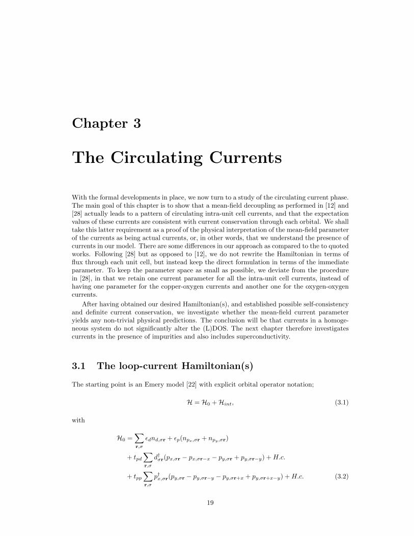
With the formal developments in place, we now turn to a study of the circulating current phase.The main goal of this chapter is to show that a mean-field decoupling as performed in [12] and[28] actually leads to a pattern of circulating intra-unit cell currents, and that the expectationvalues of these currents are consistent with current conservation through each orbital. We shalltake this latter requirement as a proof of the physical interpretation of the mean-field parameterof the currents as being actual currents, or, in other words, that we understand the presence ofcurrents in our model. There are some differences in our approach as compared to the to quotedworks. Following [28] but as opposed to [12], we do not rewrite the Hamiltonian in terms offlux through each unit cell, but instead keep the direct formulation in terms of the immediateparameter. To keep the parameter space as small as possible, we deviate from the procedurein [28], in that we retain one current parameter for all the intra-unit cell currents, instead ofhaving one parameter for the copper-oxygen currents and another one for the oxygen-oxygencurrents.
After having obtained our desired Hamiltonian(s), and established possible self-consistencyand definite current conservation, we investigate whether the mean-field current parameteryields any non-trivial physical predictions. The conclusion will be that currents in a homoge-neous system do not significantly alter the (L)DOS. The next chapter therefore investigatescurrents in the presence of impurities and also includes superconductivity.
3.1 The loop-current Hamiltonian(s)
The starting point is an Emery model [22] with explicit orbital operator notation;
H = H0 +Hint, (3.1)
with
H0 =∑r,σ
εdnd,σr + εp(npx,σr + npy,σr)
+ tpd∑r,σ
d†σr(px,σr − px,σr−x − py,σr + py,σr−y) +H.c.
+ tpp∑r,σ
p†x,σr(py,σr − py,σr−y − py,σr+x + py,σr+x−y) +H.c. (3.2)
19

20 CHAPTER 3. THE CIRCULATING CURRENTS
and
Hint = Vpd∑r,σσ′
nd,σr(npx,σ′r + npy,σ′r + npx,σ′r−x + npy,σ′r−y)
+ Ud∑r,σ
nd,σrnd,σr + Up∑r,σ
(npx,σrnpx,σr + npy,σrnpy,σr) (3.3)
where εd and εp are the orbital energies, the tpd and tpp are hopping integrals, and Ud, Up,and Vpd are the interaction strengths. The σ is understood to mean the opposite spin of σ.At this point, it is appropriate to address the issue of orbital sign conventions. As the readerwill notice, we have effectively used opposite signs for the tpd connected with copper-oxygenhopping in the x- and y-directions, respectively. This is merely a convention, amounting tochoosing one certain unit cell instead of a different one. This is illustrated in Figure 3.1. Thesign of tpp then follows from the overlap of the two p-orbitals, and will in our case be positive(see also [29]).
Cu
O
O Cu
O
O
O O
Figure 3.1: By choice of unit cell, all sign combinations for the tpd can be obtained. We usethe green unit cell. By counting colours, it is seen how the sign of tpp follows from the signson tpd in each direction.
We must also address the presence of the Ud and Up. By applying mean-field theory to theterms they appear in front of, the resulting approximated terms can be re-absorbed into thecoefficients εd and εp and thus renormalizing them (or, equivalently, the chemical potential).We do not go into great detail regarding the Ud and Up. From now on, they will be assumed tohave been absorbed into the other constants of the theory. Our main focus lies with the oxygen-copper repulsion and the consequences in mean-field of having these terms. We therefore neveraddress the question of what the actual values of Ud and Up are, except in an indirect waythrough the choice of numerical values for the input parameters.
To get currents into the picture, one must decouple the copper-oxygen interaction term inthe Fock channel (as in [28]) and then make an assumption regarding what terms to disregard.
The first thing to be noted is that a rewriting of the interaction term is
V = Vpd∑
r,m,σ,σ′
A†mrσAmrσ′ , (3.4)
where
A†(1,2),r,σ =1
2[(d†px,rσ + d†px,r−xσ)± (d†py,rσ + d†py,r−yσ)] (3.5)
A†(3,4),r,σ =i
2[(d†px,rσ − d†px,r−xσ)± (d†py,rσ − d†py,r−yσ)]. (3.6)

3.1. THE LOOP-CURRENT HAMILTONIAN(S) 21
If we write this out we see that
V = Vpd∑r,σ,σ′
∑a=x,y
d†rσ(pa,r+a,σp†a,r+aσ′ + pa,r−a,σp
†a,r−aσ′)drσ′ (3.7)
= Vpd∑r.σ,σ′
∑a=x,y
d†rσdrσ′(δσσ′ − p†a,r+aσ′pa,r+a,σ + δσσ′ − p†a,r−aσ′pa,r−a,σ). (3.8)
Now, this is the same as minus the copper-oxygen interaction in (3.3), provided we renormalisethe εd in (3.2) (due to the δσσ′) and furthermore let all operators act completely independentof their spin index, i.e., d↑ ≡ d↓. To emphasize the latter requirement and make the notationas clear as possible, we suppress spin indices for the remainder of this chapter; the spin willappear only as a factor of 2 in front of sums.
The next thing to do is then the actual decoupling. The way we do this has already beenanticipated by the notation. We introduce the complex mean-field parameter R defined by
Rm = 2Vpd 〈Am〉 . (3.9)
Then
−4Vpd∑r,m
A†rmArm ≈ −2∑r,m
(RmA†r,m + H.c.) +1
2Vpd
∑m
|Rm|2. (3.10)
For our calculations we always disregard the constant term, as it only corresponds to an absoluteshift of energies. Furthermore, the main assumption we make in order to have obtain a loop-current Hamiltonian, is that only one Am has a non-vanishing expectation value (at a time).We thus have four different loop-current Hamiltonians.
The translation invariance of the system is begging us to Fourier transform. As mentionedin the previous chapter, we employ a Fourier transform that explicitly takes inner-unit celldistances into account:
d†k =1√N
∑r
d†reik·r, p†x,k =
1√N
∑r
p†x,reik·(r+x/2), p†y,k =
1√N
∑r
p†y,reik·(r+y/2). (3.11)
Doing so yields a 3×3-block diagonal k-space Hamiltonian matrix1 in the operator basis givenby
ψ†(k) = [d†k, p†x,k, p
†y,k]. (3.12)
It has the form:
H0 =∑k
ψ†(k)
εd 2itpdsx −2itpdsy−2itpdsx εp 4tppsxsy2itpdsy 4tppsxsy εp
ψ(k). (3.13)
The decoupled interactions take the forms∑r
A†(1,2),r =∑k
cxd†kpx,k ± cyd
†kpy,k, (3.14)∑
r
A†(3,4),r =∑k
−(sxd†kpx,k ± syd
†kpy,k), (3.15)
1The aforementioned orbital convention is perhaps more obvious in this form.

22 CHAPTER 3. THE CIRCULATING CURRENTS
and we end up with four different k-space Hamiltonians:
H1 =∑k
ψ†(k)
εd 2itpdsx −R1cx −2itpdsy −R1cy−2itpdsx −R∗1cx εp 4tppsxsy2itpdsy −R∗1cy 4tppsxsy εp
ψ(k) (3.16)
H2 =∑k
ψ†(k)
εd 2itpdsx −R2cx −2itpdsy +R2cy−2itpdsx −R∗2cx εp 4tppsxsy2itpdsy +R∗2cy 4tppsxsy εp
ψ(k) (3.17)
H3 =∑k
ψ†(k)
εd 2itpdsx +R3sx −2itpdsy +R3sy−2itpdsx +R∗3sx εp 4tppsxsy2itpdsy +R∗3sy 4tppsxsy εp
ψ(k) (3.18)
H4 =∑k
ψ†(k)
εd 2itpdsx +R4sx −2itpdsy −R4sy−2itpdsx +R∗4sx εp 4tppsxsy2itpdsy −R∗4sy 4tppsxsy εp
ψ(k) (3.19)
We shall use these for calculating current expectation values, and in the next chapter to performimpurity scattering calculations. Furthermore, we shall from now on abuse our own notationsomewhat, and label these four decouplings as A = 1, 2, 3, 4. By (e.g.) taking A = 1 wemean that the decoupling of the interaction had a non-vanishing 〈A1,r,σ〉, and not that theA-operator is equal to unity. This should not cause any confusion.
3.2 The current operators
What is a current? Physically, we can think of it as something breaking time reversal symmetry,which is - as discussed in chapter 1 - of course an important property of the proposed pseudogapground state. But more specifically, a non-vanishing current should correspond to a non-vanishing expectation value of some operator. Which one? The A-operators themselves are notcurrent operators. One might naıvely take a→b = a†b− b†a, which has the nice properties that†a→b = −a→b = b→a. However, this leads to current patterns without current conservation2, athing we deem unphysical. We shall therefore define the current operators through demandingcurrent conservation. The starting point is the continuity equation:
nd,r = −∇ · d,r = −(xd,r − xd,r−x + yd,r − yd,r−y). (3.20)
Secondly, current conservation means that nd,r = 0. We calculate the time derivative using theHeisenberg equation. We do this in detail for the A = 1 case. The three other cases can theneasily be covered by small sign changes in the result.
i[H1, nd,r] =i
2[(2tpd −R1eiφ1)d†rpx,r − (R1eiφ1 + 2tpd)d
†rpx,r−x
− (R1eiφ1 + 2tpd)d†rpy,r + (2tpd −R1eiφ1)d†rpy,r−y +H.c., nd,r]. (3.21)
Using the general fermionic result that
[Ac†νcµ +A∗c†µcν , nν ] = −Ac†νcµ +A∗c†µcν , (3.22)
we then get for the time derivative of nd,r that
i[H1, nd,r] =i
2[(R1 − 2tpd)d
†rpx,r + (R1 + 2tpd)d
†rpx,r−x
+ (R1 + 2tpd)d†rpy,r + (R1 − 2tpd)d
†rpy,r−y −H.c.]. (3.23)
2This is not apparent from the equations, but turns out as one performs a numerical calculation.

3.2. THE CURRENT OPERATORS 23
The current operator identification is straightforward. We let Rd,r correspond to the currentgoing right from the d-orbital in the unit cell at r. Then
Rd,r = − i2
[(R1 − 2tpd)d†rpx,r + (2tpd −R∗1)p†x,rdr], (3.24)
Ud,r = − i2
[(R1 + 2tpd)d†rpy,r − (2tpd +R∗1)p†y,rdr], (3.25)
Ld,r = − i2
[(R1 + 2tpd)d†rpx,r−x − (2tpd +R∗1)p†x,r−xdr], (3.26)
Dd,r = − i2
[(R1 − 2tpd)d†rpy,r−y + (2tpd +R∗1)p†y,r−ydr], (3.27)
and we thus conclude that the relevant expectation values are3
⟨Rd,r⟩
= 2Im⟨(R1 − 2tpd)d
†rpx,r
⟩, (3.28)⟨
Ud,r⟩
= 2Im⟨(R1 + 2tpd)d
†rpy,r
⟩, (3.29)⟨
Ld,r⟩
= 2Im⟨(R1 − 2tpd)d
†rpx,r−x
⟩, (3.30)
and ⟨Dd,r⟩
= 2Im⟨(R1 + 2tpd)d
†rpy,r−y
⟩, (3.31)
respectively.
In a similar vein, we find for the px-py-currents that
npx,r =i
2[(2tpd +R∗1)p†x,rdr + (R∗1 − 2tpd)p
†x,rdr+x (3.32)
+ 2tppp†x,r(py,r − py,r−y − py,r+x + px,r+x−y) +H.c., npx,r] (3.33)
=− i
2[(2tpd +R∗1)p†x,rdr + (R∗1 − 2tpd)p
†x,rdr+x (3.34)
+ 2tppp†x,r(py,r − py,r−y − py,r+x + px,r+x−y)−H.c.]. (3.35)
We note the presence of currents from (or to) the d-orbital, which of course comes as no surprise.The remaining terms are then identified as px-py-currents, leading to the expectation values
⟨NWx,r
⟩= 4tppIm
⟨p†x,rpy,r
⟩,⟨NEx,r
⟩= −4tppIm
⟨p†x,r+xpy,r
⟩(3.36)⟨
SWx,r⟩
= −4tppIm⟨p†x,rpy,r
⟩,⟨SEx,r
⟩= 4tppIm
⟨p†x,rpy,r
⟩. (3.37)
By translation invariance, we now have the full current pattern for one copper atom and itsfour oxygen neighbours (see Figure 3.2).
Cu
O
O
O
Cu
O
O
Cu
O
O
O
O
Figure 3.2: It is customary to consider the current configuration to the right.
3A factor of 2 for spin and a factor of -2 from (a− a∗) = 2iIm(a).

24 CHAPTER 3. THE CIRCULATING CURRENTS
3.2.1 Evaluating the current operators
With the proper current operators defined, it is time to actually calculate the current expecta-tion value numbers. We describe this calculation for a general translation invariant three bandmodel. For simplicity, we take the temperature to be zero.
For a homogeneous system, the Hamiltonian is block diagonal in k-space. As above, wewrite
H =∑k
ψ†(k)H(k)ψ(k), (3.38)
with ψ†(k) = (d†k, p†x,k, p
†y,k). For a given chemical potential, µ, the ground state of this system
is the product of all creation operators creating states of energy less than µ working on thevacuum state. Since we are working within the three-orbital model, H is a 3 × 3 matrix, andthere are - for each given k - three bands to consider. Let us denote their correspondingannihilation operators by αk, βk and γk, and let Eγ(k) be the energy of a particle withmomentum k in the γ-band. We write the band operators as
α†k = aα(k)d†k + bα(k)p†x,k + cα(k)p†y,k,
β†k = aβ(k)d†k + bβ(k)p†x,k + cβ(k)p†y,k,
γ†k = aγ(k)d†k + bγ(k)p†x,k + cγ(k)p†y,k.
For simplicity, assume that the band structure and chemical potential are such that the groundstate consists solely of particles in the γ-band. Denote the ground state as |g〉 and define aregion Rγ in k-space by
Rγ = k ∈ FBZ | Eγ(k) ≤ µ. (3.39)
Then
|g〉 =∏
k∈Rγ
γ†k |0〉 . (3.40)
From equations (3.24) to (3.31), we see that any current operator expectation value has theform Im
(A⟨c†µcν
⟩)for some complex number A. How do we find
⟨c†µcν
⟩? Let’s take c†µ = p†x,r
and cν = py,r′ . To evaluate this number, we insert the k-space representation of the operators4.⟨px,r0→py,r0
⟩∝ Im 〈0|
∏k′′∈Rγ
γ(k′′)∑k,k′
p†x,kpy,k′ei((r′+y/2)·k′−(r+x/2)·k)
∏k′′∈Rγ
γ†(k′′) |0〉 (3.41)
Now, for any fixed pair of k, k′, the two operators in the middle can be anti-commuted past theγ’s to annihilate the vacuum (to the left respectively right), unless they meet their conjugateoperator with the same momentum on the way. In that case
〈0| γkp†x,k = 〈0| (a∗γ(k)dk + b∗γ(k)px,k + c∗γ(k)py,k)p†x,k
= 〈0| (−a∗γ(k)p†x,kdk + b∗γ(k)(1− p†x,kpx,k)− c∗γ(k)p†x,kpy,k)
= 〈0| (−p†x,k)γk + b∗γ = 〈0| b∗γ(k). (3.42)
For clarity we label the momenta in R as k1,k2, . . . ,kN . Using (3.42), we then get that⟨px,r0→py,r0
⟩∝ Im
∑k,k′∈Rγ
〈0| γk1· · · b∗(k) · · · γkNγ
†kN· · · cγ(k′) · · · γ†k1
|0〉 ei((r′+y/2)·k′−(r−x/2)·k).
(3.43)
4The reader is kindly asked to imagine the γ-operators to be ordered correctly.

3.3. SELF-CONSISTENCY OF THE CURRENTS 25
By construction of the Fock space, this is zero unless the two operator strings of remainingγs are each others conjugation. Therefore k must be equal to k′, and we arrive at the simpleformula ⟨
p†x,rpy,r′⟩
= Im∑
k∈Rγ
b∗γ(k)cγ(k)φr,r′(k), (3.44)
where φr,r′(k) := ei(r′+v(`)−r−v(`′))·k, and v is the orbital dependent Fourier factor explained
in the previous chapter. The number in equation (3.44) is easily evaluated numerically, and isreadily modified for another choice of current operator.
Now, what if more than one band were to contribute, i.e., if two bands have overlappingR-regions in momentum space? Let’s assume that both Eγ(k0) and Eα(k0) are less than µ.
Repeating the above procedure, we need to simplify 〈0| γk0αk0
p†x,k0. Using (3.42), we see that
〈0| γk0αk0
p†x,k0= 〈0| γk0
[(−p†x,k0αk0
) + b∗α(k0)]
= 〈0| (p†x,k0γk0
αk0− b∗γ(k0)αk0
+ b∗αγk0)
= 〈0| (−b∗γ(k0)αk0+ b∗αγk0
). (3.45)
The same thing of course happens to the ket part of the expectation value (we have alreadyset k = k′ by the same argument as above). Upon multiplication of the bra and the ket, allcross-terms in the product
〈0| (−b∗γ(k0)αk0+ b∗αγk0
)(−cγ(k0)α†k0+ cαγ
†k0
) |0〉 (3.46)
will vanish by construction of the Fock space. Furthermore, the a, b, c coefficient products willall be positive. The k0-term in the momentum sum thus takes the form
b∗γ(k0)cγ(k0) + b∗α(k0)cα(k0), (3.47)
and we realize that the generalization of (3.44) to the general situation of arbitrarily manyregions of band-overlap is straightforward:
⟨p†x,rpy,r′
⟩= Im
∑k∈Rα
b∗α(k)cα(k)φr,r′(k) +∑
k∈Rβ
b∗β(k)cβ(k)φr,r′(k) +∑
k∈Rγ
b∗γ(k)cγ(k)φr,r′(k)
,(3.48)
with obvious modifications for other currents. An interesting consequence of equation (3.48) isthe vanishing of orbital currents if all three bands are filled, i.e., Rα = Rβ = Rγ = FBZ , sincewe then sum inner products of different rows of a unitary matrix.
The calculation explained here in great detail is of course completely analogous to thecalculation of any expectation value of operator pairs, in particular the calculation of Rm(equation (3.9)). In the next section we extensively compute Rm.
3.3 Self-consistency of the currents
When doing mean-field theory, one must assume a certain value for the mean-field parameterin order to get a Hamiltonian. But with this Hamiltonian, one can calculate what the mean-field parameter actually is. Obviously, the two values should agree; the theory should beself-consistent. An equivalent demand is that the value of the mean-field parameter minimizesthe free energy of the system (see [23, Chapter 4]).
In this section, we present three different schemes for finding the correct value of the mean-field parameter. To our luck, they turn out to agree with each other. We do not explicitly

26 CHAPTER 3. THE CIRCULATING CURRENTS
mention the chemical potential, but it is present whenever we calculate an expectation value,and it is taken to be zero throughout this section.
We only present results for the case when A = 3, but the 1 and 2 case has essentially thesame behaviour. It was, however, not possible to stabilize an order parameter when A = 4.
Upon performing numerical calculations, we of course have to feed the computer withactual values for all the parameters in the theory. Whereas the hopping coefficients are agreedto be tpd = −1.3 eV and tpp = 1
2 tpd (see e.g. [30]), there is some uncertainty regarding thehybridization energies. Varma has εd = εp = 0 (see [12]), whilst a more realistic suggestionis εd = −1.5 eV and εp = −5 eV. A discussion of these values can be found in ref. [5]. Forthe self-consistent calculations presented here, we employed Varma’s parameters, but similarresults were obtained for the other case. Another issue regarding numerics is the units of theparameters. The computer does not take units as input, and the author admits to sometimeshaving forgotten to state the units of a parameter. We work in eV, and as can be seen frome.g. equations (3.3) and (3.16), all parameters share this unit.
3.3.1 Input/output scan
In general the self-consistency problem can be quite involved. We are, however, in the privilegedsituation of only having to determine one (although complex) mean-field parameter. We cantherefore scan all possible mean-field parameters and wee what output parameter they giverise to. That is to say, we repeat the calculation
R0 → H0 → R1 = 〈2VpdA〉H0(3.49)
for many different inputs R0. Once both real and imaginary part of R0 and R1 agree, astable solution has been found. This is illustrated in Figures 3.3 and 3.4, where we plotthe input/output relations in grey. Superimposed is the “input=output” plane in bright red,orange, and yellow. In Figures 3.3 and 3.4 we immediately see that only the trivial choice of Ris stable when Vpd = 3, whereas a non-trivial possible “ring of stability” seem to appear whenwe increase Vpd to 5 in Figure 3.4.
-5
0
5
-5
0
5-5
0
5
Im(R0)
Real part of output. A = 3 and Vpd = 3.
Re(R0)
(a)
-5
0
5
-5
0
5-5
0
5
Im(R0)
Imaginary part of output. A = 3 and Vpd = 3.
Re(R0)
(b)
Figure 3.3: We use two three-dimensional figures to display the four-dimensional graph of acomplex function of a complex variable. In both 3.3a and 3.3b, the (flat) xy-plane is thecomplex plane of R0-values. The z-axis is then the real (in 3.3a) or imaginary (in 3.3a) part ofthe output. Having Im(R0) = Im(R1) forces Im(R0) to be zero. And then Re(R0) must alsovanish.

3.3. SELF-CONSISTENCY OF THE CURRENTS 27
-5
0
5
-5
0
5-5
0
5
Im(R0)
Real part of output. A = 3 and Vpd = 5.
Re(R0)
(a)
-5
0
5
-5
0
5-5
0
5
Im(R0)
Imaginary part of output. A = 3 and Vpd = 5.
Re(R0)
(b)
Figure 3.4: Same idea as in Figure 3.3. Now more values of R0 seem to be stable, i.e., satisfythat Re(R0) = Re(R1) and Im(R0) = Im(R1).
3.3.2 Iteration for stability
The behaviour seen in the last section is also apparent when we do the self-consistency calcu-lation in a different way, namely by iterating the above procedure. Our algorithm now doesthis:
R0 → H0 → 〈2VpdA〉H0= R1 → H1 → 〈2VpdA〉H1
= R2 → . . . (3.50)
As seen from Figures 3.5 and 3.6, such a scheme does not seem to converge when Vpd = 3,whereas convergence is indeed attained for Vpd = 5. Of course, these figures do not tell usanything about the dependence of initial guesses nor of the possibilities of other stable solutions.This is exactly where plots like those in Figures 3.3 and 3.4 come in handy. However, it is veryhard to get a precise numerical value for the parameter if one does not invoke the iterativeprocedure.
(a) A = 3, Vpd = 3. (b) A = 3, Vpd = 3.
Figure 3.5: Iterative evolution of length and phase of R. The colours on the left correspondto the colours on the right, and we thus fix |R| for every initial guess but vary the phase. Thetrend is clear: everything goes to zero.
28 CHAPTER 3. THE CIRCULATING CURRENTS
(a) A = 3, Vpd = 5. (b) A = 3, Vpd = 5.
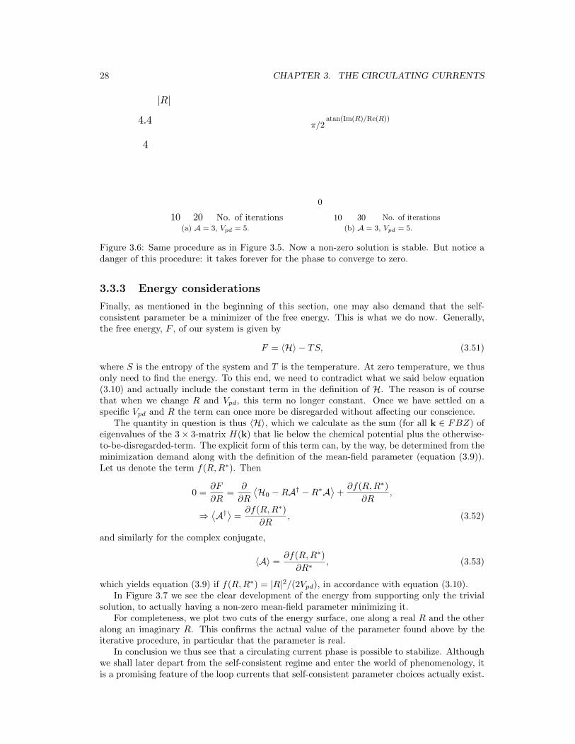
Figure 3.6: Same procedure as in Figure 3.5. Now a non-zero solution is stable. But notice adanger of this procedure: it takes forever for the phase to converge to zero.
3.3.3 Energy considerations
Finally, as mentioned in the beginning of this section, one may also demand that the self-consistent parameter be a minimizer of the free energy. This is what we do now. Generally,the free energy, F , of our system is given by
F = 〈H〉 − TS, (3.51)
where S is the entropy of the system and T is the temperature. At zero temperature, we thusonly need to find the energy. To this end, we need to contradict what we said below equation(3.10) and actually include the constant term in the definition of H. The reason is of coursethat when we change R and Vpd, this term no longer constant. Once we have settled on aspecific Vpd and R the term can once more be disregarded without affecting our conscience.
The quantity in question is thus 〈H〉, which we calculate as the sum (for all k ∈ FBZ) ofeigenvalues of the 3× 3-matrix H(k) that lie below the chemical potential plus the otherwise-to-be-disregarded-term. The explicit form of this term can, by the way, be determined from theminimization demand along with the definition of the mean-field parameter (equation (3.9)).Let us denote the term f(R,R∗). Then
0 =∂F
∂R=
∂
∂R
⟨H0 −RA† −R∗A
⟩+∂f(R,R∗)
∂R,
⇒⟨A†⟩
=∂f(R,R∗)
∂R, (3.52)
and similarly for the complex conjugate,
〈A〉 =∂f(R,R∗)
∂R∗, (3.53)
which yields equation (3.9) if f(R,R∗) = |R|2/(2Vpd), in accordance with equation (3.10).In Figure 3.7 we see the clear development of the energy from supporting only the trivial
solution, to actually having a non-zero mean-field parameter minimizing it.For completeness, we plot two cuts of the energy surface, one along a real R and the other
along an imaginary R. This confirms the actual value of the parameter found above by theiterative procedure, in particular that the parameter is real.
In conclusion we thus see that a circulating current phase is possible to stabilize. Althoughwe shall later depart from the self-consistent regime and enter the world of phenomenology, itis a promising feature of the loop currents that self-consistent parameter choices actually exist.

3.4. PHYSICAL PROPERTIES OF THE CIRCULATING CURRENT STATE 29
(a) A = 3, Vpd = 3. (b) A = 3, Vpd = 5.
Figure 3.7: For Vpd = 3 R = 0 is a distinct global minimum, whereas R 6= 0 minimizes theenergy for Vpd = 5. Note the asymmetry between Re(R) and Im(R).
(a) A = 3, Vpd = 3. (b) A = 3, Vpd = 5.
Figure 3.8: Cuts through the surfaces of Figure 3.7. Red: Imaginary R. Blue: Real R.
3.4 Physical properties of the circulating current state
Self-consistency is one thing, good as a sanity check, but another thing as actual physicalproperties. Be it stable or not, the presence of a circulating current order parameter havebetter change some measurable features of our system, or we might as well never mention it.Luckily, there are at least two predictions to be obtained from assuming one of the Hamiltoniansin (3.16) to (3.19).
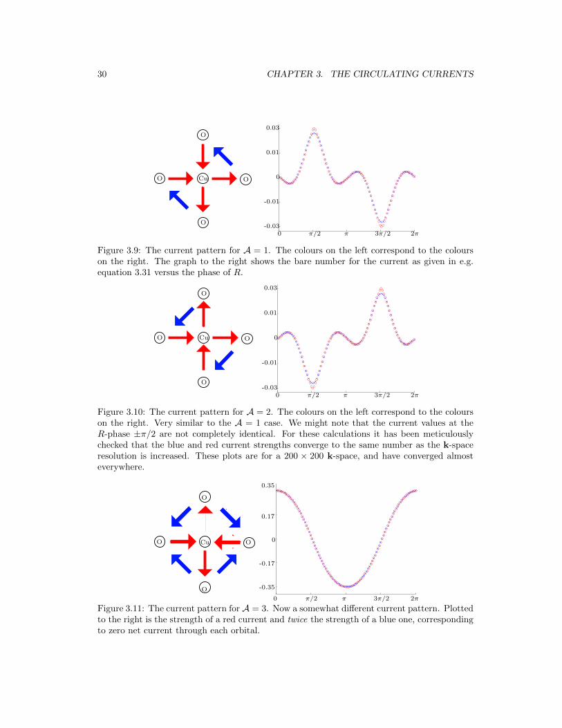
3.4.1 Actual current patterns
Even though the inter-orbital currents themselves are not directly assessable to the STM, thepatterns they form reveal something the about the (broken) symmetries of the system. As isapparent from Figure 3.1, a change of the orbital convention can correspond to a π/2 rotationof the coordinate system. We stick to our “+ − +” convention5 and then obtain the currentpatterns shown below in Figures 3.9, 3.10, and 3.11. In all three, the length of R is kept fixed at4, and we scan the phase of R. This is in order to investigate how the current parameter phaseaffects the current pattern. It was found that scaling the R parameter only had a trivial effecton the magnitude of the resulting current patters. This is a good validation of our model, weactually achieve the current patterns when doing mean-field theory. We also note with pleasurethat the total current through each orbital is zero.
5We maintain this convention throughout the thesis.
30 CHAPTER 3. THE CIRCULATING CURRENTS
0 π/2 π 3π/2 2π-0.03
-0.01
0
0.01
0.03
Cu
O
O
O
O
Figure 3.9: The current pattern for A = 1. The colours on the left correspond to the colourson the right. The graph to the right shows the bare number for the current as given in e.g.equation 3.31 versus the phase of R.
0 π/2 π 3π/2 2π-0.03
-0.01
0
0.01
0.03
Cu
O
O
O
O
Figure 3.10: The current pattern for A = 2. The colours on the left correspond to the colourson the right. Very similar to the A = 1 case. We might note that the current values at theR-phase ±π/2 are not completely identical. For these calculations it has been meticulouslychecked that the blue and red current strengths converge to the same number as the k-spaceresolution is increased. These plots are for a 200 × 200 k-space, and have converged almosteverywhere.
0 π/2 π 3π/2 2π
-0.35
-0.17
0
0.17
0.35
O
O O
O
Cu
Figure 3.11: The current pattern for A = 3. Now a somewhat different current pattern. Plottedto the right is the strength of a red current and twice the strength of a blue one, correspondingto zero net current through each orbital.
3.4. PHYSICAL PROPERTIES OF THE CIRCULATING CURRENT STATE 31
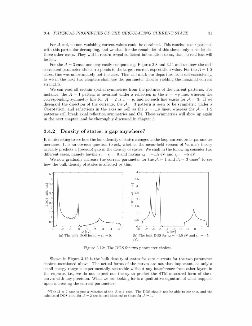
For A = 4, no non-vanishing current values could be obtained. This concludes our patiencewith this particular decoupling, and we shall for the remainder of this thesis only consider thethree other cases. They will in return reveal sufficient information to us, that no real loss willbe felt.
For the A = 3 case, one may easily compare e.g. Figures 3.8 and 3.11 and see how the self-consistent parameter also corresponds to the largest current expectation value. For the A = 1, 2cases, this was unfortunately not the case. This will mark our departure from self-consistency,as we in the next two chapters shall use the parameter choices yielding the maximal currentstrengths.
We can read off certain spatial symmetries from the pictures of the current patterns. Forinstance, the A = 1 pattern is invariant under a reflection in the x = −y line, whereas thecorresponding symmetry line for A = 2 is x = y, and no such line exists for A = 3. If wedisregard the direction of the currents, the A = 3 pattern is seen to be symmetric under aC4-rotation, and reflections in the axes as well as the x = ±y lines, whereas the A = 1, 2patterns still break axial reflection symmetries and C4. These symmetries will show up againin the next chapter, and be thoroughly discussed in chapter 5.
3.4.2 Density of states; a gap anywhere?
It is interesting to see how the bulk density of states changes as the loop-current order parameterincreases. It is an obvious question to ask, whether the mean-field version of Varma’s theoryactually predicts a (pseudo) gap in the density of states. We shall in the following consider twodifferent cases, namely having εd = εp = 0 and having εd = −1.5 eV and εp = −5 eV.
We now gradually increase the current parameter for the A = 1 and A = 3 cases6 to seehow the bulk density of states is affected by this.
-3 -2 -1 0 1 2 3 4 5
0.5
1
1.5
2
2.5
3
3.5
4
4.5
5
5.5
ω [eV]
LD
OS
[arb
.un.]
(a) The bulk DOS for εd = εp = 0.
-8 -7 -6 -5 -4 -3 -2 -1 0 10
0.5
1
1.5
2
2.5
3
3.5
4
ω [eV]
LD
OS
[arb
.un.]
(b) The bulk DOS for εd = −1.5 eV and εp = −5eV.
Figure 3.12: The DOS for two parameter choices.
Shown in Figure 3.12 is the bulk density of states for zero currents for the two parameterchoices mentioned above. The actual forms of the curves are not that important, as only asmall energy range is experimentally accessible without any interference from other layers inthe cuprate, i.e., we do not expect our theory to predict the STM-measured form of thesecurves with any precision. What we are looking for is a qualitative signature of what happensupon increasing the current parameters.
6The A = 2 case is just a rotation of the A = 1 case. The DOS should not be able to see this, and thecalculated DOS plots for A = 2 are indeed identical to those for A = 1.

32 CHAPTER 3. THE CIRCULATING CURRENTS
Shown in Figure 3.13 is the DOS evolution as R is increased from 0 to 3i (in equal stepsincreasing upwards in the Figure). We see a smearing of the DOS, but no distinct gap features.
-3 -2 -1 0 1 2 3 4 50
1
2
3
4
5
6
7
8
9
10
ω [eV]
DO
Sand
off
set
[arb
.un.]
(a) A = 1
-8 -6 -4 -2 0 2 40
1
2
3
4
5
6
7
8
9
10
ω [eV]
DO
Sand
off
set
[arb
.un.]
(b) A = 1
Figure 3.13: The evolution of the bulk DOS as R is increased in equal steps from 0 to 3i. Eachcurve is for an R-value 3i
10 higher than the curve beneath it and is set off with 1 in our arbitraryDOS-units with respect to the curve beneath it.
In Figure 3.14 we see how the bulk density of states changes as R is being cranked up from0 to 3. This time the DOS seems to get squeezed together as well as smeared out. No gapseems to manifest itself.
-3 -2 -1 0 1 2 3 4
5
10
15
20
25
30
ω [eV]
DO
Sand
off
set
[arb
.un.]
(a) A = 3
-6 -4 -2 0 2 4
2
4
6
8
10
12
14
16
18
20
ω [eV]
DO
Sand
off
set
[arb
.un.]
(b) A = 3
Figure 3.14: The evolution of the bulk DOS as R is increased in equal steps from 0 to 3. Eachcurve is for an R-value 3
10 higher than the curve beneath it and is set off with 2 in our arbitraryunits with respect to the curve beneath it.
On the basis of the Figures 3.13 and 3.14 no convincing conclusions can be drawn, or,to quote chapter 1, no smoking gun is to be seen. We thus end this chapter by concludingthat a loop current fingerprint should rather be found from the spatial symmetries of the looppatterns. The appearance of non-vanishing currents but lack of a gap feature in mean-field isin accordance with Varma’s own predictions in [12]. Here it is found that the emergence of agap requires the inclusion of fluctuations of the current parameter to be taken into account.We do not venture that far with the loop current theory, but stay within the mean-field pictureand look for the spatial symmetries of the current patterns to show up in the local density of

3.5. SUMMARY 33
states. But if we are to see spatial symmetry breaking, a homogeneous system is not a goodsystem to consider, and we therefore break the translation invariance of our model in the nextchapter, by introducing an impurity.
3.5 Summary
In summary, we have now investigated the mean-field loop current theory to an extent where wefeel confident enough to use it in actual predictions. We found the emergence of intra-orbitalcurrents along with explicit current conservation. Furthermore, we found no homogeneousfingerprints of the loop-currents, apart from the breaking of certain symmetries by the currentpatterns. These broken spatial symmetries will form the basis of our results, as presented inthe next chapter and analysed in the chapter after that.
34 CHAPTER 3. THE CIRCULATING CURRENTS

Chapter 4
Impurity scattering, the localdensity of states
We now arrive at the heart of this thesis. With a thorough understanding of the behaviour ofVarma’s mean-field theory at hand (chapter 3), we turn to the LDOS around an impurity tosearch for a loop-current fingerprint.
4.1 Introducing the impurity
In the cuprates, impurities are not a nuisance or something unfortunate a very careful experi-mentalist could have avoided. On the contrary, they are put into the material on purpose (bya very careful experimentalist) and are the cause of the doping as they “suck out” electrons orholes of the CuO2 layers. It is therefore highly realistic and relevant to include impurities intoour model.
For our purposes, a single impurity will suffice. Introducing more of them will only com-plicate things, and we want to study the LDOS modulations in the immediate vicinity of animpurity, where any other deviations from the CuO2 lattice can safely be ignored. This ofcourse implies that our results should be considered valid in the dilute limit of low impurityconcentration. This is in fine agreement with being in the lower-doping part of the phase di-agram (see Figure 1.2a). We model this single impurity as depicted graphically in Figure 4.1and mathematically in equation (4.1); by adding an extra energy to the creation/annihilationoperator pair on one specific copper orbital. The spin dependence in equation (4.1) stems fromthe possibility of having a magnetic impurity, which still resides only one particular place inspace, buts treats spin up and spin down differently.
H → H+∑σ
V impσ d†σr0dσr0 = H+
∑r,σ
V impσ d†σrdσrδ(r− r0) (4.1)
The only difference between a magnetic and non-magnetic impurity will be that V imp↑ = V imp
↓for a non-magnetic impurity and V imp
↑ = −V imp↓ for a magnetic one. In our actual calculations
we only consider a non-magnetic impurity.
It is important to note that this sort of impurity model still leaves our full Hamiltonianquadratic in creation/annihilation operators. We use this fact in the very beginning of the nextsection, more precisely in equation (4.3).
35

36 CHAPTER 4. IMPURITY SCATTERING, THE LOCAL DENSITY OF STATES
Figure 4.1: One copper atom gets modified by an enlargened on-site potential.
4.2 General case derivation
As the LDOS is our ultimate goal, we need a spectral function and to that end a Green’sfunction. We largely follow [4, Chapter 4], whence the following very nice derivation for thecase of a single impurity stems.
Let us first denote the full Hamiltonian as H where H = H0 + Himp, and furthermoreH = ψ†Hψ = ψ†(H0 + H imp)ψ. For the Green’s function of respectively thee free and fullHamiltonian we have that
[1(ω + iη)−H0]G0(ω) = 1 (4.2)
and[1(ω + iη)−H]G(ω) = 1, (4.3)
where 1 is the identity operator and a matrix structure of the Green’s functions is understood.Equating the left hand sides of equations (4.2) and (4.3) then yields that
[1(ω + iη)−H]G(ω) = [1(ω + iη)−H +H imp]G0(ω) (4.4)
= [1(ω + iη)−H]G0(ω) +H impG0(ω). (4.5)
Since, by equation (4.3), G(ω) = [1(ω+ iη)−H]−1, we can multiply by G(ω) from the left andobtain the Dyson integral equation;
G(ω) = G0(ω) +G(ω)H impG0(ω). (4.6)
In a basis where H imp is (block) diagonal, this equation takes the following appealingly simplecomponent-wise form:
Gµν(ω) = G0µν(ω) +
∑ν′
Gµν′(ω)H impν′ G0
ν′ν(ω). (4.7)
For our impurity, the position basis is just such a basis, since H imp is proportional to a δ-function (see equation (4.1)). If we understand orbital and spin matrix structure of the factors,we then have that
G(r, r′, ω) = G0(r− r′, ω) +G(r, r0, ω)H imp(r0)G0(r0 − r′, ω), (4.8)
from where it immediately follows that
G(r, r0, ω) = G0(r− r0, ω) +G(r, r0, ω)H imp(r0)G0(r0 − r0, ω), (4.9)
and hence that
G(r, r0, ω) = G0(r− r0, ω)[1−H imp(r0)G0(r0 − r0, ω)]−1. (4.10)
The exact solution to the real-space Dyson equation (equation 4.8) is thus
G(r, r′, ω) = G0(r− r′, ω)
+G0(r− r0, ω)[1−H imp(r0)G0(r0 − r0, ω)]−1H imp(r0)G0(r0 − r′, ω), (4.11)

4.3. THREE BAND CASE 37
which has the very nice feature of only involving free Green’s functions. We can rewrite thisexpression for the full Green’s function in a slightly more illustrative way.
From [23, Chapter 5] we have the following expression for the T -matrix:
T = H imp +H imp 1
ω + iη −H0︸ ︷︷ ︸G0
T, (4.12)
which can be rearranged as
T = [1−H impG0]−1H imp. (4.13)
The compact form of equation (4.11) is thus
G(r, r′, ω) = G0(r− r′, ω) +G0(r− r0, ω)T (r0, ω)G0(r0 − r′, ω), (4.14)
which is intuitively reasonable, as illustrated in Figure 4.2.
rrXXXXXXXXXz rr′@@@@@@@R
G0(r− r′)
G0(r− r0) fx T (r0)
G0(r0 − r′)
Figure 4.2: How does the particle get from r to r′? -By either propagating freely or by scatteringoff the impurity. The arrows represent unperturbed propagators, i.e., free Green’s functions.
Note that the T or scattering matrix - since it contains a Green’s function - can be advancedor retarded. As is the case with Green’s functions, we take it to be retarded if nothing elseis mentioned. It is also worth noting that the T matrix for a single impurity is a function ofenergy only. This is not really apparent from the notation of equation (4.14), but follows fromthe translation invariance of the unperturbed system;
T (r0, ω) = [1−H impG0(r0 − r0, ω)]−1H imp = [1−H impG0(0, ω)]−1H imp ≡ T (ω). (4.15)
Regardless of where we (spatially) want to calculate the LDOS, we thus only need to calculatethe T matrix once.
4.3 Three band case
We now mimic section 2.2 and demonstrate how we get from a general expression to a numericalvalue; an actual result for the LDOS around an impurity.
The first thing to consider is the form of the impurity matrix for a non-magnetic impurity.In the usual (spin degenerate) three-band basis, where ψ†(r) = (d†r, p
†x,r, p
†y,r), the impurity
matrix only has one non-zero entry;
H imp =
V 0 00 0 00 0 0
δ(r0). (4.16)

38 CHAPTER 4. IMPURITY SCATTERING, THE LOCAL DENSITY OF STATES
For a given ω, the next step is then to find the free Green’s function matrix at the origin. Asexplained in chapter 2, this is given by
G0(ω, 0) =∑k
[1(ω + iη)−H3×3(k)]−1. ∗ Fiuc(k), (4.17)
where .∗ denotes elementwise matrix multiplication and
F3×3(k) =
1 e−ikx/2 e−iky/2
eikx/2 1 ei(kx−ky)/2
eiky/2 ei(ky−kx)/2 1
. (4.18)
This gives us the T matrix of ω. Finally, as we shall only ever ask for the full Green’s functionat the same site, we find the free Green’s functions at the sites ±r;
G0(±r, ω) =∑k
[1(ω + iη)−H3×3(k)]−1. ∗ Fiuc(k)e±ik·r, (4.19)
and then perform the matrix multiplication, take the imaginary part, multiply by the appro-priate factor, and repeat for another r or ω. Just as in the bulk case described in chapter 2,our calculation scales linearly with the size of the system as it amounts to repeating the samecomputation for every point in k-space and then summing up these results.
4.3.1 Nambu-fied three band case
In the superconducting three-band model, the first thing to consider is the spin-dependence ofthe impurity. We use the same operator basis as described in chapter 2, the three-band Nambubasis given (in k-space) by
ψ†(k) = (d†↑k, p†x,↑k, p
†y,↑k, d↓−k, px,↓−k, py,↓−k), (4.20)
and take the impurity to be non-magnetic, i.e., it treats spin up and spin down on equal footing.At the impurity site, the impurity matrix can then be written as
H imp =
V 0 00 0 00 0 0
⊕−V 0 0
0 0 00 0 0
, (4.21)
where the minus arises from the reversed order of spin down operators in our basis. The secondthing to consider is how we should Fourier transform the entries of the now 6 by 6 Green’sfunction matrix. If we simply perceive each entry in the matrix as an expectation value of twooperators (which indeed is what a Green’s function is, see [23, chapters 8, 9, and 11]), we seethat the operator pairs in question are
d↑kd†↑k d↑kp
†x,↑k d↑kp
†y,↑k d↑kd↓−k d↑kpx,↓−k d↑kpy,↓−k
px,↑kd†↑k px,↑kp
†x,↑k px,↑kp
†y,↑k px,↑kd↓−k px,↑kpx,↓−k px,↑kpy,↓−k
py,↑kd†↑k py,↑kp
†x,↑k py,↑kp
†y,↑k py,↑kd↓−k py,↑kpx,↓−k py,↑kpy,↓−k
d†↓−kd†↑k d†↓−kp
†x,↑k d†↓−kp
†y,↑k d†↓−kd↓−k d†↓−kpx,↓−k d†↓−kpy,↓−k
p†x,↓−kd†↑k p†x,↓−kp
†x,↑k p†x,↓−kp
†y,↑k p†x,↓−kd↓−k p†x,↓−kpx,↓−k p†x,↓−kpy,↓−k
p†y,↓−kd†↑k p†y,↓−kp
†x,↑k p†y,↓−kp
†y,↑k p†y,↓−kd↓−k p†y,↓−kpx,↓−k p†y,↓−kpy,↓−k
.
By invoking our usual Fourier transform of each operator (equation (3.11)), we thus find thateach 3 by 3 block will have the same intra unit cell Fourier phase matrix, namely the one givenin equation (4.18).
It is indeed this Nambu-fied model we shall use in the remainder of the chapter, possiblywith some parameters set to zero. The Hamiltonian is thus the one of equations (2.45) and(2.46), with the 3-band Hamiltonian given by one of the equations (3.16) to (3.18).

4.4. RESULTS OF THE CALCULATION 39
4.4 Results of the calculation
We now present the first series of our main results, which are local density of states plots for dif-ferent relevant cases. In particular, we repeat our calculations for the two sets of hybridizationenergies mentioned in the previous chapter, namely εd = εp = 0 and εd = −1.5 eV and εp = −5eV, to find the dependence of our results on the specific parameter choices. It is of coursealways a trade-off when one performs numerical calculations, that one on one hand would liketo verify that the behaviour seen is not an artefact of the particular parameter choice invoked,but on the other hand does not want to perform an exhaustive search in the parameter space1.We choose this procedure as a sound compromise between generality and clarity.
So which parameters do we use? First of all, we restrict ourselves in this chapter to consideronly the A = 1 current pattern. This pattern will provide us with the results we shall perceiveas the main findings of our study. In the next chapter, where we present a more in-depthanalysis of our results, we shall also discuss the differences to the other current patterns. Themain conclusion hereof will be that the LDOS is sensitive to where the currents run - to beunderstood as between which orbitals there is a non-vanishing current expectation value (c.f.Figures 3.9 to 3.11) - but insensitive to the direction of the currents. It should in this respectbe mentioned that the phase-dependence of the current values was found to be very similar forboth sets of hybridization energies, in particular that the current-maximising phases are thesame for both cases. See Appendix A for details.
Secondly, as we do not have self-consistent values for the co-existing superconducting gapand current parameter at hand, we choose these large enough to see distinct effects of theirpresence, but small enough to (hopefully) avoid any pathological results. In section 4.5, we useas a good compromise the values ∆0 = 0.25, R = 1i. Our choice for the complex phase of Rdraws upon our analysis of Varma’s mean-field theory by itself; it is the phase that was foundto maximize the current expectation value (see Figure 3.9).
As a final thing before presenting the results, let us clarify how we perceive the lattice.When we calculate the local density of states, we of course have to specify a lattice point inwhich we calculate it. We count lattice points as unit cells, and then choose the appropriateorbital (Green’s function entry) for the inner structure. This is illustrated in Figure 4.3.
Figure 4.3: We perceive the lattice as a cubic square lattice (right), where each point has aninner spatial structure (left).
This spatial structure is also very important to keep in mind, when we discuss spatialsymmetries. The origin of our coordinate system (with respect to the impurity) is placedinside - but not in the middle of - the unit cell at r = (0, 0). This can potentially cause someconfusion, which we shall do our best to illustrate our way out of, whenever the need arises.
4.5 The realistic parameters
We start out by setting εd = −1.5 eV and εp = −5 eV. We shall focus on a small energy rangeclose to the fermi energy, as this is the experimentally relevant region.
1For our full theory, we provide the numerical inputs: εd, εp, tpd, tpp, ∆0, R, Vimp, and A. We only reallywant to vary R and switch between two or three values for A and ∆0.

40 CHAPTER 4. IMPURITY SCATTERING, THE LOCAL DENSITY OF STATES
-2 -1.5 -1 -0.5 0 0.5 1 1.5 20
0.2
0.4
0.6
0.8
1
1.2
1.4 A = 1, R = 0, ∆0 = 0, Vimp = 0L
DO
S[a
rb.
un.] Copper
Oxygen x
Oxygen y
(a) x-axis: ω in eV.
-2 -1.5 -1 -0.5 0 0.5 1 1.5 20
0.2
0.4
0.6
0.8
1
1.2
1.4
1.6A = 1, R = 0, ∆0 = 0.25, Vimp = 0
LD
OS
[arb
.un.] Copper
Oxygen x
Oxygen y
(b) x-axis: ω in eV.
-2 -1.5 -1 -0.5 0 0.5 1 1.5 20
0.2
0.4
0.6
0.8
1
1.2
1.4A = 1, R = 0 + 1i, ∆0 = 0, Vimp = 0
LD
OS
[arb
.un.] Copper
Oxygen x
Oxygen y
(c) x-axis: ω in eV.
-2 -1.5 -1 -0.5 0 0.5 1 1.5 20
0.1
0.2
0.3
0.4
0.5
0.6
0.7
0.8
0.9A = 1, R = 0 + 1i, ∆0 = 0.25, Vimp = 0
LD
OS
[arb
.un.] Copper
Oxygen x
Oxygen y
(d) x-axis: ω in eV.
Figure 4.4: Reference plots in the relevant energy range (extended a bit). The parameters usedin the computation are shown above each plot. The legend shows three curves, but only twoare to be seen in the plots. This is due to the two oxygen density of states being equal in thehomogeneous case. Note the two extra peaks at ω ≈ ±1 eV.
-2 -1.5 -1 -0.5 0 0.5 1 1.5 20
0.2
0.4
0.6
0.8
1
1.2
1.4
1.6
1.8
2A = 1 , R = 0 , ∆0 = 0.25 , Vimp = 10
LD
OS
[arb
.un.] Copper
Oxygen x
Oxygen y
point: [1 0]
(a) x-axis: ω in eV.
-2 -1.5 -1 -0.5 0 0.5 1 1.5 20
0.1
0.2
0.3
0.4
0.5
0.6
0.7
0.8
0.9
1A = 1 , R = 0 + 1i , ∆0 = 0.25 , Vimp = 10
LD
OS
[arb
.un.] Copper
Oxygen x
Oxygen y
point: [1 0]
(b) x-axis: ω in eV.
Figure 4.5: The characteristic nearest-neighbour sub-gap peak disappears in the presence of acurrent. The extra peaks noted also in Figure 4.4d remain.

4.5. THE REALISTIC PARAMETERS 41
As a first thing, as a reference, let us see how the orbitally resolved homogeneous density ofstates with and without superconductivity and orbital currents looks. This is shown in Figures4.4a to 4.4d. These four plots reveal some qualitative information about our model to us. Firstof all, we see that the introduction of a current does not alter the non-superconducting DOSin any significant way (compare Figures 4.4a and 4.4c), which is of course in accordance withwhat we saw in Figure 3.13b. As a second thing, we observe that although we only placedsuperconductivity on the copper atoms, the oxygen atoms resonate along, and form coherencepeaks at the same energies as the copper does. This feature is present in all of our numericaldata, whenever superconductivity can be identified. Recalling the discussion of chapter 2 onhow to put superconductivity into the model, it is noted that majority of the spectral weightat and near the Fermi level of the system actually resides on copper in the normal state, soour choice of letting all the Cooper pairs condense on copper might all in all not have been toocrude.
Furthermore, we notice the possible co-existence of superconductivity and currents in themodel. Although the superconducting gap gets reduced from Figure 4.4b to Figure 4.4d, inthe sense that the DOS at ω = 0 no longer vanishes, it is still present and the characteristic“V-neck” gap is evident also in Figure 4.4d. Also, some new peaks are present. We returnto these later in this section. This surviving gap behaviour is lost when R becomes too large,which is our main reason for keeping R and ∆0 of the same magnitude. The co-existence ofd-wave superconducting fingerprints and loop-currents is not a surprising result in itself, sincewe explicitly assumed the coexistence in the way we built our model, but it is nonetheless anindication of the model behaving in a way we understand.
On the other hand, though, some of the usual and well-understood features of a d-wavesuperconductor seem to be completely lost in the presence of currents. In a one-band super-conductor with a single impurity, one finds huge sub-gap peaks in the LDOS on the nearestneighbours away from the impurity (see [4, chapter 3] for a discussion of this). This featureclearly survives into the current-less three-band model, in the sense that the peak is on thenearest-neighbouring copper atom, as shown in Figure 4.5a, but is nowhere to be seen in Figure4.5b.
Now, as mentioned in chapter 2, is it not our aim to study the co-existence of supercon-ductivity and currents in great detail. We do phenomenology; put in the superconductivity byhand and look for a current signature. It would thus be somewhat hollow to find this signaturein the specific way the currents alter the usual superconductivity features. Instead, we looksomewhere else for our smoking gun, and find it in the spatial modulations around the impurity.
In Figure 4.6, the smoke is evident. We fix the energy at the peak value of Figure 4.5a andvary the position at which the LDOS is calculated. We can easily cover a very large plaquettethis way by virtue of equation (4.14), but as the LDOS modulations fall off quite rapidly asones moves away from the impurity, we zoom in near the impurity to get a good look of whatis going on. The real system size is of course determined by our k-space resolution, which forthe plots in Figure 4.6 is 200× 200.
A real-space plot is a very nice visualization of things, and provides us with an overviewof what is going on. But as the mind has no standard way of ordering colours (see [31] fora discussion of this), a lot of quantitative information is absent. We clearly see that the C4symmetry is broken in Figure 4.6b, but by what measure? And more importantly: what is theR dependence of the breaking? We quantify the breaking in the following way. We look at thetwo unit cells at respectively x = −1, y = 1 and x = −1, y = −1. Let us denote the formersite as r and the latter as r′. As the reader may easily verify (or deduct from Figure 5.1b), aC4 invariance implies that
ρd(r, ω) = ρd(r′, ω) and ρpx(r, ω) = ρpy (r′, ω). (4.22)
In a suitable range of ω, we now calculate the three orbital densities of states at thesetwo sites, while we gradually increase R. We then quantify the C4 breaking, denote it Bd(R)

42 CHAPTER 4. IMPURITY SCATTERING, THE LOCAL DENSITY OF STATES
-2 -1 0 1 2
-2
-1
0
1
2
A = 1 , Vimp = 10 , R = 0 , ∆0 = 0.25 , ω = 0.
0.5
1
1.5
2
2.5
(a) Superconducting state with no currents.-2 -1 0 1 2
-2
-1
0
1
2
A = 1, Vimp = 10, R = 1i , ∆0 = 0.25, ω = 0.
0.1
0.2
0.3
0.4
0.5
0.6
(b) Superconducting state with currents. C4 isbroken.
Figure 4.6: Real-space grid with the density of states at the energy shown above the plot. Thex- and y-axes are labelled in accordance with Figure 4.3. The colour scale shown to the rightof each plot is in the same arbitrary units as the previous plots of this section. The grey colourrepresents nothing; no atom resides in this location, and we thus do not calculate a value for thegrey squares; their value is taken to be zero. The impurity resides in the copper (South-West)corner of the [0 0] cell in each plot.
and Bp(R), respectively, for each ω and R-value as the absolute value of the LDOS differencedivided by the average LDOS value. In formulas,
Bd(R,ω) =2|ρd(r, ω)− ρd(r′, ω)||ρd(r, ω) + ρd(r′, ω)|
, (4.23)
and
Bp(R,ω) =2|ρpx(r, ω)− ρpy (r′, ω)||ρpx(r, ω) + ρpy (r′, ω)|
. (4.24)
We measure the Bi(R,ω) in percent. The result of this calculation is shown in Figure 4.7.Interestingly, the difference between the calculated densities of states is identically zero2 whenR = 0, but have relatively large finite values for all the non-zero R-values. The conclusion fromthe numerical point of view is thus that this effect is solely ascribable to the R-parameter. In thenext chapter, we verify analytically that no C4 breaking is possible in the normal state withoutthe currents. The energy dependence of the symmetry breaking also deserves mentioning.First of all, we note the connection between the peaks in the Bd(R,ω) and Bp(R,ω) curvesat ω ≈ R and the extra current-induced van Hove peaks in Figures 4.4d and 4.5b. We geta clear symmetry breaking a these energies, but not necessarily the largest one. Apart fromthese peaks, the vanishing Bi values are due to the local density of states graphs for each sitecrossing each other, and are therefore not an indication of an absence of current effects, butrather that currents alter the LDOS in a way we do not have a detailed description of, butis clearly different for different C4-related sites. The particular shape of the curve is not ourmain focus. The main thing to be noted is that the symmetry breaking is not present at allenergies, and vanishes for different energies for copper and oxygen. If these curves are to serveas guides for an experiment, it will thus be necessary to search for the symmetry breaking overa range of energies to find the proper signal. The result is encouraging, though, in the sensethat large peaks are present at very low energies.
2The (very) sceptical reader might see some (very) small wiggles on the Bd(0, ω)- and/or Bp(0, ω)-curve.This is due to some rounding error either in Matlab’s way of displaying data or our pdf-conversion of the figure.

4.5. THE REALISTIC PARAMETERS 43
-2 -1.6 -1.2 -0.8 -0.4 0 0.4 0.8 1.2 1.6 20
40%
Bd(R,ω
)
A = 1 , Vimp = 10 , ∆0 = 0.25
(a) The x-axis is ω in eV.
-2 -1.6 -1.2 -0.8 -0.4 0 0.4 0.8 1.2 1.6 20
40%
Bp(R,ω
)
A = 1 , Vimp = 10 , ∆0 = 0.25
(b) The x-axis is ω in eV.
0 0.1 0.2 0.3 0.4 0.5 0.6 0.7 0.8 0.9 10
10%
20%
30%
40%
50%
60%
70%
max[Bd(R,ω
)]
Copper sites
(c) The x-axis is Im(R) = |R|.
0 0.1 0.2 0.3 0.4 0.5 0.6 0.7 0.8 0.9 10
10%
20%
30%
40%
max[Bp(R,ω
)]
Oxygen sites
(d) The x-axis is Im(R) = |R|.
Figure 4.7: The quantification of the π-rotational invariance breaking. Top panels ((a) and(b)): We increase R in steps of length 0.1 from 0 to i. R is increased upwards, so that thebottom curve corresponds to R = 0. Shown are the resulting Bi curves, offset by 40% withrespect to each other. Bottom panels ((c) and (d)): The maximum of Bi(R,ω) over all ω isshown for each R-value. The eleven curves of each top panel thus become eleven points in acorresponding bottom panel.
Having established all this for the superconducting case, we must of course also investigatehow the local density of states changes around the impurity when no superconductivity ispresent in the system. We investigate this by repeating the calculation leading to Figure 4.7 butwith ∆0 = 0. In this calculation we let |R| go all the way to 2, as we have no obligations towardsthe other order parameter in the system. The result is displayed in Figure 4.8. Once again, thesymmetry is completely intact if R = 0, whereas any non-zero R yields a difference betweenthe LDOS for the sites in question. Interestingly, the magnitude of the symmetry breaking issubstantially lower than when superconductivity was also included. Retrospectively, this mightindicate why the curves in Figures 4.7c and 4.7d seem to fall off after an initial increase as |R|is increased; the current order suppresses the superconductivity, and the symmetry breakingapproaches its “normal state value”. This value - the maximal symmetry breaking as quantifiedby Bi(R,ω) in the normal state - has the expected monotonic dependence of R. We stress thatwe of course do not expect maxω[Bi(R,ω)] to be completely unbounded; there is a natural
The largest points in the plotted arrays for R = 0 have the values 1.2588 ·10−14, and 1.0540 ·10−13, respectively.The curves thus ought to be completely straight.

44 CHAPTER 4. IMPURITY SCATTERING, THE LOCAL DENSITY OF STATES
limit set by the vanishing of the LDOS value of any one particular orbital at one of the sitesin question (what we try to convey is that the difference in equations (4.23) and (4.24) is ofcourse maximal when one of the ρ’s vanishes), in which case maxω[Bi(R,ω)] is 200 %. But fornon-pathological values, a monotonic connection is the immediate expectation for the curvesin Figure 4.7.
0 0.2 0.4 0.6 0.8 1 1.2 1.4 1.6 1.8 20
10%
20%
max[Bd(R,ω
)]
Copper sites
(a) The x-axis is Im(R) = |R|.
0 0.2 0.4 0.6 0.8 1 1.2 1.4 1.6 1.8 20
10%
20%
max[Bp(R,ω
)]
Oxygen sites
(b) The x-axis is Im(R) = |R|.
Figure 4.8: A very simple relationship: the larger |R|, the larger the maximal difference betweenthe local state density on the C4-related sites.
4.6 The Varma parameters
We now present similar results for the case when the hybridization energies vanish, i.e., whenεd = εp = 0. Although these parameters are favoured by Varma and used in his own mean-fieldtheory (in [12]), they have one major drawback with respect to what we are doing: they donot support superconductivity. This can be seen from Figure 4.9, where it is obvious thatthe copper does not have enough spectral weight at the Fermi level to support Cooper paircondensation. This is also what our calculations show us, the (L)DOS is virtually unaltered bya non-vanishing ∆0. We therefore leave superconductivity out of the picture for the remainderof this section.
-2 -1 0 1 2 30
0.5
1
1.5
2
2.5
3
3.5
4
4.5R = 0 , ∆0 = 0 , Vimp = 0
LD
OS
[arb
.un.]
Copper
Oxygen x
Oxygen y
(a) The x-axis is ω in eV.
Figure 4.9: The bulk density of states with Varma’s parameters in the current-less normalstate.
Apart from the lacking support of superconductivity, the results are very similar to thoseof the previous section. In Figure 4.10 we display the real space LDOS modulations around

4.6. THE VARMA PARAMETERS 45
the impurity with and without a current value. We have set the energy to be ω = −0.5 eV,in order to pick up some signal from all three orbitals. The plot is very illustrative in showinghow the rotational invariance of the LDOS pattern is lost when a current value is present.
-2 -1 0 1 2
-2
-1
0
1
2
A = 1 , Vimp = 10 , R = 0 , ∆0 = 0 , ω = −0.5.
0
0.1
0.2
0.3
0.4
0.5
(a) The current-less normal state.-2 -1 0 1 2
-2
-1
0
1
2
A = 1 , Vimp = 10 , R = 0 + 1i , ∆0 = 0 , ω = −0.5.
0
0.05
0.1
0.15
0.2
0.25
0.3
0.35
0.4
0.45
(b) The current possesing normal state.
Figure 4.10: Real space grid with the calculated LDOS-values. The axes are labelled in accor-dance with Figure 4.3. The colour bar to the right of each plot shows the DOS in the samearbitrary units as Figure 4.9. The impurity is placed on the copper orbital in the [0 0] unit cell,and appears as a brigt blue square in both plots. The grey squares are empty positions, andthus have the LDOS value zero. One difference between the two plots is immediate: currentsalter the spatial LDOS pattern significantly.
As was the case in the previous section, we would like to press the envelope a little, andgo beyond merely depicting the effect. We therefore perform the calculation described byequations (4.22) to (4.24), once again for the unit cells at respectively x = −1, y = −1 andx = −1, y = 1. What we find - as depicted in Figure 4.11 - are some exceedingly large valuesfor maxω[Bd(R,ω)] and maxω[Bp(R,ω)]. First and foremost, these graphs solidify what we areat this point confident about: no R means an intact C4 symmetry. Furthermore, they mightloosely hint that current effects are even more predominant with the hybridization energiesthat are more or less “tailored” to this end.
0 0.2 0.4 0.6 0.8 1 1.2 1.4 1.6 1.8 20
25%
50%
75%
100%
125%
150%
max[Bd(R,ω
)]
Copper sites
(a) The x-axis is Im(R) = |R|.
0 0.2 0.4 0.6 0.8 1 1.2 1.4 1.6 1.8 20
20%
40%
60%
80%
max[Bp(R,ω
)]
Oxygen sites
(b) The x-axis is Im(R) = |R|.
Figure 4.11: Results for the same calculation as in Figure 4.7, but for εd = εp = 0 and withoutsuperconductivity.
This concludes our presentation of specific LDOS results. In the next section we introducethe Fourier transform of the LDOS, a quantity that will play an important role in the next

46 CHAPTER 4. IMPURITY SCATTERING, THE LOCAL DENSITY OF STATES
chapter, which is dedicated to a comprehensive symmetry analysis and a physical interpretationof the broken symmetries.
4.7 Homogeneous FT-LDOS
Apart from spatial symmetry breakings around an impurity, it was our hope that a second loop-current fingerprint might appear in the Fourier transform of the homogeneous local density ofstates. Obviously, a real-space LDOS grid that breaks, say, C4-symmetry will also yield aFourier transformed map that breaks C4-symmetry. But in the homogeneous case, it might berelevant to see if circulating currents would alter the weight of the different peaks that constitutethe Fourier transformed LDOS. This is a relevant question to ask, as it is experimentally acommonly employed technique to Fourier transform the real-space STM image, and do the realanalysis in the momentum representation3 (see e.g. [15]).
Our goal is now to calculate the so-called power spectrum of the homogeneous system,which is really nothing but the absolute value of the Fourier transform of the real-space LDOSgrid. Since the grid consists of non-negative numbers, the Fourier transform of it will in generalbe complex, and it is customary to look at the absolute value of it.
For a one-band system, the LDOS grid will have the same value at every, call it A, andthe FT-LDOS will simply give rise to a peak at q = 0. This is easily shown. Let ρ(r, ω) bethe local density of states and ρ(q, ω) the Fourier transform hereof. Then the LDOS can bewritten as
ρ(r, ω) =∑R
Aδ(r−R), (4.25)
with R denoting the position of each atom. For the FT-LDOS, we then find that
ρ(q, ω) =1
N
∑r
ρ(r, ω)e−ir·q
=1
NA∑R
e−iq·R
= Aδ(q), (4.26)
in other words, a peak at q = 0 with the value A and nothing else. For the three-band case,the picture is a little more complicated, but not much. Let us assume that we have a grid withfour different values, A, B, C, and D, and that they are positioned in the following way:
C D C D
A B A B
C D C D
A B A B
with this pattern repeating itself, and with the distance between two A-positions being one.Then we can write the LDOS as
ρ(r, ω) =∑n∈Z
[Aδ(x− n)δ(y − n) +Bδ(x− (n+
1
2))δ(y − n)
+ Cδ(x− n)δ(y − (n+1
2)) +Dδ(x− (n+
1
2))δ(y − (n+
1
2))]. (4.27)
3Quoth an anonymous source from the theoretical department: “He’s an experimentalist... -Those guys livein k-space!”.

4.8. SUMMARY AND OUTLOOK 47
The Fourier transform is then seen to be
ρ(q, ω) =∑n∈Z
[Ae−iqx(x−n)e−iqy(y−n) +Be−iqx(x−(n+ 1
2 ))e−iqy(y−n)
+ Ce−iqx(x−n)e−iqy(y−(n+ 12 )) +De−iqx(x−(n+ 1
2 ))e−iqy(y−(n+ 12 ))]. (4.28)
One may directly read off at which points in q-space constructive interference is obtained.At q = 0, we get a coherent contribution from all four values. At q = (0, 2π) (i.e., qx = 0and qy = 2π) A and B will have the same sign, whereas C and D will have opposite signs.Similarly one can deduct what the contributions at the two other relevant peaks will be. Now,for our purposes, D is of course always zero. If we denote the four relevant places in q-space asq1 = (0, 0), q2 = (2π, 0), q3 = (0, 2π), and q4 = (2π, 2π), and write what A, B, and C reallycorresponds to in terms of Green’s functions, we then have that
|ρ(q1, ω)| = 1
π
∣∣Im[G011(0, ω)] + Im[G0
22(0, ω)] + Im[G033(0, ω)]
∣∣ (4.29)
|ρ(q2, ω)| = 1
π
∣∣Im[G011(0, ω)]− Im[G0
22(0, ω)] + Im[G033(0, ω)]
∣∣ (4.30)
|ρ(q3, ω)| = 1
π
∣∣Im[G011(0, ω)] + Im[G0
22(0, ω)]− Im[G033(0, ω)]
∣∣ (4.31)
|ρ(q4, ω)| = 1
π
∣∣Im[G011(0, ω)]− Im[G0
22(0, ω)]− Im[G033(0, ω)]
∣∣ , (4.32)
where we have understood the free Green’s function to be a function of position and energy,and, due to the translation invariance of the free Green’s function, just simply evaluated it atthe origin. Due to the symmetry between px and py in the free case, only three different valuesare actually obtained. By means of this, the plots of Figure 4.12 were obtained.
These FT-LDOS plots look a lot similar the orbitally resolved LDOS plots of Figure 4.4,and as such do not reveal anything profoundly new to us. The somewhat fragile co-existencebetween current pattern 1 and superconductivity discussed in section 4.5 is seen again in 4.12a.For all three parameter choices, current pattern 3 hardly seems to change anything. The viewof current pattern 3 as experimentally undetectable will find further support in our analysis inthe next chapter. The conclusion is along the lines of the concluding remarks of chapter 3; animpurity is needed to reveal a loop-current fingerprint to an STM apparatus.
4.8 Summary and outlook
We have now presented the calculational scheme we employ and presented some results ofthis calculation. As there are many parameters to vary, there are many places to look forfingerprints of the loop currents. We believe to have found a good candidate for a smoking gunin the breaking of π rotational symmetry. Regardless of parameter choices and co-existencewith superconductivity, this effect is clearly present as long as the mean-field parameter for thecurrents is non-vanishing. The reader may have wondered why only the A = 1 case was covered,and if any other spatial symmetries could have been broken. In the next chapter, we presenta more detailed analysis of how the different current patterns alter the spatial symmetries ofthe system.
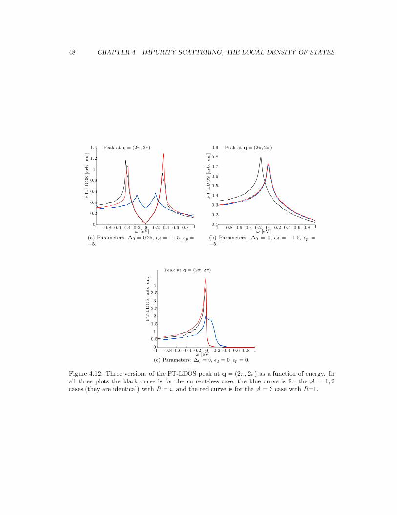
48 CHAPTER 4. IMPURITY SCATTERING, THE LOCAL DENSITY OF STATES
-1 -0.8 -0.6 -0.4 -0.2 0 0.2 0.4 0.6 0.8 10
0.2
0.4
0.6
0.8
1
1.2
1.4 Peak at q = (2π, 2π)
ω [eV]
FT
-LD
OS
[arb
.un.]
(a) Parameters: ∆0 = 0.25, εd = −1.5, εp =−5.
-1 -0.8 -0.6 -0.4 -0.2 0 0.2 0.4 0.6 0.8 10.1
0.2
0.3
0.4
0.5
0.6
0.7
0.8
0.9 Peak at q = (2π, 2π)
ω [eV]
FT
-LD
OS
[arb
.un.]
(b) Parameters: ∆0 = 0, εd = −1.5, εp =−5.
-1 -0.8 -0.6 -0.4 -0.2 0 0.2 0.4 0.6 0.8 10
0.5
1
1.5
2
2.5
3
3.5
4
Peak at q = (2π, 2π)
ω [eV]
FT
-LD
OS
[arb
.un.]
(c) Parameters: ∆0 = 0, εd = 0, εp = 0.
Figure 4.12: Three versions of the FT-LDOS peak at q = (2π, 2π) as a function of energy. Inall three plots the black curve is for the current-less case, the blue curve is for the A = 1, 2cases (they are identical) with R = i, and the red curve is for the A = 3 case with R=1.

Chapter 5
Analysing the results
In the previous chapter we found our main numerical result: that a mean-field loop currenttheory breaks a spatial symmetry of the LDOS pattern around a single impurity. In this chapterwe try to achieve a better and more systematic understanding of this phenomenon. We firsttry to classify which symmetries the different current patterns (see chapter 3) may break, andthen we give a physical reason for the occurrence of the breaking.
5.1 Symmetry considerations
We now systematically investigate how the presence of currents might affect the symmetries ofthe LDOS. We do this for the normal state of the system, in order to clearly distinguish whichfeatures are solely due to the circulating currents.
5.1.1 The impurity contribution
The key to finding spatial symmetries of the system will be the full Green’s function at a certainlattice point. As we saw in the previous chapter, this is given by
G(r, r, ω) = G0(0, ω) +G0(r, ω)TG0(−r, ω). (5.1)
Obviously, the first term will be invariant under any symmetry operation we can cook up;it is simply constant in space. We thus focus on the second term, which we shall denote asδG(r, r, ω), i.e.,
δG(r, r, ω) = G0(r, ω)TG0(−r, ω). (5.2)
In the case of a point-like impurity residing only on a copper orbital, the T -matrix takesthe following simple form:
T = [1−HimpG0(0, ω)]−1Himp (5.3)
=
1−
V 0 00 0 00 0 0
G0(0, ω)
−1 V 0 00 0 00 0 0
(5.4)
=
V1−V G0
11(0,ω)0 0
0 0 00 0 0
. (5.5)
49

50 CHAPTER 5. ANALYSING THE RESULTS
Futhermore, as our goal is to analyze the spatial symmetries of the system, we can consider ωto be fixed. The T -matrix is then just a constant. We denote the non-zero entry by α;
α :=V
1− V G011(0, ω)
. (5.6)
For each orbital, the impurity contribution to the full Green’s function can then be written as
δG11(r, r, ω) = αG011(r, ω)G0
11(−r, ω) (5.7)
δG22(r, r, ω) = αG021(r, ω)G0
12(−r, ω) (5.8)
δG33(r, r, ω) = αG031(r, ω)G0
13(−r, ω) (5.9)
These three contributions all share the same common structure of being the product of twofree Green’s function entries. In terms of momenta, we exploit the k-diagonal structure of thefree Green’s function to rewrite the product as
δGii(r, r, ω) = αG0i1(r, ω)G0
1i(−r, ω) (5.10)
= α∑k,k′
G0i1(k, ω)G0
1i(k′, ω)e−ir·(k−k
′)eφi(k,k′), (5.11)
where φi(k,k′) accounts for the intra-unit cell structure. This formula will be the starting point
for our symmetry considerations. First, we find symmetries that are present when R = 0, andsubsequently we show how many of these are (in general) broken as R is increased.
5.1.2 Symmetries for R = 0
Let us now focus on the copper Greens function. The oxygen cases are slightly more complicateddue to the way we spatially label px and py-orbitals, but largely follow the same arguments. LetS be some symmetry operation1 we suspect the system to be invariant under and let r′ = Sr.We then have invariance if δG11(r, r, ω) = δG11(r′, r′, ω). In terms of equation (5.11), this canbe recast as having (recall that φ1(k,k′) = 0)∑
k,k′
f(k)f(k′)eir·(k′−k) =
∑k,k′
f(k)f(k′)eiSr·(k′−k), (5.12)
with f(k) = G011(k, ω). The right hand side can then be further rewritten as∑
k,k′
f(k)f(k′)eiSr·(k′−k) =
∑k,k′
f(k)f(k′)eir·(STk′−STk) (5.13)
=∑
Sk,Sk′
f(Sk)f(Sk′)eir·(k′−k). (5.14)
As S by assumption leaves the sum over the Brillouin zone invariant2, the restriction forinvariance is then that∑
k,k′
f(k)f(k′)eir·(k′−k) =
∑k,k′
f(Sk)f(Sk′)eir·(k′−k), (5.15)
and if this is to hold for arbitrary r, the terms multiplying the same phase must be equal, andwe finally see that we must have∑
k,k′
f(k)f(k′) =∑k,k′
f(Sk)f(Sk′), (5.16)
1More precisely: S is an orthogonal transformation.2We still cover the exact same k-points.

5.1. SYMMETRY CONSIDERATIONS 51
along all lines where k − k′ is equal to the same constant (vector). This latter requirementcan be explicitly verified in the absence of currents for a number of symmetries, where we havef(k) = f(Sk).
Let us write out what f(kx, ky) is for copper. In order to do so, we need an explicit formof the Hamiltonian. We use our usual three-orbital one, for now with no orbital currents.
G011(kx, ky, ω) = (1(ω + iη)−H(kx, ky))−1
11 (5.17)
=(ω + iη − εp)2 − (4tppsxsy)2
det[1(ω + iη)−H(kx, ky)](5.18)
Upon expansion, the determinant takes the form
det[1(ω + iη)−H(kx, ky)] = (ω + iη − εd)(ε2p − (4tppsxsy)2)
+ 2itpdsx([ω + iη − εp]2itpdsx − 4tppsxsy2itpdsy)
+ 2itpdsy([ω + iη − εp]2itpdsy − 4tppsxsy2itpdsx). (5.19)
We can now immediately read off a number of symmetries for the LDOS. Two apparent onesare reflection symmetries around the x- and y-axes, corresponding to kx → −kx and ky → −ky.And if we can perform these two operations independently of each other, we can of course alsoperform them at once, and thus inversion invariance3 follows. C4 invariance is also noted,as a C4 operation for copper amounts to taking kx → −ky and ky → kx. From the aboveexpressions, it is clear that
G011(−ky, kx, ω) =
(ω + iη − εp)2 − (4tppsxsy)2
det[1(ω + iη)−H(−ky, kx))]= G0
11(kx, ky, ω). (5.20)
The final symmetries we care for are reflections in the x = ±y lines. These correspondrespectively to kx → ky, ky → kx and kx → −ky, ky → −kx. Once again, the numerator ofequation (5.19) is easily seen to be invariant under these transformations, and the same thingholds true for the determinant.
(a) The effect of reflec-tions in the axes and ourunit cell labelling.
(b) The effect of a C4 operation. The coloursget mapped into themselves, i.e., d→ d, px →py and py → px.
(c) The effect of the two“diagonal” reflections. Thecolours get mapped intothemselves, i.e., d → d,px → py and py → px.
Figure 5.1: The ultimate guide to our real-space grid in terms of orbitals and unit cells.
3This was already apparent from equation (5.7); sending r→ −r just corresponds to commuting two complexnumbers. Inversion symmetry is thus manifestly present for copper, irrespective of the form of the Hamiltonian.

52 CHAPTER 5. ANALYSING THE RESULTS
We now treat the slightly more complicated oxygen cases. The extra complications all arisefrom the intra-unit cell structure and the fact that the origin of the system (the position of theimpurity) is taken to be at a copper site. Upon a symmetry operation, a d-orbital is alwaysmapped into a d-orbital, but this is not the case for the px,y-orbitals, as illustrated in Figures5.1a, 5.1b, and 5.1c.
As a first thing, we need the analogue of equation (5.16) for px and py. The invariancedemand expressed in terms of equation (5.11) is∑
k,k′
fpj (k)gpj (k′)ei(kj/2−k
′j/2) =
∑k,k′
fpj (Sk)gpj (Sk′)eiS(kj/2−k′j/2), j = x, y, (5.21)
with px having
fpx(k) =−(ω + iη − εp)2itpdsx + 2itpdsy4tppsxsy
det[1(ω + iη)−H(k)](5.22)
and
gpx(k) =(ω + iη − εp)2itpdsx − 2itpdsy4tppsxsy
det[1(ω + iη)−H(k)], (5.23)
whereas it for py holds that
fpy (k) =(ω + iη − εp)2itpdsy − 2itpdsx4tppsxsy
det[1(ω + iη)−H(k)](5.24)
and
gpx(k) =−(ω + iη − εp)2itpdsy + 2itpdsx4tppsxsy
det[1(ω + iη)−H(k)]. (5.25)
We have already established the invariance of the determinant under all four reflections, inver-sion and C4, so it is up to the numerators to decide which symmetries the system possesses.We treat C4 first.
The condition for C4 invariance to hold is that we have (for S being a π/2 rotation)
δG22(r, r, ω) = δG33(Sr, Sr, ω). (5.26)
From equations (5.22) to (5.25) we see that
fpy (−ky, kx)gpy (−k′y, k′x)ei(kx−k′x) = gpx(kx, ky)fpx(k′x, k
′y)ei(kx−k
′x), (5.27)
and C4 invariance is thus also established for the oxygen orbitals.For reflections in the x = y line, the proper invariance demand is that (for S now being the
relevant reflection)δG22(r, r, ω) = δG33(Sr, Sr, ω) (5.28)
From equations (5.22) to (5.25) we see that
fpy (ky, kx)gpy (k′y, k′x)ei(kx−k
′x) = gpx(kx, ky)fpx(k′x, k
′y)ei(kx−k
′x), (5.29)
and the first reflection invariance is thus also established for the oxygen orbitals.The remaining reflections are a bit more tricky, as we - as seen from Figures 5.1a, 5.1b,
and 5.1c - should modify the S in equation (5.21) to be the symmetry we consider plus a shiftto a nearest neighbouring unit cell. Let us clarify this enigmatic statement with a concreteexample.
For a reflection in the x-axis, the utter invariance of δG33(r, r, ω) is immediate. For px, onemight naıvely assume the x → −x invariance demand to be that (for S being a reflection inthe x-axis)
δG22(r, r, ω) = δG22(Sr, Sr, ω). (5.30)

5.1. SYMMETRY CONSIDERATIONS 53
However, a careful study of Figure 5.1a reveals that the proper demand is rather
δG22(r, r, ω) = δG22(Sr− x, Sr− x, ω), (5.31)
where x is a unit vector in the x direction. A rewriting of the right hand side reveals that
δG22(Sr− x, Sr− x, ω) = α∑k,k′
fpx(kx, ky)gpx(k′x, k′y)ei(−x−1,y)·(k−k′)ei(kx/2−k
′x/2) (5.32)
= α∑k,k′
fpx(kx, ky)gpx(k′x, k′y)ei(−x,y)·(k−k′)ei(k
′x/2−kx/2) (5.33)
= α∑k,k′
fpx(−kx, ky)gpx(−k′x, k′y)ei(x,y)·(k−k′)ei(kx/2−k′x/2). (5.34)
What remains to check is therefore whether fpx(kx, ky)gpx(k′x, k′y) = fpx(−kx, ky)gpx(−k′x, k′y),
and as this holds, we have invariance under reflection in the y-axis. In a completely similarway, one can convince oneself that reflection in the x-axis is also a symmetry of the oxygenLDOS.
Finally, we treat reflections in the x = −y line. Let S be this transformation (i.e., Sx = −y,Sy = −x.). Invariance then implies that
δG22(r, r, ω) = δG33(Sr− y, Sr− y, ω), (5.35)
which is easily verified in the same manner as above.To summarize, we have now seen that the non-current carrying system in the normal state
possesses the following symmetries for the LDOS around an impurity on a copper site:
• Rotations by π (C4).
• Reflections in the axes.
• Reflections in the diagonals.
• Inversion.
A breaking of any of these will thus be a potential loop-current fingerprint.
5.1.3 Unbroken symmetries when R 6= 0
Along the lines of the previous section, we are able to show that some of the aforementionedsymmetries remain unbroken in the loop-current state. This is really a thing to rejoice in; hadthe orbital-currents broken all of the symmetries, it would experimentally be indistinguishablefrom a wild and uncontrolled impurity (a defect of the sample). Some of the symmetries weare able to show will hinge on R being either real or imaginary. We comment on this as we goalong, and then collect all these findings at the end of the section.
We follow arguments completely identical to those of the previous section. Let us thereforecut right to the chase.
For the A = 1 case, the determinant in question takes the form
det[1(ω + iη)−H1(k)] = (ω + iη − εd)([ω + iη − εd]2 − (4tppsxsy)2)
− (−2itpdsx +Rcx)(2itpdsx +R∗cx)(ω + iη − εp)+ (−2itpdsx +Rcx)4tppsxsy(2itpdsy −R∗cy)
+ (2itpdsy +Rcy)4tppsxsy(−2itpdsx −R∗cx)
− (2itpdsy +Rcy)(−2itpdsy +R∗cy)(ω + iη − εp). (5.36)

54 CHAPTER 5. ANALYSING THE RESULTS
How about the numerators in the expressions for the Green’s function entries?Well,
G011(k, ω) =
(ω + iη − εp)2 − (4tppsxsy)2
det[1(ω + iη)−H1(k)], (5.37)
and the currents thus do not alter the inversion invariance of the copper LDOS. For the oxygenatoms,
G021(k, ω) =
(ω + iη − εp)(−2itpdsx −R∗cx) + 4tppsxsy(2itpdsy −R∗cy)
det[1(ω + iη)−H1(k)], (5.38)
G012(k, ω) =
(ω + iη − εp)(2itpdsx −Rcx) + 4tppsxsy(−2itpdsy −Rcy)
det[1(ω + iη)−H1(k)](5.39)
and
G031(k, ω) =
(ω + iη − εp)(2itpdsy −R∗cy) + 4tppsxsy(−2itpdsx −R∗cx)
det[1(ω + iη)−H1(k)], (5.40)
G013(k, ω) =
(ω + iη − εp)(−2itpdsy −Rcy) + 4tppsxsy(2itpdsx −Rcx)
det[1(ω + iη)−H1(k)]. (5.41)
Under axis reflections, all the si factors change sign, whilst the ci factors go to themselves,and we see no apparent reason why this should leave the determinant invariant. Nor doesit correspond to an overall sign, and must therefore conclude that these two symmetries arepossibly not present.
For reflections in the x = y line, the determinant is only invariant if R is real (in which caseall three LDOS values are invariant), whereas this demand is not present when we considerthe x = −y line; we see that the entire LDOS grid is invariant under reflections in the x = −ylines regardless of what R is. C4 is not seen to hold under any assumptions regarding R.
For A = 2 the story is very similar, and the reader may simply let cy → −cy to obtain allthe results for this case. One interesting difference is noted, namely that we now have reflectioninvariance in the x = y line instead of the x = −y line.
For A = 3 the current pattern is a quite different from the A = 1, 2 cases, and we onceagain write out everything.
det[1(ω + iη)−H3(k)] = (ω + iη − εd)([ω + iη − εp]2 − (4tppsxsy)2)
+ (2itpdsx +Rsx)(−2itpdsx +R∗sx)(ω + iη − εp)− (2itpdsx +Rsx)(2itpdsy +R∗sy)4tppsxsy
− (−2itpdsy +Rsy)(−2tpdsx +R∗sx)4tppsxsy
+ (−2itpdsy +Rsy)(2itpdsy +R∗sy)(ω + iη − εp) (5.42)
Each term in the determinant contains an even number of sines in each direction (meaning xor y), and the determinant is therefore invariant under reflections in the axes independently ofeach other, and hence also under inversion. The numerators in the Green’s function entries areeither invariant or change sign, and their products are thus invariant. This is actually as faras we can go; no further symmetries are apparent in the system. We stress that this of coursedoes not mean that they are not present, but simply that it is not immediate whether this isthe case. We do not consider A = 4, since, as discussed in chapter 3, this parameter choice didnot lead to stable current patters.
In summary, we can draw the current symmetry table Table 5.1, where we only display thesymmetries we have explicitly verified.
These are the symmetries we could have read off of the drawings of the current pattersdepicted in chapter 3 in Figures 3.9 to 3.11, with the inversion symmetry of copper as thepossible exception.

5.1. SYMMETRY CONSIDERATIONS 55
Current pattern A = 1 A = 2 A = 3Symmetry ↓ Copper Oxygen Copper Oxygen Copper Oxygenx-axis refl. - - - - Yes Yesy-axis refl. - - - - Yes Yesinversion Yes - Yes - Yes Yesx = y refl. If R real If R real Yes Yes - -x = −y refl. Yes Yes If R real If R real - -C4 - - - - - -
Table 5.1: Symmetries analytically shown to be unbroken by R.
5.1.4 Comparison with the numerical data
These symmetry considerations for the local density of states around an impurity relate verywell to our numerical results. In Table 5.2 are displayed the results of a numerical symmetryanalysis of the LDOS around and impurity for different current patterns. The LDOS-grids werecomputed as described in the previous chapter. The procedure used to retrieve this numericaldata was the following. The real-space LDOS grid was computed for three unit cells to eachside of the impurity, yielding a total of 49 unit cells, and for the five energies ω = 0,±0.2,±0.5(in eV). Along the lines of the discussion so far, and the relation of our LDOS results to theorbital current patterns of chapter 3, we employ for each choice of A the phase of R yieldingthe maximal current expectation value. For A = 1, 2 we thus chose R = i, whereas for A = 3,we took R = 1.
The resulting 14 × 14 matrix was trimmed, so that only orbitals with symmetry partnerswere left. The meaning of this is illustrated for a slightly smaller field of view in Figure 5.2.
Figure 5.2: The idea of trimming our matrix. As described in chapter 4, what we calculate isnot symmetric around the impurity (and thus the origin when talking symmetries). Removingone row and one column fixes this. The colours and dashed lines are guides to the eyes, whereasthe solid lines define different unit cells. See also Figures 4.6 and 4.10.
This reduced matrix can then readily be checked for various symmetries by means of ele-mentary matrix operations. Our criterion for symmetry preservation was rather strict; if theabsolute value of any entry of the difference between the original matrix and its image underthe symmetry operation was non-zero4 the symmetry was deemed broken. We also did thisfor the copper sites only, and the results were identical. This was all done thrice, once for theVarma hybridizations and twice for the “realistic” hybridizations, respectively with and with-out superconductivity. All these six sets of symmetry results turned out to be in agreement,which we take as an encouraging hint on the robustness of our conclusions with respect todifferent parameter choices. The results are displayed in Table 5.2.
4With some reasonable round-off given by numerical specifications such as the k-space resolution, size of ηetc.

56 CHAPTER 5. ANALYSING THE RESULTS
Current pattern A = 1 A = 2 A = 3Symmetry ↓ Copper Oxygen Copper Oxygen Copper Oxygenx-axis refl. No No No No Yes Yesy-axis refl. No No No No Yes Yesinversion Yes Yes Yes Yes Yes Yesx = y refl. Yes Yes Yes Yes Yes Yesx = −y refl. Yes Yes Yes Yes Yes YesC4 No No No No Yes Yes
Table 5.2: Symmetries numerically found to be broken for the maximally current-yielding Rvalue. “No” means that the symmetry was explicitly broken in the numerical data, and “Yes”means that it was left unbroken.
A comparison of Tables 5.1 and 5.2 of course reveals no contradictions. But it also seemsthat a nice feature is lost. In Table 5.1 we see a possible difference in the reflectional symmetriesin the x = ±y lines, displayed by the A = 1, 2 cases. This can intuitively be related to theactual form of the current patterns. In Table 5.2 there seems to be no difference between theLDOS grids when A = 1 and when A = 2. To our contentment, one thing does not entirelyrule out the other. As seen in Figure 5.3, the intuitive connection between the actual currentpattern, seen on the right, and its manifestation as LDOS modulations is not lost. And themodulations respect the same symmetries in both cases. Note that it is the directions of thecurrents that seem to play no role.
-1 0 1
-1
0
1
0.0
0.1
0.2
0.3
0.4
0.5
0.6
(a) LDOS-grid for A = 1. (b) The current pat-tern for A = 1.
-1 0 1
-1
0
1
0.0
0.1
0.2
0.3
0.4
0.5
0.6
(c) LDOS-grid for A = 2. (d) The current pat-tern for A = 2.
Figure 5.3: Left: real-space LDOS grids. The axes denotes spatial unit cell labelling, thecolourbar is LDOS in arb. un., grey represents an empty space. The parameters shared byboth plots were R = i, ∆0 = 0.25, and εd = −1.5, εp = −5 (all in eV). Right: the currentpatterns as calculated in chapter 3.

5.2. PHYSICAL EXPLANATION IN TERMS OF ENERGY CONTOURS 57
5.2 Physical explanation in terms of energy contours
Although we in the two previous chapters concluded that no traces of the symmetry breakingwas seen in the homogeneous system, the fact that only free Green’s functions make up the fullGreen’s function (see equation (4.14)), indicates to us that the real physics of the symmetry lossshould somehow be contained in the unperturbed system. But at the same time, an impuritywas needed to bring forth this facet of the current-carrying system. The relevant questionis then what feature of the unperturbed system otherwise hidden to the density of states ascattering process reveals. The answer is the curves of constant energy, CCEs, on which thescattering takes place. In this section, we consider the Fourier transformed density of statesaround an impurity, and deduce from the CCEs via a qualitative scattering model that thesymmetry of the FT-LDOS is broken, which in turn implies a non-symmetric LDOS.
The curves of constant energy are found by diagonalizing the Hamiltonian in the absenceof an impurity.
5.2.1 The octet model
The shape and especially rate of change of constant energy curves reveal a good deal of infor-mation to us. Let us briefly explain how the rate of change affects the DOS. We implicitly usetwo facts about the Dirac-δ function, see e.g. ref. [27] for an explanation.
Let us consider the 3× 3 Green’s function written, for once, not in the orbital basis, but inthe diagonal (band) basis introduced in section 3.2.1. We use the notation of that section inthe following. In this diagonal basis, the Green’s function can be explicitly written as
G(k, ω) =
1
ω+iη−Eα(k) 0 0
0 1ω+iη−Eβ(k) 0
0 0 1ω+iη−Eγ(k)
. (5.43)
In the limit where η → 0, the spectral function is then given by
A(k, ω) =
2πδ(ω − Eα(k)) 0 00 2πδ(ω − Eβ(k)) 00 0 2πδ(ω − Eγ(k))
, (5.44)
and the density of states is readily found as
ρ(ω) =1
2πNTr[A(k, ω)]
=1
2πN
∑i=α,β,γ
∑k
2πδ(ω − Ei(k))
=1
N
∑i=α,β,γ
∑k
∑j
δ(k− kj)
|∇Ei(k)|, (5.45)
where the kj-momenta satisfy that ω = Ei(kj) for i = α, β, γ. We thus see that the largestspectral weight is obtained at those places in k-space where the bands have the lowest rate ofchange. When one makes a cut through the bands in k-space at a range of fixed energies, ω,these regions where |∇E(k)| is small will be the regions where the curves of constant energyvary the most as ω is changed. This is illustrated in one dimension in Figure 5.4a. Equation(5.45) was obtained for a three-band system in the normal state, but for a system includingsuperconductivity, the corresponding 6 × 6 derivation is completely analogous, and the mainpoint remains the same: by looking at the curves of constant energy for a small range of ω-values close to each other, we can deduce where in k-space the system has the most spectralweight.

58 CHAPTER 5. ANALYSING THE RESULTS
This rather simple observation has led to the proposal of the so-called octet model (seee.g. refs. [32] and [33]) to explain the scattering modulations in the Fourier transformed localdensity of states for a d-wave superconductor. The idea of the octet model is illustrated inFigure 5.4b. In words, the idea is that scattering from one state to another can only occur on aCCE, due to energy conservation. Whereas all energy-conserving scattering events are possible,we expect the scattering processes from a densely populated area to a densely populated area(in k-space) to be dominant. If we therefore consider the Fourier transformed local density ofstates around an impurity, we expect to see large contributions at those q-vectors correspondingto such a scattering event. For a d-wave superconductor, there are eight such regions in k-space,and an initial state from one region therefore has eight q-vectors (including the null vector)of “highly probable” scattering. These eight vectors are depicted in Figure 5.4b. Even if wedisregard the null vector, each of the eight hot spots have seven vectors connecting them toother hot spots, yielding 56 potential peaks. Although only 32 of these are actually different,this is still a vast amount of peaks, and not all of them are realized. We shall return to thissubject later in this section.
(a) Illustration of the relation between an energy bandand its ω-projection. When the band changes slowlyas a function of k, the rate of change with respect toω is large; ∆k2 > ∆k1. This particular band curve iscompletely fictitious.
−π −π/2 0 π/2−π
−π/2
0
π/2
kx
ky
A = 2 , R = 0 , ∆0 = 0.25.
(b) Illustration of the octet model. Shownare the banana shaped CCEs for our three-band (current-less) superconductor in a rangearound the Fermi energy. The biggest changeis obviously at the banana tips.
One can get a feel for the validity of this picture by looking at the actual form of theFT-LDOS. Let us now describe how to find the FT-LDOS around an impurity. In section4.7 we studied the homogeneous Fourier transformed LDOS and found four peaks in q-space.As described in that section, these peaks arise from the particular unit cell structure of ourmodel. Upon computing the FT-LDOS in the non-homogeneous case, those structural peakswill be very dominant and mask almost every other feature. We therefore disregard the freeterm in the full Greens function, and only find the Fourier transform of the δG-term as definedin equation (5.2).
Let δρ(q, ω) and δρ(r, ω) denote the impurity contributions to the FT-LDOS and LDOS,respectively. Then it holds that
δρ(q, ω) =∑r
δρ(r, ω)e−iq·r. (5.46)
Now, as described in sections 4.3.1 and 2.4, the full density of states contains the sum of theimaginary parts of six Green’s function entries. For simplicity, we now focus on the first one,

5.2. PHYSICAL EXPLANATION IN TERMS OF ENERGY CONTOURS 59
i.e., the contribution from spin up on copper.
−1
π
∑r
Im[δG11(r, ω)]e−iq·r =1
2πi
∑r
δG∗11(r, ω)e−iq·r − δG11(r, ω)e−iq·r
=1
2πi
∑r
δG∗11(−q, ω)− δG11(q, ω), (5.47)
where
δG11(q, ω) =∑r
∑k,k′
[G0(k, ω)T (ω)G0(k′, ω)]11e−iq·reik·re−ik′·r
=∑k
[G0(k + q, ω)T (ω)G0(k, ω)]11. (5.48)
The other ten terms are found in a similar manner. From equations (5.47) and (5.48), themain idea of the octet model seems plausible; the quantity in question is large if there is “alot” of Green’s function at k and k + q. It is, however, not very evident how well it describesthe shape and height of the Fourier amplitudes in question.
We stress that the octet model is not an exact result. For one thing, it does not predict therelative weights at each peak, some of which are indeed often zero. We thus do not see all 32peaks predicted by the model. Furthermore, in the actual results, the peaks that do survive areoften smeared a little to rather give small arcs of high intensity than distinct point-like peaks.But having said this, the octet model still provides us with a good qualitative explanation ofour results, especially in terms of symmetries. The validity and limitations of the octet modelis discussed further in e.g. refs. [32], [33], and [34].
−π −π/2 0 π/2−π
−π/2
0
π/2
kx
ky
(a) CCEs in the FBZ. The red CCEs are atω = 0.1 eV, the black ones slightly above thisvalue.
−2π −π 0 π 2π
2π
π
0
−π
−2π
(b) Power spectrum in q-space calculated atω = 0.1 eV.
Figure 5.4: We identify four vectors connecting banana tips as peaks in the power spectrum.These vectors, found in k-space, are then inserted into q-space, in good agreement with theFT-LDOS in this space. For both plots the parameters were: εd = −1.5 eV, εp = −5 eV,R = 0, ∆0 = 0.25.
In Figure 5.4 we explore how some of the aforementioned 32 vectors appear in the FT-LDOS(or more precisely: the power spectrum). The absolute value FT-LDOS plots were calculatedas an imitation of the experimental way, by first calculating a large LDOS grid, and thenFourier transforming that. For the plots presented here, the k-space resolution was 325× 325

60 CHAPTER 5. ANALYSING THE RESULTS
and the LDOS-grid matrix was 302×302 (corresponding to 75 unit cells in each direction awayfrom the impurity). We do not want to make a detailed account of how many peaks are absentor present, but instead focus on some places where we definitely see a signal, a signal that willbe substantially altered by the loop currents.
In the current-less case, the CCEs and the FT-LDOS posses a number of symmetries. Thesesymmetries where counted and classified in section 5.1.2. It is relatively straightforward to seehow the bunch of four vectors in Figure 5.4a could equally well have been placed at one ofthree other (left) banana tips by applying the same rotation and translation to all of them,and how this four-fold symmetry shows up in the FT-LDOS image of Figure 5.4b. Similarly, wecan rediscover all the other symmetries of section 5.1.2 by relating equivalent vectors betweenbanana tips with high power spectrum regions. It is especially worth noting how the diamond-shaped region near q = (π, 0) can be generated by q3 and q4 and their partners (not shownin the figure for reasons of graphical clarity) emanating from the lowest tip of the South-Westbanana and ending in the same places as q3 and q4.
−π −π/2 0 π/2−π
−π/2
0
π/2
kx
ky
(a) CCEs in the FBZ.
−2π −π 0 π 2π
2π
π
0
−π
−2π
(b) Power spectrum in q-space calculated atω = 0.1 eV.
Figure 5.5: We identify four vectors connecting banana tips as peaks in the power spectrum.For both plots the parameters were: εd = −1.5 eV, εp=-5 eV, R = 0.1i, ∆0 = 0.25.
If we now turn our attention to Figure 5.5, we note that the picture is somewhat different.The four bananas are no longer of the same shape, and scattering vectors in different directionsare no longer related by simple symmetry operations. In particular, the q-vectors q3 and q4
have been significantly distorted, with an evident effect on the FT-LDOS region in the vicinityof q = (π, 0). The diamond-shaped region gets distorted into a general rhombic shape, a shapethat is again in very good agreement with the four scattering vectors from the South-Westbanana to the South-East one.
5.2.2 Beyond the octet model
Although the octet model yields a nice explanation of the observed breaking of symmetry inthe FT-LDOS and hence also the LDOS around an impurity, it can not be all there is to thestory, as it hinges on the particular banana-shaped CCEs observed in d-wave superconductors,whereas our symmetry breaking was present also in the two non-superconducting cases (seechapter 4). Indeed, it is only a good qualitative explanation, not a rigorous result. Whatremains true, however, is that scattering does take place on curves of constant energy, and it istherefore a very reasonable assumption that the symmetries of the CCEs are inherited by the

5.3. RELATING OUR RESULTS TO REAL LIFE 61
density of states upon scattering off a single point-like impurity (as such an impurity is itselfmaximally symmetric). This is indeed also what we find. Below we present some calculatedCCEs in energy ranges close to the Fermi energy, and we observe a perfect agreement betweenloop-current pattern, mean-field parameter strength for the currents, broken symmetries andthe numerical results presented in section 5.1.4. A more elaborate collection of CCEs is foundin Appendix B.
In Figure 5.6 the CCEs for the same parameters as employed in the previous subsection areshown. Figure 5.6a is thus the same picture as Figure 5.4a. In these curves, we once again findthe usual symmetry relations between the different current patterns. A = 1 and A = 2 bothbreak the C4 symmetry, and their respective deviations from the currentless case are clearlypronounced in the kx = ±ky lines (cf. Figure 5.3). The energy contours when A = 3 are veryhard to distinguish from the currentless case, and in particular respect all the symmetries ofthat case.
−π −π/2 0 π/2−π
−π/2
0
π/2
kx
ky
(a) A = 1, R = 0.1i
−π −π/2 0 π/2−π
−π/2
0
π/2
kx
ky
(b) A = 2, R = 0.1i
−π −π/2 0 π/2−π
−π/2
0
π/2
kxky
(c) A = 3, R = 0.1
Figure 5.6: The curves of constant energy for a range of energy near the Fermi level. Parametersshared by all plots: εd=-1.5 eV, εp=-5 eV, ∆0 = 0.25 eV.
These features are not dependent on superconductivity. When we in Figure 5.7 consider theenergy contours for the same hybridization energies as above but without superconductivity,we see essentially the same picture, just somewhat less pronounced. Recalling the “maximumspatial C4 breaking”-plots of Figures 4.7 and 4.8, this is indeed also what we would expect. Themain thing to note is once again that the pictures for A = 1 and for A = 2 are very similar, butdiffer in that the “thickening” of the CCE-lines (i.e., the distance between each line) happenalong either the kx = ky or the kx = −ky line, and of course that A = 3 respects everysingle symmetry of the current-less system. It is not easily seen where any scattering vectorsanalogous to the scattering vectors of the octet model might be drawn, and we do not expectthe same picturesque correspondence between CCEs and FT-LDOS as in the superconductingcase. But it is convincing that the same overall symmetries are present in the CCEs presentedhere and the spatial LDOS modulations of the previous chapter.
This concludes our analysis of the symmetry breaking in terms of curves of constant energy.The main line of reasoning was the following: elastic scattering takes place from one energycontour to another one of the same energy. If these energy contours lack a certain symmetry,so will the resulting scattering processes and hence also the density of states, both in real- andmomentum space. Of course one could imagine special cases where such effects would cancelout (cf. Figure 4.7), but in general this will not be the case.
5.3 Relating our results to real life
From the discussion in this chapter, the main conclusion is clear: if the loop-current theory isrealized in the cuprates in the form of current pattern 1 or 2, we expect to see a significant

62 CHAPTER 5. ANALYSING THE RESULTS
breaking of C4 symmetry in the density of states around an impurity in the dilute concentrationlimit. If the currents are realized through current pattern 3, we predict no substantial deviationfrom not having orbital currents at all.
The latter prediction is somewhat dull. Luckily, the experimental evidence in favour of theloop current theory seems to support the view that current patterns 1 and 2 are being realizedin the cuprates. In ref. [9] the magnetic signal signal observed is corresponding to a currentpattern similar to our A = 1, 2. The authors also mention an earlier experiment that rules outthe current pattern A = 3 as a realistic current pattern. In the (controversial) experiment ofref. [13], the results are also consistent with A being 1 or 2. Finally, although not directlyrelated to the cuprates, the actual current patterns observed in “bare” CuO and reported inref. [14] showed a shape similar to the other two experiments mentioned here (cf. Figure 1.5).
If we are to believe in the loop-current theory at all, we are therefore lead to assume therealization of the orbital currents through the current patterns that gave rise to our non-trivialresults. What experimental test of Varma’s theory do we then propose?
Well, obviously, we propose an STM measurement in the vicinity of a single impurity. Inreal available samples it is highly unlikely that a single order parameter for the currents wouldsuffice to describe the entire material; instead we must expect different domains of loop orderwith different current strengths and directions to be present in the sample. Having a large fieldof view in the STM experiment might then result in an averaging over these different domains,and the symmetry breaking could then be obscured or even lost. This might explain the lackof experimental reports on this matter. As a large field of view is essential for a decent q-spaceresolution of the FT-LDOS image, our proposal is to remain in real space, and search for abroken spatial symmetry close to the impurity. This should, in the light of the findings ofchapter 4, be done for a range of energies at fixed positions. Integration over these energiesshould be avoided, as this may also result in a masking or loss of the symmetry breaking.
To our knowledge, no such systematic investigation has been performed on a cuprate in thepseudogap part of the superconducting dome.
If such an experiment finds no trace of C4 symmetry breaking, we must consider that tobe a serious problem for the loop current theory, but it might of course also indicate someshortcoming of our model. If the experiment however does succeed in capturing this featureof the LDOS modulations, we must conclude it to be a most encouraging result in favour ofthe loop-current theory. In either case, we believe that such an experiment in the light of ourresults would add to a tipping of the balance with regard to the success of intra-unit cell orbitalcurrents as the theory to properly explain the pseudogap phase of the cuprates.
−π −π/2 0 π/2−π
−π/2
0
π/2
kx
ky
(a) A = 1, R = 0.1i
−π −π/2 0 π/2−π
−π/2
0
π/2
kx
ky
(b) A = 2, R = 0.1i
−π −π/2 0 π/2−π
−π/2
0
π/2
kx
ky
(c) A = 3, R = 0.1
Figure 5.7: The curves of constant energy for a range of energy near the Fermi level. Parametersshared by all plots: εd=-1.5 eV, εp=-5 eV, ∆0 = 0.

Chapter 6
Conclusion
We have studied the loop-current theory for the pseudogap phase of the cuprates proposed byC. M. Varma (see e.g. [12] and the references herein) in a three-band mean-field approximation.We have studied the three different orbital current patterns seen in Figure 6.1 for two differenthybridization energies, and in each case found a non-vanishing mean-field parameter to yieldactual intra-orbital current patterns with the total current going through each orbital being aconserved quantity.
(a) A = 1 (b) A = 2 (c) A = 3
Figure 6.1: The three intra unit-cell current patterns studied.
Imposing into this theory - for one of the two sets of hybridization energies - a possibility ofa co-existing superconducting order parameter, we have studied the spatial modulations of thelocal density of states around a single point-like impurity using a Green’s function formalism.It was found that in either of the nine resulting cases1, the symmetries of the current patternwas reflected in the spatial symmetries of the local density of states, as exemplified in Figure6.2.
-1 0 1
-1
0
1
0.0
0.1
0.2
0.3
0.4
0.5
0.6
(a) A = 1-1 0 1
-1
0
1
0.0
0.1
0.2
0.3
0.4
0.5
0.6
(b) A = 2-1 0 1
-1
0
1
0
0.2
0.4
0.6
0.8
1
(c) A = 3
Figure 6.2: The resulting LDOS maps around an impurity. Colour bar in arb. un.
1Three current patterns, two sets of hybridization energies, one of which may or may not include supercon-ductivity.
63

64 CHAPTER 6. CONCLUSION
The LDOS patterns were found to be completely oblivious to the directions of the currents,and the A = 3 case thus respected every conceivable spatial symmetry, whereas the A = 1, 2cases broke axial reflection symmetry and C4. By comparison to the experimental literature(refs. [13] and [9]), it is found that the current patterns 1 and 2 are the most realistic candidatesas realizations of the circulating current theory.
The persistent symmetry breaking for those two current patterns whenever the mean-fieldparameter for the orbital currents was varied away from zero was then related to the dispersionrelation of the unperturbed system. It was found that the presence of orbital currents breaksthe symmetry of the curves of constant energy on which elastic scattering takes place. For thesuperconducting case, the octet model gave a good qualitative explanation of this behaviour,but even with no superconductivity, the essence of this explanation remains valid.
As the energy dependence of the symmetry breaking is a bit unclear, an experimentalsearch for the features we found should probe many different energies and avoid integratingover the energy, as this may cause cancellation or at least damping of the effect. Furthermore,as different domains of loop order may be present in a sample, it should be avoided to averageover different domains, as this may again cause cancellations.
As a consequence of our results and discussion it is suggested to search for spatial non-C4symmetric modulations of the local density of states by an STM measurement in a small fieldof view in the vicinity of a single impurity in the underdoped superconducting regime.
Appendix A
The current patterns for finitehybridizations energies
In the analysis of our data as well as in the parameter choices leading to our data, we haverelied heavily on the phase of the mean-field current parameter having a certain value, in orderfor the current expectation values to be maximal. In chapter 3, only current expectation valuescalculated for the case of vanishing hybridization energies, i.e., εd = εp = 0 were presented.In this appendix the corresponding plots (corresponding to Figures 3.9 to 3.11) for the hy-bridization energies of εd = −1.5 eV and εp = −5 eV are shown. The conclusion is the samein this case as for the vanishing hybridization energies; for A = 1, 2, R should be imaginaryto yield the maximal currents, whereas R should be real for A = 3 in order to achieve that.Furthermore, it remains true that two of the patterns break the C4 symmetry, whereas the lastone preserves it, under the assumption that current directions are not visible to the STM (donot show up in the LDOS).
For all three plots in Figures A.1 to A.3 the length of R is fixed at 3, and the phase of Ris varied. There are both red and blue points present, corresponding colour-wise to the arrowson the left. Note the nice current conservation.
65

66APPENDIX A. THE CURRENT PATTERNS FOR FINITE HYBRIDIZATIONS ENERGIES
(a) The resulting current pattern.
0 π/2 π 3π/2 2π
-0.15
-0.07
-0.00
0.07
0.15
Phase of |R|
Bare
exp.
val.[a
rbun.]
(b) The calculated current pattern.
Figure A.1: A = 1.
(a) The resulting current pattern.
0 π/2 π 3π/2 2π
-0.15
-0.07
-0.00
0.07
0.15
Phase of |R|
Bare
exp.
val.[a
rbun.]
(b) The calculated current pattern.
Figure A.2: A = 2.
(a) The resulting current pattern.
0 π/2 π 3π/2 2π
-0.29
-0.15
0.00
0.15
0.29
Phase of |R|
Bare
exp.
val.[a
rbun.]
(b) The calculated current pattern.
Figure A.3: A = 3.

Appendix B
Curves of constant energy
On the next two pages we display the curves of constant energy for the three different currentpatterns and three different parameter cases studied in chapter 5. Below each plot the hy-bridization energies used are displayed, and the parameters regarding superconductivity andorbital current strength are displayed above the plots.
For all three sets of parameter values, the same distinct pattern is clear. For A = 3 nosymmetries are broken, and a rather large R-parameter is necessary in order to see any changein the constant energy curves. For A = 1, 2 the symmetry breaking is obvious even for a smallvalue of |R|, and it is further noted that the two cases are related by a π-rotation, in accordancewith their resulting current patterns (shown in chapter 3 and in appendix A).
67

68 APPENDIX B. CURVES OF CONSTANT ENERGY
−π −π/2 0 π/2−π
−π/2
0
π/2
kx
ky
R = 0 , ∆0 = 0.
−π −π/2 0 π/2−π
−π/2
0
π/2
kx
ky
R = 0 , ∆0 = 0.25
Figure B.1: Hybridization energies: εd = −1.5 eV, εp = −5 eV.
−π −π/2 0 π/2−π
−π/2
0
π/2
kx
ky
A = 1 , R = 0 + 0.1i , ∆0 = 0.
−π −π/2 0 π/2−π
−π/2
0
π/2
kx
ky
A = 1 , R = 0 + 0.1i , ∆0 = 0.25.
Figure B.2: Hybridization energies: εd = −1.5 eV, εp = −5 eV.
−π −π/2 0 π/2−π
−π/2
0
π/2
kx
ky
A = 2 , R = 0 + 0.1i , ∆0 = 0.
−π −π/2 0 π/2−π
−π/2
0
π/2
kx
ky
A = 2 , R = 0 + 0.1i , ∆0 = 0.25.
Figure B.3: Hybridization energies: εd = −1.5 eV, εp = −5 eV.

69
−π −π/2 0 π/2−π
−π/2
0
π/2
kx
ky
A = 3 , R = 1 , ∆0 = 0.
−π −π/2 0 π/2−π
−π/2
0
π/2
kx
ky
A = 3 , R = 1 , ∆0 = 0.25.
Figure B.4: Hybridization energies: εd = −1.5 eV, εp = −5 eV.
−π −π/2 0 π/2−π
−π/2
0
π/2
kx
ky
R = 0 , ∆0 = 0.
−π −π/2 0 π/2−π
−π/2
0
π/2
kx
ky
A = 1 , R = 0 + 0.1i , ∆0 = 0.
Figure B.5: Hybridization energies: εd = εp = 0.
−π −π/2 0 π/2−π
−π/2
0
π/2
kx
ky
A = 2 , R = 0 + 0.1i , ∆0 = 0.
−π −π/2 0 π/2−π
−π/2
0
π/2
kx
ky
A = 3 , R = 1 , ∆0 = 0.
Figure B.6: Hybridization energies: εd = εp = 0.
70 APPENDIX B. CURVES OF CONSTANT ENERGY

Bibliography
[1] D. van Delft and P. Kes, Physics Today 63, 38 (2010).
[2] J. Bardeen, L. N. Cooper, and J. R. Schrieffer, Physical Review 106, 162 (1957).
[3] J. Bednorz and K. Muller, Zeitschrift fur Physik B 64, 189 (1986).
[4] B. M. Andersen, Coexistence of Magnetic and Superconducting Order in the High-TcMaterials, PhD thesis, University of Copenhagen, 2004.
[5] M. Greiter and R. Thomale, Physical Review Letters 99, 027005 (2007).
[6] D. A. Bonn, Nature Physics 2, 159 (2006).
[7] M. R. Norman, D. Pines, and C. Kallin, Advances in physics 54, 715 (2005).
[8] C. Renner, B. Revaz, J.-Y. Genoud, K. Kadowaki, and Ø. Fischer, Physical Review Letters80, 149 (1998).
[9] B. Fauque et al., Physical Review Letters 96, 197001 (2006).
[10] C. M. Varma, Physical Review B 55, 14554 (1997).
[11] C. M. Varma, Physical Review Letters 83, 3538 (1999).
[12] C. M. Varma, Physical Review B 73, 155113 (2006).
[13] A. Kaminski et al., Nature 416, 610 (2002).
[14] V. Scagnoli et al., Science 332, 696 (2011).
[15] M. J. Lawler et al., Nature 466, 347 (2010).
[16] S. Strassle, B. Graneli, M. Mali, J. Roos, and H. Keller, Physical Review Letters 106,097003 (2011).
[17] S. V. Borisenko et al., Physical Review Letters 92, 207001 (2004).
[18] J. Tersoff and D. R. Hamann, Physical Review B 31, 805 (1985).
[19] E. W. Hudson, S. H. Pan, A. K. Gupta, K.-W. Ng, and J. C. Davis, Science 285, 88(1999).
[20] J. E. Hoffman et al., Science 297, 1148 (2002).
[21] S. H. Pan, E. W. Hudson, K. M. Lang, H. Eisaki, and S. Uchida, Nature 403, 746 (2003).
[22] V. J. Emery, Physical Review Letters 58, 2794 (1987).
71

72 BIBLIOGRAPHY
[23] H. Bruus and K. Flensberg, Many-Body Quantum Theory in Condensed Matter Physics(Oxford University Press, 2004).
[24] A. Altland and B. Simons, Condensed Matter Field Theory, second ed. (Cambridge Uni-versity Press, 2010).
[25] M. Tinkham, Introduction to superconductivity, second ed. (McGraw-Hill, 1996).
[26] Y. Nambu, Physical Review 117, 648 (1960).
[27] K. Riley, M. Hobson, and S. Bence, Mathematical methods for Physics and Engineering,third ed. (Cambridge University Press, 2006).
[28] M. H. Fischer and E.-A. Kim, Physical Review B 84, 144502 (2011).
[29] Z. B. Huang, H. Q. Lin, and J. E. Gubernatis, Physical Review B 63, 115112 (2011).
[30] H. Eskes and G. A. Sawatzky, Physical Review B 44, 9656 (1991).
[31] E. R. Tufte, The Visual Display of Quantitative Information, second ed. (Graphics Press,2001).
[32] K. McElroy et al., Nature 422, 592 (2003).
[33] Q.-H. Wang and D.-H. Lee, Physical Review B 67 (2003).
[34] T. S. Nunner, W. Chen, B. M. Andersen, A. Melikyan, and P. J. Hirschfeld, PhysicalReview B 73 (2006).


![Pseudogap and Local Pairs in High- Superconductors · 2012-10-22 · describe high-Tc superconductivity as a whole and to clarify finally the PG phenomenon [2]. 2.1. Pseudogap in](https://static.fdocuments.net/doc/165x107/5fb777ef539e4c22634d02b2/pseudogap-and-local-pairs-in-high-2012-10-22-describe-high-tc-superconductivity.jpg)