EXPLORATION PHASE: DEEPWATER CARBONATE RESERVOIR DATA INTEGRATION

FOR EARLY STATIC AND DYNAMIC MODELING AND PROPERTIES PREDICTION

A Thesis by

ALAN MÖSSINGER

Submitted to the Reservoir Geoscience and Engineering department of IFP School

in partial fulfillment of the requirement for the degree of

MASTER OF SCIENCE

November 2015 Major Subject: Reservoir Engineering

ii ABSTRACT

Exploration Phase: Deepwater Carbonate Reservoir Data Integration for Early Static

and Dynamic Modeling and Properties Prediction. (November 2015) Alan Mössinger, Petrophysicist Consultant / Geologist – Reservoir Engineer

PETROBRAS

This thesis focuses on assessing and integrating the information available during the beginning of the exploration phase when an exploratory well has been drilled and has found a new accumulation. The studied data set consist of cores and fluid laboratory analysis, logs, well testing and seismic. The main objectives are: (i) develop the static and dynamic models from the outset of the exploration stage when the geological framework is still poorly understood; (ii) predict reservoir properties, e.g., permeability-thickness product, reservoir average permeability and productivity index by applying analytical and numerical solutions. In order to achieve the goals this thesis proposes an innovative manner to model the reservoir based on hydraulic flow unit concept. The workflow generated allows decoupling of geological rock facies from reservoir fluid flow behavior. The early data integration and modeling permits to identify and address the key uncertainties concerning the discovery and to assist and buttress well test design and interpretations. Moreover, it allows a preliminary understanding of the reservoir and helps to guide the subsequent steps of the exploration. The hydrocarbon accumulation consists of a deepwater carbonate reservoir revealing to be highly heterogeneous and in general composed by thin layers displaying a significant contrast in flow potential. Despite such heterogeneity the employed methodology succeeds in adjusting a permeability curve with core measurements. Following the workflow the entire upscaling process moving from cores to well-logs, from well-logs to static model and finally, from static model to dynamic model is described. Furthermore, all the steps to populate the models with petrophysical attributes and the analytical methods to predict reservoir parameters are also presented.

iii Regarding the well testing interval the analytical solutions can estimate permeability-thickness product and average reservoir permeability by an overestimation error of 19%. Using numerical simulations the transient productivity index can be foreseen by an overestimation error of 5%. The most likely reservoir characteristics and performance results are also offered in case the entire oil leg is placed into production. Simulation outcomes points out that the drilling of a horizontal well is discourage due to low performance. The dynamic cutoff estimated for the reservoir is 2.14 md and the first approximation of the recovery factor 25%. Porosity cutoff should not be implemented due to the lack of correlation between porosity and reservoir dynamic characteristics. The decision to remove skin in an exploratory/appraisal well is an economic exercise and particularly in deepwater exploration the expense associated is very high. The described analytical estimations in order to forecast the production after stimulation should be previously performed and included in the assessment plan. It might save company’s expenditures. For a skin of -5 the predicted maximum transient productivity index would be 10.5 m3/d/bar.

iv DEDICATION

To my wife, Lianara Mössinger, To my parents, Lúcia and Winfried Mössinger, To my brothers, Heino, Heiko and Elton Mössinger.

v ACKNOWLEDGMENTS

I would like to thank and acknowledge Petróleo Brasileiro S.A. (PETROBRAS) for the opportunity to study at IFP School in France - Institut Français du Pétrole - and develop this thesis at OPC in London. I also would like to thank PETROBRAS for providing me the data used in this study and for the permission to publish it. I am especially grateful to Lindemberg Pinheiro Borges for his support and suggestions and Ricardo Pinheiro Machado and Paulo Sergio Denicol for their support. I would like to thank Oilfield Production Consultants (OPC) specifically Piers Johnson for receiving me during the thesis development period in their comfortable working environment in London, for the hospitality and for allowing me to use their facilities. I am also grateful to OPC’s staff David Gorsuch for his suggestions, José Morillo for his assistance with the dynamic simulation, Yatin Suri for his assistance with PIE software, Greg Bowker for sharing Well Testing reference material, Matthew Thompson for his assistance with Petrel and Bill Robert for comments and corrections. I would like to thank PETROBRAS colleagues Paulo Filho for collecting and sending me the data set and Tiago Rossi for helping me with the software licenses. I would like to thank Isabella Rios for providing me with technical guide materials from Schlumberger. I am also grateful to classmates from IFP School Michael Oluchukwu and John Pinto. Finally, I want to thank IFP School for teaching me and for sharing the knowledge which is partly implemented in this thesis and I am grateful to Maria Eugenia Aguilera for her assistance with PVT analysis. My gratitude also goes to all my colleagues from the MSc of Reservoir Geoscience and Engineering for making my graduate life enjoyable.

vi TABLE OF CONTENTS

PAGE

ABSTRACT ................................................................................................................. ii DEDICATION............................................................................................................. iv ACKNOWLEDGMENTS ............................................................................................. v TABLE OF CONTENTS ............................................................................................. vi LIST OF TABLES ..................................................................................................... viii LIST OF FIGURES ..................................................................................................... ix CHAPTER I INTRODUCTION ............................................................................... 13

1.1 Objectives .................................................................................................... 14 1.2 Data Set Available and Software for Analysis and Interpretation ................. 15

CHAPTER II PETROPHYSICAL INTERPRETATION .......................................... 16 2.1 Permeability Curve Integral and PLT Correlation ......................................... 21 2.2 Reservoir Anisotropy ................................................................................... 23

CHAPTER III HYDRAULIC FLOW UNIT CHARACTERIZATION ..................... 24 3.1 Upscaling HFU – From Cores to Well-Logs ................................................. 29 3.2 Correlation Between HFU and Mercury Injection Capillary Pressure ........... 31

CHAPTER IV WELL TESTING INTERPRETATION ............................................ 34 4.1 Skin Pressure Drop and Transient Productivity Index ................................... 40 4.2 Skin Removal in Exploratory/Appraisal Wells ............................................. 42

CHAPTER V INTEGRATION OF CORES, WELL-LOGS AND WELL TEST ....... 48 CHAPTER VI PVT MATCHING ............................................................................. 51 CHAPTER VII STATIC RESERVOIR MODELING ............................................... 53

7.1 Populating the Static Model ......................................................................... 56 CHAPTER VIII DYNAMIC RESERVOIR MODELING ......................................... 62

vii 8.1 Well Test Analysis of Simulations ............................................................... 68 8.2 Numerical Productivity Index ...................................................................... 73 8.3 Productivity of the Entire Oil Leg ................................................................ 76 8.4 Horizontal Well Simulation .......................................................................... 78

CHAPTER IX VOLUME OF HYDROCARBON ..................................................... 84 9.1 Estimation of Dynamic Petrophysical Cutoff and Recovery Factor ............... 84

CHAPTER X SUMMARY OF THE RESERVOIR PROPERTIES PREDICTION ... 87 CHAPTER XI CONCLUSIONS AND RECOMMENDATIONS ............................. 89 REFERENCES .......................................................................................................... 93 NOMENCLATURE .................................................................................................. 94

viii LIST OF TABLES

TABLE Page Table 3.1 – Average and median pore-throat radius for each HFU. .............................. 33 Table 4.1 – Well test analysis constant ........................................................................ 36 Table 4.2 – Reservoir parameters achieved from well testing interpretation ................. 40 Table 5.1 – Calibrated alfa exponent and predicted reservoir parameters for the entire oil leg ............................................................................................................................... 49 Table 7.1 – Linear regression equations from upscaled porosity and permeability ....... 55 Table 9.1 – Original oil in place calculation for Static and Dynamic Models C ........... 84 Table 9.2 – Statistical analysis of petrophysical properties of cells not contributing or contributing very little to flow ..................................................................................... 85 Table 9.3 – Hydrocarbon volume after applying cutoff of 2.14 md in static Model C. . 86 Table 10.1 – Reservoir properties obtained from well test analysis .............................. 87 Table 10.2 – Forecasted reservoir properties from different methods ........................... 87

ix LIST OF FIGURES

FIGURE Page Fig. 2.1 – Open hole logs. Track 1: Gamma Ray; Track 2: Deep resistivity; Track 3: Photoelectric factor, Density, Neutron and Sonic; Track 4: Nuclear Magnetic Resonance (NMR) porosities; Track 5: NMR T2 distribution; Track 6: Acoustic image log .......... 16 Fig. 2.2 – Calibrated log curves, core petrophysical measurements and average reservoir petrophysical parameters. Track 1 – Adjusted core porosity curve. Dots represent core porosity measurements; Track 2 – Water saturation; Track 3 - Core derived permeability curve in logarithmic scale. Dots represent core permeability measurements ................ 17 Fig. 2.3 – Acoustic image logs. Notice the layers and the low acoustic amplitude points were sidewall cores were collected. Track 1: NMR Porosities; Track 2: Static acoustic image; Track 3: Dynamic acoustic image .................................................................... 18 Fig. 2.4 – Image log interpretation and seismic correlation defining large stratigraphic units. Track 1: Stratigraphic units; Track 2: NMR porosities; Track 3: Static acoustic image; Track 4: Dynamic acoustic image and interpreted bed-boundary sinusoids; Track 5: Tadpole dip-direction; Track 6: Seismic trace ......................................................... 19 Fig. 2.5 – Image log and core derived permeability correlation. Track 1: NMR porosities; Track 2: Static acoustic image; Track 3: Dynamic acoustic image and core derived permeability curve in logarithmic scale........................................................... 20 Fig. 2.6 – Production logging correlation with well-log data. Track 1: Well testing perforation interval; Track 2: Gamma Ray; Track 3: NMR porosities; Track 4: Integrated permeability for the entire reservoir oil zone; Track 5: Red curve - Integrated permeability for the perforation interval and, green dashed curve - Cumulative PLT; Track 6: Core derived permeability in logarithmic scale; Track 7: Core derived permeability in linear scale; Track 8: PLT interpretation; Track 9: Acoustic image log 22 Fig. 3.1 – Porosity versus permeability semi-log crossplot .......................................... 24 Fig 3.2 – cumulative frequency curve showing the identification of five HFU ..... 27 Fig. 3.3 – Log-log plot of ɸ versus displaying the 5 hydraulic flow units ......... 299

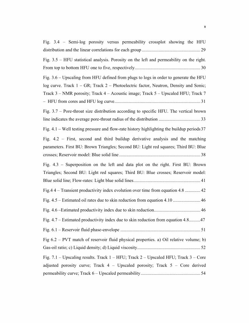
x Fig. 3.4 – Semi-log porosity versus permeability crossplot showing the HFU distribution and the linear correlations for each group ................................................. 29 Fig. 3.5 – HFU statistical analysis. Porosity on the left and permeability on the right. From top to bottom HFU one to five, respectively ....................................................... 30 Fig. 3.6 – Upscaling from HFU defined from plugs to logs in order to generate the HFU log curve. Track 1 – GR; Track 2 – Photoelectric factor, Neutron, Density and Sonic; Track 3 – NMR porosity; Track 4 – Acoustic image; Track 5 – Upscaled HFU; Track 7 – HFU from cores and HFU log curve ........................................................................ 31 Fig. 3.7 – Pore-throat size distribution according to specific HFU. The vertical brown line indicates the average pore-throat radius of the distribution ................................... 33 Fig. 4.1 – Well testing pressure and flow-rate history highlighting the buildup periods 37 Fig. 4.2 – First, second and third buildup derivative analysis and the matching parameters. First BU: Brown Triangles; Second BU: Light red squares; Third BU: Blue crosses; Reservoir model: Blue solid line .................................................................... 38 Fig. 4.3 – Superposition on the left and data plot on the right. First BU: Brown Triangles; Second BU: Light red squares; Third BU: Blue crosses; Reservoir model: Blue solid line; Flow-rates: Light blue solid lines ........................................................ 41 Fig.4 4 – Transient productivity index evolution over time from equation 4.8 ............. 42 Fig. 4.5 – Estimated oil rates due to skin reduction from equation 4.10 ....................... 46 Fig. 4.6 –Estimated productivity index due to skin reduction....................................... 46 Fig. 4.7 – Estimated productivity index due to skin reduction from equation 4.8..........47 Fig. 6.1 – Reservoir fluid phase-envelope ................................................................... 51 Fig 6.2 – PVT match of reservoir fluid physical properties. a) Oil relative volume; b) Gas-oil ratio; c) Liquid density; d) Liquid viscosity..................................................... 52 Fig. 7.1 – Upscaling results. Track 1 – HFU; Track 2 – Upscaled HFU; Track 3 – Core adjusted porosity curve; Track 4 – Upscaled porosity; Track 5 – Core derived permeability curve; Track 6 – Upscaled permeability .................................................. 54

xi Fig 7.2 – Upper figure, upscaled porosity and permeability crossplot. Lower figure, upscaled porosity and permeability crossplot highlighting the four trends used to generate the linear regressions ..................................................................................... 55 Fig. 7.3 – Fitted probability distribution function for upscaled porosity for individual HFU ............................................................................................................................ 57 Fig. 7.4 - J-function curves calculated for the HFU ..................................................... 59 Fig. 7.5 – Model C quality check using histograms. Each histogram shows the property defined from cores and well-logs, upscaling procedure and assigned for the static 3-D model. Notice that the property distribution is maintained throughout the process ....... 60 Fig. 7.6 – East-West models cross-section cutting through the well. Four different models according to the specified major = minor variogram range. The property shown is HFU with no vertical exaggeration .......................................................................... 61 Fig. 7.7 – 3-D petrophysical properties of static Model C. No vertical exaggeration. ... 61 Fig. 8.1 – Match between core relative permeability and Corey’s method ................... 63 Fig. 8.2 – Dynamic reservoir petrophysical parameters upscaled from static Model A . 64 Fig. 8.3 – Dynamic reservoir petrophysical parameters upscaled from static Model B . 65 Fig. 8.4 – Dynamic reservoir petrophysical parameters upscaled from static Model C . 66 Fig. 8.5 – Dynamic reservoir petrophysical parameters upscaled from static Model D . 67 Fig. 8.6 – Simulated bottom hole pressure and oil rate versus time for the four dynamic models ........................................................................................................................ 68 Fig. 8.7 – Third BU pressure derivative comparison between the four dynamic models ................................................................................................................................... 69 Fig. 8.8 – BU derivative analysis and the matching parameters for simulated Model C bottom hole pressure ................................................................................................... 70 Fig. 8.9 – Model C pressure analysis match of superposition plot on the left and data plot on the right ........................................................................................................... 70 Fig. 8.10 – Models cross-section displaying pressure disturbance at the final timestep of the third buildup .......................................................................................................... 72

xii Fig. 8.11 – Model C well cross-section. Notice the good agreement between the well testing cumulative PLT and the simulated cumulative PLT. Track 1 – Porosity; Track 2 – Permeability in logarithmic scale; Track 3 – Water saturation; Track 4 – Completion and perforation interval; Track 5 – Well testing cumulative PLT; Track 6 – Simulated cumulative PLT for Model C ...................................................................................... 73 Fig. 8.12 – Simulated numerical productivity index over time for Model C during the final buildup ............................................................................................................... 75 Fig. 8.13 – Simulated numerical productivity index over time for Model C based on 9-point pressure for the three flowing periods ................................................................. 75 Fig. 8.14 – Model C bottom hole pressure, rate and 9-point pressure numerical productivity index for 20 days of simulation for the entire oil section. Control set for bottom hole pressure and equivalent to 200 bar........................................................... 76 Fig 8.15 – Derivative pressure analysis for the entire oil zone ..................................... 77 Fig. 8.16 – Model C well cross-section; PLT response for the entire oil section. An increase of 27% should be expected when comparing well testing cumulative PLT with the simulated PLT and the upper and lower part of the reservoir are not contributing to production. Track 1 – Porosity; Track 2 – Permeability in logarithmic scale; Track 3 – Water Saturation; Track 4 – Completion and perforation interval; Track 5 – Well testing cumulative PLT; Track 6 – Simulated PLT ................................................................. 78 Fig. 8.17 – Bottom hole pressure, rate and numerical productivity index for a horizontal well simulation in Model C ......................................................................................... 79 Fig. 8.18 – Derivative pressure match for horizontal well simulation .......................... 80 Fig. 8.19 – Match of Superposition plot on the left and data plot on the right for the horizontal well simulation ........................................................................................... 81 Fig. 8.20 – Simulated PLT for a horizontal well. Only 30% of the total horizontal length is effectively contributing to production ...................................................................... 82 Fig. 8.21 – Model cross-section showing pressure as property and the horizontal well at the final drawdown timestep ....................................................................................... 83

13 CHAPTER I

INTRODUCTION The greatest challenge reservoir geoscientists and reservoir engineers face is performing the reservoir description from which crude oil or gas is produced and apply the results achieved on reservoir modeling in order to ultimately generate numerical simulations of reservoir performance. There are mainly two difficulties which have to be overcome to obtain a reliable description of the reservoir:

(i) Reservoir heterogeneity; (ii) The limited amount of data set available, i.e., number of wells at which

observations can be made. In the oil and gas industry the standard practice is to start the reservoir modeling after finishing the exploration phase when at least one exploratory well and a few appraisal wells have been drilled. The idea behind is to gather a minimum information required to start modeling the field with at least some degree of certainty. This thesis proposes a workflow to accomplish the reservoir description and modeling by starting assessing, correlating and integrating the available information from the outset of the exploration stage when only one exploratory well has been drilled and its data set accessible. The suggested process could allow an initial understanding of the reservoir and it could help to guide the next steps of the exploration, for instance, what the major uncertainties are and what the key aspects are that need to be addressed in order to reduce these uncertainties? Furthermore, it could permit to easier transfer a new discovery from the exploration department to the production department simply due to the fact that the static and dynamic modelings have already been started and the main uncertainties recognized and addressed. The reservoir geological framework is the cornerstone of static modeling, however during the exploration phase it is usually poorly understood and this is one of the main complications preventing companies to develop the reservoir model. In an attempt to detach the geological rock facies from the dynamic reservoir behavior and overcome

14 this issue, this thesis proposes an innovative manner to build the static reservoir model based on hydraulic flow units. The permeability-thickness product ( ℎ) and the related average reservoir permeability ( ) are the most important reservoir parameters to be measured during the exploratory phase. The well productivity is mainly controlled by ℎ and skin; even though the skin factor is noteworthy, during the exploration stage the wells are generally not optimized for production and the skin factor might be ignored. The ability to predict reservoir parameters is another vital aspect of reservoir assessment because it can support how to design and interpret the well testing and how to optimize and place the drilling in forthcoming wells. The predictability could also lead managers to find what should be the best strategy for the exploratory area or field by giving a wider picture of the current scenario and not only buttress, but also simplify crucial decisions that many times have to be made in short notice. Moreover, in case the predictions turn out to be reliable it might save company’s efforts and investments in acquiring new data. In this regard, an additional important aspect that is approached in this thesis is the ability to predict reservoir attributes, e.g., reservoir permeability-thickness product, average permeability and productivity index. Two methodologies are attempted, analytical solutions based on cores and well-logs and numerical solutions based on simulations. 1.1 Objectives This thesis has two mains objectives:

1) Generate the static and dynamic models based on hydraulic flow units through assessment and integration the data set available for an exploratory area;

2) Predict reservoir parameters, i.e., permeability-thickness product, average reservoir permeability and productivity index from analytical solutions using cores and well-logs and from numerical solutions applying simulations;

15 1.2 Data Set Available and Software for Analysis and Interpretation The full data set of a deepwater exploratory area with one drilled well responsible for a significant oil discovery is available for this study and it constitutes of:

a) Sidewall and whole cores routine and special laboratory analysis – porosity, capillary pressure, absolute permeability and relative permeability;

b) Logs from Wireline including Formation Testing; c) Transient Pressure Testing and Production Logging; d) Fluid laboratory analysis – Flash liberation and Pressure-Volume-Temperature

certificates; e) Seismic;

The following software were used to assist in the data analysis and interpretations: a) Petrel® - Schlumberger; b) Eclipse® 100 - Schlumberger; c) PVTi® - Schlumberger; d) Interactive Petrophysics® - Senergy; e) MATLAB® - The Mathworks, Inc; f) PIE® - Well Test Solutions Ltd; g) Office Package® - Microsoft;

It is important to point out that some information, such as, reservoir depths, precise well location, legends and figures are not fully displayed in order to preserve the confidential aspect of the studied region and play.

16 CHAPTER II

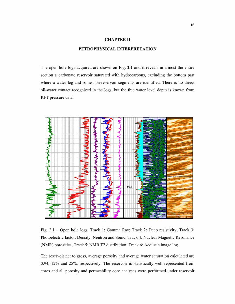
PETROPHYSICAL INTERPRETATION The open hole logs acquired are shown on Fig. 2.1 and it reveals in almost the entire section a carbonate reservoir saturated with hydrocarbons, excluding the bottom part where a water leg and some non-reservoir segments are identified. There is no direct oil-water contact recognized in the logs, but the free water level depth is known from RFT pressure data.

Fig. 2.1 – Open hole logs. Track 1: Gamma Ray; Track 2: Deep resistivity; Track 3: Photoelectric factor, Density, Neutron and Sonic; Track 4: Nuclear Magnetic Resonance (NMR) porosities; Track 5: NMR T2 distribution; Track 6: Acoustic image log. The reservoir net to gross, average porosity and average water saturation calculated are 0.94, 12% and 25%, respectively. The reservoir is statistically well represented from cores and all porosity and permeability core analyses were performed under reservoir

FWL

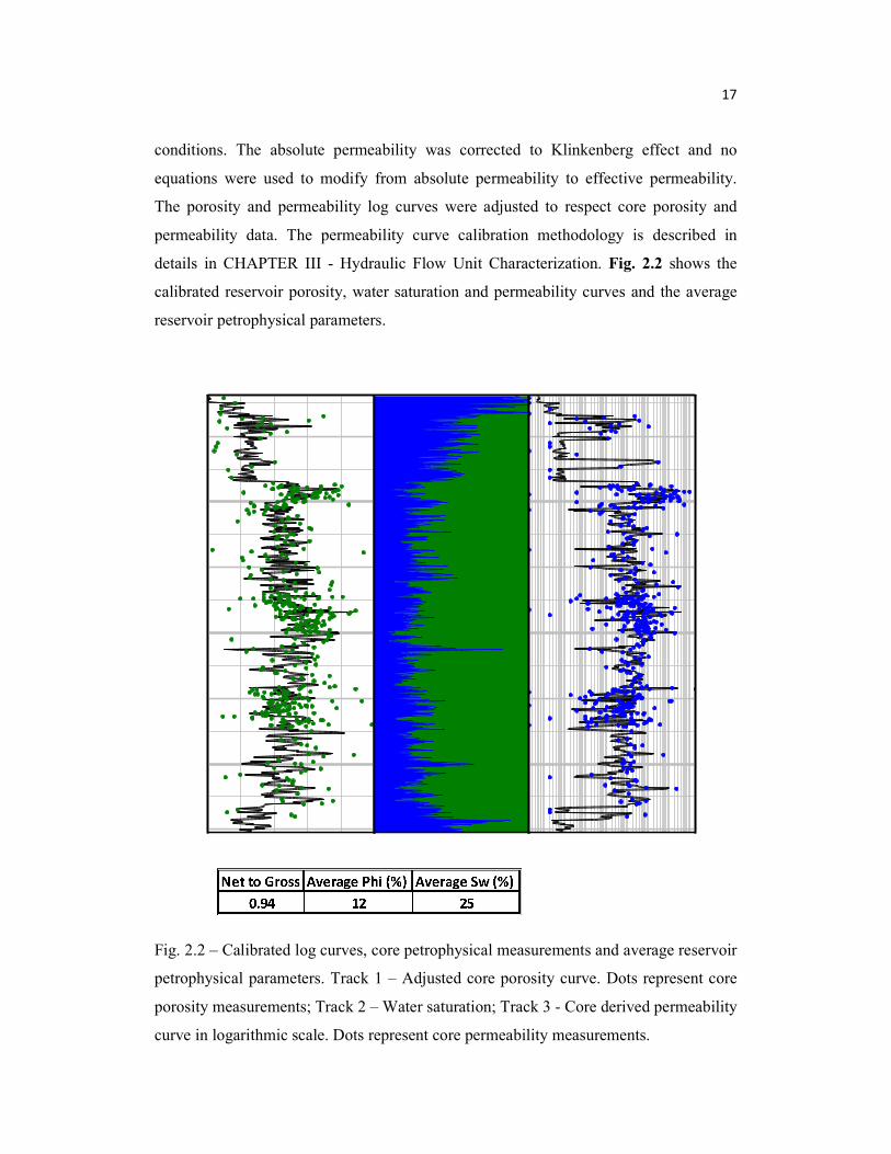
17 conditions. The absolute permeability was corrected to Klinkenberg effect and no equations were used to modify from absolute permeability to effective permeability. The porosity and permeability log curves were adjusted to respect core porosity and permeability data. The permeability curve calibration methodology is described in details in CHAPTER III - Hydraulic Flow Unit Characterization. Fig. 2.2 shows the calibrated reservoir porosity, water saturation and permeability curves and the average reservoir petrophysical parameters.

Fig. 2.2 – Calibrated log curves, core petrophysical measurements and average reservoir petrophysical parameters. Track 1 – Adjusted core porosity curve. Dots represent core porosity measurements; Track 2 – Water saturation; Track 3 - Core derived permeability curve in logarithmic scale. Dots represent core permeability measurements.

18 The image log interpretation discloses a reservoir with layers varying from a few centimeters to a few meters of thickness. Many intervals show laminations with less than 10 centimeters of thickness. In such highly heterogeneous reservoirs the precise depth of the sidewall cores are crucial to perform a reliable reservoir characterization and because the sidewall cores recovery depth are seen as points with low acoustic amplitude it was possible to define the exact depth position from where the cores were collected. All the reported cores depth were corrected to the depth encountered in the image log and the error range varied from a few centimeters to 2 meters, upward or downward (Fig 2.3).

Fig. 2.3 – Acoustic image logs. Notice the layers and the low acoustic amplitude points were sidewall cores were collected. Track 1: NMR Porosities; Track 2: Static acoustic image; Track 3: Dynamic acoustic image. Regarding the image log interpretation the entire section is dominated by bed-boundaries and no faults or fractures are present. The bed-boundaries dip are in general

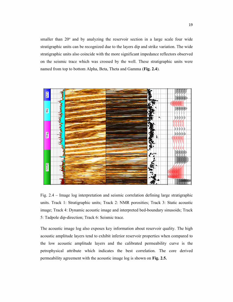
19 smaller than 20o and by analyzing the reservoir section in a large scale four wide stratigraphic units can be recognized due to the layers dip and strike variation. The wide stratigraphic units also coincide with the more significant impedance reflectors observed on the seismic trace which was crossed by the well. These stratigraphic units were named from top to bottom Alpha, Beta, Theta and Gamma (Fig. 2.4).

Fig. 2.4 – Image log interpretation and seismic correlation defining large stratigraphic units. Track 1: Stratigraphic units; Track 2: NMR porosities; Track 3: Static acoustic image; Track 4: Dynamic acoustic image and interpreted bed-boundary sinusoids; Track 5: Tadpole dip-direction; Track 6: Seismic trace. The acoustic image log also exposes key information about reservoir quality. The high acoustic amplitude layers tend to exhibit inferior reservoir properties when compared to the low acoustic amplitude layers and the calibrated permeability curve is the petrophysical attribute which indicates the best correlation. The core derived permeability agreement with the acoustic image log is shown on Fig. 2.5.

20 The high degree of correlation between the core derived permeability and the acoustic image log was only possible to be achieved due to the hydraulic flow unit characterization method which is described in details in the next chapter. This method allowed the permeability curve to move from high permeability to low permeability layers in just a few centimeters of vertical scale and such assignment is impossible to be achieved using only the basic well logging data due to vertical resolution limitations.

Fig. 2.5 – Image log and core derived permeability correlation. Track 1: NMR porosities; Track 2: Static acoustic image; Track 3: Dynamic acoustic image and core derived permeability curve in logarithmic scale.

21 2.1 Permeability Curve Integral and PLT Correlation Correlating permeability curve with production logging (PLT) is a good manner to verify the confidence of the adjusted permeability curve and it also allows accessing the flow potential of a limited reservoir interval. The calibrated permeability curve ( ) can be integrated for a defined interval from to as follows: ℎ = ( ) ……………………………………………………(2.1) and to simplify the result is also called ℎ. It is acknowledged that the core permeability used to calibrate the curve represents absolute permeability and it will be compared to effective reservoir permeability, therefore the calculated ℎ should be multiplied by the oil relative permeability ( ). However, during the exploration phase the relative permeability to hydrocarbon is little understood and it was decided to do a direct association without applying any correction to the permeability curve integral result. The production well logging was acquired during the well testing and as reported by the PLT 100% of the perforated interval is contributing to flow. Fig. 2.6 displays the well testing perforation interval and correlation between PLT, core derived permeability curve, integrated permeability and well-logs. Adjusting the permeability curve in linear scale enhances the recognition of the higher and lower production zones. The higher and lower production zones according to the core derived permeability curve shows a decent agreement with interpreted production logging. Mainly in the middle and upper parts, the integrated permeability curve relates very well with the cumulative production logging. A perceptible difference is at the bottom part of the perforated interval where the integrated permeability shows three sudden changes in the inclination, suggesting a significant increase in production coming from thin layers while in the same interval the cumulative production logging shows a smoother inclination (Fig. 2.6). However, it should be pointed out that there is a vertical resolution limitation for PLT and it might not be able to precisely distinguish laminations with only a few centimeter thicknesses. Another point is that PLT is measured in a cased hole and the fluid flows through the gun perforations and the

22 perforations might not exactly coincide with the depth of the higher production laminations.

Fig. 2.6 – Production logging correlation with well-log data. Track 1: Well testing perforation interval; Track 2: Gamma Ray; Track 3: NMR porosities; Track 4: Integrated permeability for the entire reservoir oil zone; Track 5: Red curve - Integrated permeability for the perforation interval and, green dashed curve - Cumulative PLT; Track 6: Core derived permeability in logarithmic scale; Track 7: Core derived permeability in linear scale; Track 8: PLT interpretation; Track 9: Acoustic image log. The integral of the core derived permeability curve for the perforation interval yields a permeability-thickness product ( ℎ) of 953 md.m and using 125 meters corresponding to the perforation interval as reservoir effective thickness the average reservoir permeability ( ) is 7.6 md. When taking into account the entire oil zone and applying the NTG previously computed results in 1208 md.m x 0.94 (NTG) = 1135.5 md.m and for the whole oil leg drops to 3.7 md (Fig. 2.6). Analyzing statistically the core permeability data in the perforation interval, the arithmetic, geometric and harmonic average reservoir permeabilities are 16.26 md, 1.32 md and 0.000625 md, respectively. Using 125 meters which represents the perforation

23 interval as reservoir effective thickness yields an estimated ℎ of 2032 md.m for arithmetic average permeability, 165 md.m for geometric average permeability and 0.078 md.m for harmonic average permeability. It is normally expected the reservoir permeability-thickness product lies between arithmetic and geometric average values. 2.2 Reservoir Anisotropy The reservoir anisotropy ( ) can be calculated from:

= ..……..……………………………………………….……………(2.1)

where is vertical permeability and is horizontal permeability. An approximation to calculate the reservoir anisotropy is to assume the horizontal permeability as the core arithmetic average and the vertical permeability as the core harmonic average. This yields reservoir anisotropy of 3.8 * 10-5 and since all cores were used in the computation the low value means that in a reservoir scale it is unlikely to occur any significant cross-flow between large stratigraphic zones and the reservoir flow might be controlled by pressure drop spreading laterally and not moving upward or downward through another stratigraphic unit. Another approach which unveils a different result is to calculate reservoir anisotropy using vertical permeability measured on vertical cores and use the nearest horizontal core permeability to calculate the anisotropy ratio. A few vertical cores permeability measurements are available and the depth they were collected correspond to the perforation interval depth. This method produces an anisotropy ratio extending from 0.001 to 0.6 and the arithmetic average of 0.1, meaning that in a metric to centimetric scale it might be possible to find cross-flow between some layers. This calculations regarding the reservoir anisotropy highlights that there is a significant degree of uncertainty associated with the results and in forthcoming wells this point should be addressed, perhaps by acquiring mini-DSTs after fluid sampling and from the pressure derivative analysis define a more accurate reservoir vertical permeability in case the spherical flow regime is identified.

24 CHAPTER III

HYDRAULIC FLOW UNIT CHARACTERIZATION

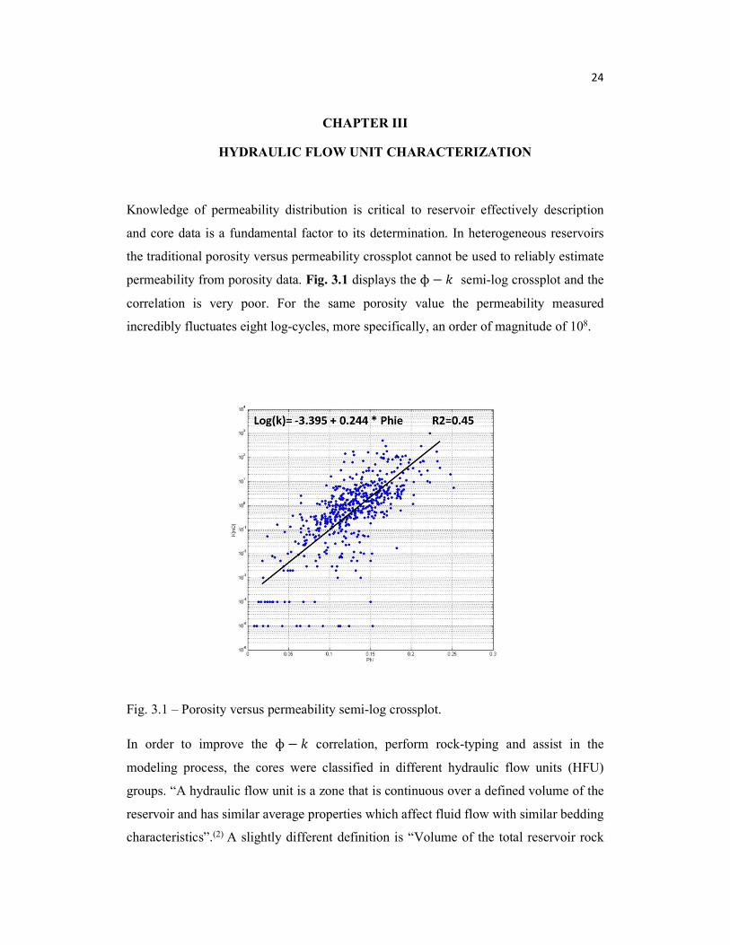
Knowledge of permeability distribution is critical to reservoir effectively description and core data is a fundamental factor to its determination. In heterogeneous reservoirs the traditional porosity versus permeability crossplot cannot be used to reliably estimate permeability from porosity data. Fig. 3.1 displays the ɸ − semi-log crossplot and the correlation is very poor. For the same porosity value the permeability measured incredibly fluctuates eight log-cycles, more specifically, an order of magnitude of 108.

Fig. 3.1 – Porosity versus permeability semi-log crossplot. In order to improve the ɸ − correlation, perform rock-typing and assist in the modeling process, the cores were classified in different hydraulic flow units (HFU) groups. “A hydraulic flow unit is a zone that is continuous over a defined volume of the reservoir and has similar average properties which affect fluid flow with similar bedding characteristics”.(2) A slightly different definition is “Volume of the total reservoir rock

25 within which geological or petrophysical properties that affect fluid flow are internally consistent and predictably different from properties of other rock volume”.(10)

Only one hydraulic flow unit could be present in several depositional facies or within a single facies several HFUs could be found.(10) This means that there is no direct relation between facies boundaries and HFU boundaries. In some geological situations the distribution of HFU could be connected to facies distribution, but this is not always the case. For instance, in carbonate reservoirs the early or late diagenesis process might be able to modify completely the rock petrophysical properties and transform an expected high porosity and/or permeability facies into a low porosity and/or permeability facies. The opposite could also happen, a low porosity and/or permeability facies become a high porosity and/or permeability facies. In other words, a “good” facies does not necessarily mean a high HFU number with high flow potential. Hydraulic flow unit could be called dynamic rock-typing and its classification allows detaching the fluid flow behavior from the rock facies giving an alternative manner to execute rock-typing classification. This is a great advantage when performing reservoir characterization studies in exploratory areas, because at the exploration stage the geological model is usually poorly understood and facies organization have not been defined. A HFU is primarily controlled by pore geometrical attributes, such as pore geometry and pore-throat distribution. The pore geometry is controlled by mineralogy, grain size, grain shape, sorting and packing and determines the rock storativity capacity. Besides the macro-sedimentary structures, such as bedding, laminations, etc., the pore-throat distribution is the major parameter determining the rock flow capacity.(10) Hydraulic unit theory is based on porosity, permeability and capillary pressure correlation. Firstly combining Darcy’s law for flow in porous media and Poiseuille’s law for flow in tubes results:(10)

= ɸ ……...…………………………………………………………….(3.1)

and the equation shows that permeability depends on pore characteristics, precisely the pore-throat radius.

26 The generalized Kozeny-Carman(12) equation for porous media is more realistic because the connected pore structure is not straight and the permeability is related to tortuosity factor ( ) and the surface area per grain volume ( ):

= ɸ( ɸ ) ………..……………………………………….……...(3.2)

where is μ and ɸ is a fractional volume. The term is known as the Kozeny constant and varies from 5 to 100 for most reservoir rocks. The term is a function of the geological characteristics of porous media and is related to pore geometry. This term is the focal point of the HFU classification technique. Dividing both sides of equation 3.2 by porosity and then taking the square root of both sides results in:(2)(10)(11)

0.0314 ɸ = ɸ( ɸ ) ………..……………………………………..(3.3)

where the constant 0.0314 comes from the square root of the conversion from μ to . The term ( /ɸ ) proves to be a very powerful correlation parameter for various

measured petrophysical properties such as formation factor. The flow zone indicator term ( ) is defined as:(2)(10)(11)

= ………………..……………………………………………..(3.4)

and reservoir quality index term ( ) is given by:

= 0.0314 ɸ ………..………………………………………………....(3.5)

The pore volume to grain volume ratio term (ɸ ) is defined as:

ɸ = ɸ( ɸ ) ………..………………………………………….……………..(3.6)

and substituting equations 3.4, 3.5 and 3.6 into equation 3.3 yields: = ɸ ………..……………………………………………………...(3.7)

27 Taking the logarithm of both sides of equation 3.7 results: log( ) = log(ɸ ) + log ( ) ………..………………………….………(3.8) where and are given in μ . On a log-log plot of ɸ versus all samples with similar values will cluster on the same straight line with unity slope and samples with different values will lie on other parallel lines. Samples with the same

classification tend to have similar pore-throat attributes; therefore, will constitute a unique hydraulic flow unit (HFU). Each defined line on the log-log plot is an HFU and the intercept of the straight line with ɸ = 1 will give the value for that group of data which defined the HFU. In order to correctly identify the numbers of HFU a cumulative frequency histogram was created using the calculated values for the samples. The number of HFU is defined by a change in the cumulative histogram slope and five HFU were recognized (Fig.3.2). It is acknowledged that many more hydraulic flow units could have been defined; however the definition of a too large number would turn the workflow impractical.

Fig 3.2 – cumulative frequency curve showing the identification of five HFU.

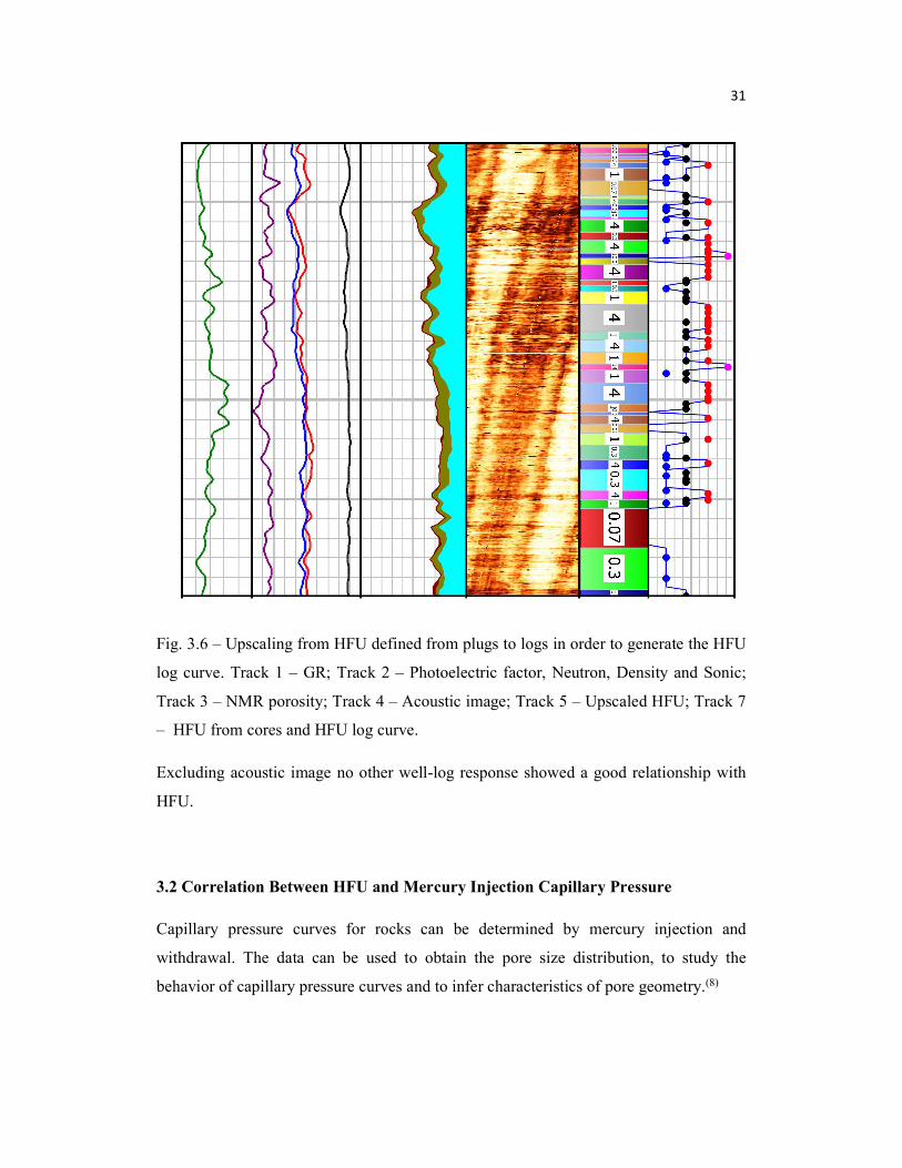
28 The log-log plot of ɸ versus is shown on Fig. 3.3. The upper and lower limits of a given HFU cluster were defined by half distance between straight lines. Fig. 3.4 illustrates the ɸ − semi-log crossplot with the HFU distribution and the ɸ − linear correlation equation for each group. Clearly the porosity versus permeability correlation is significantly improved by analyzing each group individually. Fig. 3.5 summarizes the HFU porosity and permeability statistical analysis. It is noticed that the porosity histograms for the HFU overlap and individualizing the HFU using only porosity is an impossible task. 3.1 Upscaling HFU – From Cores to Well-Logs In order to upscale the defined HFU using cores to well-log scale a manual interpretation procedure was executed assisted mainly by the acoustic image log. In general, different HFU recognized in the cores are well correlated to image layers according to its acoustic amplitude. As a result, the top and bottom of each HFU could be determined using the top and bottom of the rock layer were the sample was collected. In other words, the HFU limits were defined by the layer bed-boundary visualized on the image log. The final output is that a continuous HFU log curve was created for the entire reservoir section where cores were available and it has the vertical resolution of the image log (Fig. 3 6). It is important to highlight that the reservoir is extremely heterogeneous and due to basic logs vertical resolution limitations it is not possible to accurately fine-tune the permeability curve with cores using the standard process. This core-log upscaling workflow allowed creating a core derived permeability curve using the HFU as a constrain, i.e., HFU 1: correlation 1, HFU 2: correlation 2 and so on. The consequence is that now it is possible to move from high permeability layers to low permeability layers in just a few centimeters scale because of the high vertical resolution of the image log (Fig. 2.5).

29

Fig. 3.3 - Log-log plot of ɸ versus displaying the 5 hydraulic flow units.

Fig. 3.4 – Semi-log porosity versus permeability crossplot showing the HFU distribution and the linear correlations for each group.

30

Fig. 3.5 – HFU statistical analysis. Porosity on the left and permeability on the right. From top to bottom HFU one to five, respectively.

31

Fig. 3.6 – Upscaling from HFU defined from plugs to logs in order to generate the HFU log curve. Track 1 – GR; Track 2 – Photoelectric factor, Neutron, Density and Sonic; Track 3 – NMR porosity; Track 4 – Acoustic image; Track 5 – Upscaled HFU; Track 7 – HFU from cores and HFU log curve. Excluding acoustic image no other well-log response showed a good relationship with HFU. 3.2 Correlation Between HFU and Mercury Injection Capillary Pressure Capillary pressure curves for rocks can be determined by mercury injection and withdrawal. The data can be used to obtain the pore size distribution, to study the behavior of capillary pressure curves and to infer characteristics of pore geometry.(8)

32 The determination of the pore-throat radius ( ) distribution of rocks based on capillary pressure curve ( ) is an approximation and after conversion from laboratory conditions to reservoir conditions can be calculated by:

= 0.1450377 ………..…………………………………………….(3.9)

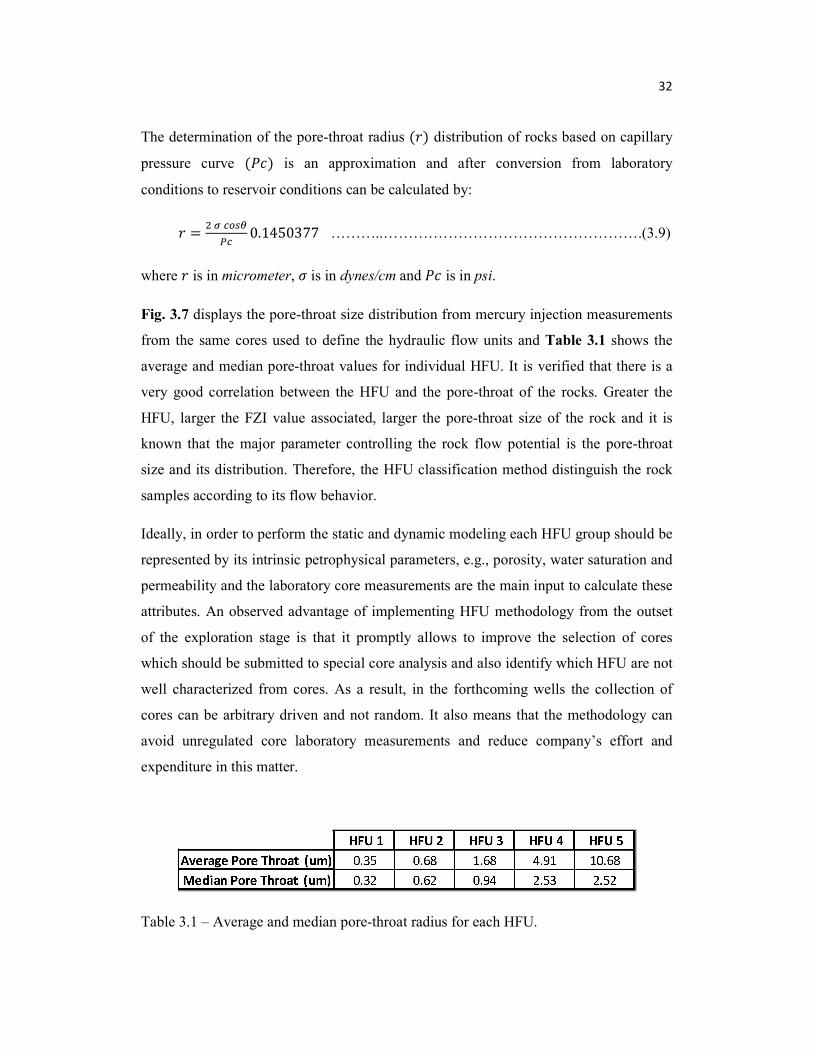
where is in micrometer, is in dynes/cm and is in psi. Fig. 3.7 displays the pore-throat size distribution from mercury injection measurements from the same cores used to define the hydraulic flow units and Table 3.1 shows the average and median pore-throat values for individual HFU. It is verified that there is a very good correlation between the HFU and the pore-throat of the rocks. Greater the HFU, larger the FZI value associated, larger the pore-throat size of the rock and it is known that the major parameter controlling the rock flow potential is the pore-throat size and its distribution. Therefore, the HFU classification method distinguish the rock samples according to its flow behavior. Ideally, in order to perform the static and dynamic modeling each HFU group should be represented by its intrinsic petrophysical parameters, e.g., porosity, water saturation and permeability and the laboratory core measurements are the main input to calculate these attributes. An observed advantage of implementing HFU methodology from the outset of the exploration stage is that it promptly allows to improve the selection of cores which should be submitted to special core analysis and also identify which HFU are not well characterized from cores. As a result, in the forthcoming wells the collection of cores can be arbitrary driven and not random. It also means that the methodology can avoid unregulated core laboratory measurements and reduce company’s effort and expenditure in this matter.

Table 3.1 – Average and median pore-throat radius for each HFU.

33

Fig. 3.7 – Pore-throat size distribution according to specific HFU. The vertical brown line indicates the average pore-throat radius of the distribution.

34 CHAPTER IV

WELL TESTING INTERPRETATION Well test analysis is an inverse problem and in general cannot be solved uniquely. Hence, more than one mathematical model will generate the output to represent the measured data. A consistent description of the reservoir can only be achieved by assessing and correlating all the available information from different sources and adjusting a comprehensible physical model of the system.(10) The well testing interpretation usually focuses on the transient pressure response and the pressure variation response is a function of well geometry and reservoir properties, e.g., permeability and heterogeneity. Transient responses are observed before constant pressure or closed boundaries effects are reached.(3) The objective of testing exploratory or appraisal wells have been summarized as follows:(10)

Acquire information on reservoir description (permeability, heterogeneity, boundaries, compartmentalization);

Measure well productivity; Obtain fluid samples for laboratory PVT analysis; Measure reservoir temperature and pressure – static and dynamic; Estimate completion efficiency, e.g., skin factor ( );

However, the completion of an exploratory/appraisal well is not optimized for production and the skin factor might not be representative. When an exploratory or appraisal well is drilled, the mud system will not be adjusted with respect to formation damage and these wells are drilled with a substantial overbalance which will result in mud filtrate loss promoting damage. In this scenario the permeability-thickness product and average reservoir permeability are the important factors which most of the attention should be focused on and the completion efficiency – skin factor – might be ignored.(10) A foremost important feature of transient well testing is that the interpretation allows the independent assessment of intrinsic formation average permeability and near

35 wellbore effects - skin factor. Consequently, even if the skin effect is high in the exploration/appraisal well, the productivity index of the future development wells may be predicted analytically or numerically. Beforehand starting the well test interpretation the following items should be incorporated in the analysis and are known from petrophysical interpretation and correlation, i.e., open hole logs, cores and seismic:

The reservoir is highly heterogeneous and stratified. Thin layers with just few centimeter thickness are present and highly differ in flow potential;

One of the main difficulties associated with the design of well testing is the requirement for a permeability estimate. From cores, the arithmetic, geometric and harmonic reservoir permeability average for the perforation interval is 16.26 md, 1.32 md and 0.000625 md, respectively. When applying 125 meters as effective reservoir thickness the permeability-thickness product is 2032 md.m for arithmetic reservoir permeability, 165 md.m for geometric reservoir permeability and 0.078 md.m for harmonic reservoir permeability. It is customary that the well testing reservoir ℎ lies between arithmetic and geometric average values;

From the integral of the core derived permeability curve the perforated interval yield a ℎ = 953 . and = 7.6 md;

The total perforation interval should contribute to production; The flow might be dominated by some high permeability thin layers; The permeability anisotropy ( / ) for the reservoir as a whole is very low

(3.8 * 10-5). No significant cross-flow between large stratigraphic layers is expected; as a result, the pressure disturbance is unlikely to move downward and/or upwards in the reservoir and might be concentrated around the perforated top and bottom boundaries. In a metric or centimetric scale the average permeability anisotropy calculated from cores is 0.1;

The reservoir permeability seems to be matrix dependent. No fractures or faults are interpreted on the image logs and there is no evidence of geological boundaries from seismic interpretation, e.g., faults (seismic interpretation will not be discussed in this thesis, but the information is known in advance);

36 The perforation interval comprehends 125 meters and the static constants applied in the well test analysis are shown on Table 4.1.

Table 4.1 – Well test analysis constants. Fig. 4.1 displays the well testing pressure and flow-rate history. The test sequence consists of three drawdowns and three buildups. After 16 hours of cleanup flow starts the first buildup and it lasts 43 hours. Then 10 hours of flowing period for the second flow followed by 8 hours of shutin and lastly 14 hours of flow followed by the third buildup which lasts 43 hours. For the first and third buildup a hard shutin maneuver was applied whereas for the second buildup a soft shutin maneuver. The consequence of the two different shutin methods can clearly be identified from evaluating the wellbore storage effect (Fig 4.2).

37

Fig. 4.1 – Well testing pressure and flow-rate history highlighting the buildup periods. The third buildup period was designated to perform the pressure test analysis and the derivative plot shows in early-time a first stabilization after 3 minutes of shutin and subsequently, corresponding to mid-time an upturn, which reflects a transitional period. Then, in late-time after three hours of shutin a second stabilization is detected (Fig 4.2). The second straight line is 45% smaller than the first straight line. In order to solve and match this derivative behavior a linear composite model was selected and it is formed by two distinct media in the reservoir. Initially the region around the well is producing alone and the pressure behavior corresponds to a homogeneous reservoir. When the linear interface is reached the two regions are producing together and a second homogeneous behavior is observed. The equivalent homogeneous system is defined by the average properties of the two regions, because during the late homogeneous regime the two regions are contributing to production and this is obtained by the average of the two regions mobility.(3)

38

Fig. 4.2 – First, second and third buildup derivative analysis and the matching parameters. First BU: Brown Triangles; Second BU: Light red squares; Third BU: Blue crosses; Reservoir model: Blue solid line. The comparison between region 1 and 2 is expressed by the Mobility ratio ( ) and Storativity ratio ( ):(3)

= ………...…………………………………………………………...(4.1)

= (ɸ )(ɸ ) ………...…………………………………………………………..(4.2)

39 The level of the plateaus indicates the apparent mobility [( /μ) ] of the total homogeneous regime:(3)

= = 0.5 1 + ………..…………………….(4.3)

The interpreted reservoir model unveils a second region 7.8 meters away from the wellbore exhibiting poorer reservoir quality when compared to the first region. The total system reservoir permeability-thickness product, ℎ, is 775 md.m and using 125 meters as effective reservoir thickness, the average reservoir permeability, , is 6.2 md. The radius of investigation reached by the pressure disturbance is 136 meters. The mobility ratio and storativity ratio attained by modeling are both equivalent to 0.1 and because both ratios change proportionally implies that the effective reservoir thickness was reduced. However, it is important to point out that using the linear composite model it would be possible to match the derivative behavior with other mobility and storativity combinations, since a decrease in reservoir quality is expressed for the second region. In other words, several mathematical solutions for mobility and storativity ratio are feasible. Apart from this non-unique mathematical solution, what is essential to be noticed is that there is a decrease in reservoir quality away from the wellbore. From the well-logs it is possible to observe that the carbonate reservoir is vertically greatly heterogeneous and this heterogeneity is also present in the cores when porosity and permeability crossplot is analyzed. From a geological point of view it is very likely that this heterogeneity is going to spread laterally and what is probably varying when moving away from the wellbore is the permeability-thickness product. As a result, not only the mobility, but also the storativity ratio will be affected and with the current information available is not practical to precisely quantify the real mobility and storativity ratios. Nevertheless, it is plausible to confirm that the reservoir flow potential is reduced by 45% when moving 7.8 meters away from the wellbore. Another interesting point is that besides the reservoir being highly heterogeneous, a homogeneous radial flow is reached, meaning that concerning fluid flow the system as a

40 whole behaves homogeneously. The increase in fluid viscosity could also cause similar derivative behavior, nonetheless is unlikely to have occurred. When comparing the first, second and third buildup derivatives there is no noteworthy change existent, apart from a slight decrease in skin from the first to the third derivative during early-time, what is perfectly normal and it reflects the release of some supercharge effect after the cleanup flow. It is interesting to notice that the second buildup wellbore storage hides the early-time stabilization present in the first and third buildup. The matching model and reservoir parameters are summarized on Table 4.2 and on Fig. 4.3 the superposition and data plot results are shown. From the superposition plot the extrapolated reservoir initial pressure ( *) is 609 bar at gauge depth and no depletion can be identified from the first BU extrapolated pressure to the third BU extrapolated pressure. Other models could also match the pressure and rate of the well testing, such as homogeneous reservoir with boundary effect. However, there is no enough evidence to support the presence of a geological boundary, for instance, a sealing fault close to the wellbore.

Table 4.2 – Reservoir parameters from well testing interpretation.

41

Fig. 4.3 – Superposition on the left and data plot on the right. First BU: Brown Triangles; Second BU: Light red squares; Third BU: Blue crosses; Reservoir model: Blue solid line; Flow-rates: Light blue solid lines. 4.1 Skin Pressure Drop and Transient Productivity Index The total skin obtained by well testing interpretation is 0.55 and can be classified as mechanical skin. The corresponding pressure change due to skin ( ) can be expressed in oilfield units as:(3) = . ………..…………………………………………...……(4.4)

resulting in 8.3 bar (120.4 psi). During the infinite acting period the productivity index is decreasing with time and can be referred as transient productivity index. The actual and ideal productivity index can be related to rate as: = ( ) ......................................................................................(4.5)

= ( ) ……....………………………………………..(4.6)

The computed using the extrapolated reservoir pressure, the final flowing pressure and the flow-rate measured during the third flowing period is 2.77 m3/d/bar

42 (1.20 stb/d/psi). When correcting for the pressure change due to skin ( ) the ideal productivity index is equal to 2.95 m3/d/bar (1.27 stb/d/psi). The flow efficiency ( ) can be computed from:(3)

= ………...………………………………………………………...(4.7)

resulting in 0.94, meaning that the reservoir is slightly damaged. The analytical solution in oilfield units for the transient productivity index ( ) is:(1)

= . ɸ . . ] ………..………………..………(4.8)

In order to calibrate equation 4.8 with the well testing the transient productivity index evolution with time was calculated using the derivative model reservoir parameters as input and skin equivalent to zero. The results are shown on Fig. 4.4 and because time enters as a logarithmic term the is quite insensitive to it. Only after 500 hours of shutin the productivity index reaches 2.99 m3/d/bar (1.29 stb/d/psi) and in this period the decay function of over time is nearly asymptotic. In forthcoming wells in the field in case equation 4.8 is used to estimate the productivity index it is recommended to apply shutin time of 500 hours to better approximate the ideal productivity index.

Fig.4 4 – Transient productivity index evolution over time from equation 4.8.

43 4.2 Skin Removal in Exploratory/Appraisal Wells The well productivity for the same drawdown pressure can be increased by reducing fluid viscosity, increasing the drainage area or reducing the skin. The skin reduction can be attained by stimulation. The skin estimation is a nearly impossible task and the only way to obtain a reliable value is by measuring and interpreting it from well testing analysis during a radial flow and after ℎ is determined. The skin is commonly referred to as “wellbore damage” and it is caused by a modification in permeability zone around the wellbore. This modified zone can extend from a few centimeters to several meters. During drilling, completion or workover some materials such as mud filtrate, cement slurry, or clay particles can enter the formation and reduce permeability, resulting in a positive skin. The permeability around the wellbore could also be increased by acidizing or fracturing, resulting in a negative skin.(1) Analytically the skin is used to describe a deviation of the diffusivity equation from these base conditions:(3)(5)

(i) Infinite acting and homogeneous reservoir; (ii) Undipping; (iii) Open hole; (iv) Vertical well and penetrating the complete reservoir thickness;

The skin measured from well testing is the total skin ( ) and it includes:(3)(5) = + + + …….………………………………….……(4.9) where

= ℎ = = − ( ):

= ( )

44 The skin factor in exploratory/appraisal wells many times is a controversial issue in terms of whether it should or not be altered by stimulation once it is determined from well testing analysis. The following points should be analyzed holistically before deciding for a stimulation operation in an exploratory/appraisal well:

(a) The decision to proceed with the stimulation should involve an economic exercise and a compromise must be reached such that the cost of the operation is compatible with the value of the information gained;

(b) In general the minimum skin attainable by acidification varies from -1 to -2 and the minimum skin attainable by fracturing is -5;(5)

(c) The only skin that will be affected by stimulation is the mechanical skin ( ); thus it is crucial to firstly identify the type of skin which is present in the reservoir and sometimes this is not a trivial task;

(d) Is the exploratory/appraisal well going to be used as a producer later on? In a positive answer the stimulation operation might be worthwhile, since item (a) is fulfilled.

(e) Analytical solutions regarding production (described below) should be performed and verified if the solutions fulfill item (a). For instance, in case the minimum economic value of the area is known and even with the lowest skin achievable the area is still non-economical, the stimulation might not be worthwhile.

(f) In case the well is going to be abandoned due to impossibility to be equipped to production, should be investigated whether it is worthwhile to just rely on the analytical solutions to estimate the new rates and avoid stimulation costs.

Two methods to estimate the production due to skin reduction are described and in the analyzed scenario both represent transient solutions. In oil reservoirs a simplified and practical analytical approximation of the new oil rate achieved by reducing the skin factor independent of reservoir attributes is from:(5)

= ( )( ) ……….…………………………………………………..…(4.10)

where

45 = = ℎ = =

The graph on Fig. 4.5 displays an example of the expected rates reached through reducing the skin factor of the reservoir using the rates from the third drawdown [380 m3/d (2390 stb/d)] and applying equation 4.10. The graph on Fig. 4.6 shows the productivity index resulting from equation 4.5 according to the increased rates due to reduced skin. The outcomes indicate that for the same reservoir pressure drawdown and assuming the well is stimulated the maximum oil rate after a skin of -5 is obtained is 1435 m3 (9023 stb) resulting in a maximum productivity index of 10.5 m3/d/bar (4.5 stb/d/psi). In this example, if the least economic value of the area is 11 3/ / , it might not be worthwhile to invest in stimulation in an attempt to reduce the skin. However, it might be worthwhile to try to reduce skin in case the gained information is applicable in forthcoming wells. This example points out that the decision to proceed with the stimulation have to involve an economic evaluation. The term 7 in equation 4.10 should be calibrated according to the progress of knowledge about the field. It is recommended to replace the term 7 by 8 in gas reservoirs as a first approach.(5) The second method to estimate the transient productivity index in terms of reduced skin is from equation 4.8 and it yields a maximum transient productivity index of 7.5 m3/d/bar (3.20 stb/d/psi) for a skin of -5 and applying the reservoir parameters interpreted from the well test analysis for 500 hours of shutin (Fig. 4.7).

46

Fig. 4.5 – Estimated oil rates due to skin reduction from equation 4.10.

Fig. 4.6 –Estimated productivity index due to skin reduction.

47

Fig. 4.7 –Estimated productivity index due to skin reduction from equation 4.8.

48 CHAPTER V

INTEGRATION OF CORES, WELL-LOGS AND WELL TEST The integration of well-logs, cores and well test data essentially revolves around geostatistical average permeability techniques in which cores permeability measurements and logs permeability curves attempt to represent the well testing results and allows predicting reservoir parameters in wells where no well testing is available. It also permits not only to assist the well testing analysis, but also to assess the consistency of the well testing interpretation. Moreover, it could guide the optimization and positioning of the perforation depth and extension. The main problem when comparing core or log permeability to well testing permeability is the scale of the investigated zone. Well testing will provide an average permeability according to the intrinsic reservoir diffusivity and it can reach dozens of meters, or sometimes, thousands of meters of investigated area, while the core and log permeability will provide permeability values reflecting just a few centimeters of the area surrounding the well location. Strictly speaking, the rock volume probed by well testing is significantly higher than the rock volume probed by cores. Based on this uncertainty many experts accept an error of 10 times as a good approximation of core or logs permeabilities compared to well testing permeability. An useful formulae to calculate average permeability is the power average ( ) and it is expressed by:(7)

= ∑ / ………...……………………………………………...(5.1)

where the alfa ( ) term will reflect the equivalent average. The arithmetic average corresponds to = 1, the harmonic average corresponds to = −1, while the geometric average corresponds to → 0. Using only the core permeability data which lies between the perforation interval equation 5.1 was used to calibrate the alfa exponent which match the well testing average permeability of 6.2 md and then the well testing permeability-thickness product

49 of 775 . . It resulted in = 0.518 and the calculated using only cores points out that the reservoir average permeability stays between arithmetic and geometric. Once the exponent is calibrated the same can be used to predict the ℎ in other wells in the field or in other zones of the reservoir in the same well, since there are core measurements available and it is assumed that the same is still valid after altering the spatial position. In order to apply the described technique, a larger reservoir zone which covers the entire oil leg was chosen and the same equation 5.1 with = 0.518 was used to calculate for this larger reservoir oil section and it resulted in 10.22 md. The next step was compute ℎ and because it is for the entire oil zone it is necessary to take into account the net to gross value, so [ ℎ = Total thickness x NTG (0.94) x 10.22 md = 2443 md.m]. After calculating ℎ the final step was estimate the productivity index from equation 4.8. Table 5.1 summarizes the reservoir parameters resolved by using the fine-tuned as input. The predicted was computed applying skin factor equal zero and shutin time of 500 hours.

Table 5.1 – Calibrated alfa exponent and predicted reservoir parameters for the entire oil leg. Assuming that the NTG value is correct, this procedure allows predicting that if a the entire oil leg was perforated and put into production the reservoir permeability-thickness product would be 2843 md.m and the transient productivity index would reach 10.63 m3/d/bar (4.61 stb/d/psi). The result states that, when compared to the well testing, the reservoir transient productivity index would have been increased by a factor of three. Another important point which deserves attention is that according to the applied methodology the predicted average reservoir permeability of 10.22 md is greater than the average reservoir permeability obtained from well testing analysis (6.2 md), meaning that perhaps the chosen perforated interval might not have been optimized.

50 The encountered above results are more optimistic than the results calculated from the integral of the core derived permeability curve which shows ℎ = 1135.5 . for the entire oil leg. In that case = 3.7 md and calculating the transient productivity index from equation 4.8 results in 4.52 m3/d/bar (1.96 stb/d/psi). When applying the ℎ = 953 . and = 7.6 md calculated from the integral of the core derived permeability curve for the perforated interval in equation 4.8 the ideal productivity index is 3.63 m3/d/bar (1.57 stb/d/psi) and represents and overestimation error of 19% when compared to the well test analysis. The average reservoir permeability calculated from the core derived permeability (7.6 md) is very close to the 6.2 md obtained from well testing. Since the permeability curve was calibrated only with cores and the measured permeability in plugs is essentially matrix permeability, it is reasonable to mention that the reservoir permeability is indeed matrix dependent and there is no significant flow contribution coming from natural fractures. This last supposition is supported by the lack of natural fractures observed on the image log interpretation.

51 CHAPTER VI

PVT MATCHING In order to perform simulations an adequate Pressure-Volume-Temperature (PVT) matching is crucial to describe a mathematical model for the reservoir fluid. A PVT laboratory analysis from a reservoir fluid sample taken under reservoir conditions was used as input for the PVT matching assignment. Fig. 6.1 shows the reservoir fluid phase diagram and the critical pressure and temperature are 175.11 bar and 564.19o C, respectively. It portrays that according to the reservoir pressure and temperature the reservoir fluid is under-saturated oil and situated to the left-side of the critical point. Assuming a pressure drop over a constant temperature the reservoir fluid reach bubble point pressure at laboratory measured 397 bar and the initial reservoir pressure at a reference depth is 620.5 bar.

Fig. 6.1 – Reservoir fluid phase-envelope. Probably due to some content of non-hydrocarbon components in the reservoir fluid it was not possible to match exactly the reservoir saturation pressure. The matching saturation pressure calculated is 7 bar smaller than the reservoir saturation pressure

52 measured in the laboratory. However, for the simulation purpose of the proposed workflow, which is simulate a well testing and estimate reservoir parameters, the error found will not affect the results because the flowing pressure will not reach the reservoir bubble point pressure. The physical properties and the PVT matching results of the reservoir fluid are displayed on Fig. 6.2. Regarding the described fluid characteristics a black-oil hydrodynamic model can well represent the reservoir fluid behavior in dynamic simulations.

Fig 6.2 – PVT match of reservoir fluid physical properties. a) Oil relative volume; b) Gas-oil ratio; c) Liquid density; d) Liquid viscosity.

53 CHAPTER VII

STATIC RESERVOIR MODELING Reservoir characterization is defined as the construction of a realistic three-dimensional image of petrophysical properties to be used to predict reservoir performance.(6) In order to build the 3-D reservoir model two steps must be accomplished, first build the static reservoir model which should reflects the geology and then the dynamic reservoir model which should reflects reservoir fluid behavior. Facies modeling is the cornerstone of the static reservoir model and it means to populate the model with discrete facies into cell grids. To build a realistic facies model the conceptual geological processes during and after deposition should be understood and the reservoir connectivity as well. The input to the model should honor the different descriptive facies information and level of heterogeneity. The ultimate target is to build a 3-D model that captures the reservoir architecture with flow units and barriers. However, usually during the exploration phase the geological model is poorly understood and due to the lack of drilled wells uncertainties are very high and in many cases not even analogues can represent the reservoir properly. In order to overcome this problem the proposed 3-D model will be based on hydraulic flow units. This approach allows disconnecting the reservoir geological facies from the reservoir dynamic behavior. Thus, the proposed 3-D model does not have as a target to represent reservoir geology, but predict reservoir parameters such as reservoir permeability-thickness product, average permeability, transient productivity index and mimic the observed well testing flow behavior, i.e., pressure derivative and production logging. Firstly a fine static model grid was build which is later upscaled to a reservoir simulation model. The fine grid size chosen is X = 5m, Y = 5m and Z = 1m over an area of 1500 x 1500 meters surrounding the exploratory well. The four large stratigraphic units detected on the image log interpretation, Alpha, Beta, Theta and Gamma, were mapped using the equivalent seismic reflectors. In order to allocate layers a follow top method is applied using the mapped seismic surfaces as reference and the layers thickness were defined as 1 meter. The created hydraulic flow units, core adjusted

54 porosity and core derived permeability curves were upscaled into the 5 x 5 x 1 meter blocks (Fig. 7.1). The upscaling process is assisted by quality checks using histograms (Fig. 7.5). The fundamental idea is to preserve the property distribution after upscaling. HFU was upscaled using the “most of” method, porosity using “arithmetic average” method and permeability using “mid-point pic” method.

Fig. 7.1 – Upscaling results. Track 1 – HFU; Track 2 – Upscaled HFU; Track 3 – Core adjusted porosity curve; Track 4 – Upscaled porosity; Track 5 – Core derived permeability curve; Track 6 – Upscaled permeability. Due to the very low fraction of HFU 5, only 0.4%, was decided to group it together with HFU 4. Fig.7.2 shows the upscaled porosity versus upscaled permeability crossplot and the equations resulting from the linear regressions are displayed in Table 7.1. Each trend reflects a hydraulic flow unit and the correlation coefficient was improved significantly when compared to the other presented Phi x K crossplots (Fig. 3.1 and Fig. 3.4).

55

Fig 7.2 – Upper figure, upscaled porosity and permeability semi-log crossplot. Lower figure, upscaled porosity and permeability semi-log crossplot highlighting the four trends used to generate the linear regressions with the specific HFU.

Table 7.1 – Linear regression equations from upscaled porosity and permeability.

56 7.1 Populating the Static Model Once the grid was defined the next step was populate it. The cells which compose the grid have the size of 5 x 5 x 1 meter and a hydraulic flow unit, porosity, permeability and water saturation value were assigned to each cell. The first step to assign discrete values to the model was distributing spatially the hydraulic flow units and the Sequential Gaussian Simulation algorithm was chosen. It is a stochastic method based on kriging and it honors variograms, input trends and specified fractions. No trend was employed, however the vertical HFU fractions for individual stratigraphic zones were respected. The variograms aims at capturing the regional organization of data which is not purely random. Four different models were created using four different major equal minor ranges, i.e., 10, 100, 500 and 1000 meters and named Models A, B, C and D, respectively. The additional variogram parameters were preserved as constant for all models and the established parameters are listed below:

Variogram type: Spherical; Nugget effect = 0.1; Sill = 1; Major range = Minor range = 10, 100, 500 and 1000 meters, respectively,

Models A, B, C and D. Vertical range: Zone Alpha: 9 meters; Zone Beta: 14 meters; Zone Theta: 20

meters; Zone Gamma: No variogram adjusted because only HFU 1 is present. Fractions:

Zone Alpha: HFU 1= 51%; HFU 2= 19%; HFU 3= 19%; HFU 4= 11%; Zone Beta: HFU 1= 2%; HFU 2= 25%; HFU 3 = 67%; HFU 4= 6%; Zone Theta: HFU 1= 55%; HFU 2= 29%; HFU 3= 15%; HFU 4= 1%; Zone Gamma: HFU 1= 100%;

The second step was distribute porosities and in order to undertake that initially the upscaled porosity data for each HFU was analyzed using frequency histograms and a

57 probability distribution function was adjusted. For HFU 2, 3, 4 and 5 a Gaussian distribution function fitted the data and for HFU 1 a log-normal distribution function was the best option (Fig 7.3). Then a Gaussian random function simulation algorithm conditioned to hydraulic flow units was used to distribute porosities spatially and the fitted probability distribution functions were applied as input data.

Fig. 7.3 – Fitted probability distribution function for upscaled porosity for individual HFU. In order to assign permeability value to each cell the linear regressions of permeability as a function of porosity were employed (Table 7.1). The final step of the petrophysical modeling was allocate water saturation to the blocks. Since membrane capillary pressure measurements from cores are available a dimensionless J-function versus water saturation could be computed.

58 The dimensionless Leverett J-function in oilfield units is defined as:(5)(8)

( ) = 0.21645 ɸ ……..……………………………………….…(7.1)

and for a set of samples a least squares regression was built using J values as the independent variable. Then a power law equation correlation of the form: = ( ) ……...…………………………………………………………..(7.2) was adjusted in order to compute and index. In oilfield units converted capillary pressures to the height domain can be written as:

= ( ) ……..…………………………………………………………(7.3)

Finally by combining equations 7.1, 7.2 and 7.3 water saturation as a function of height above the free water level ( (ℎ)) can be calculated in oilfield units from:

(ℎ) = . ( ) ɸ ……..…………………………....(7.4)

Fig. 7.4 illustrates the J-curves computed for the hydraulic flow units. Due to J-curve similarities between HFU 1 and HFU 2 both families were represented by the same function. No threshold pressure was measured in the capillary pressure experiments; therefore, the oil water contact and the free water level share the same depth. This indicates that the rock wettability is likely to be mix. In order to compute the water saturation the permeability and porosity factors applied in equation 7.4 are the discrete values defined for each cell. The water and oil densities ( , ), wettability contact angle ( ) and interfacial tension ( ) were kept as constant throughout the model. The water saturation curve computed from petrophysical interpretation was not only used as quality control to verify the consistency of the saturation height function approach, but also to adequately adjust it in order to better represent the irreducible water saturation. In order to preserve the petrophysical properties distribution while upscaling and modeling, in all the steps the results were quality check using histograms and Fig. 7.5 displays the Model C histogram distribution for HFU, porosity and permeability,

59 defined from cores and logs, calculated by the upscaling procedure and assigned for the static 3-D model. Important to notice that the distribution of the initial histograms which are derived from cores are preserved throughout the workflow, meaning that laboratory core measurements are the foundation of the static modeling.

Fig. 7.4 - J-function curves calculated for the HFU. Fig. 7.6 highlights the contrast of the four models created by different X and Y variogram ranges. It is possible to recognize that larger the range, larger the lateral continuity of the property and smaller the anisotropy. Fig. 7.7 exemplifies the HFU, porosity, permeability and water saturation for the 3-D Model C, which is based on 500 meters major = minor variogram range. The created 3-D static models seem to repeat depositional sequences and it reminds depositional environments based on cycles. When the geological 3-D model is build it is recommended to compare it to the static models based on HFU in order to identify similarities.

60

Fig. 7.5 – Model C quality check using histograms. Each histogram shows the property defined from cores and well-logs, upscaling procedure and assigned for the static 3-D model. Notice that the property distribution is maintained throughout the process.

61

Fig. 7.6 – East-West models cross-section cutting through the well. Four different models according to the specified major = minor variogram range. The property shown is HFU with no vertical exaggeration.

Fig. 7.7 – 3-D petrophysical properties of static Model C. No vertical exaggeration.

62 CHAPTER VIII

DYNAMIC RESERVOIR MODELING Reservoir simulation based on dynamic reservoir model uses finite difference method to simulate the flow of fluid within the reservoir. In order to reduce the computational time, firstly the 3-D static models were upscaled to a coarser grid with 20 x 20 x 5 meters cell size. To quality check the upscaling process, the hydrocarbon volume in place of the static and dynamic models were compared (CHAPTER IX Volume of Hydrocarbon). Porosity and water saturation were upscaled by arithmetic averaging – volume weighted technique and permeability was upscaled by directional averaging power-arithmetic technique using the alfa exponent of 0.518 calculated from cores, well- logs and well testing integration. Through the analyses of the production logging data 5 meters is the smallest vertical size which a change on the slope of the cumulative production curve can be identified (Fig. 2.6). As a result, 5 meters thickness for vertical layers in the dynamic model to represent fluid flow seems to be a good approximation. It is interesting to highlight that as reported by the PLT in 5 vertical meters the flow behaves homogeneously, despite the fact that the reservoir is organized by many thin layers, some of with just a few centimeter thickness as interpreted on the image logs and also showing a significant contrast in intrinsic permeability as observed in permeability core measurements. According to the reservoir fluid properties a black-oil simulation model can well represent the reservoir dynamic behavior. The water-oil relative permeability curves for the dynamic model were adjusted using Corey’s method(4) based on a whole core laboratory relative permeability measurement and Fig. 8.1 displays the curves match and the defined Corey’s exponents. The same relative permeability curve was applied to all hydraulic flow units. According to Corey’s exponents the reservoir has a mixed wettability and by analyzing the graph it is recognized that oil relative permeability is almost zero for water saturation higher than 0.7 (Fig. 8.1); thus 30% of the hydrocarbon accounts as residual oil saturation.

63 It is recognized that, ideally, each HFU should be represented by petrophysical properties, such as, a relative permeability curve. However, this detailed information is still not available due to the fact that this study is based on an exploratory area. Hence, it is recommended to selective collect cores in the forthcoming wells to perform relative permeability measurements to represent all HFU groups and improve the dynamic fluid behavior characterization.

Fig. 8.1 – Match between core relative permeability and Corey’s method. Fig. 8.2, 8.3, 8.4 and 8.5 depict the four dynamic models upscaled from the four static Models A, B, C and D, respectively. In order to perform the dynamic simulations the perforation interval was set to represent the same perforation interval as executed in the well testing. The prediction depletion strategy was also set to correspond to the rates, drawdown and buildup period observed in the well testing. The only alteration is that the third BU period was increased from 43 hours to 216 hours in order to represent better the reservoir pressure recovery. The vertical permeability was adjusted as 10% of the horizontal permeability. The simulated bottom hole pressure and rates versus time for the four dynamic models is shown on Fig. 8.6. The pressure drop is the largest in Model A and the lowest in Model D. It means that the lateral continuity of the hydraulic flow units plays the main role in order to control the reservoir pressure support, giving an enhanced support for models based on a larger major equal minor variogram distance.

64

Fig. 8.2 – Dynamic reservoir petrophysical parameters upscaled from static Model A.

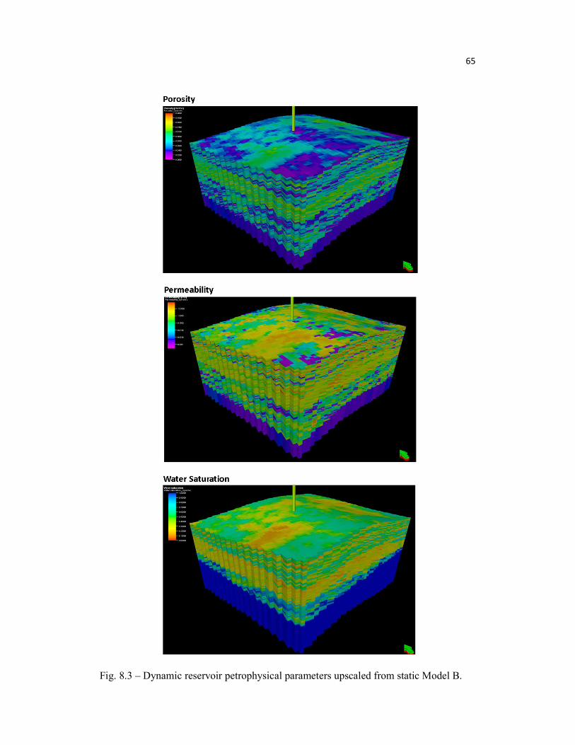
65

Fig. 8.3 – Dynamic reservoir petrophysical parameters upscaled from static Model B.

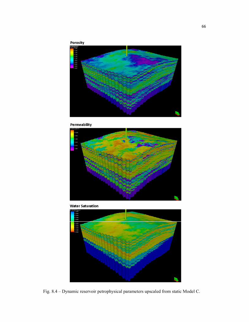
66

Fig. 8.4 – Dynamic reservoir petrophysical parameters upscaled from static Model C.

67

Fig. 8.5 – Dynamic reservoir petrophysical parameters upscaled from static Model D.

68

Fig. 8.6 – Simulated bottom hole pressure and oil rate versus time for the four dynamic Models. 8.1. Well Test Analysis of Simulations The simulated bottom hole pressure and rates were analyzed following the same procedure as a physical well testing interpretation. Fig. 8.7 displays the pressure derivative for the final BU for the simulated models. Model A derivative shows a half-wave cycle pattern, moving from steep upturn followed by a short stabilization, then a downturn. Model B derivative shows a complete wave cycle pattern, however the wavelength is larger and the amplitude is smaller when compared to Model A. Model C derivative displays first a stabilization then an upturn and a tendency for a second stabilization in late time. Model D shows a stabilization in early and middle time and a slight downturn tendency in the end of the late time. The model’s derivative behavior also reflects the spatial distribution of the HFU, decreasing anisotropy from Model A to Model D. Amid all models’ derivative, the one which represents the most similar shape when compared to the physical well testing derivative is Model C; consequently, Model C was chosen to perform a derivative match interpretation. Fig. 8.8 portrays the derivative

69 match and a linear composite derivative model was selected, which is the same derivative model observed in the well testing. The permeability-thickness product calculated is 300 md.m, resulting in an average reservoir permeability of 2.4 md. The same way as observed in the well testing the upturn in the derivative indicates a second region showing poorer reservoir properties when compared to the first region and the second region is located 55 meters away from the wellbore. The superposition and data plot match are shown on Fig. 8.9.

Fig. 8.7 – Third BU pressure derivative comparison between the four dynamic models. The wellbore storage and skin obtained by the derivative of the simulated pressure data should be neglected, because a numerical simulator cannot handle the case of nonideal wellbore storage and any proposal to analyze early time response using derivative methods have to be regarded with some skepticism.(10) Another point is that the horizontal grid size is equivalent to a square of 20 meter side and the skin occurs near the wellbore, as a result the skin factor cannot be measured with confidence.

70

Fig. 8.8 – BU derivative analysis and the matching parameters for simulated Model C bottom hole pressure.

Fig. 8.9 – Model C pressure analysis match of superposition plot on the left and data plot on the right

10-1 100 101 10210-2

10-1

Delta-T (hr)

DP &

DERIV

ATIVE

(BAR

S/M3/D

)

02-JAN-2015 02:0004-JAN-2015 07:0005-JAN-2015 05:00Base CaseBase Case

2015/01/05-0500 : OIL

Linear-Composite 2-Zone** Simulation Data ** well. storage = .9033E-03 M3/BAR skin = -1.6000 permeability = 2.4000 MD Areal Ky/Kx = 1.0000 X-Interface(1) = 55.000 METRE Mob.ratio(1) = 0.40000 Stor.ratio(1) = 0.40000 Perm-Thickness = 300.00 MD-METRE Initial Press. = 615.957 BARS

Static-Data and ConstantsVolume-Factor = 1.600 vol/volThickness = 125.0 METREViscosity = 1.030 CPTotal Compress = .8215E-04 1/BARRate = 380.0 M3/DStorivity = 0.001232 METRE/BARDiffusivity = 83.99 METRE^2/HRGauge Depth = N/A METREPerf. Depth = N/A METRE

71 Fig. 8.10 depicts an E-W cross-section of all models cutting the wellbore at the end of the third drawdown timestep. The pressure disturbance of Model A shows an oval shape, with the pressure disturbance moving upward and downward around the wellbore. Models B, C and D the pressure disturbance tends to move more laterally, following the higher permeability layers and in Model D reaches the largest investigated zone. This distinct behavior can also be explained by the different spatial distribution of the HFU, with the continuity increasing from Model A to D. The behavior of the pressure disturbance in Model C is consistent with the large scale very low reservoir anisotropy ( = 3.8 ∗ 10 ) , because the pressure disturbance is essentially distributed inside a large stratigraphic unit, mainly unit Beta, and it has not any preference to move to other stratigraphic units after moving a few meters from the wellbore. In order to verify the consistency of the dynamic Model C the PLT curve acquired during the second drawdown period of the well testing was compared to the simulated PLT and Fig. 8.11 displays a well cross-section showing the very good agreement between the acquired and simulated PLT curves.

72

Fig. 8.10 – Models cross-section displaying pressure disturbance at the final timestep of the third buildup.

73

Fig. 8.11 – Model C well cross-section. Notice the good agreement between the well testing cumulative PLT and the simulated cumulative PLT. Track 1 – Porosity; Track 2 – Permeability in logarithmic scale; Track 3 – Water saturation; Track 4 – Completion and perforation interval; Track 5 – Well testing cumulative PLT; Track 6 – Simulated cumulative PLT for Model C. 8.2 . Numerical Productivity Index The numerical productivity index in a Cartesian grid is a function of the connection factor ( and can be represented in oilfield units from:(5)(9)

= . ……...…………………………………………………..(8.1)

74 for a vertical well the permeability used is the geometric mean of X and Y direction permeabilities and is the pressure equivalent radius of the grid block and for an anisotropic reservoir in a rectangular grid is given by:(5)(9)

= 0.28( ) ∆ ( ) ∆

( ) ( ) ……..…………………………………(8.2)

Lastly, the numerical productivity index attached to one connection ( ) can be computed from:

= ………..…………………………………………………....(8.3)

and a summation of all the connections belonging to the producing interval of the well will give the total numerical productivity index ( ). To simplify the depends on the connection factor, which depends on the geometry of the grid block, the well bore radius and rock permeability. It is usually found that the numerical productivity index is higher than the natural productivity index. Fig. 8.12 illustrates the numerical productivity index calculated by the Model C simulation resulting in 3.44 m3/d/bar (1.49 stb/d/psi) for the final period of the third drawdown. A second approach to calculate the is using the 9-point pressure ( ), which is the average pressure given by 9 cells around the wellbore and can be calculated by:

= ( ) ……...……………………………………………………(8.4)

Fig. 8.13 shows the numerical calculated for Model C using equation 8.4 resulting in 3.12 m3/d/bar (1.35 stb/d/psi) at the final period of the third BU and it can be compared to the obtained by the well testing [2.95 m3/d/bar (1.27 stb/d/psi)], representing an overestimation error of only 5%.

75

Fig. 8.12 – Simulated numerical productivity index over time for Model C during the final buildup.

Fig. 8.13 – Simulated numerical productivity index over time for Model C based on 9-point pressure for the three flowing periods.

76 8.3 . Productivity of the Entire Oil Leg A scenario was simulated using Model C with a larger perforation zone covering the entire oil section and changing the control from rate to bottom hole pressure. The simulated period was set for 20 days, 10 days of drawdown and 10 days of buildup and applying a delta pressure equivalent to 200 bar. In this scenario the 9-point pressure numerical productivity index reaches 4.25 m3/d/bar (1.84 stb/d/psi) at the end of the drawdown period, representing an increase of 27% when compared to the previous simulation for the perforated interval. Fig. 8.14 displays the pressure behavior, rate and

while Fig. 8.15 illustrates the derivative pressure analysis and a linear composite model was used to match the simulated data. The permeability-thickness product calculated is 403.2 md.m with an average reservoir permeability of 1.68 md. According to the simulated PLT a cumulative rate increase of 27% should be expected when comparing to the well testing PLT and mainly the upper and lower part of the reservoir are not contributing to production. (Fig. 8.16)

Fig. 8.14 – Model C bottom hole pressure, rate and 9-point pressure numerical productivity index for 20 days of simulation for the entire oil section. Control set for bottom hole pressure and equivalent to 200 bar.

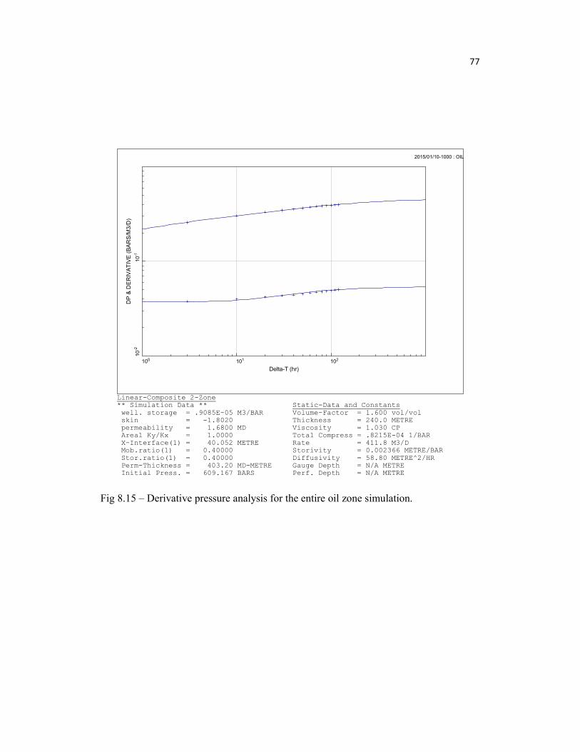
77

Fig 8.15 – Derivative pressure analysis for the entire oil zone simulation.

100 101 10210-2

10-1

Delta-T (hr)

DP &

DERIV

ATIVE

(BAR

S/M3/D

)

2015/01/10-1000 : OIL

Linear-Composite 2-Zone** Simulation Data ** well. storage = .9085E-05 M3/BAR skin = -1.8020 permeability = 1.6800 MD Areal Ky/Kx = 1.0000 X-Interface(1) = 40.052 METRE Mob.ratio(1) = 0.40000 Stor.ratio(1) = 0.40000 Perm-Thickness = 403.20 MD-METRE Initial Press. = 609.167 BARSSmoothing Coef = 0.,0.

Static-Data and ConstantsVolume-Factor = 1.600 vol/volThickness = 240.0 METREViscosity = 1.030 CPTotal Compress = .8215E-04 1/BARRate = 411.8 M3/DStorivity = 0.002366 METRE/BARDiffusivity = 58.80 METRE^2/HRGauge Depth = N/A METREPerf. Depth = N/A METREDatum Depth = N/A METRE

78

Fig. 8.16 – Model C well cross-section; PLT response for the entire oil section. An increase of 27% should be expected when comparing well testing cumulative PLT with the simulated PLT and the upper and lower part of the reservoir are not contributing to production. Track 1 – Porosity; Track 2 – Permeability in logarithmic scale; Track 3 – Water Saturation; Track 4 – Completion and perforation interval; Track 5 – Well testing cumulative PLT; Track 6 – Simulated PLT 8.4 Horizontal Well Simulation In order to investigate the performance a horizontal well scenario was simulated using Model C and it was decided to project the well in the highest permeability layers which were the most affected by pressure drop according to Fig. 8.10. The well horizontal section was set for 1200 meters with 89o of inclination and the entire horizontal interval

79 completed for production. The simulated period of time was adjusted to 10 days of drawdown and 35 days of buildup. Fig. 8.17 shows the simulated bottom hole pressure, rates and numerical productivity index which reached 6.66 m3/d/bar (2.88 stb/d/psi) at the end of the buildup.

Fig. 8.17 – Bottom hole pressure, rate and numerical productivity index for a horizontal well simulation in Model C. The derivative analysis of the horizontal well pressure simulation shows at early times a stabilization followed by an upturn, then a second stabilization. The second derivative stabilization is at a level twice the first. A horizontal well model was used to match the derivative behavior and Fig. 8.18 displays the results. The horizontal well is not centered in the zone thickness and it is closer to the upper boundary than the lower boundary of the reservoir. The first stabilization reflects a vertical radial flow and because only the upper limit of the reservoir is reached a hemi-radial flow regime develops afterwards resulting in a ¼ slope in the derivative. At late time the flow lines converge from all reservoirs directions toward the well producing a horizontal radial flow regime. The second derivative stabilization corresponds to the infinite acting radial

80 flow and gives the horizontal ℎ = 36.9 . and = 0.61 md. Fig 8.19 shows the superposition and data plot match.

Fig. 8.18 – Derivative pressure match for horizontal well simulation.

100 101 102 103

10-210-1

Delta-T (hr)

DP &

DERIV

ATIVE

(BAR

S/M3/D

)

2015/01/10-1000 : OIL

Horizontal Well and Homogeneous Reservoir** Simulation Data ** well. storage = .1078E-04 M3/BAR Skin(mech.) = -3.2434 permeability = 0.61590 MD Areal Ky/Kx = 1.0000 Kv/Kh = 0.12166 Drain Length/2 = 160.00 METRE Zw/H = 0.30000 Skin(Global) = -5.5762 Skin(geom.) = -3.8327 Perm-Thickness = 36.954 MD-METRE Initial Press. = 616.031 BARSSmoothing Coef = 0.,0.

Static-Data and ConstantsVolume-Factor = 1.600 vol/volThickness = 60.00 METREViscosity = 0.1030 CPTotal Compress = .8215E-04 1/BARRate = 876.2 M3/DStorivity = 0.0005914 METRE/BARDiffusivity = 215.5 METRE^2/HRGauge Depth = N/A METREPerf. Depth = N/A METREDatum Depth = N/A METREAnalysis-Data ID: GAU004Based on Gauge ID: GAU004

81

Fig. 8.19 – Match of Superposition plot on the left and data plot on the right for the horizontal well simulation. As discussed previously the early time response should be treated with some skepticism due to the fact that a numerical simulator cannot handle the case of nonideal wellbore storage and it is a coarse grid, thus the near wellbore skin cannot be measured with confidence. However, for horizontal wells the infinite late time horizontal radial flow is used to compute the geometrical skin, therefore the value of = −3.83 can be assumed as accurate. The simulated PLT for the horizontal well (Fig. 8.20) reveals that only 30% of the horizontal length is effectively contributing to production and Fig. 8.21 displays the model cross-sections showing the well position and the pressure disturbance at the final drawdown timestep. The pressure disturbance has a tendency to concentrate in the high permeability layers and the pressure drop spreads mainly laterally. The under-performance of the horizontal well can be attributed to the low vertical permeability and low flow contribution over the total horizontal length. A large number of cells are not contributing to flow.

82

Fig. 8.20 – Simulated PLT for a horizontal well. Only 30% of the total horizontal length is effectively contributing to production.

83

Fig. 8.21 – Model cross-section showing pressure as property and the horizontal well at the final drawdown timestep.

84 CHAPTER IX

VOLUME OF HYDROCARBON Original oil in place ( ) and original gas in place ( ) refers to the total volume of hydrocarbon stored in a reservoir prior to production. An approach to quality check the upscaling process from static model to dynamic model is comparing the volume of hydrocarbon in place before and after upscaling. In oilfield units the original oil volume in place ( ) can be computed from:

= ɸ ( ) ..……………………………………………..(9.1)

and Table 9.1 shows the results calculated for Model C. This method calculates the hydrocarbon volume in each cell and the results shown are the sum for all cells. A decrease of 6% in OOIP from static model to dynamic model is observed and according to this outcome it is acknowledged that after upscaling the dynamic grid retained the spatial petrophysical properties distribution of the static grid.

Table 9.1 – Original oil in place calculation for Static and Dynamic Models C. Usually in E&P Hydrocarbon Companies the Exploration and Production departments calculate the volume of hydrocarbon in place in different manners. Once a new accumulation is discovered the Exploration department compute OOIP using the petrophysical parameters obtained by well-log interpretation which were acquired from the drilled well responsible for the finding and then run a Monte Carlo simulation to

85 create a probability distribution of hydrocarbon in place, whereas the Production department will later compute from a 3-D model using cutoffs and in many cases there is a substantial volume contrast when comparing both calculated volumes in place. The early reservoir modeling from the outset of the exploration stage allows the Exploration department to compute in a similar way as the Production department and the contrast between hydrocarbon volumes could be reduced. 9.1 Estimation of Dynamic Petrophysical Cutoff and Recovery Factor Due to the fact that some cells are showing none to very little contribution to flow the simulated PLT can be used to estimate the reservoir petrophysical cutoff that influence the fluid behavior according to the set drawdown pressure. The total oil section PLT simulation (Fig. 8.16) and the horizontal well PLT simulation (Fig. 8.20) were analyzed and Table 9.2 displays the statistics of oil saturation, porosity and permeability for the cells which are not contributing or contributing very little to flow. The maximum delta pressure drawdown implemented was 200 bar and it should be pointed out that this analysis is valid only for this drawdown because the flow potential contribution is dependent on the delta pressure.

Table 9.2 – Statistical analysis of petrophysical properties of cells not contributing or contributing very little to flow. The maximum permeability value (K= 2.14 ) was applied as cutoff in Model C for computing and Table 9.3 displays the results. According to the relative permeability curve (Fig. 8.1) the residual oil saturation is equivalent to 30%, consequently, the moveable oil is 70%. Applying this factor over the ratio between the volume of oil in place before cutoff and after cutoff and assuming that the result might

86 be the recovery volume, an approximation of the possible Recovery Factor ( ) for the field would be: = 0.35 ∗ 0.7 = 0.25 ……..……………………………………...…(9.1)

or 25%.

Table 9.3 – Hydrocarbon volume after applying cutoff of 2.14 md in static Model C.

It is important to mention that in order to have a good approximation of the oil recovery factor is necessary to have knowledge of the driving mechanisms that control the behavior of fluid within the reservoir. The overall performance of reservoir is largely determined by the nature of the energy, i.e., driving mechanism, available for moving the oil to the wellbore and the final recovery factor will be also strongly dependent on secondary and tertiary recovery methodologies later employed in the field life-time. This = 25% should be seem as a first rough estimation of the recovery factor for the field. It should be pointed out that no porosity cutoff for the studied reservoir should be establish due to the fact that none coherent correlation between porosity and dynamic reservoir characteristics was encountered. Cells with good permeability exhibit low porosity values and vice-versa. Therefore, in case a porosity cutoff is implemented it will cut producible payzone intervals.

87 CHAPTER X

SUMMARY OF THE RESERVOIR PROPERTIES PREDICTION

Table 10.1 displays the reservoir parameters obtained from well testing interpretation and Table 10.2 displays the forecasted reservoir parameters using the different methods described in this thesis.

Table 10.1 – Reservoir properties obtained from well test analysis.

Table 10.2 – Forecasted reservoir properties from different methods.

88 Regarding reservoir permeability-thickness product and average reservoir permeability predictions for the perforated interval the integral of the core derived permeability shows the closest approximation when compared to the well testing results and the predicted parameters are overestimated by 19%. In terms of productivity index the Model C simulation using the 9-point pressure and equation 8.4 approach displays the most similar result when compared to the well testing and the foreseen is overestimated by only 5%. In case the entire oil leg was tested the power averaging technique forecasted the most optimistic results whereas the permeability integral and simulation the most pessimistic. Since the permeability integral method showed the best approximation for ℎ and for the perforated interval, it seems reasonable to assume that in case the entire oil zone was tested the best estimation should be the permeability curve integral method as well. Likewise, the best estimation for the productivity index would be the 9-point pressure approach from equation 8.4. According to the simulation and well test analysis results, despite increasing the production by a factor of two the drilling of a horizontal well is discouraged because it is considered a low performance for a horizontal well length of 1200 meters.

89 CHAPTER XI

CONCLUSIONS AND RECOMMENDATIONS

The following conclusions and recommendations are derived from this study: 1. The early assessment and integration of all available information from different sources and from the outset of the exploration phase allows to identify uncertainties, forecast reservoir properties and to start the 3-D reservoir model. 2. It also permits an initial understanding of the reservoir and could give managers a broader perspective of the exploratory area or new field and support taking decisions in short notice. Moreover, it can optimize the design of well testing and not only assist, but also validate well test interpretations. 3. Building the static and dynamic models using hydraulic flow unit concept is the key to overcome the lack of geological knowledge typically present during the exploratory stage. The proposed workflow decouples the reservoir fluid behavior from the geological facies and provides an alternative manner to create reservoir models when the geological framework is still poorly understood. 4. Laboratory core measurements are the foundation of the created 3-D models and the early data integration could save company’s investment and time in this regard, because it can avoid unrestrictive and unsupervised core laboratory analysis. The proposed workflow allows to promptly identify which cores should be selected and, in forthcoming wells, in which interval cores have to be collected to perform laboratory analysis in order to fully represent the reservoir with petrophysical attributes. It also simplifies the identification of the relevant seismic reflectors that should be mapped. 5. The described workflow permits to work with highly heterogeneous reservoirs and it succeeds in building a derived core permeability curve which honors low and high permeability core data in just a few centimeters of vertical scale and reflects the reservoir flow potential. The workflow also permits to significantly improve the correlation factor of permeability as a function of porosity through the upscaling steps.

90 6. Model C pressure derivative based on an X = Y = 500 meters range variogram exhibited the most similar pattern compared to the well testing analysis. 7. The results achieved for the perforated interval using well-logs and cores as source and permeability curve integral as method predicted reservoir permeability and permeability-thickness product by an overestimation error of 19%. Based on simulations and 9-point pressure the productivity index could be foreseen by an overestimation error of 5%. 8. In case the entire oil leg was tested the most likely ℎ , and would be 1135.5 . , 3.7 md and 4.52 m3/d/bar, respectively. 9. Considering a scenario of 200 bar of producing drawdown, the first estimation of the dynamic cutoff for the discovered field is 2.14 md and the first rough approximation of the recovery factor 25%. Porosity should not be used as cutoff because of the lack of correlation between porosity and dynamic reservoir characteristics. 10. For the dynamic model cells with 5 meters of vertical thickness seems to be a good estimation. 11. The average permeability of the carbonate reservoir examined lies between arithmetic and geometric and it is matrix dependent; no natural fractures or dissolution channels are observed. Thus the presented workflow should be replicated in similar cases. In upcoming studies it is recommended to first assess the type of reservoir permeability present and in case permeability distinct than the analyzed is identified, the workflow has to be adapted to take into account the discrepancies. 12. In forthcoming wells in the field in case equation 4.8 ( ) is used to estimate the productivity index it is recommended to extend the results until 500 hours of shutin to better approximate the ideal productivity index. 13. According to the simulations and well test analysis of the simulated pressure, despite doubling the productivity the drilling of a horizontal well is discourage because of the low performance. However, in case a better estimation of macro is obtained, new simulations should be performed and the horizontal well scenario reassessed.

91 14. A decent core statistical representation of the reservoir is crucial to develop the suggested workflow and early reservoir modeling. In reservoirs with similar features a minimum of one sidewall core each 0.5 meter is recommended. 15. The HFU classification shows a good agreement with pore-throat size distribution from mercury injection. It means that the HFU methodology indeed separate families according to its flow potential. Apart from acoustic image no other well-log response shows relationship with hydraulic flow units. 16. The anisotropy ratio of 0.1 seems to be a reasonable estimation, however, in the studied case the reservoir vertical permeability is an uncertain factor and it is suggested that mini-DSTs after sampling should be acquired in the next wells in order to confirm or better approximate . 17. When the reservoir 3-D geological model is built, it should be compared to the HFU based model in order to identify similarities and the core descriptions and rock facies should also be compared to the defined hydraulic flow units. 18. The early reservoir modeling from the onset of the exploration phase allows the Exploration department compute in a similar way which is calculated by the Production department and the contrast between hydrocarbon volume calculation usually found could be reduced. Furthermore, the early modeling permits to easier transfer a new discovery from the Exploration department to the Production department simply due to the fact that the static and dynamic modelings have already been started and the main uncertainties recognized and addressed. 19. The decision to remove skin in exploratory/appraisal wells after well testing is an economical exercise and the described analytical solutions should be included in the assessment plan. It might save company’s efforts and investments. Particularly in the offshore situation, the cost associated with rig time is very high and the adage is “time is money”. What is always recommended to be investigated are strategies to avoid and minimize formation damage in appraisal and development wells after using the exploratory well as a learning case and apply refining drilling and completion actions.

92 20. In general the minimum skin attainable by acidification varies from -1 to -2 and the minimum skin attainable by fracturing is -5. In the analyzed reservoir if stimulation is carried out and a skin of -2 is achieved the estimated transient productivity index would be around 4 m3/d/bar and in case a skin of -5 is achieved it might stay between the range of 7.5 to 10.5 m3/d/bar. 21. For future developments another option that should be implemented in the proposed workflow in order to create and populate the 3-D model with hydraulic flow units is applying co-kriging with seismic as a second correlation factor. In that case the 3-D model might also be useful to define new well prospects. 22. Geological facies and static geological models are subjected to personal interpretations and can widely vary according to the interpreter point of view and degree of information available. An advantage of the proposed modeling approach is that it is pragmatic and purely based on evidences, i.e., well testing, logs, cores and fluid laboratory measurements. Therefore, it intends to reduce the exposition to individual interpretations. In other words, geological models based on rock facies are customarily built with little data and a lot of motivation and one of the main inputs, the creativity will always have to be exposed to critics and updates, meaning that a defined “Facies A”, in the future might become “Facies B” or “Facies C”. Whereas figures can be processed and manipulated analytically or numerically, the raw input data will remain unalterable, meaning that a defined “HFU A”, in the future will continue to be “HFU A”. Moreover, the comparison and correlation between different wells in the field is much more straightforward using the HFU based model. 23. Personal interpretations are important to create different scenarios and they should be further investigated and assimilated, but hydrocarbon exploration decisions and main conclusions should be taken grounded on facts. 24. Finally, this thesis underline the importance to involve specialists with specific and diversified backgrounds since the beginning of hydrocarbon exploration, for instance, reservoir geologists, reservoir engineers and petrophysicists; essentially when exploring complex formations, low-permeability and/or unconventional reservoirs.

93 REFERENCES

1. Ahmed, T., Mckinney Paul D.; “Advanced Reservoir Engineering”, Elsevier

(2015).

2. Amaefule, J.O., Altunbay, M. Tiab, D.,Kersey, D. G., ad Keelan, D.K.: “Enhanced Reseservoir Description Using Core and Log Data to Identify Hydraulic Flow Units and Predict Permeability in Uncored Intervals or Wells,” SPE 26436, (68th Annual Technical Conference, Houston (Oct-1993)).

3. Bouldet, D.: “Well Test Analysis: The Use of Advanced Interpretation Models”, Elsevier, Amsterdam, The Netherlands (2002).

4. Corey, A. T.; “The Interpretation Between Gas and Oil Relative Permeabilities,” SPEJ. (April-1984).

5. IFP School - Institut Français du Pétrole - Masters of Reservoir Geoscience and Engineering notes; 2014/2015.

6. Lucia, F. Jerry; “Carbonate Reservoir Characterization – An Integrated Approach”, Second Edition, Springer, 2007.

7. Noetinger B., Haas A.: “Permeability Averaging for well tests in 3D Stochastic Reservoir Models”, SPE paper 36653-MS, SPE Annual Technical Conference and Exhibition, Denver, Colorado. (1996).

8. Schön, Juergen; “Physical Properties of Rocks”, Elsevier, 2011.

9. Schlumberger; “Eclipse Technical Description Manual”, Version 2012.1.

10. Stewart, G.: “Well Test Design and Analysis,” Penn Well Corporation, Tulsa, Oklahoma (2011).

11. Tiab D., Donaldson C. E.: Petrophysics: Theory and Practice of Measuring Reservoir Rock and Fluid Transport Properties,” Elsevier, Gulf Professional Publishing, Third Edition, MA, USA (2012).

12. Wylie, M.R.J. and Gardner, G.H.F.: “The Generalized Kozeny-Carmen Equation,” World Oil (March-April 1958).

94 NOMENCLATURE

= reservoir area = power average permeability

= alfa factor = reservoir anisotropy = surface area per unit grain volume

= formation volume factor = initial formation volume factor

= total compressibility = connection factor

= flow efficiency = shape factor

= flow zone indicator = reservoir thickness

ℎ = height above the free water level = Leverett J-function = average reservoir permeability

= log permeability curve calibrated with core data ℎ = permeability-thickness product

= relative permeability = vertical permeability = horizontal permeability = permeability in the X direction = permeability in the Y direction

= mobility ratio = corey exponent for water relative permeability curve = corey exponent for oil relative permeability curve

= net to gross = capillary pressure = productivity index

= numerical productivity index = transient productivity index

= actual productivity index = ideal productivity index

= initial reservoir pressure = average pressure given by 9 blocks surrounding the well

( ) = reservoir flowing pressure as a function of time = pressure change due to skin

95 = reservoir rate = total rate = capillary radius or pore-throat radius

= grid block pressure equivalent radius = recovery factor = reservoir quality index

= wellbore radius = correlation coefficient

= storativity ratio = skin factor

= geometrical skin caused by flow convergence = mechanical skin due to permeability alteration near wellbore = total skin

= pressure drop caused by tubing friction between gauge and sandface = non-Darcy (Turbulent skin): variation from linear flow

= water saturation = irreducible water saturation

= shutin time = limited reservoir interval

∆ = X dimension of the grid block ∆ = Y dimension of the grid block Greek Symbols

= water density = oil density

μ = fluid viscosity = wettability contact angle

ɸ = pore volume to grain volume ratio ɸ = porosity ɸ = effective porosity = tortuosity = interfacial tension