
CV - Electrical and Computer Engineering - University of Virginia

A STUDY OF APPLICATIONSFOR
OPTICAL CIRCUIT-SWITCHED NETWORKS
A Thesis
Presented to
the faculty of the School of Engineering and Applied Science
University of Virginia
In Partial Fulfillment
of the requirements for the Degree
Master of Science
Computer Science
by
Xiuduan Fang
May 2006

APPROVAL SHEET
This thesis is submitted in partial fulfillment of the requirements for the degree of
Master of Science
Computer Science
Xiuduan Fang
This thesis has been read and approved by the examining committee:
Malathi Veeraraghavan (Advisor)
Marty Humphrey (Chair)
Alfred Weaver
Accepted for the School of Engineering and Applied Science:
Dean, School of Engineering and Applied Science
May 2006

Abstract
The networking community has made a significant investment in GMPLS networks, which are
connection-oriented networks that support dynamic call-by-call bandwidth sharing. Currently,
GMPLS switches are call blocking and GMPLS control-plane protocols only support immediate
requests for bandwidth. This thesis first addresses the question of suitability for different types
of applications for GMPLS networks. Using the Erlang-B formula, we reason that GMPLS net-
works are well suited for applications in which the required per-circuit bandwidth is on the order of
one-hundredth the shared link capacity.
Then, we propose two applications for the GMPLS network, CHEETAH, which we have de-
ployed as part of an NSF-sponsored project. The first is a web transfer application, for which we
design and implement a software package called WebFT. We integrate the CHEETAH end-host
software modules into WebFT to provide deterministic data-transfer services transparently to users.
The CHEETAH network provides connection-oriented services in addition to the connectionless
service offered by the Internet. This “add-on” design allows the WebFT package to provide normal
web access to non–CHEETAH clients through the Internet while simultaneously serving CHEE-
TAH clients on dedicated circuits. The experiments conducted on the CHEETAH testbed show
that WebFT can achieve low-variance, end-to-end transfer delays at different circuit rates and low
transfer delays when high-speed circuits are possible.
The second application is parallel file transfers on CHEETAH. We identify that two factors
limit file-transfer throughput on networks with a high bandwidth-delay product: TCP’s congestion-
control algorithm and end-host limitations. We propose a general cluster solution to overcome these
two factors. The solution uses GridFTP striped transfer and Parallel Virtual File System, version
iii

iv
2 (PVFS2) to transfer data amongst multiple hosts in parallel over dedicated circuits. To minimize
end-host network–and–disk contention, we modify GridFTP and PVFS2 code such that all pairs
of sending and receiving hosts are only responsible for blocks located in their local disks, which
results in improved throughput.

Acknowledgments
I am indebted to my advisor, Professor Malathi Veeraraghavan, for her consistent guidance and
support. Professor Veeraraghavan has tirelessly guided me, teaching me how to do research in a
systematic way. She has spent significant time on improving my writing skills. She has been and
will always be an excellent role model for me.
I am also grateful to all the other members in our research group, Dr. Xuan Zheng, Xiangfei
Zhu, Zhanxiang Huang, Tao Li, and Anant P. Mudambi, for all their help.
I am especially grateful to my grandmother, my parents, my brother Kevin, and my husband
Lin for their continuous love and support. Without them, I could not have achieved what I have
achieved today.
Finally, this work was carried out under the sponsorship of NSF ITR-0312376, NSF EIN-
0335190, and DOE DE-FG02-04ER25640 grants.
v

Contents
Acknowledgments v
1 INTRODUCTION 1
2 BACKGROUND 3
2.1 CO Networking . . . . . . . . . . . . . . . . . . . . . . . . . . . . . . . . . . . . 3
2.1.1 CO Networks and GMPLS Control-Plane Protocols . . . . . . . . . . . . . 3
2.1.2 Existing Switches, Gateways, and Networks . . . . . . . . . . . . . . . . . 8
2.2 CHEETAH Network . . . . . . . . . . . . . . . . . . . . . . . . . . . . . . . . . 11
2.2.1 CHEETAH Concept and Network . . . . . . . . . . . . . . . . . . . . . . 11
2.2.2 CHEETAH End-Host Software . . . . . . . . . . . . . . . . . . . . . . . 13
3 ANALYTICAL MODELS OF GMPLS NETWORKS 15
3.1 Bandwidth Sharing Model . . . . . . . . . . . . . . . . . . . . . . . . . . . . . . 15
3.1.1 Model for Applications in which Call-Holding Time is Independent of Per-
Circuit Bandwidth . . . . . . . . . . . . . . . . . . . . . . . . . . . . . . 16
3.1.2 Model for Applications in which Call-Holding Time is Dependent on Per-
Circuit Bandwidth . . . . . . . . . . . . . . . . . . . . . . . . . . . . . . 17
3.2 Numerical Results . . . . . . . . . . . . . . . . . . . . . . . . . . . . . . . . . . . 19
3.2.1 Applications in which Call-Holding Time is Independent of Per-Circuit
Bandwidth . . . . . . . . . . . . . . . . . . . . . . . . . . . . . . . . . . 19
vi

Contents vii
3.2.2 Applications in which Call-Holding Time is Dependent on Per-Circuit
Bandwidth . . . . . . . . . . . . . . . . . . . . . . . . . . . . . . . . . . 23
3.3 Conclusions . . . . . . . . . . . . . . . . . . . . . . . . . . . . . . . . . . . . . . 27
4 WEB TRANSFER APPLICATION ON CHEETAH 29
4.1 WebFT Design . . . . . . . . . . . . . . . . . . . . . . . . . . . . . . . . . . . . 30
4.1.1 WebFT Architecture . . . . . . . . . . . . . . . . . . . . . . . . . . . . . 30
4.1.2 CGI Scripts . . . . . . . . . . . . . . . . . . . . . . . . . . . . . . . . . . 31
4.1.3 The WebFT Sender . . . . . . . . . . . . . . . . . . . . . . . . . . . . . . 32
4.1.4 The WebFT Receiver . . . . . . . . . . . . . . . . . . . . . . . . . . . . . 34
4.2 Experimental Testbed and Results . . . . . . . . . . . . . . . . . . . . . . . . . . 35
4.3 Conclusions . . . . . . . . . . . . . . . . . . . . . . . . . . . . . . . . . . . . . . 37
5 PARALLEL FILE TRANSFERS ON CHEETAH 38
5.1 Introduction . . . . . . . . . . . . . . . . . . . . . . . . . . . . . . . . . . . . . . 38
5.2 Background . . . . . . . . . . . . . . . . . . . . . . . . . . . . . . . . . . . . . . 41
5.2.1 FTP and GridFTP . . . . . . . . . . . . . . . . . . . . . . . . . . . . . . . 41
5.2.2 PVFS2 . . . . . . . . . . . . . . . . . . . . . . . . . . . . . . . . . . . . 45
5.3 The Single-Host Solution . . . . . . . . . . . . . . . . . . . . . . . . . . . . . . . 46
5.4 The General-Case Cluster Solution . . . . . . . . . . . . . . . . . . . . . . . . . . 48
5.4.1 The Splitting Degree . . . . . . . . . . . . . . . . . . . . . . . . . . . . . 48
5.4.2 Design . . . . . . . . . . . . . . . . . . . . . . . . . . . . . . . . . . . . 50
5.4.3 Implementation—Modifications to PVFS2 . . . . . . . . . . . . . . . . . 53
5.4.4 Implementation—Modifications to GridFTP . . . . . . . . . . . . . . . . . 61
5.4.5 Experimental Results . . . . . . . . . . . . . . . . . . . . . . . . . . . . . 65
5.5 The Specific Cluster Solution for TSI . . . . . . . . . . . . . . . . . . . . . . . . 68
5.6 Conclusions . . . . . . . . . . . . . . . . . . . . . . . . . . . . . . . . . . . . . . 69

Contents viii
6 CONCLUSIONS AND FUTURE WORK 70
6.1 Conclusions . . . . . . . . . . . . . . . . . . . . . . . . . . . . . . . . . . . . . . 70
6.2 Future Work . . . . . . . . . . . . . . . . . . . . . . . . . . . . . . . . . . . . . . 71
Bibliography 73

List of Figures
2.1 Distributed call-setup process progressing hop-by-hop . . . . . . . . . . . . . . . 6
2.2 CHEETAH concept . . . . . . . . . . . . . . . . . . . . . . . . . . . . . . . . . . 11
2.3 CHEETAH experimental testbed . . . . . . . . . . . . . . . . . . . . . . . . . . . 13
2.4 CHEETAH end-host software . . . . . . . . . . . . . . . . . . . . . . . . . . . . 14
3.1 Call-based sharing model for any single link of a switch . . . . . . . . . . . . . . 15
3.2 A bandwidth sharing model for file transfers . . . . . . . . . . . . . . . . . . . . 17
3.3 Plots of Pb vs. m for U = 40%,60%,80%, and 90% . . . . . . . . . . . . . . . . . 20
3.4 Plots of ρ vs. m and ρ/m vs. m . . . . . . . . . . . . . . . . . . . . . . . . . . . . 20
3.5 Plots of Pb vs. χ and U vs. χ for m = 10, 100, and 1000, N · λ0 = 50 and 100,
α = 1.1, and k = 1.25 MB . . . . . . . . . . . . . . . . . . . . . . . . . . . . . . 24
3.6 Plot of N ·λ0 vs. χ for m = 10, 100, and 1000, U = 60% and 80%, α = 1.1, and
k = 1.25 MB . . . . . . . . . . . . . . . . . . . . . . . . . . . . . . . . . . . . . 25
3.7 Plots of N vs. m for U = 40%, 60%, 80%, and 90% . . . . . . . . . . . . . . . . . 25
4.1 WebFT architecture . . . . . . . . . . . . . . . . . . . . . . . . . . . . . . . . . . 31
4.2 The flow of events from running CGI scripts . . . . . . . . . . . . . . . . . . . . 32
4.3 The flow chart for the WebFT sender . . . . . . . . . . . . . . . . . . . . . . . . . 33
4.4 CHEETAH testbed for WebFT . . . . . . . . . . . . . . . . . . . . . . . . . . . . 35
4.5 The web page to test WebFT . . . . . . . . . . . . . . . . . . . . . . . . . . . . . 36
5.1 The single-host solution vs. the general-case cluster solution . . . . . . . . . . . . 40
5.2 The model and flow chart of third-party control . . . . . . . . . . . . . . . . . . . 42
ix
List of Figures x
5.3 The model and flow chart of GridFTP striped transfer . . . . . . . . . . . . . . . . 43
5.4 PVFS system architecture . . . . . . . . . . . . . . . . . . . . . . . . . . . . . . 46
5.5 A model of using GridFTP partial file transfer to implement the transferring step . 52
5.6 A model of using GridFTP striped transfer to implement the transferring step . . . 53
5.7 A snippet of pvfs2-fs2.conf, the PVFS2 configuration file on sunfire6 . . . . . . . . 55
5.8 A part of the output for pvfs2-fs-dump . . . . . . . . . . . . . . . . . . . . . . . . 55
5.9 The content of an s KB file . . . . . . . . . . . . . . . . . . . . . . . . . . . . . . 56
5.10 A part of the output for the command more testfile/pvfs2cp2 | grep connect . . . . . 57
5.11 A part of the output of the command more testfile/pvfs2cp2 | grep writev | more . . 58
5.12 The pvfs2-fs-dump output for the test 1000M file . . . . . . . . . . . . . . . . . . 59
5.13 A snippet from the file pvfs2cp . . . . . . . . . . . . . . . . . . . . . . . . . . . . 59
5.14 A part of the output for the strace command . . . . . . . . . . . . . . . . . . . . . 60
5.15 A snippet of the source code for PINT cached config get next io() . . . . . . . . . 61
5.16 The commands to start GridFTP servers on sunfire . . . . . . . . . . . . . . . . . 62
5.17 A part of the debug output for the GridFTP striped transfer . . . . . . . . . . . . . 63
5.18 The tcptrace outputs for GridFTP striped transfer before we modified GridFTP code 64
5.19 The tcptrace outputs for GridFTP striped transfer after we modified GridFTP code . 67
5.20 The specific cluster solution for TSI . . . . . . . . . . . . . . . . . . . . . . . . . 68

List of Tables
2.1 A classification of networks that reflects sharing modes . . . . . . . . . . . . . . . 4
4.1 Average throughputs and delays at a variety of circuit rates . . . . . . . . . . . . . 37
5.1 A summary of possible approaches to implement the general-case cluster solution . 54
5.2 The logical server numbers for the physical I/O servers . . . . . . . . . . . . . . . 56
5.3 The file descriptors and IP addresses for sunfire6 through sunfire10 . . . . . . . . . 57
5.4 The data-distribution pattern for /pvfs2/test 1000M . . . . . . . . . . . . . . . . . 58
xi

List of Abbreviations
API application programming interface
AS autonomous system
CHEETAH Circuit-switched High-speed End-to-End Transport ArcHitecture
CGI Common Gateway Interface
CL connectionless
CN compute node
CO connection-oriented
C-TCP Circuit-TCP
DNS Domain Name Server
DRAGON Dynamic Resource Allocation via GMPLS Optical Networks
FTP File Transfer Protocol
GbE Gigabit Ethernet
Gb/s gigabit per second
GB gigabyte
GFP Generic Framing Procedure
GMPLS Generalized Multiprotocol Label Switching
GPFS General Parallel File System
GSR Gigabit Switch Router
GT Globus Toolkit
I/O Input/Output
ION I/O node
xii

List of Abbreviations xiii
IP Internet Protocol
KB kilobyte
LAN Local Area Network
LMP Link Management Protocol
MAN Metropolitan Area Network
Mb/s megabit per second
MB megabyte
MPLS Multiprotocol Label Switching
MSPP Multi-Service Provisioning Platform
MTU Maximum Transmission Unit
NCSU North Carolina State University
NFS Network File System
NIC network interface card
OC Optical Carrier
OCS Optical Connectivity Service
ORNL Oak Ridge National Laboratory (ORNL)
PCI–X Peripheral Component Interconnect Extended
PVFS2 Parallel Virtual File System, version 2
QoS Quality of Service
RAID redundant array of inexpensive disks
RD routing decision
RSVP–TE Resource ReSerVation Protocol–Traffic Engineering
RTP Research Triangle Park
RTT round-trip delay time
SDM Space Division Multiplexing
SLR Southern Light Rail
SNMP Simple Network Management Protocol
SONET Synchronous Optical Network

List of Abbreviations xiv
SOX Southern Crossroads
TB terabyte
TCP Transmission Control Protocol
TDM Time Division Multiplexing
TE traffic engineering
TSI Terascale Supernova Initiative
VC virtual circuit
VLSR Virtual Label Switch Router
WAN Wide Area Network
WDM Wavelength Division Multiplexing

Chapter 1
INTRODUCTION
The networking community has made a significant investment in connection-oriented (CO) net-
working. Allowing the reservation of bandwidth in the form of a dedicated circuit, or virtual circuit
(VC), through a CO network prior to data transfers, this networking mode is recognized for its
ability to offer service guarantees at some cost of utilization and fairness.
A number of optical CO testbeds, some of which use Generalized Multiprotocol Label Switch-
ing (GMPLS), have been deployed for research and educational purposes. These include CA-
NARIE’s CA*net 4 [11], OMNInet [34], SURFnet [49], UKLight [55], DOE’s UltraScience net
[41], Dynamic Resource Allocation via GMPLS Optical Networks (DRAGON) [46], and Circuit-
switched High-speed End-to-End Transport ArcHitecture (CHEETAH) [13]. Further software
projects to enable the use of MPLS tunnels across Internet2 [26] and across the Department of
Energy’s ESnet [15] are also underway.
Most of these networks are primarily designed for large-scale scientific applications. Some of
these applications require high-bandwidth circuits and long call-holding times. To create large-
scale circuit or VC networks, we need to extend the usage of these networks beyond scientific
applications to millions of users. Thus, we need to identify and design more applications to use
these networks efficiently.
The first goal of this thesis is to determine what applications are well served by GMPLS net-
works, which currently only support immediate-request calls. We use the Erlang-B formula to
analyze the suitability of different types of applications. The study of application suitability for
1

Chapter 1. INTRODUCTION 2
GMPLS networks identifies applications suited to these networks in general, and specifically the
CHEETAH testbed.
Then, we study two applications for CHEETAH. The first is a web transfer application, where
we present a solution to improve web performance by leveraging CHEETAH without requiring
modifications to existing web server and client software. We implement a CGI-based software pack-
age called WebFT. WebFT is integrated with the CHEETAH end-host software modules to provide
deterministic data-transfer services transparently to users. With dedicated circuits on CHEETAH,
WebFT can achieve low-variance, end-to-end transfer delays at different circuit rates and low trans-
fer delays when high-speed circuits are possible.
The second application is parallel file transfers on CHEETAH, where we study how to achieve
multi-Gb/s throughput for bulk data transfers over WANs. We identify two factors that limit
throughput to hundreds of Mb/s: TCP’s congestion-control algorithm and end-host limitations.
Then, we present a cluster solution over dedicated circuits, using GridFTP striped transfer and Par-
allel Virtual File System, version 2 (PVFS2) to achieve multiple-host parallelism, and thus, improve
overall throughput.
The rest of this thesis is organized as follows. In Chapter 2, we provide background information
on a class of call-blocking CO networks and the CHEETAH experimental testbed. In Chapter 3, we
explore the suitability of different types of applications for call-blocking CO networks. In Chap-
ter 4, we design and implement a software package, called WebFT, to improve web performance
through CHEETAH. In Chapter 5, we propose a cluster solution using GridFTP striped transfer and
PVFS2 for parallel file transfers. Finally, we present our conclusions and list future-work items in
Chapter 6.
Chapter 2
BACKGROUND
In this chapter, we first review different types of GMPLS networks and control-plane protocols. We
point out that current GMPLS implementations use a call-blocking approach. Then, we briefly de-
scribe existing equipment and networks in which CO services can be enabled. Finally, we overview
the CHEETAH network and CHEETAH end-host software because all the work in this thesis has
been conducted as a part of the CHEETAH project.
2.1 CO Networking
Networks are commonly classified by scale into Local Area Networks (LANs), Metropolitan Area
Networks (MANs), Wide Area Networks (WANs), wireless networks, home networks, and inter-
networks [50]. This classification, however, misses the critical aspect of networking—resource
sharing. To reflect how resources are shared in networks , Veeraraghavan and Karol gave a classifi-
cation of networks based on both switching type and networking type, as shown in Table 2.1 [56]. In
this section, we focus on the CO networking mode and, more specifically, on a class of call-blocking
GMPLS networks.
2.1.1 CO Networks and GMPLS Control-Plane Protocols
There are two types of CO networks: packet-switched and circuit-switched (see Table 2.1). Packet-
switched CO networks include
3

Chapter 2. BACKGROUND 4
Table 2.1: A classification of networks that reflects sharing modes
PPPPPPPPPPPPPPP
Networkingtype
Multiplexing/Switching type Circuit-switched Packet-switched
Connectionless Not an option e.g., IP networks; Ethernetnetworks
Connection-oriented e.g., Telephone network,SONET/SDH, WDM
e.g., X.25, ATM, MPLS
• “Intserv” IP networks [8]
• Multiprotocol Label Switched (MPLS) [42] and Asynchronous Transfer Mode (ATM) net-
works
• IEEE 802.1p and 802.1q Virtual LAN (VLAN) Ethernet switch based networks [25]
Circuit-switched networks include
• Time-Division Multiplexed (TDM) SONET/SDH networks
• All-optical Wavelength Division Multiplexed (WDM) networks
• Space-Division Multiplexed (SDM) Ethernet switch based networks (an SDM connection is
created by mapping two ports into an untagged VLAN)
The GMPLS control-plane protocols are defined as a “common control plane” for these differ-
ent types of CO networks even though their data-plane protocols differ significantly. This common
control plane consists of:
1. Link Management Protocol (LMP) [29]
2. Open Shortest Path First–Traffic Engineering (OSPF–TE) routing protocol [27]
3. Resource Reservation Protocol–Traffic Engineering (RSVP–TE) signaling protocol [3]

Chapter 2. BACKGROUND 5
These three protocols are designed to be implemented in a control processor at each network
switch. Each of these protocols provides an increasing degree of automation, and a corresponding
decreasing dependence upon manual network administration. This triple combination serves as an
excellent basis on which to create large-scale CO networks, in which switches can cooperate in a
completely automated fashion to respond to requests for end-to-end bandwidth. We consider each
protocol in a little more detail below, starting with LMP.
Primarily, the LMP module automatically establishes and manages the control channels be-
tween adjacent nodes, to discover and verify data-plane connectivity, and to correlate data-plane
link properties. In GMPLS networks, there could be multiple data-plane links between two adja-
cent nodes and the control channel could be established on a separate physical link from any of the
data-plane links. A mechanism is required to automatically discover these data-plane links, verify
their properties, combine them into a single traffic-engineering (TE) link, and correlate data-plane
links to the control channel. Thus, LMP contributes to our plug-and-play goal for CO networks by
minimizing manual administration.
The OSPF–TE routing protocol software module, located at a switch, enables the switch to
send topology, reachability, and the loading conditions of its interfaces to other switches, and re-
ceive corresponding information from them. This data-dissemination process allows the route com-
putation module at the switch to determine the next-hop switch toward which to direct a connection
setup (this module could be part of the signaling-protocol module or could be used to pre-compute
routing data ahead of when call-setup requests arrive). As a routing protocol, its value in creating
large-scale connectionless networks has already been observed with the success of the Internet. Ad-
mittedly, being a link-state protocol, it is only used intra-domain—that is, within the network of an
organization, referred to as an autonomous system (AS). Even within this intra-domain context, it
organizes the AS as a two-layer hierarchy, meaning that the AS is partitioned into self-contained ar-
eas interconnected by a backbone area. In conjunction with the distance-vector based inter-domain
routing protocol, Border Gateway Protocol (BGP), we have a highly decentralized automated mech-
anism to spread routing information, which was critical to the scaling of the Internet.

Chapter 2. BACKGROUND 6
Finally, an RSVP–TE signaling engine at a switch manages the bandwidth of all the interfaces
on the switch, and programs the data-plane switch hardware to enable it to forward demultiplexed
incoming user bits or packets as and when they arrive. Given that dynamic bandwidth sharing in
CO networks is controlled by the signaling engine, the call-handling performance of this engine is
critical to the scaling of CO networks. The faster the response times of signaling engines, the lower
the cost to an application to release and reacquire bandwidth as and when needed. This allows
applications to hold circuits only for the duration of their communication bursts, which, in turn,
improves link utilization. The need for high call-handling performance from signaling engines can
be met with a completely automated and distributed bandwidth-management implementation. This
will allow for both temporal and spatial scalability (i.e., shorter call-holding times and networks
with large numbers of switches and hosts).
An RSVP–TE engine implemented in a control card at a switch executes three steps when it
receives a connection setup Path message (i.e., a request for bandwidth), as show in Fig. 2.1.
BW: Bandwidth;
D: Destination address
Route lookup
Bandwidth and
label management
Switch fabric
configuration
Route lookup
Bandwidth and
label management
Switch fabric
configuration
GMPLS switch GMPLS switch
Path message (BW, D)
(from previous switch on path)Path message (BW, D)
Path message (BW, D)
(to next switch on path)
Control plane
Data plane
Route lookup
Bandwidth and
label management
Switch fabric
configuration
Route lookup
Bandwidth and
label management
Switch fabric
configuration
Figure 2.1: Distributed call-setup process progressing hop-by-hop
1. Route computation: Based on the destination address to which the connection is requested
(D, in the example shown in Fig. 2.1), the RSVP–TE engine determines the next-hop switch

Chapter 2. BACKGROUND 7
toward which to route the connection or a subset of switches on the end-to-end path within
its area of its domain. Constrained Shortest Path First (CSPF) algorithms can only be exe-
cuted intra-area because of the intra-area scope of bandwidth related parameters in OSPF–TE
messages.
2. Bandwidth and label management: If the switch is in a position to only compute the next-hop
switch in the route computation phase, then it needs to check if there is sufficient bandwidth
on a link connected to the next-hop switch. If it performs CSPF to determine a part of the
end-to-end route (i.e., the subset of switches on the path within its area of its domain), then
this step of bandwidth management is integrated with the partial route computation. But at
subsequent switches within the area, this step is required to check if there is sufficient band-
width available on the link to the next-hop indicated in the partial source route passed within
the Path signaling message (see Fig. 2.1 for how Path messages travel hop-by-hop). This
is because local conditions can change between the last routing protocol update, which pro-
vided the data used in the CSPF computation, and the arrival of the call being set up. Typical
implementations use a call-blocking approach where calls are simply rejected if sufficient
bandwidth is not available. Label management is the selection of labels to be used on in-
coming and outgoing switch interfaces. In the data plane, labels can be either explicit in the
data plane (e.g., labels used within packet headers in VC networks), or implicit (e.g., time
slots, wavelengths or interface identifiers in TDM, WDM, and SDM networks). In the con-
trol plane, labels are explicit in both types of switches, with the labels identifying time slots,
wavelengths and interface identifiers to be used for the connection across a circuit switch.
These labels are used in the next step.
3. Switch fabric configuration: This step is needed to configure the switch fabric to forward
user data as and when they arrive. This function maps incoming labels associated with input
interfaces to outgoing labels on appropriate outgoing interfaces. In packet switches, there is
an additional step to program the scheduler to enable it to serve packets arriving on the VC
being set up at the requested bandwidth level.

Chapter 2. BACKGROUND 8
We do not show the rest of the call-setup procedure in Fig. 2.1, the continuation of the Path
message propagation hop-by-hop, or the Resv message returning in the opposite direction, which
implicitly confirms successful connection setup. Detailed procedures are also defined in RSVP–TE
for call-setup failure.
As mentioned in step 2, the bandwidth-management procedure implemented in most GMPLS
switches is based on call blocking. In other words, if the requested bandwidth is not available when
a call arrives, the call request is rejected. There is support for preemption, but if no existing call is
preemptable (because of priority levels), then the call is blocked.
The counterpart call-queuing model, though analyzed in textbooks [44], is seldom imple-
mented. This is because a call traversing multiple links requires a simultaneous allocation of
bandwidth on all these links. A distributed call-queuing model requires a call (an RSVP–TE Path
message) to wait in a queue until resources become available at the first switch, and then to join a
queue at the next switch in a hop-by-hop manner as shown in Fig. 2.1. Resources allocated to a call
at upstream switches will lie unused while the Path messages are queued at downstream switches.
Parallelizing this wait time by simultaneously queuing the call at multiple switches will decrease
wasted bandwidth, but not eliminate it. Therefore, call queuing is seldom implemented.
The RSVP–TE and OSPF–TE control-plane protocols do not support advance reservations of
bandwidth. For example, there are no objects defined in RSVP–TE to specify a future start time in
a Path message. Nor are there parameters defined in OSPF–TE to report future loading conditions
in the TE link state advertisements. Hence, these GMPLS control-plane protocols only support
immediate-request or on-demand calls.
2.1.2 Existing Switches, Gateways, and Networks
The most common network switches today are Ethernet switches, IP routers and SONET/SDH
switches. The first two are primarily connectionless packet switches; however, Ethernet switches
have VLAN capabilities with limited Quality of Service (QoS) support. A VLAN is constructed
by programming the switch to include two or more ports. It can be tagged or untagged. In tagged
mode, all Ethernet frames are tagged with a VLAN header that includes a VLAN ID. Frames

Chapter 2. BACKGROUND 9
tagged with the same VLAN ID are treated in the same manner; that is, they are forwarded to all
the ports belonging to that VLAN. An untagged VLAN with two ports is essentially a SDM circuit
because all Ethernet frames arriving on either port are sent exclusively to the other port. No frames
arriving on other ports are forwarded to ports in an untagged VLAN. Ethernet switches available
from Extreme Networks, Dell, Cisco, Intel, Foundry, and Force 10, just to name a few vendors,
have these capabilities. Thus, the data-plane capabilities required to create circuits or VCs through
Ethernet switches are now available. However, control-plane software used to set up and release
circuits dynamically is not implemented within these switches. The Dragon project has developed a
software module called the Virtual Label Switch Router (VLSR), which implements the RSVP–TE
and OSPF–TE protocols. It runs on an external Linux host connected to the Ethernet switch [46] and
manages the bandwidth of the switch. It issues Simple Network Management Protocol (SNMP) [7]
commands to create the VLANs for admitted connections. With this external software, the Ethernet
switches become fully equipped CO switches.
IP routers are equipped with MPLS engines and RSVP–TE signaling software for dynamic
control of MPLS VCs. Both Cisco and Juniper routers support MPLS.
SONET/SDH and WDM switches are circuit switches in which time slots and wavelengths
are respectively mapped from incoming to outgoing interfaces. Some of these switches now sup-
port RSVP–TE and OSPF–TE control-plane implementations. For example, Sycamore SONET
switches implement these protocols. Examples of WDM switches that implement GMPLS control-
plane protocols include Movaz and Calient WDM equipment.
In addition to supporting pure CO-switching functionality, some of this equipment can be used
as gateways to interconnect different types of networks. Before describing the gateway functional-
ity of these pieces of equipment, we establish some terminology.
We define the term network to consist of switches and endpoints (data-sourcing and sink-
ing entities) interconnected by shared communication links, on which the sharing (multiplexing)
mechanism is the same on all links. Further, we define the term switch as an entity in which all
links (interfaces) support the same (single) form of multiplexing (referred to as switching capabil-
ity [45]). For example, a SONET switch is one in which all interfaces carry TDM signals formatted

Chapter 2. BACKGROUND 10
according to the SONET multiplexing standards, and a SONET network is one in which all the
switches are SONET switches. Typical endpoints in a SONET network are IP routers with SONET
line cards; these nodes are endpoints in the SONET network as they source and sink data carried on
to the SONET network.
We use the term internetwork to denote an interconnection of networks (referred to as multi-
region networks) [45]. Entities (nodes) that interconnect networks necessarily need the ability to
support interfaces with different types of multiplexing capabilities, minimally two. We use the term
gateways to refer to such nodes. An IP router is a gateway in the connectionless Internet with
different line cards implementing the protocols of the networks to which they are connected. The
gateway functionality is achieved by the IP implementation within the router examining IP datagram
headers to determine how to route a packet from an incoming network to an appropriate outgoing
network. In contrast, gateways in a CO internetwork move data from one network to another using
circuit or VC techniques. For example, Ethernet cards in a Sycamore SN16000 implement the
Generic Framing Procedure (GFP) Ethernet-to-SONET encapsulation to map all frames received
on any of its Ethernet ports into a port on a SONET line card, which connects this gateway node
to a SONET network. In this scenario, the circuit is a simple SDM circuit. We thus refer to these
gateways as circuit or VC gateways to contrast them with packet-based IP routers. An example of
a VC gateway is a Cisco GSR 12008, which supports line cards that can be programmed to map all
frames arriving on a specific VLAN into an MPLS tunnel set up on one of its other ports. It thus
interconnects a VLAN based CO network to an MPLS based CO network.
While the data-plane capabilities for extracting data from one type of multiplexed connection
and sending it on to a different type of multiplexed connection are available, the control-plane capa-
bilities for controlling such circuits or VCs are not yet standardized, and hence, not implemented.
Finally, as for current CO network deployments, SONET/SDH and WDM networks are al-
ready in widespread deployment. However, the dynamic bandwidth provisioning capability sup-
ported by the GMPLS control-plane protocols, while available on some switches in deployment, is
not yet made available to users. Similarly, the Abilene backbone of Internet2 and DOE’s ESnet has
routers with built-in MPLS and RSVP–TE capabilities. There are ongoing research projects [22,24]

Chapter 2. BACKGROUND 11
to enable the use of dynamically requested VCs through these networks, including CHEETAH [13],
a SONET based network, and DRAGON [46], a WDM based network. Both CHEETAH and
DRAGON are call-blocking and immediate-request GMPLS networks.
2.2 CHEETAH Network
Our research group has deployed the CHEETAH network as part of an NSF-sponsored project
proposed to provide high-speed, end-to-end connectivity on a call-by-call basis. In this section, we
review the CHEETAH concept and the current experimental testbed. We also describe the end-host
software needed in CHEETAH-connected computers.
2.2.1 CHEETAH Concept and Network
CHEETAH is a networking solution to provide end-host applications access to end-to-end CO ser-
vices, while preserving the connectionless services already available to them via the Internet. In
other words, CHEETAH is designed as an add-on service to existing Internet connectivity, and
further, it leverages the services of the latter.
As shown in Fig. 2.2, end hosts are equipped with two Ethernet Network Interface Cards (NICs).
The primary NICs (NIC I) in the end hosts are connected to the public Internet through the usual
Packet-switched
Internet
Packet-switched
Internet
End
host
Optical Circuit-
switched
CHEETAH Network
Optical Circuit-
switched
CHEETAH Network
NIC I
NIC II
End
host
NIC I
NIC II
IP routers IP routers
Ethernet-SONET
gateway
Ethernet-SONET
gateway
Figure 2.2: CHEETAH concept

Chapter 2. BACKGROUND 12
LAN Ethernet switches or IP routers, while the secondary NICs (NIC II) are connected to Ethernet
ports on Ethernet-to-SONET circuit gateways.
Ethernet-to-SONET circuit gateways, in turn, are connected to wide-area SONET circuit-
switched networks, in which both circuit gateways and pure SONET switches are equipped with
GMPLS protocols to support call-by-call dynamic bandwidth sharing. End-to-end CHEETAH cir-
cuits (as shown in the dashed line in Fig. 2.2) are set up dynamically between end hosts with
RSVP–TE signaling messages being processed at each intermediate gateway or switch in a hop-by-
hop manner.
The add-on design of CHEETAH network brings two benefits:
1. Connectivity to the Internet allows a CHEETAH end host to communicate with other non–
CHEETAH hosts on the Internet while it communicates with another CHEETAH end host
through a dedicated CHEETAH circuit.
2. Applications can selectively choose to request CHEETAH circuits only when the Internet
path is estimated to provide a lower service quality than the CHEETAH circuit, and further
fall back to the Internet path if the CHEETAH circuit-setup attempt fails due to an unavail-
ability of circuit resources on the CHEETAH network.
Currently, the CHEETAH network consists of three Ethernet-to-SONET circuit gateways,
which are Sycamore SN16000 switches, deployed at MCNC in Research Triangle Park (RTP),
NC, Southern Crossroads (SOX) and Southern Light Rail (SLR) in Atlanta, GA, and Oak Ridge
National Laboratory (ORNL) in Oak Ridge, TN. The testbed layout is shown in Fig. 2.3. Hosts,
running Linux, are connected via Gigabit Ethernet (GbE) NICs to the SN16000 switches. The cir-
cuits, set up and released dynamically, consist of Ethernet segments from the hosts to the switches
mapped to Ethernet-over-SONET segments between the switches. The GbE signal is mapped to a
21-OC1 virtually concatenated SONET signal to create an end-to-end 1 Gb/s dedicated circuit.

Chapter 2. BACKGROUND 13
zelda4
zelda5
Juniper
router
Con
trol c
ard
OC192
card
Cro
ssconne
ct
ca
rd
zelda1
zelda2
zelda3
Sycamore SN16000
Juniper
router
InternetInternet
ORNL, TN
SOX/SLR, GA
Contro
l card
OC192
card
Cro
ssconne
ct
card
Sycamore SN16000
wukong
MCNC/NCSU, NC
Figure 2.3: CHEETAH experimental testbed
2.2.2 CHEETAH End-Host Software
We have developed a software package for Linux hosts, called CHEETAH end-host software,
to enable the automatic use of CHEETAH circuits. Wherever possible, our goal is to integrate li-
braries of this CHEETAH end-host software into application software modules to make CHEETAH
services transparent to human users.
The CHEETAH end-host software architecture is shown in Fig. 2.4. The Optical Connectivity
Service (OCS) client module is used to determine whether the correspondent end host (called
party) is on the CHEETAH network. It does this by sending a TXT query to a Domain Name
Server (DNS). The TXT resource record is a generic type supported by DNS to allow users to store
any data about hosts. The TXT data we store for a CHEETAH end host consist of an indication that
it is a CHEETAH end host, along with the IP and MAC addresses of the host’s secondary NIC.
The routing decision (RD) module answers queries from applications as to whether to attempt
a circuit setup. It makes these decisions by using collected measurements about the two paths, the

Chapter 2. BACKGROUND 14
Application
RSVP-TE client
TCP/IPNIC 1
NIC 2
End hostCHEETAH software
Routing decision
C-TCP
OCS clientInternet
CHEETAH network
Application
RSVP-TE client
TCP/IP NIC 1
NIC 2
End hostCHEETAH software
Routing decision
C-TCP
OCS client
Figure 2.4: CHEETAH end-host software
Internet path and the CHEETAH path, along with the size of the file to be transferred.
The RSVP–TE client module is used to initiate the setup and release of CHEETAH circuits
[59]. Parameters provided to this module include the secondary NIC IP address of the destination
to which a circuit is being requested and the desired bandwidth. The Sycamore switches in the
CHEETAH network receive these RSVP–TE messages, process them and set up circuits if the
requested bandwidth is available to the specified destination. It is a distributed switch-by-switch
signaling procedure.
The Circuit-TCP (C-TCP) module is the transport protocol that we have developed for CHEE-
TAH circuits [33]. Given that the bandwidth of a dedicated circuit is known before a file transfer
starts, any changes in the sending rate will either cause the circuit to remain idle or cause the receiver
buffer to fill up. Since neither option is desirable, we essentially removed the congestion-control
algorithms of TCP that were designed to keep adjusting the sending rate based on IP network con-
ditions in order to create our C-TCP module. This disabling of the congestion control is selectively
done only by TCP connections traversing the secondary NIC, which is used for CHEETAH circuits.
TCP connections traversing the primary NIC connected to the Internet continue using the standard
TCP code.
Corresponding to each CHEETAH software module is a library providing application program-
ming interfaces (APIs) to invoke the services of each module. These libraries are expected to be
linked into applications using the CHEETAH software and network.

Chapter 3
ANALYTICAL MODELS OF GMPLS NETWORKS
In Chapter 2, we reasoned that GMPLS networks are call-blocking networks that only support
immediate-request calls. One important question is, what applications, if any, are suitable for GM-
PLS networks. This chapter addresses this problem. First, we present bandwidth sharing models for
two types of applications, ones in which the per-circuit bandwidth and mean call-holding time are
independent and ones in which they are dependent (file transfers). Then, we provide numerical re-
sults for both models. Finally, we conclude that, GMPLS networks are well suited for applications
in which the required per-circuit bandwidth on the order of one-hundredth the shared link capacity
for both types of applications.
3.1 Bandwidth Sharing Model
The switch model used in our analysis is illustrated in Fig. 3.1, in which calls originating from hosts
on the N links (e.g., the N Ethernet links connecting hosts to Ethernet interfaces on a gateway)
share the link capacity C on link L (e.g., the SONET/SDH/WDM/MPLS link out of a gateway).
We assume that call-setup requests arrive according to a Poisson process with rate λ, since many
12
N-1N
Link L,
capacity C
Figure 3.1: Call-based sharing model for any single link of a switch
15

Chapter 3. ANALYTICAL MODELS OF GMPLS NETWORKS 16
call-arrival processes observable in practice can be modeled as Poisson processes [44]. Further, we
assume that call-holding times follow arbitrary distributions with a mean call-holding time denoted
as 1/µ. To understand the types of applications that can be supported on GMPLS circuit-switched
networks, we make a simplifying assumption that all calls are of the same type—that is, they need
the same amount of bandwidth. This allows us to treat link L as a link of m circuits, where each
circuit is of capacity C/m.
We ask two questions about the suitability of applications for GMPLS networks:
1. Are applications that require high-bandwidth circuits more or less desirable than applications
that require low-bandwidth circuits?1
2. Are applications that generate calls with long mean holding times more or less desirable than
calls with short mean holding times?
The first question is related to m, the number of circuits. The larger the per-circuit bandwidth, the
smaller the m for a given link capacity C. The second question is related to the mean call-holding
time, 1/µ.
For applications such as remote visualization and video conferencing, the mean holding time is
independent of the per-circuit bandwidth. On the other hand, for file transfers, commonly identified
as an application suitable for high-speed circuits [57], m and 1/µ are related. The larger the per-
circuit bandwidth (the smaller the m), the lower the mean call-holding time, 1/µ. We describe
models for these two cases in the following subsections, respectively.
3.1.1 Model for Applications in which Call-Holding Time is Independent of Per-
Circuit Bandwidth
Given our assumptions, we can model link L as an M/G/m/m system [44]. The call-blocking
probability in this model is given by the well-known Erlang-B formula:
Pb =ρm/m!
m∑
i=0(ρi/i!)
(3.1)
1In this chapter, we only use the word “circuits,” but the same model and analysis hold for virtual circuits as well.

Chapter 3. ANALYTICAL MODELS OF GMPLS NETWORKS 17
where ρ, the offered traffic load, is given by ρ = λ/µ. Although this is a time-tested model for
telephony traffic, we found it useful to our current problem of identifying applications suited to
GMPLS networks.
Assume that the number of calls per second arriving on each of the N ports that are destined for
link L is λ′. Thus, from Fig. 3.1, the aggregate λ, call-arrival rate for link L, is given by:
λ = N ·λ′ (3.2)
The utilization of link L, U , is given by:
U =ρm
(1−Pb) (3.3)
3.1.2 Model for Applications in which Call-Holding Time is Dependent on Per-
Circuit Bandwidth
File-transfer applications belong in this category. Given that the GMPLS switch operates in a call-
blocking mode even when used for this category of applications, equations (3.1)–(3.3) apply here
as well. If file sizes are too small, the overhead incurred in call-setup delay will significantly reduce
link utilization (since call-setup delays could exceed file-transfer delays). Therefore, Veeraragha-
van’s team [57] proposed using an RD module at end hosts to decide, based on the file size and
other metrics, whether to request a circuit for a particular file transfer, or whether to simply use the
Internet connectivity.
Fig. 3.2 illustrates a model for the file transfer application. We use a settable parameter
crossover file size, χ, to model the behavior of the RD module, wherein files larger than χ are
Link L,
capacity C
...
12
N-1N
routing
decision (RD)
module
end host
λ ′0λ
Figure 3.2: A bandwidth sharing model for file transfers

Chapter 3. ANALYTICAL MODELS OF GMPLS NETWORKS 18
routed to the CO network.
We assume that file sizes are distributed according to the Pareto distribution with the probability
density function:
f (x) =αkα
xα+1 , x≥k (3.4)
where α is the shape parameter (the larger the α, the higher the probability of small file sizes),
and k is the scale parameter, denoting the minimum file size. Crovella [14] characterized web file
sizes as following this distribution and suggested α in the range from 1.0 to 1.3 and a value for k of
1000 bytes.
Given that only files larger than χ are routed to the CO network, using (3.4), we derive the mean
file size, E[X |(X ≥ χ)], as
E[X |(X ≥ χ)] =αχ
α−1(3.5)
We then estimate the mean call-holding time, 1/µ, as
1µ
= Tprop +E[Temission] (3.6)
where Tprop is the one-way propagation delay, and
E[Temission] =E[X |(X ≥ χ)]
C/m=
αχα−1
· mC
(3.7)
By neglecting Tprop, we can approximate:
1µ
=αχ
α−1· m
C(3.8)
capturing the inter-dependence of m and 1/µ. We justify neglecting Tprop as follows. E[Temission]
should be larger than Tprop because the latter is incurred as part of call-setup delay, and to maintain
a high link utilization, mean call-setup delay should be much smaller than E[Temission], which means
that Tprop is much smaller than E[Temission].

Chapter 3. ANALYTICAL MODELS OF GMPLS NETWORKS 19
From Fig. 3.2, we can derive the call-arrival rate at link L as:
λ = N ·λ′ = N ·λ0 ·P(X ≥ χ) = N ·λ0 ·(
kχ
)α(3.9)
Combining (3.9) with the mean holding time from (3.8), we get
ρ =λµ
= N ·λ0 · αα−1
· kα
χα−1 ·mC
(3.10)
3.2 Numerical Results
3.2.1 Applications in which Call-Holding Time is Independent of Per-Circuit Band-
width
Assume that the link capacity C = 10 Gb/s. This is a reasonable value if the switch is a SONET
or MPLS switch. For WDM switches, if the number of wavelengths on link L is 100, then a more
reasonable value for C would be 1 Tb/s because each wavelength is typically engineered to support
10 Gb/s. We will consider this number later in this chapter. For now, we consider C = 10 Gb/s.
We study the effect of changing m from 1 to 1000; in other words, the per-circuit bandwidth
varies inversely from 10 Mb/s to 10 Gb/s. We obtain numerical results corresponding to four differ-
ent fixed values of U , 40%, 60%, 80%, and 90%. Since we have two equations (3.1) and (3.3), if
we fix two parameters, U and m, then the other two variables, ρ and Pb, become fixed as well. We
use an iterative algorithm as follows to obtain these values. First, we observe that for a given m, U
increases as ρ increases. We also conduct experiments to confirm the observation. Then, we start
to assign ρ = m temporarily, and compute the corresponding Pb and U . If the current U is larger
than the given U , meaning that ρ is too large, we decrease ρ by ∆ρ = 0.001 until the corresponding
U in the current iteration is smaller than the given U ; otherwise, we increase ρ by ∆ρ until the
corresponding U in the current iteration is larger than the given U . Next, we compare the current U
and its neighbor in the previous iteration to get the closest one to meet the given U and m. Finally,
we compute the corresponding Pb. Fig. 3.3 plots Pb vs. m.

Chapter 3. ANALYTICAL MODELS OF GMPLS NETWORKS 20
0 20 40 60 80 1000
0.2
0.4
0.6
0.8
1
U=80%
U=90%
m
P b
U=60%
U=40%
(a) m ∈ [1,100]
101 400 700 10000
0.01
0.02
0.03
0.04
0.05
U=80%
U=90%
m
P b
(b) m ∈ [101,1000]
Figure 3.3: Plots of Pb vs. m for U = 40%,60%,80%, and 90%
From Fig. 3.3a, we see that at small values of m, it is hard to achieve high utilization combined
with low call-blocking probability. Consider m = 10, which corresponds to a per-circuit allocation
of 1 Gb/s per call (e.g., for HDTV applications). To run the link at an 80% utilization level, the
corresponding call-blocking probability will be a high 23.62%. In Fig.3.3b, we show the effect of
large m at which values both high utilization and low call-blocking probability are achievable.
The effect of traffic load ρ is not obvious from Fig. 3.3. Therefore, we plot the traffic load ρ
vs. m and ρ/m vs. m in Fig. 3.4. From Fig. 3.4a, we see that ρ should be engineered to be high
0 20 40 60 80 1000
20
40
60
80
100
U=40%
U=60%
U=80%
U=90%
m
ρ
(a) ρ vs. m
0 20 40 60 80 1000
2
4
6
8
10
U=40%U=60%U=80%
U=90%
m
ρ/m
(b) ρ/m vs. m
Figure 3.4: Plots of ρ vs. m and ρ/m vs. m

Chapter 3. ANALYTICAL MODELS OF GMPLS NETWORKS 21
when m is high. We also see that, as m increases, Pb decreases and ρ/m approaches U according to
(3.3). For example, when U = 60%, ρ/m approaches 0.6, reaching this value when m = 80. Thus,
ρ is typically close to and less than m when Pb is low (close to 0) and U is high (close to 1). For
example, at a fixed value of U = 80%, when m = 100, ρ = 80.35, Pb = 0.4%, and when m = 1000,
ρ = 800, Pb ≈ 0. Thus, ρ is close to m when Pb is low (close to 0) and U is high (close to 1).
From the two graphs (Figs. 3.3 and 3.4) we see that if we want to operate the link at a given
value of call-blocking probability, and a given value of utilization, the number of circuits, m, and
traffic load, ρ, become fixed. An alternative starting point is that a given application has a fixed
capacity requirement, which means that m is fixed. If we further assume that λ′, the call-arrival
rate per port, and mean call-holding time, 1/µ, are intrinsic to the application, then we can only
adjust the aggregate traffic load ρ by engineering N to achieve a given call-blocking probability or
utilization. But these graphs show us that once m is set, if m is small, we are highly limited in our
ability to achieve both high utilization and low call-blocking probability.
Having understood the influences of all the important variables in this model, ρ, m, Pb and U , let
us now consider three applications. The first application is a high-bandwidth application (m = 10),
the second, a low-bandwidth application (m = 1000) and finally, an intermediate-level bandwidth
application (m = 100).
High-bandwidth applications: When m = 10—that is, when the application requires a per-
circuit bandwidth of 1 Gb/s—we can achieve a target 80% utilization, only by operating the link at
a high call-blocking probability of 23.62%. Such a high call-blocking probability could be unac-
ceptable to users. We conclude that applications requiring a high per-circuit capacity relative to
the shared link capacity are unsuitable for the immediate-request call-blocking mode of bandwidth
sharing offered by GMPLS networks in situations where high utilization and low call-blocking prob-
ability are important. Since, as discussed in Chapter 2.1.1, call queuing is not an option, it appears
that we need a book-ahead mechanism for such applications.
We then ask whether the above answer is dependent on the mean call-holding time. In other
words, when m is small, do we require a book-ahead mechanism only if the mean call-holding time
is large or do we need such a mechanism even if the mean call-holding time is small? For example,

Chapter 3. ANALYTICAL MODELS OF GMPLS NETWORKS 22
in a doctor’s office, where there are three to four doctors per office (m is 3 or 4), since our mean
holding times (appointment lengths) are fairly high, on the order of 20-30 minutes, we use a book-
ahead mechanism. If the mean holding time is on the order of 1-2 minutes (e.g., at a bank teller),
could an immediate-request approach work? The answer is that it would if there was space to wait.
In other words, if the queuing system has a buffer to wait, high-bandwidth calls that have short
mean holding times could be handled without a reservation system. Unfortunately, as explained in
Chapter 2.1.1, queuing models are not suitable for calls. Therefore, for applications that require
high bandwidth (i.e., m is small, irrespective of the mean call-holding time), our conclusion of
needing a book-ahead mechanism holds.
Low-bandwidth applications: At the other extreme, consider large values of m, say m = 500
to m = 1000. For example, in a video-telephony application with motion JPEG cameras operating
at 25 frames/sec (motion-JPEG used instead of MPEG to meet the stringent delay requirements of
telephony), we could allocate 10 Mb/s on an MPLS-shared 10 Gb/s link, in which case m = 1000.
At these high values of m, call-blocking probability of almost 0 and utilization levels close to 1 are
achievable as seen in Fig. 3.3b; however, the required traffic load is high (close to m) as noted in
our analysis of Fig. 3.4.
Whether and how such traffic loads can be engineered depends upon the second important
factor, mean call-holding time. At a traffic load ρ = 500, if the mean call-holding time is small (say
3 minutes for a video-telephony call, which is the number typically quoted as the mean duration of
telephony calls), the aggregate call-arrival rate, λ, needs to be about 2.8 calls/sec. Say on average
each end host makes 1 call every two hours, which means λ′ in (3.2) is about 0.5 calls/hour. This
means that we need N to be 20160 to obtain an aggregate ρ of 500 Erlangs. In other words, we
need calls from 20106 end hosts to be multiplexed (perhaps through a multi-level hierarchy of
switches) into the switch shown in Fig. 3.1, destined to share link L’s capacity. This is a high level
of aggregation requiring switches with large numbers of ports. Since line cards (the more the ports,
the more the line cards) drive up the cost of switches, our conclusion is that to achieve a high
utilization with low-bandwidth applications that have short durations and low call-arrival rates,
we need to equip the switch with a large number of line cards to generate sufficient traffic, which
Chapter 3. ANALYTICAL MODELS OF GMPLS NETWORKS 23
could be expensive.
Consider what happens if the mean call-holding time, 1/µ, is larger, say 2 hours, and mean
call-arrival rate is still low at 1 per 2 hours. This means the number of ports, N feeding traffic into
the shared link can be 540. Building switches with this order of line cards is more feasible. We thus
conclude that the immediate-request, call-blocking mode of bandwidth sharing in GMPLS networks
can be used for low-bandwidth applications that have relatively long durations and low call-arrival
rates. There is an upper limit on mean call-holding time, because if it is very large, unless the call-
arrival rate is very low, ρ, will become very large causing a high call-blocking probability.
Intermediate-bandwidth applications: Finally, consider an intermediate level, where m is in
the range of 100. As seen from Fig. 3.3, call-blocking probabilities are very small when m = 100
even at utilizations of 90%. Now consider the question of mean call-holding times. If we again use
the video-conferencing application or eScience remote-visualization applications where the per-
circuit bandwidth is 100 Mb/s on a 10 Gb/s link (which means m = 100), and mean call-holding
times are in the 2-hour range, the required aggregate call-arrival rate is 40 per hour. If each port of
the switch offers a load of 1 call per 5 hours, we need N to be 200, which is an acceptable number
from a switch-cost perspective. Clearly, the higher the mean holding time, the smaller the N, and
hence, the more preferable the application. This result again is surprising: calls with long holding
times are preferable to calls with short holding times in a call-blocking mode of operation.
In summary, applications suitable for present-day GMPLS networks are those in which the
per-circuit capacity is 1/100th shared link capacity and have holding times on the order of tens of
minutes or higher.
3.2.2 Applications in which Call-Holding Time is Dependent on Per-Circuit Band-
width
As described in the model in Section 3.1.2, 1/(mµ) is constant if we neglect Tprop, and hence the
two questions raised at the start of Section 3.1 seem to reduce to one question. But if we study
the system at certain fixed values of m, say m = 10,100,1000 (as in Section 3.2.1), we have a
new parameter χ, the crossover file size, with which to manipulate the mean call-holding time 1/µ.

Chapter 3. ANALYTICAL MODELS OF GMPLS NETWORKS 24
Therefore, in this section, we study the effect of χ on various metrics, such as ρ, Pb, U , and N ·λ0,
which represents the total call-arrival rate for all files whose sizes are greater than k.
Fig. 3.5 plots the two metrics, Pb, and U , against χ for fixed values of m and N ·λ0. The influence
of χ on ρ is interesting because two factors operate in opposing directions. As χ increases, at a given
m, the mean call-holding time, 1/µ, increases. But from (3.9), we see that λ is proportional to χ−α
and hence decreases as χ increases. Since α is larger than 1, λ decreases at a rate faster than 1/µ
increases. As a result, ρ decreases with increasing χ. Decreasing ρ is the reason why Pb and U drop
with increasing χ.
0 5 10 15
x 107
0
0.05
0.1
0.15
0.2
0.25
0.3
0.35
m=100, N⋅λ0=100
m=10, N⋅λ0=100
m=1000, N⋅λ0=100
χ (bytes)
Pb
(a) Pb vs. χ
0 5 10 15
x 107
0.4
0.5
0.6
0.7
0.8
0.9
1
m=100, N⋅λ0=50
m=100, N⋅λ0=100
m=10, N⋅λ0=100
m=1000, N⋅λ0=100
χ (bytes)
U
(b) U vs. χ
Figure 3.5: Plots of Pb vs. χ and U vs. χ for m = 10, 100, and 1000, N ·λ0 = 50 and 100, α = 1.1,and k = 1.25 MB
In Fig. 3.5, we hold N ·λ0 constant. But to see the effect of χ on the required call-arrival rate, we
plot N ·λ0 against χ for a set of given U in Fig. 3.6. From (3.10), we see that N ·λ0 is proportional
to χα−1. Therefore, N ·λ0 increases as χ increases. From this set of graphs, we see that we should
select a smaller χ so that the required N ·λ0 is not too large. If N ·λ0 is large, and the per-host call-
arrival rate, λ0, is low, it means that we need to engineer our switches with a large number of ports.
Another interesting result seen in this set of plots is that, unlike the results in Section 3.2.1, where
as m is increased, the required traffic load increases, here we see in Fig. 3.6 that, as m increases, the
required load N ·λ0 decreases.

Chapter 3. ANALYTICAL MODELS OF GMPLS NETWORKS 25
0 5 10 15
x 107
40
60
80
100
120
140
160
U=60%, m=100
U=80%, m=100
U=80%, m=10
U=80%, m=1000
χ (bytes)
N⋅λ
0
Figure 3.6: Plot of N · λ0 vs. χ for m = 10, 100, and 1000, U = 60% and 80%, α = 1.1, andk = 1.25 MB
We further plot Fig. 3.7 to contrast the effects of m on N for non-file-transfer applications and
file-transfer applications by fixing U and χ. As shown in Fig. 3.3, ρ increases as m increases.
For non-file-transfer applications, since m and 1/µ are independent and 1/µ is constant, λ and N
increase with increasing ρ. We can also derive that the trend of N vs. m is the same as that of ρ vs.
m (see Fig. 3.4a and Fig. 3.7a). In other words, for m at a small value, the curve has a higher slope
0 20 40 60 80 1000
50
100
150
200
250
U=40%
U=60%
U=80%
U=90%
m
N
(a) N vs. m for non-file-transfer applications with λ′ =0.5 call/s and 1/µ = 0.8 s
0 20 40 60 80 1000
20
40
60
80
100
120
140
160
180
200
U=40%
U=60%
U=80%
U=90%
m
N
(b) N vs. m for file-transfer applications with λ0 =0.5 call/s, α = 1.1, k = 1.25 MB, and χ = 8 MB
Figure 3.7: Plots of N vs. m for U = 40%, 60%, 80%, and 90%

Chapter 3. ANALYTICAL MODELS OF GMPLS NETWORKS 26
than that for m at a large value. In particular, for m at a high value, the curve has an approximately
constant slope of (U ·µ)/λ0 (see Fig. 3.7a). But for file-transfer applications, 1/(mµ) is a constant
for a fixed χ, C, and α. From (3.10), we can see that the trend of N vs. m is the same as that of
ρ/m vs. m as shown in Fig. 3.4b. In particular, for large m, the curve for N vs. m is flat for a given
U (see Fig. 3.7b). Thus, for file transfers, we can allocate smaller amounts of bandwidth per call,
which means that m can be larger to achieve lower Pb and higher U without increasing N if the user
can tolerate the longer holding time.
Repeating the questions asked in Section 3.2.1, we consider whether high-bandwidth circuits
can be used for file transfers. We reach the same answer as in Section 3.2.1 if m = 10. Fig. 3.5 shows
that the call-blocking probability is quite high (at 10% even at large χ) when m = 10. Furthermore,
Fig. 3.6 shows that a higher N ·λ0 load is required to achieve a certain U when m = 10 than when
m is larger. Therefore, we conclude that high-bandwidth circuits, such as m = 10, are not suitable
even for the file-transfer application, unless latency requirements dictate its use.
We see from Fig. 3.5 that using low-bandwidth circuits (m = 1000) does not reduce Pb or
increase U significantly if appropriate values of χ are selected, although it does not increase N
either (see Fig. 3.7b). Given the natural advantage of lower delay to using lower m for file transfers,
we focus the rest of our analysis on the intermediate-bandwidth m = 100 case.
Now we consider the question of what crossover file size, χ, to select when m = 100. From
Fig. 3.5, we see that χ should be in the range from 6 MB to 29 MB to meet a utilization higher than
80% and a call-blocking probability lower than 5%. We observe that χ cannot be too large, because
if it is, then U decreases and the required call-arrival rate, N ·λ0, becomes large as seen in Fig. 3.6.
On the other hand, if it is too small, then Pb becomes too high.
To achieve a low call-blocking probability and high utilization, just as we need to choose a
fairly large m (e.g., m = 100) in Section 3.2.1, here we see the need for a fairly high call-arrival
rate, N · λ0 (e.g., N · λ0 = 100). At an aggregate value N · λ0 of 100 calls/sec, we also see that χ
should be in the range from 6 MB to 29 MB. This means that the mean holding time is in the range
of 0.5 s to 2.3 s since the per-circuit rate is 100 Mb/s when m = 100. These mean call-holding times
are significantly smaller than the numbers we consider in Section 3.2.1, where even a mean call-

Chapter 3. ANALYTICAL MODELS OF GMPLS NETWORKS 27
holding time of 3 minutes, results in a need for a large number of ports. We see from Fig. 3.5 that
lowering N ·λ0 can lower utilization significantly. To engineer an N ·λ0 rate of 100 calls/sec, if λ0
is 1 call every 10 s, it means that we require N to be 1000. This is not a small number and requires a
cascade of switches to build up this load. For example, if the bottleneck link is an enterprise access
link, it requires multiple aggregations from switches internal to the enterprise, whose links can be
run at lower utilization levels, so that the aggregate traffic load for the enterprise access link is high
enough to achieve a high utilization at an acceptable Pb.
Next, we note that the very low mean call-holding times require high-speed signaling engines
to reduce call-setup delays so that they approach round-trip propagation delays, and thus, the circuit
utilization is high. Our work on hardware-accelerated signaling [58] shows the feasibility of im-
plementing an RSVP-TE subset in hardware, which reduces per-switch call processing delays from
the 100 ms range we measured on Sycamore switches to the order of microseconds.
Finally, we note that, although a link capacity of 10 Gb/s is appropriate for SONET/SDH and
MPLS shared links, it is low for a WDM link. If we assume that the shared link supports 100 wave-
lengths, using a typical data rate of 10 Gb/s, link capacity is 1 Tb/s and the per-circuit bandwidth
is 10 Gb/s. Media-immersive applications could consume such high-levels of end-to-end capacity
(category of applications where the mean call-holding time is independent of m), but for the file-
transfer application, file sizes should increase significantly to make the use of WDM networks with
GMPLS control-plane protocols usable for file transfers.
3.3 Conclusions
In this chapter, we analyzed the call-blocking mode of operation to determine the types of appli-
cations suitable for GMPLS networks by dividing them into two categories: those for which the
per-circuit capacity is independent of the holding time, and those for which these two variables
are directly related, such as file transfers. We concluded the following for the first category. First,
applications that require high-bandwidth circuits relative to the link capacity (e.g., where the ratio
is one-tenth, say 1 Gb/s circuits on a 10 Gb/s link) are not suitable. Second, applications that re-

Chapter 3. ANALYTICAL MODELS OF GMPLS NETWORKS 28
quire low-bandwidth circuits but have short holding times (on the order of a few minutes) require a
high degree of aggregation leading to expenses from large numbers of line cards. Ideal applications
require on the order of one-hundredth the link capacity as per-circuit rates, and have long holding
times. In the second category of applications, we found that the first conclusion to the first category
still holds; however, the second does not because the number of line cards keeps almost constant
for m at a high value. In this category of applications, we also found that calls need to have very
short call-holding times (on the order of seconds).

Chapter 4
WEB TRANSFER APPLICATION ON CHEETAH
In this chapter, we describe our implementation of a software package, called WebFT, as an applica-
tion for CHEETAH [16]. WebFT accomplishes web transfers across CHEETAH without changing
existing web client and web server software by integrating the CHEETAH end-host software mod-
ules into Common Gateway Interface (CGI) and other external modules.
The main reasons why we chose web transfers as a showcase for CHEETAH are three-fold.
First, web-based applications have become ubiquitous [19] and there is significant interest in im-
proving web performance. Although solutions such as web caching focus on the problems of over-
loaded web servers [9, 17], we focus on improving network performance. Second, according to
the analysis of Chapter 3, CHEETAH network can be operated at a low call-blocking probability
and a high utilization if circuits are on the order of one-hundredth the shared link capacity, for
example, 100 Mb/s on a 10 Gb/s link, and a circuit of 100 Mb/s is suitable for either many small
web file transfers or a single bulk web transfer. Third, many new types of web-based applications,
such as large-file downloads, high-quality video streaming, and remote visualization, require high-
throughput, low-jitter, and deterministic data transfers. These applications need QoS guaranteed
network connectivity. The connectionless sharing mode of the current Internet is inadequate to
provide such connectivity. We contend that the lack of rate-guaranteed network connectivity is hin-
dering these web-based applications from being developed and deployed. An answer to this need
lies in some of the newer networking technologies—for example, CO networking technologies,
currently under development and deployment. CO networks, such as CHEETAH and DRAGON,
29

Chapter 4. WEB TRANSFER APPLICATION ON CHEETAH 30
allow for the reservation of bandwidth in the form of a dedicated circuit or VC through the networks
prior to data transfer.
This chapter determines how we can leverage these new CO technologies to improve the per-
formance of web applications. We first describe the WebFT software design and implementation.
Then, we show our experimental results and reason that WebFT can achieve low-variance, end-to-
end transfer delays at different circuit rates and low transfer delays when high-speed circuits are
possible.
4.1 WebFT Design
A primary goal of the WebFT software design is to provide deterministic data-transfer services to
clients connected to a web server via the CHEETAH network. WebFT leverages the coexistence
of two paths between a web client and a web server—that is, through the Internet and through
the CHEETAH network. It allows clients that have network connectivity to the circuit-switched
CHEETAH network to connect the WebFT server and download web content (e.g., large files or
streamed video) through dedicated end-to-end circuits, while simultaneously providing normal web
access to other non–CHEETAH clients through the Internet. The dedicated nature of the circuits
allows for user data to be streamed unhindered from a web server to a web client via the CHEETAH
network. This results in low-variance transfer delays.
Another goal of the WebFT software design is not to impose any special requirements with
regards to the operating system or the web server or client software packages executed on the client
and server hosts. We leverage the CGI technology to achieve this goal [32].
4.1.1 WebFT Architecture
The WebFT architecture is shown in Fig. 4.1. On the web server side, WebFT includes two CGI
scripts, download.cgi and redirection.cgi, and a process called WebFT sender. Download.cgi is em-
bedded into web pages as a hyperlink, with the name of the file to be served as a parameter. When
the user clicks the download.cgi hyperlink on the web page through any typical web client, the web

Chapter 4. WEB TRANSFER APPLICATION ON CHEETAH 31
Web serverWeb client
Web Server
(e.g. Apache)
CGI scripts
(download.cgi &
redirection.cgi
URL
Response
WebFT sender
OCS API RD API
RSVP-TE API
C-TCP API
Web Browser
(e.g. Mozilla)
WebFT receiver
RSVP-TE API
C-TCP API
Control messages
via InternetData transfers
via a circuit
OCS daemon
RD daemon
RSVP-TE daemon
RSVP-TE
daemon
Figure 4.1: WebFT architecture
server receives an HTTP message causing download.cgi to be initiated. Download.cgi, in turn, initi-
ates the WebFT sender process, which communicates with the WebFT receiver process on the client
host to transfer the data from the server side to the client side. By leveraging the CGI technology,
we avoid requiring any software upgrades to both web servers and web browsers.
Integrated into the WebFT sender and receiver are libraries provided with the CHEETAH end-
host software module described in Section 2.2. Through interaction with the CHEETAH end-host
software modules, the WebFT sender determines whether to use the Internet path or attempt to set
up a CHEETAH circuit, and if deemed appropriate, initiates the setup of a circuit. It then transfers
the user data, and initiates the release of the circuit. If, for some reason, the user data cannot be
transferred via the CHEETAH network (e.g., the client host is not connected to CHEETAH, the file
size is too small, which makes it inefficient to use a circuit, or bandwidth is not available on the
CHEETAH network), the WebFT sender process exits and redirection.cgi is invoked to transfer the
file via the Internet.
4.1.2 CGI Scripts
CGI defines an approach for a web server to interact with external programs, which are often re-
ferred to as CGI programs or CGI scripts. Fig. 4.2 shows the flow of events while running CGI
scripts.1
1This figure is adapted from Writing CGI Applications with Perl by Meltzer and Michalski [32].

Chapter 4. WEB TRANSFER APPLICATION ON CHEETAH 32
`
WWW Client HTTP Web Server
① HTTP request
⑥ HTTP response
Gateway programs
CGI Run CGI
Scripts
②
⑤
③ ④
Figure 4.2: The flow of events from running CGI scripts
The WebFT package contains two CGI scripts developed in Perl5 on the server side: down-
load.cgi and redirection.cgi. On receiving a request from a client, the web server invokes the
download.cgi script with one input parameter, the requested file name. Download.cgi obtains the
client’s primary IP address by querying the environment variable of REMOTE ADDR. It then calls
the WebFT sender process and passes the client’s primary IP address and the requested file name to
the WebFT sender process. If the WebFT sender returns indicating a failure to transfer the file over
the CHEETAH network, download.cgi calls redirection.cgi to initiate a normal download of the file
via the Internet.
4.1.3 The WebFT Sender
The WebFT sender is integrated with APIs for the four basic CHEETAH end-host software mod-
ules. Thus, it interacts with the CHEETAH software daemons, including the OCS daemon, the RD
daemon, and the RSVP–TE daemon, as shown in Fig. 4.1. The flowchart for the WebFT sender is
shown in Fig. 4.3. Once the sender is initiated by the download.cgi script, it calls the OCS client
module to determine whether the client host is reachable via the CHEETAH network. If the answer
is yes, the OCS client module returns with the IP address and the MAC address of client’s secondary
NIC (the one connected to the CHEETAH network).
The WebFT sender then establishes a TCP connection through the host primary NIC via the
Internet to the WebFT receiver, which is running as a daemon on a well-known port in the client
host. Once the TCP connection is successfully established, the receiver sends back a desired CHEE-
TAH circuit rate (based on its receiving capability) and a C-TCP listening port number for the data

Chapter 4. WEB TRANSFER APPLICATION ON CHEETAH 33
The client can be reached via the
CHEETAH network (OCS)
Request a CHEETAH circuit (RD)
Set up a circuit (RSVP_TE client)
Send the file via C-TCP
Release the circuit (RSVP_TE client)
Yes
Yes
Succeed
No
No
Fail
Return Success Return Failure
Figure 4.3: The flow chart for the WebFT sender
transfer on the CHEETAH circuit.
Then, the WebFT sender process calls the RD module (passing the client host’s primary IP
address, secondary IP address, client’s desired circuit rate, and file size as arguments) to deter-
mine whether to attempt a CHEETAH circuit setup. The RD module chooses between the two
options based on the loading conditions of the two networks (the Internet and the CHEETAH
circuit-switched network), the round-trip delay time (RTT), and the file size. If it returns a de-
cision to attempt a CHEETAH circuit setup, the WebFT sender process calls the RSVP–TE client
module (passing the client’s primary and secondary IP addresses and the circuit rate), asking it to
initiate circuit setup.

Chapter 4. WEB TRANSFER APPLICATION ON CHEETAH 34
If the circuit setup is successful, the WebFT sender process calls the C-TCP send() subroutine,
passing the following arguments: the circuit rate, the client’s secondary IP address, the C-TCP
port number on which the client is ready to accept an incoming C-TCP connection on the circuit,
and the file name. The C-TCP send() subroutine opens a socket and connects the client through
the secondary NIC and the CHEETAH circuit. The file is transferred on the dedicated CHEETAH
circuit at a rate equal to the circuit rate.
Once the data transfer is completed, the WebFT sender process invokes the RSVP–TE client
APIs to initiate release of the CHEETAH circuit. Finally, it returns a Success indication to the
download.cgi script.
If, during the above-mentioned procedure, the OCS client module determines that the client host
does not have CHEETAH connectivity, or the RD module decides that it is better to use the Internet
path, or the circuit setup initiated by the RSVP–TE client module fails, the WebFT sender process
immediately returns a Failure indication to the download.cgi script. The download.cgi process then
calls redirection.cgi to download the file via the Internet as mentioned in Section 4.1.2.
4.1.4 The WebFT Receiver
To avoid manual intervention, the WebFT receiver is designed to run as a daemon on a well-known
port in the background on the client host and to process incoming connection requests from the
WebFT sender automatically. The WebFT receiver is completely independent of web browser soft-
ware, and therefore does not require any modification to the latter. All clients connected to the
CHEETAH network are configured to run this daemon.
The WebFT receiver forks a child process to handle each request for a TCP connection from the
WebFT sender through the primary NIC. The forked WebFT receiver process then creates a TCP
connection with the WebFT sender to accept the request and sends to the latter the information of
a pre-computed desired circuit rate. The circuit rate is typically computed based on the disk access
rate of the client host because with today’s technology, disk access rate is usually the bottleneck for
file transfers. The forked WebFT receiver process also sends the listening C-TCP port number for
the data transfer through the secondary NIC on the CHEETAH circuit.

Chapter 4. WEB TRANSFER APPLICATION ON CHEETAH 35
The WebFT receiver includes the API libraries associated with the RSVP–TE client and C-TCP
modules of the CHEETAH end-host software. The RSVP–TE client module API library accepts
circuit setup requests from the CHEETAH network and the C-TCP module API library accepts
incoming C-TCP connection requests from the WebFT sender to transfer user data. After a data
transfer is completed, the forked child process terminates and returns to the parent WebFT receiver
process.
4.2 Experimental Testbed and Results
The Linux implementation of WebFT described in the previous section has been tested on the
CHEETAH experimental testbed. This section presents and discusses these results.
The CHEETAH portion relevant for our experiments is shown in Fig. 4.4. We chose two PCs,
zelda3 and wukong, which are located in Atlanta, GA and RTP, NC, respectively. Zelda3 is a
Dell PowerEdge 2850 with dual 2.8 GHz Xeon processors and 2 GB memory. Wukong is a Dell
PowerEdge 1850 with a 2.8 GHz Xeon processor and 1 GB memory. Both of them have an 800 MHz
front side bus and a PERC4 RAID-0 controller with two 146 GB SCSI disks. The RTT between
zelda3 and wukong is 24.7 ms for the Internet path and 8.6 ms for the CHEETAH circuit. We loaded
the Apache HTTP server 2.0 on zelda3 and ran a web client on wukong.
CHEETAH
Network
CHEETAH
Network
InternetInternet
zelda3
NIC I
NIC II
wukong
NIC I
NIC II
IP routers IP routers
Sycamore SN16000
MCNC, NC
Sycamore SN16000
Atlanta, GA
Figure 4.4: CHEETAH testbed for WebFT
We opened the mozilla web browser on wukong, entered the URL,

Chapter 4. WEB TRANSFER APPLICATION ON CHEETAH 36
http://130.207.252.133/Webapplication.htm,2 and the web page that downloaded from the server
is as shown in Fig. 4.5. After we clicked the hyperlink Download test.rm in Fig. 4.5, which was
Figure 4.5: The web page to test WebFT
linked to http://130.207.252.133/cgi-bin/download.cgi?file=test.rm, a circuit was established at a
rate of 1 Gb/s from zelda3 to wukong illustrated by the dashed line in Fig. 4.4. The file, test.rm of
a size of 1.6 GB, was downloaded from zelda3 to wukong with a delay of about 19 s (excluding the
time for circuit setup and release) at a throughput of about 680 Mb/s. The throughput was lower
than the circuit rate because of the slow disk writing rate of wukong, which was approximately
700 Mb/s. Circuit setup across the two SONET switches took approximately 170 ms and circuit
release took 9 ms.
Table 4.1 gives the average throughput and delay (excluding the time for circuit setup and
release) to download test.rm via WebFT for lower-rate circuits. We show the results of using lower-
rate circuits to make the point that, if the web server (e.g., zelda3 in our experiment) has a GbE
secondary NIC and it needs to simultaneously support multiple web downloads, it needs to allo-
cate smaller bandwidth levels per download. It is also worth mentioning that the delay variance
is negligible because circuits provide dedicated end-to-end bandwidth and the C-TCP transport
protocol maintains a fixed sending rate closely matched to the circuit rate. In contrast, the delay
varies significantly on the Internet because concurrent traffic has a significant effect on any single
download [57].2130.207.252.133 is the primary NIC IP address of zelda3

Chapter 4. WEB TRANSFER APPLICATION ON CHEETAH 37
Table 4.1: Average throughputs and delays at a variety of circuit rates
Circuit rate (Mb/s) Average throughput (Mb/s) Average delay (s)700 602.5 21.2600 515.4 25.0500 412.7 31.0400 337.3 37.9
From this experiment, we conclude that, for web downloads that require deterministic charac-
teristics (e.g., streamed data or web-based gaming applications), guaranteed services provided by
CO networks are indeed useful. Further, for large web downloads, the variability introduced by
the connectionless nature of the Internet could cause significantly large delays, especially on long
propagation-delay paths. Circuits are a better option for such downloads as well.
4.3 Conclusions
In this chapter, we described a new web-based file transfer software package, called WebFT, to
leverage new CO networking technologies that are increasingly available today. Specifically, we
used a wide-area experimental CO network testbed called CHEETAH, which we deployed as part
of an NSF-sponsored project. We integrated CHEETAH end-host software APIs into the WebFT
package to provide CHEETAH related services transparently to users. By leveraging the CGI tech-
nology, the WebFT package is completely independent of the web server and browser software, and
therefore, does not require any modifications to the latter. We tested WebFT on the experimental
CHEETAH testbed using Apache HTTP web server and Mozilla web browser (note: WebFT is
also usable with other web servers and web browsers as long as CGI is supported). Our experi-
mental results showed that WebFT can provide deterministic data services to CHEETAH clients on
dedicated end-to-end circuits, because it uses a new C-TCP transport protocol that is capable of
providing reliable end-to-end data transfers at the circuit rate.
Chapter 5
PARALLEL FILE TRANSFERS ON CHEETAH
5.1 Introduction
Today, scientists carry out experiments collaboratively on a global scale. These large-scale scien-
tific efforts are popularly termed as e-Science. E-Science projects share geographically distributed
and heterogeneous resources, such as computational systems, scientific instruments, databases, net-
works, and software. In particular, they need to share large volumes of data (terabytes or petabytes
or even larger) amongst geographically distributed applications. For example, scientists at NCSU,
who are the primary users of CHEETAH and the primary team members of the Terascale Supernova
Initiative (TSI) [54], run their simulations on a Cray X1E, located at ORNL. Each simulation cre-
ates a multi-TB dataset. These datasets are then downloaded from the Cray X1E to a local cluster,
called orbitty, for analysis. The scientists need access to the latest dataset as soon as it is created.
Currently, they use either the Logistical Runtime System (LoRS) tool [31] or bbcp [6] for these
bulk file transfers and achieve throughput in the range of 200 Mb/s to 400 Mb/s. Given that no link
has bandwidth lower than 1 Gb/s on the network path from the Cray X1E to orbitty (e.g., the back-
bone bandwidth of Internet2 is OC192), we should be able to achieve at least 1 Gb/s throughput.
In this chapter, we study the use of parallel file transfers on CHEETAH to support a broad class of
e-Science projects, including TSI.
To achieve multi-Gb/s throughput, we need to analyze why current solutions are limited to
hundreds of Mb/s. We have identified two factors for this poor performance. First, TCP’s con-
38

Chapter 5. PARALLEL FILE TRANSFERS ON CHEETAH 39
gestion control algorithm does not work well in networks with a high bandwidth-delay product.
On detecting congestion (through a packet loss or by receiving triple duplicate acknowledgments),
the TCP sender will drop its sending rate immediately and slowly increase its rate as packets get
through the network successfully. This process takes time to regain the full transfer speed. Second,
end hosts are themselves bottlenecks. Read–write speeds of hard disks are commonly hundreds
of Mb/s, which are lower than network bandwidth (several Gb/s). Therefore, hard disks create a
severe bottleneck. In addition, Baker and Feng [4] pointed out another possible limiting factor, the
PC I/O bus. Even without any other bottleneck, such as hard disks, a host that connects a 10 Gb/s
NIC through a 133 MHz, 64-bit Peripheral Component Interconnect Extended (PCI-X) bus can only
achieve a peak bandwidth of 133 MHz·64b=8.512 Gb/s.
To overcome the effects of these two factors, several solutions have been proposed. Most file-
transfer programs, such as GridFTP and bbcp, allow a user to employ multiple TCP streams to
mitigate the first factor. We propose the use of CO networks, such as CHEETAH, to overcome this
first limitation. Specifically, we reserve bandwidth (e.g., multiple Gb/s) from end host to end host
and thus avoid packet loss.
To reduce the second limitation, one possible solution is to equip each end host with high-
speed hardware, including high-speed CPUs, I/O buses, hard disks, and NICs. In this solution,
we concentrate on making each end host faster. Thus, we refer to this approach as a “single-host
solution.” Alternatively, we can relieve the end-host bottleneck by leveraging parallelism amongst
multiple end hosts, which we term a “cluster solution.” There are two variations of the cluster
solution based on whether the source file is located on a single-host file system, or distributed in
blocks across a multi-host file system, such as PVFS:
1. Non-split source file: The file is not split and is located on a file system in a single host.
2. Split source file: The file is split into multiple parts and these parts are distributed across
disks of multiple hosts.
The case of non-split source file is more general than the case of split source file. Thus, we term
the former “general case,” and the latter “special case.” For the general case, we need to carry out
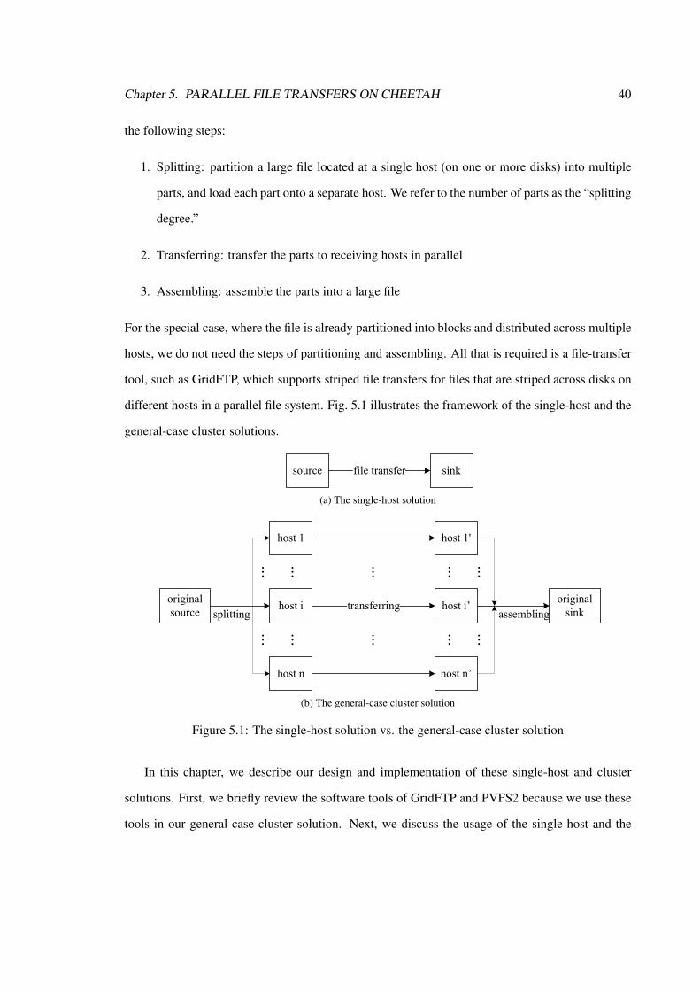
Chapter 5. PARALLEL FILE TRANSFERS ON CHEETAH 40
the following steps:
1. Splitting: partition a large file located at a single host (on one or more disks) into multiple
parts, and load each part onto a separate host. We refer to the number of parts as the “splitting
degree.”
2. Transferring: transfer the parts to receiving hosts in parallel
3. Assembling: assemble the parts into a large file
For the special case, where the file is already partitioned into blocks and distributed across multiple
hosts, we do not need the steps of partitioning and assembling. All that is required is a file-transfer
tool, such as GridFTP, which supports striped file transfers for files that are striped across disks on
different hosts in a parallel file system. Fig. 5.1 illustrates the framework of the single-host and the
general-case cluster solutions.
source sinkfile transfer
(a) The single-host solution
original
sourcehost i
host 1
host n
......
......
splitting
original
sinkhost i’
host 1'
host n’
......
......
assemblingtransferring
......
(b) The general-case cluster solution
Figure 5.1: The single-host solution vs. the general-case cluster solution
In this chapter, we describe our design and implementation of these single-host and cluster
solutions. First, we briefly review the software tools of GridFTP and PVFS2 because we use these
tools in our general-case cluster solution. Next, we discuss the usage of the single-host and the

Chapter 5. PARALLEL FILE TRANSFERS ON CHEETAH 41
general-case cluster solutions. Finally, we describe a specific-case solution for moving datasets in
the TSI project.
5.2 Background
In this section, we briefly review File Transfer Protocol (FTP) and then describe how GridFTP
extends FTP to include the new features of multi-streaming, partial file transfer, and striping. We
also provide a brief overview of PVFS.
5.2.1 FTP and GridFTP
GridFTP is a data-transfer protocol proposed for fast data transfers on the Grid [1, 2]. It extends
FTP [36] by adding features for partial file transfer, multi-streaming, striping, and Globus-based
security. It has been implemented by the Globus Alliance as a component of the Globus Toolkit
(GT) [18, 20].
In the cluster solution, we mainly use the GridFTP functionalities of third-party control, partial
data transfer, multi-streaming, and especially striped data transfer. Before we describe GridFTP’s
extensions to FTP, we overview FTP and focus on its feature of third-party control.1
There are two kinds of TCP connections in FTP: control connections and data connections. All
FTP commands are transferred over the control connection, while user data are transferred over the
data connection. The default port number of the control connection on the FTP server is 21 and that
of the data connection is 20.
Third-party control provided in FTP allows a user to transfer files between two other hosts. To
implement this feature, FTP provides two commands, PASV and PORT. PASV has no argument
and is an abbreviation for passive. Just as the term “passive” implies, PASV requests an FTP server
to wait for a data connection rather than to initiate one on receiving a data transfer command.
PORT has an argument of host–port pair, with which it specifies the data port to be used in a data
connection.1Although RFC 959 [36] specifies this feature, it does not refer to the feature as “third-party control.” Instead, the
GridFTP specification [1] introduces the term, “third-party control.”

Chapter 5. PARALLEL FILE TRANSFERS ON CHEETAH 42
FTP client
C
6. B initiates a data connection to A
1. control connection
2. PASV3. host-port pair
FTP server
A
FTP server
B
1. control connection
4. PORT <host-port pair>5. response to PORT
Figure 5.2: The model and flow chart of third-party control
Fig. 5.2 shows the model and flow chart of third-party control. First, an FTP client on a third
party, denoted as C, establishes control connections to two FTP servers, denoted as A and B. C
forwards all FTP commands, such as user and password, between A and B via the control connec-
tions. Then, C sends a PASV command to A. On receiving PASV, A listens on a data port, which it
selects to be a number distinct from the well known port number, 20, returns to C a host–port pair
(host provides A’s IP and port is the one on which A listens for a connection), and waits for a data
connection. Then, C sends a PORT command to B with the host–port pair as the argument. After B
receives the PORT command, it initiates a data connection to A at the port on which A waits for a
connection.
FTP has three transfer modes:
1. Stream mode: transmit data as a stream of bytes
2. Block mode: transmit data as a series of data blocks. Each block is identified by a 3-byte
header, which contains two fields: 1-byte descriptor and 2-byte length. The descriptor field
indicates whether the block is a special block, for example, the last block that ends a file. The
length field specifies the length of the block.
3. Compressed mode: transmit compressed data
All these modes transfer data in sequence and do not support partial file transfer.
GridFTP extends the block mode by adding an offset field in the block header to support out-of-
sequence data delivery. With this extended block mode, GridFTP can do partial file transfer, which
transfers portions of files rather than complete files. This extended block mode is also fundamental
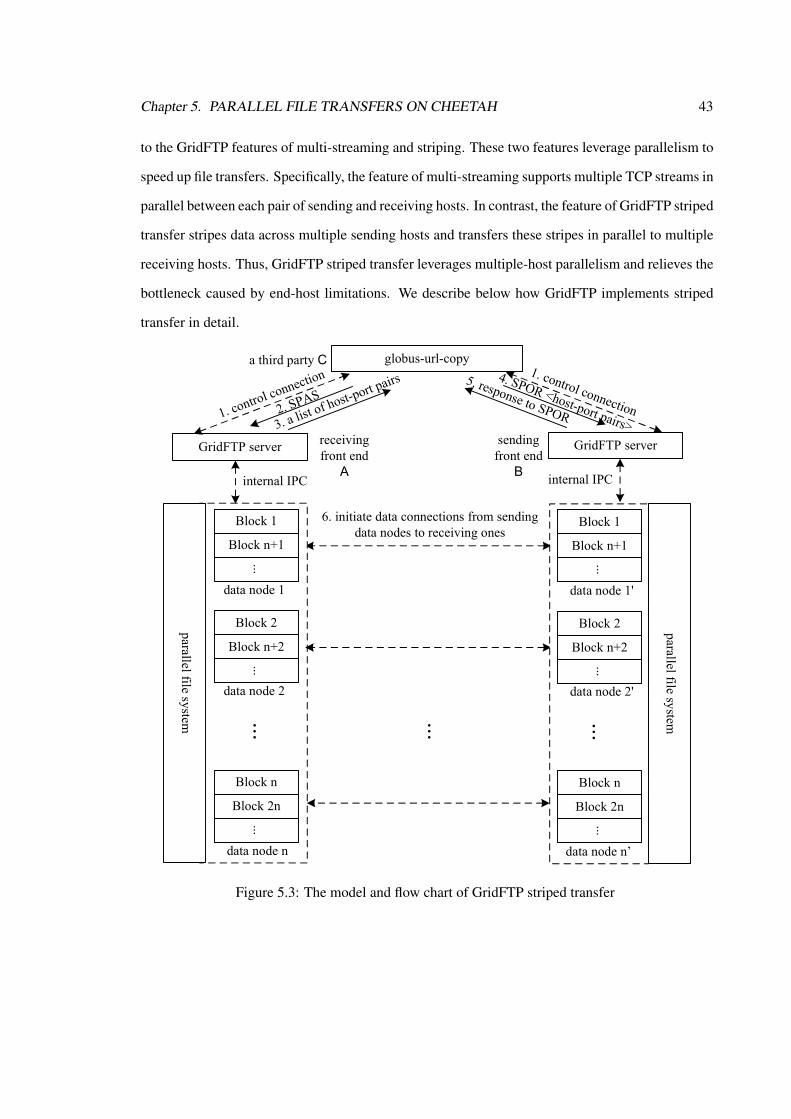
Chapter 5. PARALLEL FILE TRANSFERS ON CHEETAH 43
to the GridFTP features of multi-streaming and striping. These two features leverage parallelism to
speed up file transfers. Specifically, the feature of multi-streaming supports multiple TCP streams in
parallel between each pair of sending and receiving hosts. In contrast, the feature of GridFTP striped
transfer stripes data across multiple sending hosts and transfers these stripes in parallel to multiple
receiving hosts. Thus, GridFTP striped transfer leverages multiple-host parallelism and relieves the
bottleneck caused by end-host limitations. We describe below how GridFTP implements striped
transfer in detail.
GridFTP server
Block 1
Block n+1...
Block 2
Block n+2
...
Block n
Block 2n
...
data node 1
data node n
parallel file sy
stem
1. cont
rol con
nection
internal IPC
2. SPA
S
3. a list
of hos
t-port p
airs
globus-url-copy
receiving
front end
A
a third party C
data node 2
...
GridFTP server
Block 1
Block n+1
...
Block 2
Block n+2
...
Block n
Block 2n
...
data node 1'
data node n’
parallel file sy
stem
1. control connection
internal IPC
4. SPOR <host-port pairs>
5. response to SPOR
sending
front end
B
data node 2'
...
6. initiate data connections from sending
data nodes to receiving ones
...
Figure 5.3: The model and flow chart of GridFTP striped transfer

Chapter 5. PARALLEL FILE TRANSFERS ON CHEETAH 44
Fig. 5.3 shows the model of GridFTP striped transfer.2 Multiple pairs of end hosts, termed
as “data nodes” and typically located in two clusters, participate in a single data transfer that is
controlled by two GridFTP servers, termed as “front ends,” and a third party, which runs globus-
url-copy (a GridFTP client tool provided by GT). Each front end acts as the single GridFTP control
server on each cluster to coordinate file transfers between data nodes. Each data node moves the
parts of the file assigned to it to its peer.
To support GridFTP striped transfer, GridFTP defines two commands, SPAS and SPOR, which
extend PASV and PORT, respectively. If a front end receives a SPAS command, it requests all its
data nodes to wait for data connections and returns a list of host–port pairs for these data nodes. In
contrast, if a front end receives a SPOR command with a list of host–port pairs, it notifies its data
nodes to initiate data connections to the hosts specified in the SPOR command’s argument list.
Comparing Fig. 5.2 with Fig. 5.3, we see that the flow chart for GridFTP striped transfer is
similar to that for third-party control provided in FTP. The additional features in GridFTP striped
transfer are as follows. First, it involves many data nodes. Second, it uses SPAS and SPOR in-
stead of PASV and PORT. Third, it is required be unidirectional, which means that SPAS is paired
with a receiving front end and SPOR, with a sending one. In contrast, FTP does not have any
such restriction. Fourth, a front end communicates with its data nodes through an internal Inter-
process Communication (IPC) protocol, which is unspecified in the GridFTP specification. Finally,
although there are multiple data connections between sending and receiving data nodes, there are
only two control connections between two front ends and a third party.
In addition, as shown in Fig. 5.3, GridFTP striped transfer requires that end hosts on each cluster
have access to the file, which means that the file needs to be managed by a parallel file system.
Furthermore, the underlying parallel file system must deliver a high read–write throughput to avoid
becoming a bottleneck itself. Currently, General Parallel File System (GPFS) [21] and PVFS2 are
two popular parallel file systems. We use PVFS2 in our experiments because PVFS2 is open-source
software allowing us to make any required modifications whereas GPFS is a commercial product.
2Unless otherwise mentioned, the number of sending hosts is equal to that of receiving hosts. Although the twonumbers are not required to be equal, we make them equal to simplify our explanation.

Chapter 5. PARALLEL FILE TRANSFERS ON CHEETAH 45
5.2.2 PVFS2
Clemson University and Argonne National Laboratory jointly developed PVFS (or PVFS1) [12,37],
which has been released and supported under a GNU General Public License since 1998. The PVFS
team aimed to design and implement a parallel I/O system that handles the performance disparity
between I/O devices and processors, and addresses the scalability problem of Network File System
(NFS).
NFS is a distributed file system developed by Sun Microsystems, Inc. It is a client–server
application and allows a user to conveniently access files on a remote computer [48]. An NFS
server stores all files in a central location, which causes a scalability problem when the number of
clients exceeds the performance capacity of the machine exporting the file system. We can equip an
NFS server with more memory, a faster CPU, and higher-speed NICs, but being a central node, it
can still run out of resources. As the number of client nodes increases, each client receives a smaller
portion of the overall bandwidth for file I/O. Another problem is availability. If an NFS server goes
down, all its client nodes have to wait until the server recovers.
Unlike NFS, which is a central data storage system, PVFS uses storage on multiple computers
to create a large high-performance parallel file system. PVFS physically distributes a single file
across multiple disks in multiple nodes. For example, it stripes a file over the local disks in multiple
I/O servers using a simple round-robin style as in RAID0. Fig. 5.4 shows the system architecture
for PVFS1.3 It is still a client–server file system. Each host may play one or more of the following
three roles:
1. compute nodes (CN or clients), where applications run
2. I/O nodes (ION or I/O servers), where files are stored
3. metadata sever or management node (MGR), where metadata operations are handled
PVFS1 can have one and only one management node.
3This figure is adapted from PVFS1 user guide [37].

Chapter 5. PARALLEL FILE TRANSFERS ON CHEETAH 46
Figure 5.4: PVFS system architecture
A second version of PVFS, PVFS2, has several new features [38, 39]. For example, it allows
for several management nodes, which eliminates the possible bottleneck caused by a single man-
agement node in PVFS1. But it uses the same principles as PVFS1 to create a parallel file system.
5.3 The Single-Host Solution
The single-host solution leverages high-speed hardware to avoid the end-host bottleneck. Specif-
ically, we concentrate on the bottleneck created by hard-disk I/O. The other PC hardware compo-
nents, such as NICs, PCI-X buses, memory buses, and CPUs, are also possible bottlenecks, but as
Hurwitz and Feng [23] pointed out, these components are not the primary bottlenecks and they are
kept updated by new technologies. For example, new PCI Express×16 implementation will achieve
a peak bandwidth of 64 Gb/s [10] and thus will remove the possible bottleneck caused by the I/O
bus. To relieve the disk bottleneck, we can equip sending and receiving hosts with redundant arrays
of inexpensive disks (RAIDs). However, what is the peak write speed for a RAID?4 Is the hard-
ware solution feasible, scalable, and cost-effective? In this section, we address these questions after
4In this section, we only use write speed for our comparison because write speed is lower than read speed.

Chapter 5. PARALLEL FILE TRANSFERS ON CHEETAH 47
providing a brief overview of RAID.
Patterson, Gibson and Katz [35] formally defined RAID levels one through five and showed
that RAID outperformed single large expensive disks by an order of magnitude in speed, reliability,
scalability, and other metrics. Currently, the most commonly used RAID levels are RAID0 and
RAID5. A RAID0 stripes data evenly across all member disks without any parity or redundancy. A
RAID5 stripes data, including parity information, across all member disks.
Assume that the number of disks is M and that each disk has an equal write speed of x. If I/O
operations are ideally split into equal-sized blocks and these blocks are distributed evenly across
the M disks, then these I/O operations can be carried out concurrently on all member disks. Since
all M disks for RAID0 contain data, the maximum write speed for RAID0 is M · x. In contrast, for
RAID5, one disk contains parity information for the I/O operations, and thus, the maximum speed
is (M− 1) · x. In practice, as the number of hard disks connected to a RAID controller increases,
the write speed may not increase proportionally because the RAID controller itself becomes the
bottleneck. Currently, over 1 Gb/s read–write speeds are achievable for RAIDs. Barclay, Chong,
and Gray [5] reported that an 8-disk 3ware Escalade 8508 controller saturated at 1.8 Gb/s read
and 1.6 Gb/s write. An 8-disk Areca ARC-1120 controller, configured as RAID5, was reported to
saturate at 6.0 Gb/s read and 3.6 Gb/s write [53]. Therefore, the hardware solution is feasible.
In light of the RAID0 and RAID5s’ designs, a theoretical disk utilization for RAID0 is 100%
and for RAID5, disk utilization is (M− 1)/M. Assume that each hard disk is 146 GB SCSI disk.
To accommodate 2 TB data, we need at least (2 TB)/(146 GB) = 15 hard disks for RAID0 and
even more for RAID5. To manage an array of more than 15 hard disks, we need a high-end RAID
host adapter with an I/O processor and memory to off-load the intensive RAID5 XOR parity com-
putation. Given the trends in communication bandwidth growth from 1 Gb/s to tens of Gb/s, I/O
performance is likely to lag behind network performance for the near-term future. Hence, we con-
clude that although the single-host solution is feasible for fast file transfers, it is neither scalable nor
cost-effective.
Chapter 5. PARALLEL FILE TRANSFERS ON CHEETAH 48
5.4 The General-Case Cluster Solution
In this section, we describe the cluster solution for the general case of non-split source files at the
sending end. First, we address the problem of determining an appropriate value for the splitting
degree. Second, we discuss possible approaches to implement the general-case cluster solution and
explain why we use GridFTP and PVFS2 to implement it. We also present our specific require-
ments for GridFTP and PVFS2 to minimize network-and-disk contention. Then, we describe our
modifications to GridFTP and PVFS2 to meet these requirements. Finally, we provide experimental
results after we modified GridFTP and PVFS2.
5.4.1 The Splitting Degree
As mentioned in Section 5.1, the general-case cluster solution needs to first partition the source file.
One important question is to determine an appropriate value for the splitting degree.
First, we should select the splitting degree such that the cluster solution transfers a source
file faster than an approach without splitting. Let the size of the source file be x, the splitting
degree be d (d ≥ 1, where d = 1 means that the file is not split), and the number of pairs of
sending and receiving hosts be n (see Fig. 5.1b). Assume that the 2 ·n hosts have the same hardware
and software configurations and thus have the same processing power. Let the disk I/O for each
host be r for reading and w for writing. Let the time to split and load the file, and the time to
assemble the file be Tsplit and Tassemble, respectively. Tsplit and Tassemble are serial in nature because
the splitting and assembling steps involve a single source or sink. We assume that Tsplit and Tassemble
are independent of the splitting degree d. Since hosts at the sending cluster are typically co-located
in one geographic location, we ignore the RTT delay for inter-host communication. Similarly, we
ignore the RTT delay amongst receiving hosts. Thus, we estimate Tsplit and Tassemble as follows:
Tsplit = Tassemble =xr
+xw
(5.1)
Let the time to transfer the whole file from a single host at the sending site to a single host at the
receiving site be Ttrans f er. Assume that we evenly split the file into d parts. If d < n, it takesTtrans f er
d

Chapter 5. PARALLEL FILE TRANSFERS ON CHEETAH 49
to transfer these parts in parallel. Otherwise, the time isTtrans f er
n because we do not benefit by
increasing d to be larger than n. Hence, we have the following equation to guide us in our selection
of the splitting degree:
Tsplit +Ttrans f er
min(d,n)+Tassemble < Ttrans f er (5.2)
The speedup for the general-case cluster solution is
speedup =Ttrans f er
Tsplit +Ttrans f er
min(d,n) +Tassemble
(5.3)
Combining (5.1), (5.2), and (5.3), we reason that to get the largest speedup, we should select
the splitting degree such that
d = n if n >Ttrans f er
Ttrans f er−2(xr
+xw
)
d = 1 otherwise
(5.4)
In addition, the Ttrans f er > 2(xr + x
w) requirement should be met; otherwise, the splitting and
assembling operations take longer time than the transferring operation. The two condition of
n >Ttrans f er
Ttrans f er−2(xr
+xw
)and Ttrans f er > 2(x
r + xw) determine whether we should split the source
file, that is, whether we should use the general-case cluster solution. If the file transfer is carried
out over the Internet, Ttrans f er increases significantly as RTT increases and/or network congestion
increases. Consequently, the probability of meeting these two conditions increases.
In contrast, if the file is transferred over a CO network, such as CHEETAH, bandwidth is re-
served for the file transfer and thus, there is no congestion during data flow. Assume that a circuit
of rate b is reserved between each pair of the sending and receiving hosts. Since we do not benefit
by reserving a circuit faster than w, b should be no larger than w even if maximum bandwidth rate
is larger than w. If b < w, Ttrans f er depends on b. Hence, we estimate Ttrans f er as follows:
Ttrans f er =x
min(b,w)(5.5)

Chapter 5. PARALLEL FILE TRANSFERS ON CHEETAH 50
Thus, to use the cluster solution, we should at least satisfy
xmin(b,w)
> 2(xr
+xw
) =⇒ b <rw
2(r +w)(5.6)
However, if the circuit bandwidth is high, then the probability of meeting the condition (5.6) is
low or even zero. This argues against the cluster solution on CHEETAH. But note that during
the previous analysis, we assume that the three steps of splitting, transferring, and assembling are
carried out separately. If we pipeline them, then we can decrease the total delay. For example,
while we split some parts and load them to sending hosts, we can transfer these available parts to
receiving hosts without waiting for the splitting step to be finished. Additionally, if we use PVFS2
to manage files and the starting point is already split file, the cluster solution has value even on
CHEETAH.
5.4.2 Design
In this section, we propose possible approaches to implement the three steps of the general-case
cluster solution. We discuss their advantages and disadvantages and decide to use GridFTP striped
transfer and PVFS2.
There are several possible approaches to splitting and assembling a file. The first approach is
to use the functionalities of partial transfer and third-party control provided by some file transfer
tools. For example, we use GridFTP. However, there are two problems with this approach. Firstly,
disk space of the whole file size should be allocated on each host. Thus, this implementation is not
suitable for a large file which cannot even reside on a single host. Secondly, this approach is serial
in nature and consumes much time as we mentioned in Section 5.4.1. Thus, the overall speedup is
significantly affected even though the transferring step has a theoretical speedup of min(d,n).
Alternatively, we can write a socket program to implement splitting and assembling and thus
overcome the first space problem of using GridFTP partial transfer. However, this approach still
has significant overhead for splitting and assembling.
The best approach is to use PVFS2 to manage files. PVFS2 provides a tool, pvfs2-cp, to transfer

Chapter 5. PARALLEL FILE TRANSFERS ON CHEETAH 51
files between PVFS2 and other file systems, such as NFS, Linux ext2, and Linux ext3. Thus, we can
use it to assemble a PVFS2 file, which is distributed across multiple I/O servers, into a non-split one
stored in the other file systems, and vice versa. PVFS2 automatically manages partitioning. From
a user’s point of view, a file can be accessed as though it was stored in a single central location.
Hence, we can avoid assembling if a user chooses to access a file in PVFS2. We can even avoid
splitting if files are initially created in PVFS2. Thus, we choose to use PVFS2 to manage files and
we use pvfs2-cp to split or assemble a file if necessary (i.e., a file is not originally managed by
PVFS2, if users need to access the file via a non-PVFS2 file system).
After deciding to use PVFS2 for splitting and assembling, we study the approaches to transmit-
ting parts of a file. The first approach is to use GridFTP partial transfer (or any file transfer tools
that provide the functionality of partial transfer) to transfer partitions from one PVFS2 to another
PVFS2 in parallel but independently. To achieve highest throughput, we should avoid unnecessary
network–and–disk contention in each PVFS2 system by making all GridFTP servers responsible
for moving only the data blocks located in their local disks. For example, we should avoid the
following scenario: a GridFTP server reads a non-local data block and sends the block to its peer
receiver, which then has to move the block using PVFS2 to a disk of another host. To avoid such
network–and–disk contention, we should meet the following two conditions:
1. The software should know a priori how data are striped in PVFS2.
2. PVFS2 I/O servers and GridFTP servers run on the same hosts and GridFTP servers are
responsible only for their local data blocks.
Provided that the first condition holds, the second condition becomes trivial. However, PVFS2 does
not provide any explicit utility to examine data distribution. Therefore, to meet the first condition,
we investigated how PVFS2 works and modified PVFS2 code. We will describe our modifications
to PVFS2 in Section 5.4.3. Fig. 5.5 shows a model of using GridFTP partial file transfer to imple-
ment the transferring step, where for each data block, there is a GridFTP control connection and a
GridFTP data connection responsible for transmitting the block between the two PVFS2 systems.

Chapter 5. PARALLEL FILE TRANSFERS ON CHEETAH 52
PV
FS2
Block 6
Block 1
PVFS2 I/O server 1
GridFTP server 1
...
Block 2n
Block n
...
...
PVFS2 I/O server n
GridFTP server n
PV
FS2
Block 6
Block 1
...
Block 2n
Block n
...
...PVFS2 I/O server 1'
GridFTP server 1'
PVFS2 I/O server n’
GridFTP server n’
...
GridFTP partial file transfer
Figure 5.5: A model of using GridFTP partial file transfer to implement the transferring step
The second approach is to use GridFTP striped transfer. Similar to the first approach, to achieve
highest throughput, we should also minimize network–and–disk contention in each PVFS2 system.
For this target, we should meet the following two conditions besides the two conditions for the first
approach:
1. GridFTP stripes data across data nodes in the same sequence as PVFS2 does across PVFS2
I/O servers.
2. GridFTP and PVFS2 have the same stripe size.
We can easily meet the second condition by setting the stripe-size parameters for GridFTP and
PVFS2 to have the same value. We will address how we modified GridFTP code to meet the first
condition in Section 5.4.4.
Fig. 5.6 shows the model of using GridFTP striped transfer to implement the transferring step.
Unlike the first transferring approach, which is composed of many independent parallel partial
transfers, this approach has only a single file transfer involving many hosts (see Section 5.2.1). As
shown in Fig. 5.6, there are only two control connections between a third party and two front ends.
In addition, for each pair of sending and receiving data nodes, there is only a single data connection.

Chapter 5. PARALLEL FILE TRANSFERS ON CHEETAH 53
GridFTP server
Block 1
Block n+1
...
Block n
Block 2n...
I/O server 1
data node 1
I/O server n
data node n
PVFS2
control
connec
tion
internal IPC
globus-url-copy
receiving
front end
A
a third party C
...
GridFTP server
Block 1
Block n+1
...
Block n
Block 2n
...
I/O server 1'
data node 1'
I/O server n’
data node n’
PVFS2
control connection
internal IPC
sending
front end
B
...
data connection
...
data connection
Figure 5.6: A model of using GridFTP striped transfer to implement the transferring step
Comparing Fig. 5.5 with Fig. 5.6, we see that the approach using GridFTP striped transfer is more
natural and has less overhead to establish and release connections. For these reasons, we choose
to use GridFTP striped transfer to implement the transferring step. In conclusion, we use GridFTP
striped transfer and PVFS2 to implement the general-case cluster solution. For convenience, we
summarize the above-described approaches in Table 5.1.
5.4.3 Implementation—Modifications to PVFS2
As mentioned in Section 5.4.2, to minimize network–and–disk contention in the general-case clus-
ter solution, we need to know how a file is striped in PVFS2. In this subsection, we describe our
modifications to PVFS2 to obtain data distribution information.

Chapter 5. PARALLEL FILE TRANSFERS ON CHEETAH 54
Table 5.1: A summary of possible approaches to implement the general-case cluster solutionSteps Approach Pros. Cons.
GridFTPpartial filetransfer
wastes disk space, consumessignificant overhead to splitand assemble
splitting &assembling
socketprogram
avoids wasting disk space consumes significant overheadto split and assemble
pvfs2-cp avoids wasting disk space,avoids assembling or evensplitting overhead
transferring GridFTPpartial filetransfer
many independent transferswhich incurs much overheadto set up and release connec-tions
GridFTPstripedtransfer
a single file transfer
We installed two PVFS2 1.0.1 systems on a 22-node cluster, called sunfire. Sunfire1 through
sunfire22 are all equipped with two Intel(R)-Xeon 2.80 GHz CPUs, and 1 GB RAM, and are con-
nected to a 24-port GbE switch. They run Redhat Linux 9 and are the clients of an NFS server,
called centurion. We loaded each PVFS2 system on five sunfire hosts. For the first PVFS2 system,
we configured sunfire1 through sunfire5 as the I/O servers and compute nodes, and sunfire1 as the
only metadata server. For the second PVFS2 system, we configure sunfire6 through sunfire10 as
the I/O servers and compute nodes, and sunfire6 as the only metadata server. The configuration file
for the second PVFS2 is shown in Fig. 5.7. In this subsection, we carried out the experiments in the
second PVFS2 system unless otherwise mentioned.
Unlike PVFS1, which provides the utility of pvstat to examine physical file-distribution param-
eters (e.g., the index of the starting I/O node, the number of I/O servers, and the stripe size) [43],
PVFS2 1.0.1 does not provide any direct utility to inspect data distribution. We reported this prob-
lem to the pvfs2-user mailing list and were advised to use the tool pvfs2-fs-dump, which displays
information about the contents of the file system.5 However, the output by pvfs2-fs-dump does not
explicitly illustrate how files are striped. The output is not only hard to comprehend, but also is
5See http://www.beowulf-underground.org/pipermail/pvfs2-users/2005-April/000622.html.

Chapter 5. PARALLEL FILE TRANSFERS ON CHEETAH 55
...<MetaHandleRanges>
Range sunfire6 4-715827885</MetaHandleRanges><DataHandleRanges>
Range sunfire10 715827886-1431655767Range sunfire6 1431655768-2147483649Range sunfire7 2147483650-2863311531Range sunfire8 2863311532-3579139413Range sunfire9 3579139414-4294967295
</DataHandleRanges>...
Figure 5.7: A snippet of pvfs2-fs2.conf, the PVFS2 configuration file on sunfire6
verbose when the PVFS2 file system contains myriad files. Fig. 5.8 shows a part of the output of
the pvfs2-fs-dump command. For each file in PVFS2, pvfs2-fs-dump provides the handle number,...File: test_500M
handle = 715827830, type = Metafile, server = 0handle = 3579139362, type = Datafile, server = 3handle = 4294967244, type = Datafile, server = 4handle = 1431655716, type = Datafile, server = 0handle = 2147483598, type = Datafile, server = 1handle = 2863311480, type = Datafile, server = 2
File: test_2000Mhandle = 715827861, type = Metafile, server = 0handle = 2863311500, type = Datafile, server = 2handle = 3579139382, type = Datafile, server = 3handle = 4294967264, type = Datafile, server = 4handle = 1431655736, type = Datafile, server = 0handle = 2147483608, type = Datafile, server = 1
...
Figure 5.8: A part of the output for pvfs2-fs-dump
the type (Metafile or Datafile), and the I/O or metadata server number.We wanted answers to the
following questions. First, the I/O server numbers and metadata server numbers are logical num-
bers. It is unclear how PVFS2 match the logical server numbers with the physical servers. Second,
the order of the server numbers is not deterministic; for example, the file test 500M is striped in the

Chapter 5. PARALLEL FILE TRANSFERS ON CHEETAH 56
order 3, 4, 0, 1, and 2 whereas the file test 2000M is striped in the order 2, 3, 4, 0, and 1. How is
this order determined? Does it indicate the round-robin sequence of the I/O servers where the files
are distributed? Finally, the output of pvfs2-fs-dump does not provide any information about the
data stripe size. The default stripe size is 64 KB, but can a user set the stripe size?
The first question was easy to answer. Sunfire6 is the only metadata server (see Fig. 5.7).
Therefore, as a metadata server, sunfire6 has the logical number 0 (see Fig. 5.8). By combining the
handle numbers in Fig. 5.8 and the handle ranges for each data server in Fig. 5.7, we determined
physical servers corresponding to logical numbers (see Table 5.2). In other words, by combining
the output of pvfs2-fs-dump command and the contents of the pvfs2-fs2.conf file, we determined the
identification of the physical servers corresponding to logical numbers of I/O nodes.
Table 5.2: The logical server numbers for the physical I/O serversPhysical I/O server Logical number
sunfire10 0sunfire6 1sunfire7 2sunfire8 3sunfire9 4
To answer the other two questions, we wrote a program, called filegenerator, to create a file
such that the file stores the striping information. Consider an s-KB file with the format shown in
Fig. 5.9. We used the strace command to trace the system calls called by the utility pvfs2-cp. We
describe our trace results below.
1a...a︸ ︷︷ ︸ 2a...a︸ ︷︷ ︸ ... sa...a︸ ︷︷ ︸1024B 1024B ... 1024B
Figure 5.9: The content of an s KB file
First, we used filegenerator to create a 1000 MB file, called test 1000M, in the directory of /tmp/
on sunfire10. Then, we issued the command strace pvfs2-cp -t /tmp/test 1000M /pvfs2/test 1000M
-o testfile/pvfs2cp2 to copy the file into PVFS2 and to save the strace output into the file, called

Chapter 5. PARALLEL FILE TRANSFERS ON CHEETAH 57
[xf4c@sunfire10 xf4c]$ more testfile/pvfs2cp2 | grep connect...connect( 4,sa_family=AF_INET, sin_port=htons(3334),sin_addr=inet_addr( "128.143.63.248"), 16) = -1 EINPROGRESS(Operation now in progress)connect( 6,sa_family=AF_INET,sin_port=htons(3334),sin_addr=inet_addr( "128.143.63.216"), 16) = -1 EINPROGRESS(Operation now in progress)connect( 7,sa_family=AF_INET,sin_port=htons(3334),sin_addr=inet_addr( "128.143.63.226"), 16) = -1 EINPROGRESS(Operation now in progress)connect( 8,sa_family=AF_INET,sin_port=htons(3334),sin_addr=inet_addr( "128.143.63.224"), 16) = -1 EINPROGRESS(Operation now in progress)connect( 9,sa_family=AF_INET,sin_port=htons(3334),sin_addr=inet_addr( "128.143.63.225"), 16) = -1 EINPROGRESS(Operation now in progress)...
Figure 5.10: A part of the output for the command more testfile/pvfs2cp2 | grep connect
testfile/pvfs2cp2. Next, we identified the file descriptors used in the I/O servers on sunfire by typ-
ing the command more testfile/pvfs2cp2 | grep connect. From Fig. 5.106, we determined the file
descriptors used in sunfire6 through sunfire10 by matching IP addresses from Fig. 5.10 with the
names of these machines. The results are shown in Table 5.3. Further, we used the command,
more testfile/pvfs2cp2 | grep writev | more, to determine how the file was distributed across the I/O
servers. Fig. 5.11 shows a small part of the output for this command, where we saw that the distance
between neighboring blocks on the same host was 320 KB (e.g., 385-65, 321-1, etc.). Since each
Table 5.3: The file descriptors and IP addresses for sunfire6 through sunfire10File descriptor IP address Host name
4 128.143.63.248 sunfire106 128.143.63.216 sunfire67 128.143.63.226 sunfire98 128.143.63.224 sunfire79 128.143.63.225 sunfire8
6We configured the I/O servers and the metedata server to listen on the default TCP port number 3334.

Chapter 5. PARALLEL FILE TRANSFERS ON CHEETAH 58
writev( 4, ...,"65aaaaaaaaaaaaaaaaaaaaaaaaaaaaaa"..., 65536,"385aaaaaaaaaaaaaaaaaaaaaaaaaaaaa"..., 65536,...writev( 7,...,"1aaaaaaaaaaaaaaaaaaaaaaaaaaaaaaa"..., 65536,"321aaaaaaaaaaaaaaaaaaaaaaaaaaaaa"..., 65536,...writev( 6,...,"129aaaaaaaaaaaaaaaaaaaaaaaaaaaaa"..., 65536,"449aaaaaaaaaaaaaaaaaaaaaaaaaaaaa"..., 65536,...writev( 8,...,"193aaaaaaaaaaaaaaaaaaaaaaaaaaaaa"..., 65536,"513a aaaaaaaaaaaaaaaaaaaaaaaaaaaa"..., 65536,...writev( 9,...,"257aaaaaaaaaaaaaaaaaaaaaaaaaaaaa"..., 65536,"577aaaaaaaaaaaaaaaaaaaaaaaaaaaaa"..., 65536,...
Figure 5.11: A part of the output of the command more testfile/pvfs2cp2 | grep writev | more
stripe was 64 KB, and there were five I/O servers, neighboring blocks were 65×5 = 320 KB apart.
Combining Fig. 5.11 and Table 5.3, we summarized the data-distribution pattern for test 1000M
in Table 5.4. Thus, test 1000M was distributed cyclicly across sunfire9, sunfire10, sunfire6, sun-
fire7, and sunfire8. Finally, we examined the output of pvfs2-fs-dump for test 1000M, as shown in
Fig. 5.12. Combining Fig. 5.12 and Table 5.1, we found that the I/O-server sequence given by pvfs2-
fs-dump was also sunfire9, sunfire10, sunfire6, sunfire7, and sunfire8. Therefore, we concluded that
Table 5.4: The data-distribution pattern for /pvfs2/test 1000MFile descriptor Host name Starting offset for each block
4 sunfire10 65, 385, 705 ... 10237456 sunfire6 129, 449, 769, ... 10238097 sunfire9 1,321,641,961, ... 10236818 sunfire7 193, 513, 833, ... 10238739 sunfire8 257, 577, 897, ... 1023937

Chapter 5. PARALLEL FILE TRANSFERS ON CHEETAH 59
...File: test_1000M
handle = 715827870, type = Metafile, server = 0handle = 4294967284, type = Datafile, server = 4handle = 1431655756, type = Datafile, server = 0handle = 2147483638, type = Datafile, server = 1handle = 2863311520, type = Datafile, server = 2handle = 3579139402, type = Datafile, server = 3
...
Figure 5.12: The pvfs2-fs-dump output for the test 1000M file
pvfs2-fs-dump shows the round-robin sequence of the I/O servers for file distribution.7
For the third question on the stripe size, we first used filegenerator to create a 128 KB
file, called test 128K. Then, we typed the command strace pvfs2-cp -s 131072 -t /tmp/test 128K
/pvfs2/test 128K2 -o pvfs2cp, which specified the stripe size as 128 KB in the -s option. Fig. 5.13
shows a part of the strace output, where the stripe size was 64 KB instead. Thus, we concluded that
writev( 4,...," 1aaaaaaaaaaaaaaaaaaaaaaaaaaaaaaa"...)...writev( 6,...," 65aaaaaaaaaaaaaaaaaaaaaaaaaaaaaa"...)...
Figure 5.13: A snippet from the file pvfs2cp
in PVFS2 1.0.1, pvfs2-cp has a bug of ignoring the -s option.8 To change the default stripe size,
we investigated the PVFS2 1.0.1 source code. We found that the statement that specifies the default
stripe size (64 KB) is located in the program $PVFS2dir9/src/io/description/Dist-simple-stripe.c as
shown below:
static PVFS_simple_stripe_params simple_stripe_params = 65536 /* strip size */
;7We repeated the procedure for many files and found that the result always holds. The PVFS2 team also confirmed
this result.8we reported this problem to the pvfs2-developer mailing list and were notified that this problem would be fixed in
the future.9$PVFS2dir denotes where PVFS2 is installed

Chapter 5. PARALLEL FILE TRANSFERS ON CHEETAH 60
By setting the parameter simple stripe params, we can change the default stripe size and
thus overcome the problem of pvfs2-cp ignoring the -s option. For example, we set sim-
ple stripe params=1048576 and recompiled the code. Then, we used pvfs2-cp to copy test 1000M
into PVFS2 and used strace to observe the system calls called by pvfs2-cp. Fig. 5.14 shows a part
of the strace output, where test 1000M was distributed across the I/O servers with the 1 MB stripe
size.
writev( 4,...," 1aaaaaaaaaaaaaaaaaaaaaaaaaaaaaaa"...,)...writev( 6,...," 1025aaaaaaaaaaaaaaaaaaaaaaaaaaaa"...,)...writev( 7,...," 2049aaaaaaaaaaaaaaaaaaaaaaaaaaaa"...,)...writev( 8,...," 3073aaaaaaaaaaaaaaaaaaaaaaaaaaaa"...,)...writev( 9,...," 4097aaaaaaaaaaaaaaaaaaaaaaaaaaaa"...,)...
Figure 5.14: A part of the output for the strace command
Finally, we addressed the problem that PVFS2 stripes files across the I/O servers in a nonde-
terministic sequence. We found that inside the program $PVFS2dirsrc/common/misc/pint-cached-
config.c, there is a function, PINT cached config get next io(), which chooses a random I/O server
and then uses the order specified in pvfs2-fs2.conf to distribute a file, as shown in Fig. 5.15. The
reason that PVFS2 was designed to stripe data with a random starting I/O server is load balanc-
ing. But in our general-case cluster solution, we need to predict how a file is striped to minimize
network-and-disk contention. Hence, we modified the boldfaced statement in Fig. 5.15 into jitter
= -1 and obtained a predictable (fixed) order of data distribution. In other words, a file is distributed
across all the I/O servers according to the logical order specified in pvfs2-fs2.conf. Thus, for the
second PVFS2, the sequence is sunfire10, sunfire6, sunfire7, sunfire8, and sunfire9; and for the first
PVFS2, the sequence is sunfire1, sunfire2, sunfire3, sunfire4, and sunfire5. Consequently, given the
information of stripe size, we can exactly figure out how a file is striped across the I/O servers.

Chapter 5. PARALLEL FILE TRANSFERS ON CHEETAH 61
/* PINT_cached_config_get_next_io()* returns the address of a set of servers that should be used to* store new pieces of file data. This function is responsible for* evenly distributing the file data storage load to all servers.*/
int PINT_cached_config_get_next_io(...)
...num_io_servers = PINT_llist_count(
cur_config_cache->fs->data_handle_ranges);
/* pick random starting point */jitter = (rand() % num_io_servers);while(jitter-- > -1)
cur_mapping = PINT_llist_head(cur_config_cache->data_server_cursor);...cur_config_cache->data_server_cursor = PINT_llist_next(
cur_config_cache->data_server_cursor);
while(num_servers)
...cur_config_cache->data_server_cursor = PINT_llist_next(
cur_config_cache->data_server_cursor);data_server_bmi_str = PINT_config_get_host_addr_ptr(
config,cur_mapping->alias_mapping->host_alias);...
Figure 5.15: A snippet of the source code for PINT cached config get next io()
5.4.4 Implementation—Modifications to GridFTP
GridFTP stripes data across data nodes according to a data-connection sequence, termed “stripe
index,” in the range of 0 to n− 1. To meet the condition that GridFTP stripes data across data
nodes in the same sequence as PVFS2 does across PVFS2 I/O servers, we first need to answer
the question: what is the stripe index for each pair of sending and receiving data nodes? In other

Chapter 5. PARALLEL FILE TRANSFERS ON CHEETAH 62
words, in GridFTP striped transfer, how and in what order are sending data nodes matched with
receiving ones? The GridFTP specification [1] does not address this question. In this section, we
first investigate how sending and receiving data nodes are matched. Our experimental results show
that the matching is nondeterministic and thus, we cannot avoid the network-and-disk contention
unless we modify GridFTP code. Then, we describe how to modify the GridFTP code to get a
deterministic matching sequence between sending and receiving data nodes.
We installed the GridFTP package provided by GT3.9.5 on sunfire. This GridFTP package
contains the functionality of GridFTP striped transfer. We started GridFTP servers on sunfire1
through sunfire10 such that sunfire1 and sunfire6 are front ends and the other eight hosts are data
nodes. Fig. 5.16 shows the commands. With the -r option, we specified that the data nodes for
sunfire1 were ordered as sunfire2 through sunfire5 and those for sunfire6 were sunfire7 through
sunfire10. The -dn option means that the GridFTP server is a data node. We expected sunfire2
through sunfire5 and sunfire7 through sunfire10 were ideally matched according to the sequences
specified in the -r option, which means that sunfire2 would communicate with sunfire7, sunfire3
with sunfire8, and so on. However, the following results show that GridFTP striped transfer does
not work in this ideal way.
[xf4c@sunfire1 xf4c]$ /home/xf4c/gt3.9.5/sbin/globus-gridftp-server -aa-p 50001 -r sunfire2:5001, sunfire3:5001, sunfire4:5001, sunfire5:5001
[xf4c@sunfire6 etc]$ /home/xf4c/gt3.9.5/sbin/globus-gridftp-server -aa-p 50002 -r sunfire7:5001, sunfire8:5001, sunfire9:5001, sunfire10:5001
[xf4c@sunfire2 xf4c]$ /home/xf4c/gt3.9.5/sbin/globus-gridftp-server -aa-p 50001 -dn
...[xf4c@sunfire5 xf4c]$ /home/xf4c/gt3.9.5/sbin/globus-gridftp-server -aa
-p 50001 -dn[xf4c@sunfire7 xf4c]$ /home/xf4c/gt3.9.5/sbin/globus-gridftp-server -aa
-p 50001 -dn...[xf4c@sunfire10 xf4c]$ /home/xf4c/gt3.9.5/sbin/globus-gridftp-server -aa
-p 50001 -dn
Figure 5.16: The commands to start GridFTP servers on sunfire
We started globus-url-copy on a third party, sunfire11, to use the functionality of GridFTP striped

Chapter 5. PARALLEL FILE TRANSFERS ON CHEETAH 63
transfer (by turning on the -stripe option). The command is as follows:
[xf4c@sunfire11 xf4c]$ $GLOBUS_LOCATION/bin/globus-url-copy -vb -dbg
-stripe ftp://sunfire1:50001/home/xf4c/testfile/test_1G
ftp://sunfire6:50002/home/xf4c/testfile/test_1G1 2>dbg1.txt
We turned on the debug mode with the -dbg option so that we could obtain the details. Fig. 5.17
shows a part of the debug output. By examining the information in Fig. 5.17 below and Table 5.3
on page 57, we saw that the sequence for host–port pairs returned by the SPAS command were sun-
fire10, sunfire9, sunfire8, sunfire7 rather than the sequence of sunfire7 through sunfire10 specified
by the -r option for sunfire6.
The result of SPAS:debug: sending command: SPASdebug: response fromftp://sunfire6:50002/home/xf4c/testfile/test_1G1: 229-EnteringStriped Passive Mode.128,143,63,248,185,185128,143,63,226,186,31128,143,63,225,185,170128,143,63,224,186,15
229 End
Figure 5.17: A part of the debug output for the GridFTP striped transfer
Before the GridFTP striped transfer, we also started tcpdump [51] to capture the GridFTP traffic
amongst sunfire1 through sunfire10. After the transfer was finished, we used tcptrace [52] to ana-
lyze the captured traffic. Fig. 5.18 shows the tcptrace outputs for sunfire7–10. The GridFTP data
connections were between sunfire4 and sunfire10, sunfire3 and sunfire9, sunfire2 and sunfire8, and
sunfire5 and sunfire7. Thus, when the sending front end, sunfire1, executed the SPOR command, it
did not require its data nodes (sunfire2 through sunfire5) to establish connections sequentially with
the hosts returned by the SPAS command (sunfire10, sunfire9, sunfire8, sunfire7). We repeated the
experiment several times, and found that neither SPAS nor SPOR follows the sequence specified by
the -r option. Hence, we could not predict how data connections were established between multiple
data nodes.

Chapter 5. PARALLEL FILE TRANSFERS ON CHEETAH 64
[xf4c@sunfire10 tcptrace-6.6.7]$ tcptrace /tmp/sunfire10.log280048 packets seen, 280020 TCP packets tracedelapsed wallclock time:0:00:00.652783, 429006 pkts/sec analyzedtrace file elapsed time:0:08:30.409906TCP connection info:1: sunfire6.cs.Virginia.EDU:47763 - sunfire10.cs.Virginia.EDU:5001 (a2b)
221> 187< (complete)2: sunfire4.cs.Virginia.EDU:4878 - sunfire10.cs.Virginia.EDU:47545 (c2d)
186099> 93513< (complete)
[xf4c@sunfire9 tcptrace-6.6.7]$ tcptrace /tmp/sunfire9.log278903 packets seen, 278885 TCP packets tracedelapsed wallclock time:0:00:00.891238, 312938 pkts/sec analyzedtrace file elapsed time:0:07:27.005080TCP connection info:1: sunfire6.cs.Virginia.EDU:47764 - sunfire9.cs.Virginia.EDU:5001 (a2b)
212> 174< (complete)2: sunfire3.cs.Virginia.EDU:47586 - sunfire9.cs.Virginia.EDU:47647 (c2d)
185247> 93252< (complete)
[xf4c@sunfire8 tcptrace-6.6.7]$ tcptrace /tmp/sunfire8.log279503 packets seen, 279482 TCP packets tracedelapsed wallclock time: 0:00:00.745197, 375072 pkts/sec analyzedtrace file elapsed time: 0:07:50.749054TCP connection info:1: sunfire6.cs.Virginia.EDU:47765 - sunfire8.cs.Virginia.EDU:5001 (a2b)
215> 180< (complete)2: sunfire2.cs.Virginia.DU:48556 - sunfire8.cs.Virginia.EDU:47530 (c2d)
185827> 93260< (complete)
[xf4c@sunfire7 tcptrace-6.6.7]$ tcptrace /tmp/sunfire7.log275137 packets seen, 275109 TCP packets tracedelapsed wallclock time:0:00:01.237319, 222365 pkts/sec analyzedtrace file elapsed time:0:08:30.410378TCP connection info:1: sunfire6.cs.Virgiia.EDU:47766 - sunfire7.cs.Virginia.EDU:5001 (a2b)
209> 167< (complete)2: sunfire5.cs.Virginia.EDU:47577 - sunfire7.cs.Virginia.EDU:47631(c2d)
182995> 91738< (complete)
Figure 5.18: The tcptrace outputs for GridFTP striped transfer before we modified GridFTP code

Chapter 5. PARALLEL FILE TRANSFERS ON CHEETAH 65
These nondeterministic data connections between sending and receiving data nodes are unsuit-
able for us to deploy the general-case cluster solution on CHEETAH. We need to reserve bandwidth
before a data transfer. Given the nondeterminism, we need to reserve bandwidth between any pairs
of sending and receiving hosts—there are totally n · (n− 1) pairs. We would waste and even run
out of bandwidth if we reserved bandwidth for all possible pairs. We can solve this problem by
reserving bandwidth between two cluster switches and allows any hosts connected to a switch to
communicate with any hosts connected to the other switch. However, to minimize network–and–
disk contention, we have to make data connections deterministic.
We studied the GridFTP source code in GT3.9.5 and modified the implementation of the SPAS
and SPOR commands. For the SPAS command, we first obtained the IP addresses of data nodes
specified in the -r option for a receiving front end. Then, we sorted the list of host–port pairs
generated by the old SPAS command according to the IP-address order for receiving data nodes.
Then, we let SPAS return the sorted list to the third party negotiating the GridFTP striped transfer.
Thus, the argument for the SPOR command sent to the sending front end was also sorted by the
order of the IP addresses of the receiving data nodes. For the SPOR command, we requested
sending data nodes specified in the -r option for a sending front end to initiate data connections
sequentially to receiving data nodes specified in the argument of the SPOR command. In this
way, sending and receiving data nodes are matched according to their sequences in the -r option for
sending and receiving front ends. Additionally, their data connections have ascending stripe indexes
from 0 to n−1. Hence, it is easy to let GridFTP stripe data across data nodes in the same sequence
as PVFS2 does across PVFS2 I/O servers. We only need to set the -r option such that GridFTP data
nodes have the same sequence as PVFS2 I/O servers.
5.4.5 Experimental Results
We tested the general-case cluster solution on sunfire. In this section, we present the experimental
results to show that network–and–disk contention is minimized after we modified GridFTP and
PVFS2.
There are two PVFS2s on sunfire (see Section 5.4.3 on page 53). The I/O servers for the first

Chapter 5. PARALLEL FILE TRANSFERS ON CHEETAH 66
PVFS2 are ordered as sunfire1 through sunfire5. The I/O servers for the second PVFS2 are ordered
as sunfire10, and sunfire6 through sunfire9.
We started GridFTP front ends on sunfire1 and sunfire10 and GridFTP data nodes on sunfire1
through sunfire10. The data nodes for sunfire1 were ordered as sunfire1 through sunfire5 and those
for sunfire10 were sunfire10, sunfire6 through sunfire9.
Then, we started globus-url-copy on sunfire11 to conduct a file transfer between two PVFS2
systems on the sunfire cluster. The command is as follows:
[xf4c@sunfire11 xf4c]$ $GLOBUS_LOCATION/bin/globus-url-copy -vb -dbg
-stripe ftp://sunfire1:50001/pvfs2/test_1G
ftp://sunfire10:50002/pvfs2/test_1G1 2>dbg1.txt
Fig. 5.19 shows the tcptrace outputs for sunfire6 through sunfire10, where we saw that connec-
tions were established between sunfire1 and sunfire10, sunfire2 and sunfire6, sunfire3 and sunfire7,
sunfire4 and sunfire8, and sunfire5 and with sunfire9. Hence, the data connections were estab-
lished according to the sequences specified in the -r options for sunfire1 and sunfire10. Note that
in Fig. 5.19, we omited some TCP-connection information for sunfire6 through sunfire10 to save
space. These connections were not essential for the purpose of our experiment. They were either
for the communication between the PVFS2 metadata server and the PVFS2 I/O servers or for the
communication between the GridFTP front end and the GridFTP data nodes. Moreover, they only
contained a comparatively small number of packets. There were no other connections amongst the
PVFS2 I/O servers. In other words, each data node transfers only the data located in its local disk.
Thus, we minimized network-and-disk contention. We repeated the test many times and did not
find any exceptions to our original results.
Since we avoided unnecessary network-and-disk contention, we expected that the general-case
cluster solution would have a speedup of n (n=5 in our experiment) over normal GridFTP transfer
involving only a single source–sink pair. Surprisingly, we found that the cluster solution gained
only a small speedup. The reason for the poor performance is that PVFS2 had a much lower read–
write speed than NFS and Linux ext2 on sunfire. Thus, we need to continue working on PVFS2 or
try other parallel file systems (e.g., GPFS) to get a high read–write throughput.

Chapter 5. PARALLEL FILE TRANSFERS ON CHEETAH 67
[xf4c@sunfire6 xf4c]$ tcptracescript sunfire6.log181171 packets seen, 181163 TCP packets traced...TCP connection info:1: sunfire8.cs.Virginia.EDU:44786 - sunfire6.cs.Virginia.EDU:3334 (a2b)1565> 796<...
7: sunfire6.cs.Virginia.EDU:44721 - sunfire9.cs.Virginia.EDU:3334 (m2n)2> 1<
8: sunfire2.cs.Virginia.EDU:58306 - sunfire6.cs.Virginia.EDU:56735(o2p) 121641> 50070< (complete)
9: sunfire7.cs.Virginia.EDU:44734 - sunfire6.cs.Virginia.EDU:3334 (q2r)1571> 791<
10: sunfire9.cs.Virginia.EDU:45156 - sunfire6.cs.Virginia.EDU:3334 (s2t)1549> 789<
[xf4c@sunfire7 xf4c]$ tcptracescript sunfire7.log176887 packets seen, 176879 TCP packets traced...9: sunfire3.cs.Virginia.EDU:57513 - sunfire7.cs.Virginia.EDU:56871
(q2r) 121617> 52921< (complete)...[xf4c@sunfire8 xf4c]$ tcptracescript sunfire8.log155197 packets seen, 155189 TCP packets traced...17: sunfire4.cs.Virginia.EDU:57002 - sunfire8.cs.Virginia.EDU:56999
(ag2ah) 105821> 46770< (complete)...[xf4c@sunfire9 xf4c]$ tcptracescript sunfire9.log181769 packets seen, 181760 TCP packets traced...10: sunfire5.cs.Virginia.EDU:56857 - sunfire9.cs.Virginia.EDU:56905
(s2t) 123475> 55980< (complete)[xf4c@sunfire10 xf4c]$ tcptracescript sunfire10.log177961 packets seen, 177954 TCP packets traced...7: sunfire1.cs.Virginia.EDU:44346 - sunfire10.cs.Virginia.EDU:58105
(m2n) 122541> 53132< (complete)...
Figure 5.19: The tcptrace outputs for GridFTP striped transfer after we modified GridFTP code

Chapter 5. PARALLEL FILE TRANSFERS ON CHEETAH 68
5.5 The Specific Cluster Solution for TSI
As mentioned in Section 5.1, in the TSI project, scientists at NCSU, need to download multi-TB
datasets from the Cray X1E at ORNL to orbitty at the local site. These datasets are stored as separate
10 GB files on the Cray disks. We are not granted the permission to access the Cray directly. The
current file-transfer solutions, bbcp or LORS, use one intermediate hop to transfer the files to a
storage depot, TSILN, before moving them to orbitty. These solutions use only a single source and
sink to transfer data, and achieve a throughput of 200 Mb/s to 400 Mb/s.
We can improve the throughput by using a specific cluster solution as follows. Given that the
dataset is composed of many (e.g., about 200) separate files, we move these files from the Cray
X1E to five machines connected to CHEETAH, called zelda1 through zelda5. Then, we transfer the
files on CHEETAH circuits established between the five machines zelda1 through zelda5 and five
computing nodes of orbitty. Any file transfer tool can be used to carry out the transfers in parallel.
Fig. 5.20 shows the network configuration for this approach. This solution employs pipelining of
file movement between the Cray and the zelda hosts, and file movement between the zelda and
orbitty clusters. Since we have to move 200 files, but only have five hosts at each end, parallelism is
achieved at a file level rather than at a block level as described in the general cluster solution with
Dell
5424
.
.
.
zelda1
zelda2
zelda5
zelda4
zelda3
compute-
0-0
compute-
0-1
compute-
0-4
compute-
0-3
compute-
0-2
compute-
0-19
controller-0
(rudi)
disk-0-0
disk-3-0
disk-2-0
disk-1-0
monitoring
host
disk-4-0
controller-1
(orbitty)
orbitty at NCSU zelda at ORNL
Dell
5224
CHEETAH LAN
X1E at ORNL
X1E
Figure 5.20: The specific cluster solution for TSI

Chapter 5. PARALLEL FILE TRANSFERS ON CHEETAH 69
PVFS2 and GridFTP.
On a 1-Gb/s circuit between zelda5 at ORNL and compute-0-2 at NCSU, we achieved a disk–
to–disk throughput of 720 Mb/s using ftp. Thus, with five pairs of parallel independent transfers,
we expect an aggregate throughput of 3.6 Gb/s.
5.6 Conclusions
In this chapter, we described the single-host and cluster-based solutions to achieve throughput
above 1 Gb/s over WANs. We reasoned that the hardware solution created by equipping end hosts
with high-speed hardware is feasible but neither scalable nor cost-effective. Then, we proposed a
general-case cluster solution, which uses PVFS2 and GridFTP to transfer data between multiple
end hosts in parallel. By requiring GridFTP servers to transfer data blocks only located on their
local disks, we minimize end-host network–and–disk contention. To achieve this, we modified
source code of PVFS2 to force a fixed data-block distribution, and changed the implementation of
GridFTP SPAS and SPOR commands. Finally, we presented a solution for fast file transfers in
the TSI project. By reserving bandwidth and conducting transfers in parallel between five pairs of
senders and receivers, we achieved a disk–to–disk throughput of 3.6 Gb/s.

Chapter 6
CONCLUSIONS AND FUTURE WORK
We summarize the thesis in this chapter. We also discuss the future work needed to advance our
present research.
6.1 Conclusions
In this thesis, we studied applications for optical circuit-switched networks. In Chapter 2, we
reviewed different types of GMPLS networks and reasoned that they are call-blocking networks
that only support immediate-request calls. We also described CHEETAH as an example of GMPLS
networks. Then, in Chapters 3 through 5, we concentrated on three topics on applications for
GMPLS networks.
First, in Chapter 3, we addressed an important question: what applications are suitable to run on
GMPLS networks to achieve both high utilization and low call-blocking probability? We presented
single-link bandwidth sharing models for two categories of applications: those for which the per-
circuit capacity and the holding time are independent, and those for which they are directly related
(e.g., file transfers). For the two categories of applications, we concluded that ideal applications on
GMPLS networks require bandwidth on the order of one-hundredth the link capacity as per-circuit
rates. The first category of applications should have long call-holding times to keep the number of
line cards small. In contrast, the second category of applications need to have short call-holding
times (on the order of seconds).
70

Chapter 6. CONCLUSIONS AND FUTURE WORK 71
Second, according to the conclusions in Chapter 3, we believe that web file transfers can use
CHEETAH efficiently. Thus, in Chapter 4, we designed and implemented a new web-based file-
transfer software package, called WebFT. We integrated CHEETAH end-host software APIs into
the WebFT package to provide CHEETAH related services transparently to users. By leveraging
CGI, the WebFT package is completely independent of the web server and browser software, and
therefore, does not require any modifications to the latter. We also tested WebFT on CHEETAH and
our experimental results showed that WebFT can provide deterministic data services to CHEETAH
clients on dedicated end-to-end circuits.
Finally, in Chapter 5, we explained that TCP’s congestion-control algorithm and end-host lim-
itations made it hard to achieve a throughput above 1 Gb/s across long-RTT WANs. Then, we
described another parallel file-transfer application to overcome the two factors that limit through-
put. We used PVFS2 and GridFTP to implement a general-case cluster solution, where a source file
is not split. We also modified PVFS2 and GridFTP code to avoid unnecessary end-host network–
and–disk contentions, and thus maximized throughput. Furthermore, for the TSI project, where
a source file is already split into many parts, we presented a specific cluster solution, which used
several pairs of parallel independent transfers to get multi-Gb/s throughput.
6.2 Future Work
We list several significant directions in which we would like to advance this study:
• Analytical models of GMPLS networks: We used single-link bandwidth sharing models to
analyze the suitability of applications in GMPLS networks. We assumed that there was only
a single class of applications sharing networks. We plan to extend the analytical models to
multiple classes based on the multi-class call-blocking model presented by Kaufman [28].
We also plan to extend our models to multiple links and then to network models by referring
to the work done by Ramesh et al. [40] and Li et al. [30].
• Web transfer application on CHEETAH: Currently, only hosts directly connected to
CHEETAH can use WebFT to improve web performance. We plan to design and imple-
Chapter 6. CONCLUSIONS AND FUTURE WORK 72
ment a web application using partial-path circuits such that non–CHEETAH hosts can also
use CHEETAH. We will use the proxy software, Squid [47], to break up a long-distance con-
nectionless path into a partial circuit through CHEETAH, and two low-RTT connectionless
sub-paths. Using this approach, we can avoid congested connectionless links and reduce RTT.
Thus, non–CHEETAH hosts can use CHEETAH to improve web performance. In addition,
we can leverage web caching protocols provided by Squid to further improve web perfor-
mance. We will also extend our partial-path circuit models to include other CO networks and
reduce RTT on a national or even global scale.
• Parallel file transfers on CHEETAH: We will test the general-case cluster solution on
CHEETAH. We will work on PVFS2 or try GPFS to overcome the barrier of low I/O through-
put caused by end-hosts. For the TSI project, if we can directly access the Cray, we will
remove the intermediate step which moves data from the Cray to zelda. We will apply the
general-cluster case solution directly to a single-step file transfer between the Cray and or-
bitty.

Bibliography
[1] ALLCOCK, W. GridFTP: Protocol extensions to FTP for the Grid. Global Grid Forum Rec-
ommendation GFD.20, Mar. 2003.
[2] ALLCOCK, W., BRESNAHAN, J., KETTIMUTHU, R., LINK, M., DUMITRESCU, C., RAICU,
I., AND FOSTER, I. The Globus striped GridFTP framework and server. In Proceedings of
Super Computing 2005 (Nov. 2005).
[3] AWDUCHE, D., BERGER, L., GAN, D., LI, T., SRINIVASAN, V., AND SWALLOW, G.
RSVP-TE: Extensions to RSVP for LSP tunnels. RFC 3209, Dec. 2001.
[4] BAKER, M., AND FENG, W. 10-Gigabit Ethernet helps relieve network bottlenecks for
bandwidth-intensive applications. Dell Power Solutions (mar 2004), 113–116.
[5] BARCLAY, T., CHONG, W., AND GRAY, J. A quick look at Serial ATA (SATA) disk perfor-
mance. Technical Report MSR-TR-2003-70, Oct. 2003.
[6] bbcp. http://www.slac.stanford.edu/ ˜abh/bbcp/ .
[7] BELL, E., SMITH, A., LANGILLE, P., RIJHSINGHANI, A., AND MCCLOGHRIE, K. Defini-
tions of managed objects for bridges with traffic classes, multicast filtering and virtual LAN
extensions. RFC 2674, Aug. 1999.
[8] BRADEN, R., ZHANG, L., BERSON, S., HERZONG, S., AND JAMIN, S. Resource ReSerVa-
tion Protocol (RSVP)-version 1 fuctional specifications. IETF RFC 2205, Sept. 1997.
73

Bibliography 74
[9] BRESLAU, L., CAO, P., FAN, L., PHILLIPS, G., AND SHENKER, S. Web caching and zipf-
like distributions: Evidence and implications. In Proceedings of IEEE INFOCOM’99 (Mar.
1999).
[10] BREWER, J., AND SEKEL, J. PCI Express technology. Dell white paper, Feb 2004.
[11] CANARIE’s CA*net 4. http://www.canarie.ca/canet4/index.html .
[12] CARNS, P. H., III, W. B. L., ROSS, R. B., AND THAKUR, R. PVFS: A parallel file system
for linux clusters. In Proceedings of the 4th Annual Linux Showcase and Conference (Atlanta,
GA, Oct. 2000), pp. 317–327.
[13] CHEETAH. http://cheetah.cs.virginia.edu .
[14] CROVELLA, M., AND A.BESTAVROS. Self-similarity in World Wide Web traffic evidence
and possible causes. IEEE/ACM Transactions on Networking 5, 6 (Dec. 1997).
[15] The Energy Sciences Network (ESnet). http://www.es.net/ .
[16] FANG, X., ZHENG, X., AND VEERARAGHAVAN, M. Improving Web performance through
new networking technologies. In IEEE ICIW’06 (Feb. 2006).
[17] FLORESCU, D., VALDURIEZ, P., YAGOUB, K., AND ISSARNY, V. Caching strategies for
data-intensive Web sites. In Proceedings of the International Conference on Very Large Data
Bases (VLDB) (Sept. 2000).
[18] FOSTER, I., AND KESSELMAN, C. A metacomputing infrastructure toolkit. IEEE Commun.
Mag. 11(2) (1997), 115–128.
[19] GARZOTTO, F. Ubiquitous Web applications. In Proceedings of the 5th East European
Conference on Advances in Databases and information Systems (Springer-Verlag, London,
Sept. 2001).
[20] The Globus Alliance. http://www.globus.org/ .

Bibliography 75
[21] General Parallel File System (GPFS). http://www-1.ibm.com/servers/eserver/
clusters/software/gpfs.html .
[22] GUOK, C. ESnet On-demand Secure Circuits and Advance Reservation System (OSCARS).
http://www.es.net/oscars/index.html .
[23] HURWITZ, J., AND FENG, W. End-to-end performance of 10-Gigabit Ethernet on commodity
systems. IEEE Micro 24, 1 (2004).
[24] HWANG, S.-Y., AND RIDDLE, R. Bandwidth Reservation for User Work (BRUW), May
2003.
[25] Virtual bridged Local Area Networks, May 2003.
[26] Internet2. http://www.internet2.net .
[27] KATZ, D., KOMPELLA, K., AND YEUNG, D. Traffic engineering (TE) extensions to OSPF
version 2. RFC 3630, Sept. 2003.
[28] KAUFMAN, J. S. Blocking in a shared resource environment. IEEE Transactions on Commu-
nications 29 (Oct. 1981), 1474–1481.
[29] LANG, J. Link Management Protocol (LMP). IETF RFC 4204, Oct. 2005.
[30] LI, C. Y., WAI, P. K. A., AND LI, V. O. K. The decomposition of a blocking model for
connection-oriented networks. IEEE/ACM Trans. Netw. 12, 3 (2004), 549–558.
[31] Logistical Runtime System (LoRS). http://loci.cs.utk.edu/lors/ .
[32] MELTZER, K., AND MICHALSKI, B. Writing CGI Applications with Perl. Addison-Wesley,
Reading, MA, 2001.
[33] MUDAMBI, P., ZHENG, X., AND VEERARAGHAVAN, M. A transport protocol for dedicated
end-to-end circuit. In IEEE ICC2006 (June 2006).
[34] OMNInet. http://www.icair.org/omninet/ .

Bibliography 76
[35] PATTERSON, D. A., GIBSON, G. A., AND KATZ, R. H. A case for redundant arrays of
inexpensive disks (RAID). In Proceedings of the International Conference on Management
of Data (SIGMOD) (June 1988).
[36] POSTEL, J., AND REYNOLDS, J. File Transfer Protocol (FTP). IETF RFC 959, Oct. 1985.
[37] The parallel Virtual File System project. http://www.parl.clemson.edu/pvfs/ .
[38] PVFS2 DEVELOPMENT TEAM. Parallel Virtual File System, version 2 (PVFS2). http:
//www.pvfs.org/pvfs2/pvfs2-guide.html , Sept. 2003.
[39] Parallel Virtual File System, version 2 (PVFS2). http://www.pvfs.org/pvfs2/ .
[40] RAMESH, S., ROUSKAS, G. N., AND PERROS, H. G. Computing blocking probabilities in
multi-class wavelength routing networks with multicast calls. IEEE Journal on Selected Areas
in Communications 20 (Jan. 2002), 89–96.
[41] RAO, N. S. V., WING, W. R., CARTER, S. M., AND WU, Q. Ultrascience net: Network
testbed for large-scale science applications. IEEE Commun. Mag. 43, 11 (Nov. 2005), 12–17.
[42] ROSEN, E., VISWANATHAN, A., AND CALLON, R. Multiprotocol label switching architec-
ture. RFC 3031, Jan. 2001.
[43] ROSS, R. B., CARNS, P. H., III, W. B. L., AND LATHAM, R. Using the Parallel Virtual File
System. http://www.parl.clemson.edu/pvfs/user-guide.html , July 2002.
[44] SCHWARTZ, M. Telecommunication networks: protocols, modeling and analysis. Addison-
Wesley, Boston, MA, 1986.
[45] SHIOMOTO, K., PAPADIMITRIOU, D., ROUX, J.-L. L., VIGOUREUX, M., AND BRUN-
GARD, D. Requirements for GMPLS-based multi-region and multi-layer networks
(MRN/MLN). IETF Internet Draft, Oct. 2005.
[46] SOBIESKI, J., LEHMAN, T., AND JABBARI, B. Dynamic Resource Allocation via GMPLS
Optical Networks (DRAGON). http://dragon.east.isi.edu/ .

Bibliography 77
[47] Squid. http://www.squid-cache.org/ .
[48] SUN MICROSYSTEMS INC. NFS: Network File System protocol specification. IETF RFC
1094, Mar. 1989.
[49] SURFnet. http://www.surfnet.nl/info/en/home.jsp .
[50] TANENBAUM, A. S. Computer Networks, fourth ed. Prentice Hall PTR, Upper Saddle River,
New Jersey, 2002.
[51] Tcpdump public repository. http://www.tcpdump.org .
[52] Tcptrace – Official Homepage. http://jarok.cs.ohiou.edu/software/tcptrace/ .
[53] Tekram Systems Co., Ltd. http://www.tekram.com/ .
[54] TSI. http://www.phy.ornl.gov/tsi/ .
[55] UKLight. http://www.uklight.ac.uk/ .
[56] VEERARAGHAVAN, M., AND KAROL, M. Internetworking connectionless and connection-
oriented networks. IEEE Commun. Mag. (Dec. 1999), 130–138.
[57] VEERARAGHAVAN, M., ZHENG, X., LEE, H., GARDNER, M., AND FENG, W. CHEETAH:
Circuit-switched High-speed End-to-End Transport Architecture. In Proc. of Opticomm 2003
(Dallas, TX, Oct. 2003).
[58] WANG, H., VEERARAGHAVAN, M., KARRI, R., AND LI, T. Design of a high-performance
RSVP-TE signaling hardware accelerator. IEEE JSAC 23, 8 (Aug. 2005), 1588–1595.
[59] ZHU, X., ZHENG, X., VEERARAGHAVAN, M., LI, Z., SONG, Q., HABIB, I., AND RAO, N.
S. V. Implementation of a GMPLS-based network with end host initiated signaling. In IEEE
ICC2006 (June 2006).


