
Thesis ECED 2012 Ng
223
i Reconfigurable CMOS Receiver Front-End for Software-Defined Radios by NG, Wing Lun A Thesis Submitted to The Hong Kong University of Science and Technology in Partial Fulfillment of the Requirements for the Degree of Doctor of Philosophy in the Department of Electronic and Computer Engineering August 2012
Transcript of Thesis ECED 2012 Ng

i
Reconfigurable CMOS Receiver Front-End for
Software-Defined Radios
by
NG, Wing Lun
A Thesis Submitted to
The Hong Kong University of Science and Technology
in Partial Fulfillment of the Requirements for
the Degree of Doctor of Philosophy
in the Department of Electronic and Computer Engineering
August 2012


iv
ACKNOWLEDGMENTS
I would like to take this opportunity to express my gratitude to many people who have
provided unlimited support for me throughout my studies in the HKUST.
Firstly, I am indebted to my supervisor, Dr. Howard Cam Luong, for his patient, valuable
guidance and encouragement throughout the entire research. Also, I would like to thank him
for sharing me invaluable experience in analytical thinking. He has created an indispensable
environment for me to conduct my research.
I would like to thank Fred Kwok, S.F. Luk and K.W. Chan for their technical supports in
measurement setups and for their assistance in using the CAD tools.
In addition, I would like to express my gratitude to my friends and colleagues, Kevin Yin,
Liang Wu, Shi Yuan Zheng, Alex Pan, Alvin Li, Heyen Le, James Ng, Toni Leung, and my
former Labmates, Lincoln Leung, Shuzuo Lou, Tay Zheng, Evelyn Wang, Lu Dong Tian,
Shen Cheng, Chan Tat Fu, Camel Lok, Kay Chui and Annby Rong in the Analog Research
Group for sharing their valuable experiences and happiness with me.
I also want to thank Prof. Yue, Prof. Bermak, Prof. Cheng, Prof. Cheung and Prof. Yang
for being my thesis examiners and providing advices and suggestions for me.
Last but not the least, my deepest thanks go to my family for their unfailing love,
unlimited support and encouragement throughout my studies.

V
Table of Contents
TITLE PAGE ..................................................................................................................................... I
AUTHORIZATION PAGE ................................................................................................................ II
SIGNATURE PAGE ......................................................................................................................... III
ACKNOWLEDGMENTS ................................................................................................................ IV
LIST OF FIGURES ......................................................................................................................... IX
LIST OF TABLES ......................................................................................................................... XVI
ABSTRACT…….. ...................................................................................................................... XVII
CHAPTER 1 INTRODUCTION.......................................................................................................1
1.1 INTRODUCTION ..................................................................................................................1
1.2 CHALLENGES OF SDR RFE ................................................................................................5
1.3 EXISTING SOLUTIONS AND PROPOSED SOLUTIONS ...............................................................6
1.4 THESIS ORGANIZATION ..................................................................................................... 10
CHAPTER 2 RECEIVER FUNDAMENTS .................................................................................... 12
2.1 INTRODUCTION ................................................................................................................ 12
2.2 NOISE FIGURE .................................................................................................................. 12
2.2 LINEARITY ....................................................................................................................... 14
2.3 HARMONIC REJECTION ..................................................................................................... 16
2.4 LO PHASE NOISE .............................................................................................................. 17
CHAPTER 3 PROPOSED 900MHZ-5.8GHZ SDR RECEIVER FRONT-END............................... 22
3.1 WIRELESS STANDARD SPECIFICATIONS ............................................................................. 22
3.2 SDR RECEIVER ARCHITECTURE ........................................................................................ 24
3.2.1 IDEAL SDR RECEIVER ................................................................................................ 24
3.2.1 SUPER-HETERODYNE RECEIVER .................................................................................. 25


XVII
Reconfigurable CMOS Receiver Front-End for
Software-Defined Radios
By NG, Wing Lun
Department of Electronic and Computer Engineering
The Hong Kong University of Science and Technology
Abstract
In the past decades, wireless industry has experienced fast growth.
Software-defined-radio (SDR) concepts have received much research interest as this would
enable a device to be reconfigurable to different standards based on availability and user
needs. A SDR-enabled receiver-front-end (RFE) should be programmable to cover an
ultra-wide frequency range and to handle different system specifications without degrading
the performance as compared to designs for dedicated standards. In this dissertation,
techniques are proposed to overcome the design challenges in implementing such an SDR
RFE.
Direct-conversion receivers employing passive current-driven mixer is suitable for SDR
applications due to its superior 1/f noise and linearity. However, in this architecture, input
transconductance has to be large to provide sufficient gain and to reduce noise. A

XVIII
transformer-based current-gain-boost technique is proposed. With a transformer as the
interface between the LNA and the passive mixer, additional current gains of NQ time and N
time (where N is the transformer turn-ratio and Q is the quality factor of transformer resonator)
can be achieved for narrow-band and wide-band RFEs, respectively. Two RFEs are designed
in a 0.13μm CMOS. The first dual-band low-noise RFE measures NF of 2.5dB and 3.5dB and
voltage gain of 20.7dB and 17dB at 1.7GHz and 3.8GHz, respectively. The respective
additional current gains at the low-band and the high-band are measured to be 9dB and 5.5dB.
The second wide-band high-linearity RFE achieves 0dBm IIP3 with 4dB NF and 13dB
voltage gain from 2GHz to 5GHz. while achieving an addition current gain of 2.9dB.
Another critical sub-system for SDR RFE is an all-digital frequency synthesizer (ADFS).
Implementing the ADFS with sufficient phase noise performance for wireless applications
requires a time-to-digital converter (TDC) to have gate delay below 5ps, which is non-trivial.
A 2nd
-order noise-shaping TDC based on a two-stage gated ring oscillator (GRO) is proposed
that relaxes the gate delay to more than 60ps without any calibration. Implemented in 65nm
CMOS and sampled at 50Msps, the prototype measures 2nd
-order noise-shaping with SNDR
of 31.7dB in a 1MHz bandwidth. The SNDR is improved by 8.5dB as compared to the
1st-order noise-shaping. By embedding the TDC into a fully-integrated phase-locked loop, the
noise-shaped quantization noise is being filtered by the loop filter. The ADFS prototype
measures phase noise of -100dBc/Hz in-band and -145dBc/Hz at 20MHz offset from a

XIX
4.5GHz carrier while consuming 26mW from 1.2V and occupying 1mm2.
Finally, a 900MHz to 5.8GHz SDR RFE integrating the ADFS is proposed and
demonstrated. The RFE includes a dual-band matched LNA, a 3-coil switchable transformer,
a harmonic-rejection mixer (900MHz to 2GHz), an IQ mixer (2GHz to 5.8GHz), and a
common-gate current buffer with regulated opamp. The mixer is designed to be
reconfigurable as a harmonic-rejection (HR) mixer from 900MHz to 2GHz or as a
single-sideband (SB) mixer from 2GHz to 5.8GHz. To maximize the HR and SB ratios, an
automatic LO phase-error detection and calibration circuitry is also embedded. Fabricated in
65nm CMOS, the RFE measures NF between 2.9dB and 3.8dB, IIP3 between -1.6 dBm and
-12.8dBm, 3rd-order HRR of 81dB, 5th-order HRR of 70dB while consuming between 66mA
and 82mA from a 1.2V and occupying a total chip area of 4.2 mm2.

1
Chapter 1 Introduction
1.1 Introduction
In the past decades, wireless industry has experienced fast growth. Numerous wireless
standards have been deployed to offer users with higher data rate, and more portable
communications. Various radio access technologies have been developed to meet different
needs, ranging from personal area networks (PANs), wireless local networks (WLANs), and
wireless metropolitan networks (WMANs) to well-known cellular services like GSM and
W-CDMA. Given such a heterogeneous radio environment, it can be foreseen that user
equipment should be capable of supporting multiple standards so that the most appropriate
selection can be made based on the availability and user needs.
Fig. 1.1 shows the spectrum allocations of existing wireless standards. It can be seen that
most of the standards are allocated in the frequency range of few hundred of mega hertz to
few giga hertz. As such, a platform that is tunable from 800MHz to 6GHz will cover all major
standards in use today.

2
Fig. 1.1 Spectrum allocations of existing wireless standards
Fig. 1.2 Ideal SDR transceiver architecture
An ideal software defined radio was proposed by J.Mitola [1]. Fig. 1.2 shows the block
diagram of the ideal radio, where the receiver achieves some gain by a low-noise amplifier,
followed by an anti-aliasing filter and subsequently by the ADC at RF frequency. The
received signal is then processed digitally by a RX digital front-end. The basic idea is to shift
the signal processing from analog to digital as early as possible, such that any
re-configuration can be done digitally. Unfortunately, this architecture is not realizable in the

3
near future as the required performance is too demanding. For instant, Fig. 1.3 shows a
blocker profile for UMTS system. A desirable signal is specified to be accompanied by very
larger in and out of band blockers. Without any pre-filtering before the ADC, a dynamic range
of more than 100dB is required. Sampling at RF with such high dynamic range leads to
excessive power consumption. According to the survey published in [2], this leads to an
unacceptable power consumption of 2kW for the ADC. This architecture is not realizable in
the near future. Some pre-filtering and analog signal conditioning are still required before the
ADC.
Desired signal
Fig. 1.3 UMTS block profile
An intermediate solution is a receiver that consists of a down-conversion stage, in order
to reduce the operation frequency and the dynamic range requirement for the ADC. Fig. 1.4
shows the direct-conversion receiver architecture, in which RF signal is directly converted to
zero-IF without any intermediate frequency. In this architecture, the LO frequency is the same

4
as the RF frequency such that the image frequency is zero and no image rejection would be
required. Elimination of the image problem removes the off-chip image-rejection filters and
improves the level of integration. In addition, the direct-conversion receiver allows the
channel-selection filter to be simply low-passed and the ADC to operate at the lowest
sampling frequency. Nevertheless, fulfilling the requirement of SDR RFE requires further
advancement based on this architecture.
RF Filter LNA
FS
I
Q
LPF
LPF
VGA
VGA
ADC
ADC
On-chip
Fig. 1.4 Direct-Conversion Receiver Architecture

5
1.2 Challenges of SDR RFE
TR
Switch
Mulit-band
Multi-standard
Transceiver
2G TX
3G TX
3G RX
3G RX
Fig. 1.5 Example of existing multi-band multi-standard transceiver
To support the reception of different radio standards at different frequency bands, a SDR
enabled RFE needs to have enough frequency tuning capability. However, a RFE is not only
receiving the desired signal but also undesired interference. For example, the out-of-band
blockers for a GSM receiver can be as strong as 0dBm, and a band-selection filter is required
to suppress these blockers. These band-selection filters are difficult to integrated on-chip and
are often dedicated to one specific band, due to the high quality factor requirement. Fig. 1.5
shows an example of a typical multi-band 2/3G transceiver. Several external filters and
duplexers are needed to alleviate noise, compression and linearity issues imposed by the
blockers. In a SDR RFE, the dedicated RF filter is undesired owing to its poor flexibility. It is
clearly evident that to support the reception of a particular standard, a set of external filters are
required, which are bulky and expensive. The robustness of a SDR RFE to this out-of-band
interference has to be improved in order to relax the requirement of RF filters.

6
Besides frequency selectively and robustness to out-of-band interference, another
critical system for SDR enabled RFE is the LO generator. Given that a SDR RFE is intended
to cover a frequency range from 900MHz to 5.8GHz. A wide-band LO generator is required.
The generator needs to be highly flexible and be able to address the most stringent frequency
and phase noise requirements over this full range.
1.3 Existing solutions and proposed solutions
An 800MHz to 6GHz wide-band receiver is proposed in [3]. The work focused on the
programmability of base-band filter and proposed to use a windowed integration sampler that
samples at high rate and subsequent discrete-time decimation filters to reduce the sample rate
low enough to be digitalized by a low-power ADC. It also showed that the baseband
anti-aliasing filters are programmable by the clock to adapt for the desired bandwidth. The RF
path employed a wide-band LNA with LC ladder bandwidth extension and noise cancellation.
Current-driven passive mixer is used to provide low 1/f noise and high linearity. However, a
2.5V supply is used for the RF LNA and mixer for high linearity. Harmonic rejection mixing
is also employed to suppress harmonic down-conversion, but is only limited to 38dB. For the
LO, two VCOs and a chain of div-by-2 dividers are used for wide frequency coverage but
does not cover continuously from 800MHz to 6GHz.
Recent work in [4] proposed techniques to improve the robustness of receiver to
out-of-band interference for a wide-band SDR RFE. Passive current-driven mixer with

7
non-overlapping LO is proposed to frequency translate the baseband low pass filter response
to RF for RF filtering as illustrated in Fig. 1.6. With passive current-driven mixer, the number
of non-linear V-I to I-V conversion and high impedance node are reduced. The blocker signal
is suppressed at the LNA output. The blocker handling capability is therefore only limited by
the trans-conductor of the LNA. In-band IIP3 of 3.5dBm, out-band IIP3 of 16dBm and NF of
4dB are shown. In addition, an analog two-stage harmonic mixer is employed to enhance the
HR to 60dB. The RFE is integrated with an 8-phase clock generator with low phase mismatch.
However, the clock generator can only work up to 0.9GHz, although the S11 of the RFE is
measured to be <-10dB up to 5.5GHz.
Fig. 1.6 Blocker filtering using impedance transfer [4]
A 0.1-5GHz SDR RFE in 45nm CMOS is presented in [5] as shown in Fig. 1.7. The RFE
is based on a digitally-assisted zero-IF architecture which included a shunt-shunt feedback
LNAs, a passive mixer, and a fifth order 0.5-20MHz baseband filter. LO quadrature signals
are generated from a dual-VCO 4-10GHz fractional-N phase-locked loop. The RFE presents
comparable performance with state-of-the-art CMOS dedicated receivers. However, the
design is based on a reference platform represented in Fig. 1.7. This platform requires

8
multiple front-end modules, possibly leveraging heterogeneous and 3-D integration
technologies. Although the RFE is highly programmable and flexible, the RFE is designed
based on the assumption that dedicated off-chip band selection filter is available for each
standard. Part of the frequency selectively and tune-ability is still relied on the bulk and
expensive off-chip filter. As such, harmonic rejection mixing problem is not specified.
Fig. 1.7 SDR platform proposed in [5], requiring a multiple front-end modules and a analog
RFE.
In this thesis, a fully integrated 900MHz to 5.8GHz direct-conversion RFE for SDR is
proposed as shown in Fig. 1.8. Techniques are proposed to improve the robustness to
out-of-band interference and to improve the performance of the receiver. These included
transformer-based current-gain-boost technique for passive current-driven mixer,
common-gate current buffer with regulated opamp for low baseband impedance formation,
current-mode signal combining at base-band for high-linearity. In addition, a wide-band
generator is also integrated. Fig. 1.9 also shows the ADPLL based frequency synthesizer as

9
LO generator for the receivers. The LO generator provides LO signals continuously from
900MHz to 5.8GHz and provides LO phase calibration capability to improve harmonic
rejection ratio.
Fig. 1.8 Proposed SDR Receiver Front-End

10
Fig. 1.9 Proposed ADPLL based frequency synthesizer
1.4 Thesis organization
This thesis is organized into 9 chapters. Receiver fundaments are briefly discussed in
Chapter 2 to prepare the reader for the material in the following chapters. System
specifications for the SDR RFE are discussed in Chapter 3. Design challenges are highlighted
and the architecture and features of the proposed receiver front-end are also presented.
Chapter 4 to Chapter 6 presents circuit techniques and sub-systems for the RFE. A
transformer based current-gain boosted technique for dual-band and wide-band RFE is
presented in Chapter 4. The proposed 2nd
-order noise-shaping time-to-digital converter for
all-digital phase-locked loop is discussed in Chapter 5. The design of the all-digital
phase-locked loop is then described in Chapter 6. The design and implementation of other

11
building blocks in the proposed SDR RFE are described in Chapter 7. Experimental results of
the proposed RFE are presented in Chapter 8. Finally, conclusions and further improvement of
the proposed RFE are discussed in Chapter 9.
References
[1] J. Mitola ,”Cognitive radio architecture evolution,” Proceedings of the IEEE, vol. 97, no.
4, pp.626-641, April 2009
[2] B. Murmann, “ ADC performance survey 1997-2008” [Online]. Available:
http://www.stanford.edu/murmann/adcsurvey.html.
[3] R. Bagheri, et al., “An 800-MHz-6GHz software-defined wireless receiver in 90-nm
CMOS,” IEEE J. Sold State Circuits, vol. 41, pp. 2860-2876, Dec 2006.
[4] Z. Ru, et al,” Digitally Enhanced Software-Defined Radio Receiver Robust to
Out-of-Band Interference,” IEEE J. Sold State Circuits, vol. 44, No.12 pp. 3359-3375, Dec
2009.
[5] V. Giannini, et al, “A 2-mm2 0.1-5GHz Software-Defined Radio Recevier in 45-nm
Digital CMOS,” IEEE J. Sold State Circuits, vol. 44, No.12 pp. 3486-3498, Dec 2009.

12
Chapter 2 Receiver Fundamentals
2.1 Introduction
Driven by increasingly sophisticated user demand, wireless communication imposes
severe constraints upon transceiver design. In a typical wireless device, a receiver front-end
(RFE) tunes the local oscillator (LO) signals to the desired radio frequency (RF) channel and
converts the RF signal from an antenna to baseband for voice or data processing. Due to the
limited spectrum allocated to each standard, the channel spacing is quite narrow. Receiving
the desired channel with very closed by interference at RF requires high selectivity. Another
important concern is the dynamic range of the signal in the wireless environment. With path
loss and multipath fading, the dynamic range of the received signal can be larger than 100dB.
A receiver front-end has to be highly sensitive in order to detect this microvolt range signal.
In this chapter, some fundamental issues about RFE are discussed and figure-of-merits
(FOMs) for a RFE are defined.
2.2 Noise Figure
Analog circuits design must always deal with the noise problem. This is particular
problematic in RFE design as the desired input signal power can be very small, due to path
loss and fading in wireless environment. To distinguish noise from harmonic and
intermodulation, which are deterministic signals, noise can be defined as any random
interference unrelated to the signal of interest. In CMOS device, this noise originated from the

13
channel thermal noise, flicker noise and resistor’s thermal noise from any resistive path. To
characterize the noise performance of a RFE, a figure of merit called noise figure (NF) is
defined as
(2.1)
where SNRin and SNRout are the signal-to-noise ratios measured at the input and output,
respectively.
Noise figure is a measure of how much SNR is degraded as the signal is processed by the
system. With finite noise of a system, SNRout is decreased and NF is larger than 1. For a
typical RFE, the NF is usually ranged from 3 - 5dB.
In a system with building blocks in cascade, the system noise figure can be expressed in
terms of the gain and noise figure of individual building blocks, using the Friis equation[1],
(2.2)
where NFi is the NF of the ith
stage calculated with respect to the source impedance driving
that stage and Api is the available power gain of the ith
stage. From (2.2), it is observed that
the noise of the first few stages are the most critical and the noise from the later stage is
scaled down subsequently.
Assuming conjugate matching at the input, and with a 50-Ω source impedance, the noise
power density from the signal noise is given by
(2.3)

14
where k is the Boltzmann’s Constant (1.38x10⁻²³
J/K) and T is temperature in Kelvin. At room
temperate of 300K, the value of PRS is =174dBm/Hz
With the NF and the available noise power density defined, the sensitivity of the RFE
can be calculated. The sensitivity of a receiver is defined as the minimum signal level that the
system can detect with acceptable signal-to-noise ratio. Using equation (2.1),
(2.4)
where Ps is the input signal power density. Since signal is distributed across the channel
bandwidth, the minimum detectable signal power depends on the channel bandwidth B.
Rearrange equation (2.4) and express the quantities in dB or dBm, we have
(2.5)
For a wireless standard, the channel bandwidth, the minimum required SNR for a correct
demodulation and the sensitivity are usually specified. With the above information, the
maximum allowable noise figure is determined.
2.2 Linearity
Another important non-ideal property of analog circuit is non-linearity. When a signal is
applied to a non-linear system, the output will exhibit frequency components that are integer
multiples of the input frequency. In addition, the gain of the system can be compressed when
the signal amplitude is large. Intermodualtion is a commonly used FOM for a RFE. As shown
in Fig. 2.1, when a weak desired signal accompanied by two strong interferers at adjacent and

15
alternate channel experiences third-order non-linearity, one of the intermodulation(IM)
products falls on top of the desired signal, corrupting the desired signal and degrading the
SNR.
Non-linear
system
Desired signal
Adjacant
Interferers
Adjacant
InterferersIM Product
ω1 ω2
2ω2-ω1
Fig. 2.1 Corruption of signal due to intermodulation between two interferers
Two-tone test is used to measure the linearity of a system. Two sinusoidal signals at
fundamental frequency (ω1,ω2) are applied. As shown in Fig. 2.2, the amplitude of the input
signals are swept from small to large power. The output signals at both fundamental and IM
are measured and are plotted in a log-log scale. The magnitude of the IM products grows at
three times the rate of the fundamental. At high input power, output of both fundamental and
IM will be saturated. There is an intersection point if the two curves are extrapolated. This
point is called third intercept point (IP3). Input referred IP3 (IIP3) is often used to specify the
linearity of a RFE.

16
OIP3
IIP3
20log(Aout)
20log(Ain)
IM3
ω1
Fig. 2.2 Two-tone test of a non-linear system
Similar to the noise figure in a cascaded system, the IIP3 of the system can be expressed
in terms of the IIP3 and gain of individual building blocks. The IIP3 of a system can be
expressed as,
(2.6)
where IIP3i is the IIP3 of the ith stage and A1 is the gain of the i
th stage.
2.3 Harmonic rejection
One problem associated with frequency translation is harmonic mixing. This is
particularly problematic in wide-band receiver, as the input port of the receiver is wide-band
and does not attenuate the signal band at harmonic of the LO frequency. A hard switching
mixer is always preferred because it gives the best conversion gain. However, with a
hard-switching mixer, the RF signals is equivalently multiplied with a square wave LO signal,

17
which is rich in harmonic content. As shown in Fig. 2.3, the mixer not only downconverts the
desired signal but also downconverts the interferences around LO harmonics. The SNR of the
IF signal after mixing is therefore degraded. To maintain high SNR of the receiver, it is
necessary to remove the harmonic image from the wanted signal. Harmonic rejection mixers
are often used to suppress the image during this downconversion.
RF
LO
IF
IF
1st LO
RF
3rd LO 5th LO
Fig. 2.3 Frequency translation due to hard-switching mixer
2.4 LO phase noise
VCO, similar to other analog circuits, is very susceptible to noise. Noise in an oscillator
manifested as amplitude noise and phase noise. Mathematically, a real oscillator output can be
generally given by:
)(cos tttAtV noout (2.7)
where A(t) is the amplitude noise, t is the phase noise disturbance. Due to the amplitude
limiting mechanism of practical oscillator, the amplitude noise is normally unimportant in
compared to the phase noise. Using the narrow-band FM modulation, (2.7) can be further
simplified as:

18
ttAtAtV ooooout sin)cos( (2.8)
Equation (2.8) shows that the noise spectrum of t can be up-converted and
appeared as sideband around the carrier in the frequency domain. Fig. 2.4 shows the
frequency spectrum of a real oscillation. Instead of a Dirac-impulse function for an ideal
oscillator, a phase noise skirt is appeared.
Fig. 2.4 Frequency spectrum of a real oscillator
The frequency or phase fluctuation is usually quantified by the single sideband noise
spectral density normalized to the carrier power as given by:
carrier
osideband
P
HzffPLogfL
)1,(10)( (2.9)
where Pcarrier is the carrier power at of and Psideband( Hzffo 1, ) is the single sideband
power at the offset Δf from the carrier with a bandwidth of 1Hz and has a unit of dBc/Hz. The
noise spectrum falls at 30dB per decade close to the carrier and 20dB per decade at moderate
frequency offset.
The present of phase noise severely deteriorates the performance of wireless

19
communication systems. Fig. 2.5 shows a front-end of a typical transceiver, where LO is
used to down-convert the incoming RF signal in the receiver and to up-convert the base-band
signal in the transmitter. The LO signal is usually generated by engaging a VCO in a
phase-locked loop to achieve synchronization and at the same time, channel selection by the
altering frequency division ratio of the feedback loop. In wireless environment, the desired
signal is accompanied by a strong interferer in an adjacent channel as shown in Fig. 2.6(a).
When the signal is mixed and down-converted to IF, the noisy LO signal as illustrated in Fig.
2.6(b) is convoluted with the two signals, resulting two overlapping spectra as a result of the
skirt as shown in Fig. 2.6(c). This is called “reciprocal mixing” [2], in which the wanted
signal suffers from noise due to the LO phase noise. The signal-to-noise ratio is degraded. For
the transmitter, similar effect occurs in which the transmitted signal contains a phase noise
skirt, and deteriorated the spectrum of the adjacent channel. To ensure negligible radiation to
the adjacent channel, a modulation mask is usually defined by the standard. As such, the
present of strong interference in wireless environment present stringent phase noise
requirement on the LO signal.

20
(a) (b)
Fig. 2.5 Generic wireless transceiver (a) receiver front-end (b) transmitter
Fig. 2.6 Effect of phase noise in a receiver in the present of phase noise
The noise power located within the signal bandwidth due to the reciprocal mixing is:
(2.10)
where B is the channel bandwidth, Pint_dB is the power of the interferer. With this noise power,
the signal power is given by:
(2.11)
For a given wireless standard, the power of the interferer and the minimum required

21
SNR is specified. As such, the phase noise requirement of the LO is:
(2.12)
References
[1] H.T. Friis, “Noise Figure of Radio Receivers.” Proc. IRE. Vol.32, pp. 419-422, July 1944
[2] Behzad Razavi,” RF Microelectronics”, Prentice Hall, 1998

22
Chapter 3 Proposed 900MHz-5.8GHz SDR Receiver
Front-End
3.1 Wireless standard specifications
Table 3.1 shows the system requirements for a collection of popular radio access
technologies. Important RFE figure-of-merits like noise figure and IIP3 are derived for each
system based on the methodology given in Chapter 2. GSM and UMTS represent the vocal
and mixed voice/data cellular service. WLANs 802.11a/b/g/n are the dominant standards for
high data-rate wireless Internet access and Bluetooth enables the terminal to be air connected
with other peripherals to exchange data at low rates and is a representative of PANs. Given
such a heterogeneous radio environment, a SDR enabled RFE should cover a frequency range
from 900MHz to 5.8GHz, while be able to handle a multitude of modulation schemes with a
signal bandwidth from 200KHz to 40MHz.

23
Table 3.1 Wireless standard and system specifications
GSM
900
UMTS -
TDD
UMTS -
FDD
Blue
tooth
802.11b 802.11a 802.11g 802.11n
Frequency
Bands
(MHz)
900
1800,19
00
1900-21
00
1900-21
00
2400 2400
(ISM)
5100
(UNII)
2400
(ISM)
2400
(ISM) /
5100(UNI
I)
Modulatio
n
GMSK,
8-PSK
QPSK,
16-QAM
QPSK,
16-QAM
GFSK DBPSK
DQPSK
QPSK
BPSK,Q
PSK,16/
64 QAM
OFDM
DBPSK,
DQPSK,
QPSK,8-
PSK,16/
64QAM
BPSK,QP
SK,16QA
M/64QA
M/256QA
M
Channel
Bandwidt
h
200k 5M,1.6
M,10M
5M 1M 20M 16.6M 20M 40M
Sensitivity
(dBm)
-102 -105 -106.7 -70 -76 -65 -65 -62
Max.
input
signal
(dBm)
-15 -25 -25 -20 -10 -30 -20 -20
Max.
inband
blocker
-23 -44 -44 -27 -30 -30 -20 -20
Max.
outband
blocker
0 -15 -15 (24
dBm Tx)
-10 N/A N/A N/A N/A
Noise
Figure
(dB)
9 9.2 9 23 14.8 7.5 7.5 7.5
IIP3
(dBm)
-18 -20.9 -16.9
(-4.6 Tx
leakage)
-15 P1dB:
(High
gain) -26
(Low
Gain) 0
P1dB:
(High
gain) -26
(Low
Gain)
-20
P1dB:
(High
gain) -26
(Low
Gain)
-10
P1dB:
(High
gain) -26
(Low
Gain) -10

24
3.2 SDR receiver architecture
3.2.1 Ideal SDR receiver
An ideal software-defined radio was proposed by J.Mitola [1]. Fig. 3.1 shows the block
diagram of the ideal receiver. The receiver achieves some gain by a LNA, followed by an
anti-aliasing filter and subsequently by the ADC at RF frequency. The basic idea is to shift as
much signal processing from the analog domain to the digital domain, such that
re-configurability can be done digitally.
ADCRX
DFE
Dig.
BBLNA
Anti-aliasing
Filter
Analog Digital
Fig. 3.1 Ideal SDR receiver architecture
This approach however, suffers from a fundamental limitation. The required performance
of the building blocks is too demanding. For instant, Fig. 3.2 shows a blocker profile for
UMTS system. A desirable signal is specified to be accompanied by very larger in and out of
band blockers. Without any pre-filtering before the ADC, a dynamic range of more than
100dB is required. Sampling at RF with such high dynamic range leads to excessive power
consumption. According to the survey published in [2], this leads to an unacceptable power
consumption of 2kW for the ADC. This architecture is not realizable in the near future. Some

25
pre-filtering and analog signal conditioning are still required before the ADC.
Desired signal
Fig. 3.2 UMTS block profile
3.2.1 Super-heterodyne receiver
RF front-end is required to reduce the sampling frequency and dynamic range
requirement of the ADC. Fig. 3.3 shows the block diagram of a super-heterodyne receiver. By
means of down-conversion, a considerable portion of analog and digital signal processing is
performed at lower intermediate frequency (IF). With multiple band-selection filtering and
channel selection filtering, interferences are attenuated subsequently and the receiver features
a high dynamic range. However, the usage of the off-chip image rejection filter and IF filters
limits the integration level and also the programmability of the receiver. In addition, the usage
of this image rejection filter complicated the design of LO frequency plan that restricted the
RF frequency coverage. This makes the super-heterodyne architecture not suitable for SDR

26
applications
LNA
Band-selection
FilterImage-rejection
filterIF VGA
LO1
IQ
LO2
Channel-
selection filter
ADC
ADC
Fig. 3.3 Super-heterodyne receiver
3.2.2 Direct-conversion receiver
Fig. 3.4 shows the block diagram of the direct-conversion receiver. By selecting the LO
frequency equal to the desired RF frequency, the signal is directly down-converted to
base-band, such that the IF frequency is zero and the image of the desired signal is itself.
There is no image problem and the elimination of the image-rejection filter allows high-level
of integrations. In addition, the ADC can now operate at the lowest sampling frequency. The
receiving channel bandwidth can be flexibly controlled by adjusting the corner frequency of
the low-pass filter.
Implementing the direct-conversion receiver entails its own challenges, especially when
the receiver is implemented in CMOS. The performance of the receiver is limited by the low
frequency flicker noise and also by the DC-offset introduced from the self-mixing of the LO
signals and the leakage of the LO signal to the RF receiving path. The 1/f noise and DC
offsets are less important for system that has no information at DC, for instant, system with

27
DC free code. DC offset calibration or high-pass filtering can alleviate this problem
LNA
Band-selection
Filter
LOIQ
Channel-
selection filter
ADC
ADC
Fig. 3.4 Direct-conversion receiver
3.2.3 Low-IF receiver
To circumvent the flicker noise and DC offset problem, a receiver architecture called
low-IF can be used. Fig. 3.5 shows the low-IF receiver. Instead of choosing IF equal to zero,
as in direct-conversion receiver, the IF frequency is chosen to be very low. The image is now
the adjacent channel, which has a well-defined lower power and the image rejection
requirement is much relax. Moving the IF to low-IF also relaxes the problem due to 1/f noise
and DC offset.
Considering that if the low-IF I and Q paths are combined in the digital section to
perform the image suppression, the direct-conversion architecture and the low-IF architecture
are identical. As such, the analog front-end can be re-used and shared.

28
LNA
Band-selection
FilterLO
IQ
Complex
poly-phase
filter
ADC
ADC
Fig. 3.5 Low-IF receiver
3.3 Proposed SDR receiver
The proposed SDR RFE is shown in Fig. 3.6. The receiver targets to cover all the
existing wireless standards with carrier frequencies range from 900MHz to 5.8GHz, including
most of the cellular, WLAN, WPAN and PAN standard. The receiver is based on
direct-conversion architecture with the assuming that low-IF receiver architecture can share
the same front-end circuitry. As such, low-IF architecture can be used for narrow-band
standard like GSM, to alleviate the 1/f and DC offset problem with maximum hardware
sharing.
In order to cover a wide range of input frequency (900MHz to 5.8GHz), advancement
of the direct-conversion receiver is proposed. The SDR receiver consists of a dual-band
matched LNA, a multi-band current-gain-boost 3-coil transformer, a passive current-driven
mixer for high linearity and HRR mixer with LO phase and baseband gain tuning. To provide
a wide-range of LO for down-conversion with high programmability, ADPLL based
frequency synthesizer is also integrated into the system.

29
Fig. 3.6 Proposed SDR RFE
The LNA is a dual-band matched LNA with Low-band (LB) input matching operating
from 0-3GHz and High-band (HB) input matching operating from 3GHz-5.8GHz. For LB
mode, low-noise input matching is done based on common-gain configuration with noise
cancellation. For HB, input matching is replaced by the transformer feedback [3], which has
shown to provide higher Q and low noise at high operating frequency, comparing with
common-gate configuration. The LNA acts as a trans-conductor, feeding the current to the
switchable 3-coil transformer, which is terminated with a low input impedance passive
current-driven mixer. As will be shown in Chapter 4, by employing a transformer as interface
between the LNA and the passive current-driven mixer, additional current gain can be
achieved that improves gain and noise figure of the receiver. Switches are added at the port of
primary coils and tertiary coils for band switching. 3-bands are supported by steering the

30
output current from the LNA to the primary coil (LB), to the tertiary coil (MB) and to both the
primary coil and tertiary coil (HB) using switches. Since the intended input frequency is
ranged from 900MHz to 5.8GHz. For input frequency below 2GHz, harmonic rejection
mixing is needed as the 3rd
and 5th
order harmonics are in-band and can be down-converted by
a hard-switching mixer. As such, a reconfigurable mixer is employed which provide harmonic
rejection mixing for input frequency below 2GHz and provide IQ mixing for input frequency
above 2GHz. The harmonic mixer for I and Q paths are shared and output current from mixers
are combined in current mode using a simple current mirror for high linearity.
The LO paths consists of a wide-band LO generator that generates eight 45o
phase
shifted signal for harmonic rejection mixer from 0.9GHz to 2GHz. For frequency above
2GHz, the LO generator provides four IQ signals for IQ downconversion. Non-overlapping
LO signals are used to provide higher gain and lower noise by removing the simultaneously
turn-on time between different mixing paths [4]. The design of the synthesizer and the LO
generators will be discussed in detail in chapter 5 and chapter 6. Detailed circuit
implementations of other building blocks will be discussed in chapter 7. Addition features of
the SDR RFE are discussed in the following section.
3.3.1 Harmonic rejection calibration
For a receiver that has to receive signals from a wide-range of frequency, one critical
problem is harmonic mixing. A hard switching mixer is always preferred because it gives the

31
best conversion gain. In this mixer, the LO signal is considered to be a square wave with high
odd-harmonic content. With odd-harmonic in the LO signal, signals closed to the 3rd
and 5th
harmonic of the LO frequency will be down-converter together with the fundamental and the
signal-to-noise ratio of the received signal will be degraded.
The harmonic content associated with hard switching can be lowered by shaping the
square wave into a step-wise approximation of a sine wave as shown in Fig. 3.7 [5]. By
adding the three waveforms that are delayed by 1/8 period and with a amplitude ratio of 1:√
2:1. The resulting waveform has no third or fifth harmonic. Fig. 3.8 shows a block diagram of
a harmonic rejection mixer, the amplitude ratio can be obtained by constructing a mixer from
weighted transconducters in the ratio of 1:√2:1.
Fig. 3.7 Harmonic-rejection signal generation [5]

32
Fig. 3.8 Harmonic-rejection mixer block diagram
However, the harmonic rejection ratios are limited in the presence of gain mismatch and
phase errors in the three paths. Assuming the gain error is ΔG and the phase error is θ, the
achievable 3rd
and 5th order harmonic rejection ratios are [6],
(3.1)
(3.2)
Fig. 3.9 and Fig. 3.10 shows the expected HR3 and HR5 versus the phase error for
various gain errors. For a 60dB harmonic rejection, this requires a phase error smaller than
0.1o and a gain error smaller than 0.25%.

33
Fig. 3.9 Calculated HR3 as a function of phase error for various gain errors
Fig. 3.10 Calculated HR5 as a function of phase error for various gain errors
Without any calibration or error correction, typical achievable harmonic rejection is
limited to 30 to 40dB. If we want to suppress the harmonic response due to interferers of -40
to 0dBm down to the noise floor, a HR ratio of 60 to 100dB is required [7]. A two-step
calibration is proposed. First, the LOs for downconversion are calibrated using a high
accuracy TDC. Second, the residue errors are correct through baseband gain correction [8].

34
3.3.1.1 All-digital phase calibration system
Fig. 3.11 shows the blocks diagram of the phase selection and calibration [9]. The
8-phase signals from the frequency synthesizer drive the phase tunable buffer and go to two
8-to-1 MUXs. The output of MUX1 drives a delay buffer before the TDC input1 while the
second one goes directly to the TDC input2. The TDC converts the time delay between the
two inputs to digital. An off-chip FPGA receives the TDC output and generates the control
signals for the MUXs and phase tuning buffers.
Fig. 3.11 Blocks diagram of the phase selection and calibration
As the phase sequences are known, we can select the phase to the output of MUX1
always lead to MUX2. By inserting a fix delay with around 1/8 period between MUX1 and
IN1 of the TDC, the phase difference at the TDC inputs is reduced, so the TDC input range
can be minimized. Fig. 3.12 shows the operation principle of the calibration. First, we select
phase ph0 and ph1 to the output of MUX1 and MUX2; then we have a TDC output TO0. The
actual phase different between ph0 and ph1 is D0=DX+TO0; we use the same method and
measure D1, D2 … D7. We calculate the average phase to be:
MUX1
ph1
ph2
ph7
ph0
StatisticalTDC
Control circuit
LO+
MUX2LO-
Delay:
Dx≈T/8
8-PhaseFrequencySynthesiser
C7
C2
C1
C0
MUX and phase control
IN1
IN2

35
(3.3)
We define TOavg to be:
(3.4)
After that, we select phase ph0 and ph1 to the TDC again, and control the phase tuning
buffer C1 to let the TDC output to be TOavg. By repeating this process, all phases can be
calibrated. The phase accuracy after calibration depends on the resolution of the TDC and the
phase tuning buffers.
Fig. 3.12 8-phase to be calibrated
3.3.1.2 Harmonic rejection correction through base-band gain vector
Due to the finite quantization error in the TDC and the finite resolution of the digital
control delay buffer, the residue has to be further compensated. Fig. 3.13 shows the
cancellation of gain and phase errors by the addition of two orthogonal vectors (CAL0 and
CAL90) [8]. The compensation of the 3rd
order harmonic terms can slightly degrade the 5th
order harmonic term since the additional vectors will direct the result vector in a different
8
...
8
... 710710 TOTOTOD
DDDD Xavg
8
... 710 TOTOTOTOavg
ph0
ph1
ph2
ph3
ph4
ph5
ph6
ph7
D0
D1
D2
D3
D4
D5
D6
D7

36
direction for the 5th harmonic term. However, this is not a problem as the 5
th harmonic signal
is further away from the desired signal and is attenuated by the band-pass response of the
transformer load between LNA and the mixer. These correction vectors (CAL0 and CAL90)
are simply realized by the base-band unit-weighted current steering cell after the current
mirror as shown in Fig. 3.6. Finally, a power detector is integrated to facilitate harmonic
rejection detection.
Fig. 3.13 Vector phase sum diagram: (a) without mismatch and (b) with gain and phase
mismatch [8]
3.3.2 Non-overlapping LO down-conversion
Direct-conversion receivers employing passive current-driven mixers have recently
attracted widespread attention due to its superior 1/f noise and linearity performance [10-12].
Fig. 3.14 shows the schematic of the IQ passive mixer, the mixer commutates the RF current

37
output from a low-noise transconductance amplifier (LNTA) and delivers the down-converted
current to a low-input-impedance current buffer or trans-impedance amplifier (TIA).
Recent research on this passive current-driven [4] showed that the conversion gain, the
noise figure and the linearity of this mixer can be further improved by employing a
non-overlapping LO as shown in Fig. 3.15.
Fig. 3.14 Passive current-driven IQ mixer
Fig. 3.15 25% duty cycle LO for IQ down-conversion
In a conventional 50% duty-cycle LO system, at any given time, these exists a low
impedance path between the I and Q TIAs through the mixer. Noise and non-linearity from I

38
/Q path can be coupled to Q/I path because of the lack of isolation. In addition, when both
paths are on because of the overlapping LO, the TIA observes a low input impedance, which
amplifies its noise contribution.
This problem is alleviated by adopting a 25% duty-cycle LO, where I and Q mixer are
isolated. The non-overlapping LO also provide 3dB higher conversion gain when comparing
with system employing overlapping LO. In a receiver with overlapping LO, the conversion
gain can be expressed as,
(3.5)
where Gm is the transconductance of the LNA, 2/π is the gain of the mixer, and RBB is the
feedback resistance of the TIA. A factor of 1/2 is added as the current from LNA is being split
into I and Q path when LO is overlap. For receiver with 25% duty-cycle LO, the conversion
gain cab be expressed as,
π (3.6)
where √2/π is the conversion gain of the mixer with 25% duty-cycle LO derived from its
Fourier series expansion. The factor of 1/2 is removed as the LNA output current is feed to
only one mixer at a time. The conversion gain is therefore 3dB higher.
In addition to provide higher conversion gain and lower noise figure, employing
non-overlapping LO on passive current-driven mixer also help to filter the out-of-band
blocker [7].

39
Fig. 3.16 Illustration of impedance transfer
Fig. 3.16 shows the principle of impedance transfer when employing non-overlapping
LO for downconversion. The operational transconductance amplifier (OTA) with negative
feedback forms a low-input impedance trans-impedance amplifier. The feedback network
consists of R & C in parallel to form a LPF. At high frequency, the feedback loop gain drops
so that the virtual-ground impedance rises. Capacitor CVG lowers the impedance at high
frequency and shorts the input current to ground.
With non-overlapping LO mixing, the impedance at ZB is directly proportional to the
baseband impedance ZD plus the mixer switch-on resistance. For an N-phase mixer driven by
1/N-duty-cycle LO, the impedance ZB at an RF around mth-LO-harmonic frequency can be
written as [7]
(3.7)
The RF current from the low-noise trans-conductance amplifier at low frequency offset
is filtered by the baseband TIA, while the out-band blocker at large offset frequencies are
filtered by CVG. The impedance transfer maintains low impedance at node B for large offset
blocker and maintains the low voltage swing for high linearity.

40
With the advantage of higher conversion gain, low noise contribution from baseband and
low-pass blocker filtering, non-overlapping LO is chosen. A non-overlapping clock generator
is embedded in the LO generation system. For HRR mixing, the non-overlapping clock is
12.5% duty-cycle as each LO is separated with 1/8 period.
3.3.3 Summary of features
Summary of features:
a) The SDR RFE supports wireless standards from 0.9GHz – 5.8GHz (GSM to WLAN
802.11a).
b) Direct-conversion and low-IF architecture are used for maximum hardware sharing
(Low-IF Image-rejection Filter can be employed in digital).
c) Reconfigurable dual-band matched LNA for wide-range input matching, with
Low-band (LB) input matching operating from 0-3GHz and High-band (HB) input
matching operating from 3GHz-5.8GHz.
d) Multi-band 3-coils current-mode transformer is used as interface between LNA and
Mixer for gain and noise improvement.
e) Reconfigurable mixer is employed, with passive current-driven IQ Mixer for 2-6GHz,
harmonic rejection mixer for 0.8-2GHz.
f) Non-overlapping LO is used for gain and noise improvement
g) Wide-band LO Generator providing 45o phase-shifted LO from 900MHz to 2GHz and

41
IQ phased LO from 2GHz to 5.8GHz are designed and integrated.
h) Low-noise reconfigurable ADPLL with 2nd
-order noise-shaping TDC is used for
frequency synthesis.
i) LO phase calibration and IF gain correction are used for harmonic rejection correction.
References
[1] J. Mitola ,”Cognitive radio architecture evolution,” Proceedings of the IEEE, vol. 97, no.
4, pp.626-641, April 2009
[2] B. Murmann, “ ADC performance survey 1997-2008” [Online]. Available:
http://www.stanford.edu/murmann/adcsurvey.html.
[3] H. Leung, H. C. Luong, “A 1.2-6.6GHz LNA Using Transformer Feedback for
Wideband Input Matching and Noise Cancellation in 0.13μm CMOS”, IEEE RFIC
Symposium, June 2012
[4] D. Kaczman, et al,”A Single–Chip 10-Band WCDMA/HSDPA 4-Band GSMEDGE
SAW-less CMOS Receiver With DigRF 3G Interface and {+} 90 dBm IIP2,” IEEE J. Sold
State Circuits, vol. 44, No.3 pp. 718-739, March 2009.
[5] J.A. Weldon, et al,” A 1.75-GHz highly integrated narrow-band CMOS transmitter with
harmonic-rejection mixers” IEEE J. Sold State Circuits, vol. 36, No.12 pp. 2003-2015, Dec.
2001.

42
[6] M. Bouhamame, et al,” A 60 dB Harmonic Rejection Mixer for Digital Terrestrial TV
Tuner,” IEEE Transactions On Circuits And Systems – I:Regular Papers, vol59, No,3,
pp471-478, March 2012
[7] Z. Ru, et al,” Digitally Enhanced Software-Defined Radio Receiver Robust to
Out-of-Band Interference,” IEEE J. Sold State Circuits, vol. 44, No.12 pp. 3359-3375, Dec
2009.
[8] Hyouk-Kyu Cha, et.al “A CMOS Wideband RF Front-End With Mismatch Calibrated
Harmonic Rejection Mixer for Terrestrial Digital TV Tuner Applications” IEEE Transactions
On Microwave Theory And Techniques, Vol. 58, No. 8, August 2010
[9] S. Pellerano, et al,”A 4.75GHz fractional frequency divider with digital spur calibration in
45nm CMOS” ISSCC Dig. Tech. Papers, pp. 226-227, Feb 2009
[10] M. Valla, et al., “A 72-mW CMOS 802.11a direct conversion front-end with 3.5-dB NF
and 200-kHz 1/f noise corner,” IEEE J. Sold State Circuits, vol. 40, pp. 970-977, April 2005.
[11] A. Mirzaei, et al., “Analysis and Optimization of Current-Driven Passive Mixers in
Narrowband Direct-Conversion Receivers,” IEEE J. Sold State Circuits, vol. 44, pp.
2678-2688, Oct. 2009.
[12] R. Bagheri, et al., “An 800-MHz-6GHz software-defined wireless receiver in 90-nm
CMOS,” IEEE J. Sold State Circuits, vol. 41, pp. 2860-2876, Dec 2006.

43
Chapter 4 Transformer-Based Current-Gain-Boosted
Techniques for Dual-Band and Wide-Band Receiver
Front-Ends
4.1 Introduction
Direct-conversion receivers employing passive current-driven mixers have recently
attracted widespread attention due to its superior 1/f noise and linearity performance [1-3]. In
this architecture, a passive current-driven mixer commutates the RF current output from a
low-noise transconductance amplifier (LNTA) and delivers the down-converted current to a
low-input-impedance current buffer or trans-impedance amplifier. Current-to-voltage and
voltage-to-current conversions in conventional receiver front-ends (RFEs) are usually
removed to improve its linearity. However, the input transconductance (gm) would need to be
increased accordingly to provide sufficient gain and to reduce noise. Having additional
current gain between the LNTA and the current-driven passive mixer is therefore highly
desirable.

44
Fig. 4.1 Transformer-based current-gain-boost technique (a) Block diagram (b) Equivalent
model with Cs (c) Equivalent model by-passing Cs
4.2 Proposed current-gain-boost technique for RFE
Fig. 4.1 shows the proposed current-gain-boost RFE architecture with two key features.
First, the RFE employs a transformer as the load of the LNTA and as interface to the passive
mixer to achieve additional current gain. Second, the RFE can be reconfigured either for
narrow-band applications with high gain and low NF or for wide-band applications with high
linearity by simply controlling the series capacitor CS.
For narrow-band applications in which the NF becomes critical, the RFE can be
configured as shown Fig. 4.1 (b) in which CS is connected in series with Zm. In this
configuration, the total current gain consists of two parts. The first part is a current gain of Q,

45
which is achieved as long as the transformed impedance of CS is designed to resonate with
Lpri, where Q is the equivalent quality factor of the parallel tank [2]. The second part is an
additional current gain of N, where N is the ratio of Lpri and Lsec, due to the current transfer
from the primary coil to the secondary coil. As a result, a total current gain of NQ is achieved
at the input of the mixer, and effectively the input transconductance gm and thus the gain are
boosted by the same factor (NQ). It is critical to minimize both Zm and parasitic capacitance
to maximize Q and to ensure that the capacitive current is dominated by the transformed
impedance of CS.
On the other hand, for wideband applications in which the linearity is typically more
critical than the noise figure, the RFE can be configured as shown Fig. 4.1(c) in which CS is
shorted. Provided that the impedance of Lpri is sufficiently high, a relatively wide-band
current gain of N is achieved by terminating the transformer with low impedance Zm of the
mixer and the baseband circuitry. Maintaining low impedance at the output of LNTA reduces
signal swing and improves linearity.
4.3 Circuit design and implementation
As a proof of concepts, two RFE versions are designed and fabricated in a 0.13μm
CMOS process, one of which is for low-noise narrow-band applications with current gain of
NQ while the other is for high-linearity wide-band applications with current gain of N.
Fig. 4.2 shows the detailed schematic of the narrow-band RFE. To achieve dual-band

46
operation, a single 3-coil differential transformer is employed. The primary and tertiary coils
Lpri and Lter are connected to the outputs of the LNTA via two switchable cascode devices
Mc(LB) and Mc(HB) while the secondary coil Lsec with the smallest number of turns is connected
in series with the passive mixer via CS. The impedance of CS is transformed to the primary
and the tertiary coil and forms parallel resonant tanks, which provides current gain at the two
respective resonant frequencies. Conveniently, the transformer’s secondary coil also functions
effectively as combining or selection of the outputs of the primary and the tertiary coils to
drive the same mixer path. When the transformer is resonant, its impedance is real.
Active-feedback [4] is used at the LNTA so that 50-ohm input matching is obtained at the
tank’s resonant frequency. Band switching is achieved by tuning on the respective
active-feedback paths (Mfb(LB), Mfb(HB)) and cascode devices (Mc(LB), Mc(HB)). 3-bits
binary-weighted switched-capacitor arrays (SCA) are connected to the primary and the
tertiary coils and are used for fine frequency tuning.
Fig. 4.3 shows the block diagram and schematic of the RFE for high linearity and wide
band. To achieve high linearity, the signal swing and the impedance at the output of the LNTA
is kept low by optimizing the low impedance of the mixer and the regulated common-gate
(CG) current buffer. For the LNTA, the wide-band common-gate transistor (Mcg) provides
input matching while the ac-coupled common-source transistors (Mcsn, Mcsp) further increase
the input stage gm. The center-tap of the primary coil senses the common-mode signal and is
47
fed back to the PMOS transistors for common-mode feedback. An off-chip third-order filter
(Cpar, LBond, Coff) is used to increase the input matching bandwidth.
A common-gate (CG) current buffer with regulated opamp is used to reduce the input
impedance of the baseband circuitry. At low frequency, the equivalent input impedance is
equal to 1/(gmAamp) where gm is the input gm of the CG transistor and Aamp is the gain of the
regulated opamp. Compared to the traditional trans-impedance stage formed by an opamp and
resistor feedback, the regulated CG buffer provides lower input impedance and decouples the
trade-off between the input impedance and the trans-impedance gain. As the gain requirement
of the opamp is reduced, a simple single-stage opamp can be used. Current-mode-logic
(CML) divider and LO buffers generate IQ LO signals for the mixer.
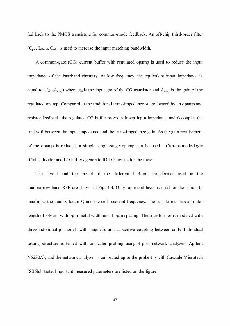
The layout and the model of the differential 3-coil transformer used in the
dual-narrow-band RFE are shown in Fig. 4.4. Only top metal layer is used for the spirals to
maximize the quality factor Q and the self-resonant frequency. The transformer has an outer
length of 346μm with 5μm metal width and 1.5μm spacing. The transformer is modeled with
three individual pi models with magnetic and capacitive coupling between coils. Individual
testing structure is tested with on-wafer probing using 4-port network analyzer (Agilent
N5230A), and the network analyzer is calibrated up to the probe-tip with Cascade Microtech
ISS Substrate. Important measured parameters are listed on the figure.

48
Cs
LO_I+
LO_I-
LO_Q+
LO_Q-
Dual-Band
Active Feedback LNTA
Passive
Current-driven MixerCG current buffer
with regulated opamp
Rout
BBout I
A
Vb
Rout
BBout Q
A
Vb
VDD
VDD
Vb(LB)
RFM1
Mc(LB)
LPri
RFin+
Vb
Mfb(HB)
Vb(HB)
Vg(LB) Vg(HB)
LSecLTer
VDD3-coil Transformer
Mfb(LB)
Mc(HB)
KPT KTS
KPS
/ 2 LO BufferLO @ 2fo
LO_I+LO_I-LO_Q+LO_Q-
Fig. 4.2 Current-gain-boost low-noise dual-narrow-band RFE with a 3-coil differential
transformer (In actual implementation, LNTA is differential and the mixer are
double-balanced)
RFin+
RFin-
Regulated
CG Buffer
Regulated
CG Buffer
LsecWideband
LNTA
Lpri
K
Wideband
LNTA
/ 2LO
BufferLO @ 2fo
LO_I+LO_I-LO_Q+LO_Q-
LO_I+ LO_I-
LO_Q+ LO_Q-
RFin+ Lbond Lbond
Cpar Cpar
Vb1
Vcm
Vb Vb
Lpri Lpri
Mcg Mcs Mcs Mcg
Coff CoffLBias
RFin-
LBias
Off-chipOff-chip
Fig. 4.3 Current-gain-boost high-linearity wide-band RFE

49
Fig. 4.4 Layout and model of the single 3-coil transformer for the dual-narrow-band RFE
4.4 Experimental Results
The dual-narrow-band and the wide-band RFEs are fabricated in a 0.13m CMOS
process, and the die micrographs are shown in Fig. 4.5, which occupy 1.2mm2 and 1.8mm
2,
respectively. Fig. 4.6 plots the measured S11, and Fig. 4.7 shows the measured voltage
conversion gain and DSB NF with IF of 5MHz
For the dual-narrow-band RFE, as shown in Fig. 4.6, S11 is measured to be below -10dB
from 1.34GHz to 1.88GHz for the low band and from 3.19GHz to 4.00GHz for the high band
with fine tuning SCAs. Fig. 4.7 shows the measured voltage conversion gain and DSB NF
with IF of 5MHz. Loaded with 200-ohm output impedance Rout, the gain and NF at 1.7GHz
LO are 20.7dB and 2.5dB while those at 4GHz LO are 17dB and 3.4dB, respectively.
Two-tone tests with 5MHz spacing measure IIP3 of -13.6dBm at 1.7GHz and -11dBm at

50
4GHz. With 1.2V supply, the narrow-band RFE consumes a total current of 19mA, out of
which 10mA is for the LNTA and 9mA is drawn by the IQ common-gate buffer and the
regulated opamp. With the assumptions that the mixer’s conversion gain coefficient is equal to
2/π, Rout is 200 ohm, and the effective gm of the input stage is 60mS, the additional current
gain at the low band and the high band are measured to be 9dB and 5.5dB, respectively, as
expected.

51
Fig. 4.5 Die micrographs of the dual-narrow-band and wide-band RFEs

52
Fig. 4.6 Measured S11 of the dual-narrow-band and the wide-band RFEs
Fig. 4.7 Measured gains and NF of the dual-narrow-band and the wide-band RFEs
The measured S11 of the wide-band RFE is below -10dB from 2GHz to 5GHz as shown in
Fig. 4.6. Fig. 4.7 also shows the measured voltage conversion gain and DSB NF with IF of

53
5MHz. At low frequency, the impedance of Lpri decreases and thus the gain decreases. Loaded
with 100-ohm output impedance Rout, the voltage conversion gain and DSB NF are measured
to be 13dB and 4dB with 3GHz LO, respectively. Two-tone tests with 5MHz spacing measure
an IIP3 of 0dBm with 3GHz LO. With 1.2V supply, the wide-band RFE consumes a total
current of 34mA, out of which 16mA is for the LNTA and 18mA is for the IQ common-gate
buffer and the regulated opamp. More current is needed for the regulated buffer as
compared to the narrow-band counterpart to improve the overall linearity. Assuming that the
mixer’s gain coefficient is equal to 2/π, Rout is 100 ohm and the effective gm of input stage is
100mS, the additional current gain is 2.9dB.
Table 4.1 summarizes the performance of the RFEs. The performance of the proposed
transformer-based dual-narrow-band and wide-band RFEs are compared with the published
state-of–the-art CMOS RFEs as shown in Table 4.2. Proposed dual-narrow-band RFE
provides low noise figure while the wide-band RFE provides high linearity.

54
Table 4.1 Performance Summary
Parameter Dual-Narrow-band RFE Wide-band RFE
Low-band High-band
RX Frequency [GHz] 1.34 - 1.84 3.19 – 4.1 2-5
Voltage Gain [dB] 20.7 (Rout=200Ω) 17
(Rout=200Ω)
13
(Rout=100Ω)
S11 [dB] <-10 <-10 <-10
IIP3 [dBm] -13.6 -11 0
DSB NF [dB] 2.5 - 3.4 3.2 - 4 3.6-4.5
Additional I-gain [dB] 9 5.5 2.9
Die Area [mm2] 1.2 1.8
Supply Voltage 1.2V
Current [mA]
LNTA :
CG Buffer (IQ) :
Total:
10
9
19
10
9
19
16
18
34
Technology 0.13μm CMOS Process

55
Parameter Proposed Dual-band
Receiver
Proposed
Wide-band
Receiver
Bagheri
JSSC’06
[4]
Lee
ISSCC
’07
[7]
Zhan
JSSC’
08
[8]
Blaakme
er
JSSC’
08 [9]
Feng
JSSC’
09 [10]
Low-band High-band
RX Frequency
[GHz]
1.34 - 1.84 3.19 – 4.1 2-5 0.8-6 2-8 2-5.8 0.5-7 2
Voltage Gain
[dB]
20.7
(Rout=200Ω
)
17
(Rout=200Ω
)
13
(Rout=100Ω)
3-36 23 44 18 30
S11 [dB] <-10 <-10 <-10 <-10 <-8 <-15 <-10 -22
IIP3 [dBm] -13.6 -11 0 -3.5 2) -7 -21 -3 -12
DSB NF [dB] 2.5 - 3.4 3.2 - 4 3.6-4.5 5 4.5 3.4 4.5-5.5 3.1
Die Area [mm2] 1.2 1.8 3.8 3) 0.48 0.2 5) <0.01 5) 1.1
Supply Voltage 1.2V 2.5V 1.2V 2.7 1.2 1.5
Current [mA]
19
19
34
LNA + MIXER 11.4 32.5 4) 28 13.3 7) 8 6, 7)
CMOS
Technology
0.13μm 90nm 65nm 90nm 65nm 0.13μm
1) Need 1.8V Vdd at (4-5GHz)
2) Mid-gain setting for RX
3) Area included Baseband filter and synthesizer
4) Reported Baseband has only I-path
5) Active Area
6) Excluding baseband Trans-impedance amplifier
7) LNA is single-ended input
Table 4.2 Performance comparison with state-of-the art receiver

56
References
[1] M. Valla, et al., “A 72-mW CMOS 802.11a direct conversion front-end with 3.5-dB
NF and 200-kHz 1/f noise corner,” IEEE J. Sold State Circuits, vol. 40, pp. 970-977, April
2005.
[2] A. Mirzaei, et al., “Analysis and Optimization of Current-Driven Passive Mixers in
Narrowband Direct-Conversion Receivers,” IEEE J. Sold State Circuits, vol. 44, pp.
2678-2688, Oct. 2009.
[3] R. Bagheri, et al., “An 800-MHz-6GHz software-defined wireless receiver in 90-nm
CMOS,” IEEE J. Sold State Circuits, vol. 41, pp. 2860-2876, Dec 2006.
[4] J. Borremans, et al., “Low-Area Active-Feedback Low-Noise Amplifier Design in
Scaled Digital CMOS,” IEEE J. Sold State Circuits, vol. 43, pp. 2422-2433, Nov. 2008.
[5] J-H. C. Zhan, et al., “A Broadband Low-Cost Direct-Conversion Receiver
Front-End in 90 nm CMOS, “IEEE J. Sold State Circuits, vol. 43, pp. 1132-1137, May
2008.
[6] S.C. Blaakmeer, et al., “ The BLIXER, a Wideband Balun-LNA-I/Q-Mixer
Topology, “IEEE J. Sold State Circuits, vol. 43, pp. 2706-2715, Dec. 2008.
[7] Y. Feng, et al., “ Design of a High Performance 2-GHz Direct-Conversion
Front-End With a Single-Ended RF Input in 0.13μm CMOS “IEEE J. Sold State Circuits,
vol. 44, pp. 1380-1390, May. 2009.

57
Chapter 5 Low-noise, high resolution 2nd-order
noise-shaped TDC for All-Digital Phase-Locked Loop
5.1 Introduction
One of the critical sub-system for highly reconfigurable front-end is the frequency
synthesizer. In order to be able to reconfigure for different existing applications and for future
applications, the parameters of the frequency synthesizer has to be highly reconfigurable.
Typical reconfigurable parameters included loop bandwidth, loop gain, frequency resolution
and output frequency. For this application, All-digital phase-locked loop (ADPLL) is more
suitable compare with the conventional Charge-Pump PLL (CP-PLL). In a charge-pump PLL
as shown in Fig. 5.1, signals are being processed in analog voltage or current domain. To
reconfigure the closed loop parameter, charge pump current and filter’s RC parameter have to
be changed, which is problematic as all nodes are very sensitive. Furthermore, the charge
pump implementation faces the problem of finite output resistance and large mismatch. The
filter capacitor also contributes large area and is sensitive to leakage current. In contrast, in an
ADPLL as shown in Fig. 5.2, the loop gain and loop bandwidth can be simply changed by
changing the filter’s coefficient. Moreover, digital filter contributes less area and is insensitive
to leakage. In addition, system calibration and divider noise compensation can be easily done
in digital domain.
To convert CP-PLL to ADPLL, signal processing blocks have to convert analog signal to

58
digital and vice versa, in order to allow the use of digital signal processing. Table 5.1
summarizes the changes in building blocks when converting from CP-PLL to ADPLL.
PFD VCO
Programmable
divider
SΔ
Fref Fvco
Up
Down
DAC
Fig. 5.1 Conventional Charge-Pump Phase-Locked Loop
TDCDigital Loop
FilterDCO
SΔ
Programmable
divider
SΔ
SΔ Noise
Compensation
Fref Fvco
Fig. 5.2 All-Digital Phase-Locked Loop

59
CP-PLL ADPLL
Phase Frequency Detector (PFD) Time-To-Digital Converter (TDC)
Voltage Controlled Oscillator (VCO) Digitally-Controlled Oscillator (DCO)
Charge-Pump and Loop Filter Digital Loop Filter
SD Noise Compensation DAC SD Noise Compensation in Digital
Table 5.1 Summary of the changes in building blocks when converting from CP-PLL to
ADPLL
Although AD-PLL offers more flexibility, the design of TDC is challenging. First, the
time resolution of TDC has to be high in order to reduce its quantization noise. For ADPLL,
TDC quantization noise dominated the noise within the loop-bandwidth. Second, the
detection range has to be large in order to cover the time variation due to the dithering of
sigma-delta modulated divider. For instance, with a MASH 1-1-1 sigma-delta modulated
divider, the modulation range is from (-3 to 4), which is 7 VCO cycles. Third, with a
sigma-delta modulated divider, there exists a lot of high frequency noise in the spectrum. To
reduce noise folding to in-band and spur generation, TDC needs to have a small mismatch for
high linearity.

60
5.2 Conventional TDC
5.2.1 Delay-Chain TDC
A classical TDC architecture comprised of a chain of delay elements is shown in Fig.
5.3[1]. It works by counting the number of sequential inverter delays that occur between the
rising edge of CKV and FREF. The rising edge of CKV signal is successively delayed by a
series of inverters, each with a delay of Tinv. The output from each of these inverters is inputed
to a register, which is clocked by FREF. Thermometer code is generated which corresponds to
the number of inverter delay transitioned within the time difference between CKV and FREF.
The resolution achieved for this architecture is one inverter delay Tinv and is about
10-20ps in deep-submicron CMOS process. The implementation is compact but the resolution
is limited to inverter delay and highly depends on the process. Furthermore, increasing the
detection range of the detector requires a linear increase in the number of delay elements,
which means that the power consumption and the area will be increased. The architecture is
similar to flash architecture in ADC.
Delay-Line (Buffer Chain)
Fig. 5.3 Classical delay-chain TDC [1]
CKV(t)
FREF (t)

61
5.2.2 Reference Recycling TDC
To limit the increase of the number of delay elements with the increase of the detection
range, the inverter chain can be re-used by re-cycling the delayed signal at the end of the
chain back to the beginning through a multiplexer as shown in Fig. 5.4. Since the delay line is
reused, a counter at output is used to count the number of recycling. The TDC output is found
by counting and summing up all of the delay elements transitions that occurred. Compared
with delay-chain TDC, the cyclic TDC does not increase linearly with the increase of the
detection range, however, the resolution is still limited to an inverter delay in the process.
Fig. 5.4 Reference Recycling TDC
5.2.3 Vernier Delay Line TDC
To improve the time resolution, Vernier Delay Lines [2] can be used to achieve time
digitations with a time resolution smaller than one inverter delay. Fig. 5.5 shows an example
of Vernier Delay Line TDC, which is composed of two buffer lines with delay of Td and Td-α.
The idea is to stretch the input time difference by delaying both the start and stop signals. The
effective resolution is the time delay difference of the two delay lines, which is equal to α

62
and can be effectively smaller than the inverter delay of the process.
Although time resolution can be improved by Vernier Delay Lines, there are a number of
problems. First, the mismatch of time quantization is increased since the resolution of each
element now depends on the time difference of two different inverters that have different time
delays. Second, the size of the TDC increases even more comparing with simple delay-line
TDC for the same detection range.
Vernier Delay-Line
Fig. 5.5 Vernier Delay-Line TDC [2]
5.2.4 Gated Ring Oscillator (GRO) TDC
As seems from all the above TDC architecture, there is a trade-off between raw time
resolution and mismatches. This trade-off is similar in conventional flash ADC design, where
the resolution will ultimately be limited by matching of the components.
To reduce this trade-off, over-sampling and noise shaping techniques are used in ADC
design. Instead of improving the quantization step, noise shaping is used to move the
quantization noise to higher frequency and the in-band noise is reduced by low-pass filtering.
Fig. 5.6 shows a Gated-Ring Oscillator TDC [3], in which a first-order quantization

63
noise transfer function is embedded during time quantization. The key idea is to hold the
quantization error at the present measurement and subtract it in the next measurement, in
order to generate the high pass function as shown in the following equation.
(5.1)
(5.2)
Fig. 5.6 Gated-Ring-Oscillator (GRO) TDC [3]
During the time measurement interval, the ring oscillator is enabled and the time internal
is measured. The state of the oscillator at the end of each measurement interval is preserved
and is carried to the following measurement, this results in a first-order noise shaping in the
frequency domain. As such, the quantization noise at low frequency can be improved by
low-pass filtering.
Fig. 5.7 shows an example of noise spectrum of a GRO TDC, in which quantization
noise is first-order noise shaped to high frequency. Although quantization noise is first-order
noise shaped, the GRO in-band low frequency spectrum can be dominated by 1/f noise. This
is because the noise-shaping function is only first-order and the raw time resolution of the

64
oscillator ( Td ) still needs to be small, in which the channel length of the transistor has to be
minimum for small delay.
Fig. 5.7 Noise Spectrum of Gated-Ring-Oscillator (GRO) TDC [4]

65
5.3 Proposed Higher order quantization noise shaped TDC
In ADPLL, a high order low-pass digital loop filter always follows the TDC in order to
filter the noise and stabilize the feedback system as shown in Fig. 5.2. The closed-loop
transfer function for TDC noise to the ADPLL output is therefore a loop-pass transfer function,
as shown in Fig. 5.8 with a loop-bandwidth of around 500kHz. If TDC noise is being
high-passed and then further filtered by this PLL transfer function, the quantization noise
contributed to the ADPLL is reduced substantially. This is similar to a Sigma-delta ADC
where resolution is improved by noise-shaping and then low-pass filtered, such that the
low-frequency noise before the low-pass filter is lower and hence improving the SNR.
Fig. 5.8 shows the noise contribution of TDC with different order of noise-shaping and
with a raw delay resolution of 60ps and without low-pass filtered by PLL. In this plot, the
following parameters are assumed for the PLL, (Output frequency = 4.5GHz, Reference
frequency (fs) = 50MHz, and frequency divider division ratio N is therefore 90). In addition,
it is assumed that the noise-floor of the TDC is equal to resolution of 1ps such that the low
frequency noise floor will not go to infinity, this should be a reasonable assumption as thermal
noise of TDC will be the in-band limitation if good noise-shaping is achieved, which is
similar to KT/C noise and opamp noise in a Sigma-delta ADC. From this figure, we can see
that for offset frequency smaller than fs/6 (8.3MHz), higher order noise-shaping contributed
lower noise due to the high-passed noise transfer function. While for offset frequency larger
than fs/6 (8.3MHz), higher order noise-shaping noise will be higher. With this observation, it

66
is expected if the ADPLL transfer function for the TDC noise has a loop bandwidth smaller
than fs/6, higher order noise-shaping TDC will contribute lower noise.
Fig. 5.10 shows the noise contribution of TDC filtered by the transfer function as shown
in Fig. 5.8 . As shown in the figure, with higher-order noise shaping, the quantization noise
contributed to the ADPLL is reduced substantially. Comparing 1st and 2
nd noise shaping, the
region that gives the most significant difference is between 100kHz to 8.3MHz.
Fig. 5.8 ADPLL Closed-loop transfer function with LBW = 500kHz (TDC noise to output)

67
Fig. 5.9 TDC quantization noise contribution to ADPLL with different noise-shaping order
Fig. 5.10 TDC noise contribution being low-pass filtered by PLL transfer function with
different TDC order
To implement a higher order noise-shaping TDC, there are two potential architectures.

68
Fig. 5.11 shows a single loop architecture in which higher order function is achieved by
having a high-order loop filter. In this architecture, an analog time-to-amplitude converter, a
loop filter and a quantizer are required, which are all difficult to be implemented for TDC
application. Fig. 5.12 shows an alternate architecture based on MASH, in which higher order
noise shaping function is obtained by the cascade of a lower order modulator. The
quantization error of a first-order section is passed to the next stage as the output of each stage
is first-order high-pass before combining. The structure is modular and simple and is
particularly suitable for TDC implementation as higher-order TDC can be done by cascading
the GRO TDC.
x[n] y[n]
+-
Quantizer Higher-order
LoopFilter
DAC
Fig. 5.11 Single-loop with higher-order loop filter
1st order
modulator
1st order
modulator
1st order
modulator
1-z-1
1-z-1
+
+
x[n]y[n]
e1[n]
e2[n]
Fig. 5.12 MASH Architecture

69
(a) (b)
Fig. 5.13 Generating second-order noise shaping TDC from first-order GRO (a) First-order
Noise-shaping TDC (b) Second-order TDC based on cascade of first-order TDC
Fig. 5.13 shows the model of second-order noise shaping TDC. For a GRO TDC, it can
be modeled by an error feedback structure, in which quantization error is delayed, feedback
and subtracted from the input. To generate second-order structure based on cascaded
first-order section, the error of the first stage is extracted and is passed to the second stage.
This means that the time error during quantization has to be extracted. This is done by edge
detection logic and MUX, where the transition edge that is closed to the stop signal is
extracted and is passed to the following stage as input.
With higher order noise shaping, the raw time quantization step can be reduced, so that

70
the demand on time resolution ( tres ) can be relaxed. Relaxing the raw time resolution
requirement can allow the following
1) High performance ADPLL implemented in low-cost process: As conventional tres
is limited by inverter delay, instead of moving to advanced process to improve
resolution, one can use less advance process for the same performance.
2) Reduce power consumption: For the same time measurement interval, reduce the
raw time resolution will reduce the no. of digital transition within the
ring-oscillator, the oscillation frequency of the oscillator is reduced.
3) Improve matching, linearity and therefore reduce spur of Fractional-N ADPLL:
As raw time resolution is relaxed, the size of the transistor can be increased with
better matching. Furthermore, mismatches due to parasitic wiring, layout
mismatch can be reduced. Improving the matching of TDC within a PLL reduces
the fractional spur of ADPLL
4) Improve 1/f noise performance of TDC and hence ADPLL in-band noise: For
conventional TDC, improving raw time resolution require advance process with
minimum feature size for smallest delay, relaxing the time resolution allow
increase in transistor size and reduce 1/f noise.

71
5.4 Circuit Implementations
Timing
Gen.
Phase to State
Mapping
Ref
Div
Enable
Clk
Coupled
Osc.
Counter
Decoder + Edge Detector
Timing
Gen.
Phase to State
Mapping
Ref 2
Delayed
Div
e’1(t)
Clk
Coupled
Osc.
Counter
Decoder
MUX
Delay
C2
Y1[n] Y2[n]
Delay
C1
Fig. 5.14 Block Diagram of the 2nd
order noise shaped TDC
As a proof of concept, a 2nd
order noise shaped TDC is designed and implemented in
tsmc 65nm CMOS Process.
Timing
Gen.Phase to State Mapping
Ref
Div
Enable
Clk
Coupled
Osc.
Counter
Decoder + Edge Detector
Timing
Gen.Phase to State Mapping
Ref 2
Delayed
Div
e’1(t)
Clk
Coupled
Osc.
Counter
Decoder
MUX
Delay
C2
Y1[n] Y2[n]
Delay
C1
Fig. 5.14 shows the block diagram of the proposed 2nd
order noise shaped TDC. The core
consists of two 1st order noise shaped GRO TDC connected in cascade. In each 1
st order GRO
TDC, there are few functional blocks, these included:

72
• Timing Generator to generate Enable and Clk signal based on Ref and Div Edge
• Multiple-phase coupled ring oscillator as GRO with clock gating to store quantization
error information
• Simple static XOR gate as Edge Detection to detect “00” “11” pattern
• Ripple carry counter to counter the number of full period during the time measurement
• Constant delay added to the second stage, which is a static time offset and will be
removed by high pass filter of MASH output combiner
X[n] Quantize
r
e1[n-
1] e1[n]Z
-1
+-
+-
Y1[n]+-
Quantize
r
e2[n-1]e2[n]
Z-1
+-
+-
Y2[n]
1-Z-1
Y3[n] = X[n] –e2[n] (1-Z-1
)2
GRO TDC Model
GRO TDC Model
Fig. 5.15 Discrete-time model of the proposed TDC
Fig. 5.15 shows the discrete time model of the TDC, where each GRO is model based on
an error-feedback structure. The quantization error of the first stage e1[n] is passed to the 2nd
stage, whose output goes through a first-order high-pass filter before being combined with the
output of the first stage. The quantization error e1[n] is cancelled, and the output is given by
(Y3[n] = X[n] –e2[n](1-Z-1
)2).

73
Fig. 5.16 Timing diagram for the residue extraction
The key challenge for the 2nd
-order structure is the accurate extraction of e1[n] without
calibration. The quantization error of the first stage e1(t), which is the time difference between
oscillator transition edge (closest to the stop signal) and Div(t), is extracted by edge-detection
logic and MUXes. As the oscillator’s transition edges always occur before Div(t), which is
used to trigger the edge-detection logic, it would not work to directly pass e1(t) to the second
stage because of the latency. To solve this problem, constant delays C1 and C2 are added to the
oscillator’s outputs and Div(t), respectively, as shown in

74
Timing
Gen.Phase to State Mapping
Ref
Div
Enable
Clk
Coupled
Osc.
Counter
Decoder + Edge Detector
Timing
Gen.Phase to State Mapping
Ref 2
Delayed
Div
e’1(t)
Clk
Coupled
Osc.
Counter
Decoder
MUX
Delay
C2
Y1[n] Y2[n]
Delay
C1
Fig. 5.14 and as illustrated in the time diagram in Fig. 5.16 . The time delay C1 has to be
longer then the latency of the detection logic for proper edge selection while the time delay C2
has to be longer than the sum of C1 and e1(t), but too large C1 and C2 would increase the
measurement interval of the 2nd
stage and hence the power consumption. Interestingly, as
revealed in Fig. 5.16, the error e’1(t) to be processed by the second stage only consists of an
unwanted but constant offset term (C2 - C1). By design, this constant offset is automatically
and completely removed by the high-pass filter with transfer function (1-z-1
), and as such no
complicated calibration is required as in existing solutions.
For the delay cell within the GRO, differential delay cell is used instead of inverter-type
delay. This is because in inverter-type delay cell, each successive stage has opposite polarity
as shown in the simulated waveform in Fig. 5.18. To equally divide all phases in time, the
state register is sensitive to the threshold (the horizontal line) of the buffer and the DFF, and is
also sensitive to the rise and fall time difference. As such, a differential cell is preferred, in

75
which the time region of each phase is defined by the zero crossing point of the delay cells.
Inverter delay cell
Differential delay cell.
Fig. 5.17 Single-ended and Differential delay-cell configuration
Phase[29] Phase[30] Phase[31]
Fig. 5.18 Simulated waveform of single-ended GRO

76
+-
-+
+-
-+
+-
-+
+-
-+
+-
-+
+- -
+ +- -
+ +- -
+ +- -
+ +- -
+
1 0 0 0 01 1 0 0 01 1 1 0 01 1 1 1 01 1 1 1 10 1 1 1 10 0 1 1 10 0 0 1 10 0 0 0 10 0 0 0 0
1 1 0 1 01 0 0 1 01 0 1 1 01 0 1 0 01 0 1 0 10 0 1 0 10 1 1 0 10 1 0 0 10 1 0 1 10 1 0 1 0
Inverting Non-Inverting
Fig. 5.19 Edge detection of Inverting and Non-Inverting delay cell configuration
For a differential delay line, the line can be configured as inverting or non-inverting. The
choice of configuration depends on the ease of edge detection. Fig. 5.19 shows the state
transition diagram of the two configurations. To detect the travelling edge of the GRO, a
simple XOR gate can be used. On the other hand, in non-inverting configuration, there are
“00…00”, “11..11” that are different from other states, which complicated the edge detection
logic.

77
Fig. 5.20 Schematic of the delay cell
Multipath GRO structure is used in [3] to reduce the delay per stages by connecting the
inputs of each stage to several stages. The same approach is used here, but the main purpose is
to reduce the gating skew error such that quantization error can be held and averaged by a
number of stages to maintain noise-shaping property. Each GRO consisted of a ring of 47
identical stages. A prime number of stages is used to have better rejection of undesirable mode
as in [3]. As illustration, Fig. 5.20 shows the schematic of one delay stage (Stage 14), in
which the input is connected to many of the previous stages, including Stages 1, 3, 5, 9, and
13. Pseudo-differential delay cells are used in order to reduce their sensitivity to mismatches
between the rise time and the fall time during the state detection. A decoder keeps track of the
phase of the GRO, and a counter determines the total number of periods during the time
measurement interval. Edge detection is done by a simple XOR gate, which detects the
positions of “11” and “00” patterns. Other logics except the edge detector are synthesized
simply using standard cell library.
Fig. 5.21 shows the simulated waveform of the GRO during a time measurement. As

78
clearly shown in the figure, the state of the GRO is being held in-between time measurement.
The FFT spectrum plot of the GRO is shown in Fig. 5.22, in which a 50MHz signal with
1MHz sinusoidal wave phase modulated signal is applied. The digital code of the TDC is
decoded and processed in Matlab. 1st and 2
nd order noise-shaping can be identified.
Fig. 5.21 Simulated waveform of the GRO during a time measurement

79
Fig. 5.22 Simulated frequency spectrum of 1st and 2
nd order noise shaped TDC
5.5 Experiment Results
The TDC was designed and implemented in a 65nm CMOS process. Fig. 5.23 shows the
die micrograph, which occupies an area of 0.42mm2. Each GRO stage occupies only 0.076
mm2. At 1.2V supply, the delay of the delay cells of TDC is measured to be 60ps by
continually enabling the GROs.
A 50MHz phase-modulated signal is employed to evaluate the dynamic performance of
the TDC. The input has a fixed time offset of about 3.5ns plus a sinusoidal time-varying phase
of 15ps peak-to-peak. Output of the TDC is captured by a logic analyzer and the data is
further processed in Matlab. The order of the TDC noise-shaping can be configured by
bypassing the combiner at the decoder. Fig. 5.24 and Fig. 5.25 show the double-sided power

80
spectral density of the TDC in the 1st-order and 2
nd-order noise-shaping modes, respectively,
using 65,536-point FFT with a Hanning window. As shown in Fig. 5.24 and Fig. 5.25, noise
shaping of 20dB and 40dB is clearly evident with 1/f noise dominating at low frequencies.
SNDRs with integrated bandwidth from 2KHz to 1MHz are measured to be 23.3dB for the
1st-order TDC and 31.7dB for the 2
nd-order TDC, corresponding to more than 8dB SNDR
improvement by the proposed 2nd
-order TDC. All SNDR measurements are quite close to
SNRs, which demonstrates good matching and high linearity of the proposed design. The
noise floor corresponds to a 50Msps classical quantizer without noise shaping and with 1.5ps
steps. Fig. 5.26 shows the time-domain waveform of the 2nd
-order TDC after being digitally
filtered with 1MHz bandwidth. The TDC power consumption is directly proportional to the
time measurement interval and ranges from 1.8 to 15mW for interval from 200ps to 17.5ns.
Fig. 5.23 Die Micrograph

81
Fig. 5.24 Measured 1st order noise-shaping power spectral density
Fig. 5.25 Measured 2nd
order noise-shaping power spectral density

82
Fig. 5.26 Measured 2nd
order noise-shaping waveform after 1MHz LPF
5.6 1/f and thermal noise of TDC
As illustrated in Fig. 5.24 and Fig. 5.25, 1/f noise and thermal noise dominated at low
frequency. This noise is originated from the free-running phase noise of the coupled oscillator
inside the GRO stage. The GRO-TDC measures the time difference between the start and end
of its enable period. The thermal noise in the delay cells will introduce jitter when GRO is
enabled during a given measurement and the jitter will not accumulate across multiple
measurements. The thermal noise inside the oscillator add while noise to the GRO-TDC
output instead of phase noise profile of ring oscillator, which has a slope of 20dBc per decade.
To verify that this low frequency noise is dominated by the thermal and 1/f noise of the
delay cell, the phase noise of the oscillator is measured by continuously enabling the GRO.
Fig. 5.27 shows the measured phase noise plot of the coupled oscillator. The measured phase
noise is -80dBc/Hz at 100kHz offset and -110dBc/Hz at 1MHz offset, respectively. The slope

83
at low frequency offset is -30dBc per decade which reveals that the 1/f noise is indeed
dominated and the 1/f noise corner is large.
Fig. 5.27 Measured phase noise of the multi-path coupled oscillator inside the GRO TDC
This measured phase noise profile is modeled in a behavioral simulator (Cppsim) [9] and
the 1st and 2
nd order GRO are modeled with this oscillator being enabled during the time
measurement interval. Fig. 5.28 and Fig. 5.29 shows the simulated PSD for 1st and 2
nd order
TDC without GRO phase noise and with a TDC raw delay of 60ps, similar to the measured
delay. The PSD shows 1st and 2
nd noise shaping without low frequency 1/f and thermal noise
floor. Fig. 5.30 and Fig. 5.31 shows the simulated PSD with phase noise of -80dBc/Hz at
100kHz offset and -110dBc/Hz at 1MHz offset for the GRO. The 1/f and thermal noise
limited the low frequency PSD and the results are close to the measured PSD in Fig. 5.24 and
Fig. 5.25.

84
Fig. 5.28 Simulated 1st order TDC PSD without GRO phase noise with 60ps resolution
Fig. 5.29 Simulated 2nd
order TDC PSD without GRO phase noise 60ps resolution

85
Fig. 5.30 Simulated 1st order TDC PSD with GRO phase noise 60ps resolution
Fig. 5.31 Simulated 2nd
order TDC PSD without GRO phase noise 60ps resolution
To further improve the low frequency PSD, the supply voltage of the GRO is increased
to 1.8V and the PSD are measured again for comparison. With a 1.8V supply, the GRO raw
delay is improved to 30ps. The measured PSDs are shown in Fig. 5.32 and Fig. 5.33, the 1/f
noise, the thermal noise floor and the quantization noise are lower compare with the nominal
case of 1.2V supply

86
Fig. 5.32 Measured 1st order noise-shaping power spectral density with 1.8V GRO Vdd (30ps
delay resolution)
Fig. 5.33 Measured 2nd
order noise-shaping power spectral density with 1.8V GRO Vdd (30ps
delay resolution)

87
5.7 Performance summary and comparison
Table 5.2 summarizes the performance of the proposed TDC. The performance is also
compare with other state-of-the art TDC. With 2nd
order noise-shaping, the raw resolution of
the delay cell can be reduced to 60ps while achieving comparable effective resolution. This
improvement is achieved without any calibration.
This work VLSI 08 [5] VLSI 07
[6]
VLSI 09 [7] VLSI 11
[8]
Scheme 2nd
order
noise-shaping
1st order
noise-shaping
2-step Vernier pipeline
Process 65nm 0.13μm 90nm 0.13μm 0.13μm
Sampling Frequency 50Msps 50Msps 10Msps 15 Msps 65 Msps
Supply Voltage 1.2V 1.5V 1 V 1.5V 1.3V
Raw delay 60ps 6ps 20ps N/A 40ps
Effective Resolution 1.5ps * 1ps * 1.25ps 8ps 0.63ps
Raw delay/Effective
Res.
40 6 16 N/A 63.5
Calibration Needed No No Yes No Yes
Chip Area 0.6 x 0.7mm2 1 x 1 mm2 0.6 mm2
(Active)
0.26 mm2
(Active)
0.32 mm2
Power Consumption
(min-max range)
1.8 – 15mW @
50Msps
2.2 – 21mW
@50Msps
3mW @
10Msps
7.5mW@
15Msps
10.5mW
@65Msps
*Effective Resolution is estimated by the measured power spectral density (PSD) as compare with a quantizer
without noise-shaping at low frequency (~1MHz)
Table 5.2 Performance summary and comparison for the 2nd
order noise-shaping TDC
5.8 Comparison with recently published work on high-order noise-shaping
TDC
TDC with higher order noise-shaping has recently attracted widespread attention since
the publication of 1st-order noise-shaping TDC [5]. With 2
nd or 3
rd order noise-shaping, the

88
quantization noise can be shaped further to high frequency comparing with 1st-order
noise-shaping and the low frequency quantization noise is reduced. A single-loop
phase-domain continuous-time ΔΣ TDC is presented in [10]. Fig 5.34 shows the block
diagram of the continuous-time ΔΣ TDC. Phase detector converts the phase domain
information into voltage domain and opamp based integrator filters the phase error before the
quantizer. The quantized output is then feedback using a digital-to-phase converter. The
architecture is similar to the conventional continuous-time (CT) ΔΣ ADC and circuit
techniques from CT ADC can be used. However, the approach is highly analog, and is
susceptible to analog circuit imperfections. For instant, opamp noise and phase detector
non-linearity. Fig. 5.35 shows the measured spectrum of the CT TDC. The low-frequency
noise can be dominated by 1/f and thermal noise. In addition, harmonic contents can be
observed. The TDC achieved a resolution of 2.4ps.
Fig. 5.34 Block diagram of a single-loop continuous-time ΔΣ TDC [10]

89
Fig. 5.35 Measured spectrum of the continuous-time ΔΣ TDC [10]
A MASH 1-1-1 TDC is presented in [11]. Fig. 5.36 shows the block diagram of the TDC.
The architecture is based on MASH architecture, with the cascade of three 1st-order
noise-shaping TDC sections. The ideal is similar to the proposed TDC, where quantization
error of the 1st stage is extracted and passed to the later stage for further processing. The core
of the first-order noise-shaping TDC is implemented using a gated relaxation oscillator, where
the quantization error and the phase information of the oscillator are stored in the voltage of a
capacitor. Since the relaxation oscillator oscillated only with 1-phase, time residue extraction
is much simpler comparing with the proposed TDC. Fig. 5.37 shows the timing diagram, the
input to the 2nd
stage is the original input time difference minus the quantization error of the
1st stage. With proper digital combining of the output of each stage, a 1-1-1 3
rd order
noise-shaping can be achieved.
Although the use of a simple gated relaxation oscillator reduces the number of phase and

90
simplifies the residue extraction, the raw delay resolution is limited. Although it is not clearly
specified in their measurement result, the raw resolution of the relaxation oscillator is
extracted to be around 6.67nS, with an effective resolution of 18ps estimated from the
low-frequency noise floor of the power spectrum density. This may not be sufficient to meet
the stringent noise requirement for wireless application. One approach to improve the raw
resolution and to improve the noise performance is the employ multi-phase coupled oscillator
as in the proposed 2nd
order TDC. The performance of noise-shaping TDCs is summarized in
Table 5.3.
Fig. 5.36 Block diagram of the MASH 1-1-1ΔΣ TDC [11]

91
Fig. 5.37 Timing diagram of the MASH 1-1-1ΔΣ TDC [11]

92
This work CICC 10 [10] ISSCC 11 [11]
Scheme 1-1 MASH 2nd
order
with multi-phase osc.
single-loop
continuous-time ΔΣ
TDC
1-1-1 MASH 3rd
order with
1-phase osc.
Process 65nm 90nm 0.13μm
Sampling Frequency 50Msps 156.25Msps 50Msps
Supply Voltage 1.2V 1.2V 1.2 V
Raw delay 60ps N/A 6.67ns
Effective Resolution 1.5ps 2.4ps 18ps
Raw delay/Effective Res. 40 N/A 370
Calibration Needed No No Yes
Chip Area 0.6 x 0.7mm2 0.12 mm2 (Active) 0.11 mm2
(Active)
Power Consumption
(min-max range)
1.8 – 15mW 2.2 mW 1.7mW
Table 5.3Performance comparison with recently published 2nd and 3rd order noise-shaping
1TDC
References
[1] R. B. Staszewski, et al.” 1.3V 20ps Time-to-Digital Converter for Frequency Synthesis in
90-nm CMOS” IEEE Transactions on circuits and systems – II: Express Briefs. Vol.53, no.3.
pp. 220-224, March 2006.
[2] M. Gorbics; K. Roberts and R. Sumner, “Vernier Delay Line Interpolator and Coarse
Counter Realignment,” U.S. Patent 5838754, Mar. 11, 1997.
[3] M.Z. Straayer, M.H. Perrott, "A Multi-Path Gated Ring Oscillator TDC With First-Order
Noise Shaping ," IEEE J. Solid-State Circuits, vol. 44, pp. 1089-1098. April 2009

93
[4] M.H. Perrott. “Tutorial on Digital Phase-Locked Loops”, ISSCC 2008
[5] M.Z. Straayer and M.H. Perrott,” An efficient high-resolution 11-bit noise-shaping
multipath gated ring oscillator TDC,” Symp. on VLSI Circuits, pp. 82-83, Jun. 2008.
[6] J. Yu, F.F. Dai, R.C. Jaeger,” A 12-Bit Vernier Ring Time-to-Digital Converter in a 0.13 m
CMOS Technology,” Symp. on VLSI Circuits, pp. 232-233, Jun. 2009.
[7] M. Lee and A.A. Abidi,” A 9b, 1.25ps Resolution Coarse-Fine Time-to-Digital Converter
in 90nm CMOS that Amplifies a Time Residue,” Symp. on VLSI Circuits, pp. 168-169, Jun.
2007.
[8] Y-H. Seo, J-S. Kim, H-J. Park and J-Y. Sim,” A 0.63ps Resolution, 11b Pipeline TDC in
0.13 m CMOS,” Symp. on VLSI Circuits, pp.152-153, Jun. 2011.
[9] M.H. Perrott, “Cppsim” available at www.cppsim.com
[10] B. Young, et.al,” A 2.4ps resolution 2.1mW second-order noise-shaped time-to-digital
converter with 3.2ns range in 1MHz bandwidth,” IEEE Custom Integrated Circuits Conf.,
Sept. 2010.
[11] Y. Cao, et.al, “A 1.7mW 11b 1-1-1 MASH ΔΣ time-to-digital converter,” ISSCC Dig.
Tech. Papers. Pp 480-481, Feb. 2011

94
Chapter 6 4.1GHz to 6.5GHz All-Digital
Phase-Locked Loop for SDR RFE
6.1 Introduction
One of the critical sub-system for highly reconfigurable front-end is the frequency
synthesizer (FS). In order to ease the reconfiguration ability of the frequency synthesizer,
All-digital phase-locked loop (ADPLL) is more suitable comparing with the conventional
Charge-Pump PLL (CP-PLL). In an ADPPL, the loop gain and loop bandwidth can be simply
changed by changing the filter’s coefficient. Besides, digital filter contributes less area and
insensitivity to leakage and system calibration and divider noise compensation can be easily
done in digital domain.
This chapter presents the design and implementation of ADPLL based frequency
synthesizer (FS) with high programmability for reconfigurable SDR front-end. The FS
covered the frequency operation range of 4.23GHz – 6.35GHz and is part of a LO generation
system as shown in Fig. 6.1. With the proposed ADPLL FS together with a chain of LO
dividers and a multiplexer (Mux), the LO generation system covered the intended frequency
range of 800MHz to 6GHz for SDR application. The specification of the system will be given
and the design and implementation of the ADPLL will be presented in this chapter. The circuit
implementation of other building blocks for LO generation system will be presented in
Chapter 7.

95
Fig. 6.1 Block diagram of the LO generation system for the SDR RFE
The important features of the LO generation system is summarized as follow:
Summary of Features:
a) LO Generator for (800MHz – 6GHz) by using Miller divider with fractional division to
lower tuning range of VCO
b) Careful frequency planning which allow IQ and 450 signals to be generated from simple
div-by-2 output
c) LO phase error correction for coarse phase calibration
d) ADPLL with reconfigurable loop bandwidth and frequency resolution
e) 2nd
order noise-shaping TDC with noise and power enhancement

96
6.2 System Specifications
As the LO generator is targeted for used in the SDR Receiver, and is intended for all
wireless application in the range of 800MHz to 6GHz. The system specifications of all the
standard has to be considered and important requirements have to be fulfilled. Table 6.1 and
Table 6.2 summarizes the important requirements for the generator. The LO generator is not
only required to generate LO at large frequency range, but also has to meet the phase noise,
resolution and settling time requirements.
Standard Frequency
(MHz)
Channel
BW
Resolution Phase Noise Phase Noise
(Derive from
TX, avoid
TX SAW filter)
Setting
Time
EGSM 876 – 915
(UL)
921 – 960
(DL)
200kHz 200kHz -121dBc/Hz
(600kHz)
-131dBc/Hz
(1.6MHz)
-141dBc/Hz
(3MHz)
-137.8dBc/Hz
(2MHz)
-143dBc/Hz
(5MHz)
-147.8dBc/Hz
(10MHz)
-162dBc/Hz(20
MHz)
576us
(speech)
200us
(Data)
DCS 1800 1710-1785(
UL)
1805-1880(
DL)
200kHz 200kHZ -121dBc/Hz
(600kHz)
-131dBc/Hz
(1.6MHz)
-138dBc/Hz
(3MHz)
PCS 1900 1850-1910(
UL)
1930-1990(
DL)
200kHz 200kHz -121dBc/Hz
(600kHz)
-131dBc/Hz
(1.6MHz)

97
-138dBc/Hz
(3MHz)
UMTS
(FDD
Band I)
1920-1980(
UL)
2110-2170(
DL)
5MHz 200kHz -120dBc/Hz
(3MHz)
-145dBc/Hz
(20MHz)
200us
UMTS
(TDD)
1900-1920
(UL)
2010-2025
(DL)
10M,5M,
1.6MHz
200kHz -120dBc/Hz
(3MHz)
-145dBc/Hz
(20MHz)
Table 6.1 LO Specifications for Cellular Standard
Standard Frequency
(MHz)
Channel BW Resolution Phase Noise Setting
Time
WLAN
802.11b
2400 – 2483.5
(ISM)
16.6MHz 1MHz -102dBc/Hz (1MHz) 225us
WLAN
802.11a
5150 - 5250
5250 - 5350
5725 - 5825
20MHz 5MHz -102dBc/Hz (1MHz)
EVM <5.6%, Rms <3.2o ,
SSB phase noise <-28dBc
500us
WLAN
802.11g
2400 – 2483.5
(ISM)
20MHz 1MHz -102dBc/Hz (1MHz) 225us
WiMax 2300 – 5850 1.25MHz –
28MHz
125kHz -95dBc/Hz (10kHz)
-95dBc/Hz (100kHz)
-120dBc/Hz (1MHz)
< 1 deg. RMS
100us
Bluetooth
802.15.1
2400 – 2483.5
(ISM)
1MHz 1MHz -109dBc/Hz (1MHz)
-89dBc/Hz (500kHz)
-121dBc/Hz (2MHz)
<220us
150us

98
GPS L1: 1575.42
L2: 1227.60
L5: 1176.45
C/A code :
1.023Mbps
P code: 10.23
Mbps
L2CM L2CL:
511.5kbps
Zigbee 868-868.6 (1
channel)
902-928 (10
channels)
2400 – 2483.5
(16 channels)
300kHz –
2MHz
915: 2M
2450: 5M
-110dBc/Hz (1MHz)
DVB 47-68 (VHF I)
174-230(VHF
II)
470-598(UHF
IV)
598-862(UHF
V)
5M,6M,7M,8
M
8MHz
Table 6.2 LO Specification for Other Data Standard

99
To summarize, Table 6.3 shows the system specification summary of the LO generation
system. For phase noise requirement, most stringent out-of band phase noise requirement is
GSM standard. While for in-band phase noise requirement, WLAN is the most stringent.
Besides, since the SDR receiver required harmonic rejection for LO frequency below 2GHz,
45o output signal is generated from 800MHz to 2GHz and IQ signal is generated from 2GHz
to 6GHz.
System Specification Summary
Output Frequency 800MHz ~ 5.825GHz
Resolution at output 200KHz
Settling Time Close-loop: < 62.5uS
Phase Noise In-band: -102dBc/Hz
Out-band: -162dBc/Hz
@20MHz (GSM TX)
Out-band: -141dBc/Hz @
3MHz (GSM RX)
Spur level < -50dBc
IQ Output 2-6GHz
45o Output 800MHz – 2GHz
Table 6.3 LO Specification Summary

100
6.3 Frequency Planning
Based on the frequency range and LO output requirement, detailed frequency planning is
carried out. The output frequency of the QDCO and the dividers are summarized in Table 6.4
and is labeled in Fig. 6.1. Miller based divider is used to provide a division ratio of 1.5 in
order to relax the QDCO tuning range. The miller divider can be configured as div-by-2 by
by-passing the feedback path such that the SSB mixer acted as a simple buffer. With the miller
divider and the following div-by-2 dividers, IQ and 45o phase signal can be generated. This is
very important in reducing the complexity of the frequency divider. All frequency range from
800MHz to 6GHz is available by using a simple MUX
MUX Output Frequency (GHz) Phase MUX Output Frequency(GHz) Phase
LO1 (QDCO) 4.23 – 6.35 IQ LO1 (QDCO) 4.23 – 6.35 IQ
LO2 ( ÷2 ) 2.115 – 3.175 IQ LO2 (÷1.5 ) 2.82 – 4.23 IQ
LO3 ( ÷4 ) 1.0575 – 1.5875 45
o
LO3 ( ÷3 ) 1.41 – 2.117
45o
LO4 ( ÷8 ) 0.5288 – 0.79375 45
o
LO4 ( ÷6 ) 0.705 – 1.058
45o
Table 6.4 QDCO and LO dividers output frequency.

101
6.4 ADPLL System Design and Considerations
6.4.1 ADPLL System modeling
TDCDigital Loop
FilterDCO
ΣΔ
Programmable
divider
ΣΔ
ΣΔ Noise
Compensation
Fref Fvco
Fig. 6.2 Block diagram of a generic ADPLL
Fig. 6.2 shows the block diagram of an ADPLL, which includes a Time-to-digital
converter (TDC), digital loop filter, programmable divider with sigma-delta modulation,
digital control oscillator, and the DCO’s fine-frequency tuning sigma-delta modulator.
Similar to a conventional PLL, transfer function of each building block can be applied to
model the dynamic of the PLL system. With proper modeling, the loop behavioral can be
determined by choosing the parameter of loop filter. In addition, noise analysis can be carried
out based on the close-loop transfer function from each noise source to PLL output. Fig. 6.3
shows a model of the ADPLL [1]. For example, for DCO, since output is phase signal and
input is controlling its output frequency, the model of the DCO is an integrator as phase is
equal to integration of frequency as function of time. For TDC, it is being modeled as phase to
time comparator with normalization with TDC resolution (△tdel).

102
Fig. 6.3 Model of an ADPLL [1]
With a closed-loop model, important transfer functions are the open loop gain A(s) and
the closed loop parameterizing function G(s), which are given by:
(6.1)
(6.2)
Where G(s) is a low-pass function with DC gain = 1, an example of G(s) is shown in Fig.
6 4.

103
Fig. 6 4 Close Loop Parameterizing Transfer function G(s)
With the above function, the transfer function from any input to output , can be
derived. For example,
Low-pass with gain of N (6.3)
High-pass function (6.4)
6.4.2 Loop Filter order (Type-2 PLL)
Loop Filter order is determined by the filtering requirement of the TDC noise and the
Divider Sigma-Delta Modulator (SDM) noise. For example, for a 3rd
order divider SDM,
frequency to phase transformation gives a 2nd
order noise shaped SD noise injection to PLL.
To ensure this noise transfer function has the same slope and roll-off as VCO noise at
out-band, the minimum required loop filter order is 3. For TDC noise, as it is 2nd
order noise

104
shaped, it has the same effect as a 3rd
order Divider. To further suppress the TDC and divider
noise at out-band, a 4th order Loop Filter are chosen.

105
6.4.3 Filter Transfer Function
The continuous time loop transfer function is derived based on the tool “PLL Design
Assistant [2]” and the discrete time transfer function is then obtained by continuous-time to
discrete time approximation. The model of the ADPLL [1] can be referred to Fig. 6.3.
At low offset frequency, sT1Z 1 , using the first two terms in the taylor series
expansion, the continuous-time approximation of the open loop transfer function is given by
sT1Z
vco
del
1)z(Hs
1
N
K
t
T)s(A
(6.5)
From PLL design assistant [2], with a 3rd
order filter and a parasitic pole (total filter
order = 4 ), the continuous-time open loop transfer function )s(Acalc is
par
2
ppp
z
Typecalc
w
s1
1
w
s
Qw
s1
w
s1
s
K)s(A (6.6)
with T
z1s
1
Assuming the digital filter is in the following form,
1
3
2
2
1
1
1
1
1
LF
za1zaza1
zb1
z1
K)z(H
(6.7)
Substitute equation (6.7) to (6.5), and comparing the coefficient with equation (6.6) the
following digital filter coefficients can be obtained,
Tw1
1b
z
1
, (6.8)
2p
p
p
p
1
TwQp
Tw1
Q
Tw2
a
, (6.9)

106
2p
p
2
TwQp
Tw1
1a
(6.10) Tw1
1a
par
3
(6.11)
2
p
p
p
par3
2
p
z1
del
LF
)Tw(Q
Tw1
1waTw
)w(b
1N
Kv
tK
(6.12)
A Matlab program is written to plot the transfer function and calculate the filter
coefficient with the parameter K, wp, wz, Qp, wpar as input.
Here is an example: Tres = 69ps, Loop BW = 500kHz, Parasitic pole = 3MHz, Type 2,
Total filter order = 3, VCO frequency = 3.6GHz, Ref. frequency = 50MHz
Digital Filter Coefficients: b1 = 0.992207222695850, a1 = 1.865975794903463, a2 =
-0.874770285329554, a3 = 0.726221096574395, KLF = 0.101200593051476

107
6.4.4 System noise analysis
With the transfer function from each input to output as derived from above, the noise
spectral density of the PLL can be calculated. Since the noise spectral density includes
continuous-time noise and discrete-time noise, the following equations are used [1],
Fig. 6.5 Power spectral density function calculation for CT and DT transformation
CT to CT (6.13)
DT to DT
(6.14)
DT to CT
(6.15)
Important noise source in an ADPLL are:
1. TDC quantization noise
2. DCO phase noise
3. Divider’s SDM noise
4. Noise from reference
5. Fine-tuning DCO’s SDM noise
With these additional noise input, the following model can be used

108
1/T
CT-DT)(tref
Fig. 6.6 Model of ADPLL with different noise sources [1].
Since the idea of the proposed ADPLL is to employ a high-order noise-shaping TDC to
reduce the raw time resolution requirement. Noise spectral density for different TDC order is
devised. Other noise source including divider’s sigma-delta modulator noise, reference noise
and DCO noise can be derived in a similar way. All the transfer function is written in a matlab
program and to be used for the ADPLL phase noise calculation.
1. TDC-referred noise power spectral density
(a) TDC quantization noise without noise-shaping
(6.16)
(6.17)
TDC quantization noise with 1st-order noise shaping
(6.18)
(6.19)
(b) TDC quantization noise with 2nd
-order noise shaping

109
(6.20)
(6.21)
Fig. 6.7 shows the power spectral density of the TDC noise with different noise-shaping
shaping order. The noise is normalized to the PLL output without PLL loop filtering and with
a TDC resolution (△tdel) of 60ps. The reference frequency / sampling frequency is 50MHz.
Fig. 6.7 TDC-referred noise power spectral density with different order
2. TDC noise filtered by ADPLL Transfer function
Output noise spectral due to TDC quantization noise is given by
(6.22)
Intuitively, we can see the transfer function from TDC noise by referring the noise to the
input and then multiply by the transfer function from input to output.
Referring the noise to input corresponding to divide by a factor (T/2π ) and then multiply

110
by the transfer function, the following equations can be derived.
(6.23)
With different TDC noise shaping order, the TDC noise contribution to the ADPLL phase
noise are derived and can summarized as follows:
(a) White TDC quantization noise
(6.24)
(b) 1st-order noise shaping
(6.25)
(c) 2nd
-order noise shaping
(6.26)
The above TDC noise contribution to the PLL output is shown in Fig. 6.8 with different
TDC order. As revealed in Fig. 6.9, the cross-over frequency is around fs/6 (8.3MHz). For
frequency below the cross-over frequency, TDC with higher order noise-shaping provides
lower noise due to noise-shaping. Since the PLL loop bandwidth is usually designed on the
order of few kilohertz to megahertz, the noise contribution of TDC with higher order
noise-shaping will be lower. This is shown in Fig. 6.8, where the PLL loop bandwidth is
around 700kHz. Fig. 6.9 shows the phase noise plot of the overall PLL, noise from the
frequency reference, VCO, TDC, Divider SDM are included in the system noise analysis. As
revealed in the figure, with a 2nd
order noise-shaping TDC with a resolution of 60ps, the

111
in-band and out-band phase noise will not be dominated by TDC and is dominated by the
DCO. In the case of 1st order TDC, the TDC noise will dominate the overall PLL phase noise
in the region of 100kHz to 8.3MHz.
Fig. 6.8 TDC noise filtered by ADPLL Transfer function
Fig. 6.9 Calculated phase noise contribution for the ADPLL with different order TDC

112
6.4.5 Digital Parts Word-Lengths
TDC
De
co
de
r
+
-
Offset Control
3rd order
ΣΔ (MASH)
Programmabl
e Divider
Fraction
+
+
Integer
Digital Loop Filter Th
erm
o
ΣΔ
/8
+
-
1/(1-z-1
)
Accumulato
r
Delay x N
+
-
Scale = Ttdc / TDCO
1
3
2
2
1
1
1
1
1
LF
za1zaza1
zb1
z1
K)z(H
16-bits frac.
4-bits
Q(1,16)
Q(4,0)
Q(4,16)
Q(6,16)
Q(10,16
)
Q(9,0)
Q(9,0)
Q(7,0)
Q(0,16)
To match
TDC delay
Q(4,16)
Q(9,0)
Q(8,0)
Q(8,0)Q(1,16)
Divider ΣΔ noise
cancellation
Fig. 6.10 Digital Parts Word-Length
TDC
Dec
od
er
+
-
Offset Control
3rd order
ΣΔ (MASH)
Programmable
Divider
Fraction
+
+
Integer
Digital Loop Filter Th
erm
o
ΣΔ
/8
+
-
1/(1-z-1)
Accumulator
Delay x N
+
-
Scale = Ttdc / TDCO
1
3
2
2
1
1
1
1
1
LF
za1zaza1
zb1
z1
K)z(H
16-bits frac.
4-bits
Q(1,16)
Q(4,0)
Q(4,16)
Q(6,16)
Q(10,16)
Q(9,0)
Q(9,0)
Q(7,0)
Q(0,16)
To match
TDC delay
Q(4,16)
Q(9,0)
Q(8,0)
Q(8,0)Q(1,16)
Divider ΣΔ noise
cancellation
Fig. 6.10 shows a more detailed block diagram of the ADPLL system. The no. of bits of each
digital signal line is indicated by Q(Integer, fraction). It is assumed every signal is in signed

113
representation unless specified.
The quantization noise of the sigma-delta modulator for the programmable divider is
compensated digitally as shown in
TDC
Dec
oder
+
-
Offset Control
3rd order
ΣΔ (MASH)
Programmable
Divider
Fraction
+
+
Integer
Digital Loop Filter Ther
mo
ΣΔ
/8
+
-
1/(1-z-1)
Accumulator
Delay x N
+
-
Scale = Ttdc / TDCO
1
3
2
2
1
1
1
1
1
LF
za1zaza1
zb1
z1
K)z(H
16-bits frac.
4-bits
Q(1,16)
Q(4,0)
Q(4,16)
Q(6,16)
Q(10,16)
Q(9,0)
Q(9,0)
Q(7,0)
Q(0,16)
To match
TDC delay
Q(4,16)
Q(9,0)
Q(8,0)
Q(8,0)Q(1,16)
Divider ΣΔ noise
cancellation
Fig. 6.10 [3]. The quantization noise is extracted from the modulator by subtracting the output
from the input of the modulator. This information is delayed and matched to the delay of the
TDC and is then subtracted from the TDC output code to compensate the modulator noise.
This is similar to the method [4] applied to CP-PLL, where modulator error is subtracted
through a DAC. The scaling factor, which is equal to the ratio of TDC resolution to the DCO
period (Ttdc/TDCO) can be obtained automatically through calibration but is controlled
externally here for simplicity.
Since the digital number is represented with fixed-point arithmetic in hardware

114
implementation, the total bit-width is defined by integer bit and fractional-bit. The integer bit
defined the range of the number while the fractional bit defined the resolution. Detailed
simulation is used to determine the required fractional bit, as every truncation adds
quantization noise. As a starting point, the fraction bit is assumed to be 16, which means the
resolution of a number is given by 1/(216
) = 0.000015258. Also, external inputs are unsigned
no. , so an unsigned to signed is needed before any arithmetic. Table 6.5 summarized the
digital parts word-length.
Signed/Unsigned Range Resol. Remarks
Fractional-in of Divider
SDM (Unsigned no.)
Signed Q(1,16)
(Unsign to sign)
0 to ( 1 – 2-16
) 2-16
Freq. resolution
=Ref/216
~762Hz
Divider SDM output Signed Q(4,0) -3 to 4 1
Integer (Unsigned no.) Signed Q(8)
(Unsign to sign)
64 to 82 1 Need unsigned
no. to control
divider
PN accumulator input Signed Q(4,16) -3 - ( 1 – 2-16
) to
4
2-16
Scale (ratio of
TDCO/Tres) (Unsigned
no.)
Signed Q(6,14)
(Unsign to sign)
0 to (32 - 2-14
) 2-14
Cover fvco and
tres process var.
TDC Output Signed Q(9,0) 256 1 Max.time = 256 x
65ps = 16.64ns
> 8 x TDCO +
offset
Offset Control Signed Q(9,0) 256 1 static offset
DCO Control unsigned Q(7,16) 0 – 128 2-16
linear range = 128
x Kvco
Table 6.5 Table of summary for digital parts word-length
6.5 Building Block Specifications Summary

115
Following the design considerations and based on the system specifications, the building
blocks specifications are derived and are summarized in the tables below.
FS Building Blocks Specifications
DCO + ΣΔ Mod. Specification
DCO Frequency ( Fvco ) 5.3GHz
Tuning Range 40 % ( 4.23 – 6.35GHz )
DCO Resolution 80 kHz
DCO Phase Noise (Derive from TX) -126dBc/Hz @ 2MHz / -146dBc/Hz @ 20MHz (3dB
margin) ( DCO/6 => GSM -162dBc/Hz @ 20MHz)
DCO Phase Noise (Derive from RX) -129dBc/Hz @ 3MHz ( DCO/6 => GSM -141dBc/Hz @
3MHz)
DCO Current < 20mA @ 1.2V
Integer bit width ( WI ) 7 bits (Fine range = 27 x 10k ~ 1.28MHz)
No. of cap. elements = 27 +ΣΔ output ~ 128+7 (max. of 3rd order) = 135
Fraction bit width ( WF ) 8 – 15 bits (input of DCO ΣΔ)
DCO ΣΔ Mod. Order 3rd
DCO ΣΔ Mod. Topology MASH 1-1-1
DCO ΣΔ Output Level -4 to 3 (MASH 1-1-1)
DCO ΣΔ Mod. Frequency ( Fdith ) ~ 400MHz

116
Div A
Fin 4.23-8.47GHz
Fout 2.115-4.23GHz
Vin (pk-pk) single-ended 0.3V
Vout (pk-pk) single-ended >0.5V
Power < 3mA @ 1.2V
Phase Noise -150dBc/Hz @ 20MHz (TX)
Div B
Fin 2.115-4.23GHz
Fout 1.0573-2.117GHz
Vin (pk-pk)
single-ended
0.3V
Vout (pk-pk)
single-ended
>0.5V
Power < 1.5mA @ 1.2V
Phase Noise -156dBc/Hz @ 20MHz (TX)
Div C
Fin 1.0573-2.117GHz
Fout 0.5288-1.05GHz
Vin (pk-pk)
single-ended
0.3V
Vout (pk-pk)
single-ended
>0.5V
Power < 0.75mA @ 1.2V
Phase Noise -162dBc/Hz @
20MHz (TX)
Mixer A
Fin 4.23 – 6.35GHz
Fout (x4/3)
Fout (by-pass)
5.64-8.47GHz
4.23-6.35GHz
Vin (pk-pk)
single-ended
0.3V
Vout (pk-pk)
single-ended
>0.4V
Power < 3mA @ 1.2V
TDC
Fref 50MHz
Static offset Min. cover ΣΔ divider
level
1st order noise leakage < 40 %
Resolution 40-60 ps
Output range to loop filter ~ 8 bits
Power <5mW

117
MUX
Fin 800M – 5.825GHz
Fout 800M – 5.825GHz
Vin (pk-pk) single-ended 0.3V
Vout (pk-pk) single-ended >0.4V
Power < 3mA @ 1.2V
Programmable Divider
Fref ( Output
Frequency )
50MHz
Fin (max.) 5.825GHz
Fixed divider after
DCO
None, Divide-by-2,
Divide-by-4
Programmable Divider
Ratio
~ 77 – 117 ( Fvco = 3.88 –
5.825 GHz )
Input Frequency ( Fref
x N )
3.88 – 5.825 GHz
Topology TSPC
Divider ΣΔ Mod.
Fref 50MHz
Fractional input bit
width
16
Topology MASH 1-1-1
ΣΔ Mod. Order 3rd
Dither PRBS

118
Digital ΣΔ Divider Noise Compensation
Fref 50MHz
Input Divider Division Ratio N
Output Quantization Error of Divider
Multiplier Coefficient Tres / TDCO ( Tres = TDC resolution )
Digital Loop Filter
Fref 50MHz
Integer bit width ( WI ) 10 bits (Fine range = 27 x 10k ~ 1.28MHz)
Fraction bit width ( WF ) 14 bits
Total output bit-width = WI + WF
Input bit-width = TDC output bits (10bits)
Topology FIR
Order 4th
Coefficient Resolutions (no. of bits) = WI + WF

119
6.4.6 System Level Simulation
Fig. 6.11 and Fig. 6.12 shows the system phase noise plot at output frequency at 5.4GHz
and 900MHz. Assuming the 900MHz output frequency is generated by a div-by-6 divider, the
phase noise plot at 900MHz is to be 20log(6)dB = 15.56dB the plot of Fig. 6.11. With the
above building block specification, the phase noise can meet the stringent GSM standard.
Fig. 6.11 System phase noise plot with output frequency at 5.4GHz

120
Fig. 6.12 System phase noise plot with output frequency @ 900MHz
Fig. 6.13 Transient Behavioral Simulation in Cppsim [3]

121
Fig. 6.14 Transient waveform of the ADPLL (TDC output)
To verify the system on a behavioral level, Cppsim [5] is used where the building blocks
can be described in C++ language with controllable level of non-idealities. These
non-idealities include VCO phase noise, quantization noise and finite digital word-length. Fig.
6.13 shows the schematic of the ADPLL in Cppsim. Fig. 6.14 shows the transient waveform
of the ADPLL’s TDC output during settling. Blue curve is the TDC output while red curve is
the TDC output after constant offset control. Green curve is the TDC output after divider
noise compensation, which is less noisy after compensating the divider noise.
Fig. 6.15 shows the Phase noise plot of the system after the transient simulation, the
phase noise is very close to the behavioral estimation in Matlab.

122
Fig. 6.15 Phase noise plot at Cppsim after transient simulation

123
6.5 Circuit Implementation
6.5.1 ADPLL Block Diagram
As a proof of concept, the ADPLL is designed and implemented in 65nm CMOS and is
part of SDR transmitter in another project. Fig. 6.16 shows the block diagram of the ADPLL
for SDR System. The ADPLL consisted of a 2nd
order noise-shaping TDC, a
transformer-coupled QDCO, a programmable divider together with a sigma-delta modulator
for fractional division. The digital parts consisted of a TDC decoder, a digital loop filter, a
sigma-delta modulator for QDCO fine frequency control and divider noise compensator. The
digital parts are synthesized using standard digital library and the layout is synthesized by
auto place and route.
Fig. 6.16 System block diagram of the ADPLL Frequency Synthesizer

124
6.5.2 2nd order noise-shaped TDC
Timing
Gen.Phase to State Mapping
Ref
Div
Enable
Clk
Multi-phase
coupled osc.
Counter
Decoder + Edge Detector
Timing
Gen.Phase to State Mapping
Ref
Delayed
Div
Enable
Clk
Multi-phase
coupled osc.
Counter
Decoder
MUX
Contstant Delay Fig. 6.17 shows the block diagram of the 2nd
order noise-shaped TDC used for the ADPLL, the detailed design considerations are given in
Chapter 5. The TDC is being integrated with the ADPLL system. For performance
comparison, the TDC can be reconfigured to 1st order by by-passing the 2
nd stage output in the
decoder.
Timing
Gen.Phase to State Mapping
Ref
Div
Enable
Clk
Multi-phase
coupled osc.
Counter
Decoder + Edge Detector
Timing
Gen.Phase to State Mapping
Ref
Delayed
Div
Enable
Clk
Multi-phase
coupled osc.
Counter
Decoder
MUX
Contstant Delay
Fig. 6.17 Block diagram of the 2nd
order noise-shaped TDC
6.5.3 Transformer Coupled QDCO[6]
Fig. 6.18(a) shows the architecture of the transformer-coupled Class-C QDCO. By
biasing Vg lower than VDD, the QDCO operates in Class-C mode [7] for better DC to RF
conversion efficiency. The primary coil of the transformer enlarges the voltage swing at the
gate to enhance the switching effectiveness. At the same time, the secondary coil reduces the
voltage swing at the drain to prevent the transistors from operating in the linear region to

125
improve phase noise. Capacitors Cs are added not only for the current shaping in Class-C
operation but also as part of the phase shifter. Fig. 6.18(b) shows the voltage and current
waveforms of M0, M1 and Cs in the QDCO. Because M0 and M1 are on only half of the period,
the Q-phase coupled current is firstly stored in Cs by M1 and then synchronously injected to
the I-phase tank by M0, which effectively generates a 90° phase shift. With this phase shifter,
the phase noise and the phase accuracy of the QDCO is improved without extra noise and
power. For the frequency tuning, an 8-bit switched-MIM-capacitor array is employed in the
primary tank for coarse tuning. Minimum-sized MOS capacitors are used in the secondary
tank for finer tuning. These MOS capacitors are controlled by a 10-bit integer and a 16-bit
fractional signal from the digital filter. A 3rd
ΣΔ modulator operating at 1/16 of the oscillator
frequency is used for the fractional bit control. Due to the noise shaping effect of the
modulator, the out-band noise floor is dominated by the modulator’s shaped noise. By
inserting a clock delay between the 4-phase fractional MOS capacitors, a 3rd
sinc filter can be
implemented. Fig. 6.18(c) shows the PSD of the modulator output. 11.3dB attenuation of the
out-of-band noise can be achieved with the embedded sinc filtering.

126
Fig. 6.18(a) Schematic of the QDCO (b) Oscillation waveform (c) Phase Noise (Courtesy of
Mr .Zheng Shi Yuan)
6.5.4 Programmable Divider
Fig. 6.19 shows the block diagram of the programmable divider, which is based on a
modular structure and is consisted of a cascade of divide-by 2/3 cell [8]. For this structure, the
division ratio is given by (2K to 2
K+1). With N=6, the division ratio is from 64 to 127, which
covered the required range of the system.
Fig. 6.20 shows the block diagram of each divide-by 2/3 cell, which consists of D-Latch
and DFF. To increase the speed of the logic and reduce power consumption, all logics are
implemented in True-single-phase clock logic family (TSPC).
VDD VDD
Vg
vI- vI+
vI- vI+
vQ- vQ+
vQ+ vQ-
Fractional-N
14 bit
MOS Cap 2nd Coil I+
3rd
Σ∆
Integer-10 bit
MIM Cap Primary Coil ICoarse 8-Bit
MIM
MOS Cap 2nd Coil I-
MOS Cap 2nd Coil Q+
MOS Cap 2nd Coil Q-
1/Z
Thermometer8X8 MOS CAP
matrix
4-bit binary MOS CAP
6 bit
Switch MIM CAP
Switch MOS CAP
(Differential)
1/Z 1/Z
4 bit
Thermometer8X8 MOS CAP
matrix
4-bit binary MOS CAP
Vg
Switch MOS CAP
(Single-ended)
MIM Cap Primary Coil Q
vI+ vI- vQ-vQ+Output Output
fVCO ÷ 16
Embedded 3rd
Sinc filter
k k k k
CsM1
M0
id0 id1 ics1
vQ+ vI-
id0
id1
ics1
(a)
(b)
(c)
VCO frequency: 5GHz
ΣΔ order: 3
Dither frequency: 312.5MHz
Integer step: 80KHz

127
Fig. 6.19 Block Diagram of the programmable divider
Fig. 6.20 Block Diagram of divide-by-2/3 cell of the programmable divider
6.5.5 Digital Parts
Fig. 6.21 shows the FIR digital loop filters, which is based on cascade of biquad filter
structure. The coefficients of each biquad filter are programmable and can be loaded through
a shift register.
Fig. 6.22 shows the MASH 1-1-1 sigma-delta modulator for modulating the
programmable divider. The digital parts are synthesized using standard digital library and the
layout is synthesized by auto place and route.

128
Fig. 6.21 FIR Digital Loop Filter (Cascade of Biquad Filter Structure)
Fig. 6.22 MASH 1-1-1 SDM for the Programmable Divider

129
6.6 Experimental Results
The ADPLL was designed and implemented in a 65nm CMOS process and was part of a
SDR transmitter. The process has 6 metal layers with MIM capacitor density of 1.5fF/μm2..
Fig. 6.23 shows the die micrograph, the ADPLL occupies an active area of 1mm2
Fig. 6.23 Die Micrograph of the ADPLL (part of SDR Transmitter)

130
6.6.1 Testing Setup
The die is wire-bonded on a 140pins general purposed printed circuit board directly for
testing. A photo of the evaluation board is shown in Fig. 6 24 and a bonding diagram is shown
in Fig. 6.25. DC signals and low-frequency digital signals are accessed through bond-wires
externally, whereas high frequency signals are tested by on-wafer probing.
Fig. 6 24 140pins general purposed PCB
Fig. 6.26 shows the detailed testing setup for the synthesizer. DC signals are applied
through the voltage regulator and resistor ladder on the PCB board. Serial control signals for
the synthesizer are programmable using a PC with Labjack controller (labjack.com). For
debugging, digital signals output from TDC and from the digital loop filter are accessible
using Logic analyzer. RF signals from the DCO and dividers are tested by an on-chip open
drain buffer using a pico-probe from GGB ind. To generate a reference signal with very low
phase noise (~-150dBc/Hz @ 100kHz with carrier frequency of 50MHz), an Agilent signal

131
generator together with a frequency divider with division ratio of 8 is used as reference source
for the synthesizer.
Fig. 6.25 An example of bonding diagram for the ADPLL
Fig. 6.26 Testing setup of the ADPLL

132
6.6.2 Measurement results of QDCO
The performance of the QDCO was evaluated with the control signal being fixed by the
digital loop filter. The output spectrum of the QDCO is measured by Agilent E4440A
spectrum analyzer with phase noise personality. The QDCO draw 15mA from 1.2V and
achieves a tuning of 46% from 4.08 to 6.52GHz by tuning the coarse tuning capacitor array,
which covered the intended frequency range specified for the receiver system. From Fig. 6.27,
phase noise of -145.3dBc/Hz at 10MHz offset is measured at 4.9 GHz, corresponding to FoM
of 186.6 dB and FOMT of 199.8 dB. The phase noise varies less than 2.8dB across the tuning
range. The worst case sideband rejection measured with an on-chip SSB up-mixer for 5
samples is 39.7dB, corresponding to an IQ phase error of 1.2°. The QDCO operates at 4.9GHz
and has an integer step 80KHz. The measured performance of the QDCO is summarized in
Table 6.6. The DCO occupies a core area of 1.0 x 0.4mm2.
Fig. 6.27 measured free-running phase noise of the DCO

133
Technology 65nm CMOS 1P6M Supply Voltage 1.2V Current Consumption 15mA Operation Frequency 4.1 – 6.5 GHz Bits of Digital Tuning 8 -bits coarse
10-bits integer 14-bits fraction
Integer-bit Resolution *
80KHz
Fractional-bit Resolution *
5Hz
Phase Noise * -145.3 dBc/Hz @10MHz
FoM * 186.6 dBc/Hz FoMT * 199.8 dBc/Hz Max Phase Error 1.2°
Table 6.6 Performance summary of the DCO

134
6.6.3 Measurement results of the synthesizer
The synthesizer is tested with a 50-MHz reference clock generated from agilent E8247C
and an external div-by-8 frequency divider for low-phase noise. Fig. 6.28 shows the
frequency spectrum measured with E4440A spectrum analyzer. The division ratio of the
programmable divider is set to be 90. Reference spur is -65dBc at an offset of 50MHz from
the carrier frequency of 4.5GHz.
Fig. 6.28 Frequency spectrum of the ADPLL

135
The phase noise of the synthesizer is measured by Agilent E4440A with phase noise
personality, as shown in Fig. 6.29. Closed-loop performance with 1st and 2
nd order
noise-shaped TDC are plotted on the same phase noise plot for comparison. The loop
band-width is programmable by changing the coefficient of the digital loop filter and is
selected to be 800kHz as an optimized value. As revealed in the figure, with 2nd
order
noise-shaped TDC, the in-band phase noise at an offset of 100kHz is -100dBc/Hz and the
out-of-band phase noise at an offset of 20MHz is -145dBc/Hz. Since the loop BW is < than
8MHz, 2nd
order noise-shaped TDC provides lower phase noise compared with 1st order, as
evident from the offset of 800kHz to 8MHz.
Fig. 6.29 Measured Phase noise plot of the ADPLL with 1st and 2
nd order noise-shaped TDC

136
With noise cancellation
Without noise cancellation
Fig. 6.30 shows the phase noise plot of the ADPLL with 2nd
order noise-shaping with and
without divider noise cancellation. As the figure reveals, greater than 10dB noise cancellation
is achieved such that the out-of-band noise is dominated by the DCO. Fractional spurs are
also tested with the spectrum analyzer as shown in Fig. 6.31, with –47.9 dBc.

137
With noise cancellation
Without noise cancellation
Fig. 6.30 Measured Phase noise plot with and without divider noise cancellation

138
Fig. 6.31 Measured fractional spur of the ADPLL

139
6.6.4 Phase noise calculation based on measured building block performance
The measured parameter of the building blocks are extracted and put back to the
behavioral phase noise calculation as in section 6.4.4. Fig. 6.32 shows the behavioral model
of the measured DCO free-running phase noise, the phase noise curve of the DCO are now
modeled with flicker noise. The phase noise at low offset frequency are dominated by flicker
noise while the phase noise at high offset frequency are dominated by thermal noise and
decrease with a slope of 20dB per decade. The modeled phase noise in Fig. 6.32 is closed to
the measured noise in Fig. 6.27 and will be used for matlab phase noise calculation.
Fig. 6.32 Behavioral model of the measured free-running DCO phase noise

140
Fig. 6.33 ADPLL phase noise calculation with measured DCO phase noise
Fig. 6.33 shows the behavioral phase noise calculation with measured DCO phase noise.
ADPLL phase noise with 1st order noise-shaping TDC and with 2
nd order noise-shaped TDC
are plotted on the same graph for comparison. In this plot, the TDC are assumed to have 60ps
raw delay resolution and has a 1.5ps thermal noise floor as measured in chapter 5. The phase
noise parameter from signal generator and external frequency divider as reference signal are
also used in this calculation.
As shown in Fig. 6.33, the in-band phase noise of the PLL is now dominated by the
flicker noise of DCO and not the reference and the TDC. The observable difference for the
purpose ADPLL with 1st and 2
nd order noise-shaping TDC are in the region of 500kHz to
8.3MHz, with 1st order noise-shaping TDC dominating the system phase noise. For 2
nd order
TDC, the noise in this region is dominated by DCO instead. This result is consistent with the

141
measured PLL phase noise as in Fig. 6.29. ADPLL with the propose 2nd
order TDC improves
phase noise of the ADPLL. The in-band noise can be further reduced by improving the flicker
noise of the DCO.
As the in-band noise of the PLL is dominated by the flicker noise of the DCO, increasing
the loop bandwidth can provide more filtering to the DCO’s flicker noise. The noise-shaped
quantization from the TDC, on the other hand, will be higher. This allow more observable
different between 1st and 2
nd order noise-shaping TDC. Fig. 6.34 shows the measured ADPLL
phase noise with increased LBW of around 1.2MHz. The low frequency in-band noise is
dominated by the flicker noise of the GRO and phase noise with 2nd
order TDC outperforms
starting from 200kHz.
Fig. 6.34 Measured ADPLL phase noise with increased LBW (~1.2MHz)

142
6.6.5 Performance summary and comparison
Operating at 4.5GHz and with a loop bandwidth of 800 KHz, the in-band noise is
-100dBc/Hz at a 100kHz offset, and the out-of-band noise is -145dBc/Hz at 20MHz offsets.
Reference spur is measured to be below -65dBc and fractional spur is below -48dBc.The
prototype consumes 21.7mA from 1.2V supply, in which the TDC consumes 2mA, the QDCO
consumes 15mA, and the digital circuitry and the dividers consume 4.7mA. Table 6.7 and
Table 6.8 summarize and compare the performance of the ADPLL with state of the arts. The
proposed ADPLL achieves comparable performance with lowest required TDC raw delay.
Process 65nm CMOS
Supply Voltage 1.2V
Frequency Range 4.1-6.5GHz
Reference Frequency 50MHz
Loop Bandwidth 800kHz
Phase Noise (In-band) -100dBc/Hz
Phase Noise (@20MHz offset) -145dBc/Hz
Reference Spur -65dBc
Fractional Spur -47dBc
Power DCO: 15mA
TDC: 2mA
Digital + Divider: 3.5mA
Total: 20.5mA = 24.6mW
Active Area 1mm2
Table 6.7 Performance summary of the ADPLL

143
This work Hsu,JSSC
08[3]
Temporiti
JSSC 09[9]
Wang, JSSC
09[10]
Staszewski,
JSSC 05
[11]
Technology (nm) 65 130 65 65 90
Supply Voltage (V) 1.2 1.5 1.2 1.5 1.2
Reference Frequency (MHz) 50 50 25 26 26
Tuning Range (GHz) 4.1 – 6.5 3.62-3.67 N/A 3.2-4 N/A
Carrier frequency (GHz) 4.5 3.67 3 3.6 0.9
Loop Bandwidth (kHz) 800 500 1200 100 40
TDC Raw Delay 60 6 40 N/A 20
Phase Noise (in band) (dBc/Hz) -100 -106* -98.1* -88* -79*
Phase Noise (20MHz) (dBc/Hz) -145 -148* -143* -149* -151*
Reference Spur (dBc) -65 -65 N/A -65 -92
Fractional Spur (dBc) -48 -42 -45 -64 N/A
Chip Area (mm2) 1 0.95 0.4 0.85 1.5
Power Consumption (mW) 26 46.7 9.5 60 50.4
Table 6.8 Performance comparison with state-of-the art ADPLL

144
References
[1] M.H. Perrott. “Tutorial on Digital Phase-Locked Loops”, ISSCC 2008
[2] M.H. Perrott, “PLL Design Assistant” available at www.cppsim.com
[3] C. M. Hsu, et al., “A Low-noise, Wide-BW 3.6GHz Digital ΔΣ Fractional Synthesizer with
a Noise Shaping Time-to-Digital Converter and Quantization Noise Cancellation,” IEEE J.
Solid-State Circuits, vol.43, no.12, pp.2776-2786, Dec.2008
[4] A. Swaminathan, et.al,” A wide-bandwidth 2.4GHz ISM-band fractional-N PLL with
adaptive phase-noise cancellation,” IEEE J. Solid-State Circuits, vol.42, no.12, pp.2639-2650,
Dec.2007
[5] M.H. Perrott, “Cppsim” available at www.cppsim.com
[6] S.Y.Zheng and H.C.Luong,” A 4.1-to-6.5GHz Transformer-Coupled CMOS Quadrature
Digitally-Controlled Oscillator with Quantization Noise Suppression,” IEEE RFIC Symp. Dig,
June 2012
[7] Mazzanti, A.; Andreani, P.; “A 1.4mW 4.90-to-5.65GHz Class-C CMOS VCO with an
Average FoM of 194.5dBc/Hz” ISSCC Dig. Tech. Papers, pp. 474-629, Feb 2008
[8] S. Vaucher,” A family of low-power truly modular programmable divider,” IEEE J.
Solid-State Circuits, vol.39, no.7, pp.230-233, Jun.2007
[9] E.Temporiti, et.al,“A 3GHz fractional all-digital PLL with a 1.8MHz bandwidth
implementing spur reduction techniques,” IEEE J. Solid-State Circuits, vol.44, no.3,

145
pp.824-834, Mar.2009
[10] W.Ping-Ying, et.al,” A digital intensive fractional-N PLL and all-digital self-calibration
schemes,” IEEE J.Solid-State Circuits. Vol.44,no.8. pp.2182-2192, Aug. 2009
[11] R.B. Staszewski, et.al,” All-digital PLL and transmitter for mobile phones,” IEEE
J.Solid-State Circuits. Vol.40,no.12. pp2469-2482, Dec. 2005

146
Chapter 7 Other building blocks of the proposed SDR
Receiver
7.1 LNA
Fig. 7.1 shows the schematic of the dual-band matched LNA. The LNA is a dual band
matched LNA with Low-Band (LB) input matching operating from 0-3GHz and High-Band
(HB) input matching operating from 3GHz – 5.8GHz, which covered the intended frequency
range of 900MHz-5.8GHz. Fig. 5.2 shows the schematic of the LNA at LB configuration, in
which common-gain transistor is used for matching and noise cancellation is used to improve
noise figure.
Fig. 7.1 Schematic of the SDR LNA

147
Fig. 7.2 Schematic of the LB LNA
As shown in Fig. 7.2, all the devices in dim color will be turned on when LB mode
is configured. In this mode, the operating frequency is from 0-3GHz. Therefore, CG,
which has RC input impedance, can be used for a low-pass input matching. To lower
the power consumption, cross-coupled capacitors C1 are employed to boost the gm of
M3, such that the current consumed by M3 can be reduced by half. However, using CG
is very noisy. This issue can be solved by using the noise-cancelling technique in
[1].This is based on the fact that the noise current of M3 generates two correlated but
out-of-phase noise voltages at the input and output of the CG. Therefore, it can be
show that when
(7.1)
there will be no noise contributed by the CG appears at the output, where Rs is the

148
source resistance. In other words, the NF can be easily improved by increasing gm1. In
addition, when low band mode is enabled, MLB and MCS are turned-on to give high
current gain at low frequencies and provide variable gain.
Fig. 7.3 Schematic of the HB LNA
Fig. 7.3 shows the schematic of the LNA at HB mode. In this figure, all the
devices in dim color will be turned on. In this mode, the operating frequency is from
3-5.8GHz. Due to the low-pass nature of the CG input matching, input matching is
replaced by the transformer feedback proposed in [2] in order to proved band pass
input matching for the HB. Transformer feedback is used for HB input matching as
transformers have higher Q at higher frequencies and it adds little noise when it is used
for input matching. In addition, transformer feedback proposed in [2] provides noise
cancellation for the noise of M1 to further enhance the NF. Perfect noise cancellation

149
for the noise of M1 occurs when [2]
(7.2)
If these conditions are satisfied, there will be no noise contributed by M1. In other
words, the gain can be doubled without doubling the total noise contribution from the
transistors. Therefore, the overall NF can be improved. In addition, when HB mode is
enabled, MHB and MCS are turned-on to give high current gain at high frequencies and
provide variable gain control.
7.2 Passive Current-driven Mixer with current steering for gain tuning
Fig. 7.4 Simplified schematic of the passive current-driven mixer with current steering
baseband for fine gain tuning
Fig. 7.4 shows the simplified schematic of the passive current-driven mixer with current
steering for gain tuning. To enhance current gain and improve interference filter, multi-band

150
current-gain boosted transformer as described in Chapter 4 is used as interface between LNA
and the passive mixer.
Common gate current buffer with regulated op-amp is also used to reduce the input
impedance of the baseband for high current gain and high linearity. It helps to decouple the
tradeoff between input impedance and the trans-conductance gain. Besides, fine gain tuning is
implemented in current domain by simple current steering transistor. As the whole receiver
part is operated in current-mode, the linearity is also improved.
7.3 CG current buffer with regulated opamp
Rout
BBout I
A
Vb
VDD
Fig. 7.5 Schematic of the Common-gain current buffer with regulated opamp

151
Vb1
Vb2
Vb3
Vb4
Vout
Vb5
Vb6
Vin+ Vin-
Mp1
Mp2
Mp4 Mp5
Mp6 Mp7
Mn1 Mn2
Mn3 Mn4
Mn5 Mn6
Vdd
Vin+
Vin-
Vb1CMFB
Fig. 7.6 Schematic of a folded cascade opamp
Fig. 7.5 shows the schematic of the common-gate current buffer, the common-gate input
impedance is reduced by the regulated op-amp. Fig. 7.6 shows the schematic of the op-amp,
which is a folded cascade op-amp with common-mode feedback. As the input common-mode
of the opamp is low, pmos input stage is used which also helps to improve the low-frequency
1/f noise. The channel length of devices operating at baseband frequency is scaled up to
improve matching and optimize for better 1/f noise and output impedance.
7.4 Power Detector
Fig. 7.7 shows the schematic of the power detector used for HRR calibration, which is a
simple rectifier with RC filtering. To improve its sensitivity, a pre-amplifier is put in front of
the rectifier circuitry. Fig. 7.8 shows the schematic of the pre-amplifier, in which DC offset
auto-calibration [3] is embedded to avoid saturation of pre-amplifier.

152
Fig. 7.7 ower Detector Circuitry
Fig. 7.8 Schematic of the pre-amplifier of the power detector [3]
7.5 3-coils transformer
The layout and the model of the differential 3-coil transformer used in the SDR RFE are
shown in Fig. 4.4. As the input transconductor and the passive mixer are fully differential,
symmetrical octagonal center-taped transformers are used. Only top metal layer is used for the
spirals to maximize the quality factor Q and the self-resonant frequency. The transformer has
an outer length of 346μm with 5μm metal width and 2μm spacing. The dimension of the
transformer is optimized first with the help of ASITIC and more accurate value is obtained

153
using a 2.5D simulator (Momentum in ADS from Agilent). Substrate profile is defined based
on the process parameters. Fig. 4.4 shows an example of the substrate profile.The transformer
is modeled with three individual pi models with magnetic and capacitive coupling between
coils. The simulated S-parameter of the transformer is then model fitted with the model. Fig.
4.4 shows an example of the 3-coil transformer model as in ADS.
Fig. 7.9 Layout and model of the 3-coils transformer

154
Fig. 7.10 Typical Substrate Profile ( From ASITIC Software Manual )
Fig. 7.11 Model fitting in ADS

155
7.6 Statistical TDC
For the phase selection PM in the all-digital phase calibration system of the LO
generator, the required phase resolution is in the range of sub-picoseconds. Although in deep
sub-micron CMOS, the minimum gate delay is in the range of few picoseconds, there are
many techniques to reduce the TDC quantization steps. Vernier [5] is one of the examples. As
shown in Fig. 7.12, the delay line with the delay unit1 is for the start signal while the delay
line with the delay unit 2 is for the stop signal. By design1 to be different from2, then the
TDC can ideally have a resolution of |1-2|, which can be much smaller than the minimum
gate delay. But due to the process variation, the time mismatches which are not only in the
delay cells but also in the DFFs limit the achievable resolution to be larger than 1pS.
Fig. 7.12 Vernier TDC
Similar to the Analog-to-Digital convertor (ADC), the TDC can make use of the time
amplifier (TA) to improve its resolution [6]. Fig. 7.13 shows the TDC architecture. To enlarge
the measurement range, the operation of the TDC is split into 2 steps: In step 1, the TDC
quantizes the time input with quantization step and selects the delayed start signal for the
next stage. In step 2, the residual quantization error in step 1 are amplified by the gain G of
the TA and then be quantized by the same quantization step . Then we can calculate the

156
effective quantization step of the TDC is: /G. Unfortunately, G is not constant and varies as
input change, which degrades the linearity of the TDC.
Fig. 7.13 Two-step TDC with time amplifier
As we seen, the non-idealities of offset, mismatch, non-linearity … in the circuits limit
the achievable TDC quantization step. On the contrary, the statistical TDC [7] makes use of
the process mismatch and achieves much smaller quantization step. Fig. 7.14 shows the
architecture of the statistical TDC. The 1023 time comparators are used to compare the same
input. Due to the process variation, the comparators have different input offset voltages which
have a Gaussian distribution. Depends on the slew rate, the input offset voltage translates to
the input offset time. By changing the slew rate of the TDC input, we can achieve different
resolutions and measurement ranges.
Fig. 7.14 Statistical TDC with gain control
Slew control
Time Comparator
Edge gating
OutputTime
Comparator
Time Comparator
Time Comparator
Time Comparator
Time Comparator
10-bit
Input Offset voltage
Number of cells
Mean
VOS
TOS
Mean

157
As shown in Fig. 7.15, the TDC input and output characteristic can be calculated by its
offset distribution function. Due to the Gaussian distribution, the linear range of the TDC is
approximately equal to the offset standand deviation which can be estimated by Monte-Carlo
simulation.
Fig. 7.15 Time offset distribution and TDC input-output characteristic
Fig. 7.16 shows the schematic of the time comparator. When the inputs IN+ and IN- are
low, the comparator is in reset state. If IN+ goes to high first, it will pull down the LTb and
make Q to be high. After that, even when IN- goes to high, it cannot change the LTb. So, this
time comparator can determine which input has the leading rising edge.
Fig. 7.16 Time comparator for the TDC
TIN
Output
Input Offset time
Number of cells
Mean
t1 t1
Accumulate the cell number
-¥~t1
LTbLT

158
References
[1] Bruccoleri, F.; Klumperink, E.A.M.; Nauta, B,” Wideband Low Noise Amplifiers Exploiting
Thermal Noise Cancellation”, Dordrecht, The Netherlands: Springer, 2005
[2] H. Leung, H. C. Luong, “A 1.2-6.6GHz LNA Using Transformer Feedback for Wideband
Input Matching and Noise Cancellation in 0.13μm CMOS”, IEEE RFIC Symposium, June
2012
[3] C.B. Guo and H. C. Luong, "A 70-MHz 70-dB-Gain VGA with Automatic Continuous-Time
Offset Cancellation," IEEE Midwest Symposium on Circuits and Systems, Michigan, USA, pp.
306-309, August 2000

159
Chapter 8 Experimental Results for the proposed
SDR RFE
8.1 Floorplan and layout of the prototype
The proposed receiver front-end is designed and implemented in a 65nm CMOS process
with 6 metal layers and with MIM capacitor density of 1.5fF/μ m2. Fig. 8.1 shows the die
micrograph together with the building blocks partitions. Total area including DC pads is about
4.2 mm2
(1.75 x 2.4 mm2).
Fig. 8.1 Die micrograph of the receiver front-end
160
The layout of the receiver (RX) is arranged in a rectangular shape in order to increase the
number of peripheral pads for more flexible testing purposes. Supply and ground for critical
building blocks are separated in order to reduce noise coupling. Guard rings and substrate
contacts are put in, encircling each building block. DC biases of building blocks are applied
externally for performance optimization. In addition, critical nodes for each building block are
accessible through internal probe pads for de-bugging and for evaluation.
In the layout floorplan, the LNA is put on the top-left corner, which is located farthest
from the digital and the LO generation parts. This helps to reduce noise coupling and any LO
signal coupling to the LNA since LNA input signal is small and is noise sensitive. Any noise
and signal coupling to the LNA will corrupt the detection of the desired signal and get
amplified through the receiver.
The RF signal path is located at the top-left corner and RX building blocks are placed as
closed as possible in order to reduce parasitic. This is critical as any signal loss in the routing
in the RF receiving path will increase noise figure of the receiver. As such, the input pad of
the receiver is placed as close as possible to the LNA as shown in Fig. 8.1. The 3-coil
transformer is then placed below the LNA and the passive mixer is placed just on the right of
the signal routing in between the LNA and transformer. This provides the shortest possible
connection from LNA to the transformer and to the passive mixer. RX signals after mixer will
be spitted into 4 paths (IQ differential) or 8 paths (45o differential) depending on the mode of

161
operation. To reduce mismatches due to signal routing, the baseband paths go to the top of the
die vertically. As such, both the input and output signal paths of the RX is located farthest
away from the digital part and the LO generation parts of the systems.
LO generation system generates four 90o phase-shifted LO signal from 2-6GHz and eight
45o phase-shifted LO signal (900M – 2GHz) to the RX mixer. These LO signals required
good matching and have to be as close as possible to the mixer to reduce parasitic and
capacitive loading from the LO buffer. The frequency divider and LO selection Mux are
therefore located just on the bottom of the mixer for minimal distance. The width of the
divider and LO selection MUX are also matched with the mixer so as to ease the LO signal
routing. The LO TDC for LO phase detection is placed on the right of the mixer and LO
interface.
Frequency synthesizer for the system is located on the bottom of the die and is far away
from the LNA and analog baseband. Digital part including digital loop filter and TDC decoder
is placed in between the noise-shaping TDC and DCO so as to ease the digital signal routing.
QDCO generating highest output frequency is located next to the frequency dividers. This
reduces the parasitic loading of QDCO and reduces power consumption.
The digital control signal for each building blocks is generated from a shift register and
can share the same clock for pad saving. The shift register is placed in between the DC pads
and the building blocks evaluation probe-pad for area saving.

162
In order to allow for RF on-wafer measurement, differential SGS probes are used for the
receiver inputs and some high-frequency output like DCO output. The signal pad of the SGS
probe pads are composed of two top metals layers, which are the farthest from the substrate,
to minimize the parasitic capacitance. These pads are being ground shielded with the bottom
metal (Metal 1) to reduce the noise coupling from the substrate to the input or output signals.
DC pads on the peripheral are composed of all metal layers and will be accessed through
bondwires, these pads are ESD protected with reversed biased diodes to the supply and
ground.
8.2 Measurement Setup
The chip is bonded on a 140pins general purposed printed circuit board directly for
testing. A photo of the evaluation board is shown in Fig. 8.2 and a bonding diagram is shown
in Fig. 8.3. DC biases are applied externally through resistive ladder and together with the
voltage regulator on board. Low-frequency serial digital control signals are accessed through
bondwires whereas high frequency signals are tested through RF on-wafer probing on a probe
station as shown in Fig. 8.4.

163
Fig. 8.2 Photo of the evaluation board.
Fig. 8.3 Bonding Diagram for the proposed SDR RFE

164
Fig. 8.4 Photo of the probe station
Fig. 8.5 shows the general testing setup for the receiver. DC biases are applied externally
through bondwires. Serial control signals for the receiver are programmable using a PC with
Labjack controller (labjack.com). Input signals are generated from the signal generator,
Agilent E4438C, and is split into differential signal by external bias-T and Balun. These
differential input signals are applied into the receiver utilizing a differential (SGS) probe. The
differential output signal from the receiver is buffered by an on-chip 50ohm open-drain buffer
and is combined with external bias-T and hybrid combiner and then connected to spectrum
analyzer.

165
Fig. 8.5 Measurement setup for the receiver.

166
Input matching of the receiver is tested using a 4-port network analyzer N5230A together
with a differential Cascade probe. The 4-port network analyzer can measure true-differential
S-parameter by generating differential stimulus. The network analyzer is calibrated using a
calibration substrate as shown in Fig. 8.6 such that the reference plane for the measurement
are moved to the probe tips and compensate the phase and loss of the connection cable and
probe. Differential S11 of the receiver can then be measured.
Fig. 8.6 Calibration setup of the 4-port network analyzer (N5230A)
Conversion gain of the receiver is measured using signal generator together with the
spectrum analyzer. The signal frequency is set together with the LO frequency and a fixed IF
output is measured. P1dB can be measured by recording the input power versus the output
power at a fixed LO frequency. Variable gain of the receiver is also recorded by measuring the

167
output and input power versus the control voltage.
Two-tone tested is used to measure the linearity of the receiver. Two sinusoidal signals
are generated from two signal generators and combined using a combiner and applied into the
proposed receiver. The fundamental and IM are being downconverted and recorded as a
function of input power. The intercept points can then be plotted and extrapolated.
Noise figure of the receiver is measured with Agilent spectrum analyzer (E4440A) with
noise figure measurement personality. A known noise source is first calibrated with the
spectrum analyzer and then applied to the receiver input for noise figure characterization.
Since external bias-T and balun are used to split the single-ended signal to differential before
applying to the receiver and microware probes, loss due to these extra components has to be
calibrated when measuring the noise figure of the receiver.
The on-chip 3-coil planar octagonal transformer was characterized as an individual test
structure. As the 3-coil transformer has more than two-port. Four-port S-parameters of the
device were measured using a 4-port vector network analyzer. High-speed on-wafer probing
method is used to obtain the four-port S-parameters of the device under test (DUT), the
network analyzer together with the coaxial cables and the SGS probe are calibrated up to the
probe tip as shown in Fig. 8.6. The measurement setup is calibrated using a differential
calibration substrate which included calibration standard of Short, Open, Load and Through.

168
Fig. 8.7 3-coil transformer S-parameter measurement
Once the setup is calibrated, the calibration substrate can be replaced by the DUT. Fig.
8.7 shows the measurement setup for the DUT. Although the 3-coil transformer is fully
differential, it is characterized in single-ended method as fully differential 3-coil transformer
will require a 6-port network analyzer. In order to characterize the transformer using only a
4-port network analyzer, one end of each coil is connected to ground and the single-ended
ports are connected to the signal pad. As the on-chip test structure included the parasitic due
to the probe pads, the measured S-parameters has to be de-embedded. This is done by
Y-parameters subtraction as follows:

169
padTSembedde YYY (8.1)
where Yde-embed is the de-embedded Y-parameters, YTS and Ypad are the Y-parameters of the test
structure and the open pad structure respectively. The de-embedded parameters are then used
for model fitting. .

170
8.3 Measurement results of the receiver
8.3.1 3-coil transformer
Fig. 8.8 shows the 3-coil transformer model for model fitting and Table 8.1. summarized
the parameters of the 3-coil transformers in momentum simulation and in measurement. The
measured self-inductance and the coupling coefficient are close to the simulation. However,
the simulated quality factors are over-estimated and the parasitic capacitances are
under-estimated. These degradations have to be taken into account during the design phase.
Fig. 8.8 3-coil transformer model for model fitting

171
Parameters Momentum Simulation Measurement
Lp (nH) 8.98 9.11
Ls (nH) 1.99 2.07
Lt (nH) 1.98 1.85
K1 0.64 0.62
K2 0.51 0.46
K3 0.4 0.43
Qp 12 7
Qs 7 3
Qt 4 2
CosP (fF) 82.6 135
CosS (fF) 14.35 38
CosT (fF) 16.28 30
Cm1 (fF) 0.5 181
Cm2 (fF) 0.4 42
Cm3 (fF) 3.3 52
Rsub_pri (kΩ ) 85 58
Rsub_sec (kΩ ) 43 21
Rsub_ter (kΩ ) 98 87
Rpri (Ω ) 3.98 6.95
Rsec (Ω ) 2.1 5.8
RTer (Ω ) 7 9.2
Table 8.1 3-coil transformer model parameters.
8.3.2 LO generator frequency range
The on-chip QDCO achieves a tuning range of 46% from 4.1 to 6.5GHz by tuning the
coarse tuning capacitor array, which covered the intended frequency range specified for the
receiver system. The programmable divider for the synthesizer achieved a division ratio from
64 to 127. With a reference frequency of 50MHz, the synthesizer output can cover a
frequency range from 4.1GHz to 6.35GHz. With the above frequency range, the frequency
dividers followed by the QDCO can cover the range from 512.5MHz to 6.35GHz

172
continuously with sufficient frequency overlapping. Table 8.2 shows the summary of
measured frequency coverage provided by the LO generator. The LO generator can provide
eight 45o phase shifted outputs for the HRR mixer from 512.5MHz to 2.117GHz. It also
provided four IQ phase LO for IQ mode from 2.05GHz to 6.5GHz. Fig. 8.1 and Fig. 8.10
shows the measured output spectrum of the LO generator at maximum and minimum output
frequency. The maximum frequency of this spectrum is measured with reference frequency of
51.2MHz for demonstration. In application, maximum frequency of 6.35GHz is enough for
the intended range.

173
MUX Output Frequency (GHz) Phase MUX Output Frequency(GHz) Phase
QDCO 4.1 – 6.35 IQ QDCO 4.1 – 6.35 IQ
/2 2.05 – 3.175 IQ /1.5 2.73 – 4.23 IQ
/4 1.025 – 1.5875 45
o
/3 1.365 – 2.117
45o
/8 0.5125 – 0.79375 45
o
/6 0.6825 – 1.058
45o
Table 8.2 Summary of LO frequency coverage
Fig. 8.9 Measured output spectrum of the LO with maximum output frequency @ 6.5GHz

174
Fig. 8.10 Measured output spectrum of the LO with minimum output frequency @ 512MHz
8.3.3 Input matching
The input matching (S11) of the RFE is shown in Fig. 8.11. Dual-band matching is
achieved by reconfiguring the input matching from low-band based on common-gate match
and to high-band based on transformer feedback. As shown in the figure, the low-band S11 is
<-10dB from DC to 2.85GHz while the high-band S11 is <-10dB from 2.85GHz to 5.85GHz.

175
Fig. 8.11 Measured S11 of the receiver
8.3.4 Conversion gain and noise figure
Fig. 8.12 shows the measured conversion gain and DSB noise figure of the proposed
receiver over an LO frequency of 900MHz to 5.8GHz. The conversion gain is measured with
a fixed IF frequency of 10MHz from the input of the balun to the output of baseband. For
instance, the conversion gain and noise figure at 1.8GHz is measured with RF input of
1.81GHz, LO of 1.8GHz and IF of 10MHz. Loss of the cable, probe, and balun are
de-embedded from the measurement. The DSB NF is measured with Agilent E4440A
spectrum analyzer with noise figure measurement personality. Non-overlapping LOs are used
for both the Harmonic-rejection (HR) mode and the IQ mode. HR mode is used when the LO
frequency is below 2GHz.
The 3-coil transformer provides three band-switching by steering the output current from

176
the LNA to the primary coil (low-band), to the tertiary coil (middle-band), and with a switch
which shorts the primary and tertiary coil together (high-band). Within each frequency band,
frequency can be fine tuned by switched capacitive array (SCA) that is connected to the port
of the primary and the tertiary coil. For low-band, the receiver achieved a conversion gain of
25dB and DSB NF of 2.9 dB from frequency range of 900MHz to 1.6GHz. For middle-band,
the receiver achieved a conversion gain of 23.6 dB and DSB NF of 3.51 dB from 1.6GHz to
3.2GHz. When LO frequency is above 2GHz, the LO and the mixer are configured as IQ
mode and there is a 1.5dB gain drop across the 2GHz band. Finally, the receiver achieved a
conversion gain of 22.2 dB and DSB NF of 3.85dB from 3GHz to 5.8GHz for the high-band.
Fig. 8.12 Measured Conversion and DSB NF of the receiver

177
As the input matching is provided by the dual-band LNA, the receiver employed
low-band CG LNA from 900MHz to 2.8GHz and switched to high-band transformer feedback
LNA from 2.8GHz to 5.8GHz. Assuming the conversion gain of the passive mixer is equal to
2/π, the transconductance of the LNA are 100mS, and with a RBB of 150ohm, the additional
current gain provided by the 3-coils transformer are 5.4dB for low-band, 7dB for the
middle-band and 5.6dB for the high-band respectively.
Voltage conversion gain of the receiver can be varied by current steering in LNA
transconductor. Fig. 8.13 shows the measured conversion gain versus the gain control voltage
in the low-band. When the control voltage is increased, the voltage gain is decreased which
provided a variable gain range of around 10dB. When the receiver is receiving a large signal,
the front-end gain can be reduced that trades-off the linearity with noise figure.
Fig. 8.13 Measured Conversion gain vs control voltage

178
8.3.5 Linearity
In-band IIP3 is measured with two tones (1MHz apart) close to the LO frequency, such
that the inputs are not attenuated by the frequency response of the transformer and the
common-gain baseband. Fig. 8.14 shows the IIP3 for the receiver at low-band with high and
low gain setting. The fundamental tones and the third-order intermodulation products are
plotted against the input power, with a slope of one and three, respectively. Table 8.3
summarizes the measured IIP3 at different band with high and low gain setting. At low-band,
the IIP3 is -12.3dBm at high gain mode and is -2.2dBm at low gain mode. At middle-band,
the IIP3 is -5dBm at high gain mode and is 3dBm at low gain mode. At high-band, the IIP3 is
-1.6dBm at high gain mode and 6dBm at low gain mode, respectively.
In-band IIP2 is also measured with two tones (1MHz apart) close to the LO frequency
and Table 8.3 also summarizes the measured IIP2 at different band. Without any calibration,
the RFE measured IIP2 higher than 45dBm.

179
Fig. 8.14 Measured Low-band IIP3 at Low-Gain and High-Gain setting

180
LB MB HB
Freq. 0.9-1.6GHz 1.6-3.2GHz 3-5.8Ghz
High Gain Low Gain High Gain Low Gain High Gain Low Gain
CG(dB) 25 13.8 23.6 12.2 22.2 10.6
IIP3(dBm) -12.3 -2.2 -5 3.5 -1.6 6
IIP2(dBm) 49.8 57 48.4 56.2 48 54
Table 8.3 Summary of the receiver IIP3 at different band and different gain setting

181
8.3.6 Non-overlapping LO vs overlapping LO
In the proposed LO generator, the non-overlapping clock generator can be bypassed and
normal overlapping LO with 50% Duty cycle can be provided for the mixer for
down-conversion. With overlapping LO, the conversion gain is lower as current is being split
to more paths at the same time. In addition, noise figure is degraded as the CG baseband will
see a lower impedance path looking back to the mixer and current noise contribution from CG
will be increased. Noise and non-linearity from Q path can flow to I path during the time
when both mixer SW are tuned on. Table 8.4 summarized the measured performance at each
band with non-overlap and overlap LO. Mixing with non-overlap LO provides higher
conversion gain and lower noise figure, however, the improvement is lower for high
frequency. As frequency increases, the LO pulse width will be reduced due to finite rise and
fall time. The duty cycle of LO will be further reduce and conversion gain start to degrade.

182
LB MB HB
Non-overlap Overlap Non-overlap Overlap Non-overlap Overlap
Freq. 0.9-1.6GHz 1.6-3.2GHz 3-5.8Ghz
CG 25dB 23.1 23.6 22 22.2 20.7
NF 2.9 5.1 3.51 5.71 3.85 7.2
IIP3
(dBm)
-12.3 -13.9 -5 -6.8 -1.6 -3.2
IIP2
(dBm)
49.8 46.1 48.4 44.3 48 45.2
LO
Buffer
Power
(mW)
5.28 5.23 4.5 4.42 5.77 5.49
Table 8.4 Performance comparison with non-overlap and overlap LO

183
8.3.7 Blocker filtering through baseband impedance transfer
By employing non-overlapping LO, the passive current-driven mixer transfer the
input-impedance at base-band common-gate input to RF frequency centre around LO
frequency. RF input at higher frequency offset Δf from fLO is suppressed by the shunt
capacitor (CVG) to ground as presented in chapter 3. Fig. 8.15 and Fig. 8.16 show the
measured P1dB at low-band and high-band as a function of offset frequency from LO. The
capacitor at the input of common-gate buffer (CVG) is controlled by a switch for comparison.
The interference at high frequency offset is suppressed and the P1dB are enhanced accordingly.
Frequency offset (Δf)
P1d
B(d
Bm
)
With Cap. (CVG )
Without Cap. (CVG )
Fig. 8.15 Measured low-band P1dB with RF located at fLO + Δf

184
P1d
B(d
Bm
)
Frequency offset (Δf)
With Cap. (CVG )
Without Cap. (CVG )
Fig. 8.16 Measured high-band P1dB with RF located at fLO + Δf
8.3.8 LO phase calibration
The LO phase differences are measured using the on-chip TDC, after that the error can
be corrected by controlling the phase delay of the respective LO buffer. Fig. 8.17 shows an
example of how the phase errors are detected by the on-chip TDC at the initial state.
d0
d1
d2
d3
d4
d5
d6
d7
0o
45o
90o
135o
180o
225o
270o
315o
Fig. 8.17 LO phase error detection

185
Table 8.5 TDC initial output during LO calibration
TDC detect the phase difference d0 d1 . d7 one by one and the output codes are recorded.
As LO phase is equal to the desired phase with time error, and the sum of that is equal to the
whole period and is a constant, the average of them is equal to the desired code. With that
information, the delay of the respective LO buffer can be corrected. Table 8.5 summarize an
example of the measured initial state of a LO phase detection. With a known TDC resolution
(100fs in this case), the initial LO phase errors are calculated and also summarized. The
average phase error without LO calibration is around 3.2o. Fig. 8.18 and Fig. 8.19 shows the
expected HR3 and HR5 versus the phase error for various gain errors. Referring the figures,
the initial 3rd
HR ratio and 5th HR ratio are expected to be 31.5 dB and 32 dB, respectively.
This is further confirmed in the HR measurement.
Time difference TDC code Δ error=average-T
(DC code)
Timing error (Tdc res.=
100fs)
Degree @
(1.1GHz)
d0 420 37.5 3.75ps 1.485
d1 400 57.5 5.75ps 2.277
d2 600 -142.5 -14.25ps -5.643
d3 480 -22.5 -2.25ps 0.891
d4 400 57.5 5.75ps 2.277
d5 400 57.5 5.75ps 2.277
d6 610 -152.5 -15.25ps 6.039
d7 350 107.5 10.75ps 4.257
Average
= 457.5
Average
= 3.2

186
Fig. 8.18 Calculated HR3 as a function of phase error for various gain errors
Fig. 8.19 Calculated HR5 as a function of phase error for various gain errors
8.3.9 Harmonic Rejection (HR)
The HR ratio was measured by comparing the gain difference between the desired signal
and the harmonic image. In the proposed receiver, harmonic image is first filtered by the
band-pass response of the transformer load between LNA and mixer, and is then further
filtered by the harmonic rejection mixer. Total HR ratio is the sum of these two effects. Since

187
the rejection due to filter is almost constant while that of HR mixer depends on the gain and
phase mismatches. We first focus on the HR due to the HR mixer and the total HR ratio of the
receiver will be presented afterward.
8.3.9.1 Harmonic rejection of HR mixer
The HR ratio of the HR mixer is determined by the total achievable HR ratio minus the
effect of filtering from transformer resonator. The HR ratio is measured with several cases,
including:
1. Without any LO phase calibration
2. With LO phase calibration only
3. With IF calibration only
4. With LO and IF calibration
Fig. 8.20 Measured 3rd
order HR ratio (HRR mixer only) versus LO frequency

188
Fig. 8.21 Measured 5th
order HR ratio (HRR mixer only) versus LO frequency
Fig. 8.20 and Fig. 8.21 shows, for one chip, the HR ratio due to HR mixer versus LO
frequency for different cases. Without any calibration, the 3rd
order HR ratio is measured to be
33.5dB at 900MHz and degraded to 27dB at 1.9GHz. The 5th order HR ratio is measured to be
33dB at 900MHz and degraded to 30dB at 1.9GHz. From the previous section, the on-chip
TDC measured the LO phase error in the initial state at around 3.2o. This is very close to the
achievable HR ratio as predicted in the ideal HR ratio plot in Fig. 8.18 and Fig. 8.19, which
means that the mismatches without any calibration is dominated by the LO phase error.
The LO phase calibration is then carried out and the HR ratio is measured again. With
LO phase calibration, the 3rd
and 5th
HR ratio is improved to 52dB and 53dB, respectively
across the LO frequency range from 900MHz to 1.9GHz. The HR ratio is limited by the
resolution of the LO phase tuning buffer. As the LSB of the LO tuning range is around 312.5fs,
together with the finite resolution of the TDC with 100fs step, the maximum timing error is

189
around 412.5fs. This is equivalent to a phase error of 0.164o at 1GHz and 0.3
o at 2GHz, which
gives an HRR of around 51dB.
The HR ratio is also tested with only IF calibration. Addition gain error vector for 0o and
90o paths are introduced to compensate the 3
rd harmonic. With only the IF calibration, the 3
rd
HR ratio is improved to around 52dB, but the 5th order HR ratio cannot be improved and are
around 31dB. This is because the addition of gain error can only correct the 3rd
HR and cannot
compensate both 3rd
and 5th
harmonic.
Finally, IF calibration is applied after the LO phase calibration, and with addition IF
calibration, the 3rd
HR ratio is further improved to around 61dB. The 5th HR ratios are slightly
degraded from 53dB to 45dB.
Fig. 8.22 Measured Total 3rd
and5th
order HR ratio (RFE) versus LO frequency

190
Fig. 8.22 shows the overall 3rd
and 5th
order HR ratio of the RFE. This overall HRR
included the filtering effect due to the band-pass response of the transformer resonator
between the LNA and the mixer. The transformer resonator provides an addition of 20dB and
26dB filtering for the 3rd
and 5th harmonic, respectively. The overall 3
rd order HRR are >
80dB and the overall 5th order HRR are > 70dB.
8.3.10 IQ imbalance
The amplitude and phase imbalance of the RFE are obtained using a sampling
oscilloscope. The I and Q output at IF of 5MHz are connected to two input channels and time
domain waveform are display simultaneously. Fig. 8.23 shows a measured waveform at IF
outputs of RFE with LO phases calibration with RF of 1.5GHz, LO of 1.45GHz and IF of
5MHz. The gain and phase imbalances are 2.3% and 0.36o
Table 8.6 summarizes the measured IQ imbalance at different frequency band.
Performance is measured with and without LO phases calibration for comparison. With LO
phase calibration, phase imbalance is improved. The phase imbalance is bounded by the
resolution of the LO phase tuning buffer and the resolution of the TDC. As the LSB of the LO
tuning range is around 312.5fs, together with the finite resolution of the TDC with 100fs step,
the maximum timing error is around 412.5fs. This is equivalent to a phase error of 0.164o at
1GHz and 0.3o at 2GHz.

191
Fig. 8.23 Time domain waveform at IF output with LO phase calibration (RF = 1.5GHz, LO
= 1.45GHz, IF = 5MHz)
LB MB HB
W/O LO
phases cal.
W LO
phases
cal.
W/O LO
phases cal.
With LO
phases
cal.
W/O LO
phases cal.
W LO
phases
cal.
Freq. 0.9-1.6GHz 1.6-3.2GHz 3-5.8Ghz
Amplitude
imbalance
<2.5% <2.5% <2% <2% <3% <3%
Phase
imbalance
< 3o <0.36
o < 3.4
o <0.4
o < 3.2
o <0.5
o
Table 8.6 Measured IQ imbalance
8.3.11 Performance summary
A fully-integrated 900MHz to 5.8GHz reconfigurable SDR RFE is presented. Table 8.7
summaries the measured performance. With LO phase calibration, IF gain correction and

192
transformer-based resonator filtering, the proposed RFE achieves 81dB 3rd
-order HRR and
70dB 5th-order HRR, respectively. Table 8.8 shows a comparison to other published
multi-band and wide-band receivers. With noise figure between 2.9dB and 3.8dB, IIP3
between -1.6 dBm and -12.8dBm, and total current consumption between 66mA and 82mA
from a 1.2-V supply, the presented RFE favorably compares with state-of-the-art multi-band
RFE, while achieving highest 3rd
-order and 5th-order HRR.

193
Measurement
Band Group I II III
Frequency 0.9-2GHz 2-3.2GHz 3-5.8GHz
NF 2.9dB 3.51 3.8dB
Conversion (Gain) 25dB 23.6dB 22.2dB
Additional current gain 5.4dB 7dB 5.6dB
IIP3(dBm) -12.8 -5 -1.6
Mode 45 IQ IQ
3rd HRR 81dB NA NA
5th HRR 70dB NA NA
Supply Voltage 1.2V
Building Blocks Current break down (mA)
LNA 18.8 18.8 22.4
Opamp 6 3 3
Common-gate buffer 8 4 4
Baseband combiner 12 4 4
Total (RX) 44.8 29.8 33.4
DCO 12 12 12
Dividers 15 15 15
LO Buffers 5.28 4.5 5.77
TDC+Dig. 4.6 4.6 4.6
Total (FS) 36.88 36.1 37.37
Total (RX including FS) 81.68 65.9 70.77
Table 8.7 Performance summary

194
1) Mid-gain setting
2) Active area
Table 8.8 Performance comparison with state-of-the-art mulit-band receiver
Parameter This
Work
Bagheri
JSSC’06
Giannini
JSSC’09
Lee
ISSCC’07
Ru
JSSC’09
Zhan
JSSC’08
Blaakmeer
JSSC’ 08
RX
Fre.[GHz]
0.9-5.8 0.8-6 0.1-5 2-8 0.4-0.9 2-5.8 0.5-7
Voltage
Gain [dB]
22-25 3-36 68-84 23 34 44 18
S11 [dB] <-10 <-10 <-10 <-8 <-10 <-15 <-10
IIP3 [dBm] -12.8 –
-1.6
-3.51)
- 11 – -4 -7 3.5 -21 -3
DSB NF
[dB]
2.9-3.8 5 2.3 – 6.5 4.5 4 3.4 4.5-5.5
3rd
HRR[dB]
81 38 NA NA 60 NA NA
5th
HRR[dB]
70 40 NA NA 64 NA NA
Die Area
[mm2]
4.2 3.8 4 0.48 1 0.2 2)
<0.01 2)
Supply
Voltage
1.2 2.5V 1.1 1.2V 1.2V 2.7 1.2
Integration RX
+FS
RX
+FS
RX
+FS
RX
+LObuf.
RX
+Div/8
RX
+LObuf.
RX
+L buf.
Power
[mW]
79-98 79.5 59.4 –
115.5
51 60 85 44
CMOS
Technology
65nm 90nm 45nm 65nm 65nm 90nm 65nm

195
References
[1] R. Bagheri, et al., “An 800-MHz-6GHz software-defined wireless receiver in 90-nm
CMOS,” IEEE J. Sold State Circuits, vol. 41, pp. 2860-2876, Dec 2006.
[2] V. Giannini, et al, “A 2-mm2 0.1-5GHz Software-Defined Radio Recevier in 45-nm
Digital CMOS,” IEEE J. Sold State Circuits, vol. 44, No.12 pp. 3486-3498, Dec 2009.
[3] S. Lee, et al,” A Broadband Receive Chain in 65nm CMOS,” ISSCC Dig. Tech. Papers,
pp.418-419, Feb. 2007
[4] Z. Ru, et al,” Digitally Enhanced Software-Defined Radio Receiver Robust to
Out-of-Band Interference,” IEEE J. Sold State Circuits, vol. 44, No.12 pp. 3359-3375, Dec
2009.
[5] J-H. C. Zhan, et al., “A Broadband Low-Cost Direct-Conversion Receiver Front-End in
90 nm CMOS, “IEEE J. Sold State Circuits, vol. 43, pp. 1132-1137, May 2008.
[6] S.C. Blaakmeer, et al., “ The BLIXER, a Wideband Balun-LNA-I/Q-Mixer Topology,
“IEEE J. Sold State Circuits, vol. 43, pp. 2706-2715, Dec. 2008.

196
Chapter 9 Conclusion
9.1 Thesis Summary
In this dissertation, circuit techniques and system architectures are investigated to realize
a reconfigurable RFE for software-defined radios. Motivation and background of
software-defined-radio are introduced in Chapter 1. Receiver fundaments are discussed in
Chapter 2. System architecture for the SDR RFE is discussed in Chapter 3. Features of the
proposed receiver front-end are also presented.
Direct-conversion receivers employing passive current-driven mixers have recently
attracted widespread attention due to its superior 1/f noise and linearity performance. In this
architecture, current-to-voltage and voltage-to-current conversions in conventional receiver
front-ends (RFEs) are removed to improve its linearity. The input transconductance (gm)
would need to be increased accordingly to provide sufficient gain and to reduce noise. In
Chapter 4, transformer-based current-gain-boost technique is proposed for both narrow-band
and wide-band receiver. By employing transformer as interface between the LNA and the
passive mixer, current gain can be enhanced, which improved noise and without any extra
power dissipation. By terminating the secondary coil with a low input impedance passive
mixer together with a regulated common-gate current buffer, the proposed transformer load
improves the current-gain by a factor of NQ for narrow-band configuration and a factor of N
for wide-band configuration, respectively. Based on the results, dual-band and wide-band

197
receiver-front-ends (RFE) are designed in a 0.13μm CMOS as a proof of concept. The
dual-band RFE measures NF of 2.5dB and 3.5dB and voltage gain of 20.7dB and 17dB at
1.7GHz and 3.8GHz, respectively. The wide-band RFE achieves 0dBm IIP3 with 4dB NF and
13dB voltage gain over a frequency range from 2GHz to 5GHz.
All-digital phase-locked loops (ADPLLs) have recently attracted a lot of attention due to
their features of high programmability, good noise immunity, and small chip area without
large on-chip passive filter. It is therefore particular suitable for SDRs application. In an
ADPLL, the in-band noise is typically dominated by the noise of the time-to-digital converter
(TDC) while the out-of-band noise is dominated by the phase noise of the digitally-controlled
oscillator (DCO). Extensive research has been carrying on in both academic and industry to
significantly reduce the TDC’s noise by increasing its time resolution. It is recognized that
noise-shaping TDC is highly beneficial because the in-band quantization noise is suppressed
while the large out-of-band quantization noise can be sufficiently filtered out by subsequent
high-order loop filters. In Chapter 5, a 2nd
-order noise-shaping TDC is proposed for this
application. A 2nd
-order noise-shaped TDC can provide more suppression of the quantization
noise as compared to a 1st-order noise-shaped TDC, which in turn helps relax the resolution of
the gate delay of the inverters in the TDC. Design consideration and circuit implementations
are described. Implemented in 65nm CMOS and sampled at 50Msps, a TDC prototype
measures 2nd
-order quantization-noise shaping with SNDR of 31.7dB in a 1MHz bandwidth.

198
The SNDR is improved by 8.5dB as compared to 1st-order noise-shaping without any
calibration. The TDC consumes 1.8mW to 15mW from 1.2V and occupies 0.42mm2.
The proposed TDC are integrated with an ADFS for SDRs application. In Chapter 6, the
design consideration of the ADFS is given. Detailed system analysis is carried out and circuit
implementations are given. Implemented in a 65nm CMOS, the prototype measures phase
noise of -100dBc/Hz in-band and -145dBc/Hz at 20MHz offset from a 4.5GHz carrier while
consuming 26mW from 1.2V supply and occupying 1mm2.
Building blocks of the rest of the SDR RFE are presented in Chapter 7. These included
LNA, harmonic rejection mixer, common-gate current buffer with regulated opamp, power
detector and the LO generation system.
By employing these circuit techniques and topologies, an 800MHz-5.8GHz SDR RFE
are integrated and implemented in a 65nm CMOS. Detailed experimental results are provided
in Chapter 8. With noise figure between 2.9dB and 3.8dB, IIP3 between -1.6 dBm and
-12.8dBm, and total current consumption between 66mA and 82mA from a 1.2-V supply, the
presented RFE favorably compares with state-of-the-art multi-band RFE, while achieving
highest 3rd
-order and 5th-order HRR.
9.2 Research challenges encountered in the development of the solutions
9.2.1 Discrepancy of 3-coil transformer model
In the first prototype of the proposed RFE, the tuning range is much lower than the

199
simulation and cannot continuously cover the intended frequency plan of 800MHz to 6GHz.
In addition, the measured conversion gain is lower and noise figure is higher. The discrepancy
is due to the overestimation of the quality factor and the underestimation of the parasitic
capacitor in the 3-coil transformer. Comparing with the individual testing structure
measurement of the 3-coil transformer, momentum EM simulation predicted the
self-inductance and the coupling coefficient closely, but the quality factor is simulated much
higher then the measurement and the parasitic capacitor is small. As a result, the measured
tuning range is much lower and gain is lower with higher loss. The RFE is re-optimized with
the measured transformer parameters with more margin in order to tolerance this degradation.
9.2.2 1/f noise and thermal noise of GRO
In the development of the 2nd
order noise-shaping TDC, much effort are spent on the
architecture level, in order to demonstrate the feasibility in having a TDC with higher-order
noise-shaping. The 1/f noise and thermal noise effect of GRO inside the TDC is underlooked
as not much research is being done on figuring the origin of noise limitation in low-frequency
region in the power spectrum density. The domination of this low frequency noise reduced the
performance advantageous in having higher order noise-shaping TDC. This noise can be
predicted if a detailed behavioral simulation is carried out. Any noise source within the circuit
level should not be underlooked and careful behavioral simulation should be carefully done to
verify their contribution to the system performance.

200
9.2.3 Mixed-signal simulation in cadence environment
In the first prototype of the TDC, there is a bug in the connection of the interface
between the TDC output and the digital decoder. The MSB to LSB connection is inverted.
The analog part of the TDC is simulated in cadence while the digital part is simulated and
verified in digital VCS, both sub-systems are correct are perform well individually. The
interfacing connection is done manually without careful mixed-signal simulation. The error is
discovered in the measurement and can be verified in mixed-signal simulation.
To ensure the interface between analog and digital part is correct. Mixed-signal
simulation in cadence should be carried out. This is done by importing the verilog code to
cadence and does a mixed-signal transient simulation using verilog-spectrum simulation. The
analog part can be model with verilog-a code or with full transistor level. This can further
ensure the finally connections between the two domain are done correctly.
9.3 Future Works
This dissertation presented circuit and system techniques to improve the performance of
a direct-conversion receiver for multi-band multi-standard SDR. For some wireless standards,
off-chip band-selection filters are still required. The requirement of these RF filters is quite
challenging such that they are usually implemented off-chip and has a limited tuning range.
This front-end filter module becomes the bottle-neck for fully-integrated SDR RFE. Research
on the design and the implementation of this band-selection filter with sufficient frequency
tuning range, while with comparable performance with off-chip filter has to be on-going.

201
These have already raised a lot of research interest in recent year, where different tuning
mechanisms are under investigation, including MEMs switched capacitors and ferro-electrical
varactor. One potential future work is to look for opportunity to implement this filter on-chip
Tunable
RF FilterLNA
FSIQ/45o
Current-mode
LPF
Current-mode
VGA
Current-mode
ADC
Passive current-
drive mixer
iRF
ibb
On-chip
Fig. 9.1 Block diagram of a current-mode RFE
To relax the requirement of this band-selection filter, the RFE linearity has to be
improved. This is particular challenging as the supply voltage of the continuously scaling
CMOS process is decreasing while the threshold voltage is kept constant or even increase to
reduce the turn-off leakage current. The voltage headroom is therefore limited.
One motivation behind the proposed transformer-based current-gain-boost technique for
passive mixer is to remove the conventional V-I and I-V conversion between LNA and active
mixer, such that linearity can be improved by reducing the number of non-linear V-I and I-V
conversions. In addition, by removing the I-V conversion, the number of high impedance and
high voltage swing nodes can be reduced. This V-I and I-V conversion can indeed be done at
the front and at the end of the receiver chain, such that linearity can be maximized. Fig. 9.1

202
shows a potential extension of the proposed RFE, where I-V conversion after the LNA can be
post-pone to the interface after ADC. The down-converted current signal are kept and passed
to a current-mode filter for channel-selection and is then digitalized by a current-mode ADC.
Research on current-mode filter and current-mode ADC can be an interesting direction for
future application when voltage headroom is limited. It is worthwhile to note that this voltage
headroom limitation has already initiated some research on using time as quantity instead of
voltage in implementing ADC. With this idea, a true current-mode receiver front-end can be
realized to maximize the linearity and for low-supply voltage applications.

203
9.4 Contributions of the dissertation
The contributions of the dissertation are summarized as below:
1. Proposed SDR receiver and LO generation system architecture
2. Proposed a transformer-based current gain boosted technique for dual-band and
wide-band receiver front-ends
3. Proposed a 2nd
order noise-shaping TDC for ADPLL application
4. Proposed ADPLL architecture with higher-order noise-shaping TDC
5. Proposed switchable 3-coil transformer load for SDR receiver
6. Proposed common-gain buffer with regulated opamp as base-band loading for passive
mixer
7. Design, integration and measurement of the LO generation system for SDR receiver
application
8. Design, integration and measurement of the whole SDR receiver front-end

204
9.5 List of Publications
1. Sujiang Rong, Alan W. L. Ng and Howard C. Luong, “0.9mW 7GHz and 1.6mW 60GHz
Frequency Dividers with Locking-Range Enhancement in 0.13m CMOS”, ISSCC Dig.
Tech. Papers, pp. 96-97, Feb. 2009
2. Alan W.L. Ng, Sujiang Rong, Hui Zheng and Howard C. Luong, “Low-Voltage
Transformer-Feedback CMOS VCOs and Frequency Dividers”, VLSI DAT., 2009 (invited
paper)
3. L. Wu, A. Ng, L. Leung, and H. C. Luong, “A 24-GHz and 60-GHzDual-Band
Standing-Wave VCO in 0.13-μm CMOS Process,” Radio-Frequency Integrated Circuits
(RFIC), June 2010
4. A. Ng and H.C.Luong,” Transformer-Based Current-Gain-Boosted Technique for
Dual-Band and Wide-Band Receiver Front-Ends,” Radio-Frequency Integrated Circuits
(RFIC), June 2012, accepted
5. Alan W.L. Ng, Shiyuan Zheng and Howard C. Luong,” A 4.1GHz-6.5GHz All-Digital
Frequency Synthesizers with a 2nd
-order Noise-Shaping TDC and a Transformer-Coupled
QVCO, European Solid-State Circuits Conference, Sept. 2012, submitted
6. Alan W.L. Ng, Sujiang Rong, and Howard C. Luong,” Design and optimization of
LC-Based Injection-Locking and Miller Frequency Dividers,” IEEE Journal of
Solid-State Circuits, to be submitted
7. Alan W.L. Ng and Howard C.Luong,” A 4.1GHz-6.5GHz All-Digital Frequency
Synthesizers with a 2nd
-order Noise-Shaping TDC and a Transformer-Coupled QVCO,”
IEEE Journal of Solid-State Circuits, to be submitted
8. Alan W.L. Ng and Howard C.Luong, “ A 900MHz to 5.8GHz SDR Receiver front-end
with transformer-based gain boosting,” IEEE Journal of Solid-State Circuits, to be
submitted


