Thermomechanical fatigue life investigation of an ultra ...

Scholars' Mine Scholars' Mine

Doctoral Dissertations Student Theses and Dissertations

Summer 2017

Thermomechanical fatigue life investigation of an ultra-large Thermomechanical fatigue life investigation of an ultra-large

mining dump truck tire mining dump truck tire

Wedam Nyaaba

Follow this and additional works at: https://scholarsmine.mst.edu/doctoral_dissertations

Part of the Mechanical Engineering Commons, and the Mining Engineering Commons

Department: Mining Engineering Department: Mining Engineering

Recommended Citation Recommended Citation Nyaaba, Wedam, "Thermomechanical fatigue life investigation of an ultra-large mining dump truck tire" (2017). Doctoral Dissertations. 2596. https://scholarsmine.mst.edu/doctoral_dissertations/2596

This thesis is brought to you by Scholars' Mine, a service of the Missouri S&T Library and Learning Resources. This work is protected by U. S. Copyright Law. Unauthorized use including reproduction for redistribution requires the permission of the copyright holder. For more information, please contact [email protected].

https://library.mst.edu/

https://library.mst.edu/

https://scholarsmine.mst.edu/

https://scholarsmine.mst.edu/doctoral_dissertations

https://scholarsmine.mst.edu/student-tds

https://scholarsmine.mst.edu/doctoral_dissertations?utm_source=scholarsmine.mst.edu%2Fdoctoral_dissertations%2F2596&utm_medium=PDF&utm_campaign=PDFCoverPages

http://network.bepress.com/hgg/discipline/293?utm_source=scholarsmine.mst.edu%2Fdoctoral_dissertations%2F2596&utm_medium=PDF&utm_campaign=PDFCoverPages

http://network.bepress.com/hgg/discipline/1090?utm_source=scholarsmine.mst.edu%2Fdoctoral_dissertations%2F2596&utm_medium=PDF&utm_campaign=PDFCoverPages

https://scholarsmine.mst.edu/doctoral_dissertations/2596?utm_source=scholarsmine.mst.edu%2Fdoctoral_dissertations%2F2596&utm_medium=PDF&utm_campaign=PDFCoverPages

mailto:[email protected]

THERMOMECHANICAL FATIGUE LIFE INVESTIGATION OF AN ULTRA-

LARGE MINING DUMP TRUCK TIRE

by

WEDAM NYAABA

A DISSERTATION

Presented to the Faculty of the Graduate School of the

MISSOURI UNIVERSITY OF SCIENCE AND TECHNOLOGY

In Partial Fulfillment of the Requirements for the Degree

DOCTOR OF PHILOSOPHY

in

MINING ENGINEERING

2017

Approved

Samuel Frimpong, Advisor

Grzegorz Galecki

Nassib Aouad

Xiaoming He

K. Chandrashekhera

ii

2017

Wedam Nyaaba

All Rights Reserved

iii

ABSTRACT

The cost benefits associated with the use of heavy mining machinery in the surface

mining industry has led to a surge in the production of ultra-large radial tires with rim

diameters in excess of 35 in. These tires experience fatigue failures in operation. The use

of reinforcing fillers and processing aids in tire compounds results in the formation of

microstructural inhomogeneity in the compounds and may serve as sources of crack

initiation in the tire. Abrasive material cutting is another source of cracks in tires used in

mining applications. It suffices, then, to assume that every material plane in the tire consists

of a crack precursor of some known size likely to nucleate under the tire’s duty cycle loads.

This assumption eliminates the need for prior knowledge of the location and geometry of

crack features to be explicitly included in a tire finite element model, overcoming the key

limitations of previous approaches.

In this study, a rainflow counting algorithm is used to consistently count strain

reversals present in the complex multiaxial variable amplitude duty-cycle loads of the tire

to assess fatigue damage on its material planes. A critical plane analysis method is then

used to account for the non-proportional loading on the tire material planes in order to

identify the plane with the highest fatigue damage. The size of the investigated tire is

56/80R63, and it is typically fitted to ultra-class trucks with payload capacities in excess

of 325 tonne (360 short ton). Experimental data obtained from extracted specimens of the

tire were used to characterize the stress-strain and fatigue behavior of the tire finite element

model in ABAQUS. A sequentially coupled thermomechanical rolling analysis of the tire

provided stress, strains, and temperature data for the computation of the tire’s component

fatigue performance in the rubber fatigue solver ENDURICA CL. The belt endings (tire

shoulder), lower sidewall, and tread lug corners are susceptible to crack initiation and

subsequent failure due to high stresses.

This pioneering research effort contributes to the body of knowledge in tire

durability issues in relation to mining applications. In addition, it provides a basis for off-

road tire compounders and developers to design durable tires to minimize tire operating

costs in the mining industry.

iv

ACKNOWLEDGMENTS

I am highly indebted to my Lord and savior Jesus Christ, who by His abundant

grace and love I am where I am today. A special thanks goes to my research advisor, Dr.

Samuel Frimpong, whose unrelented support and guidance has brought about this success.

I am grateful to my research committee members, Dr. Xiaoming He, Dr. K.

Chandrashekhara, Dr. Grzegorz Galecki, and Dr. Nassib Aouad, for their inconceivable

patience and advice. I could not have made it without their invaluable expertise.

My deepest thanks go to my parents, Mr. Sakazele Nyaaba and Mrs. Mary Nyaaba,

for investing in my education. Although you both did not get any formal education, you

endeavored to give me one. Thank you! I also thank my siblings (Joseph, Alagnona,

Comfort, and Grace) for the love shared with me during my study away from home. I am

also grateful to all my friends, especially Ms. Maame Yaa Gyimah, Ms. Elsie Assan, Ms.

Emelia Yeboah, Ms. Jennifer Gbadam, Ms. Carol Hudler, and Ms. Mavis Tetteh for their

motivation and support. I am indepted to the Rolla First Assembly of God Church (and All

Nations Christian Fellowship) for creating a home away from home for me during my stay

in Rolla.

Special thanks to the Missouri University of Science and Technology (Missouri

S&T) Mining Engineering program staff: Mrs. Shirley Hall, Mrs. Tina Alobaidan, and Mrs.

Judy Russell for their precious help during my stay in the department. I appreciate the help

of the Missouri S&T IT Research Support Services for granting me access to use the

university’s high-performance cluster computing system. I also thank the Technical Editor,

Ms. Emily Seals, for her editorial services.

I am grateful to the Department of Mining and Nuclear Engineering at Missouri

S&T for the funding support from the Saudi Mining Polytechnic Program. I also appreciate

the testing services provided by Axel Products Inc. Finally, I am indebted to Dr. William

V. Mars and Jesse Suter of Endurica LLC for the software sponsorship, technical support

and direction they freely offered me throughout this study. Their contribution and critique

were very helpful in completing the research study.

v

TABLE OF CONTENTS

Page

ABSTRACT ....................................................................................................................... iii

ACKNOWLEDGMENTS ................................................................................................. iv

LIST OF ILLUSTRATIONS ............................................................................................. ix

LIST OF TABLES ........................................................................................................... xiii

NOMENCLATURE ........................................................................................................ xiv

SECTION

1. INTRODUCTION ...................................................................................................... 1

1.1. BACKGROUND OF RESEARCH PROBLEM ................................................ 1

1.2. STATEMENT OF THE RESEARCH PROBLEM ............................................ 3

1.3. OBJECTIVES AND SCOPE OF STUDY ......................................................... 6

1.4. RESEARCH METHODOLOGY........................................................................ 7

1.5. SCIENTIFIC AND INDUSTRIAL CONTRIBUTIONS ................................... 8

1.6. RESEARCH PHILOSOPHY .............................................................................. 9

1.6.1. How Tires Are Made. ............................................................................. 10

1.6.1.1 Mixing. ........................................................................................10

1.6.1.2 Calendering. ................................................................................10

1.6.1.3 Extrusion. ....................................................................................11

1.6.1.4 Vulcanization. .............................................................................11

1.6.2. The 56/80R63 Tire Construction and Service Demand. ........................ 12

1.6.3. Thermomechanical Fatigue Problem. ..................................................... 13

1.6.4. Analytical Philosophy and Solution Procedures. ................................... 14

1.7. STRUCTURE OF DISSERTATION ............................................................... 16

2. LITERATURE REVIEW ......................................................................................... 17

2.1. STRUCTURE OF A PNEUMATIC TIRE ....................................................... 17

2.1.1. Bias-ply Tires. ........................................................................................ 19

2.1.2. Radial Tires. ........................................................................................... 19

2.1.3. Tire Materials. ........................................................................................ 20

2.1.3.1 Reinforcing particles. ..................................................................20

2.1.3.2 Reinforcing cords. .......................................................................20

vi

2.1.3.3 Rubber. ........................................................................................22

2.1.4. Tire Forces and Moments. ...................................................................... 24

2.2. HEAT GENERATION IN TIRES .................................................................... 25

2.2.1. Measurement of Viscoelastic Properties. ............................................... 26

2.2.2. Heat Generation and Temperature Rise Prediction. ............................... 32

2.3. TIRE FATIGUE STUDIES .............................................................................. 38

2.3.1. Continuum Mechanics Approach. .......................................................... 39

2.3.2. Fracture Mechanics Approach. ............................................................... 43

2.4. TIRE WEAR ..................................................................................................... 50

2.5. RATIONALE FOR PHD RESEARCH ............................................................ 51

2.6. SUMMARY ...................................................................................................... 54

3. TIRE THERMOMECHANICS ................................................................................ 57

3.1. TIRE THERMOMECHANICAL PROBLEM ................................................. 57

3.2. THERMAL SUBPROBLEM............................................................................ 58

3.2.1. Weak Formulation of the Thermal Subproblem. .................................... 60

3.2.2. Finite Element Discretization of the Thermal Subproblem. ................... 61

3.2.3. Boundary Treatment of the Thermal Subproblem. ................................ 63

3.3. MECHANICAL SUBPROBLEM .................................................................... 65

3.3.1. Weak Formulation of the Mechanical Subproblem. .............................. 67

3.3.2. Finite Element Discretization of the Mechanical Subproblem. ............. 69

3.3.3. Boundary Treatment of the Mechanical Subproblem. ........................... 75

3.4. SUMMARY ...................................................................................................... 77

4. NUMERICAL SOLUTION SCHEMES FOR TIRE THERMOMECHANICAL

PROBLEM ............................................................................................................... 78

4.1. FULL DISCRETIZATION OF THE THERMAL SUBPROBLEM ................ 78

4.2. FULL DISCRETIZATION OF THE MECHANICAL SUBPROBLEM ........ 79

4.3. ERROR ESTIMATES FOR THE FINITE ELEMENT METHOD ................. 80

4.3.1. Convergence Rate Estimates of Thermomechanical FE Method. .......... 81

4.3.2. Realistic Simulation using the FE Package. ........................................... 84

4.4. SUMMARY ...................................................................................................... 85

5. TIRE MATERIAL, GEOMETRY, AND THERMOMECHANICAL FATIGUE

MODELING ............................................................................................................. 89

vii

5.1. TIRE MATERIAL CHARACTERIZATION................................................... 89

5.1.1. Rubber Material Hyperelasticity. ........................................................... 89

5.1.2. Rubber Material Viscoelasticity. ............................................................ 95

5.1.3. Rubber Material Fatigue Behavior. ...................................................... 110

5.1.3.1 Fully relaxing crack growth test. ..............................................111

5.1.3.2 Non-relaxing crack growth test. ................................................113

5.1.4. Thermal Material Properties. ................................................................ 118

5.2. THE 56/80R63 TIRE GEOMETRY MODELING IN ABAQUS .................. 120

5.3. TIRE THERMOMECHANICAL FATIGUE MODELING AND

ANALYSIS .................................................................................................... 125

5.3.1. Deformation Module. ........................................................................... 126

5.3.2. Thermal Module. .................................................................................. 126

5.3.3. Fatigue Module. .................................................................................... 127

5.3.3.1 Multiaxial fatigue life estimation. .............................................127

5.3.3.2 Rainflow counting procedure. ...................................................130

5.3.3.3 Initial crack size calibration. .....................................................132

5.3.3.4 Critical plane analysis. ..............................................................132

5.4. SUMMARY .................................................................................................... 134

6. MODEL VALIDATION, EXPERIMENTAL DESIGN, AND

EXPERIMENTATION .......................................................................................... 136

6.1. MESH CONVERGENCE STUDY ................................................................ 136

6.2. VERTICAL STIFFNESS VALIDATION ...................................................... 137

6.2.1. Field Measurement. .............................................................................. 137

6.2.2. Static Vertical Stiffness Analysis. ........................................................ 139

6.3. FOOTPRINT VALIDATION ......................................................................... 139

6.4. DESIGN OF EXPERIMENTS ....................................................................... 141

6.5. EXPERIMENTATION OF TIRE OPERATING VARIABLES .................... 145

6.5.1. Simulating the Effects of Inflation Pressure on Fatigue Life. .............. 145

6.5.2. Simulating the Effects of Axle Load on Fatigue Life. ......................... 146

6.5.3. Simulating the Effects of Speed on Fatigue Life. ................................ 146

6.6. SUMMARY .................................................................................................... 146

7. RESULTS AND DISCUSSIONS .......................................................................... 148

viii

7.1. TIRE DEFLECTION, FORCES, AND CONTACT PRESSURE ................. 148

7.2. TIRE ENERGY LOSS AND TEMPERATURE ............................................ 156

7.3. TIRE FATIGUE PERFORMANCE ............................................................... 164

7.3.1. Local Cracking Plane Loading Histories. ............................................. 164

7.3.2. Effect of SIC on Fatigue Life. .............................................................. 169

7.3.3. Effect of Thermal Loads on Fatigue Life. ............................................ 175

7.4. SUMMARY .................................................................................................... 179

8. SUMMARY, CONCLUSIONS, AND RECOMMENDATIONS ......................... 183

8.1. SUMMARY .................................................................................................... 183

8.2. CONCLUSIONS............................................................................................. 184

8.3. PHD RESEARCH CONTRIBUTIONS ......................................................... 187

8.4. RECOMMENDATION .................................................................................. 187

APPENDIX ......................................................................................................................189

BIBLIOGRAPHY ........................................................................................................... 192

VITA .............................................................................................................................. 203

ix

LIST OF ILLUSTRATIONS

Figure Page

1.1. U.S. Percent Share of World Nonfuel Mineral Production ......................................... 2

1.2. Average Price of a 40.00R57 Tire [4] .......................................................................... 3

1.3. Mechanical Separation in a 55/80R63 Tire [10] .......................................................... 5

1.4. Fatigue failure Forms Initiated by Rock Cuts in (a) Sidewall, and (b) Tread ............. 6

1.5. Tire Aspect Ratio ....................................................................................................... 13

2.1. Schematic of a Radial Tire Cross Section.................................................................. 18

2.2. Bias-ply and Radial Tire Constructions [25] ............................................................. 19

2.3. A Steel Cord Composition [37] ................................................................................. 22

2.4. Mullins Effect in Filled Rubber ................................................................................. 24

2.5. Tire Forces and Moments [21] ................................................................................... 25

3.1. Thermal Boundary Surfaces on Tire Geometry ......................................................... 64

4.1. Tire Axisymmetric Mesh ........................................................................................... 86

4.2. Temperature (in ℃) Solution of (a) Developed Thermal FE Model Package, (b)

MATLAB PDE Toolbox Solver, and (c) ABAQUS Thermal Analysis ................... 87

4.3. Displacement (in mm) Solution of Developed FE Model Package ........................... 88

4.4. Displacement (in mm) Solution of ABAQUS Coupled Temperature-

Displacement Analysis ............................................................................................... 88

5.1. Regions of Extracted Tire Specimens ........................................................................ 90

5.2. Skived 56/80R63 Tire Specimens .............................................................................. 91

5.3. A Typical Simple Tension Specimen Geometry ....................................................... 93

5.4. Simple Tension Test Results–All Compounds .......................................................... 96

5.5. Derived Planar Tension Results–All Compounds ..................................................... 97

5.6. Derived Equibiaxial Tension Results–All Compounds ............................................. 98

5.7. Comparison of Test and Ogden Model Results–All Compounds and Modes ........... 99

5.8. Stress Relaxation Test Results–All Compounds ..................................................... 101

5.9. ABAQUS Prony Series Fitting Results–All Compounds ........................................ 104

5.10. Nonlinear Viscoelastic Model [15] ........................................................................ 105

5.11. Unit Cube Model Boundary Conditions ................................................................ 109

x

5.12. ABAQUS Unit Cube Model Analysis Results ...................................................... 109

5.13. PRF Model Calibration Workflow......................................................................... 110

5.14. Planar Tension Specimen [113] ............................................................................. 111

5.15. Crack Tip Evolution Contours of Casing Compound under Fully Relaxing

Conditions .............................................................................................................. 112

5.16. Crack Tip Evolution Contours of Casing Compound under

Non-Relaxing Condition ....................................................................................... 113

5.17. Plots of Fully Relaxing Data .................................................................................. 115

5.18. Power-law Fit to Crack Growth Curve .................................................................. 116

5.19. Casing Compound Fatigue Crack Growth Rate Curve .......................................... 116

5.20. Maximum and Minimum Strains in Non-Relaxing FCG Test............................... 117

5.21. Effect of R Ratio on Power law Slope ................................................................. 118

5.22. Effects of R Ratio on Crack Growth Rate ........................................................... 119

5.23. 56/80R63 Tire Circumferential Section Cut .......................................................... 120

5.24. Tire Axisymmetric Model...................................................................................... 121

5.25. Model of Steel Cord Reinforcement ...................................................................... 122

5.26. Fiber Orientation in Belts....................................................................................... 124

5.27. Tire Sector Model .................................................................................................. 124

5.28. Full Tire Model ...................................................................................................... 125

5.29. Thermomechanical Fatigue Analysis Algorithm ................................................... 128

5.30. Tire Duty-cycle FEA Nominal Strain History ....................................................... 129

5.31. Local Cracking Plane Loading History.................................................................. 131

5.32. Rainflow Counting Procedure................................................................................ 131

5.33. Damaging Events on Belt Failure Plane ................................................................ 133

5.34. Computed Flaw Size Calibration Curve ................................................................ 133

5.35. Crack Orientations on an Out-of-Service 56/80R63 Tire ...................................... 134

5.36. Fatigue Life Dependence on Failure Plane Orientation ......................................... 135

6.1. Maximum von Mises Stress Convergence Study on the 2D

Axisymmetric Tire Model ........................................................................................ 137

6.2. CAT 795F Truck: (a) Loaded at a Shovel Loading Area and (b) Tire

Static Loaded Radius Measurement ......................................................................... 138

6.3. Vertical Load-Deflection Plot at 724 kPa (105 psi) Inflation Pressure ................... 140

xi

6.4. Vertical Load-Deflection Plot at 793 kPa (115 psi) Inflation Pressure ................... 141

6.5. Experimental Footprint ............................................................................................ 142

6.6. Test Footprint at 793 kPa Inflation Pressure and 0.603 MN Vertical Load ............ 143

6.7. Model Footprint Contact Area (in mm2) at 793 kPa Inflation Pressure

and 0.603 MN Vertical Load ................................................................................... 143

7.1. Tire Deflection (in mm) Contour Plots at Vertical Load rate of 1.15 MN

for Inflation Rates: (a) 724 kPa (105 psi), (b) 793 kPa (115 psi),

and (c) 862 kPa (125 psi) ......................................................................................... 149

7.2. Tire Hub Deflection at 1.15 MN Vertical Load under rated Inflation

Pressure and Speed Conditions ................................................................................ 150

7.3. Effect of Rated Vertical Load on the Tire Rolling Resistance for Inflation

Rates: (a) 724 kPa (105 psi) and 862 kPa (125 psi) ................................................. 151

7.4. Tire Rolling Resistance at Rated Inflation Pressure Conditions for

Speed Levels: (a) 8.9 m/s (20 mph) and (b) 13.4 m/s (30 mph) ............................. 152

7.5. Tire Contact Pressure (in MPa) Contour Plots at 1.15 MN Vertical

Load Rate and Inflation Rates: (a) 724 kPa (105 psi), (b) 793 kPa

(115 psi), and (c) 862 kPa (125 psi) ......................................................................... 153

7.6. Strength (in MPa) Comparison of (a) Rubber Matrix, (b) Belt Rebar

Layers, and (c) Casing Rebar Layers at 1.15 MN Vertical Load and 862 kPa

Inflation Loading Condition ..................................................................................... 154

7.7. Rebar Forces (in N) of Belt Reinforcements at 1.15 MN Vertical Load and

862 kPa Inflation Loading Condition ....................................................................... 155

7.8. Twist in Elements at Belt Ends for: (a) Undeformed Model Shape, and

(b) Deformed Model Shape ...................................................................................... 156

7.9. Sidewall Viscous Dissipation Energy at 1.01 MN Vertical Load

Condition in: (a) per Revolution, and (b) per Second .............................................. 158

7.10. Sidewall Viscous Dissipation Energy at 1.15 MN Vertical Load

Condition in: (a) per Revolution, and (b) per Second ............................................ 159

7.11. Apex Viscous Dissipation Energy at 1.15 MN Vertical Load Condition

in: (a) per Revolution, and (b) per Second ............................................................. 160

7.12. Temperature Distribution at 1.01 MN Vertical Load and 8.9 m/s

Speed Conditions .................................................................................................. 161


Speed Conditions .................................................................................................. 162


Speed Condition .................................................................................................... 163

xii

7.15. Strain History Components of Critical Planes in Various Tire Parts at

1.15 MN, 8.9 m/s Speed, and 724 kPa Inflation Pressure Condition ..................... 165

7.16. Dependence of Crack Driving Forces on Plane Orientation at 1.15 MN,

8.9 m/s Speed, and 724 kPa Inflation Pressure Loading Combination .................. 166

7.17. Half-sphere Representation of Fatigue Life at 1.15 MN, 8.9 m/s Speed,

and 724 kPa Inflation Pressure Condition .............................................................. 167

7.18. Effect of Tire Vertical Load on Crack Driving Forces at 8.9 m/s Travel

Speed and 724 kPa Inflation Pressure for: (a) Apex, and (b) Belt ......................... 169

7.19. Effect of Tire Vertical Load on Crack Driving Forces at 8.9 m/s Travel

Speed and 724 kPa Inflation Pressure for: (a) Casing, and (b) Innerliner ............. 170

7.20. Effect of Tire Vertical Load on Tread Crack Driving Forces at 8.9 m/s

Travel Speed and 724 kPa Inflation Pressure for: (a) Sidewall, and (b) Tread ..... 171

7.21. Effect of Inflation Pressure on Crack Driving Force at 1.15 MN and

8.9 m/s Speed ......................................................................................................... 172

7.22. Effect of Tire Speed on Crack Driving Force ........................................................ 173

7.23. Belt Package Life (in tire revolutions) Estimates under: (a) SIC Influence,

and (b) No SIC Influence ....................................................................................... 174

7.24. Casing Life Estimates under: (a) SIC Influence, and (b) No SIC Influence .......... 175

7.25. Innerliner Life Estimates under: (a) SIC Influence, and (b) No SIC Influence ..... 176

7.26. Sidewall Life Estimates under: (a) SIC Influence, and (b) No SIC Influence ....... 177

7.27. Tread Life Estimates under: (a) SIC Influence, and (b) No SIC Influence ........... 178

7.28. A Belt Critical Plane Life at Varying Inflation Pressure, Vertical Load,

and Speed Combinations........................................................................................ 179

7.29. Comparison of Belt Fatigue Life at 724 kPa Inflation Rate under:

(a) Purely Mechanical Loads, and (b) Thermomechanical Loads ......................... 180

7.30. Comparison of Belt Fatigue Life at 793 kPa Inflation Rate under:

(a) Purely Mechanical Loads, and (b) Thermomechanical Loads ......................... 182

xiii

LIST OF TABLES

Table Page

4.1. Error Estimate of Linear FE for Thermal Subproblem with Dirichlet BCs ............... 83

4.2. Error Estimate of Linear FE for Mechanical Subproblem with Dirichlet BCs.......... 83

4.3 Error Estimate of Quadratic FE for Thermal Subproblem with Dirichlet BCs .......... 84

4.4 Error Estimate of Quadratic FE for Mechanical Subproblem with Dirichlet BCs ..... 84

4.5. Rubber Thermomechanical Material Properties ........................................................ 85

5.1. Tire Rubber Material Hyperelastic Constants–All Compounds ................................ 95

5.2. Linear Viscoelastic Material Properties–All Compounds ....................................... 103

5.3. Linearized PRF Model Parameters–All Compounds at 23℃ .................................. 107

5.4. Optimized PRF Model Parameters–All Compounds at 23℃ .................................. 108

5.5. Convection Heat Transfer Coefficients ................................................................... 118

5.6. Thermal Material Properties .................................................................................... 119

5.7. Belt and Ply Cords Geometric Specification and Material Properties .................... 123

6.1. Static Vertical Stiffness Validation .......................................................................... 139

6.2. A Full Factorial Design Matrix for Fatigue Life Prediction .................................... 144

xiv

NOMENCLATURE

Symbol Description

gT Glass transition temperature

tF Lateral component of tire contact force

lF Longitudinal component of tire contact force

nF Tire normal force

ZYX ,, Tire major axes

xM Overturning moment

yM Rolling resistance moment

zM Self-aligning moment

Slip angle

''E Loss modulus

'E Storage modulus

*E Complex modulus

tan Loss factor

''C Loss compliance

o Constant strain amplitude

o Constant stress amplitude

AW Loss energy per cycle under anharmonic loading

K Loss modulus due to anharmonic loading in Priss & Shumskaya (1983)

H Heat generate rate in Whicker et al. (1981) model

m Deformation index

1Q Energy loss per cycle in baseline FEA run (Futamura &Goldstein, 2004)

2Q Energy loss per cycle in perturbation FEA run (Futamura&Goldstein, 2004)

xv

'

1G Storage Modulus per cycle in baseline FEA run (Futamura&Goldstein,

2004)

'

2G Storage Modulus per cycle in perturbation FEA run (Futamura&Goldstein,

2004)

"G Loss modulus in Futamura&Goldstein (2004)

Q Rate of energy loss per cycle

t Current temperature subscript

ot Reference temperature subscript

α Shear coefficient in Konde (2011)

Tlocal Temperature-dependent local friction coefficient

N Contact pressure

Tu Tangential tire speed in the contact patch

fQ Frictional energy dissipation

k Proportionality constant in Greensmith (1963) and Oh (1980)

cdW Increment in cracking energy density

cW Cracking energy density

r

Unit normal vector in Mars (2001)

Cauchy traction vector

d Strain increment vector

Eshelby stress tensor

F Deformation gradient

J J-integral quantity in Oh (1980), and Jacobian in Verron&Andriyana (2008)

σ Cauchy stress tensor in Verron & Andriyana (2008)

I Identity matrix

Σ Eshelby tensor fatigue life predictor

W Strain energy density

c Change in crack width

xvi

T Tearing energy

sG Smooth cut growth constant in Thomas (1958)

t Thickness of the test piece

l Deformed length

c Crack width

U Strain energy density

G Rough cut growth constant in Gent (1965)

oc Initial crack width

fc Final crack width

N Fatigue life (number of cycles to failure)

0T Minimum tearing energy

R Ratio of minimum load to maximum load

Mass density

Temperature

C Specific heat capacity at constant volume

tDD Eulerian derivative operator (material time derivative)

Gradient operator

q Heat flux

Q Internal heat generation per unit area

u Velocity vector

k Thermal conductivity

Temperature gradient vector

2D Cartesian domain yx,

Total time in seconds

n

Unit normal vector

v Viscous part of the total viscous stress tensor

E Strain rate tensor

xvii

p Test function for thermal governing equation

Tire cross-section boundary edges

t Instantaneous time in seconds

1H Infinite Sobolev space

hW Finite dimensional subspace (thermal subproblem)

h Temperature variable in finite dimensional space

hp Test function of thermal governing equation in finite dimensional space

bN Number of finite element basis functions

j Global trial basis functions (thermal subproblem)

i Global test basis functions (thermal subproblem)

j The jth node temperature

C Thermal subproblem mass matrix

ijc Components of C

K Thermal conductivity matrix

ijk Components of matrix K

H

Heat source vector

ih Components of vector H

X

Thermal solution vector

r Tire/rim boundary edge

o Tire outer layer boundary edge

in Tire inner layer boundary edge

r Prescribed tire/rim boundary edge temperature

nq Heat flux in the normal direction

ch Coefficient of thermal convection

xviii

c Sink temperature

Matrix resulting from Neumann boundary conditions

ij Components of matrix

Vector resulting from Neumann boundary conditions

i Components of vector

ij Thermal strain tensor

ij Total strain tensor

el

ij Pure elastic strain tensor

Coefficient of thermal expansion

I Reference temperature for the thermal expansion coefficient

Delta (increment) operator

ij Kronecker delta

ij Temperature-dependent Cauchy stress tensor

ijklE Temperature-dependent elastic constants tensor

Temperature-dependent first Lamé constant

Temperature-dependent second Lamé constant

u

Displacement vector

1u First component of u

2u Second component of u

ttu

Second order derivative of displacement in time

f

Body force vector

1f First component of f

2f Second component of f

v

Mechanical problem test function vector

xix

1v First component of v

2v Second component of v

hU Finite dimensional subspace (mechanical subproblem)

hu

Displacement solution in finite dimensional space

hv

Displacement test function in finite dimensional space

j Global trial basis functions (mechanical subproblem)

i Global test basis functions (mechanical subproblem)

uA Global displacement stiffness matrix

uA Global coupling stiffness matrix

uM Global mass density matrix

tbu

Nodal force vector

ub

Final global nodal force vector

14...,,1iAi Submatrices of the global displacement stiffness matrix

2,1iMiu Submatrices of the global mass density matrix

8...,,1ibi Components of the global load vector

tXu

Displacement solution vector

g

Fixed displacement boundary conditions vector

Unit tangential vector

nq~ Magnitude of distributed pressure loads

lb

Distributed pressure load vector

Theta-scheme parameter

h Element size

t Step time in seconds

mt Time in seconds at the thm finite difference node

xx

mX

Temperature solution at time mt

1

mX

Temperature solution at time 1mt

1~

mA Coefficients matrix in the thermal subproblem linear system of equations

1~

mb Right hand side of the thermal subproblem linear system of equations

muX

Displacement solution at time mt

1muX

Displacement solution at time 1mt

2muX

Displacement solution at time 2mt

2~ muA Coefficients matrix in the displacement subproblem linear system of

equations

1~ m

ub Right hand side of the displacement subproblem linear system of

equations

Norm symbol

hO Order of convergence

3,2,1iIi Principal strain invariants

3,2,1 ii Principal stretches

3,2,1iIi Deviatoric principal strain invariants

3,2,1 ii Deviatoric principal stretches

J Jacobian matrix

ii , Ogden strain energy potential constants

0 Initial shear modulus

Rg Dimensionless relaxation modulus

i

p

ig , Prony series model constants

0

i Deviatoric instantaneous elastic moduli

R

i Material effective relaxation response

xxi

t Reduced time function

A Shift function

21,CC First and second WLF model constants

0 Reference temperature in WLF model

iSR Stiffness ratios

crF Creep portion of deformation gradient

crG Creep potential

crD Symmetric portion of the velocity gradient

q Equivalent deviatoric Cauchy stress

cr Equivalent creep strain rate

cr Equivalent creep strain

q~ Equivalent deviatoric Kirchhoff stress

nmA ,, PRF model parameters

minT Minimum fatigue cycle load

maxT Maximum fatigue cycle load

dNdc Fatigue crack growth rate

cT Material fracture strength

cr Maximum fatigue crack growth rate corresponding to cT

F Slope of fatigue crack growth law

0F Fully relaxing power-law slope

3,2,1iFi Polynomial function coefficients

v Rolling speed in m/s

r Material plane unit normal vector

Polar angle of a material plane

Azimuth angle of a material plane

CAT Caterpillar

1. INTRODUCTION

1.1. BACKGROUND OF RESEARCH PROBLEM

The United States is a major producer and exporter of mineral and non-mineral

commodities. The United Sates produces 78 major commodities and is ranked among the

top five countries in the global production of copper, gold, lead, titanium, magnesium,

molybdenum, palladium, platinum, nickel, silver, zinc, and beryllium [1]. Figure 1.1 shows

the U.S. percent share of the world’s nonferrous, nonfuel mineral production. Additionally,

the many quarrying companies produce significant amounts of aggregates and stones for

the construction and manufacturing industry. The vitality of the U.S. economy depends on

the minerals, coal, aggregates, and stone production. About 97% of nonfuel minerals are

extracted by surface mining technology [2]. Truck haulage is a primary material transport

system for most surface mining operations and constitutes a significant component of the

overall production costs.

Operations in the surface mining industry have expanded in the last two decades.

A vast portfolio of heavy duty equipment has, in turn, been employed to cope with the

increasingly large production capacities in the often unfavorable terrain conditions of

surface extraction operations. A large number of mining dump trucks are currently in use

at surface mines around the world. Caterpillar (Bucyrus/Unit Rig), Komatsu, Belaz,

Hitachi, and Liebher trucks comprise the vast majority of the installed base of mining

trucks. Truck model capacities range from 81 tonne (90 short ton) up to 360 tonne (400

short ton). The ultra-class trucks weigh 257 tonne (283 short ton) and have nominal payload

capacities as high as 360 tonne (400 short ton). It is therefore clear that mining truck tires

support very large loads.

Dump truck tires are critical components of haul trucks used in surface mining in

that they cushion trucks against the rigorous terrains, control stability, generate

maneuvering forces and provide safety during operation [3]. The increase in mining truck

size has led to a corresponding increase in ultra-class tire sizes. Following the 2008-2009

slump in commodity prices, demand for truck tires far exceeded the supply capacity. The

secondary market price of a 40.00R57 tire increased by 68% in a six-month period [4].

2

Figure 1.1. U.S. Percent Share of World Nonfuel Mineral Production

Figure 1.2 shows the average market price of the 40.00R57 tire from 2010 to 2014

[4]. The current economic environment and commodity market depression of the industry

suggest a looming tire shortage in the event of its recovery. Natural rubber supply, on the

other hand, plays a vital role in the problem of tire shortage. The soaring demand for rubber

in tire and nontire applications exceeds the current production rates. It is reported that 52–

54% of the total rubber produced is used for nontire applications, such as engine mounts,

bushings, and other automotive components [5]. Significant shortages may be seen in the

ultra-large tires as the mining industry recovers from the current commodity market crisis.

It has been indicated that a tire’s operating cost can exceed 25% of the total haul-truck’s

operating cost per tonne [6]. Studies also show that total tire maintenance and replacement

costs over the lifetime of a haul truck can exceed the truck’s original price [6].

Despite the industry’s extensive practical measures, innovative computer-based

training (CBT) programs combined with management, and operators’ commitments to

92%

7%7%

7%

4%

21%

1%

6%2%

4%2%

6%

Beryllium Copper Gold Lead

Magnesium Molybdenum Nickel Palladium

Platinum Silver Titanium Zinc

3

prolonging tire life, a lasting solution to reduce premature tire failures can only be realized

through fundamental and applied research initiatives.

Figure 1.2. Average Price of a 40.00R57 Tire [4]

1.2. STATEMENT OF THE RESEARCH PROBLEM

The increasing demand for energy, minerals, and aggregates has resulted in large-

scale surface mining operations in recent times. To keep up with the large production

capacities, ultra-class trucks with payloads in excess of 270 tonne (300 short ton) are used

in mines worldwide. Ultra-class trucks use ultra-large tires with rim diameters 1.45 m (57

in.) and 1.6 m (63 in.) for the smaller and larger units, respectively. The increasing global

demand for ultra-class trucks and tires is largely due to the number of large-scale mining

operations being open throughout the world and the increased manufacturing in some

rapidly growing economies such as China and India. Moreover, high tire demand areas

such as copper mines in Chile, Peru, and Indonesia and the iron ore and coal mines in

Australia and Russia, respectively, have all been active and are currently at peak levels of

production [7]. Dump truck productivity is critical to surface mining profitability. A single

truck requires at least six tires, and each has an average service life of about 8–12 months

4

or even less. Tire supply constraints can adversely affect truck availability for production.

In addition, tire shortage is expected to be sustained in the long term due to manufacturing

capacity constraints, raw materials supply constraints, and tire plant shutdowns for

expansion purposes [8].

Rear dump truck tire failures are predominantly caused by operating conditions

namely truck speed, road obstacles, inflation pressure, excessive truck weights,

substandard haul road designs, ozone concentration, and inherent tire design and

manufacturing flaws. High speed operating sites (e.g., hard rock mines) often experience

belt separation in tires during cornering maneuvers of the ultra-size trucks. Uneven load

transfer to tires on poorly designed superelevation in curved sections of haul roads may

result in overloading and subsequent reduction in tire performance. Although it is the

inflation pressure that carries the load, truck tires are often overloaded beyond their

pressure capacities, leading to tread and ply separation and sidewall cracking. On the other

hand, adjusting inflation pressure to compensate for excessive loads may result in rapid

tread wear, loss of strength in reinforcements, and impact breaks and cuts [9]. Figure 1.3

shows a mechanical separation failure of a 55/80R63 tire at BHP Billiton’s Escondida mine

in Chile [10]. Additionally, exposed or hidden (in stagnant water) loose rocks increase

sidewall and tread cutting in truck tires (Figure 1.4).

Cost escalation for truck tires is largely due to the limited supply of natural and

synthetic rubber, the primary ingredients used in tires. Natural rubber (NR) remains one of

the primary driving forces behind continuous tire price increases from manufacturers.

Rubber production in Thailand and Indonesia, which represents 60% of global supply, has

declined as a result of excessive precipitation in Thailand and leaf blight disease in

Indonesia [11]. Analyses have shown that global demand for NR rose 5.3% to 11.58 million

metric tons in 2012 and may be sustained in the long term. Tire shortage has had a recurring

history after every major commodity market slump. This makes tire-terrain interaction

studies one of the most important research subjects for engineers and researchers in the

mining and construction industry.

5

Figure 1.3. Mechanical Separation in a 55/80R63 Tire [10]

Selecting a tire for a given material haulage task is based on its ton-mile-per-hour

(TMPH) rating. Serious problems may occur when a tire is operated at temperatures above

its capability. Operating above the TMPH rating is not uncommon among mining truck

tires, especially during hot weather and overloading situations. Ultra-class truck tires

support a total of about 635 tonne (700 short ton) machine and payload weight. Heat is

generated due to hysteretic losses in the tire rubber as it undergoes cyclical flexing at the

ground contact patch. Tire heat generates faster than it is dissipated and thus, builds up

within the tire over time. Heat buildup from heavy vehicular loads and high speeds is

detrimental to the structural integrity of tire materials. Operating a tire above its critical

TMPH rating over time may result in a reversal of the vulcanized rubber back to the gum

state. In spite of its success, the use of the TMPH metric has still not solved the problem

of tire heat-related failures in the industry. A lasting solution appears to be possible through

fundamental and applied research initiatives.

6

(a)

(b)

Figure 1.4. Fatigue failure Forms Initiated by Rock Cuts in (a) Sidewall, and (b) Tread

Truck haulage is predominant in most surface operations and represents 50% or

more of the overall truck operating cost (tires, fuel, and labor) [12]. Tire cost per tonne-

kilometer (ton-mile) of ultra-large tires is reported to be far higher than that of lower

capacity trucks [9]. Extending tire service life is a step toward reducing high truck haulage

costs. Thermal and mechanical fatigue factors must be minimized in order to maximize tire

service life. The use of rigorous mathematical models, cutting-edge rubber material testing

techniques, computer simulations, and rubber fatigue analysis is vital to any attempt

towards solving the problem of tire premature failures in surface mining operations. Thus,

this research study seeks to address OTR tire fatigue failure problems in light of the

aforementioned methods.

1.3. OBJECTIVES AND SCOPE OF STUDY

The primary objective of this research study is to determine the combined effects

of thermomechanical loading history class of factors that contribute to fatigue failures in

ultra-large truck tires under repeated dynamic and impact loading conditions in order to

extend their service life. The components of the primary objective are to (i) investigate tire

thermal processes during manufacture and subsequent field application; (ii) model the tire

coupled thermomechanical problem using an appropriate numerical method; (iii)

7

accurately model the tire’s geometry and material for subsequent deformation, thermal,

and fatigue analyses; and (iv) predict fatigue damage on the tire’s material planes in order

to identify critical regions in the tire that are prone to fatigue crack nucleation and

subsequent propagation.

The study is limited to determining the combined effects of thermomechanical

loads on an ultra-large truck tire fatigue life. The size of the investigated tire is 56/80R63,

and it is typically fitted to ultra-class trucks with payload capacities in excess of 325 tonne

(360 short ton). Nonetheless, the theories, mathematical models, and computational

methodologies developed in this study are applicable to other OTR and light vehicle tires.

The study solves the dynamic nonlinear coupled thermo-viscoelastic problem in ultra-large

truck tires with heat sources resulting from internal dissipations in the tire body. The

resulting stresses and strains are imported into the fatigue step of the analysis to predict the

tire components’ fatigue life. An extensive simulation of the various environmental and

loading conditions highlights controllable operating variables that will extend the overall

service life of ultra-large mining tires when adjusted. A study on tire wear will not be

considered in this research.

1.4. RESEARCH METHODOLOGY

A detailed literature review has been conducted to define the existing body of

knowledge and to prove the relevance of the objectives set for the study. The in-depth

survey of the literature has placed the research study in the frontier of the body of

knowledge in OTR tire durability assessment.

The highly nonlinear rate-dependent filled rubber compounds used in the tire have

been represented by accurate material constitutive models to reflect the true local response

of the tire to thermomechanical loads. Different rubber constitutive models have been used

to characterize experimental data obtained from specimens extracted from various parts of

the tire. The material constitutive models used include the Ogden hyperelastic model [13]

and the parallel rheological framework (PRF) model [14]. A discrete analysis approach has

been used to model the large, distinct steel-cord reinforcements in the body ply and belt

composites of the tire on the assumption that steel cords are fully bonded to the rubber

8

matrix. The thermomechanical finite element (FE) analysis of a tire involves solving a

stress problem that relies on its temperature field, while simultaneously solving a heat

transfer problem based on the resulting stress solution. This fully coupled analysis

approach is computationally expensive, hence a sequentially coupled thermomechanical

FE analysis approach was used in this study. The sequentially coupled approach decouples

the problem and solves each of them separately. Given the (large) scale of the problem, the

built-in capabilities of the nonlinear FE code ABAQUS [15] was used for the inflation,

three-dimensional footprint loading and rolling analyses of the tire. Footprint and static

stiffness field test data were used to validate the FE model developed in ABAQUS.

Determining the fatigue performance of the tire hinges on quantifying the essential

factors that affect its fatigue life in service. Fatigue crack growth experiments under

relaxing and non-relaxing conditions have been used to characterize the various

compounds’ response behavior to cyclic loads. Testing rubber specimens under non-

relaxing conditions was needed in order to model the effects of strain-induced

crystallization (SIC) in the NR compounds. The critical plane analysis method was

employed to predict potential cracking planes that experience the most damage under the

tire’s duty cycle loads. The Thomas [16] fatigue crack growth law, extracted strains and

stresses from the FE model, and fatigue crack growth rate data of the tire casing compound

have provided a means for calculating the fatigue lives of the different parts of the tire. All

the fatigue life calculations were carried out in the rubber fatigue solver ENDURICA CL

[17]. A multi-level full factorial technique was used to design simulation experiments to

cover the most severe loading and ambient conditions in order to predict critical regions in

the tire that may be susceptible to crack nucleation.

1.5. SCIENTIFIC AND INDUSTRIAL CONTRIBUTIONS

This research study provides relevant knowledge to both science and industry as it

focuses on solving a real-world industry problem with scientific theories and

methodologies. Several computer and non-computer based programs are currently being

used in the surface mining industry to investigate the causes of fatigue failures among ultra-

large tires. Mostly trial and error, these industry attempts have resulted in limited success

9

rates. Fatigue processes of elastomeric structures go beyond just visually inspecting a tire

for rock cuts and/or monitoring tire pressure and travel speeds. The mathematical models,

material characterization procedures, and analytical strategies used in this research

contribute significant knowledge to the science of tire rubber fatigue degradation. Given

the little or no information on ultra-large tires in the literature due to proprietary reasons,

this research is the first of its kind to give insight into the modeling and analysis of such

tires for advanced fatigue life assessment. The industry-based experimental design setup

makes the acquired results very useful to industry practitioners, be it the consumer or the

manufacturer.

The successful use of fatigue measurement data and the critical plane analysis

method in this tire durability study adds to the existing body of knowledge available to

OTR tire designers and compounders. This knowledge will ensure that tire performance

variables are kept at desirable levels at the design stage before capital investments are

committed to developing and testing prototypes. This research provides an accurate means

of examining the 56/80R63 tire durability under varying field loading conditions.

1.6. RESEARCH PHILOSOPHY

A pneumatic tire is a complex mechanical structure that operates on varying multi-

physical phenomena. Tire materials constantly undergo thermal and mechanical processes

during manufacturing, and when in operation. Understanding the thermo-mechanical state

of tires is vital to any predictive effort aimed at discovering their failure mechanisms. This

section highlights how ultra-large tires are made (thermal processes), followed by a note

on their construction and service demands, and durability issues. The section will also

provide details on the analytical philosophies relevant to material testing and

characterization, the geometric and numerical modeling approach, and fatigue performance

assessment of the 56/80R63 tire.

10

How Tires Are Made. Four main stages are involved in the tire

manufacturing process: mixing, calendering, extrusion, and vulcanization.

1.6.1.1 Mixing. At the mixing stage, rubber (in the bale form) is fed into a powerful

internal mixer where fillers and other chemical ingredients are kneaded into it under high

shear force conditions. Commonly used fillers include carbon black and silica. The

chemical ingredients used are classified into curatives (sulfur, accelerators, activators),

antidegradants (antioxidants, antiozonants, anti-aging agents, waxes), and processing aids

(oils, peptizers, tackifiers). The recipe for rubber compounds may vary depending on the

required service performance of a part of a tire: sidewall, tread, innerliner, ply stock, apex,

and belt. Homogenization is finally achieved in the mix when the generated shear stresses

in the coherent rubber mass is high enough to further break down aggregates of additives

to approximately 1 .m The properties of the final mix are often determined by processing

conditions such as mixing sequence, mixing time, mixing energy, and stock temperature.

Internal mixer temperature could be in excess of 130℃ [18].

1.6.1.2 Calendering. The batch of mixed compound is passed through a roll mill

to produce a continuous sheet of rubber called a “slab.” The calender machinery is

equipped with three or more chrome-plated steel rolls designed to revolve in opposite

directions. Controlling roller temperature is achieved through the use of steam and water.

Ultra large tire manufacturing comprises two calendering stages: belt and ply calendering,

and innerliner calendering. Belt and ply calendering is preceded by twisting numerous

threads of steel wire into cords. Each thread is brass-coated. It is critical that the steel wires

are not exposed to moisture as they are susceptible to corrosion and have the potential to

affect the adhesion of rubber to cords. For this reason, the wires are kept in a temperature-

and humidity-controlled creel room. The wires then pass from the creel room through the

open plant to the calender. However, the area between the creel room and the plant is not

temperature- and humidity-controlled. Thus, there is a possibility of moisture accumulation

on cords prior to their encapsulation. The tensioned cords enter the calender where the slab

is grinded and heated to be forced around the steel cords to encase them. A steel-belted

rubber composite is formed.

To enhance cord-rubber bonding, the continuous rubber composite sheet goes

through several more rollers in the calendering stage. Several of the steel-belted strips are

11

cut at different sizes, shapes, and angles depending on their intended applications. The belt

ply is responsible for the tire puncture resistance characteristics. Innerliners, on the other

hand, are formed by sheeting-off batches of butyl or halogenated butyl rubber compounds

in the calender machine.

1.6.1.3 Extrusion. Tire components such as the tread and sidewall are extruded.

During extrusion, a slab of rubber is continuously forced through a shaping die to assume

an intended shape of a part. A screw or ram is used to convey the compound to the shaping

die. A typical extruder consists of the extruder barrel and extruder head. In most tread

extrusions, a co-extrusion method is employed where more than one rubber compound

entering different barrels are combined together to form a single profile in the extrusion

head. Depending on the number of components (tread cap, tread base, tread wing tips, etc.)

in the extrudate profile, a performer with different component inlets is used to put the

various compounds together and force them into the die [19]. Rubber may change in

viscoelastic behavior as it is forced through the channels of the performer and die. The

shape and dimensions of the tread is formed in the die. The tread is allowed to cool down

in order to control and stabilize its dimensions.

Sidewall extrusion is similar to tread extrusion with a slight variation in its process

setup. Different rubber compounds are used in building the sidewalls to meet the needed

curvature and flex characteristics. Extrudate profile may vary depending on the intended

make of the tire.

1.6.1.4 Vulcanization. Prior to curing, a tire builder assembles individual parts

(innerliner, bead assemblies, body plies, belts, tread, and sidewall sections) of the tire on a

drum. Ultra-large tire assembly may take four tire builders approximately 14 h in order to

prepare it for curing. Vulcanization (curing) is a high temperature-pressure process that

initiates the formation of sulfur crosslinks in the polymer chains of tire compounds.

Specified curing temperature in a conventional curing mold is in excess of 110℃ (230℉).

Accelerators such as carbon disulfide, thiocarbanilide, and aliphaitic amines serve

to boost crosslink formation during vulcanization. Accelerated sulfur vulcanization is

required to reduce vulcanization kinetics time. Sulfur reacts with accelerators to form

monomeric polysulfides which in turn react with rubber to form polymeric polysulfides.

12

Formation of polysulfide crosslinks improves all mechanical properties of the NR

vulcanizates except for tear strength [20].

The barrel-shape tire (green tire) is lifted on to a deflated bladder in an automatic

curing press mold. The curing press mold uses steam to maintain temperature and pressure

in the shell around the metal mold. The heat-resistant bladder, when inflated, supplies

internal heat and pressure to the inside of the green tire in the mold. When the press is

covered, the tread and sidewall components are forced into the mold patterns by pressure

from the internal bladder. Rubber undergoes chemical and physical changes during

vulcanization, and links are formed between polymer chain molecules. The various

components of the “green tire” are transformed from their plastic consistency to the

consistency observed in a finished tire. Curing may last a little over 20 h for very large

tires.

The 56/80R63 Tire Construction and Service Demand. This size tire is

adopted for rigid body dump trucks with payload capacities in excess of 313 tonne (345

short ton). The tire size marking ‘56/80R63’ has the following meaning. In Figure 1.5, the

section width S is shown in the tire size marking as 1.42 m (56 in.) whereas the section

height H can be derived from the tire aspect ratio S

H shown as 0.80 (80%). Given its

aspect ratio, this tire is categorized into the family of wide base tires. The letter R in the

size marking designates a radial construction tire. Finally, the rim diameter is given as 1.60

m (63 in.). Its radial construction gives the tire better performance characteristics including

increased resistance to heating, longer tread life, and reduced rolling resistance.

The 56/80R63 tire is deployed under difficult service conditions. The average (front

axle) tire vertical load is approximately 1.01 MN (227057.03 lbs) when the truck is fully

loaded. Unlike highway pavements, mining haulroads are unpaved and may be poorly

maintained. Rock cuts, uneven wear, puncture, or impact blowout are often observed in

mining tires that run on poorly maintained roads. Another factor detrimental to ultra-large

tire durability is heat. High internal temperatures in these tires is caused by the thermal and

viscoelastic properties of their materials, travel speeds, ambient conditions, and the heavy

loads they carry. Fatigue failure among mining truck tires is mostly driven by the

aforementioned factors. The tires are run an average of 20 h per day. In hot weather, heat

13

generated in the tire body is retained due to poor thermal conduction. Heat retention in a

tire over a long period of time will cause degradation in the strength properties of its rubber

materials.

Figure 1.5. Tire Aspect Ratio

Thermomechanical Fatigue Problem. The 56/80R63 tire thermo-

mechanical problem is essentially a 3D rolling problem in which stresses resulting from

the continuous cyclical loading of tire materials in the footprint initiate and/or drive the

growth of defects in the tire. A tire’s thermomechanical fatigue by definition is the

progressive and often localized damage of its materials, largely caused by combined

thermal and mechanical service loads. Two interactive fields are involved in tire material

deformation: mechanical and thermal.

The total energy transferred from the truck engine to the tires is partly converted to

heat due to the tire’s viscoelastic material properties. The generated heat increases the

14

temperature of the tire materials. Consequently, the strength properties of the materials

change due to their sensitivity to temperature. The stress-strain behavior of the tire

materials keep changing until steady-state temperature conditions are reached. In this case,

it can be said that the mechanical and thermal fields of a tire are strongly coupled together

with one depending on another. For the 56/80R63 tire, increased temperatures in the tire

components is not uncommon due to the heavy loads and difficult terrains of service. The

thick rubber stocks result in greater heat retention than dissipation. Cracks may intitate at

high stress regions in the tire. Additionally, existing microscopic defects inherent in the

rubber materials may develop into visible cracks that are likely to fail catastrophically

under the tire duty cycle loads.

Other factors that influence tire durability include environmental conditions, rubber

compound formulation irregularities, and material response behavior to service loads.

Environmental conditions, namely ozone concentration, temperature, and oxygen show

long-term effects on tire fatigue life. The carbon-carbon double bonds in the polymer

network at a crack tip exposed to ozone reacts with it, and may eventually cause scission

of the polymer chains in that vicinity. Elevated temperatures may speed up chemical

degradation processes in the tire rubber compounds. Lastly, the presence of oxygen in

rubber induces oxidative aging, which is likely to cause embrittlement and subsequent

reduction in resistance to fatigue crack growth in the rubber. Rubber compounding factors

such as filler type and volume fraction, amount and type of curatives, and antidegradants

are known to influence rubber fatigue life. In addition, tire manufacturing irregularities

such as poor ingredient dispersion, non-optimum crosslink formation during curing, and

other unintended defects are known to influence tire fatigue performance.

Analytical Philosophy and Solution Procedures. The tire size and weight

prohibits the use of experiments to determine its thermal, stress, and fatigue performance.

This research therefore uses a numerical modeling technique that discretizes the complex

tire geometry into smaller, simpler units to facilitate the solution of such quantities.

The developed tire numerical model is based on the finite element method (FEM).

Coupled temperature-displacement governing equations underlie the tire FE model

development. The tire FE model takes as input tire thermal and mechanical loads and

returns as output stresses, strains, and temperature distributions.

15

The stresses and strains represent the tire duty loads and serve as input to the fatigue

life estimation model. At the fatigue step of the solution, the stresses and strains from the

FE model are used to calculate the localized crack driving forces on each material planeof

the tire. The crack driving force is referred to as strain energy release rate. For a given

crack precursor of some known initial size occurring on a material plane of arbitrary

orientation in the tire, the available energy release rate is used together with a fatigue crack

growth law to estimate the number of fatigue cycles required to grow that precursor from

its initial size to a critical size. The magnitude of force experienced by a cracking plane is

largely defined by how that plane is oriented relative to the axis of a far-field load. A fatigue

predictor that incorporates material plane orientations in its estimation of energy release

rate at crack tips is used to capture the effects of crack orientation on fatigue life. Among

all the material planes in the model, a plane analysis technique is used to identify the plane

with the shortest fatigue life. Essentially, the fatigue life assessment approach adopted in

this research considers a tire to consist of spatially distributed microscopic crack

precursors. The crack precursors when subjected to the tire duty cycle loads may grow into

critical sizes to damage the tire.

This research provides a predictive analytic solution technique for ultra-large tires

to help eliminate the need for drum tests (which is often not possible) in order to predict

their thermal and fatigue performance. Furthermore, it provides a means for tire developers

and compounders to make informed decisions on how changes in material properties,

component geometry, or loads can influence the fatigue life of OTR earthmover tires. The

rigid body dump truck is fitted with two front and four rear axle tires. The truck axle loads

are represented as concentrated forces at a rigid body reference node defined at the center

of the tire model. Angular and translational velocities are defined at the same reference

point to simulate rolling/inertial effects on the tire deformation history. The filled rubber

compounds are considered homogeneous and isotropic, showing marked hyperelastic and

viscoelastic behavior. Thus, isotropic constitutive models are used to represent both

behaviors in the tire FE model. Cord reinforcement modeling has been achieved based on

the assumption that cords are perfectly glued to their host matrix, hence the cord-rubber

composite sections of the tire are modeled using the discrete analysis technique in which

rebar layers representing the steel cords are embedded in a continuum matrix of rubber. All

16

cord reinforcements are assigned elastic material properties and do not contribute to heat

buildup in the tire.

1.7. STRUCTURE OF DISSERTATION

The dissertation has eight main sections. Section 1 introduces the research study

and contains subsections such as the background of the research, statement of the research

problem, objectives and scope, research methodology, and the research philosophy. A

comprehensive literature survey covering relevant previous works is provided in Section

2. Particularly, the literature review encompasses tire study areas such as construction and

forces, heat buildup, fatigue, and wear. The mathematical derivation and solution of the

tire thermomechanical problem are covered in Sections 3 and 4, respectively. Section 5

contains a detailed description of the tire material, geometry, and fatigue modeling

concepts and methodologies. It features the three analytic modules needed to estimate the

tire components’ fatigue lives. The tire virtual model developed in Section 5 is validated

in Section 6. This section also contains discussions on the experimental design technique

used to configure the experiment matrix in order to achieve the objectives of the research.

The results of the experiments are analyzed and discussed in Section 7. Section 8 provides

a summary of the research findings and states the conclusions, main contributions of the

research study, and recommendations for further studies. The appendix section contains a

derivation of the stiffness relationship of isotropic, incompressible rubber between the

three general modes of deformation. A complete list of references used throughout the

study is provided under the bibliography section.

17

2. LITERATURE REVIEW

This section summarizes previous research efforts and industry practices related to

pneumatic tire structural and thermal response under various loading conditions. This

review covers pneumatic tire structure and construction, heat buildup, fatigue, and tire

wear. Abbreviations and symbols used in this section are described in the previous

Nomenclature section.

2.1. STRUCTURE OF A PNEUMATIC TIRE

The pneumatic tire is a hyperelastic mechanical structure capable of supporting

vehicle loads by its contained air pressure [21]. The pneumatic tire comprises three main

components: (i) approximately homogeneous and isotropic outer rubber stock; (ii)

reinforced parts (carcass, belt, beads); and (iii) a homogeneous layer of innerliner rubber

[22]. A tire performance characteristics can be related to the response behavior of its

structural components (Figure 2.1) to external loads. Custom formulated rubber

compounds are used in the different parts of a tire to meet specific performance needs of

an end user.

The load-carrying component of a pneumatic tire is its carcass. Structurally, the

carcass is a composite with high modulus cords encapsulated within a low modulus rubber

matrix. Depending on the intended use of a tire, its carcass cords consist of strands of,

metallic or non-metallic filaments. The casing (or carcass) may be constructed as a single

or multiple layered structure with its reinforcing cords wrapped around the two spaced bead

bundles. The bead bundles made of high strength steel wires whose functions are twofold:

(i) act as a foundation for the body plies, and (ii) provide seating for the tire on the rim

under inflation loads. The internal pressure of the tire is limited by its carcass strength.

Vehicle loads transmitted to the wheels are suspended on the carcass steel-cord

reinforcements in the sidewall and bead [21]. The sidewall rubber protects the carcass from

abrasion, impact cuts, and flex fatigue. It is also required to resist cracking that may be

caused by high levels of ozone, UV radiations, and oxygen concentrations. Butyl rubber is

18

typically used as the inner surface liner of most tubeless tires. The innerliner compound

retains air in the tire cavity. Depending on the intended use of a tire, its tread rubber

formulation may be different from others. Tread compounds are particularly formulated to

provide a balance in performance behavior including wear, traction, fuel economy,

handling, and tear resistance. For heavy-duty and rigorous terrain applications, the high

payloads require rubber compounds of high abrasive resistance, low hysteresis, and high

crack growth resistance in a tire’s tread region. Natural rubber compounds and blends tend

to meet the tread performance requirements for heavy-duty applications and therefore

constitute a significant part of ingredients used in the tread region of heavy-duty truck tires

[23].

Figure 2.1. Schematic of a Radial Tire Cross Section

The carcass construction in terms of the cords’ orientation relative to the

circumferential centerline of the tire defines the two main types of pneumatic tire designs:

bias-ply and radial-ply. Ride comfort, handling, internal heating, cornering characteristics,

and tread wear are among the tire performance areas that are likely to be affected by the

casing cord angles.

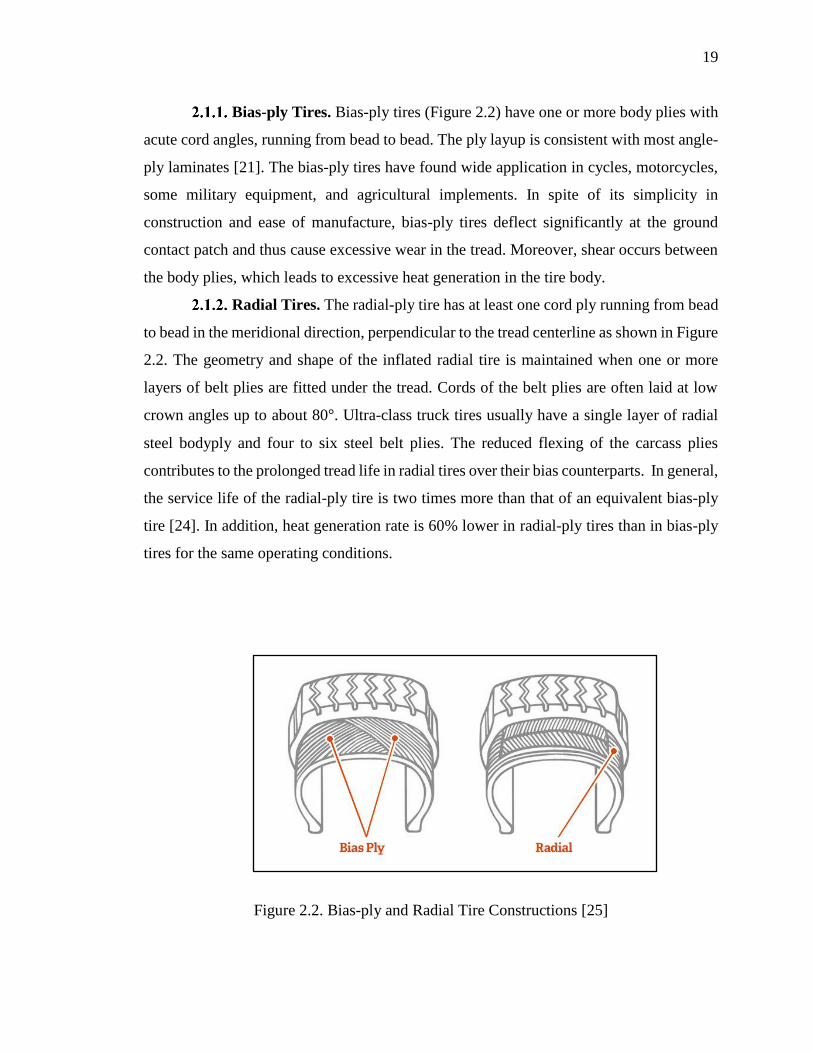
19

Bias-ply Tires. Bias-ply tires (Figure 2.2) have one or more body plies with

acute cord angles, running from bead to bead. The ply layup is consistent with most angle-

ply laminates [21]. The bias-ply tires have found wide application in cycles, motorcycles,

some military equipment, and agricultural implements. In spite of its simplicity in

construction and ease of manufacture, bias-ply tires deflect significantly at the ground

contact patch and thus cause excessive wear in the tread. Moreover, shear occurs between

the body plies, which leads to excessive heat generation in the tire body.

Radial Tires. The radial-ply tire has at least one cord ply running from bead

to bead in the meridional direction, perpendicular to the tread centerline as shown in Figure

2.2. The geometry and shape of the inflated radial tire is maintained when one or more

layers of belt plies are fitted under the tread. Cords of the belt plies are often laid at low

crown angles up to about 80°. Ultra-class truck tires usually have a single layer of radial

steel bodyply and four to six steel belt plies. The reduced flexing of the carcass plies

contributes to the prolonged tread life in radial tires over their bias counterparts. In general,

the service life of the radial-ply tire is two times more than that of an equivalent bias-ply

tire [24]. In addition, heat generation rate is 60% lower in radial-ply tires than in bias-ply

tires for the same operating conditions.

Figure 2.2. Bias-ply and Radial Tire Constructions [25]

20

Tire Materials. Tire components can be broadly grouped under reinforcing

and rubber materials. Tires are generally composed of a rubber matrix and inclusions. The

inclusions are primarily particulate and fibrous in nature. Fillers are interspersed within the

polymeric chains of the tire rubber to improve its stiffness, rupture energy, fatigue

resistance, and tear and tensile strength properties. Textile or steel fibers, twisted into cords,

make up the fibrous part of the tire composite.

The high strength, low elongation cords are embedded in a low strength, high

elongation rubber matrix [26]. Generally, they are responsible for the strength and stability

of the tire structure. The carcass and belt components have a higher volume fraction of

rubber than the fiber reinforced materials. The mechanical properties of the cord-rubber

composite system determines the global performance behavior of the tire. This section

provides a summary of the physical composition of materials used in tire development.

2.1.3.1 Reinforcing particles. Tire particulate reinforcements (fillers) include

silica, carbon black, and resins. Added fillers generally increase the strength of the

vulcanized rubber for improved tire performance [27]. The physical and chemical

interactions between the elastomer matrix and the fillers lead to improvements in rubber

mechanical properties. The entanglement of rubber molecules on the filler surface plays an

important role for rubber adhesion to fillers [28]. Thus, the effect of filler reinforcement

increases with increasing polymer-filler interfacial area. Neogi et al. [29] showed that

molecular chain mobility of rubber is greatly reduced when carbon black is mixed with the

gum rubber. The adsorption processes occurring on the filler surfaces cause reduction in

polymer chain mobility. Consequently, rubber shells are formed on the filler surface,

resulting in an increase in intermolecular friction (viscosity) [30].

2.1.3.2 Reinforcing cords. Polymeric fibers used in reinforcing the carcass of tires

include rayon, cotton, polyester, and nylon. Steel, fiberglass, and aramid filaments, on the

other hand, are used in the belts. Note that it is not uncommon to find steel plies in both

the casing and belt packages of OTR heavy-duty truck tires. While most of the polymeric

fibers have limited applications due to low strength and high cost, nylon (Nylon 6 and

Nylon 6.6) and polyester fibers have found wide application in today’s tire industry. Chen

[31] reported that a fiber’s intrinsic properties are determined by its molecular structure

(degree of orientation, crystallinity, molecular chain rigidity, and inter-chain bonding

21

forces). Polymeric fibers are typically engineered to have highly oriented molecular chains

in the fiber direction. Thus, the fibers are characterized by high modulus and strength in

the longitudinal (fiber) direction more than that observed in the transverse direction. For

tire application, the high strength, low elongation polymeric (and non-polymeric) fibers are

first assembled into yarns (strands) and then cords comprising multiple twisted strands.

Cord mechanical properties are sensitive to design variables such as lay angle, lay length,

and radius of the strand center line. Piatt [32] showed that a yarn’s strength is likely to

decrease with increasing twist level, a situation that may be caused by increased forces in

the yarn’s axis direction, which reduces the overall breaking strength of the yarn. Twist

level is also reported to impact cord fatigue resistance and durability. Kovac [33] reported

that increasing twist to some degree helps eliminate excessive buckling in cords as a tire

undergoes flexing in the contact patch.

The molecular structure of textile cords has an indistinguishable yet discrete

amorphous and crystalline phases. While the crystalline phase has a considerable amount

of secondary bonding, the amorphous phase hardly allows any secondary bonding to occur

at the interface of both phases as a result of its lack of molecular order and high free volume.

Hence, tie molecules are required to keep the amorphous and crystalline phases from

separating under any given load. Tie molecules comprise molecular segments and originate

from one crystalline phase, cross over a given amorphous region, and then lock up in an

adjacent crystalline domain. Lim [34] reported that tie molecules are formed during the

heating and drawing stages of cord manufacture. He attributed the tensile strength of textile

cords to the number and degree of orientation of tie molecules in the amorphous phase.

During the formation process, tie molecule properties are also affected by time, applied

tension, and temperature. The amorphous region of the cords determines its glass transition

temperature 𝑇𝑔. For polymeric cords such as nylon and polyester, thermal shrinkage occurs

in their amorphous structure when they are heated in the absence of applied loads [34-36].

Thermal shrinkage of carcass cords may alter the desired geometry of cured tires and

consequently affect tire uniformity and handling performance.

Steel cords, on the other hand, are made up of filaments drawn from iron-based

alloys and have greater strength, heat, and fatigue resistance properties over polymeric

cords. Figure 2.3 shows a typical steel cord’s structural components. The base element of

22

the cord is the filament (1). A group of these filaments are twisted together to form a strand

(2). Two or more strands are then twisted into a cord (3). Generally, the twist direction of

the cord is opposite to that of the strand [33]. Lastly, a filament wrap (4) is wound helically

around the cord to keep it together.

Figure 2.3. A Steel Cord Composition [37]

2.1.3.3 Rubber. Rubber is custom-formulated to meet the design and performance

requirements of a running gear for most ground vehicles. The properties of rubber that

makes it an essential component of the pneumatic tire include the ability to endure finite

strains without permanent deformation, resistance to impact cutting and abrasion, high

traction characteristics and fatigue resistance, and the ability to retain air (low permeability

23

to gases). Rubber compounds used in tires may vary depending on the performance

requirements of the tire. Natural rubber (NR) compounds are typically used in mining truck

tires for their tearing and heat resistance characteristics. Other performance parameters

such as wear resistance, casing durability, and ride comfort can be achieved by blending

various synthetic polymers for use in different regions of the tire. At the molecular level,

the vulcanized rubber consists of a crosslink of long chain-like polymer molecules. Gent

[38] pointed out that in the raw state, rubber is an extremely viscous liquid that can show

some degree of elasticity due to the temporary intertwining and entanglement of the long

chain-like molecules. Crosslinks formed during rubber vulcanization joins the highly

amorphous polymer chains in the raw rubber together into a more structured molecular

network. Consequently, the highly viscous raw rubber is transformed into a hyperelastic

solid. Some compounds used in tires are obtained from elastomers such as natural rubber,

styrene-butadiene, copolymer, and Cis-polybutadiene.

Tire compounds used in most heavy-duty tire components contain large amounts

of particulate fillers. Filled tire compounds are stiffer (by a factor of 3 or more) compared

to unfilled compounds [38]. Strength improvement and abrasion resistance are achieved

with filled compounds. However, filled rubber compounds exhibit pronounced inelastic

behavior such as shown in Figure 2.4. Mullins [39] showed through experiments that

deformation results in the softening of rubber and that the initial stress-strain curve

determined during the first deformation is unique and cannot be retraced. However, further

repeated deformations will cause the rubber stiffness behavior to reach a steady state with

an equilibrium stress-strain curve. He emphasized that softening in this manner occurs in

vulcanizates either with or without fillers, although the effects are much more significant

in highly filled vulcanizates. Mullins effect is apparently due to the sliding motion of rubber

molecules on the surface of filler particles.

Secondly, another effect is observed when strains in the range 0.1–10% are imposed

on the filled tire compound. This phenomenon, called the Payne effect, causes the dynamic

modulus of the rubber material to decrease rapidly over the specified range of strain

amplitudes. The Payne [40] effect is attributed to the disruption of agglomerates of filler

particles within the rubber matrix. While added fillers give rubber the needed enhanced

performance characteristics (stiffness and toughness properties), their presence influence

24

the dynamic and damping behavior of rubber in a very complex and disproportionate

fashion. Strain softening (such as Mullins and Payne effects) results from the high

stiffening influence of fillers when incorporated into rubber. Thus, filled rubber compounds

are inelastic in response behavior.

Figure 2.4. Mullins Effect in Filled Rubber

Tire Forces and Moments. At the tire-road contact region, the tire is

subjected to reactive forces from the road. A commonly used axis system [41] is shown in

Figure 2.5. The origin of the chosen axis system is the center of the line of tire contact with

the road.

The resultant force on the tire can be decomposed into components along the major

tire axes. The lateral component along the Y direction is tF , whereas lF is the force along

the X direction representing the direction of vehicle longitudinal motion. The normal

25

(vertical) force nF is the force along the Z direction. Three moments xM , yM , and zM

are exerted on the tire by the road. The overturning moment xM is about the X-axis, yM

is the rolling resistance moment about the Y-axis, and zM is the self-aligning moment

about the Z-axis. Wong [21] reported that the slip and camber angles are the two important

angles linked with a rolling tire. The slip angle is defined as the angular difference

between a line along the wheel travel direction and a line of intersection of the wheel plane

with the road. The camber angle, on the other hand, is the angle formed between the actual

wheel plane and the XZ plane, as shown in Figure 2.5.

Figure 2.5. Tire Forces and Moments [21]

2.2. HEAT GENERATION IN TIRES

The inelastic deformation of cords and rubber in a tire results in a partial absorption

of the energy transmitted from the engine of a vehicle to the wheels. The absorbed energy

is due to hysteretic processes occurring within the cords and rubber materials and is directly

converted into heat over time. The generated heat may increase the temperature of the tire.

Tire service conditions, construction, and material (viscoelastic) properties have been

known to contribute to the overall heat buildup in it. Kainradl and Kaufmann [42] stated in

26

a review publication that for a given tire construction, tire operating temperatures can be

reduced only by altering its rubber viscoelastic properties. Their review established the

notion that the viscoelastic properties of the elastomers in a tire determine the quantity of

heat generated in it. Over the years, viscoelastic properties of tire elastomers have been

measured in two domains: frequency and time. This section covers previous studies related

to viscoelastic property measurements and predictions for heat generation and temperature

rise in tires.

Measurement of Viscoelastic Properties. Testing for viscoelastic

properties of vulcanizates of tire compounds requires controlled conditions. Bulgin and

Hubbard [43] emphasized the importance of amplitude of deformation during testing and

have shown that its effect is more significant in rubber vulcanizates containing active

carbon blacks. They discovered that for a carbon black filled vulcanizate in the unstretched

state, the bonding of the black particles to themselves and the elastomer results in high

storage moduli. However, at high temperature and/or deformation amplitude conditions,

the filler bonds break down, decreasing the rubber moduli.

Kainradl et al. [44] developed a compression vibrational apparatus for determining

viscoelastic properties of rubber vulcanizates that worked on the principle of forced

resonant vibrations. The apparatus allowed two cylindrical test pieces arranged

symmetrically with respect to an oscillating coil to be precompressed axially by 10% of

their height at a time. The test pieces were then subjected to sinusoidal compressional

deformations at 70–100 Hz and 5–10% amplitude. A heating chamber provided in the

apparatus allowed tests to be conducted at specified temperatures. Their apparatus

supported relatively large test piece sizes and deformations. This testing approach is valid

only when the test pieces are linearly viscoelastic in nature.

Collins et al. [45] studied the contributions of the tread, sidewall and carcass

elastomers, and cords to energy loss in bias-ply tires. They considered the tread to undergo

both compressive and bending deformations as it passes through the footprint, while the

other components are only subjected to bending loads in operation. They observed that

bending deformations in tires were solely caused by the compressive deflection (rim loads

and inflation pressure) of specific components of the tire, and therefore the energy loss due

to bending should only be a function of the loss modulus "E and not the dynamic storage

27

modulus 'E . In addition, they showed that energy loss in a tread has a second component

that is due to compression in the footprint. This component of loss energy is proportional

to the loss compliance "C of the tread rubber. The authors did not extend their studies to

see if their observations were the same in radial tires.

Historically, the viscoelastic properties of tire elastomers are derived from losses

due to hysteresis in an elastomeric specimen subjected to sinusoidal loads. Willet [46]

provided mathematical relationships describing the energy loss per cycle per unit volume

under three loading states: constant strain amplitude [Equation (1)], constant stress

amplitude [Equation (2)], and constant strain and stress amplitude [Equation (3)]. He noted

that in practice, a loaded tire may be subjected to all three conditions:

''Eo

πεW 2 (1)

22

*E

''Eo

πσW (2)

δoσ

oπεW tan (3)

Willet [46] investigated the effect of viscoelastic properties, tire construction, and

tire size on heat generation in the shoulder region of a cross-ply and a radial-ply passenger,

and cross-ply truck tire constructions. The viscoelastic properties of samples removed from

the actual tires were tested using a Rheovibron (Model DD V-II at 110 Hz) and a

temperature range of 24℃ to 160℃. It is worth mentioning that the Rheovibron apparatus

was designed for relatively small specimen sizes and could only afford very small

deformations. The technique of multiple regressions was then used to develop the

relationship between heat generation and viscoelastic properties of the tire elastomeric

components. The author identified that heat generation in the tire shoulder region is

predominantly due to the condition classified as that of constant stress amplitude. The

errors due to his attempt to represent the extremely complex volumetric energy loss per

cycle in tires by three loading mechanisms limit the accuracy of this approach.

28

Kainradl and Kaufmann [47] studied the effect of various viscoelastic properties of

tire compounds on heat buildup. The study varied rubber compounds used in the tread-cap,

tread-base, and rubber matrix of the rayon cord for 12.00-20 tires to reflect alterations in

their viscoelastic properties. Needle thermocouples were used to measure the operating

temperatures of the tire shoulder region while the tires were on the test wheel. The authors

used multiple regression analysis to investigate which combinations of viscoelastic

properties of the rubber compounds would give a linear, significant correlation to the heat

buildup in the tire. They found out that the greater contribution (25–30%) to the heat

buildup came from the tread-base due to its loss factor, followed by the carcass (20%) also

by its loss factor, and the least contribution (10%) from the tread-cap due to its loss

compliance. The contributions of the tire cord to the heat buildup, however, remained

undetermined in this work.

Fillers used in rubber vulcanizates have been noted to contribute to the time-domain

transient properties of tire materials, namely creep, stress relaxation, and hysteresis. In an

early investigation, Gent [48] conducted experimental measurements of stress relaxation

and creep at room temperature in vulcanizates of NR, butyl, and styrene-butadiene rubber

(SBR) in both unfilled (gum) and filled states. He used semilogarithmic plots to obtain

linear stress-time plots of the filled (carbon black) and unfilled vulcanizates. The rate of

stress relaxation was found not to depend on strain for the gum NR up to levels where the

vulcanizates strain crystallize. The filled vulcanizates, however, showed stress relaxation

rates that were highly dependent on the applied strain and showed greater magnitudes than

those of the unfilled vulcanizates at the same strain loading [49]. Given the similarities in

the form of the plots, Gent [48] proposed the existence of a similar viscoelastic mechanism

in both filled and unfilled vulcanizates.

Cotten and Boonstra [50] expanded Gent’s [48] work by plotting both stress and

time data on logarithmic scales. Similar to Gent’s [48] plots, a power-law relationship was

found in the stress-time data. Even though there was no clear distinction between plots on

semilogarithmic and fully logarithmic scales, the authors discovered a variation in the rate

of relaxation with strain for all classes of vulcanizates in non-NR rubbers.

For both filled and unfilled SBR vulcanizates, Bartenev et al. [51] concluded that

relaxation processes occurring within the vulcanizates were the same at relaxation times

29

sec104 , an observation they attributed to the segmental movement of the polymer chains.

Furthermore, they found out that an additional process with relaxation times between

sec104 and sec106 (likely to be breakdown of rubber-filler bonds) existed in the filled

vulcanizates.

Skelton [52] studied the mechanisms of bending hysteresis losses in a single-ply

cord-rubber composite via experiments. He presented a simple and versatile experimental

technique for the determination of the bending hysteresis losses in composites containing

a range of different cord materials. Skelton [52] used composite specimens prepared from

freshly milled carcass rubber and a variety of commercial tire cords. His testing setup

involved constraining a strip of cord-rubber composite between two parallel plates and

subjecting each element of the strip to a cycle of curvature by moving one of the plates

relative to the other. The relationship between bending moment and curvature of the strip

was found to follow a hysteresis loop, where the area enclosed within the loop constitutes

the magnitude of the non-recoverable work loss. The results he obtained showed a nylon

66 ply to have the lowest hysteresis, only slightly above that of an unreinforced ply.

Sharma et al. [53] used experimentally measured temperature rise in three different

tires to calculate the temperature profiles and mechanical losses of cords and rubber in

tires. The types of tires analyzed were a bias tire, a radial passenger tire, and a series of

radial truck tires. The objective of their study was to establish the relative importance of

cords and rubber in tire rolling resistance. Cord-rubber viscoelastic hysteretic properties

were determined by a high strain dynamic viscoelastometer under various strain amplitudes

and frequencies. The results of the study showed that the contribution of cords to tire rolling

resistance varies from 10–80%. Operating conditions, variations in tire construction, and

inflation pressure were also found to affect cord-rubber characteristics. The form of

characterization used to determine the viscoelastic properties of cords and rubber lacked

universal applicability.

MacKenzie and Scanlan [49] studied the effect of strain on stress relaxation in

carbon black-filled vulcanizates at room temperature. They prepared similar filled and gum

formulations of the vulcanizates in order to clearly measure the influence of carbon black

fillers on the vulcanizates. Stress relaxation testing was done with an Instron 1026 Table

Model Tester. A pen recorder of the machine traced out the load-time data during the

30

testing. Their results revealed the existence of a transient relaxation process in HAF-filled

vulcanizates. This relaxation process is more significant at small strains than relaxation

processes occurring in gum carbon black-filled vulcanizates at higher strain levels and

longer relaxation times.

Priss and Shumskaya [54] showed that mechanical losses in rubber compounds are

more significant when under pulse loading, which simulates tire usage, than under

sinusoidal loading. They conducted laboratory experiments on rubber strips cycled under

tension using an Instron 1122 Universal Tester. Tests were all carried out at room

temperature and at a frequency of 0.021 Hz. Hysteretic loss data were measured using an

electronic integrator. A loss modulus K (as shown in Equation 4) was defined in order to

characterize the hysteretic behavior of the test strips that were under anharmonic loading:

2o

KA

W (4)

They concluded that stress and strain for anharmonic modes vary with time and cannot be

described by a sine function, thus rendering the concepts of storage modulus 'E and loss

modulus ''E irrelevant.

Modeling of elastomer time dependence under transient conditions in order to

predict rubber response to dynamic impact events has been an interesting topic for

researchers. Dalrymple et al. [55] presented a methodology for testing and calibrating an

extracted elastomer specimen (from a manufactured part) for use in a transient dynamic

FEA simulation. The first goal of their study was to determine how to capture very early

time (a fraction of a second) information in the stress relaxation test. Their next goal

focused on assessing how accurate the Prony series model derived from the uniaxial tension

test data predicts the material behavior at different strain rates. In essence, they carried out

two dynamic tests: (i) stress relaxation, and (ii) uniaxial tension (simple tension) at a

constant strain rate to define a Prony series viscoelastic model for the specimen. Prior to

the actual measurement of relaxation response, the specimen was preconditioned at a slow

strain rate of 0.01/sec. Relaxation testing of the specimen began at a strain rate of 50/sec.

The relaxation time allowed in between strain levels was approximately 110 sec. The

31

specimen was allowed 300 sec to recover after each strain level. They later curve-fitted a

representative (at 0.8 strain level) stress relaxation response in order to calculate the Prony

series coefficients for the FEA simulation. Given the high strain rates imposed on the

specimen, the test results were affected, to some degree, by inertia.

Lapczyk et al. [14] proposed a parallel rheological framework (PRF) material

model to predict nonlinear viscoelasticity, nonlinear viscosity, stress relaxation, and

permanent set in filled elastomers. Their framework was developed on elastic and

viscoelatic networks connected in parallel. The authors assumed a multiplicative split of

the deformation gradient into two parts: elastic and viscous. In each network, a hyperelastic

material response represented the elastic portion of the deformation gradient. A creep

potential was used to describe the evolution of the viscous part of the deformation gradient.

They suggested that either a power-law strain hardening law or a hyperbolic-sine law could

be used to specify the evolution of each viscoelastic network. The model was validated

using data from relaxation tests of a PC-ABS thermoplastic polymer, and was afterwards

implemented in ABAQUS to facilitate robust numerical simulations. Their model,

however, lacked the capability for predicting other filled rubber behavior such as the

Mullins effect and permanent set.

Nandi et al. [56] presented stress relaxation test data of a silicone rubber and a

typical filled elastomer to determine which of the two compounds is truly linear

viscoelastic in behavior. In order to test for linear viscoelasticity in both compounds, stress

relaxation tests were carried out for each compound at different strain levels. They then

overlaid the normalized stress relaxation plots of each compound and determined whether

or not the overlay was perfect. In theory, linear viscoelasticity is valid only when the time-

dependent shear modulus of a material is independent of loads imposed on it. The authors

found that silicone rubber showed a true linear viscoelastic response, as its normalized

stress relaxation plots overlaid with each other perfectly. The opposite was true for the

filled elastomer and therefore confirmed its nonlinear viscoelastic behavior. The authors

encouraged the use of a nonlinear viscoelastic material model such as the PRF model to

predict the response of filled elastomers.

32

Heat Generation and Temperature Rise Prediction. The dynamic

properties of materials are responsible for their heat generation. The temperature of any

material increases when the heat generated in that material exceeds the rate of dissipation.

Direct measurement of the rate of heat generation and overall rise in temperature in tires is

extremely difficult and expensive, and the results of such measurements do not provide

complete temperature distribution in a tire. However, with the advances in computer

technology, numerical methods such as FEA have been used by many researchers to study

the mechanism of heat buildup and temperature rise in pneumatic tires. The tire

deformation problem is in reality a coupled thermo-viscoelastic problem with a strong

interdependency between the nonlinear viscoelastic material properties and temperature.

That is, energy dissipation depends on temperature, and vice versa.

Trivisonno [57] noted that lower tire operating temperatures can lead to increased

tire durability, and thus the need to obtain a complete temperature distribution in a tire to

ensure that operating temperatures are kept below critical values. With this objective, he

performed a steady-state thermal analysis for a B.F Goodrich 7.75 × 14 two-ply rayon bias

tire. The tire was run on a 3.048 m (120 in.) diameter test wheel where steady-state infrared

surface temperatures were measured from bead to crown with an Ircon CH 34LC infrared

radiation thermometer. Cavity air, tread shoulder, and crown temperatures were measured

with thermocouples. Measurement of mechanical power loss on the tire was performed

alongside the temperature measurements. Power loss was calculated from the

experimentally measured moment of inertia of the tire. The author used a numerical

network analysis to obtain the rates of heat generation and temperature distributions in the

various components of the tire. However, the study did not relate the tire temperature

distribution to the viscoelastic properties of its components.

Tielking and Schapery [58] developed an analytical tire model to calculate load

transfer functions from the significant harmonics of the contact pressure distribution. The

load transfer functions represented the structural response of the modeled tire and depended

on the complex modulus of the viscoelastic materials assumed for the model. They

assumed the structural response to be linearly viscoelastic with respect to contact loads and

calculated energy dissipation from contact deformation of the rolling toroidal membrane

33

model. Their approach did not consider the interaction between the mechanical and thermal

states of the tire model.

Prevorsek et al. [59] related tire rolling resistance to its total heat loss. Their model

required the solution of the energy balance equations with heat generation terms for the

cross-sectional temperature profiles. Input data including a detailed description of the tire,

thermal properties of tire materials, dynamic viscoelastic material properties, heat transfer

coefficients, and some experimentally obtained tire temperature values were required to

calculate a complete temperature profile of the tire. Being strictly a thermal model, their

method could not account for the influence of the strain (mechanical) field on the tire.

Yeow et al. [60] presented a simplified three-dimensional model to predict a

rolling/skidding tire temperature distribution. Their thermal analysis model considered

frictional and hysteretic heating. Particularly, they considered hysteretic heating to be

proportional to the cyclic local deformation of any point within the tire. They assumed a

contact pressure distribution in the structural analysis while neglecting the effect of

radiation in the thermal analysis. Although reasonable results were obtained, their approach

did not show a clear interaction between the thermal and mechanical fields of the tire.

Whicker et al. [61] emphasized that a realistic model for tire power loss must be a

combined thermomechanical model. Thus, they developed an analytical model which was

based on an iterative thermomechanical analysis system. The model was implemented in a

modular form consisting of three analytic modules: deformation, dissipation, and thermal.

The deformation module accepts as input the internal and external geometry of the tire

being modeled, the appropriate material properties, the operating conditions of interest, and

an initial temperature distribution from which it calculates the deformation cycles for all

sections of the tire. The dissipation module then uses the resulting deformation cycles,

initial temperature distribution, and the appropriate material properties to calculate the

local heat generation rates throughout the tire. Finally, the distribution of heat generation

rates, the thermal boundary conditions, and the appropriate thermal properties of the

materials are used by the thermal module to calculate the corresponding temperature

distribution. The iterative process is repeated until thermal equilibrium is established. A

major limitation of their approach is the lack of mathematical expressions to show how

34

dissipated energy relates to heat generation rate in the tire. In addition, the underlying

assumptions and interpolations of their model makes the approach very case-specific.

In an attempt to improve the model by Whicker et al. [61], Sarkar et al. [62] used

experimental data to correlate dissipated energy to heat generation rate in tires. They

proposed a more generic approach for solving coupled thermomechanical problems in tires

by using the commercial finite element code MARC. Three stages of analysis, inflation,

contact, and temperature, were included in their model. An iterative process was used to

couple the structural (inflation and contact analysis) and thermal analysis steps to reflect

the effect of temperature changes on material properties. Hypothesizing that strain

amplitude is a key factor in tire heat generation, they obtained for each element, principal

(rubber) and tensile (cord-rubber) strains from FEA conducted on the tires. Using

laboratory measured heat generation data, they showed that the rate of heat generation for

strain amplitudes below 0.6% and above 1.0% could be approximated by Equations (5) and

(6), respectively:

2006.0 006.0 HH (5)

2010.0 010.0 HH (6)

With heat generation rates known, temperature distribution could be calculated

using the same FE models. It was further stated that depending on the sensitivity of the

material properties to temperature changes, the structural analysis could be rerun with a

new set of material properties adjusted for temperature changes to obtain updated strain

amplitudes. The new set of strain amplitudes are then used to update the temperature

distribution in the tire, and the cycle is repeated until convergence is reached. Their study

did not account for the effect of viscoelasticity on heat generation in the tire materials.

Yavari et al. [63] presented a one-way coupling algorithm that used the solution of

a mechanical rolling contact problem to provide heat source terms for the solution of a

thermal problem. In the algorithm’s implementation, the rolling contact problem with

friction was first solved, and the deformed shape and dynamic material properties were

used to compute power loss in the model. The program was then restarted and the linear

35

heat transfer equation solved for temperatures at the current configuration. Their approach

was based on irreversible thermodynamics, eliminating the need for iterative loops.

Although simple, the one-way coupling approach neglects the time and strain dependence

of the dynamic material properties of tire materials.

Based on the idea that periodic loading of viscoelastic materials results in a phase

shift between stress and strain response, Park et al. [64] presented modified stress and strain

tensors to incorporate the effect of phase shift in the tire power loss calculation. Park et al.

[64] attempted to improve the energy dissipation module proposed earlier by Whicker et

al. [61] by using a viscoelastic theory to establish an analytic method for computing heat

sources in a steady state rolling tire. Integration of the product of the stress and strain rate

tensors over one tire revolution, according to their work, results in the uncovered work

(energy dissipated) per cycle. They noted that dissipated energy and the corresponding rate

of heat generation, when integrated numerically over the circumferential direction, will

have the same values in all elements having the same cross-sectional coordinates. Their

proposed method was used to compute heat generation rates resulting from ABAQUS

deformation analysis of a 205/60R15 tire. The tire temperature profile and rolling

resistance were determined from the computed energy dissipation rates, and they showed

good correlation with measured results.

Observing the role of temperature in tire durability and the effort to reduce

temperature rise in large earthmover and aircraft tires, Ebbott et al. [65] investigated rolling

resistance and temperature distributions in tires under transient conditions using the finite

element method. Their efforts were concentrated on material properties and constitutive

models used to represent tire materials in predictive analysis. It was mentioned in their

work that predicted heat dissipation rates are highly sensitive to the used material model.

Similar to previous works, they used the three-modular thermomechanical modeling

approach to account for the temperature dependence of elastomer behavior. Specifically,

an equivalent elastic representation of the viscoelastic behavior was used in their tire FEA

that provided strain cycles to the energy dissipation module. Next, they used a linearized

viscoelastic model in the dissipation module to calculate energy loss per circumferential

ring of elements. An axisymmetric thermal model was then used to predict temperature

distributions based on results from the dissipation module. The axisymmetric thermal

36

model was used on the assumption that zero thermal gradients exist in the circumferential

direction of the tire. The steady state temperatures were mapped back to update material

properties in the deformation module and the process repeated until convergence was

reached. Measured and predicted rolling resistance results of a P175/70R13 passenger tire

were compared and showed fair agreement. Their approach would have been ideal if they

had used an accurate model to represent the nonlinear viscoelastic behavior of the highly

filled elastomers used in the tire.

Futamura and Goldstein [66] proposed a simplified method for handling the

coupled thermomechanical analysis of rolling tires. The authors used the deformation index

approach to characterize the sensitivity of the dissipated energy to changes in tire material

stiffness. In essence, the deformation index measures the type of deformation a material

point experiences in a tire’s duty cycle, namely the degree to which the material point is

stress controlled, strain controlled, or energy controlled. The deformation index m could

be obtained experimentally or computed from two FEA runs: (1) baseline structural and

energy dissipation analyses using the original material data at a reference temperature, and

(2) a perturbation structural and energy dissipation analyses where the materials are

stiffened up to 20%. The deformation index is then calculated (holding tan constant),

according to Equation (7).

'

1

'

2

1

2

G

G

Q

Qm (7)

Futamura and Goldstein [66] observed that the changes in the volumetric heat flux

causes temperatures to differ among thermomechanical analysis procedures (uncoupled,

partially coupled, and fully coupled). It was also noted that the volumetric heat flux

depends on the dynamic material properties (storage 𝐺′, loss 𝐺′′ moduli, and tan 𝛿) which,

in turn, are temperature dependent. Using ABAQUS user subroutine DFLUX, they

established a computational link between element volumetric heat flux and temperature.

The user subroutine was provided with temperature dependent 𝐺′ and 𝐺′′ expressions to

reflect the updated material properties throughout the solution. A relationship was then

developed to calculate current volumetric heat flux from knowledge of the deformation

37

index, and material properties and volumetric heat flux corresponding to a solution at a

reference (or previous) temperature. The mathematical expression in Equation (8) implies

that energy loss per cycle Q can be multiplied by a constant deformation rate, such as tire

rotational frequency to obtain Q . Futamura and Goldstein [66] therefore concluded that

Equation (8) replaces the iterative structural and energy dissipation modules used in the

conventional thermomechanical analysis technique.

to

t

m

to

tto

G

GQQ

tan

tan'

'

(8)

Thus, their technique converts the iterative looping method into a non-iterative

method where Equation (8) is contained in the thermal analysis only. The statically loaded

deformation model used to simulate tire-rolling behavior suggests that their approach is

likely to be limited to axisymmetric tires (smooth or circumferentially grooved tires).

Yin et al. [67] used a thermomechanical FEA of a heavy-duty radial truck tire to

determine the endurance performance of the tire’s shoulder compound. They developed a

semicoupled thermomechanical finite element method (FEM) in which stress-strain cycles

resulting from a deformation analysis provided the heat generation rates for a nonlinear

heat transfer analysis step. The computed stress-strain cycles (as influenced by material

hysteresis), and the loss properties of the tire materials were used to determine the heat

generation rates. Based on the assumption that variation in material temperatures is small

during one rolling cycle, the original three-dimensional thermomechanical tire (11.00R20)

was reduced to two-dimension. The computed heat fluxes were expressed as functions of

temperature and incorporated into the analysis by means of the ABAQUS user subroutine

DFLUX. Hardness, tensile, and dynamic mechanical tests conducted on rubber specimens

from specific regions of the tire provided data for calibrating the material models used in

the on-drum and on-road FE analysis. Their approach neglected the temperature

dependence of the tire material properties.

Kondé et al. [68] highlighted the effects of loading parameters (vertical load,

internal pressure, velocity) on the mechanical behavior of a rolling aircraft tire in contact

38

with the ground via FEA. They observed that the local friction coefficient in the ground

contact partly depends on temperature and therefore proposed a thermal model to

characterize the evolution of temperature in the contact patch during rolling. In their study,

it was assumed that the tire material properties do not vary with temperature and that the

only source of heat in the tire is that which comes from dissipation in the contact patch.

Thus, the dissipated heat flux due to friction and prescribed on the contact boundary was

given as in Equation (9).

TNlocalf uTQ (9)

It is clear from Equation (9) that the local friction coefficient local depends on

temperature. The results of their tire sliding simulations showed that temperature rise is

highest on the tread surface with visible thermal gradients in the thickness direction. They

therefore concluded that temperature rise in the contact patch depends on tire rolling speed.

The authors did not provide details on the thermomechanical analysis technique employed

in their studies.

2.3. TIRE FATIGUE STUDIES

A considerable number of passenger and truck tires are removed from service as a

result of fatigue failure. Tire fatigue life is known to be influenced by a class of factors:

thermomechanical loading history, irregularities in rubber formulations, environmental

factors, and effects due to the dissipative nature of the rubber materials [69]. The number

of tire failures due to mechanical fatigue accounts for 20% of working tires with 75–96%

of average service life [70]. The use of reinforcing fillers and processing aids in tire

compounds result in the formation of microstructural inhomogeneities that act as crack

precursors and are likely to develop into observable cracks under fatigue loads.

Understanding the underlying mechanics and modeling strategies of the fatigue failure

process in rubber and/or tires will provide a foundation for this research. This section

covers nearly all aspects of analytical approaches that have been used over the years to

39

predict tire mechanical fatigue life. An emphasis is placed on the two main modeling

approaches (continuum-based and fracture mechanics) used in rubber fatigue life

predictions.

Continuum Mechanics Approach. This approach considers that the history

of familiar quantities (stresses or strains) at a material point defines the life of that material.

The continuum mechanics approach is also known as the crack nucleation life approach

because it aims at predicting crack nucleation life based on known stresses and strains

available in a component. Mars [71] noted that the crack nucleation approach is best suited

for applications where the initial inherent flaws of a part are significantly larger than the

smallest dimension on the part, and where the spatial distribution of fatigue life is the

primary goal of an analysis. He also indicated that maximum principal strain and strain

energy density parameters are the two fatigue predictors generally used for crack

nucleation predictions.

Specifically, the continuum mechanics based approach computes the number of

cycles needed to cause a visible crack of a given size to appear in a cyclically loaded part.

Other crack nucleation life predictors include maximum principal Cauchy stress,

configurational stress tensor, and cracking energy density. Two mechanisms have been

found to be responsible for fatigue crack nucleation in filled rubber in the absence of

mechanical loads. Le Cam [72] and Saintier et al. [73] reported that, independent of loading

conditions, crack nucleation is likely to be caused by debonding of the rubber matrix from

rigid inclusions (silica), and cavitation in the vicinity of carbon black agglomerates.

The work of Cadwell et al. [74] is one of the earliest known studies that applied the

continuum mechanics approach to rubber fatigue studies. The authors presented testing

strategies and results of their study on the dynamic fatigue life of rubber and showed the

dependence of the rubber durability on the imposed dynamic loads. They obtained linear

dynamic fatigue life curves for different loading and environmental conditions. It was

found that rubber exhibits minimum dynamic fatigue life when subjected to linear

excitations at the zero strain loading region. Considering samples tested under shear strains,

they examined three conditions of lateral strains: 0%, 12.5% compression, and 25%

tension. For different ranges of shear cycles, they obtained the dynamic fatigue life of each

specimen under the three lateral strain levels. The results in shear fatigue were in accord

40

with that predicted from samples in tested linear vibrations. In general, they found that

fatigue life improved as strain was increased, up to a point beyond which additional strain

application decreased the fatigue life.

Fielding [75] designed an experiment similar to Cadwell et al. [74], to show the

effect of minimum strain amplitude and starting strain on fatigue life of a synthetic rubber

tested within a range where crystallization is likely to occur. The strain rate used was 550

cycles per minute. He investigated minimum strain amplitudes from 25% to 400%, and

initial strains up to 550%. Unlike the fatigue life of NR and Butyl B rubber, the synthetic

rubber (GR-S) showed no evidence of a peak. The fatigue life at different amplitudes began

to fall immediately as initial strain was ramped up from zero to the ultimate value. He

concluded that the sharp fall in fatigue life in the GR-S rubber was due to the absence of

crystallization (fibering) in the compound to retard crack growth.

It was evident in earlier studies that fatigue nucleation life parameters were

basically the minimum and alternating (tensile) strains. However, the advent of rubber

fracture mechanics saw strain energy density becoming a parameter for predicting fatigue

crack nucleation. Roberts and Benzies [76] determined the fatigue lives of gum and filled

NR and SBR under cyclic uniaxial and equibiaxial deformation conditions. The objective

of their study was to present fatigue life data from equibiaxial fatigue tests as a function of

strain energy density as is the case in tensile fatigue test conditions. For equibiaxial testing,

the authors designed an apparatus which used pulses of compressed air to inflate samples

to impose cyclic loads on them. They observed that for both NR and SBR, fatigue life was

longer under equibiaxial tension than when under uniaxial tension on the basis of strain

energy density. The opposite was true when fatigue life was expressed in terms of principal

strain—simple tension fatigue life was the greatest.

Oh [77] investigated a rubber bushing durability in which he considered the

unknown initial crack length to be a primary geometric variable, hence assuming the

bushing’s J-integral to be directly proportional to the product of the strain energy density

and the variable crack length. For the investigated bushing, Equation (10) gives an

approximation of the J-integral used.

WckJ (10)

41

Equation (10) is valid for small crack lengths under certain loading configurations.

The proposed model was developed on both nucleation life and fracture mechanics

approaches since under the small crack assumption, the fracture parameter (J-integral)

becomes a direct function of strain energy density W under the small crack assumption.

By way of using the crack nucleation approach, Grosch [78] examined the influence

of service conditions (load, inflation pressure, and speed) on temperature and fatigue

performance of a tire. Based on the cut-growth theory of Rivlin and Thomas [79], he

assumed that tearing energy is generally proportional to the elastically stored energy

density in the bulk of the test specimen. The author used estimated strain energy density

together with a semi-empirical model that relates strain energy density and fatigue life to

predict the relative differences in failure cycles of a tire under varying operating conditions.

The author concluded that a tire’s temperature influences its fatigue life since the rate of

crack growth depends on the energy input and the temperature that results from energy

loss. His claim of the effects of temperature on fatigue life in tires lacked theoretical

footing. In general, the strain energy density as a fatigue predictor is independent of

material changes. Thus, this predictor will produce a poor fatigue ranking in super heavy

duty tires whose materials change over time due to high internal temperatures.

De Eskinazi et al. [80] used the finite element method to predict relative belt edge

endurance performance in radial tires. Their study included three groups of tires: a control

group, a better edge endurance group, and a worse endurance group. They compared belt

edge stress analysis parameters obtained from the finite element models to those measured

from fleet tests. The parameters included strain energy density, von Mises stress, maximum

shear stress, maximum shear strain, hydrostatic stress, and belt edge shear. Among these

parameters, they found that strain energy density appeared to be a good predictor of rubber

failure as its maximum value and amplitude correlated well with the test results.

Considering that the strain energy density as a predictor could not be used in a case

where multiaxial loads were present, Mars [81] proposed the cracking energy density

concept. Mars’ [81] postulated fatigue predictor accounts for the fraction of the total strain

energy density available to be released as microscopic defects develop on a material plane.

Incrementally, he defined the cracking energy density on a material plane of normal vector

42

r

as a dot product of the Cauchy traction vector

and the strain increment vector d ,

as shown in Equation (11).

rdrdW T

c

(11)

The cracking energy density tensor with increment dW is accumulated over one

loading cycle for every material plane and orientation, and it is capable of predicting the

plane with the maximum available energy which will grow an intrinsic flaw.

In their recent investigation of damage in rubber under multiaxial loads, Verron and

Andriyana [82] derived a new predictor for estimating crack nucleation life in rubber. The

predictor was developed on the basis of configurational mechanics. It was noted in their

study that the smallest eigenvalue of the Eshelby stress tensor (as given in Equation 14)

determines the development of microstructural defects in rubber. They suggested that since

rubber shows a stabilized stress-strain behavior after a number of loading cycles, it was

sufficient to obtain the predictor just over that stabilized cycle. It was emphasized that only

the damage part of the configurational tensor Σ contributes to crack opening as given in

Equation (12).

TTJW FσFIΣ (12)

It was also shown in their study that a flaw grows only on condition that one or

more of the eigenvectors of the Eshelby stress tensor is negative. Their postulated fatigue

life predictor is given in Equation (13).

0,min 3,2,1

iiΣ (13)

It is important to note that the principal configurational stress 3,2,1

ii determines

the sign of the predictor which in turn predicts the opening and closing state of a flaw. In

particular, a flaw tends to open when one or more of the principal stresses is negative.

43

Fracture Mechanics Approach. In this approach, fatigue life is estimated

based on preexisting crack(s) in a material. As a requirement for the prediction of a

component life using this approach, the location of the crack in the component has to be

known beforehand. Rivlin and Thomas [79] described the growth of a cut in a rubber strip

to involve balancing of energies within the strip. They showed that catastrophic tearing in

a rubber vulcanizate could be described by an energy criterion not limited by the geometry

of the test vulcanizate. Developed based on Griffith’s failure theory, their proposed energy

criterion was based on the idea that changes in the stored strain energy as a result of crack

growth were balanced by changes in the internal energy, and not by the energy used to

create new crack surfaces.

Later, Thomas [16] showed that for a smooth cut growth (small growth of a cut

before catastrophic tearing occurs) in unfilled NR, the change in crack length c is a

function of the tearing energy T , as expressed in Equation (14).

sGTc 2 (14)

Greensmith [83] validated the energy criterion for use in a situation where a rubber

strip with a crack is loaded in simple tension. His proposed criterion is given in Equation

(15).

lc

U

tT

ˆ

1 (15)

The tearing energy T given in Equation (14) has been shown to be a characteristic

energy of any given vulcanizate, which could be determined experimentally, and be used

to predict critical forces required to rupture test strips of that vulcanizate. The Rivlin-

Thomas approach considers that during a quasi-static growth of a crack in the absence of

work done by external forces, no damage accumulates in the crack tip process zone and the

material is elastically reversible. However, all the elastic, far-field (strain) energy is

44

released to grow the crack. Equation (16) simplifies the tearing energy for a single-edge-

notched rectangular specimen under uniaxial tension fatigue loads.

WckT 2 (16)

In this case, the strain energy density W is considered a measure of the energy

release rate of the crack. Note that Equation (16) is only valid on conditions that the crack

growth is self-similar, state of stress is simple tension, and crack length to specimen width

ratio is relatively small. Thus, predicting crack initiation in rubber by the strain energy

density parameter is restrictive.

Gent et al. [84] employed the tearing energy criterion concept to study how cut

growth relates to failure caused by imposed cyclic loads in NR gum vulcanizates. They

found that when an edge-cracked test piece is repeatedly deformed below its characteristic

tearing energy value cT , crack growth per cycle is consistent with Thomas’ [16] square-

law, given in Equation (14). In a theory they propounded, it was shown that the number of

cycles required for a crack to grow from an initial state to failure in a test specimen is

independent of the geometry of the specimen as long as its smallest dimension is larger

than the initial crack size. For conditions where of cc , they suggested life to failure is

predicted using Equation (17).

ockWGN2

2 (17)

Lake and Lindley [85] extended the study of Gent et al. [84] to non-crystallizing

SBR gum vulcanizates. They prepared planar tension and tensile test strips from a 1 mm

thick SBR gum vulcanizate. In particular, the planar tension specimens were 30 cm in

width and 2.5 cm in height. Using the tearing energy theory, they discovered that the

growth of small crack precursors in the rubber specimens was due both to static and

dynamic loading conditions. The growth rate under each condition was consequently found

to be approximately equal to the fourth power of the tearing energy. The authors noted that

in spite of the resemblance in failure mechanisms between crystallizing NR and non-

45

crystallizing SBR, both rubbers still showed marked differences in behavior. First, SBR

exhibited static cut growth and fatigue, while NR did not, except at energies near the critical

tearing energy. Last, cut growth behavior in SBR is found to be highly sensitive to

temperature changes, whereas that of NR showed little to no variation.

In their investigations of the dynamic crack growth behavior of vulcanized rubbers,

Lake and Lindley [86] carried out cut growth experiments on 10 cm × 2.5 cm × 0.1 cm

strips of rubber. Each test piece was given an edge cut, about 0.05 cm long and deformed

repeatedly in simple extension. Again, the authors adopted the tearing energy concept in

determining the rate of cut growth in their tests. The results of the experiments indicated

that there exists a minimum tearing energy oT above which cut growth is attributable to

mechanico-oxidative processes. However, at tearing energies below oT they suggested cut

growth was due only to chemical ozone attack. The authors identified a critical strain in

the fatigue tests corresponding to oT , below which life to failure increased rapidly. They

concluded that the critical strain was likely to constitute the mechanical fatigue limit of the

rubber and that its value is unique for every rubber. Further, it was reported in their study

that fillers lower the fatigue limit while showing negligible effect on the oT of their matrix

compounds.

For laboratory test pieces of relatively simple shapes and dimensions, energy

release rate was easily determined by a sample’s geometry, crack size, and magnitude of

the deformation. It is almost impossible to determine energy release rate in the

aforementioned manner, especially when complex shapes and loading modes are involved.

In lieu of this, Clapson and Lake [87] presented a special technique that allowed the

estimation of energy release rate and strain cycle of a crack present at the groove base of a

tire. Their technique determined these parameters empirically from measurements obtained

from groove crack opening. A pure shear test piece with a central cut was used in their

crack opening experiments. In terms of determining the strains in the groove region based

on the crack opening technique, they inserted razor blade cuts of desired lengths in the

inner grooves of an inflated but unloaded truck tire. Using a classical elasticity theory, the

authors investigated the dependence of maximum crack opening on crack length for

46

varying values of strain and unstrained specimen heights. The variation of crack opening

was plotted as a function of crack length. The dependence was found to be similar in both

the pure shear and actual groove test cases. In addition, maximum crack opening showed

to be directly proportional to strain and hence could be used to estimate the strain cycle at

the vicinity of a crack.

Huang and Yeoh [88] studied the initiation and subsequent growth of penny-shaped

cracks in two types of cord-rubber model composites. Their attempt was to improve upon

previous similar investigations that neglected crack initiation in these composite structures.

Specifically, their model composites were such that cord ends were completely covered by

rubber. They extended the tearing energy approach to study growth of penny-shaped flaws

that initiate at the free ends of cords of composites subjected to fatigue loads. Considering

that the rubber matrix attached to the cord in their model was only able to deform

restrictively, the authors postulated that strain energy release rate available for propagation

of an existing penny-shaped crack may be governed by Equation (18).

WcT

6 (18)

Test specimens were tested in pure shear and were essentially prepared from

calendered sheets of carbon-black-filled NR vulcanizates. Their results showed that fatigue

failure in cord-rubber composites begins with penny-shaped crack initiation at cord

endings.

Ebbott [89] evaluated the energy release rate associated with an explicitly modeled

crack in a finite element model based on the J-integral and virtual crack closure technique

(VCCT). He focused his study on two rubber compounds typically used at the ply ends of

a 295/75R22.5 truck tire. The elastic and crack growth behavior of both compounds were

determined through tensile and fatigue tests, respectively. Pure shear test specimens were

used in the case of the fatigue test. In a way of simulating cyclic deformation in a tire, he

used a plane strain model to represent the condition in the footprint, and an axisymmetric

model for the region 180° opposite of the footprint. For the assumed ply end crack

extending around the circumference of the tire, Ebbott [89] adopted a submodeling

47

approach in order to refine the mesh surrounding the crack. For situations where multiaxial

modes of fracture were present, he proposed a new method to determine the cyclic energy

release rate. This method involved separating the total energy release rate into contributions

due to each fracture mode (Mode I, II, and III) and treating the cycle of each mode

independently. The three computed crack growth rates were then summed up to represent

the total crack growth rate. Although his results showed some degree of correlation

between energy release rate estimates by the J-integral and VCCT methods, his idea of

separating the total energy release rate by fracture modes lacked experimental and

theoretical basis. Another key limitation of his method is the need to assume a crack

geometry and location, which in practice is often difficult to determine in the bulk of a

material.

A newly modified VCCT has been used by Wei et al. [90] to examine a given radial

tire’s shoulder endurance performance based on the finite element method. Their modified

VCCT involved setting variable constraints at the crack tip nodes after their relative

displacements have been computed and then calculating the nodal reaction forces to

represent the crack tip forces. Strain energy release rates are subsequently determined from

the relative displacements and crack tip forces. The authors succeeded in predicting the

rate of growth of cracks in the tire analyzed with reasonable accuracy using the estimated

energy release rate and a known fatigue crack growth law. A major drawback of their

approach was seen in the efforts incurred by including an explicit crack in the finite element

model. This makes the approach not suitable for very large models. In addition, prior

knowledge of the crack location, orientation and state is required in order to include a crack

in the tire mesh.

Legorju-jago and Bathias [91] reported that rubber fatigue damage is driven by

three main processes: mechanical, thermal and chemical. Noting that filled NR

vulcanizates strain crystallize, the authors conducted some tests in order to verify this

phenomenon. In their experiments, axisymmetric hour-glass shaped specimens were used

where they varied the mean stress of the cyclic loads (at constant alternating stress) to

induce crystallization in the specimens. The experimental results showed that at a given

temperature fatigue life increases with increasing mean stress to a level where

crystallization could occur. Further, they compared the behavior of NR with SBR and

48

polychloroprene rubber (CR) under high mean stress condition. Among the three

compounds, SBR showed a decrease in fatigue life since it does not crystallize when

stretched in tension. CR showed a partial improvement in fatigue life compared with NR,

thus confirming the strong effect of crystallization on NR. For the effects of R ratio on

crack growth, the authors discovered that fatigue threshold increased with increasing R

ratio. Moreover, at high R ratio (R = 0.5) the rate of crack growth was observed to decrease

as crystallites were formed at the crack tip. However, under symmetrical tension-

compression (R = -1) conditions, the threshold disappeared and cracks grew even at the

lowest loading cycles. They attributed this phenomenon to a chemical degradation

observed at the crack tip and noted that cyclic damage in compression may lead to rubber

oxidation on a crack surface. They also presented results that showed that crack growth

rate of NR increases with increasing temperature. Consequently, fatigue threshold values

were found to decrease in the presence of high air temperatures.

Predicting the fatigue life of tires using the cracking energy density parameter

(CED) and VCCT has been proposed by Kim et al. [92]. CED was obtained for all the

elements of their finite element models. In their investigation, a plane of maximum CED

was first determined, and once found a crack was created on it. The VCCT was then used

to compute the energy release rate of the created crack. The crack was further extended to

the next plane with the highest CED, where the energy release rate is calculated. The

process was repeated for all the planes in a given model. The results obtained showed

higher energy release rate for the crack front in the direction of the chafer region than that

toward the carcass side. Fatigue life predictions of the tire models using their proposed

method and the Paris law were shown to match those obtained from field tests. The authors

did not provide details on the search algorithm for the plane of maximum CED. This limits

their methods applicability to large finite element models. In addition, manually inserting

cracks on failure planes may be highly time-consuming and labor intensive.

Park et al. [93] studied the durability of three different tires of similar size by using

CED and VCCT. Using the CED methodology, the plane of crack initiation or growth was

determined to be the plane of maximum CED. The VCCT then provided a means for

determining the strain energy release rates at the tip of cracks. The study results showed

that strain energy release rate was a direct function of frictional work on the surfaces of

49

cracks. Also, the fatigue life of the tires increased with decreasing amplitude of strain

energy release rate.

Zhong [94] used a fracture mechanics model to study fatigue crack growth and

durability of a radial medium truck tire. The author observed that rubber failure property

evolution plays more of a key role throughout a tire’s life than its constitutive behavior. He

therefore neglected the effects due to rubber constitutive property evolution in his analysis.

Furthermore, he indicated that the failure evolution experienced by tire materials was due

to the thermomechanical nature of tire deformation and hence used a thermomechanical

finite element procedure in his analysis. The energy release rate at the tip of a crack

included in the finite element model was determined using the VCCT. A simplified load

model was employed in the analysis. A straight-line rolling tire was considered where the

load on the tire was approximated as the vertical load only, neglecting the effects due to

lateral loads. Using a proprietary fatigue crack growth law, the author could successfully

apply a fracture mechanics-based fatigue analysis to rank the failure mileage of tires of

different constructions and rubber compounds. Other important factors that could influence

tire durability, such as interfacial failure, tire non-uniformity, and rubber healing, were

neglected in this study.

Mars and Fatemi [95] studied the nucleation and growth of small cracks in a filled

natural rubber compound undergoing multiaxial loading. The authors found that cracks

typically nucleate from preexisting flaws (e.g., voids, surface cavities, etc.) in virgin

materials. It was also found that particulate fillers play a vital role in the crack initiation

process in most filled rubber compounds.

Yin et al. [67] used a thermomechanical FEA-based approach to identify service

stress-strain factors and temperature distributions in a radial 11.00R20 truck tire. The FEA

results showed the tire shoulder to undergo high strain energy density cycles. Based on this

prediction, the authors conducted a series of dynamical mechanical analysis (DMA) tests

on rubber specimens extracted from the following parts of the tire: shoulder wedge, tread

cushion, and tread compound. The DMA tests were carried out before and after drum

endurance tests. Their aim was to determine the most dominant failure mechanism in the

tire. Their work indicated that the main failure mechanism of the shoulder wedge is due to

strain fatigue plus thermal oxidative aging, while the main failure mechanism of the tread

50

cushion is due to strain fatigue plus thermal revision-anaerobic aging. Although their

qualitative assessment of the tire’s fatigue performance was reasonable, a detailed

numerical investigation is still needed to fully understand the complex fatigue processes in

tires.

Previati and Kaliske [96] applied different continuum (maximum stretch, maximum

stress, strain energy density, and configurational stress) and fracture mechanics (material

forces) fatigue predictors to identify potential fatigue failure regions in a tire. The authors

examined the values of the various predictors in the rubber surrounding the belt edges

based on the results of a steady-state rolling FE model of a full 385/65R22.5 tire. It was

shown that for all predictors, the most loaded region appeared to be in the rubber in the

vicinity of the third belt edge. The predicted critical zone was in good correlation with

results obtained from an endurance test performed on the tire. The authors pointed out that

not all the predictors could be readily computed by standard FE software. In particular, the

configurational stress predictor was shown to require a more specialized computational

technique from the others, and such technique is not supported by current standard FE

codes.

2.4. TIRE WEAR

Moore [97] presented a unified approach to the study of friction and wear in rubbers

and tires. He outlined two contributions to the coefficient of rubber friction: adhesion and

hysteresis. The study showed that the adhesion component of friction leads to abrasive or

cutting wear on extremely harsh surfaces. They also suggested that the hysteresis

mechanism of friction results in fatigue wear on surfaces with smooth and rounded

asperities. A division of friction into two components does not exist in reality.

Tatsuro [98] conducted a test to investigate the correlation between rate of tire wear,

terrain surface roughness, tire cavity pressure, and tire tread width of three kinds of heavy-

duty dump truck tires: 21.00-35-36/40 PR, 27.00-49-48 PR and 33.00-51-58 PR. He used

experiments to investigate the relationship between the tire wear rate, contact pressure, and

surface roughness of crushed limestone. The author concluded that increasing inflation

pressure decreases tread wear.

51

Silva et al. [99] proposed a qualitative approach for estimating tire/road friction in

during steady-state longitudinal and cornering maneuvers. They introduced wheel slip

quantities in order to describe the frictional work, and then used the defined frictional work

to qualitatively estimate the tire wear. The authors concluded that optimal locations of axles

and steer angle ratios could reduce tire-road frictional work significantly.

Chang et al. [100] considered that different tread patterns will cause different

pressure distributions and slipping distances on tires in the form of frictional work, likely

to exert strong influence on tire wear. For this reason, the authors used a tread-patterned

tire FE model to predict true wear processes in tires. Their study showed that tire wear is

much severer on braking conditions due to high slip rates than on free rolling conditions.

2.5. RATIONALE FOR PHD RESEARCH

Tire rubber degrades rapidly when operating temperatures are high. Zhong [94]

reported that high tire temperatures induce rapid chemical changes in rubber materials. He

emphasized that rubber modulus is highly influenced by strain amplitude of a given tire’s

duty cycle load. Heat generation in tires could be linked to the viscoelastic response of their

materials. Carbon-black filled rubber vulcanizates show nonlinear viscoelastic behavior

when loaded. Lapczyk et al. [14] proposed the PRF material model to accurately capture

the nonlinear viscoelastic response of filled elastomers for the computation of heat

generation rates. Thermal and mechanical loads contribute to strains in the body of a tire.

Previous research efforts in modeling the thermal-stress state of a tire have involved using

simplifying assumptions to facilitate the solution of the complex tire thermomechanical

problem. Yin et al. [67] used a thermomechanical FEA procedure to evaluate the shoulder

endurance of a heavy-duty radial truck tire. In dealing with the fully coupled nature of the

tire thermomechanical problem, he assumed that deformations induced by heating effects

are negligible due to the incompressible nature of the tire materials and the range of

evolution of tire temperature. Although the assumption by Yin et al. [67] could be valid for

passenger and truck tires, the range of temperature evolution of mining rigid body truck

tires is significant. These tires experience long operating times under heavy machine loads

and thus accumulate enough heat to cause changes in the temperature-dependent elastic

52

properties of their materials. He also assumed that thermomechanical coupling heat sources

are negligible and that the only internal heat source is that which is due only to material

hysteresis. Thus, this research would adopt a sequentially coupled FEA procedure that

includes heat dissipations due to rubber hysteresis. The resulting multiaxial, variable

amplitude stresses and strain cycles are then used as the tire duty cycle loads in the fatigue

life assessment step of the analysis.

Assessing a pneumatic tire durability has often been done through indoor drum

endurance tests. Such tests are applicable to passenger, commercial, and truck and bus tires

but not ultra-large OTR tires due to their large size. Performing an indoor endurance test

for a tire that is 4 m (13 ft) high is presently not supported by the industry test rigs.

Consequently, OTR tire durability prediction has traditionally been done numerically on

the premise of fracture mechanics theory, and a fatigue crack growth law of its materials.

In essence, such a modeling approach requires that the size, orientation, and location of a

defect is known a priori so it could be physically included in the finite element model of a

part for subsequent fatigue life predictions. In reality, determining the geometric

configuration and location of a defect is the major reason behind any tire durability studies.

Moreover, explicitly including a microscopic flaw, even if its orientation and location are

known, in a finite element model is impossible with the currently available FEA packages.

The fracture mechanics approach has been used to predict crack growth rates based

on energy release rate cycles obtained from FEA. Ebbott [89] applied a global-local FEA

procedure to model an internal crack in a truck tire model. He first obtained a solution of

the whole tire using a coarse mesh, followed by a refined-mesh solution in the region of

the crack. His approach is limited by the effort involved in manually refining meshes in

regions of interest for each potential mode of failure, especially for ultra-large tire models.

In addition, each crack size and orientation present will require a separate mesh according

to his approach. The modeling and computational expense needed to implement Ebbott

[89] approach on a full fatigue life analysis of an ultra-large OTR tire is prohibitive.

Wei et al. [90] also evaluated a tire shoulder endurance by a modified VCCT, a

typical fracture mechanics approach. He showed that strain energy release rates can be

determined directly from the relative displacements and forces at a crack tip. Actually, the

local energy release rate available at a crack tip depends on how the crack is oriented

53

relative to the far-field strain energy. The work of Wei et al. [90] work was limited by the

fact that the crack orientation was not incorporated in the estimation of crack driving forces

at the crack tip. In both works, however, the authors showed that with a fatigue crack

growth law of tire materials along with strain energy release rate estimates from FEA, it is

possible to estimate the endurance of tire components.

This research uses a nucleation life approach, which assumes that every material

plane in a tire constitutes a crack precursor whose size is smaller than the smallest

dimension of the tire. In this case, cracks will not be explicitly included in the finite

element model of the tire. The research would then use the cracking energy density

predictor proposed by Mars [81] to estimate the true loads experienced by material planes

along arbitrary orientations in the tire based on strain histories obtained via FEA. A critical

plane search algorithm would be used to determine the material plane with the shortest

fatigue life. The combination of the cracking energy density theory and the critical plane

analysis method has been successfully used to predict the location and life of cracks in the

backerpad of an Abrams tank track system [101]. Another known use of the approach is

reported in a work byBarbash and Mars [102] on a filled NR bushing under road loads.

However, both theories have not yet been used in a durability analysis of any class of

pneumatic tires.

This research thus seeks to add to the knowledge on ultra-large tire geometry and

construction in the literature by providing details on a three-dimensional FE model

development of a 56/80R63 tire. The research would use test data obtained from specimens

extracted from the tire to characterize the elastic, viscoelastic, and fatigue behavior of the

tire elastomers. Next, it would accurately capture the nonlinear viscoelastic response of the

tire materials for correct temperature distribution predictions. Lastly, the research would

investigate the effect of strain-induced crystallization on the fatigue life of the largely used

NR compounds of the tire. In modeling the effect of strain crystallization, an in-depth novel

material calibration procedure would be provided to add to the existing body of knowledge

on elastomer fatigue characterization.

54

2.6. SUMMARY

An attempt has been made to cover all aspects of the literature relevant to pneumatic

tires structure, heat generation mechanisms, durability, and wear. A considerable amount

of effort was devoted to previous works on tire heat generation and fatigue failure as they

form the backbone of this research study. The viscoelastic properties of rubber vulcanizates

determine operating temperature levels in pneumatic tires. Collins et al. [45] discovered

that the energy loss caused by bending in a tire is a function of the loss modulus of its

viscoelastic materials. Willet [46] used the multiple regression technique to develop a

relationship between heat generation and viscoelastic properties of tire elastomeric

components. He hypothesized that tire shoulder heat generation is predominantly caused

by constant stress amplitudes. Gent [48] showed via experiments that stress relaxation rates

in filled NR vulcanizates vary with strain. Cotton and Boonstra [50] expanded Gent [48]

work and discovered that a similar phenomenon existed in filled and unfilled non-NR

rubbers. Tielking and Schapery [58] computed energy dissipation in an analytical tire

model on the assumption that the structural response of the tire was linearly viscoelastic.

Park et al. [64] used a linear viscoelastic theory to establish an analytic method for

computing heat sources in a steady-state rolling tire. Similarly, Ebbott et al. [65] used a

linearized viscoelastic model to compute energy dissipation in a finite element analysis of

a 205/60R15 tire.

Linear viscoelastic theory has been used to approximate the viscoelastic response

of rubber materials in tires. However, the true viscoelastic response of most filled rubbers

is nonlinear in nature and cannot be accurately represented by linear viscoelastic models.

Lapczyk [14] showed that superposing finite-strain viscoelastic and elastoplastic networks

in parallel could overcome the present limitation of the linear viscoelastic models. Nandi

et al. [56] proved that filled elastomers truly show nonlinear viscoelastic response when

loaded. Thus, this research will use a nonlinear viscoelastic model to capture the true

response of all the tire’s filled compounds.

The pneumatic tire deformation is a coupled thermomechanical problem

characterized by a strong dependency between the thermal and structural fields of the tire.

Past research efforts have concentrated on decoupled approaches to simplify the complex

nature of the problem due mainly to its high demand for computational resources. Strictly

55

thermal models have been used to predict the thermal state of tires [57-60]. Whicker et al.,

however, stressed the need for a thermomechanical model to accurately capture tire power

loss. He then proposed an iterative thermomechanical solution model that involved three

analytic modules: deformation, dissipation, and thermal. Sarkar et al. [62] improved the

Whicker et al. [61] model’s limitation by using experimental data to correlate the dissipated

energy to the rate of heat generation in a tire. The approach by Sarkar et al. [62] did not

account for the effect of viscoelasticity on heat generation in the rubber materials. Park et

al. [64] and Ebbott et al. [65] applied a viscoelastic theory to establish an analytic method

to estimate power loss in the dissipation module of the proposed thermomechanical model

by Whicker et al. [61].

The strong coupling between the thermal and structural fields of a deformed tire

has been reduced by uncoupled [63] and semi-coupled [65, 67] approaches. The uncoupled

approach shows no interdependency between the storage and loss moduli of the tire

materials, whereas the semi-coupled approach uses a temperature-dependent loss modulus.

This research is focused on maintaining the interactions between the thermal and

mechanical fields of the tire and therefore uses a (sequentially-) semi-coupled

thermomechanical approach to solve the tire deformation problem.

The literature review has shown that methods for predicting rubber fatigue life

follow two general approaches: continuum mechanics and fracture mechanics. The

continuum mechanics based fatigue predictors (maximum principal strain/stress, strain

energy density, configurational stress predictor, and cracking energy density) consider

every material point in the part being analyzed as a potential failure point that needs to be

included in the analysis. The proposed continuum mechanics based models [74, 76, 77, 80-

82] essentially predict crack nucleation life in regions initially free of visible cracks. The

fracture mechanics approach, however, predicts fatigue life based on the growth of

preexisting cracks in a part. Rivlin and Thomas [79] introduced the concept of cut growth

in rubber and proposed an energy criterion to describe catastrophic tearing in rubber

vulcanizates. Thomas [16] related the change in crack growth length to a square function

of the tearing energy of a rubber vulcanizate. Gent et al. [84] used the energy criterion

concept to show that when an edge-cracked test piece is repeatedly deformed below its

56

characteristic tearing energy value, crack growth per cycle is consistent with Thomas [16]

square-law.

Fracture mechanics concepts, namely J-integral and the virtual crack closure

technique (VCCT), have been used by previous researchers [89, 90, 92-94, 103] to estimate

energy release rates at explicit crack tips included in tire finite element models. These

techniques are easy to implement when the location of an initial crack is known. In practice,

however, initial crack locations and sizes are often very hard to estimate. Mars and Fatemi

[95] observed that rubber cracks may initiate from inherent flaws in virgin materials and/or

inclusions in vulcanized rubber. This work will therefore adopt an at-a-point approach,

which would consider every material plane in the tire to consist of preexisting flaws. This

approach eliminates the laborious task of including explicit cracks in the tire finite element

model. It is very effective in predicting failure plane regions likely to develop into visible

cracks in the tire.

This section also touches on OTR tire wear. Mining haul roads and loading area

terrains are often characterized by low to moderately high flow deformations. Depending

on the degree of competency of the host formation, a majority of mines hardly deal with

high flow materials on haulroads. In addition, main roads for haulage trucks have well-

compacted base and surface materials that could be represented numerically by a rigid

surface. Thus, the research would use an analytically rigid surface to effectively model the

effects of contact forces and road interface heat on the tire.

57

3. TIRE THERMOMECHANICS

3.1. TIRE THERMOMECHANICAL PROBLEM

Tires endure a combination of mechanical and thermal loads in service. Inflation

pressure, rim mounting loads, pavement forces, and centrifugal forces make up the in-

service mechanical loads imposed on tires. The elastomers in tires exhibit finite elastic

deformations in response to mechanical loads. The high elastic (hyperelastic) property of

elastomers enables them to endure the large displacements and rotations they undergo in

operation. In addition, tire rubbers show marked nonlinear viscoelasticity that varies with

strain rate and temperature. Other rubber properties such as stiffness, thermal expansion

coefficient, density, and thermal conductivity are influenced by changes in operating

temperatures. The strong dependence of tire material properties on temperature creates a

coupling interaction between the displacement and temperature fields in a loaded tire. In

general, the total deformation in a rubber piece can be decomposed into elastic and inelastic

parts.

The mechanical loss characteristics of tire compounds are attributable to their

inelastic (hysteretic) behavior under cyclic loads. Tire temperatures result mainly from the

mechanical losses that get converted into heat. Consequently, increases in material point

temperatures result in variation in the temperature-dependent material response

characteristics of the tire. Tire mechanical response is also influenced by induced thermal

expansion caused by changes in material temperature. Thus, tire mechanical loss depends

on temperature and vice versa. In reality, a fully coupled thermomechanical model

requiring the simultaneous solution of the temperature and displacement fields must be

used for tire thermal stress assessment. However, due to the extremely prohibitive

computational time requirements involved in using the transient fully coupled

thermomechanical model in large-scale analysis, a sequentially coupled thermomechanical

approach is proposed in this research.

The thermomechanical analysis approach developed in this research follows

previous simplifying assumptions [65, 67, 104]. The assumptions include the following:

58

(i) Energy dissipation due to thermomechanical coupling is negligible. The

only heat source considered is that of hysteretic losses due to the

viscoelastic nature of the rubber materials.

(ii) The tire rubber is incompressible.

(iii) There is no temperature gradient in the circumferential direction.

(iv) Tire dynamic rolling results reach steady-state conditions after 3–5

revolutions, whereas thermal steady-state conditions may take several tire

revolutions. In this case, it suffices to solve both problems separately.

The sequentially coupled approach makes use of two steps of analysis. The first

step computes viscous dissipation energy distribution in the tire at a given initial

temperature based on the specified viscoelastic properties of the rubber compounds and

strain cycles (resulting from tire rolling). A constant deformation rate in the form of the

tire’s angular velocity is multiplied by the recovered viscous dissipation energy to obtain

the rate of viscous energy dissipation. The last step uses the heat generation rates in the

first step to determine the temperature distribution of the tire in a steady-state heat transfer

analysis. Iteration to update the mechanical state of the tire is established when the

computed nodal temperatures are used to incorporate the effects of thermal strains and

changes in the temperature-dependent material properties. The governing equations and

the corresponding FE formulations for the thermal subproblem and mechanical subproblem

of the tire are discussed in the next two sections.

3.2. THERMAL SUBPROBLEM

The first law of thermodynamics, particularly, the principle of conservation of

energy—forms the governing equation for the tire thermal problem. By definition, the law

states that the change in total internal energy of any given system is equal to the sum of

work done on the system by external forces and heat flow across its boundaries [105]. The

resulting equation of energy balance is expressed in Equation (19).

QqDt

DC

(19)

59

The original form of the material time derivative (Eulerian derivative operator) in

(19) is given in Equation (20).

u

tDt

D (20)

Assuming temperature is spatially uniform and only varies with time across the tire

cross section, Equation (20) can be approximated by Equation (21).

tDt

D

(21)

Following Fourier’s Law of heat conduction, the heat flux vector q can be put in

the form presented in Equation (22).

kq (22)

Substituting Equations (21) and (22) into the energy balance equation in (19) yields

the governing equation for the thermal problem in Equation (23).

Qkt

C

in T,0 (23)

Since the problem is free from numerical convection, it suffices to derive its FE

formulation in Cartesian coordinates system. The source term Q is considered a function

of the viscous part of the Cauchy stress tensor v and the strain rate tensor E [63], as

given by Equation (24).

EvQ : (24)

60

The source term is determined from the mechanical rolling contact problem. Note

that for the sake of simplicity, small deformation theory is used throughout this section to

approximate the finite strain deformations observed in rubber.

Weak Formulation of the Thermal Subproblem. The weak formulation

follows the standard procedure where Equation (23) is multiplied by a test function

pp and integrated over the current configuration of the tire cross section to

obtain Equation (25).

0

0

pdQpdkpdt

C

pdQkt

C

(25)

The second term on the left hand side (LHS) of Equation (25) is treated by the

Gauss divergence theorem and integration by parts [106] as shown in Equation (26). This

is done to reduce the second order derivative term(s) by one. Equation (26) is then

substituted into (25) to yield Equation (27).

Ω Ω

pdSnθkpdΩθk

Ω

pdΩθk

(26)

0

pdQpdSnkpdkpdt

C

(27)

If on the domain boundary is known, then the test function can be chosen

such that 0p on . Equation (27) is therefore reduced to the form shown in Equation

(28).

0

pdQpdkpdt

C (28)

61

The following Sobolev space is defined for and p [107] as in Equation (29).

,0,,,,;,0 111 tHt

t

ptpHH (29)

Hence the weak formulation of the thermal subproblem in Equation (28) comprises

finding 11 ;,0 HH such that

pdQpdkpdt

C

pQpapt ,,,

(30)

for any 1

0Hp .

Finite Element Discretization of the Thermal Subproblem. If the infinite

dimensional Sobolev space is approximated by a finite dimensional subspace

,1 HWh then the Galerkin formulation of the thermal problem can be expressed as

finding hh WH ;,01 such that

dpQdpkdpt

C

pQpap

hhhhh

hhhhth ,,,,

(31)

for any hh Wp .

Consequently, the FE space bN

jjh spanW1

is chosen, where the global FE basis

functions are bN

jj 1 . Since hh WH ;,01 and bN

jjh spanW1

then

62

j

N

j

jh tb

1

(32)

where the coefficients bj Nj ...,,2,1 represent nodal temperatures. In order to

transform the integral equation in Equation (31) into a linear algebraic system of equations,

the following basis functions are chosen for the test function hp as shown in Equation

(33).

bih Nip ,...,2,1 (33)

Substituting Equations (32) and (33) into Equation (31) gives the FE formulation

of the thermal problem in Equation (34).

bi

N

j

ijjij

N

j

j

bi

i

N

j

jji

t

N

j

jj

NidQ

dktdCt

NidQ

dtkdtC

bb

bb

,...,1,

,...,1,

11

'

11

(34)

The mass matrix C , conductivity matrix K , heat source vector H , and unknown

temperature vector X from Equation (34) are respectively defined in Equations (35–38).

b

b

N

ji

ij

N

jiij dCcC

1,

1,

(35)

63

b

b

N

ji

ij

N

jiij dkkK

1,

1,

(36)

b

b

N

i

i

N

ii dQhH

1

1

(37)

bN

jj tX1 (38)

The resulting system of ordinary differential equations (ODEs) given in Equation

(39) is further discretized in time domain using an appropriate finite difference method as

discussed in Section 4.

tHtXKtXC

' (39)

Boundary Treatment of the Thermal Subproblem. Recall that Equation

(39) was obtained on the premise that was known on the boundary . In reality,

however, three different boundary regions can be identified on the tire axisymmetric model

shown in Figure 3.1. These regions include (i) tire/rim contact boundary Γ𝑟, (ii) outer layer

boundary Γ𝑜, and (iii) inner layer boundary Γ𝑖𝑛. Following the implementation of boundary

conditions (BC) by Yavari et al. [63], Γ𝑟 is assigned Dirichlet BC in the form of known rim

temperatures, as shown in Equation (40).

r on r (40)

Heat transfer across the inner and outer boundaries of the tire is caused by thermal

convection. Heat flux normal to either one of the thermal convective boundaries ( r \ )

is given by Equation (41) [104].

ccn hq (41)

64

Recalling the boundary term (second term on the LHS) of Equation (30) and

equating it to nq defines the Neumann BC on boundary r \ as given in Equation (42).

Equation (42) can be expressed in the Galerkin form as shown in Equation (43).

rr

rr

pdShpdSh

pdSqpdSnk

ccc

n

\\

\\

(42)

Figure 3.1. Thermal Boundary Surfaces on Tire Geometry

65

rrr

dSphdSphdSpnk hhchcchh

\\\

(43)

Equations (32) and (33) are substituted into (43) in order to define an additional

matrix and vector as given in Equation (44).

b

r

b

b

r

b

b

b

rr

r

b

rr

N

i

icc

N

ii

N

ji

ijc

N

jiij

N

ji

N

j

ijcjicc

i

N

j

jjcicchh

dSht

dSht

where

dShtdSh

dSthdShdSpnk

1\

1

1,\

1,

1,1 \\

\ 1\\

(44)

The additional matrix and vector resulting from the Neumann boundary treatment

are added to the global ODE system [Equation (39)], modifying it into the form in Equation

(45).

ttHtXtKtXC

'

(45)

3.3. MECHANICAL SUBPROBLEM

Tire mechanical response to temperature effects is realized through the significant

changes observed in its stiffness and viscoelastic properties. Dilation in tire materials due

to temperature gradients is also considered a thermal influence on tires. Thus, the tire

(linear) elasticity problem discussed in this section incorporates thermal effects in the stress

tensor definition. For a thermal expandable solid with a known constant coefficient of

66

expansion , strains induced by the temperature gradient in the solid can be expressed as

in Equation (46).

ij

I

ij (46)

An estimate of the pure elastic strain el

ij can be derived from the total (measurable)

strain ij and thermal strain ij by Equation (47).

ijij

el

ij (47)

Following Hooke’s Law, the total stress tensor can be written in the form given in

Equation (48).

klklklijklij E (48)

According to the general constitutive equation [shown in Equation (49)] for linear

elastic isotropic solids, the first term in (48) simplifies into the expression in Equation (50)

[108].

jkiljlikklijijklE (49)

ijijkkklijklE 2 (50)

Substituting (49) and (50) into (48) and simplifying further yields the temperature-

dependent stress tensor definition given in Equation (51).

67

ijijijijijijkkij

klkl

ijijklklijijijijkkij

tensororderndaforwhere

222

,22

22

(51)

Further, the stress and strain tensors are defined in Equation (52), which makes it

is easy for ij to be written in terms of displacement, as given by Equation (53).

ji

ji

x

u

x

uu

uuu

uuuu

ij

i

j

j

iij

yxkk

t

,0

,1,

2

1

,, ,2,1

2

1

21

(52)

I

y

I

yxxy

xy

I

x

I

yx

uuuuu

uuuuu

,2,2,1,2,1

,2,1,1,2,1

222

222

(53)

Lastly, the governing equation for the time-dependent linear elasticity problem can

be expressed in the form given in Equation (54). The boundary conditions in Equation (54)

are discussed in Section 4.

conditionsboundary

Tinfutt ,0

(54)

Weak Formulation of the Mechanical Subproblem. Similar to the thermal

problem, Equation (54) is multiplied by a test function vv

, resulting in the

variational form given in Equation (55).

68

dvfdvdvu

dvfu

tt

tt

0

(55)

Applying the Gauss divergence theorem and integration by parts to Equation (55)

ensures that all second order derivative terms are reduced to their corresponding first order

forms, as given in Equation (56).

dvfdSvn

dvvvvdvu

vvvvv

where

dvfdSvndvdvu

yxyxtt

yxyx

tt

,222,221,112,111

,222,221,112,111:

:

(56)

Assuming u

on the domain boundary is known, then the test function can be

chosen such that 0v

on . Equation (56) is therefore reduced to the form expressed

in Equation (57).

dvfdvvvvdvu yxyxtt

,222,221,112,111

(57)

If

,0,,,,;,0

212

211 tHttt

vtvHH

is the Sobolev

space, then the weak formulation of the elasticity problem involves finding

211 ;,0 HHu

such that

69

dvfdvvvvdvu

vfvvuavu

yxyxtt

tt

,222,221,112,111

,,,,

(58)

for any 21 Hv .

Finite Element Discretization of the Mechanical Subproblem. If the

infinite dimensional Sobolev space is approximated by a finite dimensional subspace

21 HUh, then the Galerkin formulation of the mechanical subproblem can be stated

as finding hh UHu ;,01

such that

dh

vfdSh

vn

dyh

vxh

vyh

vxh

v

dh

vtth

u

hvf

hv

hhv

hua

hv

tthu

,222,221,112,111

,

,,,,,

(59)

for any hh Uv .

Next, the FE space bN

jjh spanU1

is chosen, where bN

jj 1 are the global FE

basis functions. Since hh UHu ;,01

and bN

jjh spanU1

then

j

N

j

j

j

N

j

j

h

tu

tu

tub

b

1

2

1

1

,

(60)

70

where the coefficients bij Njiu ,...,2,1;2,1 represent nodal displacements. In order

to transform the integral equation in (58) into a linear algebraic system of equations, the

basis functions are chosen for the test function hv

as in Equation (61).

bih Niv ,...,2,1

(61)

Two stages of testing is involved in the transformation process. First, the test

function is selected as in Equation (62) to test the Galerkin form in Equation (59). The

resulting FE formulation is provided in Equation (63).

0

i

hv

(62)

dvfdvvdvu hyhxhhtth

,112,111, (63)

Substituting Equations (32), (60), and (62) into (63) and expressing the stress tensor

components 11 and 12 in terms of displacement yields the linear algebraic system in

Equation (64). Equation (64) is further simplified as shown in Equation (65).

ddf

duu

du

du

duu

xi

I

i

yixj

N

ji

jyiyj

N

ji

j

xij

N

ji

jxixj

N

ji

j

ij

N

ji

ttj

xij

N

ji

jxiyj

N

ji

jxixj

N

ji

j

bb

bb

b

bbb

,1

,,

1,

2,,

1,

1

,

1,

,,

1,

1

1,

,1

,

1,

,,

1,

2,,

1,

1

22

2

2

(64)

71

b

b

b

b

b

N

i

i

I

i

xijxij

N

ji

j

yixjxiyj

N

ji

j

yiyjxixjxixj

N

ji

j

ij

N

ji

ttj

ddf

dd

ddu

dddu

du

1

1

,,

1,

,,,,

1,

2

,,,,,,

1,

1

1,

,1

22

22

2

(65)

Here, a number of submatrices and vectors can be defined from the various integral

terms in Equation (65) as follows:

b

b

N

ji

ij

N

jiiju dmM

1,

1,1

(66)

b

b

N

ji

xixj

N

jiij daA

1,

,,1,1

(67)

b

b

N

ji

xixj

N

jiij daA

1,

,,1,2 2

(68)

b

b

N

ji

yiyj

N

jiij daA

1,

,,1,3

(69)

b

b

N

ji

xiyj

N

jiij daA

1,

,,1,4

(70)

b

b

N

ji

yixj

N

jiij daA

1,

,,1,5

(71)

b

b

N

ji

xij

N

jiij daA

1,

,1,6 2

(72)

72

b

b

N

ji

xij

N

jiij daA

1,

,1,7 2

(73)

b

b

N

i

i

N

ii dfbb1

111

(74)

b

b

N

i

xi

IN

ii dbb

1

,12 22

(75)

Second, the test function is selected as in Equation (76) to test the Galerkin form in

Equation (59). The resulting FE formulation is provided in Equation (77).

i

hv0

(76)

dvfdvvdvu hyhxhhtth

,222,221, (77)

Substituting Equations (32), (60), and (76) into (77) and expressing the stress tensor

components 21 and

22 in terms of displacement yields the linear algebraic system given

in Equation (78). Equation (78) is further simplified as shown in Equation (79).

ddf

duu

dudu

duu

yi

I

i

xixj

N

jijxiyj

N

jij

yij

N

jijyiyj

N

jijij

N

jittj

yij

N

jijyiyj

N

jijyixj

N

jij

bb

bbb

bbb

,2

,,1,

2,,1,

1

,1,

,,1,

21,

,2

,1,

,,1,

2,,1,

1

22

2

2

(78)

73

b

b

b

b

b

N

i

yi

I

i

yijyij

N

jij

xixjyiyjyiyj

N

jij

xiyjyixj

N

jij

ij

N

jittj

ddf

dd

dddu

ddu

du

1

,2

,,1,

,,,,,,1,

2

,,,,1,

1

1,,2

22

22

2

(79)

Consequently, a number of submatrices and vectors can be defined from the various

integral terms in Equation (79) as follows:

b

b

N

ji

ij

N

jiiju dmM

1,

1,2

(80)

b

b

N

ji

yixj

N

jiij daA

1,

,,1,8

(81)

b

b

N

ji

xiyj

N

jiij daA

1,

,,1,9

(82)

b

b

N

ji

yiyj

N

jiij daA

1,

,,1,10

(83)

b

b

N

ji

xixj

N

jiij daA

1,

,,1,11

(84)

b

b

N

ji

yiyj

N

jiij daA

1,

,,1,12 2

(85)

b

b

N

ji

yij

N

jiij daA

1,

,1,13 2

(86)

b

b

N

ji

yij

N

jiij daA

1,

,1,14 2

(87)

74

b

b

N

i

i

N

ii dfbb

1

213

(88)

b

b

N

i

yi

IN

ii dbb

1

,14 22

(89)

A mass and stiffness block matrices are defined in Equations (90) and (91) to

assemble the submatrices defined above.

2

1

0

0

u

u

u M

MtM (90)

12111098

54321

2

2

,

AAAAA

AAAAA

tAu (91)

Next, a coupling stiffness matrix is defined as in Equation (92) to depict the

coupling between the displacement and temperature fields of the tire domain. The load

vector assembly is given in Equation (93).

1413

76

22

22

,

AA

AA

tAu (92)

43

21

bb

bbtbu

(93)

Lastly, the unknown displacement solution vector is assembled as in Equation (94).

b

b

N

jj

N

jj

utu

tutX

1,2

1,1 (94)

75

Note that in a sequentially coupled thermomechanical analysis, the heat transfer

solution tX

is applied as thermal loads in the displacement (mechanical) problem. Thus,

the linear algebraic system can be summarized as in Equation (95).

tbtXtAtXtAtXM uuuuuu

'' (95)

Similar to Equation (39), an appropriate technique is employed to discretize

Equation (95) in time domain. Details of the time marching algorithm adopted for the

second order linear differential equation in (95) are presented in Section 4.

Boundary Treatment of the Mechanical Subproblem. The initial

simplifying assumption that u

is known on is now relaxed as not every edge on the

global boundary has known displacements. Thus, the tire/rim boundary edge r is

assigned Dirichlet BCs as given in Equation (96), whereas in and o are both assigned

stress BCs (Figure 3.1).

gu

on r (96)

Uniform pressure loads representing traction forces in the normal direction of

boundary edges on in are specified to simulate inflation pressure loading of the tire

innerliner. Considering the boundary term in Equation (56), it is possible to decompose it

into its normal and tangential components as given in Equation (97).

dSvndSvnnn

nnandnnwhere

dSvnvnnnnndSvn

rr

rr

\\

\\

01 (97)

76

Considering that pressure loads only act in the normal direction, Equation (97) can

be further simplified into the expression in Equation (98). The Galerkin form of (98) is

given in Equation (99).

nnq

where

dSvnqdSvn

n

n

inin

~

~

(98)

dSvnqdSvn hnh

inin

~ (99)

Substituting Equation (62) into (99) yields the following.

dSnqdSvn inh

inin

1~

(100)

The term on the RHS of Equation (100) constitutes the first component of the

additional force vector resulting from the tire inflation load, as shown in Equation (101).

b

in

b

N

i

in

N

ii dSnqbb

1

115~

(101)

Similarly, Equation (76) is substituted into (99) to yield the second component of

the additional force vector resulting from the tire inflation load as presented in (102) and

simplified in (103).

dSnqdSvn inh

inin

2~

(102)

b

in

b

N

i

in

N

ii dSnqbb

1

216~

(103)

77

The pressure load vector components are assembled together into a single vector

representation tbl as in Equation (104).

6

5

b

btbl

(104)

Next, tbl

is added to the nodal force vector tbu

in Equation (95) to give the final

global force vector as in Equation (105).

tbtbtb luu

(105)

The linear algebraic system in (95) finally takes the form in Equation (106) after

tbu

has been replaced with the final global nodal force vector tbu

.

tXtAtbtXtAtXM uuuuuu

'' (106)

3.4. SUMMARY

The mathematical derivation of the finite element method adopted for solving the

tire thermomechanical problem has been described in this section. A number of

assumptions have be made to reduce the complexity of the tire thermomechanical problem.

Although the mathematical model for the mechanical subproblem was based on

small strain theory, the framework can be extended to finite strain cases. The thermal

subproblem was modeled based on the first law of thermodynamics.

78

4. NUMERICAL SOLUTION SCHEMES FOR TIRE THERMOMECHANICAL

PROBLEM

The finite element discretization of the governing equations in Section 3 was only

done in space, and therefore requires that another level of discretization be done in time.

This section discusses the temporal discretization techniques adopted for the resulting

system of ODEs in Equations (39) and (95), representing the thermal and the mechanical

subproblems, respectively. On the one hand, a more general finite difference scheme (θ-

scheme) is adopted for the time integration of the thermal subproblem. On the other hand,

the equations of motion (EOM) in the mechanical subproblem are temporally discretized

based on a central difference scheme.

4.1. FULL DISCRETIZATION OF THE THERMAL SUBPROBLEM

The heat transfer system of ODEs in Equation (39) can be solved using an explicit

forward Euler scheme, implicit backward Euler scheme, or the Crank-Nicolson scheme.

The Euler and Trapezoidal (Crank-Nicolson) rules follow the form of the equation given

in (107).

1,0ˆ

,ˆ1,ˆ11

1

where

ytfytfh

yyjjjj

jj

(107)

The choice of parameter 0ˆ in Equation (107) corresponds to the forward Euler

scheme, whereas 1ˆ corresponds to the backward Euler scheme. The Crank-Nicolson

scheme is obtained when 2

1ˆ [109].

Consider a uniform partition of the time domain ,0 into a mesh of M elements,

each with a size of t . The resulting mesh nodes are defined by Equation (108).

79

Mmtmatm ,...,1,0, (108)

Recalling Equation (39) and assuming that mX

is the temperature solution at any

arbitrary time mt , a corresponding θ-scheme representation of Equation (39) can be

written as Equation (109). Equation (109) is further simplified in (110).

1...,,0,ˆ1ˆ

,ˆ1,ˆ

1

1

1

1

MmtHtH

XtKXtKt

XXC

mm

m

m

m

m

mm

(109)

1...,,0,,ˆ1

ˆ1ˆ,ˆ1

1

1

MmXtKt

C

tHtHXtKt

C

m

m

mm

m

m

(110)

In compact representation, Equation (110) can be written as the following:

m

mmm

m

m

m

mmm

XtKt

CtHtHb

andtKt

CA

where

bXA

,ˆ1ˆ1ˆ~

,ˆ~

~~

1

1

1

1

111

(111)

4.2. FULL DISCRETIZATION OF THE MECHANICAL SUBPROBLEM

The implicit central difference method is used along with the known temperature

solution 1

mX

to define the discretization technique for the second order system of ODEs

in Equation (95). Following the aforementioned time domain apportioning approach and

80

assuming that m

uX

is the displacement solution at any arbitrary time mt , the central

difference scheme is incorporated into Equation (95) as shown in Equation (112).

1

11

2

22

12 2

m

mumu

m

umu

m

u

m

u

m

uu

XtAtb

XtAt

XXXM

(112)

Consequently, a system of stiffness equations can be defined from Equation (112)

in compact form as in Equation (113).

1

12

1

21

1

22

2

122

2~

~

~~

m

mu

m

uum

uu

mu

m

u

muum

u

m

u

m

u

m

u

XtAXt

MX

t

Mtbb

andtAt

MA

where

bXA

(113)

The thermal and mechanical linear system of equations in (111) and (113),

respectively, are solved in MATLAB.

4.3. ERROR ESTIMATES FOR THE FINITE ELEMENT METHOD

The a priori type of error estimate is chosen to measure the order of convergence

of the formulated FE model. According to [110], a priori error estimates essentially

determine bounds for the error huu

introduced by the FE approximation of the analytical

solution u

in a given boundary value problem (BVP). In simple terms, error estimates

provide some idea of how fast the errors associated with a given FE method decrease with

decreasing mesh size h . The order of convergence of a given FE method, in some norm

, is hO [110].

81

Two norms, L and

2L , and a semi-norm, 1H , are used for the error

measurements in each subproblem. Definitions of the three norms in terms of u

are given

in Equations (114)–(116). The definitions in Equations (114)–(116) are also valid for

estimating errors in terms of the temperature variable .

L norm error:

hl

h uuuu

sup (114)

2L norm error: l

hh duuuu2

0

(115)

1H semi-norm error: l

hh duuuu2''

1

(116)

Convergence Rate Estimates of Thermomechanical FE Method. To

estimate the convergence rates in the three norms for the developed sequentially coupled

thermomechanical FE method, analytical solutions of and u

were first assumed. The

numerical example setup involves an initial solution of the heat transfer equations in

Equation (117) for nodal temperatures h . As shown in Equation (118) the computed vector

h becomes an essential input for the solution of hu

. The convergence rate calculations

were carried out on a rectangular domain 1,01,0 . The numerical errors were

estimated at a total time of 1 sec.

onetyx

oneyx

inQkt

C

tyx

yx

,,,

,0,,

1,0,

(117)

82

onetyxg

etyxg

oneyxu

eyxu

infu

tyx

tyx

yx

yx

tt

,,

,,

0,,

0,,

1,0

2

1

2

1

(118)

It can be observed in Equations (117) and (118) that the same analytical solution

tyxe was selected for both and u

. This was done to simplify the effort involved in

determining the source terms Q and f

, as expressed in Equations (119) and (120).

tyxtyx

v keeCQ 2 (119)

tyxtyxtyxtyx

2

tyxtyxtyxtyx

1

e2e4ee2

e2e4ee2tyx

tyx

ef

ef (120)

In addition, the boundary was assigned Dirichlet BCs in the solution for both

subproblems. The material constants , vC , , , and k were all taken as unity and

independent of temperature. Lastly, the Crank-Nicolson (2

1ˆ ) scheme was adopted to

march the heat solution in time space.

The rectangular domain was discretized using both linear and quadratic triangular

elements. A step time 3ht was used in the solution for either choice of element type.

The corresponding error estimates in the case where linear elements were used for the

thermal and mechanical solutions are presented in Tables 4.1 and 4.2, respectively.

Similarly, Tables 4.3 and 4.4 show the corresponding error estimates for the quadratic

elements. Consistent with results in the literature, it is observed that the 2/ LL norm

generally showed second order convergence 2hO , whereas first order convergence

hO was observed in 1H semi-norm, when the domain was discretized with linear

elements (Tables 4.1 and 4.2). The Crank-Nicolson scheme adopted for the temporal

83

discretization has second order accuracy. Thus, the combined accuracy orders are

22 thO in 2/ LL norm and 2thO in 1H semi-norm. For quadratic elements,

however, the overall accuracy order was found to be 23 thO in 2/ LL norm and

22 thO in 1H semi-norm, as given in Tables 4.3 and 4.4.

Table 4.1. Error Estimate of Linear FE for Thermal Subproblem with Dirichlet BCs

h

h 0h

1h

41 1103626.1 2108875.4 1108901.8

81 2106311.3 2102128.1 1104348.4

161 3103747.9 3100258.3 1102161.2

321 3103818.2 3105605.7 1101079.1

Table 4.2. Error Estimate of Linear FE for Mechanical Subproblem with Dirichlet BCs

h

huu

0huu

1huu

41 1103626.1 2107892.6 2574.1

81 2106311.3 2106743.1 1102720.6

161 3103747.9 3101546.4 1101341.3

321 3103818.2 3100361.1 1105668.1

84

Table 4.3 Error Estimate of Quadratic FE for Thermal Subproblem with Dirichlet BCs

h

h 0h

1h

41 3102575.2 4105644.7 2108656.2

81 4109782.2 5104034.9 3101543.7

161 5108256.3 5101736.1 3107880.1

321 6108486.4 6104664.1 4104695.4

Table 4.4 Error Estimate of Quadratic FE for Mechanical Subproblem with Dirichlet BCs

h

huu

0huu

1huu

41 3102613.2 3100687.1 2100579.4

81 4109799.2 4103307.1 2100121.1

161 5108265.3 5106603.1 3105288.2

321 6108486.4 6100738.2 4103211.6

Realistic Simulation using the FE Package. The 2D FE package was

implemented to solve the thermoelastic problem of the generic tire axisymmetric geometry

in Figure 4.1. A homogeneously isotropic linear elastic rubber material behavior was

assumed for all sections of the geometry. The effects of fiber reinforcements were

neglected in the present assessment. The thermal and elastic material constants used in the

simulation are summarized in Table 4.5. The partial differential equation (PDE) toolbox in

MATLAB was used to generate base triangular mesh data (points, edges, and triangles) of

the tire geometry, as shown in Figure 4.1.

The specified thermal BCs include a rim temperature of 24℃ on r and heat

convection across the inner ( in ) and outer ( o ) boundaries at a reference temperature of

85

10℃. Note that since the tire rubber is considered purely elastic, heat flux due to viscous

dissipations is ignored. The specified mechanical BCs include a 2 mm displacement on r

and a zero inflation loading on in .

The results of the thermal subproblem based on the developed FE model package

is shown in Figure 4.2a. Two additional temperature distributions were calculated on other

commercial platforms for the sake of comparison. Figure 4.2b and 4.2c show temperature

calculations in MATLAB PDE Toolbox and ABAQUS, respectively. The model results

compare well with the results obtained from commercial codes. Subsequently, the thermal

solution was read into the solution of the mechanical (displacement) subproblem to

complete the sequentially coupled thermomechanical analysis. The temperature-induced

magnitude of the displacement contour plot is shown in Figure 4.3 for the developed FE

package. Figure 4.4 shows a similar plot in ABAQUS. The results in both plots generally

compare well with each other, with minor variations. The discrepancy may be attributed to

the slightly different mesh generation techniques used in MATLB and ABAQUS.

Table 4.5. Rubber Thermomechanical Material Properties

(tonne/mm3)

E

(MPa)

ch

(mW/mm2K)

k

(mW/mmK)

vC

(mJ/tonneK)

91019.1 100 61070.6

0.05882 0.153 91088.1

4.4. SUMMARY

The temporal discretization of the thermal and mechanical subproblems to enable

the simultaneous marching of their solutions in time has been presented in this section. For

the first order system of ordinary differential equations resulting from the thermal

subproblem in particular, a theta-scheme (θ-scheme) was implemented that allowed an

easy selection from the three finite difference schemes, namely forward Euler, backward

Euler, and Crank-Nicolson. The implicit central difference scheme was suitable for

86

marching the displacement solution in time space. The rate of convergence of the finite

element (FE) solution was determined in the L and 2L norms, and an 1H semi-norm.

Figure 4.1. Tire Axisymmetric Mesh

For an assumed rectangular domain while using the Crank-Nicolson scheme, the

linear FE solution showed an overall accuracy order of 22 thO in 2/ LL norm, and

2thO in 1H semi-norm. The order of convergence of the quadratic FE solution was

23 thO in 2/ LL norm and 22 thO in 1H semi-norm.

A generic tire axisymmetric geometry was discretized and solved using the

developed thermomechanical FE model in MATLAB. A parallel analysis of the same

geometry was conducted in ABAQUS. The temperature and displacement solutions from

both platforms compared well with little to no discrepancies. This comparable results has

87

confirmed that the commercial FE solver ABAQUS can be used to accurately model and

analyze the 56/80R63 3D tire thermomechanical problem. The reason for the choice of the

commercial solver over the in-house code is threefold: (i) to accurately solve the 3D rolling

contact problem of the treaded tire, (ii) to save time on the analysis through its robust and

efficient subroutines, and (iii) to take advantage of its built-in advanced material models.

(a)

(b)

(c)

Figure 4.2. Temperature (in ℃) Solution of (a) Developed Thermal FE Model Package,

(b) MATLAB PDE Toolbox Solver, and (c) ABAQUS Thermal Analysis

88

Figure 4.3. Displacement (mm) Solution of Developed FE Model Package

Figure 4.4. Displacement (mm) Solution of ABAQUS Coupled Temperature-

Displacement Analysis

89

5. TIRE MATERIAL, GEOMETRY, AND THERMOMECHANICAL FATIGUE

MODELING

A predictive analytic model of a tire is developed based on the details of its

geometry and material properties. This section covers discussions on the 56/80R63 tire

material, geometry, and durability modeling.

5.1. TIRE MATERIAL CHARACTERIZATION

Different custom formulated rubber compounds are used in varying regions of the

56/80R63 tire. The compounds are formulated to meet specific performance characteristics

such as high heat and fatigue resistance, low wear rate, resistance to ozone attack, and

resistance to potential impact cuts. Generally, a mixture of natural rubber and its blends,

butyl rubber, and styrene-butadiene rubber make up the majority of the 56/80R63 tire

compounds. Specific details of the tire compounds was not readily known at the time of

specimen extraction since such information is highly proprietary in nature. In all, five

specimens were skived from the tread, sidewall, innerliner, casing, and apex regions of a

tire that was at the point being removed from service. The regions where the specimens

were extracted are shown in Figure 5.1. It is worth mentioning that none of the specimens

contained cord reinforcements. Figure 5.2 shows camera shots of the skived specimens.

The extracted specimens were tested for three key mechanical properties: (i)

hyperelasticity, (ii) viscoelasticity, and (iii) fatigue crack growth rate (FCGR). The testing

and subsequent characterization processes for each class of rubber behavior are provided

in the next three subsections. Generic properties such as cord elastic modulus, Poisson

ratio, and the coefficient of friction were taken from the literature.

Rubber Material Hyperelasticity. Rubber shows a nonlinear elastic

behavior when stretched, a property widely known as hyperelasticity. The molecules of

rubber in an unstrained state are in equilibrium until a disturbance (externally applied force)

is introduced, to which the rubber responds by generating internal stresses [111].

90

The work done in deforming a rubber strip is stored as strain energy that is

distributed throughout the body of the strip. A measurement of an isotropic rubber strain

energy density (SED) W under symmetry conditions can be expressed in terms of the three

principal strain invariants 3,2,1iIi , defined in Equation (121) [112]. The strain

invariants are in turn defined in terms of principal stretches 3,2,1 ii as in Equation

(122). The principal stretch directions are relative to the reference axes embedded in the

rubber.

Figure 5.1. Regions of Extracted Tire Specimens

321 ,, IIIfW (121)

91

(a) Apex

(b) Casing

(c) Innerliner

(d) Sidewall

(e) Tread

Figure 5.2. Skived 56/80R63 Tire Specimens

92

2

3

2

2

2

13

2

1

2

3

2

3

2

2

2

2

2

12

2

3

2

2

2

11

I

I

I

(122)

In simple terms, 1I measures how a line on the rubber changes in length between

the deformed and undeformed states of the rubber, whereas 2I measures area deformation.

Lastly, 3I measures volumetric strain in the rubber. Most solid rubbers are nearly

incompressible, and thus 3I in such rubbers is identically unity. Modeling rubber

hyperelastic properties for use in FE analysis requires that measures of strain be expressed

in deviatoric terms. Thus, the deviatoric principal stretches 3,2,13

1

iJ ii are used

to define the first and second deviatoric strain variants and a corresponding W in Equations

(123) and (124), respectively.

2

1

2

3

2

3

2

2

2

2

2

12

2

3

2

2

2

11

I

I (123)

JIIfW ,, 21 (124)

Accordingly, the Cauchy principal stresses can be derived from W as given in

Equation (125). The Ogden [13] strain energy potential was chosen to characterize the

multiaxial stress-strain data obtained during the testing of the specimens. The fully

incompressible form of the Ogden strain energy potential is given in Equation (126).

3,2,1,

i

W

i

i (125)

32

321

12

iii

N

i i

iW (126)

93

Testing of specimens from the aforementioned regions of the tire was conducted at

a commercial rubber material testing laboratory. Given the limited size of the extracted

rubber slabs, only one specimen could be prepared for testing the material properties of

each region. A simple tension test specimen (Figure 5.3) of 100 x 10 x 2 mm was cut from

each slab of rubber for the hyperelastic property measurements. Although the prepared

specimen size differed slightly from standard specimen size, the minimum requirement that

the specimen must be considerably longer in the stretching direction than in the width and

thickness direction was satisfied. The Elastomer Tension W400 testing apparatus was used

for the simple tension tests. It is fitted with an environmental chamber that provides a

means to test under controlled conditions such as temperature. The testing apparatus logs

engineering stresses and strains at 0.25 sec time intervals.

Figure 5.3. A Typical Simple Tension Specimen Geometry

The specimens were tested at five strain levels: 10%, 20%, 40%, 60%, and 100%.

A slow cyclic loading routine was used, through which a specimen was slowly stretched to

a given strain level followed by unloading at the same strain rate (0.01/sec) to a near-zero

stress condition [113]. This was repeated at one selected strain level and strain rate or

multiple strain levels until the stress-strain behavior reached equilibrium conditions. This

manner of loading specimen offers the opportunity to observe the initial stress-strain

(softening) behavior of the rubber at each of the maximum strain levels. The results of the

simple tension tests of all five compounds are shown in Figure 5.4. It can be observed in

all the stress-strain curves that rubber undergoes a considerable amount of stress softening

on unloading relative to the stress on loading at the same specified strain level. This

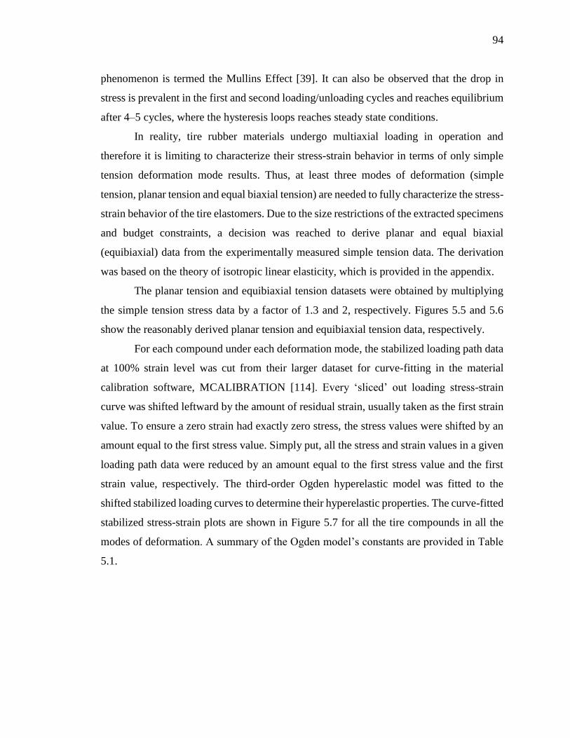
94

phenomenon is termed the Mullins Effect [39]. It can also be observed that the drop in

stress is prevalent in the first and second loading/unloading cycles and reaches equilibrium

after 4–5 cycles, where the hysteresis loops reaches steady state conditions.

In reality, tire rubber materials undergo multiaxial loading in operation and

therefore it is limiting to characterize their stress-strain behavior in terms of only simple

tension deformation mode results. Thus, at least three modes of deformation (simple

tension, planar tension and equal biaxial tension) are needed to fully characterize the stress-

strain behavior of the tire elastomers. Due to the size restrictions of the extracted specimens

and budget constraints, a decision was reached to derive planar and equal biaxial

(equibiaxial) data from the experimentally measured simple tension data. The derivation

was based on the theory of isotropic linear elasticity, which is provided in the appendix.

The planar tension and equibiaxial tension datasets were obtained by multiplying

the simple tension stress data by a factor of 1.3 and 2, respectively. Figures 5.5 and 5.6

show the reasonably derived planar tension and equibiaxial tension data, respectively.

For each compound under each deformation mode, the stabilized loading path data

at 100% strain level was cut from their larger dataset for curve-fitting in the material

calibration software, MCALIBRATION [114]. Every ‘sliced’ out loading stress-strain

curve was shifted leftward by the amount of residual strain, usually taken as the first strain

value. To ensure a zero strain had exactly zero stress, the stress values were shifted by an

amount equal to the first stress value. Simply put, all the stress and strain values in a given

loading path data were reduced by an amount equal to the first stress value and the first

strain value, respectively. The third-order Ogden hyperelastic model was fitted to the

shifted stabilized loading curves to determine their hyperelastic properties. The curve-fitted

stabilized stress-strain plots are shown in Figure 5.7 for all the tire compounds in all the

modes of deformation. A summary of the Ogden model’s constants are provided in Table

5.1.

95

Table 5.1. Tire Rubber Material Hyperelastic Constants–All Compounds

Regions

Ogden Model Constants

1 1 2 2 3 3 , ℃

Apex

2.00E-3 -7.761 0.020 12.448 2.277 -0.202 23

1.27E-3 -6.209 0.016 9..959 1.821 -0.161 35

9.52E-4 -4.66 0.012 7.469 1.366 -0.121 55

Casing

1.148 0.039 0.005 11.249 0.007 -4.734 23

0.918 0.031 0.004 8.999 0.006 -3.792 35

0.688 0.023 0.003 6.750 0.004 -2.275 55

Innerliner

2.83E-4 -7.966 0.015 9.837 0.424 -0.352 23

2.26E-4 -6.373 0.012 7.869 0.340 -0.282 35

1.69E-4 -4.779 0.009 5.902 0.255 -0.211 55

Sidewall

2.66E-4 -7.362 0.004 11.364 1.031 -0.099 23

2.13E-4 -5.890 0.0035 9.092 0.825 -0.079 35

1.59E-4 -4.417 0.0026 6.819 0.618 -0.059 55

Tread

0.0015 -5.332 0.012 8.920 1.229 -0.107 23

0.0012 -4.266 0.010 7.136 0.984 -0.086 35

8.81E-4 -3.199 0.007 4.281 0.738 -0.064 55

Rubber Material Viscoelasticity. Viscoelastic materials show both elastic

and viscous characteristics in deformation. The viscous flow in filled rubber is caused by

the molecules slipping past one another in response to applied deformations. A measure of

the rate of molecular chain motion (relaxation) in a rubber that is strained to a fixed length

constitutes a determination of its viscoelastic behavior. The mechanism of molecular

relaxation in a given rubber strip under extension load can be related to the reduction in its

dynamic modulus over the duration of the extension. In this case filled rubber is considered

96

(a) Apex (b) Casing

(c) Innerliner (d) Sidewall

(e) Tread

Figure 5.4. Simple Tension Test Results–All Compounds

97

(a) Apex (b) Casing


(e) Tread

Figure 5.5. Derived Planar Tension Results–All Compounds

98

(a) Apex (b) Casing


(e) Tread

Figure 5.6. Derived Equibiaxial Tension Results–All Compounds

99

(a) Apex (b) Casing


(e) Tread

Figure 5.7. Comparison of Test and Ogden Model Results–All Compounds and Modes

100

a rate-dependent material whose viscous response characteristics must be modeled in time

domain. In general, the effects of rubber molecular relaxation are temperature-dependent,

being more profound at higher temperatures.

Thus, stress relaxation experiments are often used to capture rubber rate-

dependencies and viscous effects at specified temperature levels. The stress relaxation

experiments conducted involved stretching the tire specimens in simple tension up to 20%

strain while collecting stress data over a time period of 2,000 sec. This class of relaxation

experiment is known as short-term stress relaxation because of the duration and manner of

straining imposed on the specimens.

The Elastocon test rig was used for the stress relaxation test. All the specimens were

tested at room temperature (23℃). Figure 5.8 shows the stress-time plots of the stress

relaxation test for all five rubber compounds. The heat generated in a tire is a function of

its rubber viscoelastic property. Rubber viscoelastic properties are in turn derived from

losses due to hysteresis (internal damping) that occurs when subjected to cyclical loads.

In practice, tire rubber materials show nonlinear viscoelastic response behavior due

to their interspersed particulate fillers. This response characteristic is partly caused by the

extreme mismatch in stiffness between the filler particles and the rubber matrix. Other

physical and chemical processes such as debonding of fillers from rubber and cavitation

around agglomerated regions of filler particles also contribute to the nonlinearity in the

viscoelastic behavior of tire rubber materials. The PRF material constitutive model [14]

provides a means for modeling nonlinear viscoelasticity in rubber.

To characterize rubber nonlinear viscoelasticity by the PRF model implemented in

ABAQUS requires parameters of a time domain Prony series to be first derived from the

experimental stress relaxation data (in Figure 5.8). Linear viscoelastic theory is numerically

implemented in ABAQUS [15] as a Prony series expansion of the dimensionless relaxation

modulus tgR , as shown in Equation (127).

itN

i

p

iR egtg

111

(127)

101

(a) Apex (b) Casing


(e) Tread

Figure 5.8. Stress Relaxation Test Results–All Compounds

102

It must be noted that tgR only accounts for the rate-dependent part of the material

relaxation behavior. A rate-independent part, specified via a hyperelastic model and

defined in terms of a deviatoric instantaneous elastic moduli 0

i , is required to completely

characterize the material effective relaxation response, as shown in Equation (128). Here,

the relaxation coefficients are applied directly to the Ogden hyperelastic strain energy

function. The generalized form of the effective relaxation moduli in Equation (128) defines

a pure linear viscoelastic model in that the stress relaxation function (second term on the

RHS) is independent of the magnitude of the deviatoric part 0

i [15].

itN

i

p

ii

R

i egt 111

0 (128)

Tire material response to changes in temperature was modeled by specifying a

temperature-dependent 0

i (see Table 5.1) as given in Equation (129) [15], and by a

reduced time concept as shown in Equations (130) and (131).

itN

i

p

ii

R

i egt 111

0 (129)

The reduced time t is given in Equation (130). The shift function A in (130)

is approximated by the Williams-Landel-Ferry (WLF) form in Equation (131) [115]. The

calibration constants 1C and 2C used in this research were taken from [116].

t

tA

dtt

0

(130)

02

0110log

C

CA (131)

103

A least-squares fit was performed on the normalized forms of the stress relaxation

data (in Figure 5.8) in order to determine the two-term Prony series parameters p

ig and

.i Figure 5.9 shows the results of the ABAQUS least-squares fitting. A summary of the

Prony series constants is provided in Table 5.2.

Table 5.2. Linear Viscoelastic Material Properties–All Compounds

Regions

Prony Series Constants WLF Constants

1g 2g 1 2 1C 2C , ℃

Apex 0.09 0.13 2.33 101.67

15

150

Casing 0.092 0.104 7.089 253.51

Innerliner 0.120 0.129 8.62 235.55

Sidewall 0.105 0.125 8.037 289.04

Tread 0.057 0.067 8.007 322.93

Consequently, the derived Prony series constants are used alongside the

hyperelastic model constants to define the initial parameters for the PRF model. The PRF

model comprises multiple viscoelastic networks connected in parallel [117], which is

shown in Figure 5.10 as a spring/damper system of multiple parallel networks. The number

of viscoelastic networks is represented by .N A purely elastic network (network 0) is

defined in the model to ensure stress does not completely relax in the material. For each

viscoelastic network, the model assumes a multiplicative split of the deformation gradient

into an elastic component and a viscous component [117]. The elastic response of each

network is considered to be provided by a hyperelastic strain energy potential [118].

104

(a) Apex (b) Casing


(e) Tread

Figure 5.9. ABAQUS Prony Series Fitting Results–All Compounds

105

Naturally, the same strain energy potential is assumed for all networks, scaled by a

stiffness ratio ( SR ) specific to each network. The stiffness ratios are material properties

and must satisfy the constraint condition in Equation (132).

11

N

i

iSR (132)

Figure 5.10. Nonlinear Viscoelastic Model [15]

The viscous behavior, on the other hand, is modeled using the creep portion of the

deformation gradient crF and a creep potential .crG A flow rule of the form in Equation

(133) can be obtained via specifying a creep potential [15].

crcr

qD

2

3 (133)

106

An evolution law is required to define the equivalent creep rate cr in (133). The

power-law strain hardening model [119] given in Equation (134) was selected for this

purpose.

1

1

1~ mmcrncr mqA (134)

Material constants ,A ,m and n are determined by calibrating the PRF model.

First, a linearized form of the model is derived from the Prony series and Ogden model

constants using Equations (135) and (136) on the assumption that 0m and 1n . Table

5.3 shows the linearized PRF model parameters for 2N viscoelastic networks. The

linearized parameters serve as starting values in the PRF model calibration process.

NigSR ii ,...,2,1, (135)

Nig

Aii

i ,...,2,1,3

1

0

(136)

A unit cube analysis is used to facilitate the calibration of the PRF model. Here, the

linearized model parameters are used as starting parameters, which are later optimized via

a workflow setup involving the ABAQUS and ISIGHT [120] platforms. The unit cube

analysis simulates the stress relaxation experiment in that the cube model is stretched up

to 20% strain while stress data is stored over the period of extension (2,000 sec). The visco

analysis procedure in ABAQUS was used to achieve this purpose. In Figure 5.11, the

inferior faces (AFHD, ABEF, ABCD, ABEF, and AFHD) are constrained along their

respective perpendicular directions ( ,X ,Y or Z ), whereas the nodes on face BEGC were

stretched along the X direction. Figure 5.12a and 5.12b show the undeformed and

deformed states of the cube element, respectively. For the unit cube, the reaction force

history output RF1 becomes its stress history—simulation stress relaxation.

107

Table 5.3. Linearized PRF Model Parameters–All Compounds at 23℃

Parameter Apex Casing Innerliner Sidewall Tread

1m 0.000 0.00 0.00 0.00 0.00

2m 0.000 0.00 0.00 0.00 0.00

1n 1.000 1.00 1.00 1.00 1.00

2n 1.000 1.00 1.00 1.00 1.00

1SR 0.086 0.09 0.120 0.105 0.057

2SR 0.131 0.10 0.129 0.125 0.068

1A 0.691 0.441 0.739 0.383 0.589

2A 0.011 0.011 0.025 0.009 0.0123

1 0.002 1.148 4108.2 4107.2 31047.1

2 0.020 0.005 0.015 0.004 0.012

3 2.277 0.007 0.420 1.031 1.229

1 -7.761 0.039 -7.970 -7.362 -5.332

2 12.448 11.250 9.84 11.364 8.920

3 -0.202 -4.740 -0.35 -0.099 -0.107

The simulation stress relaxation data is compared to the test stress relaxation data

in the data matching component of the framework software package ISIGHT. The

optimization design driver is then used to fit the simulation data to the test data using a

least-squares minimization algorithm (the Pointer algorithm). Figure 5.13 shows the

workflow setup in ISIGHT. The optimized PRF model parameters obtained from fitting

108

the simulation data to the test data are summarized in Table 5.4 for only one of the three

testing temperatures.

Table 5.4. Optimized PRF Model Parameters–All Compounds at 23℃

Parameter Apex Casing Innerliner Sidewall Tread

1m 0.00 0.00 0.00 0.00 0.00

2m 0.00 0.00 0.00 0.00 0.00

1n 1.00 8.00 3.00 1.00 4.00

2n 1.00 8.00 6.00 1.00 3.00

1SR 0.09 0.138 4104 0.153 41031.5

2SR 0.13 0.039 10104 0.095 41011.5

1A 0.39 1.677 4.886 1.083 0.0957

2A 0.006 5.069 1.096 4101 0.3665

1 4.11 0.012 0.468 0.806 0.151`

2 0.02 8109.5 0.011 0.001 0.006

3 0.05 1.252 0.001 0.001 0.755

1 0.11 4.307 -1.479 -11.197 0.195

2 11.19 16.309 9.0451 6.821 11.161

3 -4.14 -5.460 0.119 3.816 -0.295

109

Figure 5.11. Unit Cube Model Boundary Conditions

(a) Undeformed Cube (b) Stretched Cube

Figure 5.12. ABAQUS Unit Cube Model Analysis Results

110

Figure 5.13. PRF Model Calibration Workflow

Rubber Material Fatigue Behavior. Rubber as an engineering material is

often used in high strain applications and yet can fail at strain levels far lower than its

tensile failure strain. It has been established that such tendency of failure may be caused

by the growth of small preexisting cracks or initiated cracks under repeated loads during

the service life of a given rubber component. Although the initiation and growth of cracks

dominate the mechanism of fatigue in rubber, other factors such as ozone attack,

temperature effects, and loading sequence also contribute to rubber fatigue failure.

A static tearing energy testing approach was adopted for testing the casing

specimen fatigue behavior. The fatigue test was limited to only the casing compound due

to its specimen size requirement. The specimen was tested at 23℃. The static tearing

energy experiment essentially uses maximum stress, maximum strain, and tearing energy

measurements to provide a means to characterize the fatigue behavior of rubber. Figure

5.14 shows a planar tension test specimen (pure shear specimen) for the static tearing

energy experiment. The specimen was precut (25 mm) to depict the presence of an existing

crack. The specimen was then stretched until the crack grew to some extent, during which

111

maximum stress, maximum strain, crack growth length, and tearing energy data were

collected.

Figure 5.14. Planar Tension Specimen [113]

Two fatigue crack growth (FCG) testing conditions were considered in the test: (i)

fully relaxing condition, and (ii) non-relaxing condition. The latter condition was essential

for characterizing the specimen’s strain-induced crystallization behavior (SIC). Images of

the crack tip shape during testing under both conditions are respectively shown in Figures

5.15 and 5.16. Each contour in both images represents a capture of the actual crack tip

outline (in x-y coordinate pairs) at the end of each cyclic measurement.

5.1.3.1 Fully relaxing crack growth test. Under the fully relaxing fatigue testing

condition, loading was completely reversible on the unloading stroke. Thus, minimum

strains were zero duirng the entire duration of the experiment. In cyclical loading, the

112

minimum load minT experienced during the cycle is often expressed as a ratio of the cycle’s

maximum load maxT . This ratio is called the R ratio. The R ratio of a fully relaxing

fatigue crack growth test is 0R . Plots of maximum strain, maximum stress, and crack

growth as functions of the number of cycles are shown in Figure 5.17.

Figure 5.15. Crack Tip Evolution Contours of Casing Compound under Fully Relaxing

Conditions

It was assumed that the fatigue crack growth rate (FCGR) of the specimen follows

the Thomas [16] crack growth rate law in Equation (137). Note that cT and cr are material

constants representing the fracture strength and maximum fatigue crack growth rate

corresponding to cT , respectively.

F

c

cT

Tr

dN

dc

max

(137)

113

Figure 5.16. Crack Tip Evolution Contours of Casing Compound under Non-Relaxing

Condition

A power law was fitted to the crack growth curve (in Figure 5.18) in order to derive

an expression similar to that of Equation (137). The fatigue crack growth rate dN

dc was

derived from the equation of the trend line (power law fit) in Figure 5.18, as shown in

Equation (138).

428.113103428.2 NdN

dc (138)

Finally, FCGR data was generated based on Equation (138) and plotted on a double

logarithmic scale as a function of peak tearing energy (or maximum energy release rate).

The resulting Paris plot [121] is shown in Figure 5.19 for both the loading and unloading

strokes of the experiment. The material parameters cT and cr are therefore read off of the

unloading FCGR curve.

5.1.3.2 Non-relaxing crack growth test. Contrary to the fully relaxing fatigue

experiment, non-zero minimum loads were part of the non-relaxing experiment. This leads

to a condition where 0max

min RT

T. This condition mimics how the internal pressure of the

114

tire results in non-relaxing loading of the tire materials between passes of road contact

[122]. The non-relaxing crack growth testing procedure is similar to that of the fully

relaxing test except that the initial zero minimum strains are ramped up at some point

during the experiment. A fully relaxing test is required to run a non-relaxing test. Figure

5.20 shows that the crack grew steadily at the beginning when fully relaxed loads were

applied. However, as ramping of the minimum strain increased (beyond 40,000 cycles),

the crack began retarding and was completely arrested at about 70,000 cycles. It is

important to mention that the crack growth and retardation test was repeated for three

different growth and retardation rates. Figure 5.20 is used to depict a similar trend in the

remaining two repeat cases.

Testing under non-relaxing conditions was motivated by the need to model SIC in

the predominantly filled natural rubber vulcanizates used in the 56/80R63 tire. SIC is a

concept mostly observed in NR at room temperature in which a portion of the rubber

amorphous structure turns into a semicrystalline structure when stretched. The crystallites

formed act as barriers to arrest growing cracks and generally improve the tensile strength

of the strip. Thus, the non-zero loading ( 0R ) of materials surrounding a crack tip will

retard any potential crack growth in that vicinity. When ,0R the formed crystallites

melt away at the instance when loading is fully removed in each cycle. In cases where

,0R rubber fatigue crack growth rate does not only depend on the peak tearing energy

maxT but also on the R ratio. The R ratio essentially measures the size of the crystalline

zone at the instance of minimum strain relative to the size at the instance of maximum

strain. The pioneering work of Mars and Fatemi [123] was followed to introduce the R

ratio into the slope F of the Thomas FCGR model in Equation (137). The modified FCGR

model is given in Equation (139). Equation (139) was reorganized in order to define RF

in terms of the other parameters as shown in Equation (140). Cosnequently, RF data

was generated using Equation (140) and plotted as a function of R ratio, as shown in

Figure 5.21.

115

c

c

T

T

r

dNdc

RFmaxlog

log

(140)

(a) Maximum Strain (b) Maximum Stress

(a) Crack Growth

Figure 5.17. Plots of Fully Relaxing Data

116

Figure 5.18. Power-law Fit to Crack Growth Curve

Figure 5.19. Casing Compound Fatigue Crack Growth Rate Curve

117

Figure 5.20. Maximum and Minimum Strains in Non-Relaxing FCG Test

RF

c

cT

Tr

dN

dc

max

(139)

A cubic polynomial function [Equation (141)] was found to provide a good fit to

the experimental RF data. The constants of the polynomial function are subsequently

used as input parameters to the fatigue model in ENDURICA CL to include the effects of

SIC. Note that 0F represents the fully relaxing power law slope.

3

3

2

210 RFRFRFFRF (141)

118

Figure 5.21. Effect of R Ratio on Power law Slope

Figure 5.22 shows FCGR curves at varying R ratios. It can be observed that crack

growth rate decreases with increasing R ratio at any given .maxT

Thermal Material Properties. A handful of generalized thermal material

properties of rubber were taken from the literature. The convective heat transfer conditions

summarized in Table 5.5 were taken from [65, 104]. Note that v is the rolling speed of the

tire in m/s.

Table 5.5. Convection Heat Transfer Coefficients

Convection

Coefficients

(mW/mm2∙K)

Outer layer ( o ) 5.9 + 3.7v

Inner layer ( in ) 0.0030

Rim layer ( r ) 0.0030

119

Figure 5.22. Effects of R Ratio on Crack Growth Rate

Additionally, the thermal material properties given in Table 5.6 were obtained

experimentally from a similar NR compound and were assumed to approximate the true

thermal properties of the 56/80R63 tire compounds.

Table 5.6. Thermal Material Properties

,

/K

vC ,

mJ/tonne∙K

k ,

W/m∙K

,

℃

6.7E-6 1.19 0.438 23

6.7E-6 1.22 0.495 93

6.7E-6 1.23 0.513 121

6.7E-6 1.25 0.546 150

120

5.2. THE 56/80R63 TIRE GEOMETRY MODELING IN ABAQUS

Tire geometric information required for FE analysis is often supplied by a tire

original equipment manufacturer (OEM) in the form of 2D CAD sketches. An alternative

approach is to acquire geometric details of a tire cross section cut (omega cut) via image-

based techniques. However, neither the CAD drawings nor the omega cut could be obtained

from the OTR OEMs for this research study due to proprietary reasons. Hence, a manual

approach was adopted in which geometric measurements were taken from a

circumferentially cut out-of-service 56/80R63 tire, as shown in Figure 5.23.

In particular, thickness measurements were taken for the innerliner, belt layers,

undertread, and tread. In addition, the tire section height and width, and inner and outer

diameters were measured using a regular tape measure. An approximate 2D axisymmetric

model of the tire, as shown in Figure 5.24, was then built in ABAQUS using the

aforementioned measurements. The bead bundle and rim were modeled as rigid bodies

connected to the axle through a reference node (rim node) due to their relatively high

stiffness properties. The axisymmetric model was comprised of 14,771 nodes and 9,062

elements of the type CGAX4H/CGAX3H with twist degrees of freedom.

Figure 5.23. 56/80R63 Tire Circumferential Section Cut

121

(a) Meshed (b) Unmeshed

Figure 5.24. Tire Axisymmetric Model

The steel cords used in the casing and belt components of the tire were modeled as

separate entities using the wire feature in ABAQUS (Figure 5.25). The belt package

comprising six belt layers was modeled to assume a pyramidal shape, the widest layer being

the transition belt layer (radially innermost belt). Four working belt layers were modeled

between the transition layer and the outermost (penetration protection) layer. Rebar layers

defined in surface elements were used to approximate all the fiber reinforced parts of the

tire. In this case, it was assumed that the cords coating compound was of the same stiffness

as that of the casing compound. Table 5.7 summarizes the details of the geometry and

material properties of each rebar layer.

The embedded constraint option was used to embed the body ply rebars within the

host casing and apex elements of the model. However, the node sharing approach via skin

definitions was used to include shearing effects between the belt rebar layers. The rebar

layers of the casing and belt regions were assigned the 2-node SFMGAX1 elements with

twist degrees of freedom. Note that the arbitrary orientation of the rebar layers (out-of-

plane nature as shown in Figure 5.26) cause them to twist when loaded.

122

(a) Cross-section

(b) Revolved Cross-section

Figure 5.25. Model of Steel Cord Reinforcement

123

Table 5.7. Belt and Ply Cords Geometric Specification and Material Properties

Belt/Ply Spacing,

ends/mm

Orientation, ° Area, 𝐦𝟐 Density,

kg/𝐦𝟑

Elastic

Modulus,

GPa

Transition belt 0.314 10

2.7025e-6

7800

100

Working belt 1

0.434

-10

Working belt 2 22

Working belt 3 -22

Working belt 4 22

Penetration

protection belt

90

Casing ply 0.314 0

The symmetric model generation (SMG), revolve, and symmetric results transfer

(SRT) options in ABAQUS were then used to revolve the axisymmetric model into a 9°

sector model. A separately meshed tread block was then attached to the revolved sector via

tie constraints, as shown in Figure 5.27. Lastly, the sector model was revolved periodically

into the full 3D model shown in Figure 5.28.

The total nodes and elements used in the 3D model were 1,247,083 and 1,051,007,

respectively, consisting of reduced integration linear brick (C3D8R) elements and

quadrilateral surface (SFM3D4R) elements. The compact and even haul-road surfaces

meant an analytically rigid surface sufficed to be used to represent the haul road in the

static and rolling analyses.

124

Figure 5.26. Fiber Orientation in Belts

Figure 5.27. Tire Sector Model

125

Figure 5.28. Full Tire Model

5.3. TIRE THERMOMECHANICAL FATIGUE MODELING AND ANALYSIS

The effects of thermomechanical loads on the tire fatigue performance were

determined through a sequentially coupled thermal-stress analysis approach. As shown in

Figure 5.29, three modules of analysis were essential in the tire durability prediction:

deformation, thermal, and fatigue. The sequentially coupled thermomechanical FEA

procedure in Figure 5.30 first computes viscous dissipation energy for all the elements at

steady rolling conditions in the deformation module. The computed viscous dissipation

energies are then converted to heat generation rates and applied as body fluxes in the

thermal analysis module.

The output variable CENER in ABAQUS stores the magnitudes of the viscous

dissipation energy density Q in per revolution units. Consequently, the ‘per revolution’

magnitudes are converted to rate Q units by multiplying the CENER ouput by a

deformation rate such as the tire angular speed. A Python script was used to automate the

process of extracting and converting the magnitudes of the CENER output. The resulting

element temperatures are then read back into the deformation module to update the

temperature-dependent material properties for the next rolling analysis. When convergence

126

has been reached in both the thermal and mechanical field variables, nominal strains and

stresses are extracted for one tire revolution to compute the tire duty cycle loads in the

fatigue module. The following subsections discuss each analytic module.

Deformation Module. This module takes the tire geometry, rubber and rebar

material properties, and initial and boundary conditions as inputs and returns viscous

dissipation energy as output. The temperature-dependent hyperelastic and viscoelastic

rubber material properties were assigned at an initial tire temperature of 30℃.

The steel reinforcements were assigned elastic material properties that did not vary

with temperature. The deformation analysis began with an inflation loading of the 2D

axisymmetric model, followed by a footprint analysis of the full model. The deformed state

of the 2D model was used as starting values in the first step of the footprint analysis.

Subsequent steps of the footprint analysis included bringing the road surface into contact

with the 3D tire and applying vertical load through the road reference node to the tire. The

tire was fixed at its rim node throughout the footprint analysis. Both inflation and footprint

analyses were conducted in ABAQUS/Standard.

The footprint analysis was then followed by a dynamic rolling analysis in which

translational and angular initial velocity conditions were specified for all the elements in

the tire model. The rigid road surface was then fixed, while the tire rolled relative to it. The

tangential Coulomb friction model in ABAQUS was used to specify a friction coefficient

of 0.7 for the tire/road contact. Additionally, velocity boundary conditions and gravity load

were prescribed at the rim node to simulate the effects of inertia in the straight-line rolling

analysis. The resulting element stresses and strains from the rolling analysis are used to

compute the viscous dissipation energy densities via the ABAQUS output variable

CENER. It is important to mention that CENER output is only available when a

hyperelastic material model is defined with nonlinear viscoelasticity. The rolling analysis

was limited to a maximum of three tire revolutions due to computational resource

requirements of the explicit analysis. Thus, the deformation analysis was assumed to have

reached steady state conditions after three complete tire revolutions [104].

Thermal Module. The heat transfer analysis was conducted on the same

3D model of the deformation analysis, except that the structural (rebar) elements were

removed from the model. The viscous dissipation energies of the elements were the only

127

source of heat used in the thermal analysis. The computed viscous heat fluxes were

incorporated for each element into the heat transfer model under the keyword *DFLUX.

The convection heat transfer conditions (in Table 5.5) were applied to the inner, outer, and

rim layers of the model along with the thermal material properties in Table 5.6. Note that

all the thermal material properties were applied as isotropic material constants because of

the assumption of isotropy in the tire rubber behavior. Assuming thermal equilibrium

between the tire and prevailing average ambient conditions in a given U.S. mine in the

summer, each element in the model was assigned an initial temperature of 28.9℃. The

steady-state heat transfer analysis procedure in ABAQUS/Standard was used for the tire

temperature distribution calculation.

Fatigue Module. The fatigue module accepts the tire rubber hyperelastic and

crack growth properties and thermomechanical strain histories as input and returns the

fatigue cycles of the tire parts as ouptut. The rubber hyperelastic constitutive model is

needed to derive the material traction vector

in order to determine the local crack

driving force on a given material plane. The history of the strain tensor components from

the tire FE analysis (as shown in Figure 5.30 for one element) is combined with

to

define an effective loading history on the cracking plane.

A plane analysis technique is then used to identify the plane with the highest energy

release rate and/or lowest fatigue life. For the variable amplitude loading signal shown in

Figure 5.30, a rainflow counting procedure is used to identify fatigue cycles (strain-

reversals) on each cracking plane. Discussions on the cracking plane energy release rate

and fatigue cycles’ estimation, rainflow cycle counting procedure, initial crack size

calibration, and the critical plane analysis method are provided in the next subsections.

5.3.3.1 Multiaxial fatigue life estimation. For fatigue crack growth test under

small crack and uniaxial loading conditions, the energy release rate is often approximated

by the product of the strain energy density and crack size [82]. Thus, the total available

SED of the test specimen is considered to be released to grow the crack. Under multiaxial

loading conditions, however, not all of the available SED on a cracking plane is released

to grow a crack [81]. Only a fraction of the SED is actually used to grow a crack on any

given plane. The magnitude of loading experienced by a crack varies with the orientation

128

Figure 5.29. Thermomechanical Fatigue Analysis Algorithm

of the plane of the crack. The CED fatigue predictor has proven to be accurate in capturing

local crack tip loading histories at varying plane orientations. Mars [81] defined the CED

for a differential element on a given material plane as in Equation (142). The unit normal

vector r in the CED equation accounts for the material plane orientation effect on local

crack tip loading history.

129

Figure 5.30. Tire Duty-cycle FEA Nominal Strain History

rdr

ddW

T

c

εσ

εσ

(142)

Consequently, the energy release rate (crack driving force) available to grow a

potential crack on any given material plane can be expressed mathematically as in Equation

(143).

cWT c 2 (143)

By combining either Equation (137) or (139) with the local crack driving force T

in Equation (143), it is possible to compute the number of fatigue cycles N required to

develop a crack from an initial size 0c to a critical size fc on a material plane. Equation

130

(144) shows the compact form of the definition of .N In practice, when fcc 0 , N is

insensitive to the critical flaw size fc .

fc

cc

dccWTf

N0 ,

1 (144)

A CED-based algorithm implemented in the elastomer fatigue analysis code

ENDURICA CL was used to derive the CED history in Figure 5.31 from the multiaxial

FEA strain history (shown in Figure 5.30) of a failure plane in the belt region of the tire.

The corresponding fatigue life estimate on the failure plane was 510767.9 cycles (tire

revolutions).

5.3.3.2 Rainflow counting procedure. The cracking plane loading history

shown in Figure 5.31 indicates that a sequence of different events occur within the duration

of duty cycle loading of the tire parts (e.g. belt package). The events are characterized by

the sequences of (tensile) peaks and (compressive) valleys in the history plot. The rainflow

algorithm [124] provides a means for identifying fatigue cycles in complex variable

amplitude loading histories such as shown in Figure 5.31. Each identified cycle has a valley

and peak crack driving forces minT and maxT , respectively. The algorithm consists in first

rotating Figure 5.31 90° clockwise to assume the shape of a pagoda, as shown in Figure

5.32. Like a pagoda, rain would drip down an upper tensile peak or valley to a surface

beneath it. A complete cycle is obtained when rain drips to another surface. The range and

mean of each identified cycle (or event) is counted separately.

The rainflow method allows damage calculation on each material plane of the tire

for fatigue life prediction. Each identified event in a loading block (1 tire duty cycle)

contributes to the total crack growth caused by that block. The five events (cycles 1–5)

shown in Figure 5.32b are plotted on a Haigh space (Figure 5.33) to show which of them

contributes the most to damage on the failure plane.

131

Figure 5.31. Local Cracking Plane Loading History

(a) Rainflow Plot (b) Identified Cycles

Figure 5.32. Rainflow Counting Procedure

132

5.3.3.3 Initial crack size calibration. As mentioned in Section 5.3.3.1, fatigue life

strongly depends on the choice of the initial precursor size 0c , which is typically in the

range m. 200m 2 oc Intrinsic and extrinsic sources of crack precursors are

inevitable in rubber formulation and part development. Poor filler dispersion, nature of the

mixing process, and the presence of particulate ingredients comprise the intrinsic sources

of crack precursors. The extrinsic sources include the use of mold lubricants and surface

finish, mold dent, trapped air bubbles, and contaminants. Abrasive material cutting is a

typical crack precursor source in tires used in mining applications. Crack nucleation tests

provide a means for determining features of the intrinsic sources. For the extrinsic sources,

however, a precursor size is often calibrated on observed values of fatigue life of a part. As

shown in Figure 5.34, a curve can be obtained from computed values of fatigue life over a

range of crack sizes for a rubber part. A point is then established on the calibration curve

that matches an experimental fatigue life of the part. The flaw size corresponding to this

point is read off as 0c for the part. The estimated 0c of the belt compound is 0.083 mm,

as shown in Figure 5.34. Note that 0c is expected to be nearly the same in situations where

the experimental and computed fatigue life are obtained at multiple strain levels.

5.3.3.4 Critical plane analysis. It suffices, then, to assume from the previous

discussion that every material plane in the tire consists of a precursor of some known size

likely to nucleate after a given number of fatigue cycles. This assumption eliminates the

need to include explicit crack features in the tire FE model. Note that cracking occurs on

specific material planes depending on the magnitude of damage they experience in service.

Figure 5.35 shows how crack precursors, although randomly oriented in the beginning,

coalesce along material plane orientations that experience the most damage from the tire

duty cycle loads.

A potential failure (or material) plane in the tire analysis model is identified by a

unit normal vector r

in the undeformed configuration. The unit normal vector also defines

a plane’s orientation. Thus, a failure plane can assume varying orientations based on the

direction of their unit normal vector. This implies that the CED and fatigue life of a crack

precursor occurring on a given failure plane will vary with changes in the plane orientation.

133

Figure 5.33. Damaging Events on Belt Failure Plane

Figure 5.34. Computed Flaw Size Calibration Curve

134

In essence, each potential failure plane in the tire needs to be analyzed in all possible

orientations to determine the fatgue cycles required to grow precursors to catastrophic

states. The plane that minimizes the fatigue life prediction is identified as the critical plane.

This process constitutes the critical plane analysis technique used for identifying fatigue

failure planes in rubber parts [125]. The critical plane analysis algorithm implemented in

ENDURICA CL was used to predict critical planes and their fatigue lives in the different

components of the tire. For a given failure plane, the domain of search for all possible

orientations is represented by a unit half space, as shown in Figure 5.36. Here, fatigue life

varies with the plane orientation defined in terms of the spherical coordinates , . Note

that fatigue life in the contour plot of the unit damage half sphere corresponds to .log10 N

(a) Sidewall Cracking

(b) Tread Lug/Groove Cracking

Figure 5.35. Crack Orientations on an Out-of-Service 56/80R63 Tire

5.4. SUMMARY

Material characterization of the tire rubber compounds required for finite element

and fatigue analyses has been presented in this section. Raw data obtained from

hyperelastic, stress relaxation, and crack growth rate tests of five regional compounds of

the tire were used for the characterization. Existing rubber constitutive models were fitted

to the experimental datasets in order to obtain the material constants for building the tire

135

FE and fatigue models. Fatigue crack growth rate of the casing compound was

characterized under the fully relaxing and non-relaxing fatigue loading conditions.

Figure 5.36. Fatigue Life Dependence on Failure Plane Orientation

The section also includes a discussion on the approaches adopted in modeling the

tire geometric features. It has highlighted steps to develop a full 3D tire model from a 2D

geometry of its cross-section. Details of the casing and belt reinforcement geometry and

material properties have also been provided in this section.

Lastly, the tire thermomechanical fatigue analysis procedure and algorithm have

been presented in this section. Particularly, the deformation, thermal, and fatigue modules

of the iterative algorithm have been thoroughly discussed to elucidate the underlying

concepts of tire rubber fatigue processes. A calibration concept has been presented to

outline ways to determine the initial crack precursor size. Pertaining to the tire multiaxial

nature of loading histories, the cracking energy density (CED) fatigue predictor has been

shown to be very effective in accounting for multiaxial strain state conditions on the tire

local cracking planes. A critical plane analysis technique has also been shown to predict

planes with the shortest fatigue lives.

136

6. MODEL VALIDATION, EXPERIMENTAL DESIGN, AND

EXPERIMENTATION

The developed tire FE model in Section 5 is subsequently used as a results

acquisition platform to investigate the tire thermal and fatigue performance under varying

service conditions, hence the need to validate it. The section begins with a mesh sensitivity

(convergence) study that provided an optimal mesh size for the model. In the validation

effort discussed in this section, field test data of the tire vertical stiffness and footprint are

compared with the model results at specific operating conditions. The section ends with a

description of the design of experiments setup for acquiring useful data for analysis of the

tire durability performance. A full factorial technique is adopted to design the simulation

experiments based on the tire operating variables: speed, inflation pressure, ambient air

temperature, and vertical load conditions.

6.1. MESH CONVERGENCE STUDY

The degree of accuracy of the results for any given FE model depends on its mesh

quality and density. A high-density mesh will typically produce accurate results at the

expense of computational resource requirements. Given the size of the tire and the nature

of the adopted analysis (nonlinear transient), it was necessary that a mesh convergence

study be conducted to select an optimum mesh density for the model. The convergence

study involved loading the tire’s axisymmetric model at 724 kPa (105 psi) while fixing the

rim reference node. Figure 6.1 shows results of how increasing mesh density improves the

maximum stress convergence at the toeguard region of the tire.

Consequently, a global mesh density of 2,500 elements (size 15 mm) was chosen

to discretize the tire cross-section. Further mesh refinement was required at the belt region

to capture shearing effects between the belt layers. This resulted in an overall mesh density

of 9,062 elements, as shown in Figure 5.24a. The latter mesh density ensured a balance

between solution accuracy and computational efficiency.

137

Figure 6.1. Maximum von Mises Stress Convergence Study on the 2D Axisymmetric Tire

Model

6.2. VERTICAL STIFFNESS VALIDATION

Field Measurement. Tire vertical stiffness determines the level of ride

comfort in vehicles running on uneven road surfaces. Static vertical stiffness experiments

often use a loading frame that applies vertical load to an inflated tire (on a hard surface) at

the center of the axle (hub). A load cell is typically fitted to the axle of the wheel to measure

the weight of the loading frame. Load-deflection data is then collected at each instance of

vertical load application. Note that deflection is obtained by finding the difference between

the unloaded radius (UR) of a tire and its static loaded radius (SLR). UR is the radius when

no load is applied to a rim-mounted, inflated tire in contact with the ground in an upright

position. The slope of the static vertical stiffness curve becomes the vertical stiffness of the

tire.

In this research, however, such a test rig could not be afforded due to the tire size

and weight. Conversely, an approximate approach was used in which load-deflection data

was collected during a mine loading operation. The experiment involved measuring the

138

deflection of the right front axle tire under two inflation and multiple load levels. A leveled

hard surface was prepared at the shovel loading area for the test. At each shovel load pass,

a payload monitor mounted on the exterior side of the truck (CAT 795F) displayed the total

weight of payload in the dump body, while a measuring tape was used to measure the tire’s

SLR. Figures 6.2a and 6.2b show the truck payload monitor and a scene of the SLR

measurement, respectively. The vertical force on the tire was computed from the gross

machine weight at each intance of payload reading and the percent weight distribution on

the tire. The static vertical stiffness test was conducted at two inflation loads: 724 kPa (105

psi) and 793 kPa (115 psi).

(a)

(b)

Figure 6.2. CAT 795F Truck: (a) Loaded at a Shovel Loading Area and (b) Tire Static

Loaded Radius Measurement

139

Static Vertical Stiffness Analysis. The static analysis used the 3D tire

model on an anlytical rigid road surface in ABAQUS/Standard. The road was first brought

into contact with the tire in a displacement-controlled step. This was then followed by a

load-controlled step where the maximum vertical load obtained from the

experiment was specified at the rim reference node.

The response forces and displacements were measured at the road reference node.

The load-deflection curves of the test and simulation data are compared in Figures 6.3 and

6.4 for inflation loads 724 kPa and 793 kPa, respectively. A linear trend is observed in the

vertical stiffness results for both the test and simluation. Additionally, it is observed that

the tire vertical stiffness is relatively higher at 793 kPa than at 724 kPa, indicating the

influence of inflation pressure on vertical stiffness. The lower the vertical stiffness, the

higher the tire’s running temperature and wear on the outer tread contact, and vice versa.

Vertical stiffness data at different operating conditions are provided by tire manufacturers

to aid in determining vehicle dynamic ride heights. Table 6.1 summarizes the percent

absolute errors in vertical stiffness prediction by the FE tire model.

Table 6.1. Static Vertical Stiffness Validation

Inflation

Pressure (kPa)

Vertical Stiffness (N/mm) Absolute

Error Test Simulation

724 3786.41 4161.58 0.0991

793 4800.23 4911.48 0.0232

6.3. FOOTPRINT VALIDATION

A tire’s footprint shape and pressure determines its wear and traction performance.

Factors that affect the shape and area of the footprint include inflation pressure, tire size

and construction, load distribution, wheel alignment, and nature of road surface. The

experimental measurement of the 56/80R63 tire footprint was comprised of spreading a

spray paint on a section of the tread surface and rolling the tire over a piece of cardboard

140

placed on a tire pad, as shown in Figure 6.5. During the experiment, the tire inflation

pressure was set to 793 kPa and supported 0.604 MN of the empty truck distributed weight.

Although changes in inflation pressure have strong influence on the tire footprint

characteristics, only one inflation pressure footprint shape was obtained from the test. The

experimental footprint is shown in Figure 6.6.

Figure 6.3. Vertical Load-Deflection Plot at 724 kPa (105 psi) Inflation Pressure

The static vertical stiffness analysis is essentially a footprint analysis in ABAQUS.

However, only one inflation pressure (793 kPa) case was simulated to give the tire contact

nodal area output shown in Figure 6.7. Assuming an elliptical shape for both footprints,

the model’s static contact area appeared to be 49% larger than the test footprint area. The

discrepancy is caused by a number of factors, of which the stiffness and layout of the belts

might have played a major role. In addition, the variation in tread pattern geometry between

141

Figure 6.4. Vertical Load-Deflection Plot at 793 kPa (115 psi) Inflation Pressure

the model and the actual tire could be another reason for the difference. The footprint

validation experiment is needed to ensure uniform pressure distribution at the tire contact

patch. It is worth mentioning that the model’s footprint prediction accuracy is acceptable

for this experimental program. Both the test and simulation results show that the tire

maintains good grip on the road surface.

6.4. DESIGN OF EXPERIMENTS

Tire operating conditions from a U.S. coal mine were selected for the design of the

simulation experiments. The name of the mine is withheld for business reasons. The mine

selects one of three inflation pressure conditions (724 kPa, 793 kPa, and 862 kPa) for their

CAT 795F coal trucks based on heuristics. The brand of the tire and the ambient conditions

of a given season of the year are alternative factors that may determine the choice of

142

inflation pressure on this mine. The average speed of a loaded coal truck in the summer is

9.03 m/s (20.2 mph), but it can go up to 13.41 m/s (30 mph). The peak gross machine

weight (GMW), representing 17% of excess payloads, was estimated as 624 tonne (688

short ton). By proportion, according to Caterpillar specifications [126], a single front axle

tire supports approximately 1,010 kN (227,057.03 lbs) of the truck’s GMW. The poor state

of the haulroad superelevation results in an unbalanced load distribution on the tires.

Therefore, a second level of vertical load (1,151 kN) was assumed to account for tire

overloading due to poorly maintained or designed superelevation at curved sections of the

haulroad. This rated vertical load condition is selected to simulate the effect of excessive

overloading on the tire’s performance.

Figure 6.5. Experimental Footprint

143

Figure 6.6. Test Footprint at 793 kPa Inflation Pressure and 0.603 MN Vertical Load

Figure 6.7. Model Footprint Contact Area (in mm2) at 793 kPa Inflation Pressure and

0.603 MN Vertical Load

144

From the abovementioned operating conditions, a full factorial design technique

was adopted to acquire desirable simulation data to accurately and efficiently predict the

tire fatigue performance. The chosen design technique was solely based on the need to

exhaustively explore the design space of the experiment. The design matrix (Table 6.2)

comprises 12 design points obtained from a combination of all three factors at all levels.

Tire temperature distribution and stress/strain histories are the initial outputs that are used

to obtain the ultimate output variable, fatigue life, for each experiment.

Table 6.2. A Full Factorial Design Matrix for Fatigue Life Prediction

Experiment # Inflation

Pressure (kPa)

Speed (m/s) Vertical Force

(kN)

1 724 9.03 1,010

2 724 9.03 1,151

3 724 13.41 1,010

4 724 13.41 1,151

5 793 9.03 1,010

6 793 9.03 1,151

7 793 13.41 1,010

8 793 13.41 1,151

9 862 9.03 1,010

10 862 9.03 1,151

11 862 13.41 1,010

12 862 13.41 1,151

Both summer and winter average ambient air temperature conditions of the mine

site were considered in studying the tire heat loss by convection in the experiments. Thus,

for each of the 12 experiments, temperature predictions were obtained at 28.9 ℃ (84.02℉)

145

and 0.56℃ (33.08℉), representing the mean summer and winter air temperature,

respectively.

6.5. EXPERIMENTATION OF TIRE OPERATING VARIABLES

The experimental design matrix, as shown in Table 7.1, revolves around variations

in the three key service conditions of the tire: inflation pressure, vertical load, and speed.

The rationale for experimenting their effects on the tire fatigue performance are stated in

the ensuing subsections. Understanding how these factors impact the tire fatigue life will

help OTR tire compounders to develop durable compounds for the most damaging

components of the tire. Moreover, end users (truck operators and tire servicing technicians)

can be more aware of their role in extending tire service life.

Simulating the Effects of Inflation Pressure on Fatigue Life. Inflation

pressure affects traction, handling, cornering, and obstacle enveloping capability built into

tires by the OEMs. The OEM maximum recommended inflation pressure for the 56/80R63

tire is 669 kPa (97 psi). In operation, however, ultra-class tires are run on inflation pressures

in excess of 689 kPa (100 psi) because of the moderately high load and speed conditions

prevailing at the mine. An overinflated tire is stiffer and susceptible to rock impact cuts

and may lose traction due to distortion in its shape. In addition, overinflation results in

uneven and rapid wear of the tread and loss of strength in the fiber reinforcements [126].

At the recommended pressure, the tire can conform to the shape of any road obstacle that

it may run into, thereby reducing the magnitude of plausible cuts through the tread or

sidewall. On the other hand, underinflation increases tire running temperatures and can

result in a decreased belt adhesion—a key reason for tread separation.

For the NR compounds in the tire, inflation pressure ensures that the crystalline

region formed at a potential crack tip is maintained in order to impede further crack growth.

This improves the tire’s overall fatigue resistance, especially at the belt edges. The main

goal of this subset of experiments is to measure and compare tire fatigue life at the different

levels of inflation pressure for any given vertical load/speed condition.

146

Simulating the Effects of Axle Load on Fatigue Life. Truck axle (vertical)

load plays a major role in the magnitude of the crack tip energy release rate. Tire durability

sensitivity to vertical load appears to follow a linear relationship. Energy release rate (crack

driving force) increases with increasing tire vertical load and results in decreased fatigue

performance. Tires are generally designed to support loads at certain inflation pressures.

An explosion may occur if a tire is overloaded above its inflation pressure limits.

Thus, inflation pressure must be adjusted to compensate for excess loads. Note that

tire fatigue performance may be greatly affected at a small but constant increase in vertical

load [126]. By varying the tire vertical load (two levels) at different combinations of speed

and inflation pressure levels, it is possible to generate adequate data for analysis and

comparison to determine which vertical load level maximizes tire life.

Simulating the Effects of Speed on Fatigue Life. The load index of a given

tire is a function of its design speed and represents the maximum load the tire can carry

within the limits of the design speed. Heavy loads can be supported by a tire running at a

lower speed level and vice versa. Centrifugal forces acting on a tire are greatest at higher

speeds and may result in rapid growth of cracks that may be present in the belt layers of

the tire. Heat generation rate in a tire is directly related to its deformation rate (speed).

Hence, operating the tire at higher speeds at a given service condition will result in

increased running temperature. Higher operating temperatures contribute to tire aging and

subsequent reduction in fatigue performance. In this subset of experiments, speed is varied

to measure its effect on temperature rise and fatigue life of the different components of the

tire. It is expected that higher speeds will reduce the tire life.

6.6. SUMMARY

The tire FE model has been validated with field data in this section. A mesh

convergence study was carried out on the tire 2D axisymmetric model to determine a global

mesh size that ensured a balance between solution accuracy and computational efficiency.

Static vertical stiffness and tire footprint data obtained via field measurements have been

used to validate the virtual tire model. The errors of the tire FE model were within

acceptable limits, especially for the static vertical stiffness.

147

This section has also covered discussions on the type, scope, number, and control

environment of experiments needed to measure the 56/80R63 tire fatigue performance in

a U.S. coal mine operation. The design matrix of the experiments was comprised of a third-

level factor and two second-level factors, resulting in a total of twelve experiments. The

experimental design was based on the full factorial method. Additionally, this section has

highlighted the expectations of the effects of inflation pressure, axle load, and rolling speed

on the tire thermal and fatigue performance.

148

7. RESULTS AND DISCUSSIONS

This section presents a detailed analysis and discussion of the simulation results

obtained based on the experimental design and experimentation of the tire operating

conditions presented in Section 6. The investigated tire is 56/80R63 and is installed on

ultra-class rigid body dump trucks with payload capacities in excess of 313 tonne (345

short ton) operated on a coal formation. The tire operating conditions data are given in

Table 6.2. The discussion of the results revolves around the main performance

characteristics of the tire: ride quality, traction, heat, and durability.

7.1. TIRE DEFLECTION, FORCES, AND CONTACT PRESSURE

The forces and moments exerted on the tire by the road influence ride comfort and

handling performance of the truck. The fuel efficiency of a mining truck can be partly

linked to its tire rolling resistance. On hard road surfaces, the tire rolling resistance is

directly proportional to the degree of deflection in the casing component under static and

dynamic loading conditions. Tire deflection (Figure 7.1) results from rubber material

hysteresis. The level of the tire inflation pressure contributes to its deflection. Figure 7.2

shows the deflection of the tire hub (center of the axle) for a vertical load rate of 1.15 MN

and the varying conditions of inflation pressure and tire speed. A negative correlation exists

between inflation pressure and deflection. For both speed conditions, increasing pressure

decreases the amount of vertical deflection in the tire. The maximum deflection of the tire

is 303.5 mm, representing the deflection at 724 kPa pressure and 8.9 m/s speed. However,

the magnitudes of the slope of the curves for both speed conditions are different. At any

given inflation rate, the tire deflects slightly more when speed is lower (8.9 m/s) than when

it is higher (13.4m/s). This observation could be explained by the axle-rise phenomenon in

rolling tires, where loaded radius increases with increasing speed [104]. Thus, the gradient

of tire deflection is lower at 13.4 m/s than it is at 8.9 m/s, as shown in Figure 7.2.

149

(a)

(b)

(c)

Figure 7.1. Tire Deflection (mm) Contour Plots at Vertical Load Rate of 1.15 MN for

Inflation Rates: (a) 724 kPa (105 psi), (b) 793 kPa (115 psi), and (c) 862 kPa (125 psi)

In this study, the reaction force of the road in the tire travel direction was considered

as the tire rolling resistance. As in the abovementioned discussion, the rolling resistance is

caused by the hysteretic loss of energy as the tire continually deforms in the contact patch.

150

The rolling resistance force is derived from the rolling resistance moment generated when

the center of the tire’s normal pressure shifts towards the tire’s travel direction [21].

Figure 7.2. Tire Hub Deflection at 1.15 MN Vertical Load under Rated Inflation Pressure

and Speed Conditions

Figures 7.3a and 7.3b show that the rolling resistance increases with increasing tire

vertical load at any given inflation pressure condition. This observation is valid in that

rolling resistance varies linearly with the tire’s normal pressure. The effect of tire deflection

on rolling resistance is shown in Figure 7.4 for the three rated tire pressure conditions,

repeated for both speed cases. From the figure, it is clear that the peak rolling resistance

forces for both speed cases are higher at lower inflation levels than at higher inflation rates.

For a given vertical load/speed condition, tire deflection is greatest at the lowest inflation

pressure level. In this case, the degree of deflection is directly proportional to the

151

magnitude of the rolling resistance force, as shown in Figure 7.4a and 7.4b. The peak

rolling resistance force appears to be higher at 724 kPa (105 psi) than at the other two

inflation rates.

(a) (b)

Figure 7.3. Effect of Rated Vertical Load on the Tire Rolling Resistance for Inflation

Rates: (a) 724 kPa (105 psi) and 862 kPa (125 psi)

Contact pressure in the tire footprint was obtained at the rated inflation pressures

shown in Figure 7.5. The fairly uniform distribution of contact pressures across all inflation

loading cases means that the tire maintained as much contact with the road surface as

possible throughout the simulation. However, contact pressure distribution was much more

uniform and relatively low (2.695 MPa) where the tire pressure was 793 kPa. In this case,

the tire tread may wear uniformly in operation.

It was also observed that contact pressures were high at the edges and corners of

the tread lugs for all loading cases. This was expected, as sharp edges and corners are often

locations of high quantity (e.g., stress, pressure, etc.) concentration in objects. Therefore,

it is recommended that the fillet radius at the tread lug edges and corners be optimized to

create a gradual change in the cross-section between their adjoining faces.

152

(a) (b)

Figure 7.4. Tire Rolling Resistance at Rated Inflation Pressure Conditions for Speed

Levels: (a) 8.9 m/s (20 mph) and (b) 13.4 m/s (30 mph)

The steel cords in the tire carry most of the tire loads. As discussed in Section 5.2,

the large, distinct cord reinforcements in the casing and belt layers of the tire were modeled

as rebar layers embedded in a matrix of continuum (membrane) elements. Figure 7.6a and

7.6b show the von Mises stresses in the rubber matrix and belt layers, respectively. While

the maximum average stresses in the casing and belt rebar layers are respectively 3,553

MPa and 206.1 MPa, that of the (belt) host rubber is 1.163 MPa. The results confirm the

claim that the transversely isotropic steel cords used in the 56/80R63 tire (or all tires in

general) casing and belt regions carry the majority of the tire loads.

Figure 7.7 shows the contour plots of the distribution of forces on cut sections of

the tire belt layers. Two key trends are observed in the belt forces. First, the lower three

radially outer belt layers (Working Belt 3, Working Belt 4, and Penetration Protection Belt)

show maximum forces at the center of the road contact, the highest maximum force (459.7

N) being observed in the belt closest to the road contact—the penetration protection belt.

The magnitude of the road force decreases from 459.7 N to 19.67 N and 12.46N on working

belt 4 and working belt 3, respectively. Second, the tire cavity pressure loading on the

innerliner is transferred to the transition (radially innermost) belt, followed by working belt

153

1 and working belt 2 (middle belt). Here, the maximum forces on the belts are not

necessarily located in the center of the footprint.

(a) (b)

(c)

Figure 7.5. Tire Contact Pressure (in MPa) Contour Plots at 1.15 MN Vertical Load Rate

and Inflation Rates: (a) 724 kPa (105 psi), (b) 793 kPa (115 psi), and (c) 862 kPa (125

psi)

154

(a)

(b)

(c)

Figure 7.6. Strength (in MPa) Comparison of (a) Rubber Matrix, (b) Belt Rebar Layers,

and (c) Casing Rebar Layers at 1.15 MN Vertical Load and 862 kPa Inflation Loading

Condition

Due to the arbitrary orientation of the rebar layers, elements in the vicinity of the

rebars may experience out-of-plane twisting. Figure 7.8b shows such twisting deformation

in the rubber elements surrounding the belt endings.

155

(a) Transition (Innermost) Belt

(b) Working Belt 1

(c) Working Belt 2

(d) Working Belt 3

(e) Working Belt 4

(f) Penetration Protection (Outer) Belt

Figure 7.7. Rebar Forces (in N) of Belt Reinforcements at 1.15 MN Vertical Load and

862 kPa Inflation Pressure Condition

156

(a)

(b)

Figure 7.8. Twist in Elements at Belt Ends for (a) Undeformed Model Shape, and (b)

Deformed Model Shape

7.2. TIRE ENERGY LOSS AND TEMPERATURE

The inelastic deformation of the tire rubber materials results in energy dissipation

as the tire deflects in the contact patch. Viscous dissipation energy in a group of

cirmcumferential elements of the tire sidewall are shown in Figures 7.9 and 7.10 for the

vertical loading rates 1.01 MN and 1.15 MN, respectively. For the tire apex region, Figure

7.11 shows heat generation rates in a set of elements for only the 1.15 MN vertical load

case. For either vertical load case, the dissipated energy results are shown for all possible

157

loading combinations of inflation pressure and speed. Figures 7.9a, 7.10a, and 7.11a show

viscous dissipation energy per revolution, whereas Figures 7.9b, 7.10b, and 7.11b show the

rate of viscous dissipation energies that were used as heat sources in the steady-state

thermal analysis. It is obvious from Figures 7.9b, 7.10b, and 7.11b that the rate of energy

dissipation increases with increasing wheel speed at all pressure levels.

There are more tire deflections and corresponding energy loss per minute at higher

speeds than at lower speeds, hence the difference in the observed heat generation rates

between the two speed levels. Additionally, at 13.4 m/s, the heat generation rates are

observed to increase with increasing inflation pressure in all the elements at both vertical

load levels, as shown in Figures 7.9b, 7.10b, and 7.11b. This observation was, however,

different at the lowest speed level (8.9 m/s). At 8.9 m/s, maximum heat generation rates

were recorded at inflation level 862 kPa for axle load case 1.01 MN, while that at 1.15 MN

axle load was observed at 793 kPa.

At 8.9 m/s, the average maximum energy in the apex elements (Figure 11a) occurs

at 793 kPa pressure level, being 10% and 0.6% greater than the magnitudes recorded at

724 kPa and 862 kPa pressure levels, respectively. At the same speed, the average

maximum viscous dissipation energy in the sidewall elements also occurs (as shown in

Figure 7.10a) at 793 kPa, being 8% and 14% greater than the magnitudes recorded at 724

kPa and 862 kPa pressure levels, respectively.

Logically, lower inflation rates must result in increased magnitudes of viscous

energy loss each time the tire passses through the contact patch. However, the results

presented in Figures 7.9–7.11 are inconsistent with what is known in practice, as they show

a rather reversed trend of increased heat generation rates at higher inflation levels. A

number of factors may be attributed to this deviation. First, the non-steady state results of

the tire rolling could have played a key role in the inconsistency. Perhaps a much more

distinct trend would have been observed if the solution had reached an equilibrium state.

Secondly, the FE model element deformations might have been severe with increased

inflation loads.

158

(a)

(b)

Figure 7.9. Sidewall Viscous Dissipation Energy at 1.01 MN Vertical Load Condition (a)

per Revolution, and (b) per Second

The effect of axle weight on the tire sidewall heat generation rates is shown in

Figures 7.9b and 7.10b. It is apparent in the results that dissipation energies increase with

increasing tire vertical loads. However, the percent increase is dependent on the speed and

inflation loadings. The average circumferential elements’ heat generation rate increased by

35% as the tire vertical load was maxed out to 1.15 MN at 724 kPa internal pressure and

8.9 m/s speed conditions. At the same inflation pressure loading, the heat generation rate

was observed to be 15% greater in magnitude at 1.15 MN vertical load than that at 1.01

MN for speed rate 13.4 m/s. Similarly, the percent increase in rate of heat generation was

higher (64.5%) at 8.9 m/s than at 13.4 m/s (0.007%) when inflation pressure was fixed at

793 kPa. From the results, it can be concluded that inflation pressure and wheel speed

loadings influence the degree of effect of vertical loads on tire heat buildup. Note that the

above observations were found to be similar for the casing, innerliner and tread regions.

However, heat dissipation rate in the tread elements were approximately zero.

159

(a)

(b)

Figure 7.10. Sidewall Viscous Dissipation Energy at 1.15 MN Vertical Load Condition

in: (a) per Revolution, and (b) per Second

The effect of ambient temperature on tire operating temperature is significant in

surface mining operations. The maximum mean temperatures in the summer and winter

seasons of the U.S. Powder River Basin region were considered to represent the ambient

air temperature in the study. The maximum average summer and winter temperatures used

were 28.9℃ (84℉) and 0.56℃ (33℉), respectively. Figures 7.12–7.14 show contour plots

of temperature distribution in 3D cross sections of the tire carcass under varying operating

conditions. The results show an increasing tire running temperatures with increasing

ambient temperature conditions. Thus, the contribution of environmental effects on the tire

operating temperature is more significant in the summer than in the winter.

It can also be seen in the results (Figures 7.12–7.14) that temperature gradients tend

to drop through the thickness of the carcass towards the outer exposed surfaces. This

observation confirms the conclusion drawn by Kelliher [127] that the heat transfer problem

of large tires is mainly a conduction problem. The low temperature fields seen near the

outer surface layers of the tire are caused by forced convection due to airflow around the

tire. Maximum running temperatures appear at the inner lower sidewall and belt package

regions for inflation loading cases 724 kPa and 793 kPa, as shown in Figures 7.12–7.14.

The high temperatures in these locations are partly caused by the high cavity air

160

temperature and the low conductivity of rubber that inhibits heat transfer through thicker

rubber stocks.

(a)

(b)

Figure 7.11. Apex Viscous Dissipation Energy at 1.15 MN Vertical Load Condition in:

(a) per Revolution, and (b) per Second

It is clear from Figures 7.12 and 7.13 that at all pressure and ambient temperatures,

the running temperatures increase with increasing axle loads for any given speed. In almost

all the vertical load/speed loading combinations, temperature is observed to rise with

increasing inflation pressure, an observation that is contrary to what is known in the

literature. Lastly, in Figures 7.12 and 7.14, temperature is observed to rise with increasing

wheel speed for any given inflation and vertical loading condition.

161

(a) Summer (at 724 kPa)

(b) Winter (at 724 kPa)

(c) Summer (at 793 kPa)

(d) Winter (at 793 kPa)

(e) Summer (at 862 kPa)

(f) Winter (at 862 kPa)

Figure 7.12. Temperature (℃) Distribution at 1.01 MN Vertical Load and 8.9 m/s Speed

Conditions

162







Figure 7.13. Temperature (℃) Distributions at 1.15 MN Vertical Load and 8.9 m/s Speed

Conditions

163







Figure 7.14. Temperature (℃) Distribution at 1.01 MN Vertical Load and 13.4 m/s Speed

Condition

164

7.3. TIRE FATIGUE PERFORMANCE

Local Cracking Plane Loading Histories. Local cracking plane loadings

are computed from the time history of (engineering) strain components retrieved from the

results of the tire FE analysis. Figure 7.15 shows the strain history components of critical

planes of the tire apex, belt, casing, innerliner, sidewall, and tread regions obtained via the

FE analysis for the rated loading combination of 8.9 m/s speed and 1.15 MN vertical force.

The results in Figure 7.15 show strain history per one complete revolution of the tire for

each critical plane. It can also be seen from Figure 7.15 that shear deformations (12, 13,

and 23 components of strains) dominate on all except the innerliner critical plane.

Particularly, normal and shear deformations are very severe in the apex (bead) region of

the tire since it is the first point of load transfer to the tire from the rim. Normal loads are

observed to be fairly significant on the innerliner plane, whereas shearing is shown to be

prevalent on the tread plane.

It is obvious from the results that loading of the tire material planes is multiaxial in

nature. However, not every portion of the multiaxial strains is experienced by defects in

the tire, as the resultant loading on a local cracking plane depends on the plane’s orientation

relative to the axes of the externally applied loads. The effective loadings on critical planes

of the various tire components are shown in Figure 7.16. The maximum crack driving force

(CED) experienced by each (critical) cracking plane is shown as a function of their

orientation in space. Note that plane dependence here is a function of the polar angle

of the damage sphere only. The relatively large values of the apex critical plane CED results

in Figure 7.16 corroborate the observation made earlier that the apex region of the tire

endures the most loads from the tire wheel. In addition, damage of potential failure planes

in this region appears to be very significant, as depicted by the hot spot zones in Figure

7.17a. Uniform shearing on the failure planes is detected from the results. An arrow is used

to represent the unit normal vector of the critical plane of each tire component in all the

contour plots of Figure 7.17.

The damage half-sphere of the tread component (as shown in Figure 7.17f) reveals

a nearly uniform loading on all its potential failure planes. The tread critical plane is next

to the apex critical plane in terms of fatigue life. A “one-sided” shearing situation is

observed on the damage sphere of the sidewall component, as shown in Figure 7.17e.

165

(a) Apex

(b) Belt

(c) Casing

(d) Innerliner

(e) Sidewall

(f) Tread

Figure 7.15. Strain History Components of Critical Planes in Various Tire Parts at 1.15

MN, 8.9 m/s Speed, and 724 kPa Inflation Pressure Condition

166

Figure 7.16. Dependence of Crack Driving Forces on Plane Orientation at 1.15 MN, 8.9

m/s Speed, and 724 kPa Inflation Pressure Loading Combination

This is due to the dominance of the 13 strain component of the sidewall, as shown

in Figure 7.15e. The damage events and locations on the belt, casing, and innerliner

components follow a similar discussion. Fatigue life estimates in Figure 7.17 are shown in

N10log terms, where color represents life.

The effect of tire vertical loads on crack driving forces at a constant speed and

inflation pressure condition is shown in Figures 7.18, 7.19, and 7.20 for the apex and belt,

casing and innerliner, and sidewall and tread critical planes, respectively. The results show

that the CED amplitudes are slightly higher at 1.15 MN than at the 1.01 MN rated vertical

load case. The results indicate a reflection of what happens at a crack tip in practice: higher

stresses lead to increased energy release rates at the tip of cracks for rupturing rubber

molecular bonds.

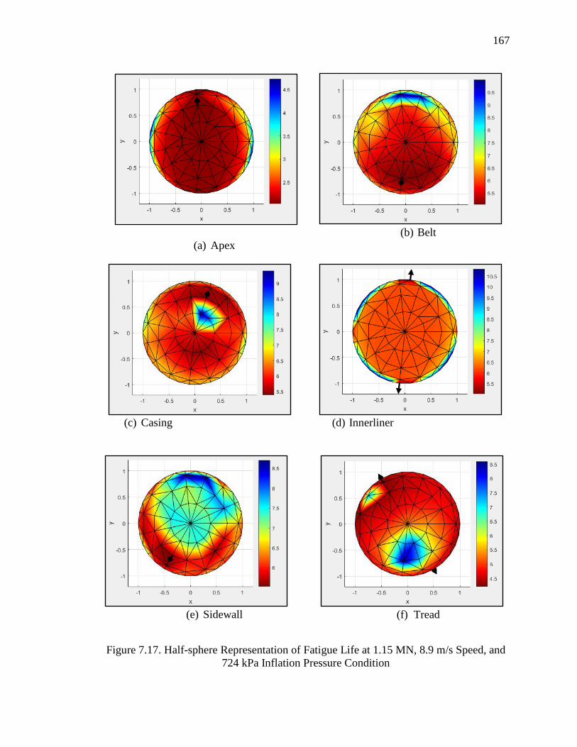
167

(a) Apex

(b) Belt

(c) Casing (d) Innerliner

(e) Sidewall (f) Tread

Figure 7.17. Half-sphere Representation of Fatigue Life at 1.15 MN, 8.9 m/s Speed, and

724 kPa Inflation Pressure Condition

168

The state of the crack (closed/open) is shown alongside the CED plots in Figures

7.18–7.20. The crack state is shown for the entire duration of the tire duty cycle for each

tire component. Depending on the degree of damage at a given time instance in the loading

cycle, a crack may be closed (shaded cell) or open. The crack states shown in Figures 7.18–

7.20 are represented by a two-layer rectangular block of cells, with the upper layer showing

the crack state at 1.01 MN rated vertical load, and the lower showing that for the 1.15 MN

vertical load case. Crack closure occurs when the compressive part of the total strain work

is unavailable to be released for crack growth on a given material plane. From Figure 7.18a,

it can be observed that the apex crack is closed throughout the loading cycle for the 1.01

MN vertical load case. However, the crack is shown to be open throughout the loading

cycle at 1.15 MN as the tensile component of strain (33) dominates on the apex critical

plane (see Figure 7.15a).

Similarly, the belt crack is shown to be mostly open throughout the entire duration

of the tire’s duty cycle except for time instance 0.72 sec, where the 33 strain component

(see Figure 7.15b) attains its most compressive value at both vertical load cases. Figures

19a and 19b show crack closure on the casing and innerliner critical planes for both vertical

load cases. Lastly, at 1.15 MN vertical load condition, the sidewall and tread cracks are

open at the start of the loading cycle and closes at 0.57–0.72 sec and 1.43 sec, repectively,

as shown in Figure 20. This is further illustrated by the values of their 33 strain components

in Figures 7.15e and 7.15f.

The effect of inflation rates on crack driving forces is shown in Figure 7.21 for

critical planes of the different tire components. Peak CED amplitudes are observed on the

innerliner and sidewall planes at 862 kPa, followed by 793 kPa, and 724 kPa. This trend,

however, is not true for the other planes. Cracks are found to initiate the fastest on the

casing plane at 793 kPa inflation loading, and the slowest at 862 kPa. Generally, no tangible

trend could be established between tire pressure and crack driving forces on the failure

planes.

The effect of speed (frequency of loading at crack tips) on crack driving forces is

shown in Figure 7.22 at a constant vertical load and inflation condition. The critical planes

in the tire sidewall and casing components show high crack driving forces when speed is

maximum (13.4 m/s), whereas peak crack driving forces are observed at 8.9 m/s for the

169

belt, innerliner, and tread components. The difference in the magnitudes of the speed used

in the study is just not high enough to clearly show how speed affects crack tip driving

forces.

(a)

(b)

Figure 7.18. Effect of Tire Vertical Load on Crack Driving Forces at 8.9 m/s Travel

Speed and 724 kPa Inflation Pressure for: (a) Apex, and (b) Belt

Effect of SIC on Fatigue Life. The effect of strain-induced crystallization

(SIC) on fatigue life is shown in contour plots for the various components of the tire. SIC

is common in natural rubber parts that undergo large deformations in service. The fatigue

life predictions in Figures 7.23–7.27 were obtained under the following loading

combinations: 1.01 MN vertical load, 8.9 m/s speed, and 724 kPa. The belt endings are

shown in Figure 7.23 to be the most critical region for crack initiation and subsequent

propagation in the belt package. This observation is consistent with results published by

Lake et al. [128], who found the belt endings in their study to be prone to high damage

170

(a)

(b)

Figure 7.19. Effect of Tire Vertical Load on Crack Driving Forces at 8.9 m/s Travel

Speed and 724 kPa Inflation Pressure for: (a) Casing, and (b) Innerliner

accumulation due to weak bonding between the cords and surrounding rubber. The point

of crack initiation is found close to the inboard end of the transition belt layer when the

belt host rubber is considered to strain-crystallize, as shown in Figure 7.23a. The fatigue

life of the crack initiation plane is 510207.1 cycles (tire revolutions), showing a 63.8%

improvement in life compared to the case where the host rubber does not strain-crystallize

(as shown in Figure 7.23b). The location of the critical plane varies depending on whether

the rubber crystallizes when loaded. In Figure 7.23a, the critical plane is located in the layer

of rubber between the transition belt and working belt 1. Figure 7.23b rather shows the

critical plane to be located underneath the transition belt at the opposite end of the package.

Under conditions of SIC, crack initiates in the shoulder region of the tire after 510867.3

cycles, as shown in Figure 7.24a. The shoulder is where the belts terminate, and it is noted

for being a stress concentration region of the tire. Fatigue failure in the shoulder region of

mining OTR tires is not uncommon, especially during high speed cornering maneuvers.

The lower innerliner and sidewall regions are shown in Figures 7.25a and 7.26a to be

171

(a)

(b)

Figure 7.20. Effect of Tire Vertical Load on Tread Crack Driving Forces at 8.9 m/s

Travel Speed and 724 kPa Inflation Pressure for: (a) Sidewall, and (b) Tread

critical with initiation lives of 510868.2 and 510031.5 cycles, respectively. The

slightly lower innerliner life can be attributed to the effect of high nodal temperatures in

the inner layer of the tire bead region (as shown in Figure 7.13a). Additionally, failure

planes are detected in the lower innerliner and sidewall regions because of the heavy rim

loads they endure. From Figures 7.25a and 7.25b, it is seen that the innerliner component

improves in durability by two orders of magnitude under conditions of SIC.

Figure 7.27 shows failure regions on the inner surface of the tread block. This

validates the fact that cracks typically initiate on free surfaces and grow progressively into

the interior of a part [129]. The corner nodes of the lugs are shown to be critical on the

tread part. This indicates high stress intensity and low fatigue strength in such locations.

Lastly, Figure 7.28 summarizes the interactive effect of the tire operating variables

(speed, vertical load, and inflation pressure) on a critical crack located in the transition belt

layer of the belt package. Note that the belt package critical crack is used to represent

similar combined effects of tire loads on cracks occurring at different locations in the tire.

172

(a) Belt

(b) Casing

(c) Innerliner

(d) Sidewall

(e) Tread

Figure 7.21. Effect of Inflation Pressure on Crack Driving Force at 1.15 MN and 8.9 m/s

Speed

173

(a) Belt

(b) Casing

(c) Innerliner

(d) Sidewall

(e) Tread

Figure 7.22. Effect of Tire Speed on Crack Driving Force

174

(a)

(b)

Figure 7.23. Belt Package Life (in tire revolutions) Estimates under (a) SIC Influence,

and (b) No SIC Influence

The results show that fatigue life increases with decreasing tire vertical loads and

travel speeds. At the lowest vertical load case (1.01 MN), the belt durability is shown to

improve by an average of 33.2% across all inflation levels when travel speed is maintained

at 8.9 m/s instead of 13.4 m/s. Similarly, a 20% average increase in fatigue life is observed

in the case when vertical load is kept at 1.15 MN. For all vertical load/speed combinations,

damage on the cracking plane is shown to be much less at 862 kPa. The worst fatigue lives

are observed at 793 kPa for all combinations of loading.

175

(a)

(b)

Figure 7.24. Casing Life Estimates under (a) SIC Influence, and (b) No SIC Influence

Effect of Thermal Loads on Fatigue Life. Fatigue life estimates are

compared between two cases where the tire analysis was conducted using (i) purely

mechanical loads and boundary conditions and (ii) combined thermal and mechanical loads

and boundary conditions. The results are shown in Figures 7.29 and 7.30 for inflation rates

724 kPa and 793 kPa, respectively, at a constant vertical load (1.01 MN) and speed (13.4

m/s) condition. Although the location of the critical planes varies at the belt endings, the

results show initiation life to be higher in the purely mechanical model than in the thermal-

stress model for both inflation rates. Particularly, crack nucleation life drops by an order of

176

magnitude as the critical element’s temperature increases from 23℃ (73.4℉) in Figure

7.29a to 37.5℃ (99.5℉) in Figure 7.29b. In general, thermal strain levels increase with

increasing tire running temperature due to expansion of the tire materials.

(a)

(b)

Figure 7.25. Innerliner Life Estimates under (a) SIC Influence, and (b) No SIC Influence

177

(a)

(b)

Figure 7.26. Sidewall Life Estimates under (a) SIC Influence, and (b) No SIC Influence

178

(a)

(b)

Figure 7.27. Tread Life Estimates under (a) SIC Influence, and (b) No SIC Influence

179

Figure 7.28. A Belt Critical Plane Life at Varying Inflation Pressure, Vertical Load, and

Speed Combinations

7.4. SUMMARY

This section covers discussions on the tire simulation results under varying field

conditions. The simulation experiments comprised rolling the tire under a combination of

two normal tire loads (1.01 MN and 1.15 MN), three rated inflation pressures (724 kPa,

793 kPa, and 862 kPa), two translational tire speeds (8.9 m/s and 13.4 m/s), and two

ambient temperature conditions (0.56℃ and 28.9℃). It has been shown in the results that

increasing tire pressure decreases the amount of vertical deflection in the tire. The

maximum tire deflection was found to be 303.5 mm when rolled at 724 kPa pressure and

8.9 m/s speed. The axle-rise phenomenon was established in the rolling simulation where

the tire loaded radius was found to increase with increasing speed. At any given inflation

rate, the tire deflected slightly more when speed was 8.9 m/s than that at 13.4m/s. The

maximum average stresses in the casing and belt rebar layers were 3,553 MPa and 206.1

MPa, respectively, whereas that of the (belt) host rubber was 1.163 MPa. This indicates the

180

transversely isotropic steel cords used in the 56/80R63 tire casing and belt regions carry

the majority of the tire loads.

(a)

(b)

Figure 7.29. Comparison of Belt Fatigue Life at 724 kPa Inflation Rate under (a) Purely

Mechanical Loads, and (b) Thermomechanical Loads

Viscous dissipation energy results were shown for the apex and sidewall

circumferential elements. The average maximum viscous dissipation energy in the apex

elements was shown to be 10% and 0.6% greater at 793 kPa inflation than the magnitudes

181

recorded at 724 kPa and 862 kPa pressure rates, respectively. A similar trend was found in

the sidewall elements. In general, the results showed an inconsistency with what is known

in practice about the effect of inflation pressure on heat generation rate. The results,

however, showed that inflation pressure and wheel speed loadings influence the degree of

effect of vertical loads on tire heat buildup. The results also showed the tire running

temperatures to increase with increasing ambient air temperature. Given the temperature

difference between the tire surface and interior elements, the results corroborated the fact

that the heat transfer problem of large tires is mainly a conduction problem.

Generally, temperature gradients were high in the vicinity of the ply turn-up (lower

sidewall region) towards the innerliner layer for all loading cases. The maximum

temperature in the ply turn-up region was 43.2 ℃ when ambient temperature is 28.9℃ and

inflation pressure is 862 kPa.

The time history of the strain components of the tire elements has shown that tire

material loading occurs in combination along multiple axes. Thus, tire loads are multiaxial

in nature. However, not every portion of the externally applied multiaxial loads is

experienced by crack precursors in the tire. The magnitude of a cracking plane loading

history depends on the plane’s orientation with respect to the axis of the externally applied

load. It has been shown that local peak crack driving forces increase with increasing tire

normal loads. The amplitudes of the crack driving forces increase with increasing inflation

loading for given vertical load and speed conditions. The crack close/open state has been

shown in the results to depend on the extent and type of deformation occurring on a given

tire material plane. Tire cracks tend to close when compressive loads dominate on local

material planes. Thus, cracks develop faster on the outer free surfaces of the tire than in the

interior where materials often attain a state of compression.

The durability benefits of strain-induced crystallization in natural rubber

compounds have been observed in the results. Fatigue life estimates have been obtained

for key components of the tire using the rainflow counting procedure and critical plane

method discussed in Section 5.3.3. The fatigue prediction results of the belt package

showed the steel cord endings to be critical in terms of crack initiation and subsequent

propagation. The initiation life of the belt critical plane was 510207.1 cycles.

Specifically, the point of crack initiation was found at the inboard end of the transition belt.

182

The shoulder region was identified to be critical with life of 510867.3 cycles. The lower

innerliner and sidewall regions have also been found to be critical with initiation lives of

510868.2 and 510031.5 cycles, respectively. Generally, the results have shown that

the tire fatigue life increases with decreasing tire vertical loads and travel speeds. Lastly,

the tire durability has been shown to improve by an order of magnitude when running

temperatures are significantly low.

(a)

(b)

Figure 7.30. Comparison of Belt Fatigue Life at 793 kPa Inflation Rate under: (a) Purely

Mechanical Loads, and (b) Thermomechanical Loads

183

8. SUMMARY, CONCLUSIONS, AND RECOMMENDATIONS

8.1. SUMMARY

Truck haulage is predominant in most surface mining operations and represents

more than 50% of the overall truck operating cost [12]. Tire cost per tonne-kilometer (ton-

mile) of ultra-large tires is reported to be far higher than that of lower capacity trucks [9].

Extending tire service life is a step toward reducing high truck haulage cost. Thermal and

mechanical fatigue factors must be minimized in order to maximize tire service life.

Adverse operating and environmental factors mainly cause tire premature failures. These

factors include excessive axle weights and travel speeds, road obstacles, poorly adjusted

cavity pressure, substandard haul road designs, ozone concentration, and inherent tire

design and manufacturing flaws. High speed operating sites (e.g., hard rock mines) often

experience belt separation in tires during cornering maneuvers of the ultra-size trucks.

Formulations of natural rubber in ultra-large tires remain one of the primary driving

forces behind continuous tire price hikes from manufacturers. Rubber production in

Thailand and Indonesia, which represents 60% of global supply, has declined as a result of

excessive precipitation in Thailand and leaf blight disease in Indonesia [11]. Analyses have

shown that global demand for NR rose 5.3% to 11.58 million metric tons in 2012 and may

be sustained in the long term. Ultra-large tire shortage has had a recurring history after

every major commodity market slump. This makes tire-terrain interaction and durability

studies one of the most important research subjects for engineers and researchers in the tire

manufacturing and mining industry.

Off-road tire damage is known to be influenced by other factors such as the degree

of thermal and mechanical loading histories, rubber formulation irregularities, and effects

due to the dissipative nature of the constitutive response of rubber materials [69]. The

mechanism of deformation in the tire follows a coupled system of heat transfer and

elasticity governing equations. The finite element formulation and solution of the system

of governing equations in MATLAB and ABAQUS have been discussed in the study. A

virtual model has therefore been proposed to simulate varying operating conditions of the

tire in order to predict damage events and the fatigue performance of its components. The

proposed virtual model overcomes the challenges involved in performing indoor endurance

184

tests on ultra-large truck tires. The research study focused on predicting crack initiation life

based on a single dynamic duty-cycle load of the 56/80R63 tire. The results of the study

provide a basis for off-road tire compounders and developers to design durable tires to

minimize tire operating costs in the mining industry.

8.2. CONCLUSIONS

A detailed literature review provided valuable knowledge relevant to pneumatic tire

structure, heat generation mechanisms, durability, and wear. The research frontier was

established based on the results of the literature review. It also showed that no studies have

ever been conducted on the 56/80R63 tire thermomechanical fatigue performance, making

this research study a pioneering effort in the area of ultra-large tire durability. Thus, this

research introduces new tire material and performance data into the literature, as it

contributes to the current body of knowledge in tire perfromance studies.

All the research objectives have been accomplished within the research scope. The

thermal processes the tire undergoes during manufacture and while in service have been

thoroughly examined to gain insights into the mechanisms of heat buildup in the tire. The

fully coupled thermomechanical deformation problem of the tire has been solved by a

sequentially coupled system of heat transfer and nonlinear elastic equations. A number of

existing rubber constitutive models have been used to characterize experimental data

obtained from specimens extracted from various parts of the tire. Fatigue crack growth

experiments under relaxing and non-relaxing conditions have been used to characterize the

tire compounds’ response behavior to cyclic loads. The tire geometry was developed from

field measurements made on an out-of-service cut tire of similar dimensions.

A rainflow counting procedure has been used to identify damage events in the

complex multiaxial variable amplitude duty-cycle loads of the tire for fatigue life

predictions. It was assumed that each material point in the tire constitutes a crack precursor

that could grow into a critical size. Based on this assumption, a plane analysis method was

implemented to analyze each material plane in the tire in order to assess their fatigue

damage under the tire’s duty cycle (thermomechanical) loads. The combined use of the

rainflow counting algorithm and plane analysis method has provided a means for

185

determining nucleation life estimates and crack closure states on all potential failure planes

in the tire.

The full factorial design process was used to design the required number of

experiments for studying the research phenomena. From the detailed experimentation and

analysis of the results, the following conclusions are drawn.

1. The tire vertical deflection is caused by the hysteretic nature of its materials when

subjected to cyclical loads. The maximum tire deflection is in excess of 300 mm.

Rolling resistance in the tire is a function of vertical deflection and increases with

decreasing inflation pressure. Rolling resistance also increases with increasing tire

axle loads.

2. Tread wear is expected to be uniform when the tire inflation pressure is maintained

at 793 kPa (115 psi).

3. A greater proportion of the tire wheel loads are supported by the tranversely

isotropic steel reinforcements in the tire. Twisting deformation is prevalent in the

rubber surrounding the steel cords.

4. Heat buildup in the tire is largely caused by internal dissipation of the rubber

components due to their viscoelastic property. Ambient temperature conditions also

influence the tire’s ability to exchange heat with its surroundings. The tire running

temperature increases with increasing ambient air temperature, speed, and vertical

load.

5. Considering the thickness of rubber in different parts of the tire and the low thermal

conductivity of the compounds, the tire heat transfer problem is mainly a

conduction problem. Cooling by forced or natural convection in large tires is less

significant.

186

6. Cracks develop on specific planes in the tire depending on the extent of damage

occuring on those planes. The magnitude of fatigue damage on a tire failure plane

is a direct function of the plane’s orientation with respect to the axis of application

of far-field loads.

7. Fatigue damage on the tire material planes is severe when vertical load and speed

are high. For any given vertical load and speed combination, the tire’s inflation

pressure has to be adjusted in order to maintain moderate loads on its material

planes.

8. The availability of energy release rate to grow cracks on a given material plane of

the tire depends on the type of deformation (tensional or compressional) that plane

is undergoing. A crack is closed when its host material plane is in a state of

compression.

9. For crystallizing compounds (e.g., natural rubber), the effect of strain-induced

crystallization can lead to several orders of magnitude improvement in tire fatigue

life.

10. The combined effect of thermal and mechanical loads (strains) on crack nucleation

life is significant and may lead to an order of magnitude reduction in nucleation life

of the tire components. Thermal strains are generally high at higher tire operating

temperatures.

11. The belt endings (tire shoulder), lower sidewall, and tread lug corners are

susceptible to crack intiation and subsequent failure due to high stresses.

187

8.3. PHD RESEARCH CONTRIBUTIONS

The research is a pioneering effort towards resolving fundamental science and

engineering problem associated with the use of ultra-large truck tires in surface mining

operations. Below are the key contributions from this research study.

1. This research is the first successful attempt in predicting an off-road ultra-large tire

nucleation life using the critical plane analysis method. The novel analytical

methodologies and algorithms contribute significant knowledge to the body of

literature in the area of tire durability modeling and analysis.

2. Prior to this investigation, there was apparently no information in the literature for

off-road ultra-large tires. This research study adds new tire geometric and material

data and results to the literature for the advancement of scientific and industrial

knowledge and insight.

3. The proposed virtual tire model provides a scientific basis for tire development

engineers and compounders to assess tire durability performance at the design stage

before investing in building prototypes.

4. This research pioneers in quantifying the benefits of strain-induced crystallization

to fatigue life in crystallizing rubber.

5. This research provides a scientific basis for evaluating the effects of tire operating

variables on tire service life especially in the mining industry where a brute-force

approach has been used in the past several years.

8.4. RECOMMENDATIONS

Availability of a CAD geoemtry and load-deflection data of the tire from its OEM

would significantly improve the accuracy of the results of the tire finite element (FE)

model. Since ultra-large off-road tire research results are not published in the literature, it

188

was difficult to adequately validate the developed FE model. Thus, further validation work

is required to ensure that the model predicts tire response to acceptable levels.

The dynamic straight-line rolling analysis simulation of the tire was

computationally too expensive to allow for steady-state solution to be attained. Hence, the

rolling simulation was assumed to have reached steady-state after three tire revolutions.

This simplifying assumption is limiting and affected the results to some degree. It is

therefore recommended that a steady-state rolling analysis be used to obtain a more

accurate local response of the tire to imposed loads. Additionally, other heat sources such

as the frictional heat dissipations in the tire footprint could be included in the thermal

analysis in future studies.

The fatigue crack growth data used in the tire life predictions were obtained at a

single temperature condition (23℃). In this case, the variation of the tire fatigue

performance with changes in temperature could not be studied. It is necessary that

temperature-dependent fatigue properties are used in the tire thermomechanical fatigue

analysis in order to accurately measure how tire life is affected by variations in temperature.

It is also recommended that fatigue crack growth test data is obtained for component of the

tire, as different compound formulations have different crack growth behavior.

Lastly, a framework needs to be developed for tire usage in the surface mining

industry based on the tire simulation results. It is anticipated that such a framework will

guide truck operators and tire technicians on selecting payload weights, travel speeds, and

inflation pressures without compromising the durability performance of the tires.

189

APPENDIX

DERIVATIONS BASED ON THE LINEAR ELASTIC THEORY

For an isotropic, incompressible, linear elastic rubber band undergoing simple

tension loading, its stiffness E can be defined as given in Equation (B.1).

E (B.1)

From Equation (B.1), it is easy to express the principal components of the stress

tensor as in Equation (B.2). Note that and ip are the Poisson ratio and hydrostatic

pressure components (resulting from the incompressibility assumption), respectively.

3

2

1

3

2

1

3

2

1

1

1

1

211p

p

pE

(B.2)

Under conditions of planar tension, can be expanded as shown in Equation (B.3).

Substituting Equation (B.3) into (B.2) simplifies each principal component of as show in

Equations (B.4)–(B.6).

1

0

1

3

2

1

(B.3)

p

Ep

E

11

2111 (B.4)

pp

E

2112 (B.5)

190

1

1211

03

Ep

pE

(B.6)

When 2

1 and

1

Ep , Equations (B.4) and (B.5) become:

EE 3.13

41

(B.7)

E3

22

(B.8)

From the abovementioned assumptions and derivation, it is clear that rubber

response is 1.3 times stiffer in planar tension than in simple tension, as shown in Equation

(B.7). Additionally, Equation (B.8) indicates the lateral stress is exactly one half of the

axial stress.

By definition, under equibiaxial tension is expressed as in Equation (B.9). Similar

to the derivation above, the principal components of are given in Equations (B.10) and

(B.11).

2

1

1

3

2

1

(B.9)

p

Ep

E

121

21121 (B.10)

191

1

2

12211

03

Ep

pE

(B.11)

When 2

1 and

1

2Ep , Equation (B.10) becomes:

E

EE2

1

2

121 (B.12)

Equation (B.12) shows that rubber is twice stiffer in equibiaxial tension than in

simple tension.

192

BIBLIOGRAPHY

1. NMA. US Percent Share of World Nonferous, Nonfuel Mineral Production. [cited

2016, August 13 ]; Available from: http://nma.org/pdf/m_us_percent_share.pdf.

2. Ewell, M.E. Mining and Quarrying Trends. [cited 2016, August, 13]; Available

from: https://minerals.usgs.gov/minerals/pubs/commodity/m&q/873400.pdf.

3. Wang, H., I.L. Al-Qadi, and I. Stanciulescu, Simulation of tyre–pavement

interaction for predicting contact stresses at static and various rolling conditions.

International Journal of Pavement Engineering, 2012. 13(4): p. 310-321.

4. On a Roll. Mar 21, 2015 [cited 2015, December 9]; Available from:

https://www.earthmovertiregroup.com/assets/haul_tyres.pdf.

5. Correlating Goodyear's Q3 Loss and Global Rubber Prices. [cited 2013, January

15]; Available from: http://seekingalpha.com/article/233283-correlating-

goodyears-q3-loss-and-global-rubber-prices.

6. OTR Tire Supply Comes Under Pressure. [cited 2013, January 15]; Available from:

http://www.e-mj.com/features/1150-otr-tire-supply-comes-under-pressure.html.

7. Mining Tyres. [cited 2014, February 06]; Available from: http://im-

mining.com/2013/12/02/mining-tyres-2/.

8. Serious Tire Shortage Looming: Caterpillar. [cited 2012, September 09];

Available from: http://www.reuters.com/article/businesspro-us-metals-cesco-

caterpillar-idUSTRE7366XV20110407.

9. Tire Maintenance Manual – Goodyear Off-The-Road (OTR). [cited 2012,

September 09]; Available from:

http://www.goodyearotr.com/cfmx/web/otr/info/pdf/otr_MaintenanceManual.pdf.

10. World Mining Equipment Haulage 2002 Ultra-Class Truck. [cited 2016, October

01]; Available from: https://www.otraco.com/custom/files/docs/otraco-web-

publications-wme-haulage-tucson-ultraclass-may-2002.pdf.

11. China Growth, Japan Production Create Strong Tire Demand. [cited 2012,

November 10]; Available from: http://www.miningtirereport.com/2011/09/china-

growth-japan-production-create.html.

http://nma.org/pdf/m_us_percent_share.pdf

http://www.earthmovertiregroup.com/assets/haul_tyres.pdf

http://seekingalpha.com/article/233283-correlating-goodyears-q3-loss-and-global-rubber-prices

http://seekingalpha.com/article/233283-correlating-goodyears-q3-loss-and-global-rubber-prices

http://www.e-mj.com/features/1150-otr-tire-supply-comes-under-pressure.html

http://im-mining.com/2013/12/02/mining-tyres-2/

http://im-mining.com/2013/12/02/mining-tyres-2/

http://www.reuters.com/article/businesspro-us-metals-cesco-caterpillar-idUSTRE7366XV20110407

http://www.reuters.com/article/businesspro-us-metals-cesco-caterpillar-idUSTRE7366XV20110407

http://www.goodyearotr.com/cfmx/web/otr/info/pdf/otr_MaintenanceManual.pdf

http://www.otraco.com/custom/files/docs/otraco-web-publications-wme-haulage-tucson-ultraclass-may-2002.pdf

http://www.otraco.com/custom/files/docs/otraco-web-publications-wme-haulage-tucson-ultraclass-may-2002.pdf

http://www.miningtirereport.com/2011/09/china-growth-japan-production-create.html

http://www.miningtirereport.com/2011/09/china-growth-japan-production-create.html

193

12. Alarie, S. and M. Gamache, Overview of solution strategies used in truck

dispatching systems for open pit mines. International Journal of Surface Mining,

Reclamation and Environment, 2002. 16(1): p. 59-76.

13. Ogden, R. Large deformation isotropic elasticity-on the correlation of theory and

experiment for incompressible rubberlike solids. in Proceedings of the Royal

Society of London A: Mathematical, Physical and Engineering Sciences. 1972. The

Royal Society.

14. Lapczyk, I., J. Hurtado, and S. Govindarajan. A parallel rheological framework for

modeling elastomers and polymers. in 182nd Fall Technical Meeting of the Rubber

Division, American Chemical Society. Cicinatti, Ohio, USA. 2012.

15. SIMULIA, Abaqus 6.14 Documentation. 2014.

16. Thomas, A., Rupture of rubber. V. Cut growth in natural rubber vulcanizates.

Journal of Polymer Science, 1958. 31(123): p. 467-480.

17. Mars, W.V., Endurica CL Rubber Fatigue Simulation Software. 2016.

18. HANSER - Mixing of Rubber Compounds. [cited 2014, June 04]; Available from:

http://files.hanser.de/hanser/docs/20120206_21226151248-67_978-3-446-41743-

4_Sample%20Pages.pdf.

19. Bansal, V., et al., Extrusion Simulation of Tire Components Using HyperXtrude.

20. Nasir, M. and G. Teh, The effects of various types of crosslinks on the physical

properties of natural rubber. European polymer journal, 1988. 24(8): p. 733-736.

21. Wong, J.Y., Theory of ground vehicles. 2008: John Wiley & Sons.

22. Koutny, F., Geometry and mechanics of pneumatic tires. Zlin: CZE–2007,–142 р,

2007.

23. French, T., Tyre technology. 1989.

24. Moore, D.F., The friction of pneumatic tyres. 1975.

25. Why Do Some Motorcycles Still Wear Bias-ply Tires? [cited 2016, September 10];

Available from: https://www.revzilla.com/common-tread/why-things-are-bias-ply-

and-radial-tires.

http://files.hanser.de/hanser/docs/20120206_21226151248-67_978-3-446-41743-4_Sample%20Pages.pdf

http://files.hanser.de/hanser/docs/20120206_21226151248-67_978-3-446-41743-4_Sample%20Pages.pdf

http://www.revzilla.com/common-tread/why-things-are-bias-ply-and-radial-tires

http://www.revzilla.com/common-tread/why-things-are-bias-ply-and-radial-tires

194

26. Brewer, H., Tire stress and deformation from composite theory. Tire Science and

Technology, 1973. 1(1): p. 47-76.

27. Khan, M., D. Lehmann, and G. Heinrich, Modification of PTFE nanopowder by

controlled electron beam irradiation: A useful approach for the development of

PTFE coupled EPDM compounds. Express Polymer Letters, 2008. 2: p. 284-293.

28. Heinrich, G. and T.A. Vilgis, Contribution of entanglements to the mechanical

properties of carbon black-filled polymer networks. Macromolecules, 1993. 26(5):

p. 1109-1119.

29. NEOGI, C., S. Basu, and A. Bhowmick, Analysis of rubber-filler interaction at

high temperature by using strain amplification factor. Plastics and rubber

processing and applications, 1989. 12(3): p. 147-151.

30. Wang, M.-J., Effect of polymer-filler and filler-filler interactions on dynamic

properties of filled vulcanizates. Rubber Chemistry and Technology, 1998. 71(3):

p. 520-589.

31. Chen, B., Material Characterization of Tire Cords and the Effects of Cord Thermal-

Mechanical Properties on Tires. Tire science and Technology, 2004. 32(1): p. 2-

22.

32. Piatt, M.M., Mechanics of Elastic Performance of Textile Materials, Part III: Some

Aspects of Stress Analysis of Textile Structures—Continuous Filament Yarns.

Textile Research Journal, 1950. 20(1): p. 1.

33. Kovac, F.J., Tire technology. 1973.

34. Lim, W.W., Thermal properties of tire cords and their effects on post-curing

inflation of tires. Rubber chemistry and technology, 2002. 75(4): p. 581-587.

35. Chen, B., Influences of thermo-mechanical properties of polymeric cords on tires

with and without post-cure inflation. Tire Science and Technology, 2002. 30(3): p.

156-179.

36. Hearle, J.W., P. Grosberg, and S. Backer, Structural mechanics of fibers, yarns,

and fabrics. 1969.

37. Steel Cord for Radial Tire. [cited 2016, September 10]; Available from:

http://www.steelwirefactory.com/products/steel-cord-for-radial-tire/.

http://www.steelwirefactory.com/products/steel-cord-for-radial-tire/

195

38. Gent, A.N. and J.D. Walter, Pneumatic tire. 2006.

39. Mullins, L., Softening of rubber by deformation. Rubber chemistry and technology,

1969. 42(1): p. 339-362.

40. Payne, A.R., The dynamic properties of carbon black‐loaded natural rubber

vulcanizates. Part I. Journal of applied polymer science, 1962. 6(19): p. 57-63.

41. Vehicles Dynamics Terminology, SAE 670E, Society of Automotive Engineers.

1978: PA, USA.

42. Kainradl, P. and G. Kaufmann, Heat generation in pneumatic tires. Rubber

Chemistry and Technology, 1976. 49(3): p. 823-861.

43. Bulgin, D. and G. Hubbard, Rotary power loss machine. Rubber Chemistry and

Technology, 1959. 32(3): p. 915-939.

44. Kainradl, P., J. JAEGER, and G. KAUFMANN, DEPENDENCE OF

TEMPERATURE BUILT UP DURING RUNNING IN DIAGONAL LORRY TIRES

UPON VISCOELASTIC PROPERTIES OF COMPOUNDS USED FOR TIRE

CONSTRUCTION. 1. KAUTSCHUK GUMMI KUNSTSTOFFE, 1972. 25(1): p.

21-&.

45. Collins, J., W. Jackson, and P. Oubridge, Relevance of Elastic and Loss Moduli of

Tire Components to Tire Energy Losses. Rubber Chemistry and Technology, 1965.

38(2): p. 400-414.

46. Willett, P., Heat generation in tires due to the viscoelastic properties of elastomeric

components. Rubber Chemistry and Technology, 1974. 47(2): p. 363-375.

47. Kainradl, P. and G. Kaufmann, Viscoelastic Properties of Truck Tire Compounds

and the Related Heat Buildup. Rubber Chemistry and Technology, 1972. 45(1): p.

1-9.

48. Gent, A., Relaxation processes in vulcanized rubber. III. Relaxation at large strains

and the effect of fillers. Rubber Chemistry and Technology, 1963. 36(3): p. 697-

708.

49. MacKenzie, C. and J. Scanlan, Stress relaxation in carbon-black-filled rubber

vulcanizates at moderate strains. Polymer, 1984. 25(4): p. 559-568.

196

50. Cotten, G. and B. Boonstra, Stress relaxation in rubbers containing reinforced

fillers. Journal of Applied Polymer Science, 1965. 9(10): p. 3395-3408.

51. Bartenev, G., L. Shelkovnikova, and L. Akopyan, The problem of relaxation time

spectra in polymers. Mekh. Polim, 1973(1): p. 151-154.

52. Skelton, J., Bending Hysteresis Losses in Cord—Rubber Composites. Rubber


53. Sharma, R., Y. Kwon, and D. Prevorsek, Relative importance of cords and rubber

in tire rolling resistance, in Tire Reinforcement and Tire Performance. 1979,

ASTM International.

54. Priss, L. and A. Shumskaya, Mechanical Losses in Rubbers Under Loading

Conditions Typical of Tires in Service. Tire Science and Technology, 1988. 16(3):

p. 171-186.

55. Dalrymple, T., J. Choi, and K. Miller. Elastomer rate-dependence: A testing and

material modeling methodology. in Fall 172nd Technical Meeting of the Rubber

Division of the American Chemical Society. 2007.

56. Nandi, B., et al. Importance of capturing non-linear viscoelastic material behavior

in tire rolling simulations. in Presented at the. 2014.

57. Trivisonno, N., Thermal analysis of a rolling tire. 1970, SAE Technical Paper.

58. Tielking, J. and R. Schapery. An Analytical Method for Tire Power Loss

Calculations. in SAE Conference Proceedings P-74, R&D Planning Workshop on

Tire Rolling Losses and Fuel Economy, Transportation Systems Center (DOT),

Cambridge, MA. 1977.

59. Prevorsek, D., Y. Kwon, and R. Sharma. The Tire Rolling Resistance via

Viscoelastic Analysis of the Components. in Society of Automotive Engineers

Conference Proceedings, P-74. 1977.

60. Yeow, S., M. El-Sherbiny, and T. Newcomb, Thermal analysis of a tyre during

rolling or sliding. Wear, 1978. 48(1): p. 157-171.

61. Whicker, D., et al., A thermomechanical approach to tire power loss modeling. Tire

Science and Technology, 1981. 9(1): p. 3-18.

197

62. Sarkar, K., Y. Kwon, and D. Prevorsek, A new approach for the thermomechanical

analysis of tires by the finite element method. Tire Science and Technology, 1987.

15(4): p. 261-275.

63. Yavari, B., W. Tworzydlo, and J. Bass, A thermomechanical model to predict the

temperature distribution of steady state rolling tires. Tire Science and Technology,

1993. 21(3): p. 163-178.

64. Park, H.-C., et al., Analysis of temperature distribution in a rolling tire due to strain

energy dissipation. Tire science and technology, 1997. 25(3): p. 214-228.

65. Ebbott, T., et al., Tire temperature and rolling resistance prediction with finite

element analysis. Tire Science and Technology, 1999. 27(1): p. 2-21.

66. Futamura, S. and A. Goldstein, A simple method of handling thermomechanical

coupling for temperature computation in a rolling tire. Tire Science and

Technology, 2004. 32(2): p. 56-68.

67. Yin, H., et al., Truck Tire Thermal-Mechanical FEA and DMA with Application to

Endurance Evaluation 4. Tire Science and Technology, 2006. 34(4): p. 220-236.

68. Kongo Kondé, A., et al. Thermomechanical couplings in aircraft tire rolling/sliding

modeling. in Advanced Materials Research. 2011. Trans Tech Publ.

69. Mars, W. and A. Fatemi, Factors that affect the fatigue life of rubber: a literature

survey. Rubber Chemistry and Technology, 2004. 77(3): p. 391-412.

70. Sokolov, S., Analysis of the heat state of pneumatic tires by the finite element

method. Journal of machinery manufacture and reliability, 2009. 38(3): p. 310-314.

71. Mars, W. and A. Fatemi, A literature survey on fatigue analysis approaches for

rubber. International Journal of Fatigue, 2002. 24(9): p. 949-961.

72. Le Cam, J.-B., Endommagement en fatigue des élastomères. 2005, Ecole Centrale

de Nantes (ECN); Université de Nantes.

73. Saintier, N., G. Cailletaud, and R. Piques, Crack initiation and propagation under

multiaxial fatigue in a natural rubber. International Journal of Fatigue, 2006. 28(1):

p. 61-72.

74. Cadwell, S., et al., Dynamic fatigue life of rubber. Rubber Chemistry and

Technology, 1940. 13(2): p. 304-315.

198

75. Fielding, J., Flex life and crystallization of synthetic rubber. Industrial &

Engineering Chemistry, 1943. 35(12): p. 1259-1261.

76. Roberts, B. and J. Benzies. The relationship between uniaxial and equibiaxial

fatigue in gum and carbon black vulcanizates. in International Rubber Conference

Rubbercon.

77. Oh, H., A fatigue-life model of a rubber bushing. Rubber Chemistry and

Technology, 1980. 53(5): p. 1226-1238.

78. Grosch, K., Rolling resistance and fatigue life of tires. Rubber Chemistry and

Technology, 1988. 61(1): p. 42-63.

79. Rivlin, R. and A.G. Thomas, Rupture of rubber. I. Characteristic energy for

tearing, in Collected Papers of RS Rivlin. 1997, Springer. p. 2615-2642.

80. De Eskinazi, J., et al., Towards predicting relative belt edge endurance with the

finite element method. Tire Science and Technology, 1990. 18(4): p. 216-235.

81. Mars, W., Multiaxial fatigue crack initiation in rubber. Tire Science and

Technology, 2001. 29(3): p. 171-185.

82. Verron, E. and A. Andriyana, Definition of a new predictor for multiaxial fatigue

crack nucleation in rubber. Journal of the Mechanics and Physics of Solids, 2008.

56(2): p. 417-443.

83. Greensmith, H., Rupture of rubber. X. The change in stored energy on making a

small cut in a test piece held in simple extension. Journal of Applied Polymer

Science, 1963. 7(3): p. 993-1002.

84. Gent, A., P. Lindley, and A. Thomas, Cut growth and fatigue of rubbers. I. The

relationship between cut growth and fatigue. Journal of Applied Polymer Science,

1964. 8(1): p. 455-466.

85. Lake, G. and P. Lindley, Cut growth and fatigue of rubbers. II. Experiments on a

noncrystallizing rubber. Journal of Applied Polymer Science, 1964. 8(2): p. 707-

721.

86. Lake, G. and P. Lindley, The mechanical fatigue limit for rubber. Journal of

Applied Polymer Science, 1965. 9(4): p. 1233-1251.

199

87. Clapson, B. and G. Lake, Truck tire groove cracking theory and practice. Rubber


88. Huang, Y. and O. Yeoh, Crack initiation and propagation in model cord-rubber

composites. Rubber chemistry and technology, 1989. 62(4): p. 709-731.

89. Ebbott, T., An application of finite element-based fracture mechanics analysis to

cord-rubber structures. Tire Science and Technology, 1996. 24(3): p. 220-235.

90. Wei, Y.-T., Z.-H. Tian, and X. Du, A finite element model for the rolling loss

prediction and fracture analysis of radial tires. Tire science and technology, 1999.

27(4): p. 250-276.

91. Legorju-Jago, K. and C. Bathias, Fatigue initiation and propagation in natural and

synthetic rubbers. International Journal of Fatigue, 2002. 24(2): p. 85-92.

92. Kim, T., et al. Prediction of the fatigue life of tires using CED and VCCT. in Key

Engineering Materials. 2005. Trans Tech Publ.

93. Park, K.-S., et al., Consideration of the frictional force on the crack surface and its

implications for durability of tires. Journal of mechanical science and technology,

2006. 20(12): p. 2159-2167.

94. Zhong, X.A., Computational fracture mechanics analysis of truck tire durability.

Journal of applied mechanics, 2006. 73(5): p. 799-806.

95. Mars, W. and A. Fatemi, Nucleation and growth of small fatigue cracks in filled

natural rubber under multiaxial loading. Journal of materials science, 2006.

41(22): p. 7324-7332.

96. Previati, G. and M. Kaliske, Crack propagation in pneumatic tires: Continuum

mechanics and fracture mechanics approaches. International Journal of Fatigue,

2012. 37: p. 69-78.

97. Moore, D.F., Friction and wear in rubbers and tyres. Wear, 1980. 61(2): p. 273-

282.

98. Muro, T., Wear rate characteristics of heavy dump truck tyres. Journal of

Terramechanics, 1989. 26(1): p. 11-23.

200

99. Da Silva, M.M., R. Cunha, and A.C. Neto, A simplified model for evaluating tire

wear during conceptual design. International Journal of Automotive Technology,

2012. 13(6): p. 915-922.

100. Chang, J., H. Chenyuan, and J. Xiaoxiong, FE simulation of tire wear with

complicated tread pattern. Procedia Engineering, 2011. 15: p. 5015-5019.

101. Mars, W.V. and D. Ostberg, Fatigue Damage Analysis of an Elastomeric Tank

Track Component. 2012, DTIC Document.

102. Barbash, K.P. and W.V. Mars, Critical Plane Analysis of Rubber Bushing

Durability under Road Loads. 2016, SAE Technical Paper.

103. Feng, X., et al., Analysis of extension propagation process of interface crack

between belts of a radial tire using a finite element method. Applied Mathematical

Modelling, 2004. 28(2): p. 145-162.

104. Narasimha Rao, K., et al., A finite element algorithm for the prediction of steady-

state temperatures of rolling tires. Tire Science and Technology, 2006. 34(3): p.

195-214.

105. Reddy, J.N. and D.K. Gartling, The finite element method in heat transfer and fluid

dynamics. 2010: CRC press.

106. Zienkiewicz, O.C., R.L. Taylor, and R.L. Taylor, The finite element method. Vol.

3. 1977: McGraw-hill London.

107. Adams, R.A. and J. Fournier, Sobolev spaces, vol. 65. Pure and applied

mathematics, 1975.

108. MIT. Module 3 Constitutive Equations. [cited 2014, August 24]; Available from:

http://web.mit.edu/16.20/homepage/3_Constitutive/Constitutive_files/module_3_

no_solutions.pdf.

109. Kalita, P., Semidiscrete variable time-step\ theta-scheme for nonmonotone

evolution inclusion. arXiv preprint arXiv:1402.3721, 2014.

110. Berger, A., Error Estimates for the Finite Element Method. 1972, Massachusetts

Institute of Technology.

111. Treloar, L.R.G., The physics of rubber elasticity. 1975: Oxford University Press,

USA.

http://web.mit.edu/16.20/homepage/3_Constitutive/Constitutive_files/module_3_no_solutions.pdf

http://web.mit.edu/16.20/homepage/3_Constitutive/Constitutive_files/module_3_no_solutions.pdf

201

112. Ogden, R., Non-linear elastic deformations. Engineering Analysis, 1984. 1(2): p.

119.

113. Inc., A.P. Physical Testing Services. [cited 2017, January 12]; Available from:

http://www.axelproducts.com/pages/hyperelastic.html.

114. VerystEngineering, Introduction to MCalibration, Version 4.2.0. 2016.

115. Williams, M.L., R.F. Landel, and J.D. Ferry, The temperature dependence of

relaxation mechanisms in amorphous polymers and other glass-forming liquids.

Journal of the American Chemical society, 1955. 77(14): p. 3701-3707.

116. Gibert, J.M., et al., Deformation Index–Based Modeling of Transient, Thermo-

mechanical Rolling Resistance for a Nonpneumatic Tire. Tire Science and

Technology, 2013. 41(2): p. 82-108.

117. Dalrymple, T., et al., Parallel Rheological Framework to model the amplitude

dependence of the dynamic stiffness in carbon-black filled rubber. Constitutive

Models for Rubber IX, 2015: p. 189.

118. Hurtado, J., I. Lapczyk, and S. Govindarajan, Parallel rheological framework to

model non-linear viscoelasticity, permanent set, and Mullins effect in elastomers.

Constitutive Models for Rubber VIII, 2013. 95.

119. Rice, J. and G.F. Rosengren, Plane strain deformation near a crack tip in a power-

law hardening material. Journal of the Mechanics and Physics of Solids, 1968.

16(1): p. 1-12.

120. SIMULIA, Isight 5.9 @ Dassault Systèmes Simulia Corp., Providence, RI. 2015.

121. Paris, P.C., M.P. Gomez, and W.E. Anderson, A rational analytic theory of fatigue.

The trend in engineering, 1961. 13(1): p. 9-14.

122. Näser, B., M. Kaliske, and W.V. Mars, Fatigue investigation of elastomeric

structures. Tire Science and Technology, 2010. 38(3): p. 194-212.

123. Mars, W. and A. Fatemi, A phenomenological model for the effect of R ratio on

fatigue of strain crystallizing rubbers. Rubber chemistry and technology, 2003.

76(5): p. 1241-1258.

124. Downing, S.D. and D. Socie, Simple rainflow counting algorithms. International

Journal of Fatigue, 1982. 4(1): p. 31-40.

http://www.axelproducts.com/pages/hyperelastic.html

202

125. Mars, W.V., Cracking energy density as a predictor of fatigue life under multiaxial

conditions. Rubber chemistry and technology, 2002. 75(1): p. 1-17.

126. CAT 795F AC Mining Truck. [cited 2017, January 30]; Available from:

http://www.cat.com/en_US/products/new/equipment/off-highway-trucks/mining-

trucks/18232553.html.

127. Kelliher, D.S. Temperature Prediction Analysis in an Off-The-Road Tire Using

ABAQUS∕ Standard. in Proceedings of 1999 ABAQUS Users’ Conference. 1999.

128. Lake, G., C. Lawrence, and A. Thomas, High-speed fracture of elastomers: Part I.

Rubber chemistry and technology, 2000. 73(5): p. 801-817.

129. Gent, A. and W. Mars, Strength of elastomers. Science and technology of rubber,

2005: p. 419-454.

http://www.cat.com/en_US/products/new/equipment/off-highway-trucks/mining-trucks/18232553.html

http://www.cat.com/en_US/products/new/equipment/off-highway-trucks/mining-trucks/18232553.html

203

VITA

Wedam Nyaaba was born in Kumasi, Ghana. He obtained his Bachelor of Science

in mining engineering from University of Mines and Technology, Ghana, in 2011. As part

of Wedam’s civic responsibility to his country, he worked for a year at AngloGold Ashanti,

Obuasi Mine, as a mining engineer. He accepted an admission offer to pursue a Master of

Science (MS) in mining engineering at Missouri University of Science and Technology

(Missouri S&T) in August 2012. However, he enrolled in the PhD mining engineering

program in August 2013, discontinuing his studies in the MS mining engineering program

for that of mechanical engineering. Wedam eventually graduated with a MS degree in

mechanical engineering in December 2015. He received his PhD in mining engineering in

July 2017.

While at Missouri S&T, Wedam worked as a graduate research and teaching

assistant and received outstanding graduate research and teaching awards in 2016 and

2017, respectively. Wedam was fortunate to have been part of the team of teaching fellows

who taught at Saudi Mining Polytechnic in the 2013/2014 academic year, and was pleased

to work under the guidance of Dr. Samuel Frimpong, director of the heavy mining

machinery research group at Missouri S&T.

Thermomechanical fatigue life investigation of an ultra ...

Documents

Transcript of Thermomechanical fatigue life investigation of an ultra ...