Thermoluminescence Basics

Theory and Applications

CONTENTS

CHAPTER - I

Introduction 1

Type of Luminescence, Applications and mechanism 1

Principle of Thermoluminescence 11

Application of Thermoluminescence 14

CHAPTER - II

Description Application of TLD System for 31

personal monitoring system

PC Controlled TLD Reader 43

(NUCLEONIX Make) and its features

Default Settings & Precautions while taking the 46

TL measurements of TLD Reader

Experiments/ Measurements with TLD Reader 58

CHAPTER - III

TLD Applications & Measurements in Radiation Oncology 64

1

CHAPTER 1

Introduction

The spontaneous emission of light upon electronic excitation (e.g. excitation by ultraviolet radiation) is called photoluminescence. Luminescence is a common phenomenon among inorganic and organic as well as in semi-conductors. However, nonradiative relaxation processes may also predominant in some compounds. In those cases where spontaneous light emission does occur, its spectral and temporal characteristics carry a lot of important information about the metastable emitting state and its relation to the ground state. Luminescence spectroscopy is thus a valuable tool to explore these properties. By studying the luminescence properties we can gain insight not only into the light emission process itself, but also into the competing nonradiative photophysical and photochemical processes. Luminescence is the emission of optical radiation (infrared, visible, or ultraviolet light) by matter. This phenomenon is to be distinguished from incandescence, which is the emission of radiation by a substance by virtue of it being at a high temperature (blackbody radiation). Luminescence can in occur in a wide variety of matter and under many different circumstances. Thus, atoms, polymers, inorganic, organic or Organo metallic molecules, organic or inorganic crystals, and amorphous substances all emit luminescence under appropriate conditions. The various luminescence phenomena are given their names, which reflect the type of radiation used to excite and to get the emission. The main characteristic of luminescence is that the emitted light is an attribute of the object itself, and the light emission is stimulated by some internal or external process. This process is quite different to the incandescence seen in an ordinary light bulb filament. In this case the energy from a current of electricity is transferred directly to the metal atoms of the wire. This causes them to vibrate and hence heat up. The wire can then glow white hot, as in an incandescent light bulb. A characteristic of this type of light is that it is accompanied with a great deal of heat! The electrical energy is converted into radiation with an efficiency of about 80%, but the visible light being emitted is less than 10% of the total radiation. The remaining radiation is mainly in the form of infra-red heat. The spectrum of radiation emitted from a hot wire, or any other object, is not sensitive to the attributes of the object. All hot objects emit light and heat with very similar characteristics and this is well described by models based on a generic blackbody. Light is a form of energy. To create the light another form of energy must be supplied. There are two common ways for this to occur, incandescence &luminescence. INCANDESCENCE: It is the light from heat energy. If you heat something to a high enough temperature it will begin to glow. When an electric stove’s heater made up of metal is put in a flame, it begins to glow “red hot”, and that is incandescence. When Tungsten filament of an ordinary incandescent light bulb is heated still hotter, by passing an electric current, it glows brightly ‘white hot’ by same means. The sun and stars glow by incandescence too.

2

LUMINESCENCE: The term luminescence implies luminous emission which is not thermal in origin i.e. luminescence is ‘cold light’, light from other sources of energy, which takes place at normal and lower temperature. In luminescence, some energy sources kicks an electron of an atom of its ground state (lowest energy) into an exited state (higher energy) by supplying extra energy, then as this excited state is not stable electron jumps back to its ground state by giving out this energy in form of light. We can observe the luminescence phenomenon in nature like, in glowworms, fireflies, and in certain sea bacteria and deep-sea animals. This phenomenon have been used in various fields by different scientist all over the world like, Archaeology, Geology, Biomedical, Engineering, Chemistry, Physics, and various Industrial Application for Quality Control, Research and Developments. LUMINESCENCE AND STOKE’S-LAW: In the process of luminescence, when radiation is incident on a material some of its energy is absorbed and re-emitted as a light of a longer wavelength (Stokes law). In the process of luminescence Wavelength of light emitted is characteristics of a luminescent substance and not on the incident radiation. The light emitted could be visible light, ultra-violet, or infrared light. This cold emission i.e. luminescence, that does not include the emission of blackbody radiation thus involve two steps. 1) The excitation of electronic system of a solid material to higher energy state and 2) Subsequent emission of photons or simply light. The emission of light takes place at characteristics time ‘τc’ after absorption of the radiation, this parameter allows us to sub classify the process of luminescence into fluorescence and phosphorescence as shown in figure1. Thus, if the characteristic time ‘τc’ is less than 10-8sec, then it is known as Fluorescence & if the characteristics time ‘τc’ is greater then that of 10-8sec, them it is known as Phosphorescence. A large number of substances both organic and inorganic show the property of luminescence, but principal materials used in various application of luminescence, involves inorganic solid insulating materials such as alkali and alkaline earth halides, Quartz (SiO2), Phosphates, Borates, and Sulphate etc. Luminescence solids are usually referred to as Phosphors.

3

The family tree of luminescence phenomena

The Fluorescence emission is seen to be spontaneous as ‘τc’<10-8sec, thus fluorescence emission is seen to be taking place simultaneously with absorption of radiation and stopping immediately as radiation ceases. Phosphorescence on the other hand is characterized by delay between the radiation absorption and the time ‘tmax’ to reach full intensity. Also phosphorescence is seen to continue for some time after the excitation has been removed. If the delay time is much shorter it is more difficult to distinguish between fluorescence and phosphorescence. Hence phosphorescence is subdivided into two main types, namely, short-period (τc< 10-4sec) & long-period (τc >10-4 sec) Phosphorescence. Fluorescence is essentially independent of temperature, whereas decay of phosphorescence exhibits strong temperature dependence.

Luminescence

Fluorescence τc < 10-8sec

(Temperature independent process)

Phosphorescence τc > 10-8sec

(Temperature dependent process)

Short period τc < 10-4 sec

Long period τc > 10-4sec

Thermoluminescence Minutes< τc< 4.6x109yrs.

4

Fluorescence:

Fluorescence is the emission of light take place with a characteristic time tc<10-8 sec. in which emission takes place from an excited singlet state and the phosphorescence (tc >

10-8 s), in which emission occurs from an excited triplet state. To clarify between fluorescence and phosphorescence is to study the effect of temperature upon the decay of the luminescence. Fluorescence is essentially independent of temperature; whereas the decay of phosphorescence exhibits strong temperature dependence.

Several types of luminescence can be recognized. Some objects, when illuminated by light of one color, are stimulated to emit light of another color. This is called fluorescence. A common example is the chemical residue left behind in clothes by some types of washing powders. These powders emit visible light when stimulated by invisible ultra-violet (UV) light found in sunlight. Thus the clothes containing the residues appear brighter because of the combined effect of the reflected visible sunlight and the fluorescence from the washing powder residues. Another example is the fluorescent chemicals that coat the inside of fluorescent tubes. In these tubes the UV light comes from excited mercury vapour inside the tube. The energetic UV light excites electrons in the fluorescent chemicals which then emit visible light (with a small amount of heat) upon decaying back to their original states. The term photoluminescence is sometimes also applied to this type of luminescence which is stimulated by light of another colour.

Another example of fluorescence is in the modern machines for producing medical x-ray images. A screen that produces a lot of visible light called fluorescence when irradiated with x-rays is used to form an image which can then be photographed with films which are sensitive to visible light. This process is more sensitive than using the film to record the x-rays directly, thus minimizing the dose of x-rays to the patient. The following are few important applications of fluorescence

Applications of fluorescence: The substances emitting the luminescence are called phosphors. Some phosphors are basically semiconductor describable in terms of energy band model. These are in biological forms. They may be in micro or macro forms. Professional have examined the PL of different materials and developed many macro and microscopic luminescence based devices. The brief account of applications of fluorescence is given below.

a) Medical application: Fluorescence is widely used in analytical work of various compounds present in cells lever’s, kidney etc. The sensitivity and selectivity of PL in many micro system facilitates the professionals to estimate amino acids, protein’s and nucleic acid in medico-logical works. b) Fluorescent Microscopy: The microscopic components of the specimen exhibit PL on the interaction with UV or blue light. Fluorescence microscopes have been developed on this premise to examine and locate fine structure of such substances. c) Fluorescent screen: Different luminescent materials under exposure of ionizing radiations; such as invisible alpha particles, electrons, ultraviolet light etc.

5

display visible emission of different colors. If the screen is prepared with luminescent material, it can be used to detect the presence of radiation field. This property of phosphors has been utilized in TV screen picture tubes, watch dials etc.

d) Fluorescent Lamp: The phosphors are pasted on inside wall of the lamp. UV light of 253.7 nm is generated through electric discharge. The phosphor absorbs the UV and through fluorescence emission it converts it in to visible light. The emission color of fluorescent lamp depends on nature of phosphor. Many varieties of fluorescent lamps are now available in market. e) Forensic Science: Luminous emission from material is highly sensitive to nature, structure and impurity (or defect) present in the specimen. PL spectrum is as good as fingerprint of the specimen. Therefore, the comparison of the PL pattern of the ideal specimen with that of specimen with defect or in different condition provides lot of information. These facts are utilized in forensic science to detect and prosecution of criminals etc. It also evaluates physico-chemical condition of the specimen. It can be used for identification of substance in forensic science.

f) Biological Application: Plants contain fluorescent compounds in small concentration and distributed in specific locations. The examination of the fluorescence pattern of these compounds and their careful analysis leads to new technique to detect fungus in specimen, individual fluorescent chemical compound of biological origin. In addition to this it has helped to study phenomena of photosynthesis, by inspecting the variation of chloro- fluorescent at the beginning and end of period of the exposure of the plant material to light. The measurements of fluorescence polarization under various conditions lead to determine along the rotation of diffusion constant of proteins. g) Fluorescence in Chemical analysis: If the different elements in the sample emits their characteristics lines by electron or X-ray bombardment, then these elements may be identified by analyzing the emitted radiation. Measurement of coating thickness on one chemical to another can be made by studying intensity of characteristics emission from material, Chemical behavior of liquids can also be studied by fluorescence method.

h) Luminescent Devices as radiation services: It includes indicator lamps, data punched type reader, position indicator, optomechanical programming, recondition equipments, thermo chrome motor controllers, advertisements etc.

i) Mechanical behavior of materials through Luminescence: Luminescence is a structure sensitive phenomenon, which is very sensitive to detect pattern inside the lattice of the materials. One may find out defect, patterns in host matrix by examining fluorescence spectra.

6

j) Fluorometry: In this technique, re-emitted visible emission from the material is analyzed critically, which gives informative about the material. It is very good technique. It is used in many fields. (a) Impurity analysis is done through comparison of PL spectra of specimen with that of standard spectra. This technique is widely used in tablet industry in medical field. (b) The detection and assessment of several fluorescing compound in the same solution is also possible. (c) Fluorometry is also useful in biology and medicine. It gives idea regarding vitamin deficiency, estimation of blood, urine and concentration of hormones. In chromatographic separation; detection of Poison and identification of strain i.e. pus, blood and urine.

Phosphorescence:

In some materials, electrons excited by the original radiation can take some time to decay back to their ground states. The decays can take as long as few hours to few or days. This type of fluorescence is called phosphorescence and the material continues to emit visible light for a while after the original radiation has been switched off. If the duration is very short, around 10-4s, then the material is a short persistence phosphor. If it lasts for seconds or longer it is a long persistence phosphor. Objects displaying phosphorescence are sometimes said to be luminous. Most luminous toys, stickers and watch dials are coated with long persistence phosphors.

Bioluminescence is the result of certain oxidation processes (usually enzymatic) in biological systems like fireflies, jellyfishes etc., Cathodoluminescence: Cathodoluminescence is due to emission of light during electron irradiation (CRO & TV Screen Phosphors). In the beginning of the last century, it was observed that invisible cathode rays, produced by electrical discharges in evacuated tubes, produced light when they struck the glass walls of the tube. The modern name for cathode rays is electrons and this type of luminescence is has retained the name cathodoluminescence. This is a very useful form of luminescence. Beams of electrons are used for many purposes. The electron microscope employs beams of electrons to produce high resolution images of small specimens. In some cases, the beam produces cathodoluminescence from the specimen. This is particularly useful for the study of minerals in rocks where the presence of transition metal trace elements can cause the mineral to give of a distinctive colour light. Often the presence of the trace element cannot be detected in any other way. Also, the ubiquitous video display tube also employs beams of electrons to selectively excite red, green or blue phosphors to display colour images. This is such an efficient process that despite continuing revolutions in the semiconductor industry, the video display industry remains dominated by the nineteenth century technology of the video tube.

Chemiluminescence:

Chemiluminescence is produced as a result of a chemical reaction usually involving an oxidation-reduction process. The most common mechanism for such an emission is the conversion of chemical energy, released in a highly exothermic reaction, into light energy in the visible region. In some chemical reactions, energy can be transferred to electrons in the chemical bonds. As these electrons decay down to lower excited states, they emit light. Some

7

of these reactions proceed slowly, so the light can be emitted for a considerable time. This is known as chemiluminescence. This is distinct from more vigorous chemical reactions where so much heat is released that the chemicals actually catch fire or otherwise glow red hot. This is nothing more than incandescence. Chemiluminescence is displayed by a variety of organisms and the chemical reaction usually involves the oxidation. This type of light emitting chemical is called luciferin. This is an organic molecule with two hydrogen atoms attached, symbol LH2. With the aid of the molecule responsible for the storage of energy in cells, adenosine triphosphate (ATP) and a special catalyst molecule (the enzyme luciferase), the luciferin is oxidized to L=O in an excited state. When it changes into the ground state a visible light photon is emitted. One visible light photon alone is emitted as each molecule of luciferin is oxidised, so this process is really light without heat. The light is typically light blue in colour, although differing chemical environments can modify the colour. It is believed that this light producing process evolved as a small side branch of the main oxidation-reduction reactions that extract energy from nutrients. Some synthetic molecules, such as Luminol (5-aminophthalhydrazide) and Cyalume are the basis of commercially available chemoluminescent products. Remarkably, some of the steps that lead to the production of light from these chemicals remain to be fully understood.

Electroluminescence: Electro-luminescence is the efficient generation of light in a non-metallic solid or gas by an applied electric field or plasmas. Another type of electro-luminescence is that produced by some crystals when an electric current passes through them. In this case the current of electrons excites electrons that occupy energy levels involved with chemical bonds inside the crystal. When the excited electrons decay back to their ground state they emit visible light. This phenomena known as electroluminescence. There are several different methods of exciting electroluminescence from a crystal. In one method, AC voltages applied to special panels produces light. About 40 years ago, it was thought this sort of light would replace ordinary light bulbs for many domestic applications. This was because electroluminescent coatings could be applied to walls, ceilings, even curtains! There was also virtually no limit to the range of colours that could be produced. Unfortunately, several practical difficulties could not be overcome, such as efficiency, and that high frequency AC was required to excite the luminescent material. However, the light emitting diode (LED), operating on a different principle, has now become a widely used application of electroluminescence including the mobile displays apart from LEDs.

Ionoluminescence:

A more exotic method of producing luminescence is the visible light produced when fast ions collide with organic, in-organics compounds. This is called ionoluminescence. An early application of ionoluminescence was to luminous clock dials. These relied upon a rather hazardous method of making light that involved radioactivity. A radioactive material, such as radium, was mixed with a material that displays luminescence, such as zinc sulphide. As the radium decays, it emits alpha particles and other radiation. This excites electrons in the luminescent material to give off light. This is very handy, since the light persists indefinitely, limited only by the half-life of the radium isotope used, 226Ra, which is 1600 years. However, the manufacturing process for such watch dials gave radiation exposure, mainly internal exposure- to workers involved in this work in 1920s and 1930s. At a luminous dial painting factory as a result of licking their paint brushes to get a fine brush point.

8

Lyoluminescence : Lyoluminescence is the phenomenon of light emission during the dissolution of previously irradiated solids in suitable solvents. Mechanoluminescence (triboluminescence or piezoluminescence): Mechanoluminescence is due to the emission of light on applying an external mechanical energy. It could be excited by cutting, cleaving, grinding, rubbing, and compressing or by impulsive deformation of solids. Optically Stimulated Luminescence (OSL) Photostimulated Luminescence (PSL) : OSL and PSL offers an alternative technique to conventional X-ray radiography, which consist of a photographic film and an intensifying screen. They are adoptable to digital radiography systems which are based on the conversion of the X-ray image pattern into digital signals utilizing laser beam scanning of an optically stimulable imaging plate. Radioluminescence (or scintillation) : Radioluminescence is produced by ionizing radiations. Some polymers contain organic molecules which emit visible light when exposed to such radiations as X-rays, gamma rays or cosmic rays, and thus act as detectors for high energy radiations. Sonoluminescence: Sonoluminescence is the emission of light due to the excitation by Sound waves including ultrasonic waves.

The Mechanism of Luminescence:

The most important characteristic of luminescence is that it is an attribute of the material producing the light, and not the method used to excite it. The production of luminescence from a solid material can be understood from the band theory for solids. This is a theory based on elementary atomic physics and quantum mechanics. The theory is briefly introduced here.

An isolated atom carries its collection of electrons in its orbitals surrounding the nucleus. These orbitals are analogous to the orbits of the planets around the Sun, although in that case gravity binds the system instead of the electromagnetic force as in an atom. The electrons can only occupy special orbits that allow them to orbit without loosing energy. These allowed orbits may be determined from the laws of quantum mechanics. Also, owing to the fact that electrons can share their orbitals with at most one other electron of the opposite spin (the Pauli Exclusion Principle), some electrons must occupy orbitals far from the nucleus because the lower energy orbitals closer to the nucleus are already occupied.

Vacancies can be created in occupied orbitals by dislodging the occupied electron with a pulse of radiation such as from a photon, a fast electron or some other process. When this occurs, an electron from an outer level will fall down to reoccupy the inner, lower energy,

9

level. The excess energy is radiated away as a photon. For some transitions, this photon can be within the visible spectrum. Gases in discharge tubes that are bombarded by currents of electricity can display a spectrum characteristic of the transitions between the allowed energy levels in the solitary gas atoms.

In a solid, the situation is more complicated. When individual atoms are joined together to make a solid, the atoms must be pushed relatively close together. When this happens, the outera electron orbitals begin to overlap. Since no more than two electrons can occupy the same level, the energy levels begin to split into sub-levels. If six atoms are joined together to make a small lump of material, the orbital of the outermost electron overlaps with the adjacent atoms and splits into six to accommodate all electrons. These new orbitals are associated with the entire lump, rather than just a single atom. Millions of atoms are joined together to make a sizable lump of material. The outer orbitals overlap and split into a number of sub-levels, all with slightly differing energies.

In practice, the energy levels are so close together, and there are so many of them, we can speak of the orbital now consisting of an energy band.

On a small scale, the solid consists of a crystal with all atoms occupying lattice sites. Some normal solids, of interest here, consist of large assemblages of microscopic crystals. The luminescent properties of the solids depend on the properties of the crystal structure.

The formation of energy bands occurs regardless of whether the energy levels are occupied by electrons or not. Therefore, in a typical material, the outermost electrons occupy a band called the valence band, above which is the next higher energy band called the conduction band. The energy difference between the highest energy (top) of the valence band and the lowest energy (bottom) of the conduction band is called the band gap energy.

If the valence band is completely full of electrons and conduction band is completely empty, the material is an insulator, since to conduct electricity the electrons must pick up energy and move to a slightly higher level. Since all available levels in the valence band are full, they cannot do this, and the material is an insulator.

If the valence band is only partially occupied, then the material is an electrical conductor since there are free energy levels available for the electrons to carry the electric current. Owing to the fact that the valence band is formed from the outermost occupied orbitals of the atoms, which can contain either one electron or two electrons of opposite spins, the valence band in any material is always either entirely full (insulators), or just half full (conductors).

10

Fig l.1 Processes involved in radiation induced electron/hole trapping and subsequent recombination on thermal stimulation with associated luminescence emission. VB- Valence band, CB - Conduction band, Eh - Trap depth for hole, Ee - Trap depth for electron,

L - Luminescent center, A - Hole trap and D - Electron trap. (a) On gamma irradiation, electrons and holes are produced and trapped at electron

hole traps. (b) On thermal stimulation, trapped electron is released and recombines at trapped

hole site. (c) e-h recombination at trapped electron site. (d) e-h recombination at luminescent center site. (e) Process of de trapping and re trapping( second order kinetics, a – de trapping

probability and p- re trapping probability) ; (f) e-h recombination via an excited state 'E' and tunneling.

In some materials, the gap between the fully occupied valence band and the empty conduction band is very narrow. So narrow in fact that ordinary heat energy at room temperature can promote electrons from the valence band into the conduction band. Such materials are semiconductors. These are generally poor conductors compared to metals.

When any solid material is excited by energetic radiation, electrons can be excited out of the valence band into the conduction band. This leaves behind a hole in the valence band. The electron in the conduction band can dissipate excess energy as small amounts of heat until it

11

reaches the lowest energy (bottom) edge of the conduction band. It can then fall back into the hole in the valence band, radiating the energy difference as a photon.

Band gap energies, and associated band gap transition wavelengths, for some semiconductors. ‘d’ indicates that a transition directly across the band gap can conserve momentum and is therefore possible. ‘L’ indicates that a direct transition is not possible and a lattice vibration, or phonon, is necessary to conserve momentum and so only indirect transitions are possible.

Doping:

It is known fact that the band gap energies of few materials have band gaps where the band width corresponds to the visible spectrum. However, materials with a relatively wide band gap can be made to luminesce in the visible. This is possible by the addition of different atoms or imperfections into the crystal. The additional atoms, called dopants have a different electron orbital structure compared to the host crystal lattice. Therefore, in regions of the crystal around the dopant atom, additional energy levels become available. That is, within the forbidden band gap of the material, energy levels can co-exist that can accommodate electrons or holes. These levels can be close to the conduction band, in which case the dopant is called a donor, or close to the valence band, in such case it is called an acceptor. Transitions between these levels can give rise to visible luminescence in such case the dopant is known as an activator. In most cases, the activator is present in extremely small concentrations, ranging from as much as one dopant atom in 5000 host atoms down to as little as one dopant atom in 1 million host atoms.

Sometimes the excited electron can find other ways to dissipate its energy. Several non-radiative recombination mechanisms are also possible. These are usually associated with defects in the crystal, or levels in the middle of the band gap, called deep levels, introduced by impurities called inhibitors. Still other defects in the crystal can result in shallow levels which are close to the edge of either the valence or conduction bands. Shallow levels in the band gap can trap the excited electrons. Certain characteristics of these shallow level prevent the electron from decaying immediately back into the valence band. Instead the decay may only occur after a very long time. However a small amount of heat may dislodge the electron back into the conduction band from where it can readily decay back to the valence band. This is the mechanism behind the technique of thermoluminescence.

Thermoluminescence (TL) or Thermally Stimulated Luminescence (TSL): TL or more specifically Thermally Stimulated Luminescence (TSL) is stimulated thermally after initial irradiation given to a phosphor by some other means (∝- rays, β -rays, γ - rays, UV rays and X-rays). Thermally stimulated luminescence (TSL) is the phenomenon of emission of light from a solid which has been previously exposed to ionizing radiation under conditions of increasing temperature. Unlike other luminescence process such as Electroluminescence, Chemiluminescence, here heat is not an exciting agent, but it acts only as a stimulant. Hence it is better known as thermally stimulated luminescence (TSL). Excitation is achieved by any conventional sources like ionizing radiation, ∝-rays, β-rays, γ-rays and UV rays and X-rays. TSL is exhibited by a host of materials, glasses, ceramics, plastics and some organic solids. By far insulating solids doped with suitable chemical

12

impurities, termed as activator, are the most sensitive TL materials. The band theory of solids is normally used to explain this phenomenon. When a solid is irradiated, electrons and holes are produced. The defects in the solid results in the presence of localized energy levels within the forbidden gap. On irradiation, electron and holes can be trapped at these defect sites. When the solid is heated, these trapped electrons/holes get enough thermal energy to escape from the trap to the conduction band (or valence band). From here they may get re-trapped again or may recombine with trapped holes/electrons. The site of recombination is called recombination center. If this recombination is radiative, then center is called luminescence center. Alternatively a trapped hole can be released by heating which can recombine with a trapped electron resulting in luminescence. These features are shown diagrammatically in Fig.1.1. It is not required that all charge recombination should result in luminescence, they may be non- radiative too. The plot of intensity of emitted light versus the temperature known as a TL glow curve. A glow curve may exhibit one or many peaks depending upon the number of electron/hole traps with different trap depths, present in the lattice. These peaks may or not be well separated. The position, shape and intensity of the glow peaks therefore are characteristic of the specific material and the impurities and defects presents. Therefore each TSL peak corresponds to the release for an electron (or hole) from a particular trap level within the band gap of the material. The nature of the TL glow peaks gives information about the luminescent centers present in the material. It may be mentioned that TSL is highly sensitive to structural imperfections in crystals. Defects densities as low as 107/ cm3 also can give measurable TSL if radiative recombinations are dominant whereas techniques such as EPR and OAS are sensitive only for relatively higher defect concentrations such as 10 12/ cm3. The first step towards understanding the mechanism for TSL glow peaks is the identification of the trapping center and the recombination centers for the observed light emission. Apart from being a tool for the study of defects in solids, TSL has also found widespread use in radiation dosimetry, archeological dating of pottery, ceramics, minerals etc; and meteorite research. Phase Change Thermoluminescence (PCTL): Some of the organic molecules, agricultural products and few minerals (zeolites) containing water molecules in their structure do exhibit the thermoluminescence without prior irradiation. This phenomenon is known as Phase Change Thermoluminescence (PCTL). Using this phenomena one can find the phase transitions of that material. Thermoluminescence (TL), more appropriately called thermally stimulated emission (TSL), is the emission of light from an insulator or semiconductor when it is heated. But it must have absorbed high energy radiation prior to its stimulation by heat. Thus three essential ingredients necessary for the production of Thermoluminescence are:

• The material must be an insulator or a semiconductor (metals do not exhibit luminescent properties)

• The materials must have at some stage absorbed energy during exposure to radiation. • The luminescence emission is triggered by heating the materials

One particular characteristics of thermoluminescence is that, once heated to excite the light emission, the materials cannot be made to emit thermoluminescence again by simply cooling the specimen and again reheating. In order to exhibit the luminescence the material has to be re-exposed to radiation and then raising the temp will once again produce light emission.

13

BASIC PHYSICAL PRINCIPLES Phosphorescence and Thermoluminescence : Luminescence is the emission of light from a material following the initial absorption of energy from an external source – e.g., ultraviolet or high-energy radiation. The emission can be categorized as either fluorescence or phosphorescence, depending upon the characteristic lifetime between absorption of the excitation energy and emission of the luminescence. The distinction between the two processes is not always clear and is perhaps most easily made using the temperature dependence of luminescence. Consider a ground-state energy level e, illustrated in figure-2 (a). Fluorescence is the emission of light that follows the excitation of an electron from g to e and its subsequent return to level g. on the other hand if the return to the ground state is delayed by a transition into and out of a metastable level m, then delays between excitation and emission can result (figure-2(b)), and in this case the process is known as phosphorescence. If the transition into level m occurs at a temperature T, where the energy E of separation between m and e is such that E> several kT (k is Boltzmann’s constant), then the electron is likely to reside in m for a considerable period. In this case, assuming a Boltzmann distribution of energies, the probability PL per unit time for thermal excitation from the trap is exponentially dependent upon temperature according to Eq. (a), and the time between excitation and final relaxation back to the ground state can be considerably delayed by the residence of the electron in the metastable state. The temperature dependence described by Eq. (a) provides a means for distinguishing between the weakly temperature-dependence process of fluorescence and the strongly temperature dependent process of phosphorescence. If the metastable level is an electron trap, at an energy Et below the conduction band. The activation energy for the phosphorescence E = Et for typical numerical values of Et = 1.5 eV and s = 1012 s-1, the calculation of p at 298 K using Eq.(a) indicates that, for all practical situations, the trap would never thermally release its trapped electron, and as a result phosphorescence would never be observed at this temperature. However if the temperature were to be raised, the temperature may be reached at which the p is high enough to ensure that electron release occurs and luminescence is observed. For e.g., at T = 300 K and using the above values for the E and s, one can calculate the lifetime τ = 1/p of 5.06x105 years, in contrast at 500 K, T = 0.36 sec. thus, consider rising the temperature of the system at some arbitrary rate β=dT/dt. As the T rise so p increases, producing enhance luminescence emission. Unlike phosphorescence, which is normally assumed to occur at a fixed temperature, this emission is stimulated in a non-isothermal situation and is thus termed as thermally stimulated luminescence (TSL), or more popularly thermoluminescence (TL). As the temperature continues to rise, so the TL intensity increases until such time as the population of trap electron in metastable state is sufficient depleted, at which point the TL intensity decreases with further increase in the temperature.

Figure-2 (a) & (b)

the result is the characteristics TL peak (glow peak) for which the temperature at the peak maximum is related to trap depth Et, the frequency factor s, the rate of heating β.

14

Here we see the metastable localized level (level 1) at an energy Et below the conduction band and a deep level (level 2) assumed to reside below the system Fermi level (Ef). Prior to irradiation level, is assumed to be empty, and level 2 is assumed to be full. During irradiation electrons are excited across the material’s band gap and become trapped at level likewise, holes become localized at level the result is a non equilibrium excess of electrons above Ef, and deficiency of electrons below Ef. Application of Thermoluminescence: The phenomenon of TL has been extensively studied by many investigators. The understanding of the mechanism of occurrence of thermally stimulated emission is the important field of fundamental research. Many researchers have suggested their views for TL mechanism for pure and impurity activated materials. With expanding knowledge of solid state physics, it is a topic of research to give latest plausible mechanism of TL. However, the present understanding of TL has explored very high application potential of it in various fields. The modernization and development in the instrumentation; and better understanding of TL have helped the professional to solve their problems in many fields. The applications of the TL are summarized in the following chart- A.

Chart-A

Applications of Thermoluminescence

Geology Biology Archaeology Biochemistry Forensic Science Radiation Dosimetry Solid State Physics Radiation Physics Space Science Spectroscopic Analysis

TL-Photography Medical Science

Exploration of Radioactive Material Exploration of Petroleum (Like Uranium) from Earth Product from earth crust

15

Basic concept of Thermoluminescence [TL OR TSL]: Thermally stimulated luminescence (TSL) is the phenomenon of light emission during warming a previously irradiated substance with uniform heating rate. When a material is exposed to ionizing radiation like; alpha, beta, gamma and X-rays or UV-rays or when it undergoes certain chemical reactions or mechanical stress, a certain percentage of the liberated charge carriers (electron and holes) may be trapped at certain imperfections in the lattice, which are called traps. If these traps are deep enough, the charge carriers remain trapped for a long time [thousands of years] before they are released by sufficient stimulation. This stimulation can be achieved by supply of optical or thermal energy to these excited solids. The return of these trapped charge carriers to a stable state due to the stimulation by external energy (e.g. heat) is always associated with the release of absorbed energy (by the charge carriers), mostly in the form of heat. A small fraction of the absorbed energy is also released in the form of light during this process. This form of emission of light is called Thermoluminescence (TL). The TL from the material is very sensitive to;

i) The amount and nature of impurity, ii) Thermal history, iii) Pre-thermal, mechanical and radiation effect, iv) Size of material particle, v) Crystallization history and vi) Defect pattern present in the material.

Theory states that no electron can exist in the material with energy states falling in the forbidden gap. When the material is excited by any ionizing radiations (Fig.1.1.a) some electrons (originally in the valence band) are excited and they attain energy states corresponding to the conduction band. Normally, these electrons cannot remain excited indefinitely, that is the lifetime of an electron in the conduction band is very short and the electron attains its ground state immediately giving away the energy to warm up the crystal lattice or in the form of light. However, an impurity atom (with an appropriate ionic size and charge) present in the material can have energy states in the forbidden band. These are the metastable energy states having appreciable lifetime. An excited electron can find itself in this state, rather than getting back to its normal valence band state. Now, one says an electron is ‘trapped’. In analogy, it is also visualized that a ‘hole’ (absence of an electron) is trapped at an energy state very close to the valence band. Depending upon the energy level of the electron trap with respect to the conduction band (or the hole trap with respect to the valence band)-called the trap depth. This stage corresponds to a energy storage after the initial excitation of a material .If now the material is warmed, the heat supplied is able to stimulate the electron out of the traps (de-trapping) and the electrons return to the ground state, if the conditions are favorable (for example, the particular atom has a light emitting property) for the emission of light in this ‘return process’ then thermoluminescence occurs (Fig.1.1 b). Alternatively, a hole may be excited into the valence band where it wanders until it combines with an electron at the trapped counter- part emitting the TSL. (Fig. 1.1 c).

16

If the traps are not very deep, de-trapping and recombination may already occur at a substantial rate around room temperature resulting in a short half-life of the stored energy. This is called phosphorescence but strictly speaking it is thermoluminescence at the room temperature. Only, if the traps are the deep enough to result in sufficient storage stability at room temperature (half-lives of trapped electrons at least several months normally corresponding to glow peak temperature greater than about 150oC), the effect becomes of dosimetric interest .The glow curve generally exhibits many peaks, each corresponding to a trap with a different energy depth.

In many phosphors it is possible that the electrons and holes are de-trapped more or less simultaneously and they recombine at an entirely new site (Fig.1.1 d) which is called luminescence center or recombination center. The TL glow curve will in this case represent an effective thermal activation energy needed by the trapped electron / hole to surmount a potential barrier between the trap and recombination center. In reality, a trapped charge when de-trapped has a finite probability of getting re-trapped as in Fig.1.1e.When this re-trapping probability is significant, the shape of the glow curve is different from the case when it is absent. Also the recombination probability for the de-trapped charge carrier may in most cases charge with time (i.e. as the heating proceeds) depending on the number of available unused recombination centers. Such a process is called a second order or bimolecular process usually while the simplest case where the recombination has a constant probability with time, is called a first order or monomolecular process. There are also practical situations where the de-trapped charge carriers recombine directly without having to be excited into the conduction / valence bands. This is a, case of TL involving isolated luminescence center and process follows first order kinetics (Fig.1.1 f). All the foregoing discussions take into account only the ionization effects of the excitation irradiation; one should not however forget about the displacement effects resulting from elastic/inelastic collisions of the atom of the phosphors with the impinging radiation. This effect is more significant for the case of particular radiations (like alpha, beta, gamma, neutron, cosmic rays). The important thing about this displacement effect is that atoms are physically moved which results in the creation of interstitials, and vacancies. In relation to thermoluminescence, these constitute defects, which have potential to influence the trapping and emission processes. Configuration co-ordination curve Model: Luminescence in atomic gases is adequately described by the concept of atomic spectroscopy, but luminescence in molecular gases, in liquids and in solid introduced two major new effects, which need special explanation. One is that the emission band appears on the long wavelength (low energy) side of the absorption band, the other is that emission and absorption often show as bands hundreds of angstroms wide instead of as the line found in atomic gases. Both of these effects may be explained by using the concept of configuration co-ordinate curves shown in Fig.1.2. As in the case of atomic gases the ground and excited states represent different electronic states of the luminescence centers, that is the region containing the atoms or electrons or both involve in the luminescent transition. On these curves energy of the ground and excited states is shown to vary parabolically as some configuration co-ordinate, usually from the luminescent center to its nearest neighbors. There is a value of the co-ordinate for heat energy is given up when the system goes from D back down to A. This loss of energy in the form of heat causes the energy associated with the emission C to D to be less than that associated with the absorption A to B.

17

Fig. 3 Figure: 3. A schematic illustration of a configurational coordinate model.

The two curves are modified by repulsion near the intersection (broken lines). The vertical broken lines A to B, B to A and C to D and D to C indicate the absorption and emission of light, respectively.

When the system is at an equilibrium position, such as C of the excited curve it is not at rest but migrates over a small region around C because of the thermal energy of the system. At the higher temperatures these fluctuations cover a wider range of the configuration co-ordinate. As a result of emission transition is not just to point D on the ground state curve but covers a region around D. In the vicinity of D the ground state curve shows a rapid change of energy, so that even a small range of values for the configuration co-ordinates leads to a large range of energies in the optical transition. This explains the broad emission and absorption bands that are observed. An analysis of this sort predicts that the widths of the band (usually measured in energy units between the points at which the emission or absorption is half its maximum value) should vary as the square root of the temperature. For many systems this relationship is valid for temperatures near and above room temperature. Two other phenomena, which can be explained on the basis of the model described in Fig. 1.2, are temperature quenching of luminescence and the variation of decay time of luminescence with temperature. On the scheme of Fig 1.2 this is interpreted as meaning that the thermal vibrations become sufficiently intense to raise the system to point E. From point E the system can fall to the ground state by emitting a small amount of heat or infrared radiation. If point E is at an energy EQ above the minimum of the excited state curve, it may be shown that the efficiency ‘η’ of luminescence is given by the following equation.

18

η = 1+C exp(-EQ/KT) where C is a constant, K is Boltzman constant and T is the temperature on the Kelvin scale. The temperature quenching tends to occur most strongly for centers that would have stayed in the excited state for a relatively long period of time. As a result, the decay time of the emission that occurs in this temperature region is largely characteristic of centers in which transitions to the ground state have been rapid; therefore, the decay time of the luminescence is observed to decrease. Applications of Thermoluminescence to Archaeology: Thermoluminescence technique has been found to be highly successful in dating ancient pottery samples. This method is suitable because of the following reasons:

i) It gives the exact date of kiln firings of the sample (the other methods mostly depends on the shape and style of the pottery and hence correlate with the civilization to which it belonged). ii) TL dating is possible even beyond 30000 years, but minimum age is 50years with an accuracy of ±1 year. iii) Authentication and detection of forgery can be quickly and easily done by using this method.

The TL/OSL dating is done from a quartz grain which is collected from pottery or brick by reading the TL-output. The TL from the specimen is mostly due to TL sensitive mineral inclusions (mostly quartz) in the host clay matrix of the pottery. The technique of the dating pottery is very much similar to that done in geological samples. In archaeology, a more precise and definite event is the basis – the kiln firing. The pottery must have fired in the kiln some time in the long past. That event is considered to be the starting of the ‘TL clock ’ for archaeological dating. Whatever TL has been stored earlier in the mineral inclusion due to internal and external irradiations over the geological times (since crystallization) is considered to be erased during the kiln firing. After the onset of the ‘TL clock’ (kiln firing) the pottery starts building up TL due to internal irradiation from radioactive emanation of uranium (U), thorium (Th), and potassium (K), contents in the clay and external radiations from the cosmic background at the excavation site. Typically the total irradiation rate is of the order of 1 rad per year of which the major part is from internal radiations and the remaining due to soil irradiation and cosmic rays. Once an accumulated TL in the specimen has been measured and expressed in terms of absorbed dose by proper calibration techniques and if the total irradiation rate for the specimen could be established, the archaeological age can be obtained by simply dividing the former by the latter. Accumulated dose i.e. Age = ------------------------ Annual dose rate But in practice many complicating factors come in the way of evaluating the age.

19

Biology and Biochemistry: Application of TL technique in the study of biological and biochemical systems is increasingly favoured in recent times and necessarily all the measurements are done in the LNT-RT range. The attempts have been successful in the study of hydroxy and aminobenzoic acids, proteins, nucleic acids, plant leaves, algae and bacteria. The TL results could indicate the proper stability of the or the orthoform of the benzoic acid, the inter and intra molecular transfer of radiation damage in nucleic acids, proteins and their constituents could be correlated with their TL behaviour; the photosynthetic electron transport routes in the Z diagram could be correlated with TL and additional routes delineated and the interaction between salts and proteins could be understood from the TL patterns. Forensic science: The major study in forensic sciences is to evolve and standardizes methods to compare evidentiary materials with similar materials of known origin, which are invariably available only in minute quantities and are required to be analyzed nondestructively for evidence purposes. Thermoluminescence can offer an attractive technique in selected materials that are commonly encountered in the criminal cases viz; glass, soil, safe insulation terials, etc . This can be used as an exclusionary evidence i.e. when the TL characteristics do not match it can be said with certainty that a particular sample has not come from a known source .To reduce the probability of any coincidental matching and improve the confidence of the TL measurements whose signal to noise ratio may be bad, examination may be made of the TL glow curves from the virgin samples as well as after a heavy artificial gamma or X-ray irradiation and also of the emission spectra. Geology:

Geology is one of the earliest disciplines to accept the TL technique in its fold in a variety of applications, such as dating of mineralization, igneous activities, sedimentation and evaluation of growth rate of beaches and sand dunes. The TL technique has been found useful in dating specimens of geologically recent origin where all other conventional methods fail. In a geological specimen, the TL would starts building up from the time of its crystallization and would normally continue throughout its existence due to the radioactivity present within the minerals and in the surrounding materials, till its saturates. If one selects a material with a negligible radioactivity in it (e.g. quartz) the accumulated TL mostly represents the environmental dose rate at a place from where the geological specimen was collected. Accumulation of TL can be affected by natural light especially its ultraviolet component. In geology the sunlight bleaching is considered to be the basis for dating the geological event. The exposure of sand grains to sunlight during their weathering and transport through wind and water results in bleaching of their geological TL. This bleaching is effective enough to reduce thermoluminescence level to a negligible value. These bleached sand particles, once embedded in a sand dune or bleach, get shielded from further exposure to sunlight. This helps particles to acquire more TL due to radiations exposure from their new environment within the sand dune or on the seashore. At present using single grain technique age of geological samples can be estimated upto 50 million years with an accuracy of +5% or –5%.

20

Quality control in Industry: As early as 1938, the application of TL in the control of feldspars in ceramic products has been described. The amount of TL given out by a ceramic after artificial irradiation is directly indicative of its feldspar contains at trace levels where any other type of quantitative analysis is time consuming. Thus in ceramic industry where a particular process is repeated many number of times to produce batches of the some materials, any controllable variations in the feldspar contents can be checked quickly and efficiently. The efficiency of certain surface catalyst like Al2O3 can be quickly and efficiently evaluated by their TL sensitivities .The lattice defects which permit the adsorption reactions might also play a role in the TL emitted by these substances and the nature and intensity of TL may be gainfully correlated with the catalytic activity. The TL glow curve in such a cases could be used as criterion in controlling the preparative parameters of a desired catalyst. In principle, TL method could be employed in the quality control of many of the glass, ceramics and semiconductor products; recently it has been shown in the case of textile fibers that the low temperature TL glow curve changes can be correlated with the structure differences and / or chemical tracer impurities. However these have not yet received the attention of the industries. Radiation Dosimetry: In the present scientific world, ionizing radiations have been found very useful in engineering, medicine, science and technology. Professionals used them at every walk of life. In all the applications, the exact amount of absorption of radiation energy in the exposed material is important factor to get the desired results. The better use can be achieved mostly by accurate determination of energy absorbed from the radiation field and it possible the distribution of this absorbed energy within the material. Measurements of these quantities form the basis of radiation dosimetry and systems used for this purpose are referred as dosimeters. Professionals have worked in this direction, investigated and standardized many analytical methods to estimate the doses of radiations. The important techniques developed and employed are as under;

1. Fluorescence technique 2. Lyoluminescence method 3. Diffused reflectance technique. 4. Thermally stimulated luminescence technique [TLD] 5. Optically stimulated luminescence technique [OSL] 6. Electron paramagnetic resonance technique [EPR dosimetry]

The main basis in the Thermoluminescence Dosimetry (TLD) is that TL output is directly proportional to the radiation dose received by the phosphor and hence provides the means of estimating unknown irradiations. Also, TL can provide a perfect passive measurement i.e. integrated irradiation levels over extended periods of the order of even years. Thus, it finds immense use in the monitoring of doses received by radiation workers on a routine basis; weakly/ monthly /yearly depending upon whatever a situation many warrant. It should however be borne in mind that most of the TL phosphors are not tissue equivalent (in terms of energy absorption by irradiation) and hence the relevant dose which is medically significant to a radiation worker from protection point of view is not readily obtained. Some

21

of the phosphors like LiF, Li2B4O7, BeO etc which are nearly tissue equivalent score 4 definite points over others like CaSO4, CaF2 Mg2SiO4 etc which are however more sensitive. Many phosphors have been developed for TLDs. The application potential of TL-dosimeter is very high. They have been found very useful in many fields on account of several favorable characteristics such as high sensitivity, small size, ability to cover wide range of exposure / dose, reusability, insensitive to environmental conditions. In the past professionals had used the film budge technique in real practice. Later on they found that TLD technique is better for many reasons. And hence during last three to four decades they have developed and established the TLD technique. This is became popular now-a-days prominent applications of thermoluminescence dosimetry and radiation protection. The dosimeters have been widely used for in-phantom and in-vivo dosimetry, in medical applications. Another area, where thermoluminescence dosimeters have found use is personal monitoring of radiation workers. On account of their ability to integrate over long periods of time and measure very low exposure, they have been widely employed for environmental monitoring of doses of the order of a few micro gray. The TLDs have been employed in protection monitoring for measurement such as leakage radiation levels on and around source containers, air scatter measurement around open top installations, area monitoring around radiation installations etc. Rapid fading ratio of main TL low temperature peal of certain phosphors such as CaSO4: Dy has been using for the estimation of time of exposure after irradiation. It has been found that this technique can also detect and assess the thermal and fast neutron doses. Since TL phosphors insensitive to thermal neutrons are also available, combination of dosimeters can be employed for estimation of gamma and thermal neutron dose in mixed field. Besides this, TL dosimetry also include archaeological dating i.e. dating of ancient potteries and ceramics, space dosimetry, dosimetry of non-ionizing radiations such as UV and microwave dosimetry. If UV dosimeter has sensitivity close to the thermal response of the human skin, it would provide a measure of the thermally effective value of the UV energy. On the other hand TLDs can also find useful in agriculture. In this field they use mainly concerned with high level photon dosimetry such as dose measurement in food preservation, radiation sterilization of seed, pest control etc. Formally, the dose measurement in agriculture relied heavily on chemical dosimeters e.g. the ferric (Fe2+, Fe3+) system. TLDs constitute a less expensive method and are applicable in the dose range of 10-4 to 108 rad.

Experimental Alkali Halide: The aim of this is to record and analyze the TL glow generated from the common salt NaCl after irradiating it with beta radiations for 5 minutes. The nature of the glow curve has already been well studied for most of the alkali halides but the trap parameters analysis of the same is not done. Alkali halides are still the predominant subjects for study in the present – day luminescence research. Their lattices are cubic and many of their properties are profoundly affected by strong coulomb interaction which results from the highly ionic nature of these solids. Their large binding energies (200Kcal/mol) result in high melting point (1000 K), which offers a vast range of temperature over which phenomena may be studied. The large electronic band

22

gap (8eV) of these solids results in wide range of optical transparency and thus a very broad spectral region is available for the study of the effects of impurities vacancies and other crystalline defects. Attempts have been made to investigate the nature of the center responsible for the intrinsic luminescence of the alkali halide first of week and Teegarden showed that an emission identical with intrinsic luminescence can be stimulated by irradiation in the F & F’ bands formed by exposure to ultraviolet light at 93K. This indicates that the luminescence is due to the recombination of electrons with trapped holes either by tunneling from an excited state of the electron trap or by electrons reaching the trapped hole via the conduction band. Presumable can be stimulated the electron is captured in an excited state about the trapped hole and luminescence occurs when the hole and electron recombine. Many investigators in the past have observed a co-relation between the bleaching temperature of some absorption band and the temperature of the maxima of TL glow peaks in several alkali halides. This led them to conclude that TL studies correlated with measurement of optical thermal bleaching of colour centers. The thermoluminescence phenomenon was known since long but real interest in it started with the realization of its usefulness in radiation of its usefulness in radiation Dosimetry. The phenomenon of TL is closely related with colour center studies specially coloration due to irradiation with ionization radiation ( X-ray ,-α ,- β,- γ radiation ). In this respect alkali halides have been studied extensively some work on TL of alkali halides other than LiF is also known but these phosphors did not find any place in radiation dosimetry, due to their low sensitivity. However, lot of study has gone into finalization the nature of the trap and various workers have come out with different models. Knowledge of the nature of traps is useful for the understanding of the TL process. In what follows the TL processes in alkali halide as reported in literature are presented in brief. TL is comparatively weak in pure alkali halides. The study of F-center formation in this phosphor has shown presence of two stages. The first stage is suggested to be due to the trapping of electrons at already existing negative ion vacancy in crystal. The second stage of F-center formation is attributed to the creating and filling of negative ion vacancies during irradiation with ionizing radiation. Correlated studies between F-center and the TL peaks in various alkali halides have shown clearly that two different peaks are associated with two stages of F-centre formation. The hole trapping is normally explain to be due to interstitial. The trapped holes are released in the TL reading processes, which combine with electrons at the F-center sites giving rise to emission. A simple Model for NaCl is shown below.

23

The simplest example is NaCl. A pure sample of NaCl will look like this (right). Here, the lattice takes on a regular, repeating shape.

After irradiation with x-rays, gamma rays, or beta radiation, the resulting crystal will look like this (left). Some of the anions have fallen out of the lattice, and single electrons have taken their place. The electron trapped at such negative ion vacancies are called F-Centers.

METHODS FOR EVALUATING PARAMETERS FROM THERMALLY STIMULATED GLOW CURVE

In the majority of cases a number of peaks are observed during the heating of the sample in a certain temperature range in more favourable cases the overlapping is minimum so we can treat as individual peak. In some of thermally stimulated phenomena the kinetics of the process is usually simple being of first order, second order or general order .Once one is satisfied that the peak under investigation is of such a simple nature , the evolution involved only of three parameters – the activation energy , the pre exponential factor and the order of kinetics. Many of the methods discussed in the present chapter were developed for the simple particular cases of two or three parameters dependent single TL peak. Some of these can quite easily be adapted, to peaks of the other thermally stimulated processes. Values of the parameters, which seem to be most important to the investigator, are:

1. E- Activation energy 2. s- The frequency factor 3. b- Order of kinetics

It is expected that these parameters are independent of each other and of concentration parameters. This means that one hopes, for example, that for a particular electron trap, the activation energy, the attempt to escape frequency factor and the retrapping probability are not dependent on the concentration of the trap. Most of these methods were developed for the evaluation of the activation energy which, therefore in many cases, be calculated by a number of methods witch thus provide a cross check on the results. In the following section we will discuss the various methods developed for the evaluation of trapping parameters.

24

In a rough way, one can divide the methods for evaluating parameters by peaks of thermally stimulated phenomena into the following groups:

Heuristic methods: Methods developed mainly in the early stages of investigation of thermally stimulated curves based on empirical ground or otherwise unproved methods which turned out to be useful for certain cases.

The initial rise method: This method is used particularly all the thermally stimulated phenomena for evaluating the activation energy.

Curve fitting methods: This method based on many measured points in a broad temperature range. The initial rise method is, in away, special case but due to its extensive use it can be taken as a separate group.

Peak shape methods: It is based on the maximum temperature and two half intensity temperature or, alternately, on the two inflexion points.

Various heating rate methods

Isothermal decay methods

HEURISTIC METHOD The methods included in the present section should be considered as being mainly of

historical values or as first approximation for the evaluation of activation energy. Although admittedly, the use of other methods usually involves approximations as well, the accuracy expected in this method is generally poor. Assuming that in a given sample, the frequency factor is more or less the same for different peaks, one would expect that the bigger the activation energy the higher the maximum of the peak. The equation given by Urbach is:

E (eV)= Tm(K)/500 -------------------------1 This can be written as in the form of Eq(2): E (eV)=23kTm --------------------------------2 And for the special case i.e. for NaCl it is the Eq(3): E (eV)=38kTm ---------------------------------3

VARIOUS HEATING RATE METHODS

A number of related methods, all based on the repeated measurement, of a certain peak at different heating rates and keeping all other parameter equal, have been independently developed in the research of practically all the thermally stimulated phenomena. These methods can be most easily introduced by studying the equation for the maximum of first order peak can be written as in Eq(4):

( ) ⎟⎠⎞⎜

⎝⎛−=

mm kT

ETEsk exp2β -------------------------(4)

25

PEAK SHAPE METHODS This method is based on a small number of points along the curve have been developed mainly in investigation of thermoluminescence. This however can very easily be applied to other thermally stimulated process also. The points used are in most cases the maximum temperature Tm, the half intensity temperature at low and high part of the peak T1 & T2 respectively and are shown in figure-1.3. In small number of cases two inflexion points are utilized rather than half intensity ones. Lushchik (1956) developed methods for evaluation of E by using the high temperature half width of the peak.

GLOW CURVE SHAPE

The glow curve shape methods extract information from the glow peak by utilizing the peak temperature Tm and two temperatures T1 and T2 on either side of Tm corresponding to half peak intensity at the low and high temperature sides of the peak as well as half width parameters and the symmetry properties.

Fig.4

26

The equation is given by E = 2kTm

2/δ -----------------------(5) Chen (1969) questioned the “triangle assumption” and tested its validity for a wide range of activation energies and pre-exponential factors for both first and second order peak. Instead of the Lushchik assumption which can be written as: δIm/ßnm = cδ ----------------------------(6) Chen has also given Eq(7) below, which is summation of all the equations and it was found to be the most appropriate in calculating the Activation energy.

( )mm kTbkTcE 2_

2

ααα α ⎟⎟⎠

⎞⎜⎜⎝

⎛= ---------------------------(7)

Where α stands for δ,ω or τ. The values of cα and bα for the three methods and for first and second order are shown in the table-1. First order Second order τ δ ω τ δ ω Cα 1.51 0.976 2.52 1.81 1.71 3.54 bα 1.58+a/2 a/2 1+a/2 2+a/2 a/2 1+a/2 Table-1: Coefficients appearing in equation for the various methods of calculating activation energies (where a in the table is the power of the temperature dependence of the pre-exponential factor). Regarding the distinction between first and second order peak, as Halperin & Braner suggested to use the “symmetric factor”µ g=δ/ω. As further discussed by Chen, a first order peak is characterized byµ g =0.42 and a second order one byµ g=0.52, when µ g is only slightly dependent on the particular activation energy and pre-exponential factor involved. A slightly different treatment of the same measured quantities has been suggested by Balarian. He also suggested the use of the symmetry of the peak to distinguish between first and second order peaks but preferred to check the value of δ/τ., which should be 0.7 to 0.8 for first order and 1.05 to 1.2 for second order kinetics. Chen has also suggested a method for finding cα and bα in Eq (7) for the non first & second order cases by the use of the known values of µg = 0.42 for first order and µg=. 0.52 for second order, and measure the µg as an interpolation parameter. The equations for this general case are still with the coefficient being:

( )42.0351.1 −+= gc µτ ---------------------(A)

( )42.03.7976.0 −+= gc µδ ---------------(B)

( )42.02.1052.2 −+= gc µω --------------(C)

( )2

42.02.458.1 ab g +−+= µτ -------(D)

2ab =δ ----------------------------------(E)

21 ab w += -------------------------------(F)

27

Figure 5: TL glow curve for the beta irradiated NaCl Analysis of Glow Peaks: The glow curve for the beta irradiated sample for NaCl is shown in figure-5. The glow curve shows well-resolved glow peaks around 127oC and another at 211oC. The TL was recorded by keeping the heating rate at 2oC/sec. The analysis of any TL glow curve i.e. the analysis of trap parameters by various methods and to see what kind and nature of traps are there, is an important tool to know about the nature of the material. The analysis of the same can be done from the various methods that are described as below and the analysis of the study was done on the same. The activation energy, the frequency factor, and the shape alone i.e. the order of kinetics can dwell so much of information to the nature and the type of the glow processes taking place in the specimen and one can conclude the mechanism for it too. The study had been extensively done by Chen et. al. and Mckeever et. al. and is still carried out till today, as the model proposed for the same are of interest to the physicists. The values for the beta irradiated NaCl peak has been tabulated in table-2. It can be seen from the evaluated results that for the different equations as proposed by different scientists, different values were obtained for all the methods. The oldest one which was proposed by Urbach is the easiest as it require only the peak temperature Tm of the glow curve. The activation energy calculated by various methods vary from 0.65 to 0.76eV for peak -1 but the equation given by Halperin et al , specially for NaCl, gives the value as 1.25 eV. For Peak-2 the activation energy was found to be varying from as low as 0.39 to 1.6 eV, the values calculated for activation energy by Chen’s equation are considerably very low compared to all the other equations. We feel that this fluctuations in the activation energy for the Chen’s equation for peak 2 are due to

28

the experimental errors or overlapping of many peaks. We found out that all the other methods except the Chen are very approximate so one has to consider the values coming from the Chen’s equation as correct. The frequency factor was calculated by Randall & Wilkins equation i.e.

E = k Tm ln s. ---------------(8)

The frequency factor, s, has also been calculated for Peak -1 and Peak-2 and are tabulated in Table - 1. It was found that the frequency factor for Peak -1 varied from 3.93x108 to 3.12x 1016 / sec. But as there was variation in activation energy for Peak-2 due to that it was found that there was also drastic variation for the frequency factor of Peak -2. The reasons for the variations were the same as stated above. TL characteristics of beta irradiated NaCl give rise to interesting results like generation of two well resolved peaks at 381 and 498K. The trapping parameters namely, activation energy, frequency factor was calculated using various methods available. It was found that the Peak-1 at 381.58 K by the Chen’s equation was most appropriate. Whereas for the peak-2 there was a drastic variation of E and s values. Since the commercial NaCl consists of many impurities which leads to mixed TL peaks and generation of the many types of traps. However the values calculated using the equation E(eV) =38kTm are simply doubled which may be due to approximation done by the Urbach.

Table-1: Tabulated form of the activation energy and the corresponding frequency

factor as calculated form the various equations given in the text. S.

No. Equations For Peak 1

Tm = 381.58 K For Peak 2

Tm = 498.7 K Energy

(eV) Frequency Factor (sec-1)

Energy (eV)

Frequency Factor (sec-1)

1. E(eV) = Tm(K)/500

0.763 1.17* 1010 0.9974 1.18* 1010

2. E(eV) =23kTm

0.7569 0.97* 1010 0.9892 0.98* 1010

3. E(eV) =38kTm

1.250 3.12* 1016 1.634 3.16* 1016

4. E=2kTm2/δ 0.6520 4.01* 108 1.479 8.66* 1014

5. ( )mm kTbkTcE 2_

2

ωωω ω ⎟⎟⎠

⎞⎜⎜⎝

⎛= 0.657 4.68* 108 0.4224 1.8* 104

6. ( )mm kTbkTcE 2_

2

τττ τ ⎟⎟⎠

⎞⎜⎜⎝

⎛=

0.6636 5.72* 108 0.44 2.77* 104

7. ( )m

m kTbkTcE 2_2

δδδ δ ⎟⎟⎠

⎞⎜⎜⎝

⎛=

0.6513 3.93* 108 0.397 1.0* 104

29

References: 1. Thermoluminescence of Solids, Cambridge University Press by S.W.S Mckeever,

1985. 2. Analysis of thermally stimulated process by – Chen & Krish. 1988 3. Theory of Thermoluminescence and related phenomena , By – Chen & S.W.S. Mc

Keever , 1997 4. Archaeological Dating, Atkin, MJ, TL Dating, Academic Press, 1985 5. Chen R and McKeever, SWS, Theory of TL and Releated Phenomena, World

Scientific, 1997 6. Luminescence and its Applications, Proceedings of ISLA-2000, Vol-1,

Ed.K.V.R.Murthy et al., Pub. Luminescence Society of India, Feb. 2000. 7. Luminescence and its Applications, Proceedings of ISLA-2000, Vol-I1,

Ed.K.V.R.Murthy et al., Pub. M.S.University of Baroda, Dec.. 2000. 8. K.V.R.Murthy et. Al Proceedings of NSTPLAR, Sept. 2002. 9. Proceedings of National Seminar on TL and its Applications, Feb. Ed.

K.V.R.Murthy et al., Pub. TaTa McGraw Hill Co., 1992

Application of TLD systems

for personnel monitoring

31

CHAPTER - II

Application of TLD systems for personnel monitoring

INTRODUCTION: Personnel monitoring is based on the international recommendations of the ICRP. The primary objective of individual monitoring for external radiation is to assess, and thus limit, radiation doses to individual workers. Supplementary objectives are to provide information about the trends of these doses and about the conditions in places of work and to give information in the event of accidental exposure [1]. Depending on the kind of radiation hazard, the ICRP recommend maximum permissible dose (MPD) values. These are the maximum dose equivalent values, which are not expected to cause appreciable body injury to a person during his lifetime. With respect to the various MPD values, the following quantities should be measured in personnel monitoring: a. Skin dose or the surface absorbed dose to assess the dose equivalent to the basal layer of

the epidermis at a depth of 5-10 mg cm-2, if only non-penetrating radiation has to be considered (x-rays<15 keV, γ-rays);

b. Whole body dose or the equivalent at a depth of 400-1000 mg cm-2 below the surface of the body to assess or over-estimate the effective dose equivalent or the average dose equivalent in the critical organs for the case of penetrating radiation and whole body irradiation (x-rays>15 keV, γ-rays, neutrons);

c. Extremity dose to assess the maximum value of the dose equivalent (skin dose) in tissue to any part of the hands, forearms, feet or ankles.

In contrast to film dosimetry, approximately tissue-equivalent TL detectors of small size and high precision in measurement are available which may serve as an ideal extremity dosimeter and as a basic dosimeter for the dose estimation of photons in the energy range of interest as well as for the detection of γ-rays and neutrons. In addition, a multi-detector badge offers practical possibilities for short-term and long-term monitoring periods, for separate indication of skin dose and body dose and finally for the estimation of radiation quality. The role of TLD for an individual monitoring service is based on the following features: a. TL phosphors are available in solid form as chips, extruded ribbons or in a Teflon matrix;

the dose reading of some materials is approximately tissue-equivalent and largely independent of the angle of radiation incidence;

b. The dose reading is practically independent of dose rate up to 1011 rad s-1 and proportional to the dose up to several hundred rem;

c. In some TL materials the fading at room temperature is so small, especially after a post-irradiation annealing, that they can be used for issue periods of up to 1yr;

d. TL detectors are convenient to wear, suitable for postal service, flexible in issue period, can be evaluated in less than 1min and can be re-used, although a regeneration procedure prior to re-use is often necessary;

32

e. TLD lends itself to automation; with an on-line computer the calibration factor for individual dosimeters can be stored and also the shape of the glow curve may be checked to verify the radiation-induced TL.

f. For the reassessment of the dose recorded, a redundant detector can be included in the badge design.

TLD, the most advanced and most intensively studied integrating dosimeter system, has now reached the stage at which it may replace or supplement film dosimetry. Primarily for applications in personnel monitoring, various suppliers offer a number of commercial TLD systems with manual or automatic evaluation systems.

Application of TLD systems for environmental monitoring A significant aspect of environmental monitoring is the limitation of radiation exposure values in man from the nuclear power fuel cycle. In the case of gaseous radionuclides released to the environment from a nuclear installation, the acceptable limit of exposure is based on an annual dose equivalent of 30 mrem, a value about a third that from natural terrestrial and cosmic radiation. An increasing amount of public interest in environmental monitoring programmes is being focused on the environmental impact of radiation arising from nuclear power operations and the corresponding detection of slight variations in the natural radiation background. TLD systems are widely applied to environmental monitoring programmes near nuclear installations. TLD systems with high reproducibility in the milliroentgen dose range are required in order to measure exposures equal to that resulting from an exposure rate of 10µR h-1 during field periods of from several days up to a year. For the application of TLD systems in environmental monitoring, therefore, special performance criteria and techniques for selecting, testing, calibrating and using a TLD system have been established: a. The ANSI N545-1975 standard [1] specifies the minimum acceptable performance of

TLD and outlines test methods for compliance. To meet these requirements, each laboratory has to carry out tests for determining their own limits of error.

b. On the basis of a standard test programme [41] and an inter-laboratory comparison, the performance and quality of a broad spectrum of TLD systems can be compared with respect to variations in the properties of reader, TL material, read-out method and annealing technique adopted in the laboratories.

c. Annual control exposures as well as inter-comparison experiments organized by the ERDA serve as a valuable way to compare one’s own results with the international level [3].

This chapter reviews the properties of TLD systems and the common techniques used in the application of TLD in environmental monitoring, taking into account the results of a test programme and recent investigations of the long-term fading as well as the calibration technique and the interpretation of experimental results.

33

PERFORMANCE SPECIFICATIONS: In contrast to the application in personal monitoring, TLD systems for environmental monitoring have to fulfill high requirements, such as a. Good precision and reproducibility of measurement over the exposure range of interest

(10-100 mrem); b. Low fading over the field exposure period (3-12 months); c. Insensitivity to environmental parameters, i.e. temperature, moisture, humidity, light; d. Approximate tissue equivalence in dose reading; e. Low self irradiation due to natural radio nuclides in the TLD phosphor or holder; f. Encapsulation in a plastic holder to provide secondary electronic equilibrium, shielding

against â-rays and light as well as water tightness; g. Calibration techniques for each field cycle to guarantee the highest precision for the

conversion to exposure and to correct for fading, transit exposure and zero-dose reading. APPLICATION OF TLD IN MEDICINE: There are two important areas of absorbed dose measurement in medicine: i. Absorbed dose measurement in radiotherapy, and ii. Absorbed dose measurement in diagnostic radiology. RADIOTHERAPY MEASUREMENTS: The difficulties of accurately predicting absorbed doses in radiotherapy by calculation have in the past led to the development of in vivo measurement techniques. While entrance and exit absorbed doses could be measured using films and conventional ionization chambers, intracavitary measurements were limited by the minimum size of available ionization chambers (typically 20mm x 5mm diam ). When Daniels first developed thermo luminescence as a practical method of assessing ionizing radiation exposure, it was realized that the technique could be applied in the field of clinical measurement. Brucer used some of Daniel’s single crystals of Harshaw LiF to make internal in vivo measurements in cancer patients injected with radioactive material. The arrangement of radiotherapy treatment fields is conventionally carried out using a combination of calculations involving standardized geometries together with depth dose and transverse dose measurements in phantoms. The final check on the absorbed dose delivered to the patient can be carried out by in vivo dosimetry. Similarly, absorbed doses to organs not involved in the treatment, which should be kept to the minimum, can be measured. Thermo luminescence dosimetry has proved a useful technique for a variety of purposes in radiotherapy, including measurements of therapy machine output, beam uniformity checks and the measurement of absorbed dose in phantoms and in vivo for both internally and externally applied fields. Thermo luminescent dosimeters have a high precision, provide rapid retrieval of information (using on-site readers), have good environmental stability, have good water or tissue equivalence and have a wide range of sensitivities. The last characteristic is particularly important for in vivo measurements of absorbed dose. Because

34

of their small size, thermo luminescent dosimeters also give good special resolution. This is of particular value in many radiotherapy techniques where the absorbed dose has a rapid special variation. Thermo luminescent dosimeters may also be used to measure the absorbed dose to experimental animals. DIAGNOSTIC RADIOLOGY MEASUREMENTS: The collective dose from medical exposure has been estimated to represent the largest single man-made contribution to both the somatic and the genetically significant dose equivalent to the population of the United Kingdom as illustrated in figure representing some 31% of the total somatic dose and 9% of the total genetic dose, and 95% and 85% respectively of the man-made contribution. In other developed countries, the estimated figures are similar. By far the largest contribution is from diagnostic radiology, estimated as 10 times the sum of the contributions from nuclear medicine and radiotherapy. New radio diagnostic techniques have been introduced, some involving the use of complex machines such as the head and body scanners (computerized axial tomography, CAT). Thermo luminescence dosimetry has proved to be a useful method in the comparison of patient absorbed dose from these new techniques as well as from the more traditional ones. Diagnostic absorbed dose measurements are important for: i. Improving the design of equipment to reduce patient absorbed dose, and ii. Improving radiographers’ techniques in the use of equipment to reduce patient

absorbed dose, and for providing a measurement database for epidemiological analysis of population radiation absorbed dose from diagnostic radiology.

Thermo luminescent phosphors such as LiF: Mg, Ti and particularly the more tissue equivalent Li2B4O7: Mn have been used for such measurements. Thermo luminescent dosimeters have three main advantages over ionization chambers for this type of measurement: a. They are small and unobtrusive, b. They are radio-transparent to most x-radiation, and c. They do not require connecting leads and are easily attached to the patient. FACTORS IN THE CHOICE OF DOSIMETERS FOR CLINICAL USE: A number of factors have to be considered in the choice of the material and form of the dosimeters for clinical dosimetry. The most important factors are: i. Estimated absorbed dose range of the intended measurements, ii. Estimated equivalent photon energy or linear energy transfer (LET) of the radiation, iii. Immediate environmental conditions around the dosimeter, and spatial resolution.

35

ABSORBED DOSE RANGE: The sensitivity of any thermo luminescent dosimeter is proportional to the mass of active phosphor present, within limits imposed by geometrical and thermal considerations relevant to the readout system. Dosimeters, which contain only thermo luminescent material, e.g. powder, extruded ribbons and rods, have a much higher sensitivity than dosimeters consisting of a phosphor held in a matrix of binder material, e.g. PTFE-based discs, tape and micro-rods. The range of absorbed doses encountered in clinical and biological irradiations is very large. In diagnostic radiology, absorbed doses may range from less than 10 µGy to 100 mGy to the gonads and from approximately 100 µGy to about 100 mGy to the skin. Hence, at the lower end of the diagnostic radiology range, there is a need for a sensitive form of dosimeter, e.g. powder or extruded forms. However, in therapy dosimetry, a single treatment fraction of absorbed dose may be several grays, and, in many animal or cell irradiations, tens of grays may be required. Less-sensitive forms of dosimeter can be used, especially those incorporating the phosphor powder in PTFE as discs, tape and micro-rods. The measurement of high-absorbed doses will often necessitate using the dosimeter above the linear thermoluminescence absorbed dose response region. Under these conditions, the degree of supralinearity needs to be determined. Often, in radiotherapy, simultaneous measurements of absorbed dose in the treatment region and the much smaller absorbed dose in the shadow of shielding may be required. In such cases, two types of dosimeter, such as extruded rods and PTFE-based rods, may be used in parallel. This particular combination of dosimeters, if appropriately oriented with respect to the absorbed dose gradient, should provide good spatial resolution.

PHOTON ENERGY RANGE AND LET OF RADIATION: Modern routine radiotherapy and radio diagnostic techniques use a wide range of photon energies from conventional x-ray machines of approximately 10 keV to200 keV, from 137Cs (0.67 MeV) and 60Co (1.25 MeV) teletherapy units and from accelerators producing high-energy electrons and mega voltage photons. The total light emitted by an irradiated phosphor is proportional to the total radiation energy absorbed by it. In tissue, the absorption of Compton-scattered electrons is the most important absorption process in the photon energy range from approximately 20keV to 10 MeV. For elements such as lithium, boron, oxygen, fluorine, etc, of low atomic number, and for photon energies up to about 15 keV, the photoelectric effect is dominant. Thereafter, up to 10 MeV, Compton scattering is most important. For elements of high atomic number, such as those used as dopants (e.g. Li, Mg, Mn, etc), the photoelectric effect is dominant up to several hundred kilo electron volts. The advantage of using materials consisting mainly of atoms of low atomic number with only a few dopant atoms of higher atomic number is obvious because of their good approximation to tissue and air. This is particularly true of phosphors based on lithium borate. In order to evaluate the absorbed dose to a phantom or patient using thermo luminescent dosimeters, it is essential to know the relative energy responses of the dosimeters throughout

36

the range of energies used. The primary response calibration of dosimeters is usually carried out using a

60Co source (1.25 MeV) and the responses at all other energies and for all other

radiations are expressed as multiples or fractions of this. For clinical applications, the response is most usefully expressed as the light emitted per unit-absorbed dose in tissue or water. This will be a function of radiation energy and of the physical form of the dosimeter. The beam quality has to be known. Photon-beam quality determination, although in principle relatively straightforward to determine in free air, is difficult to determine uniquely in water or solid phantoms because of two effects: i. The contribution from lower-energy scattered radiation from the phantom and

external shielding material, e.g. the applicator cone at short focus-to-skin distances (also at low photon energies the effects of dosimeter orientation and self-shielding become increasingly important), and

ii. The effective ‘hardening’ of the beam with increasing depth in the water or solid phantom.

The thermo luminescence absorbed dose (water and polystyrene) response of LiF: Mg, Ti to high-energy radiations, of which those of principal interest in clinical applications are mega voltage photons and high-energy electrons, has been widely investigated and reported in the literature. The results have often been inconsistent. Some investigators have measured approximately 10% reduction in response to high-energy radiations compared with that to 60Co gamma radiation, and others have not found any reduction. Much discussion has revolved around the application of various generalized cavity theories to attempt to explain the observed effects and to reconcile the differences. ENVIRONMENTAL FACTORS: Absorbed dose range and radiation energy considerations apart, environmental factors such as temperature, humidity, contact with body fluids, insertion into catheters, sterilization, etc, influence the choice of dosimeter form and packaging. If dosimeters are not protected from their environment, the result is often low precision and sometimes gross error in absorbed dose measurement.

TEMPERATURE AND HUMIDITY: During exposure under clinical conditions, dosimeters may come into contact with heat (human body core temperature is 37oC) and/or high-humidity environments. If implanted or introduced into body cavities, they can come into contact with body fluids. Some phosphors (especially in powder form) have been shown [14] to be affected by humidity as well as by storage at elevated temperatures, which induces fading.

OTHER AGENTS: If dosimeters in solid form are attached directly on to the skin using adhesive tape, care should be taken to remove all traces of adhesive from the dosimeters before readout. Adhesives often exhibit thermo luminescence following exposure to visible light and/or ultraviolet radiation. The simplest way of avoiding these effects is to seal the dosimeters inside protective envelopes (e.g. polythene).

37

STERILIZING OF DOSIMETERS: Occasionally, a clinician or biologist will require dosimeters to be sterilized. The three common methods of sterilizing. i.e. autoclaving, chemical sterilizing and irradiation with 254 nm ultraviolet radiation, can all have a gross effect on the inherent sensitivity of the dosimeter or may induce spurious luminescence. In general, provided the phosphor is effectively sealed in a protective envelope or catheter, which is opaque to the sterilizing ultraviolet radiation, either chemical or ultraviolet sterilizing at normal ambient temperature is recommended. Normal ambient temperature is emphasized, as the effects of elevated temperatures on the normal sensitivity of phosphors, especially LiF: Mg, Ti, can be significant. The effects of autoclaving can be particularly severe. SPATIAL RESOLUTION: Good Spatial resolution of absorbed dose measurement is generally useful, and is essential in the determination of high-absorbed dose gradients. Thermo luminescent dosimeters are available in many shapes. Powder acts like a fluid and will adopt the shape of its container. The micro-rod and extruded ribbon (and hot pressed) dosimeters are so small, 1 X 1 X 6 mm3 and 3.2 X 3.2 X 0.9 mm3, respectively, that the effective size of the dosimeter is often limited in practice by the requirement to have adequate build-up to ensure electronic equilibrium.

RADIOTHERAPY ABSORBED DOSE MEASUREMENTS SIMPLE GEOMETRY PHANTOMS: In radiotherapy, the specification of the complete absorbed dose distribution within the radiation beam in a phantom is a prerequisite to ensuring that the prescribed absorbed dose is delivered to the target volume in the patient. A common method is to employ published depth dose data and an isodose chart. An example of such a chart is illustrated in figure. This chart refers to a section containing the beam axis parallel to one side of a 60Co 10 X 10 cm2 therapy beam for a fixed source-to-skin distance (SSD) of 80cm. The lines mapped on the chart link points of equal absorbed dose expressed as a percentage of a peak absorbed dose. In the case of 60Co radiation, the peak-absorbed dose occurs at the optimum ‘build-up depth’ in water, 5 mm. For x-ray beams produced with generating potentials of less than 400kV, the depth doses are conventionally expressed as a percentage of the surface absorbed dose. Similar charts are used for fixed source-axis distance (SAD) beams. However, in these, the isodose values are expressed as a percentage of the absorbed dose at the target deep within the phantom. SAD isodose charts are used when the target volume is located on the axis of rotation of the tele-therapy machine. The selection of an appropriate isodose chart can be difficult, as the absorbed dose distribution in the phantom depends on the beam dimensions, SSD or SAD, the radiation quality, the source size, the geometry of the beam and the positioning of the beam collimators. The International Commission on Radiological Units (ICRU) [15] therefore recommends the use of isodose charts, which are exactly specified for the particular equipment being used. This criterion can be established, as ICRU recommend, by a series of single measurements using an ion chamber or thermo luminescent dosimeters.

38

In their simplest form, the measurements consists of: a. Measuring the depth dose distribution along the central axis of the beam in a water or

water-equivalent phantom, and b. Choosing one particular phantom depth (which in the case of 150 keV to 10 MeV and

137Cs and 60Co teletherapy beams, ICRU recommends as 5 cm) and measuring the radiation absorbed dose profile across the beam at this depth.

After normalization of the depth dose measurements at 5cm depth, the published dose data which one intends to use can be compared with them and corrected accordingly. Similarly, the measured beam profile can be compared with that obtained from the published isodose chart. Since 1968, the International Atomic Energy Agency (IAEA) and the World Health Organization (WHO) have been running a programme of inter comparison of 60Co teletherapy units in the various radiotherapy centers throughout the world. This resulted from investigations carried out in 1965 which revealed that there was no suitably calibrated radiation measuring instrument in use in about 30% of the radiotherapy centers investigated [16]. A simple test procedure based on thermo luminescence dosimetry is used to assess the accuracy of delivered absorbed doses in the centers. LiF: Mg, Ti power dosimeters contained in PTFE capsules are sent to radiotherapy centers. The measurement technique used in this study illustrates:

i. The practical use of thermo luminescent dosimeters for radiotherapy depth dose measurements in a simple phantom, and

ii. Methods to eliminate effects of fading and other variable environmental factors. The procedure used is illustrated in figure Participant centers are sent four sets of dosimeters. They are requested to irradiate one test set (A) with an absorbed dose of 2 Gy in water at 5 cm depth on the central axis of a 60Co 10 X 10 cm2 therapy beam with an 80 cm SSD. Another test set (B) is to be irradiated under similar conditions for 2min. A control set (C) which has been given a known absorbed dose by IAEA and a control set (D) which is unexposed accompany sets A and B at all times except during irradiation. Sets C and D provide information about any environmental or spurious effects, such as thermal fading, unintentional irradiation, etc, which might adversely affect the test dosimeters. In addition, reference sets (R) are irradiated by IAEA in a standardized 10 X10 cm2 60Co beam (SSD 80cm) at a depth of 5cm in water. The absorbed dose rate expressed in grays per minute in water is obtained from a measurement of the exposure rate in free air using a calibrated ionization chamber. All dosimeters are then read out together, eliminating possible calibration errors due to fading and effectively standardizing the readout procedure for all dosimeters. B. IN VIVO MEASUREMENTS

39

While the measurement of complete absorbed dose distribution in a phantom is essential in planning the treatment of a patient, the ultimate check on the absorbed dose delivered to the patient can only be made by in vivo absorbed dose measurements. Thermo luminescent dosimeters have proved to be particularly useful for this purpose. The relevance of in vivo dosimetry is illustrated by the flowchart shown in figure. This flowchart is a simplified form of that used by ICRU [15] to illustrate a systems approach to radiotherapy. In vivo measurements verify that the absorbed dose prescribed by the clinician, and calculated and set up by the physicist and the radiographer, has been delivered. Further, it may be used to monitor any change in field uniformity caused by changes in the many treatment parameters. In vivo measurements can be divided into four classes. Class 1 – entrance absorbed dose measurements. These are used mainly to check the machine output, the absorbed dose distribution profile across the patient, particularly in the penumbra of shielding, and the positioning of shielding in relation to the patient. If the measured values are at variance with those prescribed and calculated, the cause can be investigated and appropriate corrective action taken. The spatial resolution afforded by thermo luminescent dosimeters is particularly useful in these measurements. Class 2 – exit absorbed dose measurements. These are used mainly to check the absorbed dose delivered to points deep within the body. The measurements should agree with calculations for exit-absorbed doses. For such measurements, the dosimeters should be provided with sufficient backscatter material. Again, good spatial resolution may be important. Class 3 – intracavitary absorbed dose measurements. The absorbed dose within a body cavity, e.g. the mouth, nasopharynx, oesophagus, vagina, rectum, etc, can be measured using dosimeters sealed inside a catheter as shown in figure. The position of the dosimeters may be checked using radio-opaque markers and exposing an x-ray film. The increase in scattered radiation resulting from the presence of radio-opaque markers of high atomic number can cause uncertainties of a few percent in the absorbed dose to the dosimeter. This can be measured and allowed for. Class 4 – individual spared organ absorbed dose measurements. The absorbed dose to spared (shielded) organs can be measured, but often no build-up can be used as this would in itself result in an increased adsorbed dose to the organ. EXAMPLES OF THE USE OF TL DOSIMETERS IN RADIOTHERAPY Thermo luminescent dosimeters are routinely used for a number of different types of in vivo radiotherapy measurements in centers throughout the world. The following examples illustrate some of the principles of their use.

40

A. MEASUREMENT OF ABSORBED DOSE DURING ‘MANTLE THERAPY’ FOR HODGKIN’S DISEASE

The radiotherapy treatment of Hodgkin’s disease involves the irradiation of a large area of the body. The treatment field is designed to deliver a therapeutic or prophylactic absorbed dose to the axillary, cervical and mediastinal lymph nodes. Many different treatment fields have been used, but one commonly used configuration consists of anterior and posterior parallel and opposed fields as illustrated in figure. There is also the need to shield presumed healthy organs, e.g. lips, eyes, lungs, kidneys, bone joints, etc, and for posterior irradiation the spinal cord needs to be shielded. To avoid excessive exposure of the skin (skin sparing), the treatment is carried out using either 60Co or mega voltage x-ray photons and the shielding is positioned some distance (typically 20 to 50 cm) above the entrance surface of the body. This is achieved using ‘individually tailored’ moulds of polystyrene, one anterior and one posterior, with appropriately cut out channels containing lead-shot shielding. Alternately, appropriately shaped lead absorbers, placed on a Perspex plate and positioned above the body, have been used. The technique is termed the ‘Gothic arch’ or ‘mantle’ technique. A typical four-week course of treatment involves a total prescribed absorbed dose of between 30 and 40 Gy delivered in 20 fractions. Thermo luminescent dosimeters, usually LiF extruded ribbons or rods or PTFE-based discs or micro-rods sealed in thin protective polythene sachets, are attached to the body under moulded blocks of wax or in small Perspex containers. The dimensions of the wax or Perspex are chosen to provide build-up appropriate to the photon energy of the beam and to ensure electronic equilibrium. With the use of high-energy photon radiation, e.g. 42MV x-rays, Ruden [10] recommends the use of a maximum build-up of 15mm Perspex and an experimentally derived factor to correct the apparent absorbed dose. B. INTRACAVITARY ABSORBED DOSE MEASUREMENT: The small size and shape of the extruded and PTFE-based micro-rod dosimeters have enabled in vivo measurements of absorbed dose inside body cavities, which hitherto were often difficult and sometimes impossible. As illustrated in figure, these dosimeters can easily be inserted and sealed in catheters. A very good example of such applications is the in vivo measurement of absorbed dose distribution in the pelvis during intracavitary 226Ra and external beam therapy for carcinoma of the uterine cervix [17-19]. The dosimeters are introduced into the pelvis via the external femoral veins. In one technique [17], sterile PTFE catheters are first inserted in the veins. This process can be monitored using x-ray fluoroscopy and television. Inner tubes containing gold radio-opaque markers are then introduced into the catheter to assess accurately the intended positions of the TL dosimeters. The radium is then applied and its position in relation to the dosimeter markers can be assessed. The marker catheter tubes are then removed and replaced by two others, each containing 15 micro-rod dosimeters spaced some 16 mm apart. Using this technique of outer and inner catheters, there is no need to sterilize the inner dosimeter catheters.

41

DIAGNOSTIC RADIOLOGY ABSORBED DOSE MEASUREMENTS: In the diagnostic range of photon energies, LiF phosphor can over-respond by as much as 40% compared with tissue. However, Li2B4O7: Mn is an extremely good match for tissue over this range of photon energies and, by adjustment of the fractional amount of manganese present, the response can be ‘trimmed’ to match more closely that of air, water or tissue; e.g. Jayachandran [20] suggested 0.34% w/w for air equivalence and Christensen [21] 0.45% w/w. Langmead and Wall [22] found that, using Li2B4O7: Mn powder containing 0.15% w/w of manganese, they could measure absorbed dose in tissue, from x-rays of unknown quality, with a predicted error associated with photon energy of not greater than +/- 5% and an overall uncertainty of not more than +/-15%. This is an important characteristic of Li2B4O7: Mn phosphor because, while the effective energy of the primary beam can be assessed, at least in air, by half-value layer measurements, the quality of the lower-energy scattered radiation and the magnitude of its contribution to absorbed dose are difficult to assess. Li2B4O7: Mn is therefore particularly suited for such measurements. While sensitive solid forms of Li2B4O7: Mn, such as extruded ribbons, are commercially available, they are relatively expensive and this tends to exclude them from large-scale measurements programmes. Loose powder is probably most suitable for this application at present. A. HUMAN PHANTOM MEASUREMENTS: In contrast with simple homogeneous phantoms, a most useful phantom for absorbed dose measurements in radiotherapy and diagnostic radiology is one which is designed, as far as is practicable, to simulate the structure of human body. The torso and head and neck of such a phantom are shown in figure. In proportion, it is equivalent to an ‘average man’ 1.75 m tall and weighing 73.5 kg. It is made from tissue-equivalent synthetic rubber and contains a complete human skeleton, lung- equivalent material and airways corresponding to the maxillary sinuses, nasopharynx, trachea, etc. it is composed of a number of 25 mm thick transverse sections each containing a matrix of 5 mm diameter holes spaced 3 cm apart. Each hole can accommodate a dosimeter holder/capsule or a solid plug of tissue- equivalent material. The complete phantom contains over 3000 holes and additional ones can be drilled if required. Suitable Perspex or polythene capsules can each contain approximately 35 mg of powdered phosphor. Human-like phantoms are extremely useful for absorbed dose measurements in diagnostic radiology where their human form allows not only precise and realistic positioning of ‘the patient’ in the beam but also positioning of dosimeters to measure the absorbed dose to specify organs, including the gonads. Combined with the use of thermo luminescent dosimeters, they have proved especially useful in the assessment of ‘patient’ absorbed dose imparted by computerized axial tomography (CAT) (e.g. [4,5]). The recent measurements by Wall were performed using Li2B4O7: Mn powder dosimeters contained in plastic containers and inserted in the phantom slices as illustrated in figure. In these examinations, regions of dosimetric interest included not only the section of the patient (phantom) undergoing radiological examination at a particular instant in time but also the adjacent sections which are irradiated as a result of the divergence and scatter of the primary beam. Wall et al [5] also included measurements of absorbed dose to the lens of the eye, thyroid, gonads and skin. For these they used Li2B4O7: Mn powder in polythene sachets.

42

B. IN VIVO MEASUREMENTS: While measurements using human-like phantoms are extremely useful in the assessment of absorbed dose in diagnostic radiology, the measurements are not performed under entirely realistic conditions. The information gained from these measurements takes no account of the skill and experience of the radiographer, the quality and suitability of equipment and differences in shape and size of patients. In vivo measurements on patients undergoing routine radiological examinations in hospitals provide a much more realistic assessment under everyday practical conditions. Li2B4O7: Mn dosimeters are especially useful for these measurements. They are tissue-equivalent and radio-transparent except on high quality mammograms. In general they do not interfere with the diagnostic quality of the image and cause little inconvenience to patient, radiographer and radiologist. Langmead et al [23] used Li2B4O7: Mn powder dosimeters, which were the same as those shown in figure, for the measurement of absorbed doses to patients undergoing various forms of radiological examinations including cardiac catheterization, barium enemas, intravenous pyelography and mammography. Maximum skin and gonad-absorbed doses were measured. The measurement positions of the 1 X1 cm2 dosimeters for mammography are shown in figure. This series of measurements constituted a pilot survey of absorbed doses to patients, and recently this work has been extended to include other radiological techniques.

43

PC CONTROLLED TLD READER (Nucleonix make)

PC controlled TLD reader systems is designed in the following paragraphs by referring to the block diagram given below. From the block diagram it can be noticed that ir essentially has the following sub-systems/building blocks.

• LV power supply circuit board. • HV power supply circuit. • Temperature controller circuit PCB. • Micro controller PCB including . • ADC, DAC & RS22 circuits. • I to F connecter for auto ranging. • PMT, heater transformer, kanthal strip & drawer assembly to load supplies. • PC system.

Functionality of the hardware circuits can be explained in brief by referring to the following block diagram. Power supply circuit generates required low voltages (+5V, +12V) to power up, rest of the electronic circuits to function. A continuously variable stable voltage in the range of 0 – 1500V, @1mA with good load. This HV circuit board uses a DC to DC converter switched at 30 KHz, RF frequency to generate HV. HV indication is provided on a front panel DPM and a precision, ten turn dial can be used to set the desired HV for biasing the PMT. Current output from the PMT is converted to frequency output by C to F converter circuit. These pulses are counted in a serial counter under programme control in microcontroller board. Microcontroller board essentially has an ADC, DAC, EEPROM, and a serial counter apart form the serial port & embedded code. Under the command instruction from personal computer through serial port, the firmware built-in initiates hardware functional cycle which essentially involves heating of the kanthal strip at the programmed heating rate, till it reaches required set temperature & clamping it for the desired duration if defined & follow the natural cooking cycle till the end of run time defined. During this time both temperature output (as read from the amplified thermocouple amplifier built-in into TC board & through ADC built-in into controller board) and TL intensity, (as read & recorded by serial counter through C to F converter), are logged & stored into EEPROM sequentially in to 200 channels

44

(locations). Also DAC is programmed & incremented and output is fed to TC board to achieve programmed heating. As the programmed heating takes place, TL intensity is read. Personnel computer system with front end, TL glow curve data acquisition & analysis software (in VB) provides the required graphics user interface. Easy to use command buttons have been defied on the screen.

SOFTWARE FEATURES The software features provided include

• Temperature calibration • System configuration • Acquisition and processing of 200 channel TL data for • Fixed Wt. Sample (disks, crystals and micro rods etc.) • Powder samples • Saving the acquired data to a disk file for further access • Generation of reports for • Fixed Wt. Sample • Powder samples • Overlapping of glow curves for different samples. • Smoothening of acquired curve • Multiplication • Subtraction of background from the data acquired

User is provided with a menu driven graphic user interface to facilitate the user to interact with the system. This data acquisition and analysis software essentially does the following things.

TEMPERATURE CALIBRATION: The facility of doing the temperature calibration is provided in the software using which the user can calibrate the system at four temperatures which makes the system to produce accurate results.

SYSTEM CONFIGURATION:

• It facilitates the user to set the temperature profile from the computer connected to the system thru serial port of the computer.

• It also allows the user to determine the heating rate to which the TL phosphor sample placed on the khanthal strip is subjected to achieve the required glow curve.

Fig above shows temperature profile configuration dialog box with a typical temperature profile. On user’s request to set the temperature profile the dialog box pops up with default profile loaded in to it. If the user wishes to change the profile he can do it by just keying in the values, such as rise time, set temperature, clamping time and run time etc.

45

ACQUISITION AND PROCESSING OF 200 CHANNEL TL DATA : Once the required temperature profile is set the user can go directly for acquisition of 200 channels TL data for either fixed Wt. Samples or powder samples. To change the sample type either fixed Wt. Samples or powder samples user has to just click on the menu option sample type and select the required sample type. After acquisition is done the data from the system is automatically downloaded to the computers memory and a glow curve is plotted with the downloaded data with a line indicating the temperature profile and a curve intensity Vs time. As shown below.

SAVING/OPENING THE ACQUIRED DATA TO A DISK FILE FOR FURTHER ACCESS: User can save the glow curve to a disk file by a click on the menu option provided in the software menu bar. The file thus saved can be recalled at any point of time for analysis and at a max of 20 glow curves can be overlapped on one another to compare the results. User can find the TL intensity, channel number and temperature at a particular point on the curve just by clicking on any point on the curve. A typical screen with two glow curves overlapped is shown below.

SMOOTHENING OF ACQUIRED CURVE:

The plotted curve can be smoothed for error correction using the menu option or the button provided on the toolbar. Three point smoothening technique is used for this purpose.

MULTIPLICATION: The height of the glow curve can be varied by multiplying the TL intensity with a multiplication factor.

SUBTRACTION OF BACKGROUND:

User can subtract the background data from the original glow curve using the menu option subtract which will ask the user to select the original file and background file and it automatically subtracts the background data from the original data and plots a glow curve for users analysis.

46

Equipments required for Performing the Thermoluminescence Experiments

EQUIPMENT / SYSTEM: TYPE 1. TL Reader System TL1009(I)

2. Personnel Computer System 3. TL phosphors (disc & powder) 4. Annealing oven 5. UV source (80W, wave length: 360 nm) 6. Irradiation source : Sources Sr-90, β source : 50 - 100 mCi or γ - source

500mCi or X-ray source or X-ray diagnostic machine (available from a near by hospital Diagnostic centre) or Cobalt - therapy machine available at any of the cancer hospitals, could be used for this purpose.

Most of the above mentioned equipments are manufactured and or supplied by: M/S NUCLEONIX SYSTEMS Plot No:162 A & B, Phase II, I.D.A.Cherlapally, Hyderabad - 500 051. Ph : 91-040-27263701, Fax : 27262146, e-mail : info@nucleonix.com

DEFAULT SETTING & PRECAUTIONS WHILE TAKING

47

THE TL MEASUREMENTS (Using an integral Thermoluminescence reader TL 1009I) 1. Put on the High Voltage at least 30minutes before starting TL recording. 2. Wait at least 5 minutes between the two readings, which is necessary to cool down the

Kanthal Strip and the brass Studs to 50oC 3. Equal amounts of sample by weight or volume should be taken for TL measurements.

For equal volume one can use the volume dispensers. For weighting precision balance is to be used.

4. The voltage to the Photomultiplier should be constant at –700V. 5. Do not open the drawer while the heating is on. 6. Do not open the Photomultiplier in the light, which may damage the dynodes. 7. Clean the kanthal strip every time with acetone if you are measuring the TL of the

organic materials. 8. Check the sensitivity of the equipment with standard powder (CaSO4 : Dy) supplied

by the manufacturer or light source (Ni-63). 9. Use the same heating rate in the range from 2o C/sec to 40o C/sec for the same set of

sample. DEFAULT SETTINGS OF TL1009 (I) : 1. Switch ON the instrument. 2. Connect the communication cable between PC to instrument. 3. Switch ON the HV, set the operating voltage of PMT. 4 POINT TEMPERATURE CALIBRATION: Switch ON the heater and do the four point temperature calibration increase the DAC value appropriately temperature will be increase. The temperature display shows 100

oC enter the

temperature in appropriate box as shown below then select the next point. Then increase the DAC for 200, 300, & 400

oC.

EXPERIMENTS/ MEASUREMENTS WITH TLD READER

48

EXPERIMENT – 1

AIM : Study of the TL characteristics of various commonly available material and calculate the E,S and b values. INTRODUCTION : The following materials are selected (Commonly available) for the experiment. 1. CaSO4 : Dy a commercial dosimetry phosphor (powder as well as discs) 2. Fluorescent lamp phosphors (collected from the breaking of a tube light. 3. Sodium Chloride or NaCl (common salt) and salt from USA. 4. Al2O3 is other good dosimetric mineral. 5. Natural quartz is mineral dosimeter one can get the quartz very easily around us

(collect the sand and separate the glassy material, clean it and heat it upto 400oC for an hour and irradiate and record TL).

All the above materials are collected and grinded in an agate motor and pestle to get powder and annealed to have zero residual TL, by heating upto 300oC for an hour, on an SS plate, placed inside a industrial furnace. All the samples are given a test dose of 5 m.Gray (~ 500mR)from a Co 0-60 / Cs-137 gamma source. 20 mg of weighed irradiated powder (Equal volume) sample was taken for TL measurement. Put the High Voltage to (-700V)D.C, at least 20 minutes before starting TL recoding. Waiting tie of 5 minutes between the two readings, is necessary to cool down the Kanthal Strip and the brass studs to 50oC or less, before another acquisition cycle can be initiated. Note : The High voltage selected depends on the sensitivity of the PMT, used in the system.

49

EXPERIMENTAL PROCEDURE: Step 1 : Make default connections as described under system inter connections, in this

manual / user instruction manual. Step 2 : Switch on the system & go through the four point temperature calibration procedure

as described in the user manual / software manual. Also set the operating voltage as desired (-700V typical)

Step 3 : Enter configure menu & load required configuration menu, (previously saved, if

any) or configure afresh by entering the parameters such as ‘Set temperature’ ‘Rise time’ clamp time & Run time etc., (Rise time can be selected so as to achive the required heating rate). Press the OK for data acquisition.

Step 4 : Pull the drawer assembly & after allowing initial kanthal strip temperature to be less

than 50oC, place accurately weighted powder sample / disc / micro-rod / pellet etc., at the centre of kanthal heater strip.

Step 5 : Now start acquisition by

mouse click on ‘ACQ’ (A) button as shown below.

Step 6 : This initiate acquisition process & glow curve gets recorded in the TL Reader unit in

controller card EEPROM chip. Step 7 : At the end of Acquisition TL glow curve gets into PC for visualization & for

further processing. For saving the TL glow curve click on the save icon, You will see menu as shown below

50

Step 8 : After saving this glow curve, re-run to see residual TL if any. It shall be less than

10% of the area of the first peak, if TL emission is complete in the 1st

cycle. Step 9 : Allow temperature to fall to <55

oC & brush-out the powder sample into collection

tray just below the heater strip. Acquire with the same ‘temperature profile’ for background, & save the background glow curve into another file.

Step 10 : Now obtain net glow-curve as indicated below after subtracting BG file which can

be shown below.

Step 11 : For area under the glow curve analysis select the first point at the rising point of the

glow curve and press the shift key and select the second point on the glow curve. Fig shows the area under the glow curve. (Select area becomes shaded in red color). Also it reports integral counts (area under the peak)

51

Step 12 : Figures indicate glow curves recorded with different TL Phosphors. Step 13 : Follow the same steps as described above for recording the TL glowcurves for

different TL phosphors. Following table shown the TL peak temperatures of different phosphors.

Fig.No Name of the sample TL peak temperature in oC 1 CaSO4 : Dy 237 2 Salt (Catch) India 127, 211 3 Salt (USA) 175 4 CaF 140, 247 5 A12O3 140, 280 6 Quartz 89, 134 7 Tube Light coating material 135

52

EXPERIMENT - 2 Aim to study the TL growth of CaSO4 : Dy, 235oC peak & Linearity of CaSO4 : Dy Commercial TL Dosimetry Phosphor CaSO4 : Dy is taken for TL measurements after various

doses of gamma irradiation. The TL curve 235oC is selected for the present study. AIM Study of the CaSO4 : Dy 235oC peak and linearity of CaSO4 : Dy with different doses INTRODUCTION Commercial TL Dosimetry Phosphor CaSO4 : Dy is taken for TL measurements after various

doses of gamma irradiation. The TL curve 235oC is selected for the present study. Each time 20mg weight gamma irradiated powder is taken for TL measurement. The gamma dose given is 1,1.5, 1.75, 2, 4 and 8 Rads from a Cs-137 calibrated gamma source. Follow the steps as explain in experiment No : 1 Fig.1. represent the TL of 235oC TL peak growth. In graph on X-axis temperature and on Y-axis TL intensity are plotted. Total integral counts represent the glow curve under the peak. For the effect of dose verifying select the different irradiated glow curves (over lapped curves) Fig.2. represents the effect of dose on TL phosphor. Fig.3. represents the TL glowth effect of CaSO

4 : Dy

Note : One can take any good TL dosimetric material for this type of study ad mentioned in the experiment No.1

53

EXPERIMENTAL PROCEDURE : Step 1 : Refer to step 1 of Experiment No.1 Step 2 : Refer to step 2 of Experiment No.1 Step 3 : Pull the drawer assembly & after allowing initial kanthal strip temperature to be less

than 50oC, place accurately weighted powder sample / disc / micro-rod / pellet etc., at the centre of kanthal heater strip.

Step 4 : Refer to step 3 of Experiment No.1.

Step 5 : Now start acquisition by mouse click on ‘ACQ’ (A) button as shown below.

54

Step 6 : Refer to step 6 of Experiment No.1 Step 7 : Refer to Experiment No.1 Step 7 Step 8 : After saving this glow curve, re-run to see residual TL if any. It shall be less than

10% of the area of the first peak, if TL emission is complete in the 1st

cycle. Step 9 : Refer to Experiment No.1 Step 9 Step 10 : Now obtain net glow-curve as indicated below after subtracting BG file which can

be shown below.

Step 11 : Refer to step 11 of Experiment No.1

Step 12 : Do the same procedure as described above for 1,1.5, 1.75, 2, 4 and 8 Rads. Step 13 : Following figures shows the TL growth curve of CaSo4 :Dy and linearity of CaSo4

:Dy

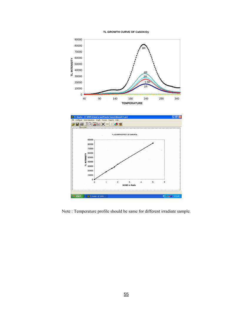
55

TL GROWTH CURVE OF CaSO4:Dy

0

10000

20000

30000

40000

50000

60000

70000

80000

90000

40 90 140 190 240 290 340

TEMPERATURE

TL IN

TEN

SITY

1R

8R

4R

1.5R

2R

Note : Temperature profile should be same for different irradiate sample.

56

EXPERIMENT - 3 Aim to study the total scatter of X-ray radiation Aim To study the irradiation of X-ray scatter and linearity of TL growth effect. Introduction Take CaSo4 : Dy or any TL Phosphor for this experiment. Take each time 20mg weight for X-ray irradiated powder is taken for TL measurement. The X-ray dose given is 100, 200, 300, 500, 600 exposure from a X-ray unit. Plot TL intensity Vs number of exposure will give the effect of X-rays on TL phosphor. EXPERIMENTAL PROCEDURE : Step 1 : Refer to step 1 of Experiment No.1 Step 2 : Refer to step 2 of Experiment No.1 Step 3 : Refer to step 3 of Experiment No.2 Step 4 : Refer to step 3 of Experiment No.1 Step 5 : Refer to step 5 of Experiment No.1 Step 6 : This initiate acquisition process & glow curve gets recorded in the TL Reader unit in

controller card EEPROM chip. Step 7 : Refer to step 7 of Experiment No.1 Step 8 : After saving this glow curve, re-run to see residual TL if any. It shall be less than

10% of the area of the first peak, if TL emission is complete in the 1st

cycle. Step 9 : Refer to step 9 of Experiment No.1 Step 10 : Now obtain net glow-curve as indicated below after subtracting BG file which can

be shown below.

57

Step 11 : Refer to step 11 of Experiment No.1 Step 12 : Do the same procedure as described above for 10, 15, 20, 25, 30 sec. Step 13 : Following figure shown the effect of X-ray Scatter on CaSo4 : Dy

Linearity of X ray

0

20000

40000

60000

80000

100000

120000

140000

160000

180000

0 5000 10000 15000 20000 25000

Dose (mR)

Rea

lativ

e TL

res

pons

e

Step 14 : Put a TLD containing plastic bags around the X-ray baggage screening unit in the main port. study TL after 1, 2, 4, 6 & 10days. Plot TL intensity / number of days. Note : Temperature profile should be same for different irradiate sample.

58

EXPERIMENT - 4 To study the UV Exposure on TL Phosphors AIM To study the UV Exposure on TL Phosphors and Linearity. INTRODUCTION Commercial TL Dosimetry Phosphor CaSO4 : Dy is taken for TL measurements. Take the TL phosphor for each time 20mg. Put the sample bottom of UV lamp, for each sample take the different time intervals (5, 10, 20, 30 and 60minutes). Plot the TL temperature Vs TL intensity EXPERIMENTAL PROCEDURE : Step 1 : Refer to step 1 of Experiment No.1 Step 2 : Refer to step 2 of Experiment No.1 Step 3 : Refer to step 4 of Experiment No.1 Step 4 : Refer to step 3 of Experiment No.1 Step 5 : Refer to step 5 of Experiment No.1 Step 6 : This initiate acquisition process & glow curve gets recorded in the TL Reader unit in

controller card EEPROM chip. Step 7 : Refer to step 7 of Experiment No.1 Step 8 : After saving this glow curve, re-run to see residual TL if any. It shall be less than

10% of the area of the first peak, if TL emission is complete in the 1st

cycle. Step 9 : Refer to step 9 of Experiment No.1 Step 10 : Now obtain net glow-curve as indicated below after subtracting BG file which can

be shown below.

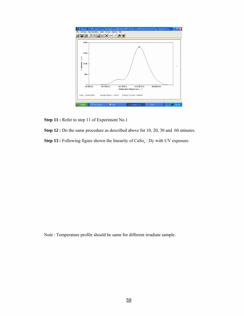
59

Step 11 : Refer to step 11 of Experiment No.1 Step 12 : Do the same procedure as described above for 10, 20, 30 and 60 minutes. Step 13 : Following figure shown the linearity of CaSo4 : Dy with UV exposure. Note : Temperature profile should be same for different irradiate sample.

60

Fig.1 TL GLOW CURVE OF CaSO4:Dy

0

5000

10000

15000

20000

35 85 135 185 235 285 335TEMPERATURE

TL IN

TEN

SITY

Fig. 2. TL of gamma irrdiated IndianSalt (Catch)

0

2000

4000

6000

8000

10000

12000

14000

40 90 140 190 240 290 340Temperature oC

TL In

tens

ity

127C

211C

The following TL curves of gamma irradiated common materials available in and around us.

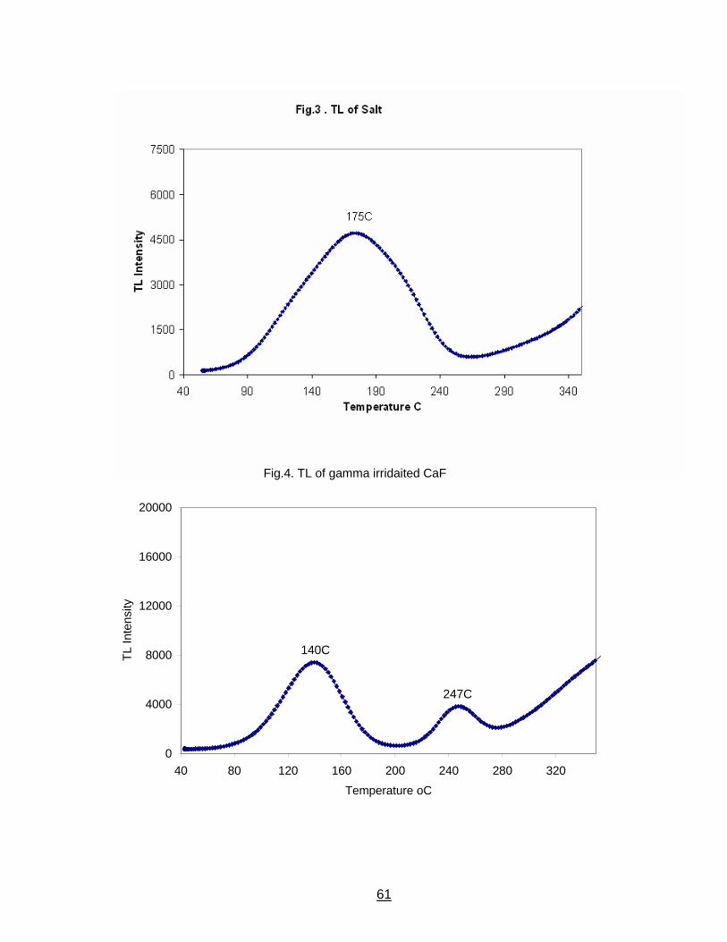
61

Fig.4. TL of gamma irridaited CaF

0

4000

8000

12000

16000

20000

40 80 120 160 200 240 280 320Temperature oC

TL In

tens

ity

140C

247C

62

Fig.5.TL of gamma irridaited Al2O3

0

5000

10000

15000

20000

25000

30000

40 90 140 190 240 290 340 390

Temperature C

TL In

tens

ity

Fig.6. TL of 10Gy gamma irridaited quartz

0

500

1000

1500

2000

40 90 140 190 240 290 340Temperature C

TL In

tens

ity

89C

134C

63

Fig.7.TL of gamma irridiated Tube Light Coated Material

0

1000

2000

3000

4000

5000

6000

40 90 140 190 240 290 340Temperature C

TL In

tens

ity

135C

The tube light coating materials are good Photoluminescence materials called phosphors. One can break any lamp carefully and collect the Phosphor irradiates and study the thermoluminescence. Salt from market different brands can be collected and dried at 200oC for an hour and irradiate with any ionizing radiation and study the thermoluminescnec.

64

TLD Applications in Radiation Oncology

*K. Ayyangar, Ph.D., A. R. Reddy, Ph.D., M. R. Raju, D.Sc. International Cancer Center,

Mahatma Gandhi Medical Trust Hospital, PedaAmiram, Bhimavaram, AP 534204

65

Chapter-III

Thermoluminescent Dosimetry (TLD) has been developed during 1960-70 for various applications in medicine and industry. A brief list of applications specific to radiation oncology is given here. In radiation oncology dosimetric accuracy demanded is on the order of 2-5%. TLDs offer a clear solution since their precision meets this criteria. 1. Calibration checks, different institutions, mailed Dosimetry- national standard

maintenance: The Radiation Safety Systems Division, BARC, Mumbai, provides national dose-inter comparison service for hospitals to check their machine calibrations independently using precisely controlled mailed TLD dosimeters. Typical service includes cobalt-60 beam output check for gamma photon beam and Linac output check for photon and electron beams. Similar more frequent service could be provided by the International Cancer Center at Mahatma Gandhi Memorial Medical Trust, Pedaamiram, Bhimavaram, A.P. to the Teletherapy Centers in that region since they have recently established a Nucleonix TLD system with LiF and CaSO4:Dy in the form of discs and chips. The Center also has a calibrated Secondary Standard Dosimeter traceable to the National Standards Laboratory at BARC, Mumbai. Intern comparison program is essentially a form of external audit of the above calibrations and it should be made mandatory for Quality Assurance of proper Radiotherapy Treatment. It is essential that both the systematic and random errors involved are quantified. Preliminary results of different measurements carried out with CaSO4:Dy teflon discs and LiF (TLD 100) chips and discs in the International Cancer Center are given as Appendix 'A' to this report. It should be mentioned that the measurements are from initial experiments carried out with the Nucleonix TLD reader recently procured by this Center. All the experiments mentioned in the Appendix need repetition and further careful investigation.

2. Treatment planning accuracy verification: The use of IMRT for patient treatments involves multiple MLC segments with odd beam shapes. Most segments deliver dose in electronic dis-equilibrium conditions. TLDs (particularly LiF) is aptly suitable to check the target dose using suitably designed multipurpose phantoms (made of tissue equivalent materials or Solid water, or PMMA sheets).

3. Patient specific Dosimetry:

Physicians request physicists to measure dose at certain anatomic positions of some patients. This is usually referred as Special physics consult. Examples of these locations on patients are a) surface dose on breast, b) dose to the scrotum for very young male patients, c) Thyroid dose d) dose to contra-lateral breast etc. In general treatment planning systems cannot calculate dose outside the radiation field accurately.

Due to the complex calculations required to obtain dose distributions and their inherent difficulties, combined with clinical issues such as patient movement, in vivo dosimetry is the optimal way to check the actual dose delivered to the patient. It is also important to know the dose delivered to a patient accurately for treatment records for comparisons of

66

treatment results, patient statistics and to assess side effects. These in vivo systems can have relatively large uncertainties, which should be assessed before using them. While in vivo systems are useful for individual patient measurements, they should not substitute for an adequate QA program.

TLDs serve an important role in this regard.

4. Brachtherapy Physics:

Small Brachytherapy sources such as Iodine seeds for prostate implants, iridium seeds in ribbon form, HDR sources etc. all use encapsulation. The dosimetry of these sources offer a challenge, since the exact amount of materials used for encapsulations is not known even to the manufacturer. Even for doing Monet Carlo simulations, one needs a precise knowledge of the source configuration. In general there are two unknowns in a given brachytherapy source, the activity of the source inside the capsule and the exact amount of encapsulation. It is not possible to solve this by any direct means without breaking the source. TLDs are often used to map the dose distribution in water equivalent medium and the data are fitted using theoretical calculations. Once accurate dosimtery is obtained, the data are fed to treatment planning computers. TLDs play a major role in the assessment of various TG-43 factors for a given brachy source.

5. Diagnostic X-rays

In X-ray diagnostics, TL dosimeters are commonly used for determining absorbed doses to patients, as well as in phantom studies. For this study, TLD-100 (LiF:Mg,Ti) TL dosimeters could be used to measure the absorbed doses. The measurements could be performed in a Alderson-Rando phantom, which is a commercially available phantom with anatomical inhomogenities in respect to the lungs and skeleton. In the irradiations, the TL dosimeters are to be fixed into the holes of the Alderson-Rando phantom so that the flat surface of the detector always faced the beam. The absorbed doses to various organs of the phantom are then derived from the doses of the reference points, i.e. those points measured directly with TL detectors or interpolated from them.

6. Research:

There are very many applications of TLD for research in radiation oncology physics. For narrow beams used in radiosurgery, ionization chambers are too large in size and hence cannot be used. Some of the stereotactic beams are very narrow, i.e. less than few mm in diameter. TLDs provide a clear advantage in the dosimetry of narrow beams. For various external beam and brachytherapy applications, physicists use special phantoms and use TLDs to map the dosimetry and compare with calculations.

67

PRELIMINARY EXPERIMENTS USING THE NUCLEONIX TLD SYSTEM

The following experiments are carried at International Cancer Center, Pedaamiram, Bhimavaram using the Nucleonix TLD reader. International Cancer Center Mahatma Gandhi Memorial Medical Trust PedaAmiram, Bhimavaram, AP 534204 The reader has the ability to be controlled through a PC. The heating cycles are controlled by giving a chosen ramp temperature rate in °C/s (range 2 - 40o per second) for a steady temperature cycle. Most importantly, this unit collects the entire glow curve in digital form into a file in the computer. The file with extension .glo is in ASCII format and is accessible through excel spread sheet. The Center has also acquired different TLD detectors; namely CaSO4:Dy discs, (sizes 13.5 mm dia x 0.8 mm thick and 6 mm dia x 0.8 mm thick); LiF TLD-100 chips of size 3.2 x 3.2 x 0.9 mm and LiF TLD100 Teflon discs of size 1 cm dia. Some of these detectors were irradiated at MNJ hospital, Hyderabad. 1. Calibration

CaSO4 dosimeters were irradiated at MNJ Hospital using their Cobalt Teletherapy machine. Three dosimeters at each dose value, viz., 5, 25, 50, 100, 200, 500 cGy were irradiated. Glow curves were obtained. The signal was integrated between 140-250°C. The background for a control sample was acquired and was subtracted from the sample signals. Fig. 1 below shows a glow curve from a CaSO4:Dy disc exposed to a dose of 100 cGy from cobalt-60 gammas. In addition the temperature profile used for the glow curve is also shown in yellow color.

68

CaSO4 100 cGy

050

100

150200250300

350400450

50 70 90 110 130 150 170 190 210 230Time

TL s

igna

l(*.0

1) &

Tem

p 0 C

Fig. 1: Glow curve (blue) for CaSO4:Dy and temperature profile (yellow) used to read TL

CASO4 MNJ Calibration

0

1000000

2000000

3000000

4000000

5000000

6000000

7000000

8000000

0 100 200 300 400 500 600

DOSE

TL

Fig. 2: Calibration plot - dose in cGy vs TL output

69

Fig. 2 above shows calibration curve obtained with CaSO4 discs exposed to cobalt-60 gamma rays at MNJ Hospital. Each point is an average of 3 dosimeter readings. Also shown at each point are the standard deviations as error bars. It is to be noted that the point at 100 cGy even though looks higher, it has an uncertainty of only 8%. The higher response from these teflon CaSO4:Dy discs, hence, is assumed to show supralinear behaviour between 50-100 cGy and again follow linearity in the range 100-500 cGy. However, this conclusion needs further investigation. Fig.3 shows a similar calibration plot for LiF TLD-100 chips irradiated with Cobalt-60 teletherapy machine at this Cancer Center. It can be seen that the response is linear. Also note that response of each chip for a given dose can be different. In this experiment, the chips have not been pre-sorted for uniform response. In principle, chips are to be grouped based on acceptable percent deviation of their TL response for the same dose.

LiF TLD-100 Calibration

020000400006000080000

100000120000140000160000

0 50 100 150 200 250 300 350

Dose cGy

TL S

igna

l

Fig.3: Calibration curve for LiF TLD-100 chips

2. Patient dose measurement

2 CaSO4 dosimeters were used one at entrance and another at exit position of the central axis of a 10 cm x 10 cm treatment field of the telecobalt machine of the Center. Measured doses revealed a 40% change in the dose values at these two positions, which is in agreement with hand calculations. Figs. 4 and 5 below show the glow peaks with CaSO4:Dy positioned respectively at the entrance and exit positions.

70

Entrance Tx position

05000

1000015000200002500030000350004000045000

0 10 20 30 40 50 60 70 80 90 100 110 120 130 140 150 160 170 180 190 200 210 220 230 240 250

Fig. 4: Glow curve of CaSO4:Dy teflon disc placed at the entrance position

71

Exit Tx position

02000400060008000

10000120001400016000

0 10 20 30 40 50 60 70 80 90 100 110 120 130 140 150 160 170 180 190 200 210 220 230 240 250

entrance 1392073exit 562090Ratio 40.4%

Fig. 5: Glow curve of CaSO4:Dy teflon disc placed at the exit position

3. HDR checks

The ouput of the cobalt HDR machine at this Center was first checked using ion chamber in the HDR calibration phantom by placing the source in the center and the ion chamber with build-up cap at 8 cm. The dose rate was computed using the chamber factors and agreement with previous calibration was observed to be within 2%.

LiF and CaSO4 TLDs were irradiated to a dose of 100 cGy in the HDR machine. The following results were obtained.

With LiF TLD-100 chips

Dosimeter TL reading Dose in cGy (from calibration curve in Fig.3)

LiF 1 37113 95 LiF 2 30828 80 LiF 3 28282 74

Average 28282 83

Standard deviation 4545 14 %

With CaSO4:Dy teflon discs

Dosimeter TL reading Dose in cGy

72

(from calibration curve in Fig.2) S1 318578 173 S2 224062 121 S3 259745 141 Average 267462 145

Standard deviation 47728 17 %

Note: Deviation of measured dose from the calibration curves established in these experiments is large as compared to the standard dose to which the dosimeters were exposed. Repeat experiments have to be conducted for better results.

The LiF detectors showed lower response by nearly 15%. This could be due to differences in position of the detectors in the placement in the cavity. A 0.5 cm variation in distance could result in 12% variation. In view of the energy response CaSO4 is reading larger than 100 cGy.

4. Mammography

TLDs were used to measure dose from the Siemens mammography machine at this Cancer Center. Three dosimeters were placed on the breast phantom and an exposure was made. Also the dose was measured using Xi chamber from Unfors Inc. The Xi chamber measured an entrance dose of 1.5 cGy for a setting of 27 kV exposure (auto 123 mAs, 1.1mGy). The three readings in each case were consistent within 3%. The dose calculated from calibration curves were 1.05 cGy for LiF and 1.93 cGy for CaSO4 respectively. For CaSO4 higher response is expected at this energy in view of its higher effective atomic number and predominant photoelectric effect at this photon energy. Also the differences seen between the dose estimates with TLDs and the Xi chamber could be due to (a) positional differences between the chamber and the TL dosimeters and b) the calibration plots used are for much higher dose ranges. Repetition of the experiments with careful planning of the experiments is needed.

Acknowledgements: Authors thanks are due to members of physics team namely Messers Fenedit Yesuraj, DhanaSekharan, Srinivasa Reddy, Madhusudan, Shamsuddin and Haritha, at this Cancer Center for carrying out of the above experiments in short time. Also, the dedication and help of Mr. Lakshminarayana of Nucleonix is greatly appreciated. Thanks are also Mr Ramakrishna Rao, Chief Medical Physicist for irradiating the CaSO4 discs in their telecobalt beam.