Thermographic Measurements of the Commercial Laser Powder Bed Fusion Process at

NIST

Brandon Lane1, Shawn Moylan

1, Eric Whitenton

1, Li Ma

2

Engineering Laboratory1

Material Measurement Laboratory2

National Institute of Standards and Technology, Gaithersburg, MD 20899

Abstract

Measurement of the high-temperature melt pool region in the laser powder bed fusion (L-

PBF) process is a primary focus of researchers to further understand the dynamic physics of the

heating, melting, adhesion, and cooling which define this commercially popular additive

manufacturing process. This paper will detail the design, execution, and results of high speed,

high magnification in-situ thermographic measurements conducted at the National Institute of

Standards and Technology (NIST) focusing on the melt pool region of a commercial L-PBF

process. Multiple phenomena are observed including plasma plume and hot particle ejection

from the melt region. The thermographic measurement process will be detailed with emphasis

on the ‘measurability’ of observed phenomena and the sources of measurement uncertainty.

Further discussion will relate these thermographic results to other efforts at NIST towards L-PBF

process finite element simulation and development of in-situ sensing and control methodologies.

Introduction

The need for improved understanding of the complex physics in laser-based metal

additive manufacturing (AM) processes is widely known and commonly stated [1], [2]. To

address this need, the National Institute of Standards and Technology (NIST) initiated the

Measurement Science for Additive Manufacturing program (MSAM). NIST has a history of

advancing the measurement science of thermography and high speed imaging in metal cutting

[3], and evaluation of associated measurement uncertainty [4], [5]. Metal cutting has similar

characteristics that provoke similar measurement challenges to laser powder bed fusion (L-PBF)

and other metal AM processes such as high temperatures and temperature gradients at near

microscopic scale, phenomena that occur at high speeds and frequencies, and complex thermally

driven processes. For this reason, advancing thermographic measurements of AM processes are

a key part of MSAM projects, with initial focus on commercial L-PBF. The goals of this

endeavor are two-fold: provide calibrated, well characterized temperature data to support

simulation and modeling research, and to acquire high-speed, high-fidelity observations and

measurements to support development of in-situ monitoring and feedback-control.

AM research has shown multiple examples of thermographic measurements. Perhaps

most notable are those that incorporate sensors co-axially with the laser optics such that the

image of the laser processing zone is maintained stationary within the field of view [6]–[11].

This method is already incorporated in some commercial systems [12], though further research

will be necessary to fully develop feed-back control and monitoring solutions to utilize these

systems to their full potential. Many commercial PBF systems do not yet have optics required

575

for co-axial imager configuration, and thus require stationary imagers placed out of the beam

path to measure the process zone. These staring configurations can be considered as either part

monitoring [13] or melt-pool monitoring [14] depending on their relative magnification and

target field of view. Part monitoring solutions observe layer formation in PBF systems, and have

demonstrated capability in detecting defects such as pores which incur measurable changes to the

temperature gradient and cooling rates on or near the defects [15]. These require low acquisition

speeds (once per layer), tend to measure lower temperatures, require lower magnification, and

benefit from larger pixel count detectors. Melt-pool monitoring systems attempt to measure

temperatures in and around the melt-pool, often for development and comparison of multi-

physics simulations [16]. These require higher magnification, higher measurable temperature

range, and higher acquisition rates. The MSAM program at NIST will initially focus on melt-

pool monitoring of their EOS M2701 system.

Few examples could be found of high speed thermography of the melt pool on a

commercial L-PBF system, despite multiple researchers and companies developing multi-physics

L-PBF simulations that will benefit from these measurements [17]. Multiple interesting works

were found looking at high speed visible-spectrum imaging of the L-PBF process on custom

systems [18], [19], and on commercial systems [20], which use active illumination to image the

melt pool. This technique provides very high speed, high contrast images of the melt pool and is

the most effective means for visualizing and measuring melt pool size and dynamics. However,

the active illumination disallows temperature measurement since the incandescent emission from

the process zone is minimized compared to the reflected illumination.

Krauss et al. captured thermal images of the laser processing zone which could be used to

identify artificial flaws. However, the long wave infrared (LWIR, 8 μm – 15 μm) camera was

limited to 50 frames/s, and a sensor time constant of 5 ms to 15 ms. At these rates, the laser

scanned about two hatch lines within each frame and moved at least four hatch lines between

each frame. Though the location and size of the melt pool cannot be distinguished, flaw

detection was still possible [14]. Bayle and Doubenskaia captured thermal images of the L-PBF

process zone at 100 μm/pixel, 2031 frames/s and 5 μs integration time with a mid-infrared (MIR,

3 μm – 5 μm) camera [21]. At these high speeds, they observed a highly dynamic process with

particles rapidly ejected from the melt pool. They quantified the ejected particle size (600 μm to

940 μm) and velocities (0.44 m/s to 4.7 m/s).

This paper describes the design of the thermographic L-PBF measurement process

employed at NIST. Results from the thermal images are quantified and compared to those seen

by Bayle et al. and others, and discussion is provided on the potential impact on the state of art of

L-PBF simulations. In addition, future endeavors and improvements to the system are discussed.

1 Certain commercial entities, equipment, or materials may be identified in this document in order to describe an

experimental procedure or concept adequately. Such identification is not intended to imply recommendation or

endorsement by the National Institute of Standards and Technology, nor is it intended to imply that the entities,

materials, or equipment are necessarily the best available for the purpose.

576

Experiment Setup

Custom Viewport Door

The size and expense of the camera and lens prohibited placement within the chamber

due to potential obstruction of the laser and contamination of the camera electronics. Also,

temperature stability of the camera body and internal electronics is important for thermal

calibration. Some important design considerations were to achieve clearance from the recoater

arm, sufficient room for the camera body, and sufficient view-port diameter and length for the

camera lens. The overall design of the NIST custom door is similar to the 45° viewport created

by Krauss et al. [14]. Some features include secondary view-ports adjacent to the main port that

can include throughputs for sensor cabling or laser-blocking glass window.

Figure 1: (Left) CAD model of the viewport location with respect to the build plane. (Right)

Picture of the thermal camera staring into the viewport.

Since the internal diameter of the viewport is larger than the outer diameter of the lens

barrel, the camera can be pitched steeper to 43.7° measured with a digital level. This allows

imaging objects on the build surface slightly closer, and shortens the working distance. Since the

object plane of the camera forms an angle with the build surface in the PBF machine, there is an

optimal line of focus in the image, and objects further from or nearer to the camera from this line

will have some defocus.

Imaging Parameters, Camera and Lens Selection

Although one goal of the thermal imaging is to validate and compare to computational

models, preliminary finite element (FE) results from simulations conducted at NIST were used to

design the required imaging parameters [22]. Figure 2 shows example temperature vs. length

along the top surface of the melt pool in the scanning direction for laser parameters similar to

those expected to be measured (800 mm/m scan speed, 195 W laser power, Inconel 625).

Build Plate

View Port

577

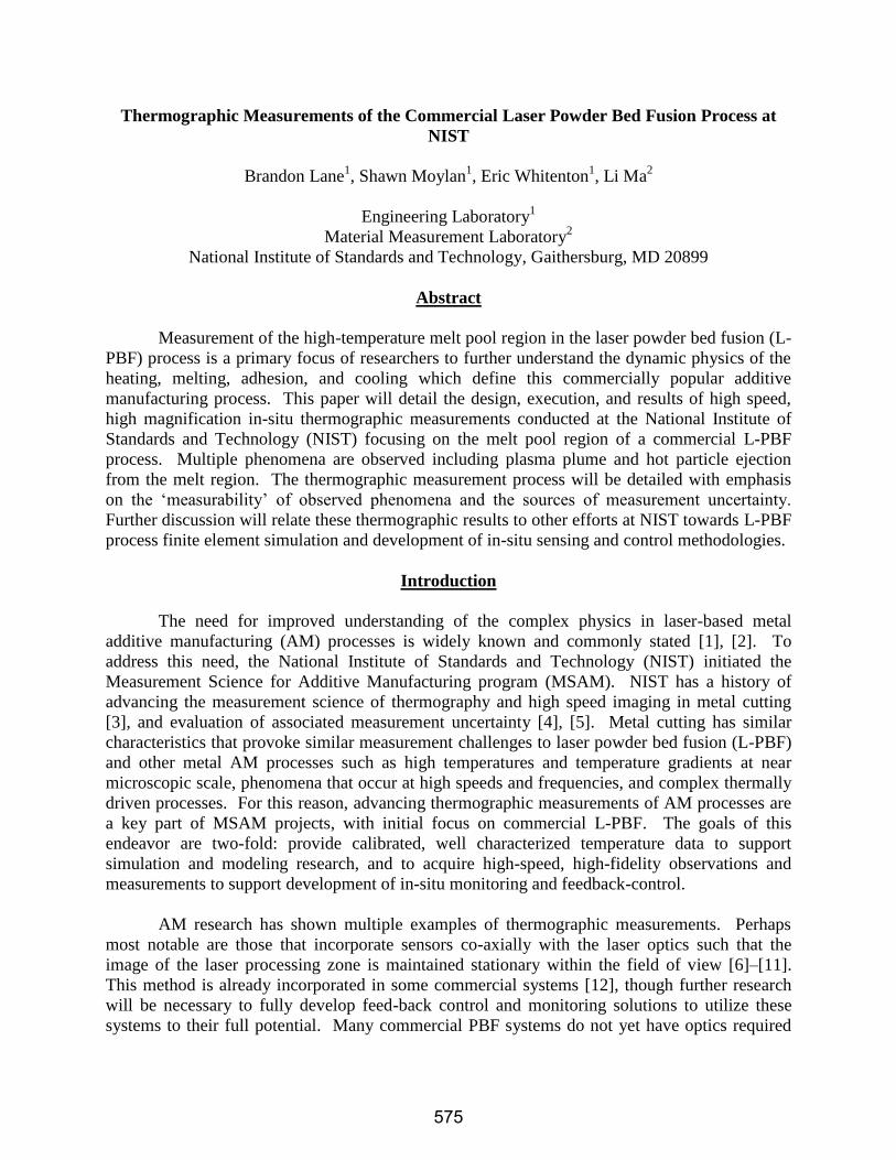
Figure 2: Cross-section of melt pool and heat-affected zone (HAZ) temperatures from

preliminary FE simulation of the L-PBF process on Inconel 625 [22]. Approximated melt pool

size, temperature, and motion from simulations were used to define thermal imaging parameters.

Knowing the approximate size of different isotherms around the melt pool help determine

the required magnification, and heating/cooling rates determine the required frame rate and

integration time to temporally resolve these phenomena. Based on the thermal traces in Figure 2

one may expect a 500 °C isotherm approximately 1 mm wide, and a 1000 °C isotherm 0.5 mm

wide. In addition, temperatures far exceeding the melting temperature are to be expected.

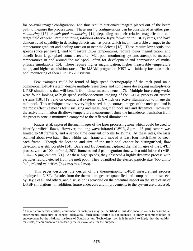
Spectral Bandwidth

Temperature measurement uncertainty due to emissivity is reduced when the system

sensitivity is reduced to shorter wavelengths as long as the system is still sensitive to the emitted

radiation. Though visible-spectrum thermography is most appropriate for measuring melt pool

temperatures, we used an extended sensitivity range InSb camera (< 1 μm to 5.3 μm) for

potential future use in measuring lower temperature phenomena (such as part monitoring

configurations). To measure at shorter wavelengths, we used a commercial off-the-shelf (COTS)

50 mm short-wave infrared (SWIR) lens and filters. Figure 3 gives the normalized transmission

curves of all optics components. Since it was known that thermal imaging would be conducted

at near-IR wavelengths, we used B270 superwhite glass for the camera viewport window in the

custom door, which blocks unused wavelengths beyond 2.7 μm.

Figure 3: Transmission spectra of individual optics components in the thermal imaging system.

Solidus TemperatureLiquidus TemperatureTime = 0.672 msTime = 1.200 msTime = 1.800 ms

B270 Glass Window

578

Magnification and Working Distance

To achieve higher magnification, we added extension rings between the lens and camera

body, and tested the resulting field of view (FoV) and working distance (distance between the

lens front and object plane) using a dot-grid calibration artifact in front of the calibration

blackbody [23]. Addition of extension rings increases magnification at the expense of shorter

working distance and smaller FoV. Since the custom door view port limits our working distance

to >162 mm, we opted to achieve maximum magnification with this constraint. A configuration

was found that achieved 0.33x magnification, and an instantaneous field of view (iFoV, or

equivalent pixel size on the object plane) of 36 μm/pixel. Since the camera is tilted 43.7°,

vertical pixels distances projected on the build plate equate to 53.3 μm/pixel. Based on this iFoV

and the size of the FE melt pool results in Figure 2, we expected to resolve a 500 °C isotherm

with about 37 pixels, and a 1000 °C isotherm with 14 pixels. A presumed 5 mm stripe width

would be resolved with 138 pixels.

Window Size and Frame Rate

Using the whole detector (1280 pixels x 1024 pixels), the thermal camera can achieve a

maximum frame rate of 120 frames/s. At a laser scan speed of 800 mm/s, and stripe width of

5 mm, the melt pool scans one hatch (one stripe width) in 6.25 ms. In order to capture at least 10

images per hatch, this requires a frame rate of at least 1600 frames/s. Ultimately, higher frame

rates provide better temporal resolution, however this comes at the expense of reduced window

size due to the finite data transfer rate of the camera electronics. A compromise was found that

achieves 1800 frames per second with a window size of 360 horizontal by 128 vertical pixels,

equivalent to an area of 12.96 mm by 6.82 mm projected on the build surface.

Calibration

Prior to acquiring thermal images within the L-PBF machine, the thermal camera was

calibrated in front of a variable temperature, spherical cavity reference blackbody source capable

of temperatures up to 1050 °C. A calibration mainly depends on a specific lens and filter

combination, as well as any window material between the lens and imaged object. At a

particular blackbody temperature value, the signal level is approximately proportional to the

integration time. Since the calibration blackbody used here is limited to 1050 °C, a filter and

integration time combination was found that saturates the camera at approximately 1050 °C.

This ensures the maximum measurable temperature range is achieved up to the maximum

calibrated temperature. To avoid effects of detector nonlinearity, the highest calibration point

was chosen at 1025 °C. Figure 4 (left) shows the calibration setup, including the B270 glass

window used in the custom door between the camera and blackbody. Figure 4 (right) shows the

effect of varying filters and integration time on the calibration curves. Extraneous light from

outside the FoV can affect pixel signal within the FoV and any resulting calibration, so a foil

aperture slightly larger than the FoV is placed at the blackbody opening aperture. The

calibration points shown in Figure 4 indicate the mean of all pixel values taken at each

calibration temperature. In order to have full control of the calibration process, and enable

methods for calculating calibration measurement uncertainty, NIST employs a custom

calibration routine, which creates a unique calibration function F for each pixel [24]. This uses

least-squares regression to fit blackbody signal Tbb (in Kelvin) to the measured signal Sbb (in

digital levels, or DLs) using the Sakuma-Hattori function shown in Equation (1). The

579

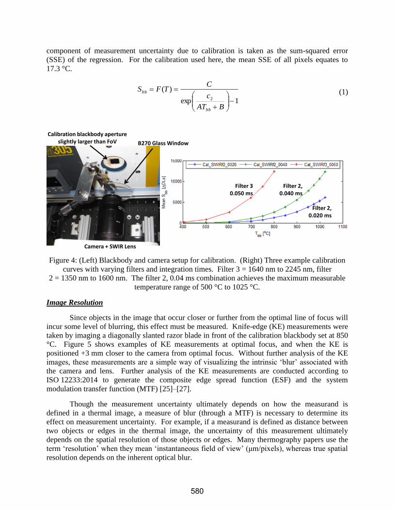
component of measurement uncertainty due to calibration is taken as the sum-squared error

(SSE) of the regression. For the calibration used here, the mean SSE of all pixels equates to

17.3 °C.

1exp

)(2

BAT

c

CTFS

bb

bb (1)

Figure 4: (Left) Blackbody and camera setup for calibration. (Right) Three example calibration

curves with varying filters and integration times. Filter 3 = 1640 nm to 2245 nm, filter

2 = 1350 nm to 1600 nm. The filter 2, 0.04 ms combination achieves the maximum measurable

temperature range of 500 °C to 1025 °C.

Image Resolution

Since objects in the image that occur closer or further from the optimal line of focus will

incur some level of blurring, this effect must be measured. Knife-edge (KE) measurements were

taken by imaging a diagonally slanted razor blade in front of the calibration blackbody set at 850

°C. Figure 5 shows examples of KE measurements at optimal focus, and when the KE is

positioned +3 mm closer to the camera from optimal focus. Without further analysis of the KE

images, these measurements are a simple way of visualizing the intrinsic ‘blur’ associated with

the camera and lens. Further analysis of the KE measurements are conducted according to

ISO 12233:2014 to generate the composite edge spread function (ESF) and the system

modulation transfer function (MTF) [25]–[27].

Though the measurement uncertainty ultimately depends on how the measurand is

defined in a thermal image, a measure of blur (through a MTF) is necessary to determine its

effect on measurement uncertainty. For example, if a measurand is defined as distance between

two objects or edges in the thermal image, the uncertainty of this measurement ultimately

depends on the spatial resolution of those objects or edges. Many thermography papers use the

term ‘resolution’ when they mean ‘instantaneous field of view’ (μm/pixels), whereas true spatial

resolution depends on the inherent optical blur.

Calibration blackbody aperture slightly larger than FoV

Filter 2, 0.040 ms

Camera + SWIR Lens

B270 Glass Window

Filter 30.050 ms

Filter 2,0.020 ms

580

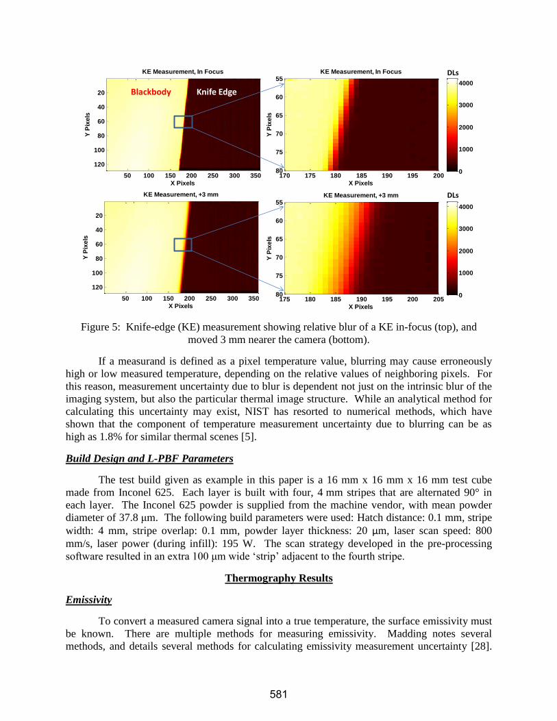
Figure 5: Knife-edge (KE) measurement showing relative blur of a KE in-focus (top), and

moved 3 mm nearer the camera (bottom).

If a measurand is defined as a pixel temperature value, blurring may cause erroneously

high or low measured temperature, depending on the relative values of neighboring pixels. For

this reason, measurement uncertainty due to blur is dependent not just on the intrinsic blur of the

imaging system, but also the particular thermal image structure. While an analytical method for

calculating this uncertainty may exist, NIST has resorted to numerical methods, which have

shown that the component of temperature measurement uncertainty due to blurring can be as

high as 1.8% for similar thermal scenes [5].

Build Design and L-PBF Parameters

The test build given as example in this paper is a 16 mm x 16 mm x 16 mm test cube

made from Inconel 625. Each layer is built with four, 4 mm stripes that are alternated 90° in

each layer. The Inconel 625 powder is supplied from the machine vendor, with mean powder

diameter of 37.8 μm. The following build parameters were used: Hatch distance: 0.1 mm, stripe

width: 4 mm, stripe overlap: 0.1 mm, powder layer thickness: 20 µm, laser scan speed: 800

mm/s, laser power (during infill): 195 W. The scan strategy developed in the pre-processing

software resulted in an extra 100 μm wide ‘strip’ adjacent to the fourth stripe.

Thermography Results

Emissivity

To convert a measured camera signal into a true temperature, the surface emissivity must

be known. There are multiple methods for measuring emissivity. Madding notes several

methods, and details several methods for calculating emissivity measurement uncertainty [28].

X Pixels

Y P

ixe

ls

KE Measurement, +3 mm

50 100 150 200 250 300 350

20

40

60

80

100

1200

1000

2000

3000

4000

X Pixels

Y P

ixe

ls

KE Measurement, +3 mm

175 180 185 190 195 200 205

55

60

65

70

75

80 0

1000

2000

3000

4000

X Pixels

Y P

ixe

ls

KE Measurement, In Focus

50 100 150 200 250 300 350

20

40

60

80

100

1200

1000

2000

3000

4000

DLs

X Pixels

Y P

ixe

ls

KE Measurement, In Focus

170 175 180 185 190 195 200

55

60

65

70

75

80 0

1000

2000

3000

4000

Blackbody Knife Edge

DLs

581

There are several examples in AM research which rely on using a liquidus-solidus transition

temperature of the melt pool [7], [16], [29], use a heated emissivity artifact [30], or only report

camera signal or intensity values [14], [31].

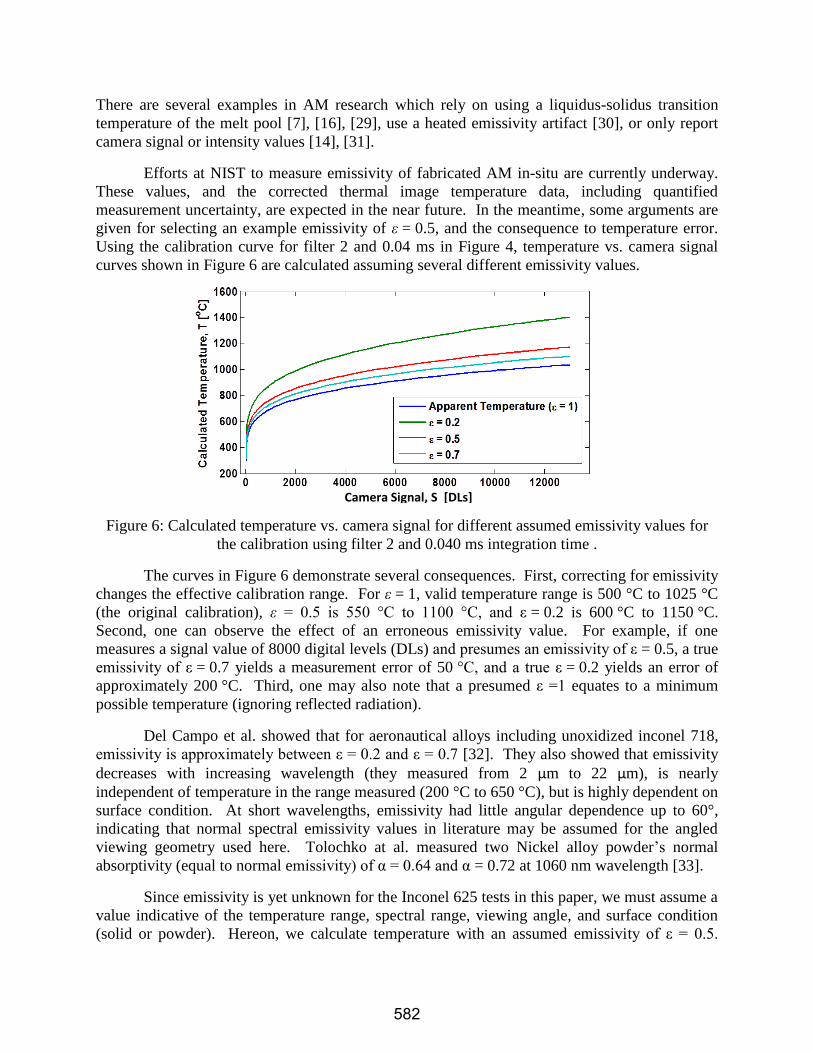
Efforts at NIST to measure emissivity of fabricated AM in-situ are currently underway.

These values, and the corrected thermal image temperature data, including quantified

measurement uncertainty, are expected in the near future. In the meantime, some arguments are

given for selecting an example emissivity of ε = 0.5, and the consequence to temperature error.

Using the calibration curve for filter 2 and 0.04 ms in Figure 4, temperature vs. camera signal

curves shown in Figure 6 are calculated assuming several different emissivity values.

Figure 6: Calculated temperature vs. camera signal for different assumed emissivity values for

the calibration using filter 2 and 0.040 ms integration time .

The curves in Figure 6 demonstrate several consequences. First, correcting for emissivity

changes the effective calibration range. For ε = 1, valid temperature range is 500 °C to 1025 °C

(the original calibration), ε = 0.5 is 550 °C to 1100 °C, and ε = 0.2 is 600 °C to 1150 °C.

Second, one can observe the effect of an erroneous emissivity value. For example, if one

measures a signal value of 8000 digital levels (DLs) and presumes an emissivity of ε = 0.5, a true

emissivity of ε = 0.7 yields a measurement error of 50 °C, and a true ε = 0.2 yields an error of

approximately 200 °C. Third, one may also note that a presumed ε =1 equates to a minimum

possible temperature (ignoring reflected radiation).

Del Campo et al. showed that for aeronautical alloys including unoxidized inconel 718,

emissivity is approximately between ε = 0.2 and ε = 0.7 [32]. They also showed that emissivity

decreases with increasing wavelength (they measured from 2 µm to 22 µm), is nearly

independent of temperature in the range measured (200 °C to 650 °C), but is highly dependent on

surface condition. At short wavelengths, emissivity had little angular dependence up to 60°,

indicating that normal spectral emissivity values in literature may be assumed for the angled

viewing geometry used here. Tolochko at al. measured two Nickel alloy powder’s normal

absorptivity (equal to normal emissivity) of α = 0.64 and α = 0.72 at 1060 nm wavelength [33].

Since emissivity is yet unknown for the Inconel 625 tests in this paper, we must assume a

value indicative of the temperature range, spectral range, viewing angle, and surface condition

(solid or powder). Hereon, we calculate temperature with an assumed emissivity of ε = 0.5.

Camera Signal, S [DLs]

582

However, the reader should bear in mind the potential temperature measurement error resulting

from emissivity error as discussed above. For example, it was shown in [5] that an emissivity

standard uncertainty of 0.1 could result in a temperature standard uncertainty of approximately

40 °C at a measured temperature of 1000 °C.

Thermal Video

All collected thermal video were converted to temperature values assuming ε = 0.5 using

the measurement equation given in [24]:

)()1()( ambtruemeas TFTFS (2)

Here, Smeas is measured signal, ε is surface emissivity, Ttrue is the true object temperature,

and Tamb is temperature of the ambient environment or source contributing to reflections. In this

analysis, the terms accounting for external reflecting sources were neglected. ‘True temperature’

is nomenclature indicating the object temperature derived from a measurement equation such as

(2). However, it should not be assumed to be the factual surface temperature until more robust

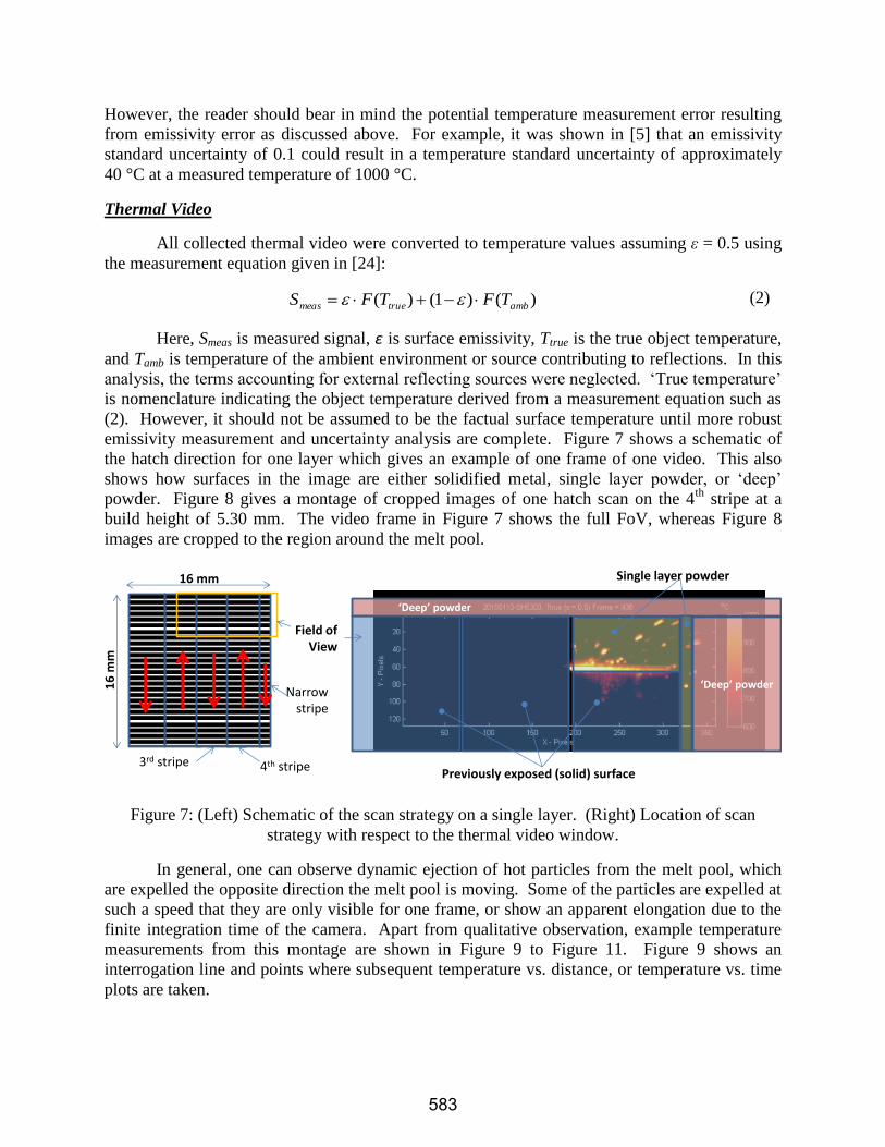
emissivity measurement and uncertainty analysis are complete. Figure 7 shows a schematic of

the hatch direction for one layer which gives an example of one frame of one video. This also

shows how surfaces in the image are either solidified metal, single layer powder, or ‘deep’

powder. Figure 8 gives a montage of cropped images of one hatch scan on the 4th

stripe at a

build height of 5.30 mm. The video frame in Figure 7 shows the full FoV, whereas Figure 8

images are cropped to the region around the melt pool.

Figure 7: (Left) Schematic of the scan strategy on a single layer. (Right) Location of scan

strategy with respect to the thermal video window.

In general, one can observe dynamic ejection of hot particles from the melt pool, which

are expelled the opposite direction the melt pool is moving. Some of the particles are expelled at

such a speed that they are only visible for one frame, or show an apparent elongation due to the

finite integration time of the camera. Apart from qualitative observation, example temperature

measurements from this montage are shown in Figure 9 to Figure 11. Figure 9 shows an

interrogation line and points where subsequent temperature vs. distance, or temperature vs. time

plots are taken.

3rd stripe 4th stripe

Field of View

Narrow stripe

16 mm

16

mm

Single layer powder

Previously exposed (solid) surface

‘Deep’ powder

‘Deep’ powder

583

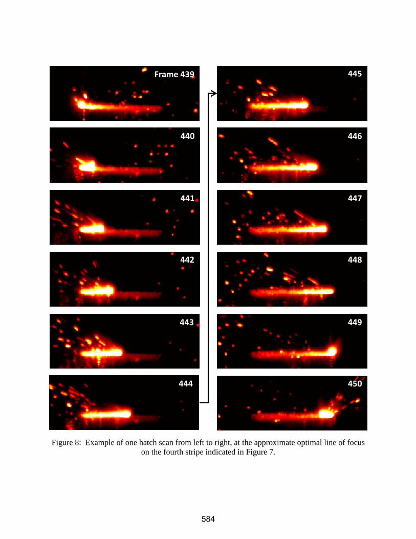
Figure 8: Example of one hatch scan from left to right, at the approximate optimal line of focus

on the fourth stripe indicated in Figure 7.

Frame 439

440

441

442

443

444

445

446

447

448

449

450

584

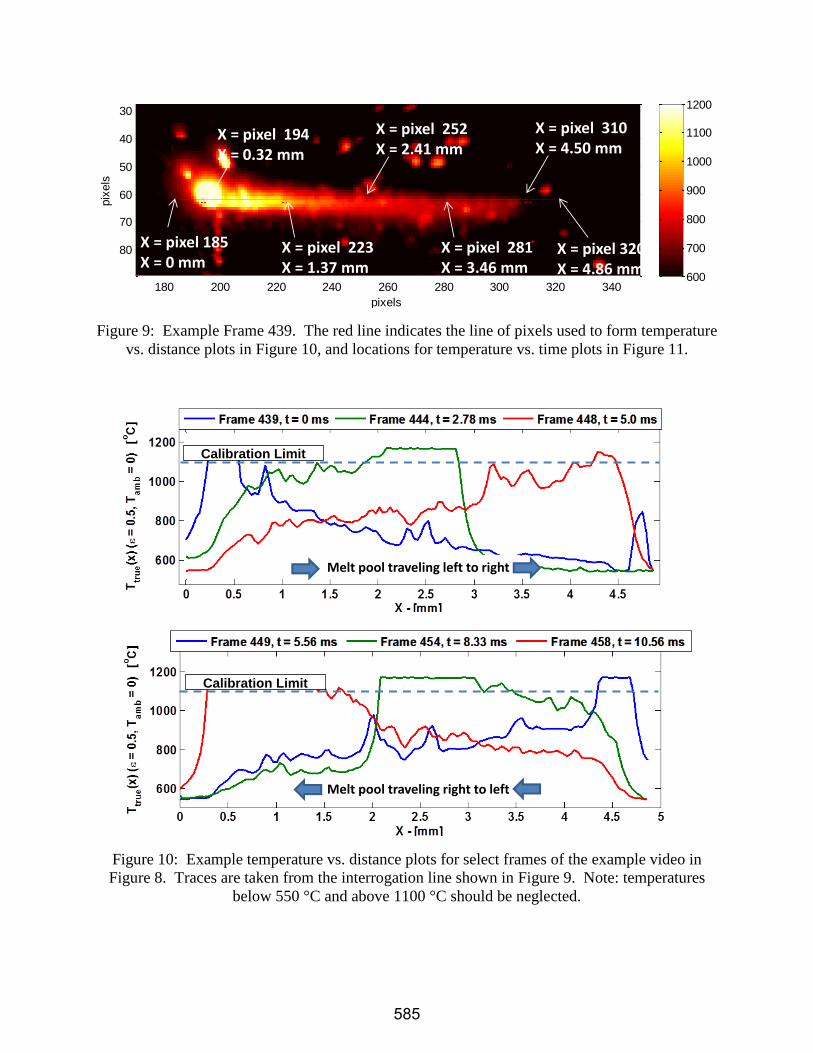
Figure 9: Example Frame 439. The red line indicates the line of pixels used to form temperature

vs. distance plots in Figure 10, and locations for temperature vs. time plots in Figure 11.

Figure 10: Example temperature vs. distance plots for select frames of the example video in

Figure 8. Traces are taken from the interrogation line shown in Figure 9. Note: temperatures

below 550 °C and above 1100 °C should be neglected.

pixels

pix

els

180 200 220 240 260 280 300 320 340

30

40

50

60

70

80

600

700

800

900

1000

1100

1200

X = pixel 185X = 0 mm

X = pixel 320X = 4.86 mm

X = pixel 223X = 1.37 mm

X = pixel 252X = 2.41 mm

X = pixel 194X = 0.32 mm

X = pixel 281X = 3.46 mm

X = pixel 310X = 4.50 mm

Melt pool traveling left to right

Melt pool traveling right to left

Calibration Limit

Calibration Limit

585

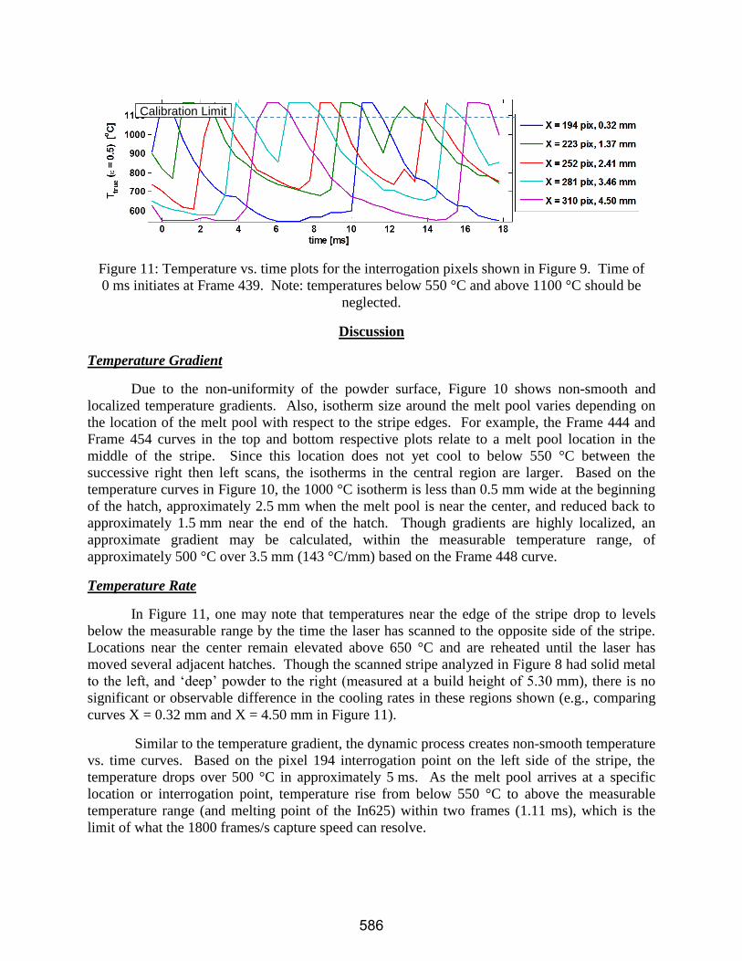
Figure 11: Temperature vs. time plots for the interrogation pixels shown in Figure 9. Time of

0 ms initiates at Frame 439. Note: temperatures below 550 °C and above 1100 °C should be

neglected.

Discussion

Temperature Gradient

Due to the non-uniformity of the powder surface, Figure 10 shows non-smooth and

localized temperature gradients. Also, isotherm size around the melt pool varies depending on

the location of the melt pool with respect to the stripe edges. For example, the Frame 444 and

Frame 454 curves in the top and bottom respective plots relate to a melt pool location in the

middle of the stripe. Since this location does not yet cool to below 550 °C between the

successive right then left scans, the isotherms in the central region are larger. Based on the

temperature curves in Figure 10, the 1000 °C isotherm is less than 0.5 mm wide at the beginning

of the hatch, approximately 2.5 mm when the melt pool is near the center, and reduced back to

approximately 1.5 mm near the end of the hatch. Though gradients are highly localized, an

approximate gradient may be calculated, within the measurable temperature range, of

approximately 500 °C over 3.5 mm (143 °C/mm) based on the Frame 448 curve.

Temperature Rate

In Figure 11, one may note that temperatures near the edge of the stripe drop to levels

below the measurable range by the time the laser has scanned to the opposite side of the stripe.

Locations near the center remain elevated above 650 °C and are reheated until the laser has

moved several adjacent hatches. Though the scanned stripe analyzed in Figure 8 had solid metal

to the left, and ‘deep’ powder to the right (measured at a build height of 5.30 mm), there is no

significant or observable difference in the cooling rates in these regions shown (e.g., comparing

curves X = 0.32 mm and X = 4.50 mm in Figure 11).

Similar to the temperature gradient, the dynamic process creates non-smooth temperature

vs. time curves. Based on the pixel 194 interrogation point on the left side of the stripe, the

temperature drops over 500 °C in approximately 5 ms. As the melt pool arrives at a specific

location or interrogation point, temperature rise from below 550 °C to above the measurable

temperature range (and melting point of the In625) within two frames (1.11 ms), which is the

limit of what the 1800 frames/s capture speed can resolve.

Calibration Limit

586

Particle Ejection

The most notable observed phenomenon is the hot particles ejected from the melt pool.

Since some particles are only visible for one frame, the frequency of particle ejection cannot be

measured solely from video. However, for some particles, velocity is measured by noting the

distance change frame to frame and multiplying by the frame rate, or measuring the elongation

due to motion blur and divide by the integration time. For example, the blurred particle in

Frame 447 directly above the melt pool in Figure 8 is approximately 12 to 17 pixels long. At in

camera integration time of 0.04 ms, this gives an ejection velocity between 11.7 m/s and 15.3

m/s for this particular particle.

Bayle et al. noted that ejected particles appeared to be much larger than the original

powder (600 μm to 900 μm) [21]. However, they did not indicate if this measurement was

affected by particles being out of focus. In our videos, it may appear that ejected particles are on

the order of three or more pixels wide (equivalent to 100 μm), however it cannot be strictly said

since this is the same size of our ESF measured in Figure 5. That is, even at optimal focus, a

point source will blur several pixels. However, some particles are obviously bigger than a few

pixels, indicating ejected particle sizes may exist up to 200 μm.

Implications to L-PBF Simulations

Smooth temperature gradients similar to those in Figure 2 are common in AM modeling

literature. However, any high magnification imaging on an L-PBF system will not result in

smooth gradients, and make comparison to these FE simulations difficult. This shows the need

for statistical approaches to both thermal video analysis and FE simulations if they are to be

compared. In addition, no FE simulation of the L-PBF process could be found that accounts for

energy loss through mass transfer due to particle ejection from the melt pool.

Implications to Process Control

The monitoring methods described in the introduction section focus on radiometric

methods to observe melt pool or build layer thermal emission characteristics. Observation of

ejected particle dynamics observed in this paper further indicate that signals measured via

thermography, pyrometry, or photodetection will encounter ‘noise’ stemming from ejected

particles hot enough to incandesce. In addition, the particles ejected in the opposite direction of

the laser scan path, and create reflections on the solid metal or even powder surface. These

reflections will complicate the signals from stationary detectors due to the changing relative view

angle, and may contribute significantly to measurement error.

Commercially realized monitoring processes are already utilizing photodetector signals to

indicate ‘good’ or ‘bad’ characteristics of L-PBF [34]. Single-point detector signal content may

provide robust correlation to build quality. However, higher-resolution, spatially-resolved

imaging methods targeting L-PBF melt pool characteristics may be used to further understand

the physical phenomena that contribute to a ‘combined’ single-point detector signal. This will

help the design of single-point monitoring methods by targeting optimal spectral bandwidth,

temporal bandwidth, view factor, gain, etc.

587

Future Work

Despite the high speed and magnification presented here, they were not enough to fully

capture the transients and peak temperatures of the melt pool or solidification region. Future

plans are to measure melt-pool temperatures employing a high speed, visible-spectrum camera

capable of 7500 frames/s at 1 megapixels. Pending tests on the calibration stability, this camera

will be calibrated to temperature at and above the melting point using a variable high

temperature blackbody. Visible-spectrum optics are also quite cheaper and higher quality than

infrared optics, and long working distance microscope objectives are in hand capable of 2x or

higher magnification.

In addition, in-situ emissivity measurements are underway. These use a heating element

to uniformly heat AM samples inside the build chamber. Heated samples include a surface-

mounted thermocouple reference, as well as a micro-blackbody cavity as a radiance reference.

Since blackbody cavities require uniform temperature to approach true blackbody radiance, the

sample cannot be heated from the surface using the laser.

Current tests are also being conducted that measure surface temperature on multiple

layers of a part with overhang structure, and synchronize the thermal video with an in-situ high

speed visible-spectrum camera, photodetector, and laser modulation signal. Synchronization

allows high-speed single-point sensors (i.e., photodetectors), with lower speed, spatially-resolved

measurements (i.e., video) to provide physical context and connection to the sensor signal.

Finally, the size and complexity of these results are suited for much more analysis than will be

conducted at NIST, therefore future plans are to provide the thermal video data online for public

use.

Conclusions

Thermal imaging experiments of the commercial L-PBF process were conducted at

higher magnification and speed than could be found in literature, although calibration was

limited to less than 1025 °C. A measurement of the optical resolution was provided. Based on

an assumed uniform emissivity of ε = 0.5, example values of temperature vs. distance (gradient)

and temperature vs. time (rate) plots are given for a sequence of thermal video frames. These

show that 1) temperature gradients are non-smooth due to the non-smooth surface, therefore

statistical analysis is necessary to compare thermography and FE results, 2) isotherms around the

melt pool vary in size depending on the respective location on the build stripe, and 3)

temperatures on the edges of scan stripes cool to lower values than the center due to reheating by

the laser. Temperature gradient and cooling rates for an example video were also calculated.

In addition, hot particles could be seen ejected from the melt pool generally opposite the

laser scan direction. Based on motion blur elongation and camera integration time, particle

velocities can be calculated, and were observed to range from almost stationary up to above

10 m/s. Optical resolution limits disallowed measurement of smaller particles, though some

ejected particles were observed that likely exceed 200 μm diameter.

588

References

[1] M. Mani, B. Lane, M. A. Alkan, S. Feng, S. Moylan, and R. Fesperman, “Measurement

science needs for real-time control of additive manufacturing powder bed fusion

processes,” National Institute of Standards and Technology, Gaithersburg, MD, NIST

Interagency/Internal Report (NISTIR) 8036, Mar. 2015.

[2] Energetics Inc. for National Institute of Standards and Technology, “Measurement science

roadmap for metal-based additive manufacturing,” May-2013. [Online]. Available:

http://www.nist.gov/el/isd/upload/NISTAdd_Mfg_Report_FINAL-2.pdf. [Accessed: 15-

Dec-2014].

[3] E. P. Whitenton, “High-speed dual-spectrum imaging for the measurement of metal cutting

temperatures,” National Institute of Standards and Technology, Gaithersburg, MD, NIST

Interagency/Internal Report (NISTIR) 7650, 2010.

[4] E. P. Whitenton, “An introduction for machining researchers to measurement uncertainty

sources in thermal images of metal cutting,” Int. J. Mach. Mach. Mater., vol. 12, pp. 195–

214, 2012.

[5] B. Lane, E. Whitenton, V. Madhavan, and A. Donmez, “Uncertainty of temperature

measurements by infrared thermography for metal cutting applications,” Metrologia, vol.

50, pp. 637–653, 2013.

[6] T. Craeghs, F. Bechmann, S. Berumen, and J.-P. Kruth, “Feedback control of Layerwise

Laser Melting using optical sensors,” Phys. Procedia, vol. 5, pp. 505–514, 2010.

[7] I. Yadroitsev, P. Krakhmalev, and I. Yadroitsava, “Selective laser melting of Ti6Al4V alloy

for biomedical applications: Temperature monitoring and microstructural evolution,” J.

Alloys Compd., vol. 583, pp. 404–409, Jan. 2014.

[8] Y. Chivel, “Optical In-Process Temperature Monitoring of Selective Laser Melting,”

Lasers Manuf. LiM 2013, vol. 41, no. 0, pp. 904–910, 2013.

[9] S. Berumen, F. Bechmann, S. Lindner, J.-P. Kruth, and T. Craeghs, “Quality control of

laser- and powder bed-based Additive Manufacturing (AM) technologies,” Phys. Procedia,

vol. 5, Part B, pp. 617–622, 2010.

[10] U. Thombansen, A. Gatej, and M. Pereira, “Tracking the course of the manufacturing

process in selective laser melting,” in Proceedings of the SPIE, San Francisco, CA, 2014,

vol. 8963, p. 89630O–89630O–7.

[11] S. Clijsters, T. Craeghs, S. Buls, K. Kempen, and J.-P. Kruth, “In situ quality control of the

selective laser melting process using a high-speed, real-time melt pool monitoring system,”

Int. J. Adv. Manuf. Technol., vol. 75, no. 5–8, pp. 1089–1101, Aug. 2014.

[12] Dunsky C 2014 Process monitoring in laser additive manufacturing Ind. Laser Solut. 29

<http://www.industrial-lasers.com/articles/print/volume-29/issue-5/features/process-

monitoring-in-laser-additive-manufacturing.html> Accessed 7/1/2015_

[13] A. Wegner and G. Witt, “Process Monitoring in Laser Sintering Using Thermal Imaging,”

in Solid Freeform Fabrication Proceedings, Austin, TX, 2011, pp. 8–10.

[14] H. Krauss, C. Eschey, and M. Zaeh, “Thermography for monitoring the selective laser

melting process,” in Solid Freeform Fabrication Proceedings, Austin, TX, 2012, pp. 999–

1014.

[15] R. B. Dinwiddie, R. R. Dehoff, P. D. Lloyd, L. E. Lowe, and J. B. Ulrich, “Thermographic

in-situ process monitoring of the electron-beam melting technology used in additive

manufacturing,” in Proceedings of the SPIE, 2013, vol. 8705, p. 87050K–87050K–9.

589

[16] S. Price, J. Lydon, K. Cooper, and K. Chou, “Temperature Measurements in Powder-Bed

Electron Beam Additive Manufacturing,” in Proceedings of the ASME 2014 International

Mechanical Engineering Congress & Exposition, Montreal, Canada, 2014.

[17] B. Schoinochoritis, D. Chantzis, and K. Salonitis, “Simulation of metallic powder bed

additive manufacturing processes with the finite element method: A critical review,” Proc.

Inst. Mech. Eng. Part B J. Eng. Manuf., p. 0954405414567522, 2015.

[18] T. Furumoto, M. R. Alkahari, T. Ueda, M. S. A. Aziz, and A. Hosokawa, “Monitoring of

laser consolidation process of metal powder with high speed video camera,” Phys.

Procedia, vol. 39, pp. 760–766, 2012.

[19] M. R. Alkahari, T. Furumoto, T. Ueda, and A. Hosokawa, “Melt Pool and Single Track

Formation in Selective Laser Sintering/Selective Laser Melting,” Adv. Mater. Res., vol.

933, pp. 196–201, May 2014.

[20] M. Islam, T. Purtonen, H. Piili, A. Salminen, and O. Nyrhilä, “Temperature profile and

imaging analysis of laser additive manufacturing of stainless steel,” Phys. Procedia, vol.

41, pp. 835–842, 2013.

[21] F. Bayle and M. Doubenskaia, “Selective laser melting process monitoring with high speed

infra-red camera and pyrometer,” in Proc. SPIE 6985, Fundamentals of Laser Assisted

Micro- and Nanotechnologies, 2008, vol. 6985, pp. 698505–698505–8.

[22] L. Ma, J. Fong, B. Lane, S. P. Moylan, and L. Levine, “Design of experiments for

uncertainty quantification of FEA modeling in DMLS additive manufacturing,” presented

at the 13th US National Congress on Computation Mechanics, Modeling and Simulation of

3D Printing and Additive Manufacturing Minisymposium, San Diego, CA, 30-Jul-2015.

[23] R. B. Dinwiddie, “The Use of Microscopes and Telescopes in IR Imaging,” presented at the

InfraMation, 2011.

[24] B. Lane and E. Whitenton, “Calibration and measurement procedures for a high

magnification thermal camera,” National Institute of Standards and Technology,

Gaithersburg, MD, NIST Interagency/Internal Report (NISTIR) (submitted, awaiting

publication), 2015.

[25] ISO 12233:2014, “Photography - Electronic still-picture cameras - Resolution

measurements,” ISO, Geneva, Switzerland.

[26] M. Estribeau and P. Magnan, “Fast MTF measurement of CMOS imagers using ISO 12333

slanted-edge methodology,” in Proceedings of the SPIE, St. Etienne, France, 2003, vol.

5251, pp. 243–252.

[27] G. C. Holst, Testing and evaluation of infrared imaging systems. Winter Park, Fla.;

Bellingham, Wash.: JCD Pub. ; SPIE Press, 2008.

[28] R. P. Madding, “Emissivity measurement and temperature correction accuracy

considerations,” in Proceedings of the SPIE, Orlando, FL, 1999, vol. 3700, pp. 393–401.

[29] M. Doubenskaia, M. Pavlov, S. Grigoriev, and I. Smurov, “Definition of brightness

temperature and restoration of true temperature in laser cladding using infrared camera,”

Surf. Coat. Technol., vol. 220, pp. 244–247, Apr. 2013.

[30] E. Rodriguez, F. Medina, D. Espalin, C. Terrazas, D. Muse, C. Henry, and R. Wicker,

“Integration of a Thermal Imaging Feedback Control System in Electron Beam Melting,” in

Solid Freeform Fabrication Proceedings, Austin, TX, 2012.

[31] S. Berumen, F. Bechmann, S. Lindner, J.-P. Kruth, and T. Craeghs, “Quality control of

laser- and powder bed-based Additive Manufacturing (AM) technologies,” Phys. Procedia,

vol. 5, Part B, pp. 617–622, 2010.

590

[32] L. del Campo, R. B. Pérez-Sáez, L. González-Fernández, X. Esquisabel, I. Fernández, P.

González-Martín, and M. J. Tello, “Emissivity measurements on aeronautical alloys,” J.

Alloys Compd., vol. 489, no. 2, pp. 482–487, Jan. 2010.

[33] N. K. Tolochko, Y. V. Khlopkov, S. E. Mozzharov, M. B. Ignatiev, T. Laoui, and V. I.

Titov, “Absorptance of powder materials suitable for laser sintering,” Rapid Prototyp. J.,

vol. 6, pp. 155–161, 2000.

[34] T. Grünberger and R. Domröse, “Optical In‐Process Monitoring of Direct Metal Laser

Sintering (DMLS),” Laser Tech. J., vol. 11, no. 2, pp. 40–42, 2014.

591